STANDARDIZED CATCH RATES FOR YELLOWFIN TUNA (Thunnus albacares) IN THE 1992-1999 GULF OF MEXICO LONGLINE FISHERY BASED UPON OBSERVER PROGRAMS FROM MEXICO AND THE UNITED STATES

Page 1

SCRS/00/67

STANDARDIZED CATCH RATES FOR YELLOWFIN TUNA (Thunnus albacares) IN THE 1992-1999 GULF OF MEXICO LONGLINE FISHERY BASED UPON

OBSERVER PROGRAMS FROM MEXICO AND THE UNITED STATES

Luis Vicente González-Ania1, Craig A. Brown2, and Enric Cortés3

SUMMARY

Abundance indices for yellowfin tuna (Thunnus albacares) in the Gulf of Mexico for the period 1992-1999 were estimated using data obtained through pelagic longline observer programs conducted by Mexico and the United States. Individual longline set catch per unit effort data, collected by scientific observers, were analyzed to assess effects of environmental factors such as sea surface temperature and depth, time-area factors, and fishery factors such as bait and fleet. Standardized catch rates were estimated through generalized linear models by applying a Poisson error distribution assumption. A stepwise approach was used to quantify the relative importance of the main factors explaining the variance in catch rates. Sea surface temperature, year, area fished, time of set start, and quarter were the factors included in the final model. This cooperative study was conducted under the auspices of the MexUS-Gulf Program.

RÉSUMÉ

Les indices d’abondance de l’albacore (Thunnus albacares) pêché dans le golfe du Mexique

pendant la période 1992-1999 ont été estimés d’après les données obtenues grâce aux programmes d’observateurs à bord de palangriers menés par le Mexique et les Etats-Unis. Les données de capture par unité d’effort correspondant à des mouillages individuels de palangres rassemblées par les observateurs scientifiques ont été analysées pour évaluer les effets de facteurs environnementaux tels que la température de surface et la profondeur, les facteurs spatio-temporels, et les facteurs de la pêche comme l’appât vivant et la flottille. Le taux standardisé de capture a été estimé par le modèle linéaire généralisé en postulant une distribution Poisson de l’erreur. Une approche par étapes a été utilisée pour quantifier l’importance relative des principaux facteurs qui expliquent la variance du taux de capture. Le modèle définitif comprenant les facteurs suivants: température de surface, année, zone de pêche, heure à laquelle commence le mouillage des lignes, et trimestre. Cette étude en coopération a été menée sous les auspices du programme MexUS-Gulf.

RESUMEN

Se estimaron los índices de abundancia para el rabil (Thunnus albacares) en el Golfo de México para el periodo 1992-1999, utilizando datos obtenidos mediante los programas de observadores de palangre pelágico llevados a cabo por México y Estados Unidos. Los datos de captura por unidad de esfuerzo de cada lance individual de palangre, recopilados por observadores científicos, fueron analizados para evaluar los efectos de factores medioambientales como la temperatura de la superficie del mar, profundidad, factores espacio-temporales, y de factores de la pesquería como el cebo y la flota. Las tasas de captura estandarizadas se estimaron mediante modelos lineales generalizados aplicando un supuesto de distribución de error Poisson. Se utilizó un enfoque paso a paso para cuantificar la importancia relativa de los principales factores que explican la varianza en las tasas de captura. En el modelo final se incluyeron los siguientes factores: temperatura de la superficie del mar, zona de pesca,

1 Instituto Nacional de la Pesca; Pitágoras 1320; Col. Santa Cruz Atoyac; 03310 México D.F., México; E-mail: [email protected] 2 National Oceanic and Atmospheric Administration; National Marine Fisheries Service; Southeast Fisheries Center; 75 Virginia Beach Drive; Miami, FL, 33149-1099, USA 3 National Oceanic and Atmospheric Administration; National Marine Fisheries Service; Panama City Laboratory; 3500 Delwood Beach Road; Panama City, FL, 32408-7403, USA

Page 2

hora de inicio del lance, y trimestre. Este estudio conjunto fue llevado a cabo bajo los auspicios del Programa MexUS-Gulf.

KEYWORDS

Abundance indices, Catch/effort, Catch composition, Catch rate standardization,

Environmental factors, Long lining, Pelagic fisheries, Surface temperature, Time series analysis, Tuna fisheries

1. INTRODUCTION

The yellowfin tuna fishery in the Gulf of Mexico was started in 1963 by the Japanese longline fleet,

which operated until 1980. Longline fleets from Mexico and the U. S. joined the fishery in the early 1980’s and presently exploit pelagic resources in the Gulf of Mexico.

The U. S. and Mexico independently developed scientific observer programs and similar databases

starting in the early 90’s. Several aspects of the longline fisheries in the Gulf of Mexico and the observer programs from both countries have been described by González Ania et al. (1998). The present cooperative project is conducted under the auspices of the MexUS-Gulf Program in response to a common interest from both Mexico and the U. S. in improving stock assessments and scientific databases for the sustainable exploitation of pelagic resources in the Gulf of Mexico.

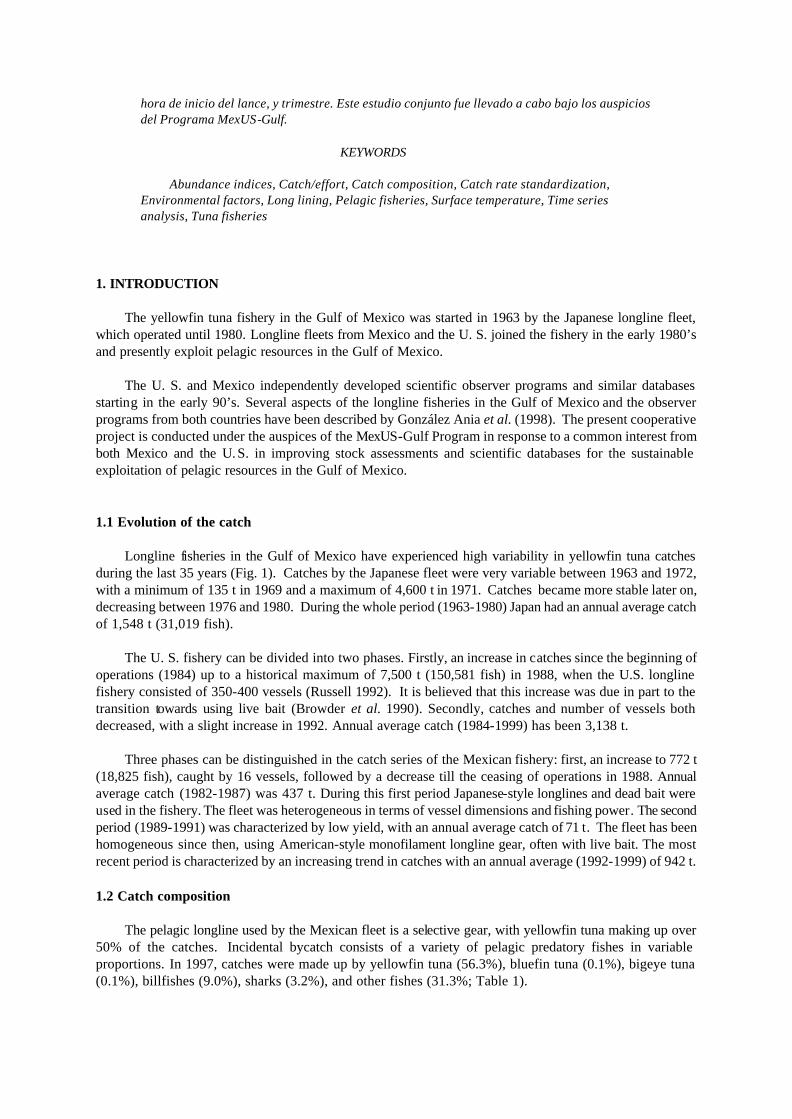
1.1 Evolution of the catch Longline fisheries in the Gulf of Mexico have experienced high variability in yellowfin tuna catches

during the last 35 years (Fig. 1). Catches by the Japanese fleet were very variable between 1963 and 1972, with a minimum of 135 t in 1969 and a maximum of 4,600 t in 1971. Catches became more stable later on, decreasing between 1976 and 1980. During the whole period (1963-1980) Japan had an annual average catch of 1,548 t (31,019 fish).

The U. S. fishery can be divided into two phases. Firstly, an increase in catches since the beginning of

operations (1984) up to a historical maximum of 7,500 t (150,581 fish) in 1988, when the U.S. longline fishery consisted of 350-400 vessels (Russell 1992). It is believed that this increase was due in part to the transition towards using live bait (Browder et al. 1990). Secondly, catches and number of vessels both decreased, with a slight increase in 1992. Annual average catch (1984-1999) has been 3,138 t.

Three phases can be distinguished in the catch series of the Mexican fishery: first, an increase to 772 t

(18,825 fish), caught by 16 vessels, followed by a decrease till the ceasing of operations in 1988. Annual average catch (1982-1987) was 437 t. During this first period Japanese-style longlines and dead bait were used in the fishery. The fleet was heterogeneous in terms of vessel dimensions and fishing power. The second period (1989-1991) was characterized by low yield, with an annual average catch of 71 t. The fleet has been homogeneous since then, using American-style monofilament longline gear, often with live bait. The most recent period is characterized by an increasing trend in catches with an annual average (1992-1999) of 942 t.

1.2 Catch composition

The pelagic longline used by the Mexican fleet is a selective gear, with yellowfin tuna making up over

50% of the catches. Incidental bycatch consists of a variety of pelagic predatory fishes in variable proportions. In 1997, catches were made up by yellowfin tuna (56.3%), bluefin tuna (0.1%), bigeye tuna (0.1%), billfishes (9.0%), sharks (3.2%), and other fishes (31.3%; Table 1).

Page 3

1.3 Nominal catch rate Nominal catch rate of yellowfin tuna, expressed as the average number of fish caught by 100 hooks

(nominal CPUE), varies by season, with higher values occurring between May and August, and in November (Fig. 2). The geographical distribution of nominal CPUE also varies owing to mesoscale movements of the resource, which are probably due in turn to trophic and reproductive causes. During spring and summer, intermediate and high values of nominal CPUE are found in the central, southern, and western portions of the Mexican EEZ, where fleet activity concentrates. In fall and winter, the fishing zone extends more to the north and east. During that time, the highest values of nominal CPUE are found off the state of Tamaulipas, to the north of the Yucatan peninsula, and near the center of the Mexican EEZ, but the values are quite lower than those from spring-summer (Fig. 3).

1.4 Catch rate standardization

Catch and effort data are being increasingly used to construct indices of relative abundance for

commercial and recreational fisheries (Hoey et al. 1996; Brown 1998; Goñi et al. 1999). However, nominal catch rates obtained from fishery statistics or observer programs require standardization to correct for the effect of factors not related to regional fish abundance but assumed to affect fish availability and vulnerability (Bigelow et al. 1999).

Use of generalized linear models (GLMs) is becoming standard practic e in catch rate standardization

because this approach allows identification of the factors that influence catch rates and calculation of standardized abundance indices through the year effect (Goñi et al. 1999). A variety of error distributions of catch rate data have been assumed in GLM analyses (Lo et al. 1992; Bigelow et al. 1999; Goñi et al. 1999; Punt et al. 1999). Brown (1998) used a two-step GLM analysis based on a delta-lognormal model proposed by Lo et al. (1992) to model the proportion of trips that caught yellowfin tuna (Thunnus albacares) or bigeye tuna (Thunnus obesus) and the catch per trip for the positive trips only in the Virginia-Massachusetts rod and reel fishery. In the present study we model standardized indices of relative abundance of yellowfin tuna assuming that the errors in the dependent variable follow a Poisson distribution.

2. MATERIAL AND METHODS Under Mexico’s fisheries regulations, vessels fishing longline gear have observers on board during all

fishing trips. The objective of the United States’ observer program is to achieve a representative, 5% sampling level of the fishing effort in the Gulf of Mexico and other fishing areas during each calendar quarter of the year. Observers of both programs record detailed, set-specific data needed to describe the catch and effort of the longline fishery.

A combined data set was created which included the variables common to both observer programs

(Table 2). For this analysis, data were available from the Mexican observer program for the period 1993-1997 and from the United States’ observer program, for the period 1992-1999. After an initial exploratory analysis, factors which were considered as possible influences on catch rates included environmental factors such as mean sea surface temperature (MEANTEMP) and depth (SEADEPTH), time-area factors such as YEAR, QUARTER, fishing area (ZONE) and two measures of the time of day during which a set was initiated (SETSTART, 2AM-11AM or 11AM-2AM as well as DAYNIGHT, day or night starts), and fishery factors such as bait category (BAITCAT, fish or cephalopod), bait status (BAITLD, live or dead) and FLEET (Mexico or United States). Mean sea surface temperature (MEANTEMP) was calculated for each set as the average of temperature data measured in situ at the beginning and end of gear setting for the U. S. fleet, and at the beginning and end of both gear setting and retrieval in the case of the Mexican fleet. Five fishing areas (ZONE) were defined based upon the latitude and longitude of the sets (Fig. 4).

Page 4

Standardized indices were developed using generalized linear models. Catch rates were modeled as a

function of the various factors. A Poisson regression was fitted to the number of yellowfin tuna per set (log link) and the natural log of the mean operating time for the set (in hours) was used as the offset term. The mean operating time of each set is intended to reflect the average time that each hook was in the water. It was calculated by dividing the total time to set out and to retrieve the gear by two, then adding the soak time during which the gear is left undisturbed.

A forward stepwise approach was used to quantify the relative importance of the main factors explaining

the variance in catch rates. First, a null model was run with no factors entered into the model. Results from the null model reflect the distribution of the nominal data. Each potential factor was then tested one at a time. The results were then ranked from greatest to least reduction in deviance per degree of freedom when compared to the null model. The factor which resulted in the greatest reduction in deviance per degree of freedom was then incorporated into the model, provided two conditions were met: 1) the effect of the factor was determined to be significant at least at the 5% level based on a Chi-Square test, and 2) the deviance per degree of freedom was reduced by at least 1% from the less complex model. This process was repeated, adding factors one at a time at each step, until no factor met the criteria for incorporation into the final model. All models in the stepwise approach were fitted with the SAS GENMOD procedure, whereas the final model was run with the SAS MIXED procedure (SAS Inst. Inc.). The relative indices of abundance by year were determined based upon the standardized year effects.

3. RESULTS AND DISCUSSION The stepwise construction of the model is shown in Table 3. The final model included the factors

MEANTEMP, YEAR, ZONE, SETSTART and QUARTER, ranked by decreasing importance. The results of the relative abundance analyses for yellowfin tuna in the Gulf of Mexico (1992-1999) are shown in Table 4. Table 5 and Figure 5 show the final model and relative index trend.

Spatial-temporal heterogeneity in the marine environment is believed to greatly affect the biology,

dynamics, and availability of tuna stocks, as well as their vulnerability to fishing gear, thus introducing a source of variability in nominal catch rates. Sea surface temperature is one of the most important physical factors because it modifies the geographical and vertical aggregation patterns of tuna, through its effect on feeding, reproductive, and migratory behavior and body thermoregulation (Fonteneau 1998). Acoustic telemetry studies of the microscale movement patterns of yellowfin tuna conducted since 1982 have demonstrated that this species occurs in the warm-water mixed surface layer and the upper part of the thermocline in tropical and subtropical seas, moving occasionally into colder waters below the thermocline, probably to feed or thermoregulate (Block et al. 1997, Bard 1998). The consistent occurrence of yellowfin tuna in this layer of homogeneous temperature allows us to assume that sea surface temperatures taken simultaneously to fishing operations, either measured in situ from fishing vessels–as in the present study–or from satellites, are representative of the thermal habitat available to this species.

The importance of sea surface temperature as an explanatory variable in the present analysis points to the

potential utility of exploring other possible relationships between catch rate and mesoscale oceanic features by including thermal gradients in the model. Detection of a strong relationship between nominal CPUE and temperature was due –at least in part– to the space-time microscale approach used. In that respect, our results differ from those by Power and May (1991), who did not find any perceptible relationship between satellite observations of sea surface temperature and yellowfin tuna nominal CPUE in the longline fishery of the northwestern Gulf of Mexico. The relationship may have been masked by data limitations and uncertainty in the geographical locations of the sets in that study.

It is possible, however, that the relationship found between nominal CPUE and temperature may not only

be due to specific temperature preferences by yellowfin tuna, especially because over 99% of the sets

Page 5

analyzed occurred in waters with surface temperatures above 21º C, considered to be the thermal minimum for the distribution of this species (Fonteneau 1998). Variability in nominal catch rates can also be related to other physical, chemical, and biological processes or factors in the ocean (e.g. water transparency, circulation patterns, frontal zones, salinity, plankton, nekton), which together with temperature define the identity, structure, and interaction of water masses and can affect the availability of potential prey and the capture efficiency of tuna (Laurs et al. 1984, Bigelow et al. 1999).

The significant effect of time of set start (SETSTART) on catch rate may be related to predatory

behavior. Yellowfin tuna tracked by acoustic telemetry have displayed a behavioral pattern in which they rapidly ascend to the surface at dawn; a similar behavior has been observed in the bluefin tuna (Block et al. 1997). This behavioral pattern may likely increase the vulnerability of yellowfin tuna to fishing gear.

The present study represents the first cooperative attempt to merge fishery and environmental

information from the complete distribution range of the yellowfin tuna in the Gulf of Mexico, estimate the best available relative abundance indices, and model recent trends in CPUE. The current analysis did not consider terms representing interactions between factors in the model. It is possible that such interaction terms might contribute substantially to a final model. Results may also be improved by adding other predictor variables to the model, extending the time series, and taking into account the size-age structure and sex of the catches. Variable transformation and use of generalized additive models (GAMs) may also increase the explanatory power of the model, due to the likely nonlinearity of many of the functional relationships between catch rate and the predictor variables.

4. REFERENCES Bard, F.X., P. Bach et E. Josse. 1998. Habitat, écophysiologie des thons: Quoi de neuf depuis 15 ans?. Int.

Comm. Conserv. Atl. Tunas, Col. Vol. Sci. Pap. 50(1): 319-341. Bigelow, K.A., C.H. Boggs, and X. He. 1999. Environmental effects on swordfish and blue shark catch rates

in the US North Pacific longline fishery. Fisheries Oceanography 8: 178-198. Block, B.A., J.E. Keen, B. Castillo, H. Dewar, E.V. Freund, D.J. Marcinek, R.W. Brill and C. Farwell. 1997.

Environmental preferences of yellowfin tuna (Thunnus albacares) at the northern extent of its range. Marine Biology 130: 119-132.

Browder, J.A., E.B. Brown and M.L. Parrack. 1990. The U.S. longline fishery for yellowfin tuna in

perspective. ICCAT Working Document SCRS/89/76 (YYP/89/15). Brown, C.A. 1998. Standardized catch rates for yellowfin tuna (Thunnus albacares) and bigeye tuna

(Thunnus obesus) in the Virginia - Massachusetts (U.S.) rod and reel fishery. Int. Comm. Conserv. Atl. Tunas, Col. Vol. Sci. Pap. 49(3): 357-369.

Fonteneau, A. 1998. Introduction aux problèmes des relations thons-environnement dans l’Atlantique. Int.

Comm. Conserv. Atl. Tunas, Col. Vol. Sci. Pap. 50(1): 275-317. González-Ania, L.V., P.A. Ulloa-Ramírez, D.W. Lee, C.J. Brown and C.A. Brown. 1998. Description of

Gulf of Mexico longline fisheries based upon observer programs from Mexico and the United States. Int. Comm. Conserv. Atl. Tunas, Col. Vol. Sci. Pap. 48(3): 308-316.

Goñi, R., F. Alvarez and S. Adlerstein. 1999. Application of generalized linear modeling to catch rate analysis

of Western Mediterranean fisheries: the Castellón trawl fleet as a case study. Fisheries Research 42: 291-302.

Page 6

Hoey, J.J., J. Mejuto, J.M. Porter, H.H. Stone and Y. Uozomi. 1996. An updated biomass index of abundance for North Atlantic swordfish. ICCAT, SCRS/96/144, 9 pp.

Laurs, R.M., P.C. Fiedler and D.R. Montgomery. 1984. Albacore tuna catch distributions relative to

environmental features observed from satellites. Deep-Sea Research 31(9): 1085-1099. Lo, N.C.H., L.D. Jacobson and J.L. Squire. 1992. Indices of relative abundance from fish spotter data based

on delta-lognormal models. Canadian Journal of Fisheries and Aquatic Sciences 49: 2515-2526. Power, J.H. and L.N. May Jr. 1991. Satellite observed sea-surface temperatures and yellowfin tuna catch

and effort in the Gulf of Mexico. Fishery Bulletin, U.S. 89(3): 429-439. Punt, A.E., T.I. Walker, B.L. Taylor and F. Pribac. 1999. Standardization of catch and effort data in a

spatially-structured shark fishery. Fisheries Research 956: 1-17. Russell, S.J. 1992. Shark bycatch in the northern Gulf of Mexico tuna longline fishery, 1988-91, with

observations on the nearshore directed shark fishery. NOAA Technical Report NMFS 115: 19-29.

Page 7

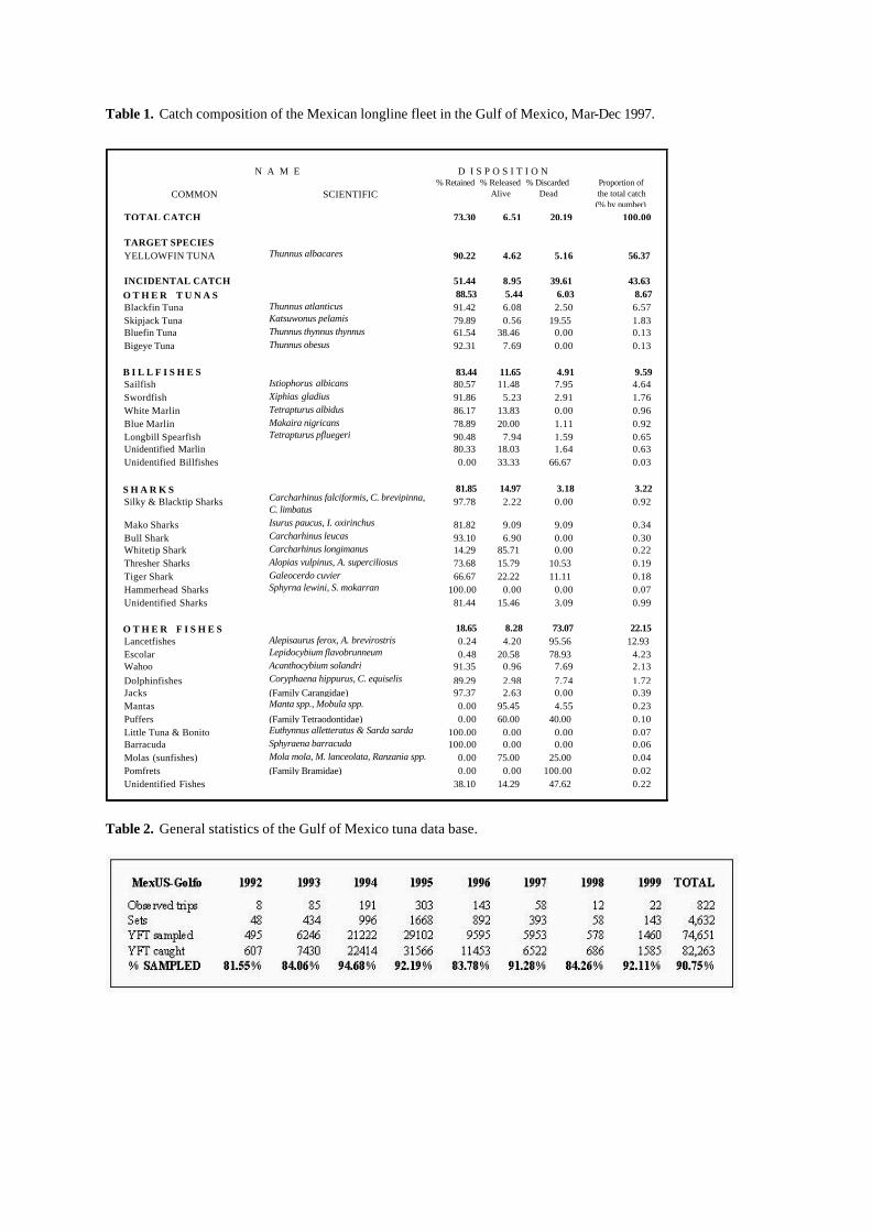
Table 1. Catch composition of the Mexican longline fleet in the Gulf of Mexico, Mar-Dec 1997.

Table 2. General statistics of the Gulf of Mexico tuna data base.

N A M E D I S P O S I T I O N

COMMON SCIENTIFIC% Retained % Released

Alive% Discarded

DeadProportion ofthe total catch(% by number)

TOTAL CATCH 73.30 6.51 20.19 100.00

TARGET SPECIESYELLOWFIN TUNA Thunnus albacares 90.22 4.62 5.16 56.37

INCIDENTAL CATCH 51.44 8.95 39.61 43.63O T H E R T U N A S 88.53 5.44 6.03 8.67Blackfin Tuna Thunnus atlanticus 91.42 6.08 2.50 6.57Skipjack Tuna Katsuwonus pelamis 79.89 0.56 19.55 1.83Bluefin Tuna Thunnus thynnus thynnus 61.54 38.46 0.00 0.13Bigeye Tuna Thunnus obesus 92.31 7.69 0.00 0.13

B I L L F I S H E S 83.44 11.65 4.91 9.59Sailfish Istiophorus albicans 80.57 11.48 7.95 4.64Swordfish Xiphias gladius 91.86 5.23 2.91 1.76White Marlin Tetrapturus albidus 86.17 13.83 0.00 0.96Blue Marlin Makaira nigricans 78.89 20.00 1.11 0.92Longbill Spearfish Tetrapturus pfluegeri 90.48 7.94 1.59 0.65Unidentified Marlin 80.33 18.03 1.64 0.63Unidentified Billfishes 0.00 33.33 66.67 0.03

S H A R K S 81.85 14.97 3.18 3.22Silky & Blacktip Sharks Carcharhinus falciformis, C. brevipinna,

C. limbatus97.78 2.22 0.00 0.92

Mako Sharks Isurus paucus, I. oxirinchus 81.82 9.09 9.09 0.34Bull Shark Carcharhinus leucas 93.10 6.90 0.00 0.30Whitetip Shark Carcharhinus longimanus 14.29 85.71 0.00 0.22Thresher Sharks Alopias vulpinus, A. superciliosus 73.68 15.79 10.53 0.19Tiger Shark Galeocerdo cuvier 66.67 22.22 11.11 0.18Hammerhead Sharks Sphyrna lewini, S. mokarran 100.00 0.00 0.00 0.07Unidentified Sharks 81.44 15.46 3.09 0.99

O T H E R F I S H E S 18.65 8.28 73.07 22.15Lancetfishes Alepisaurus ferox, A. brevirostris 0.24 4.20 95.56 12.93Escolar Lepidocybium flavobrunneum 0.48 20.58 78.93 4.23Wahoo Acanthocybium solandri 91.35 0.96 7.69 2.13Dolphinfishes Coryphaena hippurus, C. equiselis 89.29 2.98 7.74 1.72Jacks (Family Carangidae) 97.37 2.63 0.00 0.39Mantas Manta spp., Mobula spp. 0.00 95.45 4.55 0.23Puffers (Family Tetraodontidae) 0.00 60.00 40.00 0.10Little Tuna & Bonito Euthynnus alletteratus & Sarda sarda 100.00 0.00 0.00 0.07Barracuda Sphyraena barracuda 100.00 0.00 0.00 0.06Molas (sunfishes) Mola mola, M. lanceolata, Ranzania spp. 0.00 75.00 25.00 0.04Pomfrets (Family Bramidae) 0.00 0.00 100.00 0.02Unidentified Fishes 38.10 14.29 47.62 0.22

Page 8

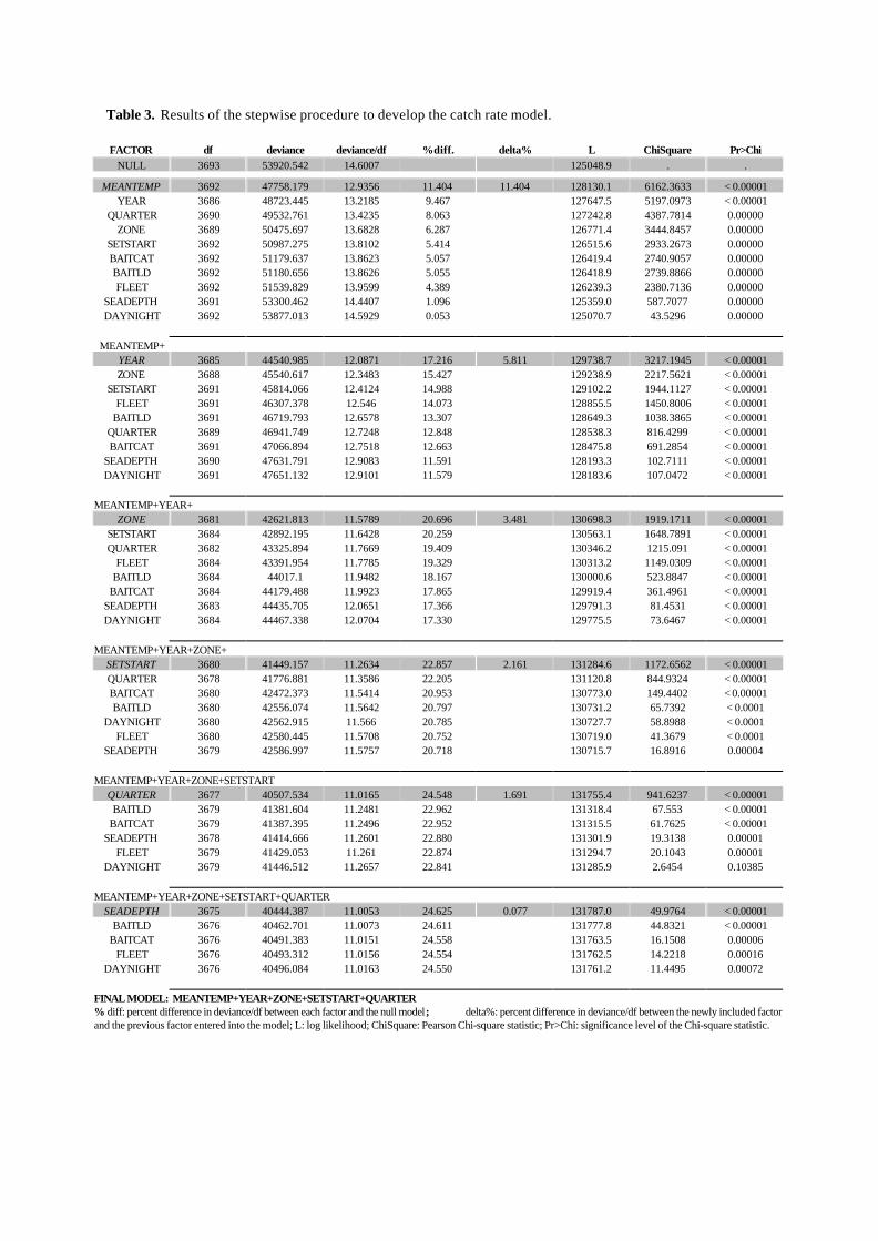
Table 3. Results of the stepwise procedure to develop the catch rate model. FACTOR

df

deviance

deviance/df

%diff.

delta%

L

ChiSquare

Pr>Chi

NULL

3693

53920.542

14.6007

125048.9

.

.

MEANTEMP

3692

47758.179

12.9356

11.404

11.404

128130.1

6162.3633

< 0.00001

YEAR

3686

48723.445

13.2185

9.467

127647.5

5197.0973

< 0.00001 QUARTER

3690

49532.761

13.4235

8.063

127242.8

4387.7814

0.00000

ZONE

3689

50475.697

13.6828

6.287

126771.4

3444.8457

0.00000 SETSTART

3692

50987.275

13.8102

5.414

126515.6

2933.2673

0.00000

BAITCAT

3692

51179.637

13.8623

5.057

126419.4

2740.9057

0.00000 BAITLD

3692

51180.656

13.8626

5.055

126418.9

2739.8866

0.00000

FLEET

3692

51539.829

13.9599

4.389

126239.3

2380.7136

0.00000 SEADEPTH

3691

53300.462

14.4407

1.096

125359.0

587.7077

0.00000

DAYNIGHT

3692

53877.013

14.5929

0.053

125070.7

43.5296

0.00000

MEANTEMP+

YEAR

3685

44540.985

12.0871

17.216

5.811

129738.7

3217.1945

< 0.00001

ZONE

3688

45540.617

12.3483

15.427

129238.9

2217.5621

< 0.00001 SETSTART

3691

45814.066

12.4124

14.988

129102.2

1944.1127

< 0.00001

FLEET

3691

46307.378

12.546

14.073

128855.5

1450.8006

< 0.00001 BAITLD

3691

46719.793

12.6578

13.307

128649.3

1038.3865

< 0.00001

QUARTER

3689

46941.749

12.7248

12.848

128538.3

816.4299

< 0.00001 BAITCAT

3691

47066.894

12.7518

12.663

128475.8

691.2854

< 0.00001

SEADEPTH

3690

47631.791

12.9083

11.591

128193.3

102.7111

< 0.00001 DAYNIGHT

3691

47651.132

12.9101

11.579

128183.6

107.0472

< 0.00001

MEANTEMP+YEAR+

ZONE

3681

42621.813

11.5789

20.696

3.481

130698.3

1919.1711

< 0.00001 SETSTART

3684

42892.195

11.6428

20.259

130563.1

1648.7891

< 0.00001

QUARTER

3682

43325.894

11.7669

19.409

130346.2

1215.091

< 0.00001 FLEET

3684

43391.954

11.7785

19.329

130313.2

1149.0309

< 0.00001

BAITLD

3684

44017.1

11.9482

18.167

130000.6

523.8847

< 0.00001 BAITCAT

3684

44179.488

11.9923

17.865

129919.4

361.4961

< 0.00001

SEADEPTH

3683

44435.705

12.0651

17.366

129791.3

81.4531

< 0.00001 DAYNIGHT

3684

44467.338

12.0704

17.330

129775.5

73.6467

< 0.00001

MEANTEMP+YEAR+ZONE+

SETSTART

3680

41449.157

11.2634

22.857

2.161

131284.6

1172.6562

< 0.00001 QUARTER

3678

41776.881

11.3586

22.205

131120.8

844.9324

< 0.00001

BAITCAT

3680

42472.373

11.5414

20.953

130773.0

149.4402

< 0.00001 BAITLD

3680

42556.074

11.5642

20.797

130731.2

65.7392

< 0.0001

DAYNIGHT

3680

42562.915

11.566

20.785

130727.7

58.8988

< 0.0001 FLEET

3680

42580.445

11.5708

20.752

130719.0

41.3679

< 0.0001

SEADEPTH

3679

42586.997

11.5757

20.718

130715.7

16.8916

0.00004

MEANTEMP+YEAR+ZONE+SETSTART QUARTER

3677

40507.534

11.0165

24.548

1.691

131755.4

941.6237

< 0.00001

BAITLD

3679

41381.604

11.2481

22.962

131318.4

67.553

< 0.00001 BAITCAT

3679

41387.395

11.2496

22.952

131315.5

61.7625

< 0.00001

SEADEPTH

3678

41414.666

11.2601

22.880

131301.9

19.3138

0.00001 FLEET

3679

41429.053

11.261

22.874

131294.7

20.1043

0.00001

DAYNIGHT

3679

41446.512

11.2657

22.841

131285.9

2.6454

0.10385

MEANTEMP+YEAR+ZONE+SETSTART+QUARTER SEADEPTH

3675

40444.387

11.0053

24.625

0.077

131787.0

49.9764

< 0.00001

BAITLD

3676

40462.701

11.0073

24.611

131777.8

44.8321

< 0.00001 BAITCAT

3676

40491.383

11.0151

24.558

131763.5

16.1508

0.00006

FLEET

3676

40493.312

11.0156

24.554

131762.5

14.2218

0.00016 DAYNIGHT

3676

40496.084

11.0163

24.550

131761.2

11.4495

0.00072

FINAL MODEL: MEANTEMP+YEAR+ZONE+SETSTART+QUARTER % diff: percent difference in deviance/df between each factor and the null model; delta%: percent difference in deviance/df between the newly included factor and the previous factor entered into the model; L: log likelihood; ChiSquare: Pearson Chi-square statistic; Pr>Chi: significance level of the Chi-square statistic.

Page 9

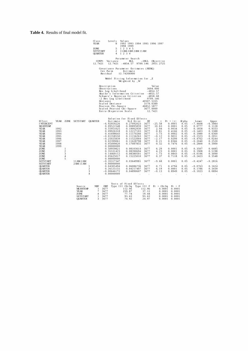
Table 4. Results of final model fit. Class Levels Values YEAR 8 1992 1993 1994 1995 1996 1997 1998 1999 ZONE 5 1 2 3 4 5 SETSTART 2 11AM-2AM 2AM-11AM QUARTER 4 1 2 3 4 Parameter Search COVP1 Variance RLL -2RLL Objective 12.7421 12.7421 -4854.57 9709.146 2951.2725 Covariance Parameter Estimates (REML) Cov Parm Estimate Residual 12.74206900 Model Fitting Information for _Z Weighted by _W Description Value Observations 3694.000 Res Log Likelihood -4854.57 Akaike's Information Criterion -4855.57 Schwarz's Bayesian Criterion -4858.68 -2 Res Log Likelihood 9709.146 Deviance 40507.5335 Scaled Deviance 3179.0389 Pearson Chi-Square 46852.5877 Scaled Pearson Chi-Square 3677.0000 Extra-Dispersion Scale 12.7421 Solution for Fixed Effects Effect YEAR ZONE SETSTART QUARTER Estimate Std Error DF t Pr > |t| Alpha Lower Upper INTERCEPT -6.92959226 0.27092023 3677 -25.58 0.0001 0.05 -7.4608 -6.3984 MEANTEMP 0.09521548 0.00895859 3677 10.63 0.0001 0.05 0.0777 0.1128 YEAR 1992 0.55951025 0.19062930 3677 2.94 0.0034 0.05 0.1858 0.9333 YEAR 1993 0.09926318 0.12217103 3677 0.81 0.4166 0.05 -0.1403 0.3388 YEAR 1994 0.41698643 0.11170266 3677 3.73 0.0002 0.05 0.1980 0.6360 YEAR 1995 -0.01358550 0.11156263 3677 -0.12 0.9031 0.05 -0.2323 0.2051 YEAR 1996 -0.25025839 0.11522004 3677 -2.17 0.0299 0.05 -0.4762 -0.0244 YEAR 1997 0.02399061 0.11628798 3677 0.21 0.8366 0.05 -0.2040 0.2520 YEAR 1998 0.05499820 0.17087855 3677 0.32 0.7476 0.05 -0.2800 0.3900 YEAR 1999 0.00000000 . . . . . . . ZONE 1 0.50959821 0.08103614 3677 6.29 0.0001 0.05 0.3507 0.6685 ZONE 2 0.35531423 0.08390694 3677 4.23 0.0001 0.05 0.1908 0.5198 ZONE 3 0.14469112 0.08380501 3677 1.73 0.0843 0.05 -0.0196 0.3090 ZONE 4 0.05625017 0.15225010 3677 0.37 0.7118 0.05 -0.2423 0.3548 ZONE 5 0.00000000 . . . . . . . SETSTART 11AM-2AM -0.35317347 0.03649981 3677 -9.68 0.0001 0.05 -0.4247 -0.2816 SETSTART 2AM-11AM 0.00000000 . . . . . . . QUARTER 1 0.04305494 0.06086736 3677 0.71 0.4794 0.05 -0.0763 0.1624 QUARTER 2 0.26125155 0.04217407 3677 6.19 0.0001 0.05 0.1786 0.3439 QUARTER 3 -0.00646172 0.04890607 3677 -0.13 0.8949 0.05 -0.1023 0.0894 QUARTER 4 0.00000000 . . . . . . . Tests of Fixed Effects Source NDF DDF Type III ChiSq Type III F Pr > ChiSq Pr > F MEANTEMP 1 3677 112.96 112.96 0.0001 0.0001 YEAR 7 3677 259.87 37.12 0.0001 0.0001 ZONE 4 3677 77.74 19.44 0.0001 0.0001 SETSTART 1 3677 93.63 93.63 0.0001 0.0001 QUARTER 3 3677 74.92 24.97 0.0001 0.0001

Page 10

Table 4. Results of final model fit (cont.) Parameter Estimates Effect YEAR ZONE SETSTART QUARTER Estimate Std Error DF t Pr > |t| Alpha Lower Upper INTERCEPT -6.9296 0.2709 3677 -25.58 0.0001 0.05 -7.4608 -6.3984 MEANTEMP 0.0952 0.0090 3677 10.63 0.0001 0.05 0.0777 0.1128 YEAR 1992 0.5595 0.1906 3677 2.94 0.0034 0.05 0.1858 0.9333 YEAR 1993 0.0993 0.1222 3677 0.81 0.4166 0.05 -0.1403 0.3388 YEAR 1994 0.4170 0.1117 3677 3.73 0.0002 0.05 0.1980 0.6360 YEAR 1995 -0.0136 0.1116 3677 -0.12 0.9031 0.05 -0.2323 0.2051 YEAR 1996 -0.2503 0.1152 3677 -2.17 0.0299 0.05 -0.4762 -0.0244 YEAR 1997 0.0240 0.1163 3677 0.21 0.8366 0.05 -0.2040 0.2520 YEAR 1998 0.0550 0.1709 3677 0.32 0.7476 0.05 -0.2800 0.3900 YEAR 1999 0.0000 . . . . . . . ZONE 1 0.5096 0.0810 3677 6.29 0.0001 0.05 0.3507 0.6685 ZONE 2 0.3553 0.0839 3677 4.23 0.0001 0.05 0.1908 0.5198 ZONE 3 0.1447 0.0838 3677 1.73 0.0843 0.05 -0.0196 0.3090 ZONE 4 0.0563 0.1523 3677 0.37 0.7118 0.05 -0.2423 0.3548 ZONE 5 0.0000 . . . . . . . SETSTART 11AM-2AM -0.3532 0.0365 3677 -9.68 0.0001 0.05 -0.4247 -0.2816 SETSTART 2AM-11AM 0.0000 . . . . . . . QUARTER 1 0.0431 0.0609 3677 0.71 0.4794 0.05 -0.0763 0.1624 QUARTER 2 0.2613 0.0422 3677 6.19 0.0001 0.05 0.1786 0.3439 QUARTER 3 -0.0065 0.0489 3677 -0.13 0.8949 0.05 -0.1023 0.0894 QUARTER 4 0.0000 . . . . . . . Least Squares Means Effect YEAR LSMEAN Std Error DF t Pr > |t| Alpha Lower YEAR 1992 -3.7105 0.1700 3677 -21.82 0.0001 0.1 -3.9902 YEAR 1993 -4.1707 0.0774 3677 -53.92 0.0001 0.1 -4.2980 YEAR 1994 -3.8530 0.0415 3677 -92.77 0.0001 0.1 -3.9213 YEAR 1995 -4.2836 0.0401 3677 -106.9 0.0001 0.1 -4.3495 YEAR 1996 -4.5202 0.0479 3677 -94.42 0.0001 0.1 -4.5990 YEAR 1997 -4.2460 0.0559 3677 -76.02 0.0001 0.1 -4.3379 YEAR 1998 -4.2150 0.1442 3677 -29.23 0.0001 0.1 -4.4522 YEAR 1999 -4.2700 0.1058 3677 -40.36 0.0001 0.1 -4.4441 Upper STDERETA Mu DMU STDERMU LowerMu UpperMu -3.4307 0.17005 0.0245 0.024466 .0041604 0.0185 0.0324 -4.0435 0.07735 0.0154 0.015441 .0011944 0.0136 0.0175 -3.7847 0.04153 0.0212 0.021216 .0008812 0.0198 0.0227 -4.2176 0.04007 0.0138 0.013793 .0005527 0.0129 0.0147 -4.4415 0.04787 0.0109 0.010886 .0005212 0.0101 0.0118 -4.1541 0.05585 0.0143 0.014322 .0007999 0.0131 0.0157 -3.9778 0.14419 0.0148 0.014773 .0021301 0.0117 0.0187 -4.0959 0.10581 0.0140 0.013982 .0014794 0.0117 0.0166

Page 11

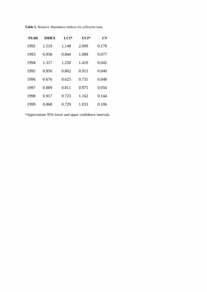
Table 5. Relative Abundance Indices for yellowfin tuna.

YEAR

INDEX

LCI*

UCI*

CV

1992

1.519

1.148

2.009

0.170

1993

0.958

0.844

1.089

0.077

1994

1.317

1.230

1.410

0.042

1995

0.856

0.802

0.915

0.040

1996

0.676

0.625

0.731

0.048

1997

0.889

0.811

0.975

0.056

1998

0.917

0.723

1.162

0.144

1999

0.868

0.729

1.033

0.106

*Approximate 95% lower and upper confidence intervals.

Page 12

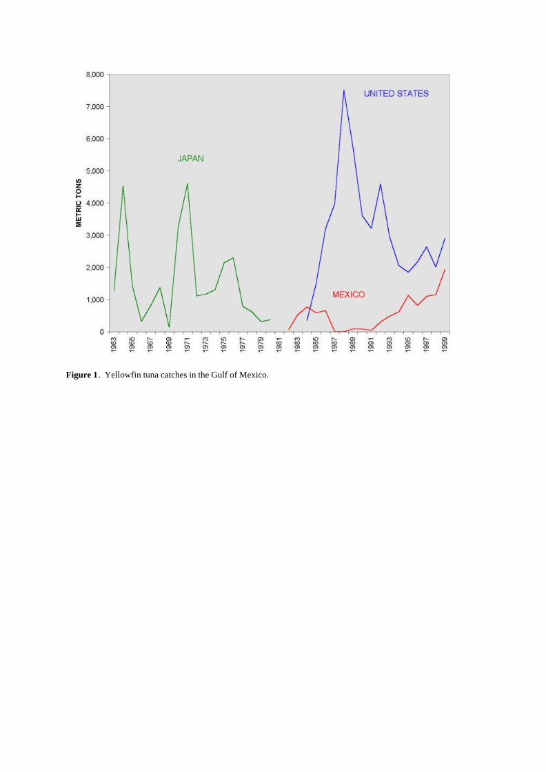
Figure 1. Yellowfin tuna catches in the Gulf of Mexico.

Page 13

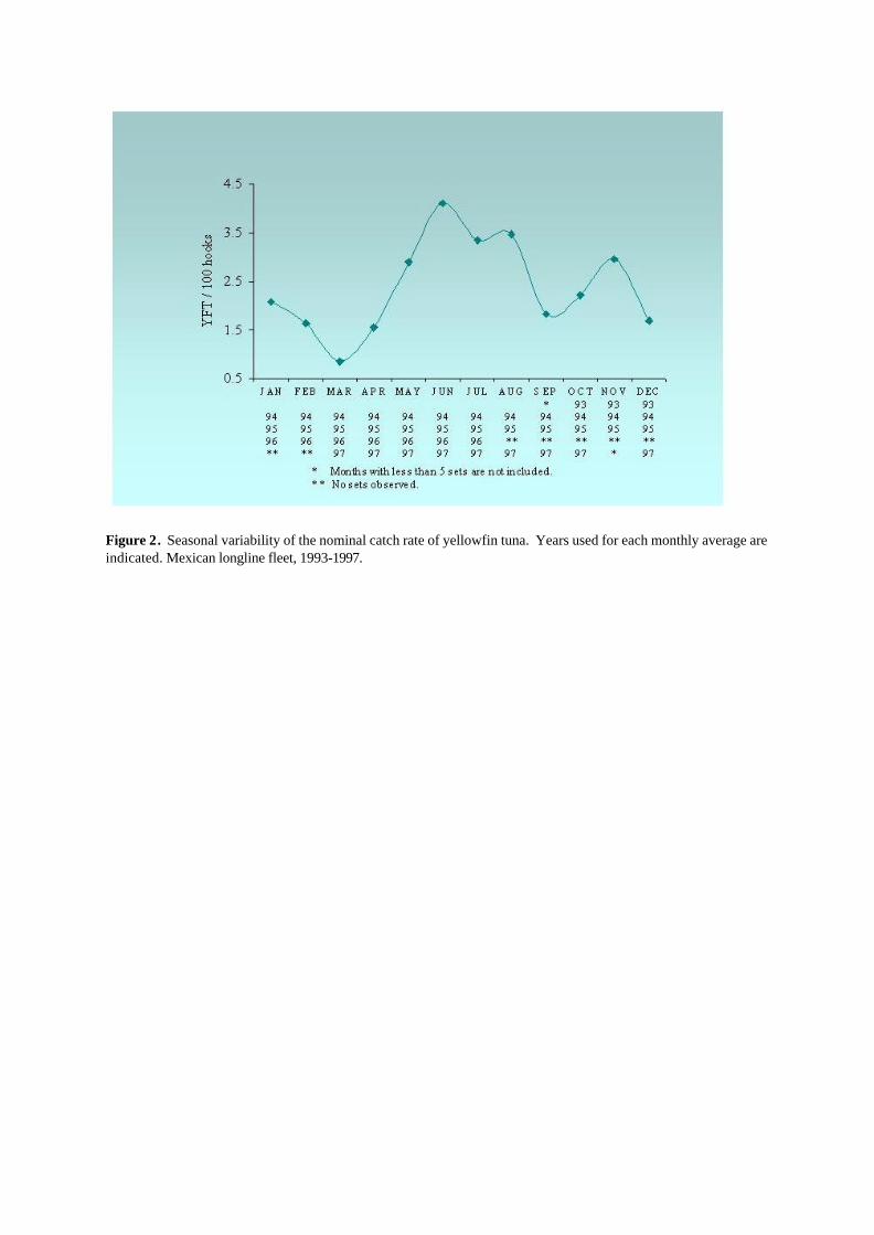
Figure 2. Seasonal variability of the nominal catch rate of yellowfin tuna. Years used for each monthly average are indicated. Mexican longline fleet, 1993-1997.

Page 14

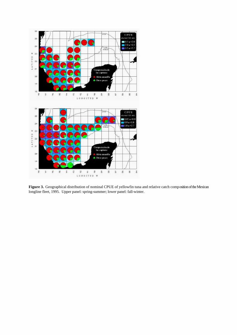
Figure 3. Geographical distribution of nominal CPUE of yellowfin tuna and relative catch composition of the Mexican longline fleet, 1995. Upper panel: spring-summer; lower panel: fall-winter.

Page 15

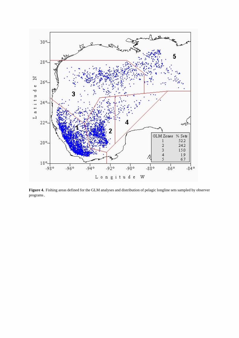
Figure 4. Fishing areas defined for the GLM analyses and distribution of pelagic longline sets sampled by observer programs .

Page 16

Figure 5. Relative abundance indices for yellowfin tuna with approximate 95% confidence intervals. (Yellowfin caught per set, offset: natural log of mean hours each hook is in the water, error distribution: Poisson). Model = MEANTEMP+YEAR+ZONE+SETSTART+QUARTER