arXiv:1503.02853v1 [stat.ME] 10 Mar 2015 Statistical Science 2014, Vol. 29, No. 4, 529–558 DOI: 10.1214/13-STS453 c Institute of Mathematical Statistics, 2014 Standardization and Control for Confounding in Observational Studies: A Historical Perspective Niels Keiding and David Clayton Abstract. Control for confounders in observational studies was gener- ally handled through stratification and standardization until the 1960s. Standardization typically reweights the stratum-specific rates so that exposure categories become comparable. With the development first of loglinear models, soon also of nonlinear regression techniques (logistic regression, failure time regression) that the emerging computers could handle, regression modelling became the preferred approach, just as was already the case with multiple regression analysis for continuous outcomes. Since the mid 1990s it has become increasingly obvious that weighting methods are still often useful, sometimes even necessary. On this background we aim at describing the emergence of the modelling approach and the refinement of the weighting approach for confounder control. Key words and phrases: 2 × 2 × K table, causality, decomposition of rates, epidemiology, expected number of deaths, log-linear model, marginal structural model, National Halothane Study, odds ratio, rate ratio, transportability, H. Westergaard, G. U. Yule. 1. INTRODUCTION: CONFOUNDING AND STANDARDIZATION In this paper we survey the development of mod- ern methods for controlling for confounding in ob- servational studies, with a primary focus on discrete responses in demography, epidemiology and social science. The forerunners of these methods are the methods of standardization of rates, which go back at least to the 18th century [see Keiding (1987) Niels Keiding is Professor, Department of Biostatistics, University of Copenhagen, P.O. Box 2099, Copenhagen 1014, Denmark e-mail: [email protected]. David Clayton is Emeritus Honorary Professor of Biostatistics, University of Cambridge, Cambridge CB2 0XY, United Kingdom e-mail: [email protected]. This is an electronic reprint of the original article published by the Institute of Mathematical Statistics in Statistical Science, 2014, Vol. 29, No. 4, 529–558. This reprint differs from the original in pagination and typographic detail. for a review]. These methods tackle the problem of comparing rates between populations with different age structures by applying age-specific rates to a single “target” age structure and, thereafter, com- paring predicted marginal summaries in this tar- get population. However, over the 20th century, the methodological focus swung toward indices which summarize comparisons of conditional (covariate- specific) rates. This difference of approach has, at its heart, the distinction between, for example, a ratio of averages and an average of ratios—a dis- tinction discussed at some length in the important papers by Yule (1934) and Kitagawa (1964), which we shall discuss in Section 4. The change of emphasis from a marginal to conditional focus led eventually to the modern dominance of the regression mod- elling approach in these fields. Clayton and Hills [(1993), page 135] likened the two approaches to the two paradigms for dealing with extraneous vari- ables in experimental science, namely, (a) to make a marginal comparison after ensuring, by random- ization, that the distributions of such variables are 1

Welcome message from author
This document is posted to help you gain knowledge. Please leave a comment to let me know what you think about it! Share it to your friends and learn new things together.
Transcript
arX
iv:1
503.
0285
3v1
[st
at.M
E]
10
Mar
201
5
Statistical Science
2014, Vol. 29, No. 4, 529–558DOI: 10.1214/13-STS453c© Institute of Mathematical Statistics, 2014
Standardization and Control forConfounding in Observational Studies:A Historical PerspectiveNiels Keiding and David Clayton
Abstract. Control for confounders in observational studies was gener-ally handled through stratification and standardization until the 1960s.Standardization typically reweights the stratum-specific rates so thatexposure categories become comparable. With the development first ofloglinear models, soon also of nonlinear regression techniques (logisticregression, failure time regression) that the emerging computers couldhandle, regression modelling became the preferred approach, just aswas already the case with multiple regression analysis for continuousoutcomes. Since the mid 1990s it has become increasingly obvious thatweighting methods are still often useful, sometimes even necessary. Onthis background we aim at describing the emergence of the modellingapproach and the refinement of the weighting approach for confoundercontrol.
Key words and phrases: 2 × 2 × K table, causality, decompositionof rates, epidemiology, expected number of deaths, log-linear model,marginal structural model, National Halothane Study, odds ratio, rateratio, transportability, H. Westergaard, G. U. Yule.
1. INTRODUCTION: CONFOUNDING AND
STANDARDIZATION
In this paper we survey the development of mod-ern methods for controlling for confounding in ob-servational studies, with a primary focus on discreteresponses in demography, epidemiology and socialscience. The forerunners of these methods are themethods of standardization of rates, which go backat least to the 18th century [see Keiding (1987)
Niels Keiding is Professor, Department of Biostatistics,
University of Copenhagen, P.O. Box 2099, Copenhagen
1014, Denmark e-mail: [email protected]. David Clayton
is Emeritus Honorary Professor of Biostatistics,
University of Cambridge, Cambridge CB2 0XY, United
Kingdom e-mail: [email protected].
This is an electronic reprint of the original articlepublished by the Institute of Mathematical Statistics inStatistical Science, 2014, Vol. 29, No. 4, 529–558. Thisreprint differs from the original in pagination andtypographic detail.
for a review]. These methods tackle the problem ofcomparing rates between populations with differentage structures by applying age-specific rates to asingle “target” age structure and, thereafter, com-paring predicted marginal summaries in this tar-get population. However, over the 20th century, themethodological focus swung toward indices whichsummarize comparisons of conditional (covariate-specific) rates. This difference of approach has, atits heart, the distinction between, for example, aratio of averages and an average of ratios—a dis-tinction discussed at some length in the importantpapers by Yule (1934) and Kitagawa (1964), whichwe shall discuss in Section 4. The change of emphasisfrom a marginal to conditional focus led eventuallyto the modern dominance of the regression mod-elling approach in these fields. Clayton and Hills[(1993), page 135] likened the two approaches tothe two paradigms for dealing with extraneous vari-ables in experimental science, namely, (a) to makea marginal comparison after ensuring, by random-
ization, that the distributions of such variables are
1
2 N. KEIDING AND D. CLAYTON
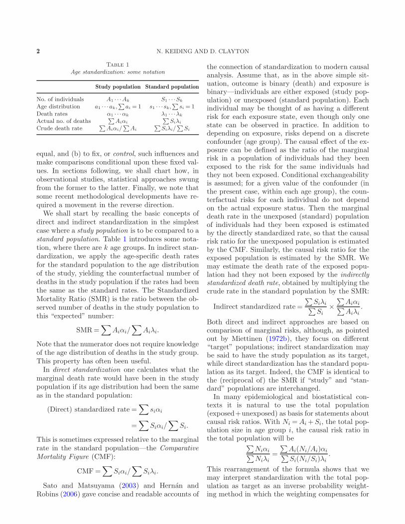
Table 1
Age standardization: some notation
Study population Standard population
No. of individuals A1 · · ·Ak S1 · · ·Sk
Age distribution a1 · · ·ak,∑
ai = 1 s1 · · ·sk,∑
si = 1Death rates α1 · · ·αk λ1 · · ·λk
Actual no. of deaths∑
Aiαi
∑Siλi
Crude death rate∑
Aiαi/∑
Ai
∑Siλi/
∑Si
equal, and (b) to fix, or control, such influences andmake comparisons conditional upon these fixed val-ues. In sections following, we shall chart how, inobservational studies, statistical approaches swungfrom the former to the latter. Finally, we note thatsome recent methodological developments have re-quired a movement in the reverse direction.We shall start by recalling the basic concepts of
direct and indirect standardization in the simplestcase where a study population is to be compared to astandard population. Table 1 introduces some nota-tion, where there are k age groups. In indirect stan-dardization, we apply the age-specific death ratesfor the standard population to the age distributionof the study, yielding the counterfactual number ofdeaths in the study population if the rates had beenthe same as the standard rates. The StandardizedMortality Ratio (SMR) is the ratio between the ob-served number of deaths in the study population tothis “expected” number:
SMR=∑
Aiαi/∑
Aiλi.
Note that the numerator does not require knowledgeof the age distribution of deaths in the study group.This property has often been useful.In direct standardization one calculates what the
marginal death rate would have been in the studypopulation if its age distribution had been the sameas in the standard population:
(Direct) standardized rate =∑
siαi
=∑
Siαi/∑
Si.
This is sometimes expressed relative to the marginalrate in the standard population—the Comparative
Mortality Figure (CMF):
CMF=∑
Siαi/∑
Siλi.
Sato and Matsuyama (2003) and Hernan andRobins (2006) gave concise and readable accounts of
the connection of standardization to modern causalanalysis. Assume that, as in the above simple sit-uation, outcome is binary (death) and exposure isbinary—individuals are either exposed (study pop-ulation) or unexposed (standard population). Eachindividual may be thought of as having a differentrisk for each exposure state, even though only onestate can be observed in practice. In addition todepending on exposure, risks depend on a discreteconfounder (age group). The causal effect of the ex-posure can be defined as the ratio of the marginalrisk in a population of individuals had they beenexposed to the risk for the same individuals hadthey not been exposed. Conditional exchangeabilityis assumed; for a given value of the confounder (inthe present case, within each age group), the coun-terfactual risks for each individual do not dependon the actual exposure status. Then the marginaldeath rate in the unexposed (standard) populationof individuals had they been exposed is estimatedby the directly standardized rate, so that the causalrisk ratio for the unexposed population is estimatedby the CMF. Similarly, the causal risk ratio for theexposed population is estimated by the SMR. Wemay estimate the death rate of the exposed popu-lation had they not been exposed by the indirectlystandardized death rate, obtained by multiplying thecrude rate in the standard population by the SMR:
Indirect standardized rate =
∑Siλi∑Si
×
∑Aiαi∑Aiλi
.
Both direct and indirect approaches are based oncomparison of marginal risks, although, as pointedout by Miettinen (1972b), they focus on different“target” populations; indirect standardization maybe said to have the study population as its target,while direct standardization has the standard popu-lation as its target. Indeed, the CMF is identical tothe (reciprocal of) the SMR if “study” and “stan-dard” populations are interchanged.In many epidemiological and biostatistical con-
texts it is natural to use the total population(exposed+unexposed) as basis for statements aboutcausal risk ratios. With Ni =Ai+Si, the total pop-ulation size in age group i, the causal risk ratio inthe total population will be∑
Niαi∑Niλi
=
∑Ai(Ni/Ai)αi∑Si(Ni/Si)λi
.
This rearrangement of the formula shows that wemay interpret standardization with the total pop-ulation as target as an inverse probability weight-ing method in which the weighting compensates for
STANDARDIZATION: A HISTORICAL PERSPECTIVE 3
nonobservation of the counterfactual exposure statefor each subject. In the numerator, the contributionsof the Ai exposed subjects are inversely weighted byAi/Ni, which estimates the probability that a sub-ject in age group i of the total study was observedin the exposed state. Similarly, in the denominator,the Si unexposed subjects are inversely weighted bythe probability that a subject was observed in theunexposed state. The method of inverse probabilityweighting is an important tool in marginal struc-tural models and other methods in modern causalanalysis.Thus, while there are obvious similarities between
direct and indirect standardization, there are alsoimportant differences. In particular, when the aimis to compare rates in several study populations, re-versal of the roles of study and standard populationis no longer possible and Yule (1934) pointed outimportant faults with the indirect approach in thiscontext. Such considerations will lead us, eventually,to see indirect standardization as dependent on animplicit model and, therefore, as a forerunner of themodern conditional modelling approach.The plan of this paper is to present selected high-
lights from the historical development of confoundercontrol with focus on the interplay between marginalor conditional choice of target, on the one hand, andthe role of (parametric or nonparametric) statisti-cal models on the other. Section 2 recalls the de-velopment of standardization techniques during the19th century. Section 3 deals with early 20th cen-tury approaches to the problem of causal inference,focusing particularly on the contributions of Yuleand Pearson. Section 4 records highlights from theparallel development in the social sciences, focus-ing on the further development of standardizationmethods in the 20th century—largely in the socialsciences. Section 5 deals with the important devel-opments in the 1950s and early 1960s surroundingthe analysis of the 2× 2×K contingency table, andSection 6 briefly summarizes the subsequent rise anddominance of regression models. Section 7 pointsout that the values of parameters in (conditional)probability models are not always the only focus ofanalysis, that marginal predictions in different tar-get populations are often important, and that suchpredictions require careful examination of our as-sumptions. Finally, Section 8 contains a brief con-cluding summary.Here we have used the word “rate” as a synonym
for “proportion”, reflecting usage at the time. It was
later recognized that a distinction should properlybe made (Elandt-Johnson, 1975, Miettinen, 1976a)and modern usage reflects this. However, for this his-torical review it has been more convenient to followthe older terminology.
2. STANDARDIZATION OF MORTALITY
RATES IN THE 19TH CENTURY
Neison’s Sanatory Comparison of Districts
It is fair to start the description of direct andindirect standardization with the paper by Neison(1844), read to the Statistical Society of London on15 January 1844, responding to claims made at theprevious meeting (18 December 1843) of the Societyby Chadwick (1844) about “representing the dura-tion of life”.Chadwick was concerned with comparing mortal-
ity “amongst different classes of the community, andamongst the populations of different districts andcountries”. He began his article by quoting the 18thcentury practice of using “proportions of death”(what we would now call the crude death rate): thesimple ratio of number of deaths in a year to thesize of the population that year. Under the Enlight-enment age assumption of stationary population, itis an elementary demographic fact that the crudedeath rate is the inverse of the average life time inthe population, but as Chadwick pointed out, thestationarity assumption was not valid in England atthe time. Instead, Chadwick proposed the averageage of death (i.e., among those dying in the yearstudied). Neison responded:
That the average age of those who die inone community cannot be taken as a testof the value of life when compared withthat in another district is evident from thefact that no two districts or places are un-der the same distribution of population asto ages.
To remedy this, Neison proposed to not only cal-culate the average age at death in each district, but
also what would have been the average ageat death if placed under the same popu-lation as the metropolis.
This is what we now call direct standardization,referring the age-specific mortality rates in the var-ious districts to the same age distribution. A littlelater Neison remarked that
4 N. KEIDING AND D. CLAYTON
Another method of viewing this questionwould be to apply the same rate of mor-tality to different populations,
what we today call indirect standardization.Keiding (1987) described the prehistory of indi-
rect standardization in 18th century actuarial con-texts; although Neison was himself an actuary, wehave found no evidence that this literature wasknown to Neison, who apparently developed directas well as indirect standardization over Christmas1843. Schweber (2001, 2006) [cf. Bellhouse (2008)]attempted a historical–sociological discussion of thedebate between Chadwick and Neison.A few years later Neison (1851) published an elab-
orate survey “On the rate of mortality among per-sons of intemperate habits” in which he wrote in thetypical style of the time:
From the rate of sixteen upwards, it willbe seen that the rate of mortality exceedsthat of the general population of Englandand Wales. In the 6111.5 years of life towhich the observations extend, 357 deathshave taken place; but if these lives hadbeen subject to the same rate of mortal-ity as the population generally, the num-ber of deaths would only have been 110,showing a difference of 3.25 times. . . . Ifthere be anything, therefore, in the us-ages of society calculated to destroy life,the most powerful is certainly the use ofstrong drink.
In other words, an SMR of 3.25.Expected numbers of deaths (indirect standard-
ization) were calculated in the English official sta-tistical literature, particularly by W. Farr, for ex-ample, Farr (1859), who chose the standard mor-tality rates as the annual age-specific death ratesfor 1849–1853 in the “healthy districts”, defined asthose with average crude mortality rates of at most17/1000 [see Keiding (1987) for an example]. W.Ogle initiated routine use of (direct) standardizationin the Registrar-General’s report of 1883, using the1881 population census of England and Wales as thestandard. In 1883, direct standardization of officialmortality statistics was also started in Hamburg byG. Koch. Elaborate discussions on the best choiceof an international standard age distribution tookplace over several biennial sessions of the Interna-tional Statistical Institute; cf. Korosi (1892–1893),Ogle (1892) and von Bortkiewicz (1904).
Westergaard and Indirect Standardization
Little methodological refinement of the standard-ization methods seems to have taken place in the19th century. One exception is the work by the Dan-ish economist and statistician H. Westergaard, whoalready in his first major publication, Westergaard(1882) (an extension, in German, of a prize paperthat he had submitted to the University of Copen-hagen the year before), carefully described what hecalled die Methode der erwartungsmassig Gestorbe-
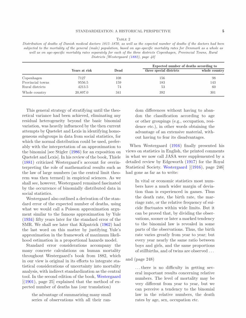
nen (the method of expected deaths), that is, indi-rect standardization. He was well aware of the dan-ger that other factors could distort the result froma standardization by age alone and illustrated in asmall introductory example the importance of whatwe would nowadays call confounder control, and howthe method of expected number of deaths could beused in this connection.Table 2 shows that when comparing the mortality
of medical doctors with that of the general popula-tion, it makes a big difference whether the calcula-tion of expected number of deaths is performed forthe country as a whole or specifically (we would say“conditionally”) for each urbanization stratum. InWestergaard’s words, our English translation:
It is seen from this how difficult it is toconduct a scientific statistical calculation.The two methods both look correct, andstill yield very different results. Accord-ing to one method one would concludethat the medical professionals live undervery unhealthy conditions, according tothe other, that their health is relativelygood.The difficulty derives from the fact thatthere exist two causes: the medical pro-fession and the place of residence; bothcauses have to be taken into account, andif one neglects one of them, the place ofresidence, and only with the help of thegeneral life table considers the influenceof the other, one will make an erroneousconclusion.The safest is to continue the stratifica-tion of the material until no further dis-ruptive causes exist; if one has no otherproof, then a safe sign that this has beenachieved, is that further stratification ofthe material does not change the results.
STANDARDIZATION: A HISTORICAL PERSPECTIVE 5
Table 2
Distribution of deaths of Danish medical doctors 1815–1870, as well as the expected number of deaths if the doctors had beensubjected to the mortality of the general (male) population, based on age-specific mortality rates for Denmark as a whole as
well as on age-specific mortality rates separately for each of the three districts Copenhagen, Provincial Towns, RuralDistricts [Westergaard (1882), page 40]
Expected number of deaths according to
Years at risk Dead three special districts whole country
Copenhagen 7127 108 156 98Provincial towns 9556.5 159 183 143Rural districts 4213.5 74 53 60
Whole country 20,897.0 341 392 301
This general strategy of stratifying until the theo-retical variance had been achieved, eliminating anyresidual heterogeneity beyond the basic binomialvariation, was heavily influenced by the then currentattempts by Quetelet and Lexis in identifying homo-geneous subgroups in data from social statistics, forwhich the normal distribution could be used, prefer-ably with the interpretation of an approximation tothe binomial [see Stigler (1986) for an exposition onQuetelet and Lexis]. In his review of the book, Thiele(1881) criticized Westergaard’s account for overin-terpreting the role of mathematical results such asthe law of large numbers (as the central limit theo-rem was then termed) in empirical sciences. As weshall see, however, Westergaard remained fascinatedby the occurrence of binomially distributed data insocial statistics.Westergaard also outlined a derivation of the stan-
dard error of the expected number of deaths, usingwhat we would call a Poisson approximation argu-ment similar to the famous approximation by Yule(1934) fifty years later for the standard error of theSMR. We shall see later that Kilpatrick (1962) hadthe last word on this matter by justifying Yule’sapproximation in the framework of maximum likeli-hood estimation in a proportional hazards model.Standard error considerations accompany the
many concrete calculations on human mortalitythroughout Westergaard’s book from 1882, whichin our view is original in its efforts to integrate sta-tistical considerations of uncertainty into mortalityanalysis, with indirect standardization as the centraltool. In the second edition of the book, Westergaard[(1901), page 25] explained that the method of ex-pected number of deaths has (our translation)
the advantage of summarizing many smallseries of observations with all their ran-
dom differences without having to aban-don the classification according to ageor other groupings (e.g., occupation, resi-dence etc.), in other words obtaining theadvantage of an extensive material, with-out having to fear its disadvantages.
When Westergaard (1916) finally presented hisviews on statistics in English, the printed commentsin what we now call JASA were supplemented by adetailed review by Edgeworth (1917) for the RoyalStatistical Society. Westergaard [(1916), page 246]had gone as far as to write:
In vital or economic statistics most num-bers have a much wider margin of devia-tion than is experienced in games. Thusthe death rate, the birth rate, the mar-riage rate, or the relative frequency of sui-cide fluctuates within wide limits. But itcan be proved that, by dividing the obser-vations, sooner or later a marked tendencyto the binomial law is revealed in someparts of the observations. Thus, the birthrate varies greatly from year to year; butevery year nearly the same ratio betweenboys and girls, and the same proportionsof stillbirths, and of twins are observed . . .
and (page 248)
. . . there is no difficulty in getting sev-eral important results concerning relativenumbers. The level of mortality may bevery different from year to year, but wecan perceive a tendency to the binomiallaw in the relative numbers, the deathrates by age, sex, occupation etc.

6 N. KEIDING AND D. CLAYTON
Edgeworth questioned that “Westergaard’s pa-nacea” would work as a general remedy in all sit-uations, and continued:
It never seems to have occurred to himthat the “physical” as distinguished fromthe “combinatorial” distribution, to useLexis’ distinction, may be treated by thelaw of error [the normal distribution].
Edgeworth here referred to the empirical (physi-cal) variance as opposed to the binomial (combina-torial). Lexis (1876), in the context of time series ofrates, had defined what we now call the overdisper-sion ratio between these two.
Indirect standardization does not require the age
distribution of the cases Regarding standardization,Westergaard [(1916), page 261 ff.] explained and ex-emplified the method of expected number of deaths,as usual without quoting Neison or other earlierusers of that method, such as Farr, and went on:
English statisticians often use a modifica-tion of the method just described of cal-culating expected deaths; viz., the methodof “standards” (in fact the method of ex-pected deaths can quite as well claim thename of a “standard” method),
and after having outlined direct standardizationconcluded,
In the present case the two forms of com-parison lead to nearly the same result, andthis will generally be the case, if the agedistribution in the special group is notmuch different from that of the generalpopulation. But on the whole the methoddescribed last is a little more complicatedthan the calculation of expected deaths,and in particular not applicable, if the agedistribution of the deaths of the barristersand solicitors is unknown.
This last point (that indirect standardization doesnot require the breakdown of cases in the study pop-ulation by age) has often been emphasized as an im-portant advantage of indirect standardization. Aninteresting application was the study of the emerg-ing fall of the birth rate read to the Royal Statis-tical Society in December 1905 by Newsholme andStevenson (1906) and Yule (1906). [Yule (1920) later
presented a concise popular version of the main find-ings to the Cambridge Eugenics Society, still inter-esting reading.] The problem was that English birthstatistics did not include the age distribution of themother, and it was therefore recommended to usesome standard age-specific birth rates (here: thoseof Sweden for 1891) and then indirect standardiza-tion.
Westergaard and an Early Randomised Clinical
Trial
Westergaard (1918) published a lengthy rebuttal(“On the future of statistics”) to Edgeworth’s cri-tique. Westergaard was here mainly concerned withthe statistician’s overall ambition of contributing to“find the causality”, and with a main point being hiscriticism of “correlation based on Bravais’s formula”as not indicating causality. However, he also had aninteresting, albeit somewhat cryptic, reference to atopic that was to become absolutely central in thecoming years: that simple binomial variation is jus-tified under random sampling. In his 1916 paper, hehad advocated (page 238) that
in many cases it will be practically impos-sible to do without representative statis-tics.
[Edgeworth (1917) taught Westergaard that thecorrect phrase was “sampling”, and Westergaardreplied that English was for him a foreign language.]To illustrate this, Westergaard [(1916), page 245]wrote:
The same formula in a little more com-plicated form can be applied to the chiefproblem in medical statistics; viz., to findwhether a particular method of treatmentof disease is effective. Let the mortalityof patients suffering from the disease bep2, when treated with a serum, p1, whentreated without it, and let the numbers ineach case be n2 and n1. Then the meanerror of the difference between the fre-quencies of dying in the two groups willbe
√p1q1/n1 + p2q2/n2 and we can get
an approximation by putting the observedrelative values instead of p1 and p2.
In his rebuttal, Westergaard [(1918), page 508] re-vealed that this was not just a hypothetical example:
A very interesting method of samplingwas tried several years ago in a Danish
STANDARDIZATION: A HISTORICAL PERSPECTIVE 7
hospital for epidemic diseases in order totest the influence of serum on patients suf-fering from diphtheria. Patients broughtinto the hospital one day were treatedwith serum, the next day’s patients gotno injection, and so on alternately. Herein all probability the two series of obser-vations were homogeneous.
Westergaard here referred to the experiment byFibiger (1898), discussed by Hrobjartsson, Gøtzscheand Gluud (1998), as “the first randomized clinicaltrial” and further documented in the James Lind Li-brary: http://www.jameslindlibrary.org/illustrating/records/om-serumbehandling-af-difteri-on-treatment-of-diphtheria-with-s/key passages.
3. ASSOCIATION, AND CAUSALITY: YULE,
PEARSON AND FOLLOWING
The topic of causality in the early statistical liter-ature is particularly associated with Yule and withPearson, although they were far from the first tograpple with the problem. Yule considered the topicmainly in the context of discrete data, while Pearsonconsidered mainly continuous variables. It is per-haps this which led to some dispute between them,particularly in regard to measures of association.For a detailed review of their differences, see Aldrich(1995).
Yule’s Measures of Association and Partial
Association
For a 2× 2 table with entries a, b, c, d, Yule (1900)defined the association measure Q= (ad− bc)/(ad+bc), noting that it equals 0 under independence and1 or −1 under complete association. There are ofcourse many choices of association measure thatfulfil these conditions. Pearson [(1900), pages 14–18] immediately made strong objections to Yule’s
choice; he wanted a parameter that agreed wellwith the correlation if the 2 × 2 table was gener-ated from an underlying bivariate normal distribu-tion. The discussion between Yule and Pearson andtheir camps went on for more than a decade. It waschronicled from a historical–sociological viewpointby MacKenzie (MacKenzie, 1978, 1981).That he regarded the concrete values of Q mean-
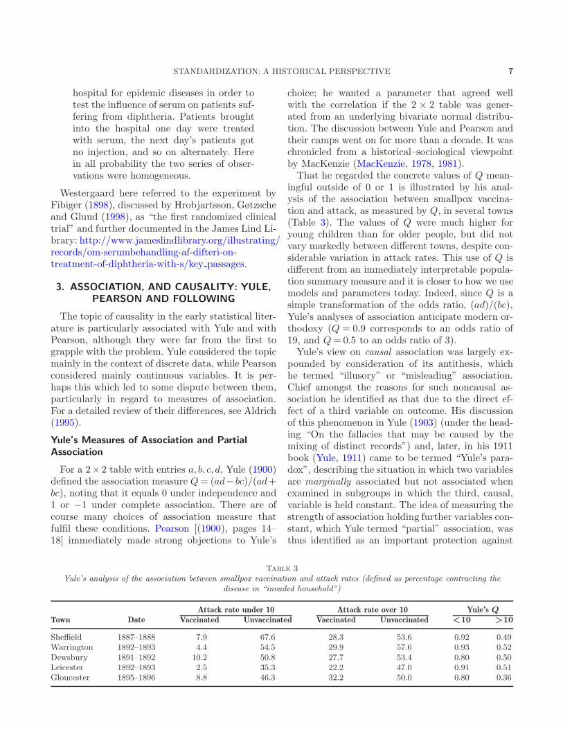
ingful outside of 0 or 1 is illustrated by his anal-ysis of the association between smallpox vaccina-tion and attack, as measured by Q, in several towns(Table 3). The values of Q were much higher foryoung children than for older people, but did notvary markedly between different towns, despite con-siderable variation in attack rates. This use of Q isdifferent from an immediately interpretable popula-tion summary measure and it is closer to how we usemodels and parameters today. Indeed, since Q is asimple transformation of the odds ratio, (ad)/(bc),Yule’s analyses of association anticipate modern or-thodoxy (Q = 0.9 corresponds to an odds ratio of19, and Q= 0.5 to an odds ratio of 3).Yule’s view on causal association was largely ex-
pounded by consideration of its antithesis, whichhe termed “illusory” or “misleading” association.Chief amongst the reasons for such noncausal as-sociation he identified as that due to the direct ef-fect of a third variable on outcome. His discussionof this phenomenon in Yule (1903) (under the head-ing “On the fallacies that may be caused by themixing of distinct records”) and, later, in his 1911book (Yule, 1911) came to be termed “Yule’s para-dox”, describing the situation in which two variablesare marginally associated but not associated whenexamined in subgroups in which the third, causal,variable is held constant. The idea of measuring thestrength of association holding further variables con-stant, which Yule termed “partial” association, wasthus identified as an important protection against
Table 3
Yule’s analysis of the association between smallpox vaccination and attack rates (defined as percentage contracting thedisease in “invaded household”)
Attack rate under 10 Attack rate over 10 Yule’s Q
Town Date Vaccinated Unvaccinated Vaccinated Unvaccinated <10 >10
Sheffield 1887–1888 7.9 67.6 28.3 53.6 0.92 0.49Warrington 1892–1893 4.4 54.5 29.9 57.6 0.93 0.52Dewsbury 1891–1892 10.2 50.8 27.7 53.4 0.80 0.50Leicester 1892–1893 2.5 35.3 22.2 47.0 0.91 0.51Gloucester 1895–1896 8.8 46.3 32.2 50.0 0.80 0.36
8 N. KEIDING AND D. CLAYTON
fallacious causal explanations. However, he did notformally consider modelling these partial associa-tions. Indeed, he commented (Yule, 1900):
The number of possible partial coefficientsbecomes very high as soon as we go be-yond four or five variables.
Yule did not discuss more parsimonious definitionsof partial association, although clearly he regardedthe empirical stability of Q over different subgroupsof data as a strong point in its favour. Commentingon some data on recovery from smallpox, in Yule(1912), he later wrote:
This, as it seems to me, is a most im-portant property . . . If you told any manof ordinary intelligence that the associa-tion between treatment and recovery waslow at the beginning of the experiment,reached a maximum when 50 per cent. ofthe cases were treated and then fell offagain as the proportion of cases treatedwas further increased, he would, I think,be legitimately puzzled, and would requirea good deal of explanation as to whatyou meant by association. . . . The associ-ation coefficient Q keeps the same valuethroughout, quite unaffected by the ratioof cases treated to cases untreated.
Pearson and Tocher’s Test for Identity of Two
Mortality Distributions
Pearson regarded the theory of correlation as offundamental importance, even to the extent of re-placing “the old idea of causality” (Pearson, 1910).Nevertheless, he recognised the existence of “spu-rious” correlations due to incorrect use of indicesor, later, due to a third variable such as race(Pearson, Lee and Bramley-Moore, 1899).Although most of Pearson’s work concerned cor-
relation between continuous variables, perhaps themost relevant to our present discussion is his work,with J. F. Tocher, on comparing mortality distribu-tions. Pearson and Tocher (1915) posed the questionof finding a proper test for comparing two mortal-ity distributions. Having pointed out the problemsof comparing crude mortality rates, they consideredcomparison of standardized rates (or, rather, pro-portions). In their notation, if we denote the numberof deaths in age group s (= 1, . . . , S) in the two sam-ples to be compared by ds, d
′
s and the corresponding
numbers of persons at risk by as, a′
s, then two age-standardized rates can be calculated as
M =1
A
∑As
dsas
and M ′ =1
A
∑As
d′sa′s
,
where As represent the standard population in agegroup s and A =
∑As. Noting that the differ-
ence between standardized rates can be expressedas a weighted mean of the differences between age-specific rates,
M ′ −M =∑ As
A
(dsas
−d′sa′s
),
they showed that, under the null hypothesis thatthe true rates are equal for the two groups to becompared,
Var(M ′ −M) =∑(
As
A
)2
ps(1− ps)
(1
as+
1
a′s
),
where ps denote the (common) age-specific binomialprobabilities. Finally, for large studies, they advo-cated estimation of ps by (ds + d′s)/(as + a′s) andtreating (M ′ −M) as approximately normally dis-tributed or, equivalently,
Q2 =(M ′ −M)2
Var(M ′ −M)
as a chi-squared variate on one degree of freedom(note that their Q2 is not directly related to Yule’sQ). However, they pointed out a major problemwith this approach; that different choices of stan-dard population lead to different answers, and thatthere would usually be objections to any one choice.In an attempt to resolve this difficulty, they pro-posed choosing the weights As/A to maximise thetest statistic and showed that the resulting Q2 is aχ2 test on S degrees of freedom. This is because, asFisher (1922) remarked, each age-specific 2×2-tableof districts vs. survival contributes an independentdegree of freedom to the χ2 test.Pearson and Tocher’s derivation of this test antici-
pates the much later, and more general, derivation ofthe score test as a “Lagrange multiplier test”. How-ever, the maximized test statistic could sometimesinvolve negative weights, As, which they describedas “irrational”. This feature of the test makes it sen-sitive to differences in mortality in different direc-tions at different ages. They discussed the desirabil-ity of this feature and noted that it should be pos-sible to carry out the maximisation subject to theweights being positive but “could not see how” to
STANDARDIZATION: A HISTORICAL PERSPECTIVE 9
do this (the derivation of a test designed to detectdifferences in the same direction in all age groupswas not to be proposed until the work of Cochran,nearly forty years later—see our discussion of the2 × 2 × K below). However, they argued that thesensitivity of their test to differences in death ratesin different directions in different age groups in factrepresented an improvement over the comparison ofcorrected, or standardized, rates since “that idea isessentially imperfect and does not really distinguishbetween differences in the manner of dying”.
Further Application of the Method of Expected
Numbers of Deaths
As described in Section 2, Westergaard (1882)from the very beginning emphasised that expectednumbers of death could be calculated accordingto any stratification, not just age. Encouraged byWestergaard’s (1916) survey in English, Woodbury(1922) demonstrated this through the example ofinfant mortality as related to mother’s age, parity(called here order of birth), earnings of father andplural births. For example, the crude death ratesby order of births form a clear J-shaped patternwith nadir at third birth; assuming that only ageof the mother was a determinant, one can calculatethe expected rates for each order of birth, and onegets still a J, though somewhat attenuated, showingthat a bit of the effect of birth order is explained bymother’s age. Woodbury did not forget to warn:
Since it is an averaging process the methodwill yield satisfactory results only when anaverage is appropriate.
Stouffer and Tibbitts (1933) followed up by point-ing out that in many situations the calculations ofexpected numbers for χ2 tests would coincide withthe “Westergaard method”.
4. STANDARDIZATION IN THE 20TH
CENTURY
Although, as we have seen, standardisation meth-ods were widely used in the 19th century, it wasin the 20th century that a more careful examina-tion of the properties of these methods was made.Particularly important are the authoritative reviewsby Yule (1934) and, thirty years later, by Kitagawa(Kitagawa, 1964, 1966). Both these authors saw theprimary aim as being the construction of what Yuletermed “an average ratio of mortalities”, althoughYule went on to remark:
in Annual Reports and Statistical Re-views the process is always carried a stagefurther, viz. to the calculation of a “stan-dardized death-rate”. This extension is re-ally superfluous, though it may have itsconveniences
(the standardized rate in the study population be-ing constructed by multiplying the crude rate in thestandard population by the standardized ratio ofrates for the study population versus the standardpopulation).
Ratio of Averages or Average of Ratios?
Both Yule and Kitagawa noted that central to thediscussion was the consideration of two sorts of in-dices. The first of these, termed a “ratio of aver-ages” by Yule, has the form
∑wixi/
∑wiyi, while
the second, which he termed an “average of ratios”,has the form
∑w∗
i (xi/yi)/∑
w∗
i . Kitagawa notedthat economists would describe the former as an“aggregative index” and the latter as an “averageof relatives”.Both authors pointed out that, although the two
types of indexes seem to be doing rather differentthings, it is somewhat puzzling that they are alge-braically equivalent—we only have to write w∗
i =wiyi. It is important to note, however, that the al-gebraic equivalence does not mean that a given in-dex is equally interpretable in either sense. Thus, forthe index to be interpretable as a ratio of averages,the weights wi must reflect some population distri-bution so that numerator and denominator of theindex represent marginal expectations in the samepopulation. Alternatively, to present the average ofthe age-specific ratios, xi/yi, as a single measure ofthe age-specific effect would be misleading if theywere not reasonably homogeneous. Kitagawa con-cluded:
the choice between an aggregative indexand an average of relatives in a mortalityanalysis, for example, should be made onthe basis of whether the researcher wantsto compare two schedules of death ratesin terms of the total number of deathsthey would yield in a standard populationor in terms of the relative (proportionate)differences between corresponding specificrates in the two schedules. Both types ofindex can be useful when correctly appliedand interpreted.
10 N. KEIDING AND D. CLAYTON
Here Kitagawa very clearly defined the distinctionbetween what we, in the Introduction, termed themarginal and the conditional targets. Immediatelyafter this definition, she hastened to point out that:
It must be recognized at the outset, how-ever, that no single summary statistic canbe a substitute for a detailed comparisonof the specific rates in two or more sched-ules of rates.
On the matter of averaging different ratios, Yule(1934) started his paper with the example of com-paring the death rates for England and Wales for1901 and 1931. His Table I contains these for bothsexes in 5-year age groups and he commented:
. . . the rates have fallen at all ages up to75 for males and 85 for females. At thesame time the amount of the fall is verydifferent at different ages, apart even fromthe actual rise in old age. The problem issimply to obtain some satisfactory form ofaverage of all the ratios shown in columns4 and 7, an average which will measurein summary form the general fall in mor-tality between the two epochs, just as anindex-number measures the general fall orrise in prices.
So far, there is no requirement for these ratios tobe similar. However, when describing indirect stan-dardisation, Yule [(1934), page 12] pointed out that
if . . . all the ratios of sub-rates are thesame, no variation of weighting can makeany difference,
and warned (page 13),
and perhaps it may be remarked that. . . if the ratios mur/msr are very differentin different age groups, any comparativemortality figure becomes of questionablevalue.
The issue of constancy of ratios was picked up inthe printed discussion of the paper [Yule, 1934, page76] by Percy Stokes, seconder of vote of thanks:
Those of us who have taught these meth-ods to students have been accustomed topoint out that they lead to identical re-sults when the local rates bear to the stan-dard rates the same proportion at everyage.
Comparability of Mortality Ratios
Yule noted that, particularly in official mortalitystatistics, standardisation is applied to many differ-ent study populations so that, as well as the stan-dardized ratio of mortality in each study popula-tion to the standard population being meaningfulin its own right, the comparison of the indices fortwo study populations should also be meaningful.He drew attention to the fact that the ratio of twoseemingly legitimate indices is not necessarily itselfa legitimate index. He concluded that either type ofindex could legitimately be used either if the sameweights wi are used across study populations (forratios of averages) or if the same w∗
i are used (foraverages of ratios).Denoting a standardized ratio for comparing
study groups A and B with standard by sRa
and sRb, respectively, Yule suggested that sRa/sRb
should be a legitimate index of the ratio of mortali-ties in population A to that in population B. He alsosuggested that, ideally, aRb = sRa/sRb but notedthat, whereas the CMF of direct standardisation ful-fills the former criterion, no method of standardisa-tion hitherto suggested fulfilled this more stringentcriterion. Indirect standardisation fulfils neither cri-terion and Yule judged it to be “hardly a method ofstandardisation at all”.Yule’s paper is also famous for its derivation of
standard errors of comparative mortality figures; forthe particular case of the SMR, we have
SMR=Observed/Expected, O/E
and
S.E.(SMR)≈√O/E.
As noted earlier, this was already derived by West-ergaard (1882), although this was apparently notgenerally known.A final matter occupying no less than twelve pages
of Yule (1934) is the discussion of a context-free av-erage, termed by Yule his C3 method or the equiv-
alent average death rate, which is just the simpleaverage of all age-specific death rates. This quantitycould also be explained as the death rate standard-ized to a population with equal numbers in eachage group. As we shall see below, it was furtherdiscussed by Kilpatrick (1962) and rediscovered byDay (1976) in an application to cancer epidemiology.In modern survival analysis it is called the cumula-tive hazard and estimated nonparametrically by theNelson–Aalen estimator (Nelson, 1972, Aalen, 1978,Andersen et al., 1993).
STANDARDIZATION: A HISTORICAL PERSPECTIVE 11
Elaboration: Rosenberg’s Test Factor
Standardisation
During World War II, the United States Armyestablished a Research Branch to investigate prob-lems of morale, soldier preferences and other issuesto provide information that would allow the mili-tary to make sensible decisions on practical issuesinvolved in army life. To formalize some of the toolsused in that generally rather practical research, il-lustrated with concrete examples from that work,Kendall and Lazarsfeld (1950) introduced and dis-cussed the terminology of elaboration: A statisticalrelation has been established between two variables,one of which is assumed to be the cause, the otherto be the effect. The aim is to further understandthat relation by introducing a third variable (calledtest factor) related to the “cause” as well as the “ef-fect”. Kendall and Lazarsfeld carefully distinguishedbetween antecedent and intervening test variables,depending on the temporal order of the “cause” andthe test variables. If the population is stratified ac-cording to an antecedent test factor, and the par-tial relationships between the two original variablesthen vanish, the relation between “cause” and “ef-fect” has been explained through their relations tothe test variable, which is then termed spurious. Ifthe association between cause and effect disappears(is reduced) by controlling on the intervening vari-able, Kendall and Lazarsfeld talk about complete(partial) interpretation of the original two-factor re-lationship.We note that interpretation has gone out of use
at least in epidemiological applications and in mostof modern causal inference where the focus is on ob-taining an undiluted measure of the causal effect ofthe “cause”, not diluting this effect by conditioningon variables on the causal pathway from cause to ef-fect [see Pearl (2001) or Petersen, Sinisi and van derLaan (2006)]. Instead, a general area of MediationAnalysis has grown up; see MacKinnon (2008), Sec-tion 1.8, for a useful historical survey.Rosenberg (1962) used standardization to obtain
a single summary measure from all the partial (i.e.,conditional) associations resulting from the stratifi-cation in an elaboration. Rosenberg’s famous exam-ple was a study of the possible association betweenreligious affiliation and self-esteem for high schoolstudents, controlling for (all combinations of) fa-ther’s education, social class identification and highschool grades. Thus, this is an example of interpreta-tion by conditioning on variables that might mediate
an effect of religious affiliation on sons’ self-esteem.The crude association showed higher self-esteem forJews than for Catholics and Protestants; by stan-dardizing on the joint distribution of the three co-variates in the total population this difference washalved.Rosenberg emphasized that in survey research the
end product of the standardisation exercise is not asingle rate as in demography, but:
In survey research, however, we are inter-ested in total distributions. Thus, if we ex-amine the association between X and Ystandardizing on Z, we must emerge witha standardised table (of the joint distribu-tion of X and Y ) which contains all thecells of the original table.
Rosenberg indicated shortcuts to avoid repeatingthe same calculations when calculating the entriesof this table.
The Peters–Belson Approach
This technique (Belson (1956), Peters (1941)) wasdeveloped for comparing an experimental groupwith a control group in an observational study onsome continuous outcome. The proposal is to regressthe outcome on covariates only in the control groupand use the resulting regression equation to predictthe results for the experimental group under the as-sumption of no difference between the groups. Asimple test of no differences concludes the analysis.Cochran (1969) showed that under some assump-tions of (much) larger variance in the experimentalgroup than the control group this technique mightyield stronger inference than standard analysis ofcovariance, and that it will also be robust to cer-tain types of effect modification. The technique hasrecently been revived by Graubard, Rao and Gast-wirth (2005).
Decomposition of Crude Rate Differences and
Ratios
Several authors have suggested a decompositionof a contrast between two crude rates into a com-ponent due to differences between the age-specificrates and a component due to differences betweenthe age structures of the two populations.Kitagawa (1955) proposed an additive decompo-
sition in which the difference in crude rates is ex-pressed as a sum of (a) the difference between the(direct) standardized rates, and (b) a residual due to
12 N. KEIDING AND D. CLAYTON
the difference in age structure. Rather than treatingone population as the standard population and thesecond as the study population, she treated themsymmetrically, standardising both to the mean ofthe two populations’ age structures:
Crude rate (study)−Crude rate (standard)
=∑
aiαi −∑
siλi
=∑
(αi − λi)ai + si
2+∑
(ai − si)αi + λi
2.
The first term contrasts the standardized rates whilethe second contrasts the age structures.However, ratio comparisons are more frequently
employed when contrasting rates and several au-thors have considered a multiplicative decomposi-tion in which the ratio of crude rates is expressedas the product of a standardized rate ratio anda factor reflecting the effect of the different agestructures. Such a decomposition, in which the age-standardized measure is the SMR, was proposed byMiettinen (1972b):
Crude rate (study)
Crude rate (standard)=
∑aiαi∑siλi
=
∑aiαi∑aiλi
×
∑aiλi∑siλi
.
The first term is the SMR and the second, whichreflects the effect of the differing age structures, Mi-ettinen termed the “confounding risk ratio”.Kitagawa (1964) had also proposed a multiplica-
tive decomposition which, as in her additive decom-position, treated the two populations symmetrically.Here, the standardized ratio measure was inspiredby the literature on price indices in economics. If, ina “base” year, the price of commodity i is p0i and thequantity purchased is q0i and, in year t the equiva-lent values are pti and qti, then an overall compar-ison of prices requires adjustment for differing con-sumption patterns. Simple relative indices can beconstructed by fixing consumption at base or at t.The former is Laspeyres’s index,
∑ptiq0i/
∑p0iq0i,
and the latter is Paasche’s index,∑
piqti/∑
p0iqti.These are asymmetric with respect to the two timepoints and this asymmetry is addressed in Fisher’s“ideal” index, defined as the geometric mean ofLaspeyres’s and Paasche’s indices. Kitagawa notedthat Laspeyres’s and Paasche’s indices are directlyanalogous to the CMF and SMR, respectively, and,
in her symmetric decomposition,
∑aiαi∑siλi
=
√∑siαi∑siλi
×
∑aiαi∑aiλi
×
√∑λiai∑λisi
×
∑αiai∑αisi
,
the first term is an “ideal” index formed by the geo-metric mean of the CMF and SMR, and the secondterm is:
the geometric mean of two indexes sum-marizing differences in I-composition; onean aggregative index using the I-specificrates of the base population as weights,and the second an aggregative index usingthe I-specific rates of the given populationas weights.
The paper by Kitagawa (1955) concluded with adetailed comparison to the “Westergaard method”as documented by Woodbury (1922). Woodbury’spaper had also inspired Kitagawa’s contemporaryR. H. Turner, also a Ph.D. from the University ofChicago, to develop an approach to additive de-composition according to several covariates (Turner,1949), showing how the “nonwhite–white” differ-ential in labour force participation is associatedwith marital status, household relationship and age.Kitagawa’s decomposition paper continues to be fre-quently cited and the technique is still includedin current textbooks in demography [e.g., Preston,Heuveline and Guillot (2001)]. There has been aconsiderable further development of additive decom-position ideas; for recent reviews see Chevan andSutherland (2009) for the development in demogra-phy and Powers and Yun (2009) for decompositionof hazard rate models and some references to de-velopments in econometrics and to some extent insociology. We return in Section 6 to the connectionwith the method of “purging” suggested by C. C.Clogg.
5. ODDS RATIOS AND THE 2× 2×K
CONTINGENCY TABLE
Case–Control Studies and the Odds Ratio
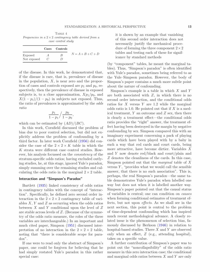
Although the case-control study has a long his-tory, its use to provide quantitative measures ofthe strength of association is more recent, gener-ally being attributed to Cornfield (1951). Table 4sets out results from a hypothetical case–controlstudy comparing some exposure in cases of a dis-ease with that in a control group of individuals free
STANDARDIZATION: A HISTORICAL PERSPECTIVE 13
Table 4
Frequencies in a 2× 2 contingency table derived from acase–control study
Cases Controls
Exposed A BNot exposed C D
N =A+B +C +D
of the disease. In this work, he demonstrated that,if the disease is rare, that is, prevalence of diseasein the population, X , is near zero and the propor-tion of cases and controls exposed are p1 and p0, re-spectively, then the prevalence of disease in exposedsubjects is, to a close approximation, Xp1/p0, andX(1 − p1)/(1 − p0) in subjects not exposed. Thus,the ratio of prevalences is approximated by the oddsratio
p11− p1
/ p01− p0
,
which can be estimated by (AD)/(BC).In this work, Cornfield discussed the problem of
bias due to poor control selection, but did not ex-plicitly address the problem of confounding by athird factor. In later work Cornfield (1956) did con-sider the case of the 2× 2 ×K table in which theK strata were different case–control studies. How-ever, his analysis focussed on the consistency of thestratum-specific odds ratios; having excluded outly-ing studies, he, at this stage, ignored Yule’s paradox,simply summing over the remaining studies and cal-culating the odds ratio in the marginal 2× 2 table.
Interaction and “Simpson’s Paradox”
Bartlett (1935) linked consistency of odds ratiosin contingency tables with the concept of “interac-tion”. Specifically, he defined zero second order in-teraction in the 2× 2× 2 contingency table of vari-ables X , Y and Z as occurring when the odds ratiosbetween X and Y conditional upon the level of Zare stable across levels of Z. (Because of the symme-try of the odds ratio measure, the roles of the threevariables are interchangeable.) In an important andmuch cited paper, Simpson (1951) discussed inter-pretation of no interaction in the 2 × 2 × 2 table,noting that “there is considerable scope for para-dox”.If one were to read only the abstract of Simpson’s
paper, one could be forgiven for believing that hehad simply restated Yule’s paradox in this ratherspecial case:
it is shown by an example that vanishingof this second order interaction does notnecessarily justify the mechanical proce-dure of forming the three component 2×2tables and testing each of these for signif-icance by standard methods
(by “component” tables, he meant the marginal ta-bles). Thus, “Simpson’s paradox” is often identifiedwith Yule’s paradox, sometimes being referred to asthe Yule–Simpson paradox. However, the body ofSimpson’s paper contains a much more subtle pointabout the nature of confounding.Simpson’s example is a table in which X and Y
are both associated with Z, in which there is nosecond order interaction, and the conditional oddsratios for X versus Y are 1.2 while the marginalodds ratio is 1.0. He pointed out that if X is a med-ical treatment, Y an outcome and Z sex, then thereis clearly a treatment effect—the conditional oddsratio provides the “right” answer, the treatment ef-fect having been destroyed in the margin by negativeconfounding by sex. Simpson compared this with animaginary experiment concerning a pack of playingcards which have been played with by a baby insuch a way that red cards and court cards, beingmore attractive, have become dirtier. Variables Xand Y now denote red/black and court/plain andZ denotes the cleanliness of the cards. In this case,Simpson pointed out that the marginal table of Xversus Y , “provides what we would call the sensibleanswer, that there is no such association”. This is,perhaps, the real Simpson’s paradox—the same ta-ble demonstrates Yule’s paradox when labelled oneway but does not when it is labelled another way.Simpson’s paper pointed out that the causal statusof variables is central; one can condition on causes
when forming conditional estimates of treatment ef-fects, but not upon effects. As we shall see in thenext section, this point is central to the problemof time-dependent confounding which has inspiredmuch recent methodological advance. A closely re-lated issue is the phenomenon of selection bias, fa-mously discussed by Berkson (1946) in relation tohospital-based studies. There X and Y are observedonly when an effect, Z (e.g., attending hospital),takes on a specific value.A further contribution of Simpson’s paper was to
point out the “noncollapsibility” of the odds ratiomeasure in this zero interaction case; the conditionaland marginal odds ratios between X and Y are only
14 N. KEIDING AND D. CLAYTON
the same if either X is conditionally independent ofZ given Y , or Y is conditionally independent of Zgiven X . Note that these conditions may not be sat-isfied even in randomised studies—another of theparadoxes to which Simpson drew attention. Fora more detailed discussion of Simpson’s paper seeHernan, Clayton and Keiding (2011).
Cochran’s Analyses of the 2× 2×K Table
In his important paper on “methods for strength-ening the common χ2 test”, Cochran (1954) pro-posed a “combined test of significance of the dif-ference in occurrence rates in the two samples”when “the whole procedure is repeated a number oftimes under somewhat differing environmental con-ditions”. He pointed out that carrying out the χ2
test in the marginal table
is legitimate only if the probability p of anoccurrence (on the null hypothesis) can beassumed to be the same in all the individ-ual 2× 2 tables.
(He did not further qualify this statement in thelight of Simpson’s insight discussed above.) He pro-posed three alternative analyses. The first of thesewas to add up the χ2 test statistics from each tableand to compare the result with the χ2 distributionon K degrees of freedom. This, as already noted, isequivalent to Pearson and Tocher’s earlier proposal,but Cochran judged it a poor method since
It takes no account of the signs of the dif-ferences (p1− p0) in the two samples, andconsequently lacks power in detecting adifference that shows up consistently inthe same direction in all or most of theindividual tables.
The second alternative he considered was to calcu-late the “χ” value for each table—the square rootsof the χ2 statistics, with signs equal to those of thecorresponding (p1 − p0)’s—and to compare the sumof these values with the normal distribution withmean zero and variance K. He noted, however, thatthis method would not be appropriate if the samplesizes (the “N ′s”) vary substantially between tables,since
Tables that have very small N ’s cannotbe expected to be of much use in detect-ing a difference, yet they receive the sameweight as tables with large N ′s.
He also noted that variation of the probabilities ofoutcome between tables would also adversely affectthe power of this method:
Further, if the p’s vary from say 0 to 50%,the difference that we are trying to detect,if present, is unlikely to be constant at alllevels of p. A large amount of experiencesuggests that the difference is more likelyto be constant on the probit or logit scale.
It is clear, therefore, that Cochran considered theideal analysis to be based on a model of “constanteffect” across the tables. Indeed, when the data weresufficiently extensive, he advocated use of empiricallogit or probit transformation of the observed pro-portions followed by model fitting by weighted leastsquares. Such an approach, based on fitting a formalmodel to a table of proportions, had already beenpioneered by Dyke and Patterson (1952), and willbe discussed in Section 6.In situations in which the data were not suffi-
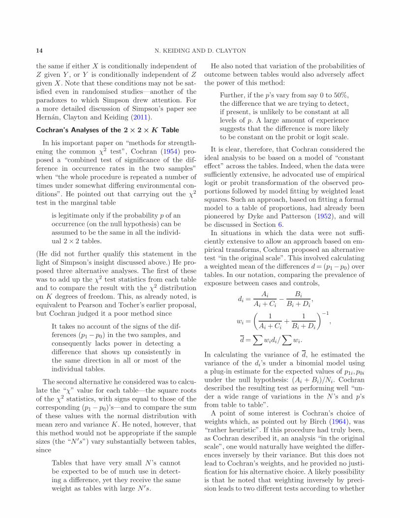
ciently extensive to allow an approach based on em-pirical transforms, Cochran proposed an alternativetest “in the original scale”. This involved calculatinga weighted mean of the differences d= (p1−p0) overtables. In our notation, comparing the prevalence ofexposure between cases and controls,
di =Ai
Ai +Ci
−Bi
Bi +Di
,
wi =
(1
Ai +Ci
+1
Bi +Di
)−1
,
d=∑
widi/∑
wi.
In calculating the variance of d, he estimated thevariance of the di’s under a binomial model usinga plug-in estimate for the expected values of p1i, p0iunder the null hypothesis: (Ai + Bi)/Ni. Cochrandescribed the resulting test as performing well “un-der a wide range of variations in the N ’s and p’sfrom table to table”.A point of some interest is Cochran’s choice of
weights which, as pointed out by Birch (1964), was“rather heuristic”. If this procedure had truly been,as Cochran described it, an analysis “in the originalscale”, one would naturally have weighted the differ-ences inversely by their variance. But this does notlead to Cochran’s weights, and he provided no justi-fication for his alternative choice. A likely possibilityis that he noted that weighting inversely by preci-sion leads to two different tests according to whether
STANDARDIZATION: A HISTORICAL PERSPECTIVE 15
we choose to compare the proportions exposed be-tween cases and control or the proportions of casesbetween exposed and unexposed groups. Cochran’schoice of weights avoided this embarrassment.
Mantel and Haenszel
Seemingly unaware of Cochran’s work, Manteland Haenszel (1959) considered the analysis of the2× 2×K contingency table. This paper explicitlyrelated the discussion to control for confounding incase–control studies. Before discussing this famouspaper, however, it is interesting that the same au-thors had suggested an alternative approach a yearearlier (Haenszel, Shimkin and Mantel, 1958).As in Cochran’s analysis, the idea was based on
post-stratification of cases and controls into stratawhich are as homogeneous as possible. Arguing byanalogy with the method of indirect standardisa-tion of rates, they suggested that the influence ofconfounding on the odds ratio could be assessed bycalculating, for each stratum, s, the “expected” fre-quencies in the 2× 2 table under the assumption ofno partial association within strata and calculatingthe marginal odds ratio under this assumption. Theobserved marginal odds ratio was then adjusted bythis factor. Thus, denoting the expected frequenciesby ai, bi, ci and di where ai = (Ai +Bi)(Ai +Ci)/Ni
etc., their proposed index was∑
Ai
∑Di∑
Bi
∑Ci
/∑ai∑
di∑bi∑
ci.
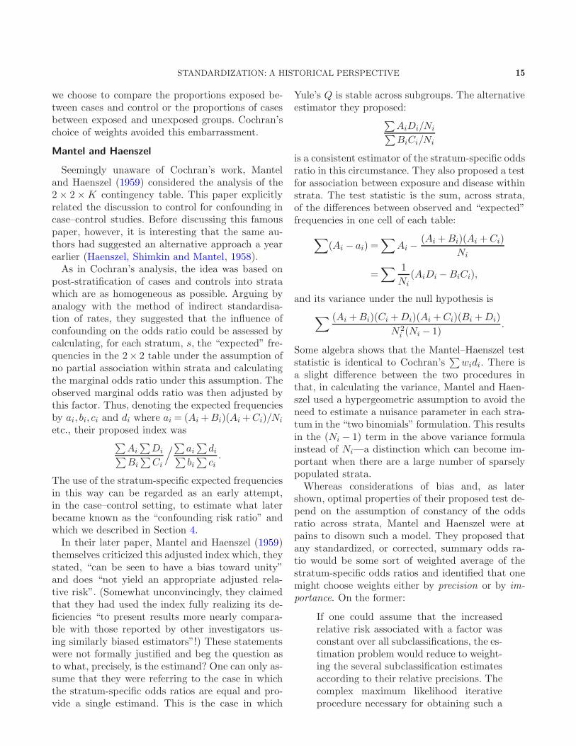
The use of the stratum-specific expected frequenciesin this way can be regarded as an early attempt,in the case–control setting, to estimate what laterbecame known as the “confounding risk ratio” andwhich we described in Section 4.In their later paper, Mantel and Haenszel (1959)
themselves criticized this adjusted index which, theystated, “can be seen to have a bias toward unity”and does “not yield an appropriate adjusted rela-tive risk”. (Somewhat unconvincingly, they claimedthat they had used the index fully realizing its de-ficiencies “to present results more nearly compara-ble with those reported by other investigators us-ing similarly biased estimators”!) These statementswere not formally justified and beg the question asto what, precisely, is the estimand? One can only as-sume that they were referring to the case in whichthe stratum-specific odds ratios are equal and pro-vide a single estimand. This is the case in which
Yule’s Q is stable across subgroups. The alternativeestimator they proposed:
∑AiDi/Ni∑BiCi/Ni
is a consistent estimator of the stratum-specific oddsratio in this circumstance. They also proposed a testfor association between exposure and disease withinstrata. The test statistic is the sum, across strata,of the differences between observed and “expected”frequencies in one cell of each table:
∑(Ai − ai) =
∑Ai −
(Ai +Bi)(Ai +Ci)
Ni
=∑ 1
Ni
(AiDi −BiCi),
and its variance under the null hypothesis is
∑ (Ai +Bi)(Ci +Di)(Ai +Ci)(Bi +Di)
N2i (Ni − 1)
.
Some algebra shows that the Mantel–Haenszel teststatistic is identical to Cochran’s
∑widi. There is
a slight difference between the two procedures inthat, in calculating the variance, Mantel and Haen-szel used a hypergeometric assumption to avoid theneed to estimate a nuisance parameter in each stra-tum in the “two binomials” formulation. This resultsin the (Ni − 1) term in the above variance formulainstead of Ni—a distinction which can become im-portant when there are a large number of sparselypopulated strata.Whereas considerations of bias and, as later
shown, optimal properties of their proposed test de-pend on the assumption of constancy of the oddsratio across strata, Mantel and Haenszel were atpains to disown such a model. They proposed thatany standardized, or corrected, summary odds ra-tio would be some sort of weighted average of thestratum-specific odds ratios and identified that onemight choose weights either by precision or by im-
portance. On the former:
If one could assume that the increasedrelative risk associated with a factor wasconstant over all subclassifications, the es-timation problem would reduce to weight-ing the several subclassification estimatesaccording to their relative precisions. Thecomplex maximum likelihood iterativeprocedure necessary for obtaining such a
16 N. KEIDING AND D. CLAYTON
weighted estimate would seem to be un-justified, since the assumption of a con-stant relative risk can be discarded as usu-ally untenable.
They described the weighting scheme used inthe Mantel–Haenszel estimator as approximatelyweighting by precision. Indeed, it turns out thatthese weights correspond to optimal weighting byprecision for odds ratios close to 1.0.An alternative standardized odds ratio estimate,
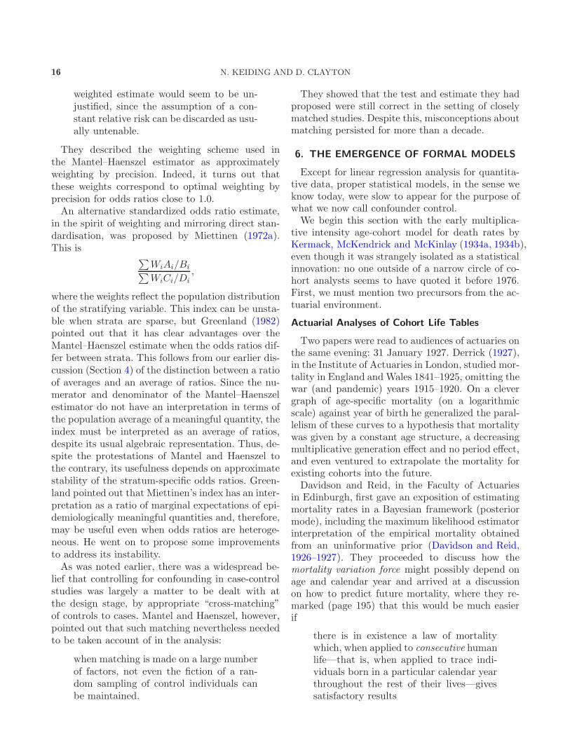
in the spirit of weighting and mirroring direct stan-dardisation, was proposed by Miettinen (1972a).This is
∑WiAi/Bi∑WiCi/Di
,
where the weights reflect the population distributionof the stratifying variable. This index can be unsta-ble when strata are sparse, but Greenland (1982)pointed out that it has clear advantages over theMantel–Haenszel estimate when the odds ratios dif-fer between strata. This follows from our earlier dis-cussion (Section 4) of the distinction between a ratioof averages and an average of ratios. Since the nu-merator and denominator of the Mantel–Haenszelestimator do not have an interpretation in terms ofthe population average of a meaningful quantity, theindex must be interpreted as an average of ratios,despite its usual algebraic representation. Thus, de-spite the protestations of Mantel and Haenszel tothe contrary, its usefulness depends on approximatestability of the stratum-specific odds ratios. Green-land pointed out that Miettinen’s index has an inter-pretation as a ratio of marginal expectations of epi-demiologically meaningful quantities and, therefore,may be useful even when odds ratios are heteroge-neous. He went on to propose some improvementsto address its instability.As was noted earlier, there was a widespread be-
lief that controlling for confounding in case-controlstudies was largely a matter to be dealt with atthe design stage, by appropriate “cross-matching”of controls to cases. Mantel and Haenszel, however,pointed out that such matching nevertheless neededto be taken account of in the analysis:
when matching is made on a large numberof factors, not even the fiction of a ran-dom sampling of control individuals canbe maintained.
They showed that the test and estimate they hadproposed were still correct in the setting of closelymatched studies. Despite this, misconceptions aboutmatching persisted for more than a decade.
6. THE EMERGENCE OF FORMAL MODELS
Except for linear regression analysis for quantita-tive data, proper statistical models, in the sense weknow today, were slow to appear for the purpose ofwhat we now call confounder control.We begin this section with the early multiplica-
tive intensity age-cohort model for death rates byKermack, McKendrick and McKinlay (1934a, 1934b),even though it was strangely isolated as a statisticalinnovation: no one outside of a narrow circle of co-hort analysts seems to have quoted it before 1976.First, we must mention two precursors from the ac-tuarial environment.
Actuarial Analyses of Cohort Life Tables
Two papers were read to audiences of actuaries onthe same evening: 31 January 1927. Derrick (1927),in the Institute of Actuaries in London, studied mor-tality in England and Wales 1841–1925, omitting thewar (and pandemic) years 1915–1920. On a clevergraph of age-specific mortality (on a logarithmicscale) against year of birth he generalized the paral-lelism of these curves to a hypothesis that mortalitywas given by a constant age structure, a decreasingmultiplicative generation effect and no period effect,and even ventured to extrapolate the mortality forexisting cohorts into the future.Davidson and Reid, in the Faculty of Actuaries
in Edinburgh, first gave an exposition of estimatingmortality rates in a Bayesian framework (posteriormode), including the maximum likelihood estimatorinterpretation of the empirical mortality obtainedfrom an uninformative prior (Davidson and Reid,1926–1927). They proceeded to discuss how themortality variation force might possibly depend onage and calendar year and arrived at a discussionon how to predict future mortality, where they re-marked (page 195) that this would be much easierif
there is in existence a law of mortalitywhich, when applied to consecutive humanlife—that is, when applied to trace indi-viduals born in a particular calendar yearthroughout the rest of their lives—givessatisfactory results
STANDARDIZATION: A HISTORICAL PERSPECTIVE 17
or, as we would say, if the cohort life table could bemodelled. Davidson and Reid also explained theiridea through a well-chosen, though purely theoreti-cal, graph.
The Multiplicative Model of Kermack,
McKendrick and McKinley
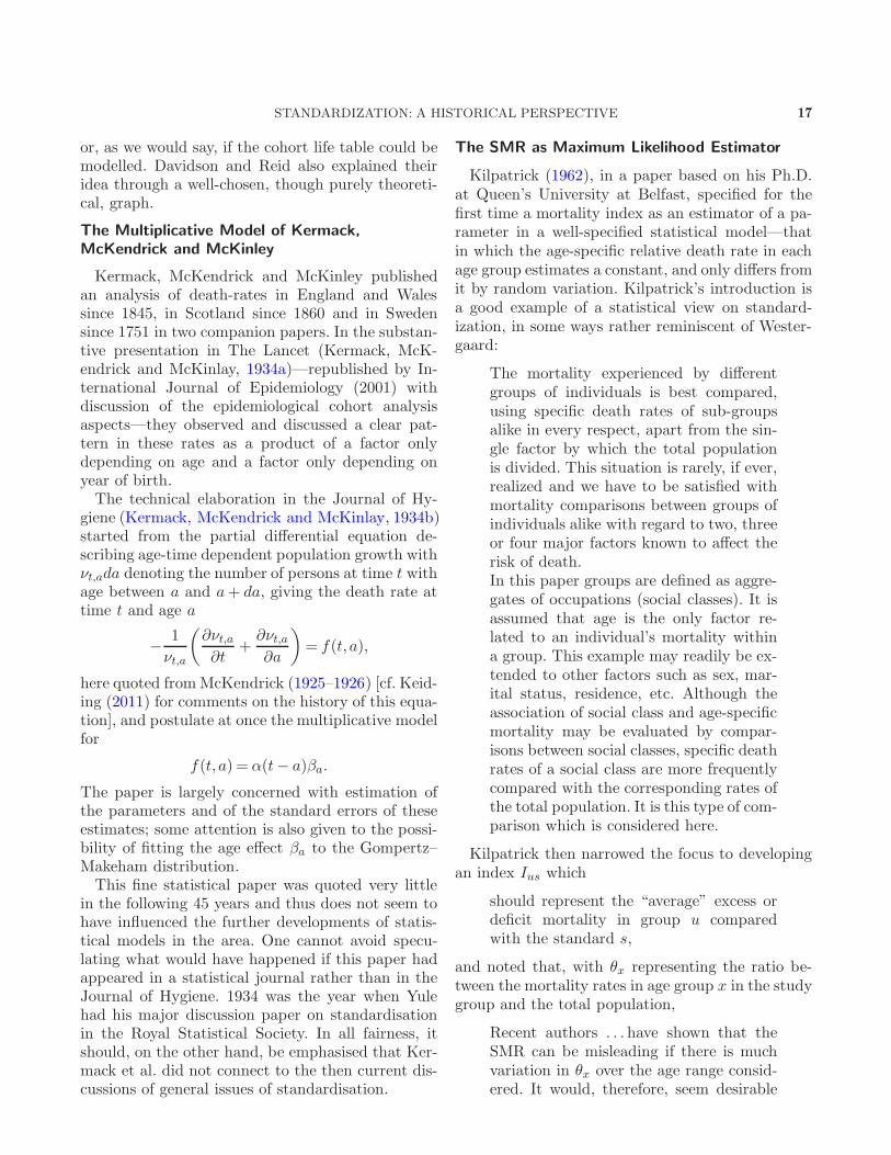
Kermack, McKendrick and McKinley publishedan analysis of death-rates in England and Walessince 1845, in Scotland since 1860 and in Swedensince 1751 in two companion papers. In the substan-tive presentation in The Lancet (Kermack, McK-endrick and McKinlay, 1934a)—republished by In-ternational Journal of Epidemiology (2001) withdiscussion of the epidemiological cohort analysisaspects—they observed and discussed a clear pat-tern in these rates as a product of a factor onlydepending on age and a factor only depending onyear of birth.The technical elaboration in the Journal of Hy-
giene (Kermack, McKendrick and McKinlay, 1934b)started from the partial differential equation de-scribing age-time dependent population growth withνt,ada denoting the number of persons at time t withage between a and a+ da, giving the death rate attime t and age a
−1
νt,a
(∂νt,a∂t
+∂νt,a∂a
)= f(t, a),
here quoted fromMcKendrick (1925–1926) [cf. Keid-ing (2011) for comments on the history of this equa-tion], and postulate at once the multiplicative modelfor
f(t, a) = α(t− a)βa.
The paper is largely concerned with estimation ofthe parameters and of the standard errors of theseestimates; some attention is also given to the possi-bility of fitting the age effect βa to the Gompertz–Makeham distribution.This fine statistical paper was quoted very little
in the following 45 years and thus does not seem tohave influenced the further developments of statis-tical models in the area. One cannot avoid specu-lating what would have happened if this paper hadappeared in a statistical journal rather than in theJournal of Hygiene. 1934 was the year when Yulehad his major discussion paper on standardisationin the Royal Statistical Society. In all fairness, itshould, on the other hand, be emphasised that Ker-mack et al. did not connect to the then current dis-cussions of general issues of standardisation.
The SMR as Maximum Likelihood Estimator
Kilpatrick (1962), in a paper based on his Ph.D.at Queen’s University at Belfast, specified for thefirst time a mortality index as an estimator of a pa-rameter in a well-specified statistical model—thatin which the age-specific relative death rate in eachage group estimates a constant, and only differs fromit by random variation. Kilpatrick’s introduction isa good example of a statistical view on standard-ization, in some ways rather reminiscent of Wester-gaard:
The mortality experienced by differentgroups of individuals is best compared,using specific death rates of sub-groupsalike in every respect, apart from the sin-gle factor by which the total populationis divided. This situation is rarely, if ever,realized and we have to be satisfied withmortality comparisons between groups ofindividuals alike with regard to two, threeor four major factors known to affect therisk of death.In this paper groups are defined as aggre-gates of occupations (social classes). It isassumed that age is the only factor re-lated to an individual’s mortality withina group. This example may readily be ex-tended to other factors such as sex, mar-ital status, residence, etc. Although theassociation of social class and age-specificmortality may be evaluated by compar-isons between social classes, specific deathrates of a social class are more frequentlycompared with the corresponding rates ofthe total population. It is this type of com-parison which is considered here.
Kilpatrick then narrowed the focus to developingan index Ius which
should represent the “average” excess ordeficit mortality in group u comparedwith the standard s,
and noted that, with θx representing the ratio be-tween the mortality rates in age group x in the studygroup and the total population,
Recent authors . . . have shown that theSMR can be misleading if there is muchvariation in θx over the age range consid-ered. It would, therefore, seem desirable

18 N. KEIDING AND D. CLAYTON
to test the significance of this variation inθx before placing confidence on the resultsof the SMR or any other index. . . . Thispaper proposes a simple test for hetero-geneity in θx and shows that the SMRis equivalent to the maximum likelihoodestimate of a common θ when the θx donot differ significantly. It follows thereforethat the SMR has a minimum standarderror.
Formally, Kilpatrick assumed the observed age-specific rates in the study group to follow Poissondistributions with rate parameters θλi. The λi’s andthe denominators, Ai, were treated as deterministicconstants, and the mortality ratio, θ, as a parameterto be estimated.We note that the view of standardisation as an
estimation problem in a well-specified statisticalmodel was principally different from earlier au-thors. One could refer to the paper by Kermack,McKendrick and McKinlay (1934b) discussed above(which specifies a similar model), but they did notexplicitly see their model as being related to stan-dardisation; their paper has been quoted rarely andit seems that Kilpatrick was unaware of it.Once standardisation is formulated as an estima-
tion problem, the obvious question is to find an opti-
mal estimator, and Kilpatrick showed that the stan-dardized mortality ratio (SMR)
θ =Observed number of deaths in the study population
Expected number of deaths in the study population
has minimum variance among all indices, andthat it is the maximum likelihood estimator inthe model specified by deterministic standard age-specific death rates and a constant age-specific rateratio.Kilpatrick noted that while the SMR is, in a sense,
optimal for comparing one study group to a stan-dard, the weights change from one study group tothe next so that it cannot be directly used for com-paring several groups. As we have seen, this pointhad been made often before, particularly forcefullyby Yule (1934). Kilpatrick compared the SMR to thecomparative mortality index (CMF) obtained fromdirect standardization and to Yule’s index (the ra-tio of “equivalent death rates”, that is, direct stan-dardization using equally large age groups). He con-cluded:
Where appropriate and possible, a test ofheterogeneity on age-specific mortality ra-tios should precede the use of an index.When there is insufficient information toconduct the test of heterogeneity, conclu-sions based solely on the index value mayapply to none of the individuals studied.Caution is strongly urged in the interpre-tation of mortality indices.
Kalton—Statistical View of Standardisation in
Survey Research
Kalton (1968) surveyed, from a rather mainstreamstatistical view, standardisation as a technique forestimating the contrast between two groups andto test the hypothesis that this contrast vanishes.Kalton emphasized that
. . . if the estimate is to be meaningful,there must be virtually no “interaction”effect in the variable under study betweenthe groups and the control variable (i.e.,there must be a constant difference in thegroup means of the variable under studyfor all levels of the control variable), butthis requirement may be somewhat re-laxed for the significance test.
This distinction implies that the optimal weightsare not the same for the estimation problem and thetesting problem. Without commenting on the causalstructure of “elaboration” Kalton (1968) also gavefurther insightful technical statistical comments toRosenberg’s example (see above) and the use of opti-mum weights for testing no effect of religious group.Kalton seems to have been unaware of Kilpatrick’s
paper six years earlier, but took a similar main-stream statistical view of standardisation: that pre-sentation of a single summary measure of the within-stratum effect of the study variable implies a modelof no interaction between stratum and study vari-able.
Indirect Standardisation without External
Standard
Kilpatrick had opened the way to a fully model-based analysis of rates in lieu of indirect standardis-ation, and authoritative surveys based on this ap-proach were indeed published by Holford (1980),Hobcraft, Menken and Preston (1982), Breslow et al.
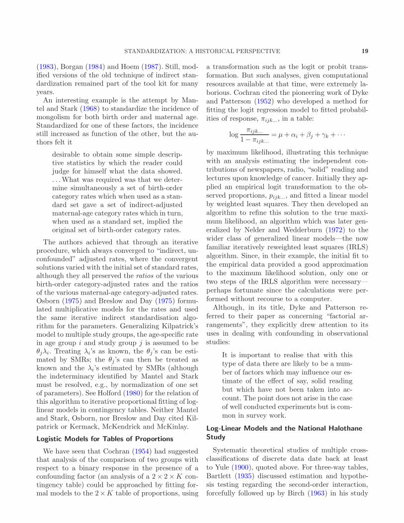
STANDARDIZATION: A HISTORICAL PERSPECTIVE 19
(1983), Borgan (1984) and Hoem (1987). Still, mod-ified versions of the old technique of indirect stan-dardization remained part of the tool kit for manyyears.An interesting example is the attempt by Man-
tel and Stark (1968) to standardize the incidence ofmongolism for both birth order and maternal age.Standardized for one of these factors, the incidencestill increased as function of the other, but the au-thors felt it
desirable to obtain some simple descrip-tive statistics by which the reader couldjudge for himself what the data showed.. . .What was required was that we deter-mine simultaneously a set of birth-ordercategory rates which when used as a stan-dard set gave a set of indirect-adjustedmaternal-age category rates which in turn,when used as a standard set, implied theoriginal set of birth-order category rates.
The authors achieved that through an iterativeprocedure, which always converged to “indirect, un-confounded” adjusted rates, where the convergentsolutions varied with the initial set of standard rates,although they all preserved the ratios of the variousbirth-order category-adjusted rates and the ratiosof the various maternal-age category-adjusted rates.Osborn (1975) and Breslow and Day (1975) formu-lated multiplicative models for the rates and usedthe same iterative indirect standardisation algo-rithm for the parameters. Generalizing Kilpatrick’smodel to multiple study groups, the age-specific ratein age group i and study group j is assumed to beθjλi. Treating λi’s as known, the θj ’s can be esti-mated by SMRs; the θj ’s can then be treated asknown and the λi’s estimated by SMRs (althoughthe indeterminacy identified by Mantel and Starkmust be resolved, e.g., by normalization of one setof parameters). See Holford (1980) for the relation ofthis algorithm to iterative proportional fitting of log-linear models in contingency tables. Neither Manteland Stark, Osborn, nor Breslow and Day cited Kil-patrick or Kermack, McKendrick and McKinlay.
Logistic Models for Tables of Proportions
We have seen that Cochran (1954) had suggestedthat analysis of the comparison of two groups withrespect to a binary response in the presence of aconfounding factor (an analysis of a 2× 2×K con-tingency table) could be approached by fitting for-mal models to the 2×K table of proportions, using
a transformation such as the logit or probit trans-formation. But such analyses, given computationalresources available at that time, were extremely la-borious. Cochran cited the pioneering work of Dykeand Patterson (1952) who developed a method forfitting the logit regression model to fitted probabil-ities of response, πijk..., in a table:
logπijk...
1− πijk...= µ+ αi + βj + γk + · · ·
by maximum likelihood, illustrating this techniquewith an analysis estimating the independent con-tributions of newspapers, radio, “solid” reading andlectures upon knowledge of cancer. Initially they ap-plied an empirical logit transformation to the ob-served proportions, pijk..., and fitted a linear modelby weighted least squares. They then developed analgorithm to refine this solution to the true maxi-mum likelihood, an algorithm which was later gen-eralized by Nelder and Wedderburn (1972) to thewider class of generalized linear models—the nowfamiliar iteratively reweighted least squares (IRLS)algorithm. Since, in their example, the initial fit tothe empirical data provided a good approximationto the maximum likelihood solution, only one ortwo steps of the IRLS algorithm were necessary—perhaps fortunate since the calculations were per-formed without recourse to a computer.Although, in its title, Dyke and Patterson re-
ferred to their paper as concerning “factorial ar-rangements”, they explicitly drew attention to itsuses in dealing with confounding in observationalstudies:
It is important to realise that with thistype of data there are likely to be a num-ber of factors which may influence our es-timate of the effect of say, solid readingbut which have not been taken into ac-count. The point does not arise in the caseof well conducted experiments but is com-mon in survey work.
Log-Linear Models and the National Halothane
Study
Systematic theoretical studies of multiple cross-classifications of discrete data date back at leastto Yule (1900), quoted above. For three-way tables,Bartlett (1935) discussed estimation and hypothe-sis testing regarding the second-order interaction,forcefully followed up by Birch (1963) in his study
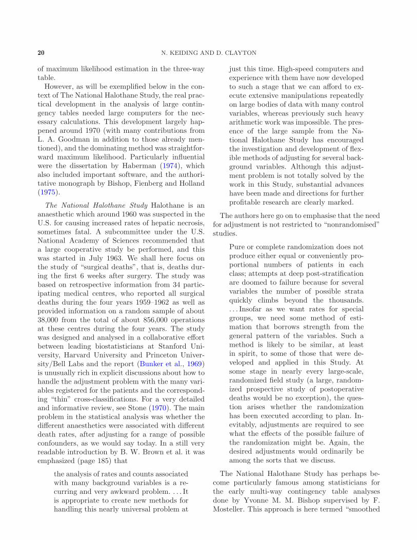
20 N. KEIDING AND D. CLAYTON
of maximum likelihood estimation in the three-waytable.However, as will be exemplified below in the con-
text of The National Halothane Study, the real prac-tical development in the analysis of large contin-gency tables needed large computers for the nec-essary calculations. This development largely hap-pened around 1970 (with many contributions fromL. A. Goodman in addition to those already men-tioned), and the dominating method was straightfor-ward maximum likelihood. Particularly influentialwere the dissertation by Haberman (1974), whichalso included important software, and the authori-tative monograph by Bishop, Fienberg and Holland(1975).
The National Halothane Study Halothane is ananaesthetic which around 1960 was suspected in theU.S. for causing increased rates of hepatic necrosis,sometimes fatal. A subcommittee under the U.S.National Academy of Sciences recommended thata large cooperative study be performed, and thiswas started in July 1963. We shall here focus onthe study of “surgical deaths”, that is, deaths dur-ing the first 6 weeks after surgery. The study wasbased on retrospective information from 34 partic-ipating medical centres, who reported all surgicaldeaths during the four years 1959–1962 as well asprovided information on a random sample of about38,000 from the total of about 856,000 operationsat these centres during the four years. The studywas designed and analysed in a collaborative effortbetween leading biostatisticians at Stanford Uni-versity, Harvard University and Princeton Univer-sity/Bell Labs and the report (Bunker et al., 1969)is unusually rich in explicit discussions about how tohandle the adjustment problem with the many vari-ables registered for the patients and the correspond-ing “thin” cross-classifications. For a very detailedand informative review, see Stone (1970). The mainproblem in the statistical analysis was whether thedifferent anaesthetics were associated with differentdeath rates, after adjusting for a range of possibleconfounders, as we would say today. In a still veryreadable introduction by B. W. Brown et al. it wasemphasized (page 185) that
the analysis of rates and counts associatedwith many background variables is a re-curring and very awkward problem. . . . Itis appropriate to create new methods forhandling this nearly universal problem at
just this time. High-speed computers andexperience with them have now developedto such a stage that we can afford to ex-ecute extensive manipulations repeatedlyon large bodies of data with many controlvariables, whereas previously such heavyarithmetic work was impossible. The pres-ence of the large sample from the Na-tional Halothane Study has encouragedthe investigation and development of flex-ible methods of adjusting for several back-ground variables. Although this adjust-ment problem is not totally solved by thework in this Study, substantial advanceshave been made and directions for furtherprofitable research are clearly marked.
The authors here go on to emphasise that the needfor adjustment is not restricted to “nonrandomised”studies.
Pure or complete randomization does notproduce either equal or conveniently pro-portional numbers of patients in eachclass; attempts at deep post-stratificationare doomed to failure because for severalvariables the number of possible strataquickly climbs beyond the thousands.. . . Insofar as we want rates for specialgroups, we need some method of esti-mation that borrows strength from thegeneral pattern of the variables. Such amethod is likely to be similar, at leastin spirit, to some of those that were de-veloped and applied in this Study. Atsome stage in nearly every large-scale,randomized field study (a large, random-ized prospective study of postoperativedeaths would be no exception), the ques-tion arises whether the randomizationhas been executed according to plan. In-evitably, adjustments are required to seewhat the effects of the possible failure ofthe randomization might be. Again, thedesired adjustments would ordinarily beamong the sorts that we discuss.
The National Halothane Study has perhaps be-come particularly famous among statisticians forthe early multi-way contingency table analysesdone by Yvonne M. M. Bishop supervised by F.Mosteller. This approach is here termed “smoothed
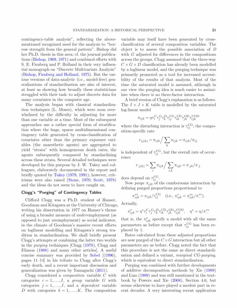
STANDARDIZATION: A HISTORICAL PERSPECTIVE 21
contingency-table analysis”, reflecting the above-mentioned recognized need for the analysis to “bor-row strength from the general pattern”. Bishop didher Ph.D. thesis in this area; cf. the journal publica-tions (Bishop, 1969, 1971) and combined efforts withS. E. Fienberg and P. Holland in their very influen-tial monograph on “Discrete Multivariate Analysis”(Bishop, Fienberg and Holland, 1975). But the var-ious versions of data-analytic (i.e., model-free) gen-eralizations of standardisation are also of interest,at least as showing how broadly these statisticiansstruggled with their task: to adjust discrete data formany covariates in the computer age.The analysis began with classical standardiza-
tion techniques (L. Moses), which were soon over-whelmed by the difficulty in adjusting for morethan one variable at a time. Most of the subsequentapproaches use a rather special form of stratifica-tion where the huge, sparse multidimensional con-tingency table generated by cross-classification ofcovariates other than the primary exposure vari-ables (the anaesthetic agents) are aggregated toyield “strata” with homogeneous death rates, theagents subsequently compared by standardizingacross these strata. Several detailed techniques weredeveloped for this purpose by J. W. Tukey and col-leagues, elaborately documented in the report andbriefly quoted by Tukey (1979, 1991); however, crit-icisms were also raised (Stone, 1970; Scott, 1978)and the ideas do not seem to have caught on.
Clogg’s “Purging” of Contingency Tables
Clifford Clogg was a Ph.D. student of Hauser,Goodman and Kitagawa at the University of Chicago,writing his dissertation in 1977 on Hauser’s themeof using a broader measure of underemployment (asopposed to just unemployment) as social indicator,in the climate of Goodman’s massive recent effortson loglinear modelling and Kitagawa’s strong tra-dition in standardisation. We shall briefly presentClogg’s attempts at combining the latter two worldsin the purging techniques [Clogg (1978), Clogg andEliason (1988) and many other articles]. A usefulconcise summary was provided by Sobel [(1996),pages 11–14] in his tribute to Clogg after Clogg’searly death, and a recent important discussion andgeneralization was given by Yamaguchi (2011).Clogg considered a composition variable C with
categories i = 1, . . . , I , a group variable G withcategories j = 1, . . . , J , and a dependent variableD with categories k = 1, . . . ,K. The composition
variable may itself have been generated by cross-classification of several composition variables. Theobject is to assess the possible association of D
with G adjusted for differences in the compositionsacross the groups. Clogg assumed that the three-wayC ×G×D classification has already been modelledby a loglinear model, and the purging technique wasprimarily promoted as a tool for increased accessi-bility of the results of that analysis. Most of thetime the saturated model is assumed, although inour view the purging idea is much easier to assimi-late when there is no three-factor interaction.A brief version of Clogg’s explanation is as follows.
The I × J ×K table is modelled by the saturatedlog-linear model
πijk = ητCi τGj τDk τCGij τCD
ik τGDjk τCGD
ijk
where the disturbing interaction is τCGij ; the compo-
sition-specific rate
rij(k) = πijk
/∑
k
πijk = πijk/πij·
is independent of τCGij , but the overall rate of occur-
rence
r·j(k) =∑
i
πijk
/∑
i,k
πijk = π·jk/π·j·
does depend on τCGij .
Now purge πijk of the cumbersome interaction bydefining purged proportions proportional to
π∗∗
ijk = πijk/τCGij (i.e., π∗
ijk = π∗∗
ijk/π∗∗
···).
Actually,
π∗
ijk = η∗τCi τGj τDk τCDik τGD
jk τCGDijk , η∗ = η/π∗∗
···
that is, the π∗
ijk specify a model with all the same
parameters as before except that τCGij has been re-
placed by 1.Rates calculated from these adjusted proportions
are now purged of the C×G interaction but all otherparameters are as before. Clogg noted the fact thatthis procedure is not the same as direct standardi-sation and defined a variant, marginal CG-purging,which is equivalent to direct standardisation.Purging was combined with further developments
of additive decomposition methods by Xie (1989)and Liao (1989) and was still mentioned in the text-book by Powers and Xie (2008), Section 4.6, butseems otherwise to have played a modest part in re-cent decades. A very interesting recent application
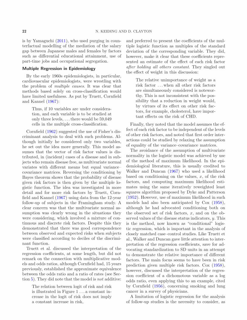
22 N. KEIDING AND D. CLAYTON
is by Yamaguchi (2011), who used purging in coun-terfactual modelling of the mediation of the salarygap between Japanese males and females by factorssuch as differential educational attainment, use ofpart-time jobs and occupational segregation.
Multiple Regression in Epidemiology
By the early 1960s epidemiologists, in particular,cardiovascular epidemiologists, were wrestling withthe problem of multiple causes. It was clear thatmethods based solely on cross-classification wouldhave limited usefulness. As put by Truett, Cornfieldand Kannel (1967):
Thus, if 10 variables are under considera-tion, and each variable is to be studied atonly three levels, . . . there would be 59,049cells in the multiple cross-classification.
Cornfield (1962) suggested the use of Fisher’s dis-criminant analysis to deal with such problems. Al-though initially he considered only two variables,he set out the idea more generally. This model as-sumes that the vector of risk factor values is dis-tributed, in (incident) cases of a disease and in sub-jects who remain disease free, as multivariate normalvariates with different means but equal variance–covariance matrices. Reversing the conditioning byBayes theorem shows that the probability of diseasegiven risk factors is then given by the multiple lo-gistic function. The idea was investigated in moredetail and for more risk factors by Truett, Corn-field and Kannel (1967) using data from the 12-yearfollow-up of subjects in the Framingham study. Aclear concern was that the multivariate normal as-sumption was clearly wrong in the situations theywere considering, which involved a mixture of con-tinuous and discrete risk factors. Despite this theydemonstrated that there was good correspondencebetween observed and expected risks when subjectswere classified according to deciles of the discrimi-nant function.Truett et al. discussed the interpretation of the
regression coefficients, at some length, but did notremark on the connection with multiplicative mod-els and odds ratios, although Cornfield had, 15 yearspreviously, established the approximate equivalencebetween the odds ratio and a ratio of rates (see Sec-tion 5). They did note that the model is not additive:
The relation between logit of risk and riskis illustrated in Figure 1 . . . a constant in-crease in the logit of risk does not implya constant increase in risk,
and preferred to present the coefficients of the mul-tiple logistic function as multiples of the standarddeviation of the corresponding variable. They did,however, make it clear that these coefficients repre-sented an estimate of the effect of each risk factorafter holding all others constant. They singled outthe effect of weight in this discussion:
The relative unimportance of weight as arisk factor . . . when all other risk factorsare simultaneously considered is notewor-thy. This is not inconsistent with the pos-sibility that a reduction in weight would,by virtues of its effect on other risk fac-tors, for example, cholesterol, have impor-tant effects on the risk of CHD.
Finally, they noted that the model assumes the ef-fect of each risk factor to be independent of the levelsof other risk factors, and noted that first order inter-actions could be studied by relaxing the assumptionof equality of the variance–covariance matrices.The avoidance of the assumption of multivariate
normality in the logistic model was achieved by useof the method of maximum likelihood. In the epi-demiological literature, this is usually credited toWalker and Duncan (1967) who used a likelihoodbased on conditioning on the values, x, of the riskfactors, and computing maximum likelihood esti-mates using the same iteratively reweighted leastsquares algorithm proposed by Dyke and Patterson(1952). However, use of maximum likelihood in suchmodels had also been anticipated by Cox (1958),although he had advocated conditioning both onthe observed set of risk factors, x, and on the ob-served values of the disease status indicators, y. Thisis the method, now known as “conditional” logis-tic regression, which is important in the analysis ofclosely matched case–control studies. Like Truett etal., Walker and Duncan gave little attention to inter-pretation of the regression coefficients, save for ad-vocating standardization to SD units in an attemptto demonstrate the relative importance of differentfactors. The main focus seems to have been in riskprediction given multiple risk factors. Cox (1958),however, discussed the interpretation of the regres-sion coefficient of a dichomotous variable as a logodds ratio, even applying this to an example, citedby Cornfield (1956), concerning smoking and lungcancer in a survey of physicians.A limitation of logistic regression for the analysis
of follow-up studies is the necessity to consider, as
STANDARDIZATION: A HISTORICAL PERSPECTIVE 23
did Truett, Cornfield and Kannel (1967), a fixed pe-riod of follow-up. A further rationalization of analyt-ical methods in epidemiology followed from the re-alization that such studies generate right-censored,and left-truncated, survival data. Mantel (1966) pio-neered the modern approach to such problems, not-ing that such data can be treated as if each sub-ject undergoes a series of Bernoulli trials (of veryshort duration). He suggested, therefore, that thecomparison of survival between two groups couldbe treated as an analysis of a 2 × 2 × K table inwhich the K “trials” are defined by the time pointsat which deaths occurred in the study (other timepoints being uninformative). In his famous paper,Cox (1972), described a regression generalization ofthis idea, in which the instantaneous risk, or “haz-ard”, is predicted by a log-linear regression model sothat effects of each risk factor may be expressed ashazard ratios. Over subsequent decades this theorywas further extended to encompass many types ofevent history data. See Andersen et al. (1993) for acomprehensive review.
Confounder Scores and Propensity Scores
Miettinen (1976b) put forward an alternative pro-posal for dealing with multiple confounders. It wasmotivated by three shortcomings he identified in themultivariate methods then available:
1. they (discriminant analysis in particular) reliedon very dubious assumptions,2. they (logistic regression) were computationally
demanding by the standards then applying, and3. they were poorly understood by substantive
scientists.
His proposal was to carry out a preliminary, per-haps crude, multivariate analysis from which couldbe computed a “confounder score”. This score couldthen be treated as a single confounder and dealtwith by conventional stratification methods. He sug-gested two ways of computing the confounder score.An outcome function was computed by an initialregression (or discriminant function) analysis of thedisease outcome variable on all of the confoundersplus the exposure variable of interest, then calculat-ing the score for a fixed value of exposure so thatit depended solely on confounders. Alternatively, anexposure function could be computed by interchang-ing the roles of outcome and exposure variables, re-gressing exposure on confounders plus outcome.
Rosenbaum and Rubin (1983) later put forwarda superficially similar proposal to the use of Mietti-nen’s exposure function. By analogy with random-ized experiments, they defined a balancing score asa function of potential confounders such that expo-sure and confounders are conditionally independentgiven the balancing score. Stratification by such ascore would then simulate a randomized experimentwithin each stratum. They further demonstrated,for a binary exposure, that the coarsest possiblebalancing score is the propensity score, the probabil-ity of exposure conditional upon confounders, whichcan be estimated by logistic regression. Note that,unlike Miettinen’s exposure score, the outcome vari-able is not included in this regression. The impact ofestimation of the nuisance parameters of the propen-sity score upon the test of exposure effect was laterexplored by Rosenbaum (1984). Hansen (2008) latershowed that a balancing score is also provided by the“prognostic analogue” to the propensity score whichis to Miettinen’s outcome function as the propen-sity score is to his exposure function, that is, theexposure variable is omitted when calculating theprognostic score.Given this later work on balancing scores, it is in-
teresting to note that Miettinen discussed at somelength why he believed it necessary to include the“conditioning variable” (either the exposure of in-terest or the outcome variable) when computingthe coefficients of the confounder score, noting thatthe need for this was “puzzling to some epidemiol-ogists”. His argument comes down to the require-ment to obtain an (approximately) unbiased esti-mate of the conditional odds ratio for exposure ver-sus outcome; omission of the conditioning variablemeans that the confounder score potentially con-tains a component related to only one of the twovariables of interest and, owing to noncollapsibilityof the odds ratio, this leads to a biased estimateof the conditional effect. Unfortunately, as demon-strated by Pike, Anderson and Day (1979), Mietti-nen’s proposal for correcting this bias comes at thecost of inflation of the type 1 error rate for the hy-pothesis test for an exposure effect. To demonstratethis, consider a logistic regression of an outcome,y, on an exposure of interest, x, and multiple con-founders, z. Miettinen proposed to first compute aconfounder score s = γT z, where γ are the coeffi-cients of z in the logistic regression of x on y and z,and then to fit the logistic regression of y on x and s.While this regression yields an identical coefficient
24 N. KEIDING AND D. CLAYTON
for x as the full logistic regression of y on x and z,and has the same maximized likelihood, in the testfor exposure effect this likelihood is compared withthe likelihood for the regression of y on s which, ingeneral, will be rather less than that for y on z—thecorrect comparison point. Thus, the likelihood ratiotest in Miettinen’s procedure will be inflated.Rosenbaum and Rubin circumvented the estima-
tion problem posed by omission of the conditioningvariable when calculating balancing scores by esti-mating a marginal causal effect using direct stan-dardization with appropriate population weights.Equivalently, inverse probability weights based onthe propensity score can be used.Owing to the focus on conditional measures of ef-
fect, the propensity score approach was little used inepidemiology during the latter part of the 20th cen-tury. However, the method has gained considerablyin popularity over the last decade. For a recent casestudy of treatment effect estimation using propen-sity score and regression methods, see Kurth et al.(2006). They emphasised that, as in classical directstandardization, precise identification of the targetpopulation is important when treatment effects arenonuniform.
Time-Dependent Confounding
Cox’s life table regression model provided an ex-ceedingly general approach to modelling the proba-bility of a failure event conditional upon exposure ortreatment variables and upon extraneous covariatesor confounders, the mathematical development ex-tending quite naturally to allow for variation of suchvariables over time. However, shortly after its publi-cation, Kalbfleisch and Prentice (1980), pages 124–126, pointed out a serious difficulty in dealing with“internal” (endogenous) time-dependent covariates.Referring to the role of variables such as the gen-eral condition of patients in therapeutic trials whichmay lie on the causal path between earlier treatmentand later outcome and, therefore, carry part of thecausal treatment effect, they wrote:
A censoring scheme that depends on thelevel of a time dependent covariate z(t)(e.g., general condition) is . . . not indepen-dent if z(t) is not included in the model.One way to circumvent this is to includez(t) in the model, but this may masktreatment differences of interest.
Put another way, to ignore such a variable in theanalysis is to disregard its confounding effect, but itsinclusion in the conditional probability model couldobscure some of the true causal effect of treatment.While Kalbfleisch and Prentice had identified a
fundamental problem with the conditional approachto confounder adjustment, they offered no convinc-ing remedy. This was left to Robins (1986). In thisand later papers Robins addressed the “healthyworker” effect in epidemiology–essentially the sameproblem identified by Kalbfleisch and Prentice.Robins proposed two lines of attack which we mayclassify as “marginal” and “conditional” in keep-ing with a distinction that has come up through-out our exposition. The original approach was “g-computation”, which may be loosely conceived assequential prediction of “what would have hap-pened” under various specified externally imposed“treatments” and thus generalizes (direct) standard-isation, basically a marginal approach. A furtherdevelopment in this direction was inverse prob-ability weighting of marginal structural models,that is, models for the counterfactual outcomes(Robins, Hernan and Brumback, 2000). Here, theessential idea is to estimate a marginal treatment ef-fect in a population in which the association betweentreatment (exposure) and the time-dependent co-variate is removed. Sato and Matsuyama (2003) andVansteelandt and Keiding (2011) gave brief discus-sions of the relationship between g-computation, in-verse probability weighting and classical standardis-ation in the simplest (nonlongitudinal) situation. Onthe other hand, the approach via structural nestedmodels [e.g., Robins and Tsiatis (1992), Robins et al.(1992)] focusses on the effect of a “blip” of exposureat time t conditional on treatments and covariatevalues before t. In the latter models, time-varyingeffect modification may be studied. See the recenttutorial surveys by Robins and Hernan (2009) orDaniel et al. (2013) for details.
7. PREDICTION AND TRANSPORTABILITY
We saw that in the National Halothane Studystandardisation methods were used analytically, inorder to control for confounders strictly within theframe of the concrete study. The general verdictin the emerging computer age regarding this useof standardisation was negative, as formulated byFienberg (1975), in a discussion of a careful and de-tailed survey on observational studies by McKinlay(1975):
STANDARDIZATION: A HISTORICAL PERSPECTIVE 25
The reader should be aware that stan-dardization is basically a descriptive tech-nique that has been made obsolete, formost of the purposes to which it has tra-ditionally been put, by the ready avail-ability of computer programs for loglinearmodel analysis of multidimensional con-tingency tables.
However, the original use of standardization notonly had this analytical ambition, it also aimedat obtaining meaningful generalizations to otherpopulations—or other circumstances in the origi-nal population. Before we sketch the recovery sincethe early 1980s of this aspect of standardization,it is useful to record the attitude to generalizationby influential epidemiologists back then. Miettinen[(1985), page 47] in his long-awaited text-book,wrote:
In science the generalization from the ac-tual study experience is not made to apopulation of which the study experienceis a sample in a technical sense of proba-bility sampling . . . In science the general-ization is from the actual study experienceto the abstract, with no referent in placeor time,
and thus did not focus on specific recommenda-tions as to how to predict precisely what mighthappen under different concrete circumstances. Asimilar attitude was voiced by Rothman [(1986),page 95] in the first edition of Modern Epidemiol-
ogy, and essentially repeated in the following edi-tions of this central reference work [Rothman andGreenland (1998), pages 133–134, Rothman, Green-land and Lash (2008), pages 146–147]. The imme-diate consequence of this attitude would be that allthat we need are the parameters in the fitted statis-tical model and assurance that no bias is present inthe genesis of the concretely analyzed data.However, as we have seen, Clogg (1978) (and later)
had felt a need for interpreting the log-linear mod-els in terms of their consequences for summary ta-bles. Freeman and Holford (1980) wrote a usefulguide to the new situation for survey analysis wherethe collected data had been analyzed using thenew statistical models. They concluded that muchfavoured keeping the reporting to the model parame-ters: these would then be available to other analystsfor comparative purposes, the model fit was nec-essary to check for interactions (including possibly
identifying a model where there is no interaction).But,
in many settings these advantages areovershadowed by the dual requirementsfor simplicity of presentation and imme-diacy of interpretation,
and Freeman and Holford (1980) therefore gave spe-cific instructions on how to calculate “summaryrates” for the total population or other populations.The main requirement for validity of such calcula-tions is that there is no interaction between popula-tion and composition.Interestingly, an influential contribution in 1982
came from a rather different research environment:the well-established agricultural statisticians P. W.Lane and J. A. Nelder (Lane and Nelder, 1982). In aspecial issue of Biometrics on the theme “the analy-sis of covariance”, they wrote a short note containingseveral germs of the later so important potential out-come view underlying modern causal inference, andplaced the good old (direct) standardisation tech-nique right in the middle of it.Their view was that the purpose of a statistical
analysis such as analysis of covariance is not onlyto estimate parameters, but also to make what theycalled predictions:
An essential feature is the division intoeffects of interest and effects for whichadjustment is required. . . . For example,a typical prediction from a variety trialis the yield that would have been ob-tained from a particular variety if it hadbeen grown over the whole experimen-tal area. When a covariate exists the ad-justed treatment mean can be thought ofas the prediction of the yield of that va-riety grown over the whole experimentalarea with the covariate fixed at its meanvalue. . . . The predictions here are not offuture events but rather of what wouldhave happened in the experiment if otherconditions had prevailed. In fact no vari-ety would have been grown over the wholeexperimental area nor would the covariatehave been constant.
Lane and Nelder proposed to use the term pre-
dictive margin for such means, avoiding the term“population treatment mean” suggested by Searle,Speed and Milliken (1980) to replace the cryptic
26 N. KEIDING AND D. CLAYTON
SAS-output term “least square means”. Lane andNelder emphasised that these means might eitherbe
conditional on the value we take as stan-dard for the covariate
or
marginal to the observed distribution ofcovariate values,
and Lane and Nelder went on to explain to thisnew audience (including agricultural statisticians)that there exist many other possibilities for choiceof standard.We find it interesting that Lane and Nelder used
the occasion of the special issue of Biometrics onanalysis of covariance to point out the similari-
ties to standardisation, and to phrase their “pre-diction” in much similar terms as the later causalanalysis would do. Of course, it should be remem-bered that Lane and Nelder manoeuvered within thecomfortable framework of randomised field trials.Rothman, Greenland and Lash [(2008), page 386 ff.]described how these ideas have developed into whatis now termed regression standardisation.
An Example: Cancer Trends
A severe practical limitation of the modelling ap-proach is that the model must encompass all thedata to be compared. However, many official statis-tics are published explicitly to allow comparisonswith other published series. Even within a singlepublication it may be inappropriate to fit a singlelarge and complex model across the entire data set.An example of the latter situation is the I.A.R.C.
monograph on Trends in Cancer Incidence and Mor-tality (Coleman et al., 1993). The primary aim ofthis monograph was to estimate cancer trends acrossthe population-based cancer registries throughoutthe world and this was addressed by fitting age-period-cohort models to the data from each registry.But comparisons of rates between registries at spe-cific time points were also required and, since the agestructures of different registries differed markedly,direct standardisation to the world population, ages30–74, was used. However, some of the cancers con-sidered were rare and this exposes a problem withthe method of direct standardization—that it can bevery inefficient when the standard population differsmarkedly from that of the test group. The authorstherefore chose to apply direct standardisation tothe fitted rates from the age-period-cohort models.
Transportability Across Studies
Pearl and Barenboim (2012) noted that preciseconditions for applying concrete results obtained ina study environment to another “target” environ-ment,
remarkably. . . have not received system-atic formal treatment. . . The standard lit-erature on this topic . . . consists primar-ily of “threats”, namely verbal narrativesof what can go wrong when we try totransport results from one study to an-other. . . Rarely do we find an analysis of“licensing assumptions”, namely, formaland transparent conditions under whichthe transport of results across differing en-vironments or populations is licensed fromfirst principles.
After further outlining the strong odds againstanyone who dares formulate such conditions, Pearland Barenboim then set out to propose one such for-malism, based on the causal diagrams developed byPearl and colleagues over the last decades; cf. Pearl(2009).In the terminology of Pearl and Barenboim, the
method of direct standardisation, together with the“predictions” of Lane and Nelder, is a transport for-
mula and, as they state,
the choice of the proper transport formuladepends on the causal context in whichpopulation differences are embedded.
Although a formal treatment of these issues isoverdue, it has been recognized in epidemiology formany years that the concept of confounding cannotbe defined solely in terms of a third variable beingrelated to both outcome and exposure of interest. Alandmark paper was that of Simpson (1951) whichdealt with the problem of interpreting associationsin three-way contingency tables. As we saw in Sec-tion 3, although “Simpson’s paradox” is widely re-garded as synonymous with Yule’s paradox, Simp-son’s primary concern was the role of the causal con-text in deciding whether the conditional or marginalassociation between two of the three factors in a ta-ble is of primary interest. The point has been under-stood by many (if not all) epidemiologists writing inthe second half of the 20th century as, for example,is demonstrated by the remark of Truett, Cornfieldand Kannel (1967), cited in Section 6, concerning
STANDARDIZATION: A HISTORICAL PERSPECTIVE 27
interpretation of the coefficient of body weight intheir regression equation for coronary disease inci-dence. However, as far as we can tell, the issue doesnot seem to have concerned 19th century writers;for example, no consideration seems to have beengiven to the possibility that age differences betweenpopulations could, in part, be a consequence of dif-ferences in “the force of mortality” and, if so, theimplication for age standardization.
8. CONCLUSION
In the fields of scientific enquiry with which weare concerned here, the causal effect of a treatment,or exposure, cannot be observed at the individuallevel. Instead, the effect measures we use contrastthe distributions of responses in populations withdiffering exposures, but in which the distributionsof other factors do not differ. In randomized studies,this equality of distribution of extraneous factors isguaranteed by randomisation and causal effects aresimply measured. In observational studies, however,differences between the distributions of relevant ex-traneous factors between exposure groups (what epi-demiologists call “confounding”) is ubiquitous andwe must rely on the assumption of “no unmeasuredconfounders” to allow us to estimate the causal ef-fect.In much recent work, the problem is approached
by postulating that each individual has a numberof potential responses, one for each possible expo-sure; only one of these is observed, the other coun-terfactual responses being assumed to be “missingat random” given measured confounders. Alterna-tively, we can restrict ourselves to dealing with ob-served outcomes, assuming that the mechanism bywhich exposure was allocated in the experiment ofnature we have observed did not depend on unmea-sured confounders. The choice between these posi-tions is philosophical and, to the applied statistician,largely a matter of convenience. The more seriousconcern, with which we have been largely concernedin this review, is the choice of effect measure; we canchoose to contrast the marginal distribution of re-sponses under equality of distribution of extraneousfactors or to contrast response distributions whichcondition on the values of these factors.Standardisation grew up in response to obvious
problems of age-confounding in actuarial (18th cen-tury) and demographic (19th century) comparativestudies of mortality. The simple intuitive calcula-tions considered scenarios in which either the age
distributions did not differ (“direct” standardisa-tion) or age-specific rates did not differ (“indirect”standardisation) between study groups. However,formal consideration of such indices as effect mea-sures came later, the contribution of Yule (1934) be-ing noteworthy.There would probably be widespread agreement
that describing causal effects in relation to all po-tential causes, as in the conditional approach, mustrepresent the most complete analysis of a data setand we have described how this approach developedthroughout the 20th century, starting with the in-fluential paper of Yule (1900). This impressive pa-per clearly described the proliferation of “partial”association measures introduced by the conditionalapproach, and drew attention to the consequentneed to use measures which remain relatively sta-ble across subgroups. In later work Yule (1934) re-visited classical standardisation in terms of an aver-age of conditional (i.e., stratum-specific) measures.Such early work sowed the seeds of the “statisti-cal” approach based on formal probability models,leading eventually to the widespread use of logis-tic regression and proportional hazard (multiplica-tive intensity) models, the contributions of Cochran(1954) and Mantel and Haenszel (1959) providingimportant staging posts along the way (even thoughthe latter authors explicitly denied any reliance on amodel). By the end of the century such approachesdominated epidemiology and biostatistics.Toward the end of the 20th century, the use of
marginal measures of causal effects emerged fromthe counterfactual approach to causal analysis inthe social sciences, the idea of propensity scores(Rosenbaum and Rubin, 1983) being particularlyinfluential. However, these methods only found theirway into mainstream biostatistics when applicationsarose for which conventional conditional probabilitymodels were not well suited, the foremost of whichbeing the problem of time-dependent confounding.Whereas, for simple problems, the parameters of lo-gistic and multiplicative intensity models have aninterpretation as measures of (conditional) causaleffects, Kalbfleisch and Prentice (1980) noted thatthis ceased to be the case in the presence of time-dependent confounding. While the statistical mod-elling approach can be extended by joint modellingof the event history and confounder trajectories,such models are complex and, again, causal effectsdo not correspond with model parameters and wouldneed to be estimated by simulations based on the
28 N. KEIDING AND D. CLAYTON
fitted model. Such models continue to be studied[see, e.g., Henderson, Diggle and Dobson (2000)],but, although it could be argued that these offerthe opportunity for a more detailed understandingof the nature of causal effects in this setting, thesimpler marginal approaches pioneered by Robins(1986) are more attractive in most applications. Thesuccess of this latter approach in offering a solutionto a previously intractable problem encouraged bio-statisticians to further explore methods for estima-tion of marginal causal effects; for example, propen-sity scores are now widely used in this literature.So where are we today? Both approaches have
strengths and weaknesses. The conditional mod-elling approach relies on the assumption of homo-geneity of effect across subgroups or, when this failsto hold, to a multiplicity of effect measures. Themarginal approach, while seemingly less reliant onsuch assumptions, encounters the same issue whenconsidering the transportability of effect measuresto different populations.
ACKNOWLEDGMENTS
This work grew out of an invited paper by DavidClayton in the session “Meaningful Parametriza-tions” at the International Biometric Conference inFreiburg in 2002. The authors are grateful to the re-viewers for comments and detailed suggestions onearlier drafts. Important parts of Niels Keiding’swork were done on study leaves at the MRC Bio-statistics Unit, Cambridge, October–November 2009and as Visiting Senior Research Fellow at Jesus Col-lege, Oxford, Hilary Term 2012; he is most gratefulfor the hospitality at these institutions. David Clay-ton was supported by a Wellcome Trust PrincipalResearch Fellowship until his retirement in March,2012.
REFERENCES
Aalen, O. (1978). Nonparametric inference for a family ofcounting processes. Ann. Statist. 6 701–726. MR0491547
Aldrich, J. (1995). Correlations genuine and spurious inPearson and Yule. Statist. Sci. 10 364–376.
Andersen, P. K., Borgan, Ø., Gill, R. D. and Keid-
ing, N. (1993). Statistical Models Based on Counting Pro-cesses. Springer, New York. MR1198884
Bartlett, M. S. (1935). Contingency table interactions.Suppl. J. Roy. Stat. Soc. 2 248–252.
Bellhouse, D. (2008). Review of “Disciplining Statistics:Demography and Vital Statistics in France and England,1830–1885” by L. Schweber. Hist. Math. 35 249–252.
Belson, W. A. (1956). A technique for studying the effectsof a television broadcast. Appl. Stat. 5 195–202.
Berkson, J. (1946). Limitations of the application of fourfoldtable analysis to hospital data. Biometrics Bull. 2 47–53.
Birch, M. W. (1963). Maximum likelihood in three-way con-tingency tables. J. R. Stat. Soc. Ser. B Stat. Methodol. 25220–233. MR0168065
Birch, M. W. (1964). The detection of partial association. I.The 2× 2 case. J. R. Stat. Soc. Ser. B Stat. Methodol. 26313–324. MR0176562
Bishop, Y. M. M. (1969). Full contingency tables, logits, andsplit contingency tables. Biometrics 25 383–399.
Bishop, Y. M. M. (1971). Effects of collapsing multidimen-sional contingency tables. Biometrics 27 545–562.
Bishop, Y. M. M., Fienberg, S. E. and Holland, P. W.
(1975). Discrete Multivariate Analysis: Theory and Prac-tice. MIT Press, Cambridge, MA. MR0381130
Borgan, Ø. (1984). Maximum likelihood estimation in para-metric counting process models, with applications to cen-sored failure time data. Scand. J. Stat. 11 1–16. MR0743234
Breslow, N. E. and Day, N. E. (1975). Indirect standard-ization and multiplicative models for rates, with referenceto age adjustment of cancer incidence and relative fre-quency data. J. Chron. Dis. 28 289–303.
Breslow, N. E., Lubin, J. H., Marek, P. andLangholz, B. (1983). Multiplicative models and cohortanalysis. J. Amer. Statist. Assoc. 78 1–12.
Bunker, J., Forrest, W., Mosteller, F. and Vandam, L.
(1969). The National Halothane Study. National Instituteof General Medical Sciences.
Chadwick, E. (1844). On the best modes of representing ac-curately, by statistical returns, the duration of life, and thepressure and progress of the causes of mortality amongstdifferent classes of the community, and amongst the pop-ulations of different districts and countries. J. Stat. Soc.London 7 1–40.
Chevan, A. and Sutherland, M. (2009). Revisiting DasGupta: Refinement and extension of standardization anddecomposition. Demography 46 429–449.
Clayton, D. and Hills, M. (1993). Statistical Models inEpidemiology. Oxford Univ. Press, Oxford.
Clogg, C. C. (1978). Adjustment of rates using multiplica-tive models. Demography 15 523–539.
Clogg, C. C. and Eliason, S. R. (1988). A flexible proce-dure for adjusting rates and proportions, including statis-tical methods for group comparisons. Am. Sociol. Rev. 53267–283.
Cochran, W. G. (1954). Some methods for strengtheningthe common χ2 tests. Biometrics 10 417–451. MR0067428
Cochran, W. G. (1969). Use of covariance in observationalstudies. Appl. Stat. 18 270–275.
Coleman, M. P., Esteve, J., Damiecki, P., Arslan, A.
and Renard, H. (1993). Trends in Cancer Incidence andMortality. No. 121 in IARC Scientific Publications. Inter-national Agency for Research on Cancer, Lyon.
Cornfield, J. (1951). A method of estimating comparativerates from clinical data; applications to cancer of the lung,breast, and cervix. J. Natl. Cancer Inst. 11 1269–1275.
Cornfield, J. (1956). A statistical problem arising fromretrospective studies. In Proceedings of the Third Berke-
STANDARDIZATION: A HISTORICAL PERSPECTIVE 29
ley Symposium on Mathematical Statistics and Probability,1954–1955, Vol. IV (J. Neyman, ed.) 135–148. Univ. Cal-ifornia Press, Berkeley, CA. MR0084935
Cornfield, J. (1962). Joint dependence of risk of coronaryheart disease on serum cholesterol and systolic blood pres-sure: A discriminant function analysis. Fed. Proc. 21 58–61.
Cox, D. R. (1958). The regression analysis of binary se-quences. J. R. Stat. Soc. Ser. B Stat. Methodol. 20 215–242.MR0099097
Cox, D. R. (1972). Regression models and life-tables. J. R.Stat. Soc. Ser. B Stat. Methodol. 34 187–220. MR0341758
Daniel, R. M., Cousens, S. N., De Stavola, B. L., Ken-
ward, M. G. and Sterne, J. A. C. (2013). Methods fordealing with time-dependent confounding. Stat. Med. 32
1584–1618. MR3060620Davidson, A. and Reid, A. (1926–1927). On the calculation
of rates of mortality. T. Fac. Actuaries 11 183–232.Day, N. E. (1976). A new measure of age standardized in-
cidence, the cumulative rate. In Cancer Incidence in FiveContinents 3 (J. Waterhouse, C. Muir, P. Correa andJ. Powell, eds.) 443–445. International Agency for Re-search on Cancer, Lyon.
Derrick, V. P. A. (1927). Observations on (1) errors of agein the population statistics of England and Wales, and (2)the changes in mortality indicated by the national records.J. Inst. Actuaries 58 117–159.
Dyke, G. and Patterson, H. (1952). Analysis of factorialarrangements when the data are proportions. Biometrics 81–12.
Edgeworth, F. Y. (1917). Review of “Scope and Methodof Statistics” by Harald Westergaard. J. Roy. Stat. Soc. 80546–551.
Elandt-Johnson, R. C. (1975). Definition of rates: Someremarks on their use and misuse. Am. J. Epidemiol. 102267–271.
Farr, W. (1859). Letter to the Registrar General. GeneralRegistrar Office, London.
Fibiger, J. (1898). Om serumbehandling af difteri. Hospital-stidende 6 337–350.
Fienberg, S. E. (1975). Design and analysis of observationalstudy—Comment. J. Amer. Statist. Assoc. 70 521–523.
Fisher, R. A. (1922). On the interpretation of χ2 from con-tingency tables, and the calculation of P . J. Roy. Stat. Soc.85 87–94.
Freeman, D. H. and Holford, T. R. (1980). Summaryrates. Biometrics 36 195–205.
Graubard, B. I., Rao, R. S. and Gastwirth, J. L. (2005).Using the Peters–Belson method to measure health caredisparities from complex survey data. Stat. Med. 24 2659–2668. MR2196206
Greenland, S. (1982). Interpretation and estimation of sum-mary ratios under heterogeneity. Stat. Med. 1 217–227.
Haberman, S. J. (1974). The Analysis of Frequency Data:Statistical Research Monographs, Vol. IV. The Univ.Chicago Press, Chicago, IL. MR0408098
Haenszel, W., Shimkin, M. B. and Mantel, N. (1958).A retrospective study of lung cancer in women. J. Natl.Cancer Inst. 21 825–842.
Hansen, B. B. (2008). The prognostic analogue of thepropensity score. Biometrika 95 481–488. MR2521594
Henderson, R., Diggle, P. and Dobson, A. (2000). Jointmodelling of longitudinal measurements and event timedata. Biostatistics 1 465–480.
Hernan, M. A., Clayton, D. and Keiding, N. (2011). TheSimpson’s paradox unraveled. Int. J. Epidemiol. 40 780–785.
Hernan, M. A. and Robins, J. M. (2006). Estimating causaleffects from epidemiological data. J. Epidemiol. Commu-nity Health 60 578–586.
Hobcraft, J., Menken, J. and Preston, S. (1982). Age,period, and cohort effects in demography: A review. Popul.Index 48 4–43.
Hoem, J. (1987). Statistical analysis of a multiplicative modeland its application to the standardization of vital rates—Areview. Int. Stat. Rev. 55 119–152.
Holford, T. R. (1980). The analysis of rates and of sur-vivorship using log-linear models. Biometrics 36 299–305.
Hrobjartsson, A., Gøtzsche, P. C. and Gluud, C.
(1998). The controlled clinical trial turns 100 years:Fibiger’s trial of serum treatment of diphtheria. Br. Med.J. 317 1243–1245.
Kalbfleisch, J. D. and Prentice, R. L. (1980). The Sta-tistical Analysis of Failure Time Data. Wiley, New York.MR0570114
Kalton, G. (1968). Standardization: A technique to con-trol for extraneous variables. Appl. Statist. 17 118–136.MR0234599
Keiding, N. (1987). The method of expected number ofdeaths, 1786–1886–1986. Internat. Statist. Rev. 55 1–20.MR0962938
Keiding, N. (2011). Age-period-cohort analysis in the 1870s:Diagrams, stereograms, and the basic differential equation.Canad. J. Statist. 39 405–420. MR2842421
Kendall, P. L. and Lazarsfeld, P. F. (1950). Problems ofsurvey analysis. In Continuities in Social Research: Stud-ies in the Scope and Method of “The American Soldier”(R. Merton and P. Lazarsfeld, eds.) 133–196. FreePress, Glencoe, IL.
Kermack, W. O., McKendrick, A. G. and McKin-
lay, P. L. (1934a). Death-rates in Great Britain andSweden—Some general regularities and their significance.Lancet 1 698–703.
Kermack, W. O., McKendrick, A. G. and McKin-
lay, P. L. (1934b). Death-rates in Great Britain and Swe-den: Expression of specific mortality rates as products oftwo factors, and some consequences thereof. J. Hyg. 34 433–457.
Kilpatrick, S. J. (1962). Occupational mortality indexes.Popul. Stud. 16 175–187.
Kitagawa, E. M. (1955). Components of a difference be-tween 2 rates. J. Amer. Statist. Assoc. 50 1168–1194.
Kitagawa, E. M. (1964). Standardized comparisons inpopulation-research. Demography 1 296–315.
Kitagawa, E. M. (1966). Theoretical considerations in theselection of a mortality index, and some empirical compar-isons. Hum. Biol. 38 293–308.
Korosi, J. (1892–1893). Report of an international mortalitystandard, or mortality index. Pub. Amer. Statist. Assoc. 3450–462.
30 N. KEIDING AND D. CLAYTON
Kurth, T., Walker, A. M., Glynn, R. J., Chan, K. A.,Gaziano, J. M., Berger, K. and Robins, J. M. (2006).Results of multivariable logistic regression, propensitymatching, propensity adjustment, and propensity-basedweighting under conditions of nonuniform effect. Am. J.Epidemiol. 163 262–270.
Lane, P. W. and Nelder, J. A. (1982). Analysis of covari-ance and standardization as instances of prediction. Bio-metrics 38 613–621.
Lexis, W. (1876). Das Geschlechtsverhaltnis der Geborenenund die Wahrscheinlichkeitsrechnung. Jahrbucher fur Na-tionalokonomie und Statistik 27 209–245.
Liao, T. F. (1989). A flexible approach for the decompositionof rate differences. Demography 26 717–726.
MacKenzie, D. (1978). Statistical theory and social inter-ests: A case-study. Soc. Stud. Sci. 8 35–83.
MacKenzie, D. A. (1981). Statistics in Britain: 1865–1930.The Social Construction of Scientific Knowledge. Edin-burgh Univ. Press, Edinburgh. MR0642200
MacKinnon, D. (2008). Introduction to Statistical MediationAnalysis. Lawrence Erbaum Associates, New York.
Mantel, N. (1966). Evaluation of survival data and two newrank order statistics arising in its consideration. CancerChemotherapy Reports 50 163–170.
Mantel, N. and Haenszel, W. (1959). Statistical aspects ofthe analysis of data from retrospective studies of disease.J. Natl. Cancer. Inst. 22 719–748.
Mantel, N. and Stark, C. R. (1968). Computation ofindirect-adjusted rates in the presence of confounding. Bio-metrics 24 997–1005.
McKendrick, A. G. (1925–1926). Applications of mathe-matics to medical problems. Proc. Edinb. Math. Soc. (2)43–44 98–130.
McKinlay, S. M. (1975). Design and analysis of observa-tional study—Review. J. Amer. Statist. Assoc. 70 503–520.
Miettinen, O. (1972a). Standardization of risk ratios. Am.J. Epidemiol. 96 383–388.
Miettinen, O. S. (1972b). Components of the crude riskratio. Am. J. Epidemiol. 96 168–172.
Miettinen, O. (1976a). Estimability and estimation in case-referent studies. Am. J. Epidemiol. 103 230–235.
Miettinen, O. S. (1976b). Stratification by a multivariateconfounder score. Am. J. Epidemiol. 104 609–620.
Miettinen, O. S. (1985). Theoretical Epidemiology. Wiley,New York.
Neison, F. (1844). On a method recently proposed for con-ducting inquiries into the comparative sanatory conditionof various districts, with illustrations, derived from numer-ous places in Great Britain at the period of the last census.J. Stat. Soc. London 7 40–68.
Neison, F. G. P. (1851). On the rate of mortality amongpersons of intemperate habits. J. Stat. Soc. London 14 200–219.
Nelder, J. and Wedderburn, R. (1972). Generalized linearmodels. J. Roy. Statist. Soc. Ser. A 135 370–384.
Nelson, W. (1972). Theory and applications of hazard plot-ting for censored failure data. Technometrics 14 945–966.
Newsholme, A. and Stevenson, T. H. C. (1906). The de-cline of human fertility in the United Kingdom and other
countries as shown by corrected birth-rates. J. Roy. Stat.Soc. 69 34–87.
Ogle, W. (1892). Proposal for the establishment and inter-national use of a standard population, with fixed sex andage distribution, in the calculation and comparison of mar-riage, birth, and death rates. Bull. Int. Stat. Inst. 6 83–85.
Osborn, J. (1975). Multiplicative model for analysis of vitalstatistics rates. Appl. Stat. 24 75–84.
Pearl, J. (2001). Direct and indirect effects. In Proceedings ofthe Seventeenth Conference on Uncertainty in Artificial In-telligence 411–420. Morgan Kaufman, San Francisco, CA.
Pearl, J. (2009). Causality: Models, Reasoning, and In-ference, 2nd ed. Cambridge Univ. Press, Cambridge.MR2548166
Pearl, J. and Barenboim, E. (2012). Transportabilityacross studies: A formal approach. Technical report, Com-puter Science Dept., Univ. California, Los Angeles.
Pearson, K. (1900). On the correlation of characters notquantitatively measurable. Philos. Trans. R. Soc. Lond.Ser. A Math. Phys. Eng. Sci. 195 1–47.
Pearson, K. (1910). The Grammar of Science, 3rd ed. Black,Edinburgh.
Pearson, K., Lee, A. and Bramley-Moore, L. (1899).Genetic (reproductive) selection: Inheritance of fertility inman and of fecundity in thoroughbred racehorses. Philos.Trans. R. Soc. Lond. Ser. A Math. Phys. Eng. Sci. 192
534–539.Pearson, K. and Tocher, J. F. (1915). On criteria for the
existence of differential deathrates. Biometrika 11 159–184.Peters, C. C. (1941). A method of matching groups for ex-
periment with no loss of population. J. Educ. Res. 34 606–612.
Petersen, M. L., Sinisi, S. E. and van der Laan, M. J.
(2006). Estimation of direct causal effects. Epidemiology 17
276–284.Pike, M., Anderson, J. and Day, N. (1979). Some insights
into Miettinen’s multivariate confounder score approach tocase-control study analysis. Epidemiol. Comm. Health 33
104–106.Powers, D. A. and Xie, Y. (2008). Statistical Methods for
Categorical Data Analysis, 2nd ed. Emerald, Bingley, UK.Powers, D. A. and Yun, M. S. (2009). Multivariate de-
composition for hazard rate models. Sociol. Methodol. 39233–263.
Preston, S. H., Heuveline, P. and Guillot, M. (2001).Demography. Blackwell, Oxford.
Robins, J. (1986). A new approach to causal inferencein mortality studies with a sustained exposure period—application to control of the healthy worker survivor effect.Math. Modelling 7 1393–1512. MR0877758
Robins, J., Blevins, D., Ritter, G. and Wulfsohn, M.
(1992). G-estimation of the effect of prophylaxis therapy forpneumocystis carinii pneumonia on the survival of AIDSpatients. Epidemiology 14 79–97.
Robins, J. M. and Hernan, M. A. (2009). Estimation of thecausal effects of time-varying exposures. In LongitudinalData Analysis (G. Fitzmaurice, G. Verbeke, M. Da-
vidian and G. Molenberghs, eds.) 553–599. CRC Press,Boca Raton, FL. MR1500133
STANDARDIZATION: A HISTORICAL PERSPECTIVE 31
Robins, J. M., Hernan, M. A. and Brumback, B. (2000).Marginal structural models and causal inference in epi-demiology. Epidemiology 11 550–560.
Robins, J. and Tsiatis, A. A. (1992). Semiparametric es-timation of an accelerated failure time model with time-dependent covariates. Biometrika 79 311–319. MR1185133
Rosenbaum, P. R. (1984). Conditional permutation testsand the propensity score in observational studies. J. Amer.Statist. Assoc. 79 565–574. MR0763575
Rosenbaum, P. R. andRubin, D. B. (1983). The central roleof the propensity score in observational studies for causaleffects. Biometrika 70 41–55. MR0742974
Rosenberg, M. (1962). Test factor standardization as amethod of interpretation. Soc. Forces 41 53–61.
Rothman, K. (1986). Modern Epidemiology. Little, Brownand Company, Boston, MA.
Rothman, K. and Greenland, S. (1998). Modern Epidemi-ology, 2nd ed. Lippincott, Williams & Wilkins, Philadel-phia, PA.
Rothman, K. J., Greenland, S. and Lash, T. L. (2008).Modern Epidemiology, 3rd ed. Lippincott, Williams &Wilkins, Philadelphia, PA.
Sato, T. and Matsuyama, Y. (2003). Marginal structuralmodels as a tool for standardization. Epidemiology 14 680–686.
Schweber, L. (2001). Manipulation and population statisticsin nineteenth-century France and England. Soc. Res. (NewYork) 68 547–582.
Schweber, L. (2006). Disciplining Statistics: Demographyand Vital Statistics in France and England. Duke Univ.Press, Durham.
Scott, R. C. (1978). Bias problem in smear-and-sweep anal-ysis. J. Amer. Statist. Assoc. 73 714–718.
Searle, S. R., Speed, F. M. and Milliken, G. A. (1980).Population marginal means in the linear model: An alter-native to least squares means. Amer. Statist. 34 216–221.MR0596242
Simpson, E. H. (1951). The interpretation of interaction incontingency tables. J. R. Stat. Soc. Ser. B Stat. Methodol.13 238–241. MR0051472
Sobel, M. E. (1996). Clifford Collier Clogg, 1949–1995: Atribute to his life and work. Sociol. Methodol. 26 1–38.
Stigler, S. M. (1986). The History of Statistics: The Mea-surement of Uncertainty Before 1900. The Belknap Pressof Harvard Univ. Press, Cambridge, MA. MR0852410
Stone, M. (1970). Review of National Halothane Study—Bunker, J. P., Forrest, W. H., Mosteller, F. and Vandam,L. D. D. J. Amer. Statist. Assoc. 65 1392–1396.
Stouffer, S. A. and Tibbitts, C. (1933). Tests of signifi-cance in applying Westergaard’s method of expected casesto sociological data. J. Amer. Statist. Assoc. 28 293–302.
Thiele, T. (1881). H. Westergaards Mortalitets-Statistik.Nationaløkonomisk Tidsskrift 18 219–227.
Truett, J., Cornfield, J. and Kannel, W. (1967). A mul-tivariate analysis of the risk of coronary heart disease inFramingham. J. Chronic. Dis. 20 511–524.
Tukey, J. W. (1979). Methodology, and the statisticiansresponsibility for both accuracy and relevance. J. Amer.Statist. Assoc. 74 786–793.
Tukey, J. W. (1991). Use of many covariates in clinical trials.Int. Stat. Rev. 59 123–137.
Turner, R. H. (1949). The expected-cases method applied tothe nonwhite male labor force. Am. J. Sociol. 55 146–156.
Vansteelandt, S. and Keiding, N. (2011). Invited com-mentary: G-computation—Lost in translation? Int. J. Epi-demiol. 173 739–742.
von Bortkiewicz, L. (1904). Uber die Methode der “stan-dard population”. Bull. Int. Stat. Inst. 14 417–437.
Walker, S. H. andDuncan, D. B. (1967). Estimation of theprobability of an event as a function of several independentvariables. Biometrika 54 167–179. MR0217928
Westergaard, H. (1882). Die Lehre von der Mortalitat undMorbilitat. Fischer, Jena.
Westergaard, H. (1901). Die Lehre von der Mortalitat undMorbilitat, 2nd ed. Fischer, Jena.
Westergaard, H. (1916). Scope and method of statistics.Pub. Am. Stat. Ass. 15 229–276.
Westergaard, H. (1918). On the future of statistics. J. Roy.Stat. Soc. 81 499–520.
Woodbury, R. M. (1922). Westergaard’s method of expecteddeaths as applied to the study of infant mortality. J. Amer.Statist. Assoc. 18 366–376.
Xie, Y. (1989). An alternative purging method—Controllingthe composition-dependent interaction in an analysis ofrates. Demography 26 711–716.
Yamaguchi, K. (2011). Decomposition of inequality amonggroups by counterfactual modeling: An analysis of the gen-der wage gap in Japan. Sociol. Methodol. 41 223–255.
Yule, G. U. (1900). On the association of attributes in statis-tics. Philos. Trans. R. Soc. Lond. Ser. A Math. Phys. Eng.Sci. 194 257–319.
Yule, G. U. (1903). Notes on the theory of association ofattributes in statistics. Biometrika 2 121–134.
Yule, G. U. (1906). On the changes in the marriage- andbirth-rates in England and Wales during the past half cen-tury; with an inquiry as to their probable causes. J. Roy.Stat. Soc. 69 88–147.
Yule, G. U. (1911). An Introduction to the Theory of Statis-tics. Griffin, London.
Yule, G. U. (1912). On the methods of measuring associationbetween two attributes. J. Roy. Stat. Soc. 75 579–652.
Yule, G. U. (1920). The Fall of the Birth-Rate. CambridgeUniv. Press, Cambridge.
Yule, G. U. (1934). On some points relating to vital statis-tics, more especially statistics of occupational mortality(with discussion). J. Roy. Stat. Soc. 97 1–84.
Related Documents