Standard Practice for Determination of Heat Gain or Loss ... · Standard Practice for Determination of Heat Gain or Loss and the Surface Temperatures of Insulated Pipe and Equipment

Designation: C 680 – 89 (Reapproved 1995) e1

Standard Practice forDetermination of Heat Gain or Loss and the SurfaceTemperatures of Insulated Pipe and Equipment Systems bythe Use of a Computer Program 1

This standard is issued under the fixed designation C 680; the number immediately following the designation indicates the year oforiginal adoption or, in the case of revision, the year of last revision. A number in parentheses indicates the year of last reapproval. Asuperscript epsilon (e) indicates an editorial change since the last revision or reapproval.

e1 NOTE—Safety Caveat and Keywords were added editorially in April 1995.

1. Scope

1.1 The computer programs included in this practice pro-vide a calculational procedure for predicting the heat loss orgain and surface temperatures of insulated pipe or equipmentsystems. This procedure is based upon an assumption of auniform insulation system structure, that is, a straight run ofpipe or flat wall section insulated with a uniform densityinsulation. Questions of applicability to real systems should beresolved by qualified personnel familiar with insulation sys-tems design and analysis. In addition to applicability, calcula-tional accuracy is also limited by the range and quality of thephysical property data for the insulation materials and systems.

1.2 This standard does not purport to address all of thesafety concerns, if any, associated with its use. It is theresponsibility of the user of this standard to establish appro-priate safety and health practices and determine the applica-bility of regulatory limitations prior to use.

2. Referenced Documents

2.1 ASTM Standards:C 168 Terminology Relating to Thermal Insulating Materi-

als2

C 177 Test Method for Steady-State Heat Flux Measure-ments and Thermal Transmission Properties by Means ofthe Guarded Hot Plate Apparatus2

C 335 Test Method for Steady-State Heat Transfer Proper-ties of Horizontal Pipe Insulation2

C 518 Test Method for Steady-State Heat Flux Measure-ments and Thermal Transmission Properties by Means ofthe Heat Flow Meter Apparatus2

C 585 Practice for Inner and Outer Diameters of RigidThermal Insulation for Nominal Sizes of Pipe and Tubing(NPS System)2

E 691 Practice for Conducting an Interlaboratory Study to

Determine the Precision of a Test Method3

2.2 ANSI Standards:X3.5 Flow Chart Symbols and Their Usage in Information

Processing4

X3.9 Standard for Fortran Programming Language4

3. Terminology

3.1 Definitions—For definitions of terms used in this prac-tice, refer to Terminology C 168.

3.2 Symbols:Symbols—The following symbols are used inthe development of the equations for this practice. Othersymbols will be introduced and defined in the detailed descrip-tion of the development.

where:h 5 surface coefficient, Btu/(h·ft2·°F) (W/(m2·K))k 5 thermal conductivity, Btu·in./(h·ft2·°F)(W/(m·K))ka 5 constant equivalent thermal conductivity introduced

by the Kirchhoff transformation, Btu·in./(h·ft2·F)(W/(m·K))

Q t 5 total time rate of heat flow, Btu/h (W)Ql 5 time rate of heat flow per unit length, Btu/h·ft (W/m)q 5 time rate of heat flow per unit area, Btu/(h·ft2)

(W/m2)R 5 thermal resistance, (°F·h·ft2)/Btu (K·m2/W)r 5 radius, in. (m)t 5 local temperature, °F (K)ti 5 temperature of inner surface of the insulation, °F (K)t a 5 temperature of ambient fluid and surroundings, °F

(K)x 5 distance in direction of heat flow (thickness), in. (m)

4. Summary of Practice

4.1 The procedures used in this practice are based uponstandard steady-state heat transfer theory as outlined in text-books and handbooks. The computer program combines thefunctions of data input, analysis, and data output into an

1 This practice is under the jurisdiction of ASTM Committee C-16 on ThermalInsulation and is the direct responsibility of Subcommittee C16.30 on ThermalMeasurements.

Current edition approved Jan. 27, 1989. Published May 1989. Originallypublished as C 680 – 71. Last previous edition C 680 – 82e1.

2 Annual Book of ASTM Standards, Vol 04.06.3 Annual Book of ASTM Standards, Vol 14.02.4 Available from American National Standards Institute, 11 W. 42nd St., 13th

Floor, New York, NY 10036.

1

Copyright © ASTM, 100 Barr Harbor Drive, West Conshohocken, PA 19428-2959, United States.

easy-to-use, interactive computer program. By making theprogram interactive, little operator training is needed to per-form fast, accurate calculations.

4.2 The operation of the computer program follows theprocedure listed below:

4.2.1 Data Input—The computer requests and the operatorinserts information that describes the system and operatingenvironment. The data include:

4.2.1.1 Analysis Identification.4.2.1.2 Date.4.2.1.3 Ambient Temperature.4.2.1.4 Surface coefficient or ambient wind speed, insula-

tion system surface emittance, and orientation.4.2.1.5 System Description—Layer number, material, and

thicknesses.4.2.2 Analysis—Once input data is entered, the program

calculates the surface coefficients (if not entered directly) andthe layer resistances, then uses that data to calculate the heatlosses and surface temperatures. The program continues torepeat the analysis using the previous temperature data toupdate the estimates of layer resistance until the temperaturesat each surface repeat with a specified tolerance.

4.2.3 Once convergence of the temperatures is reached, theprogram prints a table giving the input data, the resulting heatflows, and the inner surface and external surface temperatures.

5. Significance and Use

5.1 Manufacturers of thermal insulations express the perfor-mance of their products in charts and tables showing heat gainor loss per lineal foot of pipe or square foot of equipmentsurface. These data are presented for typical operating tem-peratures, pipe sizes, and surface orientations (facing up, down,or horizontal) for several insulation thicknesses. The insulationsurface temperature is often shown for each condition, toprovide the user with information on personnel protection orsurface condensation. Additional information on effects ofwind velocity, jacket emittance, and ambient conditions mayalso be required to properly select an insulation system. Due tothe infinite combinations of size, temperature, humidity, thick-ness, jacket properties, surface emittance, orientation, ambientconditions, etc., it is not practical to publish data for eachpossible case.

5.2 Users of thermal insulation, faced with the problem ofdesigning large systems of insulated piping and equipment,encounter substantial engineering costs to obtain the requiredthermal information. This cost can be substantially reduced byboth the use of accurate engineering data tables, or by the useof available computer analysis tools, or both.

5.3 The use of analysis procedures described in this practicecan also apply to existing systems. For example, C 680 isreferenced for use with Procedures C 1057 and C 1055 for burnhazard evaluation for heated surfaces. Infrared inspection or insitu heat flux measurements are often used in conjunction withC 680 to evaluate insulation system performance and durabilityon operating systems. This type analysis is often made prior tosystem upgrades or replacements.

5.4 The calculation of heat loss or gain and surface tem-perature of an insulated system is mathematically complex and

because of the iterative nature of the method, is best handled bycomputers.

5.5 The thermal conductivity of most insulating materialschanges with mean temperature. Since most thermal insulatingmaterials rely on enclosed air spaces for their effectiveness,this change is generally continuous and can be mathematicallyapproximated. In the cryogenic region where one or morecomponents of the air condense, a more detailed mathematicaltreatment may be required. For those insulations that dependon high molecular weight, that is, fluorinated hydrocarbons, fortheir insulating effectiveness, gas condensation will occur athigher temperatures and produce sharp changes of conductivityin the moderate temperature range. For this reason, it isnecessary to consider the temperature conductivity dependenceof an insulation system when calculating thermal performance.The use of a single value thermal conductivity at the meantemperature will provide less accurate predictions, especiallywhen bridging regions where strong temperature dependenceoccurs.

5.6 The use of this practice by both manufacturers and usersof thermal insulations will provide standardized engineeringdata of sufficient accuracy for predicting thermal insulationperformance.

5.7 Computers are now readily available to most producersand consumers of thermal insulation to permit the use of thispractice.

5.8 Two separate computer programs are described in thispractice as a guide for calculation of the heat loss or gain, andsurface temperatures, of insulated pipe and equipment systems.The range of application of these programs and the reliabilityof the output is a primary function of the range and quality ofthe input data. Both programs are intended for use with an“interactive” terminal. With this system, intermediate outputguides the user to make programming adjustments to the inputparameters as necessary. The computer controls the terminalinteractively with program-generated instructions and ques-tions, prompting user response. This facilitates problem solu-tion and increases the probability of successful computer runs.

5.8.1 Program C 608E is designed for an interactive solu-tion of equipment heat transfer problems.

5.8.2 Program C 608P is designed for interactive solution ofpiping-system problems. The subroutine SELECT has beenwritten to provide input for the nominal iron pipe sizes asshown in Practice C 585, Tables 1 and 3. The use of thisprogram for tubing-systems problems is possible by rewritingsubroutine SELECT such that the tabular data contain theappropriate data for tubing rather than piping systems (PracticeC 585, Tables 2 and 4).

5.8.3 Combinations of the two programs are possible byusing an initial selector program that would select the optionbeing used and elimination of one of thek curve and surfacecoefficient subroutines that are identical in each program.

5.8.4 These programs are designed to obtain results identi-cal to the previous batch program of the 1971 edition of thispractice. The only major changes are the use of an interactiveterminal and the addition of a subroutine for calculating surfacecoefficient.

5.9 The user of this practice may wish to modify the data

C 680

2

input and report sections of the computer program presentedhere to fit individual needs. Also, additional calculations maybe desired to include other data such as system costs oreconomic thickness. No conflict with this method in makingthese modifications exists, provided that the user has demon-strated compatibility. Compatibility is demonstrated using aseries of test cases covering the range for which the newmethod is to be used. For those cases, results for the heat flowand surface temperatures must be identical, within the resolu-tion of the method, to those obtained using the methoddescribed herein.

5.10 This practice has been prepared to provide input andoutput data that conforms to the system of units commonlyused by United States industry. Although modification of theinput/output routines would provide an SI equivalent of theheat-flow results, no such “metric” equivalent is available forthe other portions of the program. To date, there is no acceptedmetric dimensions system for pipe and insulation systems forcyclindrical shapes. The dimensions in use in Europe are the SIdimension equivalents of the American sizes, and in additionhave different designations in each country. Therefore, due tothe complexity of providing a standardized equivalent of thisprocedure, no SI version of this practice has been prepared. Atthe time in which an international standardization of piping andinsulation sizing occurs, this practice can be rewritten to meetthose needs. This system has also been demonstrated tocalculate the heat loss for bare systems by the inclusion of thepipe/equipment wall thermal resistance into the equation sys-tem. This modification, although possible, is beyond the scopeof this practice.

6. Method of Calculation

6.1 Approach:6.1.1 This calculation of heat gain or loss, and surface

temperature, requires (1) that the thermal insulation be homo-geneous as outlined by the definition of thermal conductivity inTerminology C 168; (2) that the pipe size and equipmentoperating temperature be known; (3) that the insulation thick-ness be known; (4) that the surface coefficient of the system beknown, or sufficient information be available to estimate it asdescribed in 7.4; and (5) that the relation between thermalconductivity and mean temperature for the insulation be knownin detail as described in 7.3.

6.1.2 The solution is a computer procedure calling for (1)estimation of the system temperature distribution, (2) calcula-tion of the thermal resistances throughout the system based onthat distribution, and (3) then reestimation of the temperaturedistribution from the calculated resistances. The iterationcontinues until the calculated distribution is in agreement withthe estimated distribution. The layer thermal resistance iscalculated each time with the equivalent thermal conductivitybeing obtained by integration of the conductivity curve for thelayer being considered. By this technique, the thermal conduc-tivity variation of any insulation or multiple-layer combinationof insulations can be taken into consideration when calculatingthe heat flow.

6.2 Development of Equations—The development of themathematical equations centers on heat flow through a homo-geneous solid insulation exhibiting a thermal conductivity that

is dependent on temperature. Existing methods of thermalconductivity measurement account for the thermal conduction,convection, and radiation occurring within the insulation. Afterthe basic equations are developed, they are extended tocomposite (multiple-layer) cases and supplemented with pro-vision for heat flow from the outer surface by convection orradiation, or both.

6.3 Equations—Case 1, Slab Insulation:6.3.1 Case 1 is a slab of insulation shown in Fig. 1 having

width W, heightH, and thicknessT. It is assumed that heat flowoccurs only in the thickness ofx direction. It is also assumedthat the temperaturet1 of the surface atx1 is the same as theequipment surface temperature and the time rate of heat flowper unit area entering the surface atx1 is designatedq1. Thetime rate of heat flow per unit area leaving the surfaces atx2 isq2.

6.3.1.1 For the assumption of steady-state (time-independent) condition, the law of conservation of energydictates that for any layer the time rate of heat flow in mustequal the time rate of heat flow out, i.e., there is no net storageof energy inside the layer.

6.3.1.2 Taking thin sections of thicknessDx, energy bal-ances may be written for these sections as follows:Case 1:

~WHq! | x 2 ~WHq! | x 1 Dx 5 0 (1)

NOTE 1—The vertical line with a subscript indicates the point at whichthe previous parameter is evaluated. For example:q|x + Dx reads the timerate of heat flow per unit area, evaluated atx + Dx.

6.3.1.3 After dividing Eq 1 by −WHDx and taking the limitas Dx approaches zero, the differential equation for heattransfer is obtained for the one-dimensional case:

~d/dx!q 5 0 (2)

6.3.1.4 Integrating Eq 2 and imposing the condition of heatflow stability on the result yields the following:

q 5 q1 5 q 2 (3)

FIG. 1 Single Layer Slab System

C 680

3

6.3.1.5 When the thermal conductivity,k, is a function oflocal temperature,t, the Fourier law must be substituted in Eq2. Fourier’s Law for one-dimensional heat transfer can bestated mathematically as follows:

q 5 2k~dt/dx! (4)

therefore,

~d/dx!q 5 ~d/dx!~2k~dt/dx!! 5 0 (5)

6.3.1.6 To retain generality, the functionality ofk with t isnot defined at this point, therefore, Eq 5 cannot be integrateddirectly. The Kirchhoff transformation(1)5 allows integrationby introducing an auxiliary variableu and a constantka definedby the differential equation as follows:

ka~du/dx! 5 k~dt/dx! (6)

This equation must be satisfied by the following boundaryconditions:

u 5 t1 at x 5 x1

u 5 t2 at x 5 x2

6.3.1.7 Rederiving Eq 4 in terms of Eq 6, integrating, andimposing the boundary conditions for the transformation yieldsthe following:

q1 5t1 2 t2

Fx1 2 x2

kaG (7)

6.3.1.8 Eq 7 is in a familiar form of the conductive heattransfer equation used when thermal conductivity is assumedconstant with local temperatures. To evaluate the equivalentthermal conductivity, Eq 6 is solved forka. Separating variablesin either equation and integrating through the boundary con-ditions, the following general relation is obtained:

ka 51

t2 2 t1 *t1

t2k dt (8)

Evaluation of the integral in Eq 8 can be handled analyticallywherek is a simple function, or by numerical methods wherek cannot be integrated. Particular solutions of Eq 8 arediscussed in 6.5.

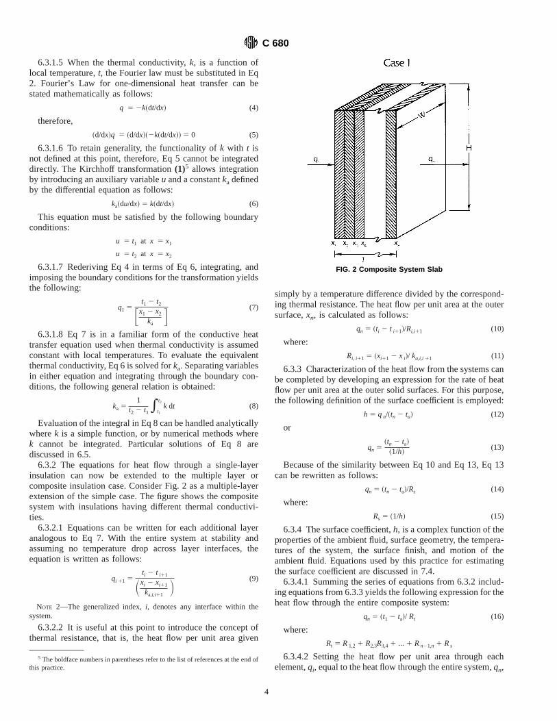
6.3.2 The equations for heat flow through a single-layerinsulation can now be extended to the multiple layer orcomposite insulation case. Consider Fig. 2 as a multiple-layerextension of the simple case. The figure shows the compositesystem with insulations having different thermal conductivi-ties.

6.3.2.1 Equations can be written for each additional layeranalogous to Eq 7. With the entire system at stability andassuming no temperature drop across layer interfaces, theequation is written as follows:

qi 11 5ti 2 t i11

Sxi 2 xi11

ka,i,i11D (9)

NOTE 2—The generalized index,i, denotes any interface within thesystem.

6.3.2.2 It is useful at this point to introduce the concept ofthermal resistance, that is, the heat flow per unit area given

simply by a temperature difference divided by the correspond-ing thermal resistance. The heat flow per unit area at the outersurface,xn, is calculated as follows:

qn 5 ~ti 2 t i11!/Ri,i11 (10)

where:

Ri, i11 5 ~xi11 2 x i!/ ka,i,i 11 (11)

6.3.3 Characterization of the heat flow from the systems canbe completed by developing an expression for the rate of heatflow per unit area at the outer solid surfaces. For this purpose,the following definition of the surface coefficient is employed:

h 5 qn/~tn 2 ta! (12)

or

qn 5~tn 2 ta!

~1/h!(13)

Because of the similarity between Eq 10 and Eq 13, Eq 13can be rewritten as follows:

qn 5 ~tn 2 ta!/Rs (14)

where:

Rs 5 ~1/h! (15)

6.3.4 The surface coefficient,h, is a complex function of theproperties of the ambient fluid, surface geometry, the tempera-tures of the system, the surface finish, and motion of theambient fluid. Equations used by this practice for estimatingthe surface coefficient are discussed in 7.4.

6.3.4.1 Summing the series of equations from 6.3.2 includ-ing equations from 6.3.3 yields the following expression for theheat flow through the entire composite system:

qn 5 ~t1 2 ta!/ Rt (16)

where:

Rt 5 R1,2 1 R2,3R3,4 1 ... 1 Rn21,n 1 Rs

6.3.4.2 Setting the heat flow per unit area through eachelement,qi, equal to the heat flow through the entire system,qn,

5 The boldface numbers in parentheses refer to the list of references at the end ofthis practice.

FIG. 2 Composite System Slab

C 680

4

shows that the ratio of the temperature across the element to thetemperature difference across the entire system is proportionalto the ratio of the thermal resistance of the element to the totalthermal resistance of the system or in general terms.

~ti 2 ti11!

~t1 2 ta!5 ~Ri,i11/ Rt! (17)

Eq 17 provides the means of solving for the temperaturedistribution. Since the resistance of each element depends onthe temperature of the element, the solution can be found onlyby iteration methods.

6.4 Equations—Case 2, Cylindrical Sections:6.4.1 For Case 2, Figs. 3 and 4, the analysis used is similar

to that described in 6.3, but with the replacement of thevariable x by the cyclindrical coordinate,r. The followinggeneralized equation is used to calculate the conductive heatflow through a layer of a cylinder wall.

qi11 5ti 2 ti11

Sri11 ln ~ri11/ri!ka,i,i 11

D (18)

Note the similarity of Eq 9 and Eq 18 and that the solutionof the transformation equation for the radical heat flow case isidentical to that of the slab case (see Eq 8).

6.4.2 As in Case 1, calculations for slabs, simplification ofthe equations for the heat loss may be accomplished bydefining the thermal resistance. For pipe insulations, the heatflow per unit area is a function of radius, so thermal resistancemust be defined in terms of the heat flow at a particular radius.The outer radius,rn, of the insulation system is chosen for thispurpose. The heat flow per unit area for cylinders, calculated atthe outer surface,rn, is:

qn 5 ~ti 2 t i11!/Ri,i11 (19)

where:

Ri, i11 5rn ln ~ri11/ri!

ka ,i,i11(20)

6.4.3 The concept of surface resistance used in an analysissimilar to 6.3.3 and 6.3.4 permits introduction of the definitionof the heat transfer as a function of the overall thermalresistance for the cylindrical case as follows:

qn 5 ~t1 2 t a!/Rt

(21)

where:

Rt 5 R1,2 1 R2,3 1 R3,4 1 ... 1 Rn21,n 1 Rs

NOTE 3—In some situations where comparisons of the insulationsystem performance is to be made, basing the areal heat loss on the insidesurface area, which is fixed by the pipe dimensions, or on the heat loss perunit length, is beneficial. The heat loss per unit area of the inside surfaceis calculated from the heat loss per unit area of the outside surface bymultiplying by the ratio of the outside radius to the inside radius. Forcalculation of the heat loss per linear foot from the heat loss per outsidearea, simply multiply by the outside area per foot or 2pro. For Case 2, theannulus, results are normally expressed as the time rate of heat flow perunit length,Q 1, which is obtained as follows:

Q 1 5 2prn qn 5 2pr n ~t1 2 t2!/Rt (22)

6.5 Calculation of Effective Conductivity:6.5.1 In Eq 11-22 it is necessary to evaluateka as a function

of temperature for each of the conductive elements. Thegeneralized solution in Eq 8 is as follows:

ka, i,i11 51

~ti11 2 t i!*ti

ti 11

kdt

6.5.2 When k may be described in terms of a simplefunction of t, an analytically exact solution forka can beobtained. The following functional types will be considered inthe examples (see 9.1-9.4).

6.5.2.1 Ifk is linear with t, k 5 a + bt and

ka 51

~t i11 2 ti!*ti

ti–1

~a 1 bt!dt 5 a 1 b Sti11 1 t i

2 D (23)

wherea andb are constants.6.5.2.2 If

k 5 ea1bt

then:

ka 51

~ti11 2 t i!*ti

ti 11

e a1bt dt

and evaluating the integral yields:

ka 5 F 1~ti11 2 t i!

GFea1bti11 2 ea1bti

b G (24)

wherea andb are constants, ande is the base of the naturallogarithm.FIG. 3 Single Layer Annulus System

FIG. 4 Composite System Annulus

C 680

5

6.5.2.3 If

k 5 a 1 bt 1 ct 2

then:

ka 51

~ti11 2 t i!*ti

ti 11

~a 1 bt 1 ct2!dt

and evaluating the integral yields:

ka 5 a 1b2 ~ti11 1 ti! 1

c3

~ti113 2 ti

3!

~ti11 2 ti!(25)

wherea, b, andc are constants.6.5.3 When the relationship ofk with t is more complex and

does not lend itself to simple mathematical treatment, anumerical method may be used. It is in these cases that thepower of the computer is particularly useful. There are a widevariety of numerical techniques available. The most suitablewill depend on the particular situation, and the details of thefactors affecting the choice are beyond the scope of thispractice.

7. Input Data

7.1 In general, data input is in accordance with ASTMStandards or American National Standards. The source of otherrequired data is noted.

7.2 Dimensions of Pipe and Pipe Insulation:7.2.1 Only nominal pipe sizes and insulation thicknesses are

required as input data. The actual dimensions of both pipe andpipe insulation are obtained by the computer from a softwarefile based on Practice C 585 during the calculation.

7.3 Thermal Conductivity Versus Mean Temperature:7.3.1 The data describing the relationship of thermal con-

ductivity to mean temperature are obtained in accordance withTest Methods C 177, C 335, or C 518, as appropriate for theproduct.

7.3.2 To describe accurately the relationship of thermalconductivity to mean temperature for thermal insulations,especially those exhibiting inflection points due to condensa-tions of the insulating gases, thermal conductivity tests at smalltemperature differences are required. The minimum tempera-ture differences used will depend on the vapor pressure totemperature of the gases involved, and the accuracy of the testapparatus at small temperature differences. Sufficient tests mustbe made to characterize the conductivity versus mean tempera-ture relationship over the desired temperature range.

NOTE 4—ASTM Committee C-16 is currently developing recommen-dations for preparing thermal conductivity curves for use in systemsanalysis. Although the exact procedures are beyond the scope of thispractice, caution should be exercised. The use of experimental data togenerate curves must include consideration of test sample geometry,temperature range of data, test temperature differentials, thickness effects,test boundary conditions, and test equipment accuracy. Especially impor-tant is that the test data should cover a temperature range of conditionswider than those of the analysis, so that the data is interpolated for theanalysis rather than extrapolated.

7.4 Surface Coeffıcients:7.4.1 The surface coefficient,h, as defined in Definitions

C 168, assumes that the surroundings (fluid and visible sur-faces) are at uniform temperature and that other visiblesurfaces are substantially perfect absorbers of radiant energy. It

includes the combined effects of radiation, conduction, andconvection.

7.4.2 In many situations surface coefficients may be esti-mated from published values(2).

7.4.3 Procedures for Calculating Surface Coeffıcients—Where known surface coefficients are not available, thispractice provides a calculational procedure to estimate thesurface coefficient. This calculation is based on the assumptionof heat flow from a uniformly heated surface. This assumptionis consistent with those used in developing the remainder ofthis practice. In simple terms, the surface coefficient equationsare based on those commonly used in heat transfer analysis. Adetailed discussion of the many heat flow mechanisms ispresent in several texts(3, 4, 5)or similar texts.

7.4.4 Analysis Configurations—Several convective condi-tions have been identified as requiring separate treatment whencalculating the surface coefficient. The first is the two geom-etries treated in this method, that is, flat (equipment) andcircular cylinder (pipe). Another case identifies the two air flowsystems common to most applications. Free convection isdefined as air motion caused by the bouyancy effects inducedby the surface-to-air temperature difference. This case ischaracterized by low velocity and, for most cases, includes anysituation where the local air velocity is less than 1 mph (0.5m/s). Forced convection is where some outside agent causesthe air movement. For high air velocities, convection is thedominant mechanism of heat flow from the surface. Theradiative heat flow surface coefficient is calculated separatelyand added to the convection losses since for a vast majority ofcases, this mechanism operates independently of the convec-tive transfer.

7.4.5 Surface Coeffıcient Calculation—Summary ofMethod—The convection coefficient calculation subroutine,SURCOF, developed for this practice, estimates the magnitudeof the convection coefficient based upon the equations for thegiven set of geometric conditions and temperature-dependentair properties. The radiative component is also determined andadded to yield the net surface coefficient. All equations used inthe analysis(3) were experimentally developed. The equationsused are briefly described in 7.4.7-7.4.9.

7.4.6 Alternative equation sets have been developed tocalculate the surface heat transfer coefficients. These equationsets often include parameters in addition to those used in thedevelopment of the SURCOF subroutine described in thispractice. These additional parameters are used to extend thedata set to a wider range of conditions or better fit the dataavailable. Use of these alternate equation sets instead of theSURCOF subroutine equation set is permitted, providingadequate documentation is provided and similarity of results isdemonstrated under the exposure conditions covered by theSURCOF documentation (See Appendix X1)(3).

7.4.7 Convection:7.4.7.1 Forced Convection—One of the major contributors

to surface heat transfer is the convection of air across a surfacewhere some difference exists between their temperatures. Notonly is the rate of heat flow controlled by the magnitude of thetemperature difference but also by the speed of the air flow as

C 680

6

it passes the surface. Since convection is a complex phenom-ena and has been studied by many researchers, many empiri-cally developed equations exist for estimating the surfacecoefficients. One of the simpler to apply and more commonlyused system of equations is that developed by Langmuir(6).His equations were developed for conditions of moderatetemperatures which are most commonly seen in cases ofinsulated piping or equipment systems. For the condition of thenatural convection of air at moderate temperature Langmuirproposed the following equation:

Qc 5 0.296~t s 2 ta!1.25 (26)

where:Qc 5 heat transferred by natural convections, Btu/ft2 (J/m2),ts 5 temperature of surface, °F (°C), andta 5 temperature of ambient, °F (°C).

7.4.7.2 Modifications for Forced Convection—When themovement of the air is caused by some outside force such asthe wind, forced ventilation systems, etc. Langmuir(6) pre-sented a modifier of Eq 26 to correct it for the forcedconvection. This multiplier was stated as follows:

ŒV 1 68.968.9

where V is the bulk air velocity (ft/min). In a morecommonly presented form where the velocity is miles per hour,this correction term reduces to

= 1.001 1.2773 Wind (27)

where Wind5 air movement speed (mph).Combining Eq 26 and Eq 27, we have Langmuir’s(6)

equation for the convection heat transfer from a surface:

Qc 5 0.296~t s 2 ta!1.25= 1 1 1.2773 Wind (28)

This equation will work for both forced and free convectionbecause when Wind equals zero, the equation returns to itsoriginal form.

7.4.7.3 Convection for Geometric Variations—Further re-search by Rice and Heilman(7) refined the technology ofLangmuir to account for changes in air film properties (density,thickness, viscosity) with the air film mean temperature. Alsotheir refinements provided corrections to the equation form forgeometric size, shape, and heat flow directions that permit useof the basic form of Langmuir’s(6) equation for a host ofconditions. The result of their research yields the followingequation set which forms the basis for the surface coefficientroutines used in this practice.

hcv 5 C 3 S1d D0.2

3 S 1tavg

D0.181

3 Dt 0.2663 =1 1 1.2773 Wind (29)

where:hcv 5 convective surface coefficient, Btu/h·ft2·°F (W/

(m2·K),d 5 diameter for cylinder, in. (m). For flat surfaces and

large cylinders d > 24, use d5 24,tavg 5 average temperature of air film, °F (°C)5 ( ts + ta)/

2, and

Dt 5 surface-to-air temperature difference, °F(°C), 5 (ts − ta).

7.4.7.4 The values of constantC are shown in Table 1 as afunction of shape and heat flow condition.

7.4.8 Radiative Component—In each previous case, theradiative exchanges are for the most part independent of theconvection exchange. The exception is that both help todetermine the average surface temperature. The radiationcoefficient is simply the radiative heat transfer rate, based uponthe Stefan-Boltzman Law, divided by the average surface-to-air temperature difference. Thus the relationship can be ex-pressed as the following:

hrad 5Emiss3 0.17133 1028 ~~ta 1 459.6!4 2 ~t s 1 459.6!4!

~ta 2 t s!(30)

where:E miss 5 effective surface emittance (includes

ambient emittance) and0.17133 10 −8 5 Stefan-Boltzman Constant (Btu/(h·ft2·

R4).7.4.9 Overall Coeffıcient—Once the radiation and convec-

tion coefficients are determined for the specific case underinvestigation, the overall coefficient is determined by addingthe two coefficients together.

h 5 hcv 1 hrad (31)

8. Computer Programs

8.1 General:8.1.1 The computer programs are written in Basic Fortran in

accordance with ANSI X3.9.

NOTE 5—Identical versions of these computer programs have beensuccessfully compiled and run on two processors. Only minor modifica-tions necessary for conformance to the resident operating system wererequired for operation.

8.1.2 Each program consists of a main program and severalsubroutines. Other subroutines may be added to make theprogram more applicable to the specific problems of individualusers.

8.1.3 The programs as presented call for the use of aninteractive terminal connected in real-time to a computer. Thecomputer controls the terminal interactively with program-generated instructions and questions transmitted to the termi-nal. Alternatively a second device could be used for display orprinting of computer messages. The final report can be dis-played or printed on the message destination device or may bedirected to a line printer or other hard copy unit. This is theusual device used for the final report when a cathode ray tubeis used as the input terminal.

TABLE 1 Shape Factors—Convection Equations

Shape and Condition Value of C

Horizontal cylinders 1.016Longer vertical cylinders 1.235Vertical Plates 1.394Horizontal plates, warmer than air, facing upward 1.79Horizontal plates, warmer than air, facing downward 0.89Horizontal plates, cooler than air, facing upward 0.89Horizontal plates, cooler than air, facing downward 1.79

C 680

7

8.2 Functional Description of Program— The flow charts,shown in Figs. 5 and 6 are a schematic representation of theoperational procedures of the respective programs. They show

that logic paths for reading data, obtaining actual systemdimensions, calculating and recalculating system thermal re-sistances and temperatures, relaxing the successive errors in

TABLE 2 Regression Analysis of Sample Data for Examples 1 to 4

Insulation TypeFunctional Relationship

Employed

Coefficients and Constants CorrelationCoefficient

F valueStandard Errorof Estimatesa b c TL TU

Type 1 (Fig. 11) k 5 a + bt + ct2 0.400 0.105 3 10−3 0.286 3 10−6 ... ... 0.999 550 0.0049Type 2 (Fig. 10) Ink 5 a + bt −1.62 0.213 3 10−2 ... ... ... 0.999 2130 0.0145Type 3 (Fig. 12) k 5 a1 + b1t; t # TL 0.201 0.39 3 10−3 ... −25 0.997 148 0.00165

k 5 a2 + b2t; TL < t < TU 0.182 −0.39 3 10−3 ... −25 50 0.997 187 0.00094k 5 a3 + b3t; t $ TU 0.141 0.37 3 10−3 ... 50 0.993 69.3 0.00320

FIG. 5 Flow Diagram of the Computer Program C 680E for Insulated Equipment Systems

C 680

8

the temperature to within 0.1° of the temperature, calculatingheat loss or gain for the system, and printing the parametersand solution in tabular form. The flow chart symbols are inaccordance with ANSI X3.5.

8.3 Computer Program Variable Description—The descrip-tion of all variables used in the programs are given in the listingof each program as comments. The listings of the mainlineprograms and the applicable subroutines are shown in Fig.7Fig. 8Fig. 9.

8.4 Program Operation:

8.4.1 Logon procedures and any executive program forexecution of this program must be followed as needed.

8.4.2 The input for the thermal conductivity versus meantemperature parameters is obtained as described in 7.3. (See thethermal curves depicted in Figs. 10-12.) The type code deter-mines the thermal conductivity versus temperature relationshipapplying to the insulation. The same type code may be used formore than one insulation. As presented, the program willoperate on the three functional relationships:

FIG. 6 Flow Diagram of Computer Program C 680P for Insulated Piping Systems

C 680

9

Type Code Functional Relationship1 k 5 a + bt + ct2 where a, b, and c are constants.2 k 5 ea+bt where a and b are constants and e is the

base of the natural logarithm3 k 5 a1 + b1 t; t < TL

k 5 a2 + b2 t; TL < t < TUk 5 a3 + b3 t; t > TUa1, a2, a3, b1, b2, b3 are constants. TL and TU are, re-spectively, the lower and upper inflection points of anS-shaped curve.

Additional or different relationships may be programmed butrequire modifications to the program.

8.4.3 For multiple number entry in a free field format, allnumbers must be separated by commas.

9. Illustration of Examples

9.1 General:9.1.1 Four examples are presented to illustrate the utility of

the program in calculating heat loss or gain and surfacetemperature. Most practical insulation design problems implic-itly or explicitly call for such calculations. Three insulatingmaterials, having equations forms for Types 1, 2, and 3, areconsidered. The fourth example illustrates a combination ofthese three materials.

NOTE 6—The curves contained herein are for illustration purposes onlyand not intended to reflect any actual product currently being produced.

FIG. 7 Computer Listing—Program C 680E—Thermal Performance of Multilayered Flat Insulation Systems

C 680

10

9.1.2 Sample data relating thermal conductivity to meantemperature data for the three insulating materials are shown inFigs. 10-12. Least-square estimates of the regression curve foreach sample data set produced a satisfactory fit to one of theprogram’s functional types. The information in Table 2 wasobtained from the regression analysis (least-squares fit) on eachmaterial.

9.2 Example 1:9.2.1 Consider application of a Type 2 insulation to the flat

vertical surfaces of a piece of hot equipment. The operatingtemperatures is 450°F (232°C). The equipment is locatedout-doors in an area where the winter design ambient tempera-

ture is 10°F (−12°C). Determine the insulation thicknessrequired to maintain the heat losses below 35 Btu/h·ft2 (110W/m2).

9.2.2 Assuming the system faces virtually blackbody sur-roundings at the design ambient temperature, the surfacecoefficient may be obtained from theASHRAE Handbook ofFundamentals(2). The value given for a nonreflective surfacein a 15-mph (6.7-m/s) wind (winter) is 6.00 Btu/h·ft2·°F (34W/m2·K).

9.2.3 From Table 2 for the material designated as Type Code2, the two coefficients required for the equation area 5 −1.62andb 5 0.00213.

FIG. 7 (continued)

C 680

11

9.2.4 From past experience, it is estimated that the requiredthicknesses will fall in the range from 4.0 to 5.0 in. (101 to 127mm). This range will be covered in increments of1⁄2 in. (3mm).

9.2.5 The resulting programing and analysis is given in Fig.13 where 4.5 in. (114 mm) is the least thickness to maintainheat loss below 35 Btu/h·ft2 (110 W/m2).

9.3 Example 2:9.3.1 Determine the minimum nominal thickness of Type 1

pipe insulation required to maintain the surface temperature ofa horizontal 3-in. (76-mm) iron pipe below 130°F (54°C).Consider a pipe temperature of 800°F (427°C). The ambienttemperature is 80°F (26°C).

9.3.2 Assuming the piping is located in a large room withsurrounding surfaces at ambient temperature and that theemissivity of the system is not significantly different from thatof bare steel pipe (0.9), the surface coefficient could beestimated from theASHRAE Handbook of Fundamentals(2).Because the thicknesses to be chosen will provide a surfacetemperature about 50°F (28°C) above the 80°F (26°C) ambi-ent, the 50° column is entered. The system diameter (insulationsize) is not known since it will depend on the insulationthickness. For the first calculation, and the estimated insulationdiameter, 9 in. (229 mm), 1.76 Btu/(h·ft2·°F) (10 W/m2·K), willbe used. The thicknesses chosen as a result of the firstcalculation will provide a basis for reestimating the surface

FIG. 7 (continued)

C 680

12

coefficients. These can be refined if a more rigorous treatmentof pipe temperature-thickness combinations that satisfy thesurface temperature criterion is required.

9.3.3 Referring to Table 2, for the material designated asType 1, the required constants for the thermal conductivityequations are:a 5 0.400, b 5 0.1053 10−3, and c5 0.2863 10

−6

.9.3.4 From experience, the nominal insulation thicknesses

of 2, 21⁄2, and 3 in. (51, 64, and 76 mm) are estimated to includethe range of solutions.

9.3.5 The solutions for this problem are given in Fig. 14where 3.0 in. (76 mm) is shown to maintain a surface

temperature below 130°F (54°C).9.4 Example 3:9.4.1 Example 3 is a repeat of Example 2 except that the

internal surface coefficient routine in the program C 680P2 isused.

9.4.2 Assume the same ambient and operating conditions,but the program calculates the surface coefficient from a flowof 0 mph (0 m/s) and a surface emittance of 0.9 instead ofchoosing from a handbook.

9.4.3 The results of this analysis (Fig. 15) yield approxi-mately the same answer as 9.3 and provide for more realistic

FIG. 7 (continued)

C 680

13

ambient input conditions and no time loss from interpolation ofthe reference tables.

9.5 Example 4—Multiple Layers:9.5.1 Determine the heat loss and surface and interface

temperatures of an insulated 4-in. (110-mm) pipe operating at600°F (315°C), insulated with 3 in. (76 mm) of Type 1material, 2-in. (51-mm) thick layer of Type 2 material and11⁄2-in. (13-mm) thick layer of Type 3 material at an ambienttemperature of − 100°F (−73°C). The wind speed is 5 mph (3.2m/s) and surface emittance is 0.9.

9.5.2 Referring to Figs. 10-12, to obtain the material prop-erties, the required constants are:

9.5.2.1 Type 1 Material:a 5 0.40b 5 0.1053 10 −3

c 5 0.2863 10 −6

9.5.2.2 Type 2 Material:a 5 −1.62b 5 0.2133 10 −2

9.5.2.3 Type 3 Material:a1 5 0.201 b1 5 0.393 10 −3

a2 5 0.182 b2 5 −0.393 10 −3

a3 5 0.141 b3 5 0.373 10 −3

(a) Transition Temperatures for Type 3:

FIG. 7 (continued)

C 680

14

TL 5 −25°F (−32°C)TU 5 50°F (10°C)9.5.3 The interactive communication record and calculated

results are shown in Fig. 16.

10. Report

10.1 The results of calculations performed in accordancewith this practice may be used as design data for specific jobconditions, or may be used in general form to represent theperformance of a particular product or system. When theresults will be used for comparison of performance of similar

products, it is recommended that reference be made to thespecific constants used in the calculations. These referencesshould include:

10.1.1 Name and other identification of products or compo-nents,

10.1.2 Identification of the nominal pipe size or surfaceinsulated, and its geometric orientation,

10.1.3 The surface temperature of the pipe or surface,10.1.4 The equations and constants selected for the thermal

conductivity versus mean temperature relationship,

FIG. 7 (continued)

C 680

15

FIG. 7 (continued)

FIG. 7 (continued)

C 680

16

10.1.5 The ambient temperature and humidity, if applicable,10.1.6 The surface coefficient and condition of surface heat

transfer,10.1.6.1 If obtained from published information, the source

and limitations,10.1.6.2 If calculated or measured, the method and signifi-

cant parameters such as emittances, fluid velocity, etc.,10.1.7 The resulting outer surface temperature, and10.1.8 The resulting heat loss or gain.10.2 Either tabular or graphical representation of the results

of the calculations may be used. No attempt is made torecommend the format of this presentation of results.

11. Precision and Bias

11.1 The precision of this practice is a function of thecomputer equipment used to generate the calculational results.In many typical computers normally used, seven significantdigits are resident in the computer for calculations. Adjust-ments to this level can be made through the use of “DoublePrecision,” however, for the intended purpose of this practice,standard levels of precision are adequate. The formatting of theoutput results, however, has been structured to provide aresolution of 0.1 % for the typical expected levels of heat fluxand within 0.1°F (0.05°C) for surface temperatures.

FIG. 8 Computer Listing—Program C 680P—Thermal Performance of Multilayered Cylindrical Insulation Systems

C 680

17

11.2 Many factors influence the accuracy of a calculationalprocedure used for predicting heat flux results. These factorsinclude computer resolution, accuracy of input data, and theapplicability of the assumptions used in the method for thesystem under study. The system of mathematical equationsused in this analysis has been accepted as applicable for mostsystems normally insulated with bulk-type insulations. Appli-cability of this practice to systems having irregular shapes,discontinuities and other variations from the one-dimensionalheat transfer assumptions should be handled on an individualbasis by professional engineers familiar with those systems.

11.3 The computer resolution effect on accuracy is only

significant if the level of precision is less than that discussed in11.1. Computers in use today are accurate in that they willreproduce the calculation results to the resolution required ifidentical input data is used.

11.4 The most significant factor influencing the accuracyclaims is the accuracy of the input thermal conductivity data.The accuracy of applicability of these data is derived from twofactors. The first is the accuracy of the test method used togenerate the data. Since the test methods used to supply thesedata are typically Test Methods C 177, C 335, or C 518 thereports should contain some statement of test data accuracy.The remaining factors influencing the accuracy are the inherent

FIG. 8 (continued)

C 680

18

variability of the product and the variability of the installationpractices. If the product variability is large or the installation ispoor, or both, serious differences might exist between mea-sured performance and predicted performance from using thispractice.

11.5 When concern exists with the accuracy of the input testdata, the recommended practice to evaluate the impact ofpossible errors is to repeat the calculation for the range of theuncertainty of the variable. This process yields a range in thedesired output variable for a given uncertainty in the input

variable uncertainty. Repeating this procedure for all the inputvariables would yield a measure of the contribution of each tothe overall uncertainty. Several methods exist for the combi-nation of these effects; however, the most commonly used is totake the square root of the sum of the squares of the percentageerrors induced by each variable’s uncertainty. Eq 32(8) givesthe expression in mathematical form.

SR 5 S (

i 5 1

n SS]R]xi

DD xiD2D 1/2 (32)

FIG. 8 (continued)

C 680

19

where:S 5 estimate of the probable error of the procedure,R 5 result of the procedure,xi 5 ith variable in procedure,]R/]x i 5 change in result with respect to, change in ith

variable,Dxi 5 uncertainty in value of variable,i, andn 5 total number of variables in procedure.

11.6 In summary, the use of this system of equations in thispractice for design and specification of insulations systemssince 1971 has demonstrated the applicability and useableaccuracy of the procedure. Although general usage attests to

acceptance of the calculational procedures, the specific appli-cability should be defined for each insulation system installa-tion at the time of its design.

11.7 Appendix X1 has been prepared by ASTM Subcom-mittee C16.30, Task Group 5.2, responsible for preparing thispractice. The appendix provides a more complete discussion ofthe precision and bias expected when using C 680 in theanalysis of operating systems. While much of that discussion isrelevant to this practice, the errors associated with its applica-tion to operating systems is beyond the primary C 680 scope.Portions of this discussion, however, were used in developing

FIG. 8 (continued)

C 680

20

the Precision and Bias statements included in Section 11.

12. Keywords

12.1 block; computer program; heat flow; heat gain; heat

loss; pipe; thermal insulation

FIG. 8 (continued)

C 680

21

FIG. 8 (continued)

C 680

22

FIG. 8 (continued)

C 680

23

FIG. 8 (continued)

FIG. 8 (continued)

C 680

24

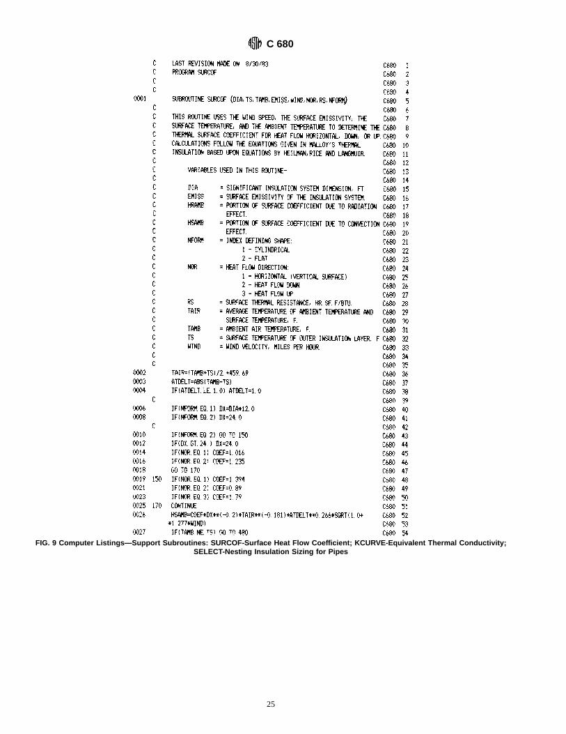
FIG. 9 Computer Listings—Support Subroutines: SURCOF-Surface Heat Flow Coefficient; KCURVE-Equivalent Thermal Conductivity;SELECT-Nesting Insulation Sizing for Pipes

C 680

25

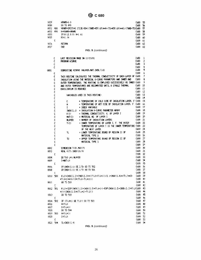
FIG. 9 (continued)

FIG. 9 (continued)

C 680

26

FIG. 9 (continued)

C 680

27

FIG. 9 (continued)

C 680

28

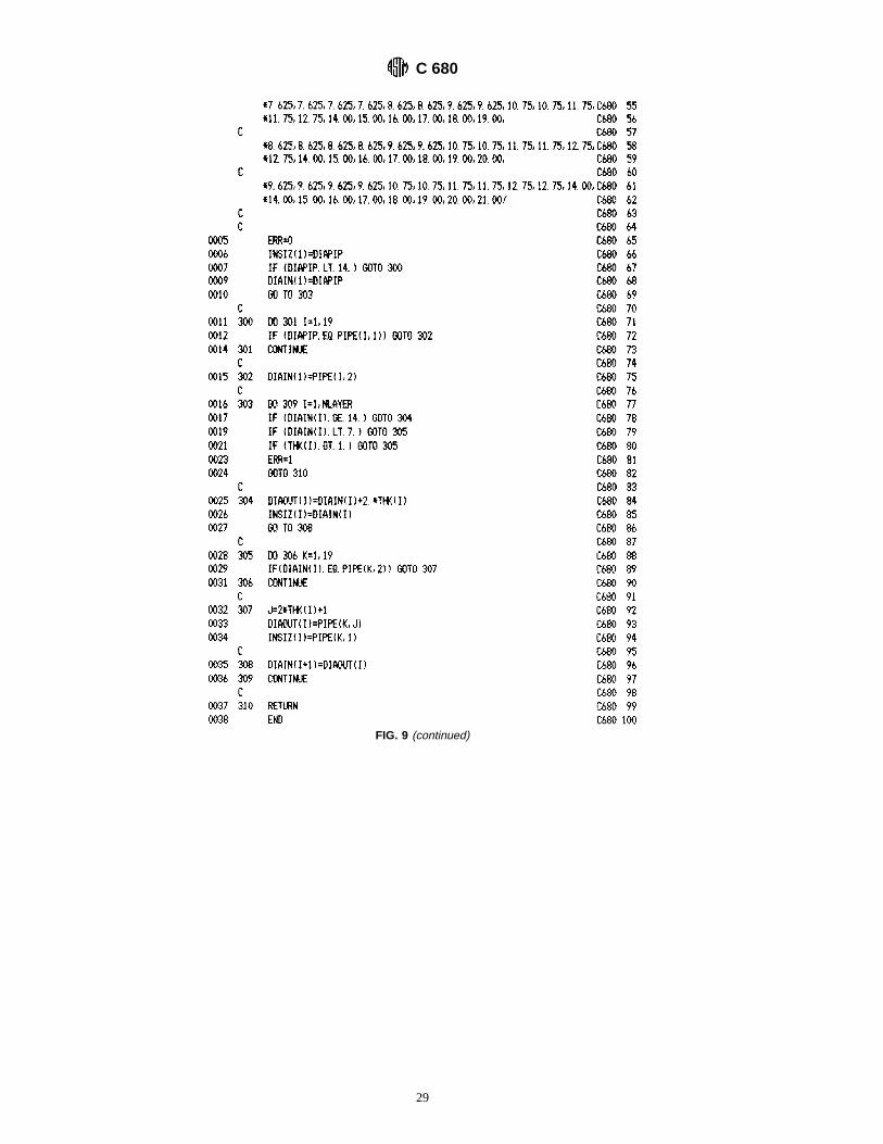
FIG. 9 (continued)

C 680

29

FIG. 10 Sample Data—Type 2 Material

FIG. 11 Sample Data—Type 1 Material

FIG. 12 Sample Data—Type 3 Material

C 680

30

FIG. 13 Sample Problem 1

C 680

31

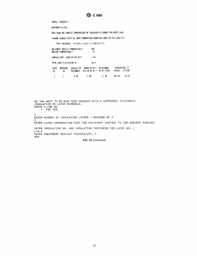
FIG. 13 (continued)

C 680

32

FIG. 13 (continued)

C 680

33

FIG. 14 Sample Problem 2

C 680

34

FIG. 14 (continued)

C 680

35

FIG. 14 (continued)

C 680

36

FIG. 14 (continued)

C 680

37

FIG. 15 Sample Problem 3

C 680

38

FIG. 15 (continued)

C 680

39

FIG. 15 (continued)

C 680

40

FIG. 15 (continued)

C 680

41

FIG. 15 (continued)

C 680

42

FIG. 16 Sample Problem 4

C 680

43

APPENDIX

(Nonmandatory Information)

X1. APPLICATION OF PRACTICE C 680 TO FIELD MEASUREMENTS

X1.1 This appendix has been included to provide a morecomplete discussion of the precision and bias expected whenusing this practice in the analysis of operating systems. Whilemuch of the discussion below is relevant to the practice, theerrors associated with its application to operating systems isbeyond the immediate scope of this task group. Portions of thisdiscussion, however, were used in developing the Precisionand Bias statements included in Section 11.

X1.2 This appendix will consider precision and bias as itrelates to the comparison between the calculated results of theC 680 analysis and measurements on operating systems. Someof the discussion here may also be found in Section 11;

however, items are expanded here to include analysis ofoperating systems.

X1.3 Precision:

X1.3.1 The precision of this practice has not yet beendemonstrated as described in Specification E 691, but aninterlaboratory comparison could be conducted, if necessary, asfacilities and schedules permit. Assuming no errors in pro-gramming or data entry, and no computer hardware malfunc-tions, an interlaboratory comparison should yield the theoreti-cal precision presented in X1.3.2.

X1.3.2 The theoretical precision of this practice is a func-tion of the computer equipment used to generate the calculated

FIG. 16 (continued)

C 680

44

results. Typically, seven significant digits are resident in thecomputer for calculations. The use of “Double Precision” canexpand the number of digits to sixteen. However, for theintended purpose of this practice, standard levels of precisionare adequate. The effect of computer resolution on accuracy isonly significant if the level of precision is higher than sevendigits. Computers in use today are accurate in that they willreproduce the calculation results to the resolution required ifidentical input data is used.

X1.3.2.1 The formatting of output results from this practicehas been structured to provide a resolution of 0.1 % for thetypically expected levels of heat flux, and within 0.1°F(0.05°C) for surface temperatures.

X1.3.2.2 A systematic precision error is possible due to thechoices of the equations and constants for convective andradiative heat transfer used in the program. The interlaboratorycomparison of X1.3.3 indicates that this error is usually withinthe bounds expected inin situ heat flow calculations.

X1.3.3 Precision of Surface Convection Equations:X1.3.3.1 Many empirically derived equation sets exist for

the solution of convective heat transfer from surfaces ofvarious shapes in various environments. The Rice Heilmanadjustments(7) to the Langmuir’s equations(6) is one com-monly used equation set. If two different equations sets arechosen and a comparison is made using identical input data, thecalculated results are never identical, not even when theconditions for application of the equations appear to beidentical. For example, if equations designed for verticalsurfaces in turbulent cross flow are compared, results from thiscomparison could be used to help predict the effect of theequation sets on overall calculation precision.

X1.3.3.2 The systematic precision of the surface coefficientequation set used in this practice has had at least one thoroughintralaboratory evaluation(9). When the surface convectivecoefficient equation (see Eq 30) of this practice was comparedto another surface equation set by computer modeling ofidentical conditions, the resultant surface coefficients for the240 typical data sets varied, in general, less than 10 %. Oneextreme case (for flat surfaces) showed variations up to 30 %.Other observers have recorded larger variations (in less rigor-ous studies) when additional equation sets have been com-pared. Unfortunately, there is no standard for comparison,since all practical surface coefficient equations are empiricallyderived. Eq 30 is widely used and accepted and will continueto be recommended until evidence suggests otherwise.

X1.3.4 Precision of Radiation Surface Equations:X1.3.4.1 The Stefen-Boltzman equation for radiant transfer

is widely applied, but still debated. In particular, there remainssome concern as to whether the exponents of temperature areexactly 4.0 in all cases. A small error in these exponents couldcause a larger error in calculated radiant heat transfer. Theexactness of the coefficient 4 is well-founded in both physicaland quantum physical theory and is therefore used here.

X1.3.4.2 On the other hand, the ability to measure andpreserve a known emittance is quite difficult. Furthermore,though the assumptions of an emittance of 1.0 for the surround-ings and a “sink’’ temperature equal to ambient air temperatureis often approximately correct in a laboratory environment,

operating systems in an industrial environment often divergewidely from these assumptions. The effect of using 0.95 for theemittance of the surroundings rather than the 1.00 assumed inthe previous version of this practice was also investigated bythe task group(9). Intralaboratory analysis of the effect ofassuming a surrounding effective emittance of 0.95 versus 1.00indicates a variation of 5 % in the radiation surface coefficientwhen the object emittance is 1.00. As the object emittance isreduced to 0.05, the difference in the surface coefficientbecomes negligible. These differences would be greater if thesurrounding effective emittance is less than 0.95.

X1.3.5 Precision of Input Data:X1.3.5.1 The heat transfer equations used in the computer

program of this practice imply possible sources of significanterrors in the data collection process, as detailed later in thisappendix.

NOTE X1.1—Although data collection is not within the scope of thispractice, the results of this practice are highly dependent on accurate inputdata. For this reason, a discussion of the data collection process is includedhere.

X1.3.5.2 A rigorous demonstration of the impact of errorsassociated with the data collection phase of an operatingsystem’s analysis using C680 is difficult without a parametricsensitivity study on the method. Since it is beyond the intent ofthis discussion to conduct a parametric study for all possiblecases, X1.3.5.3-X1.3.5.7 discuss in general terms the potentialfor such errors. It remains the responsibility of users to conducttheir own investigation into the impact of the analysis assump-tions particular to their own situations.

X1.3.5.3 Conductivity Data—The accuracy and applicabil-ity of the thermal conductivity data are derived from severalfactors. The first is the accuracy of the test method used togenerate the data. Since Test Methods C 177, C 335, and C 518are usually used to supply test data, the results reported forthese tests should contain some statement of test data accuracy.The remaining factors influencing the accuracy are the inherentvariability of the product and the variability of the insulationinstallation practice. If the product variability is large or theinstallation is poor, or both, serious differences might existbetween the measured performance and the performance pre-dicted by this method.

X1.3.5.4 Surface Temperature Data—There are many tech-niques for collecting surface temperatures from operatingsystems. Most of these methods assuredly produce some errorin the measurement due to the influence of the measurement onthe operating condition of the system. Additionally, the in-tended use of the data is important to the method of surfacetemperature data collection. Most users desire data that isrepresentative of some significant area of the surface. Sincesurface temperatures frequently vary significantly across oper-ating surfaces, single-point temperature measurements usuallylead to errors. Sometimes very large errors occur when the datais used to represent some integral area of the surface. Someusers have addressed this problem through various means ofdetermining average surface temperatures. Such techniqueswill often greatly improve the accuracy of results used torepresent average heat flows. A potential for error still exists,however, when theory is precisely applied. This practice

C 680

45

applies only to areas accurately represented by the averagepoint measurements, primarily because the radiation and con-vection equations are non-linear and do not respond correctlywhen the data is averaged. The following example is includedto illustrate this point:

Assume the system under analysis is a steam pipe. Thepipe is jacketed uniformly, but one-half of its length is poorlyinsulated, while the second half has an excellent insulationunder the jacket. The surface temperature of the good half ismeasured at 550°F. The temperature of the other half ismeasured at 660°F. The average of the two temperatures is610°F. The surface emittance is 0.92, and ambient temperatureis 70°F. Solving for the surface radiative heat loss rates for eachhalf and for the average yields the following:

The average radiative heat loss rate corresponding to a610°F temperature is 93.9 Btu/ft2/h.

The “averaged” radiative heat loss obtained by calculatingthe heat loss for the individual halves, summing the total anddividing by the area, yields an “averaged” heat loss of 102.7Btu/hr/ft2. The error in assuming the averaged surface tempera-ture when applied to the radiative heat loss for this case is8.6 %.

It is obvious from this example that analysis by the methodsdescribed in this practice should be performed only on areaswhich are thermally homogeneous. For areas in which thetemperature differences are small, the results obtained usingC680 will be within acceptable error bounds. For large systemsor systems with significant temperature variations, total areashould be subdivided into regions of nearly uniform tempera-ture difference so that analysis may be performed on eachsubregion.

X1.3.5.5 Ambient Temperature Variations—In the standardanalysis by the methods described in this practice, the tem-perature of the radiant surroundings is taken to be equal to theambient air temperature (for the designer making comparativestudies, this is a workable assumption). On the other hand, thisassumption can cause significant errors when applied toequipment in an industrial environment, where the surround-ings may contain objects at much different temperatures thanthe surrounding air. Even the natural outdoor environment doesnot conform well to the assumption of air temperatures whenthe solar or night sky radiation is considered. When thispractice is used in conjunction within situ measurements ofsurface temperatures, as would be the case in an audit survey,extreme care must be observed to record the environmentalconditions at the time of the measurements. While the com-puter program supplied in this practice does not account forthese differences, modifications to the program may be madeeasily to separate the convective ambient temperature from themean radiative environmental temperature seen by the surface.The key in this application is the evaluation of the magnitudeof this mean radiant temperature. The mechanism for thisevaluation is beyond the scope of this practice. A discussion ofthe mean radiant temperature concept is included in theASHRAE Handbook of Fundamentals(2).

X1.3.5.6 Emittance Data—Normally, the emittance valuesused in a C680 analysis account only for the emittance of thesubject of the analysis. The subject is assumed to be completely

surrounded by an environment which has an assigned emit-tance of 0.95. Although this assumption may be valid for mostcases, the effective emittance used in the calculation can bemodified to account for different values of effective emittance.If this assumption is a concern, using the following formula forthe new effective surface emittance will correct for this error:

e eff 5AA

~1 2 e A!/eAAA 1 1/AAF AB 1 ~1 2 eB!/e BAB(X1.1)

where:e eff 5 effective mean emittance for the two surface com-

bination,eA 5 mean emittance of the surfaceA,FAB 5 view factor for the surfaceA and the surrounding

regionB,eB 5 mean emittance of the surrounding regionB,AA 5 area of regionA, andA B 5 area of regionB.

This equation set is described in most heat transfer texts onradiative heat transfer. See Holman(4), p. 305.

X1.3.5.7 Wind Speed— Wind speed, as used in the Lang-muir’s (6) and Rice Heilman(7) equations, is defined as windspeed measured in the main airstream near the subject surface.Air blowing across real objects often follows flow directionsand velocities much different from the direction and velocity ofthe main free stream. The equations used in C680 analysisyield “averaged’’ results for the entire surface in question.Because of this averaging, portions of the surface will havedifferent surface temperatures and heat flux rates from theaverage. For this reason, the convective surface coefficientcalculation cannot be expected to be accurate at each locationon the surface unless the wind velocity measurements are madeclose to the surface and a separate set of equations are appliedthat calculate the local surface coefficients.

X1.3.6 Theoretical Estimates of Precision:X1.3.6.1 When concern exists regarding the accuracy of the

input test data, the recommended practice is to repeat thecalculation for the range of the uncertainty of the variable. Thisprocess yields a range of the desired output variable for a giveninput variable uncertainty. Several methods exist for evaluatingthe combined variable effects. Two of the most common areillustrated as follows:

X1.3.6.2 The most conservative method assumes that theerrors propagating from the input variable uncertainties areadditive for the function. The effect of each of the individualinput parameters is combined using Taylor’s Theorem, aspecial case of a Taylor’s series expansion(10).

SR 5 (

i 5 1

n U]R]xiU · Dx i (X1.2)

where:S 5 estimate of the probable error of the procedure,R 5 result of the procedure,xi 5 ith variable of the procedure,]R/]x i 5 change in result with respect to a change in theith

variable (also, the first derivative of the functionwith respect to theith variable),

Dxi 5 uncertainty in value of variablei, and

C 680

46

n 5 total number of input variables in the procedure.

X1.3.6.3 For the probable uncertainty of function,R, themost commonly used method is to take the square root of thesum of the squares of the fractional errors. This technique isalso known as Pythagorean summation. This relationship isdescribed in the following equation:

SR 5 S (

i 5 1

n SS]R]xi

D · DxiD 2D1/2

(X1.3)

X1.3.7 Bias of C680 Analysis:X1.3.7.1 As in the case of the precision, the bias of this

standard practice is difficult to define. From the precedingdiscussion, some bias can result due to the selection ofalternative surface coefficient equation sets. If, however, thesame equation sets are used for a comparison of two insulationsystems to be operated at the same conditions, no bias ofresults are expected from this method. The bias due tocomputer differences will be negligible in comparison withother sources of potential error. Likewise, the use of the heattransfer equations in the program implies a source of potentialbias errors, unless the user ensures the applicability of the

practice to the system.

X1.3.8 Error Avoidance— The most significant sources ofpossible error in this practice are in the misapplication of theempirical formulae for surface transfer coefficients, such asusing this practice for cases that do not closely fit the thermaland physical model of the equations. Additional errors evolvefrom the superficial treatment of the data collection process.Several promising techniques to minimize these sources oferror are in stages of development. One attempt to addresssome of the issues has been documented by Mack(11). Thistechnique addresses all of the above issues except the problemof non-standard insulationk values. As the limitations andstrengths ofin situ measurements and C680 analysis becomebetter understood, they can be incorporated into additionalstandards of analysis that should be associated with thispractice. Until such methods can be standardized, the bestassurance of accurate results from this practice is that eachapplication of the practice will be managed by a user who isknowledgeable in heat transfer theory, scientific data collectionpractices, and the mathematics of programs supplied in thispractice.

REFERENCES

(1) Arpaci, V. S., Conduction Heat Transfer, Addison-Wesley, 1966, p.129–130.

(2) ASHRAE Handbook of Fundamentals, Chapter 23, “Design HeatTransmission Coefficients,” American Society of Heating, Refrigerat-ing, and Air Conditioning Engineers Inc., Atlanta, GA, Table 1, p.23.12 and Tables 11 and Tables 12, p. 23.30, 1977.

(3) Turner, W. C., and Malloy, J. F.,Thermal Insulation Handbook,McGraw Hill, New York, NY, 1981.

(4) Holman, J. P.,Heat Transfer, McGraw Hill, New York, NY, 1976.(5) McAdams, W. H.,Heat Transmission, McGraw Hill, New York, NY,

1955.(6) Turner, W. C., and Malloy, J. F.,Thermal Insulation Handbook,

McGraw Hill, New York, NY, 1981, p. 50.

(7) Heilman, R. H., “Surface Heat Transmission,” ASME Transactions,Vol 1, Part 1, FSP-51-91, 1929, pp. 289–301.

(8) Schenck, H.,Theories of Engineering Experimentation, McGraw Hill,New York, NY, 1961.

(9) Mumaw, J. R.,C 680 Revision Update—Surface Coeffıcient Compari-sons, A report to ASTM Subcommittee C16.30, Task Group 5.2, June24, 1987.

(10) Beckwith, T. G., Buck, N. L., and Marangoni, R. D.,MechanicalMeasurement, Addison-Wesley, Reading, MA, 1973.

(11) Mack, R. T., “Energy Loss Profiles,”Proceedings of the FifthInfrared Information Exchange, AGEMA, Secaucus, NJ, 1986.

The American Society for Testing and Materials takes no position respecting the validity of any patent rights asserted in connectionwith any item mentioned in this standard. Users of this standard are expressly advised that determination of the validity of any suchpatent rights, and the risk of infringement of such rights, are entirely their own responsibility.

This standard is subject to revision at any time by the responsible technical committee and must be reviewed every five years andif not revised, either reapproved or withdrawn. Your comments are invited either for revision of this standard or for additional standardsand should be addressed to ASTM Headquarters. Your comments will receive careful consideration at a meeting of the responsibletechnical committee, which you may attend. If you feel that your comments have not received a fair hearing you should make yourviews known to the ASTM Committee on Standards, 100 Barr Harbor Drive, West Conshohocken, PA 19428.

This standard is copyrighted by ASTM, 100 Barr Harbor Drive, West Conshohocken, PA 19428-2959, United States. Individualreprints (single or multiple copies) of this standard may be obtained by contacting ASTM at the above address or at 610-832-9585(phone), 610-832-9555 (fax), or [email protected] (e-mail); or through the ASTM website (http://www.astm.org).

C 680

47