StackInsights: Cognitive Learning for Hybrid Cloud Readiness

StackInsights: Cognitive Learning for HybridCloud Readiness

Mu Qiao, Luis Bathen, Simon-Pierre Genot, Sunhwan Lee, Ramani RoutrayIBM Almaden Research Center

650 Harry RoadSan Jose, California, CA

Email: {mqiao,bathen,sgenot,shlee,routrayr}@us.ibm.com

Abstract—Hybrid cloud is an integrated cloud computingenvironment utilizing a mix of public cloud, private cloud, andon-premise traditional IT infrastructures. Workload awareness,defined as a detailed full range understanding of each individualworkload, is essential in implementing the hybrid cloud. Whileit is critical to perform an accurate analysis to determinewhich workloads are appropriate for on-premise deploymentversus which workloads can be migrated to a cloud off-premise,the assessment is mainly performed by rule or policy basedapproaches. In this paper, we introduce StackInsights, a novelcognitive system to automatically analyze and predict the cloudreadiness of workloads for an enterprise. Our system harnessesthe critical metrics across the entire stack: 1) infrastructuremetrics, 2) data relevance metrics, and 3) application taxonomy,to identify workloads that have characteristics of a) low sensitivitywith respect to business security, criticality and compliance, andb) low response time requirements and access patterns. Since thecapture of the data relevance metrics involves an intrusive andin-depth scanning of the content of storage objects, a machinelearning model is applied to perform the business relevanceclassification by learning from the meta level metrics harnessedacross stack. In contrast to traditional methods, StackInsightssignificantly reduces the total time for hybrid cloud readinessassessment by orders of magnitude.

I. INTRODUCTION

Hybrid cloud, which utilizes a mix of public cloud, pri-vate cloud, and on-premise, has become the dominant clouddeployment architecture for enterprises. Public cloud offersa multi-tenant environment, where physical resources, suchas computing, storage and network devices, are shared andaccessible over a public network, whereas private cloud isoperated solely for a single organization with dedicated re-sources. Hybrid cloud inherits the advantages of these twocloud models and allows workloads to move between themaccording to the change of business needs and cost, thereforeresulting in greater deployment flexibility. The global hybridcloud market is estimated to grow from USD 33.28 Billion in2016 to USD 91.74 Billion in 2021 [1].

Business sensitivity is one of the main factors that enter-prises consider when deciding which cloud model to deploy.For example, an enterprise can deploy public clouds for testand development workloads, where security and complianceare not an issue. However, it is hard to meet PCI (paymentcard industry) or SOX (Sarbanes-Oxley) compliance in publicclouds due to the nature of multi-tenancy. On the other hand,because private clouds are dedicated to a single organization,

the architecture can be designed to assure high level securityand stringent compliance, such as HIPAA (health insuranceportability and accountability act). Therefore, private cloudsare usually deployed for business sensitive and critical work-loads. Infrastructure is another important factor to considerwhen choosing between public and private clouds. Sinceprivate cloud is a single-tenant environment where resourcescan be specified and highly customized, it is ideal to host datawhich are frequently accessed and require fast response time.For example, high-end storage system can be used in privatecloud to deliver IOPS (input/output operations per second)within a guaranteed response time.

Moreover, business sensitivity and infrastructure are tradi-tionally considered in two separate schools of work. However,not all data is created equal, neither is the infrastructure.In this paper, we introduce StackInsights, a novel cognitivelearning system to automatically analyze and predict the cloudreadiness of workloads for an enterprise by considering bothbusiness sensitivity and infrastructure. StackInsights classifiesthe entire data into several subspaces, as shown in Figure 1,where the X-axis indicates the infrastructure heat map (e.g.,storage access intensity) and the Y -axis represents the businesssensitivity. A threshold on the X-axis is set to determineif the data is “cold” or “hot” with respect to infrastructurerelated performance metrics, and on the Y -axis, the data isclassified into three categories: “sensitive”, “non-sensitive”, or“non-classifiable”. Formally, we define sensitive data as thedata owned by the enterprise, which if lost or compromised,bares financial, integrity, and compliance damage. There aremany different forms of sensitive data, such as sensitivepersonal information (SPI), personal health information (PHI),confidential business information, client data, intellectual prop-erty, and other domain-specific sensitive information. Thecategory of “non-classifiable” includes structured data, suchas databases, the sensitivity of which can be analyzed usingdomain knowledge. For example, the databases storing em-ployment information in the HR department should be highlysensitive. All the data which are cold and non-sensitive canbe migrated to public clouds while the rest should reside inprivate clouds. The thresholds on the X-axis and Y -axis canalso be adjusted by users. The areas of the subspaces indicatethe size of data migrating to different clouds, thereby, servingas a cloud sizing tool. The hotness of data on the X-axis can

arX

iv:1

712.

0601

5v1

[cs

.LG

] 1

6 D

ec 2

017

be obtained by measuring infrastructure performance metrics.The key issue therefore lies in how to determine the businesssensitivity of data on the Y -axis.

To the best of our knowledge, StackInsights is the firstcognitive system that uses machine learning to understanddata sensitivity based on metadata, as it correlates application,data, and infrastructure metrics for hybrid cloud readinessassessment. In contrast to traditional methods which requirecontent scanning for sensitivity analysis, StackInsights sig-nificantly reduces the total running time through machinelearning. It advises users what data are appropriate to be storedon premises, or to be migrated to the cloud, and the specificcloud deployment model, by integrating both data sensitivityand hotness in terms of infrastructure performance.

The rest of the paper is organized as follows. We describeour motivation and contribution in Section II. The relevantwork is reviewed in Section III. In Section IV, we introduce theframework of StackInsights as well as the cognitive learningcomponents. Section V is on the experiments and results.Finally, we conclude in Section VI.

Fig. 1. Hybrid cloud migration overview

II. MOTIVATION AND CONTRIBUTION

The classification of data sensitivity belongs to the generaldomain of data classification, which allows organizations tocategorize data by business relevance and sensitivity in orderto maintain the confidentiality and integrity of their data. Dataclassification is a very costly activity. In large organizations,data is usually stored and secured by many repositories or sys-tems in different geo locations, which may have different dataprivacy and regulatory compliances. Various security accessapprovals have to be obtained in order to get access to data. Inaddition, traditional sensitivity assessment approaches requirean intrusive and in-depth content scanning of the objects,which is not scalable in this big data era, where numerousstructured and unstructured data are generated in real-time.To solve this issue, we develop a machine learning modelin StackInsights, which can perform a business sensitivityclassification by learning from file metadata, which is mucheasier and cost-efficient to collect. By using meta data, wecan already obtain a sensitivity prediction model with highaccuracy. Therefore, we do not have to perform a detailedcontent analysis on all the files. Instead, intensive contentanalysis can be conducted on the predicted non-sensitive filesfor further screening if needed. Our model-based approachsignificantly reduces the total sensitivity assessment time.

When migrating workloads among private, public, and hy-brid clouds, one of the biggest challenges is the storage layer.An enterprise’s infrastructure might consist of a mixture of file,block, and object storage, which have different properties andoffer their own advantages. Enterprises big or small tend tomanage large and heterogeneous environments. For example,one of our IT environments supports around 100 businessaccounts, spread over several geo locations, amassing a totalof 200 PB of block storages alone. Similarly, our file storagefabric is also massive, where file shares (mapped to volumes/q-trees) may be in the TB, or even PB scale.

Given such a large storage infrastructure with a number ofvolumes, we need to determine their cloud migration priority,i.e., which volumes should be migrated first. Data sensitivity isone of the most important factors in cloud migration. Volumesof low sensitivity can be sanitized first and then migrated tothe public cloud. From a cloud migration service admin pointof view, it is not critical to know the exact sensitivity of thevolumes, but rather the sensitivity “level” of the volumes, sothat a priority can be given to a large number of volumes.Traditional sensitivity assessment approaches, which requirecontent scanning, are very expensive. It is impractical andnot necessary to perform a full content scanning on all thevolumes in order to obtain the priority. Machine learning canhelp predict the sensitivity of files based on the easily collectedfile meta data, and then obtain the migration priority within amuch shorter time.

As it is expensive to determine the business sensitivity ofeach storage volume, we develop a clustering component inStackInsights, which identifies groups of volumes that sharesimilar characteristics. Specifically, the volumes are clusteredbased on their meta level information, which are obtainedby aggregating the file metadata at the volume level. Thesensitivity of a representative volume in each cluster is usedas the representative sensitivity of all the volumes in the samecluster. To obtain the sensitivity of a representative volume,we apply the previously introduced machine learning modelto predict the sensitivity of each single file on that volume. Thesensitivity of a volume is defined as the number of sensitivefiles divided by the total number the files.

Similarly, we also obtain the IOPS of each volume andcompute its IO density, which is defined as IOPS per GB. Allthe volumes with both low business sensitivity and IO densitycan be candidates to be migrated to public clouds while theother volumes should remain on premise or be migrated toprivate clouds.

III. RELATED WORK

In the marketplace of enterprise softwares, there are toolsdeveloped for data classification in regard of data governanceor life cycle management. For example, [2] [3] provide dataclassification services for managing and retaining various typesof data such as emails and other unstructured data throughpre-determined rules or dictionary searches. Data privacyand security have become the most pressing concerns fororganizations. To embrace the newly announced General Data

Protection Regulation (GDPR) by European Union, enterprisesare making great efforts in addressing key data protection re-quirements as well as automating the compliance process. Forexample, IBM Security Guardium solutions [4] help clientssecure their sensitive data across a full range of environments.Data classification, as the first step to security, has becomeextremely important. Only if we understand which data aresensitive through classification, we can design better securityproduct to protect them. On the other hand, [5] assesses thecloud migration readiness by providing a questionnaire to theowner of the infrastructure. Many of existing tools lack ofcognitive aspects, and even if there is, the data preparationstep requires the scanning of file content, which is not scalableor limits the type of files to which the tool can be applied.

Besides the rule-based approaches to classify data, thereare previous attempts leveraging a predictive model. Model-based approaches are much more systematic and scalablebecause there is no need to generate a rule to classify filesmanually. Data classification based on the proof-of-conceptsystem that crawls all files in order to analyze data sensitivitywas studied in [6]. A nearest neighbor algorithm was proposedin [7] to attribute the confidentiality of files. A general-purpose method to automatically detect sensitive informationfrom textual documents was presented in [8] by adapting theinformation theory and a large corpus of documents. Theapplication to data loss prevention by using automatic textclassification algorithms for classifying enterprise documentsas either sensitive or non-sensitive was introduced in [9].However, most of these previous works require an exhaustiveprocess to crawl the contents of data, which is impossible inmany applications due to privacy, governance, or regulations.[10] proposed to use the decision tree classifier for findingassociations between a file’s properties and metadata.

There are preliminary works in the field of hybrid cloudmigrations whose components include a data classificationmethod. The tool for migrating enterprise services into hybridcloud-based deployment was introduced in [11]. The complex-ity of enterprise applications is highlighted and the model,accommodating the complexity and evaluating the benefitsof a hybrid cloud migration, is developed. Though the workshed insight on security of data, the tool does not assessthe sensitivity of applications in the level of file. Rule-baseddecision support tool is deployed in [12] for the purposeof providing a modeling tool to compare various infrastruc-tures for IT architects. In many practical cases, however,IT architects are blind on the contents of data and thus itis not straightforward to model their applications, data, andinfrastructure requirements without understanding the natureof data such as sensitivity. In addition, [13] developed aframework which automates the migration of web server tothe cloud.

As observed in previous works, data classification andhybrid cloud migration are explored separately although twocomponents are tightly related. In contrast to the existingworks, our proposed framework covers the whole processincluding classifying data, assessing the readiness of cloud

migration, and finally a decision support for hybrid cloudmigration. Furthermore, we develop an efficient and scalablemethod to determine cloud readiness by considering datasensitivity and infrastructure performance through a cognitivelearning process.

IV. STACKINSIGHTS FRAMEWORK

We show the high-level framework of StackInsights inFigure 2. In order to gain insights into an existing IT envi-ronment, we scan various layers across the entire stack: 1) theapplication layer, 2) the data layer, and 3) the infrastructurelayer. The application layer tells us the types of the runningworkloads, what components they depend on, and the specificrequirements. The data layer provides file metadata as well ascontent. Finally, the infrastructure layer provides performancemetrics, such as, how often the data is accessed, and where itis stored.

A. Workload Scan

Before scanning the infrastructure and the data itself, wefirst need to understand what type of workloads are runningwithin the enterprise. This can be done through the use oftools such as IBM’s Tivoli Application Dependency Discov-ery Manager (TADDM) [14], which provides an automateddiscovery and application mappings. Additionally, the IT staffwithin each enterprise are also good sources as they areoften the subject matter experts and can give a high-leveloverview of their workloads. This step is critical as we needto understand the workloads or applications before startingany sort of scan. For example, file content scanning could beinvasive to latency-sensitive workloads and interfere with theirrunning.

B. Infrastructure Scan

In order to understand an IT environment, we need to geta picture of where the data is, how they can be accessed,and what types of storage the infrastructure consists of. Ourframework is composed of a set pluggable modules that canbe adapted to scan different infrastructures. This is importantas infrastructures tend to be heterogeneous in nature. Forexample, a storage infrastructure may have a mixture ofdifferent storages, management technologies developed bymultiple providers, as well as different ways of accessing data(e.g., via block, file, or object stores). For example, if theworkload scan tells us that the storage layer consists mostlyof storage filers, we can assume that at this layer, most datais reached through protocols such as Network File System(NFS), and Common Internet File System (CIFS), as well asmanufacturer-specific APIs such as NetApp’s ONTAP [15].Once a scan of the infrastructure has been completed, we canthen build a location map of all the data. This step is criticalas we need to be able to identify the storage volumes or datashares that are most critical for scanning. Similarly, we needto identify volumes/file shares that may host critical data ordata administrators do not wish to migrate. For the rest of thepaper, we will use volume and file share interchangeably as

Fig. 2. StackInsights framework

NetApp filers have the notion of Q-trees/Volumes as mappingpoints for file shares (which are exposed to users throughprotocols such as CIFS), the root volume/q-tree for each shareis mounted on our virtual machines as read-only directories.Similarly, with block storage, we care mostly about volumegranularity, as most migration utilities operate at this level.

C. Volume Clustering

Given a large heterogeneous IT infrastructure, we first applya clustering method to identify groups of volumes that sharesimilar characteristics. The volume are clustered based on theirmeta level information which are obtained by aggregatingthe metadata of all the files on the same volume. Eachvolume is represented by a feature vector. Note that moremeta-level information about the volumes can be collectedand included as additional features. We apply the K-meansalgorithm to obtain the volume clusters. Given a set of datapoints (x1, x2, ..., xn), where each data point is represented bya d-dimensional feature vector, K-means aims to partition then data points into k sets: S = (s1, s2, ..., sk), k ≤ n, so thatthe total within cluster distance is minimized, i.e., its objectivefunction is argminS

∑ki=1

∑x∈si||x−µi||2, where µi is the

mean of data points in si.After all the volumes are clustered, we select a represen-

tative volume from each cluster, which is defined as the onewith minimum total distance to all the other volumes in thesame cluster. We further analyze the business sensitivity ofevery representative volume. We assume that volumes in thesame cluster share a similar sensitivity score.

D. Cognitive Learning

Business sensitivity is a critical factor in hybrid cloudmigration. We need to analyze the sensitivity of the represen-tative volume of each volume cluster, which is defined as thenumber of sensitive files divided by the total number of fileson that volume. The current approach to detecting sensitivefiles requires in-depth content scanning, which is intrusiveand expensive. However, even a single storage volume may

TABLE IDICTIONARY OF SENSITIVE INFORMATION

Email address regexPhone number regex

Social Security Number regexCredit card number regex

Keywords list of tokens

contain millions of files, in TB or even PB scale. It will takea tremendous amount of time to do a full content scan in orderto determine the sensitivity of all the files. In StackInsights,we develop a cognitive learning component to predict thesensitivity of files based on easily obtained metadata, whichsignificantly reduces the total running time.

1) File Content Crawling: We randomly sample a subsetof files from the selected representative storage volume, crawltheir content, and apply the traditional rule based approach todetermine the sensitivity. Files are identified as sensitive ornon-sensitive by matching against a list of regular expressionsand keywords predefined by users. Table I shows a sampledictionary of sensitive information.

The definition of sensitive files shown above can be mod-ified or extended with the domain knowledge of specificindustry verticals. For instance, financial, healthcare, or retailindustries may have their own guidelines to define sensitivefiles but we tried to come up with a reasonable criteria to singleout sensitive files. The crawling output contains attributes suchas file name, file path, flag for whether the content was crawledor not, the number of total tokens excluding stop words, thenumber of matching key words, email address, phone number,social security number, and credit card number. Users candefine the file sensitivity labeling rule. For example, a file canbe labelled as sensitive if it contains any sensitive informationin the dictionary. Users can also specify a more stringentrule, such as the file is sensitive only if the percentage ofsensitive information is above a certain threshold. After thecontent crawling process, each sampled file is labeled as one

of the three classes, sensitive, non-sensitive, or unknown (incase they cannot be scanned, for example, unsupported fileformats and encrypted files). The sensitivity labels of thesefiles are correlated with their metadata, which compose thetraining data for building our sensitivity prediction model.

2) Intelligent File Sampling: After the training data isprepared, we can build a binary classification model andapply it to predict the sensitivity of remaining files on thevolume based on their metadata. However, it is well knowthat the quality of training data has a significant impact on theperformance of machine learning model. In Section IV-D1,to prepare the training data, we randomly sample a subsetof files, crawl their content, and determine the sensitivity ofthese files. One question remains: how should we conduct therandom sampling in order to obtain a “good” training data?In StackInsights, we develop a clustering based progressivesampling method to solve this problem.

All the files on a storage volume are first clustered usingtheir metadata, for example, via K-means. We then computethe percentage of data points assigned to each cluster. Arandom sampling is performed on each cluster to select datapoints proportionally, with respect to the previously obtainedpercentages. For example, suppose the total number of fileson the volume is 160,000, the number of files in a particularcluster takes 20%, and we want to randomly sampling 3% ofthe entire data as training. The final number of sampled filesfrom that cluster is therefore 160, 000 × 20% × 3% = 960.We crawl the content of the selected files and determine theirsensitivity using the approach introduced in Section IV-D1.

A progressive sampling method is applied to determine thefinal total sampling size. We start from a relatively smallsampling percentage and apply the aforementioned clustering-based sampling to obtain a set of training data. A machinelearning model is trained on this data set. We obtain themodel’s classification accuracy on a held-out test dataset orusing K-fold cross validation on the training data. Comparingwith the classification accuracy from the previous run (set theaccuracy to be 0 for the first run), if the accuracy improves, wewill do an incremental sampling on all the clusters, per userdefined sampling size. If the change of classification accuracyis within a predetermined threshold or the total sampling sizereaches an upper bound, the sampling process will be stopped.

3) Metadata-based Sensitivity Prediction: We use thenewly sampled dataset from Section IV-D2 to train a binaryclassification machine learning model. Each file is representedas a feature vector, derived from the file metadata, consistingof features such as tokens in file names, file extensions, paths,and sizes. The output is the classification label “sensitive” or“non-sensitive”. Once the machine learning model is built,we can then apply it to classify the remaining files on thevolume based on the available metadata obtained from theinfrastructure scan in Section IV-B.

V. EXPERIMENT

Our environment consists of roughly 100 different accounts,with a wide variety of storage requirements. Each account has

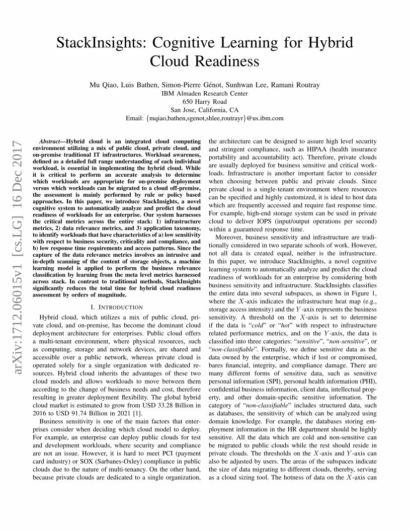
a mixture of file, block, and object storage. For experiment,we choose a mid-size account, whose storage infrastructure ispredominantly file storage. This account has two sites (datacenters), each one with a set of NetApp filers in clusteredmode (roughly 33.8 TB). We install one secure virtual machineinside each site preloaded with our StackInsights scanningcodebase. We use those virtual machines to scan the en-vironment and extract the necessary information for furtheranalysis. Figure 3 shows a high-level diagram of our sampleenvironment. The storage filer gives us a map of what the filestorage infrastructure looks like. We first build a tree of theinfrastructure by starting from the cluster and then down to thefile level (i.e., cluster ⇒ aggregate ⇒ volume ⇒ q −tree ⇒ filesystem ⇒ directory ⇒ file). A collectedfile metadata example is shown in Table III. In parallel, we pollthe storage filers for IOPS for each storage volume. This willallow us to measure the IO density for each system, thereby,to determine how volatile a given volume or file share is.

Fig. 3. Infrastructure, File Metadata and File Content Scan

We use IBM’s TADDM tool to get a picture of the differentworkloads running in the environment. Similarly, the systemadministrators also provide their valuable feedback, as theyare able to help us narrow our scanning scope. Because thefilers in the environment are all NetApp filers, we use theONTAP APIs to extract file metadata, as well as performancemetrics from the filers. All machine learning algorithms areimplemented based on the python scikit-learn library.

A. IOPS and file metadata collection

The IOPS for each volume is collected over a four-weektime window. We then compute the hourly-average IO density(IO per second per GB) for each volume. Table II showsthe total size of each volume as well as its correspondingIO density range. As we can see, except V5, the IO densityof all the other volumes is between 0.0 and 0.01, which isrelatively cold. Based on the storage performance metric, wemay recommend the tier 3 storage type for V5 and the nearlineor inactive storage type (e.g., archiving) for the other volumes.In Figure 4, all the volumes are first aligned along the X-axisaccording to their IO density. Note that since the highest IOdensity is only around 0.05, we indicate the correspondinghotness as “warm” on the X-axis.

We leverage the NetApp ONTAP APIs to extract the meta-data of all the files on these volumes. In total, we extract themetadata from more than 13 million files. One example is

Fig. 4. Volumes are aligned according to IO density

TABLE IIVOLUME IO DENSITY

Volume name Total size (TB) I/O density rangeV1 13.66 0 - 0.01V2 12.32 0 - 0.01V3 6.06 0 - 0.01V4 1.14 0 - 0.01V5 0.66 0.01 - 0.1V6 0.01 0 - 0.01V7 0.01 0 - 0.01

shown in Table III, where “Last accessed time” is the timestamp that the file was last accessed, “Creation time” is thetime stamp that the file was created, “Changed time” is thetime stamp that the file metadata (e.g., file name) was changed,“Last modified time” is the time stamp that the file itself (notmetadata) was last modified, “File size” represents the size thatwas allocated to the file on disk, and “bytes used” representsthe bytes that were actually written in that file. The volumelevel metadata is then obtained by aggregating the metadataof all the files on the same volume. One volume metadataexample is shown in Table IV. The “Top3ExtensionbySize”attribute is the top three file extensions ranked by their totalsizes. For instance, in Table IV, “.nsf”, “.zip”, and “.xls” arethe top three file extensions on that volume in terms of their to-tal sizes. “NotModifiedin1YearCount” is the percentage of fileson that volume that have not been modified in the past one yearin terms of file counts. Similarly, “notAccessedin1YearSize”is the percentage of files on that volume that have not beenaccessed in the past one year in terms of file sizes. All theother attributes are likewise. The volume metadata can provideus some further insights. For example, for one volume, wediscover that about half number of the files have not beenaccessed in the past one year, but they take about 98% storagecapacity in size.

B. Volumes clustering

After the volume level metadata is obtained, we apply K-means to do clustering on all the volumes. Due to the relativelysmall number of volumes, we empirically set K = 3. The

optimal value of K can be determined by the elbow method,which considers the percentage of variance explained by theclusters against the total number of clusters. The first clusterswill explain much of the variance. The optimal number ofclusters is chosen at the point where the marginal gain willdrop. Figure 5 shows the clustering results when K = 3. Notethat we have not considered the data sensitivity yet, so all thevolumes are still aligned along the X-axis.

Fig. 5. Volume clustering

We select a representative volume from each cluster, whichis defined as the one with the minimum total distance to theother volumes in the same cluster. A sensitivity analysis isperformed on each representative volume. The volumes in thesame cluster are assumed to share similar sensitivity scores.

C. Metadata-based Sensitivity Prediction

We present in this section the experimental results of themetadata-based sensitivity prediction.

1) Training Data: For each representative volume, we builda machine learning model to learn the sensitivity of all thefiles. One of the selected volume from the first data centercontains 3.9 million files, which are 2.64 TB in size. Throughthe infrastructure scan introduced in Section IV-B, we obtainthe metadata of all the files. We randomly select a subset of thefiles to crawl their content and determine the sensitivity usingthe dictionary based approach introduced in Section IV-D1.Specifically, we use Apache Tika to scan the file content.A file is considered as sensitive if it contains any sensitiveinformation listed in Table I. We finally obtain a set of 114,854files with both their metadata and sensitivity labels, out ofwhich, 66,221 (57.65%) files labelled as sensitive and the restas non-sensitive. Similarly, we obtain another set of 39,571files with both their metadata and sensitivity labels on arepresentative volume from the second data center. This dataset includes 21,284 sensitive files (53.79%). In the following,we will refer to these two data sets as dataset I and datasetII. Unless noted, the percentage of sensitive files in these twodatasets remain as 57.65% and 53.79%, respectively.

2) Feature Engineering: Given the training data, we de-rive features from file metadata for the classification model.Specifically, the features are divided into several categories:

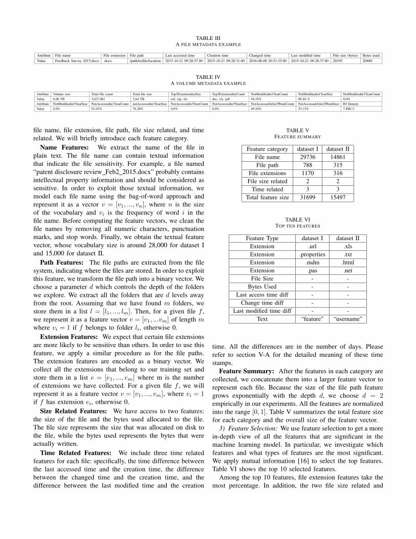
TABLE IIIA FILE METADATA EXAMPLE

Attribute File name File extension File path Last accessed time Creation time Changed time Last modified time File size (bytes) Bytes usedValue Feedback Survey 2015.docx .docx /path/to/file/location 2015-10-21 09:28:37.00 2015-10-21 09:28:31.00 2016-08-08 20:51:35.00 2015-10-21 09:28:37.00 20195 20480

TABLE IVA VOLUME METADATA EXAMPLE

Attribute Volume size Total file count Total file size Top3ExtensionbySize Top3ExtensionbyCount NotModifiedin1YearCount NotModifiedin1YearSize NotModifiedin3YearCountValue 6.06 TB 3,627,061 2.64 TB nsf, zip, xls doc, xls, pdf 94.18% 89.44 % 0.0%Attribute NotModifiedin3YearSize NotAccessedin1YearCount notAccessedin1YearSize NotAccessedin3YearCount NotAccessedin3YearSize NotAccessedAfter2WeekCount NotAccessedAfter2WeekSize IO DensityValue 0.0% 81.03% 76.28% 0.0% 0.0% 49.10% 53.13% 7.89E-3

file name, file extension, file path, file size related, and timerelated. We will briefly introduce each feature category.

Name Features: We extract the name of the file inplain text. The file name can contain textual informationthat indicate the file sensitivity. For example, a file named“patent disclosure review Feb2 2015.docx” probably containsintellectual property information and should be considered assensitive. In order to exploit those textual information, wemodel each file name using the bag-of-word approach andrepresent it as a vector v = [v1, ..., vn], where n is the sizeof the vocabulary and vi is the frequency of word i in thefile name. Before computing the feature vectors, we clean thefile names by removing all numeric characters, punctuationmarks, and stop words. Finally, we obtain the textual featurevector, whose vocabulary size is around 28,000 for dataset Iand 15,000 for dataset II.

Path Features: The file paths are extracted from the filesystem, indicating where the files are stored. In order to exploitthis feature, we transform the file path into a binary vector. Wechoose a parameter d which controls the depth of the folderswe explore. We extract all the folders that are d levels awayfrom the root. Assuming that we have found m folders, westore them in a list l = [l1, ..., lm]. Then, for a given file f ,we represent it as a feature vector v = [v1, ...vm] of length mwhere vi = 1 if f belongs to folder li, otherwise 0.

Extension Features: We expect that certain file extensionsare more likely to be sensitive than others. In order to use thisfeature, we apply a similar procedure as for the file paths.The extension features are encoded as a binary vector. Wecollect all the extensions that belong to our training set andstore them in a list e = [e1, ..., em] where m is the numberof extensions we have collected. For a given file f , we willrepresent it as a feature vector v = [v1, ..., vm], where vi = 1if f has extension ei, otherwise 0.

Size Related Features: We have access to two features:the size of the file and the bytes used allocated to the file.The file size represents the size that was allocated on disk tothe file, while the bytes used represents the bytes that wereactually written.

Time Related Features: We include three time relatedfeatures for each file: specifically, the time difference betweenthe last accessed time and the creation time, the differencebetween the changed time and the creation time, and thedifference between the last modified time and the creation

TABLE VFEATURE SUMMARY

Feature category dataset I dataset IIFile name 29736 14861File path 788 315

File extensions 1170 316File size related 2 2

Time related 3 3Total feature size 31699 15497

TABLE VITOP TEN FEATURES

Feature Type dataset I dataset IIExtension .url .xlsExtension .properties .txtExtension .mdm .htmlExtension .pas .netFile Size - -

Bytes Used - -Last access time diff - -

Change time diff - -Last modified time diff - -

Text “feature” “username”

time. All the differences are in the number of days. Pleaserefer to section V-A for the detailed meaning of these timestamps.

Feature Summary: After the features in each category arecollected, we concatenate them into a larger feature vector torepresent each file. Because the size of the file path featuregrows exponentially with the depth d, we choose d = 2empirically in our experiments. All the features are normalizedinto the range [0, 1]. Table V summarizes the total feature sizefor each category and the overall size of the feature vector.

3) Feature Selection: We use feature selection to get a morein-depth view of all the features that are significant in themachine learning model. In particular, we investigate whichfeatures and what types of features are the most significant.We apply mutual information [16] to select the top features.Table VI shows the top 10 selected features.

Among the top 10 features, file extension features take themost percentage. In addition, the two file size related and

three time related features are also significant. Text tokens“feature” and “username” are also among the top 10. Notethat we use “username” to replace an actual username forprivacy concerns. We do not find any file path features in thelist, which may indicate that the location of the file in thefilesystem carries less significance than it’s size, time, name,or extension in the prediction. For example, one particularfolder may include both sensitive and non-sensitive files.

Table VII shows the number of selected features in eachcategory when we vary the total number of top selectedfeatures. Again we notice that file extensions and text tokensin file names are significant features, while the file paths donot appear in the top list.

TABLE VIITOP FEATURE CATEGORIES

Feature Type Top 100 Top 500Extension 27 79

File size related 2 2Time related 3 3

Text 68 416

4) Prediction Models: After all the features are extracted,we build machine learning models on our training data andapply them to predict the file sensitivity based on meta data.Specifically, we compare the performance of several well-known classification models: Naive Bayes, Logistic Regres-sion, Support Vector Machines (SVM), and Random Forest.

All the experiments are conducted using the 10 fold crossvalidation. Since only file size related and time related featureshave numerical values (in total five), among the large numberof features, we apply multinomial Naive Bayes, the featuredistributions of which are modeled as multinomial distribu-tions rather than the gaussian distributions. Naive Bayes hasthe advantage of having no parameters to optimize on. LogisticRegression has only one parameter that we need to tune: theregularization parameter C. In order to select the optimalvalue C, we run grid search using 10-fold cross-validationon multiple values of C. We find that the best C value is0.9. For SVM, the linear kernel is selected. In practice, wefind that the RBF kernel takes a very long time to converge.The optimal regularization parameter C is selected followingthe same procedure as with Logistic Regression. The optimalC value is set to be 0.8 for linear SVM. We use the defaultparameter setting for Random Forest, where the number oftree in the forest is 10, no maximum tree depth constraint,and the samples are drawn with replacement. Table VIII showsthe performance of each model in terms of overall accuracy,precision, recall, and F1 score. In our classification problem,the positive class is “sensitive” while the negative class is“non-sensitive”. Specifically, the precision is defined as theratio tp/(tp + fp), where tp is the number of true positivesand fp the number of false positives. The recall is the ratiotp/(tp+ fn), where tp is the number of true positives and fnthe number of false negatives. Accuracy is defined as the ratio

between the number of samples that are correctly classifiedand the total number of samples. The F1 score is computedas 2× (precision× recall)/(precision+ recall), which is aweighted average of the precision and recall.

In Table VIII, the percentages of sensitive files in datasetI and II are 57.65% and 53.79%, respectively. Therefore,the classes in the training data are roughly balanced. As wecan see, Random Forest has the best performance among allthe models over all the metrics. The precision and recall ondataset I are above 90%. In contrast to other models, RandomForest, as an ensemble method, combines the predictions ofseveral based estimators, i.e., decision trees. Each tree in theensemble is built from a sample drawn with replacement fromthe training set. When splitting a node during the constructionof the tree, the split is chosen as the best split among arandom subset of the features. Since both the feature sizeand sample size are large in our classification, as a result ofthis randomness, the variance of the forest is reduced due toaveraging, hence yielding an overall better model.

In practice, the percentage of sensitive files in the trainingdata depends on the specific domain and sensitivity labeling.In some domain, the sensitivity labelling may be stringent,resulting in a relatively small percentage of sensitive files. Wealso design experiments to test the performance of machinelearning models for such case. Specifically, we only usethe phone regular expression in Table I to do the labelling,discarding the other sensitive information, which yields 25,256(21.99%) sensitive files for dataset I. We apply four differentmachine learning models and report the results in Table IX forimbalanced classes. The “balanced” classification mode is usedfor Logistic Regression, SVM, and Random Forest, wherethe values of prediction target y are used to automaticallyadjust weights inversely proportional to class frequencies inthe training data. As shown in Table IX, Random Forest hasthe best performance among all the models over all the metrics,except recall. Due to space limit, we only show the results ondataset I.

TABLE VIIIMODELS ON DATASETS OF BALANCED CLASSES

Model (dataset I) Accuracy Precision Recall F1

Naive Bayes 0.8044 0.8348 0.8238 0.8293Logistic Regression 0.8115 0.8664 0.7959 0.8296

SVM 0.8309 0.8730 0.8269 0.8493Random Forest 0.9014 0.9250 0.9022 0.9135

Model (dataset II) Accuracy Precision Recall F1

Naive Bayes 0.7780 0.7855 0.8081 0.7966Logistic Regression 0.7923 0.8350 0.7652 0.7985

SVM 0.8055 0.8493 0.7762 0.8111Random Forest 0.8739 0.8926 0.8703 0.8813

As we can see, Random Forest has very robust performance,and consistently outperforms the other methods in both bal-anced and imbalanced classifications. Previously, we have used10-fold cross validation to test the prediction performance,which uses 90% data for training and the remaining for testing.We now vary the percentage of training and testing, and check

TABLE IXMODELS ON DATASET OF IMBALANCED CLASSES

Model (dataset I) Accuracy Precision Recall F1

Naive Bayes 0.8813 0.8122 0.5988 0.6894Logistic Regression 0.8538 0.6270 0.8274 0.7134

SVM 0.8774 0.6836 0.8237 0.7471Random Forest 0.9361 0.9176 0.7795 0.8429

how Random Forest performs if relatively small percentage ofdata is used for training. Table X shows the performance ofRandom Forest with two-fold cross validation on both datasetI and II, where 50% data are used for training and 50% fortesting. Again, Random Forest has shown good performanceon all the metrics, even better than the other models when90% data are used for training.

TABLE XPERFORMANCE WITH TWO-FOLD CROSS VALIDATION

Accuracy Precision Recall F1

Random Forest (dataset I) 0.8790 0.9072 0.8802 0.8935Random Forest (dataset II) 0.8583 0.8820 0.8503 0.8658

To have a detailed analysis of the classification results, weshow the confusion matrices of Random Forest (one fold in atwo-fold cross validation) in Table XI, which allows us to seehow well the model performs on the classification of eachclass. Overall, the error ratios on false positives and falsenegatives are balanced on both datasets.

TABLE XIMODEL CONFUSION MATRICES

Random Forest (dataset I) Non-Sensitive SensitiveNon-Sensitive 21493 (0.88) 2824 (0.12)

Sensitive 3999 (0.12) 29112 (0.88)

Random Forest (dataset II) Non-Sensitive SensitiveNon-Sensitive 7897 (0.86) 1247 (0.14)

Sensitive 1535 (0.14) 9107 (0.86)

Prediction Model Usage: Note that we do not intendto use the above prediction model to completely replacethe traditional content scanning method, such as dictionarybased method. As we can see, the prediction model is basedon meta data and cannot achieve 100% accuracy. In datagovernance and security, the misclassification of sensitive datacan be catastrophic for an organization. For example, criticalIP documents leak or data compliance violation can lead toserious legal consequences. Therefore, a thorough sensitivityscreening can be performed to make sure all the sensitiveinformation are identified. From the machine learning model,all the files that have been predicted as sensitive will belabelled as sensitive data. We can then perform intensivecontent scanning method on all the files that are predicted tobe non-sensitive. For example, after applying Random Foreston dataset I, 25,492 files are predicted as non-sensitive. The

content scanning based method will then be applied to thesefiles, so that the 3,999 mis-classified sensitive files can beidentified. In contrast to the content scanning of all the 57,428files, we now only need to perform content scanning on 25,492files (44.38%), significantly smaller than the original numberof files. There are certainly non-sensitive files mis-calssifiedas sensitive files. For example, 2824 non-sensitive files aremis-classified as sensitive files. As a result, they are “over-protected”. However, the percentage of such files only takes4.91% of the total files. As a simple comparison baseline,with the percentage of sensitive files in the training data (i.e.,57.65%) for dataset I, a user can randomly selects 57.65%data, and label them as sensitive and the remaining as non-sensitive, without using the prediction model. They can thenperform content scanning on the previously labelled non-sensitive files in order to identify any sensitive information.Note that in this baseline, among the 57.65% files that arelabelled as sensitive, 42.35% files are actually non-sensitive(based on the percentage of non-sensitive files in the trainingdata), therefore, 57.65%× 42.35% = 24.41% amount of non-sensitive files are misclassified as sensitive, therefore “over-protected”, in contrast to 4.91% that are misclassified by theprediction model.

5) Prediction Ranking and Running Time: After the ma-chine learning model is trained, we apply it to predict thesensitivity of the remaining files on the same volume. Fordataset I, we apply Random Forest to predict the sensitivityof the remaining 3.9 million files and measure its runningtime. On a local machine with 2.5 GHz Intel Core i7 CPUand 16GB of RAM, the total running time is 112 minutes.The model classifies 1,804,798 (46.33%) files as sensitive and2,089,913 (53.67%) files as non-sensitive. As a comparison,the content scanning based approach took more than 30 hoursto process 228,000 files, which is only 5.85% of the 3.9 millionfiles. StackInsights reduces the total running time by orders ofmagnitude.

We also apply the trained learning model to predict thesensitivity of files on other volumes in the same data center.Table XII shows the prediction results: the predicted sensitivefiles #, volume sensitivity, and running time in seconds. Aswe can see, V1 and V4 have sensitivity close to 1.00. Theyalso belong to the same cluster in Figure 5. V2, V3, and V5have sensitivity between 0.45 and 0.70, which are in the samecluster. V6 and V7 are in the same cluster, with predictedsensitivity 0.5758 and 0.1728, respectively.

TABLE XIIPREDICTION RESULTS ON ALL THE VOLUMES

Total file # Sensitive file # Sensitivity Running time (sec)V1 400415 385369 0.9624 286.28V2 7798224 5501763 0.7055 5993.20V3 3894711 1804798 0.4633 6720V4 170808 170808 1.0000 134.01V5 1481322 902804 0.6095 1133.58V6 686 395 0.5758 0.51V7 81 14 0.1728 0.06

6) Migration Insights: After the sensitivity of all the fileson a storage volume is predicted, we can compute sensitivityscores at different levels. The sensitivity score is defined asthe number of sensitive files divided by the total number offiles at a targeted level. We give two examples: volume leveland user level. Similarly, we can also obtain data hotness(e.g., storage performance metrics) at different levels. From theInfrastructure scan, we compute the IO density for volumes.For the user level, we use the metric, the percentage of filesthat have not been accessed in past one year, to represent thedata hotness for a particular user folder. By correlating datasensitivity and hotness, StackInsights can provide hybrid couldmigration insights. In addition, StackInsights can be integratedwith data movement tools, such as DataDynamics [17], inorder to automate the entire migration process from recom-mendation to action.

Volume Sensitivity and Hotness Map: We get thesensitivity score for each volume from the prediction results.As shown in Figure 6, all the volumes are ordered based ontheir sensitivity level and hotness. Therefore, all the volumeswhich are cold and low sensitive can be migrated to the publiccloud. The remaining should be migrated to the private cloudor remain on premise.

Fig. 6. Volume sensitivity and IO density map

User Sensitivity and Hotness Map: Similar as thevolume level analysis, we can also obtain the data sensitivityand hotness map on the user level. The data hotness for aparticular user folder is computed as the percentage of all theassociated files that have not been accessed in the past oneyear. Specifically, we find 1,060 user folders on volume V3.We compute the sensitive score for each user folder based onthe predicted file sensitivity, as well as the data hotness usingthe file metadata collected from infrastructure scan. The usersensitivity and hotness map is shown in Figure 7. As we cansee, there are many user folders that have not been accessed inthe past one year. The percentage of sensitive files under thesefolders vary though. For user folders at the bottom right (coldand low sensitive), they may be eligible to be migrated to thepublic cloud. For those at the top left (hot and high sensitive),they should be migrated to the private cloud or remain onpremise.

Fig. 7. User sensitivity and data hotness map

VI. CONCLUSIONS AND FUTURE WORK

We have introduced StackInsights, a cognitive learningsystem which automatically analyzes and predicts the cloudreadiness of workloads. StackInsights correlates the metricsfrom application, data, and infrastructure layers to identify thebusiness sensitivity of data as well as their hotness in terms ofinfrastructure performance, and provides insights into hybridcloud migration. Given the scale of data and infrastructure,a machine learning model is developed in StackInsights topredict file sensitivity based on the metadata. In contrast totraditional approach which requires intrusive and expensivecontent scanning, StackInsights significantly reduces the totalrunning time for sensitivity classification by orders of mag-nitude, therefore, is scalable to be deployed in large scale ITenvironment. As more and more enterprises are committingto hybrid cloud architecture, StackInsights can help acceleratethis digital transformation in their organizations.

Our current system is mainly focused on understanding thesensitivity of textual files. There are many different types ofdata that can contain sensitive information, such as images,videos, and audios. In the future, we can leverage IBM Watsonservices [18] to analyze the sensitive content from thesemultimedia data. Similarly, we can predict their sensitivitybased on the meta level information. Last but not the least, thecognitive learning capabilities of StackInsights can be greatlyenhanced by collecting more metadata across the stack. Themore metadata we can collect, the more accurate the predictionmodel will be.

REFERENCES

[1] “Markets and Markets.” [Online]. Available: http://www.marketsandmarkets.com/

[2] “Symantec Data Classification Services - gathering an enterprisevault retention category list,” 2015. [Online]. Available: https://support.symantec.com/en US/article.HOWTO124009.html

[3] “Varonis Data Classification Framework.” [Online]. Available: https://www.varonis.com/products/data-classification-framework/

[4] “IBM Security Guardium Family.” [Online]. Available: http://www-03.ibm.com/software/products/en/ibm-security-guardium-family

[5] “IBM - Cloud Brokerage Solutions.” [Online].Available: https://www-935.ibm.com/services/us/en/it-services/systems/cloud-brokerage-service/

[6] Y. Park, S. C. Gates, W. Teiken, and P.-C. Cheng, “An experimentalstudy on the measurement of data sensitivity,” in Proceedings of theFirst Workshop on Building Analysis Datasets and Gathering ExperienceReturns for Security. New York, NY, USA: ACM, 2011, pp. 70–77.

[7] M. Ali and L. T. Jung, “Confidentiality based file attributes and dataclassification using tsf-knn,” in Proceedings of the 5th InternationalConference on IT Convergence and Security (ICITCS), Aug 2015, pp.1–5.

[8] D. Sanchez, M. Batet, and A. Viejo, Detecting Sensitive Informationfrom Textual Documents: An Information-Theoretic Approach. Berlin,Heidelberg: Springer Berlin Heidelberg, 2012, pp. 173–184.

[9] M. Hart, P. Manadhata, and R. Johnson, Text Classificationfor Data Loss Prevention. Berlin, Heidelberg: SpringerBerlin Heidelberg, 2011, pp. 18–37. [Online]. Available:http://dx.doi.org/10.1007/978-3-642-22263-4 2

[10] M. Mesnier, E. Thereska, G. R. Ganger, D. Ellard, and M. Seltzer,“File classification in self-* storage systems,” in Proceedings of theInternational Conference on Autonomic Computing, 2004. Proceedings.,2004, pp. 44–51.

[11] M. Hajjat, X. Sun, Y.-W. E. Sung, D. Maltz, S. Rao, K. Sripanidkulchai,and M. Tawarmalani, “Cloudward bound: Planning for beneficial mi-gration of enterprise applications to the cloud,” in Proceedings ofSIGCOMM, 2010.

[12] A. Khajeh-Hosseini, I. Sommerville, J. Bogaerts, and P. Teregowda,“Decision support tools for cloud migration in the enterprise,” in Pro-ceedings of the 4th IEEE International Conference on Cloud Computing,2011, pp. 541–548.

[13] M. Menzel and R. Ranjan, “Cloudgenius: Decision support for webserver cloud migration,” in Proceedings of the 21st InternationalConference on World Wide Web. New York, NY, USA: ACM, 2012,pp. 979–988. [Online]. Available: http://doi.acm.org/10.1145/2187836.2187967

[14] “IBM - Tivoli Application Dependency Discovery Manager.”[Online]. Available: http://www-03.ibm.com/software/products/en/tivoliapplicationdependencydiscoverymanager

[15] “NetApp ONTAP Data Management Software.” [Online]. Available:http://www.netapp.com/us/products/platform-os/ontap/index.aspx

[16] H. Peng, F. Long, and C. Ding, “Feature selection based on mu-tual information criteria of max-dependency, max-relevance, and min-redundancy,” IEEE Transactions on Pattern Analysis and MachineIntelligence, vol. 27, no. 8, pp. 1226–1238, 2005.

[17] “Policy-Based File Data Management for the Complete Data Lifecycle.”[Online]. Available: http://www.datadynamicsinc.com/solutions/

[18] “IBM Watson: API Solutions.” [Online]. Available: www-01.ibm.com/Watson/Developer