Stable carbon and nitrogen isotope analysis in aqueous ...

Stable carbon and nitrogen isotope analysis in aqueous samples – method

development, validation and application

Dissertation

zur Erlangung des akademischen Grades eines

Doktors der Naturwissenschaften

- Dr. rer. nat. –

vorgelegt von

Eugen Federherr

geboren in Petrosawodsk

Fakultät für Chemie

der

Universität Duisburg-Essen

2016

ii

Die vorliegende Arbeit wurde im Zeitraum von Juni 2012 bis April 2016 im Arbeitskreis von

Prof. Dr. Torsten Schmidt im Fachgebiet Instrumentelle Analytische Chemie der Universität

Duisburg-Essen betreut und in der Firma Elementar Analysensysteme GmbH durchgeführt.

Tag der Disputation: 26.07.2016

Gutachter: Prof. Dr. Torsten C. Schmidt

Prof. Dr. Oliver J. Schmitz

Vorsitzender: Prof. Dr. Eckart Hasselbrink

iii

“One can't understand everything at once, we can't begin with perfection all at once! In order

to reach perfection one must begin by being ignorant of a great deal. And if we understand

things too quickly, perhaps we shan't understand them thoroughly. I say that to you who have

been able to understand so much already and… have failed to understand so much.”

Fjodor Michailowitsch Dostojewski

iv

Acknowledgments

I would like to express my sincere gratitude to Prof. Dr. Torsten C. Schmidt for his invaluable

guidance, warm encouragement, helpful suggestions and discussions. It has been always an

exciting and enriching experience to carry on a lively scientific conversation with him.

Furthermore I would like to thank Prof. Dr. Oliver J. Schmitz for the acceptance being the

second referee for my theses as well as for kind and helpful support.

Special gratitude I feel to PD. Dr. Telgheder, with all her very valuable encouragement,

appreciation and advices e.g. in the field of quality management. I would like to thank Prof.

Dr. Molt for his numerous consulting, particularly in the field of statistics. Many thanks also

to Dr. M. Jochmann, Dr. H. Lutz and other colleagues from University of Duisburg-Essen for

their help at various stages of my doctorial study.

I would like to thank Dr. Hans P. Sieper, Lutz Lange, Hans J. Kupka, Dr. Ralf Dunsbach and

Dr. Filip Volders (Elementar Analysensysteme) for their support as well as for the financial

enabling to conduct my doctoral study. Thanks also to Mike Seed, Dr. Rob Berstan, Will

Price, Dr. Robert Panetta and Paul Wheeler (Isoprime) and Dr. Rolf Russow (Retired from

Helmholtz Centre for Environmental Research) for their support.

Special thanks to the awesome engineer team I had the pleasure to work with: Hans J. Kupka

(process development), Walter Weigand and Heidi Merz (electronic development), Nobert

Proba, Sebastian Schmitt and Thorsten Hänsgen (mechanical engineering), Witold Baron

(software development) and Christian Schopper (technical documentation development).

I would particularly like to thank Dr. Chiara Cerli (University of Amsterdam) and Prof. Dr.

Karsten Kalbitz (Dresden University of Technology) for the great cooperation experience,

scientific consulting and support. A special thank also for the close cooperation to Frédérique

M.S.A. Kirkels (Utrecht University), Sarah Willach (University of Duisburg-Essen) and

Natascha Roos (Agilent Technologies).

For various valuable supports I would also like to thank Fabian Ruhnau, Prof. Dr. Christof

Schulz, Prof. Dr. Andreas Kempf und Dr. Irenäus Wlokas, Prof. Dr. Pascal Boeckx, Dr.

Andriy Kuklya, Danny Loeser, Dr. Rolf Siegwolf, Prof. Dr. Ing. Ralph Hobby, Dr. Ing. Dieter

Bathen, Prof. Dr. Brian Fry, Almut Loos, Dr. Marian de Reus, Dr. Robert van Geldern, Prof.

Dr. Thomas W. Boutton, Dr. Willi A. Brandt, Dr. Abert Michael and Dr. Oliver Würfel. I

appreciate and thank the technical staff of all institutions that helped during the analytical

work.

v

Furthermore, I acknowledge financial support by the Arbeitsgemeinschaft Industrieller

Forschungsvereinigungen (AIF), Cologne, (ZIM Project no. KF 2274203BN2).

Last but not least, I want to express my gratitude to my family and friends for their love and

continuous support. I appreciate their generous patience and understanding for my

unavailability during the time of theses writing.

vi

Summary

Bulk and compound specific stable isotope analysis (BSIA and CSIA, respectively) of

dissolved matter is of high interest in many scientific fields.

Traditional BSIA methods for carbon from aqueous solutions are time-consuming, laborious

or involve the risk of isotope fractionation. No system able to analyze natural abundance

stable nitrogen isotope composition of dissolved nitrogen directly (without offline sample

preparation) has been reported so far. CSIA methods of dissolved carbon and nitrogen

containing matter require either time consuming extraction and purification followed by

elemental analysis isotope ratio mass spectrometry (EA/IRMS) or derivatization followed by

gas chromatography IRMS (GC/IRMS). The only widely adopted direct method using high

performance liquid chromatography IRMS (HPLC/IRMS) is suited for carbon only.

Based on these shortcomings the development and validation of analytical methods for

accurate and sensitive carbon and nitrogen SIA from aqueous samples are the aims of this

work.

A high-temperature combustion (HTC) system improves upon established methods. A novel

total organic carbon (TOC) system, specially designed for SIA, was coupled to an isotope

ratio mass spectrometer. The system was further modified to enable nitrogen BSIA. Finally,

an interface for carbon and nitrogen CSIA via HPLC/IRMS was developed based on the

previously developed concepts for BSIA.

Compounds resistant to oxidation, such as barbituric acid, melamine and humic acid, were

analyzed with carbon recoveries of 100 ± 1% proving complete oxidation. Complete

reduction of NOx to N2 was proven measuring different nitrogen containing species, such as

nitrates, ammonium and caffeine without systematical errors. Trueness and precision of

usually ≤0.5‰ were achieved for δ13C and δ15N CSIA, as well as BSIA. For δ13C BSIA an

integrated purge and trap technique and large volume injection system were used to achieve

LOQSIA instr of 0.2 mgC/L, considering an accuracy of ±0.5‰ as acceptable. In addition, the

method was successfully applied to various real samples, such as river water samples and soil

extracts. Further tests with caffeine solutions resulted in lower working limit values of 3.5

μgC for δ13C CSIA and 20 μgN for δ15N CSIA, considering an accuracy of ±0.5‰ as

acceptable. Lower working limit of 1.5 μgN for δ15N BSIA was achieved, considering an

accuracy of ±1.0‰ as acceptable.

vii

The novel HTC TOC analyzer coupled to an isotope ratio mass spectrometer represents a

significant progress for δ13C and δ15N BSIA of dissolved matter. The development of a novel

HPLC/IRMS interface resulted in the first system reported to be suitable for both δ13C and

δ15N in direct CSIA of non-volatile compounds. Both may open up new possibilities in SIA-

based research fields.

viii

Zusammenfassung

Stabilisotopenanalytik von Kohlenstoff und Stickstoff in

wässrigen Lösungen

– Methodenentwicklung, -validierung und -anwendung.

Bulk-Stabilisotopenanalytik (BSIA) und substanzspezifische Stabilisotopenanalyse (CSIA)

von wässrig gelösten Stoffen ist in vielen wissenschaftlichen Bereichen von großem Interesse.

Traditionelle BSIA-Methoden für Kohlenstoff in wässrigen Lösungen sind zeitaufwendig,

mühsam oder beinhalten das Risiko der Isotopenfraktionierung. Ein System, welches die

Stabile-Stickstoff-Isotopenzusammensetzung mit natürlicher Häufigkeit von gelösten

Stickstoffverbindungen direkt (ohne Offline-Probenvorbereitung) analysieren kann, ist bisher

in der Literatur nicht erwähnt.

CSIA-Methoden für gelöste Kohlen- und Stickstoffverbindungen benötigen entweder eine

zeitraubende Extraktion und Aufreinigung, gefolgt von Elementaranalyse/Isotopenverhältnis-

Massenspektrometrie (EA/IRMS) oder eine Derivatisierung, gefolgt von

Gaschromatographie/IRMS (GC/IRMS). Die einzige weit verbreitete direkte Methode für

Hochleistungsflüssigkeitschromatographie/IRMS (HPLC/IRMS) eignet sich nur für die

Kohlenstoff CSIA.

Aufgrund dieser Defizite fokussiert sich diese Arbeit auf die Entwicklung und Validierung

von Verfahren zur genauen und empfindlichen BSIA und CSIA des Kohlenstoffs und

Stickstoffs in wässrigen Proben.

Ein Hochtemperaturverbrennungs-System (HTC-System) stellt eine Verbesserung gegenüber

etablierten Methoden dar. Ein neuartiger und speziell für die BSIA entwickelter gesamter

organischer Kohlenstoff-Analysator (TOC-Analysator), wurde mit einem Isotopenverhältnis-

Massenspektrometer gekoppelt. Eine weitere Modifizierung des Systems ermöglicht die BSIA

von Stickstoff. Schließlich erfolgte, unter Verwendung der zuvor gewonnenen Erkenntnisse,

die Entwicklung eines Interfaces für Kohlenstoff- und Stickstoff-CSIA mittels HPLC/IRMS.

Schwer abbaubare Verbindungen, wie Barbitursäure, Melamin und Huminsäure, wurden mit

den Kohlenstoff Wiederfindungsraten von 100 ± 1% analysiert um die Vollständigkeit der

Oxidation zu belegen. Die vollständige Reduktion von NOx zu N2 wurde durch die erfolgreich

durchgeführten Messungen (ohne systematischen Fehler) verschiedener stickstoffhaltiger

Spezies, wie Nitraten, Ammonium und Koffein belegt. Richtigkeit und Präzision lagen in der

ix

Regel bei ≤0,5 ‰ für δ13C and δ15N für die CSIA, ebenso wie für die BSIA. Für δ13C BSIA

wurde eine integrierte Purge and Trap Technik, sowie ein großvolumiges Einspritz-System

verwendet um LOQSIA Instr von 0,2 mgC/L zu erzielen (eine Genauigkeit von ±0,5 ‰ wurde

hierfür als akzeptabel definiert). Außerdem wurde die Methode erfolgreich auf verschiedene

reale Proben, wie Flusswasserproben und Bodenextrakte angewandt. Es wurde ein unterer

Arbeitsbereich von 3,5 μgC für δ13C CSIA und 20 μgN für δ 15N CSIA ermittelt (eine

Genauigkeit von ±0,5 ‰ wurde hierfür als akzeptabel definiert). Es wurde ein unterer

Arbeitsbereich von 1,5 μgN wurde für δ15N BSIA erreicht (eine Genauigkeit von ±1,0 ‰

wurde hierfür als akzeptabel definiert).

Der neue, an einen IRMS-Detektor gekoppelte HTC TOC-Analysator, stellt einen

bedeutenden Fortschritt für δ13C und δ 15N BSIA von gelöster Materie dar. Die Entwicklung

eines neuartigen HPLC/IRMS Interfaces führte zum ersten System, welches sich sowohl für

direkte δ13C als auch δ15N CSIA von nichtflüchtigen Verbindungen als geeignet erwies.

Beides könnte neue Möglichkeiten in SIA-basierten Forschungsfeldern erschließen.

x

Table of contents

Acknowledgments ..................................................................................................................... iv

Summary ................................................................................................................................... vi

Zusammenfassung ................................................................................................................... viii

Table of contents ........................................................................................................................ x

Chapter 1 General Introduction ......................................................................................... 1

1.1 Stable isotope analysis ............................................................................................. 2

1.1.1 Elements, isotopes and isotope fractionation ................................................... 2

1.1.2 Isotope ratio mass spectrometry – the SIA detector ......................................... 6

1.2 Carbon and nitrogen in environmental research .................................................... 12

1.3 Instrumental and methodological background for SIA in aqueous samples .......... 15

1.4 References .............................................................................................................. 22

Chapter 2 Scope and Aim .................................................................................................. 29

Chapter 3 A novel high-temperature combustion based system for stable isotope

analysis of dissolved organic carbon in aqueous samples - development and validation 31

3.1 Abstract .................................................................................................................. 32

3.2 Introduction ............................................................................................................ 33

3.3 Experimental .......................................................................................................... 36

3.3.1 Chemicals and reagents .................................................................................. 36

3.3.2 Instrumentation and methodology .................................................................. 36

3.3.3 Nomenclature, evaluation and QA ................................................................. 37

Nomenclature ........................................................................................................... 37

Evaluation ................................................................................................................. 38

Quality assurance ..................................................................................................... 39

3.4 Results and discussion ........................................................................................... 40

3.4.1 Method development ...................................................................................... 40

Injection and combustion system ............................................................................. 40

Water removal .......................................................................................................... 41

xi

Sensitivity at low concentration and instrumentation blank .................................... 41

Final system .............................................................................................................. 43

3.4.2 Instrument testing/validation with aqueous compound solutions ................... 45

Carry-over (memory effects) .................................................................................... 45

Precision ................................................................................................................... 46

Linearity ................................................................................................................... 47

Blank correction ....................................................................................................... 48

Normalization and trueness ...................................................................................... 54

Uncertainty and accuracy ......................................................................................... 55

Oxidation efficiency and matrix effects ................................................................... 55

3.5 Conclusions and outlook ........................................................................................ 58

3.6 References .............................................................................................................. 59

3.7 Supporting information .......................................................................................... 63

Chapter 4 Uncertainty estimation and application of stable isotope analysis in

dissolved carbon ..................................................................................................................... 71

4.1 Abstract .................................................................................................................. 72

4.2 Introduction ............................................................................................................ 73

4.3 Experimental .......................................................................................................... 74




Nomenclature ........................................................................................................... 74

Evaluation ................................................................................................................. 75

Quality assurance ..................................................................................................... 76

4.4 Results and discussion ........................................................................................... 77

4.4.1 Novel approach for uncertainty assessment in DOC SIA .............................. 77

Derivation and validation of the approach ............................................................... 77

Application of the introduced approach to assess the uncertainties for a DOC SIA

round robin test ......................................................................................................... 81

xii

4.4.2 Round robin test and further real sample measurements ................................ 84

4.4.3 Proof of principle of TIC SIA with the iso TOC cube system ....................... 87

4.5 Conclusion and outlook ......................................................................................... 89

4.6 References .............................................................................................................. 90

4.7 Supporting information .......................................................................................... 92

Chapter 5 A novel tool for natural abundance stable nitrogen analysis in in aqueous

samples 93

5.1 Abstract .................................................................................................................. 94

5.2 Introduction ............................................................................................................ 95

5.3 Experimental .......................................................................................................... 97



HTC TOC/IRMS ...................................................................................................... 97

EA/IRMS .................................................................................................................. 98


5.4 Results and discussion ......................................................................................... 100

5.4.1 Instrumental development ............................................................................ 100

5.4.2 Instrument testing with aqueous standard solutions ..................................... 102

Carry-over (memory effects), drift and precision .................................................. 102

Trueness, accuracy and lower working limit estimation ........................................ 103

5.4.3 Simultaneous δ13C and δ15N determination in aqueous solutions ................ 107

5.5 Conclusion and outlook ....................................................................................... 110

5.6 References ............................................................................................................ 111

Chapter 6 A novel high-temperature combustion interface for compound-specific

stable isotope analysis of carbon and nitrogen via high-performance liquid

chromatography/isotope ratio mass spectrometry ............................................................ 113

6.1 Abstract ................................................................................................................ 114

6.2 Introduction .......................................................................................................... 115

6.3 Experimental ........................................................................................................ 117

xiii

6.3.1 Chemicals and reagents ................................................................................ 117

6.3.2 Instrumentation and methodology ................................................................ 117

HPLC/IRMS ........................................................................................................... 117

EA/IRMS ................................................................................................................ 119

6.3.3 Nomenclature, evaluation and QA ............................................................... 119

6.4 Results and discussion ......................................................................................... 121

6.4.1 Instrumental development ............................................................................ 121

6.4.2 Instrument testing with aqueous caffeine solutions ...................................... 123

Initial validation ..................................................................................................... 123

Trueness, accuracy and lower working limit estimation ........................................ 125

6.5 Exemplary application of C and N CSIA using the HTC interface ..................... 129

6.6 Conclusions and outlook ...................................................................................... 130

6.7 References ............................................................................................................ 131

Chapter 7 General conclusions and outlook .................................................................. 135

Chapter 8 Appendix ......................................................................................................... 141

8.1 List of abbreviations and symbols ....................................................................... 142

8.2 List of Figures ...................................................................................................... 148

8.3 List of supplementary Figures ............................................................................. 155

8.4 List of Tables ....................................................................................................... 156

8.5 List of supplementary Tables ............................................................................... 157

8.6 Curriculum vitae .................................................................................................. 158

8.7 List of Publications .............................................................................................. 160

8.7.1 Manuscripts .................................................................................................. 160

8.7.2 Presentations (first author contributions only) ............................................. 161

Scientific conferences ............................................................................................ 161

Scientific conferences (presented by a co-author) ................................................. 161

8.8 Erklärung .............................................................................................................. 162

Chapter 1

1

Chapter 1 General Introduction

Chapter 1

2

1.1 Stable isotope analysis

1.1.1 Elements, isotopes and isotope fractionation

A trend in modern analytical chemistry is not only the identification and quantification of

analytes but also the determination of their isotope composition, e.g., to infer sources or fate

in the environment. Stable isotope analysis (SIA) quantifies this isotope composition and

hence, provides additional and often unique means to allocate and distinguish sources of

analytes as well as to identify and quantify transformation reactions.[1]

The term isotopes refers to nuclides having the same atomic number (same number of

protons), but different mass numbers (different number of neutrons).[2] Object of this thesis

are solely stable isotopes, i.e., those isotopes that do not undergo radioactive decay in contrast

to radionuclides.

Up-to-date periodic tables[3] enclose for each element with two or more stable isotopes either

an interval or a weighted average representing standard atomic weight (Ar(E)). The interval

represents the span of Ar(E) values found on Earth. The weighted average is only applied if

the interval is not assessed by the International Union of Pure and Applied Chemistry

(IUPAC) yet.[4] This substantial change was implemented between publication of the IUPAC

reports “Atomic weights of the elements 2007”[5] and “Atomic weights of the elements

2009”[6]. In the report 2007 carbon and nitrogen standard atomic weights (Ar(E)) are still

given with 12.0107(8) and 14.0067(2) respectively. The number in parentheses following the

last significant figure of Ar(E) represents the uncertainty. In the report 2009 Ar(C) and Ar(N)

are given as an interval with [12.0096; 12.0116] and [14.006 43; 14.007 28] respectively.

Calculations used in the report 2007 for standard atomic weight (weighted average) of an

element are shown in Equation 1-1 and Equation 1-2.

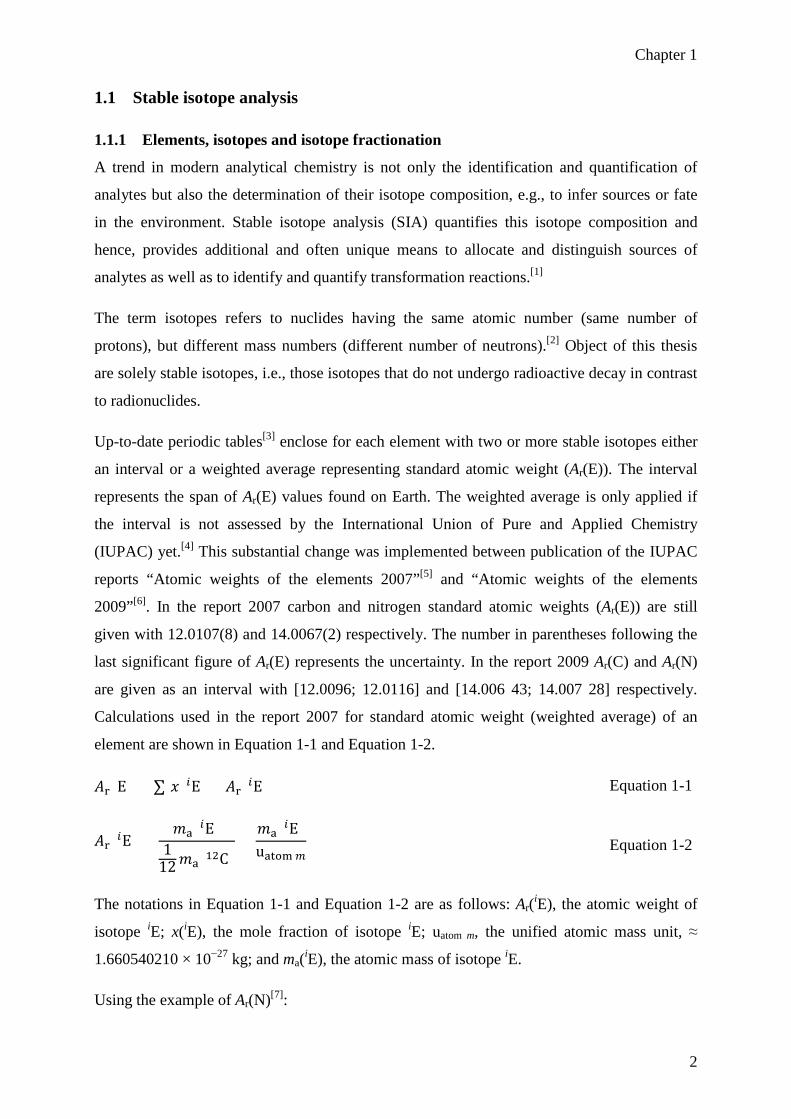
𝐴𝐴r(E) = ∑[𝑥𝑥(𝑖𝑖E) × 𝐴𝐴r(𝑖𝑖E)] Equation 1-1

𝐴𝐴r(𝑖𝑖E) =𝑚𝑚a(𝑖𝑖E)

112𝑚𝑚a(12C)

=𝑚𝑚a(𝑖𝑖E)uatom 𝑚𝑚

Equation 1-2

The notations in Equation 1-1 and Equation 1-2 are as follows: Ar(iE), the atomic weight of

isotope iE; x(iE), the mole fraction of isotope iE; uatom m, the unified atomic mass unit, ≈

1.660540210 × 10−27 kg; and ma(iE), the atomic mass of isotope iE.

Using the example of Ar(N)[7]:

Chapter 1

3

𝐴𝐴r(N) = 0.996337 × 14.0030740074 + 𝐴𝐴r(N) = 0.003663 × 15.000108973 𝐴𝐴r(N) == 14.0067

The mole fractions represent a natural abundance of corresponding isotopes as naturally found

on the planet Earth and they can vary locally (variation of isotope composition), thus in

Equation 1-1 averaged x(iE) values are used.

The Ar(E) refers to the expected atomic weight of an element in the environment of the Earth's

crust and atmosphere (extraterrestrial materials are not included[6]) and thus represents the

global distribution on Earth. The Ar(E) implement local variations[4] caused by fractionation

processes occurring during physical or chemical reactions and can be used for, e.g., origin

determination, investigation of reaction pathways etc.[8]

Carbon and nitrogen are in the focus of various disciplines in environmental biogeochemistry,

life science, chemistry, food science and water resource management and therefore play a key

role in SIA.[9,10] Figure 1-1 visualizes the range of natural variations for stable carbon and

nitrogen isotopes on Earth, directly defining the Ar(E) intervals. For the quantitative

description of stable isotope composition the delta notation was introduced by Harold Urey in

the 1940s and used for the first time in a publication by McKinney et al. in 1950.[11,12] The

following equation defines the δhE.[13]

𝛿𝛿ℎEA,ref = 𝑅𝑅� Eℎ E𝑙𝑙� �

A− 𝑅𝑅� Eℎ E𝑙𝑙� �

ref

𝑅𝑅� Eℎ E𝑙𝑙� �ref

Equation 1-3

where hE/lE expresses the isotope ratio (R) of the heavy (hE) to the light isotope (lE) in a

compound (analyte; A). δhE values define the isotope composition converted to the

international ratio scale (ref). δ13C values define carbon isotope compositions converted to the

Vienna Pee Dee Belemnite (VPDB) scale. δ15N values define nitrogen isotope compositions

converted to the AIR-N2 scale.[12,14]

Chapter 1

4

Figure 1-1 Natural variations of stable carbon (right) and nitrogen (left) isotope composition in selected materials. Isotope variations directly affect

standard atomic weight interval. δ15N and δ13C express the isotope composition. Adapted from.[4,15,7] Notes: (a) N2O in air (troposphere), sea and

ground water; (b) NOx from acid plant has an exceptional isotope composition with δ15N of -150‰ (c) Marine sediments and compounds.

standard atomic weight [14.00643, 14.00728] standard atomic weight [15.99903, 15.99977]

-80 -60 -40 -20 20 40 60 80 100 120 140 160 -120 -100 -80 -60 -40 -20 0 20 400

nitrate

nitrite

nitrogen gas

organic nitrogen

nitrogen in rocks

ammonium

δ15Ni,air δ13Ci,VPDB

carbonate & bicarbonate

carbon dioxide

oxilates

organic carbon

carbon monooxide

elemental carbon

ethane

methane

air, sea water and estuariesground water and icesoil extracts and desert salt depositssynthetic reagents and fertilizers

synthetic reagentsground waters

NOx in airN2O in air (troposphere)a

air

sedimentary basinsvolcanci gases and hot springsground waters

comercial tank gas

plants and animals

crude oilbituminous sediments, peat, and coalmarine particulate organic matter

soilsfertilizers

metamorphic rocksigneous rocksdiamonds

air

volcanic gas condensatessoil extractssea water and estuaries

synthetic reagents and fertilizers

soil gas

sea waterother watermetamorphic & igneous rocktypical marine carbonate rockother carbonate

air

commercial tank gas and reference materialsoil, gas, coal, and landfillsvolcanic gas

CaC2O4 * xH2O (whewellite)

air

land plants (C3 metabolic process)land plants (C4 metabolic process)land plants (CAM metabolic process)

coalmarine sedimentscmarine organisms

crude oilethanol (naturally occurring)

graphitediamonds

hydrocarbon gas

fresh water sourcesmarine and other sourcesair

commercial tank gas

nitrogen oxidesb

Chapter 1

5

The δ-notation has three main advantages: Relative differences in isotope ratios can be

determined far more precisely than absolute isotope ratios.[16] Additionally, it is more

important to know the differences in isotope ratios between samples or compounds rather than

absolute isotope ratios. The third advantage is that the low values are magnified for a better

readability: the δ-notation eliminates the leading digits and makes handling of SIA results

more convenient.[12,16]

Variations of isotope composition of an element occur as a result of isotope fractionation: the

separation of isotopes of an element during naturally occurring processes as a result of the

mass differences between their nuclei.[17] The isotope fractionation between two compounds

(e.g., a substrate and its degradation product) can be expressed with the fractionation factor

α[1] (see Equation 1-4).

𝛼𝛼 =R� Eh El� �

product

R� Eh El� �reactant

=𝛿𝛿ℎEproduct,ref + 1𝛿𝛿ℎEreactant,ref + 1

Equation 1-4

The δhE -value of a product depends on the initial isotope composition of a reactant and on

the extent of isotope fractionation during physical and chemical processes involved in the

transformation of the reactant[18]. Exemplarily a reversible, nucleophilic aliphatic substitution

leading to a halogen exchange in halomethanes is discussed (see Equation 1-5)[12].

CH133I + CH3F ↔ CH3I + CH13

3F Equation 1-5

Rearranging of Equation 1-4 results in:

𝛿𝛿ℎEproduct,ref = 𝛼𝛼 × �𝛿𝛿ℎEreactant,ref + 1� − 1 Equation 1-6

With the corresponding α13C(CH3F/CH3I) for the exemplary reaction, this results in:

𝛿𝛿13CCH3F,VPDB = 0.9703 × �𝛿𝛿13CCH3I,VPDB + 1� − 1 Equation 1-7

A fractionation factor <1 implies a higher content of heavier isotope in the reactant (CH3I)

than in the product (CH3F). In a closed system, if the δ-value for CH3I is -10.3‰, the δ-value

of CH3F will amount to -39.7‰. Combining the fractionation factor with the mass balance

equation a dependency of the CH3F δ13C value from its mass fraction (f(CH3F) =

m(CH3F)/m(CH3I+CH3F)) can be modeled for a certain substrate isotope composition

(δ13Ctotal) and temperature.[12]

Chapter 1

6

In literature, to express isotope fractionation also the isotope enrichment factor ε (see

Equation 1-8) and the 'isotope difference' ΔhEproduct/reactant, a simple subtraction of the δ-value

of the reactant from the δ-value of a product, are used.[12]

𝜀𝜀ℎEproduct/reactant = 𝛼𝛼ℎEproduct/reactant − 1 Equation 1-8

Main physical isotope fractionation processes can be divided in those, which evolve during

transport within a phase (e.g., diffusion) and those, which evolve during phase transfer

between phases (e.g., evaporation). The isotope fractionation during phase transfer processes

is generally small, but can be of relevance in multi-step processes. Chemical fractionation can

occur during biotic and abiotic transformation processes when for identical chemical species,

containing different isotopes, the reaction rates differ. Chemical fractionation occurs at the

atomic level during the breaking and formation of bonds and is caused by the zero point

energy differences.[17,19]

Independent of whether it is a phase transfer process or a chemical reaction the fractionation

can be caused by a thermodynamic and a kinetic isotope effect (TIE and KIE, respectively).

KIE is based on the fact that in most reactions molecules containing the light isotopes react

faster than those containing heavy ones. Typical examples are evaporation in non-equilibrium

systems or a carbon KIE for photosynthesis. TIE is also called equilibrium isotope effect and

is the net sum of two opposing KIE that apply in an exchange reaction. The heavy isotope

accumulates in a particular component of a system at equilibrium. A carbon TIE for CO2 in a

sealed headspace vial is an example.[20] According to Criss et al.[18] isotope disequilibrium at

the Earth’s surface is far more common than isotope equilibrium. Consequentially, KIEs play

a decisive role for the final isotope composition of a compound.

1.1.2 Isotope ratio mass spectrometry – the SIA detector

Measurements of isotope ratios, especially at low enrichment or natural abundance, require

such a high precision that it has resulted in a separate branch of mass spectrometer systems.

The isotope ratio mass spectrometer is a highly precise multicollector mass spectrometer and

is provided with a magnetic sector type ion optical system. Ionization in the ion source is

realized either by highly sensitive thermal ionization or electron impact. The use of multiple

Faraday collectors is a main requirement for the achievement of highly precise results because

it allows a simultaneous collection of all relevant ion beams.[14] The elements of interest have

to be converted into a gaseous form before introduction into the isotope ratio mass

spectrometer (e.g., N2 for δ15N und CO2 for δ13C determination). The introduction of the gases

Chapter 1

7

to the isotope ratio mass spectrometer is realized via an open split in case of continuous flow

isotope ratio mass spectrometry (IRMS).[12]

Figure 1-2 illustrates the set-up of an isotope ratio mass spectrometer using the example of the

system used within this thesis (IsoPrime100; Isoprime, Manchester, UK). A rectangular

housing is placed under an ultra-high vacuum (<10-8 mbar) by a turbomolecular pump located

directly under the ion source and backed by an external rotary pump. Analyte gas within He

(carrier gas) is introduced to the ion source via an open split connection (100 µm inner

diameter (ID) fused silica placed into the 2 mm ID stainless steel tube connected to the

exhaust of the inlet system, such as an elemental analyzer). Within the ion source (see Figure

1-3) analyte molecules collide with the electron beam emitted by a thorium coated iridium

filament (cathode; thermal excitation at ~ 1800 °C) and accelerated by an electrostatic

potential between the filament and the ion box (50 - 100 eV). Electrons follow a helical path

through the source under influence of the magnetic field (two permanent source magnets) and

electrons not involved in ionization are collected at the trap (anode). Analyte molecules react

within the collision zone to positively charged ions (see Equation 1-9 to Equation 1-11). Ions

are extracted out of the ion box by a lateral potential (-20 to 50 V) established by a repeller

plate inside (back of the ion box, opposite the ion exit slit) and accelerated by an electrical

potential (max. 5 kV). The ion beam leaving through the ion exit slit passes the ion optic,

consisting of half plates, defining slit, z-plates and alpha plate before entering the flight tube

of the housing. Half plates focus and steer the beam in the y-direction. The defining (source)

slit defines the ion beam and collects any scattered ions by holding the defining slit plate at

ground potential. Z-plates steer the ion beam in the z-plane. By analogy with half plates, z-

plates steer by differential offset of the voltage references (±150 V). The alpha slit finally

defines the maximum beam width prior to entry into the flight tube. The homogeneous

magnetic field established by the electromagnet (1 - 5 A) spatially separates the ions

according to their mass-to-charge ratio and thus produces defined ion beams towards the

collector cups (Faraday cups). Deflection is thereby caused by the Lorentz force (�⃗�𝐹L) and

depends on the ion charge (𝑞𝑞ion), ion velocity (�⃗�𝑣ion) and magnetic flux density vector (𝐵𝐵�⃗ ).

Finally, the separated beams are detected within the collector array by Faraday cups

(universal triple collector array for CNOS mode or four collector array, equipped with an

electrostatic filter, for CHNOS mode). The signal for the rarer isotopes is amplified, e.g., for 13CO2 (m/z: 45) by a factor of 100 relative to 12CO2 (difference between feedback resistors).

The amount of ions is represented by the ion current (I) reported in nA. Calculation of isotope

Chapter 1

8

ratios, correction for known isobaric interferences (e.g. C17O16O for 13CO2), referencing to the

reference gas and reporting of δ-values is completed by the software.[12,21]

For molecules (M), the ionization reactions by electron impact follow the relationship[12]:

M + e− → 𝑀𝑀+• + 2e− Equation 1-9

Analyte molecules and generated molecular ions (positive radical ions) can undergo further

reactions within the ion source, e.g., dissociate by further electron impact[12,22]:

M(ABC) + e− → AB+ + C• + 2e− Equation 1-10

M(𝐴𝐴𝐵𝐵𝐴𝐴)+• + e− → AB+ + C• + e− Equation 1-11

The following examples clarify why these possible reactions need to be considered. In the

presence of CO2 in the ion source, those reactions cause formation of CO+ (m/z 28) that

causes isobaric interference with N2+ (m/z 28). Therefore CO2 needs to be removed

completely, e.g., via absorption in NaOH, adsorption on silica or freezing out using liquid

nitrogen, prior to δ15N measurements. Also for δ13C measurements itself those reactions play

an important role. Formation of ions depends on the partial pressure within the ion source and

causes therefore an amount dependent non-linearity effect. This effect needs to be

experimentally determined (quantified) using reference gas pulses and corrected for (for more

details see Chapter 3).

Besides reactions caused by further electron impact, also intermolecular reactions need to be

considered[23,24]:

𝑀𝑀+ + 𝑀𝑀(𝐴𝐴𝐵𝐵𝐴𝐴) → 𝑀𝑀(𝐴𝐴)+ + 𝑀𝑀(𝐵𝐵𝐴𝐴)• Equation 1-12

Water and methane for example can protonate the analyte molecules within the ion source

possibly forming a product interfering with the heavier isotope containing molecule

(12C16O2H+ with 13CO2 and 14N2H+ with 14N15N+, respectively).[12,24] Therefore use of an

appropriate drying agent and securing complete combustion are in IRMS.

In case of δ13C isobaric interference of 13C16O2 with 12C16O17O (both m/z 45) needs to be

corrected for. This is done by monitoring m/z 46 and using a quasi-constant correlation

between 17O and 18O (Craig correction; for more details see Chapter 3). In case of δ15N

isobaric interference of 14N2 with 13C16O (both m/z 28) needs to be considered by ensuring CO

absence. This can be accomplished by complete conversion to CO2 that can be scavenged by,

e.g. the NaOH trap.

Chapter 1

9

Chapter 1

10

Figure 1-2 Functionality of an isotope ratio mass spectrometer (Background engineering drawing (grey) of the figure is reproduced by permission of

Isoprime, Manchester, UK). Detailed ion source scheme is shown in Figure 1-3.

Chapter 1

11

Figure 1-3 Ion source scheme. Note that the drawing is mirror-inverted in comparison to the

real ion source shown in Figure 1-2. Electron entrance aperture and trap aperture (located on

the upper and lower side of the ion box, respectively) are not shown.

Other common detectors for SIA are site-specific natural isotope fractionation nuclear

magnetic resonance spectroscopy (SNIF-NMR), cavity ring-down laser absorption

spectroscopy (CRLAS ≡ CRDS), Fourier transform infrared spectrometry (FTIR) and non-

dispersive isotope-selective infrared spectrometry (NDIRS).[25–27] However, these methods are

either not suited for natural isotope abundance measurements, only suited for pure liquids, not

suited for coupling with chromatographic techniques or they cannot be used for N2 SIA.

IRMS on the other hand is in particular adapted to routine isotope analysis of light

elements.[12,28] Thus, alternative detection methods have not been further considered and are

beyond the scope of this thesis.

Chapter 1

12

1.2 Carbon and nitrogen in environmental research Carbon and nitrogen play a main role on our planet and beyond.[9,10,29,30] They are required for

the existence of life and the biogeochemical cycle of C and N is indubitably an important

aspect of the Earth system.[29] Therefore, both elements, in their different chemical forms,

concentrations and isotope compositions, are in the focus of intensive research in science to

understand the main influencing factors, such as temperature, humidity and reaction

pathways, on the biogeochemical interactions on the planet Earth. Figure 1-4 systemizes the

complex interactions in a very condensed form making clear the potential and reason for

intensive investigation in various scientific disciplines and fields. Different sources of

chemical species of C and N, their varying concentrations and isotope compositions and

interactions through transport and transformation processes, e.g., between different Earth-

atmosphere eco-systems makes the potential for various research fields obvious ranging from

astronomy[30] via archaeology[31,32] to different fields of biogeochemistry.[9,10] Specific topics

in these areas include investigations of chemical reaction pathways in environmental

chemistry[33] as well as of solubility processes in physical chemistry[34].

Figure 1-4 Different sources of chemical species of C and N – an overview. Ellipses indicate

further subdivisions.

Carbon and nitrogen in aqueous samples imply some specific features.[35] In BSIA, in contrast

to CSIA, determination of isotope composition in a sample refers, strictly speaking, to the

entire set of species containing the concerned element – the isotope ratio of the bulk

sample.[12] Deviating use of the term BSIA comes from the fractionation of the bulk, typically

found in disciplines dealing with aqueous samples with dispersed carbon and nitrogen.[9,10,36]

By previous filtration of the sample through 0.45 µm filter and acidification (pH <2) for

Sources of chemical species of carbon and nitrogen,theirs varying concentrations and isotope compositons

extraterrestrial terrestrial

bioticabiotic

naturalanthropogenic

hydrospheric terrestrial atmospheric

biosphere

lithospheremarine

freshwater

Chapter 1

13

instance, the analyte is not total carbon (TC ≡ bulk), but its fraction dissolved organic carbon

(DOC).[37] An overview of carbon and nitrogen species classification is given in Figure 1-5.

To keep it simple and because the concerned SIA methods are still not compound specific the

term BSIA will be extended (bulk and groups of compounds SIA) in this thesis.

Figure 1-5 Classification of dispersed carbon and nitrogen matter; (a) defined by International

Organization for Standardization (ISO) 8245[37]; (b) considering IUPAC recommendations[38];

(c) defined by ISO 12260[39]; In, e.g., soil-science studies TNb measured in aqueous samples is

often termed total dissolved nitrogen (TDN)[40,41] (d) volatile organic carbon (VOC) and non-

volatile organic carbon (NVOC) are often incorrectly set equal with POC and NPOC

respectively[42] and are not clearly distinguished within the norm.[37] A VOC is any organic

compound having a boiling point ≤250 °C[43], thus comprised out of compounds such as

benzene, toluene, cyclohexane and so one. Besides VOC, the purging process can remove

further compounds by a continuous shift of equilibrium (Le Châtelier principle). Thus VOC is

a part of POC.

Note that dissolved matter, in contrast to particulate matter, is defined in this classification

operationally by passing a 0.45 µm filter pore size. Despite being generally accepted, this is in

contrast to the fundamental definition in chemistry, where dispersion is a solution if the

dissolved matter is <1 nm, a colloid if the dispersed matter lies between 1 nm – 1 µm and a

suspension if the dispersed matter is >1 µm.[44]

Stable isotope data is used for a broad range of applications:

Variation in δ13C values can be used to follow carbon flow through food webs as well as

identifying sources of carbon contributing to soil organic matter or sediments.[9] Application

total dispersed C and N matter

total carbon (TC)a total nitrogen (TN)

total organiccarbon (TOC)a

total inorganiccarbon (TIC)a

(total) nitrogenbound (TNb)

cdinitrogen(N2-aq)b

dissolvedTIC (DIC)

particulateTIC (PtIC)

non-purgeable organiccarbon (NPOC)a,d

purgeable organiccarbon (POC)a,d

particulateNPOC (PtOC)

dissolved organiccarbon (DOC)a

total organic nitrogen(TON)

dissolvedTON (DON)

particulateTON (PtON)

total inorganicnitrogen bound (TINb)

NO3NO-

NO-NO2

NH+NH4

Chapter 1

14

of 15N-tracer techniques helps to investigate the nitrogen cycle in marine and fresh waters.[10]

Stable carbon and nitrogen isotope composition can be used to investigate sources of

pollution and pathways of transformation.[45] Stable isotope data is also used to define atomic

weights.[4] Further examples can be found in corresponding sections.

Chapter 1

15

1.3 Instrumental and methodological background for SIA in aqueous samples While the isotope ratio mass spectrometer is considered to be the best suited detector for SIA,

as addressed in this thesis, there is a large variety of sample preparation devices for special

purposes. Classification of techniques considering the kind of sample introduced into the

conversion interface (bulk or individual compound) is generally accepted and is illustrated in

Figure 1-6. The illustration excludes position-specific stable isotope analysis (PSIA)[12],

because it is out of the scope of this thesis.

Figure 1-6 Classification of SIA techniques. Optional bulk modification is for example

removal of total inorganic carbon (TIC) (via acidification and purging) prior to total organic

carbon (TOC) SIA. Without this modification the measurement would relate to total carbon

(TC) SIA. Also removal of the main matrix such as water (via lyophilisation) is a common

bulk modification technique in BSIA.

Various analytical methods are available for stable carbon and nitrogen isotope analysis in

aqueous samples.[9,10,46–49] A closer look at these methods, combined with the classification in

Figure 1-6 reveals conversion and purification as a common central aspect of research and

development in BSIA and CSIA methodology. Isotope ratio mass spectrometer follows as a

standard detector for BSIA and CSIA and a separation technique is preceded in CSIA.

The various techniques can be classified into four main principles applied, whereby the first

two are common for BSIA and CSIA:

1. Offline sample-preparation, such as lyophilization of the whole sample (BSIA) and

extraction or purification of individual compounds from the sample (CSIA), followed by

SIA

BSIA CSIA

separationseparates individual compounds from a mixture

hE for each compound

conversion

purificationseparation of analysis gas of interest from interfering components

hE of the total E in a sample

bulk modification(optional)

isotopic composition measurement

converts „raw“ sample to analysis gases converts compound to analysis gases

Chapter 1

16

elemental analyzer/isotope ratio mass spectrometry (EA/IRMS).[46,50,51] The interface design

is shown in Figure 1-7.

The conversion of the analyte is performed in two steps. Combustion of the analyte to CO2

and N2 and NOx is performed at high temperature (usually ≥650 °C) by oxygen. Combustion

is often supported by a catalyst (e.g., Pt) and/or oxygen donor (e.g., CuO). The combustion

temperature is adjusted to the working optimum of the chosen supportive material. NOx is

converted to N2 on a reducer, such as Cu.

The conversion reaction (complete oxidation) for carbon can be expressed as following,

shown exemplarily for a hydrocarbon:

C𝑥𝑥H𝑦𝑦 + �𝑥𝑥 +𝑦𝑦4�O2 → �

𝑦𝑦2�𝐻𝐻2O + 𝑥𝑥CO2 Equation 1-13

The conversion reactions for nitrogen can be formulated in a simplified manner as follows

(Equation 1-14 (oxidation) and Equation 1-17 (reduction)):

R−N𝑢𝑢 + 𝑣𝑣O2 → 𝑤𝑤N2 + 𝑥𝑥N𝑦𝑦O𝑧𝑧 Equation 1-14

The yield of dinitrogen and nitrogen oxides depends strongly on combustion conditions

(oxygen concentration, temperature and supportive material used) and concentration and

species composition of nitrogen containing matter (e.g., nitrates, ammonium and various

organic compounds). The main nitrogen oxide species is nitric oxide (NO). Nitrous oxide

(N2O) formation is insignificant at temperatures above ca. 600 °C[52]:

2 N2O → 2N2 + O2 Equation 1-15

Nitrogen dioxide (NO2) may be initially formed, but above temperatures of ca. 650 °C the

equilibrium is shifted completely to the side of nitric oxide[52]:

2 NO2 → 2NO + O2 Equation 1-16

Reduction on cupper, typically used in elemental analysis since description by Dumas in

1833, can be formulated as:

2Cu + 2NO → 2CuO + N2 Equation 1-17

The purification system often consist of a dryer, such as a membrane dryer (NafionTM) or a

chemical dryer (Sicapent®) and further filters or traps, such as a hydrogen halides and

halogens trap. A separation unit (GC column or CO2-focusing unit) is installed to separate

CO2 prior to N2 measurements.

Chapter 1

17

Figure 1-7 EA based technique. After the sample is brought into the solid form (offline

sample-preparation), it is introduced using an autosampler into the high-temperature (HT)

system. The combustion of the analyte is performed at high temperature (usually ≥600 °C) by

oxygen and often supported by a catalyst and/or oxygen donor. Passing the reduction reactor,

He as a carrier gas transports the analyte and other contents (matrix) to the purification system

(often consisting of a dryer and a further filter). After the separation unit, analyses gases N2

and CO2, respectively, are directed by the He gas stream towards the optional concentration

detector, such as thermal conductivity detector (TCD) and subsequently towards the open

split connection of the isotope ratio mass spectrometer.

2. Wet chemical oxidation based techniques present the second principle. For BSIA a wet

chemical oxidation based total organic carbon analyzer coupled to isotope ratio mass

spectrometry (WCO TOC/IRMS) is used.[47,53] With respect to upstream separation

equipment, CSIA can use the same principle, but with different dimensions and slightly

different set-up of the instrumentation.[54,55] A typical interface design is shown in Figure 1-8

(Note that chemicals and radical generation techniques may differ).

So far, wet chemical oxidation (WCO) based systems are used for carbon SIA only. The most

common oxidation reagent is sodium peroxodisulfate. The conversion of the analyte to CO2 is

performed mainly by sulfate radicals (SO4•-; standard reduction potential E° = 2.47) as main

oxidative species, but also by peroxodisulfate (S2O82-; E° = 2.01). Sulfate radicals are

generated, e.g., thermally, by UV-photons or metal ions[12]:

S2O82− 𝑇𝑇,𝑈𝑈𝑈𝑈,𝑚𝑚𝑚𝑚𝑚𝑚𝑚𝑚𝑙𝑙𝑖𝑖𝑚𝑚𝑚𝑚𝑚𝑚�⎯⎯⎯⎯⎯⎯⎯⎯⎯� 2SO4

•− Equation 1-18

IRMSdetector

elemental analyzeroffline sample-preparation

HT-reactor (C): combustion (R): reduction

mass flow controller gas dryingfocusing unit filter

ref. gas CO2

He

ref. gas box

ref. gas N2He

O2

TCD

CO2

C R

Chapter 1

18

The conversion reaction for carbon can be expressed as following, shown exemplarily for an

average sum formula for carbohydrates CH2O[12]:

4S2O82− + 2CH2O + 2H2O → 8SO4

2− + 2CO2 + 8H+ Equation 1-19

Formed CO2 is subject to three processes: gas dissolution (Equation 1-20), carbonic acid

formation (Equation 1-21) and carbonic acid equilibrium (Equation 1-22).

CO2(g) ↔ CO2(aq) Equation 1-20

CO2(aq) + H2O ↔ H2CO3(aq) Equation 1-21

H2CO3(aq) ↔ H+(aq) + HCO3−(aq) ↔ 2H+(aq) + CO3

2−(aq) Equation 1-22

The buffer (pH ≤2) prevents bicarbonate and carbonate formation by shifting the carbonic

acid equilibrium completely to the carbonic acid side. Purging out of the CO2(g) shifts the gas

dissolution equilibrium (Equation 1-20), which results in a corresponding shift of carbonic

acid formation equilibrium (Equation 1-21).

WCO based systems for CSIA are adjusted with respect to continuous flow conditions (run-

through reactor).[12]

Purification is analogous to that of HTC based EA systems described before. Purification in

WCO based systems for CSIA is adjusted with respect to continuous flow conditions

(additional membrane separation unit).[12]

Figure 1-8 WCO TOC based technique. After the sample is introduced into the wet chemical

oxidation (WCO) based system, oxidation reagents (e.g., sodium persulfate) and buffer

solution are added. Highly reactive radicals are generated, e.g., by UV-photons. The formed

IRMSdetector

WCO TOCanalyzer

gas drying (a) condenser (b) residual H 2O remover

mass flow controller filterdosing pump NDIR detector

a

He

H3P

O4

sam

ple

purg

e ga

s

reac

tor

b

Na 2S

2O8

ref. gas CO2

He

ref. gas box

ref. gas N2

external focusingunit for CO2

Chapter 1

19

conversion product CO2 is purged out by He and transported to the purification system (often

consisting of a dryer and further filters). After the optional focusing unit (BSIA only),

analysis gas CO2 is directed towards the optional concentration detector, such as a

nondispersive infrared (NDIR) detector, and subsequently towards the open split connection

of the isotope ratio mass spectrometer.

3. High-temperature combustion TOC-analyzer coupled to an IRMS detector (HTC

TOC/IRMS) was also utilized, but for BSIA only.[56,57] The main difference to the EA/IRMS

methods is the design of the gas drying system suited to handle the large amount of water as a

main matrix of the samples used. A typical interface design is shown in Figure 1-9.

Figure 1-9 HTC TOC based technique. Aqueous samples are introduced using an autosampler

into the high-temperature combustion TOC-Analyzer. The combustion of the analyte is

performed at high temperature (usually ≥600 °C) by oxygen and often supported by a catalyst

and/or oxygen donor. He as a carrier gas transports the analyte and other contents (matrix) to

the purification system (often consisting of a condenser, dryer and further filters). After the

separation unit, analyses gases N2 and CO2, respectively, are directed by the He gas stream

towards the optional concentration detector, such as a NDIR detector and subsequently

towards the open split connection of the isotope ratio mass spectrometer.

4. Derivatization followed by gas chromatography/isotope ratio mass spectrometry

(GC/IRMS)[58] for CSIA of non-volatile compounds. The main difference of the interface to

the EA are the dimensions of the reactors (HT combustion and reduction) and gas drying

system to avoid peak broadening and suited to the continuous, but low gas flow used.

gas drying (a) condenser (b) residual H 2O remover

mass flow controller filterNDIR detector HTC-reactor

IRMSdetector

HTC TOCanalyzer

ref. gas CO2

He

ref. gas box

ref. gas N2

a

b

He

O2

external focusingunit for CO2

Chapter 1

20

In addition to these four main principles for CSIA of dissolved (non-volatile) compounds the

use of thermospray and a moving belt interface was described for the coupling of HPLC with

IRMS.[59] Simultaneously, a chemical reaction interface (CRI) following HPLC separation

was also combined with IRMS.[60] None of these technologies were further developed to a

commercial instrument, though. In the case of the CRI the large signal from the reactant gas

(O2+; m/z 32) spreads into the cup for the analyte gas (N15O+; m/z 31) preventing δ15N

measurement, while byproducts in the plasma (CO+, NO2+ and C2H5O+) led to incorrect δ13C

values.[60] In the case of the moving belt, no δ15N SIA was ever reported and for δ13C SIA the

limitations include the limited capacity of the wire, depletion of semivolatile compounds with

potential isotope fractionation and flow restriction[12].

The four main principles described are all applied, but have following limitations:

EA/IRMS BSIA and CSIA of non-volatile compounds need a very time-consuming and

laborious offline sample preparation. It also involves a higher risk of contamination and

fractionation. Possible fractionation must also be controlled in derivatization for subsequent

GC/IRMS measurements. Both EA/IRMS and GC/IRMS CSIA also require additional

corrections, which increase the uncertainty of the determined values.[50,61–65]

The WCO-based methods run the risk of carbon concentration underestimation as well as of

isotope fractionation due to incomplete oxidation.[66] Incomplete oxidation is a well-known

issue for seawater samples, in which sulfate radicals are scavenged by chloride ions, and are

therefore no longer available for analyte oxidation.[67] Similarly, in soil science, compounds

such as humic or fulvic acid that are resistant to oxidation are reported not to be completely

oxidized by WCO[66] with the risk of compound-specific isotope fractionation. For samples

with unknown composition such errors are non-systematic and cannot be corrected for in

BSIA. WCO based interface for CSIA do not allow the measurement of δ15N values.

Furthermore, WCO-based systems for δ13C CSIA suffer from the same problem as is common

in BSIA, i.e. the risk of isotope fractionation due to incomplete oxidation.[66,34]

Many publications suggest HTC TOC analyzers as the most suitable device for DOC

concentration measurements.[68] However, commercially available HTC-based systems are not

optimized for SIA mainly because of their insufficient sensitivity.[56] For CSIA the principle

was never applied.

Furthermore, a recent worldwide proficiency test[69] identified several common problems with

reproducibility and consequently data validity for interpretation and comparability among

institutes using different analytical techniques. Generally accepted or even standardized

Chapter 1

21

operating procedures have been developed for many bulk and compound-specific stable

isotope analyses.[11,23,70-73] However, the field of DOC SIA still shows a lack of standardized

methods and approaches to account for all parameters required for accurate results such as the

minimal required combustion temperature for complete mineralization or the handling of

blanks.

In view of the limitations of the analytical techniques discussed above the aim of this thesis

was to develop a novel HTC-based inlet system for δ13C and δ15N BSIA and an interface for

δ13C and δ15N CSIA in aqueous samples and also to propose a data evaluation approach for

DOC SIA.

Chapter 1

22

1.4 References [1] T. C. Schmidt, L. Zwank, M. Elsner, M. Berg, R. U. Meckenstock, S. B. Haderlein.

Compound-specific stable isotope analysis of organic contaminants in natural environments: a

critical review of the state of the art, prospects, and future challenges. Anal. Bioanal. Chem.

2004, 378, 283.

[2] IUPAC Gold Book. Isotopes. http://goldbook.iupac.org/I03331.html

[3] N. E. Holden, T. B. Coplen. ConfChem Conference on A Virtual Colloquium to Sustain

and Celebrate IYC 2011 Initiatives in Global Chemical Education: The IUPAC Periodic

Table of Isotopes for the Educational Community. J. Chem. Educ. 2013, 90, 1550.

[4] M. E. Wieser, N. Holden, T. B. Coplen, J. K. Bohlke, M. Berglund, W. A. Brand, P. De

Bievre, M. Groning, R. D. Loss, J. Meija, T. Hirata, T. Prohaska, R. Schoenberg, G.

O’Connor, T. Walczyk, S. Yoneda, X. Zhu. Atomic weights of the elements 2011 (IUPAC

technical report). Pure Appl. Chem. 2013, 85, 1047.

[5] M. E. Wieser, M. Berglund. Atomic weights of the elements 2007 (IUPAC Technical

Report). Pure Appl. Chem. 2009, 81, 2131.

[6] M. E. Wieser, T. B. Coplen. Atomic weights of the elements 2009 (IUPAC technical

report). Pure Appl. Chem. 2011, 83, 359.

[7] T. B. Coplen, J. K. Bohlke, P. De Bievre, T. Ding, N. E. Holden, J. A. Hopple, H. R.

Krouse, A. Lamberty, H. S. Peiser, K. Revesz, S. E. Rieder, K. J. R. Rosman, E. Roth, P. D.

P. Taylor, R. D. Vocke, Y. K. Xiao. Isotope-abundance variations of selected elements

(IUPAC technical report). Pure Appl. Chem. 2002, 74, 1987.

[8] R. Michener, K. Lajtha, Editors. Stable Isotopes in Ecology and Environmental Science.

Blackwell Publishing, Oxford, 2007.

[9] D. C. Coleman, B. Fry. Carbon Isotope Techniques. Academic Press, San Diego, 1991.

[10] T. H. Blackburn, R. Knowles. Nitrogen Isotope Techniques. Academic Press, San Diego,

1993.

[11] C. R. McKinney, J. M. McCrea, S. Epstein, H. A. Allen, H. C. Urey. Improvements in

mass spectrometers for the measurement of small differences in isotope abundance ratios.

Rev. Sci. Instrum. 1950, 21, 724.

Chapter 1

23

[12] M. A. Jochmann, T. C. Schmidt. Compound-Specific Stable Isotope Analysis. Royal

Society of Chemistry, Cambridge, 2012.

[13] T. B. Coplen. Guidelines and recommended terms for expression of stable-isotope-ratio

and gas-ratio measurement results. Rapid Commun. Mass Spectrom. 2011, 25, 2538.

[14] I. T. Platzner. Modern Isotope Ratio Mass Spectrometry. JohnWiley, Chichester, 1997.

[15] T. B. Coplen, J. A. Hopple, J. K. Bohlke, H. S. Peiser, S. E. Rieder, H. R. Krouse, K. J.

R. Rosman, T. Ding, R. D. Vocke Jr., K. M. Revesz, A. Lamberty, P. Taylor, P. De Bievre.

Compilation of minimum and maximum isotope ratios of selected elements in naturally

occurring terrestrial materials and reagents. U.S. Geological Survey, Denver, 2002.

[16] J. T. Brenna, T. N. Corso, H. J. Tobias, R. J. Caimi. High-precision continuous-flow

isotope ratio mass spectrometry. Mass Spectrom. Rev. 1998, 16, 227.

[17] J. Hoefs. Stable Isotope Geochemistry. Springer, Berlin, 2013.

[18] R. E. Criss. Principles of Stable Isotope Distribution. Oxford University Press, Oxford,

1999.

[19] C. M. Aelion, P. Höhener, D. Hunkeler, R. Aravena. Environmental Isotopes in

Biodegradation and Bioremediation. CRC Press, Boca Raton, 2009.

[20] B. Fry. Stable Isotope Ecology. Springer, Berlin, 2007.

[21] Isoprime Users’s Guide (Version 1.02). Isoprime, Manchester, 2012

[22] J. H. Gross, in Mass Spectrometry – A Textbook. (Eds: J. H. Gross). Springer, Berlin,

2011, pp. 21–66.

[23] A. L. Sessions, T. W. Burgoyne, J. M. Hayes. Correction of H3+ contributions in

hydrogen isotope ratio monitoring mass spectrometry. Anal. Chem. 2001, 73, 192.

[24] W. A. Brand, in Handbook of Stable Isotope Analytical Techniques, (Ed: P. A. de

Groot). Elsevier, Amsterdam, 2004, pp. 835–857.

[25] F. K. Tittel, R. Lewicki, R. Lascola, S. McWhorter, in Trace Analysis of Specialty and

Electronic Gases. (Eds: W. M. Geiger, M. W. Raynor). JohnWiley, Chichester, 2013, pp. 71–

109.

Chapter 1

24

[26] Z.-H. Du, Y.-Q. Zhai, J.-Y. Li, B. Hu. Techniques of on-line monitoring volatile organic

compounds in ambient air with optical spectroscopy. Guangpuxue Yu Guangpu Fenxi 2009,

29, 3199.

[27] G. J. Martin, S. Akoka, M. L. Martin, in Modern Magnetic Resonance, Part 3. (Eds: G.

A. Webb). Springer, Berlin, 2006, pp. 1629–1636.

[28] E. Roth. Critical evaluation of the use and analysis of stable isotopes. Pure Appl. Chem.

1997, 69, 1753.

[29] E. D. Andrulis. Theory of the origin, evolution, and nature of life. Life 2012, 2, 1.

[30] T. R. Ireland. Isotopic anomalies in extraterrestrial grains. J. R. Soc. West. Aust. 1996,

79, 43.

[31] K. J. Knudson, A. H. Peters, E. T. Cagigao. Paleodiet in the Paracas Necropolis of Wari

Kayan: carbon and nitrogen isotope analysis of keratin samples from the south coast of Peru.

J. Archaeol. Sci. 2015, 55, 231.

[32] N. Wang, Y. Hu, G. Song, C. Wang. Comparative analyses of amino acids and C, N

stable isotopes between soluble collagen and insoluble collagen within archaeological bones.

Disiji Yanjiu 2014, 34, 204.

[33] N. Zhang, S. Bashir, J. Qin, J. Schindelka, A. Fischer, I. Nijenhuis, H. Herrmann, L. Y.

Wick, H. H. Richnow. Compound specific stable isotope analysis (CSIA) to characterize

transformation mechanisms of α-hexachlorocyclohexane. J. Hazard. Mater. 2014, 280, 750.

[34] A. A. Chialvo, L. Vlcek. NO3- Coordination in Aqueous Solutions by 15N/14N and

18O/natO Isotopic Substitution: What Can We Learn from Molecular Simulation?. J. Phys.

Chem. B 2015, 119, 519.

[35] E. Federherr, C. Cerli, F. M. S. A. Kirkels, K. Kalbitz, H. J. Kupka, R. Dunsbach, L.

Lange, T. C. Schmidt. A novel high-temperature combustion based system for stable isotope

analysis of dissolved organic carbon in aqueous samples. I: development and validation.

Rapid Commun. Mass Spectrom. 2014, 28, 2559.

[36] G. Förtsch. Handbuch Betrieblicher Gewässerschutz. Springer, Berlin, 2014.

[37] ISO 8245:1999. Water quality — Guidelines for the determination of total organic

carbon (TOC) and dissolved organic carbon (DOC).

Chapter 1

25

[38] T. Damhus, R. M. Hartshorn, A. T. Hutton. Nomenclature of Inorganic Chemistry:

IUPAC Recommendations 2005. Royal Society of Chemistry, Cambridge, 2005.

[39] DIN EN 12260:2003-12. Water quality – Determination of nitrogen.

[40] R. Russow, J. Kupka, A. Goetz, B. Apelt. A New Approach to Determining the Content

and 15N Abundance of Total Dissolved Nitrogen in Aqueous Samples: TOC Analyzer-QMS

Coupling. Isot. Environ. Health Stud. 2002, 38, 215.

[41] P. Lachouani, A. H. Frank, W. Wanek. A suite of sensitive chemical methods to

determine the δ15N of ammonium, nitrate and total dissolved N in soil extracts. Rapid

Commun. Mass Spectrom. 2010, 24, 3615.

[42] ASTM D7573-09. Test Method for Total Carbon and Organic Carbon in Water by High

Temperature Catalytic Combustion and Infrared Detection. 1999.

[43] EPA Technical Overview of Volatile Organic Compounds https://www.epa.gov/indoor-

air-quality-iaq/technical-overview-volatile-organic-compounds.

[44] P. W. Atkins, J. De Paula. Physikalische Chemie. JohnWiley, Chichester, 2013.

[45] T. H. E. Heaton. Isotopic studies of nitrogen pollution in the hydrosphere and

atmosphere: A review. Chem. Geol. 1986, 59, 87.

[46] H. Gandhi, T. N. Wiegner, P. H. Ostrom, L. A. Kaplan, N. E. Ostrom. Isotopic (13C)

analysis of dissolved organic carbon in stream water using an elemental analyzer coupled to a

stable isotope ratio mass spectrometer. Rapid Commun. Mass Spectrom. 2004, 18, 903.

[47] C. L. Osburn, G. St-Jean. The use of wet chemical oxidation with high-amplification

isotope ratio mass spectrometry (WCO-IRMS) to measure stable isotope values of dissolved

organic carbon in seawater. Limnol. Oceanogr.: Methods 2007, 5, 296.

[48] R. J. Panetta, M. Ibrahim, Y. Gélinas. Coupling a High-Temperature Catalytic Oxidation

Total Organic Carbon Analyzer to an Isotope Ratio Mass Spectrometer To Measure Natural-

Abundance δ13C-Dissolved Organic Carbon in Marine and Freshwater Samples. Anal. Chem.

2008, 80, 5232.

[49] P. Albéric. Liquid chromatography/mass spectrometry stable isotope analysis of

dissolved organic carbon in stream and soil waters. Rapid Commun. Mass Spectrom. 2011,

25, 3012.

Chapter 1

26

[50] E. Richling, C. Hoehn, B. Weckerle, F. Heckel, P. Schreier. Authentication analysis of

caffeine-containing foods via elemental analysis combustion/pyrolysis isotope ratio mass

spectrometry (EA-C/P-IRMS). Eur. Food Res. Technol. 2003, 216, 544.

[51] B. Fry, S. Saupe, M. Hullar, B. J. Peterson. Platinumcatalyzed combustion of DOC in

sealed tubes for stable isotopic analysis. Mar. Chem. 1993, 41, 187.

[52] C. Walz. NOx-Minderung nach dem SCR-Verfahren: Untersuchungen zum Einfluss des

NO2-Anteils. 2000.

[53] S. Bouillon, M. Korntheuer, W. Baeyens, F. Dehairs. A new automated setup for stable

isotope analysis of dissolved organic carbon. Limnol. Oceanogr.: Methods 2006, 4, 216.

[54] L. Zhang, D. M. Kujawinski, M. A. Jochmann, T. C. Schmidt. High-temperature

reversed-phase liquid chromatography coupled to isotope ratio mass spectrometry: HT-RPLC

coupled to IRMS. Rapid Commun. Mass Spectrom. 2011, 25, 2971.

[55] G. St-Jean. Automated quantitative and isotopic (13C) analysis of dissolved inorganic

carbon and dissolved organic carbon in continuous-flow using a total organic carbon analyser.


[56] I. De Troyer, S. Bouillon, S. Barker, C. Perry, K. Coorevits, R. Merckx. Stable isotope

analysis of dissolved organic carbon in soil solutions using a catalytic combustion total

organic carbon analyzer-isotope ratio mass spectrometer with a cryofocusing interface. Rapid


[57] S. Q. Lang, M. D. Lilley, J. I. Hedges. A method to measure the isotopic (13C)

composition of dissolved organic carbon using a high temperature combustion instrument.

Mar. Chem. 2007, 103, 318.

[58] L. T. Corr, R. Berstan, R. P. Evershed. Optimization of derivatisation procedures for the

determination of δ13C values of amino acids by gas chromatography/combustion/isotope ratio

mass spectrometry. Rapid Commun. Mass Spectrom. 2007, 21, 3759.

[59] W. A. Brand, P. Dobberstein. Isotope-ratio-monitoring liquid chromatography mass

spectrometry (IRM-LCMS). First results from a moving wire interface system. Isot. Environ.

Health Stud. 1996, 32, 275.

Chapter 1

27

[60] Y. Teffera, J. J. Kusmierz, F. P. Abramson. Continuous-Flow Isotope Ratio Mass

Spectrometry Using the Chemical Reaction Interface with Either Gas or Liquid

Chromatographic Introduction. Anal. Chem. 1996, 68, 1888.

[61] D. M. Kujawinski, L. Zhang, T. C. Schmidt, M. A. Jochmann. When Other Separation

Techniques Fail: Compound-Specific Carbon Isotope Ratio Analysis of Sulfonamide

Containing Pharmaceuticals by High-Temperature-Liquid Chromatography-Isotope Ratio

Mass Spectrometry. Anal. Chem. 2012, 84, 7656.

[62] L. Zhang, D. M. Kujawinski, E. Federherr, T. C. Schmidt, M. A. Jochmann. Caffeine in

Your Drink: Natural or Synthetic?. Anal. Chem. 2012, 84, 2805.

[63] P. J. H. Dunn, N. V. Honch, R. P. Evershed. Comparison of liquid chromatography-

isotope ratio mass spectrometry (LC/IRMS) and gas chromatography-combustion-isotope

ratio mass spectrometry (GC/C/IRMS) for the determination of collagen amino acid δ13C

values for palaeodietary and palaeoecological reconstruction. Rapid Commun. Mass

Spectrom. 2011, 25, 2995.

[64] L. Zhang, M. Thevis, T. Piper, M. A. Jochmann, J. B. Wolbert, D. M. Kujawinski, S.

Wiese, T. Teutenberg, T. C. Schmidt. Carbon Isotope Ratio Analysis of Steroids by High-

Temperature Liquid Chromatography-Isotope Ratio Mass Spectrometry. Anal. Chem. 2014,

86, 2297.

[65] J.-P. Godin, J. S. O. McCullagh. Review: Current applications and challenges for liquid

chromatography coupled to isotope ratio mass spectrometry (LC/IRMS). Rapid Commun.

Mass Spectrom. 2011, 25, 3019.

[66] K.Mopper, J.Qian, in Encyclopedia of Analytical Chemistry, (Ed.: R. A. Meyers).

JohnWiley, Chichester, 2000. pp. 3532–3540.

[67] G. R. Aiken. Chloride interference in the analysis of dissolved organic carbon by the wet

oxidation method. Environ. Sci. Technol. 1992, 26, 2435.

[68] P. J. Wangersky. Dissolved organic carbon methods: a critical review. Mar. Chem. 1993,

41, 61.

[69] R. van Geldern, M. P. Verma, M. C. Carvalho, F. Grassa, A. Delgado-Huertas, G.

Monvoisin, J. A. C. Barth. Stable carbon isotope analysis of dissolved inorganic carbon (DIC)

and dissolved organic carbon (DOC) in natural waters – Results from a worldwide

Chapter 1

28

proficiency test: Carbon stable isotope proficiency test of DIC and DOC. Rapid Commun.


[70] AOAC 984.23-1988. Corn syrup and cane sugar in maple syrup. Carbon ratio mass

spectrometric method.

[71] OIV AS312-07 2010. Method for the determination of the 13C/12C isotope ratio of

glycerol in wines by gas chromatography combustion or high performance liquid

chromatography coupled to isotope ratio mass spectrometry (GC-C-IRMS or HPLC-IRMS).

[72] OIV AS314-03 2005. Determination of the carbon isotope ratio 13C/12C of CO2 in

sparkling wines – method using isotope ratio mass spectrometry (IRMS).

[73] EEC/822/97. Determination of the isotopic ratio of oxygen of the water content in wines.

Chapter 2

29

Chapter 2 Scope and Aim The state of the art in stable isotope analysis (SIA) of aqueous samples described in Chapter 1

shows that aside from the already existing number of techniques and methods, there is still a

lack of systems with the required performance for δ13C and a lack of systems per sé for δ15N

determination. This is especially challenging for samples with natural isotope abundance.

The aim of this study was to increase understanding of the processes involved in the SIA of

all dissolved forms of carbon and nitrogen and to subsequently develop suitable analytical

instrumentation for both bulk and compound-specific stable isotope analysis (BSIA and

CSIA) directly in aqueous solutions. For this purpose, four work packages were carried out as

summarized in Figure 2-1.

Figure 2-1 Overview of the contents of this thesis

Dissolved organic carbon (DOC) plays a key role in carbon cycle investigations and it is the

focus of various disciplines in environmental biogeochemistry. Both the concentration and

the stable isotope composition of DOC play an important role in carbon cycle studies, but

traditional methods are either very time-consuming or involve the risk of isotope fractionation

due to incomplete mineralization. Thus, a novel method suitable for SIA is needed. Chapter 3

comprises the detailed description of the development of an analytical system for accurate and

sensitive DOC SIA (including its validation with standard solutions and simulated matrices)

consisting in the coupling of a modified high-temperature combustion TOC analyzer with an

isotope ratio mass spectrometer.

The results obtained with the newly developed system as described in Chapter 3 met the

needed performance, thus confirmed the general suitability of the system, but further

Stable Isotope Analysis (SIA) techniques

Liquid samplesSolid samples Gas samples

Bulk StableIsotope Analysis (BSIA)

Compound-Specific StableIsotope Analysis (CSIA)

Position-Specific StableIsotope Analysis (PSIA)

HTC TOC/IRMS

WCO TOC/IRMS

Freeze-drying + EA/IRMS Extraction + purification + EA/IRMS

Derivatization + GC/IRMS

HPLC/IRMS

Chapter 3: δ13C method development

Chapter 4: δ13C application development

Chapter 5: δ15N method development

Chapter 6: δ13C and δ15N method development

Chapter 2

30

validation and proper assessment of analytical performance with the real samples was still

needed. Therefore, Chapter 4 aims at the validation of the system with a broad range of real

samples. Soil extracts, river and seawater samples were analyzed and, to further prove the

reproducibility of the developed method, a complete set of samples from an international

round robin test were analyzed as well. Additionally, given the strong interest of the scientific

community, the general suitability of the system for the determination of total inorganic

carbon (TIC) SIA was tested.

Various disciplines in environmental biogeochemistry, such as oceanography and soil science

are not only interested in δ13C but even more so in the δ15N determination directly in aqueous

samples with natural isotope abundance. Because there is no suitable system available, the

aim of Chapter 5 was to find a new analytical principle to overcome the limiting factors for

the performance and, utilizing the novel principle, to develop a new system for SIA of total

nitrogen bound (TNb), simultaneous to SIA of DOC.

All methods introduced from Chapter 3 to Chapter 5 are BSIA techniques for δ13C and δ15N

determination in aqueous solutions but the interest often focuses on specific compounds

within the aqueous samples, i.e., on CSIA especially of polar or ionic compounds. Current

methods need several preparation steps, often including either laborious extraction or

derivatization of the analyte or both. Wet chemical oxidation based HPLC/IRMS systems do

not allow for δ15N determination and also δ13C measurements have limitations – potential bias

due to incomplete mineralization. To avoid these limitations, a system for CSIA of non-

volatile, polar and thermally labile compounds directly from aqueous solutions based on a

HTC interface was conceived and is described in detail within Chapter 6.

Chapter 7 summarizes the main results of this study and depicts an outlook on the potential

direction of future research and developments in the field of SIA in aqueous solutions.

Chapter 3

31

Chapter 3 A novel high-temperature combustion based system for stable

isotope analysis of dissolved organic carbon in aqueous

samples - development and validation Adapted from: E. Federherr, C. Cerli, F. M. S. A. Kirkels, K. Kalbitz, H. J. Kupka, R.

Dunsbach, L. Lange and T. C. Schmidt; A novel high-temperature combustion based system

for stable isotope analysis of dissolved organic carbon in aqueous samples. I: development

and validation; Rapid Communications in Mass Spectrometry 2014, 28, 2559-2573

Chapter 3

32

3.1 Abstract Rationale: Traditionally, dissolved organic carbon (DOC) stable isotope analysis (SIA) is

performed using either offline sample-preparation followed by elemental analyzer/isotope

ratio mass spectrometry (EA/IRMS) or a wet chemical oxidation (WCO)-based device

coupled to an isotope ratio mass spectrometer. The first method is time-consuming and

laborious. The second involves the risks of underestimation of DOC concentration and

isotope fractionation due to incomplete oxidation. The development of an analytical method

for accurate and sensitive DOC SIA is described in this study.

Methods: A high-temperature combustion (HTC) system improves upon traditional methods.

A novel total organic carbon (TOC) system, specially designed for SIA, was coupled to an

isotope ratio mass spectrometer. An integrated trap and flash technique (peak focusing),

flexible injection volume (0.05 – 3 mL), favorable carrier gas flow, modified ash crucible,

new design of combustion tube and optimized drying system were used to achieve the

necessary performance.

Results: The system can reliably measure concentrations up to 1000 mgC/L. Compounds

resistant to oxidation, such as barbituric acid, melamine and humic acid, were analyzed with

recovery rates of 100 ± 1% proving complete oxidation. In this initial testing, the δ13C values

of these compounds were determined with precision and trueness of ≤0.2‰ even with 3.5%

salinity. Further tests with samples with low DOC concentrations resulted in LOQSIA method

values of 0.5 mgC/L and 0.2 mgC/L for LOQSIA instr, considering an accuracy of ±0.5‰ as

acceptable.

Conclusions: The novel HTC system coupled to an isotope ratio mass spectrometer resulted in

significantly improved sensitivity. The system is suitable for salt-containing liquids and

compounds that are resistant to oxidation, and it offers a large concentration range. A second

paper (which follows this one in this issue) will present a more comprehensive assessment of

the analytical performance with a broad set of solutions and real samples. This highly efficient

TOC stable isotope analyzer will probably open up new possibilities in biogeochemical

carbon cycle research.

Chapter 3

33

3.2 Introduction Dissolved organic carbon (DOC) plays a key role in carbon cycle investigations[1] and it is the

focus of various disciplines in environmental biogeochemistry, such as oceanography[2] and

soil science.[3,4] Both the concentration and the stable isotope composition of DOC play an

important role in carbon cycle studies. Concentration measurements provide the possibility to

balance the global as well as the local carbon cycle.[5–7] Stable isotope analyses (SIA) can

provide very valuable additional information about the origin and transformation of organic

matter.[8,9]

Analytical procedures for the determination of DOC concentration are well defined and

understood[10] and for some applications even standardized.[11,12] Thus, the focus of this

work is on the stable isotope analysis of dissolved organic carbon (DOC SIA). Various

analytical methods are available for DOC SIA. Initially, it was carried out either by offline

sample-preparation, such as lyophilization, followed by elemental analyzer/isotope ratio mass

spectrometry (EA/IRMS)[13,14] or by a wet chemical oxidation total organic carbon analyzer

coupled to isotope ratio mass spectrometry (WCO TOC/IRMS).[15,16] High-temperature

combustion techniques were also utilized (HTC TOC/IRMS).[17,18] The most recent

approaches include wet chemical oxidation flow injection analysis-IRMS (WCO FIA-IRMS),[19]

the use of available interfaces for liquid chromatography/IRMS (LC/IRMS), and WCO TOC

coupled to cavity ring-down spectroscopy (WCO TOC/CRDS).[20]

Table 3-1 gives an overview of the various analytical methods.

Offline sample-preparation is time-consuming and laborious.[13] The WCO-based methods run the

risk of DOC concentration underestimation as well as of isotope fractionation due to incomplete

oxidation.[10] Incomplete oxidation is a well- known issue for seawater samples, in which sulfate

radicals are scavenged by chloride ions, and are therefore no longer available for analyte

oxidation.[22] Similarly, in soil science, compounds such as humic or fulvic acid that are resistant

to oxidation are reported not to be completely oxidized by WCO[10] with the risk of compound-

specific isotope fractionation. For samples with unknown composition such errors are non-

systematic and cannot be corrected for in bulk stable isotope analysis (BSIA). Many publications

suggest HTC TOC analyzers as the most suitable device for DOC concentration measurements.[23]

However, commercially available HTC-based systems are not optimized for SIA mainly because

of their insufficient sensitivity[18] as a result of low injection volumes.

Chapter 3

34

Table 3-1 Current methods for determination of stable isotope composition of DOC.

Analyticalprinciple Sample scope Preparation

Insturmentation/Measurement

Additionalevaluation Performance Reference

WCO TOC-IRMS Sea water, Shelf,Reference material

Filtration over 0.45 µm(DOC), acidification +sparging for IC removal

OI-Aurora 10330; DeltaPlus HiPerTOC;Delta Plus

Blank correction(reagent blank)

SD typical 0.1-0.4‰at 65-200 µmol C/L

(Bouillon et al. a)[16]

(Osburn and St-Jeana)[15]

HTC TOC-IRMS Sea water, Soil solution, Reference material


Thermalox;Sercon 20-20 cryo trap MQ 1001; Delta Plus

Blank correction (instrument +reagent blank)

SD typical 0.1-0.2‰at 1-10 mg C/LSD typical 0.1-0.7‰at 40-70 µmol C/L

(Troyer et al. b)[17]

(Lang, et al. b)[18]

LC/IRMS Soil water, bulk stream


Surveyor LC unit;Thermo FisherLC-IsoLink and Delta V


SD typical 0.3‰at 1-10 mg C/L

(Albericc)[19]

EA/IRMS Sea water Filtration over 0.45 µm(DOC), acidification +sparging for IC removal,freeze-drying

Finnigan 251 Blank correction(reagent blank)

SD typical 0.01-0.04‰ (Fry et al. d)[21]

WCO TOC-CRDS River water,waste water

Filtration over 0.45 µm (DOC), acidification +sparging for IC removal

OI-Aurora 1030;Picarro G111-i


SD typical 0.5‰at 2-8 mg C/L

(Hartland et al. e)[20]

WCO: wet chemical oxidation; HTC: high temperature combustion; LC: liquid chromatography; IC: inorganic carbon; EA: elemental analyzer; WCO/CRDS: wet chemical oxidation/cavity ringdown spectroscopya No CO2 trapping, reduction of excess oxygen.bCryostatic CO2 trapping by liquid N2.cBulk analysis in FIA mode without separation column.dSamples freeze-dried in the combustion tubes, home-built combustion system.eCollection of CO2 in a gas-tight bag.

Chapter 3

35

Furthermore, a recent worldwide proficiency test[24] identified several common problems with

reproducibility and consequently data validity for interpretation and comparability among

institutes using different analytical techniques. The critical issues are not simply related to

sample type and sampling procedure, but seem to be mostly method specific for DOC SIA. This

includes sample-preparation, measurement and the evaluation of data.[25] In particular, the use

of very different methods combined with the lack of a generally accepted strategy for data

evaluation makes such comparisons very challenging. Generally accepted or even standardized

operating procedures have been developed for many bulk and compound-specific stable

isotope analyses (CSIA).[26-31] However, the field of DOC SIA still shows a lack of standardized

methods and approaches to account for all parameters required for accurate results such as the

minimal required combustion temperature for complete mineralization or the handling of

blanks.

In view of the limitations of the analytical techniques discussed above we developed a novel

HTC-based system for DOC SIA in challenging aqueous samples, and we propose a data

evaluation approach. In this first manuscript we present the technical details of the

instrument and the rationale for the proposed data processing, while, in the second one,[32] we

focus on the assessment of the analytical performance based on a broad test with real

samples.

Chapter 3

36

3.3 Experimental

3.3.1 Chemicals and reagents

Reference materials IAEA-600 caffeine CAF1 (δ13CVPDB –27.771 ± 0.043‰), USGS-41

glutamic acid GLU1 (δ13CVPDB +37.626 ± 0.049‰) and IAEA-CH-6 sucrose SUC1 (δ13CVPDB

–10.449 ± 0.033‰) were purchased from the International Atomic Energy Agency (Vienna,

Austria). The internal laboratory standards were EAS-CIT1 citric acid (purchased from

Sigma-Aldrich (Buchs, Switzerland)), EAS-CAS1 casein and EAS-GLU2 glutamic acid (in-

house standards; Elementar Analysensysteme, Hanau, Germany). Benzoic acid BEN1

(≥99.5%) and humic acid HUM1 (technical grade, ash ≈ 20%) were purchased from Fluka

(Buchs, Switzerland). Acetovanillone ACV1 (98%), caffeine CAF2 (≥99.0%) and melamine

MEL1 (99%) were obtained from Aldrich (St. Louis, MO, USA). Citric acid CIT2 (≥99.5%),

D-(+)-glucose monohydrate GLU3 (≥99.0%), barbituric acid BAR1 (≥99%), sodium chloride

(≥99.5%) and hydrochloric acid (37%) were purchased from Merck (Darmstadt, Germany).

Ultrapure, deionized water (UP water) produced by a Purelab Ultra system (MK2-Analytic,

ELGA, High Wycombe, UK) was used for solution preparation. Helium 5.0 and oxygen 4.8

were purchased from Air Liquid (Oberhausen, Germany).

3.3.2 Instrumentation and methodology

The entire system consists of three parts: the TOC analyzer, the interface and the isotope ratio

mass spectrometer (see Figure 3-1).

Figure 3-1 System setup for DOC SIA.

The TOC analyzer (iso TOC cube) is derived from the commercially available HTC-TOC

analyzer vario TOC cube (Elementar Analysensysteme GmbH) which was modified and

gas drying a: condenser b: Nafion® membrane c: Sicapent®filter (halogen adsorber)HT-reactor C: combustion R: reduction

NDIR

IRMSDetector

ref. gas CO2

He

reference gasbox

iso TOC cubeDOC Mode

a

c

b

O2

iso TOC interfaceCO2 Mode

He

R CTCD

flow sensormass flow controller

Chapter 3

37

adapted to meet the requirements for IRMS, namely, to improve the system sensitivity, to

minimize instrumental background as well as the blank contribution, and to ensure the

absence of isotope fractionation within the system.

Samples, filled in 40-mL borosilicate glass vials, are introduced using a 32-position

autosampler into the combustion system by means of a 5-mL syringe and a multiway valve.

The combustion is performed at 850 °C by oxygen and supported by a catalyst (Pt on ceramic

carrier material). Water is removed in three steps: an air-cooled condenser, a counter-flow

membrane dryer and a chemical dryer. Hydrogen halides and halogens are removed by silver

wool. After the purification steps the carrier gas oxygen enters the nondispersive infrared

(NDIR) detector for quantification of the evolved CO2 (giving the DOC concentration of a

pre-acidified sample).

The interface separates the CO2 from O2 allowing for focusing and gas exchange (replacement

of the reaction gas oxygen by carrier gas helium). This part of the system was specifically

developed for this application.

An IsoPrime100 (Isoprime Ltd, Manchester, UK) isotope ratio mass spectrometer was used to

determine the stable isotope composition. No modifications were made to this instrument. A

detailed description of all the instrument modifications and/or developments is given in the

Method development section.

3.3.3 Nomenclature, evaluation and QA

Nomenclature

To express the variations of natural stable isotope abundance the widely applied ’delta-

notation’ is used. The δ13CVPDB-value of an analyte (A) is described by Equation 3-1 as a

relative difference between the isotope ratio (R) of an analyte (R(13C/12C)A) and the isotope

ratio defining an international reference scale, for carbon Vienna Pee Dee Belemnite

(R(13C/12C)VPDB):[26]

𝛿𝛿13CA,VPDB = 𝑅𝑅� C13 C12� �

A− 𝑅𝑅� C13 C12� �

VPDB

𝑅𝑅� C13 C12� �VPDB

Equation 3-1

Please note that if no reference is mentioned, as exemplarily shown in Equation 3-2, the

reported δ-values are related to the used, in-house reference gas (RG). That concerns all data

before the final normalization to the VPDB scale.

𝛿𝛿13Clin corr A ≡ 𝛿𝛿13Clin corr A,RG Equation 3-2

Chapter 3

38

with δ13Clin corr A as a linearity corrected δ-value of an analyte A.

Evaluation

The description and rationale behind the chosen data evaluation strategy are extensively

explained in the Results and Discussion section. Here only the finally applied equations are

shown.

Non-linearity correction

Known and inevitable concentration-dependent fractionation occurs in the electron ionization

(EI) source within the isotope ratio mass spectrometer inducing isotope ratio shifts. The

isotope ratio linearity of the isotope ratio mass spectrometer (LR IRMS) was quantified as the

slope mlin of a linear regression describing the δ-value as a function of corresponding ion

current I.

𝑚𝑚lin =∑ �𝐼𝐼RG𝑘𝑘 − 𝐼𝐼RG�� 𝛿𝛿13CRG,RG��𝑘𝑘

− 𝛿𝛿13CRG,RG��𝑚𝑚

𝑘𝑘=1

∑ �𝐼𝐼RG𝑘𝑘 − 𝐼𝐼RG��2𝑚𝑚

𝑘𝑘=1

Equation 3-3

𝛿𝛿13CRG,RG��𝑘𝑘=𝑅𝑅� C13 C12� �

RG𝑘𝑘− 𝑅𝑅� C13 C12� �

RG��

𝑅𝑅� C13 C12� �RG��

Equation 3-4

LR IRMS was monitored regularly, before and after each test series. All measured δ13C raw data

(δ13Cmeas A) generated by the software IonVantage (Isoprime Ltd), and automatically corrected

for 17O-abundance and related to RG, were then linearity corrected to δ13Clin corr A as described

by Brand[27] and expressed as shown in Equation 3-5:

𝛿𝛿13Clin corr A = 𝛿𝛿13Cmeas A −𝑚𝑚lin × (𝐼𝐼A − 𝐼𝐼RG) Equation 3-5

with IA as the ion current at the maximum of the peak for analyte A and IRG the ion current of

the reference gas peak pulse.

Note that the automatically created software report gives an absolute value of the slope mlin.

Therefore, mlin was manually recalculated to account for its positive or negative sign in the

calculation.

Blank corrections

An isotope mass balance (IMB) equation[26] was utilized for corrections. The amount of

carbon is represented by the uncorrected area A from the integrated NDIR CO2 peak of the

TOC analyzer. The solution of the IMB equation for blank-’subtracted’ δ-value δ13CΣbl corr A

Chapter 3

39

results in Equation 3-6. The symbol Σ indicates that there is more than one possible blank

contribution (water blank, instrumental blank, etc.) but, as will be shown in the Results and

Discussion section, only the water blank needs to be considered (taking into account the

concentration range of interest). Thus, for determination of the concentration as well as the δ-

value of the blank, a direct determination by measuring the acidified water used for standards

solution preparation (blanks) is possible:

𝛿𝛿13C𝛴𝛴bl corr A = 𝛿𝛿13Clin corr A × 𝐴𝐴meas A − ∑ (𝛿𝛿13Cbl × 𝐴𝐴bl)𝑘𝑘𝑚𝑚

𝑘𝑘=1

𝐴𝐴meas − ∑ (𝐴𝐴bl)𝑘𝑘𝑚𝑚𝑘𝑘=1

Equation 3-6

Two-point normalization

Finally, a referencing strategy to the VPDB scale was applied as recommended in the

literature and described in Equation 3-7. Note that the equation for two-point normalization

described in the literature[26] is mathematically a linear interpolation procedure and so

equivalent to the two-point calibration equation used here. Thus, applied Equation 3-7 is

valid:

𝛿𝛿13CA,𝑈𝑈𝑉𝑉𝑉𝑉𝑉𝑉 = 𝑚𝑚norm × 𝛿𝛿13C𝛴𝛴bl corr A + 𝑏𝑏𝑚𝑚𝑚𝑚𝑛𝑛𝑚𝑚 Equation 3-7

𝑚𝑚norm =𝛿𝛿13CStd1,VPDB − 𝛿𝛿13CStd2,VPDB

𝛿𝛿13C𝛴𝛴bl corr Std1,RG − 𝛿𝛿13C𝛴𝛴bl corr Std2,RG Equation 3-8

𝑏𝑏norm = 𝛿𝛿13CStd,VPDB�� − 𝑚𝑚norm × 𝛿𝛿13C𝛴𝛴bl corr Std,RG�� Equation 3-9

Quality assurance

The developed method was tested (see Instrument testing section) with aqueous solutions

based on the validation strategy described in DIN 17025[33] (modified for SIA by applying the

recommendations of Jochmann and Schmidt[26]). In that way, the chosen referencing and

quality assurance strategy ensures the metrological traceability[34] and the accuracy – sum of

trueness and precision.[35–37] Uncertainty considerations within this work were adjusted

according to the recommendation of CAC/GL 59–2006.[38] The standard uncertainty (ustd) is

expressed as the standard deviation of replicate measurements and thus represents the

uncertainty caused by the instrumentation. Error bars shown within this work represent the

standard uncertainty (1σ). The combined uncertainty (u) estimation is discussed below in the

Uncertainty and accuracy section.

Chapter 3

40

3.4 Results and discussion

3.4.1 Method development

Injection and combustion system

A new ash crucible was designed to optimize protection of the quartz glass and catalyst from

a high salt load without disturbing the gas flow. A crucible with slits at two different heights,

as shown in Figure 3-2, led to the best peak shape results and thus to improved sensitivity and

precision. A test solution of 1 mgC/L showed an improvement in instrument precision by

nearly a factor of 2 (1.52 to 0.82% rel. SD).

Figure 3-2 Improvement of the crucible to optimize flow conditions. Crucibles and

corresponding peak shape before (a) and after (b) crucible optimization (slitted).

The bottom of the crucibles is filled with 1 cm quartz wool, which increases the area that the

injected sample stream impinges on and avoids splash effects. Finally, salt residues are

captured and thus excluded as an influence factor. North Sea water with ca 3.5% salt load was

analyzed at a combustion temperature of 850 °C with an average precision of 0.073 mgC/L.

Even brine solutions (1:1 diluted; 28% salinity) were analyzed successfully using an injection

volume of 0.1 mL. The determined DOC concentration was 2.00 mgC/L with an uncertainty

of ±0.07 mgC/L. Very high salt concentrations such as in brine solutions may adversely affect

combustion efficiency, peak shape and in the worst case even cause carry over at the regular

combustion temperature. Therefore, for the analysis of brine solutions the combustion tube

temperature was reduced from 850 °C to 680 °C. In both cases around 100 measurements

were conducted before the ash crucible was changed.

Chapter 3

41

Furthermore, to avoid an influence of the septum on the magnitude and variability of the

system blank the system was designed to be septa-free. Instead, the sample vials placed on the

autosampler were covered by tin foil. Entrance to the combustion tube was achieved via a

four-way valve. Thus, the pathway from the syringe is always connected to the system and

injection is accomplished via switching of the valve position into the column. The tubing and

multiway valve are rinsed with the sample. The rinse volume and number of rinse cycles are

programmable: usually the rinse volume is about three times 1.5 mL. The total volume of the

tubing and the multiway valve is 0.17 mL.

Water removal

Water removal is a crucial part of accurate NDIR measurements. Residual water in the system

can lead to cross sensitivity through spectral interferences. This aspect is not only important

for concentration measurements, but also for SIA, in order to conduct accurate stable isotope

blank correction using mass balance equations. A low water background is essential for IRMS

due to production of protonated species in the ion source which may interfere with the

detection of ions containing heavy isotopes. The lowest water background was achieved using

a three-step system. In the first step, the main amount of water is removed via an air-cooled

condenser that can handle large water volumes of up to 3 mL per injection. The second step

consists of a counter-flow membrane dryer (Nafion®; E. I. du Pont de Nemours and

Co.,Wilmington, DE, USA) to remove the water passing through the condenser, lowering the

concentration of water within the carrier gas further. In the third step a chemical desiccation

with phosphorus pentoxide on a porous carrier material removes any residual water.

Sensitivity at low concentration and instrumentation blank

One of the main challenges in DOC SIA is to perform accurate measurements of samples with

low DOC content. To achieve this it is necessary to increase the sensitivity of the system but

at the same time also to exclude the sources of the instrumental blank within the TOC

analyzer, such as carbon leaching out from the seals or CO2 entering from the atmosphere.

Sensitivity

The relatively low sensitivity of a continuous flow isotope ratio mass spectrometer as a

detector is one of the key issues. The sensitivity can mainly be improved by adjusting the trap

current (200→600 μA). Major improvements can be achieved by introducing a sufficiently

large amount of carbon into the system, i.e. by a large injection volume. Typical injection

volumes in current systems are in the range of several hundred microliters.[17,39] In HTC

systems the problems associated with injection of larger volumes are cooling down of the

Chapter 3

42

reactor, partial condensation of the analyte containing vapor at colder upper parts of the

combustion tube, and critical pressure peaks (causing sensor damage or leading to leakages

between the connections). Lowering of the carrier gas (O2) flow rate to 125 mL/min, the pre-

pressure to 850 mbar and the injection speed to 100 μL/s, in combination with the improved

reactor design, resulted in the injection performance necessary to introduce up to 3 mL of

sample. By these changes the sensitivity was improved sufficiently to detect DOC

concentrations below 0.2 mgC/L.

To further improve the sensitivity prior to the isotope ratio mass spectrometer measurement,

the CO2 peak is focused using an adsorption column filled with silica gel, without the need for

liquid nitrogen often used for this purpose. In the interface, CO2 is collected on the adsorption

column, whereas the O2 carrier gas passes the system without entering the isotope ratio mass

spectrometer. When generation of the CO2 peak in the TOC analyzer is complete, the

adsorption column in the interface is resistance-heated, and CO2 is released and transported

with helium through a reduction tube into the isotope ratio mass spectrometer. The reduction

tube, filled with Cu and heated to 600 °C, traps remaining traces of oxygen.

Sources of the instrumental blank

All materials that are in contact with the analyte or the carrier gas are potential sources of

instrumental blank that can hamper the sensitivity of the method. Therefore, all the materials

used were systematically reconsidered during the development of the system for DOC SIA.

All original plastic tubes were replaced by a partially fluorinated polymer (Elementar

Analysensysteme GmbH) with a low CO2 permeability (about ≈100 cm3mm/m2atmday),

which reduced the permeability by a factor of 7 compared with the commonly used plastic

tubing. Copper tubing, which has even better permeability characteristics, was adopted in the

interface but could not be used in the TOC analyzer due to susceptibility to corrosion.

Thermo stable fluoroelastomer seals (Elementar Analysensysteme GmbH) were used at all

critical passages such as hot zones, to avoid the substantial release of carbon found from

standard seals that also became loose over time.

The filling initially used in the combustion tube was identified as the main source of the

instrumental blank. Other than the catalysts all the parts used in the combustion tube (Figure

3-3(a)), i.e. the tube itself, the ash crucible and other filling materials (wool and chips), are

made of quartz glass and therefore are not sources of the instrumental blank. We tested

several catalysts, all made of platinum, on different types of ceramic carrier material. Most of

Chapter 3

43

them showed a carbon leaching effect within the TOC instrument. Probably the pellets burst

when coming in contact with the colder water vapor (see Figure 3-3(b)) because of the low

thermal shock resistance of the carrier ceramics. The exposed ceramic was thus the source of

the detected signal. Of all the materials tested, the EAS PtC04 platinum catalyst on ceramic

(Elementar Analysensysteme GmbH) was the most suitable. The material itself is not blank-

free but the signal is removed via washing during the usual conditioning phase.

Figure 3-3 Combustion tube filling (a) and non-thermal shock resistant carrier material before

optimization. The pellets are destroyed by the contact of the 850 °C hot catalyst with the

colder water vapor during sample injection (b).

No detectable peak was observed when ’collecting’ the potential background on the CO2

adsorption unit by running the system without injection for the time that a measurement takes,

including desorption at the end. This test checks for the possible contribution to the measured

signals by CO2 diffusing through the tubes, gas impurities or incompletely tight connections

and valves. The results of additional experiments supporting the statement that there is no

relevant instrumental blank can be found in Supplementary Figure S 3-5 (Supporting

Information).

Final system

First tests were performed to roughly estimate the linear range as well as the sensitivity of the

set up using sucrose solutions. Figure 3-4 shows the linear range and a good correlation

between the signals of the TOC analyzer and the isotope ratio mass spectrometer. Figure 3-5

shows a typical run after the development was completed, as well as the capability referred to

as the instrumental sensitivity.

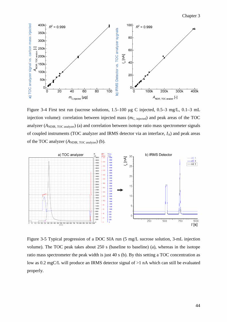
Chapter 3

44

Figure 3-4 First test run (sucrose solutions, 1.5–100 μg C injected, 0.5–3 mg/L, 0.1–3 mL

injection volume): correlation between injected mass (mC, injected) and peak areas of the TOC

analyzer (ANDIR, TOC analyzer) (a) and correlation between isotope ratio mass spectrometer signals

of coupled instruments (TOC analyzer and IRMS detector via an interface, IA) and peak areas

of the TOC analyzer (ANDIR, TOC analyzer) (b).

Figure 3-5 Typical progression of a DOC SIA run (5 mg/L sucrose solution, 3-mL injection

volume). The TOC peak takes about 250 s (baseline to baseline) (a), whereas in the isotope

ratio mass spectrometer the peak width is just 40 s (b). By this setting a TOC concentration as

low as 0.2 mgC/L will produce an IRMS detector signal of >1 nA which can still be evaluated

properly.

Chapter 3

45

3.4.2 Instrument testing/validation with aqueous compound solutions

Carry-over (memory effects)

Carry-over was tested by measuring a sequence of samples with varying stable isotope

composition. We measured each sample in four replicates in order to determine the number of

replicates necessary to obtain reliable δ13C values (SD ≤0.2‰). We chose a concentration of

10 mgC/L to avoid the water blank contribution.

Alternation of the δ-values of two sequential samples was expressed as a difference Δ(An+1 –

An) (Equation 3-10).

Δ(A𝑚𝑚+1 − A𝑚𝑚) = 𝛿𝛿13CA𝑛𝑛+1 − 𝛿𝛿13CA𝑛𝑛 Equation 3-10

A sequence within the test series is indicated by n in An. The δ-value of the first replicate for

each sample was influenced by the stable isotope composition of the previous one. The

magnitude depended on the δ13C difference between the two subsequent samples. A Δ(An+1 –

An) value of, e.g., -61.95‰ led to a bias of 2‰ within the δ13CA value of the first replicate,

while a Δ(An+1 – An) value of 10.90‰ led to a bias of 0.25‰.

Adjusting the rinse settings did not result in an improvement, indicating that the whole

pathway before the four-way valve is rinsed properly including the syringe. The carry-over

volume calculated by a mass balance equation was within a constant range of 34 ± 9 μL. The

precision of the syringe is by far smaller than this volume and could not be the source of such

carry-over. The most probable source of the observed carry-over is the injection cannula

which extends into the combustion tube and therefore cannot be rinsed during the preparation

cycle.

Figure 3-6 shows a linear relationship between the δ13C difference between two subsequent

samples, Δ(An+1 – An) and the bias of the first measured replicate of the second sample.

Together with the determined transferred volume of 34 ± 9 μL this clearly indicates a

systematic error. Unfortunately, correcting the first replicate with a range of ±9 μL would

introduce too large contribution to the combined uncertainty; therefore, this cannot be used

for correction.

Chapter 3

46

Figure 3-6 Correlation between δ13C bias and δ13C difference between two subsequent

samples, with and without consideration of the first replicate (i.e. first injection).

Supplementary Table S 3-1 (Supporting Information) shows the chosen sequence as well as

results achieved in more details.

Exclusion of the first replicate value removes the systematic bias that falsely suggested a poor

precision. Comparison of the precision with and without the first replicates shows a clear

improvement, expressed as the standard uncertainty (1σ), from an average of ±0.38‰ (max.

±1.04‰) to 0.05‰ (max 0.09‰). Even the largest measured difference in the δ13C value

between two subsequent samples shows no significant influence on δ13C values measured in

the second injection of the second sample. The entire set of results achieved within this test

series can be found in Supplementary Table S 3-1 (Supporting Information).

The carry-over cannot be avoided or corrected for. Therefore, the first value needs to be

discarded and considered as a ’dummy’ peak. This was done for all further test series and

evaluations. Kirkels et al.[32] investigated further improvements of the precision by the use of

additional replicates.

Precision

The precision obtained by averaged results of repeated measurements was ≤0.1‰ (ustd: SD ≡

1σ; Supplementary Table S 3-1, Supporting Information). Even with a Δ(An+1 – An) value of

>50‰, ustd is equal to 0.04‰.

We roughly estimated the precision under reproducibility conditions by comparing

measurements between two different instruments, run by different operators in different

Chapter 3

47

laboratories (Institute for Biodiversity and Ecosystem Dynamics (IBED), University of

Amsterdam, Amsterdam, The Netherlands). The reproducibility for the δ13C value of the same

DOC sample (compound solutions of HUM1) was ca 0.5‰. This value includes the precision

of the instrument itself and differences in the sample-preparation, laboratory environment, etc.

Inhomogeneity of the humic acid sample itself can also contribute to this number.

Linearity

The term linearity in SIA indicates that the measured isotope ratio is independent of the

amount of analyte.[26] The isotope ratio mass spectrometer and the hyphenated

instrumentation are two different, potential sources of non-linearity Equation 3-11:

LR ∑ = LR IRMS + LR TOC Equation 3-11

While the isotope ratio mass spectrometer linearity (LR IRMS) influences both the reference gas

and the analyte peak, the TOC linearity (LR TOC) contributes only to the analyte peak. Either it

needs to be demonstrated that the contributions are negligible or corrections are required

(further general principles considered for corrections are given in the Supporting

Information).

To test if there is an LR TOC effect, we measured different compounds (caffeine (CAF2),

acetovanillone (ACF1) and citric acid (CIT2)) in various concentrations (25–160 mgC/L).

Relatively high concentrations were used in order to avoid any influence of the water blanks.

Different compounds were used to check if there are any compound-specific linearity effects.

The isotope ratio mass spectrometer linearity was corrected first using Equation 3-5. Figure

3-7 exemplifies for citric acid that after LR IRMS was corrected for, no additional nonlinearity

effects remained (mlin = 0.00 ‰/nA). This is also the case for all other tested compounds (see

Supporting Information); thus, no compound-specific nonlinearities were observed.

Correcting the systematic drift caused by nonlinearity of the isotope ratio mass spectrometer

improves the ustd from ±0.22‰ to ±0.02‰. After the correction, even in cases where the data

points still show a trend, the contribution of nonlinearity is negligible (max. mlin = 0.001

‰/nA). Since no significant LR TOC effects were observed, no additional linearity corrections

are necessary. Note that if the peak height of the reference gas is adjusted to the peak height

of the analyte LR IRMS does not need to be considered (Equation 3-5).

Chapter 3

48

Figure 3-7 Correlation between δ13C values and isotope ratio mass spectrometer detector

signal (IA) before (measured: brown line and squares) and after (LR IRMS corrected: black line

and triangles) LR IRMS correction of citric acid (CIT2) solution (25–160 mgC/L).

If samples with very different DOC concentrations have to be analyzed, LR IRMS checks must

be made at the beginning and at the end of each sample series in order to enable corrections

for linearity deviations. Each correction will increase the combined uncertainty and needs to

be assessed via error propagation. The assessment of the combined uncertainty is described in

the Normalization and trueness section.

Blank correction

High concentration samples

Plausibility considerations suggest that at higher concentrations (≥10 mgC/L) the contribution

has a low but still considerable influence on the final δ13C value. Without correction a 10

mgC/L solution has a bias of 0.16‰ and a 5 mgC/L solution a bias of 0.31‰, assuming a

difference of 15‰ between the sample and the blank (for details, see Supplementary Table S

3-2, Supporting Information).

Estimation of the blank carbon concentration was conducted via a standard addition method

according to DIN 32 633.[40] The δ13C value of the blank was measured by multiple 3-mL

injections of pure water, incorporating both water and instrumentation as possible blank

sources. As previously shown in the "Sources of the instrumental blank" section, the

instrument contribution to the blank appears to be negligible. Mass balance Equation 3-6 was

used to calculate the water blank.

Chapter 3

49

After blank correction the uncertainty improved very little, indicating that the influence of the

blank is minimal at high analyte (≥10 mgC/L) concentration (considering ustd ≤0.2‰ as good

and ≤0.5‰ as acceptable). It should be noted that, especially at a very negative δ13C value

(CAF, confirmed by EA/IRMS) compared with the δ13CΣbl values, such blank corrections still

matter since a systematic bias was observed. The bias became distinct (Δ >0.2‰) at

concentrations of 10 and 25 mgC/L (Figure 3-8(a)). The magnitude of this bias depends on

the difference between the stable isotope composition of the analyte and that of the blank, and

on the carbon concentrations of both. The improvement of ustd after the correction is on

average 0.06‰ (from 0.09‰ to 0.03‰) with a maximum improvement of 0.14‰.

Figure 3-8 Evaluation inclusive blank correction (a). Correlation between δ13C values and C

concentration of caffeine (CAF2) solution (10–150 mgC/L) with proper (a) and with

simulated incorrect linearity and blank corrections (b). Measured: brown squares, LR IRMS

corrected: black triangles, blank corrected: green dots. In (b) an mlin of 0.006 ‰/nA leads to

better ustd of 0.15‰ after linearity correction and the blank correction seems to be false

because it makes the ustd even worse (0.25 ‰). This demonstrates how the interdependence of

blank and linearity correction can lead to misinterpretation and thus how important its proper

investigation is.

A wrong estimation of the blank, e.g. 10% lower, would change the calculated δ13C-value of a

10 ppm caffeine solution by only 0.06‰. Therefore, a quick estimation of the blank can be

used for high concentration samples, avoiding a laborious accurate determination. Note,

however, that the stability of the blank over time needs to be ensured. Each wrongly estimated

systematic deviation contributes to the combined uncertainty. Even when such uncertainty

stays within an acceptable range, the contribution of several small biases can become

Chapter 3

50

significant when not corrected for. Therefore, it is important also to blank correct the

measurements of samples with higher DOC concentration.

Analyses of samples containing CAF2 showed how important an appropriate correction of

linearity is. It is demonstrated by the comparison of the correlation between the δ13C value

and the C concentration with proper (Figure 3-8(a)) and with simulated incorrect linearity

Figure 3-8(b). The results achieved with other substances can be found in Supplementary

Figure S 3-3 and Figure S 3-4 (Supporting Information). Underestimation of its quantity

would lead to false interpretation of the blank correction. The interaction of the linearity and

the blanks makes a systematic and careful investigation necessary.

Samples with low DOC concentrations

Samples with low carbon content (≤10 mgC/L) differ fundamentally from those with high

DOC concentrations. The impact of isotope ratio mass spectrometer nonlinearity is very low

for such samples but the impact of the blank becomes highly significant (for explanation, see

the Supporting Information). Thus, a proper investigation of the blank is of the utmost

importance for SIA of DOC at low concentrations. At the same time this is also the most

challenging part due to the required sensitivity and high relevance of possible contamination.

Caffeine, benzoic acid, citric acid and acetovanillone solutions (0.1, 0.2, 0.4, 0.6 and 1.2

mgC/L, all concentrations measured with 1, 2, and 3 mL injection volumes) were used as

model compounds to investigate the instrumental performance in the low concentration range.

As expected, for all the compounds an increasingly evident drift towards the blank value was

found with decreasing concentration (Figure 3-9). The blank correction led to an

improvement in the SD of the δ13C values from 0.56‰ to 0.23‰. The poor precision of

±2.18‰ at 0.1 mgC/L indicates an instrumental limitation (avg. IA = 0.31 nA). Still, also at

concentrations above 0.1 mgC/L, outliers were observed. A view on the whole δ13C dataset

revealed an increase in variation with decreased concentration levels in a ’Horwitz trumpet’-

like curve[41,42] (Figure 3-10). A concentration of 1.2 mgC/L showed a good repeatability

(0.12‰), while concentrations of 0.4 and 0.6 mgC/L showed still acceptable repeatability

(0.52 and 0.66‰). A concentration of 0.2 mgC/L showed poor precision (1.48‰).

Chapter 3

51

Figure 3-9 Correlation between δ13C values and C concentration of acetovanillone (ACV1)

solution (0.1–1.2 mgC/L) Measured: brown squares, LR IRMS corrected: black triangles, blank

corrected: green dots. Blank correction corrects the values-drift towards the stable isotope

composition of the blank (10.57‰) with decreasing concentration. SD from δ13C values at all

concentrations improves from 0.56‰ to 0.23‰ after the blank correction. Poor precision of

±2.18‰ (see error bars) at 0.1 mgC/L indicates instrumental limitation (avg. IA = 0.31 nA).

Figure 3-10 Deviation (Δ) of all single δ13C-values from their respective true value (y axis)

plotted against concentration (x axis). The scattering of the values represents the repeatability

of stable isotope measurements at the corresponding concentration with the chosen method.

Chapter 3

52

The following two facts confirm the assumption that the decrease in repeatability with

decreased concentration is not an issue of poor isotope ratio mass spectrometer sensitivity.

First, down to 200 μgC/L the sample peak heights of the isotope ratio mass spectrometer

signals appear within the range where accurate values are generated (≥1 nA). Second, plotting

of NDIR detector peak area (representing DOC concentration) versus progressive

measurements (representing different concentrations, compounds and injection volumes)

showed the same ’trumpet’ progression of the variation in the low concentration range (Figure

3-11(a)) as with the stable isotope composition (Figure 3-10).

Figure 3-11 Carbon concentration values at lower carbon concentration range; (a)

Investigation of the dependence of DOC concentration (y axis, NDIR Area from TOC

analyzer) on its repeatability (x axis, number of measurements). The blank corrected NDIR

areas are normalized to the injection volume of 1 mL and concentration of 1 mgC/L to enable

comparability and they are plotted against measuring order (five replicates of each

concentration: 0.1, 0.2, 0.4, 0.6 and 1.2 mgC/L with 4 different compounds each and using 3,

2 and 1 mL injection). (b) All estimated relative uncertainties (y axis) plotted against the DOC

concentration (x axis). Instrumental caused uncertainty (uinstr = ustd, green triangles),

combined uncertainty implementing sample-preparation caused error (uinstr + sample prep, brown

dots) and combined uncertainty implementing also error caused by data evaluation (uinstr +

sample prep + bl corr, blank squares).

As a consequence, the large scatter of the measured concentrations and of the stable isotope

values at low DOC concentrations can potentially have two main sources: either the TOC

instrument itself or the sample-preparation.

Chapter 3

53

The average of standard deviations of replicate measurements from each vial was 1.2% (RSD)

and this instrumental precision indicates that the TOC instrumentation is not a source of the

observed variations at lower concentrations. In contrast, there is a substantial contribution

from sample-preparation as represented by the scattering of the DOC concentrations measured

between different vials with the same compound in the same concentration (11% RSD). Of

course, any applied correction increases the uncertainty of the measurement following the

principle of error propagation. In the case of low concentration samples, the contribution of

the blank correction to the combined uncertainty is large due to the large ratio between the

water blank and the analyte concentrations.

Our experiments confirmed these expectations, as shown in Table 3-2 and Figure 3-11(b),

which show the series with 3-mL injection (for complete table, see the Supporting

Information). Note that the high relative deviations (Figure 3-11(b)) are still small absolute

ones. The instrumental limitation is about 0.2 mgC/L. The background noise of the instrument

starts to show a significant influence on the measurements below 0.2 mgC/L. The graph

shows clearly the significance of the contribution of the blank correction: the blank

contribution to the uncertainty increases with decreasing sample concentration. At 0.1 mgC/L,

where the blank and the concentration are in the same concentration range, it amounts to

20.8%.

Table 3-2 Different sources of uncertainty and their quantities for different concentrations (4

samples and 3 replicates each); Instrumental caused uncertainty (uinstr = ustd), combined

uncertainty implementing sample-preparation caused error (uinstr + sample prep) and combined

uncertainty implementing also evaluation caused error (uinstr + sample prep + bl corr); Note that the

high relative deviations are still small absolute ones. 0.7% in brackets shows the average

without 0.1 mgC/L sample justifying LOQinstr of 0.2 mgC/L

C concentration[mgC/L]

rel. uinstr

[%]rel. uinstr + sample prep

[%]rel. uinstr + sample prep + bl corr

[%]

0,1 11,5 20,9 41,7

0,2 1,0 14,2 24,1

0,4 0,7 10,1 13,9

0,6 0,8 7,4 9,2

1,2 0,3 4,3 4,9

avg (0.7) 2.9 11,4 18,8

Chapter 3

54

The instrumental precision and sensitivity allow δ13C values to be measured accurately (with

ustd <0.2‰) down to a DOC concentration of 0.2 mgC/L. Minor contaminations and small

absolute variations of the water blank have a large relative impact and magnify the

uncertainty of the results in samples with low concentrations. Therefore, sample-preparation

further limits the performance of the method in the low concentration range and appropriate

handling of the samples and vials becomes crucial to significantly decreasing the uncertainty.

The experimentally determined combined uncertainty results in a LOQSIA method of ca 0.5

mgC/L, considering an accuracy of ±0.5‰ as acceptable and of 0.2 mgC/L for LOQSIA instr.

The entire set of results is summarized in Supplementary Table S 3-3 (Supporting

Information) together with further details regarding the results of the DOC SIA of samples

with low DOC concentrations.

Normalization and trueness

After blank correction the δ13CΣbl corr A values were related to the in-house reference gas.

Trueness quantifies the closeness of the agreement between the average value obtained from a

series of test results and an accepted reference value.[36] To prove trueness, the measured

values first have to be traced back to the VPDB scale. Therefore, to prove metrological

traceability[34] and investigate trueness, all the blank corrected values were two-point

normalized as described above.

No aqueous DOC reference materials exist for SIA. Therefore, solid reference substances

were dissolved in ultrapure water to obtain a solution with defined carbon concentrations and

δ13C values. Enriched glutamic acid GLU1 with δ13CA,VPDB 37.626 ± 0.049 and caffeine

CAF1 with δ13CA,VPDB –27.771 ± 0.043 were dissolved in pure water (10 mgC/L). This large

Δ value was chosen on purpose to test if the normalization works within a large stable isotope

composition range. The obtained stretching factors mnorm and bnorm were used to normalize all

the measured δ13CΣbl corr A,RG values to δ13CA,VPDB values.

A third reference material sucrose SUC1 with a δ13CA,VPDB value of –10.449 ± 0.033 was

analyzed to test the trueness. The closeness of the agreement between the internationally

accepted value and the obtained value of –10.40 ± 0.07‰, expressed as Δtrueness = δ13Caccepted

A,VPDB – δ13Cobtained A,VPDB, of 0.05‰ indicated good trueness.

Due to the lack of certified reference material, three additional internal laboratory standards

were used. Their traceability was ensured by referencing of the EA/IRMS δ13CA values to the

reference materials and thus indirectly to the VPDB scale.[26] The obtained values were

considered as true values for the investigation of trueness as Δtrueness.

Chapter 3

55

The obtained Δtrueness value (Table 3-3) was good (≤0.2‰). Only one value deviated more

from the accepted value, but it was still within an acceptable range of ≤0.5‰. The coefficient

of determination of the linear regression between the measured and true δ13C values (r2 =

0.994) also indicates good agreement.

Table 3-3 Trueness of the method expressed as difference between the true and measured

value

Uncertainty and accuracy

Accuracy is described as "the closeness of the agreement between the result of a measurement

and the true value of the measurand".[43] Accuracy is best assessed by the combined

uncertainty estimated by error propagation.[26] The typical standard uncertainty (expressed as

standard deviation) was ≤0.2‰ within the investigated concentration ranges. It represents

mainly the instrumental precision. The combined standard uncertainty comprises several

uncertainties and it increased to a value of up to 1.2‰. That uncertainty represents the

accuracy of the complete method, from sample-preparation to the final measurement. It

incorporates the poor accuracy of low concentration samples due to the water blank.

Furthermore, the measurement of the water blank affects the uncertainty of the standard

solution values and, through the normalization procedure, the uncertainty of the sample

values. The very good precision achieved for replicated blank measurements from the same

vial (avg. SD: 0.25‰) and the relatively poor precision for blanks measured from different

vials (avg. SD: 1.31‰) with the same ultrapure water indicated vial cleanliness being the

main contribution to the blank uncertainty. Pretreatment of the vials at 400 °C, after previous

chemical cleaning with highly concentrated oxidizing acid, may improve accuracy in

measuring low concentration samples.[44]

Oxidation efficiency and matrix effects

No component other than the analyte (matrix) should contribute to the result. Identification

and assessment of typical matrix components were performed before testing the selectivity of

Compoundtrue

δ 13C[‰]

measured

δ 13C[‰]

Δ meas-true

δ 13C[‰]

Sucrose (NIST 8542) -10,47 -10.4 ± 0.09 0.07

Citric acid (working std.) -16.00 -16.32 ± 0.05 0.32

Casein (working std.) -22.40 -22.55 ± 0.02 0.15

Glutamic acid (working std.) -26.77 -26.64 ± 0.05 0.13

Chapter 3

56

the method on the basis of model solutions (Table 3-4). DOC SIA is a bulk method and the

composition of the samples is unknown. Thus, it is not possible to correct for compound-

specific fractionation as a result of incomplete oxidation, and complete oxidation is therefore

essential.

Barbituric acid, melamine and humic acid were analyzed as model compounds that are

resistant to oxidation, and thus potentially affecting DOC and SI analyses.[23,45] We found a

recovery rate of ≥99%, proving complete oxidation. This indicated the compound

independence of the method. The precision with an average δ13C SD of 0.13‰, and trueness

with an average Δδ13C of 0.23‰, confirmed this conclusion. Kirkels et al.[32] showed similar

values using natural DOC samples from terrestrial and aquatic environments.

High salt loads are another important challenge for the SIA of DOC.[10] The HTC method has

to be used for samples with high salinity, such as seawater, as discussed in the introduction.

We dissolved humic acid in a simplified model solution of 3.5% NaCl to investigate the

influence of high salt load, e.g. possible adsorption or catalyst poisoning effects. High

concentrations of the analyte (50 mg/L) were used to avoid problems related to low

concentration (cf. the section, "Samples with low DOC concentrations"). We did not observe

significant effects of salt, as indicated by an average δ13C SD of 0.04‰ and trueness with an

average Δδ13C of 0.02‰.

The analysis of additional seawater samples (98 injections; 3 mL each; 14 samples) showed

an average δ13C SD of 0.07‰. The standards showed an average δ13C SD of 0.02‰ and an

average Δδ13C of 0.03‰measured after 230 injections (90 river water, 40 ultrapure water, 40

standard solutions and 60 seawater).

In our validation, complete removal of the total inorganic carbon (TIC) appeared essential and

thus efficient acidification and purging are crucial for accurate DOC measurements.

Therefore, we had to increase the purging time for seawater. An additional 40 min resulted in

a significant decrease in the systematic error from Δδ13C 1.18‰ to Δδ13C 0.08‰.

The conducted tests clearly indicated a general suitability of the developed system for DOC

SIA of samples with a higher salt load. The preliminary tests that we carried out should be

followed up by an intensive study with real seawater samples or brine solutions characterized

by low carbon concentration.

Further issues related to matrix effects are discussed in the Supporting Information.

Chapter 3

57

Table 3-4 Classification of potential problems and interferences related to DOC measurements in aqueous samples

MatrixInterferences/ possible sources of

isotopic discrimination (pID) Problematic stage typical issue?Handling within

developed system

water CO2 solubility inwater (pID)

gas/liquid separationwithin the instrument

no (considered as lowconc. blank issue)

Higher temperature of the water within the condenser(solubility decrease)

Non-carbon containingsalt load

pID due to not complete mineralization

Reaction tube (Mineralisation): HTC: catalyst poisoning; glas affect; WCO: radical scavenging

yes[10] HTC instead of WCOreactor; Salt trapping(ash finger)

particulate organic carbon non-analyte carbon: withinthe instrument notdistinguishable

sample preparation no separation via filtering(offline step)

total inorganic carbon non-analyte carbon: withinthe instrument notdistinguishable

sample preparation/ autosampler critical stage: typicalerror source if countermeasures insufficient

acidification and purgingout in autosampler

volatile organic carbon non-analyte carbon: withinthe instrument notdistinguishable

sample preparation/ autosampler no outgasing while samplingand sample preparation(refilling etc.) and purgingout in autosampler

attraction between atomswithin the molecule(strength of the bond)

pID due to incompletemineralization of persistent compounds

Reaction tube (mineralisation) yes[10] HTC instead of WCO reactor; Optimized conditions:Temp., catalyst and flowconditions (contact tims)

WCO: wet chemical oxidation; HTC: high temperature combustion;aDOC measurements should not be influenced by the persistence of compounds or if they are present in colloidal form or truly dissolved.

Matrix components without TC

Matrix molecular entities within TC

Molecular form of DOCa

Chapter 3

58

3.5 Conclusions and outlook A novel HTC-based TOC/IRMS system was developed and inter alia the standard uncertainty

of ≤0.2‰and the LOQSIA instr of 0.2 mgC/L confirm its suitability for accurate DOC SIA. The

oxidation efficiency of the system is ≥99% and therefore an isotope fractionation related to

limited oxidation of more resistant compounds is prevented. Compared with other methods

our new approach improved the accuracy, especially at low DOC concentrations and in the

presence of high salt loads, as well as for compounds that are resistant to oxidation. To the

best of our knowledge, this novel system is the only HTC-based system which allows a 3-mL

injection compared with a typical injection volume of <200 μL.[17,39,46] This improvement

alone resulted in an increase in sensitivity by a factor of 15. With the developed system no

laborious sample-preparation steps are necessary, such as time-consuming offline

preconcentration steps (e.g. freeze-drying). This significantly reduces the possible sources of

contamination.

This system also opens the possibility of a larger use of certified or internationally accepted

reference materials (solution of low concentration with blank correction) to assure traceability

and comparability among different laboratories. For the same reasons we proposed a method

for data treatment but an internationally agreed method of validation still needs to be defined.

In summary, the described system offers a new and promising approach for the use of DOC

SIA for routine analysis, also for the analysis of samples in difficult matrices without offline

sample-preparation. The system was intensively optimized and validated with a broad set of

real samples within the work by Kirkels et al.[32]

Additional supporting information may be found in section Supporting information.

Chapter 3

59

3.6 References [1] J. I. Hedges, in Biogeochemistry of Marine Dissolved Organic Matter, (Eds: D. A.

Hansell, C. A. Carlson). Academic Press, London, 2002. pp. 1–33.

[2] B. J. Eadie, L. M. Jeffrey, W. M. Sackett. Some observations on the stable carbon isotope

composition of dissolved and particulate organic carbon in the marine environment. Geochim.

Cosmochim. Acta 1978, 42, 1265.

[3] R. Kindler, J. Siemens, K. Kaiser, D. C. Walmsley, C. Bernhofer, N. Buchmann, P.

Cellier, W. Eugster, G. Gleixner, T. Grünwald, A. Heim, A. Ibrom, S. K. Jones, M. Jones, K.

Klumpp,W. Kutsch, K. S. Larsen, S. Lehunger, B. Loubet, R. Mckenzie, E. Moors, B.

Osborne, K. Pilegaard, C. Rebmann, M. Saunder, M. W. I. Schmidt, M Schrumpf, J.

Seyfferth, U. Skiba, J. -F. Soussana, M. A. Sutton, C. Tefs, B. Vowinckel, M. J. Zeeman, M.

Kaupenjohann. Dissolved carbon leaching from soil is a crucial component of the net

ecosystem carbon balance. Global Change Biol. 2011, 17, 1167.

[4] K. Kalbitz, S. Solinger, J.-H. Park, B. Michalzik, E. Matzner. Controls on the dynamics of

dissolved organic matter in soils: a review. Soil Sci. 2000, 165, 277.

[5] K. Mopper, E. T. Degens, in Scope 13 – The Global Carbon Cycle, (Eds: B. Bolin, E. T.

Degens, S. Kempe, P. Ketner). Scientific Committee on Problems of The Environment, Paris,

1979, pp. 293–316.

[6] D. A. Hansell, C. A. Carlson. Marine dissolved organic matter and the carbon cycle.

Oceanography 2001, 14, 41.

[7] R. A. Houghton. Balancing the Global Carbon Budget. Annu. Rev. Earth Planet. Sci.

2007, 35, 313.

[8] P. M. Williams. Stable carbon isotopes in the dissolved organic matter of the sea. Nature

1968, 219, 152.

[9] D. A. Nimick, C. H. Gammons, S. R. Parker. Diel biogeochemical processes and their

effect on the aqueous chemistry of streams: A review. Chem. Geol. 2011, 283, 3.

[10] K.Mopper, J.Qian, in Encyclopedia of Analytical Chemistry, (Ed.: R. A. Meyers).

JohnWiley, Chichester, 2000. pp. 3532–3540.

[11] ISO 8245:1999. Water quality – guidelines for the determination of total organic carbon

(TOC) and dissolved organic carbon (DOC).

Chapter 3

60

[12] ASTM D7573-09. Test Method for Total Carbon and Organic Carbon in Water by High

Temperature Catalytic Combustion and Infrared Detection.

[13] B. Fry, S. Saupe, M. Hullar, B. J. Peterson. Platinumcatalyzed combustion of DOC in

sealed tubes for stable isotopic analysis. Mar. Chem. 1993, 41, 187.







[16] S. Bouillon, M. Korntheuer, W. Baeyens, F. Dehairs. A new automated setup for stable

isotope analysis of dissolved organic carbon. Limnol. Oceanogr.: Methods 2006, 4, 216.

[17] I. De Troyer, S. Bouillon, S. Barker, C. Perry, K. Coorevits, R. Merckx. Stable isotope

analysis of dissolved organic carbon in soil solutions using a catalytic combustion total

organic carbon analyzer-isotope ratio mass spectrometer with a cryofocusing interface. Rapid




Mar. Chem. 2007, 103, 318.

[19] P. Albéric. Liquid chromatography/ mass spectrometry stable isotope analysis of

dissolved organic carbon in stream and soil waters. Rapid Commun. Mass Spectrom. 2011,

25, 3012.

[20] A. Hartland, A. Baker, W. Timms, Y. Shutova, D. Yu. Measuring dissolved organic

carbon δ13C in freshwaters using total organic carbon cavity ring-down spectroscopy (TOC-

CRDS). Environ. Chem. Lett. 2012, 10, 309.

[21] B. Fry, E. T. Peltzer, C. S. Hopkinson Jr, A. Nolin, L. Redmond. Analysis of marine

DOC using a dry combustion method. Mar. Chem. 1996, 54, 191.

[22] G. R. Aiken. Chloride interference in the analysis of dissolved organic carbon by the wet

oxidation method. Environ. Sci. Technol. 1992, 26, 2435.

Chapter 3

61

[23] P. J. Wangersky. Dissolved organic carbon methods: a critical review. Mar. Chem. 1993,

41, 61.

[24] R. van Geldern, M. P. Verma, M. C. Carvalho, F. Grassa, A. Delgado-Huertas, G.

Monvoisin, J. A. C. Barth. Stable carbon isotope analysis of dissolved inorganic carbon (DIC)

and dissolved organic carbon (DOC) in natural waters – Results from a worldwide

proficiency test: Carbon stable isotope proficiency test of DIC and DOC. Rapid Commun.


[25] G. Schwedt. Taschenatlas der Analytik. Wiley-VCH, Weinheim, 2007.





[28] AOAC 984.23-1988. Corn syrup and cane sugar in maple syrup. Carbon ratio mass

spectrometric method.

[29] OIV AS312-07 2010. Method for the determination of the 13C/12C isotope ratio of

glycerol in wines by gas chromatography combustion or high performance liquid

chromatography coupled to isotope ratio mass spectrometry (GC-C-IRMS or HPLC-IRMS).

[30] OIV AS314-03 2005. Determination of the carbon isotope ratio 13C/12C of CO2 in

sparkling wines – method using isotope ratio mass spectrometry (IRMS).

[31] EEC/822/97. Determination of the isotopic ratio of oxygen of the water content in wines.

[32] F. M. S. A. Kirkels, C. Cerli, E. Federherr, J. Gao, K. Kalbitz. A novel high-temperature

combustion based system for stable isotope analysis of dissolved organic carbon in aqueous

samples. II: optimization and assessment of analytical performance. Rapid Commun. Mass

Spectrom. 2014, 28, 2574.

[33] DIN EN ISO/IEC 17025:2005. General requirements for the competence of testing and

calibration laboratories.

[34] P. De Bièvre, R. Dybkær, A. Fajgelj, D. B. Hibbert. Metrological traceability of

measurement results in chemistry: concepts and implementation. Pure Appl. Chem. 2011, 83,

1873.

Chapter 3

62

[35] M. Thompson, S. L. Ellison, R. Wood. Harmonized guidelines for single-laboratory

validation of methods of analysis (IUPAC Technical Report). Pure Appl. Chem. 2002, 74,

835.

[36] M. Thompson, R. Wood. Harmonized guidelines for internal quality control in analytical

chemistry laboratories. Nature 1995, 4, 4.

[37] A. Menditto, M. Patriarca, B. Magnusson. Understanding the meaning of accuracy,

trueness and precision. Accredit. Qual. Assur. 2006, 12, 45.

[38] CAC/GL 59–2006: Guidelines on estimation of uncertainty of results.

[39] R. J. Panetta, M. Ibrahim, Y. Gélinas. Coupling a hightemperature catalytic oxidation

total organic carbon analyzer to an isotope ratio mass spectrometer to measure natural-

abundance δ13C dissolved organic carbon in marine and freshwater samples. Anal. Chem.

2008, 80, 5232.

[40] DIN 32633:2013. Chemical analysis – methods of standard addition.

[41] M. Thompson. The amazing Horwitz function. AMC Technical Brief. 2004, No. 17.

42] P. Hall, B. Selinger. A statistical justification to relating interlaboratory coefficients of

variation with concentration levels. Anal. Chem. 1989, 61, 1465.

[43] IUPAC Gold Book. Accuracy of measurement. http://goldbook.iupac.org/A00060.html.

[44] R. Otson, D. T. Williams, P. D. Bothwell, R. S. McCullough, R. A. Tate. Effects of

sampling, shipping, and storage on total organic carbon levels in water samples. Bull.

Environ. Contam. Toxicol. 1979, 23, 311.

[45] L. Zhang, D. M. Kujawinski, M. A. Jochmann, T. C. Schmidt. High-temperature

reversed-phase liquid chromatography coupled to isotope ratio mass spectrometry. Rapid





Chapter 3

63

3.7 Supporting information

Supporting information for section Carry-over (memory effects)

Testing protocol: 1 mL injection, 300 µL/s injection speed; 10 mgC/L; four replicates;

Table S 3-1 Sequence, single values of replicates and calculated parameters from the test

series to investigate carry over.

Supporting information for section Linearity

General considerations/ principles to handle non-linearity issue: After LR IRMS was corrected

only LR TOC remains to be quantified. LR TOC can be used for corrections only if the used

system has no additional compound-specific fractionation due to, e.g. incomplete

mineralization because the exact composition of DOC in real samples is unknown. If LR TOC

correction is necessary (system dependent), it has to be applied after the blank correction.

An replicatei

GLU1 4 35,38

1 -25,002 -27,123 -27,104 -27,04

1 -11,302 -10,553 -10,684 -10,72

1 -25,352 -26,003 -25,984 -26,06

1 -16,522 -16,213 -16,304 -16,24

1 -22,032 -22,163 -22,164 -22,13

-26,57±1,04

-10,81±0,33

-25.85±0.33

-16.32±0.14

-22.12±0.06

-27.09±0.04

-10.65±0.09

-26.01±0.04

-16.25±0.05

-22.15±0.02

-61,95

16,44

-15,36

9,76

-5,9

35

41

45

28

21

CAF1

SUC1

GLU2

CIT1

CAS1

sequence δ 13Cmeas

[‰] Vcarry-over

[µl]Δ (An +1-An )

[‰]

with 1th replicateδ 13Cmeas±ustd

[‰]

without 1th replicateδ 13Cmeas±ustd

[‰]

Chapter 3

64

Figure S 3-1 LR IRMS correction using acetovanillone solution (25-160 mgC/L)

Figure S 3-2 LR IRMS correction using caffeine solution (25-160 mgC/L)

Supporting information for section Blank correction

Chapter 3

65

Table S 3-2 Plausibility considerations a: Correction starts to matter (exceeding bias of 0.2

‰); considering worst case: high blank and large delta difference: aqueous solution; b: Bias

falsely considering no instrumental blank (exceeding bias of 0.5‰): real sample

Supporting information for section High concentration samples (Blank correction)

bias

δ 13C [‰]

δ 13C [‰]

m[µg]

δ 13C [‰]

m[µg]

δ 13C [‰]

V[mL]

ρ[µgC/mL]

δ 13C [‰]

m[µg]

δ 13C [‰]

V[mL]

ρ[µgC/mL]

0,03 -10,03 150,30 -26,00 0,30 -26 3,00 0,00 -26 0,30 -10 3,00 500,06 -10,06 75,30 -26,00 0,30 -26 3,00 0,01 -26 0,27 -10 3,00 250,16 -10,16 30,30 -26,00 0,30 -26 3,00 0,02 -26 0,24 -10 3,00 100,31 -10,31 15,30 -26,00 0,30 -26 3,00 0,04 -26 0,18 -10 3,00 51,45 -11,45 3,30 -26,00 0,30 -26 3,00 0,06 -26 0,12 -10 3,00 12,67 -12,67 1,80 -26,00 0,30 -26 3,00 0,08 -26 0,06 -10 3,00 0,58,00 -18,00 0,60 -26,00 0,30 -26 3,00 0,10 -26 0,00 -10 3,00 0,1

-0,16 -10,16 15,15 -26,00 0,15 -26 3,00 0,15 -26 -0,30 -10 3,00 5-0,11 -10,11 15,10 -26,00 0,10 -26 3,00 0,10 -26 0,00 -10 3,00 5-0,08 -10,08 15,08 -26,00 0,08 -26 3,00 0,08 -26 0,00 -10 3,00 5-0,05 -10,05 15,05 -26,00 0,05 -26 3,00 0,05 -26 0,00 -10 3,00 5

-0,10 -10,10 15,08 -30,00 0,08 -26 3,00 0,08 -26 -0,17 -10 3,00 5-0,07 -10,07 15,08 -25,00 0,08 -26 3,00 0,08 -26 0,00 -10 3,00 5-0,05 -10,05 15,08 -20,00 0,08 -26 3,00 0,08 -26 0,00 -10 3,00 5-0,02 -10,02 15,08 -15,00 0,08 -26 3,00 0,08 -26 0,00 -10 3,00 5

bias

δ 13C [‰]

δ 13C [‰]

m[µg]

δ 13C [‰]

m[µg]

δ 13C [‰]

V[mL]

ρ[µgC/mL]

δ 13C [‰]

m[µg]

δ 13C [‰]

V[mL]

ρ[µgC/mL]

0,62 -10,62 3,12 -26,00 0,30 -26 3,00 0,060 -26 0,120 -10 3,00 10,31 -10,31 3,06 -26,00 0,30 -26 3,00 0,080 -26 0,060 -10 3,00 10,16 -10,16 3,03 -26,00 0,30 -26 3,00 0,090 -26 0,030 -10 3,00 10,00 -10,00 3,00 -26,00 0,30 -26 3,00 0,100 -26 0,000 -10 3,00 1

a

b

measured Σblank water blank instr. Blank sample

measured Σblank water blank instr. Blank sample

Chapter 3

66

Figure S 3-3 Blank correction using acetovanillone solution (10-150 mgC/L)

Figure S 3-4 Blank correction using citric acid solution (10-150 mgC/L)

Supporting information for section Samples with low DOC concentrations (Blank

correction)

Chapter 3

67

Table S 3-3 Different sources of uncertainty and their quantities for different concentrations

(4 samples; 3 replicates each) and different injection volumes; Instrumental caused

uncertainty (uinstr = ustd), combined uncertainty implementing sample-preparation caused error

(uinstr + sample prep) and combined uncertainty implementing also evaluation caused error (uinstr +

sample prep + bl corr); Note that the high relative deviations are still small absolute ones. 0.7% in

brackets shows the average without 0.1 mgC/L sample justifying LOQinstr of 0.2 mgC/L

C concentration[mgC/L]

rel. uinstr

[%]rel. uinstr + sample prep

[%]rel. uinstr + sample prep + bl corr

[%]

0,1 11,5 20,9 41,70,2 1,0 14,2 24,10,4 0,7 10,1 13,90,6 0,8 7,4 9,21,2 0,3 4,3 4,9avg (0.7) 2.9 11,4 18,8

0,1 3,1% 25,7% 68,8%

0,2 0,8% 16,2% 28,2%

0,4 1,8% 13,4% 18,0%

0,6 0,3% 3,7% 4,7%

1,2 0,4% 3,8% 4,3%

avg 1,3% 12,6% 24,8%

0,1 2,5% 27,3% 72,7%

0,2 1,4% 12,8% 21,6%

0,4 0,9% 9,9% 13,5%

0,6 0,9% 2,3% 3,0%

1,2 0,7% 3,7% 4,2%

avg 1,3% 11,2% 23,0%

3 ml injection

2 ml injection

1 ml injection

Chapter 3

68

Figure S 3-5 The graph shows an additional indication for absence of considerable

instrumental blank coming from e.g. washing out effect within the combustion tube. The

amount of carbon, represented by the peak-area of NDIR, of the blank is independent of the

amount or contact time (injection speed) of the water vapor. Varying injection volume and

speed a constant NDIR peak area of 1129 ± 22 units per mL blank sample was found.

Figure S 3-6 Simplified visualization of uncertainty evolution; Instrument shows significant

contribution below 0.2 mgC/L (observed ustd at 0.1 mgC/L > 2%); above 0.2 mgC/L a sample-

preparation increases the uncertainty substantially and became a limiting factor (variations

form vial to vial of the same sample); Generally to expect is even larger contribution to

combined uncertainty coming from sampling itself.

Chapter 3

69

The impact of IRMS non-linearity issue becomes very low: Sample with double concentration

shows still a small absolute difference. Two times more concentrated sample (e.g. 0.8 mgC/L

related to 0.4 mgC/L) shows still only 0.4 mgC/L absolute difference. With 1 mL injection the

0.4 μg difference correlates to ca. 0.4 nA signal. Taken typical IRMS non-linearity’s in to

account the error introduced without IRMS linearity correction will equal in ca. 0.008‰ bias.

On the other side the impact of blank with a small absolute value of e.g. 0.1 mgC/L becomes

significant due to its addition to the sample. The small absolute difference (e.g. 0.1 mgC/L to

0.2 mgC/L sample) results in huge relative impact of ≈ 33%. Proper blank investigation

becomes highly significant for DOC SIA for low concentration samples. Due to the needed

sensitivity and high impact of possible contamination it becomes the most challenging part.

General consideration: note that the blank evaluation with aqueous solutions can differ

strongly from real sample: Contribution for aqueous solutions of compounds can consist of

both, water and instrumental blank, but for real samples it consists only of instrumental blank.

For the determination of stable isotope composition of aqueous solutions these two

contributions can be considered as one total blank using the same water and constant

measurements conditions for the standards as well as samples within the run. Blank

investigation and correction of aqueous solutions are also necessary for real sample

measurements, because there are no liquid certified referencing materials available.

Determination of stable isotope composition of real samples with only instrumental blank

contribution needs discriminability between those two sources – its quantification - or

negligibility prove of one of them. This is challenging due to the need of blank free water.

Testing protocol: Standard addition calibration method: 4 Standards for spiking + blank x 5

concentrations x 3 replicates each. Four compounds solutions were taken to investigate the

instrumental performance in low concentration range: caffeine, benzoic acid, citric acid and

acetovanillone with concentrations from 0.1 to 1.2 mgC/L and injection volumes of 1, 2 and 3

mL. The water blank concentration was estimated using standard addition calibration method

(72 single measurements) and δ-value averaging 25 single water blanks results. Blank values

of 143 ± 26 μgC/L and 10.57 ± 3.21‰ were achieved. Those values were utilized for blank

correction of stable isotope composition of the samples.

Notes: Random variation caused errors can be narrowed through larger amount of replicates.

This can be utilized for estimation of the blank δ-value. Since it was shown that right

estimation is essential regular blank value monitoring can be recommended.

Supporting information for section Oxidation efficiency and matrix effects

Chapter 3

70

Selectivity is per definition the ability of a method to determine accurately and specifically

the analyte of interest in the presence of other components in a sample matrix under the stated

conditions of the test.

Persistent compounds: Model substances were secondary standards; true value was

determined by EA/IRMS as accepted procedure.

TIC: Acidification was done by HCl pa grade, because previous experiments have shown that

ultra-high grade HCl contains a higher TOC background, most likely caused by the bottle

material (plastics instead of glass). The sparging time for TIC removal is defined by the

analysis of first replicate (ca. 15 min), which serves as “dummy” as described later on, but

can be extended for higher TIC concentrations (>20mgC/L) combined with higher salt load.

In this work systematic preinvestigations of possible non-selectivity sources of real samples

were conducted, with focus on instrumental/methodical limitations. Note that those

indications do not replace investigation with real matrices using e.g. spiking methods/ internal

standards and evaluating the recovery rates in case of concentration measurements or trueness

of the, via mass balance equation calculated, δ-values of the spiking material in case of SIA.

Chapter 4

71

Chapter 4 Uncertainty estimation and application of stable isotope

analysis in dissolved carbon

Chapter 4

72

4.1 Abstract Rationale: The results obtained with the newly developed high-temperature combustion total

organic carbon analyzer, interfaced with continuous flow isotope ratio mass spectrometry

(HTC TOC/IRMS) system confirmed the general suitability of the system for δ13C

determination directly in aqueous solutions (Chapter 3), but proper assessment of analytical

performance with real samples was still needed.

Methods: The analytical performance for determination of bulk dissolved organic carbon

(DOC) δ13C signatures was evaluated with realistic and challenging conditions, utilizing real

sample measurements and round robin test participation. As part of the validation, an

appropriate method to evaluate combined uncertainty of DOC stable isotope analysis (SIA)

results was introduced. The total inorganic carbon (TIC) mode of the system was tested for

δ13C determination in TIC.

Results: Validation of the system with a broad range of real samples such as soil extracts and

river and seawater samples was performed, and included proof of reproducibility of the

developed method via participation in a round robin test. Good precision (standard deviation

(SD) predominantly ≤0.15‰) and accuracy (coefficient of determination (R2) 1.000 ± 0.001)

were achieved for the DOC δ13C analysis of a broad range of DOC solutions. Good

reproducibility (predominantly ≤0.5‰) was shown in the context of international round robin

testing for river and seawater samples. Furthermore, the general suitability of the system for

the determination of total inorganic carbon (TIC) stable isotope analysis was tested. Precision

of SD ≤0.2‰ was achieved for SIA of TIC, but further validation tests are required.

Conclusions: The novel HTC TOC/IRMS system enables reliable and rapid determination of

δ13C values in DOC, without laborious offline sample-preparation steps. Further

investigations should focus on SIA of TIC. Thus, HTC TOC/IRMS may open new

opportunities in DOC and potentially TIC research in aquatic and terrestrial environments.

Chapter 4

73

4.2 Introduction Bulk carbon concentration and δ13C determination in aqueous samples is essential for carbon

cycle investigation in aquatic and terrestrial systems and plays a key role in biogeochemical

processes and ecosystem functioning. [1–4] Studies highlight the benefits of SIA to locate input

sources and to understand, e.g., DOC cycling and involved transport and transformation

processes.[5,6]

C3 and C4 vegetation have different photosynthetic pathways and have therefore naturally

distinct isotope signatures. In soil science DOC SIA can be used to investigate the relative

contribution of C3 and C4 vegetation to DOC percolating in soils.[7] In aquatic ecosystems,

different source-specific δ13C signatures can be used for food web studies.[8] Spatial and

temporal variability in DOC stable isotope composition in freshwater systems and marine

sites reflect changed dynamics and/or inputs.[7]

Carbonates were shown to play a main role in surface water carbon cycles.[9] Stable isotope

composition in dissolved inorganic carbon can be used to investigate dissolution of

sedimentary carbonates.[10] The general suitability of the introduced system for TIC SIA was

therefore tested in this work.

Considering findings presented in Chapter 3 the system should be applicable in limnology,

oceanography and soil science. However, further experimental proof of the suitability is

needed. Additionally a proper evaluation of uncertainties is important to justify the data

gained by DOC SIA. Participation in a round robin test, including fresh water and seawater

samples and measuring soil science extracts was chosen for real sample application

validation.

Chapter 4

74

4.3 Experimental


Reference materials IAEA-600 caffeine CAF1 (δ13CVPDB –27.771 ± 0.043‰) and IAEA-CH-6

sucrose SUC1 (δ13CVPDB –10.449 ± 0.033‰) were purchased from the International Atomic

Energy Agency (Vienna, Austria). The round robin test nine fresh water (fw i – fw ix), six sea

water (sw i – sw vi) and one deep ocean water (dow) samples were delivered by Concordia

University (Montreal, Canada). LiCO3 was provided by University of Duisburg-Essen (Essen,

Germany). Ultrapure, deionized water (UP water) produced by a Purelab Ultra system (MK2-

Analytic, ELGA, High Wycombe, UK) was used for solution preparation. Helium 5.0 and

oxygen 4.8 were purchased from Air Liquid (Oberhausen, Germany).


The HTC TOC/IRMS system consists of three parts: iso TOC cube analyzer, iso TOC LCM

focusing unit (Elementar Analysensysteme, Hanau, Germany) and IsoPrime100 isotope ratio

mass spectrometer (Isoprime, Manchester, UK) (see Figure 3-1). Samples, filled in 40-mL

borosilicate glass vials, are introduced using a 32-position autosampler into the combustion

system by means of a 5-mL syringe and a multiway valve. The combustion is performed at

850 °C and is supported by a catalyst (Pt on ceramic carrier material). Water is removed in

three steps: an air-cooled condenser, a counter-flow membrane dryer and a chemical dryer.

Hydrogen halides and halogens are removed by silver wool. After the purification steps the

carrier gas oxygen enters the nondispersive infrared (NDIR) detector for quantification of the

evolved CO2. The focusing unit separates the CO2 from O2 allowing for focusing. An

IsoPrime100 (Isoprime Ltd, Manchester, UK) isotope ratio mass spectrometer was used to

determine the stable isotope composition.


Nomenclature


notation’ is used. The δ13CVPDB-value of an analyte (A) is described by Equation 4-1 as a

relative difference between the isotope ratio (R) of an analyte (R(13C/12C)A) and the isotope

ratio defining an international reference scale, for carbon Vienna Pee Dee Belemnite

(R(13C/12C)VPDB):[11]

𝛿𝛿13CA,VPDB = 𝑅𝑅� C13 C12� �

A− 𝑅𝑅� C13 C12� �

VPDB

𝑅𝑅� C13 C12� �VPDB

Equation 4-1

Chapter 4

75


reported δ-values are related to the used, in-house reference gas (RG). That concerns all data

before the final normalization to the VPDB scale.



Evaluation

Non-linearity correction

The isotope ratio linearity of the isotope ratio mass spectrometer (LR IRMS) was quantified as

the slope mlin of a linear regression describing the δ-value as a function of corresponding ion

current I.

𝑚𝑚lin =∑ �𝐼𝐼RG𝑘𝑘 − 𝐼𝐼RG�� 𝛿𝛿13CRG,RG��𝑘𝑘

− 𝛿𝛿13CRG,RG��𝑚𝑚

𝑘𝑘=1

∑ �𝐼𝐼RG𝑘𝑘 − 𝐼𝐼RG��2𝑚𝑚

𝑘𝑘=1

Equation 4-3

𝛿𝛿13CRG,RG��𝑘𝑘=𝑅𝑅� C13 C12� �

RG𝑘𝑘− 𝑅𝑅� C13 C12� �

RG��

𝑅𝑅� C13 C12� �RG��

Equation 4-4

LR IRMS was monitored regularly, before and after each test series. All measured δ13C raw data

(δ13Cmeas A) generated by the software IonVantage (Isoprime Ltd), and automatically corrected

for 17O-abundance and related to RG, were then linearity corrected to δ13Clin corr A as described

by Brand[12] and expressed as shown in Equation 4-5:

𝛿𝛿13Clin corr A = 𝛿𝛿13Cmeas A −𝑚𝑚lin × (𝐼𝐼A − 𝐼𝐼RG) Equation 4-5

with IA as the ion current at the maximum of the peak for analyte A and IRG the ion current of

the reference gas peak pulse.

Blank corrections

An isotope mass balance (IMB) equation[11] was utilized for corrections. The amount of

carbon is represented by the uncorrected area A from the integrated NDIR CO2 peak of the

TOC analyzer. The solution of the IMB equation for blank-’subtracted’ δ-value δ13Cbl corr A

results in Equation 4-6. For determination of the concentration as well as the δ-value of the

blank, acidified water used for standards solution preparation (blanks) was used:

Chapter 4

76

𝛿𝛿13Cbl corr A = 𝛿𝛿13Clin corr A × 𝐴𝐴meas A − 𝛿𝛿13Cbl × 𝐴𝐴bl

𝐴𝐴meas − 𝐴𝐴bl Equation 4-6

Two-point normalization

Finally, a referencing strategy to the VPDB scale was applied as recommended in the

literature and described in Equation 4-7.

𝛿𝛿13CA,VPDB = 𝑚𝑚norm × 𝛿𝛿13Cbl corr A + 𝑏𝑏𝑚𝑚𝑚𝑚𝑛𝑛𝑚𝑚 Equation 4-7

𝑚𝑚norm =𝛿𝛿13CStd1,VPDB − 𝛿𝛿13CStd2,VPDB

𝛿𝛿13Cbl corr Std1,RG − 𝛿𝛿13Cbl corr Std2,RG Equation 4-8

𝑏𝑏norm = 𝛿𝛿13CStd,VPDB�� − 𝑚𝑚norm × 𝛿𝛿13Cbl corr Std,RG�� Equation 4-9

with δ13CStd1,VPDB and δ13CStd2,VPDB as the accepted δ-values of the two standards used for

normalization; and with δ13Cbl corr Std1,RG and δ13Cbl corr Std2,RG as the measured against reference

gas and then blank corrected δ-values.

Quality assurance

The developed method was tested with aqueous solutions and real samples based on the

validation strategy described in DIN 17025[13] (modified for SIA by applying the

recommendations of Jochmann and Schmidt[11]). In that way, the chosen referencing and

quality assurance strategy ensures the metrological traceability[14] and the accuracy – sum of

trueness and precision.[15–17] The standard uncertainty (ustd) is expressed as the standard

deviation of replicate measurements. A novel, SIA specific, way to asses combined

uncertainty (ucomb) is discussed in the results section. Basic error propagation equations (see

paragraph below) were modified to that end.

For addition (z = x + y + z…), addition of the absolute errors should be applied. For

multiplication (z = x × y × z…), addition of the relative errors should be applied, using

standard deviations following Equation 4-10.[18]

∆𝑧𝑧𝑧𝑧

= ��∆𝑥𝑥𝑥𝑥�2

+ �∆𝑦𝑦𝑦𝑦�2

+ ⋯ Equation 4-10

Chapter 4

77


4.4.1 Novel approach for uncertainty assessment in DOC SIA

Derivation and validation of the approach

On the basis of recommendations from the Comité International des Poids Mesures (CIPM) a

concept of dealing with measurement uncertainty was introduced (see Figure 4-1).[19]

Figure 4-1 Concept for dealing with measurement uncertainty (redrawn from Neidhart et

al.)[19]

The uncertainty assessment for DOC SIA suggested in this work, is based on a combination

of this strategy and suggestions by Jochmann and Schmidt.[11,19] It takes into account that

correction factors themselves carry an error, which can be seen as a remaining deviation after

correction of an systematic deviation and, if significant, its contribution needs to be

considered using error propagation.

The contribution of random deviation of replicate measurements and remaining deviation

after the linearity correction is derived from corresponding Equation 4-5 via propagation of

uncertainty.

measurement measurement deviation

measurement result

unknownsystematicdeviation

randomdeviation

systematicdeviation

known systematicdeviation

correction remainingdeviation

measurementvalue

measurementuncertainty

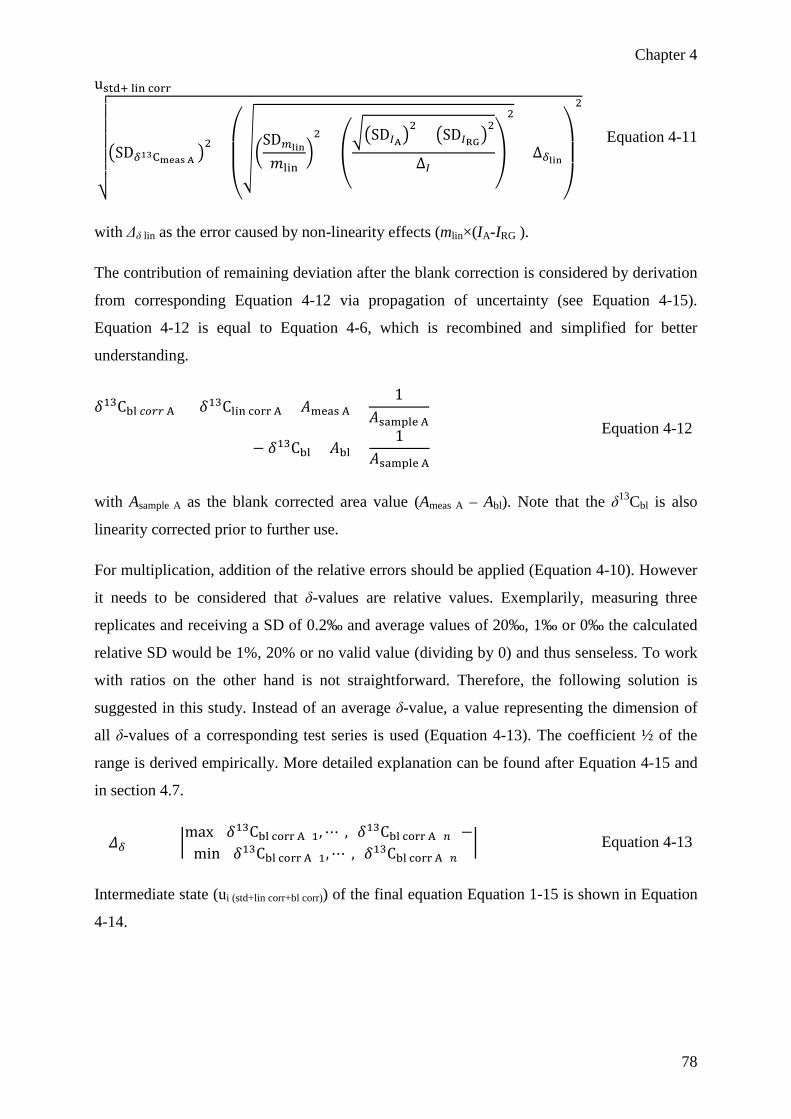
Chapter 4

78

ustd+ lin corr = ±

⎷⃓⃓⃓⃓⃓⃓⃓⃓⃓⃓�

�SD𝛿𝛿13Cmeas A �2

+

⎝

⎜⎜⎛��

SD𝑚𝑚lin

𝑚𝑚lin�2

+

⎝

⎛��SD𝐼𝐼A�

2+ �SD𝐼𝐼RG�

2

∆𝐼𝐼⎠

⎞

2

× ∆𝛿𝛿lin

⎠

⎟⎟⎞

2

Equation 4-11

with Δδ lin as the error caused by non-linearity effects (mlin×(IA-IRG ).

The contribution of remaining deviation after the blank correction is considered by derivation

from corresponding Equation 4-12 via propagation of uncertainty (see Equation 4-15).

Equation 4-12 is equal to Equation 4-6, which is recombined and simplified for better

understanding.

𝛿𝛿13Cbl 𝑐𝑐𝑚𝑚𝑛𝑛𝑛𝑛 A = 𝛿𝛿13Clin corr A × 𝐴𝐴meas A ×1

𝐴𝐴sample A

− 𝛿𝛿13Cbl × 𝐴𝐴bl ×1

𝐴𝐴sample A

Equation 4-12

with Asample A as the blank corrected area value (Ameas A – Abl). Note that the δ13Cbl is also

linearity corrected prior to further use.

For multiplication, addition of the relative errors should be applied (Equation 4-10). However

it needs to be considered that δ-values are relative values. Exemplarily, measuring three

replicates and receiving a SD of 0.2‰ and average values of 20‰, 1‰ or 0‰ the calculated

relative SD would be 1%, 20% or no valid value (dividing by 0) and thus senseless. To work

with ratios on the other hand is not straightforward. Therefore, the following solution is

suggested in this study. Instead of an average δ-value, a value representing the dimension of

all δ-values of a corresponding test series is used (Equation 4-13). The coefficient ½ of the

range is derived empirically. More detailed explanation can be found after Equation 4-15 and

in section 4.7.

½𝛥𝛥𝛿𝛿 = ½ × �max{(𝛿𝛿13Cbl corr A)1,⋯ , (𝛿𝛿13Cbl corr A)𝑚𝑚} −

min{(𝛿𝛿13Cbl corr A)1,⋯ , (𝛿𝛿13Cbl corr A)𝑚𝑚} � Equation 4-13

Intermediate state (ui (std+lin corr+bl corr)) of the final equation Equation 1-15 is shown in Equation

4-14.

Chapter 4

79

ui (std+lin corr+bl corr) = ±�uminuend2 + usubtrahend2

with uminuend = �� usl½𝛥𝛥𝛿𝛿

�2

+ �SD𝐴𝐴meas A𝐴𝐴meas A

�2

+ �u𝐴𝐴sample A

𝐴𝐴sample A�2

× ½𝛥𝛥𝛿𝛿 × 𝐴𝐴𝑚𝑚𝑚𝑚𝑚𝑚𝑚𝑚 A ×1

𝐴𝐴sample A

with usubtrahend = ��usl 𝑏𝑏𝑏𝑏½𝛥𝛥𝛿𝛿

�2

+ �SD𝐴𝐴bl𝐴𝐴bl

�2

+ �u𝐴𝐴sample A

𝐴𝐴sample A�2

× ½𝛥𝛥𝛿𝛿 × 𝐴𝐴bl ×1

𝐴𝐴sample A

with 𝐴𝐴sample A = 𝐴𝐴meas A − 𝐴𝐴bl and

with u𝐴𝐴sample A = ��SD𝐴𝐴meas A�2

+ �SD𝐴𝐴bl�2

Equation 4-14

with usl as abbreviation for ustd+lin corr. usl bl refers to the uncertainty in the blank (calculations

are equal to usl).

The next step in the uncertainty estimation is introduced to account for the difference between

the δ-value of the sample and that of the blank Equation 4-15. Meaning that if the difference

between the δ-value of the sample and that of the blank is zero the blank correction

contribution is zero and blank correction uncertainty equation gives usl as a result.

ustd+lin corr+bl corr = ± (ustd+lin corr + (ui (std+lin corr+bl corr) − ustd+lin corr) × 𝑓𝑓𝛥𝛥)

with 𝑓𝑓𝛥𝛥 = �𝛿𝛿13Cbl corr A− 𝛿𝛿13Cbl�max{|𝛿𝛿13Cbl corr A|1,⋯ ,|𝛿𝛿13Cbl corr A|𝑛𝑛}

Equation 4-15

This concept was proven via the following test procedure:

Taking the large data set (436 single measurements) obtained within the round robin test a

realistic worst case scenario could be modeled (WC-M). The WC-M was used to validate the

approach suggested in this study (exemplarily demonstrated in Supporting information). It is

proposed that the final achieved expanded uncertainty (U) should cover the maximal

deviation observed via WC-M (U ≥ max{ΔWC-M 1, ... , ΔWC-M n}). Expanded uncertainty is

calculated by multiplication of the combined uncertainty with the coverage factor k (U = ucomb

× k). The value of coverage factor k is typically 2 or 3 corresponding to the confidence

interval of U of 95.4% or 99.7%, respectively. With a k value of 2 the combined uncertainty

should cover at least 50% of maximal deviation observed with the WC-M.

Chapter 4

80

For the data achieved with the round robin test series the calculated ustd+lin corr+bl corr covers

68% of the maximal deviation observed via WC-M. Therefore, the approach is assumed to be

valid.

Note that the water blank correction and its contribution to combined uncertainty needs to be

considered only for the standards prepared with this water (not for, e.g., river water samples).

Finally, the contribution of remaining deviation after two-point normalization is considered

by derivation from corresponding Equation 4-7 to Equation 4-9 via propagation of uncertainty

(see Equation 4-16 to Equation 4-18).

u𝑚𝑚norm = ±

��uStd1,VPDB

2 + uStd2,VPDB2

𝛥𝛥std,VPDB�2

+ ��uStd1,RG

2 + uStd2,RG2

𝛥𝛥std,RG�2

× 𝑚𝑚norm Equation 4-16

with Δstd,VPDB as δ13CStd1,VPDB – δ13CStd2,VPDB, Δstd,RG as δ13CStd1,RG – δ13CStd2,RG, uncertainties in

numerator are defined by the IAEA (uStd1,VPDB, uStd1,VPDB) or derived as described before

ustd+lin corr+bl corr (uStd1,RG, uStd1,RG).

u𝑏𝑏norm = ±

�avgu𝑆𝑆𝑆𝑆𝑆𝑆,VPDB2 + ��

u𝑚𝑚norm

𝑚𝑚norm�2

+ �avguStd,RG

½𝛥𝛥Std,RG�2

× 𝑚𝑚norm × ½𝛥𝛥std,RG�

2

Equation 4-17

with half range (½ΔStd,RG) as |δ13CStd1,RG – δ13CStd2,RG|/2, average avgu(Std,VPDB) as (uStd1,VPDB +

uStd2,VPDB)/2 and avgu(Std,RG) as (uStd1,RG + uStd2,RG)/2.

The final combined uncertainty ucomb (ustd+lin corr+bl corr+norm) can then be formulated as follows.

ucomb = ±

��u𝑚𝑚norm

𝑚𝑚norm�2

+ �uslb

½𝛥𝛥Std,RG�2

× 𝑚𝑚norm × ½𝛥𝛥Std,RG�

2

+ u𝑏𝑏norm2 Equation 4-18

with uslb as abbreviation for ustd+lin corr+bl corr.

Note that for standard and blank value determinations not only the average and standard

deviations of one replicate set should be taken for each test series, but at least of three

replicates sets, measured at the beginning, mid and end of the test series to be representative

Chapter 4

81

for that test series. Use of mid replicate set (or sets) can be used to distinguish, e.g., a long

term drift from a random deviation.

The combined uncertainty ucomb obtained as described before contains contributions from

random deviation measuring replicates ustd as well as remaining deviations from linearity

correction, blank correction and normalization. Combined uncertainty defines an interval

having a level of confidence of approximately 68% (≡ ±1σ). Nevertheless, there may be

unknown deviations (Figure 4-1) which can be considered by expanded uncertainty U

obtained via multiplying of ucomb by a coverage factor (typically 2 or 3; confidence interval of

95% or 99.7%, respectively).

The combined uncertainty derived this way is representative for DOC SIA measurements, but

exclude the contribution of potential error caused by sampling or further preparation steps.

Depending on the focus it may be necessary to consider further contributions via error

propagation, but a detailed description is out of scope in this work.

Application of the introduced approach to assess the uncertainties for a DOC SIA round

robin test

The values of the data obtained from the international interlaboratory test (round robin test)

by two participants working with the same instrumentation iso TOC cube HTC analyzer

(Elementar Analysensysteme, Hanau, Germany) coupled to IsoPrime 100 isotope ratio mass

spectrometer (Isoprime, Manchester UK) are shown in Table 4-1.

Table 4-1 Data set including uncertainties assessed for DOC SIA

Chapter 4

82

sample avgn=3 ±ustd ±ucomb ±Uk=2 (95%) ±Uk=3 (99.7%) avgn=3 ±ustd ±ucomb ±Uk=2 (95%) ±Uk=3 (99.7%)

fw i -27.58 0.03 0.33 0.66 1.00 -27.96 0.01 0.33 0.66 0.99fw ii -27.01 0.05 0.33 0.67 1.00 -27.29 0.05 0.33 0.67 1.00fw iii -28.33 0.03 0.33 0.66 0.99 -28.39 0.02 0.33 0.66 0.99fw iv -27.59 0.02 0.33 0.66 0.99 -27.70 0.02 0.33 0.66 0.99fw v -28.33 0.01 0.33 0.66 0.99 -28.40 0.02 0.33 0.66 0.99fw vi -24.30 0.02 0.33 0.66 0.99 -24.45 0.01 0.33 0.66 0.99fw vii -27.63 0.04 0.33 0.67 1.00 -27.59 0.03 0.33 0.66 1.00fw viii -12.91 0.09 0.34 0.68 1.02 -14.81 0.77 0.83 1.65 2.48fw ix -16.94 0.17 0.37 0.74 1.11 -17.26 0.27 0.42 0.85 1.27sw i -16.45 0.30 0.44 0.88 0.99 -18.73 0.11 0.35 0.70 1.05sw ii -26.45 0.03 0.33 0.66 1.32 -26.30 0.03 0.33 0.66 1.00sw iii -22.66 0.10 0.34 0.69 1.00 -23.25 0.08 0.34 0.68 1.02sw iv -24.43 0.04 0.33 0.67 1.03 -24.39 0.05 0.33 0.67 1.00sw v -27.69 0.06 0.34 0.67 1.00 -27.36 0.05 0.33 0.67 1.00sw vi -21.47 0.02 0.33 0.66 1.01 -20.83 0.26 0.42 0.84 1.26dowc -23.19 0.02 0.33 0.66 0.99

Δ |a-b| [‰]avg 0.06 0.34 0.69 1.03 0.12 0.38 0.76 1.14 0.49min 0.01 0.33 0.66 0.99 0.01 0.33 0.66 0.99 0.04max 0.30 0.44 0.88 1.32 0.77 0.83 1.65 2.48 2.28

fw: fresh water sample; sw: seawater sample; dow: deep ocean water; Δ a-b difference between delta values obtained by participant a and b;aR&D, Elementar Group & Instrumental Analytical Chemistry, University of Duisburg-Essen; E. Federherr (responsible)bInstitute for Biodiversity and Ecosystem Dynamics, University of Amsterdam; C. Cerli (responsible)cThe ampules contained only ca. 20 - 25 ml sample instead of 40 ml. To ensure a sufficient sample volume for the measurement, samples of participants a and b were therfore combined.

δ 13CVPDB [‰] results participanta δ 13CVPDB [‰] results participantbΔ a-b [‰]

0.380.280.06

-0.64

0.110.070.15-0.041.900.322.28-0.150.59-0.04-0.33

Chapter 4

83

Comparing data of the two participants show clearly that ustd is less suited to represent the

deviations of the method than expanded uncertainty. Nine out of fifteen δ13CVPDB average

deviations Δa-b are not covered by ustd. Requirement for covering is that the condition ua + ub ≥

Δa-b is satisfied (Figure 4-2).

One sample is with Δa-b = 2.28 obviously out of range. That is the only deviation not covered

by Uk=3 (99,7%). A closer look on the sequence shows that this sample was measured shortly

after change of consumables (participant a). Conditioning before resuming measurement of

real samples might have been insufficient.

Average Δa-b of ±0.49‰ confirms good reproducibility (≤0.5‰).

A significant contribution to ucomb is the uncertainty of the UP water NDIR detector peak area

(±1295; corresponds to ±0.11 mgC/L) and δ13C value (±1.35‰). Nevertheless, considering 10

mgC/L IAEA-CH6 standard solution, a relatively small concentration of the blank (ca. 0.35

mgC/L) results in a contribution to ucomb of the IAEA-CH6 δ13C value of ±0.12‰, whereas

skipping of the blank correction would lead to a systematic error of +0.57‰. Therefore blank

correction was carried out. In the future, higher concentrated standards for normalization

could be taken (e.g., 25 mgC/L) to minimize the contribution of the blank. On the other hand

those standards would be less similar to the samples and therefore less representative. It is

however out of scope in this work.

For the determination of standard values for normalization not only averages and standard

deviations of one replicate set were taken (e.g., IAEA-CH6 δ13C SDn=3 ±0.03‰), but three

replicate sets for each test series, measured at the beginning, mid and end of the test series to

be representative for the test series (e.g., IAEA-CH6 δ13C SDn=9 ±0.22‰).

Chapter 4

84

4.4.2 Round robin test and further real sample measurements

Table 4-2 Comparison of own results against expected values in round robin test

The comparison (principle is shown in Figure 4-2) shows that determined values are in

agreement with the expected values. Since no uncertainty values were provided by the round

robin test organizers, uncertainties typically found in DOC SIA were taken from literature for

river water (Raymond et al.)[4], costal seawater (Raymond et. a)[4] and deep ocean water

(Follett et al.)[20]. A further evaluation of the round robin test results was announced by the

organizers but is not yet available.

sample avgn=3 ±Uk=3 (99.7%) expected ±uncertaintyc

fw i -27.58 1.00 -28.16 1.00 0.58fw ii -27.01 1.00 -27.50 1.00 0.49fw iii -28.33 0.99 -28.16 1.00 -0.17fw iv -27.59 0.99 -27.50 1.00 -0.09fw v -28.33 0.99 -28.16 1.00 -0.17fw vi -24.30 0.99 - - -fw vii -27.63 1.00 -28.16 1.00 0.53fw viii -12.91 1.02 - - -fw ix -16.94 1.11 - - -sw i -16.45 0.99 - - -sw ii -26.45 1.32 -25.63 1.02 -0.82sw iii -22.66 1.00 -21.00 1.02 -1.66sw iv -24.43 1.03 - - -sw v -27.69 1.00 -26.35 1.02 -1.34sw vi -21.47 1.01 - - -dow -23.19 0.99 -21.00 1.50 -2.19

Δ |a-b| [‰]avg 1.03 0.80min 0.99 0.09max 1.32 2.19

fw: fresh water sample; sw: seawater sample; dow: deep ocean water;aR&D, Elementar Group & Instrumental Analytical Chemistry, University of Duisburg-Essen;bexpected values provided by round robin test organizer (no further details or sources were provided)cno further details about the uncertaties of the values were provided by the round robin test organizer, therefore typical uncertainties reported in the literature were used (details can be found in text)

δ 13CVPDB [‰] results participantaΔ a-b [‰]

δ 13CVPDB [‰]b

Chapter 4

85

Figure 4-2 Visualization of principle to compare two values based on coverage through

uncertainties

However, an exemplary evaluation and comparison of the results of all participants including

the different methods used can already be shown in (Figure 4-3).

Figure 4-3 Exemplary results of the round robin test for a lake sample (left) und a marine

sample (right). Average and standard deviation for n(p) different labs using the same method

are shown (if n(p)>1). Average and standard deviation for n(r) replicate measurements of own

results (participant (a)) and for cases were only one participant has used a certain method

(n(p)=1) are shown. Wet oxidation coupled with cavity ring-down spectrometer (WO/CRDS)

was not used for DOC measurements in sea water. Expected range is shown only for the lake

sample (for sea water sample sw iv not available). For cases with more than one participant,

-24

-23.5

-23

-22.5

-22

-21.5

-21

-20.5

-20

δ13 C

[‰]

(u1+u2) ≤ Δu: true

(u1+u2) ≤ Δu: false

Chapter 4

86

no standard deviations of replicate measurements achieved by different labs using the same

method were provided.

Details, e.g., whether certain sample preparation methods such as desalinization using ion

exchanger cartridge were used or not is not available but would be essential to justify the

results. Nevertheless, it is clear that both, high temperature combustion and wet chemical

oxidation based methods are possibly suited for DOC SIA, but standard deviations are

predominantly larger in case of wet chemical oxidation based methods (WCO/IRMS,

LC/IRMS and WO/CRDS). Again, further details are necessary to draw any robust

conclusion.

Besides oceanography and limnology a direct measurement of DOC SIA is also of interest in

soil science. Using different real samples, such as rice straw or black humus layer extracts, the

suitability of the novel system as well as evaluation strategy for DOC SIA was clearly

demonstrated:[7]

Figure 4-4 Excerpt from the data obtained with various natural DOC samples (redrafted from

Kirkels et al.)[7]

The suitability of the HTC TOC/IRMS system was proven by comparison of the δ13C values

measured by HTC TOC/IRMS in aqueous, natural and complex DOC samples with those

obtained via EA/IRMS measurements, where aliquots were freeze-dried prior to IRMS

measurements. δ13C values obtained by TOC/IRMS were all in good agreement with values

obtained by EA/IRMS (R2 = 0.9997). Trueness representing absolute differences of δ13C

values obtained with HTC TOC/IRMS and EA/IRMS were all ≤0.10‰. For both methods

y = 1.0022x + 0.0268R² = 0.9997

-34

-32

-30

-28

-26

-24-34 -32 -30 -28 -26 -24

EA/IR

MS δ1

3 CVP

DB

[‰]

TOC/IRMS δ13CVPDB [‰]

eroded sedimenthumic acid

black humus layersubsoil

rice straw

ashbeech

pinespruce

moss

eroded sedimenthumic acid

black humus layersubsoil

rice straw

ashbeech

pinespruce

moss

avg maxSD (EA/IRMS) 0.03 0.10SD (TOC/IRMS) 0.06 0.11Δ (∣EA-TOC∣) 0.04 0.10n = 3

Chapter 4

87

similar precision of δ13C values was achieved, with SD always ≤0.12 ‰. Obviously, there

was no isotope fractionation observed for δ13C analysis by HTC TOC/IRMS. Moreover, the

high accuracy in terms of δ13C values is in good accordance with the strongly linear

relationship previously reported between HTC TOC/IRMS and EA/IRMS for a variety of

chemical compounds (see Chapter 3).

Data gained with the novel HTC TOC/IRMS system demonstrate the suitability of the system

for application in oceanography, limnology and soil since.[7]

4.4.3 Proof of principle of TIC SIA with the iso TOC cube system

A TIC mode instrumentation was implemented in iso TOC cube, derived from the

commercially available HTC-TOC analyzer vario TOC cube (Elementar Analysensysteme

GmbH). The HTC TOC system in TIC mode was coupled with the isotope ratio mass

spectrometer using the focusing unit developed for DOC SIA. The final setup is shown in

Figure 4-5.

Figure 4-5 System setup for TIC SIA (simplified graph focusing on main principles). 0.05 to

3 mL of sample is injected in the sparger automatically via a syringe from an autosampler (not

shown in the graph). Acid is added to the sample via an acid pump (not shown in the graph) to

achieve a pH of ca. 2. Helium as a carrier gas is added via a mass flow controller, mixes the

reactant with the sample in the reaction side in the sparger and provides the evaluated CO2 to

the purification system. The purification system consists of condenser, membrane dryer

(Nafion®), chemical dryer (Sicapent®) and a halogen scrubber. After purification, the gas,

passing the flow meter and NDIR detector enters the focusing unit with an adsorption column.

Using high heating rates the CO2 is rapidly focused desorbed and transported by helium gas

towards the isotope ratio mass spectrometer for stable isotope composition measurement.

NDIR

IRMS Detector IsoPrime 100

ref. gas CO2

He

reference gasbox

HTC TOC analyzer(TIC mode)

a

c

b

focusing unitHe

CO2

gas drying a: condenser b: Nafion® membrane c: Sicapent®filter (halogen scrubber)

flow sensormass flow controller

ref. gas N2

spar

ger

H3PO4sample

Chapter 4

88

The system is fully automated and a first proof of principle for its general suitability for the

determination of TIC SIA was carried out using five vials containing the same solution of 10

mgC/L LiCO3. The precision obtained by averaged results of triplicate measurements with

five sample vials, expressed as ustd (SD ≡ 1σ), was ≤0.20‰ (ustd,avg = 0.10‰; ustd,max = 0.19‰)

for δ13C values. However, further tests are necessary to investigate the performance, mainly

LOQ and accuracy using standard solutions and suitability for real samples.

Chapter 4

89

4.5 Conclusion and outlook Good precision (standard deviation (SD) predominantly ≤0.15‰) and accuracy (coefficient of

determination (R2) 1.000 ± 0.001) were achieved for the δ13C analysis of a broad diversity of

DOC solutions. Good reproducibility (predominantly ≤0.5‰) was shown in the context of

international round robin testing for river and seawater samples.

A novel strategy to evaluate combined uncertainty for DOC SIA was introduced and

validated. Significance of the use of expanded uncertainty U, rather than standard uncertainty

ustd to compare results was shown. Proper assessment of combined uncertainty is essential to

obtain the expanded uncertainty. To ensure an international comparability of the data a

standardized procedure would be necessary, which is not available to date.

A precision of SD ≤0.2‰ was achieved for fully automated SIA of TIC, but further validation

tests are clearly required for that application.

Chapter 4

90

4.6 References [1] R. Kindler, J. Siemens, K. Kaiser, D. C. Walmsley, C. Bernhofer, N. Buchmann, P.

Cellier, W. Eugster, G. Gleixner, T. Grünwald, A. Heim, A. Ibrom, S. K. Jones, M. Jones, K.

Klumpp,W. Kutsch, K. S. Larsen, S. Lehunger, B. Loubet, R. Mckenzie, E. Moors, B.

Osborne, K. Pilegaard, C. Rebmann, M. Saunder, M. W. I. Schmidt, M Schrumpf, J.

Seyfferth, U. Skiba, J. -F. Soussana, M. A. Sutton, C. Tefs, B. Vowinckel, M. J. Zeeman, M.

Kaupenjohann. Dissolved carbon leaching from soil is a crucial component of the net

ecosystem carbon balance. Global Change Biol. 2011, 17, 1167.

[2] K. Kalbitz, S. Solinger, J.-H. Park, B. Michalzik, E. Matzner. Controls on the dynamics of

dissolved organic matter in soils: a review. Soil Sci. 2000, 165, 277.

[3] J. E. Bauer, in Biogeochemistry of Marine Dissolved Organic Matter, (Ed: D. A. Hansell,

C. A. Carison). Elsevier, Amsterdam, 2002, pp. 405-453.

[4] P. A. Raymond, J. E. Bauer. Use of 14C and 13C natural abundances for evaluating

riverine, estuarine, and coastal DOC and POC sources and cycling: a review and synthesis.

Org. Geochem. 2001, 32, 469.

[5] S. Steinbeiss, V. M. Temperton, G. Gleixner. Mechanisms of short-term soil carbon

storage in experimental grasslands. Soil Biol. Biochem. 2008, 40, 2634.


[7] M. S. A. K. Frédérique, C. Cerli, E. Federherr, K. Kalbitz. A novel high temperature


samples (II): optimization and assessment of analytical performance. Rapid Commun. Mass

Spectrom. 2014, 28, 2574.

[8] T. A. Schlacher, R. M. Connolly. Land–Ocean Coupling of Carbon and Nitrogen Fluxes

on Sandy Beaches. Ecosystems 2009, 12, 311.

[9] J. Barth. Influence of carbonates on the riverine carbon cycle in an anthropogenically

dominated catchment basin: evidence from major elements and stable carbon isotopes in the

Lagan River (N. Ireland). Chem. Geol. 2003, 200, 203.

[10] P. Schulte, R. van Geldern, H. Freitag, A. Karim, P. Negrel, E. Petelet-Giraud, A. Probst,

J.-L. Probst, K. Telmer, J. Veizer, J. A. C. Barth. Applications of stable water and carbon

isotopes in watershed research: Weathering, carbon cycling, and water balances. Earth-Sci.

Rev. 2011, 109, 20.

Chapter 4

91





[13] DIN EN ISO/IEC 17025:2005. General requirements for the competence of testing and

calibration laboratories.

[14] P. De Bièvre, R. Dybkær, A. Fajgelj, D. B. Hibbert. Metrological traceability of

measurement results in chemistry: concepts and implementation. Pure Appl. Chem. 2011, 83,

1873.

[15] M. Thompson, S. L. Ellison, R. Wood. Harmonized guidelines for single-laboratory

validation of methods of analysis (IUPAC Technical Report). Pure Appl. Chem. 2002, 74,

835.

[16] M. Thompson, R. Wood. Harmonized guidelines for internal quality control in analytical

chemistry laboratories. Nature 1995, 4, 4.

[17] A. Menditto, M. Patriarca, B. Magnusson. Understanding the meaning of accuracy,

trueness and precision. Accredit. Qual. Assur. 2006, 12, 45.

[18] V. Lindberg. Uncertainties and Error Propagation. http://www.rit.edu/~w-

uphysi/uncertainties/Uncertaintiespart2.html

[19] B. Neidhart, W. Wegscheider. Quality in Chemical Measurements: Training Concepts

and Teaching Materials. Springer, Berlin, 2012.

[20] C. L. Follett, D. J. Repeta, D. H. Rothman, L. Xu, C. Santinelli. Hidden cycle of

dissolved organic carbon in the deep ocean. Proc. Natl. Acad. Sci. U. S. A. 2014, 111, 16706.

Chapter 4

92

4.7 Supporting information Assessment of the uncertainty via a worst case model (WC-M)

A simple example is chosen to demonstrate the principle to assess the uncertainty (Table S

4-1). An area of a rectangle (A) is calculated using average lengths (l) of sides a and b. A

standard error propagation approach (method i) is chosen to calculate the uncertainty of the

area u(Aab) out of lengths uncertainties u(la) and u(lb). Using the same data set (lengths and

their uncertainties) four worst case scenarios are modeled (WC-M) (four areas are calculated).

These four scenarios are the four possible permutations with two variables a and b. Each of

them can have a positive and a negative deviation: la + u(la) and lb + u(lb) (++), la + u(la) and lb

- u(lb) (+-), la - u(la) and lb + u(lb) (-+), and la - u(la) and lb - u(lb) (--). In the next step, each of

the calculated WC-M areas is subtracted from the area observed using average lengths. These

subtractions results in four deviation values Δ(Aab). Taking the absolute values of deviations a

maximum deviation is determined. Maximum deviation observed via WC-M is used for

comparison with the uncertainty derived with the method i using coverage value

(Aab,avg/Aab,WC-Mmax).

Table S 4-1 Demonstration of the principle used to assess uncertainty

The empirical factor (½) was chosen to calculate the value representing the dimensions of the

δ-value. This factor was validated under the consideration that the combined uncertainty

should cover at least 50% of maximal deviation observed via WC-M. All samples of the test

series were taken for validation. Coverage below 50% would mean underestimation of the

uncertainty (Uk=2 would not cover the maximal deviation observed via WC-M).

sidel

[mm]u(l )

[mm]rel. u(l )

[mm]

A ab

[mm2]

u(A AB)

[mm2]l

[mm]

A AB

[mm2]

Δ(A AB )

[mm2]l

[mm]

A AB

[mm2]

Δ(A AB )

[mm2]a 10.0 0.3 3.0% 10.30 9.70

b 5.0 0.1 2.0% 5.10 4.90

l[mm]

A AB

[mm2]

Δ(A AB )

[mm2]l

[mm]

A AB

[mm2]

Δ(A AB )

[mm2]10.30 9.70

4.90 5.10

maximum deviation observed via WC-M: 2.53

coverage of maximal deviation by uncertainty calculated via method (i): 1.80/2.53 = 71%

aestimated via error propagation

50.47 0.47 49.47 0.53

worst case model (WC-M)

47.53 2.47

scenario 2 (--)

scenario 3 (+-) scenario 4 (-+)

method for uncertainty estimationa (i)

50 1.80 52.53 2.53

scenario 1 (++)

Chapter 5

93

Chapter 5 A novel tool for natural abundance stable nitrogen analysis in

in aqueous samples

Chapter 5

94

5.1 Abstract Rationale: The bulk stable isotope analysis (BSIA) of dissolved matter (e.g. dissolved organic

carbon, total nitrogen bound (TNb), etc.) is of particular importance since this pool is a prime

conduit in the cycling of N and C. Studying the two elemental pools is of importance, as the

transformation and transport processes of N and C are inextricably linked in all biologically

mediated systems. No system able to analyze natural abundance stable carbon and nitrogen

isotope composition of dissolved nitrogen directly (without offline sample preparation) and

simultaneously has been reported so far. Extension of the high temperature combustion

(HTC) total organic carbon (TOC) analyzer, to the ability to measure TNb stable nitrogen

isotope composition is described in this study.

Methods: To extent the TOC analyzer to the ability to measure TNb, modifications from the

HTC high performance liquid chromatography/isotope ratio mass spectrometry

(HPLC/IRMS) interface were implemented and expanded. Reduction reactor for conversion

of NOx to N2 was implemented into the new developed system. Extension addresses mainly

the development of the focusing unit for nitrogen and a degassing device for online separation

of TNb from in the sample solved N2 prior to injection.

Results: The proof of principle of the system with different compound solutions succeeded. In

this initial testing, δ15NAIR-N2 values of tested compounds were determined with precision and

trueness of typically ≤0.5‰. Further tests aimed at the working range investigation. Good

results (U ≤ 0.5‰) could be achieved down to a TNb concentration of 40 mgN/L and

sufficient results (U ≤ 1.0‰) down to 5 mgN/L. Additionally the development resulted in the

first system reported to be suitable for simultaneous δ13C and δ15N direct BSIA of aqueous

samples.

Conclusions: The expansion of a TOC analyzer, specially designed for coupling with isotope

ratio mass spectrometry (IRMS) to the ability to measure TNb resulted in the first system

reported to be suitable for both δ13C and δ15N direct BSIA in aqueous samples. This system

could open up new possibilities in SIA based research fields.

Chapter 5

95

5.2 Introduction The investigation of transformation and transport processes of carbon and nitrogen in

ecosystems plays a vital role in understanding their biogeochemical dynamics.[1–4] Sources of

dissolved organic matter (DOM) in soils are, e.g., the recent photosynthate and the leaching or

further decomposition of microbially processed, older soil organic matter.[3] DOM sinks are

among others mineralization, precipitation, adsorption, microbial immobilization, and

transformation.[3] The stable isotope composition can be used as a marker of matter flow and

to evaluate the direction and rate of those ecological processes.[4] Consequently, suitable and

accurate online methods for stable isotope analysis (SIA) of carbon and nitrogen in aqueous

samples such as soil extracts are required.[1,2] Over the last decade, there has been much effort

to establish the routine analysis of δ13C of dissolved organic carbon (DOC) through the

coupling of total organic carbon analyzers with isotope ratio mass spectrometers

(TOC/IRMS)[5–9]. The natural abundance bulk stable isotope analysis (BSIA) of δ15N of total

nitrogen bound (TNb) still has large limitations and cannot be analyzed simultaneously with

δ13C directly from an aqueous sample. Low concentration of TNb makes elemental analysis

coupled to isotope ratio mass spectrometry (EA/IRMS) laborious, time and sample

consuming[10,11]. Russow et al.[12] introduced a first on-line measurement method for total

dissolved nitrogen BSIA using the coupling of a high temperature combustion (HTC) based

TOC analyzer and a quadrupole mass spectrometer. However, beside of other limitations such

as a relatively high memory effect and a logarithmic non-linearity effect, this system was

suitable only for samples enriched in the heavier isotope (15N) because the observed detection

limit was insufficient for natural abundance measurements. Indeed, the limiting factor of the

system could have been the use of a quadrupole mass spectrometer instead of an isotope ratio

mass spectrometer. However, the introduced HTC TOC analyzer inlet system was never

coupled with an IRMS detector.

A first coupling of another HTC based TOC analyzer to isotope ratio mass spectrometer was

carried out later for determining δ15N in aqueous samples[13,14]. A first study of the system

resulted in a SD of 2.8‰, which was still insufficient for natural abundance studies.[13] In a

following study[14] the authors noted that the relatively high solubility of molecular nitrogen

(N2-aq) in water remained a technical challenge and might be limiting. The SIA limit of

quantification (LOQSIA) of 20 mgN/L and a corresponding precision for δ15N with average SD

of 0.8‰ and maximum SD of 1.8‰ for different compounds remained too high for routine

measurement of natural abundance samples. Furthermore, a simultaneous δ13C and δ15N was

neither reported with this system.

Chapter 5

96

With respect to the shortcomings described, this study has the following aims: (i) an

additional on-line separation step to separate N2-aq from TNb prior to its SIA, (ii) a focusing

unit for N2, and (iii) a simultaneous δ13C, δ15N SIA mode. To that end, we describe the further

development of a high-temperature combustion (HTC) based TOC/IRMS system for the

simultaneous determination of δ15N in addition to δ13C in aqueous solutions.

Chapter 5

97

5.3 Experimental


The reference material IAEA-600 caffeine CAF1 (δ15N 1.0 ± 0.2‰), USGS 41 glutamic acid

(δ15N 47.6 ± 0.2‰), USGS 25 ammonium sulfate (δ15N -30.4 ± 0.4‰), USGS 26 glutamic

acid (53.7 ± 0.4‰) and IAEA-N-2 ammonium sulfate (20.3 ± 0.2‰) were purchased from

the International Atomic Energy Agency (Vienna, Austria). The internal laboratory standards

were EAS-GLU1 glutamic acid, EAS-CAF2 caffeine, EAS-CAF3 caffeine, EAS-ACA1

acetanilide, EAS-GLU2 glutamic acid, EAS-SNO1 sodium nitrate and EAS-ANH1

ammonium chloride (in-house standards; Elementar Analysensysteme, Hanau, Germany).

Ultrapure, deionized water (UP water) produced by a Milli-Q® system (Merck Millipore,

Billerica, US) was used for solution preparation. Helium 4.6 was purchased from Air Liquide

(Oberhausen, Germany) and used in combination with Helium purifier ExcelaSorb™ 27600-

U (Supelco®; Sigma-Aldrich Group; Darmstadt, Germany). Oxygen 4.8 was purchased from

Air Liquide (Oberhausen, Germany).


HTC TOC/IRMS

The entire system consists of two parts: the modified TOC analyzer and the isotope ratio mass

spectrometer. The, for SIA adapted TOC analyzer iso TOC cube (Elementar Analysensysteme

GmbH) was used for further modifications, namely, (i) implementation of N2 focusing unit to

improve the system sensitivity, (ii) implementation of on-line degassing unit to minimize

blank contribution, and (iii) a reduction tube. Reduction tube is implemented to ensure

complete conversion of NO to N2 and the absence of isotope fractionation within the system

for δ15N BSIA. An additional mass flow controller was implemented to dose oxygen gas

accurately.

Samples, filled in 40-mL borosilicate glass vials, are introduced using a 32-position

autosampler into the combustion system by means of a 5-mL syringe and a 5/4 multiway

valve. Filling the syringe the sample is degassed automatically passing the vacuum/membrane

degassing unit. The combustion is performed at 850 °C by oxygen and supported by a catalyst

(Pt on ceramic carrier material). A reduction step over elemental copper at 500 °C is carried

out to convert nitrogen oxides to N2. Water is removed in three steps: an air-cooled

condenser, a counterflow membrane dryer and a chemical dryer. Hydrogen halides and

halogens are removed by silver wool. After the purification steps the carrier gas enters the

nondispersive infrared (NDIR) detector. The sample is then directed to the interface

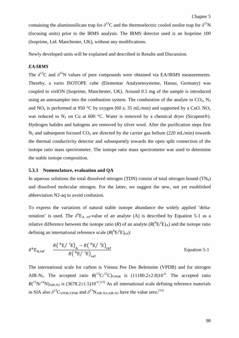
Chapter 5

98

containing the aluminosilicate trap for δ13C and the thermoelectric cooled zeolite trap for δ15N

(focusing units) prior to the IRMS analysis. The IRMS detector used is an Isoprime 100

(Isoprime, Ltd. Manchester, UK), without any modifications.

Newly developed units will be explained and described in Results and Discussion.

EA/IRMS

The δ13C and δ15N values of pure compounds were obtained via EA/IRMS measurements.

Thereby, a vario ISOTOPE cube (Elementar Analysensysteme, Hanau, Germany) was

coupled to visION (Isoprime, Manchester, UK). Around 0.5 mg of the sample is introduced

using an autosampler into the combustion system. The combustion of the analyte to CO2, N2

and NOx is performed at 950 °C by oxygen (60 s; 35 mL/min) and supported by a CuO. NOx

was reduced to N2 on Cu at 600 °C. Water is removed by a chemical dryer (Sicapent®).

Hydrogen halides and halogens are removed by silver wool. After the purification steps first

N2 and subsequent focused CO2 are directed by the carrier gas helium (220 mL/min) towards

the thermal conductivity detector and subsequently towards the open split connection of the

isotope ratio mass spectrometer. The isotope ratio mass spectrometer was used to determine

the stable isotope composition.


In aqueous solutions the total dissolved nitrogen (TDN) consist of total nitrogen bound (TNb)

and dissolved molecular nitrogen. For the latter, we suggest the new, not yet established

abbreviation N2-aq to avoid confusion.


notation’ is used. The δhEA, ref-value of an analyte (A) is described by Equation 5-1 as a

relative difference between the isotope ratio (R) of an analyte (R(hE/lE)A) and the isotope ratio

defining an international reference scale (R(hE/lE)ref):



ref


Equation 5-1

The international scale for carbon is Vienna Pee Dee Belemnite (VPDB) and for nitrogen

AIR-N2. The accepted ratio R(13C/12C)VPDB is (11180.2±2.8)10-6. The accepted ratio

R(15N/14N)AIR-N2 is (3678.2±1.5)10-6.[15] As all international scale defining reference materials

in SIA also δ13CVPDB,VPDB and δ15NAIR-N2,AIR-N2 have the value zero.[15]

Chapter 5

99


reported δ-values are related to the used reference gas (RG). That concerns all data before the

final normalization to the international reference scale.



All measured δ13C and δ15N raw data (δ13Cmeas A and δ15Nmeas A) generated by the software

IonVantage (IsoPrime100 operating system) or IonOS (visION operating system) are

automatically related to RG and in case of δ13C values additionally corrected for 17O-

abundance. Then the values are linearity corrected to δ13Clin corr A and δ15Nlin corr A and in case

of EA/IRMS measurement blank corrected to δ13Cbl corr A and δ15Nbl corr A. Finally, a

referencing strategy to the international scale is applied using two-point normalization to

δ13CA,VPDB and δ15NA,AIR-N2.

The described evaluation strategy follows accepted recommendations in literature[15]. The

standard uncertainty (ustd) is expressed as the standard deviation of replicate measurements

and thus represents the uncertainty caused by the instrumentation. Error bars shown within

this work represent the standard uncertainty (1σ).

Chapter 5

100


5.4.1 Instrumental development

In the focus of this work was the development and testing of a novel system for HTC

TOC/IRMS δ15N BSIA. A HTC based system rather than a WCO based system to enable

measurement of δ15N-values was selected based on previous findings[8]. Additionally,

previous findings with a HTC based HPLC/IRMS-interface, such as the need of a reduction

oven and additional mass flow controller were implemented.[16] To measure nitrogen stable

isotope composition, all nitrogen species created within the oxidation reactor (combustion

tube), mainly N2 and NO need to be converted to N2 completely.

A vacuum-membrane degassing unit was developed and installed in order to reduce the

impact of dissolved molecular nitrogen.[17] The combination of a Teflon AF® membrane,

sample drawing up speed of 5 µL/s and 50 mbar absolute in vacuum chamber showed the best

performance regarding degassing efficiency. The degassing unit effectively (degassing

efficiency 83%) removes N2-aq from the sample prior to combustion, decreasing its amount

from 22 mgN/L to ≤4 mgN/L (Figure 5-1). This fully automated procedure improves and

replaces the time consuming and laborious offline degassing procedure (degassing efficiency

of the offline procedure 80%)[18]. The online removal of N2-aq also reduces the risk of

contamination. Without degassing the equivalent of 22 mgN/L N2-aq would contribute to the

TNb signal using a focusing unit.

Figure 5-1 Test series with TNb solutions (10 to 80 mgN/L as CAF2 solutions); Without (a)

and with (b) membrane-based on-line degassing unit (b).

Chapter 5

101

When measuring nitrogen stable isotope composition with IRMS, sensitivity is often a

limiting factor, especially compared with determination of carbon isotope composition. Less

nitrogen bound in organic matter compared with carbon is one reason, but also the lower

isotope abundance of the heavier nitrogen compared to that of carbon (≈0.0107 for 13C mole

fraction; ≈0.00364 for 15N mole fraction) as well as the need of two N atoms for one analyte

molecule (N2) make nitrogen SIA challenging. Therefore finding a way to concentrate the

nitrogen peak was one of the goals of this work. The result was a focusing unit installed after

conversion and purification of the carrier and analyte gas-mix stream (see Figure 5-2a and

Figure 5-3). The promising adsorption material molecular sieve EAS-MS-10A-PF (compare

Figure 5-2b i and ii), was used for further tests (see Instrument testing with aqueous standard

solutions). The focusing performance depends on the analytical conditions, mainly the

injection speed and volume, as well as on the sample composition and concentration and was

between factor two and five (peak height comparison) using EAS-MS-10A-PF. Preliminary

tests as well as proof of concept were conducted with EAS-MS-10A-PF, but further and

parallel conducted experiments with adsorption materials resulted already in discovery of

even more promising material (EAS-MS-5A-45/60M; see Figure 5-2b ii and iii). Its proper

testing should be part of further system optimization.

Figure 5-2 Focusing of nitrogen peak. Schematic few of the focusing unit (a). Focusing

performance (174.6 mgN/L solution; adsorption temperature -38 °C; desorption temperature

100 °C; heating rate 3.4 °C/s; an EA analyzer was connected behind the focusing unit in order

to record the TCD signal) (b): nitrogen peak without focusing (peak height 167 TCD units)

(i); nitrogen peak using focusing unit with adsorption material EAS-MS-10A-PF (peak height

1064 TCD units) (ii); nitrogen peak using focusing unit with adsorption material EAS-MS-

5A-45/60M (peak height 1690 TCD units) (iii).

Chapter 5

102

The final set up of the HTC TOC/IRMS system with the possibility of direct TNb SIA in

aqueous solutions without any sample preparation is shown in Figure 5-3.

Figure 5-3 System setup for HTC TOC/IRMS BSIA.

5.4.2 Instrument testing with aqueous standard solutions

Carry-over (memory effects), drift and precision

The precision obtained by averaged results of quadruplicate measurements with standard

solutions and expressed as ustd (SD≡1σ) was typically ≤0.15‰ (ustd,avg=0.13‰;

ustd,max=0.22‰) for δ15N.

Carry-over was tested by measuring a sequence of samples with varying stable isotope

composition (see Figure 5-4). Alternation of the delta values of two sequential samples Δ(An+1

– An) up to 48‰ for δ15N did not lead to any detectable carry over. The first replicate was not

influenced by the sample before, proving absence of a significant bias caused by carry over .

The averaged bias of ±0.07‰ is within the variation caused by respective precision. This

performance could be achieved using a dummy peak injection implemented in the flushing

sequence as shown in Figure 5-4. The achieved elimination of bias is an improvement

compared to the previously reported HTC based systems.[12,13]

Chapter 5

103

Figure 5-4 Test series to investigate the carry over effect. Shown data are referenced to the

working gas only.

Trueness, accuracy and lower working limit estimation

Two-point normalization is suggested for the evaluation of data[15]. Either accepted

international reference standards values or, due to the lack of further certified reference

materials, the values obtained via EA/IRMS were considered as true values for the

investigation of accuracy. Traceability was ensured by referencing of the EA/IRMS δ15N

values to the reference material and thus indirectly to the AIR-N2 scale.

In order to cover the isotope range of interest, reference materials USGS 25 (δ15NAIR-N2 -30.4

± 0.4‰) was used as a first standard and USGS 26 (δ15NAIR-N2 53.7 ± 0.4‰) as a second

standard for normalization for N BSIA.

Trueness is the difference between the true (either accepted value of an international reference

material or, if that was not available, the value obtained via EA/IRMS ) and measured (HTC

TOC/IRMS) values. The obtained Δtrueness values were typically ≤0.5‰ (average 0.5‰;

maximum 0.85‰) for δ15NAIR-N2 using the international standards. Using all compound

solutions (incl. in-house standards) the average trueness was 0.5‰ and maximum 1.09‰. No

compound specific effects were observed. The coefficient of determination of the linear

regression between the measured and true values (R2=0.9997) also indicates a good

agreement (see Figure 5-5 and Table 5-1).

Chapter 5

104

Figure 5-5 Least-squares linear regressions between true values and HTC TOC/IRMS

measured values for nitrogen. Error bars represent the standard deviation of each sample.

Error bars are typically smaller than symbol sizes. δ15N values are referenced to AIR-N2 scale.

Chapter 5

105

Table 5-1 Trueness test with different species expressed as difference between true and

measured value

Additionally, carbon NDIR detector peak areas were used in case of organic compounds to

check the completeness of the combustion. An average rel. SD(ANDIR) of 0.3% and max rel.

SD(ANDIR) of 0.4% and a correlation coefficient of the linear regression (ANDIR vs. carbon

concentration) of 0.999 demonstrate the efficiency of the combustion unit.

Considering the obtained trueness and precision, the accuracy can be quantified in a first

approximation as ≤0.65‰.

Further tests aimed at the working range investigation. CAF2 solution and concentrations

from 2.5 to 320 mgN/L (injection volume of 0.6 mL) were used to that end. Good (U ≤ 0.5‰)

results could be achieved down to nitrogen concentration of 40 mgN/L and sufficient (U ≤

1.0‰) down to 5 mgN/L. A concentration of 2.5 mgN/L could not be measured with the

accepted accuracy (insufficient; U ≥ 1.0 ‰). As shown in Figure 5-6, with δ15NAIR-N2 value

-0.01‰ the 2.5 mgN/L of CAF2 solution was the first outside the accuracy range of 1.0‰

with Δ of -1.75‰. 5 mgN/L herewith marks the lower working limit.

CompoundΔ |meas-true|

δ 15NAIR-N2

[‰]

glutamic acid (GLU1) -4.66 ± 0.5* -4.56 ± 0.08 0.10caffeine (CAF2) -1.76 ± 1.0* -2.04 ± 0.04 0.28

acetanilide (ACA1) 1.52 ± 0.5* 0.71 ± 0.22 0.81glutamic acid (GLU2) -4.1 ± 0.5* -3.97 ± 0.14 0.13

sodium nitrate (SNO1) 16.28 ± 0.5* 16.85 ± 0.10 0.57ammonium chloride (ANH1) -1.03 ± 1.0* -2.12 ± 0.13 1.09

ammonium sulfate (IAEA-N-2) 20.3 ± 0.2** 20.00 ± 0.13 0.30caffeine (IAEA-600) 1.0 ± 0.2** 0.65 ± 0.02 0.35

glutamic acid (USGS 41) 47.6 ± 0.2** 48.45 ± 0.12 0.85ammonium sulfate (USGS 25) -30.4 ± 0.4** (calc) ± 0.12

glutamic acid (USGS 26) 53.7 ± 0.4** (calc) ± 0.19

averaged values 0.12 0.50

a internationally accepted value if international reference material (*) and value obtained via EA/IRMS and traced back to AIR-N2 scale using international reference materials if in-house standard (**).bvia HTC TOC/IRMS obtained and subsequent normalized valuescinternational reference materials used for two-point normalization

truea

δ 15 NAIR-N2

accept. ± U [‰]

measuredb

δ 15 NAIR-N2

avg ±SD [‰] (n = 3)

Chapter 5

106

Figure 5-6 Working range investigation test series; orange lines mark upper and lower

uncertainty interval defined as good (U ≤ 0.5‰) and indicate a nitrogen concentration of 40

mgN/L as the lowest concentration within that interval; red lines mark upper and lower

uncertainty interval defined as sufficient (U ≤ 1.0‰) and indicate 5 mgN/L as the lowest

concentration within that interval. Concentration of 2.5 mgN/L could not be measured with

the accepted accuracy (insufficient; U ≥ 1.0 ‰).

Reported performance is achieved without any additional background correction. Further

investigations of the background contribution were necessary in order to perform background

corrections and it may improve the quality of the final results. That is however out of scope in

this work. Shown data are only linear corrected and normalized as suggested in the

literature[15]. Anyway background and blank correction cannot be applied at this stage,

because there are different, not yet quantified and partially contrary effects. The remaining

N2-aq is for example expected to be “heavier” compared to its original isotope composition.

Together with N2 evolved from TNb it passes the condenser. Even the solubility is decreased

by roughly factor of three (ca. 60 °C), restrained by dissolution nitrogen is expected to be

heavier and thus lighter composition in the released gas stream is to expect. The course of the

curve (Figure 5-6) probably reflects those exemplarily explained contrary effects. The effects

need further investigation and together with removal of the condenser can lead to better

understanding of the system and better performance regarding sensitivity. Removal of the

condenser can be compensated by e.g. slower sample injection speed in combination with

higher flow rate of drying gas on the membrane. This optimization step is promising due to

water-selectivity of the used membrane.

Chapter 5

107

The first proof of principle showed promising results. Still further optimization and

measurements with real samples, containing different matrixes are required for a fully

validated and optimized system.

5.4.3 Simultaneous δ13C and δ15N determination in aqueous solutions

Considering the special importance of simultaneous δ13C and δ15N determination in aqueous

samples the system set-up (Figure 5-3) was developed to enable a simultaneous mode. In

order to proof the principle of simultaneous δ13C, δ15N SIA mode following tests were

performed.

The HTC TOC/IRMS system in simultaneous mode, in particular the software sequence, was

set up as following. The syringe injects the sample, which passes the degassing unit and

enters the conversion and purification zone of the TOC analyzer. O2 is automatically added to

the carrier gas helium via a second mass flow controller for the time of the combustion.

Required O2 volume flow and dosage time needed were empirically derived during the

preliminary tests and depend generally on the volume injected, concentration range of DOM

in the sample and injection speed. The NDIR CO2 cell detects the CO2 peak start and

integrates the peak. During CO2 peak detection CO2 is adsorbed in the CO2 adsorption

column and N2 is adsorbed in the N2 adsorption column within the focusing unit. N2 is not

detectable in the TOC analyzer. The NDIR NO cell is set up to control for the breakthrough of

the NO during the test series (indicating a used up reduction tube). After the CO2 peak end is

detected, desorption of N2 is initialized. Desorbed N2 is directed to the isotope ratio mass

spectrometer, where its isotope composition is determined. After the fixed desorption time has

passed and therefore N2 is desorbed completely, the N2 column is automatically bypassed and

desorption of CO2 is initialized. Desorbed CO2 is directed to the isotope ratio mass

spectrometer, where its isotope composition is determined. After desorption of the CO2 and

completing of the run, the next injection is initialized.

First tests for simultaneous δ13C and δ15N determination with this system were successfully

performed. Figure 5-7a shows a typical HTC TOC run in δ13C, δ15N SIA mode used for

subsequent IRMS meassurements. Figure 5-7b shows a typical HTC TOC/IRMS run in

simultaneous mode. 1 mL injections of caffeine solutions (CAF3; 50 mgN/L) were used.

Chapter 5

108

Figure 5-7 Typical HTC TOC/IRMS run in simultaneous δ13C, δ15N SIA mode. (a) TOC run

course; black line: NDIR cell CO2 signal; dark blue line: temperature of the restriction heater

(RH) of the N2 adsorption column; light blue line: temperature of the peltier element (PE) of

the N2 adsorption column; red line: temperature of the restriction heater (RH) of the CO2

0

2

4

6

8

10

12

0 200 400 600 800 1000

I A[n

A]

t [s]

m/z 28m/z 44

(a)

(b)

Chapter 5

109

adsorption column; green line: flow of the carrier gas helium controlled by the mass flow

controller (MFC). (b) IRMS run course: black line: m/z 28 signal with the sample peak at ca.

500 s and the reference gas pulse at ca. 75 s; blue line: m/z 44 signal with the sample peak at

ca. 780 s and the reference gas pulse at ca. 980 s.

A long measurement sequence with 189 single measurements (63 triplicates) conducted over

ca. 52 h (ca 16.7 min per run) showed no significant drift over time and a good precision

(δ13C SDn=189 = 0.07‰; δ15N SDn=189 = 0.42‰). Precision expressed as SDn=3 of the 63

triplicates is for δ13C values averaged 0.04‰ (maximum of 0.11‰; minimum of 0.00‰) and

for δ15N values averaged 0.12‰ (maximum of 0.44‰; minimum of 0.01‰). Three δ13C and

δ15N outlier (single replicates; out of 189) were excluded from the long test series evaluation.

Outliers were very obvious, with δ-value bias >1‰. Small air bubbles in the syringe might be

a possible reason, but further investigations are necessary. The reduction lasts at least 189

measurements, which is threefold longer than in the system reported in 2007[14].

Chapter 5

110

5.5 Conclusion and outlook A novel high-temperature based TOC-system for direct bulk stable carbon isotope analysis

out of aqueous samples was successfully extended to the possibility to measure also stable

nitrogen isotope composition. Proof of principle demonstrated that nitrogen can be measured

with precision and trueness of ≤0.5‰. Lower working limit of 5 mgN/L for δ15N BSIA, was

achieved with a caffeine solution considering an accuracy of ±1.0‰ as acceptable. No sample

preparation is required and the system works fully automated. Main innovations are the

automated degassing unit and zeolite based focusing unit.

Further work needs to focus on further validation of the system with real samples. Further

investigation and quantification of the background as well as blank contribution for stable

nitrogen isotope measurements are necessary. Further method development should focus on

optimization e.g. by bypassing of the condenser and development of an automated blank and

background correction software sequence. Also a high injection and its result on the

performance regarding sensitivity should be further tested.

Finally it is the first carry-over free, on-line system for simultaneously measurements of

dissolved carbon and nitrogen isotope composition in aqueous solutions.

In summary, the described system offers new possibilities for automated TNb SIA directly

from aqueous solutionsand in combination with simultaneous DOC SIA opens new

opportunities for a wide range of stable isotope applications in, among others, soil science and

limnology.

Chapter 5

111

5.6 References [1] T. H. Blackburn, R. Knowles. Nitrogen Isotope Techniques. Academic Press, San Diego,

1993.


[3] W. H. McDowell. Dissolved organic matter in soils-future directions and unanswered

questions. Geoderma 2003, 113, 179.

[4] A. V. Tiunov. Stable isotopes of carbon and nitrogen in soil ecological studies. Biol. Bull.

(N. Y., NY, U. S.) 2007, 34, 395.






Mar. Chem. 2007, 103, 318.

[7] R. J. Panetta, M. Ibrahim, Y. Gélinas. Coupling a hightemperature catalytic oxidation total

organic carbon analyzer to an isotope ratio mass spectrometer to measure natural-abundance

δ13C dissolved organic carbon in marine and freshwater samples. Anal. Chem. 2008, 80,

5232.








Spectrom. 2014, 28, 2574.

[10] S. D. Kelly, C. Stein, T. D. Jickells. Carbon and nitrogen isotopic analysis of

atmospheric organic matter. Atmos. Environ. 2005, 39, 6007.

Chapter 5

112

[11] F. C. Batista, A. C. Ravelo, J. Crusius, M. A. Casso, M. D. McCarthy. Compound

specific amino acid δ15N in marine sediments: A new approach for studies of the marine

nitrogen cycle. Geochim. Cosmochim. Acta 2014, 142, 553.




[13] D. Huygens, P. Boeckx, J. Vermeulen, X. D. Paepe, A. Park, S. Barker, C. Pullan, C. O.

Van. Advances in coupling a commercial total organic carbon analyser with an isotope ratio

mass spectrometer to determine the isotopic signal of the total dissolved nitrogen pool. Rapid


[14] D. Huygens, P. Boeckx, J. Vermeulen, X. De Paepe, A. Park, S. Barker, O. Van

Cleemput. On-Line Technique to Determine the Isotopic Composition of Total Dissolved

Nitrogen. Anal. Chem. (Washington, DC, U. S.) 2007, 79, 8644.



[16] E. Federherr, S. Willach, N. Roos, L. Lange, K. Molt, T. C. Schmidt. A novel high-

temperature combustion interface for compound-specific stable isotope analysis of carbon and

nitrogen via high-performance liquid chromatography/isotope ratio mass spectrometry. Rapid


[17] H.-P. Sieper, L. Lange, E. Federherr, H.-J. Kupka. Verfahren und Vorrichtung zur

Analyse von Stickstoff (N) in einer Probe. 2015, 10 2014 002 266.

[18] M. Holtappels, G. Lavik, M. M. Jensen, M. M. M. Kuypers. 15N-labeling experiments to

dissect the contributions of heterotrophic denitrification and anammox to nitrogen removal in

the OMZ waters of the ocean. Methods Enzymol. 2011, 486, 223.

Chapter 6

113

Chapter 6 A novel high-temperature combustion interface for compound-

specific stable isotope analysis of carbon and nitrogen via high-

performance liquid chromatography/isotope ratio mass spectrometry Adapted from: E. Federherr, S. Willach, N. Roos, L. Lange, K. Molt and T. C. Schmidt; A

novel high-temperature combustion interface for compound-specific stable isotope analysis of

carbon and nitrogen via high-performance liquid chromatography/isotope ratio mass

spectrometry; Rapid Communications in Mass Spectrometry 2016, 30, 944-952

Chapter 6

114

6.1 Abstract Rationale: In aqueous samples compound-specific stable isotope analysis (CSIA) plays an

important role. No direct method (without sample preparation) for stable nitrogen isotope

analysis (δ15N SIA) of non-volatile compounds is known yet. The development of a novel

HPLC/IRMS interface based on high-temperature combustion (HTC) for both δ13C and δ15N

CSIA and its proof of principle are described in this study.

Methods: To hyphenate high-performance liquid chromatography (HPLC) with isotope ratio

mass spectrometry (IRMS) a modified high-temperature combustion total organic carbon

analyzer (HTC TOC) was used. A system to handle a continuously large amount of water

(three-step drying system), favorable carrier and reaction gas mix and flow, an efficient high-

temperature-based oxidation and subsequent reduction system and a collimated beam transfer

system were the main requirements to achieve the necessary performance.

Results: The proof of principle with caffeine solutions of the system succeeded. In this initial

testing, both δ13C and δ15N values of tested compounds were determined with precision and

trueness of ≤0.5‰. Further tests resulted in lower working limit values of 3.5 μgC for δ13C

SIA and 20 μgN for δ15N SIA, considering an accuracy of ±0.5‰as acceptable.

Conclusions: The development of a novel HPLC/IRMS interface resulted in the first system

reported to be suitable for both δ13C and δ15N direct CSIA of non-volatile compounds. This

highly efficient system will probably open up new possibilities in SIA-based research fields.

Chapter 6

115

6.2 Introduction Stable isotope analysis has proven to be a powerful tool in many research areas. In aqueous

samples, in addition to bulk stable isotope analysis (BSIA), compound-specific stable isotope

analysis (CSIA) also plays an important role and it has become an established tool in many

application areas over the last two decades with large further potential.[1,2] Environmental[3]

and forensic sciences[4–7] are prominent examples of such applications, utilizing naturally

occurring fractionation processes during transport and transformation processes to, e.g.,

allocate contaminants or drugs sources. The broad range of involved application areas

includes agriculture (e.g. biocides; glyphosate),[8] medicine (e.g. pharmaceuticals;

sulphonamides),[9] the food industry (e.g. food components; caffeine),[10] archaeology (e.g.

body tissue components; amino acids),[11] geology (soil components; e.g. amino sugars)[12]

and sports (e.g. doping; steroids).[13] A number of these disciplines utilize standard analytical

CSIA techniques. However, potential applications, such as the identification of contaminant

sources where the determination of carbon isotope ratios is insufficient for an unequivocal

result, are still often limited by the lack of optimal – simple and accurate – or even suitable

methods. Therefore, further developments in analytical instrumentation and methods play an

important role for progress in the mentioned areas.[3,4]

Various analytical approaches have been used for the CSIA of non-volatile, polar (water-

soluble) compounds. CSIA was carried out either by offline sample preparation, such as

extraction and purification of the analyte, followed by elemental analyzer/isotope ratio mass

spectrometry (EA/IRMS),[14] or by derivatization followed by gas chromatography/isotope

ratio mass spectrometry (GC/IRMS).[15] High-performance liquid chromatography

(HPLC)/IRMS was the only direct method (i.e. without previous sample modification) also

utilized.[1,16]

EA/IRMS CSIA of non-volatile compounds still dominates biogeochemical and ecological

studies[16] although offline sample preparation is very time-consuming and laborious. It also

involves a higher risk of contamination and fractionation. Possible fractionation must also be

controlled in derivatization for subsequent GC/IRMS measurements. Both EA/IRMS and

GC/IRMS CSIA also require additional corrections, which increase the uncertainty of the

determined values.[9–11,13,16]

Based on these shortcomings of the described approaches for the CSIA of non-volatile, polar

and thermally labile compounds, HPLC separation has become the method of choice,[16] and

much effort has been aimed at the development of a suitable HPLC/IRMS interface. The main

Chapter 6

116

problem results from the need to convert the analyte into the gas required for the IRMS

analysis (CO2 and NO or N2 for C and N isotope ratio determination, respectively). In the

1990s, the use of thermospray and a moving belt interface led to the successful coupling of

HPLC with IRMS.[17] Simultaneously, a chemical reaction interface (CRI) was also combined

with IRMS.[18] None of these technologies were further developed to a commercial

instrument, however. In the case of the CRI the large signal from the reactant gas (O2+; m/z

32) spreads into the cup for the analyte gas (N15O+; m/z 31) preventing δ15N measurement,

while byproducts in the plasma (CO+, NO2+ and C2H5O+) led to incorrect δ13C values.[18] In

the case of the moving belt, no δ15N SIA was ever reported and for δ13C SIA the limitations

include the limited capacity of the wire, depletion of semivolatile compounds with potential

isotope fractionation and flow restriction. One decade later the principle of wet chemical

oxidation (WCO)-based total organic carbon (TOC) analyzers was utilized to couple IRMS

with HPLC,[19] and two HPLC/IRMS interfaces based on this principle are commercially

available, the LiquiFace™ (Elementar Analysensysteme, Hanau, Germany) and the LC-

IsoLink™ (Thermo Fisher Scientific, Bremen, Germany), which enable online δ13C CSIA

following HPLC separations. However, these interfaces do not allow the measurement of δ15N

values. Furthermore, WCO-based systems for δ13C CSIA suffer from the same problem as is

common in BSIA, i.e. the risk of isotope fractionation due to incomplete oxidation.[10,20]

In view of the limitations of the existing instrumental approaches and taking into account the

positive experience with the HTC TOC analyzer,[20,21] we have developed a novel high-

temperature combustion (HTC)-based HPLC/IRMS system for δ13C and δ15N CSIA. In this

manuscript, we present the technical details of the system and results of a first proof of

principle study.

Chapter 6

117

6.3 Experimental


The reference material IAEA-600 caffeine CAF1 was purchased from the International

Atomic Energy Agency (IAEA, Vienna, Austria). Caffeine CAF2 (≥98.5%) and an internal

laboratory standard EAS-ACA1 (p.a.) were purchased from Merck (Darmstadt, Germany).

Caffeine standards CAF3 (ID C0751; ≥99.0%), CAF7 (ID C0750; Lot 061M0052V; ≥98.5%)

and CAF8 (ID C0750; Lot 028 K0757; ≥98.5%) were purchased from Sigma-Aldrich (Buchs,

Switzerland). Caffeine CAF4 (99.70%) was purchased from Alfa Aesar (Karlsruhe,

Germany). Caffeine CAF5 was provided by the Institute for Biodiversity and Ecosystem

Dynamics (in-house standard; University of Amsterdam, Amsterdam, The Netherlands).

Caffeine CAF6 was purchased from NATECO2 (Wolnzach, Germany). Ultrapure, deionized

water (UP water) produced by a Milli-Q® system (Merck Millipore, Billerica, MA, USA)

was used for solution preparation. Helium 4.6 was purchased from Air Liquide (Oberhausen,

Germany) and used in combination with helium purifier ExcelaSorb™ 27600-U (Supelco®;

Sigma-Aldrich Group; Darmstadt, Germany). Oxygen 4.8 was purchased from Air Liquide.


HPLC/IRMS

The entire system consists of three parts: the HPLC Infinity system (Agilent Technologies,

Santa Clara, CA, USA), the HPLC/IRMS HTC interface (Elementar Analysensysteme) and

the IsoPrime100 isotope ratio mass spectrometer (Isoprime, Manchester, UK) (see Figure

6-1).

Figure 6-1 System setup for HPLC/IRMS CSIA

Chapter 6

118

The Agilent HPLC system previously used with the LiquiFace WCO-based interface

(Isoprime) was modified as follows. The column unit was replaced because of the need for a

diverter valve controllable by the Agilent software for the heart-cut mode. The refractive

index detector, which exhibited unsuitable pressure resistance, was replaced by an UV/Vis

detector; the pressure resistance is required due to the back pressure caused by the transfer

line capillary (i.d. ≤100 μm), installed after the HPLC detector and leading to the HTC

interface.

The final HPLC system is modular and consists of a degasser unit (1260 degasser; G1322A),

a pump unit (1260 iso pump; G1310B), an autosampler unit (1260 ALS; G1329B), a

thermostatted column unit equipped with a diverter valve (1290 TCC; G1316C) and a

multiple wavelength ultraviolet/visible spectroscopic (UV/Vis) detector unit, equipped with

10-mm cell path length flow cell with a pressure maximum of 120 bar (1260 MWD;

G1365C). The column unit was equipped with a XBridge C18 guard column (2.1 × 10 mm, 3.5

μm; Waters, Eschborn, Germany) followed by a XBridge C18 reversed-phase column (2.1 ×

100 mm, 3.5 μm, Waters). A mobile phase flow rate of 0.5 mL/min (UP water) was used.

In a previously reported HTC interface, oxygen was used as carrier and reaction gas.[20] Due

to the need of a reduction tube (conversion of NO into N2), the oxygen carrier gas had to be

replaced by helium. The oxygen reaction gas could be added with the help of an additional

mass flow controller. The unit to replace oxygen by helium installed between the iso TOC and

isotope ratio mass spectrometer in the BSIA system[20] became redundant and it was removed.

However, it turned out in preliminary experiments with caffeine that the addition of oxygen is

not always necessary since water in combination with the platinum catalyst is sufficient as

oxygen donor. The obtained δ-values were with 10 mL/min oxygen gas: δ13Cunc: 9.52 ±

0.03‰; C: 21.94 ± 0.16 mgC/L (rel. SD: 0.7%); and without oxygen gas: δ13Cunc: 9.47 ±

0.05‰; C: 22.54 ± 0.15 mgC/L (rel. SD: 0.7%). Therefore, all the caffeine results reported

have been measured without addition of oxygen. However, a systematic investigation of

oxygen gas demands requires further tests and is outside the scope of this work.

The final HPLC/IRMS HTC interface is derived from the commercially available SIA HTC-

TOC analyzer iso TOC cube (Elementar Analysensysteme). The outflow from the HPLC

system is either completely (continuous-flow (CF) mode) or partially (heart-cutting (HC)

mode) introduced into the combustion system. The combustion within the interface takes

place on the catalyst (Pt on ceramic carrier material) at 850 °C and can be supported by the

addition of oxygen gas. The reduction is performed at 500 °C using reduced copper. Water is

removed in three steps: an air-cooled condenser, a counter-flow membrane dryer and a

Chapter 6

119

chemical dryer. Hydrogen halides and halogens are removed by silver wool placed between

the condenser and the membrane dryer. After the purification steps the helium carrier gas with

the analyte enters the nondispersive infrared (NDIR) detector and subsequently the open split

of the mass spectrometer.

An IsoPrime100 isotope ratio mass spectrometer was used to determine the stable isotope

composition. No modifications were made to this instrument.

A detailed description of the significant system modifications to the HTC interface and the

HPLC system and/or developments is given in the Instrumental development section.

EA/IRMS

The δ13C and δ15N values of pure compounds were obtained via EA/IRMS measurements,

where a vario ISOTOPE cube (Elementar Analysensysteme) was coupled to a visION isotope

ratio mass spectrometer (Isoprime). Around 0.5 mg of the sample is introduced using an

autosampler into the combustion system. The combustion of the analyte to CO2 and N2 and

NOx is performed at 950 °C by oxygen (60 s; 35 mL/min) and supported by CuO. NOx is

reduced to N2 on Cu at 600 °C. Water is removed by a chemical dryer (Sicapent®). Hydrogen

halides and halogens are removed by silver wool. After the purification steps and focusing of

the CO2 the helium carrier gas (220 mL/min) directs the analyte towards the thermal

conductivity detector and subsequently towards the open split connection of the isotope ratio

mass spectrometer.


To express the variations of natural stable isotope abundance the widely applied ‘delta-

notation’ is used. The δhEA, ref value of an analyte (A) is described by Equation 6-1 as a

relative difference between the isotope ratio (R) of an analyte (R(hE/lE)A) and the isotope ratio

defining an international reference scale (R(hE/lE)ref):



ref


Equation 6-1

The international scale for carbon is Vienna Pee Dee Belemnite (VPDB) and for nitrogen

AIR-N2. The accepted ratio R(13C/12C)VPDB is (11180.2 ± 2.8)10-6, and for R(15N/14N)AIR-N2 is

(3678.2 ± 1.5)10-6. As for all international scale defining reference materials in SIA,

δ13CVPDB,VPDB and δ15NAIR-N2,AIR-N2 have the value zero.[1]

Chapter 6

120


reported δ-values are related to the used in-house reference gas (RG). That concerns all data

before the final normalization to the international reference scale.



All the measured δ13C and δ15N raw data (δ13Cmeas A and δ15Nmeas A) generated by the software

IonVantage (IsoPrime100 operating system) or IonOS (visION operating system) are

automatically related to the RG and, in the case of δ13C values, additionally corrected for 17O-

abundance. The values are then linearity corrected to δ13Clin corr A and δ15Nlin corr A values and,

in the case of EA/IRMS measurements, blank corrected to δ13Cbl corr A and δ15Nbl corr A values.

Finally, a referencing strategy to the international scale was applied using two-point

normalization to δ13CA,VPDB and δ15NA,AIR-N2 values.

The described evaluation strategy follows accepted recommendations in the literature.[1] The

chosen referencing and quality assurance strategy ensures the metrological traceability and

accuracy. The standard uncertainty (ustd) is expressed as the standard deviation of replicate

measurements and thus represents the uncertainty caused by the instrumentation. Error bars

shown within this work represent the standard uncertainty (1σ).

The rationale behind the chosen data evaluation and QA strategy is further explained in the

Results and Discussion section.

Chapter 6

121


6.4.1 Instrumental development

The focus of this work was the development and testing of the novel interface. Therefore, a

known HPLC/IRMS method for caffeinewas used[10] in order to allowfor a comparison of

results. The method was also chosen because it used a constant temperature of 80 °C thus

avoiding the need for temperature gradients for which a special column ovenwould be

required.[22]

A HTC-based system rather than a WCO-based system to enable measurement of both δ13C

and δ15N values via HPLC/IRMS was selected based on previous findings.[20] The BSIA

system (iso TOC)[20] can be seen as a precursor for the CSIA system that should allow its

general advantage of complete mineralization to be transferred to CSIA(more details can be

found above in the subsection headed HPLC/IRMS). To expand the BSIA system by online

hyphenation to a separation technique required the following modifications.

The first modification refers to the transfer system. In BSIA the injection speeds of the

autosampler syringe range typically from 100 to 300 μL/s. Connecting the HPLC effluent

capillary to the corresponding injection cannula (i.d. 500 μm; wall thickness 250 μm) in the

combustion tube led to droplet formation due to the relatively low flow rate of 0.5 mL/min (ca

8.3 μL/s). Therefore, the cannula was replaced by a fused silica capillary (i.d. 100 μm; wall

thickness 130 μm) to exclude droplet formation. A clean cut (cutting edge has to be smooth

and perpendicular to the capillary itself) of the capillary and a suitable carrier gas feed are

essential to provide the jet spread-free injection. The finally used collimated beam transfer

system (injection device) is shown in Figure 6-2.

Chapter 6

122

Figure 6-2 Transfer of the mobile phase into the combustion tube of the interface. (a)

Injection beam related issues and solution: (i) Droplet formation leads to peak fission. (ii) Jet

spread beam leads to condensation of fine droplets touching the colder part of the combustion

tube of the interface and thus causes tailing and carry over. (iii) Solution: collimated beam

injection (iii). (b) Schematic view of the collimated beam transfer system (injection device).

A further main modification of the reported BSIA system was the installation of an additional

oven for the reduction tube. To measure the nitrogen stable isotope composition, all the

nitrogen-containing species created within the oxidation reactor (combustion tube), mainly N2

and NO, need to be converted into N2 completely. It was shown that reduced copper fulfills

the requirements at 500 °C: no nitric oxide could be detected with the nondispersive infrared

detector (limit of detection 2 μgN absolute). The interface was tested by injecting 100 mgN/L

solutions of different species (sodium nitrate, ammonium sulfate and acetanilide) directly into

the interface (flow injection analysis mode). The obtained results indicated the absence of

significant undesirable compound-specific effects since no systematic deviation from the

certified or via EA/IRMS obtained values was observed (δ15NAIR-N2 accuracy ≤0.5‰; average

0.34‰). Details in Table 6-1 prove the completeness of fractionation free conversion.

Chapter 6

123

Table 6-1 Comparison of true and via HPLC/IRMS obtained δ-values for different species

6.4.2 Instrument testing with aqueous caffeine solutions

Initial validation

All the following measurements were conducted in HPLC/IRMS mode using an XBridge C18

column. The following conditions were used: standard continuous flow HPLC/IRMS mode;

17 μgC injected (2 μL; 89.2 mmolCAF/L; IRMS detector signal of ca 4.1 nA); 60 μgN

injected (12 μL; 89.2 mmolCAF/L; IRMS detector signal of ca 2.4 nA).

Although the UV signal is not optimal due to overloading in order to ensure the required

amount of caffeine for the IRMS, it can already be deduced from Figure 6-3 that any

additional peak broadening caused by the HT interface after the UV detector is very small.

Furthermore, no pronounced asymmetry effects caused by the interface could be observed.

Figure 6-3 demonstrates the HTC interface performance regarding the peak shape.

Compoundtruea

δ 15 NAIR-N2

[‰]

measuredb

δ 15 NAIR-N2

avg ±SD [‰] (n = 3)

Δ |meas-true|

δ 15NAIR-N2

[‰]

glutamic acid(EAS-GLU)

-4.66 ± 0.5** -4.51 ± 0.05 0.15

sodium nitrate(EAS-NIT)

16.28 ± 0.5** 16.87 ± 0.05 0.59

ammonium sulfate(IAEA-N-2)

20.30 ± 0.2* 20.03 ± 0.07 0.27

ammonium sulfate(USGS 25)

-30.40 ± 0.4* (calc) ± 0.08

glutamic acid(USGS 26)

53.70 ± 0.4* (calc) ± 0.05

analysis mode

a internationally accepted value if international reference material (*) and value obtained via EA/IRMS and traced back to AIR-N2 scale using international reference materials if in-house standard (**).bvia HTC interface coupled to IRMS obtained and subsequent normalized values; flow injection

cinternational reference materials used for two-point normalization thus referred to as "cal"

Chapter 6

124

Figure 6-3 HPLC/IRMS run chosen to describe the typical HTC interface performance

regarding the peak shape. Left: HPLC detector (UV250, green) and IRMS detector (m/z 28,

black and m/z 29, blue) signal curves. UV250 scale range is represented by the secondary

ordinate. Note that the two flat IRMS detector peaks at the beginning and end of the run are

in-house reference gas pulses. The signal between them is the sample peak. The IRMS signal

appears delayed relative to the HPLC sample peak due to the additional time needed to pass

the interface volume. No significant fronting or tailing could be observed. Right: Shifting of

the HPLC detector signal curve (UV250) on the time scale to overlap the sample peak with

that of the IRMS detector signal curve (m/z 28). Magnification and the additional removal of

the m/z 29 IRMS detector signal curve enable better observation of the significant lower peak

part.

The precision obtained by averaged results of triplicate measurements with eight caffeine

standards, expressed as ustd (SD ≡ 1σ), was typically ≤0.10‰ (ustd,avg = 0.07‰; ustd,max =

0.11‰) for δ13C values and ≤0.15‰ (ustd,avg = 0.11‰; ustd,max = 0.19‰) for δ15N values. No

precision gain was observed conducting four replicates.

Carry over was tested by measuring a sequence of samples with varying stable isotope

composition. Alternation of the δ-values of two sequential samples Δ(An+1 – An) of maximal

20.56‰ for δ13C and 10.71‰ for δ15N did not lead to any detectable carry over. The result of

the first replicate was not influenced by the sample before and the bias quantity of 0.001‰ for

δ13C values and 0.01‰ for δ15N values lies within the variation caused by the respective

precision.

A long measurement sequence with 60 replicates conducted over 19 h (ca 19 min per run)

showed no drift over time and a SD of ≤0.1‰ for δ13C values and ≤0.2‰ for δ15N values.

Chapter 6

125

Trueness, accuracy and lower working limit estimation

Two-point normalization is suggested for the evaluation of data,[1] but the only IAEA standard

caffeine available is the used IAEA-600. Due to the lack of further certified reference

materials, the values obtained via EA/IRMS were considered as true values for the

investigation of accuracy. Traceability was ensured by referencing of the EA/IRMS δ13C and

δ15N values to the reference material and thus indirectly to the VPDB and AIR-N2 scale,

respectively.

In order to cover the isotope range of interest, reference material IAEA-600 (δ13CVPDB –

27.771 ± 0.043‰; δ15NAIR-N2 1.0 ± 0.2‰) was used as a first standard for both C and N CSIA

and in-house standards CAF5 (δ13CVPDB –48.33 ± 0.02‰) for C and CAF4 (δ15NAIR-N2 –9.67

± 0.08‰) for N SIA in each case as a second standard for normalization.

Wet chemical oxidation (WCO)-based methods run the risk of concentration underestimation

as well as of isotope fractionation due to incomplete oxidation, thus resulting in an offset

(bias).[10] Contrary to a WCO-based interface, the HTC-based system presented does not show

such an offset (bias). We found a recovery rate of ≥99%, proving complete conversion. In

addition, the efficiency of the same combustion reactor was proven in previous work using

barbituric acid, melamine and humic acid that are resistant to oxidation in a WCO-based

method, and thus potentially affect the SIA. The mineralization was proven to be complete.[20]

Trueness is the difference between the true and measured (HPLC/IRMS) values. The obtained

Δtrueness values were typically ≤0.05‰ (average 0.02‰; maximum 0.15‰) for C CSIA and

≤0.20‰ (average 0.20‰; maximum 0.41‰) for N CSIA. The coefficient of determination of

the linear regression between the measured and true values (R2 = 0.9999 for carbon and R2 =

0.9966 for nitrogen) also indicates a good agreement (see Figure 6-4). Caffeine solutions of

44.6 nmol/μL (4.3 μgC/μL and 2.5 μgN/μL) and injections of 16 μL were used for

determination of trueness.

Chapter 6

126

Figure 6-4 Least-squares linear regressions between EA/IRMS and HPLC/IRMS δ-values for

carbon and nitrogen. The green dashed line (1:1 line) indicates the ideal estimation, and the

solid line corresponds to the regression equation Line. Error bars represent the standard

deviation of each sample. Left: δ13C values are all referenced to the VPDB scale. Right: δ15N

values are referenced to the AIR-N2 scale.

Taking into account the trueness and the precision (described above), the accuracy can be

quantified in a first approximation as <0.15‰ for δ13C values and <0.35‰ for δ15N values

(see Table 6-2).[23]

Table 6-2 Accuracy (trueness and precision) estimation of δ-values

The lower limits of the working range were determined to validate the minimal absolute

amount of carbon and nitrogen which can still be measured with the agreed accuracy of

≤0.5‰. A 89.2 nmol/μL CAF3 solution (8.6 μgC/μL and 5.0 μgN/μL) and injections from 0.2

μL to 20 μL were used for both C and N CSIA via HPLC/IRMS. The corresponding

precisionaverage (estimation)

[‰]

truenessaverage (estimation)

[‰]

accuracyestimationa

[‰]

δ 13CVPDB 0.07 (≤0.10) 0.02 (≤0.05) ≤0.15

δ 15NAIR-N2 0.11 (≤0.15) 0.20 (≤0.20) ≤0.35

a as a sum precision and trueness

Chapter 6

127

EA/IRMS values for CAF3 were for δ13CVPDB –31.32 ± 0.02‰ and for δ15NAIR-N2 –3.28 ±

0.13‰.

As shown in Figure 6-5, with a δ13CVPDB value of -30.60‰, the 1.7 μgC injection of CAF3

solution was the first outside the accuracy range of 0.5 ‰ with Δ of 0.63‰. 3.5 μgC herewith

marks the lower working limit. Within the range from 3.5 to 173 μgC the average ustd is

0.06‰ and relative standard deviation (RSD) for the IRMS detector peak area 1.4%.

Figure 6-5 Lower working range estimation for C CSIA via HPLC/IRMS. Left: Correlation

between δ13CVPDB values and C amount injected as CAF3 solution. The green line marks the

δ13CVPDB reference value obtained via EA/ IRMS, considered as true. The red lines mark the

agreed upper and lower limits for an accepted accuracy of 0.5‰. Right: Linear correlation

between the IRMS detector peak area and C amount injected.

As shown in Figure 6-6, with a δ15NAIR-N2 value of -4.49‰ the 10 μgN injection of CAF3

solution was the first outside the accuracy range of 0.5‰ with Δ of 1.21‰. 20 μgN herewith

marks the lower working limit. Within the range from 20 to 100 μg the average ustd is 0.07‰

and RSD for the IRMS detector peak area 2.2%.

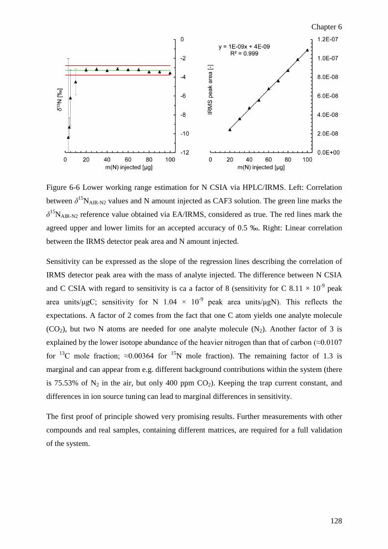
Chapter 6

128

Figure 6-6 Lower working range estimation for N CSIA via HPLC/IRMS. Left: Correlation

between δ15NAIR-N2 values and N amount injected as CAF3 solution. The green line marks the

δ15NAIR-N2 reference value obtained via EA/IRMS, considered as true. The red lines mark the

agreed upper and lower limits for an accepted accuracy of 0.5 ‰. Right: Linear correlation

between the IRMS detector peak area and N amount injected.

Sensitivity can be expressed as the slope of the regression lines describing the correlation of

IRMS detector peak area with the mass of analyte injected. The difference between N CSIA

and C CSIA with regard to sensitivity is ca a factor of 8 (sensitivity for C 8.11 × 10-9 peak

area units/μgC; sensitivity for N 1.04 × 10-9 peak area units/μgN). This reflects the

expectations. A factor of 2 comes from the fact that one C atom yields one analyte molecule

(CO2), but two N atoms are needed for one analyte molecule (N2). Another factor of 3 is

explained by the lower isotope abundance of the heavier nitrogen than that of carbon (≈0.0107

for 13C mole fraction; ≈0.00364 for 15N mole fraction). The remaining factor of 1.3 is

marginal and can appear from e.g. different background contributions within the system (there

is 75.53% of N2 in the air, but only 400 ppm CO2). Keeping the trap current constant, and

differences in ion source tuning can lead to marginal differences in sensitivity.

The first proof of principle showed very promising results. Further measurements with other

compounds and real samples, containing different matrices, are required for a full validation

of the system.

Chapter 6

129

6.5 Exemplary application of C and N CSIA using the HTC interface In an earlier paper[10] it was reported that δ13CVPDB data can be used to discriminate between

natural and synthetic caffeine with δ13C = -32‰ as threshold. This is in agreement with the

data gained in this work with the exception that the horizontal border line in Figure 6-7(a) lies

here at δ13C = -31‰. The δ15NAIR-N2 data gained in this study obviously are also suitable for

such a discrimination, shown by the vertical line at δ15N = -0.4‰ in Figure 6-7(a). However,

in both cases, the samples which are nearest to the border lines have only a very small

distance to these. Therefore, a bivariate approach using simultaneously both δ13CVPDB and

δ15NAIR-N2 values as discriminating variables was taken.[26,27] As a result of applying a Support

Vector Machine (SVM),[28] Figure 6-7(b) shows the line partitioning the data into natural and

synthetic samples. The partitioning was performed with the R[26]-package klaR[27] using the

program ‘partimat’ together with the method ‘svm’ which applies the support vector machine

SVM-Light.[28] Now the two types of caffeine are considerably more clearly distinguishable

because the samples which are nearest to this border line have a considerably larger distance

to this. Obviously, this bivariate approach makes the distinction between synthetic and natural

caffeine more robust. There may be also a chance for further distinction, e.g. regarding

geographical location, which is not possible with the aid of δ13CVPDB data alone.[29–31]

Figure 6-7 Two-dimensional graphs with δ13CVPDB plotted versus δ15NAIR-N2 values measured

by HPLC/IRMS. The two points in the upper right corner are natural caffeine samples CAF1

(IAEA-600[24,25]) and CAF6 (NATECO2) (green dots). The remaining six points are synthetic

caffeine samples (red diamonds). The black lines display the classification borders. (a)

Discrimination using either δ13C or δ15N values. (b) Bivariate discrimination using both δ13C

and δ15N values.

Chapter 6

130

6.6 Conclusions and outlook A novel system for compound-specific stable isotope analysis of carbon and nitrogen via

HPLC/IRMS was developed and its proof of principle demonstrated. Both carbon and

nitrogen can be measured with precision and trueness of ≤0.5‰. Lower working limit values

of 3.5 μgC for δ13C CSIA and 20 μgN for δ15N CSIA were achieved for caffeine, considering

an accuracy of ±0.5 ‰ as acceptable. The novel interface is carry over free and without

detectable compound-specific fractionation. No time-consuming sample preparation is

required and the system works in a fully automated fashion.

Future work needs to focus on further validation of the system with real samples and in

combination with other HPLC separation methods. Further method development should focus

on optimization of the interface, e.g. by bypassing the condenser and miniaturization of the

interface.

In summary, the described system offers the first possibility for δ15N CSIA via HPLC/IRMS

and together with C CSIA opens new opportunities for a wide range of stable isotope

applications in, among others, environmental and forensic research.

Chapter 6

131

6.7 References [1] M. A. Jochmann, T. C. Schmidt. Compound-specific Stable Isotope Analysis. The Royal


[2] J. McCullagh, J.-P. Godin, H. Schierbeek, T. Preston. Liquid Chromatography-Isotope

Ratio Mass Spectrometry Users Meeting, November 23-24, 2010, University of Oxford, UK.


[3] T. C. Schmidt, L. Zwank, M. Elsner, M. Berg, R. U. Meckenstock, S. B. Haderlein.

Compound-specific stable isotope analysis of organic contaminants in natural environments: a

critical review of the state of the art, prospects, and future challenges. Anal. Bioanal. Chem.

2004, 378, 283.

[4] S. Benson, C. Lennard, P. Maynard, C. Roux. Forensic applications of isotope ratio mass

spectrometry - A review. Forensic Sci. Int. 2006, 157, 1.

[5] N. NicDaeid, S. Jayamana, W. J. Kerr, W. Meier-Augenstein, H. F. Kemp. Influence of

precursor solvent extraction on stable isotope signatures of methylamphetamine prepared

from over-the-counter medicines using the Moscow and Hypophosphorous routes. Anal.

Bioanal. Chem. 2013, 405, 2931.

[6] N. Gentile, R. T. W. Siegwolf, P. Esseiva, S. Doyle, K. Zollinger, O. Delemont. Isotope

ratio mass spectrometry as a tool for source inference in forensic science: A critical review.

Forensic Sci. Int. 2015, 251, 139.

[7] N. NicDaeid, W. Meier-Augenstein, H. F. Kemp, O. B. Sutcliffe. Using Isotopic

Fractionation to Link Precursor to Product in the Synthesis of (±)-Mephedrone: A New Tool

for Combating “Legal High” Drugs. Anal. Chem. 2012, 84, 8691.

[8] E. O. Mogusu, J. B. Wolbert, D. M. Kujawinski, M. A. Jochmann, M. Elsner. Dual

element (15N/14N, 13C/12C) isotope analysis of glyphosate and AMPA by derivatization-gas

chromatography isotope ratio mass spectrometry (GC/IRMS) combined with LC/IRMS. Anal.

Bioanal. Chem. 2015, 407, 5249.





Chapter 6

132



[11] P. J. H. Dunn, N. V. Honch, R. P. Evershed. Comparison of liquid chromatography-

isotope ratio mass spectrometry (LC/IRMS) and gas chromatography-combustion-isotope

ratio mass spectrometry (GC/C/IRMS) for the determination of collagen amino acid δ13C

values for palaeodietary and palaeoecological reconstruction. Rapid Commun. Mass

Spectrom. 2011, 25, 2995.

[12] C. Decock, K. Denef, S. Bode, J. Six, P. Boeckx. Critical assessment of the applicability

of gas chromatography-combustion-isotope ratio mass spectrometry to determine amino sugar

dynamics in soil. Rapid Commun. Mass Spectrom. 2009, 23, 1201.

[13] L. Zhang, M. Thevis, T. Piper, M. A. Jochmann, J. B. Wolbert, D. M. Kujawinski, S.

Wiese, T. Teutenberg, T. C. Schmidt. Carbon Isotope Ratio Analysis of Steroids by High-

Temperature Liquid Chromatography-Isotope Ratio Mass Spectrometry. Anal. Chem. 2014,

86, 2297.

[14] E. Richling, C. Hoehn, B. Weckerle, F. Heckel, P. Schreier. Authentication analysis of

caffeine-containing foods via elemental analysis combustion/pyrolysis isotope ratio mass

spectrometry (EA-C/P-IRMS). Eur. Food Res. Technol. 2003, 216, 544.









Health Stud. 1996, 32, 275.

[18] Y. Teffera, J. J. Kusmierz, F. P. Abramson. Continuous-Flow Isotope Ratio Mass

Spectrometry Using the Chemical Reaction Interface with Either Gas or Liquid

Chromatographic Introduction. Anal. Chem. 1996, 68, 1888.

Chapter 6

133

[19] G. St-Jean. Automated quantitative and isotopic (13C) analysis of dissolved inorganic

carbon and dissolved organic carbon in continuous-flow using a total organic carbon analyser.









Spectrom. 2014, 28, 2574.

[22] M. Krummen, A. W. Hilkert, D. Juchelka, A. Duhr, H.-J. Schlüter, R. Pesch. A new

concept for isotope ratio monitoring liquid chromatography/mass spectrometry. Rapid


[23] B. W. Wenclawiak, M. Koch, E. Hadjicostas. Quality Assurance in Analytical

Chemistry. Springer, Berlin, 2004.

[24] T. B. Coplen, W. A. Brand, M. Gehre, M. Groning, H. A. J. Meijer, B. Toman, R. M.

Verkouteren. New Guidelines for δ13C Measurements. Anal. Chem. 2006, 78, 2439.

[25] M. Gehre. IAEA-600 natural caffeine; personal communication, November 9, 2015.

[26] R: A language and environment for statistical computing. (http://www.R-project.org/)

[27] C. Weihs, U. Ligges, K. Luebke, N. Raabe. klaR Analyzing German Business Cycles, in

Data Analysis and Decision Support. Springer, Berlin, 2005.

[28] SVM light (http://svmlight.joachims.org/)

[29] J. Dunbar, A. T. Wilson. Determination of Geographic Origin of Caffeine by Stable

Isotope Analysis. Anal. Chem. 1982, 54, 590.

[30] B. Weckerle, E. Richling, S. Heinrich, P. Schreier. Origin assessment of green coffee

(Coffea arabica) by multi-element stable isotope analysis of caffeine. Anal. Bioanal. Chem.

2002, 374, 886.

Chapter 6

134

[31] F. Serra, C. G. Guillou, F. Reniero, L. Ballarin, M. I. Cantagallo, M. Wieser, S. S. Iyer,

K. Heberger, F. Vanhaecke. Determination of the geographical origin of green coffee by

principal component analysis of carbon, nitrogen and boron stable isotope ratios. Rapid


Chapter 7

135

Chapter 7 General conclusions and outlook A trend in modern analytical chemistry is not only the identification and quantification of

analytes but also the determination of their isotope composition, e.g., to infer sources or fate

in the environment. In the work presented here stable isotope analysis (SIA) methods were

developed to measure δ13C and δ15N directly from aqueous solutions. Overcoming some of

the drawbacks, such as need of laborious sample preparation, this work resulted particularly

in the first system reported to be suitable for both δ13C and δ15N direct compound specific

stable isotope analysis (CSIA) of non-volatile compounds.

Dissolved organic carbon (DOC) plays a key role in carbon cycle investigations. A novel

HTC-based TOC/IRMS system was developed specially for DOC SIA. Standard uncertainty

of ≤0.2‰, the LOQSIA instr of 0.2 mgC/L and the oxidation efficiency of ≥99% confirm its

suitability for accurate DOC SIA and good analytical performance, in particular compared

with alternative methods[1,2]. To the best of our knowledge, this novel system is the only

HTC-based system that allows a 3-mL injection compared with a typical injection volume of

<200 μL.[3] This improvement alone resulted in an increase in sensitivity by a factor of 15.

With the developed system no laborious sample-preparation steps are necessary, such as time-

consuming offline preconcentration steps (e.g. freeze-drying) as they are needed using

EA/IRMS methods[2].

Good precision and accuracy were achieved for the δ13C analysis of a broad diversity of DOC

solutions. Good reproducibility (predominantly ≤0.5‰) was shown in the context of

international round robin testing for river and seawater samples. The HTC TOC/IRMS system

introduced in this thesis showed predominantly better performance compared to other

methods, such as wet chemical oxidation based methods. Similar averaged results were

achieved compared with other HTC TOC/IRMS methods. However, no proper comparison of

the performance was possible within the scope of this work, because in most cases

uncertainties achieved by each participant were not reported or, if reported, a notation how

uncertainties were assessed was missing. This system opens the possibility of a larger use of

certified or internationally accepted reference materials (solutions of low concentration) to

assure traceability and comparability among different laboratories. For the same reasons we

proposed a method for data treatment and evaluation of uncertainty, but an internationally

agreed method of validation still needs to be defined.

δ15N bulk stable isotope analysis (BSIA) in aqueous samples plays a significant role in many

fields of environmental research. A novel high-temperature based TOC-system was

Chapter 7

136

successfully extended to the possibility to measure also stable nitrogen isotope composition,

resulting, to the best of our knowledge, in the first system reported to be suitable for

simultaneous δ13C, δ15N BSIA in aqueous samples. No sample preparation is required and the

system works fully automated, in contrast to the established EA/IRMS based methods[4,5]. An

automated degassing unit and a zeolite adsorber based focusing unit are main innovations.

Complete conversion of nitrogen species to N2 was demonstrated using a broad range of

inorganic and organic nitrogen species. The system is carry over free and showed good

analytical performance, in particular in comparison to the reported methods for δ15N BSIA in

aqueous samples.[6-8] Further work needs to focus on investigation and quantification of the

background as well as blank contribution for stable nitrogen isotope measurements and on

validation of the system with real samples. Further method development should focus on

optimization e.g. by bypassing of the condenser and development of an automated blank and

background correction procedure. The described system offers new possibilities for

automated TNb SIA directly from aqueous solutions and in combination with simultaneous

DOC SIA opens new opportunities for a wide range of stable isotope applications in, among

others, soil science and limnology.

In the future two different main directions could be followed for further development of BSIA

methods of aqueous solutions. First, the existing system could be extended by flow injection

analysis (FIA) to enable automated SIA, not only of total nitrogen bound, but also of its

fractions, such as inorganic and organic nitrogen. Ammonium could be measured by

alkalization and purging out of ammonia into the HTC TOC system coupled to the IRMS

detector, then nitrate and nitrite could be reduced to ammonium before being treated as

described before. The remaining solution should contain dissolved organic nitrogen (DON)

only[9], which could then be than injected into the HTC TOC/IRMS system for DON SIA. A

second direction would be the further development of the HTC TOC based system to a

method suitable for sulfur BSIA in aqueous solutions, which is of high interest for

environmental scientists. Adjustment of the combustion conditions, ensuring no cold places

before water removal and removal of the condenser could be probably the steps to start with.

A direct method,without sample preparation, such as derivatisation needed in corresponding

GC/IRMS methods[10], for stable nitrogen isotope analysis (δ15N SIA) of non-volatile

compounds was successfully developed within this work. Both carbon and nitrogen can be

measured with precision and trueness of ≤0.5‰. Lower working limit values of 3.5 μgC for

δ13C CSIA and 20 μgN for δ15N CSIA were achieved for caffeine, considering an accuracy of

±0.5 ‰ as acceptable. This performance is suitable for natural abundance CSIA of non-

Chapter 7

137

volatile compounds, in particular compared to the alternative methods, such as derivatisation

followed by GC/IRMS for δ13C and δ15N determinations, with found precision and trueness

often exceeding 0.5‰.[11] The novel HTC based interface is carry over free and without

detectable compound-specific fractionation. This is an advantage compared to the commercial

wet chemical oxidation based systems, which are reported to suffer from the risk of isotope

fractionation[12,13]. No time-consuming sample preparation is required and the system works

in a fully automated fashion, which is a substantial advantage compared to the reported

EA/IRMS based methods for CSIA of polar compounds.[14] The described system offers the

first possibility for δ15N CSIA via HPLC/IRMS and together with δ13C CSIA opens new

opportunities for a wide range of stable isotope applications in, among others, environmental

and forensic research. Future work needs to focus on further validation of the system with real

samples and in combination with other HPLC separation methods. Further method

development should focus on optimization of the interface, e.g. by bypassing the condenser,

implementing of a degassing unit and miniaturization of the interface.

In an earlier paper[12] it was reported that δ13CVPDB data can be used to discriminate between

natural and synthetic caffeine. This is in agreement with the data gained in this work. The

δ15NAIR-N2 data gained in this study obviously are also suitable for such discrimination.

However, in both cases, the samples which are nearest to the border lines have only a very

small distance to these. A bivariate approach using simultaneously both δ13CVPDB and δ15NAIR-

N2 values as discriminating variables could successfully be taken to distinguish between those

two types of caffeine considerably more clear. Obviously, this bivariate approach makes the

distinction between synthetic and natural caffeine more robust and highlights the potential of

multi-element CSIA of non-volatile substances. There may be also a chance for further

distinction, e.g. regarding geographical location, which is not possible with the aid of

δ13CVPDB data alone. Applications which require currently derivatization followed by

GC/IRMS measurements due to the need of (additional) δ15N value are of potential interest to

be tested with the novel method, but in many cases suitable HT HPLC or IC separation

methods have to be developed first since only a few ones are yet available[15,16].

Further directions could involve the development of a HTC based interface for δ34S CSIA via

HPLC/IRMS. The focus could be on a continuous flow system, using one element but all

compounds properly separated in HPLC, or on a heart-cut system, using one compound but

for simultaneous multi-element SIA (CNS SIA). Both approaches are of interest in different

fields. For sure also a combination could be desirable, which could be realized via peak-

parking or fraction collection. A second interesting direction is the development of

Chapter 7

138

approaches to overcome the limitations in the eluent selection in HPLC/IRMS to water or

water based inorganic buffers. Hereby again two different ways could be followed: a

continuous flow mode with the interface capable to handle a certain amount of organic

solvent (N or S only) or a heart-cut mode, where a replacement of the organic solvent by

water or water buffer (solid-phase extraction based principle) or a thermal separation of

organic solvent from the analyte prior to injection into the interface takes place. The thermal

separation principle is analogous to that of the moving wire system[17] but without the need to

handle continuous flow its limitations, regarding limited capacity, depletion of semivolatile

compounds and flow restriction[11] can be avoided.

Chapter 7

139




[2] B. Fry, E. T. Peltzer, C. S. Hopkinson Jr, A. Nolin, L. Redmond. Analysis of marine DOC

using a dry combustion method. Mar. Chem. 1996, 54, 191.



Mar. Chem. 2007, 103, 318.

[4] S. D. Kelly, C. Stein, T. D. Jickells. Carbon and nitrogen isotopic analysis of atmospheric

organic matter. Atmos. Environ. 2005, 39, 6007.

[5] F. C. Batista, A. C. Ravelo, J. Crusius, M. A. Casso, M. D. McCarthy. Compound specific

amino acid δ15N in marine sediments: A new approach for studies of the marine nitrogen

cycle. Geochim. Cosmochim. Acta 2014, 142, 553.




[7] D. Huygens, P. Boeckx, J. Vermeulen, X. D. Paepe, A. Park, S. Barker, C. Pullan, C. O.

Van. Advances in coupling a commercial total organic carbon analyser with an isotope ratio

mass spectrometer to determine the isotopic signal of the total dissolved nitrogen pool. Rapid


[8] D. Huygens, P. Boeckx, J. Vermeulen, X. De Paepe, A. Park, S. Barker, O. Van Cleemput.

On-Line Technique to Determine the Isotopic Composition of Total Dissolved Nitrogen.

Anal. Chem. (Washington, DC, U. S.) 2007, 79, 8644.

[9] R. P. Axler, J. E. Reuter. A Simple Method for Estimating the 15N Content of Dissolved

Organic Matter (DO15N) in N-Cycling Studies. Can. J. Fish. Aquat. Sci. 1987, 44, 130.






Chapter 7

140














[16] D. M. Kujawinski, J. B. Wolbert, L. Zhang, M. A. Jochmann, D. Widory, N. Baran, T. C.

Schmidt. Carbon isotope ratio measurements of glyphosate and AMPA by liquid

chromatography coupled to isotope ratio mass spectrometry. Anal. Bioanal. Chem. 2013, 405,

2869.



Health Stud. 1996, 32, 275.

Chapter 8

141

Chapter 8 Appendix

Chapter 8

142

8.1 List of abbreviations and symbols ½Δδ half range δ-value [‰]

α fractionation factor [-]

Δ the difference of two values or the range of a set of values (context

defined by suffix)

δ13C SIA stable carbon isotope analysis

δ15N SIA stable nitrogen isotope analysis

δhEA, ref δ-value (expresses isotope composition) [‰]; E, chemical element

symbol; h, mass of the less abundant (heavier) isotope; A, analyte; ref,

reference material

δhEbl corr A for blank-’subtracted’ δ-value of an analyte A [‰]

δhElin corr A linearity corrected δ –value of an analyte A [‰]

δhEmeas A measured raw δ –value of an analyte A [‰]

�⃗�𝑣ion ion velocity [cm/s]

x(iE) the mole fraction of isotope iE [-]

A analyte

A peak area [-]

ACV Acetovanillone

Abl blank peak area [-]

Ameas A uncorrected peak area of an analyte A [-]

Ar(E) standard atomic weight [-]

Ar(iE) atomic weight of isotope iE [-]

Asaple A for blank-’subtracted’ peak area of an analyte A (Ameas A - Abl) [-]

avg average

𝐵𝐵�⃗ magnetic flux density vector [T]

Chapter 8

143

BSIA bulk stable isotope analysis

BAR barbituric acid

BEN benzoic acid

C3 vegetation plants that utilizes C3 carbon fixation pathway

C4 vegetation plants that utilizes C4 carbon fixation pathway

CAF caffeine

CAS casein

CF continuous flow

CIPM Comité International des Poids Mesures

CIT citric acid

CRDS cavity ring-down spectroscopy

CRI chemical reaction interface

CSIA compound-specific stable isotope analyses

DOC dissolved organic carbon

DIC dissolved inorganic carbon

DON dissolved total organic nitrogen

dow deep ocean water

EA elemental analyzer

EA/IRMS elemental analyzer/isotope ratio mass spectrometry

EI electron ionization

FIA flow injection analysis

�⃗�𝐹L Lorenz force [N]

fw fresh water

GC/IRMS gas chromatography/isotope ratio mass spectrometry

Chapter 8

144

GLU glutamic acid

HC heart cutting

HPLC/IRMS high performance liquid chromatography/isotope ratio mass

spectrometry

HTC high-temperature combustion

HTC TOC/IRMS high-temperature combustion total organic carbon analyzer, interfaced

with continuous flow isotope ratio mass spectrometer

HUM humic acid

I ion current [nA]

IC inorganic carbon

ID inner diameter

IMB isotope mass balance

IAEA international atomic energy agency

IRMS isotope ratio mass spectrometry

ISO International Organization for Standardization

IUPAC International Union of Pure and Applied Chemistry

k coverage factor

KIE kinetic isotope effect

LC liquid chromatography

LCM low concentration module (focusing unit)

LOQ limit of quantification [mg/L]

LR IRMS isotope ratio linearity of the isotope ratio mass spectrometer

M molecule

ma(iE) atomic mass of isotope iE [uatom m]

Chapter 8

145

MEL melamine

mlin slope of the linear regression; for LR IRMS [‰/nA]

m/z mass-to-charge ratio

n(p) number of different labs (participants) used for average and SD

calculations

n(r) number of replicate measurements used for average and SD calculations

N2-aq dissolved molecular nitrogen

NDIR detector nondispersive infrared detector

NPOC non-purgeable organic carbon

NVOC non-volatile organic carbon

POC purgeable organic carbon

PSIA position-specific stable isotope analyses

PtIC particulate total inorganic carbon

PtOC particulate non-purgeable organic carbon

PtON particulate total organic nitrogen

qion ion charge [C]

R isotope ratio [-]

R2 coefficient of determination

RG reference gas

RSD relative standard deviation

SD standard deviation

SDR reproducibility standard deviation

SIA stable isotope analysis

SUC sucrose

Chapter 8

146

sw sea water

TC total carbon

TDN total dissolved nitrogen

TIC total inorganic carbon

TINb total inorganic nitrogen bound

TIE thermodynamic isotope effect

TN total nitrogen

TOC total organic carbon

TON total organic nitrogen

TNb total nitrogen bound

U expanded uncertaity

uatom m unified atomic mass unit [≈ 1.660540210 × 10−27 kg]

ucomb combined uncertainty = ustd + lin corr+ bl corr + norm

ui intermediate state uncertainty (context defined by suffix)

UP water ultrapure, deionized water

ustd standard uncertainty = SD = 1σ (confidence interval 68.3%)

ustd + lin corr uncertainty containing standard uncertainty and contribution from

linearity correction

ustd + lin corr + bl corr uncertainty containing standard uncertainty and contribution from

linearity correction and blanc correction = uslb (abbreviation)

UV/Vis detector ultraviolet/visible spectroscopic detector

USGS United States geological survey

VOC volatile organic carbon

VPDB Vienna Pee Dee Belemnite

Chapter 8

147

WC-M worst case scenario model

WCO wet chemical oxidation

WO wet oxidation

Chapter 8

148

8.2 List of Figures Figure 1-1 Natural variations of stable carbon (right) and nitrogen (left) isotope composition

in selected materials. Isotope variations directly affect standard atomic weight interval. δ15N

and δ13C express the isotope composition. Adapted from.[4,15,7] Notes: (a) N2O in air

(troposphere), sea and ground water; (b) NOx from acid plant has an exceptional isotope

composition with δ15N of -150‰ (c) Marine sediments and compounds. ................................. 4

Figure 1-2 Functionality of an isotope ratio mass spectrometer (Background engineering

drawing (grey) of the figure is reproduced by permission of Isoprime, Manchester, UK).

Detailed ion source scheme is shown in Figure 1-3. ................................................................ 10

Figure 1-3 Ion source scheme. Note that the drawing is mirror-inverted in comparison to the

real ion source shown in Figure 1-2. Electron entrance aperture and trap aperture (located on

the upper and lower side of the ion box, respectively) are not shown. .................................... 11

Figure 1-4 Different sources of chemical species of C and N – an overview. Ellipses indicate

further subdivisions. ................................................................................................................. 12

Figure 1-5 Classification of dispersed carbon and nitrogen matter; (a) defined by International

Organization for Standardization (ISO) 8245[37]; (b) considering IUPAC recommendations[38];

(c) defined by ISO 12260[39]; In, e.g., soil-science studies TNb measured in aqueous samples is

often termed total dissolved nitrogen (TDN)[40,41] (d) volatile organic carbon (VOC) and non-

volatile organic carbon (NVOC) are often incorrectly set equal with POC and NPOC

respectively[42] and are not clearly distinguished within the norm.[37] A VOC is any organic

compound having a boiling point ≤250 °C[43], thus comprised out of compounds such as

benzene, toluene, cyclohexane and so one. Besides VOC, the purging process can remove

further compounds by a continuous shift of equilibrium (Le Châtelier principle). Thus VOC is

a part of POC. ........................................................................................................................... 13

Figure 1-6 Classification of SIA techniques. Optional bulk modification is for example

removal of total inorganic carbon (TIC) (via acidification and purging) prior to total organic

carbon (TOC) SIA. Without this modification the measurement would relate to total carbon

(TC) SIA. Also removal of the main matrix such as water (via lyophilisation) is a common

bulk modification technique in BSIA. ...................................................................................... 15

Figure 1-7 EA based technique. After the sample is brought into the solid form (offline

sample-preparation), it is introduced using an autosampler into the high-temperature (HT)

system. The combustion of the analyte is performed at high temperature (usually ≥600 °C) by

Chapter 8

149

oxygen and often supported by a catalyst and/or oxygen donor. Passing the reduction reactor,

He as a carrier gas transports the analyte and other contents (matrix) to the purification system

(often consisting of a dryer and a further filter). After the separation unit, analyses gases N2

and CO2, respectively, are directed by the He gas stream towards the optional concentration

detector, such as thermal conductivity detector (TCD) and subsequently towards the open

split connection of the isotope ratio mass spectrometer. .......................................................... 17

Figure 1-8 WCO TOC based technique. After the sample is introduced into the wet chemical

oxidation (WCO) based system, oxidation reagents (e.g., sodium persulfate) and buffer

solution are added. Highly reactive radicals are generated, e.g., by UV-photons. The formed

conversion product CO2 is purged out by He and transported to the purification system (often

consisting of a dryer and further filters). After the optional focusing unit (BSIA only),

analysis gas CO2 is directed towards the optional concentration detector, such as a

nondispersive infrared (NDIR) detector, and subsequently towards the open split connection

of the isotope ratio mass spectrometer. .................................................................................... 18

Figure 1-9 HTC TOC based technique. Aqueous samples are introduced using an autosampler

into the high-temperature combustion TOC-Analyzer. The combustion of the analyte is

performed at high temperature (usually ≥600 °C) by oxygen and often supported by a catalyst

and/or oxygen donor. He as a carrier gas transports the analyte and other contents (matrix) to

the purification system (often consisting of a condenser, dryer and further filters). After the

separation unit, analyses gases N2 and CO2, respectively, are directed by the He gas stream

towards the optional concentration detector, such as a NDIR detector and subsequently

towards the open split connection of the isotope ratio mass spectrometer. ............................. 19

Figure 2-1 Overview of the contents of this thesis ................................................................... 29

Figure 3-1 System setup for DOC SIA. ................................................................................... 36

Figure 3-2 Improvement of the crucible to optimize flow conditions. Crucibles and

corresponding peak shape before (a) and after (b) crucible optimization (slitted). ................. 40

Figure 3-3 Combustion tube filling (a) and non-thermal shock resistant carrier material before

optimization. The pellets are destroyed by the contact of the 850 °C hot catalyst with the

colder water vapor during sample injection (b). ...................................................................... 43

Figure 3-4 First test run (sucrose solutions, 1.5–100 μg C injected, 0.5–3 mg/L, 0.1–3 mL

injection volume): correlation between injected mass (mC, injected) and peak areas of the TOC

analyzer (ANDIR, TOC analyzer) (a) and correlation between isotope ratio mass spectrometer signals

Chapter 8

150

of coupled instruments (TOC analyzer and IRMS detector via an interface, IA) and peak areas

of the TOC analyzer (ANDIR, TOC analyzer) (b). ............................................................................. 44

Figure 3-5 Typical progression of a DOC SIA run (5 mg/L sucrose solution, 3-mL injection

volume). The TOC peak takes about 250 s (baseline to baseline) (a), whereas in the isotope

ratio mass spectrometer the peak width is just 40 s (b). By this setting a TOC concentration as

low as 0.2 mgC/L will produce an IRMS detector signal of >1 nA which can still be evaluated

properly. ................................................................................................................................... 44

Figure 3-6 Correlation between δ13C bias and δ13C difference between two subsequent

samples, with and without consideration of the first replicate (i.e. first injection).

Supplementary Table S 3-1 (Supporting Information) shows the chosen sequence as well as

results achieved in more details. .............................................................................................. 46

Figure 3-7 Correlation between δ13C values and isotope ratio mass spectrometer detector

signal (IA) before (measured: brown line and squares) and after (LR IRMS corrected: black line

and triangles) LR IRMS correction of citric acid (CIT2) solution (25–160 mgC/L). .................. 48

Figure 3-8 Evaluation inclusive blank correction (a). Correlation between δ13C values and C

concentration of caffeine (CAF2) solution (10–150 mgC/L) with proper (a) and with

simulated incorrect linearity and blank corrections (b). Measured: brown squares, LR IRMS

corrected: black triangles, blank corrected: green dots. In (b) an mlin of 0.006 ‰/nA leads to

better ustd of 0.15‰ after linearity correction and the blank correction seems to be false

because it makes the ustd even worse (0.25 ‰). This demonstrates how the interdependence of

blank and linearity correction can lead to misinterpretation and thus how important its proper

investigation is. ......................................................................................................................... 49

Figure 3-9 Correlation between δ13C values and C concentration of acetovanillone (ACV1)

solution (0.1–1.2 mgC/L) Measured: brown squares, LR IRMS corrected: black triangles, blank

corrected: green dots. Blank correction corrects the values-drift towards the stable isotope

composition of the blank (10.57‰) with decreasing concentration. SD from δ13C values at all

concentrations improves from 0.56‰ to 0.23‰ after the blank correction. Poor precision of

±2.18‰ (see error bars) at 0.1 mgC/L indicates instrumental limitation (avg. IA = 0.31 nA). 51

Figure 3-10 Deviation (Δ) of all single δ13C-values from their respective true value (y axis)

plotted against concentration (x axis). The scattering of the values represents the repeatability

of stable isotope measurements at the corresponding concentration with the chosen method. 51

Chapter 8

151

Figure 3-11 Carbon concentration values at lower carbon concentration range; (a)

Investigation of the dependence of DOC concentration (y axis, NDIR Area from TOC

analyzer) on its repeatability (x axis, number of measurements). The blank corrected NDIR

areas are normalized to the injection volume of 1 mL and concentration of 1 mgC/L to enable

comparability and they are plotted against measuring order (five replicates of each

concentration: 0.1, 0.2, 0.4, 0.6 and 1.2 mgC/L with 4 different compounds each and using 3,

2 and 1 mL injection). (b) All estimated relative uncertainties (y axis) plotted against the DOC

concentration (x axis). Instrumental caused uncertainty (uinstr = ustd, green triangles),

combined uncertainty implementing sample-preparation caused error (uinstr + sample prep, brown

dots) and combined uncertainty implementing also error caused by data evaluation (uinstr +

sample prep + bl corr, blank squares). ................................................................................................. 52

Figure 4-1 Concept for dealing with measurement uncertainty (redrawn from Neidhart et

al.)[19] ........................................................................................................................................ 77

Figure 4-2 Visualization of principle to compare two values based on coverage through

uncertainties ............................................................................................................................. 85

Figure 4-3 Exemplary results of the round robin test for a lake sample (left) und a marine

sample (right). Average and standard deviation for n(p) different labs using the same method

are shown (if n(p)>1). Average and standard deviation for n(r) replicate measurements of own

results (participant (a)) and for cases were only one participant has used a certain method

(n(p)=1) are shown. Wet oxidation coupled with cavity ring-down spectrometer (WO/CRDS)

was not used for DOC measurements in sea water. Expected range is shown only for the lake

sample (for sea water sample sw iv not available). For cases with more than one participant,

no standard deviations of replicate measurements achieved by different labs using the same

method were provided. ............................................................................................................. 85

Figure 4-4 Excerpt from the data obtained with various natural DOC samples (redrafted from

Kirkels et al.)[7] ......................................................................................................................... 86

Figure 4-5 System setup for TIC SIA (simplified graph focusing on main principles). 0.05 to

3 mL of sample is injected in the sparger automatically via a syringe from an autosampler (not

shown in the graph). Acid is added to the sample via an acid pump (not shown in the graph) to

achieve a pH of ca. 2. Helium as a carrier gas is added via a mass flow controller, mixes the

reactant with the sample in the reaction side in the sparger and provides the evaluated CO2 to

the purification system. The purification system consists of condenser, membrane dryer

(Nafion®), chemical dryer (Sicapent®) and a halogen scrubber. After purification, the gas,

Chapter 8

152

passing the flow meter and NDIR detector enters the focusing unit with an adsorption column.

Using high heating rates the CO2 is rapidly focused desorbed and transported by helium gas

towards the isotope ratio mass spectrometer for stable isotope composition measurement. ... 87

Figure 5-1 Test series with TNb solutions (10 to 80 mgN/L as CAF2 solutions); Without (a)

and with (b) membrane-based on-line degassing unit (b). ..................................................... 100

Figure 5-2 Focusing of nitrogen peak. Schematic few of the focusing unit (a). Focusing

performance (174.6 mgN/L solution; adsorption temperature -38 °C; desorption temperature

100 °C; heating rate 3.4 °C/s; an EA analyzer was connected behind the focusing unit in order

to record the TCD signal) (b): nitrogen peak without focusing (peak height 167 TCD units)

(i); nitrogen peak using focusing unit with adsorption material EAS-MS-10A-PF (peak height

1064 TCD units) (ii); nitrogen peak using focusing unit with adsorption material EAS-MS-

5A-45/60M (peak height 1690 TCD units) (iii). .................................................................... 101

Figure 5-3 System setup for HTC TOC/IRMS BSIA. ........................................................... 102

Figure 5-4 Test series to investigate the carry over effect. Shown data are referenced to the

working gas only. ................................................................................................................... 103

Figure 5-5 Least-squares linear regressions between true values and HTC TOC/IRMS

measured values for nitrogen. Error bars represent the standard deviation of each sample.

Error bars are typically smaller than symbol sizes. δ15N values are referenced to AIR-N2 scale.

................................................................................................................................................ 104

Figure 5-6 Working range investigation test series; orange lines mark upper and lower

uncertainty interval defined as good (U ≤ 0.5‰) and indicate a nitrogen concentration of 40

mgN/L as the lowest concentration within that interval; red lines mark upper and lower

uncertainty interval defined as sufficient (U ≤ 1.0‰) and indicate 5 mgN/L as the lowest

concentration within that interval. Concentration of 2.5 mgN/L could not be measured with

the accepted accuracy (insufficient; U ≥ 1.0 ‰). ................................................................... 106

Figure 5-7 Typical HTC TOC/IRMS run in simultaneous δ13C, δ15N SIA mode. (a) TOC run

course; black line: NDIR cell CO2 signal; dark blue line: temperature of the restriction heater

(RH) of the N2 adsorption column; light blue line: temperature of the peltier element (PE) of

the N2 adsorption column; red line: temperature of the restriction heater (RH) of the CO2

adsorption column; green line: flow of the carrier gas helium controlled by the mass flow

controller (MFC). (b) IRMS run course: black line: m/z 28 signal with the sample peak at ca.

Chapter 8

153

500 s and the reference gas pulse at ca. 75 s; blue line: m/z 44 signal with the sample peak at

ca. 780 s and the reference gas pulse at ca. 980 s. ................................................................ 108

Figure 6-1 System setup for HPLC/IRMS CSIA ................................................................... 117

Figure 6-2 Transfer of the mobile phase into the combustion tube of the interface. (a)

Injection beam related issues and solution: (i) Droplet formation leads to peak fission. (ii) Jet

spread beam leads to condensation of fine droplets touching the colder part of the combustion

tube of the interface and thus causes tailing and carry over. (iii) Solution: collimated beam

injection (iii). (b) Schematic view of the collimated beam transfer system (injection device).

................................................................................................................................................ 122

Figure 6-3 HPLC/IRMS run chosen to describe the typical HTC interface performance

regarding the peak shape. Left: HPLC detector (UV250, green) and IRMS detector (m/z 28,

black and m/z 29, blue) signal curves. UV250 scale range is represented by the secondary

ordinate. Note that the two flat IRMS detector peaks at the beginning and end of the run are

in-house reference gas pulses. The signal between them is the sample peak. The IRMS signal

appears delayed relative to the HPLC sample peak due to the additional time needed to pass

the interface volume. No significant fronting or tailing could be observed. Right: Shifting of

the HPLC detector signal curve (UV250) on the time scale to overlap the sample peak with

that of the IRMS detector signal curve (m/z 28). Magnification and the additional removal of

the m/z 29 IRMS detector signal curve enable better observation of the significant lower peak

part. ......................................................................................................................................... 124

Figure 6-4 Least-squares linear regressions between EA/IRMS and HPLC/IRMS δ-values for

carbon and nitrogen. The green dashed line (1:1 line) indicates the ideal estimation, and the

solid line corresponds to the regression equation Line. Error bars represent the standard

deviation of each sample. Left: δ13C values are all referenced to the VPDB scale. Right: δ15N

values are referenced to the AIR-N2 scale. ............................................................................ 126

Figure 6-5 Lower working range estimation for C CSIA via HPLC/IRMS. Left: Correlation

between δ13CVPDB values and C amount injected as CAF3 solution. The green line marks the

δ13CVPDB reference value obtained via EA/ IRMS, considered as true. The red lines mark the

agreed upper and lower limits for an accepted accuracy of 0.5‰. Right: Linear correlation

between the IRMS detector peak area and C amount injected. .............................................. 127

Figure 6-6 Lower working range estimation for N CSIA via HPLC/IRMS. Left: Correlation

between δ15NAIR-N2 values and N amount injected as CAF3 solution. The green line marks the

Chapter 8

154

δ15NAIR-N2 reference value obtained via EA/IRMS, considered as true. The red lines mark the

agreed upper and lower limits for an accepted accuracy of 0.5 ‰. Right: Linear correlation

between the IRMS detector peak area and N amount injected. ............................................. 128

Figure 6-7 Two-dimensional graphs with δ13CVPDB plotted versus δ15NAIR-N2 values measured

by HPLC/IRMS. The two points in the upper right corner are natural caffeine samples CAF1

(IAEA-600[24,25]) and CAF6 (NATECO2) (green dots). The remaining six points are synthetic

caffeine samples (red diamonds). The black lines display the classification borders. (a)

Discrimination using either δ13C or δ15N values. (b) Bivariate discrimination using both δ13C

and δ15N values. ..................................................................................................................... 129

Chapter 8

155

8.3 List of supplementary Figures Figure S 3-1 LR IRMS correction using acetovanillone solution (25-160 mgC/L) ..................... 64

Figure S 3-2 LR IRMS correction using caffeine solution (25-160 mgC/L) ............................... 64

Figure S 3-3 Blank correction using acetovanillone solution (10-150 mgC/L) ....................... 66

Figure S 3-4 Blank correction using citric acid solution (10-150 mgC/L) .............................. 66

Figure S 3-5 The graph shows an additional indication for absence of considerable

instrumental blank coming from e.g. washing out effect within the combustion tube. The

amount of carbon, represented by the peak-area of NDIR, of the blank is independent of the

amount or contact time (injection speed) of the water vapor. Varying injection volume and

speed a constant NDIR peak area of 1129 ± 22 units per mL blank sample was found. ......... 68

Figure S 3-6 Simplified visualization of uncertainty evolution; Instrument shows significant

contribution below 0.2 mgC/L (observed ustd at 0.1 mgC/L > 2%); above 0.2 mgC/L a sample-

preparation increases the uncertainty substantially and became a limiting factor (variations

form vial to vial of the same sample); Generally to expect is even larger contribution to

combined uncertainty coming from sampling itself. ................................................................ 68

Chapter 8

156

8.4 List of Tables Table 3-1 Current methods for determination of stable isotope composition of DOC. ........... 34

Table 3-2 Different sources of uncertainty and their quantities for different concentrations (4

samples and 3 replicates each); Instrumental caused uncertainty (uinstr = ustd), combined

uncertainty implementing sample-preparation caused error (uinstr + sample prep) and combined

uncertainty implementing also evaluation caused error (uinstr + sample prep + bl corr); Note that the

high relative deviations are still small absolute ones. 0.7% in brackets shows the average

without 0.1 mgC/L sample justifying LOQinstr of 0.2 mgC/L .................................................. 53

Table 3-3 Trueness of the method expressed as difference between the true and measured

value ......................................................................................................................................... 55

Table 3-4 Classification of potential problems and interferences related to DOC

measurements in aqueous samples ........................................................................................... 57

Table 4-1 Data set including uncertainties assessed for DOC SIA .......................................... 81

Table 4-2 Comparison of own results against expected values in round robin test ................. 84

Table 5-1 Trueness test with different species expressed as difference between true and

measured value ....................................................................................................................... 105

Table 6-1 Comparison of true and via HPLC/IRMS obtained δ-values for different species 123

Table 6-2 Accuracy (trueness and precision) estimation of δ-values .................................... 126

Chapter 8

157

8.5 List of supplementary Tables Table S 3-1 Sequence, single values of replicates and calculated parameters from the test

series to investigate carry over. ................................................................................................ 63

Table S 3-2 Plausibility considerations a: Correction starts to matter (exceeding bias of 0.2

‰); considering worst case: high blank and large delta difference: aqueous solution; b: Bias

falsely considering no instrumental blank (exceeding bias of 0.5‰): real sample .................. 65

Table S 3-3 Different sources of uncertainty and their quantities for different concentrations

(4 samples; 3 replicates each) and different injection volumes; Instrumental caused

uncertainty (uinstr = ustd), combined uncertainty implementing sample-preparation caused error

(uinstr + sample prep) and combined uncertainty implementing also evaluation caused error (uinstr +

sample prep + bl corr); Note that the high relative deviations are still small absolute ones. 0.7% in

brackets shows the average without 0.1 mgC/L sample justifying LOQinstr of 0.2 mgC/L ..... 67

Table S 4-1 Demonstration of the principle used to assess uncertainty ................................... 92

Chapter 8

158

8.6 Curriculum vitaeDer Lebenslauf ist in der Online-Version aus Gründen des Datenschutzes nicht enthalten.

mailto:[email protected]

Chapter 8

159

Chapter 8

160

8.7 List of Publications

8.7.1 Manuscripts

1. Eugen Federherr, Sarah Willach, Natascha Roos, Lutz Lange, Karl Molt, Torsten C.

Schmidt: A novel high temperature combustion interface for compound-specific stable

isotope analysis of carbon and nitrogen via HPLC/IRMS Rapid Communications in Mass

Spectrometry, 30 (7), (2016), 944-952 (peer-reviewed international journal)

2. Eugen Federherr, Chiara Cerli, Frédérique M. S. A. Kirkels, Karsten Kalbitz, Hans J.

Kupka, Ralf Dunsbach, Lutz Lange, Torsten C. Schmidt Analyse der stabilen

Isotopenzusammen-setzung des gelösten organischen Kohlenstoffs in wässrigen Proben Vom

Wasser, 113 (2015), 56-59 (non peer-reviewed journal)

3. Eugen Federherr, Hans J. Kupka, Lutz Lange, Hans P. Sieper Verfahren und Vorrichtung

zur Analyse von Stickstoff (N) in einer Probe DE102014002266 B3 & EP2919005 A1

(patent)

4. Eugen Federherr, Chiara Cerli, Hans J. Kupka, Almut Loos, Ralf Dunsbach, Lutz Lange

Torsten C. Schmidt Dem Ursprung auf der Spur Laborpraxis, Dezember (2014) 52-54 (non

peer-reviewed journal)

5. Eugen Federherr, Chiara Cerli, Frédérique M. S. A. Kirkels, Karsten Kalbitz, Hans J.

Kupka, Ralf Dunsbach, Lutz Lange, Torsten C. Schmidt: A novel high-temperature


samples. I: development and validation Rapid Communications in Mass Spectrometry, 28

(23) (2014), 2559-2573 (peer-reviewed international journal)

6. Frédérique M. S. A. Kirkels, Chiara Cerli, Eugen Federherr, Jiajia Gao, Karsten Kalbitz:

A novel high-temperature combustion based system for stable isotope analysis of dissolved

organic carbon in aqueous samples. II: optimization and assessment of analytical performance

Rapid Communications in Mass Spectrometry, 28 (23) (2014), 2574-2586 (peer-reviewed

international journal)

7. Thomas Piper, Karoline Degenhardt, Eugen Federherr, Andreas Thomas, Mario Thevis,

Martial Saugy: Effect of changes in the deuterium content of drinking water on the hydrogen

isotope ratio of urinary steroids in the context of sports drug testing Analytical and

Bioanalytical Chemistry, 405 (9) (2013), 2911-2921 (peer-reviewed international journal)

Chapter 8

161

8. Lijun Zhang, Dorothea M. Kujawinski, Eugen Federherr, Torsten C. Schmidt, Maik A.

Jochmann: Caffeine in Your Drink: Natural or Synthetic? Analytical Chemistry, 84 (6)

(2012), 2805-2810 (peer-reviewed international journal)

8.7.2 Presentations (first author contributions only)

Scientific conferences

2015, Wasser (German water chemistry society - annual meeting), Stable isotope analysis

(SIA) of carbon and nitrogen in waters and aqueous solutions, Schwerin (Oral presentation)

2014, ASI (German Association for Stable Isotope Research – annual meeting), Total

Dissolved Matter Analyzer - novel tool for carbon and nitrogen stable isotope analyses in

aqueous samples, München, (Oral presentation)

2014, BIOGEOMON (International Symposium on Ecosystem Behavior), Novel tool for

δ13C and δ15N determination in aqueous samples, Bayreuth, (Poster)

2013, ANAKON (analytical conference), A novel method for stable isotope analysis of

dissolved organic carbon in the trace range in aqueous samples, Essen, (Oral presentation)

2012, JESIUM (Joint European Stable Isotope Users Group Meeting), Ultralow

concentration TOC stable isotope measurements, Leipzig, (Oral presentation)

Scientific conferences (presented by a co-author)

2015, BASIS (Benelux Association of Stable Isotope Scientists – annual meeting) (Oral

presentation); 2015, AIG-11 (Applied Isotope Geochemistry Conference) (Oral

presentation); 2014, AGU (American Geophysical Union Fall Meeting) (Poster)

Chapter 8

162

8.8 Erklärung Hiermit versichere ich, dass ich die vorliegende Arbeit mit dem Titel

„Stable carbon and nitrogen isotope analysis in aqueous samples – method development,

validation and application”

selbst verfasst und keine außer den angegebenen Hilfsmitteln und Quellen benutzt habe, und

dass die Arbeit in dieser oder ähnlicher Form noch bei keiner anderen Universität eingereicht

wurde.

Essen, April 2016

Eugen Federherr

Stable carbon and nitrogen isotope analysis in aqueous ...

Documents