Stabilizing effect of random waves on rip currents

Stabilizing effect of random waves on rip currents

Haider Hasan,1,2 Nicholas Dodd,1 and Roland Garnier1,3

Received 18 July 2008; revised 16 February 2009; accepted 16 April 2009; published 9 July 2009.

[1] The instability leading to the formation of rip currents in the nearshore for normalwaves on a nonbarred, nonerodible beach is examined with a comprehensive linearstability numerical model. In contrast to previous studies, the hypothesis of regular waveshas been relaxed. The results obtained here point to the existence of a purelyhydrodynamical positive feedback mechanism that can drive rip cells, which is consistentwith previous studies. This mechanism is physically interpreted and is due to refractionand shoaling. However, this mechanism does not exist when the surf zone is not saturatedbecause negative feedback provided by increased (decreased) breaking for positive(negative) wave energy perturbations overwhelms the shoaling/refraction mechanism.Moreover, turbulent Reynolds stress and bottom friction also cause damping of the ripcurrent growth. All the nonregular wave dissipations examined give rise to thesehydrodynamical instabilities when feedback onto dissipation is neglected. When thisfeedback is included, the dominant effect that destroys these hydrodynamical instabilitiesis the feedback of the wave energy onto the dissipation. It turns out that this effect isstrong and does not allow hydrodynamical instabilities on a planar beach to grow forrandom seas.

Citation: Hasan, H., N. Dodd, and R. Garnier (2009), Stabilizing effect of random waves on rip currents, J. Geophys. Res., 114,

C07010, doi:10.1029/2008JC005031.

1. Introduction

[2] Normally incident waves approaching a straightshoreline shoal and eventually break. This generates set-up(increased elevation in mean free surface), through radiationstresses [Longuet-Higgins and Stewart, 1962, 1964], andtherefore also offshore directed horizontal pressure gradients.In theory this dynamical balance can pertain along analongshore uniform shore with correspondingly uniformwave conditions. In reality water is often seen to recirculateback to sea at certain locations, in rip currents, which are, inturn, fed by alongshore flowing currents on either side.[3] Studies have shown that rip currents may approach

speeds of up to 2 m s�1 [see MacMahan et al., 2006],although the average strength is often less than that. Thesecirculations therefore can become an issue for beach safety[see Short and Hogan, 1994]. Nearshore circulation alsoresults in the circulation of cleaner water from the offshoreinto the nearshore region [see Inman et al., 1971]. Impor-tantly, nearshore circulation together with waves also trans-port beach sediment, and indeed the rips themselvesapparently erode rip channels. Hence it is vital to understand

the physical mechanisms of the generation of rip currents ifwe are to understand the nearshore sediment budget. It shouldbe noted, however, that it is not clear whether these channelsare passively eroded by the currents, or if the channels appearin combination with the currents as part of a dynamicalinteraction. We return to this point later.[4] On a long straight coast, rip currents can occur at

quite regular intervals so one can often assign an alongshorespacing to these features, which ranges from 50 to 1000 m[Short, 1999], and as reported by Short [1999], rip currentsare most readily formed on intermediate energetic beachescharacterized by slopes of 1:30 to 1:10. This quasi-regularityin spacing of rip currents is intriguing, and has received someattention in previous studies.[5] Early observational studies of rip currents in the field

such as that made by Shepard et al. [1941] and Shepard andInman [1950], and more recent ones by Brander and Short[2000] andMacMahan et al. [2005], have found rip currentsto occur where there are alongshore variations in thebathymetry with rip channels cut through the alongshorebar. This alongshore variation in the bathymetry results in anaccompanying variation in wave height. These wave heightvariations generate alongshore variable pressure gradientsthat drive nearshore circulation cells. Experimental studies inlaboratories have also supported this idea where measure-ments were conducted for a barred beach profile with incisedrip channels [see Haller et al., 2002; Haas and Svendsen,2002]. Using the concept of radiation stresses, Bowen [1969]showed that nearshore circulation cells, including rips, can beforced by imposing alongshore variations in wave height on aplane sloping beach for waves normal to the shoreline. Thealongshore variation in wave height results in corresponding

JOURNAL OF GEOPHYSICAL RESEARCH, VOL. 114, C07010, doi:10.1029/2008JC005031, 2009ClickHere

for

FullArticle

1Environmental Fluid Mechanics Research Centre, Process andEnvironmental Division, Faculty of Engineering, University of Nottingham,Nottingham, UK.

2Now at Department of Mathematics and Basic Sciences, NED

University of Engineering and Technology, Karachi,Pakistan.

3Now at Applied Physics Department, Universitat Politecnica deCatalunya, Barcelona, Spain.

Copyright 2009 by the American Geophysical Union.0148-0227/09/2008JC005031$09.00

C07010 1 of 14

http://dx.doi.org/10.1029/2008JC005031

variations in radiation stresses, thus driving the circulationcells as areas of large set-up (large wave height) drive acurrent alongshore into the rips.[6] The model of Bowen [1969], however, does not

explain the quasiperiodicity itself, and nor does it consideran erodible beach. Attention has therefore subsequentlybeen focused on examining the stability to periodic pertur-bations of alongshore uniform setup on an erodible beach,namely, the morphodynamical stability. The pioneeringstudy of Hino [1974] identified such an instability, and,for normal incident waves, rip currents/channels were formedtogether with cuspate morphological features when an along-shore periodic perturbation was imposed. This theory wassubstantially progressed by Deigaard et al. [1999] and aninstability mechanism identified by Falques et al. [2000],who noted that the potential stirring (depth-averaged con-centration) gradient governed the positive feedback mech-anism by which the rips and their associated morphologyevolve. Thus, for an offshore flowing current (the rip), anynegative perturbation (the incipient rip channel) will beenhanced (positive feedback, and therefore instability)where the concentration is increasing offshore, becausethe current flows from regions of lower to greater concen-tration, so that erosion must take place for the concentrationprofile to be maintained. Studies with more comprehensivemodels have been presented by Damgaard et al. [2002],Caballeria et al. [2002], Calvete et al. [2005], and Garnieret al. [2006].[7] These explanations have focused onmorphodynamical

instability. However, it has also been suggested that along-shore variations in wave height may arise as a result of wave -current interaction, which poses the question about theformation of rip channels alluded to earlier: do channelsand currents form together as a morphodynamical instabil-ity, or do rip currents form as a hydrodynamical instabilityand then erode the channels. The episodic nature of ripcurrents observed by Smith and Largier [1995] at Scrippsbeach possibly indicates that rip currents are a result of ahydrodynamic instability, but these events could also bedue to temporal variations in the incoming wavefield[Reniers et al., 2004]. Field evidence of rip currents withoutchannels is hard to find. MacMahan et al. [2006] note thatall currents are accompanied by perturbations in the bedlevel, albeit small ones at some locations. The laboratoryinvestigation by Bowen and Inman [1969] on a plane slopingbeach found rip currents generated as a result of the interac-tion between edge waves and incoming incident waves, withrip spacing equal to (and therefore dictated by) the alongshorewavelength of the edge wave. Nevertheless, some otherstudies have continued to consider the purely hydrodynam-ical instability (or something akin to this) to investigatewhether rip currents can be formed without perturbations inthe bed.[8] The analytical study of Dalrymple and Lozano [1978],

who extended the work of LeBlond and Tang [1974],suggested that wave refraction and shoaling (as opposed toshoaling alone) was responsible for the existence of ripcurrents. The authors considered normally incident waveson a planar foreshore of constant slope and a flat offshorebathymetry, on which they imposed an alongshore periodicperturbation (neither growing nor decaying), and noted that

the interaction of the wavefield with the offshore currents actsto intensify them.[9] For incoming waves normal to the shoreline, Falques

et al. [1999] examined the growth of nearshore circulationcells (rip cells) using linear stability analysis (thus allowinggrowing modes) on a non-erodible, plane beach. Two caseswere considered. The first was set-up in isolation; that is,waves were normally incident on a monotonic beach andwave refraction because of current neglected. An analyticalanalysis showed that the set-up did not induce instability.The subsequent inclusion of wave refraction on current, thesecond case, led to instability. Here Falques et al. [1999]considered a simplistic situation in which waves approachedover a flat bathymetry, and perturbations in wave energydissipation due to wave breaking were neglected. The flatbed was chosen so as to avoid dealing with wave breakingand the discontinuities at the breaking line, and to allow theapplication of shallow water theory throughout.[10] An alternative hydrodynamical rip current study was

made by Murray and Reydellet [2001]. The focus of theirstudy was on self-organized rip currents driven by a feedbackinvolving a newly hypothesized interaction between wavesand currents, in which the rip current causes a diminution inwave height, through turbulence generated by shears inorbital velocities. This would then lead to reduced shorelineset-up, now no longer balanced because of decrease in waveheight, which then leads to alongshore flows into the rip. Asimple model with effects of currents on wave number fieldnot included was developed on the basis of cellular automatawhere each variable defined in a particular cell in a grid ofcells interacted according to rules encapsulating the abovephysics, which then indeed led to a positive feedback thatintensified the current [see Murray and Reydellet, 2001].[11] Yu [2006] examined the growth of rip current cells

due to the inclusion of wave-current interactions. This wasmotivated by the uncertainties in the results obtained byDalrymple and Lozano [1978].[12] Assuming monochromatic waves, Yu [2006] split the

cross-shore domain into an offshore part (prior to breaking)

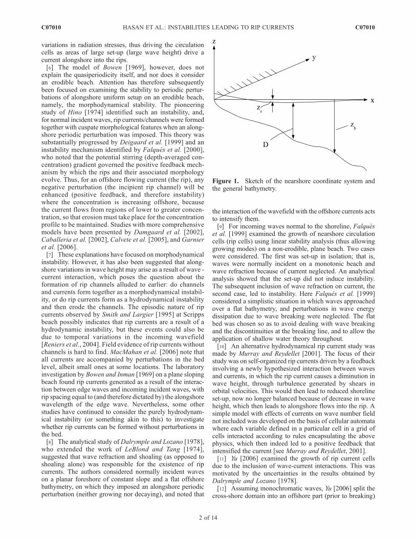
Figure 1. Sketch of the nearshore coordinate system andthe general bathymetry.

C07010 HASAN ET AL.: INSTABILITIES LEADING TO RIP CURRENTS

2 of 14

C07010

mostly on constant depth and therefore allowing shallowwater theory to be used in the offshore portion of thedomain, and a part in the surf zone (plane beach). Beforebreaking a wave energy equation is implemented to trans-form wave height; within the surf zone the wave height iscontrolled by the local water depth. The break point occurson the slope, and a moving shoreline is implemented.[13] For an offshore wave height H1 of 1.88 m and

period T = 8.17 s Yu [2006] predicts a growing ‘‘rip cell’’mode with e-folding time 14.83 s. This increased rapidly forsmaller wave heights: H1 = 1.12 m possessed an e-foldingtime of 97.20 s. The comparison of predicted rip-spacingwith field observations showed fairly good agreement forlarge wave breaker heights. However, for smaller breakerheights the agreement was poor. For more details, see Yu[2006].[14] The idealized nature of the study of Falques et al.

[1999] and the more sophisticated but still restricted (e.g.,shallow water theory and the use of regular waves) study of

Yu [2006], thus leads us to re-examine the hydrodynamicalinstability to alongshore periodic disturbances of normallyincident waves on a plane beach, but this time using acomprehensive model incorporating finite depth wavepropagation and random waves. To this end we investigatethe possible formation of rip cells under more realisticconditions (random waves) using the model of Calvete etal. [2005], which also includes other effects (e.g., turbu-lent Reynolds stresses) not considered by the earlierauthors.[15] In section 2, we describe the model used in the

present study. In section 3, we show results for the numer-ical investigations. Thereafter we draw some conclusions.

2. Model Description

[16] The model used here is described in detail by Calveteet al. [2005]. It is based on the depth and time averagedmass (1) and momentum (2) equations and wave energy (3),

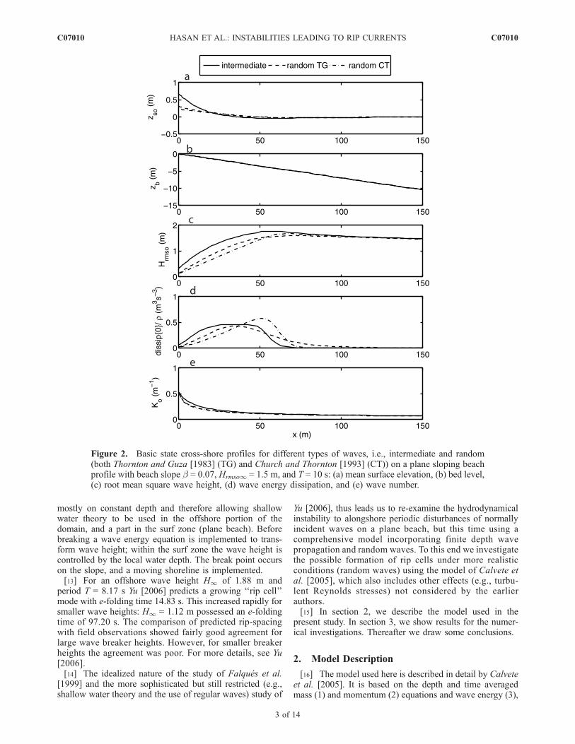
Figure 2. Basic state cross-shore profiles for different types of waves, i.e., intermediate and random(both Thornton and Guza [1983] (TG) and Church and Thornton [1993] (CT)) on a plane sloping beachprofile with beach slope b = 0.07, Hrmso1 = 1.5 m, and T = 10 s: (a) mean surface elevation, (b) bed level,(c) root mean square wave height, (d) wave energy dissipation, and (e) wave number.


3 of 14

C07010

wave phase (4), and sediment conservation equations. Sincewe are examining hydrodynamical instabilities we do notconsider the sediment conservation equation here. Thegoverning equations are

@D

@tþ @Dvi

@xi¼ 0; ð1Þ

@vi@t

þ vj@vi@xj

¼ �g@zs@xi

� 1

rD@

@xjS0ij � S00ij

� �� tbirD

; ð2Þ

@E

@tþ @

@xivi þ cgi� �

E� �

þ S0ij@vj@xi

¼ �D; ð3Þ

@F@t

þ s þ vi@F@xi

¼ 0; ð4Þ

where i, j = 1, 2, so xi = (x1, x2) = (x, y), where x and y arecross-shore and alongshore coordinates. Horizontal veloci-ties are vi = (v1, v2) = (u, v), g is acceleration due to gravity andr is water density. Total water depth is denoted D = zs � zb,where zs is the mean surface elevation and zb is the (fixed)bed level: see Figure 1. Further, E = 1

8rgHrms

2 is wave energydensity, where Hrms is root mean squared wave height, F isthe wave phase, S0ij are the components of the radiationstress tensor, S00ij are the Reynolds stress tensor compo-nents, tbi is the ith component of the bottom friction, D isthe dissipation due to wave breaking, and cgi are the group

velocity vector components. s is the intrinsic frequencygiven by

s ¼ffiffiffiffiffiffiffiffiffiffiffiffiffiffiffiffiffiffiffiffiffiffiffiffiffiffigK tanh KDð Þ

p; ð5Þ

whereK is the wave number (K = j~Kj). The wave vector~K isgiven by ~K = ~rF.[17] The expression for the Reynolds’ stresses applied

here is [see, e.g., Svendsen, 2006]

S00ij ¼ rntD@vi@xj

þ @vj@xi

� �; ð6Þ

where the Battjes [1975] parameterization for horizontaleddy viscosity has been implemented

nt ¼ MDr

� �13

Hrms; ð7Þ

where M is a parameter that characterizes turbulence and isof O(1). Calvete et al. [2005] choose M = 1 [Battjes, 1975].However, Svendsen et al. [2002] recommended 0.05 < M <0.1. Here we take a default value M = 0.5. Bed shear stressis parameterized using a linear friction law:

tbi ¼ r2

p

� �CDurmsvi; ð8Þ

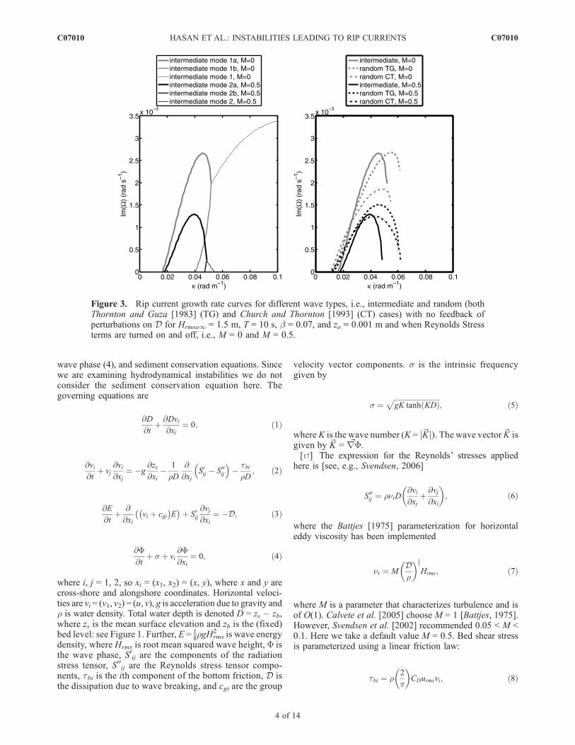
Figure 3. Rip current growth rate curves for different wave types, i.e., intermediate and random (bothThornton and Guza [1983] (TG) and Church and Thornton [1993] (CT) cases) with no feedback ofperturbations on D for Hrmso1 = 1.5 m, T = 10 s, b = 0.07, and zo = 0.001 m and when Reynolds Stressterms are turned on and off, i.e., M = 0 and M = 0.5.


4 of 14

C07010

where CD is the drag coefficient and is given as

CD ¼ 0:40

ln D=zoð Þ � 1

� �2

; ð9Þ

where zo is the bed roughness length (default value taken aszo = 0.001 m), and urms, wave orbital velocity at the sub-stitute for the boundary layer edge, is determined using lineartheory:

urms ¼Hrms

2

gK

scoshKzo

coshKD: ð10Þ

2.1. Wave Energy Dissipation

[18] In real seas waves are random and so will not breakat one point. As a result, the surf zone can be quite extensivecompared to that for quasi-regular waves. For randomwaves, breaking can be a result of short wave interaction,the interaction of waves with the bottom, current or wind[Roelvink, 1993]. Here the interaction of current and windare neglected, and wave transformation is linear. Therefore,wave breaking is dictated by the effect of changes in theseabed (for energy dissipation due to current-limited wavebreaking, see Chawla and Kirby [2002]). Apart from thesesimplifications, which were also imposed by Yu [2006] andFalques et al. [1999], the effects of different types ofrandom wave breaking are here examined in detail. Thisis motivated both by the consideration of regular waves inprevious studies, and by related work [see Van Leeuwen etal., 2006] that showed the importance of the type of wavebreaking on the evolution of bed forms.[19] Three types of random waves are considered here.

They are distinguished by the extent of the surf zone and thesize and shape of the dissipation profile, and are imple-mented by changing the energy dissipation term D in (3), sothat they describe transition between random and quasi-regular (intermediate) waves. We use the models of Thorntonand Guza [1983] and Church and Thornton [1993], the firstbecause it is standard in the literature and the second becauseit allows for somewhat more concentrated breaking at theshore. The model of Church and Thornton [1993] is

D ¼ 3ffiffiffip

p

16rgB3fp

H3rms

D1þ tanh 8

Hrms

gbD� 1

� � � �

� 1� 1þ Hrms

gbD

� �2 !�5=2

24

35; ð11Þ

where B = 1.3 (describes the type of breaking) and gb = 0.42are used, and where fp = s/2p is the intrinsic peak frequency(for Thornton and Guza [1983], B = 1 and gb = 0.42).[20] The model of Van Leeuwen et al. [2006], which is

based on that of Roelvink [1993], and which allows forregular, depth-limited regular and random waves, is usedhere for what we term ‘‘intermediate’’ waves, to provide thelink between regular and fully random waves. This thusallows us to suggest trends as wemove toward regular waves,the situation examined by earlier authors. For intermediate

waves B = 1 and gb = 0.55. See Appendix A for thesedissipation expressions.

2.2. Linear Stability Analysis

[21] The standard practice of linear stability analysis is tofirst define a basic state, which is a time-invariant solutionto the equations. The stability of this basic state is thenanalyzed by superimposing periodic perturbations and thenlinearizing with respect to the perturbations. In the basicstate an alongshore uniform beach, zb = �bx is assumed,with the basic state variables uo = 0, vo = 0 (since we areconsidering normal incidence), zs = zso(x), E = Eo(x) andF = Fo(x) (the subscript o denotes basic state terms; notethat we do not use it for zb, which is kept fixed throughout).[22] The basic state variables are found by integrating

onshore the basic state equations (1), (2), (3), and (4), thusdetermining the shoreline position with a prescribedtolerance depth of Do(0) = 15 cm, which is used through-out this study to avoid numerical problems. Hrmso andthe wave period, T are prescribed in deep water (offshore)conditions.

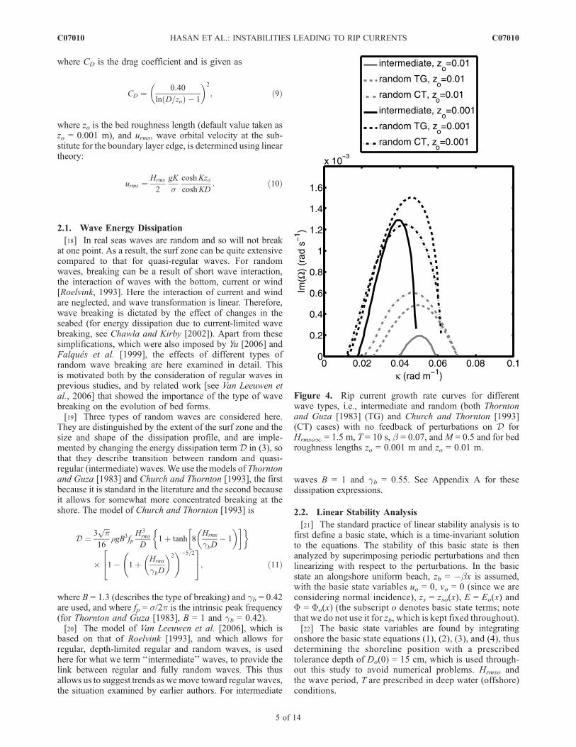
Figure 4. Rip current growth rate curves for differentwave types, i.e., intermediate and random (both Thorntonand Guza [1983] (TG) and Church and Thornton [1993](CT) cases) with no feedback of perturbations on D forHrmso1 = 1.5 m, T = 10 s, b = 0.07, and M = 0.5 and for bedroughness lengths zo = 0.001 m and zo = 0.01 m.


5 of 14

C07010

[23] The basic state variables plus perturbations are

zs ¼ zso xð Þ þ z0s xð Þ exp i ky� Wtð Þ½ �;u ¼ u0 xð Þ exp i ky� Wtð Þ½ �;v ¼ v0 xð Þ exp i ky� Wtð Þ½ �;E ¼ Eo xð Þ þ e0 xð Þ exp i ky� Wtð Þ½ �;F ¼ Fo xð Þ þ f0 xð Þ exp i ky� Wtð Þ½ �; ð12Þ

where the eigenvalue W = Wr + iWi and k is the radian wavenumber, indicating the spatial periodicity in the alongshoredirection. Thus, for a given spacing (wavelength) L= 2p/k, thegrowth (or decay) rate of the resulting eigenfunction [z0s, u

0,v0, e0, f0]T is given by Wi, with corresponding e-foldingtime Te = Wi

�1, and the (alongshore) propagation velocity isgiven by Wr/k. The eigenfunction (mode) with the largestgrowth rate is considered to be the one that will be seen innature: the fastest growing mode or FGM. The resultinglinear stability equations thus define an eigenvalue problem,

which is solved using collocation methods, with the pertur-bations decaying to zero far offshore [see Calvete et al.,2005]. The shoreline is taken to be fixed at x = 0, with a basicstate shoreline depth of 15 cm. The amplitude of all per-turbed variables is arbitrary. When M 6¼ 0 (Reynolds stressterms included) u0 = v0 = 0 at x = 0; when M = 0 (Reynoldsstress terms excluded) u0(x = 0) = 0. Numerical experi-ments here were performed for 250 grid points with halfthe grid points within 300 m of the shoreline, for whichsettings numerical convergence was achieved.

3. Generation of Rip Currents

[24] We examine a plane sloping beach with beach slopeb = 0.07, chosen because it was used by Yu [2006]. Thebeach profile here extends to 4 km offshore (where D0 =280 m, so that deep water conditions pertain and we canexpect perturbations to be negligible), after which a constantdepth is assumed. The beach is thus, for practical purposes,plane. A similar profile was taken by Yu [2006]; however,the constant depth section began after 45.76 m (D0 = 3.2 m),so shallow water conditions were assumed everywhere.[25] The default value for offshoreHrmso isHrmso1 = 1.5 m,

with period T = 10s following Yu [2006]; this was also theapproximate observed period on Narrabeen beach, Australia[see Short, 1985]. Unlike previous studies, where Reynoldsstress was neglected, we include these terms, although,because we consider normal incidence, turbulent diffusivityand bottom friction are not present in the basic state. Thebasic states for the different wave dissipations can be seen inFigure 2.[26] Results are roughly as expected. There is increased

set-up for intermediate waves, which break later, therefore

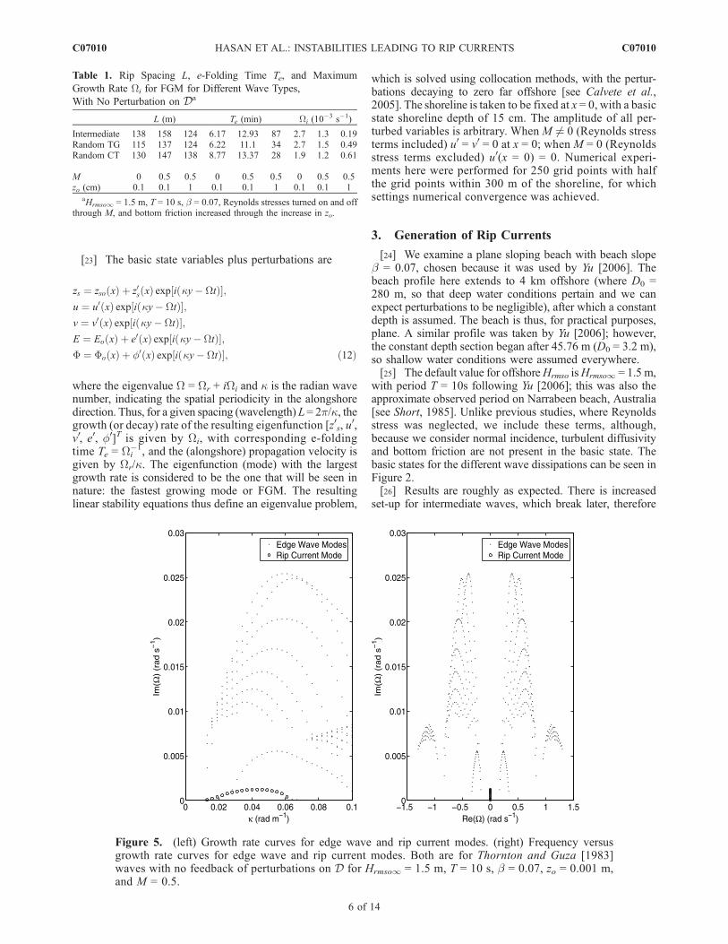
Figure 5. (left) Growth rate curves for edge wave and rip current modes. (right) Frequency versusgrowth rate curves for edge wave and rip current modes. Both are for Thornton and Guza [1983]waves with no feedback of perturbations on D for Hrmso1 = 1.5 m, T = 10 s, b = 0.07, zo = 0.001 m,and M = 0.5.

Table 1. Rip Spacing L, e-Folding Time Te, and Maximum

Growth Rate Wi for FGM for Different Wave Types,

With No Perturbation on Da

L (m) Te (min) Wi (10�3 s�1)

Intermediate 138 158 124 6.17 12.93 87 2.7 1.3 0.19Random TG 115 137 124 6.22 11.1 34 2.7 1.5 0.49Random CT 130 147 138 8.77 13.37 28 1.9 1.2 0.61

M 0 0.5 0.5 0 0.5 0.5 0 0.5 0.5zo (cm) 0.1 0.1 1 0.1 0.1 1 0.1 0.1 1

aHrmso1 = 1.5 m, T = 10 s, b = 0.07, Reynolds stresses turned on and offthrough M, and bottom friction increased through the increase in zo.


6 of 14

C07010

allowing more shoaling prior to breaking and thereforelarger set-down. The maximum breaker height decreasesand moves offshore as waves become more random, thusresulting in the reduction in set-up. Note also in Figure 2the differences in the dissipation: with delayed breakingthe dissipation in the inner surf zone is higher because thesame offshore wave energy density must be dissipated in ashorter distance.[27] An integration from the shore to deep water shows

that the quantity�R10

Ddx + EcgjD=D(shore) must be equal forall formulas (in the basic state), and this provides a usefulcheck on the model. It turns out that D plays a crucial role indetermining whether or not instabilities develop, and for thisreason, in sections 3.1 and 3.2 we isolate this physics by firstexcluding it in the perturbation equations (i.e., we neglect thefeedback of the perturbations on this term), consistent withFalques et al. [1999] and Yu [2006], and then reincorporate itinto the full equations (1)–(4).

3.1. No Feedback of Perturbations Onto Dissipation

[28] Figures 3 and 4 show the growth rate curves fordifferent basic state D terms (excluding feedback, as previ-ously mentioned) when turbulent Reynolds stresses areturned off and on, and when bottom friction is increasedthrough the increase in bed roughness length, zo. The pre-dicted rip spacing and the FGM e-folding time (Te = 1/Wi) (thetime taken for the rip currents to grow a factor of e) are shownin Table 1. Figure 3 shows the reduction in growth rates whenthe turbulent Reynolds stress term is included. Figure 3 (left)also shows the detailed structure of the growth rate curves. Itcan be seen that two imaginary modes (for instance, mode 1aand mode 1b) merge to form a complex conjugate solution(mode 1), the solutions to which have equal growth andmigration rate magnitudes but are migrating in oppositedirections. The bifurcation behavior seen here is similar tothat given by Van Leeuwen et al. [2006], who investigatedmorphodynamical instabilities on a plane sloping beach.Here, we only consider the fastest growing imaginary mode,i.e., mode 1a. The alongshore propagating complex conju-gate modes, by themselves, are not expected to correspond tophysical rip currents (because of the migration). Note that ifthese two modes were to possess equal amplitudes, however,the result is a standing wave solution. We neverthelessexclude this solution, because it would comprise a reversingonshore and offshore propagating rip current mode, which isalso nonphysical. Note also that the inclusion of the Reynoldsstresses minimizes the range of wave numbers over whichthese complex conjugate solutions exist, and also reducestheir growth rates. Furthermore, the unstable complex con-jugate solutions are no longer present for increased bottomfriction. Similarly, when bed friction is increased, growthrates are reduced: see Figure 4. The observed damping effectof Reynolds stress and bed friction terms on growth rates ofrip currents is consistent with other kinds of instability studies(e.g., the shear wave studies by Dodd et al. [1992] andFalques and Iranzo [1994]).[29] When Reynolds stress terms are included, the peak of

the growth rate curve shifts toward larger rip spacing,consistent with greater diffusion; the opposite is true forincreased bottom friction. Figures 3 and 4 also indicate thatrip spacings are slightly higher for intermediate waves, whichhave a higher shoreline basic state setup (see Figure 2a).

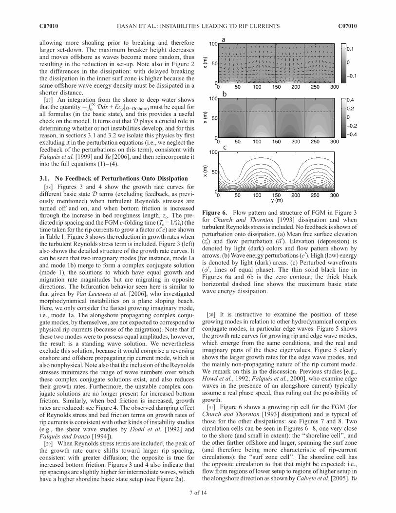
[30] It is instructive to examine the position of thesegrowing modes in relation to other hydrodynamical complexconjugate modes, in particular edge waves. Figure 5 showsthe growth rate curves for growing rip and edge wave modes,which emerge from the same conditions, and the real andimaginary parts of the these eigenvalues. Figure 5 clearlyshows the larger growth rates for the edge wave modes, andthe mainly non-propagating nature of the rip current mode.We remark on this in the discussion. Previous studies [e.g.,Howd et al., 1992; Falques et al., 2000], who examine edgewaves in the presence of an alongshore current) typicallyassume a real phase speed, thus ruling out the possibility ofgrowth.[31] Figure 6 shows a growing rip cell for the FGM (for

Church and Thornton [1993] dissipation) and is typical ofthose for the other dissipations: see Figures 7 and 8. Twocirculation cells can be seen in Figures 6–8, one very closeto the shore (and small in extent): the ‘‘shoreline cell’’, andthe other farther offshore and larger, spanning the surf zone(and therefore being more characteristic of rip-currentcirculations): the ‘‘surf zone cell’’. The shoreline cell hasthe opposite circulation to that that might be expected: i.e.,flow from regions of lower setup to regions of higher setup inthe alongshore direction as shown byCalvete et al. [2005]. Yu

Figure 6. Flow pattern and structure of FGM in Figure 3for Church and Thornton [1993] dissipation and whenturbulent Reynolds stress is included. No feedback is shown ofperturbation onto dissipation. (a) Mean free surface elevation(z0s) and flow perturbation (~u0). Elevation (depression) isdenoted by light (dark) colors and flow pattern shown byarrows. (b)Wave energy perturbations (e0). High (low) energyis denoted by light (dark) areas. (c) Perturbed wavefronts(f0, lines of equal phase). The thin solid black line inFigures 6a and 6b is the zero contour; the thick blackhorizontal dashed line shows the maximum basic statewave energy dissipation.


7 of 14

C07010

and Slinn [2003] also observe these circulations, although itis not clear which are regions of high or low setup in theirstudy. Note, however, that for Calvete et al. [2005], both forfixed and mobile beds, the set-up at the shore is opposite tothat observed here; that is, it is negative where there isoffshore flow in the shoreline cell, although the set-upquickly reverses sign at these locations just a little furtheroffshore. There are, however, significant differences betweenthe present study and that of Calvete et al. [2005], whoexamined a barred beach with mean slope less than b = 0.07with an alongshore bar. Moreover, the shoreline cells theyobserve are less energetic compared to the surf zone cells theyobserve. Further, it must be remembered that here we excludefeedback onto wave dissipation. Thus, the rip currents heredo not induce further breaking, as they did for Calvete et al.[2005], but only shoaling and refraction. Thus, for Calvete etal. [2005], where wave heights are larger in the rip channelsbecause of the larger depth there, there is intense breaking atthe corresponding shoreline position of the channel locations,and therefore a large set-up there. In contrast, offshore flowsin the cells considered here also lead to increased waveheights, because of shoaling, but there is no associatedbreaking, so set-up decreases. Shoreline cells have also beenobserved in laboratory experiments by Haller et al. [2002]and Haas and Svendsen [2002].

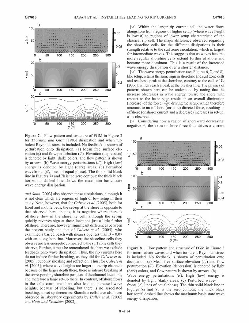
[32] Within the larger rip current cell the water flowsalongshore from regions of higher setup (where wave heightis lowest) to regions of lower setup characteristic of theclassical rip cell. The major difference observed regardingthe shoreline cells for the different dissipations is theirstrength relative to the surf zone circulation, which is largestfor intermediate waves. This suggests that as waves becomemore regular shoreline cells extend further offshore andbecome more dominant. This is a result of the increasedwave energy dissipation over a shorter distance.[33] The wave energy perturbation (see Figures 6, 7, and 8),

like setup, retains the same sign in shoreline and surf zone cellsand reaches a peak at the shoreline, contrary to the cells of Yu[2006], which reach a peak at the breaker line. The physics ofpatterns shown here can be understood by noting that theincrease (decrease) in wave energy toward the shore withrespect to the basic state results in an overall diminution(increase) of the force (

@S011

@x ) driving the setup, which thereforeamounts to an offshore (onshore) directed force, resulting inoffshore (onshore) current and a decrease (increase) in set-up,as is observed.[34] Considering now a region of shoreward decreasing,

negative e0, the extra onshore force thus drives a current

Figure 8. Flow pattern and structure of FGM in Figure 3for intermediate waves and when turbulent Reynolds stressis included. No feedback is shown of perturbation ontodissipation. (a) Mean free surface elevation (zs

0) and flowperturbation (~u0). Elevation (depression) is denoted by light

(dark) colors, and flow pattern is shown by arrows. (b)Wave energy perturbations (e0). High (low) energy is

denoted by light (dark) areas. (c) Perturbed wave-fronts (f0, lines of equal phase). The thin solid black line inFigures 8a and 8b is the zero contour; the thick blackhorizontal dashed line shows the maximum basic state waveenergy dissipation.

Figure 7. Flow pattern and structure of FGM in Figure 3for Thornton and Guza [1983] dissipation and when tur-bulent Reynolds stress is included. No feedback is shown ofperturbation onto dissipation. (a) Mean free surface ele-vation (z0s) and flow perturbation (~u0). Elevation (depression)is denoted by light (dark) colors, and flow pattern is shownby arrows. (b) Wave energy perturbations (e0). High (low)energy is denoted by light (dark) areas. (c) Perturbedwavefronts (f0, lines of equal phase). The thin solid blackline in Figures 7a and 7b is the zero contour; the thick blackhorizontal dashed line shows the maximum basic statewave energy dissipation.


8 of 14

C07010

onshore. This onshore current is opposed by the increasedset-up gradient at the shore that accompanies the increasedwave energy dissipation; this comprises a negative feed-back. To understand the positive feedback necessary for theinstability we must consider the shoaling and refraction.This onshore current will effectively increase cg (becausecg + U > cg) and so deshoal the wave, thus furtherdecreasing e0 and moving the break point onshore. Further-more, the onshore current de-focuses the waves, thus alsoproviding a positive feedback; this effect can be seen in thelines of equal phase in Figure 6, 7, and 8). In the surf zone thiseffect will be felt as (1) a decrease in e0 due to the deshoaling,which provides a positive feedback, and (2) a decrease inbreaking (because of decreased wave height), thus providinga negative feedback because reduced breaking will increasewave heights. This is the very term that we omit here, and weknow its effect to be strong because it ‘‘kills’’ the growing cell(i.e., renders it stable): see section 3.2.[35] The rest of the two cell dynamics can be understood

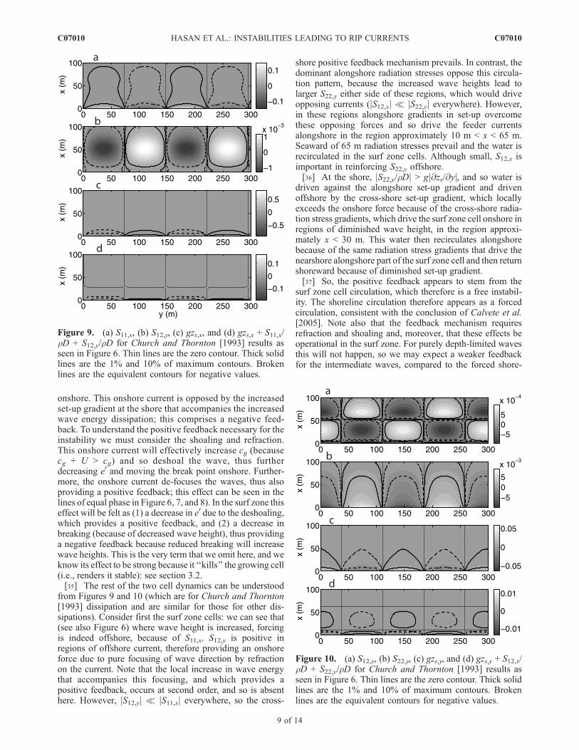
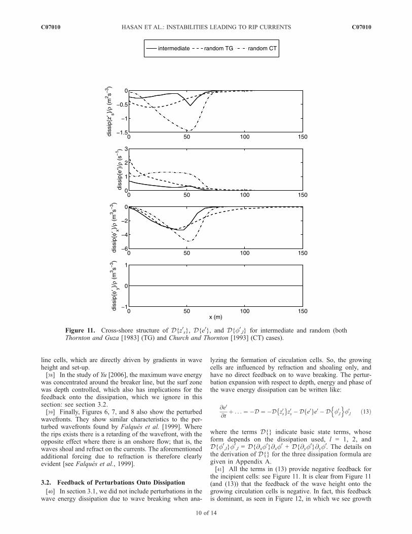
from Figures 9 and 10 (which are for Church and Thornton[1993] dissipation and are similar for those for other dis-sipations). Consider first the surf zone cells: we can see that(see also Figure 6) where wave height is increased, forcingis indeed offshore, because of S11,x. S12,y is positive inregions of offshore current, therefore providing an onshoreforce due to pure focusing of wave direction by refractionon the current. Note that the local increase in wave energythat accompanies this focusing, and which provides apositive feedback, occurs at second order, and so is absenthere. However, jS12,yj � jS11,xj everywhere, so the cross-

shore positive feedback mechanism prevails. In contrast, thedominant alongshore radiation stresses oppose this circula-tion pattern, because the increased wave heights lead tolarger S22,y either side of these regions, which would driveopposing currents (jS12,xj � jS22,yj everywhere). However,in these regions alongshore gradients in set-up overcomethese opposing forces and so drive the feeder currentsalongshore in the region approximately 10 m < x < 65 m.Seaward of 65 m radiation stresses prevail and the water isrecirculated in the surf zone cells. Although small, S12,x isimportant in reinforcing S22,y offshore.[36] At the shore, jS22,y/rDj > gj@zs/@yj, and so water is

driven against the alongshore set-up gradient and drivenoffshore by the cross-shore set-up gradient, which locallyexceeds the onshore force because of the cross-shore radia-tion stress gradients, which drive the surf zone cell onshore inregions of diminished wave height, in the region approxi-mately x < 30 m. This water then recirculates alongshorebecause of the same radiation stress gradients that drive thenearshore alongshore part of the surf zone cell and then returnshoreward because of diminished set-up gradient.[37] So, the positive feedback appears to stem from the

surf zone cell circulation, which therefore is a free instabil-ity. The shoreline circulation therefore appears as a forcedcirculation, consistent with the conclusion of Calvete et al.[2005]. Note also that the feedback mechanism requiresrefraction and shoaling and, moreover, that these effects beoperational in the surf zone. For purely depth-limited wavesthis will not happen, so we may expect a weaker feedbackfor the intermediate waves, compared to the forced shore-

Figure 10. (a) S12,x, (b) S22,y, (c) gzs,y, and (d) gzs,y + S12,x/rD + S22,y/rD for Church and Thornton [1993] results asseen in Figure 6. Thin lines are the zero contour. Thick solidlines are the 1% and 10% of maximum contours. Brokenlines are the equivalent contours for negative values.

Figure 9. (a) S11,x, (b) S12,y, (c) gzs,x, and (d) gzs,x + S11,x/rD + S12,y/rD for Church and Thornton [1993] results asseen in Figure 6. Thin lines are the zero contour. Thick solidlines are the 1% and 10% of maximum contours. Brokenlines are the equivalent contours for negative values.


9 of 14

C07010

line cells, which are directly driven by gradients in waveheight and set-up.[38] In the study of Yu [2006], the maximum wave energy

was concentrated around the breaker line, but the surf zonewas depth controlled, which also has implications for thefeedback onto the dissipation, which we ignore in thissection: see section 3.2.[39] Finally, Figures 6, 7, and 8 also show the perturbed

wavefronts. They show similar characteristics to the per-turbed wavefronts found by Falques et al. [1999]. Wherethe rips exists there is a retarding of the wavefront, with theopposite effect where there is an onshore flow; that is, thewaves shoal and refract on the currents. The aforementionedadditional forcing due to refraction is therefore clearlyevident [see Falques et al., 1999].

3.2. Feedback of Perturbations Onto Dissipation

[40] In section 3.1, we did not include perturbations in thewave energy dissipation due to wave breaking when ana-

lyzing the formation of circulation cells. So, the growingcells are influenced by refraction and shoaling only, andhave no direct feedback on to wave breaking. The pertur-bation expansion with respect to depth, energy and phase ofthe wave energy dissipation can be written like:

@e0

@tþ . . . ¼ �D ¼ �D z0s

� �z0s �D e0f ge0 � D f0

;l

n of0;l ð13Þ

where the terms D{} indicate basic state terms, whoseform depends on the dissipation used, l = 1, 2, andD{f0

,l}f0,l = D{@xf

0}@xf0 + D{@yf

0}@yf0. The details on

the derivation of D{} for the three dissipation formula aregiven in Appendix A.[41] All the terms in (13) provide negative feedback for

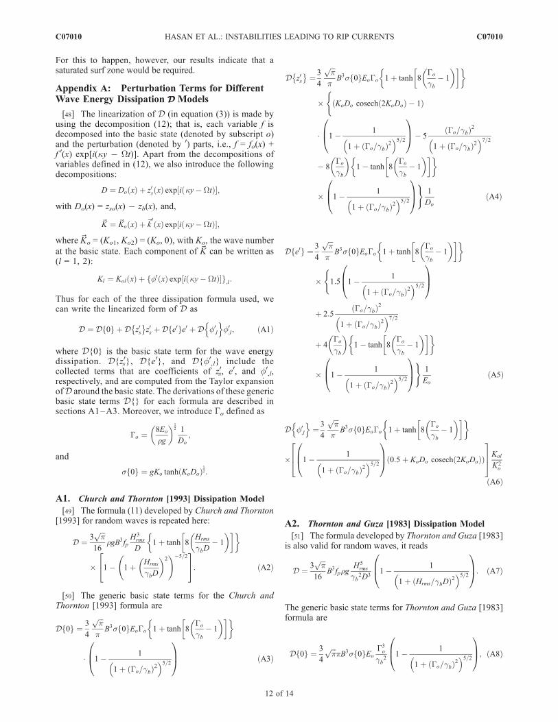
the incipient cells: see Figure 11. It is clear from Figure 11(and (13)) that the feedback of the wave height onto thegrowing circulation cells is negative. In fact, this feedbackis dominant, as seen in Figure 12, in which we see growth

Figure 11. Cross-shore structure of D{z0s}, D{e0}, and D{f0,l} for intermediate and random (both

Thornton and Guza [1983] (TG) and Church and Thornton [1993] (CT) cases).


10 of 14

C07010

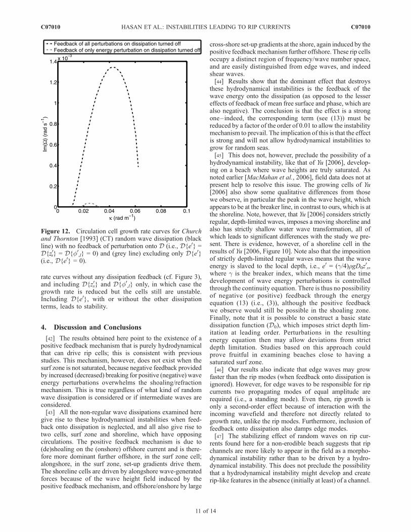
rate curves without any dissipation feedback (cf. Figure 3),and including D{z0s} and D{f0

,l} only, in which case thegrowth rate is reduced but the cells still are unstable.Including D{e0}, with or without the other dissipationterms, leads to stability.

4. Discussion and Conclusions

[42] The results obtained here point to the existence of apositive feedback mechanism that is purely hydrodynamicalthat can drive rip cells; this is consistent with previousstudies. This mechanism, however, does not exist when thesurf zone is not saturated, because negative feedback providedby increased (decreased) breaking for positive (negative) waveenergy perturbations overwhelms the shoaling/refractionmechanism. This is true regardless of what kind of randomwave dissipation is considered or if intermediate waves areconsidered.[43] All the non-regular wave dissipations examined here

give rise to these hydrodynamical instabilities when feed-back onto dissipation is neglected, and all also give rise totwo cells, surf zone and shoreline, which have opposingcirculations. The positive feedback mechanism is due to(de)shoaling on the (onshore) offshore current and is there-fore more dominant further offshore, in the surf zone cell;alongshore, in the surf zone, set-up gradients drive them.The shoreline cells are driven by alongshore wave-generatedforces because of the wave height field induced by thepositive feedback mechanism, and offshore/onshore by large

cross-shore set-up gradients at the shore, again induced by thepositive feedbackmechanism further offshore. These rip cellsoccupy a distinct region of frequency/wave number space,and are easily distinguished from edge waves, and indeedshear waves.[44] Results show that the dominant effect that destroys

these hydrodynamical instabilities is the feedback of thewave energy onto the dissipation (as opposed to the lessereffects of feedback of mean free surface and phase, which arealso negative). The conclusion is that the effect is a strongone–indeed, the corresponding term (see (13)) must bereduced by a factor of the order of 0.01 to allow the instabilitymechanism to prevail. The implication of this is that the effectis strong and will not allow hydrodynamical instabilities togrow for random seas.[45] This does not, however, preclude the possibility of a

hydrodynamical instability, like that of Yu [2006], develop-ing on a beach where wave heights are truly saturated. Asnoted earlier [MacMahan et al., 2006], field data does not atpresent help to resolve this issue. The growing cells of Yu[2006] also show some qualitative differences from thosewe observe, in particular the peak in the wave height, whichappears to be at the breaker line, in contrast to ours, which is atthe shoreline. Note, however, that Yu [2006] considers strictlyregular, depth-limited waves, imposes a moving shoreline andalso has strictly shallow water wave transformation, all ofwhich leads to significant differences with the study we pre-sent. There is evidence, however, of a shoreline cell in theresults of Yu [2006, Figure 10]. Note also that the impositionof strictly depth-limited regular waves means that the waveenergy is slaved to the local depth, i.e., e0 = (g/4)rgD0z

0s,

where g is the breaker index, which means that the timedevelopment of wave energy perturbations is controlledthrough the continuity equation. There is thus no possibilityof negative (or positive) feedback through the energyequation (13) (i.e., (3)), although the positive feedbackwe observe would still be possible in the shoaling zone.Finally, note that it is possible to construct a basic statedissipation function (D0), which imposes strict depth lim-itation at leading order. Perturbations in the resultingenergy equation then may allow deviations from strictdepth limitation. Studies based on this approach couldprove fruitful in examining beaches close to having asaturated surf zone.[46] Our results also indicate that edge waves may grow

faster than the rip modes (when feedback onto dissipation isignored). However, for edge waves to be responsible for ripcurrents two propagating modes of equal amplitude arerequired (i.e., a standing mode). Even then, rip growth isonly a second-order effect because of interaction with theincoming wavefield and therefore not directly related togrowth rate, unlike the rip modes. Furthermore, inclusion offeedback onto dissipation also damps edge modes.[47] The stabilizing effect of random waves on rip cur-

rents found here for a non-erodible beach suggests that ripchannels are more likely to appear in the field as a morpho-dynamical instability rather than to be driven by a hydro-dynamical instability. This does not preclude the possibilitythat a hydrodynamical instability might develop and createrip-like features in the absence (initially at least) of a channel.

Figure 12. Circulation cell growth rate curves for Churchand Thornton [1993] (CT) random wave dissipation (blackline) with no feedback of perturbation onto D (i.e., D{e0} =D{z0s} = D{f0

,l} = 0) and (grey line) excluding only D{e0}(i.e., D{e0} = 0).


11 of 14

C07010

For this to happen, however, our results indicate that asaturated surf zone would be required.

Appendix A: Perturbation Terms for DifferentWave Energy Dissipation DDDD Models

[48] The linearization of D (in equation (3)) is made byusing the decomposition (12); that is, each variable f isdecomposed into the basic state (denoted by subscript o)and the perturbation (denoted by 0) parts, i.e., f = fo(x) +f 0(x) exp[i(ky � Wt)]. Apart from the decompositions ofvariables defined in (12), we also introduce the followingdecompositions:

D ¼ Do xð Þ þ z0s xð Þ exp i ky� Wtð Þ½ �;

with Do(x) = zso(x) � zb(x), and,

~K ¼ ~Ko xð Þ þ~k0xð Þ exp i ky� Wtð Þ½ �;

where ~Ko = (Ko1, Ko2) = (Ko, 0), with Ko, the wave number

at the basic state. Each component of ~K can be written as(l = 1, 2):

Kl ¼ Kol xð Þ þ f0 xð Þ exp i ky� Wtð Þ½ �f g;l:

Thus for each of the three dissipation formula used, wecan write the linearized form of D as

D ¼ D 0f g þ D z0s� �

z0s þD e0f ge0 þ D f0;l

n of0;l; ðA1Þ

where D{0} is the basic state term for the wave energydissipation. D{z0s}, D{e0}, and D{f0

,l} include thecollected terms that are coefficients of z0s, e0, and f0

,l,respectively, and are computed from the Taylor expansionofD around the basic state. The derivations of these genericbasic state terms D{} for each formula are described insections A1–A3. Moreover, we introduce Go defined as

Go ¼8Eo

rg

� �12 1

Do

;

and

s 0f g ¼ gKo tanh KoDoð Þ12:

A1. Church and Thornton [1993] Dissipation Model

[49] The formula (11) developed by Church and Thornton[1993] for random waves is repeated here:

D ¼ 3ffiffiffip

p

16rgB3fp

H3rms

D1þ tanh 8

Hrms

gbD� 1

� � � �

� 1� 1þ Hrms

gbD

� �2 !�5=2

24

35: ðA2Þ

[50] The generic basic state terms for the Church andThornton [1993] formula are

D 0f g ¼ 3

4

ffiffiffip

p

pB3s 0f gEoGo 1þ tanh 8

Go

gb� 1

� � � �

� 1� 1

1þ Go=gbð Þ2� �5=2

0B@

1CA ðA3Þ

D z0s� �

¼ 3

4

ffiffiffip

p


Go

gb� 1

� � � �

�(

KoDo cosech 2KoDoð Þ � 1ð Þ

� 1� 1

1þ Go=gbð Þ2� �5=2

0B@

1CA� 5

Go=gbð Þ2

1þ Go=gbð Þ2� �7=2

� 8Go

gb

� �1� tanh 8

Go

gb� 1

� � � �

� 1� 1

1þ Go=gbð Þ2� �5=2

0B@

1CA)

1

Do

ðA4Þ

D e0f g ¼ 3

4

ffiffiffip

p


Go

gb� 1

� � � �

�(1:5 1� 1

1þ Go=gbð Þ2� �5=2

0B@

1CA

þ 2:5Go=gbð Þ2

1þ Go=gbð Þ2� �7=2

þ 4Go

gb

� �1� tanh 8

Go

gb� 1

� � � �

� 1� 1

1þ Go=gbð Þ2� �5=2

0B@

1CA)

1

Eo

ðA5Þ

D f0;l

n o¼ 3

4

ffiffiffip

p


Go

gb� 1

� � � �

� 1� 1

1þ Go=gbð Þ2� �5=2

0B@

1CA 0:5þ KoDo cosech 2KoDoð Þð Þ

264

375Kol

K2o

ðA6Þ

A2. Thornton and Guza [1983] Dissipation Model

[51] The formula developed by Thornton and Guza [1983]is also valid for random waves, it reads

D ¼ 3ffiffiffip

p

16B3fprg

H5rms

gb2D31� 1

1þ Hrms=gbDð Þ2� �5=2

0B@

1CA: ðA7Þ

The generic basic state terms for Thornton and Guza [1983]formula are

D 0f g ¼ 3

4

ffiffiffip

ppB3s 0f gEo

G3o

gb21� 1

1þ Go=gbð Þ2� �5=2

0B@

1CA; ðA8Þ


12 of 14

C07010

D z0s� �

¼� 3

4

ffiffiffip

p

pB3s 0f gEo

G3o

gb2

�

3� KoDo cosech 2KoDoð Þð!

� 1� 1

1þ Go=gbð Þ2� �5=2

0B@

1CA

þ 5Go=gbð Þ2

1þ Go=gbð Þ2� �7=2

!1

Do

; ðA9Þ

D e0f g ¼ 3

4

ffiffiffip

p

pB3s 0f gEo

G3o

gb25

21� 1

1þ Go=gbð Þ2� �5=2

0B@

1CA

0B@

þ 5

2

Go=gbð Þ2

1þ Go=gbð Þ2� �7=2

1CA 1

Eo

; ðA10Þ

D f0;l

n o¼ 3

4

ffiffiffip

p

pB3s 0f gEo

G3o

gb21� 1

1þ Go=gbð Þ2� �5=2

0B@

1CA

� 0:5þ KoDo cosech 2KoDoð Þð ÞKol

K2o

: ðA11Þ

A3. Van Leeuwen et al. [2006] Dissipation Model

[52] The formula developed by Van Leeuwen et al. [2006]can be used for depth-limited regular, regular and interme-diate waves, depending on the value chosen for m and n. Itreads

D ¼ rgfpB3H3rms

4D

Hrms

gbD

� �m

1� exp � Hrms

gbD

� �n � �: ðA12Þ

In the paper we set m = 0 and n = 10, which representintermediate waves [Van Leeuwen et al., 2006]. The genericbasic state terms for the Van Leeuwen et al. [2006] formulaare

D 0f g ¼ B3s 0f gEoGo

pGo

gb

� �m

1� exp � Go

gb

� �n ; ðA13Þ

D z0s� �

¼� B3s 0f gEoGo

pGo

gb

� �m

nGo

gb

� �n

exp � Go

gb

� �n

� 1� exp � Go

gb

� �n � �

� KoDo cosech 2KoDoð Þ � mþ 1ð Þð Þ� 1Do

; ðA14Þ

D e0f g ¼B3s 0f gEoGo

pGo

gb

� �m

0:5nGo

gb

� �n

exp � Go

gb

� �n

þ 1� exp � Go

gb

� �n � �1:5þ 0:5mð Þ

1

Eo

; ðA15Þ

D f0;l

n o¼ B3s 0f gEoGo

pGo

gb

� �m

1� exp � Go

gb

� �n � �

� 0:5þ KoDo cosech 2KoDoð Þð Þ�Kol

K2o

: ðA16Þ

[53] Acknowledgments. Haider Hasan was funded by an EPSRCdoctoral training account award. Roland Garnier received financial supportfrom the University of Nottingham. The authors gratefully acknowledge thissupport. The authors thank two anonymous reviewers for helpful commentsand also thank Albert Falques and Daniel Calvete of Applied PhysicsDepartment, Universitat Politecnica de Catalunya, for useful discussionsconcerning this manuscript.

ReferencesBattjes, J. A. (1975), Modeling of turbulence in the surf zone, in ModelingTechniques, vol. 2, pp. 1050–1061, Am. Soc. of Civ. Eng., New York.

Bowen, A. J. (1969), Rip currents: 1. Theoretical investigations, J. Geophys.Res., 74, 5467–5478.

Bowen, A. J., and D. I. Inman (1969), Rip currents: 2. Laboratory and fieldobservations, J. Geophys. Res., 74, 5479–5490.

Brander, R. W., and A. D. Short (2000), Morphodynamics of a large-scalerip current system at Muriwai, New Zealand, Mar. Geol., 165, 27–39.

Caballeria, M., G. Coco, A. Falques, and D. A. Huntley (2002), Self-organization mechanism for the formation of nearshore crescentic andtransverse bars, J. Fluid Mech., 465, 379–410.

Calvete, D., N. Dodd, A. Falques, and S. M. van Leeuwen (2005),Morphological development of rip channel systems: Normal andnear-normal wave incidence, J. Geophys. Res., 110, C10006, doi:10.1029/2004JC002803.

Chawla, A., and J. T. Kirby (2002), Monochromatic and random wavebreaking at blocking points, J. Geophys. Res., 107(C7), 3067,doi:10.1029/2001JC001042.

Church, J. C., and E. B. Thornton (1993), Effects of breaking wave inducedturbulence within a longshore current model, Coastal Eng., 20, 1–28.

Dalrymple, R. A., and C. J. Lozano (1978), Wave-current interaction for ripcurrents, J. Geophys. Res., 83, 6063–6071.

Damgaard, J., N. Dodd, L. Hall, and T. Chesher (2002), Morphodynamicmodelling of rip channel growth, Coastal Eng., 45, 199–221.

Deigaard, R., N. Dronen, J. Fredsoe, J. H. Jensen, and M. P. Jorgesen(1999), A morphological stability analysis for a long straight barredcoast, Coastal Eng., 36, 171–195.

Dodd, N., J. Oltman-Shay, and E. B. Thornton (1992), Shear instabilities inthe longshore current: A comparison of observations and theory, J. Phys.Oceanogr., 22, 62–82.

Falques, A., and V. Iranzo (1994), Numerical simulation of vorticity wavesin the nearshore, J. Geophys. Res., 99, 825–841.

Falques, A., A. Montoto, and D. Vila (1999), A note on hydrodynamicinstabilities and horizontal circulation in the surf zone, J. Geophys. Res.,104, 20,605–20,615.

Falques, A., G. Coco, and D. A. Huntley (2000), A mechanism for thegeneration of wave-driven rhythmic patterns in the surf zone, J. Geophys.Res., 105, 24,071–24,087.

Garnier, R., D. Calvete, A. Falques, and M. Caballeria (2006), Generationand nonlinear evolution of shore-oblique/transverse bars, J. Fluid Mech.,567, 327–360.

Haas, K. A., and I. A. Svendsen (2002), Laboratory measurements of thevertical structure of rip currents, J. Geophys. Res., 107(C5), 3047,doi:10.1029/2001JC000911.

Haller, M. C., R. A. Dalrymple, and I. A. Svendsen (2002), Experimentalstudy of nearshore dynamics on a barred beach with rip channels, J.Geophys. Res., 107(C6), 3061, doi:10.1029/2001JC000955.

Hino, M. (1974), Theory on the formation of rip currents and cuspidalcoast, in Coastal Engineering 1974, pp. 901–919, Am. Soc. of Civ.Eng., New York.

Howd, P. A., A. J. Bowen, and R. A. Holman (1992), Edge waves in thepresence of strong longshore currents, J. Geophys. Res., 97, 11,357–11,371.


13 of 14

C07010

Inman, D. L., R. T. Tait, and C. E. Nordstrom (1971), Mixing in the surfzone, J. Geophys. Res., 76, 3493–3514.

LeBlond, P. H., and C. L. Tang (1974), On the energy coupling betweenwaves and rip currents, J. Geophys. Res., 79, 811–816.

Longuet-Higgins, M. S., and R. W. Stewart (1962), Radiation stress andmass transport in gravity waves, with application to ‘‘surf beats,’’ J. FluidMech., 10, 481–504.

Longuet-Higgins, M. S., and R. W. Stewart (1964), Radiation stresses inwater waves: A physical discussion, with applications, Deep Sea Res., 11,529–562.

MacMahan, J. H., E. B. Thornton, T. P. Stanton, and A. J. H. M. Reniers(2005), RIPEX: Rip currents on a shore-connected shoal beach, Mar.Geol., 218, 113–134.

MacMahan, J. H., E. B. Thornton, and A. J. H. M. Reniers (2006), Ripcurrent review, Coastal Eng., 53, 191–208.

Murray, A. B., and B. Reydellet (2001), A rip-current model based on anewly hypothesized interaction between waves and currents, J. CoastalRes., 17, 517–531.

Reniers, A. J. H. M., J. A. Roelvink, and E. B. Thornton (2004), Morpho-dynamic modeling of an embayed beach under wave group forcing,J. Geophys. Res., 109, C01030, doi:10.1029/2002JC001586.

Roelvink, J. A. (1993), Dissipation in random wave groups incident on abeach, Coastal Eng., 19, 127–150.

Shepard, F. P., and D. L. Inman (1950), Nearshore circulation related tobottom topography and wave refraction, Eos Trans. AGU, 31, 555–565.

Shepard, F. P., K. O. Emery, and E. C. LaFond (1941), Rip currents: Aprocess of geological importance, J. Geophys. Res., 49, 337–369.

Short, A. D. (1985), Rip-current type, spacing and persistence, Narrabeenbeach, Australia, Mar. Geol., 65, 47–71.

Short, A. D. (1999), Handbook of Beach and Shoreface Morphodynamics,1 ed., John Wiley, New York.

Short, A. D., and C. L. Hogan (1994), Rip currents and beach hazards:Their impact on public safety and implications for coastal management,J. Coastal Res., 12, 197–209.

Smith, J. A., and J. Largier (1995), Observations of nearshore circulation:Rip currents, J. Geophys. Res., 100, 10,967–10,975.

Svendsen, I. A. (2006), Introduction to Nearshore Hydrodynamics, Adv.Ser. Ocean Eng., vol. 24, World Sci., Singapore.

Svendsen, I. A., K. Haas, and Q. Zhao (2002), Quasi-3D nearshore circula-tion model SHORECIRC, Int. Rep. CACR-02-01, Cent. for Appl. CoastalRes., Univ. of Del., Newark.

Thornton, E. B., and R. T. Guza (1983), Transformation of wave heightdistribution, J. Geophys. Res., 88, 5925–5938.

van Leeuwen, S. M., N. Dodd, D. Calvete, and A. Falques (2006), Physicsof nearshore bed pattern formation under regular or random waves, J. Geo-phys. Res., 111, F01023, doi:10.1029/2005JF000360.

Yu, J. (2006), On the instability leading to rip currents due to wave-currentinteraction, J. Fluid Mech., 549, 403–428.

Yu, J., and D. N. Slinn (2003), Effects of wave-current interaction on ripcurrents, J. Geophys. Res., 108(C3), 3088, doi:10.1029/2001JC001105.

��N. Dodd, Environmental Fluid Mechanics Research Centre, Process and

Environmental Division, Faculty of Engineering, University of Nottingham,University Park, NG7 2RD Nottingham, UK. ([email protected])R. Garnier, Applied Physics Department, Universitat Politecnica de

Catalunya, Modul B4/5, c/o Jordi Girona, E-08034 Barcelona, Spain.([email protected])H. Hasan, Department of Mathematics and Basic Sciences, NED Uni-

versity of Engineering and Technology, University Road, Karachi 75270,Pakistan. ([email protected])


14 of 14

C07010

Stabilizing effect of random waves on rip currents

Documents