Stability of time-varying nonlinear switching systems under perturbations

arX

iv:1

109.

1102

v1 [

cs.S

Y]

6 S

ep 2

011

STABILITY OF TIME-VARYING NONLINEAR SWITCHING

SYSTEMS UNDER PERTURBATIONS

XIONGPING DAI, YU HUANG, AND MINGQING XIAO

Abstract. By introducing a new type of exponent that is more general thanthe one given in [10], we present a criterion of asymptotic exponential stabilityfor a deterministic, quasi-linear switching system that may consist of infinitelymany time-dependent subsystems:

x(t) = Au(t)(t)x(t) + Fu(t)(t, x(t)), x(0) = x0 ∈ Rd, t > 0,

where u(t) is a switching control function.

Let Σ+I

be the space of all one-sided infinite sequences i· : N → I, where Iis a countable index set. We apply our criterion to a random control systemdriven by the one-sided Markov shift θ : Σ+

I→ Σ+

I; i· 7→ i

·+1 which preserves

an ergodic Borel probability P. For any i· = (in)+∞

n=1 ∈ Σ+I, it defines an

admissible continuous-time switching law ui·

: (0,+∞) → I by ui·

(t) = in

when n− 1 < t ≤ n for all n ∈ {1, 2, . . . }. Let Ai ∈ Rd×d be upper-triangularand Fi(t, x) = o(‖x‖) ∈ Rd for i ∈ I. Then, we give a sufficient condition ofP-a.s. exponential stability for the randomly-switched system

x(t) = Aui·

(t)x(t) + Fui·

(t)(t, x(t)), x(0) = x0 ∈ Rd, t > 0; i· ∈ Σ+I,

by its corresponding “linear approximation”.

1. Introduction

Let I be a topological space of control values and write Σ+I as the set of all

one-sided infinite sequences i·: N → I endowed with standard product topology,

where N = {1, 2, . . .}. We define the one-sided Markov shift transformation

θ : Σ+I → Σ+

I ; i·= (in)

+∞n=1 7→ i

·+1 = (in+1)+∞n=1.

Let R+ = (0,+∞) and we denote by C0(X,Rn) the set of all continuous functionsf : X → Rn endowed with the uniform-convergence topology (i.e., the topology isinduced by the metric |fi − fj| = supx∈X ‖fi(x) − fj(x)‖). Here ‖ · ‖ denotes theusual Euclidean norm on Rn or its induced matrix norm on Rn×n. Let d ≥ 2 be aninteger and there be given arbitrarily a continuous, matrix-valued function

A : I → C0(R+,Rd×d); i 7→ Ai(·) =

[Aℓm

i (·)]1≤ℓ,m≤d

and a continuous function-valued function

F : I → C0(R+ × Rd,Rd); i 7→ Fi(·, ·)

2000 Mathematics Subject Classification. Primary: 93C15, 34H05 Secondary: 93D20, 93D09,93E15.

Key words and phrases. Continuous-time randomly switched system; Exponential stability;Periodically-switching stability; Lyapunov-type exponent; Liao-type exponent.

This work was supported partly by National Natural Science Foundation of China (GrantNos. 11071112, 11071263), NSF of Guangdong Province and in part by NSF 1021203 of the UnitedStates.

1

2 X. DAI, Y. HUANG, AND M. XIAO

where A,F satisfy

‖Ai(t)‖ ≤ α and ‖Fi(t, x)‖ ≤ L‖x‖ ∀(t, x) ∈ R+ × Rd

for some α > 0 and L > 0, uniformly for i ∈ I. We notice here that F (t, x) is notnecessarily linear w.r.t. the space variable x.

For any infinite sequence i·= (i1, i2, . . . ) ∈ Σ+

I , it defines a piecewise constant,

left continuous switching law with switching-time sequence {Tn = n}+∞n=1 as follows:

ui·

: R+ → I; ui·

(t) = in for n− 1 < t ≤ n and n ∈ N.

Let U ={ui

·

(t) | i·∈ Σ+

I

}as the set of admissible continuous-time switching laws.

For any ui·

∈ U , there then generates a quasi-linear switching system:

(1.1) x(t) = Aui·(t)(t)x(t) + Fui

·(t)(t, x(t)), t ∈ R+, x(0) = x0 ∈ Rd.

In this paper, we study the stabilization problem of above system by using theswitching control ui

·

(t) and develop a sufficient condition for ui·

(t) which can war-rant the global exponential stability of the system. Furthermore, when Ai(t) = Ai

and a Borel probability distribution P on U is known, we establish a sufficient andverifiable condition that guarantees the solution

x(·, x0, ui·

) : R+ → Rd

with x(0, x0, ui·

) = x0, of (1.1) to be exponentially stable for P-almost sure switchingcontrol functions ui

·

∈ U .The interest of this goal has been primarily motivated due to this type of model

is governed by many man-made and natural systems in mathematics, control en-gineering, biology and physics; for example, see [18, 28] and references therein.Studies of this type of problems fall under the category of “stabilization analysis”in the control theory.

In order to study the stability of (1.1) with a class of Fi, an effective approach inliterature is the perturbation method. That is, instead of considering (1.1) directly,we consider the asymptotic stability of the linear approximation system

(1.2) v(t) = Aui·(t)(t)v(t), v(0) = v0 ∈ Rd, t ∈ R+

If a control ui·

(t) can stabilize the above system, then we study (1.1) by viewingFui

·(t) as an perturbation of (1.2) to seek under what condition the asymptotic

stability can still be maintained.Given a switching control ui

·

(t), the fundamental characteristic for the stabilityof the deterministic switching system (1.2) is the maximal Lyapunov exponent,whose mathematical expression is given by

(1.3) λ(v0, ui·

) = lim supt→+∞

1

tlog ‖v(t, v0, ui

·

)‖ < 0.

However, it is known that for time-varying systems, its Lyapunov exponent in gen-eral is not robust under (even arbitrary small) perturbation, as illustrated by fol-lowing two examples.

Example 1 (See [3, Theorem 2.5]). Consider the diagonal equations

d

dt

[v1v2

]=

[−a 00 sin log t+ cos log t− 2a

] [v1v2

], t ∈ R+, v = (v1, v2)

T ∈ R2

STABILITY OF TIME-VARYING SWITCHING SYSTEMS 3

for any constant 1 < 2a < 1 + e−π/2. Its Lyapunov exponents are λ1 = −a < 0and λ2 = −2a+ 1 < 0. If we choose as our perturbing matrix as follows

F (t, x) =

[0 0

e−at 0

]x ∀t > 0,

the perturbed equations has the form

dx1

dt= −ax1,

dx2

dt= (sin log t+ cos log t− 2a)x2 + x1e

−at.

The above system has a solution x(t) whose Lyapunov exponent is positive eventhough the coefficient of linear perturbation decays exponentially.

Example 2 (See [21]). Let

A(t) =

[−ω − a(sin log t+ cos log t) 0

0 −ω + a(sin log t+ cos log t)

].

Consider the linear equations

d

dt

[v1v2

]= A(t)

[v1v2

], t ∈ R+, v = (v1, v2)

T ∈ R2

for some positive constants ω and a such that a < ω < 2(e−π+1)a. It is easy to seethat its Lyapunov exponent is λ(v0) = −ω + a < 0 for any nonzero vector v0 ∈ R2.Now, let

F (t, x) =

[0

|x1|1+λ

]

for some 0 < λ < 2aω−a

− eπ. Then the equilibrium of the perturbed equations

dx

dt= A(t)x + F (t, x)

is not exponentially stable although we have ‖F (t, x)‖ = o(‖x‖) as ‖x‖ → 0.

The above two examples reveal that it is not suitable for us to use the Lyapunovexponent of (1.2) to “approximate” (1.1) to determine its asymptotic stability. Evenwhen Ai(t) = Ai is a constant matrix for each i, the system (1.1) becomes

(1.4) x(t) = Aui·(t)x(t) + Fui

·(t)(t, x(t)), t ∈ R+, x(0) = x0 ∈ Rd,

whose dynamics behavior is known to be similar to the time-varying systems due tothe switching action. Thus the same issue mentioned above still remains. In light ofthis, in [10] the authors introduce so called Liao-type exponent for (1.4) as follows

(1.5) χ(Aui·

) = lim supN→+∞

1

N

N∑

n=1

max{Ajj

ui·(n) | j = 1, . . . , d

}

when Ai, ∀i ∈ I, is upper triangular, and show that this Liao-type exponent isrobust with respect to perturbation. The detail description is given below.

Theorem 1 (See [10, Theorem 2.2]). Assume Ai ∈ Rd×d are upper-triangular forevery i ∈ I. Suppose that χ(Aui

·

) < 0 associated with the switching control ui·

.Then there is a constant δ > 0 which is independent of F , such that for ε ∈ R with|ε|L < δ, the system

x(t) = Aui·(t)x(t) + εFui

·(t)(t, x(t)), t ∈ R+, x(0) = x0 ∈ Rd

is globally exponentially stable. Particularly, for the case that Aui·(i) are diagonal

for all i ∈ I, here δ = |χ(Aui·

)|.

4 X. DAI, Y. HUANG, AND M. XIAO

Since we here are interested in the time-varying switched systems (1.1), the Liao-type exponent defined by (1.5) is no longer to be valid. This motivates us to lookfor a new type of exponent that can carry the asymptotic stability from the linearapproximation of (1.1) to (1.1) with a class of admissible perturbation functionsF . In this paper, we will develop a new Liao-type exponent for linear system(1.2) which has three important properties: (i) it is robust to a class of admissibleperturbations; (ii) it can capture the stability even if subsystems have unstablemodes; (iii) it includes the Liao-type exponent defined by (1.5) as a special case.

The properties (i) and (iii) are easy to understand according to the goal of thispaper. Let us make some comments on property (ii). For simplicity, we let thecontrol set I be finite, Fi(t, x) = Fi(x) = o(‖x‖), and µ be the finite-dimensionalstationary distribution of the associated Markov chain, and set

[i] = {i·= (i1, i2, . . . ) ∈ Σ+

I | i1 = i}.

Standard approach is to define a positive definite, norm-like function V , called theLyapunov function, on Rd such that V (x(t)) is a decreasing function of t for allsolutions x(t) of (1.4). For this, one needs to seek a symmetric and positive definitematrix G such that the mean value of the maximum eigenvalues in terms of µ isnegative, i.e.,

(1.6)∑

i∈I

λmax(GAiG−1 +G−1AT

i G)µ([i]) < 0;

see, e.g., [16, 22, 28] for more details. This condition requires that there exists atleast one index i such that λmax(GAiG

−1 +G−1ATi G) < 0, which is equivalent to

λmax(Ai + ATi ) < 0 . Thus a necessary condition for this approach is to require

at least one subsystem to be dissipative. In other words, there is a real positiveconstant γ such that ‖eAit‖ ≤ e−γt for some index i ∈ I. If this necessary condi-tion is not satisfied, e.g. all subsystems have unstable models, then the approachmentioned above cannot be applied. To require at least one subsystem to be dissi-pative seems too restrictive since even an exponentially stable subsystem may notbe dissipative.

Based on the new Liao-type exponent developed in this paper, we are able toprovide weaker sufficient condition than current available results. Consider thefollowing example:

Example 3. Let I = {0, 1} and

A0 =

[1 00 −2

], A1 =

[−2 00 1

]

and define i′·= (︷︸︸︷0, 1 ,

︷︸︸︷0, 1 , . . .) ∈ Σ+

I a periodically switching control. For the linearswitching system (A)u

i′·

:

v(t) = Aui′·

(t)v(t), v(0) = v0 ∈ R2, t ∈ R+.

It is easy to see that although each subsystem has an unstable mode, the system(A)u

i′·

, associated with this periodically switching control ui′·

(t), is exponentially

stable. We show that if the condition

max1≤j≤d

∑

i∈I

Ajji µ([i]) < 0

STABILITY OF TIME-VARYING SWITCHING SYSTEMS 5

holds, then the system

x(t) = Aui·(t)x(t) + Fui

·(t)(t, x(t)), t ∈ R+, x(0) ∈ R2

is exponentially stable for µ-a.s. i·∈ Σ+

I provided that Fi(t, x) = o(‖x‖).

The rest of the paper is arranged as follows. In Section 2 we will provide theadaptive definition of the Liao-type exponents and prove our criterion of asymptoticexponential stability, Theorem 2.1. In Section 3 we will present sufficient conditionsof exponential stability for random-switching systems, i.e., Theorems 3.1. Finally,we will conclude the paper with concluding remarks and provide some further ques-tions in Section 4.

2. Liao-type exponents and a criterion of exponential stability

In this section, by introducing the Liao-type exponent more general than [10], wewill provide a criterion of asymptotic exponential stability for a kind of deterministicswitching systems that are defined by switching the following infinitely many non-autonomous subsystems:

x = Ai(t)x+ Fi(t, x), (t, x) ∈ R+ × Rd; i ∈ I,

where, for each control value i ∈ I, Ai(t) =[Aℓm

i (t)]1≤ℓ,m≤d

∈ Rd×d is a continuous

upper-triangular matrix-valued function of t and Fi(·, ·) ∈ Rd is continuous withrespect to (t, x), such that

‖Ai(t)x‖ ≤ α‖x‖ ∀(t, x) ∈ R+ × Rd and ‖Fi(t, x)‖ ≤ ℓ(t)‖x‖ ∀x ∈ Rd

where α, ℓ(t) both are independent of the indices i ∈ I.Let u : R+ → I be an arbitrarily given T∗-switching law (control function) piece-

wise constant with a switching-time sequence {Tn}∞1 with 0 (=: T0) < T1 < · · · ,

Tn → +∞; i.e.,

u(t) ≡ in ∈ I when Tn−1 < t ≤ Tn and Tn − Tn−1 ≤ T∗

for all n ≥ 1. Then, u defines a quasi-linear switching system

(A+ F )u x(t) = Au(t)(t)x(t) + Fu(t)(t, x(t)), (t, x) ∈ R+ × Rd.

For any x0 ∈ Rd, we let x(t, x0) stand for an absolutely continuous solution of(A+ F )u satisfying the initial condition x(0, x0) = x0.

Here we will present a criterion of asymptotic, exponential stability for the de-terministic switching system (A+ F )u, which is an extension of Theorem 1 statedin Section 1.

2.1. Liao-type exponents. Let {ns}+∞s=1 be an arbitrarily given integer sequence

such that

n0 := 0, 1 ≤ ns − ns−1 ≤ ∆ ∀s ∈ N,

where ∆ is a positive integer. Associated to this sequence, the real number

χ+∗ (Au) = lim sup

s→+∞

1

Tns

s∑

ℓ=1

max1≤j≤d

{∫ Tnℓ

Tnℓ−1

Ajj

u(t)(t) dt

}

is called a Liao-type exponent of Au. Notice that the new defined Liao-Type expo-nent depends on (i) the switching control u(t); (ii) the duration period [Tns−1

, Tns]

on the corresponding subsystems. In particular, if we choose {ns = s}+∞s=1, then χ+

∗

is equal to the Liao-type exponent χ defined by (1.5) when the switched system is

6 X. DAI, Y. HUANG, AND M. XIAO

time invariant. Thus, the new definition is a generalization of the one introducedby Dai, Huang and Xiao in [10].

Next we consider the following linear switching system

(Au) v(t) = Au(t)(t)v(t), t ∈ R+, v(0) = v0 ∈ Rd,

which is thought of as the “linear approximation” of (A+ F )u. Then,

λ(Au) := max1≤j≤d

{lim supT→+∞

1

T

∫ T

0

Ajj

u(t)(t) dt

}

is the (maximal) Lyapunov exponent of the linear system (Au). From these defi-nitions, we have λ(Au) ≤ χ+

∗ (Au). For Example 3 in Section 1, λ(Aui′·

) = −1/2,

and associated to the sequence {ns = 2s}+∞s=1, χ

+∗ (Au

i′·

) = −1/2. So, in this case,

λ(Aui′·

) = χ+∗ (Au

i′·

) < 0 < χ(Aui′·

) = 1.

This shows that the new Liao-type exponent captures the stability better than theone defined by (1.5). Examples 1 and 2 together with Theorem 2.1 below showthat, in general, λ(Au) � χ+

∗ (Au).In addition, it should be noted that, as is shown by Example 3, χ+

∗ (Au) < 0does not imply any subsystems of (Au) to be stable.

2.2. Global exponential stability. We can now state our exponential stabilitycriterion for the quasi-linear switching system (A + F )u above via a Liao-typeexponent as follows:

Theorem 2.1. Let Ai(t) ∈ Rd×d be upper-triangular for each i ∈ I. Assume (Au)has the Liao-type exponent χ+

∗ (Au) < 0 associated to a sequence {ns}+∞s=1. Then,

there exists a constant δ > 0 such that whenever ℓ(t) ≤ L < δ for t sufficiently large,the switching system (A + F )u is globally, asymptotically, exponentially stable. Inother words, the switching control stabilizes the system (1.1) exponentially.

Remark 2.2. If Ai(t) = diag(A11i (t), . . . , Add

i (t)) for all i ∈ I, then δ can be definedby

δ = |χ+∗ (Au)| exp(−2γ∆T∗)

where γ = sup{Ajj

u(t)(t) | t > 0, 1 ≤ j ≤ n}− inf

{Ajj

u(t)(t) | t > 0, 1 ≤ j ≤ n}.

Since under the hypothesis of Theorem 2.1 every subsystems are non-autonomousand not necessarily Lyapunov asymptotically stable, the standard method of Lya-punov functions for proving Lyapunov stability is hardly applied (cf. [4, §4.1]).In addition, since here lacks the regularity condition of (Au), the classical the-ory of Lyapunov exponents [6] is invalid for the stability of (A + F )u even if‖Fi(t, x)‖ ≤ L‖x‖1+ε, as it is shown by Example 2 in Section 1. Theorem 2.1 showsthe importance of the new Liao-type exponents defined above, since λ(Au) < 0cannot guarantee the stability of a deterministic system (A + F )u as shown byExamples 1, 2 in Section 1.

Proof. The following proof is motivated by the one given in [10]. The approach isa subtle combination of the new Liao-type exponent and Lyapunov functions.

Notice that there is no loss of generality in assuming that ℓ(t) ≤ L for any t > 0.Next, we will first show the case when Ai(t) = diag

(A11

i (t), . . . , Addi (t)

)for all i ∈ I.

The upper-triangular case will be discussed afterwards.

STABILITY OF TIME-VARYING SWITCHING SYSTEMS 7

We define a sequence of constants {χ+s }

+∞s=1 by

(2.1) χ+s = max

1≤j≤d

{1

Tns− Tns−1

∫ Tns

Tns−1

Ajj

u(t)(t) dt

}

and define, for 1 ≤ j ≤ d and s = 1, . . . , continuous functions

hjjs (t) = exp

{(t− Tns−1

)χ+s −

∫ t

Tns−1

Ajj

u(τ)(τ) dτ

}for Tns−1

< t ≤ Tns,(2.2a)

which are piecewise differentiable. Let

Hs(t) = diag(h11s (t), . . . , hdd

s (t))

for Tns−1< t ≤ Tns

(2.2b)

be the diagonal d-by-d matrix for s = 1, . . . . Then from (2.2a), it follows that

(2.3) sups∈N

{max1≤j≤d

{sup

Tns−1<t≤Tns

{hjjs (t), hjj

s (t)−1}}}

≤ exp(γ∆T∗),

where γ is defined in Remark 2.2 and ∆ is an upper bound of ns − ns−1 describedin Section 2.1. Notice that for each s ≥ 1,

(2.4) hjjs (Tns−1

) = 1 and hjjs (Tns

) ≥ 1.

By the non-autonomous linear transformations of variables

(2.5) y = Hs(t)x for Tns−1< t ≤ Tns

for s = 1, . . . , (A+ F )u restricted to (Tns−1, Tns

] is transformed into the followingquasi-linear system

(2.6) y(t) = As(t)y(t) + F s(t, y(t)), Tns−1< t ≤ Tns

, y ∈ Rd,

where for Tns−1< t ≤ Tns

, As(t) and F s(t, y) satisfy, respectively,

As(t) = Au(t)(t) +d−Hs(t)

dtHs(t)

−1(2.7a)

and

F s(t, y) = Hs(t)Fu(t)

(t,Hs(t)

−1y).(2.7b)

Notice here that d−

dtdenotes d

dtat any regular time t and the left-derivative at a

switching time t = Tn. According to (2.7a) and (2.2a), a direct calculation yields

(2.8) As(t) ≡ diag(χ+s , . . . , χ

+s

)for Tns−1

< t ≤ Tns,

for all s ∈ N.Next, we will prove that (2.6) satisfies some important estimation. For any s ∈ N,

any Tns−1< t ≤ Tns

, and any y = (y1, . . . , yd)T ∈ Rd, (2.7b) together with (2.3)

leads to

(2.9) ‖F s(t, y)‖ ≤ ‖Fu(t)

(t,Hs(t)

−1y)‖ exp(γ∆T∗).

Accordingly, it is easily seen that for any nonzero x = Hs(t)−1y, we obtain by (2.3)

(2.10)‖F s(t, y)‖

‖y‖≤

‖Fu(t)(t, x)‖ exp(2γ∆T∗)

‖x‖≤ L exp(2γ∆T∗)

for any Tns−1< t ≤ Tns

, for all s ∈ N. Denote

(2.11) F s(t, y) =(fs,1(t, y), . . . , fs,d(t, y)

)T∀s ∈ N, y ∈ Rd, t ∈ (Tns−1

, Tns].

8 X. DAI, Y. HUANG, AND M. XIAO

Hence, from the Cauchy inequality, it follows that for all s ∈ N, Tns−1< t ≤ Tns

,

and any y = (y1, . . . , yd)T ∈ Rd

(2.12)

∣∣∣∣∣∣

d∑

j=1

yj fs,j(t, y)

∣∣∣∣∣∣≤

d∑

j=1

y2j

12

d∑

j=1

f2s,j(t, y)

12

= L exp(2γ∆T∗)‖y‖2.

Now, take arbitrarily a constant ε with 0 < ε < 1. Define

(2.13) δε(Au) = ε|χ+∗ (Au)| exp(−2γ∆T∗).

Then from (2.12), the condition L ≤ δε(Au) yields

(2.14)

∣∣∣∣∣∣

n∑

j=1

yj fs,j(t, y)

∣∣∣∣∣∣≤ ε|χ+

∗ (Au)|‖y‖2

for any s = 1, 2, . . . , Tns−1< t ≤ Tns

, and any y = (y1, . . . , yd)T ∈ Rd.

Hereafter, let L ≤ δε(Au) and x0 ∈ Rd be arbitrarily taken. Let

x(t) = x(t, x0) = (x1(t, x0), . . . , xd(t, x0))T∈ Rd

be a solution of (A + F )u with x(0) = x0, which is continuous and piecewisedifferentiable in t ∈ R+. If x0 = 0 the origin of Rd, then x(t) ≡ 0 for all t > 0 froma Osgood-type uniqueness theorem [10, Lemma 2.5].

Next, assume x0 6= 0 and so x(t) 6= 0 for all t > 0. For all s ∈ N, we now definethe Lyapunov functions as follows:

(2.15) Vs(t) =1

2

d∑

j=1

y2s,j(t) for Tns−1≤ t ≤ Tns

,

where for each s ∈ N,

ys(t) = (ys,1(t), . . . , ys,d(t))T= Hs(t)x(t, x0) for Tns−1

< t ≤ Tns,

and at the time instant t = Tns−1

Vs(Tns−1) = lim

t↓Tns−1

Vs(t).

Thus, by (2.4) we have

(2.16) Vs(Tns) ≥ Vs(Tns−1

), Vs(t) > 0 and ys(t) = As(t)ys(t) + F s(t, ys(t))

for any Tns−1< t ≤ Tns

and any s = 1, 2, . . . . This together with (2.8) yields that

(2.17) ys,j(t) = χ+s ys,j(t) + fs,j(t, ys(t)), Tns−1

< t ≤ Tns,

for each j = 1, . . . , d, where fs,j(t, ys(t)) is defined in the same way as in (2.11).Then from (2.15), (2.16) and (2.14), it follows that for any s = 1, 2, . . . and any

Tns−1< t ≤ Tns

, we have

d−

dtVs(t) =

d∑

j=1

ys,j(t)ys,j(t)

= χ+s

d∑

j=1

y2s,j(t) +

d∑

j=1

ys,j(t)fs,j(t, ys(t))

≤ 2χ+s Vs(t) + 2ε|χ+

∗ (Au)|Vs(t)

= 2(χ+s + ε|χ+

∗ (Au)|)Vs(t).

(2.18)

STABILITY OF TIME-VARYING SWITCHING SYSTEMS 9

Thus, for any s = 1, 2, . . . and any Tns−1< t ≤ Tns

, by the Gronwall inequality(see [4, Lemma 2.1.2], for example) we can obtain

Vs(t) ≤ Vs(Tns−1) exp

{2(χ+s + ε|χ+

∗ (Au)|)(t− Tns−1

)}.(2.19a)

Particularly, at the time instant t = Tnsfor s = 1, 2, . . . , we have

Vs(Tns) ≤ Vs(Tns−1

) exp{2(χ+

s + ε|χ+∗ (Au)|)(Tns

− Tns−1)}.(2.19b)

Repeatedly applying (2.19b) yields

(2.20) Vs(Tns) ≤ V1(Tn0

) exp

{s∑

ℓ=1

2(χ+ℓ + ε|χ+

∗ (Au)|)(Tnℓ− Tnℓ−1

)

}.

Notice that y1,j(Tn0) = x0,j for j = 1, . . . , d, where x0 = (x0,1, . . . , x0,d)

T ∈ Rd asthe initial value of the solution x(t) to (A+ F )u. Thus

V1(Tn0) =

1

2

d∑

j=1

y21,j(Tn0) =

1

2‖x0‖

2

and furthermore, for Tns−1< t ≤ Tns

,

Vs(t) ≤1

2‖x0‖

2 exp

{2

(ε|χ+

∗ (Au)|t+ χ+s (t− Tns−1

) +

s∑

ℓ=1

χ+ℓ (Tnℓ

− Tnℓ−1)

)}.

Also according to (2.3), we know |xj(t, x0)| ≤ |ys,j(t)| exp(γ∆T∗) for j = 1, . . . , dand t > 0. Thus for any Tns−1

< t ≤ Tnsfor s = 1, 2, . . . , we have

‖x(t)‖ ≤ ‖x0‖ exp

{γ∆T∗ + 2[ε|χ+

∗ (Au)|t+ χ+s (t− Tns−1

) +

s∑

ℓ=1

χ+ℓ (Tnℓ

− Tnℓ−1)]

}.

Therefore, there follows that

(2.21) λ(x0) = lim supt→+∞

1

tlog ‖x(t, x0)‖ ≤ ε|χ+

∗ (Au)|+ χ+∗ (Au) < 0

for any nonzero vector x0 ∈ Rd and that x(t, x0) is Lyapunov asymptotically stable.Next, notice that if L < δ then, we can always choose some ε with 0 < ε < 1 so

that L ≤ δε(Au).Now we assume that Ai is upper-triangular, i.e.

Ai =

a11i a12i · · · a1di0 a22i · · · a2di...

.... . .

...0 0 · · · addi

.

10 X. DAI, Y. HUANG, AND M. XIAO

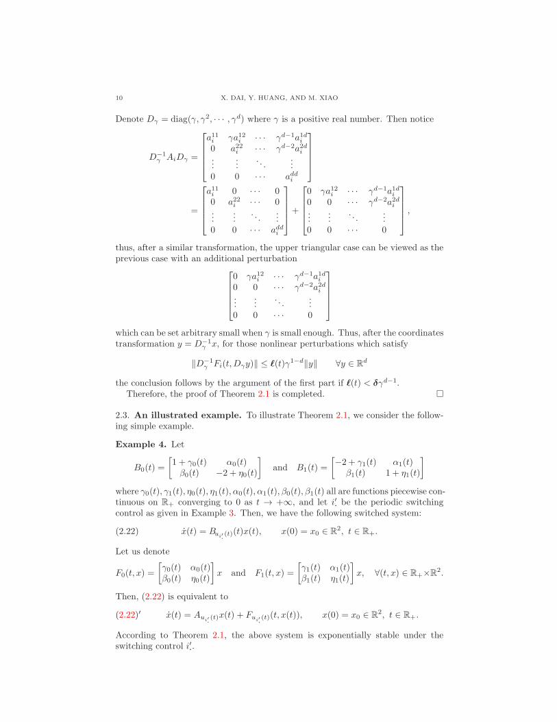
Denote Dγ = diag(γ, γ2, · · · , γd) where γ is a positive real number. Then notice

D−1γ AiDγ =

a11i γa12i · · · γd−1a1di0 a22i · · · γd−2a2di...

.... . .

...0 0 · · · addi

=

a11i 0 · · · 00 a22i · · · 0...

.... . .

...0 0 · · · addi

+

0 γa12i · · · γd−1a1di0 0 · · · γd−2a2di...

.... . .

...0 0 · · · 0

,

thus, after a similar transformation, the upper triangular case can be viewed as theprevious case with an additional perturbation

0 γa12i · · · γd−1a1di0 0 · · · γd−2a2di...

.... . .

...0 0 · · · 0

which can be set arbitrary small when γ is small enough. Thus, after the coordinatestransformation y = D−1

γ x, for those nonlinear perturbations which satisfy

‖D−1γ Fi(t,Dγy)‖ ≤ ℓ(t)γ1−d‖y‖ ∀y ∈ Rd

the conclusion follows by the argument of the first part if ℓ(t) < δγd−1.Therefore, the proof of Theorem 2.1 is completed. �

2.3. An illustrated example. To illustrate Theorem 2.1, we consider the follow-ing simple example.

Example 4. Let

B0(t) =

[1 + γ0(t) α0(t)β0(t) −2 + η0(t)

]and B1(t) =

[−2 + γ1(t) α1(t)

β1(t) 1 + η1(t)

]

where γ0(t), γ1(t), η0(t), η1(t), α0(t), α1(t), β0(t), β1(t) all are functions piecewise con-tinuous on R+ converging to 0 as t → +∞, and let i′

·be the periodic switching

control as given in Example 3. Then, we have the following switched system:

(2.22) x(t) = Bui′·

(t)(t)x(t), x(0) = x0 ∈ R2, t ∈ R+.

Let us denote

F0(t, x) =

[γ0(t) α0(t)β0(t) η0(t)

]x and F1(t, x) =

[γ1(t) α1(t)β1(t) η1(t)

]x, ∀(t, x) ∈ R+×R2.

Then, (2.22) is equivalent to

(2.22)′ x(t) = Aui′·

(t)x(t) + Fui′·

(t)(t, x(t)), x(0) = x0 ∈ R2, t ∈ R+.

According to Theorem 2.1, the above system is exponentially stable under theswitching control i′

·.

STABILITY OF TIME-VARYING SWITCHING SYSTEMS 11

3. Randomly switching systems

We now apply our criterion Theorem 2.1 proved in Section 2 and ergodic theory([19, 24]) to the study of almost sure stability of the following randomly switchingsystem (A+ F )Σ+

I

:

x(t) = Aui·(t)x(t) + Fui

·(t)(t, x(t)), t ∈ R+, x(0) = x0 ∈ Rd; i

·∈ Σ+

I

driven by the one-sided Markov shift of countable states set I = {1, 2, . . . }:

θ : Σ+I → Σ+

I ; i·= (i1, i2, . . . ) 7→ i

·+1 = (i2, i3, . . . )

which preserves an ergodic Borel probability measure µ on Σ+I , where

Ai =[Aℓm

i

]1≤ℓ,m≤d

∈ Rd×d and Fi(t, x) ∈ Rd

for each i ∈ I and ui·

: R+ → I is the switching law associated to i·∈ Σ+

I definedas in Section 1.

In this section, we will mainly prove two almost sure stability results, Theo-rems 3.1 and 3.6 below.

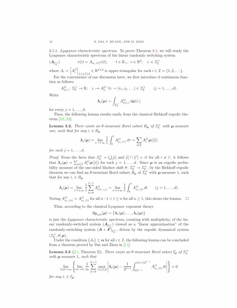
3.1. Nonlinear randomly switching systems. We now consider the stability ofnonlinear randomly switching systems.

Theorem 3.1. Assume Ai ∈ Rd×d are upper-triangular for each i ∈ I, whereI = {1, 2, . . .} not necessarily finite but countable, and θ : Σ+

I → Σ+I is the one-

sided Markov shift which preserves an ergodic Borel probability µ. If it holds that

‖Ai‖ ≤ α ∀i ∈ I and λ(µ) = max1≤j≤d

{∑

i∈I

Ajji µ([i])

}< 0

then, the equilibrium point x(t) = 0 of (A+ F )ui·

:

x(t) = Aui·(t)x(t) + Fui

·(t)(t, x(t)), t ∈ R+, x(0) ∈ Rd,

is asymptotically exponentially stable for µ-a.s. i·∈ Σ+

I if Fi(t, x) = o(‖x‖) as‖x‖ → 0 uniformly for t sufficiently large.

Here λ(µ) is just the maximal Lyapunov exponent of (AΣ+

I

) in terms of µ and

the condition λ(µ) < 0 implies that for µ-a.e. i·∈ Σ+

I

λ(ui·

, v0) := limt→+∞

1

tlog ‖v(t, v0)‖ < 0 ∀v0 ∈ Rd

where v(t, v0) is the solution of (Aui·

) with v(0, v0) = v0; see Lemma 3.2 below.But even in the case I finite, it is not easy to find a desirable G as in (1.2) for theLyapunov-function methods.

Because for a deterministic nonlinear switching system (A+F )ui·

, its Lyapunovexponent does not satisfy the upper semi-continuity with respect to the perturba-tions F as is known by Examples 1 and 2 in Section 1, the statement of Theorem 3.1is of interest.

12 X. DAI, Y. HUANG, AND M. XIAO

3.1.1. Lyapunov characteristic spectrum. To prove Theorem 3.1, we will study theLyapunov characteristic spectrum of the linear randomly switching system

(AΣ+

I

) v(t) = Aui·(t)v(t), t ∈ R+, v ∈ Rd; i

·∈ Σ+

I

where Ai =[Ajl

i

]1≤j,l≤d

∈ Rd×d is upper-triangular for each i ∈ I = {1, 2, . . .}.

For the convenience of our discussion later, we first introduce d continuous func-tion as follows:

Ajj

π(·) : Σ+I → R; i

·7→ Ajj

i1∀i

·= (i1, i2, . . . ) ∈ Σ+

I (j = 1, . . . , d).

Write

λj(µ) =

∫

Σ+

I

Ajj

π(i·) dµ(i·)

for every j = 1, . . . , d.Then, the following lemma results easily from the classical Birkhoff ergodic the-

orem [19, 24]:

Lemma 3.2. There exists an θ-invariant Borel subset Bµ of Σ+I with µ-measure

one, such that for any i·∈ Bµ

λj(µ) = limt→+∞

1

t

∫ t

0

Ajj

ui·(τ) dτ =

∑

i∈I

Ajji µ([i])

for each j = 1, . . . , d.

Proof. From the facts that Σ+I =

⋃i[i] and [i] ∩ [i′] = ∅ for all i 6= i′, it follows

that λj(µ) =∑

i∈I Ajji µ([i]) for each j = 1, . . . , d. Since µ is an ergodic proba-

bility measure of the one-sided Markov shift θ : Σ+I → Σ+

I , by the Birkhoff ergodic

theorem we can find an θ-invariant Borel subset Bµ of Σ+I with µ-measure 1, such

that for any i·∈ Bµ

λj(µ) = limℓ→+∞

1

ℓ

ℓ−1∑

k=0

Ajj

π(i·+k)

= limℓ→+∞

1

ℓ

∫ ℓ

0

Ajj

ui·(t) dt (j = 1, . . . , d).

Noting Ajj

ui·(n) = Ajj

ui·(t) for all n−1 < t ≤ n for all n ≥ 1, this shows the lemma. �

Thus, according to the classical Lyapunov exponent theory

SpLya(µ) = {λ1(µ), . . . ,λd(µ)}

is just the Lyapunov characteristic spectrum, counting with multiplicity, of the lin-ear randomly-switched system (AΣ

+

I

) viewed as a “linear approximation” of the

randomly-switching system (A + F )Σ+

I

, driven by the ergodic dynamical system

(Σ+I , θ;µ).Under the condition ‖Ai‖ ≤ α for all i ∈ I, the following lemma can be concluded

from a theorem proved by Dai and Zhou in [11]:

Lemma 3.3 ([11, Theorem 2]). There exists an θ-invariant Borel subset Γµ of Σ+I

with µ-measure 1, such that

limN∋ℓ→∞

{lim

m→∞

1

m

m−1∑

k=0

max1≤j≤d

∣∣∣∣∣λj(µ)−1

2ℓ−1

∫ (k+1)2ℓ−1

k2ℓ−1

Ajj

ui·(t) dt

∣∣∣∣∣

}= 0

for any i·∈ Γµ.

STABILITY OF TIME-VARYING SWITCHING SYSTEMS 13

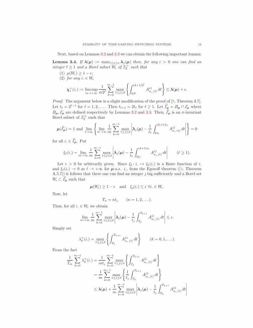
Next, based on Lemmas 3.2 and 3.3 we can obtain the following important lemma:

Lemma 3.4. If λ(µ) := max1≤j≤n λj(µ) then, for any ǫ > 0 one can find an

integer ℓ ≥ 1 and a Borel subset Wǫ of Σ+I such that

(1) µ(Wǫ) ≥ 1− ǫ;(2) for any i

·∈ Wǫ

χ+∗ (i·) := lim sup

m→+∞

1

m2ℓ

m−1∑

k=0

max1≤j≤d

{∫ (k+1)2ℓ

k2ℓAjj

ui·(t) dt

}≤ λ(µ) + ǫ.

Proof. The argument below is a slight modification of the proof of [9, Theorem 3.7].

Let tℓ = 2ℓ−1 for ℓ = 1, 2, . . . . Then tℓ+1 = 2tℓ for ℓ ≥ 1. Let Γµ = Bµ ∩ Γµ where

Bµ, Γµ are defined respectively by Lemmas 3.2 and 3.3. Then, Γµ is an σ-invariantBorel subset of Σ+

I such that

µ(Γµ) = 1 and limℓ→∞

{lim

m→∞

1

m

m−1∑

k=0

max1≤j≤d

∣∣∣∣∣λj(µ)−1

tℓ

∫ (k+1)tℓ

ktℓ

Ajj

ui·(t) dt

∣∣∣∣∣

}= 0

for all i·∈ Γµ. Put

ξℓ(i·) = limm→∞

1

m

m−1∑

k=0

max1≤j≤d

∣∣∣∣∣λj(µ)−1

tℓ

∫ (k+1)tℓ

ktℓ

Ajj

ui·(t) dt

∣∣∣∣∣ (ℓ ≥ 1).

Let ǫ > 0 be arbitrarily given. Since ξℓ : i· 7→ ξℓ(i·) is a Baire function of i·

and ξℓ(i·) → 0 as ℓ → +∞ for µ-a.s. i·, from the Egoroff theorem ([4, Theorem

A.5.7]) it follows that there one can find an integer big sufficiently and a Borel set

Wǫ ⊂ Γµ such that

µ(Wǫ) ≥ 1− ǫ and ξ(i·) ≤ ǫ ∀i·∈ Wǫ.

Now, let

Tn = nt (n = 1, 2, . . . ).

Thus, for all i·∈ Wǫ we obtain

limm→∞

1

m

m−1∑

k=0

max1≤j≤d

∣∣∣∣∣λj(µ)−1

t

∫ Tk+1

Tk

Ajj

ui·(t) dt

∣∣∣∣∣ ≤ ǫ.

Simply set

λ+k (i·) = max

1≤j≤d

{∫ Tk+1

Tk

Ajj

ui·(t) dt

}(k = 0, 1, . . . ).

From the fact

1

Tm

m−1∑

k=0

λ+k (i·) =

1

mt

m−1∑

k=0

max1≤j≤d

{∫ Tk+1

Tk

Ajj

ui·(t) dt

}

=1

m

m−1∑

k=0

max1≤j≤d

{1

t

∫ Tk+1

Tk

Ajj

ui·(t) dt

}

≤ λ(µ) +1

m

m−1∑

k=0

max1≤j≤d

∣∣∣∣∣λj(µ)−1

t

∫ Tk+1

Tk

Ajj

ui·(t) dt

∣∣∣∣∣

14 X. DAI, Y. HUANG, AND M. XIAO

since λj(µ) ≤ λ(µ) for 1 ≤ j ≤ d, it follows that

χ+∗ (i·) = lim sup

m→+∞

1

Tm

m−1∑

k=0

λ+k (i·) ≤ λ(µ) + ξ(i·) ≤ λ(µ) + ǫ ∀i

·∈ Wǫ.

This completes the proof of Lemma 3.4 by letting ℓ = − 1. �

Clearly, χ+∗ (i·) defined by Lemma 3.4 is a Liao-type exponent of the linear switch-

ing system (Aui·

) associated to {ns = s2ℓ}+∞s=1, where the switching-time sequence

is {Tn = n}+∞1 for any i

·∈ Wǫ. This is a key point for the proof of Theorem 3.1

below.

3.1.2. Proof of Theorem 3.1. Theorem 3.1 is a corollary of Theorem 2.1 and Lemma 3.4proved above.

Proof. In fact, for any sequence ǫk ↓ 0, from Lemma 3.4 we can define a sequence ofBorel subsets Wǫk ⊂ Σ+

I satisfies the properties (1) and (2) of Lemma 3.4. For eachk, the equilibrium solution x(t) = 0 of (A+ F )ui

·

is asymptotically, exponentiallystable for all i

·∈ Wǫk from Theorem 2.1. This is because Fi(t, x) = o(‖x‖) as

‖x‖ → 0 uniformly for t ≥ 0. Noting µ(⋃

k Wǫk) = 1, this completes the proof ofTheorem 3.1. �

3.2. Randomly switched systems with diagonal linear approximations.

For A ∈ Rd×d being a symmetric matrix, we use λmax(A) to denote the maximumeigenvalue of A. The following result follows from the original work [16]:

Theorem 3.5 (See [16] or [28, Theorem 3.2]). Let I = {1, . . . , κ}, κ ≥ 2 andA = {A1, . . . , Aκ} ⊂ Rd×d. If there exists a symmetric and positive definite matrixG such that ∑

i∈I

λmax(GAiG−1 +G−1AT

i G)µ([i]) < 0,

then for µ-a.s. i·∈ Σ+

I , the equilibrium point x(t) = 0 of (A+ F )ui·

:

x(t) = Aui·(t)x(t) + Fui

·(t)(x)

is asymptotically stable when Fi(x) = o(‖x‖) for all i = 1, . . . , κ.

We next give an extension of the above criterion in the diagonal case using ourTheorem 2.1 before.

Theorem 3.6. Let I = {1, 2, . . .} be countable and Ai = diag(A11

i , . . . , Addi

)in

Rd×d for all i ∈ I. If

‖Ai‖ ≤ α ∀i ∈ I and χ(µ) :=∑

i∈I

λmax(Ai)µ([i]) < 0,

then for µ-a.s. i·∈ Σ+

I , the equilibrium point v(t) = 0 of the switching system

(A+ F )ui·

x(t) = Aui·(t)x(t) + Fui

·(t)(t, x(t))

is asymptotically, exponentially stable when ‖Fi(t, x)‖ < ‖x‖ · |χ(µ)| uniformly fori ∈ I and for t sufficiently large.

STABILITY OF TIME-VARYING SWITCHING SYSTEMS 15

Proof. Notice first that λmax(Ai) = max{Ajji | 1 ≤ j ≤ d} for all i ∈ I. Similar to

Lemma 3.2, we see that for µ-a.s. i·∈ Σ+

I

χ(µ) = limℓ→∞

1

ℓ

ℓ∑

k=1

max{Ajj

ui·(k) | 1 ≤ j ≤ d

}< 0.

This means that for the 1-switching-time sequence {Tn = n}+∞n=1, there holds that

χ+∗ (Aui

·

) = χ(µ) = χ(Aui·

) µ-a.s. i·∈ Σ+

I

associated to {ns = s}+∞s=1, from Section 2.1 and (1.3).

Thus, the theorem follows immediately from Theorem 2.1 or Theorem 1. �

Comparison this theorem with Theorems 3.1 and 3.5, here the nonlinear termsFi(t, x) are not of o(‖x‖) for all i ∈ I.

4. Concluding remarks and further questions

4.1. Concluding remarks. In this paper, by using methods developed in a seriesof papers [17, 9, 10], we obtain a criterion of asymptotic exponential stability forthe quasi-linear continuous-time switching system by a Liao-type exponent (The-orem 2.1). And as a result of our criterion, by making use of ergodic theory weprove a stability theorem almost surely for a quasi-linear, continuous-time, andtime-dependent randomly switched system based on the one-sided Markov shift(Theorem 3.1). This paper can be viewed a further development of [10]. Compar-ing to [10], its significance includes the following:

(1) For a deterministic switching system (A+ F )u, the formal “linear approx-imations” of its subsystems are time dependent;

(2) the new Liao-type exponent χ+∗ (Au) defined in this paper can deal with

broader class of systems than the one given in [10];(3) Theorem 3.1 can be viewed as a stochastic version of the main result The-

orem 2 of [10] and the condition is simpler than those in current literature.In addition, the assumption that Ai is upper-triangular is mainly due tothe technical transparency. The general case will be reported elsewhere.

A Liao-type exponent χ+∗ of a deterministic system is generally larger than its

maximal Lyapunov exponent λ. Hence, χ+∗ < 0 can provide us more information

than λ < 0. But from the viewpoint of measure theory, χ+∗ can approach arbitrarily

λ according to the assertion of Lemma 3.4.Furthermore, the Liao-type exponent presented in this paper can guide us to

choose a stabilizing switching control for nonlinear switched systems.

4.2. Further questions. We end this paper with two open questions for furtherstudy:

Question 1. Does the statement of Theorem 3.1 still hold if perturbation conditionFi(t, x) = o(‖x‖) is replaced by ‖Fi(t, x)‖ ≤ L‖x‖?

Question 2. Does the statement of Theorem 3.5 still hold if the control set Iis countable and perturbation condition Fi(x) = o(‖x‖) is relaxed by ‖Fi(t, x)‖ ≤L‖x‖?

16 X. DAI, Y. HUANG, AND M. XIAO

References

[1] N.E. Barabanov, A method for calculating the Lyapunov exponent of a differential inclusion,Automat. Remote Control, 50 (1989), pp. 475–479

[2] S. Battilotti and A.D. Santis, Dwell time controllers for stochastic systems with switching

Markov chain, Automatica, 41 (2005), pp. 923–934.[3] R. Bellman, Stability Theory of Differential Equations, McGraw-Hill. New York, 1953.[4] A. Bressan and B. Piccoli, Introduction to the Mathematical Theory of Control, AIMS on

Applied Math. Vol. 2, American Institute of Mathematical Science, 2007.[5] M.L. Bujorianu and J. Lygeros, Reachability questions in piecewise deterministic Markov

processes, Lecture Notes in Computer Science, Springer-Verlag, 2623 (2003), pp. 126–140.[6] B.F. Bylov, R.E. Vinograd, D.M. Grobman, and V.V. Nemytskii, Theory of Lyapunov

Exponents and its Applications to Stability Theory, Moscow, Nauka, 1966 (Russian).[7] D. Chatterjee and D. Liberzon, On stability of randomly switched nonlinear systems, IEEE

Trans. Automat. Control, 52 (2007), pp. 2390–2394.[8] D. Chatterjee and D. Liberzon, Stabilizing randomly switched systems, arXiv:0806.1293v1

[math.OC] 9 Jun 2008.[9] X. Dai, Exponential stability of nonautonomous linear differential equations with linear per-

turbations by Liao methods, J. Differential Equations, 225 (2006), pp. 549–572.[10] X. Dai, Y. Huang and M. Xiao, Criteria of stability for continuous-time switched systems

by using Liao-type exponents, SIAM J. Control Optim., 48 (2010), pp. 3271–3296.[11] X. Dai and Z.-L. Zhou, A generalization of a theorem of Liao, Acta Math. Sin. (Engl. Ser.),

22 (2006), pp. 207–210.[12] X. Feng, K.A. Loparo, Y. Ji and H.J. Chizeck, Stochastic stability properties of jump

linear systems, IEEE Trans. Automat. Control, 37 (1992), pp. 38–53.[13] H. Furstenberg and H. Kesten, Products of random matrices, Ann. Math. Statist., 31

(1960), pp. 457–469.[14] J.P. Hespanha, Stochastic hybrid systems: application to communication networks, Lecture

Notes in Computer Science, Springer-Verlag, 2993 (2004), pp. 387–401.[15] Y. Ji and H.J. Chizeck, Controllability, stabilizability, and continuous-time Markovian jump

linear quadratic control, IEEE Trans. Automat. Control, 35 (1990), pp. 777–788.[16] I.Ia. Kac and N.N. Krasovskii, On the stability of systems with random parameters, J.

Appl. Math. Mech., 24 (1960), pp. 1225–1246.[17] S.-T. Liao, An ergodic property theorem for a differential system, Scientia Sinica, 16 (1973),

pp. 1–24.[18] X. Mao and C. Yuan, Stochastic Differential Equations with Markovian Switching, Imperial

College Press, London, 2006.[19] V.V. Nemytskii and V.V. Stepanov, Qualitative Theory of Differential Equations, Princeton

University Press, Princeton, New Jersey 1960.[20] V.I. Oseledec, A multiplicative ergodic theorem, Lyapunov characteristic numbers for dy-

namical systems, Trudy Mosk Mat. Obsec., 19 (1968), pp. 119–210.[21] O. Perron, Die Ordnunfszahlen linearer Differentialgleichungssysteme, Math. Z., 31 (1930),

pp. 748–766.[22] R. Shorten, F. Wirth, O. Mason, K. Wulff and C. King, Stability criteria for switched

and hybrid systems, SIAM Rev., 49 (2007), pp. 545–592.

[23] V.A. Ugrinovskii, Randomized algorithms for robust stability and guaranteed cost control

of stochastic jump parameter systems with uncertain switching policies, J. Optim. TheoryAppl., 124 (2005), pp. 227–245.

[24] P. Walters, An Introduction to Ergodic Theory, GTM 79, Springer-Verlag, New York, 1982.[25] C. Yuan and J. Lygeros, Stabilization of a class of stochastic differential equations with

Markovian switching, Systems & Control Letters, 54 (2005), pp. 819–833.[26] C. Yuan and X. Mao, Asymptotic stability in distribution of stochastic differential equations

with Markovian switching, Stochastic Processes Appl., 103 (2003), pp. 277–291.[27] G. Zhai, B. Hu, K. Yasuda and A.N. Michel, Stability analysis of switched systems with

stable and unstable subsystems: an average dwell time approach, Internat. J. Systems Sci.,32 (2001), pp. 1055–1061.

[28] C. Zhu, G. Yin and Q.S. Song, Stability of random-switching systems of differential equa-

tions, Quart. Appl. Math., 67 (2009), pp. 201–220.

STABILITY OF TIME-VARYING SWITCHING SYSTEMS 17

Department of Mathematics, Nanjing University, Nanjing 210093, People’s Republicof China

E-mail address: [email protected]

Department of Mathematics, Zhongshan (Sun Yat-Sen) University, Guangzhou 510275,People’s Republic of China

E-mail address: [email protected]

Department of Mathematics, Southern Illinois University, Carbondale, IL 62901-4408, USA

E-mail address: [email protected]