Stability and Variability: Indicators for Passive Stability and Active Control in a Rhythmic Task

Stability and Variability: Indicators for Passive Stability and Active Controlin a Rhythmic Task

Kunlin Wei,1 Tjeerd M. H. Dijkstra,2,3 and Dagmar Sternad3

1Rehabilitation Institute of Chicago, Northwestern University, Chicago, Illinois; 2Institute for Computing and Information Sciences,Radboud University Nijmegen, Nijmegen, The Netherlands; and 3Departments of Kinesiology and Integrative Biosciences,The Pennsylvania State University, University Park, Pennsylvania

Submitted 18 December 2007; accepted in final form 12 March 2008

Wei K, Dijkstra TM, Sternad D. Stability and variability: indicatorsfor passive stability and active control in a rhythmic task. J Neuro-physiol 99: 3027–3041, 2008. First published March 19, 2008;doi:10.1152/jn.01367.2007. Using a rhythmic task where human sub-jects bounced a ball with a handheld racket, fine-grained analyses ofstability and variability extricated contributions from open-loop con-trol, noise strength, and active error compensation. Based on stabilityanalyses of a stochastic-deterministic model of the task—a surfacecontacting the ball by periodic movements—open-loop or dynamicstability was assessed by the acceleration of the racket at contact.Autocovariance analyses of model and data were further used togauge the contributions of open-loop stability and noise strength.Variability and regression analyses estimated active error compensa-tion. Empirical results demonstrated that experienced actors exploitedopen-loop stability more than novices, had lower noise strength, andapplied more active error compensations. By manipulating the modelparameter coefficient of restitution, task stability was varied andshowed that actors graded these three components as a function oftask stability. It is concluded that actors tune into task stability whenstability is high but use more active compensation when stability isreduced. Implications for the neural underpinnings for passive stabil-ity and active control are discussed. Further, results showed thatstability and variability are not simply the inverse of each other butcontain more quantitative information when combined with modelanalyses.

I N T R O D U C T I O N

It is widely recognized that stability is a core requirement formany motor tasks. Despite external perturbations and variabil-ity generated by the sensorimotor system itself, humans andanimals can maintain static postures and perform movementsconsistently and reliably. The neurophysiological system hasdeveloped a variety of mechanisms at different levels toachieve stable postures and movements, ranging from mechan-ical stiffness of the muscular and tendonous tissues (Loeb1995; Wagner and Blickhan 1999), to stiffness generated bymuscular reflexes with short and long loops (Nichols and Houk1976; Popescu et al. 2003), to voluntary intervention on thebasis of perceptual information (Hasan 2005; Loram and Lakie2002; Morasso and Sanguineti 2002). Besides these mecha-nisms, there is another contribution to stability originatingfrom the interaction between the actor and the environment.Since humans interact with objects in the environment thatpose physical constraints but also afford inherent stability,

further understanding of the challenges for the neurophysio-logical control system can be derived from analysis of thedynamics of this interaction in the context of a task (Saltzmanand Kelso 1987; Warren 2006).

Some tasks are inherently stable, others inherently unstable.Upright posture when viewed as an inverted pendulum isunstable but it is stabilized by active control processes in thecentral and peripheral nervous system, as evidenced by thecontinuous sway during quiet standing. Other behaviors haveinherent stability and require no additional control. For exam-ple, your arm hanging at the side of your body does not requireactive muscle activations and perturbations die out withouterror correction. Although this trivial example shows staticstability, more complex behaviors can have dynamic stability.One illustrative example is the passive dynamic walker.McGeer (1990) first demonstrated that a mechanical bipedcould walk down a gentle slope without any control. Smallfluctuations naturally arising in the stepping motion weredissipated, solely by relying on the stability properties of thispassive mechanical system. Based on the understanding of thepassive dynamic stability, actuated robots have been designedthat exploit the self-stabilizing properties and thereby canfunction with minimal control (Collins et al. 2005). The im-plication for the study of biological systems is that the dynamicinteractions of the actor with the physical environment cansimilarly afford passively stable coordination strategies. Weand others have hypothesized that the CNS seeks solutions toa task that exploit such passive stability to reduce the burden oncontrol (Warren 2006). Hence, the research strategy in thepresent work is first to examine the stability that is afforded bythe task without control and, on this basis, to identify additionalfeatures of active control that the nervous system may apply.Specifically, the present study pursues to identify active andpassive contributions to the dynamic stability of steady-staterhythmic bouncing of a ball with a racket.

This complex interactive task and its dynamics have alreadybeen investigated in a series of studies on human sensorimotorcontrol but also in robotic and theoretical studies (Buhler et al.1994; de Rugy et al. 2003; Dijkstra et al. 2004; Guckenheimerand Holmes 1983; Rizzi et al. 1992; Ronsse et al. 2006; Schaalet al. 1996; Sternad 2006; Tufillaro et al. 1992; Wei et al.2007). The task requires the actor (or actuator) to use ahandheld racket to rhythmically bounce a ball vertically intothe air to a consistent height. Using a dynamical model of the

Address for reprint requests and other correspondence: D. Sternad,Departments of Kinesiology and Integrative Biosciences, The PennsylvaniaState University, 266 Rec Hall, University Park, PA 16803 (E-mail: [email protected]).

The costs of publication of this article were defrayed in part by the paymentof page charges. The article must therefore be hereby marked “advertisement”in accordance with 18 U.S.C. Section 1734 solely to indicate this fact.

J Neurophysiol 99: 3027–3041, 2008.First published March 19, 2008; doi:10.1152/jn.01367.2007.

30270022-3077/08 $8.00 Copyright © 2008 The American Physiological Societywww.jn.org

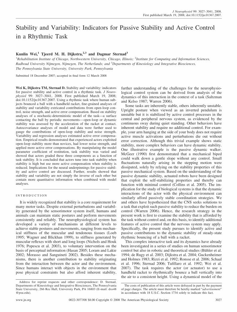
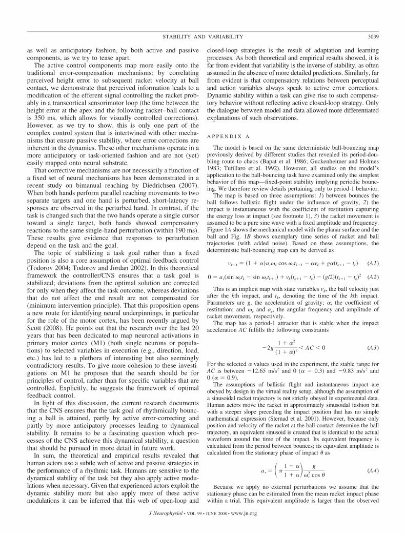
task, mathematical stability analyses revealed that the systemhas a stable solution if the racket is decelerating in its upwardmovement before contacting the ball (Fig. 1A; for a review ofthe model see APPENDIX A). This criterion can be intuited withthe help of Fig. 1B, which shows a time series of racket andball: if the ball arrives early after a low-amplitude bounce, asfor example the impact of the “noisy” (dashed) trajectory at2.3 s, then the ball is hit with a relatively higher velocity,leading to a higher ball amplitude in the subsequent cycle.Thus the condition for stability is that the ball is hit with ahigher velocity when the impact is relatively early and with alower velocity when the impact is late. This condition isequivalent to stating that the impact should happen during thedecelerating portion of the racket trajectory. For an actormoving a racket in this way, this means that small fluctuationsor perturbations from this stable racket trajectory do not haveto be explicitly corrected; stability can be achieved “passively”(i.e., without error correction or closed-loop control). A seriesof previous empirical studies of our group demonstrated thatactors indeed hit the ball with negative acceleration, consistentwith the interpretation that humans exploit dynamical—pas-sive—stability (e.g., Schaal et al. 1996; Sternad 2006; Weiet al. 2007).

Note that the comparison of the mechanical model with theball–racket system of the actor necessitates some terminolog-

ical clarification: To obtain passive stability as defined bymodel analysis the actor still has to (actively) generate arhythmic racket movement; however, it is sufficient that theactor controls the racket movement in an open-loop manner. Incontrast, when the actor applies explicit active error-compen-sating mechanisms this implies closed-loop control. Hence, inthe discussion of human performance we equate passive sta-bility with open-loop control, whereas active control is equatedwith closed-loop control.

These two control strategies, however, are not simple alter-natives. The dynamical stability of the ball-bouncing systemcan vary in degree, as shown in more detailed analyses inAPPENDIX A. This degree of stability, as quantified by theabsolute eigenvalue of the Jacobian, is dependent on its pa-rameters, in particular the coefficient of restitution �. Thecoefficient of restitution expresses the amount of energy lost atthe contact.1 Although it is straightforward to expect thatcontrol requirements change when more energy has to beimparted on the ball to achieve the same ball amplitude, themathematical result is not as easily intuited and the reader isreferred to APPENDIX A. Given these new model predictions thepresent study will manipulate the coefficient of restitution andassess whether different degrees of stability lead to differentperformances.

The finding that actors can exploit passive stability does notnecessarily imply that they always use only open-loop control.For example, a learning study revealed that novice actorsinitially performed the bouncing task with positive-impactacceleration and gradually tuned to the passive regime withnegative-impact acceleration only after 30 min of practice(Dijkstra et al. 2004). Importantly, novices could maintain arhythmic bouncing pattern similar to that of more experiencedactors, although their performance variability was higher. Itcould be concluded that they used an error-correcting closed-loop strategy. A similar difference in strategy was observedacross selected individuals with more or less experience in thetask (Sternad et al. 2000). These findings suggest that usingnegative impact acceleration is not an intuitive solution for theactor but rather one that it is learned with practice.

Further, perturbation studies suggested that actors used amixed strategy involving both open-loop control exploitingpassive stability and active control mechanisms based onperceived error information. When experimentally controlledperturbations were applied to the ball trajectory, actors ad-justed their racket movements according to target errors, eventhough racket impact acceleration values returned to the neg-ative range immediately after the perturbation (de Rugy et al.2003; Wei et al. 2007). As a result, the errors introduced by theperturbation were corrected faster than the relaxation processesof the model would have predicted, suggesting that actors useda blend of passive stability and active control.

Given this evidence in the case of large perturbations itremains an open question whether there are also active controlcomponents intertwined with the observed passive stabilitywhen the task is performed at steady state. At steady state thereare always small fluctuations or perturbations induced by

1 The coefficient of restitution can be illustrated with the following example:assuming the ball prior to contact to have a velocity of �2 m/s (relative to theracket) and the coefficient of restitution to be 0.5, the ball would bounce off theracket with a positive velocity of �1 m/s.

0 1 2 3 4 50

0.2

0.4

0.6

0.8

1

Time (s)

Pos

ition

(m

)

ωα

A

B

FIG. 1. Model and simulation of exemplary time series. A: mechanicalmodel with 2 state variables (vk and tk) and 4 parameters (�, g, �r, and ar) (seetext for details). B: time series of racket and ball trajectories of the determin-istic model (solid black lines) and the stochastic model (dashed and gray lines).The noisy simulations are created by introducing low-amplitude noise at eachball–racket contact leading to perturbations of the ball amplitude that thenpercolate across bounces and relax back to steady state. Similarly, noise isadded at the phase of the sinusoid at each impact. The dependent measures areshown graphically: racket period (T) and amplitude (A); racket acceleration atimpact (AC); height error (HE); ball velocity at release (v); and impact-to-impact time (t).

3028 K. WEI, T.M.H. DIJKSTRA, AND D. STERNAD

J Neurophysiol • VOL 99 • JUNE 2008 • www.jn.org

internal and external “noise.” Do actors completely rely on theslower self-correcting properties of the task? Whereas the twoprevious experiments examined the response following explicitrelatively large perturbations, identification of error-compen-sating strategies during unperturbed steady-state performancerequires a detailed time-series analysis of the sequence ofbounces. However, as pointed out earlier, error-correctingrelations naturally exist and are characteristic of dynamicstability. Therefore a simple autocorrelation analysis of bounce-to-bounce fluctuations will not be able to distinguish between theinherent stabilizing relations and error-compensating control bythe actor.

To tease apart the self-stabilizing from the active correctionswe extended the current deterministic ball-bouncing modelwith a stochastic component representing the inherent fluctu-ations during dynamically stable performance. Covarianceanalysis of the model across bounces then quantifies the self-correcting properties of the open-loop model. Any deviationsfrom this prediction in an actor’s performance can then beattributed to additional active corrections. Figure 1B illustratesthe model behavior: the ball trajectory with a solid line is asimulation of stable behavior from the deterministic modelwith no noise; the dashed trajectory shows a simulation whereeach racket cycle is slightly perturbed by adding random noiseto the amplitude and period of the racket. Assuming that theserandom perturbations are small, they propagate across bounceswith a specific relaxation behavior. The ball-bouncing map atdynamic stability will produce a structure in the fluctuationsthat can be quantified by the covariance of the state variablesover successive contacts. Based on the analyses of the autoco-variance functions of this stochastic-deterministic model, ad-ditional more fine-grained quantitative predictions were de-rived (APPENDIX B). In short, the auto- and cross-covariancesbetween the state variables of the model, velocity after impact,and time between impacts, are predicted to approach zero overlags. The time of return to zero is inversely related to thedegree of stability of the system. As stated earlier, the degreeof stability depends on the coefficient of restitution �. Testingthese predictions in human performance will provide a fine-grained assessment of how sensitive the physiological systemis to stability properties of the task.

To this end the present empirical study examined steady-state bouncing under seven conditions of �. In addition, be-cause different skill levels of actors were previously shown tolead to different performance strategies, we compared noviceand expert participants. Specifically, we examined whetherskilled actors showed higher contributions of open-loop stabil-ity compared with error-based corrections. The predictions canbe summarized as follows:

Prediction 1a. Consistent with previous analyses, perfor-mance with dynamic stability is indicated by negative accel-erations of the racket at contact. This passive stability isexpected for all � conditions, yet with a lower degree ofstability for higher �.

Prediction 1b. Consistent with previous empirical findings,it is expected that experienced actors rely more on dynamicstability. This is evidenced in more negative accelerations atcontact in the performance of experts, in contrast to morepositive values in nonexperienced actors.

Prediction 2. Stability, as quantified by the autocovariancefunction, decreases with increasing coefficients of restitution �.

This prediction is expressed in an autocorrelation structure inthe data with significant auto- and cross-correlations overlonger lags for higher � conditions.

Alternatively, it may be expected that with decreasing pas-sive stability at higher � values, the CNS utilizes more activecontrol to stabilize performance.

Prediction 3a. Given lower stability for higher � conditions,such active corrections are expected to be more prominent athigher � conditions.

Prediction 3b. Experienced actors require less active correc-tions to stabilize performance and decrease performancevariability.

The results with respect to these predictions will give insightinto how sensitive human actors at different degrees of expertiseare to dynamical properties of the task. The data will provide arich basis to assess how different neurophysiological processes,both corrective and anticipatory, lead to stable task performance.The results will be discussed in light of new perspectives on thecontrol principles that the CNS uses.

M E T H O D S

Participants

Eight volunteers, ranging in age from 21 to 47 yr, participated inthis experiment. Four participants had previously taken part in severalball-bouncing experiments and were considered experienced in thistask. Four other volunteers had never performed the task prior to thisexperiment. All participants were right-handed and used their pre-ferred right hand to bounce the ball with the racket. Before theexperiment, all participants were informed about the procedure andsigned the consent form approved by the Regulatory Committee of thePennsylvania State University.

Experimental apparatus

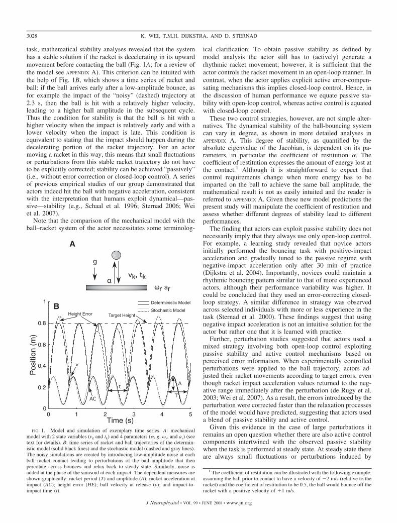
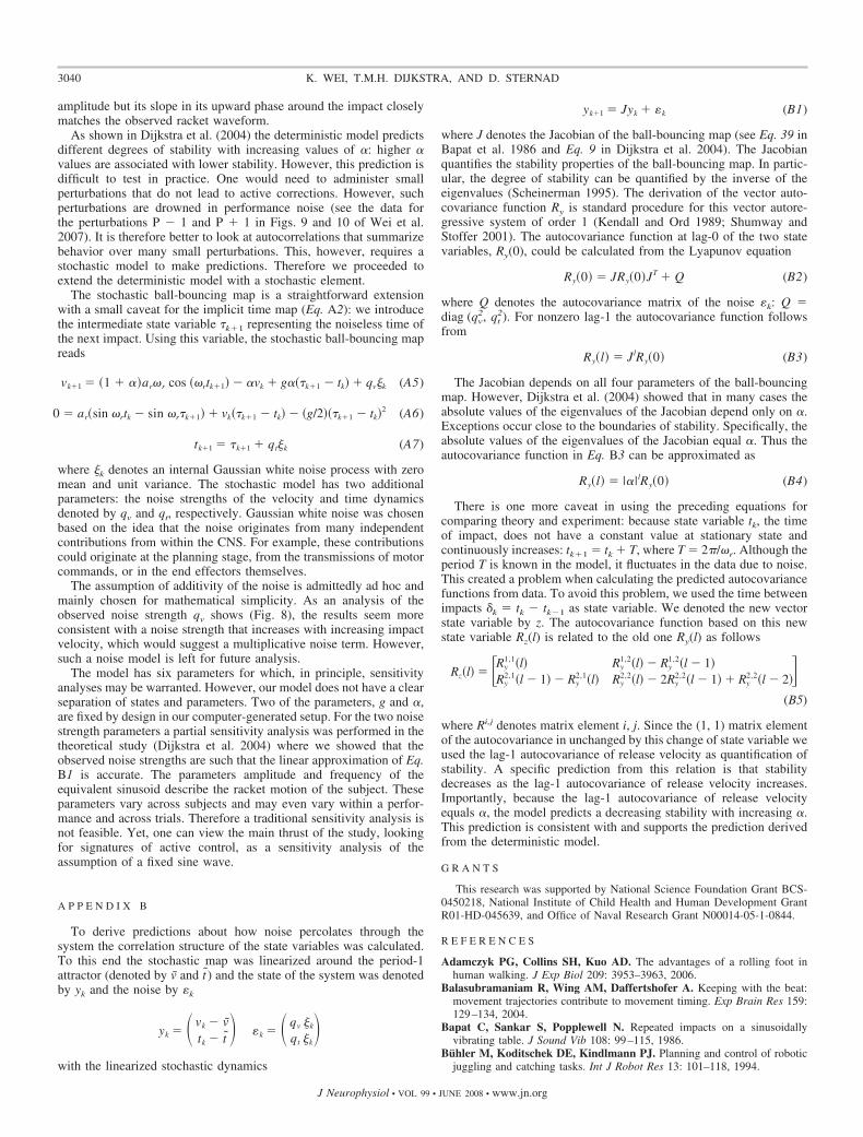
Participants manipulated a real table tennis racket to bounce avirtual ball that was projected onto a backprojection screen (2.5 �1.8 m) in front of them (Fig. 2). Using custom-made software a PCcontrolled the data collection and generated the images that wereprojected onto a backprojection screen (60-Hz refresh rate). Acceler-ations were measured directly using an accelerometer mounted on topof the racket. The mechanical brake on the rod attached to the racketwas controlled by a solenoid. A light rigid rod with three hinge jointswas attached to the racket surface and ran through a wheel whoserotation was registered by an optical encoder. The racket could moveand tilt with minimal friction in three dimensions but only the verticaldisplacement was measured. Racket movements in other than verticaldirections were minimal because only vertical movements were dis-played on the screen and interacted with the virtual ball. The delaybetween real and virtual racket movements was 22 ms on average withSD of 0.5 ms (for more details on the experimental setup see Wei et al.2007).

The virtual racket was displayed at the same height as the realracket and its displacement was the same as that of the real racket (thegain between real and virtual movements was 1). The ball displayedon the screen was a virtual ball and its movement was governed byballistic flight and an instantaneous impact event when the virtualracket impacted the virtual ball. Just before the virtual ball hit thevirtual racket a trigger signal was sent out to the mechanical brake thatwas attached to the rod. The trigger signal was sent out 15 ms beforethe ball–racket contact to overcome the mechanical and electronicdelay of the brake. The brake applied a brief force pulse to the rod tocreate the feeling of a real ball hitting the racket. Thus the impactcaused by the brake and the impact observed on the screen coincided.

3029STABILITY AND VARIABILITY


The duration of the force pulse (30 ms) was consistent with the impactduration observed in a real ball–racket experiment (Katsumata et al.2003).

Procedure and experimental conditions

Each trial began with a ball appearing at the left side of the screenand rolling on a horizontal line extending to the center of the screen.On reaching the center, the ball dropped from the horizontal line (0.8m high) to the racket. The task for the participant was to bounce theball periodically to the target line (the line on which the ball started).The experiment was conducted in 14 blocks with seven different �values (0.3, 0.4, 0.5, 0.6, 0.7, 0.8, and 0.9). Each � condition waspresented in two blocks with three trials in each block. For fourparticipants (two from each group), the blocks were presented first inascending and then descending order of � values, i.e., from 0.3 to 0.9then from 0.9 to 0.3. For the other four participants (two from eachgroup), the blocks were presented first in descending order and then inascending order. Each trial lasted 40 s.

Data reduction and analysis

The first 5 s of data were eliminated from the analysis becausesubjects stabilized their performance in the initial part of the trial. Theraw data of the racket displacement and acceleration were resampledat a fixed frequency of 400 Hz and filtered by a fourth-order Savitzky–Golay filter with a window size of 0.01 s on both sides (Gander and

Hrebicek 2004). Compared with conventional filters like Butterworthfilters, the Savitzky–Golay filter is superior for smoothing data thathave abrupt changes. These abrupt changes occurred when the racketexhibited a sudden drop in acceleration at impact, caused by the brake.The filter order and window size were chosen empirically to removethe measurement noise while not excessively smoothing the sig-nals. The ball-displacement data were generated by the computer andcontained no measurement noise. Therefore no filtering was per-formed.

As a verification of our setup, the racket displacement was double-differentiated using a Savitzky–Golay filter and compared with theacceleration data from the accelerometer (see Wei et al. 2007). Onaverage the accelerometer signal rendered estimates for the impactacceleration that were 0.52 m/s2 more positive than the position signal(compare with mean values in Fig. 4). To be conservative and giventhat the variability of the impact accelerations from the accelerometerwas smaller we opted to report the estimates from the accelerometer.

Dependent measures

Performance was evaluated by the ball height error HE, defined asthe signed difference between the maximum ball height and the targetheight (Fig. 1B). The amplitude of the racket movement A wascalculated as half the distance from the minimum to the maximum ofthe racket trajectory during one cycle. The racket period T wascalculated from the intervals between the times of peak velocities ofsuccessive bounces. The acceleration of the racket at impact AC was

Screen

Projector

PC

Rigid Rod

Wheel and Optical Encoder

Brake

Virtual Racket

Virtual Ball

Target Height

Front View

HingeJoints

Accelerometer

FIG. 2. Sketch of the virtual reality setup with the haptic interface. The inset shows the screen display with a horizontal line where the ball initially rolls anddrops. For the rhythmic performance the line becomes the target height.



determined from the raw accelerometer signal one sample before thestart of the impact. The mean and SDs for HE, A, T, and AC werecalculated over occurrences (bounces) within trials, then averagedacross trials per condition, and finally averaged over the four partic-ipants of each group.

Correlation function

The vector autocorrelation function ACF was calculated from thevector covariance function of the state variables ball velocity atrelease v, and the time between impacts t (Fig. 1B). The ACF capturesthe correlation of state variables across lags, where lags correspond tobounces in the data and model. The ACF, normalized by the lag-0covariance, encompasses both the autocorrelations ACF(v-v) andACF(t-t) and the cross-correlations ACF(t-v) and ACF(v-t) for ballrelease velocity and impact period. For a given lag number the vectorautocorrelation function equals the Pearson product-moment correla-tion of state variable (e.g., release velocity) and a lagged copy of astate variable (e.g., time between impacts). Before calculating theACF for each trial, the series of v and t were detrended because someparticipants showed slow drifts in their impact position or ball am-plitudes. To calculate the mean ACF, the ACFs of all trials wereaveraged for a given � and for all participants within a group. Toquantify the variability of the ACF, the SDs over six trials per �condition were calculated for each participant.

To calculate the ACF from the model, the four deterministic modelparameters had to be specified. The two noise strengths did not matterbecause they were divided out by the normalization inherent in thecalculation of the ACF. Two parameters were specified by the exper-imental design: g was fixed at �9.81 m/s2 and � varied with condi-tion. The other two parameters were set from the average values fromeach group: the average bouncing frequency �r and amplitude ar (Eq.A4). We chose to fit the parameters at the level of the group, notindividual actors or individual trials, because impact acceleration waspositive for several trials in the nonexperienced group. The impactphase, which was used in the calculation of equivalent amplitude (Eq.A4), was calculated from the time difference between time of maxi-mal velocity and time of impact divided by the period T. Severalchoices are possible in calculating an average equivalent frequencyand phase from experimental data: from an individual bounce, from atrial average, from a condition average, or from a group average.Since the comparisons are between � conditions and groups, we choseto average over bounces in a trial and over trials of the same conditionbut not over participants in a group nor over conditions nor groups.From these four parameters, the Jacobian and the ACF could becalculated (Eqs. B3, B4, and B5).

A problem arises when the impact phase is negative because theACF is not defined in this case. Therefore we eliminated trials forwhich impact phase was negative. This led to the elimination of 46trials (14% of all trials). These trials occurred mainly in threenonexperienced participants in the lower � conditions. Note that thetrials were eliminated for calculating only the theoretical predictions.The corresponding data were not eliminated when calculating perfor-mance measures because we did not regard it justified to eliminatedata that did not fit the theory.

Noise level

The noise strengths qv and qt are additional parameters that wereintroduced by the stochastic extension of the deterministic model(Appendix B). The noise strengths were estimated from the experimen-tal data by the unexplained variance in Eq. B1. In detail, we firstobtained an estimate of the Jacobian, as described in the appendix andthen calculated the residual �k from the Jacobian J and the observedstate variables yk and yk�1. The noise strengths were then estimatedfrom the root mean square of the residuals.

Regression analysis

To directly assess compensatory adjustments between a perceivedvariable with respect to a controlled variable, linear regression anal-yses were conducted. The idea is that if a perceptual variable is usedto control an action variable, then we expect a significant nonzeroslope in a regression. This slope can be interpreted as a feedback gainin a proportional controller. The most insightful regression proved tobe the one of the racket contact velocity at bounce k � 1 on the heighterror in bounce k. For comparison, the same regression analyses wereconducted for model simulations that were performed by iterating thestochastic ball-bouncing map (Eqs. A5, A6, and A7) with the same setof parameters as for the autocorrelation analysis. For the noisestrengths we took small values (qv � 10�3 m/s, qt � 10�4 s) becausethe slopes do not depend on the noise strengths.

Statistical analyses

All dependent measures were subjected to a two-way mixed-effectANOVA with group (between-subjects factor, 2 levels) and � (withinsubjects factor, 7 levels). For this ANOVA averages of the six trialsfor each � condition per participant were used (to satisfy the assump-tion of independent samples). Although the ANOVA gave significantresults, the relatively small number of subjects may have violated orgiven insufficient support to the assumptions underlying the ANOVA.Further, due to taking the averages across six trials, the variance fromthese six trials was lost. Hence, to provide additional statistical tests ofthe group differences in lag-1 autocorrelation and regression slope,which are a core result of the study, permutation tests were conductedthat did not rely on the assumption of independence of samples(Wassermann 2003). For this test, all 336 data points were pooled [6(trials) � 7 (�) � 4 (subjects) � 2 (group)] and a bootstrappingmethod was applied: first, from the pooled data two data sets weresampled randomly (without replacement) to represent a new samplefor each subject group. Second, for each sampled group a mean wascalculated (over six repetitions, seven alpha conditions, and fouractors). Third, the difference between the two groups served as thetest statistic. Fourth, the three steps generating bootstrap data setswere repeated 1,000,000 times to yield a distribution of differencevalues. Fifth, the observed group difference was compared againstthe distribution of differences of the bootstrap data sets. Theobserved value was significant if it was not very probable. Prob-ability was estimated by calculating the P value as the ratiobetween the number of values from the random permutations thatexceeded the observed value and the total number of bootstrap datasets.

To compare the experimentally observed and theoretically pre-dicted lag-1 autocorrelations and regression slopes, we used a t-testfor each � condition. We could not use ANOVAs for this comparisonbecause the model predicted only one value per group. The signifi-cance level for the t-test was 0.05, but since we ran seven tests, onefor each � condition, we applied a Bonferroni correction to thissignificance level (0.05/7 � 0.007). We also used the permutation testto investigate the influence of experience on how much the observedvalues of the lag-1 autocorrelation differ from their values predictedfrom the ball-bouncing map. The procedure was identical to the onedescribed earlier except that the difference between the observed lag-1autocorrelations and the theoretical prediction was entered into thecalculations.

In most figures, we plotted mean values averaged over trials andactors in a group (exception is the inherent noise level of Fig. 8where the median was used). The error bars in all data plots denotethe SEs over actors within a group (except Fig. 8; see figurecaption).



R E S U L T S

Height error

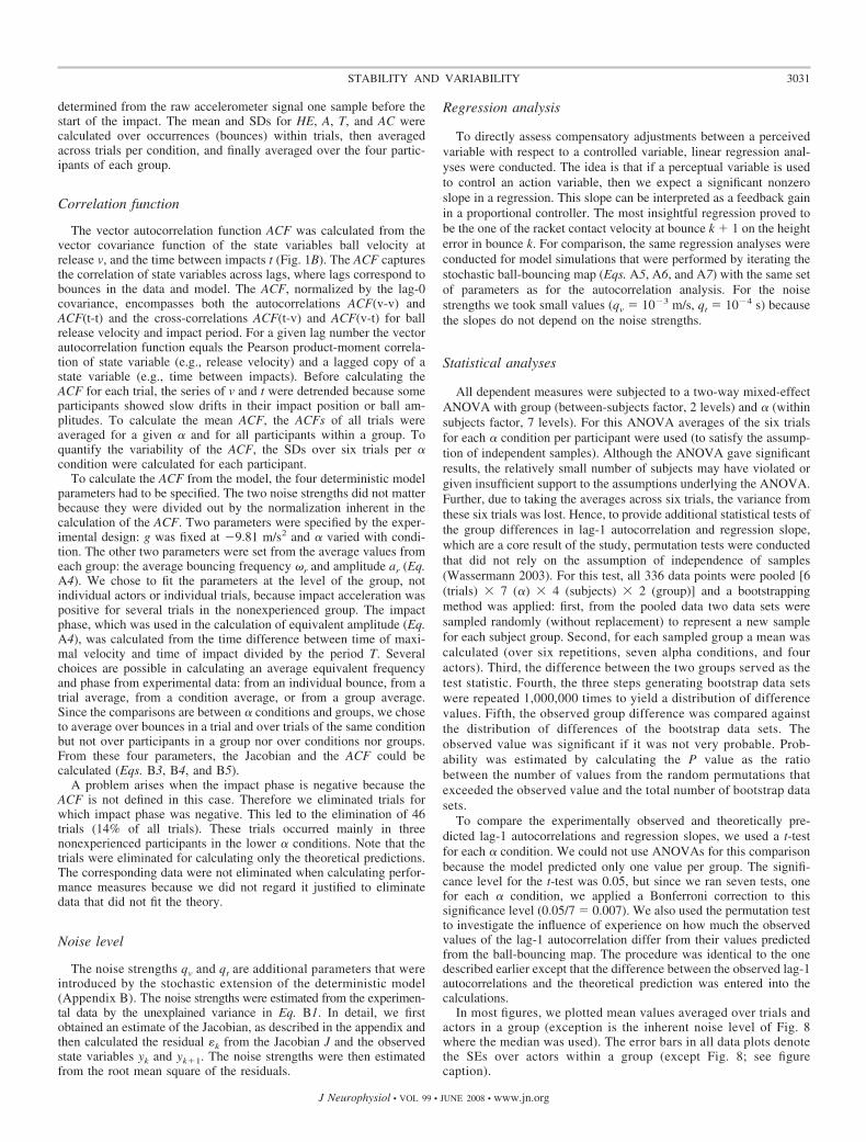
To evaluate task performance both the means and SDs of theheight error HE were compared across the seven � conditionsfor all participants. To assess whether the different experienceof the eight participants was evident in performance theirindividual scores were assessed. The mean HE values for thetwo participant groups are listed in Table 1. The average valuespooled over trials and participants were positive and showed atendency to overshoot the target, which was larger for higher �values [F(6,36) � 24.54, P � 0.0001] (Table 1). The differentexperience with the task between participants did not lead to adifference in the mean HE itself. The apparent tendency thatnonexperienced subjects have smaller mean HE values doesnot indicate higher accuracy; because HE is a signed error, andlarge alternations between positive and negative errors causedthese seemingly smaller mean errors. Note this difference wasalso not significant due to the large variance of HE. Hence, abetter reflection of the different experience levels was given bythe SDs of HE shown in Fig. 3.

Consistent with subjects’ previous experience, their perfor-mance variability shows significant differences between theexperts and novices. The ANOVA verified that experiencedparticipants showed significantly higher variability, F(1,6) �112.25, P � 0.0001. On the basis of this clear difference invariability, the participants were separated into two groups offour participants each for the following analyses. The interac-tion was also significant signaling larger separation for the

smaller � values, F(6,36) � 2.94, P � 0.05. The main effectfor � was also significant and showed that for higher �, thevariability decreased, F(6,36) � 11.70, P � 0.0001. Thedecrease in variability at larger � conditions ran counter toPrediction 2 and will be examined in more detail below.

Racket acceleration at impact

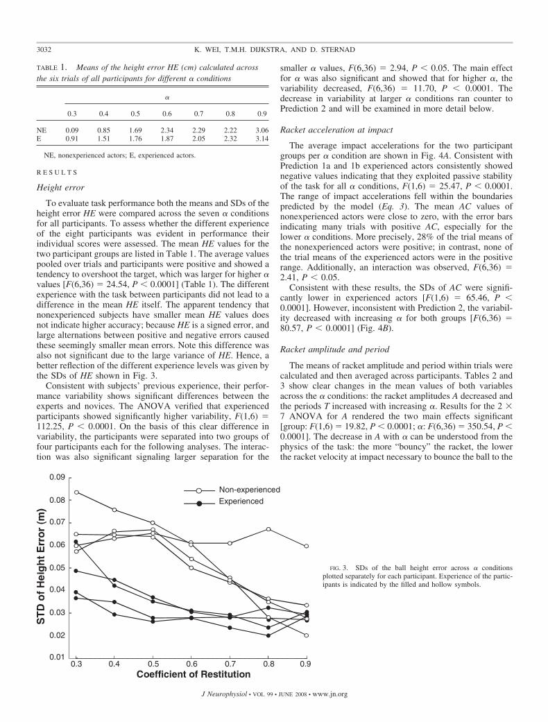
The average impact accelerations for the two participantgroups per � condition are shown in Fig. 4A. Consistent withPrediction 1a and 1b experienced actors consistently showednegative values indicating that they exploited passive stabilityof the task for all � conditions, F(1,6) � 25.47, P � 0.0001.The range of impact accelerations fell within the boundariespredicted by the model (Eq. 3). The mean AC values ofnonexperienced actors were close to zero, with the error barsindicating many trials with positive AC, especially for thelower � conditions. More precisely, 28% of the trial means ofthe nonexperienced actors were positive; in contrast, none ofthe trial means of the experienced actors were in the positiverange. Additionally, an interaction was observed, F(6,36) �2.41, P � 0.05.

Consistent with these results, the SDs of AC were signifi-cantly lower in experienced actors [F(1,6) � 65.46, P �0.0001]. However, inconsistent with Prediction 2, the variabil-ity decreased with increasing � for both groups [F(6,36) �80.57, P � 0.0001] (Fig. 4B).

Racket amplitude and period

The means of racket amplitude and period within trials werecalculated and then averaged across participants. Tables 2 and3 show clear changes in the mean values of both variablesacross the � conditions: the racket amplitudes A decreased andthe periods T increased with increasing �. Results for the 2 �7 ANOVA for A rendered the two main effects significant[group: F(1,6) � 19.82, P � 0.0001; �: F(6,36) � 350.54, P �0.0001]. The decrease in A with � can be understood from thephysics of the task: the more “bouncy” the racket, the lowerthe racket velocity at impact necessary to bounce the ball to the

0.3 0.4 0.5 0.6 0.7 0.8 0.90.01

0.02

0.03

0.04

0.05

0.06

0.07

0.08

0.09

Coefficient of Restitution

Non-experiencedExperienced

FIG. 3. SDs of the ball height error across � conditionsplotted separately for each participant. Experience of the partic-ipants is indicated by the filled and hollow symbols.

TABLE 1. Means of the height error HE (cm) calculated acrossthe six trials of all participants for different � conditions

�

0.3 0.4 0.5 0.6 0.7 0.8 0.9

NE 0.09 0.85 1.69 2.34 2.29 2.22 3.06E 0.91 1.51 1.76 1.87 2.05 2.32 3.14

NE, nonexperienced actors; E, experienced actors.



fixed target height. The mean T values showed the oppositetrend: both groups increased their periods for higher � values[F(6,36) � 53.06, P � 0.0001]. This increase in T is partly dueto the increase in HE because larger ball amplitudes increasethe time intervals between bounces. Further, participantstended to lower the racket impact position for the higher �values. This was possible given that participants were free to

choose their preferred impact position while the target heightwas fixed.

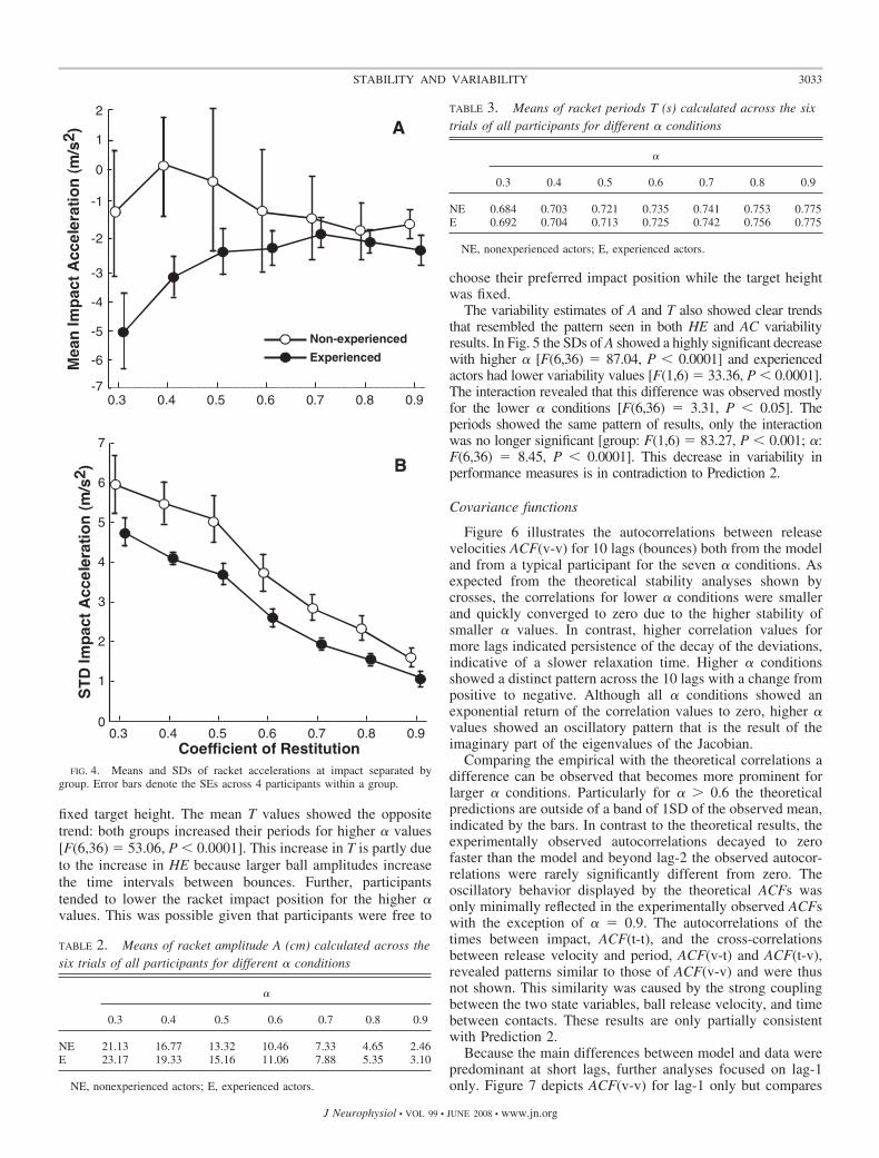
The variability estimates of A and T also showed clear trendsthat resembled the pattern seen in both HE and AC variabilityresults. In Fig. 5 the SDs of A showed a highly significant decreasewith higher � [F(6,36) � 87.04, P � 0.0001] and experiencedactors had lower variability values [F(1,6) � 33.36, P � 0.0001].The interaction revealed that this difference was observed mostlyfor the lower � conditions [F(6,36) � 3.31, P � 0.05]. Theperiods showed the same pattern of results, only the interactionwas no longer significant [group: F(1,6) � 83.27, P � 0.001; �:F(6,36) � 8.45, P � 0.0001]. This decrease in variability inperformance measures is in contradiction to Prediction 2.

Covariance functions

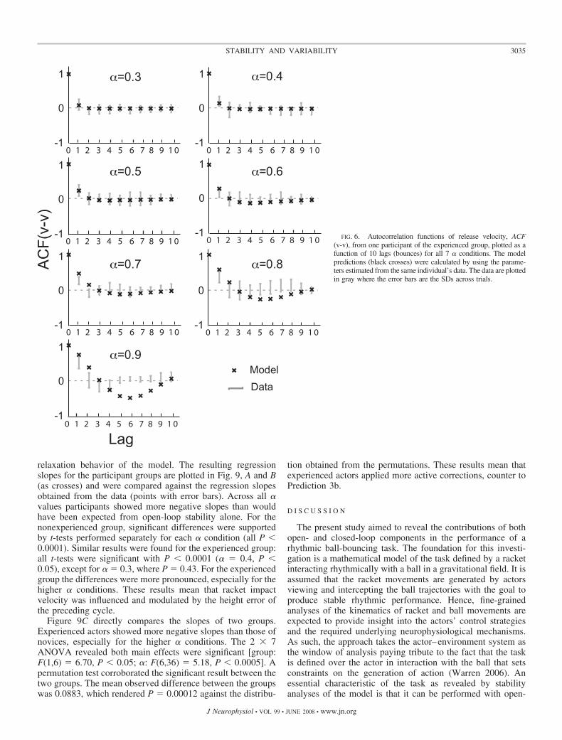
Figure 6 illustrates the autocorrelations between releasevelocities ACF(v-v) for 10 lags (bounces) both from the modeland from a typical participant for the seven � conditions. Asexpected from the theoretical stability analyses shown bycrosses, the correlations for lower � conditions were smallerand quickly converged to zero due to the higher stability ofsmaller � values. In contrast, higher correlation values formore lags indicated persistence of the decay of the deviations,indicative of a slower relaxation time. Higher � conditionsshowed a distinct pattern across the 10 lags with a change frompositive to negative. Although all � conditions showed anexponential return of the correlation values to zero, higher �values showed an oscillatory pattern that is the result of theimaginary part of the eigenvalues of the Jacobian.

Comparing the empirical with the theoretical correlations adifference can be observed that becomes more prominent forlarger � conditions. Particularly for � � 0.6 the theoreticalpredictions are outside of a band of 1SD of the observed mean,indicated by the bars. In contrast to the theoretical results, theexperimentally observed autocorrelations decayed to zerofaster than the model and beyond lag-2 the observed autocor-relations were rarely significantly different from zero. Theoscillatory behavior displayed by the theoretical ACFs wasonly minimally reflected in the experimentally observed ACFswith the exception of � � 0.9. The autocorrelations of thetimes between impact, ACF(t-t), and the cross-correlationsbetween release velocity and period, ACF(v-t) and ACF(t-v),revealed patterns similar to those of ACF(v-v) and were thusnot shown. This similarity was caused by the strong couplingbetween the two state variables, ball release velocity, and timebetween contacts. These results are only partially consistentwith Prediction 2.

Because the main differences between model and data werepredominant at short lags, further analyses focused on lag-1only. Figure 7 depicts ACF(v-v) for lag-1 only but compares

0.3 0.4 0.5 0.6 0.7 0.8 0.9

-6

-5

-4

-3

-2

-1

0

1

2

-7

Non-experienced

Experienced

0.3 0.4 0.5 0.6 0.7 0.8 0.90

1

2

3

4

5

6

7


A

B

FIG. 4. Means and SDs of racket accelerations at impact separated bygroup. Error bars denote the SEs across 4 participants within a group.

TABLE 2. Means of racket amplitude A (cm) calculated across thesix trials of all participants for different � conditions

�

0.3 0.4 0.5 0.6 0.7 0.8 0.9

NE 21.13 16.77 13.32 10.46 7.33 4.65 2.46E 23.17 19.33 15.16 11.06 7.88 5.35 3.10


TABLE 3. Means of racket periods T (s) calculated across the sixtrials of all participants for different � conditions

�

0.3 0.4 0.5 0.6 0.7 0.8 0.9

NE 0.684 0.703 0.721 0.735 0.741 0.753 0.775E 0.692 0.704 0.713 0.725 0.742 0.756 0.775




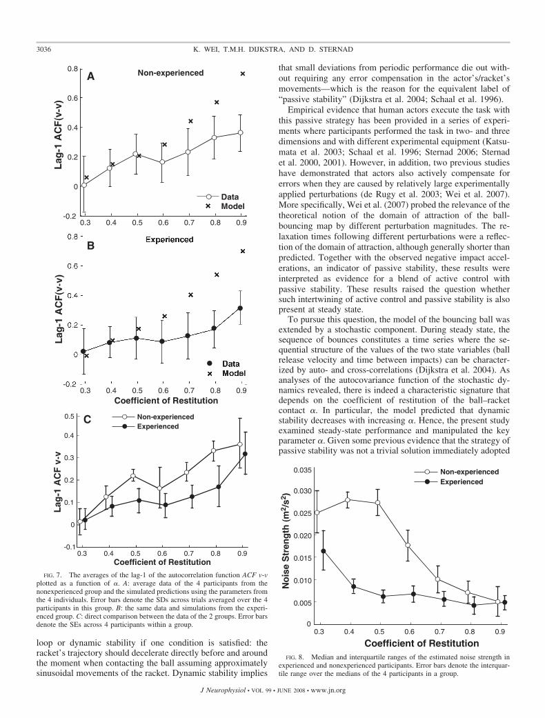
the correlation values against � for experienced and nonexpe-rienced participants separately. The lag-1 ACF(v-v) from thedata increased with increasing �, corresponding to the model’sprediction for both groups. Thus overall, Prediction 2 wassupported by the data. However, although the ACF values ofmodel and data matched closely for � �0.5, for higher �conditions the data exhibited smaller ACF values and themodel values were no longer within the error band of the data.This indicates that in real bouncing fluctuations were compen-sated faster than in the model, probably due to active errorcompensation. Separate t-tests compared model and data foreach � condition for both groups and supported this impres-sion: for � �0.5 there were significant differences between the

model and the data (all P � 0.001); for � �0.5, the differenceswere not significant (all P � 0.05).

Although the plots at first sight suggest similar behavior forboth participant groups, a direct comparison of the perfor-mance data shown in Fig. 7C revealed that there were signif-icant differences between groups. The 2 � 7 ANOVA renderedthe comparisons between groups and � significant [group:F(1,6) � 11.32, P � 0.01; �: F(6,36) � 12.62, P � 0.0001].To corroborate the significant difference between the smallnumber of participants a permutation test was applied (Was-sermann 2003). Results revealed that the observed differenceof 0.0751 between the two groups was highly significant (P �0.00003).

The results suggested that experienced actors deviated morefrom the model predictions than did nonexperienced actors. Totest this observation directly, we calculated the difference ofthe observed lag-1 autocorrelations of all 336 data and therespective predicted values and applied the same permutationtest as described earlier. The observed difference between thetwo groups was 0.0328, rendering P � 0.04. Hence, it can beconcluded that experienced subjects deviated more from thepredictions.

Noise level

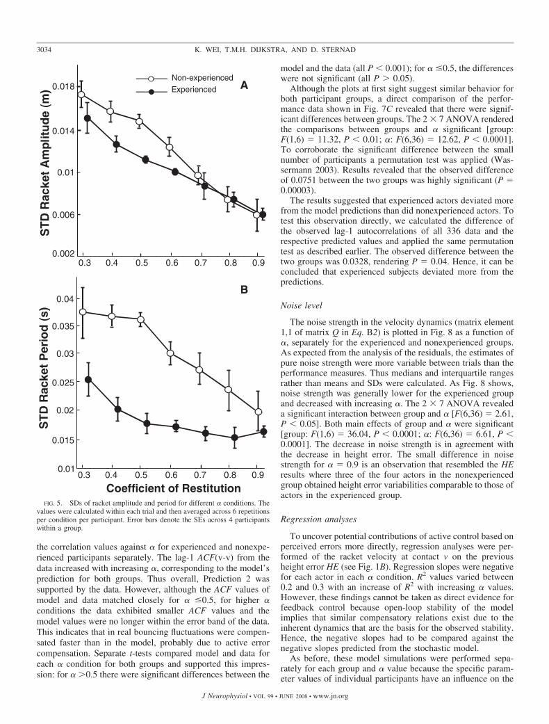
The noise strength in the velocity dynamics (matrix element1,1 of matrix Q in Eq. B2) is plotted in Fig. 8 as a function of�, separately for the experienced and nonexperienced groups.As expected from the analysis of the residuals, the estimates ofpure noise strength were more variable between trials than theperformance measures. Thus medians and interquartile rangesrather than means and SDs were calculated. As Fig. 8 shows,noise strength was generally lower for the experienced groupand decreased with increasing �. The 2 � 7 ANOVA revealeda significant interaction between group and � [F(6,36) � 2.61,P � 0.05]. Both main effects of group and � were significant[group: F(1,6) � 36.04, P � 0.0001; �: F(6,36) � 6.61, P �0.0001]. The decrease in noise strength is in agreement withthe decrease in height error. The small difference in noisestrength for � � 0.9 is an observation that resembled the HEresults where three of the four actors in the nonexperiencedgroup obtained height error variabilities comparable to those ofactors in the experienced group.

Regression analyses

To uncover potential contributions of active control based onperceived errors more directly, regression analyses were per-formed of the racket velocity at contact v on the previousheight error HE (see Fig. 1B). Regression slopes were negativefor each actor in each � condition. R2 values varied between0.2 and 0.3 with an increase of R2 with increasing � values.However, these findings cannot be taken as direct evidence forfeedback control because open-loop stability of the modelimplies that similar compensatory relations exist due to theinherent dynamics that are the basis for the observed stability.Hence, the negative slopes had to be compared against thenegative slopes predicted from the stochastic model.

As before, these model simulations were performed sepa-rately for each group and � value because the specific param-eter values of individual participants have an influence on the

0.4 0.6 0.80.3 0.5 0.7 0.90.01

0.015

0.02

0.025

0.03

0.035

0.04

Non-experiencedExperienced A


0.002

0.01

0.014

0.018

0.006

0.4 0.6 0.80.3 0.5 0.7 0.9

B

FIG. 5. SDs of racket amplitude and period for different � conditions. Thevalues were calculated within each trial and then averaged across 6 repetitionsper condition per participant. Error bars denote the SEs across 4 participantswithin a group.



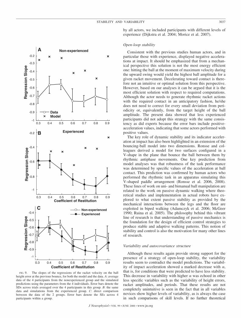
relaxation behavior of the model. The resulting regressionslopes for the participant groups are plotted in Fig. 9, A and B(as crosses) and were compared against the regression slopesobtained from the data (points with error bars). Across all �values participants showed more negative slopes than wouldhave been expected from open-loop stability alone. For thenonexperienced group, significant differences were supportedby t-tests performed separately for each � condition (all P �0.0001). Similar results were found for the experienced group:all t-tests were significant with P � 0.0001 (� � 0.4, P �0.05), except for � � 0.3, where P � 0.43. For the experiencedgroup the differences were more pronounced, especially for thehigher � conditions. These results mean that racket impactvelocity was influenced and modulated by the height error ofthe preceding cycle.

Figure 9C directly compares the slopes of two groups.Experienced actors showed more negative slopes than those ofnovices, especially for the higher � conditions. The 2 � 7ANOVA revealed both main effects were significant [group:F(1,6) � 6.70, P � 0.05; �: F(6,36) � 5.18, P � 0.0005]. Apermutation test corroborated the significant result between thetwo groups. The mean observed difference between the groupswas 0.0883, which rendered P � 0.00012 against the distribu-

tion obtained from the permutations. These results mean thatexperienced actors applied more active corrections, counter toPrediction 3b.

D I S C U S S I O N

The present study aimed to reveal the contributions of bothopen- and closed-loop components in the performance of arhythmic ball-bouncing task. The foundation for this investi-gation is a mathematical model of the task defined by a racketinteracting rhythmically with a ball in a gravitational field. It isassumed that the racket movements are generated by actorsviewing and intercepting the ball trajectories with the goal toproduce stable rhythmic performance. Hence, fine-grainedanalyses of the kinematics of racket and ball movements areexpected to provide insight into the actors’ control strategiesand the required underlying neurophysiological mechanisms.As such, the approach takes the actor–environment system asthe window of analysis paying tribute to the fact that the taskis defined over the actor in interaction with the ball that setsconstraints on the generation of action (Warren 2006). Anessential characteristic of the task as revealed by stabilityanalyses of the model is that it can be performed with open-

1

0

-1

1

0

-1

1

0

-1

1

0

-1

1

0

-1

1

0

-1

1

0

-11 2 3 4 6 7 8 90 5 1 0

Lag

=0.3

=0.5

=0.4

=0.6

=0.8=0.7

=0.9

DataModel

1 2 3 4 6 7 8 90 5 10

1 2 3 4 6 7 8 90 5 101 2 3 4 6 7 8 90 5 10

1 2 3 4 6 7 8 90 5 1 0

1 2 3 4 6 7 8 90 5 1 0

1 2 3 4 6 7 8 90 5 10

FIG. 6. Autocorrelation functions of release velocity, ACF(v-v), from one participant of the experienced group, plotted as afunction of 10 lags (bounces) for all 7 � conditions. The modelpredictions (black crosses) were calculated by using the parame-ters estimated from the same individual’s data. The data are plottedin gray where the error bars are the SDs across trials.



loop or dynamic stability if one condition is satisfied: theracket’s trajectory should decelerate directly before and aroundthe moment when contacting the ball assuming approximatelysinusoidal movements of the racket. Dynamic stability implies

that small deviations from periodic performance die out with-out requiring any error compensation in the actor’s/racket’smovements—which is the reason for the equivalent label of“passive stability” (Dijkstra et al. 2004; Schaal et al. 1996).

Empirical evidence that human actors execute the task withthis passive strategy has been provided in a series of experi-ments where participants performed the task in two- and threedimensions and with different experimental equipment (Katsu-mata et al. 2003; Schaal et al. 1996; Sternad 2006; Sternadet al. 2000, 2001). However, in addition, two previous studieshave demonstrated that actors also actively compensate forerrors when they are caused by relatively large experimentallyapplied perturbations (de Rugy et al. 2003; Wei et al. 2007).More specifically, Wei et al. (2007) probed the relevance of thetheoretical notion of the domain of attraction of the ball-bouncing map by different perturbation magnitudes. The re-laxation times following different perturbations were a reflec-tion of the domain of attraction, although generally shorter thanpredicted. Together with the observed negative impact accel-erations, an indicator of passive stability, these results wereinterpreted as evidence for a blend of active control withpassive stability. These results raised the question whethersuch intertwining of active control and passive stability is alsopresent at steady state.

To pursue this question, the model of the bouncing ball wasextended by a stochastic component. During steady state, thesequence of bounces constitutes a time series where the se-quential structure of the values of the two state variables (ballrelease velocity and time between impacts) can be character-ized by auto- and cross-correlations (Dijkstra et al. 2004). Asanalyses of the autocovariance function of the stochastic dy-namics revealed, there is indeed a characteristic signature thatdepends on the coefficient of restitution of the ball–racketcontact �. In particular, the model predicted that dynamicstability decreases with increasing �. Hence, the present studyexamined steady-state performance and manipulated the keyparameter �. Given some previous evidence that the strategy ofpassive stability was not a trivial solution immediately adopted

0.3 0.4 0.5 0.6 0.7 0.8 0.9-0.2

0

0.2

0.4

0.6

0.8 Non-experienced

DataModel

0.3 0.4 0.5 0.6 0.7 0.8 0.9-0.2

0.2

0.4

0.6

0.8


Model

A

B

0.3 0.4 0.5 0.6 0.7 0.8 0.9-0.1

0

0.1

0.2

0.3

0.4

Non-experiencedExperienced

0.5


C

FIG. 7. The averages of the lag-1 of the autocorrelation function ACF v-vplotted as a function of �. A: average data of the 4 participants from thenonexperienced group and the simulated predictions using the parameters fromthe 4 individuals. Error bars denote the SDs across trials averaged over the 4participants in this group. B: the same data and simulations from the experi-enced group. C: direct comparison between the data of the 2 groups. Error barsdenote the SEs across 4 participants within a group.

0.3 0.4 0.5 0.6 0.7 0.8 0.90

0.005

0.010

0.015

0.020

0.025

0.030


0.035 Non-experiencedExperienced

FIG. 8. Median and interquartile ranges of the estimated noise strength inexperienced and nonexperienced participants. Error bars denote the interquar-tile range over the medians of the 4 participants in a group.



by all actors, we included participants with different levels ofexperience (Dijkstra et al. 2004; Morice et al. 2007).

Open-loop stability

Consistent with the previous studies human actors, and inparticular those with experience, displayed negative accelera-tions at impact. It should be emphasized that from a mechan-ical perspective this solution is not the most energy efficientone: hitting the ball at the moment of maximum velocity duringthe upward swing would yield the highest ball amplitude for agiven racket movement. Decelerating toward contact is there-fore not an intuitive or optimal solution from this perspective.However, based on our analyses it can be argued that it is themost efficient solution with respect to required computations.Although the actor needs to generate rhythmic racket actionswith the required contact in an anticipatory fashion, he/shedoes not need to correct for every small deviation from peri-odicity or, equivalently, from the target height of the ballamplitude. The present data showed that less experiencedparticipants did not adopt this strategy with the same consis-tency as did experts because the error bars include positive-acceleration values, indicating that some actors performed withpositive values.

The key role of dynamic stability and its indicator acceler-ation at impact has also been highlighted in an extension of thebouncing-ball model into two dimensions. Ronsse and col-leagues derived a model for two surfaces configured in aV-shape in the plane that bounce the ball between them byrhythmic antiphase movements. One key prediction frommodel analyses was that robustness of the task performancewas determined by specific values of the acceleration at ballcontact. This prediction was confirmed by human actors whoperformed the rhythmic task in an apparatus simulating thisV-shaped paddle arrangement (Ronsse et al. 2006, 2008).These lines of work on uni- and bimanual ball manipulation arerelated to the work on passive dynamic walking where theo-retical studies and implementation in actual robots have ex-plored to what extent passive stability as provided by themechanical interactions between the legs and the floor areexploited in biped walking (Adamczyk et al. 2006; McGeer1990; Ruina et al. 2005). The philosophy behind this vibrantline of research is that understanding of passive mechanics isthe foundation for the design of efficient control strategies toproduce stable and adaptive walking patterns. This notion ofstability and control is also the motivation for many other linesof research.

Variability and autocovariance structure

Although these results again provide strong support for thepresence of a strategy of open-loop stability, the variabilityresults seem to contradict the model predictions. The variabil-ity of impact acceleration showed a marked decrease with �,that is, for conditions that were predicted to have less stability.This decrease in variability with higher � was echoed in otherless specific variables such as the variability of height errors,racket amplitudes, and periods. That these results are notcompletely unintuitive is seen in the fact that in all variablesnovices show higher levels of variability, as is always the casein such comparisons of skill levels. If no further theoretical

0.3 0.4 0.5 0.6 0.7 0.8 0.9

-1

-0.8

-0.6

-0.4

-0.2 Experienced


0.3 0.4 0.5 0.6 0.7 0.8 0.9-1

-0.9

-0.8

-0.7

-0.6

-0.5

-0.4

-0.3

-0.2

Non-experienced

DataModel

A

B

0.3 0.4 0.5 0.6 0.7 0.8 0.9


-1

-0.9

-0.8

-0.7

-0.6

-0.5

-0.4Non-experiencedExperienced

C

FIG. 9. The slopes of the regressions of the racket velocity on the ballheight error at the previous bounce, for both the model and the data. A: averagedata of the 4 participants from the nonexperienced group and the simulatedpredictions using the parameters from the 4 individuals. Error bars denote theSDs across trials averaged over the 4 participants in this group. B: the samedata and simulations from the experienced group. C: direct comparisonbetween the data of the 2 groups. Error bars denote the SEs across 4participants within a group.



analyses were available, this decrease would be interpreted ashigher stability in the “bouncier” racket–ball conditions. None-theless, this mismatch with the model predictions motivated morefine-grained analyses of variability and its temporal structure.

Analyses of the sequential structure of the state variables viaauto- and cross-correlations in both model and data providedanother window into assessing the relation between open-loopstability and variability. Performance measures like the SDs ofheight errors within a trial are relatively unspecific and consti-tute both the self-correcting properties, due to dynamic stabil-ity quantified by the eigenvalues of the Jacobian, and theinternal noise. In contrast, the autocovariance function (ACF)is determined only by the dynamic stability measure. ACFanalyses of the model yielded that the lag-1 autocorrelation ofthe state variables increased with increasing �, indicating adecrease of dynamic stability with �. The data on lag-1autocorrelations were in qualitative agreement with this modelprediction, although only for � conditions �0.6. In conditionswith higher � subjects showed smaller lag-1 correlations. Thismismatch with the predictions was seen in both groups, al-though it was more pronounced in the experienced actors. Oneviable explanation for this mismatch is that other than open-loop strategies are present. In particular, lower lag-1 valuesindicate faster relaxation processes, suggesting that active errorcorrections were present. It makes sense that such activecontrol processes are more prominent for less stable condi-tions. It also is not unintuitive that experienced actors showedmore of these subtle corrective processes.

Yet, before drawing further conclusions, the ACF analysesalso provided a rationale for how to assess the amplitude of theinternal noise q from the data. Given its independence fromthe autocorrelative structure, the noise q was quantified by theresidual or unexplained variance of the ACF fits. Interestingly,the data showed that this noise amplitude decreased withincreasing � and that skilled actors showed a generally lowernoise level. Returning to the results on variability in perfor-mance measures these two results from the ACF analysissuggest that this decrease in performance variability at thehigher and theoretically less stable � conditions is broughtabout by a decrease in the level of internal noise. This decreasein internal noise can be interpreted as a signature of activecontrol. Because the amplitude of movement decreases with �and presumably the control signal also decreases we caninterpret the observed decrease in internal noise as also con-sistent with the idea of signal-dependent noise (Harris andWolpert 1998).

Another line of research that has used autocovariance anal-ysis as a tool to understand human motor behavior is the workon rhythmic timing by Wing and Vorberg (1996). Although thetask of bouncing a ball to a target height shares some similar-ities with finger tapping—in that both are rhythmic movementswith a collision—there are critical differences in the task andthe analysis approach. First, in rhythmic tapping the task isonly about the time between contacts; the contact force andspatiotemporal aspects of the trajectory are typically not pre-scribed nor within the purview of the analyses (Balasubrama-niam et al. 2004; Sternad, et al. 2000). Hence, corrections foran early or late tap only require that the actor catches up orslows down on the next tap. In contrast, in ball bouncing theeffect of an early or late contact depends on the impactacceleration and has a consequence on the subsequent ball

amplitude. Moreover, how hard an actor hits the ball is crucialto success in the task. Second, in our approach to ball bouncingthe modeled mechanics of the task is hypothesized to constrainthe solutions chosen by the actor. The trajectory is analyzed toexamine whether the actor makes use of the dynamics of thetask. The autocovariance structure is derived from a model ofthe task dynamics and the parameters of this task dynamics arethe window into the CNS. In contrast, in tapping the observedautocovariance structure is interpreted directly in terms of theunderlying neural mechanisms because the dynamics of thefinger-surface contact is not analyzed.

Active error corrections

To strengthen the inference of active control we scouted thedata for direct evidence for active error compensation. Al-though many variables can be considered as candidates forerror correction the most plausible perceived variable was theheight error of the ball amplitude. Because subjects wereinstructed to bounce the ball to a visible target height withevery contact, the height error provided direct information toadjust the racket trajectory at the subsequent ball contact: Ahigher than desired ball amplitude would necessitate a lowerracket velocity at the next contact to compensate for theincreased ball velocity at contact. Hence, the perceptual vari-able height error and the action variable racket velocity atcontact were hypothesized to be negatively related to achieveactive error correction. This choice of variable was also moti-vated by results from research on juggling and other ball skills,where the apex of the ball amplitude was shown to carry themost salient information for controlling the next ball catch (vanSantvoord and Beek 1994).

The regressions of the action variable on the perceptualvariable indeed revealed significant negative slopes that can beinterpreted as evidence for servo-control. Again, the theoreticalanalyses provided information to qualify this result: becausethe dynamically stable stochastic system also displays suchnegative slopes, only the comparison between observed andpredicted slopes allowed us to draw inferences about active andpassive corrections. The slopes in the data were more negativefor all � conditions and thereby confirmed the presence ofactive compensation. Consistent with the better (i.e., less vari-able) performance in experienced actors, these individualsshowed more pronounced compensatory relations. Addition-ally, these deviations were slightly higher for the higher �conditions. Together with the deviations of lag-1 results forhigher � conditions, these results clearly indicate that subjectsapply more active control for less stable conditions.

Neurophysiological mechanisms

The concept of stability has been helpful in much neuro-physiological research that aimed to shed light on the mecha-nisms of the peripheral nervous system. In many elegantstudies it was shown how short- and long-latency reflex mech-anisms operate to stabilize position and trajectories (Nicholsand Houk 1976; Popescu et al. 2003). Such mapping ofstability to explicit neural mechanisms is not so easy in morecomplex tasks such as ball bouncing. Dynamic stability in ballbouncing not only is maintained through servo-control medi-ated by reflex mechanism, but also is established in a corrective



as well as anticipatory fashion, by both active and passivecomponents, as we try to tease apart.

The active control components map more easily onto thetraditional error-compensation mechanisms: by correlatingperceived height error to subsequent racket velocity at ballcontact, we demonstrate that perceived information leads to amodification of the efferent signal controlling the racket prob-ably in a transcortical sensorimotor loop (the time between theheight error at the apex and the following racket–ball contactis 350 ms, which allows for visually controlled corrections).However, as we try to show, this is only one part of thecomplex control system that is intertwined with other mecha-nisms that ensure passive stability, where error corrections areinherent in the dynamics. These other mechanisms operate in amore anticipatory or task-oriented fashion and are not (yet)easily mapped onto neural substrate.

That corrective mechanisms are not necessarily a function ofa fixed set of neural mechanisms has been demonstrated in arecent study on bimanual reaching by Diedrichsen (2007).When both hands perform parallel reaching movements to twoseparate targets and one hand is perturbed, short-latency re-sponses are observed in the perturbed hand. In contrast, if thetask is changed such that the two hands operate a single cursortoward a single target, both hands showed compensatoryreactions to the same single-hand perturbation (within 190 ms).These results give evidence that responses to perturbationdepend on the task and the goal.

The topic of stabilizing a task goal rather than a fixedposition is also a core assumption of optimal feedback control(Todorov 2004; Todorov and Jordan 2002). In this theoreticalframework the controller/CNS ensures that a task goal isstabilized; deviations from the optimal solution are correctedfor only when they affect the task outcome, whereas deviationsthat do not affect the end result are not compensated for(minimum-intervention principle). That this proposition opensa new route for identifying neural underpinnings, in particularfor the role of the motor cortex, has been recently argued byScott (2008). He points out that the research over the last 20years that has been dedicated to map neuronal activations inprimary motor cortex (M1) (both single neurons or popula-tions) to selected variables in execution (e.g., direction, load,etc.) has led to a plethora of interesting but also seeminglycontradictory results. To give more cohesion to these investi-gations on M1 he proposes that the search should be forprinciples of control, rather than for specific variables that arecontrolled. Explicitly, he suggests the framework of optimalfeedback control.

In light of this discussion, the current research documentsthat the CNS ensures that the task goal of rhythmically bounc-ing a ball is attained, partly by active error-correcting andpartly by more anticipatory processes leading to dynamicalstability. It remains to be a fascinating question which pro-cesses of the CNS achieve this dynamical stability, a questionthat should be pursued in more detail in future work.

In sum, the theoretical and empirical results revealed thathuman actors use a subtle web of active and passive strategies inthe performance of a rhythmic task. Humans are sensitive to thedynamical stability of the task but they also apply active modu-lations when necessary. Given that experienced actors exploit thedynamic stability more but also apply more of these activemodulations it can be inferred that this web of open-loop and

closed-loop strategies is the result of adaptation and learningprocesses. As both theoretical and empirical results showed, it isfar from evident that variability is the inverse of stability, as oftenassumed in the absence of more detailed predictions. Similarly, farfrom evident is that compensatory relations between perceptualand action variables always speak to active error corrections.Dynamic stability within a task can give rise to such compensa-tory behavior without reflecting active closed-loop strategy. Onlythe dialogue between model and data allowed more differentiatedexplanations of such observations.

A P P E N D I X A

The model is based on the same deterministic ball-bouncing mappreviously derived by different studies that revealed its period-dou-bling route to chaos (Bapat et al. 1986; Guckenheimer and Holmes1983; Tufillaro et al. 1992). However, all studies on the model’sapplication to the ball-bouncing task have examined only the simplestbehavior of this map—fixed-point stability implying periodic bounc-ing. We therefore review details pertaining only to period-1 behavior.

The map is based on three assumptions: 1) between bounces theball follows ballistic flight under the influence of gravity, 2) theimpact is instantaneous with the coefficient of restitution capturingthe energy loss at impact (see footnote 1), 3) the racket movement isassumed to be a pure sine wave with a fixed amplitude and frequency.Figure 1A shows the mechanical model with the planar surface and theball and Fig. 1B shows exemplary time series of racket and balltrajectories (with added noise). Based on these assumptions, thedeterministic ball-bouncing map can be derived as

vk�1 � �1 � ��ar�r cos �rtk�1 � �vk � g��tk�1 � tk� (A1)

0 � ar�sin �rtk � sin �rtk�1� � vk�tk�1 � tk� � �g/2��tk�1 � tk�2 (A2)

This is an implicit map with state variables vk, the ball velocity justafter the kth impact, and tk, denoting the time of the kth impact.Parameters are g, the acceleration of gravity; �, the coefficient ofrestitution; and �r and ar, the angular frequency and amplitude ofracket movement, respectively.

The map has a period-1 attractor that is stable when the impactacceleration AC fulfills the following constraints

�2g1 � �2

�1 � ��2 � AC � 0 (A3)

For the selected � values used in the experiment, the stable range forAC is between �12.65 m/s2 and 0 (� � 0.3) and �9.83 m/s2 and0 (� � 0.9).

The assumptions of ballistic flight and instantaneous impact areobeyed by design in the virtual reality setup, although the assumption ofa sinusoidal racket trajectory is not strictly obeyed in experimental data.Human actors move the racket in approximately sinusoidal fashion butwith a steeper slope preceding the impact position that has no simplemathematical expression (Sternad et al. 2001). However, because onlyposition and velocity of the racket at the ball contact determine the balltrajectory, an equivalent sinusoid is created that is identical to the actualwaveform around the time of the impact. Its equivalent frequency iscalculated from the period between bounces; its equivalent amplitude iscalculated from the stationary phase of impact as

ar � �1 � �

1 � �� g

�r2 cos

(A4)

Because we apply no external perturbations we assume that thestationary phase can be estimated from the mean racket impact phasewithin a trial. This equivalent amplitude is larger than the observed



amplitude but its slope in its upward phase around the impact closelymatches the observed racket waveform.

As shown in Dijkstra et al. (2004) the deterministic model predictsdifferent degrees of stability with increasing values of �: higher �values are associated with lower stability. However, this prediction isdifficult to test in practice. One would need to administer smallperturbations that do not lead to active corrections. However, suchperturbations are drowned in performance noise (see the data forthe perturbations P � 1 and P � 1 in Figs. 9 and 10 of Wei et al.2007). It is therefore better to look at autocorrelations that summarizebehavior over many small perturbations. This, however, requires astochastic model to make predictions. Therefore we proceeded toextend the deterministic model with a stochastic element.

The stochastic ball-bouncing map is a straightforward extensionwith a small caveat for the implicit time map (Eq. A2): we introducethe intermediate state variable �k�1 representing the noiseless time ofthe next impact. Using this variable, the stochastic ball-bouncing mapreads

vk�1 � �1 � ��ar�r cos ��rtk�1� � �vk � g��k�1 � tk� � qv�k (A5)

0 � ar�sin �rtk � sin �r�k�1� � vk��k�1 � tk� � �g/2��k�1 � tk�2 (A6)

tk�1 � �k�1 � qt�k (A7)

where �k denotes an internal Gaussian white noise process with zeromean and unit variance. The stochastic model has two additionalparameters: the noise strengths of the velocity and time dynamicsdenoted by qv and qt, respectively. Gaussian white noise was chosenbased on the idea that the noise originates from many independentcontributions from within the CNS. For example, these contributionscould originate at the planning stage, from the transmissions of motorcommands, or in the end effectors themselves.

The assumption of additivity of the noise is admittedly ad hoc andmainly chosen for mathematical simplicity. As an analysis of theobserved noise strength qv shows (Fig. 8), the results seem moreconsistent with a noise strength that increases with increasing impactvelocity, which would suggest a multiplicative noise term. However,such a noise model is left for future analysis.

The model has six parameters for which, in principle, sensitivityanalyses may be warranted. However, our model does not have a clearseparation of states and parameters. Two of the parameters, g and �,are fixed by design in our computer-generated setup. For the two noisestrength parameters a partial sensitivity analysis was performed in thetheoretical study (Dijkstra et al. 2004) where we showed that theobserved noise strengths are such that the linear approximation of Eq.B1 is accurate. The parameters amplitude and frequency of theequivalent sinusoid describe the racket motion of the subject. Theseparameters vary across subjects and may even vary within a perfor-mance and across trials. Therefore a traditional sensitivity analysis isnot feasible. Yet, one can view the main thrust of the study, lookingfor signatures of active control, as a sensitivity analysis of theassumption of a fixed sine wave.

A P P E N D I X B

To derive predictions about how noise percolates through thesystem the correlation structure of the state variables was calculated.To this end the stochastic map was linearized around the period-1attractor (denoted by v and t ) and the state of the system was denotedby yk and the noise by �k

yk � � vk � vtk � t � �k � � qv �k

qt �k�

with the linearized stochastic dynamics

yk�1 � Jyk � �k (B1)

where J denotes the Jacobian of the ball-bouncing map (see Eq. 39 inBapat et al. 1986 and Eq. 9 in Dijkstra et al. 2004). The Jacobianquantifies the stability properties of the ball-bouncing map. In partic-ular, the degree of stability can be quantified by the inverse of theeigenvalues (Scheinerman 1995). The derivation of the vector auto-covariance function Ry is standard procedure for this vector autore-gressive system of order 1 (Kendall and Ord 1989; Shumway andStoffer 2001). The autocovariance function at lag-0 of the two statevariables, Ry(0), could be calculated from the Lyapunov equation

Ry�0� � JRy�0�JT � Q (B2)

where Q denotes the autocovariance matrix of the noise �k: Q �diag (qv

2, qt2). For nonzero lag-1 the autocovariance function follows

from

Ry�l� � JlRy�0� (B3)

The Jacobian depends on all four parameters of the ball-bouncingmap. However, Dijkstra et al. (2004) showed that in many cases theabsolute values of the eigenvalues of the Jacobian depend only on �.Exceptions occur close to the boundaries of stability. Specifically, theabsolute values of the eigenvalues of the Jacobian equal �. Thus theautocovariance function in Eq. B3 can be approximated as

Ry�l� � |�|lRy�0� (B4)

There is one more caveat in using the preceding equations forcomparing theory and experiment: because state variable tk, the timeof impact, does not have a constant value at stationary state andcontinuously increases: tk�1 � tk � T, where T � 2/�r. Although theperiod T is known in the model, it fluctuates in the data due to noise.This created a problem when calculating the predicted autocovariancefunctions from data. To avoid this problem, we used the time betweenimpacts k � tk � tk�1 as state variable. We denoted the new vectorstate variable by z. The autocovariance function based on this newstate variable Rz(l) is related to the old one Ry(l) as follows

Rz�l� � �Ry1,1�l� Ry

1,2�l� � Ry1,2�l � 1�

Ry2,1�l � 1� � Ry

2,1�l� Ry2,2�l� � 2Ry

2,2�l � 1� � Ry2,2�l � 2��

(B5)

where Ri,j denotes matrix element i, j. Since the (1, 1) matrix elementof the autocovariance in unchanged by this change of state variable weused the lag-1 autocovariance of release velocity as quantification ofstability. A specific prediction from this relation is that stabilitydecreases as the lag-1 autocovariance of release velocity increases.Importantly, because the lag-1 autocovariance of release velocityequals �, the model predicts a decreasing stability with increasing �.This prediction is consistent with and supports the prediction derivedfrom the deterministic model.

G R A N T S

This research was supported by National Science Foundation Grant BCS-0450218, National Institute of Child Health and Human Development GrantR01-HD-045639, and Office of Naval Research Grant N00014-05-1-0844.

R E F E R E N C E S

Adamczyk PG, Collins SH, Kuo AD. The advantages of a rolling foot inhuman walking. J Exp Biol 209: 3953–3963, 2006.

Balasubramaniam R, Wing AM, Daffertshofer A. Keeping with the beat:movement trajectories contribute to movement timing. Exp Brain Res 159:129–134, 2004.

Bapat C, Sankar S, Popplewell N. Repeated impacts on a sinusoidallyvibrating table. J Sound Vib 108: 99–115, 1986.

Buhler M, Koditschek DE, Kindlmann PJ. Planning and control of roboticjuggling and catching tasks. Int J Robot Res 13: 101–118, 1994.



Collins SH, Ruina A, Wisse M, Tedrake R. Efficient bipedal robots based onpassive-dynamic walkers. Science 307: 1082–1085, 2005.

de Rugy A, Wei K, Muller H, Sternad D. Actively tracking “passive”stability. Brain Res 982: 64–78, 2003.

Diedrichsen J. Optimal task-dependent changes of bimanual feedback controland adaptation. Curr Biol 17: 1675–1679, 2007.

Dijkstra TMH, Katsumata H, de Rugy A, Sternad D. The dialogue betweendata and model: passive stability and relaxation behavior in a ball bouncingtask. Nonlinear Studies 11: 319–345, 2004.

Gander W, Hrebicek J. Solving Problems in Scientific Computing UsingMaple and Matlab. New York: Springer, 2004.

Guckenheimer J, Holmes P. Nonlinear Oscillations, Dynamical Systems, andBifurcations of Vector Fields. New York: Springer, 1983.

Harris CM, Wolpert DM. Signal-dependent noise determines motor plan-ning. Nature 394: 780–784, 1998.

Hasan Z. The human motor control system’s response to mechanical pertur-bation: should it, can it, and does it ensure stability? J Mot Behav 37:484–493, 2005.

Katsumata H, Zatsiorsky V, Sternad D. Control of ball–racket interactionsin the rhythmic propulsion of elastic and non-elastic balls. Exp Brain Res149: 17–29, 2003.

Kendall M, Ord K. Time Series. Oxford, UK: Oxford Univ. Press, 1989.Loeb GE. Control implications of musculoskeletal mechanics. Annu Int Conf

IEEE-EMBS 17: 1393–1394, 1995.Loram ID, Lakie M. Direct measurement of human ankle stiffness during

quiet standing: the intrinsic mechanical stiffness is insufficient for stability.J Physiol 556: 683–689, 2002.

McGeer T. Passive dynamic walking. Int J Robot Res 9: 633–643, 1990.Morasso PG, Sanguineti V. Ankle muscle stiffness alone cannot stabilize

balance during quiet standing. J Neurophysiol 88: 2157–2162, 2002.Morice AH, Siegler IA, Bardy B, Warren WH. Learning new perception-

action solutions in virtual ball bouncing. Exp Brain Res 181: 249–265,2007.

Nichols TR, Houk JC. Improvement in linearity and regulation of stiffness thatresults from actions of stretch reflex. J Neurophysiol 39: 119–142, 1976.

Popescu F, Hidler JM, Rymer WZ. Elbow impedance during goal-directedmovements. Exp Brain Res 152: 17–28, 2003.

Rizzi AA, Whitcomb LL, Koditschek DE. Distributed real time control of aspatial robot juggler. IEEE Comput 25: 59–71, 1992.

Ronsse R, Lefevre P, Sepulchre R. Sensorless stabilization of bouncejuggling. IEEE Trans Robot 22: 147–159, 2006.

Ronsse R, Thonnard J-L, Lefevre P, Sepulchre R. Control of bimanualrhythmic movements: trading efficiency for robustness depending on thecontext. Exp Brain Res (February 14, 2008) [Epub ahead of print].

Ruina A, Bertram J, Srinivasan M. A collisional model of the energetic costof support work qualitatively explains leg sequencing in walking andgalloping, pseudo-elastic leg behavior in running and the walk-to-runtransition. J Theor Biol 37: 170–192, 2005.

Saltzman EL, Kelso JAS. Skilled actions: a task-dynamic approach. PsycholRev 94: 84–106, 1987.

Schaal S, Sternad D, Atkeson CG. One-handed juggling: a dynamicalapproach to a rhythmic movement task. J Mot Behav 28: 165–183, 1996.

Scheinerman ER. Invitation to Dynamical Systems. Englewood Cliffs, NJ:Prentice Hall, 1995.

Scott SH. Inconvenient truths about neural processing in primary motorcortex. J Physiol 586: 1217–1224, 2008.

Shumway RH, Stoffer DS. Time Series Analysis and Its Applications. NewYork: Springer, 2001.

Sternad D. Stability and variability in skilled rhythmic actions: a dynamicalanalysis of rhythmic ball bouncing. In: Motor Control and Learning, editedby Latash ML, Lestienne F. New York: Springer, 2006, p. 55–63.

Sternad D, Dean WJ, Newell KM. Force and timing variability in rhythmicunimanual tapping. J Mot Behav 32: 249–268, 2000.

Sternad D, Duarte M, Katsumata H, Schaal S. Dynamics of a bouncing ballin human performance. Phys Rev E 63: 011902-1–011902-8, 2000.

Sternad D, Duarte M, Katsumata H, Schaal S. Bouncing a ball: tuning intodynamic stability. J Exp Psychol Hum Percept Perform 27: 1163–1184,2001.

Todorov E. Optimality principles in sensorimotor control. Nat Neurosci 7:907–915, 2004.

Todorov E, Jordan MI. Optimal feedback control as a theory of motorcoordination. Nat Neurosci 5: 1226–1235, 2002.

Tufillaro NB, Abbott T, Reilly J. An Experimental Approach to NonlinearDynamics and Chaos. Redwood City, CA: Addison–Wesley, 1992.

van Santvoord AAM, Beek PJ. Phasing and the pickup of optical informationin cascade juggling. Ecol Psychol 6: 239–263, 1994.

Vorberg D, Wing AM. Modeling variability and dependence in timing. In:Handbook of Perception and Action, edited by Heuer H, Keele SW. London:Academic, 1996, vol. 2, p. 181–262.

Wagner H, Blickhan R. Stabilizing function of skeletal muscles: an analyticalinvestigation. J Theor Biol 199: 163–179, 1999.

Warren WH. The dynamics of perception and action. Psychol Rev 113:358–389, 2006.

Wassermann L. All of Statistics. New York: Springer, 2003.Wei K, Dijkstra TMH, Sternad D. Passive stability and active control in a

rhythmic task. J Neurophysiol 98: 2633–2646, 2007.



Stability and Variability: Indicators for Passive Stability and Active Control in a Rhythmic Task

Documents