Stability and bifurcation analysis of a SIR model with saturated incidence rate and saturated treatment

Stability and bifurcation analysis of a SIR model with saturated incidence rateand saturated treatment

Erika Rivero-Esquivel1, Eric Avila-Vales2, Gerardo E. Garcıa-Almeida3

1,2,3 Facultad de Matematicas, Universidad Autonoma de Yucatan,

Anillo Periferico Norte, Tablaje 13615, C.P. 97119, Merida, Yucatan, Mexico

Abstract

We study the dynamics of a SIR epidemic model with nonlinear incidencerate, vertical transmission vaccination for the newborns and the capac-ity of treatment, that takes into account the limitedness of the medicalresources and the efficiency of the supply of available medical resources.Under some conditions we prove the existence of backward bifurcation,the stability and the direction of Hopf bifurcation. We also explore howthe mechanism of backward bifurcation affects the control of the infectiousdisease. Numerical simulations are presented to illustrate the theoreticalfindings.

Keywords: Local Stability, Hopf Bifurcation, Global Stability, Backward Bi-furcation

1 Introduction

Mathematical models that describe the dynamics of infectious diseases in com-munities, regions and countries can contribute to have better approaches in thedisease control in epidemiology. Researchers always look for thresholds, equilib-ria, periodic solutions, persistence and eradication of the disease. For classicaldisease transmission models, it is common to have one endemic equilibrium andthat the basic reproduction number tells us that a disease is persistent if isgreater than 1,and dies out if is less than 1. This kind of behaviour associatesto forward bifurcation. However, there are epidemic models with multiple en-demic equilibria [1, 2, 3, 4], within these models it can happen that a stableendemic equilibrium coexist with a disease free equilibrium, this phenomenonis called backward bifurcation [5].

In order to prevent and control the spread of infectious diseases like, measles,tuberculosis and influenza, treatment is an important and effective method. Inclassical epidemic models, the treatment rate of the infectious is assumed to beproportional to the number of the infective individuals [6]. Therefore we need toinvestigate how the application of treatment affects the dynamical behaviour of

1email: [email protected]: [email protected] author. email: [email protected] Tel. (999) 942 31 40 Ext. 1108.

1

arX

iv:1

501.

0617

9v1

[m

ath.

DS]

25

Jan

2015

these diseases. In that direction in [7], Wang and Ruan, considered the removalrate

T (I) =

{k, if I > 00, if I = 0.

In the following model

dS

dt= A− dS − λSI,

dI

dt= λSI − (d+ γ)I − T (I),

dR

dt= γI + T (I)− dR,

where S, I , and R denote the numbers of the susceptible, infective and recoveredindividuals at time t , respectively. The authors study the stability of equilibriaand prove the model exhibits Bogdanov-Takens bifurcation, Hopf bifurcationand Homoclinic bifurcation. In [15], the authors introduce a saturated treatment

T (I) =βI

1 + αI.

A related work is [13], [16].Hu, Ma and Ruan [8] studied the model

dS

dt=bm(S +R)− βSI

1 + αI− bS + pδI

dI

dt=

βSI

1 + αI+ (qδ − δ − γ)I − T (I)

dR

dt=γI − bR+ bm′(S +R) + T (I)

(1)

the basic assumptions for the model (1) are, the total population size at timet is denoted by N = S + I + R. The newborns of S and R are susceptibleindividuals, and the newborns of I who are not vertically infected are alsosusceptible individuals, b denotes the death rate and birth rate of susceptibleand recovered individuals, δ denotes the death rate and birth rate of infectiveindividuals, γ is the natural recovery rate of infective individuals. q (q ≤ 1) isthe vertical transmission rate, and note p = 1 − q, then 0 ≤ p ≤ 1. Fractionm′ of all newborns with mothers in the susceptible and recovered classes arevaccinated and appeared in the recovered class, while the remaining fraction,m = 1−m′, appears in the susceptible class, the incidence rate is described bya nonlinear function βSI/(1 + αI), where β is a positive constant describingthe infection rate and α is a nonnegative constant. The treatment rate of thedisease is

T (I) =

{kI, if 0 ≤ I ≤ I0,u = kI0, if I > I0

where I0 is the infective level at which the healthcare systems reaches capacity.In this work we will extend model (1) introducing the treatment rate β2I

1+α2I,

2

where α2, β2 > 0, obtaining the following model

dS

dt=bm(S +R)− βSI

1 + αI− bS + pδI

dI

dt=

βSI

1 + αI+ (qδ − δ − γ)I − β2I

1 + α2IdR

dt=γI − bR+ bm′(S +R) +

β2I

1 + α2I.

(2)

Because dNdt = 0, the total number of population N is constant. For convenience,

it is assumed that N = S + I + R = 1. By using S + R = 1 − I, the firsttwo equations of (2) do not contain the variable R. Therefore, system (2) isequivalent to the following 2-dimensional system:

dS

dt= − βSI

1 + αI− bS + bm(1− I) + pδI

dI

dt=

βSI

1 + αI− pδI − γI − β2I

1 + α2I.

(3)

The parameters in the model are described below:

• S, I,R are the normalized susceptible, infected, and recovered population,respectively, therefore it follows that S, I,R ≤ 1.

• b is a positive number representing the birth and death rate of susceptibleand recovered population.

• δ is a positive number representing the birth and death rate of infectedpopulation.

• γ is a positive number giving the natural recovery rate of infected popu-lation.

• q is positive (q ≤ 1) representing the vertical transmission rate (diseasetransmission from mother to son before or during birth). It is assumedthat descendents of the susceptible and recovered classes belong to thesusceptible class, in the same way to the fraction of the newborns of theinfected class not affected by vertical transmission.

• p = 1− q therefore 0 ≤ p ≤ 1.

• m′ is positive and it is the fraction of vaccinated newborns from susceptibleand recovered mothers and therefore belong to the recovered class. m =1−m′ ≥ 0 is the rest of newborns, which belong to the susceptible class.

• β is positive, representing the infection rate, α is a positive saturationconstant (In the model the incidence rate is given by the nonlinear functionβSI

1+αI ).

3

• β2I1+α2I

is the treatment function, satisfying limI→∞β2I

1+α2I= β2

α2, where

α2, β2 > 0.

We note that if α2 = 0 the treatment becomes bilinear, case considered in[8], whereas if β2 = 0 treatment is null, not being of interest here. Therefore wewill assume β2, α2 > 0.

The paper in distributed as follows: in section 2 we compute the equilibriapoints and determine the conditions of its existence (as real values) and posi-tivity, in section 3 we analyze the stability of the disease free equilibrium andendemic equilibria points in terms of value of R0 and the parameters of treat-ment function. Section 4 is dedicated to study Hopf bifurcation of the endemicequilibria points and section 5 shows discussion of all our results and we givesome control measures that could be effective to eradicate the disease in eachcase.

Following [8] we define

R0 :=βm

β2 + pδ + γ. (4)

When β2 = 0, R0 reduces to

R∗0 =βm

pδ + γ, (5)

which is the basic reproduction number of model (3) without treatment.

Lemma 1. Given the initial conditions S(0) = S0 > 0, I(0) = I0 > 0, then thesolution of (3) satisfies S(t), I(t) > 0 ∀t > 0 and S(t) + I(t) ≤ 1.

Proof. Take the solution S(t), I(t) satisfying the initial conditions S(0) = S0 >0, I(0) = I0 > 0. Assume that the solution is not always positive, i.e., thereexists a t0 such that S(t0) ≤ 0 or I(t0) ≤ 0. By Bolzano’s theorem thereexists a t1 ∈ (0, t0] such that S(t1) = 0 or I(t1) = 0, which can be written asS(t1)I(t1) = 0 for some t1 ∈ (0, t0]. Let

t2 = min{ti, S(ti)I(ti) = 0}. (6)

Assume first that S(t2) = 0, then dS(t2)dt > 0 implying that S is increasing at t =

t2. Hence S(t) is negative for values of t < t2 near t2, a contradiction. Therefore

S(t) > 0 ∀t > 0 and we must have I(t2) = 0, implying dI(t2)dt = 0. Note that if

for some t ≥ 0 I(t) = 0, then dI(t)dt = 0. Then any solution with I(0) = I0 = 0

will satisfy I(t) = 0 ∀t > 0. By uniqueness of solutions this fact implies that ifI(0) = I0 > 0, then I(t) will remain positive for all t > 0. Therefore I(t2) = 0leads to a contradiction. Hence both S and I are nonnegative for all t > 0.Finally, adding both derivatives of S(t) and I(t) we get:

d(S + I)

dt= −bS + bm− bmI − γI − β2I

1 + α2I(7)

4

Being S, I ≥ 0, if S+I = 1 then 0 ≤ S ≤ 1, 0 ≤ I ≤ 1. Analyzing the expression−bS + bm− bmI,

−bS + bm− bmI = b(m−mI −S) = b(m−mI − 1 + I) = b(m− 1 + I(1−m)).

Note that by the definition of the model parameters, 1−m = m′ ≥ 0. Knowingthat I ≤ 1, then

I(1−m) ≤ 1−m⇒ I(1−m) +m− 1 ≤ 0. (8)

Therefore −bS + bm− bmI ≤ 0. Hence d(S+I)dt ≤ 0 and S + I is non increasing

along the line S + I = 1, implying that S + I ≤ 1. Note also that S + I cannotbe grater than 1, otherwise from R = 1 − (S + I), R would be negative, anonsense.

2 Existence and positivity of equilibria

Assume that system (3) has a constant solution (S0, I0), then:

− βS0I01 + αI0

− bS0 + bm(1− I0) + pδI0 = 0 (9)

βS0I01 + αI0

− pδI0 − γI0 −β2I0

1 + α2I0= 0 (10)

From (9) we obtain

S0 =(1 + αI0)(bm(1− I0) + pδI0)

βI0 + b(1 + αI0). (11)

And we get from (10):

I0

(βS0

1 + αI0− pδ − γ − β2

1 + α2I0

)= 0

⇒ I0 = 0 orβS0

1 + αI0− pδ − γ − β2

1 + α2I0= 0. (12)

If I0 = 0 then S0 = m, obtaining in that way the disease-free equilibriumE = (m, 0).

Theorem 2. System (3) has a positive disease-free equilibrium E = (m, 0).

In order to obtain positive solutions of system 3 if I0 6= 0 then:

βS0

1 + αI0− pδ − γ − β2

1 + α2I0= 0

⇒ S0 =1 + αI0

β

(pδ + γ +

β2

1 + α2I0

)(13)

5

We obtain the following quadratic equation:

AI20 +BI0 + C = 0. (14)

OrI20 + (B/A)I0 + C/A = 0, (15)

where the coefficients are given by:

A = α2(β(γ + bm) + αb(pδ + γ)) > 0

B = β(γ + β2 + bm(1− α2)) + bα(pδ + γ + β2) + bα2(pδ + γ)

= β(γ + β2 + bm− bmα2) + bα(1−R0)(pδ + γ + β2) + βmbα+ bα2(pδ + γ)

C = b(pδ + γ + β2 − βm) = b(pδ + γ + β2)(1−R0). (16)

Its roots are:

I1 =−B −

√B2 − 4AC

2A

I2 =−B +

√B2 − 4AC

2A. (17)

And using these values in (13) we obtain its respective values

S1 =1 + αI1

β

(pδ + γ +

β2

1 + α2I1

)S2 =

1 + αI2β

(pδ + γ +

β2

1 + α2I2

). (18)

Then our candidate for endemic equilibria are E1 = (S1, I1), E2 = (S2, I2).Note that C = 0 if and only if R0 = 1, C > 0 if and only if R0 < 1, and

C < 0 if and only if R0 > 1 .For R∗0 > 1 we define the following sets:

A1 = {(β2, α2) : β2 > 0, 0 < α2 ≤ α02,

A2 = {(β2, α2) : β2 ≥ g(α2), α2 > α02 > 0},

A3 = {(β2, α2) : 0 < β2 < g(α2), α2 > α02 > 0}. (19)

Where

α02 =−β(mbα+ γ + bm)

b(pδ + γ − βm)

g(α2) = − 1

β(bα2(pδ + γ − βm) + β(γ + bm+mbα)).

Define :

6

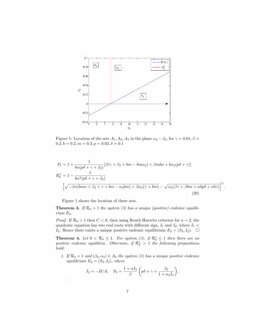
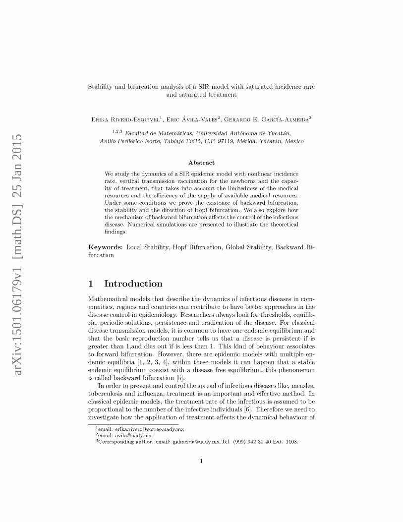
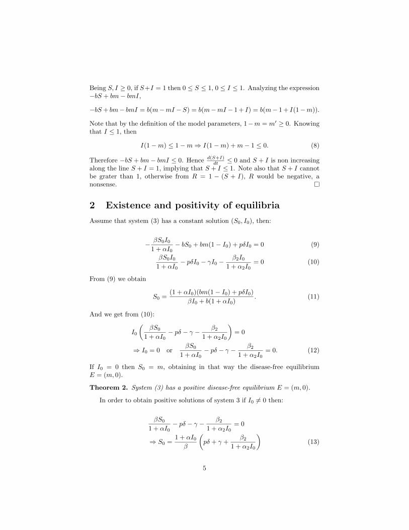
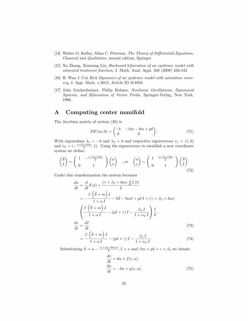
Figure 1: Location of the sets A1, A2, A3 in the plane α2−β2, for γ = 0.01, β =0.2, b = 0.2,m = 0.3, p = 0.02, δ = 0.1

P1 = 1 +1

bα(pδ + γ + β2)[β(γ + β2 + bm− bmα2) + βmbα+ bα2(pδ + γ)]

R+0 = 1− 1

bα2(pδ + γ + β2)[√−βα(bmα+ β2 + γ + bm− α2bm) + βα2(γ + bm)−

√α2(βγ + βbm+ αbpδ + αbγ)

]2.

(20)

Figure 1 shows the location of these sets.

Theorem 3. If R0 > 1 the system (3) has a unique (positive) endemic equilib-rium E2.

Proof. If R0 > 1 then C < 0, then using Routh Hurwitz criterion for n = 2, thequadratic equation has two real roots with different sign, I1 and I2, where I1 <I2. Hence there exists a unique positive endemic equilibrium E2 = (S2, I2).

Theorem 4. Let 0 < R0 ≤ 1. For system (3), if R∗0 ≤ 1 then there are nopositive endemic equilibria. Otherwise, if R∗0 > 1 the following propositionshold:

1. If R0 = 1 and (β2, α2) ∈ A3 the system (3) has a unique positive endemicequilibrium E2 = (S2, I2), where

I2 = −B/A, S2 =1 + αI2

β

(pδ + γ +

β2

1 + α2I2

).

.

7

2. If max{P1, R+0 } < R0 < 1 and (β2, α2) ∈ A3, the system (3) has a pair of

positive endemic equilibria E1, E2.

3. If 1 > R0 = R+0 > P1 and (β2, α2) ∈ A3, the system (3) has a unique

positive endemic equilibrium E1 = E2.

4. If 1 > R0 = P1 and (β2, α2) ∈ A3, the system (3) has no positive endemicequilibria.

5. If 0 < R0 ≤ 1 and (β2, α2) ∈ A1 ∪ A2, the system (3) has no positiveendemic equilibria.

6. If (β2, α2) ∈ A3 and 0 < R0 < max(R+0 , P1) < 1, then there are no

positive endemic equilibria.

Proof. If 0 < R0 ≤ 1, then C ≥ 0, so the roots of the equation AI2 +BI+C = 0are not real with different sign, but real with equal signs, complex conjugateor some of them are zero. If endemic equilibria exist and are positive, it isnecessary that B < 0. After some calculations we can see that:

B < 0⇔ R0 > 1 +β(γ + β2 + bm− bmα2) + βmbα+ bα2(pδ + γ)

bα(pδ + γ + β2):= P1.

(21)

From the assumption that R0 ≤ 1 then P1 < 1, hence the expression β(γ+β2 +bm− bmα2) +βmbα+ bα2(pδ+ γ) must be negative, this happens if and only if

β2 < −1

β(bα2(pδ + γ − βm) + β(γ + bm+mbα)) = g(α2). (22)

If R∗0 ≤ 1 then − 1β (bα2(pδ + γ − βm) + β(γ + bm + mbα)) < 0 and it is not

possible to find a value of β2 fulfilling the previous inequality, therefore thereare no positive endemic equilibria.

Now, if R∗0 > 1 we have that.

1. If R0 = 1 then C = 0 and the equation (14) is transformed into

AI20 +BI0 = 0, (23)

with A > 0. Its roots are I1 = 0 and I2 = −B/A, and there exists aunique endemic equilibrium that is positive if and only if B < 0, that isgiven by E2 = (S2, I2), where

I2 = −B/A

S2 =1 + αI2

β

(pδ + γ +

β2

1 + α2I2

). (24)

Note that if α2 > α02 and R∗0 > 1 then g(α2) > 0.

HenceA3 is nonempty and its elements satisfyB < 0, therefore if (β2, α2) ∈A3 there exists a unique positive endemic equilibrium E2.

8

2. If R0 < 1 then C > 0 and the roots of the quadratic equation for I0 mustbe real of equal sign or complex conjugate. By the previous part we knowthat if (β2, α2) ∈ A3 then P1 < 1, moreover if R0 > P1 then B < 0 andtherefore both roots must have positive real part. Finally, to assure thatequilibria are both real, we demand that ∆ ≥ 0 . Computing ∆:

∆ = B2 − 4AC

= A2R20 +B2R0 + C2 = ∆(R0), (25)

where:

A2 = α2b2 (pδ + γ + β2 )2

(26)

B2 = −2 [β (γ + β2 + bm (1− α2 )) + α b (pδ + γ + β2 ) + β mbα

+ bα2 (pδ + γ)]α b (pδ + γ + β2 ) + 4α2 (β (γ + bm)α b (pδ + γ))

b (pδ + γ + β2 ) (27)

C2 = (β (γ + β2 + bm (1− α2 )) + α b (pδ + γ + β2 ) + β mbα+ bα2 (pδ + γ))2

− 4α2 (β (γ + bm) + α b (pδ + γ)) b (pδ + γ + β2 ) . (28)

The previous expression is a quadratic function of R0. To establish theregion where ∆ ≥ 0, it is necessary to know how the roots of ∆(R0)behave. The discriminant of the quadratic function ∆(R0) is

∆2 = −16α2 b2β (pδ + γ + β2 )

2(β γ + β bm+ α bpδ + α bγ)

(α(αbm+ β2 + γ + bm)− α2(γ + bm+ αbm)) . (29)

If we assume that ∆2 < 0, then α2 <α(bmα−β2+γ+bm)

γ+bm+αbm and in this case wehave that:

γ + β2 + bm− bmα2 + bmα >2β2αbm+ (γ + bm)(γ + β2 + bm+ bmα)

γ + bm+ αbm> 0.

(30)

So we get that P1 > 1 > R0, which is a contradiction with the assumptionin this part, therefore ∆2 ≥ 0 and in consequence ∆(R0) has two realroots,

R−0 =−B2 −

√∆2

2A2

= 1− 1

bα2(pδ + γ + β2)[√−β(α(bmα+ β2 + γ + bm− bmα2)− α2(γ + bm))

+√α2(β(γ + bm) + αb(pδ + γ))]2,

R+0 =

−B2 +√

∆2

2A2

1− 1

bα2(pδ + γ + β2)[√−β(α(bmα+ β2 + γ + bm− bmα2)− α2(γ + bm))

−√α2(β(γ + bm) + αb(pδ + γ))]2. (31)

9

Note that due to the positivity of ∆2 and (29), we have that

−β(α(bmα+ β2 + γ + bm− bmα2)− α2(γ + bm))

is positive, allowing its roots to be well defined. Analyzing the derivativeof ∆(R0) we have that

∆′(R+0 ) =

√∆2 > 0 and ∆′(R−0 ) = −

√∆2 < 0,

moreover R−0 < R+0 making ∆ positive for R0 > R+

0 or R0 < R−0 . Never-theless

R−0 = 1 +1

bα(pδ + γ + β2)(β(γ + β2 + bm− bmα2 + bmα))− ε,

while

P1 = 1 +1

bα(pδ + γ + β2)(β(γ + β2 + bm− bmα2 + bmα)) + ε2,

with ε, ε2 > 0, making R−0 < P1 < R0. Therefore for R0 > max(P1, R+0 ),

we have that there exists two positive endemic equilibria E1, E2, provingthis part.

3. If (β2, α2) ∈ A3 then P1 < 1. If 1 > R0 > P1, then we have that B < 0and C > 0, therefore we have a pair of roots of the quadratic for I withpositive real part. In the previous part it was proven that for P1 < 1 thediscriminant ∆2 ≥ 0 and both roots R+

0 , R−0 are real and less than one. If

R0 = R+0 then ∆ = 0 and both roots are fused in one I1 = −B/2A = I2.

Therefore we have a unique positive endemic equilibrium E1 = E2.

4. If (β2, α2) ∈ A3 then P1 < 1. If R0 = P1 < 1 then C > 0, implyingthat the roots are complex conjugate or real of the same sign. BeingR0 = P1 then B = 0, implying that both roots have real part equal tozero, therefore there are no positive endemic equilibria.

5. If 0 < R0 ≤ 1 and (β2, α2) ∈ A1 ∪ A2 then P1 ≥ 1, therefore R0 ≤ P1

, B ≥ 0, and C ≥ 0. Hence there are two roots with real part zero ornegative, which are not positive equilibria.

6. If (β2, α2) ∈ A3 we have that P1 < 1 and the roots of the discriminantR+

0 , R−0 are real, in addition that R−0 < P1 and R+

0 < 1 by definition ofthis case. If 0 < R0 < max{R+

0 , P1} < 1, then C > 0 and the roots I2, I3are complex conjugate or real with the same sign. If R0 < P1 then B > 0,and the roots have negative real part, so there are not positive endemicequilibria. If 0 < R0 < R+

0 and R0 > R−0 , then ∆ < 0 and the rootsare complex conjugate, therefore there is not real endemic equilibria. If0 < R0 < R+

0 and R0 ≤ R−0 < P1, then it reduces to the first case inwhich there are not positive endemic equilibria.

10

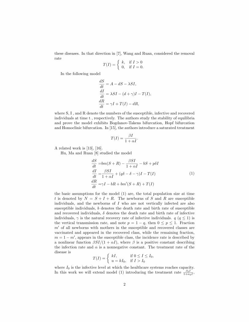
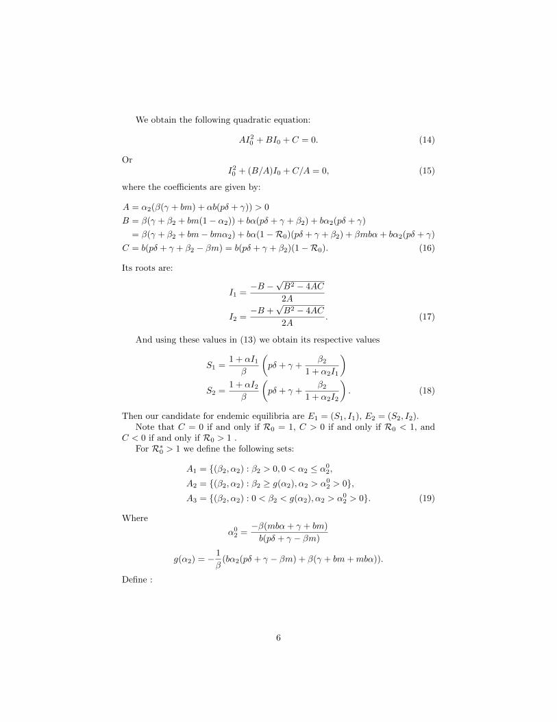
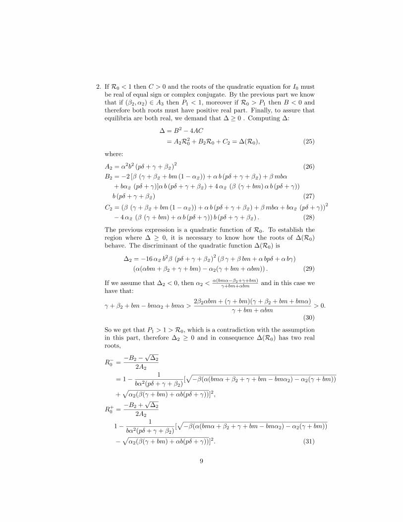
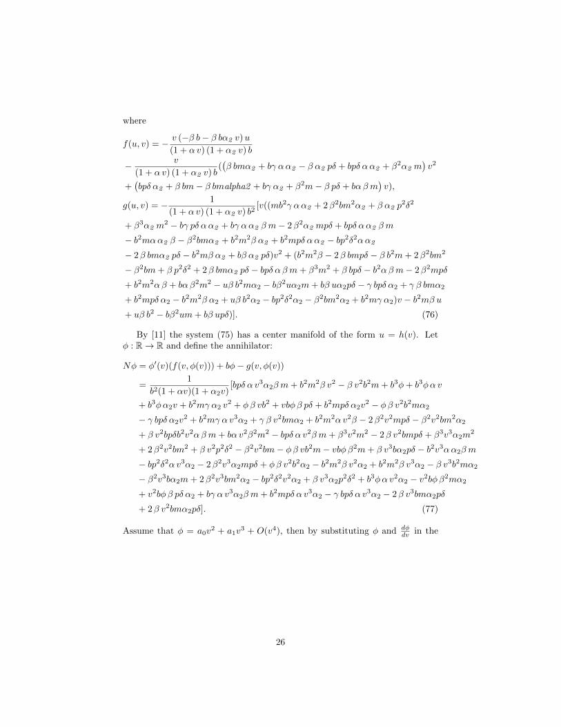
Figure 2: Graph of R0 versus the values I of equilibria. Parameter values usedare α = 0.4, α2 = 3.8, β = 0.2, b = 0.2, γ = 0.01, δ = 0.01, p = 0.02,m = 0.1.In this example β2 varies from 0 to 0.025, therefore R0 varies between 0.5682and 1.9682. g(α2) = −0.0017 and α0

2 = 3.8776, so (β2, α2) ∈ A1 ∪ A2. Forwardbifurcation can be observed in R0 = 1.

Theorem 4 gives us a complete scenario of the existence of endemic equilibria.When R∗0 ≤ 1 we have that R0 < 1, it follows from the fact that R0 < R∗0whenever β2 > 0; then system 3 has only a disease free equilibrium and noendemic equilibria.

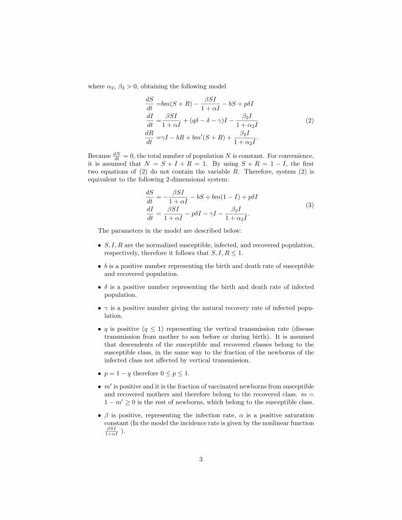
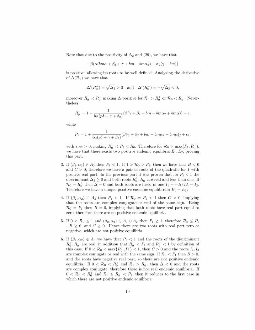
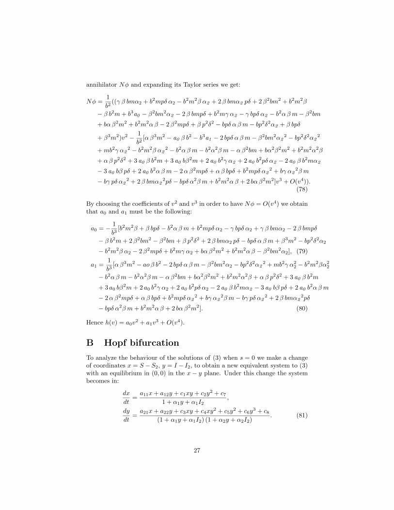
Otherwise, when R∗0 > 1 . If (β2, α2) ∈ A1 ∪ A2 then we have no endemicequilibria for 0 < R0 < 1 and a unique endemic equilibria E2 when R0 > 1, sothere exists a forward bifurcation in R0 = 1 from the disease free equilibriumto E2 (see figure 2 ). If (β2, α2) ∈ A3 there exist two positive endemic equilibriawhenever max{P1, R

+0 } < R0 < 1 ( P1 and R+

0 depend on β2), we can observethe backward bifurcation of the equilibrium E to two endemic equilibria (seefigure 3 ).

As an immediate consequence of the previous theorem we have that ifR0 > 1there exists a unique positive endemic equilibrium, while if R0 < 1 and theconditions of the second part are fulfilled, there exist two positive endemicequilibria. Hence we have the following corollary:

Corollary 5. If R0 = 1, R∗0 > 1 and (β, α2) ∈ A3, system (3) has a backwardbifurcation of the disease-free equilibrium E.

Proof. First we note that if (β2, α2) ∈ A3 then R+0 is real less than one and P1 <

1, therefore we can find a neighborhood of points in the interval (max{R+0 , P1}, 1).

By case 2 of theorem, if R0 lies in this neighborhood there exist two positiveendemic equilibria E1, E2; for R0 = 1 there exists a unique positive endemic

11

Figure 3: Graph ofR0 versus the values I of equilibria. In this example β2 variesfrom 0 to 0.025 thereforeR0 varies between 0.5682 and 1.9682. Parameter valuesused are α = 0.4, α2 = 16, β = 0.2, b = 0.2, γ = 0.01, δ = 0.01, p = 0.02,m = 0.1.g(α2) = 0.1188 and α0

2 = 3.8776, so (β2, α2) ∈ A3 . Backward bifurcation canbe observed in R0 = 1 and the existence of two positive endemic equilibriawhenever max{P1, R

+0 } < R0 < 1.

equilibrium E2, while the other endemic equilibrium becomes zero. Finally forR0 > 1 there exists a unique positive endemic equilibrium as the zero ”endemic”equilibrium becomes negative.

3 Characteristic Equation and Stability

The characteristic equation of the linearization of system (3) in the equilibrium(S0, I0) is given by:

det(DF − λI), (32)

where

DF =

(∂f1∂S

∂f1∂I

∂f2∂S

∂f2∂I

). (33)

Matrix is evaluated in the equilibrium (S0, I0). Functions f1, f2 are the follow-ing:

f1 = − βSI

1 + αI− bS + bm(1− I) + pδI (34)

f2 =βSI

1 + αI− pδI − γI − β2I

1 + α2I. (35)

Computing the matrix DF we obtain:

12

DF (S, I) =

−βI

1 + αI− b −βS

(1 + αI)2− bm+ pδ

βI

1 + αI

βS

(1 + αI)2− pδ − γ − β2

(1 + α2I)2

. (36)

3.1 Stability of disease free equilibrium

For the disease free equilibrium E = (m, 0) the Jacobian matrix is:

DF (m, 0) =

(−b −βm− bm+ pδ0 βm− pδ − γ − β2

).

Theorem 6. If R0 < 1 then the equilibrium E = (m, 0) of model (3) is locallyasymptotically stable, while if R0 > 1 then it is unstable.

Proof. The characteristic equation for the equilibrium E is given by

P (λ) = det(DF (m, 0)− λI2x2)

= det

(−b− λ −βm− bm+ pδ

0 βm− pδ − γ − β2 − λ

)= (−b− λ)(βm− pδ − γ − β2 − λ). (37)

The equation (37) has two real roots λ1 = −b and λ2 = βm− pδ − γ − β2. ByHartman-Grobman’s theorem, if the roots of (37) have non-zero real part thenthe solutions of system (3) and its linearization are qualitatively equivalent. Ifboth roots have negative real part then the equilibrium E is locally asymptot-ically stable, whilst if any of the roots has positive real part the equilibrium isunstable. Clearly λ1 < 0, but λ2 < 0 if and only if

βm− pδ − γ < β2,

if and only if R0 < 1.

According to the previous theorem and theorem 4 we obtain the followingresult for the global stability of equilibrium E :

Theorem 7. If 0 < R0 < 1 and one of the following conditions holds:

• R∗0 ≤ 1.

• R0 = P1 and (β2, α2) ∈ A3.

• (β2, α2) ∈ A1 ∪A2.

• (β2, α2) ∈ A3 and 0 < R0 < max{R+0 , P1}.

Then equilibrium E of system (3) is globally asymptoticaly stable.

13

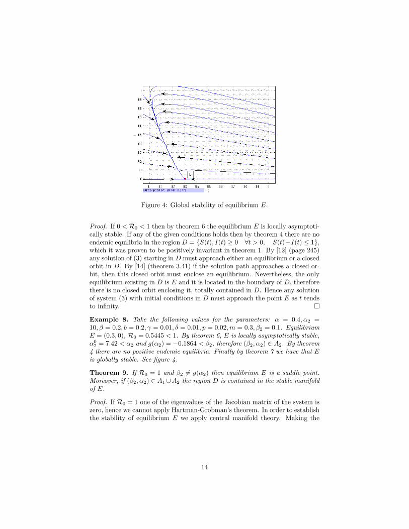
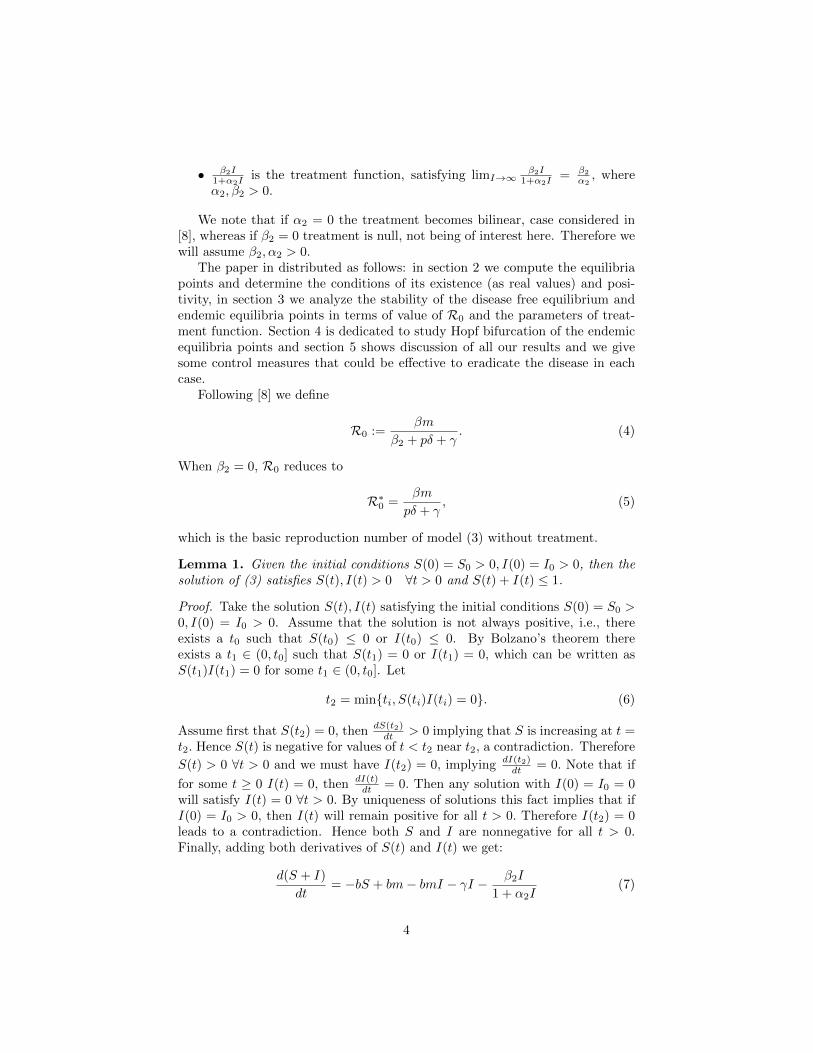
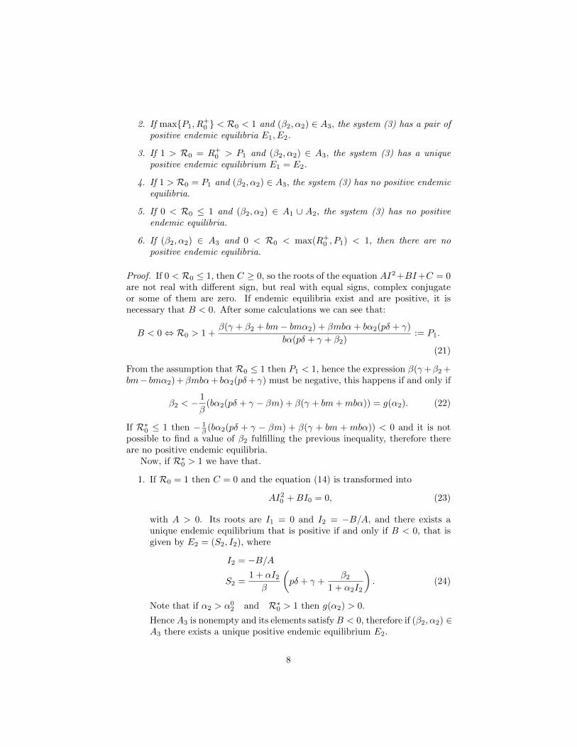
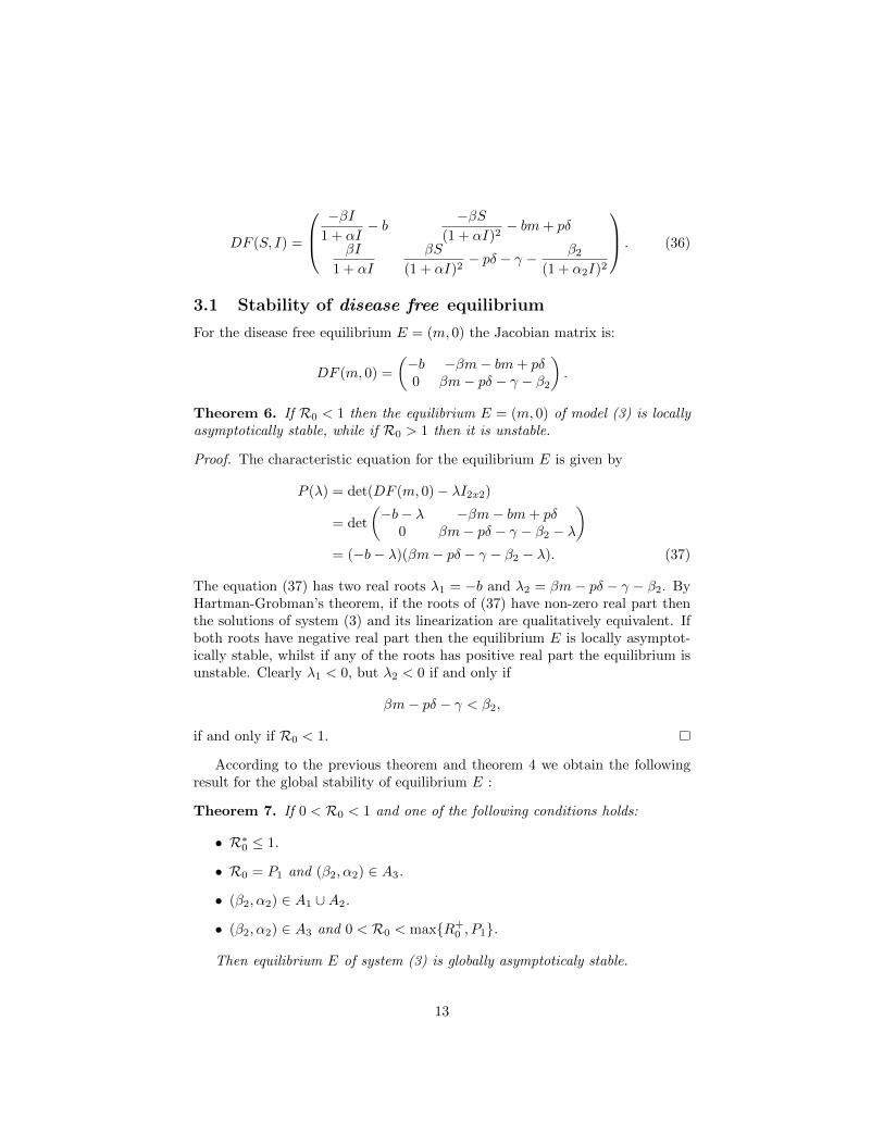
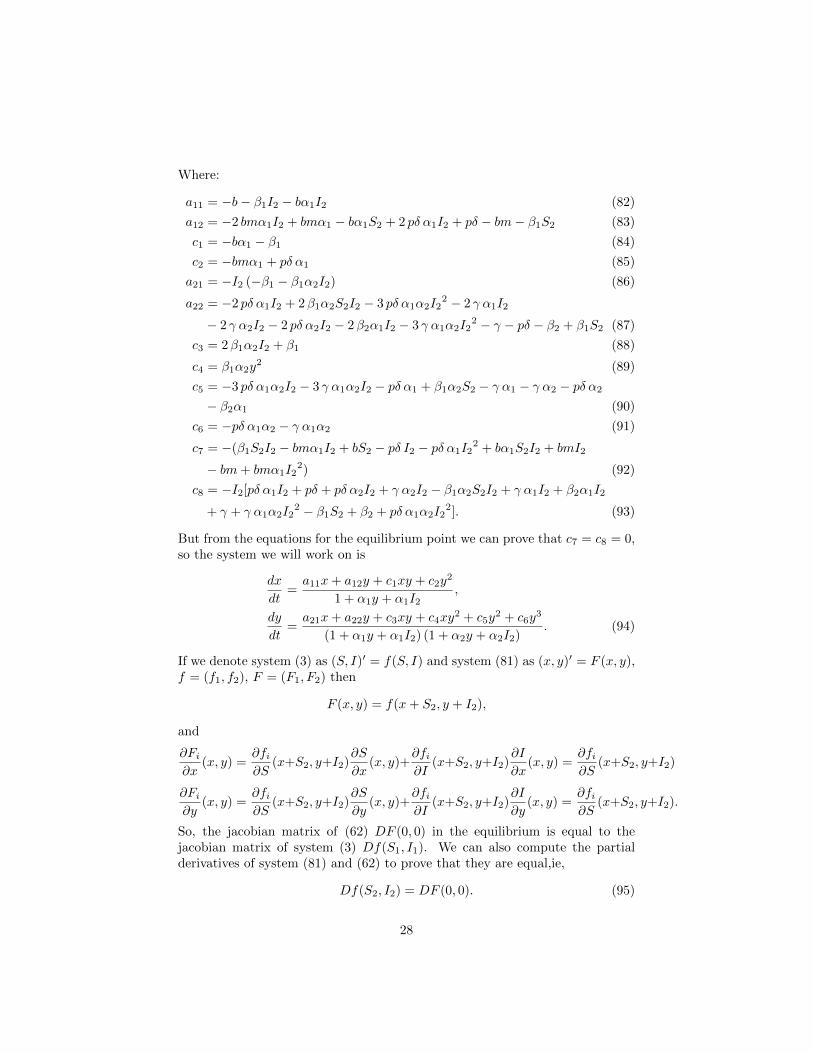
Figure 4: Global stability of equilibrium E.

Proof. If 0 < R0 < 1 then by theorem 6 the equilibrium E is locally asymptoti-cally stable. If any of the given conditions holds then by theorem 4 there are noendemic equilibria in the region D = {S(t), I(t) ≥ 0 ∀t > 0, S(t)+I(t) ≤ 1},which it was proven to be positively invariant in theorem 1. By [12] (page 245)any solution of (3) starting in D must approach either an equilibrium or a closedorbit in D. By [14] (theorem 3.41) if the solution path approaches a closed or-bit, then this closed orbit must enclose an equilibrium. Nevertheless, the onlyequilibrium existing in D is E and it is located in the boundary of D, thereforethere is no closed orbit enclosing it, totally contained in D. Hence any solutionof system (3) with initial conditions in D must approach the point E as t tendsto infinity.

Example 8. Take the following values for the parameters: α = 0.4, α2 =10, β = 0.2, b = 0.2, γ = 0.01, δ = 0.01, p = 0.02,m = 0.3, β2 = 0.1. EquilibriumE = (0.3, 0), R0 = 0.5445 < 1. By theorem 6, E is locally asymptotically stable,α0

2 = 7.42 < α2 and g(α2) = −0.1864 < β2, therefore (β2, α2) ∈ A2. By theorem4 there are no positive endemic equilibria. Finally by theorem 7 we have that Eis globally stable. See figure 4.

Theorem 9. If R0 = 1 and β2 6= g(α2) then equilibrium E is a saddle point.Moreover, if (β2, α2) ∈ A1 ∪A2 the region D is contained in the stable manifoldof E.

Proof. If R0 = 1 one of the eigenvalues of the Jacobian matrix of the system iszero, hence we cannot apply Hartman-Grobman’s theorem. In order to establishthe stability of equilibrium E we apply central manifold theory. Making the

14

change of variables, S = S −m, I = I, we obtain the equivalent system

dS

dt= −β(S +m)I

1 + αI− bS − bmI + pδI

dI

dt=β(S +m)I

1 + αI− pδI − γI − β2I

1 + α2I. (38)

Because I = I we ignore the hat and use only I. This new system has anequilibrium in E = (0, 0) and its Jacobian matrix in that point is

DF (m, 0) =

(−b −βm− bm+ pδ0 0

). (39)

Using change of variables S = u− (γ+beta2+bm)vb , I = v and βm = pδ+γ+β2

we obtain the equivalent system (see appendix A):

dv

dt= 0u+ f(v, u)

du

dt= −bu+ g(v, u), (40)

where f and g are defined in Appendix A.By [11], system (3) has a center manifold of the form u = h(v) and the flow

in the center manifold ( and therefore in the system ) is given by the equation

v′ = f(v, h(v)) ∼ f(v, φ(v)),

where h(v) = a0v2 +a1v

3 +O(v4), and ai’s are given in Appendix A. Expandingthe Taylor series of f we obtain the flow equation

v′ = −b3β m+ b2β2m+ b3γ α2 − b2β pδ + b3αβm+ b3pδ α2 − b3β mα2

b3v2 +O(v3)

= Hv2 +O(v3). (41)

Therefore the dynamics of solutions near the equilibrium E = (0, 0) is given bythe quadratic term, whenever this term is not zero. We note that H = 0 if andonly if

α2 =−β(bm+ βm− pδ + bαm)

b(pδ + γ − βm). (42)

Substituting again R0 = 1, expressed as βm = pδ + γ + β2, we obtain H = 0 ifand only if β2 = g(α2).

If (β2, α2) ∈ A3 then H > 0. v′ > 0 for v 6= 0. If (β2, α2) ∈ A1 ∪ A2 thenH < 0, v′ < 0 for v 6= 0. In both cases E is a saddle point. Moreover, if(β2, α2) ∈ A1 ∪ A2 then H < 0 and v′ < 0 for v > 0. Recalling v(t) = I(t) wehave under this assumption that I ′(t) < 0 for I > 0 therefore I(t)→ 0+, whileas v1 = (1, 0) is the stable direction of the point E then S(t)→ 0, therefore thesolutions in the region D approach the equilibrium E as t→∞.

15

Figure 5: Phase plane of the system for R0 = 1 with (β2, α2) ∈ A3

Example 10. Take the following values for the parameters: β = 0.2, α =0.4, δ = 0.01, γ = 0.01, α2 = 10,m = 0.3, p = 0.02, b = 0.2, β2 = 0.0498. Inthis case R0 = 1, α0

2 = 1.8876 and g(α2) = 0.4040, hence (β2, α2) ∈ A3.By the first case of theorem 4 the system has a unique endemic equilibrium inS2 = 0.11210, I2 = 0.4781. By theorem 9 the equilibrium E is a saddle point,see figure 5.

Example 11. If we take the same values as in the previous example exceptα2 = 2, then g(α2) = 0.0056 < β2, hence (β2, α2) ∈ A2. By theorem 4 thesystem has no endemic equilibria, and by theorem 9 the point E is a saddlepoint. Moreover, the region D is totally contained in the stable manifold, seefigure 6.

3.2 Stability of endemic equilibria

The general form of the Jacobian matrix is

DF =

−βI

1 + αI− b − βS

(1 + αI)2− bm+ pδ

βI

1 + αI

βS

(1 + αI)2− pδ − γ − β2

(1 + α2I)2

. (43)

Therefore the characteristic equation for an endemic equilibrium is

P (λ) =

(− βI

1 + αI− b− λ

)(βS

(1 + αI)2− pδ − γ − β2

(1 + α2I)2− λ)

−(

βI

1 + αI

)(− βS

(1 + αI)2− bm+ pδ

). (44)

16

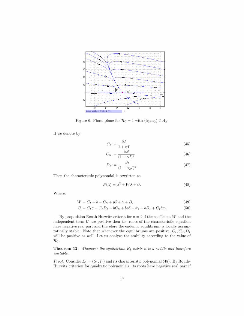
Figure 6: Phase plane for R0 = 1 with (β2, α2) ∈ A2

If we denote by

CI :=βI

1 + αI(45)

CS :=βS

(1 + αI)2(46)

DI :=β2

(1 + α2I)2. (47)

Then the characteristic polynomial is rewritten as

P (λ) = λ2 +Wλ+ U. (48)

Where:

W = CI + b− CS + pδ + γ +DI (49)

U = CIγ + CIDI − bCS + bpδ + bγ + bDI + CIbm. (50)

By proposition Routh Hurwitz criteria for n = 2 if the coefficient W and theindependent term U are positive then the roots of the characteristic equationhave negative real part and therefore the endemic equilibrium is locally asymp-totically stable. Note that whenever the equilibriums are positive, CI , CS , DI

will be positive as well. Let us analyze the stability according to the value ofR0.

Theorem 12. Whenever the equilibrium E1 exists it is a saddle and thereforeunstable.

Proof. Consider E1 = (S1, I1) and its characteristic polynomial (48). By Routh-Hurwitz criterion for quadratic polynomials, its roots have negative real part if

17

and only if U > 0 and W > 0 , where U,W depend on E1. Moreover, whenU < 0 its roots are both real with different sign and when U > 0 and W < 0the roots have positive real part. Computing the value of U and expressing S1

in terms of I1 we obtain

U =I1(a1I

21 + b1I1 + c1)

(1 + αI1)(1 + α2I1)2=

I1F (I1)

(1 + αI1)(1 + α2I1)2. (51)

Where:

a1 = α22(βγ + bpαδ + bαγ + bmβ) = α2A > 0,

b1 = 2α2(βγ + bpαδ + bαγ + bmβ) = 2A > 0,

c1 = ββ2 + bmβ + bpαδ + bαβ2 + βγ − bα2β2 + bαγ = B − α2C. (52)

We are assuming that equilibrium E1 exists and it is positive, and these happens(by previous section) when B < 0 and C > 0, so c1 < 0. The sign of U is equalto sgn(F (I1)). F (I1) has two roots of the form:

I∗ =−b1 +

√b21 − 4a1c1

2a1(53)

I ∗ ∗ =−b1 −

√b21 − 4a1c1

2a1. (54)

Where b21 − 4a1c1 > 0 and therefore I∗ and I ∗ ∗ are both real values withI ∗ ∗ < 0. F (I1) > 0 for I1 > I∗ and I1 < I ∗ ∗, but second condition neverholds because I1 > 0, so F (I1) < 0 for 0 < I1 < I∗.

Computing I∗ in terms of A,B,C:

I∗ = − 1

α2+

1

α2A

√(A2 − α2AB + α2

2AC). (55)

Substituting ∆ = B2 − 4AC > 0

I∗ = − 1

α2+

1

α2A

√(A2 − α2AB +

α22

4(B2 −∆)

)= − 1

α2+

1

2α2A

√(2A− α2B)2 − α2

2∆

> − 1

α2+

1

2α2A

(√(2A− α2B)2 −

√α2

2∆

)=−B −

√∆

2A= I1. (56)

Therefore U < 0 and the equilibrium E1 is a saddle.

Theorem 13. Assume the conditions of theorem 4 for existence and positivityof the endemic equilibrium E2. If I2 < I∗ the equilibrium E2 is unstable, else ifI2 > I∗ then E2 is locally asymptotically stable for s > 0 and unstable for s < 0.

18

Where s = m1(−B +√B2 − 4AC) + 2Am2,

m1 = (r + β2α− β2α2 + 2Bα2)A2 − α22rAC −ABα2(bα2 + 2r +B2α2

2r),

m2 = bA2 −ACα2(bα2 + 2r) + α22rBC,

r = α(pδ + b+ γ) + β. (57)

Proof. Consider E2 = (S2, I2) be real and positive, and its characteristic poly-nomial (48). We will have that the equilibrium is unstable when U < 0 andlocally asymptotically stable when U > 0,W > 0. Following the previous proof

U =I2(a1I

22 + b1I2 + c1)

(1 + αI2)(1 + α2I2)2=

I2F (I2)

(1 + αI2)(1 + α2I2)2. (58)

Where a1, b1, c1 are the same as in previous theorem. Therefore sgn(U) =sgn(F (I2)). We have seen that F (I2) has two real roots I∗ and I ∗ ∗. AgainF (I2) > 0 for I2 > I∗ and I2 < I ∗ ∗ (which does not holds because I ∗ ∗ < 0),and F (I2) < 0 for 0 < I2 < I∗ . So if I2 < I∗ the equilibrium E2 is unstable.

When I2 > I∗ then U > 0 and

W =1

(1 + αI2)(1 + α2I2)2[α2

2 (αγ + bα+ β + αpδ) I23

+ α2 (bα2 + 2αpδ + 2 bα+ 2αγ + 2β) I22

+ (αpδ + bα+ β + αβ2 − β2 α2 + αγ + 2 bα2) I2 + b]

=G(I2)

(1 + αI2)(1 + α2I2)2. (59)

By using the division algorithm,

G(I2) = (AI22 +BI2 + C)P (I2)

+1

A2[(r + β2α− β2α2 + 2Bα2)A2 − α2

2rAC −ABα2(bα2 + 2r +B2α22r)I2

+ bA2 −ACα2(bα2 + 2r) + α22rBC],

= (AI22 +BI2 + C)P (I2) +

m1I2 +m2

A2. (60)

Where P (I2) is a polynomial in I2 of degree one. Being I2 a coordinate of anequilibrium then AI2

2 +BI2 + C = 0 and

G(I2) =m1I2 +m2

A2.

Hence sgn(W ) = sgn(G(I2)) = sgn(m1I2+m2

A2 ) = sgn(m1I2 + m2). Substitutingthe value of I2,

m1I2 +m2 =m1

2A(−B +

√B2 − 4AC) +m2.

19

It follows that sgn(m1I2 +m2) = sgn(m1(−B+√B2 − 4AC)+2Am2) = sgn(s).

Therefore E2 is unstable if s < 0 and locally asymptotically stable if s > 0.

4 Hopf bifurcation

By previous section we know that the system (3) has two positive endemic equi-libria under the conditions of theorem (4) . Equilibrium E1 is always a saddle,so its stability does not change and there is no possibility of a Hopf bifurca-tion in it. So let us analyse the existence of a Hopf bifurcation of equilibriumE2 = (S2, I2). Analysing the characteristic equation for E2, it has a pair of pureimaginary roots if and only if U > 0 and W = 0 .

Theorem 14. System (3) undergoes a Hopf bifurcation of the endemic equilib-rium E2 (whenever it exists) if I2 > I∗ and s = 0. Moreover, if a2 < 0, there isa family of stable periodic orbits of (3) as s decreases from 0; if a2 > 0, thereis a family of unstable periodic orbits of (3) as s increases from 0.

The characteristical polinomial for E2 has a pair of pure imaginary roots iffU > 0 and W = 0. From the proof of theorem 12 we have that U > 0 if andonly if one of the conditions (i),(ii) is satisfied .

Although, sgn(W ) =sgn(s), so W = 0 if and only if s = 0. By first part oftheorem 3.4.2 of [17] the roots λ and λ of (48) for E2 vary smoothly, so we canaffirm that near s = 0 these roots are still complex conjugate and

dRe(λ(s))

ds|s=0 =

d

ds

(1

2W (s)

)=

1

2

d

ds

(1

2A3(1 + α1I1)(1 + α2I1)2s

)=

1

4A3(1 + α1I1)(1 + α2I1)26= 0. (61)

Therefore s = 0 is the Hopf bifurcation point for (3) .To analyze the behaviour of the solutions of (3) when s = 0 we make a change

of coordinates to obtain a new equivalent system to (3) with an equilibrium in(0, 0) in the x − y plane ( see appendix B ). Under this change the systembecomes:

dx

dt=a11x+ a12y + c1xy + c2y

2

1 + α1y + α1I2,

dy

dt=a21x+ a22y + c3xy + c4xy

2 + c5y2 + c6y

3

(1 + α1y + α1I2) (1 + α2y + α2I2). (62)

Where the aij ’s and ci’s are defined in appendix B.

20

System (62) and (3) are equivalent ( appendix B ), so we can work with(62). This system has a pair of pure imaginary eigenvalues if and only if (3) hasthem too. As we said before it happens if and only if any of conditions (i),(ii)is satisfied and s = 0. Computing jacobian matrix DF (0, 0) of (62)

DF (0, 0) =

a11

1 + α1I2

a12

(1 + α1I2)

a21

(1 + α2I2) (1 + α1I2)

a22

(1 + α2I2) (1 + α1I2)

. (63)

Tr(DF (0, 0)) = Tr(Df(S2, I2)), det(DF (0, 0)) = det(Df(S2, I2)).

So condition s = 0 is equivalent to a11(1 + α2I2) + a22 = 0 and (i),(ii) areequivalent to a22a11 − a12a21 > 0.

System (62) can be rewritten as

dx

dt=

a11x

1 + α1I2+

a12y

1 + α1I2+G1(x, y) (64)

dy

dt=

a21x

(1 + α1I2) (1 + α2I2)+

a22y

(1 + α1I2) (1 + α2I2)+G2(x, y). (65)

Where G1, G2 are defined in appendix B.Let Λ =

√det(DF (0, 0)). We use the change of variable u = x, v =

a11Λ(1+α1I2) + a12y

Λ(1+α1I2) , to obtain the following equivalent system:(uv

)=

(0 Λ−Λ 0

)(uv

)+

(H1(u, v)H2(u, v)

). (66)

Where

H1(u, v) = − ((−a12c1 + a11c2)u+ (−Λc2α1I2 + Λa12α1 − Λc2) v) ((Λ + Λα1I2) v − a11u)

a12 ((α1Λ + Λα12I2) v + a12 − α1a11u+ a12α1I2)

(67)

H2(u, v) = − 1

h(u, v)

[(Λ(1 + α1I2)v − a11u)

(A1v

2 +A2uv +A3v +A4u2 +A5u

)](68)

And A1, ..., A5, h(u, v) are defined in appendix B. Let

a2 =1

16[(H1)uuu + (H1)uvv + (H2)uuv + (H2)vvv] +

1

16(−Λ)[(H1)uv((H1)uu + (H1)vv)

− (H2)uv((H2)uu + (H2)vv)− (H1)uu(H2)uu + (H1)vv(H2)vv]. (69)

Where

(H1)uuu =∂

∂u

(∂

∂u

(∂H1

∂u

))(0, 0),

and so on (a2 is explicitly expressed in appendix B) .Then by theorem 3.4.2 of [17] if a2 6= 0 then there exist a surface of periodic

solutions, if a2 < 0 then these cycles are stable, but if a2 > 0 then cycles arerepelling.

21

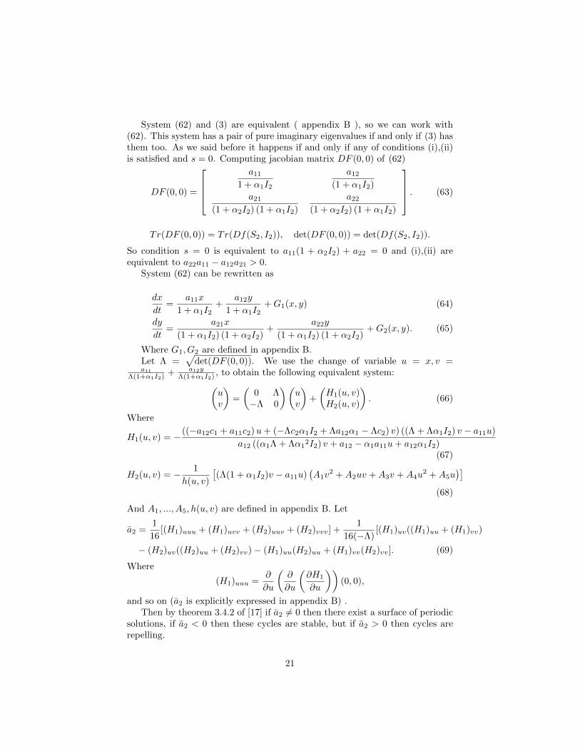
5 Discussion

As we said in the introduction, traditional epidemic models have always stabil-ity results in terms of R0, such that we need only reduce R0 < 1 to eradicatethe disease. However, including the treatment function brings new epidemicequilibria that make the dynamics of the model more complicated. Now, let’sdiscuss some control strategies for the infectious disease, analysing the parame-ters of the treatment function (α2, β2) and looking for conditions that allow usto eliminate the disease. We make this study by cases.

A first approach is focus on the definition ofR0, we can see thatR0 decreaseswhen β2 increases, so the first measure suggesting control is a big value for β2.But this is not always a good way to proceed. Let us divide our analysis in thefollowing cases:

Case 1: There is no positive endemic equilibrium for R0 ≤ 1. This happenswhen R∗0 ≤ 1 ( by theorem 4 ) or when R∗0 > 1 and (α2, β2) ∈ A1 ∪ A2 (theorem 4 , number 5). In this case if R0 > 1 there is a unique positive endemicequilibrium, therefore there exists a bifurcation atR0 = 1 : from the disease freeequilibrium, which is globally asymptotically stable for 0 < R0 < 1 (by theorem6) and a saddle for R0 = 1 and β2 6= g(α2) (theorem 9 ), to the positiveendemic equilibrium E2 as R0 increase. E2 will be locally asymptotic stable orunstable depending on theorem 13 or surrounded by a limit cycle (theorem 14) . If conditions for Hopf bifurcation hold then the stability of the limit cycleis determined by a2; when a2 < 0 the periodic orbit is stable and therefore E2

is unstable, while if a2 > 0 then the periodic orbit is unstable and E2 is stable. In this case the best way to eradicate the disease is finding parameters thatallow R0 < 1, because then all the infectious states tend to I = 0.

Case 2: There exist endemic equilibria for R0 ≤ 1. This happens when(α2, β2) ∈ A3. The existence of endemic equilibria is determined by the rela-tionship between R0 and max{P1,R+

0 }. Let F (α2, β2) = R0−R+0 , G(α2, β2) =

R0 − P1, and focus on the implicit curves defined by F = 0 and G = 0. Thesecurves divide the domain A3 in another ones (see figure 7 ):

A13 = {(α2, β2) ∈ A3, 0 < R0 < R+

0 }A2

3 = {(α2, β2) ∈ A3,R0 > R+0 }

A33 = {(α2, β2) ∈ A3, 0 < R0 < P1}

A43 = {(α2, β2) ∈ A3,R0 > P1}. (70)

If (α2, β2) ∈ A23 ∩A4

3 then there exist two endemic equilibria E1( a saddle )and E2 ( stable or unstable depending on conditions of theorems 13 and possiblywith a periodic orbit around (theorems 14 )), but when R0 = 1 one of thembecomes negative, leaving us with E2. In this case R0 < 1 is not a sufficientcondition to control the disease, because even with R0 < 1 we have endemicpositive equilibria that could be stable and then the disease will tend to a nonzero value; also we have the possibility of a periodic solution, or biologically, anoutbreak that will apparently “ disappear ” but will re-emerge after some time.

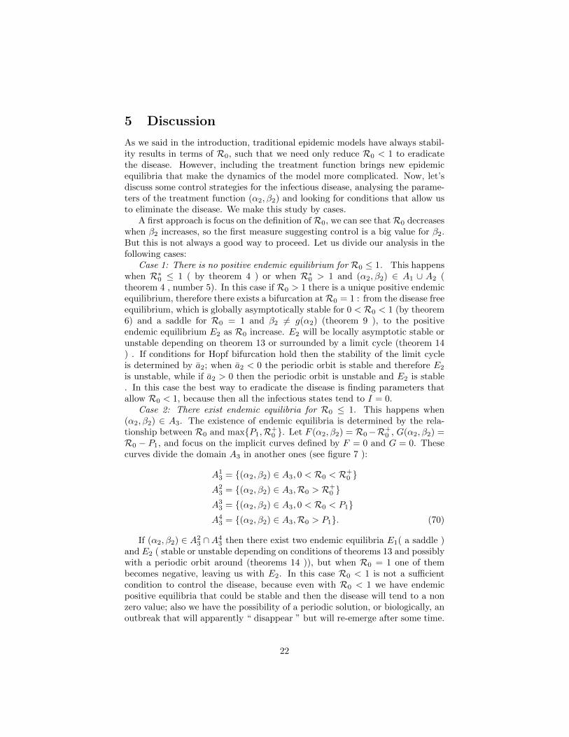
22

Figure 7: Bifurcation diagram in terms of β2 and α2. The values of the param-eters taken are α = 0.4, β = 0.3, b = 0.2, γ = 0.03, δ = 0.05, p = 0.3,m = 0.3.Here R0 < R+

0 inside the solid curve ( R0 = R+0 ) and R0 > R+

0 outsideit, whenever (β2, α2) is in its domain (under the long dashed line “root=0”). R0 < 1 above the dot-lined line and R0 > 1 under it; R0 < P1 above thedotted line and R0 > P1 under that one. The areas A1, A2, A3 are delimitedby the dashed line g = 0 and α2 = 3.8. In this case the endemic equilibria E1

and E2 exists both in the area delimited by the line R0 = 1 and the dotted lineR0 = P1 , while E2 exists by itself under the line R0 = 1.

23

The best way in this case is ensuring (α2, β2) ∈ (A23 ∩A4

3)c because then wedon’t have endemic equilibria for R0 < 1 and the disease free will be globallyasymptotically stable.

References

[1] Hadeler, K.P., van den Driessche, P. Backward bifurcation in epidemiccontrol. Math. Biosci. 146, 15–35 (1997).

[2] J. Dushoff, W. Huang, C. Castillo-Chavez, Backwards bifurcations andcatastrophe in simple models of fatal diseases, J. Math. Biol. 36 227–248,(1998).

[3] P. van den Driessche, J. Watmough, A simple SIS epidemic model with abackward bifurcation, J. Math. Biol. 40 525–540 (2000).

[4] Brauer, F.: Backward bifurcations in simple vaccination models. J. Math.Anal. Appl. 298, 418–431 (2004)

[5] K.P. Hadeler, C. Castillo-Chavez, A core group model for disease transmis-sion, Math. Biosci. 128 (1995) 41.

[6] R.M. Anderson, R.M. May, Infectious Diseases of Humans, Oxford Univer-sity Press, London, 1991.

[7] W. Wang, S. Ruan, Bifurcation in an epidemic model with constant removalrate of the infectives, J. Math. Anal. Appl. 291 (2004) 775.

[8] Zhixing Hu, Wanbiao Ma, Shigui Ruan, Analysis of SIR epidemic modelswith nonlinear incidence rate and treatment, Mathematical Biosciences, 238(2012) 12-20.

[9] Zhang Zhonghua, Suo Yaohong, Qualitative analysis of a SIR epidemicmodel with saturated treatment rate, J Appl Math Comput (2010) 34: 177-194.

[10] Bingtuan Li, Yang Kuang, Simple Food Chain in a Chemostat with Distinct.Removal Rates,Journal of Mathematical Analysis and Applications 242, 75-92(2000).

[11] Jack Carr, Applications of Centre Manifold Theory, (1981), pp 1-13

[12] Lawrence Perko, Differential Equations and Dynamical Systems, 3rd edi-tion, Springer,107-108.

[13] Linhua Zhou, Meng Fan, Dynamics of an SIR epidemic model with limitedmedical resources revisited, Nonlinear Analysis: Real World Application13(2012)312-324.

24

[14] Walter G. Kelley, Allan C. Peterson, The Theory of Differential Equations,Classical and Qualitative, second edition, Springer

[15] Xu Zhang, Xianning Liu, Backward bifurcation of an epidemic model withsaturated treatment function, J. Math. Anal. Appl. 348 (2008) 433-443

[16] H. Wan J. Cui Rich Dynamics of an epidemic model with saturation recov-ery, J. App. Math. v.2013, Article ID 314958.

[17] John Guckenheimer, Philip Holmes, Nonlinear Oscillations, DynamicalSystems, and Bifurcation of Vector Fields, Springer-Verlag, New York,1996.

A Computing center manifold

The Jacobian matrix of system (38) is

DF (m, 0) =

(−b −βm− bm+ pδ0 0

). (71)

With eigenvalues λ1 = −b and λ2 = 0 and respective eigenvectors v1 = (1, 0)and v2 = (−γ+β2+bm

b , 1). Using the eigenvectors to establish a new coordinatesystem we define:(

SI

)=

(1 −γ+β2+bm

b

0 1

)(uv

), or

(uv

)=

(1 γ+β2+bm

b

0 1

)(SI

).

(72)Under this transformation the system becomes

du

dt=

d

dtS (t) +

(γ + β2 + bm) ddtI (t)

b

= −β(S +m

)I

1 + α I− bS − bmI + pδ I + (γ + β2 + bm)β

(S +m

)I

1 + α I− (pδ + γ) I − β2 I

1 + α2 I

1

b,

dv

dt=dI

dt(73)

=β(S +m

)I

1 + α I− (pδ + γ) I − β2 I

1 + α2 I. (74)

Substituting S = u− (γ+β2+bm)vb , I = v and βm = pδ + γ + β2 we obtain:

dv

dt= 0u+ f(v, u)

du

dt= −bu+ g(v, u), (75)

25

where

f(u, v) = − v (−β b− β bα2 v)u

(1 + α v) (1 + α2 v) b

− v

(1 + α v) (1 + α2 v) b((β bmα2 + bγ αα2 − β α2 pδ + bpδ αα2 + β2α2 m

)v2

+(bpδ α2 + β bm− β bmalpha2 + bγ α2 + β2m− β pδ + bα β m

)v),

g(u, v) = − 1

(1 + α v) (1 + α2 v) b2[v((mb2γ αα2 + 2β2bm2α2 + β α2 p

2δ2

+ β3α2 m2 − bγ pδ αα2 + bγ αα2 β m− 2β2α2 mpδ + bpδ αα2 β m

− b2mαα2 β − β2bmα2 + b2m2β α2 + b2mpδ αα2 − bp2δ2αα2

− 2β bmα2 pδ − b2mβ α2 + bβ α2 pδ)v2 + (b2m2β − 2β bmpδ − β b2m+ 2β2bm2

− β2bm+ β p2δ2 + 2β bmα2 pδ − bpδ α β m+ β3m2 + β bpδ − b2αβm− 2β2mpδ

+ b2m2αβ + bα β2m2 − uβ b2mα2 − bβ2uα2m+ bβ uα2pδ − γ bpδ α2 + γ β bmα2

+ b2mpδ α2 − b2m2β α2 + uβ b2α2 − bp2δ2α2 − β2bm2α2 + b2mγ α2)v − b2mβ u+ uβ b2 − bβ2um+ bβ upδ)]. (76)

By [11] the system (75) has a center manifold of the form u = h(v). Letφ : R→ R and define the annihilator:

Nφ = φ′(v)(f(v, φ(v))) + bφ− g(v, φ(v))

=1

b2(1 + αv)(1 + α2v)[bpδ α v3α2β m+ b2m2β v2 − β v2b2m+ b3φ+ b3φα v

+ b3φα2v + b2mγ α2 v2 + φβ vb2 + vbφ β pδ + b2mpδ α2v

2 − φβ v2b2mα2

− γ bpδ α2v2 + b2mγ αv3α2 + γ β v2bmα2 + b2m2α v2β − 2β2v2mpδ − β2v2bm2α2

+ β v2bpδb2v2αβm+ bα v2β2m2 − bpδ α v2β m+ β3v2m2 − 2β v2bmpδ + β3v3α2m2

+ 2β2v2bm2 + β v2p2δ2 − β2v2bm− φβ vb2m− vbφ β2m+ β v3bα2pδ − b2v3αα2β m

− bp2δ2α v3α2 − 2β2v3α2mpδ + φβ v2b2α2 − b2m2β v2α2 + b2m2β v3α2 − β v3b2mα2

− β2v3bα2m+ 2β2v3bm2α2 − bp2δ2v2α2 + β v3α2p2δ2 + b3φα v2α2 − v2bφ β2mα2

+ v2bφ β pδ α2 + bγ α v3α2β m+ b2mpδ α v3α2 − γ bpδ α v3α2 − 2β v3bmα2pδ

+ 2β v2bmα2pδ]. (77)

Assume that φ = a0v2 + a1v

3 + O(v4), then by substituting φ and dφdv in the

26

annihilator Nφ and expanding its Taylor series we get:

Nφ =1

b2((γ β bmα2 + b2mpδ α2 − b2m2β α2 + 2β bmα2 pδ + 2β2bm2 + b2m2β

− β b2m+ b3a0 − β2bm2α2 − 2β bmpδ + b2mγ α2 − γ bpδ α2 − b2αβm− β2bm

+ bα β2m2 + b2m2αβ − 2β2mpδ + β p2δ2 − bpδ α β m− bp2δ2α2 + β bpδ

+ β3m2)v2 − 1

b2[αβ3m2 − a0 β b

2 − b3a1 − 2 bpδ α β m− β2bm2α22 − bp2δ2α2

2

+mb2γ α22 − b2m2β α2

2 − b2αβm− b2α2β m− αβ2bm+ bα2β2m2 + b2m2α2β

+ αβ p2δ2 + 3 a0 β b2m+ 3 a0 bβ

2m+ 2 a0 b2γ α2 + 2 a0 b

2pδ α2 − 2 a0 β b2mα2

− 3 a0 bβ pδ + 2 a0 b2αβm− 2αβ2mpδ + αβ bpδ + b2mpδ α2

2 + bγ α22β m

− bγ pδ α22 + 2β bmα2

2pδ − bpδ α2β m+ b2m2αβ + 2 bα β2m2]v3 +O(v4)).(78)

By choosing the coefficients of v2 and v3 in order to have Nφ = O(v4) we obtainthat a0 and a1 must be the following:

a0 = − 1

b3[b2m2β + β bpδ − b2αβm+ b2mpδ α2 − γ bpδ α2 + γ β bmα2 − 2β bmpδ

− β b2m+ 2β2bm2 − β2bm+ β p2δ2 + 2β bmα2 pδ − bpδ α β m+ β3m2 − bp2δ2α2

− b2m2β α2 − 2β2mpδ + b2mγ α2 + bα β2m2 + b2m2αβ − β2bm2α2], (79)

a1 =1

b3[αβ3m2 − ao β b2 − 2 bpδ α β m− β2bm2α2 − bp2δ2α2

2 +mb2γ α22 − b2m2βα2

2

− b2αβm− b2α2β m− αβ2bm+ bα2β2m2 + b2m2α2β + αβ p2δ2 + 3 a0 β b2m

+ 3 a0 bβ2m+ 2 a0 b

2γ α2 + 2 a0 b2pδ α2 − 2 a0 β b

2mα2 − 3 a0 bβ pδ + 2 a0 b2αβm

− 2αβ2mpδ + αβ bpδ + b2mpδ α22 + bγ α2

2β m− bγ pδ α22 + 2β bmα2

2pδ

− bpδ α2β m+ b2m2αβ + 2 bα β2m2]. (80)

Hence h(v) = a0v2 + a1v

3 +O(v4).

B Hopf bifurcation

To analyze the behaviour of the solutions of (3) when s = 0 we make a changeof coordinates x = S − S2, y = I − I2, to obtain a new equivalent system to (3)with an equilibrium in (0, 0) in the x− y plane. Under this change the systembecomes in:

dx

dt=a11x+ a12y + c1xy + c2y

2 + c71 + α1y + α1I2

,

dy

dt=a21x+ a22y + c3xy + c4xy

2 + c5y2 + c6y

3 + c8(1 + α1y + α1I2) (1 + α2y + α2I2)

. (81)

27

Where:

a11 = −b− β1I2 − bα1I2 (82)

a12 = −2 bmα1I2 + bmα1 − bα1S2 + 2 pδ α1I2 + pδ − bm− β1S2 (83)

c1 = −bα1 − β1 (84)

c2 = −bmα1 + pδ α1 (85)

a21 = −I2 (−β1 − β1α2I2) (86)

a22 = −2 pδ α1I2 + 2β1α2S2I2 − 3 pδ α1α2I22 − 2 γ α1I2

− 2 γ α2I2 − 2 pδ α2I2 − 2β2α1I2 − 3 γ α1α2I22 − γ − pδ − β2 + β1S2 (87)

c3 = 2β1α2I2 + β1 (88)

c4 = β1α2y2 (89)

c5 = −3 pδ α1α2I2 − 3 γ α1α2I2 − pδ α1 + β1α2S2 − γ α1 − γ α2 − pδ α2

− β2α1 (90)

c6 = −pδ α1α2 − γ α1α2 (91)

c7 = −(β1S2I2 − bmα1I2 + bS2 − pδ I2 − pδ α1I22 + bα1S2I2 + bmI2

− bm+ bmα1I22) (92)

c8 = −I2[pδ α1I2 + pδ + pδ α2I2 + γ α2I2 − β1α2S2I2 + γ α1I2 + β2α1I2

+ γ + γ α1α2I22 − β1S2 + β2 + pδ α1α2I2

2]. (93)

But from the equations for the equilibrium point we can prove that c7 = c8 = 0,so the system we will work on is

dx

dt=a11x+ a12y + c1xy + c2y

2

1 + α1y + α1I2,

dy

dt=a21x+ a22y + c3xy + c4xy

2 + c5y2 + c6y

3

(1 + α1y + α1I2) (1 + α2y + α2I2). (94)

If we denote system (3) as (S, I)′ = f(S, I) and system (81) as (x, y)′ = F (x, y),f = (f1, f2), F = (F1, F2) then

F (x, y) = f(x+ S2, y + I2),

and

∂Fi∂x

(x, y) =∂fi∂S

(x+S2, y+I2)∂S

∂x(x, y)+

∂fi∂I

(x+S2, y+I2)∂I

∂x(x, y) =

∂fi∂S

(x+S2, y+I2)

∂Fi∂y

(x, y) =∂fi∂S

(x+S2, y+I2)∂S

∂y(x, y)+

∂fi∂I

(x+S2, y+I2)∂I

∂y(x, y) =

∂fi∂S

(x+S2, y+I2).

So, the jacobian matrix of (62) DF (0, 0) in the equilibrium is equal to thejacobian matrix of system (3) Df(S1, I1). We can also compute the partialderivatives of system (81) and (62) to prove that they are equal,ie,

Df(S2, I2) = DF (0, 0). (95)

28

Therefore the system (62) and (3) are equivalent and we can work with system(62). The jacobian matrix DF (0, 0) of (62) is:

DF (0, 0) =

a11

1 + α1I2

a12

(1 + α1I2)

a21

(1 + α2I2) (1 + α1I2)

a22

(1 + α2I2) (1 + α1I2)

. (96)

So system (62) can be rewritten as

dx

dt=

a11x

1 + α1I2+

a12y

1 + α1I2+G1(x, y) (97)

dy

dt=

a21x

(1 + α1I2) (1 + α2I2)+

a22y

(1 + α1I2) (1 + α2I2)+G2(x, y). (98)

Where

G1 =1

(1 + α1y + α1I2)(1 + α1I2){[(1 + α1I2)c1 − a11α1]xy + [c2(1 + α1I2)− α1a12]y2}

(99)

G2 =1

(1 + α1y + α1I2)(1 + α2y + α2I2)(1 + α1I2)(1 + α2I2){[c3(1 + α1I2)(1 + α2I2)

− a21(α2 + α1 + 2α1α2I2)]xy + [c4(1 + α1I2)(1 + α2I2)− a21α1α2]xy2

+ [c5(1 + α1I2)(1 + α2I2)− a22(α2 + α1 + 2α1α2I1)]y2 + [c6(1 + α1I2)(1 + α2I2)

− a22α1α2]y3}. (100)

We need the normal form of the system (62). The eigenvalues of DF (0, 0)when s2 = 0 and (i),(ii) are satisfied are:

Λi,−Λi.

With complex eigenvector

v =

−1−Λi(1 + α1I2) + a11

a12

, v =

−1Λi(1 + α1I2) + a11

a12

.

Using the Jordan Canonical form of matrix DF (0, 0) and the procedure in [12](p. 107, 108) we use the change of variable u = x, v = a11

Λ(1+α1I2) + a12yΛ(1+α1I2) , to

obtain the following equivalent system:(uv

)=

(0 Λ−Λ 0

)(uv

)+

(H1(u, v)H2(u, v)

). (101)

29

Where

H1(u, v) = − ((−a12c1 + a11c2)u+ (−Λc2α1I2 + Λa12α1 − Λc2) v) ((Λ + Λα1I2) v − a11u)

a12 ((α1Λ + Λα12I2) v + a12 − α1a11u+ a12α1I2)

(102)

H2(u, v) = − 1

h(u, v)

[(Λ(1 + α1I2)v − a11u)

(A1v

2 +A2uv +A3v +A4u2 +A5u

)].

(103)

And:

A1 = Λ2 (1 + α1I2)2

[−a12c6α2I22α1 − a11c2α1I2

2α22 − a11c2α1I2α2

− a12c6α1I2 + a11a12α1α22I2 + a11a12α1α2 + a12a22α1α2

− a11c2α22I2 − a12c6α2I2 − a11c2α2 − a12c6]

A2 = −Λ (1 + α1I2) [a11a12c1α22α1I2

2 + a122c4α2I2

2α1 − 2 a12a11c6α2I22α1

− 2 c2α1I22α2

2a112 + a12α1α2

2a112I2 − 2 a12a11c6α1I2 − 2 c2α1I2α2a11

2

+ a122c4α1I2 + a11a12c1α2α1I2 + a11a12c1α2

2I2 + a122c4α2I2 − 2 a12a11c6α2I2

− 2 a112c2α2

2I2 + a122c4 − 2 a11

2c2α2 − 2 a12a11c6 + a11a12c1α2 + a12α1α2a112

− a122α1a21α2 + 2 a12a11a22α1α2]

A3 = Λ (1 + α1I2) a12[−a12c5α1I22α2 + a12a11α1α2

2I22 + 2 a12a22α1α2I2

+ 2 a12a11α1α2I2 − a12c5α1I2 + a12a22α1 + a11a12α1 − a12c5α2I2 + a12a22α2

− 2 a11c2α1I22α2 − a11c2α1I2 − a11c2 − a11c2α2

2I22 − 2 a11c2α2I2]

A4 = −a11[−a122c4α2I2 − a11a12c1α2α1I2 + c2α1I2α2a11

2 − a122c4α2I2

2α1

− a122c4α1I2 − a12

2c4 + a122α1a21α2 − a12a11a22α1α2 − a11a12c1α2

2α1I22

+ a12a11c6 + a112c2α2

2I2 + a12a11c6α2I22α1 + a11

2c2α2 − a11a12c1α2

+ a12a11c6α2I2 + a12a11c6α1I2 + c2α1I22α2

2a112 − a11a12c1α2

2I2]

A5 = a12[2 a112c2α2I2 + a11

2c2α1I2 + a122α1a21 + a11

2c2α22I2

2 − a12a11a22α2

− a12a11a22α1 − a122c3α2I2 − a12

2c3α1I2 + a11a12c5 + a122α2a21 − a12a11c1

+ 2 a122α1a21α2I2 − a12a11c1α2

2I22 − a12a11c1α1I2 − 2 a12a11c1α2I2

+ a11a12c5α2I2 + a11a12c5α1I2 − a122c3α1I2

2α2 − a122c3 + a11a12c5α1I2

2α2

− 2 a12a11a22α1α2I2 − 2 a12a11c1α1I22α2 − a12a11c1α1I2

3α22 + 2 a11

2c2α1I22α2

+ a112c2α1I2

3α22 + a11

2c2]

h(u, v) = Λ (1 + α1I2)2a12[

(α1Λ + Λα1

2I2)v + a12 − α1a11u+ a12α1I2]

[(α2Λ + α2Λα1I2) v + a12 − α2a11u+ α2I2a12] (1 + α2I2) .

30

Let

a2 =1

16[(H1)uuu + (H1)uvv + (H2)uuv + (H2)vvv] +

1

16(−Λ)[(H1)uv((H1)uu + (H1)vv)

− (H2)uv((H2)uu + (H2)vv)− (H1)uu(H2)uu + (H1)vv(H2)vv]. (104)

Then

a2 =3((−c1Λ vα1

2I2 + Λ va11α12 − a12c1α1I2 + a11c2α1I2 − c1Λ vα1 − a12c1 + a11c2

)a12a11

2α1

)8 (a12 + α1Λ v)

4(1 + α1I2)

3

− (−3 a11c2 − 3 a11c2α1I2 + 2 a12a11α1 + a12c1 + a12c1α1I2)α1Λ2

8 (1 + α1I2) a123

− 1

8Λ (1 + α1I2)4a12

4 (1 + α2I2)3 [2 a11A5α1Λ + 6 a11A5α1Λα2I2 + 2 a11A5α1

2Λ I2

+ 4 a11A5α12Λ I2

2α2 + 2 a11A5α2Λ− a112A3α1 − 2 a11

2A3α1α2I2 − a112A3α2 − a11A2a12

− a11A2a12α2I2 − a11A2a12α1I2 − a11A2a12α1I22α2 +A4Λ a12 +A4Λ a12α2I2

+ 2A4Λ a12α1I2 + 2A4Λ a12α1I22α2 +A4Λ a12α1

2I22 +A4Λ a12α1

2I23α2]

+3

8

(−A1a12 −A1a12α2I2 +A3α1Λ + 2A3α1Λα2I2 +A3α2Λ)

(1 + α1I2)2a12

4 (1 + α2I2)3

− 1

16Λ[−2

Λ (−2 a11c2 − 2 a11c2α1I2 + a12a11α1 + a12c1 + a12c1α1I2)

a124 (1 + α1I2)

2

− 2(A5Λ +A5Λα1I2 − a11A3) (−a11A5 +A3Λ +A3Λα1I2)

Λ2 (1 + α1I2)6a12

6 (1 + α2I2)4

− 4(−a12c1 + a11c2) a11

2A5

a125 (1 + α1I2)

4Λ (1 + α2I2)

2 4(−c2α1I2 + a12α1 − c2) Λ2A3

a125 (1 + α1I2)

2(1 + α2I2)

2 ]. (105)

31