Stability analysis of the POD reduced order method for solving the … · 2020-03-27 · Stability analysis of the POD reduced order method for solving the bidomain model in cardiac

HAL Id: hal-01245685https://hal.inria.fr/hal-01245685

Submitted on 17 Dec 2015

HAL is a multi-disciplinary open accessarchive for the deposit and dissemination of sci-entific research documents, whether they are pub-lished or not. The documents may come fromteaching and research institutions in France orabroad, or from public or private research centers.

L’archive ouverte pluridisciplinaire HAL, estdestinée au dépôt et à la diffusion de documentsscientifiques de niveau recherche, publiés ou non,émanant des établissements d’enseignement et derecherche français ou étrangers, des laboratoirespublics ou privés.

Stability analysis of the POD reduced order method forsolving the bidomain model in cardiac electrophysiology

Cesare Corrado, Jamila Lassoued, Moncef Mahjoub, Nejib Zemzemi

To cite this version:Cesare Corrado, Jamila Lassoued, Moncef Mahjoub, Nejib Zemzemi. Stability analysis of the PODreduced order method for solving the bidomain model in cardiac electrophysiology. MathematicalBiosciences, Elsevier, 2015, 10.1016/j.mbs.2015.12.005. hal-01245685

Stability analysis of the POD reduced order method forsolving the bidomain model in cardiac

electrophysiology

Cesare Corradoa, Jamila Lassouedb,c, Moncef Mahjoubb,c, Nejib Zemzemia,c

aINRIA, Bordeaux - Sud-Ouest, 200 Avenue de la vielle Tour 33405 Talence Cedex France.bUniversity of Tunis El Manar, LAMSIN−ENIT , BP 37, 1002 Tunis Belvedere, Tunisia.

cLIRIMA - Laboratoire International de Recherche en Informatique et MathematiquesAppliquees.

Abstract

In this work we show the numerical stability of the Proper Orthogonal Decomposi-tion (POD) reduced order method used in cardiac electrophysiology applications.The difficulty of proving the stability comes from the fact that we are interestedin the bidomain model, which is a system of degenerate parabolic equations cou-pled to a system of ODEs representing the cell membrane electrical activity. Theproof of the stability of this method is based an a priori estimate controlling thegap between the reduced order solution and the Galerkin finite element one. Wepresent some numerical simulations confirming the theoretical results. We alsocombine the POD method with a time splitting scheme allowing a faster solu-tion of the bidomain problem and show numerical results. Finally, we conductnumerical simulation in 2D illustrating the stability of the POD method in its sen-sitivity to the ionic model parameters. We also perform 3D simulation using amassively parallel code. We show the computational gain using the POD reducedorder model. We also show that this method has a better scalability than the fullfinite element method.

Keywords:Bidomain equation, reduced order method, proper orthogonal decomposition,stability analysis, a priori estimates, ionic parameters, Mitchell-Schaeffer model.2000 Math Subject Classification: 34A12, 34A34, 35K20, 35B45, 35K57,35K60, 35B65, 49M27

Preprint submitted to Mathematical Biosciences December 9, 2015

1. Introduction

The electric wave in the heart is governed by a system of reaction-diffusionpartial differential equations called bidomain model. This system is coupled non-linearly to an ordinary differential equations (ODEs) modeling the cellular mem-brane dynamics (see [5, 27]). The bidomain model is widely used in cardiacelectrophysiology simulation. This mathematical model takes into account theelectrical properties of the cardiac muscle.

Different numerical methods have been used for solving the bidomain model.Finite element method has been used in most of the works [35, 8, 10, 21, 4, 34, 14].Some groups use finite difference method [27, 32] and others use finite volumemethod [9]. All these methods lead to a large linear system to solve, especiallywhen using implicit schemes. Here we don’t cite all the works that have beendone in the literature, some other works could be found in the recent review of thebidomain model [15]. The computational cost of solving the bidomain problembecomes very important when we are interested in solving inverse problems [2].Thus reducing the computational cost of the forward problem is a challenging is-sue. One of the most popular approaches used in model reduction is the ProperOrthogonal Decomposition (POD) method. This method was initially introducedfor analyzing multidimensional data. In [26], Holmes et al. used this approachfor understanding the turbulence flow phenomena. Until there, the POD was pre-sented only as an efficient post-processing technique in order to extract coherentstructures of data from numerical simulations or experiments. The proper orthog-onal decomposition modes allow to provide basis functions that could be used todefine a low-dimensional subspace on which one would project a linear system.This idea was first applied by Aubry et al. [23] to model the wall region of aturbulent boundary layer. More recently Delville et al. [11] used it to study thedynamics of coherent structures in turbulent mixing layer. Moreover, existing er-ror estimates are expressed with respect to quantities which are not controlled inthe construction of the POD basis [36]. In the literature, there are some a pri-ori estimates results: Henri and Yvon [13] show an error estimate for continuousand linear parabolic problems. Kunisch and Volkwein [17] show a priori errorestimates for a generic non linear parabolic evolution PDEs at the discrete level.

As concerns its use in the cardiac electrophysiology field, the reduced ordermodelling based on POD has been used by Chapelle et al. [7]. The authorsdemonstrate an a priori error estimates result that guaranties the stability of thePOD method in case of a nonlinear parabolic wave-like equation where the non-linear term is a cubic Lipschitz function. This model is known as the monodomain

2

equation and allows to describe the propagation of the electrical wave but havesome limitation in application like electrocardiograms modelling [3]. The use ofthe bidomain model is necessary in this case. Recent works have shown the us-ability and the efficiency of the reduced order modelling based on POD for thenumerical simulation of electrocardiograms based on the bidomain model [4].

It has also been used for the ionic model parameter estimation but more inter-estingly for infarction localisation based on simulated data [2]. The applicationof reduced order is appealing because it allows to dramatically decrease the com-putational cost of the forward problem and consequently in the inverse problem.The problem is that for the bidomain model there is no study showing the stabilityof the reduced order method. The work by Chapelle et al. [7] does not coverthe bidomain problem, the main difficulty comes from the fact that the bidomainmodel is degenerated. In this work we prove the stability of the POD methodfor the bidomain model based on an a priori error estimates and we illustrate thetheoretical results by some numerical simulations.

In section 2 we present the mathematical model of the electrical activity in theheart based on the bidomain equations [33]. In section 3, we present the procedureused to generate the POD basis. The main results is provided in section 4 wherewe prove a new error estimates between the standard finite elements Galerkinapproximation of the solution and a spacial Galerkin approximation of the PODsolution for the bidomain model. Finally, in section 5 we show how the PODreduced order method could be combined with time splitting schemes allowingto reduce the computational cost of the linear problem. Then, we carry out somenumerical simulations showing the robustness of the POD method. The mainconclusions of the study are then summarized in section 7.

2. Modelling and numerical methods

2.1. Electric model and some preliminary resultsThe heart is assumed to be isolated, the propagation of the electrical wave in

myocardium is governed by the following system of equations [33, 29, 8]:χm∂tVm− Iion(Vm,w)−div(σσσ i∇Vm)−div(σσσ i∇ue) = Iapp in Ω× (0,T ),

−div((σσσ i +σσσ e)∇ue)−div(σσσ i∇Vm) = 0 in Ω× (0,T ),∂tw+G(Vm,w) = 0 in Ω× (0,T ),

σσσ i∇Vm.n = 0 on ∂Ω× (0,T ),σσσ e∇ue.n = 0 on ∂Ω× (0,T ).

(1)

3

where Ω and ∂Ω denote respectively the heart domain and its boundary. The timedomain is given by (0,T ), and χm the membrane capacitance per area unit. Thevariables Vm and ue denote the action potential and the extracellular potential. Theconductivity tensors σσσ i(x) in the intracellular domain and σσσ e(x) in the extracellu-lar domain could then be written as follows

σσσ i,e(x)def= σ

ti,eIII +(σ l

i,e−σti,e)aaa(x)⊗aaa(x),

where aaa(x) is the fiber direction, III is the identity tensor and σ li,e and σ t

i,e are con-ductivities values in the intra-cellular and extracellular along the fibers and in thetransverse directions.

The term Iapp is a given source function, used in particular to initiate the ac-tivation, w represents the concentrations of different chemical species, and vari-ables representing the openings or closures of some gates of the ionic channels.The ionic current Iion and the function G(Vm,w) depends on the considered ionicmodel.

In [30], more than 28 models of cardiac cells are reported, some of them in-cluding more than 50 parameters [31]. In this study, the dynamics of w and Iionare described by the Mitchell and Schaeffer model [22]:

Iion(v,w) =wτin

v2(1− v)− vτout

and G(v,w) =

w−1τopen

if v≤ vgate

wτclose

if v > vgate

The time constants τin, τout are respectively related to the length of the depo-larization and repolarization, τopen and τclose are the characteristic times of gateopening and closing respectively and vgate corresponds to the change-over voltage.

Problem (1) is completed with initial conditions

Vm(0,x) = v0(x) and w(0,x) = w0(x) ∀x ∈Ω .

Finally, let us notice that ue is unique up to additive constant. This constant canbe fixed by the following condition∫

Ω

uedx = 0.

Let [0,T ] be a bounded interval of R, we consider the Lebesgue measure dtover the time interval [0,T ]. We denote by Lp(Ω) the space of real functions which

4

are in the pth power integrable (1 ≤ p < ∞), or are measurable and essentiallybounded (for p = ∞), and by W 1,p(Ω) the Sobolev space of functions ψ : Ω→R which, together with their first-order weak partial derivatives, belong to thespace Lp(Ω) (1 ≤ p < ∞). For X a Banach space, denote C(0,T ;X) the space ofcontinuous functions from [0,T ] into X equipped with the uniform convergencenorm, and

‖ f‖Lp(0,T ;X) =

(∫ T

0‖ f (t)‖p

X dt)1/p (

= sup0<t<T

ess‖ f (t)‖p if p = ∞

).

By definition Lp(0,T ;X), p<∞, is the seperated space of C(0,T ;X) for this norm;for p = ∞, L∞(0,T ;X) is the subset of L1(0,T ;X) on which the L∞ norm is finite.It is a Banach space for 0≤ p≤ ∞. For p = 2 and X =W 1,2(Ω), we say space ofBochner integrable mappings, see [19]. Further, we set (see [6])

W 1,2(Ω)/R = u ∈W 1,2(Ω) ,∫

Ω

udx = 0 ⊂W 1,2(Ω),

that is a Banach space with the norm ‖u‖W 1,2(Ω)/R= ‖u‖W 1,2(Ω). We have the

Poincare-Wirtinger inequality

∃C > 0, ∀u ∈W 1,2(Ω)/R,∫

Ω

|u|2 dx≤C∫

Ω

|∇u|2 dx. (2)

The gradient ∇ is always taken only with respect to the spatial variables x.Let us make the following assumptions on the ”data”.

Assumption 1. Let Ω∈R3 be a bounded domain with Lipschitz-continuous bound-ary ∂Ω and 0 < T < ∞. Furthermore define Q := Ω× [0,T ] and Σ = ∂Ω× [0,T ].

Assumption 2. We assume that the conductivities of the intracellular and extra-cellular σσσ i,σσσ e ∈ [L∞(Ω)]3×3 are symmetric and uniformly positive definite, i.e.there exist αi > 0 and αe > 0 such that, ∀ξ ∈ R3,

ξT

σσσ i(x)ξ ≥ αi |ξ |2 , ξT

σσσ e(x)ξ ≥ αe |ξ |2 . (3)

Namely, we assume that there exists constants 0 < ν < µ such that

ν |ξ |2 ≤ ξT

σσσ i,eξ ≤ µ |ξ |2 . (4)

Assumption 3. We assume that the function Iion is Lipschitz with respect to thevariable Vm.

5

We have the following existence and regularity results of the weak solution ofthe bidomain system (1) (see [6, 24, 18, 38]).

Theorem 1. Let T > 0, Iapp ∈ L2(0,T ;W 1,2(Ω)∗) and v0 ∈ L2(Ω) be given data.If the assumptions (1)-(3) hold and w0 ∈ L2(Ω), such that

0≤ w0 ≤ 1 in Ω ,

then, system (1) has a weak solution in the following sense:

Vm ∈C(0,T ;L2(Ω))∩L2(0,T ;W 1,2(Ω))∩L4(Q)

ue ∈ L2(0,T ;L2(Ω)) and w ∈C(0,T ;L2(Ω)) ,

such that for all ψ1 ∈W 1,2(Ω) and ψ2 ∈W 1,2(Ω)/R

χm

∫Ω

∂tVmψ1dx+∫

Ω

σσσ i∇Vm∇ψ1dx+∫

Ω

σσσ i∇ue∇ψ1dx

+∫

Ω

Iion(Vm,w)ψ1dx =∫

Ω

Iappψ1dx,(5)

∫Ω

σσσ i∇Vm∇ψ2dx+∫

Ω

(σσσ i +σσσ e)∇ue∇ψ2dx = 0, (6)

∂tw+G(Vm,w) = 0. (7)

Moreover, 0 ≤ w ≤ 1 a.e. in Q, and there exists a constant C > 0 such that thefollowing a-priori bound holds:

‖Vm‖2L2(0,T ;W 1,2(Ω))+‖Vm‖2

L4(Q)+‖ue‖2L2(0,T ;L2(Ω)) ≤C

(1+‖v0‖2

L2(Ω)

+‖w0‖2L2(Ω)+

∥∥Iapp∥∥2

L2(0,T ;W 1,2(Ω)∗)

).

(8)

2.2. Abstract discretization of bidomain systemIn order to actually compute a solution of system(1), we shall discretize the

problem and we try to approximate the problem in a finite dimension subspace.We approximate W 1,2(Ω) by a finite dimensional space, spanned by ”Galerkinfunctions” (ϕk)k=1,··· ,M:

Wh := span(ϕ1, · · · ,ϕM)⊂W 1,2(Ω) , M ∈ N .

A suitable initial value v0,h may be obtained by an (., .)W 1,2(Ω)-orthogonal projec-tion of v0 ∈W 1,2(Ω) on Wh, for instance. The discrete problem statement thenreads:

6

Problem 1. Find (Vm,h,ue,h) ∈ L2(0,T ;Wh)×L2(0,T ;Wh)/R where we have∇Vm,h ∈ L2(0,T ;W ∗h ), such that for an appropriate initial value v0,h ∈W 1,2(Ω),there holds

χm

∫Ω

∂tVm,hψ1dx+∫

Ω

σσσ i∇Vm,h∇ψ1dx

+∫

Ω

σσσ i∇ue,h∇ψ1dx =∫

Ω

(Iapp− Iion(Vm,h,wh))ψ1, ∀ψ1 ∈Wh,

(9)

∫Ω

σσσ i∇Vm,h∇ψ2dx+∫

Ω

(σσσ i +σσσ e)∇ue,h∇ψ2dx = 0 ∀ψ2 ∈Wh/R, (10)

Vm,h(0, .) = v0,h ∈W 1,2(Ω) and ue,h(0, .) = ue,0,h ∈ L2(Ω). (11)

Due to the non-linearity of the reaction term most of works use a semi-implicitscheme for the time discretization to solve the bidomain equations [38, 35, 8, 10,21, 4, 34, 14, 27], problem (1) is equivalent to a linear system whose matrix inR2M×2M and given by

(χm

δ tS1 +S2)Vn+1

m +S2un+1e =

χm

δ tS1Vn

m +M(In+1app − Iion(Vn

m,wn+1))

S2Vn+1m +S3un+1

e = 0wn+1 = wn−δ tG(Vn

m,wn+1)

(12)

where Vnm, un

e and wn ∈ RM are the vectors the contain the value of Vm,h,ue,h andwh at time tn(

χm

δ tS1 +S2 S2

S2 S3

)×(

Vn+1m

un+1e

)=

(χm

δ tS1Vn

m +S1(In+1app − Iion(Vn

m,wn+1))

0

)

where matrices S1 ∈ RM×M, S2 ∈ RM×M and S3 ∈ RM×M are defined by

S1 = (∫

Ω

ϕiϕ j)i, j=1,··· ,M S2 = (∫

Ω

σσσ i∇ϕi∇ϕ j)i, j=1,··· ,M

S3 = (∫

Ω

(σσσ i +σσσ e)∇ϕi∇ϕ j)i, j=1,··· ,M

7

Remark 1. The subset Wh = span(ϕ1, · · · ,ϕM) is in general an approximation ofW 1,2(Ω). This approximation could be done using the standard finite elementbasis for example (e1, · · · ,eM). If we consider a first order approximation (knownas P1), the basis elements are piecewise polynomial functions. The size of thelinear system to solve in this case is 2×M, where M represents also the numberof nodes in the space discretization of the domain Ω.

The goal of this work is to reduce the size of the linear system to solve, by project-ing the variational formulation on a very low dimensional subspace of the finiteelement space span(e1, · · · ,eM) and to demonstrate that this approach is stable.

3. Reduced order method

A full order code based on the finite elements method requires many thousandsof degrees of freedom for the accurate numerical simulation of cardiac electro-physiology. To reduce its complexity, following [4, 2], we choose to use the PODmethod (see [16, 37]). This method is applied to data compression and modelreduction of finite dimensional nonlinear systems, it’s still known in other areasof science as the Karhunen-Loeve (Karhunen, 1946; Loeve, 1955). Today, PODanalysis is the most popular reduced-order modeling approach for complex sys-tems, the first natural question to ask is: How does one determine a reduced basisof very low dimension? In the following section, we briefly recall the principle ofthe POD method.

3.1. Generation of the reduced order basisFor a given dimension K ≤ Nt , our goal is to determine a POD basis (φk)

Kk=1

of rank K such that describes best a ”snapshot set”:

VP := Vm,k =Vm(tk, .) | tk ∈ΓNt⊂R2M with ΓNt := tk ∈ [0,T ] |k= 1, · · ·Nt ,

In this section we detail the case of an explicit method. The implicit one issimilar. We look for a reduced order basis Φ = (φk)

Kk=1 that is able to accurately

8

regenerate the data stored in the following snapshots matrix

A =

Vm(x1, t1) Vm(x1, t2) . . Vm(x1, tNt ). . . .. . . .

Vm(xM, t1) Vm(xM, t2) . . Vm(xM, tNt )ue(xM+1, t1) ue(xM+1, t2) . . ue(xM+1, tNt )

. . . .

. . . .ue(x2M, t1) ue(x2M, t2) . . ue(x2M, tNt )

∈ R2M×Nt (13)

In our case, the snapshots matrix contains a solution precomputed using a fullorder method based on the finite elements method. The K-dimensional POD basisis then determined from the K eigenvectors corresponding to the K most dominanteigenvalues of the correlation matrix for the snapshots. Then we determine theorthonormal basis φk(x)

Kk=1 with K < Nt solution of the problem:

min(φk)

Kk=1∈R2M

∑Nt

i=1

∥∥∥u(x, ti)−∑Kk=1(u(x, ti),φk(x))φk(x)

∥∥∥2

euclidean norm. (14)

where

u(x, ti)=(

Vm(x1, ti), · · · , Vm(xM, ti), ue(x1, ti), · · · , ue(xM, ti))T ∈R2M×1

This minimization problem is solved using the singular value decomposition (SVD)procedure. See [28, 36] for more details. There are three ways of computing thebasis (φk)

Kk=1:

• Calculate a SVD of A=UDV T and let φkKk=1 consist of the first K columns

of U .

• (Classical POD) Find ”orthonormal” eignvectors to the K largest eigenval-ues of:

AATφk = λkφk in R2M .

• Find ”orthonormal” eigenvectors to the K largest eigenvalues of

AT Auk = λkuk .

Then, the POD basis of rank K for this case, is given by φkKk=1 which

consists ofφk :=

1√λk

Auk , k = 1, · · · ,K .

9

Remark 2. For large scale problems, the SVD method is not a good choice interms of computational cost and machine memory issues. Since we are only in-terested in computing the K first columns of U , in practice, we use the second orthe third methods depending on the size of AAT and AAT .

3.2. Solving the reduced order problemInstead of being projected on the full finite element basis, the variational for-

mulation (12) would now be projected on the POD basis Φ = (φk)Kk=1 . Knowing

the reduced order solution (V npod;un

e,pod) =∑Kk=1un

pod,kφk at time tn, we look for thereduced order solution (V n+1

pod ,un+1e,pod) = ∑

Kk=1un+1

pod,kφk where un+1pod = (un+1

pod,k)Kk=1 is

solution of the following reduced order problem

ΦT(

χmS1 +δ tS2 δ tS2S2 S3

)Φun+1

pod = ΦT(

S1(χmV npod +δ t(In+1

app − Iion(V npod ,w

n+1)))

0

)Remark 3. The left hand side matrix is the reduced order matrix and could beeasily inverted once for all in our problem. The right hand side is the finite elementright hand-side vector projected on the POD basis and it has to be updated at eachtime step.

4. New estimates for the POD reduction error

Our aim is to control the gap between the reduced order and the finite ele-ment bidomain solutions. The problem (1) could be rewritten as a single abstractparabolic equation with the action potential Vm and w as unknowns, see for exam-ple [6]

χm∂tVm +AVm = Iapp− Iion(Vm,w) in Ω× (0,T )∂tw+G(Vm,w) = 0 in Ω× (0,T )σσσ i∇Vm.n = 0 on Σ

(15)

where A is an abstract integro-differential second order elliptic operator given by

Au =−div(σσσ i∇u)+div(σσσ i∇div(σσσ i +σσσ e)∇−1(div(σσσ i∇u)) (16)

This representation has been used in order to show the existence of a solutionfor the bidomain problem [6]. In the Galerkin approach for Problem (15), wechoose Vh to be Φ = spanφ1, · · · ,φK and denote the corresponding solution byV K

m instead of Vm,h. Then we have,

Vm,h ∈Φ, (17)

10

χm

∫Ω

∂tV Km ψdx+

∫Ω

AV Km ψdx =

∫Ω

(Iapp− Iion(V Km ,wh))ψdx ∀ψ ∈Φ (18)

V Km (0, .) = vK

0 . (19)

We refer to [7], that if Iapp− Iion ∈ L2(0,T ;L2(Ω)) and vK0 ∈ Φ, then there exists

a unique solution V Km of Eqs. (18)-(19) such that V K

m ∈C([0,T ];Φ).Let PK

L2 the L2(Ω)-orthogonal projectors onto the reduction space Φ. For allv ∈W 1,2(Ω) ∥∥v−PK

L2v∥∥

L2(Ω)= inf

vK∈Φ

∥∥v− vK∥∥L2(Ω)

.

For u,v ∈W 1,2(Ω) we write

(u,v) :=∫

Ω

uvdx , a(u,v) :=1

χm

∫Ω

Auvdx

and f : [0,T ]×W 1,2(Ω)→W 1,2(Ω),(t,u) 7→ 1χm

(Iapp(t)− Iion(u,w))

The function f is Lipschitz because of the assumption (Assumption 3).We decompose the POD Galerkin error expression as follows

Vm−Vm,pod = pK +qK (20)

into the time discretization error

pK :=Vm−PKL2Vm

as well as the restriction to the POD subspace error

qK := PKL2Vm−Vm,pod ,

where we denote by Vm,pod the spacial Galerkin approximation in the POD spaceΦ = spanϕ1, · · · ,ϕK and by Q = L2(0,T ;W 1,2(Ω)). Our main result in thissection is the following:

Theorem 2. For all T ≥ 0 , if (Vm,ue) is the solution of the bidomain equations(12) computed with the full order method based in the finite elements methodand (Vm,pod,ue,pod) is a spatial Galerkin approximation in the POD space Φ =spanφ1, ..,φK, then, there exists three constants C1,C2,C3 > 0 such that

11

∥∥Vm−Vm,pod∥∥Q ≤C1(

∥∥PKL2v0− v0,pod

∥∥L2(Ω)

+∥∥Vm−PK

L2Vm∥∥Q) (21)∥∥ue−ue,pod

∥∥Q ≤C2

∥∥Vm,pod−Vm∥∥Q . (22)

Or equivalently,∥∥Vm−Vm,pod∥∥Q ≤C1(

∥∥PKL2v0− v0,pod

∥∥L2(Ω)

+∥∥Vm−PK

L2Vm∥∥Q) (23)∥∥ue−ue,pod

∥∥Q ≤C3(

∥∥PKL2ue,0−ue,0,pod

∥∥L2(Ω)

+∥∥ue−PK

L2ue∥∥Q) (24)

Remark 4. The first estimate (21)-(22) shows that if the projection of the finiteelement solution on the POD basis is able to sufficiently represent the dynamic ofthe action potential Vm, we control the error between the finite element solutionand the POD solution for both state variables Vm and ue. The second estimate(23)-(24) shows that the error between the finite element and the POD solutionsfor Vm (respectively, ue) is proportional to the the error between Vm (respectively,ue) and its projection on the POD basis PK

L2Vm, (respectively, PKL2ue).

To prove Theorem 2, we would need a preliminary estimate. The followinglemma establishes an a priori estimate on qK .

Lemma 3. Under the Assumption (2) and Assumption (3) we have

∥∥qK∥∥2Q ≤

e2LT

ca

(∥∥qK(0)∥∥2

L2(Ω)+

(Ca +LC2Ω)2

ca

∥∥pK∥∥Q

), (25)

where ca =1

χmmin(α/2,α/2cp) given by the coercivity of the bilinear form a,

Ca =3µ

χm(1+Mµ/2ν) is the continuity constant of a, with α =

ν

3(1+ν/2µ) and

cp is the constant of the Poincare inequality.

Proof. The solution Vm,pod verify, for all v ∈Φ

(∂tVm,pod,v)+a(Vm,pod,v) = ( f (Vm,pod),v)

Taking v = qK and Vm,pod = PKL2Vm−qK , we can write

(∂tqK(t),qK(t))+a(qK(t),qK(t))=−a(pK(t),qK(t))+( f (Vm)− f (Vm,pod),qK(t)).

12

We integrate on [0, t] for 0≤ t ≤ T and using the coercivity of the bilinear form a(see [6]), we obtain the following estimation:

12

∥∥qK(t)∥∥2

L2(Ω)+ca

∥∥qK∥∥2L2(0,t;W 1,2(Ω))

≤ 12

∥∥qK(0)∥∥2

L2(Ω)+L

∥∥qK∥∥2L2(0,t;L2(Ω))

+(Ca +LC2Ω)∥∥pK∥∥

L2(0,t;W 1,2(Ω))

∥∥qK∥∥L2(0,t;W 1,2(Ω))

(26)

where the constant CΩ verify ‖v‖L2(Ω) ≤CΩ ‖v‖W 1,2(Ω) ∀v ∈W 1,2(Ω).Applying the young inequality

xy≤ xp

ε p+

εyq

q

for x = (Ca + LC2Ω)‖pk‖L2(0,T ;W 1,2(Ω)) , y = ‖qk‖L2(0,t;W 1,2(Ω)) , p = q = 2 and

ε = ca, we can deduce∥∥qK(t)∥∥2

L2(Ω)+ ca

∥∥qK∥∥2L2(0,t;W 1,2(Ω))

≤∥∥qK(0)

∥∥2L2(Ω)

+2L∥∥qK∥∥2

L2(0,t;L2(Ω))

+(Ca +LC2

Ω)2

ca

∥∥pK∥∥2Q .

(27)

From the Gronwall’s inequality for t 7→∥∥qK(t)

∥∥2L2(Ω)

, we have∥∥qK(t)∥∥2

L2(Ω)≤ e2Lt

(∥∥qK(0)∥∥2

L2(Ω)+

(Ca +LC2Ω)2

ca

∥∥pK∥∥2Q

)(28)

We integrate on [0, t], we obtain:

2L∥∥qK∥∥2

L2(0,t;L2(Ω))≤ (e2Lt−1)

(∥∥qK(0)∥∥2

L2(Ω)+

(Ca +LC2Ω)2

ca

∥∥pK∥∥2Q

)(29)

From (26)-(27)-(29), we have

ca∥∥qK∥∥2

L2(0,t;W 1,2(Ω))≤∥∥qK(t)

∥∥2L2(Ω)

+ ca∥∥qK∥∥2

L2(0,t;W 1,2(Ω))

≤∥∥qK(0)

∥∥2L2(Ω)

+2L∥∥qK∥∥2

L2(0,t;L2(Ω))

+(Ca +LC2

Ω)2

ca

∥∥pK∥∥2L2(0,t;W 1,2(Ω))

≤ e2Lt(∥∥qK(0)

∥∥2L2(Ω)

+(Ca +LC2

Ω)2

ca‖pK‖2

Q),

13

Let us now complete the proof of Theorem 2.

PROOF OF THEOREM 2. For the first inequality, using the decomposition (20)and Lemma 3, we have

‖Vm−Vm,pod‖Q ≤∥∥pK∥∥

Q+∥∥qK∥∥

Q

≤∥∥pK∥∥

Q+eLT√

ca(∥∥qK(0)

∥∥L2(Ω)

+Ca +LC2

Ω√ca

∥∥pK∥∥Q)

≤C1(∥∥PK

L2v0− v0,pod∥∥

L2(Ω)+∥∥Vm−PK

L2Vm∥∥Q)

with C1 = max( eLT√

ca,1+ Ca+LCΩ√

ca).

Let us now prove the second estimation (22). In Ω× [0,T ] we have

−div((σσσ i +σσσ e)∇ue)−div(σσσ i∇Vm) = 0 (30)and

−div((σσσ i +σσσ e)∇ue,pod)−div(σσσ i∇Vm,pod) = 0 (31)We multiply by a test function v ∈W 1,2(Ω) and integrate by parts, we obtain∫

Ω

(σσσ i +σσσ e)∇(ue−ue,pod)∇vdx+∫

Ω

σσσ i∇(Vm−Vm,pod)∇vdx = 0, (32)

taking v = ue−ue,pod , we deduce that∫Ω

(σσσ i +σσσ e)∇(ue−ue,pod)∇(ue−ue,pod) =∫

Ω

σσσ i∇(Vm,pod−Vm)∇(ue−ue,pod).

Using the assumption (2) in the left hand side and the Cauchy-Schwarz inequalityin the right hand side, we obtain∥∥∇(ue−ue,pod)

∥∥L2(Ω)

≤ µ

2ν

∥∥∇(Vm,pod−Vm)∥∥

L2(Ω). (33)

Using Poincare-Wirtinger inequality (2) on the left hand side and by integratingon [0,T ], we conclude that∥∥ue−ue,pod

∥∥Q ≤

µC2ν

∥∥Vm,pod−Vm∥∥Q . (34)

This proves (22).In order to prove (24), we use the following integro-differential equation

Vm = div(σσσ i∇)−1(div(σσσ i +σσσ e)∇ue)) := Bue ,

We can see that the operator B is linear and uniformly continuous. Replacing thenew expression of Vm in the right hand side of (22), using the estimate (21) andthe uniform contunuity of B we deduce the second estimate (24).

14

5. 2D Numerical results

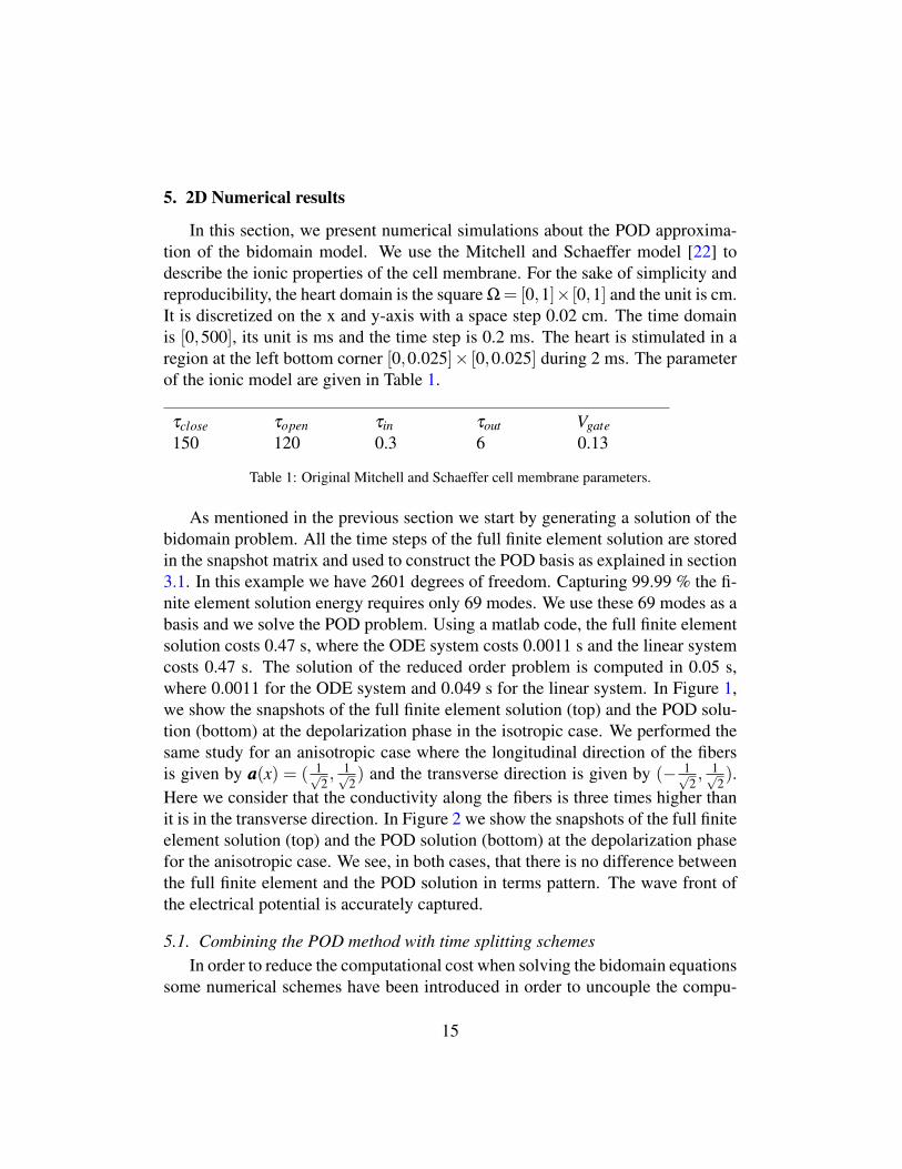
In this section, we present numerical simulations about the POD approxima-tion of the bidomain model. We use the Mitchell and Schaeffer model [22] todescribe the ionic properties of the cell membrane. For the sake of simplicity andreproducibility, the heart domain is the square Ω= [0,1]× [0,1] and the unit is cm.It is discretized on the x and y-axis with a space step 0.02 cm. The time domainis [0,500], its unit is ms and the time step is 0.2 ms. The heart is stimulated in aregion at the left bottom corner [0,0.025]× [0,0.025] during 2 ms. The parameterof the ionic model are given in Table 1.

τclose τopen τin τout Vgate150 120 0.3 6 0.13

Table 1: Original Mitchell and Schaeffer cell membrane parameters.

As mentioned in the previous section we start by generating a solution of thebidomain problem. All the time steps of the full finite element solution are storedin the snapshot matrix and used to construct the POD basis as explained in section3.1. In this example we have 2601 degrees of freedom. Capturing 99.99 % the fi-nite element solution energy requires only 69 modes. We use these 69 modes as abasis and we solve the POD problem. Using a matlab code, the full finite elementsolution costs 0.47 s, where the ODE system costs 0.0011 s and the linear systemcosts 0.47 s. The solution of the reduced order problem is computed in 0.05 s,where 0.0011 for the ODE system and 0.049 s for the linear system. In Figure 1,we show the snapshots of the full finite element solution (top) and the POD solu-tion (bottom) at the depolarization phase in the isotropic case. We performed thesame study for an anisotropic case where the longitudinal direction of the fibersis given by aaa(x) = ( 1√

2, 1√

2) and the transverse direction is given by (− 1√

2, 1√

2).

Here we consider that the conductivity along the fibers is three times higher thanit is in the transverse direction. In Figure 2 we show the snapshots of the full finiteelement solution (top) and the POD solution (bottom) at the depolarization phasefor the anisotropic case. We see, in both cases, that there is no difference betweenthe full finite element and the POD solution in terms pattern. The wave front ofthe electrical potential is accurately captured.

5.1. Combining the POD method with time splitting schemesIn order to reduce the computational cost when solving the bidomain equations

some numerical schemes have been introduced in order to uncouple the compu-

15

Vm ue

Vm,pod ue,pod

Figure 1: Top (respectively, bottom): Snapshots of the full finite element (respectively POD)solution at time 20 ms. at the depolarization phase. The action potential distribution is in the leftcolumn and the extracellular potential distribution is in the right column.

tation of the action potential and the extracellular potential [29, 20, 1, 35]. Theauthors propose a decoupled (Gauss-Seidel-like) time-marching schemes allow-ing at each time step to solve first the action potential and then the extracellularpotential. After performing time and space discretization, this scheme reads asfollows:• Solve the ionic model:

wn+1 = wn−δ tG(V nm,w

n+1) (35)

• Solve the action potential :

(χmS1 +δ tS2)V n+1m =−δ tS2un

e +χmS1V nm +δ tS1(In+1

app − Iion(V nm,w

n+1)) (36)

16

Vm ue

Vm,pod ue,pod

Figure 2: Top (respectively, bottom): Snapshots of the full finite element (respectively POD)solution at time 20 ms computed using the coupling method. at the depolarization phase. Theaction potential distribution is in the left column and the extracellular potential distribution is inthe right column.

• Solve the extra-cellular potential :

S3un+1e =−S2V n+1

m (37)

The stability of this Gauss-Seidel-like and a Jacobi-like schemes have been provedin [12]. Here we present a numerical scheme that combines both time splitting andPOD reduced order methods. Suppose that we have a solution once this problemfor a set of parameters, we build the new snapshot matrix by concatenating the the

17

action potential and extracellular potential as follows:

A =

Vm(x1, t1) · · · Vm(x1, tNt ), ue(x1, t1) · · · ue(x1, tNt )

......

......

......

......

Vm(xM, t1) · · · Vm(xM, tNt ), ue(xM, t1) · · · ue(xM, tNt )

∈ RM×2Nt

(38)After performing a SVD as explained above, we build a POD basis Φ = (φk)

Kk=1

where φk ∈RM for k = 1, ...,M. Each of the equations is now projected on this newbasis and solved using the same strategy as in Section 3.2 . The numerical resultsshowing the accuracy of combining the pod method to time splitting scheme isshown in the next paragraph.

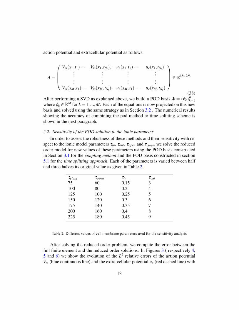
5.2. Sensitivity of the POD solution to the ionic parameterIn order to assess the robustness of these methods and their sensitivity with re-

spect to the ionic model parameters τin, τout , τopen and τclose, we solve the reducedorder model for new values of these parameters using the POD basis constructedin Section 3.1 for the coupling method and the POD basis constructed in section5.1 for the time splitting approach. Each of the parameters is varied between halfand three halves its original value as given in Table 2.

τclose τopen τin τout75 60 0.15 3100 80 0.2 4125 100 0.25 5150 120 0.3 6175 140 0.35 7200 160 0.4 8225 180 0.45 9

Table 2: Different values of cell membrane parameters used for the sensitivity analysis

After solving the reduced order problem, we compute the error between thefull finite element and the reduced order solutions. In Figures 3 ( respectively 4,5 and 6) we show the evolution of the L2 relative errors of the action potentialVm (blue continuous line) and the extra-cellular potential ue (red dashed line) with

18

respect to parameter τclose (respectively τopen , τout and τin ) . In each figure theresult provided by the coupling method is on the left and the result of the the timesplitting approach is on the right. We remark that both the coupling method andthe time splitting approach provide the same accuracy for all the parameters. Thisis in line with the stability result obtained in [12] for the finite element methodbut also with the stability result (21)-(24). We also remark in Figures (3, 4, 5and 6) that for each parameter the minimum of L2 relative error between the PODsolution and the finite element solution is reached at the control values providedin Table1. This is expected because the POD basis was built using the controlparameters.

100 150 20010−4

10−3

10−2

τclose value

erro

r

∥∥Vm−Vm,pod∥∥Q∥∥ue−ue,pod

∥∥Q

100 150 20010−4

10−3

10−2

τclose value

erro

r

∥∥Vm−Vm,pod∥∥Q∥∥ue−ue,pod

∥∥Q

(a) (b)

Figure 3: (a) (respectively, (b)): The error between the finite elements solution and the PODsolution when the value of the paramerter τclose vary using full coupling (respectively, Gauss-Seidel) method. .

50 100 150

10−4

10−3

10−2

τopen value

erro

r

∥∥Vm−Vm,pod∥∥Q∥∥ue−ue,pod

∥∥Q

50 100 150

10−4

10−3

10−2

τopen value

erro

r

∥∥Vm−Vm,pod∥∥Q∥∥ue−ue,pod

∥∥Q

(a) (b)

Figure 4: (a) (respectively, (b)): The error between the finite elements solution and the PODsolution when the value of the paramerter τopen vary using full coupling (respectively, Gauss-Seidel) method.

As concerns the robustness of the POD method with respect to parametersvariation, we remark that for parameters τclose, τopen and τout the relative error is

19

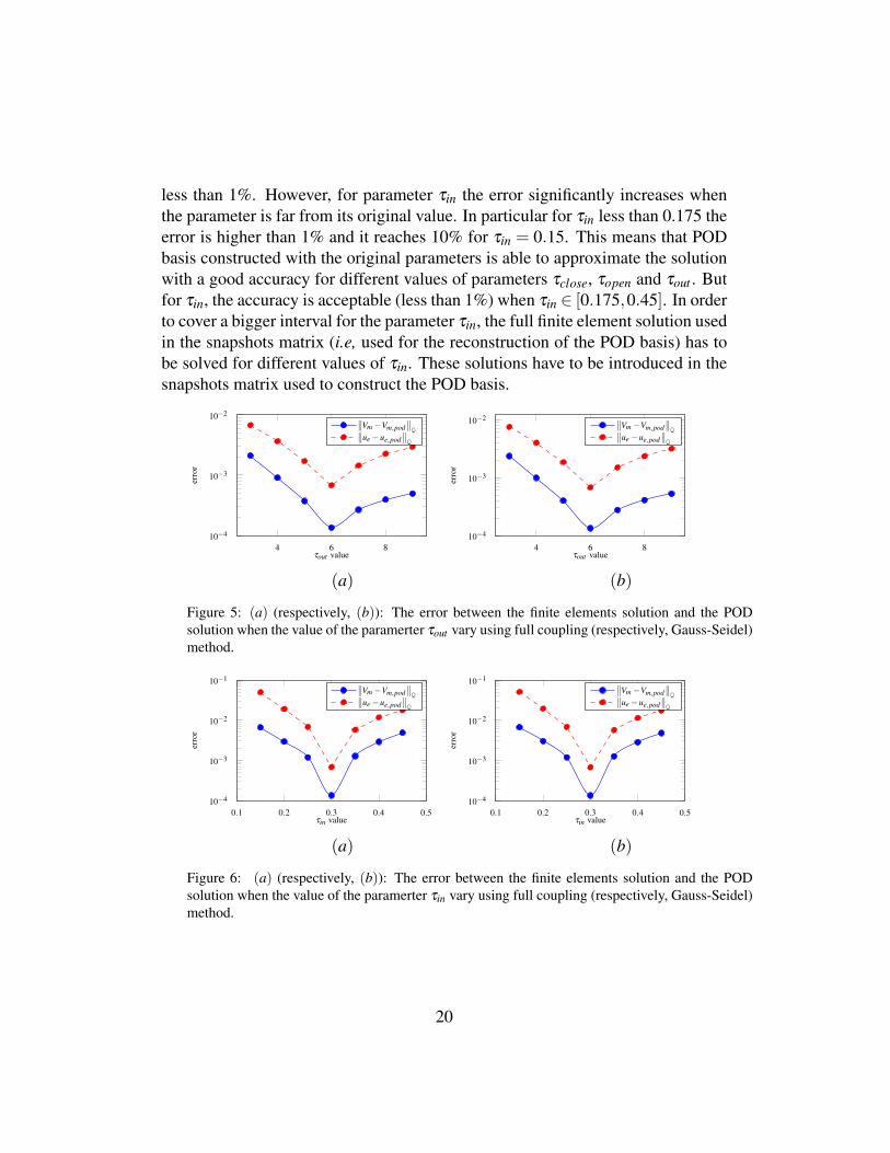
less than 1%. However, for parameter τin the error significantly increases whenthe parameter is far from its original value. In particular for τin less than 0.175 theerror is higher than 1% and it reaches 10% for τin = 0.15. This means that PODbasis constructed with the original parameters is able to approximate the solutionwith a good accuracy for different values of parameters τclose, τopen and τout . Butfor τin, the accuracy is acceptable (less than 1%) when τin ∈ [0.175,0.45]. In orderto cover a bigger interval for the parameter τin, the full finite element solution usedin the snapshots matrix (i.e, used for the reconstruction of the POD basis) has tobe solved for different values of τin. These solutions have to be introduced in thesnapshots matrix used to construct the POD basis.

4 6 810−4

10−3

10−2

τout value

erro

r

∥∥Vm−Vm,pod∥∥Q∥∥ue−ue,pod

∥∥Q

4 6 810−4

10−3

10−2

τout value

erro

r

∥∥Vm−Vm,pod∥∥Q∥∥ue−ue,pod

∥∥Q

(a) (b)

Figure 5: (a) (respectively, (b)): The error between the finite elements solution and the PODsolution when the value of the paramerter τout vary using full coupling (respectively, Gauss-Seidel)method.

0.1 0.2 0.3 0.4 0.510−4

10−3

10−2

10−1

τin value

erro

r

∥∥Vm−Vm,pod∥∥Q∥∥ue−ue,pod

∥∥Q

0.1 0.2 0.3 0.4 0.510−4

10−3

10−2

10−1

τin value

erro

r

∥∥Vm−Vm,pod∥∥Q∥∥ue−ue,pod

∥∥Q

(a) (b)

Figure 6: (a) (respectively, (b)): The error between the finite elements solution and the PODsolution when the value of the paramerter τin vary using full coupling (respectively, Gauss-Seidel)method.

20

6. 3D Numerical results

In this section we apply the POD method to the case studied in the N-versionbenchmark paper by Niederer et al. [25]. The tissue geometry is defined as acuboid, with dimensions of 3×7×20 mm (see Figure 7), fibres are defined par-allel the long direction and conductivity tensor is axisymmetric, with values re-ported in Table 3. In all the simulations performed in this section the space andtime steps are respectively h = 0.02 cm and dt = 0.005 ms, the simulation dura-tion is 600ms. The stimulus is applied within the cube marked S in Figure 7. Thenumber of nodes in the finite element mesh is 52,500 and the number of degreesof freedom in the linear system to be solved is 105,000.

σ li [mS/cm] σ t

i [mS/cm] σ le [mS/cm] σ t

e [mS/cm]1.3342 0.17606 4.0025 2.1127

Table 3: Adopted value for the intra and extracellular conductivities in fiber and cross-fiber direc-tions.

Cardiac physiology simulator benchmark 4339

3 mm

(a)

(b)

7 mm20 mm

1.5 mm 1.5 mm

1.5 mm S

P6 P5

P2

P1

P3

P7P8

P4

P9

Figure 1. (a) Schematic showing the dimensions of the simulation domain. The stimulus wasapplied within the cube marked S. (b) Summary of points at which activation time was evaluated.Activation times at points P1–P9 were evaluated and are available in the electronic supplementarymaterial. Plots of the activation time were evaluated along the line from P1 to P8 and plots of theactivation along the plane shown are provided in two dimensions.

Table 3. Model-specific parameters.

variable description

geometric domain cuboiddimensions 20 × 7 × 3 mmfibre orientation fibres are aligned in the long, 20 mm, axisdiscretization 0.5, 0.2 and 0.1 mm isotropicPDE time steps 0.05, 0.01 and 0.005 msstimulation geometry 1.5 × 1.5 × 1.5 mm cube from a cornerstimulation protocol 2 ms at 50 000 mA cm−3

surface area to volume ratio 140 mm−1, 1400 cm−1 or 0.14 mm−1

membrane capacitance 0.01 mF mm−2 or 1 mF cm−2

intra-longitudinal, intra-transversal,extra-longitudinal and extra-transversalconductivities, using s = sise(se + si)−1

in the monodomain model

0.17, 0.019, 0.62, 0.24 S m−1

their raw format, which were converted to the CMISS graphical user interface(CMGUI) [47] format to allow for a consistent visualization platform. Oncea result was analysed, the participant was contacted if their results differedsignificantly from the other results. This process identified user error andmisunderstandings in the problem definition as well as numerical errors in some ofthe submitted results. This process led to an iterative refinement of the problemdescription, resulting in a complete definition that provided participants withsufficient information to reproduce the simulations.

Phil. Trans. R. Soc. A (2011)

on October 25, 2011rsta.royalsocietypublishing.orgDownloaded from

Figure 7: Schematic representation of the computational domain. Reproduced from paper [25].

We then present a study on the usefulness of the POD method when applied tothe massively parallel code Chaste and we show the gain in terms of computationalcost and the scalability of this approach. We also use the physiologically detailedhuman cardiomyocyte ionic model developed by Ten Tusscher and Panfilov [31]This model consists of of 18 state variables some of them represent gate variablesand others concentrations of different ionic entities and one variable representsthe action potential.

6.1. Choice of the POD basisIn order to test the reduced order model, we first solve the full finite elements

problem. Then, from the time snapshots of the full solution we extract the POD

21

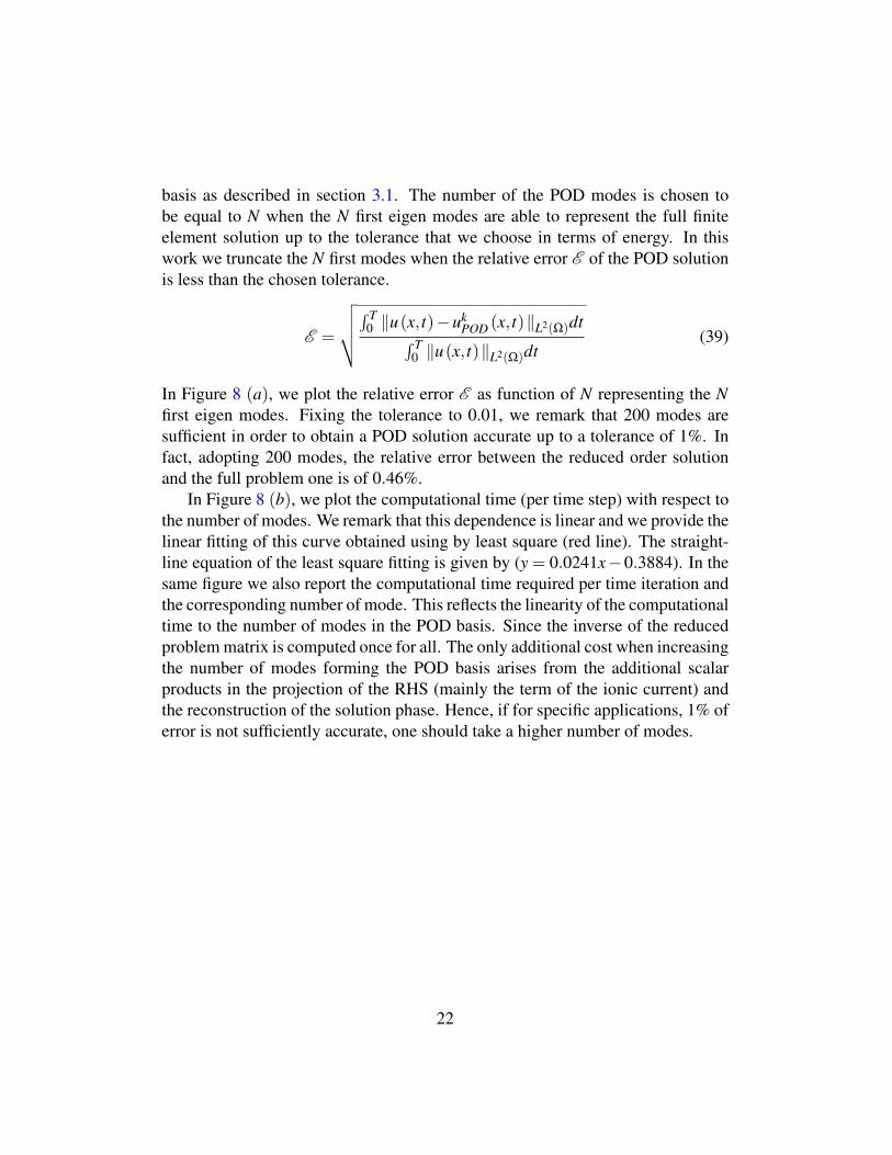
basis as described in section 3.1. The number of the POD modes is chosen tobe equal to N when the N first eigen modes are able to represent the full finiteelement solution up to the tolerance that we choose in terms of energy. In thiswork we truncate the N first modes when the relative error E of the POD solutionis less than the chosen tolerance.

E =

√√√√∫ T0 ‖u(x, t)−uk

POD (x, t)‖L2(Ω)dt∫ T0 ‖u(x, t)‖L2(Ω)dt

(39)

In Figure 8 (a), we plot the relative error E as function of N representing the Nfirst eigen modes. Fixing the tolerance to 0.01, we remark that 200 modes aresufficient in order to obtain a POD solution accurate up to a tolerance of 1%. Infact, adopting 200 modes, the relative error between the reduced order solutionand the full problem one is of 0.46%.

In Figure 8 (b), we plot the computational time (per time step) with respect tothe number of modes. We remark that this dependence is linear and we provide thelinear fitting of this curve obtained using by least square (red line). The straight-line equation of the least square fitting is given by (y = 0.0241x−0.3884). In thesame figure we also report the computational time required per time iteration andthe corresponding number of mode. This reflects the linearity of the computationaltime to the number of modes in the POD basis. Since the inverse of the reducedproblem matrix is computed once for all. The only additional cost when increasingthe number of modes forming the POD basis arises from the additional scalarproducts in the projection of the RHS (mainly the term of the ionic current) andthe reconstruction of the solution phase. Hence, if for specific applications, 1% oferror is not sufficiently accurate, one should take a higher number of modes.

22

200 400 600 800 1,000

10−3

10−2

10−1

Nb of modes

Rel

ativ

eer

ror,

E

200 400 600 800 1,000 1,200

0

10

20

30

y = 0.0241x−0.3884

Nb of modes

Com

puta

tiona

ltim

epe

rtim

est

ep[m

s]

datafitted (least square)

(a) (b)

Nb of modes 100 300 500 700 900 1100Computational time 2.24 7.03 10.6 16.23 21.04 26.91

Figure 8: (a): Evolution of the energy relative error E in terms of number of modes forthe bidomain problem. (b): Evolution of Computational cost per time iteration in termsof number of modes for the biodomain problem. (blue line, bottom table) and the leastsquare fitting (red line).

For the sake of illustration, we show in Figure 9 a snapshot of the 3D solutionof the action potential for the full bidomain and POD solutions at the depolariza-tion phase (25 ms). We clearly see that wave fronts are well synchronized.

(a) (b)

Figure 9: Snapshot of the action potential computed with the full finite element model (a) and thereduced order bidomain model using 200 modes (b) at time 25 ms.

23

6.2. Scalability of the POD methodIn this paragraph we propose to test the scalability of the reduced order method.

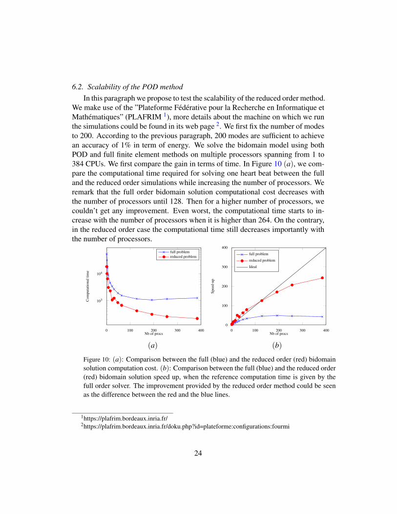
We make use of the ”Plateforme Federative pour la Recherche en Informatique etMathematiques” (PLAFRIM 1), more details about the machine on which we runthe simulations could be found in its web page 2. We first fix the number of modesto 200. According to the previous paragraph, 200 modes are sufficient to achievean accuracy of 1% in term of energy. We solve the bidomain model using bothPOD and full finite element methods on multiple processors spanning from 1 to384 CPUs. We first compare the gain in terms of time. In Figure 10 (a), we com-pare the computational time required for solving one heart beat between the fulland the reduced order simulations while increasing the number of processors. Weremark that the full order bidomain solution computational cost decreases withthe number of processors until 128. Then for a higher number of processors, wecouldn’t get any improvement. Even worst, the computational time starts to in-crease with the number of processors when it is higher than 264. On the contrary,in the reduced order case the computational time still decreases importantly withthe number of processors.

0 100 200 300 400

103

104

Nb of procs

Com

puta

tiona

ltim

e

full problemreduced problem

0 100 200 300 4000

100

200

300

400

Nb of procs

Spee

d-up

full problem

reduced problem

Ideal

(a) (b)

Figure 10: (a): Comparison between the full (blue) and the reduced order (red) bidomainsolution computation cost. (b): Comparison between the full (blue) and the reduced order(red) bidomain solution speed up, when the reference computation time is given by thefull order solver. The improvement provided by the reduced order method could be seenas the difference between the red and the blue lines.

1https://plafrim.bordeaux.inria.fr/2https://plafrim.bordeaux.inria.fr/doku.php?id=plateforme:configurations:fourmi

24

Using one processor the reduced order solver is 3 times faster than the fullorder solver while it is 8 times faster when using 384 processors for both solvers.In Figure 10 (b), we show the speed up curves for both methods, defined as thecomputation time of the full order problem on one CPU over the computationtime of the full and reduced order problems on multiple CPUs. In agreementwith the results shown for the computational time, we see that the speed up curveof the full order solver increases until 128 processors and starts to decrease from264 processors; as far as the reduced order solver is concerned, we remark a super-linear speed up between 1 and 128 CPUs, and it increases monotonously until 384CPUs. If we compare the gain that we obtained by combining HPC and reducedorder problem, since the time cost of the full order problem using one processor is52,500 seconds and the time cost of reduced order solution using 384 processorsis 216 seconds, we obtain a speed-up of 243. In this case, solving the bidomainproblem with the POD method is six times faster than the full finite element.

7. Conclusion

We have presented in this work a reduced order approach based on PODmethod for the computation of the electrical activity of the heart. Our main findingin this paper is the proof of the stability of the POD method based on an a priorierror estimate. This theoretical result shows that we can control the gap betweenthe full finite element solution and the POD solution of the bidomain equation bycontrolling the gap between the finite element solution and its projection on theused POD basis. We also showed that the POD method could be used for differentstrategies of solving the bidomain model. It could be used for a fully coupledscheme or by using a time splitting schemes. The numerical results show that itis stable in both cases. In order to evaluate the usefulness of this approach in pa-rameter estimation problem, we conduct numerical simulations in a 2D case. Webuild a POD basis using the original parameters of the ionic model and we com-puted the L2 relative error between the finite elements solution and the reducedorder solution for different parameters. We conclude that in case of parameter es-timation framework it is recommended to use the POD in order to estimate τclose,τopen and τout . But to estimate τin, the data from which the POD basis is computedshould be sufficiently rich in order to maintain a good accuracy of the results. Wealso studied the scalability of the POD method and compare it to the scalability ofthe full finite element method using a 3D model. Our results show that using 384CPUs we obtain a speed up of 243 for the POD method and only 42 using the fullfinite element method.

25

Acknowledgements

This work has been supported by EPICARD cooperative research program, fundedby INRIA international laboratory LIRIMA. The LAMSIN researchers work is supportedon a regular basis by the Tunisian Ministry for Higher Education, Scientific Researchand Technology. 3D experiments presented in this paper were carried out using thePLAFRIM experimental testbed, being developed under the Inria PlaFRIM developmentaction with support from Bordeaux INP, LABRI and IMB and other entities: ConseilRgional d’Aquitaine, Universit de Bordeaux and CNRS (and ANR in accordance to theprogramme d?investissements d?Avenir (see http://www.plafrim.fr/). We also thank theanonymous reviewers for their recommandations that helped us to improve the quality ofthe paper.

[1] T.M. Austin, M.L. Trew, and A.J. Pullan. Solving the cardiac bidomain equationsfor discontinuous conductivities. IEEE Trans. Biomed. Eng., 53(7):1265–72, 2006.

[2] M. Boulakia, E. Schenone, and J.F. Gerbeau. Reduced-order modeling for cardiacelectrophysiology, application to parameter identification. International Journal forNumerical Methods in Biomedical Engineering, 28(6-7), 2012.

[3] Muriel Boulakia, Serge Cazeau, Miguel A Fernandez, Jean-Frederic Gerbeau, andNejib Zemzemi. Mathematical modeling of electrocardiograms: a numerical study.Annals of biomedical engineering, 38(3):1071–1097, 2010.

[4] Muriel Boulakia, Miguel A Fernandez, Jean-Frederic Gerbeau, and Nejib Zemzemi.Numerical simulation of electrocardiograms. In Modeling of Physiological Flows,pages 77–106. Springer, 2012.

[5] Muriel Boulakia, Miguel Angel Fernandez, Jean-Frederic Gerbeau, and NejibZemzemi. A coupled system of pdes and odes arising in electrocardiograms model-ing. Applied Mathematics Research eXpress, 2008:abn002, 2008.

[6] Yves Bourgault, Yves Coudiere, and Charles Pierre. Existence and uniqueness ofthe solution for the bidomain model used in cardiac electrophysiology. Nonlinearanalysis: Real world applications, 10(1):458–482, 2009.

[7] Dominique Chapelle, Asven Gariah, and Jacques Sainte-Marie. Galerkin approxi-mation with proper orthogonal decomposition: new error estimates and illustrativeexamples. ESAIM: Mathematical Modelling and Numerical Analysis, 46(04):731–757, 2012.

[8] Piero Colli Franzone and Luca F Pavarino. A parallel solver for reaction–diffusionsystems in computational electrocardiology. Mathematical models and methods inapplied sciences, 14(06):883–911, 2004.

26

[9] Yves Coudiere, Charles Pierre, Olivier Rousseau, and Rodolphe Turpault. A 2d/3ddiscrete duality finite volume scheme. application to ecg simulation. InternationalJournal On Finite Volumes, 6(1):1–24, 2009.

[10] Husnu Dal, Serdar Goktepe, Michael Kaliske, and Ellen Kuhl. A fully implicitfinite element method for bidomain models of cardiac electromechanics. Computermethods in applied mechanics and engineering, 253:323–336, 2013.

[11] J Delville, L Ukeiley, L Cordier, JP Bonnet, and M Glauser. Examination of large-scale structures in a turbulent plane mixing layer. part 1. proper orthogonal decom-position. Journal of Fluid Mechanics, 391:91–122, 1999.

[12] Miguel A Fernandez and Nejib Zemzemi. Decoupled time-marching schemes incomputational cardiac electrophysiology and ecg numerical simulation. Mathemat-ical biosciences, 226(1):58–75, 2010.

[13] Thibault Henri and Jean-Pierre Yvon. Convergence estimates of pod-galerkin meth-ods for parabolic problems. In John Cagnol and Jean-Paul Zolsio, editors, SystemModeling and Optimization, volume 166 of IFIP International Federation for Infor-mation Processing, pages 295–306. Springer US, 2005.

[14] Craig S Henriquez. Simulating the electrical behavior of cardiac tissue using thebidomain model. Critical reviews in biomedical engineering, 21(1):1–77, 1992.

[15] Sunil M Kandel. The electrical bidomain model: A review. Scholars AcademicJournal of Biosciences, 3(7):633–639, 2015.

[16] Pierre Kerfriden, Pierre Gosselet, Sondipon Adhikari, and Stephane Pierre-AlainBordas. Bridging proper orthogonal decomposition methods and augmentednewton–krylov algorithms: an adaptive model order reduction for highly nonlinearmechanical problems. Computer Methods in Applied Mechanics and Engineering,200(5):850–866, 2011.

[17] K Kunisch and Stefan Volkwein. Galerkin proper orthogonal decomposition meth-ods for a general equation in fluid dynamics. SIAM Journal on Numerical analysis,40(2):492–515, 2002.

[18] Karl Kunisch and Aurora Marica. Well-posedness for the mitchell-scheaffer modelof the cardiac membrane. Technical Report SFB-Report No. 2013-018, Karl-Franzens Universitat Graz, A-8010 Graz, Heinrichstrasse 36, Austria, December2013.

27

[19] Karl Kunisch and Marcus Wagner. Optimal control of the bidomain system(iv): Corrected proofs of the stability and regularity theorems. arXiv preprintarXiv:1409.6904, 2014.

[20] G.T. Lines, P. Grøttum, and A. Tveito. Modeling the electrical activity of the heart: abidomain model of the ventricles embedded in a torso. Comput. Vis. Sci., 5(4):195–213, 2003.

[21] Gary R Mirams, Christopher J Arthurs, Miguel O Bernabeu, Rafel Bordas, JonathanCooper, Alberto Corrias, Yohan Davit, Sara-Jane Dunn, Alexander G Fletcher,Daniel G Harvey, et al. Chaste: an open source c++ library for computational phys-iology and biology. PLoS computational biology, 9(3):e1002970, 2013.

[22] Colleen C Mitchell and David G Schaeffer. A two-current model for the dynamicsof cardiac membrane. Bulletin of mathematical biology, 65(5):767–793, 2003.

[23] R. Guyonnet N. Aubry and R. Lima. Spatio-temporal analysis of complex signals :theory and applications. J. Statis. Phys, 64(3/4):683–739, 1991.

[24] Chamakuri Nagaiah, Karl Kunisch, and Gernot Plank. On boundary stimulation andoptimal boundary control of the bidomain equations. Math Biosci., 245(2):206–215,2013.

[25] S.A. Niederer, E. Kerfoot, A.P. Benson, M.O. Bernabeu, O. Bernus, C. Bradley,E.M. Cherry, R. Clayton, F.H. Fenton, A. Garny, et al. Verification of cardiac tissueelectrophysiology simulators using an n-version benchmark. Philosophical Trans-actions of the Royal Society A: Mathematical, Physical and Engineering Sciences,369(1954):4331–4351, 2011.

[26] J.L. Lumley P. Holmes and G. Berkooz. Turbulence, Coherent Structures, Dynami-cal Systems and Symmetry. Cambridge Monographs on Mechanics, 1996.

[27] Mark Potse, Bruno Dube, Jacques Richer, Alain Vinet, and Ramesh M Gulrajani. Acomparison of monodomain and bidomain reaction-diffusion models for action po-tential propagation in the human heart. Biomedical Engineering, IEEE Transactionson, 53(12):2425–2435, 2006.

[28] Muruhan Rathinam and Linda R Petzold. A new look at proper orthogonal decom-position. SIAM Journal on Numerical Analysis, 41(5):1893–1925, 2003.

[29] J. Sundnes, G.T. Lines, and A. Tveito. Efficient solution of ordinary differentialequations modeling electrical activity in cardiac cells. Math. Biosci., 172(2):55–72,2001.

28

[30] Joakim Sundnes, Glenn Terje Lines, Xing Cai, Bjørn Frederik Nielsen, Kent-AndreMardal, and Aslak Tveito. Computing the electrical activity in the heart, volume 1.Springer Science & Business Media, 2007.

[31] KHWJ Ten Tusscher and AV Panfilov. Cell model for efficient simulation of wavepropagation in human ventricular tissue under normal and pathological conditions.Physics in medicine and biology, 51(23):6141, 2006.

[32] Mark L Trew, Bruce H Smaill, David P Bullivant, Peter J Hunter, and Andrew JPullan. A generalized finite difference method for modeling cardiac electrical ac-tivation on arbitrary, irregular computational meshes. Mathematical biosciences,198(2):169–189, 2005.

[33] Leslie Tung. A bi-domain model for describing ischemic myocardial dc potentials.PhD thesis, Massachusetts Institute of Technology, 1978.

[34] Edward J Vigmond, Felipe Aguel, Natalia Trayanova, et al. Computational tech-niques for solving the bidomain equations in three dimensions. Biomedical Engi-neering, IEEE Transactions on, 49(11):1260–1269, 2002.

[35] E.J. Vigmond, R. Weber dos Santos, A.J. Prassl, M Deo, and G. Plank. Solvers forthe cardiac bidomain equations. Progr. Biophys. Molec. Biol., 96(1–3):3–18, 2008.

[36] Stefan Volkwein. Model reduction using proper orthogonal decomposition. LectureNotes, Institute of Mathematics and Scientific Computing, University of Graz. seehttp://www. uni-graz. at/imawww/volkwein/POD. pdf, 2011.

[37] Zhu Wang, Imran Akhtar, Jeff Borggaard, and Traian Iliescu. Proper orthogonal de-composition closure models for turbulent flows: a numerical comparison. ComputerMethods in Applied Mechanics and Engineering, 237:10–26, 2012.

[38] Nejib Zemzemi. Etude theorique et numerique de lactivite electrique du cœur: Ap-plications aux electrocardiogrammes. PhD thesis, Paris 11, 2009.

29