STA 3024 Practice Problems Exam 2 NOTE: These are just Practice Problems. This is NOT meant to look just like the test, and it is NOT the only thing that you should study. Make sure you know all the material from the notes, quizzes, suggested homework and the corresponding chapters in the book. 1. The parameters to be estimated in the simple linear regression model Y=α+βx+ε ε~N(0,σ) are: a) α, β, σ b) α, β, ε c) a, b, s d) ε, 0, σ 2. We can measure the proportion of the variation explained by the regression model by: a) r b) R 2 c) σ 2 d) F 3. The MSE is an estimator of: a) ε b) 0 c) σ 2 d) Y 4. In multiple regression with p predictor variables, when constructing a confidence interval for any β i , the degrees of freedom for the tabulated value of t should be: a) n-1 b) n-2 c) n- p-1 d) p-1 5. In a regression study, a 95% confidence interval for β 1 was given as: (-5.65, 2.61). What would a test for H 0 : β 1 =0 vs H a : β 1 0 conclude? a) reject the null hypothesis at α=0.05 and all smaller α b) fail to reject the null hypothesis at α=0.05 and all smaller α c) reject the null hypothesis at α=0.05 and all larger α d) fail to reject the null hypothesis at α=0.05 and all larger α 6. In simple linear regression, when β is not significantly different from zero we conclude that: a) X is a good predictor of Y b) there is no linear relationship between X and Y c) the relationship between X and Y is quadratic d) there is no relationship between X and Y 7. In a study of the relationship between X=mean daily temperature for the month and Y=monthly charges on electrical bill, the following data was gathered: X 20 30 50 60 80 90 Which of the following seems the most likely model? Y 125 110 95 90 110 130 a) Y= α +βx+ε β<0 b) Y= α +βx+ε β>0 c) Y= α +β 1 x+β 2 x 2 +ε β 2 <0 d) Y= α +β 1 x+β 2 x 2 +ε β 2 >0 8. If a predictor variable x is found to be highly significant we would conclude that: a) a change in y causes a change in x b) a change in x causes a change in y c) changes in x are not related to changes in y d) changes in x are associated to changes in y 9. At the same confidence level, a prediction interval for a new response is always; a) somewhat larger than the corresponding confidence interval for the mean response b) somewhat smaller than the corresponding confidence interval for the mean response c) one unit larger than the corresponding confidence interval for the mean response d) one unit smaller than the corresponding confidence interval for the mean response 10. Both the prediction interval for a new response and the confidence interval for the mean response are narrower when made for values of x that are: a) closer to the mean of the x’s b) further from the mean of the x’s c) closer to the mean of the y’s d) further from the mean of the y’s

Welcome message from author
This document is posted to help you gain knowledge. Please leave a comment to let me know what you think about it! Share it to your friends and learn new things together.
Transcript

STA 3024 Practice Problems Exam 2
NOTE: These are just Practice Problems. This is NOT meant to look just like the test, and it is NOT the only
thing that you should study. Make sure you know all the material from the notes, quizzes, suggested
homework and the corresponding chapters in the book.
1. The parameters to be estimated in the simple linear regression model Y=α+βx+ε ε~N(0,σ) are:
a) α, β, σ b) α, β, ε c) a, b, s d) ε, 0, σ
2. We can measure the proportion of the variation explained by the regression model by:
a) r b) R2 c) σ
2 d) F
3. The MSE is an estimator of:
a) ε b) 0 c) σ2 d) Y
4. In multiple regression with p predictor variables, when constructing a confidence interval for any βi, the degrees of
freedom for the tabulated value of t should be:
a) n-1 b) n-2 c) n- p-1 d) p-1
5. In a regression study, a 95% confidence interval for β1 was given as: (-5.65, 2.61). What would a test for H0: β1=0 vs
Ha: β10 conclude?
a) reject the null hypothesis at α=0.05 and all smaller α
b) fail to reject the null hypothesis at α=0.05 and all smaller α
c) reject the null hypothesis at α=0.05 and all larger α
d) fail to reject the null hypothesis at α=0.05 and all larger α
6. In simple linear regression, when β is not significantly different from zero we conclude that:
a) X is a good predictor of Y b) there is no linear relationship between X and Y
c) the relationship between X and Y is quadratic d) there is no relationship between X and Y
7. In a study of the relationship between X=mean daily temperature for the month and Y=monthly charges on electrical
bill, the following data was gathered: X 20 30 50 60 80 90
Which of the following seems the most likely model? Y 125 110 95 90 110 130
a) Y= α +βx+ε β<0
b) Y= α +βx+ε β>0
c) Y= α +β1x+β2x2+ε β2<0
d) Y= α +β1x+β2x2+ε β2>0
8. If a predictor variable x is found to be highly significant we would conclude that:
a) a change in y causes a change in x b) a change in x causes a change in y
c) changes in x are not related to changes in y d) changes in x are associated to changes in y
9. At the same confidence level, a prediction interval for a new response is always;
a) somewhat larger than the corresponding confidence interval for the mean response
b) somewhat smaller than the corresponding confidence interval for the mean response
c) one unit larger than the corresponding confidence interval for the mean response
d) one unit smaller than the corresponding confidence interval for the mean response
10. Both the prediction interval for a new response and the confidence interval for the mean response are narrower
when made for values of x that are:
a) closer to the mean of the x’s b) further from the mean of the x’s
c) closer to the mean of the y’s d) further from the mean of the y’s
11. In the regression model Y = α + βx + ε the change in Y for a one unit increase in x:
a) will always be the same amount, α b) will always be the same amount, β
c) will depend on the error term d) will depend on the level of x
12. In a regression model with a dummy variable without interaction there can be:
a) more than one slope and more than one intercept b) more than one slope, but only one intercept
c) only one slope, but more than one intercept d) only one slope and one intercept
13. In a multiple regression model, where the x's are predictors and y is the response, multicollinearity occurs when:
a) the x's provide redundant information about y
b) the x's provide complementary information about y
c) the x's are used to construct multiple lines, all of which are good predictors of y
d) the x's are used to construct multiple lines, all of which are bad predictors of y
14. Compute the simple linear regression equation if:
15. Match the statements below with the corresponding terms from the list.
a) multicollinearity b) extrapolation
c) R2 adjusted d) quadratic regression
e) interaction f) residual plots
g) fitted equation h) dummy variables
i) cause and effect j) multiple regression model
k) R2 l) residual
m) influential points n) outliers
____ Used when a numerical predictor has a curvilinear relationship with the response.
____ Worst kind of outlier, can totally reverse the direction of association between x and y.
____ Used to check the assumptions of the regression model.
____ Used when trying to decide between two models with different numbers of predictors.
____ Used when the effect of a predictor on the response depends on other predictors.
____ Proportion of the variability in y explained by the regression model.
____ Is the observed value of y minus the predicted value of y for the observed x..
____ A point that lies far away from the rest.
____ Can give bad predictions if the conditions do not hold outside the observed range of x's.
____ Can be erroneously assumed in an observational study.
____ y= α +β1x1+β2x2+...+βpxp+ε ε~N(0,σ2)
____ y =a+b1x1+b2x2+...+bpxp
____ Problem that can occur when the information provided by several predictors overlaps.
____ Used in a regression model to represent categorical variables.
mean stdev correlation
x 163.5 16.2 -0.774
y 874.1 54.2
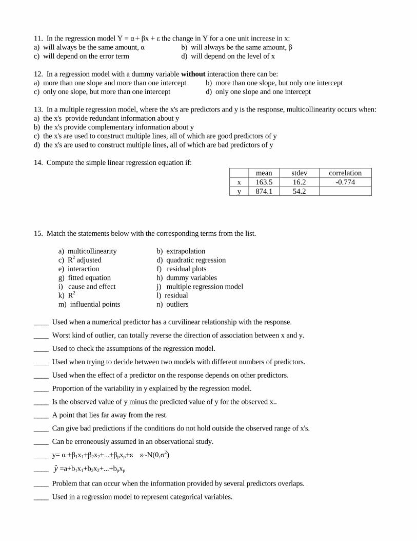
Questions 16 - 19 Palm readers claim to be able to tell how long your life will be by looking at a specific line on your
hand. The following is a plot of age of person at death (in years) vs length of life line on the right hand (in cm) for a
sample of 28 (dead) people.
age -
16. If we fit a simple linear regression model 90 -
to these data, what would the value of r be? -
a) close to -1 70 -
b) close to 0 -
c) close to 1 50 -
d) it's impossible to tell - - - - - - - - - - - - length
7.5 10 12.5 of line
17. Would you say:
a) length of life line is a very good predictor of age of person at death
b) length of life line is a poor predictor of age of person at death
c) length of life line is a reasonably good predictor of age of person at death
d) cannot determine how good a predictor length of life line is of age of person at death
18. The ANOVA p-value will be around
a) 1.00 b) 0.000 c) 0.05 d) 0.01
19. A better way of modeling age of person at death using this data set would be to use:
a) a nonparametric procedure c) a contingency table
b) the average age at death d) quadratic regression
20. According to the null hypothesis of the ANOVA F test, which predictor variables are providing significant
information about the response?
a) most of them b) none of them c) all of them d) some of them
21. According to the alternative hypothesis of the ANOVA F test, which predictor variables are providing significant
information about the response?
a) most of them b) none of them c) all of them d) some of them
22. In general, the Least Squares Regression approach finds the equation:
a) that includes the best set of predictor variables
b) of the best fitting straight line through a set of points
c) with the highest R2, after comparing all possible models
d) that has the smallest sum of squared errors
23. Studies have shown a high positive correlation between the number of firefighters dispatched
to combat a fire and the financial damages resulting from it. A politician commented that the fire chief should stop
sending so many firefighters since they are clearly destroying the place. This is an example of:
a) extrapolation
b) dummy variables
c) misuse of causality
d) multicollinearity
24. The following appeared in the magazine Financial Times, March 23, 1995: "When Elvis Presley died in 1977,
there were 48 professional Elvis impersonators. Today there are an estimated 7328. If that growth is projected, by the
year 2012 one person in four on the face of the globe will be an Elvis impersonator." This is an example of:
a) extrapolation
b) dummy variables
c) misuse of causality
d) multicollinearity

Questions 25 – 43 Most supermarkets use scanners at the checkout counters. The data collected this way can be used
to evaluate the effect of price and store's promotional activities on the sales of any product. The promotions at a store
change weekly, and are mainly of two types: flyers distributed outside the store and through newspapers (which may or
may not include that particular product), and in-store displays at the end of an aisle that call the customers' attention to
the product. Weekly data was collected on a particular beverage brand, including sales (in number of units), price (in
dollars), flyer (1 if product appeared that week, 0 if it didn't) and display (1 if a special display of the product was used
that week, 0 if it wasn't).
As a preliminary analysis, a simple linear regression model was done.
The fitted regression equation was: sales = 2259 - 1418 price.
The ANOVA F test p-value was .000, and R2= 59.7%.
25. The response variable is:
a) quantitative b) y c) sales d) all of the above
26. Which of the following is the best interpretation of the slope of the line?
a) As the price increases by 1 dollar, sales will increase, on average, by 2259 units.
b) As the price increases by 1 dollar, sales will decrease, on average, by 1418 units.
c) As the sales increase by 1 unit, the price will increase, on average, by 2259 dollars.
d) As the sales increase by 1 unit, the price will decrease, on average, by 1418 dollars.
27. Should the intercept of the line be interpreted in this case?
a) Yes, as the average price when no units are sold.
b) Yes, as the average sales when the price is zero dollars.
c) No, since sales of zero units are probably out of the range observed.
d) No, since a price of zero dollars is probably out of the range observed.
28. The proportion of the variability in sales accounted for by the price of the product is:
a) 14.18% b) 22.59%
c) 59.70% d) 100%
29. The coefficient of linear correlation, r, for this analysis is:
a) 7.73 b) -7.73
c) .773 d) -.773
30. According to this model, how many units will be sold, on average, when the price of the beverage is $1.10?
a) 3818.8
b) 699.2
c) 1066.9
d) 3902.9
31. Is price a good predictor of sales?
a) Yes, the p-value is very small. b) Yes, the intercept is very large.
c) No, R-square is not too good. d) No, the slope is negative.
32. Below is a sketch of the residual plot for this analysis. What can you conclude from it?
a) All the assumptions seem to be satisfied. | * *
b) There seems to be an outlier in the data. | * *
c) Simple linear regression might not be the best model. | * *
d) The assumption of constant variance might be violated. |________________

Next, a quadratic regression was fitted to the data. Parts of the computer output appear below.
Predictor Coef Stdev t-ratio p
Constant 7990.0 724.7 11.03 0.000
price -10660 1151 -9.26 0.000
price2 3522.3 436.8 _____ 0.000
Analysis of Variance
SOURCE DF SS MS F p
Regression 2 16060569 8030284 125.11 0.000
Error 60 3851231 64187
Total 62 19911800
33. We can write the model fitted here as:
a) Y= α +βx+ε b) Y= α +β1x1+β2x2+ε
c) Y= α +β1x+β2x2+ε d) Y= α +β1x1+β2x2+β3x1x2+ε
34. What is R2?
a) 19.3% b) 80.7% c) 23.98% d) 76.06%
35. What is the test statistic to determine if the quadratic term significantly differs from zero?
a) 125.11 b) 11.03 c) -9.26 d) 8.06
36. Based on the results of the two regression analyses presented here, which of the following sketches best describes
the relationship between price of the item and sales?
a) b) c) d)
sales sales sales sales
| * | * |* |*
| * * | * | * | *
|* * | * | * | *
| |* | * | * * *
|____________ |______________ |____________ |_____________
price price price price
37. According to this model, how many units will be sold, on average, when the price of the beverage is $1.10?
a) 525.98
b) 138.53
c) 10660
d) 3522.3
38. Is the quadratic model preferable to the linear model in this case?
a) No, we always prefer the simpler model.
b) No, the p-value for the quadratic term is zero.
c) Yes, the p-value for the quadratic term is zero.
d) Yes, we had more data for the quadratic model.
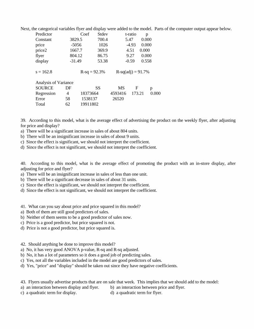
Next, the categorical variables flyer and display were added to the model. Parts of the computer output appear below.
Predictor Coef Stdev t-ratio p
Constant 3829.5 700.4 5.47 0.000
price -5056 1026 -4.93 0.000
price2 1667.7 369.9 4.51 0.000
flyer 804.12 86.75 9.27 0.000
display -31.49 53.38 -0.59 0.558
s = 162.8 R-sq = 92.3% R-sq(adj) = 91.7%
Analysis of Variance
SOURCE DF SS MS F p
Regression 4 18373664 4593416 173.21 0.000
Error 58 1538137 26520
Total 62 19911802
39. According to this model, what is the average effect of advertising the product on the weekly flyer, after adjusting
for price and display?
a) There will be a significant increase in sales of about 804 units.
b) There will be an insignificant increase in sales of about 9 units.
c) Since the effect is significant, we should not interpret the coefficient.
d) Since the effect is not significant, we should not interpret the coefficient.
40. According to this model, what is the average effect of promoting the product with an in-store display, after
adjusting for price and flyer?
a) There will be an insignificant increase in sales of less than one unit.
b) There will be a significant decrease in sales of about 31 units.
c) Since the effect is significant, we should not interpret the coefficient.
d) Since the effect is not significant, we should not interpret the coefficient.
41. What can you say about price and price squared in this model?
a) Both of them are still good predictors of sales.
b) Neither of them seems to be a good predictor of sales now.
c) Price is a good predictor, but price squared is not.
d) Price is not a good predictor, but price squared is.
42. Should anything be done to improve this model?
a) No, it has very good ANOVA p-value, R-sq and R-sq adjusted.
b) No, it has a lot of parameters so it does a good job of predicting sales.
c) Yes, not all the variables included in the model are good predictors of sales.
d) Yes, "price" and "display" should be taken out since they have negative coefficients.
43. Flyers usually advertise products that are on sale that week. This implies that we should add to the model:
a) an interaction between display and flyer. b) an interaction between price and flyer.
c) a quadratic term for display. d) a quadratic term for flyer.
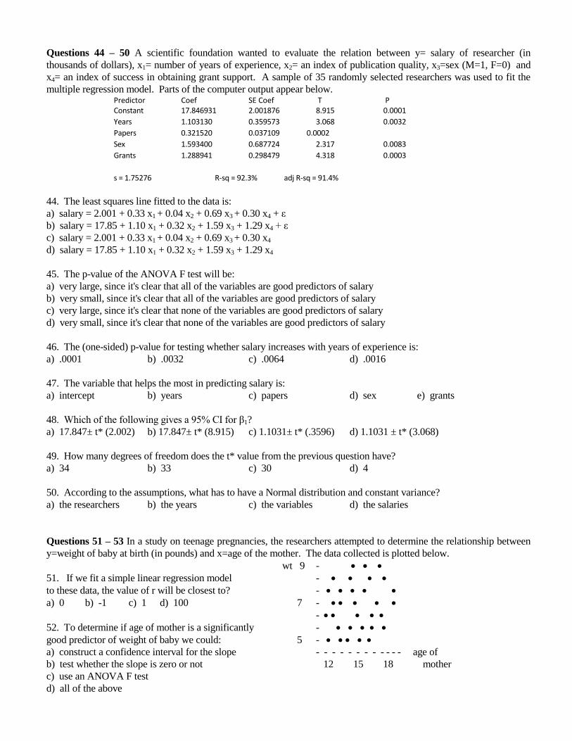
Questions 44 – 50 A scientific foundation wanted to evaluate the relation between y= salary of researcher (in
thousands of dollars), x1= number of years of experience, x2= an index of publication quality, x3=sex (M=1, F=0) and
x4= an index of success in obtaining grant support. A sample of 35 randomly selected researchers was used to fit the
multiple regression model. Parts of the computer output appear below. Predictor Coef SE Coef T P Constant 17.846931 2.001876 8.915 0.0001
Years 1.103130 0.359573 3.068 0.0032
Papers 0.321520 0.037109 0.0002
Sex 1.593400 0.687724 2.317 0.0083
Grants 1.288941 0.298479 4.318 0.0003
s = 1.75276 R-sq = 92.3% adj R-sq = 91.4%
44. The least squares line fitted to the data is:
a) salary = 2.001 + 0.33 x1 + 0.04 x2 + 0.69 x3 + 0.30 x4 + ε
b) salary = 17.85 + 1.10 x1 + 0.32 x2 + 1.59 x3 + 1.29 x4 + ε
c) salary = 2.001 + 0.33 x1 + 0.04 x2 + 0.69 x3 + 0.30 x4
d) salary = 17.85 + 1.10 x1 + 0.32 x2 + 1.59 x3 + 1.29 x4
45. The p-value of the ANOVA F test will be:
a) very large, since it's clear that all of the variables are good predictors of salary
b) very small, since it's clear that all of the variables are good predictors of salary
c) very large, since it's clear that none of the variables are good predictors of salary
d) very small, since it's clear that none of the variables are good predictors of salary
46. The (one-sided) p-value for testing whether salary increases with years of experience is:
a) .0001 b) .0032 c) .0064 d) .0016
47. The variable that helps the most in predicting salary is:
a) intercept b) years c) papers d) sex e) grants
48. Which of the following gives a 95% CI for β1?
a) 17.847± t* (2.002) b) 17.847± t* (8.915) c) 1.1031± t* (.3596) d) 1.1031 ± t* (3.068)
49. How many degrees of freedom does the t* value from the previous question have?
a) 34 b) 33 c) 30 d) 4
50. According to the assumptions, what has to have a Normal distribution and constant variance?
a) the researchers b) the years c) the variables d) the salaries
Questions 51 – 53 In a study on teenage pregnancies, the researchers attempted to determine the relationship between
y=weight of baby at birth (in pounds) and x=age of the mother. The data collected is plotted below.
wt 9 -
51. If we fit a simple linear regression model -
to these data, the value of r will be closest to? -
a) 0 b) -1 c) 1 d) 100 7 -
-
52. To determine if age of mother is a significantly -
good predictor of weight of baby we could: 5 -
a) construct a confidence interval for the slope - - - - - - - - - - - - age of
b) test whether the slope is zero or not 12 15 18 mother
c) use an ANOVA F test
d) all of the above

53. The best fitting line through these points will probably have a slope that is:
a) positive and significantly different from zero.
b) positive but not significantly different from zero.
c) negative and significantly different from zero.
d) negative but not significantly different from zero.
Questions 54 – 63 The following is a plot of the same data, but using different symbols to represent mothers who
received prenatal care (*) and those who didn't (). We fit the model:
Y= α +β1x1+β2x2+β3x1x2+ε, where Y= wt x1=age x2= 0 for prenatal care, 1 if not
wt 9 - * * *
54. The model we fit to these data is not: - * * * *
a) Multiple Regression - * * * *
b) Regression with Dummy Variables 7 - * * *
c) Least Squares Regression - * *
d) Quadratic Regression -
5 -
- - - - - - - - - - - - age of
12 15 18 mother
55. The baseline group is:
a) age b) weight c) prenatal care d) random
Match each parameter with the interpretations at right:
56. β3 a) change in intercept
57. β2 b) intercept for baseline group
58. β1 c) slope for baseline group
59. α d) change in slope
e) slope for non-baseline group
60. For the model above, and based on the plot, which of the following statements is true?
a) Age of mother does not seem to be a good predictor of weight of baby.
b) Prenatal care will probably have a significant effect on weight of baby.
c) There appears to be an interaction between prenatal care and age of mother.
d) all the statements are false.
61. Which parameter would we test for to determine if the rate at which weight of baby increases with age of mother
differs for mothers who receive prenatal care and those who don't?
a) β3 b) β2 c) β1 d) α
The computer output reports following equation: wt= -1.84 + 0.53x1 + 1.79x2 - .003 x1x2 .
Use that equation to answer the next two questions:
62. To predict weight of babies born to teenagers who do not receive prenatal care we use the
equation:
a) wt= -0.05 + .527x1 b) wt= -1.84 + 0.53x1
c) wt= 1.79 + .003x1 d) wt= 1.79 + 0.53x1
63. To predict weight of babies born to teenagers who receive prenatal care we use the equation:
a) wt= -0.05 + .527x1 b) wt= -1.84 + 0.53x1
c) wt= 1.79 + .003x1 d) wt= 1.79 + 0.53x1
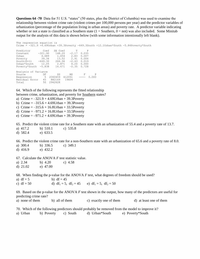
Questions 64 -70 Data for 51 U.S. “states” (50 states, plus the District of Columbia) was used to examine the
relationship between violent crime rate (violent crimes per 100,000 persons per year) and the predictor variables of
urbanization (percentage of the population living in urban areas) and poverty rate. A predictor variable indicating
whether or not a state is classified as a Southern state (1 = Southern, 0 = not) was also included. Some Minitab
output for the analysis of this data is shown below (with some information intentionally left blank).
The regression equation is Crime = -321.9 +4.69Urban +39.3Poverty -649.3South +12.1Urban*South -5.84Poverty*South Predictor Coef SE Coef T P Constant -321.90 148.20 -2.17 0.035 Urban 4.689 1.654 2.83 0.007 Poverty 39.34 13.52 2.91 0.006 South(S=1) -649.30 266.96 -2.43 0.019 Urban*South 12.05 2.871 4.20 0.000 Poverty*South -5.838 16.671 –0.35 0.728 Analysis of Variance
Source DF SS MS F P Regression 5 2060459 412091 ———— 0.000 Residual Error 45 882169 19604 Total 50 2942628
64. Which of the following represents the fitted relationship
between crime, urbanization, and poverty for Southern states?
a) Crime = –321.9 + 4.69Urban + 39.3Poverty
b) Crime = –315.6 + 4.69Urban + 39.3Poverty
c) Crime = –315.6 + 16.8Urban + 33.5Poverty
d) Crime = –971.2 + 16.8Urban + 33.5Poverty
e) Crime = –971.2 + 4.69Urban + 39.3Poverty
65. Predict the violent crime rate for a Southern state with an urbanization of 55.4 and a poverty rate of 13.7.
a) 417.2 b) 510.1 c) 535.8
d) 582.4 e) 633.5
66. Predict the violent crime rate for a non-Southern state with an urbanization of 65.6 and a poverty rate of 8.0.
a) 300.4 b) 336.5 c) 349.1
d) 416.9 e) 432.2
67. Calculate the ANOVA F test statistic value.
a) 2.34 b) 4.20 c) 4.58
d) 21.02 e) 47.00
68. When finding the p-value for the ANOVA F test, what degrees of freedom should be used?
a) df = 5 b) df = 45
c) df = 50 d) df1 = 5, df2 = 45 e) df1 = 5, df2 = 50
69. Based on the p-value for the ANOVA F test shown in the output, how many of the predictors are useful for
predicting crime rate?
a) none of them b) all of them c) exactly one of them d) at least one of them
70. Which of the following predictors should probably be removed from the model to improve it?
a) Urban b) Poverty c) South d) Urban*South e) Poverty*South
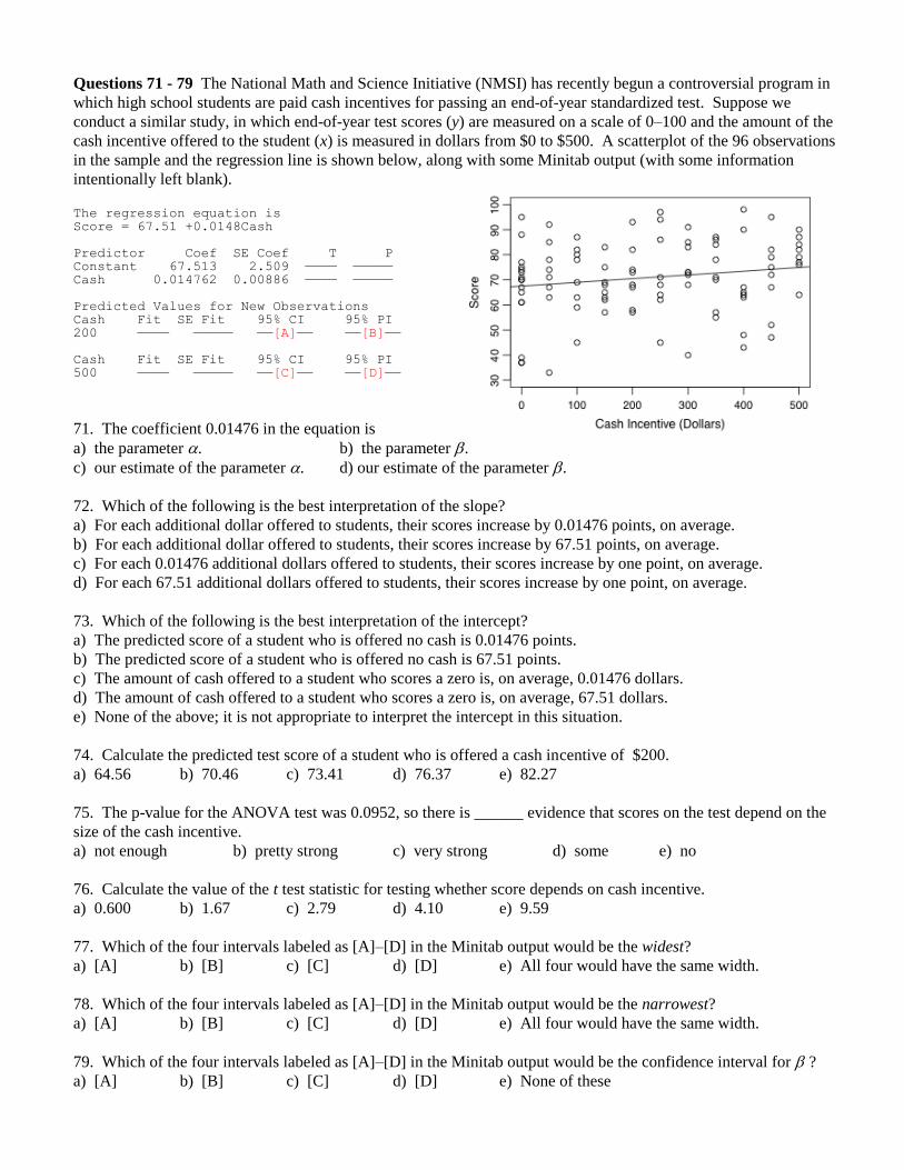
Questions 71 - 79 The National Math and Science Initiative (NMSI) has recently begun a controversial program in
which high school students are paid cash incentives for passing an end-of-year standardized test. Suppose we
conduct a similar study, in which end-of-year test scores (y) are measured on a scale of 0–100 and the amount of the
cash incentive offered to the student (x) is measured in dollars from $0 to $500. A scatterplot of the 96 observations
in the sample and the regression line is shown below, along with some Minitab output (with some information
intentionally left blank).
The regression equation is Score = 67.51 +0.0148Cash Predictor Coef SE Coef T P Constant 67.513 2.509 ———— ————— Cash 0.014762 0.00886 ———— ————— Predicted Values for New Observations Cash Fit SE Fit 95% CI 95% PI
200 ———— ————— ——[A]—— ——[B]—— Cash Fit SE Fit 95% CI 95% PI 500 ———— ————— ——[C]—— ——[D]——
71. The coefficient 0.01476 in the equation is
a) the parameter . b) the parameter .
c) our estimate of the parameter . d) our estimate of the parameter .
72. Which of the following is the best interpretation of the slope?
a) For each additional dollar offered to students, their scores increase by 0.01476 points, on average.
b) For each additional dollar offered to students, their scores increase by 67.51 points, on average.
c) For each 0.01476 additional dollars offered to students, their scores increase by one point, on average.
d) For each 67.51 additional dollars offered to students, their scores increase by one point, on average.
73. Which of the following is the best interpretation of the intercept?
a) The predicted score of a student who is offered no cash is 0.01476 points.
b) The predicted score of a student who is offered no cash is 67.51 points.
c) The amount of cash offered to a student who scores a zero is, on average, 0.01476 dollars.
d) The amount of cash offered to a student who scores a zero is, on average, 67.51 dollars.
e) None of the above; it is not appropriate to interpret the intercept in this situation.
74. Calculate the predicted test score of a student who is offered a cash incentive of $200.
a) 64.56 b) 70.46 c) 73.41 d) 76.37 e) 82.27
75. The p-value for the ANOVA test was 0.0952, so there is ______ evidence that scores on the test depend on the
size of the cash incentive.
a) not enough b) pretty strong c) very strong d) some e) no
76. Calculate the value of the t test statistic for testing whether score depends on cash incentive.
a) 0.600 b) 1.67 c) 2.79 d) 4.10 e) 9.59
77. Which of the four intervals labeled as [A]–[D] in the Minitab output would be the widest?
a) [A] b) [B] c) [C] d) [D] e) All four would have the same width.
78. Which of the four intervals labeled as [A]–[D] in the Minitab output would be the narrowest?
a) [A] b) [B] c) [C] d) [D] e) All four would have the same width.
79. Which of the four intervals labeled as [A]–[D] in the Minitab output would be the confidence interval for ?
a) [A] b) [B] c) [C] d) [D] e) None of these

Questions 80 - 87 The economic structure of Major League Baseball allows some teams to make substantially more
money than others, which in turn allows some teams to spend much more on player salaries. These teams might
therefore be expected to have better players and win more games on the field as a result. Suppose that after
collecting data on team payroll (in millions of dollars) and season win total for 2010, we find a regression equation
of Wins = 71.87 + 0.101Payroll - 0.060League where League is an indicator variable that equals 0 if the team plays
in the National League or 1 if the team plays in the American League.
80. If Teams A and B both play in the same league, and Team A’s payroll is $1 million higher than Team B’s, then
we would expect Team A to win, on average,
a) 0.101 games more than Team B. b) 71.87 games more than Team B.
c) 0.060 games more than Team B. d) 0.060 games fewer than Team B.
81. If Teams A and B have the same payroll, but Team A plays in the National League while Team B plays in the
American League, then we would expect Team A to win, on average,
a) 0.101 games more than Team B. b) 71.87 games more than Team B.
c) 0.060 games more than Team B. d) 0.060 games fewer than Team B.
82. Suppose we plotted the data and drew the regression lines for National League and American League teams.
What would be the slope of the line for American League teams?
a) –0.060 b) 0.060 c) 0.941
d) 0.101 e) 71.81
83. Suppose we plotted the data and drew the regression lines for National League and American League teams.
What would be the intercept of the line for American League teams?
a) –0.060 b) 0.060 c) 0.941
d) 0.101 e) 71.81
84. Calculate the predicted number of wins for a National League team with a payroll of $98 million.
a) 65.99 b) 77.75 c) 77.85
d) 81.71 e) 81.77
85. One American League team in the data set had a payroll of $108 million and won 88 games. Calculate the
residual for this observation.
a) –1.26 b) 5.28 c) 9.65
d) 11.70 e) 22.61
86. The t tests for which variable would have the same p-value as the ANOVA test?
a) constant b) payroll
c) league d) wins
e) none of them
87. Common sense suggests that teams with a higher payroll should have a strong tendency to win more games, but
that league affiliation should not matter. Then common sense suggests that the ANOVA F test for this data would
probably have
a) a small test statistic value and a small p-value.
b) a small test statistic value and a large p-value.
c) a large test statistic value and a small p-value.
d) a large test statistic value and a large p-value.
88. Based on the common sense described in the previous question, in which of the following t tests would we
probably reject the null hypothesis?
a) the t test for Payroll b) the t test for League
c) both t tests d) neither t test

Questions 89 -95 Ecologists have long known that there is a relationship between the amount of precipitation a
location receives and the number of trees that grow in the area. Suppose that the yearly rainfall (x, measured in mm)
and the amount of the ground covered by trees (y, measured on a scale from 0 to 100) are recorded for 49 geographic
locations. In the sample data, x has a sample mean of 1182.4 and a sample standard deviation of 226.0, while y has a
sample mean of 49.6 and a sample standard deviation of 7.1. The sample correlation between x and y is 0.673.
89. In a simple linear regression analysis of this data, when we write
y x , which of the following do we
assume?
a) The x values are independent and normally distributed with mean 0 and constant variance.
b) The x values are independent and normally distributed with variance 0 and constant mean.
c) The errors are independent and normally distributed with mean 0 and constant variance.
d) The errors are independent and normally distributed with variance 0 and constant mean.
e) both a) and c)
90. Use the information provided to calculate the regression equation.
a) TreeCover = 24.70 + 0.0211 Rainfall
b) TreeCover = 0.0211 + 24.70 Rainfall
c) TreeCover = –25371.8 + 21.5 Rainfall
d) TreeCover = 21.5 – 25371.8 Rainfall
e) TreeCover = 25471.0 + 21.5 Rainfall
91. Calculate the predicted amount of tree cover for an area that receives 1230 mm of rainfall per year.
a) 50.6 b) 52.3 c) 55.9 d) 60.9 e) 63.8
92. What percentage of the variability in tree cover is explained by rainfall?
a) 2.1% b) 21.5% c) 24.7% d) 45.3% e) 67.3%
93. For this data set, find the degrees of freedom for regression.
a) 1 b) 2 c) 47 d) 48 e) 49
94. For this data set, find the degrees of freedom for error.
a) 1 b) 2 c) 47 d) 48 e) 49
95. In a regression t test for this data, which of the following statements is the alternative hypothesis (in words)?
a) The population mean of tree cover is not zero.
b) The population mean of tree cover is zero.
c) Tree cover depends on rainfall.
d) Tree cover does not depend on rainfall.
e) The population means of tree cover and rainfall are not equal.
96. Suppose now that we record a 50th observation, include it in the data set, and recalculate the regression
equation. Which of the following possibilities for the 50th observation would probably change the regression
equation the most?
a) x = 900, y = 45
b) x = 1200, y = 40
c) x = 1200, y = 60
d) x = 2400, y = 75
e) x = 2400, y = 25

ANSWERS
1. a
2. b
3. c
4. c
5. b
6. b
7. d (Plot the data)
8. d
9. a
10. a
11. b
12. c
13. a
14. y-hat = 1297.49 – 2.59 x
15. d m f c e k l n b I j g a h
16. b
17. b
18. a
19. b
20. b
21. d
22. d
23. c
24. a
25. d
26. b
27. d
28. c
29. d
30. b
31. a
32. c
33. c
34. b
35. d
36. d
37. a
38. c
39. a
40. d
41. a
42. c
43. b
44. d
45. b
46. d
47. c
48. c
49. c
50. d
51. a
52. d
53. b
54. d
55. c
56. d
57. a
58. c
59. b
60. b
61. a
62. a
63. b
64. d
65. a
66. a
67. d
68. d
69. d
70. e
71. d
72. a
73. b
74. b
75. d
76. b
77. d
78. a
79. e
80. a (Write down the two equations
81. c and plot them for 80 – 88)
82. d
83. e
84. e
85. b
86. e
87. c
88. a
89. c
90. a
91. a
92. d
93. a
94. c
95. c
96. e
Related Documents