SSN: Learning Sparse Switchable Normalization via SparsestMaxopenaccess.thecvf.com/content_CVPR_2019/papers/Shao_SSN_Learning... · the recently-proposed switchable normalization

SSN: Learning Sparse Switchable Normalization via SparsestMax

Wenqi Shao1∗, Tianjian Meng2,3∗, Jingyu Li2, Ruimao Zhang1, Yudian Li2, Xiaogang Wang1, Ping Luo1

1 CHUK-SenseTime Joint Laboratory, Chinese University of Hong Kong2 SenseTime Research 3 University of Pittsburgh

weqish@link., ruimao.zhang@, [email protected], [email protected]

lijingyu, [email protected], [email protected]

Abstract

Normalization methods improve both optimization and

generalization of ConvNets. To further boost performance,

the recently-proposed switchable normalization (SN) pro-

vides a new perspective for deep learning: it learns to se-

lect different normalizers for different convolution layers of

a ConvNet. However, SN uses softmax function to learn im-

portance ratios to combine normalizers, leading to redun-

dant computations compared to a single normalizer.

This work addresses this issue by presenting Sparse

Switchable Normalization (SSN) where the importance ra-

tios are constrained to be sparse. Unlike ℓ1 and ℓ0 con-

straints that impose difficulties in optimization, we turn this

constrained optimization problem into feed-forward com-

putation by proposing SparsestMax, which is a sparse ver-

sion of softmax. SSN has several appealing properties.

(1) It inherits all benefits from SN such as applicability

in various tasks and robustness to a wide range of batch

sizes. (2) It is guaranteed to select only one normalizer

for each normalization layer, avoiding redundant compu-

tations. (3) SSN can be transferred to various tasks in

an end-to-end manner. Extensive experiments show that

SSN outperforms its counterparts on various challenging

benchmarks such as ImageNet, Cityscapes, ADE20K, and

Kinetics. Code is available at https://github.com/

switchablenorms/Sparse_SwitchNorm.

1. Introduction

Normalization techniques [1,9,25,28] such as batch nor-

malization (BN) [9] are indispensable components in deep

neural networks (DNNs) [6,8]. They improve both learning

and generalization capacity of DNNs. Different normaliz-

ers have different properties. For example, BN [9] acts as a

regularizer and improves generalization of a deep network

[15]. Layer normalization (LN) [1] accelerates the train-

∗Equal contribution.

ing of recurrent neural networks (RNNs) by stabilizing the

hidden states in them. Instance normalization (IN) [25] is

able to filter out complex appearance variances [19]. Group

normalization (GN) [28] achieves stable accuracy in a wide

range of batch sizes.

To further boost performance of DNNs, the recently-

proposed Switchable Normalization (SN) [14] offers a new

viewpoint in deep learning: it learns importance ratios to

compute the weighted average statistics of IN, BN and LN,

so as to learn different combined normalizers for different

convolution layers of a DNN. SN is applicable in various

computer vision problems and robust to a wide range of

batch sizes. Although SN has great successes, it suffers

from slowing the testing speed because each normalization

layer is a combination of multiple normalizers.

To address the above issue, this work proposes Sparse

Switchable Normalization (SSN) that learns to select a sin-

gle normalizer from a set of normalization methods for each

convolution layer. Instead of using ℓ1 and ℓ0 regularization

to learn such sparse selection, which increases the difficulty

of training deep networks, SSN turns this constrained opti-

mization problem into feed-forward computations, making

auto-differentiation applicable in most popular deep learn-

ing frameworks to train deep models with sparse constraints

in an end-to-end manner.

In general, this work has three main contributions.

(1) We present Sparse Switchable Normalization (SSN)

that learns to select a single normalizer for each normaliza-

tion layer of a deep network to improve generalization abil-

ity and speed up inference compared to SN. SSN inherits all

advantages from SN, for example, it is applicable to many

different tasks and robust to various batch sizes without any

sensitive hyper-parameter.

(2) SSN is trained using a novel SparsestMax function

that turns the sparse optimization problem into a simple for-

ward propagation of a deep network. SparsestMax is an ex-

tension of softmax with sparsity guarantee and is designed

to be a general technique to learn one-hot distribution. We

provide its geometry interpretations compared to its coun-

443

terparts such as softmax and sparsemax [17].

(3) SSN is demonstrated in multiple computer vision

tasks including image classification in ImageNet [21], se-

mantic segmentation in Cityscapes [4] and ADE20K [30],

and action recognition in Kinetics [11]. Systematic exper-

iments show that SSN with SparsestMax achieves compa-

rable or better performance than the other normalization

methods.

2. Sparse Switchable Normalization (SSN)

This section introduces SSN and SparsestMax.

2.1. Formulation of SSN

We formulate SSN as

hncij = γhncij −

∑|Ω|k=1 pkµk

√

∑|Ω|k=1 p

′kσ

2k + ǫ

+ β, (1)

s.t.

|Ω|∑

k=1

pk = 1,

|Ω|∑

k=1

p′k = 1, ∀pk, p′k ∈ 0, 1

where hncij and hncij indicate a hidden pixel before and

after normalization. The subscripts represent a pixel (i, j)in the c-th channel of the n-th sample in a minibatch. γand β are a scale and a shift parameter respectively. Ω =IN,BN,LN is a set of normalizers. µk and σ2

k are their

means and variances, where k ∈ 1, 2, 3 corresponds to

different normalizers. Moreover, pk and p′k are importance

ratios of mean and variance respectively. We denote p =(p1, p2, p3) and p′ = (p′1, p

′2, p

′3) as two vectors of ratios.

According to Eqn.(1), SSN is a normalizer with three

constraints including ‖p‖1 = 1, ‖p′‖1 = 1, and for

all pk, p′k ∈ 0, 1. These constraints encourage SSN to

choose a single normalizer from Ω for each normalization

layer. If the sparse constraint ∀pk, p′k ∈ 0, 1 is relaxed to

a soft constraint ∀pk, p′k ∈ (0, 1), SSN degrades SN [14].

For example, the importance ratios p in SN can be learned

using p = softmax(z), where z are the learnable control

parameters of a softmax function1 and z can be optimized

using back-propagation (BP). Such slackness has been ex-

tensively employed in existing works [10, 12, 16].

Requirements. Let p = f(z) be a function to learn p in

SSN. Before presenting its formulation, we introduce four

requirements of f(z) in order to make SSN effective and

easy to use as much as possible. (1) Unit length. The ℓ1norm of p is 1 and for all pk ≥ 0. (2) Completely sparse

ratios. p is completely sparse. In other words, f(z) is re-

quired to return an one-hot vector where only one entry is

1 and the others are 0s. (3) Easy to use. SSN can be im-

plemented as a module and easily plugged into any network

1The softmax function is defined by pk = softmaxk(z) =

exp(zk)/∑|Ω|

k=1exp(zk).

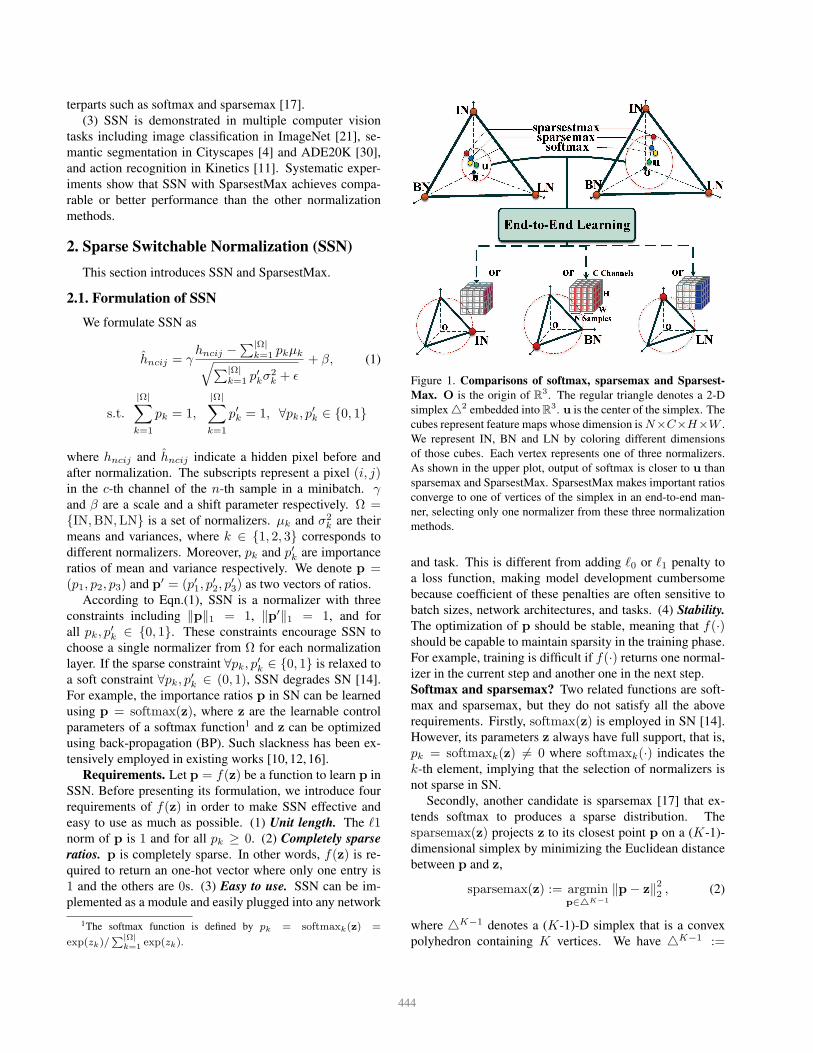
Figure 1. Comparisons of softmax, sparsemax and Sparsest-

Max. O is the origin of R3. The regular triangle denotes a 2-D

simplex 2 embedded into R3. u is the center of the simplex. The

cubes represent feature maps whose dimension is N×C×H×W .

We represent IN, BN and LN by coloring different dimensions

of those cubes. Each vertex represents one of three normalizers.

As shown in the upper plot, output of softmax is closer to u than

sparsemax and SparsestMax. SparsestMax makes important ratios

converge to one of vertices of the simplex in an end-to-end man-

ner, selecting only one normalizer from these three normalization

methods.

and task. This is different from adding ℓ0 or ℓ1 penalty to

a loss function, making model development cumbersome

because coefficient of these penalties are often sensitive to

batch sizes, network architectures, and tasks. (4) Stability.

The optimization of p should be stable, meaning that f(·)should be capable to maintain sparsity in the training phase.

For example, training is difficult if f(·) returns one normal-

izer in the current step and another one in the next step.

Softmax and sparsemax? Two related functions are soft-

max and sparsemax, but they do not satisfy all the above

requirements. Firstly, softmax(z) is employed in SN [14].

However, its parameters z always have full support, that is,

pk = softmaxk(z) 6= 0 where softmaxk(·) indicates the

k-th element, implying that the selection of normalizers is

not sparse in SN.

Secondly, another candidate is sparsemax [17] that ex-

tends softmax to produces a sparse distribution. The

sparsemax(z) projects z to its closest point p on a (K-1)-

dimensional simplex by minimizing the Euclidean distance

between p and z,

sparsemax(z) := argminp∈K−1

‖p− z‖22 , (2)

where K−1 denotes a (K-1)-D simplex that is a convex

polyhedron containing K vertices. We have K−1 :=

444

p ∈ RK |1Tp = 1,p ≥ 0 where 1 is a vector of ones. For

example, when K = 3, 2 represents a 2-D simplex that is

a regular triangle. The vertices of the triangle indicate BN,

IN, and LN respectively as shown in Fig.1.

By comparing softmax and sparsemax on the top of

Fig.1 when z is the same, the output p of softmax yel-

low dot is closer to u (center of the simplex) than that of

sparsemax blue dot. In other words, sparsemax produces

p that are closer to the boundary of the simplex than soft-

max, implying that sparsemax produces more sparse ratios

than softmax. Take z = (0.8, 0.6, 0.1) as an example,

softmax(z) = (0.43, 0.35, 0.22) while sparsemax(z) =(0.6, 0.4, 0), showing that sparsemax is likely to make some

elements of p be zero. However, completely sparse ratios

cannot be guaranteed because every point on the simplex

could be a solution of Eqn.(2).

2.2. SparsestMax

To satisfy all the constraints as discussed above, we in-

troduce SparsestMax, which is a novel sparse version of the

softmax function. The SparsestMax function is defined by

SparsestMax(z; r) := argminp∈K−1

r

‖p− z‖22 , (3)

where K−1r := p ∈ R

K |1Tp = 1, ‖p− u‖2 ≥ r,p ≥0 is a simplex with a circular constraint ‖p− u‖2 ≥r,1Tp = 1. Here u = 1

K1 is the center of the simplex

and 1 is a vector of ones, and r is radius of the circle.

Compared to sparsemax, SparsestMax introduces a cir-

cular constraint ‖p− u‖2 ≥ r, 1Tp = 1 that has an in-

tuitively geometric meaning. Unlike sparsemax where the

solution space is K−1, the solution space of SparsestMax

is a circle with center u and radius r excluded from a sim-

plex.

In order to satisfy the completely sparse requirement, we

linearly increase r from zero to rc in the training phase. rc is

the radius of a circumcircle of the simplex. We understand

the important role that r plays by emphasizing two cases.

When r ≤ ‖p0 − u‖2, where p0 is the output of sparsemax,

then p0 is also the solution of Eqn.(3) because p0 satisfies

the circular constraint. When r = rc, the solution space

of Eqn.(3) contains only K vertices of the simplex, making

SparsestMax(z; rc) completely sparse.

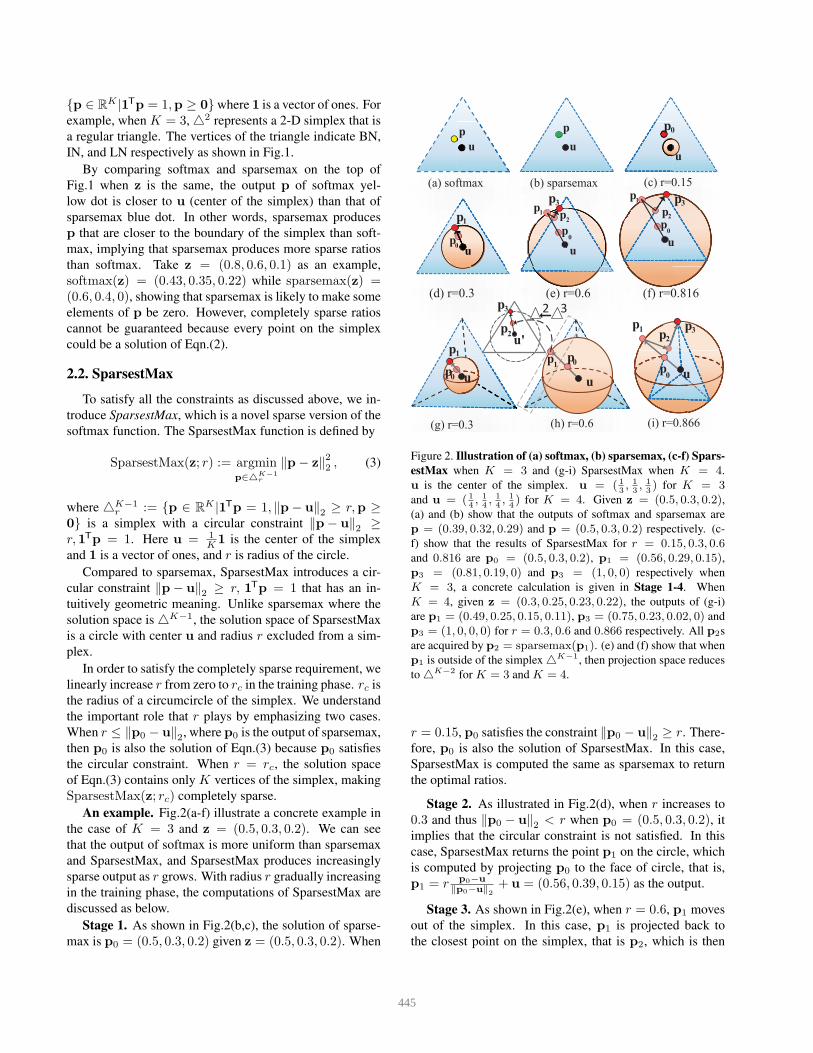
An example. Fig.2(a-f) illustrate a concrete example in

the case of K = 3 and z = (0.5, 0.3, 0.2). We can see

that the output of softmax is more uniform than sparsemax

and SparsestMax, and SparsestMax produces increasingly

sparse output as r grows. With radius r gradually increasing

in the training phase, the computations of SparsestMax are

discussed as below.

Stage 1. As shown in Fig.2(b,c), the solution of sparse-

max is p0 = (0.5, 0.3, 0.2) given z = (0.5, 0.3, 0.2). When

u

up0uu

0u

p0

p1 p

2

pp

uu

u

p0

p1

p2

u'

up0

p1

p2

p0

2 3

uu

p1

p0

(a) softmax (b) sparsemax (c) r=0.15

(d) r=0.3 (e) r=0.6 (f) r=0.816

(g) r=0.3 (h) r=0.6 (i) r=0.866

p3

p1

p3 p3

p1

p3

p0

p2

Figure 2. Illustration of (a) softmax, (b) sparsemax, (c-f) Spars-

estMax when K = 3 and (g-i) SparsestMax when K = 4.

u is the center of the simplex. u = ( 13, 1

3, 1

3) for K = 3

and u = ( 14, 1

4, 1

4, 1

4) for K = 4. Given z = (0.5, 0.3, 0.2),

(a) and (b) show that the outputs of softmax and sparsemax are

p = (0.39, 0.32, 0.29) and p = (0.5, 0.3, 0.2) respectively. (c-

f) show that the results of SparsestMax for r = 0.15, 0.3, 0.6and 0.816 are p0 = (0.5, 0.3, 0.2), p1 = (0.56, 0.29, 0.15),p3 = (0.81, 0.19, 0) and p3 = (1, 0, 0) respectively when

K = 3, a concrete calculation is given in Stage 1-4. When

K = 4, given z = (0.3, 0.25, 0.23, 0.22), the outputs of (g-i)

are p1 = (0.49, 0.25, 0.15, 0.11), p3 = (0.75, 0.23, 0.02, 0) and

p3 = (1, 0, 0, 0) for r = 0.3, 0.6 and 0.866 respectively. All p2s

are acquired by p2 = sparsemax(p1). (e) and (f) show that when

p1 is outside of the simplex K−1, then projection space reduces

to K−2 for K = 3 and K = 4.

r = 0.15, p0 satisfies the constraint ‖p0 − u‖2 ≥ r. There-

fore, p0 is also the solution of SparsestMax. In this case,

SparsestMax is computed the same as sparsemax to return

the optimal ratios.

Stage 2. As illustrated in Fig.2(d), when r increases to

0.3 and thus ‖p0 − u‖2 < r when p0 = (0.5, 0.3, 0.2), it

implies that the circular constraint is not satisfied. In this

case, SparsestMax returns the point p1 on the circle, which

is computed by projecting p0 to the face of circle, that is,

p1 = r p0−u

‖p0−u‖2

+ u = (0.56, 0.39, 0.15) as the output.

Stage 3. As shown in Fig.2(e), when r = 0.6, p1 moves

out of the simplex. In this case, p1 is projected back to

the closest point on the simplex, that is p2, which is then

445

pushed to p3 by the SparsestMax function using

p3 = r′p2 − u′

‖p2 − u′‖2+ u′, (4)

where u′i = max (p1)i

2 , 0, i = 1, 2, 3, p2 =

sparsemax(p1) and r′ =√

r2 − ‖u− u′‖22. In fact, p2

lies on 1, u′ is the center of 1 and 1 is one of the

three edges of 2. Eqn.(4) represents the projection from

p2 to p3. We have p3 = (0.81, 0.19, 0) as the output. It is

noteworthy that when p1 is out of the simplex, p3 is a point

of intersection of the simplex and the circle. In this way,

Eqn.(4) can be substituted by argmax function. However,

Eqn.(4) shows great advantage on differentiable learning of

parameter z when K > 3.

Stage 4. As shown in Fig.2(f), the circle becomes the

circumcircle of the simplex when r = rc = 0.816 for K =3,

p3 moves to one of the three vertices. This vertex would

be the closest point to p0. We have p3 = (1, 0, 0) as the

output.

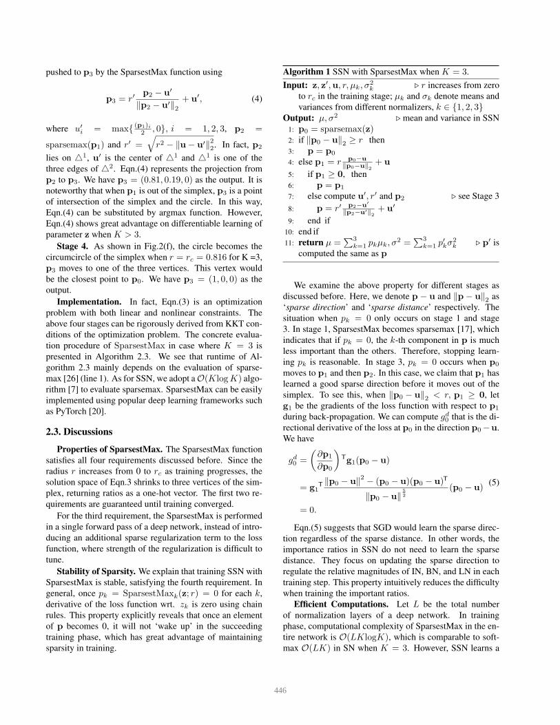
Implementation. In fact, Eqn.(3) is an optimization

problem with both linear and nonlinear constraints. The

above four stages can be rigorously derived from KKT con-

ditions of the optimization problem. The concrete evalua-

tion procedure of SparsestMax in case where K = 3 is

presented in Algorithm 2.3. We see that runtime of Al-

gorithm 2.3 mainly depends on the evaluation of sparse-

max [26] (line 1). As for SSN, we adopt a O(KlogK) algo-

rithm [7] to evaluate sparsemax. SparsestMax can be easily

implemented using popular deep learning frameworks such

as PyTorch [20].

2.3. Discussions

Properties of SparsestMax. The SparsestMax function

satisfies all four requirements discussed before. Since the

radius r increases from 0 to rc as training progresses, the

solution space of Eqn.3 shrinks to three vertices of the sim-

plex, returning ratios as a one-hot vector. The first two re-

quirements are guaranteed until training converged.

For the third requirement, the SparsestMax is performed

in a single forward pass of a deep network, instead of intro-

ducing an additional sparse regularization term to the loss

function, where strength of the regularization is difficult to

tune.

Stability of Sparsity. We explain that training SSN with

SparsestMax is stable, satisfying the fourth requirement. In

general, once pk = SparsestMaxk(z; r) = 0 for each k,

derivative of the loss function wrt. zk is zero using chain

rules. This property explicitly reveals that once an element

of p becomes 0, it will not ‘wake up’ in the succeeding

training phase, which has great advantage of maintaining

sparsity in training.

Algorithm 1 SSN with SparsestMax when K = 3.

Input: z, z′,u, r, µk, σ2k ⊲ r increases from zero

to rc in the training stage; µk and σk denote means and

variances from different normalizers, k ∈ 1, 2, 3Output: µ, σ2 ⊲ mean and variance in SSN

1: p0 = sparsemax(z)2: if ‖p0 − u‖2 ≥ r then

3: p = p0

4: else p1 = r p0−u

‖p0−u‖2

+ u

5: if p1 ≥ 0, then

6: p = p1

7: else compute u′, r′ and p2 ⊲ see Stage 3

8: p = r′ p2−u′

‖p2−u′‖2

+ u′

9: end if

10: end if

11: return µ =∑3

k=1 pkµk, σ2 =

∑3k=1 p

′kσ

2k ⊲ p′ is

computed the same as p

We examine the above property for different stages as

discussed before. Here, we denote p − u and ‖p− u‖2 as

‘sparse direction’ and ‘sparse distance’ respectively. The

situation when pk = 0 only occurs on stage 1 and stage

3. In stage 1, SparsestMax becomes sparsemax [17], which

indicates that if pk = 0, the k-th component in p is much

less important than the others. Therefore, stopping learn-

ing pk is reasonable. In stage 3, pk = 0 occurs when p0

moves to p1 and then p2. In this case, we claim that p1 has

learned a good sparse direction before it moves out of the

simplex. To see this, when ‖p0 − u‖2 < r, p1 ≥ 0, let

g1 be the gradients of the loss function with respect to p1

during back-propagation. We can compute gd0 that is the di-

rectional derivative of the loss at p0 in the direction p0−u.

We have

gd0 =

(

∂p1

∂p0

)

Tg1(p0 − u)

= g1T‖p0 − u‖2 − (p0 − u)(p0 − u)T

‖p0 − u‖5

2

(p0 − u)

= 0.

(5)

Eqn.(5) suggests that SGD would learn the sparse direc-

tion regardless of the sparse distance. In other words, the

importance ratios in SSN do not need to learn the sparse

distance. They focus on updating the sparse direction to

regulate the relative magnitudes of IN, BN, and LN in each

training step. This property intuitively reduces the difficulty

when training the important ratios.

Efficient Computations. Let L be the total number

of normalization layers of a deep network. In training

phase, computational complexity of SparsestMax in the en-

tire network is O(LKlogK), which is comparable to soft-

max O(LK) in SN when K = 3. However, SSN learns a

446

completely sparse selection of normalizers, making it faster

than SN in testing phase. Unlike SN that needs to estimate

statistics of IN, BN, and LN in every normalization layers,

SSN computes statistics for only one normalizer. On the

other hand, we can turn BN in SSN into a linear transforma-

tion and then merge it into the previous convolution layer,

which reduces computations.

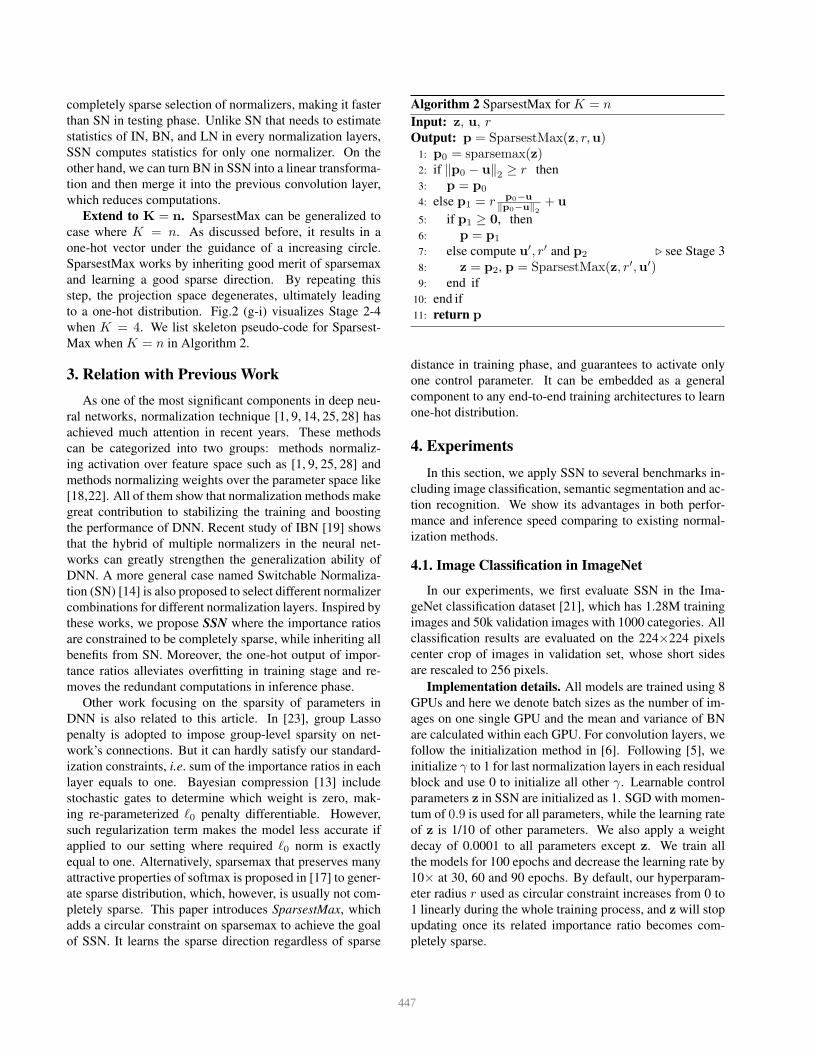
Extend to K = n. SparsestMax can be generalized to

case where K = n. As discussed before, it results in a

one-hot vector under the guidance of a increasing circle.

SparsestMax works by inheriting good merit of sparsemax

and learning a good sparse direction. By repeating this

step, the projection space degenerates, ultimately leading

to a one-hot distribution. Fig.2 (g-i) visualizes Stage 2-4

when K = 4. We list skeleton pseudo-code for Sparsest-

Max when K = n in Algorithm 2.

3. Relation with Previous Work

As one of the most significant components in deep neu-

ral networks, normalization technique [1, 9, 14, 25, 28] has

achieved much attention in recent years. These methods

can be categorized into two groups: methods normaliz-

ing activation over feature space such as [1, 9, 25, 28] and

methods normalizing weights over the parameter space like

[18,22]. All of them show that normalization methods make

great contribution to stabilizing the training and boosting

the performance of DNN. Recent study of IBN [19] shows

that the hybrid of multiple normalizers in the neural net-

works can greatly strengthen the generalization ability of

DNN. A more general case named Switchable Normaliza-

tion (SN) [14] is also proposed to select different normalizer

combinations for different normalization layers. Inspired by

these works, we propose SSN where the importance ratios

are constrained to be completely sparse, while inheriting all

benefits from SN. Moreover, the one-hot output of impor-

tance ratios alleviates overfitting in training stage and re-

moves the redundant computations in inference phase.

Other work focusing on the sparsity of parameters in

DNN is also related to this article. In [23], group Lasso

penalty is adopted to impose group-level sparsity on net-

work’s connections. But it can hardly satisfy our standard-

ization constraints, i.e. sum of the importance ratios in each

layer equals to one. Bayesian compression [13] include

stochastic gates to determine which weight is zero, mak-

ing re-parameterized ℓ0 penalty differentiable. However,

such regularization term makes the model less accurate if

applied to our setting where required ℓ0 norm is exactly

equal to one. Alternatively, sparsemax that preserves many

attractive properties of softmax is proposed in [17] to gener-

ate sparse distribution, which, however, is usually not com-

pletely sparse. This paper introduces SparsestMax, which

adds a circular constraint on sparsemax to achieve the goal

of SSN. It learns the sparse direction regardless of sparse

Algorithm 2 SparsestMax for K = n

Input: z, u, rOutput: p = SparsestMax(z, r,u)

1: p0 = sparsemax(z)2: if ‖p0 − u‖2 ≥ r then

3: p = p0

4: else p1 = r p0−u

‖p0−u‖2

+ u

5: if p1 ≥ 0, then

6: p = p1

7: else compute u′, r′ and p2 ⊲ see Stage 3

8: z = p2, p = SparsestMax(z, r′,u′)9: end if

10: end if

11: return p

distance in training phase, and guarantees to activate only

one control parameter. It can be embedded as a general

component to any end-to-end training architectures to learn

one-hot distribution.

4. Experiments

In this section, we apply SSN to several benchmarks in-

cluding image classification, semantic segmentation and ac-

tion recognition. We show its advantages in both perfor-

mance and inference speed comparing to existing normal-

ization methods.

4.1. Image Classification in ImageNet

In our experiments, we first evaluate SSN in the Ima-

geNet classification dataset [21], which has 1.28M training

images and 50k validation images with 1000 categories. All

classification results are evaluated on the 224×224 pixels

center crop of images in validation set, whose short sides

are rescaled to 256 pixels.

Implementation details. All models are trained using 8

GPUs and here we denote batch sizes as the number of im-

ages on one single GPU and the mean and variance of BN

are calculated within each GPU. For convolution layers, we

follow the initialization method in [6]. Following [5], we

initialize γ to 1 for last normalization layers in each residual

block and use 0 to initialize all other γ. Learnable control

parameters z in SSN are initialized as 1. SGD with momen-

tum of 0.9 is used for all parameters, while the learning rate

of z is 1/10 of other parameters. We also apply a weight

decay of 0.0001 to all parameters except z. We train all

the models for 100 epochs and decrease the learning rate by

10× at 30, 60 and 90 epochs. By default, our hyperparam-

eter radius r used as circular constraint increases from 0 to

1 linearly during the whole training process, and z will stop

updating once its related importance ratio becomes com-

pletely sparse.

447

0 20 40 60 80epochs

0.3

0.4

0.5

0.6

0.7

0.8

Top-

1 Ac

cura

cy

SN TrainSN ValidationSSN TrainSSN Validation

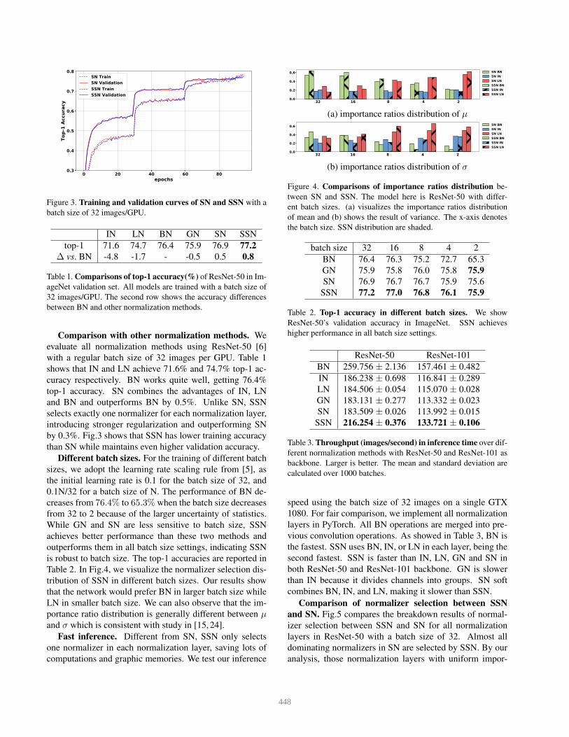
Figure 3. Training and validation curves of SN and SSN with a

batch size of 32 images/GPU.

IN LN BN GN SN SSN

top-1 71.6 74.7 76.4 75.9 76.9 77.2

∆ vs. BN -4.8 -1.7 - -0.5 0.5 0.8

Table 1. Comparisons of top-1 accuracy(%) of ResNet-50 in Im-

ageNet validation set. All models are trained with a batch size of

32 images/GPU. The second row shows the accuracy differences

between BN and other normalization methods.

Comparison with other normalization methods. We

evaluate all normalization methods using ResNet-50 [6]

with a regular batch size of 32 images per GPU. Table 1

shows that IN and LN achieve 71.6% and 74.7% top-1 ac-

curacy respectively. BN works quite well, getting 76.4%

top-1 accuracy. SN combines the advantages of IN, LN

and BN and outperforms BN by 0.5%. Unlike SN, SSN

selects exactly one normalizer for each normalization layer,

introducing stronger regularization and outperforming SN

by 0.3%. Fig.3 shows that SSN has lower training accuracy

than SN while maintains even higher validation accuracy.

Different batch sizes. For the training of different batch

sizes, we adopt the learning rate scaling rule from [5], as

the initial learning rate is 0.1 for the batch size of 32, and

0.1N/32 for a batch size of N. The performance of BN de-

creases from 76.4% to 65.3% when the batch size decreases

from 32 to 2 because of the larger uncertainty of statistics.

While GN and SN are less sensitive to batch size, SSN

achieves better performance than these two methods and

outperforms them in all batch size settings, indicating SSN

is robust to batch size. The top-1 accuracies are reported in

Table 2. In Fig.4, we visualize the normalizer selection dis-

tribution of SSN in different batch sizes. Our results show

that the network would prefer BN in larger batch size while

LN in smaller batch size. We can also observe that the im-

portance ratio distribution is generally different between µand σ which is consistent with study in [15, 24].

Fast inference. Different from SN, SSN only selects

one normalizer in each normalization layer, saving lots of

computations and graphic memories. We test our inference

32 16 8 4 20.0

0.2

0.4

0.6 SN BNSN INSN LNSSN BNSSN INSSN LN

(a) importance ratios distribution of µ

32 16 8 4 20.0

0.2

0.4

0.6 SN BNSN INSN LNSSN BNSSN INSSN LN

(b) importance ratios distribution of σ

Figure 4. Comparisons of importance ratios distribution be-

tween SN and SSN. The model here is ResNet-50 with differ-

ent batch sizes. (a) visualizes the importance ratios distribution

of mean and (b) shows the result of variance. The x-axis denotes

the batch size. SSN distribution are shaded.

batch size 32 16 8 4 2

BN 76.4 76.3 75.2 72.7 65.3

GN 75.9 75.8 76.0 75.8 75.9

SN 76.9 76.7 76.7 75.9 75.6

SSN 77.2 77.0 76.8 76.1 75.9

Table 2. Top-1 accuracy in different batch sizes. We show

ResNet-50’s validation accuracy in ImageNet. SSN achieves

higher performance in all batch size settings.

ResNet-50 ResNet-101

BN 259.756 ± 2.136 157.461 ± 0.482

IN 186.238 ± 0.698 116.841 ± 0.289

LN 184.506 ± 0.054 115.070 ± 0.028

GN 183.131 ± 0.277 113.332 ± 0.023

SN 183.509 ± 0.026 113.992 ± 0.015

SSN 216.254 ± 0.376 133.721 ± 0.106

Table 3. Throughput (images/second) in inference time over dif-

ferent normalization methods with ResNet-50 and ResNet-101 as

backbone. Larger is better. The mean and standard deviation are

calculated over 1000 batches.

speed using the batch size of 32 images on a single GTX

1080. For fair comparison, we implement all normalization

layers in PyTorch. All BN operations are merged into pre-

vious convolution operations. As showed in Table 3, BN is

the fastest. SSN uses BN, IN, or LN in each layer, being the

second fastest. SSN is faster than IN, LN, GN and SN in

both ResNet-50 and ResNet-101 backbone. GN is slower

than IN because it divides channels into groups. SN soft

combines BN, IN, and LN, making it slower than SSN.

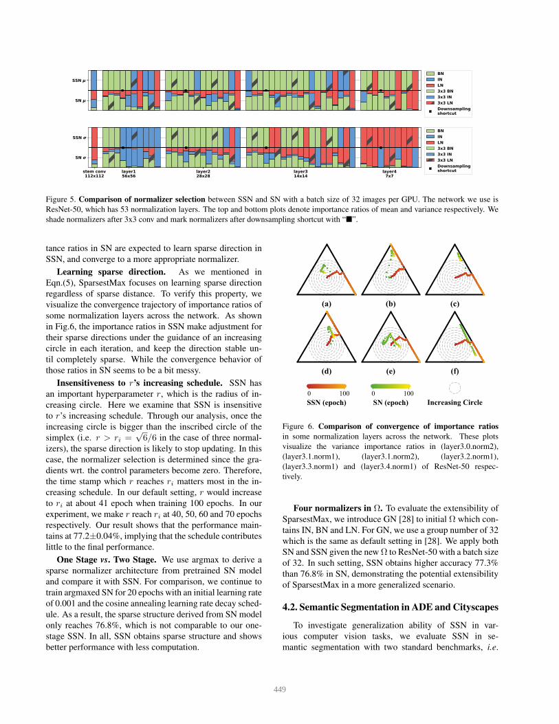
Comparison of normalizer selection between SSN

and SN. Fig.5 compares the breakdown results of normal-

izer selection between SSN and SN for all normalization

layers in ResNet-50 with a batch size of 32. Almost all

dominating normalizers in SN are selected by SSN. By our

analysis, those normalization layers with uniform impor-

448

SN

SSN BNINLN3x3 BN3x3 IN3x3 LNDownsamplingshortcut

stem conv112x112

layer156x56

layer228x28

layer314x14

layer47x7

SN

SSN BNINLN3x3 BN3x3 IN3x3 LNDownsamplingshortcut

Figure 5. Comparison of normalizer selection between SSN and SN with a batch size of 32 images per GPU. The network we use is

ResNet-50, which has 53 normalization layers. The top and bottom plots denote importance ratios of mean and variance respectively. We

shade normalizers after 3x3 conv and mark normalizers after downsampling shortcut with “”.

tance ratios in SN are expected to learn sparse direction in

SSN, and converge to a more appropriate normalizer.

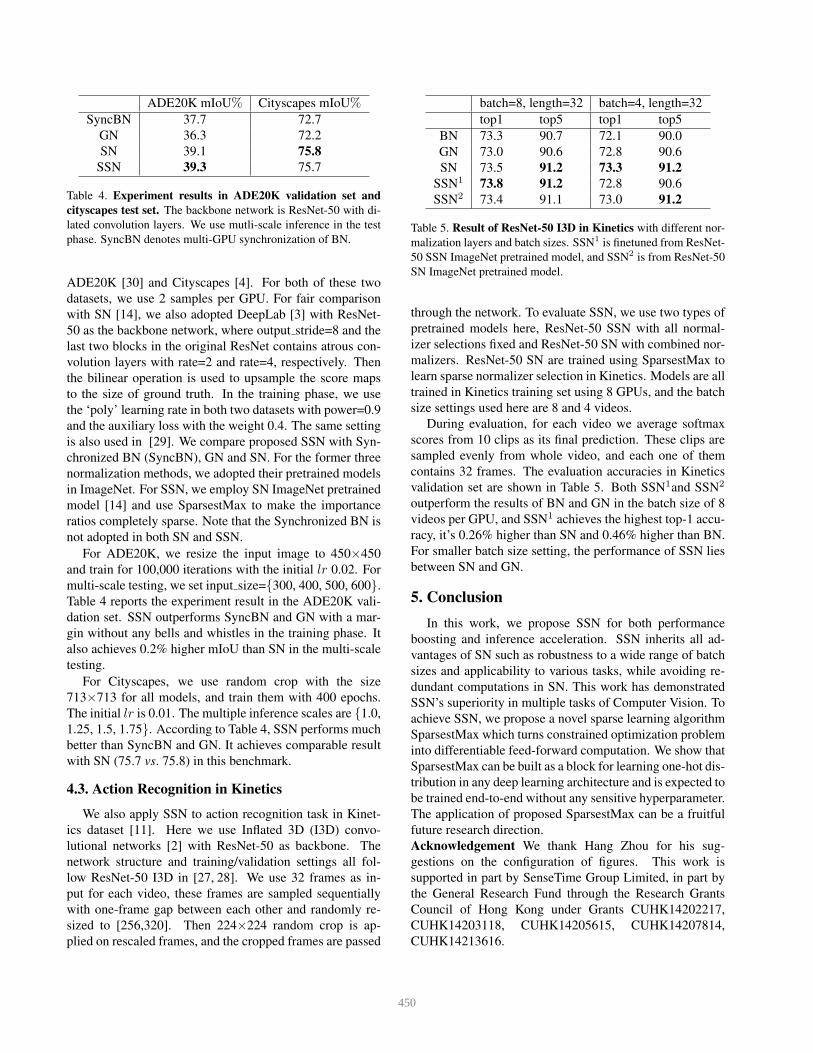
Learning sparse direction. As we mentioned in

Eqn.(5), SparsestMax focuses on learning sparse direction

regardless of sparse distance. To verify this property, we

visualize the convergence trajectory of importance ratios of

some normalization layers across the network. As shown

in Fig.6, the importance ratios in SSN make adjustment for

their sparse directions under the guidance of an increasing

circle in each iteration, and keep the direction stable un-

til completely sparse. While the convergence behavior of

those ratios in SN seems to be a bit messy.

Insensitiveness to r’s increasing schedule. SSN has

an important hyperparameter r, which is the radius of in-

creasing circle. Here we examine that SSN is insensitive

to r’s increasing schedule. Through our analysis, once the

increasing circle is bigger than the inscribed circle of the

simplex (i.e. r > ri =√6/6 in the case of three normal-

izers), the sparse direction is likely to stop updating. In this

case, the normalizer selection is determined since the gra-

dients wrt. the control parameters become zero. Therefore,

the time stamp which r reaches ri matters most in the in-

creasing schedule. In our default setting, r would increase

to ri at about 41 epoch when training 100 epochs. In our

experiment, we make r reach ri at 40, 50, 60 and 70 epochs

respectively. Our result shows that the performance main-

tains at 77.2±0.04%, implying that the schedule contributes

little to the final performance.

One Stage vs. Two Stage. We use argmax to derive a

sparse normalizer architecture from pretrained SN model

and compare it with SSN. For comparison, we continue to

train argmaxed SN for 20 epochs with an initial learning rate

of 0.001 and the cosine annealing learning rate decay sched-

ule. As a result, the sparse structure derived from SN model

only reaches 76.8%, which is not comparable to our one-

stage SSN. In all, SSN obtains sparse structure and shows

better performance with less computation.

Figure 6. Comparison of convergence of importance ratios

in some normalization layers across the network. These plots

visualize the variance importance ratios in (layer3.0.norm2),

(layer3.1.norm1), (layer3.1.norm2), (layer3.2.norm1),

(layer3.3.norm1) and (layer3.4.norm1) of ResNet-50 respec-

tively.

Four normalizers in Ω. To evaluate the extensibility of

SparsestMax, we introduce GN [28] to initial Ω which con-

tains IN, BN and LN. For GN, we use a group number of 32

which is the same as default setting in [28]. We apply both

SN and SSN given the new Ω to ResNet-50 with a batch size

of 32. In such setting, SSN obtains higher accuracy 77.3%

than 76.8% in SN, demonstrating the potential extensibility

of SparsestMax in a more generalized scenario.

4.2. Semantic Segmentation in ADE and Cityscapes

To investigate generalization ability of SSN in var-

ious computer vision tasks, we evaluate SSN in se-

mantic segmentation with two standard benchmarks, i.e.

449

ADE20K mIoU% Cityscapes mIoU%SyncBN 37.7 72.7

GN 36.3 72.2

SN 39.1 75.8

SSN 39.3 75.7

Table 4. Experiment results in ADE20K validation set and

cityscapes test set. The backbone network is ResNet-50 with di-

lated convolution layers. We use mutli-scale inference in the test

phase. SyncBN denotes multi-GPU synchronization of BN.

ADE20K [30] and Cityscapes [4]. For both of these two

datasets, we use 2 samples per GPU. For fair comparison

with SN [14], we also adopted DeepLab [3] with ResNet-

50 as the backbone network, where output stride=8 and the

last two blocks in the original ResNet contains atrous con-

volution layers with rate=2 and rate=4, respectively. Then

the bilinear operation is used to upsample the score maps

to the size of ground truth. In the training phase, we use

the ‘poly’ learning rate in both two datasets with power=0.9

and the auxiliary loss with the weight 0.4. The same setting

is also used in [29]. We compare proposed SSN with Syn-

chronized BN (SyncBN), GN and SN. For the former three

normalization methods, we adopted their pretrained models

in ImageNet. For SSN, we employ SN ImageNet pretrained

model [14] and use SparsestMax to make the importance

ratios completely sparse. Note that the Synchronized BN is

not adopted in both SN and SSN.

For ADE20K, we resize the input image to 450×450

and train for 100,000 iterations with the initial lr 0.02. For

multi-scale testing, we set input size=300, 400, 500, 600.

Table 4 reports the experiment result in the ADE20K vali-

dation set. SSN outperforms SyncBN and GN with a mar-

gin without any bells and whistles in the training phase. It

also achieves 0.2% higher mIoU than SN in the multi-scale

testing.

For Cityscapes, we use random crop with the size

713×713 for all models, and train them with 400 epochs.

The initial lr is 0.01. The multiple inference scales are 1.0,

1.25, 1.5, 1.75. According to Table 4, SSN performs much

better than SyncBN and GN. It achieves comparable result

with SN (75.7 vs. 75.8) in this benchmark.

4.3. Action Recognition in Kinetics

We also apply SSN to action recognition task in Kinet-

ics dataset [11]. Here we use Inflated 3D (I3D) convo-

lutional networks [2] with ResNet-50 as backbone. The

network structure and training/validation settings all fol-

low ResNet-50 I3D in [27, 28]. We use 32 frames as in-

put for each video, these frames are sampled sequentially

with one-frame gap between each other and randomly re-

sized to [256,320]. Then 224×224 random crop is ap-

plied on rescaled frames, and the cropped frames are passed

batch=8, length=32 batch=4, length=32

top1 top5 top1 top5

BN 73.3 90.7 72.1 90.0

GN 73.0 90.6 72.8 90.6

SN 73.5 91.2 73.3 91.2

SSN1 73.8 91.2 72.8 90.6

SSN2 73.4 91.1 73.0 91.2

Table 5. Result of ResNet-50 I3D in Kinetics with different nor-

malization layers and batch sizes. SSN1 is finetuned from ResNet-

50 SSN ImageNet pretrained model, and SSN2 is from ResNet-50

SN ImageNet pretrained model.

through the network. To evaluate SSN, we use two types of

pretrained models here, ResNet-50 SSN with all normal-

izer selections fixed and ResNet-50 SN with combined nor-

malizers. ResNet-50 SN are trained using SparsestMax to

learn sparse normalizer selection in Kinetics. Models are all

trained in Kinetics training set using 8 GPUs, and the batch

size settings used here are 8 and 4 videos.

During evaluation, for each video we average softmax

scores from 10 clips as its final prediction. These clips are

sampled evenly from whole video, and each one of them

contains 32 frames. The evaluation accuracies in Kinetics

validation set are shown in Table 5. Both SSN1and SSN2

outperform the results of BN and GN in the batch size of 8

videos per GPU, and SSN1 achieves the highest top-1 accu-

racy, it’s 0.26% higher than SN and 0.46% higher than BN.

For smaller batch size setting, the performance of SSN lies

between SN and GN.

5. Conclusion

In this work, we propose SSN for both performance

boosting and inference acceleration. SSN inherits all ad-

vantages of SN such as robustness to a wide range of batch

sizes and applicability to various tasks, while avoiding re-

dundant computations in SN. This work has demonstrated

SSN’s superiority in multiple tasks of Computer Vision. To

achieve SSN, we propose a novel sparse learning algorithm

SparsestMax which turns constrained optimization problem

into differentiable feed-forward computation. We show that

SparsestMax can be built as a block for learning one-hot dis-

tribution in any deep learning architecture and is expected to

be trained end-to-end without any sensitive hyperparameter.

The application of proposed SparsestMax can be a fruitful

future research direction.

Acknowledgement We thank Hang Zhou for his sug-

gestions on the configuration of figures. This work is

supported in part by SenseTime Group Limited, in part by

the General Research Fund through the Research Grants

Council of Hong Kong under Grants CUHK14202217,

CUHK14203118, CUHK14205615, CUHK14207814,

CUHK14213616.

450

References

[1] Jimmy Lei Ba, Jamie Ryan Kiros, and Geoffrey E Hin-

ton. Layer normalization. arXiv preprint arXiv:1607.06450,

2016.

[2] Joao Carreira and Andrew Zisserman. Quo vadis, action

recognition? a new model and the kinetics dataset. In Com-

puter Vision and Pattern Recognition (CVPR), 2017 IEEE

Conference on, pages 4724–4733. IEEE, 2017.

[3] Liang-Chieh Chen, George Papandreou, Iasonas Kokkinos,

Kevin Murphy, and Alan L Yuille. Deeplab: Semantic image

segmentation with deep convolutional nets, atrous convolu-

tion, and fully connected crfs. IEEE transactions on pattern

analysis and machine intelligence, 40(4):834–848, 2018.

[4] Marius Cordts, Mohamed Omran, Sebastian Ramos, Timo

Rehfeld, Markus Enzweiler, Rodrigo Benenson, Uwe

Franke, Stefan Roth, and Bernt Schiele. The cityscapes

dataset for semantic urban scene understanding. In Proc.

of the IEEE Conference on Computer Vision and Pattern

Recognition (CVPR), 2016.

[5] Priya Goyal, Piotr Dollar, Ross Girshick, Pieter Noord-

huis, Lukasz Wesolowski, Aapo Kyrola, Andrew Tulloch,

Yangqing Jia, and Kaiming He. Accurate, large mini-

batch sgd: training imagenet in 1 hour. arXiv preprint

arXiv:1706.02677, 2017.

[6] Kaiming He, Xiangyu Zhang, Shaoqing Ren, and Jian Sun.

Deep residual learning for image recognition. In Proceed-

ings of the IEEE conference on computer vision and pattern

recognition, pages 770–778, 2016.

[7] Michael Held, Philip Wolfe, and Harlan P Crowder. Vali-

dation of subgradient optimization. Mathematical program-

ming, 6(1):62–88, 1974.

[8] Gao Huang, Zhuang Liu, Laurens van der Maaten, and Kil-

ian Q Weinberger. Densely connected convolutional net-

works. In Proceedings of the IEEE Conference on Computer

Vision and Pattern Recognition, 2017.

[9] Sergey Ioffe and Christian Szegedy. Batch normalization:

Accelerating deep network training by reducing internal co-

variate shift. arXiv preprint arXiv:1502.03167, 2015.

[10] Eric Jang, Shixiang Gu, and Ben Poole. Categorical

reparameterization with gumbel-softmax. arXiv preprint

arXiv:1611.01144, 2016.

[11] Will Kay, Joao Carreira, Karen Simonyan, Brian Zhang,

Chloe Hillier, Sudheendra Vijayanarasimhan, Fabio Viola,

Tim Green, Trevor Back, Paul Natsev, et al. The kinetics hu-

man action video dataset. arXiv preprint arXiv:1705.06950,

2017.

[12] Hanxiao Liu, Karen Simonyan, and Yiming Yang.

Darts: Differentiable architecture search. arXiv preprint

arXiv:1806.09055, 2018.

[13] Christos Louizos, Max Welling, and Diederik P Kingma.

Learning sparse neural networks through l 0 regularization.

arXiv preprint arXiv:1712.01312, 2017.

[14] Ping Luo, Jiamin Ren, and Zhanglin Peng. Differentiable

learning-to-normalize via switchable normalization. arXiv

preprint arXiv:1806.10779, 2018.

[15] Ping Luo, Xinjiang Wang, Wenqi Shao, and Zhanglin Peng.

Understanding regularization in batch normalization. arXiv

preprint arXiv:1809.00846, 2018.

[16] Chris J Maddison, Andriy Mnih, and Yee Whye Teh. The

concrete distribution: A continuous relaxation of discrete

random variables. arXiv preprint arXiv:1611.00712, 2016.

[17] Andre F. T. Martins and Ramon Fernandez Astudillo. From

softmax to sparsemax: A sparse model of attention and

multi-label classification. CoRR, abs/1602.02068, 2016.

[18] Takeru Miyato, Toshiki Kataoka, Masanori Koyama, and

Yuichi Yoshida. Spectral normalization for generative ad-

versarial networks. arXiv preprint arXiv:1802.05957, 2018.

[19] Xingang Pan, Ping Luo, Jianping Shi, and Xiaoou Tang. Two

at once: Enhancing learning and generalization capacities

via ibn-net. arXiv preprint arXiv:1807.09441, 2018.

[20] Adam Paszke, Sam Gross, Soumith Chintala, Gregory

Chanan, Edward Yang, Zachary DeVito, Zeming Lin, Al-

ban Desmaison, Luca Antiga, and Adam Lerer. Automatic

differentiation in pytorch. In NIPS-W, 2017.

[21] Olga Russakovsky, Jia Deng, Hao Su, Jonathan Krause, San-

jeev Satheesh, Sean Ma, Zhiheng Huang, Andrej Karpathy,

Aditya Khosla, Michael Bernstein, et al. Imagenet large

scale visual recognition challenge. International Journal of

Computer Vision, 115(3):211–252, 2015.

[22] Tim Salimans and Diederik P Kingma. Weight normaliza-

tion: A simple reparameterization to accelerate training of

deep neural networks. In Advances in Neural Information

Processing Systems, pages 901–909, 2016.

[23] Simone Scardapane, Danilo Comminiello, Amir Hussain,

and Aurelio Uncini. Group sparse regularization for deep

neural networks. Neurocomputing, 241:81–89, 2017.

[24] Mattias Teye, Hossein Azizpour, and Kevin Smith. Bayesian

uncertainty estimation for batch normalized deep networks.

arXiv preprint arXiv:1802.06455, 2018.

[25] D Ulyanov, A Vedaldi, and V Lempitsky. Instance nor-

malization: the missing ingredient for fast stylization. cscv.

arXiv preprint arXiv:1607.08022, 2017.

[26] Ewout Van Den Berg and Michael P Friedlander. Probing

the pareto frontier for basis pursuit solutions. SIAM Journal

on Scientific Computing, 31(2):890–912, 2008.

[27] Xiaolong Wang, Ross Girshick, Abhinav Gupta, and Kaim-

ing He. Non-local neural networks. CVPR, 2018.

[28] Yuxin Wu and Kaiming He. Group normalization. arXiv

preprint arXiv:1803.08494, 2018.

[29] Hengshuang Zhao, Jianping Shi, Xiaojuan Qi, Xiaogang

Wang, and Jiaya Jia. Pyramid scene parsing network. In

Proceedings of IEEE Conference on Computer Vision and

Pattern Recognition (CVPR), 2017.

[30] Bolei Zhou, Hang Zhao, Xavier Puig, Sanja Fidler, Adela

Barriuso, and Antonio Torralba. Scene parsing through

ade20k dataset. In Proceedings of the IEEE Conference on

Computer Vision and Pattern Recognition, 2017.

451