SRS-EEU - srs-project.eu | Multi-Role Shadow Robotic ...srs-project.eu/sites/default/files/SRS DELIVERABLE 4.6.2.pdf · Project title : Multi-Role Shadow Robotic System for Independent

FP7 ICT Contract No. 247772 1 February 2010 – 30 April 2013 Page 1 of 41

Deliverable D4.6.2 – Shape-based object detection and reconstruction

Final Report

Contract number : 247772

Project acronym : SRS-EEU

Project title : Multi-Role Shadow Robotic System for Independent Living –

Enlarged EU

Deliverable number : D4.6.2

Nature : R – Report

Dissemination level : PU – Public

Delivery date : 31-03-13 (month 38)

Author(s) : Michal Spanel, Tomas Hodan, Radim Kriz, Rostislav Hulik, Pavel

Smrz, Pavel Zemcik

Partners contributed : BUT

Contact : [email protected]

The SRS-EEU project was funded by the European

Commission under the 7th Framework Programme (FP7) –

Challenges 7: Independent living, inclusion and

Governance

Coordinator: Cardiff University

SRS-EEU

Multi-Role Shadow Robotic

System for Independent Living –

Enlarged EU

Small or Medium-Scale Focused Research

Project (STREP)

mailto:[email protected]

http://srs-project.eu/


DOCUMENT HISTORY

Version Author(s) Date Changes

V1 Michal Spanel 23rd January 2012 First draft version

V2 Michal Spanel, Rostislav Hulik

March 2013

Document structure

updated, description

of new methods

added

V3 Michal Spanel 30th March 2013 Second draft revision


EXECUTIVE SUMMARY

SRS (Multi-Role Shadow Robotic System for Independent Living) focuses on the development and

prototyping of remotely-controlled, semi-autonomous robotic solutions in domestic environments

to support elderly people. SRS solutions are designed to enable a robot to act as a shadow of its

controller. For example, elderly parents can have a robot as a shadow of their children or carers. In

this case, adult children or carers can help them remotely and physically with daily living tasks as if

the children or carers were resident in the house. Remote presence via robotics is the key to

achieve targeted SRS goal.

A specialized task that helps recognition of the environment and enables the “embedded

intelligence” of the Human Robot Interaction (HRI) is the object and shape detection. The SRS-EEU

investigates shape-similarity approaches to object detection (that will supplement the current

texture-based techniques of the running SRS project) by employing advanced linear statistical

classifiers implemented using novel algorithmic improvements as well as advanced shape features

and acceleration techniques. Shape-similarity object detection forms a standard part of the state-of-

the-art image processing. Various object detection methods employing shape similarity through

shape detection algorithms, geometry description using Hough transform and shape detection

using RANSAC are proposed, investigated and reported in this deliverable.

Deliverable D4.6.2 (M38) comprises full report on full report on specification and performance of

developed software components.


TABLE OF CONTENTS

1 Introduction ............................................................................................................................................. 5

2 Detection of Geometric Primitives ................................................................................................... 6

2.1 Related work ........................................................................................................................................................... 6

2.2 Plane detection based on 3D Hough Transform ...................................................................................... 7

2.3 Experimental results ........................................................................................................................................ 10

2.4 Depth data segmentation ............................................................................................................................... 15

3 Object Detection for Human-robot Interaction ........................................................................ 21

3.1 3D localization in the environment ............................................................................................................ 21

3.1 Feature points and shape descriptors ....................................................................................................... 24

3.2 Object detection based on RGB-D sensor data ...................................................................................... 28

4 Prerequisities ....................................................................................................................................... 33

5 Documentation of Packages ............................................................................................................ 34

5.1 Plane detection based on 3D Hough Transform ................................................................................... 34

5.2 3D localization in the environment ............................................................................................................ 35

5.3 Depth image segmentation ............................................................................................................................ 35

6 References .............................................................................................................................................. 37


1 INTRODUCTION

The task of shape-similarity based object detection is closely associated with assisted object

detection and the work of other SRS partners (IPA and PRO) on texture-based and shape-based

object detection. BUT’s development of shape detection techniques is more focused on object

detection for visualization and environment mapping purposes. It means the automatic detection

and possible tagging of household objects assigning each object into categories (table top, bowl,

cup, bottle, etc.). Information on the object category can be used for visualization in the virtual

display to allow proper level of interaction.

This kind of detection provides only rough information on the object pose so it can’t be directly

used for grasping. However, it can be more general than specifically trained object detectors and it

might provide useful information for either manual or semi-automatic fitting of predefined 3D

shapes from the household object database constructed by HPIS to an unknown object (i.e. objects

that are not present in the database of known graspable objects).

In order to visualize the environment and found objects, SRS-EEU also focuses on detection of

geometric primitives in point-cloud data (i.e. planes) and a rough approximation of detected objects

by means of bounding volumes. The detection of a bounding volume is achieved by fitting simple

geometry (i.e. box) to the object. These approximate object shapes are very useful for the user

interaction dividing a complex scene into logical parts.


2 DETECTION OF GEOMETRIC PRIMITIVES

The main objective of environment perception is to simplify the representation of the environment

by means of detection of geometric primitives (planes, boxes, etc.) in point-cloud data. This may

significantly reduce amount of data necessary to send to the remote client in order to visualize the

environment and quickly assess the situation around the robot.

2.1 RELATED WORK

Regarding the nature of the input data (indoor human made scenes), we have chosen the plane

detection as the primary detection primitive. Several approaches are widely used today, which can

be divided into three sections.

REGION GROWING

An efficient algorithm based on region growing was presented by Poppinga et al. [Pop08]. During

the growth of the region, a mean square error from an optimal plane of the region is compared to a

threshold. Deschaud and Goulette [Des10] proposed similar algorithm, which describes fast and

accurate plane detection in unorganized point clouds using filtered normals and voxel growing.

This method is based on a robust estimation of normals. The main problem of region growing

methods on Kinect sensor is primarily the specific noise.

RANSAC BASED DETECTION

Random Sample Consensus is another possibility how to detect parametrized primitives from the

point cloud. Firstly, it was mentioned by Fischler [Fis87], who described an algorithm able to fit the

accurate model without trying all the possibilities. Many modifications were then presented to

achieve better time complexity of the stochastic algorithm.

RANSAC based plane detection was presented by Schnabel et al. [Sch07] who chose iteratively

three points from which the plane model is computed. A score function is used to determine the

model fitting. A large comparison of RANSAC and 3D Hough Transform methods is presented by

Tarsha-Kurdi et al. [Tar07]. They compared results on detection of roof planes in 3D building point

cloud.

FEATURE SPACE TRANSFORMATION

Last mentioned approach is the feature space transformation. Originally, Hough [Hou62] defined

the transformation for detecting lines, later it was extended to more complex shapes and

generalized for arbitrary patterns [Bal87]. Multiple modifications were also proposed to enhance

the time complexity of Hough Transform method. Such comparison is presented by Bormann et al.

[Bor11], who evaluate different variants of the 3D HT with respect to their applicability.


Mochizuki et al. [Moc09] also compare different Hough methods. Both Bormann and Mochizuki

agreed that the Randomized HT is the method of choice in the real world problems. They also

compare randomized HT and the three-point HT [Che01] to enhance robustness in noisy images

while retaining the speed of the randomized approach.

The environment perception components process sensor data (i.e. point clouds from the RGB-D

sensor) or the global voxel-based model built by the Dynamic Environment Model (see D4.5.2). In

the second case, the point-cloud processing and segmentation routines may run occasionally only

when a new portion of the global map is obtained, or when a meaningful part of the voxel-based

map is refined.

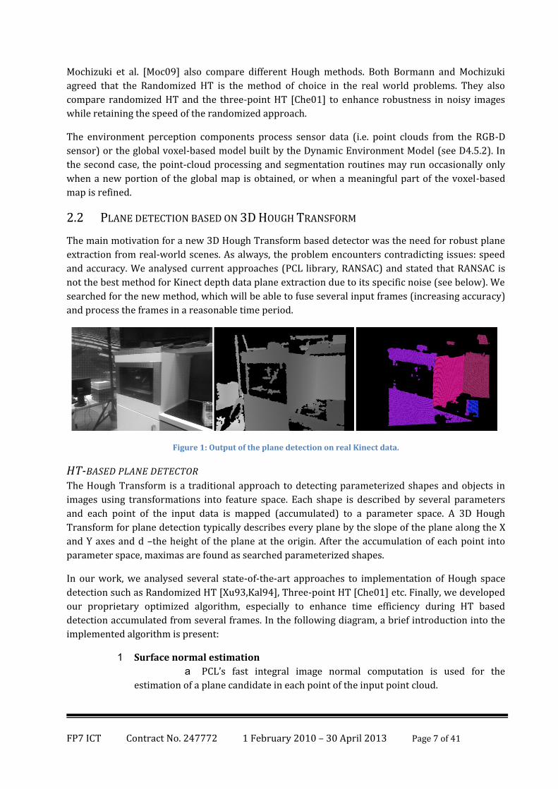
2.2 PLANE DETECTION BASED ON 3D HOUGH TRANSFORM

The main motivation for a new 3D Hough Transform based detector was the need for robust plane

extraction from real-world scenes. As always, the problem encounters contradicting issues: speed

and accuracy. We analysed current approaches (PCL library, RANSAC) and stated that RANSAC is

not the best method for Kinect depth data plane extraction due to its specific noise (see below). We

searched for the new method, which will be able to fuse several input frames (increasing accuracy)

and process the frames in a reasonable time period.

Figure 1: Output of the plane detection on real Kinect data.

HT-BASED PLANE DETECTOR The Hough Transform is a traditional approach to detecting parameterized shapes and objects in

images using transformations into feature space. Each shape is described by several parameters

and each point of the input data is mapped (accumulated) to a parameter space. A 3D Hough

Transform for plane detection typically describes every plane by the slope of the plane along the X

and Y axes and d –the height of the plane at the origin. After the accumulation of each point into

parameter space, maximas are found as searched parameterized shapes.

In our work, we analysed several state-of-the-art approaches to implementation of Hough space

detection such as Randomized HT [Xu93,Kal94], Three-point HT [Che01] etc. Finally, we developed

our proprietary optimized algorithm, especially to enhance time efficiency during HT based

detection accumulated from several frames. In the following diagram, a brief introduction into the

implemented algorithm is present:

1 Surface normal estimation

a PCL’s fast integral image normal computation is used for the

estimation of a plane candidate in each point of the input point cloud.


2 Accumulation to the parameter space

a The parameter space is represented by a hierarchical structure

which brings a significant memory saving while preserving the accuracy.

b For each point, parameters of a plane are estimated so the point

contributes to the Hough space only once (this corresponds to the Randomized

Hough Transform [Che01]).

c Every point contribution is smoothed by a pre-computed Gaussian

function (noise suppression).

d Hough space caching is used to speed up the accumulation process.

3 Extraction of maxima

a A sliding window technique is applied to search for maxima in the

Hough space.

4 Refining of planes

a A two-level parameter space computation is used to filter artifacts

arising when several noisy frames are accumulated.

Surface normal estimation We tested several methods for the surface normal estimation from the Kinect point cloud. The

computation itself can work in several modes. The covariance matrix method is the slowest, but the

most precise method. It computes the normal vector by the eigenanalysis of point’s neighborhood.

Other methods consist of average 3D gradient analysis and average depth change (the fastest

approach, yet the least precise). For use in our work, the covariance matrix was computed from a

large neighborhood. The other mentioned methods remain as parameters of the plane detection

module.

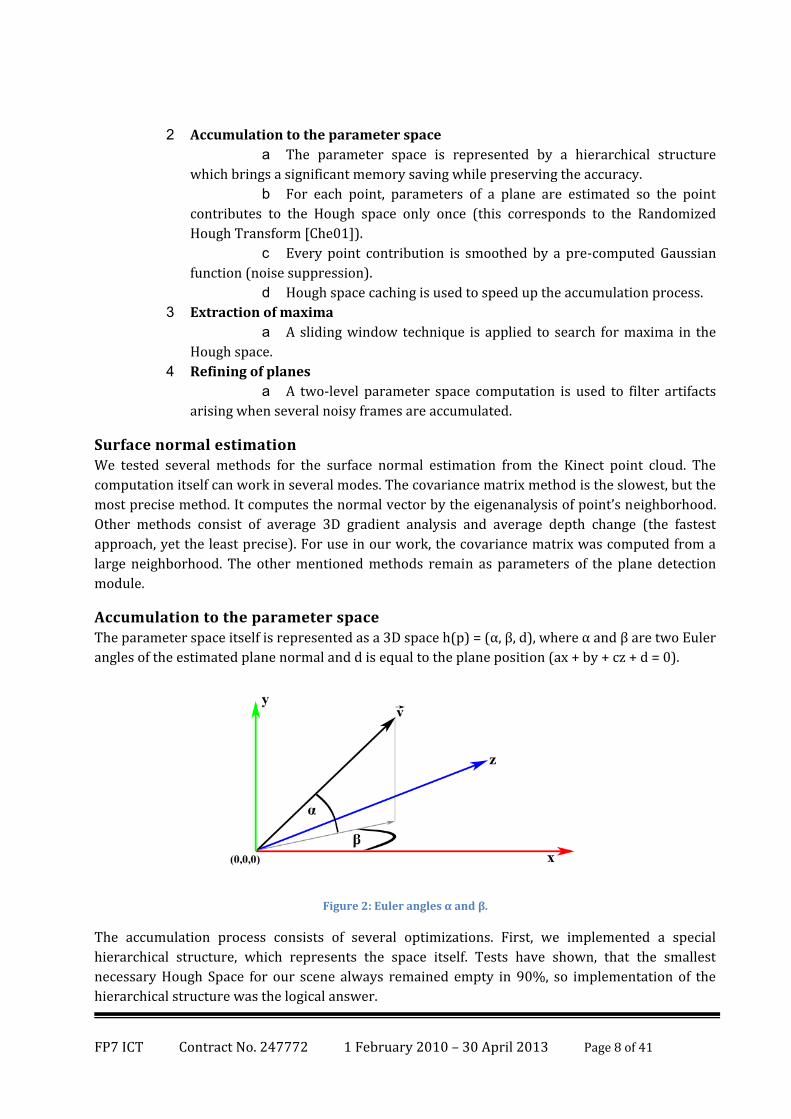
Accumulation to the parameter space The parameter space itself is represented as a 3D space h(p) = (α, β, d), where α and β are two Euler

angles of the estimated plane normal and d is equal to the plane position (ax + by + cz + d = 0).

Figure 2: Euler angles α and β.

The accumulation process consists of several optimizations. First, we implemented a special

hierarchical structure, which represents the space itself. Tests have shown, that the smallest

necessary Hough Space for our scene always remained empty in 90%, so implementation of the

hierarchical structure was the logical answer.


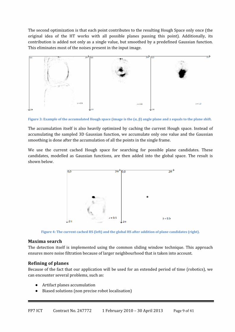
The second optimization is that each point contributes to the resulting Hough Space only once (the

original idea of the HT works with all possible planes passing this point). Additionally, its

contribution is added not only as a single value, but smoothed by a predefined Gaussian function.

This eliminates most of the noises present in the input image.

Figure 3: Example of the accumulated Hough space (image is the (α, β) angle plane and z equals to the plane shift.

The accumulation itself is also heavily optimized by caching the current Hough space. Instead of

accumulating the sampled 3D Gaussian function, we accumulate only one value and the Gaussian

smoothing is done after the accumulation of all the points in the single frame.

We use the current cached Hough space for searching for possible plane candidates. These

candidates, modelled as Gaussian functions, are then added into the global space. The result is

shown below.

Figure 4: The current cached HS (left) and the global HS after addition of plane candidates (right).

Maxima search The detection itself is implemented using the common sliding window technique. This approach

ensures more noise filtration because of larger neighbourhood that is taken into account.

Refining of planes Because of the fact that our application will be used for an extended period of time (robotics), we

can encounter several problems, such as:

● Artifact planes accumulation

● Biased solutions (non precise robot localisation)


● Non-delimited maximum

● Non static objects

We solved these problems by implementing a simple Hough Space thinning algorithm, which

decrements each cell of the HS by a specified value (we propose a value from 0.1 to 0.001). By this

means, we are able to successfully filter non stable and artifact planes in the global Hough Space.

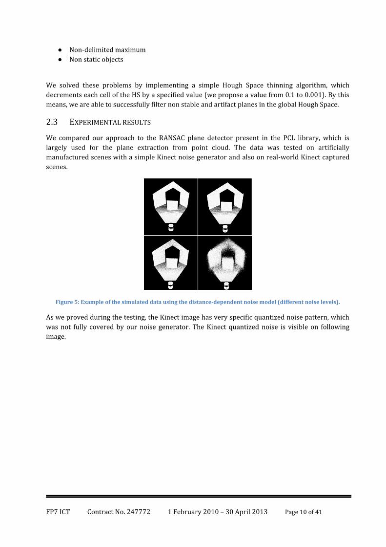
2.3 EXPERIMENTAL RESULTS

We compared our approach to the RANSAC plane detector present in the PCL library, which is

largely used for the plane extraction from point cloud. The data was tested on artificially

manufactured scenes with a simple Kinect noise generator and also on real-world Kinect captured

scenes.

Figure 5: Example of the simulated data using the distance-dependent noise model (different noise levels).

As we proved during the testing, the Kinect image has very specific quantized noise pattern, which

was not fully covered by our noise generator. The Kinect quantized noise is visible on following

image.


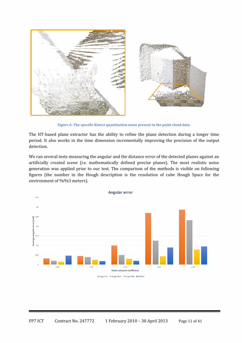
Figure 6: The specific Kinect quantization noise present in the point cloud data.

The HT-based plane extractor has the ability to refine the plane detection during a longer time

period. It also works in the time dimension incrementally improving the precision of the output

detection.

We ran several tests measuring the angular and the distance error of the detected planes against an

artificially created scene (i.e. mathematically defined precise planes). The most realistic noise

generation was applied prior to our test. The comparison of the methods is visible on following

figures (the number in the Hough description is the resolution of cube Hough Space for the

environment of 9x9x3 meters).


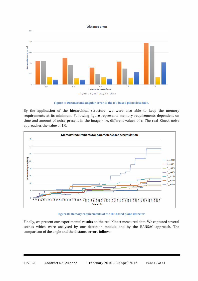
Figure 7: Distance and angular error of the HT-based plane detection.

By the application of the hierarchical structure, we were also able to keep the memory

requirements at its minimum. Following figure represents memory requirements dependent on

time and amount of noise present in the image - i.e. different values of c. The real Kinect noise

approaches the value of 1.0.

Figure 8: Memory requirements of the HT-based plane detector.

Finally, we present our experimental results on the real Kinect measured data. We captured several

scenes which were analysed by our detection module and by the RANSAC approach. The

comparison of the angle and the distance errors follows:


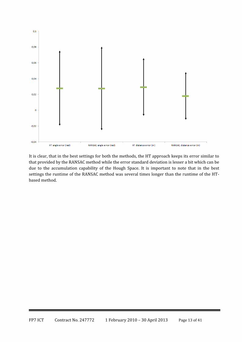
It is clear, that in the best settings for both the methods, the HT approach keeps its error similar to

that provided by the RANSAC method while the error standard deviation is lesser a bit which can be

due to the accumulation capability of the Hough Space. It is important to note that in the best

settings the runtime of the RANSAC method was several times longer than the runtime of the HT-

based method.


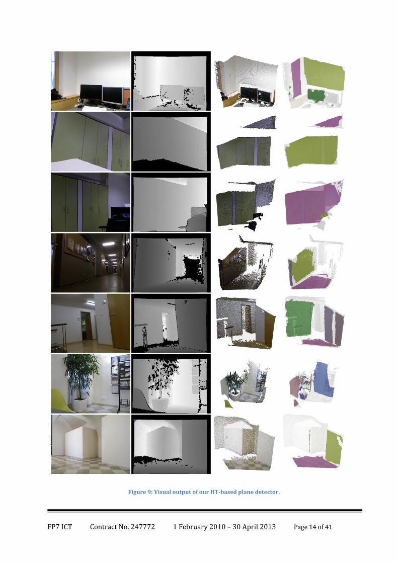
Figure 9: Visual output of our HT-based plane detector.


DISCUSSION In preceding lines, we described a novel approach for the plane segmentation which was

developed, tested and published [Hul13] on behalf of the SRS project. We were able to create robust

detection tool that can easily match against the commonly used RANSAC approach. Moreover, real

data testing shown that using our method we were able to detect the planes with the better

accuracy than the RANSAC method while setting both the methods to have almost similar running

time. The running time was about 530 ms for the RANSAC and 450 ms for the HT-based method.

2.4 DEPTH DATA SEGMENTATION

Depth image segmentation is well known pre-processing task. We implemented several algorithms

for depth image segmentation due to need for fast pre-processing of the visible scene. Using the

segmentation, we can easily divide the image into several regions with a similar meaning and thus

significantly reduce possible load on successive data processing.

Many approaches for the depth map segmentation exist nowadays. Pulli and Pietikäinen [Pul88]

use normal decomposition to achieve requested results. They explore various techniques of range

normal estimation, such as quadratic surface least squares [Bes88] or least squares planar fitting

[Tay89]. Similar work was presented by Baccar et al. [Bac96] where a simple extraction of roof and

step edges is described. Also, an averaging method was presented (the fusion using Dempster-

Shafer or Bernouilli’s rule combinations) which was the inspiration to our modifications.

Other works segments the data into planar regions using RANSAC as the plane detection algorithm

(Ying Yang and Förstner [Yin10]), the 3D Hough Transform (Borrmann et al. [Bor11]), randomized

3D Hough Transform (Dube and Zell [Dub11]), non-associative Markov models [Sha11] or

multidimensional particle swarm optimization [Wan12]. All of these algorithms are used for the

plane segmentation on depth data set dealing always with the noise and time complexity of

proposed algorithms. However, we focused on computational speed while achieving satisfactory

results.

Due to the specific noise of the Kinect sensor, we have been forced to modify several existing

methods and to develop new ones regarding the specific target robot environment. We successfully

applied proposed algorithms as a pre-processing step for our object detectors (fast but reliable

segmentation) [Hul12b].

We compared several approaches to the depth image segmentation. Although there exist many

segmentation methods for the depth maps, we have chosen the fastest algorithms due to the nature

of future use – a fast pre-processing of a scene for further environment perception tasks.

The first set of the analyzed algorithms are modifications of existing segmentation methods. We

simplified the work of Baccar et al. [Bac96] to meet our requirements for speed and real time use.

As a result, we obtained three different algorithms based on surface normal and depth

segmentations combining the depth and the surface normal information with morphological

watersheds segmentation method.


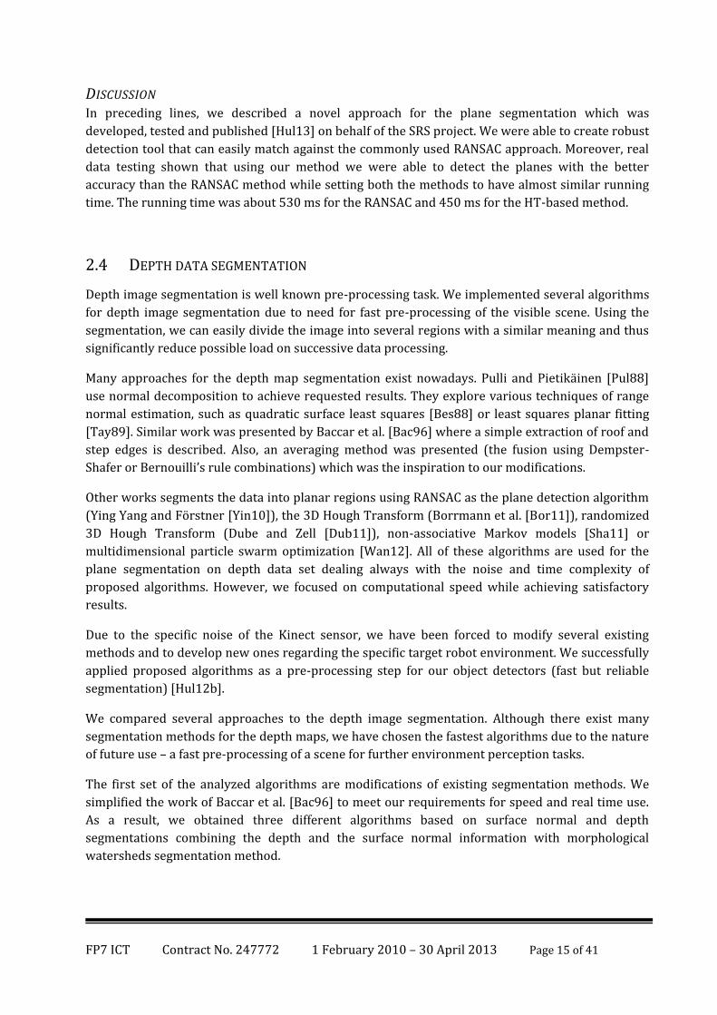
Depth based segmentation This segmentation method is our fastest algorithm because of the simplicity of the computation on

the depth image. It segments the image according to depth differences. We modified the original

work to maximally simplify the computation. First, the algorithm computes an edge strength image

which serves as an input for the watersheds segmentation. Each pixel of the edge strength map is

computed as follows:

where t is the threshold depth difference specifying a step edge, W is the window of neighbouring

pixels and d is a depth information at pixel x. This simple approach was chosen for speed and

simplicity, but also for its ability to filter out the Kinect noise.

Figure 10: Example of a pixel neighbourhood W from which we compute the edge strength.

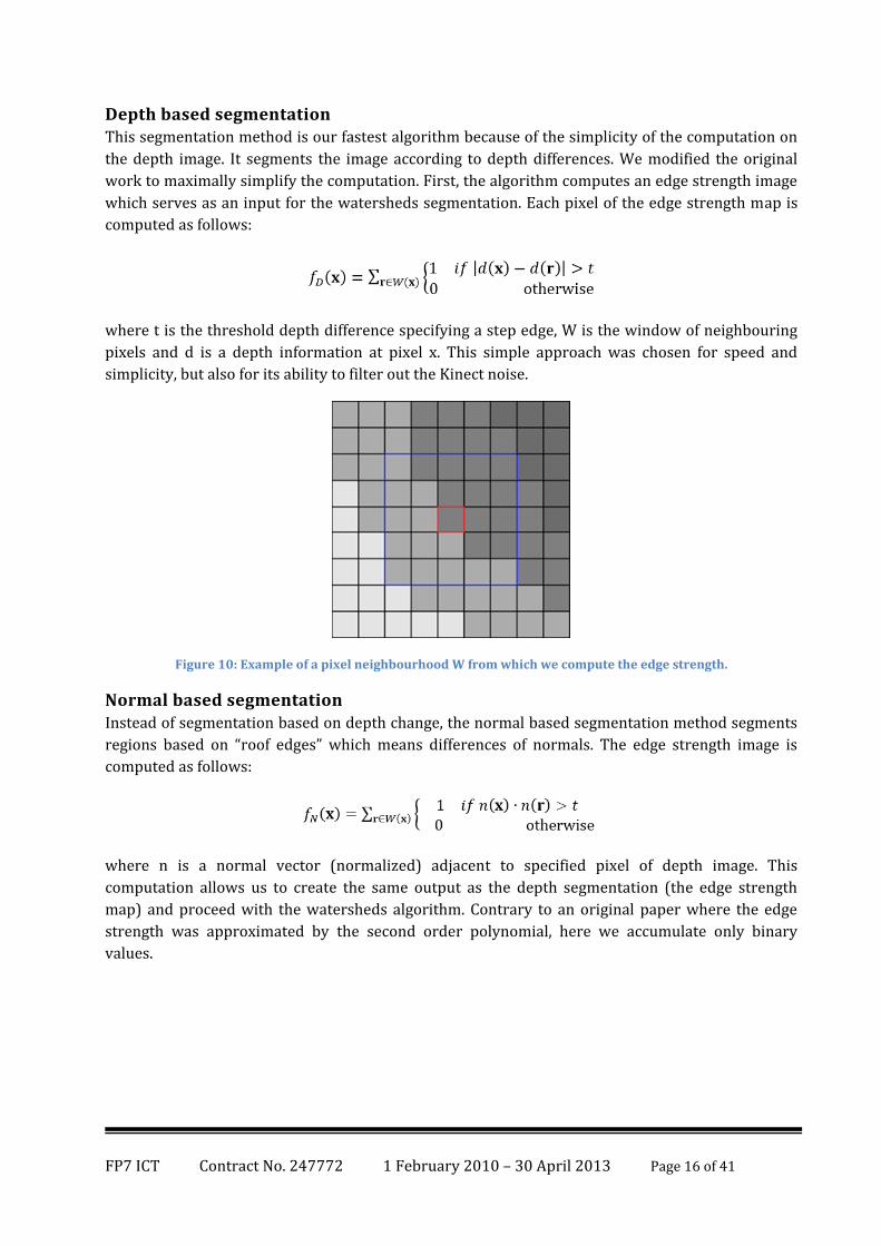
Normal based segmentation Instead of segmentation based on depth change, the normal based segmentation method segments

regions based on “roof edges” which means differences of normals. The edge strength image is


where n is a normal vector (normalized) adjacent to specified pixel of depth image. This

computation allows us to create the same output as the depth segmentation (the edge strength

map) and proceed with the watersheds algorithm. Contrary to an original paper where the edge

strength was approximated by the second order polynomial, here we accumulate only binary

values.


Figure 11: Example of a pixel neighbourhood W – the roof edge.

Fused approach The similar kind of output of the normal and the depth segmentation leads to the idea of fusion of

these two algorithms into a single method. By this technique, we are able to segment the objects not

only based on their distance, but also on the changes on their surface. The fusion algorithm keeps

the same idea of two accumulators. Instead of difficult Super Bayesian combination rules from the

original paper, we implemented simple weighted sum of these two detectors:

,

where w are the appropriate weights. After several experiments with this segmentation method, we

found that the use of weight equal to 1 is the most desirable solution. It keeps ordinal arithmetic

while retaining the accuracy of combined segmentation.

Plane prediction segmentation Plane prediction is our newly proposed algorithm which was developed consequently after

experiments with the normal segmentation method. The normal segmentation keeps the

computational difficult problem in the step of computing normals. If we want to have precise

normals (noise filtered), it is necessary to use quite large window size which leads to slow

algorithm.

This method benefits from an assumption that the majority of all objects in the scene with large

significance (objects that should be detected) are human made. This means they are supposed to

have (or can be approximated by) planar faces. Two gradient images are computed:

and


where d represents a real depth of specified pixel and p is predicted theoretical depth of pixel


The c defines a center point with specified gradient. p(x, c) is a theoretical depth of a point x

predicted from point c using its gradient. This algorithm keeps segmenting the scene based on

normal difference, but without the necessity of computing the normals. The time cost at the end of

this section will show achieved improvement.

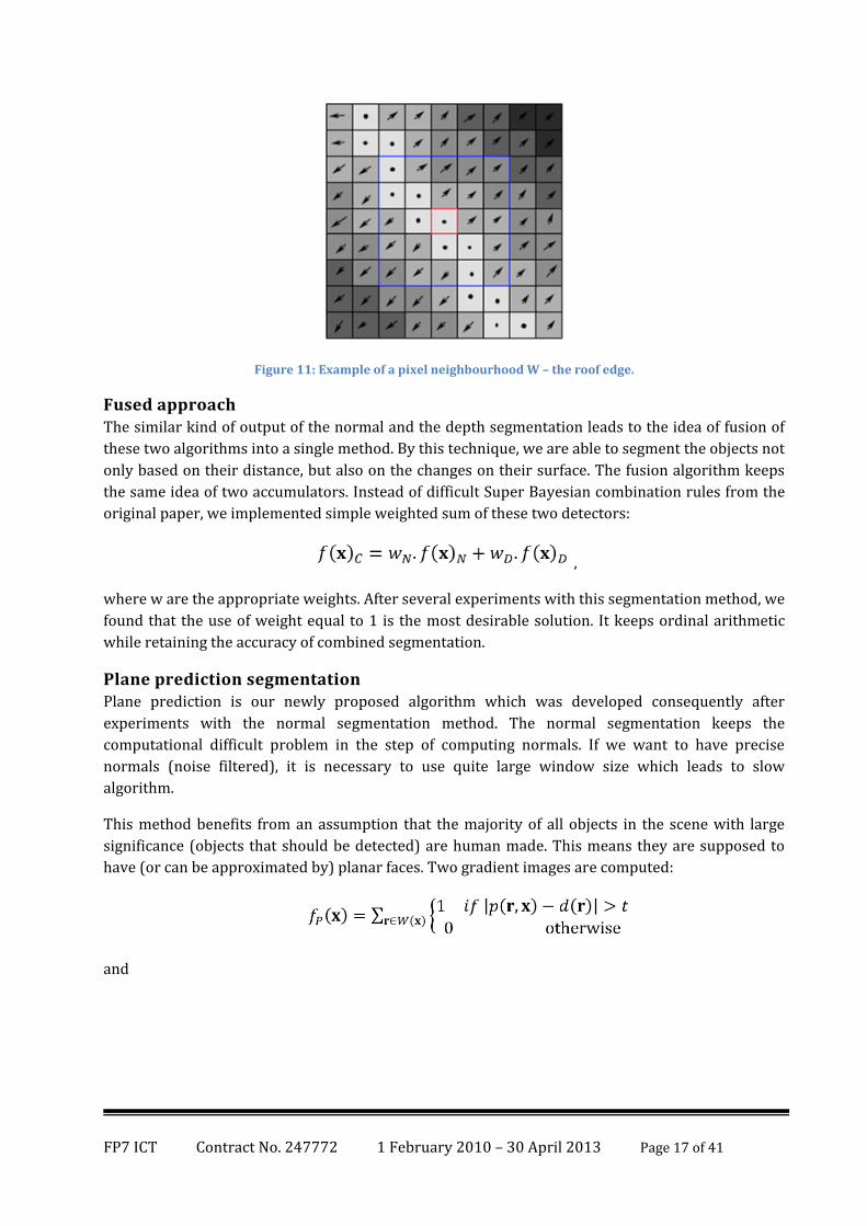
Tiled RANSAC approach The last segmentation algorithm proposed and implemented is the modified RANSAC. We tried to

adapt this approach and turn a planar detector into depth map planar region segmentation

procedure. The main problem of RANSAC approach is the time complexity, because of large space

for random search. We applied easy divide-merge algorithm, which firstly segments the image into

a regular grid where it performs RANSAC segmentation independently. After a plane is found in

each tile, it is flooded into other regions to avoid the creation of the tile artifacts. Proposed

algorithm overview follows:

Figure 12: Example of the tiled input image (Kinect depth channel).

EXPERIMENTS AND RESULTS During the development, we made several tests to measure the effectivity of our algorithms. We

analysed mainly speed and accuracy of detection.


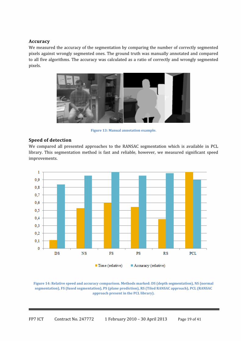
Accuracy We measured the accuracy of the segmentation by comparing the number of correctly segmented

pixels against wrongly segmented ones. The ground truth was manually annotated and compared

to all five algorithms. The accuracy was calculated as a ratio of correctly and wrongly segmented

pixels.

Figure 13: Manual annotation example.

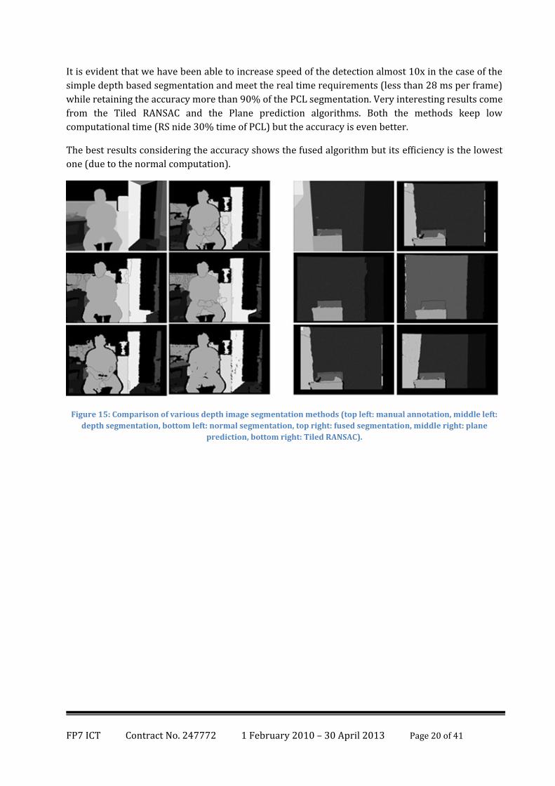
Speed of detection We compared all presented approaches to the RANSAC segmentation which is available in PCL

library. This segmentation method is fast and reliable, however, we measured significant speed

improvements.

Figure 14: Relative speed and accuracy comparison. Methods marked: DS (depth segmentation), NS (normal

segmentation), FS (fused segmentation), PS (plane prediction), RS (Tiled RANSAC approach), PCL (RANSAC

approach present in the PCL library).


It is evident that we have been able to increase speed of the detection almost 10x in the case of the

simple depth based segmentation and meet the real time requirements (less than 28 ms per frame)

while retaining the accuracy more than 90% of the PCL segmentation. Very interesting results come

from the Tiled RANSAC and the Plane prediction algorithms. Both the methods keep low

computational time (RS nide 30% time of PCL) but the accuracy is even better.

The best results considering the accuracy shows the fused algorithm but its efficiency is the lowest

one (due to the normal computation).

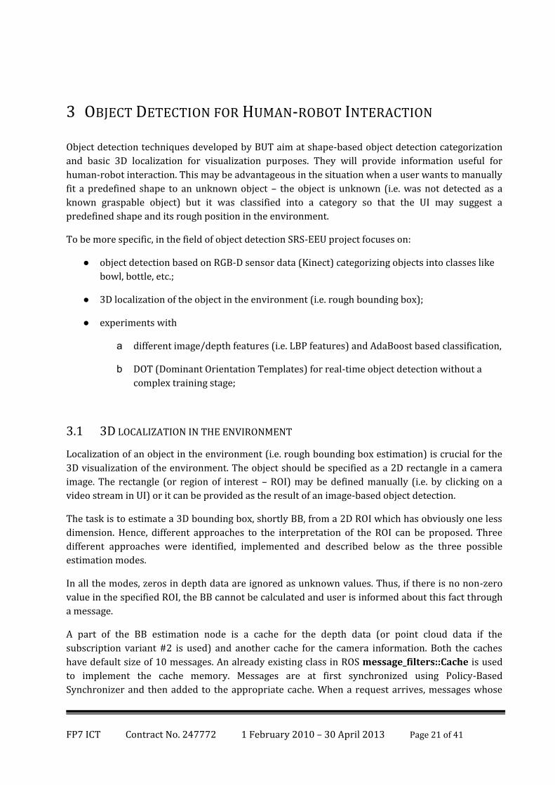
Figure 15: Comparison of various depth image segmentation methods (top left: manual annotation, middle left:

depth segmentation, bottom left: normal segmentation, top right: fused segmentation, middle right: plane

prediction, bottom right: Tiled RANSAC).


3 OBJECT DETECTION FOR HUMAN-ROBOT INTERACTION

Object detection techniques developed by BUT aim at shape-based object detection categorization

and basic 3D localization for visualization purposes. They will provide information useful for

human-robot interaction. This may be advantageous in the situation when a user wants to manually

fit a predefined shape to an unknown object – the object is unknown (i.e. was not detected as a

known graspable object) but it was classified into a category so that the UI may suggest a

predefined shape and its rough position in the environment.

To be more specific, in the field of object detection SRS-EEU project focuses on:

● object detection based on RGB-D sensor data (Kinect) categorizing objects into classes like

bowl, bottle, etc.;

● 3D localization of the object in the environment (i.e. rough bounding box);

● experiments with

a different image/depth features (i.e. LBP features) and AdaBoost based classification,

b DOT (Dominant Orientation Templates) for real-time object detection without a

complex training stage;

3.1 3D LOCALIZATION IN THE ENVIRONMENT

Localization of an object in the environment (i.e. rough bounding box estimation) is crucial for the

3D visualization of the environment. The object should be specified as a 2D rectangle in a camera

image. The rectangle (or region of interest – ROI) may be defined manually (i.e. by clicking on a

video stream in UI) or it can be provided as the result of an image-based object detection.

The task is to estimate a 3D bounding box, shortly BB, from a 2D ROI which has obviously one less

dimension. Hence, different approaches to the interpretation of the ROI can be proposed. Three

different approaches were identified, implemented and described below as the three possible

estimation modes.

In all the modes, zeros in depth data are ignored as unknown values. Thus, if there is no non-zero

value in the specified ROI, the BB cannot be calculated and user is informed about this fact through

a message.

A part of the BB estimation node is a cache for the depth data (or point cloud data if the

subscription variant #2 is used) and another cache for the camera information. Both the caches

have default size of 10 messages. An already existing class in ROS message_filters::Cache is used

to implement the cache memory. Messages are at first synchronized using Policy-Based

Synchronizer and then added to the appropriate cache. When a request arrives, messages whose


timestamp is the latest one before the request timestamp are retrieved from both the caches. These

messages are then used for the bounding box estimation.

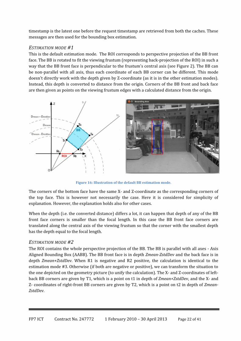
ESTIMATION MODE #1 This is the default estimation mode. The ROI corresponds to perspective projection of the BB front

face. The BB is rotated to fit the viewing frustum (representing back-projection of the ROI) in such a

way that the BB front face is perpendicular to the frustum's central axis (see Figure 2). The BB can

be non-parallel with all axis, thus each coordinate of each BB corner can be different. This mode

doesn't directly work with the depth given by Z-coordinate (as it is in the other estimation modes).

Instead, this depth is converted to distance from the origin. Corners of the BB front and back face

are then given as points on the viewing frustum edges with a calculated distance from the origin.

Figure 16: Illustration of the default BB estimation mode.

The corners of the bottom face have the same X- and Z-coordinate as the corresponding corners of

the top face. This is however not necessarily the case. Here it is considered for simplicity of

explanation. However, the explanation holds also for other cases.

When the depth (i.e. the converted distance) differs a lot, it can happen that depth of any of the BB

front face corners is smaller than the focal length. In this case the BB front face corners are

translated along the central axis of the viewing frustum so that the corner with the smallest depth

has the depth equal to the focal length.

ESTIMATION MODE #2 The ROI contains the whole perspective projection of the BB. The BB is parallel with all axes - Axis

Aligned Bounding Box (AABB). The BB front face is in depth Zmean-ZstdDev and the back face is in

depth Zmean+ZstdDev. When R1 is negative and R2 positive, the calculation is identical to the

estimation mode #3. Otherwise (if both are negative or positive), we can transform the situation to

the one depicted on the geometry picture (to unify the calculation). The X- and Z-coordinates of left-

back BB corners are given by T1, which is a point on t1 in depth of Zmean+ZstdDev, and the X- and

Z- coordinates of right-front BB corners are given by T2, which is a point on t2 in depth of Zmean-

ZstdDev.


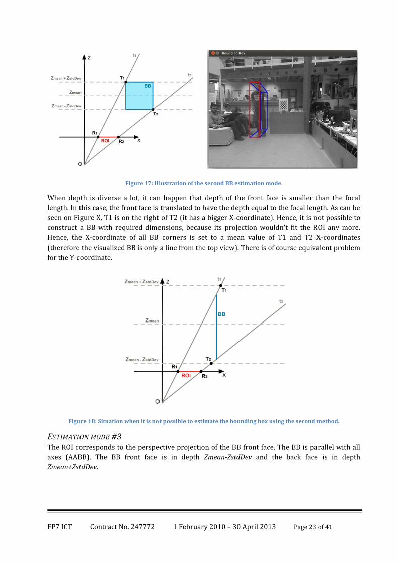
Figure 17: Illustration of the second BB estimation mode.

When depth is diverse a lot, it can happen that depth of the front face is smaller than the focal

length. In this case, the front face is translated to have the depth equal to the focal length. As can be

seen on Figure X, T1 is on the right of T2 (it has a bigger X-coordinate). Hence, it is not possible to

construct a BB with required dimensions, because its projection wouldn't fit the ROI any more.

Hence, the X-coordinate of all BB corners is set to a mean value of T1 and T2 X-coordinates

(therefore the visualized BB is only a line from the top view). There is of course equivalent problem

for the Y-coordinate.

Figure 18: Situation when it is not possible to estimate the bounding box using the second method.

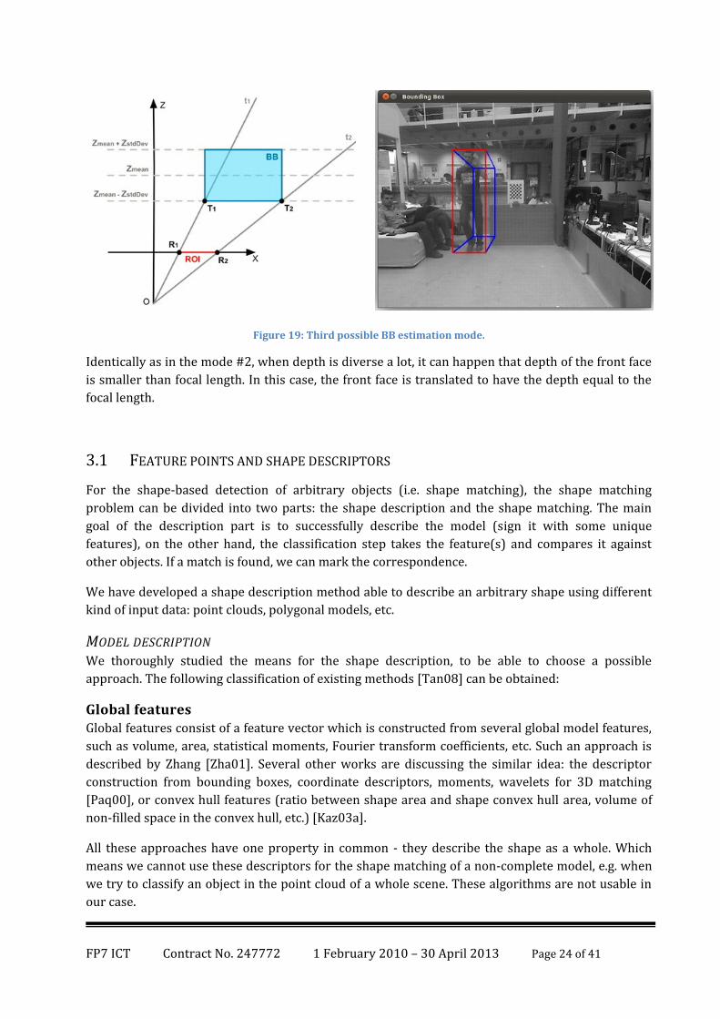
ESTIMATION MODE #3 The ROI corresponds to the perspective projection of the BB front face. The BB is parallel with all

axes (AABB). The BB front face is in depth Zmean-ZstdDev and the back face is in depth

Zmean+ZstdDev.


Figure 19: Third possible BB estimation mode.

Identically as in the mode #2, when depth is diverse a lot, it can happen that depth of the front face

is smaller than focal length. In this case, the front face is translated to have the depth equal to the

focal length.

3.1 FEATURE POINTS AND SHAPE DESCRIPTORS

For the shape-based detection of arbitrary objects (i.e. shape matching), the shape matching

problem can be divided into two parts: the shape description and the shape matching. The main

goal of the description part is to successfully describe the model (sign it with some unique

features), on the other hand, the classification step takes the feature(s) and compares it against

other objects. If a match is found, we can mark the correspondence.

We have developed a shape description method able to describe an arbitrary shape using different

kind of input data: point clouds, polygonal models, etc.

MODEL DESCRIPTION We thoroughly studied the means for the shape description, to be able to choose a possible

approach. The following classification of existing methods [Tan08] can be obtained:

Global features Global features consist of a feature vector which is constructed from several global model features,

such as volume, area, statistical moments, Fourier transform coefficients, etc. Such an approach is

described by Zhang [Zha01]. Several other works are discussing the similar idea: the descriptor

construction from bounding boxes, coordinate descriptors, moments, wavelets for 3D matching

[Paq00], or convex hull features (ratio between shape area and shape convex hull area, volume of

non-filled space in the convex hull, etc.) [Kaz03a].

All these approaches have one property in common - they describe the shape as a whole. Which

means we cannot use these descriptors for the shape matching of a non-complete model, e.g. when

we try to classify an object in the point cloud of a whole scene. These algorithms are not usable in

our case.


Global feature descriptors Compared to the previous global features, the global feature descriptors are not taken globally, but

one global descriptor is created based on several distributions of local features on the model. Osada

et al. [Osa02] compute the model descriptor as a distribution of distance, angles, area and volume

between randomly chosen points on the model’s surface. For the matching itself, the authors use

their pseudo-metric comparison of distance between the distributions. The same authors also

propose to use the shape histograms parametrized by their main axes of inertia which leads to

three histograms: a momentum of inertia around the axis, mean distance of surface to the axis of

inertia and distance change of axis and the surface. With this modification, the algorithm works

quite well on rotationally symmetric shapes.

Ip et al. [Ip02] described the shape distributions in the context of CAD and solid modeling. They

construct a histogram of IN and OUT distances. IN distance is measured as a line length between

two points, which lies all inside the model. On the contrary, OUT distance is the line length which

lies outside the model. They also propose a MIXED descriptor.

An algorithm proposed by Ohbuchi et al. [Ohb02] who describe a model as an Absolute Angle

Distance histogram which accumulates distances between two randomly chosen points along with

the angle between their normal. Its algorithm is more precise, however more computationally

expensive.

Global feature descriptors are very precise concerning the resolution of model classes, however

they are not so strong in comparison of objects that differ only in details. Moreover, it is not

possible to compare non-complete models.


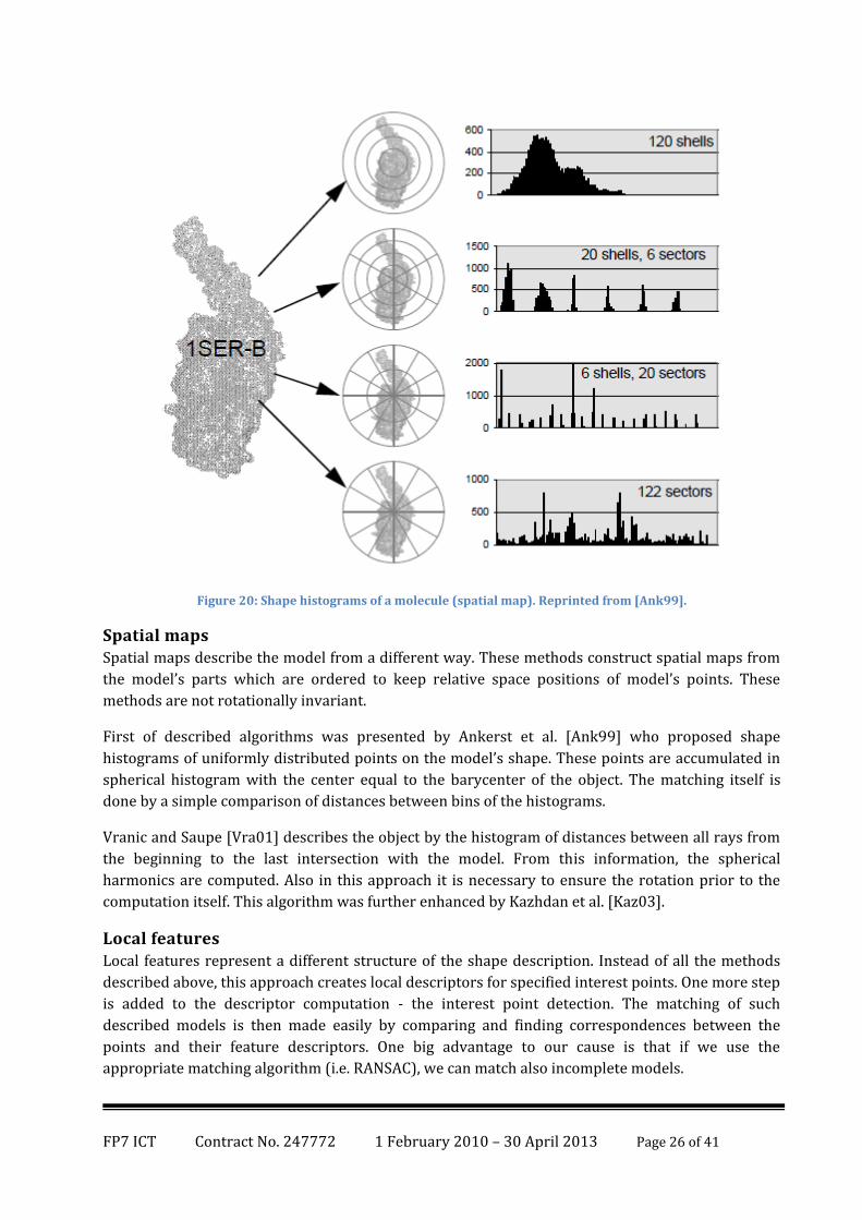
Figure 20: Shape histograms of a molecule (spatial map). Reprinted from [Ank99].

Spatial maps Spatial maps describe the model from a different way. These methods construct spatial maps from

the model’s parts which are ordered to keep relative space positions of model’s points. These

methods are not rotationally invariant.

First of described algorithms was presented by Ankerst et al. [Ank99] who proposed shape

histograms of uniformly distributed points on the model’s shape. These points are accumulated in

spherical histogram with the center equal to the barycenter of the object. The matching itself is

done by a simple comparison of distances between bins of the histograms.

Vranic and Saupe [Vra01] describes the object by the histogram of distances between all rays from

the beginning to the last intersection with the model. From this information, the spherical

harmonics are computed. Also in this approach it is necessary to ensure the rotation prior to the

computation itself. This algorithm was further enhanced by Kazhdan et al. [Kaz03].

Local features Local features represent a different structure of the shape description. Instead of all the methods

described above, this approach creates local descriptors for specified interest points. One more step

is added to the descriptor computation - the interest point detection. The matching of such

described models is then made easily by comparing and finding correspondences between the

points and their feature descriptors. One big advantage to our cause is that if we use the

appropriate matching algorithm (i.e. RANSAC), we can match also incomplete models.


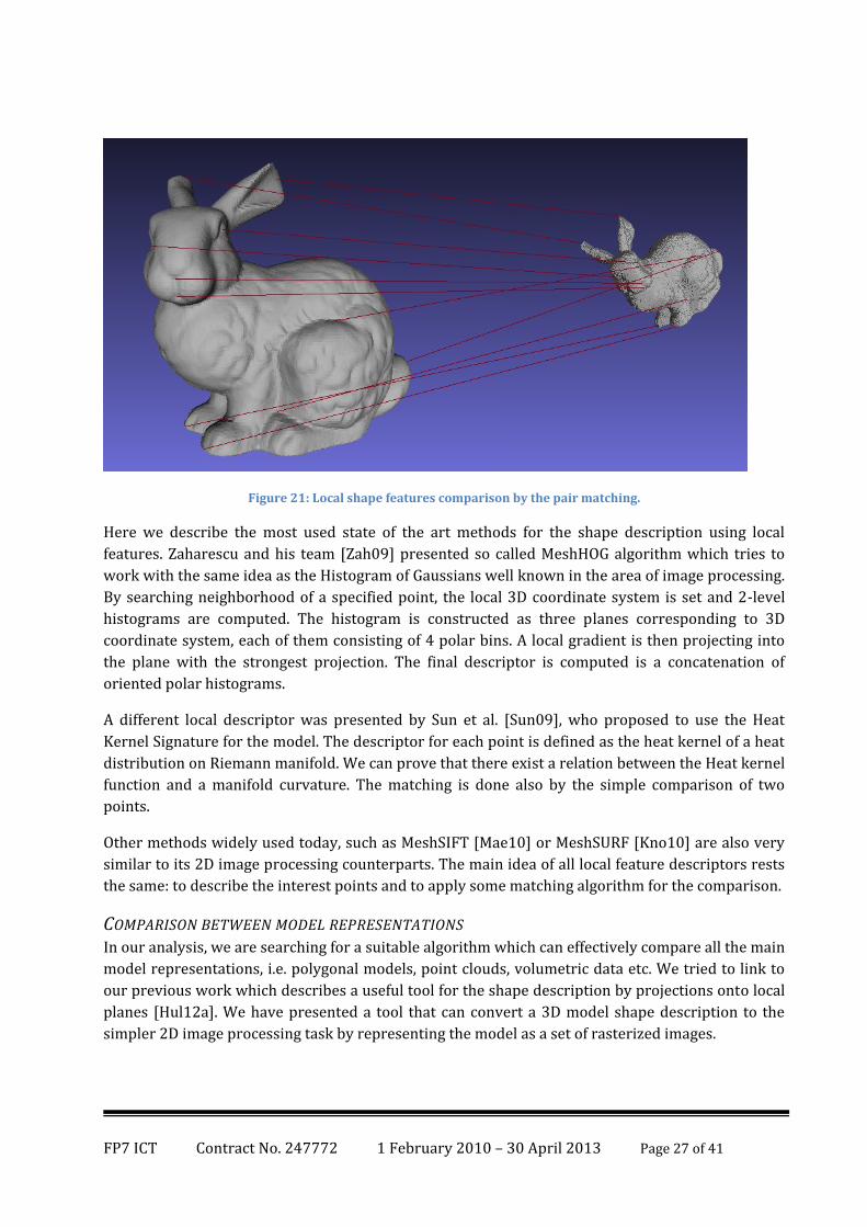
Figure 21: Local shape features comparison by the pair matching.

Here we describe the most used state of the art methods for the shape description using local

features. Zaharescu and his team [Zah09] presented so called MeshHOG algorithm which tries to

work with the same idea as the Histogram of Gaussians well known in the area of image processing.

By searching neighborhood of a specified point, the local 3D coordinate system is set and 2-level

histograms are computed. The histogram is constructed as three planes corresponding to 3D

coordinate system, each of them consisting of 4 polar bins. A local gradient is then projecting into

the plane with the strongest projection. The final descriptor is computed is a concatenation of

oriented polar histograms.

A different local descriptor was presented by Sun et al. [Sun09], who proposed to use the Heat

Kernel Signature for the model. The descriptor for each point is defined as the heat kernel of a heat

distribution on Riemann manifold. We can prove that there exist a relation between the Heat kernel

function and a manifold curvature. The matching is done also by the simple comparison of two

points.

Other methods widely used today, such as MeshSIFT [Mae10] or MeshSURF [Kno10] are also very

similar to its 2D image processing counterparts. The main idea of all local feature descriptors rests

the same: to describe the interest points and to apply some matching algorithm for the comparison.

COMPARISON BETWEEN MODEL REPRESENTATIONS In our analysis, we are searching for a suitable algorithm which can effectively compare all the main

model representations, i.e. polygonal models, point clouds, volumetric data etc. We tried to link to

our previous work which describes a useful tool for the shape description by projections onto local

planes [Hul12a]. We have presented a tool that can convert a 3D model shape description to the

simpler 2D image processing task by representing the model as a set of rasterized images.


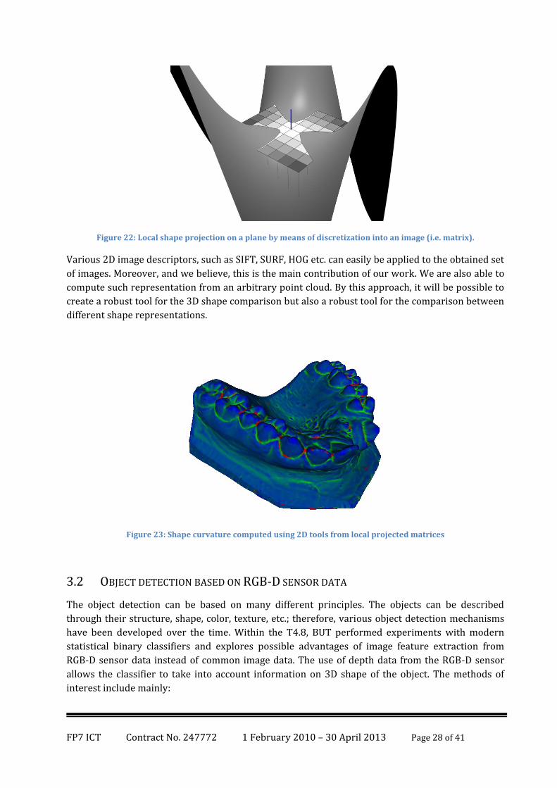
Figure 22: Local shape projection on a plane by means of discretization into an image (i.e. matrix).

Various 2D image descriptors, such as SIFT, SURF, HOG etc. can easily be applied to the obtained set

of images. Moreover, and we believe, this is the main contribution of our work. We are also able to

compute such representation from an arbitrary point cloud. By this approach, it will be possible to

create a robust tool for the 3D shape comparison but also a robust tool for the comparison between

different shape representations.

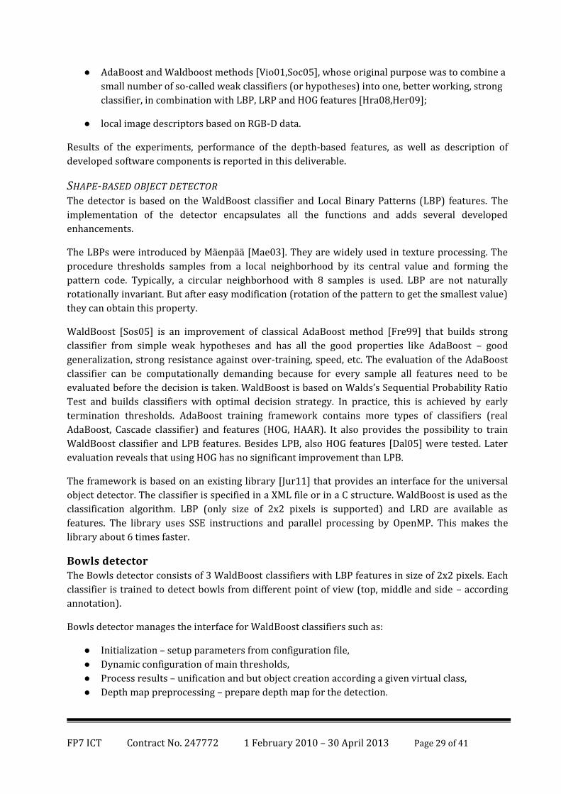
Figure 23: Shape curvature computed using 2D tools from local projected matrices

3.2 OBJECT DETECTION BASED ON RGB-D SENSOR DATA

The object detection can be based on many different principles. The objects can be described

through their structure, shape, color, texture, etc.; therefore, various object detection mechanisms

have been developed over the time. Within the T4.8, BUT performed experiments with modern

statistical binary classifiers and explores possible advantages of image feature extraction from

RGB-D sensor data instead of common image data. The use of depth data from the RGB-D sensor

allows the classifier to take into account information on 3D shape of the object. The methods of

interest include mainly:


● AdaBoost and Waldboost methods [Vio01,Soc05], whose original purpose was to combine a

small number of so-called weak classifiers (or hypotheses) into one, better working, strong

classifier, in combination with LBP, LRP and HOG features [Hra08,Her09];

● local image descriptors based on RGB-D data.

Results of the experiments, performance of the depth-based features, as well as description of

developed software components is reported in this deliverable.

SHAPE-BASED OBJECT DETECTOR The detector is based on the WaldBoost classifier and Local Binary Patterns (LBP) features. The

implementation of the detector encapsulates all the functions and adds several developed

enhancements.

The LBPs were introduced by Mäenpää [Mae03]. They are widely used in texture processing. The

procedure thresholds samples from a local neighborhood by its central value and forming the

pattern code. Typically, a circular neighborhood with 8 samples is used. LBP are not naturally

rotationally invariant. But after easy modification (rotation of the pattern to get the smallest value)

they can obtain this property.

WaldBoost [Sos05] is an improvement of classical AdaBoost method [Fre99] that builds strong

classifier from simple weak hypotheses and has all the good properties like AdaBoost – good

generalization, strong resistance against over-training, speed, etc. The evaluation of the AdaBoost

classifier can be computationally demanding because for every sample all features need to be

evaluated before the decision is taken. WaldBoost is based on Walds’s Sequential Probability Ratio

Test and builds classifiers with optimal decision strategy. In practice, this is achieved by early

termination thresholds. AdaBoost training framework contains more types of classifiers (real

AdaBoost, Cascade classifier) and features (HOG, HAAR). It also provides the possibility to train

WaldBoost classifier and LPB features. Besides LPB, also HOG features [Dal05] were tested. Later

evaluation reveals that using HOG has no significant improvement than LPB.

The framework is based on an existing library [Jur11] that provides an interface for the universal

object detector. The classifier is specified in a XML file or in a C structure. WaldBoost is used as the

classification algorithm. LBP (only size of 2x2 pixels is supported) and LRD are available as

features. The library uses SSE instructions and parallel processing by OpenMP. This makes the

library about 6 times faster.

Bowls detector The Bowls detector consists of 3 WaldBoost classifiers with LBP features in size of 2x2 pixels. Each

classifier is trained to detect bowls from different point of view (top, middle and side – according

annotation).

Bowls detector manages the interface for WaldBoost classifiers such as:

● Initialization – setup parameters from configuration file,

● Dynamic configuration of main thresholds,

● Process results – unification and but object creation according a given virtual class,

● Depth map preprocessing – prepare depth map for the detection.


A very important task is merging the results from all three classifiers. Every classifier usually

produces more than one detection for the same object. Sometimes even more than one detector

detects the same object. Implemented non-maxima suppression takes the bounding box from

detections with the highest response value first, detections with lesser response are handled later –

detections has to be sorted beforehand. Two different detections represent two different objects

when circles inscribed into the bounding boxes have overlaps less than 10% of their sizes.

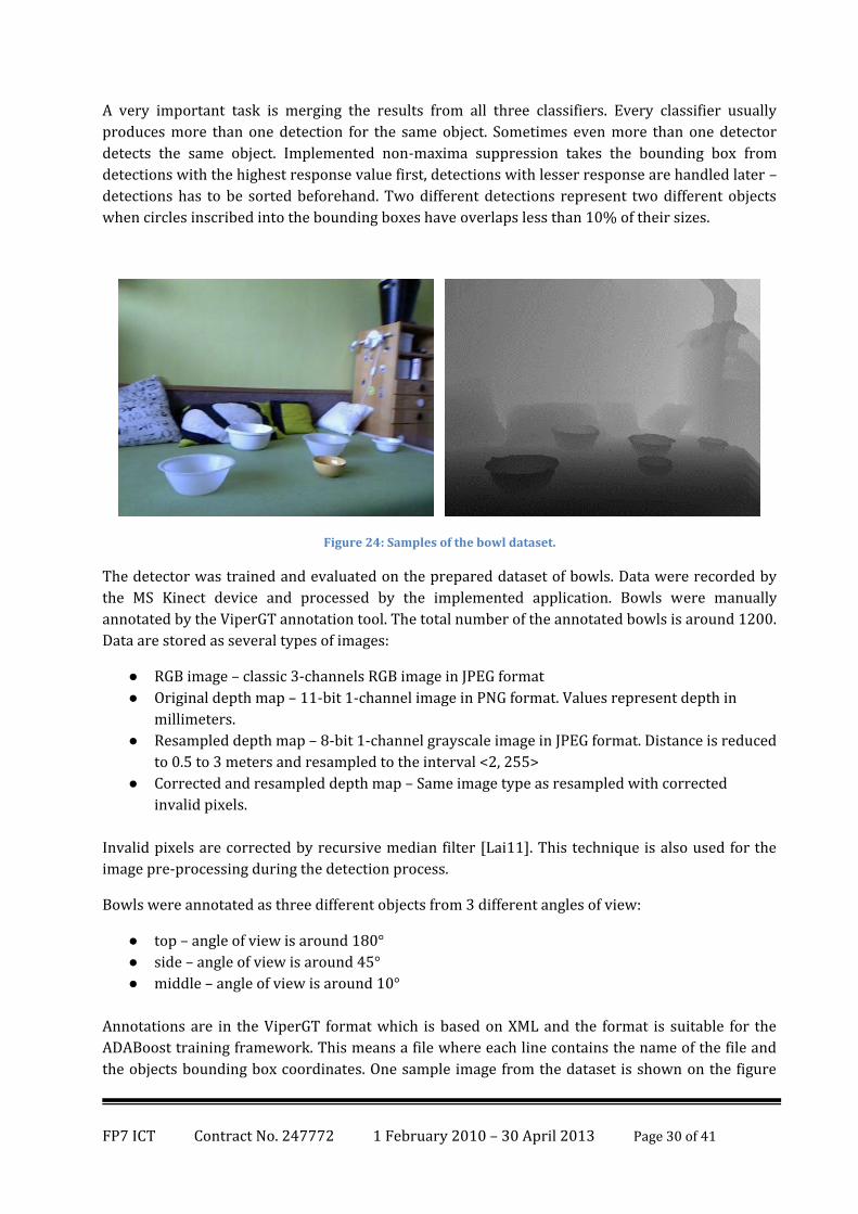
Figure 24: Samples of the bowl dataset.

The detector was trained and evaluated on the prepared dataset of bowls. Data were recorded by

the MS Kinect device and processed by the implemented application. Bowls were manually

annotated by the ViperGT annotation tool. The total number of the annotated bowls is around 1200.

Data are stored as several types of images:

● RGB image – classic 3-channels RGB image in JPEG format

● Original depth map – 11-bit 1-channel image in PNG format. Values represent depth in

millimeters.

● Resampled depth map – 8-bit 1-channel grayscale image in JPEG format. Distance is reduced

to 0.5 to 3 meters and resampled to the interval <2, 255>

● Corrected and resampled depth map – Same image type as resampled with corrected

invalid pixels.

Invalid pixels are corrected by recursive median filter [Lai11]. This technique is also used for the

image pre-processing during the detection process.

Bowls were annotated as three different objects from 3 different angles of view:

● top – angle of view is around 180°

● side – angle of view is around 45°

● middle – angle of view is around 10°

Annotations are in the ViperGT format which is based on XML and the format is suitable for the

ADABoost training framework. This means a file where each line contains the name of the file and

the objects bounding box coordinates. One sample image from the dataset is shown on the figure


below. The original depth image is not shown, because an 11-bit image is impossible to show

without resampling.

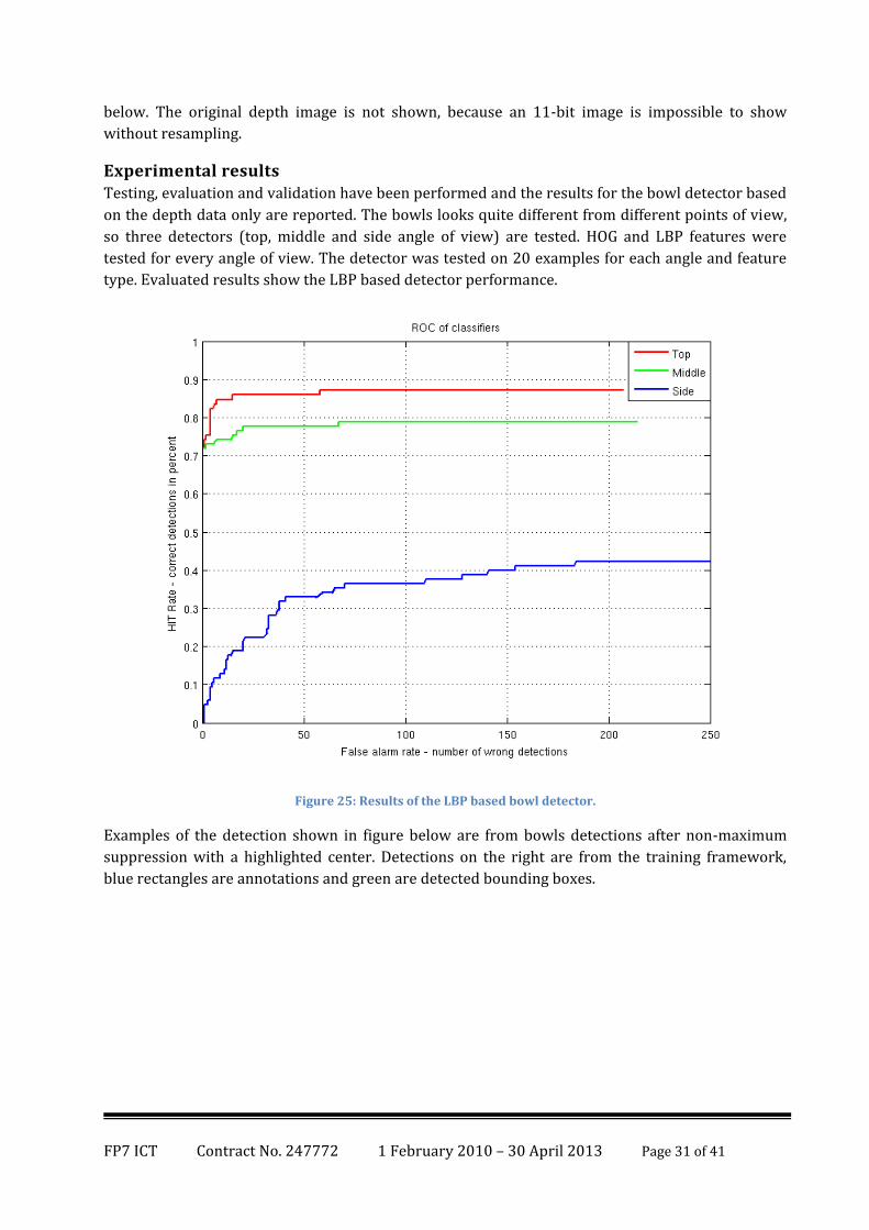
Experimental results Testing, evaluation and validation have been performed and the results for the bowl detector based

on the depth data only are reported. The bowls looks quite different from different points of view,

so three detectors (top, middle and side angle of view) are tested. HOG and LBP features were

tested for every angle of view. The detector was tested on 20 examples for each angle and feature

type. Evaluated results show the LBP based detector performance.

Figure 25: Results of the LBP based bowl detector.

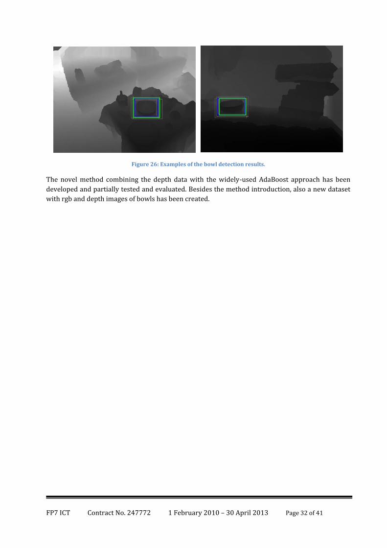
Examples of the detection shown in figure below are from bowls detections after non-maximum

suppression with a highlighted center. Detections on the right are from the training framework,

blue rectangles are annotations and green are detected bounding boxes.


Figure 26: Examples of the bowl detection results.

The novel method combining the depth data with the widely-used AdaBoost approach has been

developed and partially tested and evaluated. Besides the method introduction, also a new dataset

with rgb and depth images of bowls has been created.


4 PREREQUISITIES

The core prerequisites for the software to be used are:

● Linux OS (developed on Ubuntu 11.10),

● Robot Operating System (ROS) (developed on Electric version),

● Care-O-bot stacks installed in ROS,

● Stacks for COB simulation in robot simulator Gazebo.

PLANE DETECTION BASED ON 3D HOUGH TRANSFORM

● OpenCV library (developed on version 2.2)

● Eigen library (version 3)

● Point Clouds Library (PCL version 1.1)

DEPTH IMAGE SEGMENTATION



● Point Clouds Library (PCL version 1.1)

BOWL OBJECT DETECTOR



● BUT’s Object Detection API for ROS (git://github.com/robofit/but_object_detection.git)

The software components are property of Brno University of Technology, a license for

academic/research purposes can be granted to any prospective user.


5 DOCUMENTATION OF PACKAGES

This section very briefly describes newly created software components. It is expected that the

interface may change according to requirements and needs of the project in the future.

5.1 PLANE DETECTION BASED ON 3D HOUGH TRANSFORM

The plane detection is realized as a ROS node. The relevant source files are included in

srs_env_model_percp package. The node processes point-cloud data from Kinect sensor or Kinect

depth image and publishes all found planes as Interactive Markers (visualization_msgs::Marker)

and COB Shape Array (cob_3d_mapping_msgs::ShapeArray).

An important part of developed software is a C++ library with implemented pre-processing and

plane detection functions. The precise description of API can be found in Doxygen generated

documentation in the package folder.

USAGE:

rosrun srs_env_model_percp but_plane_detector

○ Starts a node with our 3D Hough transform plane extractor

○ Possible ROS parameters can be found in /config/planedet_params.yaml file along

with the description.

○

rosrun srs_env_model_percp but_plane_detector_ransac

○ Starts a node with PCL RANSAC plane extractor user for comparison with our

method.

○ Possible ROS parameters can be found in /config/planedet_params.yaml file along

with the description.

INPUT: ● If using Kinect depth image

○ sensor_msgs::Image depth - Kinect depth image

○ sensor_msgs::CameraInfo cam_info - Kinect camera info message

○ sensor_msgs::Image rgb - (optional, if we want to color planes according to their

real color), Kinect RGB image

● If using Kinect point cloud

○ sensor_msgs::PointCloud2 cloud - Kinect point cloud (ordered)

○ sensor_msgs::Image rgb - (optional, if we want to color planes according to their

real color), Kinect RGB image

OUTPUT: ● cob_3d_mapping_msgs::ShapeArray array1 - COB shape array of triangulated planes


● visualization_msgs::MarkerArray array2 - Marker array of triangulated planes

● pcl::PointCloud<pcl::PointXYZRGB> cloud - Colored (optional) cloud of associated points

to found planes

5.2 3D LOCALIZATION IN THE ENVIRONMENT

The 3D localization is realized as a ROS service called bb_estimate performing rough bounding box

(BB) estimation from specified 2D region of interest (ROI) using the Kinect depth data. The relevant

source files are included in srs_env_model_percp package. The server provides the service whose

request and response are defined as follows.

REQUEST:

● header (type: Header) - contains (among others) a timestamp, which is necessary for time

synchronization,

● p1 and p2 (type: int16[2]) - 2D points representing two diagonally opposite corners of ROI

(the first element of array = X-coordinate, the second = Y-coordinate),

● mode (type: int8) - BB estimation mode. If it isn't specified, the default value is 1 (=

estimation mode #1).

RESPONSE:

● p1, p2, p3, p4, p5, p6, p7, p8 (type: float32[3]) - 3D points representing the corners of the

resulting BB (the first element of array = X-coordinate, the second = Y-coordinate, the third

= Z-coordinate).

There are all eight corners in the response, because estimation mode #1 can produce a BB which is

non-parallel with all axis. In fact, this BB could be uniquely represented by only four corners, but

there are included all of them to avoid troubles with calculation of the remaining four corners.

5.3 DEPTH IMAGE SEGMENTATION

The depth image segmentation is realized as a C++ library - but_segmentation. The relevant

source files are included in srs_env_model_percp package. The library consists of functions for

preprocessing and segmentation of Kinect depth maps or point clouds and produces a region image

(grayscale image with intensities equal to the segment IDs). The precise description of API can be

found in Doxygen generated documentation in the package folder.

USAGE ● but_plane_detector::Plane

○ Class encapsulates necessary functions for operations with plane, including

transformations.

● but_plane_detector::Normals

○ Class for normal computations


○ Constructor computes real point positions and normals (works with point clouds or

depth image with camera info).

○ Uses but_plane_detector::NormalType as parameter, which specifies type of

computation.

● but_plane_detector::Regions

○ Class encapsulates functions for segmentation.

○ Constructor initializes variables and must be succeeded by watershedRegions

function, which implements one of four segmentation methods which uses edge

strength map and watershed segmentation.

○ Last method, tiled RANSAC, is implemented in independentTileRegions function.


6 REFERENCES

[Yin10] Ying Yang, M. and Forstner, W.: Plane Detection in Point Cloud Data. TR-IGG-P-2010-

01, January 25, 2010.

[Bau06] Baumstarck, P. G., Brudevold, B. D., and Reynolds, P. D.: Learning Planar Geometric

Scene Context Using Stereo Vision. CS229 Final Project Report, December 15, 2006.

[Pop08] Poppinga, J., Vaskevicius, N., Birk, A. and Pathak, K.: Fast Plane Detection and

Polygonalization in noisy 3D Range Images. International Conference on Intelligent Robots and

Systems (IROS), Nice, France, IEEE Press, 2008.

[Vio01] Viola, P. and Jones, M.: Rapid object detection using a boosted cascade of simple

features, IEEE Computer Society Conference on Computer Vision and Pattern Recognition 1: 51–

518, 2001.

[Soc05] Sochman, J. and Matas, J.: Waldboost - learning for time constrained sequential

detection, CVPR ’05: Proceedings of the 2005 IEEE Computer Society Conference on Computer

Vision and Pattern Recognition (CVPR’05), IEEE Computer Society, Washington, 2005, DC, USA, pp.

150–156.

[Zem10] Zemcik, P, Hradis, M., and Herout, A.: Exploiting neighbors for faster scanning window

detection in images, Advanced Concepts for Intelligent Vision Systems 2010 (ACIVS 2010), LNCS

6475, Sydney, AU, 2010.

[Hra08] Hradis, M., Herout, A. and Zemcik, P.: Local rank patterns - novel features for rapid

object detection, Proceedings of International Conference on Computer Vision and Graphics, Lecture

Notes in Computer Science, 2008.

[Her09] Herout, A., Zemcik, P., Hradis, M., Juranek, R., Havel, J., Josth, R. and Zadnik, M.: Low-

Level Image Features for Real-Time Object Detection, IN-TECH Education and Publishing, 2009, p. 25.

[Hin10] Hinterstoisser, S., Lepetit, V., Ilic, S., Fua, P. and Navab, N.: Dominant Orientation

Templates for Real-Time Detection of Texture-Less Objects. IEEE Computer Society Conference on

Computer Vision and Pattern Recognition (CVPR), San Francisco, California (USA), 2010.

[Xu93] Xu, L. and Oja, E.: Randomized hough transform (rht): Basic mechanisms,

algorithms, and computational complexities, CVGIP: Image Understanding 57 (2) (1993) 131 – 154.

doi:10.1006/ciun.1993.1009.

[Kal94] Kalviainen, H., Hirvonen, P., Xu, L. and Oja, E.: Comparisons of probabilistic and non-

probabilistic hough transforms, in: Proc. of 3rd European Conference on Computer Vision ECCV’94,

1994, pp. 351–360.

[Che01] Chen, T.-C. and Chung, K.-L.: Detecting lines, A new randomized algorithm for


Real-Time Imaging 7 (6) (2001) 473 – 481. doi:10.1006/rtim.2001.0233. URL

http://www.sciencedirect.com/science/article/pii/S1077201401902335

[Tan08] Tangelder, J. W. and Veltkamp, R. C.: A survey of content based 3D shape retrieval

methods. Multimedia Tools Appl. 39, 3, September 2008, 441-471. DOI=10.1007/s11042-007-0181-

0 http://dx.doi.org/10.1007/s11042-007-0181-0

[Zha01] Zhang, C., Chen, T.: Efficient feature extraction for 2D/3D objects in mesh

representation Image Processing, 2001. Proceedings. 2001 International Conference on In Image

Processing, 2001. Proceedings. 2001 International Conference on, Vol. 3 (2001), pp. 935-938 vol.3,

doi:10.1109/icip.2001.958278

[Paq00] Paquet, E., Rioux, M., Murching, A., Naveen, T., Tabatabai, A.: Description of shape

information for 2D and 3D objects. Signal Processing: Image Communication 16 (2000), 103-122

[Kaz03a] Kazhdan, M., Chazelle, B., Dobkin, D., Funkhouser, T., and Rusinkiewicz, S.: A

Reflective Symmetry Descriptor for 3D Models. Algorithmica 38, 1 (October 2003), 201-225.

DOI=10.1007/s00453-003-1050-5 http://dx.doi.org/10.1007/s00453-003-1050-5

[Osa02] Osada, R., Funkhouser, T., Chazelle, B., and Dobkin, D.: Shape distributions. ACM

Trans. on Graph. 21, 4 (October 2002), 807-832. DOI=10.1145/571647.571648

http://doi.acm.org/10.1145/571647.571648

[Ip02] Ip, C. Y., Lapadat, D., Sieger, L. and Regli, W. C.: Using shape distributions to compare

solid models. In Proceedings of the seventh ACM symposium on Solid modeling and applications (SMA

'02). ACM, New York, NY, USA, 2002, 273-280. DOI=10.1145/566282.566322

http://doi.acm.org/10.1145/566282.566322

[Ohb02] Ohbuchi, R., Otagiri, T., Ibato, M. and Take, T.: Shape-Similarity Search of Three-

Dimensional Models Using Parameterized Statistics. In Proceedings of the 10th Pacific Conference on

Computer Graphics and Applications (PG '02). IEEE Computer Society, Washington, DC, USA, 2002,

265-.

[Ank99] Ankerst, M., Kastenmüller, G., Kriegel, H.-P., and Seidl, T.: 3D Shape Histograms for

Similarity Search and Classification in Spatial Databases. In Proceedings of the 6th International

Symposium on Advances in Spatial Databases (SSD '99), Ralf Hartmut Güting, Dimitris Papadias, and

Frederick H. Lochovsky (Eds.). Springer-Verlag, London, UK, UK, 1999, 207-226.

[Vra01] Saupe, D. and Vranic, D. V.: 3D Model Retrieval with Spherical Harmonics and

Moments. In Proceedings of the 23rd DAGM-Symposium on Pattern Recognition, Bernd Radig and

Stefan Florczyk (Eds.). Springer-Verlag, London, UK, 2001, 392-397.

[Kaz03b] Kazhdan, M., Funkhouser, T., and Rusinkiewicz, S.: Rotation invariant spherical

harmonic representation of 3D shape descriptors. In Proceedings of the 2003 Eurographics/ACM

SIGGRAPH symposium on Geometry processing (SGP '03). Eurographics Association, Aire-la-Ville,

Switzerland, 2003, 156-164.

http://www.sciencedirect.com/science/article/pii/S1077201401902335

http://dx.doi.org/10.1109/icip.2001.958278




[Zah09] Zaharescu, A.; Boyer, E.; Varanasi, K.; Horaud, R., "Surface feature detection and

description with applications to mesh matching," Computer Vision and Pattern Recognition, 2009.

CVPR 2009. IEEE Conference on , vol., no., pp.373,380, 20-25 June 2009

[Sun09] Jian Sun, Maks Ovsjanikov and Leonidas Guibas, A Concise and Provably Informative

Multi-Scale Signature Based on Heat Diffusion, Comput. Graph. Forum, Volume 28 Issue 5, pages

1383-1392, 2009

[Mae10] Maes, C., Fabry, T., Keustermans, J., Smeets, D., Suetens, P., and Vandermeulen, D.:

Feature detection on 3D face surfaces for pose normalisation and recogntiion. In BTAS '10, IEEE Int.

Conf. on Biometrics: Theory, Applications and Systems, pp. 1-6, September 2010, Washington D.C.,

USA.

[Kno10] Knopp, J., Prasad, M. and Van Gool, L.: Orientation invariant 3D object Classification

using Hough Transform based methods. In ACM Multimedia WS on 3D Object Retrieval, Firenze,

2010.

[Hul12a] Hulík, R., Kršek, P.: Local Projections Method and Curvature Approximation on 3D

Polygonal Models, In: Communications proceedings of WSCG, Plzen, CZ, UPGM FIT VUT, 2012, s.

223-230, ISBN 978-80-86943-79-4

[Hul12b] Hulík, R., Beran, V., Španěl, M., Kršek, P., Smrž, P.: Fast and Accurate Plane

Segmentation in Depth Maps for Indoor Scenes, In: IEEE/RSJ International Conference on

Intelligent Robots and Systems, Vilamoura, Algarve, PT, UPGM FIT VUT, 2012, s. 1-6

[Hul13] Hulík, R., Španěl, M., Smrž, P.:Continuous Plane Detection in Point-cloud Data Based

on 3D Hough Transform, In: Journal of Visual Communication and Image Representation, 2013, 24,

Amsterdam, NL, ISSN 1047-3203

[Bac96] Baccar M., Gee, L. A., Gonzalez, R. C. and Abidi, M. A.: Segmentation of Range Images

Via Data Fusion and Morphological Watersheds. Pattern Recognition, Vol. 29, No. 10. (October

1996), pp. 1673-1687

[Pul88] Pulli, K., Pietikäinen, M.: Range Image Segmentation Based on Decomposition of

Surface Normals. University of Oulu, Finland, 1988.

[Bes88] Besl P.: Surfaces in Range Image Understanding, Springer-Verlag. New York, 1988.

[Tay89] Taylor, R., Savini, M., Reeves A.: Fast Segmentation of Range Imagery into Planar

Regions. Computer Vision, Graphics, and Image Processing, vol. 45, pp. 42-60, 1989.

[Yin10] Ying Yang, M., Förstner, W.: Plane Detection in Point Cloud Data. Proceedings of the

2nd International Conference on Machine Control Guidance Bonn (2010), Issue: 1, Pages: 95-104

[Bor11] Borrmann, D., Elseberg, J., Lingemann, and K., Nüchter, A.: The 3D Hough transform

for plane detection in point clouds – A review and a new accumulator design. 3D research, Springer,

Volume 2, Number 2, March 2011.


[Dub11] Dube, D. and Zell, A.: Real-time plane extraction from depth images with the

Randomized Hough Transform. In IEEE ICCV Workshop on Challenges and Opportunities in Robot

Perception, pages 1084 -1091, Barcelona, Spain, November 2011.

[Sha11] Shapovalov, R. and Velizhev, A.: Cutting-Plane Training of Non-associative Markov

Network for 3D Point Cloud Segmentation. In Proceedings of the 2011 International Conference on

3D Imaging, Modeling, Processing, Visualization and Transmission (3DIMPVT’11). IEEE Computer

Society, Washington, DC, USA, 2011, pp. 1-8.

[Wan12] Wang, L., Cao, J. and Han, C.: Multidimensional particle swarm optimization-based

unsupervised planar segmentation algorithm of unorganized point clouds. Pattern Recogn. 45, 11,

November 2012. pp. 4034-4043.

[Pop08] Poppinga, J., Vaskevicius, N., Birk, A. and Pathak, K.: Fast plane detection and

polygonalization in noisy 3d range images, in: IROS’08, 2008, pp. 3378–3383.

[Des10] Deschaud, J.-E. and Goulette, F.: A fast and accurate plane detection algorithm for

large noisy point clouds using filtered normals and voxel growing, in: 3DPVT’10, 2010.

[Fis87] Fischler, M. A. and Bolles, R. C.: Readings in computer vision: issues, problems,

principles, and paradigms, Morgan Kaufmann Publishers Inc., San Francisco, CA, USA, 1987, Ch.

Random sample consensus: a paradigm for model fitting with applications to image analysis and

automated cartography, pp. 726–740.

[Sch07] Schnabel, R., Wahl, R., Klein, R.: Efficient ransac for point-cloud shape detection,

Comput. Graph. Forum, 2007, 214–226.

[Tar07] Tarsha-Kurd, F., Landes, T. and Grussenmeyer, P.: Hough-transform and extended

ransac algorithms for automatic detection of 3d building roof planes from lidar data scanner data,

in: ISPRS Workshop on Laser Scanning 2007 and SilviLaser 2007, Vol. XXXVI, Espoo, Finland, 2007,

pp. 407–412.

[Hou62] Hough, P.: Method and means for recognizing complex patterns, in: US Patent, 1962.

[Bal87] Ballard, D. H.: Readings in computer vision: issues, problems, principles, and

paradigms, Morgan Kaufmann Publishers Inc., San Francisco, CA, USA, 1987, Ch. Generalizing the

hough transform to detect arbitrary shapes, pp. 714–725.

[Bor11] Borrmann, D., Elseberg, J., Lingemann, K., and Nuchter, A.: The 3d hough transform

for plane detection in point clouds: A review and a new accumulator design, 3D Res. 2 (2) (2011)

32:1–32:13. doi:10.1007/3DRes.02(2011)3.

[Moc09] Mochizuki, Y., Torii, A. and Imiya, A.: N-point hough transform for line detection,

Journal of Visual Communication and Image Representation 20 (4), 2009, 242–253.

doi:10.1016/j.jvcir.2009.01.004.

[Che01] Chen, T.-C. and Chung, K.-L.: A new randomized algorithm for detecting lines, Real-

Time Imaging 7 (6), 2001, 473–481. doi:10.1006/rtim.2001.0233.


[Jur11] Juranek R., Zemcik P., libabr - Simple object detection, [online], URL:

http://medusa.fit.vutbr.cz/libabr/

[Mae03] Mäenpää , T.:The local binary pattern approach to texture analysis – extensions and

applications. University of Oulu, 2003.

[Soc05] Sochman, J., Matas, J.: WaldBoost - Learning for Time Constrained Sequential

Detection. IEEE Computer Society Conference on Computer Vision and Pattern Recognition (CVPR),

2: 150-156, 2005.

[Dal05] Dalal, N., Triggs, B.: Histograms of Oriented Gradients for Human Detection. Proc. of

the IEEE Conf. on Comp. Vis. and Pat. Rec. (CVPR), 2005.

[Fre95] Freund, Y., Schapire, R.E.: A decision-theoretic generalization of on-line learning and

an application to boosting. In Computational Learning Theory: Eurocolt `95, pages 23-37. Springer-

Verlag, 1995.

[Lai11] Lai K., Bo L., Ren X., Fox D.: A Large-Scale Hierarchical Multi-View RGB-D Object

Dataset. Proc. of International Conference on Robotics and Automation, 2011.

http://medusa.fit.vutbr.cz/libabr/

SRS-EEU - srs-project.eu | Multi-Role Shadow Robotic ...srs-project.eu/sites/default/files/SRS DELIVERABLE 4.6.2.pdf · Project title : Multi-Role Shadow Robotic System for Independent

Documents