Springer Undergraduate Texts in Mathematics and Technology Differential Equations Christian Constanda A Primer for Scientists and Engineers

Welcome message from author
This document is posted to help you gain knowledge. Please leave a comment to let me know what you think about it! Share it to your friends and learn new things together.
Transcript
Springer Undergraduate Texts in Mathematics and Technology
Diff erential Equations
Christian Constanda
A Primer for Scientists and Engineers
Springer Undergraduate Textsin Mathematics and Technology
Series Editors:J. M. Borwein, Callaghan, NSW, AustraliaH. Holden, Trondheim, Norway
Editorial Board:L. Goldberg, Berkeley, CA, USAA. Iske, Hamburg, GermanyP.E.T. Jorgensen, Iowa City, IA, USAS. M. Robinson, Madison, WI, USA
For further volumes:http://www.springer.com/series/7438

123
Christian Constanda
Differential Equations
A Primer for Scientists and Engineers
Christian ConstandaThe Charles W. Oliphant Professor
of Mathematical SciencesDepartment of MathematicsThe University of TulsaTulsa, OK, USA
ISSN 1867-5506 ISSN 1867-5514 (electronic)ISBN 978-1-4614-7296-4 ISBN 978-1-4614-7297-1 (eBook)DOI 10.1007/978-1-4614-7297-1Springer New York Heidelberg Dordrecht London
Library of Congress Control Number: 2013937945
Mathematics Subject Classification (2010): 34-01
© Springer Science+Business Media New York 2013This work is subject to copyright. All rights are reserved by the Publisher, whether the whole or part of the material isconcerned, specifically the rights of translation, reprinting, reuse of illustrations, recitation, broadcasting, reproductionon microfilms or in any other physical way, and transmission or information storage and retrieval, electronic adaptation,computer software, or by similar or dissimilar methodology now known or hereafter developed. Exempted from thislegal reservation are brief excerpts in connection with reviews or scholarly analysis or material supplied specificallyfor the purpose of being entered and executed on a computer system, for exclusive use by the purchaser of the work.Duplication of this publication or parts thereof is permitted only under the provisions of the Copyright Law of thePublisher’s location, in its current version, and permission for use must always be obtained from Springer. Permissionsfor use may be obtained through RightsLink at the Copyright Clearance Center. Violations are liable to prosecutionunder the respective Copyright Law.The use of general descriptive names, registered names, trademarks, service marks, etc. in this publication does notimply, even in the absence of a specific statement, that such names are exempt from the relevant protective laws andregulations and therefore free for general use.While the advice and information in this book are believed to be true and accurate at the date of publication, neitherthe authors nor the editors nor the publisher can accept any legal responsibility for any errors or omissions that may bemade. The publisher makes no warranty, express or implied, with respect to the material contained herein.
Printed on acid-free paper
Springer is part of Springer Science+Business Media (www.springer.com)

For Lia

Preface
Arguably, one of the principles underpinning classroom success is that the instructoralways knows best. Whether this mildly dictatorial premise is correct or not, it seemslogical that performance can only improve if said instructor also pays attention tocustomer feedback. Students’ opinion sometimes contains valuable points and, properlycanvassed and interpreted, may exercise a positive influence on the quality of a courseand the manner of its teaching.
When I polled my students about what they wanted from a textbook, their answersclustered around five main issues.
The book should be easy to follow without being excessively verbose. A crisp, con-cise, and to-the-point style is much preferred to long-winded explanations that tend toobscure the topic and make the reader lose the thread of the argument.
The book should not talk down to the readers. Students feel slighted when they aretreated as if they have no basic knowledge of mathematics, and many regard the multi-colored, heavily illustrated texts as better suited for inexperienced high schoolers thanfor second-year university undergraduates.
The book should keep the theory to a minimum. Lengthy and convoluted proofs shouldbe dropped in favor of a wide variety of illustrative examples and practice exercises.
The book should not embed computational devices in the instruction process. Althoughborn in the age of the computer, a majority of students candidly admit that they donot learn much from electronic number-crunching.
The book should be ‘slim’. The size and weight of a 500-page volume tend to discour-age potential readers and bode ill for its selling price.
In my view, a book that tries to be ‘all things to all men’ often ends up disappoint-ing its intended audience, who might derive greater profit from a less ambitious butmore focused text composed with a twist of pragmatism. The textbooks on differentialequations currently on the market, while professionally written and very comprehen-sive, fail, I believe, on at least one of the above criteria; by contrast, this book attemptsto comply with the entire set. To what extent it has succeeded is for the end user todecide. All I can say at this stage is that students in my institution and elsewhere, hav-ing adopted an earlier draft as prescribed text, declared themselves fully satisfied by itand agreed that every one of the goals on the above wish list had been met. The finalversion incorporates several additions and changes that answer some of their commentsand a number of suggestions received from other colleagues involved in the teaching ofthe subject.
In earlier times, mathematical analysis was tackled from the outset with what is calledthe ε–δ methodology. Those times are now long gone. Today, with a few exceptions, all
vii
Preface
science and engineering students, including mathematics majors, start by going throughCalculus I, II, and III, where they learn the mechanics of differentiation and integrationbut are not shown the proofs of some of the statements in which the formal technics arerooted, because they have not been exposed yet to the ε–δ language. Those who wantto see these proofs enroll in Advanced Calculus. Consequently, the natural continuationof the primary Calculus sequence for all students is a differential equations coursethat teaches them solution techniques without the proofs of a number of fundamentaltheorems. The missing proofs are discussed later in an Advanced Differential Equationssequel (compulsory for mathematics majors and optional for the interested engineeringstudents), where they are developed with the help of Advanced Calculus concepts. Thisbook is intended for use with the first—elementary—differential equations course, takenby mathematics, physics, and engineering students alike.
Omitted proofs aside, every building block of every method described in this textbookis assembled with total rigor and accuracy.
The book is written in a style that uses words (sparingly) as a bonding agent betweenconsecutive mathematical passages, keeping the author’s presence in the backgroundand allowing the mathematics to be the dominant voice. This should help the readersnavigate the material quite comfortably on their own. After the first examples in eachsection or subsection are solved with full details, the solutions to the rest of themare presented more succinctly: every intermediate stage is explained, but incidentalcomputation (integration by parts or by substitution, finding the roots of polynomialequations, etc.) is entrusted to the students, who have learned the basics of calculusand algebra and should thus be able to perform it routinely.
The contents, somewhat in excess of what can be covered during one semester, includeall the classical topics expected to be found in a first course on ordinary differentialequations. Numerical methods are off the ingredient list since, in my view, they fallunder the jurisdiction of numerical analysis. Besides, students are already acquaintedwith such approximating procedures from Calculus II, where they are introduced toEuler’s method. Graphs are used only occasionally, to offer help with less intuitiveconcepts (for instance, the stability of an equilibrium solution) and not to present avisual image of the solution of every example. If the students are interested in thelatter, they can generate it themselves in the computer lab, where qualified guidance isnormally provided.
The book formally splits the ‘pure’ and ‘applied’ sides of the subject by placing theinvestigation of selected mathematical models in separate chapters. Boundary valueproblems are touched upon briefly (for the benefit of the undergraduates who intend togo on to study partial differential equations) but without reference to Sturm–Liouvilleanalysis.
Although only about 260 pages long, the book contains 232 worked examples and 810exercises. There is no duplication among the examples: no two of them are of exactlythe same kind, as they are intended to make the user understand how the methods areapplied in a variety of circumstances. The exercises aim to cement this knowledge andare all suitable as homework; indeed, each and every one of them is part of my students’assignments.
Computer algebra software—specifically, Mathematica R©—is employed in the bookfor only one purpose: to show how to verify quickly that the solutions obtained arecorrect. Since, in spite of its name, this package has not been created by mathematicians,it does not always do what a mathematician wants. In many other respects, it is aperfectly good instrument, which, it is hoped, will keep on improving so that when,say, version 54 is released, all existing deficiencies will have been eliminated. I takethe view that to learn mathematics properly, one must use pencil and paper and solve
viii
Preface
problems by brain and hand alone. To encourage and facilitate this process, almost allthe examples and exercises in the book have been constructed with integers and a feweasily managed fractions as coefficients and constant terms.
Truth be told, it often seems that the aim of the average student in any coursethese days is to do just enough to pass it and earn the credits. This book providessuch students with everything they need to reach their goal. The gifted ones, who areinterested not only in the how but also in the why of mathematical methods and tryhard to improve from a routinely achieved 95% on their tests to a full 100%, can usethe book as a springboard for progress to more specialized sources (see the list underFurther Reading) or for joining an advanced course where the theoretical aspects leftout of the basic one are thoroughly investigated and explained.
And now, two side issues related to mathematics, though not necessarily to differen-tial equations.
Scientists, and especially mathematicians, need in their work more symbols than theLatin alphabet has to offer. This forces them to borrow from other scripts, among whichGreek is the runaway favorite. However, academics—even English-speaking ones—cannot agree on a common pronunciation of the Greek letters. My choice is to go tothe source, so to speak, and simply follow the way of the Greeks themselves. If anyoneelse is tempted to try my solution, they can find details in Appendix D.
Many instructors would probably agree that one of the reasons why some studentsdo not get the high grades they aspire to is a cocktail of annoying bad habits and incor-rect algebra and calculus manipulation ‘techniques’ acquired (along with the misuse ofthe word “like”) in elementary school. My book Dude, Can You Count? (Copernicus,Springer, 2009) systematically collects the most common of these bloopers and showshow any number of absurdities can be ‘proved’ if such errors are accepted as legitimatemathematical handling. Dude is recommended reading for my classroom attendees, who,I am pleased to report, now commit far fewer errors in their written presentations thanthey used to. Alas, the cure for the “like” affliction continues to elude me.
This book would not have seen the light of day without the special assistance thatI received from Elizabeth Loew, my mathematics editor at Springer–New York. Shemonitored the evolution of the manuscript at every stage, offered advice and encourage-ment, and was particularly understanding over deadlines. I wish to express my gratitudeto her for all the help she gave me during the completion of this project.
I am also indebted to my colleagues Peyton Cook and Kimberly Adams, who trawledthe text for errors and misprints and made very useful remarks; to Geoffrey Price foruseful discussions; and to Dale Doty, our departmental Mathematica R© guru. (Readersinterested in finding out more about this software are directed to the web site http://www.wolfram.com/mathematica/.)
Finally, I want to acknowledge my students for their interest in working through allthe examples and exercises and for flagging up anything that caught their attention asbeing inaccurate or incomplete.
My wife, of course, receives the highest accolade for her inspiring professionalism,patience, and steadfast support.
Tulsa, OK, USA Christian Constanda
ix

Contents
1 Introduction 11.1 Calculus Prerequisites . . . . . . . . . . . . . . . . . . . . . . . . . . . . . . . . . . . . . . . . . . . . 11.2 Differential Equations and Their Solutions . . . . . . . . . . . . . . . . . . . . . . . . . . 31.3 Initial and Boundary Conditions . . . . . . . . . . . . . . . . . . . . . . . . . . . . . . . . . . 61.4 Classification of Differential Equations . . . . . . . . . . . . . . . . . . . . . . . . . . . . . 9
2 First-Order Equations 152.1 Separable Equations . . . . . . . . . . . . . . . . . . . . . . . . . . . . . . . . . . . . . . . . . . . . . 152.2 Linear Equations . . . . . . . . . . . . . . . . . . . . . . . . . . . . . . . . . . . . . . . . . . . . . . . . 202.3 Homogeneous Polar Equations . . . . . . . . . . . . . . . . . . . . . . . . . . . . . . . . . . . . 242.4 Bernoulli Equations . . . . . . . . . . . . . . . . . . . . . . . . . . . . . . . . . . . . . . . . . . . . . . 262.5 Riccati Equations . . . . . . . . . . . . . . . . . . . . . . . . . . . . . . . . . . . . . . . . . . . . . . . 282.6 Exact Equations . . . . . . . . . . . . . . . . . . . . . . . . . . . . . . . . . . . . . . . . . . . . . . . . 302.7 Existence and Uniqueness Theorems . . . . . . . . . . . . . . . . . . . . . . . . . . . . . . . 352.8 Direction Fields . . . . . . . . . . . . . . . . . . . . . . . . . . . . . . . . . . . . . . . . . . . . . . . . . 40
3 Mathematical Models with First-Order Equations 413.1 Models with Separable Equations . . . . . . . . . . . . . . . . . . . . . . . . . . . . . . . . . . 413.2 Models with Linear Equations . . . . . . . . . . . . . . . . . . . . . . . . . . . . . . . . . . . . . 443.3 Autonomous Equations . . . . . . . . . . . . . . . . . . . . . . . . . . . . . . . . . . . . . . . . . . . 49
4 Linear Second-Order Equations 614.1 Mathematical Models with Second-Order Equations . . . . . . . . . . . . . . . . . 614.2 Algebra Prerequisites . . . . . . . . . . . . . . . . . . . . . . . . . . . . . . . . . . . . . . . . . . . . 624.3 Homogeneous Equations . . . . . . . . . . . . . . . . . . . . . . . . . . . . . . . . . . . . . . . . . . 67
4.3.1 Initial Value Problems . . . . . . . . . . . . . . . . . . . . . . . . . . . . . . . . . . . . . 674.3.2 Boundary Value Problems . . . . . . . . . . . . . . . . . . . . . . . . . . . . . . . . . . 70
4.4 Homogeneous Equations with Constant Coefficients . . . . . . . . . . . . . . . . . . 714.4.1 Real and Distinct Characteristic Roots . . . . . . . . . . . . . . . . . . . . . . . 724.4.2 Repeated Characteristic Roots . . . . . . . . . . . . . . . . . . . . . . . . . . . . . . 744.4.3 Complex Conjugate Characteristic Roots . . . . . . . . . . . . . . . . . . . . . 77
4.5 Nonhomogeneous Equations . . . . . . . . . . . . . . . . . . . . . . . . . . . . . . . . . . . . . . 804.5.1 Method of Undetermined Coefficients: Simple Cases . . . . . . . . . . . 814.5.2 Method of Undetermined Coefficients: General Case . . . . . . . . . . . 884.5.3 Method of Variation of Parameters . . . . . . . . . . . . . . . . . . . . . . . . . . 94
xi
Contents
4.6 Cauchy–Euler Equations . . . . . . . . . . . . . . . . . . . . . . . . . . . . . . . . . . . . . . . . . 974.7 Nonlinear Equations . . . . . . . . . . . . . . . . . . . . . . . . . . . . . . . . . . . . . . . . . . . . . 100
5 Mathematical Models with Second-Order Equations 1035.1 Free Mechanical Oscillations . . . . . . . . . . . . . . . . . . . . . . . . . . . . . . . . . . . . . . 103
5.1.1 Undamped Free Oscillations . . . . . . . . . . . . . . . . . . . . . . . . . . . . . . . . 1035.1.2 Damped Free Oscillations . . . . . . . . . . . . . . . . . . . . . . . . . . . . . . . . . . 106
5.2 Forced Mechanical Oscillations . . . . . . . . . . . . . . . . . . . . . . . . . . . . . . . . . . . . 1105.2.1 Undamped Forced Oscillations . . . . . . . . . . . . . . . . . . . . . . . . . . . . . . 1105.2.2 Damped Forced Oscillations . . . . . . . . . . . . . . . . . . . . . . . . . . . . . . . . 112
5.3 Electrical Vibrations . . . . . . . . . . . . . . . . . . . . . . . . . . . . . . . . . . . . . . . . . . . . . 114
6 Higher-Order Linear Equations 1176.1 Modeling with Higher-Order Equations . . . . . . . . . . . . . . . . . . . . . . . . . . . . . 1176.2 Algebra Prerequisites . . . . . . . . . . . . . . . . . . . . . . . . . . . . . . . . . . . . . . . . . . . . 117
6.2.1 Matrices and Determinants of Higher Order . . . . . . . . . . . . . . . . . . 1186.2.2 Systems of Linear Algebraic Equations . . . . . . . . . . . . . . . . . . . . . . . 1196.2.3 Linear Independence and the Wronskian . . . . . . . . . . . . . . . . . . . . . 124
6.3 Homogeneous Differential Equations . . . . . . . . . . . . . . . . . . . . . . . . . . . . . . . 1266.4 Nonhomogeneous Equations . . . . . . . . . . . . . . . . . . . . . . . . . . . . . . . . . . . . . . 130
6.4.1 Method of Undetermined Coefficients . . . . . . . . . . . . . . . . . . . . . . . . 1306.4.2 Method of Variation of Parameters . . . . . . . . . . . . . . . . . . . . . . . . . . 134
7 Systems of Differential Equations 1377.1 Modeling with Systems of Equations . . . . . . . . . . . . . . . . . . . . . . . . . . . . . . . 1377.2 Algebra Prerequisites . . . . . . . . . . . . . . . . . . . . . . . . . . . . . . . . . . . . . . . . . . . . 139
7.2.1 Operations with Matrices . . . . . . . . . . . . . . . . . . . . . . . . . . . . . . . . . . . 1397.2.2 Linear Independence and the Wronskian . . . . . . . . . . . . . . . . . . . . . 1457.2.3 Eigenvalues and Eigenvectors . . . . . . . . . . . . . . . . . . . . . . . . . . . . . . . 147
7.3 Systems of First-Order Differential Equations . . . . . . . . . . . . . . . . . . . . . . . 1517.4 Homogeneous Linear Systems with Constant Coefficients . . . . . . . . . . . . . 154
7.4.1 Real and Distinct Eigenvalues . . . . . . . . . . . . . . . . . . . . . . . . . . . . . . . 1557.4.2 Complex Conjugate Eigenvalues . . . . . . . . . . . . . . . . . . . . . . . . . . . . . 1617.4.3 Repeated Eigenvalues . . . . . . . . . . . . . . . . . . . . . . . . . . . . . . . . . . . . . . 165
7.5 Other Features of Homogeneous Linear Systems . . . . . . . . . . . . . . . . . . . . . 1737.6 Nonhomogeneous Linear Systems . . . . . . . . . . . . . . . . . . . . . . . . . . . . . . . . . . 178
8 The Laplace Transformation 1878.1 Definition and Basic Properties . . . . . . . . . . . . . . . . . . . . . . . . . . . . . . . . . . . 1878.2 Further Properties . . . . . . . . . . . . . . . . . . . . . . . . . . . . . . . . . . . . . . . . . . . . . . . 1948.3 Solution of IVPs for Single Equations . . . . . . . . . . . . . . . . . . . . . . . . . . . . . . 199
8.3.1 Continuous Forcing Terms . . . . . . . . . . . . . . . . . . . . . . . . . . . . . . . . . . 1998.3.2 Piecewise Continuous Forcing Terms . . . . . . . . . . . . . . . . . . . . . . . . . 2048.3.3 Forcing Terms with the Dirac Delta . . . . . . . . . . . . . . . . . . . . . . . . . . 2088.3.4 Equations with Variable Coefficients . . . . . . . . . . . . . . . . . . . . . . . . . 212
8.4 Solution of IVPs for Systems . . . . . . . . . . . . . . . . . . . . . . . . . . . . . . . . . . . . . . 215
9 Series Solutions 2219.1 Power Series . . . . . . . . . . . . . . . . . . . . . . . . . . . . . . . . . . . . . . . . . . . . . . . . . . . . 2219.2 Series Solution Near an Ordinary Point . . . . . . . . . . . . . . . . . . . . . . . . . . . . 2229.3 Singular Points . . . . . . . . . . . . . . . . . . . . . . . . . . . . . . . . . . . . . . . . . . . . . . . . . . 229
xii
Contents
9.4 Solution Near a Regular Singular Point . . . . . . . . . . . . . . . . . . . . . . . . . . . . . 2319.4.1 Distinct Roots That Do Not Differ by an Integer . . . . . . . . . . . . . . 2329.4.2 Equal Roots . . . . . . . . . . . . . . . . . . . . . . . . . . . . . . . . . . . . . . . . . . . . . . 2369.4.3 Distinct Roots Differing by an Integer . . . . . . . . . . . . . . . . . . . . . . . . 241
A Algebra Techniques 249A.1 Partial Fractions . . . . . . . . . . . . . . . . . . . . . . . . . . . . . . . . . . . . . . . . . . . . . . . . 249A.2 Synthetic Division . . . . . . . . . . . . . . . . . . . . . . . . . . . . . . . . . . . . . . . . . . . . . . . 251
B Calculus Techniques 253B.1 Sign of a Function . . . . . . . . . . . . . . . . . . . . . . . . . . . . . . . . . . . . . . . . . . . . . . . 253B.2 Integration by Parts . . . . . . . . . . . . . . . . . . . . . . . . . . . . . . . . . . . . . . . . . . . . . 253B.3 Integration by Substitution . . . . . . . . . . . . . . . . . . . . . . . . . . . . . . . . . . . . . . . 254
C Table of Laplace Transforms 255
D The Greek Alphabet 257
Further Reading 259
Index 261
xiii

Acronyms
DE Differential equation
IC Initial condition
BC Boundary condition
IVP Initial value problem
BVP Boundary value problem
GS General solution
PS Particular solution
FSS Fundamental set of solutions
xv
Chapter 1
Introduction
Mathematical modeling is one of the most important and powerful methods for studyingphenomena occurring in our universe. Generally speaking, such a model is made upof one or several equations from which we aim to determine one or several unknownquantities of interest in terms of other, prescribed, quantities. The unknown quantitiesturn out in many cases to be functions of a set of variables. Since very often the physicalor empirical laws governing evolutionary processes implicate the rates of change of thesefunctions with respect to their variables, and since rates of change are represented inmathematics by derivatives, it is important for us to gain knowledge of how to solveequations where the unknown functions occur together with their derivatives.
Mathematical modeling consists broadly of three stages: the construction of themodel in the form of a collection of equations, the solution of these equations, and theinterpretation of the results from a practical point of view. In what follows we are con-cerned mostly with the second stage, although at times we briefly touch upon the othertwo as well. Furthermore, we restrict our attention to equations where the unknownsare functions of only one independent (real) variable. We also assume throughout thatevery equation we mention and study obeys the principle of physical unit consistency,and that the quantities involved have been scaled and non-dimensionalized accordingto some suitable criteria. Consequently, with very few exceptions, no explicit referencewill be made to any physical units.
1.1 Calculus Prerequisites
Let f be a function of a variable x, defined on an interval J of the real line. We denoteby f(x) the value of f at x.
Leaving full mathematical rigor aside, we recall that f is said to have a limit α at apoint x0 in J if the values f(x) get arbitrarily close to α as x gets arbitrarily close tox0 from either side of x0; in this case, we write
limx→x0
f(x) = α.
We also say that f is continuous at x0 if
limx→x0
f(x) = f(x0),
C. Constanda, Differential Equations: A Primer for Scientists and Engineers, SpringerUndergraduate Texts in Mathematics and Technology, DOI 10.1007/978-1-4614-7297-1 1,© Springer Science+Business Media New York 2013
1
2 1 Introduction
and that f is differentiable at x0 if
f ′(x0) = limh→0
f(x0 + h)− f(x0)
h
exists. If this happens at every point in J , the function f is said to be differentiable onJ and f ′ is called the (first-order) derivative of f . This process can be generalized todefine higher-order derivatives. We denote the derivatives of f by f ′, f ′′, f ′′′, f (4), f (5),and so on; alternatively, sometimes we use the more formal notation
df
dx,
d2f
dx2,
d3f
dx3, . . . .
Since at some points in the book we have brief encounters with functions of severalvariables, it is useful to list in advance some of the properties of these functions thatare relevant to their differentiation and integration. For simplicity and without loss ofgenerality, we confine ourselves to the two-dimensional case.
Let f be a function of two variables x and y, defined in a region S (called the domainof f) in the Cartesian (x, y)-plane. We denote the value of f at a point P (x, y) in S byf(x, y) or f(P ).
(i) The function f is said to have a limit α at a point P0 in its domain S if
limP→P0
f(P ) = α,
with P approaching P0 on any path lying in S. The function f is called continuousat P0 if
limP→P0
f(P ) = f(P0).
(ii) Suppose that we fix the value of y. Then f becomes a function f1 that depends onx alone. If f1 is differentiable, we call f ′
1 the partial derivative of f with respect tox and write
f ′1 = fx =
∂f
∂x.
The other way around, when x is fixed, f becomes a function f2 of y alone, which,if differentiable, defines the partial derivative of f with respect to y, denoted by
f ′2 = fy =
∂f
∂y.
Formally, the definitions of these first-order partial derivatives are
fx(x, y) = limh→0
f(x+ h, y)− f(x, y)
h, fy(x, y) = lim
h→0
f(x, y + h)− f(x, y)
h.
(iii) We can repeat the above process starting with fx and then fy, and define thesecond-order partial derivatives of f , namely
fxx = (fx)x =∂
∂x
(∂f
∂x
)=
∂2f
∂x2, fxy = (fx)y =
∂
∂y
(∂f
∂x
)=
∂2f
∂y∂x,
fyx = (fy)x =∂
∂x
(∂f
∂y
)=
∂2f
∂x∂y, fyy = (fy)y =
∂
∂y
(∂f
∂y
)=
∂2f
∂y2.
1.2 Differential Equations and Their Solutions 3
If the mixed second-order derivatives fxy and fyx are continuous in a disk (thatis, in a finite region bounded by a circle) inside the domain S of f , then fxy = fyxat every point in that disk. Since all the functions in our examples satisfy thiscontinuity condition, we will not verify it explicitly.
(iv) The differential of the function f is
df = fx dx+ fy dy.
(v) The chain rule of differentiation is also a logical extension of the same rule forfunctions of one variable. Thus, if x = x(r, s), y = y(r, s), and f(x, y) = g(r, s),then
gr = fxxr + fyyr, gs = fxxs + fyys.
(vi) When we evaluate the indefinite integral of a two-variable function f with respectto one of its variables, the arbitrary constant of integration is a constant only asfar as that variable is concerned, but may depend on the other variable. If, say, F1
is an antiderivative of f with respect to x, then
∫f(x, y) dx = F1(x, y) + C1(y),
where C1 is an arbitrary function of y. Symmetrically, if F2 is an antiderivative off with respect to y, then∫
f(x, y) dy = F2(x, y) + C2(x),
where C2 is an arbitrary function of x.
1.1 Example. Forf(x, y) = 6x2y − 4xy3
we have
fx = 12xy − 4y3, fy = 6x2 − 12xy2,
fxx = 12y, fxy = fyx = 12x− 12y2, fyy = −24xy,∫f(x, y) dx =
∫(6x2y − 4xy3) dx = 2x3y − 2x2y3 + C1(y),∫
f(x, y) dy =
∫(6x2y − 4xy3) dy = 3x2y2 − xy4 + C2(x).
1.2 Remark. We use a number of different symbols for functions and their variables.Usually—but not always—a generic unknown function (to be determined) is denotedby y and its variable by t or x.
1.2 Differential Equations and Their Solutions
To avoid cumbersome language and notation, unless specific restrictions are mentioned,all mathematical expressions and relationships in what follows will be understood tobe defined for the largest set of ‘admissible’ values of their variables and functioncomponents—in other words, at all the points on the real line where they can be eval-uated according to context.
4 1 Introduction
1.3 Definition. Roughly speaking, a differential equation (DE, for short) is an equationthat contains an unknown function and one or more of its derivatives.
Here are a few examples of DEs that occur in some simple mathematical models.
1.4 Example. (Population growth) If P (t) is the size of a population at time t > 0 andβ(t) and δ(t) are the birth and death rates within the population, then
P ′ =[β(t)− δ(t)
]P.
1.5 Example. (Radioactive decay) The number N(t) of atoms of a radioactive isotopepresent at time t > 0 satisfies the equation
N ′ = −κN,
where κ = const > 0 is the constant rate of decay of the isotope.
1.6 Example. (Free fall in gravity) If v(t) is the velocity at time t > 0 of a materialparticle falling in a gravitational field, then
mv′ = mg − γv,
where the positive constants m, g, and γ are, respectively, the particle mass, the accel-eration of gravity, and a coefficient characterizing the resistance of the ambient mediumto motion.
1.7 Example. (Newton’s law of cooling) Let T (t) be the temperature at time t > 0 ofan object immersed in an outside medium of temperature θ. Then
T ′ = −k(T − θ),
where k = const > 0 is the heat transfer coefficient of the object material.
1.8 Example. (RC electric circuit) Consider an electric circuit with a source, a resistor,and a capacitor connected in series. We denote by V (t) and Q(t) the voltage generatedby the source and the electric charge at time t > 0, and by R and C the (constant)resistance and capacitance. Then
RQ′ +1
CQ = V (t).
1.9 Example. (Compound interest) If S(t) is the sum of money present at time t > 0in a savings account that pays interest (compounded continuously) at a rate of r, then
S′ = rS.
1.10 Example. (Loan repayment) Suppose that a sum of money is borrowed from abank at a (constant) interest rate of r. If m is the (constant) repayment per unit time,then the outstanding loan amount A(t) at time t > 0 satisfies the differential equation
A′ = rA−m
for 0 < t < n, where n is the number of time units over which the loan is taken.
1.2 Differential Equations and Their Solutions 5
1.11 Example. (Equilibrium temperature in a rod) The equilibrium distribution oftemperature u(x) in a heat-conducting rod of length l with an insulated lateral surfaceand an internal heat source proportional to the temperature is the solution of the DE
u′′ + qu = 0
for 0 < x < l, where q is a physical constant of the rod material.
Informally, we say that a function is a solution of a DE if, when replaced in theequation, satisfies it identically (that is, for all admissible values of the variable). Amore rigorous definition of this concept will be given at the end of the chapter.
1.12 Example. Consider the equation
y′′ − 3y′ + 2y = 0.
If y1(t) = et, then y′1(t) = et and y′′1 (t) = et, so, for all real values of t,
y′′1 − 3y′1 + 2y1 = et − 3et + 2et = 0,
which means that y1 is a solution of the given DE. Also, for y2(t) = e2t we havey′2(t) = 2e2t and y′′2 (t) = 4e2t, so
y′′2 − 3y′2 + 2y2 = 4e2t − 6e2t + 2e2t = 0;
hence, y2 is another solution of the equation.
1.13 Example. The functions defined by
y1(t) = 2t2 + ln t, y2(t) = −t−1 + ln t
are solutions of the equation
t2y′′ − 2y = −1− 2 ln t
for t > 0 sincey′1(t) = 4t+ t−1, y′′1 (t) = 4− t−2,y′2(t) = t−2 + t−1, y′′2 (t) = −2t−3 − t−2
and so, for all t > 0,
t2y′′1 − 2y1 = t2(4− t−2)− 2(2t2 + ln t) = −1− 2 ln t,
t2y′′2 − 2y2 = t2(−2t−3 − t−2)− 2(−t−1 + ln t) = −1− 2 ln t.
1.14 Remark. Every solution y = y(t) is represented graphically by a curve in the(t, y)-plane, which is called a solution curve.
Exercises
Verify that the function y is a solution of the given DE.
1 y(t) = 5e−3t + 2, y′ + 3y = 6.
2 y(t) = −2tet/2, 2y′ − y = −4et/2.
6 1 Introduction
3 y(t) = −4e2t cos(3t) + t2 − 2, y′′ − 4y′ + 13y = 13t2 − 8t− 24.
4 y(t) = (2t− 1)e−3t/2 − 4e2t, 2y′′ − y′ − 6y = −14e−3t/2.
5 y(t) = 2e−2t − e−3t + 8e−t/2, y′′′ + 4y′′ + y′ − 6y = −45e−t/2.
6 y(t) = cos(2t)− 3 sin(2t) + 2t, y′′′ + y′′ + 4y′ + 4y = 8(t+ 1).
7 y(t) = 2t2 + 3t−3/2 − 2et/2, 2t2y′′ + ty′ − 6y = (12− t− t2)et/2.
8 y(t) = 1− 2t−1 + t−2(2 ln t− 1), t2y′′ + 5ty′ + 4y = 4− 2t−1.
1.3 Initial and Boundary Conditions
Examples 1.12 and 1.13 show that a DE may have more than one solution. This seemsto contradict our expectation that one set of physical data should produce one andonly one effect. We therefore conclude that, to yield a unique solution, a DE must beaccompanied by some additional restrictions.
To further clarify what was said in Remark 1.2, we normally denote the indepen-dent variable by t in DE problems where the solution—and, if necessary, some of itsderivatives—are required to assume prescribed values at an admissible point t0. Re-strictions of this type are called initial conditions (ICs). They are appropriate for themodels mentioned in Examples 1.4–1.9 with t0 = 0.
The independent variable is denoted by x mostly when the DE is to be satisfied ona finite interval a < x < b, as in Example 1.11 with a = 0 and b = l, and the solutionand/or some of its derivatives must assume prescribed values at the two end-pointsx = a and x = b. These restrictions are called boundary conditions (BCs).
1.15 Definition. The solution obtained without supplementary conditions is termedthe general solution (GS) of the given DE. Clearly, the GS includes all possible solutionsof the equation and, therefore, contains a certain degree of arbitrariness. When ICs orBCs are applied to the GS, we arrive at a particular solution (PS).
1.16 Definition. A DE and its attending ICs (BCs) form an initial value problem(IVP) (boundary value problem (BVP)).
1.17 Example. For the simple DE
y′ = 5− 6t
we have, by direct integration,
y(t) =
∫(5− 6t) dt = 5t− 3t2 + C,
where C is an arbitrary constant. This is the GS of the equation, valid for all real valuesof t. However, if we turn the DE into an IVP by adjoining, say, the IC y(0) = −1, thenthe GS yields y(0) = C = −1, and we get the PS
y(t) = 5t− 3t2 − 1.
1.18 Example. To obtain the GS of the DE
y′′ = 6t+ 8,
1.3 Initial and Boundary Conditions 7
we need to integrate both sides twice; thus, in the first instance we have
y′(t) =∫(6t+ 8) dt = 3t2 + 8t+ C1, C1 = const,
from which
y(t) =
∫(3t2 + 8t+ C1) dt = t3 + 4t2 + C1t+ C2, C2 = const,
for all real values of t. Since the GS here contains two arbitrary constants, we will needtwo ICs to identify a PS. Suppose that
y(0) = 1, y′(0) = −2;
then, replacing t by 0 in the expressions for y and y′, we find that C1 = −2 and C2 = 1,so the PS corresponding to our choice of ICs is
y(t) = t3 + 4t2 − 2t+ 1.
1.19 Example. Let us rewrite the DE in Example 1.18 as
y′′ = 6x+ 8
and restrict it to the finite interval 0 < x < 1. Obviously, the GS remains the same(with t replaced by x), but this time we determine the constants by prescribing BCs.If we assume that
y(0) = −3, y(1) = 6,
we set x = 0 and then x = 1 in the GS and use these conditions to find that C1 and C2
satisfyC2 = −3, C1 + C2 = 1;
hence, C1 = 4, which means that the solution of our BVP is
y(x) = x3 + 4x2 + 4x− 3.
1.20 Example. A material particle moves without friction along a straight line, andits acceleration at time t > 0 is a(t) = e−t. If the particle starts moving from the point 1with initial velocity 2, then its subsequent position s(t) can be computed very easily byrecalling that acceleration is the derivative of velocity, which, in turn, is the derivativeof the function that indicates the position of the particle; that is,
v′ = a, s′ = v.
Hence, we need to solve two simple IVPs: one to compute v and the other to compute s.In view of the additional information given in the problem, the first IVP is
v′ = e−t, v(0) = 2.
Here, the DE has the GS
v(t) =
∫e−t dt = −e−t + C.
8 1 Introduction
Using the IC, we find that C = 3, so
v(t) = 3− e−t.
The second IVP now iss′ = 3− e−t, s(0) = 1,
whose solution, obtained in a similar manner, is
s(t) = 3t+ e−t.
1.21 Example. A stone is thrown upward from the ground with an initial speed of39.2. To describe its motion when the air resistance is negligible, we need to establisha formula that gives the position h(t) at time t > 0 of a heavy object moving verticallyunder the influence of the force of gravity alone. If g = 9.8 is the acceleration of gravityand the object starts moving from a height h0 with initial velocity v0, and if we assumethat the vertical axis points upward, then Newton’s second law yields the IVP
h′′ = −g, h(0) = h0, h′(0) = v0.
Integrating the DE twice and using the ICs, we easily find that
h(t) = − 12 gt
2 + v0t+ h0.
In our specific case, we have g = 9.8, h0 = 0, and v0 = 39.2, so
h(t) = −4.9t2 + 39.2t.
If we now want, for example, to find the maximum height that the stone reachesabove the ground, then we need to compute h at the moment when the stone’s velocityis zero. Since
v(t) = h′(t) = −9.8t+ 39.2,
we immediately see that v vanishes at t = 4, so
hmax = h(4) = 78.4.
If, on the other hand, we want to know when the falling stone will hit the ground,then we need to determine the nonzero root t of the equation h(t) = 0, which, as caneasily be seen, is t = 8.
Exercises
In 1–4, solve the given IVP.
1 y′′ = −2(6t+ 1); y(0) = 2, y′(0) = 0.
2 y′′ = −12e2t; y(0) = −3, y′(0) = −6.
3 y′′ = −2 sin t− t cos t; y(0) = 0, y′(0) = 1.
4 y′′ = 2t−3; y(1) = −1, y′(1) = 1.
In 5–8, solve the given BVP.
5 y′′ = 2, 0 < x < 1; y(0) = 2, y(1) = 0.
1.4 Classification of Differential Equations 9
6 y′′ = 4 cos(2x), 0 < x < π; y(0) = −3, y(π) = π − 3.
7 y′′ = −x−1 − x−2, 1 < x < e; y′(1) = 0, y(e) = 1− e.
8 y′′ = (2x− 3)e−x, 0 < x < 1; y(0) = 1, y′(1) = −e−1.
In 9–12, find the velocity v(t) and position s(t) at time t > 0 of a material particle thatmoves without friction along a straight line, when its acceleration, initial position, andinitial velocity are as specified.
9 a(t) = 2, s(0) = −4, v(0) = 0.
10 a(t) = −12 sin(2t), s(0) = 0, v(0) = 6.
11 a(t) = 3(t+ 4)−1/2, s(0) = 1, v(0) = −1.
12 a(t) = (t+ 3)et, s(0) = 1, v(0) = 2.
In 13 and 14, solve the given problem.
13 A ball, thrown downward from the top of a building with an initial speed of 3.4,hits the ground with a speed of 23. How tall is the building if the acceleration ofgravity is 9.8 and the air resistance is negligible?
14 A stone is thrown upward from the top of a tower, with an initial velocity of 98.Assuming that the height of the tower is 215.6, the acceleration of gravity is 9.8,and the air resistance is negligible, find the maximum height reached by the stone,the time when it passes the top of the tower on its way down, and the total timeit has been traveling from launch until it hits the ground.
Answers to Odd-Numbered Exercises
1 y(t) = 2− t2 − 2t3. 3 y(t) = t cos t. 5 y(x) = x2 − 3x+ 2.
7 y(x) = (1− x) ln x. 9 v(t) = 2t, s(t) = t2 − 4.
11 v(t) = 6(t+ 4)1/2 − 13, s(t) = 4(t+ 4)3/2 − 13t− 31. 13 26.4.
1.4 Classification of Differential Equations
We recall that, in calculus, a function is a correspondence between one set of numbers(called domain) and another set of numbers (called range), which has the propertythat it associates each number in the domain with exactly one number in the range.If the domain and range consist not of numbers but of functions, then this type ofcorrespondence is called an operator. The image of a number t under a function f isdenoted, as we already said, by f(t); the image of a function y under an operator L isusually denoted by Ly. In special circumstances, we may also write L(y).
1.22 Example. We can define an operator D that associates each differentiable func-tion with its derivative; that is,
Dy = y′.
Naturally, D is referred to as the operator of differentiation. For twice differentiablefunctions, we can iterate this operator and write
D(Dy) = D2y = y′′.
10 1 Introduction
This may be extended in the obvious way to higher-order derivatives.
1.23 Remark. Taking the above comments into account, we can write a differentialequation in the generic form
Ly = f, (1.1)
where L is defined by the sequence of operations performed on the unknown functiony on the left-hand side, and f is a given function. We will use form (1.1) only innon-specific situations; in particular cases, this form is rather cumbersome and will beavoided.
1.24 Example. The DE in the population growth model (see Example 1.4) can bewritten as P ′ − (β − δ)P = 0. In the operator notation (1.1), this is
LP = DP − (β − δ)P = [D − (β − δ)]P = 0;
in other words, L = D − (β − δ) and f = 0.
1.25 Example. It is not difficult to see that form (1.1) for the DE
t2y′′ − 2y′ = e−t
isLy = (t2D2)y − (2D)y = (t2D2 − 2D)y = e−t,
so L = t2D2 − 2D and f(t) = e−t.
1.26 Remarks. (i) The notation in the preceding two example is not entirely rigorous.Thus, in the expressionD−(β−δ) in Example 1.24, the first term is an operator andthe second one is a function. However, we adopted this form because it is intuitivelyhelpful.
(ii) A similar comment can be made about the term t2D2 in Example 1.25, where t2 isa function and D2 is an operator. In this context, it must be noted that t2D2 andD2t2 are not the same operator. When applied to a function y, the former yields
(t2D2)y = t2(D2y) = t2y′′,
whereas the latter generates the image
(D2t2)y = D2(t2y) = (t2y)′′ = 2y + 4ty′ + t2y′′.
(iii) The rigorous definition of a mathematical operator is more general, abstract, andprecise than the one given above, but it is beyond the scope of this book.
1.27 Definition. An operator L is called linear if for any two functions y1 and y2 inits domain and any two numbers c1 and c2 we have
L(c1y1 + c2y2) = c1Ly1 + c2Ly2. (1.2)
Otherwise, L is called nonlinear.
1.28 Example. The differentiation operator D is linear because for any differentiablefunctions y1 and y2 and any constants c1 and c2,
D(c1y1 + c2y2) = (c1y1 + c2y2)′ = c1y
′1 + c2y
′2 = c1Dy1 + c2Dy2.
1.4 Classification of Differential Equations 11
1.29 Example. The operator L = tD2 − 3 is also linear, since
L(c1y1 + c2y2) = (tD2)(c1y1 + c2y2)− 3(c1y1 + c2y2)
= t(c1y1 + c2y2)′′ − 3(c1y1 + c2y2)
= t(c1y′′1 + c2y
′′2 )− 3(c1y1 + c2y2)
= c1(ty′′1 − 3y1) + c2(ty
′′2 − 3y2) = c1Ly1 + c2Ly2.
1.30 Remark. By direct verification of property (1.2), it can be shown that, moregenerally:
(i) the operator Dn of differentiation of any order n is linear;(ii) the operator of multiplication by a fixed function (in particular, a constant) is linear;(iii) the sum of finitely many linear operators is a linear operator.
1.31 Example. According to the above remark, the operators written formally as
L = a(t)D + b(t), L = D2 + p(t)D + q(t)
with given functions a, b, p, and q, are linear.
1.32 Example. Let L be the operator defined by Ly = yy′. Then, taking, say, y1(t) = t,y2(t) = t2, and c1 = c2 = 1, we have
L(c1y1 + c2y2) = L(t+ t2) = (t+ t2)(t+ t2)′ = t+ 3t2 + 2t3,
c1Ly1 + c2Ly2 = (t)(t)′ + (t2)(t2)′ = t+ 2t3,
which shows that (1.2) does not hold for this particular choice of functions and numbers.Consequently, L is a nonlinear operator.
DEs can be placed into different categories according to certain relevant criteria.Here we list the most important ones, making reference to the generic form (1.1).
Number of independent variables. If the unknown is a function of a singleindependent variable, the DE is called an ordinary differential equation. If several inde-pendent variables are involved, then the DE is called a partial differential equation.
1.33 Example. The DE
ty′′ − (t2 − 1)y′ + 2y = t sin t
is an ordinary differential equation for the unknown function y = y(t).The DE
ut − 3(x+ t)uxx = e2x−t
is a partial differential equation for the unknown function u = u(x, t).
Order. The order of a DE is the order of the highest derivative occurring in theexpression Ly in (1.1).
1.34 Example. The equation
t2y′′ − 2y′ + (t− cos t)y = 3
is a second-order DE.
12 1 Introduction
Linearity. If the differential operator L in (1.1) is linear (see Definition 1.27), thenthe DE is a linear equation; otherwise it is a nonlinear equation.
1.35 Example. The equation
ty′′ − 3y = t2 − 1
is linear since the operator L = tD2 − 3 defined by its left-hand side was shown inExample 1.29 to be linear. On the other hand, the equation
y′′ + yy′ − 2ty = 0
is nonlinear: as seen in Example 1.32, the term yy′ defines a nonlinear operator.
Nature of coefficients. If the coefficients of y and its derivatives in every termin Ly are constant, the DE is said to be an equation with constant coefficients. If atleast one of these coefficients is a prescribed function, we have an equation with variablecoefficients.
1.36 Example. The DE3y′′ − 2y′ + 4y = 0
is an equation with constant coefficients, whereas the DE
y′ − (2t+ 1)y = 1− et
is an equation with variable coefficients.
Homogeneity. If f = 0 in (1.1), the DE is called homogeneous; otherwise it is callednonhomogeneous.
1.37 Example. The DE(t− 2)y′ − ty2 = 0
is homogenous; the DEy′′′ − e−ty′ + sin y = 4t− 3
is nonhomogeneous.
Of course, any equation can be classified by means of all these criteria at the sametime.
1.38 Example. The DEy′′ − y′ + 2y = 0
is a linear, homogeneous, second-order ordinary differential equation with constant co-efficients. The linearity of the operator D2−D+2 defined by the left-hand side is easilyverified.
1.39 Example. The DEy′′′ − y′y′′ + 4ty = 3
is a nonlinear, nonhomogeneous, third-order ordinary differential equation with variablecoefficients. The nonlinearity is caused by the second term on the left-hand side.
1.40 Example. The DE
ut + (x2 − t)ux − xtu = ex sin t
1.4 Classification of Differential Equations 13
is a linear, nonhomogeneous, first-order partial differential equation with variablecoefficients.
1.41 Definition. An ordinary differential equation of order n is said to be in normalform if it is written as
y(n) = F (t, y, y′, . . . , y(n−1)), (1.3)
where F is some function of n+ 1 variables.
1.42 Example. The equation
(t+ 1)y′′ − 2ty′ + 4y = t+ 3
is not in normal form. To write it in normal form, we solve for y′′:
y′′ =1
t+ 1(2ty′ − 4y + t+ 3) = F (t, y, y′).
1.43 Definition. A function y defined on an open interval J (of the real line) is saidto be a solution of the DE (1.3) on J if the derivatives y′, y′′, . . . , y(n) exist on J and(1.3) is satisfied at every point of J .
1.44 Remark. Sometimes a model is described by a system of DEs, which consists ofseveral DEs for several unknown functions.
1.45 Example. The pair of equations
x′1 = 3x1 − 2x2 + t,
x′2 = −2x1 + x2 − et
form a linear, nonhomogeneous, first-order system of ordinary DEs with constant coef-ficients for the unknown functions x1 and x2.
Exercises
Classify the given DE in terms of all the criteria listed in this section.
1 y(4) − ty′′ + y2 = 0. 2 y′′ − 2y = sin t.
3 y′ − 2 sin y = t. 4 ut − 2uxx + (2xt+ 1)u = 0.
5 2y′′′ + yey = 0. 6 uux − 2uxx + 3uxxyy = 1.
7 tut − 4ux − u = x. 8 y′y′′′ − t2u = cos(2t).
Answers to Odd-Numbered Exercises
1 Nonlinear, homogeneous, fourth-order ordinary DE with variable coefficients.
3 Nonlinear, nonhomogeneous, first-order ordinary DE with constant coefficients.
5 Nonlinear, homogeneous, third-order ordinary DE with constant coefficients.
7 Linear, nonhomogeneous, first-order partial DE with variable coefficients.
Chapter 2
First-Order Equations
Certain types of first-order equations can be solved by relatively simple methods. Since,as seen in Sect. 1.2, many mathematical models are constructed with such equations, itis important to get familiarized with their solution procedures.
2.1 Separable Equations
These are equations of the form
dy
dx= f(x)g(y), (2.1)
where f and g are given functions.We notice that if there is any value y0 such that g(y0) = 0, then y = y0 is a solution
of (2.1). Since this is a constant function (that is, independent of x), we call it anequilibrium solution.
To find all the other (non-constant) solutions of the equation, we now assume thatg(y) �= 0. Applying the definition of the differential of y and using (2.1), we have
dy = y′(x) dx =dy
dxdx = f(x)g(y) dx,
which, after division by g(y), becomes
1
g(y)dy = f(x) dx.
Next, we integrate each side with respect to its variable and arrive at the equality
G(y) = F (x) + C, (2.2)
where F and G are any antiderivatives of f and 1/g, respectively, and C is an arbitraryconstant. For each value of C, (2.2) provides a connection between y and x, whichdefines a function y = y(x) implicitly.
We have shown that every solution of (2.1) also satisfies (2.2). To confirm that thesetwo equations are fully equivalent, we must also verify that, conversely, any functiony = y(x) satisfying (2.2) also satisfies (2.1). This is easily done by differentiating bothsides of (2.2) with respect to x. The derivative of the right-hand side is f(x); on theleft-hand side, by the chain rule and bearing in mind that G(y) = G(y(x)), we have
C. Constanda, Differential Equations: A Primer for Scientists and Engineers, SpringerUndergraduate Texts in Mathematics and Technology, DOI 10.1007/978-1-4614-7297-1 2,© Springer Science+Business Media New York 2013
15
16 2 First-Order Equations
d
dxG(y(x)) =
d
dyG(y)
dy
dx=
1
g(y)
dy
dx,
which, when equated to f(x), yields equation (2.1).In some cases, the solution y = y(x) can be determined explicitly.
2.1 Remark. The above handling suggests that dy/dx could be treated formally as aratio, but this would not be technically correct.
2.2 Example. Bringing the DE
y′ + 8xy = 0
to the formdy
dx= −8xy,
we see that it has the equilibrium solution y = 0. Then for y �= 0,
∫dy
y=
∫−8x dx,
from which
ln |y| = −4x2 + C,
where C is the amalgamation of the arbitrary constants of integration from both sides.Exponentiating, we get
|y| = e−4x2+C = eC e−4x2
,
so
y(x) = ±eCe−4x2
= C1e−4x2
.
Here, as expected, C1 is an arbitrary nonzero constant (it replaces ±eC �= 0), whichgenerates all the nonzero solutions y. However, if we allow C1 to take the value 0 aswell, then the above formula also captures the equilibrium solution y = 0 and, thus,becomes the GS of the given equation.
Verification with Mathematica R©. The input
y=C1 ∗E∧(-4 ∗x∧2);D[y,x]+8 ∗x ∗y
evaluates the difference between the left-hand and right-hand sides of our DE for thefunction y computed above. This procedure will be followed in all similar situations. Asexpected, the output here is 0, which confirms that this function is indeed the GS ofthe given equation.
2.3 Example. In view of the properties of the exponential function, the DE in the IVP
y′ + 4xey−2x = 0, y(0) = 0
can be rewritten asdy
dx= −4xe−2xey,
and we see that, since ey �= 0 for any real value of y, the equation has no equilibriumsolutions. After separating the variables, we arrive at
2.1 Separable Equations 17
∫e−y dy = −
∫4xe−2x dx,
from which, using integration by parts (see Sect. B.2) on the right-hand side, we findthat
−e−y = 2xe−2x −∫
2e−2x dx = (2x+ 1)e−2x + C.
We now change the signs of both sides, take logarithms, and produce the GS
y(x) = − ln[−(2x+ 1)e−2x − C].
The constant C is more easily computed if we apply the IC not to this explicit expressionof y but to the equality immediately above it. The value is C = −2, so the solution ofthe IVP is
y(x) = − ln[2− (2x+ 1)e−2x].
Verification with Mathematica R©. The input
y=-Log[2 - (2 ∗x + 1) ∗E∧(-2 ∗x);{D[y,x] + 4 ∗x ∗E∧(y - 2 ∗x),y/.x→ 0}//Simplify
evaluates both the difference between the left-hand and right-hand sides (as in thepreceding example) and the value of the computed function y at x = 0. Again, thistype of verification will be performed for all IVPs and BVPs in the rest of the bookwith no further comment. Here, the output is, of course, {0, 0}.
2.4 Example. Form (2.1) for the DE of the IVP
xy′ = y + 2, y(1) = −1
isdy
dx=
y + 2
x.
Clearly, y = −2 is an equilibrium solution. For y �= −2 and x �= 0, we separate thevariables and arrive at ∫
dy
y + 2=
∫dx
x;
hence,
ln |y + 2| = ln |x|+ C,
from which, by exponentiation,
|y + 2| = eln |x|+C = eCeln |x| = eC |x|.
This means that
y + 2 = ±eCx = C1x, C1 = const �= 0,
soy(x) = C1x− 2.
18 2 First-Order Equations
To make this the GS, we need to allow C1 to be zero as well, which includes theequilibrium solution y = −2 in the above equality. Applying the IC, we now find thatC1 = 1; therefore, the solution of the IVP is
y(x) = x− 2.
Verification with Mathematica R©. The input
y=x - 2;{x ∗D[y,x] - y - 2,y/.x→ 1}//Simplify
generates the output {0,−1}.
2.5 Example. The DE in the IVP
2(x+ 1)yy′ − y2 = 2, y(5) = 2,
rewritten in the formdy
dx=
y2 + 2
2(x+ 1)y,
can be seen to have no equilibrium solutions; hence, after separation, for x �= −1 wehave ∫
2y dy
y2 + 2=
∫dx
x+ 1,
soln(y2 + 2) = ln |x+ 1|+ C,
which, after simple algebraic manipulation, leads to
y2 = C1(x+ 1)− 2, C1 = const �= 0.
Applying the IC, we obtain y2 = x − 1, or y = ±(x − 1)1/2. However, the functionwith the ‘−’ sign must be rejected because it does not satisfy the IC. In conclusion, thesolution to our IVP is
y(x) = (x− 1)1/2.
If the IC were y(5) = −2, then the solution would be
y(x) = −(x− 1)1/2.
Verification with Mathematica R©. The input
y=(x - 1) ∗(1/2);{2 ∗(x + 1) ∗y ∗D[y,x] - y∧2 - 2,y/.x→ 5}//Simplify
generates the output {0, 2}.
2.6 Example. Treating the DE in the IVP
(5y4 + 3y2 + ey)y′ = cosx, y(0) = 0
in the same way, we arrive at
∫(5y4 + 3y2 + ey) dy =
∫cosx dx;
2.1 Separable Equations 19
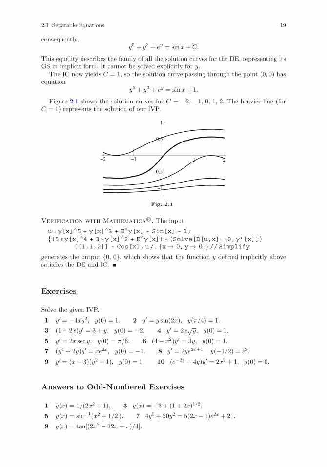
consequently,y5 + y3 + ey = sinx+ C.
This equality describes the family of all the solution curves for the DE, representing itsGS in implicit form. It cannot be solved explicitly for y.
The IC now yields C = 1, so the solution curve passing through the point (0, 0) hasequation
y5 + y3 + ey = sinx+ 1.
Figure 2.1 shows the solution curves for C = −2, −1, 0, 1, 2. The heavier line (forC = 1) represents the solution of our IVP.
1 2
0.5
1
−1
−1
−0.5
−2
Fig. 2.1
Verification with Mathematica R©. The input
u=y[x]∧5 + y[x]∧3 + E∧y[x] - Sin[x] - 1;{(5 ∗y[x]∧4 + 3 ∗y[x]∧2 + E∧y[x]) ∗(Solve[D[u,x]==0,y’[x]])
[[1,1,2]] - Cos[x],u/. {x→ 0,y→ 0}}//Simplifygenerates the output {0, 0}, which shows that the function y defined implicitly abovesatisfies the DE and IC.
Exercises
Solve the given IVP.
1 y′ = −4xy2, y(0) = 1. 2 y′ = y sin(2x), y(π/4) = 1.
3 (1 + 2x)y′ = 3 + y, y(0) = −2. 4 y′ = 2x√y, y(0) = 1.
5 y′ = 2x sec y, y(0) = π/6. 6 (4− x2)y′ = 3y, y(0) = 1.
7 (y4 + 2y)y′ = xe2x, y(0) = −1. 8 y′ = 2ye2x+1, y(−1/2) = e2.
9 y′ = (x− 3)(y2 + 1), y(0) = 1. 10 (e−2y + 4y)y′ = 2x2 + 1, y(0) = 0.
Answers to Odd-Numbered Exercises
1 y(x) = 1/(2x2 + 1). 3 y(x) = −3 + (1 + 2x)1/2.
5 y(x) = sin−1(x2 + 1/2 ). 7 4y5 + 20y2 = 5(2x− 1)e2x + 21.
9 y(x) = tan[(2x2 − 12x+ π)/4].
20 2 First-Order Equations
2.2 Linear Equations
The standard form of this type of DE is
y′ + p(t)y = q(t), (2.3)
where p and q are prescribed functions. To solve the equation, we first multiply it by anunknown nonzero function μ(t), called an integrating factor. Omitting, for simplicity,the mention of the variable t, we have
μy′ + μpy = μq. (2.4)
We now choose μ so that the left-hand side in (2.4) is the derivative of the product μy;that is,
μy′ + μpy = (μy)′ = μy′ + μ′y.
Clearly, this occurs ifμ′ = μp.
The above separable equation yields, in the usual way,
∫dμ
μ=
∫p dt.
Integrating, we arrive at
ln |μ| =∫
p dt,
so, as in Example 2.4,
μ = C exp
{∫p dt
}, C = const �= 0.
Since we need just one such function, we may take C = 1 and thus consider the inte-grating factor
μ(t) = exp
{∫p(t) dt
}. (2.5)
With this choice of μ, equation (2.4) becomes
(μy)′ = μq; (2.6)
hence,
μy =
∫μq dt+ C,
or
y(t) =1
μ(t)
{∫μ(t)q(t) dt+ C
}. (2.7)
2.7 Remarks. (i) Technically, C does not need to be inserted explicitly in (2.7) sincethe indefinite integral on the right-hand side produces an arbitrary constant, but itis good practice to have it in the formula for emphasis and to prevent its accidentalomission when the integration is performed.
(ii) It should be obvious that the factor 1/μ cannot be moved inside the integral to becanceled with the factor μ already there.
2.2 Linear Equations 21
(iii) Points (i) and (ii) become moot if the equality (μy)′ = μq (see (2.6)) is integratedfrom some admissible value t0 to a generic value t. Then
μ(t)y(t)− μ(t0)y(t0) =
t∫t0
μ(τ)q(τ) dτ,
from which we easily deduce that
y(t) =1
μ(t)
{ t∫t0
μ(τ)q(τ) dτ + μ(t0)y(t0)
}. (2.8)
In the case of an IVP, it is convenient to choose t0 as the point where the IC isprescribed.
(iv) In (2.8) we used the ‘dummy’ variable τ in the integrand to avoid a clash with theupper limit t of the definite integral.
2.8 Example. Consider the IVP
y′ − 3y = 6, y(0) = −1,
where, by comparison to (2.3), we have p(t) = −3 and q(t) = 6. The GS of the DE iscomputed from (2.5) and (2.7). Thus,
μ(t) = exp
{∫−3 dt
}= e−3t,
so
y(t) = e3t{∫
6e−3t dt+ C
}= e3t(−2e−3t + C) = Ce3t − 2.
Applying the IC, we find that C = 1, which yields the IVP solution
y(t) = e3t − 2.
Alternatively, we could use formula (2.8) with μ as determined above and t0 = 0, toobtain directly
y(t) = e3t{ t∫
0
6e−3τ dτ + μ(0)y(0)
}= e3t
[− 2e−3τ∣∣t0− 1]= e3t − 2.
Verification with Mathematica R©. The input
y=E∧(3 ∗t) - 2;{D[y,t] - 3 ∗y - 6,y/.t→ 0}//Simplify
generates the output {0, −1}.
2.9 Example. The DE in the IVP
ty′ + 4y = 6t2, y(1) = 4
is not in the standard form (2.3). Assuming that t �= 0, we divide the equation by t andrewrite it as
22 2 First-Order Equations
y′ +4
ty = 6t.
This shows that p(t) = 4/t and q(t) = 6t, so, by (2.5),
μ(t) = exp
{∫4
tdt
}= e4 ln |t| = eln(t
4) = t4.
Using (2.8) with t0 = 1, we now find the solution of the IVP to be
y(t) = t−4
{ t∫1
6τ5 dτ + μ(1)y(1)
}= t−4
(τ6∣∣t1+ 4)= t−4(t6 + 3) = t2 + 3t−4.
Verification with Mathematica R©. The input
y=t∧2 + 3 ∗t∧(-4);{t ∗D[y,t] + 4 ∗y - 6 ∗t∧2,y/.t→ 1}//Simplify
generates the output {0, 4}.
2.10 Example. To bring the DE in the IVP
y′ = (2 + y) sin t, y(π/2) = −3
to the standard form, we move the y-term to the left-hand side and write
y′ − y sin t = 2 sin t.
This shows that p(t) = − sin t and q(t) = 2 sin t; hence, by (2.5),
μ(t) = exp
{−∫
sin t dt
}= ecos t,
and, by (2.8) with t0 = π/2,
y(t) = e− cos t
{2
t∫π/2
ecos τ sin τ dτ + μ(π/2)y(π/2)
}
= e− cos t
{− 2
t∫π/2
ecos τ d(cos τ)− 3
}= e− cos t
(− 2ecos τ∣∣tπ/2
− 3)
= e− cos t(−2ecos t − 1) = −e− cos t − 2.
Verification with Mathematica R©. The input
y=-E∧(-Cos[t]) - 2;{D[y,t] - (2 + y) ∗Sin[t],y/.t→ Pi/2}//Simplify
generates the output {0, −3}.
2.11 Example. Consider the IVP
(t2 + 1)y′ − ty = 2t(t2 + 1)2, y(0) = 23 .
2.2 Linear Equations 23
Proceeding as in Example 2.9, we start by rewriting the DE in the standard form
y′ − t
t2 + 1y = 2t(t2 + 1).
Then, with p(t) = −t/(t2 + 1) and q(t) = 2t(t2 + 1), we have, first,
μ(t) = exp
{−∫
t
t2 + 1dt
}= exp
{− 1
2
∫d(t2 + 1)
t2 + 1
}
= e−(1/2) ln(t2+1) = eln[(t2+1)−1/2] = (t2 + 1)−1/2,
followed by
y(t) = (t2 + 1)1/2{ t∫
0
(τ2 + 1)−1/22τ(τ2 + 1) dτ + μ(0)y(0)
}
= (t2 + 1)1/2{ t∫
0
(τ2 + 1)1/2 d(τ2 + 1) + 23
}
= (t2 + 1)1/2{23 (τ
2 + 1)3/2∣∣t0+ 2
3
}= 2
3 (t2 + 1)2.
Verification with Mathematica R©. The input
y=(2/3) ∗(t∧2 + 1)∧2;{(t∧2 + 1) ∗D[y,t] - t ∗y - 2 ∗t ∗(t∧2 + 1)∧2,y/.t→ 0}//Simplify
generates the output{0, 2/3
}.
2.12 Example. The standard form of the DE in the IVP
(t− 1)y′ + y = (t− 1)et, y(2) = 3
is
y′ +1
t− 1y = et,
so p(t) = 1/(t− 1) and q(t) = et. Consequently, for t �= 1,
μ(t) = exp
{∫1
t− 1dt
}= eln |t−1| = |t− 1| =
{t− 1, t > 1,
−(t− 1), t < 1.
Since formula (2.8) uses the value of μ at t0 = 2 > 1, we take μ(t) = t − 1 and, afterintegration by parts and simplification, obtain the solution
y(t) =1
t− 1
{ t∫2
(τ − 1)eτ dτ + μ(2)y(2)
}=
(t− 2)et + 3
t− 1.
Verification with Mathematica R©. The input
y=((t - 2) ∗E∧t + 3)/(t - 1);{(t-1) ∗D[y,t] + y - (t - 1) ∗E∧t,y/.t→ 2}//Simplify
generates the output {0, 3}.
24 2 First-Order Equations
2.13 Remark. If we do not have an IC and want to find only the GS of the equationin Example 2.12, it does not matter if we take μ to be t−1 or −(t−1) since μ has to bereplaced in (2.6) and, in the latter case, the ‘−’ sign would cancel out on both sides.
Exercises
Solve the given IVP.
1 y′ + 4y + 16 = 0, y(0) = −2. 2 y′ + y = 4te−3t, y(0) = 3.
3 2ty′ + y + 12t√t = 0, y(1) = −1. 4 t2y′ + 3ty = 4e2t, y(1) = e2.
5 (t− 2)y′ + y = 8(t− 2) cos(2t), y(π) = 2/(π − 2).
6 y′ + y cot t = 2 cos t, y(π/2) = 1/2.
7 (t2 + 2)y′ + 2ty = 3t2 − 4t, y(0) = 3/2.
8 ty′ + (2t− 1)y = 9t3et, y(1) = 2e−2 + 2e.
9 (t2 − 1)y′ + 4y = 3(t+ 1)2(t2 − 1), y(0) = 0.
10 (t2 + 2t)y′ + y =√t, y(2) = 0.
Answers to Odd-Numbered Exercises
1 y = 2e−4t − 4. 3 y = (2− 3t2)t−1/2.
5 y = [2 cos(2t) + 4(t− 2) sin(2t)]/(t− 2). 7 y = (t3 − 2t2 + 3)/(t2 + 2).
9 y = (t3 − 3t2 + 3t)(t+ 1)2/(t− 1)2.
2.3 Homogeneous Polar Equations
These are DEs of the formy′(x) = f
(y
x
), (2.9)
where f is a given one-variable function. Making the substitution
y(x) = xv(x) (2.10)
and using the fact that, by the product rule, y′ = v + xv′, from (2.9) we see that thenew unknown function v satisfies the DE
xv′ + v = f(v),
ordv
dx=
f(v)− v
x.
This is a separable equation, so ∫dv
f(v)− v=
∫dx
x, (2.11)
2.3 Homogeneous Polar Equations 25
which, with v replaced by y/x in the result, produces the GS of (2.9). Clearly, in thistype of problem we must assume that x �= 0.
2.14 Example. The DE in the IVP
xy′ = x+ 2y, y(1) = 1
can be written asy′ = 1 + 2
y
x,
so f(v) = 1 + 2v. Then f(v)− v = v + 1 and, by (2.11),
∫dv
v + 1=
∫dx
x,
which yieldsln |v + 1| = ln |x|+ C.
Exponentiating and simplifying, we find that
v + 1 = C1x;
hence, using (2.10), we obtain the GS
y = C1x2 − x.
The constant is found from the IC; specifically, C1 = 2, so the solution of the IVP is
y(x) = 2x2 − x.
Verification with Mathematica R©. The input
y=2 ∗x∧2 - x;{x ∗D[y,x] - x - 2 ∗y,y/.x→ 1}//Simplify
generates the output {0, 1}.
2.15 Example. Consider the IVP
(x2 + 2xy)y′ = 2(xy + y2), y(1) = 2.
Solving for y′ and then dividing both numerator and denominator by x2 brings the DEto the form
y′ =2(xy + y2)
x2 + 2xy=
2y
x+ 2
(y
x
)2
1 + 2y
x
=2(v + v2)
1 + 2v= f(v),
from which
f(v)− v =2(v + v2)
1 + 2v− v =
v
1 + 2v.
By (2.11), we have ∫1 + 2v
vdv =
∫ (2 +
1
v
)dv =
∫dx
x,
26 2 First-Order Equations
so2v + ln |v| = ln |x|+ C,
or, according to (2.10),
2y
x+ ln
∣∣∣∣ yx2∣∣∣∣ = C.
Applying the IC, we get C = 4+ln 2; hence, the solution of the IVP is defined implicitlyby the equality
2y
x+ ln
∣∣∣∣ y
2x2
∣∣∣∣ = 4.
Verification with Mathematica R©. The input
u=2 ∗y[x]/x + Log[y[x]/(2 ∗x∧2)]-4;{(x∧2 + 2 ∗x ∗y[x]) ∗(Solve[D[u,x]==0,y’[x]])[[1,1,2]]
- 2 ∗(x ∗y[x] + y[x]∧2),u/. {x→ 1,y[x]→ 2}}//Simplifygenerates the output {0, 0}.
Exercises
Solve the given IVP, or find the GS of the DE if no IC is given.
1 xy′ = 3y − x, y(1) = 1. 2 x2y′ = xy + y2.
3 3xy2y′ = x3 + 3y3. 4 x2y′ − 2xy − y2 = 0, y(1) = 1.
5 (2x2 − xy)y′ = xy − y2.
6 (2x2 − 3xy)y′ = x2 + 2xy − 3y2.
Answers to Odd-Numbered Exercises
1 y(x) = (x3 + x)/2. 3 y(x) = x(C + ln |x|)1/3. 5 y(x) = x[ln(y2/|x|) +C].
2.4 Bernoulli Equations
The general form of a Bernoulli equation is
y′ + p(t)y = q(t)yn, n �= 1. (2.12)
Making the substitutiony(t) = (w(t))1/(1−n) (2.13)
and using the chain rule, we have
y′ =1
1− nw1/(1−n)−1w′ =
1
1− nwn/(1−n)w′,
so (2.12) becomes
2.4 Bernoulli Equations 27
1
1− nwn/(1−n)w′ + pw1/(1−n) = qwn/(1−n).
Since 1/(1− n)− n/(1− n) = 1, after division by wn/(1−n) and multiplication by 1− nthis simplifies further to
w′ + (1− n)pw = (1 − n)q. (2.14)
Equation (2.14) is linear and can be solved by the method described in Sect. 2.2. Onceits solution w has been found, the GS y of (2.12) is given by (2.13).
2.16 Example. Comparing the DE in the IVP
y′ + 3y + 6y2 = 0, y(0) = −1
to (2.12), we see that this is a Bernoulli equation with p(t) = 3, q(t) = −6, and n = 2.Substitution (2.13) in this case is y = w−1; hence,
y′ = −w−2w′, w(0) = (y(0))−1 = −1,
so the IVP becomesw′ − 3w = 6, w(0) = −1.
This problem was solved in Example 2.8, and its solution is
w(t) = e3t − 2;
hence, the solution of the IVP for y is
y(t) = (w(t))−1 =1
e3t − 2.
Verification with Mathematica R©. The input
y=(E∧(3 ∗t) - 2)∧(-1);{D[y,t] + 3 ∗y + 6 ∗y∧2,y/.t→ 0}//Simplify
generates the output {0, −1}.
2.17 Example. For the DE in the IVP
ty′ + 8y = 12t2√y, y(1) = 16
we have p(t) = 8/t, q(t) = 12t, and n = 1/2; therefore, by (2.13), we substitute y = w2
and, since y′ = 2ww′, arrive at the new IVP
tw′ + 4w = 6t2, w(1) = 4.
From Example 2.9 we see that w(t) = t2 + 3t−4, so
y(t) = (w(t))2 = (t2 + 3t−4)2.
Verification with Mathematica R©. The input
y=(t∧2 + 3 ∗t∧(-4))∧2;Simplify[{t ∗D[y,t] + 8 ∗y - 12 ∗t∧2 ∗Sqrt[y],y/.t→ 1},t>0]
generates the output {0, 16}.
28 2 First-Order Equations
Exercises
Solve the given IVP, or find the GS of the DE if no IC is given.
1 y′ + y = −y3, y(0) = 1. 2 2ty′ + 3y = 9y−1/3, y(1) = 1.
3 y′ − y + 6ety3/2 = 0, y(0) = 1/4. 4 9y′ + 2y = 30e−2ty−1/2, y(0) = 41/3.
5 3ty′ − y = 4t2y−2, y(1) = 61/3. 6 5t2y′ + 2ty = 2y−3/2.
Answers to Odd-Numbered Exercises
1 y(t) = (2e2t − 1)−1/2. 3 y(t) = e−2t/4. 5 y(t) = (4t2 + 2t)1/3.
2.5 Riccati Equations
The general form of these DEs is
y′ = q0(t) + q1(t)y + q2(t)y2, (2.15)
where q0, q1, and q2 are given functions, with q0, q2 �= 0. After some analytic manipu-lation, we can rewrite (2.15) as
v′′ + p1(t)v′ + p2(t)v = 0. (2.16)
This is a second-order DE whose coefficients p1 and p2 are combinations of q0, q1, q2,and their derivatives. In general, the solution of (2.16) cannot be obtained be means ofintegrals. However, when we know a PS y1 of (2.15), we are able to compute the GS ofthat equation by reducing it to a linear first-order DE by means of the substitution
y = y1 +1
w. (2.17)
In view of (2.15) and (2.17), we then have
y′ = y′1 −w′
w2= q0 + q1
(y1 +
1
w
)+ q2
(y1 +
1
w
)2
.
Since y1 is a solution of (2.15), it follows that
q0 + q1y1 + q2y21 −
w′
w2= q0 + q1y1 +
q1w
+ q2y21 + 2
q2y1w
+q2w2
,
which, after a rearrangement of the terms, becomes
w′ + (q1 + 2q2y1)w = −q2. (2.18)
Equation (2.18) is now solved by the method described in Sect. 2.2.The matrix version of the Riccati equation occurs in optimal control. Its practical
importance and the fact that it cannot be solved by means of integrals have led to thedevelopment of the so-called qualitative theory of differential equations.
2.5 Riccati Equations 29
2.18 Example. The DE in the IVP
y′ = −1− t2 + 2(t−1 + t)y − y2, y(1) = 107
is of the form (2.15) with q0(t) = −1− t2, q1(t) = 2(t−1 + t), and q2(t) = −1, and it iseasy to check that y1(t) = t satisfies it; hence, according to (2.18),
w′ + 2t−1w = 1,
whose solution, constructed by means of (2.5) and (2.7), is
w(t) = 13 t+ Ct−2.
Next, by (2.17),
y(t) = t+3t2
t3 + 3C.
The constant C is determined from the IC as C = 2, so the solution of the IVP is
y(t) =t4 + 3t2 + 6t
t3 + 6.
Verification with Mathematica R©. The input
y=(t∧4 + 3 ∗t∧2 + 6 ∗t)/(t∧3 + 6);Simplify[{D[y,t] + 1 + t∧2 - 2 ∗(t∧( - 1) + t) ∗y + y∧2,y/.t→ 1}]
generates the output {0, 10/7}.
2.19 Example. The IVP
y′ = − cos t+ (2− tan t)y − (sec t)y2, y(0) = 0
admits the PS y1(t) = cos t. Then substitution (2.17) is y = cos t+ 1/w, and the linearfirst-order equation (2.18) takes the form
w′ − (tan t)w = sec t,
with GS
w(t) =t+ C
cos t,
from which
y(t) =
(1 +
1
t+ C
)cos t.
The IC now yields C = −1, so the solution of the IVP is
y(t) =t cos t
t− 1.
Verification with Mathematica R©. The input
y=(t + Cos[t])/(t - 1);Simplify[{D[y,t] + Cos[t] - (2 - Tan[t]) ∗y + Sec[t] ∗y∧2,
y/.t→ 0}]generates the output {0, 0}.
30 2 First-Order Equations
Exercises
In the given IVP, verify that y1 is a solution of the DE, use the substitution y = y1+1/wto reduce the DE to a linear first-order equation, then find the solution of the IVP.
1 y′ = t−2 + 3t−1 − (4t−1 + 3)y + 2y2, y(1) = 5/2; y1(t) = 1/t.
2 y′ = −(t2 + 6t+ 4) + 2(t+ 3)y − y2, y(0) = 9/5; y1(t) = t+ 1.
3 y′ = 3t−2 − t−4 + 2(t−1 − t−3)y − t−2y2, y(1) = −1/2; y1(t) = −1/t.
4 y′ = 4t− 4e−t2 + (2t− 4e−t2)y − e−t2y2, y(0) = −1; y1(t) = −2.
5 y′ = 2−4 cos t+4 sin t+(4 cos t−4 sin t−1)y+(sin t−cos t)y2, y(0) = 3; y1(t) = 2.
6 y′ = 2t2 − 1− t tan t+ (4t− tan t)y + 2y2, y(π/4) = −1/2− π/4; y1(t) = −t.
Answers to Odd-Numbered Exercises
1 y(t) = (3t+ 2)/(2t). 3 y(t) = (t3 − t− 1)/(t2 + t).
5 y(t) = 2 + 1/(et + sin t).
2.6 Exact Equations
Consider an equation of the form
P (x, y) +Q(x, y)y′ = 0, (2.19)
where P and Q are given two-variable functions. Recalling that the differential of afunction y = y(x) is dy = y′(x) dx, we multiply (2.19) by dx and rewrite it as
P dx+Qdy = 0. (2.20)
The DE (2.19) is called an exact equation when the left-hand side above is the differentialof a function f(x, y). If f is found, then (2.20) becomes
df(x, y) = 0,
with GSf(x, y) = C, C = const. (2.21)
2.20 Remark. Suppose that such a function f exists; then (see item (iv) in Sect. 1.1)
df = fx dx+ fy dy,
so, by comparison to (2.20), this happens if
fx = P, fy = Q. (2.22)
In view of the comment made in item (iii) in Sect. 1.1, we have fxy = fyx, which, by(2.22), translates as
Py = Qx. (2.23)
2.6 Exact Equations 31
Therefore, if a function of the desired type exists, then equality (2.23) must hold.The other way around, it turns out that for coefficients P and Q continuously differ-
entiable in an open disc in the (x, y)-plane, condition (2.23), if satisfied, guarantees theexistence of a function f with the required property. Since in all our examples P andQ meet this degree of smoothness, we simply confine ourselves to checking that (2.23)holds and, when it does, determine f from (2.22).
2.21 Example. For the DE in the IVP
y2 − 4xy3 + 2 + (2xy − 6x2y2)y′ = 0, y(1) = 1
we haveP (x, y) = y2 − 4xy3 + 2, Q(x, y) = 2xy − 6x2y2,
soPy = 2y − 12xy2 = Qx,
which means that the equation is exact. Then, according to Remark 2.20, there is afunction f = f(x, y) such that
fx(x, y) = P (x, y) = y2 − 4xy3 + 2,
fy(x, y) = Q(x, y) = 2xy − 6x2y2.(2.24)
Integrating, say, the first equation (2.24) with respect to x, we find that
f(x, y) =
∫fx(x, y) dx =
∫P (x, y) dx
=
∫(y2 − 4xy3 + 2) dx = xy2 − 2x2y3 + 2x+ g(y),
where, as mentioned in item (vi) in Sect. 1.1, g is an arbitrary function of y. To find g,we use this expression of f in the second equation (2.24):
fy(x, y) = 2xy − 6x2y2 + g′(y) = 2xy − 6x2y2;
consequently, g′(y) = 0, from which g(y) = c = const. Since, by (2.21), we equate fto an arbitrary constant, it follows that, without loss of generality, we may take c = 0.Therefore, the GS of the DE is defined implicitly by the equality
xy2 − 2x2y3 + 2x = C.
Using the IC, we immediately see that C = 1; hence,
xy2 − 2x2y3 + 2x = 1
is the equation of the solution curve for the given IVP.Instead of integrating fx, we could equally start by integrating fy from the second
equation (2.24); that is,
f(x, y) =
∫fy(x, y) dy =
∫Q(x, y) dy
=
∫(2xy − 6x2y2) dy = xy2 − 2x2y3 + h(x),
32 2 First-Order Equations
where h is a function of x to be found by means of the first equation (2.24). Using thisexpression of f in that equation, we have
fx(x, y) = y2 − 4xy3 + h′(x) = y2 − 4xy3 + 2,
so h′(x) = 2, giving h(x) = 2x. (Just as before, and for the same reason, we suppress theintegration constant.) This expression of h gives rise to the same function f as above.
Verification with Mathematica R©. The input
u=x ∗y[x]∧2 - 2 ∗x∧2 ∗y[x]∧3 + 2 ∗x - 1;{y[x]∧2 - 4 ∗x ∗y[x]∧3 + 2 + (2 ∗x ∗y[x] - 6 ∗x∧2 ∗y[x]∧2)
∗(Solve[D[u,x]==0,y’[x]])[[1,1,2]],u/. {x→ 1,y[x]→ 1}}//Simplify
generates the output {0, 0}, which confirms that the function y defined implicitly bythe equation of the solution curve satisfies both the DE and the IC.
2.22 Example. The DE in the IVP
6xy−1 + 8x−3y3 + (4y − 3x2y−2 − 12x−2y2)y′ = 0, y(1) = 12
has P (x, y) = 6xy−1 + 8x−3y3 and Q(x, y) = 4y − 3x2y−2 − 12x−2y2. Obviously, herewe must have x, y �= 0.
SincePy(x, y) = −6xy−2 + 24x−3y2 = Qx(x, y),
it follows that this is an exact equation. The function f we are seeking, obtained as inExample 2.21, is
f(x, y) =
∫fx(x, y) dx =
∫P (x, y) dx
=
∫(6xy−1 + 8x−3y3) dx = 3x2y−1 − 4x−2y3 + g(y),
with g determined from
fy(x, y) = −3x2y−2 − 12x−2y2 + g′(y) = 4y − 3x2y−2 − 12x−2y2;
hence, g′(y) = 4y, so g(y) = 2y2, which produces the GS of the DE in the implicit form
3x2y−1 − 4x−2y3 + 2y2 = C.
The IC now yields C = 6.
Verification with Mathematica R©. The input
u=3 ∗x∧2 ∗y[x]∧(-1) - 4 ∗x∧(-2) ∗y[x]∧3 + 2 ∗y[x]∧2-6;{6 ∗x ∗y[x]∧(-1) + 8 ∗x∧(-3) ∗y[x]∧3 + (4 ∗y[x]
- 3 ∗x∧2 ∗y[x]∧(-2) - 12 ∗x∧(-2) ∗y[x]∧2)∗(Solve[D[u,x]==0,y’[x]])[[1,1,2]],u/. {x→ 1,y[x]→ 1/2}}//Simplify
generates the output {0, 0}.
2.6 Exact Equations 33
2.23 Example. Consider the IVP
x sin(2y)− 3x2 +(y + x2 cos(2y)
)y′ = 0, y(1) = π.
Since, as seen from the left-hand side of the DE, we have P (x, y) = x sin(2y)− 3x2 andQ(x, y) = y + x2 cos(2y), we readily verify that
Py(x, y) = 2x cos(2y) = Qx(x, y),
so this is an exact equation. Then, integrating, say, the y-derivative of the desiredfunction f , we find that
f(x, y) =
∫fy(x, y) dy =
∫Q(x, y) dy
=
∫[y + x2 cos(2y)] dy = 1
2 y2 + 1
2 x2 sin(2y) + g(x).
The function g is determined by substituting this expression in the x-derivative of f ;that is,
fx(x, y) = x sin(2y) + g′(x) = x sin(2y)− 3x2,
which yields g′(x) = −3x2; therefore, g(x) = −x3, and we obtain the function
f(x, y) = 12 y
2 + 12 x
2 sin(2y)− x3.
Writing the GS of the DE as f(x, y) = C and using the IC, we find that C = π2/2− 1,so the solution of the IVP is given in implicit form by
y2 + x2 sin(2y)− 2x3 = π2 − 2.
Verification with Mathematica R©. The input
u=y[x]∧2 + x∧2 ∗Sin[2 ∗y[x]] - 2 ∗x∧3 - Pi∧2 + 2;{x ∗Sin[2 ∗y[x]] - 3 ∗x∧2 + (y[x] + x∧2 ∗Cos[2∧y[x]])
∗(Solve[D[u,x]==0,y’[x]])[[1,1,2]],u/. {x→ 1,y[x]→Pi}}//Simplify
generates the output {0, 0}.
2.24 Example. The general procedure does not work for the IVP
2y−2 − 4xy + 1+ (2xy−1 − 6x2)y′ = 0, y(1) = 1
because here, with P (x, y) = 2y−2 − 4xy + 1 and Q(x, y) = 2xy−1 − 6x2, we have
Py(x, y) = −4y−3 − 4x �= Qx(x, y) = 2y−1 − 12x,
so the DE is not exact. However, it may be possible to transform the equation into anexact one by using an integrating factor μ(x, y). Writing the DE as P + Qy′ = 0 andmultiplying it by μ, we arrive at P1 +Q1y
′ = 0, where P1 = Pμ and Q1 = Qμ. We nowtry to find a function μ such that (P1)y = (Q1)x; that is, (Pμ)y = (Qμ)x, which leadsto the partial differential equation
Pμy + Pyμ = Qμx +Qxμ. (2.25)
34 2 First-Order Equations
Since, in general, this equation may be difficult to solve, we attempt to see if μ can befound in a simpler form, for example, as a one-variable function. In our case, let us tryμ = μ(y). Then (2.25) simplifies to
Pμ′ = (Qx − Py)μ,
and with our specific P and Q we get
μ′ =2y−1 − 12x+ 4y−3 + 4x
2y−2 − 4xy + 1μ =
2(y−1 − 4x+ 2y−3)
y(2y−3 − 4x+ y−1)μ =
2
yμ,
which is a separable equation with solution μ(y) = y2. Multiplying the DE in the givenIVP by y2, we arrive at the new problem
2− 4xy3 + y2 + (2xy − 6x2y2)y′ = 0, y(1) = 1.
This IVP was solved in Example 2.21.
2.25 Remark. It should be pointed out that, in general, looking for an integrating fac-tor of a certain form is a matter of trial and error, and that, unless some special featureof the equation gives us a clear hint, this type of search might prove unsuccessful.
Exercises
In 1–6, solve the given IVP, or find the GS of the DE if no IC is given.
1 4xy + (2x2 − 6y)y′ = 0, y(1) = 1.
2 12x−4 + 2xy−3 + 6x2y + (2x3 − 3x2y−4)y′ = 0, y(1) = 2.
3 3x2y−2 + x−2y2 − 2x−3 + (6y−4 − 2x3y−3 − 2x−1y)y′ = 0, y(1) = −1.
4 2x sin y − y cosx+ (x2 cos y − sinx)y′ = 0, y(π/2) = π/2.
5 2e2x − 2 sin(2x) sin y + [2y−3 + cos(2x) cos y]y′ = 0, y(0) = π/2.
6 (x+ y)−1 − x−2 − 4 cos(2x− y) + [(x+ y)−1 + 2 cos(2x− y)]y′ = 0, y(π/2) = 0.
In 7–10, find an integrating factor (of the indicated form) that makes the DE exact,then solve the given IVP or find the GS of the DE if no IC is given.
7 y + 3y−1 + 2xy′ = 0, y(1) = 1, μ = μ(y).
8 2xy + y2 + xyy′ = 0, y(1) = 2, μ = μ(y).
9 1 + 2x2 − (x+ 4xy)y′ = 0, μ = μ(x).
10 −2x3 − y + (x+ 2x2)y′ = 0, y(1) = 1, μ = μ(x).
Answers to Odd-Numbered Exercises
1 2x2y − 3y2 + 1 = 0. 3 x−2 − 2y−3 + x3y−2 − x−1y2 = 3.
5 cos(2x) sin y + e2x − y−2 = 2− 4/π2. 7 3x+ xy2 = 4.
9 x2 + ln |x| − y − 2y2 = C.
2.7 Existence and Uniqueness Theorems 35
2.7 Existence and Uniqueness Theorems
Before attempting to solve an IVP or BVP for a mathematical model, it is essential toconvince ourselves that the problem is uniquely solvable. This requirement is based onthe reasonable expectation that, as mentioned at the beginning of Sect. 1.3, a physicalsystem has one and only one response to a given set of admissible constraints.
Assertions that provide conditions under which a given problem has a unique solutionare called existence and uniqueness theorems. We discuss the linear and nonlinear casesseparately.
2.26 Theorem. Let J be an open interval of the form a < t < b, let t0 be a point in J ,and consider the IVP
y′ + p(t)y = q(t), y(t0) = y0, (2.26)
where y0 is a given initial value. If p and q are continuous on J , then the IVP (2.26)has a unique solution on J for any y0.
2.27 Remark. In fact, we already know that the unique solution mentioned inTheorem 2.26 can be constructed by means of formulas (2.5) and (2.8).
2.28 Definition. The largest open interval J on which an IVP has a unique solutionis called the maximal interval of existence for that solution.
2.29 Remarks. (i) Theorem 2.26 gives no indication as to what the maximal intervalof existence for the solution might be. This needs to be determined by other means—for example, by computing the solution explicitly when such computation is possible.
(ii) If no specific mention is made of an interval associated with an IVP, we assumethat this is the maximal interval of existence as defined above.
(iii) Many IVPs of the form (2.26) model physical processes in which the DE is mean-ingful only for t > 0. This would seem to create a problem when we try to applyTheorem 2.26 because an open interval of the form 0 < t < b does not contain thepoint t0 = 0 where the IC is prescribed. A brief investigation, however, will easilyconvince us that, in fact, there is no inconsistency here. If the IVP in question iscorrectly formulated, we will find that the maximal interval of existence for thesolution is larger than 0 < t < b, extending to the left of the point t0 = 0. TheDE is formally restricted to the interval 0 < t < b simply because that is where itmakes physical sense.
2.30 Example. In the IVP
y′ − (t2 + 1)y = sin t, y(1) = 2
we have
p(t) = −(t2 + 1), q(t) = sin t.
Since both p and q are continuous on the interval −∞ < t < ∞, from Theorem 2.26 itfollows that this IVP has a unique solution on the entire real line.
2.31 Example. Bringing the equation in the IVP
(t+ 1)y′ + y = e2t, y(2) = 3
36 2 First-Order Equations
to the standard form, we see that
p(t) =1
t+ 1, q(t) =
e2t
t+ 1.
The functions p and q are continuous on each of the open intervals −∞ < t < −1 and−1 < t < ∞; they are not defined at t = −1. Since the IC is given at t0 = 2 > −1,from Theorem 2.26 we conclude that the IVP has a unique solution in the interval−1 < t < ∞.
2.32 Remark. If the IC in Example 2.31 were replaced by, say, y(−5) = 2, then,according to Theorem 2.26, the IVP would have a unique solution in the open interval−∞ < t < −1, which contains the point t0 = −5.
2.33 Example. To get a better understanding of the meaning and limitations of The-orem 2.26, consider the IVP
ty′ − y = 0, y(t0) = y0,
where p(t) = −1/t and q(t) = 0. The function q is continuous everywhere, but p iscontinuous only for t > 0 or t < 0 since it is not defined at t = 0. Treating the DE aseither a separable or linear equation, we find that its GS is
y(t) = Ct. (2.27)
The IC now yields y0 = Ct0, which gives rise to three possibilities.
(i) If t0 �= 0, then, by Theorem 2.26, the IVP is guaranteed to have a unique solution
y(t) =y0t0
t (2.28)
on any open interval containing t0 but not containing 0; more specifically, on anyinterval of the form 0 < a < t < b (if t0 > 0) or a < t < b < 0 (if t0 < 0). However,direct verification shows that the function (2.28) satisfies the DE at every real valueof t, so its maximal interval of existence is the entire real line.
(ii) If t0 = 0 but y0 �= 0, then the IVP has no solution since the equality y0 = Ct0 = 0is impossible for any value of C.
(iii) If t0 = y0 = 0, then the IVP has infinitely many solutions, given by (2.27) with anyconstant C, each of them existing on the entire real line.
The ‘anomalous’ cases (ii) and (iii) are explained by the fact that they prescribe theIC at the point where p is undefined, so Theorem 2.26 does not apply.
We now turn our attention to the nonlinear case.
2.34 Theorem. Consider the IVP
y′ = f(t, y), y(t0) = y0, (2.29)
where f is a given function such that f and fy are continuous in an open rectangle
R = {(t, y) : a < t < b, c < y < d}. (2.30)
If the point (t0, y0) lies in R, then the IVP (2.29) has a unique solution in some openinterval J of the form t0 − h < t < t0 + h contained in the interval a < t < b.
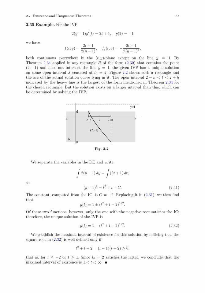
2.7 Existence and Uniqueness Theorems 37
2.35 Example. For the IVP
2(y − 1)y′(t) = 2t+ 1, y(2) = −1
we have
f(t, y) =2t+ 1
2(y − 1), fy(t, y) = − 2t+ 1
2(y − 1)2,
both continuous everywhere in the (t, y)-plane except on the line y = 1. ByTheorem 2.34 applied in any rectangle R of the form (2.30) that contains the point(2,−1) and does not intersect the line y = 1, the given IVP has a unique solutionon some open interval J centered at t0 = 2. Figure 2.2 shows such a rectangle andthe arc of the actual solution curve lying in it. The open interval 2 − h < t < 2 + hindicated by the heavy line is the largest of the form mentioned in Theorem 2.34 forthe chosen rectangle. But the solution exists on a larger interval than this, which canbe determined by solving the IVP.
y=1
R
ba
c
d))
(2,−1)
2−h 2+h2
Fig. 2.2
We separate the variables in the DE and write
∫2(y − 1) dy =
∫(2t+ 1) dt,
so(y − 1)2 = t2 + t+ C. (2.31)
The constant, computed from the IC, is C = −2. Replacing it in (2.31), we then findthat
y(t) = 1± (t2 + t− 2)1/2.
Of these two functions, however, only the one with the negative root satisfies the IC;therefore, the unique solution of the IVP is
y(t) = 1− (t2 + t− 2)1/2. (2.32)
We establish the maximal interval of existence for this solution by noticing that thesquare root in (2.32) is well defined only if
t2 + t− 2 = (t− 1)(t+ 2) ≥ 0;
that is, for t ≤ −2 or t ≥ 1. Since t0 = 2 satisfies the latter, we conclude that themaximal interval of existence is 1 < t < ∞.
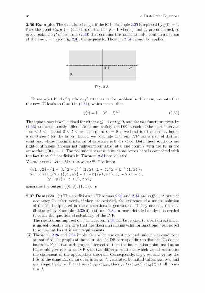
38 2 First-Order Equations
2.36 Example. The situation changes if the IC in Example 2.35 is replaced by y(0) = 1.Now the point (t0, y0) = (0, 1) lies on the line y = 1 where f and fy are undefined, soevery rectangle R of the form (2.30) that contains this point will also contain a portionof the line y = 1 (see Fig. 2.3). Consequently, Theorem 2.34 cannot be applied.
(0,1) y=1
R
Fig. 2.3
To see what kind of ‘pathology’ attaches to the problem in this case, we note thatthe new IC leads to C = 0 in (2.31), which means that
y(t) = 1± (t2 + t)1/2. (2.33)
The square root is well defined for either t ≤ −1 or t ≥ 0, and the two functions given by(2.33) are continuously differentiable and satisfy the DE in each of the open intervals−∞ < t < −1 and 0 < t < ∞. The point t0 = 0 is well outside the former, but isa limit point for the latter. Hence, we conclude that our IVP has a pair of distinctsolutions, whose maximal interval of existence is 0 < t < ∞. Both these solutions areright-continuous (though not right-differentiable) at 0 and comply with the IC in thesense that y(0+) = 1. The nonuniqueness issue we came across here is connected withthe fact that the conditions in Theorem 2.34 are violated.
Verification with Mathematica R©. The input
{y1,y2}= {1 + (t∧2 + t)∧(1/2),1 - (t∧2 + t)∧(1/2)};Simplify[{2 ∗({y1,y2} - 1) ∗D[{y1,y2},t] - 2 ∗t - 1,
{y1,y2}/.t→0},t>0]generates the output {{0, 0}, {1, 1}}.
2.37 Remarks. (i) The conditions in Theorems 2.26 and 2.34 are sufficient but notnecessary. In other words, if they are satisfied, the existence of a unique solutionof the kind stipulated in these assertions is guaranteed. If they are not, then, asillustrated by Examples 2.33(ii), (iii) and 2.36, a more detailed analysis is neededto settle the question of solvability of the IVP.The restrictions imposed on f in Theorem 2.34 can be relaxed to a certain extent. Itis indeed possible to prove that the theorem remains valid for functions f subjectedto somewhat less stringent requirements.
(ii) Theorems 2.26 and 2.34 imply that when the existence and uniqueness conditionsare satisfied, the graphs of the solutions of a DE corresponding to distinct ICs do notintersect. For if two such graphs intersected, then the intersection point, used as anIC, would give rise to an IVP with two different solutions, which would contradictthe statement of the appropriate theorem. Consequently, if y1, y2, and y3 are thePSs of the same DE on an open interval J , generated by initial values y01, y02, andy03, respectively, such that y01 < y02 < y03, then y1(t) < y2(t) < y3(t) at all pointst in J .
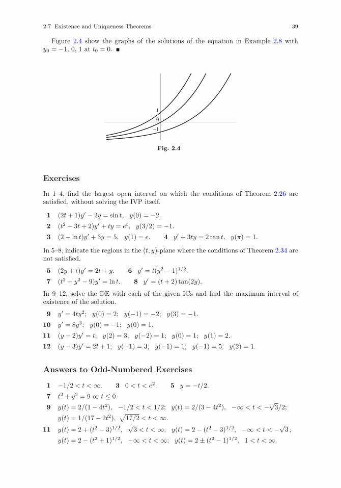
2.7 Existence and Uniqueness Theorems 39
Figure 2.4 show the graphs of the solutions of the equation in Example 2.8 withy0 = −1, 0, 1 at t0 = 0.
−1
0
1
Fig. 2.4
Exercises
In 1–4, find the largest open interval on which the conditions of Theorem 2.26 aresatisfied, without solving the IVP itself.
1 (2t+ 1)y′ − 2y = sin t, y(0) = −2.
2 (t2 − 3t+ 2)y′ + ty = et, y(3/2) = −1.
3 (2− ln t)y′ + 3y = 5, y(1) = e. 4 y′ + 3ty = 2 tan t, y(π) = 1.
In 5–8, indicate the regions in the (t, y)-plane where the conditions of Theorem 2.34 arenot satisfied.
5 (2y + t)y′ = 2t+ y. 6 y′ = t(y2 − 1)1/2.
7 (t2 + y2 − 9)y′ = ln t. 8 y′ = (t+ 2) tan(2y).
In 9–12, solve the DE with each of the given ICs and find the maximum interval ofexistence of the solution.
9 y′ = 4ty2; y(0) = 2; y(−1) = −2; y(3) = −1.
10 y′ = 8y3; y(0) = −1; y(0) = 1.
11 (y − 2)y′ = t; y(2) = 3; y(−2) = 1; y(0) = 1; y(1) = 2.
12 (y − 3)y′ = 2t+ 1; y(−1) = 3; y(−1) = 1; y(−1) = 5; y(2) = 1.
Answers to Odd-Numbered Exercises
1 −1/2 < t < ∞. 3 0 < t < e2. 5 y = −t/2.7 t2 + y2 = 9 or t ≤ 0.
9 y(t) = 2/(1− 4t2), −1/2 < t < 1/2; y(t) = 2/(3− 4t2), −∞ < t < −√3/2;
y(t) = 1/(17− 2t2),√17/2 < t < ∞.
11 y(t) = 2 + (t2 − 3)1/2,√3 < t < ∞; y(t) = 2− (t2 − 3)1/2, −∞ < t < −√
3 ;
y(t) = 2− (t2 + 1)1/2, −∞ < t < ∞; y(t) = 2± (t2 − 1)1/2, 1 < t < ∞.
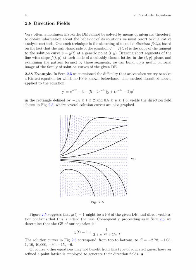
40 2 First-Order Equations
2.8 Direction Fields
Very often, a nonlinear first-order DE cannot be solved by means of integrals; therefore,to obtain information about the behavior of its solutions we must resort to qualitativeanalysis methods. One such technique is the sketching of so-called direction fields, basedon the fact that the right-hand side of the equation y′ = f(t, y) is the slope of the tangentto the solution curve y = y(t) at a generic point (t, y). Drawing short segments of theline with slope f(t, y) at each node of a suitably chosen lattice in the (t, y)-plane, andexamining the pattern formed by these segments, we can build up a useful pictorialimage of the family of solution curves of the given DE.
2.38 Example. In Sect. 2.5 we mentioned the difficulty that arises when we try to solvea Riccati equation for which no PS is known beforehand. The method described above,applied to the equation
y′ = e−2t − 3 + (5− 2e−2t)y + (e−2t − 2)y2
in the rectangle defined by −1.5 ≤ t ≤ 2 and 0.5 ≤ y ≤ 1.6, yields the direction fieldshown in Fig. 2.5, where several solution curves are also graphed.
y=1
Fig. 2.5
Figure 2.5 suggests that y(t) = 1 might be a PS of the given DE, and direct verifica-tion confirms that this is indeed the case. Consequently, proceeding as in Sect. 2.5, wedetermine that the GS of our equation is
y(t) = 1 +1
2 + e−2t + Ce−t.
The solution curves in Fig. 2.5 correspond, from top to bottom, to C = −2.78, −1.05,1, 10, 10,000, −30, −15, −6.
Of course, other equations may not benefit from this type of educated guess, howeverrefined a point lattice is employed to generate their direction fields.
Chapter 3
Mathematical Models with First-OrderEquations
In Sect. 1.2 we listed examples of DEs arising in some mathematical models. We nowshow how these equations are derived, and find their solutions under suitable ICs.
3.1 Models with Separable Equations
Population growth. Let P (t) be the size of a population at time t, and let β(t)and δ(t) be, respectively, the birth and death rates (that is, measured per unit ofpopulation per unit time) within the population. For a very short interval of time Δt,we may assume that β and δ are constant, so we approximate the change ΔP in thepopulation during that interval by
ΔP ≈ (β − δ)PΔt,
or, on division by Δt,ΔP
Δt≈ (β − δ)P. (3.1)
Clearly, this approximation improves when Δt decreases, becoming an equality in thelimit as Δt → 0. But the limit of the left-hand side in (3.1) as Δt → 0 defines thederivative P ′ of P ; therefore, we have
P ′ = (β − δ)P, (3.2)
which is a separable DE that yields
dP
P= (β − δ) dt.
If the size of the population at t = 0 is P (0) = P0, then, integrating the two sides abovefrom P0 to P and from 0 to t, respectively, we arrive at
lnP − lnP0 =
t∫0
[β(τ) − δ(τ)
]dτ.
C. Constanda, Differential Equations: A Primer for Scientists and Engineers, SpringerUndergraduate Texts in Mathematics and Technology, DOI 10.1007/978-1-4614-7297-1 3,© Springer Science+Business Media New York 2013
41
42 3 Mathematical Models with First-Order Equations
We now use the fact that lnP − lnP0 = ln(P/P0) and take exponentials to obtain thesolution of the IVP as
P (t) = P0 exp
{ t∫0
[β(τ) − δ(τ)
]dτ
}, t > 0. (3.3)
3.1 Remark. By (3.3), when β and δ are constant we have
P (t) = P0e(β−δ)t,
so the population decreases asymptotically to zero if δ > β and increases exponentiallywithout bound if β > δ. The latter conclusion seems unreasonable because any limitedenvironment has limited resources and can, therefore, sustain only a limited population.This leads us to the conclusion that the model governed by equation (3.2) is valid onlyfor relatively small populations and for a finite time interval. A more refined model,with a wider range of validity, will be discussed in Sect. 3.3.
3.2 Example. Suppose that the annual birth and death rates in a population of initialsize P0 = 100 are β(t) = 2t + 1 and δ(t) = 4t + 4. Then β(t) − δ(t) = −2t − 3 and,by (3.3),
P (t) = 100 exp
{ t∫0
(−2τ − 3) dτ
}= 100e−t2−3t.
Since β(t) < δ(t) for all t > 0, the population is in permanent decline. If we want tofind out how long it takes for its size to decrease to, say, 40, we replace P (t) by 40, takelogarithms on both sides, and reduce the problem to the quadratic equation
t2 + 3t− ln 52 = 0.
This has two roots: t = [−3− (9+4 ln(5/2))1/2]/2 ≈ −3.28, which must be discarded asphysically unacceptable, and t = [−3+(9+4 ln(5/2))1/2]/2 ≈ 0.28, which is the desiredanswer.
Verification with Mathematica R©. The input
Round[100 ∗E∧( - 0.28∧2 - 3 ∗0.28)]generates the output 40. Since the computed result is an approximation, the commandinstructs the program to round the output to the nearest integer.
Radioactive decay. As in the preceding model, if κ = const > 0 is the rate ofdecay of a radioactive isotope (that is, the number of decaying atoms per unit of atom‘population’ per unit time), then the approximate change ΔN in the number N(t) ofatoms during a very short time interval Δt is
ΔN ≈ −κNΔt;
so, dividing by Δt and letting Δt → 0, we obtain the DE
N ′ = −κN.
After separating the variables, integrating, and using an IC of the form N(0) = N0, wefind the solution
N(t) = N0e−κt, t > 0. (3.4)
3.1 Models with Separable Equations 43
3.3 Example. An important characteristic of a radioactive substance is its so-calledhalf-life, which is the length of time t∗ it takes the substance to decay by half. SinceN(t∗) = N0/2, from (3.4) it follows that
12 N0 = N0e
−κt∗ .
Dividing both sides by N0 and taking logarithms, we find that
t∗ =ln 2
κ.
Compound interest. A sum S0 of money is deposited in a savings account thatpays interest compounded continuously at a constant rate of r per unit of money perunit time. If S(t) is the size of the deposit at time t, then, for a very short interval oftime Δt, the approximate increment ΔS in S is
ΔS ≈ rSΔt.
Dividing by Δt and letting Δt → 0, we arrive at the exact equality
S′ = rS,
which is a separable equation. The procedure described in Sect. 2.1 with the ICS(0) = S0 now yields
S(t) = S0ert, t > 0. (3.5)
3.4 Example. If we want to find out how long it takes an initial deposit to double insize at a rate of 6%, we replace S(t) = 2S0 and r = 0.06 in (3.5) and divide both sidesby S0 to find that
2 = e0.06t.
Using logarithms to solve for t, we obtain t ≈ 11.55.
Verification with Mathematica R©. The input
S0 ∗Round[E∧(0.06 ∗11.55)]generates the output 2S0.
3.5 Remarks. (i) It is obvious that the result in Example 3.4 is independent of thesize of the initial deposit.
(ii) Suppose, for simplicity, that time is measured in years. If interest is not compoundedcontinuously, but n times a year (for example, monthly, or weekly, or daily) at aconstant annual rate of r, then it can be shown by mathematical induction thatafter t years the capital is
S(t) = S0
(1 +
r
n
)nt
.
We can easily verify that for any positive integer n, this value of S(t) is smaller thanthe value given by (3.5), and that the right-hand side above tends to the right-handside in (3.5) as n → ∞.
Verification with Mathematica R©. The input
Limit[S0 ∗(1 + r/n)∧(n ∗t),n→ ∞]
generates the output S0ert.
44 3 Mathematical Models with First-Order Equations
Exercises
Use the mathematical models discussed in this section to solve the given problem.In each case, assume that the conditions under which the models are constructed aresatisfied.
1 The birth and death rates of two non-competing populations are β1 = 1/(t + 1),δ1 = 1/10 and β2 = 2/(t + 2), δ2 = 1/10, respectively. If their starting sizes areP10 = 2 and P20 = 1 units, find out how long it takes the second population to(i) become larger than the first one, and (ii) be twice as large as the first population.
2 For two non-competing populations, the birth and death rates and starting sizesare β1 = 1/20, δ1 = 2t/(t2 + 1), P10 = 1 and β2 = 1/(t + 1), δ2 = a = const,P20 = 3, respectively. Find the value of a if the two populations become equal insize after 5 time units.
3 The half-life of a radioactive isotope is 8. Compute the initial amount (number ofatoms) of substance if the amount is 6,000 at time t = 4.
4 A radioactive substance with an initial size of 10 has a decaying coefficient of 1/16.At t = 8, the amount of substance is increased by 5. Find out how long it takesthe increased amount of substance to decay to its original size.
5 A sum of money is invested at an annual interest rate of 3%. Two years later, anequal sum is invested at an annual rate of 5%. Determine after how many yearsthe second investment starts being more profitable than the first one.
6 A bank pays an annual rate of interest of 5%, and an annual fixed loyalty bonusof 1/100 of a money unit. Modify the compound interest model accordingly, thencompute the value of one money unit after 5 years. Also, find out what interestrate would need to be paid by the bank to generate the same amount at that timeif there was no loyalty bonus.
Answers to Odd-Numbered Exercises
1 t = 2(1 +√2 ) ≈ 4.83; t = 2(3 + 2
√3 ) ≈ 12.93.
3 N0 = 6,000√2 ≈ 8,485. 5 t = 3 years.
3.2 Models with Linear Equations
Free fall in gravity. Let m = const > 0 be the mass of an object falling in agravitational field, and let y(t), v(t), and a(t), respectively, be its position, velocity,and acceleration at time t. Also, let g be the acceleration of gravity and γ = const > 0a coefficient characterizing the resistance of the ambient medium to the motion ofthe object. Assuming that the vertical coordinate axis is directed downward and thatresistance is proportional to the object’s velocity, from Newton’s second law we deducethat
ma = mg − γv,
or, since a = v′,v′ +
γ
mv = g. (3.6)
3.2 Models with Linear Equations 45
This is a linear equation that we can solve by means of formulas (2.5) and (2.8). Thus,an integrating factor is
μ(t) = exp
{∫γ
mdt
}= e(γ/m)t,
so, with an IC of the form v(0) = v0, we obtain the solution
v(t) = e−(γ/m)t
{ t∫0
e(γ/m)τg dτ + μ(0)v(0)
}
= e−(γ/m)t
{mg
γe(γ/m)τ
∣∣t0+ v0
}
=mg
γ+
(v0 − mg
γ
)e−(γ/m)t, t > 0. (3.7)
Since v = y′, integrating the right-hand side above and using a second IC, of theform y(0) = y0, we find that
y(t) =mg
γt+
m
γ
(mg
γ− v0
)(e−(γ/m)t − 1) + y0, t > 0. (3.8)
If v is replaced by y′ in (3.6), we see that the function y is a solution of the DE
y′′ +γ
my′ = g.
This is a second-order equation, of a type investigated in Chap. 4.
3.6 Example. An object of mass m = 10 dropped into a liquid-filled reservoir reachesthe bottom with velocity vb = 24.5. If g = 9.8 and the motion resistance coefficient ofthe liquid is γ = 2, we can use (3.7) and (3.8) to compute the depth of the reservoir.First, we rewrite these two formulas in terms of the specific data given to us, whichalso include y0 = 0 and v0 = 0 (since the object is dropped, not thrown, from the top,where we choose the origin on the vertical downward-pointing axis); that is,
y(t) = 49t+ 245(e−t/5 − 1), v(t) = 49− 49e−t/5.
The latter allows us to find the time tb when the object reaches the bottom. This is theroot of the equation v(t) = vb, which, after simplification, reduces to
1− e−t/5 = 12
and yields tb ≈ 3.466. Then the depth of the reservoir is given by the position y(tb) ofthe object at that time, namely
y(tb) ≈ 49 · 3.466 + 245(e−3.466/5 − 1) ≈ 47.33.
Verification with Mathematica R©. The input
y=49 ∗t + 245 ∗(E∧(-t/5) - 1);tb=Solve[{y==47.33,t>0},t][[1,1,2]];Round[D[y,t]/.t→tb,0.5]
generates the output 24.5. The last command asks for the rounding of the result to thenearest half unit.
46 3 Mathematical Models with First-Order Equations
Newton’s law of cooling. As mentioned in Example 1.7, the temperature T (t) of abody immersed in a medium of (constant) temperature θ satisfies the DE
T ′ + kT = kθ,
where k = const > 0 is the heat transfer coefficient. This is a linear equation, so, by(2.5), an integrating factor is
μ(t) = exp
{∫k dt
}= ekt;
hence, by (2.8) and with an IC of the form T (0) = T0,
T (t) = e−kt
{ t∫0
kτekτ dτ + μ(0)T (0)
}
= e−kt{θ(ekt − 1) + T0} = θ + (T0 − θ)e−kt, t > 0. (3.9)
3.7 Example. The temperature of a dead body found in a room at 6 a.m. is 32 ◦C.One hour later, its temperature has dropped to 30 ◦C. The room has been kept all thetime at a constant temperature of 17 ◦C. Assuming that just before dying the person’stemperature had the ‘normal’ value of 37 ◦C, we want to determine the time of death.
Let us measure time in hours from 6 a.m. With T (0) = T0 = 32 and θ = 17, formula(3.9) becomes
T (t) = 17 + 15e−kt; (3.10)
hence, since T (1) = 30, it follows that
30 = 17 + 15e−k,
which yieldsk = ln(15/13). (3.11)
If td is the time of death, then, by (3.10),
T (td) = 37 = 17 + 15e−ktd . (3.12)
The value of td is now computed from (3.12) with k given by (3.11):
td = − ln(4/3)
ln(15/13)≈ −2;
that is, death occurred at approximately 4 a.m.
Verification with Mathematica R©. The input
Round[N[17 + (32 - 17) ∗E∧(-Log[15/13] ∗(-2))]]generates the output 37, rounded to the nearest integer.
RC electric circuit. In a series RC circuit, the voltage across the resistor and thevoltage across the capacitor are, respectively,
VR = RI, VC =Q
C,
3.2 Models with Linear Equations 47
where the positive constants R and C are the resistance and capacitance, respectively,I is the current, and Q is the charge. If V is the voltage of the source, then, since I = Q′
and since, by Kirchhoff’s law, V = VR + VC , we have
V = RI +Q
C= RQ′ +
1
CQ,
or, what is the same,
Q′ +1
RCQ =
1
RV.
By (2.5), an integrating factor is
μ(t) = exp
{∫1
RCdt
}= et/(RC),
so, by (2.8) and with an IC of the form Q(0) = Q0,
Q(t) = e−t/(RC)
{1
R
t∫0
eτ/(RC)V (τ) dτ +Q0
}. (3.13)
3.8 Example. Suppose that R = 20, C = 1/20, V (t) = cos t, and Q0 = −1/100. By(3.13) and formula (B.1),
Q(t) = e−t
{120
t∫0
eτ cos τ dτ − 1100
}= e−t
{120
12 [(cos t+ sin t)et − 1]− 1
100
}
= 1200 (5 cos t+ 5 sin t− 7e−t).
The current in the circuit is then computed as
I(t) = Q′(t) = 1200 (5 cos t− 5 sin t+ 7e−t).
Verification with Mathematica R©. The input
Q=(1/200) ∗(5 ∗Cos[t] + 5 ∗Sin[t] - 7 ∗E∧(-t));{D[Q,t] + Q - (1/20) ∗Cos[t],Q/.t→ 0}//Simplify
generates the output {0, −1/100}.Loan repayment. Let A(t) be the amount of outstanding loan at time t, let r = constbe the rate at which the money has been borrowed, and let p = const be the repaymentper unit time. Again considering a very short interval of time Δt, we see that thevariation ΔA of A during this interval can be written as
ΔA ≈ rAΔt − pΔt,
which, when we divide by Δt and let Δt → 0, becomes
A′ − rA = −p.
By (2.5), an integrating factor for this linear equation is
μ(t) = exp
{−∫
r dt
}= e−rt,
48 3 Mathematical Models with First-Order Equations
so, by (2.8) and with an IC of the form A(0) = A0,
A(t) = ert{ t∫
0
e−rτ (−p) dτ + μ(0)A(0)
}
= ert{p
r(e−rt − 1) +A0
}=
p
r+
(A0 − p
r
)ert. (3.14)
3.9 Example. To be specific, let us compute the monthly repayment for a mortgageof $100,000 taken out over 30 years at a fixed annual interest rate of 6%. We replaceA0 = 100,000, r = 0.06, t = 30, and A(30) = 0 in (3.14), then solve for p to obtain
p =rA0
1− e−rt=
6,000
1− e−1.8≈ 7,188,
which, divided by 12, yields a monthly repayment of approximately $600.
Verification with Mathematica R©. The input
Round[7188/0.06 + (100000 - 7188/0.06) ∗E∧(0.06 ∗30),100]generates the output 0. The rounding is to the nearest 100.
Exercises
Use the mathematical models discussed in this section to solve the given problem.In each case, consider that the assumptions under which the models are constructedare satisfied.
1 An object of unit mass is dropped from a height of 20 above a liquid-filled reser-voir of depth 50. If the acceleration of gravity is 9.8 and the resistance-to-motioncoefficients of air and liquid are 1 and 4, respectively, compute the time taken bythe object to hit the bottom of the reservoir.
2 An object of mass 4, projected vertically upward with a speed of 100 from thebottom of a liquid-filled reservoir, starts sinking back as soon as it reaches thesurface. If the acceleration of gravity is 9.8 and the resistance-to-motion coefficientof the liquid is 1, find the depth of the reservoir.
3 An object is immersed in a medium kept at a constant temperature of 100. Afterone unit of time, the temperature of the object is 10. After another unit of time, itstemperature is 15. The object starts melting when the temperature reaches 40. Findout (i) when the object starts melting, and (ii) the object’s initial temperature.
4 An object with a heat exchange coefficient of 1/10 and an initial temperature of10 is immersed in a medium of temperature t − 3. Given that the object startsfreezing when the temperature reaches 0, find out how long it takes the object tostart freezing.
5 An RC circuit has a resistance of 1, a capacitance of 2, an initial charge of 2/17,and a voltage V (t) = cos(2t). At time t = π/4, the resistance is doubled. Find thecharge Q at time t = π.
6 An RC circuit has a resistance of 2, a capacitance of 1, and a voltage given byV (t) = cos(t/2). Find the value of the initial charge if the current at t = π is −1/4.
3.3 Autonomous Equations 49
7 A loan of $200,000 is taken out over 20 years at an annual interest rate of 4%.Compute the (constant) loan repayment rate and the total interest paid. Also, findout how much sooner the loan would be repaid and what savings in interest wouldbe achieved if the loan repayment rate were increased by one half from the start.
8 A loan of $1,000 is taken out over 15 years at a variable annual rate of interest of(5/(t+ 1))%. Compute the (constant) repayment rate.
Answers to Odd-Numbered Exercises
1 t ≈ 22.7.
3 t = 1 + (ln(3/2))/(ln(18/17)) ≈ 8.09; T = 80/17 ≈ 4.7.
5 Q = 2/65 + (8/17)e−π/4 − (16/65)e−3π/16 ≈ 0.108749.
7 r = 1,210.64/month; $90,554.60; 8.56 years earlier; $41,332.30.
3.3 Autonomous Equations
These are equations of the formy′(t) = f(y);
that is, where the function f on the right-hand side does not depend explicitly on t. Suchequations are encountered in a variety of models, especially in population dynamics.
The simplest version of the population model discussed in Sect. 3.1 is described byan IVP that can be written as
y′ = ry, y(0) = y0, (3.15)
where the DE is an autonomous equation with f(y) = ry, r = const. But, as observedin Remark 3.1, this model is useful only for small populations and finite time inter-vals, becoming inadequate for large time when r > 0 and the environment has limitedresources. To make the model realistic also in this case, we need to consider a morerefined version of it.
Population with logistic growth.We replace the constant rate r in the function fby a variable one u(y), which, for a physically plausible model, should have the followingproperties:
(i) u(y) ≈ r when y is small (so for a small population, the new model gives approx-imately the same results as (3.15));
(ii) u(y) decreases as y increases (the rate of growth diminishes as the population getslarger);
(iii) u(y) < 0 when y is very large (the population is expected to decline as the envi-ronment resources are stretched too far).
The simplest function with these properties is of the form u(y) = r − ay, wherea = const > 0. Therefore, the logistic equation is
y′ = (r − ay)y,
50 3 Mathematical Models with First-Order Equations
or, with B = r/a,
y′ = r
(1− y
B
)y. (3.16)
The roots of the algebraic equation f(y) = 0 are called critical points. Here, sincef(y) = r[1− (y/B)]y, they are 0 and B. The constant functions y(t) = 0 and y(t) = Bare the equilibrium solutions of the DE (3.16).
We notice that (3.16) is a separable equation. To compute its non-equilibrium solu-tions, first we separate the variables and write it as
B
y(B − y)dy = r dt,
then use partial fraction decomposition (see Sect. A.1) on the left-hand side, followedby integration:
∫ (1
y+
1
B − y
)dy = r
∫dt.
This leads toln |y| − ln |B − y| = rt + C,
or
ln
∣∣∣∣ y
B − y
∣∣∣∣ = rt+ C,
which, after exponentiation, becomes
y
B − y= ±eCert = C1e
rt.
The constant C1, determined from the generic initial condition y(0) = y0 > 0, isC1 = y0/(B − y0). Replacing it in the above equality and solving for y, we arrive at
y(t) =y0Be
rt
B − y0 + y0ert.
Finally, we multiply both numerator and denominator by e−rt and bring the solutionto the form
y(t) =y0B
y0 + (B − y0)e−rt. (3.17)
3.10 Remark. The denominator on the right-hand side in (3.17) is never equal to zerofor any t > 0. This is clear when 0 < y0 ≤ B. If y0 > B, then, solving the algebraicequation
y0 + (B − y0)e−rt = 0
for t, we find that
t = −1
rln
y0y0 −B
,
which is a negative number because the argument of the logarithm is greater than 1.Hence, the function (3.17) is defined for all t > 0, so we can compute its limit when tincreases without bound. Since e−rt → 0 as t → ∞, we have
limt→∞ y(t) = B.
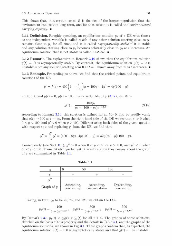
3.3 Autonomous Equations 51
This shows that, in a certain sense, B is the size of the largest population that theenvironment can sustain long term, and for that reason it is called the environmentalcarrying capacity.
3.11 Definition. Roughly speaking, an equilibrium solution y0 of a DE with time tas the independent variable is called stable if any other solution starting close to y0remains close to y0 for all time, and it is called asymptotically stable if it is stableand any solution starting close to y0 becomes arbitrarily close to y0 as t increases. Anequilibrium solution that is not stable is called unstable.
3.12 Remark. The explanation in Remark 3.10 shows that the equilibrium solutiony(t) = B is asymptotically stable. By contrast, the equilibrium solution y(t) = 0 isunstable since any solution starting near 0 at t = 0 moves away from it as t increases.
3.13 Example. Proceeding as above, we find that the critical points and equilibriumsolutions of the DE
y′ = f(y) = 400
(1− y
100
)y = 400y − 4y2 = 4y(100− y)
are 0, 100 and y(t) = 0, y(t) = 100, respectively. Also, by (3.17), its GS is
y(t) =100y0
y0 + (100− y0)e−400t. (3.18)
According to Remark 3.10, this solution is defined for all t > 0, and we readily verifythat y(t) → 100 as t → ∞. From the right-hand side of the DE we see that y′ > 0 when0 < y < 100, and y′ < 0 when y > 100. Differentiating both sides of the given equationwith respect to t and replacing y′ from the DE, we find that
y′′ =df
dyy′ = (400− 8y) · 4y(100− y) = 32y(50− y)(100− y).
Consequently (see Sect. B.1), y′′ > 0 when 0 < y < 50 or y > 100, and y′′ < 0 when50 < y < 100. These details together with the information they convey about the graphof y are summarized in Table 3.1.
Table 3.1
y 0 50 100
y′ + + −y′′ + − +
Graph of yAscending, Ascending, Descending,concave up concave down concave up
Taking, in turn, y0 to be 25, 75, and 125, we obtain the PSs
y1(t) =100
1 + 3e−400t, y2(t) =
300
3 + e−400t, y3(t) =
500
5− e−400t.
By Remark 2.37, y1(t) < y2(t) < y3(t) for all t > 0. The graphs of these solutions,sketched on the basis of this property and the details in Table 3.1, and the graphs of theequilibrium solutions, are shown in Fig. 3.1. These graphs confirm that, as expected, theequilibrium solution y(t) = 100 is asymptotically stable and that y(t) = 0 is unstable.
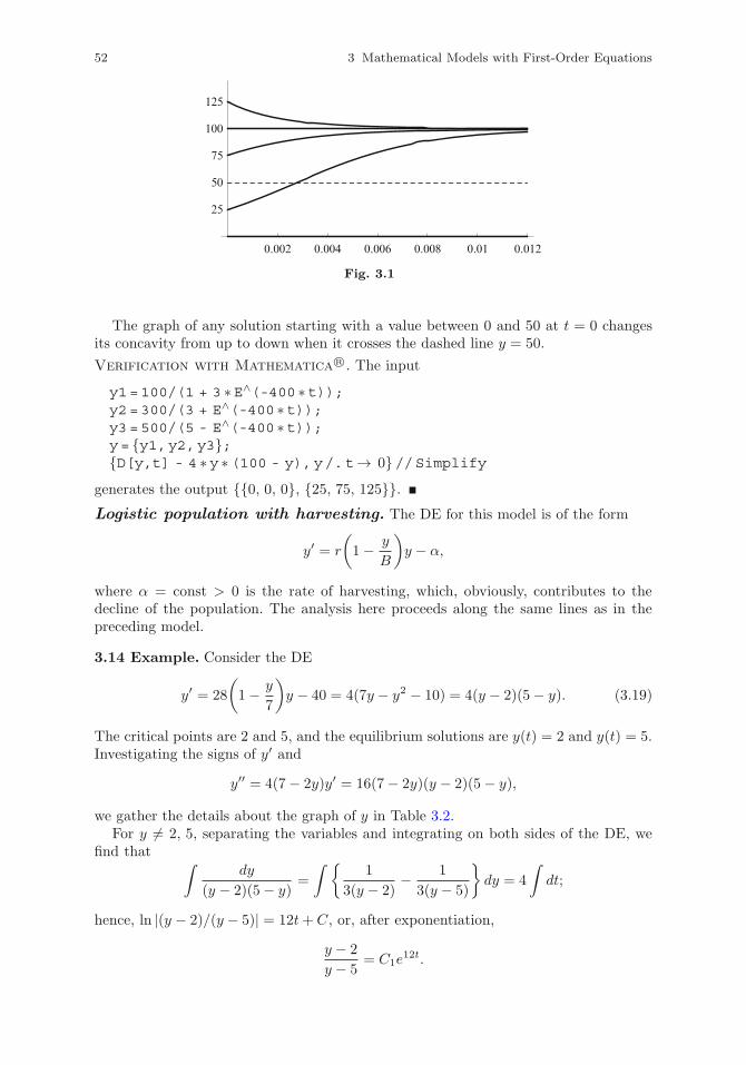
52 3 Mathematical Models with First-Order Equations
0.002 0.004 0.006 0.008 0.01 0.012
25
50
75
100
125
Fig. 3.1
The graph of any solution starting with a value between 0 and 50 at t = 0 changesits concavity from up to down when it crosses the dashed line y = 50.
Verification with Mathematica R©. The input
y1=100/(1 + 3 ∗E∧(-400 ∗t));y2=300/(3 + E∧(-400 ∗t));y3=500/(5 - E∧(-400 ∗t));y= {y1,y2,y3};{D[y,t] - 4 ∗y ∗(100 - y),y/.t→ 0}//Simplify
generates the output {{0, 0, 0}, {25, 75, 125}}.Logistic population with harvesting. The DE for this model is of the form
y′ = r
(1− y
B
)y − α,
where α = const > 0 is the rate of harvesting, which, obviously, contributes to thedecline of the population. The analysis here proceeds along the same lines as in thepreceding model.
3.14 Example. Consider the DE
y′ = 28
(1− y
7
)y − 40 = 4(7y − y2 − 10) = 4(y − 2)(5− y). (3.19)
The critical points are 2 and 5, and the equilibrium solutions are y(t) = 2 and y(t) = 5.Investigating the signs of y′ and
y′′ = 4(7− 2y)y′ = 16(7− 2y)(y − 2)(5− y),
we gather the details about the graph of y in Table 3.2.For y �= 2, 5, separating the variables and integrating on both sides of the DE, we
find that ∫dy
(y − 2)(5− y)=
∫ {1
3(y − 2)− 1
3(y − 5)
}dy = 4
∫dt;
hence, ln |(y − 2)/(y − 5)| = 12t+ C, or, after exponentiation,
y − 2
y − 5= C1e
12t.
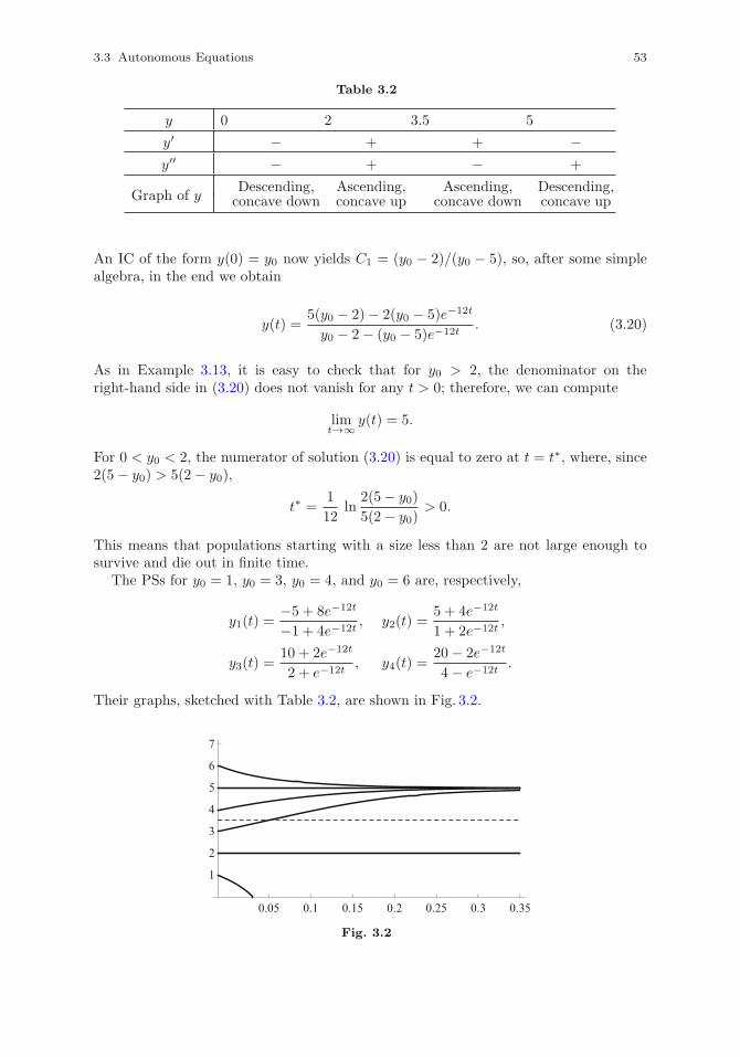
3.3 Autonomous Equations 53
Table 3.2
y 0 2 3.5 5
y′ − + + −y′′ − + − +
Graph of yDescending, Ascending, Ascending, Descending,concave down concave up concave down concave up
An IC of the form y(0) = y0 now yields C1 = (y0 − 2)/(y0 − 5), so, after some simplealgebra, in the end we obtain
y(t) =5(y0 − 2)− 2(y0 − 5)e−12t
y0 − 2− (y0 − 5)e−12t. (3.20)
As in Example 3.13, it is easy to check that for y0 > 2, the denominator on theright-hand side in (3.20) does not vanish for any t > 0; therefore, we can compute
limt→∞ y(t) = 5.
For 0 < y0 < 2, the numerator of solution (3.20) is equal to zero at t = t∗, where, since2(5− y0) > 5(2− y0),
t∗ =1
12ln
2(5− y0)
5(2− y0)> 0.
This means that populations starting with a size less than 2 are not large enough tosurvive and die out in finite time.
The PSs for y0 = 1, y0 = 3, y0 = 4, and y0 = 6 are, respectively,
y1(t) =−5 + 8e−12t
−1 + 4e−12t, y2(t) =
5 + 4e−12t
1 + 2e−12t,
y3(t) =10 + 2e−12t
2 + e−12t, y4(t) =
20− 2e−12t
4− e−12t.
Their graphs, sketched with Table 3.2, are shown in Fig. 3.2.
0.05 0.1 0.15 0.2 0.25 0.3 0.35
1
2
3
4
5
6
7
Fig. 3.2
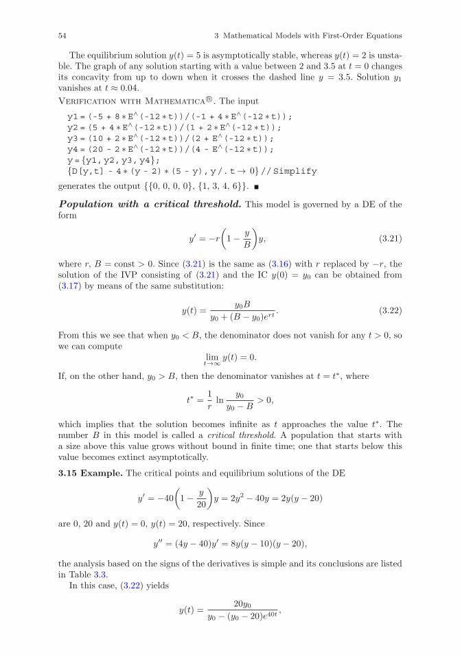
54 3 Mathematical Models with First-Order Equations
The equilibrium solution y(t) = 5 is asymptotically stable, whereas y(t) = 2 is unsta-ble. The graph of any solution starting with a value between 2 and 3.5 at t = 0 changesits concavity from up to down when it crosses the dashed line y = 3.5. Solution y1vanishes at t ≈ 0.04.
Verification with Mathematica R©. The input
y1=(-5 + 8 ∗E∧(-12 ∗t))/(-1 + 4 ∗E∧(-12 ∗t));y2=(5 + 4 ∗E∧(-12 ∗t))/(1 + 2 ∗E∧(-12 ∗t));y3=(10 + 2 ∗E∧(-12 ∗t))/(2 + E∧(-12 ∗t));y4=(20 - 2 ∗E∧(-12 ∗t))/(4 - E∧(-12 ∗t));y= {y1,y2,y3,y4};{D[y,t] - 4 ∗(y - 2) ∗(5 - y),y/.t→ 0}//Simplify
generates the output {{0, 0, 0, 0}, {1, 3, 4, 6}}.Population with a critical threshold. This model is governed by a DE of theform
y′ = −r(1− y
B
)y, (3.21)
where r, B = const > 0. Since (3.21) is the same as (3.16) with r replaced by −r, thesolution of the IVP consisting of (3.21) and the IC y(0) = y0 can be obtained from(3.17) by means of the same substitution:
y(t) =y0B
y0 + (B − y0)ert. (3.22)
From this we see that when y0 < B, the denominator does not vanish for any t > 0, sowe can compute
limt→∞ y(t) = 0.
If, on the other hand, y0 > B, then the denominator vanishes at t = t∗, where
t∗ =1
rln
y0y0 −B
> 0,
which implies that the solution becomes infinite as t approaches the value t∗. Thenumber B in this model is called a critical threshold. A population that starts witha size above this value grows without bound in finite time; one that starts below thisvalue becomes extinct asymptotically.
3.15 Example. The critical points and equilibrium solutions of the DE
y′ = −40
(1− y
20
)y = 2y2 − 40y = 2y(y − 20)
are 0, 20 and y(t) = 0, y(t) = 20, respectively. Since
y′′ = (4y − 40)y′ = 8y(y − 10)(y − 20),
the analysis based on the signs of the derivatives is simple and its conclusions are listedin Table 3.3.
In this case, (3.22) yields
y(t) =20y0
y0 − (y0 − 20)e40t,
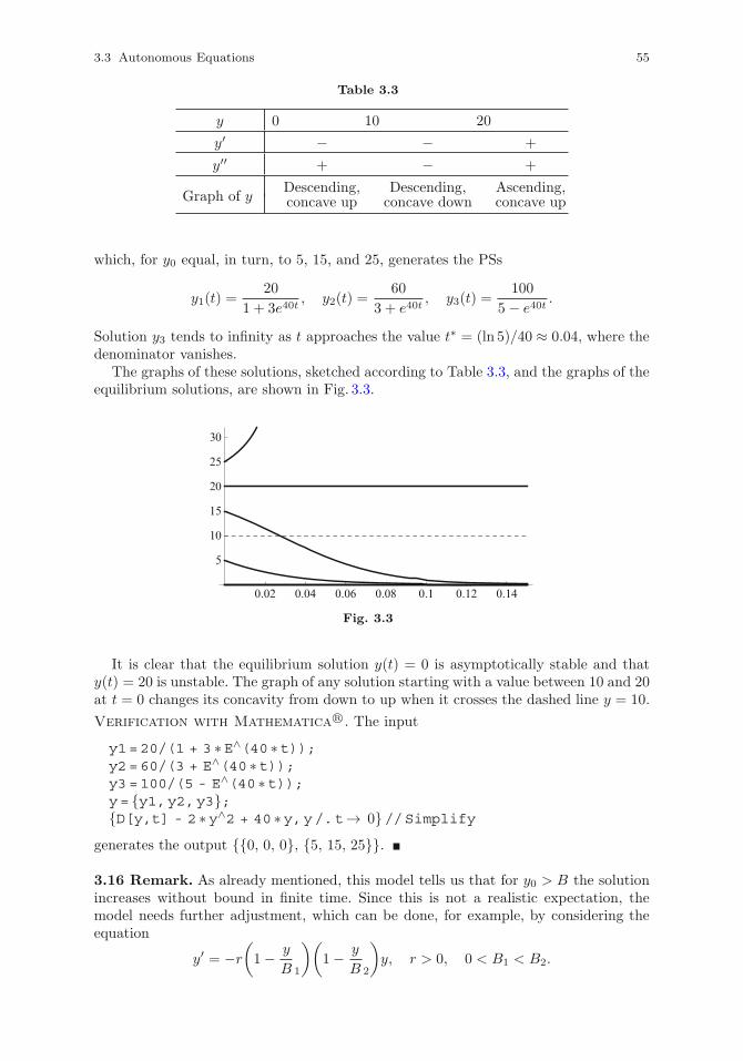
3.3 Autonomous Equations 55
Table 3.3
y 0 10 20
y′ − − +
y′′ + − +
Graph of yDescending, Descending, Ascending,concave up concave down concave up
which, for y0 equal, in turn, to 5, 15, and 25, generates the PSs
y1(t) =20
1 + 3e40t, y2(t) =
60
3 + e40t, y3(t) =
100
5− e40t.
Solution y3 tends to infinity as t approaches the value t∗ = (ln 5)/40 ≈ 0.04, where thedenominator vanishes.
The graphs of these solutions, sketched according to Table 3.3, and the graphs of theequilibrium solutions, are shown in Fig. 3.3.
0.02 0.04 0.06 0.08 0.1 0.12 0.14
5
10
15
20
25
30
Fig. 3.3
It is clear that the equilibrium solution y(t) = 0 is asymptotically stable and thaty(t) = 20 is unstable. The graph of any solution starting with a value between 10 and 20at t = 0 changes its concavity from down to up when it crosses the dashed line y = 10.
Verification with Mathematica R©. The input
y1=20/(1 + 3 ∗E∧(40 ∗t));y2=60/(3 + E∧(40 ∗t));y3=100/(5 - E∧(40 ∗t));y= {y1,y2,y3};{D[y,t] - 2 ∗y∧2 + 40 ∗y,y/.t→ 0}//Simplify
generates the output {{0, 0, 0}, {5, 15, 25}}.
3.16 Remark. As already mentioned, this model tells us that for y0 > B the solutionincreases without bound in finite time. Since this is not a realistic expectation, themodel needs further adjustment, which can be done, for example, by considering theequation
y′ = −r(1− y
B 1
)(1− y
B 2
)y, r > 0, 0 < B1 < B2.
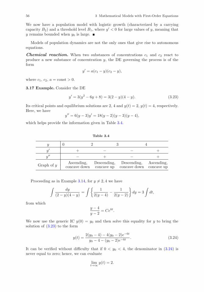
56 3 Mathematical Models with First-Order Equations
We now have a population model with logistic growth (characterized by a carryingcapacity B2) and a threshold level B1, where y
′ < 0 for large values of y, meaning thaty remains bounded when y0 is large.
Models of population dynamics are not the only ones that give rise to autonomousequations.
Chemical reaction. When two substances of concentrations c1 and c2 react toproduce a new substance of concentration y, the DE governing the process is of theform
y′ = a(c1 − y)(c2 − y),
where c1, c2, a = const > 0.
3.17 Example. Consider the DE
y′ = 3(y2 − 6y + 8) = 3(2− y)(4 − y). (3.23)
Its critical points and equilibrium solutions are 2, 4 and y(t) = 2, y(t) = 4, respectively.Here, we have
y′′ = 6(y − 3)y′ = 18(y − 2)(y − 3)(y − 4),
which helps provide the information given in Table 3.4.
Table 3.4
y 0 2 3 4
y′ + − − +
y′′ − + − +
Graph of yAscending, Descending, Descending, Ascending,
concave down concave up concave down concave up
Proceeding as in Example 3.14, for y �= 2, 4 we have
∫dy
(2 − y)(4− y)=
∫ {1
2(y − 4)− 1
2(y − 2)
}dy = 3
∫dt,
from whichy − 4
y − 2= Ce6t.
We now use the generic IC y(0) = y0 and then solve this equality for y to bring thesolution of (3.23) to the form
y(t) =2(y0 − 4)− 4(y0 − 2)e−6t
y0 − 4− (y0 − 2)e−6t. (3.24)
It can be verified without difficulty that if 0 < y0 < 4, the denominator in (3.24) isnever equal to zero; hence, we can evaluate
limt→∞ y(t) = 2.
3.3 Autonomous Equations 57
When y0 > 4, however, the denominator vanishes at t = t∗, where
t∗ =1
6lny0 − 2
y0 − 4> 0.
Consequently, physically meaningful solutions obtained with such ICs do not exist fort ≥ t∗.
The PSs corresponding to, say, y0 equal to 1, 2.5, 3.5, and 5 are
y1(t) =6− 4e−6t
3− e−6t, y2(t) =
6 + 4e−6t
3 + e−6t,
y3(t) =2 + 12e−6t
1 + 3e−6t, y4(t) =
2− 12e−6t
1− 3e−6t.
As expected, the first three functions approach the equilibrium solution y(t) = 2 ast → ∞, whereas the fourth one becomes infinite at t = t∗ = (ln 3)/6 ≈ 0.18.
The graphs of these functions, sketched in accordance with the details in Table 3.4,are shown in Fig. 3.4 and indicate that, of the two equilibrium solutions, y(t) = 2 isasymptotically stable and y(t) = 4 is unstable. The graph of any solution starting witha value between 3 and 4 at t = 0 changes its concavity from down to up when it crossesthe dashed line y = 3.
0.1 0.2 0.3 0.4 0.5 0.6
1
2
3
4
5
6
Fig. 3.4
Verification with Mathematica R©. The input
y1=(6 - 4 ∗E∧(-6 ∗t))/(3 - E∧(-6 ∗t));y2=(6 + 4 ∗E∧(-6 ∗t))/(3 + E∧(-6 ∗t));y3=(2 + 12 ∗E∧(-6 ∗t))/(1 + 3 ∗E∧(-6 ∗t));y4=(2 - 12 ∗E∧(-6 ∗t))/(1 - 3 ∗E∧(-6 ∗t));y= {y1,y2,y3,y4};{D[y,t] - 3 ∗(y∧2 - 6 ∗y + 8),y/.t→ 0}//Simplify
generates the output {{0, 0, 0, 0}, {1, 2.5, 3.5, 5}}.
3.18 Remark. Clearly, the methodology used in Examples 3.13–3.15 and 3.17 can beapplied to any autonomous equation of the form y′ = ay2 + by + c with constantcoefficients a, b, and c, where the quadratic polynomial on the right-hand side has realroots.
58 3 Mathematical Models with First-Order Equations
Exercises
Find the critical points and equilibrium solutions of the given DE and follow theprocedure set out in this section to solve the DE with each of the prescribed ICs.Sketch the graphs of the solutions obtained and comment on the stability/instability ofthe equilibrium solutions. Identify the model governed by the IVP, if any, and describeits main elements.
1 y′ = 300y − 2y2; y(0) = 50; y(0) = 100; y(0) = 200.
2 y′ = 240y − 3y2; y(0) = 20; y(0) = 60; y(0) = 100.
3 y′ = 15y − y2/2; y(0) = 10; y(0) = 20; y(0) = 40.
4 y′ = 5y − y2/4; y(0) = 5; y(0) = 15; y(0) = 25.
5 y′ = 8y − 2y2 − 6; y(0) = 1/2; y(0) = 3/2; y(0) = 5/2; y(0) = 7/2.
6 y′ = 30y − 3y2 − 48; y(0) = 1; y(0) = 3; y(0) = 6; y(0) = 9.
7 y′ = 2y2 − 80y; y(0) = 10; y(0) = 30; y(0) = 50.
8 y′ = 3y2 − 180y; y(0) = 20; y(0) = 40; y(0) = 70.
9 y′ = y2/5− 4y; y(0) = 5; y(0) = 15; y(0) = 25.
10 y′ = y2/20− y/2; y(0) = 2; y(0) = 7; y(0) = 11.
11 y′ = 2y2 − 12y + 10; y(0) = 0; y(0) = 2; y(0) = 4; y(0) = 6.
12 y′ = y2 − 9y + 18; y(0) = 2; y(0) = 7/2; y(0) = 5; y(0) = 7.
13 y′ = 2y − y2 + 8; y(0) = −3; y(0) = −1; y(0) = 2; y(0) = 5.
14 y′ = 2y − y2 + 3; y(0) = −3/2; y(0) = 0; y(0) = 3/2; y(0) = 7/2.
15 y′ = y2 + y − 6; y(0) = −4; y(0) = −2; y(0) = 1; y(0) = 3.
16 y′ = y2 + 8y + 7; y(0) = −8; y(0) = −6; y(0) = −3; y(0) = 1.
Answers to Odd-Numbered Exercises
1 0, 150; y(t) = 0 (unstable), y(t) = 150 (asymptotically stable);y = 150y0/[y0 − (y0 − 150)e−300t]; population with logistic growth;r = 300, B = 150.
3 0, 30; y(t) = 0 (unstable), y(t) = 30 (asymptotically stable);y = 30y0/[y0 − (y0 − 30)e−15t]; population with logistic growth; r = 15, B = 30.
5 1, 3; y(t) = 1 (unstable), y(t) = 3 (asymptotically stable);y = [3(y0 − 1)− (y0 − 3)e−4t]/[y0 − 1− (y0 − 3)e−4t];population with logistic growth and harvesting; r = 8, B = 4, α = 6.
7 0, 40; y(t) = 0 (asymptotically stable), y(t) = 40 (unstable);y = 40y0/[y0− (y0−40)e80t]; population with a critical threshold; r = 80, T = 40.
9 0, 20; y(t) = 0 (asymptotically stable), y(t) = 20 (unstable);y = 20y0/[y0 − (y0 − 20)e4t]; population with a critical threshold; r = 4, T = 20.
11 1, 5; y(t) = 1 (asymptotically stable), y(t) = 5 (unstable);y = [y0 − 5− 5(y0 − 1)e−8t]/[y0 − 5− (y0 − 1)e−8t]; chemical reaction;c1 = 1, c2 = 5, a = 2.
3.3 Autonomous Equations 59
13 −2, 4; y(t) = −2 (unstable), y(t) = 4 (asymptotically stable);y = [4(y0 + 2) + 2(y0 − 4)e−6t]/[y0 + 2− (y0 − 4)e−6t].
15 −3, 2; y(t) = −3 (asymptotically stable), y(t) = 2 (unstable);y = [−3(y0 − 2)− 2(y0 + 3)e−5t]/[y0 − 2− (y0 + 3)e−5t].
Chapter 4
Linear Second-Order Equations
A large number of mathematical models, particularly in the physical sciences andengineering, consist of IVPs or BVPs for second-order DEs. Among the latter, a veryimportant role is played by linear equations. Even if the model is nonlinear, the studyof its linearized version can provide valuable hints about the quantitative and qualita-tive behavior of the full model, and perhaps suggest a method that might lead to itscomplete solution.
4.1 Mathematical Models with Second-Order Equations
Below, we mention briefly a few typical examples of such models.
Free fall in gravity. As stated in Sect. 3.2, the position y(t) of a heavy object fallingin a gravitational field is a solution of the IVP
y′′ +γ
my′ = g, y(0) = y0, y′(0) = y10,
where m is the mass of the object and γ = const > 0 is a coefficient related to theresistance of the surrounding medium to motion.
RLC electric circuit. If an inductor (of inductance L) is added to the series circuitdiscussed in Sect. 3.2, and if the voltage generated by the source is constant, then thecurrent I(t) in the circuit satisfies the IVP
I ′′ +R
LI ′ +
1
LCI = 0, I(0) = I0, I ′(0) = I10.
Harmonic oscillator. A material point of mass m moving in a straight line isattached on one side to a spring characterized by an elastic coefficient k and on theother side to a shock absorber (damper) characterized by a damping coefficient γ. Thepoint is also subjected to an additional external force f(t). When the displacement ofthe point is small, the elastic force in the spring is proportional to the displacement,and the friction force in the damper is proportional to velocity. Since both these forcesoppose the motion, it follows that, according to Newton’s second law, the position y(t)of the point at time t is the solution of the IVP
my′′ + γy′ + ky = f(t), y(0) = y0, y′(0) = y10,
where the numbers y0 and y10 are the initial position and velocity of the point.
C. Constanda, Differential Equations: A Primer for Scientists and Engineers, SpringerUndergraduate Texts in Mathematics and Technology, DOI 10.1007/978-1-4614-7297-1 4,© Springer Science+Business Media New York 2013
61
62 4 Linear Second-Order Equations
Steady-state convective heat. In this process, the distribution of temperature ina very thin, laterally insulated, uniform rod occupying the segment 0 ≤ x ≤ l on thex-axis is the solution of the BVP
ky′′ − αy′ + f(x) = 0, y(0) = y0, y(l) = yl,
where k and α are positive coefficients related to the thermal properties of the rodmaterial, f represents the heat sources and sinks inside the rod, and the numbers y0and yl are the values of the temperature prescribed at the end-points. Of course, theBCs may have alternative forms, depending on the physical setup. For example, if theheat flux is prescribed at x = l instead of the temperature, then the second BC isreplaced by
y′(l) = yl.
Temperature distribution in a circular annulus. If the heat sources and sinksinside a uniform annulus a < r < b are described by a circularly symmetric and time-independent function g(r), and the inner and outer boundary circles r = a and r = b areheld at constant temperatures ya and yb, respectively, then the equilibrium temperaturey(r) in the annulus is the solution of the BVP
k(y′′ + r−1y′) + g(r) = 0, y(a) = ya, y(b) = yb,
where k is the (constant) thermal diffusivity of the material.
Time-independent Schrodinger equation. The wave function ψ(x) of aparticle at a point x in a quantum field satisfies the DE
�2ψ′′(x) − 2m[V (x) − E]ψ(x) = 0, −∞ < x < ∞,
where m, V , and E are the mass, potential energy, and total energy of the particle,respectively, and � is the reduced Planck constant. Also, the solution ψ must not growat infinity.
Motion of a pendulum. The position at time t of a pendulum of length l isidentified by its angular displacement θ(t), which is a solution of the nonlinear IVP
lθ′′ + g sin θ = 0, θ(0) = θ0, θ′(0) = θ10,
where g is the acceleration of gravity and we have assumed that the air resistance isnegligible.
4.2 Algebra Prerequisites
Before discussing solution methods for DEs, we recall a few basic concepts of linearalgebra and some related properties. The presentation of these concepts is restrictedhere to the form they assume in the context of second-order linear equations.
4.1 Definition. A 2 × 2 matrix is an array of four numbers a11, a12, a21, and a22(called elements, or entries), arranged in two rows and two columns:
A =
(a11 a12a21 a22
).
4.2 Algebra Prerequisites 63
The number defined by
det(A) =
∣∣∣∣a11 a12a21 a22
∣∣∣∣ = a11a22 − a21a12
is called the determinant of A.
4.2 Remarks. (i) It is obvious that if we swap its rows (columns), the sign of thedeterminant changes.
(ii) It is also clear that if the elements of a row (column) have a common factor, thenthis factor can be taken out and multiplied by the value of the new, simplifieddeterminant; in other words,
∣∣∣∣ca11 ca12a21 a22
∣∣∣∣ =∣∣∣∣ca11 a12ca21 a22
∣∣∣∣ = c
∣∣∣∣a11 a12a21 a22
∣∣∣∣ = c(a11a22 − a21a12).
(iii) Determinants are very useful in algebraic calculations, for example, in the solutionof a linear system by Cramer’s rule. Specifically, this rule gives the solution of thesystem
a11x1 + a12x2 = b1,
a21x1 + a22x2 = b2
as
x1 =
∣∣∣∣b1 a12b2 a22
∣∣∣∣∣∣∣∣a11 a12a21 a22
∣∣∣∣=
b1a22 − b2a12det(A)
, x2 =
∣∣∣∣a11 b1a21 b2
∣∣∣∣∣∣∣∣a11 a12a21 a22
∣∣∣∣=
b2a11 − b1a21det(A)
. (4.1)
Obviously, Cramer’s rule can be applied only if det(A) �= 0.
4.3 Example. By Cramer’s rule, the solution of the system
2x1 − x2 = 4,x1 + 3x2 = −5
is
x1 =
∣∣∣∣ 4 −1−5 3
∣∣∣∣∣∣∣∣ 2 −11 3
∣∣∣∣=
7
7= 1, x2 =
∣∣∣∣ 2 41 −5
∣∣∣∣∣∣∣∣ 2 −11 3
∣∣∣∣=
−14
7= −2.
4.4 Definition. Let f1 and f2 be two continuously differentiable functions on aninterval J . The determinant
W [f1, f2](t) =
∣∣∣∣ f1(t) f2(t)f ′1(t) f
′2(t)
∣∣∣∣ = f1(t)f′2(t)− f ′
1(t)f2(t)
is called the Wronskian of f1 and f2.
4.5 Example. If f1(t) = 2t− 1 and f2(t) = t2, then f ′1(t) = 2 and f ′
2(t) = 2t, so
W [f1, f2](t) =
∣∣∣∣2t− 1 t2
2 2t
∣∣∣∣ = 4t2 − 2t− 2t2 = 2t2 − 2t.
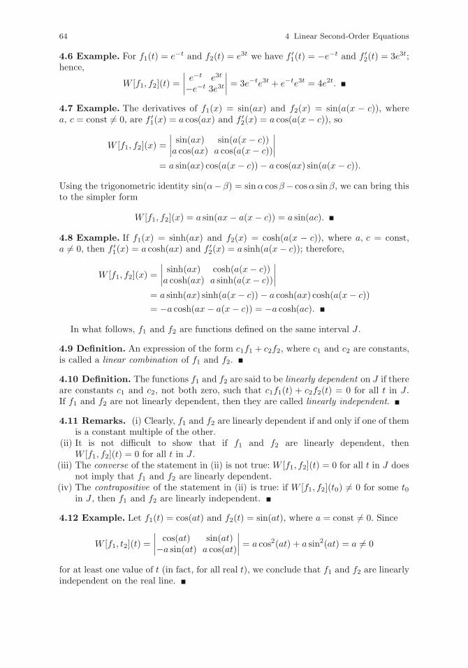
64 4 Linear Second-Order Equations
4.6 Example. For f1(t) = e−t and f2(t) = e3t we have f ′1(t) = −e−t and f ′
2(t) = 3e3t;hence,
W [f1, f2](t) =
∣∣∣∣ e−t e3t
−e−t 3e3t
∣∣∣∣ = 3e−te3t + e−te3t = 4e2t.
4.7 Example. The derivatives of f1(x) = sin(ax) and f2(x) = sin(a(x − c)), wherea, c = const �= 0, are f ′
1(x) = a cos(ax) and f ′2(x) = a cos(a(x− c)), so
W [f1, f2](x) =
∣∣∣∣ sin(ax) sin(a(x− c))a cos(ax) a cos(a(x− c))
∣∣∣∣= a sin(ax) cos(a(x − c))− a cos(ax) sin(a(x− c)).
Using the trigonometric identity sin(α−β) = sinα cosβ− cosα sinβ, we can bring thisto the simpler form
W [f1, f2](x) = a sin(ax− a(x− c)) = a sin(ac).
4.8 Example. If f1(x) = sinh(ax) and f2(x) = cosh(a(x − c)), where a, c = const,a �= 0, then f ′
1(x) = a cosh(ax) and f ′2(x) = a sinh(a(x − c)); therefore,
W [f1, f2](x) =
∣∣∣∣ sinh(ax) cosh(a(x− c))a cosh(ax) a sinh(a(x− c))
∣∣∣∣= a sinh(ax) sinh(a(x− c))− a cosh(ax) cosh(a(x− c))
= −a cosh(ax− a(x− c)) = −a cosh(ac).
In what follows, f1 and f2 are functions defined on the same interval J .
4.9 Definition. An expression of the form c1f1 + c2f2, where c1 and c2 are constants,is called a linear combination of f1 and f2.
4.10 Definition. The functions f1 and f2 are said to be linearly dependent on J if thereare constants c1 and c2, not both zero, such that c1f1(t) + c2f2(t) = 0 for all t in J .If f1 and f2 are not linearly dependent, then they are called linearly independent.
4.11 Remarks. (i) Clearly, f1 and f2 are linearly dependent if and only if one of themis a constant multiple of the other.
(ii) It is not difficult to show that if f1 and f2 are linearly dependent, thenW [f1, f2](t) = 0 for all t in J .
(iii) The converse of the statement in (ii) is not true: W [f1, f2](t) = 0 for all t in J doesnot imply that f1 and f2 are linearly dependent.
(iv) The contrapositive of the statement in (ii) is true: if W [f1, f2](t0) �= 0 for some t0in J , then f1 and f2 are linearly independent.
4.12 Example. Let f1(t) = cos(at) and f2(t) = sin(at), where a = const �= 0. Since
W [f1, t2](t) =
∣∣∣∣ cos(at) sin(at)−a sin(at) a cos(at)
∣∣∣∣ = a cos2(at) + a sin2(at) = a �= 0
for at least one value of t (in fact, for all real t), we conclude that f1 and f2 are linearlyindependent on the real line.
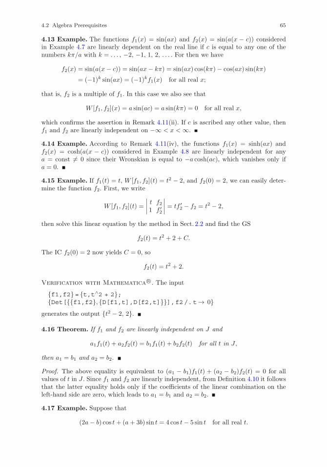
4.2 Algebra Prerequisites 65
4.13 Example. The functions f1(x) = sin(ax) and f2(x) = sin(a(x − c)) consideredin Example 4.7 are linearly dependent on the real line if c is equal to any one of thenumbers kπ/a with k = . . . , −2, −1, 1, 2, . . . . For then we have
f2(x) = sin(a(x − c)) = sin(ax− kπ) = sin(ax) cos(kπ)− cos(ax) sin(kπ)
= (−1)k sin(ax) = (−1)kf1(x) for all real x;
that is, f2 is a multiple of f1. In this case we also see that
W [f1, f2](x) = a sin(ac) = a sin(kπ) = 0 for all real x,
which confirms the assertion in Remark 4.11(ii). If c is ascribed any other value, thenf1 and f2 are linearly independent on −∞ < x < ∞.
4.14 Example. According to Remark 4.11(iv), the functions f1(x) = sinh(ax) andf2(x) = cosh(a(x − c)) considered in Example 4.8 are linearly independent for anya = const �= 0 since their Wronskian is equal to −a cosh(ac), which vanishes only ifa = 0.
4.15 Example. If f1(t) = t, W [f1, f2](t) = t2 − 2, and f2(0) = 2, we can easily deter-mine the function f2. First, we write
W [f1, f2](t) =
∣∣∣∣ t f21 f ′
2
∣∣∣∣ = tf ′2 − f2 = t2 − 2,
then solve this linear equation by the method in Sect. 2.2 and find the GS
f2(t) = t2 + 2 + C.
The IC f2(0) = 2 now yields C = 0, so
f2(t) = t2 + 2.
Verification with Mathematica R©. The input
{f1,f2}= {t,t∧2 + 2};{Det[{{f1,f2}, {D[f1,t],D[f2,t]}}],f2/.t→ 0}
generates the output {t2 − 2, 2}.
4.16 Theorem. If f1 and f2 are linearly independent on J and
a1f1(t) + a2f2(t) = b1f1(t) + b2f2(t) for all t in J,
then a1 = b1 and a2 = b2.
Proof. The above equality is equivalent to (a1 − b1)f1(t) + (a2 − b2)f2(t) = 0 for allvalues of t in J . Since f1 and f2 are linearly independent, from Definition 4.10 it followsthat the latter equality holds only if the coefficients of the linear combination on theleft-hand side are zero, which leads to a1 = b1 and a2 = b2.
4.17 Example. Suppose that
(2a− b) cos t+ (a+ 3b) sin t = 4 cos t− 5 sin t for all real t.
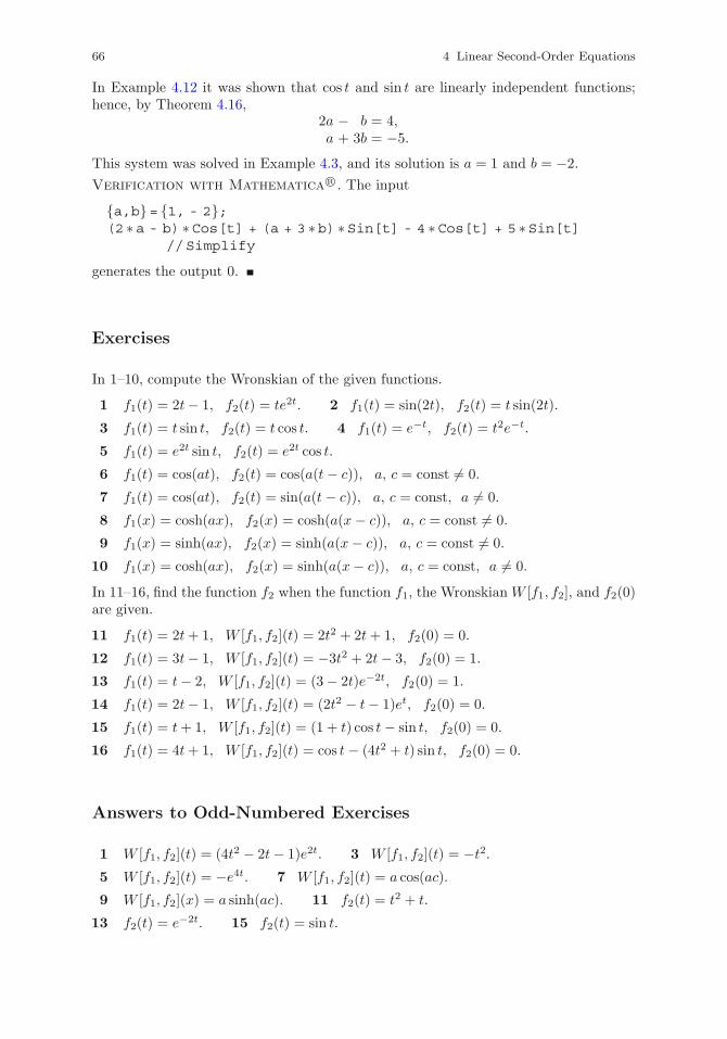
66 4 Linear Second-Order Equations
In Example 4.12 it was shown that cos t and sin t are linearly independent functions;hence, by Theorem 4.16,
2a − b = 4,a + 3b = −5.
This system was solved in Example 4.3, and its solution is a = 1 and b = −2.
Verification with Mathematica R©. The input
{a,b}= {1, - 2};(2 ∗a - b) ∗Cos[t] + (a + 3 ∗b) ∗Sin[t] - 4 ∗Cos[t] + 5 ∗Sin[t]
//Simplify
generates the output 0.
Exercises
In 1–10, compute the Wronskian of the given functions.
1 f1(t) = 2t− 1, f2(t) = te2t. 2 f1(t) = sin(2t), f2(t) = t sin(2t).
3 f1(t) = t sin t, f2(t) = t cos t. 4 f1(t) = e−t, f2(t) = t2e−t.
5 f1(t) = e2t sin t, f2(t) = e2t cos t.
6 f1(t) = cos(at), f2(t) = cos(a(t− c)), a, c = const �= 0.
7 f1(t) = cos(at), f2(t) = sin(a(t− c)), a, c = const, a �= 0.
8 f1(x) = cosh(ax), f2(x) = cosh(a(x − c)), a, c = const �= 0.
9 f1(x) = sinh(ax), f2(x) = sinh(a(x− c)), a, c = const �= 0.
10 f1(x) = cosh(ax), f2(x) = sinh(a(x− c)), a, c = const, a �= 0.
In 11–16, find the function f2 when the function f1, the WronskianW [f1, f2], and f2(0)are given.
11 f1(t) = 2t+ 1, W [f1, f2](t) = 2t2 + 2t+ 1, f2(0) = 0.
12 f1(t) = 3t− 1, W [f1, f2](t) = −3t2 + 2t− 3, f2(0) = 1.
13 f1(t) = t− 2, W [f1, f2](t) = (3− 2t)e−2t, f2(0) = 1.
14 f1(t) = 2t− 1, W [f1, f2](t) = (2t2 − t− 1)et, f2(0) = 0.
15 f1(t) = t+ 1, W [f1, f2](t) = (1 + t) cos t− sin t, f2(0) = 0.
16 f1(t) = 4t+ 1, W [f1, f2](t) = cos t− (4t2 + t) sin t, f2(0) = 0.
Answers to Odd-Numbered Exercises
1 W [f1, f2](t) = (4t2 − 2t− 1)e2t. 3 W [f1, f2](t) = −t2.5 W [f1, f2](t) = −e4t. 7 W [f1, f2](t) = a cos(ac).
9 W [f1, f2](x) = a sinh(ac). 11 f2(t) = t2 + t.
13 f2(t) = e−2t. 15 f2(t) = sin t.
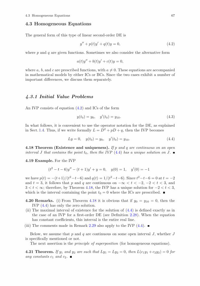
4.3 Homogeneous Equations 67
4.3 Homogeneous Equations
The general form of this type of linear second-order DE is
y′′ + p(t)y′ + q(t)y = 0, (4.2)
where p and q are given functions. Sometimes we also consider the alternative form
a(t)y′′ + b(t)y′ + c(t)y = 0,
where a, b, and c are prescribed functions, with a �= 0. These equations are accompaniedin mathematical models by either ICs or BCs. Since the two cases exhibit a number ofimportant differences, we discuss them separately.
4.3.1 Initial Value Problems
An IVP consists of equation (4.2) and ICs of the form
y(t0) = y0, y′(t0) = y10. (4.3)
In what follows, it is convenient to use the operator notation for the DE, as explainedin Sect. 1.4. Thus, if we write formally L = D2 + pD + q, then the IVP becomes
Ly = 0, y(t0) = y0, y′(t0) = y10. (4.4)
4.18 Theorem (Existence and uniqueness). If p and q are continuous on an openinterval J that contains the point t0, then the IVP (4.4) has a unique solution on J .
4.19 Example. For the IVP
(t2 − t− 6)y′′ − (t+ 1)y′ + y = 0, y(0) = 1, y′(0) = −1
we have p(t) = −(t+1)/(t2−t−6) and q(t) = 1/(t2−t−6). Since t2−t−6 = 0 at t = −2and t = 3, it follows that p and q are continuous on −∞ < t < −2, −2 < t < 3, and3 < t < ∞; therefore, by Theorem 4.18, the IVP has a unique solution for −2 < t < 3,which is the interval containing the point t0 = 0 where the ICs are prescribed.
4.20 Remarks. (i) From Theorem 4.18 it is obvious that if y0 = y10 = 0, then theIVP (4.4) has only the zero solution.
(ii) The maximal interval of existence for the solution of (4.4) is defined exactly as inthe case of an IVP for a first-order DE (see Definition 2.28). When the equationhas constant coefficients, this interval is the entire real line.
(iii) The comments made in Remark 2.29 also apply to the IVP (4.4).
Below, we assume that p and q are continuous on some open interval J , whether Jis specifically mentioned or not.
The next assertion is the principle of superposition (for homogeneous equations).
4.21 Theorem. If y1 and y2 are such that Ly1 = Ly2 = 0, then L(c1y1 + c2y2) = 0 forany constants c1 and c2.
68 4 Linear Second-Order Equations
Proof. Since L is a linear operator (see Example 1.31), it follows that
L(c1y1 + c2y2) = c1Ly1 + c2Ly2 = 0.
We now turn our attention to finding the GS of the equation Ly = 0.
4.22 Theorem. If y1 and y2 are solutions of Ly = 0 on an open interval J andW [y1, y2](t0) �= 0 at some point t0 in J , then there are unique numbers c1 and c2such that c1y1 + c2y2 is the solution of the IVP (4.4) on J .
Proof. By Theorem 4.21, y = c1y1 + c2y2 satisfies Ly = 0. The ICs now yield
c1y1(t0) + c2y2(t0) = y0,
c1y′1(t0) + c2y
′2(t0) = y10,
which is a linear algebraic system for the unknowns c1 and c2. Since the determinantof the system is ∣∣∣∣ y1(t0) y2(t0)
y′1(t0) y′2(t0)
∣∣∣∣ = W [y1, y2](t0) �= 0,
we conclude that the system has a unique solution. This solution can be computed ina variety of ways, for example, by Cramer’s rule (4.1).
4.23 Example. Consider the IVP
y′′ − 2y′ − 3y = 0, y(0) = 1, y′(0) = −5.
We can readily check that y1(t) = e−t and y2(t) = e3t are solutions of the equation onthe entire real line, and that W [y1, y2](0) = 4 �= 0. By Theorem 4.22, the solution ofthe IVP is of the form y = c1y1 + c2y2. Applying the ICs, we arrive at the system
c1 + c2 = 1,−c1 + 3c2 = −5,
which has the unique solution c1 = 2 and c2 = −1. Consequently, the solution of theIVP is
y(t) = 2e−t − e3t.
4.24 Theorem. If y1 and y2 are two solutions of the equation Ly = 0 on an openinterval J and there is a point t0 in J such that W [y1, y2](t0) �= 0, then c1y1 + c2y2,where c1 and c2 are arbitrary constants, is the GS of the equation Ly = 0 on J .
Proof. By Theorem 4.21, any function of the form c1y1 + c2y2 satisfies the equationLy = 0. Conversely, let y be any solution of this equation, and let y(t0) = y0 andy′(t0) = y10. By Theorem 4.22, y can be written uniquely as c1y1 + c2y2, which provesthe assertion.
4.25 Remark. It can be shown that if y1 and y2 are two solutions of (4.2) on an openinterval J and t0 is a point in J , then for any t in J ,
W [y1, y2](t) = W [y1, y2](t0) exp
{−
t∫t0
p(τ) dτ
}.
This implies that the Wronskian of two solutions is either zero at every point in J ornonzero everywhere on J .
4.3 Homogeneous Equations 69
4.26 Definition. A pair of functions {y1, y2} with the properties mentioned in Theo-rem 4.24 is called a fundamental set of solutions (FSS) for equation (4.2).
4.27 Example. Clearly, {e−t, e3t} is an FSS for the DE in Example 4.23, whose GScan therefore be written as y(t) = c1e
−t + c2e3t.
4.28 Remarks. (i) The conclusion in Theorem 4.24 is independent of any additionalconditions accompanying the DE.
(ii) Combining the statements in Remarks 4.11(iv) and 4.25 and Theorem 4.22, wecan show that two solutions of (4.2) form an FSS if and only if they are linearlyindependent. This means that we may equally define an FSS as being any pair oflinearly independent solutions.
(iii) In practice, it is generally very difficult to find particular solutions of homogeneouslinear equations with variable coefficients. However, as we see in Sect. 4.4, this taskis relatively simple when the coefficients are constant.
Exercises
In 1–10, find the largest interval on which the conditions of Theorem 4.18 are satisfied,without solving the given IVP.
1 ty′′ + t2y′ + 2y = 0, y(1) = 2, y′(1) = 0.
2 (1− 2t)y′′ − 2ty′ + y sin t = 0, y(0) = 4, y′(0) = −1.
3 (t2 − 3t+ 2)y′′ + y′ + (t− 1)y = 0, y(0) = 0, y′(0) = 1.
4 (t2 − 2t+ 1)y′′ + ty′ − y = 0, y(2) = 1, y′(2) = −1.
5 (t2 − 4)y′′ + 2y′ − 3(t+ 2)y = 0, y(0) = 1, y′(0) = 1.
6 (t2 + 3t− 4)y′′ − y′ + e−ty = 0, y(3) = 0, y′(3) = 2.
7 y′′ sin t+ y′ = 0, y(3π/2) = 1, y′(3π/2) = −2.
8 y′′ cos(2t)− 3y = 0, y(−π/2) = 2, y′(−π/2) = 3.
9 (2− et)y′′ + ty′ + 4ty = 0, y(1) = 1, y′(1) = −2.
10 (tan t+ 1)y′′ + y′ sin t+ y = 0, y(π) = −1, y′(π) = 4.
In 11–16, use the formula in Remark 4.25 to compute the value at the indicated pointt of the Wronskian of two solutions y1, y2 of the given DE when its value at anotherpoint is as prescribed.
11 ty′′ + 2y′ + 3ty = 0, t = 2, W [y1, y2](1) = 4.
12 (t+ 1)y′′ − y′ + 2(t2 + t)y = 0, t = 3, W [y1, y2](0) = 2.
13 (t2 + 1)y′′ − ty′ + ety = 0, t = 1, W [y1, y2](0) = −1.
14 (t2 + t)y′′ + (2t+ 1)y′ + y sin(2t) = 0, t = 4, W [y1, y2](1) = 9.
15 y′′ + y′ cot t+ e−ty = 0, t = π/2, W [y1, y2](π/6) = −2.
16 y′′ sin t+ y′ sec t+ y = 0, t = π/3, W [y1, y2](π/4) = 1.
Answers to Odd-Numbered Exercises
1 t > 0. 3 t < 1. 5 −2 < t < 2. 7 π < t < 2π. 9 t > ln 2.
11 W [y1, y2](2) = 1. 13 W [y1, y2](1) = −√2. 15 W [y1, y2](π/2) = −1.
70 4 Linear Second-Order Equations
4.3.2 Boundary Value Problems
A BVP consists of equation (4.2) (with t usually replaced by x as the independentvariable) on a finite open interval a < x < b, and BCs prescribed at the end-pointsx = a and x = b of this interval. Here we consider the following three types of BCs:
y(a) = α, y(b) = β; y(a) = α, y′(b) = β; y′(a) = α, y(b) = β, (4.5)
where α and β are given numbers.It turns out that the different nature of conditions (4.5), compared to (4.3), makes
BVPs less simple to analyze than IVPs when it comes to the existence and uniquenessof solutions. Even when we can construct the GS of the DE, the outcome for thecorresponding BVP is not necessarily a unique solution: it could be that, or multiplesolutions, or no solution at all, depending on the BCs attached to the equation.
4.29 Example. Consider the BVP
y′′ + y = 0, y(0) = 3, y(π/2) = −2.
We easily verify that y1 = cosx and y2 = sinx are solutions of the DE. Since, as shownin Example 4.12 with a = 1, they are also linearly independent, from Remark 4.28(ii)it follows that they form an FSS. Hence, by Theorem 4.24,
y(x) = c1 cosx+ c2 sinx
is the GS of the equation. Applying the BCs, we obtain c1 = 3 and c2 = −2, so theunique solution of the BVP is
y(x) = 3 cosx− 2 sinx.
If we now consider the same DE on the interval 0 < x < 2π with y(0) = 3, y(2π) = 3,then the GS and the new BCs yield c1 = 3 but no specific value for c2, so the modifiedBVP has infinitely many solutions of the form
y(x) = 3 cosx+ c2 sinx,
where c2 is an arbitrary constant.Finally, if the interval and the BCs are changed to 0 < x < π and y(0) = 3,
y(π) = −2, then we get c1 = 3 and c1 = 2, which is impossible; therefore, this thirdBVP has no solution.
The next assertion states conditions under which BVPs of interest to us are uniquelysolvable.
4.30 Theorem. If J is an open finite interval a < x < b and p and q are continuousfunctions on J , with q(x) < 0 for all x in J , then the BVP consisting of (4.2) and anyone of the sets of BCs in (4.5) has a unique solution on J .
4.31 Remark. As happens with many existence and uniqueness theorems, the condi-tions in the above assertion are sufficient but not necessary. When they are not satisfied,we cannot draw any conclusion about the solvability of the BVP. In Example 4.29 wehave q(x) = 1 > 0, which contravenes one of the conditions in Theorem 4.30 and,therefore, makes the theorem inapplicable.
4.4 Homogeneous Equations with Constant Coefficients 71
Exercises
Verify that the given functions y1 and y2 form an FSS for the accompanying DE, thendiscuss the existence and uniqueness of solutions for the equation with each set of BCson the appropriate interval. Compute the solutions where possible.
1 4y′′ + y = 0, y1(x) = cos(x/2), y2(x) = sin(x/2).
(i) y(0) = 2, y(π) = −4; (ii) y(0) = 2, y(2π) = −2; (iii) y(0) = 2, y(2π) = 3.
2 y′′ − 4y′ + 8y = 0, y1(x) = e2x cos(2x), y2(x) = e2x sin(2x).
(i) y′(0) = 2, y(π/8) = eπ/4/√2 ; (ii) y′(0) = −4, y(π/4) = −3eπ/2;
(iii) y′(0) = 2, y(π/8) = 1.
3 y′′ + 2y′ + 2y = 0, y1(x) = e−x cosx, y2(x) = e−x sinx.
(i) y(0) = 1, y′(π/4) = 2; (ii) y(0) = 3, y′(π/2) = −e−π/2;
(iii) y(0) = 1, y′(π/4) = −√2 e−π/4.
4 4y′′ − 8y′ + 5y = 0, y1(x) = ex cos(x/2), y2(x) = ex sin(x/2).
(i) y′(0) = 2, y′(π) = 3eπ/2; (ii) y′(0) = −4, y′(2π) = 2;
(iii) y′(0) = −4, y′(2π) = 4e2π.
Answers to Odd-Numbered Exercises
1 (i) y(x) = 2 cos(x/2)− 4 sin(x/2);
(ii) y(x) = 2 cos(x/2) + c sin(x/2), c = const arbitrary; (iii) no solution.
3 (i) No solution; (ii) y(x) = e−x(3 cosx− 2 sinx);
(iii) y(x) = e−x(cosx+ c sinx), c = const arbitrary.
4.4 Homogeneous Equations with Constant Coefficients
As mentioned in Remark 4.28(iii), for a DE of the form
ay′′ + by′ + cy = 0, a, b, c = const, a �= 0, (4.6)
it is fairly easy to find an FSS. Since the left-hand side in (4.6) is a linear combinationof y, y′, and y′′, we are looking for a function that keeps its original ‘shape’ whendifferentiated. A reasonable candidate is a solution of the form
y(t) = ert, r = const.
Replacing this in (4.6), we arrive at the equality (ar2 + br + c)ert = 0 for all real t,which holds if and only if
ar2 + br + c = 0. (4.7)
The quadratic equation (4.7) is called the characteristic equation corresponding to (4.6),and its left-hand side is called the characteristic polynomial. This equation has two
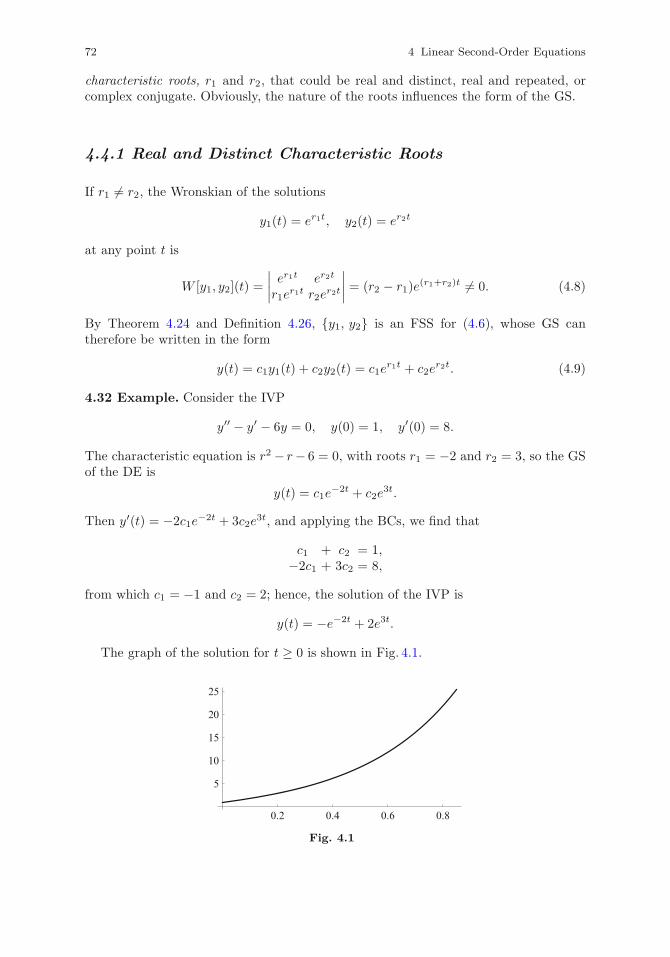
72 4 Linear Second-Order Equations
characteristic roots, r1 and r2, that could be real and distinct, real and repeated, orcomplex conjugate. Obviously, the nature of the roots influences the form of the GS.
4.4.1 Real and Distinct Characteristic Roots
If r1 �= r2, the Wronskian of the solutions
y1(t) = er1t, y2(t) = er2t
at any point t is
W [y1, y2](t) =
∣∣∣∣ er1t er2t
r1er1t r2e
r2t
∣∣∣∣ = (r2 − r1)e(r1+r2)t �= 0. (4.8)
By Theorem 4.24 and Definition 4.26, {y1, y2} is an FSS for (4.6), whose GS cantherefore be written in the form
y(t) = c1y1(t) + c2y2(t) = c1er1t + c2e
r2t. (4.9)
4.32 Example. Consider the IVP
y′′ − y′ − 6y = 0, y(0) = 1, y′(0) = 8.
The characteristic equation is r2 − r− 6 = 0, with roots r1 = −2 and r2 = 3, so the GSof the DE is
y(t) = c1e−2t + c2e
3t.
Then y′(t) = −2c1e−2t + 3c2e
3t, and applying the BCs, we find that
c1 + c2 = 1,−2c1 + 3c2 = 8,
from which c1 = −1 and c2 = 2; hence, the solution of the IVP is
y(t) = −e−2t + 2e3t.
The graph of the solution for t ≥ 0 is shown in Fig. 4.1.
0.2 0.4 0.6 0.8
5
10
15
20
25
Fig. 4.1
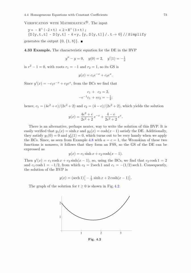
4.4 Homogeneous Equations with Constant Coefficients 73
Verification with Mathematica R©. The input
y= - E∧(-2 ∗t) + 2 ∗E∧(3 ∗t);{D[y,t,t] - D[y,t] - 6 ∗y,{y,D[y,t]}/.t→ 0}//Simplify
generates the output {0, {1, 8}}.
4.33 Example. The characteristic equation for the DE in the BVP
y′′ − y = 0, y(0) = 2, y′(1) = − 12
is r2 − 1 = 0, with roots r1 = −1 and r2 = 1, so its GS is
y(x) = c1e−x + c2e
x.
Since y′(x) = −c1e−x + c2ex, from the BCs we find that
c1 + c2 = 2,
−e−1c1 + ec2 = − 12 ;
hence, c1 = (4e2 + e)/(2e2 + 2) and c2 = (4− e)/(2e2 + 2), which yields the solution
y(x) =4e2 + e
2e2 + 2e−x +
4− e
2e2 + 2ex.
There is an alternative, perhaps neater, way to write the solution of this BVP. It iseasily verified that y1(x) = sinhx and y2(x) = cosh(x− 1) satisfy the DE. Additionally,they satisfy y1(0) = 0 and y′2(1) = 0, which turns out to be very handy when we applythe BCs. Since, as seen from Example 4.8 with a = c = 1, the Wronskian of these twofunctions is nonzero, it follows that they form an FSS, so the GS of the DE can beexpressed as
y(x) = c1 sinhx+ c2 cosh(x− 1).
Then y′(x) = c1 coshx + c2 sinh(x − 1), so, using the BCs, we find that c2 cosh 1 = 2and c1 cosh 1 = −1/2, from which c2 = 2 sech1 and c1 = −(1/2) sech1. Consequently,the solution of the BVP is
y(x) = (sech 1)[− 1
2 sinhx+ 2 cosh(x− 1)].
The graph of the solution for t ≥ 0 is shown in Fig. 4.2.
1 2 3
1
2
Fig. 4.2
74 4 Linear Second-Order Equations
Verification with Mathematica R©. The input
y=Sech[1] ∗(Sinh[x] + 2 ∗Cosh[x-1]);{D[y,x,x] - y, {y/.x→ 0,D[y,x]/.x→ 1}}//Simplify
generates the output {0, {2, 1}}.
Exercises
In 1–8, find the solution y(t) of the given IVP.
1 y′′ + y′ − 6y = 0, y(0) = 2, y′(0) = 9.
2 y′′ − 4y′ + 3y = 0, y(0) = 0, y′(0) = −4.
3 2y′′ + y′ − y = 0, y(0) = 4, y′(0) = −5/2.
4 3y′′ − 4y′ − 4y = 0, y(0) = 1, y′(0) = −10/3.
5 y′′ + 4y′ = 0, y(0) = −2, y′(0) = −4.
6 3y′′ − y′ = 0, y(0) = 2, y′(0) = −2/3.
7 6y′′ − y′ − y = 0, y(0) = 2, y′(0) = −3/2.
8 4y′′ + 4y′ − 15y = 0, y(0) = 2, y′(0) = 11.
In 9–16, find the solution y(x) of the given BVP.
9 y′′ − 2y′ − 3y = 0, y(0) = 0, y(1) = e−1 − e3.
10 2y′′ + 3y′ − 2y = 0, y′(−1) = e−1/2 − 2e2, y(1) = 2e1/2 + e−2.
11 y′′ − 2y′ = 0, y(0) = 1, y′(ln 2) = −16.
12 y′′ − 2y′ − 8y = 0, y′(− ln 2) = 63/4, y′(0) = 0.
13 y′′ − 4y = 0, y(0) = 2, y(1) = 3.
14 9y′′ − y = 0, y′(0) = 4/3, y(1) = −2.
15 y′′ − 16y = 0, y(0) = −1, y′(2) = 12.
16 9y′′ − 4y = 0, y′(0) = −2, y′(3) = −1/3.
Answers to Odd-Numbered Exercises
1 y(t) = 3e2t − e−3t. 3 y(t) = 3e−t + et/2. 5 y(t) = −3 + 4e−4t.
7 y(t) = 3e−t/3 − et/2. 9 y(x) = e−x − e3x. 11 y(x) = 3− 2e2x.
13 y(x) = (csch 2)[3 sinh(2x)− 2 sinh(2(x− 1))].
15 y(x) = (sech 8)[3 sinh(4x)− cosh(4(x− 2))].
4.4.2 Repeated Characteristic Roots
When the characteristic equation has a repeated root r1 = r2 = r0, we have only onepurely exponential solution available, namely y1(t) = er0t. To find a second one that
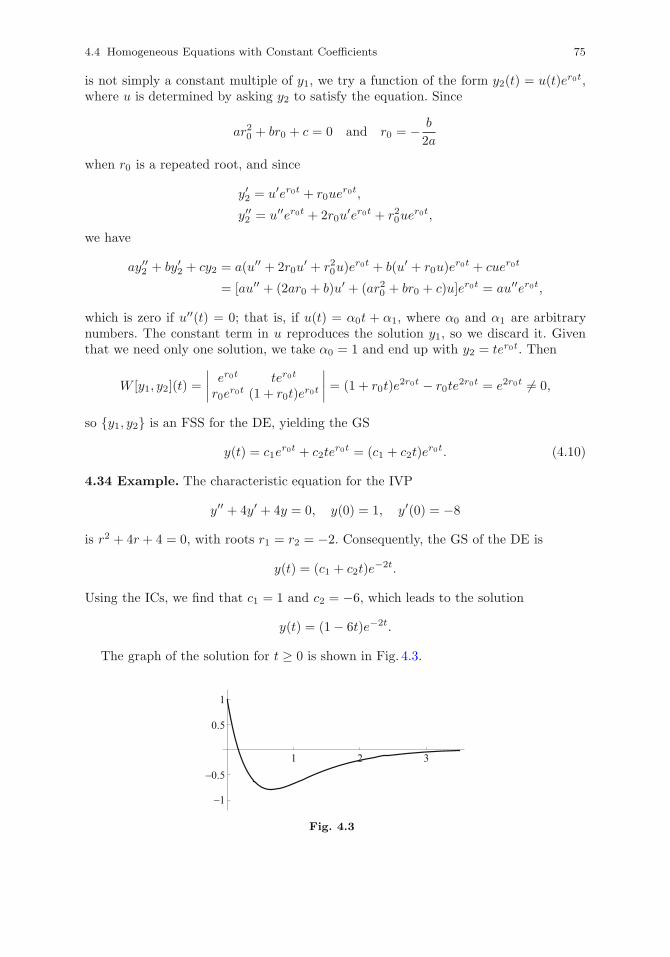
4.4 Homogeneous Equations with Constant Coefficients 75
is not simply a constant multiple of y1, we try a function of the form y2(t) = u(t)er0t,where u is determined by asking y2 to satisfy the equation. Since
ar20 + br0 + c = 0 and r0 = − b
2a
when r0 is a repeated root, and since
y′2 = u′er0t + r0uer0t,
y′′2 = u′′er0t + 2r0u′er0t + r20ue
r0t,
we have
ay′′2 + by′2 + cy2 = a(u′′ + 2r0u′ + r20u)e
r0t + b(u′ + r0u)er0t + cuer0t
= [au′′ + (2ar0 + b)u′ + (ar20 + br0 + c)u]er0t = au′′er0t,
which is zero if u′′(t) = 0; that is, if u(t) = α0t + α1, where α0 and α1 are arbitrarynumbers. The constant term in u reproduces the solution y1, so we discard it. Giventhat we need only one solution, we take α0 = 1 and end up with y2 = ter0t. Then
W [y1, y2](t) =
∣∣∣∣ er0t ter0t
r0er0t (1 + r0t)e
r0t
∣∣∣∣ = (1 + r0t)e2r0t − r0te
2r0t = e2r0t �= 0,
so {y1, y2} is an FSS for the DE, yielding the GS
y(t) = c1er0t + c2te
r0t = (c1 + c2t)er0t. (4.10)
4.34 Example. The characteristic equation for the IVP
y′′ + 4y′ + 4y = 0, y(0) = 1, y′(0) = −8
is r2 + 4r + 4 = 0, with roots r1 = r2 = −2. Consequently, the GS of the DE is
y(t) = (c1 + c2t)e−2t.
Using the ICs, we find that c1 = 1 and c2 = −6, which leads to the solution
y(t) = (1− 6t)e−2t.
The graph of the solution for t ≥ 0 is shown in Fig. 4.3.
1 2 3
−1
−0.5
0.5
1
Fig. 4.3
76 4 Linear Second-Order Equations
Verification with Mathematica R©. The input
y=(1 - 2 ∗t) ∗E∧(-2 ∗t);{D[y,t,t] + 4 ∗D[y,t] + 4 ∗y,{y,D[y,t]}/.t→ 0}//Simplify
generates the output {0, {1, −4}}.
Reduction of order. The characteristic equation method does not work for a linearDE with variable coefficients. Sometimes, however, when by some means or other wemanage to find a PS y1 of such an equation, the technique described above may helpus compute a second one, and, thus, the GS.
4.35 Example. It is easy to verify that the DE
2t2y′′ + ty′ − 3y = 0
admits the solution y1 = t−1. To find a second, linearly independent, solution, we sety2(t) = u(t)y1(t) = t−1u(t). Then
y′2 = −t−2u+ t−1u′, y′′2 = 2t−3u− 2t−2u′ + t−1u′′,
which, replaced in the DE, lead to
2tu′′ − 3u′ = 0.
Setting first u′ = v, we arrive at the separable equation 2tv′ = 3v, with solutionv(t) = u′(t) = t3/2 + C. Since we need only one solution, we discard the constant andintegrate again to obtain u(t) = (2/5)t5/2. Hence, we may take y2(t) = u(t)y1(t) = t3/2.(The coefficient 2/5 is unnecessary because y2 is multiplied by an arbitrary constant inthe GS.) The Wronskian of y1 and y2 is
W [y1, y2](t) =
∣∣∣∣ t−1 t3/2
−t−2 32 t
1/2
∣∣∣∣ = 32 t
−1/2 + t−1/2 = 52 t
−1/2 �= 0
for any t �= 0, so {y1, y2} is an FSS, which means that the GS of the given DE is
y(t) = c1y1(t) + c2y2(t) = c1t−1 + c2t
3/2.
Verification with Mathematica R©. The input
y=c1 ∗t∧(-1) + c2 ∗t∧(3/2);2 ∗t∧2 ∗D[y,t,t] + t ∗D[y,t] - 3 ∗y//Simplify
generates the output 0.
Exercises
In 1–4, find the solution y(t) of the given IVP.
1 y′′ + 6y′ + 9y = 0, y(0) = −3, y′(0) = 11.
2 4y′′ + 4y′ + y = 0, y(0) = 1, y′(0) = −9/2.
3 25y′′ − 20y′ + 4y = 0, y(0) = 10, y′(0) = 9.
4.4 Homogeneous Equations with Constant Coefficients 77
4 y′′ − 8y′ + 16y = 0, y(0) = 3, y′(0) = 8.
In 5 and 6, find the solution y(x) of the given BVP.
5 9y′′ − 6y′ + y = 0, y(0) = 1, y(1) = 3e1/3.
6 y′′ + 10y′ + 25y = 0, y(0) = −2, y((ln 2)/5) = −1 + (ln 2)/10.
In 7–12, use the method of reduction of order and the solution provided for the givenDE to find a second, linearly independent, solution of the equation.
7 t2y′′ + 2ty′ − 6y = 0, y1(t) = t−3.
8 3t2y′′ − 5ty′ + 4y = 0, y1(t) = t2.
9 t2y′′ + 3ty′ + y = 0 (t > 0), y1(t) = t−1.
10 4t2y′′ + y = 0 (t > 0), y1(t) = t1/2.
11 (t− 1)y′′ − (t+ 1)y′ + 2y = 0, y1(t) = et.
12 (t2 + t)y′′ − ty′ + y = 0 (t > 0), y1(t) = t.
Answers to Odd-Numbered Exercises
1 y(t) = (2t− 3)e−3t. 3 y(t) = 5(t+ 2)e2t/5. 5 y(x) = (2x+ 1)ex/3.
7 y2(t) = t2. 9 y2(t) = t−1 ln t. 11 y2(t) = −(t2 + 1).
4.4.3 Complex Conjugate Characteristic Roots
We recall the Taylor series expansions
eα = 1 +α
1!+α2
2!+α3
3!+α4
4!+α5
5!+ · · · ,
cosα = 1− α2
2!+α4
4!− α6
6!+ · · · ,
sinα =α
1!− α3
3!+α5
5!− α7
7!+ · · · .
Replacing α = iθ in the first one and taking the other two and the fact that i2 = −1into account, we now obtain
eiθ = 1+iθ
1!+
(iθ)2
2!+
(iθ)3
3!+
(iθ)4
4!+
(iθ)5
5!+ · · ·
= 1+θ
1!i− θ2
2!− θ3
3!i+
θ4
4!+θ5
5!i− · · ·
=
(1− θ2
2!+θ4
4!− · · ·
)+ i
(θ
1!− θ3
3!+θ5
5!− · · ·
)
= cos θ + i sin θ. (4.11)
This equality is known as Euler’s formula.
78 4 Linear Second-Order Equations
Suppose that the characteristic equation has complex conjugate roots
r1 = λ+ iμ, r2 = λ− iμ, μ �= 0,
and consider the complex-valued solutions y1 and y2 defined by
y1(t) = er1t = e(λ+iμ)t = eλteiμt = eλt[cos(μt) + i sin(μt)],
y2(t) = er2t = e(λ−iμ)t = eλte−iμt = eλt[cos(μt)− i sin(μt)].(4.12)
By (4.8),W [y1, y2](t) = 2iμ e2λt �= 0
at any point t, so these functions form an FSS. However, since we are dealing exclusivelywith real DEs and real ICs or BCs, we want to write the GS of the equation in terms ofa fundamental set of real-valued solutions. This is easily done if we notice, from (4.12),that the functions
u(t) =1
2y1(t) +
1
2y2(t) = eλt cos(μt),
v(t) =1
2iy1(t)− 1
2iy2(t) = eλt sin(μt)
are real-valued and, by Theorem 4.21, are solutions of the DE. Also, since
u′(t) = eλt[λ cos(μt)− μ sin(μt)],
v′(t) = eλt[λ sin(μt) + μ cos(μt)],
we have
W [u, v](t) =
∣∣∣∣∣eλt cos(μt) eλt sin(μt)
eλt[λ cos(μt)− μ sin(μt)] eλt[λ sin(μt) + μ cos(μt)]
∣∣∣∣∣= e2λt[λ cos(μt) sin(μt) + μ cos2(μt)
− λ cos(μt) sin(μt) + μ sin2(μt)] = μe2λt �= 0,
which shows that {u, v} is an FSS. Consequently, the real GS of the DE is
y(t) = c1u(t) + c2v(t) = eλt[c1 cos(μt) + c2 sin(μt)], (4.13)
with real arbitrary constants c1 and c2.
4.36 Example. Consider the IVP
9y′′ − 6y′ + 10y = 0, y(0) = 2, y′(0) = 113 .
The roots of the characteristic equation 9r2−6r+10 = 0 are r1 = 1/3+i and r2 = 1/3−i,so, by (4.13) with λ = 1/3 and μ = 1, the GS of the DE is
y(t) = et/3(c1 cos t+ c2 sin t).
The constants c1 and c2, determined from the ICs, are found to be c1 = 2 and c2 = 3;hence, the solution of the IVP is
y(t) = et/3(2 cos t+ 3 sin t).
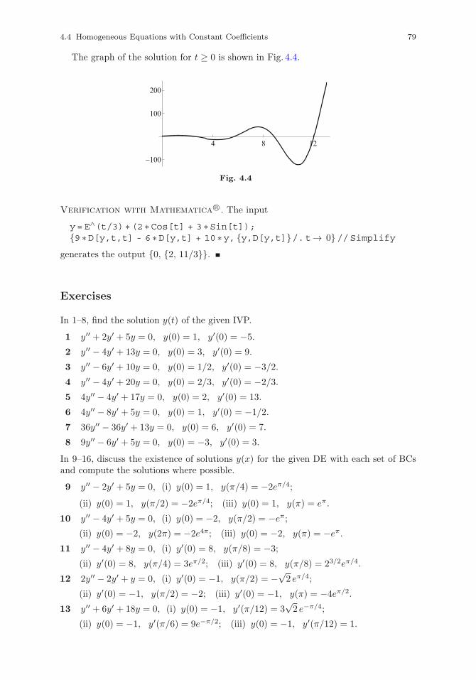
4.4 Homogeneous Equations with Constant Coefficients 79
The graph of the solution for t ≥ 0 is shown in Fig. 4.4.
4 8 12
−100
100
200
Fig. 4.4
Verification with Mathematica R©. The input
y=E∧(t/3) ∗(2 ∗Cos[t] + 3 ∗Sin[t]);{9 ∗D[y,t,t] - 6 ∗D[y,t] + 10 ∗y, {y,D[y,t]}/.t→ 0}//Simplify
generates the output {0, {2, 11/3}}.
Exercises
In 1–8, find the solution y(t) of the given IVP.
1 y′′ + 2y′ + 5y = 0, y(0) = 1, y′(0) = −5.
2 y′′ − 4y′ + 13y = 0, y(0) = 3, y′(0) = 9.
3 y′′ − 6y′ + 10y = 0, y(0) = 1/2, y′(0) = −3/2.
4 y′′ − 4y′ + 20y = 0, y(0) = 2/3, y′(0) = −2/3.
5 4y′′ − 4y′ + 17y = 0, y(0) = 2, y′(0) = 13.
6 4y′′ − 8y′ + 5y = 0, y(0) = 1, y′(0) = −1/2.
7 36y′′ − 36y′ + 13y = 0, y(0) = 6, y′(0) = 7.
8 9y′′ − 6y′ + 5y = 0, y(0) = −3, y′(0) = 3.
In 9–16, discuss the existence of solutions y(x) for the given DE with each set of BCsand compute the solutions where possible.
9 y′′ − 2y′ + 5y = 0, (i) y(0) = 1, y(π/4) = −2eπ/4;
(ii) y(0) = 1, y(π/2) = −2eπ/4; (iii) y(0) = 1, y(π) = eπ.
10 y′′ − 4y′ + 5y = 0, (i) y(0) = −2, y(π/2) = −eπ;(ii) y(0) = −2, y(2π) = −2e4π; (iii) y(0) = −2, y(π) = −eπ.
11 y′′ − 4y′ + 8y = 0, (i) y′(0) = 8, y(π/8) = −3;
(ii) y′(0) = 8, y(π/4) = 3eπ/2; (iii) y′(0) = 8, y(π/8) = 23/2eπ/4.
12 2y′′ − 2y′ + y = 0, (i) y′(0) = −1, y(π/2) = −√2 eπ/4;
(ii) y′(0) = −1, y(π/2) = −2; (iii) y′(0) = −1, y(π) = −4eπ/2.
13 y′′ + 6y′ + 18y = 0, (i) y(0) = −1, y′(π/12) = 3√2 e−π/4;
(ii) y(0) = −1, y′(π/6) = 9e−π/2; (iii) y(0) = −1, y′(π/12) = 1.
80 4 Linear Second-Order Equations
14 9y′′ + 12y′ + 8y = 0, (i) y(0) = 2, y′(3π/8) = 3;
(ii) y(0) = 2, y′(3π/8) = −(4√2/3)e−π/4; (iii) y(0) = 2, y′(3π/4) = −e−π/2.
15 9y′′ − 12y′ + 13y = 0, (i) y′(0) = 5/2, y′(π/2) = −(8/3)eπ/3;
(ii) y′(0) = 5/2, y′(π) = −(5/2)e2π/3; (iii) y′(0) = 5/2, y′(π) = 1.
16 2y′′ − 2y′ + 5y = 0, (i) y′(0) = −1, y′(2π/3) = −2;
(ii) y′(0) = −1, y′(π/3) = −7eπ/6; (iii) y′(0) = −1, y′(2π/3) = −(5/2)eπ/3.
Answers to Odd-Numbered Exercises
1 y(t) = e−t[cos(2t)− 2 sin(2t)]. 3 y(t) = e3t[(1/2) cos t− 3 sin t].
5 y(t) = et/2[2 cos(2t) + 6 sin(2t)]. 7 y(t) = et/2[6 cos(t/3) + 12 sin(t/3)].
9 (i) y(x) = ex[cos(2x)− 2 sin(2x)]; (ii) no solution;
(iii) y(x) = ex[cos(2x) + c sin(2x)], c = const arbitrary.
11 (i) No solution; (ii) y(x) = e2x[cos(2x) + 3 sin(2x)];
(iii) y(x) = e2x{4 cos(2x) + c[sin(2x)− cos(2x)]}, c = const arbitrary.
13 (i) y(x) = e−3x[− cos(3x) + c sin(3x)], c = const arbitrary;
(ii) y(x) = e3x[− cos(3x)− 2 sin(3x)]; (iii) no solution.
15 (i) y(x) = e2x/3[3 cosx+ (1/2) sinx];
(ii) y(x) = e2x/3{(15/4) cosx+ c[sinx− (3/2) cosx]}, c = const arbitrary;
(iii) no solution.
4.5 Nonhomogeneous Equations
Using the operator notation introduced in Sect. 1.4, we can write the general linear,nonhomogeneous, second-order DE in the form
Ly = y′′ + p(t)y′ + q(t)y = f(t), (4.14)
where the functions p, q, and f are prescribed.
4.37 Theorem. The GS of equation (4.14) is
y(t) = yc(t) + yp(t), (4.15)
where yc (called the complementary function) is the GS of the associated homogeneousequation Ly = 0 and yp is any PS of the full nonhomogeneous equation Ly = f .
Proof. Let {y1, y2} be an FSS for the associated homogeneous DE. Then, as we knowfrom Sect. 4.3, yc = c1y1 + c2y2 with arbitrary constants c1 and c2. Since L is a linearoperator, it follows that for any numbers c1 and c2,
L(c1y1 + c2y2 + yp) = L(c1y1 + c2y2) + Lyp = 0 + f = f,
4.5 Nonhomogeneous Equations 81
so any function of the formy = c1y1 + c2y2 + yp (4.16)
is a solution of (4.14).Now suppose that there is a solution y of (4.14) that cannot be written in the
form (4.16). AsL(y − yp) = Ly − Lyp = f − f = 0,
we deduce that y − yp is a solution of the associated homogeneous equation, so thereare c1, c2 = const such that
y − yp = c1y1 + c2y2;
hence,y = c1y1 + c2y2 + yp,
which contradicts our assumption.In conclusion, every solution of (4.14) is of the form (4.16), confirming that (4.15) is
the GS of the given nonhomogeneous equation.
Below, we restrict our attention to nonhomogeneous DEs with constant coefficients.Since we already know how to find yc for such equations, we need to design a suitableprocedure for computing yp.
4.5.1 Method of Undetermined Coefficients: Simple Cases
This technique, based on educated guesses suggested by the nature of the nonhomoge-neous term f , is best illustrated by examples.
4.38 Example. Consider the IVP
y′′ − 2y′ + y = 2t− 7, y(0) = −5, y′(0) = 1.
The roots of the characteristic equation r2−2r+1 = 0 are r1 = r2 = 1. Hence, by (4.10),
yc = (c1 + c2t)et.
To find a PS yp of the full equation, we notice that f is a first-degree polynomial, sowe try yp in the form of a first-degree polynomial with unknown coefficients; that is,
yp(t) = α0t+ α1.
Substituting in the DE, we arrive at
y′′p − 2y′p + yp = α0t− 2α0 + α1 = 2t− 7.
We now equate the coefficients of t and the constant terms on both sides and obtainα0 = 2 and −2α0 + α1 = −7, from which α1 = −3; therefore, the GS of the DE is
y(t) = yc(t) + yp(t) = (c1 + c2t)et + 2t− 3.
The constants c1 and c2, determined from the ICs, are c1 = −2 and c2 = 1, so thesolution of the IVP is
y(t) = (t− 2)et + 2t− 3.
82 4 Linear Second-Order Equations
Verification with Mathematica R©. The input
y=(t - 2) ∗E∧t + 2 ∗t - 3;{D[y,t,t] - 2 ∗D[y,t] + y - 2 ∗t + 7,{y,D[y,t]}/.t→ 0}//Simplify
generates the output {0, {−5, 1}}.4.39 Example. The characteristic equation in the IVP
y′′ + 3y′ + 2y = −12e2t, y(0) = −2, y′(0) = 2
is r2 + 3r + 2 = 0, with roots r1 = −1 and r2 = −2; hence, by (4.9),
yc(t) = c1e−t + c2e
−2t.
Since the right-hand side in the DE is an exponential, we try to find a function yp ofthe same form; that is,
yp(t) = αe2t.
From the DE we then obtain
y′′p + 3y′p + 2y = 4αe2t + 6αe2t + 2αe2t = 12αe2t = −12e2t,
so α = −1, which yields the GS
y(t) = yc(t) + yp(t) = c1e−t + c2e
−2t − e2t.
Applying the ICs, we find that c1 = 2 and c2 = −3, so the solution of the IVP is
y(t) = 2e−t − 3e−2t − e2t.
Verification with Mathematica R©. The input
y=2 ∗E∧(-t) - 3 ∗E∧(-2 ∗t) - E∧(2 ∗t);{D[y,t,t] + 3 ∗D[y,t] + 2 ∗y + 12 ∗E∧(2 ∗t), {y,D[y,t]}/.t→ 0}
//Simplify
generates the output {0, {−2, 2}}.4.40 Example. In the IVP
y′′ − 6y′ + 8y = 40 sin(2t), y(0) = 1, y′(0) = −10,
the characteristic equation r2 − 6r + 8 = 0 has roots r1 = 2 and r2 = 4, so, by (4.9),
yc(t) = c1e2t + c2e
4t.
The function f is a multiple of sin(2t). However, if we tried yp in the form α sin(2t),the DE would lead to
y′′p − 6y′p + 8yp = 4α sin(2t)− 12α cos(2t) = 40 sin(2t),
and, matching the coefficients of the linearly independent functions sin(2t) and cos(2t)on both sides, we would get α = 10 and α = 0, which is impossible. To avoid this, wetry yp as a linear combination of both cos(2t) and sin(2t); that is,
yp(t) = α cos(2t) + β sin(2t).
4.5 Nonhomogeneous Equations 83
Then, substituting in the DE, we find that
y′′p − 6y′p + 8yp = (4α− 12β) cos(2t) + (12α+ 4β) sin(2t) = 40 sin(2t),
and the matching of the coefficients now leads to the system
4α − 12β = 0,12α + 4β = 40,
from which α = 3 and β = 1. Consequently, the GS of the DE is
y(t) = yc(t) + yp(t) = c1e2t + c2e
4t + 3 cos(2t) + sin(2t).
The constants c1 and c2 are determined from the ICs; they are c1 = 2 and c2 = −4, sothe solution of the IVP is
y(t) = 2e2t − 4e4t + 3 cos(2t) + sin(2t).
Verification with Mathematica R©. The input
y=2 ∗E∧(2 ∗t) - 4 E∧(4 ∗t) + 3 ∗Cos[2 ∗t] + Sin[2 ∗t];{D[y,t,t] - 6 ∗D[y,t] + 8 ∗y - 40 ∗Sin[2 ∗t], {y,D[y,t]}/.t→ 0}
//Simplify
generates the output {0, {1, −10}}.
4.41 Example. Consider the IVP
y′′ + 2y′ + 2y = (5t− 11)et, y(0) = −1, y′(0) = −3.
The characteristic equation r2 + 2r + 2 = 0 has roots r1 = −1 + i and r2 = −1 − i,which means that, by (4.13),
yc(t) = e−t(c1 cos t+ c2 sin t).
Given the form of f on the right-hand side of the DE, we try
yp(t) = (α0t+ α1)et.
Then, differentiating this expression, replacing it and its derivatives in the equation,and sorting out the terms, we arrive at
y′′p + 2y′p + 2yp = (5α0t+ 4α0 + 5α1)et = (5t− 11)et.
In Sect. 4.4.2 it was shown that tet and et are linearly independent functions, so, equat-ing their coefficients on both sides, we obtain 5α0 = 5 and 4α0 + 5α1 = −11, fromwhich α0 = 1 and α1 = −3. Thus, the GS solution of the DE is
y(t) = yc(t) + yp(t) = e−t(c1 cos t+ c2 sin t) + (t− 3)et.
We now apply the ICs and find that c1 = 2 and c2 = 1, which means that the solutionof the IVP is
y(t) = e−t(2 cos t+ sin t) + (t− 3)et.
84 4 Linear Second-Order Equations
Verification with Mathematica R©. The input
y=E∧(-t) ∗(2 ∗Cos[t] + Sin[t]) + (t - 3) ∗E∧t;{D[y,t,t] + 2 ∗D[y,t] + 2 ∗y - (5 ∗t - 11) ∗E∧t,
{y,D[y,t]}/.t→ 0}//Simplifygenerates the output {0, {−1, −3}}.
4.42 Example. The IVP
y′′ + 2y′ + y = −24et cos(2t), y(0) = −2, y′(0) = −3
is handled similarly. The roots of the characteristic equation are r1 = r2 = −1, so,by (4.10),
yc(t) = (c1 + c2t)e−t.
Recalling the argument used in Example 4.40, we seek a PS of the form
yp(t) = et[α cos(2t) + β sin(2t)]
and, in the usual way, arrive at the equality
et[8β cos(2t)− 8α sin(2t)] = −24et cos(2t).
We know from Sect. 4.4.3 that functions such as et cos(2t) and et sin(2t) are linearlyindependent, so, equating their coefficients on both sides, we find that α = 0 andβ = −3. Consequently, the GS of the IVP is
y(t) = yc(t) + yp(t) = (c1 + c2t)e−t − 3et sin(2t).
The ICs now produce the values c1 = −2 and c2 = 1, which means that the solution ofthe IVP is
y(t) = (t− 2)e−t − 3et sin(2t).
Verification with Mathematica R©. The input
y=(t - 2) ∗E∧( - t) - 3 ∗E∧t ∗Sin[2 ∗t];{D[y,t,t] + 2 ∗D[y,t] + y + 24 ∗E∧t ∗Cos[2 ∗t],
{y,D[y,t]}/.t→ 0}//Simplifygenerates the output {0, {−2, −3}}.
4.43 Example. The characteristic equation for the IVP
3y′′ − 4y′ + y = 50t cos t, y(0) = 0, y′(0) = 0
is 3r2 − 4r + 1 = 0, with roots r1 = 1/3 and r2 = 1; therefore, by (4.9), we have
yc(t) = c1et/3 + c2e
t.
To find a PS, we note that the right-hand side of the DE is a product of a first-degreepolynomial and a cosine. In this case, we try a function of the form
yp(t) = (α0t+ α1) cos t+ (β0t+ β1) sin t,
which, replaced in the equation, leads to the equality
4.5 Nonhomogeneous Equations 85
[(−2α0 − 4β0)t− 4α0 + 6β0 − 2α1 − 4β1] cos t
+ [(4α0 − 2β0)t− 6α0 − 4β0 + 4α1 − 2b1] sin t = 50t cos t.
Using the Wronskian, we now convince ourselves that the functions t cos t, cos t, t sin t,and sin t are linearly independent; hence, equating their coefficients on both sides above,we obtain the set of four equations
−2α0 − 4β0 = 50, −4α0 + 6β0 − 2α1 − 4β1 = 0,4α0 − 2β0 = 0, −6α0 − 4β0 + 4α1 − 2β1 = 0,
from which α0 = −5, β0 = −10, α1 = −18, and β1 = −1, so the GS of the full DE is
y(t) = yc(t) + yp(t) = c1et/3 + c2e
t − (5t+ 18) cos t− (10t+ 1) sin t.
Finally, using the ICs, we find that c1 = 18 and c2 = 0; therefore,
y(t) = 18et/3 − (5t+ 18) cos t− (10t+ 1) sin t.
Verification with Mathematica R©. The input
y=18 ∗E∧(t/3) - (5 ∗t + 18) ∗Cos[t] - (10 ∗t + 1) ∗Sin[t];{3 ∗D[y,t,t] - 4 ∗D[y,t] + y - 50 ∗t ∗Cos[t], {y,D[y,t]}/.t→ 0}
//Simplify
generates the output {0, {0, 0}}.4.44 Example. For the BVP
y′′ + 4y′ + 5y = −4 cosx− 4 sinx, y′(0) = −3, y(π) = −e−2π
we have r1 = −2 + i, r2 = −2− i, so, by (4.13),
yc(x) = e−2x(c1 cosx+ c2 sinx).
Trying a PS of the formyp(x) = α cosx+ β sinx
in the DE, we find in the usual way that α = 0 and β = −1, so the GS of the DE is
y(x) = yc(x) + yp(x) = e−2x(c1 cosx+ c2 sinx)− sinx.
Since, as is easily seen,
y′(x) = e−2x[(c2 − 2c1) cosx− (c1 + 2c2) sinx],
the BCs now yield c1 = 1 and c2 = 0, which means that
y(x) = e−2x cosx− sinx.
Verification with Mathematica R©. The input
y=E∧(-2 ∗x) ∗Cos[x] - Sin[x];{D[y,x,x] + 4 ∗D[y,x] + 5 ∗y + 4 ∗Cos[x] + 4 ∗Sin[x],
{D[y,x]/.x→ 0,y/.x→Pi}}//Simplifygenerates the output {0, {−3, −e−2π}}.
86 4 Linear Second-Order Equations
4.45 Example. The characteristic roots for the DE in the BVP
4y′′ − y = 32 + x− 4x2, y(0) = 2, y′(2) = 292
are r1 = 1/2 and r2 = −1/2. By analogy with the comment made in Example 4.33,here it is more advantageous to write yc as a combination of hyperbolic functions. Inview of the given BCs, we choose the (admissible) form
yc(x) = c1 sinh(12 x)+ c2 cosh
(12 (x− 2)
).
For a PS, we try a quadratic polynomial
yp(x) = α0x2 + α1x+ α2,
which, when replaced in the equation, produces the coefficients α0 = 4, α1 = −1, andα2 = 0, so the GS is
y(x) = yc(x) + yp(x) = c1 sinh(12 x)+ c2 cosh
(12 (x− 2)
)+ 4x2 − x.
Using the fact that
y′(x) = 12 c1 cosh
(12 x)+ 1
2 c2 sinh(12 (x − 2)
)+ 8x− 1,
we apply the BCs and arrive at the pair of simple equations
c2 cosh 1 = 2, 12 c1 cosh 1 + 15 = 29
2 ,
from which c1 = − sech 1 and c2 = 2 sech 1. Hence, the solution of the BVP is
y(x) = (sech 1)[− sinh
(12 x)+ 2 cosh
(12 (x− 2)
)]+ 4x2 − x.
Verification with Mathematica R©. The input
y=Sech[1] ∗(- Sinh[x/2] + 2 ∗Cosh[(x - 2)/2]) + 4 ∗x∧2 - x;{4 ∗D[y,x,x] - y - 32 - x + 4 ∗x∧2, {y/.x→ 0,D[y,x]/.x→ 2}}
//Simplify
generates the output {0, {2, 29/2}}.
Exercises
In 1–30, use the method of undetermined coefficients to find a particular solution of theDE and then solve the given IVP.
1 y′′ + 3y′ + 2y = 8t+ 8, y(0) = −1, y′(0) = 0.
2 y′′ + y′ − 6y = 14t− 6t2, y(0) = 4, y′(0) = −9.
3 y′′ − 8y′ + 16y = 6(8t2 − 8t+ 1), y(0) = −2, y′(0) = −7.
4 y′′ + 6y′ + 9y = 9t− 39, y(0) = −6, y′(0) = 6.
5 y′′ − 2y′ + 2y = 2(t2 − 5t+ 6), y(0) = 3, y′(0) = 0.
6 y′′ − 2y′ + 5y = 5t3 − 6t2 − 4t+ 4, y(0) = 3/2, y′(0) = −9/2.
4.5 Nonhomogeneous Equations 87
7 y′′ + 2y′ − 8y = −16e−2t, y(0) = 3, y′(0) = 4.
8 2y′′ − 7y′ + 3y = (7/2)e4t, y(0) = 3, y′(0) = 7.
9 9y′′ + 12y′ + 4y = 2e−t, y(0) = −1, y′(0) = 1.
10 y′′ − 6y′ + 9y = −25e−2t, y(0) = 1, y′(0) = 10.
11 4y′′ − 4y′ + 5y = 58e3t, y(0) = 4, y′(0) = 13/2.
12 4y′′ − 16y′ + 17y = (1/2)e2t, y(0) = 7/6, y′(0) = 17/6.
13 y′′ + 2y′ − 3y = 8 cos(2t)− 14 sin(2t), y(0) = 4, y′(0) = −4.
14 y′′ − 6y′ + 8y = 85 cos t, y(0) = 11, y′(0) = 8.
15 y′′ + 2y′ + y = 25 sin(2t), y(0) = 0, y′(0) = 0.
16 9y′′ + 6y′ + y = (53/8) cos(t/2)− sin(t/2), y(0) = −7/2, y′(0) = 3.
17 y′′ − 6y′ + 10y = (89/6) cos(t/3) + 3 sin(t/3), y(0) = 1/2, y′(0) = −2.
18 4y′′ − 8y′ + 5y = −17 cos t− 6 sin t, y(0) = 1, y′(0) = 5.
19 2y′′ + y′ − y = −18(t+ 1)e2t, y(0) = −1, y′(0) = −4.
20 3y′′ − 7y′ + 2y = (25− 12t)e−t, y(0) = 6, y′(0) = 3.
21 y′′ − 4y′ + 4y = (t− 4)et, y(0) = −4, y′(0) = −4.
22 y′′ − 2y′ + 5y = (65t− 56)e−2t, y(0) = −3, y′(0) = 2.
23 4y′′ − 5y′ + y = 2e−t(−13 cos t+ 6 sin t), y(0) = −3, y′(0) = 2.
24 y′′ − 2y′ + y = −e2t[3 cos(2t) + 4 sin(2t)], y(0) = 1, y′(0) = 5.
25 4y′′ + 4y′ + y = e−2t(29 cos t+ 2 sin t), y(0) = 2, y′(0) = −13/2.
26 4y′′ − 4y′ + 17y = −et[cos(2t)− 8 sin(2t)], y(0) = 0, y′(0) = 15/2.
27 y′′ − y = 4 cos(2t)− 5t sin(2t), y(0) = −1, y′(0) = 1.
28 y′′ − 2y′ + y = 2[(2t− 3) cos t+ (t+ 1) sin t], y(0) = −2, y′(0) = −1.
29 y′′ + y = 3(t+ 1) cos(2t) + 4 sin(2t), y(0) = 0, y′(0) = −1.
30 y′′ − 2y′ + 2y = (8− 7t) cos(t/2) + 4(1− t) sin(t/2), y(0) = 0, y′(0) = −2.
In 31–38, use the method of undetermined coefficients to find a particular solution ofthe DE and then solve the given BVP.
31 y′′ + 4y′ + 3y = 30e2x, y(0) = 3, y(ln 2) = 17/2.
32 y′′ + 5y′ + 6y = −(15/2)e−x/2, y(− ln 2) = 4− 23/2, y′(0) = 2.
33 y′′ − 4y = 4x, y′(0) = 1, y(1) = 0.
34 9y′′ − 4y = 18(9− 2x2), y′(0) = 2/3, y′(3/2) = 85/3.
35 y′′ − 4y′ + 4y = (2π2 − 8) cos(πx) − 8π sin(πx), y(0) = 1, y(3) = 2.
36 9y′′ + 6y′ + y = x2 + 9x+ 2, y′(0) = 1/3, y(2) = 0.
37 y′′ − 4y′ + 5y = −9 cos(2x)− 7 sin(2x), y′(0) = −3, y(π) = −1 + 2e2π.
38 y′′ + 2y′ + 10y = 13ex, y′(0) = 3/2, y′(π/3) = eπ/3 − (1/2)e−π/3.
Answers to Odd-Numbered Exercises
1 yp(t) = 4t− 2, y(t) = 3e−2t − 2e−t + 4t− 2.
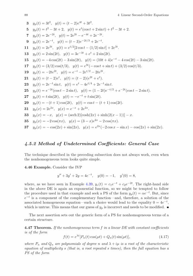
88 4 Linear Second-Order Equations
3 yp(t) = 3t2, y(t) = (t− 2)e4t + 3t2.
5 yp(t) = t2 − 3t+ 2, y(t) = et(cos t+ 2 sin t) + t2 − 3t+ 2.
7 yp(t) = 2e−2t, y(t) = 2e2t − e−4t + 2e−2t.
9 yp(t) = 2e−t, y(t) = (t− 3)e−2t/3 + 2e−t.
11 yp(t) = 2e3t, y(t) = et/2[2 cos t− (1/2) sin t] + 2e3t.
13 yp(t) = 2 sin(2t), y(t) = 3e−3t + et + 2 sin(2t).
15 yp(t) = −4 cos(2t)− 3 sin(2t), y(t) = (10t+ 4)e−t − 4 cos(2t)− 3 sin(2t).
17 yp(t) = (3/2) cos(t/3), y(t) = e3t(− cos t+ sin t) + (3/2) cos(t/3).
19 yp(t) = −2te2t, y(t) = e−t − 2et/2 − 2te2t.
21 yp(t) = (t− 2)et, y(t) = (t− 2)(e2t + et).
23 yp(t) = 2e−t sin t, y(t) = et − 4et/4 + 2e−t sin t.
25 yp(t) = e−2t(cos t− 2 sin t), y(t) = (1− 2t)e−t/2 + e−2t(cos t− 2 sin t).
27 yp(t) = t sin(2t), y(t) = −e−t + t sin(2t).
29 yp(t) = −(t+ 1) cos(2t), y(t) = cos t− (t+ 1) cos(2t).
31 yp(x) = 2e2x, y(x) = e−x + 2e2x.
33 yp(x) = −x, y(x) = (sech 2)[cosh(2x) + sinh(2(x− 1))]− x.
35 yp(x) = −2 cos(πx), y(x) = (3− x)e2x − 2 cos(πx).
37 yp(x) = − cos(2x) + sin(2x), y(x) = e2x(−2 cosx− sinx)− cos(2x) + sin(2x).
4.5.2 Method of Undetermined Coefficients: General Case
The technique described in the preceding subsection does not always work, even whenthe nonhomogeneous term looks quite simple.
4.46 Example. Consider the IVP
y′′ + 3y′ + 2y = 4e−t, y(0) = −1, y′(0) = 8,
where, as we have seen in Example 4.39, yc(t) = c1e−t + c2e
−2t. The right-hand sidein the above DE is again an exponential function, so we might be tempted to followthe procedure used in that example and seek a PS of the form yp(t) = αe−t. But, sincee−t is a component of the complementary function—and, therefore, a solution of theassociated homogeneous equation—such a choice would lead to the equality 0 = 4e−t,which is untrue. This means that our guess of yp is incorrect and needs to be modified.
The next assertion sets out the generic form of a PS for nonhomogeneous terms of acertain structure.
4.47 Theorem. If the nonhomogeneous term f in a linear DE with constant coefficientsis of the form
f(t) = eλt[Pn(t) cos(μt) +Qn(t) sin(μt)], (4.17)
where Pn and Qn are polynomials of degree n and λ+ iμ is a root of the characteristicequation of multiplicity s (that is, a root repeated s times), then the full equation has aPS of the form
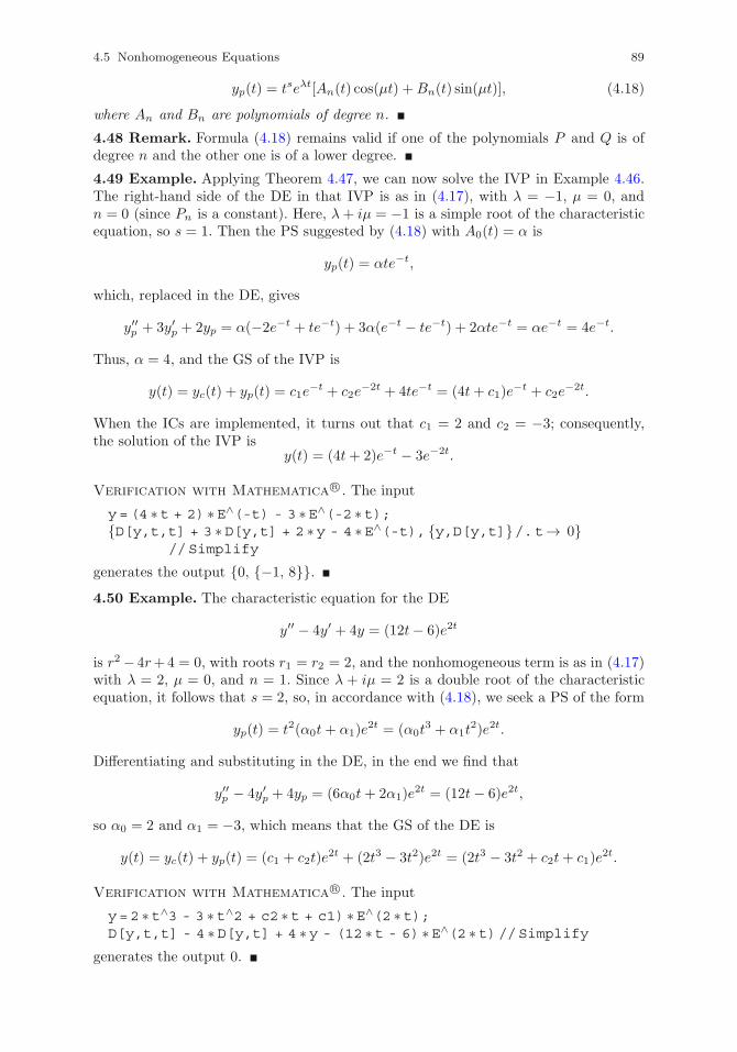
4.5 Nonhomogeneous Equations 89
yp(t) = tseλt[An(t) cos(μt) +Bn(t) sin(μt)], (4.18)
where An and Bn are polynomials of degree n.
4.48 Remark. Formula (4.18) remains valid if one of the polynomials P and Q is ofdegree n and the other one is of a lower degree.
4.49 Example. Applying Theorem 4.47, we can now solve the IVP in Example 4.46.The right-hand side of the DE in that IVP is as in (4.17), with λ = −1, μ = 0, andn = 0 (since Pn is a constant). Here, λ+ iμ = −1 is a simple root of the characteristicequation, so s = 1. Then the PS suggested by (4.18) with A0(t) = α is
yp(t) = αte−t,
which, replaced in the DE, gives
y′′p + 3y′p + 2yp = α(−2e−t + te−t) + 3α(e−t − te−t) + 2αte−t = αe−t = 4e−t.
Thus, α = 4, and the GS of the IVP is
y(t) = yc(t) + yp(t) = c1e−t + c2e
−2t + 4te−t = (4t+ c1)e−t + c2e
−2t.
When the ICs are implemented, it turns out that c1 = 2 and c2 = −3; consequently,the solution of the IVP is
y(t) = (4t+ 2)e−t − 3e−2t.
Verification with Mathematica R©. The input
y=(4 ∗t + 2) ∗E∧(-t) - 3 ∗E∧(-2 ∗t);{D[y,t,t] + 3 ∗D[y,t] + 2 ∗y - 4 ∗E∧(-t), {y,D[y,t]}/.t→ 0}
//Simplify
generates the output {0, {−1, 8}}.4.50 Example. The characteristic equation for the DE
y′′ − 4y′ + 4y = (12t− 6)e2t
is r2 − 4r+4 = 0, with roots r1 = r2 = 2, and the nonhomogeneous term is as in (4.17)with λ = 2, μ = 0, and n = 1. Since λ + iμ = 2 is a double root of the characteristicequation, it follows that s = 2, so, in accordance with (4.18), we seek a PS of the form
yp(t) = t2(α0t+ α1)e2t = (α0t
3 + α1t2)e2t.
Differentiating and substituting in the DE, in the end we find that
y′′p − 4y′p + 4yp = (6α0t+ 2α1)e2t = (12t− 6)e2t,
so α0 = 2 and α1 = −3, which means that the GS of the DE is
y(t) = yc(t) + yp(t) = (c1 + c2t)e2t + (2t3 − 3t2)e2t = (2t3 − 3t2 + c2t+ c1)e
2t.
Verification with Mathematica R©. The input
y=2 ∗t∧3 - 3 ∗t∧2 + c2 ∗t + c1) ∗E∧(2 ∗t);D[y,t,t] - 4 ∗D[y,t] + 4 ∗y - (12 ∗t - 6) ∗E∧(2 ∗t)//Simplify
generates the output 0.
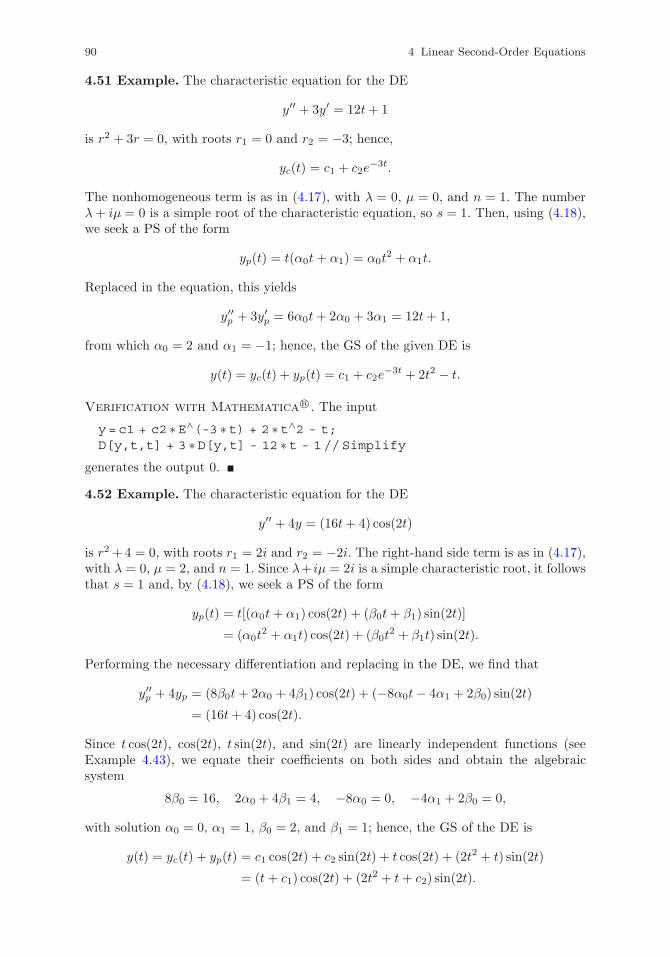
90 4 Linear Second-Order Equations
4.51 Example. The characteristic equation for the DE
y′′ + 3y′ = 12t+ 1
is r2 + 3r = 0, with roots r1 = 0 and r2 = −3; hence,
yc(t) = c1 + c2e−3t.
The nonhomogeneous term is as in (4.17), with λ = 0, μ = 0, and n = 1. The numberλ+ iμ = 0 is a simple root of the characteristic equation, so s = 1. Then, using (4.18),we seek a PS of the form
yp(t) = t(α0t+ α1) = α0t2 + α1t.
Replaced in the equation, this yields
y′′p + 3y′p = 6α0t+ 2α0 + 3α1 = 12t+ 1,
from which α0 = 2 and α1 = −1; hence, the GS of the given DE is
y(t) = yc(t) + yp(t) = c1 + c2e−3t + 2t2 − t.
Verification with Mathematica R©. The input
y=c1 + c2 ∗E∧(-3 ∗t) + 2 ∗t∧2 - t;D[y,t,t] + 3 ∗D[y,t] - 12 ∗t - 1//Simplify
generates the output 0.
4.52 Example. The characteristic equation for the DE
y′′ + 4y = (16t+ 4) cos(2t)
is r2 +4 = 0, with roots r1 = 2i and r2 = −2i. The right-hand side term is as in (4.17),with λ = 0, μ = 2, and n = 1. Since λ+ iμ = 2i is a simple characteristic root, it followsthat s = 1 and, by (4.18), we seek a PS of the form
yp(t) = t[(α0t+ α1) cos(2t) + (β0t+ β1) sin(2t)]
= (α0t2 + α1t) cos(2t) + (β0t
2 + β1t) sin(2t).
Performing the necessary differentiation and replacing in the DE, we find that
y′′p + 4yp = (8β0t+ 2α0 + 4β1) cos(2t) + (−8α0t− 4α1 + 2β0) sin(2t)
= (16t+ 4) cos(2t).
Since t cos(2t), cos(2t), t sin(2t), and sin(2t) are linearly independent functions (seeExample 4.43), we equate their coefficients on both sides and obtain the algebraicsystem
8β0 = 16, 2α0 + 4β1 = 4, −8α0 = 0, −4α1 + 2β0 = 0,
with solution α0 = 0, α1 = 1, β0 = 2, and β1 = 1; hence, the GS of the DE is
y(t) = yc(t) + yp(t) = c1 cos(2t) + c2 sin(2t) + t cos(2t) + (2t2 + t) sin(2t)
= (t+ c1) cos(2t) + (2t2 + t+ c2) sin(2t).
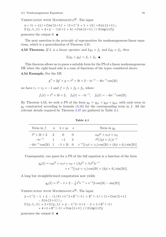
4.5 Nonhomogeneous Equations 91
Verification with Mathematica R©. The input
y=(t + c1) ∗Cos[2 ∗t] + (2 ∗t∧2 + t + c2) ∗Sin[2 ∗t];D[y,t,t] + 4 ∗y - (16 ∗t + 4) ∗Cos[2 ∗t]//Simplify
generates the output 0.
The next assertion is the principle of superposition for nonhomogeneous linear equa-tions, which is a generalization of Theorem 4.21.
4.53 Theorem. If L is a linear operator and Ly1 = f1 and Ly2 = f2, then
L(y1 + y2) = f1 + f2.
This theorem allows us to guess a suitable form for the PS of a linear nonhomogeneousDE when the right-hand side is a sum of functions of the types considered above.
4.54 Example. For the DE
y′′ + 2y′ + y = t2 + 3t+ 2− te−t − 4te−t cos(2t)
we have r1 = r2 = −1 and f = f1 + f2 + f3, where
f1(t) = t2 + 3t+ 2, f2(t) = −te−t, f3(t) = −4te−t cos(2t).
By Theorem 4.53, we seek a PS of the form yp = yp1 + yp2 + yp3, with each term inyp constructed according to formula (4.18) for the corresponding term in f . All therelevant details required by Theorem 4.47 are gathered in Table 4.1.
Table 4.1
Term in f n λ+ iμ s Term in yp
t2 + 3t+ 2 2 0 0 α0t2 + α1t+ α2
−te−t 1 −1 2 t2(β0t+ β1)e−t
−4te−t cos(2t) 1 −1 + 2i 0 e−t[(γ0t+ γ1) cos(2t) + (δ0t+ δ1) sin(2t)]
Consequently, our guess for a PS of the full equation is a function of the form
yp(t) = α0t2 + α1t+ α2 + (β0t
3 + β1t2)e−t
+ e−t[(γ0t+ γ1) cos(2t) + (δ0t+ δ1) sin(2t)].
A long but straightforward computation now yields
yp(t) = t2 − t+ 2− 16 t
3e−t + e−t[t cos(2t)− sin(2t)].
Verification with Mathematica R©. The input
y=t∧2 - t + 2 - (1/6) ∗t∧3 ∗E∧(-t) + E∧(-t) ∗(t ∗Cos[2 ∗t]- Sin[2 ∗t]);
D[y,t,t] + 2 ∗D[y,t] + y - t∧2-3 ∗t - 2 + t ∗E∧(-t)+ 4 ∗t ∗E∧(-t) ∗Cos[2 ∗t]//Simplify
generates the output 0.
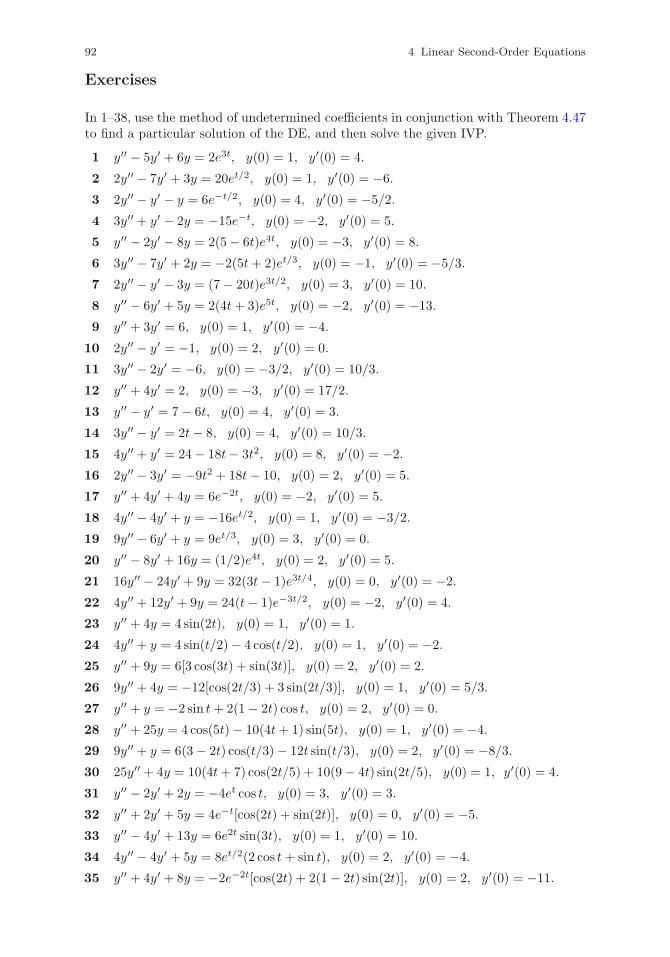
92 4 Linear Second-Order Equations
Exercises
In 1–38, use the method of undetermined coefficients in conjunction with Theorem 4.47to find a particular solution of the DE, and then solve the given IVP.
1 y′′ − 5y′ + 6y = 2e3t, y(0) = 1, y′(0) = 4.
2 2y′′ − 7y′ + 3y = 20et/2, y(0) = 1, y′(0) = −6.
3 2y′′ − y′ − y = 6e−t/2, y(0) = 4, y′(0) = −5/2.
4 3y′′ + y′ − 2y = −15e−t, y(0) = −2, y′(0) = 5.
5 y′′ − 2y′ − 8y = 2(5− 6t)e4t, y(0) = −3, y′(0) = 8.
6 3y′′ − 7y′ + 2y = −2(5t+ 2)et/3, y(0) = −1, y′(0) = −5/3.
7 2y′′ − y′ − 3y = (7− 20t)e3t/2, y(0) = 3, y′(0) = 10.
8 y′′ − 6y′ + 5y = 2(4t+ 3)e5t, y(0) = −2, y′(0) = −13.
9 y′′ + 3y′ = 6, y(0) = 1, y′(0) = −4.
10 2y′′ − y′ = −1, y(0) = 2, y′(0) = 0.
11 3y′′ − 2y′ = −6, y(0) = −3/2, y′(0) = 10/3.
12 y′′ + 4y′ = 2, y(0) = −3, y′(0) = 17/2.
13 y′′ − y′ = 7− 6t, y(0) = 4, y′(0) = 3.
14 3y′′ − y′ = 2t− 8, y(0) = 4, y′(0) = 10/3.
15 4y′′ + y′ = 24− 18t− 3t2, y(0) = 8, y′(0) = −2.
16 2y′′ − 3y′ = −9t2 + 18t− 10, y(0) = 2, y′(0) = 5.
17 y′′ + 4y′ + 4y = 6e−2t, y(0) = −2, y′(0) = 5.
18 4y′′ − 4y′ + y = −16et/2, y(0) = 1, y′(0) = −3/2.
19 9y′′ − 6y′ + y = 9et/3, y(0) = 3, y′(0) = 0.
20 y′′ − 8y′ + 16y = (1/2)e4t, y(0) = 2, y′(0) = 5.
21 16y′′ − 24y′ + 9y = 32(3t− 1)e3t/4, y(0) = 0, y′(0) = −2.
22 4y′′ + 12y′ + 9y = 24(t− 1)e−3t/2, y(0) = −2, y′(0) = 4.
23 y′′ + 4y = 4 sin(2t), y(0) = 1, y′(0) = 1.
24 4y′′ + y = 4 sin(t/2)− 4 cos(t/2), y(0) = 1, y′(0) = −2.
25 y′′ + 9y = 6[3 cos(3t) + sin(3t)], y(0) = 2, y′(0) = 2.
26 9y′′ + 4y = −12[cos(2t/3) + 3 sin(2t/3)], y(0) = 1, y′(0) = 5/3.
27 y′′ + y = −2 sin t+ 2(1− 2t) cos t, y(0) = 2, y′(0) = 0.
28 y′′ + 25y = 4 cos(5t)− 10(4t+ 1) sin(5t), y(0) = 1, y′(0) = −4.
29 9y′′ + y = 6(3− 2t) cos(t/3)− 12t sin(t/3), y(0) = 2, y′(0) = −8/3.
30 25y′′ + 4y = 10(4t+ 7) cos(2t/5) + 10(9− 4t) sin(2t/5), y(0) = 1, y′(0) = 4.
31 y′′ − 2y′ + 2y = −4et cos t, y(0) = 3, y′(0) = 3.
32 y′′ + 2y′ + 5y = 4e−t[cos(2t) + sin(2t)], y(0) = 0, y′(0) = −5.
33 y′′ − 4y′ + 13y = 6e2t sin(3t), y(0) = 1, y′(0) = 10.
34 4y′′ − 4y′ + 5y = 8et/2(2 cos t+ sin t), y(0) = 2, y′(0) = −4.
35 y′′ + 4y′ + 8y = −2e−2t[cos(2t) + 2(1− 2t) sin(2t)], y(0) = 2, y′(0) = −11.
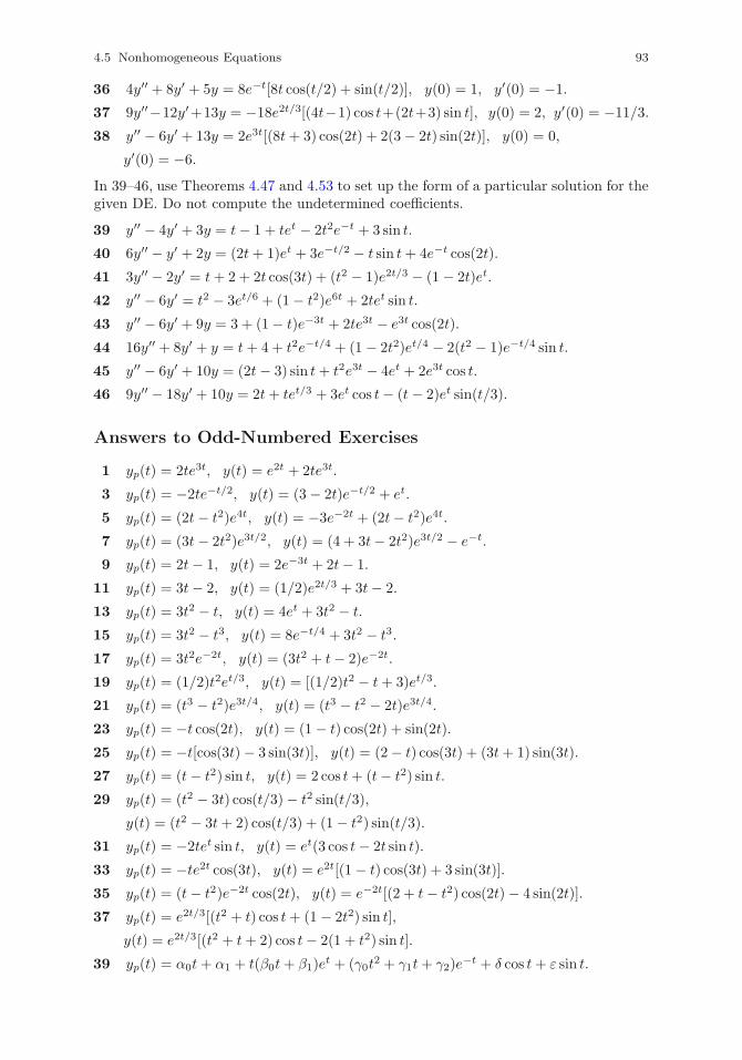
4.5 Nonhomogeneous Equations 93
36 4y′′ + 8y′ + 5y = 8e−t[8t cos(t/2) + sin(t/2)], y(0) = 1, y′(0) = −1.
37 9y′′−12y′+13y = −18e2t/3[(4t−1) cos t+(2t+3) sin t], y(0) = 2, y′(0) = −11/3.
38 y′′ − 6y′ + 13y = 2e3t[(8t+ 3) cos(2t) + 2(3− 2t) sin(2t)], y(0) = 0,
y′(0) = −6.
In 39–46, use Theorems 4.47 and 4.53 to set up the form of a particular solution for thegiven DE. Do not compute the undetermined coefficients.
39 y′′ − 4y′ + 3y = t− 1 + tet − 2t2e−t + 3 sin t.
40 6y′′ − y′ + 2y = (2t+ 1)et + 3e−t/2 − t sin t+ 4e−t cos(2t).
41 3y′′ − 2y′ = t+ 2 + 2t cos(3t) + (t2 − 1)e2t/3 − (1 − 2t)et.
42 y′′ − 6y′ = t2 − 3et/6 + (1− t2)e6t + 2tet sin t.
43 y′′ − 6y′ + 9y = 3 + (1− t)e−3t + 2te3t − e3t cos(2t).
44 16y′′ + 8y′ + y = t+ 4 + t2e−t/4 + (1 − 2t2)et/4 − 2(t2 − 1)e−t/4 sin t.
45 y′′ − 6y′ + 10y = (2t− 3) sin t+ t2e3t − 4et + 2e3t cos t.
46 9y′′ − 18y′ + 10y = 2t+ tet/3 + 3et cos t− (t− 2)et sin(t/3).
Answers to Odd-Numbered Exercises
1 yp(t) = 2te3t, y(t) = e2t + 2te3t.
3 yp(t) = −2te−t/2, y(t) = (3− 2t)e−t/2 + et.
5 yp(t) = (2t− t2)e4t, y(t) = −3e−2t + (2t− t2)e4t.
7 yp(t) = (3t− 2t2)e3t/2, y(t) = (4 + 3t− 2t2)e3t/2 − e−t.
9 yp(t) = 2t− 1, y(t) = 2e−3t + 2t− 1.
11 yp(t) = 3t− 2, y(t) = (1/2)e2t/3 + 3t− 2.
13 yp(t) = 3t2 − t, y(t) = 4et + 3t2 − t.
15 yp(t) = 3t2 − t3, y(t) = 8e−t/4 + 3t2 − t3.
17 yp(t) = 3t2e−2t, y(t) = (3t2 + t− 2)e−2t.
19 yp(t) = (1/2)t2et/3, y(t) = [(1/2)t2 − t+ 3)et/3.
21 yp(t) = (t3 − t2)e3t/4, y(t) = (t3 − t2 − 2t)e3t/4.
23 yp(t) = −t cos(2t), y(t) = (1 − t) cos(2t) + sin(2t).
25 yp(t) = −t[cos(3t)− 3 sin(3t)], y(t) = (2− t) cos(3t) + (3t+ 1) sin(3t).
27 yp(t) = (t− t2) sin t, y(t) = 2 cos t+ (t− t2) sin t.
29 yp(t) = (t2 − 3t) cos(t/3)− t2 sin(t/3),
y(t) = (t2 − 3t+ 2) cos(t/3) + (1− t2) sin(t/3).
31 yp(t) = −2tet sin t, y(t) = et(3 cos t− 2t sin t).
33 yp(t) = −te2t cos(3t), y(t) = e2t[(1 − t) cos(3t) + 3 sin(3t)].
35 yp(t) = (t− t2)e−2t cos(2t), y(t) = e−2t[(2 + t− t2) cos(2t)− 4 sin(2t)].
37 yp(t) = e2t/3[(t2 + t) cos t+ (1 − 2t2) sin t],
y(t) = e2t/3[(t2 + t+ 2) cos t− 2(1 + t2) sin t].
39 yp(t) = α0t+ α1 + t(β0t+ β1)et + (γ0t
2 + γ1t+ γ2)e−t + δ cos t+ ε sin t.
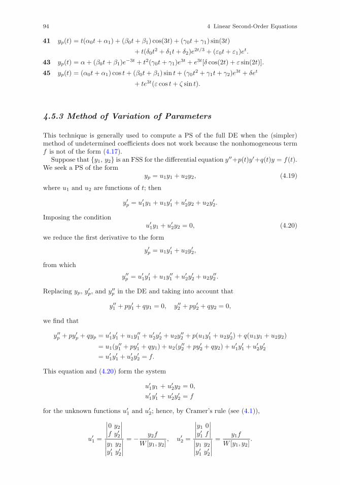
94 4 Linear Second-Order Equations
41 yp(t) = t(α0t+ α1) + (β0t+ β1) cos(3t) + (γ0t+ γ1) sin(3t)
+ t(δ0t2 + δ1t+ δ2)e
2t/3 + (ε0t+ ε1)et.
43 yp(t) = α+ (β0t+ β1)e−3t + t2(γ0t+ γ1)e
3t + e3t[δ cos(2t) + ε sin(2t)].
45 yp(t) = (α0t+ α1) cos t+ (β0t+ β1) sin t+ (γ0t2 + γ1t+ γ2)e
3t + δet
+ te3t(ε cos t+ ζ sin t).
4.5.3 Method of Variation of Parameters
This technique is generally used to compute a PS of the full DE when the (simpler)method of undetermined coefficients does not work because the nonhomogeneous termf is not of the form (4.17).
Suppose that {y1, y2} is an FSS for the differential equation y′′+p(t)y′+q(t)y = f(t).We seek a PS of the form
yp = u1y1 + u2y2, (4.19)
where u1 and u2 are functions of t; then
y′p = u′1y1 + u1y′1 + u′2y2 + u2y
′2.
Imposing the conditionu′1y1 + u′2y2 = 0, (4.20)
we reduce the first derivative to the form
y′p = u1y′1 + u2y
′2,
from which
y′′p = u′1y′1 + u1y
′′1 + u′2y
′2 + u2y
′′2 .
Replacing yp, y′p, and y′′p in the DE and taking into account that
y′′1 + py′1 + qy1 = 0, y′′2 + py′2 + qy2 = 0,
we find that
y′′p + py′p + qyp = u′1y′1 + u1y
′′1 + u′2y
′2 + u2y
′′2 + p(u1y
′1 + u2y
′2) + q(u1y1 + u2y2)
= u1(y′′1 + py′1 + qy1) + u2(y
′′2 + py′2 + qy2) + u′1y
′1 + u′2y
′2
= u′1y′1 + u′2y
′2 = f.
This equation and (4.20) form the system
u′1y1 + u′2y2 = 0,
u′1y′1 + u′2y
′2 = f
for the unknown functions u′1 and u′2; hence, by Cramer’s rule (see (4.1)),
u′1 =
∣∣∣∣0 y2f y′2
∣∣∣∣∣∣∣∣y1 y2y′1 y′2
∣∣∣∣= − y2f
W [y1, y2], u′2 =
∣∣∣∣y1 0y′1 f
∣∣∣∣∣∣∣∣y1 y2y′1 y′2
∣∣∣∣=
y1f
W [y1, y2].
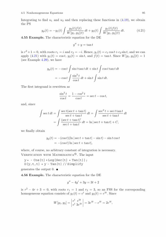
4.5 Nonhomogeneous Equations 95
Integrating to find u1 and u2 and then replacing these functions in (4.19), we obtainthe PS
yp(t) = −y1(t)∫
y2(t)f(t)
W [y1, y2](t)dt+ y2(t)
∫y1(t)f(t)
W [y1, y2](t)dt. (4.21)
4.55 Example. The characteristic equation for the DE
y′′ + y = tan t
is r2+1 = 0, with roots r1 = i and r2 = −i. Hence, yc(t) = c1 cos t+c2 sin t, and we canapply (4.21) with y1(t) = cos t, y2(t) = sin t, and f(t) = tan t. Since W [y1, y2](t) = 1(see Example 4.29), we have
yp(t) = − cos t
∫sin t tan t dt+ sin t
∫cos t tan t dt
= − cos t
∫sin2 t
cos tdt+ sin t
∫sin t dt.
The first integrand is rewritten as
sin2 t
cos t=
1− cos2 t
cos t= sec t− cos t,
and, since
∫sec t dt =
∫sec t(sec t+ tan t)
sec t+ tan tdt =
∫sec2 t+ sec t tan t
sec t+ tan tdt
=
∫(sec t+ tan t)′
sec t+ tan tdt = ln | sec t+ tan t|+ C,
we finally obtain
yp(t) = −(cos t)(ln | sec t+ tan t| − sin t)− sin t cos t
= −(cos t) ln | sec t+ tan t|,
where, of course, no arbitrary constant of integration is necessary.
Verification with Mathematica R©. The input
y= - Cos[t] ∗Log[Sec[t] + Tan[t]];D[y,t,t] + y - Tan[t]//Simplify
generates the output 0.
4.56 Example. The characteristic equation for the DE
y′′ − 4y′ + 3y = 3t+ 2
is r2 − 4r + 3 = 0, with roots r1 = 1 and r2 = 3, so an FSS for the correspondinghomogeneous equation consists of y1(t) = et and y2(t) = e3t. Since
W [y1, y2] =
∣∣∣∣ et e3t
et 3e3t
∣∣∣∣ = 3e4t − e4t = 2e4t,
96 4 Linear Second-Order Equations
from (4.21) with f(t) = 3t+ 2 and integration by parts it follows that
yp(t) = −et∫
(3t+ 2)e3t
2e4tdt+ e3t
∫(3t+ 2)et
2e4tdt
= − 12 e
t
∫(3t+ 2)e−t dt+ 1
2 e3t
∫(3t+ 2)e−3t dt
= 12 e
t(3t+ 5)e−t − 12 e
3t(t+ 1)e−3t = t+ 2.
Verification with Mathematica R©. The input
y=t + 2;D[y,t,t] - 4 ∗D[y,t] + 3 ∗y - 3 ∗t - 2//Simplify
generates the output 0.
4.57 Example. Applying the same treatment to the DE
y′′ − 2y′ + y = 4et,
we have r1 = r2 = 1, so y1(t) = et, y2(t) = tet, f(t) = 4et, and W [y1, y2](t) = e2t; then,by (4.21),
yp(t) = −et∫
4tet
e2tdt+ tet
∫4et
e2tdt = −2t2et + 4t2et = 2t2et.
Verification with Mathematica R©. The input
y=2 ∗t∧2 ∗E∧t;D[y,t,t] - 2 ∗D[y,t] + y - 4 ∗E∧t//Simplify
generates the output 0.
4.58 Remark. Obviously, if the DE is written as a(t)y′′ + b(t)y′ + c(t)y = f(t) witha �= 0, then division by the coefficient a brings it to the form considered at the beginningof this section so that formula (4.21) can be applied.
Exercises
In 1–26, use the method of variation of parameters to find a particular solution yp ofthe given DE. Work from first principles, without applying formula (4.21) directly.
1 y′′ + 2y′ − 3y = 9− 9t. 2 y′′ − y′ − 6y = 4(3t− 4).
3 y′′ − 4y′ + 4y = 4(5 + 2t). 4 9y′′ − 6y′ + y = 19− 3t.
5 y′′ + y = −t2 − 2. 6 4y′′ + y = 2t2 + t+ 16.
7 2y′′ − 5y′ + 2y = 40e−2t. 8 3y′′ − 2y′ − y = 4(t− 2)e−t.
9 y′′ − 2y′ + 2y = et. 10 y′′ + 2y′ + 5y = 8e−t.
11 25y′′ − 20y′ + 4y = −98e−t. 12 y′′ − 6y′ + 9y = (5/4)(5t− 14)et/2.
13 2y′′ − 3y′ − 2y = −18et/2. 14 4y′′ − y′ − 3y = (22t+ 19)e2t.
15 y′′ + 2y′ + y = 2e−t. 16 4y′′ + 4y′ + y = 8(3t− 2)e−t/2.
4.6 Cauchy–Euler Equations 97
17 y′′ − 6y′ + 10y = te3t. 18 y′′ + 2y′ + 10y = 9(2− t)e−t.
19 y′′ − 9y = 12e−3t. 20 y′′ − 2y′ − 8y = 6e4t.
21 y′′ + 2y = 4. 22 3y′′ − y′ = 2(4− t).
23 y′′ + 4y = 4 cos(2t). 24 9y′′ + 4y = −48 sin(2t/3).
25 y′′ − 2y′ + y = t−3et. 26 4y′′ + 4y′ + y = −8(t−2 + t−4)e−t/2.
In 27–30, verify that the given pair of functions form an FSS for the associated homoge-neous DE, then, working from first principles, use the method of variation of parametersto find a particular solution yp of the nonhomogeneous equation.
27 (t+ 1)y′′ + ty′ − y = (t+ 1)2, y1(t) = t, y2(t) = e−t.
28 2ty′′ − (t+ 2)y′ + y = −t2, y1(t) = t+ 2, y2(t) = et/2.
29 ty′′ + (2t− 1)y′ − 2y = 32t3e2t, y1(t) = 2t− 1, y2(t) = e−2t.
30 (t− 2)y′′ + (1 − t)y′ + y = 2(t− 1)e−t, y1(t) = t− 1, y2(t) = et.
Answers to Odd-Numbered Exercises
1 yp(t) = 3t− 1. 3 yp(t) = 2t+ 3. 5 yp(t) = −t2.7 yp(t) = 2e−2t. 9 yp(t) = et. 11 yp(t) = −2e−t.
13 yp(t) = 6et/2. 15 yp(t) = t2e−t. 17 yp(t) = te3t.
19 yp(t) = −(2t+ 1/3)e−3t. 21 yp(t) = 2t− 1.
23 yp(t) = (1/4) cos(2t) + t sin(2t). 25 yp(t) = (1/2)t−1et.
27 yp(t) = t2 − t+ 1. 29 yp(t) = (2t− 1)2e2t.
4.6 Cauchy–Euler Equations
The general form of this class of linear second-order DEs with variable coefficients is
at2y′′ + bty′ + cy = 0, (4.22)
where a, b, and c are constants.Suppose that t > 0. To find an FSS for (4.22), we try a power-type solution; that is,
y(t) = tr, r = const.
Replacing in (4.22), we arrive at
[ar(r − 1) + br + c]tr = 0,
which holds for all t > 0 if and only if the coefficient of tr is zero:
ar2 + (b− a)r + c = 0. (4.23)
The quadratic equation (4.23) has two roots, r1 and r2, and it is clear that the form ofthe GS of (4.22) depends on the nature of these roots.
98 4 Linear Second-Order Equations
(i) If r1 and r2 are real and distinct, we construct the functions y1(t) = tr1 andy2(t) = tr2 . Since their Wronskian
W [y1, y2](t) =
∣∣∣∣ tr1 tr2
r1tr1−1 r2t
r2−1
∣∣∣∣ = (r2 − r1)tr1+r2−1
is nonzero for all t > 0, the pair {y1, y2} is an FSS and we can write the GS of theDE as
y(t) = c1y1(t) + c2y2(t) = c1tr1 + c2t
r2 .
4.59 Example. For the DE in the IVP
t2y′′ − ty′ − 3y = 0, y(1) = 1, y′(1) = 7
we have a = 1, b = −1, and c = −3, so equation (4.23) is r2 − 2r − 3 = 0, with rootsr1 = 3 and r2 = −1. Hence, the GS of the DE is y(t) = c1t
3 + c2t−1. Applying the ICs,
we now obtain c1 = 2 and c2 = −1, which means that the solution of the IVP is
y(t) = 2t3 − t−1,
with maximal interval of existence 0 < t < ∞.
Verification with Mathematica R©. The input
y=2 ∗t∧3 - 1/t;{t∧2 ∗D[y,t,t] - t ∗D[y,t] - 3 ∗y, {y,D[y,t]}/.t→ 1}//Simplify
generates the output {0, {1, 7}}.(ii) If r1 = r2 = r0, it is not difficult to verify (by direct replacement in the equation
and use of the Wronskian) that y1(t) = tr0 and y2(t) = tr0 ln t form an FSS. Then theGS of (4.22) is
y(t) = c1y1(t) + c2y2(t) = (c1 + c2 ln t)tr0 .
4.60 Example. In the case of the IVP
t2y′′ + 5ty′ + 4y = 0, y(1) = 2, y′(1) = −5
we have r2+4r+4 = 0, so r1 = r2 = −2, which leads to the GS y(t) = (c1+ c2 ln t)t−2.
Using the ICs, we find that c1 = 2 and c2 = −1; hence, the solution of the IVP is
y(t) = (2− ln t)t−2,
with maximal interval of existence 0 < t < ∞.
Verification with Mathematica R©. The input
y=(2 - Log[t]) ∗t∧(-2);{t∧2 ∗D[y,t,t] + 5 ∗t ∗D[y,t] + 3 ∗y, {y,D[y,t]}/.t→ 1}
//Simplify
generates the output {0, {2, −5}}.(iii) If r1 and r2 are complex conjugate roots—that is, r1 = λ+ iμ and r2 = λ− iμ,
where μ �= 0—we start with the complex FSS {tλ+iμ, tλ−iμ} and then use the formulaab = eb lna to form the real FSS {tλ cos(μ ln t), tλ sin(μ ln t)}. Hence, the real GS of theDE is
y(t) = tλ[c1 cos(μ ln t) + c2 sin(μ ln t)].
4.6 Cauchy–Euler Equations 99
4.61 Example. For the IVP
t2y′′ − 5ty′ + 10y = 0, y(1) = 1, y′(1) = 0
we have r2 − 6r + 10 = 0, so r1 = 3 + i and r2 = 3− i. The real GS is
y(t) = t3[c1 cos(ln t) + c2 sin(ln t)],
with the two constants computed from the ICs as c1 = 1 and c2 = −3; therefore, thesolution of the IVP is
y(t) = t3[cos(ln t)− 3 sin(ln t)],
with maximal interval of existence 0 < t < ∞.
Verification with Mathematica R©. The input
y=t∧3 ∗(Cos[Log[t]] - 3 ∗Sin[Log[t]]);{t∧2 ∗D[y,t,t] - 5 ∗t ∗D[y,t] + 10 ∗y, {y,D[y,t]}/.t→ 1}
//Simplify
generates the output {0, {1, 0}}.
4.62 Remark. If t < 0, we substitute t = −τ and y(t) = u(τ) in the DE and bring itto the form
aτ2u′′ + bτu′ + cu = 0,
which is the same as (4.22) with τ > 0.
Exercises
Solve the given IVP.
1 t2y′′ + ty′ − 4y = 0, y(1) = −2, y′(1) = 8.
2 t2y′′ − 4ty′ + 4y = 0, y(−1) = 1, y′(−1) = −10.
3 3t2y′′ − 2ty′ − 2y = 0, y(−1) = 5, y′(−1) = −2/3.
4 t2y′′ + 5ty′ + 3y = 0, y(2) = −1, y′(2) = −1/2.
5 6t2y′′ + 5ty′ − y = 0, y(1) = −2, y′(1) = 7/3.
6 2t2y′′ − 7ty′ + 4y = 0, y(1) = 1, y′(1) = 11.
7 t2y′′ − ty′ + y = 0, y(1) = 1, y′(1) = −1.
8 4t2y′′ + 8ty′ + y = 0, y(1) = 0, y′(1) = 3.
9 t2y′′ − ty′ + 5y = 0, y(1) = 1, y′(1) = 3.
10 t2y′′ + 5ty′ + 5y = 0, y(1) = 3, y′(1) = −7.
Answers to Odd-Numbered Exercises
1 y(t) = t2 − 3t−2. 3 y(t) = t2 − 4t−1/3. 5 y(t) = 2t1/2 − 4t−1/3.
7 y(t) = t(1 − 2 ln t). 9 y(t) = t[cos(2 ln t) + sin(2 ln t)].
100 4 Linear Second-Order Equations
4.7 Nonlinear Equations
Consider an IVP of the form
y′′ = f(t, y, y′), y(t0) = y0, y′(t0) = y10, (4.24)
where the function f satisfies certain smoothness requirements guaranteeing the exis-tence of a unique solution in some open interval J that contains the point t0. As wewould expect, no method is available for solving (4.24) analytically when f is a genericadmissible function. In certain cases, however, this problem can be reduced to one fora first-order equation, which, depending on its structure, we may be able to solve bymeans of one of the techniques described in Chap. 2. We discuss two such specific cases.
Function f does not contain y explicitly. If f = f(t, y′), we substitute
y′(t) = u(t), (4.25)
so (4.24) becomesu′ = f(t, u), u(t0) = y10.
Once we find u, we integrate it and use the IC y(t0) = y0 to determine y.
4.63 Example. With (4.25), the IVP
2ty′y′′ + 4(y′)2 = 5t+ 8, y(2) = 163 , y′(2) = 2
changes to2tuu′ + 4u2 = 5t+ 8, u(2) = 2,
or, on division of the DE by u,
2tu′ + 4u = (5t+ 8)u−1, u(2) = 2.
This is an IVP for a Bernoulli equation (see Sect. 2.4), so we set u = w1/2 and arriveat the new IVP
tw′ + 4w = 5t+ 8, w(2) = 4.
Since the DE above is linear, the procedure laid out in Sect. 2.2 yields the integratingfactor
μ(t) = exp
{∫4
tdt
}= t4
and then the solution
w(t) =1
t4
{ t∫2
τ3(5τ + 8) dτ + μ(2)w(2)
}= t+ 2,
from which
y′ = u = w1/2 = (t+ 2)1/2.
Consequently, taking the IC y(2) = 16/3 into account, we find that the solution of thegiven IVP is
y(t) =
∫(t+ 2)1/2 dt = 2
3 (t+ 2)3/2 + C = 23 (t+ 2)3/2.
4.7 Nonlinear Equations 101
Verification with Mathematica R©. The input
y=(2/3) ∗(t + 2)∧(3/2);{2 ∗t ∗D[y,t] ∗D[y,t,t] + 4 ∗(D[y,t])∧2 - 5 ∗t - 8,
{y,D[y,t]}/.t→ 2}//Simplifygenerates the output {0, {16/3, 2}}.Function f does not contain t explicitly. If f = f(y, y′), we set
u = y′ (4.26)
and see that, by the chain rule of differentiation,
y′′ =dy′
dt=
du
dy
dy
dt= y′
du
dy= uu′, (4.27)
where u is now regarded as a function of y. Also, at t = t0 we have
u(y0) = y′(t0) = y10, (4.28)
so the IVP (4.24) changes to
uu′ = f(y, u), u(y0) = y10.
Once u is found, we integrate it and use the IC y(t0) = y0 to determine y.
4.64 Example. Consider the IVP
yy′′ = y′(y′ + 2), y(0) = 1, y′(0) = −1.
Implementing (4.26)–(4.28), we arrive at the new IVP
yu′ = u+ 2, u(1) = −1,
which can be solved by separation of variables. Thus,
∫du
u+ 2=
∫dy
y,
so ln |u+ 2| = ln |y|+ C, or, after exponentiation,
u = C1y − 2.
Since the IC gives C1 = 1, we have
y′ = u = y − 2.
A second separation of variables now leads to∫dy
y − 2=
∫dt;
hence, ln |y − 2| = t+ C, ory = 2 + C1e
t.
Using the first IC from the original IVP, we finally obtain the solution of that problem as
y(t) = 2− et.
102 4 Linear Second-Order Equations
Verification with Mathematica R©. The input
y=2 - E∧t;{y ∗D[y,t,t] - D[y,t] ∗(D[y,t] + 2), {y,D[y,t]}/.t→ 0}
//Simplify
generates the output {0, {1, −1}}.
Exercises
Solve the given IVP and state the maximal interval of existence for the solution.
1 y′′ = 2e−2t(y′)2, y(0) = −1, y′(0) = 1.
2 2ty′y′′ = 3(y′)2 + t2, y(1) = 4/15, y′(1) = 1.
3 ty′′ = (4t2 − 9t)(y′)2 + 2y′, y(1) = −(1/3) ln2, y′(1) = 1/2.
4 2t− 2 + (y′)2 + 2ty′y′′ = 0, y(1) = −2/3, y′(1) = 1.
5 y2y′′ = y′, y(0) = 1, y′(0) = −1.
6 3y′y′′ = 16y, y(0) = 1, y′(0) = 2.
7 2yy′′ = (y′)2 + 1, y(0) = 5/2, y′(0) = 2.
8 y′′ = 2y(y′)3, y(0) =√2, y′(0) = −1.
Answers to Odd-Numbered Exercises
1 y(t) = (1/2)e2t − 3/2, −∞ < t < ∞.
3 y(t) = (1/3) ln(t/(3− t)), 0 < t < 3.
5 y(t) = (1 − 2t)1/2, −∞ < t < 1/2.
7 y(t) = (1/2)(t2 + 4t+ 5), −∞ < t < ∞.
Chapter 5
Mathematical Models with Second-OrderEquations
In this chapter we illustrate the use of linear second-order equations with constantcoefficients in the analysis of mechanical oscillations and electrical vibrations.
5.1 Free Mechanical Oscillations
We recall that the small oscillations of a mass–spring–damper system (see Sect. 4.1) aredescribed by the IVP
my′′ + γy′ + ky = f(t), y(0) = y0, y′(0) = y10, (5.1)
where t is time, γ = const > 0 and k = const > 0 are the damping and elasticcoefficients, respectively, m is the moving mass, and f is an external (driving) force.The system undergoes so-called free oscillations when f = 0.
5.1.1 Undamped Free Oscillations
As the label shows, oscillations of this type occur if γ = 0, in which case the IVPreduces to
my′′ + ky = 0, y(0) = y0, y′(0) = y10.
Since k/m > 0, we can write ω20 = k/m, so the DE becomes
y′′ + ω20y = 0,
with GS
y(t) = c1 cos(ω0t) + c2 sin(ω0t).
The constants are determined from the ICs as c1 = y0 and c2 = y10/ω0; therefore, thesolution of the IVP is
y(t) = y0 cos(ω0t) +y10ω0
sin(ω0t). (5.2)
The numbers ω0 and T = 2π/ω0 are called, respectively, the natural frequency and theperiod of the oscillations.
C. Constanda, Differential Equations: A Primer for Scientists and Engineers, SpringerUndergraduate Texts in Mathematics and Technology, DOI 10.1007/978-1-4614-7297-1 5,© Springer Science+Business Media New York 2013
103
104 5 Mathematical Models with Second-Order Equations
5.1 Remark. Solution (5.2) can be changed to an alternative, more convenient form.It is easy to show that for generic nonzero coefficients a and b and argument θ, we canwrite
a cos θ + b sin θ = A cos(θ − ϕ), (5.3)
with A > 0 and 0 ≤ ϕ < 2π. Since, according to a well-known trigonometric formula,the right-hand side expands as A(cos θ cosϕ+ sin θ sinϕ), it follows that
A cosϕ = a, A sinϕ = b,
from which, first eliminating ϕ and then A, we readily find that
A =√a2 + b2, tanϕ =
b
a. (5.4)
It should be noted that the value of tanϕ in (5.4) is not enough to find the correct ϕ inthe interval 0 ≤ ϕ < 2π. For that, we also need to consider the signs of cosϕ and sinϕ—that is, of a and b—and make any necessary adjustment. For example, tanϕ = −1 hastwo solutions between 0 and 2π, namely ϕ = 3π/4 and ϕ = 7π/4. However, the formerhas sinϕ > 0, cosϕ < 0, whereas the latter has sinϕ < 0, cosϕ > 0.
For function (5.2), we have a = y0, b = y10/ω0, and θ = ω0t, so, by (5.4),
A =
√y20 +
y210ω20
=1
ω0
√y20ω
20 + y210, tanϕ =
y10y0ω0
, (5.5)
and (5.3) yieldsy(t) = A cos(ω0t− ϕ). (5.6)
In the context of oscillations, the numbers A and ϕ are referred to as the amplitudeand phase angle, respectively.
The physical phenomenon described by this model is called simple harmonic motion.
5.2 Example. A unit mass in a mass–spring system with k = 4 and no external forcesstarts oscillating from the point 3/
√2 with initial velocity 3
√2. Consequently, the
position y(t) of the mass at time t > 0 is the solution of the IVP
y′′ + 4y = 0, y(0) =3√2, y′(0) = 3
√2.
Here, ω0 = 2, y0 = 3/√2, and y10 = 3
√2; hence, by (5.5), we get A = 3 and tanϕ = 1.
Given that a = y0 > 0 and b = y10/ω0 > 0, the angle ϕ has a value between 0 and π/2;that is, ϕ = tan−1 1 = π/4, and, by (5.2), (5.5), and (5.6), the solution of the IVP is
y(t) =3√2cos(2t) +
3√2sin(2t) = 3 cos
(2t− π
4
).
If the ICs are changed to y(0) = 3/√2 and y′(0) = −3
√2, then a > 0 and b < 0, so ϕ
is an angle between 3π/2 and 2π; specifically, ϕ = 2π+ tan−1(−1) = 2π− π/4 = 7π/4.Since A obviously remains the same, the solution is
y(t) = 3 cos
(2t− 7π
4
).
5.1 Free Mechanical Oscillations 105
For the pair of ICs y(0) = −3/√2 and y′(0) = 3
√2, we have a < 0 and b > 0, so ϕ
is between π/2 and π; that is, ϕ = π + tan−1(−1) = π − π/4 = 3π/4, and
y(t) = 3 cos
(2t− 3π
4
).
Finally, if y(0) = −3/√2 and y′(0) = −3
√2, then a < 0 and b < 0, which
indicates that ϕ is an angle between π and 3π/2; more precisely, ϕ = π + tan−11= π + π/4 = 5π/4, so
y(t) = 3 cos
(2t− 5π
4
).
Verification with Mathematica R©. The input
y=3 ∗Cos[2 ∗t - {Pi/4,7 ∗Pi/4,3 ∗Pi/4,5 ∗Pi/4}];{D[y,t,t] + 4 ∗y,{y,D[y,t]}/.t→ 0}//Simplify
generates the output
{{0, 0, 0, 0}, {{3/√2, 3/
√2,−3/
√2, −3/
√2}, {3
√2, −3
√2, 3
√2, −3
√2 }}}.
Exercises
1 In a system with k = 1, the position and velocity of a unit mass at t = π/2 are −3and −2, respectively. Determine the position y(t) of the mass at any time t > 0,its initial position and velocity, and the amplitude of the oscillations.
2 In a system with k = π2, the position and velocity of a unit mass at t = 3 are −1and −4π, respectively. Determine the position y(t) of the mass at any time t > 0,its initial position and velocity, and the amplitude of the oscillations.
3 (i) Determine the position y(t) at time t > 0 of a unit mass in a system with k = 9,which starts oscillating from rest at the point 2.
(ii) Find the times when the mass passes through the origin between t = 0 andt = 3.
4 (i) Determine the position y(t) at any time t > 0 of a unit mass in a system withk = 4, which starts oscillating from the point 1 with initial velocity 2.
(ii) Compute the amplitude and phase angle of the oscillations and write y(t) inthe form (5.6).
(iii) Find the time of the next passage of the mass through its initial position.
5 An object of unit mass starts oscillating from the origin with initial velocity 12 andfrequency 4. At t = 3π/8, the object’s mass is increased four-fold. Determine thenew oscillation frequency and the position y(t) of the object at any time t > 0.
6 A unit mass starts oscillating from the point 1 with initial velocity 3√3 and fre-
quency 3. At the first passage of the mass through the origin, its velocity is increasedby three units. Determine the position of the mass at any time t > 0 and expressit in the form (5.6).
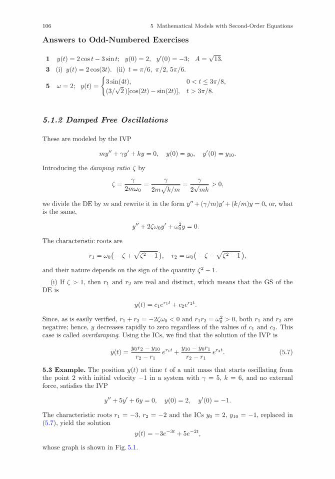
106 5 Mathematical Models with Second-Order Equations
Answers to Odd-Numbered Exercises
1 y(t) = 2 cos t− 3 sin t; y(0) = 2, y′(0) = −3; A =√13.
3 (i) y(t) = 2 cos(3t). (ii) t = π/6, π/2, 5π/6.
5 ω = 2; y(t) =
{3 sin(4t), 0 < t ≤ 3π/8,
(3/√2 )[cos(2t)− sin(2t)], t > 3π/8.
5.1.2 Damped Free Oscillations
These are modeled by the IVP
my′′ + γy′ + ky = 0, y(0) = y0, y′(0) = y10.
Introducing the damping ratio ζ by
ζ =γ
2mω0=
γ
2m√k/m
=γ
2√mk
> 0,
we divide the DE by m and rewrite it in the form y′′+(γ/m)y′+(k/m)y = 0, or, whatis the same,
y′′ + 2ζω0y′ + ω2
0y = 0.
The characteristic roots are
r1 = ω0
(− ζ +√ζ2 − 1
), r2 = ω0
(− ζ −√ζ2 − 1
),
and their nature depends on the sign of the quantity ζ2 − 1.
(i) If ζ > 1, then r1 and r2 are real and distinct, which means that the GS of theDE is
y(t) = c1er1t + c2e
r2t.
Since, as is easily verified, r1 + r2 = −2ζω0 < 0 and r1r2 = ω20 > 0, both r1 and r2 are
negative; hence, y decreases rapidly to zero regardless of the values of c1 and c2. Thiscase is called overdamping. Using the ICs, we find that the solution of the IVP is
y(t) =y0r2 − y10r2 − r1
er1t +y10 − y0r1r2 − r1
er2t. (5.7)
5.3 Example. The position y(t) at time t of a unit mass that starts oscillating fromthe point 2 with initial velocity −1 in a system with γ = 5, k = 6, and no externalforce, satisfies the IVP
y′′ + 5y′ + 6y = 0, y(0) = 2, y′(0) = −1.
The characteristic roots r1 = −3, r2 = −2 and the ICs y0 = 2, y10 = −1, replaced in(5.7), yield the solution
y(t) = −3e−3t + 5e−2t,
whose graph is shown in Fig. 5.1.
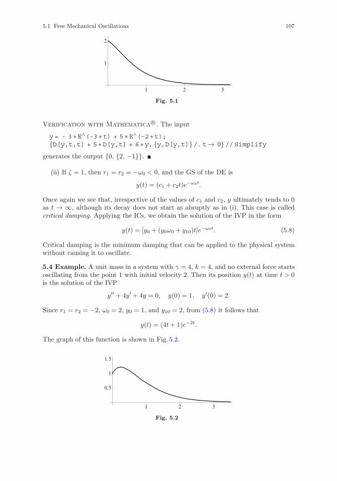
5.1 Free Mechanical Oscillations 107
1 2 3
2
1
Fig. 5.1
Verification with Mathematica R©. The input
y= - 3 ∗E∧(-3 ∗t) + 5 ∗E∧(-2 ∗t);{D[y,t,t] + 5 ∗D[y,t] + 6 ∗y,{y,D[y,t]}/.t→ 0}//Simplify
generates the output {0, {2, −1}}.
(ii) If ζ = 1, then r1 = r2 = −ω0 < 0, and the GS of the DE is
y(t) = (c1 + c2t)e−ω0t.
Once again we see that, irrespective of the values of c1 and c2, y ultimately tends to 0as t → ∞, although its decay does not start as abruptly as in (i). This case is calledcritical damping. Applying the ICs, we obtain the solution of the IVP in the form
y(t) = [y0 + (y0ω0 + y10)t]e−ω0t. (5.8)
Critical damping is the minimum damping that can be applied to the physical systemwithout causing it to oscillate.
5.4 Example. A unit mass in a system with γ = 4, k = 4, and no external force startsoscillating from the point 1 with initial velocity 2. Then its position y(t) at time t > 0is the solution of the IVP
y′′ + 4y′ + 4y = 0, y(0) = 1, y′(0) = 2.
Since r1 = r2 = −2, ω0 = 2, y0 = 1, and y10 = 2, from (5.8) it follows that
y(t) = (4t+ 1)e−2t.
The graph of this function is shown in Fig. 5.2.
1 2 3
0.5
1
1.5
Fig. 5.2
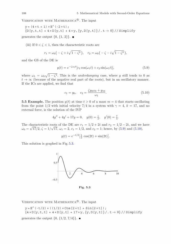
108 5 Mathematical Models with Second-Order Equations
Verification with Mathematica R©. The input
y=(4 ∗t + 1) ∗E∧(-2 ∗t);{D[y,t,t] + 4 ∗D[y,t] + 4 ∗y,{y,D[y,t]}/.t→ 0}//Simplify
generates the output {0, {1, 2}}.
(iii) If 0 < ζ < 1, then the characteristic roots are
r1 = ω0
(− ζ + i√1− ζ2
), r2 = ω0
(− ζ − i√1− ζ2
),
and the GS of the DE is
y(t) = e−ζω0t[c1 cos(ω1t) + c2 sin(ω1t)], (5.9)
where ω1 = ω0
√1− ζ2. This is the underdamping case, where y still tends to 0 as
t → ∞ (because of the negative real part of the roots), but in an oscillatory manner.If the ICs are applied, we find that
c1 = y0, c2 =ζy0ω0 + y10
ω1. (5.10)
5.5 Example. The position y(t) at time t > 0 of a mass m = 4 that starts oscillatingfrom the point 1/2 with initial velocity 7/4 in a system with γ = 4, k = 17, and noexternal force, is the solution of the IVP
4y′′ + 4y′ + 17y = 0, y(0) = 12 , y′(0) = 7
4 .
The characteristic roots of the DE are r1 = 1/2 + 2i and r2 = 1/2 − 2i, and we haveω0 =
√17/2, ζ = 1/
√17, ω1 = 2, c1 = 1/2, and c2 = 1; hence, by (5.9) and (5.10),
y(t) = e−t/2[12 cos(2t) + sin(2t)
].
This solution is graphed in Fig. 5.3.
2 4 6 8 10
−0.5
0.5
1
Fig. 5.3
Verification with Mathematica R©. The input
y=E∧(-t/2) ∗((1/2) ∗Cos[2 ∗t] + Sin[2 ∗t]);{4 ∗D[y,t,t] + 4 ∗D[y,t] + 17 ∗y,{y,D[y,t]}/.t→ 0}//Simplify
generates the output {0, {1/2, 7/4}}.
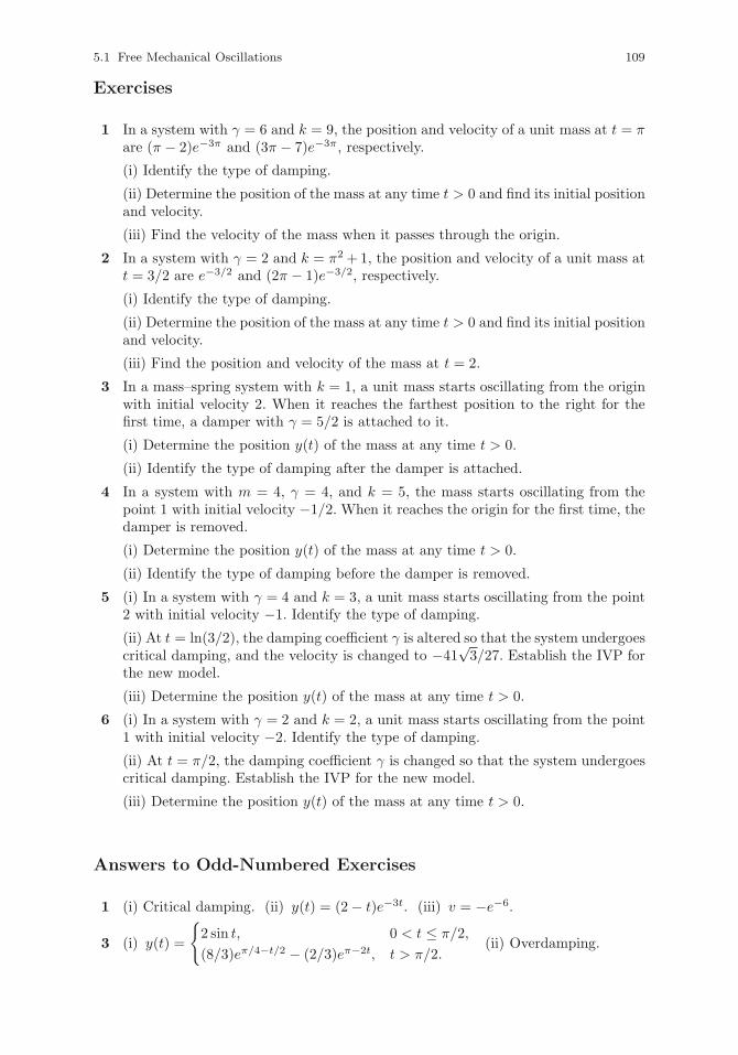
5.1 Free Mechanical Oscillations 109
Exercises
1 In a system with γ = 6 and k = 9, the position and velocity of a unit mass at t = πare (π − 2)e−3π and (3π − 7)e−3π, respectively.
(i) Identify the type of damping.
(ii) Determine the position of the mass at any time t > 0 and find its initial positionand velocity.
(iii) Find the velocity of the mass when it passes through the origin.
2 In a system with γ = 2 and k = π2 +1, the position and velocity of a unit mass att = 3/2 are e−3/2 and (2π − 1)e−3/2, respectively.
(i) Identify the type of damping.
(ii) Determine the position of the mass at any time t > 0 and find its initial positionand velocity.
(iii) Find the position and velocity of the mass at t = 2.
3 In a mass–spring system with k = 1, a unit mass starts oscillating from the originwith initial velocity 2. When it reaches the farthest position to the right for thefirst time, a damper with γ = 5/2 is attached to it.
(i) Determine the position y(t) of the mass at any time t > 0.
(ii) Identify the type of damping after the damper is attached.
4 In a system with m = 4, γ = 4, and k = 5, the mass starts oscillating from thepoint 1 with initial velocity −1/2. When it reaches the origin for the first time, thedamper is removed.
(i) Determine the position y(t) of the mass at any time t > 0.
(ii) Identify the type of damping before the damper is removed.
5 (i) In a system with γ = 4 and k = 3, a unit mass starts oscillating from the point2 with initial velocity −1. Identify the type of damping.
(ii) At t = ln(3/2), the damping coefficient γ is altered so that the system undergoescritical damping, and the velocity is changed to −41
√3/27. Establish the IVP for
the new model.
(iii) Determine the position y(t) of the mass at any time t > 0.
6 (i) In a system with γ = 2 and k = 2, a unit mass starts oscillating from the point1 with initial velocity −2. Identify the type of damping.
(ii) At t = π/2, the damping coefficient γ is changed so that the system undergoescritical damping. Establish the IVP for the new model.
(iii) Determine the position y(t) of the mass at any time t > 0.
Answers to Odd-Numbered Exercises
1 (i) Critical damping. (ii) y(t) = (2− t)e−3t. (iii) v = −e−6.
3 (i) y(t) =
{2 sin t, 0 < t ≤ π/2,
(8/3)eπ/4−t/2 − (2/3)eπ−2t, t > π/2.(ii) Overdamping.
110 5 Mathematical Models with Second-Order Equations
5 (i) Overdamping.
(ii) y′′ + 2√3 y′ + 3y = 0, y(ln(3/2)) = 41/27, y′(ln(3/2)) = −41
√3/27.
(iii) y(t) =
{−(1/2)e−3t + (5/2)e−t, 0 < t ≤ ln(3/2),
(41/27)(3/2)√3e−
√3 t, t > ln(3/2).
5.2 Forced Mechanical Oscillations
As we did for free oscillations, we discuss the undamped and damped cases separately.
5.2.1 Undamped Forced Oscillations
Here, the governing IVP is
my′′ + ky = f0 cos(ωt), y(0) = y0, y′(0) = y10,
where ω is the frequency of an external driving force and f0 = const. Using the notationk/m = ω2
0 introduced in Sect. 5.1.1, we divide the DE by m and rewrite it as
y′′ + ω20y =
f0m
cos(ωt). (5.11)
The complementary function for this nonhomogeneous DE is
yc(t) = c1 cos(ω0t) + c2 sin(ω0t).
Clearly, the form of a convenient particular solution depends on whether ω coincideswith ω0 or not.
(i) If ω �= ω0, then, by Theorem 4.47 with n = 0, λ = 0, μ = ω, and s = 0, we seeka PS of the form yp(t) = α cos(ωt) + β sin(ωt). Replacing in the DE and equating thecoefficients of cos(ωt) and sin(ωt) on both sides, we find that α = f0/(m(ω2
0 −ω2)) andβ = 0, so the GS of the equation is
y(t) = c1 cos(ω0t) + c2 sin(ω0t) +f0
m(ω20 − ω2)
cos(ωt). (5.12)
The constants, determined from the ICs, are
c1 = y0 − f0m(ω2
0 − ω2), c2 =
y10ω0
. (5.13)
5.6 Example. In a mass–spring system with k = 1, a unit mass starts oscillating fromrest at the origin and is acted upon by an external driving force of amplitude 1 andfrequency 11/10. The position y(t) of the mass at time t > 0 is, therefore, the solutionof the IVP
y′′ + y = cos(1110 t), y(0) = 0, y′(0) = 0.
Then ω0 = 1, ω = 11/10, f0 = 1, y0 = 0, and y10 = 0, so, by (5.12), (5.13), and thetrigonometric identity cos a− cos b = 2 sin((a+ b)/2) sin((b − a)/2), we have
y(t) = 10021 cos t− 100
21 cos(1110 t)=[20021 sin
(120 t)]
sin(2120 t).
5.2 Forced Mechanical Oscillations 111
The function y represents an oscillation whose amplitude (given by the quantity betweenthe square brackets) is itself oscillatory; this is known as amplitude modulation.
Figure 5.4 shows the graphs of the full function y (continuous line) and those of itsamplitude and its reflection in the t-axis (dashed lines). A forcing frequency ω close tothe natural frequency ω0, as is the case here, produces so-called beats.
20 40 60 80 100 120
−10
−5
5
10
Fig. 5.4
Verification with Mathematica R©. The input
y=((200/21) ∗Sin[t/20]) ∗Sin[(21/20) ∗t];{D[y,t,t] + y - Cos[(11/10) ∗t],{y,D[y,t]}/.t→ 0}//Simplify
generates the output {0, {0, 0}}.
(ii) If ω = ω0, then, by Theorem 4.47 with n = 0, λ = 0, μ = ω0, and s = 1, we seeka PS of the form
yp(t) = t[α cos(ω0t) + β sin(ω0t)].
Replacing in (5.11) and identifying the coefficients of cos(ω0t) and sin(ω0t) on bothsides, we find that α = 0 and β = f0/(2mω0), so the GS of the DE is
y(t) = c1 cos(ω0t) + c2 sin(ω0t) +f0
2mω0t sin(ω0t).
As the last term shows, this solution increases without bound as t → ∞, a phenomenonknown as resonance.
Exercises
1 In a system with m = 4, k = 1, and no external driving force, the mass startsoscillating from rest at the point 1. At t = π, a driving force f(t) = 6 cos t beginsto act on the mass. Determine the position of the mass at any time t > 0.
2 In a system with k = 9π2 and no external driving force, a unit mass starts oscillatingfrom the point 2 with initial velocity 3π. At t = 1/6, a driving force given byf(t) = 8π2 cos(πt) begins to act on the mass. Determine the position of the massat any time t > 0.
3 In a system with k = 1 and an external driving force f(t) = 3 cos(2t), a unitmass starts oscillating from rest at the point −2. At t = π/2, the driving force isremoved. Determine the position of the mass at any time t > 0.
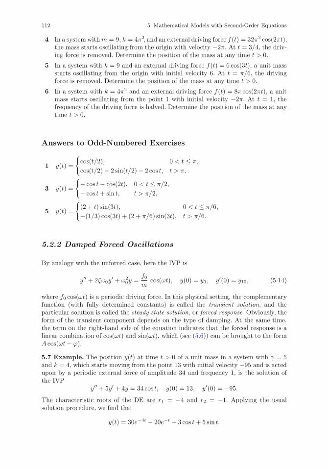
112 5 Mathematical Models with Second-Order Equations
4 In a system withm = 9, k = 4π2, and an external driving force f(t) = 32π2 cos(2πt),the mass starts oscillating from the origin with velocity −2π. At t = 3/4, the driv-ing force is removed. Determine the position of the mass at any time t > 0.
5 In a system with k = 9 and an external driving force f(t) = 6 cos(3t), a unit massstarts oscillating from the origin with initial velocity 6. At t = π/6, the drivingforce is removed. Determine the position of the mass at any time t > 0.
6 In a system with k = 4π2 and an external driving force f(t) = 8π cos(2πt), a unitmass starts oscillating from the point 1 with initial velocity −2π. At t = 1, thefrequency of the driving force is halved. Determine the position of the mass at anytime t > 0.
Answers to Odd-Numbered Exercises
1 y(t) =
{cos(t/2), 0 < t ≤ π,
cos(t/2)− 2 sin(t/2)− 2 cos t, t > π.
3 y(t) =
{− cos t− cos(2t), 0 < t ≤ π/2,
− cos t+ sin t, t > π/2.
5 y(t) =
{(2 + t) sin(3t), 0 < t ≤ π/6,
−(1/3) cos(3t) + (2 + π/6) sin(3t), t > π/6.
5.2.2 Damped Forced Oscillations
By analogy with the unforced case, here the IVP is
y′′ + 2ζω0y′ + ω2
0y =f0m
cos(ωt), y(0) = y0, y′(0) = y10, (5.14)
where f0 cos(ωt) is a periodic driving force. In this physical setting, the complementaryfunction (with fully determined constants) is called the transient solution, and theparticular solution is called the steady state solution, or forced response. Obviously, theform of the transient component depends on the type of damping. At the same time,the term on the right-hand side of the equation indicates that the forced response is alinear combination of cos(ωt) and sin(ωt), which (see (5.6)) can be brought to the formA cos(ωt− ϕ).
5.7 Example. The position y(t) at time t > 0 of a unit mass in a system with γ = 5and k = 4, which starts moving from the point 13 with initial velocity −95 and is actedupon by a periodic external force of amplitude 34 and frequency 1, is the solution ofthe IVP
y′′ + 5y′ + 4y = 34 cos t, y(0) = 13, y′(0) = −95.
The characteristic roots of the DE are r1 = −4 and r2 = −1. Applying the usualsolution procedure, we find that
y(t) = 30e−4t − 20e−t + 3 cos t+ 5 sin t.
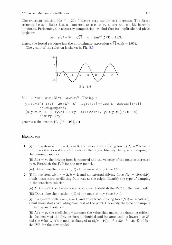
5.2 Forced Mechanical Oscillations 113
The transient solution 30e−4t − 20e−t decays very rapidly as t increases. The forcedresponse 3 cos t + 5 sin t has, as expected, an oscillatory nature and quickly becomesdominant. Performing the necessary computation, we find that its amplitude and phaseangle are
A =√32 + 52 =
√34, ϕ = tan−1(5/3) ≈ 1.03;
hence, the forced response has the approximate expression√34 cos(t− 1.03).
The graph of the solution is shown in Fig. 5.5.
2 4 6 8 10 12 14
−5
5
10
Fig. 5.5
Verification with Mathematica R©. The input
y=30 ∗E∧(-4*t) - 20 ∗E∧(-t) + Sqrt[34] ∗(Cos[t - ArcTan[5/3]]//TrigExpand;
{D[y,t,t] + 5 ∗D[y,t] + 4 ∗y - 34 ∗Cos[t],{y,D[y,t]}/.t→ 0}//Simplify
generates the output {0, {13, −95}}.
Exercises
1 (i) In a system with γ = 4, k = 3, and an external driving force f(t) = 20 cos t, aunit mass starts oscillating from rest at the origin. Identify the type of damping inthe transient solution.
(ii) At t = π, the driving force is removed and the velocity of the mass is increasedby 6. Establish the IVP for the new model.
(iii) Determine the position y(t) of the mass at any time t > 0.
2 (i) In a system with γ = 2, k = 2, and an external driving force f(t) = 10 cos(2t),a unit mass starts oscillating from rest at the origin. Identify the type of dampingin the transient solution.
(ii) At t = π/2, the driving force is removed. Establish the IVP for the new model.
(iii) Determine the position y(t) of the mass at any time t > 0.
3 (i) In a system with γ = 5, k = 4, and an external driving force f(t) = 65 cos(t/2),a unit mass starts oscillating from rest at the point 1. Identify the type of dampingin the transient solution.
(ii) At t = π, the coefficient γ assumes the value that makes the damping critical,the frequency of the driving force is doubled and its amplitude is lowered to 25,and the velocity of the mass is changed to (5/π− 10)e−4π + 32e−π − 26. Establishthe IVP for the new model.
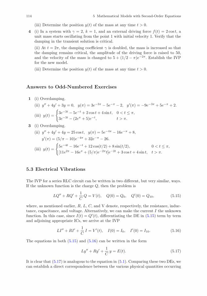
114 5 Mathematical Models with Second-Order Equations
(iii) Determine the position y(t) of the mass at any time t > 0.
4 (i) In a system with γ = 2, k = 1, and an external driving force f(t) = 2 cos t, aunit mass starts oscillating from the point 1 with initial velocity 1. Verify that thedamping in the transient solution is critical.
(ii) At t = 2π, the damping coefficient γ is doubled, the mass is increased so thatthe damping remains critical, the amplitude of the driving force is raised to 50,and the velocity of the mass is changed to 5 + (1/2 − π)e−2π . Establish the IVPfor the new model.
(iii) Determine the position y(t) of the mass at any time t > 0.
Answers to Odd-Numbered Exercises
1 (i) Overdamping.
(ii) y′′ + 4y′ + 3y = 0, y(π) = 3e−3π − 5e−π − 2, y′(π) = −9e−3π + 5e−π + 2.
(iii) y(t) =
{3e−3t − 5e−t + 2 cos t+ 4 sin t, 0 < t ≤ π,
3e−3t − (2eπ + 5)e−t, t > π.
3 (i) Overdamping.
(ii) y′′ + 4y′ + 4y = 25 cos t, y(π) = 5e−4π − 16e−π + 8,
y′(π) = (5/π − 10)e−4π + 32e−π − 26.
(iii) y(t) =
{5e−4t − 16e−t + 12 cos(t/2) + 8 sin(t/2), 0 < t ≤ π,
[11e2π − 16eπ + (5/π)e−2πt]e−2t + 3 cos t+ 4 sin t, t > π.
5.3 Electrical Vibrations
The IVP for a series RLC circuit can be written in two different, but very similar, ways.If the unknown function is the charge Q, then the problem is
LQ′′ +RQ′ +1
CQ = V (t), Q(0) = Q0, Q′(0) = Q10, (5.15)
where, as mentioned earlier, R, L, C, and V denote, respectively, the resistance, induc-tance, capacitance, and voltage. Alternatively, we can make the current I the unknownfunction. In this case, since I(t) = Q′(t), differentiating the DE in (5.15) term by termand adjoining appropriate ICs, we arrive at the IVP
LI ′′ +RI ′ +1
CI = V ′(t), I(0) = I0, I ′(0) = I10. (5.16)
The equations in both (5.15) and (5.16) can be written in the form
Ly′′ +Ry′ +1
Cy = E(t). (5.17)
It is clear that (5.17) is analogous to the equation in (5.1). Comparing these two DEs, wecan establish a direct correspondence between the various physical quantities occurring
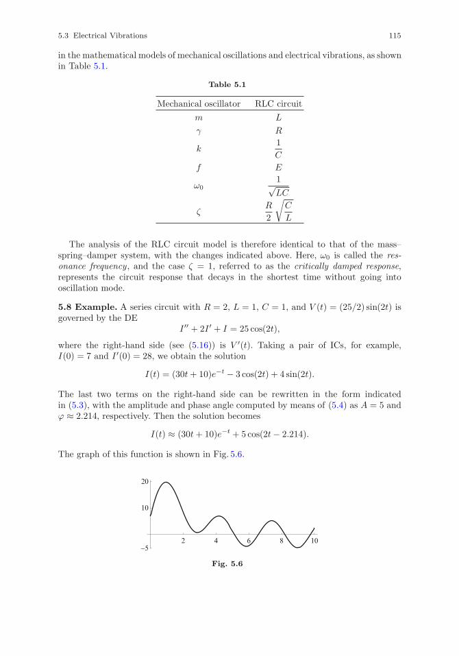
5.3 Electrical Vibrations 115
in the mathematical models of mechanical oscillations and electrical vibrations, as shownin Table 5.1.
Table 5.1
Mechanical oscillator RLC circuit
m L
γ R
k1
C
f E
ω01√LC
ζR
2
√C
L
The analysis of the RLC circuit model is therefore identical to that of the mass–spring–damper system, with the changes indicated above. Here, ω0 is called the res-onance frequency, and the case ζ = 1, referred to as the critically damped response,represents the circuit response that decays in the shortest time without going intooscillation mode.
5.8 Example. A series circuit with R = 2, L = 1, C = 1, and V (t) = (25/2) sin(2t) isgoverned by the DE
I ′′ + 2I ′ + I = 25 cos(2t),
where the right-hand side (see (5.16)) is V ′(t). Taking a pair of ICs, for example,I(0) = 7 and I ′(0) = 28, we obtain the solution
I(t) = (30t+ 10)e−t − 3 cos(2t) + 4 sin(2t).
The last two terms on the right-hand side can be rewritten in the form indicatedin (5.3), with the amplitude and phase angle computed by means of (5.4) as A = 5 andϕ ≈ 2.214, respectively. Then the solution becomes
I(t) ≈ (30t+ 10)e−t + 5 cos(2t− 2.214).
The graph of this function is shown in Fig. 5.6.
2 4 6 8 10−5
10
20
Fig. 5.6
116 5 Mathematical Models with Second-Order Equations
Verification with Mathematica R©. The input
y=(30 ∗t + 10) ∗E∧(-t) + 5 ∗((Cos[a1 - a2]//TrigExpand)/. {a1→2 ∗t,a2→2.214});
Eqn=D[y,t,t] + 2 ∗D[y,t] + y - 25 ∗Cos[2 ∗t]//Simplify;{Ccos,Csin}=Round[{Coefficient[Eqn,Cos[2 ∗t]],
Coefficient[Eqn,Sin[2 ∗t]]}];{Ccos ∗Cos[2 ∗t] + Csin ∗Sin[2 ∗t],Round[{y,D[y,t]}/.t→ 0]}
generates the output {0, {7, 28}}. The input commands are rather convoluted since,our solution being an approximate one, we want the program to round the numericalcoefficients to the nearest integer.
Exercises
1 (i) In an RLC circuit with R = 6, L = 1, C = 1/8, and V (t) = 85 cos t, the initialvalues of the charge and current are 8 and 4, respectively. Determine the chargeQ(t) and current I(t) at any time t > 0.
(ii) Write the forced response for Q in the form (5.6) and find when it attains itsmaximum value for the first time.
2 (i) In an RLC circuit with R = 4, L = 4, C = 1, and V (t) = 289 cos(2t), theinitial values of the charge and current are −15 and 17, respectively. Determinethe charge Q(t) and then the current I(t) at any time t > 0.
(ii) Write the forced response for Q in the form (5.6) and find when it attains itsmaximum value for the first time.
3 In an RLC circuit with R = 0, L = 1, C = 1, and V (t) = 6 sin(t/2), the initialvalues of the current and its derivative are 4 and 1, respectively. At t = π, aresistance R = 2 is added to the circuit. Compute the current I(t) at any timet > 0.
4 In an RLC circuit with R = 0, L = 1, C = 1/(4π2), and V (t) = 3π sin(πt), theinitial values of the current and its derivative are 3 and 2π, respectively. At t = 1/2,a resistance R = 5π is added to the circuit. Compute the current I(t) at any timet > 0.
Answers to Odd-Numbered Exercises
1 (i) Q(t) = e−2t + 7 cos t+ 6 sin t; I(t) = −2e−2t + 6 cos t− 7 sin t.
(ii) Forced response ≈ √85 cos(t− 0.7); t ≈ 0.7.
3 I(t) =
{sin t+ 4 cos(t/2), 0 < t ≤ π,
(3/25)(35π− 16− 35t)eπ−t + 12 cos(t/2 + 16 sin(t/2), t > π.
Chapter 6
Higher-Order Linear Equations
Certain physical phenomena give rise to mathematical models that involve DEs of anorder higher than two.
6.1 Modeling with Higher-Order Equations
We mention a couple of examples.
Generalized Airy equation. The motion of a particle in a triangular potential wellis the solution of the IVP
y′′′ + aty′ + by = 0, y(0) = y0, y′(0) = y10, y′′(0) = y20,
where a, b = const. This type of DE is also encountered in the study of a particularkind of waves in a rotating inhomogeneous plasma.
Harmonic oscillations of a beam. The stationary oscillations of a uniform,load-free beam of length l with both ends embedded in a rigid medium is modeled bythe BVP
EIy(4) −mω2y = 0, y(0) = 0, y′(0) = 0, y(l) = 0, y′(l) = 0,
where y(x) is the deflection of the beam at a generic point x in the open interval0 < x < l, the constants E, I, and m are the Young modulus of the material, themoment of inertia of the cross section, and the mass, and ω is the oscillation frequency.If the end-point x = l is free, then the BCs at that point are y′′(l) = 0 and y′′′(l) = 0.If, on the other hand, the beam is simply supported at both end-points, the BCs are
y(0) = 0, y′′(0) = 0, y(l) = 0, y′′(l) = 0.
6.2 Algebra Prerequisites
All the concepts of linear algebra discussed in Sect. 4.2 can be extended to more generalcases in the obvious way, although, as expected, in such generalizations the computationbecomes more laborious.
C. Constanda, Differential Equations: A Primer for Scientists and Engineers, SpringerUndergraduate Texts in Mathematics and Technology, DOI 10.1007/978-1-4614-7297-1 6,© Springer Science+Business Media New York 2013
117
118 6 Higher-Order Linear Equations
6.2.1 Matrices and Determinants of Higher Order
An n× n matrix is a number array of the form
A =
⎛⎜⎜⎜⎝a11 a12 · · · a1na21 a22 · · · a2n...
.... . .
...an1 an2 · · · ann
⎞⎟⎟⎟⎠ .
For simplicity, we denote the generic element of such a matrix by aij and write A = (aij).The elements a11, a22, . . . , ann are said to form the leading diagonal of A.
6.1 Remark. The calculation of the determinant of an n× n matrix is more involved,and lengthier, than that of a 2× 2 determinant. A method for evaluating det(A), calledexpansion in the elements of a row or column, consists of the following steps:
(1) Choose a row or a column of the given determinant—it does not matter which onebecause the result is always the same. If some of the entries are zero, it is advisableto choose a row or a column that contains as many zeros as possible, to simplify thecalculation.
(2) For each element aij in that row/column, note the number i of the row and thenumber j of the column where the element is positioned, then multiply the elementby (−1)i+j ; that is, form the product (−1)i+jaij .
(3) For each element in the chosen row/column, delete the row and the column to whichthe element belongs and compute the (n− 1)× (n− 1) determinant dij formed bythe remaining rows and columns.
(4) For each element in the chosen row/column, multiply the determinant computed instep (3) by the number obtained in step (2): (−1)i+jaijdij .
(5) Sum up the numbers computed in step (4) for all the elements of the chosenrow/column.
6.2 Example. The 3× 3 determinant below is expanded in its second column:
∣∣∣∣∣∣2 0 −13 −1 21 −2 4
∣∣∣∣∣∣ = (−1)1+2 0
∣∣∣∣ 3 21 4
∣∣∣∣+ (−1)2+2(−1)
∣∣∣∣ 2 −11 4
∣∣∣∣+ (−1)3+2(−2)
∣∣∣∣ 2 −13 2
∣∣∣∣= −(8 + 1) + 2(4 + 3) = 5.
This column has been chosen because it contains a zero. If instead of the second columnwe choose, say, the third row, then, once again,
∣∣∣∣∣∣2 0 −13 −1 21 −2 4
∣∣∣∣∣∣ = (−1)3+11
∣∣∣∣ 0 −1−1 2
∣∣∣∣+ (−1)3+2(−2)
∣∣∣∣ 2 −13 2
∣∣∣∣+ (−1)3+34
∣∣∣∣ 2 03 −1
∣∣∣∣= −1 + 2(4 + 3) + 4(−2) = 5.
6.3 Remark. The properties listed in Remarks 4.2 remain valid in the case of an n×ndeterminant.
(i) Swapping any two rows (columns) changes the sign of the determinant.
(ii) If the elements of a row (column) have a common factor, then this factor can betaken out and multiplied by the value of the new determinant.
6.2 Algebra Prerequisites 119
(iii) Cramer’s rule for solving a linear algebraic system is adapted in the obvious way tothe case of n equations in n unknowns. Thus, by analogy with formulas (4.1), forevery j = 1, . . . , n, the value of xj is given by the ratio of two n× n determinants:the one in the denominator (which must be nonzero) is formed from the systemcoefficients, and the one in the numerator is obtained by replacing the jth columnin the former by the column of the terms on the right-hand side of the system. Wewill say more about the solution of such systems in Sect. 6.2.2.
Exercises
In 1–6, compute the given determinant by expanding it in a row or a column.
1
∣∣∣∣∣∣2 −1 30 2 11 0 −2
∣∣∣∣∣∣. 2
∣∣∣∣∣∣4 2 32 1 0
−1 −2 1
∣∣∣∣∣∣.
3
∣∣∣∣∣∣1 3 −2
−1 4 −12 1 −3
∣∣∣∣∣∣. 4
∣∣∣∣∣∣2 −3 21 −2 14 3 −1
∣∣∣∣∣∣.
5
∣∣∣∣∣∣∣∣
2 1 0 −11 3 1 2
−1 4 −2 0−2 1 0 3
∣∣∣∣∣∣∣∣. 6
∣∣∣∣∣∣∣∣
0 3 1 12 −1 0 21 5 1 3
−2 1 −3 4
∣∣∣∣∣∣∣∣.
In 7–10, solve the given equation for the parameter a.
7
∣∣∣∣∣∣3 −1 02 1 1
−4 0 a
∣∣∣∣∣∣ = −1. 8
∣∣∣∣∣∣1 0 2
−3 4 1−1 5 a
∣∣∣∣∣∣ = 1.
9
∣∣∣∣∣∣a 1 −13 0 2
−2 −a 7
∣∣∣∣∣∣ = 2. 10
∣∣∣∣∣∣2 a −10 1 3a3 −2 4
∣∣∣∣∣∣ = 8.
Answers to Odd-Numbered Exercises
1 −15. 3 −8. 5 −20. 7 a = −1. 9 a = 3,−9/2.
6.2.2 Systems of Linear Algebraic Equations
The general form of a system of n linear algebraic equations in n unknowns is
a11x1 + · · ·+ a1nxn = b1,
...
an1x1 + · · ·+ annxn = bn,
(6.1)
where A = (aij) is the n × n matrix of the system coefficients, x1, . . . , xn are theunknowns, and b1, . . . , bn are given numbers.
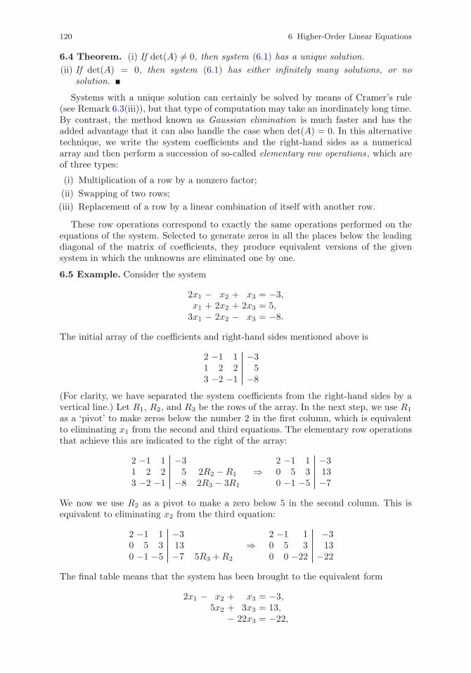
120 6 Higher-Order Linear Equations
6.4 Theorem. (i) If det(A) �= 0, then system (6.1) has a unique solution.
(ii) If det(A) = 0, then system (6.1) has either infinitely many solutions, or nosolution.
Systems with a unique solution can certainly be solved by means of Cramer’s rule(see Remark 6.3(iii)), but that type of computation may take an inordinately long time.By contrast, the method known as Gaussian elimination is much faster and has theadded advantage that it can also handle the case when det(A) = 0. In this alternativetechnique, we write the system coefficients and the right-hand sides as a numericalarray and then perform a succession of so-called elementary row operations , which areof three types:
(i) Multiplication of a row by a nonzero factor;
(ii) Swapping of two rows;
(iii) Replacement of a row by a linear combination of itself with another row.
These row operations correspond to exactly the same operations performed on theequations of the system. Selected to generate zeros in all the places below the leadingdiagonal of the matrix of coefficients, they produce equivalent versions of the givensystem in which the unknowns are eliminated one by one.
6.5 Example. Consider the system
2x1 − x2 + x3 = −3,x1 + 2x2 + 2x3 = 5,
3x1 − 2x2 − x3 = −8.
The initial array of the coefficients and right-hand sides mentioned above is
2 −1 1 −31 2 2 53 −2 −1 −8
(For clarity, we have separated the system coefficients from the right-hand sides by avertical line.) Let R1, R2, and R3 be the rows of the array. In the next step, we use R1
as a ‘pivot’ to make zeros below the number 2 in the first column, which is equivalentto eliminating x1 from the second and third equations. The elementary row operationsthat achieve this are indicated to the right of the array:
2 −1 1 −31 2 2 5 2R2 −R1
3 −2 −1 −8 2R3 − 3R1
⇒2 −1 1 −30 5 3 130 −1 −5 −7
We now we use R2 as a pivot to make a zero below 5 in the second column. This isequivalent to eliminating x2 from the third equation:
2 −1 1 −30 5 3 130 −1 −5 −7 5R3 +R2
⇒2 −1 1 −30 5 3 130 0 −22 −22
The final table means that the system has been brought to the equivalent form
2x1 − x2 + x3 = −3,5x2 + 3x3 = 13,
− 22x3 = −22,
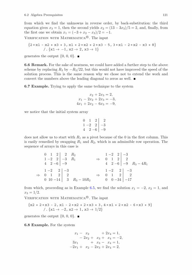
6.2 Algebra Prerequisites 121
from which we find the unknowns in reverse order, by back-substitution: the thirdequation gives x3 = 1, then the second yields x2 = (13− 3x3)/5 = 2, and, finally, fromthe first one we obtain x1 = (−3 + x2 − x3)/2 = −1.
Verification with Mathematica R©. The input
{2 ∗x1 - x2 + x3 + 3,x1 + 2 ∗x2 + 2 ∗x3 - 5,3 ∗x1 - 2 ∗x2 - x3 + 8}/. {x1→ −1,x2→ 2,x3→ 1}
generates the output {0, 0, 0}.
6.6 Remark. For the sake of neatness, we could have added a further step to the abovescheme by replacing R3 by −R3/22, but this would not have improved the speed of thesolution process. This is the same reason why we chose not to extend the work andconvert the numbers above the leading diagonal to zeros as well.
6.7 Example. Trying to apply the same technique to the system
x2 + 2x3 = 2,x1 − 2x2 + 2x3 = −3,
4x1 + 2x2 − 6x3 = −9,
we notice that the initial system array
0 1 2 21 −2 2 −34 2 −6 −9
does not allow us to start with R1 as a pivot because of the 0 in the first column. Thisis easily remedied by swapping R1 and R2, which is an admissible row operation. Thesequence of arrays in this case is
0 1 2 2 R2
1 −2 2 −3 R1
4 2 −6 −9⇒
1 −2 2 −30 1 2 24 2 −6 −9 R3 − 4R1
⇒1 −2 2 −30 1 2 20 10 −14 3 R3 − 10R2
⇒1 −2 2 −30 1 2 20 0 −34 −17
from which, proceeding as in Example 6.5, we find the solution x1 = −2, x2 = 1, andx3 = 1/2.
Verification with Mathematica R©. The input
{x2 + 2 ∗x3 - 2,x1 - 2 ∗x2 + 2 ∗x3 + 3,4 ∗x1 + 2 ∗x2 - 6 ∗x3 + 9}/. {x1→ −2,x2→ 1,x3→ 1/2}
generates the output {0, 0, 0}.
6.8 Example. For the system
x1 − x2 + 2x4 = 1,− 2x2 + x3 + x4 = −2,
3x1 + x3 − x4 = 1,−2x1 + x2 − 2x3 + 2x4 = 2,
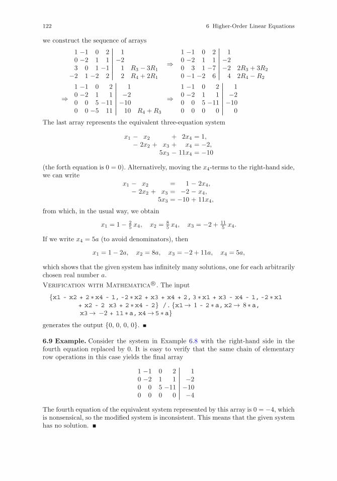
122 6 Higher-Order Linear Equations
we construct the sequence of arrays
1 −1 0 2 10 −2 1 1 −23 0 1 −1 1 R3 − 3R1
−2 1 −2 2 2 R4 + 2R1
⇒1 −1 0 2 10 −2 1 1 −20 3 1 −7 −2 2R3 + 3R2
0 −1 −2 6 4 2R4 −R2
⇒1 −1 0 2 10 −2 1 1 −20 0 5 −11 −100 0 −5 11 10 R4 +R3
⇒1 −1 0 2 10 −2 1 1 −20 0 5 −11 −100 0 0 0 0
The last array represents the equivalent three-equation system
x1 − x2 + 2x4 = 1,− 2x2 + x3 + x4 = −2,
5x3 − 11x4 = −10
(the forth equation is 0 = 0). Alternatively, moving the x4-terms to the right-hand side,we can write
x1 − x2 = 1 − 2x4,− 2x2 + x3 = −2 − x4,
5x3 = −10 + 11x4,
from which, in the usual way, we obtain
x1 = 1− 25 x4, x2 = 8
5 x4, x3 = −2 + 115 x4.
If we write x4 = 5a (to avoid denominators), then
x1 = 1− 2a, x2 = 8a, x3 = −2 + 11a, x4 = 5a,
which shows that the given system has infinitely many solutions, one for each arbitrarilychosen real number a.
Verification with Mathematica R©. The input
{x1 - x2 + 2 ∗x4 - 1,-2 ∗x2 + x3 + x4 + 2,3 ∗x1 + x3 - x4 - 1,-2 ∗x1+ x2 - 2 x3 + 2 ∗x4 - 2} /. {x1→ 1 - 2 ∗a,x2→ 8 ∗a,x3→ −2 + 11 ∗a,x4→5 ∗a}
generates the output {0, 0, 0, 0}.
6.9 Example. Consider the system in Example 6.8 with the right-hand side in thefourth equation replaced by 0. It is easy to verify that the same chain of elementaryrow operations in this case yields the final array
1 −1 0 2 10 −2 1 1 −20 0 5 −11 −100 0 0 0 −4
The fourth equation of the equivalent system represented by this array is 0 = −4, whichis nonsensical, so the modified system is inconsistent. This means that the given systemhas no solution.
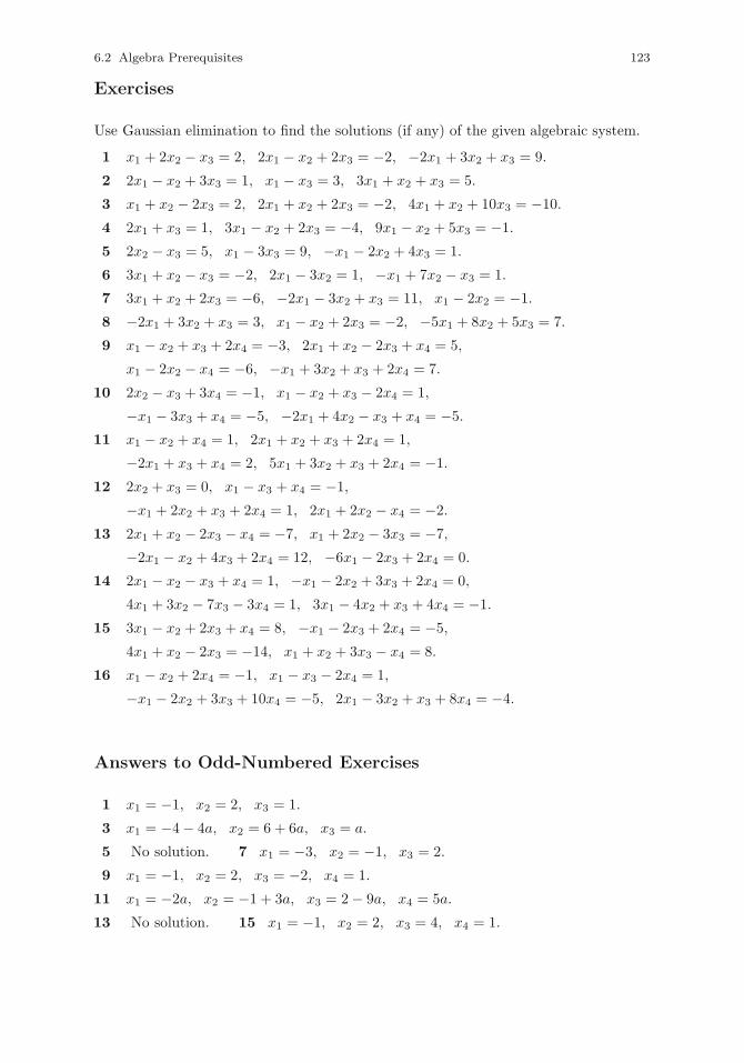
6.2 Algebra Prerequisites 123
Exercises
Use Gaussian elimination to find the solutions (if any) of the given algebraic system.
1 x1 + 2x2 − x3 = 2, 2x1 − x2 + 2x3 = −2, −2x1 + 3x2 + x3 = 9.
2 2x1 − x2 + 3x3 = 1, x1 − x3 = 3, 3x1 + x2 + x3 = 5.
3 x1 + x2 − 2x3 = 2, 2x1 + x2 + 2x3 = −2, 4x1 + x2 + 10x3 = −10.
4 2x1 + x3 = 1, 3x1 − x2 + 2x3 = −4, 9x1 − x2 + 5x3 = −1.
5 2x2 − x3 = 5, x1 − 3x3 = 9, −x1 − 2x2 + 4x3 = 1.
6 3x1 + x2 − x3 = −2, 2x1 − 3x2 = 1, −x1 + 7x2 − x3 = 1.
7 3x1 + x2 + 2x3 = −6, −2x1 − 3x2 + x3 = 11, x1 − 2x2 = −1.
8 −2x1 + 3x2 + x3 = 3, x1 − x2 + 2x3 = −2, −5x1 + 8x2 + 5x3 = 7.
9 x1 − x2 + x3 + 2x4 = −3, 2x1 + x2 − 2x3 + x4 = 5,
x1 − 2x2 − x4 = −6, −x1 + 3x2 + x3 + 2x4 = 7.
10 2x2 − x3 + 3x4 = −1, x1 − x2 + x3 − 2x4 = 1,
−x1 − 3x3 + x4 = −5, −2x1 + 4x2 − x3 + x4 = −5.
11 x1 − x2 + x4 = 1, 2x1 + x2 + x3 + 2x4 = 1,
−2x1 + x3 + x4 = 2, 5x1 + 3x2 + x3 + 2x4 = −1.
12 2x2 + x3 = 0, x1 − x3 + x4 = −1,
−x1 + 2x2 + x3 + 2x4 = 1, 2x1 + 2x2 − x4 = −2.
13 2x1 + x2 − 2x3 − x4 = −7, x1 + 2x2 − 3x3 = −7,
−2x1 − x2 + 4x3 + 2x4 = 12, −6x1 − 2x3 + 2x4 = 0.
14 2x1 − x2 − x3 + x4 = 1, −x1 − 2x2 + 3x3 + 2x4 = 0,
4x1 + 3x2 − 7x3 − 3x4 = 1, 3x1 − 4x2 + x3 + 4x4 = −1.
15 3x1 − x2 + 2x3 + x4 = 8, −x1 − 2x3 + 2x4 = −5,
4x1 + x2 − 2x3 = −14, x1 + x2 + 3x3 − x4 = 8.
16 x1 − x2 + 2x4 = −1, x1 − x3 − 2x4 = 1,
−x1 − 2x2 + 3x3 + 10x4 = −5, 2x1 − 3x2 + x3 + 8x4 = −4.
Answers to Odd-Numbered Exercises
1 x1 = −1, x2 = 2, x3 = 1.
3 x1 = −4− 4a, x2 = 6 + 6a, x3 = a.
5 No solution. 7 x1 = −3, x2 = −1, x3 = 2.
9 x1 = −1, x2 = 2, x3 = −2, x4 = 1.
11 x1 = −2a, x2 = −1 + 3a, x3 = 2− 9a, x4 = 5a.
13 No solution. 15 x1 = −1, x2 = 2, x3 = 4, x4 = 1.
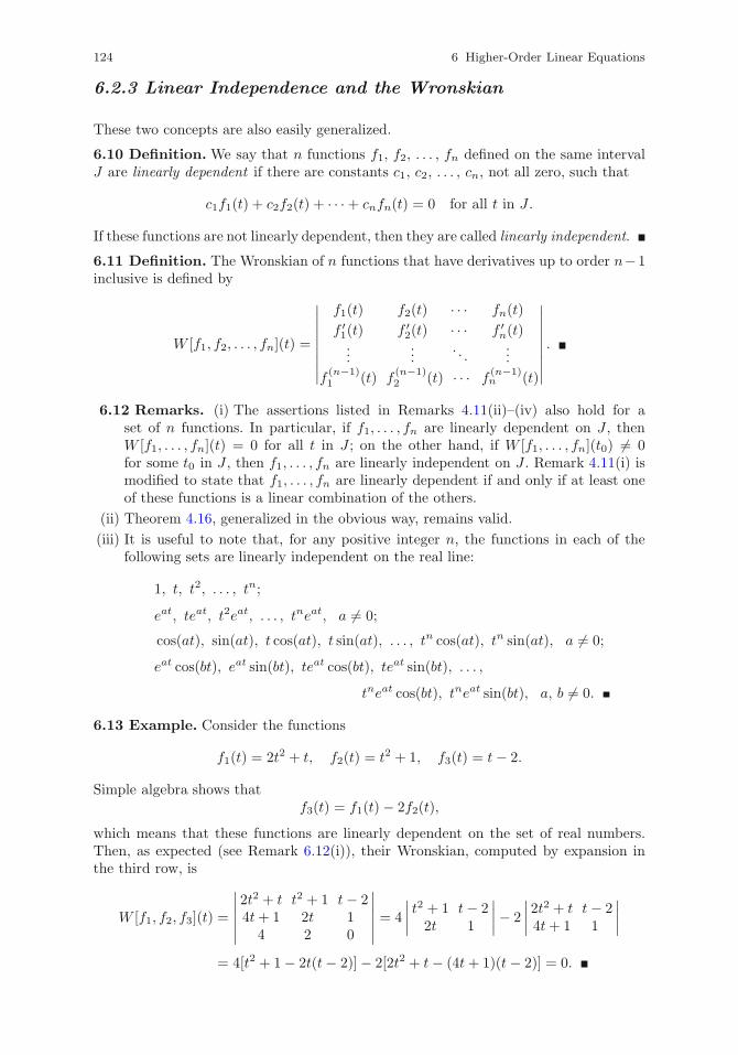
124 6 Higher-Order Linear Equations
6.2.3 Linear Independence and the Wronskian
These two concepts are also easily generalized.
6.10 Definition. We say that n functions f1, f2, . . . , fn defined on the same intervalJ are linearly dependent if there are constants c1, c2, . . . , cn, not all zero, such that
c1f1(t) + c2f2(t) + · · ·+ cnfn(t) = 0 for all t in J .
If these functions are not linearly dependent, then they are called linearly independent.
6.11 Definition. The Wronskian of n functions that have derivatives up to order n−1inclusive is defined by
W [f1, f2, . . . , fn](t) =
∣∣∣∣∣∣∣∣∣
f1(t) f2(t) · · · fn(t)
f ′1(t) f ′
2(t) · · · f ′n(t)
......
. . ....
f(n−1)1 (t) f
(n−1)2 (t) · · · f
(n−1)n (t)
∣∣∣∣∣∣∣∣∣.
6.12 Remarks. (i) The assertions listed in Remarks 4.11(ii)–(iv) also hold for aset of n functions. In particular, if f1, . . . , fn are linearly dependent on J , thenW [f1, . . . , fn](t) = 0 for all t in J ; on the other hand, if W [f1, . . . , fn](t0) �= 0for some t0 in J , then f1, . . . , fn are linearly independent on J . Remark 4.11(i) ismodified to state that f1, . . . , fn are linearly dependent if and only if at least oneof these functions is a linear combination of the others.
(ii) Theorem 4.16, generalized in the obvious way, remains valid.
(iii) It is useful to note that, for any positive integer n, the functions in each of thefollowing sets are linearly independent on the real line:
1, t, t2, . . . , tn;
eat, teat, t2eat, . . . , tneat, a �= 0;
cos(at), sin(at), t cos(at), t sin(at), . . . , tn cos(at), tn sin(at), a �= 0;
eat cos(bt), eat sin(bt), teat cos(bt), teat sin(bt), . . . ,
tneat cos(bt), tneat sin(bt), a, b �= 0.
6.13 Example. Consider the functions
f1(t) = 2t2 + t, f2(t) = t2 + 1, f3(t) = t− 2.
Simple algebra shows thatf3(t) = f1(t)− 2f2(t),
which means that these functions are linearly dependent on the set of real numbers.Then, as expected (see Remark 6.12(i)), their Wronskian, computed by expansion inthe third row, is
W [f1, f2, f3](t) =
∣∣∣∣∣∣2t2 + t t2 + 1 t− 24t+ 1 2t 1
4 2 0
∣∣∣∣∣∣ = 4
∣∣∣∣ t2 + 1 t− 22t 1
∣∣∣∣− 2
∣∣∣∣ 2t2 + t t− 2
4t+ 1 1
∣∣∣∣= 4[t2 + 1− 2t(t− 2)]− 2[2t2 + t− (4t+ 1)(t− 2)] = 0.
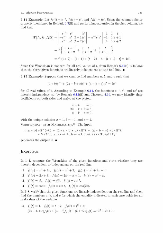
6.2 Algebra Prerequisites 125
6.14 Example. Let f1(t) = e−t, f2(t) = et, and f3(t) = tet. Using the common factorproperty mentioned in Remark 6.3(ii) and performing expansion in the first column, wefind that
W [f1, f2, f3](t) =
∣∣∣∣∣∣e−t et tet
−e−t et (t+ 1)et
e−t et (t+ 2)et
∣∣∣∣∣∣ = e−tetet
∣∣∣∣∣∣1 1 t
−1 1 t+ 11 1 t+ 2
∣∣∣∣∣∣= et
{ ∣∣∣∣ 1 t+ 11 t+ 2
∣∣∣∣+∣∣∣∣ 1 t1 t+ 2
∣∣∣∣+∣∣∣∣ 1 t1 t+ 1
∣∣∣∣}
= et[(t+ 2)− (t+ 1) + (t+ 2)− t+ (t+ 1)− t] = 4et.
Since the Wronskian is nonzero for all real values of t, from Remark 6.12(i) it followsthat the three given functions are linearly independent on the real line.
6.15 Example. Suppose that we want to find numbers a, b, and c such that
(a+ b)e−t + (2a− b+ c)et + (a− b− c)tet = 5et
for all real values of t. According to Example 6.14, the functions e−t, et, and tet arelinearly independent, so, by Remark 6.12(ii) and Theorem 4.16, we may identify theircoefficients on both sides and arrive at the system
a + b = 0,2a − b + c = 5,a − b − c = 0,
with the unique solution a = 1, b = −1, and c = 2.
Verification with Mathematica R©. The input
((a + b) ∗E∧(-t) + (2 ∗a - b + c) ∗E∧t + (a - b - c) ∗t ∗E∧t- 5 ∗E∧t)/. {a→ 1,b→ −1,c→ 2}//Simplify
generates the output 0.
Exercises
In 1–4, compute the Wronskian of the given functions and state whether they arelinearly dependent or independent on the real line.
1 f1(x) = x2 + 3x, f2(x) = x2 + 2, f3(x) = x2 + 9x− 4.
2 f1(x) = 2x+ 3, f2(x) = 2x2 − x+ 1, f3(x) = x2 − x.
3 f1(t) = et, f2(t) = e2t, f3(t) = te−t.
4 f1(t) = cos t, f2(t) = sin t, f3(t) = cos(2t).
In 5–8, verify that the given functions are linearly independent on the real line and thenfind the numbers a, b, and c for which the equality indicated in each case holds for allreal values of the variable.
5 f1(t) = 1, f2(t) = t− 2, f3(t) = t2 + t;
(2a+ b+ c)f1(t) + (a− c)f2(t) + (b+ 2c)f3(t) = 3t2 + 2t+ 5.
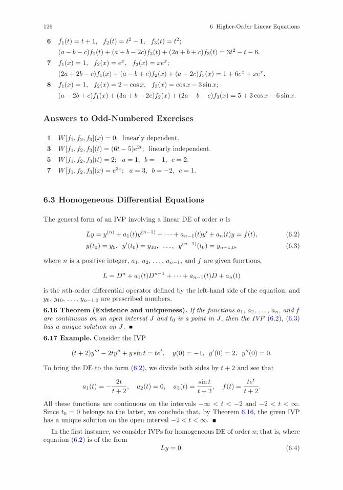
126 6 Higher-Order Linear Equations
6 f1(t) = t+ 1, f2(t) = t2 − 1, f3(t) = t2;
(a− b− c)f1(t) + (a+ b− 2c)f2(t) + (2a+ b+ c)f3(t) = 3t2 − t− 6.
7 f1(x) = 1, f2(x) = ex, f3(x) = xex;
(2a+ 2b− c)f1(x) + (a− b+ c)f2(x) + (a− 2c)f3(x) = 1 + 6ex + xex.
8 f1(x) = 1, f2(x) = 2− cosx, f3(x) = cosx− 3 sinx;
(a− 2b+ c)f1(x) + (3a+ b− 2c)f2(x) + (2a− b− c)f3(x) = 5 + 3 cosx− 6 sinx.
Answers to Odd-Numbered Exercises
1 W [f1, f2, f3](x) = 0; linearly dependent.
3 W [f1, f2, f3](t) = (6t− 5)e2t; linearly independent.
5 W [f1, f2, f3](t) = 2; a = 1, b = −1, c = 2.
7 W [f1, f2, f3](x) = e2x; a = 3, b = −2, c = 1.
6.3 Homogeneous Differential Equations
The general form of an IVP involving a linear DE of order n is
Ly = y(n) + a1(t)y(n−1) + · · ·+ an−1(t)y
′ + an(t)y = f(t), (6.2)
y(t0) = y0, y′(t0) = y10, . . . , y(n−1)(t0) = yn−1,0, (6.3)
where n is a positive integer, a1, a2, . . . , an−1, and f are given functions,
L = Dn + a1(t)Dn−1 + · · ·+ an−1(t)D + an(t)
is the nth-order differential operator defined by the left-hand side of the equation, andy0, y10, . . . , yn−1,0 are prescribed numbers.
6.16 Theorem (Existence and uniqueness). If the functions a1, a2, . . . , an, and fare continuous on an open interval J and t0 is a point in J , then the IVP (6.2), (6.3)has a unique solution on J .
6.17 Example. Consider the IVP
(t+ 2)y′′′ − 2ty′′ + y sin t = tet, y(0) = −1, y′(0) = 2, y′′(0) = 0.
To bring the DE to the form (6.2), we divide both sides by t+ 2 and see that
a1(t) = − 2t
t+ 2, a2(t) = 0, a3(t) =
sin t
t+ 2, f(t) =
tet
t+ 2.
All these functions are continuous on the intervals −∞ < t < −2 and −2 < t < ∞.Since t0 = 0 belongs to the latter, we conclude that, by Theorem 6.16, the given IVPhas a unique solution on the open interval −2 < t < ∞.
In the first instance, we consider IVPs for homogeneous DE of order n; that is, whereequation (6.2) is of the form
Ly = 0. (6.4)
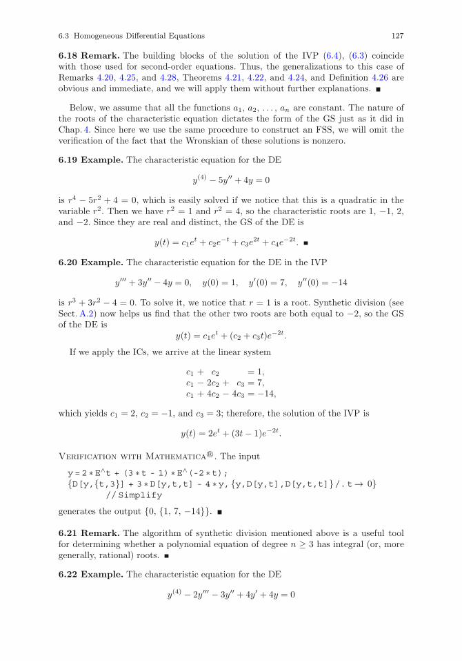
6.3 Homogeneous Differential Equations 127
6.18 Remark. The building blocks of the solution of the IVP (6.4), (6.3) coincidewith those used for second-order equations. Thus, the generalizations to this case ofRemarks 4.20, 4.25, and 4.28, Theorems 4.21, 4.22, and 4.24, and Definition 4.26 areobvious and immediate, and we will apply them without further explanations.
Below, we assume that all the functions a1, a2, . . . , an are constant. The nature ofthe roots of the characteristic equation dictates the form of the GS just as it did inChap. 4. Since here we use the same procedure to construct an FSS, we will omit theverification of the fact that the Wronskian of these solutions is nonzero.
6.19 Example. The characteristic equation for the DE
y(4) − 5y′′ + 4y = 0
is r4 − 5r2 + 4 = 0, which is easily solved if we notice that this is a quadratic in thevariable r2. Then we have r2 = 1 and r2 = 4, so the characteristic roots are 1, −1, 2,and −2. Since they are real and distinct, the GS of the DE is
y(t) = c1et + c2e
−t + c3e2t + c4e
−2t.
6.20 Example. The characteristic equation for the DE in the IVP
y′′′ + 3y′′ − 4y = 0, y(0) = 1, y′(0) = 7, y′′(0) = −14
is r3 + 3r2 − 4 = 0. To solve it, we notice that r = 1 is a root. Synthetic division (seeSect. A.2) now helps us find that the other two roots are both equal to −2, so the GSof the DE is
y(t) = c1et + (c2 + c3t)e
−2t.
If we apply the ICs, we arrive at the linear system
c1 + c2 = 1,c1 − 2c2 + c3 = 7,c1 + 4c2 − 4c3 = −14,
which yields c1 = 2, c2 = −1, and c3 = 3; therefore, the solution of the IVP is
y(t) = 2et + (3t− 1)e−2t.
Verification with Mathematica R©. The input
y=2 ∗E∧t + (3 ∗t - 1) ∗E∧(-2 ∗t);{D[y,{t,3}] + 3 ∗D[y,t,t] - 4 ∗y, {y,D[y,t],D[y,t,t]}/.t→ 0}
//Simplify
generates the output {0, {1, 7, −14}}.
6.21 Remark. The algorithm of synthetic division mentioned above is a useful toolfor determining whether a polynomial equation of degree n ≥ 3 has integral (or, moregenerally, rational) roots.
6.22 Example. The characteristic equation for the DE
y(4) − 2y′′′ − 3y′′ + 4y′ + 4y = 0
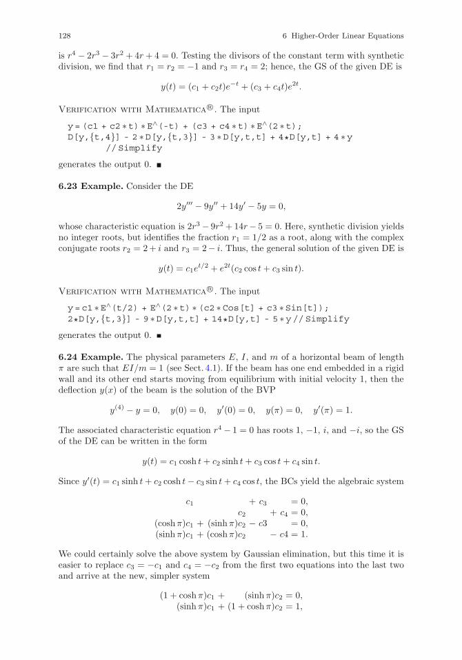
128 6 Higher-Order Linear Equations
is r4 − 2r3 − 3r2 + 4r+ 4 = 0. Testing the divisors of the constant term with syntheticdivision, we find that r1 = r2 = −1 and r3 = r4 = 2; hence, the GS of the given DE is
y(t) = (c1 + c2t)e−t + (c3 + c4t)e
2t.
Verification with Mathematica R©. The input
y=(c1 + c2 ∗t) ∗E∧(-t) + (c3 + c4 ∗t) ∗E∧(2 ∗t);D[y,{t,4}] - 2 ∗D[y,{t,3}] - 3 ∗D[y,t,t] + 4*D[y,t] + 4 ∗y
//Simplify
generates the output 0.
6.23 Example. Consider the DE
2y′′′ − 9y′′ + 14y′ − 5y = 0,
whose characteristic equation is 2r3 − 9r2 +14r− 5 = 0. Here, synthetic division yieldsno integer roots, but identifies the fraction r1 = 1/2 as a root, along with the complexconjugate roots r2 = 2+ i and r3 = 2− i. Thus, the general solution of the given DE is
y(t) = c1et/2 + e2t(c2 cos t+ c3 sin t).
Verification with Mathematica R©. The input
y=c1 ∗E∧(t/2) + E∧(2 ∗t) ∗(c2 ∗Cos[t] + c3 ∗Sin[t]);2*D[y,{t,3}] - 9 ∗D[y,t,t] + 14*D[y,t] - 5 ∗y//Simplify
generates the output 0.
6.24 Example. The physical parameters E, I, and m of a horizontal beam of lengthπ are such that EI/m = 1 (see Sect. 4.1). If the beam has one end embedded in a rigidwall and its other end starts moving from equilibrium with initial velocity 1, then thedeflection y(x) of the beam is the solution of the BVP
y(4) − y = 0, y(0) = 0, y′(0) = 0, y(π) = 0, y′(π) = 1.
The associated characteristic equation r4 − 1 = 0 has roots 1, −1, i, and −i, so the GSof the DE can be written in the form
y(t) = c1 cosh t+ c2 sinh t+ c3 cos t+ c4 sin t.
Since y′(t) = c1 sinh t+ c2 cosh t− c3 sin t+ c4 cos t, the BCs yield the algebraic system
c1 + c3 = 0,c2 + c4 = 0,
(coshπ)c1 + (sinhπ)c2 − c3 = 0,(sinhπ)c1 + (coshπ)c2 − c4 = 1.
We could certainly solve the above system by Gaussian elimination, but this time it iseasier to replace c3 = −c1 and c4 = −c2 from the first two equations into the last twoand arrive at the new, simpler system
(1 + coshπ)c1 + (sinhπ)c2 = 0,(sinhπ)c1 + (1 + coshπ)c2 = 1,
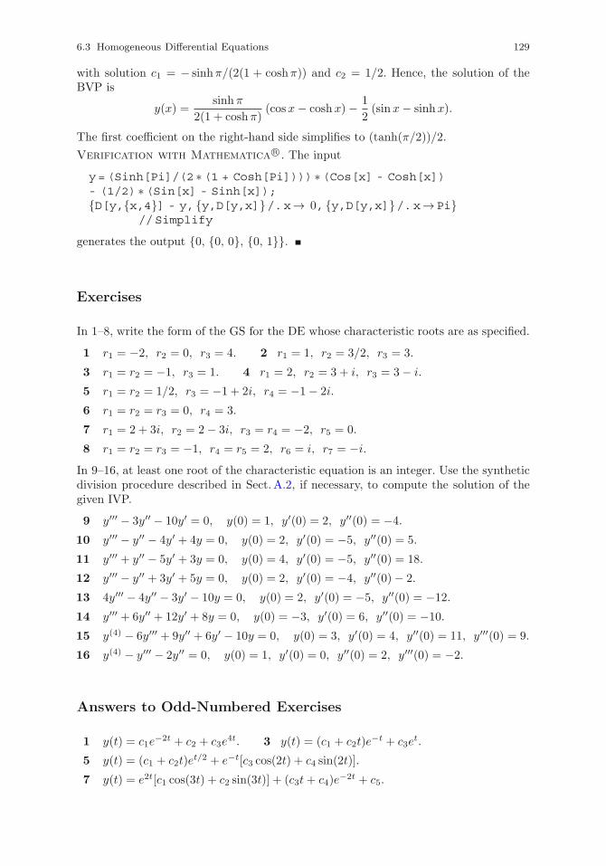
6.3 Homogeneous Differential Equations 129
with solution c1 = − sinhπ/(2(1 + coshπ)) and c2 = 1/2. Hence, the solution of theBVP is
y(x) =sinhπ
2(1 + coshπ)(cosx− coshx)− 1
2(sinx− sinhx).
The first coefficient on the right-hand side simplifies to (tanh(π/2))/2.
Verification with Mathematica R©. The input
y=(Sinh[Pi]/(2 ∗(1 + Cosh[Pi]))) ∗(Cos[x] - Cosh[x])- (1/2) ∗(Sin[x] - Sinh[x]);{D[y,{x,4}] - y, {y,D[y,x]}/.x→ 0, {y,D[y,x]}/.x→Pi}
//Simplify
generates the output {0, {0, 0}, {0, 1}}.
Exercises
In 1–8, write the form of the GS for the DE whose characteristic roots are as specified.
1 r1 = −2, r2 = 0, r3 = 4. 2 r1 = 1, r2 = 3/2, r3 = 3.
3 r1 = r2 = −1, r3 = 1. 4 r1 = 2, r2 = 3 + i, r3 = 3− i.
5 r1 = r2 = 1/2, r3 = −1 + 2i, r4 = −1− 2i.
6 r1 = r2 = r3 = 0, r4 = 3.
7 r1 = 2 + 3i, r2 = 2− 3i, r3 = r4 = −2, r5 = 0.
8 r1 = r2 = r3 = −1, r4 = r5 = 2, r6 = i, r7 = −i.In 9–16, at least one root of the characteristic equation is an integer. Use the syntheticdivision procedure described in Sect. A.2, if necessary, to compute the solution of thegiven IVP.
9 y′′′ − 3y′′ − 10y′ = 0, y(0) = 1, y′(0) = 2, y′′(0) = −4.
10 y′′′ − y′′ − 4y′ + 4y = 0, y(0) = 2, y′(0) = −5, y′′(0) = 5.
11 y′′′ + y′′ − 5y′ + 3y = 0, y(0) = 4, y′(0) = −5, y′′(0) = 18.
12 y′′′ − y′′ + 3y′ + 5y = 0, y(0) = 2, y′(0) = −4, y′′(0)− 2.
13 4y′′′ − 4y′′ − 3y′ − 10y = 0, y(0) = 2, y′(0) = −5, y′′(0) = −12.
14 y′′′ + 6y′′ + 12y′ + 8y = 0, y(0) = −3, y′(0) = 6, y′′(0) = −10.
15 y(4) − 6y′′′ + 9y′′ + 6y′ − 10y = 0, y(0) = 3, y′(0) = 4, y′′(0) = 11, y′′′(0) = 9.
16 y(4) − y′′′ − 2y′′ = 0, y(0) = 1, y′(0) = 0, y′′(0) = 2, y′′′(0) = −2.
Answers to Odd-Numbered Exercises
1 y(t) = c1e−2t + c2 + c3e
4t. 3 y(t) = (c1 + c2t)e−t + c3e
t.
5 y(t) = (c1 + c2t)et/2 + e−t[c3 cos(2t) + c4 sin(2t)].
7 y(t) = e2t[c1 cos(3t) + c2 sin(3t)] + (c3t+ c4)e−2t + c5.
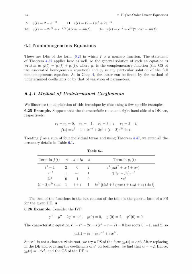
130 6 Higher-Order Linear Equations
9 y(t) = 2− e−2t. 11 y(t) = (2− t)et + 2e−3t.
13 y(t) = −2e2t + e−t/2(4 cos t+ sin t). 15 y(t) = e−t + e3t(2 cos t− sin t).
6.4 Nonhomogeneous Equations
These are DEs of the form (6.2) in which f is a nonzero function. The statementof Theorem 4.37 applies here as well, so the general solution of such an equation iswritten as y(t) = yc(t) + yp(t), where yc is the complementary function (the GS ofthe associated homogeneous equation) and yp is any particular solution of the fullnonhomogeneous equation. As in Chap. 4, the latter can be found by the method ofundetermined coefficients or by that of variation of parameters.
6.4.1 Method of Undetermined Coefficients
We illustrate the application of this technique by discussing a few specific examples.
6.25 Example. Suppose that the characteristic roots and right-hand side of a DE are,respectively,
r1 = r2 = 0, r3 = −1, r4 = 3 + i, r5 = 3− i,
f(t) = t2 − 1 + te−t + 2et + (t− 2)e3t sin t.
Treating f as a sum of four individual terms and using Theorem 4.47, we enter all thenecessary details in Table 6.1.
Table 6.1
Term in f(t) n λ+ iμ s Term in yp(t)
t2 − 1 2 0 2 t2(α0t2 + α1t+ α2)
te−t 1 −1 1 t(β0t+ β1)e−t
2et 0 1 0 γet
(t− 2)e3t sin t 1 3 + i 1 te3t[(δ0t+ δ1) cos t+ (ε0t+ ε1) sin t]
The sum of the functions in the last column of the table is the general form of a PSfor the given DE.
6.26 Example. Consider the IVP
y′′′ − y′′ − 2y′ = 4et, y(0) = 0, y′(0) = 2, y′′(0) = 0.
The characteristic equation r3 − r2 − 2r = r(r2 − r − 2) = 0 has roots 0, −1, and 2, so
yc(t) = c1 + c2e−t + c3e
2t.
Since 1 is not a characteristic root, we try a PS of the form yp(t) = αet. After replacingin the DE and equating the coefficients of et on both sides, we find that α = −2. Hence,yp(t) = −2et, and the GS of the DE is
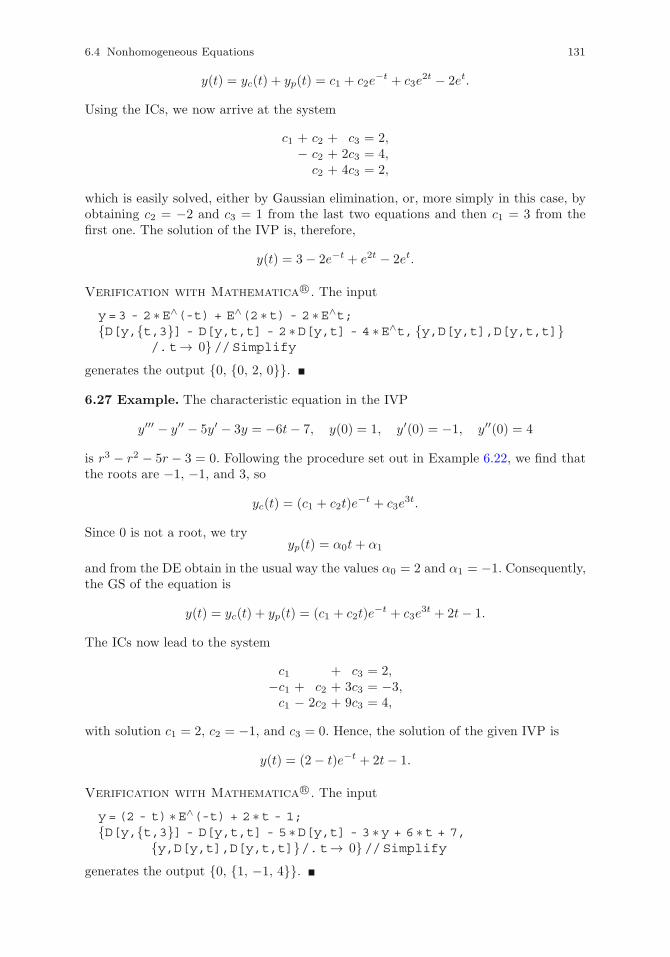
6.4 Nonhomogeneous Equations 131
y(t) = yc(t) + yp(t) = c1 + c2e−t + c3e
2t − 2et.
Using the ICs, we now arrive at the system
c1 + c2 + c3 = 2,− c2 + 2c3 = 4,c2 + 4c3 = 2,
which is easily solved, either by Gaussian elimination, or, more simply in this case, byobtaining c2 = −2 and c3 = 1 from the last two equations and then c1 = 3 from thefirst one. The solution of the IVP is, therefore,
y(t) = 3− 2e−t + e2t − 2et.
Verification with Mathematica R©. The input
y=3 - 2 ∗E∧(-t) + E∧(2 ∗t) - 2 ∗E∧t;{D[y,{t,3}] - D[y,t,t] - 2 ∗D[y,t] - 4 ∗E∧t, {y,D[y,t],D[y,t,t]}
/.t→ 0}//Simplifygenerates the output {0, {0, 2, 0}}.
6.27 Example. The characteristic equation in the IVP
y′′′ − y′′ − 5y′ − 3y = −6t− 7, y(0) = 1, y′(0) = −1, y′′(0) = 4
is r3 − r2 − 5r − 3 = 0. Following the procedure set out in Example 6.22, we find thatthe roots are −1, −1, and 3, so
yc(t) = (c1 + c2t)e−t + c3e
3t.
Since 0 is not a root, we tryyp(t) = α0t+ α1
and from the DE obtain in the usual way the values α0 = 2 and α1 = −1. Consequently,the GS of the equation is
y(t) = yc(t) + yp(t) = (c1 + c2t)e−t + c3e
3t + 2t− 1.
The ICs now lead to the system
c1 + c3 = 2,−c1 + c2 + 3c3 = −3,c1 − 2c2 + 9c3 = 4,
with solution c1 = 2, c2 = −1, and c3 = 0. Hence, the solution of the given IVP is
y(t) = (2− t)e−t + 2t− 1.
Verification with Mathematica R©. The input
y=(2 - t) ∗E∧(-t) + 2 ∗t - 1;{D[y,{t,3}] - D[y,t,t] - 5 ∗D[y,t] - 3 ∗y + 6 ∗t + 7,
{y,D[y,t],D[y,t,t]}/.t→ 0}//Simplifygenerates the output {0, {1, −1, 4}}.
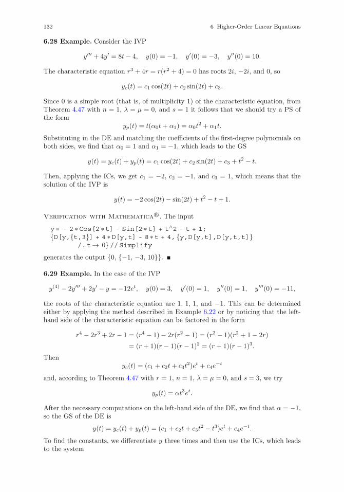
132 6 Higher-Order Linear Equations
6.28 Example. Consider the IVP
y′′′ + 4y′ = 8t− 4, y(0) = −1, y′(0) = −3, y′′(0) = 10.
The characteristic equation r3 + 4r = r(r2 + 4) = 0 has roots 2i, −2i, and 0, so
yc(t) = c1 cos(2t) + c2 sin(2t) + c3.
Since 0 is a simple root (that is, of multiplicity 1) of the characteristic equation, fromTheorem 4.47 with n = 1, λ = μ = 0, and s = 1 it follows that we should try a PS ofthe form
yp(t) = t(α0t+ α1) = α0t2 + α1t.
Substituting in the DE and matching the coefficients of the first-degree polynomials onboth sides, we find that α0 = 1 and α1 = −1, which leads to the GS
y(t) = yc(t) + yp(t) = c1 cos(2t) + c2 sin(2t) + c3 + t2 − t.
Then, applying the ICs, we get c1 = −2, c2 = −1, and c3 = 1, which means that thesolution of the IVP is
y(t) = −2 cos(2t)− sin(2t) + t2 − t+ 1.
Verification with Mathematica R©. The input
y= - 2 ∗Cos[2 ∗t] - Sin[2 ∗t] + t∧2 - t + 1;{D[y,{t,3}] + 4 ∗D[y,t] - 8 ∗t + 4, {y,D[y,t],D[y,t,t]}
/.t→ 0}//Simplifygenerates the output {0, {−1, −3, 10}}.
6.29 Example. In the case of the IVP
y(4) − 2y′′′ + 2y′ − y = −12et, y(0) = 3, y′(0) = 1, y′′(0) = 1, y′′′(0) = −11,
the roots of the characteristic equation are 1, 1, 1, and −1. This can be determinedeither by applying the method described in Example 6.22 or by noticing that the left-hand side of the characteristic equation can be factored in the form
r4 − 2r3 + 2r − 1 = (r4 − 1)− 2r(r2 − 1) = (r2 − 1)(r2 + 1− 2r)
= (r + 1)(r − 1)(r − 1)2 = (r + 1)(r − 1)3.
Thenyc(t) = (c1 + c2t+ c3t
2)et + c4e−t
and, according to Theorem 4.47 with r = 1, n = 1, λ = μ = 0, and s = 3, we try
yp(t) = αt3et.
After the necessary computations on the left-hand side of the DE, we find that α = −1,so the GS of the DE is
y(t) = yc(t) + yp(t) = (c1 + c2t+ c3t2 − t3)et + c4e
−t.
To find the constants, we differentiate y three times and then use the ICs, which leadsto the system
6.4 Nonhomogeneous Equations 133
c1 + c4 = 3,c1 + c2 − c4 = 1,c1 + 2c2 + 2c3 + c4 = 1,c1 + 3c2 + 6c3 − c4 = −5.
We could, of course, apply Gaussian elimination, but this time we prefer to simplify theprocedure by making use of the peculiarities of the system’s structure. Thus, replacingc1 + c4 = 3 from the first equation into the third and c1 − c4 = 1− c2 from the secondequation into the fourth, after simplification we obtain the new system
c2 + c3 = −1,c2 + 3c3 = −3,
with solution c2 = 0 and c3 = −1. Then c1 = 2 and c4 = 1, so the solution of the IVP is
y(t) = (2− t2 − t3)et + e−t.
Verification with Mathematica R©. The input
y=(2 - t∧2 - t∧3) ∗E∧t + E∧(-t);{D[y,{t,4}] - 2 ∗D[y,{t,3}] + 2 ∗D[y,t] - y + 12 ∗E∧t,{y,D[y,t],D[y,t,t],D[y,{t,3}]}/.t→ 0}//Simplify
generates the output {0, {3, 1, 1, −11}}.
Exercises
In 1–8, use Theorem 4.47 to write the form of a PS for the DE whose characteristicroots and right-hand side are as specified.
1 r1 = 1, r2 = −2, r3 = r4 = 4; f(t) = 2− e2t + tet + (t− 3)e4t.
2 r1 = 2, r2 = r3 = r4 = −1, r5 = 4; f(t) = t+ (2t+ 1)e−4t + 3e2t − (t+ 1)e−t.
3 r1 = 0, r2 = r3 = −3, r4 = 2i, r5 = −2i; f(t) = −1+ t2e−3t + 2 cos t− 3 sin(2t).
4 r1 = r2 = 0, r3 = r4 = r5 = 1, r6 = i/2, r7 = −i/2;f(t) = 2t− 1 + 4tet + 3 cos(2t) + et/2 sin t.
5 r1 = 0, r2 = r3 = 1/3, r4 = 4i, r5 = −4i;
f(t) = tet + (t2 − 1)et/3 + et sin t+ t cos(4t).
6 r1 = r2 = 0, r3 = r4 = r5 = −1, r6 = i, r7 = −i;f(t) = t3 − 2t+ 4tet + t2e−t + (1− t) sin t.
7 r1 = r2 = r3 = 0, r4 = r5 = 2, r6 = 1 + i, r7 = 1− i;
f(t) = t+ 2 + (3t2 − 1)e2t + tet − 2e−t sin t.
8 r1 = r2 = r3 = r4 = 0, r5 = 1, r6 = 1 + 2i, r7 = 1− 2i;
f(t) = 2 + 3t2et + (t− 1)e2t + t2et cos(2t).
In 9–20, at least one of the roots of the characteristic equation is an integer. Use themethod of undetermined coefficients in conjunction with synthetic division, if necessary,to find a PS of the DE, then solve the given IVP.
134 6 Higher-Order Linear Equations
9 y′′′ − 2y′′ − 8y′ = −27et, y(0) = 3, y′(0) = −7, y′′(0) = −25.
10 y′′′ − (5/2)y′′ + y′ = 9e−t, y(0) = −3, y′(0) = 2, y′′(0) = 1.
11 y′′′ − 2y′′ − 7y′ − 4y = 10e−t, y(0) = 4, y′(0) = 0, y′′(0) = 19.
12 y′′′ − y′′ − 8y′ + 12y = 20e2t, y(0) = 1, y′(0) = 8, y′′(0) = 7.
13 y′′′ − 2y′ + 4y = 4t− 14, y(0) = −3, y′(0) = 6, y′′(0) = 0.
14 y′′′ + 3y′′ + 7y′ + 5y = −8e−t, y(0) = 3, y′(0) = −7, y′′(0) = 11.
15 y(4) − 2y′′′ + y′′ = −2, y(0) = −3, y′(0) = 0, y′′(0) = 1, y′′′(0) = 5.
16 y(4) − y′′′ + 4y′′ − 4y′ = −3(cos t+ sin t),
y(0) = −1, y′(0) = 5, y′′(0) = 6, y′′′(0) = −7.
17 y(4) + y′′′ − y′′ + y′ − 2y = −4 cos t+ 12 sin t,
y(0) = 2, y′(0) = 5, y′′(0) = −5, y′′′(0) = 3.
18 y(4) − 2y′′′ − 2y′′ + 6y′ + 5y = −20e−t,
y(0) = −1, y′(0) = 1, y′′(0) = 1, y′′′(0) = 29.
19 y(5) − 2y(4) + 5y′′′ = 48− 120t,
y(0) = 0, y′(0) = −1, y′′(0) = 0, y′′′(0) = 2, y(4)(0) = 0.
20 y(5) − 2y(4) − 3y′′′ + 4y′′ + 4y′ = −18e−t,
y(0) = 2, y′(0) = 1, y′′(0) = 8, y′′′(0) = −1, y(4)(0) = 32.
Answers to Odd-Numbered Exercises
1 yp(t) = α+ βe2t + t(γ1 + γ2t)et + t2(δ1 + δ2t)e
4t.
3 yp(t) = αt+ t2(β1 + β2t+ β3t2)e−3t + γ1 cos t+ γ2 sin t+ t[δ1 cos(2t) + δ2 sin(2t)].
5 yp(t) = (α1 + α2t)et + t2(β1 + β2t+ β3t
2)et/3 + et(γ1 cos t+ γ2 sin t)
+ t[(δ1+δ2t) cos(4t)+(ε1+ε2t) sin(4t)].
7 yp(t) = t3(α1 +α2t)+ t2(β1 + β2t+ β3t2)e2t +(γ1 + γ2t)e
t + e−t(δ1 cos t+ δ2 sin t).
9 y(t) = 1 + e−2t − 2e4t + 3et. 11 y(t) = (3− t)e−t + e4t − t2e−t.
13 y(t) = −e−2t + et(cos t+ 2 sin t) + t− 3. 15 y(t) = (2t− 1)et − t2 − t− 2.
17 y(t) = et − e−2t + (2t+ 2) cos t. 19 y(t) = t+ 2t2 − t4 − et sin(2t).
6.4.2 Method of Variation of Parameters
This solution technique for higher-order DEs is based on the same idea as for second-order equations.
6.30 Example. The characteristic equation for the DE
y′′′ − 2y′′ − y′ + 2y = 2t− 5
is r3 − 2r2 − r + 2 = 0, with roots 1, −1, and 2. Therefore, {et, e−t, e2t} is an FSS, sowe seek a PS of the form
6.4 Nonhomogeneous Equations 135
yp = u1et + u2e
−t + u3e2t,
where u1, u2, and u3 are functions of t. Then
y′p = u′1et + u1e
t + u′2e−t − u2e
−t + u′3e2t + 2u3e
2t,
and we impose the usual restriction on the functions u1, u2, and u3, namely
u′1et + u′2e
−t + u′3e2t = 0. (6.5)
The second-order derivative is now
y′′p = u′1et + u1e
t − u′2e−t + u2e
−t + 2u′3e2t + 4u3e
2t,
and we impose the second restriction
u′1et − u′2e
−t + 2u′3e2t = 0. (6.6)
In view of this, the third-order derivative is
y′′′p = u′1et + u1e
t + u′2e−t − u2e
−t + 4u′3e2t + 8u3e
2t.
Replacing y′p, y′′p , and y
′′′p in the DE and sorting out the terms, we arrive at the equality
u′1et + u′2e
−t + 4u′3e2t = 2t− 5. (6.7)
Equations (6.5)–(6.7) form a linear system for u′1et, u′2e
−t, and u′3e2t, which, when
solved by Gaussian elimination, gives rise to the arrays
1 1 1 01 −1 2 0 R2 −R1
1 1 4 2t− 5 R3 −R1
⇒1 1 1 00 −2 1 00 0 3 2t− 5
and, hence, to the simpler system
u′1et + u′2e
−t + u′3e2t = 0,
− 2u′2e−t + u′3e2t = 0,
3u′3e2t = 2t− 5,
with solution
u′1et = 1
2 (5− 2t), u′2e−t = 1
6 (2t− 5), u′3e2t = 1
3 (2t− 5).
Solving for u′1, u′2, and u′3, integrating by parts, and omitting the arbitrary constants
of integration, we now obtain
u1(t) =12 (2t− 3)e−t, u2(t) =
16 (2t− 7)et, u3(t) =
13 (2− t)e−2t,
so
yp(t) =12 (2t− 3) + 1
6 (2t− 7) + 13 (2 − t) = t− 2.
Verification with Mathematica R©. The input
y=t - 2;D[y,{t,3}] - 2 ∗D[y,t,t] - D[y,t] + 2 ∗y - 2 ∗t + 5//Simplify
generates the output 0.
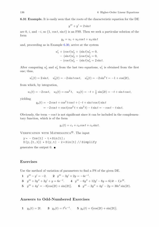
136 6 Higher-Order Linear Equations
6.31 Example. It is easily seen that the roots of the characteristic equation for the DE
y′′′ + y′ = 2 sin t
are 0, i, and −i, so {1, cos t, sin t} is an FSS. Then we seek a particular solution of theform
yp = u1 + u2 cos t+ u3 sin t
and, proceeding as in Example 6.30, arrive at the system
u′1 + (cos t)u′2 + (sin t)u′3 = 0,
− (sin t)u′2 + (cos t)u′3 = 0,
− (cos t)u′2 − (sin t)u′3 = 2 sin t.
After computing u′2 and u′3 from the last two equations, u′1 is obtained from the firstone; thus,
u′1(t) = 2 sin t, u′2(t) = −2 sin t cos t, u′3(t) = −2 sin2 t = −1 + cos(2t),
from which, by integration,
u1(t) = −2 cos t, u2(t) = cos2 t, u3(t) = −t+ 12 sin(2t) = −t+ sin t cos t,
yieldingyp(t) = −2 cos t+ cos2 t cos t+ (−t+ sin t cos t) sin t
= −2 cos t+ cos t(cos2 t+ sin2 t)− t sin t = − cos t− t sin t.
Obviously, the term − cos t is not significant since it can be included in the complemen-tary function, which is of the form
yc(t) = c1 + c2 cos t+ c3 sin t.
Verification with Mathematica R©. The input
y= - Cos[t] - t ∗Sin[t];D[y,{t,3}] + D[y,t] - 2 ∗Sin[t]//Simplify
generates the output 0.
Exercises
Use the method of variation of parameters to find a PS of the given DE.
1 y′′′ − y′ = −2. 2 y′′′ − 3y′ + 2y = −4e−t.
3 y′′′ + 3y′′ + 3y′ + y = 6e−t. 4 y′′′ − 6y′′ + 12y′ − 8y = 6(4t− 1)e2t.
5 y′′′ + 4y′ = −8[cos(2t) + sin(2t)]. 6 y′′′ − 3y′′ + 4y′ − 2y = 30et sin(2t).
Answers to Odd-Numbered Exercises
1 yp(t) = 2t. 3 yp(t) = t3e−t. 5 yp(t) = t[cos(2t) + sin(2t)].
Chapter 7
Systems of Differential Equations
As physical phenomena increase in complexity, their mathematical models require theuse of more than one unknown function. This gives rise to systems of DEs.
7.1 Modeling with Systems of Equations
Here are a few simple illustrations of such models.
Parallel LRC circuit. If an inductor of inductance L, a resistor of resistanceR, anda capacitor of capacitance C are connected in parallel, then the current I(t) throughthe inductor and the voltage drop V (t) across the capacitor are the solutions of the IVP
I ′ =1
LV, I(0) = I0,
V ′ = − 1
CI − 1
RCV, V (0) = V0.
The (first-order) DEs in this IVP are linear and homogeneous.
Military combat. Suppose that two military forces of strengths x1(t) and x2(t),respectively, engage in battle, and that the rate at which the troops of each of them areput out of action is proportional to the troop strength of the enemy. If the correspondingproportionality constants are a > 0 and b > 0, then the evolution of the combat isdescribed by the IVP
x′1 = −ax2, x1(0) = x10,
x′2 = −bx1, x2(0) = x20,
where x10 and x20 are the initial strengths of the two opposing forces. The above systemconsists of two linear, homogeneous, first-order DEs.
Solution mix. Consider two containers linked by two pipes. The containers holdvolumes v1 and v2 of water in which initial amounts s10 and s20, respectively, of salthave been dissolved. Additional salt solution is being poured into the containers at ratesr1 and r2, with salt concentrations c1 and c2. Solution flows from the second containerinto the first one through one of the connecting pipes at a rate r21, and from the firstcontainer into the second one through the other connecting pipe at a rate r12. Also,solution is drained from the containers outside the system at rates r10 and r20. If s1(t)and s2(t) are the amounts of salt in the two containers at time t and all the salt solutionsinvolved are homogeneous, then the process is described by the IVP
C. Constanda, Differential Equations: A Primer for Scientists and Engineers, SpringerUndergraduate Texts in Mathematics and Technology, DOI 10.1007/978-1-4614-7297-1 7,© Springer Science+Business Media New York 2013
137
138 7 Systems of Differential Equations
s′1 = c1r1 − r12 + r10v1
s1 +r21v2
s2, s1(0) = s10,
s′2 = c2r2 +r12v1
s1 − r21 + r20v2
s2, s2(0) = s20,
where all the constants involved are nonnegative. The two first-order DEs in this systemare linear and nonhomogeneous.
Predator–prey. Suppose that an ecological system consists of only two species: a preypopulation p1(t) and a predator population p2(t). Also, suppose that the net growthrate α > 0 of prey in the absence of predator is proportional to the size of the preypopulation, the death rate δ > 0 of predator in the absence of prey is proportional tothe size of the predator population, the predation rate β > 0 is proportional to the rateof predator–prey encounters, and the birth rate γ > 0 of predator is proportional to thesize of its food supply—in other words, of prey—and to the size of its own population.Under these assumptions, the evolution of the system is described by the IVP
p′1 = αp1 − βp1p2, p1(0) = p10,
p′2 = γp1p2 − δp2, p2(0) = p20,
where p10 and p20 are the initial sizes of the two populations. This system, whichconsists of two nonlinear, homogeneous, first-order DEs, also describes certain processesin chemistry and economics and is referred to generically as a consumer–resource model.
Contagious disease epidemic. In a given population, let S(t) be the number ofindividuals susceptible (exposed) to some disease but not yet infected, I(t) the numberof those already infected, R(t) the number of those recovered from the disease, α therate of infection (assumed to be proportional to the number of infected individuals), βthe recovery rate of those infected, and γ the reinfection rate of those recovered. Theevolution of the disease in the population is modeled by the IVP
S′ = −αIS + γR, S(0) = S0,
I ′ = αIS − βI, I(0) = I0,
R′ = βI − γR, R(0) = R0,
where S0, I0, and R0 are the initial sizes of the corresponding population groups. Allthe first-order DEs above are homogeneous; the first two are nonlinear, whereas thethird one is linear.
Coupled mechanical oscillators. Consider two collinear mass–spring systems(see Sect. 5.2.1) with spring constants k1 and k2, where the masses m1 and m2 areconnected to each other by a third spring of constant k3. Initially in equilibrium (thatis, at rest) at points x10 and x20, respectively, the two masses are acted upon by twoexternal forces f1 and f2. If x1(t) and x2(t) are the displacements of the masses fromtheir equilibrium positions at time t, then Newton’s second law applied to each massleads to the IVP
m1x′′1 = −k1x1 + k3(x2 − x1) + f1, x1(0) = x10, x′1(0) = 0,
m2x′′2 = −k2x2 − k3(x2 − x1) + f2, x2(0) = x20, x′2(0) = 0.
Both equations above are linear, nonhomogeneous, second-order DEs. Their ensemblecan easily be rewritten as a system of four first-order equations. Indeed, if we set x′1 = y1and x′2 = y2 and perform simple algebraic manipulations, we arrive at the equivalentIVP
7.2 Algebra Prerequisites 139
x′1 = y1, x1(0) = x10,
y′1 = −k1 + k3m1
x1 +k3m1
x2 +1
m1f1, y1(0) = 0,
x′2 = y2, x2(0) = x20,
y′2 =k3m2
x1 − k2 + k3m2
x2 +1
m2f2, y2(0) = 0.
7.2 Algebra Prerequisites
The algebraic concepts and methods mentioned in this section can be developed forgeneral m× n matrices with either real or complex elements. However, we restrict ourattention to square n × n real matrices since this is the only type that occurs in ourtreatment of systems of DEs.
7.2.1 Operations with Matrices
Let Mn be the set of n× n matrices introduced in Sect. 6.2.1. This set can be endowedwith a structure of vector space, characterized by two operations: one ‘external’ (calledmultiplication of a matrix by a number, or scalar) and one ‘internal’ (called additionof matrices). Thus, if A = (aij) and B = (bij) are elements of Mn and λ is anynumber, then
λA = (λaij), A+B = (aij + bij), (7.1)
both of which also belong to Mn.
7.1 Example. Let
A =
⎛⎝2 −1 31 1 −24 0 1
⎞⎠ , B =
⎛⎝1 2 −12 −2 13 1 −5
⎞⎠ , λ = −2.
By (7.1), we have
λA =
⎛⎝−4 2 −6−2 −2 4−8 0 −2
⎞⎠ , A+B =
⎛⎝3 1 23 −1 −17 1 −4
⎞⎠ .
Two particular matrices play a special role in matrix manipulation: the zero matrix 0and the identity matrix I defined, respectively, by
0 =
⎛⎜⎜⎝0 0 · · · 00 0 · · · 0...
.... . .
...0 0 · · · 0
⎞⎟⎟⎠ , I =
⎛⎜⎜⎝1 0 · · · 00 1 · · · 0...
.... . .
...0 0 · · · 1
⎞⎟⎟⎠ .
The use of the same symbol 0 for both the number zero and the zero matrix shouldcreate no ambiguity since its meaning will be clear from the context.
If A = (aij), then we write −A = (−aij).
140 7 Systems of Differential Equations
7.2 Remarks. (i) As expected, two matrices inMn are said to be equal if each elementin one matrix is equal to the element at the same location in the other.
(ii) It is easily verified that for any matrices A, B, and C in Mn and any numbers λand μ,
A+ (B + C) = (A+B) + C,
A+B = B +A,
A+ 0 = A,
A+ (−A) = 0,
λ(A +B) = λA+ λB,
(λ + μ)A = λA+ μA.
These properties have special names in linear algebra but, for simplicity, we omitthem.
On Mn we can also define multiplication of matrices. If A = (aij) and B = (bij),then
AB = (cij) =
( n∑k=1
aikbkj
). (7.2)
We note that to form the matrix AB, we operate with one row of A and one column ofB at a time. The generic element cij in AB consists of the sum of the products of eachelement in row i in A and the corresponding element in column j in B.
7.3 Example. Let A and B be the matrices defined in Example 7.1. According toformula (7.2), the first element in the matrix AB is
c11 =
3∑k=1
a1kbk1 = a11b11 + a12b21 + a13b31 = (2)(1) + (−1)(2) + (3)(3) = 9.
The element in the second row and third column is
c23 =
3∑k=1
a2kbk3 = a21b13 + a22b23 + a23b33 = (1)(−1) + (1)(1) + (−2)(−5) = 10.
Calculating the remaining elements cij in a similar manner, we find that
AB =
⎛⎝ 9 9 −18−3 −2 107 9 −9
⎞⎠ .
7.4 Remarks. (i) Using definition (7.2), we readily verify that for any elements A, B,and C of Mn,
A(BC) = (AB)C,
A(B + C) = AB +AC,
(A+B)C = AC +BC,
IA = AI = A.
(ii) In general, AB �= BA. As an illustration, we see that for the matrices A and B inExample 7.3 we have
7.2 Algebra Prerequisites 141
BA =
⎛⎝ 0 1 −2
6 −4 11−13 −2 2
⎞⎠ �= AB.
(iii) A 1 × n matrix is usually called an n-component row vector. Similarly, an n × 1matrix is called an n-component column vector. In what follows we operate mainlywith column vectors, which, to make the notation clearer, are denoted by boldletters.
(iv) As mentioned in Sect. 6.2.1, the elements a11, . . . , ann of an n × n matrix A aresaid to form the leading diagonal of A.
7.5 Definition. If A = (aij), then AT = (aji) is called the transpose of A.
7.6 Example. The transpose of the matrix
A =
⎛⎝−2 1 4
3 −1 05 2 −3
⎞⎠
is
AT =
⎛⎝−2 3 5
1 −1 24 0 −3
⎞⎠ .
The transpose of the column vector
v =
⎛⎝ 2
5−4
⎞⎠
is the row vector vT = (2, 5, −4).
In view of the definition of matrix multiplication, the linear algebraic system (6.1)can be written generically as
Ax = b, (7.3)
where A = (aij) is the n×n matrix of the system coefficients, x is the column vector ofthe unknowns x1, . . . , xn, and b is the column vector of the right-hand sides b1, . . . , bn.
7.7 Example. For the system
3x1 − 2x2 + 4x3 =−1,2x1 − x3 = 3,x1 + x2 − 3x3 = 7
we have
A =
⎛⎝3 −2 42 0 −11 1 −3
⎞⎠ , x =
⎛⎝x1x2x3
⎞⎠ , b =
⎛⎝−1
37
⎞⎠ ,
so, in matrix notation, the given system is
⎛⎝3 −2 42 0 −11 1 −3
⎞⎠⎛⎝x1x2x3
⎞⎠ =
⎛⎝−1
37
⎞⎠ .
7.8 Definition. A square matrix A such that det(A) �= 0 is called nonsingular, orinvertible. If det(A) = 0, the matrix is called singular, or non-invertible.
142 7 Systems of Differential Equations
Every nonsingular matrix A has a (unique) inverse; that is, there is a matrix A−1 ofthe same type as A that satisfies AA−1 = A−1A = I.
The inverse matrix can be found by means of an extended version of Gaussian elim-ination. We place the identity matrix I to the right of A and then perform suitableelementary row operations simultaneously on both sides until the matrix on the leftbecomes I. It can be shown that the matrix we end up with on the right is A−1.
7.9 Example. Applying the above procedure to the matrix
A =
⎛⎝2 3 −11 2 01 3 2
⎞⎠ ,
we generate the chain of arrays
2 3 −1 1 0 01 2 0 0 1 0 2R2 −R1
1 3 2 0 0 1 2R3 −R1
⇒2 3 −1 1 0 0 R1 − 3R2
0 1 1 −1 2 00 3 5 −1 0 2 R3 − 3R2
⇒2 0 −4 4 −6 0 R1/2 +R3
0 1 1 −1 2 0 R2 −R3/20 0 2 2 −6 2 R3/2
⇒1 0 0 4 −9 20 1 0 −2 5 −10 0 1 1 −3 1
from which we conclude that
A−1 =
⎛⎝ 4 −9 2−2 5 −11 −3 1
⎞⎠ .
Verification with Mathematica R©. The input
A= {{w2,3,-1}, {1,2,0}, {1,3,2}};InvA= {{4,-9,2}, {-2,5,-1}, {1,-3,1}};A.InvA
generates the output {{1, 0, 0, }, {0, 1, 0}, {0, 0, 1}}.
7.10 Remark. In the case of a nonsingular 2× 2 matrix
A =
(a11 a12a21 a22
),
the above procedure reduces to swapping the elements on the leading diagonal, changingthe sign of the other two elements, and dividing all the elements by the determinant ofthe matrix; that is,
A−1 =1
det(A)
(a22 −a12
−a21 a11
).
7.2 Algebra Prerequisites 143
7.11 Example. If
A =
(−2 31 −4
),
then det(A) = 5, so
A−1 = −1
5
(4 31 2
)=
(− 45 − 3
5
− 15 − 2
5
).
Verification with Mathematica R©. The input
A= {{-2,3}, {1,-4}};InvA= - (1/5) ∗ {{4,3}, {1,2}};A.InvA
generates the output {{1, 0}, {0, 1}}.7.12 Remark. If A is nonsingular, then
A−1(Ax) = (A−1A)x = Ix = x,
so, multiplying both sides of (7.3) on the left by A−1, we obtain the solution as
x = A−1b.
7.13 Example. The matrix of coefficients for the system
2x1 + 3x2 − x3 =−3,x1 + 2x2 =−1,x1 + 3x2 + 2x3 = 2
is the matrix A whose inverse A−1 was computed in Example 7.9. Hence, according toRemark 7.12, the solution of the given system is
x = A−1b =
⎛⎝ 4 −9 2−2 5 −11 −3 1
⎞⎠⎛⎝−3−12
⎞⎠ =
⎛⎝ 1−12
⎞⎠ ;
that is, x1 = 1, x2 = −1, and x3 = 2.
Verification with Mathematica R©. The input
{2 ∗x1 + 3 ∗x2 - x3 + 3,x1 + 2 ∗x2 + 1,x1 + 3 ∗x2 + 2 ∗x3-2}/. {x1→ 1,x2→ −1,x3→ 2}
generates the output {0, 0, 0}.7.14 Remark. Sometimes we encounter matrix functions. These are matrices whose el-ements are functions of the same independent variable or variables, and, just as for singlefunctions, we can talk about their continuity and differentiability, and their derivativesand integrals. Thus, if A(t) = (fij(t)) and each of the fij is differentiable, we writeA′(t) = (f ′
ij(t)). For any such n× n matrix functions A and B and any n× n constantmatrix C,
(CA)′ = CA′,(A+B)′ = A′ +B′,(AB)′ = A′B +AB′.
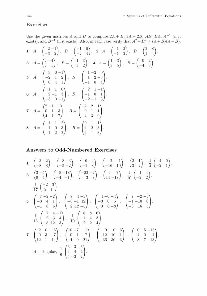
144 7 Systems of Differential Equations
Exercises
Use the given matrices A and B to compute 2A + B, 3A − 2B, AB, BA, A−1 (if itexists), and B−1 (if it exists). Also, in each case verify that A2−B2 �= (A+B)(A−B).
1 A =
(2 −1
−3 2
), B =
(−1 0−2 4
). 2 A =
(1 3
−1 2
), B =
(2 81 4
).
3 A =
(2 −42 1
), B =
(−1 35 2
). 4 A =
(1 −33 5
), B =
(0 2
−4 3
).
5 A =
⎛⎝ 3 0 −1−2 1 20 4 1
⎞⎠ , B =
⎛⎝ 1 −2 0
1 2 −3−1 0 4
⎞⎠.
6 A =
⎛⎝ 1 1 0
2 −1 3−3 0 −1
⎞⎠ , B =
⎛⎝ 2 1 −1−1 0 1−2 −1 3
⎞⎠.
7 A =
⎛⎝2 −1 10 1 −34 1 −7
⎞⎠ , B =
⎛⎝−2 2 1
0 1 −14 −3 0
⎞⎠.
8 A =
⎛⎝ 1 1 2
1 0 3−1 −2 2
⎞⎠ , B =
⎛⎝0 −1 14 −2 32 1 −3
⎞⎠.
Answers to Odd-Numbered Exercises
1
(3 −2
−8 8
),
(8 −3
−5 −2
),
(0 −4
−1 8
),
( −2 1−16 10
),
(2 13 2
),
1
4
(−4 0−2 1
).
3
(3 −59 4
),
(8 −18
−4 −1
),
(−22 −23 8
),
(4 714 −18
),
1
10
(1 4
−2 2
),
1
17
(−2 35 1
).
5
⎛⎝ 7 −2 −2−3 4 1−1 8 6
⎞⎠ ,
⎛⎝ 7 4 −3−8 −1 122 12 −5
⎞⎠ ,
⎛⎝ 4 −6 −4−3 6 53 8 −8
⎞⎠ ,
⎛⎝ 7 −2 −5−1 −10 0−3 16 5
⎞⎠,
1
13
⎛⎝ 7 4 −1−2 −3 48 12 −3
⎞⎠ ,
1
10
⎛⎝ 8 8 6−1 4 32 2 4
⎞⎠.
7
⎛⎝ 2 0 3
0 3 −712 −1 −14
⎞⎠ ,
⎛⎝10 −7 1
0 1 −74 9 −21
⎞⎠ ,
⎛⎝ 0 0 3−12 10 −1−36 30 3
⎞⎠ ,
⎛⎝ 0 5 −15−4 0 48 −7 13
⎞⎠,
A is singular,1
6
⎛⎝3 3 34 4 24 −2 2
⎞⎠.
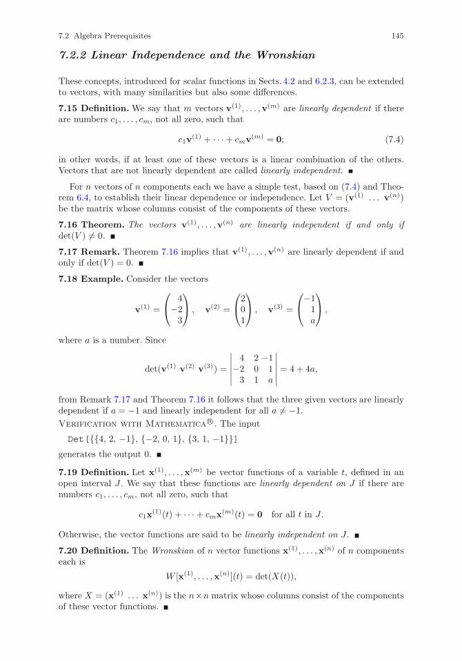
7.2 Algebra Prerequisites 145
7.2.2 Linear Independence and the Wronskian
These concepts, introduced for scalar functions in Sects. 4.2 and 6.2.3, can be extendedto vectors, with many similarities but also some differences.
7.15 Definition. We say that m vectors v(1), . . . ,v(m) are linearly dependent if thereare numbers c1, . . . , cm, not all zero, such that
c1v(1) + · · ·+ cmv(m) = 0; (7.4)
in other words, if at least one of these vectors is a linear combination of the others.Vectors that are not linearly dependent are called linearly independent.
For n vectors of n components each we have a simple test, based on (7.4) and Theo-rem 6.4, to establish their linear dependence or independence. Let V = (v(1) . . . v(n))be the matrix whose columns consist of the components of these vectors.
7.16 Theorem. The vectors v(1), . . . ,v(n) are linearly independent if and only ifdet(V ) �= 0.
7.17 Remark. Theorem 7.16 implies that v(1), . . . ,v(n) are linearly dependent if andonly if det(V ) = 0.
7.18 Example. Consider the vectors
v(1) =
⎛⎝ 4−23
⎞⎠ , v(2) =
⎛⎝201
⎞⎠ , v(3) =
⎛⎝−1
1a
⎞⎠ ,
where a is a number. Since
det(v(1) v(2) v(3)) =
∣∣∣∣∣∣4 2 −1
−2 0 13 1 a
∣∣∣∣∣∣ = 4 + 4a,
from Remark 7.17 and Theorem 7.16 it follows that the three given vectors are linearlydependent if a = −1 and linearly independent for all a �= −1.
Verification with Mathematica R©. The input
Det[{{4, 2, −1}, {−2, 0, 1}, {3, 1, −1}}]generates the output 0.
7.19 Definition. Let x(1), . . . ,x(m) be vector functions of a variable t, defined in anopen interval J . We say that these functions are linearly dependent on J if there arenumbers c1, . . . , cm, not all zero, such that
c1x(1)(t) + · · ·+ cmx(m)(t) = 0 for all t in J.
Otherwise, the vector functions are said to be linearly independent on J .
7.20 Definition. The Wronskian of n vector functions x(1), . . . ,x(n) of n componentseach is
W [x(1), . . . ,x(n)](t) = det(X(t)),
where X = (x(1) . . . x(n)) is the n×n matrix whose columns consist of the componentsof these vector functions.
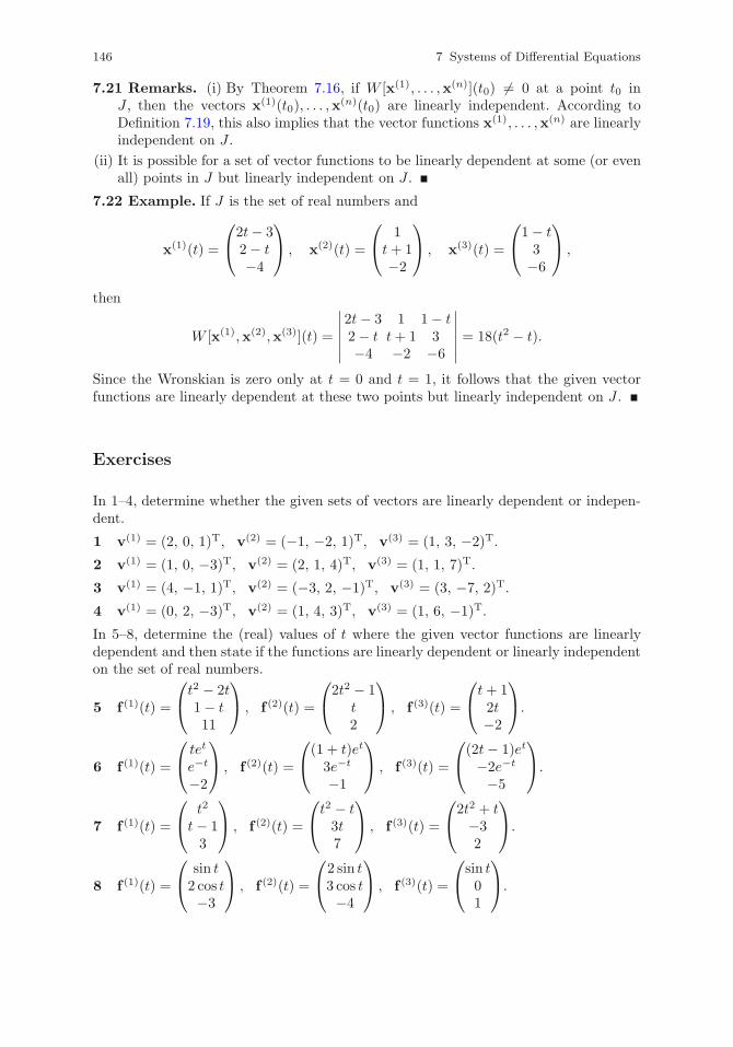
146 7 Systems of Differential Equations
7.21 Remarks. (i) By Theorem 7.16, if W [x(1), . . . ,x(n)](t0) �= 0 at a point t0 inJ , then the vectors x(1)(t0), . . . ,x
(n)(t0) are linearly independent. According toDefinition 7.19, this also implies that the vector functions x(1), . . . ,x(n) are linearlyindependent on J .
(ii) It is possible for a set of vector functions to be linearly dependent at some (or evenall) points in J but linearly independent on J .
7.22 Example. If J is the set of real numbers and
x(1)(t) =
⎛⎝2t− 3
2− t−4
⎞⎠ , x(2)(t) =
⎛⎝ 1t+ 1−2
⎞⎠ , x(3)(t) =
⎛⎝1− t
3−6
⎞⎠ ,
then
W [x(1),x(2),x(3)](t) =
∣∣∣∣∣∣2t− 3 1 1− t2− t t+ 1 3−4 −2 −6
∣∣∣∣∣∣ = 18(t2 − t).
Since the Wronskian is zero only at t = 0 and t = 1, it follows that the given vectorfunctions are linearly dependent at these two points but linearly independent on J .
Exercises
In 1–4, determine whether the given sets of vectors are linearly dependent or indepen-dent.
1 v(1) = (2, 0, 1)T, v(2) = (−1, −2, 1)T, v(3) = (1, 3, −2)T.
2 v(1) = (1, 0, −3)T, v(2) = (2, 1, 4)T, v(3) = (1, 1, 7)T.
3 v(1) = (4, −1, 1)T, v(2) = (−3, 2, −1)T, v(3) = (3, −7, 2)T.
4 v(1) = (0, 2, −3)T, v(2) = (1, 4, 3)T, v(3) = (1, 6, −1)T.
In 5–8, determine the (real) values of t where the given vector functions are linearlydependent and then state if the functions are linearly dependent or linearly independenton the set of real numbers.
5 f (1)(t) =
⎛⎝t
2 − 2t1− t11
⎞⎠ , f (2)(t) =
⎛⎝2t2 − 1
t2
⎞⎠ , f (3)(t) =
⎛⎝t+ 1
2t−2
⎞⎠.
6 f (1)(t) =
⎛⎝ tet
e−t
−2
⎞⎠ , f (2)(t) =
⎛⎝(1 + t)et
3e−t
−1
⎞⎠ , f (3)(t) =
⎛⎝(2t− 1)et
−2e−t
−5
⎞⎠.
7 f (1)(t) =
⎛⎝ t2
t− 13
⎞⎠ , f (2)(t) =
⎛⎝t
2 − t3t7
⎞⎠ , f (3)(t) =
⎛⎝2t2 + t
−32
⎞⎠.
8 f (1)(t) =
⎛⎝ sin t2 cos t−3
⎞⎠ , f (2)(t) =
⎛⎝2 sin t3 cos t−4
⎞⎠ , f (3)(t) =
⎛⎝sin t
01
⎞⎠.
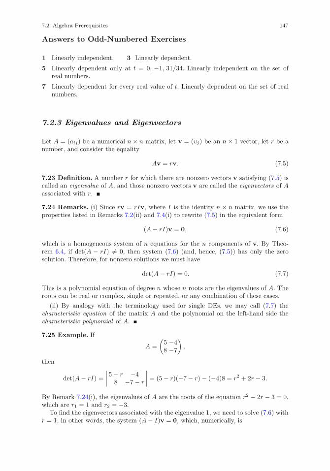
7.2 Algebra Prerequisites 147
Answers to Odd-Numbered Exercises
1 Linearly independent. 3 Linearly dependent.
5 Linearly dependent only at t = 0, −1, 31/34. Linearly independent on the set ofreal numbers.
7 Linearly dependent for every real value of t. Linearly dependent on the set of realnumbers.
7.2.3 Eigenvalues and Eigenvectors
Let A = (aij) be a numerical n× n matrix, let v = (vj) be an n× 1 vector, let r be anumber, and consider the equality
Av = rv. (7.5)
7.23 Definition. A number r for which there are nonzero vectors v satisfying (7.5) iscalled an eigenvalue of A, and those nonzero vectors v are called the eigenvectors of Aassociated with r.
7.24 Remarks. (i) Since rv = rIv, where I is the identity n × n matrix, we use theproperties listed in Remarks 7.2(ii) and 7.4(i) to rewrite (7.5) in the equivalent form
(A− rI)v = 0, (7.6)
which is a homogeneous system of n equations for the n components of v. By Theo-rem 6.4, if det(A − rI) �= 0, then system (7.6) (and, hence, (7.5)) has only the zerosolution. Therefore, for nonzero solutions we must have
det(A− rI) = 0. (7.7)
This is a polynomial equation of degree n whose n roots are the eigenvalues of A. Theroots can be real or complex, single or repeated, or any combination of these cases.
(ii) By analogy with the terminology used for single DEs, we may call (7.7) thecharacteristic equation of the matrix A and the polynomial on the left-hand side thecharacteristic polynomial of A.
7.25 Example. If
A =
(5 −48 −7
),
then
det(A− rI) =
∣∣∣∣ 5− r −48 −7− r
∣∣∣∣ = (5− r)(−7 − r)− (−4)8 = r2 + 2r − 3.
By Remark 7.24(i), the eigenvalues of A are the roots of the equation r2 − 2r − 3 = 0,which are r1 = 1 and r2 = −3.
To find the eigenvectors associated with the eigenvalue 1, we need to solve (7.6) withr = 1; in other words, the system (A− I)v = 0, which, numerically, is
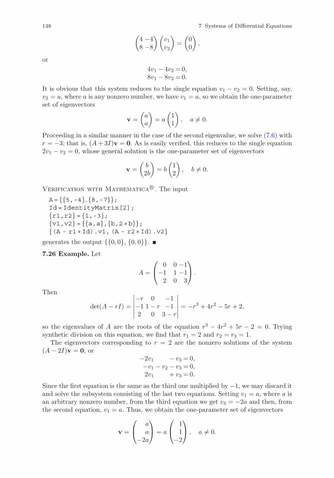
148 7 Systems of Differential Equations
(4 −48 −8
)(v1v2
)=
(00
),
or
4v1 − 4v2 = 0,8v1 − 8v2 = 0.
It is obvious that this system reduces to the single equation v1 − v2 = 0. Setting, say,v2 = a, where a is any nonzero number, we have v1 = a, so we obtain the one-parameterset of eigenvectors
v =
(aa
)= a
(11
), a �= 0.
Proceeding in a similar manner in the case of the second eigenvalue, we solve (7.6) withr = −3; that is, (A+3I)v = 0. As is easily verified, this reduces to the single equation2v1 − v2 = 0, whose general solution is the one-parameter set of eigenvectors
v =
(b2b
)= b
(12
), b �= 0.
Verification with Mathematica R©. The input
A= {{5,-4}, {8,-7}};Id=IdentityMatrix[2];{r1,r2}= {1,-3};{v1,v2}= {{a,a},{b,2 ∗b}};{(A - r1 ∗Id).v1,(A - r2 ∗Id).v2}
generates the output {{0, 0}, {0, 0}}.7.26 Example. Let
A =
⎛⎝ 0 0 −1−1 1 −12 0 3
⎞⎠ .
Then
det(A− rI) =
∣∣∣∣∣∣−r 0 −1−1 1− r −12 0 3− r
∣∣∣∣∣∣ = −r3 + 4r2 − 5r + 2,
so the eigenvalues of A are the roots of the equation r3 − 4r2 + 5r − 2 = 0. Tryingsynthetic division on this equation, we find that r1 = 2 and r2 = r3 = 1.
The eigenvectors corresponding to r = 2 are the nonzero solutions of the system(A− 2I)v = 0, or
−2v1 − v3 = 0,−v1 − v2 − v3 = 0,2v1 + v3 = 0.
Since the first equation is the same as the third one multiplied by −1, we may discard itand solve the subsystem consisting of the last two equations. Setting v1 = a, where a isan arbitrary nonzero number, from the third equation we get v3 = −2a and then, fromthe second equation, v1 = a. Thus, we obtain the one-parameter set of eigenvectors
v =
⎛⎝ a
a−2a
⎞⎠ = a
⎛⎝ 1
1−2
⎞⎠ , a �= 0.
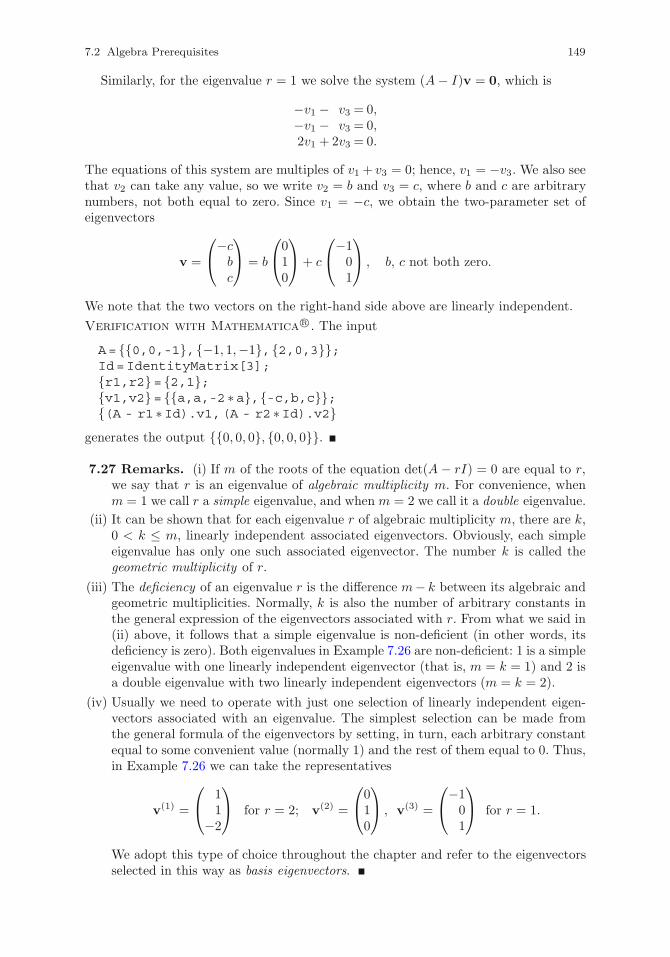
7.2 Algebra Prerequisites 149
Similarly, for the eigenvalue r = 1 we solve the system (A− I)v = 0, which is
−v1 − v3 = 0,−v1 − v3 = 0,2v1 + 2v3 = 0.
The equations of this system are multiples of v1 + v3 = 0; hence, v1 = −v3. We also seethat v2 can take any value, so we write v2 = b and v3 = c, where b and c are arbitrarynumbers, not both equal to zero. Since v1 = −c, we obtain the two-parameter set ofeigenvectors
v =
⎛⎝−c
bc
⎞⎠ = b
⎛⎝010
⎞⎠+ c
⎛⎝−1
01
⎞⎠ , b, c not both zero.
We note that the two vectors on the right-hand side above are linearly independent.
Verification with Mathematica R©. The input
A= {{0,0,-1},{−1, 1,−1},{2,0,3}};Id=IdentityMatrix[3];{r1,r2}= {2,1};{v1,v2}= {{a,a,-2 ∗a},{-c,b,c}};{(A - r1 ∗Id).v1,(A - r2 ∗Id).v2}
generates the output {{0, 0, 0}, {0, 0, 0}}.
7.27 Remarks. (i) If m of the roots of the equation det(A − rI) = 0 are equal to r,we say that r is an eigenvalue of algebraic multiplicity m. For convenience, whenm = 1 we call r a simple eigenvalue, and when m = 2 we call it a double eigenvalue.
(ii) It can be shown that for each eigenvalue r of algebraic multiplicity m, there are k,0 < k ≤ m, linearly independent associated eigenvectors. Obviously, each simpleeigenvalue has only one such associated eigenvector. The number k is called thegeometric multiplicity of r.
(iii) The deficiency of an eigenvalue r is the difference m− k between its algebraic andgeometric multiplicities. Normally, k is also the number of arbitrary constants inthe general expression of the eigenvectors associated with r. From what we said in(ii) above, it follows that a simple eigenvalue is non-deficient (in other words, itsdeficiency is zero). Both eigenvalues in Example 7.26 are non-deficient: 1 is a simpleeigenvalue with one linearly independent eigenvector (that is, m = k = 1) and 2 isa double eigenvalue with two linearly independent eigenvectors (m = k = 2).
(iv) Usually we need to operate with just one selection of linearly independent eigen-vectors associated with an eigenvalue. The simplest selection can be made fromthe general formula of the eigenvectors by setting, in turn, each arbitrary constantequal to some convenient value (normally 1) and the rest of them equal to 0. Thus,in Example 7.26 we can take the representatives
v(1) =
⎛⎝ 1
1−2
⎞⎠ for r = 2; v(2) =
⎛⎝010
⎞⎠ , v(3) =
⎛⎝−1
01
⎞⎠ for r = 1.
We adopt this type of choice throughout the chapter and refer to the eigenvectorsselected in this way as basis eigenvectors.
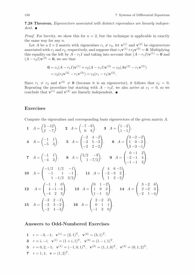
150 7 Systems of Differential Equations
7.28 Theorem. Eigenvectors associated with distinct eigenvalues are linearly indepen-dent.
Proof. For brevity, we show this for n = 2, but the technique is applicable in exactlythe same way for any n.
Let A be a 2 × 2 matrix with eigenvalues r1 �= r2, let v(1) and v(2) be eigenvectors
associated with r1 and r2, respectively, and suppose that c1v(1)+c2v
(2) = 0. Multiplyingthis equality on the left by A− r1I and taking into account that (A− r1I)v
(1) = 0 and(A− r2I)v
(2) = 0, we see that
0 = c1(A− r1I)v(1) + c2(A− r1I)v
(2) = c2(Av(2) − r1v
(2))
= c2(r2v(2) − r1v
(2)) = c2(r1 − r2)v(2).
Since r1 �= r2 and v(2) �= 0 (because it is an eigenvector), it follows that c2 = 0.Repeating the procedure but starting with A − r2I, we also arrive at c1 = 0, so weconclude that v(1) and v(2) are linearly independent.
Exercises
Compute the eigenvalues and corresponding basis eigenvectors of the given matrix A.
1 A =
(3 −122 −7
). 2 A =
(−7 −96 8
). 3 A =
(1 −21 −1
).
4 A =
(−1 1−5 3
). 5 A =
⎛⎝−2 4 −2−3 5 −3−2 2 −2
⎞⎠. 6 A =
⎛⎝3 −2 −21 0 −23 −3 −1
⎞⎠.
7 A =
(−1 1−4 3
). 8 A =
(5/2 −91 −7/2
). 9 A =
⎛⎝ 0 −1 2−2 −1 4−1 −1 3
⎞⎠.
10 A =
⎛⎝−1/2 1/2 −1
−1 1 −11 −1/2 3/2
⎞⎠. 11 A =
⎛⎝ 4 6 −5−2 −3 21 2 −2
⎞⎠.
12 A =
⎛⎝−1 1 0
4 −1 −4−4 2 3
⎞⎠. 13 A =
⎛⎝0 1 −21 0 21 −1 3
⎞⎠. 14 A =
⎛⎝ 3 −2 6
2 −2 3−2 1 −4
⎞⎠.
15 A =
⎛⎝−3 2 −1−3 3 −2−2 4 −3
⎞⎠. 16 A =
⎛⎝ 2 −2 3
0 1 1−1 2 0
⎞⎠.
Answers to Odd-Numbered Exercises
1 r = −3,−1; v(1) = (2, 1)T, v(2) = (3, 1)T.
3 r = i,−i; v(1) = (1 + i, 1)T, v(2) = (1− i, 1)T.
5 r = 0, 2,−1; v(1) = (−1, 0, 1)T, v(2) = (1, 1, 0)T, v(3) = (0, 1, 2)T.
7 r = 1, 1; v = (1, 2)T.
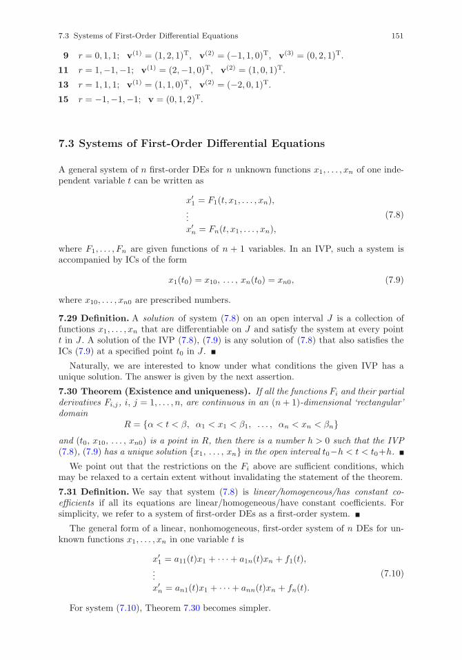
7.3 Systems of First-Order Differential Equations 151
9 r = 0, 1, 1; v(1) = (1, 2, 1)T, v(2) = (−1, 1, 0)T, v(3) = (0, 2, 1)T.
11 r = 1,−1,−1; v(1) = (2,−1, 0)T, v(2) = (1, 0, 1)T.
13 r = 1, 1, 1; v(1) = (1, 1, 0)T, v(2) = (−2, 0, 1)T.
15 r = −1,−1,−1; v = (0, 1, 2)T.
7.3 Systems of First-Order Differential Equations
A general system of n first-order DEs for n unknown functions x1, . . . , xn of one inde-pendent variable t can be written as
x′1 = F1(t, x1, . . . , xn),...x′n = Fn(t, x1, . . . , xn),
(7.8)
where F1, . . . , Fn are given functions of n + 1 variables. In an IVP, such a system isaccompanied by ICs of the form
x1(t0) = x10, . . . , xn(t0) = xn0, (7.9)
where x10, . . . , xn0 are prescribed numbers.
7.29 Definition. A solution of system (7.8) on an open interval J is a collection offunctions x1, . . . , xn that are differentiable on J and satisfy the system at every pointt in J . A solution of the IVP (7.8), (7.9) is any solution of (7.8) that also satisfies theICs (7.9) at a specified point t0 in J .
Naturally, we are interested to know under what conditions the given IVP has aunique solution. The answer is given by the next assertion.
7.30 Theorem (Existence and uniqueness). If all the functions Fi and their partialderivatives Fi,j , i, j = 1, . . . , n, are continuous in an (n+ 1)-dimensional ‘rectangular’domain
R = {α < t < β, α1 < x1 < β1, . . . , αn < xn < βn}and (t0, x10, . . . , xn0) is a point in R, then there is a number h > 0 such that the IVP(7.8), (7.9) has a unique solution {x1, . . . , xn} in the open interval t0−h < t < t0+h.
We point out that the restrictions on the Fi above are sufficient conditions, whichmay be relaxed to a certain extent without invalidating the statement of the theorem.
7.31 Definition. We say that system (7.8) is linear/homogeneous/has constant co-efficients if all its equations are linear/homogeneous/have constant coefficients. Forsimplicity, we refer to a system of first-order DEs as a first-order system.
The general form of a linear, nonhomogeneous, first-order system of n DEs for un-known functions x1, . . . , xn in one variable t is
x′1 = a11(t)x1 + · · ·+ a1n(t)xn + f1(t),...x′n = an1(t)x1 + · · ·+ ann(t)xn + fn(t).
(7.10)
For system (7.10), Theorem 7.30 becomes simpler.
152 7 Systems of Differential Equations
7.32 Theorem (Existence and uniqueness). If all aij and fi, i, j = 1, . . . , n, arecontinuous on an open interval J and t0 is a point in J , then the IVP (7.10), (7.9) hasa unique solution on J .
7.33 Remark. As in Definition 2.28, in what follows we take J to be the largest openinterval (maximal interval of existence) on which the unique solution of the IVP can bedefined. For our specific examples, J will normally be the entire real line.
Sometimes it is possible to change an IVP for a first-order linear system into anequivalent IVP for a single higher-order equation.
7.34 Example. Consider the IVP
x′1 = x1 + x2, x1(0) = −2,x′2 = 4x1 + x2, x2(0) = −4.
Differentiating the first equation and then replacing x′2 from the second equation, wefind that
x′′1 = x′1 + x′2 = x′1 + (4x1 + x2).
Since, from the first equation, x2 = x′1 − x1, it follows that
x′′1 = x′1 + 4x1 + (x′1 − x1) = 2x′1 + 3x1,
which is a second-order DE for x1, with GS
x1(t) = c1e−t + c2e
3t.
We are already given that x1(0) = 2; the second IC for x1 is obtained from the firstequation:
x′1(0) = x1(0) + x2(0) = −2− 4 = −6.
Applying the ICs to the GS, we arrive at
x1(t) = −2e3t.
Finally, from the first equation we have
x2(t) = x′1(t)− x1(t) = −6e3t + 2e3t = −4e3t.
Verification with Mathematica R©. The input
{x1,x2}= {-2 ∗E∧(3 ∗t),-4 ∗E∧(3 ∗t)};{{D[x1,t] - x1 - x2,D[x2,t] - 4 ∗x1 - x2}, {x1,x2}/.t→ 0}
generates the output {{0, 0}, {−2,−4}}.
In matrix form, an IVP for a general linear first-order system of n DEs in n unknownscan be written as
x′ = A(t)x+ f(t), (7.11)
x(t0) = x0, (7.12)
where A is the n × n coefficient matrix, x is the column vector of the unknowns, f isthe column vector of the nonhomogeneous terms, and x0 is the column vector of theICs.
7.3 Systems of First-Order Differential Equations 153
When the system is homogeneous, (7.11) reduces to
x′ = A(t)x. (7.13)
The principle of superposition mentioned in Sect. 4.3.1 also applies to homogeneouslinear systems.
7.35 Theorem. If x(1), . . . ,x(n) are solutions of system (7.13) in J , then so is thelinear combination c1x
(1) + · · ·+ cnx(n) for any constants c1, . . . , cn.
7.36 Theorem. If x(1), . . . ,x(n) are linearly independent solutions of (7.13) in J , thenfor any solution x of (7.13) there are unique numbers c1, . . . , cn such that
x(t) = c1x(1)(t) + · · ·+ cnx
(n)(t) for all t in J. (7.14)
7.37 Remark. According to Theorems 7.35 and 7.36, formula (7.14) with arbitraryconstants c1, . . . , cn represents the GS of system (7.13).
7.38 Definition. As in the case of a single DE of order n (see Remark 4.28(ii) forn = 2), a set of n linearly independent solutions of (7.13) is called a fundamental set ofsolutions (FSS).
7.39 Remark. The property of the Wronskian stated in Remark 4.25 carries over un-changed to homogeneous systems; that is, if x(1), . . . ,x(n) are solutions of (7.13) on J ,then their Wronskian is either zero at every point of J or nonzero everywhere on J .
Exercises
In 1–6, use the method of reduction to a second-order equation to solve the IVP x′ = Ax,x(0) = x0 for the given matrix A and vector x0.
1 A =
(1 2
−1 4
), x0 =
(1
−1
). 2 A =
( −7 3−18 8
), x0 =
(03
).
3 A =
(−1 −41 3
), x0 =
(21
). 4 A =
(−5/2 9−1 7/2
), x0 =
(−11
).
5 A =
(−2 1−5 2
), x0 =
(2
−1
). 6 A =
(4 1
−10 −2
), x0 =
(01
).
In 7–10, use the method of reduction to a second-order equation to solve the IVPx′ = Ax+ f(t), x(0) = x0 for the given matrix A, vector function f(t), and vector x0.
7 A =
(2 −63 −7
), f(t) =
(2t
t− 2
), x0 =
(2
−1
).
8 A =
(2 3/2
−3 −5/2
), f(t) =
(8e2t
6(t− 3)e2t
), x0 =
(−30
).
9 A =
(−8 −94 4
), f(t) =
(17 cos t− 8 sin t−8 cos t+ 2 sin t
), x0 =
(7
−3
).
10 A =
(−4/3 1−1 2/3
), f(t) =
(6t+ e−t
4t− 6 + 3e−t
), x0 =
(55
).
154 7 Systems of Differential Equations
Answers to Odd-Numbered Exercises
1 x(t) =
(4e2t − 3e3t
2e2t − 3e3t
). 3 x(t) =
((2− 8t)et
(1 + 4t)et
).
5 x(t) =
(2 cos t− 5 sin t− cos t− 12 sin t
). 7 x(t) =
(4e−t − 3e−4t + 2t+ 1
2e−t − 3e−4t + t
).
9 x(t) =
((3t+ 7)e−2t − sin t
−(2t+ 5)e−2t + 2 cos t
).
7.4 Homogeneous Linear Systems with Constant Coefficients
It is useful to have a quick look at this type of system for n = 1, which is, of course,the single DE
x′ = ax, a = const �= 0. (7.15)
As we know, the GS of (7.15) isx(t) = Ceat, (7.16)
where C is an arbitrary constant. Among all the solutions (7.16) there is one, and onlyone, which is time-independent, namely x = 0; we call it an equilibrium solution.
If a < 0, then
limt→−∞ |x(t)| = ∞, lim
t→∞x(t) = 0.
On the other hand, if a > 0, then
limt→−∞x(t) = 0, lim
t→∞ |x(t)| = ∞.
Recalling Definition 3.11, this means that the equilibrium solution x = 0 of equa-tion (7.15) is asymptotically stable if a < 0 and unstable if a > 0.
Now consider a general homogeneous linear system of DEs of the form
x′ = Ax, (7.17)
where A is a constant nonsingular n×n matrix. The equilibrium (or time-independent)solutions of (7.17) are obtained by setting x′ = 0; that is, by solving Ax = 0. Sincedet(A) �= 0, this homogeneous algebraic system has only the zero solution. In otherwords, just as for equation (7.15), the only equilibrium solution here is x = 0. In thecase of (7.15), the stability or instability of the equilibrium solution depends on thesign of the number a. In the case of system (7.17), that property depends on the signof the eigenvalues of the matrix A. Later in this section we will have a full discussionof several specific examples for n = 2.
By analogy with single DEs, we seek solutions of (7.17) of the form
x(t) = vert, (7.18)
where v is an unknown constant, nonzero, n-component column vector and r is anunknown number. Differentiating (7.18), we have x′ = rvert, which, substituted in(7.17), yields the equality rvert = Avert. Since the coefficients of ert on both sidesmust be the same, it follows that Av = rv, so, by Definition 7.23, r is an eigenvalue ofA and v is an eigenvector associated with r. Once we have computed the eigenvalues
7.4 Homogeneous Linear Systems with Constant Coefficients 155
and eigenvectors of A—the former as the roots of the equation det(A− rI) = 0 and thelatter as the nonzero solutions of (7.6) (see Remark 7.24)—we use them in (7.18) togenerate solutions of system (7.17). However, in view of Theorem 7.36 and Remark 7.37,to write the GS of the system we need to construct n linearly independent solutions.Below, we examine in turn each of the several situations that may occur in this type ofconstruction.
Solutions of the form (7.18) have an important property.
7.40 Theorem. If the eigenvalues of A are distinct, then the solutions of system (7.17)obtained from (7.18) are linearly independent.
Proof. Let r1, . . . , rn be the (real or complex) distinct eigenvalues of A, let v(1), . . . ,v(n)
be corresponding associated eigenvectors, and let x(1), . . . ,x(n) be the solutions con-structed from these elements according to (7.18). Given that x(i)(0) = v(i), i = 1, . . . , n,we have
W [x(1), . . . ,x(n)](0) = det(v(1) . . . v(n)),
and since, by Theorem 7.28, v(1), . . . ,v(n) are linearly independent, from Theo-rem 7.16 it follows that the above determinant is nonzero. Hence, by Remark 7.21(i),x(1), . . . ,x(n) are linearly independent.
7.4.1 Real and Distinct Eigenvalues
For simplicity, we restrict our attention to systems in two or three unknown functionsand discuss several specific illustrations.
In the two-dimensional case, we may regard the components x1(t) and x2(t) of theGS x(t) as the coordinates of a point moving in the (x1, x2)-plane, called the phaseplane. The curves traced by this point for various values of the arbitrary constants c1and c2 are graphical representations (called trajectories) of the solutions, and form whatis known as the phase portrait of the system. If the eigenvectors are real, a line throughthe origin and parallel to an eigenvector is called an eigenline.
7.41 Example. For the IVP
x′1 = 3x1 + 4x2, x1(0) = 2,
x′2 = 3x1 + 2x2, x2(0) = 5
we have
det(A− rI) =
∣∣∣∣3− r 43 2− r
∣∣∣∣ = (3− r)(2 − r) − 12 = r2 − 5r − 6.
Setting r2 − 5r − 6 = 0, we find the eigenvalues r1 = −1 and r2 = 6. For r = −1,the system (A + I)v = 0 reduces to the equation v1 + v2 = 0, so an associated basiseigenvector (see Remark 7.27(iii)) is
v(1) =
(−11
).
Similarly, for r = 6 the system (A−6I)v = 0 reduces to the single equation 3v1−4v2 = 0,which yields the basis eigenvector
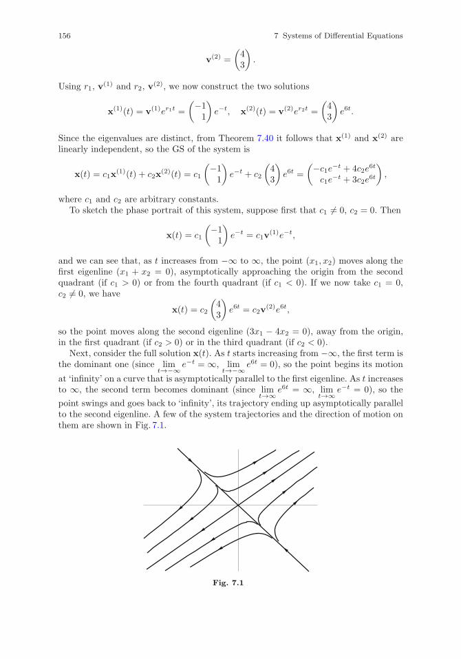
156 7 Systems of Differential Equations
v(2) =
(43
).
Using r1, v(1) and r2, v
(2), we now construct the two solutions
x(1)(t) = v(1)er1t =
(−11
)e−t, x(2)(t) = v(2)er2t =
(43
)e6t.
Since the eigenvalues are distinct, from Theorem 7.40 it follows that x(1) and x(2) arelinearly independent, so the GS of the system is
x(t) = c1x(1)(t) + c2x
(2)(t) = c1
(−11
)e−t + c2
(43
)e6t =
(−c1e−t + 4c2e6t
c1e−t + 3c2e
6t
),
where c1 and c2 are arbitrary constants.To sketch the phase portrait of this system, suppose first that c1 �= 0, c2 = 0. Then
x(t) = c1
(−11
)e−t = c1v
(1)e−t,
and we can see that, as t increases from −∞ to ∞, the point (x1, x2) moves along thefirst eigenline (x1 + x2 = 0), asymptotically approaching the origin from the secondquadrant (if c1 > 0) or from the fourth quadrant (if c1 < 0). If we now take c1 = 0,c2 �= 0, we have
x(t) = c2
(43
)e6t = c2v
(2)e6t,
so the point moves along the second eigenline (3x1 − 4x2 = 0), away from the origin,in the first quadrant (if c2 > 0) or in the third quadrant (if c2 < 0).
Next, consider the full solution x(t). As t starts increasing from −∞, the first term isthe dominant one (since lim
t→−∞ e−t = ∞, limt→−∞ e6t = 0), so the point begins its motion
at ‘infinity’ on a curve that is asymptotically parallel to the first eigenline. As t increasesto ∞, the second term becomes dominant (since lim
t→∞ e6t = ∞, limt→∞ e−t = 0), so the
point swings and goes back to ‘infinity’, its trajectory ending up asymptotically parallelto the second eigenline. A few of the system trajectories and the direction of motion onthem are shown in Fig. 7.1.
Fig. 7.1
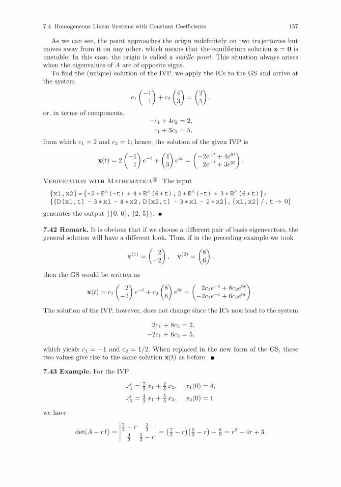
7.4 Homogeneous Linear Systems with Constant Coefficients 157
As we can see, the point approaches the origin indefinitely on two trajectories butmoves away from it on any other, which means that the equilibrium solution x = 0 isunstable. In this case, the origin is called a saddle point. This situation always ariseswhen the eigenvalues of A are of opposite signs.
To find the (unique) solution of the IVP, we apply the ICs to the GS and arrive atthe system
c1
(−11
)+ c2
(43
)=
(25
),
or, in terms of components,−c1 + 4c2 = 2,
c1 + 3c2 = 5,
from which c1 = 2 and c2 = 1; hence, the solution of the given IVP is
x(t) = 2
(−11
)e−t +
(43
)e6t =
(−2e−t + 4e6t
2e−t + 3e6t
).
Verification with Mathematica R©. The input
{x1,x2}= {-2 ∗E∧(-t) + 4 ∗E∧(6 ∗t),2 ∗E∧(-t) + 3 ∗E∧(6 ∗t)};{{D[x1,t] - 3 ∗x1 - 4 ∗x2,D[x2,t] - 3 ∗x1 - 2 ∗x2},{x1,x2}/.t→ 0}
generates the output {{0, 0}, {2, 5}}.
7.42 Remark. It is obvious that if we choose a different pair of basis eigenvectors, thegeneral solution will have a different look. Thus, if in the preceding example we took
v(1) =
(2
−2
), v(2) =
(86
),
then the GS would be written as
x(t) = c1
(2
−2
)e−t + c2
(86
)e6t =
(2c1e
−t + 8c2e6t
−2c1e−t + 6c2e
6t
).
The solution of the IVP, however, does not change since the ICs now lead to the system
2c1 + 8c2 = 2,
−2c1 + 6c2 = 5,
which yields c1 = −1 and c2 = 1/2. When replaced in the new form of the GS, thesetwo values give rise to the same solution x(t) as before.
7.43 Example. For the IVP
x′1 = 73 x1 +
23 x2, x1(0) = 4,
x′2 = 43 x1 +
53 x2, x2(0) = 1
we have
det(A− rI) =
∣∣∣∣∣73 − r 2
343
53 − r
∣∣∣∣∣ =(73 − r
)(53 − r
)− 89 = r2 − 4r + 3.
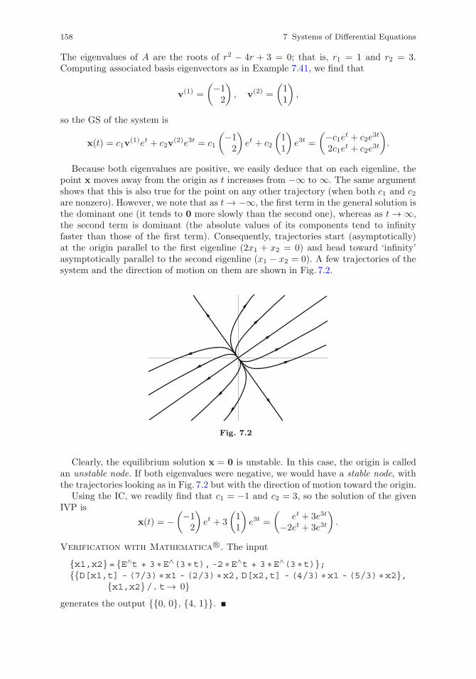
158 7 Systems of Differential Equations
The eigenvalues of A are the roots of r2 − 4r + 3 = 0; that is, r1 = 1 and r2 = 3.Computing associated basis eigenvectors as in Example 7.41, we find that
v(1) =
(−12
), v(2) =
(11
),
so the GS of the system is
x(t) = c1v(1)et + c2v
(2)e3t = c1
(−12
)et + c2
(11
)e3t =
(−c1et + c2e3t
2c1et + c2e
3t
).
Because both eigenvalues are positive, we easily deduce that on each eigenline, thepoint x moves away from the origin as t increases from −∞ to ∞. The same argumentshows that this is also true for the point on any other trajectory (when both c1 and c2are nonzero). However, we note that as t → −∞, the first term in the general solution isthe dominant one (it tends to 0 more slowly than the second one), whereas as t → ∞,the second term is dominant (the absolute values of its components tend to infinityfaster than those of the first term). Consequently, trajectories start (asymptotically)at the origin parallel to the first eigenline (2x1 + x2 = 0) and head toward ‘infinity’asymptotically parallel to the second eigenline (x1 − x2 = 0). A few trajectories of thesystem and the direction of motion on them are shown in Fig. 7.2.
Fig. 7.2
Clearly, the equilibrium solution x = 0 is unstable. In this case, the origin is calledan unstable node. If both eigenvalues were negative, we would have a stable node, withthe trajectories looking as in Fig. 7.2 but with the direction of motion toward the origin.
Using the IC, we readily find that c1 = −1 and c2 = 3, so the solution of the givenIVP is
x(t) = −(−1
2
)et + 3
(11
)e3t =
(et + 3e3t
−2et + 3e3t
).
Verification with Mathematica R©. The input
{x1,x2}= {E∧t + 3 ∗E∧(3 ∗t),-2 ∗E∧t + 3 ∗E∧(3 ∗t)};{{D[x1,t] -(7/3) ∗x1 -(2/3) ∗x2,D[x2,t] -(4/3) ∗x1 -(5/3) ∗x2},
{x1,x2}/.t→ 0}generates the output {{0, 0}, {4, 1}}.
7.4 Homogeneous Linear Systems with Constant Coefficients 159
7.44 Example. Consider the IVP
x′1 = 5x1 − 6x3, x1(0) = −2,
x′2 = 2x1 − x2 − 2x3, x2(0) = −1,
x′3 = 4x1 − 2x2 − 4x3, x3(0) = −1.
Expanding the determinant, say, in the first row, we see that
det(A− rI) =
∣∣∣∣∣∣∣5− r 0 −6
2 −1− r −2
4 −2 −4− r
∣∣∣∣∣∣∣= r − r3,
so the eigenvalues of A are r1 = 0, r2 = −1, and r3 = 1. The corresponding algebraicsystems (A−rI)v = 0 for these values of r reduce, respectively, to the pairs of equations
5v1 −6v3 = 0,
2v1 −v2 −2v3 = 0,
v1 − v3 = 0,
4v1 −2v2 −3v3 = 0,
2v1 −3v3 = 0,
2v2 − v3 = 0
and yield associated basis eigenvectors
v(1) =
⎛⎝625
⎞⎠ , v(2) =
⎛⎝212
⎞⎠ , v(3) =
⎛⎝312
⎞⎠ .
Therefore, the GS of the system is
x(t) = c1
⎛⎝625
⎞⎠+ c2
⎛⎝212
⎞⎠ e−t + c3
⎛⎝312
⎞⎠ et.
Using the ICs, in terms of components we have
6c1 + 2c2 + 3c3 = −2,
2c1 + c2 + c3 = −1,
5c1 + 2c2 + 2c3 = −1.
We can solve this system by Gaussian elimination and arrive at the values c1 = 1,c2 = −1, and c3 = −2, so the solution of the IVP is
x(t) =
⎛⎝625
⎞⎠−
⎛⎝212
⎞⎠ e−t − 2
⎛⎝312
⎞⎠ et =
⎛⎝6− 2e−t − 6et
2− e−t − 2et
5− 2e−t − 4et
⎞⎠ .
Verification with Mathematica R©. The input
{x1,x2,x3}= {6 - 2 ∗E∧(-t) - 6 ∗E∧t,2 - E∧(-t) - 2 ∗E∧t,5 - 2 ∗E∧(-t) - 4 ∗E∧t};
{{D[x1,t] - 5 ∗x1 + 6 ∗x3,D[x2,t] - 2 ∗x1 + x2 + 2 ∗x3,D[x3,t] - 4 ∗x1 + 2 ∗x2 + 4 ∗x3},{x1,x2,x3}/.t→ 0}
generates the output {{0, 0, 0}, {−2, −1, −1}}.
160 7 Systems of Differential Equations
Exercises
In 1–10, use the eigenvalue-eigenvector method to solve the IVP x′ = Ax, x(0) = x0 forthe given matrix A and vector x0, and sketch the phase portrait of the general solutionof the system.
1 A =
(−8 18−3 7
), x0 =
(−3−1
). 2 A =
(−7 8−6 7
), x0 =
(−2−1
).
3 A =
(−7 10−5 8
), x0 =
(−5−2
). 4 A =
(0 −42 6
), x0 =
(4
−1
).
5 A =
(−5/2 3−3/2 2
), x0 =
(12
). 6 A =
(5/2 6−1 −5/2
), x0 =
(9
−4
).
7 A =
(11 18−3 −4
), x0 =
(−32
). 8 A =
(−1/2 −12 5/2
), x0 =
(6
−10
).
9 A=
(5/3 −4/32/3 −1/3
), x0=
(−4−1
). 10 A =
(−11/2 5/2−15 7
), x0 =
(7/210
).
In 11–16, use the eigenvalue–eigenvector method to solve the IVP x′ = Ax, x(0) = x0
for the given matrix A and vector x0.
11 A =
⎛⎝5 −4 −31 0 −14 −4 −2
⎞⎠ , x0 =
⎛⎝ 1
2−1
⎞⎠. 12 A =
⎛⎝0 −1 13 2 −31 −1 0
⎞⎠ , x0 =
⎛⎝ 3−31
⎞⎠.
13 A =
⎛⎝ 0 4 −2−1 2 1−1 4 −1
⎞⎠ , x0 =
⎛⎝203
⎞⎠. 14 A =
⎛⎝−4 −7 6
1 4 −2−2 −2 3
⎞⎠ , x0 =
⎛⎝424
⎞⎠.
15 A =
⎛⎝−1 −1 −1−2 −2 −14 4 3
⎞⎠ , x0 =
⎛⎝−3
31
⎞⎠. 16 A =
⎛⎝ 1 1 −1−4 −1 4−2 1 2
⎞⎠ , x0 =
⎛⎝ 5−34
⎞⎠.
Answers to Odd-Numbered Exercises
1 x(t) =
(−3e−2t
−e−2t
). 3 x(t) =
(−6e−2t + e3t
−3e−2t + e3t
).
5 x(t) =
(−2e−t + 3et/2
−e−t + 3et/2
). 7 x(t) =
(−6e2t + 3e5t
3e2t − e5t
).
9 x(t) =
(2et/3 − 6et
2et/3 − 3et
). 11 x(t) =
⎛⎝2et − e2t
2et
−e2t
⎞⎠.
13 x(t) =
⎛⎝3e−2t − 2et + e2t
−et + e2t
3e−2t − et + e2t
⎞⎠, 15 x(t) =
⎛⎝ −2− et
2 + e−t
−e−t + 2et
⎞⎠.
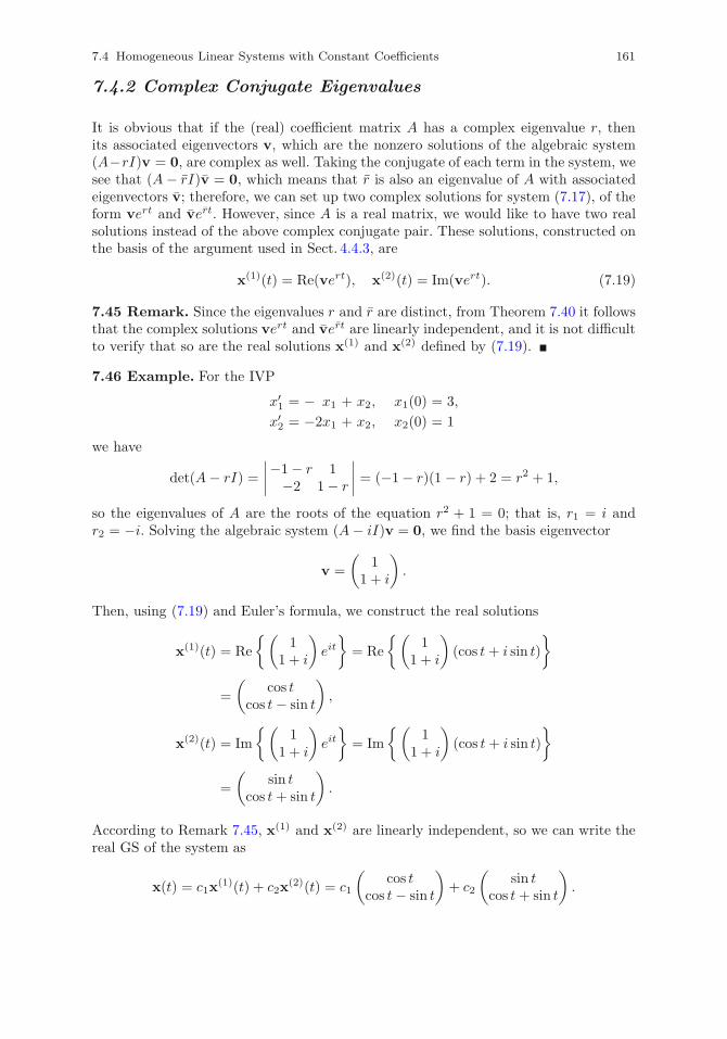
7.4 Homogeneous Linear Systems with Constant Coefficients 161
7.4.2 Complex Conjugate Eigenvalues
It is obvious that if the (real) coefficient matrix A has a complex eigenvalue r, thenits associated eigenvectors v, which are the nonzero solutions of the algebraic system(A−rI)v = 0, are complex as well. Taking the conjugate of each term in the system, wesee that (A− rI)v = 0, which means that r is also an eigenvalue of A with associatedeigenvectors v; therefore, we can set up two complex solutions for system (7.17), of theform vert and vert. However, since A is a real matrix, we would like to have two realsolutions instead of the above complex conjugate pair. These solutions, constructed onthe basis of the argument used in Sect. 4.4.3, are
x(1)(t) = Re(vert), x(2)(t) = Im(vert). (7.19)
7.45 Remark. Since the eigenvalues r and r are distinct, from Theorem 7.40 it followsthat the complex solutions vert and vert are linearly independent, and it is not difficultto verify that so are the real solutions x(1) and x(2) defined by (7.19).
7.46 Example. For the IVP
x′1 = − x1 + x2, x1(0) = 3,
x′2 = −2x1 + x2, x2(0) = 1
we have
det(A− rI) =
∣∣∣∣−1− r 1−2 1− r
∣∣∣∣ = (−1− r)(1 − r) + 2 = r2 + 1,
so the eigenvalues of A are the roots of the equation r2 + 1 = 0; that is, r1 = i andr2 = −i. Solving the algebraic system (A− iI)v = 0, we find the basis eigenvector
v =
(1
1 + i
).
Then, using (7.19) and Euler’s formula, we construct the real solutions
x(1)(t) = Re
{(1
1 + i
)eit}
= Re
{(1
1 + i
)(cos t+ i sin t)
}
=
(cos t
cos t− sin t
),
x(2)(t) = Im
{(1
1 + i
)eit}
= Im
{(1
1 + i
)(cos t+ i sin t)
}
=
(sin t
cos t+ sin t
).
According to Remark 7.45, x(1) and x(2) are linearly independent, so we can write thereal GS of the system as
x(t) = c1x(1)(t) + c2x
(2)(t) = c1
(cos t
cos t− sin t
)+ c2
(sin t
cos t+ sin t
).
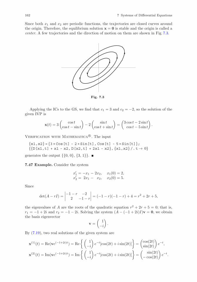
162 7 Systems of Differential Equations
Since both x1 and x2 are periodic functions, the trajectories are closed curves aroundthe origin. Therefore, the equilibrium solution x = 0 is stable and the origin is called acenter. A few trajectories and the direction of motion on them are shown in Fig. 7.3.
Fig. 7.3
Applying the ICs to the GS, we find that c1 = 3 and c2 = −2, so the solution of thegiven IVP is
x(t) = 3
(cos t
cos t− sin t
)− 2
(sin t
cos t+ sin t
)=
(3 cos t− 2 sin tcos t− 5 sin t
).
Verification with Mathematica R©. The input
{x1,x2}= {3 ∗Cos[t] - 2 ∗Sin[t],Cos[t] - 5 ∗Sin[t]};{{D[x1,t] + x1 - x2,D[x2,t] + 2x1 - x2}, {x1,x2}/.t→ 0}
generates the output {{0, 0}, {3, 1}}.
7.47 Example. Consider the system
x′1 = −x1 − 2x2, x1(0) = 2,x′2 = 2x1 − x2, x2(0) = 5.
Since
det(A− rI) =
∣∣∣∣−1− r −22 −1− r
∣∣∣∣ = (−1− r)(−1 − r) + 4 = r2 + 2r + 5,
the eigenvalues of A are the roots of the quadratic equation r2 + 2r + 5 = 0; that is,r1 = −1 + 2i and r2 = −1− 2i. Solving the system (A − (−1 + 2i)I)v = 0, we obtainthe basis eigenvector
v =
(1
−i).
By (7.19), two real solutions of the given system are
x(1)(t) = Re(ve(−1+2i)t) = Re
{(1
−i)e−t[cos(2t) + i sin(2t)]
}=
(cos(2t)sin(2t)
)e−t,
x(2)(t) = Im(ve(−1+2i)t) = Im
{(1
−i)e−t[cos(2t) + i sin(2t)]
}=
(sin(2t)
− cos(2t)
)e−t.
7.4 Homogeneous Linear Systems with Constant Coefficients 163
As in Example 7.46, from Theorem 7.40 and Remark 7.45 we conclude that these twosolutions are linearly independent, so the real GS of the system is
x(t) = c1x(1)(t) + c2x
(2)(t) =
{c1
(cos(2t)sin(2t)
)+ c2
(sin(2t)
− cos(2t)
)}e−t.
The periodic factor in the solution indicates that, as t increases from −∞ to ∞, thetrajectories keep going around the origin. The exponential factor shows that they aregetting arbitrarily close to the origin, which means that the equilibrium solution x = 0is asymptotically stable. The origin is called a stable spiral point. A few trajectories andthe direction of motion on them are shown in Fig. 7.4. If the real part of the eigenvalueswere positive, the motion on each trajectory would be away from the origin, whichmeans that the origin would be an unstable spiral point.
Fig. 7.4
The ICs yield c1 = 2 and c2 = −5, so the solution of the IVP is
x(t) =
(2 cos(2t)− 5 sin(2t)5 cos(2t) + 2 sin(2t)
)e−t.
Verification with Mathematica R©. The input
{x1,x2}= {E∧(-t) ∗(2 ∗Cos[2 ∗t] - 5 ∗Sin[2 ∗t]),E∧(-t) ∗(5 ∗Cos[2 ∗t] + 2 ∗Sin[2 ∗t])};
{{D[x1,t] + x1 + 2 ∗x2,D[x2,t] - 2 ∗x1 + x2}, {x1,x2}/.t→ 0}generates the output {{0, 0}, {2, 5}}.
7.48 Example. For the system in the IVP
x′1 = 2x1 + x2 − x3, x1(0) = −2,x′2 = −4x1 − 3x2 − x3, x2(0) = 3,x′3 = 4x1 + 4x2 + 2x3, x3(0) = −2
we have, after expansion of the determinant in any of its rows or columns,
det(A− rI) =
∣∣∣∣∣∣2− r 1 −1−4 −3− r −14 4 2− r
∣∣∣∣∣∣ = 4− 4r + r2 − r3,
164 7 Systems of Differential Equations
so the eigenvalues of A are the roots of the equation r3 − r2 + 4r − 4 = 0. Using thesynthetic division algorithm or taking advantage of the symmetry of the coefficients,we find that r1 = 1, r2 = 2i, and r3 = −2i. A basis eigenvector associated with r = 1is found by solving the algebraic system (A− I)v = 0, and gives rise to a first solutionof the DE system as
x(1)(t) =
⎛⎝−1
10
⎞⎠ et.
A basis eigenvector associated with r = 2i is a solution of (A− 2iI)v = 0; specifically,
v =
⎛⎝1 + i
−22
⎞⎠ e2i,
so, by (7.19), two other—this time, real—solutions of the system are
x(2)(t) = Re(ve2it) =
⎛⎝cos(2t)− sin(2t)
−2 cos(2t)2 cos(2t)
⎞⎠ ,
x(3)(t) = Im(ve2it) =
⎛⎝cos(2t) + sin(2t)
−2 sin(2t)2 sin(2t)
⎞⎠ .
Since, by direct computation, W [x(1),x(2),x(3)](t) = 2et �= 0, it follows that the threesolutions constructed above are linearly independent, which means that the real GS ofthe system can be written in the form
x(t) = c1
⎛⎝−1
10
⎞⎠ et + c2
⎛⎝cos(2t)− sin(2t)
−2 cos(2t)2 cos(2t)
⎞⎠+ c3
⎛⎝cos(2t) + sin(2t)
−2 sin(2t)2 sin(2t)
⎞⎠ .
Applying the ICs, we find that c1 = 1, c2 = −1, and c3 = 0. Hence, the solution of theIVP is
x(t) =
⎛⎝−et − cos(2t) + sin(2t)
et + 2 cos(2t)−2 cos(2t)
⎞⎠ .
Verification with Mathematica R©. The input
{x1,x2,x3}= { - E∧t - Cos[2 ∗t] + Sin[2 ∗t],E∧t + 2 ∗Cos[2 ∗t],-2 ∗Cos[2 ∗t]};
{{D[x1,t] - 2 ∗x1 - x2 + x3,D[x2,t] + 4 ∗x1 + 3 ∗x2 + x3,D[x3,t] - 4 ∗x1 - 4 ∗x2 - 2 ∗x3},{x1,x2,x3}/.t→ 0}
generates the output {{0, 0, 0}, {−2, 3, −2}}.
Exercises
In 1–6, use the eigenvalue-eigenvector method to solve the IVP x′ = Ax, x(0) = x0
for the given matrix A and vector x0, and sketch the phase portrait of the GS of thesystem.
7.4 Homogeneous Linear Systems with Constant Coefficients 165
1 A =
( −4 2−10 4
), x0 =
(23
). 2 A =
(−1/2 1/4−2 1/2
), x0 =
(18
).
3 A =
(−1 1−5 3
), x0 =
(−10
). 4 A =
(3/2 1
−5/4 5/2
), x0 =
(2
−1
).
5 A =
(0 −1/25/2 2
), x0 =
(2
−1
). 6 A =
( −2 −213/2 4
), x0 =
(−46
).
In 7–10, use the eigenvalue–eigenvector method to solve the IVP x′ = Ax, x(0) = x0
for the given matrix A and vector x0.
7 A =
⎛⎝1 −2 22 −4 61 −2 3
⎞⎠ , x0 =
⎛⎝320
⎞⎠. 8 A =
⎛⎝ 1 0 −2−1 3 41 −2 −3
⎞⎠ , x0 =
⎛⎝ 3
2−1
⎞⎠.
9 A =
⎛⎝ 1 0 1
1 −1 −2−1 0 1
⎞⎠, x0 =
⎛⎝ 0
3−1
⎞⎠. 10 A =
⎛⎝ 3 2 −2−1 2 11 1 0
⎞⎠, x0 =
⎛⎝−1
20
⎞⎠.
Answers to Odd-Numbered Exercises
1 x(t) =
(2 cos(2t)− sin(2t)3 cos(2t)− 4 sin(2t)
). 3 x(t) =
(− cos t+ 2 sin t5 sin t
)et.
5 x(t) =
(2 cos(t/2)− 3 sin(t/2)− cos(t/2) + 8 sin(t/2)
)et. 7 x(t) =
⎛⎝4− cos t− sin t
2− 2 sin t− sin t
⎞⎠.
9 x(t) =
⎛⎝ −et sin t2e−t + et cos t
−et cos t
⎞⎠.
7.4.3 Repeated Eigenvalues
If all the eigenvalues of the coefficient matrix A are non-deficient, then the GS of system(7.17) is written, as before, in the form
x(t) = c1x(1)(t) + · · ·+ cnx
(n)(t) = c1v(1)er1t + · · ·+ cnv
(n)ernt, (7.20)
where the eigenvalues are repeated according to algebraic multiplicity and v(1), . . . ,v(n)
are linearly independent basis eigenvectors associated with the eigenvalues.
7.49 Example. Consider the system
x′1 =−2x1 − 2x2 + 2x3, x1(0) = 0,x′2 =−4x1 + 2x3, x2(0) = 4,x′3 =−8x1 − 4x2 + 6x3, x3(0) = 3.
Since
det(A− rI) =
∣∣∣∣∣∣−2− r −2 2−4 −r 2−8 −4 6− r
∣∣∣∣∣∣ = −r3 + 4r2 − 4r = −r(r − 2)2,
166 7 Systems of Differential Equations
the eigenvalues are r1 = 0 and r2 = r3 = 2. Computing the solutions of the algebraicsystems Av = 0 and (A− 2I)v = 0, respectively, we obtain the basis eigenvectors
v(1) =
⎛⎝112
⎞⎠ for r = 0; v(2) =
⎛⎝ 1−11
⎞⎠ and v(3) =
⎛⎝011
⎞⎠ for r = 2.
These eigenvectors are linearly independent, so, by (7.20), the GS of the system is
x(t) = c1
⎛⎝112
⎞⎠+ c2
⎛⎝ 1−11
⎞⎠ e2t + c3
⎛⎝011
⎞⎠ e2t.
Applying the ICs, we find that c1 = 1, c2 = −1, and c3 = 2; hence, the solution of thegiven IVP is
x(t) =
⎛⎝112
⎞⎠−
⎛⎝ 1−11
⎞⎠ e2t + 2
⎛⎝011
⎞⎠ e2t =
⎛⎝ 1− e2t
1 + 3e2t
2 + e2t
⎞⎠ .
Verification with Mathematica R©. The input
{x1,x2,x3}= {1 - E∧(2 ∗t),1 + 3 ∗E∧(2 ∗t),2 + E∧(2 ∗t)};{{D[x1,t] + 2 ∗x1 + 2 ∗x2 - 2 ∗x3,D[x2,t] + 4 ∗x1 - 2 ∗x3,
D[x3,t] + 8 ∗x1 + 4 ∗x2 - 6 ∗x3},{x1,x2,x3}/.t→ 0}generates the output {{0, 0, 0}, {0, 4, 3}}.
7.50 Remark. In the case of deficient eigenvalues, we do not have enough basis eigen-vectors for a full FSS and must construct the missing solutions in some other way.Suppose that the coefficient matrix A has a double eigenvalue r0 with deficiency 1, andlet v be a (single) basis eigenvector associated with r0; that is, Av = r0v. This yieldsthe solution x(1)(t) = ver0t for system (7.17). By analogy with the case of a doubleroot of the characteristic equation for a DE, we seek a second solution of the system ofthe form
x = (u+ vt)er0t, (7.21)
where u is a constant column vector. Then
x′ = [v + r0(u+ vt)]er0t,
which, replaced in (7.17), leads to the equality
(v + r0u+ r0vt)er0t = A((u+ vt)er0t) = (Au+Avt)er0t.
Since Av = r0v, this reduces to
(v + r0u)er0t = Auer0t.
Equating the coefficients of er0t on both sides and writing r0u = r0Iu, we see that usatisfies the algebraic system
(A− r0I)u = v. (7.22)
We notice that the left-hand side of this system is the same as that of the systemsatisfied by v. The vector u is called a generalized eigenvector.
7.4 Homogeneous Linear Systems with Constant Coefficients 167
7.51 Example. For the system in the IVP
x′1 = − 12 x1 − 1
2 x2, x1(0) = 0,
x′2 = 12 x1 − 3
2 x2, x2(0) = 2
we have
det(A− rI) =
∣∣∣∣∣− 1
2 − r − 12
12 − 3
2 − r
∣∣∣∣∣ = r2 + 2r + 1 = (r + 1)2,
which yields the eigenvalues r1 = r2 = −1. The algebraic system (A+ I)v = 0 reducesto the single equation x1 − x2 = 0, so we obtain only one basis eigenvector, namely
v =
(11
),
which generates the solution
x(1)(t) = ve−t =
(11
)e−t.
Writing out (7.22), we see that it reduces to the single equation
12 u1 − 1
2 u2 = 1.
Since we need only one such vector u, we can choose, say, u2 = 0 and obtain thegeneralized eigenvector
u =
(20
).
Then the solution (7.21) is
x(2)(t) = (u+ vt)e−t =
(2 + tt
)e−t.
The Wronskian of x(1) and x(2) computed at t = 0 is
W [x(1), x(2)](0) =
∣∣∣∣ 1 21 0
∣∣∣∣ = −2 �= 0,
so, by Remark 7.21(i), x(1) and x(2) are linearly independent. Therefore, the GS of oursystem is
x(t) = c1x(1)(t) + c2x
(2)(t) = c1
(11
)e−t + c2
(2 + tt
)e−t =
(c1 + c2(2 + t)
c1 + c2t
)e−t.
Given that e−t decays to zero much faster than t increases to infinity, the point(x1, x2) approaches the origin asymptotically on each trajectory. Also, rewriting theGS in the form
x(t) = (c1 + c2t)
(11
)e−t + c2
(20
)e−t,
we note that the first term is the dominant one when t increases without bound in ab-solute value, so all trajectories are asymptotically parallel to the eigenline (x1−x2 = 0)both as t → −∞ and as t → ∞.
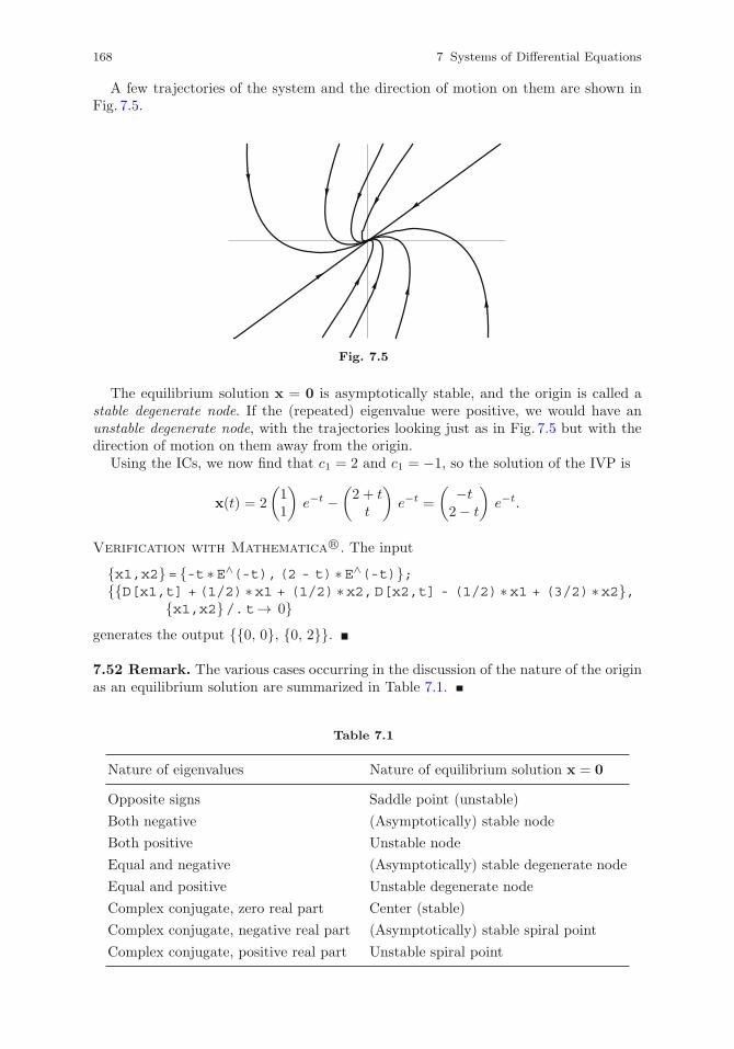
168 7 Systems of Differential Equations
A few trajectories of the system and the direction of motion on them are shown inFig. 7.5.
Fig. 7.5
The equilibrium solution x = 0 is asymptotically stable, and the origin is called astable degenerate node. If the (repeated) eigenvalue were positive, we would have anunstable degenerate node, with the trajectories looking just as in Fig. 7.5 but with thedirection of motion on them away from the origin.
Using the ICs, we now find that c1 = 2 and c1 = −1, so the solution of the IVP is
x(t) = 2
(11
)e−t −
(2 + tt
)e−t =
( −t2− t
)e−t.
Verification with Mathematica R©. The input
{x1,x2}= {-t ∗E∧(-t),(2 - t) ∗E∧(-t)};{{D[x1,t] +(1/2) ∗x1 + (1/2) ∗x2,D[x2,t] - (1/2) ∗x1 + (3/2) ∗x2},
{x1,x2}/.t→ 0}generates the output {{0, 0}, {0, 2}}.
7.52 Remark. The various cases occurring in the discussion of the nature of the originas an equilibrium solution are summarized in Table 7.1.
Table 7.1
Nature of eigenvalues Nature of equilibrium solution x = 0
Opposite signs Saddle point (unstable)
Both negative (Asymptotically) stable node
Both positive Unstable node
Equal and negative (Asymptotically) stable degenerate node
Equal and positive Unstable degenerate node
Complex conjugate, zero real part Center (stable)
Complex conjugate, negative real part (Asymptotically) stable spiral point
Complex conjugate, positive real part Unstable spiral point
7.4 Homogeneous Linear Systems with Constant Coefficients 169
7.53 Remark. In the case of a system that consists of at least three DEs, the methodfor computing a generalized eigenvector needs to be modified slightly if there is morethan one basis eigenvector for a deficient eigenvalue. Again, suppose that the coefficientmatrix A has an eigenvalue r0 with deficiency 1 but two associated basis eigenvectorsv(1) and v(2), which give rise to the solutions x(1)(t) = v(1)er0t and x(2)(t) = v(2)er0t
for (7.17). We seek a third solution of that system in the form
x(t) = [u+ (a1v(1) + a2v
(2))t]er0t, (7.23)
where a1 and a2 are nonzero constants chosen later in the procedure to ensure compu-tational consistency. Then x′ = {a1v(1)+a2v
(2)+r0[u+(a1v(1)+a2v
(2))t]}er0t, which,replaced in (7.17), yields
[a1v(1) + a2v
(2) + r0u+ a1r0v(1)t+ a2r0v
(2)t]er0t
= A[u+ (a1v(1) + a2v
(2))t]er0t = [Au+ a1Av(1)t+ a2Av
(2)t]er0t.
Recalling that Av(1) = r0v(1) and Av(2) = r0v
(2), canceling the like terms, writingr0u = r0Iu, and equating the coefficients of er0t on both sides, we conclude that thegeneralized eigenvector u is a solution of the algebraic system
(A− r0I)u = a1v(1) + a2v
(2). (7.24)
7.54 Example. For the system
x′1 =− 2x1 − 9x2, x1(0) = −1,
x′2 = x1 + 4x2, x2(0) = 1,
x′3 = x1 + 3x2 + x3, x3(0) = 2
we have
det(A− rI) =
∣∣∣∣∣∣−2− r −9 0
1 4− r 01 3 1− r
∣∣∣∣∣∣ = (1− r)(r2 − 2r + 1) = (1− r)3,
so the eigenvalues of the matrix A are r1 = r2 = r3 = 1. Since the algebraic system(A− I)v = 0 reduces to the single equation v1 +3v2 = 0, it follows that v3 is arbitraryand that, consequently, two (linearly independent) basis eigenvectors are
v(1) =
⎛⎝−3
10
⎞⎠ , v(2) =
⎛⎝001
⎞⎠ .
In this case, (7.24) with r0 = 1 yields the three equations
−3u1 − 9u2 = −3a1,
u1 + 3u2 = a1,
u1 + 3u2 = a2,
which are consistent if a1 = a2. We notice that u3 remains arbitrary. Setting, say,a1 = a2 = 1 and u2 = u3 = 0, we obtain the generalized eigenvector
u =
⎛⎝100
⎞⎠ .
170 7 Systems of Differential Equations
Hence, using the eigenvectors, u, and (7.23), we construct the three solutions
x(1)(t) = v(1)et =
⎛⎝−3
10
⎞⎠ et, x(2)(t) = v(2)et =
⎛⎝001
⎞⎠ et,
x(3)(t) = [u+ (v(1) + v(2))t]et =
⎛⎝1− 3t
tt
⎞⎠ et.
Since the Wronskian of these solutions at t = 0 is
W [x(1), x(2), x(3)](0) =
∣∣∣∣∣∣−3 0 11 0 00 1 0
∣∣∣∣∣∣ = 1 �= 0,
from Remark 7.21(i) it follows that they are linearly independent, so the GS of oursystem is
x(t) = c1x(1)(t) + c2x
(2)(t) + c3x(3)(t) =
⎛⎝−3c1 + c3(1− 3t)
c1 + c3tc2 + c3t
⎞⎠ et.
Applying the ICs leads to the values c1 = 1, c2 = 2, and c3 = 2, which means that thesolution of the given IVP is
x(t) =
⎛⎝−1− 6t
1 + 2t2 + 2t
⎞⎠ et.
Verification with Mathematica R©. The input
{x1,x2,x3}= {( - 1 - 6 ∗t) ∗E∧t,(1 + 2 ∗t) ∗E∧t,(2 + 2 ∗t) ∗E∧t};{{D[x1,t] + 2 ∗x1 + 9 ∗x2,D[x2,t] - x1 - 4 ∗x2,
D[x3,t] - x1 - 3 ∗x2 - x3}, {x1,x2,x3}/.t→ 0}generates the output {{0, 0, 0}, {−1, 1, 2}}.7.55 Remark. If the deficiency of an eigenvalue is m > 1, we need to construct achain of m generalized eigenvectors to have a full FSS for the homogeneous system(7.17). For definiteness, suppose that the coefficient matrix A has an eigenvalue r0 withdeficiency 2 and one basis eigenvector v, which gives rise to a solution x(1)(t) = ver0t. Asin Remark 7.50, we can use (7.21) and (7.22) to produce a first generalized eigenvectoru and, thus, a second solution x(2). To obtain a third solution of (7.17), we seek it inthe form
x(t) =(w + ut+ 1
2 vt2)er0t, (7.25)
where w is a second generalized eigenvector. Then, replacing x in (7.17) and recallingthat Av = r0v and Au = r0u + v, we easily find that w is a solution of the algebraicsystem
(A− r0I)w = u. (7.26)
7.56 Example. Consider the system
x′1 = x1 − x2 + 2x3, x1(0) = 6,
x′2 = 6x1 − 4x2 + 5x3, x2(0) = 3,
x′3 = 2x1 − x2, x3(0) = −5.
7.4 Homogeneous Linear Systems with Constant Coefficients 171
Here we have
det(A− rI) =
∣∣∣∣∣∣1− r −1 26 −4− r 52 −1 −r
∣∣∣∣∣∣ = (−1− r)(r2 + 2r + 1) = −(r + 1)3,
so the eigenvalues are r1 = r2 = r3 = −1. Solving the algebraic system (A + I)v = 0,we find that this triple eigenvalue has geometric multiplicity 1, and we choose theassociated basis eigenvector
v =
⎛⎝120
⎞⎠ .
By (7.22), the first generalized eigenvector, u, satisfies (A+ I)u = v. On components,this is equivalent to
2u1 − u2 + 2u3 = 1,
6u1 − 3u2 + 5u3 = 2,
2u1 − u2 + u3 = 0,
which Gaussian elimination reduces to the equations 2u1 − u2 + 2u3 = 1 and u3 = 1.Since one of u1 and u2 may be chosen arbitrarily, we take, say, u1 = 0, and obtain
u =
⎛⎝011
⎞⎠ .
Then, by (7.26),2w1 − w2 + 2w3 = 0,
6w1 − 3w2 + 5w3 = 1,
2w1 − w2 + w3 = 1.
Applying Gaussian elimination once more, we reduce this system to the pair of equations2w1−w2+2w3 = 0 and w3 = −1, and, with the choice w2 = 0, get the second generalizedeigenvector
w =
⎛⎝ 1
0−1
⎞⎠ .
According to (7.21) and (7.25), we can now construct for the system the three solutions
x(1)(t) = ve−t =
⎛⎝120
⎞⎠ e−t, x(2)(t) = (u+ vt)e−t =
⎛⎝ t1 + 2t
1
⎞⎠ e−t,
x(3)(t) =(w + ut+ 1
2 vt2)e−t =
⎛⎜⎝1 + 1
2 t2
t+ t2
−1 + t
⎞⎟⎠ e−t.
Since their Wronskian at t = 0 is
W [x(1), x(2), x(3)](0) =
∣∣∣∣∣∣1 0 12 1 00 1 −1
∣∣∣∣∣∣ = 1 �= 0,
172 7 Systems of Differential Equations
from Remarks 7.39 and 7.21(ii) it follows that they are linearly independent, so the GSof the system is
x(t) = c1x(1)(t) + c2x
(2)(t) + c3x(3)(t) =
⎛⎜⎝
c1 + c2t+ c3(1 + 1
2 t2)
2c1 + c2(1 + 2t) + c3(t+ t2)
c2 + c3(t− 1)
⎞⎟⎠ e−t.
To compute the solution of the given IVP, we apply the ICs and find that c1 = 2,c2 = −1, and c3 = 4; hence,
x(t) =
⎛⎝ 2t2 − t+ 6
4t2 + 2t+ 3
4t− 5
⎞⎠ e−t.
Verification with Mathematica R©. The input
{x1,x2,x3}= {(2 ∗t∧2 - t + 6) ∗E∧(-t),(4 ∗t∧2 + 2 ∗t + 3) ∗E∧(-t),(4 ∗t - 5) ∗E∧(-t)};
{{D[x1,t] - x1 + x2 - 2 ∗x3,D[x2,t] - 6 ∗x1 + 4 ∗x2 - 5 ∗x3,D[x3,t] - 2 ∗x1 + x2}, {x1,x2,x3}/.t→ 0}
generates the output {{0, 0, 0}, {6, 3, −5}}.
Exercises
In 1–6, use the eigenvalue–eigenvector method to solve the IVP x′ = Ax, x(0) = x0 forthe given matrix A and vector x0, and sketch the phase portrait of the general solutionof the system.
1 A =
(1 4
−1 −3
), x0 =
(01
). 2 A =
(3 −11 1
), x0 =
(01
).
3 A =
(−2/3 −11 4/3
), x0 =
(−34
). 4 A =
(3/2 −14 −5/2
), x0 =
(13
).
5 A =
(1 −91 −5
), x0 =
(01
). 6 A =
(2 −1/2
1/2 1
), x0 =
(04
).
In 7–16, use the eigenvalue–eigenvector method to solve the IVP x′ = Ax, x(0) = x0
for the given matrix A and vector x0.
7 A =
⎛⎝2 −1 −11 0 −11 −1 0
⎞⎠ , x0 =
⎛⎝203
⎞⎠. 8 A =
⎛⎝ 0 −1 −1−1 0 11 −1 −2
⎞⎠ , x0 =
⎛⎝441
⎞⎠.
9 A =
⎛⎝ 2 −3 −3−3 2 33 −3 −4
⎞⎠, x0 =
⎛⎝ 4−13
⎞⎠. 10 A =
⎛⎝ 1/4 −1/4 1/2
1/4 −1/4 1/2−1/4 1/4 −1/2
⎞⎠, x0 =
⎛⎝240
⎞⎠.
11 A =
⎛⎝−2 −3 4
1 2 −2−1 −1 2
⎞⎠, x0 =
⎛⎝ 5−21
⎞⎠. 12 A =
⎛⎝1 −1 −21 −2 −10 1 −1
⎞⎠ , x0 =
⎛⎝430
⎞⎠.
7.5 Other Features of Homogeneous Linear Systems 173
13 A =
⎛⎝−2 1 −3
2 −3 61 −1 2
⎞⎠, x0 =
⎛⎝−1
31
⎞⎠. 14 A =
⎛⎝ 3 1 1−6 −2 −32 1 2
⎞⎠, x0 =
⎛⎝ 1
2−3
⎞⎠.
15 A =
⎛⎝−2 5 6−1 2 2−1 2 3
⎞⎠, x0 =
⎛⎝ 1
1−1
⎞⎠. 16 A =
⎛⎝−3 2 −3−1 0 −21 −1 0
⎞⎠, x0 =
⎛⎝ 2−2−2
⎞⎠.
Answers to Odd-Numbered Exercises
1 x(t) =
(4t
1− 2t
)e−t. 3 x(t) =
(−t− 3t+ 4
)et/3.
5 x(t) =
( −9t1− 3t
)e−2t. 7 x(t) =
⎛⎝ 1 + et
1− et
1 + 2et
⎞⎠.
9 x(t) =
⎛⎝2e−t + 2e2t
e−t − 2e2t
e−t + 2e2t
⎞⎠. 11 x(t) =
⎛⎝4 + (1− t)et
(t− 2)et
2− et
⎞⎠.
13 x(t) =
⎛⎝ t− 13− 2t1− t
⎞⎠ e−t. 15 x(t) =
⎛⎝1− 4t− 2t2
1− 2t−1− t− t2
⎞⎠ et.
7.5 Other Features of Homogeneous Linear Systems
Fundamental matrices. Consider the general homogeneous linear system (7.13);that is,
x′ = A(t)x, (7.27)
let x(1), . . . ,x(n) be an FSS for it, and construct the matrix
X(t) = (x(1)(t) . . . x(n)(t)),
whose columns are the components of the vector functions x(1), . . . ,x(n).
7.57 Definition. The matrix function X is called a fundamental matrix for system(7.27).
7.58 Remarks. (i) Obviously, there are infinitely many fundamental matrices for anygiven system.
(ii) Since each column of a fundamental matrix X is a solution of (7.27), it follows thatX satisfies the matrix equation X ′ = AX .
(iii) A fundamental matrix X allows us to construct an alternative form of the solutionof an IVP for system (7.27). Let c be a column vector of constant components
c1, . . . , cn. Denoting by x(j)i the ith component of x(j), we can write the GS of
(7.27) as
174 7 Systems of Differential Equations
x = c1x(1) + · · ·+ cnx
(n) = c1
⎛⎜⎜⎝x(1)1...
x(1)n
⎞⎟⎟⎠+ · · ·+ cn
⎛⎜⎜⎝x(n)1...
x(n)n
⎞⎟⎟⎠
=
⎛⎜⎜⎝c1x
(1)1 + · · ·+ cnx
(n)1
...
c1x(1)n + · · ·+ cnx
(n)n
⎞⎟⎟⎠ =
⎛⎜⎜⎝x(1)1 . . . x
(n)1
.... . .
...
x(1)n . . . x
(n)n
⎞⎟⎟⎠⎛⎜⎝c1...cn
⎞⎟⎠ = Xc. (7.28)
The columns of X(t) are linearly independent vector functions, so, according toDefinition 7.19, there is at least one point t where det(X(t)) �= 0 and where, therefore,X(t) is invertible. If we are also given an IC of the form x(t0) = x0, where x0 is aprescribed constant vector and t0 is such that det(X(t0)) �= 0, then, in view of (7.28),we have X(t0)c = x0, from which c = X−1(t0)x0. Replacing in (7.28), we conclude thatthe solution of the IVP is
x(t) = X(t)(X−1(t0)x0) = (X(t)X−1(t0))x0. (7.29)
7.59 Example. The IVP
x′1 = 3x1 + 4x2, x1(0) = 2,x′2 = 3x1 + 2x2, x2(0) = 5
was discussed in Example 7.41, where we constructed for it the two linearly independentsolutions
x(1)(t) =
(−11
)e−t, x(2)(t) =
(43
)e6t.
Using these solutions, we have
X(t) = (x(1)(t) x(2)(t)) =
(−e−t 4e6t
e−t 3e6t
),
X(0) =
(−1 41 3
), X−1(0) =
(− 37
47
17
17
),
so
X(t)X−1(0) =
(−e−t 4e6t
e−t 3e6t
)(− 37
47
17
17
)=
1
7
(3e−t + 4e6t −4e−t + 4e6t
−3e−t + 3e6t 4e−t + 3e6t
);
hence, by (7.29) with t0 = 0, the solution of the given IVP is
x(t) = (X(t)X−1(0))x0 =1
7
(3e−t + 4e6t −4e−t + 4e6t
−3e−t + 3e6t 4e−t + 3e6t
)(25
)=
(−2e−t + 4e6t
2e−t + 3e6t
),
confirming the earlier result.
Exponential matrix. As mentioned at the beginning of Sect. 7.4, the solution of thescalar IVP x′ = ax, x(0) = x0, a = const, is x = x0e
at. It can be shown that a similarformula exists for the solution of the corresponding IVP in the case of systems of theform
x′ = Ax, (7.30)
x(0) = x0, (7.31)
7.5 Other Features of Homogeneous Linear Systems 175
where A is a constant n × n matrix. To construct this formula, we need a definitionfor eAt, which can easily be formulated if we make use of series expansions. The Taylorseries
eat =∞∑n=0
1
n!antn = 1 +
1
1!at+
1
2!a2t2 + · · · (7.32)
is convergent for any real values of a and t. Since the power An of an n × n matrix Acan be computed for any positive integer n (by multiplying A by itself n times) and theresult is always an n × n matrix, it follows that the right-hand side in (7.32) remainsmeaningful if a is replaced by A, and we write formally
eAt =
∞∑n=0
1
n!Antn = I +
1
1!At+
1
2!A2t2 + · · · , (7.33)
where we have set A0 = I. It turns out that, just like (7.32), series (7.33) converges forany constant n × n matrix A and any value of t. Its sum, which we have denoted byeAt, is referred to as an exponential matrix.
7.60 Remark. The matrix function eAt has many of the properties of the scalar expo-nential function eat. Thus,
(i) e0 = I, where 0 is the zero matrix;
(ii) If AB = BA, then eAt+Bt = eAteBt;
(iii)(eAt)′
= AeAt = eAtA.
These properties are proved directly from definition (7.33).
7.61 Remarks. (i) The vector function x(t) = eAtx0 is the solution of the IVP (7.30),(7.31) since, by properties (i) and (iii) in Remark 7.60,
x′(t) = AeAtx0 = Ax(t), x(0) = Ix0 = x0.
But the same solution is also given by (7.29), so
eAt = X(t)X−1(0),
where X is any fundamental matrix for the system.
(ii) If the ICs are given at t = t0, then it is easily verified that the solution of thenew IVP is
x(t) = eA(t−t0)x0.
7.62 Example. As can be seen from the solution of Example 7.59 in conjunction withRemark 7.61(i), for the matrix
A =
(3 43 2
)
we have
eAt = X(t)X−1(0) =1
7
(3e−t + 4e6t −4e−t + 4e6t
−3e−t + 3e6t 4e−t + 3e6t
).
Diagonalization. The IVP (7.30), (7.31) would be much easier to solve if the equa-tions of the system were decoupled; that is, if they were individual (first-order) DEsfor each of the unknown components of the vector function x. As it happens, thereis a procedure that, under certain conditions, allows us to reduce the problem to anequivalent one of just this form.
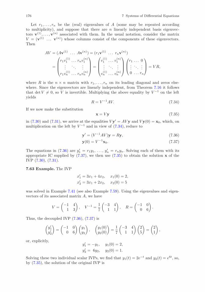
176 7 Systems of Differential Equations
Let r1, . . . , rn be the (real) eigenvalues of A (some may be repeated accordingto multiplicity), and suppose that there are n linearly independent basis eigenvec-tors v(1), . . . ,v(n) associated with them. In the usual notation, consider the matrixV = (v(1) . . . v(n)) whose columns consist of the components of these eigenvectors.Then
AV = (Av(1) . . . Av(n)) = (r1v(1) . . . rnv
(n))
=
⎛⎜⎜⎝r1v
(1)1 . . . rnv
(n)1
.... . .
...
r1v(1)n . . . rnv
(n)n
⎞⎟⎟⎠ =
⎛⎜⎜⎝v(1)1 . . . v
(n)1
.... . .
...
v(1)n . . . v
(n)n
⎞⎟⎟⎠⎛⎜⎝r1 . . . 0.... . .
...0 . . . rn
⎞⎟⎠ = V R,
where R is the n × n matrix with r1, . . . , rn on its leading diagonal and zeros else-where. Since the eigenvectors are linearly independent, from Theorem 7.16 it followsthat detV �= 0, so V is invertible. Multiplying the above equality by V −1 on the leftyields
R = V −1AV. (7.34)
If we now make the substitutionx = V y (7.35)
in (7.30) and (7.31), we arrive at the equalities V y′ = AV y and V y(0) = x0, which, onmultiplication on the left by V −1 and in view of (7.34), reduce to
y′ = (V −1AV )y = Ry, (7.36)
y(0) = V −1x0. (7.37)
The equations in (7.36) are y′1 = r1y1, . . . , y′n = rnyn. Solving each of them with its
appropriate IC supplied by (7.37), we then use (7.35) to obtain the solution x of theIVP (7.30), (7.31).
7.63 Example. The IVP
x′1 = 3x1 + 4x2, x1(0) = 2,
x′2 = 3x1 + 2x2, x2(0) = 5
was solved in Example 7.41 (see also Example 7.59). Using the eigenvalues and eigen-vectors of its associated matrix A, we have
V =
(−1 41 3
), V −1 =
1
7
(−3 41 1
), R =
(−1 00 6
).
Thus, the decoupled IVP (7.36), (7.37) is
(y′1y′2
)=
(−1 00 6
)(y1y2
),
(y1(0)y2(0)
)=
1
7
(−3 41 1
)(25
)=
(21
),
or, explicitly,y′1 = −y1, y1(0) = 2,
y′2 = 6y2, y2(0) = 1.
Solving these two individual scalar IVPs, we find that y1(t) = 2e−t and y2(t) = e6t, so,by (7.35), the solution of the original IVP is
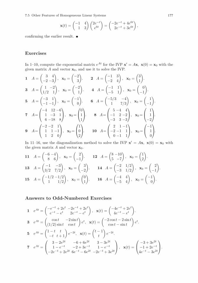
7.5 Other Features of Homogeneous Linear Systems 177
x(t) =
(−1 41 3
)(2e−t
e6t
)=
(−2e−t + 4e6t
2e−t + 3e6t
),
confirming the earlier result.
Exercises
In 1–10, compute the exponential matrix eAt for the IVP x′ = Ax, x(0) = x0 with thegiven matrix A and vector x0, and use it to solve the IVP.
1 A =
(3 4
−2 −3
), x0 =
(−23
). 2 A =
(−1 3−2 4
), x0 =
(31
).
3 A =
(1 −21/2 1
), x0 =
(−21
). 4 A =
(−1 1−5 1
), x0 =
(0
−1
).
5 A =
(−3 1−1 −1
), x0 =
(−10
). 6 A =
(−5/3 −41 7/3
), x0 =
(1
−1
).
7 A=
⎛⎝−4 12 −6
1 −3 16 −18 8
⎞⎠, x0=
⎛⎝011
⎞⎠. 8 A=
⎛⎝ 5 −4 4−1 2 −2−3 3 −3
⎞⎠, x0=
⎛⎝ 1
1−2
⎞⎠.
9 A=
⎛⎝−2 −2 1
1 1 −11 2 0
⎞⎠, x0=
⎛⎝102
⎞⎠. 10 A=
⎛⎝ 2 1 −1−2 −1 10 −1 1
⎞⎠, x0=
⎛⎝−1
10
⎞⎠.
In 11–16, use the diagonalization method to solve the IVP x′ = Ax, x(0) = x0 withthe given matrix A and vector x0.
11 A =
(−6 −48 6
), x0 =
(2
−1
). 12 A =
(8 −105 −7
), x0 =
(12
).
13 A =
(−1 −33/2 7/2
), x0 =
(3
−2
). 14 A =
(−2 1/2−3 1/2
), x0 =
(2
−1
).
15 A =
(−1/2 −1/21 1/2
), x0 =
(01
). 16 A =
(−4 4−5 4
), x0 =
(−10
).
Answers to Odd-Numbered Exercises
1 eAt =
(−e−t + 2et −2e−t + 2et
e−t − et 2e−t − et
), x(t) =
(−4e−t + 2et
4e−t − et
).
3 eAt =
(cos t −2 sin t
(1/2) sin t cos t
)et, x(t) =
(−2 cos t− 2 sin tcos t− sin t
)et.
5 eAt =
(1− t t−t t+ 1
)e−2t, x(t) =
(t− 1t
)e−2t.
7 eAt =
⎛⎝ 3− 2e2t −6 + 6e2t 3− 3e2t
1− e−t −2 + 3e−t 1− e−t
−2e−t + 2e2t 6e−t − 6e2t −2e−t + 3e2t
⎞⎠ , x(t) =
⎛⎝ −3 + 3e2t
−1 + 2e−t
4e−t − 3e2t
⎞⎠.
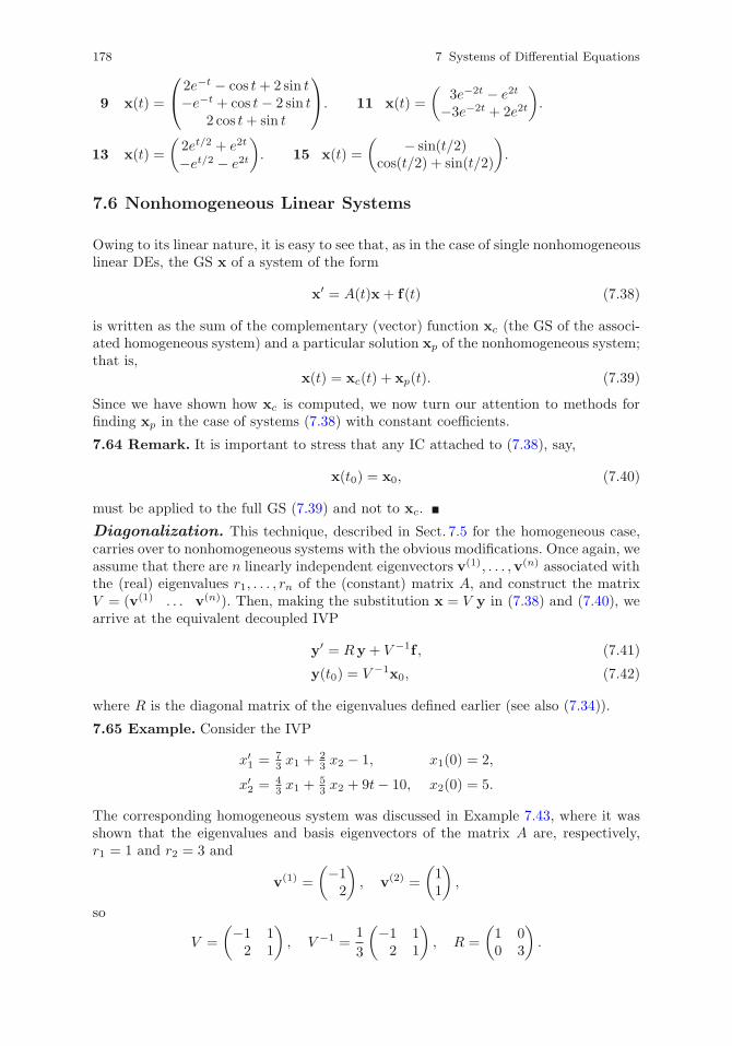
178 7 Systems of Differential Equations
9 x(t) =
⎛⎝2e−t − cos t+ 2 sin t−e−t + cos t− 2 sin t
2 cos t+ sin t
⎞⎠. 11 x(t) =
(3e−2t − e2t
−3e−2t + 2e2t
).
13 x(t) =
(2et/2 + e2t
−et/2 − e2t
). 15 x(t) =
( − sin(t/2)cos(t/2) + sin(t/2)
).
7.6 Nonhomogeneous Linear Systems
Owing to its linear nature, it is easy to see that, as in the case of single nonhomogeneouslinear DEs, the GS x of a system of the form
x′ = A(t)x + f(t) (7.38)
is written as the sum of the complementary (vector) function xc (the GS of the associ-ated homogeneous system) and a particular solution xp of the nonhomogeneous system;that is,
x(t) = xc(t) + xp(t). (7.39)
Since we have shown how xc is computed, we now turn our attention to methods forfinding xp in the case of systems (7.38) with constant coefficients.
7.64 Remark. It is important to stress that any IC attached to (7.38), say,
x(t0) = x0, (7.40)
must be applied to the full GS (7.39) and not to xc.
Diagonalization. This technique, described in Sect. 7.5 for the homogeneous case,carries over to nonhomogeneous systems with the obvious modifications. Once again, weassume that there are n linearly independent eigenvectors v(1), . . . ,v(n) associated withthe (real) eigenvalues r1, . . . , rn of the (constant) matrix A, and construct the matrixV = (v(1) . . . v(n)). Then, making the substitution x = V y in (7.38) and (7.40), wearrive at the equivalent decoupled IVP
y′ = Ry + V −1f , (7.41)
y(t0) = V −1x0, (7.42)
where R is the diagonal matrix of the eigenvalues defined earlier (see also (7.34)).
7.65 Example. Consider the IVP
x′1 = 73 x1 +
23 x2 − 1, x1(0) = 2,
x′2 = 43 x1 +
53 x2 + 9t− 10, x2(0) = 5.
The corresponding homogeneous system was discussed in Example 7.43, where it wasshown that the eigenvalues and basis eigenvectors of the matrix A are, respectively,r1 = 1 and r2 = 3 and
v(1) =
(−12
), v(2) =
(11
),
so
V =
(−1 12 1
), V −1 =
1
3
(−1 12 1
), R =
(1 00 3
).
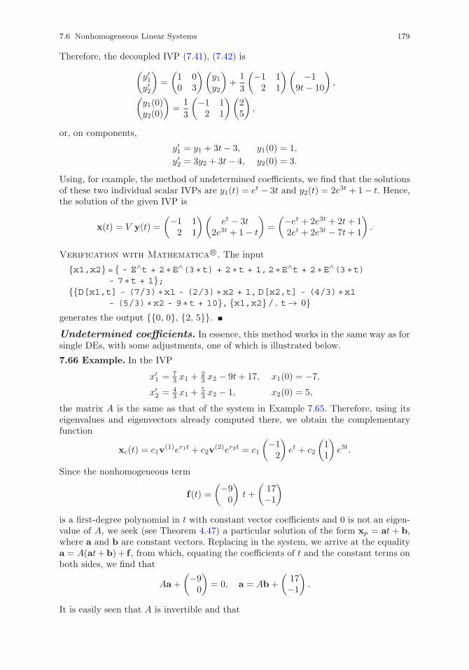
7.6 Nonhomogeneous Linear Systems 179
Therefore, the decoupled IVP (7.41), (7.42) is
(y′1y′2
)=
(1 00 3
)(y1y2
)+
1
3
(−1 12 1
)( −19t− 10
),
(y1(0)y2(0)
)=
1
3
(−1 12 1
)(25
),
or, on components,
y′1 = y1 + 3t− 3, y1(0) = 1,
y′2 = 3y2 + 3t− 4, y2(0) = 3.
Using, for example, the method of undetermined coefficients, we find that the solutionsof these two individual scalar IVPs are y1(t) = et − 3t and y2(t) = 2e3t + 1− t. Hence,the solution of the given IVP is
x(t) = V y(t) =
(−1 12 1
)(et − 3t
2e3t + 1− t
)=
(−et + 2e3t + 2t+ 12et + 2e3t − 7t+ 1
).
Verification with Mathematica R©. The input
{x1,x2}= { - E∧t + 2 ∗E∧(3 ∗t) + 2 ∗t + 1,2 ∗E∧t + 2 ∗E∧(3 ∗t)- 7 ∗t + 1};
{{D[x1,t] - (7/3) ∗x1 - (2/3) ∗x2 + 1,D[x2,t] - (4/3) ∗x1- (5/3) ∗x2 - 9 ∗t + 10}, {x1,x2}/.t→ 0}
generates the output {{0, 0}, {2, 5}}.Undetermined coefficients. In essence, this method works in the same way as forsingle DEs, with some adjustments, one of which is illustrated below.
7.66 Example. In the IVP
x′1 = 73 x1 +
23 x2 − 9t+ 17, x1(0) = −7,
x′2 = 43 x1 +
53 x2 − 1, x2(0) = 5,
the matrix A is the same as that of the system in Example 7.65. Therefore, using itseigenvalues and eigenvectors already computed there, we obtain the complementaryfunction
xc(t) = c1v(1)er1t + c2v
(2)er2t = c1
(−12
)et + c2
(11
)e3t.
Since the nonhomogeneous term
f(t) =
(−90
)t+
(17−1
)
is a first-degree polynomial in t with constant vector coefficients and 0 is not an eigen-value of A, we seek (see Theorem 4.47) a particular solution of the form xp = at + b,where a and b are constant vectors. Replacing in the system, we arrive at the equalitya = A(at+b) + f , from which, equating the coefficients of t and the constant terms onboth sides, we find that
Aa+
(−90
)= 0, a = Ab+
(17−1
).
It is easily seen that A is invertible and that
180 7 Systems of Differential Equations
A−1 =1
9
(5 −2
−4 7
);
hence,
a = A−1
(90
)=
1
9
(5 −2
−4 7
)(90
)=
(5
−4
),
b = A−1
[a−
(17−1
)]=
1
9
(5 −2
−4 7
)(−12−3
)=
(−63
),
so
xp =
(5t− 63− 4t
).
Then the GS of the system is
x(t) = c1
(−12
)et + c2
(11
)e3t +
(5t− 63− 4t
).
Applying the ICs, we now find that c1 = 1 and c2 = 0, which means that the solutionof the IVP is
x(t) =
(−12
)et +
(5t− 63− 4t
)=
(−et + 5t− 62et + 3− 4t
).
Verification with Mathematica R©. The input
{x1,x2}= { - E∧t + 5 ∗t - 6,2 ∗E∧t + 3 - 4 ∗t};{{D[x1,t] - (7/3) ∗x1 - (2/3) ∗x2 + 9 ∗t - 17,D[x2,t] - (4/3) ∗x1
- (5/3) ∗x2 + 1}, {x1,x2}/.t→ 0}generates the output {{0, 0}, {−7, 5}}.
7.67 Example. Consider the IVP
x′1 = 73 x1 +
23 x2 − 5et, x1(0) = 1,
x′2 = 43 x1 +
53 x2 − 8et, x2(0) = 4.
The matrix A is the same as that in the preceding example, so the complementaryfunction xc is unchanged:
xc(t) = c1v(1)er1t + c2v
(2)er2t = c1
(−12
)et + c2
(11
)e3t.
We notice that the exponential function et in the nonhomogeneous terms also occursin xc, and that the eigenvalue r = 1 has algebraic multiplicity 1. In the case of a singleDE, for a characteristic root r = 1 of multiplicity 1 and a similar nonhomogeneousterm, it would suffice to try a PS of the form atet, a = const. For a system, however,the corresponding form atet, where a is a constant vector, does not work. Instead, herewe need to try
xp(t) = (at + b)et,
where a and b are constant vectors of components a1, a2 and b1, b2, respectively. Sub-stituting in (7.38) and denoting the column vector of components −5, −8 by q, wehave
aet + (at+ b)et = A(at + b)et + qet.
7.6 Nonhomogeneous Linear Systems 181
The functions tet and et are linearly independent (see Sect. 4.4.2), so from Theorem 4.16it follows that we can match their coefficients on both sides and arrive at the algebraicsystem
a = Aa,
a+ b = Ab+ q,
or, what is the same,(A− I)a = 0,
(A− I)b = a− q.
The first equality shows that a is an eigenvector of A associated with the eigenvaluer = 1, so its components are a1 = −p and a2 = 2p for some number p. Then the secondequality yields the pair of equations
43 b1 +
23 b2 = a1 + 5 = −p+ 5,
43 b1 +
23 b2 = a2 + 8 = 2p+ 8,
which are consistent if and only if −p + 5 = 2p + 8; that is, p = −1. Inthis case, a1 = 1 and a2 = −2, and the above system reduces to the single equation2b1 + b2 = 9. If we choose, say, b1 = 4 and b2 = 1, then the GS of the given nonhomo-geneous system can be written as
x(t) = xc(t) + xp(t) = c1
(−12
)et + c2
(11
)e3t +
[(1
−2
)t+
(41
)]et.
Applying the ICs, we find that c1 = 2 and c2 = −1, so the solution of the IVP is
x(t) = 2
(−12
)et −
(11
)e3t +
[(1
−2
)t+
(41
)]et =
((t+ 2)et − e3t
(5 − 2t)et − e3t
).
Verification with Mathematica R©. The input
{x1,x2}= {(t + 2) ∗E∧t - E∧(3 ∗t),(5 - 2 ∗t) ∗E∧t - E∧(3 ∗t)};{{D[x1,t] - (7/3) ∗x1 - (2/3) ∗x2 + 5 ∗E∧t,D[x2,t] - (4/3) ∗x1
- (5/3) ∗x2 + 8 ∗E∧t},{x1,x2}/.t→ 0}generates the output {{0, 0}, {1, 4}}.7.68 Remark. Just as in the case of single DEs, if the nonhomogeneous term f is a sumof several terms, then, by the principle of superposition (formulated for nonhomogeneouslinear systems), xp is the sum of the individual PSs computed for each of those terms.
7.69 Example. Suppose that the eigenvalues of the 2×2 coefficient matrix A are r1 = 1and r2 = −1, and that the nonhomogeneous term is
f(t) =
(2t− 3− 4et
1 + 2e2t − 5e−t
).
This term is a linear combination of a first degree polynomial and the exponentialfunctions et, e2t, and e−t, with constant vector coefficients. Since 0 and 2 are noteigenvalues of A and both 1 and −1 are eigenvalues of algebraic multiplicity 1, we seeka PS of the form
xp(t) = at+ b+ (ct+ d)et + ee2t + (gt+ h)e−t,
where a, b, c, d, e, g, and h are constant vectors.
182 7 Systems of Differential Equations
Variation of parameters. Consider the homogeneous system x′ = Ax in an openinterval J , and let x(1) and x(2) be two solutions of this system such that x(1)(t) andx(2)(t) are linearly independent for all t in J . According to (7.27), the complementaryfunction for the nonhomogeneous system (7.38) is then written in the form
xc(t) = X(t)c,
where c is an arbitrary constant vector and X = (x(1) x(2)). By analogy with the caseof a single DE, we seek a PS of (7.38) of the form
xp(t) = X(t)u(t), (7.43)
where u is a vector function to be determined. Replacing in the system, we find that
X ′u+Xu′ = A(Xu) + f = (AX)u+ f .
As noted in Remark 7.58(i), we have X ′ = AX , so the above equality reduces to
Xu′ = f . (7.44)
The linear independence of the columns of X also implies that detX(t) �= 0 for alladmissible t. Consequently, X(t) is invertible, and we can multiply both sides of (7.44)on the left by X−1(t) to obtain
u′(t) = X−1(t)f(t). (7.45)
Hence, a PS of the nonhomogeneous system is given by (7.43) with u computed byintegration from (7.45).
7.70 Example. The IVP
x′1 = 73 x1 +
23 x2 − 5et, x1(0) = 1,
x′2 = 43 x1 +
53 x2 − 8et, x2(0) = 4
was discussed in Example 7.67. From the eigenvalues and eigenvectors used there, wecan construct the fundamental matrix
X(t) = {v(1)et v(2)e3t} =
(−et e3t
2et e3t
).
Then
X−1(t) =1
3
(−e−t e−t
2e−3t e−3t
), f(t) =
(−5et
−8et
),
so, by (7.45),
u′(t) =1
3
(−e−t e−t
2e−3t e−3t
)(−5et
−8et
)=
( −1−6e−2t
).
Integrating (and setting the integration constant equal to zero since we need only onePS), we find that
u(t) =
( −t3e−2t
);
hence, by (7.43),
7.6 Nonhomogeneous Linear Systems 183
xp(t) =
(−et e3t
2et e3t
)( −t3e−2t
)=
(t+ 33− 2t
)et.
Consequently, the GS of the nonhomogeneous system (with the complementary functionxc as mentioned in Example 7.67) is
x(t) = xc(t) + xp(t) = c1
(−12
)et + c2
(11
)e3t +
(t+ 33− 2t
)et.
The constants c1 and c2, determined from the ICs, are c1 = 1 and c2 = −1, whichmeans that the solution of the given IVP is the same one we computed earlier, namely
x(t) =
(−12
)et −
(11
)e3t +
(t+ 33− 2t
)et =
((t+ 2)et − e3t
(5− 2t)et − e3t
).
Exercises
In 1–16, compute the solution of the IVP x′ = Ax + f(t), x(0) = x0 with the givenmatrix A, vector function f , and vector x0, by each of (a) the method of undeterminedcoefficients, (b) diagonalization, and (c) variation of parameters.
1 A =
(−7 −84 5
), f(t) =
(8t+ 9−5t− 5
), x0 =
(01
).
2 A =
(−1 −26 6
), f(t) =
(t− 4
18− 6t
), x0 =
(0
−3
).
3 A =
(9 −105 −6
), f(t) =
(9 + 3e2t
5 + 3e2t
), x0 =
(02
).
4 A =
(−7/2 −39/2 4
), f(t) =
(3 + 3e−t
−4− 5e−t
), x0 =
(−12
).
5 A =
( −1/3 −5/3−10/3 4/3
), f(t) =
(e3t
−2e3t
), x0 =
(−2−5
).
6 A =
(−5 −82 5
), f(t) =
(5 + 12e−3t
−2− 9e−3t
), x0 =
(−73
).
7 A =
⎛⎝ 4 0 −6−2 0 43 0 −5
⎞⎠ , f(t) =
⎛⎝−6− 5e−t
4 + 2e−t
−5− 3e−t
⎞⎠ , x0 =
⎛⎝ 3
2−1
⎞⎠.
8 A =
⎛⎝ 1 −2 −1
4 −5 −4−6 6 6
⎞⎠ , f(t) =
⎛⎝t− 1t− 46
⎞⎠ , x0 =
⎛⎝411
⎞⎠.
9 A =
(1 −1
−2 0
), f(t) =
( −22t+ 5
), x0 =
(31
).
10 A =
(5 −46 −5
), f(t) =
(1− 6t−7t
), x0 =
(56
).
11 A =
(4 −21 1
), f(t) =
(−12e−t
0
), x0 =
(93
).
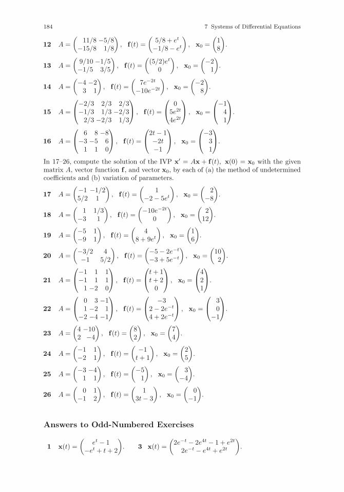
184 7 Systems of Differential Equations
12 A =
(11/8 −5/8
−15/8 1/8
), f(t) =
(5/8 + et
−1/8− et
), x0 =
(18
).
13 A =
(9/10 −1/5−1/5 3/5
), f(t) =
((5/2)et
0
), x0 =
(−21
).
14 A =
(−4 −23 1
), f(t) =
(7e−2t
−10e−2t
), x0 =
(−28
).
15 A =
⎛⎝−2/3 2/3 2/3−1/3 1/3 −2/32/3 −2/3 1/3
⎞⎠ , f(t) =
⎛⎝ 05e2t
4e2t
⎞⎠ , x0 =
⎛⎝−1
41
⎞⎠.
16 A =
⎛⎝ 6 8 −8−3 −5 61 1 0
⎞⎠ , f(t) =
⎛⎝2t− 1
−2t−1
⎞⎠ , x0 =
⎛⎝−3
31
⎞⎠.
In 17–26, compute the solution of the IVP x′ = Ax + f(t), x(0) = x0 with the givenmatrix A, vector function f , and vector x0, by each of (a) the method of undeterminedcoefficients and (b) variation of parameters.
17 A =
(−1 −1/25/2 1
), f(t) =
(1
−2− 5et
), x0 =
(2
−8
).
18 A =
(1 1/3
−3 1
), f(t) =
(−10e−2t
0
), x0 =
(2
12
).
19 A =
(−5 1−9 1
), f(t) =
(4
8 + 9et
), x0 =
(16
).
20 A =
(−3/2 4−1 5/2
), f(t) =
(−5− 2e−t
−3 + 5e−t
), x0 =
(102
).
21 A =
⎛⎝−1 1 1−1 1 11 −2 0
⎞⎠ , f(t) =
⎛⎝t+ 1t+ 20
⎞⎠ , x0 =
⎛⎝421
⎞⎠.
22 A =
⎛⎝ 0 3 −1
1 −2 1−2 −4 −1
⎞⎠ , f(t) =
⎛⎝ −32− 2e−t
4 + 2e−t
⎞⎠ , x0 =
⎛⎝ 3
0−1
⎞⎠.
23 A =
(4 −102 −4
), f(t) =
(82
), x0 =
(74
).
24 A =
(−1 1−2 1
), f(t) =
( −1t+ 1
), x0 =
(25
).
25 A =
(−3 −41 1
), f(t) =
(−51
), x0 =
(3
−4
).
26 A =
(0 1
−1 2
), f(t) =
(1
3t− 3
), x0 =
(0
−1
).
Answers to Odd-Numbered Exercises
1 x(t) =
(et − 1
−et + t+ 2
). 3 x(t) =
(2e−t − 2e4t − 1 + e2t
2e−t − e4t + e2t
).
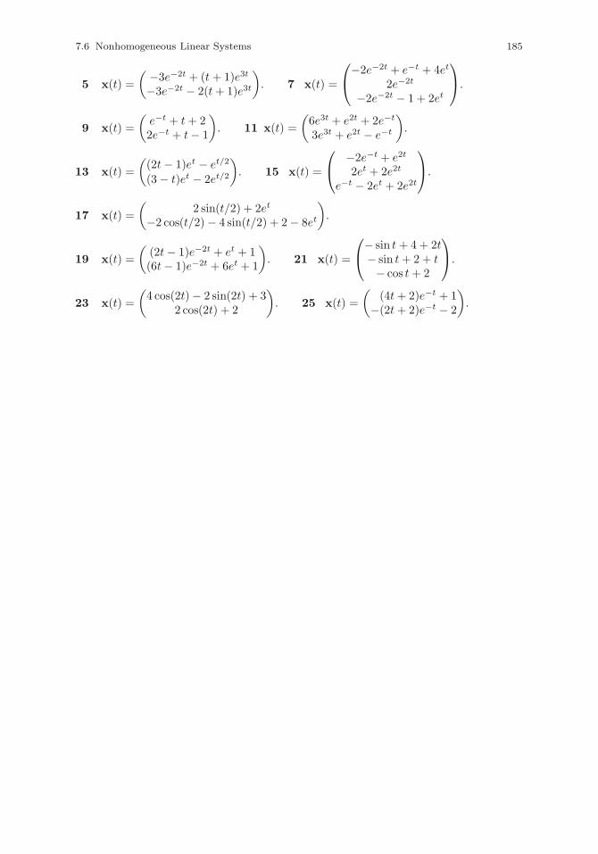
7.6 Nonhomogeneous Linear Systems 185
5 x(t) =
( −3e−2t + (t+ 1)e3t
−3e−2t − 2(t+ 1)e3t
). 7 x(t) =
⎛⎝−2e−2t + e−t + 4et
2e−2t
−2e−2t − 1 + 2et
⎞⎠.
9 x(t) =
(e−t + t+ 22e−t + t− 1
). 11 x(t) =
(6e3t + e2t + 2e−t
3e3t + e2t − e−t
).
13 x(t) =
((2t− 1)et − et/2
(3− t)et − 2et/2
). 15 x(t) =
⎛⎝ −2e−t + e2t
2et + 2e2t
e−t − 2et + 2e2t
⎞⎠.
17 x(t) =
(2 sin(t/2) + 2et
−2 cos(t/2)− 4 sin(t/2) + 2− 8et
).
19 x(t) =
((2t− 1)e−2t + et + 1(6t− 1)e−2t + 6et + 1
). 21 x(t) =
⎛⎝− sin t+ 4 + 2t
− sin t+ 2 + t− cos t+ 2
⎞⎠.
23 x(t) =
(4 cos(2t)− 2 sin(2t) + 3
2 cos(2t) + 2
). 25 x(t) =
((4t+ 2)e−t + 1
−(2t+ 2)e−t − 2
).
Chapter 8
The Laplace Transformation
The purpose of an analytic transformation is to change a more complicated probleminto a simpler one. The Laplace transformation, which is applied chiefly with respect tothe time variable, maps an IVP onto an algebraic equation or system. Once the latteris solved, its solution is fed into the inverse transformation to yield the solution of theoriginal IVP.
8.1 Definition and Basic Properties
Let f be a function of one independent variable t on the interval 0 ≤ t < ∞.
8.1 Definition. The function
F (s) = L{f(t)} =
∞∫0
e−stf(t) dt, (8.1)
if it exists, is called the Laplace transform of f . The variable s of F is called thetransformation parameter. The operation L that produces F from the given function fis called the Laplace transformation.
8.2 Remarks. (i) The right-hand side in (8.1) must be understood as an improperintegral; that is,
F (s) = limp→∞
p∫0
e−stf(t) dt. (8.2)
(ii) It is clear from the above definition that we must distinguish between the terms‘transformation’ and ‘transform’: the former is a mathematical operator, the latteris a function.
(iii) In general, the transformation parameter s is a complex number, but for the dis-cussion in this chapter it suffices to consider it real.
We now indicate a class of functions for which the improper integral (8.1) exists.
8.3 Definition. A function f is said to be piecewise continuous on 0 ≤ t ≤ p if it iscontinuous everywhere on this interval except at a finite number of points, where it may
C. Constanda, Differential Equations: A Primer for Scientists and Engineers, SpringerUndergraduate Texts in Mathematics and Technology, DOI 10.1007/978-1-4614-7297-1 8,© Springer Science+Business Media New York 2013
187
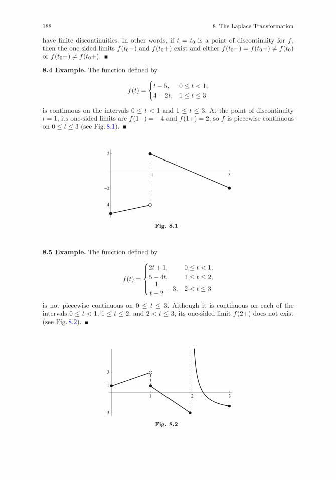
188 8 The Laplace Transformation
have finite discontinuities. In other words, if t = t0 is a point of discontinuity for f ,then the one-sided limits f(t0−) and f(t0+) exist and either f(t0−) = f(t0+) �= f(t0)or f(t0−) �= f(t0+).
8.4 Example. The function defined by
f(t) =
{t− 5, 0 ≤ t < 1,
4− 2t, 1 ≤ t ≤ 3
is continuous on the intervals 0 ≤ t < 1 and 1 ≤ t ≤ 3. At the point of discontinuityt = 1, its one-sided limits are f(1−) = −4 and f(1+) = 2, so f is piecewise continuouson 0 ≤ t ≤ 3 (see Fig. 8.1).
31
2
−2
−4
Fig. 8.1
8.5 Example. The function defined by
f(t) =
⎧⎪⎪⎨⎪⎪⎩2t+ 1, 0 ≤ t < 1,
5− 4t, 1 ≤ t ≤ 2,1
t− 2− 3, 2 < t ≤ 3
is not piecewise continuous on 0 ≤ t ≤ 3. Although it is continuous on each of theintervals 0 ≤ t < 1, 1 ≤ t ≤ 2, and 2 < t ≤ 3, its one-sided limit f(2+) does not exist(see Fig. 8.2).
1 2 3
3
−3
1
Fig. 8.2
8.1 Definition and Basic Properties 189
8.6 Theorem. If f is piecewise continuous on 0 ≤ t ≤ p for any p > 0 and there areconstants M ≥ 0, k ≥ 0, and γ such that
|f(t)| ≤ Meγt for all t > k, (8.3)
then the Laplace transform F of f exists for all s > γ. Furthermore, F (s) → 0 ass → ∞.
8.7 Remarks. (i) Since all the functions occurring in the rest of this chapter satisfythe conditions of Theorem 8.6, they will not be verified explicitly. Also, to keepthe presentation simple, the constants M , k, and γ in (8.3) will be mentioned (ifrequired) only in mathematical arguments of a general nature but not in specificcases.
(ii) The inverse Laplace transformation is the operator L−1 defined by
f(t) = L−1{F (s)} =1
2πilimβ→∞
α+iβ∫α−iβ
estF (s) ds,
where α and β are real numbers. This formula involves integration in the complexdomain, which is beyond the scope of this book, so we do not use it. Instead, wefind the original function f corresponding to a transform F by means of the tablein Appendix C.
(iii) For practical purposes, the Laplace transformation is bijective; in other words,each admissible function has a unique transform, and each transform has a uniqueinverse transform (or original).
(iv) As is easily verified, both L and L−1 are linear operators; that is, for any functionsf1 and f2 whose transforms F1 and F2 exist for s > γ, and any constants c1 and c2,
L{c1f1(t) + c2f2(t)} = c1L{f1(t)} + c2L{f2(t)},L−1{c1F1(s) + c2F2(s)} = c1L−1{F1(s)} + c2L−1{F2(s)}.
8.8 Example. By (8.2), the Laplace transform of the constant function f(t) = 1 is
F (s) = L{1} = limp→∞
p∫0
e−st dt = limp→∞
[− 1
se−st
]p0
= limp→∞
(1
s− 1
se−ps
)=
1
s,
which exists for all s > 0. This implies that we can also write L−1{1/s} = 1.
Verification with Mathematica R©. The input
F=1/s;InverseLaplaceTransform[F,s,t]
generates the output 1.
8.9 Example. The transform of the function f(t) = eat, a = const, is
190 8 The Laplace Transformation
F (s) = L{eat} = limp→∞
p∫0
e−steat dt = limp→∞
p∫0
e−(s−a)t dt
= limp→∞
[− 1
s− ae−(s−a)t
]p0
= limp→∞
[− 1
s− a
(e−(s−a)p − 1
)].
The limit on the right-hand side exists if and only if s > a (which makes the coefficientof p negative). In this case, e−(s−a)p → 0 as p → ∞, so
F (s) = L{eat} =1
s− a, s > a. (8.4)
Clearly, we can also say that, the other way around, L−1{1/(s− a)} = eat.
Verification with Mathematica R©. The input
F=1/(s - a);InverseLaplaceTransform[F,s,t]
generates the output eat.
8.10 Example. By the linearity of the Laplace transformation and the result in Ex-ample 8.9,
L{sinh(at)} = L{ 12 (e
at − e−at)}=
1
2
{1
s− a− 1
s+ a
}=
a
s2 − a2
for s > |a|. This also means that L−1{a/(s2 − a2)} = sinh(at).
Verification with Mathematica R©. The input
F=a/(s∧2 - a∧2);InverseLaplaceTransform[F,s,t]//ExpToTrig//Simplify
generates the output sinh(at).
8.11 Remark. If a in formula (8.4) is a complex number—that is, a = a1 + ia2—then,by Euler’s formula,
e−(s−a)p = e−(s−a1)p+ia2p = e−(s−a1)peia2p
= e−(s−a1)p[cos(a2p) + i sin(a2p)].
Since the factor multiplying the exponential is bounded, the left-hand side above tendsto zero as p → ∞ when s > a1. Consequently, formula (8.4) remains valid if a is acomplex number, and the transform of eat in this case exists for s > Re(a).
8.12 Example. From Euler’s formula applied to eiat and e−iat we readily find thatcos(at) = (eiat + e−iat)/2. The real parts of the coefficients of t in both terms are zero,so, by (8.4) and Remark 8.11,
L{cos(at)} =1
2
(1
s− ia+
1
s+ ia
)=
s
s2 + a2, s > 0.
At the same time, we can write L−1{s/(s2 + a2)} = cos(at).
Verification with Mathematica R©. The input
F=s/(s∧2 + a∧2);InverseLaplaceTransform[F,s,t]
generates the output cos(at).
8.1 Definition and Basic Properties 191
8.13 Example. Using formulas 6–8 in Appendix C and the linearity of the Laplacetransformation, we have
L{2e−3t − 5t+ sin(4t)} = 2L{e−3t} − 5L{t}+ L{sin(4t)}=
2
s+ 3− 5
s2+
4
s2 + 16, s > 0.
Verification with Mathematica R©. The input
F=2/(s + 3) - 5/s∧2 + 4/(s∧2 + 16);InverseLaplaceTransform[F,s,t]
generates the output 2e−3t − 5t+ sin(4t).
8.14 Example. If F (s) = 4/s3, then from formula 6 in Appendix C it follows that
f(t) = L−1{F (s)} = L−1
{4
s3
}= 2L−1
{2
s3
}= 2t2.
Verification with Mathematica R©. The input
f=2 ∗t∧2;LaplaceTransform[f,t,s]
generates the output 4/s3.
8.15 Example. The computation of the inverse transform of F (s) = (3s+ 5)/(s2 + 4)requires some simple algebraic manipulation. Thus,
f(t) = L−1{F (s)} = L−1
{3s+ 5
s2 + 4
}= L−1
{3s
s2 + 4+
5
s2 + 4
}
= 3L−1
{s
s2 + 22
}+
5
2L−1
{2
s2 + 22
},
from which, by formulas 8 and 9 in Appendix C,
f(t) = 3 cos(2t) + 52 sin(2t).
Verification with Mathematica R©. The input
f=3 ∗Cos[2 ∗t] + (5/2) ∗Sin[2 ∗t];LaplaceTransform[f,t,s]//Simplify
generates the output (3s+ 5)/(s2 + 4).
8.16 Example. Some preliminary algebraic work is also necessary to find the inversetransform of the function F (s) = (s+7)/(2 + s− s2). Since 2+ s− s2 = (s+1)(2− s),we set up the partial fraction decomposition (see Sect. A.1)
s+ 7
(s+ 1)(2− s)=
A
s+ 1+
B
2− s=
2
s+ 1− 3
s− 2
and then use the linearity of L−1 and formula 7 in Appendix C to deduce that
f(t) = L−1
{s+ 7
2 + s− s2
}= 2e−t − 3e2t.
192 8 The Laplace Transformation
Verification with Mathematica R©. The input
f=2 ∗E∧(-t) - 3 ∗E∧(2 ∗t);LaplaceTransform[f,t,s]//Simplify
generates the output (s+ 7)/(2 + s− s2).
8.17 Remark. In general, L{f(t)g(t)} �= L{f(t)}L{g(t)}.8.18 Definition. Let f and g be functions defined for t ≥ 0. The function f ∗ gdefined by
(f ∗ g)(t) =t∫
0
f(t− τ)g(τ) dτ, t > 0 (8.5)
is called the convolution of f and g.
8.19 Remark. It is not difficult to prove that
f ∗ g = g ∗ f ;(f ∗ g) ∗ h = f ∗ (g ∗ h);f ∗ (g + h) = f ∗ g + f ∗ h;f ∗ 0 = 0 ∗ f = 0,
where 0 is the zero function. Since these properties are also satisfied by multiplica-tion of functions, the convolution operation is sometimes referred to as the product ofconvolution.
8.20 Theorem. If the Laplace transforms F1 and F2 of f1 and f2 exist for s > a ≥ 0,then
L{(f1 ∗ f2)(t)} = L{f1(t)}L{f2(t)} = F1(s)F2(s).
8.21 Remark. The formula in Theorem 8.20 has the equivalent alternative
L−1{F1(s)F2(s)} = (f1 ∗ f2)(t), (8.6)
which is particularly useful in the computation of some inverse transforms.
8.22 Example. Let F be the transform defined by
F (s) =1
s4 + s2=
1
s21
s2 + 1= F1(s)F2(s).
Then
f1(t) = L−1{F1(s)} = L−1
{1
s2
}= t,
f2(t) = L−1{F2(s)} = L−1
{1
s2 + 1
}= sin t,
so, by (8.6) and integration by parts,
f(t) = L−1{F (s)} = L−1{F1(s)F2(s)} = (f1 ∗ f2)(t)
=
t∫0
f1(t− τ)f2(τ) dτ =
t∫0
(t− τ) sin τ dτ = t− sin t.
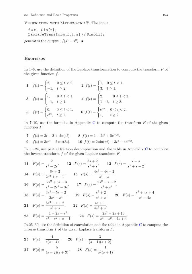
8.1 Definition and Basic Properties 193
Verification with Mathematica R©. The input
f=t - Sin[t];LaplaceTransform[f,t,s]//Simplify
generates the output 1/(s4 + s2).
Exercises
In 1–6, use the definition of the Laplace transformation to compute the transform F ofthe given function f .
1 f(t) =
{2, 0 ≤ t < 2,
−1, t ≥ 2.2 f(t) =
{1, 0 ≤ t < 1,
3, t ≥ 1.
3 f(t) =
{t, 0 ≤ t < 1,
−1, t ≥ 1.4 f(t) =
{2, 0 ≤ t < 3,
1− t, t ≥ 3.
5 f(t) =
{0, 0 ≤ t < 1,
e2t, t ≥ 1.6 f(t) =
{e−t, 0 ≤ t < 2,
1, t ≥ 2.
In 7–10, use the formulas in Appendix C to compute the transform F of the givenfunction f .
7 f(t) = 3t− 2 + sin(4t). 8 f(t) = 1− 2t3 + 5e−2t.
9 f(t) = 3e2t − 2 cos(3t). 10 f(t) = 2 sin(πt) + 3t2 − 4et/2.
In 11–24, use partial fraction decomposition and the table in Appendix C to computethe inverse transform f of the given Laplace transform F .
11 F (s) =2
s2 − 2s. 12 F (s) =
3s+ 2
s2 + s. 13 F (s) =
7− s
s2 + s− 2.
14 F (s) =6s+ 3
2s2 + s− 1. 15 F (s) =
4s2 − 4s− 2
s3 − s.
16 F (s) =2s2 + 3s− 3
s3 − 2s2 − 3s. 17 F (s) =
2s2 − s− 2
s3 + s2.
18 F (s) =3s2 − 5s− 2
2s2 − s3. 19 F (s) =
s2 + 2
s3 + s. 20 F (s) =
s2 + 4s+ 4
s3 + 4s.
21 F (s) =5s2 − s+ 2
s3 + s. 22 F (s) =
4s+ 1
4s3 + s.
23 F (s) =1 + 2s− s2
s3 − s2 + s− 1. 24 F (s) =
2s2 + 2s+ 10
s3 + s2 + 4s+ 4.
In 25–30, use the definition of convolution and the table in Appendix C to compute theinverse transform f of the given Laplace transform F .
25 F (s) =4
s(s+ 4). 26 F (s) =
3
(s− 1)(s+ 2).
27 F (s) =5
(s− 2)(s+ 3). 28 F (s) =
1
s2(s+ 1).
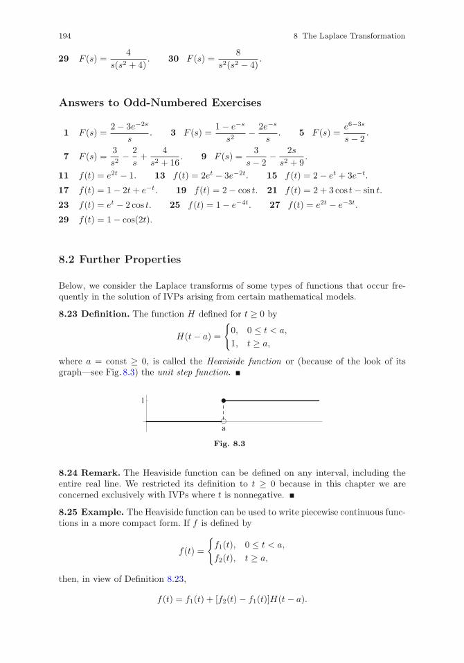
194 8 The Laplace Transformation
29 F (s) =4
s(s2 + 4). 30 F (s) =
8
s2(s2 − 4).
Answers to Odd-Numbered Exercises
1 F (s) =2− 3e−2s
s. 3 F (s) =
1− e−s
s2− 2e−s
s. 5 F (s) =
e6−3s
s− 2.
7 F (s) =3
s2− 2
s+
4
s2 + 16. 9 F (s) =
3
s− 2− 2s
s2 + 9.
11 f(t) = e2t − 1. 13 f(t) = 2et − 3e−2t. 15 f(t) = 2− et + 3e−t.
17 f(t) = 1− 2t+ e−t. 19 f(t) = 2− cos t. 21 f(t) = 2 + 3 cos t− sin t.
23 f(t) = et − 2 cos t. 25 f(t) = 1− e−4t. 27 f(t) = e2t − e−3t.
29 f(t) = 1− cos(2t).
8.2 Further Properties
Below, we consider the Laplace transforms of some types of functions that occur fre-quently in the solution of IVPs arising from certain mathematical models.
8.23 Definition. The function H defined for t ≥ 0 by
H(t− a) =
{0, 0 ≤ t < a,
1, t ≥ a,
where a = const ≥ 0, is called the Heaviside function or (because of the look of itsgraph—see Fig. 8.3) the unit step function.
8.24 Remark. The Heaviside function can be defined on any interval, including theentire real line. We restricted its definition to t ≥ 0 because in this chapter we areconcerned exclusively with IVPs where t is nonnegative.
8.25 Example. The Heaviside function can be used to write piecewise continuous func-tions in a more compact form. If f is defined by
f(t) =
{f1(t), 0 ≤ t < a,
f2(t), t ≥ a,
then, in view of Definition 8.23,
f(t) = f1(t) + [f2(t)− f1(t)]H(t− a).
a
1
Fig. 8.3
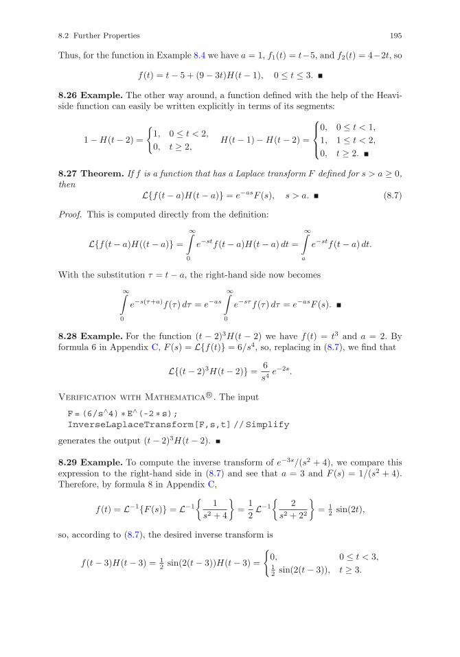
8.2 Further Properties 195
Thus, for the function in Example 8.4 we have a = 1, f1(t) = t−5, and f2(t) = 4−2t, so
f(t) = t− 5 + (9− 3t)H(t− 1), 0 ≤ t ≤ 3.
8.26 Example. The other way around, a function defined with the help of the Heavi-side function can easily be written explicitly in terms of its segments:
1−H(t− 2) =
{1, 0 ≤ t < 2,
0, t ≥ 2,H(t− 1)−H(t− 2) =
⎧⎪⎨⎪⎩0, 0 ≤ t < 1,
1, 1 ≤ t < 2,
0, t ≥ 2.
8.27 Theorem. If f is a function that has a Laplace transform F defined for s > a ≥ 0,then
L{f(t− a)H(t− a)} = e−asF (s), s > a. (8.7)
Proof. This is computed directly from the definition:
L{f(t− a)H((t− a)} =
∞∫0
e−stf(t− a)H(t− a) dt =
∞∫a
e−stf(t− a) dt.
With the substitution τ = t− a, the right-hand side now becomes
∞∫0
e−s(τ+a)f(τ) dτ = e−as
∞∫0
e−sτf(τ) dτ = e−asF (s).
8.28 Example. For the function (t − 2)3H(t − 2) we have f(t) = t3 and a = 2. Byformula 6 in Appendix C, F (s) = L{f(t)} = 6/s4, so, replacing in (8.7), we find that
L{(t− 2)3H(t− 2)} =6
s4e−2s.
Verification with Mathematica R©. The input
F=(6/s∧4) ∗E∧(-2 ∗s);InverseLaplaceTransform[F,s,t]//Simplify
generates the output (t− 2)3H(t− 2).
8.29 Example. To compute the inverse transform of e−3s/(s2 + 4), we compare thisexpression to the right-hand side in (8.7) and see that a = 3 and F (s) = 1/(s2 + 4).Therefore, by formula 8 in Appendix C,
f(t) = L−1{F (s)} = L−1
{1
s2 + 4
}=
1
2L−1
{2
s2 + 22
}= 1
2 sin(2t),
so, according to (8.7), the desired inverse transform is
f(t− 3)H(t− 3) = 12 sin(2(t− 3))H(t− 3) =
{0, 0 ≤ t < 3,12 sin(2(t− 3)), t ≥ 3.
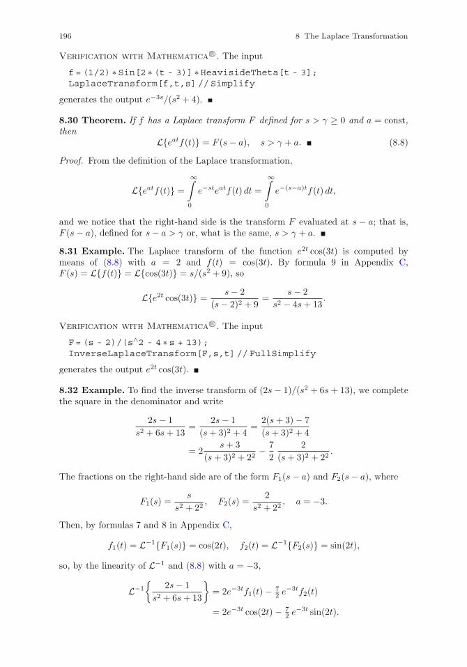
196 8 The Laplace Transformation
Verification with Mathematica R©. The input
f=(1/2) ∗Sin[2 ∗(t - 3)] ∗HeavisideTheta[t - 3];LaplaceTransform[f,t,s]//Simplify
generates the output e−3s/(s2 + 4).
8.30 Theorem. If f has a Laplace transform F defined for s > γ ≥ 0 and a = const,then
L{eatf(t)} = F (s− a), s > γ + a. (8.8)
Proof. From the definition of the Laplace transformation,
L{eatf(t)} =
∞∫0
e−steatf(t) dt =
∞∫0
e−(s−a)tf(t) dt,
and we notice that the right-hand side is the transform F evaluated at s − a; that is,F (s− a), defined for s− a > γ or, what is the same, s > γ + a.
8.31 Example. The Laplace transform of the function e2t cos(3t) is computed bymeans of (8.8) with a = 2 and f(t) = cos(3t). By formula 9 in Appendix C,F (s) = L{f(t)} = L{cos(3t)} = s/(s2 + 9), so
L{e2t cos(3t)} =s− 2
(s− 2)2 + 9=
s− 2
s2 − 4s+ 13.
Verification with Mathematica R©. The input
F=(s - 2)/(s∧2 - 4 ∗s + 13);InverseLaplaceTransform[F,s,t]//FullSimplify
generates the output e2t cos(3t).
8.32 Example. To find the inverse transform of (2s− 1)/(s2 + 6s+ 13), we completethe square in the denominator and write
2s− 1
s2 + 6s+ 13=
2s− 1
(s+ 3)2 + 4=
2(s+ 3)− 7
(s+ 3)2 + 4
= 2s+ 3
(s+ 3)2 + 22− 7
2
2
(s+ 3)2 + 22.
The fractions on the right-hand side are of the form F1(s− a) and F2(s− a), where
F1(s) =s
s2 + 22, F2(s) =
2
s2 + 22, a = −3.
Then, by formulas 7 and 8 in Appendix C,
f1(t) = L−1{F1(s)} = cos(2t), f2(t) = L−1{F2(s)} = sin(2t),
so, by the linearity of L−1 and (8.8) with a = −3,
L−1
{2s− 1
s2 + 6s+ 13
}= 2e−3tf1(t)− 7
2 e−3tf2(t)
= 2e−3t cos(2t)− 72 e
−3t sin(2t).
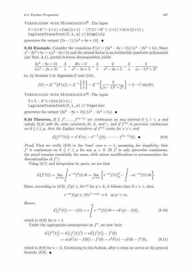
8.2 Further Properties 197
Verification with Mathematica R©. The input
f=2 ∗E∧(-3 ∗t) ∗Cos[2 ∗t] - (7/2) ∗E∧(-3 ∗t) ∗Sin[2 ∗t];LaplaceTransform[f,t,s]//Simplify
generates the output (2s− 1)/(s2 + 6s+ 13).
8.33 Example. Consider the transform F (s) = (3s2 − 8s+ 15)/(s3 − 2s2 + 5s). Sinces3−2s2+5s = s(s2−2s+5) and the second factor is an irreducible quadratic polynomial(see Sect. A.1), partial fraction decomposition yields
3s2 − 8s+ 15
s(s2 − 2s+ 5)=
A
s+
Bs+ C
s2 − 2s+ 5=
3
s− 2
s2 − 2s+ 5=
3
s− 2
(s− 1)2 + 22,
so, by formula 5 in Appendix C and (8.8),
f(t) = L−1{F (s)} = L−1
{3
s
}− L−1
{2
(s− 1)2 + 22
}= 3− et sin(2t).
Verification with Mathematica R©. The input
f=3 - E∧t ∗Sin[2 ∗t];LaplaceTransform[f,t,s]//Together
generates the output (3s2 − 8s+ 15)/(s3 − 2s2 + 5s).
8.34 Theorem. If f, f ′, . . . , f (n−1) are continuous on any interval 0 ≤ t ≤ p andsatisfy (8.3) with the same constants M , k, and γ, and if f (n) is piecewise continuouson 0 ≤ t ≤ p, then the Laplace transform of f (n) exists for s > γ and
L{f (n)(t)} = snF (s)− sn−1f(0)− · · · − f (n−1)(0). (8.9)
Proof. First we verify (8.9) in the ‘base’ case n = 1, assuming, for simplicity, thatf ′ is continuous on 0 ≤ t ≤ p for any p > 0. (If f ′ is only piecewise continuous,the proof remains essentially the same, with minor modifications to accommodate thediscontinuities of f ′.)
Using (8.7) and integration by parts, we see that
L{f ′(t)} = limp→∞
p∫0
e−stf ′(t) dt = limp→∞
{e−stf(t)
∣∣p0−
p∫0
−se−stf(t) dt
}.
Since, according to (8.3), f(p) ≤ Meγp for p > k, it follows that if s > γ, then
e−spf(p) ≤ Me(γ−s)p → 0 as p → ∞.
Hence,
L{f ′(t)} = −f(0) + s
∞∫0
e−stf(t) dt = sF (s)− f(0), (8.10)
which is (8.9) for n = 1.Under the appropriate assumptions on f ′′, we now have
L{f ′′(t)} = L{(f ′(t))′} = sL{f ′(t)} − f ′(0)
= s(sF (s)− f(0))− f ′(0) = s2F (s)− sf(0)− f ′(0), (8.11)
which is (8.9) for n = 2. Continuing in this fashion, after n steps we arrive at the generalformula (8.9).
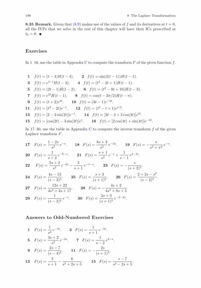
198 8 The Laplace Transformation
8.35 Remark. Given that (8.9) makes use of the values of f and its derivatives at t = 0,all the IVPs that we solve in the rest of this chapter will have their ICs prescribed att0 = 0.
Exercises
In 1–16, use the table in Appendix C to compute the transform F of the given function f .
1 f(t) = (t− 4)H(t− 4). 2 f(t) = sin(2(t− 1))H(t− 1).
3 f(t) = e3−tH(t− 3). 4 f(t) = (t2 − 2t+ 1)H(t− 1).
5 f(t) = (2t− 1)H(t− 2). 6 f(t) = (t2 − 8t+ 10)H(t− 3).
7 f(t) = e2tH(t− 1). 8 f(t) = cos(t− 3π/2)H(t− π).
9 f(t) = (t+ 2)e4t. 10 f(t) = (3t− 1)e−2t.
11 f(t) = (t2 − 2t)e−t. 12 f(t) = (t2 − t+ 1)et/2.
13 f(t) = [2− 3 sin(2t)]e−t. 14 f(t) = [3t− 2 + 2 cos(3t)]e2t.
15 f(t) = [cos(2t)− 3 sin(2t)]et. 16 f(t) = [2 cos(4t) + sin(4t)]e−3t.
In 17–30, use the table in Appendix C to compute the inverse transform f of the givenLaplace transform F .
17 F (s) =1− 2s
s2e−s. 18 F (s) =
8s+ 3
s2e−2s. 19 F (s) = − π
s2 + π2e−s.
20 F (s) =1
s+ 2e−6−s. 21 F (s) =
s+ 1
s2e−s +
1
s− 1e2−2s.
22 F (s) =5s+ 2
s2e−2s − 3
s+ 1e−1−s. 23 F (s) = − s
(s+ 2)2.
24 F (s) =4s− 13
(s− 3)2. 25 F (s) =
s+ 3
(s+ 1)3. 26 F (s) =
2 + 2s− s2
(s− 2)3.
27 F (s) =12s+ 22
4s2 + 4s+ 17. 28 F (s) = − 4s+ 2
4s2 + 8s+ 5.
29 F (s) =1
(s− 2)2e−s. 30 F (s) =
2s+ 3
(s+ 1)2e−2−2s.
Answers to Odd-Numbered Exercises
1 F (s) =1
s2e−4s. 3 F (s) =
1
s+ 1e−3s.
5 F (s) =3s+ 2
s2e−2s. 7 F (s) =
1
s− 2e2−s.
9 F (s) =2s− 7
(s− 4)2. 11 F (s) = − 2s
(s+ 1)3.
13 F (s) =2
s+ 1− 6
s2 + 2s+ 5. 15 F (s) =
s− 7
s2 − 2s+ 5.
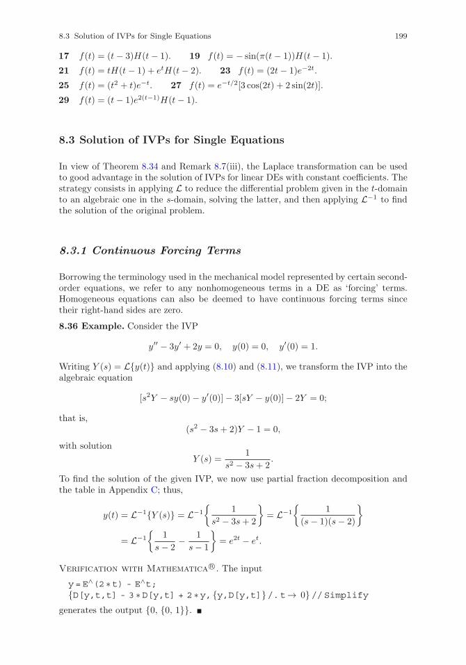
8.3 Solution of IVPs for Single Equations 199
17 f(t) = (t− 3)H(t− 1). 19 f(t) = − sin(π(t− 1))H(t− 1).
21 f(t) = tH(t− 1) + etH(t− 2). 23 f(t) = (2t− 1)e−2t.
25 f(t) = (t2 + t)e−t. 27 f(t) = e−t/2[3 cos(2t) + 2 sin(2t)].
29 f(t) = (t− 1)e2(t−1)H(t− 1).
8.3 Solution of IVPs for Single Equations
In view of Theorem 8.34 and Remark 8.7(iii), the Laplace transformation can be usedto good advantage in the solution of IVPs for linear DEs with constant coefficients. Thestrategy consists in applying L to reduce the differential problem given in the t-domainto an algebraic one in the s-domain, solving the latter, and then applying L−1 to findthe solution of the original problem.
8.3.1 Continuous Forcing Terms
Borrowing the terminology used in the mechanical model represented by certain second-order equations, we refer to any nonhomogeneous terms in a DE as ‘forcing’ terms.Homogeneous equations can also be deemed to have continuous forcing terms sincetheir right-hand sides are zero.
8.36 Example. Consider the IVP
y′′ − 3y′ + 2y = 0, y(0) = 0, y′(0) = 1.
Writing Y (s) = L{y(t)} and applying (8.10) and (8.11), we transform the IVP into thealgebraic equation
[s2Y − sy(0)− y′(0)]− 3[sY − y(0)]− 2Y = 0;
that is,(s2 − 3s+ 2)Y − 1 = 0,
with solution
Y (s) =1
s2 − 3s+ 2.
To find the solution of the given IVP, we now use partial fraction decomposition andthe table in Appendix C; thus,
y(t) = L−1{Y (s)} = L−1
{1
s2 − 3s+ 2
}= L−1
{1
(s− 1)(s− 2)
}
= L−1
{1
s− 2− 1
s− 1
}= e2t − et.
Verification with Mathematica R©. The input
y=E∧(2 ∗t) - E∧t;{D[y,t,t] - 3 ∗D[y,t] + 2 ∗y,{y,D[y,t]}/.t→ 0}//Simplify
generates the output {0, {0, 1}}.
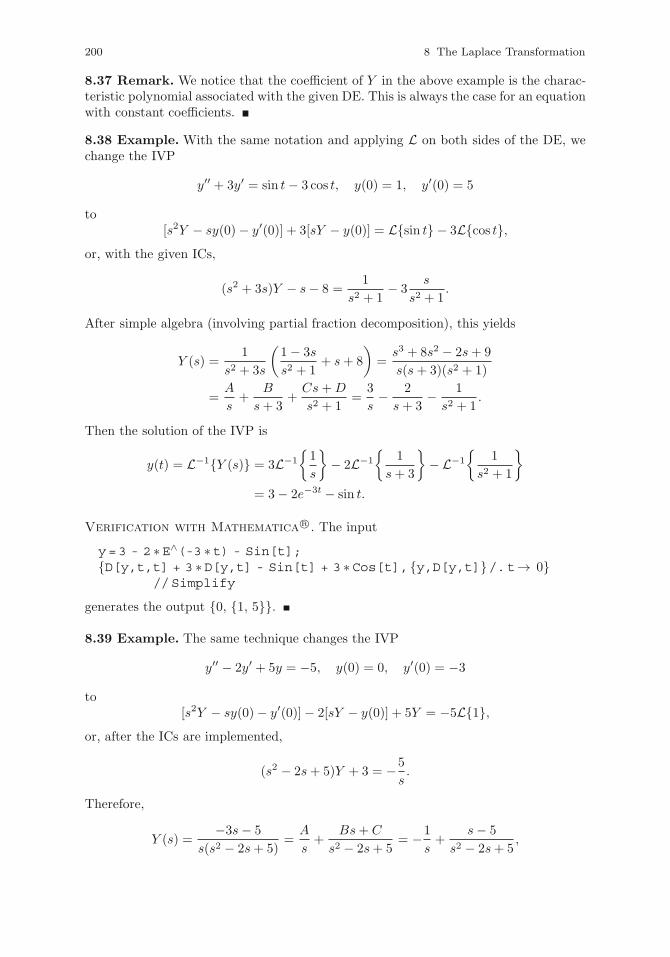
200 8 The Laplace Transformation
8.37 Remark. We notice that the coefficient of Y in the above example is the charac-teristic polynomial associated with the given DE. This is always the case for an equationwith constant coefficients.
8.38 Example. With the same notation and applying L on both sides of the DE, wechange the IVP
y′′ + 3y′ = sin t− 3 cos t, y(0) = 1, y′(0) = 5
to[s2Y − sy(0)− y′(0)] + 3[sY − y(0)] = L{sin t} − 3L{cos t},
or, with the given ICs,
(s2 + 3s)Y − s− 8 =1
s2 + 1− 3
s
s2 + 1.
After simple algebra (involving partial fraction decomposition), this yields
Y (s) =1
s2 + 3s
(1− 3s
s2 + 1+ s+ 8
)=
s3 + 8s2 − 2s+ 9
s(s+ 3)(s2 + 1)
=A
s+
B
s+ 3+Cs+D
s2 + 1=
3
s− 2
s+ 3− 1
s2 + 1.
Then the solution of the IVP is
y(t) = L−1{Y (s)} = 3L−1
{1
s
}− 2L−1
{1
s+ 3
}− L−1
{1
s2 + 1
}
= 3− 2e−3t − sin t.
Verification with Mathematica R©. The input
y=3 - 2 ∗E∧(-3 ∗t) - Sin[t];{D[y,t,t] + 3 ∗D[y,t] - Sin[t] + 3 ∗Cos[t],{y,D[y,t]}/.t→ 0}
//Simplify
generates the output {0, {1, 5}}.
8.39 Example. The same technique changes the IVP
y′′ − 2y′ + 5y = −5, y(0) = 0, y′(0) = −3
to[s2Y − sy(0)− y′(0)]− 2[sY − y(0)] + 5Y = −5L{1},
or, after the ICs are implemented,
(s2 − 2s+ 5)Y + 3 = −5
s.
Therefore,
Y (s) =−3s− 5
s(s2 − 2s+ 5)=
A
s+
Bs+ C
s2 − 2s+ 5= −1
s+
s− 5
s2 − 2s+ 5,
8.3 Solution of IVPs for Single Equations 201
which, since s2 − 2s+ 5 = (s− 1)2 + 4, can be written as
Y (s) = −1
s+
(s− 1)− 4
(s− 1)2 + 4= −1
s+
s− 1
(s− 1)2 + 22− 2
2
(s− 1)2 + 22.
By Theorem 8.30 with a = 1 and formulas 5, 8, and 9 in Appendix C, we see that thesolution of the given IVP is
y(t) = L−1{Y (s)} = −1 + et[cos(2t)− 2 sin(2t)].
Verification with Mathematica R©. The input
y= - 1 + E∧t ∗(Cos[2 ∗t] - 2 ∗Sin[2 ∗t]);{D[y,t,t] - 2 ∗D[y,t] + 5 ∗y + 5, {y,D[y,t]}/.t→ 0}//Simplify
generates the output {0, {0, −3}}.
8.40 Example. After application of the Laplace transformation, the IVP
y′′ − 2y′ + y = 2t− 1, y(0) = 1, y′(0) = 5
reduces to
(s2 − 2s+ 1)Y − s− 3 =2
s2− 1
s,
which, since s2 − 2s+ 1 = (s− 1)2, in final analysis leads to
Y (s) =s3 + 3s2 − s+ 2
s2(s− 1)2=
A
s+
B
s2+
C
s− 1+
D
(s− 1)2
=3
s+
2
s2− 2
s− 1+
5
(s− 1)2.
The formulas in Appendix C now yield
y(t) = L−1{Y (s)} = 3 + 2t− 2et + 5tet = (5t− 2)et + 2t+ 3.
Verification with Mathematica R©. The input
y=(5 ∗t - 2) ∗E∧t + 2 ∗t + 3;{D[y,t,t] - 2 ∗D[y,t] + y - 2 ∗t + 1, {y,D[y,t]}/.t→ 0}//Simplify
generates the output {0, {1, 5}}.
8.41 Example. Applying L to the IVP
y′′′ − 2y′′ − y′ + 2y = −6, y(0) = −1, y′(0) = 6, y′′(0) = 8
and sorting out the terms, we arrive at
(s3 − 2s2 − s+ 2)Y + s2 − 8s+ 3 = −6
s,
from which
Y (s) =−s3 + 8s2 − 3s− 6
s(s3 − 2s2 − s+ 2).
202 8 The Laplace Transformation
We now use synthetic division or the symmetry of the coefficients to obtain
s3 − 2s2 − s+ 2 = (s− 1)(s+ 1)(s− 2),
so, by partial fraction decomposition,
Y (s) =A
s+
B
s− 1+
C
s+ 1+
D
s− 2= −3
s+
1
s− 1− 1
s+ 1+
2
s− 2.
Hence, the solution of the given IVP is
y(t) = L−1{Y (s)} = −3 + et − e−t + 2e2t.
Verification with Mathematica R©. The input
y= - 3 + E∧t - E∧(-t) + 2 ∗E∧(2 ∗t);{D[y,t,3] - 2 ∗D[y,t,t] - D[y,t] + 2 ∗y + 6, {y,D[y,t],D[y,t,t]}
/.t→ 0}//Simplifygenerates the output {0, {−1, 6, 8}}.
8.42 Example. Consider the IVP
y′′ − 6y′ + 8y = f(t), y(0) = 2, y′(0) = 1,
where f is an unspecified function with Laplace transform F . Applying L and perform-ing the necessary algebra, we arrive at
(s2 − 6s+ 8)Y = 2s− 11 + F (s).
Since s2 − 6s+ 8 = (s− 2)(s− 4), partial fraction decomposition now yields
Y (s) =7
2(s− 2)− 3
2(s− 4)+
{1
2(s− 4)− 1
2(s− 2)
}F (s).
The last term on the right-hand side can be written as F (s)G(s), where
G(s) =1
2(s− 4)− 1
2(s− 2),
sog(t) = L−1{G(s)} = 1
2 e4t − 1
2 e2t.
Then, by (8.6) and (8.5), the inverse transform of that term is
L−1{F (s)G(s)} = (f ∗ g)(t) =t∫
0
f(t− τ)g(τ) dτ
= 12
t∫0
f(t− τ)(e4τ − e2τ ) dτ.
Hence, the solution of the IVP is
y(t) = L−1{Y (s)} = 72 e
2t − 32 e
4t + 12
t∫0
f(t− τ)(e4τ − e2τ ) dτ.
8.3 Solution of IVPs for Single Equations 203
If, say, f(t) = 8t+ 2, then, integrating by parts, we have
12
t∫0
f(t− τ)(e4τ − e2τ ) dτ =
t∫0
(e4τ − 22τ )[1 + 4(t− τ)] dτ
= 12 e
4t − 32 e
2t + t+ 1,
and so,
y(t) = 72 e
2t − 32 e
4t + 12 e
4t − 32 e
2t + t+ 1 = 2e2t − e4t + t+ 1.
Verification with Mathematica R©. The input
y=2 ∗E∧(2 ∗t) - E∧(4 ∗t) + t + 1;{D[y,t,t] - 6 ∗D[y,t] + 8 ∗y - 8 ∗t - 2, {y,D[y,t]}/.t→ 0}
//Simplify
generates the output {0, {2, 1}}.
Exercises
Use the Laplace transformation method to solve the given IVP.
1 y′′ + 4y′ + 3y = −3, y(0) = −2, y′(0) = 5.
2 2y′′ − 3y′ + y = 2, y(0) = 7, y′(0) = 3.
3 y′′ + 2y′ + y = 4, y(0) = 2, y′(0) = 3.
4 4y′′ − 4y′ + y = −3, y(0) = −5, y′(0) = 1.
5 y′′ + y = 1, y(0) = 4, y′(0) = −1.
6 y′′ + 4y = −8, y(0) = −1, y′(0) = 4.
7 y′′ − 5y′ + 6y = 6t− 5, y(0) = −3, y′(0) = −7.
8 2y′′ + y′ − 6y = 7− 6t, y(0) = 0, y′(0) = −8.
9 y′′ − 6y′ + 9y = 24− 9t, y(0) = 2, y′(0) = 0.
10 y′′ − 2y′ + 2y = 4− 2t, y(0) = 3, y′(0) = 2.
11 y′′ − 4y′ + 5y = 10t− 13, y(0) = 1, y′(0) = 3.
12 y′′ + 4y′ = −3e−t, y(0) = −1, y′(0) = −5.
13 y′′ + 4y′ − 5y = −14e2t, y(0) = −3, y′(0) = 7.
14 y′′ + 8y′ + 16y = −75et, y(0) = −1, y′(0) = −11.
15 9y′′ − 12y′ + 4y = 50e−t, y(0) = −1, y′(0) = −2.
16 4y′′ − 4y′ + 5y = 13e−t, y(0) = 3, y′(0) = −2.
17 4y′′ + 8y′ + 5y = −37e2t, y(0) = −5, y′(0) = 3.
18 y′′ + 2y′ − 8y = −2 cos t+ 9 sin t, y(0) = 2, y′(0) = 9.
19 y′′ − 2y′ = −12 cos(2t) + 4 sin(2t), y(0) = 4, y′(0) = 0.
20 9y′′ − 6y′ + y = 4(3 cos t+ 4 sin t), y(0) = 0, y′(0) = −1.
204 8 The Laplace Transformation
21 y′′ + 6y′ + 9y = 7 cos(2t) + 17 sin(2t), y(0) = −3, y′(0) = 8.
22 y′′ − 2y′ − 3y = −3t− 8− 12et, y(0) = 7, y′(0) = 2.
23 y′′ + 3y′ − 10y = 30− 12e−t, y(0) = −2, y′(0) = 6.
24 y′′ + 4y′ + 4y = 2(e−t − 8), y(0) = −3, y′(0) = 1.
25 y′′ + y′ = 3, y(0) = 2, y′(0) = 2.
26 2y′′ − y′ − y = 3et, y(0) = 2, y′(0) = −3.
27 y′′′ − 4y′ = 8, y(0) = 2, y′(0) = −8, y′′(0) = −4.
28 y′′′ + 2y′′ − 3y′ = −3, y(0) = 3, y′(0) = 6, y′′(0) = −7.
29 y′′′ − 2y′′ + y′ = 2e2t, y(0) = 2, y′(0) = 2, y′′(0) = 5.
30 y′′′ − 4y′′ + 4y′ = −9e−t, y(0) = 4, y′(0) = 2, y′′(0) = 5.
31 y′′′ − y′′ − 4y′ + 4y = 4, y(0) = 0, y′(0) = 5, y′′(0) = −7.
32 y′′′ − 3y′′ + 4y = 2et, y(0) = 2, y′(0) = −2, y′′(0) = 3.
Answers to Odd-Numbered Exercises
1 y(t) = e−t − 2e−3t − 1. 3 y(t) = (t− 2)e−t + 4.
5 y(t) = 3 cos t− sin t+ 1. 7 y(t) = t− e2t − 2e3t.
9 y(t) = te3t + 2− t. 11 y(t) = e2t(2 cos t− 3 sin t) + 2t− 1.
13 y(t) = et − 2e−5t − 2e2t. 15 y(t) = (2t− 3)e2t/3 + 2e−t.
17 y(t) = 2e−t[sin(t/2)− 2 cos(t/2)]− e2t.
19 y(t) = 3− e2t + 2 cos(2t) + sin(2t).
21 y(t) = −2e−3t − cos(2t) + sin(2t). 23 y(t) = e2t − e−5t + e−t − 3.
25 y(t) = 3t+ 1 + e−t. 27 y(t) = e−2t − 2e2t − 2t+ 3.
29 y(t) = 2 + (t− 1)et + e2t. 31 y(t) = et − 2e−2t + 1.
8.3.2 Piecewise Continuous Forcing Terms
The Laplace transformation method is particularly useful when the right-hand side ofthe DE is a discontinuous function, since in such cases it is very difficult to find a PSof the nonhomogeneous equation by the methods discussed in Sect. 4.5.
8.43 Example. Consider the IVP
y′′ + y = g(t),
y(0) = 0, y′(0) = 0,g(t) =
{1, 0 < t < 1,
0, t ≥ 1.
Noticing that g(t) = 1 − H(t − 1) and recalling Theorem 8.27 (with f(t) = 1 and,therefore, F (s) = 1/s), we apply L to every term in the equation and arrive at
[s2Y − sy(0)− y′(0)] + Y = (s2 + 1)Y = L{1−H(t− 1)} =1
s− 1
se−s;
8.3 Solution of IVPs for Single Equations 205
hence,
Y (s) =1
s(s2 + 1)(1− e−s).
Since, by partial fraction decomposition,
1
s(s2 + 1)=
A
s+Bs+ C
s2 + 1=
1
s− s
s2 + 1,
it follows that
Y (s) =
(1
s− s
s2 + 1
)(1− e−s),
so, by (8.7),
y(t) = L−1{Y (s)} = L−1
{1
s− s
s2 + 1−(1
s− s
s2 + 1
)e−s
}
= 1− cos t− [1− cos(t− 1)]H(t− 1).
Verification with Mathematica R©. The input
y=1 - Cos[t] - (1 - Cos[t - 1]) ∗HeavisideTheta[t - 1];{D[y,t,t] + y - 1 + HeavisideTheta[t - 1], {y,D[y,t]}/.t→ 0}
//Simplify
generates the output {0, {0, 0}}.
8.44 Example. Consider the IVP
y′′ + 5y′ + 4y = g(t),
y(0) = 0, y′(0) = 0,g(t) =
{12, 1 ≤ t < 2,
0, 0 < t < 1, t ≥ 2.
The right-hand side of the DE can be written in the form g(t) = 12[H(t−1)−H(t−2)],so, proceeding as in Example 8.43, we find that
(s2 + 5s+ 4)Y = L{H(t− 1)} − L{H(t− 2)} =12
s(e−s − e−2s);
therefore,
Y (s) =12
s(s2 + 5s+ 4)(e−s − e−2s).
Since s2 + 5s+ 4 = (s+ 1)(s+ 4), partial fraction decomposition gives
12
s(s+ 1)(s+ 4)=
A
s+
B
s+ 1+
C
s+ 4=
3
s− 4
s+ 1+
1
s+ 4,
from which
y(t) = L−1{Y (s)} = L−1
{(3
s− 4
s+ 1+
1
s+ 4
)(e−s − e−2s)
},
so, by (8.7),
y(t) = [3− 4e−(t−1) + e−4(t−1)]H(t− 1)
− [3 − 4e−(t−2) + e−4(t−2)]H(t− 2).
206 8 The Laplace Transformation
Verification with Mathematica R©. The input
y=(3 - 4 ∗E∧(-(t - 1)) + E∧(-4 ∗(t - 1))) ∗HeavisideTheta[t - 1]- (3 - 4 ∗E∧(-(t - 2)) + E∧(-4 ∗(t - 2)))∗HeavisideTheta[t - 2];
{D[y,t,t] + 5 ∗D[y,t] + 4 ∗y - 12 ∗(HeavisideTheta[t - 1]- HeavisideTheta[t - 2]), {y,D[y,t]}/.t→ 0}//Simplify
generates the output {0, {0, 0}}.8.45 Example. The forcing term in the IVP
y′′ + 4y′ + 4y = g(t),
y(0) = 0, y′(0) = 1,g(t) =
{t, 1 ≤ t < 3,
0, 0 < t < 1, t ≥ 3
can be written as
g(t) = t[H(t− 1)−H(t− 3)]
= (t− 1)H(t− 1)− (t− 3)H(t− 3) +H(t− 1)− 3H(t− 3),
so, by Theorem 8.27 with f(t) = t and then f(t) = 1,
L{g(t)} =1
s2e−s − 1
s2e−3s +
1
se−s − 3
se−3s =
s+ 1
s2e−s − 3s+ 1
s2e−3s.
After application of L, the left-hand side of the DE becomes
[s2Y − sy(0)− y′(0)] + 4[sY − y(0)] + 4Y
= (s2 + 4s+ 4)Y − 1 = (s+ 2)2Y − 1;
therefore, equating the transforms of the two sides, solving for Y , and using partialfraction decomposition, we arrive at
Y (s) =1
(s+ 2)2+
s+ 1
s2(s+ 2)2e−s − 3s+ 1
s2(s+ 2)2e−3s
=1
(s+ 2)2+
1
4
[1
s2− 1
(s+ 2)2
]e−s
− 1
4
[2
s+
1
s2− 2
s+ 2− 5
(s+ 2)2
]e−3s.
Then, by Theorem 8.27 in conjunction with Theorem 8.30,
y(t) = te−2t + 14 [1− e−2(t−1)](t− 1)H(t− 1)
− 14 [2− 2e−2(t−3) + (t− 3)− 5(t− 3)e−2(t−3)]H(t− 3).
Verification with Mathematica R©. The input
y=t ∗E∧(-2 ∗t) + (1/4) ∗(1 - E∧(-2 ∗(t - 1))) ∗(t - 1)∗HeavisideTheta[t - 1] - (1/4) ∗(2 - 2 ∗E∧( - 2*(t - 3))+ t-3 - 5 ∗(t - 3) ∗E∧(-2 ∗(t - 3))) ∗HeavisideTheta[t - 3];
{D[y,t,t] + 4 ∗D[y,t] + 4 ∗y - t ∗(HeavisideTheta[t - 1]- HeavisideTheta[t - 3]), {y,D[y,t]}/.t→ 0}//Simplify
generates the output {0, {0, 1}}.
8.3 Solution of IVPs for Single Equations 207
Exercises
Use the Laplace transformation method to solve the given IVP.
1 y′′ − y′ = H(t− 1), y(0) = 0, y′(0) = 0.
2 y′′ + 2y′ = −4H(t− 2), y(0) = 0, y′(0) = 0.
3 2y′′ − y′ = 1−H(t− 1), y(0) = 0, y′(0) = 0.
4 y′′ − 4y′ = 16[2−H(t− 2)], y(0) = 0, y′(0) = 0.
5 y′′ + y′ − 2y = 6H(t− 1/2), y(0) = 0, y′(0) = 0.
6 y′′ − 4y′ + 3y = 6[1− 2H(t− 3)], y(0) = 0, y′(0) = 0.
7 y′′ − 2y′ + y = H(t− 2), y(0) = 0, y′(0) = 0.
8 y′′ − 6y′ + 9y = 9[1−H(t− 1)], y(0) = 0, y′(0) = 0.
9 y′′ − 4y′ + 5y = 5H(t− 1), y(0) = 0, y′(0) = 0.
10 y′′ + 4y = 4[2−H(t− 2)], y(0) = 0, y′(0) = 0.
11 y′′ − 3y′ + 2y = 4tH(t− 1), y(0) = 0, y′(0) = 0.
12 y′′ + y′ − 6y = 30H(t− 2), y(0) = 5, y′(0) = 0.
13 2y′′ − 3y′ − 2y = 10H(t− 3), y(0) = 0, y′(0) = 5.
14 y′′ + 3y′ = 18H(t− 1/2), y(0) = 3, y′(0) = −3.
15 y′′ + 2y′ + y = tH(t− 4), y(0) = 2, y′(0) = 1.
16 4y′′ + y = 1− 5e1−tH(t− 1), y(0) = 4, y′(0) = 0.
17 3y′′ + y′ = H(t− 1)−H(t− 2), y(0) = 0, y′(0) = 0.
18 y′′ − 5y′ + 4y = 12[H(t− 2) +H(t− 3)], y(0) = 3, y′(0) = 0.
19 y′′ + 9y = 9[3tH(t− 1)−H(t− 2)], y(0) = 0, y′(0) = 0.
20 y′′ − 4y′ + 4y = et−1H(t− 1)− 4H(t− 3), y(0) = 0, y′(0) = 1.
Answers to Odd-Numbered Exercises
1 y(y) = (et−1 − t)H(t− 1).
3 y(t) = 2et/2 − t− 2 + [t+ 1− 2e(t−1)/2]H(t− 1).
5 y(t) = [e−2(t−1/2) + 2et−1/2 − 3]H(t− 1/2).
7 y(t) = [1 + (t− 3)et−2]H(t− 2).
9 y(t) = {1− e2(t−1)[cos(t− 1)− 2 sin(t− 1)]}H(t− 1).
11 y(t) = [3e2(t−1) − 8et−1 + 2t+ 3]H(t− 1).
13 y(t) = 2e2t − 2e−t/2 + [e2(t−3) + 4e(t−3)/2 − 5]H(t− 3).
15 y(t) = (3t+ 2)e−t + [t− 2 + (10− 3t)e4−t]H(t− 4).
17 y(t) = [t− 4 + 3e(1−t)/3]H(t− 1) + [5− t− 3e(2−t)/3]H(t− 2).
19 y(t) = [3t− 3 cos(3(t− 1))− sin(3(t− 1))]H(t− 1)
+ [cos(3(t− 2))− 1]H(t− 2).
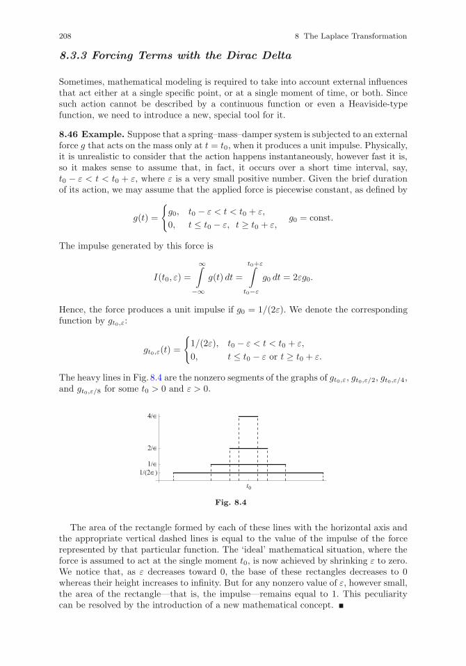
208 8 The Laplace Transformation
8.3.3 Forcing Terms with the Dirac Delta
Sometimes, mathematical modeling is required to take into account external influencesthat act either at a single specific point, or at a single moment of time, or both. Sincesuch action cannot be described by a continuous function or even a Heaviside-typefunction, we need to introduce a new, special tool for it.
8.46 Example. Suppose that a spring–mass–damper system is subjected to an externalforce g that acts on the mass only at t = t0, when it produces a unit impulse. Physically,it is unrealistic to consider that the action happens instantaneously, however fast it is,so it makes sense to assume that, in fact, it occurs over a short time interval, say,t0 − ε < t < t0 + ε, where ε is a very small positive number. Given the brief durationof its action, we may assume that the applied force is piecewise constant, as defined by
g(t) =
{g0, t0 − ε < t < t0 + ε,
0, t ≤ t0 − ε, t ≥ t0 + ε,g0 = const.
The impulse generated by this force is
I(t0, ε) =
∞∫−∞
g(t) dt =
t0+ε∫t0−ε
g0 dt = 2εg0.
Hence, the force produces a unit impulse if g0 = 1/(2ε). We denote the correspondingfunction by gt0,ε:
gt0,ε(t) =
{1/(2ε), t0 − ε < t < t0 + ε,
0, t ≤ t0 − ε or t ≥ t0 + ε.
The heavy lines in Fig. 8.4 are the nonzero segments of the graphs of gt0,ε, gt0,ε/2, gt0,ε/4,and gt0,ε/8 for some t0 > 0 and ε > 0.
t0
4/∈
2/∈
1/∈1/(2∈)
Fig. 8.4
The area of the rectangle formed by each of these lines with the horizontal axis andthe appropriate vertical dashed lines is equal to the value of the impulse of the forcerepresented by that particular function. The ‘ideal’ mathematical situation, where theforce is assumed to act at the single moment t0, is now achieved by shrinking ε to zero.We notice that, as ε decreases toward 0, the base of these rectangles decreases to 0whereas their height increases to infinity. But for any nonzero value of ε, however small,the area of the rectangle—that is, the impulse—remains equal to 1. This peculiaritycan be resolved by the introduction of a new mathematical concept.
8.3 Solution of IVPs for Single Equations 209
8.47 Definition. The quantity
δ(t− t0) = limε→0
gt0,ε(t)
is called the Dirac delta.
8.48 Remark. It is obvious that δ(t − t0) is characterized by the following two prop-erties:
(i) δ(t− t0) = 0 for t �= t0;
(ii)∞∫
−∞δ(t− t0) dt = 1.
Clearly, the limiting process by means of which the Dirac delta is defined does notascribe it a finite value at t = t0. (If it did, then the integral in (ii) would be zero.)Consequently, δ is not a function. In mathematics this object is called a distribution,or generalized function.
8.49 Theorem. If f is a continuous function on the real line, then
∞∫−∞
f(t) δ(t− t0) dt = f(t0). (8.12)
Proof. By the mean value theorem for integrals, there is at least one point t∗ in theinterval t0 − ε ≤ t ≤ t0 + ε such that
∞∫−∞
f(t) gt0,ε(t) dt =
t0+ε∫t0−ε
1
2εf(t) dt =
1
2ε
t0+ε∫t0−ε
f(t) dt =1
2ε· 2εf(t∗) = f(t∗).
Letting ε → 0, we obtain (8.12).
8.50 Example. If t0 ≥ 0, then, by the definitions of L and δ and Theorem 8.49 withf(t) = e−st,
L{δ(t− t0)} =
∞∫0
e−stδ(t− t0) dt =
∞∫−∞
e−stδ(t− t0) dt = e−st0 , s > 0.
In particular, L{δ(t)} = 1.
8.51 Example. Let g be a continuous function. A direct application of Theorem 8.49with f(t) = e−stg(t) yields
L{g(t)δ(t− t0)} =
∞∫0
e−stg(t)δ(t− t0) dt =
∞∫−∞
e−stg(t)δ(t− t0) dt = g(t0)e−st0 .
8.52 Example. Let α = const > 0. To compute L{δ(α(t− t0))}, we use the definitionof L and the substitution α(t− t0) = τ (or, what is the same, t = τ/α+ t0):
L{δ(α(t − t0))} =
∞∫−∞
e−stδ(α(t− t0)) dt =
∞∫−∞
e−s(τ/α+t0)δ(τ) · 1αdτ ;
so, by (8.12),
L{δ(α(t− t0))} =1
αe−st0 .
210 8 The Laplace Transformation
8.53 Example. Consider the IVP
y′′ + π2y = δ(t− 1), y(0) = 1, y′(0) = 0.
Applying L to all the terms in the DE, we change the IVP to
[s2Y − sy(0)− y′(0)] + π2Y = e−s,
from which, after using the ICs, we obtain
Y (s) =s+ e−s
s2 + π2=
s
s2 + π2+
1
π
π
s2 + π2e−s.
Then the solution of the IVP is
y(t) = L−1{Y (s)} = cos(πt) +1
πsin(π(t− 1))H(t− 1).
Writing sin(π(t−1)) = sin(πt−π) = sin(πt) cosπ−cos(πt) sin π = − sin(πt), we simplifythis to
y(t) = cos(πt)− 1
πsin(πt)H(t − 1) =
{cos(πt), 0 ≤ t < 1,
cos(πt)− (1/π) sin(πt), t ≥ 1.
Verification with Mathematica R©. The input
y=Cos[Pi ∗t] - (1/Pi) ∗Sin[Pi ∗t] ∗HeavisideTheta[t - 1];{D[y,t,t] + Pi∧2 ∗y - DiracDelta[t - 1], {y,D[y,t]}/.t→ 0}
//Simplify
generates the output {0, {1, 0}}.8.54 Example. From formula 14 in Appendix C with f(t) = 2t + 1 and a = 1/2 itfollows that L{(2t + 1) δ(t − 1/2)} = 2e−s/2, so the Laplace transformation changesthe IVP
y′′ − 4y′ + 3y = (2t+ 1)δ(t− 1
2
), y(0) = 0, y′(0) = 2
into the algebraic problem
(s2 − 4s+ 3)Y − 2 = 2e−s/2;
hence,
Y (s) =2
s2 − 4s+ 3(1 + e−s/2) =
(1
s− 3− 1
s− 1
)(1 + e−s/2).
By formula 2 in Appendix C, we now obtain
y(t) = L−1{Y (s)} = e3t − et + [e3(t−1/2) − et−1/2]H(t− 1
2
).
Verification with Mathematica R©. The input
y=E∧(3 ∗t) - E∧t + (E∧(3 ∗(t - 1/2)) - E∧(t - 1/2))∗HeavisideTheta[t - 1/2];
{D[y,t,t] - 4 ∗D[y,t] + 3 ∗y - (2 ∗t + 1) ∗DiracDelta[t - 1/2],{y,D[y,t]}/.t→ 0}//Simplify
generates the output {0, {0, 2}}.
8.3 Solution of IVPs for Single Equations 211
8.55 Example. Applying the Laplace transformation to the IVP
y′′ + y′ = δ(t− 1)− δ(t− 2), y(0) = 0, y′(0) = 0,
we arrive at
(s2 + s)Y = e−s − e−2s;
therefore,
Y (s) =1
s2 + s(e−s − e−2s) =
(1
s− 1
s+ 1
)(e−s − e−2s),
which yields the solution
y(t) = L−1{Y (s)} = [1− e−(t−1)]H(t− 1)− [1− e−(t−2)]H(t− 2).
Explicitly, this is
y(t) =
⎧⎪⎨⎪⎩0, 0 ≤ t < 1,
1− e−(t−1), 1 ≤ t < 2,
−e−(t−1) + e−(t−2), t ≥ 2.
Verification with Mathematica R©. The input
y=(1 - E∧(-(t - 1))) ∗HeavisideTheta[t - 1] - (1 - E∧(-(t - 2)))∗HeavisideTheta[t - 2];
{D[y,t,t] + D[y,t] - DiracDelta[t - 1] + DiracDelta[t - 2],{y,D[y,t]}/.t→ 0}//Simplify
generates the output {0, {0, 0}}.
Exercises
Use the Laplace transformation method to solve the given IVP.
1 y′′ − 2y′ = 2δ(t− 2), y(0) = 0, y′(0) = 0.
2 2y′′ + y′ = δ(t− 1), y(0) = 1, y′(0) = 0.
3 y′′ − y′ = 1− δ(t− 1), y(0) = 0, y′(0) = 0.
4 y′′ + y′ = 2δ(t− 1)− δ(t− 3), y(0) = 0, y′(0) = 1.
5 y′′ + 4y = δ(t− 3), y(0) = −1, y′(0) = 0.
6 y′′ + y = 2− δ(t− 2), y(0) = 2, y′(0) = 1.
7 y′′ − y = t− δ(t− 1), y(0) = 0, y′(0) = 0.
8 y′′ − 4y = e−t + 2δ(t− 2), y(0) = −1, y′(0) = 1.
9 y′′ + 9y = (t+ 1)δ(t− 2), y(0) = 2, y′(0) = 9.
10 9y′′ − 4y = etδ(t− 2), y(0) = 1, y′(0) = 0.
11 y′′ + 3y′ + 2y = δ(t− 1), y(0) = 0, y′(0) = 0.
12 y′′ − y′ − 2y = t− 1 + δ(t− 2), y(0) = 0, y′(0) = −1.
13 y′′ + 2y′ + y = 3− δ(t− 1/2), y(0) = 2, y′(0) = 0.
212 8 The Laplace Transformation
14 y′′ − 4y′ + 4y = 2δ(t− 1), y(0) = 0, y′(0) = 0.
15 y′′ − 2y′ − 3y = 4(cos t)δ(t− π), y(0) = 0, y′(0) = 0.
16 y′′ − 2y′ + 2y = (sin t)δ(t− π/2), y(0) = 0, y′(0) = 1.
17 y′′ + y′ = 2δ(t− 1)− δ(t− 2), y(0) = 1, y′(0) = 0.
18 y′′ + y = δ(t− π/2) + δ(t− π), y(0) = 0, y′(0) = 1.
19 y′′ − 4y = δ(t− 1/2) + δ(t− 1), y(0) = 1, y′(0) = −1.
20 y′′ − y′ − 6y = (t+ 1)δ(t− 2)− δ(t− 3), y(0) = 0, y′(0) = 0.
Answers to Odd-Numbered Exercises
1 y(t) = [e2(t−2) − 1]H(t− 2). 3 y(t) = et − t− 1 + (1 − et−1)H(t− 1).
5 y(t) = − cos(2t) + (1/2) sin(2(t− 3))H(t− 3).
7 y(t) = sinh t− t− sinh(t− 1)H(t− 1).
9 y(t) = 2 cos(3t) + 3 sin(3t) + sin(3(t− 2))H(t− 2).
11 y(t) = [e1−t − e2(1−t)]H(t− 1).
13 y(t) = 3− (t+ 1)e−t − (t− 1/2)e1/2−tH(t− 1/2).
15 y(t) = [eπ−t − e3(t−π)]H(t− π).
17 y(t) = 1 + 2(1− e1−t)H(t− 1)− (1− e2−t)H(t− 2).
19 y(t) = cosh(2t)− (1/2) sinh(2t) + (1/2) sinh(2t− 1)H(t− 1/2)
+ (1/2) sinh(2(t− 1))H(t− 1).
8.3.4 Equations with Variable Coefficients
In special circumstances, the Laplace transformation can also be used to solve IVPsfor DEs with nonconstant coefficients. Owing to the difficulties that arise in such cases,however, the scope of the method here is very limited.
8.56 Example. Consider the IVP
y′′ + ty′ − 2y = 4, y(0) = 0, y′(0) = 0.
As usual, let L{y(t)} = Y (s). By formula 16 (with n = 1) in Appendix C,
L{ty′(t)} = − d
dsL{y′}(s) = −[sY (s)− y(0)]′ = −[sY (s)]′ = −Y − sY ′.
Consequently, the transformed problem is
[s2Y − sy(0)− y′(0)]− Y − sY ′ − 2Y =4
s,
or, in view of the ICs,
sY ′ + (3− s2)Y = −4
s.
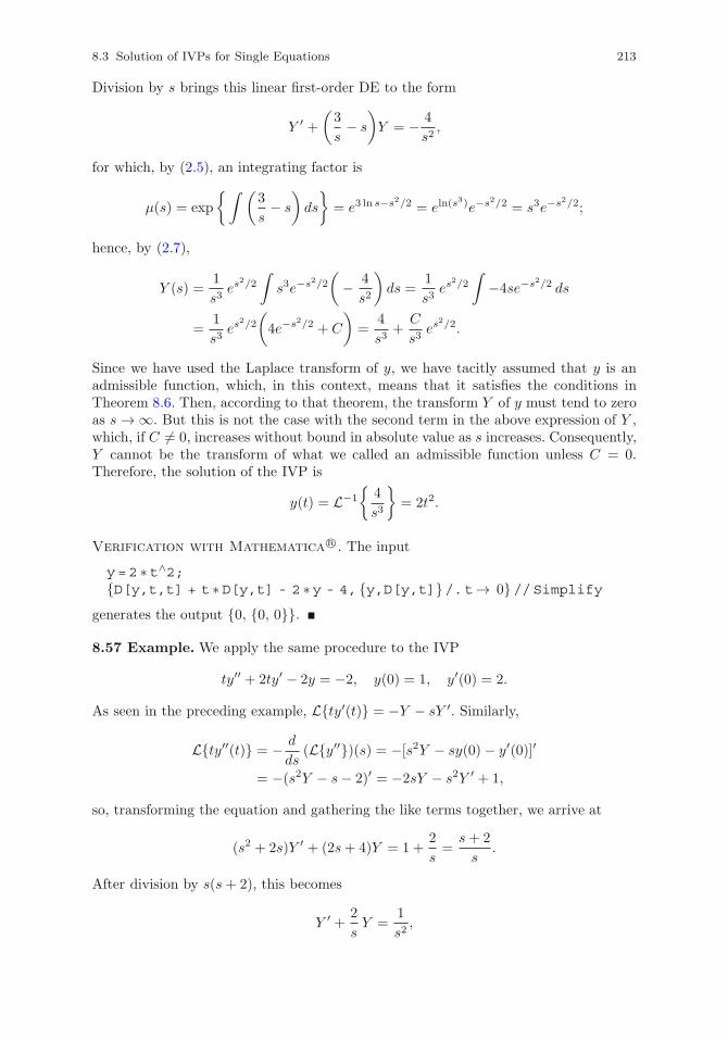
8.3 Solution of IVPs for Single Equations 213
Division by s brings this linear first-order DE to the form
Y ′ +(3
s− s
)Y = − 4
s2,
for which, by (2.5), an integrating factor is
μ(s) = exp
{∫ (3
s− s
)ds
}= e3 ln s−s2/2 = eln(s
3)e−s2/2 = s3e−s2/2;
hence, by (2.7),
Y (s) =1
s3es
2/2
∫s3e−s2/2
(− 4
s2
)ds =
1
s3es
2/2
∫−4se−s2/2 ds
=1
s3es
2/2
(4e−s2/2 + C
)=
4
s3+
C
s3es
2/2.
Since we have used the Laplace transform of y, we have tacitly assumed that y is anadmissible function, which, in this context, means that it satisfies the conditions inTheorem 8.6. Then, according to that theorem, the transform Y of y must tend to zeroas s → ∞. But this is not the case with the second term in the above expression of Y ,which, if C �= 0, increases without bound in absolute value as s increases. Consequently,Y cannot be the transform of what we called an admissible function unless C = 0.Therefore, the solution of the IVP is
y(t) = L−1
{4
s3
}= 2t2.
Verification with Mathematica R©. The input
y=2 ∗t∧2;{D[y,t,t] + t ∗D[y,t] - 2 ∗y - 4, {y,D[y,t]}/.t→ 0}//Simplify
generates the output {0, {0, 0}}.
8.57 Example. We apply the same procedure to the IVP
ty′′ + 2ty′ − 2y = −2, y(0) = 1, y′(0) = 2.
As seen in the preceding example, L{ty′(t)} = −Y − sY ′. Similarly,
L{ty′′(t)} = − d
ds(L{y′′})(s) = −[s2Y − sy(0)− y′(0)]′
= −(s2Y − s− 2)′ = −2sY − s2Y ′ + 1,
so, transforming the equation and gathering the like terms together, we arrive at
(s2 + 2s)Y ′ + (2s+ 4)Y = 1 +2
s=
s+ 2
s.
After division by s(s+ 2), this becomes
Y ′ +2
sY =
1
s2,
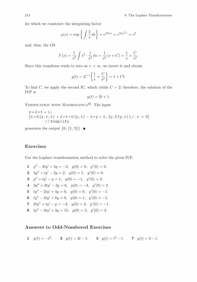
214 8 The Laplace Transformation
for which we construct the integrating factor
μ(s) = exp
{∫2
sds
}= e2 ln s = eln(s
2) = s2
and, thus, the GS
Y (s) =1
s2
∫s2 · 1
s2ds =
1
s2(s+ C) =
1
s+
C
s2.
Since this transform tends to zero as s → ∞, we invert it and obtain
y(t) = L−1
{1
s+
C
s2
}= 1 + Ct.
To find C, we apply the second IC, which yields C = 2; therefore, the solution of theIVP is
y(t) = 2t+ 1.
Verification with Mathematica R©. The input
y=2 ∗t + 1;{t ∗D[y,t,t] + 2 ∗t ∗D[y,t] - 2 ∗y + 2, {y,D[y,t]}/.t→ 0}
//Simplify
generates the output {0, {1, 2}}.
Exercises
Use the Laplace transformation method to solve the given IVP.
1 y′′ − 2ty′ + 4y = −2, y(0) = 0, y′(0) = 0.
2 2y′′ + ty′ − 2y = 2, y(0) = 1, y′(0) = 0.
3 y′′ + ty′ − y = 1, y(0) = −1, y′(0) = 3.
4 3y′′ + 2ty′ − 2y = 6, y(0) = −3, y′(0) = 2.
5 ty′′ − 2ty′ + 4y = 0, y(0) = 0, y′(0) = −1.
6 ty′′ − 4ty′ + 8y = 8, y(0) = 1, y′(0) = −1.
7 2ty′′ + ty′ − y = −3, y(0) = 3, y′(0) = −1.
8 ty′′ − 3ty′ + 3y = 15, y(0) = 5, y′(0) = 2.
Answers to Odd-Numbered Exercises
1 y(t) = −t2. 3 y(t) = 3t− 1. 5 y(t) = t2 − t. 7 y(t) = 3− t.
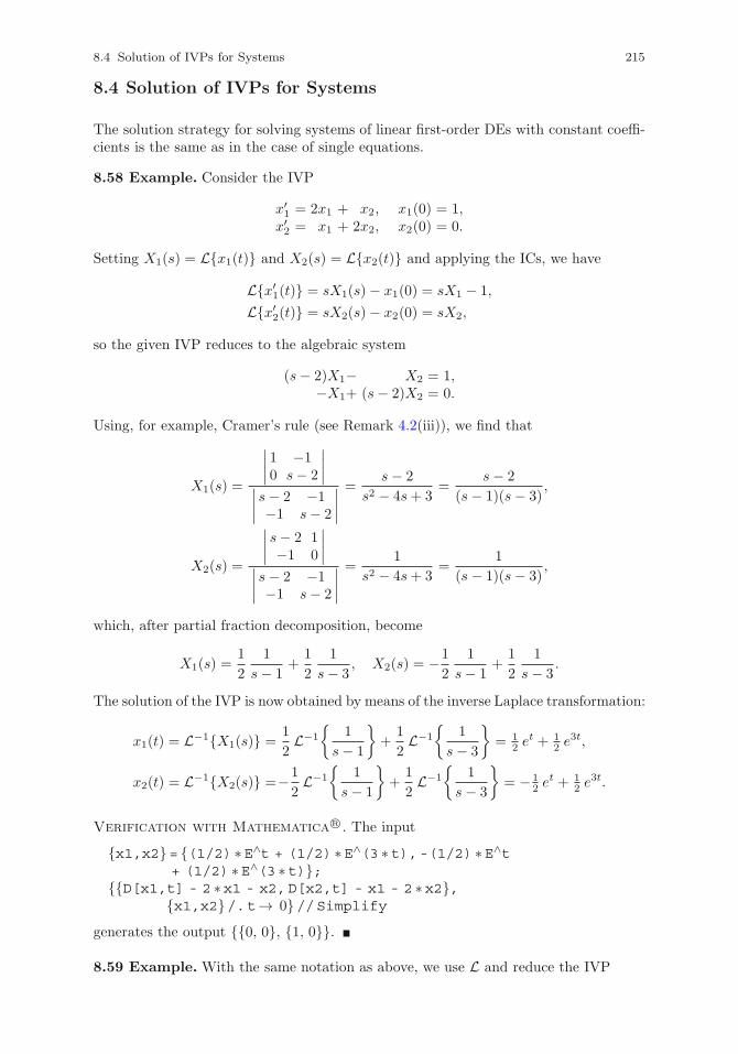
8.4 Solution of IVPs for Systems 215
8.4 Solution of IVPs for Systems
The solution strategy for solving systems of linear first-order DEs with constant coeffi-cients is the same as in the case of single equations.
8.58 Example. Consider the IVP
x′1 = 2x1 + x2, x1(0) = 1,x′2 = x1 + 2x2, x2(0) = 0.
Setting X1(s) = L{x1(t)} and X2(s) = L{x2(t)} and applying the ICs, we have
L{x′1(t)} = sX1(s)− x1(0) = sX1 − 1,
L{x′2(t)} = sX2(s)− x2(0) = sX2,
so the given IVP reduces to the algebraic system
(s− 2)X1− X2 = 1,−X1+ (s− 2)X2 = 0.
Using, for example, Cramer’s rule (see Remark 4.2(iii)), we find that
X1(s) =
∣∣∣∣ 1 −10 s− 2
∣∣∣∣∣∣∣∣ s− 2 −1−1 s− 2
∣∣∣∣=
s− 2
s2 − 4s+ 3=
s− 2
(s− 1)(s− 3),
X2(s) =
∣∣∣∣ s− 2 1−1 0
∣∣∣∣∣∣∣∣ s− 2 −1−1 s− 2
∣∣∣∣=
1
s2 − 4s+ 3=
1
(s− 1)(s− 3),
which, after partial fraction decomposition, become
X1(s) =1
2
1
s− 1+
1
2
1
s− 3, X2(s) = −1
2
1
s− 1+
1
2
1
s− 3.
The solution of the IVP is now obtained by means of the inverse Laplace transformation:
x1(t) = L−1{X1(s)} =1
2L−1
{1
s− 1
}+
1
2L−1
{1
s− 3
}= 1
2 et + 1
2 e3t,
x2(t) = L−1{X2(s)} =−1
2L−1
{1
s− 1
}+
1
2L−1
{1
s− 3
}= − 1
2 et + 1
2 e3t.
Verification with Mathematica R©. The input
{x1,x2}= {(1/2) ∗E∧t + (1/2) ∗E∧(3 ∗t),-(1/2) ∗E∧t+ (1/2) ∗E∧(3 ∗t)};
{{D[x1,t] - 2 ∗x1 - x2,D[x2,t] - x1 - 2 ∗x2},{x1,x2}/.t→ 0}//Simplify
generates the output {{0, 0}, {1, 0}}.
8.59 Example. With the same notation as above, we use L and reduce the IVP
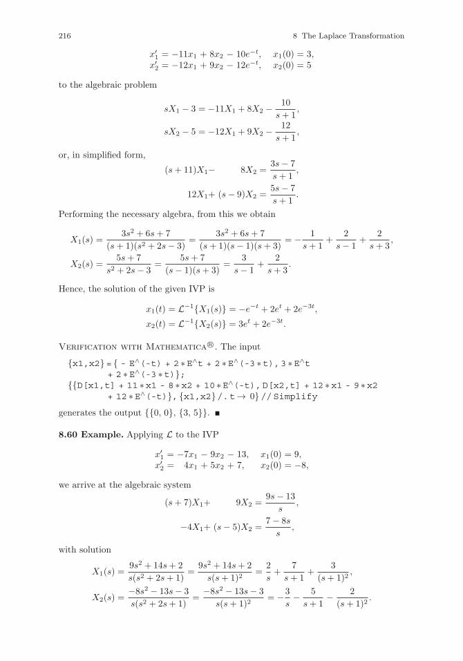
216 8 The Laplace Transformation
x′1 = −11x1 + 8x2 − 10e−t, x1(0) = 3,x′2 = −12x1 + 9x2 − 12e−t, x2(0) = 5
to the algebraic problem
sX1 − 3 = −11X1 + 8X2 − 10
s+ 1,
sX2 − 5 = −12X1 + 9X2 − 12
s+ 1,
or, in simplified form,
(s+ 11)X1− 8X2 =3s− 7
s+ 1,
12X1+ (s− 9)X2 =5s− 7
s+ 1.
Performing the necessary algebra, from this we obtain
X1(s) =3s2 + 6s+ 7
(s+ 1)(s2 + 2s− 3)=
3s2 + 6s+ 7
(s+ 1)(s− 1)(s+ 3)= − 1
s+ 1+
2
s− 1+
2
s+ 3,
X2(s) =5s+ 7
s2 + 2s− 3=
5s+ 7
(s− 1)(s+ 3)=
3
s− 1+
2
s+ 3.
Hence, the solution of the given IVP is
x1(t) = L−1{X1(s)} = −e−t + 2et + 2e−3t,
x2(t) = L−1{X2(s)} = 3et + 2e−3t.
Verification with Mathematica R©. The input
{x1,x2}= { - E∧(-t) + 2 ∗E∧t + 2 ∗E∧(-3 ∗t),3 ∗E∧t+ 2 ∗E∧(-3 ∗t)};
{{D[x1,t] + 11 ∗x1 - 8 ∗x2 + 10 ∗E∧(-t),D[x2,t] + 12 ∗x1 - 9 ∗x2+ 12 ∗E∧(-t)}, {x1,x2}/.t→ 0}//Simplify
generates the output {{0, 0}, {3, 5}}.
8.60 Example. Applying L to the IVP
x′1 = −7x1 − 9x2 − 13, x1(0) = 9,x′2 = 4x1 + 5x2 + 7, x2(0) = −8,
we arrive at the algebraic system
(s+ 7)X1+ 9X2 =9s− 13
s,
−4X1+ (s− 5)X2 =7− 8s
s,
with solution
X1(s) =9s2 + 14s+ 2
s(s2 + 2s+ 1)=
9s2 + 14s+ 2
s(s+ 1)2=
2
s+
7
s+ 1+
3
(s+ 1)2,
X2(s) =−8s2 − 13s− 3
s(s2 + 2s+ 1)=
−8s2 − 13s− 3
s(s+ 1)2= −3
s− 5
s+ 1− 2
(s+ 1)2.
8.4 Solution of IVPs for Systems 217
Then the solution of the given IVP is
x1(t) = L−1{X1(s)} = 2+ 7e−t + 3te−t = 2 + (3t+ 7)e−t,
x2(t) = L−1{X2(s)} = −3− 5e−t − 2te−t = −3− (2t+ 5)e−t.
Verification with Mathematica R©. The input
{x1,x2}= {2 + (3 ∗t + 7) ∗E∧(-t), - 3 - (2 ∗t + 5) ∗E∧(-t)};{{D[x1,t] + 7 ∗x1 + 9 ∗x2 + 13,D[x2,t] - 4 ∗x1 - 5 ∗x2 - 7},
{x1,x2}/.t→ 0}//Simplifygenerates the output {{0, 0}, {9, −8}}.
8.61 Example. The same technique applied to the IVP
x′1 = 2x1 − x2 + x3, x1(0) = 1,x′2 = 2x1 − x2 + 2x3, x2(0) = 1,x3 = x1 − x2, x3(0) = 2
leads to(s− 2)X1 + X2 − X3 = 1,
−2X1 + (s+ 1)X2 − 2X3 = 1,−X1 + X2 + sX3 = 2.
Using Gaussian elimination to solve this algebraic system, synthetic division or thesymmetry of the coefficients to factor out the denominator, and partial fraction decom-position, after a rather long but straightforward calculation we find that
X1 =s2 + 2s− 1
s3 − s2 + s− 1=
s2 + 2s− 1
(s− 1)(s2 + 1)=
1
s− 1+
2
s2 + 1,
X2 =s2 + 4s− 3
s3 − s2 + s− 1=
s2 + 4s− 3
(s− 1)(s2 + 1)=
1
s− 1+
4
s2 + 1,
X3 =2s
s2 + 1,
which yields
x1(t) = L−1{X1(s)} = et + 2 sin t,
x2(t) = L−1{X2(s)} = et + 4 sin t,
x3(t) = L−1{X3(s)} = 2 cos t.
Verification with Mathematica R©. The input
{x1,x2,x3}= {E∧t + 2 ∗Sin[t],E∧t + 4 ∗Sin[t],2 ∗Cos[t]};{{D[x1,t] - 2 ∗x1 + x2 - x3,D[x2,t] - 2 ∗x1 + x2 - 2 ∗x3,
D[x3,t] - x1 + x2}, {x1,x2,x3}/.t→ 0}//Simplifygenerates the output {{0, 0, 0}, {1, 1, 2}}.
218 8 The Laplace Transformation
Exercises
Use the Laplace transformation method to solve the IVP x′ = Ax+ f , x(0) = x0, withthe given matrix A, vector function f , and constant vector x0.
1 A =
(7 −48 −5
), f(t) =
(00
), x0 =
(13
).
2 A =
(7 10
−5 −8
), f(t) =
(00
), x0 =
(−12
).
3 A =
( −4 2−10 4
), f(t) =
(00
), x0 =
(23
).
4 A =
(2 1
−1 2
), f(t) =
(00
), x0 =
(31
).
5 A =
(5 −49 −7
), f(t) =
(00
), x0 =
(13
).
6 A =
(2 1
−1 4
), f(t) =
(00
), x0 =
(21
).
7 A =
(−8 18−3 7
), f(t) =
(−2−1
), x0 =
(11
).
8 A =
(8 −39 −4
), f(t) =
(05
), x0 =
(615
).
9 A =
(1 4
−1 −3
), f(t) =
(10
), x0 =
(16−6
).
10 A =
(−1 −1/25/2 1
), f(t) =
(0
−1
), x0 =
(−11
).
11 A =
(3 1
−1 3
), f(t) =
(−4−2
), x0 =
(2
−1
).
12 A =
(−1 −21 −4
), f(t) =
(t− 1
−t− 4
), x0 =
(52
).
13 A =
(3/2 1
−1/2 0
), f(t) =
(3
t− 2
), x0 =
(1
−2
).
14 A =
(−1 −91 5
), f(t) =
(11− 4t−3
), x0 =
(−42
).
15 A =
(1/2 −11 1/2
), f(t) =
(5
−5t− 1
), x0 =
(03
).
16 A =
(7 3
−6 −2
), f(t) =
(−2e−t
4e−t
), x0 =
(5
−7
).
17 A =
(0 1
−1 2
), f(t) =
(2e−t
10e−t
), x0 =
(2
−3
).
18 A =
(2 1/2
−9/2 −1
), f(t) =
(0et
), x0 =
(6
−14
).
19 A =
(−1 4−2 3
), f(t) =
(02et
), x0 =
(41
).
8.4 Solution of IVPs for Systems 219
20 A =
(−3 −64 7
), f(t) =
(4 cos t
−6 cos t
), x0 =
(−11
).
21 A =
⎛⎝−5 6 −3−1 2 −14 −4 2
⎞⎠ , f(t) =
⎛⎝000
⎞⎠ , x0 =
⎛⎝035
⎞⎠ .
22 A =
⎛⎝ 1 −1 1
2 −2 1−2 1 0
⎞⎠ , f(t) =
⎛⎝000
⎞⎠ , x0 =
⎛⎝ 2
3−2
⎞⎠ .
23 A =
⎛⎝−1 1 0−1 1 11 −1 −2
⎞⎠ , f(t) =
⎛⎝000
⎞⎠ , x0 =
⎛⎝522
⎞⎠ .
24 A =
⎛⎝−3 −2 2
2 1 −1−2 −2 2
⎞⎠ , f(t) =
⎛⎝ 1−10
⎞⎠ , x0 =
⎛⎝−1
43
⎞⎠ .
25 A =
⎛⎝−1/2 −3/2 −1/2
1/2 3/2 1/2−3 −5 1
⎞⎠ , f(t) =
⎛⎝004
⎞⎠ , x0 =
⎛⎝−4
3−5
⎞⎠ .
26 A =
⎛⎝3 −2 −20 2 11 −2 −1
⎞⎠ , f(t) =
⎛⎝−5
0−1
⎞⎠ , x0 =
⎛⎝−1
2−5
⎞⎠ .
Answers to Odd-Numbered Exercises
1 x(t) =
(2e−t − e3t
4e−t − e3t
). 3 x(t) =
(2 cos(2t)− sin(2t)3 cos(2t)− 4 sin(2t)
).
5 x(t) =
(1− 6t3− 9t
)e−t. 7 x(t) =
(2et − 3e−2t + 2et − e−2t + 1
).
9 x(t) =
((6t+ 13)e−t + 3−(3t+ 5)e−t − 1
). 11 x(t) =
(e3t(cos t− 2 sin t) + 1
−e3t(2 cos t+ sin t) + 1
).
13 x(t) =
(2et − 3et/2 + 2t+ 2−et + 3et/2 − 3t− 4
). 15 x(t) =
(−et/2(2 cos t+ sin t) + 4t+ 2et/2(cos t− 2 sin t) + 2t+ 2
).
17 x(t) =
((1− t)et + e−t
−tet − 3e−t
). 19 x(t) =
(2 cos(2t)− 2 sin(2t) + 2
−2 sin(2t) + 1
)et.
21 x(t) =
⎛⎝e
t − e−2t
2 + et
4 + e−2t
⎞⎠ . 23 x(t) =
⎛⎝(t+ 4)e−t + 1
e−t + 1(t+ 2)e−t
⎞⎠ .
25 x(t) =
⎛⎝ et(sin t− cos t)− 3
et(cos t− sin t) + 2−2et(cos t+ sin t)− 3
⎞⎠ .
Chapter 9
Series Solutions
Owing to the complicated structure of some DEs, it is not always possible to obtain theexact solution of an IVP. In such situations, we need to resort to methods that producean approximate solution, which is usually constructed in the form of an infinite series.In what follows we illustrate a procedure of this type, based on series expansions forfunctions of a real variable.
9.1 Power Series
9.1 Definition. A power series is an expression of the form
∞∑n=0
an(t− t0)n, (9.1)
where t0 is a given real number and the an, n = 0, 1, 2, . . . , are constant real coefficients.Series (9.1) is said to be convergent at t if
s(t) = limm→∞ sm(t) = lim
m→∞
m∑n=0
an(t− t0)n exists;
sm(t) is called the sequence of partial sums and s(t) is the sum of the series.
Series (9.1) is said to be absolutely convergent at t if the series∞∑n=0
|an||t− t0|n isconvergent.
A series that is not convergent is called divergent.The radius of convergence of series (9.1) is a nonnegative number ρ such that the
series is absolutely convergent for all t satisfying |t− t0| < ρ (that is, t0−ρ < t < t0+ρ)and divergent for all t satisfying |t− t0| > ρ (that is, t < t0 − ρ or t > t0 + ρ).
9.2 Remarks. (i) The radius of convergence may be a finite number (including 0) orinfinite, and its definition is independent of the behavior (convergence or divergence)of the series at the points t = t0 − ρ and t = t0 + ρ.
(ii) Power series with the same radius of convergence ρ can be added, subtracted,multiplied, and differentiated term by term, and the result is always a series withradius of convergence ρ.
(iii) Two power series are equal if they have the same coefficients an. In particular, aseries is equal to zero if all its coefficients are 0.
C. Constanda, Differential Equations: A Primer for Scientists and Engineers, SpringerUndergraduate Texts in Mathematics and Technology, DOI 10.1007/978-1-4614-7297-1 9,© Springer Science+Business Media New York 2013
221
222 9 Series Solutions
9.3 Example. Let f be an infinitely differentiable function, and let t0 be a point in itsdomain. The Taylor series of f about t0, namely
∞∑n=0
f (n)(t0)
n!(t− t0)
n, (9.2)
where f (n)(t0) is the derivative of order n of f at t0, is a power series.
9.4 Definition. If the Taylor series (9.2) converges to f(t) at all points t in some openinterval containing t0, then the function f is said to be analytic at t0.
9.5 Remarks. (i) The sum f + g and product fg of two analytic functions at t0 arealso analytic at t0. The same is true for the quotient f/g provided that g(t0) �= 0.
(ii) Polynomials are terminating power series; that is, they are power series with finitelymany terms, and, therefore, an infinite radius of convergence. The ratio of twopolynomials is analytic at t0 if t0 is not a zero of the denominator.
In what follows we investigate equations of the form
P (t)y′′ +Q(t)y′ +R(t)y = 0, (9.3)
where P, Q, and R are given analytic functions.
9.6 Definition. A point t0 such that P (t0) �= 0 is called an ordinary point for (9.3). IfP (t0) = 0, then t0 is called a singular point.
9.7 Remarks. (i) The above definition implies that if t0 is an ordinary point, thenthe functions Q/P and R/P are analytic at t0 and, thus, can be expanded in powerseries around this point.
(ii) To simplify the computation, in the examples discussed below we confine ourselvesalmost exclusively to the case where P, Q, and R are polynomials.
9.2 Series Solution Near an Ordinary Point
In the neighborhood of an ordinary point t0, we may consider a solution of (9.3) of theform (9.1), where the coefficients an are determined from a recurrence relation obtainedby replacing series (9.1) in the equation.
9.8 Theorem. If t0 is an ordinary point for equation (9.3), then the general solutionof the equation can be written as
y = c1y1 + c2y2,
where c1 and c2 are arbitrary constants and y1 and y2 are linearly independent seriessolutions of the form (9.1). The radius of convergence of y1 and y2 is at least as largeas that of the series for Q/P and R/P .
9.9 Example. For the equationy′′ + y = 0
we have P (t) = 1, Q(t) = 0, and R(t) = 1, so Q(t)/P (t) = 0 and R(t)/P (t) = 1. Itis trivial to see that the radius of convergence of the series for both Q/P and R/P is
9.2 Series Solution Near an Ordinary Point 223
infinite, and that t = 0 is an ordinary point for the equation. This allows us to seek thesolution of the DE in the neighborhood of 0 in the form (9.1) with t0 = 0. Substitutingthe series in the equation, we arrive at
∞∑n=0
n(n− 1)antn−2 +
∞∑n=0
antn = 0. (9.4)
To write both terms as a single infinite sum, we change the index of summation in thefirst term by setting m = n − 2, so the summation is now over m from −2 to ∞; thatis, the first term becomes
∞∑m=−2
(m+ 2)(m+ 1)am+2tm.
Noting that the summand above vanishes for m = −2 and m = −1, we start thesummation from 0 and, replacing m by n, we combine the two terms in (9.4) to obtain
∞∑n=0
[(n+ 1)(n+ 2)an+2 + an]tn = 0.
Hence, by Remark 9.2(iii), the coefficient of tn must be 0 for all nonnegative integersn, which yields the recurrence relation
an+2 = − 1
(n+ 1)(n+ 2)an, n = 0, 1, . . . .
Taking, in turn, n = 0, 1, . . . , we compute all the coefficients an in terms of a0 and a1,which remain arbitrary; specifically,
a2 = − 1
1 · 2 a0 = − 1
2!a0,
a3 = − 1
2 · 3 a1 = − 1
3!a1,
a4 = − 1
3 · 4 a2 =1
2! · 3 · 4 a0 =1
4!a0,
a5 = − 1
4 · 5 a3 =1
3! · 4 · 5 a1 =1
5!a1,
...
We now replace these coefficients in (9.1), gather the like terms together, and write thesolution of the given equation as
y(t) = c1y1(t) + c2y2(t),
where
y1(t) = 1− 12! t
2 + 14! t
4 − · · · ,y2(t) =
11! t− 1
3! t3 + 1
5! t5 − · · · ,
and the arbitrary constants c1 and c2 stand for a0 and a1, respectively. Since, clearly,y1 and y2 are solutions of the equation and since they are linearly independent
224 9 Series Solutions
(one is not a multiple of the other), this formula represents the GS of the DE. In fact,we recall that the power series for y1 and y2 are the Taylor series about t = 0 of cos tand sin t. This confirms what we already knew from Sect. 4.3 about the form of the GSof our equation.
We also mention that, by Theorem 9.8, the series for y1 and y2 have an infinite radiusof convergence; that is, they converge for all real values of t.
Verification with Mathematica R©. The input
y1=(1 - (1/2!) ∗t∧2 + (1/4!) ∗t∧4;y2=(1/1!) ∗t - (1/3!) ∗t∧3 + (1/5!) ∗t∧5;y=c1 ∗y1 + c2 ∗y2;rem=D[y,t,t] + y;rem//Expand
generates the output c1t4/24+c2t
5/120, which is the remainder when the GS is replacedin the equation.
9.10 Remark. A ‘rule of thumb’ for determining the expected order of magnitude ofthe remainder when a truncated series solution is substituted in the given DE is basedon considering the lowest power of t that occurs on the left-hand side of the equationafter the replacement. If that power is N , then we anticipate the lowest power of t inthe remainder to be no less than N + 1. In the above example, N for y1 and y2 is 2and 3, respectively, and the corresponding remainders confirm our prediction. The ruleis invalid for a solution represented by a terminating series, where the remainder isobviously zero.
This type of comment will be omitted in the rest of the examples.
9.11 Example. The series solution method does not always produce the general so-lution of a DE with constant coefficients in the form supplied by the characteristicequation technique. For the equation
y′′ − 3y′ + 2y = 0,
the latter leads toy(t) = c1e
t + c2e2t.
On the other hand, substituting series (9.1) in the equation and manipulating thesummation index as we did in Example 9.9, we arrive at the equality
∞∑n=0
[(n+ 1)(n+ 2)an+2 − 3(n+ 1)an+1 + 2an]tn = 0,
from which we obtain the recurrence relation
an+2 =1
(n+ 1)(n+ 2)[3(n+ 1)an+1 − 2an], n = 0, 1, . . . .
Hence, with arbitrary coefficients a0 and a1, we get the GS
y(t) = a0(1− t2 − t3 − 7
12 t4 − 1
4 t5 + · · · )+ a1
(t+ 3
2 t2 + 7
6 t3 + 5
8 t4 + 31
120 t5 + · · · ).
A quick check shows that the series multiplied by a0 and a1 are not the Taylor expan-sions around t = 0 of et and e2t. Further checking shows that they are, in fact, the
9.2 Series Solution Near an Ordinary Point 225
expansions of 2et − e2t and e2t − et. But that is perfectly acceptable since, as is easilyverified by means of their Wronskian, these two functions also form an FSS for ourequation and are, therefore, a legitimate alternative choice for writing its GS. We easilydeduce from the (constant) coefficients of the equation that both series occurring in yconverge for all real t.
Verification with Mathematica R©. The input
y1=1 - t∧2 - t∧3 - (7/12) ∗t∧4 - (1/4) ∗t∧5;y2=t + (3/2) ∗t∧2 + (7/6) ∗t∧3 + (5/8) ∗t∧4 + (31/120) ∗t∧5;y=c1 ∗y1 + c2 ∗y2;rem=D[y,t,t] - 3 ∗D[y,t] + 2 ∗y;rem//Expand
generates the output c1(31t4/12− t5/2) + c2(−21t4/8 + 31t5/60).
9.12 Example. It is obvious that t = 0 is an ordinary point for the DE
(t+ 2)y′′ + (t− 1)y′ + 2ty = 0.
Here, we have Q(t)/P (t) = (t − 1)/(t + 2) and R(t)/P (t) = 2t/(t + 2). Since thesefunctions are undefined at t = −2, it follows that their power series in the neighborhoodof t = 0 converge for |t| < 2; in other words, their radius of convergence is ρ = 2.
Replacing y by (9.1) in the equation, we find that
∞∑n=0
n(n− 1)antn−1 + 2
∞∑n=0
n(n− 1)antn−2
+
∞∑n=0
nantn −
∞∑n=0
nantn−1 + 2
∞∑n=0
antn+1 = 0.
To even out the various powers of t in the sums above, we set m = n − 1 in the firstand fourth terms, m = n− 2 in the second, and m = n+ 1 in the fifth, then change mback to n; thus,
∞∑n=−1
(n+ 1)nan+1tn + 2
∞∑n=−2
(n+ 2)(n+ 1)an+2tn
+
∞∑n=0
nantn −
∞∑n=−1
(n+ 1)an+1tn + 2
∞∑n=1
an−1tn = 0.
We notice that the terms with n = −2 and n = −1 vanish, and that the terms withn = 0 are 4a2 − a1. Therefore, using only one summation symbol for n ≥ 1, we canwrite
4a2 − a1 +
∞∑n=1
[2(n+ 2)(n+ 1)an+2 + (n2 − 1)an+1 + nan + 2an−1]tn = 0,
from which4a2 − a1 = 0,
2(n+ 2)(n+ 1)an+2 + (n2 − 1)an+1 + nan + 2an−1 = 0, n = 1, 2, . . . .
Consequently, a2 = a1/4 and
an+2 = − 1
2(n+ 2)(n+ 1)[(n2 − 1)an+1 + nan + 2an−1], n = 1, 2, . . . ,
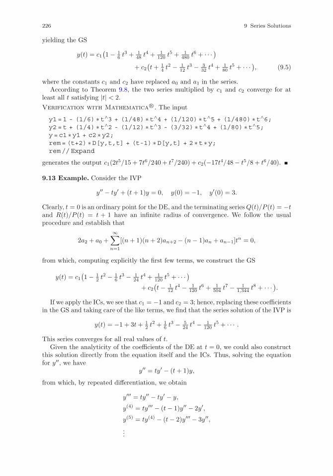
226 9 Series Solutions
yielding the GS
y(t) = c1(1− 1
6 t3 + 1
48 t4 + 1
120 t5 + 1
480 t6 + · · · )
+ c2(t+ 1
4 t2 − 1
12 t3 − 3
32 t4 + 1
80 t5 + · · · ), (9.5)
where the constants c1 and c2 have replaced a0 and a1 in the series.According to Theorem 9.8, the two series multiplied by c1 and c2 converge for at
least all t satisfying |t| < 2.
Verification with Mathematica R©. The input
y1=1 - (1/6) ∗t∧3 + (1/48) ∗t∧4 + (1/120) ∗t∧5 + (1/480) ∗t∧6;y2=t + (1/4) ∗t∧2 - (1/12) ∗t∧3 - (3/32) ∗t∧4 + (1/80) ∗t∧5;y=c1 ∗y1 + c2 ∗y2;rem=(t+2) ∗D[y,t,t] + (t-1) ∗D[y,t] + 2 ∗t ∗y;rem//Expand
generates the output c1(2t5/15 + 7t6/240 + t7/240) + c2(−17t4/48− t5/8 + t6/40).
9.13 Example. Consider the IVP
y′′ − ty′ + (t+ 1)y = 0, y(0) = −1, y′(0) = 3.
Clearly, t = 0 is an ordinary point for the DE, and the terminating seriesQ(t)/P (t) = −tand R(t)/P (t) = t + 1 have an infinite radius of convergence. We follow the usualprocedure and establish that
2a2 + a0 +
∞∑n=1
[(n+ 1)(n+ 2)an+2 − (n− 1)an + an−1]tn = 0,
from which, computing explicitly the first few terms, we construct the GS
y(t) = c1(1− 1
2 t2 − 1
6 t3 − 1
24 t4 + 1
120 t5 + · · · )
+ c2(t− 1
12 t4 − 1
120 t6 + 1
504 t7 − 1
1,344 t8 + · · · ).
If we apply the ICs, we see that c1 = −1 and c2 = 3; hence, replacing these coefficientsin the GS and taking care of the like terms, we find that the series solution of the IVP is
y(t) = −1 + 3t+ 12 t
2 + 16 t
3 − 524 t
4 − 1120 t
5 + · · · .
This series converges for all real values of t.Given the analyticity of the coefficients of the DE at t = 0, we could also construct
this solution directly from the equation itself and the ICs. Thus, solving the equationfor y′′, we have
y′′ = ty′ − (t+ 1)y,
from which, by repeated differentiation, we obtain
y′′′ = ty′′ − ty′ − y,
y(4) = ty′′′ − (t− 1)y′′ − 2y′,
y(5) = ty(4) − (t− 2)y′′′ − 3y′′,...
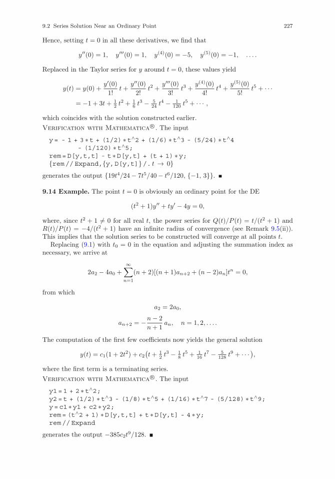
9.2 Series Solution Near an Ordinary Point 227
Hence, setting t = 0 in all these derivatives, we find that
y′′(0) = 1, y′′′(0) = 1, y(4)(0) = −5, y(5)(0) = −1, . . . .
Replaced in the Taylor series for y around t = 0, these values yield
y(t) = y(0) +y′(0)1!
t+y′′(0)2!
t2 +y′′′(0)3!
t3 +y(4)(0)
4!t4 +
y(5)(0)
5!t5 + · · ·
= −1 + 3t+ 12 t
2 + 16 t
3 − 524 t
4 − 1120 t
5 + · · · ,
which coincides with the solution constructed earlier.
Verification with Mathematica R©. The input
y= - 1 + 3 ∗t + (1/2) ∗t∧2 + (1/6) ∗t∧3 - (5/24) ∗t∧4- (1/120) ∗t∧5;
rem=D[y,t,t] - t ∗D[y,t] + (t + 1) ∗y;{rem//Expand,{y,D[y,t]}/. t → 0}
generates the output {19t4/24− 7t5/40− t6/120, {−1, 3}}.
9.14 Example. The point t = 0 is obviously an ordinary point for the DE
(t2 + 1)y′′ + ty′ − 4y = 0,
where, since t2 + 1 �= 0 for all real t, the power series for Q(t)/P (t) = t/(t2 + 1) andR(t)/P (t) = −4/(t2 + 1) have an infinite radius of convergence (see Remark 9.5(ii)).This implies that the solution series to be constructed will converge at all points t.
Replacing (9.1) with t0 = 0 in the equation and adjusting the summation index asnecessary, we arrive at
2a2 − 4a0 +
∞∑n=1
(n+ 2)[(n+ 1)an+2 + (n− 2)an]tn = 0,
from which
a2 = 2a0,
an+2 = −n− 2
n+ 1an, n = 1, 2, . . . .
The computation of the first few coefficients now yields the general solution
y(t) = c1(1 + 2t2) + c2(t+ 1
2 t3 − 1
8 t5 + 1
16 t7 − 5
128 t9 + · · · ),
where the first term is a terminating series.
Verification with Mathematica R©. The input
y1=1 + 2 ∗t∧2;y2=t + (1/2) ∗t∧3 - (1/8) ∗t∧5 + (1/16) ∗t∧7 - (5/128) ∗t∧9;y=c1 ∗y1 + c2 ∗y2;rem=(t∧2 + 1) ∗D[y,t,t] + t ∗D[y,t] - 4 ∗y;rem//Expand
generates the output −385c2t9/128.
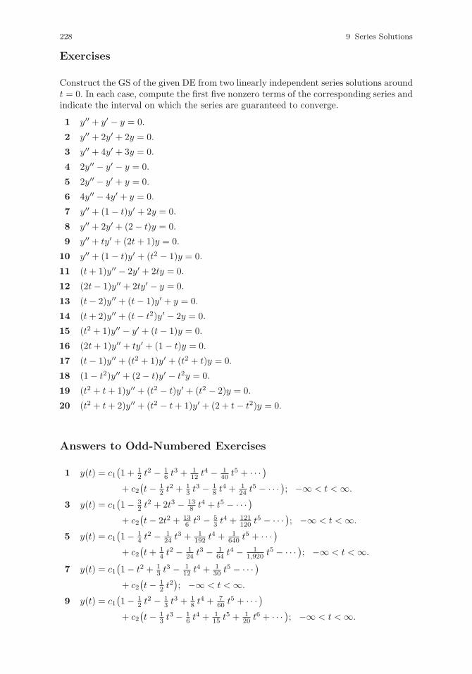
228 9 Series Solutions
Exercises
Construct the GS of the given DE from two linearly independent series solutions aroundt = 0. In each case, compute the first five nonzero terms of the corresponding series andindicate the interval on which the series are guaranteed to converge.
1 y′′ + y′ − y = 0.
2 y′′ + 2y′ + 2y = 0.
3 y′′ + 4y′ + 3y = 0.
4 2y′′ − y′ − y = 0.
5 2y′′ − y′ + y = 0.
6 4y′′ − 4y′ + y = 0.
7 y′′ + (1− t)y′ + 2y = 0.
8 y′′ + 2y′ + (2− t)y = 0.
9 y′′ + ty′ + (2t+ 1)y = 0.
10 y′′ + (1− t)y′ + (t2 − 1)y = 0.
11 (t+ 1)y′′ − 2y′ + 2ty = 0.
12 (2t− 1)y′′ + 2ty′ − y = 0.
13 (t− 2)y′′ + (t− 1)y′ + y = 0.
14 (t+ 2)y′′ + (t− t2)y′ − 2y = 0.
15 (t2 + 1)y′′ − y′ + (t− 1)y = 0.
16 (2t+ 1)y′′ + ty′ + (1 − t)y = 0.
17 (t− 1)y′′ + (t2 + 1)y′ + (t2 + t)y = 0.
18 (1− t2)y′′ + (2− t)y′ − t2y = 0.
19 (t2 + t+ 1)y′′ + (t2 − t)y′ + (t2 − 2)y = 0.
20 (t2 + t+ 2)y′′ + (t2 − t+ 1)y′ + (2 + t− t2)y = 0.
Answers to Odd-Numbered Exercises
1 y(t) = c1(1 + 1
2 t2 − 1
6 t3 + 1
12 t4 − 1
40 t5 + · · · )
+ c2(t− 1
2 t2 + 1
3 t3 − 1
8 t4 + 1
24 t5 − · · · ); −∞ < t < ∞.
3 y(t) = c1(1− 3
2 t2 + 2t3 − 13
8 t4 + t5 − · · · )+ c2
(t− 2t2 + 13
6 t3 − 53 t
4 + 121120 t
5 − · · · ); −∞ < t < ∞.
5 y(t) = c1(1− 1
4 t2 − 1
24 t3 + 1
192 t4 + 1
640 t5 + · · · )
+ c2(t+ 1
4 t2 − 1
24 t3 − 1
64 t4 − 1
1,920 t5 − · · · ); −∞ < t < ∞.
7 y(t) = c1(1− t2 + 1
3 t3 − 1
12 t4 + 1
30 t5 − · · · )
+ c2(t− 1
2 t2); −∞ < t < ∞.
9 y(t) = c1(1− 1
2 t2 − 1
3 t3 + 1
8 t4 + 7
60 t5 + · · · )
+ c2(t− 1
3 t3 − 1
6 t4 + 1
15 t5 + 1
20 t6 + · · · ); −∞ < t < ∞.
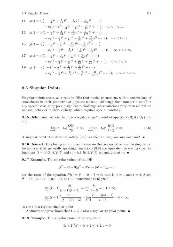
9.3 Singular Points 229
11 y(t) = c1(1− 1
3 t3 + 1
45 t6 − 1
105 t7 + 1
210 t8 − · · · )
+ c2(t+ t2 + 1
3 t3 − 1
6 t4 − 1
15 t5 + · · · ); −1 < t < 1.
13 y(t) = c1(1 + 1
4 t2 + 1
32 t4 + 1
160 t5 + 1
240 t6 + · · · )
+ c2(t− 1
4 t2 + 1
6 t3 − 1
96 t4 + 7
480 t5 + · · · ); −2 < t < 2.
15 y(t) = c1(1− 1
2 t2 + 1
8 t4 − 13
240 t6 − 1
210 t7 + · · · )
+ c2(t+ 1
2 t2 − 1
24 t4 + 1
60 t5 + 1
48 t6 + · · · ); −∞ < t < ∞.
17 y(t) = c1(1 + 1
6 t3 + 5
24 t4 + 1
6 t5 + 29
180 t6 + · · · )
+ c2(t+ 1
2 t2 + 1
3 t3 + 5
12 t4 + 11
24 t5 + · · · ); −1 < t < 1.
19 y(t) = c1(1− t2 + 1
3 t3 + 1
12 t4 − 1
30 t5 + · · · )
+ c2(t− 1
6 t3 + 11
120 t5 − 2
45 t6 − 47
5,040 t7 + · · · ); −∞ < t < ∞.
9.3 Singular Points
Singular points occur, as a rule, in DEs that model phenomena with a certain lack ofsmoothness in their geometric or physical makeup. Although their number is small inany specific case, they pose a significant challenge since solutions very often exhibit anunusual behavior in their vicinity, which requires special handling.
9.15 Definition. We say that t0 is a regular singular point of equation (9.3) if P (t0) = 0and
limt→t0
(t− t0)Q(t)
P (t)< ∞, lim
t→t0(t− t0)
2 R(t)
P (t)< ∞. (9.6)
A singular point that does not satisfy (9.6) is called an irregular singular point.
9.16 Remark. Employing an argument based on the concept of removable singularity,we may say that, generally speaking, conditions (9.6) are equivalent to stating that thefunctions (t− t0)Q(t)/P (t) and (t− t0)
2R(t)/P (t) are analytic at t0.
9.17 Example. The singular points of the DE
(t2 − 4t+ 3)y′′ + 8ty′ + (5t− 1)y = 0
are the roots of the equation P (t) = t2 − 4t + 3 = 0; that is, t = 1 and t = 3. Sincet2 − 4t+ 3 = (t− 1)(t− 3), at t = 1 conditions (9.6) yield
limt→1
(t− 1)8t
(t− 1)(t− 3)= lim
t→1
8t
t− 3= −4 < ∞,
limt→1
(t− 1)25t− 1
(t− 1)(t− 3)= lim
t→1
(t− 1)(5t− 1)
t− 3= 0 < ∞,
so t = 1 is a regular singular point.A similar analysis shows that t = 3 is also a regular singular point.
9.18 Example. The singular points of the equation
t(t+ 1)2y′′ + (t+ 2)y′ + 2ty = 0
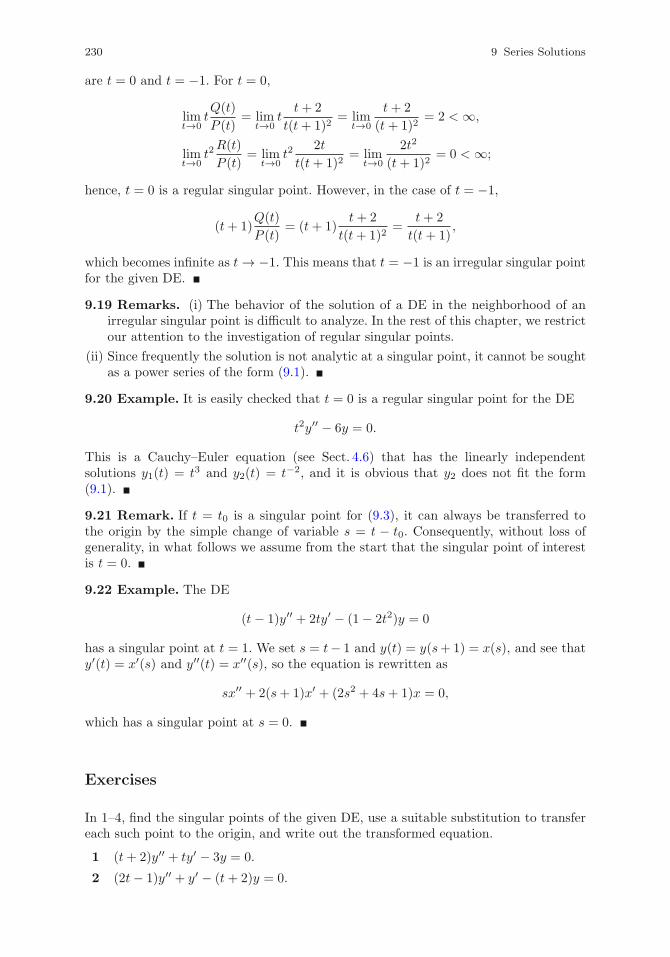
230 9 Series Solutions
are t = 0 and t = −1. For t = 0,
limt→0
tQ(t)
P (t)= lim
t→0t
t+ 2
t(t+ 1)2= lim
t→0
t+ 2
(t+ 1)2= 2 < ∞,
limt→0
t2R(t)
P (t)= lim
t→0t2
2t
t(t+ 1)2= lim
t→0
2t2
(t+ 1)2= 0 < ∞;
hence, t = 0 is a regular singular point. However, in the case of t = −1,
(t+ 1)Q(t)
P (t)= (t+ 1)
t+ 2
t(t+ 1)2=
t+ 2
t(t+ 1),
which becomes infinite as t → −1. This means that t = −1 is an irregular singular pointfor the given DE.
9.19 Remarks. (i) The behavior of the solution of a DE in the neighborhood of anirregular singular point is difficult to analyze. In the rest of this chapter, we restrictour attention to the investigation of regular singular points.
(ii) Since frequently the solution is not analytic at a singular point, it cannot be soughtas a power series of the form (9.1).
9.20 Example. It is easily checked that t = 0 is a regular singular point for the DE
t2y′′ − 6y = 0.
This is a Cauchy–Euler equation (see Sect. 4.6) that has the linearly independentsolutions y1(t) = t3 and y2(t) = t−2, and it is obvious that y2 does not fit the form(9.1).
9.21 Remark. If t = t0 is a singular point for (9.3), it can always be transferred tothe origin by the simple change of variable s = t − t0. Consequently, without loss ofgenerality, in what follows we assume from the start that the singular point of interestis t = 0.
9.22 Example. The DE
(t− 1)y′′ + 2ty′ − (1− 2t2)y = 0
has a singular point at t = 1. We set s = t− 1 and y(t) = y(s+ 1) = x(s), and see thaty′(t) = x′(s) and y′′(t) = x′′(s), so the equation is rewritten as
sx′′ + 2(s+ 1)x′ + (2s2 + 4s+ 1)x = 0,
which has a singular point at s = 0.
Exercises
In 1–4, find the singular points of the given DE, use a suitable substitution to transfereach such point to the origin, and write out the transformed equation.
1 (t+ 2)y′′ + ty′ − 3y = 0.
2 (2t− 1)y′′ + y′ − (t+ 2)y = 0.
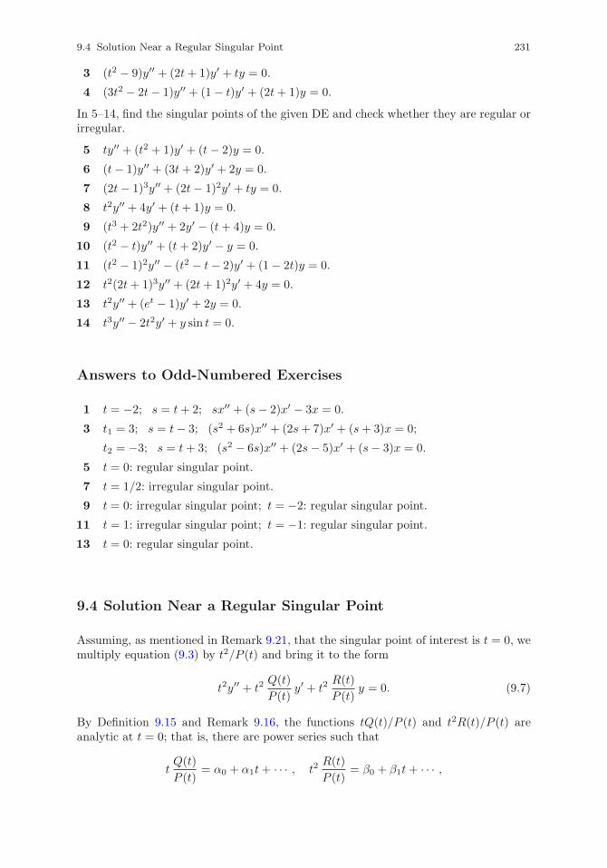
9.4 Solution Near a Regular Singular Point 231
3 (t2 − 9)y′′ + (2t+ 1)y′ + ty = 0.
4 (3t2 − 2t− 1)y′′ + (1− t)y′ + (2t+ 1)y = 0.
In 5–14, find the singular points of the given DE and check whether they are regular orirregular.
5 ty′′ + (t2 + 1)y′ + (t− 2)y = 0.
6 (t− 1)y′′ + (3t+ 2)y′ + 2y = 0.
7 (2t− 1)3y′′ + (2t− 1)2y′ + ty = 0.
8 t2y′′ + 4y′ + (t+ 1)y = 0.
9 (t3 + 2t2)y′′ + 2y′ − (t+ 4)y = 0.
10 (t2 − t)y′′ + (t+ 2)y′ − y = 0.
11 (t2 − 1)2y′′ − (t2 − t− 2)y′ + (1− 2t)y = 0.
12 t2(2t+ 1)3y′′ + (2t+ 1)2y′ + 4y = 0.
13 t2y′′ + (et − 1)y′ + 2y = 0.
14 t3y′′ − 2t2y′ + y sin t = 0.
Answers to Odd-Numbered Exercises
1 t = −2; s = t+ 2; sx′′ + (s− 2)x′ − 3x = 0.
3 t1 = 3; s = t− 3; (s2 + 6s)x′′ + (2s+ 7)x′ + (s+ 3)x = 0;
t2 = −3; s = t+ 3; (s2 − 6s)x′′ + (2s− 5)x′ + (s− 3)x = 0.
5 t = 0: regular singular point.
7 t = 1/2: irregular singular point.
9 t = 0: irregular singular point; t = −2: regular singular point.
11 t = 1: irregular singular point; t = −1: regular singular point.
13 t = 0: regular singular point.
9.4 Solution Near a Regular Singular Point
Assuming, as mentioned in Remark 9.21, that the singular point of interest is t = 0, wemultiply equation (9.3) by t2/P (t) and bring it to the form
t2y′′ + t2Q(t)
P (t)y′ + t2
R(t)
P (t)y = 0. (9.7)
By Definition 9.15 and Remark 9.16, the functions tQ(t)/P (t) and t2R(t)/P (t) areanalytic at t = 0; that is, there are power series such that
tQ(t)
P (t)= α0 + α1t+ · · · , t2
R(t)
P (t)= β0 + β1t+ · · · ,
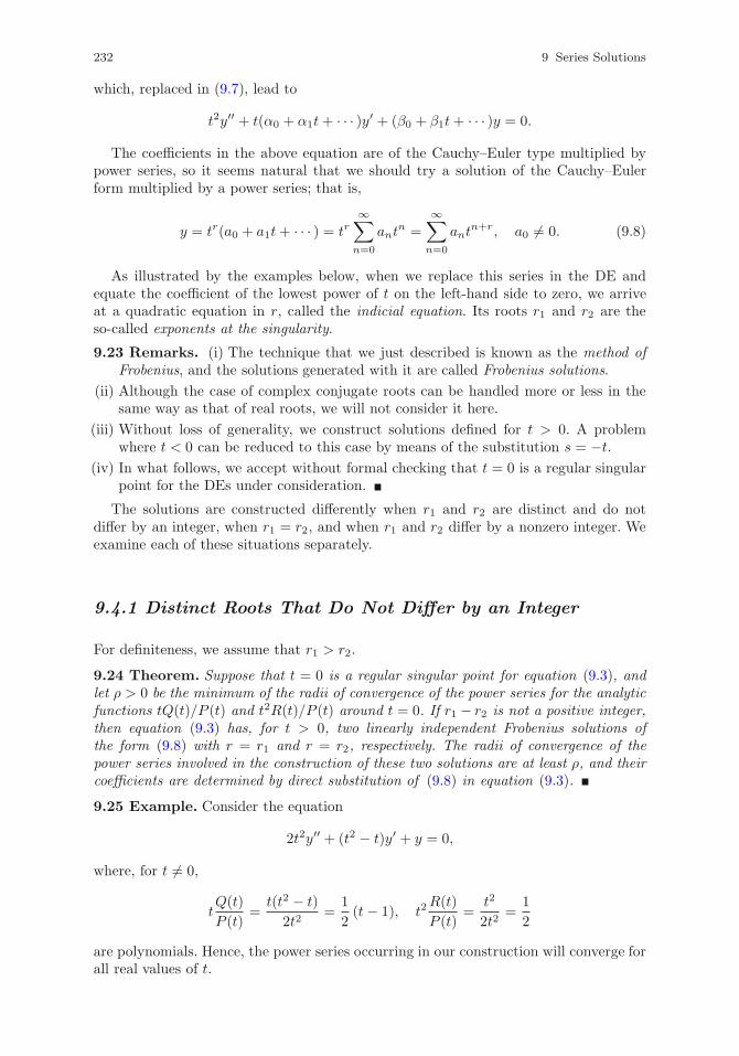
232 9 Series Solutions
which, replaced in (9.7), lead to
t2y′′ + t(α0 + α1t+ · · · )y′ + (β0 + β1t+ · · · )y = 0.
The coefficients in the above equation are of the Cauchy–Euler type multiplied bypower series, so it seems natural that we should try a solution of the Cauchy–Eulerform multiplied by a power series; that is,
y = tr(a0 + a1t+ · · · ) = tr∞∑n=0
antn =
∞∑n=0
antn+r, a0 �= 0. (9.8)
As illustrated by the examples below, when we replace this series in the DE andequate the coefficient of the lowest power of t on the left-hand side to zero, we arriveat a quadratic equation in r, called the indicial equation. Its roots r1 and r2 are theso-called exponents at the singularity.
9.23 Remarks. (i) The technique that we just described is known as the method ofFrobenius, and the solutions generated with it are called Frobenius solutions.
(ii) Although the case of complex conjugate roots can be handled more or less in thesame way as that of real roots, we will not consider it here.
(iii) Without loss of generality, we construct solutions defined for t > 0. A problemwhere t < 0 can be reduced to this case by means of the substitution s = −t.
(iv) In what follows, we accept without formal checking that t = 0 is a regular singularpoint for the DEs under consideration.
The solutions are constructed differently when r1 and r2 are distinct and do notdiffer by an integer, when r1 = r2, and when r1 and r2 differ by a nonzero integer. Weexamine each of these situations separately.
9.4.1 Distinct Roots That Do Not Differ by an Integer
For definiteness, we assume that r1 > r2.
9.24 Theorem. Suppose that t = 0 is a regular singular point for equation (9.3), andlet ρ > 0 be the minimum of the radii of convergence of the power series for the analyticfunctions tQ(t)/P (t) and t2R(t)/P (t) around t = 0. If r1 − r2 is not a positive integer,then equation (9.3) has, for t > 0, two linearly independent Frobenius solutions ofthe form (9.8) with r = r1 and r = r2, respectively. The radii of convergence of thepower series involved in the construction of these two solutions are at least ρ, and theircoefficients are determined by direct substitution of (9.8) in equation (9.3).
9.25 Example. Consider the equation
2t2y′′ + (t2 − t)y′ + y = 0,
where, for t �= 0,
tQ(t)
P (t)=
t(t2 − t)
2t2=
1
2(t− 1), t2
R(t)
P (t)=
t2
2t2=
1
2
are polynomials. Hence, the power series occurring in our construction will converge forall real values of t.
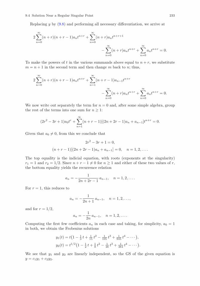
9.4 Solution Near a Regular Singular Point 233
Replacing y by (9.8) and performing all necessary differentiation, we arrive at
2
∞∑n=0
(n+ r)(n+ r − 1)antn+r +
∞∑n=0
(n+ r)antn+r+1
−∞∑n=0
(n+ r)antn+r +
∞∑n=0
antn+r = 0.
To make the powers of t in the various summands above equal to n+ r, we substitutem = n+ 1 in the second term and then change m back to n; thus,
2
∞∑n=0
(n+ r)(n+ r − 1)antn+r +
∞∑n=1
(n+ r − 1)an−1tn+r
−∞∑n=0
(n+ r)antn+r +
∞∑n=0
antn+r = 0.
We now write out separately the term for n = 0 and, after some simple algebra, groupthe rest of the terms into one sum for n ≥ 1:
(2r2 − 3r + 1)a0tr +
∞∑n=1
(n+ r − 1)[(2n+ 2r − 1)an + an−1]tn+r = 0.
Given that a0 �= 0, from this we conclude that
2r2 − 3r + 1 = 0,
(n+ r − 1)[(2n+ 2r − 1)an + an−1] = 0, n = 1, 2, . . . .
The top equality is the indicial equation, with roots (exponents at the singularity)r1 = 1 and r2 = 1/2. Since n+ r − 1 �= 0 for n ≥ 1 and either of these two values of r,the bottom equality yields the recurrence relation
an = − 1
2n+ 2r − 1an−1, n = 1, 2, . . . .
For r = 1, this reduces to
an = − 1
2n+ 1an−1, n = 1, 2, . . . ,
and for r = 1/2,
an = − 1
2nan−1, n = 1, 2, . . . .
Computing the first few coefficients an in each case and taking, for simplicity, a0 = 1in both, we obtain the Frobenius solutions
y1(t) = t(1− 1
3 t+115 t
2 − 1105 t
3 + 1945 t
4 − · · · ),y2(t) = t1/2
(1− 1
2 t+18 t
2 − 148 t
3 + 1384 t
4 − · · · ).We see that y1 and y2 are linearly independent, so the GS of the given equation isy = c1y1 + c2y2.
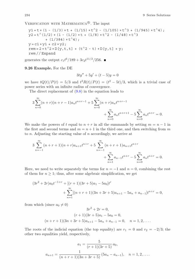
234 9 Series Solutions
Verification with Mathematica R©. The input
y1=t ∗(1 - (1/3) ∗t + (1/15) ∗t∧2 - (1/105) ∗t∧3 + (1/945) ∗t∧4);y2=t∧(1/2) ∗(1 - (1/2) ∗t + (1/8) ∗t∧2 - (1/48) ∗t∧3
+ (1/384) ∗t∧4);y=c1 ∗y1 + c2 ∗y2;rem=2 ∗t∧2 ∗D[y,t,t] + (t∧2 - t) ∗D[y,t] + y;rem//Expand
generates the output c1t6/189 + 3c2t
11/2/256.
9.26 Example. For the DE
3ty′′ + 5y′ + (t− 5)y = 0
we have tQ(t)/P (t) = 5/3 and t2R(t)/P (t) = (t2 − 5t)/3, which is a trivial case ofpower series with an infinite radius of convergence.
The direct replacement of (9.8) in the equation leads to
3
∞∑n=0
(n+ r)(n+ r − 1)antn+r−1 + 5
∞∑n=0
(n+ r)antn+r−1
+
∞∑n=0
antn+r+1 − 5
∞∑n=0
antn+r = 0.
We make the powers of t equal to n + r in all the summands by setting m = n− 1 inthe first and second terms and m = n+ 1 in the third one, and then switching from mto n. Adjusting the starting value of n accordingly, we arrive at
3
∞∑n=−1
(n+ r + 1)(n+ r)an+1tn+r + 5
∞∑n=−1
(n+ r + 1)an+1tn+r
+
∞∑n=1
an−1tn+r − 5
∞∑n=0
antn+r = 0.
Here, we need to write separately the terms for n = −1 and n = 0, combining the restof them for n ≥ 1; thus, after some algebraic simplification, we get
(3r2 + 2r)a0t−1+r + [(r + 1)(3r + 5)a1 − 5a0]t
r
+
∞∑n=1
[(n+ r + 1)(3n+ 3r + 5)an+1 − 5an + an−1]tn+r = 0,
from which (since a0 �= 0)3r2 + 2r = 0,
(r + 1)(3r + 5)a1 − 5a0 = 0,
(n+ r + 1)(3n+ 3r + 5)an+1 − 5an + an−1 = 0, n = 1, 2, . . . .
The roots of the indicial equation (the top equality) are r1 = 0 and r2 = −2/3; theother two equalities yield, respectively,
a1 =5
(r + 1)(3r + 5)a0,
an+1 =1
(n+ r + 1)(3n+ 3r + 5)(5an − an−1), n = 1, 2, . . . .
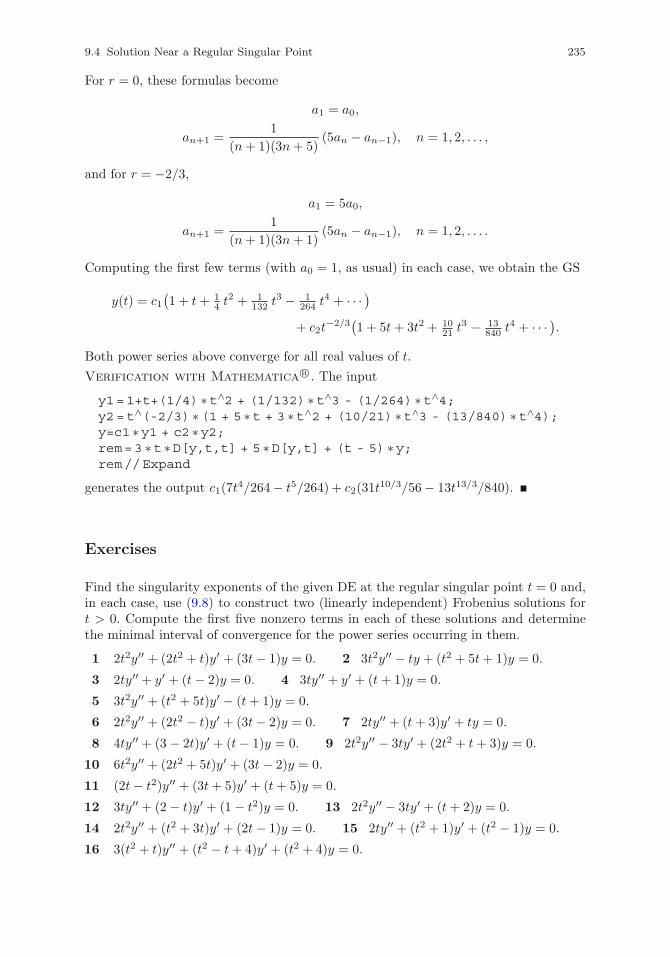
9.4 Solution Near a Regular Singular Point 235
For r = 0, these formulas become
a1 = a0,
an+1 =1
(n+ 1)(3n+ 5)(5an − an−1), n = 1, 2, . . . ,
and for r = −2/3,
a1 = 5a0,
an+1 =1
(n+ 1)(3n+ 1)(5an − an−1), n = 1, 2, . . . .
Computing the first few terms (with a0 = 1, as usual) in each case, we obtain the GS
y(t) = c1(1 + t+ 1
4 t2 + 1
132 t3 − 1
264 t4 + · · · )
+ c2t−2/3
(1 + 5t+ 3t2 + 10
21 t3 − 13
840 t4 + · · · ).
Both power series above converge for all real values of t.
Verification with Mathematica R©. The input
y1=1+t+(1/4) ∗t∧2 + (1/132) ∗t∧3 - (1/264) ∗t∧4;y2=t∧(-2/3) ∗(1 + 5 ∗t + 3 ∗t∧2 + (10/21) ∗t∧3 - (13/840) ∗t∧4);y=c1 ∗y1 + c2 ∗y2;rem=3 ∗t ∗D[y,t,t] + 5 ∗D[y,t] + (t - 5) ∗y;rem//Expand
generates the output c1(7t4/264− t5/264) + c2(31t
10/3/56− 13t13/3/840).
Exercises
Find the singularity exponents of the given DE at the regular singular point t = 0 and,in each case, use (9.8) to construct two (linearly independent) Frobenius solutions fort > 0. Compute the first five nonzero terms in each of these solutions and determinethe minimal interval of convergence for the power series occurring in them.
1 2t2y′′ + (2t2 + t)y′ + (3t− 1)y = 0. 2 3t2y′′ − ty + (t2 + 5t+ 1)y = 0.
3 2ty′′ + y′ + (t− 2)y = 0. 4 3ty′′ + y′ + (t+ 1)y = 0.
5 3t2y′′ + (t2 + 5t)y′ − (t+ 1)y = 0.
6 2t2y′′ + (2t2 − t)y′ + (3t− 2)y = 0. 7 2ty′′ + (t+ 3)y′ + ty = 0.
8 4ty′′ + (3 − 2t)y′ + (t− 1)y = 0. 9 2t2y′′ − 3ty′ + (2t2 + t+ 3)y = 0.
10 6t2y′′ + (2t2 + 5t)y′ + (3t− 2)y = 0.
11 (2t− t2)y′′ + (3t+ 5)y′ + (t+ 5)y = 0.
12 3ty′′ + (2 − t)y′ + (1 − t2)y = 0. 13 2t2y′′ − 3ty′ + (t+ 2)y = 0.
14 2t2y′′ + (t2 + 3t)y′ + (2t− 1)y = 0. 15 2ty′′ + (t2 + 1)y′ + (t2 − 1)y = 0.
16 3(t2 + t)y′′ + (t2 − t+ 4)y′ + (t2 + 4)y = 0.
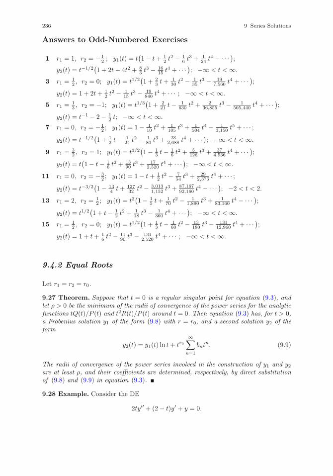
236 9 Series Solutions
Answers to Odd-Numbered Exercises
1 r1 = 1, r2 = − 12 ; y1(t) = t
(1− t+ 1
2 t2 − 1
6 t3 + 1
24 t4 − · · · );
y2(t) = t−1/2(1 + 2t− 4t2 + 8
3 t3 − 16
15 t4 + · · · ); −∞ < t < ∞.
3 r1 = 12 , r2 = 0; y1(t) = t1/2
(1 + 2
3 t+130 t
2 − 135 t
3 − 197,560 t
4 + · · · );y2(t) = 1 + 2t+ 1
2 t2 − 1
15 t3 − 19
840 t4 + · · · ; −∞ < t < ∞.
5 r1 = 13 , r2 = −1; y1(t) = t1/3
(1 + 2
21 t− 1630 t
2 + 236,855 t
3 − 1505,440 t
4 + · · · );y2(t) = t−1 − 2− 1
2 t; −∞ < t < ∞.
7 r1 = 0, r2 = − 12 ; y1(t) = 1− 1
10 t2 + 1
105 t3 + 1
504 t4 − 1
3,150 t5 + · · · ;
y2(t) = t−1/2(1 + 1
2 t− 124 t
2 − 180 t
3 + 232,688 t
4 + · · · ); −∞ < t < ∞.
9 r1 = 32 , r2 = 1; y1(t) = t3/2
(1− 1
3 t− 16 t
2 + 5126 t
3 + 374,536 t
4 + · · · );y2(t) = t
(1− t− 1
6 t2 + 13
90 t3 + 17
2,520 t4 + · · · ); −∞ < t < ∞.
11 r1 = 0, r2 = − 32 ; y1(t) = 1− t+ 1
2 t2 − 7
54 t3 + 29
2,376 t4 + · · · ;
y2(t) = t−3/2(1− 13
4 t+ 12732 t2 − 3,013
1,152 t3 + 87,167
92,160 t4 − · · · ); −2 < t < 2.
13 r1 = 2, r2 = 12 ; y1(t) = t2
(1− 1
5 t+170 t
2 − 11,890 t
3 + 183,160 t
4 − · · · );y2(t) = t1/2
(1 + t− 1
2 t2 + 1
18 t3 − 1
360 t4 + · · · ); −∞ < t < ∞.
15 r1 = 12 , r2 = 0; y1(t) = t1/2
(1 + 1
3 t− 160 t
2 − 13180 t
3 − 13112,960 t
4 + · · · );y2(t) = 1 + t+ 1
6 t2 − 11
90 t3 − 131
2,520 t4 + · · · ; −∞ < t < ∞.
9.4.2 Equal Roots
Let r1 = r2 = r0.
9.27 Theorem. Suppose that t = 0 is a regular singular point for equation (9.3), andlet ρ > 0 be the minimum of the radii of convergence of the power series for the analyticfunctions tQ(t)/P (t) and t2R(t)/P (t) around t = 0. Then equation (9.3) has, for t > 0,a Frobenius solution y1 of the form (9.8) with r = r0, and a second solution y2 of theform
y2(t) = y1(t) ln t+ tr0∞∑
n=1
bntn. (9.9)
The radii of convergence of the power series involved in the construction of y1 and y2are at least ρ, and their coefficients are determined, respectively, by direct substitutionof (9.8) and (9.9) in equation (9.3).
9.28 Example. Consider the DE
2ty′′ + (2− t)y′ + y = 0.
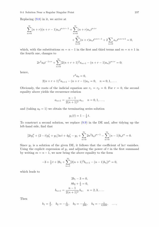
9.4 Solution Near a Regular Singular Point 237
Replacing (9.8) in it, we arrive at
∞∑n=0
(n+ r)(n + r − 1)antn+r−1 +
∞∑n=0
(n+ r)antn+r
+
∞∑n=0
(n+ r)antn+r−1 + 2
∑n=0
antn+r+1 = 0,
which, with the substitutions m = n− 1 in the first and third terms and m = n+ 1 inthe fourth one, changes to
2r2a0t−1+r +
∞∑n=0
[2(n+ r + 1)2an+1 − (n+ r − 1)an]tn+r = 0;
hence,r2a0 = 0,
2(n+ r + 1)2an+1 − (n+ r − 1)an = 0, n = 0, 1, . . . .
Obviously, the roots of the indicial equation are r1 = r2 = 0. For r = 0, the secondequality above yields the recurrence relation
an+1 =n− 1
2(n+ 1)2an, n = 0, 1, . . . ,
and (taking a0 = 1) we obtain the terminating series solution
y1(t) = 1− 12 t.
To construct a second solution, we replace (9.9) in the DE and, after tidying up theleft-hand side, find that
[2ty′′1 + (2− t)y′1 + y1] ln t+ 4y′1 − y1 +
∞∑n=0
2n2bntn−1 −
∞∑n=0
(n− 1)bntn = 0.
Since y1 is a solution of the given DE, it follows that the coefficient of ln t vanishes.Using the explicit expression of y1 and adjusting the power of t in the first summandby writing m = n− 1, we now bring the above equality to the form
−3 + 12 t+ 2b1 +
∞∑n=1
[2(n+ 1)2bn+1 − (n− 1)bn]tn = 0,
which leads to
2b1 − 3 = 0,
8b2 +12 = 0,
bn+1 =n− 1
2(n+ 1)2bn, n = 2, 3, . . . .
Then
b1 = 32 , b2 = − 1
16 , b3 = − 1288 , b4 = − 1
4,608 , . . . ,
238 9 Series Solutions
soy2(t) = y1(t) ln t+
32 t− 1
16 t2 − 1
288 t3 − 1
4,608 t4 − · · · .
It is easy to see that y1 and y2 are linearly independent; hence, the GS of our DE maybe expressed as y = c1y1 + c2y2. The power series occurring in both y1 and y2 convergefor all real values of t.
Verification with Mathematica R©. The input
y1=1 - (1/2) ∗t;y2=y1 ∗Log[t] + (3/2) ∗t - (1/16) ∗t∧2 - (1/288) ∗t∧3
- (1/4608) ∗t∧4;y=c1 ∗y1 + c2 ∗y2;rem=2 ∗t ∗D[y,t,t] + (2 - t) ∗D[y,t] + y;rem//Expand
generates the output c2t4/1,536.
9.29 Example. Starting with (9.8) and applying the same procedure to the DE
t2y′′ + (t2 + 5t)y′ + (3t+ 4)y = 0,
after the customary manipulation of the terms and powers of t we arrive at the equality
(r + 2)2a0tr + [(r + 3)2a1 + 3a0]t
1+r +
∞∑n=2
(n+ r + 2)[(n+ r + 2)an + an−1]tn+r = 0,
from which
(r + 2)2a0 = 0,
(r + 3)2a1 + 3a0 = 0,
(n+ r + 2)[(n+ r + 2)an + an−1] = 0, n = 2, 3, . . . .
The roots of the indicial equation are r1 = r2 = −2, and for r = −2 we use the secondand third equalities above with a0 = 1 to produce the Frobenius solution
y1(t) = t−2(1− t+ 1
2 t2 − 1
6 t3 + 1
24 t4 + · · · ).
Continuing the procedure with (9.9) and performing the necessary computation, wefind that
2ty′1 + ty1 + 4y1 + b1t−1 +
∞∑n=2
n(nbn + bn−1)tn−2 = 0.
After y1 is replaced by its expression, this leads to
(b1 − 1)t−1 + 4b2 + 2b1 + 1 +(9b3 + 3b2 − 1
2
)t+(16b4 + 4b3 +
16
)t2 + · · · = 0
and, hence, to the coefficients
b1 = 1, b2 = − 34 , b3 = 11
36 , b4 = − 25288 , . . . ,
which give the solution
y2(t) = y1(t) ln t+ t−2(t− 3
4 t2 + 11
36 t3 − 25
288 t4 + · · · ).
9.4 Solution Near a Regular Singular Point 239
In view of the obvious linear independence of y1 and y2, the GS of the equation isy = c1y1 + c2y2, with the power series occurring in both y1 and y2 convergent for allreal values of t.
Verification with Mathematica R©. The input
y1=t∧( - 2) ∗(1 - t + (1/2) ∗t∧2 - (1/6) ∗t∧3+(1/24) ∗t∧4);y2=y1 ∗Log[t] + t∧( - 1) ∗(1-(3/4) ∗t+(11/36) ∗t∧2
- (25/288) ∗t∧3);y=c1 ∗y1 + c2 ∗y2;rem=t∧2 ∗D[y,t,t] + (t∧2 + 5 ∗t) ∗D[y,t] + (3 ∗t + 4) ∗y;rem//Expand
generates the output 5c1t3/24 + c2[5(t
3 ln t)/24− 113t3/288].
9.30 Example. The usual treatment based on (9.8) and applied to the DE
t2y′′ + ty′ + t2y = 0 (9.10)
produces the equality
r2a0tr + (r + 1)2a1t
1+r +
∞∑n=2
[(n+ r)2an + an−2]tn+r = 0,
so
r2a0 = 0,
(r + 1)2a1 = 0,
(n+ r)2an + an−2 = 0, n = 2, 3, . . . .
This means that the roots of the indicial equation are r1 = r2 = 0. For r = 0, the abovecoefficient relationships (with a0 = 1) yield the Frobenius solution
y1(t) = 1− 14 t
2 + 164 t
4 − 12,304 t
6 + · · · .
A second solution y2 is now constructed from (9.9). Carrying out the necessarydifferentiation and algebra, we get
2ty′1 +∞∑n=1
n2bntn +
∞∑n=3
bn−2tn = 0,
or, with y1 replaced by its computed expansion,
b1t+ (4b2 − 1)t2 + (9b3 + b1)t3 +(16b4 + b2 +
18
)t4
+ (25b5 + b3)t5 +(36b6 + b4 − 1
192
)t6 + · · · = 0.
We then have
b1 = 0, b2 = 14 , b3 = 0, b4 = − 3
128 , b5 = 0, b6 = 1113,824 , . . . ,
soy2(t) = y1(t) ln t+
14 t
2 − 3128 t
4 + 1113,824 t
6 − · · · .Since y1 and y2 are linearly independent, we may write the GS of the equation asy = c1y1 + c2y2. The power series occurring in y1 and y2 converge for all real t.
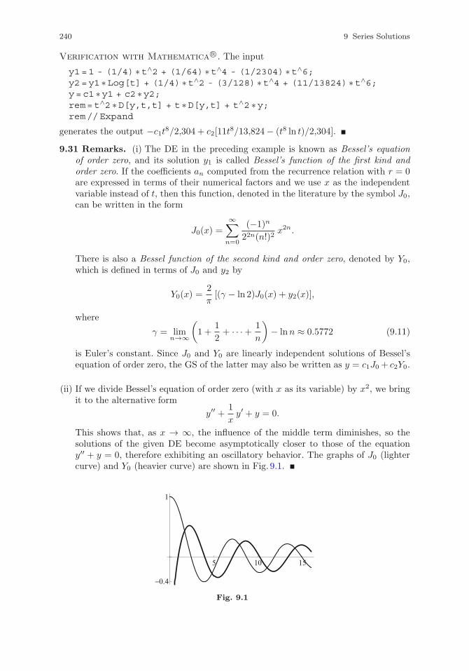
240 9 Series Solutions
Verification with Mathematica R©. The input
y1=1 - (1/4) ∗t∧2 + (1/64) ∗t∧4 - (1/2304) ∗t∧6;y2=y1 ∗Log[t] + (1/4) ∗t∧2 - (3/128) ∗t∧4 + (11/13824) ∗t∧6;y=c1 ∗y1 + c2 ∗y2;rem=t∧2 ∗D[y,t,t] + t ∗D[y,t] + t∧2 ∗y;rem//Expand
generates the output −c1t8/2,304 + c2[11t8/13,824− (t8 ln t)/2,304].
9.31 Remarks. (i) The DE in the preceding example is known as Bessel’s equationof order zero, and its solution y1 is called Bessel’s function of the first kind andorder zero. If the coefficients an computed from the recurrence relation with r = 0are expressed in terms of their numerical factors and we use x as the independentvariable instead of t, then this function, denoted in the literature by the symbol J0,can be written in the form
J0(x) =
∞∑n=0
(−1)n
22n(n!)2x2n.
There is also a Bessel function of the second kind and order zero, denoted by Y0,which is defined in terms of J0 and y2 by
Y0(x) =2
π[(γ − ln 2)J0(x) + y2(x)],
where
γ = limn→∞
(1 +
1
2+ · · ·+ 1
n
)− lnn ≈ 0.5772 (9.11)
is Euler’s constant. Since J0 and Y0 are linearly independent solutions of Bessel’sequation of order zero, the GS of the latter may also be written as y = c1J0 + c2Y0.
(ii) If we divide Bessel’s equation of order zero (with x as its variable) by x2, we bringit to the alternative form
y′′ +1
xy′ + y = 0.
This shows that, as x → ∞, the influence of the middle term diminishes, so thesolutions of the given DE become asymptotically closer to those of the equationy′′ + y = 0, therefore exhibiting an oscillatory behavior. The graphs of J0 (lightercurve) and Y0 (heavier curve) are shown in Fig. 9.1.
5 10 15
−0.4
1
Fig. 9.1
9.4 Solution Near a Regular Singular Point 241
Exercises
Find the exponents at the singularity for the given DE at the regular singular pointt = 0 and, in each case, use (9.8) and (9.9) to construct two (linearly independent)series solutions for t > 0. Compute the first five nonzero terms in each of the powerseries occurring in these solutions and determine the minimal interval of convergencefor these power series.
1 ty′′ + (t+ 1)y′ + 2ty = 0. 2 t2y′′ + 3ty′ + (1− t)y = 0.
3 t2y′′ − ty′ + (t2 − t+ 1)y = 0. 4 ty′′ + (1 − 2t)y′ + (1− t)y = 0.
5 ty′′ + (1− t2)y′ − y = 0. 6 4t2y′′ + 2t2y′ + (3t+ 1)y = 0.
7 t2y′′ + 3(t2 + t)y′ + (2t+ 1)y = 0. 8 (t2 + t)y′′ + y′ + 2y = 0.
9 (t2 − t)y′′ + (t2 − 1)y′ − (t+ 2)y = 0. 10 4t2y′′ + 4(t2 + 2t)y′ + (1− 2t)y = 0.
Answers to Odd-Numbered Exercises
1 r1 = r2 = 0; y1(t) = 1− 12 t
2 + 19 t
3 + 124 t
4 − 7450 t
5 + · · · ;y2(t) = y1(t) ln t+
(− t+ 34 t
2 + 127 t
3 − 37288 t
4 + 29913,500 t
5 + · · · ); −∞ < t < ∞.
3 r1 = r2 = 1; y1(t) = t(1 + t− 1
9 t3 − 1
144 t4 + 1
240 t5 + · · · );
y2(t) = y1(t) ln t+ t(− 2t− 1
2 t2 + 13
54 t3 + 43
864 t4 − 67
7,200 t5 + · · · ); −∞ < t < ∞.
5 r1 = r2 = 0; y1(t) = 1 + t+ 14 t
2 + 536 t
3 + 23576 t
4 + · · · ;y2(t) = y1(t) ln t+
(− 2t− 12 t
2 − 727 t
3 − 2873,456 t
4 − 15,631432,000 t
5 + · · · ); −∞ < t < ∞.
7 r1 = r2 = −1; y1(t) = t−1(1 + t− 1
2 t2 + 5
18 t3 − 5
36 t4 + · · · );
y2(t) = y1(t) ln t+ t−1(−5t+ 9
4 t2− 137
108 t3+ 563
864 t4− 6,361
21,600 t5+ · · · ); −∞ < t < ∞.
9 r1 = r2 = 0; y1(t) = 1− 2t+ 34 t
2 + 364 t
4 + 3160 t
5 + · · · ;y2(t) = y1(t) ln t+
(3t− 5
2 t2 + 1
36 t3 − 145
1,152 t4 − 17
400 t5 + · · · ); −1 < t < 1.
9.4.3 Distinct Roots Differing by an Integer
Let r1 = r2 + n0, where n0 is a positive integer.
9.32 Theorem. Suppose that t = 0 is a regular singular point for equation (9.3), andlet ρ > 0 be the minimum of the radii of convergence of the power series for the analyticfunctions tQ(t)/P (t) and t2R(t)/P (t) around t = 0. Then equation (9.3) has, for t > 0,a Frobenius solution y1 of the form (9.8) with r = r1, and a second solution y2 of theform
y2(t) = cy1(t) ln t+ tr2(1 +
∞∑n=1
bntn
), c = const. (9.12)
The radii of convergence of the power series involved in the construction of y1 and y2are at least ρ, and their coefficients are determined, respectively, by direct substitutionof (9.8) and (9.12) in equation (9.3).
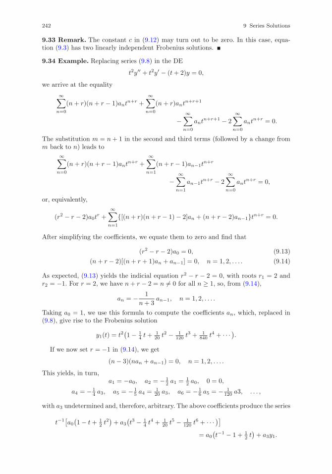
242 9 Series Solutions
9.33 Remark. The constant c in (9.12) may turn out to be zero. In this case, equa-tion (9.3) has two linearly independent Frobenius solutions.
9.34 Example. Replacing series (9.8) in the DE
t2y′′ + t2y′ − (t+ 2)y = 0,
we arrive at the equality
∞∑n=0
(n+ r)(n + r − 1)antn+r +
∞∑n=0
(n+ r)antn+r+1
−∞∑n=0
antn+r+1 − 2
∞∑n=0
antn+r = 0.
The substitution m = n+ 1 in the second and third terms (followed by a change fromm back to n) leads to
∞∑n=0
(n+ r)(n + r − 1)antn+r +
∞∑n=1
(n+ r − 1)an−1tn+r
−∞∑
n=1
an−1tn+r − 2
∞∑n=0
antn+r = 0,
or, equivalently,
(r2 − r − 2)a0tr +
∞∑n=1
{[(n+ r)(n + r − 1)− 2]an + (n+ r − 2)an−1}tn+r = 0.
After simplifying the coefficients, we equate them to zero and find that
(r2 − r − 2)a0 = 0, (9.13)
(n+ r − 2)[(n+ r + 1)an + an−1] = 0, n = 1, 2, . . . . (9.14)
As expected, (9.13) yields the indicial equation r2 − r − 2 = 0, with roots r1 = 2 andr2 = −1. For r = 2, we have n+ r − 2 = n �= 0 for all n ≥ 1, so, from (9.14),
an = − 1
n+ 3an−1, n = 1, 2, . . . .
Taking a0 = 1, we use this formula to compute the coefficients an, which, replaced in(9.8), give rise to the Frobenius solution
y1(t) = t2(1− 1
4 t+120 t
2 − 1120 t
3 + 1840 t
4 + · · · ).If we now set r = −1 in (9.14), we get
(n− 3)(nan + an−1) = 0, n = 1, 2, . . . .
This yields, in turn,a1 = −a0, a2 = − 1
2 a1 = 12 a0, 0 = 0,
a4 = − 14 a3, a5 = − 1
5 a4 = 120 a3, a6 = − 1
6 a5 = − 1120 a3, . . . ,
with a3 undetermined and, therefore, arbitrary. The above coefficients produce the series
t−1[a0(1− t+ 1
2 t2)+ a3
(t3 − 1
4 t4 + 1
20 t5 − 1
120 t6 + · · · )]= a0
(t−1 − 1 + 1
2 t)+ a3y1.
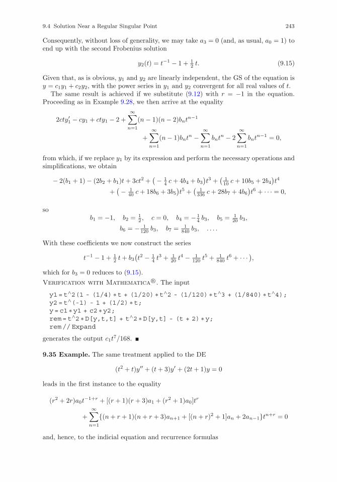
9.4 Solution Near a Regular Singular Point 243
Consequently, without loss of generality, we may take a3 = 0 (and, as usual, a0 = 1) toend up with the second Frobenius solution
y2(t) = t−1 − 1 + 12 t. (9.15)
Given that, as is obvious, y1 and y2 are linearly independent, the GS of the equation isy = c1y1 + c2y2, with the power series in y1 and y2 convergent for all real values of t.
The same result is achieved if we substitute (9.12) with r = −1 in the equation.Proceeding as in Example 9.28, we then arrive at the equality
2cty′1 − cy1 + cty1 − 2 +
∞∑n=1
(n− 1)(n− 2)bntn−1
+
∞∑n=1
(n− 1)bntn −
∞∑n=1
bntn − 2
∞∑n=1
bntn−1 = 0,
from which, if we replace y1 by its expression and perform the necessary operations andsimplifications, we obtain
− 2(b1 + 1)− (2b2 + b1)t+ 3ct2 +(− 1
4 c+ 4b4 + b3)t3 +
(110 c+ 10b5 + 2b4
)t4
+(− 1
40 c+ 18b6 + 3b5)t5 +
(1
336 c+ 28b7 + 4b6)t6 + · · · = 0,
sob1 = −1, b2 = 1
2 , c = 0, b4 = − 14 b3, b5 = 1
20 b3,
b6 = − 1120 b3, b7 = 1
840 b3, . . . .
With these coefficients we now construct the series
t−1 − 1 + 12 t+ b3
(t2 − 1
4 t3 + 1
20 t4 − 1
120 t5 + 1
840 t6 + · · · ),
which for b3 = 0 reduces to (9.15).
Verification with Mathematica R©. The input
y1=t∧2(1 - (1/4) ∗t + (1/20) ∗t∧2 - (1/120) ∗t∧3 + (1/840) ∗t∧4);y2=t∧(-1) - 1 + (1/2) ∗t;y=c1 ∗y1 + c2 ∗y2;rem=t∧2 ∗D[y,t,t] + t∧2 ∗D[y,t] - (t + 2) ∗y;rem//Expand
generates the output c1t7/168.
9.35 Example. The same treatment applied to the DE
(t2 + t)y′′ + (t+ 3)y′ + (2t+ 1)y = 0
leads in the first instance to the equality
(r2 + 2r)a0t−1+r + [(r + 1)(r + 3)a1 + (r2 + 1)a0]t
r
+∞∑n=1
{(n+ r + 1)(n+ r + 3)an+1 + [(n+ r)2 + 1]an + 2an−1}tn+r = 0
and, hence, to the indicial equation and recurrence formulas
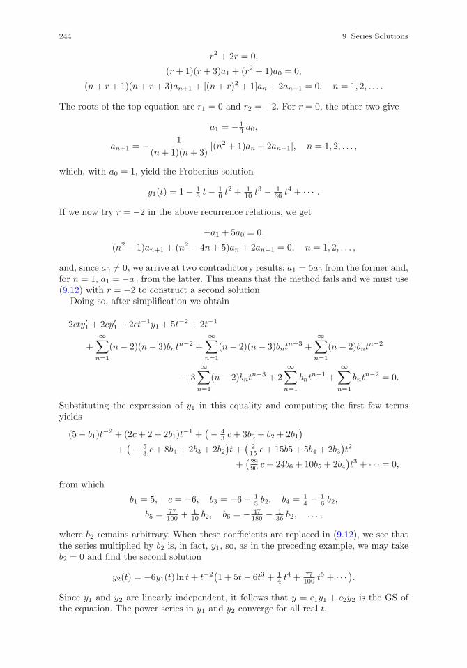
244 9 Series Solutions
r2 + 2r = 0,
(r + 1)(r + 3)a1 + (r2 + 1)a0 = 0,
(n+ r + 1)(n+ r + 3)an+1 + [(n+ r)2 + 1]an + 2an−1 = 0, n = 1, 2, . . . .
The roots of the top equation are r1 = 0 and r2 = −2. For r = 0, the other two give
a1 = − 13 a0,
an+1 = − 1
(n+ 1)(n+ 3)[(n2 + 1)an + 2an−1], n = 1, 2, . . . ,
which, with a0 = 1, yield the Frobenius solution
y1(t) = 1− 13 t− 1
6 t2 + 1
10 t3 − 1
36 t4 + · · · .
If we now try r = −2 in the above recurrence relations, we get
−a1 + 5a0 = 0,
(n2 − 1)an+1 + (n2 − 4n+ 5)an + 2an−1 = 0, n = 1, 2, . . . ,
and, since a0 �= 0, we arrive at two contradictory results: a1 = 5a0 from the former and,for n = 1, a1 = −a0 from the latter. This means that the method fails and we must use(9.12) with r = −2 to construct a second solution.
Doing so, after simplification we obtain
2cty′1 + 2cy′1 + 2ct−1y1 + 5t−2 + 2t−1
+
∞∑n=1
(n− 2)(n− 3)bntn−2 +
∞∑n=1
(n− 2)(n− 3)bntn−3 +
∞∑n=1
(n− 2)bntn−2
+ 3
∞∑n=1
(n− 2)bntn−3 + 2
∞∑n=1
bntn−1 +
∞∑n=1
bntn−2 = 0.
Substituting the expression of y1 in this equality and computing the first few termsyields
(5− b1)t−2 + (2c+ 2 + 2b1)t
−1 +(− 4
3 c+ 3b3 + b2 + 2b1)
+(− 5
3 c+ 8b4 + 2b3 + 2b2)t+(
215 c+ 15b5 + 5b4 + 2b3
)t2
+(2990 c+ 24b6 + 10b5 + 2b4
)t3 + · · · = 0,
from which
b1 = 5, c = −6, b3 = −6− 13 b2, b4 = 1
4 − 16 b2,
b5 = 77100 + 1
10 b2, b6 = − 47180 − 1
36 b2, . . . ,
where b2 remains arbitrary. When these coefficients are replaced in (9.12), we see thatthe series multiplied by b2 is, in fact, y1, so, as in the preceding example, we may takeb2 = 0 and find the second solution
y2(t) = −6y1(t) ln t+ t−2(1 + 5t− 6t3 + 1
4 t4 + 77
100 t5 + · · · ).
Since y1 and y2 are linearly independent, it follows that y = c1y1 + c2y2 is the GS ofthe equation. The power series in y1 and y2 converge for all real t.
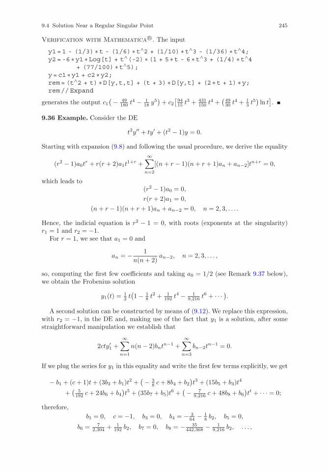
9.4 Solution Near a Regular Singular Point 245
Verification with Mathematica R©. The input
y1=1 - (1/3) ∗t - (1/6) ∗t∧2 + (1/10) ∗t∧3 - (1/36) ∗t∧4;y2=-6 ∗y1 ∗Log[t] + t∧(-2) ∗(1 + 5 ∗t - 6 ∗t∧3 + (1/4) ∗t∧4
+ (77/100) ∗t∧5);y=c1 ∗y1 + c2 ∗y2;rem=(t∧2 + t) ∗D[y,t,t] + (t + 3) ∗D[y,t] + (2 ∗t + 1) ∗y;rem//Expand
generates the output c1(− 49
180 t4 − 1
18 y5)+ c2
[9415 t
3 + 431150 t
4 +(4930 t
4 + 13 t
5)ln t].
9.36 Example. Consider the DE
t2y′′ + ty′ + (t2 − 1)y = 0.
Starting with expansion (9.8) and following the usual procedure, we derive the equality
(r2 − 1)a0tr + r(r + 2)a1t
1+r +
∞∑n=2
[(n+ r − 1)(n+ r + 1)an + an−2]tn+r = 0,
which leads to(r2 − 1)a0 = 0,
r(r + 2)a1 = 0,
(n+ r − 1)(n+ r + 1)an + an−2 = 0, n = 2, 3, . . . .
Hence, the indicial equation is r2 − 1 = 0, with roots (exponents at the singularity)r1 = 1 and r2 = −1.
For r = 1, we see that a1 = 0 and
an = − 1
n(n+ 2)an−2, n = 2, 3, . . . ,
so, computing the first few coefficients and taking a0 = 1/2 (see Remark 9.37 below),we obtain the Frobenius solution
y1(t) =12 t(1− 1
8 t2 + 1
192 t4 − 1
9,216 t6 + · · · ).
A second solution can be constructed by means of (9.12). We replace this expression,with r2 = −1, in the DE and, making use of the fact that y1 is a solution, after somestraightforward manipulation we establish that
2cty′1 +∞∑n=1
n(n− 2)bntn−1 +
∞∑n=3
bn−2tn−1 = 0.
If we plug the series for y1 in this equality and write the first few terms explicitly, we get
− b1 + (c+ 1)t+ (3b3 + b1)t2 +(− 3
8 c+ 8b4 + b2)t3 + (15b5 + b3)t
4
+(
5192 c+ 24b6 + b4
)t5 + (35b7 + b5)t
6 +(− 7
9,216 c+ 48b8 + b6)tt + · · · = 0;
therefore,
b1 = 0, c = −1, b3 = 0, b4 = − 364 − 1
8 b2, b5 = 0,
b6 =7
2,304 + 1192 b2, b7 = 0, b8 = − 35
442,368 − 19,216 b2, . . . ,
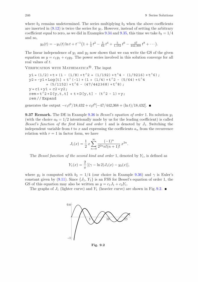
246 9 Series Solutions
where b2 remains undetermined. The series multiplying b2 when the above coefficientsare inserted in (9.12) is twice the series for y1. However, instead of setting the arbitrarycoefficient equal to zero, as we did in Examples 9.34 and 9.35, this time we take b2 = 1/4and so,
y2(t) = −y1(t) ln t+ t−1(1 + 1
4 t2 − 5
64 t4 + 5
1,152 t6 − 47
442,368 t8 + · · · ).
The linear independence of y1 and y2 now shows that we can write the GS of the givenequation as y = c1y1 + c2y2. The power series involved in this solution converge for allreal values of t.
Verification with Mathematica R©. The input
y1=(1/2) ∗t ∗(1 - (1/8) ∗t∧2 + (1/192) ∗t∧4 - (1/9216) ∗t∧6);y2=-y1 ∗Log[t] + t∧(-1) ∗(1 + (1/4) ∗t∧2 - (5/64) ∗t∧4
+ (5/1152) ∗t∧6 - (47/442368) ∗t∧8);y=c1 ∗y1 + c2 ∗y2;rem=t∧2 ∗D[y,t,t] + t ∗D[y,t] - (t∧2 - 1) ∗y;rem//Expand
generates the output −c1t9/18,432 + c2t9[−47/442,368 + (ln t)/18,432].
9.37 Remark. The DE in Example 9.36 is Bessel’s equation of order 1. Its solution y1(with the choice a0 = 1/2 intentionally made by us for the leading coefficient) is calledBessel’s function of the first kind and order 1 and is denoted by J1. Switching theindependent variable from t to x and expressing the coefficients an from the recurrencerelation with r = 1 in factor form, we have
J1(x) =1
2x
∞∑n=0
(−1)n
22nn!(n+ 1)!x2n.
The Bessel function of the second kind and order 1, denoted by Y1, is defined as
Y1(x) =2
π[(γ − ln 2)J1(x) − y2(x)],
where y2 is computed with b2 = 1/4 (our choice in Example 9.36) and γ is Euler’sconstant given by (9.11). Since {J1, Y1} is an FSS for Bessel’s equation of order 1, theGS of this equation may also be written as y = c1J1 + c2Y1.
The graphs of J1 (lighter curve) and Y1 (heavier curve) are shown in Fig. 9.2.
5 10 15
−1
0.6
Fig. 9.2
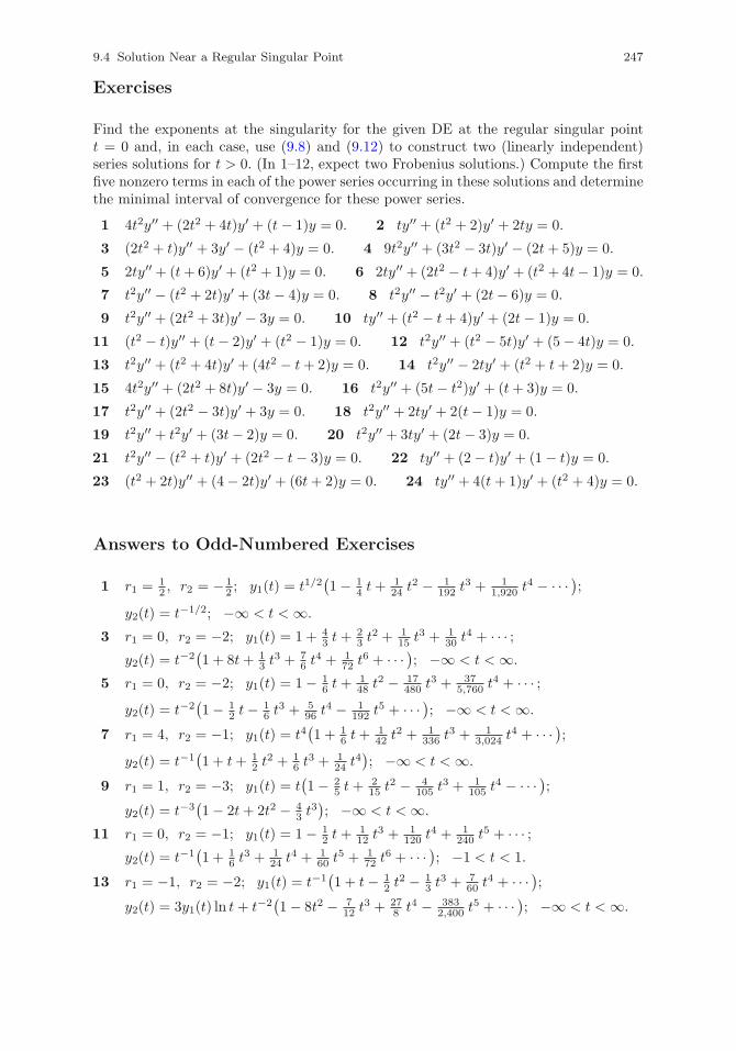
9.4 Solution Near a Regular Singular Point 247
Exercises
Find the exponents at the singularity for the given DE at the regular singular pointt = 0 and, in each case, use (9.8) and (9.12) to construct two (linearly independent)series solutions for t > 0. (In 1–12, expect two Frobenius solutions.) Compute the firstfive nonzero terms in each of the power series occurring in these solutions and determinethe minimal interval of convergence for these power series.
1 4t2y′′ + (2t2 + 4t)y′ + (t− 1)y = 0. 2 ty′′ + (t2 + 2)y′ + 2ty = 0.
3 (2t2 + t)y′′ + 3y′ − (t2 + 4)y = 0. 4 9t2y′′ + (3t2 − 3t)y′ − (2t+ 5)y = 0.
5 2ty′′ + (t+ 6)y′ + (t2 + 1)y = 0. 6 2ty′′ + (2t2 − t+ 4)y′ + (t2 + 4t− 1)y = 0.
7 t2y′′ − (t2 + 2t)y′ + (3t− 4)y = 0. 8 t2y′′ − t2y′ + (2t− 6)y = 0.
9 t2y′′ + (2t2 + 3t)y′ − 3y = 0. 10 ty′′ + (t2 − t+ 4)y′ + (2t− 1)y = 0.
11 (t2 − t)y′′ + (t− 2)y′ + (t2 − 1)y = 0. 12 t2y′′ + (t2 − 5t)y′ + (5− 4t)y = 0.
13 t2y′′ + (t2 + 4t)y′ + (4t2 − t+ 2)y = 0. 14 t2y′′ − 2ty′ + (t2 + t+ 2)y = 0.
15 4t2y′′ + (2t2 + 8t)y′ − 3y = 0. 16 t2y′′ + (5t− t2)y′ + (t+ 3)y = 0.
17 t2y′′ + (2t2 − 3t)y′ + 3y = 0. 18 t2y′′ + 2ty′ + 2(t− 1)y = 0.
19 t2y′′ + t2y′ + (3t− 2)y = 0. 20 t2y′′ + 3ty′ + (2t− 3)y = 0.
21 t2y′′ − (t2 + t)y′ + (2t2 − t− 3)y = 0. 22 ty′′ + (2− t)y′ + (1− t)y = 0.
23 (t2 + 2t)y′′ + (4− 2t)y′ + (6t+ 2)y = 0. 24 ty′′ + 4(t+ 1)y′ + (t2 + 4)y = 0.
Answers to Odd-Numbered Exercises
1 r1 = 12 , r2 = − 1
2 ; y1(t) = t1/2(1− 1
4 t+124 t
2 − 1192 t
3 + 11,920 t
4 − · · · );y2(t) = t−1/2; −∞ < t < ∞.
3 r1 = 0, r2 = −2; y1(t) = 1 + 43 t+
23 t
2 + 115 t
3 + 130 t
4 + · · · ;y2(t) = t−2
(1 + 8t+ 1
3 t3 + 7
6 t4 + 1
72 t6 + · · · ); −∞ < t < ∞.
5 r1 = 0, r2 = −2; y1(t) = 1− 16 t+
148 t
2 − 17480 t
3 + 375,760 t
4 + · · · ;y2(t) = t−2
(1− 1
2 t− 16 t
3 + 596 t
4 − 1192 t
5 + · · · ); −∞ < t < ∞.
7 r1 = 4, r2 = −1; y1(t) = t4(1 + 1
6 t+142 t
2 + 1336 t
3 + 13,024 t
4 + · · · );y2(t) = t−1
(1 + t+ 1
2 t2 + 1
6 t3 + 1
24 t4); −∞ < t < ∞.
9 r1 = 1, r2 = −3; y1(t) = t(1− 2
5 t+215 t
2 − 4105 t
3 + 1105 t
4 − · · · );y2(t) = t−3
(1− 2t+ 2t2 − 4
3 t3); −∞ < t < ∞.
11 r1 = 0, r2 = −1; y1(t) = 1− 12 t+
112 t
3 + 1120 t
4 + 1240 t
5 + · · · ;y2(t) = t−1
(1 + 1
6 t3 + 1
24 t4 + 1
60 t5 + 1
72 t6 + · · · ); −1 < t < 1.
13 r1 = −1, r2 = −2; y1(t) = t−1(1 + t− 1
2 t2 − 1
3 t3 + 7
60 t4 + · · · );
y2(t) = 3y1(t) ln t+ t−2(1− 8t2 − 7
12 t3 + 27
8 t4 − 3832,400 t
5 + · · · ); −∞ < t < ∞.
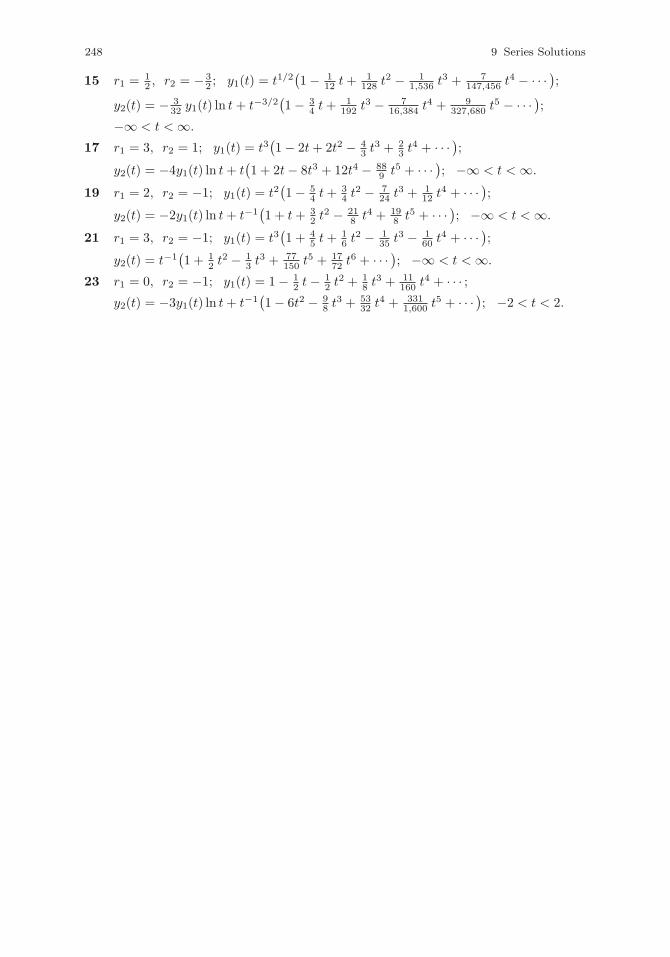
248 9 Series Solutions
15 r1 = 12 , r2 = − 3
2 ; y1(t) = t1/2(1− 1
12 t+1
128 t2 − 1
1,536 t3 + 7
147,456 t4 − · · · );
y2(t) = − 332 y1(t) ln t+ t−3/2
(1− 3
4 t+1
192 t3 − 7
16,384 t4 + 9
327,680 t5 − · · · );
−∞ < t < ∞.
17 r1 = 3, r2 = 1; y1(t) = t3(1− 2t+ 2t2 − 4
3 t3 + 2
3 t4 + · · · );
y2(t) = −4y1(t) ln t+ t(1 + 2t− 8t3 + 12t4 − 88
9 t5 + · · · ); −∞ < t < ∞.
19 r1 = 2, r2 = −1; y1(t) = t2(1− 5
4 t+34 t
2 − 724 t
3 + 112 t
4 + · · · );y2(t) = −2y1(t) ln t+ t−1
(1 + t+ 3
2 t2 − 21
8 t4 + 198 t5 + · · · ); −∞ < t < ∞.
21 r1 = 3, r2 = −1; y1(t) = t3(1 + 4
5 t+16 t
2 − 135 t
3 − 160 t
4 + · · · );y2(t) = t−1
(1 + 1
2 t2 − 1
3 t3 + 77
150 t5 + 17
72 t6 + · · · ); −∞ < t < ∞.
23 r1 = 0, r2 = −1; y1(t) = 1− 12 t− 1
2 t2 + 1
8 t3 + 11
160 t4 + · · · ;
y2(t) = −3y1(t) ln t+ t−1(1− 6t2 − 9
8 t3 + 53
32 t4 + 331
1,600 t5 + · · · ); −2 < t < 2.
Appendix A
Algebra Techniques
A.1 Partial Fractions
The integration of a rational function—that is, a function of the form P/Q, where Pand Q are polynomials—becomes much easier if the function can be written as a sumof simpler expressions, commonly referred to as partial fractions. This is done by meansof a procedure that consists of the following steps:
(i) Using long division, if necessary, we isolate the fractional part of the given function,for which the degree of P is strictly less than the degree of Q.
(ii) We split Q into a product of linear factors (first-degree polynomials) and irre-ducible quadratic factors (second-degree polynomials with complex roots). Someof these factors may be repeated.
(iii) For each single linear factor ax + b, we write a fraction of the form C/(ax + b).For each repeated linear factor (ax+ b)n, we write a sum of fractions of the form
C1
ax+ b+
C2
(ax + b)2+ · · ·+ Cn
(ax + b)n.
(iv) For each single irreducible quadratic factor ax2 + bx + c, we write a fraction ofthe form (C1x+C2)/(ax
2+ bx+ c). For each repeated irreducible quadratic factor(ax2 + bx+ c)n, we write a sum of fractions of the form
C11x+ C12
ax2 + bx+ c+
C21x+ C22
(ax2 + bx+ c)2+ · · ·+ Cn1x+ Cn2
(ax2 + bx+ c)n.
(v) The fractional part of the given function is equal to the sum of all the partialfractions and sums of partial fractions constructed in steps (iii) and (iv). Theunknown coefficients C, Ci, and Cij are determined (uniquely) from this equality.
A.1 Example. The denominator of the fraction (x − 5)/(x2 − 4x + 3) is a quadraticpolynomial, but it is not irreducible. Its roots are 1 and 3, so we write
x− 5
x2 − 4x+ 3=
x− 5
(x− 1)(x− 3)=
A
x− 1+
B
x− 3.
If we eliminate the denominators, we arrive at the equality
x− 5 = A(x − 3) +B(x − 1) = (A+B)x− 3A−B,
C. Constanda, Differential Equations: A Primer for Scientists and Engineers, SpringerUndergraduate Texts in Mathematics and Technology, DOI 10.1007/978-1-4614-7297-1 10,© Springer Science+Business Media New York 2013
249
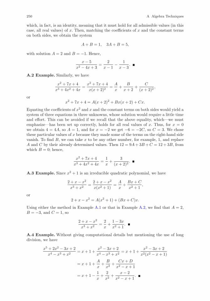
250 A Algebra Techniques
which, in fact, is an identity, meaning that it must hold for all admissible values (in thiscase, all real values) of x. Then, matching the coefficients of x and the constant termson both sides, we obtain the system
A+B = 1, 3A+B = 5,
with solution A = 2 and B = −1. Hence,
x− 5
x2 − 4x+ 3=
2
x− 1− 1
x− 3.
A.2 Example. Similarly, we have
x2 + 7x+ 4
x3 + 4x2 + 4x=
x2 + 7x+ 4
x(x+ 2)2=
A
x+
B
x+ 2+
C
(x+ 2)2,
orx2 + 7x+ 4 = A(x+ 2)2 +Bx(x+ 2) + Cx.
Equating the coefficients of x2 and x and the constant terms on both sides would yield asystem of three equations in three unknowns, whose solution would require a little timeand effort. This can be avoided if we recall that the above equality, which—we mustemphasize—has been set up correctly, holds for all real values of x. Thus, for x = 0we obtain 4 = 4A, so A = 1, and for x = −2 we get −6 = −2C, so C = 3. We chosethese particular values of x because they made some of the terms on the right-hand sidevanish. To find B, we can take x to be any other number, for example, 1, and replaceA and C by their already determined values. Then 12 = 9A+3B+C = 12+ 3B, fromwhich B = 0; hence,
x2 + 7x+ 4
x3 + 4x2 + 4x=
1
x+
3
(x + 2)2.
A.3 Example. Since x2 + 1 is an irreducible quadratic polynomial, we have
2 + x− x2
x3 + x2=
2 + x− x2
x(x2 + 1)=
A
x+Bx+ C
x2 + 1,
or2 + x− x2 = A(x2 + 1) + (Bx+ C)x.
Using either the method in Example A.1 or that in Example A.2, we find that A = 2,B = −3, and C = 1, so
2 + x− x2
x3 + x2=
2
x+
1− 3x
x2 + 1.
A.4 Example. Without giving computational details but mentioning the use of longdivision, we have
x5 + 2x2 − 3x+ 2
x4 − x3 + x2= x+ 1 +
x2 − 3x+ 2
x4 − x3 + x2= x+ 1 +
x2 − 3x+ 2
x2(x2 − x+ 1)
= x+ 1 +A
x+
B
x2+
Cx +D
x2 − x+ 1
= x+ 1− 1
x+
2
x2+
x− 2
x2 − x+ 1.
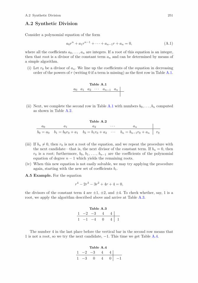
A.2 Synthetic Division 251
A.2 Synthetic Division
Consider a polynomial equation of the form
a0rn + a1r
n−1 + · · ·+ an−1r + an = 0, (A.1)
where all the coefficients a0, . . . , an are integers. If a root of this equation is an integer,then that root is a divisor of the constant term an and can be determined by means ofa simple algorithm.
(i) Let r0 be a divisor of an. We line up the coefficients of the equation in decreasingorder of the powers of r (writing 0 if a term is missing) as the first row in Table A.1.
Table A.1
a0 a1 a2 · · · an−1 an
(ii) Next, we complete the second row in Table A.1 with numbers b0, . . . , bn computedas shown in Table A.2.
Table A.2
a0 a1 a2 · · · an
b0 = a0 b1 = b0r0 + a1 b2 = b1r0 + a2 · · · bn = bn−1r0 + an r0
(iii) If bn �= 0, then r0 is not a root of the equation, and we repeat the procedure withthe next candidate—that is, the next divisor of the constant term. If bn = 0, thenr0 is a root; furthermore, b0, b1, . . . , bn−1 are the coefficients of the polynomialequation of degree n− 1 which yields the remaining roots.
(iv) When this new equation is not easily solvable, we may try applying the procedureagain, starting with the new set of coefficients bi.
A.5 Example. For the equation
r4 − 2r3 − 3r2 + 4r + 4 = 0,
the divisors of the constant term 4 are ±1, ±2, and ±4. To check whether, say, 1 is aroot, we apply the algorithm described above and arrive at Table A.3.
Table A.3
1 −2 −3 4 4
1 −1 −4 0 4 1
The number 4 in the last place before the vertical bar in the second row means that1 is not a root, so we try the next candidate, −1. This time we get Table A.4.
Table A.4
1 −2 −3 4 4
1 −3 0 4 0 −1
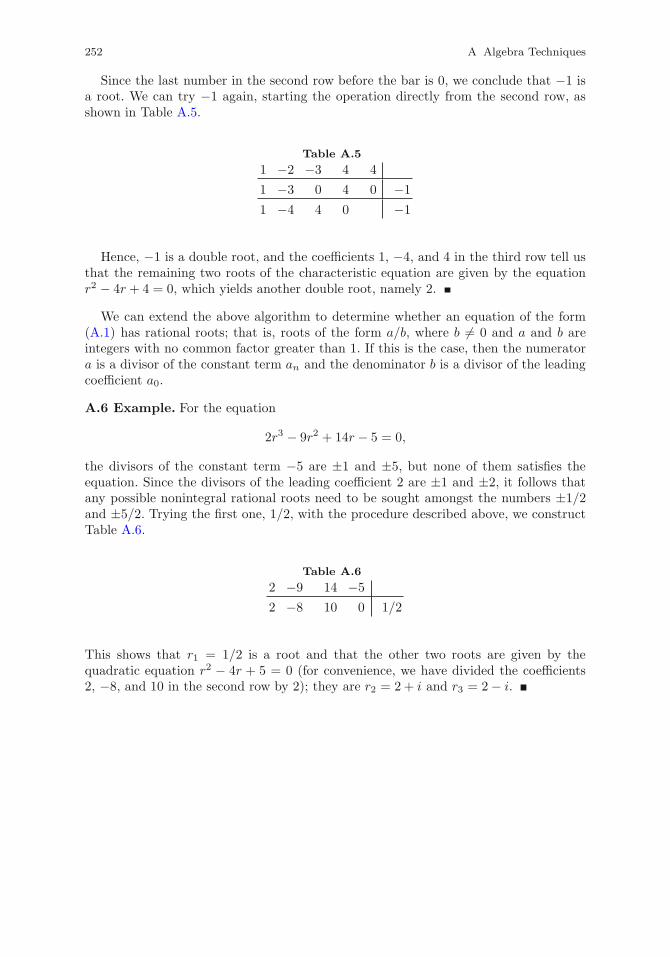
252 A Algebra Techniques
Since the last number in the second row before the bar is 0, we conclude that −1 isa root. We can try −1 again, starting the operation directly from the second row, asshown in Table A.5.
Table A.5
1 −2 −3 4 4
1 −3 0 4 0 −1
1 −4 4 0 −1
Hence, −1 is a double root, and the coefficients 1, −4, and 4 in the third row tell usthat the remaining two roots of the characteristic equation are given by the equationr2 − 4r + 4 = 0, which yields another double root, namely 2.
We can extend the above algorithm to determine whether an equation of the form(A.1) has rational roots; that is, roots of the form a/b, where b �= 0 and a and b areintegers with no common factor greater than 1. If this is the case, then the numeratora is a divisor of the constant term an and the denominator b is a divisor of the leadingcoefficient a0.
A.6 Example. For the equation
2r3 − 9r2 + 14r − 5 = 0,
the divisors of the constant term −5 are ±1 and ±5, but none of them satisfies theequation. Since the divisors of the leading coefficient 2 are ±1 and ±2, it follows thatany possible nonintegral rational roots need to be sought amongst the numbers ±1/2and ±5/2. Trying the first one, 1/2, with the procedure described above, we constructTable A.6.
Table A.6
2 −9 14 −5
2 −8 10 0 1/2
This shows that r1 = 1/2 is a root and that the other two roots are given by thequadratic equation r2 − 4r + 5 = 0 (for convenience, we have divided the coefficients2, −8, and 10 in the second row by 2); they are r2 = 2+ i and r3 = 2− i.
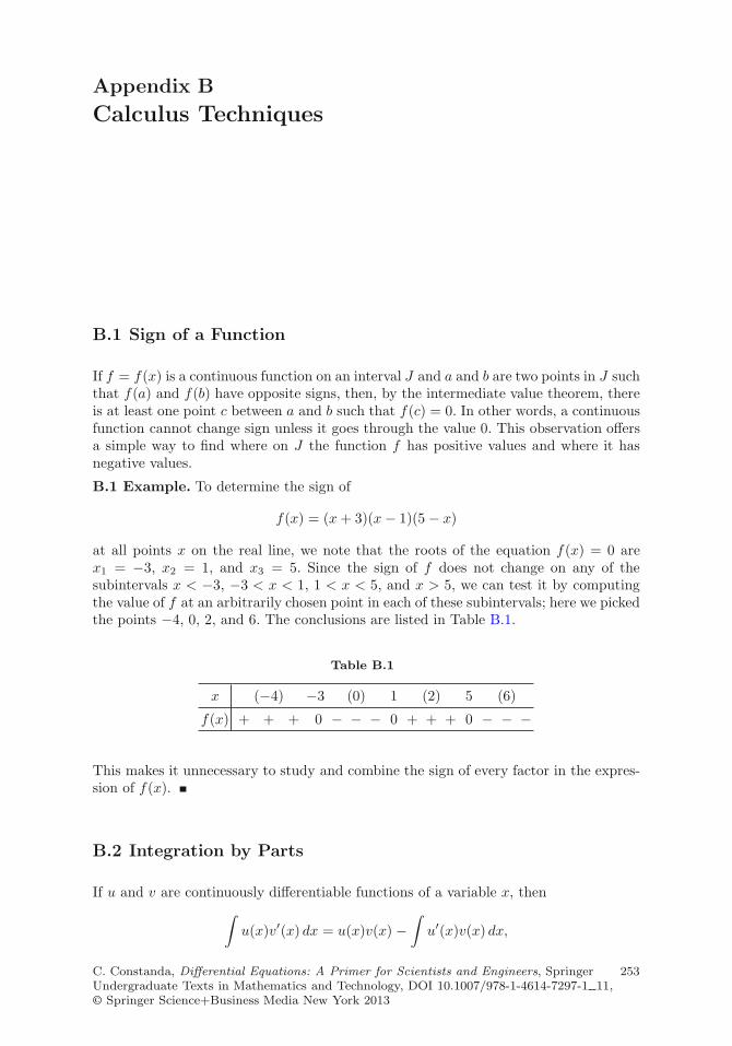
Appendix B
Calculus Techniques
B.1 Sign of a Function
If f = f(x) is a continuous function on an interval J and a and b are two points in J suchthat f(a) and f(b) have opposite signs, then, by the intermediate value theorem, thereis at least one point c between a and b such that f(c) = 0. In other words, a continuousfunction cannot change sign unless it goes through the value 0. This observation offersa simple way to find where on J the function f has positive values and where it hasnegative values.
B.1 Example. To determine the sign of
f(x) = (x+ 3)(x− 1)(5 − x)
at all points x on the real line, we note that the roots of the equation f(x) = 0 arex1 = −3, x2 = 1, and x3 = 5. Since the sign of f does not change on any of thesubintervals x < −3, −3 < x < 1, 1 < x < 5, and x > 5, we can test it by computingthe value of f at an arbitrarily chosen point in each of these subintervals; here we pickedthe points −4, 0, 2, and 6. The conclusions are listed in Table B.1.
Table B.1
x (−4) −3 (0) 1 (2) 5 (6)
f(x) + + + 0 − − − 0 + + + 0 − − −
This makes it unnecessary to study and combine the sign of every factor in the expres-sion of f(x).
B.2 Integration by Parts
If u and v are continuously differentiable functions of a variable x, then
∫u(x)v′(x) dx = u(x)v(x) −
∫u′(x)v(x) dx,
C. Constanda, Differential Equations: A Primer for Scientists and Engineers, SpringerUndergraduate Texts in Mathematics and Technology, DOI 10.1007/978-1-4614-7297-1 11,© Springer Science+Business Media New York 2013
253
254 B Calculus Techniques
or, in abbreviated form, ∫u dv = uv −
∫v du.
B.2 Example. Let
I1 =
∫eax cos(bx) dx, I2 =
∫eax sin(bx) dx.
Then
I1 =1
aeax cos(bx)−
∫1
aeax(− sin(bx))b dx =
1
aeax cos(bx) +
b
aI2,
I2 =1
aeax sin(bx)−
∫1
aeax cos(bx)b dx =
1
aeax sin(bx)− b
aI1.
This is a simple algebraic system for I1 and I2, which yields
I1 =
∫eax cos(bx) dx =
1
a2 + b2eax[a cos(bx) + b sin(bx)] + C, (B.1)
I2 =
∫eax sin(bx) dx =
1
a2 + b2eax[a sin(bx) − b cos(bx)] + C. (B.2)
B.3 Integration by Substitution
Let f = f(x) be a continuous function on an interval [a, b], and let x = x(t) be acontinuously differentiable function on an interval [c, d], which takes values in [a, b] andis such that x(c) = a and x(d) = b. Then
b∫a
f(x) dx =
d∫c
f(x(t))x′(t) dt.
B.3 Example. If g = g(t), then, in the absence of prescribed limits,
∫g′(t)g(t)
dt =
∫1
g(t)g′(t) dt =
∫dg
g= ln |g|+ C.
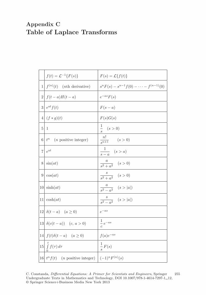
Appendix C
Table of Laplace Transforms
C. Constanda, Differential Equations: A Primer for Scientists and Engineers, SpringerUndergraduate Texts in Mathematics and Technology, DOI 10.1007/978-1-4614-7297-1 12,© Springer Science+Business Media New York 2013
255
f(t) = L−1{F (s)} F (s) = L{f(t)}
1 f (n)(t) (nth derivative) snF (s)− sn−1f(0)− · · · − f (n−1)(0)
2 f(t− a)H(t− a) e−asF (s)
3 eatf(t) F (s− a)
4 (f ∗ g)(t) F (s)G(s)
5 11
s(s > 0)
6 tn (n positive integer)n!
sn+1(s > 0)
7 eat1
s− a(s > a)
8 sin(at)a
s2 + a2(s > 0)
9 cos(at)s
s2 + a2(s > 0)
10 sinh(at)a
s2 − a2(s > |a|)
11 cosh(at)s
s2 − a2(s > |a|)
12 δ(t− a) (a ≥ 0) e−as
13 δ(c(t− a)) (c, a > 0)1
ce−as
14 f(t)δ(t− a) (a ≥ 0) f(a)e−as
15t∫0
f(τ) dτ1
sF (s)
16 tnf(t) (n positive integer) (−1)nF (n)(s)
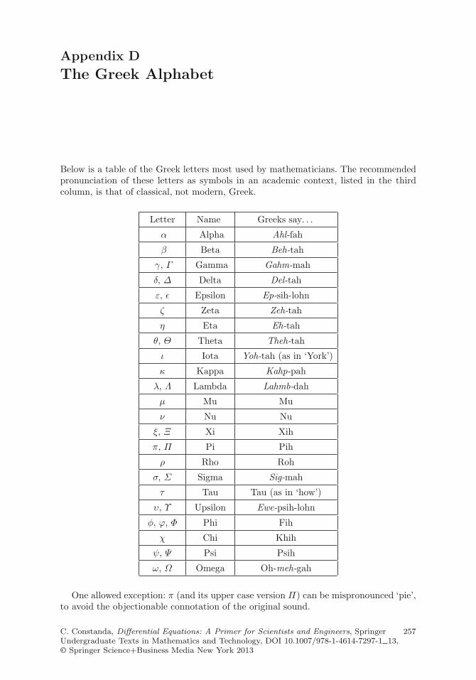
Appendix D
The Greek Alphabet
Below is a table of the Greek letters most used by mathematicians. The recommendedpronunciation of these letters as symbols in an academic context, listed in the thirdcolumn, is that of classical, not modern, Greek.
Letter Name Greeks say. . .
α Alpha Ahl-fah
β Beta Beh-tah
γ, Γ Gamma Gahm-mah
δ, Δ Delta Del-tah
ε, ε Epsilon Ep-sih-lohn
ζ Zeta Zeh-tah
η Eta Eh-tah
θ, Θ Theta Theh-tah
ι Iota Yoh-tah (as in ‘York’)
κ Kappa Kahp-pah
λ, Λ Lambda Lahmb-dah
μ Mu Mu
ν Nu Nu
ξ, Ξ Xi Xih
π, Π Pi Pih
ρ Rho Roh
σ, Σ Sigma Sig-mah
τ Tau Tau (as in ‘how’)
υ, Υ Upsilon Ewe-psih-lohn
φ, ϕ, Φ Phi Fih
χ Chi Khih
ψ, Ψ Psi Psih
ω, Ω Omega Oh-meh-gah
One allowed exception: π (and its upper case version Π) can be mispronounced ‘pie’,to avoid the objectionable connotation of the original sound.
C. Constanda, Differential Equations: A Primer for Scientists and Engineers, SpringerUndergraduate Texts in Mathematics and Technology, DOI 10.1007/978-1-4614-7297-1 13,© Springer Science+Business Media New York 2013
257
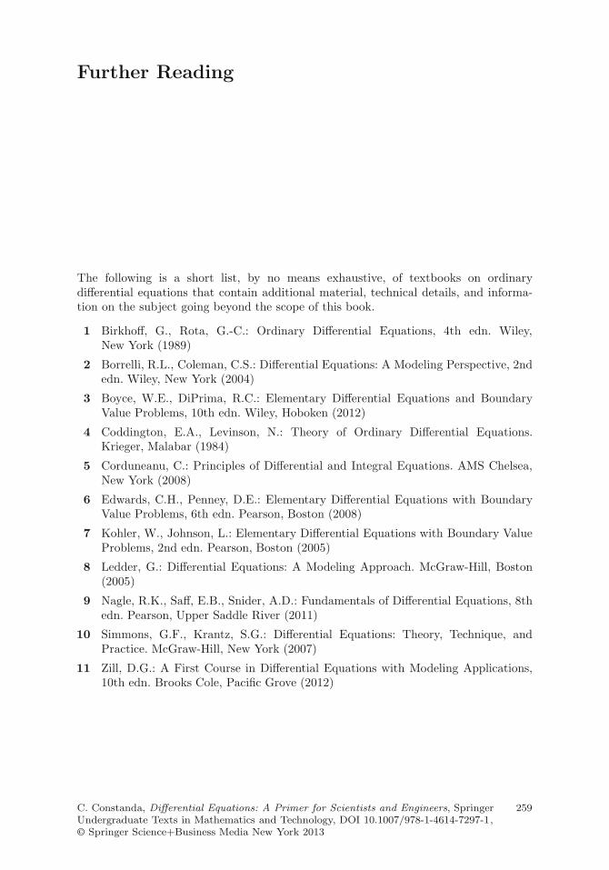
Further Reading
The following is a short list, by no means exhaustive, of textbooks on ordinarydifferential equations that contain additional material, technical details, and informa-tion on the subject going beyond the scope of this book.
1 Birkhoff, G., Rota, G.-C.: Ordinary Differential Equations, 4th edn. Wiley,New York (1989)
2 Borrelli, R.L., Coleman, C.S.: Differential Equations: A Modeling Perspective, 2ndedn. Wiley, New York (2004)
3 Boyce, W.E., DiPrima, R.C.: Elementary Differential Equations and BoundaryValue Problems, 10th edn. Wiley, Hoboken (2012)
4 Coddington, E.A., Levinson, N.: Theory of Ordinary Differential Equations.Krieger, Malabar (1984)
5 Corduneanu, C.: Principles of Differential and Integral Equations. AMS Chelsea,New York (2008)
6 Edwards, C.H., Penney, D.E.: Elementary Differential Equations with BoundaryValue Problems, 6th edn. Pearson, Boston (2008)
7 Kohler, W., Johnson, L.: Elementary Differential Equations with Boundary ValueProblems, 2nd edn. Pearson, Boston (2005)
8 Ledder, G.: Differential Equations: A Modeling Approach. McGraw-Hill, Boston(2005)
9 Nagle, R.K., Saff, E.B., Snider, A.D.: Fundamentals of Differential Equations, 8thedn. Pearson, Upper Saddle River (2011)
10 Simmons, G.F., Krantz, S.G.: Differential Equations: Theory, Technique, andPractice. McGraw-Hill, New York (2007)
11 Zill, D.G.: A First Course in Differential Equations with Modeling Applications,10th edn. Brooks Cole, Pacific Grove (2012)
C. Constanda, Differential Equations: A Primer for Scientists and Engineers, SpringerUndergraduate Texts in Mathematics and Technology, DOI 10.1007/978-1-4614-7297-1,© Springer Science+Business Media New York 2013
259
Index
Aamplitude, 104
modulation, 111analytic function, 222antiderivative, 3autonomous equations, 49
Bbasis eigenvectors, 149beats, 111Bernoulli equations, 26Bessel’s
equation, 240, 246function, 240, 246
boundaryconditions, 6value problem, 6, 70
CCauchy–Euler equations, 97center, 162characteristic
equation, 71, 147polynomial, 71, 147roots, 72complex conjugate, 77real and distinct, 72repeated, 74
chemical reaction, 56column vector, 141complementary function, 80, 130, 178compound interest, 4, 43consumer–resource model, 138contagious disease epidemic, 138convective heat, 62convolution, 192coupled mechanical oscillators, 138Cramer’s rule, 63critical
damping, 107point, 50
critically damped response, 115
Ddamped
forced oscillations, 112free oscillations, 106
dampingcoefficient, 61, 103ratio, 106
determinant, 63, 118expansion in a row or column, 118
diagonalization, method of, 175, 178differential, 3differential equations, 4
classification of, 9homogeneous, 12linear, 12order of, 11ordinary, 11partial, 11with constant coefficients, 12
Dirac delta, 209direction field, 40distribution, 209driving force, 103
Eeigenline, 155eigenvalues, 147
algebraic multiplicity of, 149complex conjugate, 161deficiency of, 149geometric multiplicity of, 149real and distinct, 155repeated, 165
eigenvectors, 147generalized, 166
elastic coefficient, 103electrical vibrations, 114elementary row operations, 120environmental carrying capacity, 51equilibrium solution, 15, 50, 154
asymptotically stable, 51, 154
C. Constanda, Differential Equations: A Primer for Scientists and Engineers, SpringerUndergraduate Texts in Mathematics and Technology, DOI 10.1007/978-1-4614-7297-1,© Springer Science+Business Media New York 2013
261
262 Index
equilibrium solution (cont.)stable, 51unstable, 51, 154
Euler’s formula, 77exact equations, 30existence and uniqueness theorem, 70
for linear equations, 35for nonlinear equations, 36for systems, 151
exponents at the singularity, 232
Fforced
mechanical oscillations, 110response, 112
forcing termscontinuous, 199piecewise continuous, 204with the Dirac delta, 208
freefall in gravity, 4, 44, 61mechanical oscillations, 103
Frobeniusmethod of, 232solutions, 232
fundamental set of solutions, 69, 153
GGaussian elimination, 120general solution, 6, 222generalized
Airy equation, 117function, 209
Hhalf-life, 43harmonic
oscillations of a beam, 117oscillator, 61
Heaviside function, 194homogeneous
equations, 67, 126with constant coefficients, 71
linear systemswith constant coefficients, 154
polar equations, 24
Iindicial equation, 232
with distinct roots differing by an integer,241
with equal roots, 236with roots that do not differ by an integer,
232initial
conditions, 6value problem, 6, 67
integrating factor, 20, 33integration
by parts, 253by substitution, 254
intermediate value theorem, 253
KKirchhoff’s law, 47
LLaplace
transform, 187transformation, 187inverse, 189properties of, 187, 194
limit, 1linear
first-order equations, 20independence, 124, 145operator, 10second-order equations, 61
linearly dependentfunctions, 64, 124vector functions, 145vectors, 145
loan repayment, 4, 47
Mmathematical models, 4
with first-order equations, 41with higher-order equations, 117with second-order equations, 61, 103
matrix, 62, 118exponential, 174functions, 143fundamental, 173inverse of, 142invertible, 141leading diagonal of, 118, 141multiplication, 140nonsingular, 141transpose of, 141
maximal interval of existence, 35, 152military combat, 137motion of a pendulum, 62
Nnatural frequency, 103Newton’s
law of cooling, 4, 46second law, 8, 61
node, 158degenerate, 168
nonhomogeneous equations, 80, 130nonlinear equations, 100
Ooperations with matrices, 139operator, 9
of differentiation, 9ordinary point, 222overdamping, 106
Ppartial
derivative, 2fractions, 249
Index 263
particular solution, 6, 88, 178period of oscillation, 103phase
angle, 104plane, 155portrait, 155
piecewise continuous function, 187population
growth, 4, 41with a critical threshold, 54with logistic growth, 49with logistic growth and a threshold, 56with logistic growth and harvesting, 52
power series, 221predator–pray, 138principle of superposition, 67, 91, 153, 181
Rradioactive decay, 4, 42radius of convergence, 221RC electric circuit, 4, 46recurrence relation, 222resonance, 111
frequency, 115Riccati equations, 28RLC electric circuit, 61row vector, 141
Ssaddle point, 157Schrodinger equation, 62separable equations, 15sequence of partial sums, 221series solution, 221
convergence theorem for, 222near a regular singular point, 231near an ordinary point, 222
simple harmonic motion, 104singular point, 222
regular, 229
solution, 151curve, 5, 19, 31mix, 137
spiral point, 163steady-state solution, 112synthetic division, 127, 251systems
of algebraic equations, 63, 119of differential equations, 13, 137, 151nonhomogeneous linear, 178
TTaylor series, 222temperature in a circular annulus, 62temperature in a rod, 5trajectories, 155transformation parameter, 187transient solution, 112
Uundamped
forced oscillations, 110free oscillations, 103
underdamping, 108undetermined coefficients, method of, 81, 88,
130, 179unit
impulse, 208step function, 194
Vvariation of parameters, method of, 94, 134,
182vector space, 139
WWronskian, 63, 124, 145
YYoung modulus, 117
Related Documents


