Welcome message from author
This document is posted to help you gain knowledge. Please leave a comment to let me know what you think about it! Share it to your friends and learn new things together.
Transcript

S. Sumathi, S. Esakkirajan
Fundamentals of Relational Database Management Systems
Studies in Computational Intelligence, Volume 47
Editor-in-chiefProf. Janusz KacprzykSystems Research InstitutePolish Academy of Sciencesul. Newelska 601-447 WarsawPolandE-mail: [email protected]
Further volumes of this seriescan be found on our homepage:springer.com
Vol. 29. Sai Sumathi, S.N. SivanandamIntroduction to Data Mining and itsApplication, 2006ISBN 978-3-540-34350-9
Vol. 30. Yukio Ohsawa, Shusaku Tsumoto (Eds.)Chance Discoveries in Real World Decision Making,2006ISBN 978-3-540-34352-3
Vol. 31. Ajith Abraham, Crina Grosan, VitorinoRamos (Eds.)Stigmergic Optimization, 2006ISBN 978-3-540-34689-0
Vol. 32. Akira HiroseComplex-Valued Neural Networks, 2006ISBN 978-3-540-33456-9
Vol. 33. Martin Pelikan, Kumara Sastry, ErickCantu-Paz (Eds.)Scalable Optimization via ProbabilisticModeling, 2006ISBN 978-3-540-34953-2
Vol. 34. Ajith Abraham, Crina Grosan, VitorinoRamos (Eds.)Swarm Intelligence in Data Mining, 2006ISBN 978-3-540-34955-6
Vol. 35. Ke Chen, Lipo Wang (Eds.)Trends in Neural Computation, 2007ISBN 978-3-540-36121-3
Vol. 36. Ildar Batyrshin, Janusz Kacprzyk, LeonidSheremetor, Lotfi A. Zadeh (Eds.)Preception-based Data Mining and Decision Makingin Economics and Finance, 2006ISBN 978-3-540-36244-9
Vol. 37. Jie Lu, Da Ruan, Guangquan Zhang (Eds.)E-Service Intelligence, 2007ISBN 978-3-540-37015-4
Vol. 38. Art Lew, Holger MauchDynamic Programming, 2007ISBN 978-3-540-37013-0
Vol. 39. Gregory Levitin (Ed.)Computational Intelligence in ReliabilityEngineering, 2007ISBN 978-3-540-37367-4
Vol. 40. Gregory Levitin (Ed.)Computational Intelligence in ReliabilityEngineering, 2007ISBN 978-3-540-37371-1
Vol. 41. Mukesh Khare, S.M. Shiva Nagendra (Eds.)Artificial Neural Networks in Vehicular PollutionModelling, 2007ISBN 978-3-540-37417-6
Vol. 42. Bernd J. Kramer, Wolfgang A. Halang (Eds.)Contributions to Ubiquitous Computing, 2007ISBN 978-3-540-44909-6
Vol. 43. Fabrice Guillet, Howard J. Hamilton (Eds.)Quality Measures in Data Mining, 2007ISBN 978-3-540-44911-9
Vol. 44. Nadia Nedjah, Luiza de MacedoMourelle, Mario Neto Borges, Nival Nunesde Almeida (Eds.)Intelligent Educational Machines, 2007ISBN 978-3-540-44920-1
Vol. 45. Vladimir G. Ivancevic, Tijana T. IvancevicNeuro-Fuzzy Associative Machinery forComprehensive Brain and Cognition Modelling,2007ISBN 978-3-540-47463-0
Vol. 46. Valentina Zharkova, Lakhmi C. Jain (Eds.)Artificial Intelligence in Recognition andClassification of Astrophysical and MedicalImages, 2007ISBN 978-3-540-47511-8
Vol. 47. S. Sumathi, S. EsakkirajanFundamentals of Relational Database ManagementSystems, 2007ISBN 978-3-540-48397-7
S. SumathiS. Esakkirajan
Fundamentals of RelationalDatabase ManagementSystems
With 312 Figures and 30 Tables
Dr. S. SumathiAssistant Professor
Department of Electrical and Electronics Engineering
PSG College of Technology
P.O. Box 1611
Peelamedu
Coimbatore 641 004
Tamil Nadu, India
E-mail: ss [email protected]
S. EsakkirajanLecturer
Department of Electrical and Electronics Engineering
PSG College of Technology
P.O. Box 1611
Peelamedu
Coimbatore 641 004
Tamil Nadu, India
E-mail: [email protected]
Library of Congress Control Number: 2006935984
ISSN print edition: 1860-949XISSN electronic edition: 1860-9503ISBN-10 3-540-48397-7 Springer Berlin Heidelberg New YorkISBN-13 978-3-540-48397-7 Springer Berlin Heidelberg New York
This work is subject to copyright. All rights are reserved, whether the whole or part of the materialis concerned, specifically the rights of translation, reprinting, reuse of illustrations, recitation, broad-casting, reproduction on microfilm or in any other way, and storage in data banks. Duplication ofthis publication or parts thereof is permitted only under the provisions of the German Copyright Lawof September 9, 1965, in its current version, and permission for use must always be obtained fromSpringer-Verlag. Violations are liable to prosecution under the German Copyright Law.
Springer is a part of Springer Science+Business Mediaspringer.comc© Springer-Verlag Berlin Heidelberg 2007
The use of general descriptive names, registered names, trademarks, etc. in this publication does notimply, even in the absence of a specific statement, that such names are exempt from the relevantprotective laws and regulations and therefore free for general use.
Cover design: deblik, BerlinTypesetting by SPi using a Springer LATEX macro packagePrinted on acid-free paper SPIN: 11820970 89/SPi 5 4 3 2 1 0
Preface
Information is a valuable resource to an organization. Computer softwareprovides an efficient means of processing information, and database systemsare becoming increasingly common means by which it is possible to store andretrieve information in an effective manner. This book provides comprehen-sive coverage of fundamentals of database management system. This book isfor those who wish a better understanding of relational data modeling, itspurpose, its nature, and the standards used in creating relational data model.
Relational databases are the most popular database management systemsin the world and are supported by a variety of vendor implementations.Majority of the practical tasks in industry require applying relatively notcomplex algorithms to huge amounts of well-structured data. The efficiencyof the application depends on the quality of data organization. Advances indatabase technology and processing offer opportunities for using informationflexibility and efficiently when data is organized and stored in relational struc-tures. The relational DBMS is a success in the commercial market place withrespect to business data processing and related applications. This success isa result of cost effective application development combined with high dataconsistency. The success has led to the use of relational DBMS technology inother application environments requesting its traditional virtues, while at thesame time adding new requirements.
SQL is the standard computer language used to communicate with rela-tional database management systems. Chapter 4 gives an introduction to SQLwith illustrative examples. The limitations of SQL and how to overcome thatlimitations using PL/SQL are discussed in Chap. 5.
The current trends in hardware like RAID technology made relationalDBMSs to support high transmission rates, very high availability, and a softreal-time transaction a cost effective possibility. The basics of RAID technol-ogy, different levels of RAID are discussed in this book.
Object-oriented databases are also becoming important. As object-oriented programming continues to increase in popularity, the demand for
VI Preface
such databases will grow. Due to this reason a separate chapter is beingdevoted to object-oriented DBMS and object-relational DBMS.
This text discusses a number of new technologies and challenges indatabase management systems like Genome Database Management System,Mobile Database Management System, Multimedia Database ManagementSystem, Spatial Database Management Systems, and XML.
Finally, there is no substitute for experience. To ensure that everystudent can have experience for creating data models and database design,list of projects along with codes in VB and Oracle are given. The goal inproviding the list of projects is to ensure that students should have atleastone commercial product at their disposal.
About the Book
The book is meant for wide range of readers from College, University Studentswho wish to learn basics as well as advanced concepts in Database Manage-ment System. It can also be meant for the programmers who may be involvedin the programming based on the Oracle and Visual Basic applications.
Database Management System, at present is a well-developed field, amongacademicians as well as between program developers. The principles of Data-base Management System are dealt in depth with the information and theuseful knowledge available for computing processes. The various approachesto data models and the relative advantages of relational model are given indetail.
Relational databases are the most popular database management systemsin the world and are supported by a variety of vendor implementations. Thesolutions to the problems are programmed using Oracle and the results aregiven. The overview of Oracle and Visual Basic is provided for easy referenceto the students and professionals. This book also provides introduction tocommercial DBMS, pioneers in DBMS, and dictionary of DBMS terms inappendix.
The various worked out examples and the solutions to the problems arewell balanced pertinent to the RDBMS Projects, Labs, and for College andUniversity Level Studies.
This book provides data models, database design, and application-orientedstructures to help the reader to move in to the database management world.The book also presents application case studies on a wide range of connectedfields to facilitate the reader for better understanding. This book can be usedfrom Under Graduation to Post-Graduate Level. Some of the projects done arealso added in the book. The book contains solved example problems, reviewquestions, and solutions.
This book can be used as a ready reference guide for computer professionalswho are working in DBMS field. Most of the concepts, solved problems and
Preface VII
applications for wide variety of areas covered in this book, which can fulfill asan advanced academic book.
We hope that the reader will find this book a truly helpful guide and avaluable source of information about the database management principles fortheir numerous practical applications.
Salient Features
The salient features of this book includes:
– Detailed description on relational database management system concepts– Variety of solved examples– Review questions with solutions– Worked out results to understand the concepts of relational database man-
agement Systems using Oracle Version 8.0.– Application case studies and projects on database management system
in various fields like Transport Management, Hospital Management, andAcademic Institution Management, Hospital Management, Railway Man-agement and Election Voting System.
Organization of the Book
The book covers 14 chapters altogether. The fundamentals of relational data-base management systems are discussed with basic principles, advanced con-cepts, and recent challenges. The application case studies are also discussed.
The chapters are organized as follows:
– Chapter 1 gives an overview of database management system, Evolutionof Database Management System, ANSI/SPARK data model, Two-tier,Three-tier and Multi-tier database architecture.
– The preliminaries of the Entity Relation (ER) data model are described inChap. 2. Different types of entities, attributes and relations are discussedwith examples. Mapping from ER model to relational model, EnhancedER model, which includes generalization, specialization, are given withrelevant examples.
– Chapter 3 deals with relational data model. In this chapter E.F. Codd rule,basic definition of relation, cardinality of the relation, arity of the rela-tion, constraints in relation are given with suitable examples. Relationalalgebra, tuple relational calculus, domain relational calculus and differentoperations involved are explained with lucid examples. This chapter alsodiscusses the features of QBE with examples.
– Chapter 4 exclusively deals with Structured Query Language. The datadefinition language, data manipulation language and the data control lan-guage were explained with suitable examples. Views, imposition of con-straints in a relation are discussed with examples.
VIII Preface
– Chapter 5 deals with PL/SQL. The shortcomings of SQL and how theyare overcome in PL/SQL, the structure of PL/SQL are given in detail. Theiterative control like FOR loop, WHILE loop are explained with exam-ples. The concept of CURSOR and the types of CURSORS are explainedwith suitable examples. The concept of PROCEDURE, FUNCTION, andPACKAGE are explained in detail. The concept of EXCEPTION HAN-DLING and the different types of EXCEPTION HANDLING are givenwith suitable examples. This chapter also gives an introduction to data-base triggers and the different types of triggers.
– Chapter 6 deals with various phases in database design. The concept ofdatabase design tools and the different types of database design toolsare given in this chapter. Functional dependency, normalization are alsodiscussed in this chapter. Different types of functional dependency, normalforms, conversion from one normal form to the other are explained withexamples. The idea of denormalization is also introduced in this chapter.
– Chapter 7 gives details on transaction processing. Detailed descrip-tion about deadlock condition and two phase locking are given throughexamples. This chapter also discusses the concept of query optimization,architecture of query optimizer and query optimization through GeneticAlgorithm.
– Chapter 8 deals with database security and recovery. The need for data-base security, different types of database security is explained in detail.The different types of database failures and the method to recover thedatabase is given in this chapter. ARIES recovery algorithm is explainedin a simple manner in this chapter.
– Chapter 9 discusses the physical database design. The different typesof File organization like Heap file, sequential file, and indexed file areexplained in this chapter. The concept of B tree and B+ tree are explainedwith suitable example. The different types of data storage devices are dis-cussed in this chapter. Advanced data storage concept like RAID, differentlevels of RAID, hardware and software RAID are explained in detail.
– Advanced concepts like data mining, data warehousing, and spatial data-base management system are discussed in Chap. 10. The data mining con-cept and different types of data mining systems are given in this chapter.The performance issues, data integration, data mining rules are explainedin this chapter.
– Chapter 11 throws light on the concept of object-oriented and objectRelational DBMS. The benefits of object-oriented programming, object-oriented programming languages, characteristics of object-oriented data-base, application of OODBMS are discussed in detail. This chapteralso discusses the features of ORDBMS, comparison of ORDBMS withOODBMS.
– Chapter 12 deals with distributed and parallel database management sys-tem. The features of distributed database, distributed DBMS architecture,distributed database design, distributed concurrency control are discussed
Preface IX
in depth. This chapter also discusses the basics of parallel database man-agement, parallel database architecture, parallel query optimization.
– Recent challenges in DBMS are given in Chap. 13 which includes genomedatabase management, mobile database management, spatial databasemanagement system and XML. In genome database management, theconcept of genome, genetic code, genome directory system project isdiscussed. In mobile database, mobile database center, mobile databasearchitecture, mobile transaction processing, distributed database for mo-bile are discussed in detail. In spatial database, spatial data types, spatialdatabase modeling, querying spatial data, spatial DBMS implementationare analyzed. In XML, the origin of XML, XML family, XSL, XML, anddatabase applications are discussed.
– Few projects related to bus transport management system, hospital man-agement, course administration system, Election voting system, librarymanagement system and railway management system are implementedusing Oracle as front end and Visual Basic as back end are discussed inChap. 14. This chapter also gives an idea of how to do successful projectsin DBMS.
– Four appendices given in this book includes dictionary of DBMS terms,overview of commands in SQL, pioneers in DBMS, commercial DBMS.Dictionary of DBMS terms gives the definition of commonly used termsin DBMS. Overview of commands in SQL gives the commonly used com-mands and their function. Pioneers in DBMS introduce great people likeE.F. Codd, Peter Chen who have contributed for the development of data-base management system. Commercial DBMS introduces some of the pop-ular commercial DBMS like System R, DB2 and Informix.
– The bibliography is given at the end after the appendix chapter.
About the Authors
S. Sumathi, B.E. in Electronics and Communication Engineering andMasters degree in Applied Electronics, Government College of Technology,Coimbatore, TamilNadu and Ph.D. in the area of Data Mining, is currentlyworking as Assistant Professor in the Department of Electrical and Elec-tronics Engineering, PSG College of Technology, Coimbatore with teachingand research experience of 16 years. She received the prestigious Gold Medalfrom the Institution of Engineers Journal Computer Engineering Division, forthe research paper titled, “Development of New Soft Computing Models forData Mining” and also Best project award for UG Technical Report, “Self-Organized Neural Network Schemes: As a Data mining tool”. She receivedDr. R. Sundramoorthy award for Outstanding Academic of PSG College ofTechnology in the year 2006. She has guided a project which received BestM.Tech Thesis award from Indian Society for Technical Education, New Delhi.In appreciation of publishing various technical articles the she has received
X Preface
National and International Journal Publication Awards. She has also pre-pared manuals for Electronics and Instrumentation Laboratory and Electricaland Electronics Laboratory of EEE Department, PSG College of Technology,Coimbatore, has organized second National Conference on Intelligent andEfficient Electrical Systems and has conducted short-term courses on “NeuroFuzzy System Principles and Data Mining Applications.” She has publishedseveral research articles in National and International Journals/Conferencesand guided many UG and PG projects. She has also reviewed papers inNational/International Journals and Conferences. She has published threebooks on “Introduction to Neural Networks with Matlab,” “Introduction toFuzzy Systems with Matlab,” and “Introduction to Data Mining and its Ap-plications.” The research interests include neural networks, fuzzy systems andgenetic algorithms, pattern recognition and classification, data warehousingand data mining, operating systems and parallel computing, etc.
S. Esakkirajan has a B.Tech Degree from Cochin University of Scienceand Technology, Cochin and M.E. Degree from PSG College of Technology,Coimbatore, with a Rank in M.E. He has received Alumni Award in hisM.E. He has presented papers in International and National Conferences. Hisresearch areas include database management system, neural network, geneticalgorithm, and digital image processing.
Acknowledgment
The authors are always thankful to the Almighty for perseverance and achieve-ments.
Sumathi and Esakkirajan wish to thank Mr. Rangaswamy, ManagingTrustee, PSG Institutions, Mr. C.R. Swaminathan, Chief Executive, andDr. R. Rudramoorthy, Principal, PSG College of Technology, Coimbatore, fortheir whole-hearted cooperation and great encouragement given in this suc-cessful endeavor. The authors appreciate and acknowledge Mr. Karthikeyan,Mr. Ponson, Mr. Manoj Kumar, Mr. Afsar Ahmed, Mr. Harikumar,Mr. Abdus Samad, Mr. Antony and Mr. Balumahendran who have beenwith them in their endeavors with their excellent, unforgettable help, andassistance in the successful execution of the work.
Dr. Sumathi owe much to her daughter Priyanka, who has helped her andto the support rendered by her husband, brother, and family. Mr. Esakkirajanlike to thank his wife Akila, who shouldered a lot of extra responsibilities anddid this with the long-term vision, depth of character, and positive outlookthat are truly befitting of her name. He like to thank his father Sankaralingamfor providing moral support and constant encouragement.
DEDICATED TO ALMIGHTY
Contents
1 Overview of Database Management System . . . . . . . . . . . . . . . . 11.1 Introduction . . . . . . . . . . . . . . . . . . . . . . . . . . . . . . . . . . . . . . . . . . . . 11.2 Data and Information . . . . . . . . . . . . . . . . . . . . . . . . . . . . . . . . . . . . 21.3 Database . . . . . . . . . . . . . . . . . . . . . . . . . . . . . . . . . . . . . . . . . . . . . . . 21.4 Database Management System . . . . . . . . . . . . . . . . . . . . . . . . . . . . 3
1.4.1 Structure of DBMS . . . . . . . . . . . . . . . . . . . . . . . . . . . . . . . 31.5 Objectives of DBMS . . . . . . . . . . . . . . . . . . . . . . . . . . . . . . . . . . . . . 4
1.5.1 Data Availability . . . . . . . . . . . . . . . . . . . . . . . . . . . . . . . . . 41.5.2 Data Integrity . . . . . . . . . . . . . . . . . . . . . . . . . . . . . . . . . . . 41.5.3 Data Security . . . . . . . . . . . . . . . . . . . . . . . . . . . . . . . . . . . . 41.5.4 Data Independence . . . . . . . . . . . . . . . . . . . . . . . . . . . . . . . 5
1.6 Evolution of Database Management Systems . . . . . . . . . . . . . . . . 51.7 Classification of Database Management System. . . . . . . . . . . . . . 61.8 File-Based System . . . . . . . . . . . . . . . . . . . . . . . . . . . . . . . . . . . . . . . 71.9 Drawbacks of File-Based System . . . . . . . . . . . . . . . . . . . . . . . . . . 8
1.9.1 Duplication of Data . . . . . . . . . . . . . . . . . . . . . . . . . . . . . . 81.9.2 Data Dependence . . . . . . . . . . . . . . . . . . . . . . . . . . . . . . . . 81.9.3 Incompatible File Formats . . . . . . . . . . . . . . . . . . . . . . . . . 81.9.4 Separation and Isolation of Data . . . . . . . . . . . . . . . . . . . 9
1.10 DBMS Approach . . . . . . . . . . . . . . . . . . . . . . . . . . . . . . . . . . . . . . . . 91.11 Advantages of DBMS . . . . . . . . . . . . . . . . . . . . . . . . . . . . . . . . . . . . 10
1.11.1 Centralized Data Management . . . . . . . . . . . . . . . . . . . . . 101.11.2 Data Independence . . . . . . . . . . . . . . . . . . . . . . . . . . . . . . . 101.11.3 Data Inconsistency . . . . . . . . . . . . . . . . . . . . . . . . . . . . . . . 10
1.12 Ansi/Spark Data Model . . . . . . . . . . . . . . . . . . . . . . . . . . . . . . . . . . 111.12.1 Need for Abstraction . . . . . . . . . . . . . . . . . . . . . . . . . . . . . 111.12.2 Data Independence . . . . . . . . . . . . . . . . . . . . . . . . . . . . . . . 12
1.13 Data Models . . . . . . . . . . . . . . . . . . . . . . . . . . . . . . . . . . . . . . . . . . . . 131.13.1 Early Data Models . . . . . . . . . . . . . . . . . . . . . . . . . . . . . . . 14
1.14 Components and Interfaces of Database ManagementSystem . . . . . . . . . . . . . . . . . . . . . . . . . . . . . . . . . . . . . . . . . . . . . . . . . 14
XII Contents
1.14.1 Hardware . . . . . . . . . . . . . . . . . . . . . . . . . . . . . . . . . . . . . . . 141.14.2 Software . . . . . . . . . . . . . . . . . . . . . . . . . . . . . . . . . . . . . . . . 151.14.3 Data . . . . . . . . . . . . . . . . . . . . . . . . . . . . . . . . . . . . . . . . . . . . 161.14.4 Procedure . . . . . . . . . . . . . . . . . . . . . . . . . . . . . . . . . . . . . . . 161.14.5 People Interacting with Database . . . . . . . . . . . . . . . . . . . 161.14.6 Data Dictionary . . . . . . . . . . . . . . . . . . . . . . . . . . . . . . . . . . 201.14.7 Functional Components of Database System
Structure . . . . . . . . . . . . . . . . . . . . . . . . . . . . . . . . . . . . . . . . 211.15 Database Architecture . . . . . . . . . . . . . . . . . . . . . . . . . . . . . . . . . . . 22
1.15.1 Two-Tier Architecture . . . . . . . . . . . . . . . . . . . . . . . . . . . . 221.15.2 Three-tier Architecture . . . . . . . . . . . . . . . . . . . . . . . . . . . . 241.15.3 Multitier Architecture . . . . . . . . . . . . . . . . . . . . . . . . . . . . 24
1.16 Situations where DBMS is not Necessary . . . . . . . . . . . . . . . . . . . 261.17 DBMS Vendors and their Products . . . . . . . . . . . . . . . . . . . . . . . . 26
2 Entity–Relationship Model . . . . . . . . . . . . . . . . . . . . . . . . . . . . . . . . 312.1 Introduction . . . . . . . . . . . . . . . . . . . . . . . . . . . . . . . . . . . . . . . . . . . . 312.2 The Building Blocks of an Entity–Relationship Diagram . . . . . . 32
2.2.1 Entity . . . . . . . . . . . . . . . . . . . . . . . . . . . . . . . . . . . . . . . . . . 322.2.2 Entity Type . . . . . . . . . . . . . . . . . . . . . . . . . . . . . . . . . . . . . 322.2.3 Relationship . . . . . . . . . . . . . . . . . . . . . . . . . . . . . . . . . . . . . 322.2.4 Attributes . . . . . . . . . . . . . . . . . . . . . . . . . . . . . . . . . . . . . . . 322.2.5 ER Diagram . . . . . . . . . . . . . . . . . . . . . . . . . . . . . . . . . . . . . 33
2.3 Classification of Entity Sets . . . . . . . . . . . . . . . . . . . . . . . . . . . . . . . 342.3.1 Strong Entity . . . . . . . . . . . . . . . . . . . . . . . . . . . . . . . . . . . . 342.3.2 Weak Entity . . . . . . . . . . . . . . . . . . . . . . . . . . . . . . . . . . . . . 34
2.4 Attribute Classification . . . . . . . . . . . . . . . . . . . . . . . . . . . . . . . . . . . 352.4.1 Symbols Used in ER Diagram . . . . . . . . . . . . . . . . . . . . . . 35
2.5 Relationship Degree . . . . . . . . . . . . . . . . . . . . . . . . . . . . . . . . . . . . . 392.5.1 Unary Relationship . . . . . . . . . . . . . . . . . . . . . . . . . . . . . . . 392.5.2 Binary Relationship . . . . . . . . . . . . . . . . . . . . . . . . . . . . . . 402.5.3 Ternary Relationship . . . . . . . . . . . . . . . . . . . . . . . . . . . . . 402.5.4 Quaternary Relationships . . . . . . . . . . . . . . . . . . . . . . . . . 40
2.6 Relationship Classification . . . . . . . . . . . . . . . . . . . . . . . . . . . . . . . . 412.6.1 One-to-Many Relationship Type . . . . . . . . . . . . . . . . . . . . 412.6.2 One-to-One Relationship Type . . . . . . . . . . . . . . . . . . . . . 412.6.3 Many-to-Many Relationship Type . . . . . . . . . . . . . . . . . . 412.6.4 Many-to-One Relationship Type . . . . . . . . . . . . . . . . . . . . 42
2.7 Reducing ER Diagram to Tables . . . . . . . . . . . . . . . . . . . . . . . . . . 422.7.1 Mapping Algorithm. . . . . . . . . . . . . . . . . . . . . . . . . . . . . . . 422.7.2 Mapping Regular Entities . . . . . . . . . . . . . . . . . . . . . . . . . 432.7.3 Converting Composite Attribute in an ER Diagram
to Tables . . . . . . . . . . . . . . . . . . . . . . . . . . . . . . . . . . . . . . . . 442.7.4 Mapping Multivalued Attributes in ER Diagram
to Tables . . . . . . . . . . . . . . . . . . . . . . . . . . . . . . . . . . . . . . . . 45
Contents XIII
2.7.5 Converting “Weak Entities” in ER Diagramto Tables . . . . . . . . . . . . . . . . . . . . . . . . . . . . . . . . . . . . . . . . 45
2.7.6 Converting Binary Relationship to Table . . . . . . . . . . . . 462.7.7 Mapping Associative Entity to Tables . . . . . . . . . . . . . . . 472.7.8 Converting Unary Relationship to Tables . . . . . . . . . . . . 492.7.9 Converting Ternary Relationship to Tables . . . . . . . . . . 50
2.8 Enhanced Entity–Relationship Model (EER Model) . . . . . . . . . . 512.8.1 Supertype or Superclass . . . . . . . . . . . . . . . . . . . . . . . . . . . 512.8.2 Subtype or Subclass . . . . . . . . . . . . . . . . . . . . . . . . . . . . . . 52
2.9 Generalization and Specialization . . . . . . . . . . . . . . . . . . . . . . . . . . 522.10 ISA Relationship and Attribute Inheritance . . . . . . . . . . . . . . . . . 532.11 Multiple Inheritance . . . . . . . . . . . . . . . . . . . . . . . . . . . . . . . . . . . . . 532.12 Constraints on Specialization and Generalization . . . . . . . . . . . . 54
2.12.1 Overlap Constraint . . . . . . . . . . . . . . . . . . . . . . . . . . . . . . . 542.12.2 Disjoint Constraint . . . . . . . . . . . . . . . . . . . . . . . . . . . . . . . 552.12.3 Total Specialization . . . . . . . . . . . . . . . . . . . . . . . . . . . . . . . 552.12.4 Partial Specialization . . . . . . . . . . . . . . . . . . . . . . . . . . . . . 56
2.13 Aggregation and Composition . . . . . . . . . . . . . . . . . . . . . . . . . . . . . 562.14 Entity Clusters . . . . . . . . . . . . . . . . . . . . . . . . . . . . . . . . . . . . . . . . . . 572.15 Connection Traps . . . . . . . . . . . . . . . . . . . . . . . . . . . . . . . . . . . . . . . 58
2.15.1 Fan Trap . . . . . . . . . . . . . . . . . . . . . . . . . . . . . . . . . . . . . . . . 592.15.2 Chasm Trap . . . . . . . . . . . . . . . . . . . . . . . . . . . . . . . . . . . . . 59
2.16 Advantages of ER Modeling . . . . . . . . . . . . . . . . . . . . . . . . . . . . . . 60
3 Relational Model . . . . . . . . . . . . . . . . . . . . . . . . . . . . . . . . . . . . . . . . . . 653.1 Introduction . . . . . . . . . . . . . . . . . . . . . . . . . . . . . . . . . . . . . . . . . . . . 653.2 CODD’S Rules . . . . . . . . . . . . . . . . . . . . . . . . . . . . . . . . . . . . . . . . . . 653.3 Relational Data Model . . . . . . . . . . . . . . . . . . . . . . . . . . . . . . . . . . . 67
3.3.1 Structural Part . . . . . . . . . . . . . . . . . . . . . . . . . . . . . . . . . . 673.3.2 Integrity Part . . . . . . . . . . . . . . . . . . . . . . . . . . . . . . . . . . . . 673.3.3 Manipulative Part . . . . . . . . . . . . . . . . . . . . . . . . . . . . . . . . 683.3.4 Table and Relation . . . . . . . . . . . . . . . . . . . . . . . . . . . . . . . 69
3.4 Concept of Key . . . . . . . . . . . . . . . . . . . . . . . . . . . . . . . . . . . . . . . . . 693.4.1 Superkey . . . . . . . . . . . . . . . . . . . . . . . . . . . . . . . . . . . . . . . . 693.4.2 Candidate Key . . . . . . . . . . . . . . . . . . . . . . . . . . . . . . . . . . . 703.4.3 Foreign Key . . . . . . . . . . . . . . . . . . . . . . . . . . . . . . . . . . . . . 70
3.5 Relational Integrity . . . . . . . . . . . . . . . . . . . . . . . . . . . . . . . . . . . . . . 703.5.1 Entity Integrity . . . . . . . . . . . . . . . . . . . . . . . . . . . . . . . . . . 703.5.2 Null Integrity . . . . . . . . . . . . . . . . . . . . . . . . . . . . . . . . . . . . 713.5.3 Domain Integrity Constraint . . . . . . . . . . . . . . . . . . . . . . . 713.5.4 Referential Integrity . . . . . . . . . . . . . . . . . . . . . . . . . . . . . . 71
3.6 Relational Algebra . . . . . . . . . . . . . . . . . . . . . . . . . . . . . . . . . . . . . . . 723.6.1 Role of Relational Algebra in DBMS . . . . . . . . . . . . . . . . 72
3.7 Relational Algebra Operations . . . . . . . . . . . . . . . . . . . . . . . . . . . . 723.7.1 Unary and Binary Operations . . . . . . . . . . . . . . . . . . . . . . 72
XIV Contents
3.7.2 Rename operation (ρ) . . . . . . . . . . . . . . . . . . . . . . . . . . . . . 763.7.3 Union Operation . . . . . . . . . . . . . . . . . . . . . . . . . . . . . . . . . 773.7.4 Intersection Operation . . . . . . . . . . . . . . . . . . . . . . . . . . . . 783.7.5 Difference Operation . . . . . . . . . . . . . . . . . . . . . . . . . . . . . . 793.7.6 Division Operation . . . . . . . . . . . . . . . . . . . . . . . . . . . . . . . 803.7.7 Cartesian Product Operation . . . . . . . . . . . . . . . . . . . . . . 823.7.8 Join Operations . . . . . . . . . . . . . . . . . . . . . . . . . . . . . . . . . . 83
3.8 Advantages of Relational Algebra . . . . . . . . . . . . . . . . . . . . . . . . . . 893.9 Limitations of Relational Algebra . . . . . . . . . . . . . . . . . . . . . . . . . . 893.10 Relational Calculus . . . . . . . . . . . . . . . . . . . . . . . . . . . . . . . . . . . . . . 90
3.10.1 Tuple Relational Calculus . . . . . . . . . . . . . . . . . . . . . . . . . 903.10.2 Set Operators in Relational Calculus . . . . . . . . . . . . . . . . 92
3.11 Domain Relational Calculus (DRC) . . . . . . . . . . . . . . . . . . . . . . . . 973.11.1 Queries in Domain Relational Calculus: . . . . . . . . . . . . . 983.11.2 Queries and Domain Relational Calculus
Expressions . . . . . . . . . . . . . . . . . . . . . . . . . . . . . . . . . . . . . . 983.12 QBE . . . . . . . . . . . . . . . . . . . . . . . . . . . . . . . . . . . . . . . . . . . . . . . . . . . 102
4 Structured Query Language . . . . . . . . . . . . . . . . . . . . . . . . . . . . . . . 1114.1 Introduction . . . . . . . . . . . . . . . . . . . . . . . . . . . . . . . . . . . . . . . . . . . . 1114.2 History of SQL Standard . . . . . . . . . . . . . . . . . . . . . . . . . . . . . . . . . 112
4.2.1 Benefits of Standardized Relational Language . . . . . . . . 1134.3 Commands in SQL . . . . . . . . . . . . . . . . . . . . . . . . . . . . . . . . . . . . . . 1134.4 Datatypes in SQL . . . . . . . . . . . . . . . . . . . . . . . . . . . . . . . . . . . . . . . 1144.5 Data Definition Language (DDL) . . . . . . . . . . . . . . . . . . . . . . . . . . 1174.6 Selection Operation . . . . . . . . . . . . . . . . . . . . . . . . . . . . . . . . . . . . . . 1214.7 Projection Operation . . . . . . . . . . . . . . . . . . . . . . . . . . . . . . . . . . . . 1224.8 Aggregate Functions . . . . . . . . . . . . . . . . . . . . . . . . . . . . . . . . . . . . . 124
4.8.1 COUNT Function . . . . . . . . . . . . . . . . . . . . . . . . . . . . . . . . 1244.8.2 MAX, MIN, and AVG Aggregate Function. . . . . . . . . . . 127
4.9 Data Manipulation Language . . . . . . . . . . . . . . . . . . . . . . . . . . . . . 1354.9.1 Adding a New Row to the Table . . . . . . . . . . . . . . . . . . . 1364.9.2 Updating the Data in the Table . . . . . . . . . . . . . . . . . . . . 1374.9.3 Deleting Row from the Table . . . . . . . . . . . . . . . . . . . . . . 138
4.10 Table Modification Commands . . . . . . . . . . . . . . . . . . . . . . . . . . . . 1384.10.1 Adding a Column to the Table . . . . . . . . . . . . . . . . . . . . . 1394.10.2 Modifying the Column of the Table . . . . . . . . . . . . . . . . . 1414.10.3 Deleting the Column of the Table . . . . . . . . . . . . . . . . . . 142
4.11 Table Truncation . . . . . . . . . . . . . . . . . . . . . . . . . . . . . . . . . . . . . . . . 1434.11.1 Dropping a Table . . . . . . . . . . . . . . . . . . . . . . . . . . . . . . . . . 145
4.12 Imposition of Constraints . . . . . . . . . . . . . . . . . . . . . . . . . . . . . . . . . 1464.12.1 NOT NULL Constraint . . . . . . . . . . . . . . . . . . . . . . . . . . . 1474.12.2 UNIQUE Constraint . . . . . . . . . . . . . . . . . . . . . . . . . . . . . . 1494.12.3 Primary Key Constraint . . . . . . . . . . . . . . . . . . . . . . . . . . . 1514.12.4 CHECK Constraint . . . . . . . . . . . . . . . . . . . . . . . . . . . . . . . 154
Contents XV
4.12.5 Referential Integrity Constraint . . . . . . . . . . . . . . . . . . . . 1554.12.6 ON DELETE CASCADE . . . . . . . . . . . . . . . . . . . . . . . . . 1594.12.7 ON DELETE SET NULL . . . . . . . . . . . . . . . . . . . . . . . . . 161
4.13 Join Operation . . . . . . . . . . . . . . . . . . . . . . . . . . . . . . . . . . . . . . . . . . 1634.13.1 Equijoin . . . . . . . . . . . . . . . . . . . . . . . . . . . . . . . . . . . . . . . . . 165
4.14 Set Operations . . . . . . . . . . . . . . . . . . . . . . . . . . . . . . . . . . . . . . . . . . 1664.14.1 UNION Operation . . . . . . . . . . . . . . . . . . . . . . . . . . . . . . . . 1664.14.2 INTERSECTION Operation . . . . . . . . . . . . . . . . . . . . . . . 1684.14.3 MINUS Operation . . . . . . . . . . . . . . . . . . . . . . . . . . . . . . . . 169
4.15 View . . . . . . . . . . . . . . . . . . . . . . . . . . . . . . . . . . . . . . . . . . . . . . . . . . . 1694.15.1 Nonupdatable View . . . . . . . . . . . . . . . . . . . . . . . . . . . . . . . 1724.15.2 Views from Multiple Tables . . . . . . . . . . . . . . . . . . . . . . . . 1764.15.3 View From View . . . . . . . . . . . . . . . . . . . . . . . . . . . . . . . . . 1794.15.4 VIEW with CHECK Constraint . . . . . . . . . . . . . . . . . . . . 1864.15.5 Views with Read-only Option . . . . . . . . . . . . . . . . . . . . . . 1874.15.6 Materialized Views . . . . . . . . . . . . . . . . . . . . . . . . . . . . . . . 191
4.16 Subquery . . . . . . . . . . . . . . . . . . . . . . . . . . . . . . . . . . . . . . . . . . . . . . . 1924.16.1 Correlated Subquery . . . . . . . . . . . . . . . . . . . . . . . . . . . . . . 194
4.17 Embedded SQL . . . . . . . . . . . . . . . . . . . . . . . . . . . . . . . . . . . . . . . . . 201
5 PL/SQL . . . . . . . . . . . . . . . . . . . . . . . . . . . . . . . . . . . . . . . . . . . . . . . . . . . 2135.1 Introduction . . . . . . . . . . . . . . . . . . . . . . . . . . . . . . . . . . . . . . . . . . . . 2135.2 Shortcomings in SQL . . . . . . . . . . . . . . . . . . . . . . . . . . . . . . . . . . . . 2135.3 Structure of PL/SQL . . . . . . . . . . . . . . . . . . . . . . . . . . . . . . . . . . . . 2145.4 PL/SQL Language Elements . . . . . . . . . . . . . . . . . . . . . . . . . . . . . . 2155.5 Data Types . . . . . . . . . . . . . . . . . . . . . . . . . . . . . . . . . . . . . . . . . . . . . 2225.6 Operators Precedence . . . . . . . . . . . . . . . . . . . . . . . . . . . . . . . . . . . . 2235.7 Control Structure . . . . . . . . . . . . . . . . . . . . . . . . . . . . . . . . . . . . . . . 2245.8 Steps to Create a PL/SQL Program . . . . . . . . . . . . . . . . . . . . . . . 2265.9 Iterative Control . . . . . . . . . . . . . . . . . . . . . . . . . . . . . . . . . . . . . . . . 2285.10 Cursors . . . . . . . . . . . . . . . . . . . . . . . . . . . . . . . . . . . . . . . . . . . . . . . . 231
5.10.1 Implicit Cursors . . . . . . . . . . . . . . . . . . . . . . . . . . . . . . . . . . 2325.10.2 Explicit Cursor . . . . . . . . . . . . . . . . . . . . . . . . . . . . . . . . . . 234
5.11 Steps to Create a Cursor . . . . . . . . . . . . . . . . . . . . . . . . . . . . . . . . . 2355.11.1 Declare the Cursor . . . . . . . . . . . . . . . . . . . . . . . . . . . . . . . 2355.11.2 Open the Cursor . . . . . . . . . . . . . . . . . . . . . . . . . . . . . . . . . 2365.11.3 Passing Parameters to Cursor . . . . . . . . . . . . . . . . . . . . . . 2375.11.4 Fetch Data from the Cursor . . . . . . . . . . . . . . . . . . . . . . . 2375.11.5 Close the Cursor . . . . . . . . . . . . . . . . . . . . . . . . . . . . . . . . . 237
5.12 Procedure . . . . . . . . . . . . . . . . . . . . . . . . . . . . . . . . . . . . . . . . . . . . . . 2435.13 Function . . . . . . . . . . . . . . . . . . . . . . . . . . . . . . . . . . . . . . . . . . . . . . . 2475.14 Packages . . . . . . . . . . . . . . . . . . . . . . . . . . . . . . . . . . . . . . . . . . . . . . . 2525.15 Exceptions Handling . . . . . . . . . . . . . . . . . . . . . . . . . . . . . . . . . . . . . 2555.16 Database Triggers . . . . . . . . . . . . . . . . . . . . . . . . . . . . . . . . . . . . . . . 2645.17 Types of Triggers . . . . . . . . . . . . . . . . . . . . . . . . . . . . . . . . . . . . . . . . 267
XVI Contents
6 Database Design . . . . . . . . . . . . . . . . . . . . . . . . . . . . . . . . . . . . . . . . . . . 2836.1 Introduction . . . . . . . . . . . . . . . . . . . . . . . . . . . . . . . . . . . . . . . . . . . . 2836.2 Objectives of Database Design . . . . . . . . . . . . . . . . . . . . . . . . . . . . 2856.3 Database Design Tools . . . . . . . . . . . . . . . . . . . . . . . . . . . . . . . . . . . 286
6.3.1 Need for Database Design Tool . . . . . . . . . . . . . . . . . . . . . 2866.3.2 Desired Features of Database Design Tools . . . . . . . . . . 2866.3.3 Advantages of Database Design Tools . . . . . . . . . . . . . . . 2876.3.4 Disadvantages of Database Design Tools . . . . . . . . . . . . . 2876.3.5 Commercial Database Design Tools . . . . . . . . . . . . . . . . . 287
6.4 Redundancy and Data Anomaly . . . . . . . . . . . . . . . . . . . . . . . . . . . 2886.4.1 Problems of Redundancy . . . . . . . . . . . . . . . . . . . . . . . . . . 2886.4.2 Insertion, Deletion, and Updation Anomaly . . . . . . . . . . 288
6.5 Functional Dependency . . . . . . . . . . . . . . . . . . . . . . . . . . . . . . . . . . 2896.6 Functional Dependency Inference Rules
(Armstrong’s Axioms) . . . . . . . . . . . . . . . . . . . . . . . . . . . . . . . . . . . 2926.7 Closure of Set of Functional Dependencies . . . . . . . . . . . . . . . . . . 294
6.7.1 Closure of a Set of Attributes . . . . . . . . . . . . . . . . . . . . . . 2946.7.2 Minimal Cover . . . . . . . . . . . . . . . . . . . . . . . . . . . . . . . . . . . 295
6.8 Normalization . . . . . . . . . . . . . . . . . . . . . . . . . . . . . . . . . . . . . . . . . . . 2966.8.1 Purpose of Normalization . . . . . . . . . . . . . . . . . . . . . . . . . 296
6.9 Steps in Normalization . . . . . . . . . . . . . . . . . . . . . . . . . . . . . . . . . . . 2966.10 Unnormal Form to First Normal Form . . . . . . . . . . . . . . . . . . . . . 2986.11 First Normal Form to Second Normal Form . . . . . . . . . . . . . . . . . 3006.12 Second Normal Form to Third Normal Form . . . . . . . . . . . . . . . . 3016.13 Boyce–Codd Normal Form (BCNF) . . . . . . . . . . . . . . . . . . . . . . . . 3046.14 Fourth and Fifth Normal Forms . . . . . . . . . . . . . . . . . . . . . . . . . . . 307
6.14.1 Fourth Normal Form. . . . . . . . . . . . . . . . . . . . . . . . . . . . . . 3076.14.2 Fifth Normal Form . . . . . . . . . . . . . . . . . . . . . . . . . . . . . . . 311
6.15 Denormalization . . . . . . . . . . . . . . . . . . . . . . . . . . . . . . . . . . . . . . . . . 3116.15.1 Basic Types of Denormalization . . . . . . . . . . . . . . . . . . . . 3116.15.2 Table Denormalization Algorithm . . . . . . . . . . . . . . . . . . 312
7 Transaction Processing and Query Optimization . . . . . . . . . . . 3197.1 Transaction Processing . . . . . . . . . . . . . . . . . . . . . . . . . . . . . . . . . . . 319
7.1.1 Introduction . . . . . . . . . . . . . . . . . . . . . . . . . . . . . . . . . . . . . 3197.1.2 Key Notations in Transaction Management . . . . . . . . . . 3207.1.3 Concept of Transaction Management . . . . . . . . . . . . . . . . 3207.1.4 Lock-Based Concurrency Control . . . . . . . . . . . . . . . . . . . 326
7.2 Query Optimization . . . . . . . . . . . . . . . . . . . . . . . . . . . . . . . . . . . . . 3327.2.1 Query Processing . . . . . . . . . . . . . . . . . . . . . . . . . . . . . . . . . 3337.2.2 Need for Query Optimization . . . . . . . . . . . . . . . . . . . . . . 3337.2.3 Basic Steps in Query Optimization . . . . . . . . . . . . . . . . . 3347.2.4 Query Optimizer Architecture . . . . . . . . . . . . . . . . . . . . . 3357.2.5 Basic Algorithms for Executing Query Operations . . . . 341
Contents XVII
7.2.6 Query Evaluation Plans . . . . . . . . . . . . . . . . . . . . . . . . . . . 3447.2.7 Optimization by Genetic Algorithms . . . . . . . . . . . . . . . . 346
8 Database Security and Recovery . . . . . . . . . . . . . . . . . . . . . . . . . . 3538.1 Database Security . . . . . . . . . . . . . . . . . . . . . . . . . . . . . . . . . . . . . . . 353
8.1.1 Introduction . . . . . . . . . . . . . . . . . . . . . . . . . . . . . . . . . . . . . 3538.1.2 Need for Database Security . . . . . . . . . . . . . . . . . . . . . . . . 3548.1.3 General Considerations . . . . . . . . . . . . . . . . . . . . . . . . . . . . 3548.1.4 Database Security System . . . . . . . . . . . . . . . . . . . . . . . . . 3568.1.5 Database Security Goals and Threats . . . . . . . . . . . . . . . 3568.1.6 Classification of Database Security . . . . . . . . . . . . . . . . . 357
8.2 Database Recovery . . . . . . . . . . . . . . . . . . . . . . . . . . . . . . . . . . . . . . 3688.2.1 Different Types of Database Failures . . . . . . . . . . . . . . . . 3688.2.2 Recovery Facilities . . . . . . . . . . . . . . . . . . . . . . . . . . . . . . . . 3688.2.3 Main Recovery Techniques . . . . . . . . . . . . . . . . . . . . . . . . . 3708.2.4 Crash Recovery . . . . . . . . . . . . . . . . . . . . . . . . . . . . . . . . . . 3708.2.5 ARIES Algorithm . . . . . . . . . . . . . . . . . . . . . . . . . . . . . . . . 371
9 Physical Database Design . . . . . . . . . . . . . . . . . . . . . . . . . . . . . . . . . 3819.1 Introduction . . . . . . . . . . . . . . . . . . . . . . . . . . . . . . . . . . . . . . . . . . . . 3819.2 Goals of Physical Database Design . . . . . . . . . . . . . . . . . . . . . . . . . 382
9.2.1 Physical Design Steps . . . . . . . . . . . . . . . . . . . . . . . . . . . . . 3829.2.2 Implementation of Physical Model . . . . . . . . . . . . . . . . . . 383
9.3 File Organization . . . . . . . . . . . . . . . . . . . . . . . . . . . . . . . . . . . . . . . . 3849.3.1 Factors to be Considered in File Organization . . . . . . . . 3849.3.2 File Organization Classification . . . . . . . . . . . . . . . . . . . . 384
9.4 Heap File Organization . . . . . . . . . . . . . . . . . . . . . . . . . . . . . . . . . . . 3859.4.1 Uses of Heap File Organization . . . . . . . . . . . . . . . . . . . . 3859.4.2 Drawback of Heap File Organization . . . . . . . . . . . . . . . . 3859.4.3 Example of Heap File Organization . . . . . . . . . . . . . . . . . 386
9.5 Sequential File Organization . . . . . . . . . . . . . . . . . . . . . . . . . . . . . . 3869.5.1 Sequential Processing of File . . . . . . . . . . . . . . . . . . . . . . . 3879.5.2 Draw Back . . . . . . . . . . . . . . . . . . . . . . . . . . . . . . . . . . . . . . 387
9.6 Hash File Organization . . . . . . . . . . . . . . . . . . . . . . . . . . . . . . . . . . . 3879.6.1 Hashing Function . . . . . . . . . . . . . . . . . . . . . . . . . . . . . . . . 3879.6.2 Bucket . . . . . . . . . . . . . . . . . . . . . . . . . . . . . . . . . . . . . . . . . . 3889.6.3 Choice of Bucket . . . . . . . . . . . . . . . . . . . . . . . . . . . . . . . . . 3899.6.4 Extendible Hashing . . . . . . . . . . . . . . . . . . . . . . . . . . . . . . . 391
9.7 Index File Organization . . . . . . . . . . . . . . . . . . . . . . . . . . . . . . . . . . 3929.7.1 Advantage of Indexing . . . . . . . . . . . . . . . . . . . . . . . . . . . . 3929.7.2 Classification of Index . . . . . . . . . . . . . . . . . . . . . . . . . . . . 3929.7.3 Search Key . . . . . . . . . . . . . . . . . . . . . . . . . . . . . . . . . . . . . . 393
9.8 Tree-Structured Indexes . . . . . . . . . . . . . . . . . . . . . . . . . . . . . . . . . . 3949.8.1 ISAM . . . . . . . . . . . . . . . . . . . . . . . . . . . . . . . . . . . . . . . . . . . 394
XVIII Contents
9.8.2 B-Tree . . . . . . . . . . . . . . . . . . . . . . . . . . . . . . . . . . . . . . . . . . 3949.8.3 Building a B+ Tree . . . . . . . . . . . . . . . . . . . . . . . . . . . . . . . 3949.8.4 Bitmap Index . . . . . . . . . . . . . . . . . . . . . . . . . . . . . . . . . . . . 396
9.9 Data Storage Devices . . . . . . . . . . . . . . . . . . . . . . . . . . . . . . . . . . . . 3979.9.1 Factors to be Considered in Selecting Data Storage
Devices . . . . . . . . . . . . . . . . . . . . . . . . . . . . . . . . . . . . . . . . . 3979.9.2 Magnetic Technology . . . . . . . . . . . . . . . . . . . . . . . . . . . . . 3979.9.3 Fixed Magnetic Disk . . . . . . . . . . . . . . . . . . . . . . . . . . . . . . 3989.9.4 Removable Magnetic Disk . . . . . . . . . . . . . . . . . . . . . . . . . 3989.9.5 Floppy Disk . . . . . . . . . . . . . . . . . . . . . . . . . . . . . . . . . . . . . 3989.9.6 Magnetic Tape . . . . . . . . . . . . . . . . . . . . . . . . . . . . . . . . . . . 398
9.10 Redundant Array of Inexpensive Disk . . . . . . . . . . . . . . . . . . . . . . 3989.10.1 RAID Level 0+1. . . . . . . . . . . . . . . . . . . . . . . . . . . . . . . . . 3999.10.2 RAID Level 0 . . . . . . . . . . . . . . . . . . . . . . . . . . . . . . . . . . . . 4009.10.3 RAID Level 1 . . . . . . . . . . . . . . . . . . . . . . . . . . . . . . . . . . . . 4019.10.4 RAID Level 2 . . . . . . . . . . . . . . . . . . . . . . . . . . . . . . . . . . . . 4019.10.5 RAID Level 3 . . . . . . . . . . . . . . . . . . . . . . . . . . . . . . . . . . . . 4029.10.6 RAID Level 4 . . . . . . . . . . . . . . . . . . . . . . . . . . . . . . . . . . . . 4039.10.7 RAID Level 5 . . . . . . . . . . . . . . . . . . . . . . . . . . . . . . . . . . . . 4049.10.8 RAID Level 6 . . . . . . . . . . . . . . . . . . . . . . . . . . . . . . . . . . . . 4059.10.9 RAID Level 10 . . . . . . . . . . . . . . . . . . . . . . . . . . . . . . . . . . . 406
9.11 Software-Based RAID . . . . . . . . . . . . . . . . . . . . . . . . . . . . . . . . . . . . 4069.12 Hardware-Based RAID . . . . . . . . . . . . . . . . . . . . . . . . . . . . . . . . . . . 407
9.12.1 RAID Controller . . . . . . . . . . . . . . . . . . . . . . . . . . . . . . . . . 4079.12.2 Types of Hardware RAID . . . . . . . . . . . . . . . . . . . . . . . . . 408
9.13 Optical Technology . . . . . . . . . . . . . . . . . . . . . . . . . . . . . . . . . . . . . . 4099.13.1 Advantages of Optical Disks . . . . . . . . . . . . . . . . . . . . . . . 4099.13.2 Disadvantages of Optical Disks . . . . . . . . . . . . . . . . . . . . . 409
10 Data Mining and Data Warehousing . . . . . . . . . . . . . . . . . . . . . . . 41510.1 Data Mining . . . . . . . . . . . . . . . . . . . . . . . . . . . . . . . . . . . . . . . . . . . . 415
10.1.1 Introduction . . . . . . . . . . . . . . . . . . . . . . . . . . . . . . . . . . . . . 41510.1.2 Architecture of Data Mining Systems . . . . . . . . . . . . . . . 41610.1.3 Data Mining Functionalities . . . . . . . . . . . . . . . . . . . . . . . 41710.1.4 Classification of Data Mining Systems . . . . . . . . . . . . . . 41710.1.5 Major Issues in Data Mining . . . . . . . . . . . . . . . . . . . . . . . 41810.1.6 Performance Issues . . . . . . . . . . . . . . . . . . . . . . . . . . . . . . . 41910.1.7 Data Preprocessing . . . . . . . . . . . . . . . . . . . . . . . . . . . . . . . 42010.1.8 Data Mining Task . . . . . . . . . . . . . . . . . . . . . . . . . . . . . . . . 42310.1.9 Data Mining Query Language . . . . . . . . . . . . . . . . . . . . . . 42510.1.10 Architecture Issues in Data Mining System . . . . . . . . . . 42610.1.11 Mining Association Rules in Large Databases . . . . . . . . 42710.1.12 Mining Multilevel Association From Transaction
Databases . . . . . . . . . . . . . . . . . . . . . . . . . . . . . . . . . . . . . . . 430
Contents XIX
10.1.13 Rule Constraints . . . . . . . . . . . . . . . . . . . . . . . . . . . . . . . . . 43310.1.14 Classification and Prediction . . . . . . . . . . . . . . . . . . . . . . . 43410.1.15 Comparison of Classification Methods . . . . . . . . . . . . . . . 43610.1.16 Prediction . . . . . . . . . . . . . . . . . . . . . . . . . . . . . . . . . . . . . . . 44110.1.17 Cluster Analysis . . . . . . . . . . . . . . . . . . . . . . . . . . . . . . . . . . 44210.1.18 Mining Complex Types of Data . . . . . . . . . . . . . . . . . . . . 44910.1.19 Applications and Trends in Data Mining . . . . . . . . . . . . 45310.1.20 How to Choose a Data Mining System . . . . . . . . . . . . . . 45610.1.21 Theoretical Foundations of Data Mining . . . . . . . . . . . . . 458
10.2 Data Warehousing . . . . . . . . . . . . . . . . . . . . . . . . . . . . . . . . . . . . . . . 46110.2.1 Goals of Data Warehousing . . . . . . . . . . . . . . . . . . . . . . . . 46110.2.2 Characteristics of Data in Data Warehouse . . . . . . . . . . 46210.2.3 Data Warehouse Architectures . . . . . . . . . . . . . . . . . . . . . 46210.2.4 Data Warehouse Design . . . . . . . . . . . . . . . . . . . . . . . . . . . 46510.2.5 Classification of Data Warehouse Design . . . . . . . . . . . . 46710.2.6 The User Interface . . . . . . . . . . . . . . . . . . . . . . . . . . . . . . . . 471
11 Objected-Oriented and Object Relational DBMS . . . . . . . . . . 47711.1 Objected oriented DBMS . . . . . . . . . . . . . . . . . . . . . . . . . . . . . . . . . 477
11.1.1 Introduction . . . . . . . . . . . . . . . . . . . . . . . . . . . . . . . . . . . . . 47711.1.2 Object-Oriented Programming Languages (OOPLs) . . . 47911.1.3 Availability of OO Technology and Applications . . . . . . 48111.1.4 Overview of OODBMS Technology . . . . . . . . . . . . . . . . . 48211.1.5 Applications of an OODBMS . . . . . . . . . . . . . . . . . . . . . . 48711.1.6 Evaluation Criteria . . . . . . . . . . . . . . . . . . . . . . . . . . . . . . . 49111.1.7 Evaluation Targets . . . . . . . . . . . . . . . . . . . . . . . . . . . . . . . 51911.1.8 Object Relational DBMS . . . . . . . . . . . . . . . . . . . . . . . . . . 52511.1.9 Object-Relational Model . . . . . . . . . . . . . . . . . . . . . . . . . . 52611.1.10 Aggregation and Composition in UML . . . . . . . . . . . . . . 52911.1.11 Object-Relational Database Design . . . . . . . . . . . . . . . . . 53011.1.12 Comparison of OODBMS and ORDBMS . . . . . . . . . . . . 537
12 Distributed and Parallel Database Management Systems . . 55912.1 Distributed Database . . . . . . . . . . . . . . . . . . . . . . . . . . . . . . . . . . . . 559
12.1.1 Features of Distributed vs. Centralized Databases . . . . 56112.2 Distributed DBMS Architecture . . . . . . . . . . . . . . . . . . . . . . . . . . . 562
12.2.1 DBMS Standardization . . . . . . . . . . . . . . . . . . . . . . . . . . . 56212.2.2 Architectural Models for Distributed DBMS . . . . . . . . . 56312.2.3 Types of Distributed DBMS Architecture . . . . . . . . . . . . 564
12.3 Distributed Database Design . . . . . . . . . . . . . . . . . . . . . . . . . . . . . . 56512.3.1 Framework for Distributed Database Design . . . . . . . . . 56612.3.2 Objectives of the Design of Data Distribution . . . . . . . . 56712.3.3 Top-Down and Bottom-Up Approaches to the Design
of Data Distribution . . . . . . . . . . . . . . . . . . . . . . . . . . . . . . 56812.3.4 Design of Database Fragmentation . . . . . . . . . . . . . . . . . . 568
XX Contents
12.4 Semantic Data Control . . . . . . . . . . . . . . . . . . . . . . . . . . . . . . . . . . . 57212.4.1 View Management . . . . . . . . . . . . . . . . . . . . . . . . . . . . . . . . 57212.4.2 Views in Centralized DBMSs . . . . . . . . . . . . . . . . . . . . . . 57312.4.3 Update Through Views . . . . . . . . . . . . . . . . . . . . . . . . . . . 57312.4.4 Views in Distributed DBMS . . . . . . . . . . . . . . . . . . . . . . . 57412.4.5 Data Security . . . . . . . . . . . . . . . . . . . . . . . . . . . . . . . . . . . . 57412.4.6 Centralized Authorization Control . . . . . . . . . . . . . . . . . . 57512.4.7 Distributed Authorization Control . . . . . . . . . . . . . . . . . . 57512.4.8 Semantic Integrity Control . . . . . . . . . . . . . . . . . . . . . . . . 57612.4.9 Distributed Semantic Integrity Control . . . . . . . . . . . . . . 577
12.5 Distributed Concurrency Control . . . . . . . . . . . . . . . . . . . . . . . . . . 57812.5.1 Serializability Theory . . . . . . . . . . . . . . . . . . . . . . . . . . . . . 57812.5.2 Taxonomy of Concurrency Control Mechanism . . . . . . . 57812.5.3 Locking-Based Concurrency Control . . . . . . . . . . . . . . . . 58012.5.4 Timestamp-Based Concurrency Control Algorithms . . . 58212.5.5 Optimistic Concurrency Control Algorithms . . . . . . . . . 58312.5.6 Deadlock Management . . . . . . . . . . . . . . . . . . . . . . . . . . . . 583
12.6 Distributed DBMS Reliability . . . . . . . . . . . . . . . . . . . . . . . . . . . . . 58612.6.1 Reliability Concepts and Measures . . . . . . . . . . . . . . . . . . 58612.6.2 Failures in Distributed DBMS. . . . . . . . . . . . . . . . . . . . . . 58812.6.3 Basic Fault Tolerance Approaches and Techniques . . . . 59012.6.4 Distributed Reliability Protocols . . . . . . . . . . . . . . . . . . . 590
12.7 Parallel Database . . . . . . . . . . . . . . . . . . . . . . . . . . . . . . . . . . . . . . . . 59212.7.1 Database Server and Distributed Databases . . . . . . . . . . 59312.7.2 Main Components of Parallel Processing . . . . . . . . . . . . 59512.7.3 Functional Aspects . . . . . . . . . . . . . . . . . . . . . . . . . . . . . . . 59712.7.4 Various Parallel System Architectures . . . . . . . . . . . . . . . 59912.7.5 Parallel DBMS Techniques . . . . . . . . . . . . . . . . . . . . . . . . 602
13 Recent Challenges in DBMS . . . . . . . . . . . . . . . . . . . . . . . . . . . . . . . 61113.1 Genome Databases . . . . . . . . . . . . . . . . . . . . . . . . . . . . . . . . . . . . . . 612
13.1.1 Introduction . . . . . . . . . . . . . . . . . . . . . . . . . . . . . . . . . . . . . 61213.1.2 Basic Idea of Genome . . . . . . . . . . . . . . . . . . . . . . . . . . . . . 61213.1.3 Building Block of DNA . . . . . . . . . . . . . . . . . . . . . . . . . . . 61213.1.4 Genetic Code . . . . . . . . . . . . . . . . . . . . . . . . . . . . . . . . . . . . 61413.1.5 GDS (Genome Directory System) Project . . . . . . . . . . . 61413.1.6 Conclusion . . . . . . . . . . . . . . . . . . . . . . . . . . . . . . . . . . . . . . 619
13.2 Mobile Database . . . . . . . . . . . . . . . . . . . . . . . . . . . . . . . . . . . . . . . . 61913.2.1 Concept of Mobile Database . . . . . . . . . . . . . . . . . . . . . . . 61913.2.2 General Block Diagram of Mobile Database Center . . . 62013.2.3 Mobile Database Architecture . . . . . . . . . . . . . . . . . . . . . . 62013.2.4 Modes of Operations of Mobile Database . . . . . . . . . . . . 62213.2.5 Mobile Database Management . . . . . . . . . . . . . . . . . . . . . 62213.2.6 Mobile Transaction Processing . . . . . . . . . . . . . . . . . . . . . 62313.2.7 Distributed Database for Mobile . . . . . . . . . . . . . . . . . . . 624
Contents XXI
13.3 Spatial Database . . . . . . . . . . . . . . . . . . . . . . . . . . . . . . . . . . . . . . . . 62613.3.1 Spatial Data Types . . . . . . . . . . . . . . . . . . . . . . . . . . . . . . . 62713.3.2 Spatial Database Modeling . . . . . . . . . . . . . . . . . . . . . . . . 62813.3.3 Discrete Geometric Spaces . . . . . . . . . . . . . . . . . . . . . . . . . 62813.3.4 Querying . . . . . . . . . . . . . . . . . . . . . . . . . . . . . . . . . . . . . . . . 62913.3.5 Integrating Geometry into a Query Language . . . . . . . . 63013.3.6 Spatial DBMS Implementation . . . . . . . . . . . . . . . . . . . . . 631
13.4 Multimedia Database Management System . . . . . . . . . . . . . . . . . 63213.4.1 Introduction . . . . . . . . . . . . . . . . . . . . . . . . . . . . . . . . . . . . . 63213.4.2 Multimedia Data . . . . . . . . . . . . . . . . . . . . . . . . . . . . . . . . . 63213.4.3 Multimedia Data Model . . . . . . . . . . . . . . . . . . . . . . . . . . . 63313.4.4 Architecture of Multimedia System . . . . . . . . . . . . . . . . 63513.4.5 Multimedia Database Management System
Development . . . . . . . . . . . . . . . . . . . . . . . . . . . . . . . . . . . . . 63613.4.6 Issues in Multimedia DBMS . . . . . . . . . . . . . . . . . . . . . . . 636
13.5 XML . . . . . . . . . . . . . . . . . . . . . . . . . . . . . . . . . . . . . . . . . . . . . . . . . . 63713.5.1 Introduction . . . . . . . . . . . . . . . . . . . . . . . . . . . . . . . . . . . . . 63713.5.2 Origin of XML . . . . . . . . . . . . . . . . . . . . . . . . . . . . . . . . . . . 63713.5.3 Goals of XML . . . . . . . . . . . . . . . . . . . . . . . . . . . . . . . . . . . 63813.5.4 XML Family . . . . . . . . . . . . . . . . . . . . . . . . . . . . . . . . . . . . . 63813.5.5 XML and HTML . . . . . . . . . . . . . . . . . . . . . . . . . . . . . . . . . 63813.5.6 XML Document . . . . . . . . . . . . . . . . . . . . . . . . . . . . . . . . . . 63913.5.7 Document Type Definitions (DTD) . . . . . . . . . . . . . . . . . 64013.5.8 Extensible Style Sheet Language (XSL) . . . . . . . . . . . . . 64013.5.9 XML Namespaces . . . . . . . . . . . . . . . . . . . . . . . . . . . . . . . . 64113.5.10 XML and Datbase Applications . . . . . . . . . . . . . . . . . . . . 643
14 Projects in DBMS . . . . . . . . . . . . . . . . . . . . . . . . . . . . . . . . . . . . . . . . . 64514.1 List of Projects . . . . . . . . . . . . . . . . . . . . . . . . . . . . . . . . . . . . . . . . . 64514.2 Overview of the Projects . . . . . . . . . . . . . . . . . . . . . . . . . . . . . . . . . 645
14.2.1 Front-End: Microsoft Visual Basic . . . . . . . . . . . . . . . . . . 64514.2.2 Back-End: Oracle 9i . . . . . . . . . . . . . . . . . . . . . . . . . . . . . . 64614.2.3 Interface: ODBC . . . . . . . . . . . . . . . . . . . . . . . . . . . . . . . . . 646
14.3 First Project: Bus Transport Management System . . . . . . . . . . . 64714.3.1 Description . . . . . . . . . . . . . . . . . . . . . . . . . . . . . . . . . . . . . . 64714.3.2 Features of the Project . . . . . . . . . . . . . . . . . . . . . . . . . . . . 64714.3.3 Source Code . . . . . . . . . . . . . . . . . . . . . . . . . . . . . . . . . . . . . 649
14.4 Second Project: Course Administration System . . . . . . . . . . . . . . 65614.4.1 Description . . . . . . . . . . . . . . . . . . . . . . . . . . . . . . . . . . . . . . 65614.4.2 Source Code . . . . . . . . . . . . . . . . . . . . . . . . . . . . . . . . . . . . . 656
14.5 Third Project: Election Voting System . . . . . . . . . . . . . . . . . . . . . 66614.5.1 Description . . . . . . . . . . . . . . . . . . . . . . . . . . . . . . . . . . . . . . 66614.5.2 Source Code . . . . . . . . . . . . . . . . . . . . . . . . . . . . . . . . . . . . . 666
14.6 Fourth Project: Hospital Management System . . . . . . . . . . . . . . . 67314.6.1 Description . . . . . . . . . . . . . . . . . . . . . . . . . . . . . . . . . . . . . . 67314.6.2 Source Code . . . . . . . . . . . . . . . . . . . . . . . . . . . . . . . . . . . . . 674
XXII Contents
14.7 Fifth Project: Library Management System . . . . . . . . . . . . . . . . . 68014.7.1 Description . . . . . . . . . . . . . . . . . . . . . . . . . . . . . . . . . . . . . . 68014.7.2 Source Code . . . . . . . . . . . . . . . . . . . . . . . . . . . . . . . . . . . . . 680
14.8 Sixth Project: Railway Management System . . . . . . . . . . . . . . . . 69014.8.1 Description . . . . . . . . . . . . . . . . . . . . . . . . . . . . . . . . . . . . . . 69014.8.2 Source Code . . . . . . . . . . . . . . . . . . . . . . . . . . . . . . . . . . . . . 690
14.9 Some Hints to Do Successful Projects in DBMS . . . . . . . . . . . . . 696
A Dictionary of DBMS Terms . . . . . . . . . . . . . . . . . . . . . . . . . . . . . . . . . 699
B Overview of Commands in SQL . . . . . . . . . . . . . . . . . . . . . . . . . . . . . 721
C Pioneers in DBMS . . . . . . . . . . . . . . . . . . . . . . . . . . . . . . . . . . . . . . . . . . 727C.1 About Dr. Edgar F. Codd . . . . . . . . . . . . . . . . . . . . . . . . . . . . . . . . 728C.2 Ronald Fagin . . . . . . . . . . . . . . . . . . . . . . . . . . . . . . . . . . . . . . . . . . . 736
C.2.1 Abstract of Ronald Fagin’s Article . . . . . . . . . . . . . . . . . . 737
D Popular Commercial DBMS . . . . . . . . . . . . . . . . . . . . . . . . . . . . . . . . . 739D.1 System R . . . . . . . . . . . . . . . . . . . . . . . . . . . . . . . . . . . . . . . . . . . . . . . 739
D.1.1 Introduction to System R . . . . . . . . . . . . . . . . . . . . . . . . . 739D.1.2 Keywords Used . . . . . . . . . . . . . . . . . . . . . . . . . . . . . . . . . . 739D.1.3 Architecture and System Structure . . . . . . . . . . . . . . . . . 740D.1.4 Relational Data Interface . . . . . . . . . . . . . . . . . . . . . . . . . . 742D.1.5 Data Manipulation Facilities in SEQUEL . . . . . . . . . . . . 743D.1.6 Data Definition Facilities . . . . . . . . . . . . . . . . . . . . . . . . . . 745D.1.7 Data Control Facilities . . . . . . . . . . . . . . . . . . . . . . . . . . . . 746
D.2 Relational Data System . . . . . . . . . . . . . . . . . . . . . . . . . . . . . . . . . . 749D.3 DB2 . . . . . . . . . . . . . . . . . . . . . . . . . . . . . . . . . . . . . . . . . . . . . . . . . . . 752
D.3.1 Introduction to DB2 . . . . . . . . . . . . . . . . . . . . . . . . . . . . . . 752D.3.2 Definition of DB2 Data Structures . . . . . . . . . . . . . . . . . . 753D.3.3 DB2 Stored Procedure . . . . . . . . . . . . . . . . . . . . . . . . . . . . 753D.3.4 DB2 Processing Environment . . . . . . . . . . . . . . . . . . . . . . 755D.3.5 DB2 Commands . . . . . . . . . . . . . . . . . . . . . . . . . . . . . . . . . 757D.3.6 Data Sharing in DB2 . . . . . . . . . . . . . . . . . . . . . . . . . . . . . 759D.3.7 Conclusion . . . . . . . . . . . . . . . . . . . . . . . . . . . . . . . . . . . . . . 760
D.4 Informix . . . . . . . . . . . . . . . . . . . . . . . . . . . . . . . . . . . . . . . . . . . . . . . 760D.4.1 Introduction to Informix . . . . . . . . . . . . . . . . . . . . . . . . . . 760D.4.2 Informix SQL and ANSI SQL . . . . . . . . . . . . . . . . . . . . . . 761D.4.3 Software Dependencies . . . . . . . . . . . . . . . . . . . . . . . . . . . . 762D.4.4 New Features in Version 7.3 . . . . . . . . . . . . . . . . . . . . . . . 763D.4.5 Conclusion . . . . . . . . . . . . . . . . . . . . . . . . . . . . . . . . . . . . . . 766
Bibliography . . . . . . . . . . . . . . . . . . . . . . . . . . . . . . . . . . . . . . . . . . . . . . . . . . . 767
Abbreviations
ACM Association of Computing MachineryACID Atomicity, Consistency, Isolation, and DurabilityANSI American National Standard InstituteANSI/SPARK American National Standard Institute/Standards Planning
And Requirements CommitteeAPI Application Program InterfaceARIES Algorithms for Recovery and Isolation Exploiting -SemanticsASCII American Standard Code for Information InterchangeASP Active Server PageBCNF Boyce-Codd Normal FormBLOB Binary Large ObjectCAD/CAM Computer Aided Design/Computer Aided ManufacturingCAEP Classification by Aggregating Emerging PatternsCASE Computer Aided Software EngineeringCLOB Character Large ObjectCD Compact DiskCD-ROM Compact Disk Read Only MemoryCD-RW Compact Disk ReWritableCLARA Clustering LARge ApplicationCLARANS Clustering Large Application based upon Randomized SearchCODASYL Conference On Data System LanguageCPT Conditional Probability TableCSS Cascade Style SheetCURE Clustering Using RepresentativesCURSOR Current Set of RecordsDB DatabaseDB2 Database 2 (an IBM Relational DBMS)DBMS Database Management SystemDBA Database Administrator
XXIV Abbreviations
DBTG Database Task GroupDCL Data Control LanguageDD Data DictionaryDDBMS Distributed Database Management SystemsDDL Data Description LanguageDKNF Domain Key Normal FormDLM Distributed Lock ManagerDL/I Data Language IDM Data ManagerDML Data Manipulation LanguageDOM Document Object ModelDRC Domain Relational CalculusDSS Decision Support SystemDTD Document Type DefinitionDW Data WarehouseER Model Entity Relationship ModelEER Model Enhanced Entity Relationship ModelERD Entity Relationship DiagramFD Functional DependencyGDS Genome Directory SystemGIS Geographical Information SystemGLS Global Language SupportGMOD Generic Model Organism DatabaseGUAM Generalized Update Access MethodGUI Graphical User InterfaceHGP Human Genome ProjectHTML Hyper Text Markup LanguageNAS Network Attached StorageIBM International Business MachinesIDE Integrated Development EnvironmentIMS Information Management SystemISAM Indexed Sequential Access MethodISO International Standard OrganizationJDBC Java Database ConnectivityLAN Local Area NetworkMARS Multimedia Analysis and Retrieval SystemMMDBMS Multimedia Database Management SystemMM Media ManagerMOLAP Multidimensional Online Analytical ProcessingMPEG Motion Picture Expert GroupMTL Multimedia Transaction LanguageODBC Open Database ConnectivityODMG Object Database Management Group
Abbreviations XXV
OLAP Online Analytical ProcessingOLTP Online Transaction ProcessingOMG Object Management GroupOOPL Object Oriented Programming LanguageORDBMS Object Relational Database Management SystemOODBMS Object Oriented Database Management SystemOS Operating SystemPAM Partitioning Around MedoidsPCTE Portable Common Tool EnvironmentPL/SQL Programming Language/Structured Query LanguageQBE Query By ExampleRAID Redundant Array of Inexpensive/Independent DiskRDBMS Relational Database Management SystemROLAP Relational Online Analytical ProcessingSCSI Small Computer System InterfaceSEQUEL Structured Query English LanguageSGML Standard Generalized Markup LanguageSQL Structured Query LanguageSQL/DS Structured Query Language/Data SystemTM Transaction ManagerTRC Tuple Relational CalculusUML Unified Modeling LanguageVB Visual BasicVSAM Virtual Storage Access MethodWORM Write Once Read ManyWWW World Wide WebW3C World Wide Web ConsortiumXML Extended Markup LanguageXSL Extensible Style Sheet Language2PL Two Phase Lock4GL Fourth Generation Language1:1 One-to-One1:M One-to-Many1NF First Normal Form2NF Second Normal Form3NF Third Normal Form4NF Fourth Normal Form5NF Fifth Normal Form
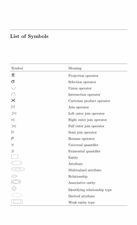
List of Symbols
Symbol Meaning
Projection operator
Selection operator
Union operator
Intersection operator
Cartesian product operator
Join operator
Left outer join operator
Right outer join operator
Full outer join operator
Semi join operator
Rename operator
Universal quantifier
Existential quantifier
Entity
Attribute
Multivalued attribute
Relationship
Associative entity
Identifying relationship type
Derived attribute
Weak entity type
1
Overview of Database Management System
Learning Objectives. This chapter provides an overview of database managementsystem which includes concepts related to data, database, and database managementsystem. After completing this chapter the reader should be familiar with thefollowing concepts:
– Data, information, database, database management system– Need and evolution of DBMS– File management vs. database management system– ANSI/SPARK data model– Database architecture: two-, three-, and multitier architecture
1.1 Introduction
Science, business, education, economy, law, culture, all areas of human deve-lopment “work” with the constant aid of data. Databases play a crucial rolewithin science research: the body of scientific and technical data and infor-mation in the public domain is massive and factual data are fundamental tothe progress of science. But the progress of science is not the only processaffected by the way people use databases. Stock exchange data are absolutelynecessary to any analyst; access to comprehensive databases of large scaleis an everyday activity of a teacher, an educator, an academic or a lawyer.There are databases collecting all sorts of different data: nuclear structure andradioactive decay data for isotopes (the Evaluated Nuclear Structure DataFile) and genes sequences (the Human Genome Database), prisoners’ DNAdata (“DNA offender database”), names of people accused for drug offenses,telephone numbers, legal materials and many others. In this chapter, the ba-sic idea about database management system, its evolution, its advantage overconventional file system, database system structure is discussed.
S. Sumathi: Overview of Database Management System, Studies in Computational Intelligence
(SCI) 47, 1–30 (2007)
www.springerlink.com c© Springer-Verlag Berlin Heidelberg 2007
2 1 Overview of Database Management System
1.2 Data and Information
Data are raw facts that constitute building block of information. Data arethe heart of the DBMS. It is to be noted that all the data will not conveyuseful information. Useful information is obtained from processed data. Inother words, data has to be interpreted in order to obtain information. Good,timely, relevant information is the key to decision making. Good decisionmaking is the key to organizational survival.
Data are a representation of facts, concepts, or instructions in a formalizedmanner suitable for communication, interpretation, or processing by humansor automatic means. The data in DBMS can be broadly classified into twotypes, one is the collection of information needed by the organization and theother is “metadata” which is the information about the database. The term“metadata” will be discussed in detail later in this chapter.
Data are the most stable part of an organization’s information system.A company needs to save information about employees, departments, andsalaries. These pieces of information are called data. Permanent storage ofdata are referred to as persistent data. Generally, we perform operations ondata or data items to supply some information about an entity. For examplelibrary keeps a list of members, books, due dates, and fines.
1.3 Database
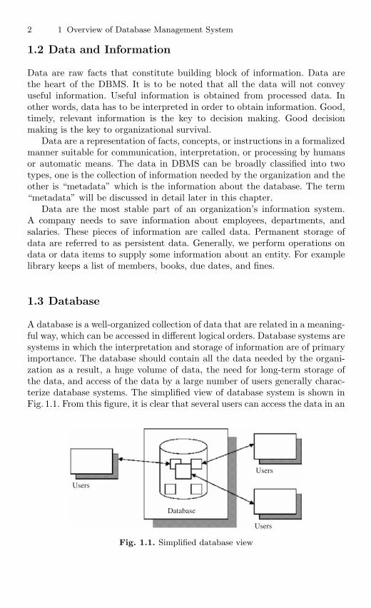
A database is a well-organized collection of data that are related in a meaning-ful way, which can be accessed in different logical orders. Database systems aresystems in which the interpretation and storage of information are of primaryimportance. The database should contain all the data needed by the organi-zation as a result, a huge volume of data, the need for long-term storage ofthe data, and access of the data by a large number of users generally charac-terize database systems. The simplified view of database system is shown inFig. 1.1. From this figure, it is clear that several users can access the data in an
Users
Users
Users
Database
Fig. 1.1. Simplified database view
1.4 Database Management System 3
organization still the integrity of the data should be maintained. A databaseis integrated when same information is not recorded in two places.
1.4 Database Management System
A database management system (DBMS) consists of collection of interrelateddata and a set of programs to access that data. It is software that is helpfulin maintaining and utilizing a database.
A DBMS consists of:
– A collection of interrelated and persistent data. This part of DBMS isreferred to as database (DB).
– A set of application programs used to access, update, and manage data.This part constitutes data management system (MS).
– A DBMS is general-purpose software i.e., not application specific. Thesame DBMS (e.g., Oracle, Sybase, etc.) can be used in railway reservationsystem, library management, university, etc.
– A DBMS takes care of storing and accessing data, leaving only applicationspecific tasks to application programs.
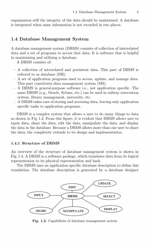
DBMS is a complex system that allows a user to do many things to dataas shown in Fig. 1.2. From this figure, it is evident that DBMS allows user toinput data, share the data, edit the data, manipulate the data, and displaythe data in the database. Because a DBMS allows more than one user to sharethe data; the complexity extends to its design and implementation.
1.4.1 Structure of DBMS
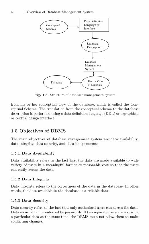
An overview of the structure of database management system is shown inFig. 1.3. A DBMS is a software package, which translates data from its logicalrepresentation to its physical representation and back.
The DBMS uses an application specific database description to define thistranslation. The database description is generated by a database designer
DBMS
UPDATE
INPUT
MANIPULATE
SELECT
DISPLAYSHARE
EDIT
Fig. 1.2. Capabilities of database management system
4 1 Overview of Database Management System
Data DefinitionLanguage orInterface
DatabaseManagementSystem
DatabaseDescription
ConceptualSchema
User’s Viewof Database
Database
Fig. 1.3. Structure of database management system
from his or her conceptual view of the database, which is called the Con-ceptual Schema. The translation from the conceptual schema to the databasedescription is performed using a data definition language (DDL) or a graphicalor textual design interface.
1.5 Objectives of DBMS
The main objectives of database management system are data availability,data integrity, data security, and data independence.
1.5.1 Data Availability
Data availability refers to the fact that the data are made available to widevariety of users in a meaningful format at reasonable cost so that the userscan easily access the data.
1.5.2 Data Integrity
Data integrity refers to the correctness of the data in the database. In otherwords, the data available in the database is a reliable data.
1.5.3 Data Security
Data security refers to the fact that only authorized users can access the data.Data security can be enforced by passwords. If two separate users are accessinga particular data at the same time, the DBMS must not allow them to makeconflicting changes.
1.6 Evolution of Database Management Systems 5
1.5.4 Data Independence
DBMS allows the user to store, update, and retrieve data in an efficientmanner. DBMS provides an “abstract view” of how the data is stored in thedatabase.
In order to store the information efficiently, complex data structures areused to represent the data. The system hides certain details of how the dataare stored and maintained.
1.6 Evolution of Database Management Systems
File-based system was the predecessor to the database management system.Apollo moon-landing process was started in the year 1960. At that time, therewas no system available to handle and manage large amount of information. Asa result, North American Aviation which is now popularly known as Rock-well International developed software known as Generalized Update AccessMethod (GUAM). In the mid-1960s, IBM joined North American Aviationto develop GUAM into Information Management System (IMS). IMS wasbased on Hierarchical data model. In the mid-1960s, General Electric releasedIntegrated Data Store (IDS). IDS were based on network data model. CharlesBachmann was mainly responsible for the development of IDS. The networkdatabase was developed to fulfill the need to represent more complex datarelationships than could be modeled with hierarchical structures. Conferenceon Data System Languages formed Data Base Task Group (DBTG) in 1967.DBTG specified three distinct languages for standardization. They are DataDefinition Language (DDL), which would enable Database Administrator todefine the schema, a subschema DDL, which would allow the application pro-grams to define the parts of the database and Data Manipulation Language(DML) to manipulate the data.
The network and hierarchical data models developed during that time hadthe drawbacks of minimal data independence, minimal theoretical foundation,and complex data access. To overcome these drawbacks, in 1970, Codd of IBMpublished a paper titled “A Relational Model of Data for Large Shared DataBanks” in Communications of the ACM, vol. 13, No. 6, pp. 377–387, June1970. As an impact of Codd’s paper, System R project was developed dur-ing the late 1970 by IBM San Jose Research Laboratory in California. Theproject was developed to prove that relational data model was implementable.The outcome of System R project was the development of Structured QueryLanguage (SQL) which is the standard language for relational database man-agement system. In 1980s IBM released two commercial relational databasemanagement systems known as DB2 and SQL/DS and Oracle Corporation re-leased Oracle. In 1979, Codd himself attempted to address some of the failingsin his original work with an extended version of the relational model calledRM/T in 1979 and RM/V2 in 1990. The attempts to provide a data model
6 1 Overview of Database Management System
that represents the “real world” more closely have been loosely classified asSemantic Data Modeling.
In recent years, two approaches to DBMS are more popular, which areObject-Oriented DBMS (OODBMS) and Object Relational DBMS (OR-DBMS).
The chronological order of the development of DBMS is as follows:
– Flat files – 1960s–1980s– Hierarchical – 1970s–1990s– Network – 1970s–1990s– Relational – 1980s–present– Object-oriented – 1990s–present– Object-relational – 1990s–present– Data warehousing – 1980s–present– Web-enabled – 1990s–present
Early 1960s. Charles Bachman at GE created the first general purpose DBMSIntegrated Data Store. It created the basis for the network model which wasstandardized by CODASYL (Conference on Data System Language).Late 1960s. IBM developed the Information Management System (IMS). IMSused an alternate model, called the Hierarchical Data Model.1970. Edgar Codd, from IBM created the Relational Data Model. In 1981Codd received the Turing Award for his contributions to database theory.Codd Passed away in April 2003.1976. Peter Chen presented Entity-Relationship model, which is widely usedin database design.1980. SQL developed by IBM, became the standard query language for data-bases. SQL was standardized by ISO.1980s and 1990s. IBM, Oracle, Informix and others developed powerfulDBMS.
1.7 Classification of Database Management System
The database management system can be broadly classified into (1) PassiveDatabase Management System and (2) Active Database Management System:
1. Passive Database Management System. Passive Database ManagementSystems are program-driven. In passive database management system theusers query the current state of database and retrieve the information cur-rently available in the database. Traditional DBMS are passive in the sensethat they are explicitly and synchronously invoked by user or applicationprogram initiated operations. Applications send requests for operations tobe performed by the DBMS and wait for the DBMS to confirm and returnany possible answers. The operations can be definitions and updates ofthe schema, as well as queries and updates of the data.
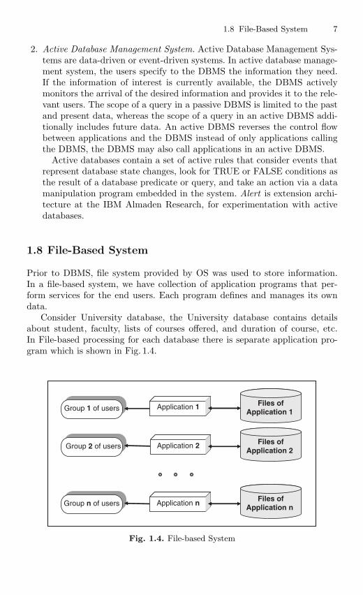
1.8 File-Based System 7
2. Active Database Management System. Active Database Management Sys-tems are data-driven or event-driven systems. In active database manage-ment system, the users specify to the DBMS the information they need.If the information of interest is currently available, the DBMS activelymonitors the arrival of the desired information and provides it to the rele-vant users. The scope of a query in a passive DBMS is limited to the pastand present data, whereas the scope of a query in an active DBMS addi-tionally includes future data. An active DBMS reverses the control flowbetween applications and the DBMS instead of only applications callingthe DBMS, the DBMS may also call applications in an active DBMS.
Active databases contain a set of active rules that consider events thatrepresent database state changes, look for TRUE or FALSE conditions asthe result of a database predicate or query, and take an action via a datamanipulation program embedded in the system. Alert is extension archi-tecture at the IBM Almaden Research, for experimentation with activedatabases.
1.8 File-Based System
Prior to DBMS, file system provided by OS was used to store information.In a file-based system, we have collection of application programs that per-form services for the end users. Each program defines and manages its owndata.
Consider University database, the University database contains detailsabout student, faculty, lists of courses offered, and duration of course, etc.In File-based processing for each database there is separate application pro-gram which is shown in Fig. 1.4.
Group n of users
Group 2 of users
Group 1 of users Application 1 Files ofApplication 1
Application 2
Application n
Files ofApplication 2
Files ofApplication n
Fig. 1.4. File-based System
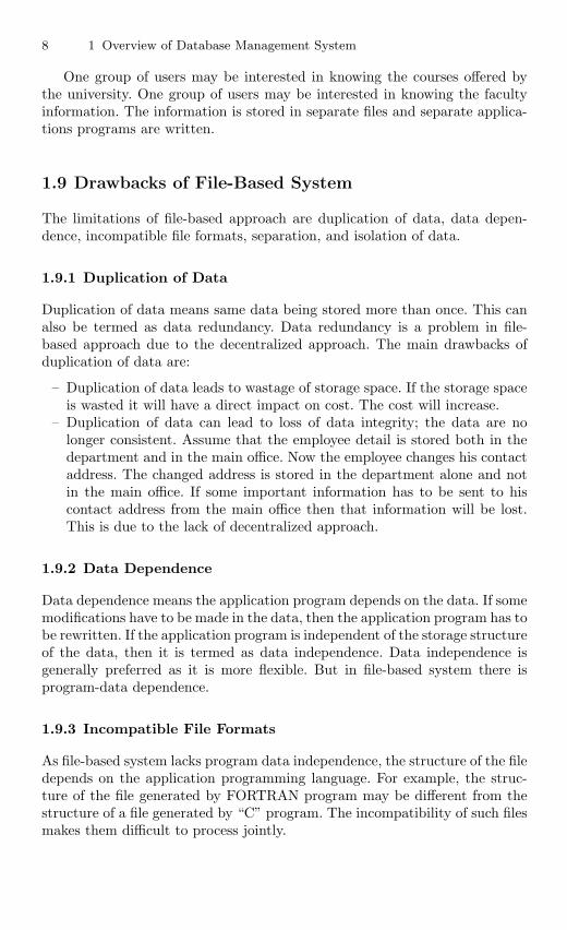
8 1 Overview of Database Management System
One group of users may be interested in knowing the courses offered bythe university. One group of users may be interested in knowing the facultyinformation. The information is stored in separate files and separate applica-tions programs are written.
1.9 Drawbacks of File-Based System
The limitations of file-based approach are duplication of data, data depen-dence, incompatible file formats, separation, and isolation of data.
1.9.1 Duplication of Data
Duplication of data means same data being stored more than once. This canalso be termed as data redundancy. Data redundancy is a problem in file-based approach due to the decentralized approach. The main drawbacks ofduplication of data are:
– Duplication of data leads to wastage of storage space. If the storage spaceis wasted it will have a direct impact on cost. The cost will increase.
– Duplication of data can lead to loss of data integrity; the data are nolonger consistent. Assume that the employee detail is stored both in thedepartment and in the main office. Now the employee changes his contactaddress. The changed address is stored in the department alone and notin the main office. If some important information has to be sent to hiscontact address from the main office then that information will be lost.This is due to the lack of decentralized approach.
1.9.2 Data Dependence
Data dependence means the application program depends on the data. If somemodifications have to be made in the data, then the application program has tobe rewritten. If the application program is independent of the storage structureof the data, then it is termed as data independence. Data independence isgenerally preferred as it is more flexible. But in file-based system there isprogram-data dependence.
1.9.3 Incompatible File Formats
As file-based system lacks program data independence, the structure of the filedepends on the application programming language. For example, the struc-ture of the file generated by FORTRAN program may be different from thestructure of a file generated by “C” program. The incompatibility of such filesmakes them difficult to process jointly.
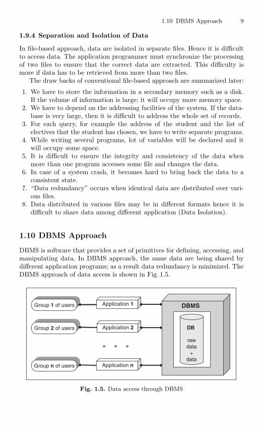
1.10 DBMS Approach 9
1.9.4 Separation and Isolation of Data
In file-based approach, data are isolated in separate files. Hence it is difficultto access data. The application programmer must synchronize the processingof two files to ensure that the correct data are extracted. This difficulty ismore if data has to be retrieved from more than two files.
The draw backs of conventional file-based approach are summarized later:
1. We have to store the information in a secondary memory such as a disk.If the volume of information is large; it will occupy more memory space.
2. We have to depend on the addressing facilities of the system. If the data-base is very large, then it is difficult to address the whole set of records.
3. For each query, for example the address of the student and the list ofelectives that the student has chosen, we have to write separate programs.
4. While writing several programs, lot of variables will be declared and itwill occupy some space.
5. It is difficult to ensure the integrity and consistency of the data whenmore than one program accesses some file and changes the data.
6. In case of a system crash, it becomes hard to bring back the data to aconsistent state.
7. “Data redundancy” occurs when identical data are distributed over vari-ous files.
8. Data distributed in various files may be in different formats hence it isdifficult to share data among different application (Data Isolation).
1.10 DBMS Approach
DBMS is software that provides a set of primitives for defining, accessing, andmanipulating data. In DBMS approach, the same data are being shared bydifferent application programs; as a result data redundancy is minimized. TheDBMS approach of data access is shown in Fig. 1.5.
Group n of users
Group 2 of users
Group 1 of users Application 1
Application 2
Application n
DBMS
DB
rawdata
+ data
Fig. 1.5. Data access through DBMS
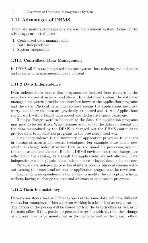
10 1 Overview of Database Management System
1.11 Advantages of DBMS
There are many advantages of database management system. Some of theadvantages are listed later:
1. Centralized data management.2. Data Independence.3. System Integration.
1.11.1 Centralized Data Management
In DBMS all files are integrated into one system thus reducing redundanciesand making data management more efficient.
1.11.2 Data Independence
Data independence means that programs are isolated from changes in theway the data are structured and stored. In a database system, the databasemanagement system provides the interface between the application programsand the data. Physical data independence means the applications need notworry about how the data are physically structured and stored. Applicationsshould work with a logical data model and declarative query language.
If major changes were to be made to the data, the application programsmay need to be rewritten. When changes are made to the data representation,the data maintained by the DBMS is changed but the DBMS continues toprovide data to application programs in the previously used way.
Data independence is the immunity of application programs to changesin storage structures and access techniques. For example if we add a newattribute, change index structure then in traditional file processing system,the applications are affected. But in a DBMS environment these changes arereflected in the catalog, as a result the applications are not affected. Dataindependence can be physical data independence or logical data independence.
Physical data independence is the ability to modify physical schema with-out causing the conceptual schema or application programs to be rewritten.
Logical data independence is the ability to modify the conceptual schemawithout having to change the external schemas or application programs.
1.11.3 Data Inconsistency
Data inconsistency means different copies of the same data will have differentvalues. For example, consider a person working in a branch of an organization.The details of the person will be stored both in the branch office as well as inthe main office. If that particular person changes his address, then the “changeof address” has to be maintained in the main as well as the branch office.
1.12 Ansi/Spark Data Model 11
For example the “change of address” is maintained in the branch office butnot in the main office, then the data about that person is inconsistent.
DBMS is designed to have data consistency. Some of the qualities achievedin DBMS are:
1. Data redundancy −→ Reduced in DBMS.2. Data independence −→ Activated in DBMS.3. Data inconsistency −→ Avoided in DBMS.4. Centralizing the data −→ Achieved in DBMS.5. Data integrity −→ Necessary for efficient Transaction.6. Support for multiple views −→ Necessary for security reasons.
– Data redundancy means duplication of data. Data redundancy will occupymore space hence it is not desirable.
– Data independence means independence between application program andthe data. The advantage is that when the data representation changes, itis not necessary to change the application program.
– Data inconsistency means different copies of the same data will have dif-ferent values.
– Centralizing the data means data can be easily shared between the usersbut the main concern is data security.
– The main threat to data integrity comes from several different usersattempting to update the same data at the same time. For example, “Thenumber of booking made is larger than the capacity of the aircraft/train.”
– Support for multiple views means DBMS allows different users to seedifferent “views” of the database, according to the perspective each onerequires. This concept is used to enhance the security of the database.
1.12 Ansi/Spark Data Model (American NationalStandard Institute/ Standards Planningand Requirements Committee)
The distinction between the logical and physical representation of data wererecognized in 1978 when ANSI/SPARK committee proposed a generalizedframework for database systems. This framework provided a three-level archi-tecture, three levels of abstraction at which the database could be viewed.
1.12.1 Need for Abstraction
The main objective of DBMS is to store and retrieve information efficiently;all the users should be able to access same data. The designers use complexdata structure to represent the data, so that data can be efficiently storedand retrieved, but it is not necessary for the users to know physical databasestorage details. The developers hide the complexity from users through severallevels of abstraction.
12 1 Overview of Database Management System
1.12.2 Data Independence
Data independence means the internal structure of database should beunaffected by changes to physical aspects of storage. Because of data in-dependence, the Database administrator can change the database storagestructures without affecting the users view.The different levels of data abstraction are:
1. Physical level or internal level2. Logical level or conceptual level3. View level or external level
Physical Level
It is concerned with the physical storage of the information. It provides theinternal view of the actual physical storage of data. The physical leveldescribes complex low-level data structures in detail.
Logical Level
Logical level describes what data are stored in the database and what rela-tionships exist among those data.
Logical level describes the entire database in terms of a small number ofsimple structures. The implementation of simple structure of the logical levelmay involve complex physical level structures; the user of the logical leveldoes not need to be aware of this complexity. Database administrator use thelogical level of abstraction.
View Level
View level is the highest level of abstraction. It is the view that the individualuser of the database has. There can be many view level abstractions of thesame data. The different levels of data abstraction are shown in Fig. 1.6.
Database Instances
Database change over time as information is inserted and deleted. The collec-tion of information stored in the database at a particular moment is called aninstance of the database.
Database Schema
The overall design of the database is called the database schema. A schema isa collection of named objects. Schemas provide a logical classification of ob-jects in the database. A schema can contain tables, views, triggers, functions,packages, and other objects.
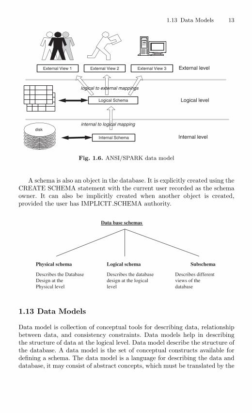
1.13 Data Models 13
External level
internal to logical mapping
logical to external mappings
disk
Internal Schema Internal level
External View 1 External View 2 External View 3
Logical Schema Logical level
Fig. 1.6. ANSI/SPARK data model
A schema is also an object in the database. It is explicitly created using theCREATE SCHEMA statement with the current user recorded as the schemaowner. It can also be implicitly created when another object is created,provided the user has IMPLICIT SCHEMA authority.
Data base schemas
Physical schema Logical schema Subschema
Describes the Database Design at thePhysical level
Describes the databasedesign at the logicallevel
Describes differentviews of thedatabase
1.13 Data Models
Data model is collection of conceptual tools for describing data, relationshipbetween data, and consistency constraints. Data models help in describingthe structure of data at the logical level. Data model describe the structure ofthe database. A data model is the set of conceptual constructs available fordefining a schema. The data model is a language for describing the data anddatabase, it may consist of abstract concepts, which must be translated by the
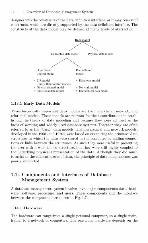
14 1 Overview of Database Management System
designer into the constructs of the data definition interface, or it may consist ofconstructs, which are directly supported by the data definition interface. Theconstructs of the data model may be defined at many levels of abstraction.
Data model
Conceptual data model Physical data model
Object basedLogical model
Record based model
∗ E-R model ∗ Relational model(Entity-Relationship model)
∗ Object-oriented model ∗ Network model∗ Functional data model ∗ Hierarchical data model
1.13.1 Early Data Models
Three historically important data models are the hierarchical, network, andrelational models. These models are relevant for their contributions in estab-lishing the theory of data modeling and because they were all used as thebasis of working and widely used database systems. Together they are oftenreferred to as the “basic” data models. The hierarchical and network models,developed in the 1960s and 1970s, were based on organizing the primitive datastructures in which the data were stored in the computer by adding connec-tions or links between the structures. As such they were useful in presentingthe user with a well-defined structure, but they were still highly coupled tothe underlying physical representation of the data. Although they did muchto assist in the efficient access of data, the principle of data independence waspoorly supported.
1.14 Components and Interfaces of DatabaseManagement System
A database management system involves five major components: data, hard-ware, software, procedure, and users. These components and the interfacebetween the components are shown in Fig. 1.7.
1.14.1 Hardware
The hardware can range from a single personal computer, to a single main-frame, to a network of computers. The particular hardware depends on the
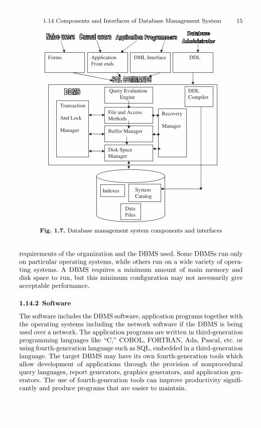
1.14 Components and Interfaces of Database Management System 15
Forms
DataFiles
ApplicationFront ends
DML Interface DDL
Query EvaluationEngine
File and AccessMethods
Buffer Manager
Disk SpaceManager
Transaction
And Lock
Manager
Recovery
Manager
DDLCompiler
Indexes SystemCatalog
Fig. 1.7. Database management system components and interfaces
requirements of the organization and the DBMS used. Some DBMSs run onlyon particular operating systems, while others run on a wide variety of opera-ting systems. A DBMS requires a minimum amount of main memory anddisk space to run, but this minimum configuration may not necessarily giveacceptable performance.
1.14.2 Software
The software includes the DBMS software, application programs together withthe operating systems including the network software if the DBMS is beingused over a network. The application programs are written in third-generationprogramming languages like “C,” COBOL, FORTRAN, Ada, Pascal, etc. orusing fourth-generation language such as SQL, embedded in a third-generationlanguage. The target DBMS may have its own fourth-generation tools whichallow development of applications through the provision of nonproceduralquery languages, report generators, graphics generators, and application gen-erators. The use of fourth-generation tools can improve productivity signifi-cantly and produce programs that are easier to maintain.
16 1 Overview of Database Management System
1.14.3 Data
A database is a repository for data which, in general, is both integrated andshared. Integration means that the database may be thought of as a unifi-cation of several otherwise distinct files, with any redundancy among thosefiles partially or wholly eliminated. The sharing of a database refers to thesharing of data by different users, in the sense that each of those users mayhave access to the same piece of data and may use it for different purposes.Any given user will normally be concerned with only a subset of the wholedatabase. The main features of the data in the database are listed later:
1. The data in the database is well organized (structured)2. The data in the database is related3. The data are accessible in different orders without great difficulty
The data in the database is persistent, integrated, structured, and shared.
Integrated Data
A data can be considered to be a unification of several distinct data files andwhen any redundancy among those files is eliminated, the data are said to beintegrated data.
Shared Data
A database contains data that can be shared by different users for differentapplication simultaneously. It is important to note that in this way of sharingof data, the redundancy of data are reduced, since repetitions are avoided, thepossibility of inconsistencies is reduced.
Persistent Data
Persistent data are one, which cannot be removed from the database as a sideeffect of some other process. Persistent data have a life span that is not limitedto single execution of the programs that use them.
1.14.4 Procedure
Procedures are the rules that govern the design and the use of database. Theprocedure may contain information on how to log on to the DBMS, startand stop the DBMS, procedure on how to identify the failed component, howto recover the database, change the structure of the table, and improve theperformance.
1.14.5 People Interacting with Database
Here people refers to the people who manages the database, database admin-istrator, people who design the application program, database designer andthe people who interacts with the database, database users.
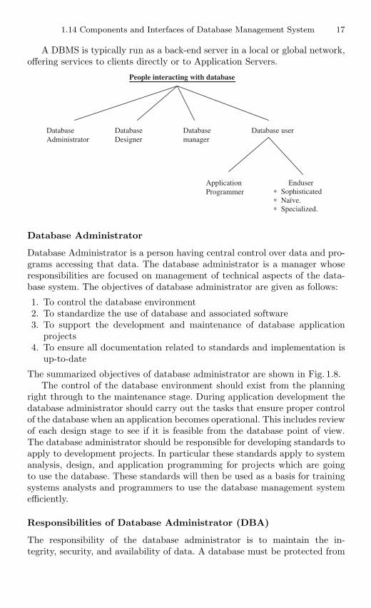
1.14 Components and Interfaces of Database Management System 17
A DBMS is typically run as a back-end server in a local or global network,offering services to clients directly or to Application Servers.
People interacting with database
DatabaseAdministrator
DatabaseDesigner
Databasemanager
Database user
ApplicationProgrammer
Enduser ∗ Sophisticated∗ Naïve.∗ Specialized.
Database Administrator
Database Administrator is a person having central control over data and pro-grams accessing that data. The database administrator is a manager whoseresponsibilities are focused on management of technical aspects of the data-base system. The objectives of database administrator are given as follows:
1. To control the database environment2. To standardize the use of database and associated software3. To support the development and maintenance of database application
projects4. To ensure all documentation related to standards and implementation is
up-to-date
The summarized objectives of database administrator are shown in Fig. 1.8.The control of the database environment should exist from the planning
right through to the maintenance stage. During application development thedatabase administrator should carry out the tasks that ensure proper controlof the database when an application becomes operational. This includes reviewof each design stage to see if it is feasible from the database point of view.The database administrator should be responsible for developing standards toapply to development projects. In particular these standards apply to systemanalysis, design, and application programming for projects which are goingto use the database. These standards will then be used as a basis for trainingsystems analysts and programmers to use the database management systemefficiently.
Responsibilities of Database Administrator (DBA)
The responsibility of the database administrator is to maintain the in-tegrity, security, and availability of data. A database must be protected from
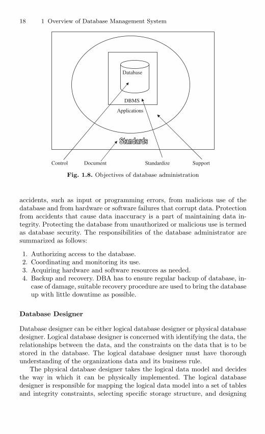
18 1 Overview of Database Management System
Control Document Standardize Support
Applications
DBMS
Database
Fig. 1.8. Objectives of database administration
accidents, such as input or programming errors, from malicious use of thedatabase and from hardware or software failures that corrupt data. Protectionfrom accidents that cause data inaccuracy is a part of maintaining data in-tegrity. Protecting the database from unauthorized or malicious use is termedas database security. The responsibilities of the database administrator aresummarized as follows:
1. Authorizing access to the database.2. Coordinating and monitoring its use.3. Acquiring hardware and software resources as needed.4. Backup and recovery. DBA has to ensure regular backup of database, in-
case of damage, suitable recovery procedure are used to bring the databaseup with little downtime as possible.
Database Designer
Database designer can be either logical database designer or physical databasedesigner. Logical database designer is concerned with identifying the data, therelationships between the data, and the constraints on the data that is to bestored in the database. The logical database designer must have thoroughunderstanding of the organizations data and its business rule.
The physical database designer takes the logical data model and decidesthe way in which it can be physically implemented. The logical databasedesigner is responsible for mapping the logical data model into a set of tablesand integrity constraints, selecting specific storage structure, and designing
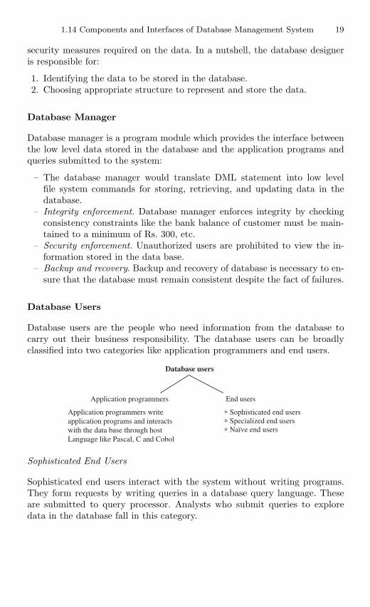
1.14 Components and Interfaces of Database Management System 19
security measures required on the data. In a nutshell, the database designeris responsible for:
1. Identifying the data to be stored in the database.2. Choosing appropriate structure to represent and store the data.
Database Manager
Database manager is a program module which provides the interface betweenthe low level data stored in the database and the application programs andqueries submitted to the system:
– The database manager would translate DML statement into low levelfile system commands for storing, retrieving, and updating data in thedatabase.
– Integrity enforcement. Database manager enforces integrity by checkingconsistency constraints like the bank balance of customer must be main-tained to a minimum of Rs. 300, etc.
– Security enforcement. Unauthorized users are prohibited to view the in-formation stored in the data base.
– Backup and recovery. Backup and recovery of database is necessary to en-sure that the database must remain consistent despite the fact of failures.
Database Users
Database users are the people who need information from the database tocarry out their business responsibility. The database users can be broadlyclassified into two categories like application programmers and end users.
Database users
Application programmers End users
Application programmers writeapplication programs and interactswith the data base through hostLanguage like Pascal, C and Cobol
∗ Sophisticated end users ∗ Specialized end users ∗ Naïve end users
Sophisticated End Users
Sophisticated end users interact with the system without writing programs.They form requests by writing queries in a database query language. Theseare submitted to query processor. Analysts who submit queries to exploredata in the database fall in this category.
20 1 Overview of Database Management System
Specialized End Users
Specialized end users write specialized database application that does not fitinto data-processing frame work. Application involves knowledge base andexpert system, environment modeling system, etc.
Naive End Users
Naıve end user interact with the system by using permanent application pro-gram Example: Query made by the student, namely number of books borrowedin library database.
System Analysts
System analysts determine the requirements of end user, and develop specifi-cation for canned transaction that meets this requirement.
Canned Transaction
Ready made programs through which naıve end users interact with the data-base is called canned transaction.
1.14.6 Data Dictionary
A data dictionary, also known as a “system catalog,” is a centralized store ofinformation about the database. It contains information about the tables, thefields the tables contain, data types, primary keys, indexes, the joins whichhave been established between those tables, referential integrity, cascades up-date, cascade delete, etc. This information stored in the data dictionary iscalled the “Metadata.” Thus a data dictionary can be considered as a filethat stores Metadata. Data dictionary is a tool for recording and processinginformation about the data that an organization uses. The data dictionaryis a central catalog for Metadata. The data dictionary can be integratedwithin the DBMS or separate. Data dictionary may be referenced duringsystem design, programming, and by actively-executing programs. One ofthe major functions of a true data dictionary is to enforce the constraintsplaced upon the database by the designer, such as referential integrity andcascade delete.
Metadata
The information (data) about the data in a database is called Metadata. TheMetadata are available for query and manipulation, just as other data in thedatabase.
1.14 Components and Interfaces of Database Management System 21
1.14.7 Functional Components of Database System Structure
The functional components of database system structure are:
1. Storage manager.2. Query processor.
Storage Manager
Storage manager is responsible for storing, retrieving, and updating data inthe database. Storage manager components are:
1. Authorization and integrity manager.2. Transaction manager.3. File manager.4. Buffer manager.
Transaction Management
– A transaction is a collection of operations that performs a single logicalfunction in a database application.
– Transaction-management component ensures that the database remainsin a consistent state despite system failures and transaction failure.
– Concurrency control manager controls the interaction among the concur-rent transactions, to ensure the consistency of the database.
Authorization and Integrity Manager
Checks the integrity constraints and authority of users to access data.
Transaction Manager
It ensures that the database remains in a consistent state despite system fail-ures. The transaction manager manages the execution of database manipula-tion requests. The transaction manager function is to ensure that concurrentaccess to data does not result in conflict.
File Manager
File manager manages the allocation of space on disk storage. Files areused to store collections of similar data. A file management system man-ages independent files, helping to enter and retrieve information records.File manager establishes and maintains the list of structure and indexesdefined in the internal schema. The file manager can:
– Create a file– Delete a file– Update the record in the file– Retrieve a record from a file
22 1 Overview of Database Management System
Buffer
The area into which a block from the file is read is termed a buffer. Themanagement of buffers has the objective of maximizing the performance or theutilization of the secondary storage systems, while at the same time keepingthe demand on CPU resources tolerably low. The use of two or more buffersfor a file allows the transfer of data to be overlapped with the processing ofdata.
Buffer Manager
Buffer manager is responsible for fetching data from disk storage into mainmemory. Programs call on the buffer manager when they need a block fromdisk. The requesting program is given the address of the block in main memory,if it is already present in the buffer. If the block is not in the buffer, the buffermanager allocates space in the buffer for the block, replacing some other block,if required, to make space for new block. Once space is allocated in the buffer,the buffer manager reads in the block from the disk to the buffer, and passesthe address of the block in main memory to the requester.
Indices
Indices provide fast access to data items that hold particular values. An indexis a list of numerical values which gives the order of the records when theyare sorted on a particular field or column of the table.
1.15 Database Architecture
Database architecture essentially describes the location of all the pieces ofinformation that make up the database application. The database architecturecan be broadly classified into two-, three-, and multitier architecture.
1.15.1 Two-Tier Architecture
The two-tier architecture is a client–server architecture in which the clientcontains the presentation code and the SQL statements for data access. Thedatabase server processes the SQL statements and sends query results back tothe client. The two-tier architecture is shown in Fig. 1.9. Two-tier client/serverprovides a basic separation of tasks. The client, or first tier, is primarily re-sponsible for the presentation of data to the user and the “server,” or secondtier, is primarily responsible for supplying data services to the client.
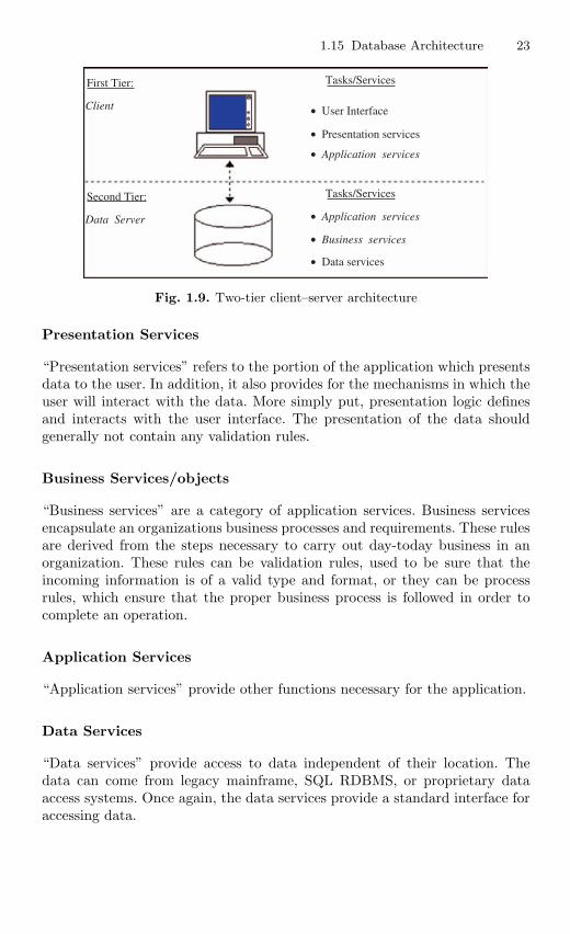
1.15 Database Architecture 23
First Tier: Tasks/Services
• User Interface
• Data services
• Presentation services
• Application services
• Application services
• Business services
Client
Second Tier:
Data Server
Tasks/Services
Fig. 1.9. Two-tier client–server architecture
Presentation Services
“Presentation services” refers to the portion of the application which presentsdata to the user. In addition, it also provides for the mechanisms in which theuser will interact with the data. More simply put, presentation logic definesand interacts with the user interface. The presentation of the data shouldgenerally not contain any validation rules.
Business Services/objects
“Business services” are a category of application services. Business servicesencapsulate an organizations business processes and requirements. These rulesare derived from the steps necessary to carry out day-today business in anorganization. These rules can be validation rules, used to be sure that theincoming information is of a valid type and format, or they can be processrules, which ensure that the proper business process is followed in order tocomplete an operation.
Application Services
“Application services” provide other functions necessary for the application.
Data Services
“Data services” provide access to data independent of their location. Thedata can come from legacy mainframe, SQL RDBMS, or proprietary dataaccess systems. Once again, the data services provide a standard interface foraccessing data.
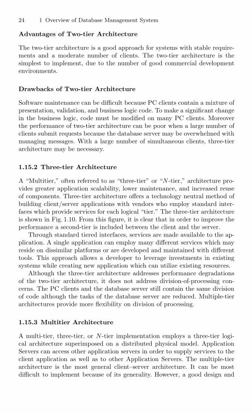
24 1 Overview of Database Management System
Advantages of Two-tier Architecture
The two-tier architecture is a good approach for systems with stable require-ments and a moderate number of clients. The two-tier architecture is thesimplest to implement, due to the number of good commercial developmentenvironments.
Drawbacks of Two-tier Architecture
Software maintenance can be difficult because PC clients contain a mixture ofpresentation, validation, and business logic code. To make a significant changein the business logic, code must be modified on many PC clients. Moreoverthe performance of two-tier architecture can be poor when a large number ofclients submit requests because the database server may be overwhelmed withmanaging messages. With a large number of simultaneous clients, three-tierarchitecture may be necessary.
1.15.2 Three-tier Architecture
A “Multitier,” often referred to as “three-tier” or “N -tier,” architecture pro-vides greater application scalability, lower maintenance, and increased reuseof components. Three-tier architecture offers a technology neutral method ofbuilding client/server applications with vendors who employ standard inter-faces which provide services for each logical “tier.” The three-tier architectureis shown in Fig. 1.10. From this figure, it is clear that in order to improve theperformance a second-tier is included between the client and the server.
Through standard tiered interfaces, services are made available to the ap-plication. A single application can employ many different services which mayreside on dissimilar platforms or are developed and maintained with differenttools. This approach allows a developer to leverage investments in existingsystems while creating new application which can utilize existing resources.
Although the three-tier architecture addresses performance degradationsof the two-tier architecture, it does not address division-of-processing con-cerns. The PC clients and the database server still contain the same divisionof code although the tasks of the database server are reduced. Multiple-tierarchitectures provide more flexibility on division of processing.
1.15.3 Multitier Architecture
A multi-tier, three-tier, or N -tier implementation employs a three-tier logi-cal architecture superimposed on a distributed physical model. ApplicationServers can access other application servers in order to supply services to theclient application as well as to other Application Servers. The multiple-tierarchitecture is the most general client–server architecture. It can be mostdifficult to implement because of its generality. However, a good design and
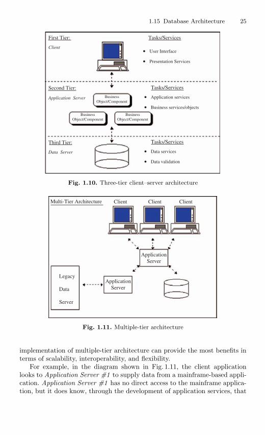
1.15 Database Architecture 25
Third Tier:
Data Server
First Tier:
Client
BusinessObject/Component
BusinessObject/Component
BusinessObject/Component
Tasks/Services
• User Interface
• Presentation Services
Tasks/Services
• Application services
• Business services/objects
Tasks/Services
• Data services
• Data validation
Second Tier:
Application Server
Fig. 1.10. Three-tier client–server architecture
Multi-Tier Architecture Client
Legacy
Data
Server
ApplicationServer
ApplicationServer
Client Client
Fig. 1.11. Multiple-tier architecture
implementation of multiple-tier architecture can provide the most benefits interms of scalability, interoperability, and flexibility.
For example, in the diagram shown in Fig. 1.11, the client applicationlooks to Application Server #1 to supply data from a mainframe-based appli-cation. Application Server #1 has no direct access to the mainframe applica-tion, but it does know, through the development of application services, that
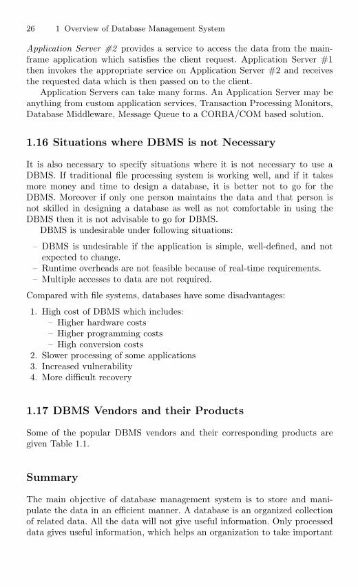
26 1 Overview of Database Management System
Application Server #2 provides a service to access the data from the main-frame application which satisfies the client request. Application Server #1then invokes the appropriate service on Application Server #2 and receivesthe requested data which is then passed on to the client.
Application Servers can take many forms. An Application Server may beanything from custom application services, Transaction Processing Monitors,Database Middleware, Message Queue to a CORBA/COM based solution.
1.16 Situations where DBMS is not Necessary
It is also necessary to specify situations where it is not necessary to use aDBMS. If traditional file processing system is working well, and if it takesmore money and time to design a database, it is better not to go for theDBMS. Moreover if only one person maintains the data and that person isnot skilled in designing a database as well as not comfortable in using theDBMS then it is not advisable to go for DBMS.
DBMS is undesirable under following situations:
– DBMS is undesirable if the application is simple, well-defined, and notexpected to change.
– Runtime overheads are not feasible because of real-time requirements.– Multiple accesses to data are not required.
Compared with file systems, databases have some disadvantages:
1. High cost of DBMS which includes:– Higher hardware costs– Higher programming costs– High conversion costs
2. Slower processing of some applications3. Increased vulnerability4. More difficult recovery
1.17 DBMS Vendors and their Products
Some of the popular DBMS vendors and their corresponding products aregiven Table 1.1.
Summary
The main objective of database management system is to store and mani-pulate the data in an efficient manner. A database is an organized collectionof related data. All the data will not give useful information. Only processeddata gives useful information, which helps an organization to take important
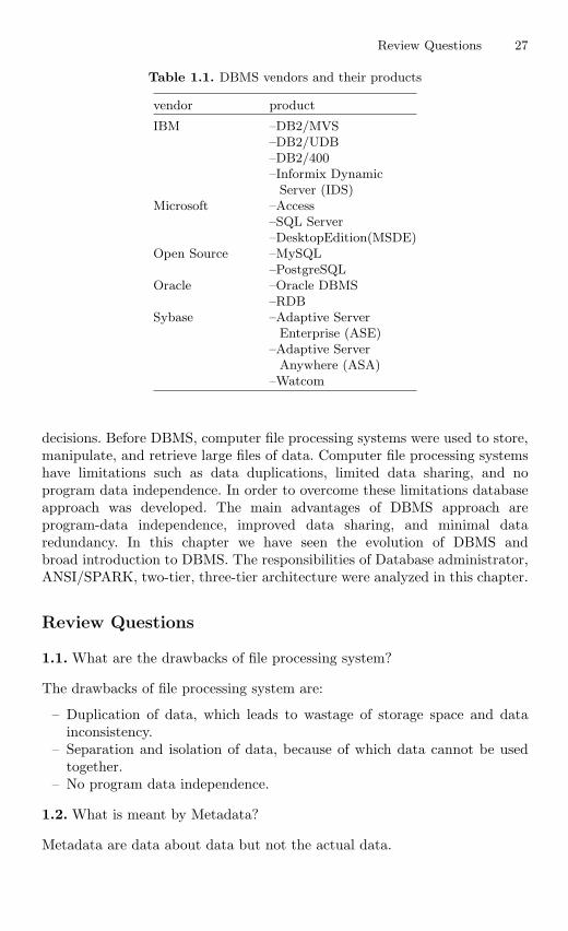
Review Questions 27
Table 1.1. DBMS vendors and their products
vendor product
IBM –DB2/MVS–DB2/UDB–DB2/400–Informix Dynamic
Server (IDS)Microsoft –Access
–SQL Server–DesktopEdition(MSDE)
Open Source –MySQL–PostgreSQL
Oracle –Oracle DBMS–RDB
Sybase –Adaptive ServerEnterprise (ASE)
–Adaptive ServerAnywhere (ASA)
–Watcom
decisions. Before DBMS, computer file processing systems were used to store,manipulate, and retrieve large files of data. Computer file processing systemshave limitations such as data duplications, limited data sharing, and noprogram data independence. In order to overcome these limitations databaseapproach was developed. The main advantages of DBMS approach areprogram-data independence, improved data sharing, and minimal dataredundancy. In this chapter we have seen the evolution of DBMS andbroad introduction to DBMS. The responsibilities of Database administrator,ANSI/SPARK, two-tier, three-tier architecture were analyzed in this chapter.
Review Questions
1.1. What are the drawbacks of file processing system?
The drawbacks of file processing system are:
– Duplication of data, which leads to wastage of storage space and datainconsistency.
– Separation and isolation of data, because of which data cannot be usedtogether.
– No program data independence.
1.2. What is meant by Metadata?
Metadata are data about data but not the actual data.
28 1 Overview of Database Management System
1.3. Define the term data dictionary?
Data dictionary is a file that contains Metadata.
1.4. What are the responsibilities of database administrator?
1.5. Mention three situations where it is not desirable to use DBMS?
The situations where it is not desirable to use DBMS are:
– The database and applications are not expected to change.– Data are not accessed by multiple users.
1.6. What is meant by data independence?
Data independence renders application programs (e.g., SQL scripts) immuneto changes in the logical and physical organization of data in the system.Logical organization refers to changes in the Schema. Example adding a col-umn or tuples does not stop queries from working.Physical organization refers to changes in indices, file organizations, etc.
1.7. What is meant by Physical and Logical data independence?
In logical data independence, the conceptual schema can be changed with-out changing the external schema. In physical data independence, the internalschema can be changed without changing the conceptual schema.
1.8. What are some disadvantages of using a DBMS over flat file system?
– DBMS initially costs more than flat file system– DBMS requires skilled staff
1.9. What are the steps to design a good database?
– First find out the requirements of the user– Design a view for each important application– Integrate the views giving the conceptual schema, which is the union of
all views– Map to the data model provided by the DBMS (usually relational)– Design external views– Choose physical structures (indexes, etc.)
1.10. What is Database? Give an example.
A Database is a collection of related data. Here, the term “data” means thatknown facts that can be record. Examples of database are library informationsystem, bus, railway, and airline reservation system, etc.
Review Questions 29
1.11. Define – DBMS.
DBMS is a collection of programs that enables users to create and maintaina database.
1.12. Mention various types of databases?
The different types of databases are:
– Multimedia database– Spatial database (Geographical Information System Database)– Real-time or Active Database– Data Warehouse or On-line Analytical Processing Database
1.13. Mention the advantages of using DBMS?
The advantages of using DBMS are:
– Controlling Redundancy– Enforcing Integrity Constraints so as to maintain the consistency of the
database– Providing Backup and recovery facilities– Restricting unauthorized access– Providing multiple user interfaces– Providing persistent storage of program objects and datastructures
1.14. What is “Snapshot” or “Database State”?
The data in the database at a particular moment is known as “DatabaseState” or “Snapshot” of the Database.
1.15. Define Data Model.
It is a collection of concepts that can be used to describe the structure of adatabase.
The datamodel provides necessary means to achieve the abstraction i.e.,hiding the details of data storage.
1.16. Mention the various categories of Data Model.
The various categories of datamodel are:
– High Level or Conceptual Data Model (Example: ER model)– Low Level or Physical Data Model– Representational or Implementational Data Model– Relational Data Model– Network and Hierarchal Data Model– Record-based Data Model– Object-based Data Model
30 1 Overview of Database Management System
1.17. Define the concept of “database schema.” Describe the types of schemasthat exist in a database complying with the three levels ANSI/SPARC archi-tecture.
Database schema is nothing but description of the database. The types ofschemas that exist in a database complying with three levels of ANSI/SPARCarchitecture are:
– External schema– Conceptual schema– Internal schema
2
Entity–Relationship Model
Learning Objectives. This chapter presents a top-down approach to data model-ing. This chapter deals with ER and Enhanced ER (EER) model and conversion ofER model to relational model. After completing this chapter the reader should befamiliar with the following concepts:
– Entity, Attribute, and Relationship.– Entity classification – Strong entity, Weak entity, and Associative entity.– Attribute classification – Single value, Multivalue, Derived, and Null attribute.– Relationship – Unary, binary, and ternary relationship.– Enhanced ER model – Generalization, Specialization.– Mapping ER model to relation model or table.– Connection traps.
2.1 Introduction
Peter Chen first proposed modeling databases using a graphical techniquethat humans can relate to easily. Humans can easily perceive entities andtheir characteristics in the real world and represent any relationship withone another. The objective of modeling graphically is even more profoundthan simply representing these entities and relationship. The database de-signer can use tools to model these entities and their relationships and thengenerate database vendor-specific schema automatically. Entity–Relationship(ER) model gives the conceptual model of the world to be represented in thedatabase. ER Model is based on a perception of a real world that consists ofcollection of basic objects called entities and relationships among these ob-jects. The main motivation for defining the ER model is to provide a highlevel model for conceptual database design, which acts as an intermediatestage prior to mapping the enterprise being modeled onto a conceptual level.The ER model achieves a high degree of data independence which means thatthe database designer do not have to worry about the physical structure ofthe database. A database schema in ER model can be pictorially representedby Entity–Relationship diagram.
S. Sumathi: Entity–Relationship Model, Studies in Computational Intelligence (SCI) 47, 31–63
(2007)
www.springerlink.com c© Springer-Verlag Berlin Heidelberg 2007
32 2 Entity–Relationship Model
2.2 The Building Blocks of an Entity–RelationshipDiagram
ER diagram is a graphical modeling tool to standardize ER modeling. Themodeling can be carried out with the help of pictorial representation ofentities, attributes, and relationships. The basic building blocks of Entity-Relationship diagram are Entity, Attribute and Relationship.
2.2.1 Entity
An entity is an object that exists and is distinguishable from other objects.In other words, the entity can be uniquely identified.
The examples of entities are:
– A particular person, for example Dr. A.P.J. Abdul Kalam is an entity.– A particular department, for example Electronics and Communication
Engineering Department.– A particular place, for example Coimbatore city can be an entity.
2.2.2 Entity Type
An entity type or entity set is a collection of similar entities. Some examplesof entity types are:
– All students in PSG, say STUDENT.– All courses in PSG, say COURSE.– All departments in PSG, say DEPARTMENT.
An entity may belong to more than one entity type. For example, a staffworking in a particular department can pursue higher education as part-time.Hence the same person is a LECTURER at one instance and STUDENT atanother instance.
2.2.3 Relationship
A relationship is an association of entities where the association includes oneentity from each participating entity type whereas relationship type is a mean-ingful association between entity types.
The examples of relationship types are:
– Teaches is the relationship type between LECTURER and STUDENT.– Buying is the relationship between VENDOR and CUSTOMER.– Treatment is the relationship between DOCTOR and PATIENT.
2.2.4 Attributes
Attributes are properties of entity types. In other words, entities are describedin a database by a set of attributes.
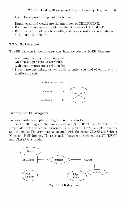
2.2 The Building Blocks of an Entity–Relationship Diagram 33
The following are example of attributes:
– Brand, cost, and weight are the attributes of CELLPHONE.– Roll number, name, and grade are the attributes of STUDENT.– Data bus width, address bus width, and clock speed are the attributes of
MICROPROCESSOR.
2.2.5 ER Diagram
The ER diagram is used to represent database schema. In ER diagram:
– A rectangle represents an entity set.– An ellipse represents an attribute.– A diamond represents a relationship.– Lines represent linking of attributes to entity sets and of entity sets to
relationship sets.
Entity sets ---------->
Attributes ----------->
Relationship ---------->
Example of ER diagram
Let us consider a simple ER diagram as shown in Fig. 2.1.In the ER diagram the two entities are STUDENT and CLASS. Two
simple attributes which are associated with the STUDENT are Roll numberand the name. The attributes associated with the entity CLASS are SubjectName and Hall Number. The relationship between the two entities STUDENTand CLASS is Attends.
CLASSSTUDENT Attends
Name
Roll Number
SubjectName
Hall No
Fig. 2.1. ER diagram
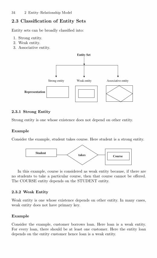
34 2 Entity–Relationship Model
2.3 Classification of Entity Sets
Entity sets can be broadly classified into:
1. Strong entity.2. Weak entity.3. Associative entity.
Entity Set
Strong entity Weak entity Associative entity
Representation
2.3.1 Strong Entity
Strong entity is one whose existence does not depend on other entity.
Example
Consider the example, student takes course. Here student is a strong entity.
Student takes Course
In this example, course is considered as weak entity because, if there areno students to take a particular course, then that course cannot be offered.The COURSE entity depends on the STUDENT entity.
2.3.2 Weak Entity
Weak entity is one whose existence depends on other entity. In many cases,weak entity does not have primary key.
Example
Consider the example, customer borrows loan. Here loan is a weak entity.For every loan, there should be at least one customer. Here the entity loandepends on the entity customer hence loan is a weak entity.
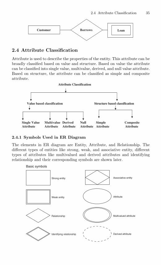
2.4 Attribute Classification 35
LoanCustomer Borrows
2.4 Attribute Classification
Attribute is used to describe the properties of the entity. This attribute can bebroadly classified based on value and structure. Based on value the attributecan be classified into single value, multivalue, derived, and null value attribute.Based on structure, the attribute can be classified as simple and compositeattribute.
Attribute Classification
Value based classification Structure based classification
Single ValueAttribute
MultivalueAttribute
DerivedAttribute
NullAttribute
SimpleAttribute
CompositeAttribute
2.4.1 Symbols Used in ER Diagram
The elements in ER diagram are Entity, Attribute, and Relationship. Thedifferent types of entities like strong, weak, and associative entity, differenttypes of attributes like multivalued and derived attributes and identifyingrelationship and their corresponding symbols are shown later.
Basic symbols
Strong entity Associative entity
Attribute
Multivalued attribute
Derived attribute
Weak entity
Relationship
Identifying relationship
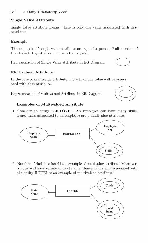
36 2 Entity–Relationship Model
Single Value Attribute
Single value attribute means, there is only one value associated with thatattribute.
Example
The examples of single value attribute are age of a person, Roll number ofthe student, Registration number of a car, etc.
Representation of Single Value Attribute in ER Diagram
Multivalued Attribute
In the case of multivalue attribute, more than one value will be associ-ated with that attribute.
Representation of Multivalued Attribute in ER Diagram
Examples of Multivalued Attribute
1. Consider an entity EMPLOYEE. An Employee can have many skills;hence skills associated to an employee are a multivalue attribute.
EMPLOYEE EmployeeName
EmployeeAge
Skills
2. Number of chefs in a hotel is an example of multivalue attribute. Moreover,a hotel will have variety of food items. Hence food items associated withthe entity HOTEL is an example of multivalued attribute.
HOTEL HotelName
Fooditems
Chefs
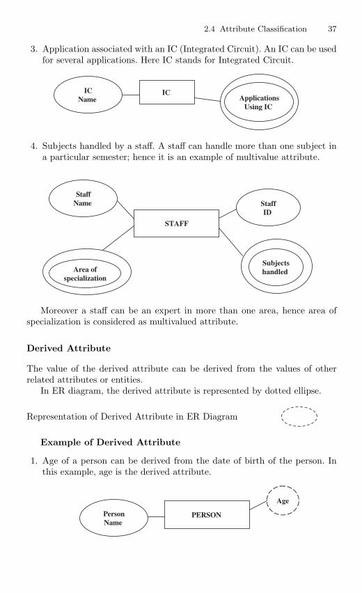
2.4 Attribute Classification 37
3. Application associated with an IC (Integrated Circuit). An IC can be usedfor several applications. Here IC stands for Integrated Circuit.
IC ICName Applications
Using IC
4. Subjects handled by a staff. A staff can handle more than one subject ina particular semester; hence it is an example of multivalue attribute.
STAFF
StaffName
Subjectshandled
StaffID
Area ofspecialization
Moreover a staff can be an expert in more than one area, hence area ofspecialization is considered as multivalued attribute.
Derived Attribute
The value of the derived attribute can be derived from the values of otherrelated attributes or entities.
In ER diagram, the derived attribute is represented by dotted ellipse.
Representation of Derived Attribute in ER Diagram
Example of Derived Attribute
1. Age of a person can be derived from the date of birth of the person. Inthis example, age is the derived attribute.
PERSON PersonName
Age
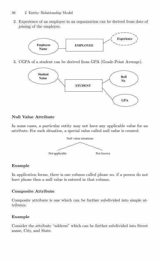
38 2 Entity–Relationship Model
2. Experience of an employee in an organization can be derived from date ofjoining of the employee.
EMPLOYEE EmployeeName
Experience
3. CGPA of a student can be derived from GPA (Grade Point Average).
STUDENT
StudentName
GPA
RollNo
Null Value Attribute
In some cases, a particular entity may not have any applicable value for anattribute. For such situation, a special value called null value is created.
Null value situations
Not applicable Not known
Example
In application forms, there is one column called phone no. if a person do nothave phone then a null value is entered in that column.
Composite Attribute
Composite attribute is one which can be further subdivided into simple at-tributes.
Example
Consider the attribute “address” which can be further subdivided into Streetname, City, and State.
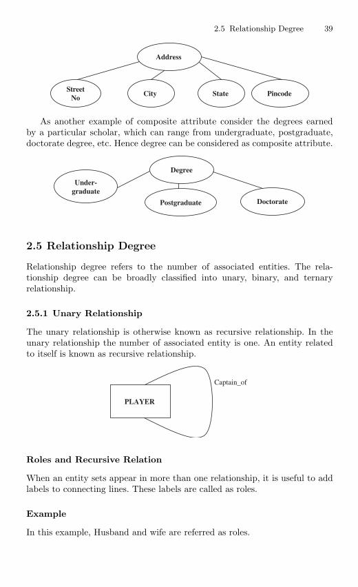
2.5 Relationship Degree 39
StreetNo
City State Pincode
Address
As another example of composite attribute consider the degrees earnedby a particular scholar, which can range from undergraduate, postgraduate,doctorate degree, etc. Hence degree can be considered as composite attribute.
Degree
Under-graduate
Postgraduate Doctorate
2.5 Relationship Degree
Relationship degree refers to the number of associated entities. The rela-tionship degree can be broadly classified into unary, binary, and ternaryrelationship.
2.5.1 Unary Relationship
The unary relationship is otherwise known as recursive relationship. In theunary relationship the number of associated entity is one. An entity relatedto itself is known as recursive relationship.
Captain_of
PLAYER
Roles and Recursive Relation
When an entity sets appear in more than one relationship, it is useful to addlabels to connecting lines. These labels are called as roles.
Example
In this example, Husband and wife are referred as roles.
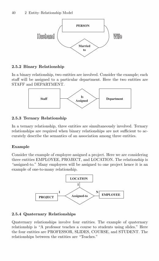
40 2 Entity–Relationship Model
PERSON
Marriedto
2.5.2 Binary Relationship
In a binary relationship, two entities are involved. Consider the example; eachstaff will be assigned to a particular department. Here the two entities areSTAFF and DEPARTMENT.
Staff Is
Assigned Department
2.5.3 Ternary Relationship
In a ternary relationship, three entities are simultaneously involved. Ternaryrelationships are required when binary relationships are not sufficient to ac-curately describe the semantics of an association among three entities.
Example
Consider the example of employee assigned a project. Here we are consideringthree entities EMPLOYEE, PROJECT, and LOCATION. The relationship is“assigned-to.” Many employees will be assigned to one project hence it is anexample of one-to-many relationship.
PROJECT
LOCATION
EMPLOYEE Assigned-to
1
1 N
2.5.4 Quaternary Relationships
Quaternary relationships involve four entities. The example of quaternaryrelationship is “A professor teaches a course to students using slides.” Herethe four entities are PROFESSOR, SLIDES, COURSE, and STUDENT. Therelationships between the entities are “Teaches.”
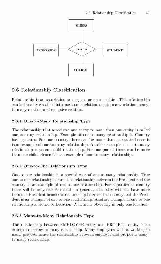
2.6 Relationship Classification 41
PROFESSOR
COURSE
SLIDES
STUDENT Teaches
2.6 Relationship Classification
Relationship is an association among one or more entities. This relationshipcan be broadly classified into one-to-one relation, one-to-many relation, many-to-many relation and recursive relation.
2.6.1 One-to-Many Relationship Type
The relationship that associates one entity to more than one entity is calledone-to-many relationship. Example of one-to-many relationship is Countryhaving states. For one country there can be more than one state hence itis an example of one-to-many relationship. Another example of one-to-manyrelationship is parent–child relationship. For one parent there can be morethan one child. Hence it is an example of one-to-many relationship.
2.6.2 One-to-One Relationship Type
One-to-one relationship is a special case of one-to-many relationship. Trueone-to-one relationship is rare. The relationship between the President and thecountry is an example of one-to-one relationship. For a particular countrythere will be only one President. In general, a country will not have morethan one President hence the relationship between the country and the Presi-dent is an example of one-to-one relationship. Another example of one-to-onerelationship is House to Location. A house is obviously in only one location.
2.6.3 Many-to-Many Relationship Type
The relationship between EMPLOYEE entity and PROJECT entity is anexample of many-to-many relationship. Many employees will be working inmany projects hence the relationship between employee and project is many-to-many relationship.
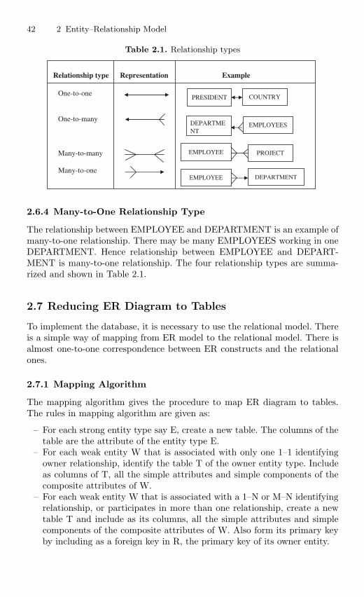
42 2 Entity–Relationship Model
Table 2.1. Relationship types
Relationship type Representation Example
One-to-one
One-to-many
Many-to-many
Many-to-one
PRESIDENT COUNTRY
DEPARTMENT
EMPLOYEES
EMPLOYEE PROJECT
EMPLOYEE DEPARTMENT
2.6.4 Many-to-One Relationship Type
The relationship between EMPLOYEE and DEPARTMENT is an example ofmany-to-one relationship. There may be many EMPLOYEES working in oneDEPARTMENT. Hence relationship between EMPLOYEE and DEPART-MENT is many-to-one relationship. The four relationship types are summa-rized and shown in Table 2.1.
2.7 Reducing ER Diagram to Tables
To implement the database, it is necessary to use the relational model. Thereis a simple way of mapping from ER model to the relational model. There isalmost one-to-one correspondence between ER constructs and the relationalones.
2.7.1 Mapping Algorithm
The mapping algorithm gives the procedure to map ER diagram to tables.The rules in mapping algorithm are given as:
– For each strong entity type say E, create a new table. The columns of thetable are the attribute of the entity type E.
– For each weak entity W that is associated with only one 1–1 identifyingowner relationship, identify the table T of the owner entity type. Includeas columns of T, all the simple attributes and simple components of thecomposite attributes of W.
– For each weak entity W that is associated with a 1–N or M–N identifyingrelationship, or participates in more than one relationship, create a newtable T and include as its columns, all the simple attributes and simplecomponents of the composite attributes of W. Also form its primary keyby including as a foreign key in R, the primary key of its owner entity.
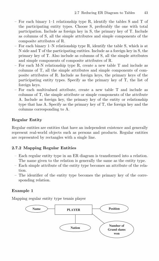
2.7 Reducing ER Diagram to Tables 43
– For each binary 1–1 relationship type R, identify the tables S and T ofthe participating entity types. Choose S, preferably the one with totalparticipation. Include as foreign key in S, the primary key of T. Includeas columns of S, all the simple attributes and simple components of thecomposite attributes of R.
– For each binary 1–N relationship type R, identify the table S, which is atN side and T of the participating entities. Include as a foreign key in S, theprimary key of T. Also include as columns of S, all the simple attributesand simple components of composite attributes of R.
– For each M-N relationship type R, create a new table T and include ascolumns of T, all the simple attributes and simple components of com-posite attributes of R. Include as foreign keys, the primary keys of theparticipating entity types. Specify as the primary key of T, the list offoreign keys.
– For each multivalued attribute, create a new table T and include ascolumns of T, the simple attribute or simple components of the attributeA. Include as foreign key, the primary key of the entity or relationshiptype that has A. Specify as the primary key of T, the foreign key and thecolumns corresponding to A.
Regular Entity
Regular entities are entities that have an independent existence and generallyrepresent real-world objects such as persons and products. Regular entitiesare represented by rectangles with a single line.
2.7.2 Mapping Regular Entities
– Each regular entity type in an ER diagram is transformed into a relation.The name given to the relation is generally the same as the entity type.
– Each simple attribute of the entity type becomes an attribute of the rela-tion.
– The identifier of the entity type becomes the primary key of the corre-sponding relation.
Example 1
Mapping regular entity type tennis player
PLAYERName Position
NationNumber of
Grand slamswon
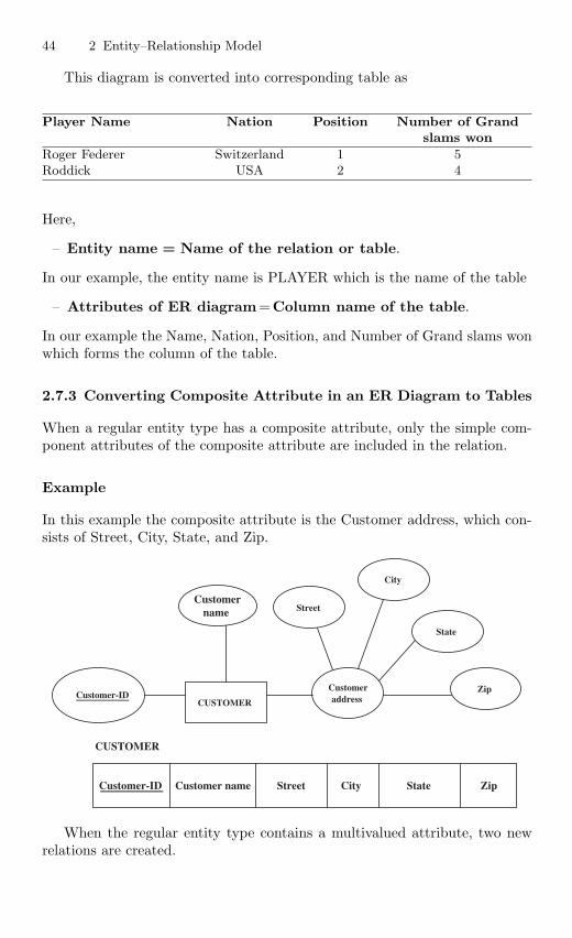
44 2 Entity–Relationship Model
This diagram is converted into corresponding table as
Player Name Nation Position Number of Grandslams won
Roger Federer Switzerland 1 5Roddick USA 2 4
Here,
– Entity name = Name of the relation or table.
In our example, the entity name is PLAYER which is the name of the table
– Attributes of ER diagram=Column name of the table.
In our example the Name, Nation, Position, and Number of Grand slams wonwhich forms the column of the table.
2.7.3 Converting Composite Attribute in an ER Diagram to Tables
When a regular entity type has a composite attribute, only the simple com-ponent attributes of the composite attribute are included in the relation.
Example
In this example the composite attribute is the Customer address, which con-sists of Street, City, State, and Zip.
CUSTOMER
CUSTOMER Customer-ID
Street
City
Customeraddress
Zip
Customername
State
Customer-ID Customer name Street City State Zip
When the regular entity type contains a multivalued attribute, two newrelations are created.
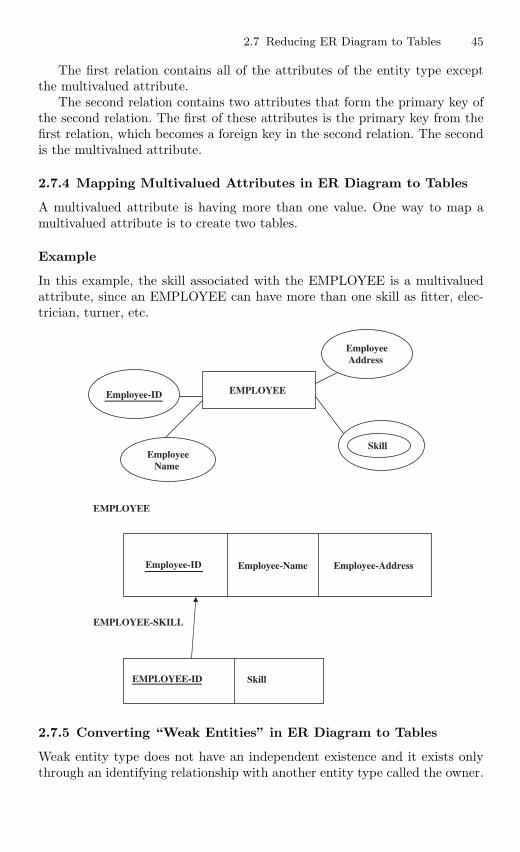
2.7 Reducing ER Diagram to Tables 45
The first relation contains all of the attributes of the entity type exceptthe multivalued attribute.
The second relation contains two attributes that form the primary key ofthe second relation. The first of these attributes is the primary key from thefirst relation, which becomes a foreign key in the second relation. The secondis the multivalued attribute.
2.7.4 Mapping Multivalued Attributes in ER Diagram to Tables
A multivalued attribute is having more than one value. One way to map amultivalued attribute is to create two tables.
Example
In this example, the skill associated with the EMPLOYEE is a multivaluedattribute, since an EMPLOYEE can have more than one skill as fitter, elec-trician, turner, etc.
EMPLOYEE
EMPLOYEE-SKILL
EMPLOYEE Employee-ID
EmployeeAddress
Skill Employee
Name
Employee-ID Employee-Name Employee-Address
EMPLOYEE-ID Skill
2.7.5 Converting “Weak Entities” in ER Diagram to Tables
Weak entity type does not have an independent existence and it exists onlythrough an identifying relationship with another entity type called the owner.
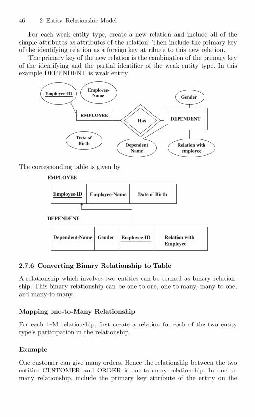
46 2 Entity–Relationship Model
For each weak entity type, create a new relation and include all of thesimple attributes as attributes of the relation. Then include the primary keyof the identifying relation as a foreign key attribute to this new relation.
The primary key of the new relation is the combination of the primary keyof the identifying and the partial identifier of the weak entity type. In thisexample DEPENDENT is weak entity.
EMPLOYEE
Date ofBirth
Has DEPENDENT
DependentName
Gender
Relation withemployee
Employee-IDEmployee-
Name
The corresponding table is given by
EMPLOYEE
DEPENDENT
Employee-ID Employee-Name Date of Birth
Dependent-Name Gender Employee-ID Relation withEmployee
2.7.6 Converting Binary Relationship to Table
A relationship which involves two entities can be termed as binary relation-ship. This binary relationship can be one-to-one, one-to-many, many-to-one,and many-to-many.
Mapping one-to-Many Relationship
For each 1–M relationship, first create a relation for each of the two entitytype’s participation in the relationship.
Example
One customer can give many orders. Hence the relationship between the twoentities CUSTOMER and ORDER is one-to-many relationship. In one-to-many relationship, include the primary key attribute of the entity on the
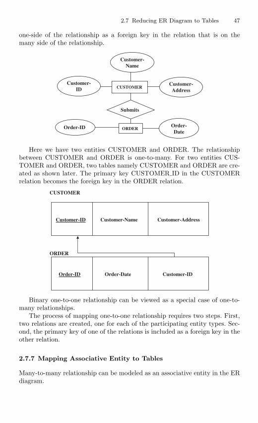
2.7 Reducing ER Diagram to Tables 47
one-side of the relationship as a foreign key in the relation that is on themany side of the relationship.
CUSTOMER
ORDER
Customer-Address
Customer-ID
Customer-Name
Order-ID Order-Date
Submits
Here we have two entities CUSTOMER and ORDER. The relationshipbetween CUSTOMER and ORDER is one-to-many. For two entities CUS-TOMER and ORDER, two tables namely CUSTOMER and ORDER are cre-ated as shown later. The primary key CUSTOMER ID in the CUSTOMERrelation becomes the foreign key in the ORDER relation.
CUSTOMER
ORDER
Customer-ID Customer-Name Customer-Address
Order-ID Order-Date Customer-ID
Binary one-to-one relationship can be viewed as a special case of one-to-many relationships.
The process of mapping one-to-one relationship requires two steps. First,two relations are created, one for each of the participating entity types. Sec-ond, the primary key of one of the relations is included as a foreign key in theother relation.
2.7.7 Mapping Associative Entity to Tables
Many-to-many relationship can be modeled as an associative entity in the ERdiagram.
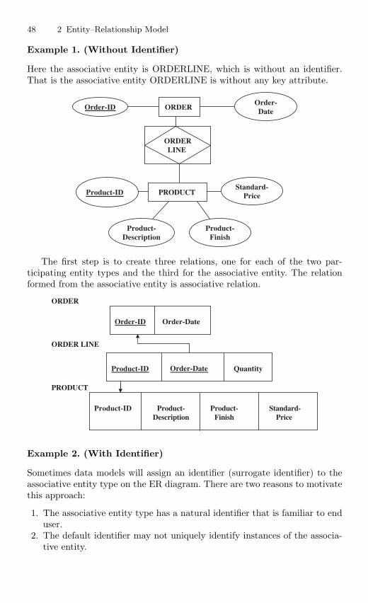
48 2 Entity–Relationship Model
Example 1. (Without Identifier)
Here the associative entity is ORDERLINE, which is without an identifier.That is the associative entity ORDERLINE is without any key attribute.
ORDER Order-IDOrder-
Date
ORDERLINE
PRODUCT Standard-
PriceProduct-ID
Product- Description
Product- Finish
The first step is to create three relations, one for each of the two par-ticipating entity types and the third for the associative entity. The relationformed from the associative entity is associative relation.
ORDER
ORDER LINE
PRODUCT
Order-ID Order-Date
Product-ID Order-Date Quantity
Product-ID Product-Description
Product-Finish
Standard-Price
Example 2. (With Identifier)
Sometimes data models will assign an identifier (surrogate identifier) to theassociative entity type on the ER diagram. There are two reasons to motivatethis approach:
1. The associative entity type has a natural identifier that is familiar to enduser.
2. The default identifier may not uniquely identify instances of the associa-tive entity.
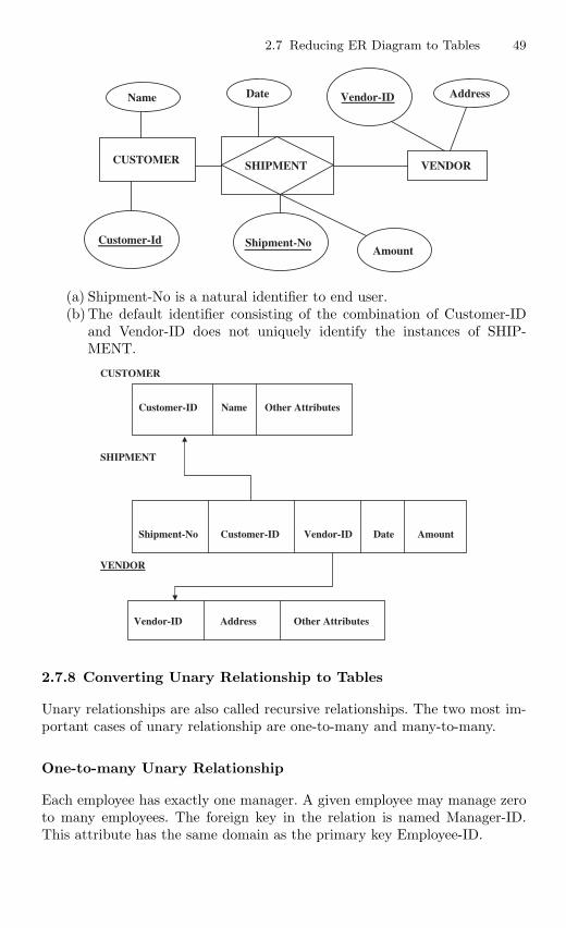
2.7 Reducing ER Diagram to Tables 49
Date Vendor-ID Address
VENDOR SHIPMENT CUSTOMER
Customer-Id Shipment-NoAmount
Name
(a) Shipment-No is a natural identifier to end user.(b) The default identifier consisting of the combination of Customer-ID
and Vendor-ID does not uniquely identify the instances of SHIP-MENT.
CUSTOMER
SHIPMENT
VENDOR
Customer-ID Name Other Attributes
Shipment-No Customer-ID Vendor-ID Date Amount
Vendor-ID Address Other Attributes
2.7.8 Converting Unary Relationship to Tables
Unary relationships are also called recursive relationships. The two most im-portant cases of unary relationship are one-to-many and many-to-many.
One-to-many Unary Relationship
Each employee has exactly one manager. A given employee may manage zeroto many employees. The foreign key in the relation is named Manager-ID.This attribute has the same domain as the primary key Employee-ID.
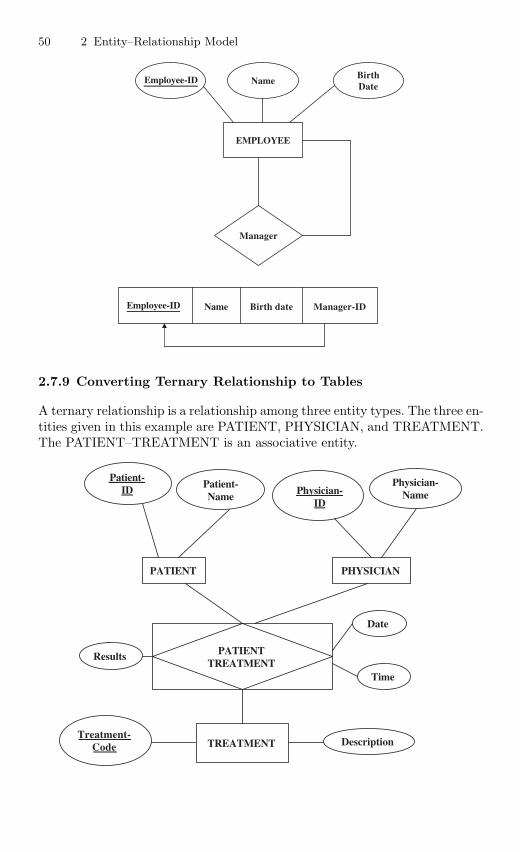
50 2 Entity–Relationship Model
EMPLOYEE
Employee-ID BirthDate
Name
Manager
Employee-ID Name Birth date Manager-ID
2.7.9 Converting Ternary Relationship to Tables
A ternary relationship is a relationship among three entity types. The three en-tities given in this example are PATIENT, PHYSICIAN, and TREATMENT.The PATIENT–TREATMENT is an associative entity.
Patient-ID
Patient-Name
PATIENT
Physician-ID
Physician-Name
PHYSICIAN
PATIENT TREATMENT
Date
Time
Results
TREATMENT Treatment-
Code Description
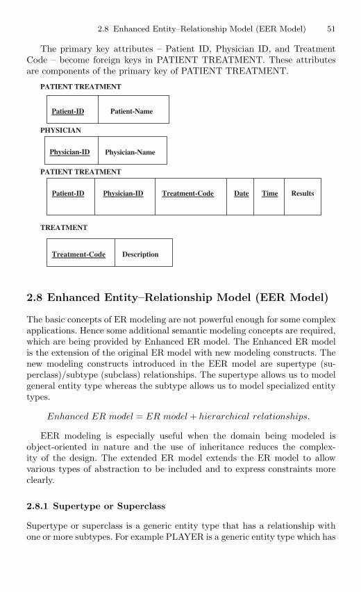
2.8 Enhanced Entity–Relationship Model (EER Model) 51
The primary key attributes – Patient ID, Physician ID, and TreatmentCode – become foreign keys in PATIENT TREATMENT. These attributesare components of the primary key of PATIENT TREATMENT.
PATIENT TREATMENT
PHYSICIAN
PATIENT TREATMENT
Patient-ID Patient-Name
Physician-ID Physician-Name
Patient-ID Physician-ID Treatment-Code Date Time Results
TREATMENT
Treatment-Code Description
2.8 Enhanced Entity–Relationship Model (EER Model)
The basic concepts of ER modeling are not powerful enough for some complexapplications. Hence some additional semantic modeling concepts are required,which are being provided by Enhanced ER model. The Enhanced ER modelis the extension of the original ER model with new modeling constructs. Thenew modeling constructs introduced in the EER model are supertype (su-perclass)/subtype (subclass) relationships. The supertype allows us to modelgeneral entity type whereas the subtype allows us to model specialized entitytypes.
Enhanced ER model = ER model + hierarchical relationships.
EER modeling is especially useful when the domain being modeled isobject-oriented in nature and the use of inheritance reduces the complex-ity of the design. The extended ER model extends the ER model to allowvarious types of abstraction to be included and to express constraints moreclearly.
2.8.1 Supertype or Superclass
Supertype or superclass is a generic entity type that has a relationship withone or more subtypes. For example PLAYER is a generic entity type which has
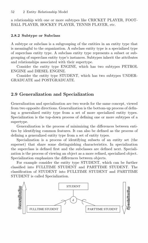
52 2 Entity–Relationship Model
a relationship with one or more subtypes like CRICKET PLAYER, FOOT-BALL PLAYER, HOCKEY PLAYER, TENNIS PLAYER, etc.
2.8.2 Subtype or Subclass
A subtype or subclass is a subgrouping of the entities in an entity type thatis meaningful to the organization. A subclass entity type is a specialized typeof superclass entity type. A subclass entity type represents a subset or sub-grouping of superclass entity type’s instances. Subtypes inherit the attributesand relationships associated with their supertype.
Consider the entity type ENGINE, which has two subtypes PETROLENGINE and DIESEL ENGINE.
Consider the entity type STUDENT, which has two subtypes UNDER-GRADUATE and POSTGRADUATE.
2.9 Generalization and Specialization
Generalization and specialization are two words for the same concept, viewedfrom two opposite directions. Generalization is the bottom-up process of defin-ing a generalized entity type from a set of more specialized entity types.Specialization is the top-down process of defining one or more subtypes of asupertype.
Generalization is the process of minimizing the differences between enti-ties by identifying common features. It can also be defined as the process ofdefining a generalized entity type from a set of entity types.
Specialization is a process of identifying subsets of an entity set (thesuperset) that share some distinguishing characteristics. In specializationthe superclass is defined first and the subclasses are defined next. Speciali-zation is the process of viewing an object as a more refined, specialized object.Specialization emphasizes the differences between objects.
For example consider the entity type STUDENT, which can be furtherclassified into FULLTIME STUDENT and PARTTIME STUDENT. Theclassification of STUDENT into FULLTIME STUDENT and PARTTIMESTUDENT is called Specialization.
STUDENT
FULLTIME STUDENT PARTTIME STUDENT
d
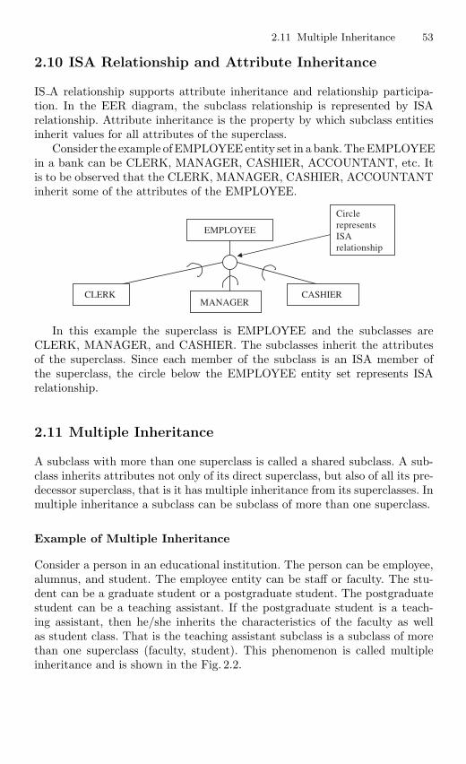
2.11 Multiple Inheritance 53
2.10 ISA Relationship and Attribute Inheritance
IS A relationship supports attribute inheritance and relationship participa-tion. In the EER diagram, the subclass relationship is represented by ISArelationship. Attribute inheritance is the property by which subclass entitiesinherit values for all attributes of the superclass.
Consider the example of EMPLOYEE entity set in a bank. The EMPLOYEEin a bank can be CLERK, MANAGER, CASHIER, ACCOUNTANT, etc. Itis to be observed that the CLERK, MANAGER, CASHIER, ACCOUNTANTinherit some of the attributes of the EMPLOYEE.
EMPLOYEE
CLERK MANAGER
CASHIER
CirclerepresentsISArelationship
In this example the superclass is EMPLOYEE and the subclasses areCLERK, MANAGER, and CASHIER. The subclasses inherit the attributesof the superclass. Since each member of the subclass is an ISA member ofthe superclass, the circle below the EMPLOYEE entity set represents ISArelationship.
2.11 Multiple Inheritance
A subclass with more than one superclass is called a shared subclass. A sub-class inherits attributes not only of its direct superclass, but also of all its pre-decessor superclass, that is it has multiple inheritance from its superclasses. Inmultiple inheritance a subclass can be subclass of more than one superclass.
Example of Multiple Inheritance
Consider a person in an educational institution. The person can be employee,alumnus, and student. The employee entity can be staff or faculty. The stu-dent can be a graduate student or a postgraduate student. The postgraduatestudent can be a teaching assistant. If the postgraduate student is a teach-ing assistant, then he/she inherits the characteristics of the faculty as wellas student class. That is the teaching assistant subclass is a subclass of morethan one superclass (faculty, student). This phenomenon is called multipleinheritance and is shown in the Fig. 2.2.
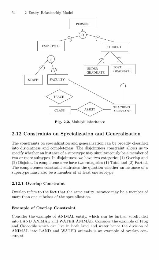
54 2 Entity–Relationship Model
PERSON
STAFF
EMPLOYEE STUDENT
O
d
FACULTY
UNDERGRADUATE
POST GRADUATE
TEACH
CLASS TEACHINGASSISTANT ASSIST
Fig. 2.2. Multiple inheritance
2.12 Constraints on Specialization and Generalization
The constraints on specialization and generalization can be broadly classifiedinto disjointness and completeness. The disjointness constraint allows us tospecify whether an instance of a supertype may simultaneously be a member oftwo or more subtypes. In disjointness we have two categories (1) Overlap and(2) Disjoint. In completeness we have two categories (1) Total and (2) Partial.The completeness constraint addresses the question whether an instance of asupertype must also be a member of at least one subtype.
2.12.1 Overlap Constraint
Overlap refers to the fact that the same entity instance may be a member ofmore than one subclass of the specialization.
Example of Overlap Constraint
Consider the example of ANIMAL entity, which can be further subdividedinto LAND ANIMAL and WATER ANIMAL. Consider the example of Frogand Crocodile which can live in both land and water hence the division ofANIMAL into LAND and WATER animals is an example of overlap con-straint.
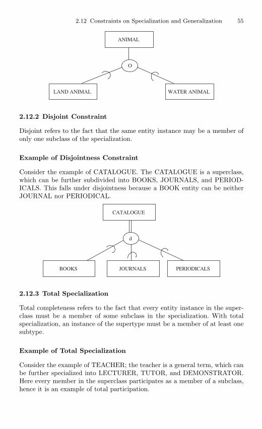
2.12 Constraints on Specialization and Generalization 55
ANIMAL
LAND ANIMAL WATER ANIMAL
O
2.12.2 Disjoint Constraint
Disjoint refers to the fact that the same entity instance may be a member ofonly one subclass of the specialization.
Example of Disjointness Constraint
Consider the example of CATALOGUE. The CATALOGUE is a superclass,which can be further subdivided into BOOKS, JOURNALS, and PERIOD-ICALS. This falls under disjointness because a BOOK entity can be neitherJOURNAL nor PERIODICAL.
CATALOGUE
BOOKS JOURNALS PERIODICALS
d
2.12.3 Total Specialization
Total completeness refers to the fact that every entity instance in the super-class must be a member of some subclass in the specialization. With totalspecialization, an instance of the supertype must be a member of at least onesubtype.
Example of Total Specialization
Consider the example of TEACHER; the teacher is a general term, which canbe further specialized into LECTURER, TUTOR, and DEMONSTRATOR.Here every member in the superclass participates as a member of a subclass,hence it is an example of total participation.
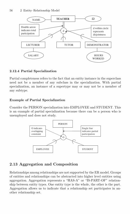
56 2 Entity–Relationship Model
TEACHER
LECTURER TUTOR DEMONSTRATOR
d
IDNAME
SALARY HOURSWORKED
d within circlerepresentsdisjointness
Double arrowindicates totalparticipation
2.12.4 Partial Specialization
Partial completeness refers to the fact that an entity instance in the superclassneed not be a member of any subclass in the specialization. With partialspecialization, an instance of a supertype may or may not be a member ofany subtype.
Example of Partial Specialization
Consider the PERSON specialization into EMPLOYEE and STUDENT. Thisis an example of partial specialization because there can be a person who isunemployed and does not study.
PERSON
EMPLOYEE STUDENT
O
Single lineindicates partialparticipation
O indicatesoverlappingconstraint
2.13 Aggregation and Composition
Relationships among relationships are not supported by the ER model. Groupsof entities and relationships can be abstracted into higher level entities usingaggregation. Aggregation represents a “HAS-A” or “IS-PART-OF” relation-ship between entity types. One entity type is the whole, the other is the part.Aggregation allows us to indicate that a relationship set participates in an-other relationship set.
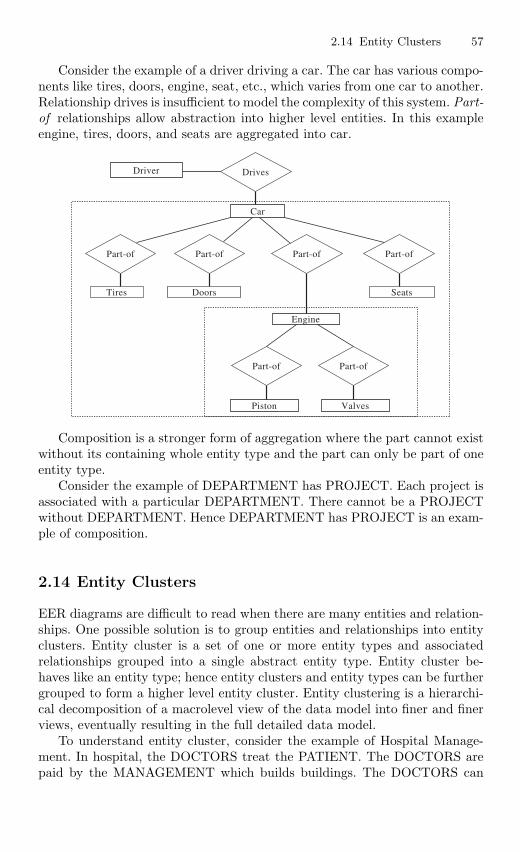
2.14 Entity Clusters 57
Consider the example of a driver driving a car. The car has various compo-nents like tires, doors, engine, seat, etc., which varies from one car to another.Relationship drives is insufficient to model the complexity of this system. Part-of relationships allow abstraction into higher level entities. In this exampleengine, tires, doors, and seats are aggregated into car.
Driver Drives
Car
Tires Doors Seats
Engine
Part-of
Piston Valves
Part-of
Part-of Part-of Part-of Part-of
Composition is a stronger form of aggregation where the part cannot existwithout its containing whole entity type and the part can only be part of oneentity type.
Consider the example of DEPARTMENT has PROJECT. Each project isassociated with a particular DEPARTMENT. There cannot be a PROJECTwithout DEPARTMENT. Hence DEPARTMENT has PROJECT is an exam-ple of composition.
2.14 Entity Clusters
EER diagrams are difficult to read when there are many entities and relation-ships. One possible solution is to group entities and relationships into entityclusters. Entity cluster is a set of one or more entity types and associatedrelationships grouped into a single abstract entity type. Entity cluster be-haves like an entity type; hence entity clusters and entity types can be furthergrouped to form a higher level entity cluster. Entity clustering is a hierarchi-cal decomposition of a macrolevel view of the data model into finer and finerviews, eventually resulting in the full detailed data model.
To understand entity cluster, consider the example of Hospital Manage-ment. In hospital, the DOCTORS treat the PATIENT. The DOCTORS arepaid by the MANAGEMENT which builds buildings. The DOCTORS can
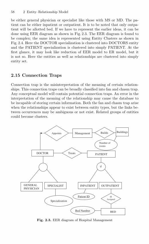
58 2 Entity–Relationship Model
be either general physician or specialist like those with MS or MD. The pa-tient can be either inpatient or outpatient. It is to be noted that only outpa-tient will be allotted bed. If we have to represent the earlier ideas, it can bedone using EER diagram as shown in Fig. 2.3. The EER diagram is found tobe complex; the same idea is represented using Entity Clusters as shown inFig. 2.4. Here the DOCTOR specialization is clustered into DOCTORS entityand the PATIENT specialization is clustered into simply PATIENT. At thefirst glance, it may look like reduction of EER model to ER model, but itis not so. Here the entities as well as relationships are clustered into simplyentity set.
2.15 Connection Traps
Connection trap is the misinterpretation of the meaning of certain relation-ships. This connection traps can be broadly classified into fan and chasm trap.Any conceptual model will contain potential connection traps. An error in theinterpretation of the meaning of the relationship may cause the database tobe incapable of storing certain information. Both the fan and chasm trap arisewhen the relationships appear to exist between entity types, but the links be-tween occurrences may be ambiguous or not exist. Related groups of entitiescould become clusters.
DOCTOR
GENERALPHYSICIAN
SPECIALIST
PATIENT
d
INPATIENT OUTPATIENT
ISAssigned
BEDBed Number
Treats
Appoints Management
Specialization
Patient ID
Builds Buildings
Number ofrooms
Fig. 2.3. EER diagram of Hospital Management
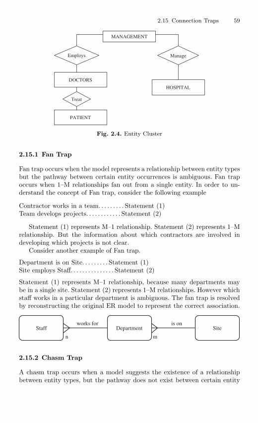
2.15 Connection Traps 59
MANAGEMENT
PATIENT
DOCTORS
HOSPITAL
Employs Manage
Treat
Fig. 2.4. Entity Cluster
2.15.1 Fan Trap
Fan trap occurs when the model represents a relationship between entity typesbut the pathway between certain entity occurrences is ambiguous. Fan trapoccurs when 1–M relationships fan out from a single entity. In order to un-derstand the concept of Fan trap, consider the following example
Contractor works in a team. . . . . . . . . Statement (1)Team develops projects. . . . . . . . . . . . Statement (2)
Statement (1) represents M–1 relationship. Statement (2) represents 1–Mrelationship. But the information about which contractors are involved indeveloping which projects is not clear.
Consider another example of Fan trap.
Department is on Site. . . . . . . . . Statement (1)Site employs Staff. . . . . . . . . . . . . . . Statement (2)
Statement (1) represents M–1 relationship, because many departments maybe in a single site. Statement (2) represents 1–M relationships. However whichstaff works in a particular department is ambiguous. The fan trap is resolvedby reconstructing the original ER model to represent the correct association.
Staffworks for
n m
is onDepartment Site
2.15.2 Chasm Trap
A chasm trap occurs when a model suggests the existence of a relationshipbetween entity types, but the pathway does not exist between certain entity
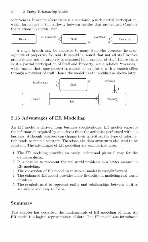
60 2 Entity–Relationship Model
occurrences. It occurs where there is a relationship with partial participation,which forms part of the pathway between entities that are related. Considerthe relationship shown later.
Branch Staffoversees
Propertyis_allocated
n OO
A single branch may be allocated to many staff who oversees the man-agement of properties for rent. It should be noted that not all staff overseeproperty and not all property is managed by a member of staff. Hence thereexist a partial participation of Staff and Property in the relation “oversees,”which means that some properties cannot be associated with a branch officethrough a member of staff. Hence the model has to modified as shown later.
is_allocated nStaff
oversees
Propertyhas
Branch
O
O
2.16 Advantages of ER Modeling
An ER model is derived from business specifications. ER models separatethe information required by a business from the activities performed within abusiness. Although business can change their activities, the type of informa-tion tends to remain constant. Therefore, the data structures also tend to beconstant. The advantages of ER modeling are summarized later:
1. The ER modeling provides an easily understood pictorial map for thedatabase design.
2. It is possible to represent the real world problems in a better manner inER modeling.
3. The conversion of ER model to relational model is straightforward.4. The enhanced ER model provides more flexibility in modeling real world
problems.5. The symbols used to represent entity and relationships between entities
are simple and easy to follow.
Summary
This chapter has described the fundamentals of ER modeling of data. AnER model is a logical representation of data. The ER model was introduced
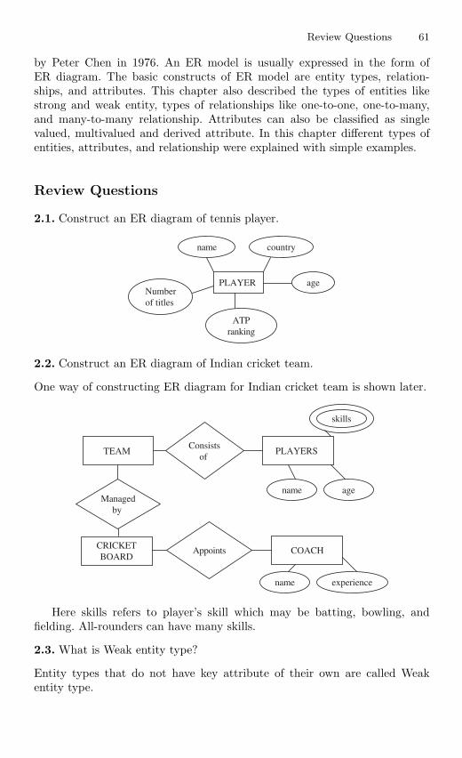
Review Questions 61
by Peter Chen in 1976. An ER model is usually expressed in the form ofER diagram. The basic constructs of ER model are entity types, relation-ships, and attributes. This chapter also described the types of entities likestrong and weak entity, types of relationships like one-to-one, one-to-many,and many-to-many relationship. Attributes can also be classified as singlevalued, multivalued and derived attribute. In this chapter different types ofentities, attributes, and relationship were explained with simple examples.
Review Questions
2.1. Construct an ER diagram of tennis player.
PLAYER
name country
ageNumberof titles
ATPranking
2.2. Construct an ER diagram of Indian cricket team.
One way of constructing ER diagram for Indian cricket team is shown later.
TEAM
CRICKETBOARD
PLAYERS Consists
of
name age
skills
Managedby
Appoints COACH
name experience
Here skills refers to player’s skill which may be batting, bowling, andfielding. All-rounders can have many skills.
2.3. What is Weak entity type?
Entity types that do not have key attribute of their own are called Weakentity type.
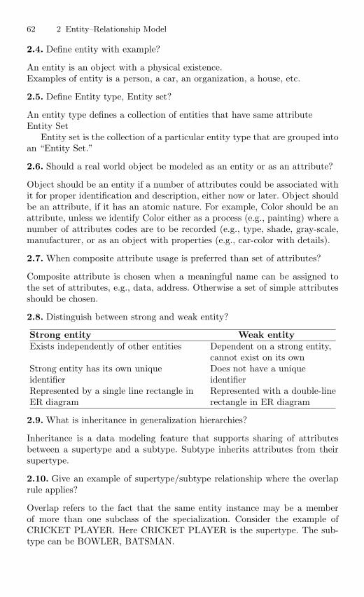
62 2 Entity–Relationship Model
2.4. Define entity with example?
An entity is an object with a physical existence.Examples of entity is a person, a car, an organization, a house, etc.
2.5. Define Entity type, Entity set?
An entity type defines a collection of entities that have same attributeEntity Set
Entity set is the collection of a particular entity type that are grouped intoan “Entity Set.”
2.6. Should a real world object be modeled as an entity or as an attribute?
Object should be an entity if a number of attributes could be associated withit for proper identification and description, either now or later. Object shouldbe an attribute, if it has an atomic nature. For example, Color should be anattribute, unless we identify Color either as a process (e.g., painting) where anumber of attributes codes are to be recorded (e.g., type, shade, gray-scale,manufacturer, or as an object with properties (e.g., car-color with details).
2.7. When composite attribute usage is preferred than set of attributes?
Composite attribute is chosen when a meaningful name can be assigned tothe set of attributes, e.g., data, address. Otherwise a set of simple attributesshould be chosen.
2.8. Distinguish between strong and weak entity?
Strong entity Weak entityExists independently of other entities Dependent on a strong entity,
cannot exist on its ownStrong entity has its own unique Does not have a uniqueidentifier identifierRepresented by a single line rectangle in Represented with a double-lineER diagram rectangle in ER diagram
2.9. What is inheritance in generalization hierarchies?
Inheritance is a data modeling feature that supports sharing of attributesbetween a supertype and a subtype. Subtype inherits attributes from theirsupertype.
2.10. Give an example of supertype/subtype relationship where the overlaprule applies?
Overlap refers to the fact that the same entity instance may be a memberof more than one subclass of the specialization. Consider the example ofCRICKET PLAYER. Here CRICKET PLAYER is the supertype. The sub-type can be BOWLER, BATSMAN.
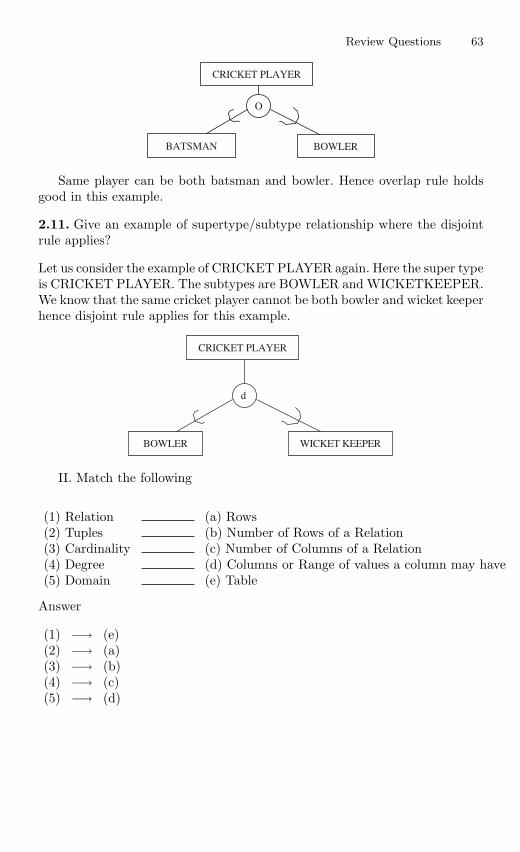
Review Questions 63
CRICKET PLAYER
BATSMAN BOWLER
O
Same player can be both batsman and bowler. Hence overlap rule holdsgood in this example.
2.11. Give an example of supertype/subtype relationship where the disjointrule applies?
Let us consider the example of CRICKET PLAYER again. Here the super typeis CRICKET PLAYER. The subtypes are BOWLER and WICKETKEEPER.We know that the same cricket player cannot be both bowler and wicket keeperhence disjoint rule applies for this example.
CRICKET PLAYER
BOWLER WICKET KEEPER
d
II. Match the following
(1) Relation (a) Rows(2) Tuples (b) Number of Rows of a Relation(3) Cardinality (c) Number of Columns of a Relation(4) Degree (d) Columns or Range of values a column may have(5) Domain (e) Table
Answer
(1) −→ (e)(2) −→ (a)(3) −→ (b)(4) −→ (c)(5) −→ (d)
3
Relational Model
Learning Objectives. This chapter is dedicated to relational model which is inuse since late 1970s. Various operations in relational algebra and relational calculusare given in this chapter. After completing this chapter the reader should be familiarwith the following concepts:
– Evolution and importance of relational model– Terms in relational model like tuple, domain, cardinality, and degree of a relation– Operations in relational algebra and relational calculus– Relational algebra vs relational calculus– QBE and various operations in QBE
3.1 Introduction
E.F. Codd (Edgar Frank Codd) of IBM had written an article “A relationalmodel for large shared data banks” in June 1970 in the Association of Com-puter Machinery (ACM) Journal, Communications of the ACM. His worktriggered people to work in relational model. One of the most significantimplementations of the relational model was “System R,” which was develo-ped by IBM during the late 1970s. System R was intended as a “proof ofconcept” to show that relational database systems could really build andwork efficiently. It gave rise to major developments such as a structured querylanguage called SQL which has since become an ISO standard and de factostandard relational language. Various commercial relational DBMS productswere developed during the 1980s such as DB2, SQL/DS, and Oracle. In rela-tional data model the data are stored in the form of tables.
3.2 CODD’S Rules
In 1985, Codd published a list of rules that became a standard way of eval-uating a relational system. After publishing the original article Codd statedthat there are no systems that will satisfy every rule. Nevertheless the rulesrepresent relational ideal and remain a goal for relational database designers.
S. Sumathi: Relational Model, Studies in Computational Intelligence (SCI) 47, 65–110 (2007)
www.springerlink.com c© Springer-Verlag Berlin Heidelberg 2007
66 3 Relational Model
Note: The rules are numbered from 1 to 12 whereas the statements precededby the bullet mark are interpretations of the Codd’s rule:
1. The Information Rule. All information in a relational database is repre-sented explicitly at the logical level and in exactly one way-by values intables:• Data should be presented to the user in the tabular form.
2. Guaranteed Access Rule. Each and every datum (atomic value) in a rela-tional database is guaranteed to be logically accessible by resorting to acombination of table name, primary key value, and column name:• Every data element should be unambiguously accessible.
3. Systematic Treatment of Null Values. Null values (distinct from the emptycharacter string or a string of blank characters and distinct from zero orany other number) are supported in fully relational DBMS for representingmissing information and inapplicable information in a systematic way,independent of data type.
4. Dynamic On-line Catalog Based on the Relational Model. The databasedescription is represented at the logical level in the same way as ordinarydata, so that authorized users can apply the same relational language toits interrogation as they apply to the regular data:• The database description should be accessible to the users.
5. Comprehensive Data Sublanguage Rule. A relational system may supportseveral languages and various modes of terminal use (for example thefill-in-the-blanks mode). However, there must be at least one languagewhose statements are expressible, per some well-defined syntax, as char-acter strings and whose ability to support all the following is comprehen-sive: data definition, view definition, data manipulation (interactive andby program), integrity constraints, and transaction boundaries:• A database supports a clearly defined language to define the database,
view the definition, manipulate the data, and restrict some data valuesto maintain integrity.
6. View Updating Rule. All views that are theoretically updatable are alsoupdatable by the system:• Data should be able to be changed through any view available to the
user.7. High-level Insert, Update, and Delete. The capacity of handling a base
relation or a derived relation as a single operand applies not only to theretrieval of data but also to the insertion, update, and deletion of data:• All records in a file must be able to be added, deleted, or updated with
singular commands8. Physical Data Independence. Application programs and terminal activities
remain logically unimpaired whenever any changes are made in eitherstorage representations or access methods:
3.3 Relational Data Model 67
• Changes in how data are stored or retrieved should not affect how auser accesses the data.
9. Logical Data Independence. Application programs and terminal activitiesremain logically unimpaired whenever information-preserving changes ofany kind that theoretically permit unimpairment are made to the basetables:• A user’s view of data should be unaffected by its actual form in files.
10. Integrity Independence. Integrity constraints specific to a particular rela-tional database must be definable in a relational data sublanguage andstorable in the catalog, not in the application programs.• Constraints on user input should exist to maintain data integrity.
11. Distribution Independence. A relational DBMS has distribution indepen-dence. Distribution independence implies that users should not have tobe aware of whether a database is distributed.• A database design should allow for distribution of data over several
computer sites.12. Nonsubversion Rule. If a relational system has a low-level (single-record-
at-a-time) language, that low level cannot be used to subvert or bypassthe integrity rules and constraints expressed in the higher level relationallanguage (multiple-records-at-a-time):• Data fields that affect the organization of the database cannot be
changed.
There is one more rule called Rule Zero which states that “For any systemthat is claimed to be a relational database management system, that systemmust be able to manage data entirely through capabilities.”
3.3 Relational Data Model
The relational model uses a collection of tables to represent both data andthe relationships among those data. Tables are logical structures maintainedby the database manager. The relational model is a combination of threecomponents, such as Structural, Integrity, and Manipulative parts.
3.3.1 Structural Part
The structural part defines the database as a collection of relations.
3.3.2 Integrity Part
The database integrity is maintained in the relational model using primaryand foreign keys.
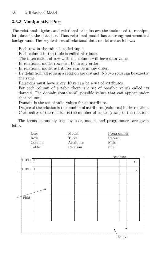
68 3 Relational Model
3.3.3 Manipulative Part
The relational algebra and relational calculus are the tools used to manipu-late data in the database. Thus relational model has a strong mathematicalbackground. The key features of relational data model are as follows:
– Each row in the table is called tuple.– Each column in the table is called attribute.– The intersection of row with the column will have data value.– In relational model rows can be in any order.– In relational model attributes can be in any order.– By definition, all rows in a relation are distinct. No two rows can be exactly
the same.– Relations must have a key. Keys can be a set of attributes.– For each column of a table there is a set of possible values called its
domain. The domain contains all possible values that can appear underthat column.
– Domain is the set of valid values for an attribute.– Degree of the relation is the number of attributes (columns) in the relation.– Cardinality of the relation is the number of tuples (rows) in the relation.
The terms commonly used by user, model, and programmers are givenlater.
User Model Programmer
Row Tuple RecordColumn Attribute FieldTable Relation File
TUPLE 0
TUPLE 1
Attribute
Field
Entity
3.4 Concept of Key 69
3.3.4 Table and Relation
The general doubt that will rise when one reads the relational model is thedifference between table and relation. For a table to be relation, the followingrules holds good:
– The intersection row with the column should contain single value (atomicvalue).
– All entries in a column are of same type.– Each column has a unique name (column order not significant).– No two rows are identical (row order not significant).
Example of Relational Model
Representation of Movie data in tabular form is shown later.
MOVIE
Movie Name Director Actor Actress
Titanic James Cameron Leonardo DiCapiro Kate WinsletAutograph Cheran Cheran GopikaRoja Maniratnam AravindSwamy Madubala
In the earlier relation:The degree of the relation (i.e., is the number of column in the relation) = 4.The cardinality of the relation (i.e., the number of rows in the relation) = 3.
3.4 Concept of Key
Key is an attribute or group of attributes, which is used to identify a row ina relation. Key can be broadly classified into (1) Superkey (2) Candidate key,and (3) Primary key
Key Classification
Superkey Candidate key Primary key
3.4.1 Superkey
A superkey is a subset of attributes of an entity-set that uniquely identifiesthe entities. Superkeys represent a constraint that prevents two entities fromever having the same value for those attributes.
70 3 Relational Model
3.4.2 Candidate Key
Candidate key is a minimal superkey. A candidate key for a relation schemais a minimal set of attributes whose values uniquely identify tuples in thecorresponding relation.
Primary Key
The primary key is a designated candidate key. It is to be noted that theprimary key should not be null.
Example
Consider the employee relation, which is characterized by the attributes,employee ID, employee name, employee age, employee experience, employeesalary, etc. In this employee relation:
Superkeys can be employee ID, employee name, employee age, employeeexperience, etc.
Candidate keys can be employee ID, employee name, employee age.Primary key is employee ID.
Note: If we declare a particular attribute as the primary key, then that attri-bute value cannot be NULL. Also it has to be distinct.
3.4.3 Foreign Key
Foreign key is set of fields or attributes in one relation that is used to “refer”to a tuple in another relation.
3.5 Relational Integrity
Data integrity constraints refer to the accuracy and correctness of data inthe database. Data integrity provides a mechanism to maintain data con-sistency for operations like INSERT, UPDATE, and DELETE. The differenttypes of data integrity constraints are Entity, NULL, Domain, and Referentialintegrity.
3.5.1 Entity Integrity
Entity integrity implies that a primary key cannot accept null value. Theprimary key of the relation uniquely identifies a row in a relation. Entityintegrity means that in order to represent an entity in the database it isnecessary to have a complete identification of the entity’s key attributes.
3.5 Relational Integrity 71
Consider the entity PLAYER; the attributes of the entity PLAYER areName, Age, Nation, and Rank. In this example, let us consider PLAYER’sname as the primary key even though two players can have same name. Wecannot insert any data in the relation PLAYER without entering the name ofthe player. This implies that primary key cannot be null.
3.5.2 Null Integrity
Null implies that the data value is not known temporarily. Consider therelation PERSON. The attributes of the relation PERSON are name, age,and salary. The age of the person cannot be NULL.
3.5.3 Domain Integrity Constraint
Domains are used in the relational model to define the characteristics of thecolumns of a table. Domain refers to the set of all possible values that attributecan take. The domain specifies its own name, data type, and logical size.The logical size represents the size as perceived by the user, not how it isimplemented internally. For example, for an integer, the logical size representsthe number of digits used to display the integer, not the number of bytes usedto store it. The domain integrity constraints are used to specify the validvalues that a column defined over the domain can take. We can define thevalid values by listing them as a set of values (such as an enumerated datatype in a strongly typed programming language), a range of values, or anexpression that accepts the valid values. Strictly speaking, only values fromthe same domain should ever be compared or be integrated through a unionoperator. The domain integrity constraint specifies that each attribute musthave values derived from a valid range.
Example 1
The age of the person cannot have any letter from the alphabet. The ageshould be a numerical value.
Example 2
Consider the relation APPLICANT. Here APPLICANT refers to the personwho is applying for job. The sex of the applicant should be either male (M)or female (F). Any entry other than M or F violates the domain constraint.
3.5.4 Referential Integrity
In the relational data model, associations between tables are defined throughthe use of foreign keys. The referential integrity rule states that a database
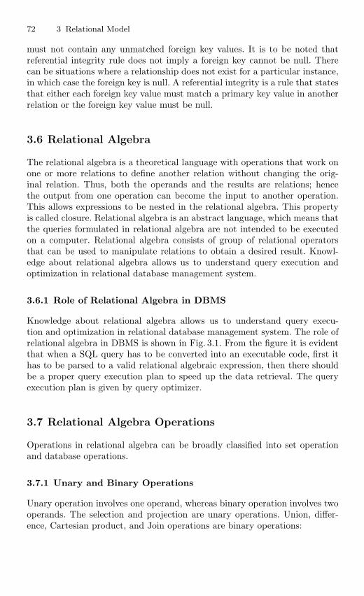
72 3 Relational Model
must not contain any unmatched foreign key values. It is to be noted thatreferential integrity rule does not imply a foreign key cannot be null. Therecan be situations where a relationship does not exist for a particular instance,in which case the foreign key is null. A referential integrity is a rule that statesthat either each foreign key value must match a primary key value in anotherrelation or the foreign key value must be null.
3.6 Relational Algebra
The relational algebra is a theoretical language with operations that work onone or more relations to define another relation without changing the orig-inal relation. Thus, both the operands and the results are relations; hencethe output from one operation can become the input to another operation.This allows expressions to be nested in the relational algebra. This propertyis called closure. Relational algebra is an abstract language, which means thatthe queries formulated in relational algebra are not intended to be executedon a computer. Relational algebra consists of group of relational operatorsthat can be used to manipulate relations to obtain a desired result. Knowl-edge about relational algebra allows us to understand query execution andoptimization in relational database management system.
3.6.1 Role of Relational Algebra in DBMS
Knowledge about relational algebra allows us to understand query execu-tion and optimization in relational database management system. The role ofrelational algebra in DBMS is shown in Fig. 3.1. From the figure it is evidentthat when a SQL query has to be converted into an executable code, first ithas to be parsed to a valid relational algebraic expression, then there shouldbe a proper query execution plan to speed up the data retrieval. The queryexecution plan is given by query optimizer.
3.7 Relational Algebra Operations
Operations in relational algebra can be broadly classified into set operationand database operations.
3.7.1 Unary and Binary Operations
Unary operation involves one operand, whereas binary operation involves twooperands. The selection and projection are unary operations. Union, differ-ence, Cartesian product, and Join operations are binary operations:
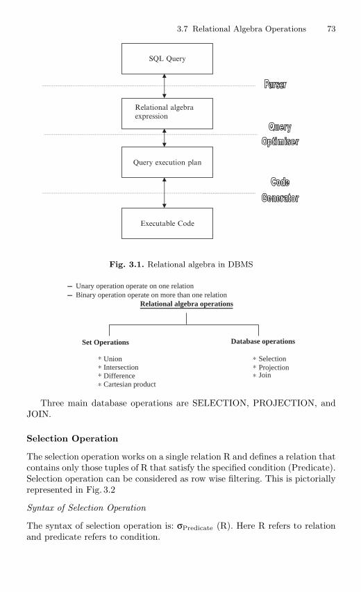
3.7 Relational Algebra Operations 73
SQL Query
Relational algebraexpression
Query execution plan
Executable Code
Fig. 3.1. Relational algebra in DBMS
Unary operation operate on one relation
Binary operation operate on more than one relation
Relational algebra operations
Set Operations Database operations
∗ Union Selection
∗ Intersection Projection∗
∗∗∗Difference Join
∗ Cartesian product
––
Three main database operations are SELECTION, PROJECTION, andJOIN.
Selection Operation
The selection operation works on a single relation R and defines a relation thatcontains only those tuples of R that satisfy the specified condition (Predicate).Selection operation can be considered as row wise filtering. This is pictoriallyrepresented in Fig. 3.2
Syntax of Selection Operation
The syntax of selection operation is: σPredicate (R). Here R refers to relationand predicate refers to condition.
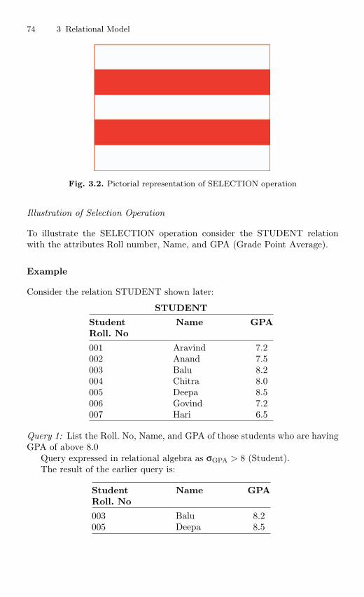
74 3 Relational Model
Fig. 3.2. Pictorial representation of SELECTION operation
Illustration of Selection Operation
To illustrate the SELECTION operation consider the STUDENT relationwith the attributes Roll number, Name, and GPA (Grade Point Average).
Example
Consider the relation STUDENT shown later:
STUDENT
Student Name GPARoll. No
001 Aravind 7.2002 Anand 7.5003 Balu 8.2004 Chitra 8.0005 Deepa 8.5006 Govind 7.2007 Hari 6.5
Query 1: List the Roll. No, Name, and GPA of those students who are havingGPA of above 8.0
Query expressed in relational algebra as σGPA > 8 (Student).The result of the earlier query is:
Student Name GPARoll. No
003 Balu 8.2005 Deepa 8.5
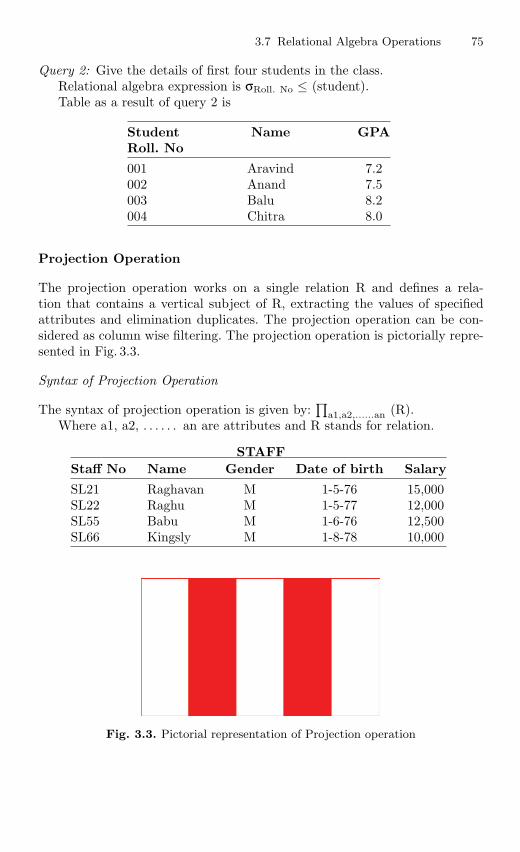
3.7 Relational Algebra Operations 75
Query 2: Give the details of first four students in the class.Relational algebra expression is σRoll. No ≤ (student).Table as a result of query 2 is
Student Name GPARoll. No
001 Aravind 7.2002 Anand 7.5003 Balu 8.2004 Chitra 8.0
Projection Operation
The projection operation works on a single relation R and defines a rela-tion that contains a vertical subject of R, extracting the values of specifiedattributes and elimination duplicates. The projection operation can be con-sidered as column wise filtering. The projection operation is pictorially repre-sented in Fig. 3.3.
Syntax of Projection Operation
The syntax of projection operation is given by:∏
a1,a2,......an (R).Where a1, a2, . . . . . . an are attributes and R stands for relation.
STAFFStaff No Name Gender Date of birth Salary
SL21 Raghavan M 1-5-76 15,000SL22 Raghu M 1-5-77 12,000SL55 Babu M 1-6-76 12,500SL66 Kingsly M 1-8-78 10,000
Fig. 3.3. Pictorial representation of Projection operation
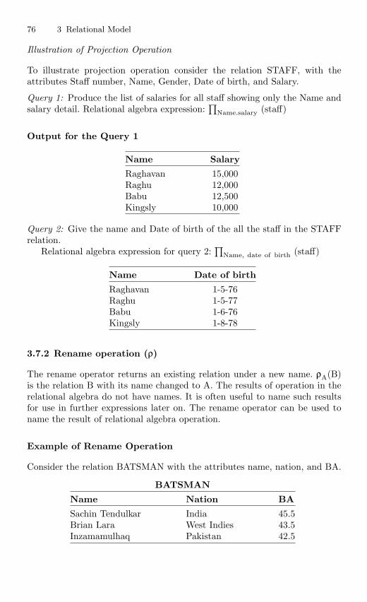
76 3 Relational Model
Illustration of Projection Operation
To illustrate projection operation consider the relation STAFF, with theattributes Staff number, Name, Gender, Date of birth, and Salary.
Query 1: Produce the list of salaries for all staff showing only the Name andsalary detail. Relational algebra expression:
∏Name.salary (staff)
Output for the Query 1
Name Salary
Raghavan 15,000Raghu 12,000Babu 12,500Kingsly 10,000
Query 2: Give the name and Date of birth of the all the staff in the STAFFrelation.
Relational algebra expression for query 2:∏
Name, date of birth (staff)
Name Date of birth
Raghavan 1-5-76Raghu 1-5-77Babu 1-6-76Kingsly 1-8-78
3.7.2 Rename operation (ρ)
The rename operator returns an existing relation under a new name. ρA(B)is the relation B with its name changed to A. The results of operation in therelational algebra do not have names. It is often useful to name such resultsfor use in further expressions later on. The rename operator can be used toname the result of relational algebra operation.
Example of Rename Operation
Consider the relation BATSMAN with the attributes name, nation, and BA.
BATSMAN
Name Nation BA
Sachin Tendulkar India 45.5Brian Lara West Indies 43.5Inzamamulhaq Pakistan 42.5
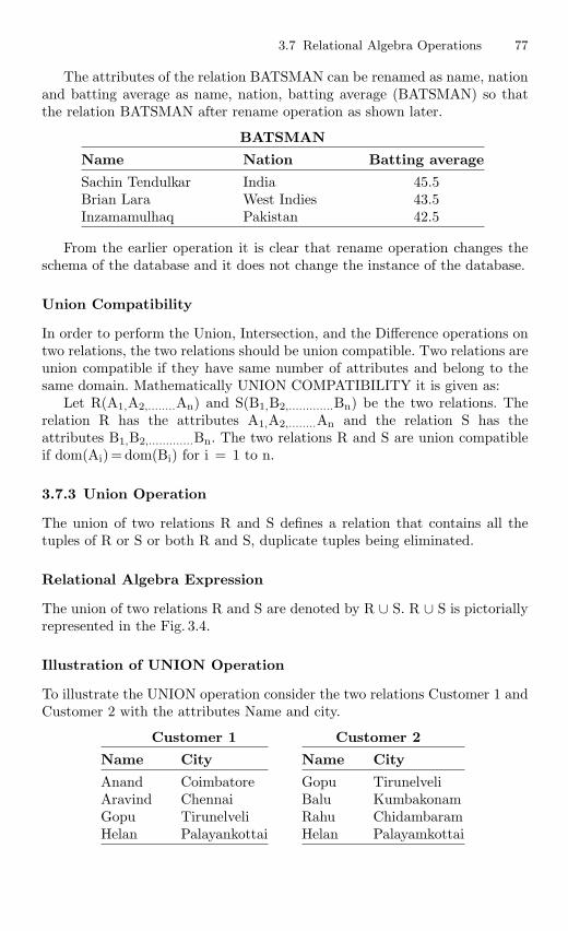
3.7 Relational Algebra Operations 77
The attributes of the relation BATSMAN can be renamed as name, nationand batting average as name, nation, batting average (BATSMAN) so thatthe relation BATSMAN after rename operation as shown later.
BATSMAN
Name Nation Batting average
Sachin Tendulkar India 45.5Brian Lara West Indies 43.5Inzamamulhaq Pakistan 42.5
From the earlier operation it is clear that rename operation changes theschema of the database and it does not change the instance of the database.
Union Compatibility
In order to perform the Union, Intersection, and the Difference operations ontwo relations, the two relations should be union compatible. Two relations areunion compatible if they have same number of attributes and belong to thesame domain. Mathematically UNION COMPATIBILITY it is given as:
Let R(A1,A2,........An) and S(B1,B2,.............Bn) be the two relations. Therelation R has the attributes A1,A2,........An and the relation S has theattributes B1,B2,.............Bn. The two relations R and S are union compatibleif dom(Ai) = dom(Bi) for i = 1 to n.
3.7.3 Union Operation
The union of two relations R and S defines a relation that contains all thetuples of R or S or both R and S, duplicate tuples being eliminated.
Relational Algebra Expression
The union of two relations R and S are denoted by R ∪ S. R ∪ S is pictoriallyrepresented in the Fig. 3.4.
Illustration of UNION Operation
To illustrate the UNION operation consider the two relations Customer 1 andCustomer 2 with the attributes Name and city.
Customer 1 Customer 2
Name City
Anand CoimbatoreAravind ChennaiGopu TirunelveliHelan Palayankottai
Name City
Gopu TirunelveliBalu KumbakonamRahu ChidambaramHelan Palayamkottai
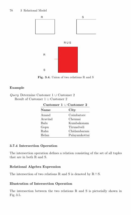
78 3 Relational Model
R
R U S
R
S
S
Fig. 3.4. Union of two relations R and S
Example
Query Determine Customer 1 ∪ Customer 2Result of Customer 1 ∪ Customer 2
Customer 1 ∪ Customer 2
Name City
Anand CoimbatoreAravind ChennaiBalu KumbakonamGopu TirunelveliRahu ChidambaramHelan Palayamkottai
3.7.4 Intersection Operation
The intersection operation defines a relation consisting of the set of all tuplesthat are in both R and S.
Relational Algebra Expression
The intersection of two relations R and S is denoted by R ∩ S.
Illustration of Intersection Operation
The intersection between the two relations R and S is pictorially shown inFig. 3.5.
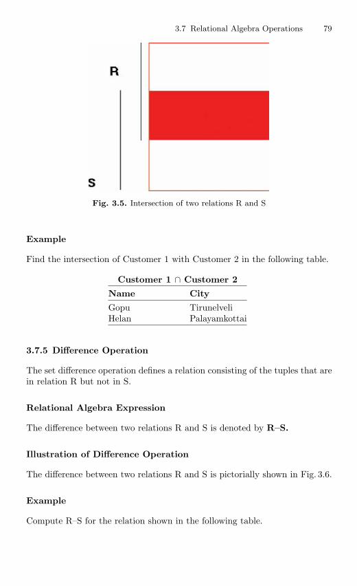
3.7 Relational Algebra Operations 79
Fig. 3.5. Intersection of two relations R and S
Example
Find the intersection of Customer 1 with Customer 2 in the following table.
Customer 1 ∩ Customer 2
Name City
Gopu TirunelveliHelan Palayamkottai
3.7.5 Difference Operation
The set difference operation defines a relation consisting of the tuples that arein relation R but not in S.
Relational Algebra Expression
The difference between two relations R and S is denoted by R–S.
Illustration of Difference Operation
The difference between two relations R and S is pictorially shown in Fig. 3.6.
Example
Compute R–S for the relation shown in the following table.
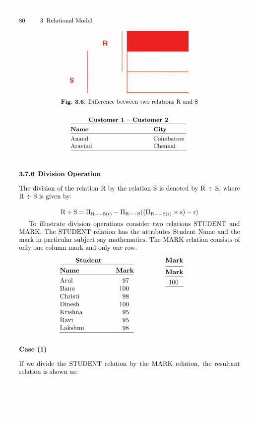
80 3 Relational Model
Fig. 3.6. Difference between two relations R and S
Customer 1 – Customer 2
Name City
Anand CoimbatoreAravind Chennai
3.7.6 Division Operation
The division of the relation R by the relation S is denoted by R ÷ S, whereR ÷ S is given by:
R ÷ S = ΠR−−S(r) − ΠR−−S((ΠR−−S(r) × s) − r)
To illustrate division operations consider two relations STUDENT andMARK. The STUDENT relation has the attributes Student Name and themark in particular subject say mathematics. The MARK relation consists ofonly one column mark and only one row.
Student Mark
Name Mark
Arul 97Banu 100Christi 98Dinesh 100Krishna 95Ravi 95Lakshmi 98
Mark
100
Case (1)
If we divide the STUDENT relation by the MARK relation, the resultantrelation is shown as:
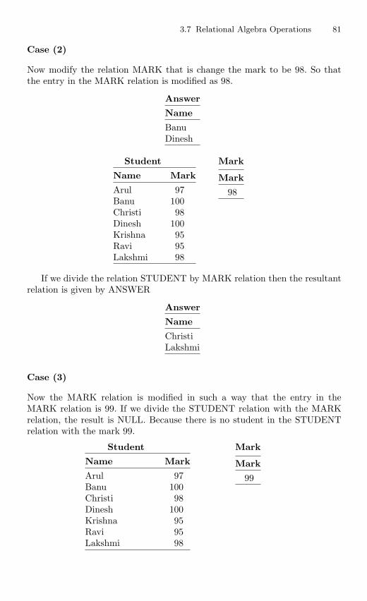
3.7 Relational Algebra Operations 81
Case (2)
Now modify the relation MARK that is change the mark to be 98. So thatthe entry in the MARK relation is modified as 98.
Answer
Name
BanuDinesh
Student Mark
Name Mark
Arul 97Banu 100Christi 98Dinesh 100Krishna 95Ravi 95Lakshmi 98
Mark
98
If we divide the relation STUDENT by MARK relation then the resultantrelation is given by ANSWER
Answer
Name
ChristiLakshmi
Case (3)
Now the MARK relation is modified in such a way that the entry in theMARK relation is 99. If we divide the STUDENT relation with the MARKrelation, the result is NULL. Because there is no student in the STUDENTrelation with the mark 99.
Student Mark
Name Mark
Arul 97Banu 100Christi 98Dinesh 100Krishna 95Ravi 95Lakshmi 98
Mark
99
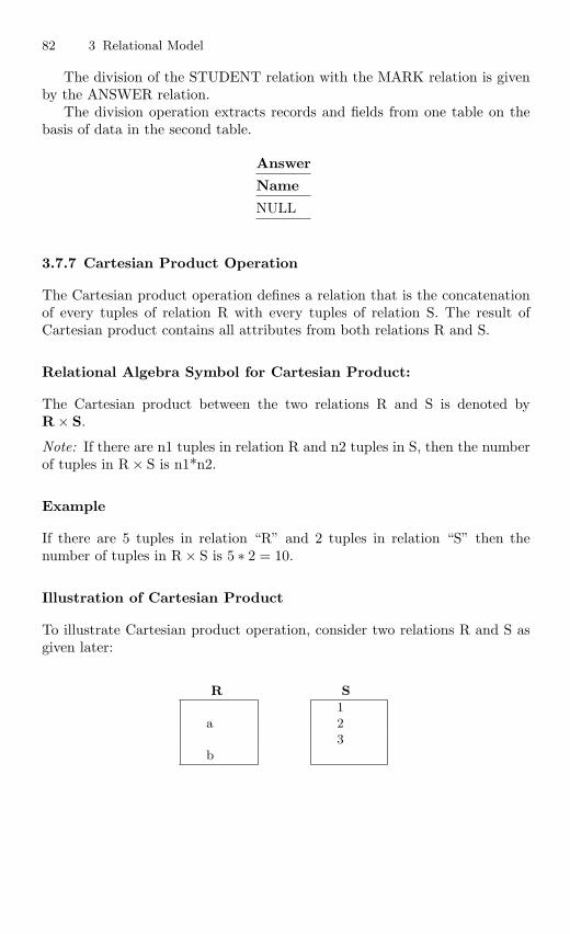
82 3 Relational Model
The division of the STUDENT relation with the MARK relation is givenby the ANSWER relation.
The division operation extracts records and fields from one table on thebasis of data in the second table.
Answer
Name
NULL
3.7.7 Cartesian Product Operation
The Cartesian product operation defines a relation that is the concatenationof every tuples of relation R with every tuples of relation S. The result ofCartesian product contains all attributes from both relations R and S.
Relational Algebra Symbol for Cartesian Product:
The Cartesian product between the two relations R and S is denoted byR × S.
Note: If there are n1 tuples in relation R and n2 tuples in S, then the numberof tuples in R × S is n1*n2.
Example
If there are 5 tuples in relation “R” and 2 tuples in relation “S” then thenumber of tuples in R × S is 5 ∗ 2 = 10.
Illustration of Cartesian Product
To illustrate Cartesian product operation, consider two relations R and S asgiven later:
R S
a
b
123
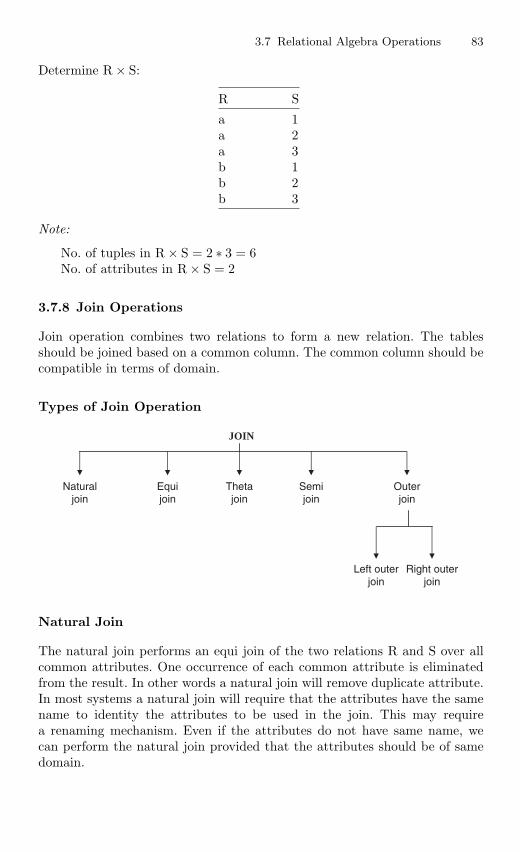
3.7 Relational Algebra Operations 83
Determine R × S:
R S
a 1a 2a 3b 1b 2b 3
Note:
No. of tuples in R × S = 2 ∗ 3 = 6No. of attributes in R × S = 2
3.7.8 Join Operations
Join operation combines two relations to form a new relation. The tablesshould be joined based on a common column. The common column should becompatible in terms of domain.
Types of Join Operation
Naturaljoin
Equijoin
Thetajoin
Semijoin
Outerjoin
JOIN
Left outerjoin
Right outerjoin
Natural Join
The natural join performs an equi join of the two relations R and S over allcommon attributes. One occurrence of each common attribute is eliminatedfrom the result. In other words a natural join will remove duplicate attribute.In most systems a natural join will require that the attributes have the samename to identity the attributes to be used in the join. This may requirea renaming mechanism. Even if the attributes do not have same name, wecan perform the natural join provided that the attributes should be of samedomain.
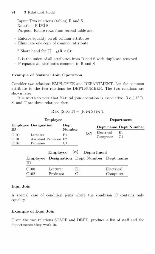
84 3 Relational Model
Input: Two relations (tables) R and SNotation: R SPurpose: Relate rows from second table and
– Enforce equality on all column attributes– Eliminate one copy of common attribute
* Short hand for∏
L(R × S):
– L is the union of all attributes from R and S with duplicate removed– P equates all attributes common to R and S
Example of Natural Join Operation
Consider two relations EMPLOYEE and DEPARTMENT. Let the commonattribute to the two relations be DEPTNUMBER. The two relations areshown later:
It is worth to note that Natural join operation is associative. (i.e.,) If R,S, and T are three relations then
R (S T) = (R S) T
Employee Department
Employee Designation DeptID Number
C100 Lecturer E1C101 Assistant Professor E2C102 Professor C1
Dept name Dept Number
Electrical E1Computer C1
Employee DepartmentEmployee Designation Dept Number Dept nameID
C100 Lecturer E1 ElectricalC102 Professor C1 Computer
Equi Join
A special case of condition joins where the condition C contains onlyequality.
Example of Equi Join
Given the two relations STAFF and DEPT, produce a list of staff and thedepartments they work in.
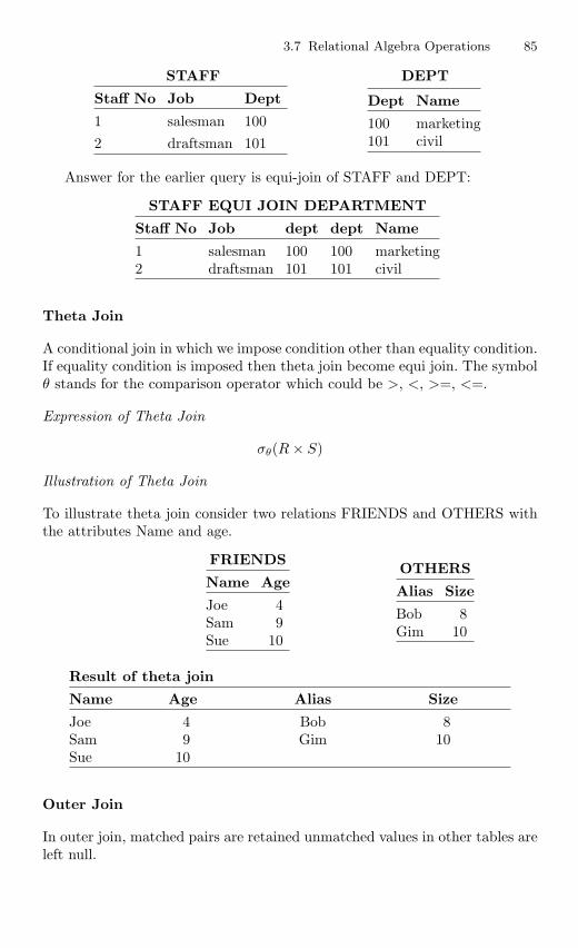
3.7 Relational Algebra Operations 85
STAFF DEPT
Staff No Job Dept
1 salesman 1002 draftsman 101
Dept Name
100 marketing101 civil
Answer for the earlier query is equi-join of STAFF and DEPT:
STAFF EQUI JOIN DEPARTMENT
Staff No Job dept dept Name
1 salesman 100 100 marketing2 draftsman 101 101 civil
Theta Join
A conditional join in which we impose condition other than equality condition.If equality condition is imposed then theta join become equi join. The symbolθ stands for the comparison operator which could be >, <, >=, <=.
Expression of Theta Join
σθ(R × S)
Illustration of Theta Join
To illustrate theta join consider two relations FRIENDS and OTHERS withthe attributes Name and age.
FRIENDS
Name Age
Joe 4Sam 9Sue 10
OTHERS
Alias Size
Bob 8Gim 10
Result of theta join
Name Age Alias Size
Joe 4 Bob 8Sam 9 Gim 10Sue 10
Outer Join
In outer join, matched pairs are retained unmatched values in other tables areleft null.
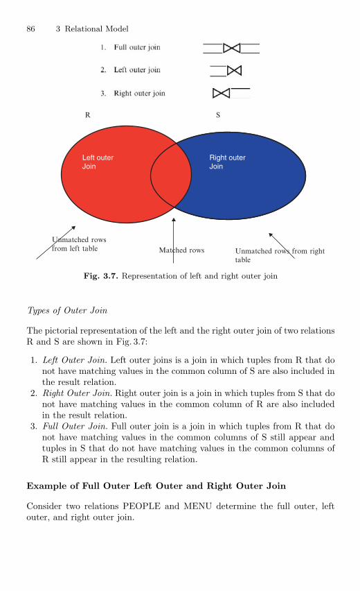
86 3 Relational Model
R
Unmatched rowsfrom left table
S
Matched rows Unmatched rows from righttable
Right outerJoin
Left outerJoin
Fig. 3.7. Representation of left and right outer join
Types of Outer Join
The pictorial representation of the left and the right outer join of two relationsR and S are shown in Fig. 3.7:
1. Left Outer Join. Left outer joins is a join in which tuples from R that donot have matching values in the common column of S are also included inthe result relation.
2. Right Outer Join. Right outer join is a join in which tuples from S that donot have matching values in the common column of R are also includedin the result relation.
3. Full Outer Join. Full outer join is a join in which tuples from R that donot have matching values in the common columns of S still appear andtuples in S that do not have matching values in the common columns ofR still appear in the resulting relation.
Example of Full Outer Left Outer and Right Outer Join
Consider two relations PEOPLE and MENU determine the full outer, leftouter, and right outer join.
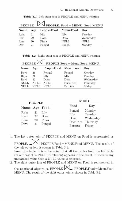
3.7 Relational Algebra Operations 87
Table 3.1. Left outer join of PEOPLE and MENU relation
PEOPLE PEOPLE. Food = MENU. Food MENU
Name Age People.Food Menu.Food Day
Raja 21 Idly Idly TuesdayRavi 22 Dosa Dosa WednesdayRani 20 Pizza NULL NULLDevi 21 Pongal Pongal Monday
Table 3.2. Right outer join of PEOPLE and MENU relation
PEOPLE PEOPLE.Food = Menu.Food MENU
Name Age People.Food Menu.Food Day
Devi 21 Pongal Pongal MondayRaja 21 Idly Idly TuesdayRavi 22 Dosa Dosa WednesdayNULL NULL NULL Fried rice ThursdayNULL NULL NULL Parotta Friday
PEOPLE
Name Age Food
Raja 21 IdlyRavi 22 DosaRani 20 PizzaDevi 21 Pongal
MENU
Food Day
Pongal MondayIdly TuesdayDosa WednesdayFried rice ThursdayParotta Friday
1. The left outer join of PEOPLE and MENU on Food is represented as
PEOPLE. PEOPLE.Food =MENU.Food MENU. The result ofthe left outer join is shown in Table 3.1.From this table, it is to be noted that all the tuples from the left table(in our case it is PEOPLE relation) appears in the result. If there is anyunmatched value then a NULL value is returned.
2. The right outer join of PEOPLE and MENU on Food is represented in
the relational algebra as PEOPLE PEOPLE.Food = Menu.FoodMENU. The result of the right outer join is shown in Table 3.2.
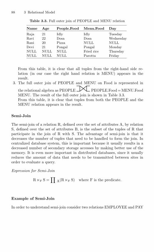
88 3 Relational Model
Table 3.3. Full outer join of PEOPLE and MENU relation
Name Age People.Food Menu.Food Day
Raja 21 Idly Idly TuesdayRavi 22 Dosa Dosa WednesdayRani 20 Pizza NULL NULLDevi 21 Pongal Pongal MondayNULL NULL NULL Fried rice ThursdayNULL NULL NULL Parotta Friday
From this table, it is clear that all tuples from the right-hand side re-lation (in our case the right hand relation is MENU) appears in theresult.
3. The full outer join of PEOPLE and MENU on Food is represented in
the relational algebra as PEOPLE PEOPLE.Food =MENU.FoodMENU. The result of the full outer join is shown in Table 3.3.From this table, it is clear that tuples from both the PEOPLE and theMENU relation appears in the result.
Semi-Join
The semi-join of a relation R, defined over the set of attributes A, by relationS, defined over the set of attributes B, is the subset of the tuples of R thatparticipate in the join of R with S. The advantage of semi-join is that itdecreases the number of tuples that need to be handled to form the join. Incentralized database system, this is important because it usually results in adecreased number of secondary storage accesses by making better use of thememory. It is even more important in distributed databases, since it usuallyreduces the amount of data that needs to be transmitted between sites inorder to evaluate a query.
Expression for Semi-Join
R F S =∏
A(R F S) where F is the predicate.
Example of Semi-Join
In order to understand semi-join consider two relations EMPLOYEE and PAY
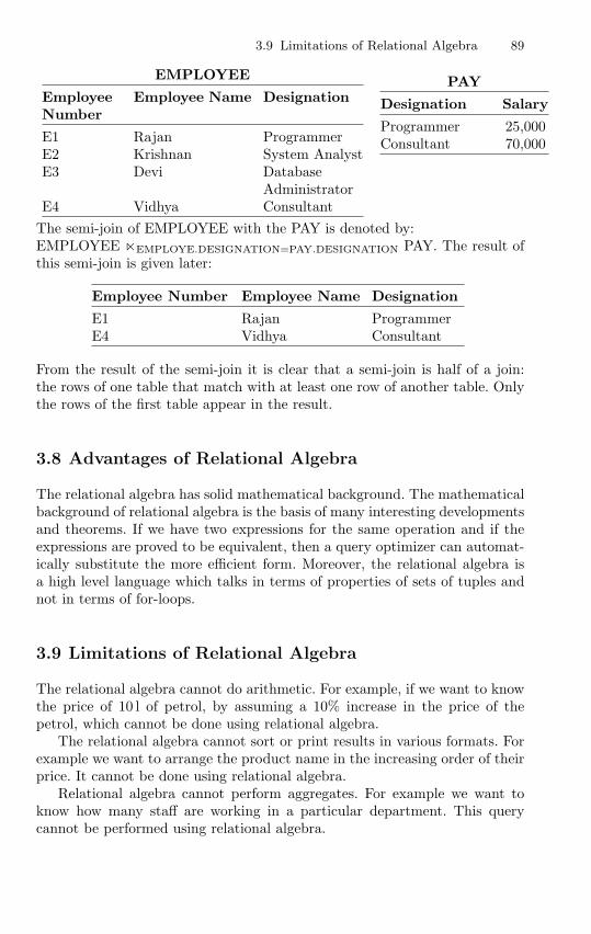
3.9 Limitations of Relational Algebra 89
EMPLOYEE
EmployeeNumber
Employee Name Designation
E1 Rajan ProgrammerE2 Krishnan System AnalystE3 Devi Database
AdministratorE4 Vidhya Consultant
PAY
Designation Salary
Programmer 25,000Consultant 70,000
The semi-join of EMPLOYEE with the PAY is denoted by:EMPLOYEE EMPLOYE.DESIGNATION=PAY.DESIGNATION PAY. The result ofthis semi-join is given later:
Employee Number Employee Name Designation
E1 Rajan ProgrammerE4 Vidhya Consultant
From the result of the semi-join it is clear that a semi-join is half of a join:the rows of one table that match with at least one row of another table. Onlythe rows of the first table appear in the result.
3.8 Advantages of Relational Algebra
The relational algebra has solid mathematical background. The mathematicalbackground of relational algebra is the basis of many interesting developmentsand theorems. If we have two expressions for the same operation and if theexpressions are proved to be equivalent, then a query optimizer can automat-ically substitute the more efficient form. Moreover, the relational algebra isa high level language which talks in terms of properties of sets of tuples andnot in terms of for-loops.
3.9 Limitations of Relational Algebra
The relational algebra cannot do arithmetic. For example, if we want to knowthe price of 10 l of petrol, by assuming a 10% increase in the price of thepetrol, which cannot be done using relational algebra.
The relational algebra cannot sort or print results in various formats. Forexample we want to arrange the product name in the increasing order of theirprice. It cannot be done using relational algebra.
Relational algebra cannot perform aggregates. For example we want toknow how many staff are working in a particular department. This querycannot be performed using relational algebra.
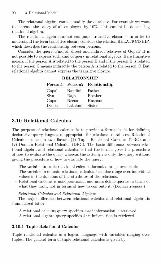
90 3 Relational Model
The relational algebra cannot modify the database. For example we wantto increase the salary of all employees by 10%. This cannot be done usingrelational algebra.
The relational algebra cannot compute “transitive closure.” In order tounderstand the term transitive closure consider the relation RELATIONSHIP,which describes the relationship between persons.
Consider the query, Find all direct and indirect relatives of Gopal? It isnot possible to express such kind of query in relational algebra. Here transitivemeans, if the person A is related to the person B and if the person B is relatedto the person C means indirectly the person A is related to the person C. Butrelational algebra cannot express the transitive closure.
RELATIONSHIP
Person1 Person2 Relationship
Gopal Nandini FatherSiva Raja BrotherGopal Neena HusbandDeepa Lakshmi Sister
3.10 Relational Calculus
The purpose of relational calculus is to provide a formal basis for definingdeclarative query languages appropriate for relational databases. RelationalCalculus comes in two flavors (1) Tuple Relational Calculus (TRC) and(2) Domain Relational Calculus (DRC). The basic difference between rela-tional algebra and relational calculus is that the former gives the procedureof how to evaluate the query whereas the latter gives only the query withoutgiving the procedure of how to evaluate the query:
– The variable in tuple relational calculus formulae range over tuples.– The variable in domain relational calculus formulae range over individual
values in the domains of the attributes of the relations.– Relational calculus is nonoperational, and users define queries in terms of
what they want, not in terms of how to compute it. (Declarativeness.)
Relational Calculus and Relational Algebra:The major difference between relational calculus and relational algebra is
summarized later:
– A relational calculus query specifies what information is retrieved– A relational algebra query specifies how information is retrieved
3.10.1 Tuple Relational Calculus
Tuple relational calculus is a logical language with variables ranging overtuples. The general form of tuple relational calculus is given by:
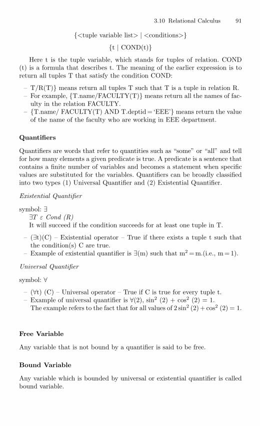
3.10 Relational Calculus 91
<tuple variable list> | <conditions>
t | COND(t)
Here t is the tuple variable, which stands for tuples of relation. COND(t) is a formula that describes t. The meaning of the earlier expression is toreturn all tuples T that satisfy the condition COND:
– T/R(T) means return all tuples T such that T is a tuple in relation R.– For example, T.name/FACULTY(T) means return all the names of fac-
ulty in the relation FACULTY.– T.name/ FACULTY(T) AND T.deptid = ‘EEE’ means return the value
of the name of the faculty who are working in EEE department.
Quantifiers
Quantifiers are words that refer to quantities such as “some” or “all” and tellfor how many elements a given predicate is true. A predicate is a sentence thatcontains a finite number of variables and becomes a statement when specificvalues are substituted for the variables. Quantifiers can be broadly classifiedinto two types (1) Universal Quantifier and (2) Existential Quantifier.
Existential Quantifier
symbol: ∃∃T ε Cond (R)It will succeed if the condition succeeds for at least one tuple in T.
– (∃t)(C) – Existential operator – True if there exists a tuple t such thatthe condition(s) C are true.
– Example of existential quantifier is ∃(m) such that m2 = m.(i.e., m = 1).
Universal Quantifier
symbol: ∀
– (∀t) (C) – Universal operator – True if C is true for every tuple t.– Example of universal quantifier is ∀(2), sin2 (2) + cos2 (2) = 1.
The example refers to the fact that for all values of 2 sin2 (2) + cos2 (2) = 1.
Free Variable
Any variable that is not bound by a quantifier is said to be free.
Bound Variable
Any variable which is bounded by universal or existential quantifier is calledbound variable.
92 3 Relational Model
Example of selection operation in TRC:
1. To find details of all staff earning more than Rs. 10,000:
S | Staff(S) ∧ S.salary > 10000
Example of projection operation in TRC:2. To find a particular attribute, such as salary, write:
S.salary | Staff(S) ∧ S.salary > 10000
Quantifier Example
Client(ID, fName, lName, Age)Matches(Client1, Client2, Type)
– List the first and last names of clients that appear as client1 in a matchof any type.RAlg: p(fName, lName)(Client (ID = Client1) Matches)RCalc: c.fName, c.lName | CLIENT(c) AND (∃m)(MATCHES(m) ANDc.ID = m.Client1)
Joins in Relational Calculus
Consider the two relations Client and Matches asClient(ID, fName, lName, Age)Matches(Client1, Client2, Type)
– List all information about clients and the corresponding matchesthat appear as client1 in a match of any type.
The earlier query can be expressed both in Relational Algebra and Tuplerelational Calculus as:
– RAlg: Client (ID =Client1) Matches– RCalc:c, m | CLIENT(c) AND MATCHES(m) AND c.ID = m.Client1
3.10.2 Set Operators in Relational Calculus
The set operations like Union, Intersection, difference, and Cartesian Productcan be expressed in Tuple Relational Calculus as:
3.10 Relational Calculus 93
Union
– R1(A,B,C) ∪ R2(A, B, C)– r | R1(r) OR R2(r)
Intersection
– R1(A,B,C) ∩ R2(A, B, C)– r | R1(r) AND R2(r)
Cartesian Product
– R(A, B, C) × S(D, E, F)– r, s | R(r) AND S(s) // same as join without the select condition
Subtraction
– R1(A,B,C) − R2(A, B, C)– r | R1(r) AND NOT R2(r)
Queries and Tuple Relational Calculus Expressions
Some of the queries and the corresponding relational calculus and their expla-nations are given later. Here we have given set of queries like SET 1, SET 2,and SET 3.
– Query set 1 deals with Railway Reservation Management– Query set 2 deals with Library Database Management– Query set 3 deals with Hostel Database Management
Query Set1: Query set 1 deals with railway reservation system.
Query 1: Find all the train details for the trains where starting place is“Chennai.”
Relational calculus expression: t | t ∈ train details ∧ start place= “Chennai”
Explanation: Set of all tuples “t” that belong to the relation “train details”and also the starting place is “Chennai” is found by the query.
Query 2: Find all train names whose destination is “Salem.”
Relational calculus expression
t | ∃ s ∈ train details (t [ train no] = s [ train no] ∧ s [destination] = “Salem”)
Explanation: There exist a tuple “t” in the relation “r” such that the predicateis true.
94 3 Relational Model
The set of all tuples “t” such that, there exists a tuple “s” in relation traindetails for which the values of “t” and “s” for the train no attribute are equaland the value of “s” for the destination is “Salem.”
Query 3: Find the names of all passengers who have canceled the ticket andwhose age is above 40.
Relational calculus expression t | ∃ s ∈ cancel (t [train no] = s[train no] ∧∃ u ∈ passen details (u [name] = s [name] ∧ u[age] >40))
Explanation: Set of all passenger names tuples for which the age is above 40and the ticket is canceled. The tuple variable “s” ensures that the passengercanceled the ticket. The tuple “u” is restricted to having the same passengername as “s.”
Query 4: List the train numbers of all trains which has no cancelation andonly reservation.
Relational Calculus Expression
t | ∃ s ∈ reserve (t [train no] = s [train no]) ¬∃ u ∈ cancel(t [train no] = u[train no])Explanation: Set of all tuples “t” such that there exists a tuple “s” thatbelongs to reserve such that the train no attribute is equal for “t” and “s”and there exists a tuple “u” that belongs to cancel where the values of “t”and “u” for the train no attribute is the same.
Query 5: List all female passengers name who are traveling by the train “BlueMountain.”
Relational Calculus Expression
t | ∃ s ∈ passen details (t [p name] = s [p name] ∧ s[sex] = “female”∧ s[train name] = “Blue mountain”).
Explanation: Set of all tuples “t” such that there exists a tuple “s” thatbelongs to passen details for which the values of “t” and “s” for the p nameattribute is same and the sex attribute = “female” and train name attribute =“Blue mountain.”
Query Set 2: Query set 2 deals with frequent queries in library databasemanagement.
Query 1: Find the acc no/- for each book whose price >1000.
Relational Calculus Expression
t | ∃ s ∈ book (t[acc no/-] = s[acc no/-] ∧ s[price] > 1000)
3.10 Relational Calculus 95
Explanation: The set of all tuples “t” such that there exists a tuple “s” inrelation book for which the values “t” and “s” for the acc no/- attribute areequal an the value of the s for the price attribute is greater than 1000.
Query 2: Find the name of all the students who have borrowed a book andprice of those book is greater than 1000.
Relational Calculus Expression
t | ∃ s ∈ books borrowed(t[std name] = s[std name] ∧ ∃ u ∈ book(u[acc no/-] = s[acc no/-] ∧ u[price] > 1000))Explanation: The set of all tuples “t” such that there exists a tuple “s” inrelation books borrowed for which the values “t” and “s” for the student nameattribute are equal and “u” tuple variable on book relation for which “u” and“s” for the acc no/- attribute are equal and the value of “u” for the priceattribute is greater than 1000.
Query 3: Find the name of the students who borrowed book, have book inhis account or both.
Relational Calculus Expression
t | ∃ s ∈ books borrowed (t[stud name] = s[std name]) ∨ ∃ u ∈books remaining (t[std name] = su[std name])Explanation: The set of all tuples “t” such that there exists a tuple “s” inrelation books borrowed for which the values “t” and “s” for the studentname attribute are equal and “u” tuple variable on books remaining relationfor which “u” and “s” for the stud name attribute are equal.
Query 4: Find only those students’ names who are having both the books intheir account as well as the books borrowed from their account.
Relational Calculus Expression
t | ∃ s ∈ books borrowed (t[std name] = s[std name])∧ ∃ u ∈ booksremaining (t[std name] = s[std name])Explanation: The set of all tuples “t” such that there exists a tuple “s” suchthat in relation books borrowed for which the values “t” and “s” for thestudent name attribute are equal and “u” tuple variable on books remainingrelation for which “u” and “s” for the student name attribute areequal.
Query 5: Query that uses implication symbol p ⇒ q find all students belongsto EEE department who borrowed the books.
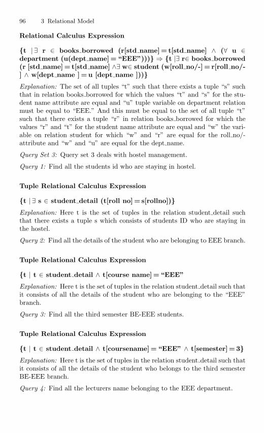
96 3 Relational Model
Relational Calculus Expression
t | ∃ r ∈ books borrowed (r[std name] = t[std name] ∧ (∀ u ∈department (u(dept name] = “EEE”))) ⇒ t |∃ r∈ books borrowed(r [std name] = t[std name] ∧∃ w∈ student (w[roll no/-] = r[roll no/-] ∧ w[dept name ] =u [dept name ]))Explanation: The set of all tuples “t” such that there exists a tuple “s” suchthat in relation books borrowed for which the values “t” and “s” for the stu-dent name attribute are equal and “u” tuple variable on department relationmust be equal to “EEE.” And this must be equal to the set of all tuple “t”such that there exists a tuple “r” in relation books borrowed for which thevalues “r” and “t” for the student name attribute are equal and “w” the vari-able on relation student for which “w” and “r” are equal for the roll no/-attribute and “w” and “u” are equal for the dept name.
Query Set 3: Query set 3 deals with hostel management.
Query 1: Find all the students id who are staying in hostel.
Tuple Relational Calculus Expression
t | ∃ s ∈ student detail (t[roll no] = s[rollno])Explanation: Here t is the set of tuples in the relation student detail suchthat there exists a tuple s which consists of students ID who are staying inthe hostel.
Query 2: Find all the details of the student who are belonging to EEE branch.
Tuple Relational Calculus Expression
t | t ∈ student detail ∧ t[course name] =“EEE”
Explanation: Here t is the set of tuples in the relation student detail such thatit consists of all the details of the student who are belonging to the “EEE”branch.
Query 3: Find all the third semester BE-EEE students.
Tuple Relational Calculus Expression
t | t ∈ student detail ∧ t[coursename] = “EEE” ∧ t[semester] = 3Explanation: Here t is the set of tuples in the relation student detail such thatit consists of all the details of the student who belongs to the third semesterBE-EEE branch.
Query 4: Find all the lecturers name belonging to the EEE department.
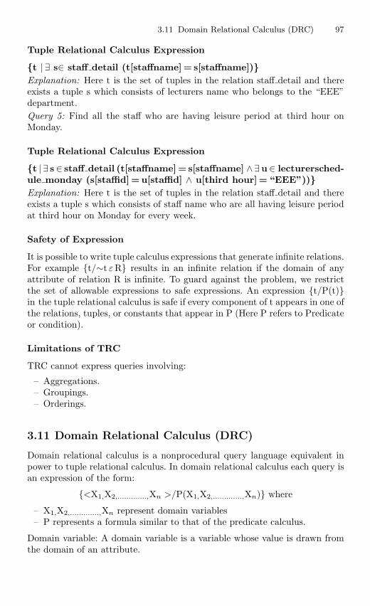
3.11 Domain Relational Calculus (DRC) 97
Tuple Relational Calculus Expression
t | ∃ s∈ staff detail (t[staffname]= s[staffname])Explanation: Here t is the set of tuples in the relation staff detail and thereexists a tuple s which consists of lecturers name who belongs to the “EEE”department.Query 5: Find all the staff who are having leisure period at third hour onMonday.
Tuple Relational Calculus Expression
t | ∃ s∈ staff detail (t[staffname] = s[staffname] ∧∃u∈ lecturersched-ule monday (s[staffid] =u[staffid] ∧ u[third hour] = “EEE”))Explanation: Here t is the set of tuples in the relation staff detail and thereexists a tuple s which consists of staff name who are all having leisure periodat third hour on Monday for every week.
Safety of Expression
It is possible to write tuple calculus expressions that generate infinite relations.For example t/∼t ε R results in an infinite relation if the domain of anyattribute of relation R is infinite. To guard against the problem, we restrictthe set of allowable expressions to safe expressions. An expression t/P(t)in the tuple relational calculus is safe if every component of t appears in one ofthe relations, tuples, or constants that appear in P (Here P refers to Predicateor condition).
Limitations of TRC
TRC cannot express queries involving:
– Aggregations.– Groupings.– Orderings.
3.11 Domain Relational Calculus (DRC)
Domain relational calculus is a nonprocedural query language equivalent inpower to tuple relational calculus. In domain relational calculus each query isan expression of the form:
<X1,X2,.............,Xn >/P(X1,X2,.............,Xn) where
– X1,X2,.............,Xn represent domain variables– P represents a formula similar to that of the predicate calculus.
Domain variable: A domain variable is a variable whose value is drawn fromthe domain of an attribute.
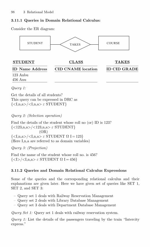
98 3 Relational Model
3.11.1 Queries in Domain Relational Calculus:
Consider the ER diagram:
STUDENT TAKES COURSE
STUDENT
ID Name Address
123 Anbu456 Anu
CLASS
CID CNAME location
TAKES
ID CID GRADE
Query 1:
Get the details of all students?This query can be expressed in DRC as<I,n,a>/<I,n,a> ε STUDENT
Query 2: (Selection operation)
Find the details of the student whose roll no (or) ID is 123?<123,n,a>/<123,n,a> ε STUDENT
(OR)<I,n,a>/<I,n,a> ε STUDENT Ω I =123(Here I,n,a are referred to as domain variables)
Query 3: (Projection)
Find the name of the student whose roll no. is 456?<I>/<I,n,a> ε STUDENT Ω I =456
3.11.2 Queries and Domain Relational Calculus Expressions
Some of the queries and the corresponding relational calculus and theirexplanations are given later. Here we have given set of queries like SET 1,SET 2, and SET 3:
– Query set 1 deals with Railway Reservation Management– Query set 2 deals with Library Database Management– Query set 3 deals with Department Database Management
Query Set 1: Query set 1 deals with railway reservation system.
Query 1: List the details of the passengers traveling by the train “Intercityexpress.”
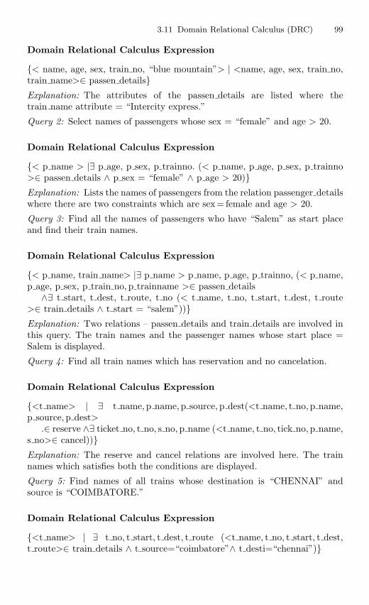
3.11 Domain Relational Calculus (DRC) 99
Domain Relational Calculus Expression
< name, age, sex, train no, “blue mountain”> | <name, age, sex, train no,train name>∈ passen detailsExplanation: The attributes of the passen details are listed where thetrain name attribute = “Intercity express.”
Query 2: Select names of passengers whose sex = “female” and age > 20.
Domain Relational Calculus Expression
< p name > |∃ p age, p sex, p trainno. (< p name, p age, p sex, p trainno>∈ passen details ∧ p sex = “female” ∧ p age > 20)Explanation: Lists the names of passengers from the relation passenger detailswhere there are two constraints which are sex= female and age > 20.
Query 3: Find all the names of passengers who have “Salem” as start placeand find their train names.
Domain Relational Calculus Expression
< p name, train name> |∃ p name > p name, p age, p trainno, (< p name,p age, p sex, p train no, p trainname >∈ passen details
∧∃ t start, t dest, t route, t no (< t name, t no, t start, t dest, t route>∈ train details ∧ t start = “salem”))Explanation: Two relations – passen details and train details are involved inthis query. The train names and the passenger names whose start place =Salem is displayed.
Query 4: Find all train names which has reservation and no cancelation.
Domain Relational Calculus Expression
<t name> | ∃ t name, p name, p source, p dest(<t name, t no, p name,p source, p dest>
.∈ reserve ∧∃ ticket no, t no, s no, p name (<t name, t no, tick no, p name,s no>∈ cancel))Explanation: The reserve and cancel relations are involved here. The trainnames which satisfies both the conditions are displayed.
Query 5: Find names of all trains whose destination is “CHENNAI” andsource is “COIMBATORE.”
Domain Relational Calculus Expression
<t name> | ∃ t no, t start, t dest, t route (<t name, t no, t start, t dest,t route>∈ train details ∧ t source=“coimbatore”∧ t desti=“chennai”)
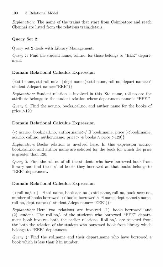
100 3 Relational Model
Explanation: The name of the trains that start from Coimbatore and reachChennai are listed from the relations train details.
Query Set 2:
Query set 2 deals with Library Management.
Query 1: Find the student name, roll no. for those belongs to “EEE” depart-ment.
Domain Relational Calculus Expression
<std name, std roll no> | dept name (<std name, roll no, depart name>∈student ∧depart name=“EEE”)Explanation: Student relation is involved in this. Std name, roll no are theattribute belongs to the student relation whose department name is “EEE.”
Query 2: Find the acc no, books cal no, and author name for the books ofprice >120.
Domain Relational Calculus Expression
< acc no, book call no, author name>/ ∃ book name, price (<book name,acc no, call no, author name, price> ∈ books ∧ price >120)Explanation: Books relation is involved here. In this expression acc no,book call no, and author name are selected for the book for which the priceis greater than 120.
Query 3: Find the roll no of all the students who have borrowed book fromlibrary and find the no/- of books they borrowed an that books belongs to“EEE” department.
Domain Relational Calculus Expression
<roll no/-> | ∃ std name, book acc no (<std name, roll no, book accc no,number of books borrowed >∈books borrowed ∧ ∃ name, dept name(<name,roll no, dept name>∈ student ∧dept name=“EEE”))Explanation: Here two relations are involved (1) books borrowed and(2) student. The roll no/- of the students who borrowed “EEE” depart-ment book involves both the earlier relations. Roll no/- are selected fromthe both the relation of the student who borrowed book from library whichbelongs to “EEE” department.
Query 4: Find the std name and their depart name who have borrowed abook which is less than 2 in number.
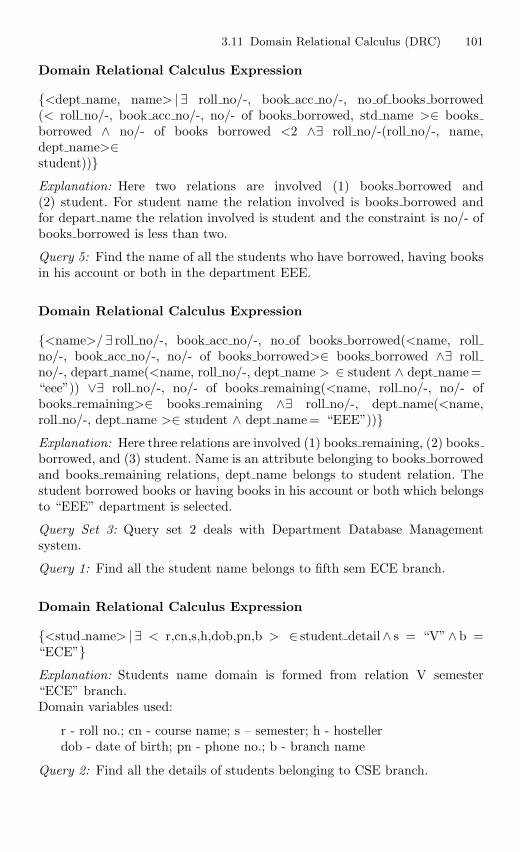
3.11 Domain Relational Calculus (DRC) 101
Domain Relational Calculus Expression
<dept name, name> | ∃ roll no/-, book acc no/-, no of books borrowed(< roll no/-, book acc no/-, no/- of books borrowed, std name >∈ booksborrowed ∧ no/- of books borrowed <2 ∧∃ roll no/-(roll no/-, name,dept name>∈student))Explanation: Here two relations are involved (1) books borrowed and(2) student. For student name the relation involved is books borrowed andfor depart name the relation involved is student and the constraint is no/- ofbooks borrowed is less than two.
Query 5: Find the name of all the students who have borrowed, having booksin his account or both in the department EEE.
Domain Relational Calculus Expression
<name>/∃ roll no/-, book acc no/-, no of books borrowed(<name, rollno/-, book acc no/-, no/- of books borrowed>∈ books borrowed ∧∃ rollno/-, depart name(<name, roll no/-, dept name > ∈ student ∧ dept name =“eee”)) ∨∃ roll no/-, no/- of books remaining(<name, roll no/-, no/- ofbooks remaining>∈ books remaining ∧∃ roll no/-, dept name(<name,roll no/-, dept name >∈ student ∧ dept name = “EEE”))Explanation: Here three relations are involved (1) books remaining, (2) booksborrowed, and (3) student. Name is an attribute belonging to books borrowedand books remaining relations, dept name belongs to student relation. Thestudent borrowed books or having books in his account or both which belongsto “EEE” department is selected.
Query Set 3: Query set 2 deals with Department Database Managementsystem.
Query 1: Find all the student name belongs to fifth sem ECE branch.
Domain Relational Calculus Expression
<stud name> | ∃ < r,cn,s,h,dob,pn,b > ∈ student detail∧ s = “V”∧b =“ECE”Explanation: Students name domain is formed from relation V semester“ECE” branch.Domain variables used:
r - roll no.; cn - course name; s – semester; h - hostellerdob - date of birth; pn - phone no.; b - branch name
Query 2: Find all the details of students belonging to CSE branch.
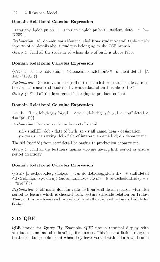
102 3 Relational Model
Domain Relational Calculus Expression
<sn,r,cn,s,h,dob,pn,b> | <sn,r,cn,s,h,dob,pn,b>∈ student–detail ∧ b=“CSE”Explanation: All domain variables included from student-detail table whichconsists of all details about students belonging to the CSE branch.
Query 3: Find all the students id whose date of birth is above 1985.
Domain Relational Calculus Expression
<r> | ∃ sn,cn,s,h,dob,pn,b (<r,sn,cn,b,s,h,dob,pn>∈ student detail |∧dob>“1985”)Explanation: Domain variable r (roll no) is included from student detail rela-tion, which consists of students ID whose date of birth is above 1985.
Query 4: Find all the lecturers id belonging to production dept.
Domain Relational Calculus Expression
<sid> |∃ sn,dob,desg,y,foi,e,d | <sid,sn,dob,desg,y,foi,e,d ∈ staff detail ∧d =“prod”)Explanation: Domain variables from staff detail:
sid - staff ID; dob - date of birth; sn - staff name; desg - designationy - year since serving; foi - field of interest; e - email id; d - department
The sid (staff id) from staff detail belonging to production department.
Query 5: Find all the lecturers’ names who are having fifth period as leisureperiod on Friday.
Domain Relational Calculus Expression
<sn> |∃ sed,dob,desg,y,foi,e,d | <sn,sid,dob,desg,y,foi,e,d> ∈ staff detail∧∃ <sid,i,ii,iii,iv,v,vi,vii)(<sid,sn,i,ii,iii,iv,v,vi,vii> ∈ rev schedul friday ∧ v=“free”)))Explanation: Staff name domain variable from staff detail relation with fifthperiod as leisure which is checked using lecture schedule relation on Friday.Thus, in this, we have used two relations: staff detail and lecture schedule forFriday.
3.12 QBE
QBE stands for Query By Example. QBE uses a terminal display withattribute names as table headings for queries. This looks a little strange intextbooks, but people like it when they have worked with it for a while on a
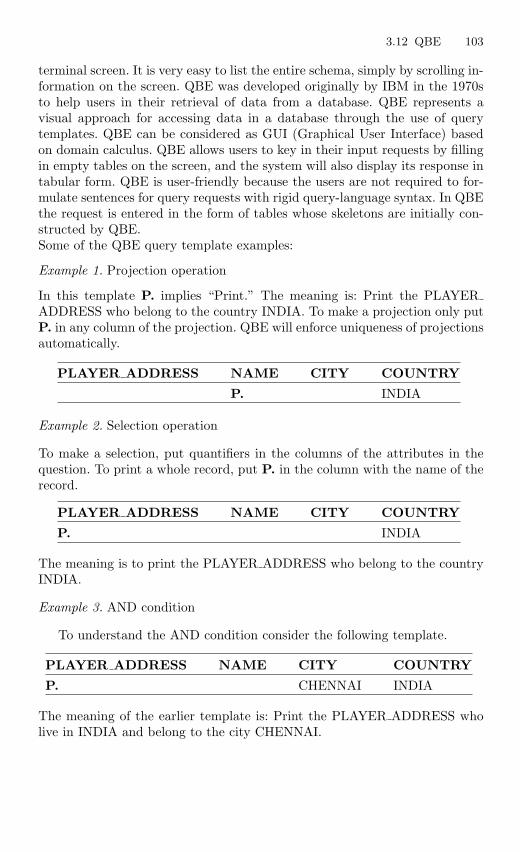
3.12 QBE 103
terminal screen. It is very easy to list the entire schema, simply by scrolling in-formation on the screen. QBE was developed originally by IBM in the 1970sto help users in their retrieval of data from a database. QBE represents avisual approach for accessing data in a database through the use of querytemplates. QBE can be considered as GUI (Graphical User Interface) basedon domain calculus. QBE allows users to key in their input requests by fillingin empty tables on the screen, and the system will also display its response intabular form. QBE is user-friendly because the users are not required to for-mulate sentences for query requests with rigid query-language syntax. In QBEthe request is entered in the form of tables whose skeletons are initially con-structed by QBE.Some of the QBE query template examples:
Example 1. Projection operation
In this template P. implies “Print.” The meaning is: Print the PLAYERADDRESS who belong to the country INDIA. To make a projection only putP. in any column of the projection. QBE will enforce uniqueness of projectionsautomatically.
PLAYER ADDRESS NAME CITY COUNTRY
P. INDIA
Example 2. Selection operation
To make a selection, put quantifiers in the columns of the attributes in thequestion. To print a whole record, put P. in the column with the name of therecord.
PLAYER ADDRESS NAME CITY COUNTRY
P. INDIA
The meaning is to print the PLAYER ADDRESS who belong to the countryINDIA.
Example 3. AND condition
To understand the AND condition consider the following template.
PLAYER ADDRESS NAME CITY COUNTRY
P. CHENNAI INDIA
The meaning of the earlier template is: Print the PLAYER ADDRESS wholive in INDIA and belong to the city CHENNAI.
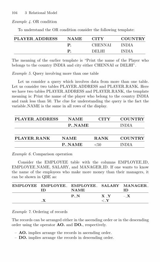
104 3 Relational Model
Example 4. OR condition
To understand the OR condition consider the following template:
PLAYER ADDRESS NAME CITY COUNTRY
P. CHENNAI INDIAP. DELHI INDIA
The meaning of the earlier template is “Print the name of the Player whobelongs to the country INDIA and city either CHENNAI or DELHI”.
Example 5. Query involving more than one table
Let us consider a query which involves data from more than one table.Let us consider two tables PLAYER ADDRESS and PLAYER RANK. Herewe have two tables PLAYER ADDRESS and PLAYER RANK, the templatemeaning is: Print the name of the player who belong to the country INDIAand rank less than 50. The clue for understanding the query is the fact thevariable NAME is the same in all rows of the display.
PLAYER ADDRESS NAME CITY COUNTRY
P. NAME INDIA
PLAYER RANK NAME RANK COUNTRY
P. NAME <50 INDIA
Example 6. Comparison operation
Consider the EMPLOYEE table with the columns EMPLOYEE ID,EMPLOYEE NAME, SALARY, and MANAGER ID. If one wants to knowthe name of the employees who make more money than their managers, itcan be shown in QBE as:
EMPLOYEE EMPLOYEE EMPLOYEE SALARY MANAGERID NAME ID
P. N X Y – XX < Y
Example 7. Ordering of records
The records can be arranged either in the ascending order or in the descendingorder using the operator AO. and DO., respectively.
– AO. implies arrange the records in ascending order.– DO. implies arrange the records in descending order.
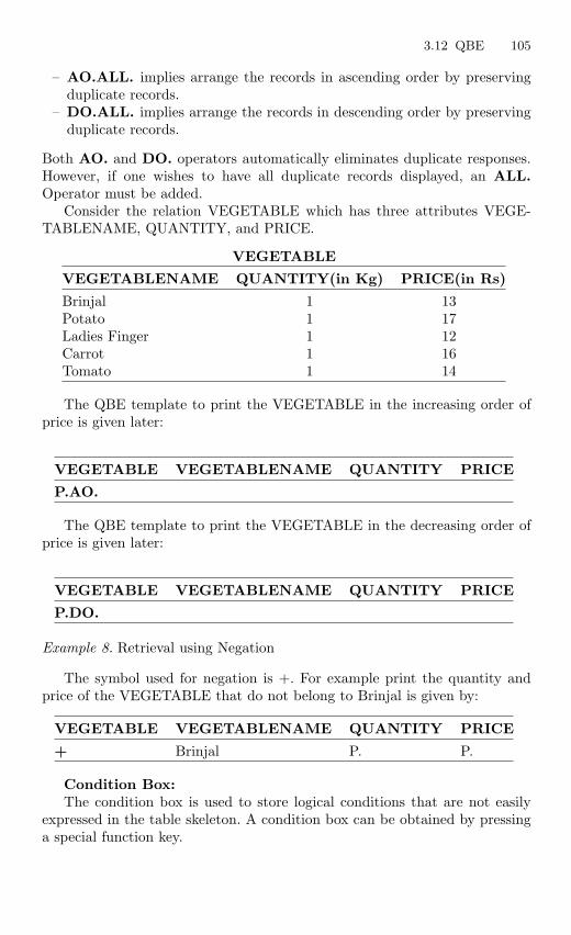
3.12 QBE 105
– AO.ALL. implies arrange the records in ascending order by preservingduplicate records.
– DO.ALL. implies arrange the records in descending order by preservingduplicate records.
Both AO. and DO. operators automatically eliminates duplicate responses.However, if one wishes to have all duplicate records displayed, an ALL.Operator must be added.
Consider the relation VEGETABLE which has three attributes VEGE-TABLENAME, QUANTITY, and PRICE.
VEGETABLE
VEGETABLENAME QUANTITY(in Kg) PRICE(in Rs)
Brinjal 1 13Potato 1 17Ladies Finger 1 12Carrot 1 16Tomato 1 14
The QBE template to print the VEGETABLE in the increasing order ofprice is given later:
VEGETABLE VEGETABLENAME QUANTITY PRICE
P.AO.
The QBE template to print the VEGETABLE in the decreasing order ofprice is given later:
VEGETABLE VEGETABLENAME QUANTITY PRICE
P.DO.
Example 8. Retrieval using Negation
The symbol used for negation is +. For example print the quantity andprice of the VEGETABLE that do not belong to Brinjal is given by:
VEGETABLE VEGETABLENAME QUANTITY PRICE
+ Brinjal P. P.
Condition Box:The condition box is used to store logical conditions that are not easily
expressed in the table skeleton. A condition box can be obtained by pressinga special function key.
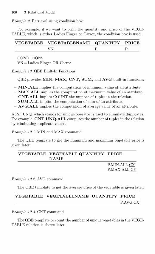
106 3 Relational Model
Example 9. Retrieval using condition box:
For example, if we want to print the quantity and price of the VEGE-TABLE, which is either Ladies Finger or Carrot, the condition box is used.
VEGETABLE VEGETABLENAME QUANTITY PRICE
VN P. P.
CONDITIONSVN= Ladies Finger OR Carrot
Example 10. QBE Built-In Functions
QBE provides MIN, MAX, CNT, SUM, and AVG built-in functions:
– MIN.ALL implies the computation of minimum value of an attribute.– MAX.ALL implies the computation of maximum value of an attribute.– CNT.ALL implies COUNT the number of tuples in the relation.– SUM.ALL implies the computation of sum of an attribute.– AVG.ALL implies the computation of average value of an attribute.
Note: UNQ. which stands for unique operator is used to eliminate duplicates.For example, CNT.UNQ.ALL computes the number of tuples in the relationby eliminating duplicate values.
Example 10.1. MIN and MAX command
The QBE template to get the minimum and maximum vegetable price isgiven later:
VEGETABLE VEGETABLE QUANTITY PRICENAME
P.MIN.ALL.CXP.MAX.ALL.CY
Example 10.2. AVG command
The QBE template to get the average price of the vegetable is given later.
VEGETABLE VEGETABLENAME QUANTITY PRICE
P.AVG.CX
Example 10.3. CNT command
The QBE template to count the number of unique vegetables in the VEGE-TABLE relation is shown later.
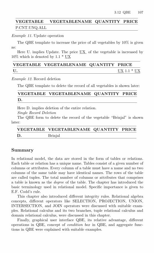
3.12 QBE 107
VEGETABLE VEGETABLENAME QUANTITY PRICE
P.CNT.UNQ.ALL
Example 11. Update operation
The QBE template to increase the price of all vegetables by 10% is givenas:
Here U. implies Update. The price UX of the vegetable is increased by10% which is denoted by 1.1 * UX
VEGETABLE VEGETABLENAME QUANTITY PRICE
U. UX 1.1 * UX
Example 12. Record deletion
The QBE template to delete the record of all vegetables is shown later:
VEGETABLE VEGETABLENAME QUANTITY PRICE
D.
Here D. implies deletion of the entire relation.Single Record DeletionThe QBE form to delete the record of the vegetable “Brinjal” is shown
later:
VEGETABLE VEGETABLENAME QUANTITY PRICE
D. Brinjal
Summary
In relational model, the data are stored in the form of tables or relations.Each table or relation has a unique name. Tables consist of a given number ofcolumns or attributes. Every column of a table must have a name and no twocolumns of the same table may have identical names. The rows of the tableare called tuples. The total number of columns or attributes that comprisesa table is known as the degree of the table. The chapter has introduced thebasic terminology used in relational model. Specific importance is given toE.F. Codd’s rule.
This chapter also introduced different integrity rules. Relational algebraconcepts, different operators like SELECTION, PROJECTION, UNION,INTERSECTION, and JOIN operators were discussed with suitable exam-ples. Relational calculus and its two branches, tuple relational calculus anddomain relational calculus, were discussed in this chapter.
Finally, graphical user interface QBE, its relative advantage, differentoperations in QBE, concept of condition box in QBE, and aggregate func-tions in QBE were explained with suitable examples.
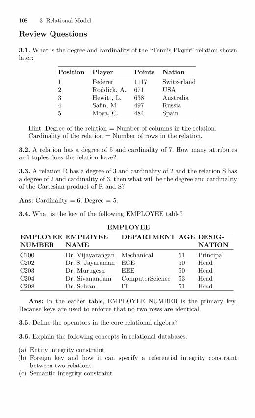
108 3 Relational Model
Review Questions
3.1. What is the degree and cardinality of the “Tennis Player” relation shownlater:
Position Player Points Nation
1 Federer 1117 Switzerland2 Roddick, A. 671 USA3 Hewitt, L. 638 Australia4 Safin, M 497 Russia5 Moya, C. 484 Spain
Hint: Degree of the relation = Number of columns in the relation.Cardinality of the relation = Number of rows in the relation.
3.2. A relation has a degree of 5 and cardinality of 7. How many attributesand tuples does the relation have?
3.3. A relation R has a degree of 3 and cardinality of 2 and the relation S hasa degree of 2 and cardinality of 3, then what will be the degree and cardinalityof the Cartesian product of R and S?
Ans: Cardinality = 6, Degree = 5.
3.4. What is the key of the following EMPLOYEE table?
EMPLOYEE
EMPLOYEE EMPLOYEE DEPARTMENT AGE DESIG-NUMBER NAME NATION
C100 Dr. Vijayarangan Mechanical 51 PrincipalC202 Dr. S. Jayaraman ECE 50 HeadC203 Dr. Murugesh EEE 50 HeadC204 Dr. Sivanandam ComputerScience 53 HeadC208 Dr. Selvan IT 51 Head
Ans: In the earlier table, EMPLOYEE NUMBER is the primary key.Because keys are used to enforce that no two rows are identical.
3.5. Define the operators in the core relational algebra?
3.6. Explain the following concepts in relational databases:
(a) Entity integrity constraint(b) Foreign key and how it can specify a referential integrity constraint
between two relations(c) Semantic integrity constraint
Review Questions 109
3.7. Mention the pros and cons of relational data model?
Pros of relational data model:
1. The relational data model is a well formed and data independent modelwhich is easy to use for applications which fit well into the model.
2. The data used by most business applications fits this model, and thatbusiness applications were the first large customers of database systemexplains the popularity of the model.
Cons of relational data model:
1. The simplicity of the model restricts the amount of semantics, which canbe expressed directly by the database.
2. Different groups of information, or tables, must be joined in many casesto retrieve data.
3.8. Bring out the reasons, why relational model became more popular?
1. Relational model was based on strong mathematical background.2. Relational model used the power of mathematical abstraction. Operations
do not require user to know storage structures used.3. Strong mathematical theory provides tool for improving design.4. Basic structure of the relation is simple, easy to understand and imple-
ment.
3.9. A union, intersection or difference can only be performed between tworelations if they are type compatible. What is meant by type compatibility?Give an example of two type compatible and two nontype compatible rela-tions?
Two relations are type compatible if they have same set of attributes.Example of two type compatible relations is:
Men <name:varchar>, <dob:date>, <address:varchar>Women <name:varchar>, <dob:date>, <address:varchar>Example of two relations which are nontype compatible is:Husband <name:varchar>, <dob:date>, <salary: number>Wife <name:varchar>, <dob:date>, <address:varchar>
3.10. What are the advantages of QBE?
QBE can be considered as GUI (Graphical User Interface) based on domaincalculus. QBE allows users to key in their input requests by filling in emptytables on the screen, and the system will also display its response in tabularform. QBE is user-friendly because the users are not required to formulatesentences for query requests with rigid query-language syntax.
110 3 Relational Model
3.11. What do you understand by domain integrity constraint?
The domain integrity constraints are used to specify the valid values that acolumn defined over the domain can take. We can define the valid values bylisting them as a set of values (such as an enumerated data type in a stronglytyped programming language), a range of values, or an expression that acceptsthe valid values.
3.12. What do you understand by “safety of expressions”?
It is possible to write tuple calculus expressions that generate infinite relations.For example t/∼t ε R results in an infinite relation if the domain of anyattribute of relation R is infinite. To guard against the problem, we restrictthe set of allowable expressions to safe expressions.
3.13. What are “quantifiers”? How will you classify them?
Quantifiers are words that refer to quantities such as “some” or “all” and tellfor how many elements a given predicate is true. A predicate is a sentence thatcontains a finite number of variables and becomes a statement when specificvalues are substituted for the variables. Quantifiers can be broadly classifiedinto two types (1) Universal Quantifier and (2) Existential Quantifier.
4
Structured Query Language
Learning Objectives. This chapter focuses on how to access the data within aDBMS. An introduction to SQL, an international standard language for manipula-ting relational database is given in this chapter. After completing this chapter thereader should be familiar with the following concepts in SQL.
– Evolution and benefits of SQL– Datatypes in SQL– SQL commands to create a table, inserting records into the table, and extracting
information from the table– Aggregate functions, GROUP BY clause– Implementation of constraints in SQL using CHECK, PRIMARY KEY,
FOREIGN KEY, NOT NULL, UNIQUE commands– Concepts of sub query, view, and trigger
4.1 Introduction
SQL stands for “Structured Query Language.” The Structured Query Lan-guage is a relational database language. By itself, SQL does not make a DBMS.SQL is a medium which is used to communicate to the DBMS. SQL commandsconsist of English-like statements which are used to query, insert, update,and delete data. English-like statements mean that SQL commands resembleEnglish language sentences in their construction and use and therefore areeasy to learn and understand.
SQL is referred to as nonprocedural database language. Here nonproce-dural means that, when we want to retrieve data from the database it isenough to tell SQL what data to be retrieved, rather than how to retrieve it.The DBMS will take care of locating the information in the database.
Commercial database management systems allow SQL to be used in twodistinct ways. First, SQL commands can be typed at the command linedirectly. The DBMS interprets and processes the SQL commands immedi-ately, and the results are displayed. This method of SQL processing is calledinteractive SQL. The second method is called programmatic SQL. Here, SQL
S. Sumathi: Structured Query Language, Studies in Computational Intelligence (SCI) 47,
111–212 (2007)
www.springerlink.com c© Springer-Verlag Berlin Heidelberg 2007
112 4 Structured Query Language
statements are embedded in a host language such as COBOL, FORTRAN, C,etc. SQL needs a host language because SQL is not a really complete computerprogramming language as such because it has no statements or constructs thatallow branch or loop. The host language provides the necessary looping andbranching structures and the interface with the user, while SQL provides thestatements to communicate with the DBMS.
Some of the features of SQL are:
– SQL is a language used to interact with the database.– SQL is a data access language.– SQL is based on relational tuple calculus.– SQL is a standard relational database management language.– The first commercial DBMS that supported SQL was Oracle in 1979.– SQL is a “nonprocedural” or “declarative” language.
4.2 History of SQL Standard
The origin of the SQL language date back to a research project conducted byIBM at their research laboratories in San Jose, California in the early 1970s.The aim of the project was to develop an experimental RDBMS which wouldeventually lead to a marketable product. At that time, there was a lot of inter-est in the relational model for databases at the academic level, in conferencesand seminars. IBM, which already had a large share of the commercial data-base market with hierarchical and network model DBMSs, realized that therelational model would dominate the future database products. The projectat IBM’s San Jose labs was started in 1974 and was named System R. Alanguage called SEQUEL (Structured English QUEry Language) was chosenas the relational database language for System R. A version of SEQUEL wasdeveloped at the IBM San Jose research facilities and tested with college stu-dents.
In November 1976, specifications for SEQUEL2 were published. In 1980minor revisions were made to SEQUEL, and it was renamed “SQL.” SEQUELwas renamed to SQL because the name SEQUEL had already been used forhardware product. In order to avoid confusion and legal problems SEQUELwas renamed to SQL. In the first phase of the System R project, researchersconcentrated on developing a basic version of the RDBMS. The main aimat this stage was to verify that the theories of the relational model could betranslated into a working, commercially viable product. This first phase wassuccessfully completed by the end of 1975, and resulted in a single-user DBMSbased on the relational model. The System R project was completed in 1979.The theoretical work of the System R project resulted in the developmentand release of IBM’s first commercial relational database management systemin 1981. The product was called SQL/DS (Structured Query Language/DataStore) and ran under the DOS/VSE operating system environment. Two yearslater, IBM announced a version of SQL/DS for VM/CMS operating system.
4.3 Commands in SQL 113
In 1983, IBM released a second SQL-based RDBMS called DB2, which ranunder the MVS operating system. DB2 quickly gained widespread popularityand even today, versions of DB2 form the basis of many database systemsfound in large corporate data-centers. During the development of System Rand SQL/DS, other companies were also at work creating their own relationaldatabase management systems. Some of them, Oracle being an example, evenimplemented SQL as the relational database language for their DBMSs con-currently with IBM. Later on, SQL language was standardized by ANSI andISO. The ANSI SQL standards were first published in 1986 and updated in1989, 1992, and 1999.
4.2.1 Benefits of Standardized Relational Language
The main advantages of standardized language are given below.
1. Reduced training cost2. Enhanced productivity3. Application portability
Application portability means applications can be moved frommachine to machine when each machine uses SQL.
4. Application longevityA standard language tends to remain so for a long time, hence therewill be little pressure to rewrite old applications.
5. Reduced dependence on a single vendor
SQL language development is given in a nutshell below:
1. In 1970 E.F. Codd of IBM released a paper “A relational model of data forlarge shared data banks.” IBM started the project System R to demon-strate the feasibility of implementing the relational model in a databasemanagement system. The language used in system R project was SE-QUEL. SEQUEL was renamed SQL during the project, which took placefrom 1974 to 1979.
2. The first commercial RDBMS from IBM was SQL/DS. It was available in1981.
3. Oracle from relational software (now Oracle corporation) was on the mar-ket before SQL/DS, i.e., 1979.
4. Other products included INGRES from relational Technology Sybase fromSybase, Inc. (1986), DG/SQL from Data General Corporation (1984).
4.3 Commands in SQL
SQL commands can be classified in to three types:
1. Data Definition Language commands (DDL)2. Data Manipulation Language commands (DML)3. Data Control Language commands (DCL)
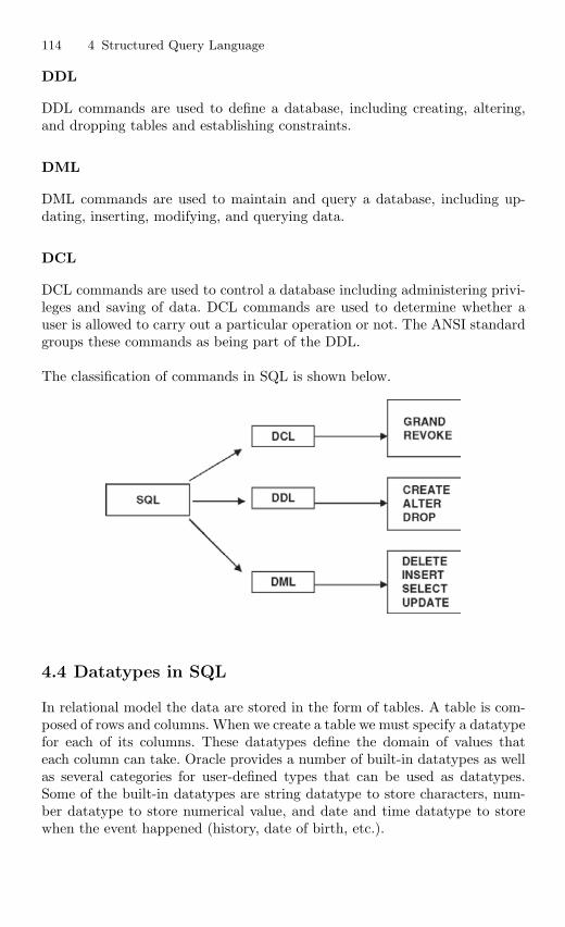
114 4 Structured Query Language
DDL
DDL commands are used to define a database, including creating, altering,and dropping tables and establishing constraints.
DML
DML commands are used to maintain and query a database, including up-dating, inserting, modifying, and querying data.
DCL
DCL commands are used to control a database including administering privi-leges and saving of data. DCL commands are used to determine whether auser is allowed to carry out a particular operation or not. The ANSI standardgroups these commands as being part of the DDL.
The classification of commands in SQL is shown below.
4.4 Datatypes in SQL
In relational model the data are stored in the form of tables. A table is com-posed of rows and columns. When we create a table we must specify a datatypefor each of its columns. These datatypes define the domain of values thateach column can take. Oracle provides a number of built-in datatypes as wellas several categories for user-defined types that can be used as datatypes.Some of the built-in datatypes are string datatype to store characters, num-ber datatype to store numerical value, and date and time datatype to storewhen the event happened (history, date of birth, etc.).
4.4 Datatypes in SQL 115
STRING
In string we have CHAR and VARCHAR datatypes. Character datatype storedata which are words and free-form text, in the database character set.
CHAR Datatype
The CHAR datatype specifies a fixed-length character string. The syntax ofCHAR datatype declaration is:
CHAR (n) – Fixed length character data, “n” characters long.
Here “n” specifies the character length. If we insert a value that is shorterthan the column length, then Oracle blank-pads the value to column length.If we try to insert a value that is too long for the column then Oracle returnserror message.
VARCHAR2 Datatype
The VARCHAR2 datatype specifies a variable-length character string. Thesyntax of VARCHAR2 datatype declaration is:
VARCHAR2 (n) – Variable length character of “n” length.
Here “n” specifies the character length.
VARCHAR vs. VARCHAR2
The VARCHAR datatype behaves like VARCHAR2 datatype in the currentversion of Oracle.
In order to justify the above statement, let us create a table CHAMPION,which refers to Wimbledon Champions. The attributes of the table CHAM-PION are Name, Nation, Year (the year in which the sportsman has won thetitle). For our example, let us use the datatype VARCHAR for the attributeName and VARCHAR2 for the datatype Nation. The SQL command to createCHAMPION is shown in Fig. 4.1.
Now let us try to see the description of the table. The description of thetable is shown in Fig. 4.2.
From Fig. 4.2, it is clear that both name and nation are stored as VAR-CHAR2(12). This means that VARCHAR datatype in the Oracle 8i versionbehaves the same as VARCHAR2.
NUMBER Datatype
The NUMBER datatype stores zero, positive, and negative fixed and floatingpoint numbers.
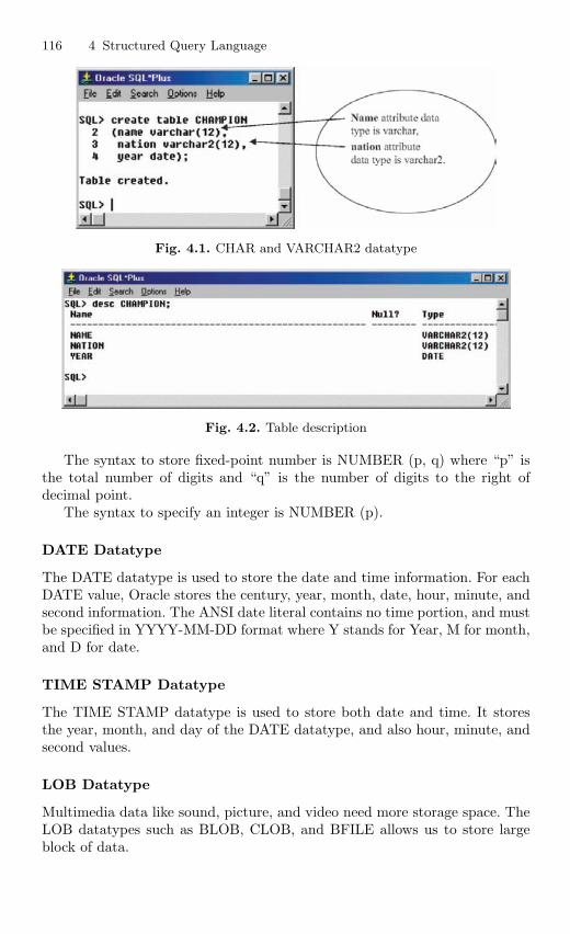
116 4 Structured Query Language
Fig. 4.1. CHAR and VARCHAR2 datatype
Fig. 4.2. Table description
The syntax to store fixed-point number is NUMBER (p, q) where “p” isthe total number of digits and “q” is the number of digits to the right ofdecimal point.
The syntax to specify an integer is NUMBER (p).
DATE Datatype
The DATE datatype is used to store the date and time information. For eachDATE value, Oracle stores the century, year, month, date, hour, minute, andsecond information. The ANSI date literal contains no time portion, and mustbe specified in YYYY-MM-DD format where Y stands for Year, M for month,and D for date.
TIME STAMP Datatype
The TIME STAMP datatype is used to store both date and time. It storesthe year, month, and day of the DATE datatype, and also hour, minute, andsecond values.
LOB Datatype
Multimedia data like sound, picture, and video need more storage space. TheLOB datatypes such as BLOB, CLOB, and BFILE allows us to store largeblock of data.
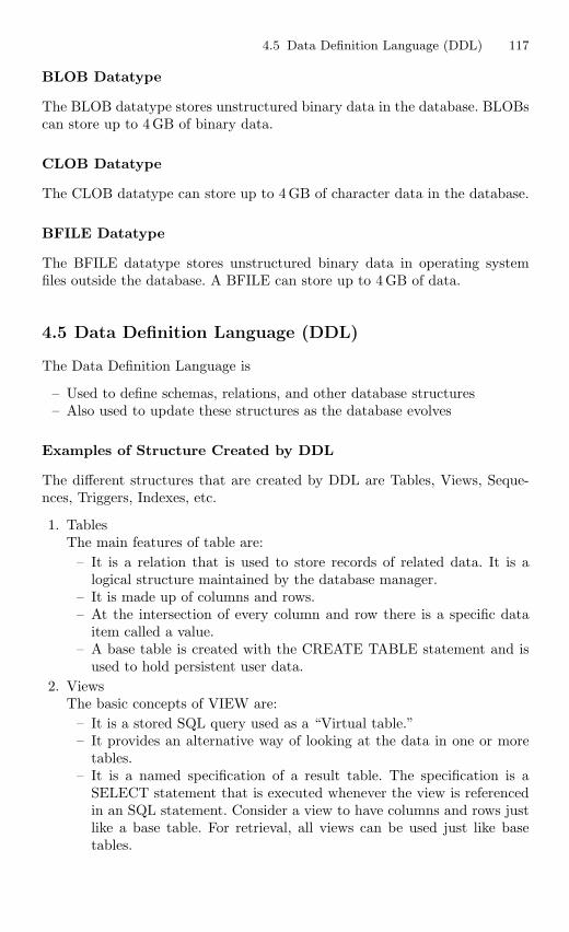
4.5 Data Definition Language (DDL) 117
BLOB Datatype
The BLOB datatype stores unstructured binary data in the database. BLOBscan store up to 4 GB of binary data.
CLOB Datatype
The CLOB datatype can store up to 4 GB of character data in the database.
BFILE Datatype
The BFILE datatype stores unstructured binary data in operating systemfiles outside the database. A BFILE can store up to 4 GB of data.
4.5 Data Definition Language (DDL)
The Data Definition Language is
– Used to define schemas, relations, and other database structures– Also used to update these structures as the database evolves
Examples of Structure Created by DDL
The different structures that are created by DDL are Tables, Views, Seque-nces, Triggers, Indexes, etc.
1. TablesThe main features of table are:
– It is a relation that is used to store records of related data. It is alogical structure maintained by the database manager.
– It is made up of columns and rows.– At the intersection of every column and row there is a specific data
item called a value.– A base table is created with the CREATE TABLE statement and is
used to hold persistent user data.2. Views
The basic concepts of VIEW are:– It is a stored SQL query used as a “Virtual table.”– It provides an alternative way of looking at the data in one or more
tables.– It is a named specification of a result table. The specification is a
SELECT statement that is executed whenever the view is referencedin an SQL statement. Consider a view to have columns and rows justlike a base table. For retrieval, all views can be used just like basetables.
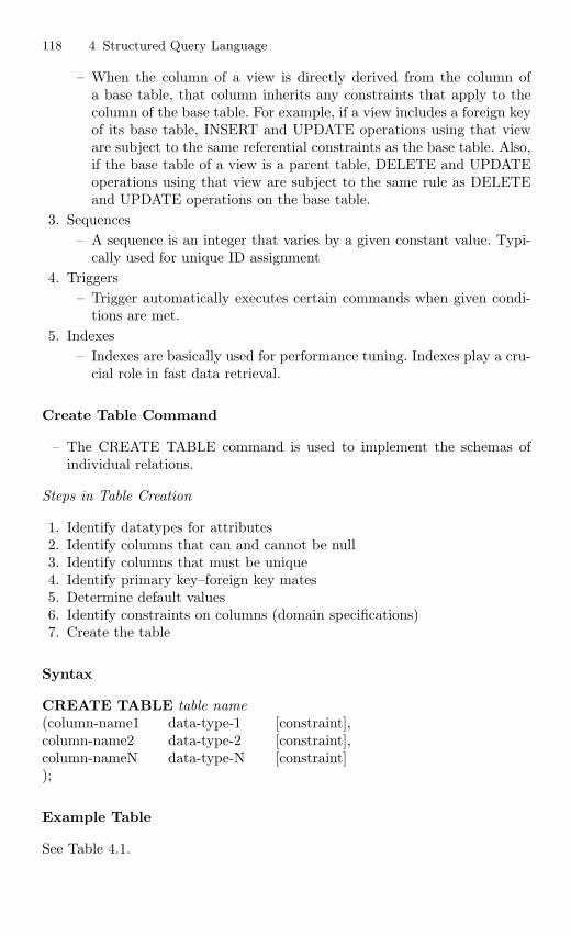
118 4 Structured Query Language
– When the column of a view is directly derived from the column ofa base table, that column inherits any constraints that apply to thecolumn of the base table. For example, if a view includes a foreign keyof its base table, INSERT and UPDATE operations using that vieware subject to the same referential constraints as the base table. Also,if the base table of a view is a parent table, DELETE and UPDATEoperations using that view are subject to the same rule as DELETEand UPDATE operations on the base table.
3. Sequences– A sequence is an integer that varies by a given constant value. Typi-
cally used for unique ID assignment4. Triggers
– Trigger automatically executes certain commands when given condi-tions are met.
5. Indexes– Indexes are basically used for performance tuning. Indexes play a cru-
cial role in fast data retrieval.
Create Table Command
– The CREATE TABLE command is used to implement the schemas ofindividual relations.
Steps in Table Creation
1. Identify datatypes for attributes2. Identify columns that can and cannot be null3. Identify columns that must be unique4. Identify primary key–foreign key mates5. Determine default values6. Identify constraints on columns (domain specifications)7. Create the table
Syntax
CREATE TABLE table name(column-name1 data-type-1 [constraint],column-name2 data-type-2 [constraint],column-nameN data-type-N [constraint]);
Example Table
See Table 4.1.
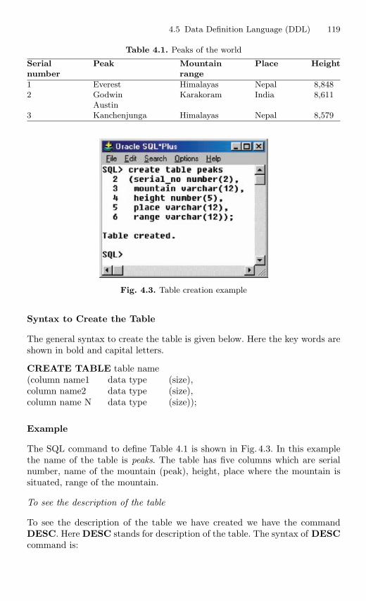
4.5 Data Definition Language (DDL) 119
Table 4.1. Peaks of the world
Serial Peak Mountain Place Heightnumber range
1 Everest Himalayas Nepal 8,8482 Godwin Karakoram India 8,611
Austin3 Kanchenjunga Himalayas Nepal 8,579
Fig. 4.3. Table creation example
Syntax to Create the Table
The general syntax to create the table is given below. Here the key words areshown in bold and capital letters.
CREATE TABLE table name(column name1 data type (size),column name2 data type (size),column name N data type (size));
Example
The SQL command to define Table 4.1 is shown in Fig. 4.3. In this examplethe name of the table is peaks. The table has five columns which are serialnumber, name of the mountain (peak), height, place where the mountain issituated, range of the mountain.
To see the description of the table
To see the description of the table we have created we have the commandDESC. Here DESC stands for description of the table. The syntax of DESCcommand is:
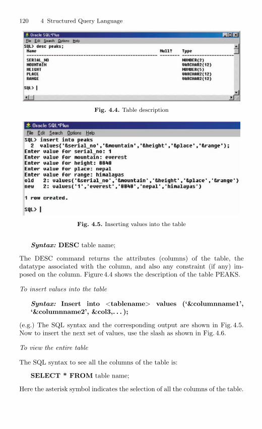
120 4 Structured Query Language
Fig. 4.4. Table description
Fig. 4.5. Inserting values into the table
Syntax: DESC table name;
The DESC command returns the attributes (columns) of the table, thedatatype associated with the column, and also any constraint (if any) im-posed on the column. Figure 4.4 shows the description of the table PEAKS.
To insert values into the table
Syntax: Insert into <tablename> values (‘&columnname1’,‘&columnname2’, &col3,. . . );
(e.g.) The SQL syntax and the corresponding output are shown in Fig. 4.5.Now to insert the next set of values, use the slash as shown in Fig. 4.6.
To view the entire table
The SQL syntax to see all the columns of the table is:
SELECT * FROM table name;
Here the asterisk symbol indicates the selection of all the columns of the table.
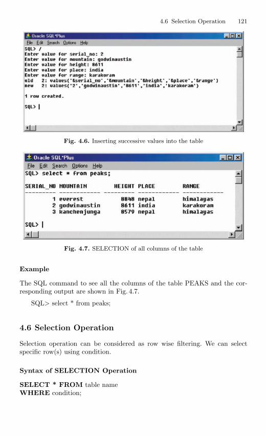
4.6 Selection Operation 121
Fig. 4.6. Inserting successive values into the table
Fig. 4.7. SELECTION of all columns of the table
Example
The SQL command to see all the columns of the table PEAKS and the cor-responding output are shown in Fig. 4.7.
SQL> select * from peaks;
4.6 Selection Operation
Selection operation can be considered as row wise filtering. We can selectspecific row(s) using condition.
Syntax of SELECTION Operation
SELECT * FROM table nameWHERE condition;
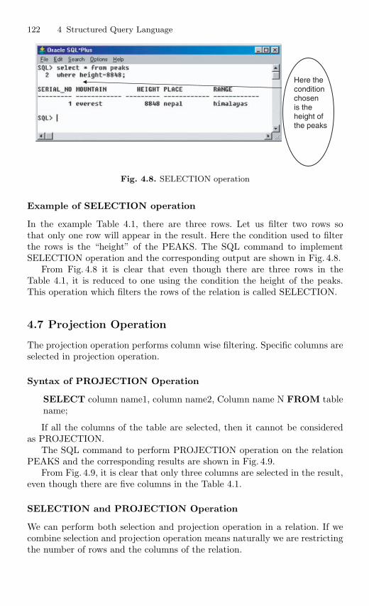
122 4 Structured Query Language
Here the condition chosen is the height ofthe peaks
Fig. 4.8. SELECTION operation
Example of SELECTION operation
In the example Table 4.1, there are three rows. Let us filter two rows sothat only one row will appear in the result. Here the condition used to filterthe rows is the “height” of the PEAKS. The SQL command to implementSELECTION operation and the corresponding output are shown in Fig. 4.8.
From Fig. 4.8 it is clear that even though there are three rows in theTable 4.1, it is reduced to one using the condition the height of the peaks.This operation which filters the rows of the relation is called SELECTION.
4.7 Projection Operation
The projection operation performs column wise filtering. Specific columns areselected in projection operation.
Syntax of PROJECTION Operation
SELECT column name1, column name2, Column name N FROM tablename;
If all the columns of the table are selected, then it cannot be consideredas PROJECTION.
The SQL command to perform PROJECTION operation on the relationPEAKS and the corresponding results are shown in Fig. 4.9.
From Fig. 4.9, it is clear that only three columns are selected in the result,even though there are five columns in the Table 4.1.
SELECTION and PROJECTION Operation
We can perform both selection and projection operation in a relation. If wecombine selection and projection operation means naturally we are restrictingthe number of rows and the columns of the relation.
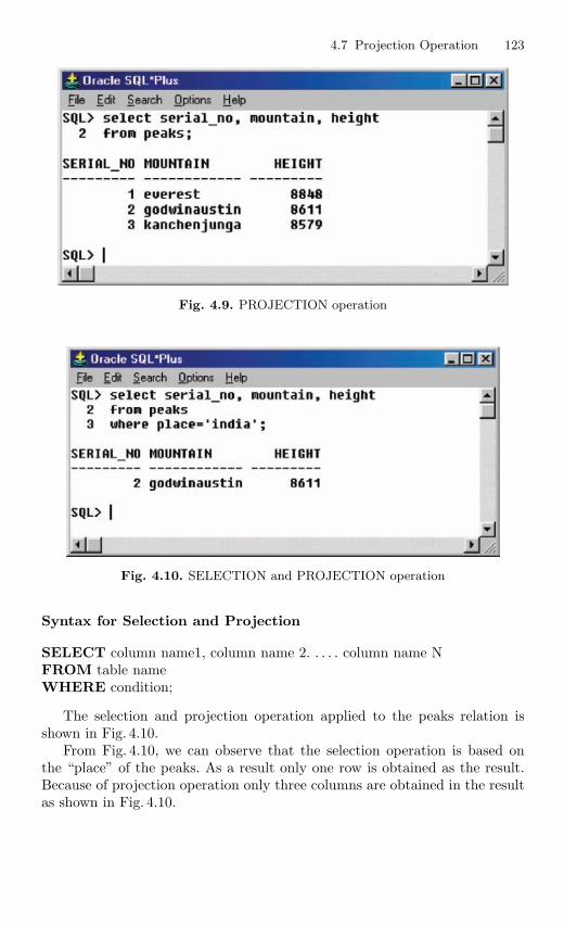
4.7 Projection Operation 123
Fig. 4.9. PROJECTION operation
Fig. 4.10. SELECTION and PROJECTION operation
Syntax for Selection and Projection
SELECT column name1, column name 2. . . . . column name NFROM table nameWHERE condition;
The selection and projection operation applied to the peaks relation isshown in Fig. 4.10.
From Fig. 4.10, we can observe that the selection operation is based onthe “place” of the peaks. As a result only one row is obtained as the result.Because of projection operation only three columns are obtained in the resultas shown in Fig. 4.10.
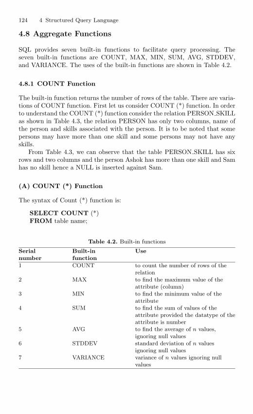
124 4 Structured Query Language
4.8 Aggregate Functions
SQL provides seven built-in functions to facilitate query processing. Theseven built-in functions are COUNT, MAX, MIN, SUM, AVG, STDDEV,and VARIANCE. The uses of the built-in functions are shown in Table 4.2.
4.8.1 COUNT Function
The built-in function returns the number of rows of the table. There are varia-tions of COUNT function. First let us consider COUNT (*) function. In orderto understand the COUNT (*) function consider the relation PERSON SKILLas shown in Table 4.3, the relation PERSON has only two columns, name ofthe person and skills associated with the person. It is to be noted that somepersons may have more than one skill and some persons may not have anyskills.
From Table 4.3, we can observe that the table PERSON SKILL has sixrows and two columns and the person Ashok has more than one skill and Samhas no skill hence a NULL is inserted against Sam.
(A) COUNT (*) Function
The syntax of Count (*) function is:
SELECT COUNT (*)FROM table name;
Table 4.2. Built-in functions
Serial Built-in Usenumber function
1 COUNT to count the number of rows of therelation
2 MAX to find the maximum value of theattribute (column)
3 MIN to find the minimum value of theattribute
4 SUM to find the sum of values of theattribute provided the datatype of theattribute is number
5 AVG to find the average of n values,ignoring null values
6 STDDEV standard deviation of n valuesignoring null values
7 VARIANCE variance of n values ignoring nullvalues
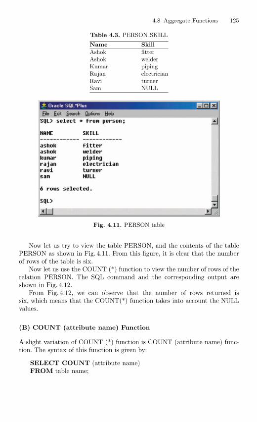
4.8 Aggregate Functions 125
Table 4.3. PERSON SKILL
Name Skill
Ashok fitterAshok welderKumar pipingRajan electricianRavi turnerSam NULL
Fig. 4.11. PERSON table
Now let us try to view the table PERSON, and the contents of the tablePERSON as shown in Fig. 4.11. From this figure, it is clear that the numberof rows of the table is six.
Now let us use the COUNT (*) function to view the number of rows of therelation PERSON. The SQL command and the corresponding output areshown in Fig. 4.12.
From Fig. 4.12, we can observe that the number of rows returned issix, which means that the COUNT(*) function takes into account the NULLvalues.
(B) COUNT (attribute name) Function
A slight variation of COUNT (*) function is COUNT (attribute name) func-tion. The syntax of this function is given by:
SELECT COUNT (attribute name)FROM table name;
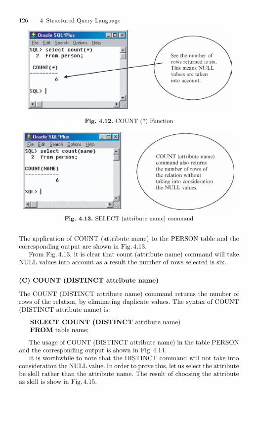
126 4 Structured Query Language
Fig. 4.12. COUNT (*) Function
Fig. 4.13. SELECT (attribute name) command
The application of COUNT (attribute name) to the PERSON table and thecorresponding output are shown in Fig. 4.13.
From Fig. 4.13, it is clear that count (attribute name) command will takeNULL values into account as a result the number of rows selected is six.
(C) COUNT (DISTINCT attribute name)
The COUNT (DISTINCT attribute name) command returns the number ofrows of the relation, by eliminating duplicate values. The syntax of COUNT(DISTINCT attribute name) is:
SELECT COUNT (DISTINCT attribute name)FROM table name;
The usage of COUNT (DISTINCT attribute name) in the table PERSONand the corresponding output is shown in Fig. 4.14.
It is worthwhile to note that the DISTINCT command will not take intoconsideration the NULL value. In order to prove this, let us select the attributebe skill rather than the attribute name. The result of choosing the attributeas skill is show in Fig. 4.15.
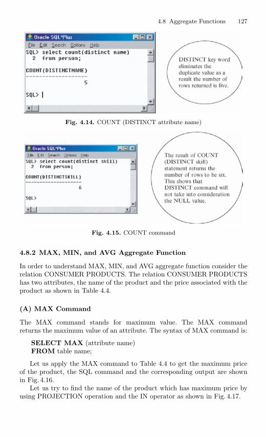
4.8 Aggregate Functions 127
Fig. 4.14. COUNT (DISTINCT attribute name)
Fig. 4.15. COUNT command
4.8.2 MAX, MIN, and AVG Aggregate Function
In order to understand MAX, MIN, and AVG aggregate function consider therelation CONSUMER PRODUCTS. The relation CONSUMER PRODUCTShas two attributes, the name of the product and the price associated with theproduct as shown in Table 4.4.
(A) MAX Command
The MAX command stands for maximum value. The MAX commandreturns the maximum value of an attribute. The syntax of MAX command is:
SELECT MAX (attribute name)FROM table name;
Let us apply the MAX command to Table 4.4 to get the maximum priceof the product, the SQL command and the corresponding output are shownin Fig. 4.16.
Let us try to find the name of the product which has maximum price byusing PROJECTION operation and the IN operator as shown in Fig. 4.17.
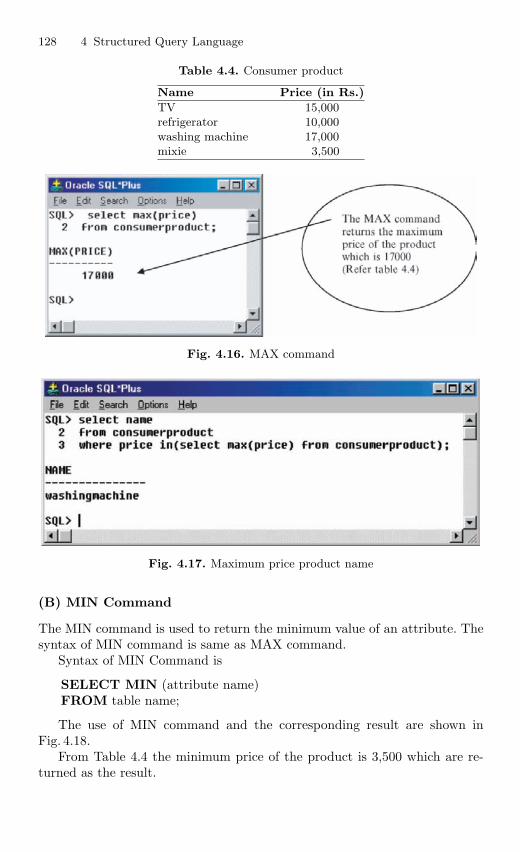
128 4 Structured Query Language
Table 4.4. Consumer product
Name Price (in Rs.)
TV 15,000refrigerator 10,000washing machine 17,000mixie 3,500
Fig. 4.16. MAX command
Fig. 4.17. Maximum price product name
(B) MIN Command
The MIN command is used to return the minimum value of an attribute. Thesyntax of MIN command is same as MAX command.
Syntax of MIN Command is
SELECT MIN (attribute name)FROM table name;
The use of MIN command and the corresponding result are shown inFig. 4.18.
From Table 4.4 the minimum price of the product is 3,500 which are re-turned as the result.
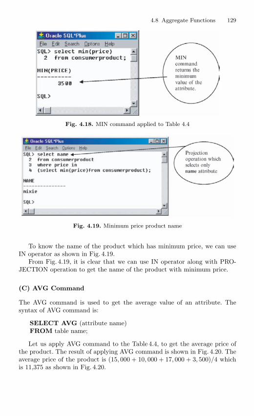
4.8 Aggregate Functions 129
Fig. 4.18. MIN command applied to Table 4.4
Fig. 4.19. Minimum price product name
To know the name of the product which has minimum price, we can useIN operator as shown in Fig. 4.19.
From Fig. 4.19, it is clear that we can use IN operator along with PRO-JECTION operation to get the name of the product with minimum price.
(C) AVG Command
The AVG command is used to get the average value of an attribute. Thesyntax of AVG command is:
SELECT AVG (attribute name)FROM table name;
Let us apply AVG command to the Table 4.4, to get the average price ofthe product. The result of applying AVG command is shown in Fig. 4.20. Theaverage price of the product is (15, 000 + 10, 000 + 17, 000 + 3, 500)/4 whichis 11,375 as shown in Fig. 4.20.
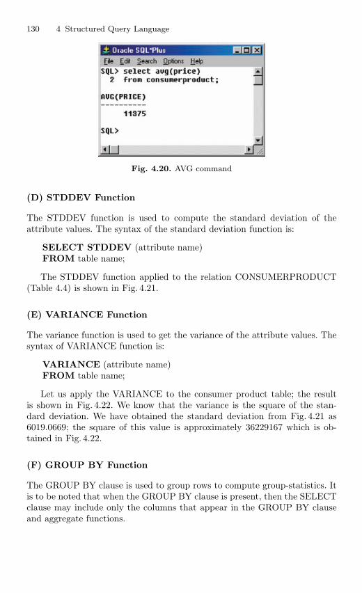
130 4 Structured Query Language
Fig. 4.20. AVG command
(D) STDDEV Function
The STDDEV function is used to compute the standard deviation of theattribute values. The syntax of the standard deviation function is:
SELECT STDDEV (attribute name)FROM table name;
The STDDEV function applied to the relation CONSUMERPRODUCT(Table 4.4) is shown in Fig. 4.21.
(E) VARIANCE Function
The variance function is used to get the variance of the attribute values. Thesyntax of VARIANCE function is:
VARIANCE (attribute name)FROM table name;
Let us apply the VARIANCE to the consumer product table; the resultis shown in Fig. 4.22. We know that the variance is the square of the stan-dard deviation. We have obtained the standard deviation from Fig. 4.21 as6019.0669; the square of this value is approximately 36229167 which is ob-tained in Fig. 4.22.
(F) GROUP BY Function
The GROUP BY clause is used to group rows to compute group-statistics. Itis to be noted that when the GROUP BY clause is present, then the SELECTclause may include only the columns that appear in the GROUP BY clauseand aggregate functions.
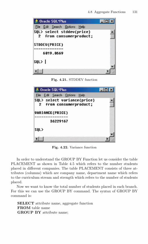
4.8 Aggregate Functions 131
Fig. 4.21. STDDEV function
Fig. 4.22. Variance function
In order to understand the GROUP BY Function let us consider the tablePLACEMENT as shown in Table 4.5 which refers to the number studentsplaced in different companies. The table PLACEMENT consists of three at-tributes (columns) which are company name, department name which refersto the curriculum stream and strength which refers to the number of studentsplaced.
Now we want to know the total number of students placed in each branch.For this we can use the GROUP BY command. The syntax of GROUP BYcommand is:
SELECT attribute name, aggregate functionFROM table nameGROUP BY attribute name;
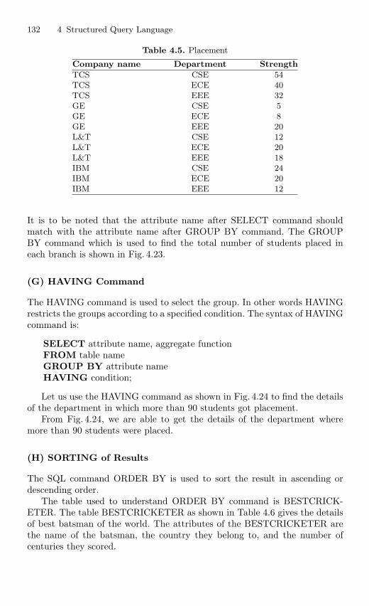
132 4 Structured Query Language
Table 4.5. Placement
Company name Department Strength
TCS CSE 54TCS ECE 40TCS EEE 32GE CSE 5GE ECE 8GE EEE 20L&T CSE 12L&T ECE 20L&T EEE 18IBM CSE 24IBM ECE 20IBM EEE 12
It is to be noted that the attribute name after SELECT command shouldmatch with the attribute name after GROUP BY command. The GROUPBY command which is used to find the total number of students placed ineach branch is shown in Fig. 4.23.
(G) HAVING Command
The HAVING command is used to select the group. In other words HAVINGrestricts the groups according to a specified condition. The syntax of HAVINGcommand is:
SELECT attribute name, aggregate functionFROM table nameGROUP BY attribute nameHAVING condition;
Let us use the HAVING command as shown in Fig. 4.24 to find the detailsof the department in which more than 90 students got placement.
From Fig. 4.24, we are able to get the details of the department wheremore than 90 students were placed.
(H) SORTING of Results
The SQL command ORDER BY is used to sort the result in ascending ordescending order.
The table used to understand ORDER BY command is BESTCRICK-ETER. The table BESTCRICKETER as shown in Table 4.6 gives the detailsof best batsman of the world. The attributes of the BESTCRICKETER arethe name of the batsman, the country they belong to, and the number ofcenturies they scored.
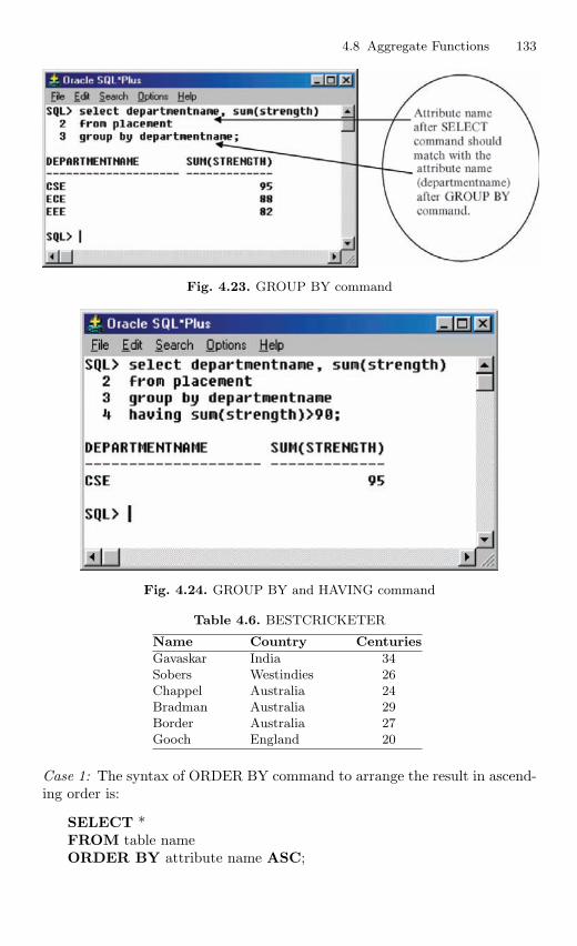
4.8 Aggregate Functions 133
Fig. 4.23. GROUP BY command
Fig. 4.24. GROUP BY and HAVING command
Table 4.6. BESTCRICKETER
Name Country Centuries
Gavaskar India 34Sobers Westindies 26Chappel Australia 24Bradman Australia 29Border Australia 27Gooch England 20
Case 1: The syntax of ORDER BY command to arrange the result in ascend-ing order is:
SELECT *FROM table nameORDER BY attribute name ASC;
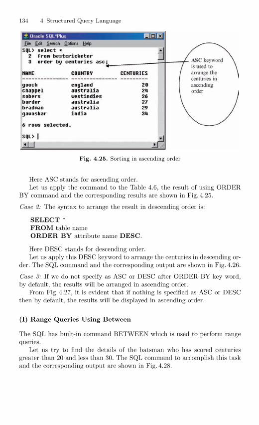
134 4 Structured Query Language
Fig. 4.25. Sorting in ascending order
Here ASC stands for ascending order.Let us apply the command to the Table 4.6, the result of using ORDER
BY command and the corresponding results are shown in Fig. 4.25.
Case 2: The syntax to arrange the result in descending order is:
SELECT *FROM table nameORDER BY attribute name DESC.
Here DESC stands for descending order.Let us apply this DESC keyword to arrange the centuries in descending or-
der. The SQL command and the corresponding output are shown in Fig. 4.26.
Case 3: If we do not specify as ASC or DESC after ORDER BY key word,by default, the results will be arranged in ascending order.
From Fig. 4.27, it is evident that if nothing is specified as ASC or DESCthen by default, the results will be displayed in ascending order.
(I) Range Queries Using Between
The SQL has built-in command BETWEEN which is used to perform rangequeries.
Let us try to find the details of the batsman who has scored centuriesgreater than 20 and less than 30. The SQL command to accomplish this taskand the corresponding output are shown in Fig. 4.28.
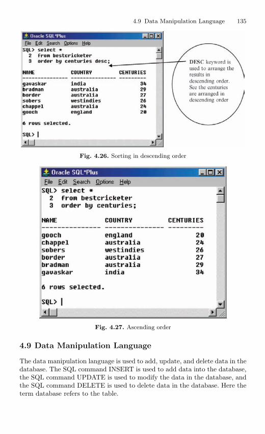
4.9 Data Manipulation Language 135
Fig. 4.26. Sorting in descending order
Fig. 4.27. Ascending order
4.9 Data Manipulation Language
The data manipulation language is used to add, update, and delete data in thedatabase. The SQL command INSERT is used to add data into the database,the SQL command UPDATE is used to modify the data in the database, andthe SQL command DELETE is used to delete data in the database. Here theterm database refers to the table.
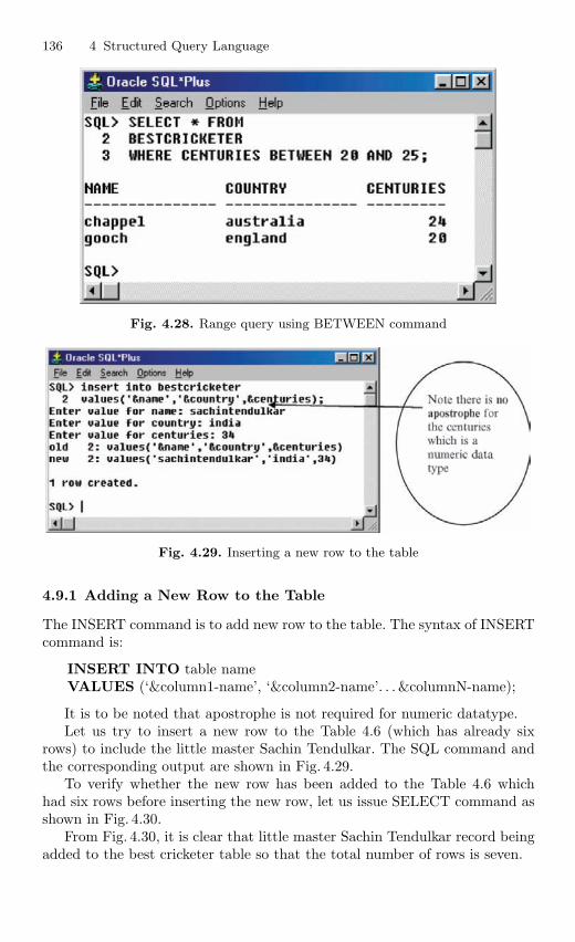
136 4 Structured Query Language
Fig. 4.28. Range query using BETWEEN command
Fig. 4.29. Inserting a new row to the table
4.9.1 Adding a New Row to the Table
The INSERT command is to add new row to the table. The syntax of INSERTcommand is:
INSERT INTO table nameVALUES (‘&column1-name’, ‘&column2-name’. . . &columnN-name);
It is to be noted that apostrophe is not required for numeric datatype.Let us try to insert a new row to the Table 4.6 (which has already six
rows) to include the little master Sachin Tendulkar. The SQL command andthe corresponding output are shown in Fig. 4.29.
To verify whether the new row has been added to the Table 4.6 whichhad six rows before inserting the new row, let us issue SELECT command asshown in Fig. 4.30.
From Fig. 4.30, it is clear that little master Sachin Tendulkar record beingadded to the best cricketer table so that the total number of rows is seven.
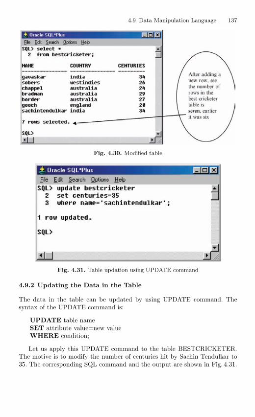
4.9 Data Manipulation Language 137
Fig. 4.30. Modified table
Fig. 4.31. Table updation using UPDATE command
4.9.2 Updating the Data in the Table
The data in the table can be updated by using UPDATE command. Thesyntax of the UPDATE command is:
UPDATE table nameSET attribute value=new valueWHERE condition;
Let us apply this UPDATE command to the table BESTCRICKETER.The motive is to modify the number of centuries hit by Sachin Tendulkar to35. The corresponding SQL command and the output are shown in Fig. 4.31.
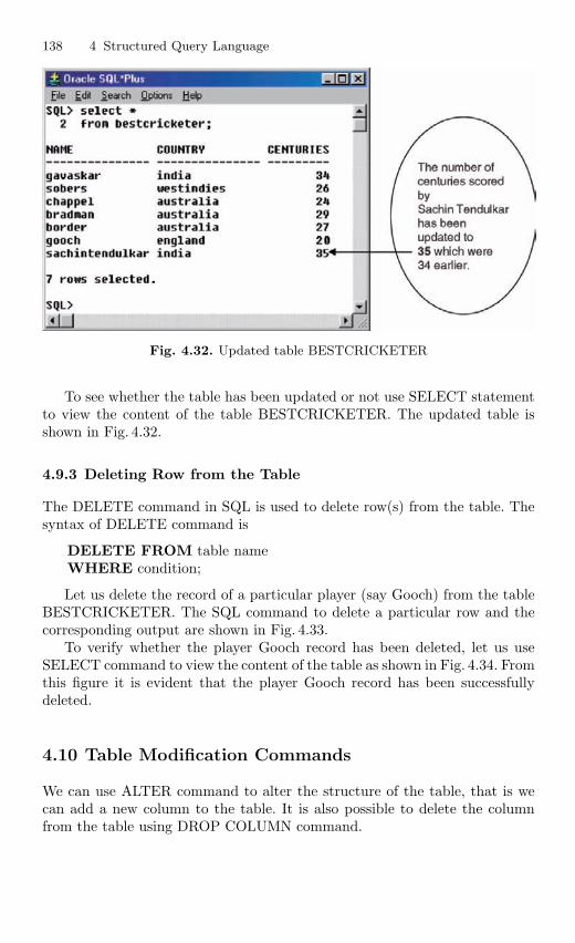
138 4 Structured Query Language
Fig. 4.32. Updated table BESTCRICKETER
To see whether the table has been updated or not use SELECT statementto view the content of the table BESTCRICKETER. The updated table isshown in Fig. 4.32.
4.9.3 Deleting Row from the Table
The DELETE command in SQL is used to delete row(s) from the table. Thesyntax of DELETE command is
DELETE FROM table nameWHERE condition;
Let us delete the record of a particular player (say Gooch) from the tableBESTCRICKETER. The SQL command to delete a particular row and thecorresponding output are shown in Fig. 4.33.
To verify whether the player Gooch record has been deleted, let us useSELECT command to view the content of the table as shown in Fig. 4.34. Fromthis figure it is evident that the player Gooch record has been successfullydeleted.
4.10 Table Modification Commands
We can use ALTER command to alter the structure of the table, that is wecan add a new column to the table. It is also possible to delete the columnfrom the table using DROP COLUMN command.
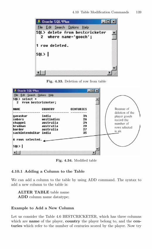
4.10 Table Modification Commands 139
Fig. 4.33. Deletion of row from table
Fig. 4.34. Modified table
4.10.1 Adding a Column to the Table
We can add a column to the table by using ADD command. The syntax toadd a new column to the table is:
ALTER TABLE table nameADD column name datatype;
Example to Add a New Column
Let us consider the Table 4.6 BESTCRICKETER, which has three columnswhich are name of the player, country the player belong to, and the cen-turies which refer to the number of centuries scored by the player. Now try
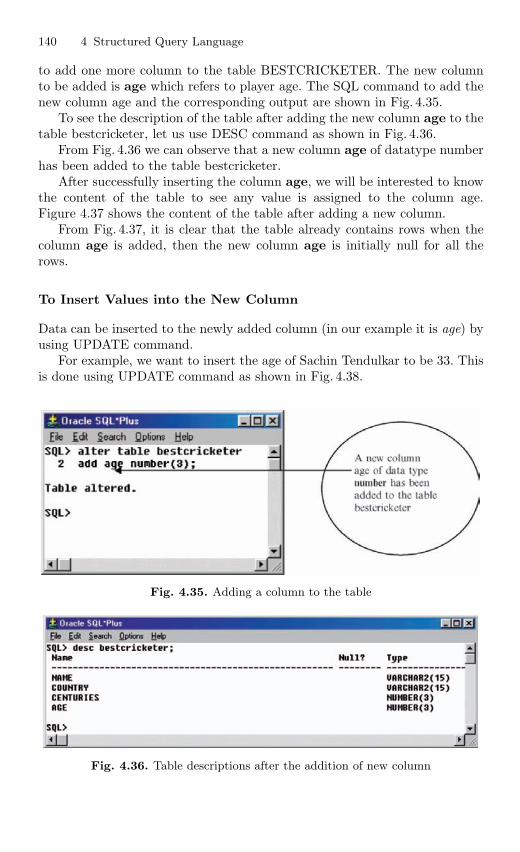
140 4 Structured Query Language
to add one more column to the table BESTCRICKETER. The new columnto be added is age which refers to player age. The SQL command to add thenew column age and the corresponding output are shown in Fig. 4.35.
To see the description of the table after adding the new column age to thetable bestcricketer, let us use DESC command as shown in Fig. 4.36.
From Fig. 4.36 we can observe that a new column age of datatype numberhas been added to the table bestcricketer.
After successfully inserting the column age, we will be interested to knowthe content of the table to see any value is assigned to the column age.Figure 4.37 shows the content of the table after adding a new column.
From Fig. 4.37, it is clear that the table already contains rows when thecolumn age is added, then the new column age is initially null for all therows.
To Insert Values into the New Column
Data can be inserted to the newly added column (in our example it is age) byusing UPDATE command.
For example, we want to insert the age of Sachin Tendulkar to be 33. Thisis done using UPDATE command as shown in Fig. 4.38.
Fig. 4.35. Adding a column to the table
Fig. 4.36. Table descriptions after the addition of new column
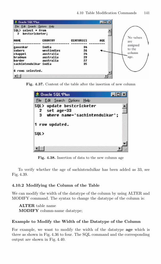
4.10 Table Modification Commands 141
Fig. 4.37. Content of the table after the insertion of new column
Fig. 4.38. Insertion of data to the new column age
To verify whether the age of sachintendulkar has been added as 33, seeFig. 4.39.
4.10.2 Modifying the Column of the Table
We can modify the width of the datatype of the column by using ALTER andMODIFY command. The syntax to change the datatype of the column is:
ALTER table nameMODIFY column-name datatype;
Example to Modify the Width of the Datatype of the Column
For example, we want to modify the width of the datatype age which isthree as shown in Fig. 4.36 to four. The SQL command and the correspondingoutput are shown in Fig. 4.40.
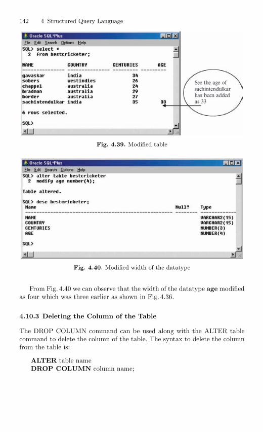
142 4 Structured Query Language
Fig. 4.39. Modified table
Fig. 4.40. Modified width of the datatype
From Fig. 4.40 we can observe that the width of the datatype age modifiedas four which was three earlier as shown in Fig. 4.36.
4.10.3 Deleting the Column of the Table
The DROP COLUMN command can be used along with the ALTER tablecommand to delete the column of the table. The syntax to delete the columnfrom the table is:
ALTER table nameDROP COLUMN column name;
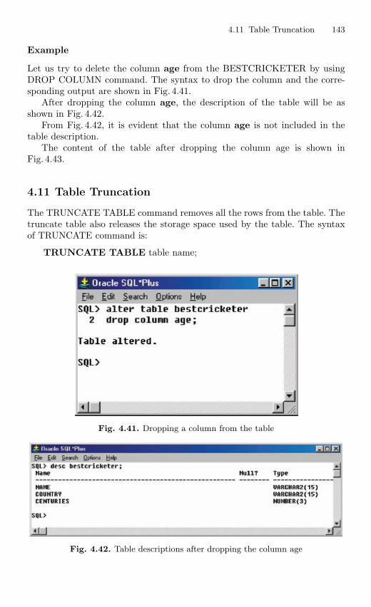
4.11 Table Truncation 143
Example
Let us try to delete the column age from the BESTCRICKETER by usingDROP COLUMN command. The syntax to drop the column and the corre-sponding output are shown in Fig. 4.41.
After dropping the column age, the description of the table will be asshown in Fig. 4.42.
From Fig. 4.42, it is evident that the column age is not included in thetable description.
The content of the table after dropping the column age is shown inFig. 4.43.
4.11 Table Truncation
The TRUNCATE TABLE command removes all the rows from the table. Thetruncate table also releases the storage space used by the table. The syntaxof TRUNCATE command is:
TRUNCATE TABLE table name;
Fig. 4.41. Dropping a column from the table
Fig. 4.42. Table descriptions after dropping the column age
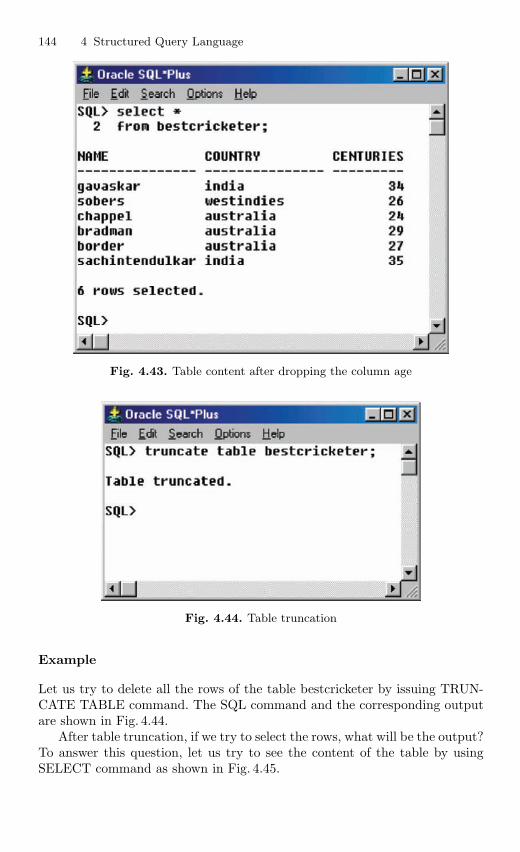
144 4 Structured Query Language
Fig. 4.43. Table content after dropping the column age
Fig. 4.44. Table truncation
Example
Let us try to delete all the rows of the table bestcricketer by issuing TRUN-CATE TABLE command. The SQL command and the corresponding outputare shown in Fig. 4.44.
After table truncation, if we try to select the rows, what will be the output?To answer this question, let us try to see the content of the table by usingSELECT command as shown in Fig. 4.45.
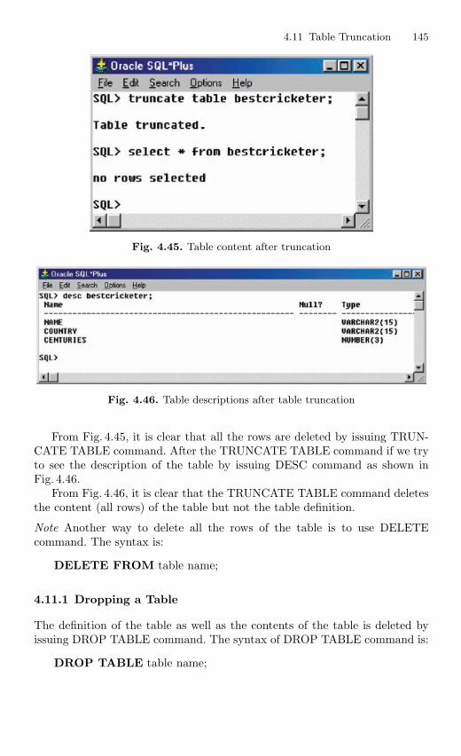
4.11 Table Truncation 145
Fig. 4.45. Table content after truncation
Fig. 4.46. Table descriptions after table truncation
From Fig. 4.45, it is clear that all the rows are deleted by issuing TRUN-CATE TABLE command. After the TRUNCATE TABLE command if we tryto see the description of the table by issuing DESC command as shown inFig. 4.46.
From Fig. 4.46, it is clear that the TRUNCATE TABLE command deletesthe content (all rows) of the table but not the table definition.
Note Another way to delete all the rows of the table is to use DELETEcommand. The syntax is:
DELETE FROM table name;
4.11.1 Dropping a Table
The definition of the table as well as the contents of the table is deleted byissuing DROP TABLE command. The syntax of DROP TABLE command is:
DROP TABLE table name;
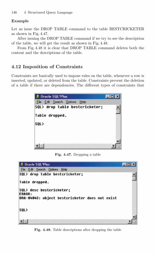
146 4 Structured Query Language
Example
Let us issue the DROP TABLE command to the table BESTCRICKETERas shown in Fig. 4.47.
After issuing the DROP TABLE command if we try to see the descriptionof the table, we will get the result as shown in Fig. 4.48.
From Fig. 4.48 it is clear that DROP TABLE command deletes both thecontent and the descriptions of the table.
4.12 Imposition of Constraints
Constraints are basically used to impose rules on the table, whenever a row isinserted, updated, or deleted from the table. Constraints prevent the deletionof a table if there are dependencies. The different types of constraints that
Fig. 4.47. Dropping a table
Fig. 4.48. Table descriptions after dropping the table
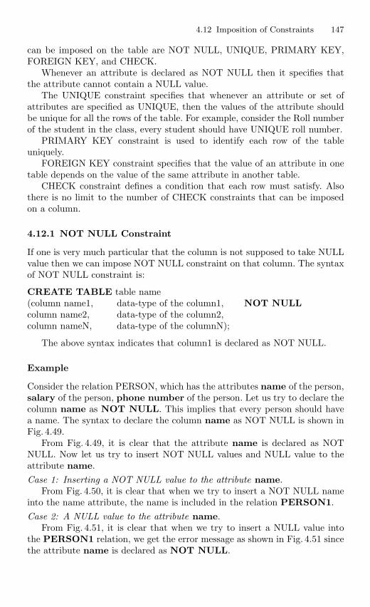
4.12 Imposition of Constraints 147
can be imposed on the table are NOT NULL, UNIQUE, PRIMARY KEY,FOREIGN KEY, and CHECK.
Whenever an attribute is declared as NOT NULL then it specifies thatthe attribute cannot contain a NULL value.
The UNIQUE constraint specifies that whenever an attribute or set ofattributes are specified as UNIQUE, then the values of the attribute shouldbe unique for all the rows of the table. For example, consider the Roll numberof the student in the class, every student should have UNIQUE roll number.
PRIMARY KEY constraint is used to identify each row of the tableuniquely.
FOREIGN KEY constraint specifies that the value of an attribute in onetable depends on the value of the same attribute in another table.
CHECK constraint defines a condition that each row must satisfy. Alsothere is no limit to the number of CHECK constraints that can be imposedon a column.
4.12.1 NOT NULL Constraint
If one is very much particular that the column is not supposed to take NULLvalue then we can impose NOT NULL constraint on that column. The syntaxof NOT NULL constraint is:
CREATE TABLE table name(column name1, data-type of the column1, NOT NULLcolumn name2, data-type of the column2,column nameN, data-type of the columnN);
The above syntax indicates that column1 is declared as NOT NULL.
Example
Consider the relation PERSON, which has the attributes name of the person,salary of the person, phone number of the person. Let us try to declare thecolumn name as NOT NULL. This implies that every person should havea name. The syntax to declare the column name as NOT NULL is shown inFig. 4.49.
From Fig. 4.49, it is clear that the attribute name is declared as NOTNULL. Now let us try to insert NOT NULL values and NULL value to theattribute name.Case 1: Inserting a NOT NULL value to the attribute name.
From Fig. 4.50, it is clear that when we try to insert a NOT NULL nameinto the name attribute, the name is included in the relation PERSON1.Case 2: A NULL value to the attribute name.
From Fig. 4.51, it is clear that when we try to insert a NULL value intothe PERSON1 relation, we get the error message as shown in Fig. 4.51 sincethe attribute name is declared as NOT NULL.
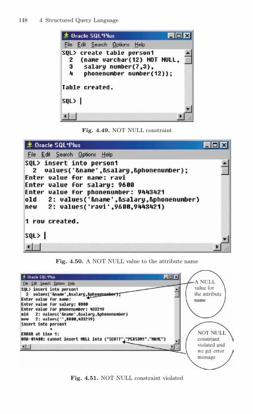
148 4 Structured Query Language
Fig. 4.49. NOT NULL constraint
Fig. 4.50. A NOT NULL value to the attribute name
Fig. 4.51. NOT NULL constraint violated
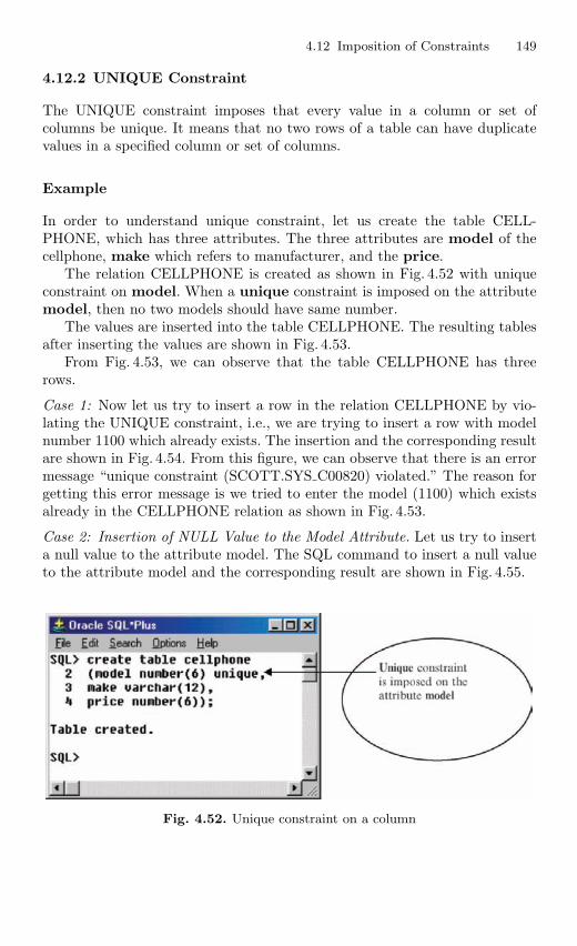
4.12 Imposition of Constraints 149
4.12.2 UNIQUE Constraint
The UNIQUE constraint imposes that every value in a column or set ofcolumns be unique. It means that no two rows of a table can have duplicatevalues in a specified column or set of columns.
Example
In order to understand unique constraint, let us create the table CELL-PHONE, which has three attributes. The three attributes are model of thecellphone, make which refers to manufacturer, and the price.
The relation CELLPHONE is created as shown in Fig. 4.52 with uniqueconstraint on model. When a unique constraint is imposed on the attributemodel, then no two models should have same number.
The values are inserted into the table CELLPHONE. The resulting tablesafter inserting the values are shown in Fig. 4.53.
From Fig. 4.53, we can observe that the table CELLPHONE has threerows.
Case 1: Now let us try to insert a row in the relation CELLPHONE by vio-lating the UNIQUE constraint, i.e., we are trying to insert a row with modelnumber 1100 which already exists. The insertion and the corresponding resultare shown in Fig. 4.54. From this figure, we can observe that there is an errormessage “unique constraint (SCOTT.SYS C00820) violated.” The reason forgetting this error message is we tried to enter the model (1100) which existsalready in the CELLPHONE relation as shown in Fig. 4.53.
Case 2: Insertion of NULL Value to the Model Attribute. Let us try to inserta null value to the attribute model. The SQL command to insert a null valueto the attribute model and the corresponding result are shown in Fig. 4.55.
Fig. 4.52. Unique constraint on a column
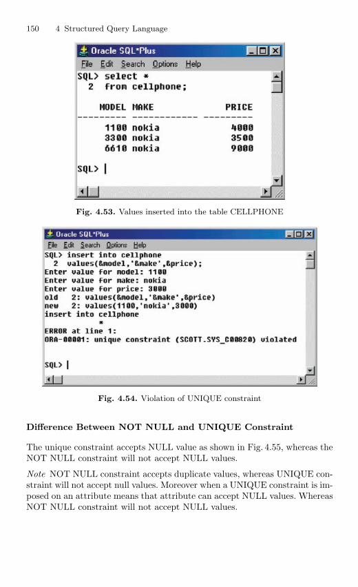
150 4 Structured Query Language
Fig. 4.53. Values inserted into the table CELLPHONE
Fig. 4.54. Violation of UNIQUE constraint
Difference Between NOT NULL and UNIQUE Constraint
The unique constraint accepts NULL value as shown in Fig. 4.55, whereas theNOT NULL constraint will not accept NULL values.
Note NOT NULL constraint accepts duplicate values, whereas UNIQUE con-straint will not accept null values. Moreover when a UNIQUE constraint is im-posed on an attribute means that attribute can accept NULL values. WhereasNOT NULL constraint will not accept NULL values.
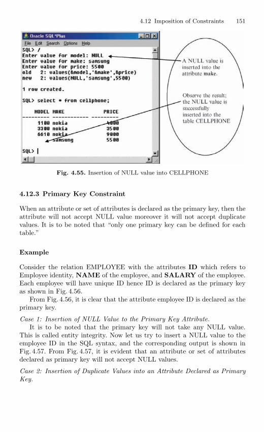
4.12 Imposition of Constraints 151
Fig. 4.55. Insertion of NULL value into CELLPHONE
4.12.3 Primary Key Constraint
When an attribute or set of attributes is declared as the primary key, then theattribute will not accept NULL value moreover it will not accept duplicatevalues. It is to be noted that “only one primary key can be defined for eachtable.”
Example
Consider the relation EMPLOYEE with the attributes ID which refers toEmployee identity, NAME of the employee, and SALARY of the employee.Each employee will have unique ID hence ID is declared as the primary keyas shown in Fig. 4.56.
From Fig. 4.56, it is clear that the attribute employee ID is declared as theprimary key.
Case 1: Insertion of NULL Value to the Primary Key Attribute.It is to be noted that the primary key will not take any NULL value.
This is called entity integrity. Now let us try to insert a NULL value to theemployee ID in the SQL syntax, and the corresponding output is shown inFig. 4.57. From Fig. 4.57, it is evident that an attribute or set of attributesdeclared as primary key will not accept NULL values.
Case 2: Insertion of Duplicate Values into an Attribute Declared as PrimaryKey.
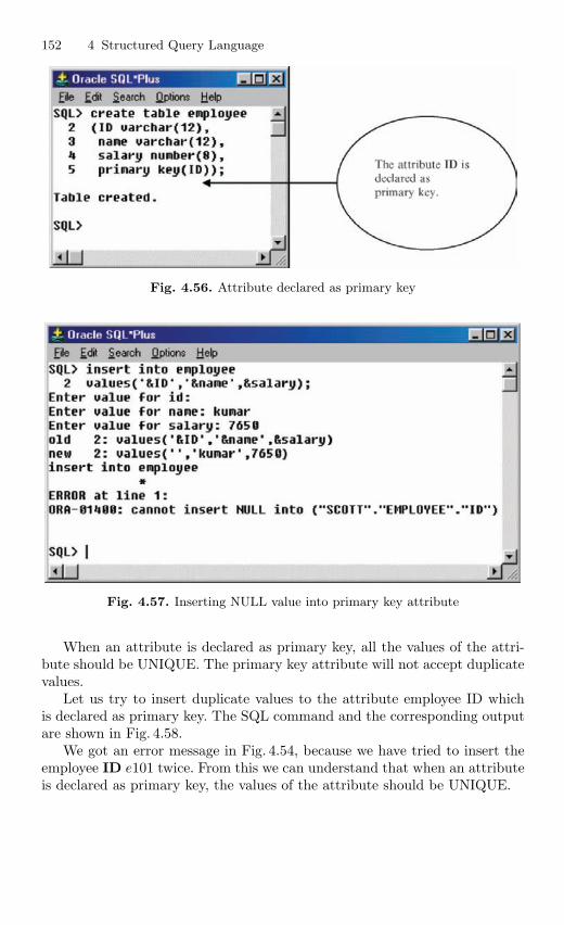
152 4 Structured Query Language
Fig. 4.56. Attribute declared as primary key
Fig. 4.57. Inserting NULL value into primary key attribute
When an attribute is declared as primary key, all the values of the attri-bute should be UNIQUE. The primary key attribute will not accept duplicatevalues.
Let us try to insert duplicate values to the attribute employee ID whichis declared as primary key. The SQL command and the corresponding outputare shown in Fig. 4.58.
We got an error message in Fig. 4.54, because we have tried to insert theemployee ID e101 twice. From this we can understand that when an attributeis declared as primary key, the values of the attribute should be UNIQUE.
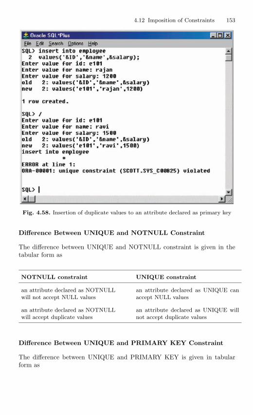
4.12 Imposition of Constraints 153
Fig. 4.58. Insertion of duplicate values to an attribute declared as primary key
Difference Between UNIQUE and NOTNULL Constraint
The difference between UNIQUE and NOTNULL constraint is given in thetabular form as
NOTNULL constraint UNIQUE constraint
an attribute declared as NOTNULLwill not accept NULL values
an attribute declared as UNIQUE canaccept NULL values
an attribute declared as NOTNULLwill accept duplicate values
an attribute declared as UNIQUE willnot accept duplicate values
Difference Between UNIQUE and PRIMARY KEY Constraint
The difference between UNIQUE and PRIMARY KEY is given in tabularform as
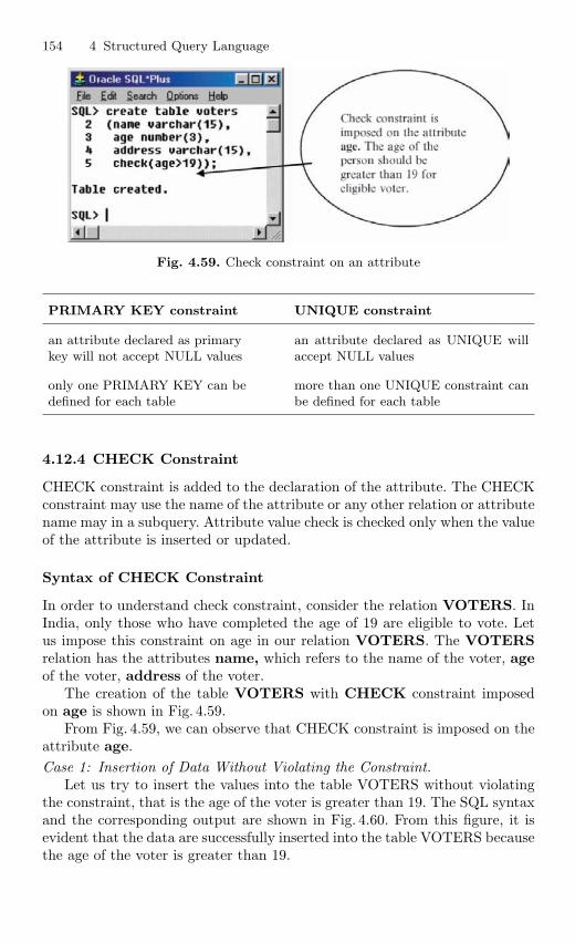
154 4 Structured Query Language
Fig. 4.59. Check constraint on an attribute
PRIMARY KEY constraint UNIQUE constraint
an attribute declared as primarykey will not accept NULL values
an attribute declared as UNIQUE willaccept NULL values
only one PRIMARY KEY can bedefined for each table
more than one UNIQUE constraint canbe defined for each table
4.12.4 CHECK Constraint
CHECK constraint is added to the declaration of the attribute. The CHECKconstraint may use the name of the attribute or any other relation or attributename may in a subquery. Attribute value check is checked only when the valueof the attribute is inserted or updated.
Syntax of CHECK Constraint
In order to understand check constraint, consider the relation VOTERS. InIndia, only those who have completed the age of 19 are eligible to vote. Letus impose this constraint on age in our relation VOTERS. The VOTERSrelation has the attributes name, which refers to the name of the voter, ageof the voter, address of the voter.
The creation of the table VOTERS with CHECK constraint imposedon age is shown in Fig. 4.59.
From Fig. 4.59, we can observe that CHECK constraint is imposed on theattribute age.Case 1: Insertion of Data Without Violating the Constraint.
Let us try to insert the values into the table VOTERS without violatingthe constraint, that is the age of the voter is greater than 19. The SQL syntaxand the corresponding output are shown in Fig. 4.60. From this figure, it isevident that the data are successfully inserted into the table VOTERS becausethe age of the voter is greater than 19.
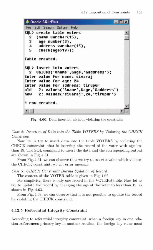
4.12 Imposition of Constraints 155
Fig. 4.60. Data insertion without violating the constraint
Case 2: Insertion of Data into the Table VOTERS by Violating the CHECKConstraint.
Now let us try to insert data into the table VOTERS by violating theCHECK constraint, that is inserting the record of the voter with age lessthan 19. The SQL command to insert the data and the corresponding outputare shown in Fig. 4.61.
From Fig. 4.61, we can observe that we try to insert a value which violatesthe CHECK constraint, we get error message.
Case 3: CHECK Constraint During Updation of Record.The content of the VOTER table is given in Fig. 4.62.For simplicity, there is only one record in the VOTERS table. Now let us
try to update the record by changing the age of the voter to less than 19, asshown in Fig. 4.63.
From Fig. 4.63, we can observe that it is not possible to update the recordby violating the CHECK constraint.
4.12.5 Referential Integrity Constraint
According to referential integrity constraint, when a foreign key in one rela-tion references primary key in another relation, the foreign key value must
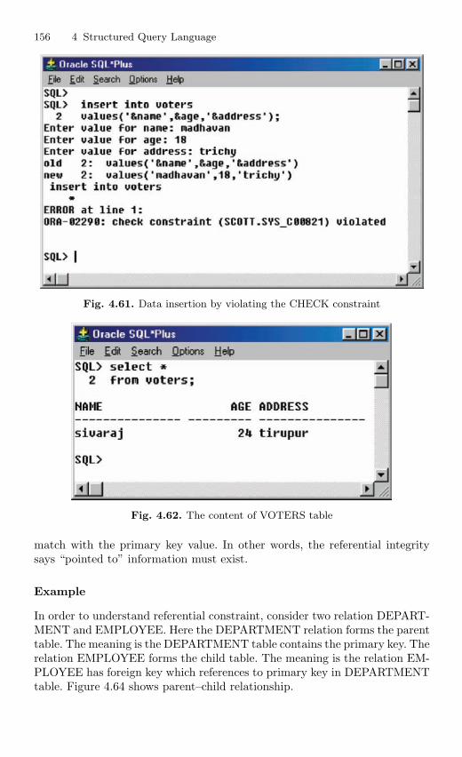
156 4 Structured Query Language
Fig. 4.61. Data insertion by violating the CHECK constraint
Fig. 4.62. The content of VOTERS table
match with the primary key value. In other words, the referential integritysays “pointed to” information must exist.
Example
In order to understand referential constraint, consider two relation DEPART-MENT and EMPLOYEE. Here the DEPARTMENT relation forms the parenttable. The meaning is the DEPARTMENT table contains the primary key. Therelation EMPLOYEE forms the child table. The meaning is the relation EM-PLOYEE has foreign key which references to primary key in DEPARTMENTtable. Figure 4.64 shows parent–child relationship.
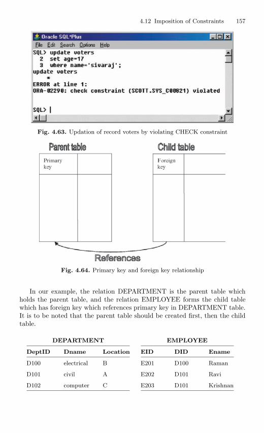
4.12 Imposition of Constraints 157
Fig. 4.63. Updation of record voters by violating CHECK constraint
Fig. 4.64. Primary key and foreign key relationship
In our example, the relation DEPARTMENT is the parent table whichholds the parent table, and the relation EMPLOYEE forms the child tablewhich has foreign key which references primary key in DEPARTMENT table.It is to be noted that the parent table should be created first, then the childtable.
DEPARTMENT
DeptID Dname Location
D100 electrical B
D101 civil A
D102 computer C
EMPLOYEE
EID DID Ename
E201 D100 Raman
E202 D101 Ravi
E203 D101 Krishnan
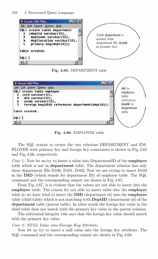
158 4 Structured Query Language
Fig. 4.65. DEPARTMENT table
Fig. 4.66. EMPLOYEE table
The SQL syntax to create the two relations DEPARTMENT and EM-PLOYEE with primary key and foreign key constraints is shown in Fig. 4.65and Fig. 4.66, respectively.
Case 1: Now let us try to insert a value into DepartmentID of the employeetable which is not in department table. The department relation has onlythree department IDs D100, D101, D102. Now we are trying to insert D103in the DID (which stands for department ID) of employee table. The SQLcommand and the corresponding output are shown in Fig. 4.67.
From Fig. 4.67, it is evident that the values are not able to insert into theemployee table. The reason for not able to insert value into the employeetable is: we have tried to insert the DID (department id) into the employeetable (child table) which is not matching with DeptID (department id) of thedepartment table (parent table). In other words the foreign key value in thechild table does not match with the primary key value in the parent relation.
The referential integrity rule says that the foreign key value should matchwith the primary key value.
Case 2: NULL Value into Foreign Key Attribute.Now let us try to insert a null value into the foreign key attribute. The
SQL command and the corresponding output are shown in Fig. 4.68.
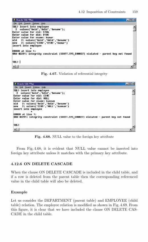
4.12 Imposition of Constraints 159
Fig. 4.67. Violation of referential integrity
Fig. 4.68. NULL value to the foreign key attribute
From Fig. 4.68, it is evident that NULL value cannot be inserted intoforeign key attribute unless it matches with the primary key attribute.
4.12.6 ON DELETE CASCADE
When the clause ON DELETE CASCADE is included in the child table, andif a row is deleted from the parent table then the corresponding referencedvalue in the child table will also be deleted.
Example
Let us consider the DEPARTMENT (parent table) and EMPLOYEE (childtable) relation. The employee relation is modified as shown in Fig. 4.69. Fromthis figure, it is clear that we have included the clause ON DELETE CAS-CADE in the child table.
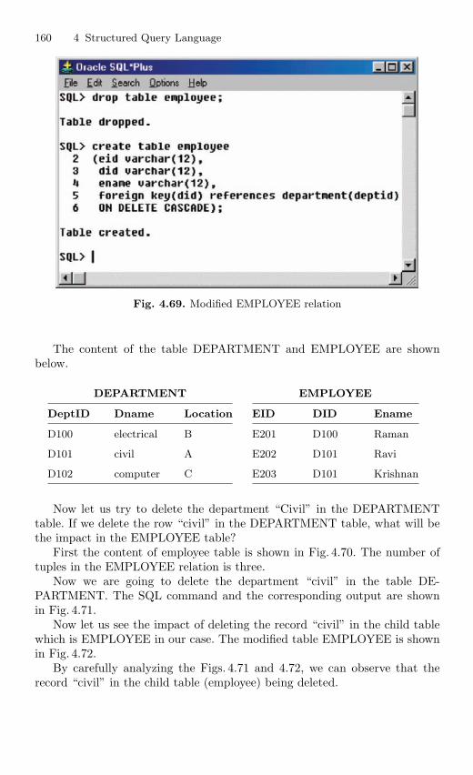
160 4 Structured Query Language
Fig. 4.69. Modified EMPLOYEE relation
The content of the table DEPARTMENT and EMPLOYEE are shownbelow.
DEPARTMENT
DeptID Dname Location
D100 electrical B
D101 civil A
D102 computer C
EMPLOYEE
EID DID Ename
E201 D100 Raman
E202 D101 Ravi
E203 D101 Krishnan
Now let us try to delete the department “Civil” in the DEPARTMENTtable. If we delete the row “civil” in the DEPARTMENT table, what will bethe impact in the EMPLOYEE table?
First the content of employee table is shown in Fig. 4.70. The number oftuples in the EMPLOYEE relation is three.
Now we are going to delete the department “civil” in the table DE-PARTMENT. The SQL command and the corresponding output are shownin Fig. 4.71.
Now let us see the impact of deleting the record “civil” in the child tablewhich is EMPLOYEE in our case. The modified table EMPLOYEE is shownin Fig. 4.72.
By carefully analyzing the Figs. 4.71 and 4.72, we can observe that therecord “civil” in the child table (employee) being deleted.
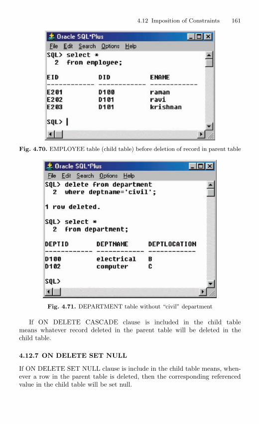
4.12 Imposition of Constraints 161
Fig. 4.70. EMPLOYEE table (child table) before deletion of record in parent table
Fig. 4.71. DEPARTMENT table without “civil” department
If ON DELETE CASCADE clause is included in the child tablemeans whatever record deleted in the parent table will be deleted in thechild table.
4.12.7 ON DELETE SET NULL
If ON DELETE SET NULL clause is include in the child table means, when-ever a row in the parent table is deleted, then the corresponding referencedvalue in the child table will be set null.
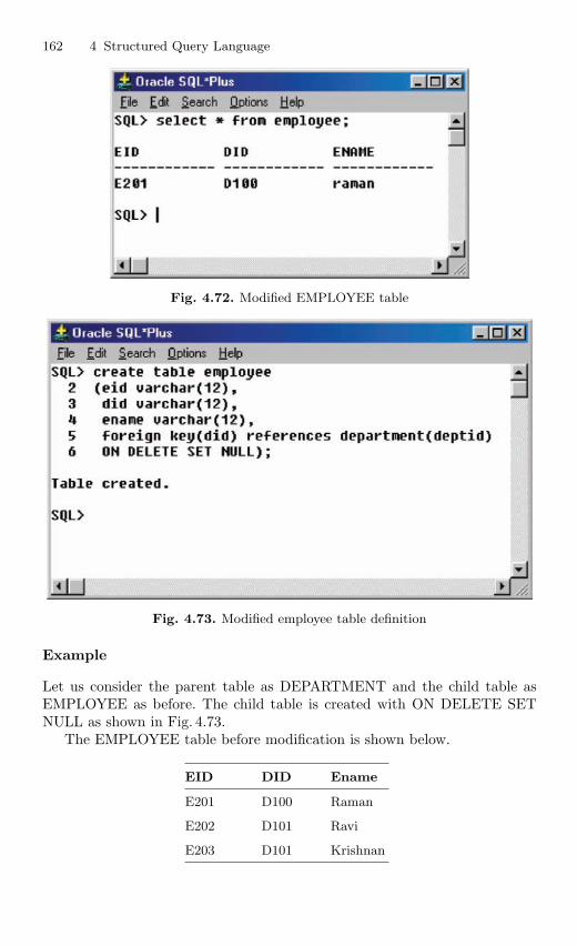
162 4 Structured Query Language
Fig. 4.72. Modified EMPLOYEE table
Fig. 4.73. Modified employee table definition
Example
Let us consider the parent table as DEPARTMENT and the child table asEMPLOYEE as before. The child table is created with ON DELETE SETNULL as shown in Fig. 4.73.
The EMPLOYEE table before modification is shown below.
EID DID Ename
E201 D100 Raman
E202 D101 Ravi
E203 D101 Krishnan
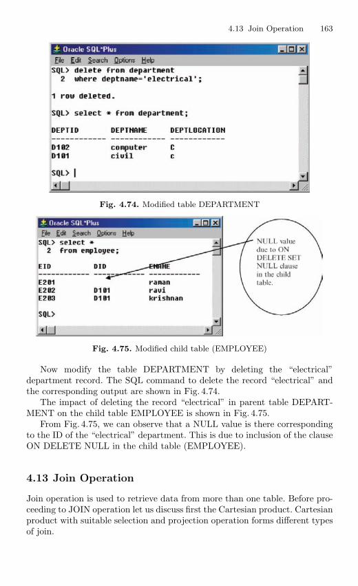
4.13 Join Operation 163
Fig. 4.74. Modified table DEPARTMENT
Fig. 4.75. Modified child table (EMPLOYEE)
Now modify the table DEPARTMENT by deleting the “electrical”department record. The SQL command to delete the record “electrical” andthe corresponding output are shown in Fig. 4.74.
The impact of deleting the record “electrical” in parent table DEPART-MENT on the child table EMPLOYEE is shown in Fig. 4.75.
From Fig. 4.75, we can observe that a NULL value is there correspondingto the ID of the “electrical” department. This is due to inclusion of the clauseON DELETE NULL in the child table (EMPLOYEE).
4.13 Join Operation
Join operation is used to retrieve data from more than one table. Before pro-ceeding to JOIN operation let us discuss first the Cartesian product. Cartesianproduct with suitable selection and projection operation forms different typesof join.

164 4 Structured Query Language
Cartesian Product
If we have two tables A and B, then Cartesian product combines all rows inthe table A with all rows in the table B. If n1 is the number of rows in thetable A and n2 is the number of rows in the table B. Then the Cartesianproduct between A and B will have n1 × n2 rows.
Example
In order to understand Cartesian product, let us consider two relations doctorand nurse. The relation doctor has the attribute ID which refers to identityof the doctor, name and department. Similarly, the relation nurse has threeattributes NID, which refers to nurse identity, name and department. Thedoctor relation is shown in Fig. 4.76.
Similarly the nurse relation is shown in Fig. 4.77.
Fig. 4.76. DOCTOR relation
Fig. 4.77. NURSE relation
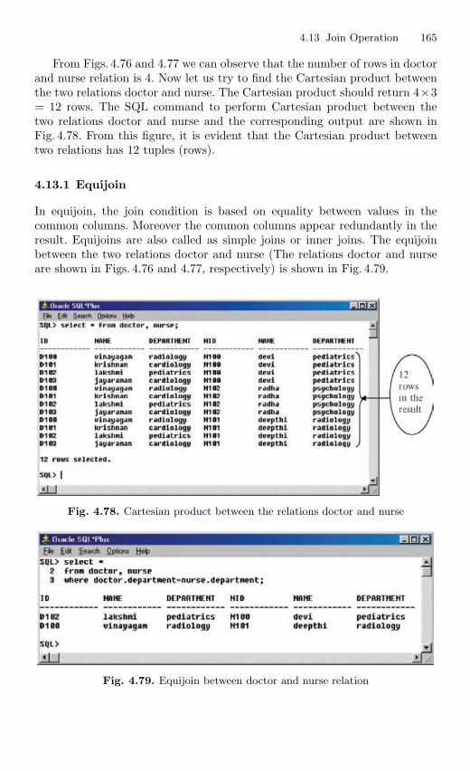
4.13 Join Operation 165
From Figs. 4.76 and 4.77 we can observe that the number of rows in doctorand nurse relation is 4. Now let us try to find the Cartesian product betweenthe two relations doctor and nurse. The Cartesian product should return 4×3= 12 rows. The SQL command to perform Cartesian product between thetwo relations doctor and nurse and the corresponding output are shown inFig. 4.78. From this figure, it is evident that the Cartesian product betweentwo relations has 12 tuples (rows).
4.13.1 Equijoin
In equijoin, the join condition is based on equality between values in thecommon columns. Moreover the common columns appear redundantly in theresult. Equijoins are also called as simple joins or inner joins. The equijoinbetween the two relations doctor and nurse (The relations doctor and nurseare shown in Figs. 4.76 and 4.77, respectively) is shown in Fig. 4.79.
Fig. 4.78. Cartesian product between the relations doctor and nurse
Fig. 4.79. Equijoin between doctor and nurse relation
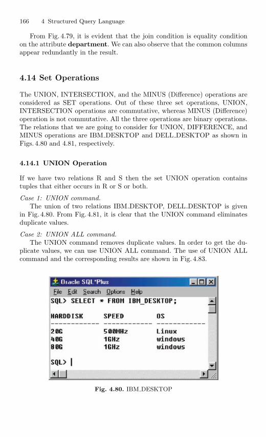
166 4 Structured Query Language
From Fig. 4.79, it is evident that the join condition is equality conditionon the attribute department. We can also observe that the common columnsappear redundantly in the result.
4.14 Set Operations
The UNION, INTERSECTION, and the MINUS (Difference) operations areconsidered as SET operations. Out of these three set operations, UNION,INTERSECTION operations are commutative, whereas MINUS (Difference)operation is not commutative. All the three operations are binary operations.The relations that we are going to consider for UNION, DIFFERENCE, andMINUS operations are IBM DESKTOP and DELL DESKTOP as shown inFigs. 4.80 and 4.81, respectively.
4.14.1 UNION Operation
If we have two relations R and S then the set UNION operation containstuples that either occurs in R or S or both.
Case 1: UNION command.The union of two relations IBM DESKTOP, DELL DESKTOP is given
in Fig. 4.80. From Fig. 4.81, it is clear that the UNION command eliminatesduplicate values.
Case 2: UNION ALL command.The UNION command removes duplicate values. In order to get the du-
plicate values, we can use UNION ALL command. The use of UNION ALLcommand and the corresponding results are shown in Fig. 4.83.
Fig. 4.80. IBM DESKTOP
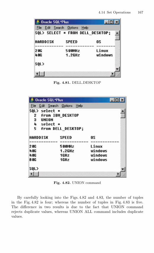
4.14 Set Operations 167
Fig. 4.81. DELL DESKTOP
Fig. 4.82. UNION command
By carefully looking into the Figs. 4.82 and 4.83, the number of tuplesin the Fig. 4.82 is four; whereas the number of tuples in Fig. 4.83 is five.The difference in two results is due to the fact that UNION commandrejects duplicate values, whereas UNION ALL command includes duplicatevalues.
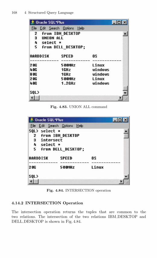
168 4 Structured Query Language
Fig. 4.83. UNION ALL command
Fig. 4.84. INTERSECTION operation
4.14.2 INTERSECTION Operation
The intersection operation returns the tuples that are common to thetwo relations. The intersection of the two relations IBM DESKTOP andDELL DESKTOP is shown in Fig. 4.84.
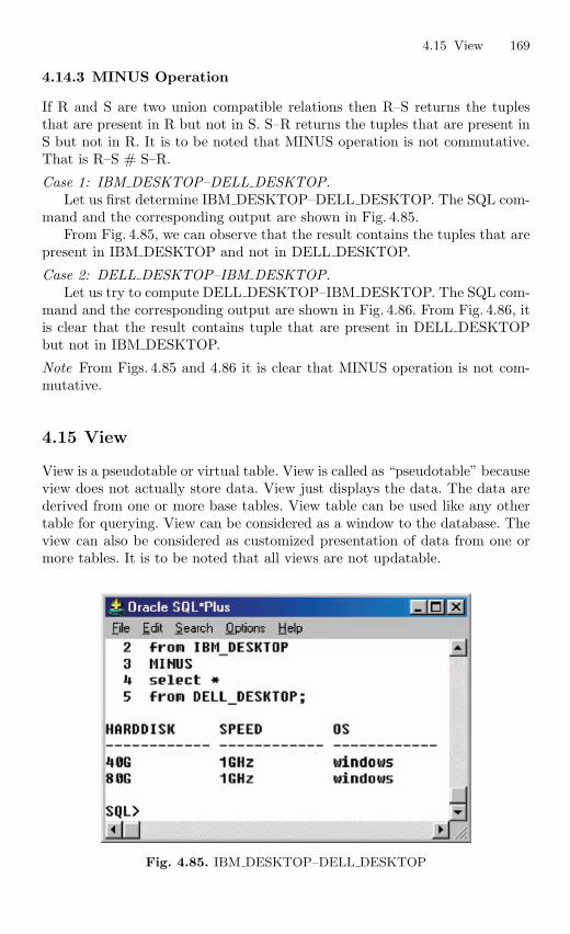
4.15 View 169
4.14.3 MINUS Operation
If R and S are two union compatible relations then R–S returns the tuplesthat are present in R but not in S. S–R returns the tuples that are present inS but not in R. It is to be noted that MINUS operation is not commutative.That is R–S # S–R.
Case 1: IBM DESKTOP–DELL DESKTOP.Let us first determine IBM DESKTOP–DELL DESKTOP. The SQL com-
mand and the corresponding output are shown in Fig. 4.85.From Fig. 4.85, we can observe that the result contains the tuples that are
present in IBM DESKTOP and not in DELL DESKTOP.
Case 2: DELL DESKTOP–IBM DESKTOP.Let us try to compute DELL DESKTOP–IBM DESKTOP. The SQL com-
mand and the corresponding output are shown in Fig. 4.86. From Fig. 4.86, itis clear that the result contains tuple that are present in DELL DESKTOPbut not in IBM DESKTOP.
Note From Figs. 4.85 and 4.86 it is clear that MINUS operation is not com-mutative.
4.15 View
View is a pseudotable or virtual table. View is called as “pseudotable” becauseview does not actually store data. View just displays the data. The data arederived from one or more base tables. View table can be used like any othertable for querying. View can be considered as a window to the database. Theview can also be considered as customized presentation of data from one ormore tables. It is to be noted that all views are not updatable.
Fig. 4.85. IBM DESKTOP–DELL DESKTOP
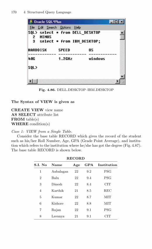
170 4 Structured Query Language
Fig. 4.86. DELL DESKTOP–IBM DESKTOP
The Syntax of VIEW is given as
CREATE VIEW view nameAS SELECT attribute listFROM table(s)WHERE condition(s)
Case 1: VIEW from a Single Table.Consider the base table RECORD which gives the record of the student
such as his/her Roll Number, Age, GPA (Grade Point Average), and institu-tion which refers to the institution where he/she has got the degree (Fig. 4.87).The base table RECORD is shown below.
RECORD
S.I. No Name Age GPA Institution
1 Anbalagan 22 9.2 PSG
2 Balu 22 9.4 PSG
3 Dinesh 22 8.4 CIT
4 Karthik 21 8.5 REC
5 Kumar 22 8.7 MIT
6 Kishore 22 8.8 MIT
7 Rajan 22 9.1 PSG
8 Lavanya 21 9.1 CIT
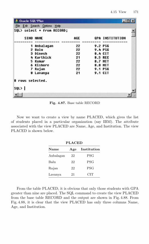
4.15 View 171
Fig. 4.87. Base table RECORD
Now we want to create a view by name PLACED, which gives the listof students placed in a particular organization (say IBM). The attributeassociated with the view PLACED are Name, Age, and Institution. The viewPLACED is shown below.
PLACED
Name Age Institution
Anbalagan 22 PSG
Balu 22 PSG
Rajan 22 PSG
Lavanya 21 CIT
From the table PLACED, it is obvious that only those students with GPAgreater than nine are placed. The SQL command to create the view PLACEDfrom the base table RECORD and the output are shown in Fig. 4.88. FromFig. 4.88, it is clear that the view PLACED has only three columns Name,Age, and Institution.
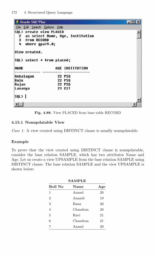
172 4 Structured Query Language
Fig. 4.88. View PLACED from base table RECORD
4.15.1 Nonupdatable View
Case 1: A view created using DISTINCT clause is usually nonupdatable.
Example
To prove that the view created using DISTINCT clause is nonupdatable,consider the base relation SAMPLE, which has two attributes Name andAge. Let us create a view UPSAMPLE from the base relation SAMPLE usingDISTINCT clause. The base relation SAMPLE and the view UPSAMPLE isshown below:
SAMPLE
Roll No Name Age
1 Anand 20
2 Anandi 19
3 Banu 20
4 Chandran 20
5 Ravi 21
6 Chandran 21
7 Anand 20
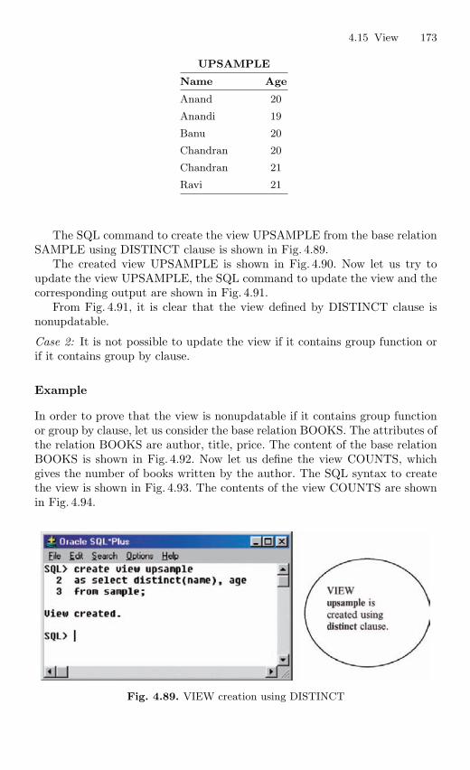
4.15 View 173
UPSAMPLE
Name Age
Anand 20
Anandi 19
Banu 20
Chandran 20
Chandran 21
Ravi 21
The SQL command to create the view UPSAMPLE from the base relationSAMPLE using DISTINCT clause is shown in Fig. 4.89.
The created view UPSAMPLE is shown in Fig. 4.90. Now let us try toupdate the view UPSAMPLE, the SQL command to update the view and thecorresponding output are shown in Fig. 4.91.
From Fig. 4.91, it is clear that the view defined by DISTINCT clause isnonupdatable.
Case 2: It is not possible to update the view if it contains group function orif it contains group by clause.
Example
In order to prove that the view is nonupdatable if it contains group functionor group by clause, let us consider the base relation BOOKS. The attributes ofthe relation BOOKS are author, title, price. The content of the base relationBOOKS is shown in Fig. 4.92. Now let us define the view COUNTS, whichgives the number of books written by the author. The SQL syntax to createthe view is shown in Fig. 4.93. The contents of the view COUNTS are shownin Fig. 4.94.
Fig. 4.89. VIEW creation using DISTINCT
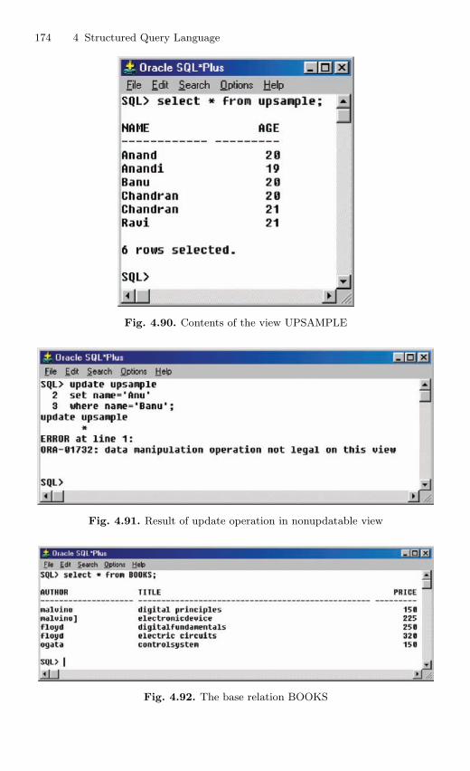
174 4 Structured Query Language
Fig. 4.90. Contents of the view UPSAMPLE
Fig. 4.91. Result of update operation in nonupdatable view
Fig. 4.92. The base relation BOOKS
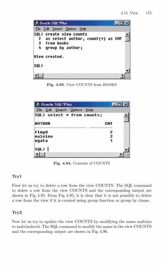
4.15 View 175
Fig. 4.93. View COUNTS from BOOKS
Fig. 4.94. Contents of COUNTS
Try1
First let us try to delete a row from the view COUNTS. The SQL commandto delete a row from the view COUNTS and the corresponding output areshown in Fig. 4.95. From Fig. 4.95, it is clear that it is not possible to deletea row from the view if it is created using group function or group by clause.
Try2
Now let us try to update the view COUNTS by modifying the name malvinoto malvinoleech. The SQL command to modify the name in the view COUNTSand the corresponding output are shown in Fig. 4.96.
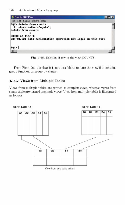
176 4 Structured Query Language
Fig. 4.95. Deletion of row in the view COUNTS
From Fig. 4.96, it is clear it is not possible to update the view if it containsgroup function or group by clause.
4.15.2 Views from Multiple Tables
Views from multiple tables are termed as complex views, whereas views fromsingle table are termed as simple views. View from multiple tables is illustratedas follows:
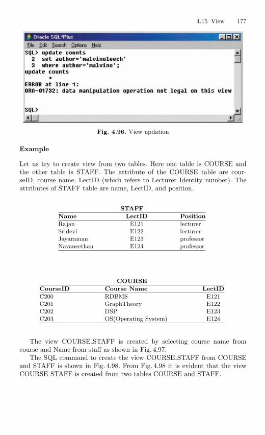
4.15 View 177
Fig. 4.96. View updation
Example
Let us try to create view from two tables. Here one table is COURSE andthe other table is STAFF. The attribute of the COURSE table are cour-seID, course name, LectID (which refers to Lecturer Identity number). Theattributes of STAFF table are name, LectID, and position.
STAFF
Name LectID Position
Rajan E121 lecturerSridevi E122 lecturerJayaraman E123 professorNavaneethan E124 professor
COURSE
CourseID Course Name LectID
C200 RDBMS E121C201 GraphTheory E122C202 DSP E123C203 OS(Operating System) E124
The view COURSE STAFF is created by selecting course name fromcourse and Name from staff as shown in Fig. 4.97.
The SQL command to create the view COURSE STAFF from COURSEand STAFF is shown in Fig. 4.98. From Fig. 4.98 it is evident that the viewCOURSE STAFF is created from two tables COURSE and STAFF.
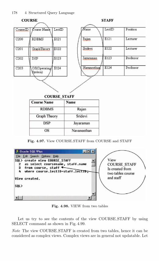
178 4 Structured Query Language
Fig. 4.97. View COURSE STAFF from COURSE and STAFF
Fig. 4.98. VIEW from two tables
Let us try to see the contents of the view COURSE STAFF by usingSELECT command as shown in Fig. 4.99.
Note The view COURSE STAFF is created from two tables, hence it can beconsidered as complex views. Complex views are in general not updatable. Let
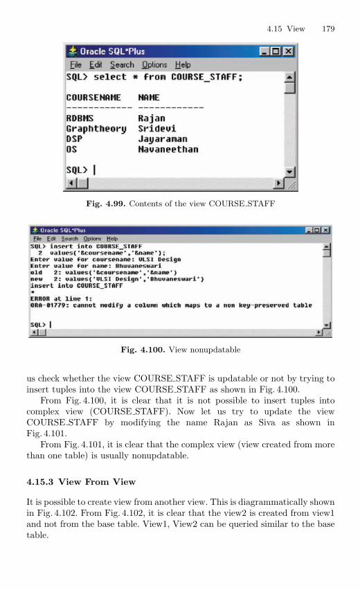
4.15 View 179
Fig. 4.99. Contents of the view COURSE STAFF
Fig. 4.100. View nonupdatable
us check whether the view COURSE STAFF is updatable or not by trying toinsert tuples into the view COURSE STAFF as shown in Fig. 4.100.
From Fig. 4.100, it is clear that it is not possible to insert tuples intocomplex view (COURSE STAFF). Now let us try to update the viewCOURSE STAFF by modifying the name Rajan as Siva as shown inFig. 4.101.
From Fig. 4.101, it is clear that the complex view (view created from morethan one table) is usually nonupdatable.
4.15.3 View From View
It is possible to create view from another view. This is diagrammatically shownin Fig. 4.102. From Fig. 4.102, it is clear that the view2 is created from view1and not from the base table. View1, View2 can be queried similar to the basetable.
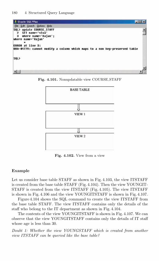
180 4 Structured Query Language
Fig. 4.101. Nonupdatable view COURSE STAFF
Fig. 4.102. View from a view
Example
Let us consider base table STAFF as shown in Fig. 4.103, the view ITSTAFFis created from the base table STAFF (Fig. 4.104). Then the view YOUNGIT-STAFF is created from the view ITSTAFF (Fig. 4.105). The view ITSTAFFis shown in Fig. 4.106 and the view YOUNGITSTAFF is shown in Fig. 4.107.
Figure 4.104 shows the SQL command to create the view ITSTAFF fromthe base table STAFF. The view ITSTAFF contains only the details of thestaff who belong to the IT department as shown in Fig. 4.104.
The contents of the view YOUNGITSTAFF is shown in Fig. 4.107. We canobserve that the view YOUNGITSTAFF contains only the details of IT staffwhose age is less than 30.
Doubt 1: Whether the view YOUNGSTAFF which is created from anotherview ITSTAFF can be queried like the base table?
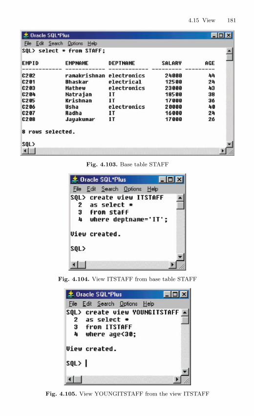
4.15 View 181
Fig. 4.103. Base table STAFF
Fig. 4.104. View ITSTAFF from base table STAFF
Fig. 4.105. View YOUNGITSTAFF from the view ITSTAFF
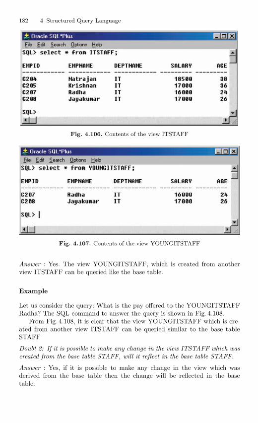
182 4 Structured Query Language
Fig. 4.106. Contents of the view ITSTAFF
Fig. 4.107. Contents of the view YOUNGITSTAFF
Answer : Yes. The view YOUNGITSTAFF, which is created from anotherview ITSTAFF can be queried like the base table.
Example
Let us consider the query: What is the pay offered to the YOUNGITSTAFFRadha? The SQL command to answer the query is shown in Fig. 4.108.
From Fig. 4.108, it is clear that the view YOUNGITSTAFF which is cre-ated from another view ITSTAFF can be queried similar to the base tableSTAFF
Doubt 2: If it is possible to make any change in the view ITSTAFF which wascreated from the base table STAFF, will it reflect in the base table STAFF.
Answer : Yes, if it is possible to make any change in the view which wasderived from the base table then the change will be reflected in the basetable.
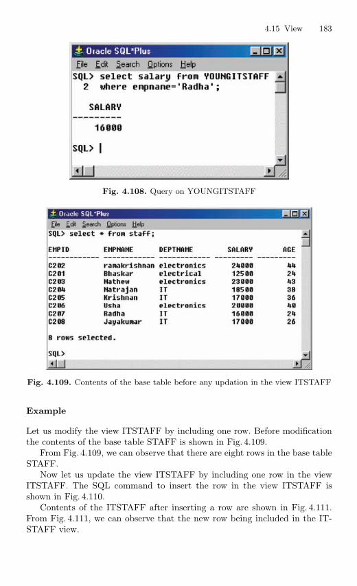
4.15 View 183
Fig. 4.108. Query on YOUNGITSTAFF
Fig. 4.109. Contents of the base table before any updation in the view ITSTAFF
Example
Let us modify the view ITSTAFF by including one row. Before modificationthe contents of the base table STAFF is shown in Fig. 4.109.
From Fig. 4.109, we can observe that there are eight rows in the base tableSTAFF.
Now let us update the view ITSTAFF by including one row in the viewITSTAFF. The SQL command to insert the row in the view ITSTAFF isshown in Fig. 4.110.
Contents of the ITSTAFF after inserting a row are shown in Fig. 4.111.From Fig. 4.111, we can observe that the new row being included in the IT-STAFF view.
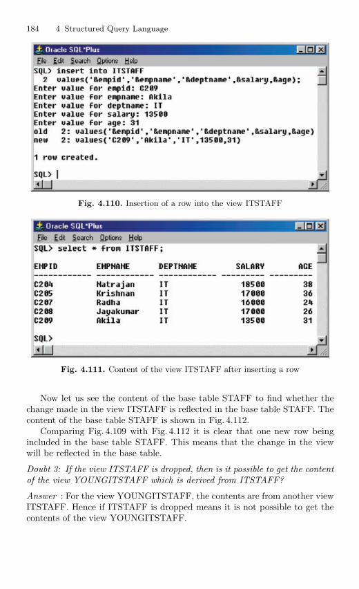
184 4 Structured Query Language
Fig. 4.110. Insertion of a row into the view ITSTAFF
Fig. 4.111. Content of the view ITSTAFF after inserting a row
Now let us see the content of the base table STAFF to find whether thechange made in the view ITSTAFF is reflected in the base table STAFF. Thecontent of the base table STAFF is shown in Fig. 4.112.
Comparing Fig. 4.109 with Fig. 4.112 it is clear that one new row beingincluded in the base table STAFF. This means that the change in the viewwill be reflected in the base table.
Doubt 3: If the view ITSTAFF is dropped, then is it possible to get the contentof the view YOUNGITSTAFF which is derived from ITSTAFF?
Answer : For the view YOUNGITSTAFF, the contents are from another viewITSTAFF. Hence if ITSTAFF is dropped means it is not possible to get thecontents of the view YOUNGITSTAFF.
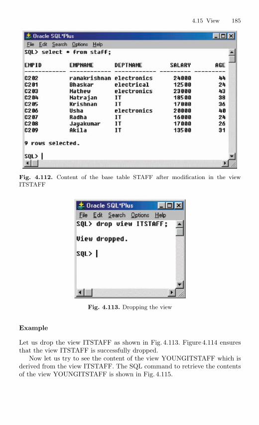
4.15 View 185
Fig. 4.112. Content of the base table STAFF after modification in the viewITSTAFF
Fig. 4.113. Dropping the view
Example
Let us drop the view ITSTAFF as shown in Fig. 4.113. Figure 4.114 ensuresthat the view ITSTAFF is successfully dropped.
Now let us try to see the content of the view YOUNGITSTAFF which isderived from the view ITSTAFF. The SQL command to retrieve the contentsof the view YOUNGITSTAFF is shown in Fig. 4.115.
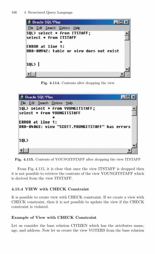
186 4 Structured Query Language
Fig. 4.114. Contents after dropping the view
Fig. 4.115. Contents of YOUNGITSTAFF after dropping the view ITSTAFF
From Fig. 4.115, it is clear that once the view ITSTAFF is dropped thenit is not possible to retrieve the contents of the view YOUNGITSTAFF whichis derived from the view ITSTAFF.
4.15.4 VIEW with CHECK Constraint
It is possible to create view with CHECK constraint. If we create a view withCHECK constraint, then it is not possible to update the view if the CHECKconstraint is violated.
Example of View with CHECK Constraint
Let us consider the base relation CITIZEN which has the attributes name,age, and address. Now let us create the view VOTERS from the base relation
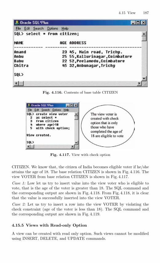
4.15 View 187
Fig. 4.116. Contents of base table CITIZEN
Fig. 4.117. View with check option
CITIZEN. We know that, the citizen of India becomes eligible voter if he/sheattains the age of 18. The base relation CITIZEN is shown in Fig. 4.116. Theview VOTER from base relation CITIZEN is shown in Fig. 4.117.
Case 1: Low let us try to insert value into the view voter who is eligible tovote, that is the age of the voter is greater than 18. The SQL command andthe corresponding output are shown in Fig. 4.118. From Fig. 4.118, it is clearthat the value is successfully inserted into the view VOTER.
Case 2: Let us try to insert a row into the view VOTER by violating thecheck constraint (age of the voter is less than 18). The SQL command andthe corresponding output are shown in Fig. 4.119.
4.15.5 Views with Read-only Option
A view can be created with read only option. Such views cannot be modifiedusing INSERT, DELETE, and UPDATE commands.
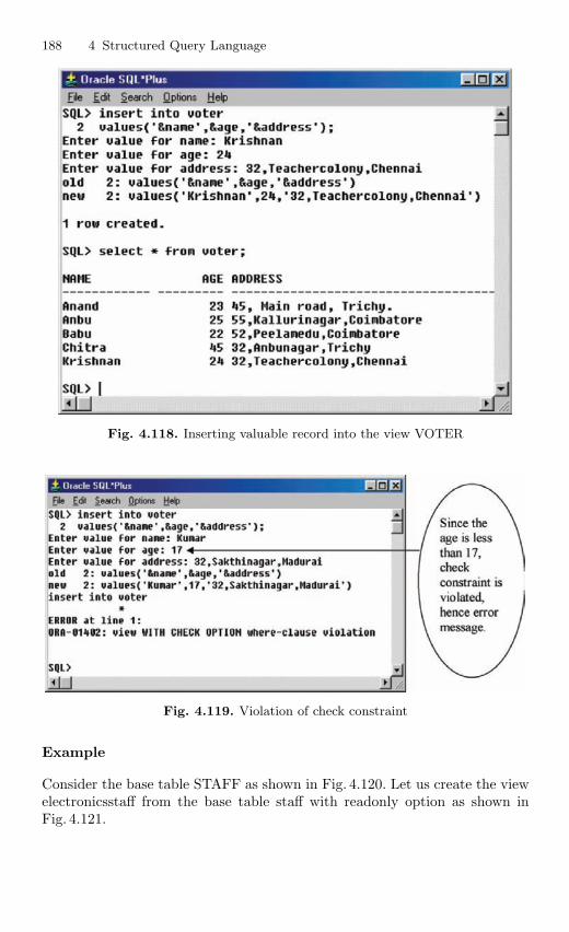
188 4 Structured Query Language
Fig. 4.118. Inserting valuable record into the view VOTER
Fig. 4.119. Violation of check constraint
Example
Consider the base table STAFF as shown in Fig. 4.120. Let us create the viewelectronicsstaff from the base table staff with readonly option as shown inFig. 4.121.
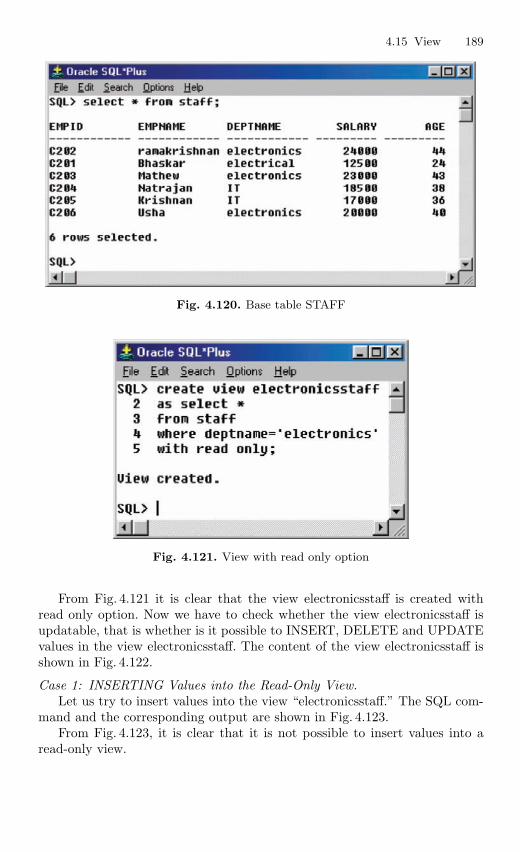
4.15 View 189
Fig. 4.120. Base table STAFF
Fig. 4.121. View with read only option
From Fig. 4.121 it is clear that the view electronicsstaff is created withread only option. Now we have to check whether the view electronicsstaff isupdatable, that is whether is it possible to INSERT, DELETE and UPDATEvalues in the view electronicsstaff. The content of the view electronicsstaff isshown in Fig. 4.122.
Case 1: INSERTING Values into the Read-Only View.Let us try to insert values into the view “electronicsstaff.” The SQL com-
mand and the corresponding output are shown in Fig. 4.123.From Fig. 4.123, it is clear that it is not possible to insert values into a
read-only view.
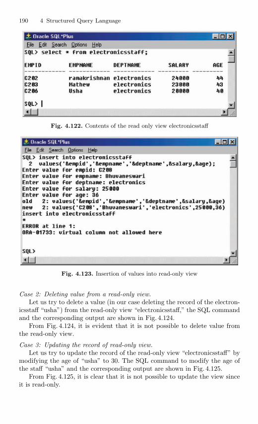
190 4 Structured Query Language
Fig. 4.122. Contents of the read only view electronicsstaff
Fig. 4.123. Insertion of values into read-only view
Case 2: Deleting value from a read-only view.Let us try to delete a value (in our case deleting the record of the electron-
icsstaff “usha”) from the read-only view “electronicsstaff,” the SQL commandand the corresponding output are shown in Fig. 4.124.
From Fig. 4.124, it is evident that it is not possible to delete value fromthe read-only view.
Case 3: Updating the record of read-only view.Let us try to update the record of the read-only view “electronicsstaff” by
modifying the age of “usha” to 30. The SQL command to modify the age ofthe staff “usha” and the corresponding output are shown in Fig. 4.125.
From Fig. 4.125, it is clear that it is not possible to update the view sinceit is read-only.
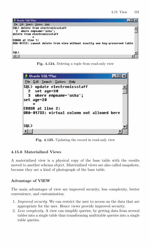
4.15 View 191
Fig. 4.124. Deleting a tuple from read-only view
Fig. 4.125. Updating the record in read-only view
4.15.6 Materialized Views
A materialized view is a physical copy of the base table with the resultsmoved to another schema object. Materialized views are also called snapshots,because they are a kind of photograph of the base table.
Advantage of VIEW
The main advantages of view are improved security, less complexity, betterconvenience, and customization.
1. Improved security. We can restrict the user to access on the data that areappropriate for the user. Hence views provide improved security.
2. Less complexity. A view can simplify queries, by getting data from severaltables into a single table thus transforming multitable queries into a singletable queries.
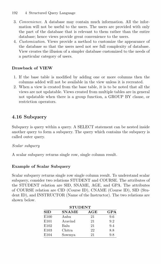
192 4 Structured Query Language
3. Convenience. A database may contain much information. All the infor-mation will not be useful to the users. The users are provided with onlythe part of the database that is relevant to them rather than the entiredatabase; hence views provide great convenience to the users.
4. Customization. Views provide a method to customize the appearance ofthe database so that the users need not see full complexity of database.View creates the illusion of a simpler database customized to the needs ofa particular category of users.
Drawback of VIEW
1. If the base table is modified by adding one or more columns then thecolumns added will not be available in the view unless it is recreated.
2. When a view is created from the base table, it is to be noted that all theviews are not updatable. Views created from multiple tables are in generalnot updatable when there is a group function, a GROUP BY clause, orrestriction operators.
4.16 Subquery
Subquery is query within a query. A SELECT statement can be nested insideanother query to form a subquery. The query which contains the subquery iscalled outer query.
Scalar subquery
A scalar subquery returns single row, single column result.
Example of Scalar Subquery
Scalar subquery returns single row single column result. To understand scalarsubquery, consider two relations STUDENT and COURSE. The attributes ofthe STUDENT relation are SID, SNAME, AGE, and GPA. The attributesof COURSE relation are CID (Course ID), CNAME (Course ID), SID (Stu-dent ID), and INSTRUCTOR (Name of the Instructor). The two relations areshown below.
STUDENT
SID SNAME AGE GPA
E100 Anbu 21 9.6E101 Aravind 21 9.2E102 Balu 21 9.4E103 Chitra 22 8.8E104 Sowmya 21 9.8
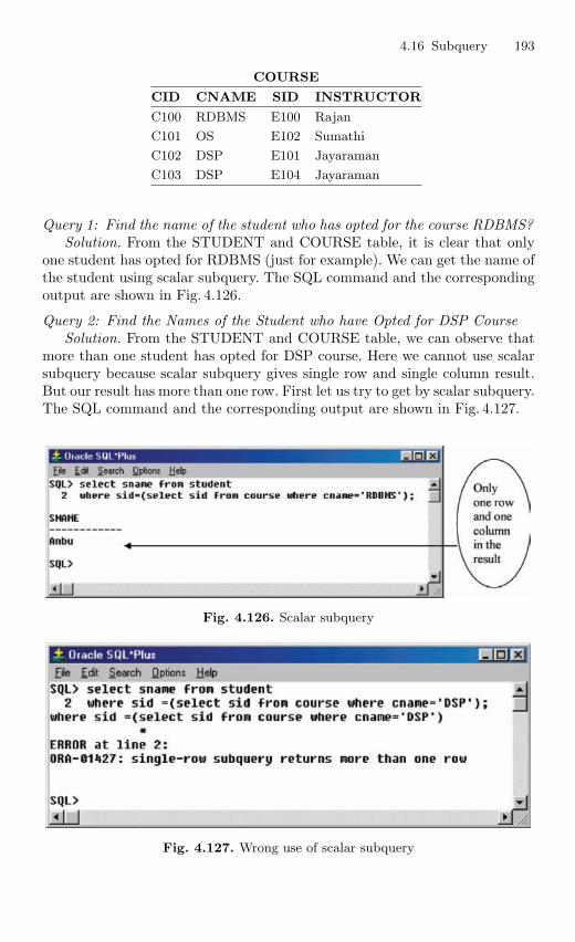
4.16 Subquery 193
COURSE
CID CNAME SID INSTRUCTOR
C100 RDBMS E100 Rajan
C101 OS E102 Sumathi
C102 DSP E101 Jayaraman
C103 DSP E104 Jayaraman
Query 1: Find the name of the student who has opted for the course RDBMS?Solution. From the STUDENT and COURSE table, it is clear that only
one student has opted for RDBMS (just for example). We can get the name ofthe student using scalar subquery. The SQL command and the correspondingoutput are shown in Fig. 4.126.
Query 2: Find the Names of the Student who have Opted for DSP CourseSolution. From the STUDENT and COURSE table, we can observe that
more than one student has opted for DSP course. Here we cannot use scalarsubquery because scalar subquery gives single row and single column result.But our result has more than one row. First let us try to get by scalar subquery.The SQL command and the corresponding output are shown in Fig. 4.127.
Fig. 4.126. Scalar subquery
Fig. 4.127. Wrong use of scalar subquery
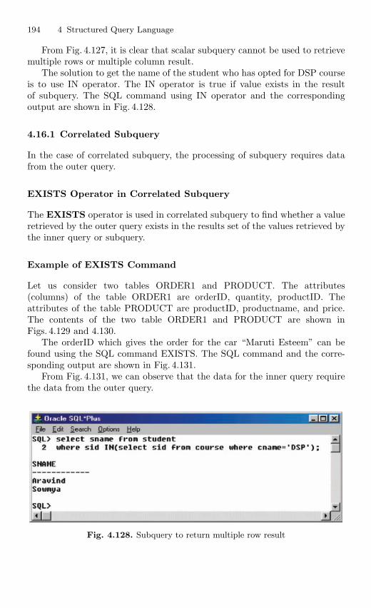
194 4 Structured Query Language
From Fig. 4.127, it is clear that scalar subquery cannot be used to retrievemultiple rows or multiple column result.
The solution to get the name of the student who has opted for DSP courseis to use IN operator. The IN operator is true if value exists in the resultof subquery. The SQL command using IN operator and the correspondingoutput are shown in Fig. 4.128.
4.16.1 Correlated Subquery
In the case of correlated subquery, the processing of subquery requires datafrom the outer query.
EXISTS Operator in Correlated Subquery
The EXISTS operator is used in correlated subquery to find whether a valueretrieved by the outer query exists in the results set of the values retrieved bythe inner query or subquery.
Example of EXISTS Command
Let us consider two tables ORDER1 and PRODUCT. The attributes(columns) of the table ORDER1 are orderID, quantity, productID. Theattributes of the table PRODUCT are productID, productname, and price.The contents of the two table ORDER1 and PRODUCT are shown inFigs. 4.129 and 4.130.
The orderID which gives the order for the car “Maruti Esteem” can befound using the SQL command EXISTS. The SQL command and the corre-sponding output are shown in Fig. 4.131.
From Fig. 4.131, we can observe that the data for the inner query requirethe data from the outer query.
Fig. 4.128. Subquery to return multiple row result
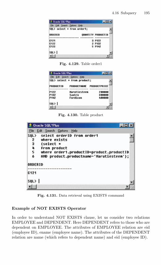
4.16 Subquery 195
Fig. 4.129. Table order1
Fig. 4.130. Table product
Fig. 4.131. Data retrieval using EXISTS command
Example of NOT EXISTS Operator
In order to understand NOT EXISTS clause, let us consider two relationsEMPLOYEE and DEPENDENT. Here DEPENDENT refers to those who aredependent on EMPLOYEE. The attributes of EMPLOYEE relation are eid(employee ID), ename (employee name). The attributes of the DEPENDENTrelation are name (which refers to dependent name) and eid (employee ID).
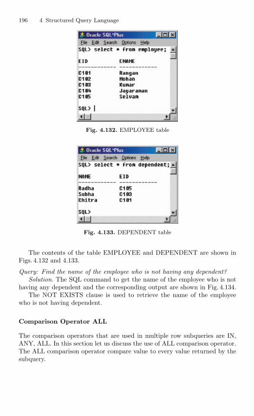
196 4 Structured Query Language
Fig. 4.132. EMPLOYEE table
Fig. 4.133. DEPENDENT table
The contents of the table EMPLOYEE and DEPENDENT are shown inFigs. 4.132 and 4.133.
Query: Find the name of the employee who is not having any dependent?Solution. The SQL command to get the name of the employee who is not
having any dependent and the corresponding output are shown in Fig. 4.134.The NOT EXISTS clause is used to retrieve the name of the employee
who is not having dependent.
Comparison Operator ALL
The comparison operators that are used in multiple row subqueries are IN,ANY, ALL. In this section let us discuss the use of ALL comparison operator.The ALL comparison operator compare value to every value returned by thesubquery.
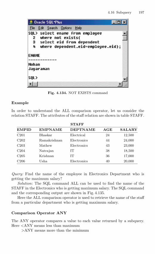
4.16 Subquery 197
Fig. 4.134. NOT EXISTS command
Example
In order to understand the ALL comparison operator, let us consider therelation STAFF. The attributes of the staff relation are shown in table STAFF.
STAFF
EMPID EMPNAME DEPTNAME AGE SALARY
C201 Bhaskar Electrical 24 12,500
C202 Ramakrishnan Electronics 44 24,000
C203 Mathew Electronics 43 23,000
C204 Natrajan IT 38 18,500
C205 Krishnan IT 36 17,000
C206 Usha Electronics 40 20,000
Query: Find the name of the employee in Electronics Department who isgetting the maximum salary?
Solution: The SQL command ALL can be used to find the name of theSTAFF in the Electronics who is getting maximum salary. The SQL commandand the corresponding output are shown in Fig. 4.135.
Here the ALL comparison operator is used to retrieve the name of the stafffrom a particular department who is getting maximum salary.
Comparison Operator ANY
The ANY operator compares a value to each value returned by a subquery.Here <ANY means less than maximum
>ANY means more than the minimum
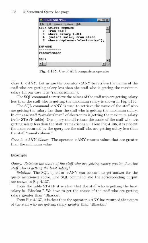
198 4 Structured Query Language
Fig. 4.135. Use of ALL comparison operator
Case 1: <ANY. Let us use the operator <ANY to retrieve the names of thestaff who are getting salary less than the staff who is getting the maximumsalary (in our case it is “ramakrishnan”).
The SQL command to retrieve the names of the staff who are getting salaryless than the staff who is getting the maximum salary is shown in Fig. 4.136.
The SQL command <ANY is used to retrieve the name of the staff whoare getting the salary less than the staff who is getting the maximum salary.In our case staff “ramakrishnan” of electronics is getting the maximum salary(refer STAFF table). Our query should return the name of the staff who aregetting salary less than the staff “ramakrishnan.” From Fig. 4.136, it is evidentthe name returned by the query are the staff who are getting salary less thanthe staff “ramakrishnan.”
Case 2: >ANY Clause. The operator >ANY returns values that are greaterthan the minimum value.
Example
Query: Retrieve the name of the staff who are getting salary greater than thestaff who is getting the least salary?
Solution: The SQL operator >ANY can be used to get answer for thequery mentioned above. The SQL command and the corresponding outputare shown in Fig. 4.137.
From the table STAFF it is clear that the staff who is getting the leastsalary is “Bhaskar.” We have to get the names of the staff who are gettingsalary greater than “Bhaskar.”
From Fig. 4.137, it is clear that the operator >ANY has returned the namesof the staff who are getting salary greater than “Bhaskar.”
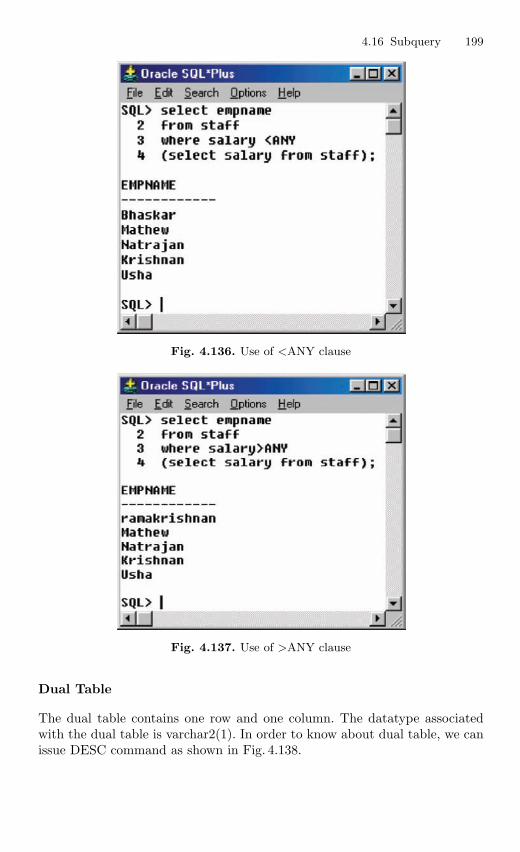
4.16 Subquery 199
Fig. 4.136. Use of <ANY clause
Fig. 4.137. Use of >ANY clause
Dual Table
The dual table contains one row and one column. The datatype associatedwith the dual table is varchar2(1). In order to know about dual table, we canissue DESC command as shown in Fig. 4.138.
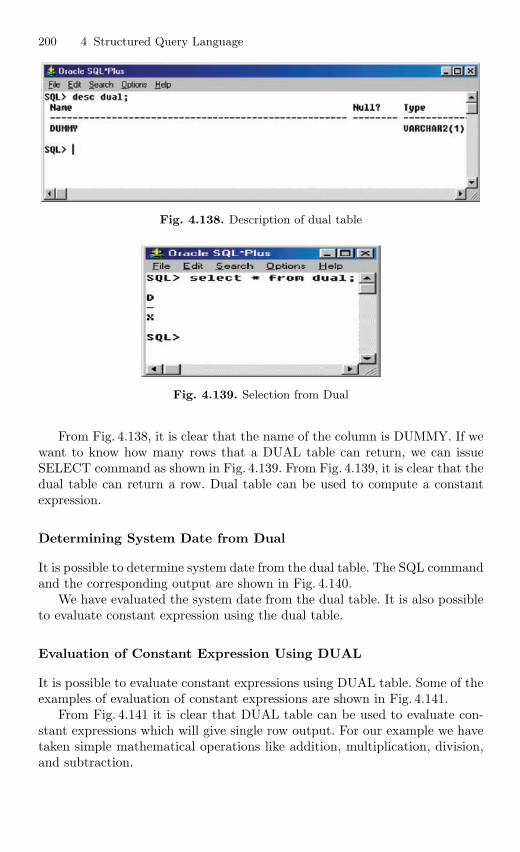
200 4 Structured Query Language
Fig. 4.138. Description of dual table
Fig. 4.139. Selection from Dual
From Fig. 4.138, it is clear that the name of the column is DUMMY. If wewant to know how many rows that a DUAL table can return, we can issueSELECT command as shown in Fig. 4.139. From Fig. 4.139, it is clear that thedual table can return a row. Dual table can be used to compute a constantexpression.
Determining System Date from Dual
It is possible to determine system date from the dual table. The SQL commandand the corresponding output are shown in Fig. 4.140.
We have evaluated the system date from the dual table. It is also possibleto evaluate constant expression using the dual table.
Evaluation of Constant Expression Using DUAL
It is possible to evaluate constant expressions using DUAL table. Some of theexamples of evaluation of constant expressions are shown in Fig. 4.141.
From Fig. 4.141 it is clear that DUAL table can be used to evaluate con-stant expressions which will give single row output. For our example we havetaken simple mathematical operations like addition, multiplication, division,and subtraction.
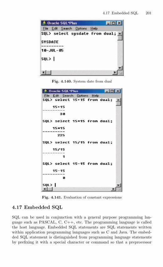
4.17 Embedded SQL 201
Fig. 4.140. System date from dual
Fig. 4.141. Evaluation of constant expressions
4.17 Embedded SQL
SQL can be used in conjunction with a general purpose programming lan-guage such as PASCAL, C, C++, etc. The programming language is calledthe host language. Embedded SQL statements are SQL statements writtenwithin application programming languages such as C and Java. The embed-ded SQL statement is distinguished from programming language statementsby prefixing it with a special character or command so that a preprocessor
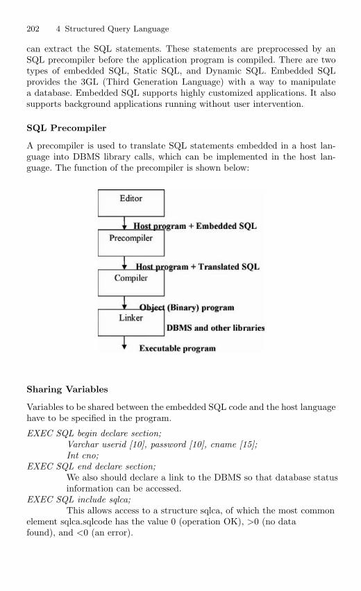
202 4 Structured Query Language
can extract the SQL statements. These statements are preprocessed by anSQL precompiler before the application program is compiled. There are twotypes of embedded SQL, Static SQL, and Dynamic SQL. Embedded SQLprovides the 3GL (Third Generation Language) with a way to manipulatea database. Embedded SQL supports highly customized applications. It alsosupports background applications running without user intervention.
SQL Precompiler
A precompiler is used to translate SQL statements embedded in a host lan-guage into DBMS library calls, which can be implemented in the host lan-guage. The function of the precompiler is shown below:
Sharing Variables
Variables to be shared between the embedded SQL code and the host languagehave to be specified in the program.
EXEC SQL begin declare section;Varchar userid [10], password [10], cname [15];Int cno;
EXEC SQL end declare section;We also should declare a link to the DBMS so that database statusinformation can be accessed.
EXEC SQL include sqlca;This allows access to a structure sqlca, of which the most common
element sqlca.sqlcode has the value 0 (operation OK), >0 (no datafound), and <0 (an error).
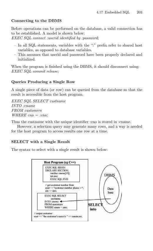
4.17 Embedded SQL 203
Connecting to the DBMS
Before operations can be performed on the database, a valid connection hasto be established. A model is shown below:EXEC SQL connect :userid identified by :password;
– In all SQL statements, variables with the “:” prefix refer to shared hostvariables, as opposed to database variables.
– This assumes that userid and password have been properly declared andinitialized.
When the program is finished using the DBMS, it should disconnect using:EXEC SQL commit release;
Queries Producing a Single Row
A single piece of data (or row) can be queried from the database so that theresult is accessible from the host program.
EXEC SQL SELECT custnameINTO :cnameFROM customersWHERE cno = :cno;
Thus the custname with the unique identifier :cno is stored in :cname.However, a selection query may generate many rows, and a way is needed
for the host program to access results one row at a time.
SELECT with a Single Result
The syntax to select with a single result is shown below:
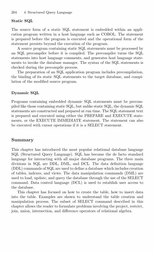
204 4 Structured Query Language
Static SQL
The source form of a static SQL statement is embedded within an appli-cation program written in a host language such as COBOL. The statementis prepared before the program is executed and the operational form of thestatement persists beyond the execution of the program.
A source program containing static SQL statements must be processed byan SQL precompiler before it is compiled. The precompiler turns the SQLstatements into host language comments, and generates host language state-ments to invoke the database manager. The syntax of the SQL statements ischecked during the precompile process.
The preparation of an SQL application program includes precompilation,the binding of its static SQL statements to the target database, and compi-lation of the modified source program.
Dynamic SQL
Programs containing embedded dynamic SQL statements must be precom-piled like those containing static SQL, but unlike static SQL, the dynamic SQLstatements are constructed and prepared at run time. The SQL statement textis prepared and executed using either the PREPARE and EXECUTE state-ments, or the EXECUTE IMMEDIATE statement. The statement can alsobe executed with cursor operations if it is a SELECT statement.
Summary
This chapter has introduced the most popular relational database languageSQL (Structured Query Language). SQL has become the de facto standardlanguage for interacting with all major database programs. The three maindivisions in SQL are DDL, DML, and DCL. The data definition language(DDL) commands of SQL are used to define a database which includes creationof tables, indexes, and views. The data manipulation commands (DML) areused to load, update, and query the database through the use of the SELECTcommand. Data control language (DCL) is used to establish user access tothe database.
This chapter has focused on how to create the table, how to insert datainto the table. Examples are shown to understand the table creation andmanipulation process. The subset of SELECT command described in thischapter allows the reader to formulate problems involving the project, restrict,join, union, intersection, and difference operators of relational algebra.
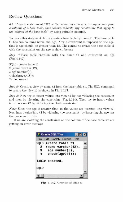
Review Questions 205
Review Questions
4.1. Prove the statement “When the column of a view is directly derived froma column of a base table, that column inherits any constraints that apply tothe column of the base table” by using suitable example.
To prove this statement, let us create a base table by name t1. The base tablet1 has two columns name and age. Now a constraint is imposed on the age,that is age should be greater than 18. The syntax to create the base table t1with the constraint on the age is shown below:
Step 1: Base table creation with the name t1 and constraint on age(Fig. 4.142).
SQL> create table t12 (name varchar(12),3 age number(3),4 check(age>18));Table created.
Step 2: Create a view by name t2 from the base table t1. The SQL commandto create the view t2 is shown in Fig. 4.143.
Step 3: Now try to insert values into view t2 by not violating the constraintand then by violating the constraint (Fig. 4.144). Then try to insert valuesinto the view t2 by violating the check constraint.
Note: Since the age is greater than 18 the values are inserted into view t2.Now insert value into t2 by violating the constraint (by inserting the age lessthan or equal to 18).
If we are violating the constraints on the column of the base table we aregetting an error message.
Fig. 4.142. Creation of table t1
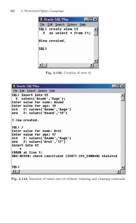
206 4 Structured Query Language
Fig. 4.143. Creation of view t2
Fig. 4.144. Insertion of values into t2 without violating and violating constraint
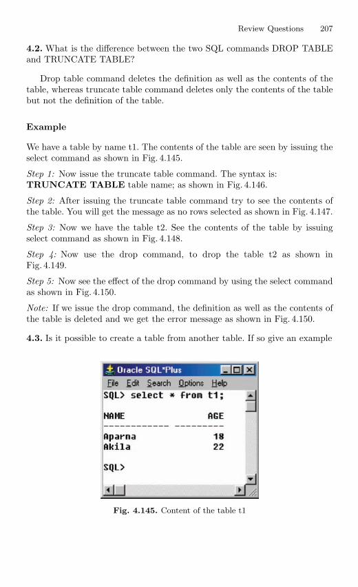
Review Questions 207
4.2. What is the difference between the two SQL commands DROP TABLEand TRUNCATE TABLE?
Drop table command deletes the definition as well as the contents of thetable, whereas truncate table command deletes only the contents of the tablebut not the definition of the table.
Example
We have a table by name t1. The contents of the table are seen by issuing theselect command as shown in Fig. 4.145.
Step 1: Now issue the truncate table command. The syntax is:TRUNCATE TABLE table name; as shown in Fig. 4.146.
Step 2: After issuing the truncate table command try to see the contents ofthe table. You will get the message as no rows selected as shown in Fig. 4.147.
Step 3: Now we have the table t2. See the contents of the table by issuingselect command as shown in Fig. 4.148.
Step 4: Now use the drop command, to drop the table t2 as shown inFig. 4.149.
Step 5: Now see the effect of the drop command by using the select commandas shown in Fig. 4.150.
Note: If we issue the drop command, the definition as well as the contents ofthe table is deleted and we get the error message as shown in Fig. 4.150.
4.3. Is it possible to create a table from another table. If so give an example
Fig. 4.145. Content of the table t1
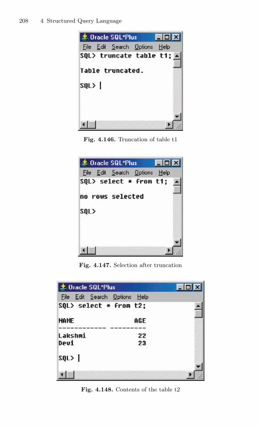
208 4 Structured Query Language
Fig. 4.146. Truncation of table t1
Fig. 4.147. Selection after truncation
Fig. 4.148. Contents of the table t2
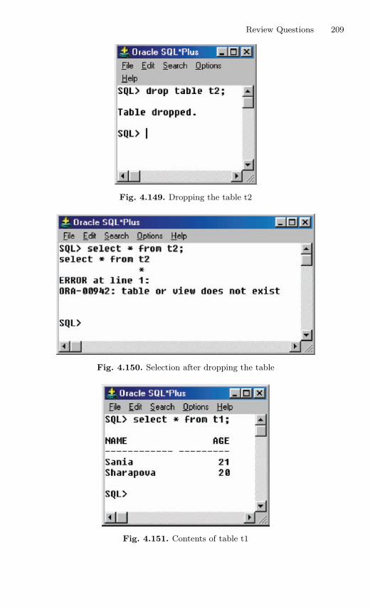
Review Questions 209
Fig. 4.149. Dropping the table t2
Fig. 4.150. Selection after dropping the table
Fig. 4.151. Contents of table t1
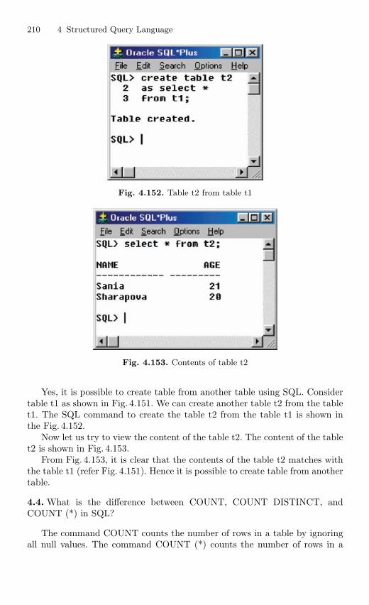
210 4 Structured Query Language
Fig. 4.152. Table t2 from table t1
Fig. 4.153. Contents of table t2
Yes, it is possible to create table from another table using SQL. Considertable t1 as shown in Fig. 4.151. We can create another table t2 from the tablet1. The SQL command to create the table t2 from the table t1 is shown inthe Fig. 4.152.
Now let us try to view the content of the table t2. The content of the tablet2 is shown in Fig. 4.153.
From Fig. 4.153, it is clear that the contents of the table t2 matches withthe table t1 (refer Fig. 4.151). Hence it is possible to create table from anothertable.
4.4. What is the difference between COUNT, COUNT DISTINCT, andCOUNT (*) in SQL?
The command COUNT counts the number of rows in a table by ignoringall null values. The command COUNT (*) counts the number of rows in a
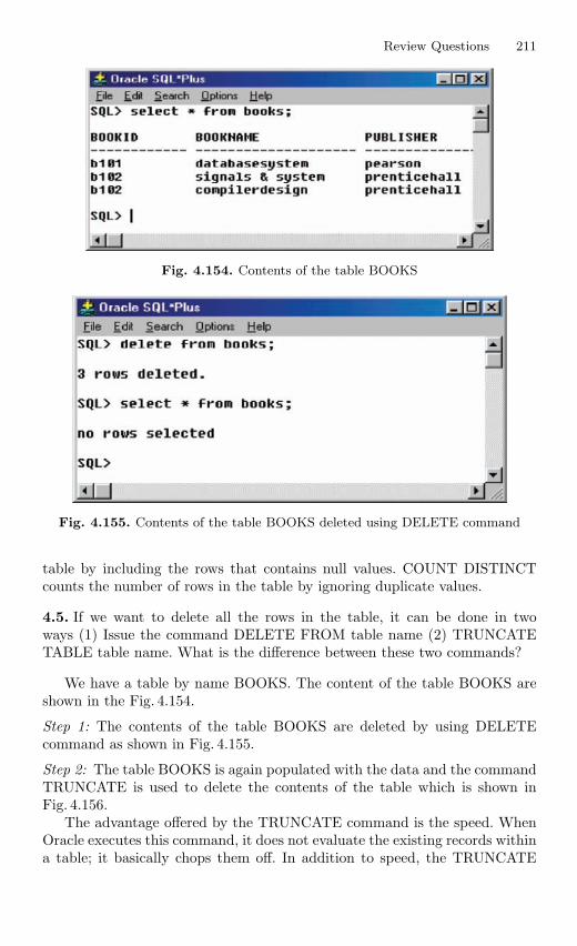
Review Questions 211
Fig. 4.154. Contents of the table BOOKS
Fig. 4.155. Contents of the table BOOKS deleted using DELETE command
table by including the rows that contains null values. COUNT DISTINCTcounts the number of rows in the table by ignoring duplicate values.
4.5. If we want to delete all the rows in the table, it can be done in twoways (1) Issue the command DELETE FROM table name (2) TRUNCATETABLE table name. What is the difference between these two commands?
We have a table by name BOOKS. The content of the table BOOKS areshown in the Fig. 4.154.
Step 1: The contents of the table BOOKS are deleted by using DELETEcommand as shown in Fig. 4.155.
Step 2: The table BOOKS is again populated with the data and the commandTRUNCATE is used to delete the contents of the table which is shown inFig. 4.156.
The advantage offered by the TRUNCATE command is the speed. WhenOracle executes this command, it does not evaluate the existing records withina table; it basically chops them off. In addition to speed, the TRUNCATE
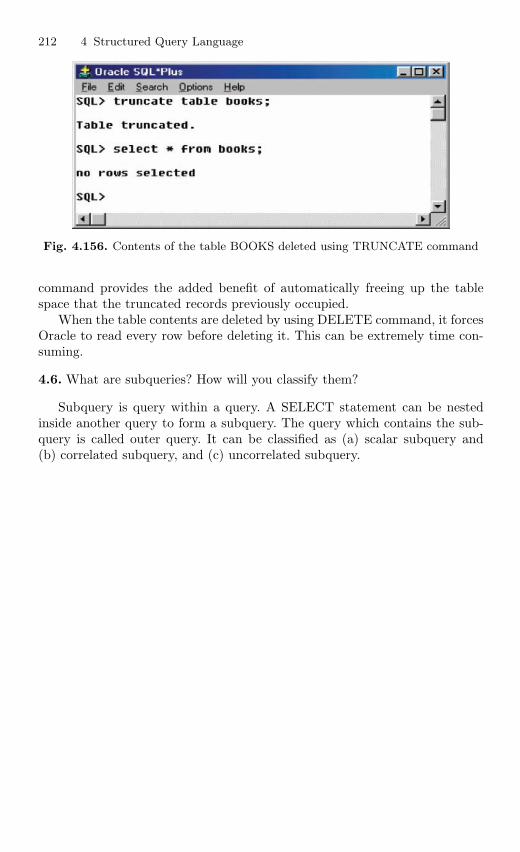
212 4 Structured Query Language
Fig. 4.156. Contents of the table BOOKS deleted using TRUNCATE command
command provides the added benefit of automatically freeing up the tablespace that the truncated records previously occupied.
When the table contents are deleted by using DELETE command, it forcesOracle to read every row before deleting it. This can be extremely time con-suming.
4.6. What are subqueries? How will you classify them?
Subquery is query within a query. A SELECT statement can be nestedinside another query to form a subquery. The query which contains the sub-query is called outer query. It can be classified as (a) scalar subquery and(b) correlated subquery, and (c) uncorrelated subquery.
5
PL/SQL
Learning Objectives. This chapter focuses on the shortcomings of SQL and howit is overcome by PL/SQL. An introduction to PL/SQL is given in this chapter. Aftercompleting this chapter the reader should be familiar with the following concepts inPL/SQL.
– Structure of PL/SQL– PL/SQL language elements– Control structure in PL/SQL– Steps to create PL/SQL program– Concept of CURSOR– Basic concepts related to Procedure, Functions– Basic concept of Trigger
5.1 Introduction
PL/SQL stands for Procedural Language/Structured Query Language, whichis provided by Oracle as a procedural extension to SQL. SQL is a declara-tive language. In SQL, the statements have no control to the program andcan be executed in any order. PL/SQL, on the other hand, is a procedurallanguage that makes up for all the missing elements in SQL. PL/SQL arosefrom the desire of programmers to have a language structure that was morefamiliar than SQL’s purely declarative nature.
5.2 Shortcomings in SQL
We know, SQL is a powerful tool for accessing the database but it suffers fromsome deficiencies as follows:
(a) SQL statements can be executed only one at a time. Every time to executea SQL statement, a call is made to Oracle engine, thus it results in anincrease in database overheads.
S. Sumathi: PL/SQL, Studies in Computational Intelligence (SCI) 47, 213–282 (2007)
www.springerlink.com c© Springer-Verlag Berlin Heidelberg 2007
214 5 PL/SQL
(b) While processing an SQL statement, if an error occurs, Oracle generatesits own error message, which is sometimes difficult to understand. If auser wants to display some other meaningful error message, SQL does nothave provision for that.
(c) SQL is not able to do the conditional query on RDBMS, this means onecannot use the conditions like if . . . then, in a SQL statement. Also loopingfacility (repeating a set of instructions) is not provided by SQL.
5.3 Structure of PL/SQL
PL/SQL is a 4GL (fourth generation) programming language. It offers all fea-tures of advanced programming language such as portability, security, dataencapsulation, information hiding, etc. A PL/SQL program may consist ofmore than one SQL statements, while execution of a PL/SQL program makesonly one call to Oracle engine, thus it helps in reducing the database over-heads. With PL/SQL, one can use the SQL statements together with the con-trol structures (like if . . . then) for data manipulation. Besides this, user candefine his/her own error messages to display. Thus we can say that PL/SQLcombines the data manipulation power of SQL with data processing power ofprocedural language.
PL/SQL is a block structured language. This means a PL/SQL programis made up of blocks, where block is a smallest piece of PL/SQL code havinglogically related statements and declarations. A block consists of three sectionsnamely:
Declare, Begin, and Exception followed by an End statement. We will seethe different sections of PL/SQL block.
Declare Section
Declare section declares the variables, constants, processes, functions, etc., tobe used in the other parts of program. It is an optional section.
Begin Section
It is the executable section. It consists of a set of SQL and PL/SQL statements,which is executed when PL/SQL block runs. It is a compulsory section.
Exception Section
This section handles the errors, which occurs during execution of the PL/SQLblock. This section allows the user to define his/her own error messages. Thissection executes only when an error occurs. It is an optional section.
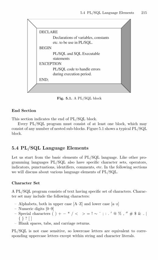
5.4 PL/SQL Language Elements 215
DECLARE
BEGIN
EXCEPTION
END;
Declarations of variables, constantsetc. to be use in PL/SQL.
PL/SQL and SQL Executablestatements
PL/SQL code to handle errorsduring execution period.
Fig. 5.1. A PL/SQL block
End Section
This section indicates the end of PL/SQL block.Every PL/SQL program must consist of at least one block, which may
consist of any number of nested sub-blocks. Figure 5.1 shows a typical PL/SQLblock.
5.4 PL/SQL Language Elements
Let us start from the basic elements of PL/SQL language. Like other pro-gramming languages PL/SQL also have specific character sets, operators,indicators, punctuations, identifiers, comments, etc. In the following sectionswe will discuss about various language elements of PL/SQL.
Character Set
A PL/SQL program consists of text having specific set of characters. Charac-ter set may include the following characters:
– Alphabets, both in upper case [A–Z] and lower case [a–z]– Numeric digits [0–9]– Special characters ( ) + − * / < > = ! ∼ ˆ ; : . ′ @ % , ′′ # $ & |
? [ ]– Blank spaces, tabs, and carriage returns.
PL/SQL is not case sensitive, so lowercase letters are equivalent to corre-sponding uppercase letters except within string and character literals.
216 5 PL/SQL
Lexical Units
A line of PL/SQL program contains groups of characters known as lexicalunits, which can be classified as follows:
– Delimiters– Identifiers– Literals– Comments
Delimiters
A delimiter is a simple or compound symbol that has a special meaning toPL/SQL. Simple symbol consists of one character, while compound symbolconsists of more than one character. For example, to perform the addition andexponentiation operation in PL/SQL, simple symbol delimiter + and com-pound symbol delimiter ** is used, respectively. PL/SQL supports followingsimple symbol delimiters:
+ − * / = > < ; % ′ , ( ) @ : ′′
Compound symbol delimiters legal in PL/SQL are as follows:<> ! =∼= ˆ= <=>= := ** .. || << >>In the following sections we will discuss about these delimiters.
Identifiers
Identifiers are used in the PL/SQL programs to name the PL/SQL programitems as constants, variables, cursors, cursor variables, subprograms, etc.
Identifiers can consists of alphabets, numerals, dollar signs, underscores,and number signs only. Any other characters like hyphens, slashes, blankspaces, etc. are illegal. An identifier must begin with an alphabetic letteroptionally followed by one or more characters (permissible in identifier). Anidentifier cannot contain more than 30 characters.
Example
Some of the valid identifiers are as follows:
A – Identifier may consist of a single characterA1 – identifier may consist of numerals after first characterShare$price – dollar sign is permittede mail – under score is permittedphone# – number sign is permitted
The following identifiers are illegal:
mine&yours – ampersand is illegaldebit-amount – hyphen is illegalon/off – slash is illegaluser id – space is illegal
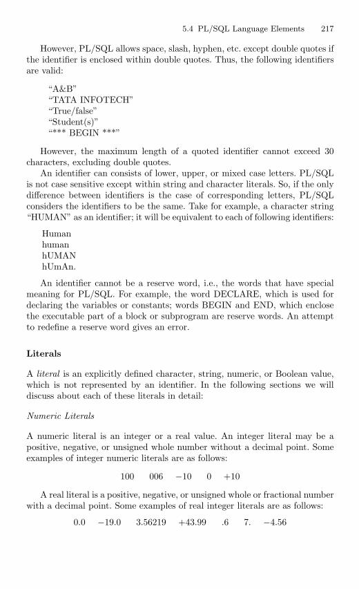
5.4 PL/SQL Language Elements 217
However, PL/SQL allows space, slash, hyphen, etc. except double quotes ifthe identifier is enclosed within double quotes. Thus, the following identifiersare valid:
“A&B”“TATA INFOTECH”“True/false”“Student(s)”“*** BEGIN ***”
However, the maximum length of a quoted identifier cannot exceed 30characters, excluding double quotes.
An identifier can consists of lower, upper, or mixed case letters. PL/SQLis not case sensitive except within string and character literals. So, if the onlydifference between identifiers is the case of corresponding letters, PL/SQLconsiders the identifiers to be the same. Take for example, a character string“HUMAN” as an identifier; it will be equivalent to each of following identifiers:
HumanhumanhUMANhUmAn.
An identifier cannot be a reserve word, i.e., the words that have specialmeaning for PL/SQL. For example, the word DECLARE, which is used fordeclaring the variables or constants; words BEGIN and END, which enclosethe executable part of a block or subprogram are reserve words. An attemptto redefine a reserve word gives an error.
Literals
A literal is an explicitly defined character, string, numeric, or Boolean value,which is not represented by an identifier. In the following sections we willdiscuss about each of these literals in detail:
Numeric Literals
A numeric literal is an integer or a real value. An integer literal may be apositive, negative, or unsigned whole number without a decimal point. Someexamples of integer numeric literals are as follows:
100 006 −10 0 +10
A real literal is a positive, negative, or unsigned whole or fractional numberwith a decimal point. Some examples of real integer literals are as follows:
0.0 −19.0 3.56219 +43.99 .6 7. −4.56
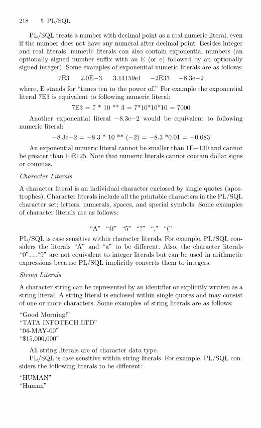
218 5 PL/SQL
PL/SQL treats a number with decimal point as a real numeric literal, evenif the number does not have any numeral after decimal point. Besides integerand real literals, numeric literals can also contain exponential numbers (anoptionally signed number suffix with an E (or e) followed by an optionallysigned integer). Some examples of exponential numeric literals are as follows:
7E3 2.0E−3 3.14159e1 −2E33 −8.3e−2
where, E stands for “times ten to the power of.” For example the exponentialliteral 7E3 is equivalent to following numeric literal:
7E3 = 7 * 10 ** 3 = 7*10*10*10 = 7000
Another exponential literal −8.3e−2 would be equivalent to followingnumeric literal:
−8.3e−2 = −8.3 * 10 ** (−2) = −8.3 *0.01 = −0.083
An exponential numeric literal cannot be smaller than 1E−130 and cannotbe greater than 10E125. Note that numeric literals cannot contain dollar signsor commas.
Character Literals
A character literal is an individual character enclosed by single quotes (apos-trophes). Character literals include all the printable characters in the PL/SQLcharacter set: letters, numerals, spaces, and special symbols. Some examplesof character literals are as follows:
“A” “@” “5” “?” “,” “(”
PL/SQL is case sensitive within character literals. For example, PL/SQL con-siders the literals “A” and “a” to be different. Also, the character literals“0”. . .“9” are not equivalent to integer literals but can be used in arithmeticexpressions because PL/SQL implicitly converts them to integers.
String Literals
A character string can be represented by an identifier or explicitly written as astring literal. A string literal is enclosed within single quotes and may consistof one or more characters. Some examples of string literals are as follows:
“Good Morning!”“TATA INFOTECH LTD”“04-MAY-00”“$15,000,000”
All string literals are of character data type.PL/SQL is case sensitive within string literals. For example, PL/SQL con-
siders the following literals to be different:
“HUMAN”“Human”
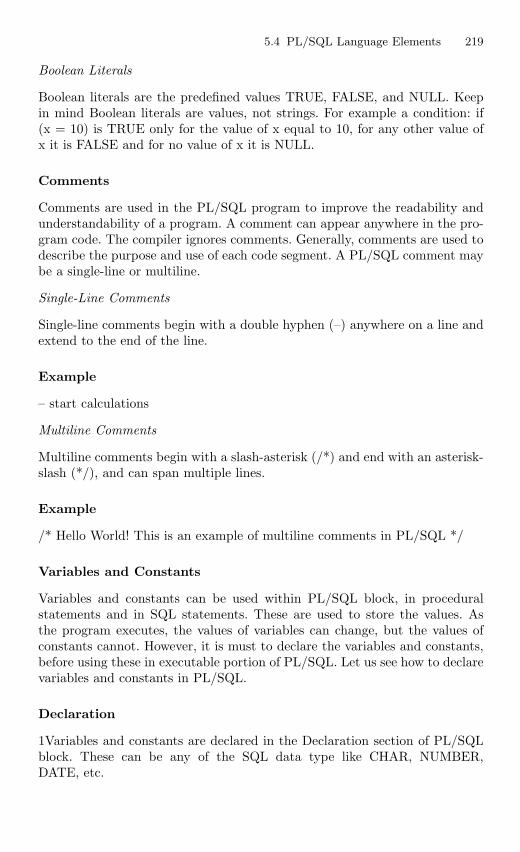
5.4 PL/SQL Language Elements 219
Boolean Literals
Boolean literals are the predefined values TRUE, FALSE, and NULL. Keepin mind Boolean literals are values, not strings. For example a condition: if(x = 10) is TRUE only for the value of x equal to 10, for any other value ofx it is FALSE and for no value of x it is NULL.
Comments
Comments are used in the PL/SQL program to improve the readability andunderstandability of a program. A comment can appear anywhere in the pro-gram code. The compiler ignores comments. Generally, comments are used todescribe the purpose and use of each code segment. A PL/SQL comment maybe a single-line or multiline.
Single-Line Comments
Single-line comments begin with a double hyphen (–) anywhere on a line andextend to the end of the line.
Example
– start calculations
Multiline Comments
Multiline comments begin with a slash-asterisk (/*) and end with an asterisk-slash (*/), and can span multiple lines.
Example
/* Hello World! This is an example of multiline comments in PL/SQL */
Variables and Constants
Variables and constants can be used within PL/SQL block, in proceduralstatements and in SQL statements. These are used to store the values. Asthe program executes, the values of variables can change, but the values ofconstants cannot. However, it is must to declare the variables and constants,before using these in executable portion of PL/SQL. Let us see how to declarevariables and constants in PL/SQL.
Declaration
1Variables and constants are declared in the Declaration section of PL/SQLblock. These can be any of the SQL data type like CHAR, NUMBER,DATE, etc.
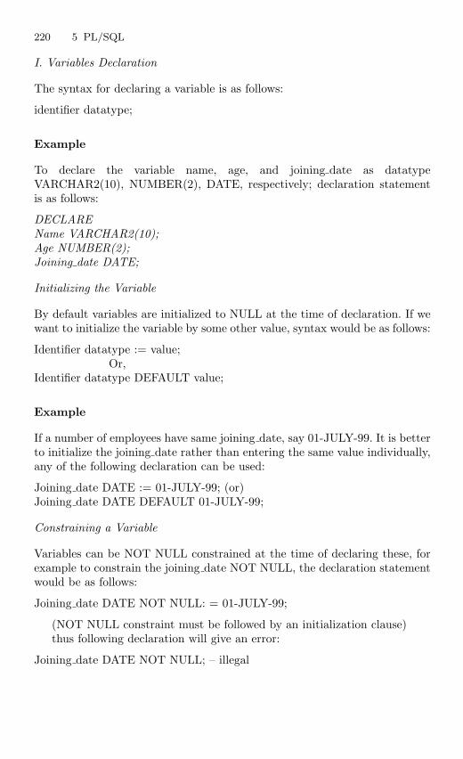
220 5 PL/SQL
I. Variables Declaration
The syntax for declaring a variable is as follows:
identifier datatype;
Example
To declare the variable name, age, and joining date as datatypeVARCHAR2(10), NUMBER(2), DATE, respectively; declaration statementis as follows:
DECLAREName VARCHAR2(10);Age NUMBER(2);Joining date DATE;
Initializing the Variable
By default variables are initialized to NULL at the time of declaration. If wewant to initialize the variable by some other value, syntax would be as follows:
Identifier datatype := value;Or,
Identifier datatype DEFAULT value;
Example
If a number of employees have same joining date, say 01-JULY-99. It is betterto initialize the joining date rather than entering the same value individually,any of the following declaration can be used:
Joining date DATE := 01-JULY-99; (or)Joining date DATE DEFAULT 01-JULY-99;
Constraining a Variable
Variables can be NOT NULL constrained at the time of declaring these, forexample to constrain the joining date NOT NULL, the declaration statementwould be as follows:
Joining date DATE NOT NULL: = 01-JULY-99;
(NOT NULL constraint must be followed by an initialization clause)thus following declaration will give an error:
Joining date DATE NOT NULL; – illegal
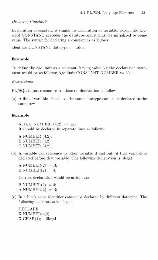
5.4 PL/SQL Language Elements 221
Declaring Constants
Declaration of constant is similar to declaration of variable, except the key-word CONSTANT precedes the datatype and it must be initialized by somevalue. The syntax for declaring a constant is as follows:
identifier CONSTANT datatype := value;
Example
To define the age limit as a constant, having value 30; the declaration state-ment would be as follows: Age limit CONSTANT NUMBER := 30;
Restrictions
PL/SQL imposes some restrictions on declaration as follows:
(a) A list of variables that have the same datatype cannot be declared in thesame row
Example
A, B, C NUMBER (4,2); – illegalIt should be declared in separate lines as follows:
A NUMBER (4,2);B NUMBER (4,2);C NUMBER (4,2);
(b) A variable can reference to other variable if and only if that variable isdeclared before that variable. The following declaration is illegal:
A NUMBER(2) := B;B NUMBER(2) := 4;
Correct declaration would be as follows:
B NUMBER(2) := 4;A NUMBER(2) := B;
(c) In a block same identifier cannot be declared by different datatype. Thefollowing declaration is illegal:
DECLAREX NUMBER(4,2);X CHAR(4); – illegal
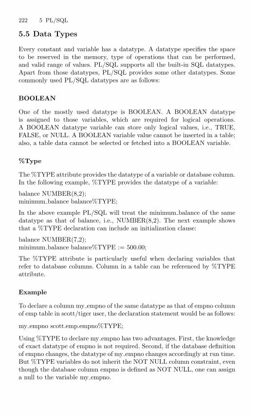
222 5 PL/SQL
5.5 Data Types
Every constant and variable has a datatype. A datatype specifies the spaceto be reserved in the memory, type of operations that can be performed,and valid range of values. PL/SQL supports all the built-in SQL datatypes.Apart from those datatypes, PL/SQL provides some other datatypes. Somecommonly used PL/SQL datatypes are as follows:
BOOLEAN
One of the mostly used datatype is BOOLEAN. A BOOLEAN datatypeis assigned to those variables, which are required for logical operations.A BOOLEAN datatype variable can store only logical values, i.e., TRUE,FALSE, or NULL. A BOOLEAN variable value cannot be inserted in a table;also, a table data cannot be selected or fetched into a BOOLEAN variable.
%Type
The %TYPE attribute provides the datatype of a variable or database column.In the following example, %TYPE provides the datatype of a variable:
balance NUMBER(8,2);minimum balance balance%TYPE;
In the above example PL/SQL will treat the minimum balance of the samedatatype as that of balance, i.e., NUMBER(8,2). The next example showsthat a %TYPE declaration can include an initialization clause:
balance NUMBER(7,2);minimum balance balance%TYPE := 500.00;
The %TYPE attribute is particularly useful when declaring variables thatrefer to database columns. Column in a table can be referenced by %TYPEattribute.
Example
To declare a column my empno of the same datatype as that of empno columnof emp table in scott/tiger user, the declaration statement would be as follows:
my empno scott.emp.empno%TYPE;
Using %TYPE to declare my empno has two advantages. First, the knowledgeof exact datatype of empno is not required. Second, if the database definitionof empno changes, the datatype of my empno changes accordingly at run time.But %TYPE variables do not inherit the NOT NULL column constraint, eventhough the database column empno is defined as NOT NULL, one can assigna null to the variable my empno.
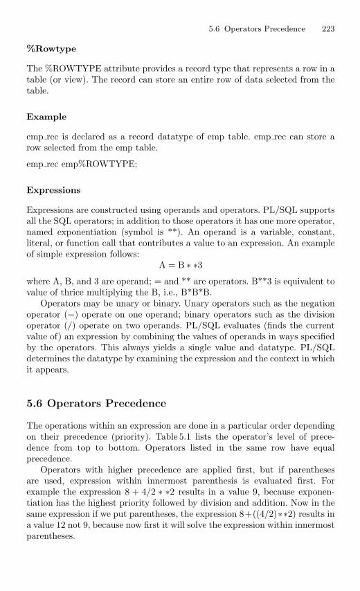
5.6 Operators Precedence 223
%Rowtype
The %ROWTYPE attribute provides a record type that represents a row in atable (or view). The record can store an entire row of data selected from thetable.
Example
emp rec is declared as a record datatype of emp table. emp rec can store arow selected from the emp table.
emp rec emp%ROWTYPE;
Expressions
Expressions are constructed using operands and operators. PL/SQL supportsall the SQL operators; in addition to those operators it has one more operator,named exponentiation (symbol is **). An operand is a variable, constant,literal, or function call that contributes a value to an expression. An exampleof simple expression follows:
A = B ∗ ∗3where A, B, and 3 are operand; = and ** are operators. B**3 is equivalent tovalue of thrice multiplying the B, i.e., B*B*B.
Operators may be unary or binary. Unary operators such as the negationoperator (−) operate on one operand; binary operators such as the divisionoperator (/) operate on two operands. PL/SQL evaluates (finds the currentvalue of) an expression by combining the values of operands in ways specifiedby the operators. This always yields a single value and datatype. PL/SQLdetermines the datatype by examining the expression and the context in whichit appears.
5.6 Operators Precedence
The operations within an expression are done in a particular order dependingon their precedence (priority). Table 5.1 lists the operator’s level of prece-dence from top to bottom. Operators listed in the same row have equalprecedence.
Operators with higher precedence are applied first, but if parenthesesare used, expression within innermost parenthesis is evaluated first. Forexample the expression 8 + 4/2 ∗ ∗2 results in a value 9, because exponen-tiation has the highest priority followed by division and addition. Now in thesame expression if we put parentheses, the expression 8+((4/2)∗∗2) results ina value 12 not 9, because now first it will solve the expression within innermostparentheses.
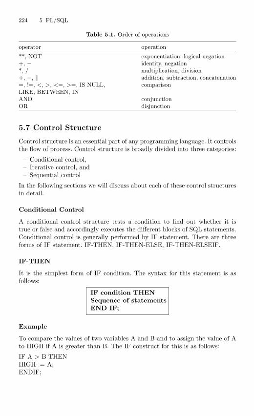
224 5 PL/SQL
Table 5.1. Order of operations
operator operation
**, NOT exponentiation, logical negation+, − identity, negation*, / multiplication, division+, −, || addition, subtraction, concatenation=, !=, <, >, <=, >=, IS NULL, comparisonLIKE, BETWEEN, INAND conjunctionOR disjunction
5.7 Control Structure
Control structure is an essential part of any programming language. It controlsthe flow of process. Control structure is broadly divided into three categories:
– Conditional control,– Iterative control, and– Sequential control
In the following sections we will discuss about each of these control structuresin detail.
Conditional Control
A conditional control structure tests a condition to find out whether it istrue or false and accordingly executes the different blocks of SQL statements.Conditional control is generally performed by IF statement. There are threeforms of IF statement. IF-THEN, IF-THEN-ELSE, IF-THEN-ELSEIF.
IF-THEN
It is the simplest form of IF condition. The syntax for this statement is asfollows:
IF condition THENSequence of statementsEND IF;
Example
To compare the values of two variables A and B and to assign the value of Ato HIGH if A is greater than B. The IF construct for this is as follows:
IF A > B THENHIGH := A;ENDIF;
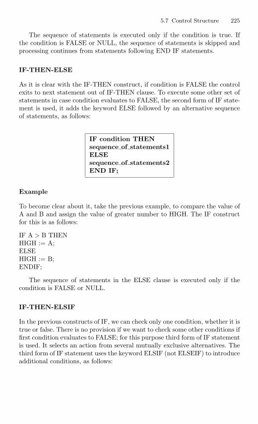
5.7 Control Structure 225
The sequence of statements is executed only if the condition is true. Ifthe condition is FALSE or NULL, the sequence of statements is skipped andprocessing continues from statements following END IF statements.
IF-THEN-ELSE
As it is clear with the IF-THEN construct, if condition is FALSE the controlexits to next statement out of IF-THEN clause. To execute some other set ofstatements in case condition evaluates to FALSE, the second form of IF state-ment is used, it adds the keyword ELSE followed by an alternative sequenceof statements, as follows:
IF condition THENsequence of statements1ELSEsequence of statements2END IF;
Example
To become clear about it, take the previous example, to compare the value ofA and B and assign the value of greater number to HIGH. The IF constructfor this is as follows:
IF A > B THENHIGH := A;ELSEHIGH := B;ENDIF;
The sequence of statements in the ELSE clause is executed only if thecondition is FALSE or NULL.
IF-THEN-ELSIF
In the previous constructs of IF, we can check only one condition, whether it istrue or false. There is no provision if we want to check some other conditions iffirst condition evaluates to FALSE; for this purpose third form of IF statementis used. It selects an action from several mutually exclusive alternatives. Thethird form of IF statement uses the keyword ELSIF (not ELSEIF) to introduceadditional conditions, as follows:
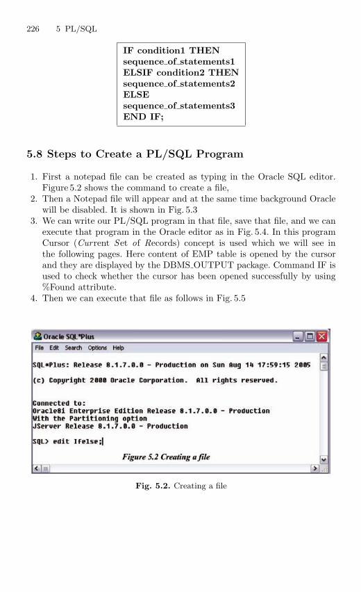
226 5 PL/SQL
IF condition1 THENsequence of statements1ELSIF condition2 THENsequence of statements2ELSEsequence of statements3END IF;
5.8 Steps to Create a PL/SQL Program
1. First a notepad file can be created as typing in the Oracle SQL editor.Figure 5.2 shows the command to create a file,
2. Then a Notepad file will appear and at the same time background Oraclewill be disabled. It is shown in Fig. 5.3
3. We can write our PL/SQL program in that file, save that file, and we canexecute that program in the Oracle editor as in Fig. 5.4. In this programCursor (Current Set of Records) concept is used which we will see inthe following pages. Here content of EMP table is opened by the cursorand they are displayed by the DBMS OUTPUT package. Command IF isused to check whether the cursor has been opened successfully by using%Found attribute.
4. Then we can execute that file as follows in Fig. 5.5
Fig. 5.2. Creating a file
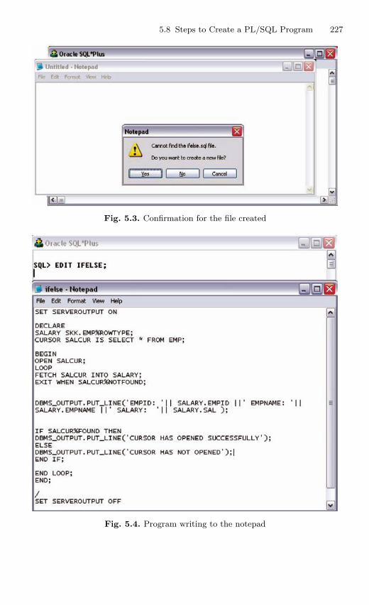
5.8 Steps to Create a PL/SQL Program 227
Fig. 5.3. Confirmation for the file created
Fig. 5.4. Program writing to the notepad
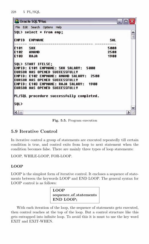
228 5 PL/SQL
Fig. 5.5. Program execution
5.9 Iterative Control
In iterative control a group of statements are executed repeatedly till certaincondition is true, and control exits from loop to next statement when thecondition becomes false. There are mainly three types of loop statements:
LOOP, WHILE-LOOP, FOR-LOOP.
LOOP
LOOP is the simplest form of iterative control. It encloses a sequence of state-ments between the keywords LOOP and END LOOP. The general syntax forLOOP control is as follows:
LOOPsequence of statementsEND LOOP;
With each iteration of the loop, the sequence of statements gets executed,then control reaches at the top of the loop. But a control structure like thisgets entrapped into infinite loop. To avoid this it is must to use the key wordEXIT and EXIT-WHEN.
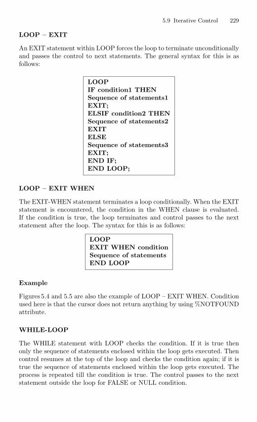
5.9 Iterative Control 229
LOOP – EXIT
An EXIT statement within LOOP forces the loop to terminate unconditionallyand passes the control to next statements. The general syntax for this is asfollows:
LOOPIF condition1 THENSequence of statements1EXIT;ELSIF condition2 THENSequence of statements2EXITELSESequence of statements3EXIT;END IF;END LOOP;
LOOP – EXIT WHEN
The EXIT-WHEN statement terminates a loop conditionally. When the EXITstatement is encountered, the condition in the WHEN clause is evaluated.If the condition is true, the loop terminates and control passes to the nextstatement after the loop. The syntax for this is as follows:
LOOPEXIT WHEN conditionSequence of statementsEND LOOP
Example
Figures 5.4 and 5.5 are also the example of LOOP – EXIT WHEN. Conditionused here is that the cursor does not return anything by using %NOTFOUNDattribute.
WHILE-LOOP
The WHILE statement with LOOP checks the condition. If it is true thenonly the sequence of statements enclosed within the loop gets executed. Thencontrol resumes at the top of the loop and checks the condition again; if it istrue the sequence of statements enclosed within the loop gets executed. Theprocess is repeated till the condition is true. The control passes to the nextstatement outside the loop for FALSE or NULL condition.
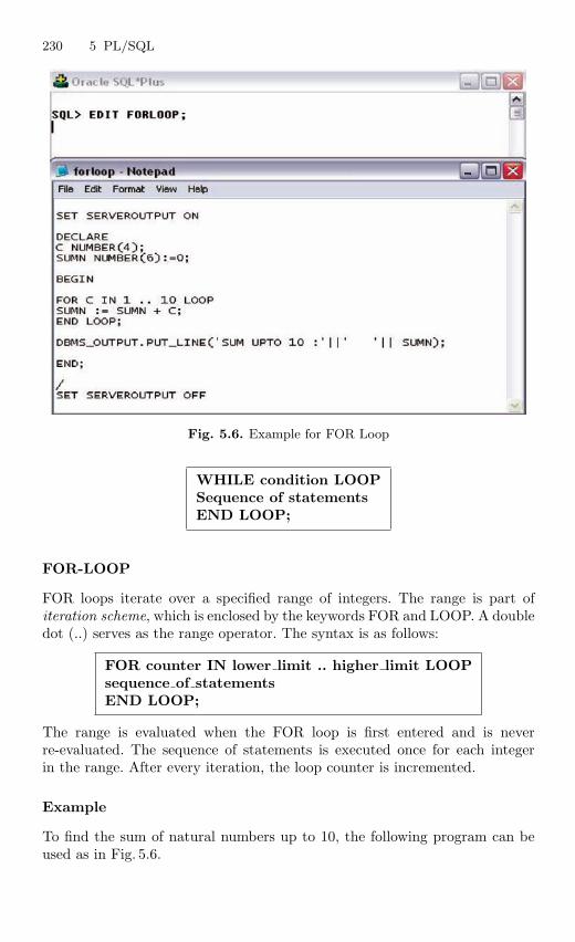
230 5 PL/SQL
Fig. 5.6. Example for FOR Loop
WHILE condition LOOPSequence of statementsEND LOOP;
FOR-LOOP
FOR loops iterate over a specified range of integers. The range is part ofiteration scheme, which is enclosed by the keywords FOR and LOOP. A doubledot (..) serves as the range operator. The syntax is as follows:
FOR counter IN lower limit .. higher limit LOOPsequence of statementsEND LOOP;
The range is evaluated when the FOR loop is first entered and is neverre-evaluated. The sequence of statements is executed once for each integerin the range. After every iteration, the loop counter is incremented.
Example
To find the sum of natural numbers up to 10, the following program can beused as in Fig. 5.6.
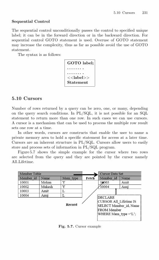
5.10 Cursors 231
Sequential Control
The sequential control unconditionally passes the control to specified uniquelabel; it can be in the forward direction or in the backward direction. Forsequential control GOTO statement is used. Overuse of GOTO statementmay increase the complexity, thus as far as possible avoid the use of GOTOstatement.
The syntax is as follows:
GOTO label;. . . . . . . .. . . . . . . .<<label>>Statement
5.10 Cursors
Number of rows returned by a query can be zero, one, or many, dependingon the query search conditions. In PL/SQL, it is not possible for an SQLstatement to return more than one row. In such cases we can use cursors.A cursor is a mechanism that can be used to process the multiple row resultsets one row at a time.
In other words, cursors are constructs that enable the user to name aprivate memory area to hold a specific statement for access at a later time.Cursors are an inherent structure in PL/SQL. Cursors allow users to easilystore and process sets of information in PL/SQL program.
Figure 5.7 shows the simple example for the cursor where two rowsare selected from the query and they are pointed by the cursor namelyAll Lifetime.
Fig. 5.7. Cursor example
232 5 PL/SQL
There are two types of cursors in Oracle
1. Implicit cursors2. Explicit cursors
5.10.1 Implicit Cursors
PL/SQL implicitly declares a cursor for every SQL DML statement, such asINSERT, DELETE, UPDATE, and SELECT statement that is not a partof an explicitly declared cursor, even if the statement processes a single row.PL/SQL allows referencing the most recent cursor or the cursor associatedwith the most recently executed SQL statement, as the “SQL” cursor. Cursorattributes are used to access information about the most recently executedSQL statement, using SQL cursor.
Implicit Cursor Attributes
In PL/SQL every cursor, implicit or explicit, has four attributes: %NOT-FOUND, %FOUND, %ROWCOUNT, and %ISOPEN. These cursor attributescan be used in procedural statements (PL/SQL), but not in SQL statements.These attributes let user access information about the most recent executionof INSERT, UPDATE, SELECT INTO, and DELETE commands. Theseattributes are associated with the implicit “SQL” cursor and can be accessedby appending the attribute name to the implicit cursor name (SQL). Syntaxto use cursor attribute is as follows:
SQL %<attribute name>
%Notfound
This attribute is used to determine if any rows were processed by a SQLDML statement. This attribute evaluates to TRUE if an INSERT, UPDATE,or DELETE affected no rows or a SELECT INTO returned no rows. Other-wise, it returns FALSE. %NOTFOUND attribute can be useful in reportingor processing when no data is affected. If a SELECT statement does not re-turn any data, the predefined exception NO DATA FOUND is automaticallyraised, and program control is sent to an exception handler, if it is present inthe program. If a check is made on %NOTFOUND attribute after a SELECTstatement, it will be completely skipped when the SELECT statement returnsno data.
Example
Figures 5.8 and 5.9 show the example of all the implicit cursor attributes.The program will return the status of each cursor attribute depending on thepreviously executed DML statement.
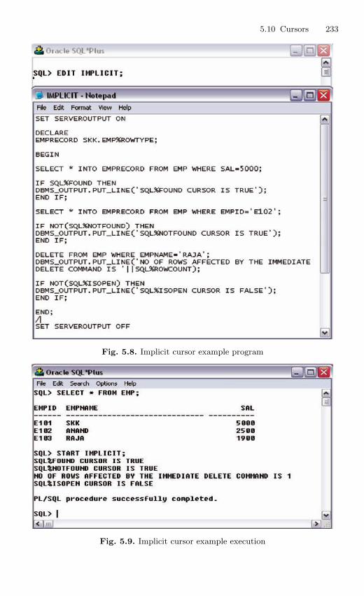
5.10 Cursors 233
Fig. 5.8. Implicit cursor example program
Fig. 5.9. Implicit cursor example execution
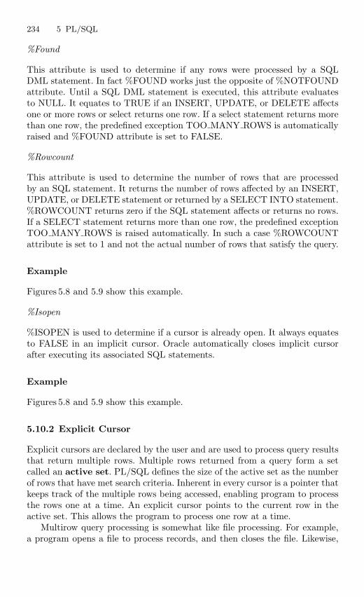
234 5 PL/SQL
%Found
This attribute is used to determine if any rows were processed by a SQLDML statement. In fact %FOUND works just the opposite of %NOTFOUNDattribute. Until a SQL DML statement is executed, this attribute evaluatesto NULL. It equates to TRUE if an INSERT, UPDATE, or DELETE affectsone or more rows or select returns one row. If a select statement returns morethan one row, the predefined exception TOO MANY ROWS is automaticallyraised and %FOUND attribute is set to FALSE.
%Rowcount
This attribute is used to determine the number of rows that are processedby an SQL statement. It returns the number of rows affected by an INSERT,UPDATE, or DELETE statement or returned by a SELECT INTO statement.%ROWCOUNT returns zero if the SQL statement affects or returns no rows.If a SELECT statement returns more than one row, the predefined exceptionTOO MANY ROWS is raised automatically. In such a case %ROWCOUNTattribute is set to 1 and not the actual number of rows that satisfy the query.
Example
Figures 5.8 and 5.9 show this example.
%Isopen
%ISOPEN is used to determine if a cursor is already open. It always equatesto FALSE in an implicit cursor. Oracle automatically closes implicit cursorafter executing its associated SQL statements.
Example
Figures 5.8 and 5.9 show this example.
5.10.2 Explicit Cursor
Explicit cursors are declared by the user and are used to process query resultsthat return multiple rows. Multiple rows returned from a query form a setcalled an active set. PL/SQL defines the size of the active set as the numberof rows that have met search criteria. Inherent in every cursor is a pointer thatkeeps track of the multiple rows being accessed, enabling program to processthe rows one at a time. An explicit cursor points to the current row in theactive set. This allows the program to process one row at a time.
Multirow query processing is somewhat like file processing. For example,a program opens a file to process records, and then closes the file. Likewise,
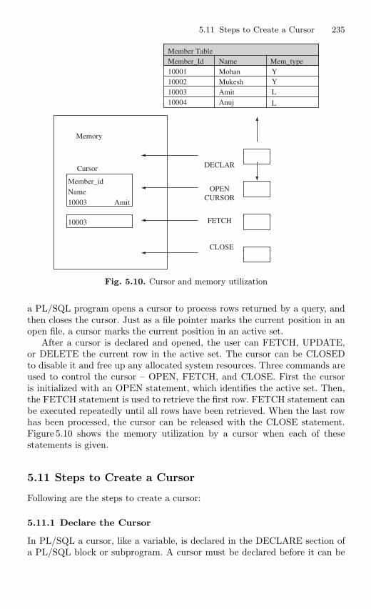
5.11 Steps to Create a Cursor 235
Member TableMember_Id Name
Mohan YYL
L
MukeshAmitAnuj
DECLAR
OPENCURSOR
FETCH
CLOSE
Mem_type10001100021000310004
Memory
Cursor
Member_idName
10003
10003 Amit
Fig. 5.10. Cursor and memory utilization
a PL/SQL program opens a cursor to process rows returned by a query, andthen closes the cursor. Just as a file pointer marks the current position in anopen file, a cursor marks the current position in an active set.
After a cursor is declared and opened, the user can FETCH, UPDATE,or DELETE the current row in the active set. The cursor can be CLOSEDto disable it and free up any allocated system resources. Three commands areused to control the cursor – OPEN, FETCH, and CLOSE. First the cursoris initialized with an OPEN statement, which identifies the active set. Then,the FETCH statement is used to retrieve the first row. FETCH statement canbe executed repeatedly until all rows have been retrieved. When the last rowhas been processed, the cursor can be released with the CLOSE statement.Figure 5.10 shows the memory utilization by a cursor when each of thesestatements is given.
5.11 Steps to Create a Cursor
Following are the steps to create a cursor:
5.11.1 Declare the Cursor
In PL/SQL a cursor, like a variable, is declared in the DECLARE section ofa PL/SQL block or subprogram. A cursor must be declared before it can be
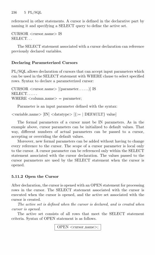
236 5 PL/SQL
referenced in other statements. A cursor is defined in the declarative part bynaming it and specifying a SELECT query to define the active set.
CURSOR <cursor name> ISSELECT. . .
The SELECT statement associated with a cursor declaration can referencepreviously declared variables.
Declaring Parameterized Cursors
PL/SQL allows declaration of cursors that can accept input parameters whichcan be used in the SELECT statement with WHERE clause to select specifiedrows. Syntax to declare a parameterized cursor:
CURSOR <cursor name> [(parameter. . . . . .)] ISSELECT. . . . . .WHERE <column name> = parameter;
Parameter is an input parameter defined with the syntax:
<variable name> [IN] <datatype> [:= | DEFAULT value]
The formal parameters of a cursor must be IN parameters. As in theexample above, cursor parameters can be initialized to default values. Thatway, different numbers of actual parameters can be passed to a cursor,accepting or overriding the default values.
Moreover, new formal parameters can be added without having to changeevery reference to the cursor. The scope of a cursor parameter is local onlyto the cursor. A cursor parameter can be referenced only within the SELECTstatement associated with the cursor declaration. The values passed to thecursor parameters are used by the SELECT statement when the cursor isopened.
5.11.2 Open the Cursor
After declaration, the cursor is opened with an OPEN statement for processingrows in the cursor. The SELECT statement associated with the cursor isexecuted when the cursor is opened, and the active set associated with thecursor is created.
The active set is defined when the cursor is declared, and is created whencursor is opened.
The active set consists of all rows that meet the SELECT statementcriteria. Syntax of OPEN statement is as follows.
OPEN <cursor name>;
5.11 Steps to Create a Cursor 237
5.11.3 Passing Parameters to Cursor
Parameters to a parameterized cursor can be passed when the cursor is opened.For example, given the cursor declaration
CURSOR Mem detail (MType VARCHAR2) IS SELECT. . .
Any of the following statements opens the cursor.
OPEN Mem detail(‘L’);OPEN Mem detail(Mem); where Mem is another variable.
Unless default values are to be accepted, each formal parameter in thecursor declaration must have a corresponding actual parameter in the OPENstatement. Formal parameters declared with a default value need not havea corresponding actual parameter. They can simply assume their defaultvalues when the OPEN statement is executed. The formal parameters of acursor must be IN parameters. Therefore, they cannot return values to actualparameters. Each actual parameter must belong to a datatype compatiblewith the datatype of its corresponding formal parameter.
5.11.4 Fetch Data from the Cursor
After a cursor has been opened, the SELECT statement associated withthe cursor is executed and the active set is created. To retrieve the rowsin the active set one row at a time, the rows must be fetched individuallyfrom the cursor. After each FETCH statement, the cursor advances to thenext row in the active set and retrieves it. Syntax of FETCH is:
FETCH <cursor name> INTO <variable name>, <variable name>. . . .
where variable name is the name of a variable to which a column value isassigned. For each column value returned by the query associated with thecursor, there must be a corresponding variable in the INTO list. This variabledatatype must be compatible with the corresponding database column.
5.11.5 Close the Cursor
After processing the rows in the cursor, it is released with the CLOSE state-ment. To change the active set in a cursor or the values of the variablesreferenced in the cursor SELECT statement, the cursor must be released withCLOSE statement. Once a cursor is CLOSEd, it can be reOPENed. TheCLOSE statement disables the cursor, and the active set becomes undefined.For example, to CLOSE Mem detail close statement will be:
CLOSE <cursor name>;
238 5 PL/SQL
Example
Figures 5.4 and 5.5 show the example of declaring, opening, and fetching thecursor called SALCUR.
Explicit Cursor Attributes
It is used to access useful information about the status of an explicit cursor.Explicit cursors have the same set of cursor attributes %NOTFOUND,%FOUND, %ROWCOUNT, and %ISOPEN. These attributes can be accessedin PL/SQL statements only, not in SQL statements. Syntax to access anexplicit cursor attributes:
<cursor name>%<attribute name>
%Notfound
When a cursor is OPENed, the rows that satisfy the associated query areidentified and form the active set. Before the first fetch, %NOTFOUNDevaluates to NULL. Rows are FETCHed from the active set one at a time. Ifthe last fetch returned a row, %NOTFOUND evaluates to FALSE. If the lastfetch failed to return a row because the active set was empty, %NOTFOUNDevaluates to TRUE. FETCH is expected to fail eventually, so when thathappens, no exception is raised.
Example
Figures 5.4 and 5.5 show the example for this attribute. In this example, it isused for checking whether all the rows have been fetched or not.
%Found
%FOUND is the logical opposite of %NOTFOUND. After an explicit cursoris open but before the first fetch, %FOUND evaluates to NULL. Thereafter,it evaluates to TRUE if the last fetch returned a row or to FALSE if no rowwas returned. If a cursor is not open, referencing it with %FOUND raisesINVALID CURSOR exception.
Example
Figures 5.4 and 5.5 show the example for this attribute. In this example, it isused for checking whether the cursor has been opened successfully or not.
%Rowcount
When you open a cursor, %ROWCOUNT is initialized to zero. Before thefirst fetch, %ROWCOUNT returns a zero. Thereafter, it returns the numberof rows fetched so far. The number is incremented if the latest fetch returneda row.
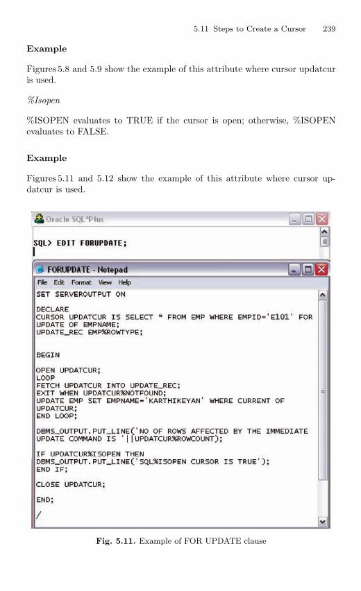
5.11 Steps to Create a Cursor 239
Example
Figures 5.8 and 5.9 show the example of this attribute where cursor updatcuris used.
%Isopen
%ISOPEN evaluates to TRUE if the cursor is open; otherwise, %ISOPENevaluates to FALSE.
Example
Figures 5.11 and 5.12 show the example of this attribute where cursor up-datcur is used.
Fig. 5.11. Example of FOR UPDATE clause
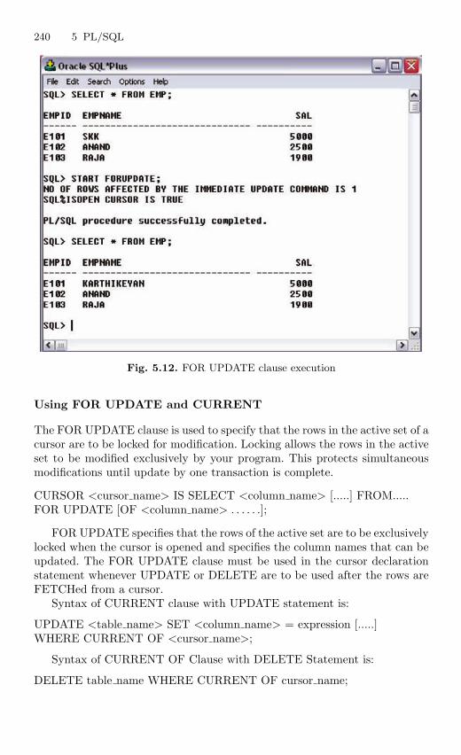
240 5 PL/SQL
Fig. 5.12. FOR UPDATE clause execution
Using FOR UPDATE and CURRENT
The FOR UPDATE clause is used to specify that the rows in the active set of acursor are to be locked for modification. Locking allows the rows in the activeset to be modified exclusively by your program. This protects simultaneousmodifications until update by one transaction is complete.
CURSOR <cursor name> IS SELECT <column name> [.....] FROM.....FOR UPDATE [OF <column name> . . . . . .];
FOR UPDATE specifies that the rows of the active set are to be exclusivelylocked when the cursor is opened and specifies the column names that can beupdated. The FOR UPDATE clause must be used in the cursor declarationstatement whenever UPDATE or DELETE are to be used after the rows areFETCHed from a cursor.
Syntax of CURRENT clause with UPDATE statement is:
UPDATE <table name> SET <column name> = expression [.....]WHERE CURRENT OF <cursor name>;
Syntax of CURRENT OF Clause with DELETE Statement is:
DELETE table name WHERE CURRENT OF cursor name;
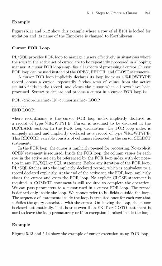
5.11 Steps to Create a Cursor 241
Example
Figures 5.11 and 5.12 show this example where a row of id E101 is locked forupdation and its name of the Employee is changed to Karthikeyan.
Cursor FOR Loop
PL/SQL provides FOR loop to manage cursors effectively in situations wherethe rows in the active set of cursor are to be repeatedly processed in a loopingmanner. A cursor FOR loop simplifies all aspects of processing a cursor. CursorFOR loop can be used instead of the OPEN, FETCH, and CLOSE statements.
A cursor FOR loop implicitly declares its loop index as a %ROWTYPErecord, opens a cursor, repeatedly fetches rows of values from the activeset into fields in the record, and closes the cursor when all rows have beenprocessed. Syntax to declare and process a cursor in a cursor FOR loop is:
FOR <record name> IN <cursor name> LOOP. . . . . . . . .END LOOP;
where record name is the cursor FOR loop index implicitly declared asa record of type %ROWTYPE. Cursor is assumed to be declared in theDECLARE section. In the FOR loop declaration, the FOR loop index isuniquely named and implicitly declared as a record of type %ROWTYPE.This RECORD variable consists of columns referenced in the cursor SELECTstatement.
In the FOR loop, the cursor is implicitly opened for processing. No explicitOPEN statement is required. Inside the FOR loop, the column values for eachrow in the active set can be referenced by the FOR loop index with dot nota-tion in any PL/SQL or SQL statement. Before any iteration of the FOR loop,PL/SQL fetches into the implicitly declared record, which is equivalent to arecord declared explicitly. At the end of the active set, the FOR loop implicitlycloses the cursor and exits the FOR loop. No explicit CLOSE statement isrequired. A COMMIT statement is still required to complete the operation.We can pass parameters to a cursor used in a cursor FOR loop. The recordis defined only inside the loop. We cannot refer to its fields outside the loop.The sequence of statements inside the loop is executed once for each row thatsatisfies the query associated with the cursor. On leaving the loop, the cursoris closed automatically. This is true even if an EXIT or GOTO statement isused to leave the loop prematurely or if an exception is raised inside the loop.
Example
Figures 5.13 and 5.14 show the example of cursor execution using FOR loop.
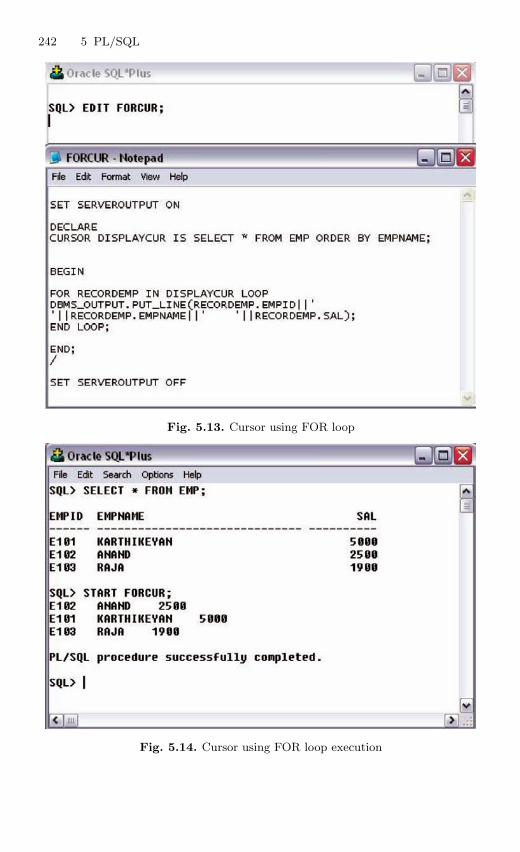
242 5 PL/SQL
Fig. 5.13. Cursor using FOR loop
Fig. 5.14. Cursor using FOR loop execution
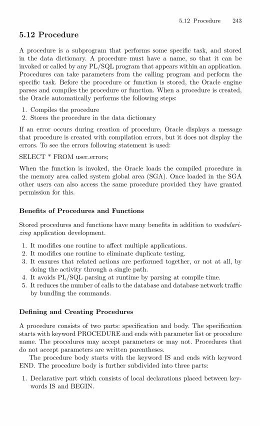
5.12 Procedure 243
5.12 Procedure
A procedure is a subprogram that performs some specific task, and storedin the data dictionary. A procedure must have a name, so that it can beinvoked or called by any PL/SQL program that appears within an application.Procedures can take parameters from the calling program and perform thespecific task. Before the procedure or function is stored, the Oracle engineparses and compiles the procedure or function. When a procedure is created,the Oracle automatically performs the following steps:
1. Compiles the procedure2. Stores the procedure in the data dictionary
If an error occurs during creation of procedure, Oracle displays a messagethat procedure is created with compilation errors, but it does not display theerrors. To see the errors following statement is used:
SELECT * FROM user errors;
When the function is invoked, the Oracle loads the compiled procedure inthe memory area called system global area (SGA). Once loaded in the SGAother users can also access the same procedure provided they have grantedpermission for this.
Benefits of Procedures and Functions
Stored procedures and functions have many benefits in addition to modulari-zing application development.
1. It modifies one routine to affect multiple applications.2. It modifies one routine to eliminate duplicate testing.3. It ensures that related actions are performed together, or not at all, by
doing the activity through a single path.4. It avoids PL/SQL parsing at runtime by parsing at compile time.5. It reduces the number of calls to the database and database network traffic
by bundling the commands.
Defining and Creating Procedures
A procedure consists of two parts: specification and body. The specificationstarts with keyword PROCEDURE and ends with parameter list or procedurename. The procedures may accept parameters or may not. Procedures thatdo not accept parameters are written parentheses.
The procedure body starts with the keyword IS and ends with keywordEND. The procedure body is further subdivided into three parts:
1. Declarative part which consists of local declarations placed between key-words IS and BEGIN.
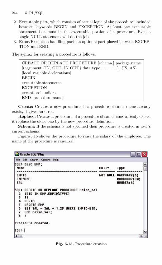
244 5 PL/SQL
2. Executable part, which consists of actual logic of the procedure, includedbetween keywords BEGIN and EXCEPTION. At least one executablestatement is a must in the executable portion of a procedure. Even asingle NULL statement will do the job.
3. Error/Exception handling part, an optional part placed between EXCEP-TION and END.
The syntax for creating a procedure is follows:
CREATE OR REPLACE PROCEDURE [schema.] package name[(argument IN, OUT, IN OUT data type,. . . . . . . . .)] IS, AS[local variable declarations]BEGINexecutable statementsEXCEPTIONexception handlersEND [procedure name];
Create: Creates a new procedure, if a procedure of same name alreadyexists, it gives an error.
Replace: Creates a procedure, if a procedure of same name already exists,it replace the older one by the new procedure definition.
Schema: If the schema is not specified then procedure is created in user’scurrent schema.
Figure 5.15 shows the procedure to raise the salary of the employee. Thename of the procedure is raise sal.
Fig. 5.15. Procedure creation
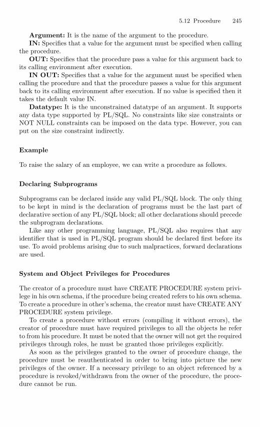
5.12 Procedure 245
Argument: It is the name of the argument to the procedure.IN: Specifies that a value for the argument must be specified when calling
the procedure.OUT: Specifies that the procedure pass a value for this argument back to
its calling environment after execution.IN OUT: Specifies that a value for the argument must be specified when
calling the procedure and that the procedure passes a value for this argumentback to its calling environment after execution. If no value is specified then ittakes the default value IN.
Datatype: It is the unconstrained datatype of an argument. It supportsany data type supported by PL/SQL. No constraints like size constraints orNOT NULL constraints can be imposed on the data type. However, you canput on the size constraint indirectly.
Example
To raise the salary of an employee, we can write a procedure as follows.
Declaring Subprograms
Subprograms can be declared inside any valid PL/SQL block. The only thingto be kept in mind is the declaration of programs must be the last part ofdeclarative section of any PL/SQL block; all other declarations should precedethe subprogram declarations.
Like any other programming language, PL/SQL also requires that anyidentifier that is used in PL/SQL program should be declared first before itsuse. To avoid problems arising due to such malpractices, forward declarationsare used.
System and Object Privileges for Procedures
The creator of a procedure must have CREATE PROCEDURE system privi-lege in his own schema, if the procedure being created refers to his own schema.To create a procedure in other’s schema, the creator must have CREATE ANYPROCEDURE system privilege.
To create a procedure without errors (compiling it without errors), thecreator of procedure must have required privileges to all the objects he referto from his procedure. It must be noted that the owner will not get the requiredprivileges through roles, he must be granted those privileges explicitly.
As soon as the privileges granted to the owner of procedure change, theprocedure must be reauthenticated in order to bring into picture the newprivileges of the owner. If a necessary privilege to an object referenced by aprocedure is revoked/withdrawn from the owner of the procedure, the proce-dure cannot be run.
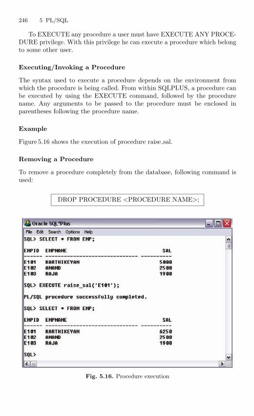
246 5 PL/SQL
To EXECUTE any procedure a user must have EXECUTE ANY PROCE-DURE privilege. With this privilege he can execute a procedure which belongto some other user.
Executing/Invoking a Procedure
The syntax used to execute a procedure depends on the environment fromwhich the procedure is being called. From within SQLPLUS, a procedure canbe executed by using the EXECUTE command, followed by the procedurename. Any arguments to be passed to the procedure must be enclosed inparentheses following the procedure name.
Example
Figure 5.16 shows the execution of procedure raise sal.
Removing a Procedure
To remove a procedure completely from the database, following command isused:
DROP PROCEDURE <PROCEDURE NAME>;
Fig. 5.16. Procedure execution
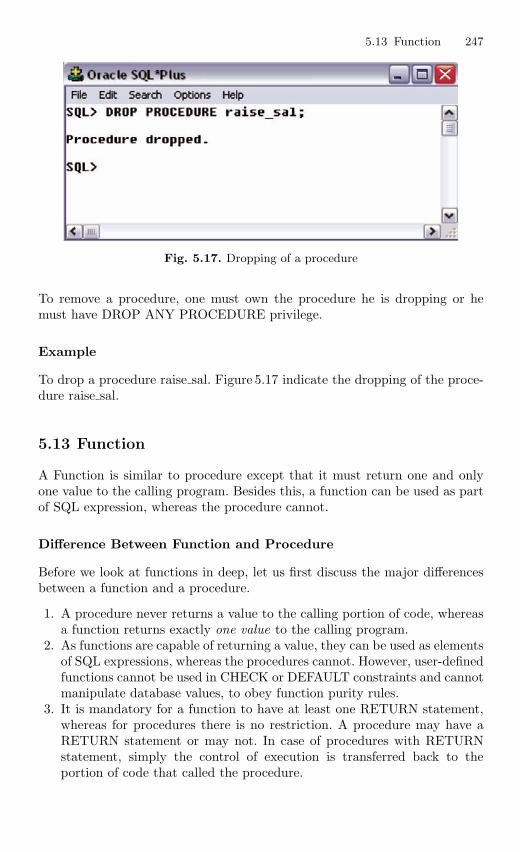
5.13 Function 247
Fig. 5.17. Dropping of a procedure
To remove a procedure, one must own the procedure he is dropping or hemust have DROP ANY PROCEDURE privilege.
Example
To drop a procedure raise sal. Figure 5.17 indicate the dropping of the proce-dure raise sal.
5.13 Function
A Function is similar to procedure except that it must return one and onlyone value to the calling program. Besides this, a function can be used as partof SQL expression, whereas the procedure cannot.
Difference Between Function and Procedure
Before we look at functions in deep, let us first discuss the major differencesbetween a function and a procedure.
1. A procedure never returns a value to the calling portion of code, whereasa function returns exactly one value to the calling program.
2. As functions are capable of returning a value, they can be used as elementsof SQL expressions, whereas the procedures cannot. However, user-definedfunctions cannot be used in CHECK or DEFAULT constraints and cannotmanipulate database values, to obey function purity rules.
3. It is mandatory for a function to have at least one RETURN statement,whereas for procedures there is no restriction. A procedure may have aRETURN statement or may not. In case of procedures with RETURNstatement, simply the control of execution is transferred back to theportion of code that called the procedure.
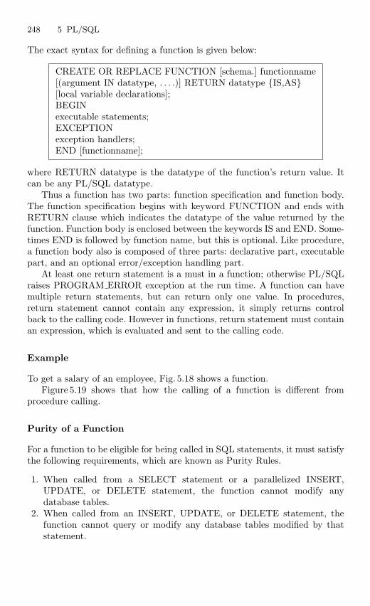
248 5 PL/SQL
The exact syntax for defining a function is given below:
CREATE OR REPLACE FUNCTION [schema.] functionname[(argument IN datatype, . . . .)] RETURN datatype IS,AS[local variable declarations];BEGINexecutable statements;EXCEPTIONexception handlers;END [functionname];
where RETURN datatype is the datatype of the function’s return value. Itcan be any PL/SQL datatype.
Thus a function has two parts: function specification and function body.The function specification begins with keyword FUNCTION and ends withRETURN clause which indicates the datatype of the value returned by thefunction. Function body is enclosed between the keywords IS and END. Some-times END is followed by function name, but this is optional. Like procedure,a function body also is composed of three parts: declarative part, executablepart, and an optional error/exception handling part.
At least one return statement is a must in a function; otherwise PL/SQLraises PROGRAM ERROR exception at the run time. A function can havemultiple return statements, but can return only one value. In procedures,return statement cannot contain any expression, it simply returns controlback to the calling code. However in functions, return statement must containan expression, which is evaluated and sent to the calling code.
Example
To get a salary of an employee, Fig. 5.18 shows a function.Figure 5.19 shows that how the calling of a function is different from
procedure calling.
Purity of a Function
For a function to be eligible for being called in SQL statements, it must satisfythe following requirements, which are known as Purity Rules.
1. When called from a SELECT statement or a parallelized INSERT,UPDATE, or DELETE statement, the function cannot modify anydatabase tables.
2. When called from an INSERT, UPDATE, or DELETE statement, thefunction cannot query or modify any database tables modified by thatstatement.
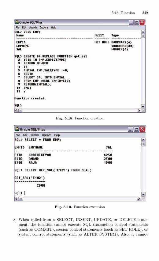
5.13 Function 249
Fig. 5.18. Function creation
Fig. 5.19. Function execution
3. When called from a SELECT, INSERT, UPDATE, or DELETE state-ment, the function cannot execute SQL transaction control statements(such as COMMIT), session control statements (such as SET ROLE), orsystem control statements (such as ALTER SYSTEM). Also, it cannot
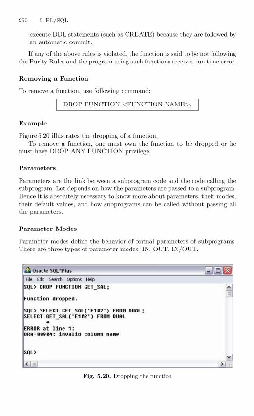
250 5 PL/SQL
execute DDL statements (such as CREATE) because they are followed byan automatic commit.
If any of the above rules is violated, the function is said to be not followingthe Purity Rules and the program using such functions receives run time error.
Removing a Function
To remove a function, use following command:
DROP FUNCTION <FUNCTION NAME>;
Example
Figure 5.20 illustrates the dropping of a function.To remove a function, one must own the function to be dropped or he
must have DROP ANY FUNCTION privilege.
Parameters
Parameters are the link between a subprogram code and the code calling thesubprogram. Lot depends on how the parameters are passed to a subprogram.Hence it is absolutely necessary to know more about parameters, their modes,their default values, and how subprograms can be called without passing allthe parameters.
Parameter Modes
Parameter modes define the behavior of formal parameters of subprograms.There are three types of parameter modes: IN, OUT, IN/OUT.
Fig. 5.20. Dropping the function
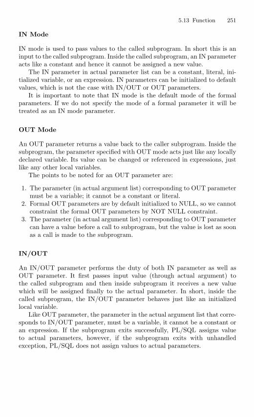
5.13 Function 251
IN Mode
IN mode is used to pass values to the called subprogram. In short this is aninput to the called subprogram. Inside the called subprogram, an IN parameteracts like a constant and hence it cannot be assigned a new value.
The IN parameter in actual parameter list can be a constant, literal, ini-tialized variable, or an expression. IN parameters can be initialized to defaultvalues, which is not the case with IN/OUT or OUT parameters.
It is important to note that IN mode is the default mode of the formalparameters. If we do not specify the mode of a formal parameter it will betreated as an IN mode parameter.
OUT Mode
An OUT parameter returns a value back to the caller subprogram. Inside thesubprogram, the parameter specified with OUT mode acts just like any locallydeclared variable. Its value can be changed or referenced in expressions, justlike any other local variables.
The points to be noted for an OUT parameter are:
1. The parameter (in actual argument list) corresponding to OUT parametermust be a variable; it cannot be a constant or literal.
2. Formal OUT parameters are by default initialized to NULL, so we cannotconstraint the formal OUT parameters by NOT NULL constraint.
3. The parameter (in actual argument list) corresponding to OUT parametercan have a value before a call to subprogram, but the value is lost as soonas a call is made to the subprogram.
IN/OUT
An IN/OUT parameter performs the duty of both IN parameter as well asOUT parameter. It first passes input value (through actual argument) tothe called subprogram and then inside subprogram it receives a new valuewhich will be assigned finally to the actual parameter. In short, inside thecalled subprogram, the IN/OUT parameter behaves just like an initializedlocal variable.
Like OUT parameter, the parameter in the actual argument list that corre-sponds to IN/OUT parameter, must be a variable, it cannot be a constant oran expression. If the subprogram exits successfully, PL/SQL assigns valueto actual parameters, however, if the subprogram exits with unhandledexception, PL/SQL does not assign values to actual parameters.
252 5 PL/SQL
5.14 Packages
A package can be defined as a collection of related program objects such asprocedures, functions, and associated cursors and variables together as a unitin the database. In simpler term, a package is a group of related proceduresand functions stored together and sharing common variables, as well as localprocedures and functions. A package contains two separate parts: the packagespecification and the package body. The package specification and packagebody are compiled separately and stored in the data dictionary as two sepa-rate objects. The package body is optional and need not to be created if thepackage specification does not contain any procedures or functions. Applica-tions or users can call packaged procedures and functions explicitly similar tostandalone procedures and functions.
Advantages of Packages
Packages offer a lot of advantages. They are as follows.
1. Stored packages allow us to sum up (group logically) related stored pro-cedures, variables, and data types, and so forth in a single-named, storedunit in the database. This provides for better orderliness during thedevelopment process. In other words packages and its modules are easilyunderstood because of their logical grouping.
2. Grouping of related procedures, functions, etc. in a package also makeprivilege management easier. Granting the privilege to use a packagemakes all components of the package accessible to the grantee.
3. Package helps in achieving data abstraction. Package body hides thedetails of the package contents and the definition of private programobjects so that only the package contents are affected if the package bodychanges.
4. An entire package is loaded into memory when a procedure within thepackage is called for the first time. This load is completed in one opera-tion, as opposed to the separate loads required for standalone procedures.Therefore, when calls to related packaged procedures occur, no disk I/Ois necessary to execute the compiled code already in memory. This resultsin faster and efficient operation of programs.
5. Packages provide better performance than stored procedures and functionsbecause public package variables persist in memory for the duration of asession. So that they can be accessed by all procedures and functions thattry to access them.
6. Packages allow overloading of its member modules. More than one func-tion in a package can be of same name. The functions are differentiated,depending upon the type and number of parameters it takes.
5.14 Packages 253
Units of Packages
As described earlier, a package is used to store together, the logically relatedPL/SQL units. In general, following units constitute a package.
– Procedures– Functions– Triggers– Cursors– Variables
Parts of Package
A Package has two parts. They are:
– Package specification– Package body
Package Specification
The specification declares the types, variables, constants, exceptions, cursors,and subprograms that are public and thus available for use outside the pack-age. In case in the package specification declaration there is only types, con-stants, exception, or variables, then there is no need for the package bodybecause package specification are sufficient for them. Package body is requiredwhen there is subprograms like cursors, functions, etc.
Package Body
The package body fully defines subprograms such as cursors, functions, andprocedures. All the private declarations of the package are included in thepackage body. It implements the package specification. A package specifica-tion and the package body are stored separately in the database. This allowscalling objects to depend on the specification only, not on both. This separa-tion enables to change the definition of program object in the package bodywithout causing Oracle to interfere with other objects that call or referencethe program object. Oracle invalidates the calling object if the package spec-ification is changed.
Creating a Package
A package consists of package specification and package body. Hence creationof a package involves creation of the package specification and then creationof the package body.
The package specification is declared using the CREATE PACKAGE com-mand.
254 5 PL/SQL
The syntax for package specification declaration is as follows.
CREATE[OR REPLACE] PACKAGE <package name>[AS/IS]PL/SQL package specification
All the procedures, sub programs, cursors declared in the CREATE PACK-AGE command are described and implemented fully in the package bodyalong with private members. The syntax for declaring a package body is asfollows:
CREATE[OR REPLACE] PACKAGE BODY <package name>[AS/IS]PL/SQL package body
Member functions and procedures can be declared in a package and canbe made public or private member using the keywords public and private.Use of all the private members of the package is restricted within the packagewhile the public members of the package can be accessed and used outsidethe package.
Referencing Package Subprograms
Once the package body is created with all members as public, we can accessthem from outside the program. To access these members outside the packageswe have to use the dot operator, by prefixing the package object with thepackage name. The syntax for referencing any member object is as follows:
<PACKAGE NAME>.<VARIABLE NAME>
To reference procedures we have to use the syntax as follows:
EXECUTE <package name>.<procedure name(variables)>;
But the package member can be referenced by only its name if we referencethe member within the package. Moreover the EXECUTE command is notrequired if procedures are called within PL/SQL. Functions can be referencedsimilar to that of procedures from outside the package using the dot operator.
Public and Private Members of a Package
A package can consist of public as well as private members. Public membersare those members which are accessible outside the package, whereas the pri-vate members are accessible only from within the package. Private membersare just like local members whose are not visible outside the enclosing codeblock (in this case, a package).
5.15 Exceptions Handling 255
The place where a package member is declared, also matters in decidingthe visibility of that member. Those members whose declaration is foundin the package specification are the public members. The package membersthat are not declared in the package specification but directly defined in thepackage body become the private members.
Viewing Existing Procedural Objects
The source code for the existing procedures, functions, and packages can bequeried from the following data dictionary views.
USER SOURCE Procedural objects owned by the user.
ALL SOURCE Procedural objects owned by the user orto which the user has been granted access.
DBA SOURCE Procedural objects in the database.
Removing a Package
A package can be dropped from the database just like any other table ordatabase object. The exact syntax of the command to be used for dropping apackage is:
DROP PACKAGE <PACKAGE NAME>;
To drop a package a user either must own the package or he should haveDROP ANY PACKAGE privilege.
5.15 Exceptions Handling
During execution of a PL/SQL block of code, Oracle executes every SQLsentence within the PL/SQL block. If an error occurs or an SQL sentencefails, Oracle considers this as an Exception. Oracle engine immediately triesto handle the exception and resolve it, by raising a built-in Exception handler.
Introduction to Exceptions
One can define an EXCEPTION as any error or warning condition that arisesduring runtime. The main intention of building EXCEPTION technique is tocontinue the processing of a program even when it encounters runtime erroror warning and display suitable messages on console so that user can handlethose conditions next time.
In absence of exceptions, unless the error checking is disabled, a programwill exit abnormally whenever some runtime error occurs. But with exceptions,
256 5 PL/SQL
if at all some error situation occurs, the exceptional handler unit will flag anappropriate error/warning message and will continue the execution of programand finally come out of the program successfully.
An exception handler is a code block in memory that attempts to resolvethe current exception condition. To handle very common and repetitive excep-tion conditions Oracle has about 20 Named Exception Handlers. In additionto these for other exception conditions Oracle has about 20,000 NumberedException Handlers, which are identified by four integers preceded by hy-phen. Each exception handler, irrespective of how it is defined, (i.e., by Nameor Number) has code attached to it that attempts to resolve the exceptioncondition. This is how Oracle’s Internal Exception handling strategy works.
Oracle’s internal exception handling code can be overridden. When this isdone Oracle’s internal exception handling code is not executed but the codeblock that takes care of the exception condition, in the exception section, ofthe PL/SQL block is executed. As soon as the Oracle invokes an exceptionhandler the exception handler goes back to the PL/SQL block from whichthe exception condition was raised. The exception handler scans the PL/SQLblock for the existence of exception section within the PL/SQL block. If anexception section within the PL/SQL block exists the exception handler scansthe first word, after the key word WHEN, within the exception section. If thefirst word after the key word WHEN is the exception handler’s name thenthe exception handler executes the code contained in the THEN section ofthe construct, the syntax follows:
EXCEPTIONWHEN exception name THENUser defined action to be carried out.
Exceptions can be internally defined (by the run-time system) or userdefined. Internally defined exceptions are raised implicitly (automatically) bythe run-time system. User-defined exceptions must be raised explicitly byRAISE statements, which can also raise internally defined exceptions. Raisedexceptions are handled by separate routines called exception handlers. Afteran exception handler runs, the current block stops executing and the enclosingblock resumes with the next statement. If there is no enclosing block, controlreturns to the host environment.
Advantages of Using Exceptions
1. Control over abnormal exits of executing programs on encountering errorconditions, hence the behavior of application becomes more reliable.
2. Meaningful messages can be flagged so that the developer can becomeaware of error and warning conditions and act upon them.
3. In traditional error checking system, if same error is to be checked atseveral places, you are required to code the same error check at all those
5.15 Exceptions Handling 257
places. But with exception handling technique, we will write the exceptionfor that particular error only once in the entire code. Whenever that typeerror occurs at any place in code, the exceptional handler will automati-cally raise the defined exception.
4. Being a part of PL/SQL, exceptions can be coded at suitable places andcan be coded isolated like procedures and functions. This improves theoverall readability of a PL/SQL program.
5. Oracle’s internal exception mechanism combined with user-definedexceptions, considerably reduce the development efforts required forcumbersome error handling.
Predefined and User-Defined Exceptions
As discussed earlier there are some predefined or internal exceptions, and adeveloper can also code user-defined exceptions according to his requirement.In next session we will be looking closely at these two types of exceptions.
Internally (Predefined) Defined Exceptions
An internal exception is raised implicitly whenever a PL/SQL program vio-lates an Oracle rule or exceeds a system-dependent limit. Every Oracle errorhas a number, but exceptions must be handled by name. So, PL/SQL prede-fines a name for some common errors to raise them as exception. For example,if a SELECT INTO statement returns no rows, PL/SQL raises the predefinedexception NO DATA FOUND, which has the associated Oracle error numberORA-01403.
Example
Figure 5.21 shows the internally defined exception NO DATA FOUND, whenwe want to get a salary of an employee who is not in the EMP table.
If we execute this query with some emp name say “XYZ” as input and ifemp name column of employee table does not contain any value “XYZ,” Or-acle’s internal exception handling mechanism will raise NO DATA FOUNDexception even when we have not coded for it.
PL/SQL declares predefined exceptions globally in package STANDARD,which defines the PL/SQL environment. Some of the commonly usedexceptions are as follows:
User Defined Exceptions
Unlike internally defined exceptions, user-defined exceptions must be declaredand raised explicitly by RAISE statements. Exceptions can be declared only inthe declarative part of a PL/SQL block, subprogram, or package. An exceptionis declared by introducing its name, followed by the keyword EXCEPTION.
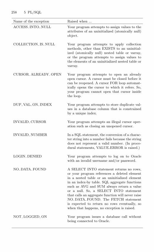
258 5 PL/SQL
Name of the exception Raised when ...
ACCESS INTO NULL Your program attempts to assign values to theattributes of an uninitialized (atomically null)object.
COLLECTION IS NULL Your program attempts to apply collectionmethods, other than EXISTS to an uninitial-ized (atomically null) nested table or varray,or the program attempts to assign values tothe elements of an uninitialized nested table orvarray.
CURSOR ALREADY OPEN Your program attempts to open an alreadyopen cursor. A cursor must be closed before itcan be reopened. A cursor FOR loop automat-ically opens the cursor to which it refers. So,your program cannot open that cursor insidethe loop.
DUP VAL ON INDEX Your program attempts to store duplicate val-ues in a database column that is constrainedby a unique index.
INVALID CURSOR Your program attempts an illegal cursor oper-ation such as closing an unopened cursor.
INVALID NUMBER In a SQL statement, the conversion of a charac-ter string into a number fails because the stringdoes not represent a valid number. (In proce-dural statements, VALUE ERROR is raised.)
LOGIN DENIED Your program attempts to log on to Oraclewith an invalid username and/or password.
NO DATA FOUND A SELECT INTO statement returns no rows,or your program references a deleted elementin a nested table or an uninitialized elementin an index-by table. SQL aggregate functionssuch as AVG and SUM always return a valueor a null. So, a SELECT INTO statementthat calls an aggregate function will never raiseNO DATA FOUND. The FETCH statementis expected to return no rows eventually, sowhen that happens, no exception is raised.
NOT LOGGED ON Your program issues a database call withoutbeing connected to Oracle.
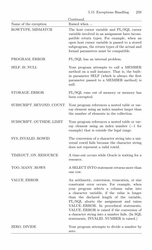
5.15 Exceptions Handling 259
Continued.
Name of the exception Raised when ...
ROWTYPE MISMATCH The host cursor variable and PL/SQL cursorvariable involved in an assignment have incom-patible return types. For example, when anopen host cursor variable is passed to a storedsubprogram, the return types of the actual andformal parameters must be compatible.
PROGRAM ERROR PL/SQL has an internal problem.
SELF IS NULL Your program attempts to call a MEMBERmethod on a null instance. That is, the built-in parameter SELF (which is always the firstparameter passed to a MEMBER method) isnull.
STORAGE ERROR PL/SQL runs out of memory or memory hasbeen corrupted.
SUBSCRIPT BEYOND COUNT Your program references a nested table or var-ray element using an index number larger thanthe number of elements in the collection.
SUBSCRIPT OUTSIDE LIMIT Your program references a nested table or var-ray element using an index number (−1 forexample) that is outside the legal range.
SYS INVALID ROWID The conversion of a character string into a uni-versal rowid fails because the character stringdoes not represent a valid rowid.
TIMEOUT ON RESOURCE A time-out occurs while Oracle is waiting for aresource.
TOO MANY ROWS A SELECT INTO statement returns more thanone row.
VALUE ERROR An arithmetic, conversion, truncation, or sizeconstraint error occurs. For example, whenyour program selects a column value intoa character variable, if the value is longerthan the declared length of the variable,PL/SQL aborts the assignment and raisesVALUE ERROR. In procedural statements,VALUE ERROR is raised if the conversion ofa character string into a number fails. (In SQLstatements, INVALID NUMBER is raised.)
ZERO DIVIDE Your program attempts to divide a number byzero.
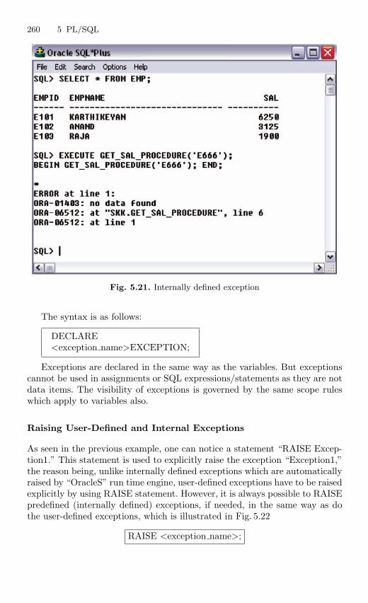
260 5 PL/SQL
Fig. 5.21. Internally defined exception
The syntax is as follows:
DECLARE<exception name>EXCEPTION;
Exceptions are declared in the same way as the variables. But exceptionscannot be used in assignments or SQL expressions/statements as they are notdata items. The visibility of exceptions is governed by the same scope ruleswhich apply to variables also.
Raising User-Defined and Internal Exceptions
As seen in the previous example, one can notice a statement “RAISE Excep-tion1.” This statement is used to explicitly raise the exception “Exception1,”the reason being, unlike internally defined exceptions which are automaticallyraised by “OracleS” run time engine, user-defined exceptions have to be raisedexplicitly by using RAISE statement. However, it is always possible to RAISEpredefined (internally defined) exceptions, if needed, in the same way as dothe user-defined exceptions, which is illustrated in Fig. 5.22
RAISE <exception name>;
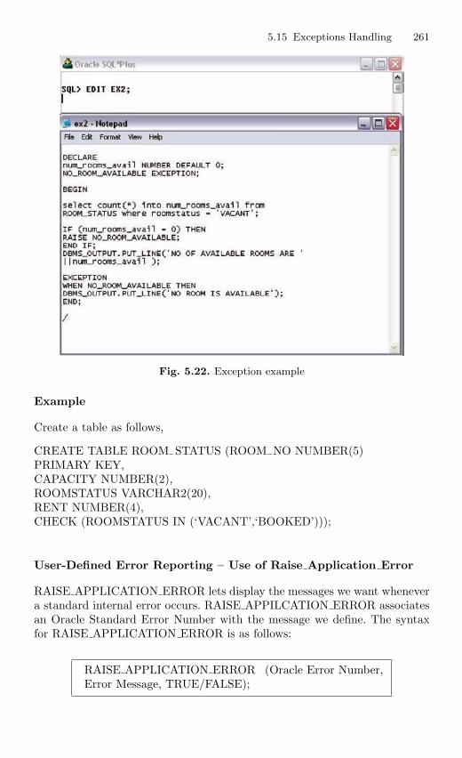
5.15 Exceptions Handling 261
Fig. 5.22. Exception example
Example
Create a table as follows,
CREATE TABLE ROOM STATUS (ROOM NO NUMBER(5)PRIMARY KEY,CAPACITY NUMBER(2),ROOMSTATUS VARCHAR2(20),RENT NUMBER(4),CHECK (ROOMSTATUS IN (‘VACANT’,‘BOOKED’)));
User-Defined Error Reporting – Use of Raise Application Error
RAISE APPLICATION ERROR lets display the messages we want whenevera standard internal error occurs. RAISE APPILCATION ERROR associatesan Oracle Standard Error Number with the message we define. The syntaxfor RAISE APPLICATION ERROR is as follows:
RAISE APPLICATION ERROR (Oracle Error Number,Error Message, TRUE/FALSE);
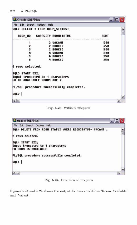
262 5 PL/SQL
Fig. 5.23. Without exception
Fig. 5.24. Execution of exception
Figures 5.23 and 5.24 shows the output for two conditions ‘Room Available’and ‘Vacant’.
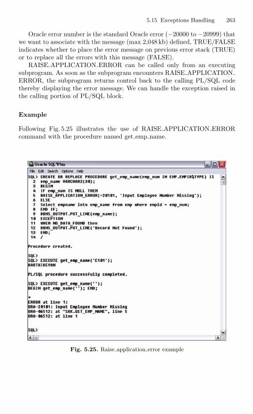
5.15 Exceptions Handling 263
Oracle error number is the standard Oracle error (−20000 to −20999) thatwe want to associate with the message (max 2,048 kb) defined, TRUE/FALSEindicates whether to place the error message on previous error stack (TRUE)or to replace all the errors with this message (FALSE).
RAISE APPLICATION ERROR can be called only from an executingsubprogram. As soon as the subprogram encounters RAISE APPLICATIONERROR, the subprogram returns control back to the calling PL/SQL codethereby displaying the error message. We can handle the exception raised inthe calling portion of PL/SQL block.
Example
Following Fig. 5.25 illustrates the use of RAISE APPLICATION ERRORcommand with the procedure named get emp name.
Fig. 5.25. Raise application error example
264 5 PL/SQL
5.16 Database Triggers
A database trigger is a stored PL/SQL program unit associated with a spe-cific database table. It can perform the role of a constraint, which forces theintegrity of data. It is the most practical way to implement routines and grant-ing integrity of data. Unlike the stored procedures or functions, which haveto be explicitly invoked, these triggers implicitly get fired whenever the tableis affected by the SQL operation. For any event that causes a change in thecontents of a table, a user can specify an associated action that the DBMSshould carry out. Trigger follows the Event-Condition-Action scheme (ECAscheme).
Privileges Required for Triggers
Creation or alteration of a TRIGGER on a specific table requires TRIGGERprivileges as well as table privileges. They are:
1. To create TRIGGER in one’s own schema, he must have CREATE TRIG-GER privilege. To create a trigger in any other’s schema, one must haveCREATE ANY TRIGGER system privilege.
2. To create a trigger on table, one must own the table or should have ALTERprivilege for that table or should have ALTER ANY TABLE privilege.
3. To ALTER a trigger, one must own that trigger or should have ALTERANY TRIGGER privilege. Also since the trigger will be operating onsome table, one also requires ALTER privilege on that table or ALTERANY TABLE table privilege.
4. To create a TRIGGER on any database level event, one must have AD-MINISTER DATABASE TRIGGER system privilege.
Context to Use Triggers
Following are the situations to use the triggers efficiently:
– Use triggers to guarantee that when a specific operation is performed,related actions are performed.
– Do not define triggers that duplicate the functionality already built intoOracle. For example, do not define triggers to enforce data integrity rulesthat can be easily enforced using declarative integrity constraints.
– Limit the size of triggers. If the logic for our trigger requires much morethan 60 lines of PL/SQL code, then it is better to include most of thecode in a stored procedure and call the procedure from the trigger.
– Use triggers only for centralized, global operations that should be fired forthe triggering statement, regardless of which user or database applicationissues the statement.
– Do not create recursive triggers which cause the trigger to fire recursivelyuntil it has run out of memory.
5.16 Database Triggers 265
– Use triggers on DATABASE judiciously. They are executed for every userevery time the event occurs on which the trigger is created.
Uniqueness of Trigger
Different types of integrity constraints provide a declarative mechanism toassociate “simple” conditions with a table such as a primary key, foreignkeys, or domain constraints. Complex integrity constraints that refer to severaltables and attributes cannot be specified within table definitions. Triggers, incontrast, provide a procedural technique to specify and maintain integrityconstraints.
Triggers even allow users to specify more complex integrity constraintssince a trigger essentially is a PL/SQL procedure. Such a procedure is associ-ated with a table and is automatically called by the database system whenevera certain modification (event) occurs on that table.
Simply we can say that trigger is less declarative and more pro-
cedural type constraint enforcement. Triggers are used generally toimplement business rules in the database. It is the major difference betweenTriggers and Integrity Constraints.
Create Trigger Syntax
The Create trigger syntax is as follows:
CREATE [OR REPLACE] TRIGGER <trigger name>[BEFORE/AFTER/INSTEAD OF][INSERT/UPDATE/DELETE [of column,..]] ON <table name>[REFERENCING [OLD [AS] <old name> | NEW [AS]<new name>][FOR EACH STATEMENT/FOR EACH ROW][WHEN <condition>][BEGIN–PL/SQL blockEND];
This syntax can be explained as follows.
Parts of Trigger
A trigger has three basic parts:
– A triggering event or statement– A trigger restriction– A trigger action
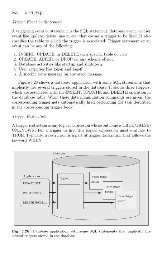
266 5 PL/SQL
Trigger Event or Statement
A triggering event or statement is the SQL statement, database event, or userevent like update, delete, insert, etc. that causes a trigger to be fired. It alsospecifies the table to which the trigger is associated. Trigger statement or anevent can be any of the following:
1. INSERT, UPDATE, or DELETE on a specific table or view.2. CREATE, ALTER, or DROP on any schema object.3. Database activities like startup and shutdown.4. User activities like logon and logoff.5. A specific error message on any error message.
Figure 5.26 shows a database application with some SQL statements thatimplicitly fire several triggers stored in the database. It shows three triggers,which are associated with the INSERT, UPDATE, and DELETE operation inthe database table. When these data manipulation commands are given, thecorresponding trigger gets automatically fired performing the task describedin the corresponding trigger body.
Trigger Restriction
A trigger restriction is any logical expression whose outcome is TRUE/FALSE/UNKNOWN. For a trigger to fire, this logical expression must evaluate toTRUE. Typically, a restriction is a part of trigger declaration that follows thekeyword WHEN.
Database
Table tUpdate Trigger
BEGIIT- - -
Insert Trigger
BEGIIT- - -
Delete Trigger
BEGIIT- - -
Applications
UPDATE:SET...:
INSERT INTOt...:
DELETE FROMt...:
Fig. 5.26. Database application with some SQL statements that implicitly fireseveral triggers stored in the database
5.17 Types of Triggers 267
Trigger Action
A trigger action is the PL/SQL block that contains the SQL statements andcode to be executed when a triggering statement is issued and the triggerrestriction evaluates to TRUE. It is also called the trigger body. Like storedprocedures, a trigger action can contain SQL and PL/SQL.
Following statements will explain the various keywords used in the syntax.BEFORE and AFTER keyword indicates whether the trigger should be
executed before or after the trigger event, where a triggering event can beINSERT, UPDATE, or DELETE. Any combination of triggering events canbe included in the same database trigger.
When referring the old and new values of columns, we can use the defaults(“old” and “new”) or we can use the REFERENCING clause to specify othernames. FOR EACH ROW clause causes the trigger to fire once for each recordcreated, deleted, or modified by the triggering statement. When working withrow triggers, the WHEN clause can be used to restrict the records for whichthe trigger fires.
We can use INSTEAD OF triggers to tell the database what to do insteadof performing the actions that invoked the trigger. For example, we can useit on a VIEW to redirect the inserts into a table or to update multiple tablesthat are parts of the view.
5.17 Types of Triggers
Type of trigger firing, level at which a trigger is executed, and the types ofevents form the basis classification of triggers into different categories. Thissection describes the different types of triggers. The broad classification oftriggers is as shown below.
On the Basis of Type of Events– Triggers on System events– Trigger on User events
On the Basis of the Level at which Triggers are Executed– Row Level Triggers– Statement Level Triggers
On the Basis of Type of Trigger/Firing or Triggering Transaction– BEFORE Triggers– AFTER Triggers– INSTEAD OF
Triggers on System Events
System events that can fire triggers are related to instance startup and shut-down and error messages. Triggers created on startup and shutdown eventshave to be associated with the database; triggers created on error events canbe associated with the database or with a schema.
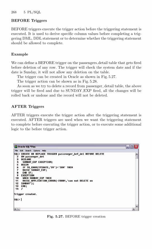
268 5 PL/SQL
BEFORE Triggers
BEFORE triggers execute the trigger action before the triggering statement isexecuted. It is used to derive specific column values before completing a trig-gering DML, DDL statement or to determine whether the triggering statementshould be allowed to complete.
Example
We can define a BEFORE trigger on the passengers detail table that gets firedbefore deletion of any row. The trigger will check the system date and if thedate is Sunday, it will not allow any deletion on the table.
The trigger can be created in Oracle as shown in Fig. 5.27.The trigger action can be shown as in Fig. 5.28.As soon as we try to delete a record from passenger detail table, the above
trigger will be fired and due to SUNDAY EXP fired, all the changes will berolled back or undone and the record will not be deleted.
AFTER Triggers
AFTER triggers execute the trigger action after the triggering statement isexecuted. AFTER triggers are used when we want the triggering statementto complete before executing the trigger action, or to execute some additionallogic to the before trigger action.
Fig. 5.27. BEFORE trigger creation
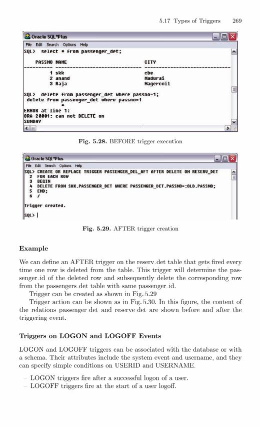
5.17 Types of Triggers 269
Fig. 5.28. BEFORE trigger execution
Fig. 5.29. AFTER trigger creation
Example
We can define an AFTER trigger on the reserv det table that gets fired everytime one row is deleted from the table. This trigger will determine the pas-senger id of the deleted row and subsequently delete the corresponding rowfrom the passengers det table with same passenger id.
Trigger can be created as shown in Fig. 5.29Trigger action can be shown as in Fig. 5.30. In this figure, the content of
the relations passenger det and reserve det are shown before and after thetriggering event.
Triggers on LOGON and LOGOFF Events
LOGON and LOGOFF triggers can be associated with the database or witha schema. Their attributes include the system event and username, and theycan specify simple conditions on USERID and USERNAME.
– LOGON triggers fire after a successful logon of a user.– LOGOFF triggers fire at the start of a user logoff.
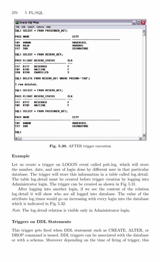
270 5 PL/SQL
Fig. 5.30. AFTER trigger execution
Example
Let us create a trigger on LOGON event called pub log, which will storethe number, date, and user of login done by different user in that particulardatabase. The trigger will store this information in a table called log detail.The table log detail must be created before trigger creation by logging intoAdministrator login. The trigger can be created as shown in Fig. 5.31.
After logging into another login, if we see the content of the relationlog detail it will show who are all logged into database. The value of theattribute log times would go on increasing with every login into the databasewhich is indicated in Fig. 5.32.
Note The log detail relation is visible only in Administrator login.
Triggers on DDL Statements
This trigger gets fired when DDL statement such as CREATE, ALTER, orDROP command is issued. DDL triggers can be associated with the databaseor with a schema. Moreover depending on the time of firing of trigger, this
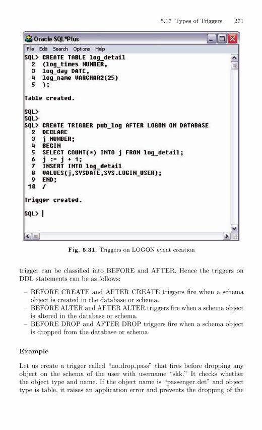
5.17 Types of Triggers 271
Fig. 5.31. Triggers on LOGON event creation
trigger can be classified into BEFORE and AFTER. Hence the triggers onDDL statements can be as follows:
– BEFORE CREATE and AFTER CREATE triggers fire when a schemaobject is created in the database or schema.
– BEFORE ALTER and AFTER ALTER triggers fire when a schema objectis altered in the database or schema.
– BEFORE DROP and AFTER DROP triggers fire when a schema objectis dropped from the database or schema.
Example
Let us create a trigger called “no drop pass” that fires before dropping anyobject on the schema of the user with username “skk.” It checks whetherthe object type and name. If the object name is “passenger det” and objecttype is table, it raises an application error and prevents the dropping of the
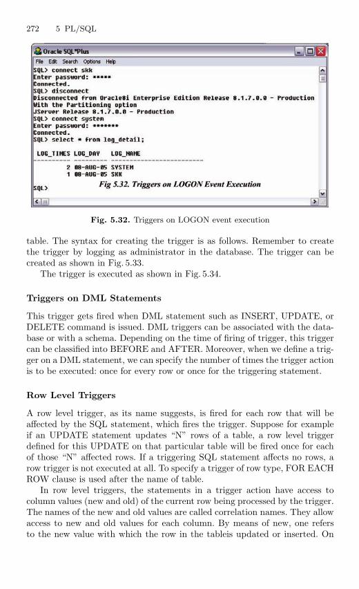
272 5 PL/SQL
Fig. 5.32. Triggers on LOGON event execution
table. The syntax for creating the trigger is as follows. Remember to createthe trigger by logging as administrator in the database. The trigger can becreated as shown in Fig. 5.33.
The trigger is executed as shown in Fig. 5.34.
Triggers on DML Statements
This trigger gets fired when DML statement such as INSERT, UPDATE, orDELETE command is issued. DML triggers can be associated with the data-base or with a schema. Depending on the time of firing of trigger, this triggercan be classified into BEFORE and AFTER. Moreover, when we define a trig-ger on a DML statement, we can specify the number of times the trigger actionis to be executed: once for every row or once for the triggering statement.
Row Level Triggers
A row level trigger, as its name suggests, is fired for each row that will beaffected by the SQL statement, which fires the trigger. Suppose for exampleif an UPDATE statement updates “N” rows of a table, a row level triggerdefined for this UPDATE on that particular table will be fired once for eachof those “N” affected rows. If a triggering SQL statement affects no rows, arow trigger is not executed at all. To specify a trigger of row type, FOR EACHROW clause is used after the name of table.
In row level triggers, the statements in a trigger action have access tocolumn values (new and old) of the current row being processed by the trigger.The names of the new and old values are called correlation names. They allowaccess to new and old values for each column. By means of new, one refersto the new value with which the row in the tableis updated or inserted. On
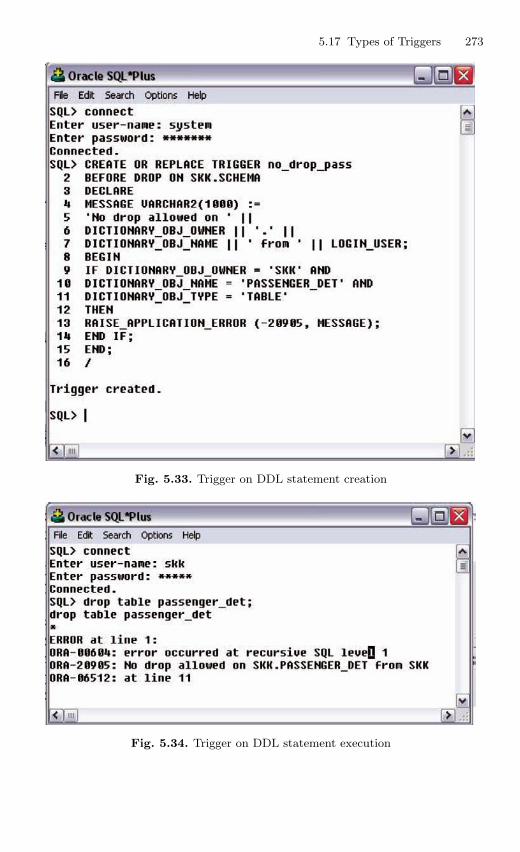
5.17 Types of Triggers 273
Fig. 5.33. Trigger on DDL statement creation
Fig. 5.34. Trigger on DDL statement execution
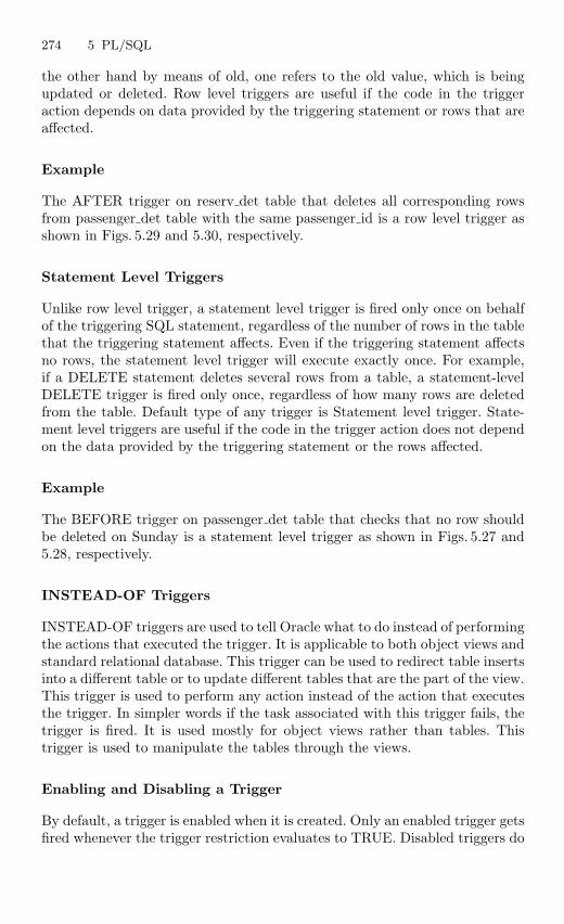
274 5 PL/SQL
the other hand by means of old, one refers to the old value, which is beingupdated or deleted. Row level triggers are useful if the code in the triggeraction depends on data provided by the triggering statement or rows that areaffected.
Example
The AFTER trigger on reserv det table that deletes all corresponding rowsfrom passenger det table with the same passenger id is a row level trigger asshown in Figs. 5.29 and 5.30, respectively.
Statement Level Triggers
Unlike row level trigger, a statement level trigger is fired only once on behalfof the triggering SQL statement, regardless of the number of rows in the tablethat the triggering statement affects. Even if the triggering statement affectsno rows, the statement level trigger will execute exactly once. For example,if a DELETE statement deletes several rows from a table, a statement-levelDELETE trigger is fired only once, regardless of how many rows are deletedfrom the table. Default type of any trigger is Statement level trigger. State-ment level triggers are useful if the code in the trigger action does not dependon the data provided by the triggering statement or the rows affected.
Example
The BEFORE trigger on passenger det table that checks that no row shouldbe deleted on Sunday is a statement level trigger as shown in Figs. 5.27 and5.28, respectively.
INSTEAD-OF Triggers
INSTEAD-OF triggers are used to tell Oracle what to do instead of performingthe actions that executed the trigger. It is applicable to both object views andstandard relational database. This trigger can be used to redirect table insertsinto a different table or to update different tables that are the part of the view.This trigger is used to perform any action instead of the action that executesthe trigger. In simpler words if the task associated with this trigger fails, thetrigger is fired. It is used mostly for object views rather than tables. Thistrigger is used to manipulate the tables through the views.
Enabling and Disabling a Trigger
By default, a trigger is enabled when it is created. Only an enabled trigger getsfired whenever the trigger restriction evaluates to TRUE. Disabled triggers do
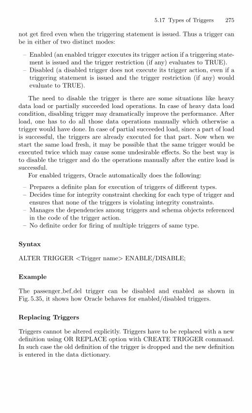
5.17 Types of Triggers 275
not get fired even when the triggering statement is issued. Thus a trigger canbe in either of two distinct modes:
– Enabled (an enabled trigger executes its trigger action if a triggering state-ment is issued and the trigger restriction (if any) evaluates to TRUE).
– Disabled (a disabled trigger does not execute its trigger action, even if atriggering statement is issued and the trigger restriction (if any) wouldevaluate to TRUE).
The need to disable the trigger is there are some situations like heavydata load or partially succeeded load operations. In case of heavy data loadcondition, disabling trigger may dramatically improve the performance. Afterload, one has to do all those data operations manually which otherwise atrigger would have done. In case of partial succeeded load, since a part of loadis successful, the triggers are already executed for that part. Now when westart the same load fresh, it may be possible that the same trigger would beexecuted twice which may cause some undesirable effects. So the best way isto disable the trigger and do the operations manually after the entire load issuccessful.
For enabled triggers, Oracle automatically does the following:
– Prepares a definite plan for execution of triggers of different types.– Decides time for integrity constraint checking for each type of trigger and
ensures that none of the triggers is violating integrity constraints.– Manages the dependencies among triggers and schema objects referenced
in the code of the trigger action.– No definite order for firing of multiple triggers of same type.
Syntax
ALTER TRIGGER <Trigger name> ENABLE/DISABLE;
Example
The passenger bef del trigger can be disabled and enabled as shown inFig. 5.35, it shows how Oracle behaves for enabled/disabled triggers.
Replacing Triggers
Triggers cannot be altered explicitly. Triggers have to be replaced with a newdefinition using OR REPLACE option with CREATE TRIGGER command.In such case the old definition of the trigger is dropped and the new definitionis entered in the data dictionary.
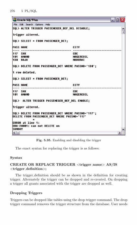
276 5 PL/SQL
Fig. 5.35. Enabling and disabling the trigger
The exact syntax for replacing the trigger is as follows:
Syntax
CREATE OR REPLACE TRIGGER <trigger name> AS/IS<trigger definition>;
The trigger definition should be as shown in the definition for creatingtrigger. Alternately the trigger can be dropped and re-created. On droppinga trigger all grants associated with the trigger are dropped as well.
Dropping Triggers
Triggers can be dropped like tables using the drop trigger command. The droptrigger command removes the trigger structure from the database. User needs
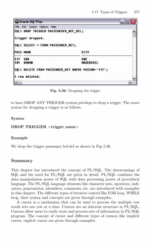
5.17 Types of Triggers 277
Fig. 5.36. Dropping the trigger
to have DROP ANY TRIGGER system privilege to drop a trigger. The exactsyntax for dropping a trigger is as follows.
Syntax
DROP TRIGGER <trigger name>
Example
We drop the trigger passenger bef del as shown in Fig. 5.36.
Summary
This chapter has introduced the concept of PL/SQL. The shortcomings ofSQL and the need for PL/SQL are given in detail. PL/SQL combines thedata manipulation power of SQL with data processing power of procedurallanguage. The PL/SQL language elements like character sets, operators, indi-cators, punctuation, identifiers, comments, etc. are introduced with examplesin this chapter. The different types of iterative control like FOR loop, WHILEloop, their syntax and concepts are given through examples.
A cursor is a mechanism that can be used to process the multiple rowresult sets one row at a time. Cursors are an inherent structure in PL/SQL.Cursors allow users to easily store and process sets of information in PL/SQLprogram. The concept of cursor and different types of cursors like implicitcursor, explicit cursor are given through examples.
278 5 PL/SQL
A procedure is a subprogram that performs some specific task, and storedin the data dictionary. The concept of procedure, function, the differencebetween procedure and function are given in this chapter.
A package is a collection of related program objects such as procedures,functions, and associated cursors and variables together as a unit in the data-base. In simpler term, a package is a group of related procedures and functionsstored together and sharing common variables, as well as local procedures andfunction. In this chapter, the package body and how to create a package areexplained with examples.
An EXCEPTION is any error or warning condition that arises during run-time. The main intention of building EXCEPTION technique is to continuethe processing of a program even when it encounters runtime error or warn-ing and display suitable messages on console so that user can handle thoseconditions next time. The advantage of using EXCEPTION, different typesof EXCEPTIONS are given through example in this chapter.
A database trigger is a stored PL/SQL program unit associated with aspecific database table. It can perform the role of a constraint, which forcesthe integrity of data. The concept of trigger, the uniqueness of trigger, andthe use of trigger are explained with examples in this chapter.
Review Questions
5.1. Mention the key difference between SQL and PL/SQL?
SQL is a declarative language. PL/SQL is a procedural language thatmakes up for all the missing elements in SQL.
5.2. Mention two drawbacks of SQL?
– SQL statements can be executed only one at a time. Every time to executea SQL statement, a call is made to Oracle engine, thus it results in anincrease in database overheads.
– While processing an SQL statement, if an error occurs, Oracle generatesits own error message, which is sometimes difficult to understand. If auser wants to display some other meaningful error message, SQL does nothave provision for that.
5.3. Identify which one is not included in PL/SQL Character Set?(a) * (b)> (c)! (d) \
Answer : (d)
5.4. What are Lexical units related with PL/SQL?
A line of PL/SQL program contains groups of characters known as lexicalunits, which can be classified as follows:
Review Questions 279
– Delimiters– Identifiers– Literals– Comments
5.5. What is Delimiter?
A delimiter is a simple or compound symbol that has a special meaningto PL/SQL.
5.6. Identify which identifier is not permitted in PL/SQL?(a) Bn12 (b) Girt–1 (c) Hay# (d) I am
Answer : (d)
5.7. Give the syntax for single-line comments and multiline comments?
Single line comment: –Multiline comment: /* . . . . . . Some text. . . . . . */
5.8. How you declare a record type variable in PL/SQL?
We can declare record type variable for particular table by using the syn-tax.
<Variable Name> <Table name>%ROWTYPE.ROWTYPE is a keyword for defining record type variables.
5.9. Find out the error in the following PL/SQL statement?
IF condition THENsequence of statements1ELSEsequence of statements2END IF;
Answer : No Error in the Statement.
5.10. Mention the facilities available for iterating the statements in PL/SQL?
(a) For-loop(b) While-loop(c) Loop-Exit
5.11. What is cursor and mention its types in Oracle?
A cursor is a mechanism that can be used to process the multiple rowresult sets one row at a time.
In other words, cursors are constructs that enable the user to name aprivate memory area to hold a specific statement for access at a later time.Cursors are an inherent structure in PL/SQL. Cursors allow users to easilystore and process sets of information in PL/SQL program.
280 5 PL/SQL
There are two types of cursors in Oracle
(a) Implicit and(b) Explicit cursors.
5.12. Mention the syntax for opening and closing a cursor.
For Opening: Open <cursor name>For Closing: Close <cursor name>
5.13. Mention some implicit and explicit cursor attributes.
Implicit:%NOTFOUND, %FOUND, % ROWCOUNT, and %ISOPEN
Explicit:Similar to Implicit.%NOTFOUND, %FOUND, %ROWCOUNT, and %ISOPEN
5.14. What is Procedure in PL/SQL?
A procedure is a subprogram that performs some specific task, and storedin the data dictionary. A procedure must have a name so that it can beinvoked or called by any PL/SQL program that appears within an application.Procedures can take parameters from the calling program and perform thespecific task. Before the procedure or function is stored, the Oracle engineparses and compiles the procedure or function.
5.15. Mention any four advantages of procedures and function?
1. It modifies one routine to affect multiple applications.2. It modifies one routine to eliminate duplicate testing.3. It ensures that related actions are performed together, or not at all, by
doing the activity through a single path.4. It avoids PL/SQL parsing at runtime by parsing at compile time.
5.16. What is the syntax used in PL/SQL for dropping a procedure?
DROP PROCEDURE <PROCEDURE NAME>
5.17. Mention three differences between functions and procedures?
1. A procedure never returns a value to the calling portion of code, whereasa function returns exactly one value to the calling program.
2. As functions are capable of returning a value, they can be used as elementsof SQL expressions, whereas the procedures cannot. However, user definedfunctions cannot be used in CHECK or DEFAULT constraints and cannot manipulate database values, to obey function purity rules.
Review Questions 281
3. It is mandatory for a function to have at least one RETURN statement,whereas for procedures there is no restriction. A procedure may have aRETURN statement or may not. In case of procedures with RETURNstatement, simply the control of execution is transferred back to the por-tion of code that called the procedure.
5.18. What is Purity rule for functions in PL/SQL?
For a function to be eligible for being called in SQL statements, it mustsatisfy following requirements, which are known as Purity Rules.
1. When called from a SELECT statement or a parallelized INSERT,UPDATE, or DELETE statement, the function cannot modify any data-base tables.
2. When called from an INSERT, UPDATE, or DELETE statement, thefunction cannot query or modify any database tables modified by thatstatement.
3. When called from a SELECT, INSERT, UPDATE, or DELETE state-ment, the function cannot execute SQL transaction control statements(such as COMMIT), session control statements (such as SET ROLE), orsystem control statements (such as ALTER SYSTEM). Also, it cannotexecute DDL statements (such as CREATE) because they are followed byan automatic commit.
5.19. What is a syntax for deleting a function in PL/SQL?
DROP FUNCTION <FUNCTION NAME>
5.20. What are parameters?
Parameters are the link between a subprogram code and the code callingthe subprogram. Lot depends on how the parameters are passed to a subpro-gram.
5.21. What are Packages?
A package can be defined as a collection of related program objects such asprocedures, functions, and associated cursors and variables together as a unitin the database. In simpler term, a package is a group of related proceduresand functions stored together and sharing common variables, as well as localprocedures and functions.
5.22. Mention any two advantages of Packages?
1. Stored packages allow you to sum up (group logically) related stored pro-cedures, variables, and datatypes, and so forth in a single-named, storedunit in the database. This provides for better orderliness during the de-velopment process. In other words packages and its modules are easilyunderstood because of their logical grouping.
282 5 PL/SQL
2. Grouping of related procedures, functions, etc. in a package also makeprivilege management easier. Granting the privilege to use a packagemakes all components of the package accessible to the grantee.
5.23. Mention how exception handling is done in Oracle?
During execution of a PL/SQL block of code, Oracle executes every SQLsentence within the PL/SQL block. If an error occurs or an SQL sentencefails, Oracle considers this as an Exception. Oracle engine immediately triesto handle the exception and resolve it, by raising a built-in Exception handler.
5.24. Mention two advantages of using exceptions in Oracle?
1. Control over abnormal exits of executing programs on encountering errorconditions, hence the behavior of application becomes more reliable.
2. In traditional error checking system, if same error is to be checked atseveral places, you are required to code the same error check at all thoseplaces. But with exception handling technique, you will write the excep-tion for that particular error only once in the entire code. Whenever thattype error occurs at any place in code, the exceptional handler will auto-matically raise the defined exception.
6
Database Design
Learning Objectives. This chapter deals with various phases in database design,objectives of database design, database design tools. The important concept indatabase design like functional dependency and normalization are also discussedin this chapter. After completing this chapter the reader should be familiar with thefollowing concepts:
– Various phases in database design– Database design tools– Identify modification anomalies in tables– Functional dependency, Armstrong’s axioms– Concept of normalization and different normal forms– Denormalization
6.1 Introduction
Database design process integrates relevant data in such a manner that itcan be processed through a mechanism for recording the facts. A database ofan organization is an information repository that represents facts about theorganization. It is manipulated by some software to incorporate the changesthat take place in the organization. The database design is a complex process.The complexity arises mainly because of the identification of relationshipsamong individual components and their representation for maintaining correctfunctionality are highly involved. The degree of complexity increases if thereare many-to-many relationships among individual components. The processof database design usually requires a number of steps which are in Fig. 6.1.
Feasibility Study
When designing a database, the purpose for which the database is beingdesigned must be clearly defined. In other words the objective of creatingthe database must be crystal clear.
S. Sumathi: Database Design, Studies in Computational Intelligence (SCI) 47, 283–317 (2007)
www.springerlink.com c© Springer-Verlag Berlin Heidelberg 2007
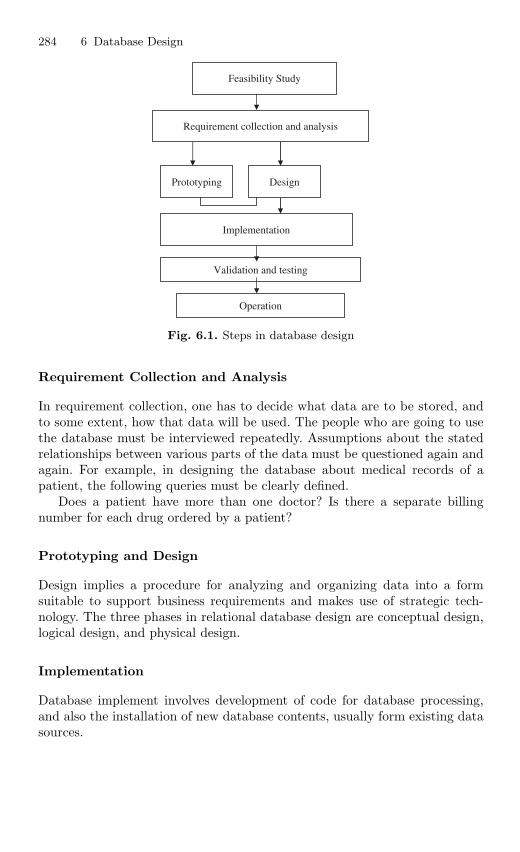
284 6 Database Design
Feasibility Study
Requirement collection and analysis
Prototyping Design
Implementation
Validation and testing
Operation
Fig. 6.1. Steps in database design
Requirement Collection and Analysis
In requirement collection, one has to decide what data are to be stored, andto some extent, how that data will be used. The people who are going to usethe database must be interviewed repeatedly. Assumptions about the statedrelationships between various parts of the data must be questioned again andagain. For example, in designing the database about medical records of apatient, the following queries must be clearly defined.
Does a patient have more than one doctor? Is there a separate billingnumber for each drug ordered by a patient?
Prototyping and Design
Design implies a procedure for analyzing and organizing data into a formsuitable to support business requirements and makes use of strategic tech-nology. The three phases in relational database design are conceptual design,logical design, and physical design.
Implementation
Database implement involves development of code for database processing,and also the installation of new database contents, usually form existing datasources.
6.2 Objectives of Database Design 285
6.2 Objectives of Database Design
The objectives of database design vary from implementation to implementa-tion. Some of the important factors like efficiency, integrity, privacy, security,implementability, flexibility have to be considered in the design of the data-base.
Efficiency
Efficiency is generally considered to be the most important. Given a piece ofhardware on which the database will run and a piece of software (DBMS) torun it, the design should make full and efficient use of the facilities provided. Ifthe database is made online, then the users should interact with the databasewithout any time delay.
Integrity
The term integrity means that the database should be as accurate as possible.The problem of preserving the integrity of data in a database can be viewedat a number of levels. At a low level it concerns ensuring that the data are notcorrupted by hardware or software errors. At a higher level, the problem ofpreserving database integrity concerns maintaining an accurate representationof the real world.
Privacy
The database should not allow unauthorized access to files. This is veryimportant in the case of financial data. For example the bank balance ofone customer should not be revealed to other customers.
Security
The database, once loaded, should be safe from physical corruption whetherfrom hardware or software failure or from unauthorized access. This is ageneral requirement of most databases.
Implementation
The conceptual model should be simple and effective so that mapping fromconceptual model to logical model is easy. Moreover while designing the data-base, care has to be taken such that application programs should interacteffectively with the database.
286 6 Database Design
Flexibility
The database should not be implemented in a rigid way that assumes thebusiness will remain constant forever. Changes will occur and the databasemust be capable of responding readily to such change.
Other than the factors which were mentioned above, the design of thedatabase should ensure that data redundancy is not there.
6.3 Database Design Tools
Once the objectives of the database design and the various steps in databasedesign is known, it is essential to know the database design tools which areused to automate the task of designing a business system. Using automateddesign tools is the process of using a GUI tool to assist in the design of adatabase or database application. Many database design tools are availablewith a variety of features. The design tools are vendor-specific. CASE toolsare software that provides automated support for some portion of the systemsdevelopment process. Database drawing tools are used in enterprise model-ing, conceptual data modeling, logical database design, and physical datamodeling.
6.3.1 Need for Database Design Tool
The database design tools increase the overall productivity because themanual tasks are automated and less time is spent in performing tedious tasksand more time is spent in thinking about the actual design of the database.The quality of the end product is improved in using database design tools;because the design tool automates much of the design process as a result thetime taken to design a database is reduced. As a result, more time is availableto interview the customer, conduct user feedback sessions, and naturally thequality of the product is improved.
6.3.2 Desired Features of Database Design Tools
The database design tools should help the developer to complete the databasemodel of database application in a timely fashion. Some of the features of thedatabase design tools are given below:
– The database design tools should capture the user needs.– The capability to model the flow of data in an organization.– The database design tool should have the capability to model entities and
their relationships.– The database design tool should have the capability to generate Data
Definition Language (DDL) to create database object.
6.3 Database Design Tools 287
– The database design tool should support full life cycle database support.– Database and application version control.– The database design tool should generate reports for documentation and
user-feedback sessions.
6.3.3 Advantages of Database Design Tools
Some of the advantages of using database design tools for system design orapplication development are given as:
– The amount of code to be written is reduced as a result the databasedesign time is reduced.
– Chances of errors because of manual work are reduced.– Easy to convert the business model to working database model.– Easy to ensure that all business requirements are met with.– A higher quality, more accurate product is produced.
6.3.4 Disadvantages of Database Design Tools
Some of the disadvantages of database design tools are given below:
– More expenses involved for the tool itself.– Developers might require special training to use the tool.
6.3.5 Commercial Database Design Tools
The database design tools which are commercially popular are given alongwith their websites.
1. CASE Studio 2 – Powerful database modeling, management, and reportingtool.http://www.casestudio.com/enu/default.aspx
2. Design for Databases V3 – Database development tool using an entityrelationship diagram.http://www.datanamic.com/dezign
3. DBDesigner4 – Visual database design system that integrates databasedesign, modeling.
4. ER/Studio – Multilevel data modeling application for logical and physicaldatabase design and construction.http://www.embarcadero.com/products/erstudio/index.html
5. Happy Fish Database Designer – Visual database design tool supportingmultiple database platforms. Happy Fish generates complete DDL scripts,defining metadata with table creates, indexes, foreign keys.http://www.embarcadero.com/products/erstudio/index.html
6. Oracle Designer 2000 – Provides complete toolset to model, generate, andcapture the requirements and design of enterprise applications.http://www.Oracle.com/technology/products/designer/index.html
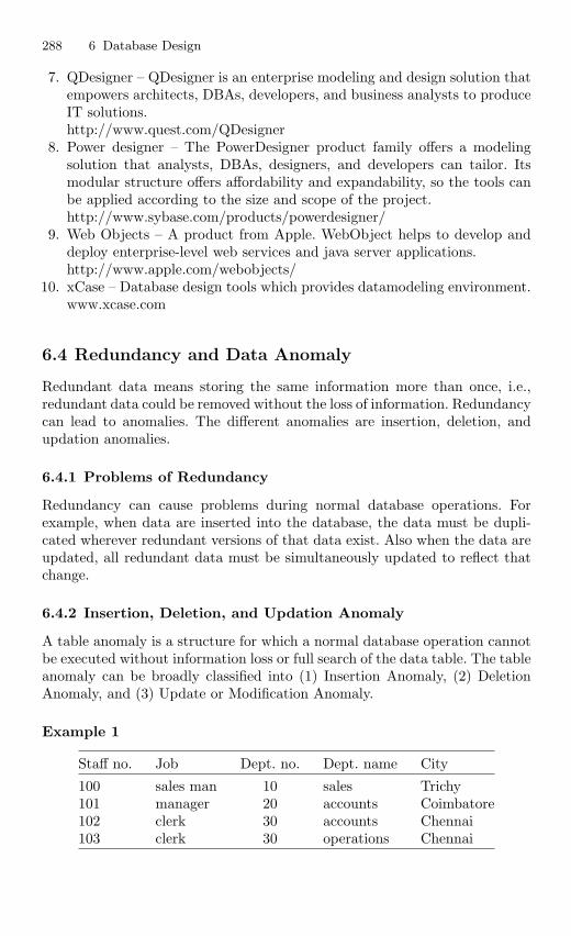
288 6 Database Design
7. QDesigner – QDesigner is an enterprise modeling and design solution thatempowers architects, DBAs, developers, and business analysts to produceIT solutions.http://www.quest.com/QDesigner
8. Power designer – The PowerDesigner product family offers a modelingsolution that analysts, DBAs, designers, and developers can tailor. Itsmodular structure offers affordability and expandability, so the tools canbe applied according to the size and scope of the project.http://www.sybase.com/products/powerdesigner/
9. Web Objects – A product from Apple. WebObject helps to develop anddeploy enterprise-level web services and java server applications.http://www.apple.com/webobjects/
10. xCase – Database design tools which provides datamodeling environment.www.xcase.com
6.4 Redundancy and Data Anomaly
Redundant data means storing the same information more than once, i.e.,redundant data could be removed without the loss of information. Redundancycan lead to anomalies. The different anomalies are insertion, deletion, andupdation anomalies.
6.4.1 Problems of Redundancy
Redundancy can cause problems during normal database operations. Forexample, when data are inserted into the database, the data must be dupli-cated wherever redundant versions of that data exist. Also when the data areupdated, all redundant data must be simultaneously updated to reflect thatchange.
6.4.2 Insertion, Deletion, and Updation Anomaly
A table anomaly is a structure for which a normal database operation cannotbe executed without information loss or full search of the data table. The tableanomaly can be broadly classified into (1) Insertion Anomaly, (2) DeletionAnomaly, and (3) Update or Modification Anomaly.
Example 1
Staff no. Job Dept. no. Dept. name City
100 sales man 10 sales Trichy101 manager 20 accounts Coimbatore102 clerk 30 accounts Chennai103 clerk 30 operations Chennai
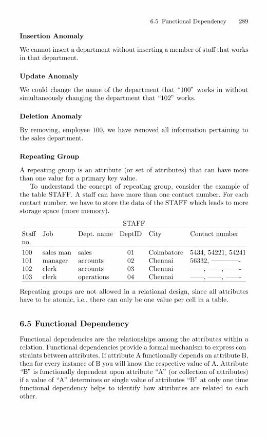
6.5 Functional Dependency 289
Insertion Anomaly
We cannot insert a department without inserting a member of staff that worksin that department.
Update Anomaly
We could change the name of the department that “100” works in withoutsimultaneously changing the department that “102” works.
Deletion Anomaly
By removing, employee 100, we have removed all information pertaining tothe sales department.
Repeating Group
A repeating group is an attribute (or set of attributes) that can have morethan one value for a primary key value.
To understand the concept of repeating group, consider the example ofthe table STAFF. A staff can have more than one contact number. For eachcontact number, we have to store the data of the STAFF which leads to morestorage space (more memory).
STAFF
Staff Job Dept. name DeptID City Contact numberno.
100 sales man sales 01 Coimbatore 5434, 54221, 54241101 manager accounts 02 Chennai 56332, ————-102 clerk accounts 03 Chennai ——, ——, ——-103 clerk operations 04 Chennai ——, ——, ——-
Repeating groups are not allowed in a relational design, since all attributeshave to be atomic, i.e., there can only be one value per cell in a table.
6.5 Functional Dependency
Functional dependencies are the relationships among the attributes within arelation. Functional dependencies provide a formal mechanism to express con-straints between attributes. If attribute A functionally depends on attribute B,then for every instance of B you will know the respective value of A. Attribute“B” is functionally dependent upon attribute “A” (or collection of attributes)if a value of “A” determines or single value of attributes “B” at only one timefunctional dependency helps to identify how attributes are related to eachother.
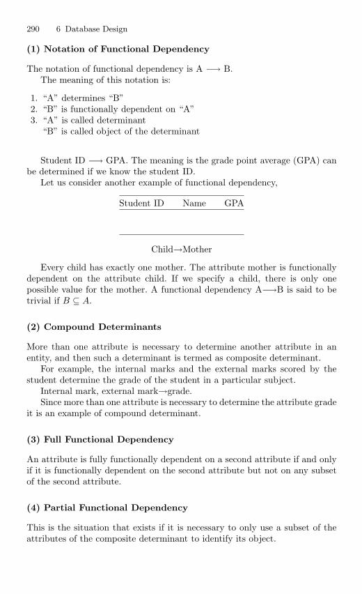
290 6 Database Design
(1) Notation of Functional Dependency
The notation of functional dependency is A −→ B.The meaning of this notation is:
1. “A” determines “B”2. “B” is functionally dependent on “A”3. “A” is called determinant
“B” is called object of the determinant
Student ID −→ GPA. The meaning is the grade point average (GPA) canbe determined if we know the student ID.
Let us consider another example of functional dependency,
Student ID Name GPA
Child→Mother
Every child has exactly one mother. The attribute mother is functionallydependent on the attribute child. If we specify a child, there is only onepossible value for the mother. A functional dependency A−→B is said to betrivial if B ⊆ A.
(2) Compound Determinants
More than one attribute is necessary to determine another attribute in anentity, and then such a determinant is termed as composite determinant.
For example, the internal marks and the external marks scored by thestudent determine the grade of the student in a particular subject.
Internal mark, external mark→grade.Since more than one attribute is necessary to determine the attribute grade
it is an example of compound determinant.
(3) Full Functional Dependency
An attribute is fully functionally dependent on a second attribute if and onlyif it is functionally dependent on the second attribute but not on any subsetof the second attribute.
(4) Partial Functional Dependency
This is the situation that exists if it is necessary to only use a subset of theattributes of the composite determinant to identify its object.
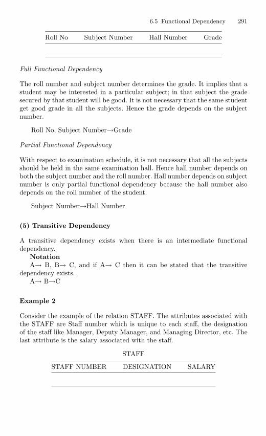
6.5 Functional Dependency 291
Roll No Subject Number Hall Number Grade
Full Functional Dependency
The roll number and subject number determines the grade. It implies that astudent may be interested in a particular subject; in that subject the gradesecured by that student will be good. It is not necessary that the same studentget good grade in all the subjects. Hence the grade depends on the subjectnumber.
Roll No, Subject Number→Grade
Partial Functional Dependency
With respect to examination schedule, it is not necessary that all the subjectsshould be held in the same examination hall. Hence hall number depends onboth the subject number and the roll number. Hall number depends on subjectnumber is only partial functional dependency because the hall number alsodepends on the roll number of the student.
Subject Number→Hall Number
(5) Transitive Dependency
A transitive dependency exists when there is an intermediate functionaldependency.
NotationA→ B, B→ C, and if A→ C then it can be stated that the transitive
dependency exists.A→ B→C
Example 2
Consider the example of the relation STAFF. The attributes associated withthe STAFF are Staff number which is unique to each staff, the designationof the staff like Manager, Deputy Manager, and Managing Director, etc. Thelast attribute is the salary associated with the staff.
STAFF
STAFF NUMBER DESIGNATION SALARY
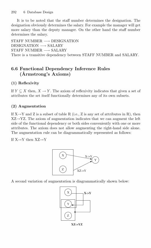
292 6 Database Design
It is to be noted that the staff number determines the designation. Thedesignation obviously determines the salary. For example the manager will getmore salary than the deputy manager. On the other hand the staff numberdetermines the salary.
STAFF NUMBER −→ DESIGNATIONDESIGNATION −→ SALARYSTAFF NUMBER −→ SALARYThere is a transitive dependency between STAFF NUMBER and SALARY.
6.6 Functional Dependency Inference Rules(Armstrong’s Axioms)
(1) Reflexivity
If Y ⊆ X then, X → Y . The axiom of reflexivity indicates that given a set ofattributes the set itself functionally determines any of its own subsets.
(2) Augmentation
If X→Y and Z is a subset of table R (i.e., Z is any set of attributes in R), thenXZ→YZ. The axiom of augmentation indicates that we can augment the leftside of the functional dependency or both sides conveniently with one or moreattributes. The axiom does not allow augmenting the right-hand side alone.The augmentation rule can be diagrammatically represented as follows:
If X→Y then XZ→Y
X
Z
YX->Y
XZ->Y
A second variation of augmentation is diagrammatically shown below:
X
Y
Z
X->Y
XZ->YZ
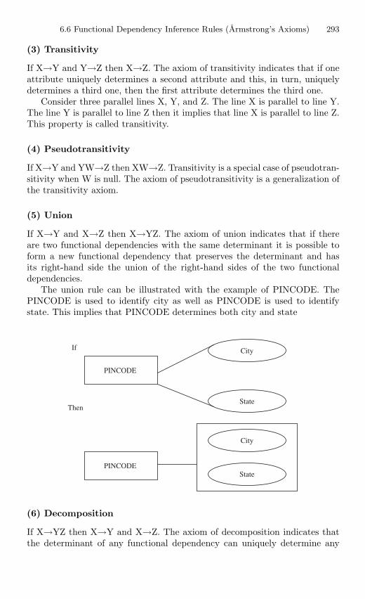
6.6 Functional Dependency Inference Rules (Armstrong’s Axioms) 293
(3) Transitivity
If X→Y and Y→Z then X→Z. The axiom of transitivity indicates that if oneattribute uniquely determines a second attribute and this, in turn, uniquelydetermines a third one, then the first attribute determines the third one.
Consider three parallel lines X, Y, and Z. The line X is parallel to line Y.The line Y is parallel to line Z then it implies that line X is parallel to line Z.This property is called transitivity.
(4) Pseudotransitivity
If X→Y and YW→Z then XW→Z. Transitivity is a special case of pseudotran-sitivity when W is null. The axiom of pseudotransitivity is a generalization ofthe transitivity axiom.
(5) Union
If X→Y and X→Z then X→YZ. The axiom of union indicates that if thereare two functional dependencies with the same determinant it is possible toform a new functional dependency that preserves the determinant and hasits right-hand side the union of the right-hand sides of the two functionaldependencies.
The union rule can be illustrated with the example of PINCODE. ThePINCODE is used to identify city as well as PINCODE is used to identifystate. This implies that PINCODE determines both city and state
PINCODE
City
State
PINCODE
City
State
If
Then
(6) Decomposition
If X→YZ then X→Y and X→Z. The axiom of decomposition indicates thatthe determinant of any functional dependency can uniquely determine any
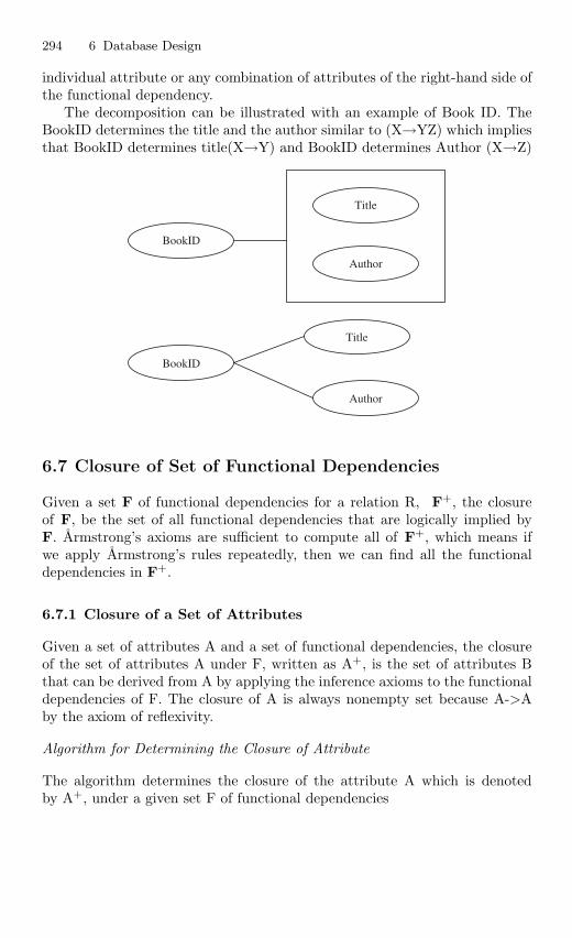
294 6 Database Design
individual attribute or any combination of attributes of the right-hand side ofthe functional dependency.
The decomposition can be illustrated with an example of Book ID. TheBookID determines the title and the author similar to (X→YZ) which impliesthat BookID determines title(X→Y) and BookID determines Author (X→Z)
BookID
Title
Author
BookID
Title
Author
6.7 Closure of Set of Functional Dependencies
Given a set F of functional dependencies for a relation R, F+, the closureof F, be the set of all functional dependencies that are logically implied byF. Armstrong’s axioms are sufficient to compute all of F+, which means ifwe apply Armstrong’s rules repeatedly, then we can find all the functionaldependencies in F+.
6.7.1 Closure of a Set of Attributes
Given a set of attributes A and a set of functional dependencies, the closureof the set of attributes A under F, written as A+, is the set of attributes Bthat can be derived from A by applying the inference axioms to the functionaldependencies of F. The closure of A is always nonempty set because A->Aby the axiom of reflexivity.
Algorithm for Determining the Closure of Attribute
The algorithm determines the closure of the attribute A which is denotedby A+, under a given set F of functional dependencies
6.7 Closure of Set of Functional Dependencies 295
I=0; A[0]=A;REPEAT
I=I+1;A[I] = A[I − 1];FOR ALL Z->W in F
IF Z ⊆ A[I]THEN A[I] = A[I] ∪ W ;
END FORUNTIL A[I] = A[I − 1];RETURN A+ = A[I];
In the above algorithm I is an integer. In the algorithm A → A[I] andafter finding Z → W in F with Z ⊆ A[I], A[I] can be represented as YZwhere Y = A[I] − Z. We can write A → A[I] as A → Y Z. Since F containsZ → W , it can be concluded by set accumulation rule that A → Y ZW , orin other words, A → A[I] ∪ W and the induction hypothesis A → A[I] ismaintained.
Covers
If F and G represents two sets of functional dependencies defined over the samerelational scheme, F and G are equivalent if F+ = G+. Whenever F+ = G+,F covers G and vice versa.
Nonredundant cover
Consider two sets of functional dependencies F and G defined over the samerelational scheme, if G covers F and no proper subset H of G is such thatH+ = G+, then G is a nonredundant cover of F.
6.7.2 Minimal Cover
A set of nonredundant functional dependencies, which is obtained by remov-ing all redundant functional dependencies using the functional dependencyinference rule (Armstrong axiom), is termed as minimal cover.
Use of Functional Dependency
Functional dependency can be used to test relations to see if the relationsare legal under a given set of functional dependencies. If a relation R is legalunder a set F of functional dependencies, then the relation R satisfies F.
Functional dependency specifies constraints on the set of legal relations.F holds on R if all legal relations on R satisfy the set of functional depen-dencies of F.
296 6 Database Design
6.8 Normalization
Normalization is the process of organizing data in a database. This includescreating tables and establishing relationships between those tables accordingto rules designed both to protect the data and to make the database moreflexible by eliminating two factors: redundancy and inconsistent dependency.Redundant data wastes disk space and creates maintenance problems. If datathat exists in more than one place must be changed, the data must be changedin exactly the same way in all locations. Inconsistent dependencies can makedata difficult to access; the path to find the data may be missing.
Normalization is the analysis of functional dependencies betweenattributes. It is the process of decomposing relations with anomalies toproduce well-structured relations. Well-structured relation contains minimalredundancy and allows insertion, modification, and deletion without errorsor inconsistencies. Normalization is a formal process for deciding whichattributes should be grouped together in a relation. It is the primary toolto validate and improve a logical design so that it satisfies certain con-straints that avoid unnecessary duplication of data. Normalization theory isbased on the concepts of normal forms. A relational table is said to be aparticular normal form if it satisfied a certain set of constraints. There arecurrently five normal forms that have been defined. Normalization shouldremove redundancy but not at the expense of data integrity. In general, thenormalization process generates many simple entity specifications from a fewsemantically complex entity specifications. Here entity specification refers tothe declaration of entity attribute.
6.8.1 Purpose of Normalization
Normalization allows us to minimize insert, update, and delete anomalies andhelp maintain data consistency in the database.
1. To avoid redundancy by storing each fact within the database only once2. To put data into the form that is more able to accurately accommodate
change3. To avoid certain updating “anomalies”4. To facilitate the enforcement of data constraint5. To avoid unnecessary coding. Extra programming in triggers, stored
procedures can be required to handle the non-normalized data and this inturn can impair performance significantly.
6.9 Steps in Normalization
The degree of normalization is defined by normal forms. The normal forms inan increasing level of normalization, are first normal form (1NF), second nor-mal form (2NF), 3NF, Boyce-Codd Normal form,4NF and 5NF. Each normal
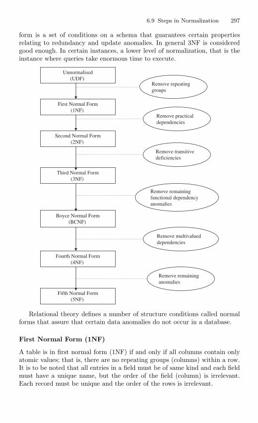
6.9 Steps in Normalization 297
form is a set of conditions on a schema that guarantees certain propertiesrelating to redundancy and update anomalies. In general 3NF is consideredgood enough. In certain instances, a lower level of normalization, that is theinstance where queries take enormous time to execute.
First Normal Form(1NF)
Second Normal Form(2NF)
Third Normal Form(3NF)
Unnormalised(UDF)
Remove repeatinggroups
Remove practicaldependencies
Remove transitivedeficiencies
Boyce Normal Form(BCNF)
Fourth Normal Form(4NF)
Fifth Normal Form(5NF)
Remove remainingfunctional dependencyanomalies
Remove multivalueddependencies
Remove remaininganomalies
Relational theory defines a number of structure conditions called normalforms that assure that certain data anomalies do not occur in a database.
First Normal Form (1NF)
A table is in first normal form (1NF) if and only if all columns contain onlyatomic values; that is, there are no repeating groups (columns) within a row.It is to be noted that all entries in a field must be of same kind and each fieldmust have a unique name, but the order of the field (column) is irrelevant.Each record must be unique and the order of the rows is irrelevant.
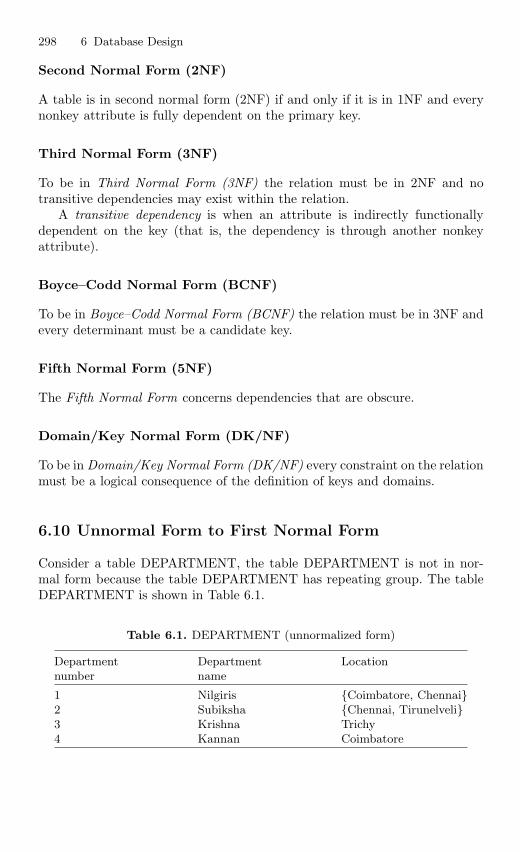
298 6 Database Design
Second Normal Form (2NF)
A table is in second normal form (2NF) if and only if it is in 1NF and everynonkey attribute is fully dependent on the primary key.
Third Normal Form (3NF)
To be in Third Normal Form (3NF) the relation must be in 2NF and notransitive dependencies may exist within the relation.
A transitive dependency is when an attribute is indirectly functionallydependent on the key (that is, the dependency is through another nonkeyattribute).
Boyce–Codd Normal Form (BCNF)
To be in Boyce–Codd Normal Form (BCNF) the relation must be in 3NF andevery determinant must be a candidate key.
Fifth Normal Form (5NF)
The Fifth Normal Form concerns dependencies that are obscure.
Domain/Key Normal Form (DK/NF)
To be in Domain/Key Normal Form (DK/NF) every constraint on the relationmust be a logical consequence of the definition of keys and domains.
6.10 Unnormal Form to First Normal Form
Consider a table DEPARTMENT, the table DEPARTMENT is not in nor-mal form because the table DEPARTMENT has repeating group. The tableDEPARTMENT is shown in Table 6.1.
Table 6.1. DEPARTMENT (unnormalized form)
Department Department Locationnumber name
1 Nilgiris Coimbatore, Chennai2 Subiksha Chennai, Tirunelveli3 Krishna Trichy4 Kannan Coimbatore
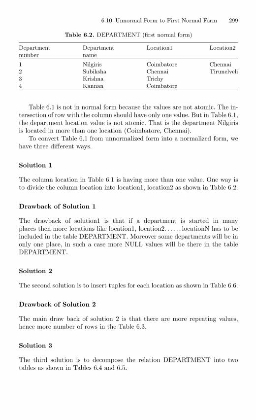
6.10 Unnormal Form to First Normal Form 299
Table 6.2. DEPARTMENT (first normal form)
Department Department Location1 Location2number name
1 Nilgiris Coimbatore Chennai2 Subiksha Chennai Tirunelveli3 Krishna Trichy4 Kannan Coimbatore
Table 6.1 is not in normal form because the values are not atomic. The in-tersection of row with the column should have only one value. But in Table 6.1,the department location value is not atomic. That is the department Nilgirisis located in more than one location (Coimbatore, Chennai).
To convert Table 6.1 from unnormalized form into a normalized form, wehave three different ways.
Solution 1
The column location in Table 6.1 is having more than one value. One way isto divide the column location into location1, location2 as shown in Table 6.2.
Drawback of Solution 1
The drawback of solution1 is that if a department is started in manyplaces then more locations like location1, location2. . . . . . locationN has to beincluded in the table DEPARTMENT. Moreover some departments will be inonly one place, in such a case more NULL values will be there in the tableDEPARTMENT.
Solution 2
The second solution is to insert tuples for each location as shown in Table 6.6.
Drawback of Solution 2
The main draw back of solution 2 is that there are more repeating values,hence more number of rows in the Table 6.3.
Solution 3
The third solution is to decompose the relation DEPARTMENT into twotables as shown in Tables 6.4 and 6.5.
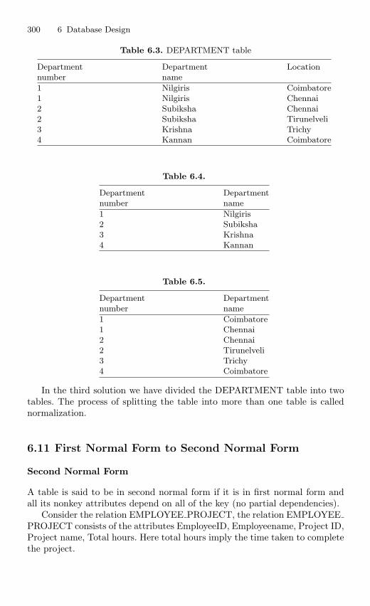
300 6 Database Design
Table 6.3. DEPARTMENT table
Department Department Locationnumber name
1 Nilgiris Coimbatore1 Nilgiris Chennai2 Subiksha Chennai2 Subiksha Tirunelveli3 Krishna Trichy4 Kannan Coimbatore
Table 6.4.
Department Departmentnumber name
1 Nilgiris2 Subiksha3 Krishna4 Kannan
Table 6.5.
Department Departmentnumber name
1 Coimbatore1 Chennai2 Chennai2 Tirunelveli3 Trichy4 Coimbatore
In the third solution we have divided the DEPARTMENT table into twotables. The process of splitting the table into more than one table is callednormalization.
6.11 First Normal Form to Second Normal Form
Second Normal Form
A table is said to be in second normal form if it is in first normal form andall its nonkey attributes depend on all of the key (no partial dependencies).
Consider the relation EMPLOYEE PROJECT, the relation EMPLOYEEPROJECT consists of the attributes EmployeeID, Employeename, Project ID,Project name, Total hours. Here total hours imply the time taken to completethe project.
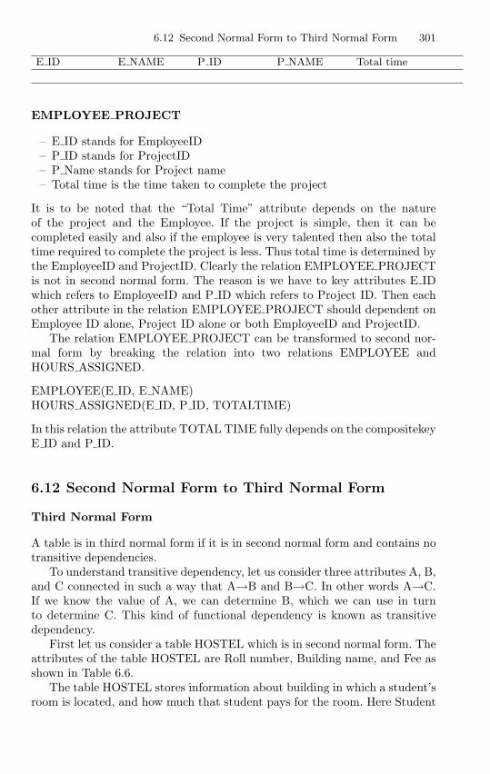
6.12 Second Normal Form to Third Normal Form 301
E ID E NAME P ID P NAME Total time
EMPLOYEE PROJECT
– E ID stands for EmployeeID– P ID stands for ProjectID– P Name stands for Project name– Total time is the time taken to complete the project
It is to be noted that the “Total Time” attribute depends on the natureof the project and the Employee. If the project is simple, then it can becompleted easily and also if the employee is very talented then also the totaltime required to complete the project is less. Thus total time is determined bythe EmployeeID and ProjectID. Clearly the relation EMPLOYEE PROJECTis not in second normal form. The reason is we have to key attributes E IDwhich refers to EmployeeID and P ID which refers to Project ID. Then eachother attribute in the relation EMPLOYEE PROJECT should dependent onEmployee ID alone, Project ID alone or both EmployeeID and ProjectID.
The relation EMPLOYEE PROJECT can be transformed to second nor-mal form by breaking the relation into two relations EMPLOYEE andHOURS ASSIGNED.
EMPLOYEE(E ID, E NAME)HOURS ASSIGNED(E ID, P ID, TOTALTIME)
In this relation the attribute TOTAL TIME fully depends on the compositekeyE ID and P ID.
6.12 Second Normal Form to Third Normal Form
Third Normal Form
A table is in third normal form if it is in second normal form and contains notransitive dependencies.
To understand transitive dependency, let us consider three attributes A, B,and C connected in such a way that A→B and B→C. In other words A→C.If we know the value of A, we can determine B, which we can use in turnto determine C. This kind of functional dependency is known as transitivedependency.
First let us consider a table HOSTEL which is in second normal form. Theattributes of the table HOSTEL are Roll number, Building name, and Fee asshown in Table 6.6.
The table HOSTEL stores information about building in which a student’sroom is located, and how much that student pays for the room. Here Student
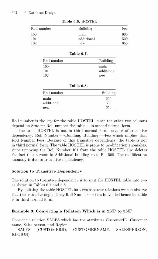
302 6 Database Design
Table 6.6. HOSTEL
Roll number Building Fee
100 main 600101 additional 500102 new 650
Table 6.7.
Roll number Building
100 main101 additional102 new
Table 6.8.
Roll number Building
main 600additional 500new 650
Roll number is the key for the table HOSTEL, since the other two columnsdepend on Student Roll number the table is in second normal form.
The table HOSTEL is not in third normal form because of transitivedependency. Roll Number−→Building, Building−→Fee which implies thatRoll Number Fees. Because of this transitive dependency, the table is notin third normal form. The table HOSTEL is prone to modification anomalies,since removing the Roll Number 101 from the table HOSTEL also deletesthe fact that a room in Additional building costs Rs. 500. The modificationanomaly is due to transitive dependency.
Solution to Transitive Dependency
The solution to transitive dependency is to split the HOSTEL table into twoas shown in Tables 6.7 and 6.8.
By splitting the table HOSTEL into two separate relations we can observethat the transitive dependency Roll Number−→Fees is avoided hence the tableis in third normal form.
Example 3: Converting a Relation Which is in 2NF to 3NF
Consider a relation SALES which has the attributes CustomerID, Customername, Sales person, and Region.
SALES (CUSTOMERID, CUSTOMERNAME, SALESPERSON,REGION)
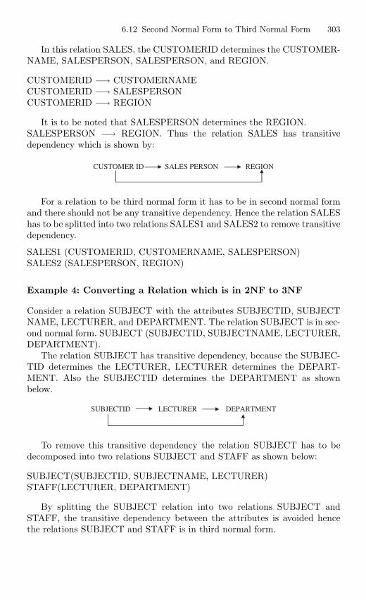
6.12 Second Normal Form to Third Normal Form 303
In this relation SALES, the CUSTOMERID determines the CUSTOMER-NAME, SALESPERSON, SALESPERSON, and REGION.
CUSTOMERID −→ CUSTOMERNAMECUSTOMERID −→ SALESPERSONCUSTOMERID −→ REGION
It is to be noted that SALESPERSON determines the REGION.SALESPERSON −→ REGION. Thus the relation SALES has transitivedependency which is shown by:
CUSTOMER ID SALES PERSON REGION
For a relation to be third normal form it has to be in second normal formand there should not be any transitive dependency. Hence the relation SALEShas to be splitted into two relations SALES1 and SALES2 to remove transitivedependency.
SALES1 (CUSTOMERID, CUSTOMERNAME, SALESPERSON)SALES2 (SALESPERSON, REGION)
Example 4: Converting a Relation which is in 2NF to 3NF
Consider a relation SUBJECT with the attributes SUBJECTID, SUBJECTNAME, LECTURER, and DEPARTMENT. The relation SUBJECT is in sec-ond normal form. SUBJECT (SUBJECTID, SUBJECTNAME, LECTURER,DEPARTMENT).
The relation SUBJECT has transitive dependency, because the SUBJEC-TID determines the LECTURER, LECTURER determines the DEPART-MENT. Also the SUBJECTID determines the DEPARTMENT as shownbelow.
SUBJECTID LECTURER DEPARTMENT
To remove this transitive dependency the relation SUBJECT has to bedecomposed into two relations SUBJECT and STAFF as shown below:
SUBJECT(SUBJECTID, SUBJECTNAME, LECTURER)STAFF(LECTURER, DEPARTMENT)
By splitting the SUBJECT relation into two relations SUBJECT andSTAFF, the transitive dependency between the attributes is avoided hencethe relations SUBJECT and STAFF is in third normal form.
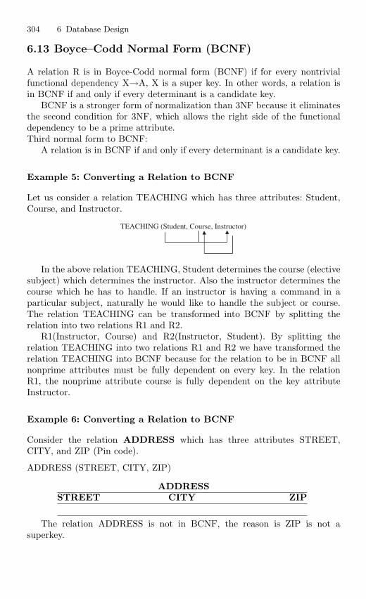
304 6 Database Design
6.13 Boyce–Codd Normal Form (BCNF)
A relation R is in Boyce-Codd normal form (BCNF) if for every nontrivialfunctional dependency X→A, X is a super key. In other words, a relation isin BCNF if and only if every determinant is a candidate key.
BCNF is a stronger form of normalization than 3NF because it eliminatesthe second condition for 3NF, which allows the right side of the functionaldependency to be a prime attribute.Third normal form to BCNF:
A relation is in BCNF if and only if every determinant is a candidate key.
Example 5: Converting a Relation to BCNF
Let us consider a relation TEACHING which has three attributes: Student,Course, and Instructor.
TEACHING (Student, Course, Instructor)
In the above relation TEACHING, Student determines the course (electivesubject) which determines the instructor. Also the instructor determines thecourse which he has to handle. If an instructor is having a command in aparticular subject, naturally he would like to handle the subject or course.The relation TEACHING can be transformed into BCNF by splitting therelation into two relations R1 and R2.
R1(Instructor, Course) and R2(Instructor, Student). By splitting therelation TEACHING into two relations R1 and R2 we have transformed therelation TEACHING into BCNF because for the relation to be in BCNF allnonprime attributes must be fully dependent on every key. In the relationR1, the nonprime attribute course is fully dependent on the key attributeInstructor.
Example 6: Converting a Relation to BCNF
Consider the relation ADDRESS which has three attributes STREET,CITY, and ZIP (Pin code).
ADDRESS (STREET, CITY, ZIP)
ADDRESSSTREET CITY ZIP
The relation ADDRESS is not in BCNF, the reason is ZIP is not asuperkey.
6.13 Boyce–Codd Normal Form (BCNF) 305
From the relation ADDRESS we can infer thatCITY, STREET −→ ZIPZIP −→ CITYThe relation ADDRESS has insertion anomaly, that is a city of ZIP codecannot be stored if the street is not given. To overcome this insertion anomaly,the relation ADDRESS has to be split into two relations R1 and R2. Therelation R1 has two attributes STREET, ZIP, and the relation R2 has twoattributes ZIP, CITY.
R1(STREET, ZIP) and R2(ZIP, CITY). The splitting of the relationADDRESS into two relations R1 and R2 eliminates insertion anomaly.
Example 7: Converting a Relation to BCNF
In this example, let us consider a relation which is in 3NF but not in BCNF.The relation which we are going to consider is R which has three attributes,PATIENT, DOCTOR, and HOSPITAL.
RPATIENT, DOCTOR, HOSPITALIn this relation HOSPITALPATIENT, HOSPITAL −→ DOCTORDOCTOR −→ HOSPITAL
The relation R is not in BCNF because DOCTOR is not the superkey. Toconvert the relation R into BCNF, split the relation R into two relations R1and R2 as shown below:
R1PATIENT, DOCTORR2DOCTOR, HOSPITALBy splitting the relation R into two relations R1 and R2 we have convertedthe relation R which is in 3NF to BCNF.
BCNF and Third Normal Form
All BCNF are in 3NF but not all 3NF are in BCNF. BCNF does not make anyreference to the concepts of full or partial dependency. BCNF is a strongerform of normalization than 3NF because it eliminates the second conditionfor 3NF, which allows the right side of the FD to be a prime attribute. Thus,every left side of a FD in a table must be a super key.
Multivalued Dependency
To understand multivalued dependency, consider a relation R which has threeattributes: A, B, and C. For each value of A there is a set of values for B and setof values for C. However, the set of values for B and C are independent of eachother, and then there exists multivalued dependency between the attributesA, B, and C in the relation R. It is represented by
306 6 Database Design
A→B implies that for each value of A there is set of values for B.A→C implies that for each value of A there is set of values for C.
If we have multivalued dependency in a relation we may have to repeatvalues redundantly in the tuples which is clearly undesirable.
Trivial Multivalued Dependency
Consider a relation R with two attributes A and B. The multivalued depen-dency between the attributes A and B is denoted by A−→B is trivial if B isa subset of A or A∪B = R.
Multivalued Dependency Inference Rules
The inference rules for multivalued dependency are given below:
Reflexivity
The axiom of reflexivity indicates that given a set of attributes the set itselffunctionally determines any of its own subsets. It is represented by
X→X
Augmentation
The axiom of augmentation indicates that we can augment the left side of thefunctional dependency or both sides conveniently with one or more attributes.It is represented by
If X→Y then XZ→Y
Transitivity
The axiom of transitivity indicates that if one attribute uniquely determinesa second attribute and this, in turn, uniquely determines a third one, thenthe first attribute determines the third one. It is represented by
If X→Y and Y→Z then X→Z
Pseudotransitivity
The axiom of pseudotransitivity is a generalization of the transitivity axiom.Transitivity is a special case of pseudotransitivity when W is null. Pseudo-transitivity is represented by
If X→Y and YW→Z then XW→Z
Union
The axiom of union indicates that if there are two functional dependencieswith the same determinant it is possible to form a new functional dependencythat preserves the determinant and has its right-hand side the union of theright-hand sides of the two functional dependencies. It is represented by
6.14 Fourth and Fifth Normal Forms 307
If X→Y and X→Z then X→YZ
Decomposition
The axiom of decomposition indicates that the determinant of any functionaldependency can uniquely determine any individual attribute or any combi-nation of attributes of the right-hand side of the functional dependency. Thedecomposition axiom is represented by
If X→Y and X→Z, then X→Y∩Z and X→(Z−Y)
6.14 Fourth and Fifth Normal Forms
Normal forms up to BCNF have been defined solely on functional dependency,and for most database practitioners, either 3NF or BCNF is a sufficient levelof normalization. However, there are in fact two more normal forms that areneeded to eliminate the rest of the currently known anomalies. If multivalueddependency and join dependency do not exist in a table, which is the mostcommon situation, then any table in BCNF is automatically in fourth nor-mal form (4NF) and fifth normal form (5NF) as well. However, when theseconstraints do exist, there may be further update anomalies that need to becorrected.
6.14.1 Fourth Normal Form
The goal of fourth normal form is to eliminate nontrivial multivalued depen-dencies from a table by projecting them onto separate smaller tables, thuseliminating the update anomalies associated with the multivalued dependen-cies. Under 4NF, a record type should not contain two or more independentmultivalued facts about an entity.
Definition of Fourth Normal Form
A table R is in fourth normal form (4NF) if and only if it is in BCNF and,whenever there exists an multivalued dependency in R (for example X→Y),at least one of the following holds: The multivalued dependency is trivial orX is a super key for relation R.
Example 8: Converting a Relation to Fourth Normal Form
Consider a relation SUBJECT which has the attributes COURSE, INSTRUC-TOR, and TEXTBOOK
SUBJECT (COURSE, INSTRUCTOR, TEXTBOOK)
308 6 Database Design
The relation SUBJECT is not in fourth normal form because of multivalueddependency between attributes.COURSE→INSTRUCTOR which implies that for one course there may bemany instructors.COURSE→TEXTBOOK which implies that for a course that may be manytextbooks.
Hence there exists multivalued dependency between attributes in SUB-JECT relation. The relation SUBJECT can be converted to fourth normalform by splitting the relation SUBJECT into two relations TEACHER ANDTEXT.
TEACHER (COURSE, INSTRUCTOR)TEXT (COURSE, TEXTBOOK)
The relation TEACHER and TEXT is in fourth normal form.
Example 9: Converting a Relation to Fourth Normal Form
Consider the relation EMPLOYEE with the attributes employee number,project name, and department name as shown below:
EMPLOYEE (ENO, PNAME, DNAME)
where ENO stands for Employee number, PNAME for project name, andDNAME for department name.
The relation EMPLOYEE has the following multivalued dependencies:
ENO→PNAME (One employee can work in several projects)ENO→DNAME.
ENO is not the superkey of the relation EMPLOYEE. To convert the relationto fourth normal form decompose EMPLOYEE relation into two relations
EMP PROJ and EMP DEPT as shown below.EMP PROJ (ENO, PNAME) and EMP DEPT (ENO, DNAME)
Now the relations EMP PROJ and EMP DEPT are in fourth normal form.
Preferred Qualities of Decomposition
During normalization, the given relation is split-up into two or more rela-tions. The splitting up of a given relation into two or more relations is knownas decomposition. The decomposition should always satisfy the properties oflossless decomposition and dependency preservation
– Lossless decomposition ensures that the information in the original rela-tion can be accurately reconstructed without spurious information.
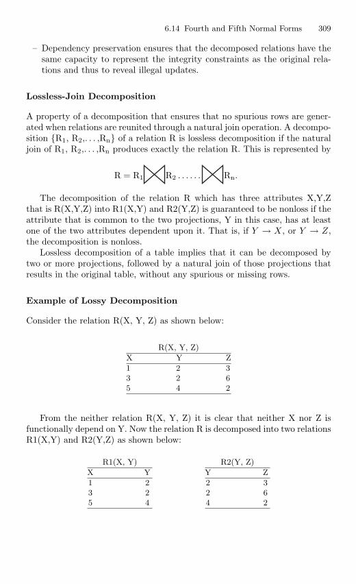
6.14 Fourth and Fifth Normal Forms 309
– Dependency preservation ensures that the decomposed relations have thesame capacity to represent the integrity constraints as the original rela-tions and thus to reveal illegal updates.
Lossless-Join Decomposition
A property of a decomposition that ensures that no spurious rows are gener-ated when relations are reunited through a natural join operation. A decompo-sition R1, R2,. . . ,Rn of a relation R is lossless decomposition if the naturaljoin of R1, R2,. . . ,Rn produces exactly the relation R. This is represented by
R = R1 R2 . . . . . . Rn.
The decomposition of the relation R which has three attributes X,Y,Zthat is R(X,Y,Z) into R1(X,Y) and R2(Y,Z) is guaranteed to be nonloss if theattribute that is common to the two projections, Y in this case, has at leastone of the two attributes dependent upon it. That is, if Y → X, or Y → Z,the decomposition is nonloss.
Lossless decomposition of a table implies that it can be decomposed bytwo or more projections, followed by a natural join of those projections thatresults in the original table, without any spurious or missing rows.
Example of Lossy Decomposition
Consider the relation R(X, Y, Z) as shown below:
R(X, Y, Z)
X Y Z
1 2 33 2 65 4 2
From the neither relation R(X, Y, Z) it is clear that neither X nor Z isfunctionally depend on Y. Now the relation R is decomposed into two relationsR1(X,Y) and R2(Y,Z) as shown below:
R1(X, Y)
X Y
1 23 25 4
R2(Y, Z)
Y Z
2 32 64 2
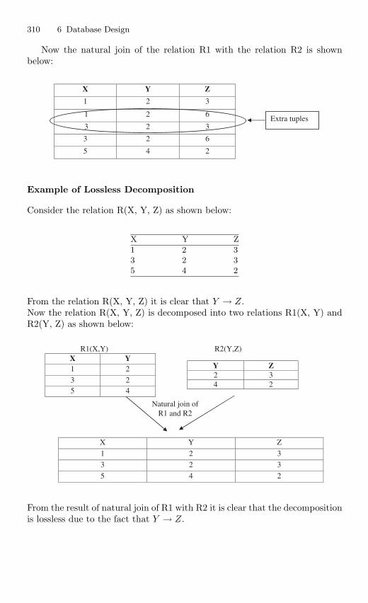
310 6 Database Design
Now the natural join of the relation R1 with the relation R2 is shownbelow:
X Y Z
1 2 3
1 2 6
3 2 3
3 2 6
5 4 2
Extra tuples
Example of Lossless Decomposition
Consider the relation R(X, Y, Z) as shown below:
X Y Z
1 2 33 2 35 4 2
From the relation R(X, Y, Z) it is clear that Y → Z.Now the relation R(X, Y, Z) is decomposed into two relations R1(X, Y) andR2(Y, Z) as shown below:
R1(X,Y) R2(Y,Z) X Y1 2
3 25 4
Natural join ofR1 and R2
Y Z2 34 2
X Y Z
1 2 3
3 2 3
5 4 2
From the result of natural join of R1 with R2 it is clear that the decompositionis lossless due to the fact that Y → Z.
6.15 Denormalization 311
6.14.2 Fifth Normal Form
A table R is in fifth normal form (5NF) or project-join normal form (PJ/NF)if and only if every join dependency in R is implied by the keys of R. In otherwords, a relation is in fifth normal form if it has no join dependency. Joindependency is the term used to indicate the property of a relation that can bedecomposed losslessly into “m” simpler relations but cannot be decomposedlosslessly into fewer relations.
Domain Key/Normal Form
In 1981 Fagin described a different approach to normalize tables when he pro-posed domain key/normal form. Domain key/normal form (DKNF) is basedon three concepts domain key and constraint. We know that domain is a setof all values of the same datatype, a key is a unique identifier and constraintis a rule governing attribute values. A relation is in domain key/normal formif and only if every constraint on the relation is a logical consequence of thedomain constraints and the key constraints that apply to the relation. DonaldFagin was the first person to devise a formal definition in 1981. Domain/keynormal form is considered as the perfect normal form because of no insertionor deletion anomalies.
Disadvantages of Normalization
The disadvantage of normalization is that it produces many tables. A querymight require retrieval of data from multiple normalized tables. This can resultin complicated table joins. Decomposition of tables has two primary impacts.The first is performance. All the joins required to merge data will slow downthe process.
6.15 Denormalization
Denormalization is used primarily to improve performance in cases whereover-normalized structures are causing overhead to the query processor.
6.15.1 Basic Types of Denormalization
Five basic types of Denormalization are:
1. Two entities in a many-to-many relationship. The relationship tableresulting from this construct is composed of the primary keys of each
312 6 Database Design
of the associated entities. If we implement the join of this table with oneof the entity tables as a single table instead of the original tables, we canavoid certain frequent joins that are based on both keys, but only thenonkey data from one of the original entities.
2. Two entities in a one-to-one relationship. The table for these entities couldbe implemented as a single table, thus avoiding frequent joins required bycertain applications.
3. Reference data in a one-to-many relationship. When artificial primarykeys are introduced to tables that either have no primary keys or havekeys that are very large composites, they can be added to the child entityin a one-to-many relationship as a foreign key and avoid certain joins incurrent applications.
4. Entities with the most detailed data. Multivalued attributes are usuallyimplemented as entities and are thus represented as separate records ina table. Sometimes it is more efficient to implement them as individu-ally named columns as an extension of the parent entity when the num-ber of replications is a small fixed number for all instances of the parententity.
5. Derived attributes. If one attribute is derived from another at executiontime, then in some cases it is more efficient to store both the originalvalue and the derived value directly in the database. This adds at leastone extra column to the original table and avoids repetitive computation.
6.15.2 Table Denormalization Algorithm
The strategy for table Denormalization is to select only the most dominantprocess to determine those modifications that will most likely improve perfor-mance. The basic modification is to add attributes to existing tables to reducejoin operations. The steps of strategy are as follows:
1. Select the dominant processes based on such criteria as high frequencyof execution, high volume of data accessed, response time constraints,or explicit high priority. It can be considered as a rule of thumb as anyprocess whose frequency of execution or data volume accessed is ten timesthat of another process is considered dominant.
2. Define join tables, when appropriate, for the dominant processes.3. Evaluate total cost for storage, query, and update for the database schema,
with and without the extended table, and determine which configurationminimizes total cost.
4. Consider also the possibility of Denormalization due to a join table andits side effects. If a join table schema appears to have lower storage andprocessing cost and insignificant side effects, then consider using thatschema for physical design in addition to the original candidate tableschema. Otherwise, use only the original schema.
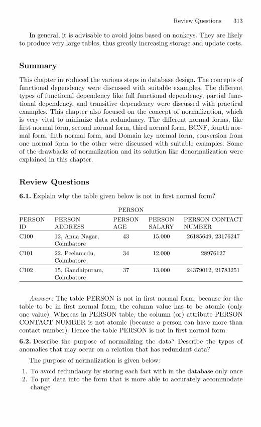
Review Questions 313
In general, it is advisable to avoid joins based on nonkeys. They are likelyto produce very large tables, thus greatly increasing storage and update costs.
Summary
This chapter introduced the various steps in database design. The concepts offunctional dependency were discussed with suitable examples. The differenttypes of functional dependency like full functional dependency, partial func-tional dependency, and transitive dependency were discussed with practicalexamples. This chapter also focused on the concept of normalization, whichis very vital to minimize data redundancy. The different normal forms, likefirst normal form, second normal form, third normal form, BCNF, fourth nor-mal form, fifth normal form, and Domain key normal form, conversion fromone normal form to the other were discussed with suitable examples. Someof the drawbacks of normalization and its solution like denormalization wereexplained in this chapter.
Review Questions
6.1. Explain why the table given below is not in first normal form?
PERSON
PERSON PERSON PERSON PERSON PERSON CONTACTID ADDRESS AGE SALARY NUMBER
C100 12, Anna Nagar, 43 15,000 26185649, 23176247Coimbatore
C101 22, Peelamedu, 34 12,000 28976127Coimbatore
C102 15, Gandhipuram, 37 13,000 24379012, 21783251Coimbatore
Answer : The table PERSON is not in first normal form, because for thetable to be in first normal form, the column value has to be atomic (onlyone value). Whereas in PERSON table, the column (or) attribute PERSONCONTACT NUMBER is not atomic (because a person can have more thancontact number). Hence the table PERSON is not in first normal form.
6.2. Describe the purpose of normalizing the data? Describe the types ofanomalies that may occur on a relation that has redundant data?
The purpose of normalization is given below:
1. To avoid redundancy by storing each fact with in the database only once2. To put data into the form that is more able to accurately accommodate
change
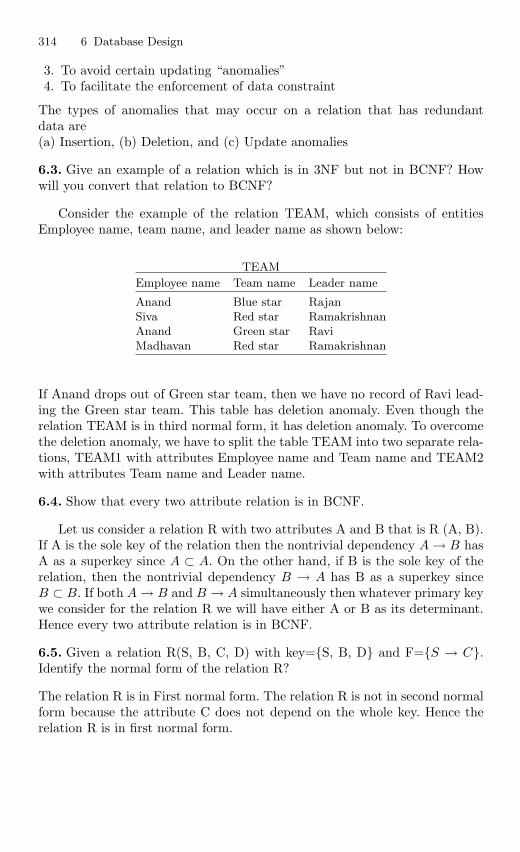
314 6 Database Design
3. To avoid certain updating “anomalies”4. To facilitate the enforcement of data constraint
The types of anomalies that may occur on a relation that has redundantdata are(a) Insertion, (b) Deletion, and (c) Update anomalies
6.3. Give an example of a relation which is in 3NF but not in BCNF? Howwill you convert that relation to BCNF?
Consider the example of the relation TEAM, which consists of entitiesEmployee name, team name, and leader name as shown below:
TEAM
Employee name Team name Leader name
Anand Blue star RajanSiva Red star RamakrishnanAnand Green star RaviMadhavan Red star Ramakrishnan
If Anand drops out of Green star team, then we have no record of Ravi lead-ing the Green star team. This table has deletion anomaly. Even though therelation TEAM is in third normal form, it has deletion anomaly. To overcomethe deletion anomaly, we have to split the table TEAM into two separate rela-tions, TEAM1 with attributes Employee name and Team name and TEAM2with attributes Team name and Leader name.
6.4. Show that every two attribute relation is in BCNF.
Let us consider a relation R with two attributes A and B that is R (A, B).If A is the sole key of the relation then the nontrivial dependency A → B hasA as a superkey since A ⊂ A. On the other hand, if B is the sole key of therelation, then the nontrivial dependency B → A has B as a superkey sinceB ⊂ B. If both A → B and B → A simultaneously then whatever primary keywe consider for the relation R we will have either A or B as its determinant.Hence every two attribute relation is in BCNF.
6.5. Given a relation R(S, B, C, D) with key=S, B, D and F=S → C.Identify the normal form of the relation R?
The relation R is in First normal form. The relation R is not in second normalform because the attribute C does not depend on the whole key. Hence therelation R is in first normal form.
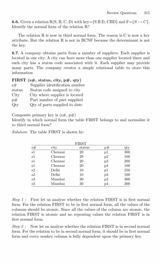
Review Questions 315
6.6. Given a relation R(S, B, C, D) with key=S B D, CBD and F=S → C.Identify the normal form of the relation R?
The relation R is now in third normal form. The reason is C is now a keyattribute. But the relation R is not in BCNF because the determinant is notthe key.
6.7. A company obtains parts from a number of suppliers. Each supplier islocated in one city. A city can have more than one supplier located there andeach city has a status code associated with it. Each supplier may providemany parts. The company creates a simple relational table to store thisinformation
FIRST (s#, status, city, p#, qty)s# Supplier identification numberstatus Status code assigned to cityCity City where supplier is locatedp# Part number of part suppliedQty Qty of parts supplied to date
Composite primary key is (s#, p#)Identify in which normal form the table FIRST belongs to and normalize itto third normal form?
Solution: The table FIRST is shown by:
FIRSTs# city status p# qty
s1 Chennai 20 p1 300s1 Chennai 20 p2 100s1 Chennai 20 p3 200s1 Chennai 20 p4 100s2 Delhi 10 p1 250s2 Delhi 10 p3 100s3 Mumbai 30 p2 300s3 Mumbai 30 p4 200
Step 1 : First let us analyze whether the relation FIRST is in first normalform. For the relation FIRST to be in first normal form, all the values of thecolumns should be atomic. Since all the values of the column are atomic, therelation FIRST is atomic and no repeating values the relation FIRST is infirst normal form.
Step 2 : Now let us analyze whether the relation FIRST is in second normalform. For the relation to be in second normal form, it should be in first normalform and every nonkey column is fully dependent upon the primary key.
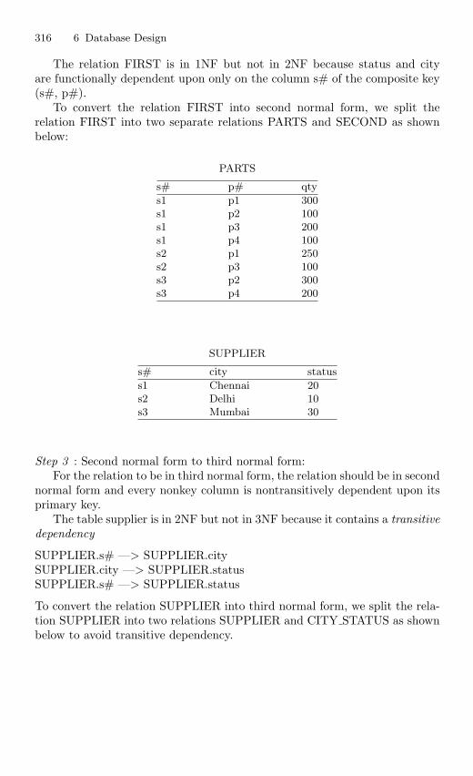
316 6 Database Design
The relation FIRST is in 1NF but not in 2NF because status and cityare functionally dependent upon only on the column s# of the composite key(s#, p#).
To convert the relation FIRST into second normal form, we split therelation FIRST into two separate relations PARTS and SECOND as shownbelow:
PARTS
s# p# qty
s1 p1 300s1 p2 100s1 p3 200s1 p4 100s2 p1 250s2 p3 100s3 p2 300s3 p4 200
SUPPLIER
s# city status
s1 Chennai 20s2 Delhi 10s3 Mumbai 30
Step 3 : Second normal form to third normal form:For the relation to be in third normal form, the relation should be in second
normal form and every nonkey column is nontransitively dependent upon itsprimary key.
The table supplier is in 2NF but not in 3NF because it contains a transitivedependency
SUPPLIER.s# —> SUPPLIER.citySUPPLIER.city —> SUPPLIER.statusSUPPLIER.s# —> SUPPLIER.status
To convert the relation SUPPLIER into third normal form, we split the rela-tion SUPPLIER into two relations SUPPLIER and CITY STATUS as shownbelow to avoid transitive dependency.
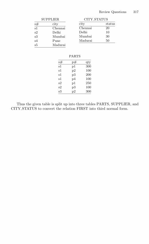
Review Questions 317
SUPPLIER CITY STATUS
s# city
s1 Chennais2 Delhis3 Mumbais4 Punes5 Madurai
city status
Chennai 20Delhi 10Mumbai 30Madurai 50
PARTS
s# p# qty
s1 p1 300s1 p2 100s1 p3 200s1 p4 100s2 p1 250s2 p3 100s3 p2 300
Thus the given table is split up into three tables PARTS, SUPPLIER, andCITY STATUS to convert the relation FIRST into third normal form.
7
Transaction Processing and QueryOptimization
Learning Objectives. This chapter deals with various concepts in transactionprocessing. The ACID property that is necessary in transaction processing is dis-cussed in detail. The anomalies in interleaved transactions like Write–Read Conflicts(WR Conflicts), Read–Write Conflicts (RW Conflicts), and Write–Write Conflicts(WW Conflicts) are illustrated with examples. This chapter also discusses differentquery evaluation plans in query optimization. This chapter throws light on advancedconcept of query optimization using Genetic Algorithm. After completing this chap-ter the reader should be familiar with the following concepts.
– Principle of Transaction Management System– Concept of Lock-Based Concurrency Control– Dead Lock, Two Phase Locking Scheme– Need for Query Optimization– Query Optimizer Architecture– Query Evaluation Plans– Query Optimization Using Genetic Algorithm
7.1 Transaction Processing
7.1.1 Introduction
Managing Data is the critical role in each and every organization. To achievethe hike in business they need to manage data efficiently. DBMS providesa better environment to store and retrieve the data in an economical andefficient manner. User can store and retrieve data through various sets ofinstructions. These sets of instructions do several read and write operationson database. These processes are denoted by a special term “Transaction” inDBMS.
Transaction is the execution of user program in DBMS. It is different fromthe execution of the program external to DBMS. In other words it can bestated as the various read and write operations done by the user program onthe DBMS, when it is executed in DBMS environment.
S. Sumathi: Transaction Processing and Query Optimization, Studies in Computational
Intelligence (SCI) 47, 319–352 (2007)
www.springerlink.com c© Springer-Verlag Berlin Heidelberg 2007
320 7 Transaction Processing and Query Optimization
Transaction Management plays a crucial role in DBMS. It is responsiblefor the efficiency and consistency of the DBMS. Partial transaction let thedatabase in an inconsistency state, so they should be avoided.
7.1.2 Key Notations in Transaction Management
The key notations in transaction management are as follows:
Object. The smallest Data item which is read or updated by the Transactionis called as Object in this case.
Transaction. Transaction is represented by the symbol T. It is termed as theexecution of query in DBMS.
Read Operation. Read operation on particular object is notated by symbolR (object-name).
Write Operation. Write operation on particular object is notated by symbolW (object-name).
Commit. This term used to denote the successful completion of one Trans-action.
Abort. This term used to denote the unsuccessful interrupted Transaction.
7.1.3 Concept of Transaction Management
User program executed by DBMS may claim several transactions. In the webenvironment, there is a possibility to several users’ attempt to access the datastored in same database. To maintain the accuracy and the consistency of thedatabase several scheduling algorithms are used.
To improve the effective throughput of the DBMS we need to enforcecertain concurrent executions in DBMS. Transaction Manager is responsiblefor scheduling the Transactions and providing the safest path to completethe task. To maintain the data in the phase of concurrent access and systemfailure, DBMS need to ensure four important properties. These properties arecalled as ACID properties.
ACID Properties of DBMS
ACID is an acronym for Atomicity, Consistency, Isolation, and Durability.
A – AtomicityC – ConsistencyI – IsolationD – Durability
Atomicity and Durability are closely related.Consistency and Isolation are closely related.The ACID properties are explained as follows.
7.1 Transaction Processing 321
Atomicity and Durability
Atomicity
Either all Transactions are carried out or none are. The meaning is the trans-action cannot be subdivided, and hence, it must be processed in its entiretyor not at all. Users should not have to worry about the effect of incompleteTransactions in case of any system crash occurs.
Transactions can be incomplete for three kinds of reasons:
1. Transaction can be aborted, or terminated unsuccessfully. This happensdue to some anomalies arises during execution. If a transaction is abortedby the DBMS for some internal reason, it is automatically restarted andexecuted as new.
2. Due to system crash. This may be happen due to Power Supply failurewhile one or more Transactions in execution.
3. Due to unexpected situations. This may be happen due to unexpected datavalue or be unable to access some disk. So the transaction will decide toabort. (Terminate itself).
Durability
If the System crashes before the changes made by a completed Transactionare written to disk, then it should be remembered and restored during thesystem restart phase.
Partial TransactionIf the Transaction is interrupted in the middle way it leaves the database in the
inconsistency state. These types of transactions are called as Partial Transactions.
Partial Transactions should be avoided to gain consistency of database.To undo the operations done by the Partial Transactions DBMS maintainscertain log files. Each and every moment of disk writes are recorded in this logfiles before they are reflected to disk. These are used to undo the operationsdone when the system failure occurs.
Consistency and Isolation
Consistency
Users are responsible for ensuring transaction consistency. User who submitsthe transaction should make sure the transaction will leave the database in aconsistent state.
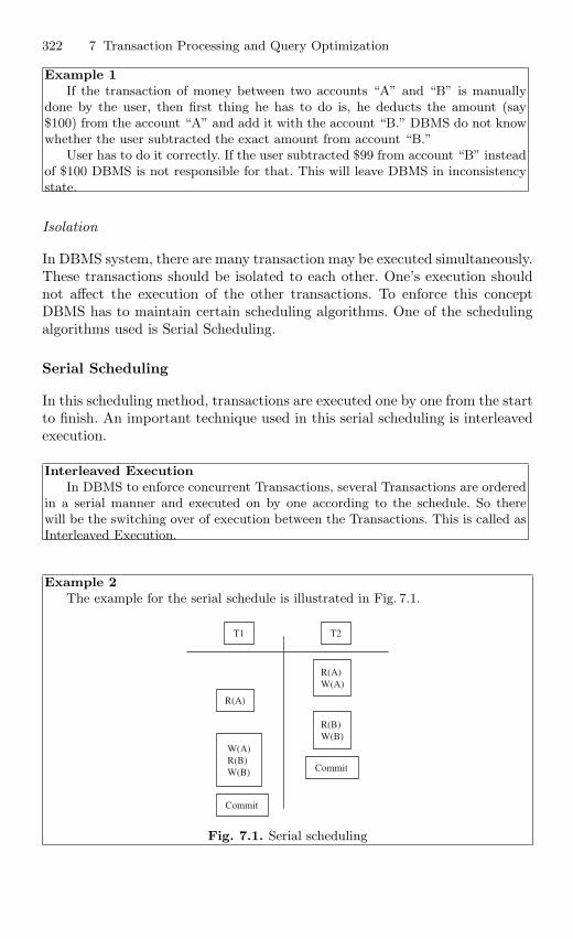
322 7 Transaction Processing and Query Optimization
Example 1If the transaction of money between two accounts “A” and “B” is manually
done by the user, then first thing he has to do is, he deducts the amount (say$100) from the account “A” and add it with the account “B.” DBMS do not knowwhether the user subtracted the exact amount from account “B.”
User has to do it correctly. If the user subtracted $99 from account “B” insteadof $100 DBMS is not responsible for that. This will leave DBMS in inconsistencystate.
Isolation
In DBMS system, there are many transaction may be executed simultaneously.These transactions should be isolated to each other. One’s execution shouldnot affect the execution of the other transactions. To enforce this conceptDBMS has to maintain certain scheduling algorithms. One of the schedulingalgorithms used is Serial Scheduling.
Serial Scheduling
In this scheduling method, transactions are executed one by one from the startto finish. An important technique used in this serial scheduling is interleavedexecution.
Interleaved ExecutionIn DBMS to enforce concurrent Transactions, several Transactions are ordered
in a serial manner and executed on by one according to the schedule. So therewill be the switching over of execution between the Transactions. This is called asInterleaved Execution.
Example 2The example for the serial schedule is illustrated in Fig. 7.1.
T1 T2
R(A)W(A)
R(A)
R(B)W(B)
W(A)R(B)W(B)
Commit
Commit
Fig. 7.1. Serial scheduling
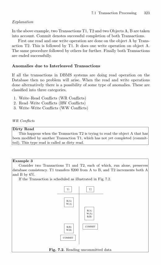
7.1 Transaction Processing 323
Explanation
In the above example, two Transactions T1, T2 and two Objects A, B are takeninto account. Commit denotes successful completion of both Transactions.
First one read and one write operation are done on the object A by Trans-action T2. This is followed by T1. It does one write operation on object A.The same procedure followed by others for further. Finally both Transactionsare ended successfully.
Anomalies due to Interleaved Transactions
If all the transactions in DBMS systems are doing read operation on theDatabase then no problem will arise. When the read and write operationsdone alternatively there is a possibility of some type of anomalies. These areclassified into three categories.
1. Write–Read Conflicts (WR Conflicts)2. Read–Write Conflicts (RW Conflicts)3. Write–Write Conflicts (WW Conflicts)
WR Conflicts
Dirty ReadThis happens when the Transaction T2 is trying to read the object A that has
been modified by another Transaction T1, which has not yet completed (commit-ted). This type read is called as dirty read.
Example 3Consider two Transactions T1 and T2, each of which, run alone, preserves
database consistency. T1 transfers $200 from A to B, and T2 increments both Aand B by 6%.
If the Transaction is scheduled as illustrated in Fig. 7.2.
T1 T2
R(A)W(A)
R(A)W(A)R(B)
R(B)W(B)
COMMIT
COMMIT
Fig. 7.2. Reading uncommitted data
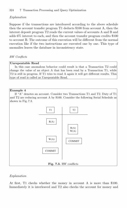
324 7 Transaction Processing and Query Optimization
Explanation
Suppose if the transactions are interleaved according to the above schedulethen the account transfer program T1 deducts $100 from account A, then theinterest deposit program T2 reads the current values of accounts A and B andadds 6% interest to each, and then the account transfer program credits $100to account B. The outcome of this execution will be different from the normalexecution like if the two instructions are executed one by one. This type ofanomalies leaves the database in inconsistency state.
RW Conflicts
Unrepeatable ReadIn this case anomalous behavior could result is that a Transaction T2 could
change the value of an object A that has been read by a Transaction T1, whileT2 is still in progress. If T1 tries to read A again it will get different results. Thistype of read is called as Unrepeatable Read.
Example 4If “A” denotes an account. Consider two Transactions T1 and T2. Duty of T1
and T2 are reducing account A by $100. Consider the following Serial Schedule asshown in Fig. 7.3.
T1 T2
R(A)
R(A)W(A)
W(A)
COMMIT
COMMIT
Fig. 7.3. RW conflicts
Explanation
At first, T1 checks whether the money in account A is more than $100.Immediately it is interleaved and T2 also checks the account for money and
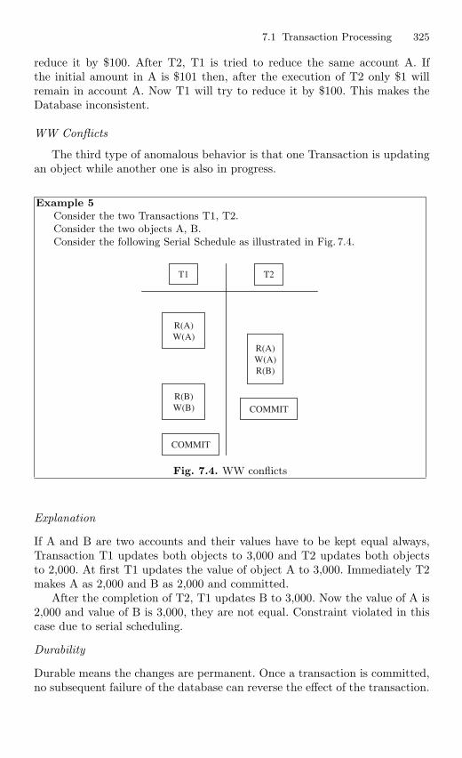
7.1 Transaction Processing 325
reduce it by $100. After T2, T1 is tried to reduce the same account A. Ifthe initial amount in A is $101 then, after the execution of T2 only $1 willremain in account A. Now T1 will try to reduce it by $100. This makes theDatabase inconsistent.
WW Conflicts
The third type of anomalous behavior is that one Transaction is updatingan object while another one is also in progress.
Example 5Consider the two Transactions T1, T2.Consider the two objects A, B.Consider the following Serial Schedule as illustrated in Fig. 7.4.
T1 T2
R(A)W(A)
R(A)W(A)R(B)
R(B)W(B)
COMMIT
COMMIT
Fig. 7.4. WW conflicts
Explanation
If A and B are two accounts and their values have to be kept equal always,Transaction T1 updates both objects to 3,000 and T2 updates both objectsto 2,000. At first T1 updates the value of object A to 3,000. Immediately T2makes A as 2,000 and B as 2,000 and committed.
After the completion of T2, T1 updates B to 3,000. Now the value of A is2,000 and value of B is 3,000, they are not equal. Constraint violated in thiscase due to serial scheduling.
Durability
Durable means the changes are permanent. Once a transaction is committed,no subsequent failure of the database can reverse the effect of the transaction.
326 7 Transaction Processing and Query Optimization
7.1.4 Lock-Based Concurrency Control
Concurrency Control is the control on the Database and Transactions whichare executed concurrently to ensure that each Transaction completed healthy.Concurrency control is concerned with preventing loss of data integrity dueto interference between users in a multiuser environment.
Need for Concurrency Control
In database management system several transactions are executed simultane-ously. In order to achieve concurrent transactions, the technique of interleavedexecution is used. But in this technique there is a possibility for the occur-rence of certain anomalies, due to the overriding of one transaction on theparticular Database Object which is already referred by another Transaction.
Lock-Based Concurrency Control
It is the best method to control the concurrent access to the Database Objectsby providing suitable permissions to the Transactions. Also it is the onlymethod which takes less cost of Time and less program complexity in termsof code development.
Key Terms in Lock-Based Concurrency Control
Database Object
Database Object is the small data element, the value of which one is alteredduring the execution of transactions.
Lock
Lock is a small object associated with Database Object which gives the infor-mation about the type of operations allowed on a particular Database Object.
Lock can be termed as a type of permission provided by the transactionmanager to the transactions to do a particular operation on a Database Obj-ect. The transaction must get this permission from Transaction Manager toaccess any Database Object for alteration. Locking mechanisms are the mostcommon type of concurrency control mechanism. With locking, any data thatis retrieved by a user for updating must be locked, or denied to other users,until the update is complete.
Locking Protocol
It is the set of rules to be followed by each transaction, to ensure that the neteffect of execution of eachTransaction in interleaved fashion will be same as,
7.1 Transaction Processing 327
the result obtained when the Transactions executed in serial fashion. Generallylocks can be classified into two. First one is related to what already told inthe previous paragraph. Next one is the unwanted effect when we implementlock of the first type.
The two types of Lock are:
1. Strict Two-Phase Locking (Strict 2PL)2. Deadlock
Strict Two-Phase Locking (Strict 2PL)
It is a most widely used locking protocol. It provides few rules to the Trans-actions to access the Database Objects. They are:
Rule 1:If a Transaction “T” wants to read, modify an object, it first requests a shared,
exclusive lock on the Database Object respectively.Rule 2:
All Locks held by the Transaction will be released when it is completed.
Shared Lock. It is type of lock established on a Database Object. It is likea component which is sharable within all active transactions. A DatabaseObject can be shared locked by more than one number of transactions. Toget a shared lock on particular Database Object the Database Object shouldsatisfy the following condition.
Condition. It should not be exclusively locked by any of the other Trans-actions.
Example 6If a person updates his bank account then the Database will lock that Database
Object exclusively to avoid RW conflicts. So the Transactions which are requestingto read that Database Object will be suspended until the completion of updating.
Exclusive Lock. It is type of lock established on a Database Object. It islike a component which cannot be shared within all active Transactions. Itis dedicated to particular transaction; only that particular transaction canaccess and modify that object.
Condition. It should not be exclusively locked by any one of the otherTransactions.
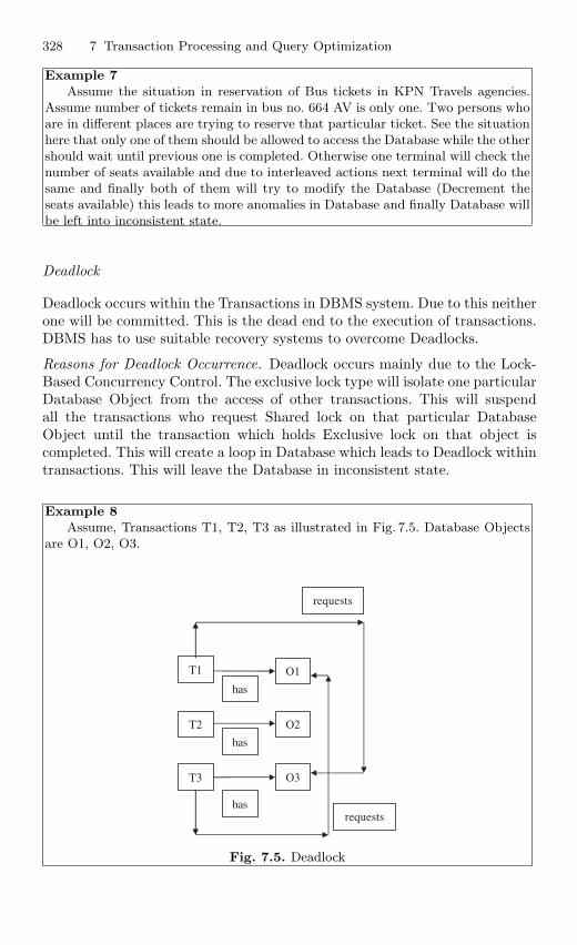
328 7 Transaction Processing and Query Optimization
Example 7Assume the situation in reservation of Bus tickets in KPN Travels agencies.
Assume number of tickets remain in bus no. 664 AV is only one. Two persons whoare in different places are trying to reserve that particular ticket. See the situationhere that only one of them should be allowed to access the Database while the othershould wait until previous one is completed. Otherwise one terminal will check thenumber of seats available and due to interleaved actions next terminal will do thesame and finally both of them will try to modify the Database (Decrement theseats available) this leads to more anomalies in Database and finally Database willbe left into inconsistent state.
Deadlock
Deadlock occurs within the Transactions in DBMS system. Due to this neitherone will be committed. This is the dead end to the execution of transactions.DBMS has to use suitable recovery systems to overcome Deadlocks.
Reasons for Deadlock Occurrence. Deadlock occurs mainly due to the Lock-Based Concurrency Control. The exclusive lock type will isolate one particularDatabase Object from the access of other transactions. This will suspendall the transactions who request Shared lock on that particular DatabaseObject until the transaction which holds Exclusive lock on that object iscompleted. This will create a loop in Database which leads to Deadlock withintransactions. This will leave the Database in inconsistent state.
Example 8Assume, Transactions T1, T2, T3 as illustrated in Fig. 7.5. Database Objects
are O1, O2, O3.
T1
T2
T3
O1
O2
O3
has
has
has
requests
requests
Fig. 7.5. Deadlock
7.1 Transaction Processing 329
Explanation
Here we can observe that the loop occurs between T1 and T3. Neither T1 norT3 are completed.
Methods to Overcome Deadlock
Mostly it is not possible to avoid the occurrence of Deadlock. Most of themethods available are detection and recovery based.
Detection from the Average Waiting Time of the Transaction
If more than two transactions are waiting for the long time, then it impliesthat at some part of the database, deadlock has occurred. So we can detectDeadlock easily.
Deadlock Detection algorithm
Deadlock detection algorithms are used to find any loops in the Database.The main advantage is that we can find the locked transactions quickly andit is enough to restart only those particular transactions.
Recovery Mechanism
Once if Deadlock is found then we have several methods to release lockedTransactions.
Method 1: Release of Objects from Big Transaction
In this method the transaction which holds more number of Database Objectwill be taken and all Database Objects associated with that Big Transactionwill be removed.
Example 9If Transaction say, T1 holds exclusive lock on four objects, T2 holds same on
three objects and T3 holds same on two objects then if Deadlock occurred withinthese transactions then T1 will be restarted.
Method 2: Restarting the Locked Transactions
In this method Database Objects associated with all Transactions are releasedand they will be restarted.
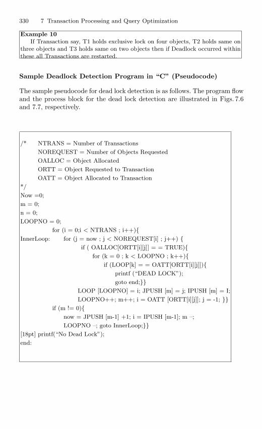
330 7 Transaction Processing and Query Optimization
Example 10If Transaction say, T1 holds exclusive lock on four objects, T2 holds same on
three objects and T3 holds same on two objects then if Deadlock occurred withinthese all Transactions are restarted.
Sample Deadlock Detection Program in “C” (Pseudocode)
The sample pseudocode for dead lock detection is as follows. The program flowand the process block for the dead lock detection are illustrated in Figs. 7.6and 7.7, respectively.
/* NTRANS = Number of Transactions
NOREQUEST = Number of Objects Requested
OALLOC = Object Allocated
ORTT = Object Requested to Transaction
OATT = Object Allocated to Transaction
*/
Now =0;
m = 0;
n = 0;
LOOPNO = 0;
for (i = 0;i < NTRANS ; i++)InnerLoop: for (j = now ; j < NOREQUEST[i] ; j++)
if ( OALLOC[ORTT[i][j]] = = TRUE)for (k = 0 ; k < LOOPNO ; k++)
if (LOOP[k] = = OATT[ORTT[i][j]])printf (“DEAD LOCK”);
goto end;LOOP [LOOPNO] = i; JPUSH [m] = j; IPUSH [m] = I;
LOOPNO++; m++; i = OATT [ORTT[i][j]]; j = -1; if (m != 0)
now = JPUSH [m-1] +1; i = IPUSH [m-1]; m –;
LOOPNO –; goto InnerLoop;[18pt] printf(“No Dead Lock”);
end:
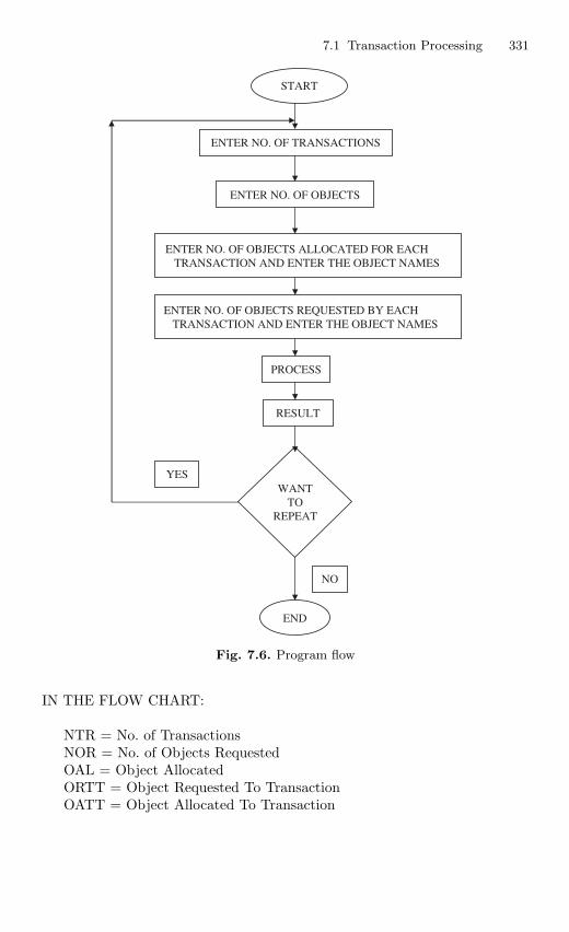
7.1 Transaction Processing 331
START
ENTER NO. OF TRANSACTIONS
ENTER NO. OF OBJECTS
ENTER NO. OF OBJECTS ALLOCATED FOR EACH TRANSACTION AND ENTER THE OBJECT NAMES
ENTER NO. OF OBJECTS REQUESTED BY EACH TRANSACTION AND ENTER THE OBJECT NAMES
PROCESS
RESULT
WANTTO
REPEAT
END
YES
NO
Fig. 7.6. Program flow
IN THE FLOW CHART:
NTR = No. of TransactionsNOR = No. of Objects RequestedOAL = Object AllocatedORTT = Object Requested To TransactionOATT = Object Allocated To Transaction
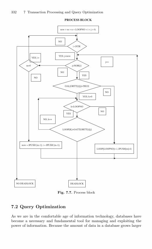
332 7 Transaction Processing and Query Optimization
PROCESS BLOCK
now = m = n = LOOPNO = i = j = 0;
OAL[ORTT[i][j]=TRUE
i <NTR
j<NOR[i]
k<LOOPNO
LOOP[K]=OATT[ORTT[i][j]
m=0
DEADLOCKNO DEADLOCK
YES; j=now
NO
YES
YES; i+
LOOP[LOOPNO]= i; JPUSH[m]=J;
NO
YES; k=0
YES
NO; k++
NO
j++
NO
now = JPUSH [m-1]; i = IPUSH [m-1];
NO
Fig. 7.7. Process block
7.2 Query Optimization
As we are in the comfortable age of information technology, databases havebecome a necessary and fundamental tool for managing and exploiting thepower of information. Because the amount of data in a database grows larger
7.2 Query Optimization 333
and larger as time passes, one of the most important characteristics of a data-base is its ability to maintain a consistent and acceptable level of performance.The principal mechanism through which a database maintains an optimallevel of performances is known as the database query optimizer; without awell-designed query optimizer, even small databases would be noticeably slug-gish. The query optimizers for some of the most popular commercial-qualitydatabases are estimated to have required about 50 man-years of development.It should therefore go without saying that the specific processes involved indesigning the internal structure of a real-world optimizer can be overwhelm-ingly complex. Nevertheless, because of the optimizer’s paramount importanceto the robustness and flexibility of a database, it is worthwhile to engage in asurvey of the theory behind the rudimentary components of a basic, cost-basedquery optimizer.
7.2.1 Query Processing
The activities involved in retrieving data from the database are called as queryprocessing. The aims of query processing are to transform a query written ina high-level language typically SQL, into a correct and efficient executionstrategy expressed in a low-level language (implementing relational algebra),and to execute the strategy to retrieve the required data. An important aspectof query processing is Query Optimization.
The activity of choosing an efficient execution strategy for processing aquery is called as query optimization. As there are many equivalent trans-formations of the same high-level query, the aim of query optimization is tochoose the one that minimizes the resource usage.
A DBMS uses different techniques to process, optimize, and execute high-level queries (SQL). A query expressed in high-level query language must befirst scanned, parsed, and validated.
The scanner identifies the language components (tokens) in the text ofthe query, while the parser checks the correctness of the query syntax. Thequery is also validated (by accessing the system catalog) whether the attributenames and relation names are valid. An internal representation (tree or graph)of the query is created.
Queries are parsed and then presented to a query optimizer, which isresponsible for identifying an efficient plan. The optimizer generates alter-native plans and chooses the plan with the least estimated cost.
7.2.2 Need for Query Optimization
In high-level query languages, any given query can be processed in differentways. Resources required by each query will be different.
DBMS has the responsibility to select the optimized way to process thequery. Query optimizers do not “optimize” – just try to find “reasonably good”evaluation strategies. Query optimizer uses relational algebra expressions.
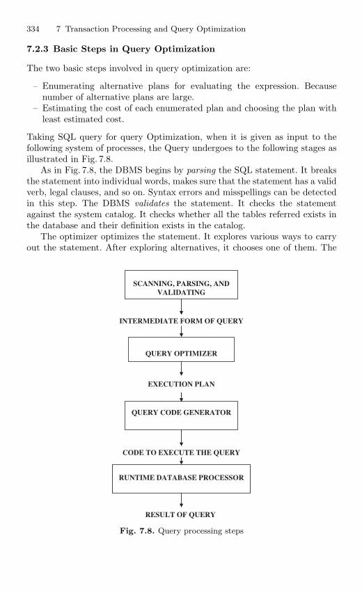
334 7 Transaction Processing and Query Optimization
7.2.3 Basic Steps in Query Optimization
The two basic steps involved in query optimization are:
– Enumerating alternative plans for evaluating the expression. Becausenumber of alternative plans are large.
– Estimating the cost of each enumerated plan and choosing the plan withleast estimated cost.
Taking SQL query for query Optimization, when it is given as input to thefollowing system of processes, the Query undergoes to the following stages asillustrated in Fig. 7.8.
As in Fig. 7.8, the DBMS begins by parsing the SQL statement. It breaksthe statement into individual words, makes sure that the statement has a validverb, legal clauses, and so on. Syntax errors and misspellings can be detectedin this step. The DBMS validates the statement. It checks the statementagainst the system catalog. It checks whether all the tables referred exists inthe database and their definition exists in the catalog.
The optimizer optimizes the statement. It explores various ways to carryout the statement. After exploring alternatives, it chooses one of them. The
SCANNING, PARSING, ANDVALIDATING
EXECUTION PLAN
CODE TO EXECUTE THE QUERY
QUERY CODE GENERATOR
RESULT OF QUERY
QUERY OPTIMIZER
RUNTIME DATABASE PROCESSOR
INTERMEDIATE FORM OF QUERY
Fig. 7.8. Query processing steps
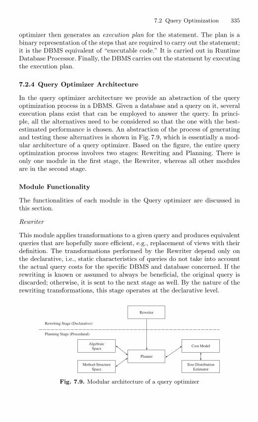
7.2 Query Optimization 335
optimizer then generates an execution plan for the statement. The plan is abinary representation of the steps that are required to carry out the statement;it is the DBMS equivalent of “executable code.” It is carried out in RuntimeDatabase Processor. Finally, the DBMS carries out the statement by executingthe execution plan.
7.2.4 Query Optimizer Architecture
In the query optimizer architecture we provide an abstraction of the queryoptimization process in a DBMS. Given a database and a query on it, severalexecution plans exist that can be employed to answer the query. In princi-ple, all the alternatives need to be considered so that the one with the best-estimated performance is chosen. An abstraction of the process of generatingand testing these alternatives is shown in Fig. 7.9, which is essentially a mod-ular architecture of a query optimizer. Based on the figure, the entire queryoptimization process involves two stages: Rewriting and Planning. There isonly one module in the first stage, the Rewriter, whereas all other modulesare in the second stage.
Module Functionality
The functionalities of each module in the Query optimizer are discussed inthis section.
Rewriter
This module applies transformations to a given query and produces equivalentqueries that are hopefully more efficient, e.g., replacement of views with theirdefinition. The transformations performed by the Rewriter depend only onthe declarative, i.e., static characteristics of queries do not take into accountthe actual query costs for the specific DBMS and database concerned. If therewriting is known or assumed to always be beneficial, the original query isdiscarded; otherwise, it is sent to the next stage as well. By the nature of therewriting transformations, this stage operates at the declarative level.
Rewriter
AlgebraicSpace
Method-StructureSpace
Planner
Cost Model
Size-DistributionEstimator
Rewriting Stage (Declarative)
Planning Stage (Procedural)
Fig. 7.9. Modular architecture of a query optimizer
336 7 Transaction Processing and Query Optimization
Planner
This is the main module of the ordering stage. It examines all possibleexecution plans for each query produced in the previous stage and selectsthe overall cheapest one to be used to generate the answer of the originalquery. It employs a search strategy, which examines the space of executionplans in a particular fashion. This space is determined by two other modulesof the optimizer, the Algebraic Space and the Method-Structure Space. Forthe most part, these two modules and the search strategy determine the cost,i.e., running time, of the optimizer itself, which should be as low as possi-ble. The execution plans examined by the Planner are compared based onestimates of their cost so that the cheapest may be chosen. These costs arederived by the last two modules of the optimizer namely the Cost Model andthe Size-Distribution Estimator.
Algebraic Space
This module determines the action execution orders that are to be consideredby the Planner for each query sent to it. All such series of actions producethe same query answer, but usually differ in performance. They are usuallyrepresented in relational algebra as formulas or in tree form. Because ofthe algorithmic nature of the objects generated by this module and sent tothe Planner, the overall planning stage is characterized as operating at theprocedural level.
Method-Structure Space
This module determines the implementation choices that exist for the execu-tion of each ordered series of actions specified by the Algebraic Space. Thischoice is related to the available join methods for each join (e.g., nested loops,merge scan, and hash join). This choice is also related to the available indicesfor accessing each relation, which is determined by the physical schema of eachdatabase stored in its catalogs. Given an algebraic formula or tree from theAlgebraic Space, this module produces all corresponding complete executionplans, which specify the implementation of each algebraic operator and theuse of any indices.
Cost Model
This module specifies the arithmetic formulas that are used to estimate thecost of execution plans. For every different join method, for every differ-ent index type access, and in general for every distinct kind of step thatcan be found in an execution plan, there is a formula that gives its cost.Given the complexity of many of these steps, most of these formulas aresimple approximations of what the system actually does and are based oncertain assumptions regarding issues like buffer management, disk–CPU over-lap, sequential vs. random I/O, etc. The most important input parameters
7.2 Query Optimization 337
to a formula are the size of the buffer pool used by the corresponding step,the sizes of relations or indices accessed, and possibly various distributions ofvalues in these relations. While the first one is determined by the DBMS foreach query, the other two are estimated by the Size-Distribution Estimator.
Size-Distribution Estimator
This module specifies how the sizes (and possibly frequency distributions ofattribute values) of database relations and indices as well as (sub) query resultsare estimated. As mentioned above, these estimates are needed by the CostModel. The specific estimation approach adopted in this module also deter-mines the form of statistics that need to be maintained in the catalogs of eachdatabase, if any.
Detailed Description
This section provides a detailed description of the Algebraic Space, thePlanner, and Size-Distribution Estimator, respectively.
Algebraic Space
SQL query corresponds to a select-project-join query in relational algebra.Typically, such an algebraic query is represented by a query tree whose leavesare database relations and nonleaf nodes are algebraic operators like selections(denoted by σ) projections (denoted by π), and joins (denoted by ). Anintermediate node indicates the application of the corresponding operator onthe relations generated by its children, the result of which is then sent furtherup. Thus, the edges of a tree represent data flow from bottom to top, i.e., fromthe leaves, which correspond to data in the database, to the root, which is thefinal operator producing the query answer. Figure 7.10 gives three examplesof query trees for the query.
SELECT name, floor FROM emp, dept WHERE emp.dno =dept.dno AND sal > 100 K
For a complicated query, the number of all query trees may be enormous. Toreduce the size of the space that the search strategy has to explore, DBMSsusually restrict the space in several ways. The first typical restriction dealswith selections and projections:
R1 Selections and projections are processed on the “y” and almost nevergenerate intermediate relations. Selections are processed as relations areaccessed for the first time. Projections are processed as the results of otheroperators are generated.
For example, plan P1 of Sect. 7.1.1 satisfies restriction R1: the index scanof emp finds emp tuples that satisfy the selection on emp.sal on the “y”
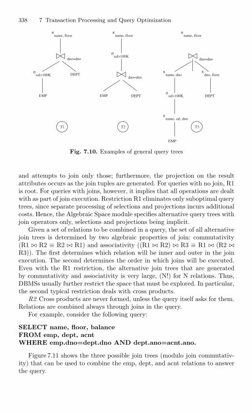
338 7 Transaction Processing and Query Optimization
πname, floor
sal>100K
dno=dno
DEPT
EMP
T1
σ
πname, floor
sal>100K
dno=dno
DEPTEMP
T2
σ
πname, floor
πname, dno
πname, sal, dno
πdno, floor
dno=dno
DEPT
EMP
T3
sal>100Kσ
Fig. 7.10. Examples of general query trees
and attempts to join only those; furthermore, the projection on the resultattributes occurs as the join tuples are generated. For queries with no join, R1is root. For queries with joins, however, it implies that all operations are dealtwith as part of join execution. Restriction R1 eliminates only suboptimal querytrees, since separate processing of selections and projections incurs additionalcosts. Hence, the Algebraic Space module specifies alternative query trees withjoin operators only, selections and projections being implicit.
Given a set of relations to be combined in a query, the set of all alternativejoin trees is determined by two algebraic properties of join: commutativity(R1 R2 ≡ R2 R1) and associativity ((R1 R2) R3 ≡ R1 (R2 R3)). The first determines which relation will be inner and outer in the joinexecution. The second determines the order in which joins will be executed.Even with the R1 restriction, the alternative join trees that are generatedby commutativity and associativity is very large, (N!) for N relations. Thus,DBMSs usually further restrict the space that must be explored. In particular,the second typical restriction deals with cross products.
R2 Cross products are never formed, unless the query itself asks for them.Relations are combined always through joins in the query.
For example, consider the following query:
SELECT name, floor, balanceFROM emp, dept, acntWHERE emp.dno=dept.dno AND dept.ano=acnt.ano.
Figure 7.11 shows the three possible join trees (modulo join commutativ-ity) that can be used to combine the emp, dept, and acnt relations to answerthe query.
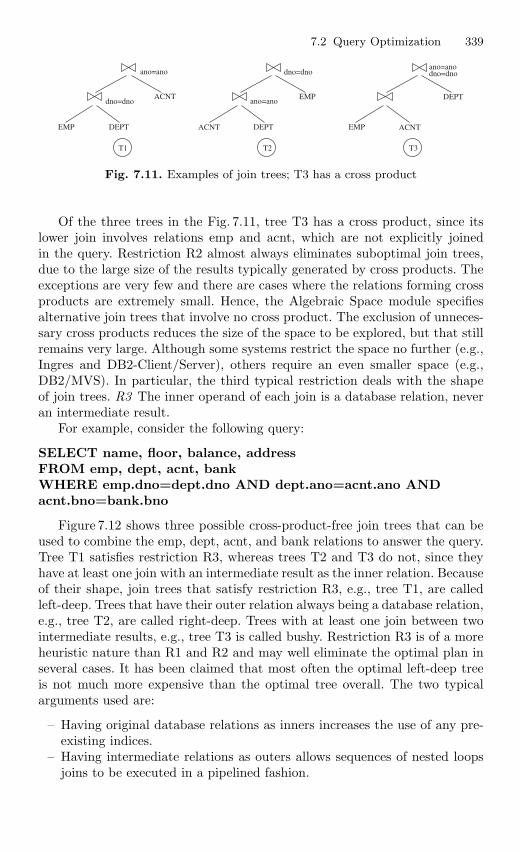
7.2 Query Optimization 339
ACNT
ano=ano
dno=dno
DEPTEMP
T1
ACNT
ano=ano
dno=dno
DEPT
EMP
T2
ACNT
ano=anodno=dno
DEPT
EMP
T3
Fig. 7.11. Examples of join trees; T3 has a cross product
Of the three trees in the Fig. 7.11, tree T3 has a cross product, since itslower join involves relations emp and acnt, which are not explicitly joinedin the query. Restriction R2 almost always eliminates suboptimal join trees,due to the large size of the results typically generated by cross products. Theexceptions are very few and there are cases where the relations forming crossproducts are extremely small. Hence, the Algebraic Space module specifiesalternative join trees that involve no cross product. The exclusion of unneces-sary cross products reduces the size of the space to be explored, but that stillremains very large. Although some systems restrict the space no further (e.g.,Ingres and DB2-Client/Server), others require an even smaller space (e.g.,DB2/MVS). In particular, the third typical restriction deals with the shapeof join trees. R3 The inner operand of each join is a database relation, neveran intermediate result.
For example, consider the following query:
SELECT name, floor, balance, addressFROM emp, dept, acnt, bankWHERE emp.dno=dept.dno AND dept.ano=acnt.ano ANDacnt.bno=bank.bno
Figure 7.12 shows three possible cross-product-free join trees that can beused to combine the emp, dept, acnt, and bank relations to answer the query.Tree T1 satisfies restriction R3, whereas trees T2 and T3 do not, since theyhave at least one join with an intermediate result as the inner relation. Becauseof their shape, join trees that satisfy restriction R3, e.g., tree T1, are calledleft-deep. Trees that have their outer relation always being a database relation,e.g., tree T2, are called right-deep. Trees with at least one join between twointermediate results, e.g., tree T3 is called bushy. Restriction R3 is of a moreheuristic nature than R1 and R2 and may well eliminate the optimal plan inseveral cases. It has been claimed that most often the optimal left-deep treeis not much more expensive than the optimal tree overall. The two typicalarguments used are:
– Having original database relations as inners increases the use of any pre-existing indices.
– Having intermediate relations as outers allows sequences of nested loopsjoins to be executed in a pipelined fashion.
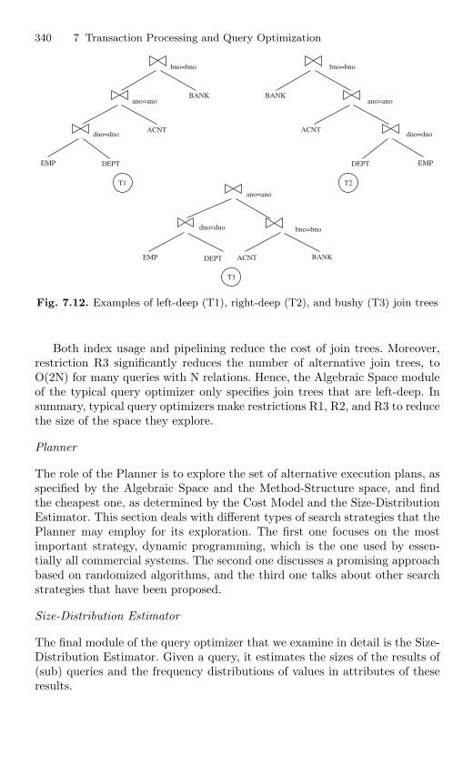
340 7 Transaction Processing and Query Optimization
ACNT
DEPT
T1
BANK
EMP
dno=dno
ano=ano
bno=bno
ACNTDEPT
T3
BANKEMP
dno=dno
ano=ano
bno=bno
ACNT
DEPT
T2
BANK
EMP
dno=dno
ano=ano
bno=bno
Fig. 7.12. Examples of left-deep (T1), right-deep (T2), and bushy (T3) join trees
Both index usage and pipelining reduce the cost of join trees. Moreover,restriction R3 significantly reduces the number of alternative join trees, toO(2N) for many queries with N relations. Hence, the Algebraic Space moduleof the typical query optimizer only specifies join trees that are left-deep. Insummary, typical query optimizers make restrictions R1, R2, and R3 to reducethe size of the space they explore.
Planner
The role of the Planner is to explore the set of alternative execution plans, asspecified by the Algebraic Space and the Method-Structure space, and findthe cheapest one, as determined by the Cost Model and the Size-DistributionEstimator. This section deals with different types of search strategies that thePlanner may employ for its exploration. The first one focuses on the mostimportant strategy, dynamic programming, which is the one used by essen-tially all commercial systems. The second one discusses a promising approachbased on randomized algorithms, and the third one talks about other searchstrategies that have been proposed.
Size-Distribution Estimator
The final module of the query optimizer that we examine in detail is the Size-Distribution Estimator. Given a query, it estimates the sizes of the results of(sub) queries and the frequency distributions of values in attributes of theseresults.
7.2 Query Optimization 341
7.2.5 Basic Algorithms for Executing Query Operations
A query basically consists of following operations. The query can be analyzedby analyzing these operations separately.
– Selection Operation– Join Operation– Projection Operation– Set Operations
Select Operation
A query can have condition to select the required data. For that selection itmay use several ways to search for the data. The following are some of theways to search:
– File Scan– Index Scan
File Scan
A number of search algorithms are possible for selecting the records from afile. The selection of records from a file is known as file scan, as the algorithmscans the records of a file to search for and retrieve records that satisfy theselection condition.
Index Scan
If the search algorithm uses an index to perform the search, then it is referredas Index Scan.
– Linear Search: This is also known as Brute Force method. In this method,every record in the file is retrieved and tested as to whether its attributevalues satisfy the selection condition.
– Binary Search: If a selection condition involves an equality comparison ona key attribute on which the file is ordered, a binary search can be used.Binary search is more efficient than linear search.
– Primary Index Single Record Retrieval : If a selection condition involvesan equality comparison on a primary key attribute with a primary index,we can use the primary index to retrieve that record.
– Secondary Index : This search method can be used to retrieve a singlerecord if the indexing field has unique values (key field) or to retrievemultiple records if the indexing field is not a key. This can also be usedfor comparisons involving <, >, <= or >=
342 7 Transaction Processing and Query Optimization
– Primary Index Multiple Records Retrieval : A search condition uses com-parison condition <, >, etc. on a key field with primary index is knownas Primary index multiple records retrieval.
– Clustering Index : If the selection condition involves an equality compari-son on a nonkey attribute with a clustering index, we can use that indexto retrieve all the records satisfying the condition.
Conjunctive Condition Selection
If the selection condition of the SELECT operation is a conjunctive con-dition (a condition that is made up of several simple conditions with theAND operator), then the DBMS can use the following additional methods toperform the selection.
Conjunctive selection: If an attribute in any single simple condition in theconjunctive condition has an access path that permits use of binary search oran index search, use that condition to retrieve the records and then check ifthat record satisfies the remaining condition.
Conjunctive selection using composite index : If two or more attributes areinvolved in equality conditions in the conjunctive condition and a compositeindex exists on the combined fields we can use the index.
Query Optimization for Select Operation
Following method gives query optimization for selection operation:
1. If more than one of the attributes has an access path, then use the onethat retrieves fewer disk blocks.
2. Need to consider the selectivity of a condition: Selectivity of a condition isthe number of tuples that satisfy the condition divided by total number oftuples. The smaller the selectivity the fewer the number of tuples retrievedand higher the desirability of using that condition to retrieve the records.
Join Operation
Join is one of the most time-consuming operations in query processing. Herewe consider only equijoin or natural join. Two-way join is a join of tworelations, and there are many ways to perform the join. Multiway join is ajoin of more than two relations and number of ways to execute multiway joinsincreases rapidly with number of relations.
We use methods for implementing two-way joins of form
RJN(a = b)S
7.2 Query Optimization 343
where, R and S are relations which need to be joined, a and b are attributesused for conditions, and JN → Type of join.
Methods for Implementing Joins
Following are various methods to implement join operations.
Nested (Inner–Outer) Loop
For each record t in R (outer loop), retrieve every record s from S (inner loop)and test whether the two records satisfy the join condition t[A] = s[B].
Access Structure Based Retrieval of Matching Records
If an index (or hash key) exists for one of the two join attributes – say, B of S –retrieve each record t in R, one at a time, and then use the access structureto retrieve directly all matching records from S that satisfy s[B] = t[A].
Sort-merge join
If the records of R and S are physically sorted (ordered) by value of the joinattributes A and B, respectively, then both the relations are scanned in orderto the join attributes, matching the records that have same values for A andB. In this case, the relations R and S are only scanned once.
Hash-join
The tuples of relations R and S are both hashed to the same hash file, usingthe same hashing function on the join attributes A of R and B of S as hashkeys. A single pass through the relation with fewer records (say, R) hashes itstuples to the hash file buckets. A single pass through the other relation (S)then hashes each of its tuples to the appropriate bucket, where the record iscombined with all matching records from R.
In practice all the above techniques are implemented by accessing wholedisk blocks of a relation, rather than individual records. Depending on theavailability of buffer space in memory the number of blocks read in from thefile can be adjusted. It is advantageous to use the relation with fewer blocksas the outer loop relation in nested loop method.
For method using access structures to retrieve matching tuples, eitherthe smaller relation or the file that has a match for every record (high joinselection factor) should be used in the outer loop. In some cases an index maybe created specifically for performing the join operation if one does not existalready.
Sort-Merge algorithm is the most efficient, sometimes the relations aresorted before merging. Hash join method is efficient if the hash file can bekept in the main memory.
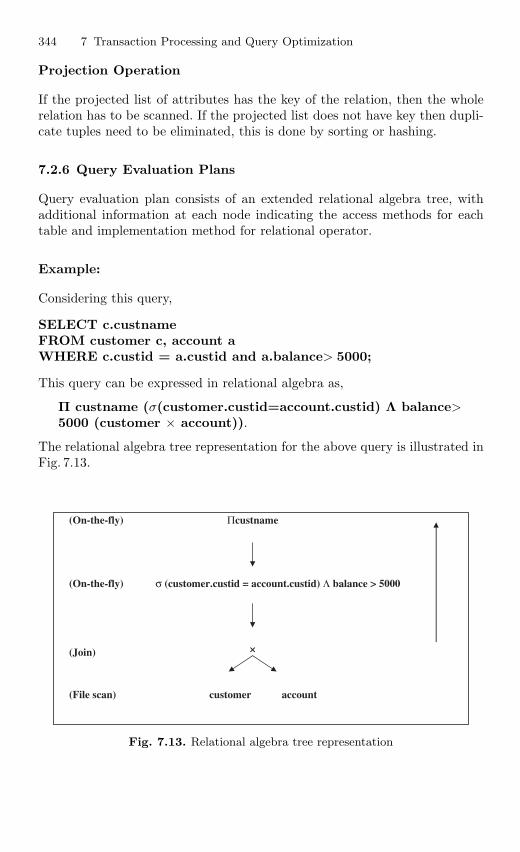
344 7 Transaction Processing and Query Optimization
Projection Operation
If the projected list of attributes has the key of the relation, then the wholerelation has to be scanned. If the projected list does not have key then dupli-cate tuples need to be eliminated, this is done by sorting or hashing.
7.2.6 Query Evaluation Plans
Query evaluation plan consists of an extended relational algebra tree, withadditional information at each node indicating the access methods for eachtable and implementation method for relational operator.
Example:
Considering this query,
SELECT c.custnameFROM customer c, account aWHERE c.custid = a.custid and a.balance> 5000;
This query can be expressed in relational algebra as,
Π custname (σ(customer.custid=account.custid) Λ balance>5000 (customer × account)).
The relational algebra tree representation for the above query is illustrated inFig. 7.13.
(On-the-fly) Πcustname
(On-the-fly) σ (customer.custid = account.custid) Λ balance > 5000
(Join)
(File scan) customer account
×
Fig. 7.13. Relational algebra tree representation
7.2 Query Optimization 345
Pipelined Evaluation
From Fig. 7.13, we can visualize that each operation is carried out and inputtedto the next section. In this type of evaluation is called as Pipelined evaluationwhich is more efficient than conventional method. In conventional methodwe use temporary memory to hold the evaluated operation and from that,memory next operation will be carried out.
So, pipelined evaluation has the advantage of not using temporary memoryand this method is thus a control strategy.
On-the-fly
When the input table to a unary operator (for e.g., Selection or projection)is pipelined into it, which is referred as on-the-fly.
The Iterator Interface
To simplify the code responsible for coordinating the execution of a plan,the relational operators that form the nodes of a plan tree typically supportuniform iterator interface, hiding internal implementation details of eachoperator.
The iterator interfaces for an operator includes the functions open, getnext, close.Open( )
It initializes the state of the iterator by allocating buffers for its inputsand output.It calls for the operator specific code to process the input tuples.
Close( )
To deallocate the memory allocated during the process.The iterator interface is also used to encapsulate access methods such asB+ trees and Hash-based indexes.
Pushing Selection Method
In this method, it is considered that the selection operator can be appliedbefore the join operation to be performed. So, it is only necessary to join theselected tuples which reduces considerable memory requirement as shown inFig. 7.14.
In our previous example we can apply the “balance” condition beforejoin operation is to be applied. We push the selection before applying joinoperation.
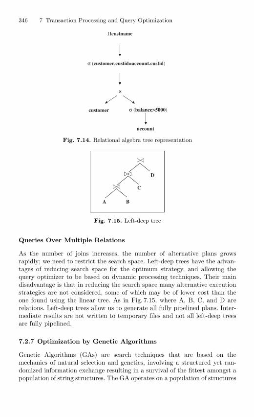
346 7 Transaction Processing and Query Optimization
Πcustname
σ (customer.custid=account.custid)
×
customer
account
σ (balance>5000)
Fig. 7.14. Relational algebra tree representation
D
A B
C
Fig. 7.15. Left-deep tree
Queries Over Multiple Relations
As the number of joins increases, the number of alternative plans growsrapidly; we need to restrict the search space. Left-deep trees have the advan-tages of reducing search space for the optimum strategy, and allowing thequery optimizer to be based on dynamic processing techniques. Their maindisadvantage is that in reducing the search space many alternative executionstrategies are not considered, some of which may be of lower cost than theone found using the linear tree. As in Fig. 7.15, where A, B, C, and D arerelations. Left-deep trees allow us to generate all fully pipelined plans. Inter-mediate results are not written to temporary files and not all left-deep treesare fully pipelined.
7.2.7 Optimization by Genetic Algorithms
Genetic Algorithms (GAs) are search techniques that are based on themechanics of natural selection and genetics, involving a structured yet ran-domized information exchange resulting in a survival of the fittest amongst apopulation of string structures. The GA operates on a population of structures
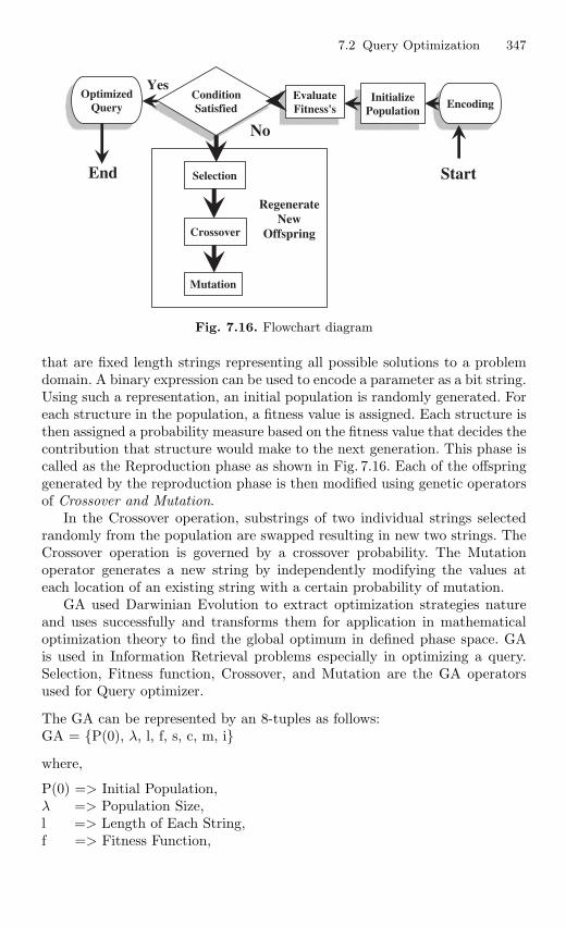
7.2 Query Optimization 347
ConditionSatisfied
OptimizedQuery Encoding
RegenerateNew
Offspring
EvaluateFitness's
Selection
Crossover
Mutation
StartEnd
YesInitialize
Population
No
Fig. 7.16. Flowchart diagram
that are fixed length strings representing all possible solutions to a problemdomain. A binary expression can be used to encode a parameter as a bit string.Using such a representation, an initial population is randomly generated. Foreach structure in the population, a fitness value is assigned. Each structure isthen assigned a probability measure based on the fitness value that decides thecontribution that structure would make to the next generation. This phase iscalled as the Reproduction phase as shown in Fig. 7.16. Each of the offspringgenerated by the reproduction phase is then modified using genetic operatorsof Crossover and Mutation.
In the Crossover operation, substrings of two individual strings selectedrandomly from the population are swapped resulting in new two strings. TheCrossover operation is governed by a crossover probability. The Mutationoperator generates a new string by independently modifying the values ateach location of an existing string with a certain probability of mutation.
GA used Darwinian Evolution to extract optimization strategies natureand uses successfully and transforms them for application in mathematicaloptimization theory to find the global optimum in defined phase space. GAis used in Information Retrieval problems especially in optimizing a query.Selection, Fitness function, Crossover, and Mutation are the GA operatorsused for Query optimizer.
The GA can be represented by an 8-tuples as follows:GA = P(0), λ, l, f, s, c, m, i
where,
P(0) => Initial Population,λ => Population Size,l => Length of Each String,f => Fitness Function,
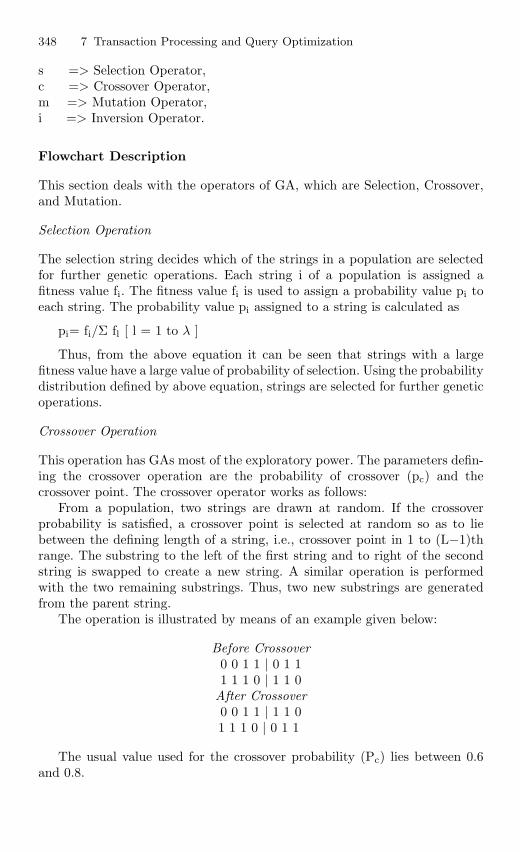
348 7 Transaction Processing and Query Optimization
s => Selection Operator,c => Crossover Operator,m => Mutation Operator,i => Inversion Operator.
Flowchart Description
This section deals with the operators of GA, which are Selection, Crossover,and Mutation.
Selection Operation
The selection string decides which of the strings in a population are selectedfor further genetic operations. Each string i of a population is assigned afitness value fi. The fitness value fi is used to assign a probability value pi toeach string. The probability value pi assigned to a string is calculated as
pi= fi/Σ fl [ l = 1 to λ ]
Thus, from the above equation it can be seen that strings with a largefitness value have a large value of probability of selection. Using the probabilitydistribution defined by above equation, strings are selected for further geneticoperations.
Crossover Operation
This operation has GAs most of the exploratory power. The parameters defin-ing the crossover operation are the probability of crossover (pc) and thecrossover point. The crossover operator works as follows:
From a population, two strings are drawn at random. If the crossoverprobability is satisfied, a crossover point is selected at random so as to liebetween the defining length of a string, i.e., crossover point in 1 to (L−1)thrange. The substring to the left of the first string and to right of the secondstring is swapped to create a new string. A similar operation is performedwith the two remaining substrings. Thus, two new substrings are generatedfrom the parent string.
The operation is illustrated by means of an example given below:
Before Crossover0 0 1 1 | 0 1 11 1 1 0 | 1 1 0
After Crossover0 0 1 1 | 1 1 01 1 1 0 | 0 1 1
The usual value used for the crossover probability (Pc) lies between 0.6and 0.8.
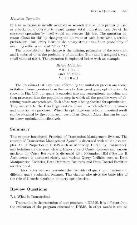
Review Questions 349
Mutation Operation
In GAs mutation is usually assigned as secondary role. It is primarily usedas a background operator to guard against total premature loss. Use of thecrossover operation by itself would not recover this loss. The mutation op-erator allows for this by changing the bit value at each locus with a certainprobability. Thus, every locus on the binary string has a finite probability ofassuming either a value of “0” or “1.”
The probability of this change is the defining parameter of the operationand is referred to as the probability of mutation (Pm) and is assigned a verysmall value of 0.001. The operation is explained below with an example:
Before Mutation0 0 1 1 0 1 1
After Mutation1 0 1 1 0 0 1
The bit values that have been affected by the mutation process are shownin italics. These operators form the basis for GA-based query optimization. Asshown in Fig. 7.16, our query is encoded into any conventional modeling andthen processed into the population step in which all the possible ways of ob-taining results are produced. Each of the way is being checked for optimization.They are sent to the GAs Regeneration phase in which selection, crossoverand mutation are processed. When the optimized one is found, required resultcan be obtained by the optimized query. Thus Genetic Algorithm can be usedfor query optimization effectively.
Summary
This chapter introduced Principle of Transaction Management System. Theconcept of Transaction Management System is discussed with suitable exam-ples. ACID Properties of DBMS such as Atomicity, Durability, Consistency,and Isolation are discussed clearly. Importance of Crash Recovery and variousmethods for Crash Recovery is discussed with Examples. IBM’s System RArchitecture is discussed clearly and various Query facilities such as DataManipulation Facilities, Data Definition Facilities, and Data Control Facilitiesare described.
In this chapter we have presented the basic idea of query optimization anddifferent query evaluation schemes. This chapter also gives the basic idea ofthe role of Genetic algorithm in query optimization.
Review Questions
7.1. What is Transaction?
Transaction is the execution of user program in DBMS. It is different fromthe execution of the program external to DBMS. In other words it can be
350 7 Transaction Processing and Query Optimization
stated as the various read and write operations done by the user program onthe DBMS, when it is executed in DBMS environment.
7.2. What are ACID properties of the DBMS?
ACID is an acronym for Atomicity, Consistency, Isolation, and Durability.A – AtomicityC – ConsistencyI – IsolationD – DurabilityAtomicity and Durability are closely related. Consistency and Isolation
are closely related.
7.3. What is strict 2PL? Explain its role in Lock-Based Concurrency Control.
It is a most widely used locking protocol.It provides few rules to the Transactions to access the Database Objects.
They are:Rule 1If a Transaction say T wants to read, modify an object, it first requests a
shared, exclusive lock on the Database Object, respectively.Rule 2All Locks held by the Transaction will be released when it is completed.
7.4. What is WR conflict?
This happens when the Transaction T2 is trying to read the object A thathas been modified by another Transaction T1, which has not yet completed(committed). This type read is called as dirty read or Write read conflict.
7.5. What is Deadlock?
It is the lock that occurs within the Transactions in DBMS system. Dueto this neither one will be committed. This is the dead end to the executionof Transactions. DBMS has to use suitable recovery systems to overcomeDeadlocks.
7.6. Why Deadlock Occurs?
It occurs mainly due to the Lock Based Concurrency Control. In theexclusive lock type it will isolate one particular Database Object from theaccess to the other Transactions. This will suspend all the Transactions whorequest Shared lock on that particular Database Object until the Transactionwhich holds Exclusive lock on that object is completed. This will create a loopin Database. This leads to Deadlock within Transactions. This will leave theDatabase in inconsistent state.
Review Questions 351
7.7. Mention the three major methods used to handle Deadlock?
(a) Deadlock Prevention(b) Deadlock Avoidance(c) Deadlock Detection
Deadlock prevention: Transaction aborts if there is a possibility of deadlockoccurring. If the transaction aborts, it must be rollback and all locks it hasare released.
Deadlock detection: DBMS occasionally checks for deadlock. If there isdeadlock, it randomly picks one of the transactions to kill (i.e., rollback) andthe other continues.
Deadlock avoidance: A transaction must obtain all its locks before it canbegin so deadlock will never occur.
7.8. What is Interleaved Execution?
In DBMS to enforce concurrent Transactions, several Transactions areordered in a serial manner and executed one by one according to the schedule.So there will be switching over of execution between the Transactions. Thisis called as Interleaved Execution.
7.9. What is Partial Transaction?
If the Transaction is interrupted in the middle way it leaves the databasein the inconsistency state. These types of transactions are called as PartialTransactions.
7.10. What is Unrepeatable Read?
In this case anomalous behavior could result in that a transaction T2 couldchange the value of an object A that has been read by a Transaction T1, whileT2 is still in progress. If T1 tries to read A again it will get different results.This type of read is called as Unrepeatable Read.
7.11. Find out whether the following system is in Deadlock or not?
Total Number of Processes 3 (P1, P2, P3)Total Number of Resources 3 (R1, R2, R3)P1 holds R1 and waiting for R2.P2 holds R2 and waiting for R3.P3 holds nothing and waiting for R3.
Answer : System is in safe state.Since R3 is not assigned yet it can be assigned to P3 and it can be finished.
After P3, P2, and P1 can be completed sequentially.
7.12. What is meant by query optimization?
The activity of choosing an efficient execution strategy for processing a queryis called as query optimization. As there are many equivalent transformationsof the same high-level query, the aim of query optimization is to choose theone that minimizes the resource usage.
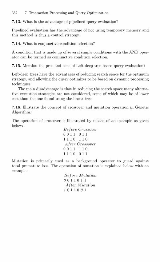
352 7 Transaction Processing and Query Optimization
7.13. What is the advantage of pipelined query evaluation?
Pipelined evaluation has the advantage of not using temporary memory andthis method is thus a control strategy.
7.14. What is conjunctive condition selection?
A condition that is made up of several simple conditions with the AND oper-ator can be termed as conjunctive condition selection.
7.15. Mention the pros and cons of Left-deep tree based query evaluation?
Left-deep trees have the advantages of reducing search space for the optimumstrategy, and allowing the query optimizer to be based on dynamic processingtechniques.
The main disadvantage is that in reducing the search space many alterna-tive execution strategies are not considered, some of which may be of lowercost than the one found using the linear tree.
7.16. Illustrate the concept of crossover and mutation operation in GeneticAlgorithm.
The operation of crossover is illustrated by means of an example as givenbelow:
Before Crossover0 0 1 1 | 0 1 11 1 1 0 | 1 1 0After Crossover0 0 1 1 | 1 1 01 1 1 0 | 0 1 1
Mutation is primarily used as a background operator to guard againsttotal premature loss. The operation of mutation is explained below with anexample:
Before Mutation0 0 1 1 0 1 1After Mutation
1 0 1 1 0 0 1
8
Database Security and Recovery
Learning Objectives. This chapter provides an overview of database security andrecovery. In this chapter the need for database security, the classification of databasesecurity, and different types of database failures are discussed with suitable examples.Advanced concept in database recovery like ARIES algorithm is illustrated. Aftercompleting this chapter the reader should be familiar with the following concepts:
– Need for database security– Classification of database security– Database security at design and maintenance level– Types of failure– ARIES recovery algorithm
8.1 Database Security
8.1.1 Introduction
Database security issues are often lumped together with data integrity issues,but the two concepts are really quite distinct. Security refers to the protectionof data against unauthorized disclosure, alteration, or destruction; integrityrefers to the accuracy or validity of that data. To put it a little glibly:
– Security means protecting the data against unauthorized users.– Integrity means protecting the data against authorized users.
In both cases, system needs to be aware of certain constraints that usersmust not violate; in both cases those constraints must be specified (typicallyby the DBA) in some suitable language, and must be maintained in the systemcatalog; and in both cases the DBMS must monitor user operations in order toensure that the constraints are enforced. The main reason to clearly separatethe discussion of the two topics is that integrity is regarded as absolutelyfundamental but security as more of a secondary issue.
S. Sumathi: Database Security and Recovery, Studies in Computational Intelligence (SCI) 47,
353–379 (2007)
www.springerlink.com c© Springer-Verlag Berlin Heidelberg 2007
354 8 Database Security and Recovery
Data are the most valuable resource for an organization. Security in adatabase involves mechanisms to protect the data and ensure that it is notaccessed, altered, or deleted without proper authorization. The databasein Defense Research Development Organization (DRDO), Atomic ResearchCentre, and Space Research Centre contains vital data and it should not berevealed to unauthorized persons. To protect the secret data there should berestriction to data access. This ensures the confidentiality of the data. Alsothe data should be protected from accidental destruction. Due to advance-ment in information technology, people share the data through World WideWeb. As a result the data become vulnerable to hackers. A database shouldnot only provide the end user with the data needed to function, but also itshould provide protection for the data.
8.1.2 Need for Database Security
The need for database security is given below:
– In the case of shared data, multiple users try to access the data at the sametime. In order to maintain the consistency of the data in the database,database security is needed.
– Due to the advancement of internet, data are accessed through WorldWide Web, to protect the data against hackers, database security isneeded.
– The plastic money (Credit card) is more popular. The money transactionhas to be safe. More specialized software both to enter the system ille-gally to extract data and to analyze the information obtained is available.Hence, it is necessary to protect the data/money.
8.1.3 General Considerations
There are numerous aspects to the security problem, some of them are:
– Legal, social, and ethical aspects– Physical controls– Policy questions– Operational problems– Hardware control– Operating system support– Issues that are the specific concern of the database system itself
There are two broad approaches to data security. The approaches areknown as discretionary and mandatory control, respectively. In both cases,the unit of data or “data object” that might need to be protected can rangeall the way from an entire database on the one hand to a specific componentwithin a specific tuple on the other. How the two approaches differ is indicatedby the following brief outline.
8.1 Database Security 355
In the case of discretionary control, a given user will typically have differentaccess rights (also known as privileges) on different objects; further, there arevery few – inherent limitations, that is – regarding which users can have whichrights on which object (for example, user U1 might be able to see A but notB, while user U2 might be able to see B but not A). Discretionary schemesare thus very flexible.
In the case of mandatory control, each data object is labeled with acertain classification level, and each user is given a certain clearance level.A given data object can then be accessed only by users with the appropriateclearance. Mandatory schemes thus tend to be hierarchic in nature and arehence comparatively rigid. (If user U1 can see A but not B, then the classifi-cation of B must be higher than that of A, and so no user U2 can see B butnot A.)
Regardless of whether we are dealing with a discretionary scheme or amandatory one, all decisions as to which users are allowed to perform whichoperations on which objects are policy decisions, not technical ones. As such,they are clearly outside the jurisdiction of the DBMS as such; all the DBMScan do is enforcing those decisions once they are made. It follows that:
– The results of policy decisions made must be known to the system (this isdone by means of statement in some appropriate definitional language).
– There must be a means of checking a given access request against theapplicable security constraint in the catalog. (By “access request” herewe mean the combination of requested operation plus requested objectplus requesting user, in general.) That checking is done by the DBMS’ssecurity subsystem, also known as the authorization subsystem.
In order to decide which security constraints are applicable to a givenaccess request, the system must be able to recognize the source of that request,i.e., it must be able to recognize the requesting user. For that reason, whenusers sign on to the system, they are typically required to supply, not onlytheir user ID (to say who they are), but also a password (to prove they arewho they say they are). The password is supposedly known only to the systemand to legitimate users of the user ID concerned.
Regarding the last point, incidentally, note that any number of distinctusers might be able to share the same ID. In this way the system can sup-port user groups, and can thus provide a way of allowing everyone in theaccounting department to share the same privileges on the same objects. Theoperations of adding individual users to or removing individual users from agiven group can then be performed independently of the operation of speci-fying which privileges on which objects apply to that group. Note, however,that the obvious place to keep a record of which users are in which groups isonce again the catalog (or perhaps the database itself).
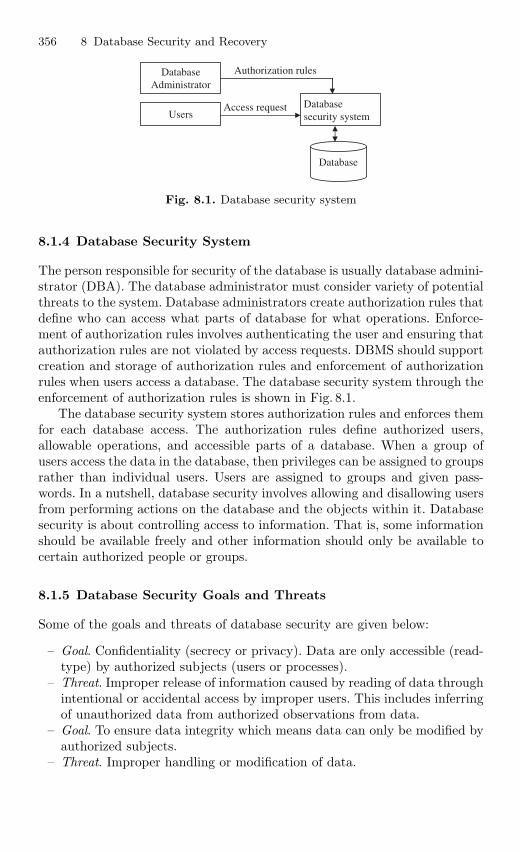
356 8 Database Security and Recovery
DatabaseAdministrator
Authorization rules
Access request
Database
Databasesecurity systemUsers
Fig. 8.1. Database security system
8.1.4 Database Security System
The person responsible for security of the database is usually database admini-strator (DBA). The database administrator must consider variety of potentialthreats to the system. Database administrators create authorization rules thatdefine who can access what parts of database for what operations. Enforce-ment of authorization rules involves authenticating the user and ensuring thatauthorization rules are not violated by access requests. DBMS should supportcreation and storage of authorization rules and enforcement of authorizationrules when users access a database. The database security system through theenforcement of authorization rules is shown in Fig. 8.1.
The database security system stores authorization rules and enforces themfor each database access. The authorization rules define authorized users,allowable operations, and accessible parts of a database. When a group ofusers access the data in the database, then privileges can be assigned to groupsrather than individual users. Users are assigned to groups and given pass-words. In a nutshell, database security involves allowing and disallowing usersfrom performing actions on the database and the objects within it. Databasesecurity is about controlling access to information. That is, some informationshould be available freely and other information should only be available tocertain authorized people or groups.
8.1.5 Database Security Goals and Threats
Some of the goals and threats of database security are given below:
– Goal. Confidentiality (secrecy or privacy). Data are only accessible (read-type) by authorized subjects (users or processes).
– Threat. Improper release of information caused by reading of data throughintentional or accidental access by improper users. This includes inferringof unauthorized data from authorized observations from data.
– Goal. To ensure data integrity which means data can only be modified byauthorized subjects.
– Threat. Improper handling or modification of data.
8.1 Database Security 357
– Goal. Availability (denial of service). Data are accessible to authorizedsubjects.
– Threat. Action could prevent subjects from accessing data for which theyare authorized.
Security Threat Classification
Security threat can be broadly classified into accidental, intentional accordingto the way they occur.
The accidental threats include human errors, errors in software, and nat-ural or accidental disasters:
– Human errors include giving incorrect input, incorrect use of applications.– Errors in software include incorrect application of security policies, denial
of access to authorized users.– Natural or accidental disasters include the damage of hardware or soft-
ware.
The intentional threat includes authorized users who abuse their privilegesand authority, hostile agents like improper users executing improper readingor writing of data, legal use of applications can mask fraudulent purpose.
8.1.6 Classification of Database Security
The database security can be broadly classified into physical and logical secu-rity. Database recovery refers to the process of restoring database to a correctstate in the event of a failure.
Physical security. Physical security refers to the security of the hardwareassociated with the system and the protection of the site where the computerresides. Natural events such as fire, floods, and earthquakes can be consi-dered as some of the physical threats. It is advisable to have backup copies ofdatabases in the face of massive disasters.
Logical security. Logical security refers to the security measures residingin the operating system or the DBMS designed to handle threats to the data.Logical security is far more difficult to accomplish.
Database Security at Design Level
It is necessary to take care of the database security at the stage of databasedesign. Few guidelines to build the most secure system are:
1. The database design should be simple. If the database is simple and easierto use, then the possibility that the data being corrupted by the authorizeduser is less.
358 8 Database Security and Recovery
2. The database has to be normalized. The normalized database is almostfree from update anomalies. It is harder to impose normalization on therelations after the database is in use. Hence, it is necessary to normalizethe database at the design stage itself.
3. The designer of the database should decide the privilege for each groupof users. If no privileges are assumed by any user, there is less likelihoodthat a user will be able to gain illegal access.
4. Create unique view for each user or group of users. Although “VIEW”promotes security by restricting user access to data, they are not adequatesecurity measures, because unauthorized persons may gain knowledge ofor access to a particular view.
Database Security at the Maintenance Level
Once the database is designed, the database administrator is playing a crucialrole in the maintenance of the database. The security issues with respect tomaintenance can be classified into:
1. Operating system issues and availability2. Confidentiality and accountability through authorization rules3. Encryption4. Authentication schemes
(1) Operating System Issues and Availability
The system administrator normally takes care of the operating systemsecurity. The database administrator is playing a key role in the physicalsecurity issues. The operating system should verify that users and appli-cation programs attempting to access the system are authorized. Accountsand passwords for the entire database system are handled by the databaseadministrator.
(2) Confidentiality and Accountability
Accountability means that the system does not allow illegal entry. Account-ability is related to both prevention and detection of illegal actions. Ac-countability is assured by monitoring the authentication and authorization ofusers.
Authorization rules are controls incorporated in the data managementsystem that restrict access to data and also restrict the actions that peoplemay take when they access data.
Authentication can be carried out by the operating system level or bythe relational database management system (RDBMS). In case, the systemadministrator or the database administrator creates for every user an individ-ual account or username. In addition to these accounts, users are also assignedpasswords.
8.1 Database Security 359
(3) Encryption
Encryption can be used for highly sensitive data like financial data, mili-tary data. Encryption is the coding of data so that they cannot be read andunderstood easily. Some DBMS products include encryption routines thatautomatically encode sensitive data when they are stored or transmitted overcommunication channel. Any system that provides encryption facilities mustalso provide complementary routines for decoding the data. These decodingroutines must be protected by adequate security, or else the advantage ofencryption is lost.
(4) Authentication Schemes
Authentication schemes are the mechanisms that determine whether a user iswho he or she claims to be. Authentication can be carried out at the operatingsystem level or by the RDBMS. The database administrator creates for everyuser an individual account or user name. In addition to these accounts, usersare also assigned passwords. A password is a sequence of characters, numbers,or a combination of both which is known only to the system and its legiti-mate user. Since the password is the first line of defense against unauthorizeduse by outsiders, it needs to be kept confidential by its legitimate user. It ishighly recommended that users change their password frequently. The pass-word needs to be hard to guess, but easy for the user to remember. Passwordscannot, of themselves, ensure the security of a computer and its databases,because they give no indication of who is trying to gain access.
The password can also be tapped; hence mere password cannot ensure thesecurity of the database. To circumvent this problem, the industry is devel-oping devices and techniques to positively identify any prospective user. Themost promising of these appear to be biometric devices, which measure ordetect personal characteristics such as fingerprints, voice prints, retina prints,or signature dynamics. To implement this approach, several companies havedeveloped a smart card which is a thin plastic card with an embedded micro-processor. An individual’s unique biometric data are stored permanently onthe card. To access the database the user inserts the card and the biometricdevice reads the person’s unique feature. The actual biometric data are thencompared with the stored data, and the two must match for the user to gaincomputer access. A lost or stolen card would be useless to another person,since biometric data would not match.
Database Security Through Access Control
A database for an enterprise contains a great deal of information and usuallyhas several groups of users. Most users need to access only a small portion ofthe database which is allocated to them. Allowing users unrestricted access
360 8 Database Security and Recovery
to all the data can be undesirable, and a DBMS should provide mechanismsto access the data. Especially, it is a way to control the data accessible by agiven user.
Two main mechanisms of access control at the DBMS level are:
– Discretionary access control– Mandatory access control
In fact it would be more accurate to say that most systems support dis-cretionary control, and some systems support mandatory control as well;discretionary control is thus more likely to be encountered in practice, and sowe deal with it first.
Discretionary Access Control
Discretionary access control regulates all user access to named objects throughprivileges, based on the concept of access rights or privileges for objects(tables and views), and mechanisms for giving users’ privileges (and revokingprivileges). A privilege allows a user to access some data object in a manner(to read or modify). Creator of a table or a view automatically gets all privi-leges on it. DBMS keeps track of who subsequently gains and loses privileges,and ensures that only requests from users who have the necessary privileges(at the time the request is issued) are allowed.
There needs to be a language that supports the definition of (discretionary)security constraints. For fairly obvious reasons, however, it is easier to statewhat is allowed rather than what is not allowed; languages therefore typi-cally support the definition, not of security constraints as such, but ratherof authorities, which are effectively the opposite of security constraints (ifsomething is authorized, it is not constrained). We therefore begin by brieflydescribing a language for defining authorities with a simple example:
AUTHORITY SA3GRANT RETRIEVE (S#, SNAME, CITY), DELETEON STO Jim, Fred, Mary;
This example is intended to illustrate the point that (in general) authoritieshave four components, as follows:
1. A name (SA3 – “suppliers authority three” – in the example). The autho-rity will be registered in the catalog under this name.
2. One or more privileges (RETRIEVE – on certain attributes only – andDELETE, in the example), specified by means of the GRANT clause.
3. The relvar to which the authority applies (relvar S in the example), speci-fied by means of the ON clause.
8.1 Database Security 361
4. One or more “users” (more accurately, user IDs) who are to be grantedthe specified privileges over the specified relvar, specified by means of theTO clause.
Here is the general syntax:
AUTHORITY <authority name>GRANT <privilege commalist>ON <relvar name>TO <user ID commalist>;
Explanation The <authority name>, <relvar name>, and <user IDcommalist> are self-explanatory (except that we regard ALL, meaning allknown users, as a legal “user ID” in this context). Each <privilege> is one ofthe following:
RETRIEVE [(<attribute name commalist>)]INSERT [(<attribute name commalist>)]UPDATE [(<attribute name commalist>)]ALL
RETRIEVE (unqualified), INSERT (unqualified), UPDATE (unqualified),and DELETE are self-explanatory. If a commalist of attribute names isspecified with RETRIEVE, then the privilege applies only to the attributesspecified; INSERT and UPDATE with a commalist of attribute names aredefined analogously. The specification ALL is shorthand for all privileges:RETRIEVE (all attributes), INSERT (all attributes), UPDATE (all attri-butes), and DELETE.
Note. For simplicity, we ignore the question of whether any special privilegesare required in order to perform general relational assignment operations.Also, we deliberately limit our attention only to data manipulation operations;in practice, of course, there are many other operations that we would want, tobe subject to authorization checking as well, such as the operations of definingand dropping relvars and the operations of defining and dropping authoritiesthemselves. We omit detailed consideration of such operations here which isbeyond the scope of this book.
What should happen if some user attempts some operation on some objectfor which he or she is not authorized? The simplest option is obviously just toreject the attempt (and to provide suitable diagnostic information, of course);such a response will surely be the one most commonly required in practice. Sowe might as well make it as default. In more sensitive situations, however, someother action might be more appropriate; for example, it might be necessary toterminate the program or lock the user’s keyboard. It might also be desirableto record such attempts in a special log (threat monitoring), in order to permitsubsequent analysis of attempted security breaches and also to serve in itselfas a deterrent against illegal infiltration (see the discussion of audit trails atthe end of this section).
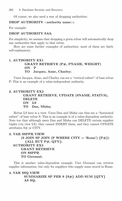
362 8 Database Security and Recovery
Of course, we also need a way of dropping authorities:
DROP AUTHORITY <authority name>;
For example:
DROP AUTHORITY SA3;
For simplicity, we assume that dropping a given relvar will automatically dropany authorities that apply to that relvar.
Here are some further examples of authorities, most of them are fairlyself-explanatory.
1. AUTHORITY EX1GRANT RETRIEVE (P#, PNAME, WEIGHT)ON PTO Jacques, Anne, Charley;
Users Jacques, Anne, and Charley can see a “vertical subset” of base relvarP. This is an example of a value-independent authority.
2. AUTHORITY EX2GRANT RETRIEVE, UPDATE (SNAME, STATUS),DELETEON LSTO Dan, Misha;
Relvar LS here is a view. Users Dan and Misha can thus see a “horizontalsubset” of base relvar S. This is an example is of a value-dependent authority.Note too that although users Dan and Misha can DELETE certain suppliertuples (via view LS), they cannot INSERT them, and they cannot UPDATEattributes S# or CITY.
3. VAR SSPPR VIEW(S JOIN SP JOIN (P WHERE CITY = ‘Rome’) P#)
ALL BUT P#, QTY;AUTHORITY EX3
GRANT RETRIEVEON SSPPRTO Giovanni;
This is another value-dependent example. User Giovanni can retrievesupplier information, but only for suppliers who supply some stored in Rome.
4. VAR SSQ VIEWSUMMARIZE SP PER S S# ADD SUM QTYAS SQ;
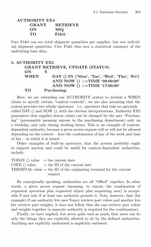
8.1 Database Security 363
AUTHORITY EX4GRANT RETRIEVEON SSQTO Fidel;
User Fidel can see total shipment quantities per supplier, but not individ-ual shipment quantities. User Fidel thus sees a statistical summary of theunderlying base data.
5. AUTHORITY EX5GRANT RETRIEVE, UPDATE (STATUS)ON SWHEN DAY () IN (‘Mon’, ‘Tue’, ‘Wed’, ‘Thu’, ‘Fri’)
AND NOW () >=TIME ‘09:00:00’AND NOW () >=TIME ‘17:00:00’
TO Purchasing;
Here, we are extending our AUTHORITY syntax to include a WHENclause to specify certain “context controls”; we are also assuming that thesystem provides two niladic operators – i.e., operators that take no operands –called DAY () and NOW (), with the obvious interpretations. Authority EX5guarantees that supplier status values can be changed by the user “Purchas-ing” (presumably meaning anyone in the purchasing department) only ona weekday, and only during working hours. This is an example of context-dependent authority, because a given access request will or will not be alloweddepending on the context – here the combination of day of the week and timeof day – in which it is issued.
Other examples of built-in operators, that the system probably oughtto support anyway and could be useful for context-dependent authorities,include:
TODAY () value = the current dateUSER () value = the ID of the current userTERMINAL value = the ID of the originating terminal for the current
request
By conceptually speaking, authorities are all “ORed” together. In otherwords, a given access request (meaning, to repeat, the combination ofrequested operation plus requested object plus requesting user) is accept-able if and only if at least one authority permits it. Note, however, that (forexample) if one authority lets user Nancy retrieve part colors and another letsher retrieve part weights, it does not follow that she can retrieve part colorsand weights together (a separate authority is required for the combination).
Finally, we have implied, but never quite said as much, that users can doonly the things they are explicitly allowed to do by the defined authorities.Anything not explicitly authorized is implicitly outlawed.
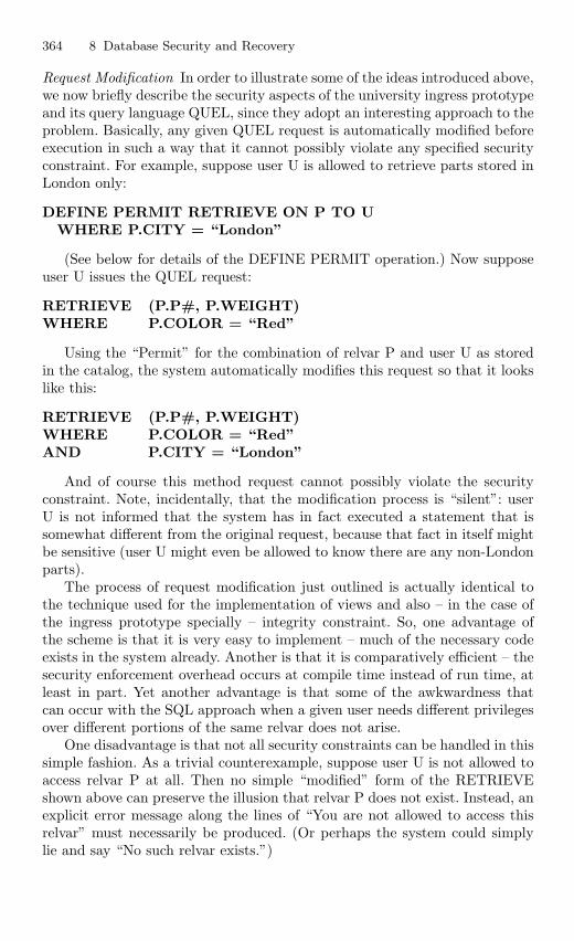
364 8 Database Security and Recovery
Request Modification In order to illustrate some of the ideas introduced above,we now briefly describe the security aspects of the university ingress prototypeand its query language QUEL, since they adopt an interesting approach to theproblem. Basically, any given QUEL request is automatically modified beforeexecution in such a way that it cannot possibly violate any specified securityconstraint. For example, suppose user U is allowed to retrieve parts stored inLondon only:
DEFINE PERMIT RETRIEVE ON P TO UWHERE P.CITY = “London”
(See below for details of the DEFINE PERMIT operation.) Now supposeuser U issues the QUEL request:
RETRIEVE (P.P#, P.WEIGHT)WHERE P.COLOR = “Red”
Using the “Permit” for the combination of relvar P and user U as storedin the catalog, the system automatically modifies this request so that it lookslike this:
RETRIEVE (P.P#, P.WEIGHT)WHERE P.COLOR = “Red”AND P.CITY = “London”
And of course this method request cannot possibly violate the securityconstraint. Note, incidentally, that the modification process is “silent”: userU is not informed that the system has in fact executed a statement that issomewhat different from the original request, because that fact in itself mightbe sensitive (user U might even be allowed to know there are any non-Londonparts).
The process of request modification just outlined is actually identical tothe technique used for the implementation of views and also – in the case ofthe ingress prototype specially – integrity constraint. So, one advantage ofthe scheme is that it is very easy to implement – much of the necessary codeexists in the system already. Another is that it is comparatively efficient – thesecurity enforcement overhead occurs at compile time instead of run time, atleast in part. Yet another advantage is that some of the awkwardness thatcan occur with the SQL approach when a given user needs different privilegesover different portions of the same relvar does not arise.
One disadvantage is that not all security constraints can be handled in thissimple fashion. As a trivial counterexample, suppose user U is not allowed toaccess relvar P at all. Then no simple “modified” form of the RETRIEVEshown above can preserve the illusion that relvar P does not exist. Instead, anexplicit error message along the lines of “You are not allowed to access thisrelvar” must necessarily be produced. (Or perhaps the system could simplylie and say “No such relvar exists.”)
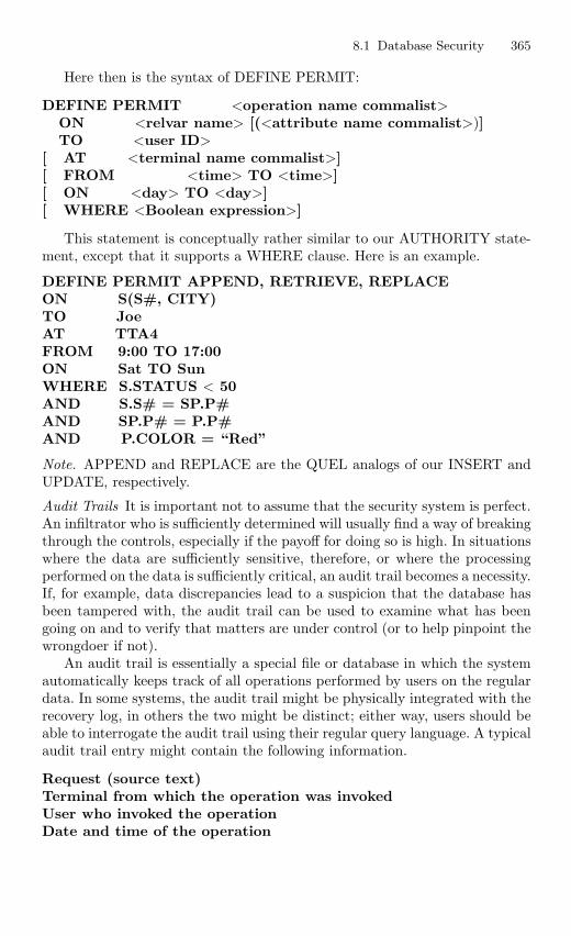
8.1 Database Security 365
Here then is the syntax of DEFINE PERMIT:
DEFINE PERMIT <operation name commalist>ON <relvar name> [(<attribute name commalist>)]TO <user ID>
[ AT <terminal name commalist>][ FROM <time> TO <time>][ ON <day> TO <day>][ WHERE <Boolean expression>]
This statement is conceptually rather similar to our AUTHORITY state-ment, except that it supports a WHERE clause. Here is an example.
DEFINE PERMIT APPEND, RETRIEVE, REPLACEON S(S#, CITY)TO JoeAT TTA4FROM 9:00 TO 17:00ON Sat TO SunWHERE S.STATUS < 50AND S.S# = SP.P#AND SP.P# = P.P#AND P.COLOR = “Red”
Note. APPEND and REPLACE are the QUEL analogs of our INSERT andUPDATE, respectively.
Audit Trails It is important not to assume that the security system is perfect.An infiltrator who is sufficiently determined will usually find a way of breakingthrough the controls, especially if the payoff for doing so is high. In situationswhere the data are sufficiently sensitive, therefore, or where the processingperformed on the data is sufficiently critical, an audit trail becomes a necessity.If, for example, data discrepancies lead to a suspicion that the database hasbeen tampered with, the audit trail can be used to examine what has beengoing on and to verify that matters are under control (or to help pinpoint thewrongdoer if not).
An audit trail is essentially a special file or database in which the systemautomatically keeps track of all operations performed by users on the regulardata. In some systems, the audit trail might be physically integrated with therecovery log, in others the two might be distinct; either way, users should beable to interrogate the audit trail using their regular query language. A typicalaudit trail entry might contain the following information.
Request (source text)Terminal from which the operation was invokedUser who invoked the operationDate and time of the operation
366 8 Database Security and Recovery
Relvar(s), tuple(s), attribute(s) affectedOld valuesNew values
As mentioned earlier in this section, the very fact that an audit trail isbeing maintained might be sufficient in itself to detect an infiltrator in somesituations.
SQL supports discretionary access control through the GRANT andREVOKE commands. The GRANT command gives users privileges to basetables and tables and REVOKE command takes away privileges.
Grant Command This command is used to give privileges to other users ofthe database by the administrator.
SyntaxGRANT privileges ON object TO users [WITH GRANT OPTION]
where objects is either a base table or views.
Mandatory Access Control
It is based on system-wide policies that cannot be changed by individualusers. In this each DB object is assigned a security class. Each subject (useror user program) is assigned a clearance for a security class. Rules basedon security classes and clearances govern who can read/write which objects.Most commercial systems do not support mandatory access control. Versionsof some DBMSs do support it; used for specialized (e.g., military) applications.
Mandatory controls are applicable to databases in which the data have arather static and rigid classification structure, as might be the case in certainmilitary or government environments. As explained briefly in previous sectionthe basic idea is that each data object has a classification level (e.g., top secret,secret, confidential, etc.), and each user has a clearance level (with the samepossibilities as for the classification levels). The levels are assumed to forma strict ordering (e.g., top secret> secret > confidential, etc.). The followingsimple rules, due to Bell and La Padula, are then imposed:
1. User I can retrieve object j only if the clearance level of I is greater orequal to the classification level of j (the “simple security property”).
2. User I can update object j only if the clearance of I is equal to theclassification level of j (the “star property”).
The first rule here is obvious enough, but the second requires a word ofexplanation. Observe first that another way of stating that second rule is tosay that, by definition, anything written by user I automatically acquires aclassification level equal to I’s clearance level. Such a rule is necessary in orderto prevent a user with, e.g., “secret” classification scheme.
8.1 Database Security 367
Note. From the point of view of pure “write” (INSERT) operations only, itwould be sufficient for the classification for the second rule to say that theclearance level of I must be less than or equal to the classification level of j,and the rule is often stated in this form in the literature.
Mandatory controls began to receive a lot of attention in the databaseworld in the early 1990s, because that was when the US Department ofDefense (DoD) began to require any system it purchased to support such con-trols. As a consequence, DBMS vendors have been vying with one another toimplement them. The controls in question are documented in two importantDoD publications known informally as the Orange Book and the LavenderBook, respectively; the Orange Book defines a set of security requirements forany “Trusted Computing Base” (TCB), and the Lavender Book defines and“interpretation” of the TCB requirements for database systems specifically.
First of all, the documents define four security classes (D, C, B, and A);broadly speaking, class D is the least secure, class C is more secure thanclass D, and so on. Class D is said to provide minimal protection, class Cdiscretionary protection, class B mandatory protection, and class A verifiedprotection.
Discretionary Protection Class C is divided into two subclasses C1 and C2(where C1 is less secures that C2), each supports discretionary controls, mean-ing that access is subject to the discretion of the data owner. In addition:
1. Class C1 distinguishes between ownership and access, i.e., it supports theconcept of shared data, while allowing users to have private data of theirown as well.
2. Class C2 additionally requires accountability support through sign-on pro-cedures, auditing, and resource isolation.
Mandatory Protection Class B is the class that deals mandatory controls. Itis further divided into subclasses B1, B2, and B3, as follows:
1. Class B1 requires “labeled security protection” (i.e., it requires each dataobject to be labeled with its classification level – secret, confidential, etc.).It also requires an informal statement of the security policy in effect.
2. Class B2 additionally requires a formal statement of the same thing. Italso requires that covert channels be identified and eliminated. Examplesof covert channels might be the possibility of inferring the answer to anillegal query from the answer to a legal one.
3. Class B3 specifically requires audit and recovery support as well as adesignated security administrator.
Verified Protection Class A, the most secure, requires a mathematical proofthat the security mechanism is consistent and that it is adequate to supportthe specified security policy.
Several commercial DBMS products currently provide mandatory controlsat the B1 level. They also typically provide discretionary controls at the C2
368 8 Database Security and Recovery
level. Terminology: DBMS’s that support mandatory controls are sometimescalled multilevel secure systems. The term trusted system is also used withmuch the same meaning.
Suppose we want to apply the ideas of mandatory access control to thesuppliers relvar S. For definiteness and simplicity, suppose the unit of data wewish to control access to the individual tuple within that relvar. Then eachtuple needs to be labeled with its classification level.
Advantages of Mandatory Access Control Discretionary control has someflaws, e.g., the Trojan horse problem. In this, a devious unauthorized usercan trick an authorized user into disclosing sensitive data. The modificationof the code is beyond the DBMSs control, but it can try and prevent the useof the database as a channel for secret information.
8.2 Database Recovery
Recovery brings the database from the temporary inconsistent state to aconsistent state. Database recovery can also be defined as mechanisms forrestoring a database quickly and accurately after loss or damage. Data-bases are damaged due to human error, hardware failure, incorrect or invaliddata, program errors, computer viruses, or natural catastrophes. Since theorganization depends on its database, the database management system mustprovide mechanisms for restoring a database quickly and accurately after lossor damage.
8.2.1 Different Types of Database Failures
A wide variety of failures can occur in processing a database, ranging fromthe input of an incorrect data value or complete loss or destruction of thedatabase. Some of the types of failures are listed below:
1. System crashes, resulting in loss of main memory2. Media failures, resulting in loss of parts of secondary storage3. Application software errors4. Natural physical disasters5. Carelessness or unintentional destruction of data or facilities6. Sabotage
8.2.2 Recovery Facilities
DBMS should provide following facilities to assist with recovery.
1. Backup mechanism, which makes periodic backup copies of database2. Logging facilities, which keep track of current state of transactions and
database changes
8.2 Database Recovery 369
3. Checkpoint facility, which enables updates to database in progress to bemade permanent
4. Recovery manager, which allows DBMS to restore the database to a con-sistent state following a failure
Backup Mechanism
The DBMS should provide backup facilities that produce a backup copy ofthe entire database. Typically, a backup copy is produced at least once perday. The copy should be stored in a secured location where it is protectedfrom loss or damage. The backup copy is used to restore the database in theevent of hardware failure, catastrophic loss, or damage.
With large databases, regular backups may be impractical, as the timerequired to perform the backup may exceed that available. As a result, backupsmay be taken of dynamic data regularly but backups of static data, which donot change frequently, may be taken less often.
Logging Facilities
Basically there are two types of log, “transaction log” and “database changelog.” A transaction log is a record of the essential data for each transactionthat is processed against the database. In database change log, there are beforeand after images of records that have been modified.
Transaction log. Transaction log contains a record of the essential datafor each transaction that is processed against the database. Data that aretypically recorded for each transaction include the transaction code or identifi-cation, action or type of transaction, time of the transaction, terminal numberor user ID, input data values, table and records accessed, records modified,and possibly the old and new field values.
Database change log. The database change log contains before and afterimages of records that have been modified by transactions. A before-image isa copy of a record before it has been modified, and an after-image is a copyof the same record after it has been modified.
Checkpoint Facility
A checkpoint facility in a DBMS periodically refuses to accept any newtransactions. All transactions in progress are completed, and the journal filesare brought up to date. At this point, the system is in a quiet state, andthe database and transaction logs are synchronized. The DBMS writes a spe-cial record (called a checkpoint record) to the log file, which is like a snap-shot of the state of the database. The checkpoint record contains informationnecessary to restart the system. Any dirty data blocks are written from mem-ory to disk storage, thus ensuring that all changes made prior to taking the
370 8 Database Security and Recovery
checkpoint have been written to long-term storage. A DBMS may performcheckpoints automatically or in response to commands in user applicationprograms. Checkpoints should be taken frequently.
Recovery Manager
The recovery manager is a module of the DBMS which restores the databaseto a correct condition when a failure occurs and which resumes processinguser requests. The recovery manager uses the logs to restore the database.
8.2.3 Main Recovery Techniques
Three main recovery techniques that are commonly employed are:
1. Deferred update2. Immediate update3. Shadow paging
Deferred update. Deferred updates are not written to the database untilafter a transaction has reached its commit point. If transaction fails beforecommit, it will not have modified database and so no undoing of changes arerequired. Deferred update may be necessary to redo updates of committedtransactions as their effect may not have reached database.
Immediate update. In the case of immediate update, updates are appliedto database as they occur. There is a need to redo updates of committedtransactions following a failure. Also there may be need to undo effects oftransactions that had not committed at time of failure. It is essential thatlog records are written before write to database. If no “transaction commit”record in log, then that transaction was active at failure and must be undone.Undo operations are performed in reverse order in which they were written tolog.
Shadow paging. Shadow paging maintains two page tables during life of atransaction, current page and shadow page table. When transaction starts, twopages are the same. Shadow page table is never changed thereafter and is usedto restore database in the event of failure. During transaction, current pagetable records all updates to database. When transaction completes, currentpage table becomes shadow page table.
8.2.4 Crash Recovery
Crash recovery is the process of protecting the database from catastrophicsystem failures and media failures. Recovery manager of a DBMS is respon-sible for ensuring transaction atomicity and durability. Atomicity is attainedby undoing the actions of transactions that do not commit. Durability isattained by making sure that all actions of committed transactions survivesystem crashes.
8.2 Database Recovery 371
Recovery Manager
Recovery manager is responsible for ensuring transaction atomicity anddurability. To save the state of database for the period of times it performsfew operations. They are:
1. Saving checkpoints2. Stealing frames3. Forcing pages
Saving checkpoints. It will save the status of the database in the periodof time duration. So if any crashes occur, then database can be restored intolast saved check point.
Steal approach. In this case, the object can be written into disk before thetransaction which holds the object is committed. This is happening when thebuffer manager chooses the same place to replace by some other page andat the same time another transaction require the same page. This method iscalled as stealing frames.
Forcing pages. In this case, once if the transaction completed the entireobjects associated with it should be forced to disk or written to the disk. Butit will result in more I/O cost. So normally we use only no-force approach.
8.2.5 ARIES Algorithm
ARIES is a recovery algorithm designed to work with a steal, no-forceapproach. It is more simple and flexible than other algorithms.
ARIES algorithm is used by the recovery manager which is invoked aftera crash. Recovery manager will perform restart operations.
Main Key Terms Used in ARIES
Log. These are all file which contain several records. These records containthe information about the state of database at any time. These records arewritten by the DBMS while any changes done in the database. Normally copyof the log file placed in the different parts of the disk for safety.
LSN. The abbreviation of LSN is log sequence number. It is the ID givento each record in the log file. It will be in monotonically ascending order.
Page LSN. For recovery purpose, every page in the database contains theLSN of the most recent log record that describes a change to this page. ThisLSN is called the page LSN.
CLR. The abbreviation of CLR is compensation log record. It is writtenjust before the change recorded in an update log record U is undone.
WAL. The abbreviation of WAL is write-ahead log. Before updating a pageto disk, every update log record that describes a change to this page must beforced to stable storage. This is accomplished by forcing all log records up
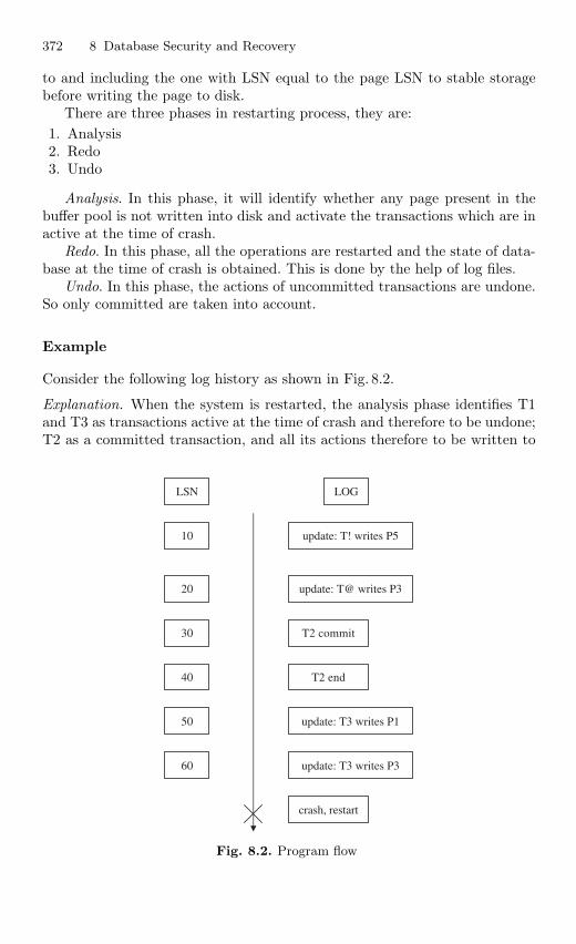
372 8 Database Security and Recovery
to and including the one with LSN equal to the page LSN to stable storagebefore writing the page to disk.
There are three phases in restarting process, they are:1. Analysis2. Redo3. Undo
Analysis. In this phase, it will identify whether any page present in thebuffer pool is not written into disk and activate the transactions which are inactive at the time of crash.
Redo. In this phase, all the operations are restarted and the state of data-base at the time of crash is obtained. This is done by the help of log files.
Undo. In this phase, the actions of uncommitted transactions are undone.So only committed are taken into account.
Example
Consider the following log history as shown in Fig. 8.2.
Explanation. When the system is restarted, the analysis phase identifies T1and T3 as transactions active at the time of crash and therefore to be undone;T2 as a committed transaction, and all its actions therefore to be written to
T2 commit
update: T3 writes P1
update: T@ writes P3
crash, restart
T2 end
update: T3 writes P3
update: T! writes P5
LOGLSN
10
20
30
40
50
60
Fig. 8.2. Program flow
8.2 Database Recovery 373
disk, and P1, P3, and P5 as potentially dirty pages (not yet written intodisk). All the updates are reapplied in the order shown during the redo phase.Finally the actions of T1 and T3 are undone in reverse order during the undophase; that is, T3’s write of P3 is undone, T3’s write of P1 is undone, andthen T1’s write of P5 is undone.
ARIES algorithm has three main principles:
1. Write-ahead logging2. Repeating history during redo3. Logging changes during undo
Write-ahead logging. This states that any change to a database object isfirst recorded in the log; the record in the log must be written to stable storagebefore the change to the database object is written to disk.
Repeating history during redo. On restart after a crash, ARIES retracesall actions of the DBMS before the crash and brings the system back to theexact state that it was in at the time of crash. Then, it undoes the actions oftransactions still active at the time of crash.
Logging changes during undo. Changes made to the database while undoinga transaction are logged to ensure such an action is not repeated in the eventof repeated restarts.
Elements of ARIES
1. The log2. Tables3. The write-ahead log protocol4. Checkpointing
The Log
It records a history of actions that are executed by DBMS. The most recentportion of the log is called as log tail. This page will be kept at main memoryand periodically it will be forced to disk. It contains several records. Eachrecord is uniquely identified by LSN.
A log record is written for each of the following actions:
1. Updating a page2. Commit3. Abort4. End5. Undoing an update
Updating a page. After modifying the page, an update type record is ap-pended to the log tail. The page LSN of this page is then set to the updatelog record as illustrated in the Fig. 8.3.
Before-image is the value of the changed bytes before the change. After-image is the value of the changed bytes after the change.
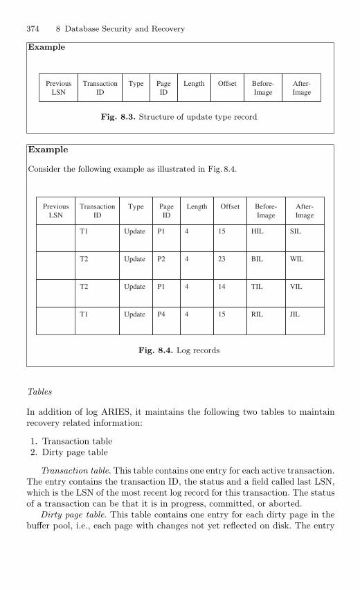
374 8 Database Security and Recovery
Example
PreviousLSN
TransactionID
Type PageID
Length Offset Before-Image
After-Image
Fig. 8.3. Structure of update type record
Example
Consider the following example as illustrated in Fig. 8.4.
PreviousLSN
TransactionID
Type PageID
Length Offset Before-Image
After-Image
T1 Update P1 4 15 HIL SIL
T2 Update P2 4 23 BIL WIL
T2 Update P1 4 14 TIL VIL
T1 Update P4 4 15 RIL JIL
Fig. 8.4. Log records
Tables
In addition of log ARIES, it maintains the following two tables to maintainrecovery related information:
1. Transaction table2. Dirty page table
Transaction table. This table contains one entry for each active transaction.The entry contains the transaction ID, the status and a field called last LSN,which is the LSN of the most recent log record for this transaction. The statusof a transaction can be that it is in progress, committed, or aborted.
Dirty page table. This table contains one entry for each dirty page in thebuffer pool, i.e., each page with changes not yet reflected on disk. The entry
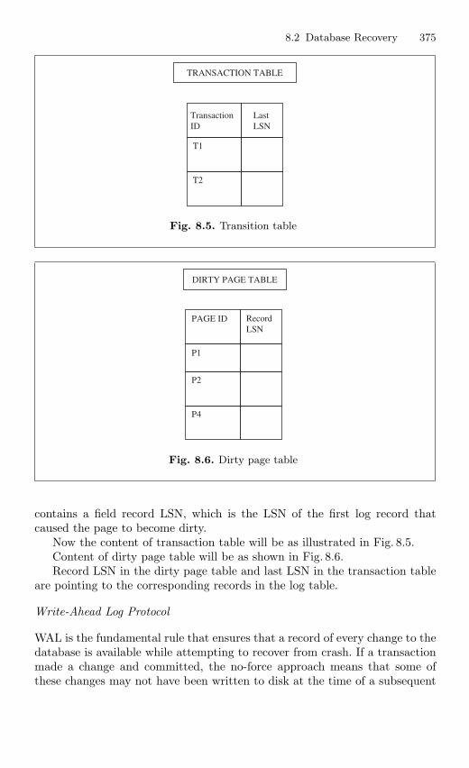
8.2 Database Recovery 375
TransactionID
LastLSN
T1
T2
TRANSACTION TABLE
Fig. 8.5. Transition table
PAGE ID RecordLSN
P1
P2
DIRTY PAGE TABLE
P4
Fig. 8.6. Dirty page table
contains a field record LSN, which is the LSN of the first log record thatcaused the page to become dirty.
Now the content of transaction table will be as illustrated in Fig. 8.5.Content of dirty page table will be as shown in Fig. 8.6.Record LSN in the dirty page table and last LSN in the transaction table
are pointing to the corresponding records in the log table.
Write-Ahead Log Protocol
WAL is the fundamental rule that ensures that a record of every change to thedatabase is available while attempting to recover from crash. If a transactionmade a change and committed, the no-force approach means that some ofthese changes may not have been written to disk at the time of a subsequent
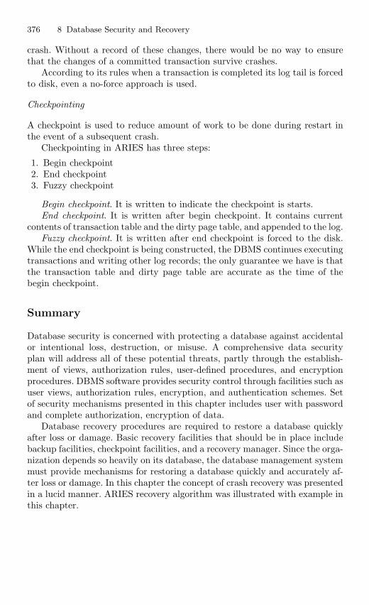
376 8 Database Security and Recovery
crash. Without a record of these changes, there would be no way to ensurethat the changes of a committed transaction survive crashes.
According to its rules when a transaction is completed its log tail is forcedto disk, even a no-force approach is used.
Checkpointing
A checkpoint is used to reduce amount of work to be done during restart inthe event of a subsequent crash.
Checkpointing in ARIES has three steps:
1. Begin checkpoint2. End checkpoint3. Fuzzy checkpoint
Begin checkpoint. It is written to indicate the checkpoint is starts.End checkpoint. It is written after begin checkpoint. It contains current
contents of transaction table and the dirty page table, and appended to the log.Fuzzy checkpoint. It is written after end checkpoint is forced to the disk.
While the end checkpoint is being constructed, the DBMS continues executingtransactions and writing other log records; the only guarantee we have is thatthe transaction table and dirty page table are accurate as the time of thebegin checkpoint.
Summary
Database security is concerned with protecting a database against accidentalor intentional loss, destruction, or misuse. A comprehensive data securityplan will address all of these potential threats, partly through the establish-ment of views, authorization rules, user-defined procedures, and encryptionprocedures. DBMS software provides security control through facilities such asuser views, authorization rules, encryption, and authentication schemes. Setof security mechanisms presented in this chapter includes user with passwordand complete authorization, encryption of data.
Database recovery procedures are required to restore a database quicklyafter loss or damage. Basic recovery facilities that should be in place includebackup facilities, checkpoint facilities, and a recovery manager. Since the orga-nization depends so heavily on its database, the database management systemmust provide mechanisms for restoring a database quickly and accurately af-ter loss or damage. In this chapter the concept of crash recovery was presentedin a lucid manner. ARIES recovery algorithm was illustrated with example inthis chapter.
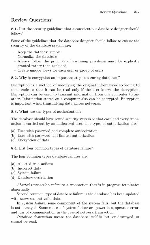
Review Questions 377
Review Questions
8.1. List the security guidelines that a conscientious database designer shouldfollow?
Some of the guidelines that the database designer should follow to ensure thesecurity of the database system are:
– Keep the database simple– Normalize the database– Always follow the principle of assuming privileges must be explicitly
granted rather than excluded– Create unique views for each user or group of users
8.2. Why is encryption an important step in securing databases?
Encryption is a method of modifying the original information according tosome code so that it can be read only if the user knows the decryption.Encryption can be used to transmit information from one computer to an-other. Information stored on a computer also can be encrypted. Encryptionis important when transmitting data across networks.
8.3. What are the types of authorization?
The database should have sound security system so that each and every trans-action is carried out by an authorized user. The types of authorization are:
(a) User with password and complete authorization(b) User with password and limited authorization(c) Encryption of data
8.4. List four common types of database failure?
The four common types database failures are:
(a) Aborted transactions(b) Incorrect data(c) System failure(d) Database destruction
Aborted transaction refers to a transaction that is in progress terminatesabnormally.
Second common type of database failure is the database has been updatedwith incorrect, but valid data.
In system failure, some component of the system fails, but the databaseis not damaged. Some causes of system failure are power loss, operator error,and loss of communication in the case of network transaction.
Database destruction means the database itself is lost, or destroyed, orcannot be read.
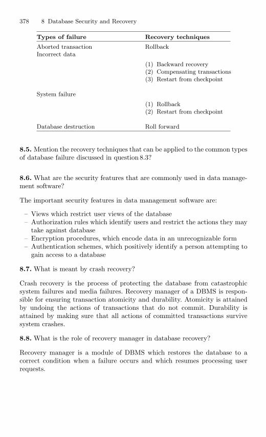
378 8 Database Security and Recovery
Types of failure Recovery techniques
Aborted transaction RollbackIncorrect data
(1) Backward recovery(2) Compensating transactions(3) Restart from checkpoint
System failure
(1) Rollback(2) Restart from checkpoint
Database destruction Roll forward
8.5. Mention the recovery techniques that can be applied to the common typesof database failure discussed in question 8.3?
8.6. What are the security features that are commonly used in data manage-ment software?
The important security features in data management software are:
– Views which restrict user views of the database– Authorization rules which identify users and restrict the actions they may
take against database– Encryption procedures, which encode data in an unrecognizable form– Authentication schemes, which positively identify a person attempting to
gain access to a database
8.7. What is meant by crash recovery?
Crash recovery is the process of protecting the database from catastrophicsystem failures and media failures. Recovery manager of a DBMS is respon-sible for ensuring transaction atomicity and durability. Atomicity is attainedby undoing the actions of transactions that do not commit. Durability isattained by making sure that all actions of committed transactions survivesystem crashes.
8.8. What is the role of recovery manager in database recovery?
Recovery manager is a module of DBMS which restores the database to acorrect condition when a failure occurs and which resumes processing userrequests.
Review Questions 379
8.9. Discuss the importance of database recovery?
A database is a centralized facility for the entire organization. When it isaccessed and used by several users of the organizations, several types of failuresare bound to occur. These failures will affect the content of the database whichis highly sensitive. If there is damage to the database, then one can identifythe activities which are performed just prior to the point of failure of thedatabase system. Based on this, the database is to be restored as quickly aspossible to the state just prior to the occurrence of the damage.
8.10. Distinguish between logical and physical security of the database?
Physical security. Physical security refers to the security of the hardware as-sociated with the system and the protection of the site where the computerresides. Natural events such as fire, floods, and earthquakes can be consid-ered as some of the physical threats. It is advisable to have backup copies ofdatabases in the face of massive disasters.Logical security. Logical security refers to the security measures residing inthe operating system or the DBMS designed to handle threats to the data.Logical security is far more difficult to accomplish.
9
Physical Database Design
Learning Objectives. This chapter describes physical database design which isthe final phase of the database development process. During physical databasedesign, the designer translates the logical description of data into the technicalspecifications for storing and retrieving data. The goal of physical database designis to create a design for storing data that will provide adequate performance andensure database integrity. This chapter also throws light in different types of fileorganization. File organization is a technique for physically arranging the records ofa file on secondary storage devices. The different types of file organization discussedin this chapter include sequential file organization, heap file organization, hash fileorganization, and index file organization.
Different types of data storage devices are discussed in this chapter. Moreemphasis is given to Redundant Array of Inexpensive Disk (RAID) technology. RAIDis array of physical disk drives that appear to the database set as if they form onelarge logical storage unit. Different levels of RAID are illustrated in this chapter.
– Physical database design concept– Access methods– Different types of file organization– Data storage devices– RAID concepts and different levels of RAID
9.1 Introduction
Physical database design describes the storage structures and access methodsused in system. The goal of physical database design is to specify all iden-tifying and operational characteristics of the data that will be recorded inthe information system. The physical database design specifies how databaserecords are stored, accessed, and related to ensure adequate performance. Thephysical database design specifies the base relations, file organizations, andindexes used to achieve efficient access to the data, and any associated inte-grity constraints and security measures. The physical organization of datahas a major impact on database system performance because it is the level atwhich actual implementation takes place in physical storage.
S. Sumathi: Physical Database Design, Studies in Computational Intelligence (SCI) 47, 381–413
(2007)
www.springerlink.com c© Springer-Verlag Berlin Heidelberg 2007
382 9 Physical Database Design
9.2 Goals of Physical Database Design
The goal of physical database design is to create a design providing thebest response time at the lowest cost. Here response time refers to the timerequired to access the data, and the cost associated with CPU, memory diskinput/output. The main goals of good physical database design are summa-rized as:
– A good physical database design should achieve high packing density,which implies minimum wastage space.
– A good physical database design should achieve fast response time.– The physical database design should also support a high volume of trans-
actions.
9.2.1 Physical Design Steps
The various steps in physical database design are:
1. Stored record format design2. Stored record clustering3. Access method design4. Program design
Step 1: Stored Record Format Design
The visible component of the physical database structure is the stored recordformat design. Stored record format design addresses the problem of format-ting stored data by analysis of the characteristics of data item types, dis-tribution of their values, and their usage by various applications. Decisionson redundancy of data, derived vs. explicitly stored values of data, and datacompression are made here. Certain data items are often accessed far morefrequently than others, but each time a particular piece of data is needed,the entire stored record, and all stored records in a physical block as well,must be accessed. Record partitioning defines an allocation of individual dataitems to separate physical devices of the same or different type, or separateextents on the same device, so that total cost of accessing data for a givenset of user applications is minimized. Logically, data items related to a singleentity are still considered to be connected, and physically they can still beretrieved together when necessary. An extent is a contiguous area of physicalstorage on a particular device.
Step 2: Stored Record Clustering
One of the most important physical design considerations is the physical allo-cations of stored records, as a whole, to physical extents. Record clustering
9.2 Goals of Physical Database Design 383
refers to the allocation of records of different types into physical clusters totake advantage of physical sequentiality whenever possible. Analysis of recordclustering must take access path configuration into account to avoid accesstime degradation due to new placement of records. Associated with bothrecord clustering and record partitioning is the selection of physical blocksize. Blocks in a given clustered extent are influenced to some extent by storedrecord size, storage characteristics of the physical devices. Larger blocks aretypically associated with sequential processing and smaller blocks with ran-dom processing.
Step 3: Access Method Design
The critical components of an access method are storage structure and searchmechanisms. Storage structure defines the limits of possible access pathsthrough indexes and stored records, and the search mechanisms define whichpaths are to be taken for a given applications. Access method design is oftendefined in terms of primary and secondary access path structure. The primaryaccess paths are associated with initial record loading, or placement, and usu-ally involve retrieval via the primary key. Individual files are first designedin this manner to process the dominant application most efficiently. Accesstime can be greatly reduced through secondary indexes, but at the expenseof increased storage space overhead and index maintenance.
Step 4: Program Design
Standard DBMS routines should be used for all accessing, and query or updatetransaction optimization should be performed at the systems software level.Consequently, application program design should be completed when the log-ical database structure is known.
9.2.2 Implementation of Physical Model
The implementation of the physical model is dependent on the hardwareand software being used by the company. The hardware can determine whattype of software can be used because software is normally developed accord-ing to common hardware and operating system platforms. Some databasesoftware might only be available for Windows NT systems, whereas othersoftware products such as Oracle are available on a wider range of operatingsystem platforms, such as UNIX. The available hardware is also importantduring the implementation of the physical model because data are physi-cally distributed into one or more physical disk drives. Normally, the morephysical drives available, the better the performance of the database afterthe implementation.
384 9 Physical Database Design
9.3 File Organization
A database is stored as collection of files. A file is a set of records or relationsof same type. This definition includes files of text, which can be regarded asfiles of 1-byte records. A record can be seen as a collection of related fieldscontaining elementary data. Data files can exist in both primary and secondarymemory, they are almost always held in secondary memory because data filesare often voluminous, and the capacity of a data file can easily exceed thecapacity of primary memory. Consequently, only portions of large files canbe held in main memory at one time. File organization is a technique forarranging records of a file in secondary storage.
9.3.1 Factors to be Considered in File Organization
The problem in selecting a particular file organization is to choose a structurethat will satisfy certain requirements. For example, a user may need to retrieverecords in sequence and may also need fast access to a particular record. Inthis case, suitable organizations include hash files in which the key order ispreserved, B-trees and indexed sequential access method (ISAM) files.
Some of the factors which are preferred in choosing the file organizationare given below:
– Access should be fast. Here access refers to data access– Storage space has to be efficiently used– Minimizing the need for reorganization– Accommodating growth
It is difficult to determine the best file organization and the most efficientaccess technique for a given situation. A good approach is to simulate thebehavior of a number of candidate organizations. The simulator requiresthree sets of input parameters: file characteristics, user requirements, andhardware characteristics. File characteristics are logical properties of the file.File characteristics include the number of records in the file and the aver-age attribute length. User requirements are concerned with the accesses andchanges to the file. This includes the number of deletions per day and thenumber of times a month the whole file is read serially. Hardware character-istics are parameters of the available storage devices. These characteristicsinclude block size, tracks per cylinder, and the storage cost per megabyte.
9.3.2 File Organization Classification
File organization can be broadly classified into two types (1) primary fileorganization and (2) secondary file organization as shown below.
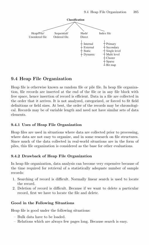
9.4 Heap File Organization 385
Classification
Heap/Pile/Unordered file
Sequential/Ordered file.
Hash/Direct
Index file
Internal PrimaryExternal SecondaryStatic Single levelDynamic Multi level
ClusterSparseBit map
9.4 Heap File Organization
Heap file is otherwise known as random file or pile file. In heap file organiza-tion, file records are inserted at the end of the file or in any file block withfree space, hence insertion of record is efficient. Data in a file are collected inthe order that it arrives. It is not analyzed, categorized, or forced to fit fielddefinitions or field sizes. At best, the order of the records may be chronologi-cal. Records may be of variable length and need not have similar sets of dataelements.
9.4.1 Uses of Heap File Organization
Heap files are used in situations where data are collected prior to processing,where data are not easy to organize, and in some research on file structures.Since much of the data collected in real-world situations are in the form ofpiles, this file organization is considered as the base for other evaluations.
9.4.2 Drawback of Heap File Organization
In heap file organization, data analysis can become very expensive because ofthe time required for retrieval of a statistically adequate number of samplerecords:
1. Searching of record is difficult. Normally linear search is used to locatethe record.
2. Deletion of record is difficult. Because if we want to delete a particularrecord, first we have to locate the file and delete.
Good in the Following Situations
Heap file is good under the following situations:
– Bulk data have to be loaded.– Relations which are always few pages long. Because search is easy.
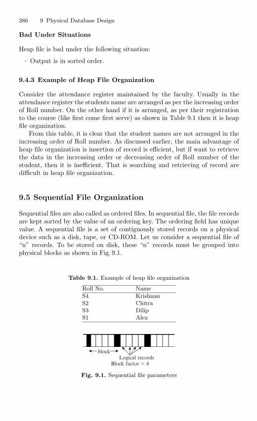
386 9 Physical Database Design
Bad Under Situations
Heap file is bad under the following situation:
– Output is in sorted order.
9.4.3 Example of Heap File Organization
Consider the attendance register maintained by the faculty. Usually in theattendance register the students name are arranged as per the increasing orderof Roll number. On the other hand if it is arranged, as per their registrationto the course (like first come first serve) as shown in Table 9.1 then it is heapfile organization.
From this table, it is clear that the student names are not arranged in theincreasing order of Roll number. As discussed earlier, the main advantage ofheap file organization is insertion of record is efficient, but if want to retrievethe data in the increasing order or decreasing order of Roll number of thestudent, then it is inefficient. That is searching and retrieving of record aredifficult in heap file organization.
9.5 Sequential File Organization
Sequential files are also called as ordered files. In sequential file, the file recordsare kept sorted by the value of an ordering key. The ordering field has uniquevalue. A sequential file is a set of contiguously stored records on a physicaldevice such as a disk, tape, or CD-ROM. Let us consider a sequential file of“n” records. To be stored on disk, these “n” records must be grouped intophysical blocks as shown in Fig. 9.1.
Table 9.1. Example of heap file organization
Roll No. Name
S4 KrishnanS2 ChitraS3 DilipS1 Alex
blockLogical records
Block factor = 4
Fig. 9.1. Sequential file parameters
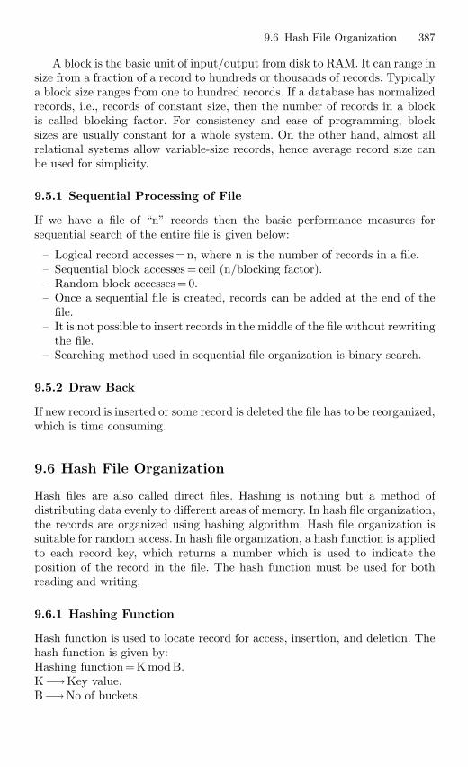
9.6 Hash File Organization 387
A block is the basic unit of input/output from disk to RAM. It can range insize from a fraction of a record to hundreds or thousands of records. Typicallya block size ranges from one to hundred records. If a database has normalizedrecords, i.e., records of constant size, then the number of records in a blockis called blocking factor. For consistency and ease of programming, blocksizes are usually constant for a whole system. On the other hand, almost allrelational systems allow variable-size records, hence average record size canbe used for simplicity.
9.5.1 Sequential Processing of File
If we have a file of “n” records then the basic performance measures forsequential search of the entire file is given below:
– Logical record accesses =n, where n is the number of records in a file.– Sequential block accesses = ceil (n/blocking factor).– Random block accesses = 0.– Once a sequential file is created, records can be added at the end of the
file.– It is not possible to insert records in the middle of the file without rewriting
the file.– Searching method used in sequential file organization is binary search.
9.5.2 Draw Back
If new record is inserted or some record is deleted the file has to be reorganized,which is time consuming.
9.6 Hash File Organization
Hash files are also called direct files. Hashing is nothing but a method ofdistributing data evenly to different areas of memory. In hash file organization,the records are organized using hashing algorithm. Hash file organization issuitable for random access. In hash file organization, a hash function is appliedto each record key, which returns a number which is used to indicate theposition of the record in the file. The hash function must be used for bothreading and writing.
9.6.1 Hashing Function
Hash function is used to locate record for access, insertion, and deletion. Thehash function is given by:Hashing function = Kmod B.K−→Key value.B−→No of buckets.
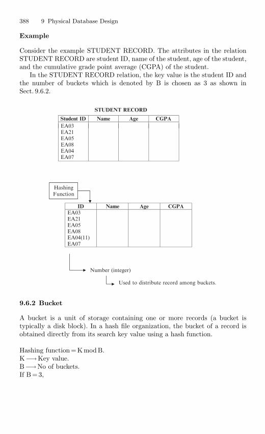
388 9 Physical Database Design
Example
Consider the example STUDENT RECORD. The attributes in the relationSTUDENT RECORD are student ID, name of the student, age of the student,and the cumulative grade point average (CGPA) of the student.
In the STUDENT RECORD relation, the key value is the student ID andthe number of buckets which is denoted by B is chosen as 3 as shown inSect. 9.6.2.
STUDENT RECORD
Number (integer)
Used to distribute record among buckets.
Student ID Name Age CGPAEA03EA21EA05EA08EA04EA07
ID Name Age CGPAEA03EA21EA05EA08EA04(11)EA07
HashingFunction
9.6.2 Bucket
A bucket is a unit of storage containing one or more records (a bucket istypically a disk block). In a hash file organization, the bucket of a record isobtained directly from its search key value using a hash function.
Hashing function = Kmod B.K−→Key value.B−→No of buckets.If B =3,
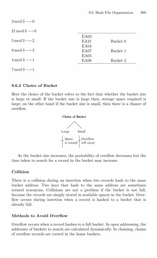
9.6 Hash File Organization 389
3 mod 3−→ 0
21 mod 3−→ 0EA03EA21 Bucket 0EA04EA07 Bucket 1EA05EA08 Bucket 2
5 mod 3−→ 2
8 mod 3−→ 2
4 mod 3−→ 1
7 mod 3−→ 1
9.6.3 Choice of Bucket
Here the choice of the bucket refers to the fact that whether the bucket sizeis large or small. If the bucket size is large then, storage space required islarge; on the other hand if the bucket size is small, then there is a chance ofoverflow.
Choice of Bucket
Large Small
Spaceis wasted
Overflowwill occur
As the bucket size increases, the probability of overflow decreases but thetime taken to search for a record in the bucket may increase.
Collision
There is a collision during an insertion when two records hash to the samebucket address. Two keys that hash to the same address are sometimestermed synonyms. Collisions are not a problem if the bucket is not full,because the records are simply stored in available spaces in the bucket. Over-flow occurs during insertion when a record is hashed to a bucket that isalready full.
Methods to Avoid Overflow
Overflow occurs when a record hashes to a full bucket. In open addressing, theaddresses of buckets to search are calculated dynamically. In chaining, chainsof overflow records are rooted in the home buckets.
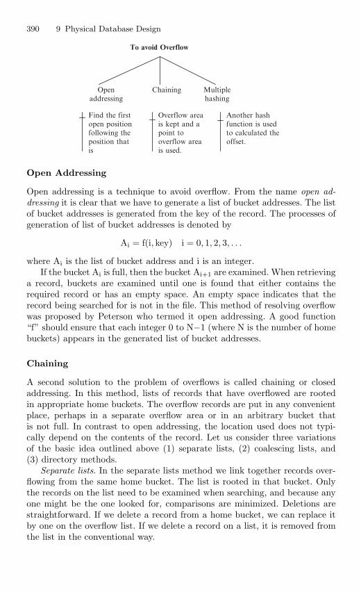
390 9 Physical Database Design
To avoid Overflow
Openaddressing
Chaining Multiplehashing
Find the firstopen positionfollowing theposition thatis
Overflow areais kept and apoint tooverflow areais used.
Another hashfunction is usedto calculated theoffset.
Open Addressing
Open addressing is a technique to avoid overflow. From the name open ad-dressing it is clear that we have to generate a list of bucket addresses. The listof bucket addresses is generated from the key of the record. The processes ofgeneration of list of bucket addresses is denoted by
Ai = f(i, key) i = 0, 1, 2, 3, . . .
where Ai is the list of bucket address and i is an integer.If the bucket Ai is full, then the bucket Ai+1 are examined. When retrieving
a record, buckets are examined until one is found that either contains therequired record or has an empty space. An empty space indicates that therecord being searched for is not in the file. This method of resolving overflowwas proposed by Peterson who termed it open addressing. A good function“f” should ensure that each integer 0 to N−1 (where N is the number of homebuckets) appears in the generated list of bucket addresses.
Chaining
A second solution to the problem of overflows is called chaining or closedaddressing. In this method, lists of records that have overflowed are rootedin appropriate home buckets. The overflow records are put in any convenientplace, perhaps in a separate overflow area or in an arbitrary bucket thatis not full. In contrast to open addressing, the location used does not typi-cally depend on the contents of the record. Let us consider three variationsof the basic idea outlined above (1) separate lists, (2) coalescing lists, and(3) directory methods.
Separate lists. In the separate lists method we link together records over-flowing from the same home bucket. The list is rooted in that bucket. Onlythe records on the list need to be examined when searching, and because anyone might be the one looked for, comparisons are minimized. Deletions arestraightforward. If we delete a record from a home bucket, we can replace itby one on the overflow list. If we delete a record on a list, it is removed fromthe list in the conventional way.
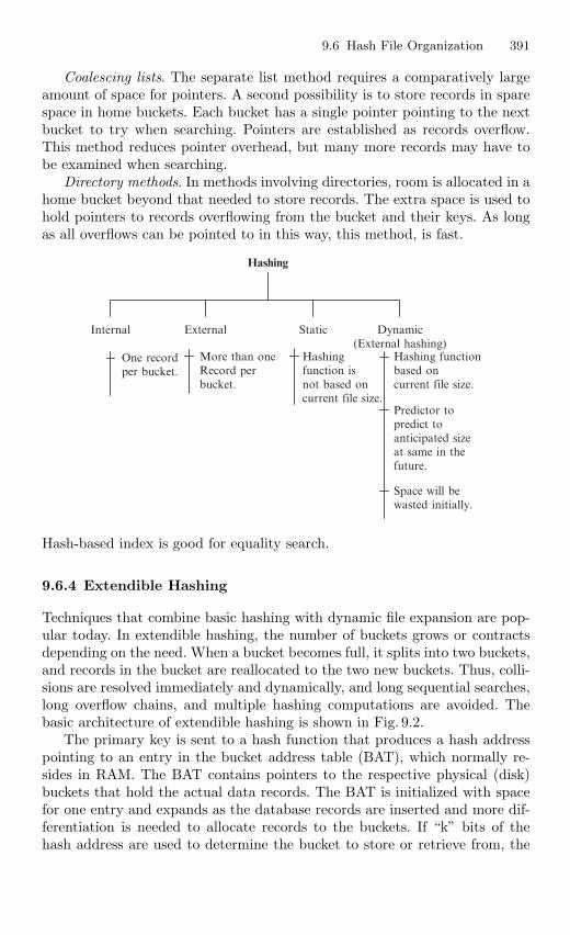
9.6 Hash File Organization 391
Coalescing lists. The separate list method requires a comparatively largeamount of space for pointers. A second possibility is to store records in sparespace in home buckets. Each bucket has a single pointer pointing to the nextbucket to try when searching. Pointers are established as records overflow.This method reduces pointer overhead, but many more records may have tobe examined when searching.
Directory methods. In methods involving directories, room is allocated in ahome bucket beyond that needed to store records. The extra space is used tohold pointers to records overflowing from the bucket and their keys. As longas all overflows can be pointed to in this way, this method, is fast.
Hashing
Internal External Static Dynamic(External hashing)
One recordper bucket.
More than oneRecord perbucket.
Hashingfunction isnot based oncurrent file size.
Hashing functionbased oncurrent file size.
Predictor topredict toanticipated sizeat same in thefuture.
Space will bewasted initially.
Hash-based index is good for equality search.
9.6.4 Extendible Hashing
Techniques that combine basic hashing with dynamic file expansion are pop-ular today. In extendible hashing, the number of buckets grows or contractsdepending on the need. When a bucket becomes full, it splits into two buckets,and records in the bucket are reallocated to the two new buckets. Thus, colli-sions are resolved immediately and dynamically, and long sequential searches,long overflow chains, and multiple hashing computations are avoided. Thebasic architecture of extendible hashing is shown in Fig. 9.2.
The primary key is sent to a hash function that produces a hash addresspointing to an entry in the bucket address table (BAT), which normally re-sides in RAM. The BAT contains pointers to the respective physical (disk)buckets that hold the actual data records. The BAT is initialized with spacefor one entry and expands as the database records are inserted and more dif-ferentiation is needed to allocate records to the buckets. If “k” bits of thehash address are used to determine the bucket to store or retrieve from, the
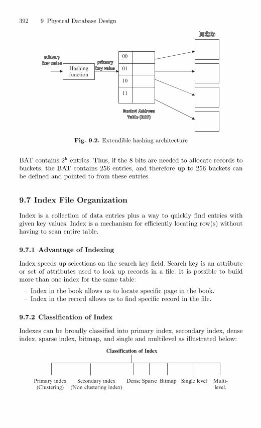
392 9 Physical Database Design
Hashingfunction
00
01
10
11
Fig. 9.2. Extendible hashing architecture
BAT contains 2k entries. Thus, if the 8-bits are needed to allocate records tobuckets, the BAT contains 256 entries, and therefore up to 256 buckets canbe defined and pointed to from these entries.
9.7 Index File Organization
Index is a collection of data entries plus a way to quickly find entries withgiven key values. Index is a mechanism for efficiently locating row(s) withouthaving to scan entire table.
9.7.1 Advantage of Indexing
Index speeds up selections on the search key field. Search key is an attributeor set of attributes used to look up records in a file. It is possible to buildmore than one index for the same table:
– Index in the book allows us to locate specific page in the book.– Index in the record allows us to find specific record in the file.
9.7.2 Classification of Index
Indexes can be broadly classified into primary index, secondary index, denseindex, sparse index, bitmap, and single and multilevel as illustrated below:
Classification of Index
Primary index(Clustering)
Secondary index(Non clustering index)
Dense Sparse Bitmap Single level Multi-level.
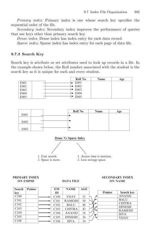
9.7 Index File Organization 393
Primary index. Primary index is one whose search key specifies thesequential order of the file.
Secondary index. Secondary index improves the performance of queriesthat use keys other than primary search key.
Dense index. Dense index has index entry for each data record.Sparse index. Sparse index has index entry for each page of data file.
9.7.3 Search Key
Search key is attribute or set attributes used to look up records in a file. Inthe example shown below, the Roll number associated with the student is thesearch key as it is unique for each and every student.
E001E002E003E004E005
E001
E002
E003
Roll No Name AgeE001E002E003E004E005
Roll No Name Age
Dense Vs Sparse Index
1. Fast search. 1. Access time is increase. 2. Space is more. 2. Less storage space.
PRIMARY INDEXON EMPID
SECONDARY INDEXON NAMEDATA FILE
Searchkey
Pointer
C100C101C102C103C104C105C106
EMID
NAME AGE
C100 VIJAY 52C101 RAMESH 50C102 BALU 48C103 CHITRA 43C104 ANAND 38C105 DINESH 36C106 SIVA 34
Pointer Search keyANANDBALUCHITRADINESHRAMESHSIVAVIJAY
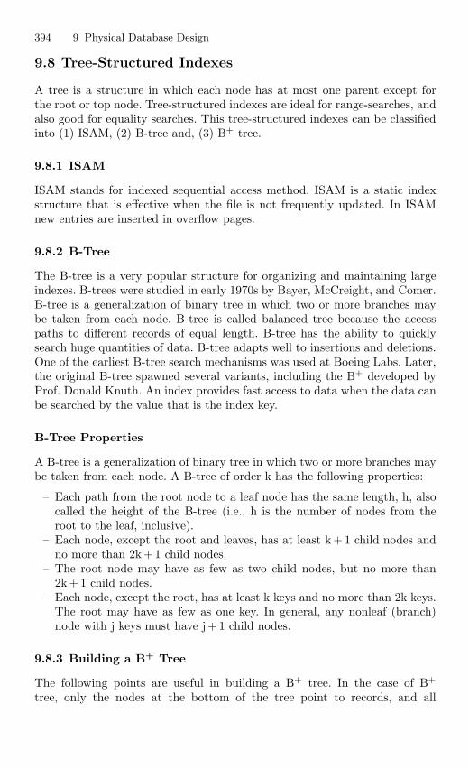
394 9 Physical Database Design
9.8 Tree-Structured Indexes
A tree is a structure in which each node has at most one parent except forthe root or top node. Tree-structured indexes are ideal for range-searches, andalso good for equality searches. This tree-structured indexes can be classifiedinto (1) ISAM, (2) B-tree and, (3) B+ tree.
9.8.1 ISAM
ISAM stands for indexed sequential access method. ISAM is a static indexstructure that is effective when the file is not frequently updated. In ISAMnew entries are inserted in overflow pages.
9.8.2 B-Tree
The B-tree is a very popular structure for organizing and maintaining largeindexes. B-trees were studied in early 1970s by Bayer, McCreight, and Comer.B-tree is a generalization of binary tree in which two or more branches maybe taken from each node. B-tree is called balanced tree because the accesspaths to different records of equal length. B-tree has the ability to quicklysearch huge quantities of data. B-tree adapts well to insertions and deletions.One of the earliest B-tree search mechanisms was used at Boeing Labs. Later,the original B-tree spawned several variants, including the B+ developed byProf. Donald Knuth. An index provides fast access to data when the data canbe searched by the value that is the index key.
B-Tree Properties
A B-tree is a generalization of binary tree in which two or more branches maybe taken from each node. A B-tree of order k has the following properties:
– Each path from the root node to a leaf node has the same length, h, alsocalled the height of the B-tree (i.e., h is the number of nodes from theroot to the leaf, inclusive).
– Each node, except the root and leaves, has at least k+ 1 child nodes andno more than 2k+ 1 child nodes.
– The root node may have as few as two child nodes, but no more than2k+ 1 child nodes.
– Each node, except the root, has at least k keys and no more than 2k keys.The root may have as few as one key. In general, any nonleaf (branch)node with j keys must have j+ 1 child nodes.
9.8.3 Building a B+ Tree
The following points are useful in building a B+ tree. In the case of B+
tree, only the nodes at the bottom of the tree point to records, and all
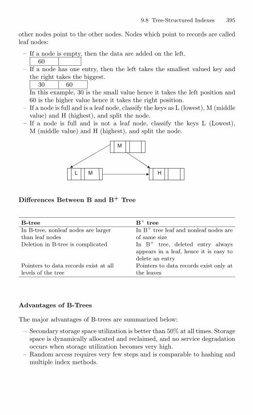
9.8 Tree-Structured Indexes 395
other nodes point to the other nodes. Nodes which point to records are calledleaf nodes:
– If a node is empty, then the data are added on the left.60
∣∣
– If a node has one entry, then the left takes the smallest valued key andthe right takes the biggest.
30∣∣ 60
In this example, 30 is the small value hence it takes the left position and60 is the higher value hence it takes the right position.
– If a node is full and is a leaf node, classify the keys as L (lowest), M (middlevalue) and H (highest), and split the node.
– If a node is full and is not a leaf node, classify the keys L (Lowest),M (middle value) and H (highest), and split the node.
M
L M H
Differences Between B and B+ Tree
B-tree B+ tree
In B-tree, nonleaf nodes are largerthan leaf nodes
In B+ tree leaf and nonleaf nodes areof same size
Deletion in B-tree is complicated In B+ tree, deleted entry alwaysappears in a leaf, hence it is easy todelete an entry
Pointers to data records exist at alllevels of the tree
Pointers to data records exist only atthe leaves
Advantages of B-Trees
The major advantages of B-trees are summarized below:
– Secondary storage space utilization is better than 50% at all times. Storagespace is dynamically allocated and reclaimed, and no service degradationoccurs when storage utilization becomes very high.
– Random access requires very few steps and is comparable to hashing andmultiple index methods.
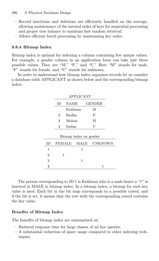
396 9 Physical Database Design
– Record insertions and deletions are efficiently handled on the average,allowing maintenance of the natural order of keys for sequential processingand proper tree balance to maintain fast random retrieval.
– Allows efficient batch processing by maintaining key order.
9.8.4 Bitmap Index
Bitmap index is optimal for indexing a column containing few unique values.For example, a gender column in an application form can take just threepossible values. They are “M,” “F,” and “U.” Here “M” stands for male,“F” stands for female, and “U” stands for unknown.
In order to understand how bitmap index organizes records let us considera database table APPLICANT as shown below and the corresponding bitmapindex:
APPLICANT
ID NAME GENDER
Krishnan M
2 Radha F
3 Mohan M
4 Sudan U
Bitmap index on gender
ID FEMALE MALE UNKNOWN
1 1
2 1
3 1
4 1
The person corresponding to ID 1 is Krishnan who is a male hence a “1” isinserted in MALE in bitmap index. In a bitmap index, a bitmap for each keyvalue is used. Each bit in the bit map corresponds to a possible rowed, andif the bit is set, it means that the row with the corresponding rowed containsthe key value.
Benefits of Bitmap Index
The benefits of bitmap index are summarized as:
– Reduced response time for large classes of ad hoc queries.– A substantial reduction of space usage compared to other indexing tech-
niques.
9.9 Data Storage Devices 397
Fully indexing a large table with a normal index can be expensive in terms ofspace since the index can be several times larger than the data in the table.Bitmap indexes are typically only a fraction of the size of the indexed data inthe table.
9.9 Data Storage Devices
The data stored by an organization double in every 3 or 4 years. Hence theselection of data storage devices is a key consideration for data managers.
9.9.1 Factors to be Considered in Selecting Data Storage Devices
The following factors have to be considered while evaluating data storageoptions:
– Online storage– Backup files– Archival storage
When the device is used to store online data, then one has to give importanceto access speed and capacity, because many firms require rapid response tolarge volumes of data.
Backup files are required to provide security against data loss. Ideally,backup storage is a high volume capacity at low cost.
Archived data may need to be stored for many years; so archival mediumshould be highly reliable, with no data decay over extended periods, and lowcost.
The following factors have to be considered in storing the data in a par-ticular medium:
– Volume of data– Volatility of data– Required speed of access to data– Cost of data storage– Reliability of data storage medium
9.9.2 Magnetic Technology
Magnetic technology is based on magnetization and demagnetization of spotson a magnetic recording surface. The same spot can be magnetized anddemagnetized repeatedly. Magnetic recording materials may be coated on rigidplotters (hard disks), flexible circular substrates (floppy disks), thin ribbonsof material (magnetic tapes), or rectangular sheets (magnetic cards).
The main advantages of magnetic technology are its relative maturity andwidespread use. A major disadvantage is susceptibility to strong magnetic
398 9 Physical Database Design
fields that can corrupt data stored on a disk. Also magnetization decays withtime. Hence it is not a preferable medium to store legal documents, archivaldata.
9.9.3 Fixed Magnetic Disk
A fixed magnetic disk contains one or more recording surfaces that are per-manently mounted in the disk drive and cannot be removed. Fixed disk is themedium of choice from personal computers to super computers. Fixed disksgives rapid, direct access to large volumes of data, and is ideal for highlyvolatile files. The major disadvantage of magnetic disk is the possibility ofhead crash that destroys the disk surface and data hence it is necessary toregularly make backup copies of hard disk files.
9.9.4 Removable Magnetic Disk
A removable disk comes in two formats: single disk and disk pack. Disk packsconsist of multiple disks mounted together on a common spindle in a stack,usually on a disk drive with a retractable read/write heads. The disk’s remov-ability is its primary advantage making it ideal for backup.
9.9.5 Floppy Disk
Floppy low cost makes them ideal for storing and transporting small files andprograms. But the reliability is not so good. A speck of dust can cause readerror.
9.9.6 Magnetic Tape
In magnetic tape, the data storage and retrieval are in sequential manner.Hence the access time, which refers to data access, is high. Magnetic tape wasused extensively for archiving and backup in early database systems.
9.10 Redundant Array of Inexpensive Disk
RAID stands for Redundant Array of Inexpensive (Independent) Disk. A diskarray comprises of several disks managed by a controller. Disks and controllerscan be joined together in RAID combinations. First, they can provide faulttolerance by introducing redundancy across multiple disks. Second, they canprovide increased throughput because disk array controller supports parallelaccess to multiple disks. Instead of using one massive drive, RAID technologystores several smaller drives in one container.
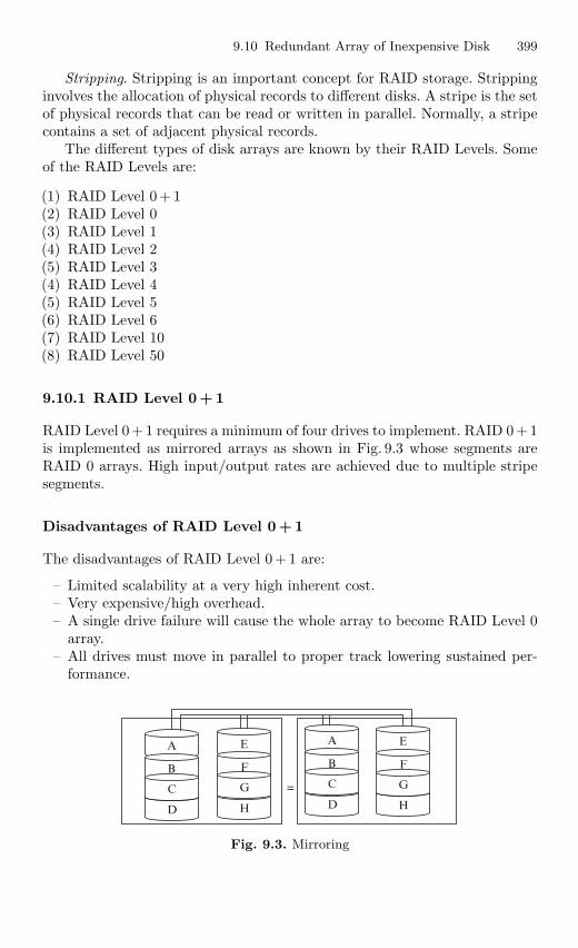
9.10 Redundant Array of Inexpensive Disk 399
Stripping. Stripping is an important concept for RAID storage. Strippinginvolves the allocation of physical records to different disks. A stripe is the setof physical records that can be read or written in parallel. Normally, a stripecontains a set of adjacent physical records.
The different types of disk arrays are known by their RAID Levels. Someof the RAID Levels are:
(1) RAID Level 0 + 1(2) RAID Level 0(3) RAID Level 1(4) RAID Level 2(5) RAID Level 3(4) RAID Level 4(5) RAID Level 5(6) RAID Level 6(7) RAID Level 10(8) RAID Level 50
9.10.1 RAID Level 0 + 1
RAID Level 0+ 1 requires a minimum of four drives to implement. RAID 0+ 1is implemented as mirrored arrays as shown in Fig. 9.3 whose segments areRAID 0 arrays. High input/output rates are achieved due to multiple stripesegments.
Disadvantages of RAID Level 0+1
The disadvantages of RAID Level 0+ 1 are:
– Limited scalability at a very high inherent cost.– Very expensive/high overhead.– A single drive failure will cause the whole array to become RAID Level 0
array.– All drives must move in parallel to proper track lowering sustained per-
formance.
D H D H
A
B
C
E
F
G
A
B
C
E
F
G=
Fig. 9.3. Mirroring
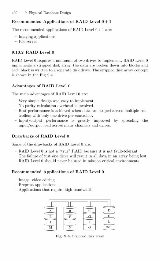
400 9 Physical Database Design
Recommended Applications of RAID Level 0 +1
The recommended applications of RAID Level 0+ 1 are:
– Imaging applications– File server
9.10.2 RAID Level 0
RAID Level 0 requires a minimum of two drives to implement. RAID Level 0implements a stripped disk array, the data are broken down into blocks andeach block is written to a separate disk drive. The stripped disk array conceptis shown in the Fig. 9.4.
Advantages of RAID Level 0
The main advantages of RAID Level 0 are:
– Very simple design and easy to implement.– No parity calculation overhead is involved.– Best performance is achieved when data are striped across multiple con-
trollers with only one drive per controller.– Input/output performance is greatly improved by spreading the
input/output load across many channels and drives.
Drawbacks of RAID Level 0
Some of the drawbacks of RAID Level 0 are:
– RAID Level 0 is not a “true” RAID because it is not fault-tolerant.– The failure of just one drive will result in all data in an array being lost.– RAID Level 0 should never be used in mission critical environments.
Recommended Applications of RAID Level 0
– Image, video editing– Prepress applications– Applications that require high bandwidth
M
A
E
I
N
B
F
J
O
C
G
K
etc...
D
H
L
Fig. 9.4. Stripped disk array
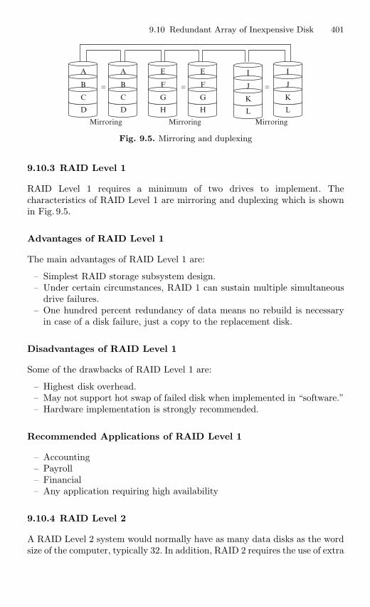
9.10 Redundant Array of Inexpensive Disk 401
= = =
Mirroring Mirroring Mirroring
D
A
B
C
D
A
B
C
H
E
F
G
H
E
F
G
L
I
J
K
L
I
J
K
Fig. 9.5. Mirroring and duplexing
9.10.3 RAID Level 1
RAID Level 1 requires a minimum of two drives to implement. Thecharacteristics of RAID Level 1 are mirroring and duplexing which is shownin Fig. 9.5.
Advantages of RAID Level 1
The main advantages of RAID Level 1 are:
– Simplest RAID storage subsystem design.– Under certain circumstances, RAID 1 can sustain multiple simultaneous
drive failures.– One hundred percent redundancy of data means no rebuild is necessary
in case of a disk failure, just a copy to the replacement disk.
Disadvantages of RAID Level 1
Some of the drawbacks of RAID Level 1 are:
– Highest disk overhead.– May not support hot swap of failed disk when implemented in “software.”– Hardware implementation is strongly recommended.
Recommended Applications of RAID Level 1
– Accounting– Payroll– Financial– Any application requiring high availability
9.10.4 RAID Level 2
A RAID Level 2 system would normally have as many data disks as the wordsize of the computer, typically 32. In addition, RAID 2 requires the use of extra
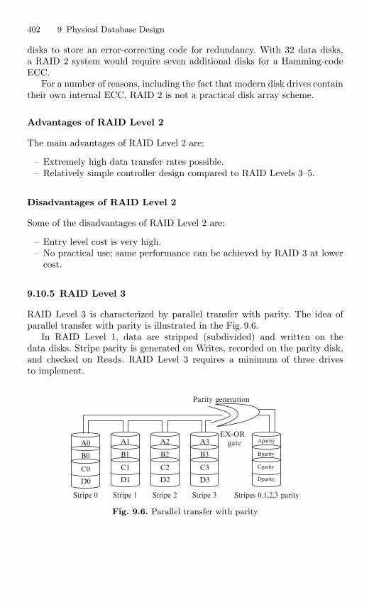
402 9 Physical Database Design
disks to store an error-correcting code for redundancy. With 32 data disks,a RAID 2 system would require seven additional disks for a Hamming-codeECC.
For a number of reasons, including the fact that modern disk drives containtheir own internal ECC, RAID 2 is not a practical disk array scheme.
Advantages of RAID Level 2
The main advantages of RAID Level 2 are:
– Extremely high data transfer rates possible.– Relatively simple controller design compared to RAID Levels 3–5.
Disadvantages of RAID Level 2
Some of the disadvantages of RAID Level 2 are:
– Entry level cost is very high.– No practical use; same performance can be achieved by RAID 3 at lower
cost.
9.10.5 RAID Level 3
RAID Level 3 is characterized by parallel transfer with parity. The idea ofparallel transfer with parity is illustrated in the Fig. 9.6.
In RAID Level 1, data are stripped (subdivided) and written on thedata disks. Stripe parity is generated on Writes, recorded on the parity disk,and checked on Reads. RAID Level 3 requires a minimum of three drivesto implement.
Parity generation
EX-ORgate
Stripe 0 Stripe 1 Stripe 2 Stripe 3 Stripes 0,1,2,3 parity
D0
A0
B0
C0D1
A1
B1
C1
D2
A2
B2
C2
D3
A3
B3
C3Dparity
Aparityyyy
Bparity
Cparity
Fig. 9.6. Parallel transfer with parity
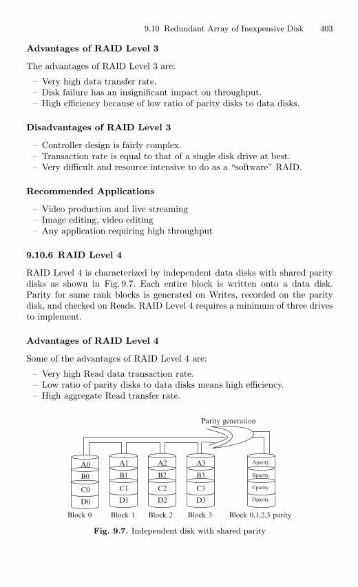
9.10 Redundant Array of Inexpensive Disk 403
Advantages of RAID Level 3
The advantages of RAID Level 3 are:
– Very high data transfer rate.– Disk failure has an insignificant impact on throughput.– High efficiency because of low ratio of parity disks to data disks.
Disadvantages of RAID Level 3
– Controller design is fairly complex.– Transaction rate is equal to that of a single disk drive at best.– Very difficult and resource intensive to do as a “software” RAID.
Recommended Applications
– Video production and live streaming– Image editing, video editing– Any application requiring high throughput
9.10.6 RAID Level 4
RAID Level 4 is characterized by independent data disks with shared paritydisks as shown in Fig. 9.7. Each entire block is written onto a data disk.Parity for same rank blocks is generated on Writes, recorded on the paritydisk, and checked on Reads. RAID Level 4 requires a minimum of three drivesto implement.
Advantages of RAID Level 4
Some of the advantages of RAID Level 4 are:
– Very high Read data transaction rate.– Low ratio of parity disks to data disks means high efficiency.– High aggregate Read transfer rate.
Parity generation
Block 0 Block 1 Block 2 Block 3 Block 0,1,2,3 parity
D0
A0
B0
C0
D1
A1
B1
C1
D2
A2
B2
C2
D3
A3
B3
C3Dparity
Aparityyyy
Bparity
Cparity
Fig. 9.7. Independent disk with shared parity
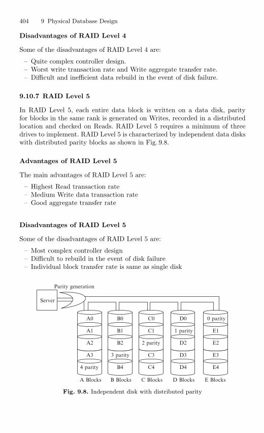
404 9 Physical Database Design
Disadvantages of RAID Level 4
Some of the disadvantages of RAID Level 4 are:
– Quite complex controller design.– Worst write transaction rate and Write aggregate transfer rate.– Difficult and inefficient data rebuild in the event of disk failure.
9.10.7 RAID Level 5
In RAID Level 5, each entire data block is written on a data disk, parityfor blocks in the same rank is generated on Writes, recorded in a distributedlocation and checked on Reads. RAID Level 5 requires a minimum of threedrives to implement. RAID Level 5 is characterized by independent data diskswith distributed parity blocks as shown in Fig. 9.8.
Advantages of RAID Level 5
The main advantages of RAID Level 5 are:
– Highest Read transaction rate– Medium Write data transaction rate– Good aggregate transfer rate
Disadvantages of RAID Level 5
Some of the disadvantages of RAID Level 5 are:
– Most complex controller design– Difficult to rebuild in the event of disk failure– Individual block transfer rate is same as single disk
3 parity
B0
B1
B2
B4
C3
C0
C1
2 parity
C4
D3
D0
1 parity
D2
D4
E3
0 parity
E1
E2
E4
A3
A0
A1
A2
4 parity
Server
Parity generation
A Blocks B Blocks C Blocks D Blocks E Blocks
Fig. 9.8. Independent disk with distributed parity
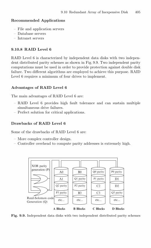
9.10 Redundant Array of Inexpensive Disk 405
Recommended Applications
– File and application servers– Database servers– Intranet servers
9.10.8 RAID Level 6
RAID Level 6 is characterized by independent data disks with two indepen-dent distributed parity schemes as shown in Fig. 9.9. Two independent paritycomputations must be used in order to provide protection against double diskfailure. Two different algorithms are employed to achieve this purpose. RAIDLevel 6 requires a minimum of four drives to implement.
Advantages of RAID Level 6
The main advantages of RAID Level 6 are:
– RAID Level 6 provides high fault tolerance and can sustain multiplesimultaneous drive failures.
– Perfect solution for critical applications.
Drawbacks of RAID Level 6
Some of the drawbacks of RAID Level 6 are:
– More complex controller design.– Controller overhead to compute parity addresses is extremely high.
P3 parity
A0
A1
Q2 parity
etc...
B3
B0
Q1 parity
P2 parity
etc...
C3
Q0 parity
P1 parity
C2
etc...
Q3 parity
P0 parity
D1
D2
etc...
XOR paritygeneration (P)
Reed-Solomon codeGeneration (Q)
A Blocks B Blocks C Blocks D Blocks
Fig. 9.9. Independent data disks with two independent distributed parity schemes
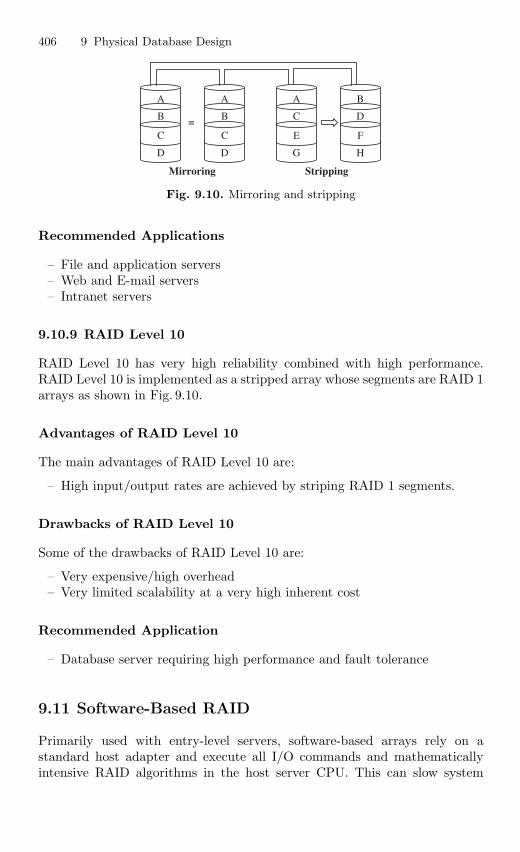
406 9 Physical Database Design
=
Mirroring Stripping
D
A
B
C
D
A
B
C
G
A
C
E
H
B
D
F
Fig. 9.10. Mirroring and stripping
Recommended Applications
– File and application servers– Web and E-mail servers– Intranet servers
9.10.9 RAID Level 10
RAID Level 10 has very high reliability combined with high performance.RAID Level 10 is implemented as a stripped array whose segments are RAID 1arrays as shown in Fig. 9.10.
Advantages of RAID Level 10
The main advantages of RAID Level 10 are:
– High input/output rates are achieved by striping RAID 1 segments.
Drawbacks of RAID Level 10
Some of the drawbacks of RAID Level 10 are:
– Very expensive/high overhead– Very limited scalability at a very high inherent cost
Recommended Application
– Database server requiring high performance and fault tolerance
9.11 Software-Based RAID
Primarily used with entry-level servers, software-based arrays rely on astandard host adapter and execute all I/O commands and mathematicallyintensive RAID algorithms in the host server CPU. This can slow system
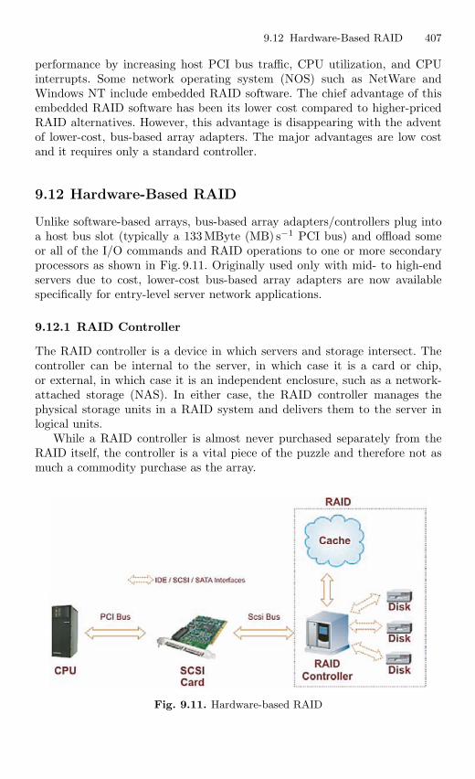
9.12 Hardware-Based RAID 407
performance by increasing host PCI bus traffic, CPU utilization, and CPUinterrupts. Some network operating system (NOS) such as NetWare andWindows NT include embedded RAID software. The chief advantage of thisembedded RAID software has been its lower cost compared to higher-pricedRAID alternatives. However, this advantage is disappearing with the adventof lower-cost, bus-based array adapters. The major advantages are low costand it requires only a standard controller.
9.12 Hardware-Based RAID
Unlike software-based arrays, bus-based array adapters/controllers plug intoa host bus slot (typically a 133 MByte (MB) s−1 PCI bus) and offload someor all of the I/O commands and RAID operations to one or more secondaryprocessors as shown in Fig. 9.11. Originally used only with mid- to high-endservers due to cost, lower-cost bus-based array adapters are now availablespecifically for entry-level server network applications.
9.12.1 RAID Controller
The RAID controller is a device in which servers and storage intersect. Thecontroller can be internal to the server, in which case it is a card or chip,or external, in which case it is an independent enclosure, such as a network-attached storage (NAS). In either case, the RAID controller manages thephysical storage units in a RAID system and delivers them to the server inlogical units.
While a RAID controller is almost never purchased separately from theRAID itself, the controller is a vital piece of the puzzle and therefore not asmuch a commodity purchase as the array.
Fig. 9.11. Hardware-based RAID
408 9 Physical Database Design
In addition to offering the fault-tolerant benefits of RAID, bus-based arrayadapters/controllers perform connectivity functions that are similar to stan-dard host adapters. By residing directly on a host PCI bus, they provide thehighest performance of all array types. Bus-based arrays also deliver morerobust fault-tolerant features than embedded NOS RAID software.
9.12.2 Types of Hardware RAID
There are two main types of hardware RAID, differing primarily in how theyinterface the array to the system.
Bus-Based or Controller Card Hardware RAID
This is the more conventional type of hardware RAID, and the type most com-monly used, particularly for lower-end systems. A specialized RAID controlleris installed into the PC or server, and the array drives are connected to it. Itessentially takes the place of the small computer system interface (SCSI) hostadapter or integrated development environment (IDE) controller that wouldnormally be used for interfacing between the system and the hard disks; itinterfaces to the drives using SCSI or IDE/ATA, and sends data to the rest ofthe PC over the system bus. Some motherboards, particularly those intendedfor server systems, come with some variant of integrated RAID controller.These are built into the motherboard, but function is precisely the same man-ner as an add-in bus-based card. (This is analogous to the way that the inte-grated IDE/ATA controllers on all modern motherboards function the sameway that add-in IDE/ATA controllers once did on older systems.) The onlydifference is that integrated controllers can reduce overall cost at the price offlexibility.
Intelligent, External RAID Controller
In this higher-end design, the RAID controller is removed completely from thesystem to a separate box. Within the box the RAID controller manages thedrives in the array, typically using SCSI, and then presents the logical drivesof the array over a standard interface (again, typically a variant of SCSI) tothe server using the array. The server sees the array or arrays as just one ormore very fast hard disks; the RAID is completely hidden from the machine.In essence, one of these units really is an entire computer unto itself, witha dedicated processor that manages the RAID array and acts as a conduitbetween the server and the array.
Advantages are data protection and performance benefits of RAID andmore robust fault-tolerant features and increased performance vs. software-based RAID.
9.13 Optical Technology 409
9.13 Optical Technology
Optical storage systems work by reflecting beams of laser light off a rotatingdisk with a minutely pitted surface. As the disk rotates, the amount of lightreflected back to a sensor varies, generating a stream of ones and zeros. Theadvantages of optical technology are high storage densities, low cost media,and direct access.
There are four storage media based on optical technology. They areCD-ROM, WORM, magneto-optical, and DVD. Optical technology is highlyreliable because it is not susceptible to head crashes.
CD-ROM. CD-ROM stands for compact disk-read only memory. CD-ROMis a compact, robust, high capacity medium for the storage of permanent data.Once the data are written, it cannot be altered.
CD-R. CD-R stands for CD-recordable. CD-R writers are used to preparedisks for CD mastering, test prototype applications, and backup systems.
CD-RW. CD-RW stands for CD-rewritable. This format allows erasing andrewriting to a disk many times.
WORM. WORM stands for write once read many. WORM is the majorstorage device for images. Information once written to a blank disk cannot bealtered. WORM jukeboxes are used to store high volumes of data. A jukeboxmay contain up to 2,000 WORM disks. A WORM jukebox makes terabytesof data available in about 10 s.
9.13.1 Advantages of Optical Disks
The main advantages of optical disk are given below:
1. Physical. An optical disk is much sturdier than tape or a floppy disk. It isphysically harder to break, melt, or warp.
2. Delicacy. It is not sensitive to being touched, though it can get too dirtyor scratched to be read. It can be cleaned.
3. Magnetic. It is entirely unaffected by magnetic fields.4. Capacity. Optical disks hold much more data than floppy disks.
9.13.2 Disadvantages of Optical Disks
Some of the disadvantages of optical disks are:Cost. The cost of the optical disk is high. But due to the advancement
in technology, the price has come down drastically. Hence cost cannot beconsidered as drawback.
Duplication. It is not easy to copy an optical disk as it is a floppy disk.Software and hardware is necessary for writing disks. This is balanced by thefact that it is not as necessary to have extra copies since the disk is so muchsturdier than other media.
410 9 Physical Database Design
Summary
The primary goal of physical database design is data processing efficiency.Today, with ever-decreasing costs of computer technology per unit of measure,it is typically important that the physical database design must minimize thetime required by users to interact with the information system. During phys-ical database design, the database designer translates the logical descriptionof data into the technical specifications for storing and retrieving data.
A physical file is a named portion of secondary memory allocated for thepurpose of storing physical records. Data within a physical file are organizedthrough a combination of sequential storage and pointers. A file organizationarranges the records of a file on a secondary storage device. The three majorcategories of file organizations are sequential file organization, index file orga-nization, and hash file organization. In sequential file organization, records arestored in a sequence to a primary key value. In index file organization, recordsare stored sequentially or nonsequentially and an index is used to keep trackof where the records are stored. In hash file organization, the address of eachrecord is determined using an algorithm that converts a primary key valueinto a record address. In this chapter the different types of file organizationare explained through illustrative examples.
File access efficiency and file reliability can be enhanced by the use ofa RAID, which allows blocks of data from one or several programs to beread and written in parallel to different disks, thus reducing the input/outputdelays with traditional sequential I/O operations on a single disk drive. Inthis chapter, the basic concept of RAID and different levels of RAID areexplained. Various levels of RAID allow a file and database designer to choosethe combination of access efficiency, space utilization, and fault tolerance bestsuited for the database applications.
Review Questions
9.1. What are the main differences between ISAM and B+ tree indexes?
The main difference between ISAM and B+ tree indexes is that ISAM is staticwhile B+ tree is dynamic. Another difference between the two indexes is thatISAM’s leaf pages are allocated in sequence.
9.2. What is the order of B+ tree?
The order of a B+ tree is denoted by which is a measure of the capacity of thetree node. Every node in the B+ tree contains “m” entries where d ≤ m ≤ 2d.
9.3. How many nodes must be examined for equality search in a B+ tree?How many for a range selection? Compare this with ISAM?
For equality search in a B+ tree, l nodes must be examined, where l =heightof the tree. For range selection, number of nodes examined = l + m− 1, where
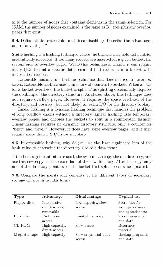
Review Questions 411
m is the number of nodes that contains elements in the range selection. ForISAM, the number of nodes examined is the same as B+ tree plus any overflowpages that exist.
9.4. Define static, extensible, and linear hashing? Describe the advantagesand disadvantages?
Static hashing is a hashing technique where the buckets that hold data entriesare statically allocated. If too many records are inserted for a given bucket, thesystem creates overflow pages. While this technique is simple, it can requiremany I/Os to find a specific data record if that record is in a bucket withmany other records.
Extensible hashing is a hashing technique that does not require overflowpages. Extensible hashing uses a directory of pointers to buckets. When a pagefor a bucket overflows, the bucket is split. This splitting occasionally requiresthe doubling of the directory structure. As stated above, this technique doesnot require overflow pages. However, it requires the space overhead of thedirectory, and possibly (but not likely) an extra I/O for the directory lookup.
Linear hashing is a dynamic hashing technique that handles the problemof long overflow chains without a directory. Linear hashing uses temporaryoverflow pages, and chooses the buckets to split in a round-robin fashion.Linear hashing requires no dynamic directory structure, only a counter for“next” and “level.” However, it does have some overflow pages, and it mayrequire more than 1–2 I/Os for a lookup.
9.5. In extensible hashing, why do you use the least significant bits of thehash value to determine the directory slot of a data item?
If the least significant bits are used, the system can copy the old directory, anduse this new copy as the second half of the new directory. After the copy, onlyone of the directory pointers for the bucket that split needs to be updated.
9.6. Compare the merits and demerits of the different types of secondarystorage devices in tabular form?
Type Advantage Disadvantage Typical use
Floppy disk Inexpensive,direct access,removable
Low capacity, slowaccess
Store files forword processorsand spreadsheets
Hard disk Fast, directaccess
Limited capacity Store programsand data
CD-ROM High capacity,direct access
Slow access Referencematerial
Magnetic tape High capacity Slow sequential dataaccess
Backup programsand data
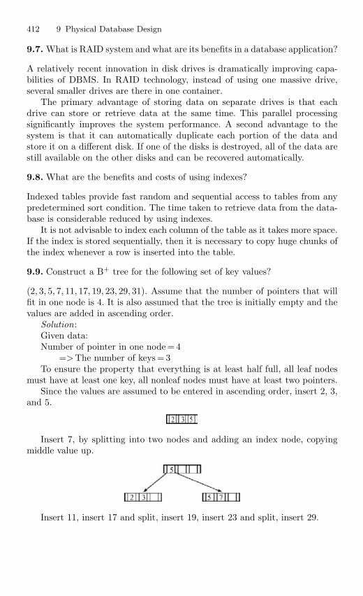
412 9 Physical Database Design
9.7. What is RAID system and what are its benefits in a database application?
A relatively recent innovation in disk drives is dramatically improving capa-bilities of DBMS. In RAID technology, instead of using one massive drive,several smaller drives are there in one container.
The primary advantage of storing data on separate drives is that eachdrive can store or retrieve data at the same time. This parallel processingsignificantly improves the system performance. A second advantage to thesystem is that it can automatically duplicate each portion of the data andstore it on a different disk. If one of the disks is destroyed, all of the data arestill available on the other disks and can be recovered automatically.
9.8. What are the benefits and costs of using indexes?
Indexed tables provide fast random and sequential access to tables from anypredetermined sort condition. The time taken to retrieve data from the data-base is considerable reduced by using indexes.
It is not advisable to index each column of the table as it takes more space.If the index is stored sequentially, then it is necessary to copy huge chunks ofthe index whenever a row is inserted into the table.
9.9. Construct a B+ tree for the following set of key values?
(2, 3, 5, 7, 11, 17, 19, 23, 29, 31). Assume that the number of pointers that willfit in one node is 4. It is also assumed that the tree is initially empty and thevalues are added in ascending order.
Solution:Given data:Number of pointer in one node =4
=> The number of keys = 3To ensure the property that everything is at least half full, all leaf nodes
must have at least one key, all nonleaf nodes must have at least two pointers.Since the values are assumed to be entered in ascending order, insert 2, 3,
and 5.
Insert 7, by splitting into two nodes and adding an index node, copyingmiddle value up.
Insert 11, insert 17 and split, insert 19, insert 23 and split, insert 29.
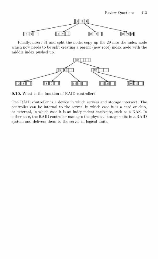
Review Questions 413
Finally, insert 31 and split the node, copy up the 29 into the index nodewhich now needs to be split creating a parent (new root) index node with themiddle index pushed up.
9.10. What is the function of RAID controller?
The RAID controller is a device in which servers and storage intersect. Thecontroller can be internal to the server, in which case it is a card or chip,or external, in which case it is an independent enclosure, such as a NAS. Ineither case, the RAID controller manages the physical storage units in a RAIDsystem and delivers them to the server in logical units.
10
Data Mining and Data Warehousing
Learning Objectives. This chapter provides an overview of advanced concepts indatabase management system, which includes concepts related to data mining anddata warehousing. This chapter deals with classification of data mining system, datamining issues, prediction, clustering, association rules, trends, and applications ofdata mining system. The data warehouse architectures, design, and user interfaceconcepts are discussed. After completing this chapter the reader should be familiarwith the following concepts:
– Need for data mining– Data mining functionalities– Classification and prediction of data mining– Performance issues in data mining– Data mining association rules– Application and trends in data mining– Goals of Data Warehousing– Characteristics of Data in Data Warehouse– Data Warehouse Architectures– Data Warehouse Design– The User Interface
10.1 Data Mining
10.1.1 Introduction
Data mining refers to extracting or “mining” knowledge from large amounts ofdata. The data mining is appropriately named as “Knowledge Mining.” Thereare many other terms carrying a similar or slightly different meaning to datamining, such as Knowledge Mining from Databases, Knowledge Extraction,Data/Pattern Analysis, Data Archaeology, and Data dredge.
Data mining is an essential process where intelligent methods are appliedin order to extract data patterns. Data mining is the process of discoveringinteresting knowledge from large amounts of data stored in databases, datawarehouses, or other information repositories.
S. Sumathi: Data Mining and Data Warehousing, Studies in Computational Intelligence
(SCI) 47, 415–475 (2007)
www.springerlink.com c© Springer-Verlag Berlin Heidelberg 2007
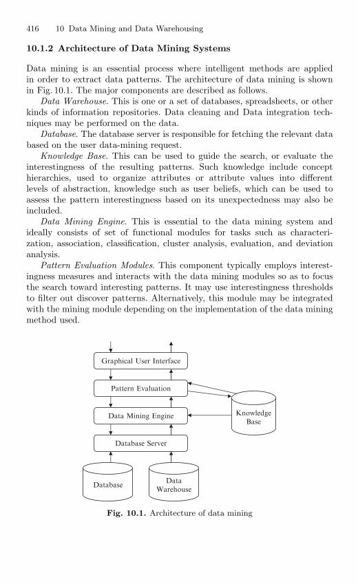
416 10 Data Mining and Data Warehousing
10.1.2 Architecture of Data Mining Systems
Data mining is an essential process where intelligent methods are appliedin order to extract data patterns. The architecture of data mining is shownin Fig. 10.1. The major components are described as follows.
Data Warehouse. This is one or a set of databases, spreadsheets, or otherkinds of information repositories. Data cleaning and Data integration tech-niques may be performed on the data.
Database. The database server is responsible for fetching the relevant databased on the user data-mining request.
Knowledge Base. This can be used to guide the search, or evaluate theinterestingness of the resulting patterns. Such knowledge include concepthierarchies, used to organize attributes or attribute values into differentlevels of abstraction, knowledge such as user beliefs, which can be used toassess the pattern interestingness based on its unexpectedness may also beincluded.
Data Mining Engine. This is essential to the data mining system andideally consists of set of functional modules for tasks such as characteri-zation, association, classification, cluster analysis, evaluation, and deviationanalysis.
Pattern Evaluation Modules. This component typically employs interest-ingness measures and interacts with the data mining modules so as to focusthe search toward interesting patterns. It may use interestingness thresholdsto filter out discover patterns. Alternatively, this module may be integratedwith the mining module depending on the implementation of the data miningmethod used.
Graphical User Interface
Pattern Evaluation
Data Mining Engine
Database Server
Database
KnowledgeBase
DataWarehouse
Fig. 10.1. Architecture of data mining
10.1 Data Mining 417
Graphical User Interface. This module communicates between the userand the data mining system, allowing the user to interact with the systemby specifying the data mining query or task, providing the information tohelp focus the search, and performing exploratory data mining based on theintermediate data mining results.
10.1.3 Data Mining Functionalities
Functionalities of data mining are used to specify the kind of patterns to befound in data mining tasks. It can be classified into two categories such asDescriptive and Predictive. Descriptive mining task characterize the generalproperties of data in the database, whereas predictive mining task performinference on the current data in order to make predictions.
These functionalities are classified as follows:
– Characterization and discrimination– Association analysis– Classification and prediction– Cluster analysis– Outlier analysis– Evolution analysis
10.1.4 Classification of Data Mining Systems
Data mining is an interdisciplinary field, the confluence of set of disciplines,including database system statistics, machine learning, visualization, andinformation science. Moreover, depending on the data mining approach used,techniques from other disciplines may be applied. Data mining research isexpected to generate a large variety of data mining systems. It can be descri-bed as follows.
Classification According to the Kinds of Database Mined
Database system themselves can be classified according to different criteriasuch as data models, each of which may require its own data mining tech-niques. If classifying according to the special types of data handled, we mayhave a spatial, time series, text, or world wide mining system.
Classification According to the Kinds of Knowledge Mined
It can be categorized according to the kinds of knowledge they mine, i.e.,based on data mining functionalities, such as characterization, discrimina-tion, association, classification, clustering, cluster outlier analysis, and evolu-tion analysis. It can be based on granularity or levels of abstraction of theknowledge mined.
418 10 Data Mining and Data Warehousing
Classification According to the Kinds of Techniques Utilized
Data mining techniques can be categorized according to the degree of userinteraction involved or methods of data analysis employed. A sophisticateddata mining system will often adopt multiple data mining techniques or workout an effective integrated technique that combines the merits of a few indivi-dual approaches.
10.1.5 Major Issues in Data Mining
Major issues in data mining are mining methodology, user interaction, per-formance, and diverse data types. These are described follows.
Mining Methodologies and User Interaction Issues
These reflect the kind of knowledge mine, the ability to mined knowledgeat multiple granularities, the user domain knowledge, and knowledge visual-ization.
Mining Different Kind of Knowledge in Database
Since different users can be interested in different kinds of knowledge, datamining should cover a wide spectrum of data analysis and knowledge discoverytask, including data characterization discrimination, association, classifica-tion, clustering, trend and deviation analysis, and similarity analysis. Thesetasks may be used in the same database in different ways and require thedevelopment of numerous data mining techniques.
Incorporation of Background Knowledge
Background knowledge or information regarding the domain under study maybe used to guide the discovery process and allows discovered patterns to beexpressed in concise terms and at different levels of abstraction.
Presentation and Visualization of Data Mining Results
Discover knowledge should be expressed in high-level languages, visual rep-resentations, or other expressive forms so that knowledge can be easilyunderstood and directly used by humans. This is especially crucial if the datamining system is to be interactive.
Handling Noisy or Incomplete Data
The data stored in database may reflect noise, exceptional cases, or incompletedata objects. When mining data regularities, these objects may confuse theprocess, causing knowledge model constructed to over fit the data. As a result,the accuracy of the discovered pattern can be poor.
10.1 Data Mining 419
10.1.6 Performance Issues
The performance issues in data mining include efficiency, scalability, and par-allelization of data mining algorithms.
Efficiency and Scalability of Data Mining Algorithms
To effectively extract information from a huge amount of data in databases,data mining algorithm must be efficient and scalable. Many of the issuesare followed under mining methodology, and user interaction must considerefficiency and scalability.
Parallel, Distributed, and Incremental Mining Algorithms
The huge size of many databases, the wide distribution of data, and compu-tational complexity of some data mining methods are factors motivating thedevelopment of parallel and distributed data mining algorithm. Such algo-rithms divide the data into partitions, which are processed in parallel. Theresults from the partitions are then merged. Therefore, this algorithm per-forms the knowledge modification incrementally to amend and strengthened.
Issues Relating to the Diversity of Database Types
The main issues related to the diversity of the database types are handling ofrelational and complex types of data and mining information from heteroge-neous database.
Handling of Relational and Complex Types of Data
Relational databases are widely used, the development of efficient and effectivedata mining systems for such data are important. However, other databasemay contain complex data object, hypertext and multimedia data, spatialdata, temporal data, or transaction data. It is unrealistic to expect one systemto mine all kinds of data, given the diversity of data types and different goalsof data mining.
Mining Information from Heterogeneous Database and GlobalInformation Systems
LAN connects many sources of data, forming huge, distributed, and heteroge-neous databases. The discovery of knowledge from different sources of struc-ture and semistructured or unstructured data with diverse data semanticsposes great challenges to data mining. Web mining, which uncovers interest-ing knowledge about Web contents, Web usage became a very challenging andhighly dynamic field in data mining.
420 10 Data Mining and Data Warehousing
10.1.7 Data Preprocessing
Today’s real world databases are highly susceptible to noisy, missing, andinconsistent data due to their typically huge size, often several giga bytes ormore. To improve the quality of the data and efficiency, data preprocessing isintroduced.
Real world data tends to be dirty incomplete and inconsistent. This tech-nique can improve the quality of data, thereby improving accuracy and effi-ciency of the subsequent data mining process. It is an important step in theknowledge discovery process. Since quality decisions must be based on qualitydata. Detecting data anomalies, rectifying them early, and reducing the datato be analyzed can lead to huge payoffs for decision making.
There are a number of data preprocessing techniques. They are:
– Data Cleaning– Data Integration– Data Transformation– Data Reduction
Data Cleaning
Data cleaning routines attempt to fill in the missing values, smooth out noisewhile identifying outliers, and correct inconsistencies in the data.
Noisy Data
Noise is a random error or variance in a measured variable. Smooth out thedata to remove the noise. The smoothing techniques are as follows:Binning. This method smoothen a sorted data value by consulting its “neigh-borhood,” that is, the values around it. The sorted values are distributed intoa number of “buckets,” or bins:
A. Smoothing by bin means each value in a bin is replace by the meanvalue of the bin.
B. Smoothing by bin medians means each bin value is replaced by binmedian.
Clustering. Outliers may be detected by clustering, where similar values areorganized into groups or clusters. The values outside the set of clusters areoutliers.Combined Computer and Human Inspection. Outliers may be identifiedthrough a combination of computer and human inspection. A human can sortthrough the patterns in the list to identify the actual garbage ones (e.g., MissLabeled Character). This is much faster than manually searching through theentire database.Regressions. Data can be smoothed by fitting the data to a function such aswith regression.
10.1 Data Mining 421
a. Linear Regression. This involves finding the “best” line to fit two vari-ables so that one variable can be used to predict the other.
b. Multiple Linear Regression. It is an extension of linear regressions, wheremore than two variables are involved and the data are fit to a multi-dimensional surface.
Inconsistent Data
There may be inconsistencies in the data recorded for some transactions. Somedata inconsistencies may be corrected manually using external references.
Data Integration
Data mining often requires data integration, the merging of data from multipledata stores. There are a number of issues to consider during data integration,which combines data from multiple sources into a coherent data store. Thesesources may include multiple databases, data cubes, or flat files. The issuesin data integration are:
A. Schema Integration. It is referred to as entity identification problem. Sothe databases typically have metadata, that is, data about the data.The metadata can be used to help avoid errors in Schema integration.
B. Redundancy. An attribute may be redundant if it can be derived fromanother table. Inconsistencies in attribute or dimension naming can alsocause redundancies in the resulting data set. Some redundancies can bedetected by correlation analysis. The correlation between attributes Aand B can be measured by:
rA,B =∑
(A − A)(B − B)(n − 1)σAσB
where n is the number of tuples, A and B are the respective mean valuesof A and B, and σ
Careful integration of the data from multiple sources can help reduce andavoid redundancies and inconsistencies in the resulting data set.
Data Transformation
In data transformation, the data are transformed or consolidated into formsappropriate for mining. Data transformations can involve the following:
1. Smoothing. Smoothing works to remove the noise from data, such tech-nique include binning, clustering, and regression.
422 10 Data Mining and Data Warehousing
2. Aggregation. Aggregation operations are applied to the data, this stepis typically used in constructing a data cube for analysis of the data atmultiple granulaires.
3. Generalization. Generalization of the data, where low-level or “primitive”data are replaced by higher-level concepts through the use of concepthierarchies.
4. Normalization. Normalization implies that the attribute data are scaledso as to fall within a small specified range, such as –1.0–1.0 or 0.0–1.0
5. Attribute Construction. In attribute construction, new attributes are con-structed and added from the given set of attributes to help the miningprocess.
Data Reduction
Data reduction technique can be applied to obtain a reduced representationof the data set that is much smaller in volume. It maintains the integrationof original data that is mining on the reduced data set more efficiently.
There are several types of data reduction, which are given as follows:
1. Data Cube Aggregation. The aggregation operations are applied to thedata in the construction of a data cube.
2. Dimension Reduction. In dimension reduction, the irrelevant, weakly rele-vant or redundant attributes or dimensions may be detected and removed.
3. Data Compression. In data compression, the encoding mechanisms areused to reduce the data set size.
4. Numerosity Reduction. In numerosity reduction, the data are replaced orestimated by alternative, smaller data representations such as parametricmodels or nonparametric methods such as clustering, sampling, and useof histograms.
5. Discretization and Concept Hierarchy Generation. The raw data valuesfor attributes are replaced by ranges or higher conceptual levels. Concepthierarchies allow the mining of data at multiple levels of abstraction andare a powerful tool for data mining.
Data Mining Primitives
A popular misconception about data mining is to expect that data mining sys-tems can autonomously dig out all of the valuable knowledge that is embeddedin a given large database, without human intervention or guidance. It maybe the first sound appealing to have an autonomous data mining system. Amore realistic scenario is to expect that users can communicate with the datamining system using a set of data mining primitives designed in order to faci-litate efficient and fruitful knowledge discovery. Such primitives include thespecification of the portions of the database.
10.1 Data Mining 423
These primitives allow the user to interactively communicate with the datamining system during discovery in order to examine the findings from differentangles or depths, and direct the mining process. A data mining query languagecan be designed to incorporate these primitives, allowing users to flexiblyinteract with data mining systems. Data mining query language provides afoundation on which user-friendly graphical interfaces can be built.
10.1.8 Data Mining Task
Data mining task can be specified in the form of a data mining query, whichis input to the data mining system. A data mining query is defined in termsof the following primitives.
The Kinds of Knowledge to be Mined
This specifies the data mining function to be performed, such as characteriza-tion, discrimination, association, classification, clustering or evaluation analy-sis. In addition to specifying the kind of knowledge to be mined for a givendata mining task, the user can be more specific and provide pattern templatesthat all discovered patterns must match. These templates are Meta patterns(meta rules or meta queries) and can be used to guide the discovery process.
Background Knowledge
User can specify background knowledge or knowledge about the domain to bemined. This knowledge is useful for guiding the knowledge discovery processand evaluating the patterns found. There are several kinds of backgroundknowledge such as concept hierarchies, schema hierarchies, and operationderived hierarchies.
Concept hierarchy defines a sequence of mapping from a set of low-levelconcepts to higher-level, more general concepts. It is useful to allow the datato be mined with multiple levels of abstraction. It is represented as a setof nodes organized in a tree, where each node in itself represents a conceptas illustrated in Fig. 10.2. A special node, all, is reserved for root of tree. Itdenotes the most generalized value of the given dimension.
A Schema Hierarchy is a total or partial order among attributes in thedatabase schema. This hierarchy may formally express existing schematicrelationships between attributes. Typically, it specifies a data warehousedimension.
An Operation Derived Hierarchy is based on operation specified by users,experts, or the data mining system. Operation can include the decoding ofinformation-encoded strings, information, and extraction from complex dataobjects and data clustering.
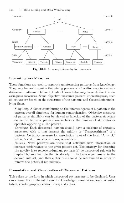
424 10 Data Mining and Data Warehousing
Country
City
All
Canada USA
British Columbia Ontario New Illinois
Location
State
Level 0
Level 2
Level 1
Vancouver Victoria Toronto Ottawa
Level 3
ChicagoBuffaloNewyork
Fig. 10.2. A concept hierarchy for dimension
Interestingness Measures
These functions are used to separate uninteresting patterns from knowledge.They may be used to guide the mining process or after discovery to evaluatediscovered patterns. Different kinds of knowledge may have different inter-estingness measures. Some objective measures pattern interestingness, suchobjectives are based on the structures of the patterns and the statistic under-lying them.
– Simplicity. A factor contributing to the interestingness of a pattern is thepattern overall simplicity for human comprehension. Objective measuresof patterns simplicity can be viewed as function of the pattern structuredefined in terms of pattern size in bits or the number of attributes oroperator appearing in the pattern.
– Certainty. Each discovered pattern should have a measure of certaintyassociated with it that assesses the validity or “Trustworthiness” of apattern. Certainty measure for association rules of the form “A ⇒ B,”where A and B are sets of items, is confidence.
– Novelty. Novel patterns are those that attribute new information orincrease performance to the given pattern set. The strategy for detectingthe novelty is to remove redundant patterns if the discovered rule can beimplied by another rule that is already in the knowledge base or in thederived rule set, and then either rule should be reexamined in order toremove the potential redundancy.
Presentation and Visualization of Discovered Patterns
This refers to the form in which discovered patterns are to be displayed. Usercan choose from different forms for knowledge presentation, such as rules,tables, charts, graphs, decision trees, and cubes.
10.1 Data Mining 425
Allowing the visualization of discovered patterns can help users with adifferent backgrounds to identify patterns of interest and to interact or guidethe system in further discovery. A user should be able to specify the forms ofpresentation to be used for displaying the discover patterns. The use of concepthierarchies plays an important role in aiding the user to visualize the discoverpatterns. The mining with concept hierarchies allows the representation todiscover knowledge in high-level concepts, which may be more understandableto user than rules expressed in terms of primitive data such as functional ormultivalued dependency rules or integrity constants.
10.1.9 Data Mining Query Language
The importance of design of a good data mining query language can also beseen by observing history of relational database system. Relational databasesystems have dominated the database market for decades. The standardiza-tion of relational query language, which occurred at early stages of relationaldatabase development, is widely credited for success of the relational databasefield. Hence having a good query language may help standardize the develop-ment of platforms for data mining system. Designing a comprehensive datamining language is challenging because data mining covers wide spectrum oftask, from data characterization to mining association rules, data classifica-tion, and evaluation analysis.
Designing the data mining query language is specified by the followingprimitives:
– The kind of knowledge to be mined.– The background knowledge to be used in the discovery process.– The Interestingness measures and threshold or pattern evaluation.
Syntax for Specifying the Kind of Knowledge to be Mined
This statement is used to specify the kind of knowledge to be mined. Its syntaxis defined later for characterization, association, and classification.
Characterization
〈Mine Knowledge Specification〉 ::=minecharacteristics [as〈pattern name〉]Analyze 〈measure(s)〉This specifies the characteristic descriptions are to be mined, the analyzed
class is used for characterization, and specific aggregate measures.
Association
〈Mine Knowledge Specification〉 ::= mine association [as 〈pattern name〉][Matching 〈metapattern〉]This specifies the mining patterns of association, the user providing the
option with the matching clause. The Meta patterns can be used to focus
426 10 Data Mining and Data Warehousing
the discovery toward the patterns that match the given Meta patterns, therebyenforcing additional syntactic constraints for the mining task.
Classification
〈Mine Knowledge Specification〉 ::= mine classification [as 〈pattern name〉]Analyze 〈classifying attribute or dimension〉It specifies that the patterns for data classification are to be mined; the
analyze clause specifies that the classification is performed according to thevalues of classifying attribute or dimension.
Syntax for Concept Hierarchy Specification
It allows mining of knowledge at multiple levels of abstraction. To accommo-date a different viewpoint of uses with regard to the data, there may be morethan one concept hierarchy per attribute or dimension. For instance, someusers prefer organizing branch locations by provinces and states, while othersorganizing them according to languages used.Syntax: use hierarchy 〈hierarchy name〉 for 〈attribute or dimension〉
Syntax for Interestingness Measure Specification
The user can help control the number uninteresting patterns returned by thedata mining system by specifying measures of pattern interestingness and theircorresponding threshold. Interestingness measure includes the confidence, sup-port, noise, and novelty.Syntax: with [〈interest measure name〉] threshold = 〈threshold value〉
10.1.10 Architecture Issues in Data Mining System
The architecture and design of data mining system is critically important.Based on the different architecture designs data mining systems can be inte-grated with a DB/DW (database/data warehouse) system using the followingcoupling schemes:
– No coupling . No coupling means that a data mining system will not uti-lize any function of a DB/DW system. It may fetch data from a particularsource, process data using some data mining algorithms, and then storethe mining results in another file. Moreover, most data have been or willbe stored in DB/DW system. Without any coupling of such systems, adata mining system will need to use other tools to extract data, mak-ing it difficult to integrate such a system into an information processingenvironment. This represents a poor design.
10.1 Data Mining 427
– Loose coupling . It means the data mining system will use some facilitiesof a DB or DW system, fetching data from a data repository managedby these systems, performing data mining, and then storing the miningresults either in a file or in a designated place in a database. Loose couplingis better than no coupling since it can fetch any portion of data stored in adatabase by using query processing, indexing, and other system facilities.
– Semitight coupling . It means that besides linking a data mining system toa DB/DW system, efficient implementations of a few essentials data min-ing primitives can be provided in the DB/DW system. These primitivescan include sorting, indexing, aggregation, histogram analysis, multiwayjoint, and precomputation of some essential statistical measures such assum, count, max, minimum, and standard deviation.
– Tight coupling . It means that data mining system is smoothing integratorsin to the DB/DW system. The data mining subsystem is treated as onefunctional component of an information system. Data mining queries andfunctions are optimized based on mining query analysis, data structures,indexing scheme, and query process methods of DB or DW system.
This approach is highly desirable since it facilitates efficient implementa-tion of data mining functions, high system performances, and an integratedinformation processing environment.
With these analysis data mining system should be coupled with theDB/DW system. Loose coupling is, though not efficient, is better than nocoupling. Since it makes use of both delta and system facilities of a DB/DWsystem. Tight coupling is highly desirable but its implementation is nontrivialand more research is needed in this area. Semitight coupling is a compromisebetween loose and tight coupling. It is important to identify commonly useddata mining primitives and provide efficient implementation of such primitivesin DB/DW system.
10.1.11 Mining Association Rules in Large Databases
Association rule mining finds interesting association or correlation relation-ships among a large set of data items, with a massive amounts of data contin-uously being collected and stored, many industries are becoming interested inmining association rules from their databases.
The discovery of interesting association relationships among huge amountsof business transaction records can help in many business decision makingprocess, such as catalog design, cross marketing, and loss-leader analysis.
Basic Concepts
Let j=i1, i2, im be a set of items, let D, the task-relevant data, be a set ofdatabase transactions where each transaction T is a set of items such thatT⊆J. Each transaction is associated with an identifier called TID. Let A bea set of items, A transaction T is said to contain A if and only if A⊆T.
428 10 Data Mining and Data Warehousing
An association rule is an implication of the form A⇒B, where A⊂J, B⊂J,and A ∩ B = φ, so the rule is an implication of the form A⇒B holds in thetransaction set D with support S, where S is percentage of transactions in Dthat contain A∪B.
Association Rule Mining is a Two-step Process
1. Find all frequent itemsets. Each of these itemsets will occur at least asfrequently as a predetermined minimum support count.
2. Generate strong association rules from the frequent itemsets. These rulesmust satisfy minimum support and minimum confidence, it is the easi-est process of the two methods. So, the overall performance of miningassociation rule is determined by the first step.
The Apriori Algorithm
A. Finding Frequent Itemsets Using Candidate Generation
The Apriori algorithm is an influential algorithm for mining frequent itemsets for Boolean association rules. This algorithm uses prior knowledge offrequent itemset properties. Apriori employs an iterative approach known aslevel-wise search, where k itemsets are used to explore (k+1) itemsets. It alsoimproves the efficiency of level-wise generation of frequent itemsets, which isan important property and is called Apriori property and it is used to reducethe search space.
Improving the Efficiency of Apriori The techniques for improving the effi-ciency of Apriori is summarized later:
1. Hash-based technique (Hashing itemset counts). This technique can beused to reduce the size of the candidate k-itemsets, Ck for k>1.
2. Transaction reduction. A transaction that does not contain any frequentk-itemsets cannot contain any frequent (k+1) itemsets. Therefore such atransaction can be marked or removed from further consideration to thesubsequent for j-itemsets, where j>k.
3. Partitioning. A partitioning technique that requires just two databasescans to mine the frequent itemsets can be used. It consists of two phases asshown in Fig. 10.3, in phase one, the algorithm subdivides the transactionsof D into n nonoverlapping partitions. If the minimum support thresholdfor transactions in D is min sup then the minimum itemset support countfor a partition is min sup × number of transaction in the partition. Foreach partition, all frequent itemset within the partition are found. Thisrefers to a local frequent itemsets. These itemsets are candidate itemsetswith respect to D.In phase two, a second scan of D is conducted in which the actual supportof each candidate is assessed to determine the frequent itemsets. Since the
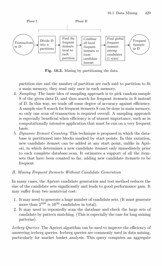
10.1 Data Mining 429
Phase I Phase II
Transactionsin D
Divide Dinto npartitions
Find thefrequentitemsetslocal toeachpartition
Combineall localfrequentitemsets toformcandidateitemset
Find globalfrequentitemsetsamongcandidates(1 scan)
Frequentitemsetsin D
Fig. 10.3. Mining by partitioning the data
partition size and the number of partition are each said to partition to fita main memory, they read only once in each memory.
4. Sampling. The basic idea of sampling approach is to pick random sampleS of the given data D, and then search for frequent itemsets in S insteadof D. In this way, we trade off some degree of accuracy against efficiency.A sample size S search for frequent itemsets S can be done in main memory,so only one scan of transaction is required overall. A sampling approachis especially beneficial when efficiency is of utmost importance, such as incomputationally intensive application that must be run on a very frequentbasis.
5. Dynamic Itemset Counting. This technique is proposed in which the data-base is partitioned into blocks marked by start points. In this variation,new candidate itemset can be added at any start point, unlike in Apri-ori, in which determines a new candidate itemset only immediately priorto each complete database scan. It estimates a support of all the item-sets that have been counted so far, adding new candidate itemsets to befrequent.
B. Mining Frequent Itemsets Without Candidate Generation
In many cases, the Apriori candidate generation and test method reduces thesize of the candidate sets significantly and leads to good performance gain. Itmay suffer from two nontrivial cost:
1. It may need to generate a huge number of candidate sets. (It must generatemore than 2100 ≈ 1030 candidates in total).
2. It may need to repeatedly scan the database and check the large sets ofcandidate by pattern matching. (This is especially the case for long miningpatterns).
Iceberg Queries The Apriori algorithm can be used to improve the efficiency ofanswering iceberg queries. Iceberg queries are commonly used in data mining,particularly for market basket analysis. This query computes an aggregate
430 10 Data Mining and Data Warehousing
function over an attribute or set of attributes in order to find aggregate valuesabove specified threshold.
10.1.12 Mining Multilevel Association From TransactionDatabases
This section deals with multilevel and multidimensional association rules ofdata mining.
Multilevel Association Rules
For many applications, it is difficult to find strong association among dataitems at low or primitive levels of abstraction due to the sparsity of data inmultidimensional space. Strong association discovered at high-concept levelsmay represent common sense knowledge. However, what may represent com-mon sense to one user may seem novel to another. Therefore, data miningsystem should provide capabilities to mine association rules at multiple levelsof abstraction and traverse easily among different abstraction spaces.
Approaches to Mining Multilevel Association Rules
The approaches to mining multilevel association rules are summarized later:
1. Using Uniform Minimum Support for all Levels. The same minimum sup-port threshold is used when mining at each level of abstraction. When auniform minimum support threshold is used, the search procedure is sim-plified. The method is also simple in that users are required to specify onlyone minimum support threshold. This approach has some difficulties; it isunlikely that items at lower levels of abstraction will occur as frequentlyas those at higher levels of abstraction. If the minimum support thresholdis set to high, it could miss several meaningful associations occurring atlow abstraction levels. If the threshold is set to low, it may generate manyuninteresting associations occurring at high abstraction levels.
2. Using Reduced Minimum Support at Lower Levels. Each level of abstrac-tion has its own minimum support threshold. The lower the abstractionlevel, the smaller the corresponding threshold. For mining multiple levelassociations with reduced support, there are numbers of alternative searchstrategies:
– Level by level independent. This is a full breadth search, where nobackground knowledge of frequent itemsets is used for prunting.
– Level cross-filtering by single item. An item at the ith level is examinedif and only if parent node at the (i − 1)th level is frequent.
– Level cross-filtering by k-itemset. A k-itemset at the ithlevel is exam-ined if and only if its corresponding parent k-itemsets at the (i− 1)th
level is frequent.
10.1 Data Mining 431
Multidimensional Association Rules
For example, consider a Samsung Electronics database; we may discover theBoolean association rule, “IBM desktop computer ⇒ Samsung color printer,”which can be written as:
Buys (X, “IBM Desktop computer”) ⇒ Buys (X, “Samsung Color printer”)where X is a variable representing customers who purchased items in
Samsung Electronics transactions. Following the terminology used in mul-tidimensional databases, we refer to each distinct predicate in a rule as adimension. Hence, we can refer to rule as a single-dimensional or intradimen-sional association rule since it contains a single distinct predicate (e.g., buys)with multiple occurrences (i.e., the predicate occurs more than once withinthe rule). Techniques for mining multidimensional association rules can becategorized according to three basic approaches regarding the treatment ofquantitative attributes.
In the first approach, quantitative attributes are discretized using pre-defined concept hierarchies. This discretization occurs prior to mining. Aconcept hierarchy for income may be used to replace the original numericvalues of this attribute by ranges, such as “0–20 K,” “21–30 K,” “31–40 K,”and so on. The discretization is static here and it can be predetermined. Thediscretized numeric attributes, with their range values, can be treated as cat-egorical attributes. This is referred as Mining Multidimensional Associationrules using static discretization of quantitative attributes.
In the second approach, quantitative attributes are discretized into “bins”based on the distribution of the data. These bins may be further combinedduring the mining process. The discretization process is dynamic and estab-lished so as to satisfy some mining criteria, such as maximizing the confi-dence of the rules mined. This strategy treats the numeric attribute valuesas quantities rather than as predefined ranges or categories, association rulesmined from this approach are also referred to as Quantitative AssociationRules.
In the third approach, quantitative attributes are discretized so as to cap-ture the semantic meaning of such interval data. This dynamic discretizationprocedure considers the distance between data points. Hence, such quantita-tive association rules are also referred to as Distance-Based Association rules.
Mining Quantitative Association Rules
Quantitative association rules are multidimensional association rules in whichthe numeric attributes are dynamically discretized during the mining processso as to satisfy some mining criteria, such as maximizing the confidence orcompactness of the rules mined. The quantitative association rules are focusedby the two quantitative attributes on the left side of the rule and one cate-gorical attribute on the right side of the rule.
432 10 Data Mining and Data Warehousing
Binning. The grids in the ranges of Quantitative attributes are partitionedinto intervals. These intervals are dynamic in that they may later be furthercombined during mining process. This partitioning process is referred to asBinning and the intervals are referred as bins. The three common binningstrategies are:
1. Equiwidth Binning, where the interval size of each bin is the same.2. Equidepth Binning, where each bin has approximately the same number
of tuples assigned to it.3. Homogeneity-based Binning, where bin size is determined so that the tup-
les in each bin are uniformly distributed.
From Association Mining to Correlation Analysis. Most of the associationrule-mining algorithm employs a support-confidence framework. In spite ofusing minimum support and confidence thresholds to help weed out or excludethe exploration of uninteresting rules, many rules that are not interesting tothe user may still be produced. Even the strong association rules can beuninteresting and misleading, and then discuss additional measures based onstatistical independence and correlation analysis.
Strong Rules are not Necessarily Interesting. In data mining, whether a ruleis interesting or not can be judged subjectively or objectively. Ultimately, onlythe user can judge if a given rule is interesting or not, and this judgments,being subjective, may differ from one user to another. However, objectiveinterestingness measures, based on the statistics behind the data, can be usedas one step toward the goal of weeding out uninteresting rules from presenta-tion to the user.
From Association Analysis to Correlation Analysis. Association rules minedusing a support and support-confidence frameworks are useful for many appli-cations. However, the support-confidence framework can be misleading thatis it may identify a rule A ⇒ B as interesting when, in fact, the occurrence ofA does not imply the occurrence of B.
The occurrence of itemset A is independent of the occurrence of itemsetB if P(A∪B) = P(A)P(B); otherwise itemsets A and B are dependent andcorrelated as events. This definition can be easily extended to more item-sets. The correlation between the occurrence of A and B can be measured bycomputing,
corrA,B =P (A ∪ B)P (A)P (B)
If the resulting value of the equation is less than 1, then the occurrence ofA is negatively correlated with the occurrence of B. If the resulting value isgreater than 1, then A and B are positively correlated, meaning the occurrenceof the other. If the resulting value is equal to 1, then A and B are independentand there is no correlation between them.
10.1 Data Mining 433
Constraint-Based Association Mining. For a given set of task-relevant data,the data mining process may uncover thousands of rules, many of which areuninteresting to the user. In constraint-based mining, mining is performedunder the guidance of various kinds of constraints provided by the user. Theseconstraints include the following:
– Knowledge type constraints. These specify the type knowledge to bemined, such as association.
– Data Constraints. These specify the set of task-relevant data.– Dimension/level Constraints. These specify the dimension of the data, or
levels of the concept hierarchies, to be used.– Interestingness Constraints.These specify thresholds on statistical mea-
sures of rule interestingness, such as support and confidence.
10.1.13 Rule Constraints
These specify the form of rules to be mined. Such constraints may be expressedas metarules (rule templates), as the maximum or minimum number of pred-icates that can occur in the rule antecedent or consequent, or as relationshipsamong attributes, attribute values, and/or aggregates. The use of rule con-straint is to focus the mining task. This form of constraint-based mining allowsthe user to specify the rules to be mined according to their intention, therebymaking the data mining process more effective.
Metarules-guided Mining of Association Rules
Metarules allow users to specify the syntactic form of rules that they areinterested in mining. It can be used as constraints to help improve theefficiency of the mining process. It may be based on the analyst’s experi-ence, expectations, or intuition regarding the data, or automatically generatedbased on the database scheme.
Mining Guided by Additional Rule Constraints
Rule constraints specifying set/subset relationships, constant intuition of vari-ables, and aggregate functions can be specified by the user. These may beused together with, or as an alternative to, metarules guided mining. Ruleconstraints can be classified into five categories with respect to frequent item-sets mining, namely as antimonotone, monotone, succinct, convertible, andinconvertible.
– If an itemsets does not satisfy this rule constraint, none of its supersets cansatisfy the constraint. If rule constraint obeys this property, it is calledantimonotone. Prunting by antimonotone constraints can be applied ateach iteration of Apriori style algorithms to help improve the efficiency ofthe overall mining process.
434 10 Data Mining and Data Warehousing
– If itemsets satisfies this rule constraint, so do all of its supersets. If a ruleconstraint obeys this property, it is called monotone.
– In this category, we can enumerate all and only those sets that are guaran-teed to satisfy the constraint. If a rule is succinct we can directly generateprecisely the sets that satisfy it, even before support counting begins. Itavoids the substantial overhead of the generation and test paradigm.
– Some constraints belong to none of the earlier three categories. However, ifthe items in the itemsets are arranged in a particular order, the constraintmay become monotone or antimonotone with regard to a frequent itemsetsmining process, these constraints are called as convertible constraints.
For example average price is not more than 100, aside from “avg(s) ≤ v,”and avg(s) ≥ v,” there are many other convertible constraints, such as “vari-ance(s) ≥ v,” “standard deviation(s) ≥ v”
– For example, “sum (G) θ v,” where θ ∈≤, ≥ and each element in G couldbe of any real value, which is not convertible and this is called inconvertibleconstraints. Although there still exist some tough constraints that are notconvertible. So the SQL aggregate belongs to one of the four categories towhich efficient constraint mining methods can be applied.
10.1.14 Classification and Prediction
Databases are rich with hidden information that can be used for makingintelligent business decisions. Classification and prediction are two forms ofdata analysis that can be used to extract models describing important dataclasses or predict future data trends. Whereas classification predicts categor-ical labels, prediction models continuous-valued functions.
Data Classification
It is a two-step process and in the first step, a model is built by describinga predetermined set of data classes or concepts. The model is constructed byanalyzing database tuples described by attributes. Each tuple is assumed tobelong to a predefined class, as determined by one of the attributes, called theclass-label attribute. The data tuples analyzed to build the model collectivelyform the training data set. The individual tuples making up the training setare referred to as training samples and are randomly selected from the samepopulation. Since the class label of each training sample is provided, this stepis also known as supervised learning.
In the second step, the model is used for classification. First, the predictiveaccuracy of the model is estimated. The hold-out method is a simple techniquefor estimating classifier accuracy that uses a test set of class-labeled samples.These samples are randomly selected and are independent of the trainingsamples as shown in Fig. 10.4. The accuracy of a model on a given test set is
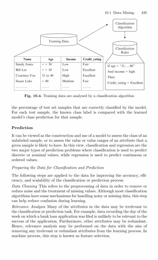
10.1 Data Mining 435
Name Age Income Credit_rating
Sandy Jones
Bill Lee
Courtney Fox
Susan Lake
………..
< = 30
< = 30
31 to 40
> 40
…….
Low
Low
High
Medium
…….
Fair
Excellent
Excellent
Fair
……..
ClassificationAlgorithm
Training Data
ClassificationRules
If age = “31…..40”
And income = high
Then
Credit_rating = Excellent
Fig. 10.4. Training data are analyzed by a classification algorithm
the percentage of test set samples that are correctly classified by the model.For each test sample, the known class label is compared with the learnedmodel’s class prediction for that sample.
Prediction
It can be viewed as the construction and use of a model to assess the class of anunlabeled sample, or to assess the value or value ranges of an attribute that agiven sample is likely to have. In this view, classification and regression are thetwo major types of prediction problems where classification is used to predictdiscrete or nominal values, while regression is used to predict continuous orordered values.
Preparing the Data for Classification and Prediction
The following steps are applied to the data for improving the accuracy, effi-ciency, and scalability of the classification or prediction process.Data Cleaning This refers to the preprocessing of data in order to remove orreduce noise and the treatment of missing values. Although most classificationalgorithms have some mechanisms for handling noisy or missing data, this stepcan help reduce confusion during learning.Relevance Analysis Many of the attributes in the data may be irrelevant tothe classification or prediction task. For example, data recording the day of theweek on which a bank loan application was filed is unlikely to be relevant to thesuccess of the application. Furthermore, other attributes may be redundant.Hence, relevance analysis may be performed on the data with the aim ofremoving any irrelevant or redundant attributes from the learning process. Inmachine process, this step is known as feature selection.
436 10 Data Mining and Data Warehousing
Data Transformation The data can be generalized to higher-level concepts.Concept hierarchies may be used for this purpose. This is particularly usefulfor continuous-valued attributes. The data may also be normalized, particu-larly when neural networks or methods involving distance measurements areused in the learning step. Normalization involves scaling all values for a givenattribute so that they fall within a small-specified range, such as −1.0–1.0or 0.0–1.0.
10.1.15 Comparison of Classification Methods
Classification and prediction methods can be compared and evaluated accord-ing to the following criteria:
– Predictive Accuracy. This refers to the ability of the model to correctlypredict the class label of new or previously unseen data.
– Speed. This refers to the computation costs involved in generating andusing the model.
– Robustness. This refers to the ability of the model to make correct pre-dictions given noisy data or data with missing values.
– Scalability. This refers to the ability to construct the model efficientlygiven large amounts of data.
– Interpretability. This refers to the level of understanding and insight thatis provided by the model.
Classification by Decision Tree Induction
A decision tree is a flow-chart-like tree structure, where each internal nodedenotes a test on an attribute, each branch represents an outcome of the test,and leaf nodes represent classes or class distributions. The topmost node isthe root node.
In order to classify an unknown sample, the attribute values of the sampleare tested against the decision tree. A path is traced from the root to a leafnode that holds the class prediction for that sample. Decision trees can easilybe converted to classification rules.
The basic algorithm for decision-tree induction is a greedy algorithm thatconstructs decision trees in a top-down recursive divide and conquer manner.The basic strategy is as follows:
1. The tree starts as a single node representing the training samples.2. If the samples are all of the same class, then the node becomes a leaf and
is labeled with that class.3. Otherwise, the algorithm uses an entropy-based measure known as infor-
mation gain as a heuristic for selecting the attribute that will best separatethe samples into individual classes.
10.1 Data Mining 437
4. This attribute becomes the “test” or “decision” attribute at the node. Allattributes used in this algorithm are categorized into discrete valued. So,continuous-valued attributes must be discretized.
5. A branch is created for each known value of the test attribute, and thesamples are partitioned.
6. The algorithm uses the same process recursively to form a decision treefor the samples at each partition. Once an attribute has occurred at anode, it need not be considered in any of the node’s descendents.
7. The recursive partitioning stops only when any one of the following con-ditions is true:(a) All samples for a given node belong to the same class.(b) There are no remaining attributes on which the samples may be fur-
ther partitioned.(c) There are no samples for the branch test-attribute = ai. in this case,
a leaf is created with the majority class in samples.
Tree Pruning
When a decision tree is built, many of the branches will reflect anomaliesin the training data due to noise or outliers. Tree-pruning methods addressthis problem of over fitting the data. Such methods typically use statisticalmeasures to remove the least reliable branches, generally resulting in fasterclassification and an improvement in the ability of the tree to correctly classifyindependent test data.
There are two common approaches to tree pruning. The first approachis the prepruning approach; a tree is “pruned” by halting its constructionearlier. Upon halting, the node becomes a leaf. The leaf may hold the mostfrequent class among the subset samples. If partitioning the samples at a nodewould result in a split that falls below a prespecified threshold, then furtherpartitioning of the given subset is halted. High thresholds would result in over-simplified trees, while low thresholds could result in very little simplification.
The second approach, postpruning, removes branches from a “fully grown”tree. A tree node is pruned by removing its branches. The cost complexitypruning is an example of the postpruning approach. If pruning the node leadsto a greater expected error rate, then the subtree is kept. Otherwise, it ispruned. Alternatively prepruning and postpruning may be interleaved for acombined approach. Postpruning requires more computation than prepruning,yet generally leads to a more reliable tree.
Extracting Classification Rules from Decision Trees
The knowledge represented in decision trees can be extracted and representedin the form of classification, IF-THEN rules. One rule is created from eachpath from the root to a leaf node. Each attribute-value pair along a givenpath forms a conjunction in the rule antecedent (“IF” part). The leaf node
438 10 Data Mining and Data Warehousing
holds the class prediction, forming the rule consequent (“THEN” part). TheIF-THEN rules may be easier for humans to understand, particularly if thegiven tree is very large.
Scalability and Decision Tree Induction
The efficiency of existing decision tree algorithms, such as ID3 and C4.5, hasbeen well established for relatively small data sets. Efficiency and Scalabilitybecome issues of concern when these algorithms are applied to the miningof very large real-world databases. Most decision tree algorithms have therestriction that the training samples should reside in main memory. In datamining applications, very large training sets of millions of samples are com-mon. Hence, this restriction limits the scalability of such algorithms, wherethe decision tree construction can become inefficient due to swapping of allthe training samples in and out of main cache memories.
More recent decision tree algorithms that address the scalability issue havebeen proposed. Algorithms for the induction of decision trees from very largetraining sets include SLIQ and SPRINT, both of which can handle categoricaland continuous-valued attributes. Both algorithms propose presorting tech-niques on disk-resident data sets that are too large to fit in memory.
Bayesian Classification
Bayesian classifiers are statistical classifiers. They can predict class member-ship probabilities, that is a given sample belongs to a particular class. Studiescomparing classification algorithms have found a simple Bayesian classifierknown as the native Bayesian classifier to be comparable in performancewith decision tree and neural network classifiers. Bayesian classifiers have alsoexhibited high accuracy and speed when applied to large databases.
Bayesian belief networks are graphical models, which unlike nativeBayesian classifiers allow the representation of dependencies among sub-sets of attributes. Bayesian belief networks can also be used for classification.Bayesian classification is based on Bayes theorem, described later.
Bayes Theorem
Assume X is a data sample whose class label is unknown and H be somehypothesis, such that the data sample X belongs to a specified class C. Forclassification problems, we want to determine P(H|X), the probability thatthe hypothesis H holds for the given observed data sample X. P(H|X) is theposterior probability, or a posteriori probability, of H conditions on X. Incontrast, P(H) is the prior probability, or a priori probability, of H. P(X),P(H) and P(X|H) may be estimated from the given data.
P (H|X) =P (X|H)P (H)
P (X)
10.1 Data Mining 439
Naive Bayesian Classification
The naive Bayesian classifier, or simple Bayesian classifier, works as follows:
– Each data sample is represented by an n-dimensional feature vector,X = (x1, x2, . . .xn), depicting n measurements made on the sample fromn attributes, respectively, A1,A2,. . .An.
– As P (X) is constant for all classes, only P (X | Ci) P (Ci) needs tobe maximized. If the class prior probabilities, are not known, then it iscommonly assumed that the classes are equally likely, that is P(C1) =P(C2) = . . . = P(Cn). Therefore maximize P (X | Ci).
Bayesian Belief Networks
This network classifier makes the assumption of class conditional indepen-dence, that is, given the class label of a sample, the values of the attributesare conditionally independent of one another, and it simplifies the computa-tion. When the assumption holds true this network classifier is most accuratein comparison with all other classifiers. This network specifies joint condi-tional probability distributions and it is defined by two components. The firstis directed acyclicgraph, where each node represents a random variable andeach arc represents a probabilistic dependence. The second component is defin-ing a belief network consists of one Conditional Probability Table (CPT). TheCPT for a variable Z specifies the conditional distributions P(Z | Parents (Z)).
Training Bayesian Belief Networks
In the learning or training of this network, a number of scenarios are possible.In the network, structure may be given in advance inferred from the data. Thenetwork variables may be observable or hidden in all or some of the trainingsamples. The hidden data are also referred to as missing or incomplete data.
If the network structure is known and the variables are observable, thenthe training network is straightforward. It consists of computing the CPTentries, as is similarly done when computing the probabilities involved in thisnetwork when the network structure is given and some of the variables arehidden then the method of gradient descent can be used to train this network.
Classification Based on Concepts from AssociationRule Mining (ARC)
Association rule mining is an important and highly active area of data miningresearch. Recently, data mining techniques that apply concepts used in asso-ciation rule mining to the problem of classification have been developed. Theclustered association rules generated by ARCS were applied to classification,and then accuracy was compared to C4.5.
The first network mines association rules based on clustering and thenemploys the rules for classification. In general, ARC is empirically found to
440 10 Data Mining and Data Warehousing
be slightly more accurate than C4.5 when there are outliers in the data. Theaccuracy of ARCS is related degree of discretization used. The second methodis referred to as Associative Classification. It mines rules of the form condset⇒ y, where condset is a set of items and y is a class label. The third method,Classification by Aggregating Emerging Patterns (CAEP), uses the notation ofitemset support to mine Emerging Patterns (EP), which are used to constructthe classifier. EP is an itemset whose support increases significantly from oneclass of data to another. The ratio of two supports is called growth rate of EP.
Other Classification Methods
There are several other classification methods, which are discussed as follows:K -Nearest Neighbors classifiers. This classifier can also be used for predic-
tion, that is, to return a real-valued prediction for a given unknown sample.In this case, the classifier returns the average value of the real-valued labelsassociated with the k-nearest neighbor of the unknown sample.
Case-Based Reasoning
These classifiers are instance based. The case-based reasoned may employbackground knowledge and problem-solving strategies in order to propose afeasible combined solution. It include finding a good similarity metric, develop-ing efficient techniques for indexing training cases, and methods for combiningsolutions.
Genetic Algorithm
Genetic algorithms attempt to incorporate ideas of natural evolution. It iseasily parallelizable and has been used for classification as well as optimizationproblems. In data mining, they may be used to evaluate the fitness of otheralgorithms.
Rough Set Approach
Rough set theory is based on the establishment of equivalence classes withinthe given training data. All of the data samples forming an equivalenceclass are indiscernible, that is, the samples are identical with respect to theattributes describing the data. This Rough set can also be used for featurereduction and relevance analysis, however, algorithms to reduce the compu-tation intensity have been proposed.
Fuzzy Set Approach
Rule-based Systems for classification have the disadvantage that they involvesharp cutoffs for continuous attributes, so fuzzy logic is useful for data miningsystems performing classification. It provides the advantage of working at
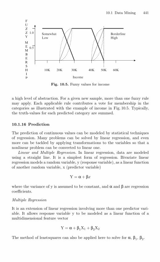
10.1 Data Mining 441
10K 20K 30K 40K 50K 60K
BorderlineHigh
SomewhatLow
1.0
0.5
Income
F
U
Z
Z
Y
M
E
M
B
E
R S
H I P
Fig. 10.5. Fuzzy values for income
a high level of abstraction. For a given new sample, more than one fuzzy rulemay apply. Each applicable rule contributes a vote for membership in thecategories as illustrated with the example of income in Fig. 10.5. Typically,the truth-values for each predicted category are summed.
10.1.16 Prediction
The prediction of continuous values can be modeled by statistical techniquesof regression. Many problems can be solved by linear regression, and evenmore can be tackled by applying transformations to the variables so that anonlinear problem can be converted to linear one.
Linear and Multiple Regression. In linear regression, data are modeledusing a straight line. It is a simplest form of regression. Bivariate linearregression models a random variable, y (response variable), as a linear functionof another random variable, x (predictor variable)
Y = α + βx
where the variance of y is assumed to be constant, and α and β are regressioncoefficients.
Multiple Regression
It is an extension of linear regression involving more than one predictor vari-able. It allows response variable y to be modeled as a linear function of amultidimensional feature vector
Y = α + β1X1 + β2X2
The method of leastsquares can also be applied here to solve for α, β1, β2.
442 10 Data Mining and Data Warehousing
Nonlinear Regression
Polynomial regression can be modeled by adding polynomial terms to thebasic linear model. By applying transformation to the variables, we convertthe nonlinear model into linear one that can then be solved by method of leastsquares.
Other Regression Models
Linear regression is used to model continuous valued functions. It is widelyused, owing largely to its simplicity. Generalized linear model represent thetheoretical foundation on which linear regression can be applied to the mod-eling of categorical response variables. Common types of generalized linearmodels include logistic and poisson regression. Logistic regression models theprobability of some event occurring as a linear function of set of predictorvariables. Count data frequency exhibits a poisson distribution and is com-monly modeled using poisson regression. Log linear models approximate dis-crete multidimensional probability distribution. They may be used to estimatethe probability value associated with the data cube cells.
10.1.17 Cluster Analysis
Imagine that we are given a set of data objects for analysis where, unlike inclassification, the class label of each object is not known. Clustering is theprocess of grouping the data into classes or clusters so that objects withina cluster have high similarity in comparison to one another, but are verydissimilar to objects in other clusters. Dissimilarities are assessed based onthe attribute values describing the objects.
The process of grouping a set of physical or abstract objects into classes ofsimilar objects is called clustering. A cluster is a collection of data objects thatare similar to one another within the same cluster and are dissimilar to theobjects in other clusters. A cluster of data objects can be treated collectivelyas one group in many applications.
Some typical application of clustering are in business, clustering can helpmarketers discover distinct groups in their customer bases and characterizecustomer groups based on purchasing patterns. In biology, it can be used toderive plant and animal taxonomies, categorize genes with similar functional-ity, and gain insight into structures inherent in populations.
As a data mining function, cluster analysis can be used as a stand-alonetool to gain insight into the distribution of data, to observe the characteristicsof each cluster, and to focus on a particular set of clusters for further analysis.
Data clustering is under vigorous development. Contributing areas ofresearch include data mining, statistics, machine learning, spatial databasetechnology, biology, and marketing.
10.1 Data Mining 443
Cluster analysis tools based on k-means, k-medoids, and several othermethods have also been built into many statistical analysis software packagesor systems, such as S-plus, SPSS, and SAS. Clustering is an example forunsupervised learning.
Requirements of Clustering in Data Mining
Scalability. Many clustering algorithms work well on small data sets containingfewer than 200 data objects; however, a large database may contain millionsof objects. Clustering on a sample of a given large set may lead to biasedresults. Highly scalable clustering algorithms are needed.
Ability to deal with different types of Attributes. Many algorithms are desig-ned to cluster interval-based (numerical) data. However, applications mayrequire clustering other types of data, such as binary, categorical (nominal),and ordinal data, or mixtures of these data types.
Discovery of Clusters with Arbitrary Shape
Many clustering algorithms determine clusters based on Euclidean or Manhat-tan distance measures. Algorithms based on such distance measures tend tofind spherical clusters with similar size and density. However, a cluster couldbe of any shape. It is important to develop algorithms that can detect clustersof arbitrary shape.
Minimal Requirements for Domain Knowledge to Determine InputParameters
Many clustering algorithms require users to input certain parameters in clusteranalysis (such as the number of desired clusters). The clustering results can bequite sensitive to input parameters. Parameters are often hard to determine,especially for data sets containing high-dimensional objects. This not onlyburdens users, but also makes the quality of clustering difficult to control.
Ability to Deal with Noisy Data
Most real-world databases contain outliers or missing, unknown, or erroneousdata. Some clustering algorithms are sensitive to such data and may lead toclusters of poor quality.
Insensitivity to the Order of Input Records
Some clustering algorithms are sensitive to the order of input data; for exam-ple, the same set of data, when presented with different orderings to suchan algorithm, may generate dramatically different clusters. It is important todevelop algorithm that are insensitive to the order of input.
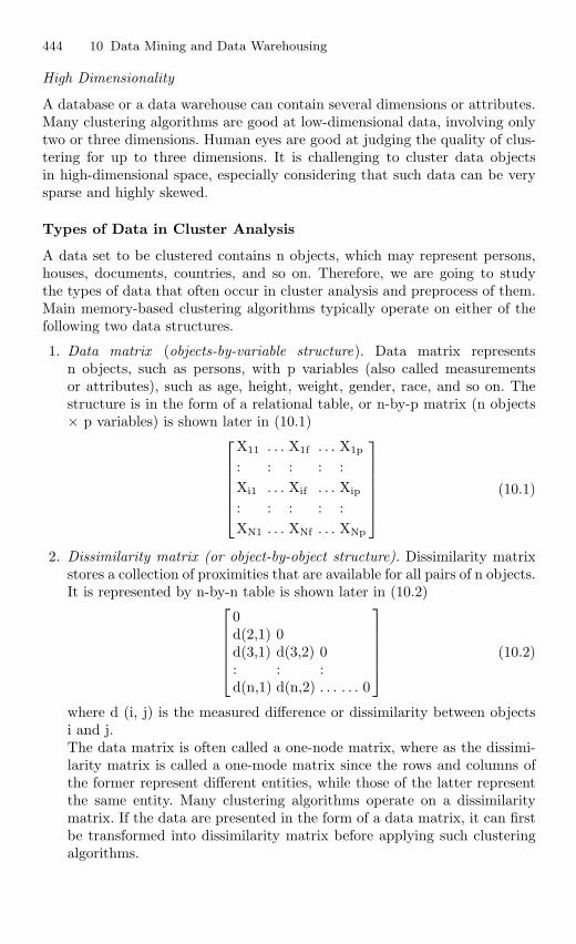
444 10 Data Mining and Data Warehousing
High Dimensionality
A database or a data warehouse can contain several dimensions or attributes.Many clustering algorithms are good at low-dimensional data, involving onlytwo or three dimensions. Human eyes are good at judging the quality of clus-tering for up to three dimensions. It is challenging to cluster data objectsin high-dimensional space, especially considering that such data can be verysparse and highly skewed.
Types of Data in Cluster Analysis
A data set to be clustered contains n objects, which may represent persons,houses, documents, countries, and so on. Therefore, we are going to studythe types of data that often occur in cluster analysis and preprocess of them.Main memory-based clustering algorithms typically operate on either of thefollowing two data structures.
1. Data matrix (objects-by-variable structure). Data matrix representsn objects, such as persons, with p variables (also called measurementsor attributes), such as age, height, weight, gender, race, and so on. Thestructure is in the form of a relational table, or n-by-p matrix (n objects× p variables) is shown later in (10.1)
⎡
⎢⎢⎢⎢⎢⎣
X11 . . . X1f . . . X1p
: : : : :Xi1 . . . Xif . . . Xip
: : : : :XN1 . . . XNf . . . XNp
⎤
⎥⎥⎥⎥⎥⎦
(10.1)
2. Dissimilarity matrix (or object-by-object structure). Dissimilarity matrixstores a collection of proximities that are available for all pairs of n objects.It is represented by n-by-n table is shown later in (10.2)
⎡
⎢⎢⎢⎢⎣
0d(2,1) 0d(3,1) d(3,2) 0: : :d(n,1) d(n,2) . . . . . . 0
⎤
⎥⎥⎥⎥⎦
(10.2)
where d (i, j) is the measured difference or dissimilarity between objectsi and j.The data matrix is often called a one-node matrix, where as the dissimi-larity matrix is called a one-mode matrix since the rows and columns ofthe former represent different entities, while those of the latter representthe same entity. Many clustering algorithms operate on a dissimilaritymatrix. If the data are presented in the form of a data matrix, it can firstbe transformed into dissimilarity matrix before applying such clusteringalgorithms.
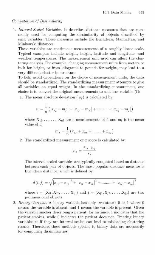
10.1 Data Mining 445
Computation of Dissimilarity
1. Interval-Scaled Variables. It describes distance measures that are com-monly used for computing the dissimilarity of objects described bysuch variables. These measures include the Euclidean, Manhattan, andMinkowski distances.These variables are continuous measurements of a roughly linear scale.Typical examples include weight, height, latitude and longitude, andweather temperatures. The measurement unit used can affect the clus-tering analysis. For example, changing measurement units from meters toinch for height, or from kilograms to pounds for weight, may lead to avery different cluster in structure.To help avoid dependence on the choice of measurement units, the datashould be standardized. The standardizing measurement attempts to giveall variables an equal weight. In the standardizing measurement, onechoice is to convert the original measurements to unit less variable (f):1. The mean absolute deviation ( sf ) is calculated by:
sf =1n
(∣∣x1f
− mf
∣∣ +
∣∣x2f
− mf
∣∣ + .......... +
∣∣x
nf− m
f
∣∣)
where X1f . . . . . . . . . Xnf are n measurements of f, and mf is the meanvalue of f.
mf
=1n
(x1f
+ x2f+ ........ + x
nf
)
2. The standardized measurement or z score is calculated by:
zif
=x
if−mf
sf
The interval-scaled variables are typically computed based on distancebetween each pair of objects. The most popular distance measure isEuclidean distance, which is defined by:
d (i, j) =√∣
∣xi1 − x
j1
∣∣2 +
∣∣x
i2 − xj2
∣∣2 + ......... +
∣∣x
ip− x
jp
∣∣2
where i = (Xi1,Xi2, . . . . . .Xip) and j = (Xj1,Xj2, . . . . . .Xjp) are twop-dimensional objects
2. Binary Variable. A binary variable has only two states: 0 or 1 where 0means the variable is absent, and 1 means the variable is present. Giventhe variable smoker describing a patient, for instance, 1 indicates that thepatient smokes, while 0 indicates the patient does not. Treating binaryvariables as if they are interval scaled can lead to misleading clusteringresults. Therefore, these methods specific to binary data are necessarilyfor computing dissimilarities.
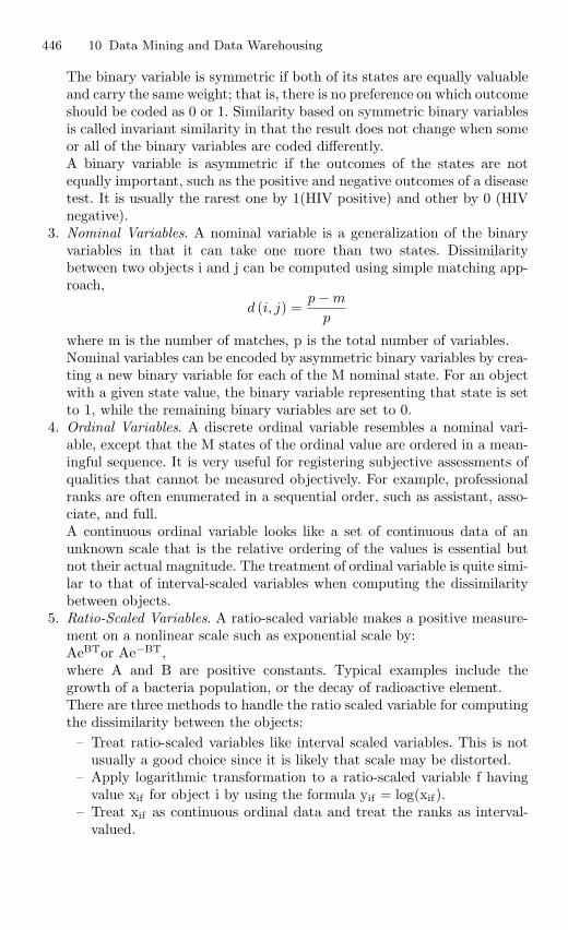
446 10 Data Mining and Data Warehousing
The binary variable is symmetric if both of its states are equally valuableand carry the same weight; that is, there is no preference on which outcomeshould be coded as 0 or 1. Similarity based on symmetric binary variablesis called invariant similarity in that the result does not change when someor all of the binary variables are coded differently.A binary variable is asymmetric if the outcomes of the states are notequally important, such as the positive and negative outcomes of a diseasetest. It is usually the rarest one by 1(HIV positive) and other by 0 (HIVnegative).
3. Nominal Variables. A nominal variable is a generalization of the binaryvariables in that it can take one more than two states. Dissimilaritybetween two objects i and j can be computed using simple matching app-roach,
d (i, j) =p − m
p
where m is the number of matches, p is the total number of variables.Nominal variables can be encoded by asymmetric binary variables by crea-ting a new binary variable for each of the M nominal state. For an objectwith a given state value, the binary variable representing that state is setto 1, while the remaining binary variables are set to 0.
4. Ordinal Variables. A discrete ordinal variable resembles a nominal vari-able, except that the M states of the ordinal value are ordered in a mean-ingful sequence. It is very useful for registering subjective assessments ofqualities that cannot be measured objectively. For example, professionalranks are often enumerated in a sequential order, such as assistant, asso-ciate, and full.A continuous ordinal variable looks like a set of continuous data of anunknown scale that is the relative ordering of the values is essential butnot their actual magnitude. The treatment of ordinal variable is quite simi-lar to that of interval-scaled variables when computing the dissimilaritybetween objects.
5. Ratio-Scaled Variables. A ratio-scaled variable makes a positive measure-ment on a nonlinear scale such as exponential scale by:AeBTor Ae−BT,where A and B are positive constants. Typical examples include thegrowth of a bacteria population, or the decay of radioactive element.There are three methods to handle the ratio scaled variable for computingthe dissimilarity between the objects:
– Treat ratio-scaled variables like interval scaled variables. This is notusually a good choice since it is likely that scale may be distorted.
– Apply logarithmic transformation to a ratio-scaled variable f havingvalue xif for object i by using the formula yif = log(xif).
– Treat xif as continuous ordinal data and treat the ranks as interval-valued.
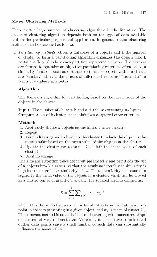
10.1 Data Mining 447
Major Clustering Methods
There exist a large number of clustering algorithms in the literature. Thechoice of clustering algorithm depends both on the type of data availableand on the particular purpose and application. In general, major clusteringmethods can be classified as follows
1. Partitioning methods. Given a database of n objects and k the numberof cluster to form a partitioning algorithm organizes the objects into kpartitions (k ≤ n), where each partition represents a cluster. The clustersare formed to optimize an objective-partitioning criterion, often called asimilarity function, such as distance, so that the objects within a clusterare “similar,” whereas the objects of different clusters are “dissimilar” interms of database attributes
Algorithm
The K-means algorithm for partitioning based on the mean value of theobjects in the cluster
Input: The number of clusters k and a database containing n-objects.Output: A set of k clusters that minimizes a squared error criterion.
Method:1. Arbitrarily choose k objects as the initial cluster centers.2. Repeat.3. Assign/Reassign each object to the cluster to which the object is the
most similar based on the mean value of the objects in the cluster.4. Update the cluster means value (Calculate the mean value of each
cluster).5. Until no change.
The k means algorithm takes the input parameter k and partitions the setof n objects into k clusters, so that the resulting intercluster similarity ishigh but the intercluster similarity is low. Cluster similarity is measured inregard to the mean value of the objects in a cluster, which can be viewedas a cluster center of gravity. Typically, the squared error is defined as:
E =k∑
i=1
∑
pεCi
|p − mi|2
where E is the sum of squared error for all objects in the database, p ispoint in space representing in a given object, and mi is mean of cluster Ci.The k-means method is not suitable for discovering with nonconvex shapeor clusters of very different size. Moreover, it is sensitive to noise andoutlier data points since a small number of such data can substantiallyinfluence the mean value.
448 10 Data Mining and Data Warehousing
2. Partitioning Around Medoids (PAM). It is the one of the first k-medoidsalgorithms introduced. It attempts to determine k partition for n objects.After an initial random selection of k-medoids the algorithm repeatedlytries to make a better choice of medoids.
Algorithm: k-Medoids algorithms for partitioning based onmethod or central objects.
Input: The number of clusters k and a database containing n objects.Output: In a set of k cluster that minimize the sum of the dissimilarities
of all the objects to the nearest medoids.Methods
1. Arbitrarily choose k objects as the initial medoids.2. Repeat.3. Assign each remaining object to the cluster to the nearest medoids.4. Randomly select the nonmedoid object, Orandom.
5. Complete the total cost S, of swapping Oj with Orandom.6. If S < 0 then swap Oj with Orandom to form the new set of k-medoids.7. Until no change.
The set of best objects for each cluster in a single iteration forms themedoids for the next iteration. For large values of n and k, such compu-tation becomes very costly. The k medoids method is more robust thanthe k means in the presence of noise and outliers because the medoids isless influenced by outliers or other extreme values than a mean. Howeverit is processing is more costly than the k means method. Both methodsrequire the user to specify k, the number of clusters.
3. Partitioning Methods in Large Database. A typical k medoids-partitioningalgorithm like PAM works effectively for small data set, but does not scalewell for large data sets. To deal with large data sets, a sampling-basedmethod called Clustering LARge Application (CLARA) can be used.The effectiveness of CLARA depends on sample size to notice that PAMsearches for the best k-medoids among given data set, whereas CLARAsearches for the best k-medoids among the selected sample of the data set.A k-medoids type algorithm called Clustering Large Application basedupon Randomized Search (CLARANS) was proposed that combines thesampling technique with PAM.However unlike, CLARA, CLARANS does not confine itself to any sampleat any given time. While CLARA has fixed sample at each stage of search,CLARANS draws sample with some randomness in each step of search,it has been experimentally shown to be more effective than PAM andCLARA. It can be used to find the most “Natural” number of clustersusing a silhouette coefficient – a property of an object that specifies howmuch the object truly belongs to the cluster.
4. Hierarchical Methods. A hierarchical clustering method works on thegrouping data objects into a tree of clusters. This method can be further
10.1 Data Mining 449
classified into agglomerative and divisive hierarchical clustering, depen-ding on whether the hierarchical decomposition is formed in a bottom-upor top-down fashion. The quality of this method suffers from its inabilityto perform adjustment once a merge or split decision has been executed.
Agglomerative Hierarchical Clustering. This bottom-up strategy starts byplacing each object in its own cluster and then merges these atomic clus-ters into larger clusters, until all of the objects are in a single cluster oruntil certain termination conditions are satisfied. Most hierarchical clus-tering methods belong to this category. They differ only in their definitionof intercluster similarity.
Divisive Hierarchical Clustering. This top-down strategy does the reverseof agglomerative hierarchical clustering by starting with all objects in onecluster. It subdivides the cluster into smaller pieces, until each objectforms a cluster on its own or until it satisfies certain termination con-ditions, such as a desired number of clusters is obtained or the distancebetween the two closest clusters is above a certain threshold distance.
5. CURE: Clustering Using Representatives. Most clustering algorithmseither favor clusters with spherical shape and similar sizes, or are fragilein the presence of outliers. CURE overcomes this problem by using morerobust spherical shapes and similar sizes with respect to their outliers.To handle large databases, CURE employs a combination of random sam-pling and partitioning, a random sample is first partitioned, and eachpartition is partially clustered. The partial clusters are then clustered ina second pass to yield the desired clusters. The following steps outline thespirit of the CURE algorithm:1. Draw a random sample, S, of the original objects.2. Partition sample S into a set of partitions.3. Partially cluster each partition.4. Eliminate outliers by random sampling. If a cluster grows too slowly,
remove it.5. Cluster the partial clusters. The representative points falling in each
newly formed cluster are “shrinked” or moved toward the cluster cen-ter by a user specified fraction, or shrinking factor, α. These pointsthen represent and capture the shape of the cluster.
6. Mark the data with the corresponding cluster labels.
10.1.18 Mining Complex Types of Data
An increasing important task in data mining is to mine complex types of data,including complex objects, spatial data, multimedia data, and worldwide data.To further, develop the essential data mining techniques (such as Characteri-zation, Association) and how to develop new ones to cope with complex typesof data and perform fruitful knowledge mining in complex information repo-sitories.
450 10 Data Mining and Data Warehousing
Multidimensional Analysis and Descriptive Miningof Complex Data Objects
To introduce data mining and multidimensional data analysis for complexobjects, this examines how to perform generalization on complex structuredobjects and construct object cubes for OLAP and mining in object databases.This system organizes a large set of complex data objects into classes, whichare in turn organize into class/subclass hierarchies. Each object in a classis associated with an object identifier, a set of attributes that may containsophisticated data structures, set or list value data, class composition hierar-chies, multimedia data, and a set of methods that specify the computationalroutines or rules associated with the object class.
Generalization of Structured Data
An important feature of object relational and object oriented database aretheir capability of storing, accessing, and modeling complex structured valueddata, such as set valued and list valued data.
A set valued attribute may be of homogeneous or heterogeneous type.Typically, this can be generalized by generalization of each value in the set intoits corresponding higher level concepts and derivation of the general behaviorof the set, such as number of elements in the types or value ranges in the setor weighted average for numerical data.
A list valued or sequence valued attribute can be generalized in a mannersimilar to that for set valued attributes except that the order of the elementsin the sequence should be observed in the generalization. Each value in thelist can be generalized into its corresponding higher-level concepts.
Generalization of Object Identifiers and Class/Subclass Hierarchies
Objects in an object oriented databases are organized into classes, which inturn are organized into class/subclass hierarchies. The generalization of anobject can be performed by referring to its associated hierarchy. The objectidentifier is generalized to the identifier of the lowest subclass to which theobject belongs. The identifier of the subclass can be generalized into higher-level class/subclass identifier by climbing up the class/subclass hierarchy. Thismethod is usually defined by a computational procedure with a set of deduc-tion rules; it is impossible to perform generalization on the method itself.
Construction and Mining of Object Cubes
Consider that a generalization of base data mining process can be view asapplication of a sequence of class-based generalization operators on differentattributes. Generalization can continue until the resulting class contains asmall number of generalized objects that can be summarized as a concisegeneralized rule in high-level terms. For efficient implementation, the general-ization of multidimensional attributes of a complex objects can be performed
10.1 Data Mining 451
by examining each attribute, generalizing each attribute to simple valued dataand constructing multidimensional data cube called an object cube.
Mining Spatial Databases
Spatial data mining refers to the extraction of knowledge, spatial relationship,or other interesting patterns not explicitly stored in spatial databases. It canbe used for understanding spatial data, discovering spatial relationship andrelationship between spatial and nonspatial data, constructing spatial know-ledge bases, reorganizing spatial data spaces, and optimizing spatial queries.
A crucial challenge to spatial data mining is the exploration of efficientspatial data mining techniques due to the huge amount of spatial data thecomplexity of spatial data types, and spatial access methods. Spatial datamining allows the extension of traditional spatial analysis method by plac-ing emphasis on efficiency, scalability, co-operation with database systems,improved interaction with the user, and discovery of new types of knowledge.
Spatial Association Analysis
A Spatial association rule is of the form A⇒ B [s%, c%], where A and B aresets of spatial or nonspatial predicates, s% is the support of the rule, and c%is the confidence of the rule.
An interesting mining optimization method called progressive refinementcan be adapted in spatial association analysis. This method first mines largedata sets roughly using a fast algorithm and then improves the qualities ofmining in a pruned data sets using a more expensive algorithm, an importantrequirement for the rough mining algorithm applied in the early stage supersetcoverage property that is it preserve all of the potentials answers. For miningspatial association related to the spatial predicate, we can first collect thecandidate that pass the minimum of threshold by:
– Applying certain rough spatial evolution algorithm– Evaluating the relax spatial predicate
Mining Multimedia Databases
The multimedia database system stores and manages a large collection multi-media objects, such as audio data, image data, video data sequence data, andhypertext data, which contains text, text markups and linkages. Multimediadatabase systems are increasingly common owing to the popular use of audio–video equipment, CD-ROMs, and the Internet.
Classification and Prediction Analysis of Multimedia Data
Classification and prediction modeling have been used for mining multime-dia data, especially in scientific research, such as astronomy, seismology, and
452 10 Data Mining and Data Warehousing
geoscientific research. Decision tree classification is an essential data miningmethod in reported image data mining applications.
Data preprocessing is important when mining such image data and caninclude data cleaning, data focusing, and feature extraction. The image dataare often in huge volumes and may require substantial processing power, para-llel, and distributed processing. Image data mining classification and cluster-ing are closely linked to image analysis and scientific data mining, and thusmany image analysis techniques and scientific data analysis methods can beapplied to image data mining.
Mining Associations in Multimedia Data
Association rules involving multimedia objects can be mined in image andvideo databases. At least three categories should be observed as follows:
1. Association between image content and nonimage content features. A rulelike “If at least 50% of the upper part of the picture is blue, it is likely torepresent sky” belongs to this category since it links the image content tothe keyword sky.
2. Association among image contents that are not related to spatial relation-ships. A rule like “If a picture contains two blue squares, it is likely tocontain one red circle as well” belongs to this category since the associa-tions are regarding image contents.
3. Association among image contents related to spatial relationships. A rulelike “If a red triangle is in between two yellow squares, it is likely there isa big oval shaped underneath” belongs to this category since it associatesobjects in the image with spatial relationships.
A progressive resolution refinement approach is essential in mining the multi-media data. We should first mine frequently occurring patterns at a relativelyrough resolution level, and then focus only on those that have passed the min-imum threshold when mining at a finer resolution level. The efficiency will beimproved because the overall data mining cost is reduced without loss of thequality.
Secondly, the picture containing multiple recurrent objects is an importantfeature in image analysis, recurrence of the same objects should not be ignoredin association analysis. Therefore, the definition of multimedia associationand its measurements, such as support and confidence, should be adjustedaccordingly.
Thirdly, there exists an important spatial relationship among multimediaobjects, such as beneath, above, between, nearby, left-of, and so on. These fea-tures are very useful for exploring object associations and correlations. Thus,spatial data mining methods and properties of topological spatial relationshipsbecome quite important for multimedia mining.
10.1 Data Mining 453
Mining the World Wide Web
The Web contains a rich and dynamic collection of hyperlink information, Webpage access, and usage information, providing rich sources for data mining.The Web also poses great challenges for effective resource and knowledgediscovery that are as follows:
– The Web seems to be huge for effective data mining– The complexity of pages is greater than that of traditional text document
collection– The Web is a highly dynamic information source– The Web serves a broad diversity of user communities– Only a small portion of the information on the Web is truly relevant or
useful
Web Usage Mining
Besides mining Web contents and Web linkage structures, another importanttask for Web mining is Web usage mining, which mines Web log records to dis-cover user access patterns of Web pages. Analyzing and exploring regularitiesin Weblog records can identify potential customers for electronic commerce,enhance the quality and delivery of Internet information services to the enduser, and improve Web server system performance. In developing techniquesfor Web usage mining, we should consider three important factors.
First, it is important to know about the application and it depends onwhat and how much valid and reliable knowledge can be discovered from thelarge raw log data. Often, raw Weblog data need to be cleaned, condensed, andtransformed in order to retrieve and analyze significant and useful information.
Second, with the available URL, time, IP address, and Web page contentinformation, a multidimensional view can be constructed on the Weblog data-base, and multidimensional OLAP analysis can be performed to find the topN users, top N accessed Web pages, most frequently accessed time periods,and so on, which will help discover potential customers, users, markets, andothers.
Third, data mining can be performed on Weblog records to find associ-ation patterns, sequential patterns, and trends of Web accessing. For Webaccess pattern mining, it is often necessary to take further measures to obtainadditional information of user traversal to facilitate detailed Weblog analysis.Such additional information may include user-browsing sequences of the Webpages in the Web server buffer, and so on.
10.1.19 Applications and Trends in Data Mining
Data mining is a young discipline with wide and diverse applications, there isstill a nontrivial gap between general principles of data mining and domainspecific for effective data mining tools for particular applications.
454 10 Data Mining and Data Warehousing
Data Mining for Biomedical and DNA Data Analysis
Biomedical research, ranges from the development of pharmaceutical andadvances in cancer therapies, identification, and study of the human genomeby discovering large-scale sequencing patterns. A gene is usually comprised ofhundreds of individual nucleotides arranged in a particular order. There arealmost an unlimited number of ways that the nucleotides can be ordered andsequenced to form distinct genes. Data Mining has become a powerful tooland contributes substantially to DNA analysis in the following ways.
Semantic Integration of Heterogeneous, Distributed GenomeDatabases
Due to the highly distributed, uncontrolled generation and use of a wide vari-ety of DNA data, the semantic integration of such heterogeneous and widelydistributed genome databases becomes an important task for systematic andcoordinated analysis of DNA databases. Data cleaning and data integrationmethods will help the integration of genetic data and the construction of datawarehouses for genetic data analysis.
Similarity Search and Comparison Among DNA Sequences
One of the most important search problems in genetic analysis is similaritysearch and comparison among DNA sequences. The techniques needed here isquite different from that used for time series data: For example, data transfor-mation methods such as scaling, normalization, and window stitching, whichare popularly used in the analysis of time series data, are ineffective for geneticdata.
Association Analysis: Identification of Co-occurring GeneSequences
Association analysis methods can be used to help determine the kinds of genesthat are likely to co-occur in target samples. Such analysis would facilitate thediscovery of groups of genes and the study of interactions and relationshipsbetween them.
Path Analysis: Linking Genes to Different Stages of Disease Development
While a group of genes may contribute to a disease process, different genesmay become active at different stages of the disease, therefore achieving moreeffective treatment of the disease. Such path analysis is expected to play animportant role in genetic studies.
10.1 Data Mining 455
Visualization Tools and Genetic Data Analysis
Complex structures and sequencing patterns of genes are most effectively pre-sented in graphs, trees, cuboids, and chains by various kinds of visualiza-tion tools. Visualization therefore plays an important role in biomedical datamining.
Data Mining for Financial Data Analysis
Financial data collected in the banking and financial industry is often rela-tively complete, reliable, and of high quality, which facilitates systematic dataanalysis and data mining. Here we present a few typical cases:
Loan payment prediction and customer credit policy analysis
Loan payment prediction and customer credit analysis are critical to the busi-ness of a bank. Many factors can strongly or weakly influence loan paymentperformance and customer credit rating. Data mining methods, such as fea-ture selection and attribute relevance ranking, may help identify importantfactors and eliminate irrelevant ones.
Classification and clustering of customers for customer group identificationtargeted marketing
Customers with similar behaviors regarding banking and loan payments maybe grouped together by multidimensional clustering techniques. Effective clus-tering and collaborative filtering methods can help identify customer groups,associate a new customer with an appropriate customer group, and facilitatetargeted marketing.
Data Mining for the Retail Industry
The retail industry is a major application area for data mining since it col-lects huge amounts of data on sales, customer shopping history, goods trans-portation, consumption and service records, and so on. The quantity of datacollected continues to expand rapidly, especially due to the increasing ease,availability, and popularity of business conducted on the Web; or e-commerce.
Retail data mining can help identify customer buying behaviors, discovercustomer shopping patterns and trend, improve the quality of customer ser-vice, achieve better customer retention and satisfaction, enhance goods con-sumption ratios, design more effective goods transportation and distributionpolicies, and reduce the cost of business.
A few examples of data mining in the retail industry are:
– Design and construction of data warehouses based on the benefits of datamining
456 10 Data Mining and Data Warehousing
– Multidimensional analysis of sales, customers, products, time, and religion– Analysis of the effectiveness of sales campaigns– Customer retention – analysis of customer loyalty– Purchase recommendation and cross reference of items
Data Mining for the Telecommunication Industry
The telecommunication industry has quickly evolved from offering local andlong distance telephone services for providing many other comprehensive com-munication services including voice, fax, pager, cellular phone, images, e-mail,computer and Web data transmission, and other data traffic. The integrationof telecommunication, computer network, Internet, and numerous other meansof communication and computing is also underway.
The following are a few scenarios where data mining may improve telecom-munication services.
Multidimensional analysis of telecommunication data
Telecommunication data are intrinsically multidimensional with dimensionssuch as calling time, duration, and location of caller, location of called, andtype of call. The multidimensional analysis of such data can be used to identifyand compare the data traffic, system workload, resource usage, user groupbehavior, profit, and so on.
Multidimensional association and sequential pattern analysis
The discovery of association and sequential patterns in multidimensionalanalysis can be used to promote telecommunication services. The callingrecords may be grouped by customer in the following form:
(Customer id, residence, office, time, date, service 1, service 2, . . . )
A sequential pattern can help to promote the sales of specific long distanceand cellular phone combinations, and improve the availability of particularservices in the region.
Use of visualization tools in telecommunication data analysis
Tools for OLAP, linkage, association, clustering, and outlier visualization havebeen shown to be very useful for telecommunication and data analysis.
10.1.20 How to Choose a Data Mining System
To choose a data mining system that is appropriate for your task, it isimportant to have a multiple dimensional view of data mining systems. Ingeneral, data mining systems should be assessed based on the following multi-ple dimensional features.
10.1 Data Mining 457
Data Types
Most data mining systems that are available on the market handle formatted,record-based, relational-like data with numerical, categorical, and symbolicattributes. The data could be in the form of ASCII text, relational databasedata, or data warehouse data. It is important to check what exact format(s)each system we are considering can handle. Moreover, many data miningcompanies offer customized data mining solutions that incorporate essentialdata mining functions or methodologies.
System Issues
A given data mining system may run on only one or several operating systems.The most popular operating systems that host data mining software are UNIXand Microsoft Windows (including 95, 98, 2000, and NT). There are also datamining systems that run on OS/2, Macintosh, and Linux.
Data Mining Functions and Methodologies
Data mining functions form the core of a data mining system. Some datamining systems provide only one data mining function, such as classifica-tion. Others may support multiple data mining functions, such as description,discovery-driven OLAP analysis, association, classification, prediction, clus-tering, outlier analysis, similarly search, sequential paten analysis, and visualdata mining.
Coupling Data Mining with Database and/or Data Warehouse Systems
A data mining system should be coupled with a database and/or data ware-house system, where the coupled components are seamlessly integrated into auniform information-processing environment.
Ideally, a data mining systems should be tightly coupled with a databasesystem in the sense that the data mining and data retrieval processes areintegrated by optimizing data mining queries deep into the iterative miningand retrieval process. Tight coupling of data mining with OLAP-based datawarehouse systems is also desirable so that data mining and OLAP operationscan be integrated to provide OLAP mining features.
Scalability. Data mining has two kinds of scalability issues: row (or databasesize) and column (or dimension) scalability. A data mining system is consid-ered row scalable if, when the number of rows is enlarged ten times, it takes nomore than ten times to execute the same data mining queries. A data miningsystem is considered column scalable than row scalable.
Visualization tools. “A picture is worth a thousand word” – this is verytrue in data mining. Visualization in data mining can be categorized intodata visualization, mining result visualization, mining process visualizations,
458 10 Data Mining and Data Warehousing
and visual data mining. The variety, quality, and flexibility of visualizationtools may strongly influence the usability, interpretability, and attractivenessof a data mining system.
10.1.21 Theoretical Foundations of Data Mining
Research on the theoretical foundations of data mining has yet to mature.A solid and systematic theoretical foundation is important because it can helpprovide a coherent framework for the development, evaluation, and practiceof data mining technology. There are a number of theories for the basis ofdata mining, such as the following.
Data Reduction. In this theory, the basis of data mining is to reduce thedata representation. Data reduction trades accuracy for speed in response tothe need to obtain quick approximate answers to queries on very large data-bases. Data reduction techniques include singular value decomposition (thedriving element behind principal components analysis), wavelets, regression,long-linear models, histograms, clustering sampling, and the construction ofindex trees.
Data Compression. According to this theory, the basis of data mining is todiscover patterns occurring in the database, such as associations, classificationmodels, sequential patterns, and so on.
Profitability Theory. This is based on statistical theory. In this theory,the basis of data mining is to discover joint probability distributions of ran-dom variables, for example, Bayesian belief networks or hierarchical Bayesianmodels.
Microeconomic Views. The microeconomic view considers data mining asthe task of finding patterns that are interesting only to the extent that theycan be used in the decision-making process of some enterprise (e.g., regardingmarketing strategies, production plans, etc.). This view is one of the utilities inwhich patterns are considered interesting if they can be acted on. Enterprisesare regarded as facing optimization problems where the object is to maxi-mize the utility or value of a decision. In this theory, data mining becomes anonlinear optimization problem.
Inductive Databases. According to this theory, a database scheme consistsof data and patterns that are stored in the database. Data mining is thereforethe problem of performing induction on databases, where the task is to querythe data and the theory (i.e., patterns) of the database. This view is popularamong many researchers in database systems.
Is Data Mining a Threat to Privacy and Data Security?
With more information accessible in electronic forms and available on theWeb, and with increasingly powerful data mining tools being developed and
10.1 Data Mining 459
put into use. Since data mining may disclose patterns and various kinds ofknowledge that are difficult to find otherwise, it may pose a threat to privacyand information security if not done or used properly.
Most consumers do not mind providing companies with personal informa-tion if they think it will enable the companies to better service their needs.
“Will the data be sold to other companies?”“Can I find out what is recorded about me?”“Will the information about me be “anonymized,” or will it be traceable
to me ?”“How to secure are the data?”“How accountable is the company who collects or stores my data, if these
data are stolen or misused?”
This includes the following principles:
Purpose Specification and Use Limitation
The purposes for which personal data are collected should be specified atthe time of collection, and the data collected should not exceed the statedpurpose. Data mining is typically a secondary purpose of the data collection.
Openness
Individuals have the right to know what information is collected about themwho have access to the data, and how the data are being used.
Companies should provide consumers with multiple opt-out choices, allow-ing consumers to specify limitations on the use of their personal data, suchas (1) the consumer’s personal data are not to be used at all for data mining;(2) the consumer’s data can be used for data mining, but the identity of eachconsumer or any information that may lead to disclosure of a person’s identityshould be removed.
The field of database systems was initially met with some opposition,as many individuals were concerned about the security risks associated withlarge on-line data storage. Many data security-enhancing techniques have beendeveloped so that, although some “hacker infractions” do occur, people aregenerally secure about the safety of their data and now accept the benefitsoffered by database management systems. Such data security enhancing tech-niques can be used to anonymous information and securely protect privacy indata mining.
Data mining may pose a threat to our privacy and data security. However,as we have seen, many solutions are being developed to help prevent misuseof the data collected. In addition, the field of database systems has many datasecurity enhancing techniques that can be used to guard the security of datacollected for and resulting from data mining.
460 10 Data Mining and Data Warehousing
Trends in Data Mining
The diversity of data, data mining tasks, and data mining approaches posesmany challenging research issues in data mining. The design of data mininglanguages, the development of efficient and effective data mining methods andsystems, the construction of interactive and integrated data mining environ-ments, and the application of data mining techniques to solve large applicationproblems are important tasks for data mining researchers and data miningsystem and application developers.
Application Exploration
Early data mining applications focused mainly on helping businesses gainingcompetitive edge. As data mining became more popular, it is increasinglyused for the exploration of applications in other areas, such as biomedicine,financial analysis, and telecommunications.
Scalable data mining methods. In contrast with traditional data analysismethods, data mining must be able to handle huge amounts of data efficientlyand, if possible, interactively. Since the amount of data, being collected con-tinues to increase rapidly, scalable algorithms for individual and integrateddata mining functions become essential.
Integration of data mining with database, data warehouse, and Web data-base systems. Database systems, data warehouse systems, and the WWWhave become mainstream information processing systems. It is important toensure that data mining serves as an essential data analysis component thatcan be smoothly integrated into such an information-processing environment.This will ensure data availability, data mining portability scalability, highperformance, and an integrated information-processing environment for multi-dimensional data analysis and exploration.
Standardization of data mining language. A standard data mining languageor other standardization efforts will facilitate the systematic development ofdata mining solutions, improve interoperability among multiple data miningsystems and functions, and promote the education and use of data miningsystems in industry and society.
Visual data mining. Visual data mining is an effective way to discover know-ledge from huge amounts of data. The systematic study and development ofvisual data mining techniques will facilitate the promotion and use of datamining as a tool for data analysis.
New methods for mining complex types of data. Mining complex types of dataare an important research frontier in data mining. Although progress has beenmade at mining geospatial, multimedia, time-series, sequence, and text data,there is still a huge gap between the needs for these applications and theavailable technology.
10.2 Data Warehousing 461
Web mining. The huge amounts of information available on the Web and theincreasingly important role that the Web plays in today’s society, Web contentmining, Weblog mining, and data mining services on the Internet will becomeone of the most important and flourishing subfields in data mining.
Privacy protection and information security in data mining. With the increas-ingly popular use of data mining tools and telecommunication and computernetworks, an important issue to face in data mining is privacy protectionand information security. Further methods should be developed to ensure pri-vacy protection and information security while facilitating proper informationaccess and mining.
10.2 Data Warehousing
A Data Warehouse (DW) is a database that stores information oriented tosatisfy decision-making requests. It is a database with some particular featuresconcerning the data it contains and its utilization. A very frequent prob-lem in enterprises is the impossibility for accessing to corporate, complete,and integrated information of the enterprise that can satisfy decision-makingrequests. A paradox occurs: data exists but information cannot be obtained.In general, a DW is constructed with the goal of storing and providing allthe relevant information that is generated along the different databases ofan enterprise. A data warehouse helps turn data into information. In today’sbusiness world, data warehouses are increasingly being used to make strategicbusiness decisions.
10.2.1 Goals of Data Warehousing
Data warehousing technology comprises a set of new concepts and tools whichsupport the knowledge worker like executive, manager, and analyst withinformation material for decision making. The fundamental reason for buildinga data warehouse is to improve the quality of information in the organization.The key issues are the provision of access to a company-wide view of datawhenever it resides. Data coming from internal and external sources, existingin a variety of forms form traditional structural data to unstructured data liketext files or multimedia is cleaned and integrated into a single repository. Adata warehouse is the consistent store of this data which is made available toend users in a way they can understand and use in a business context.
The need for data warehousing originated in the mid-to-late 1980s withthe fundamental recognition that information systems must be distinguishedinto operational and informational systems. Operational systems support theday-to-day conduct of the business, and are optimized for fast response time ofpredefined transactions, with a focus on update transactions. Operational dataare a current and real-time representation of the business state. In contrast,
462 10 Data Mining and Data Warehousing
informational systems are used to manage and control the business. Theysupport the analysis of data for decision making about how the enterprisewill operate now and in the future. They are designed mainly for ad hoc,complex, and mostly read-only queries over data obtained from a variety ofsources. Information data are historical, i.e., they represent a stable view ofthe business over a period of time.
Limitations of current technology to bring together information from manydisparate systems hinder the development of informational systems. Datawarehousing technology aims at providing a solution for these problems.
10.2.2 Characteristics of Data in Data Warehouse
Data in the Data Warehouse is integrated from various, heterogeneous opera-tional systems like database systems, flat files, etc. Before the integration,structural and semantic differences have to be reconciled, i.e., data have to be“homogenized” according to a uniform data model. Furthermore, data valuesfrom operational systems have to be cleaned in order to get correct datainto the data warehouse. Since a data warehouse is used for decision making,it is important that the data in the warehouse be correct. However, largevolumes of data from multiple sources are involved; there is a high probabilityof errors and anomalies in the data. Therefore, tools that help to detect dataanomalies and correct them can have a high payoff. Some examples wheredata cleaning becomes necessary are: inconsistent field lengths, inconsistentdescriptions, inconsistent value assignments, missing entries, and violation ofintegrity constraints.
The need to access historical data are one of the primary incentives foradopting the data warehouse approach. Historical data are necessary for busi-ness trend analysis which can be expressed in terms of understanding thedifferences between several views of the real-time data. Maintaining histor-ical data means that periodical snapshots of the corresponding operationaldata are propagated and stored in the warehouse without overriding previ-ous warehouse states. However, the potential volume of historical data andthe associated storage costs must always be considered in relation to theirbusiness benefits.
Data warehouse contains usually additional data, not explicitly stored inthe operational sources, but derived through some process from operationaldata. For example, operational sales data could be stored in several aggrega-tion levels in the warehouse.
10.2.3 Data Warehouse Architectures
Data warehouses and their architectures vary depending upon the specificsof an organization’s situation. Three common data warehouse architectureswhich are discussed in this section are:
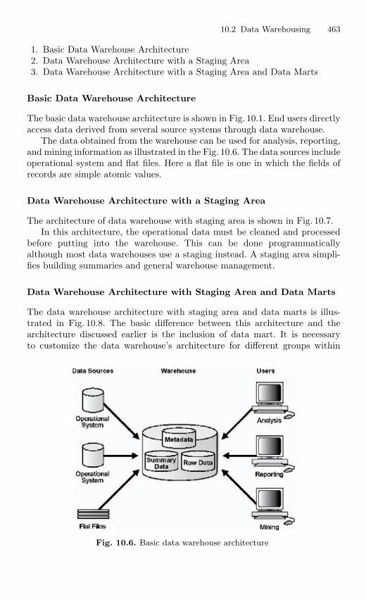
10.2 Data Warehousing 463
1. Basic Data Warehouse Architecture2. Data Warehouse Architecture with a Staging Area3. Data Warehouse Architecture with a Staging Area and Data Marts
Basic Data Warehouse Architecture
The basic data warehouse architecture is shown in Fig. 10.1. End users directlyaccess data derived from several source systems through data warehouse.
The data obtained from the warehouse can be used for analysis, reporting,and mining information as illustrated in the Fig. 10.6. The data sources includeoperational system and flat files. Here a flat file is one in which the fields ofrecords are simple atomic values.
Data Warehouse Architecture with a Staging Area
The architecture of data warehouse with staging area is shown in Fig. 10.7.In this architecture, the operational data must be cleaned and processed
before putting into the warehouse. This can be done programmaticallyalthough most data warehouses use a staging instead. A staging area simpli-fies building summaries and general warehouse management.
Data Warehouse Architecture with Staging Area and Data Marts
The data warehouse architecture with staging area and data marts is illus-trated in Fig. 10.8. The basic difference between this architecture and thearchitecture discussed earlier is the inclusion of data mart. It is necessaryto customize the data warehouse’s architecture for different groups within
Fig. 10.6. Basic data warehouse architecture
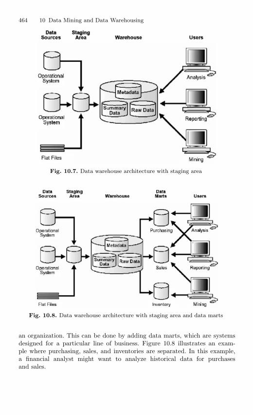
464 10 Data Mining and Data Warehousing
Fig. 10.7. Data warehouse architecture with staging area
Fig. 10.8. Data warehouse architecture with staging area and data marts
an organization. This can be done by adding data marts, which are systemsdesigned for a particular line of business. Figure 10.8 illustrates an exam-ple where purchasing, sales, and inventories are separated. In this example,a financial analyst might want to analyze historical data for purchasesand sales.
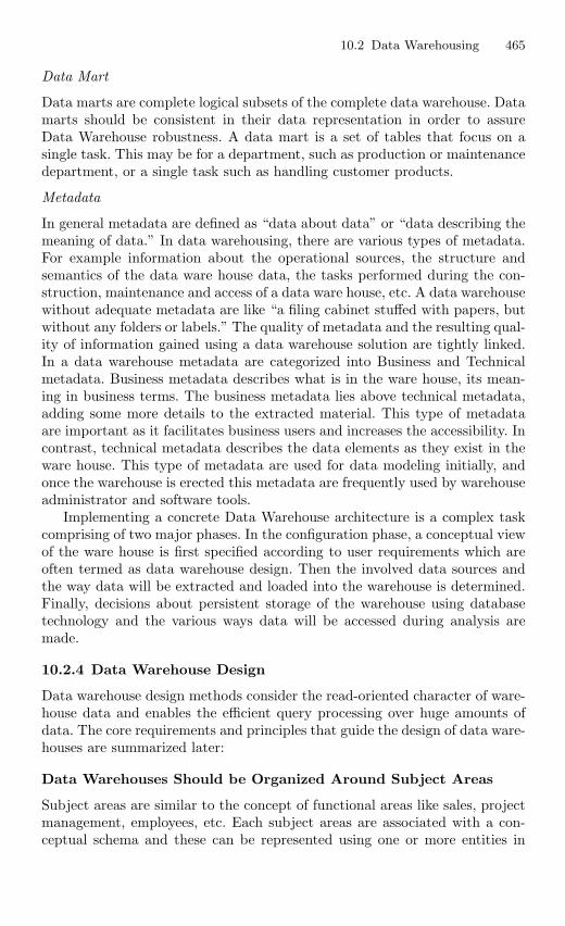
10.2 Data Warehousing 465
Data Mart
Data marts are complete logical subsets of the complete data warehouse. Datamarts should be consistent in their data representation in order to assureData Warehouse robustness. A data mart is a set of tables that focus on asingle task. This may be for a department, such as production or maintenancedepartment, or a single task such as handling customer products.
Metadata
In general metadata are defined as “data about data” or “data describing themeaning of data.” In data warehousing, there are various types of metadata.For example information about the operational sources, the structure andsemantics of the data ware house data, the tasks performed during the con-struction, maintenance and access of a data ware house, etc. A data warehousewithout adequate metadata are like “a filing cabinet stuffed with papers, butwithout any folders or labels.” The quality of metadata and the resulting qual-ity of information gained using a data warehouse solution are tightly linked.In a data warehouse metadata are categorized into Business and Technicalmetadata. Business metadata describes what is in the ware house, its mean-ing in business terms. The business metadata lies above technical metadata,adding some more details to the extracted material. This type of metadataare important as it facilitates business users and increases the accessibility. Incontrast, technical metadata describes the data elements as they exist in theware house. This type of metadata are used for data modeling initially, andonce the warehouse is erected this metadata are frequently used by warehouseadministrator and software tools.
Implementing a concrete Data Warehouse architecture is a complex taskcomprising of two major phases. In the configuration phase, a conceptual viewof the ware house is first specified according to user requirements which areoften termed as data warehouse design. Then the involved data sources andthe way data will be extracted and loaded into the warehouse is determined.Finally, decisions about persistent storage of the warehouse using databasetechnology and the various ways data will be accessed during analysis aremade.
10.2.4 Data Warehouse Design
Data warehouse design methods consider the read-oriented character of ware-house data and enables the efficient query processing over huge amounts ofdata. The core requirements and principles that guide the design of data ware-houses are summarized later:
Data Warehouses Should be Organized Around Subject Areas
Subject areas are similar to the concept of functional areas like sales, projectmanagement, employees, etc. Each subject areas are associated with a con-ceptual schema and these can be represented using one or more entities in
466 10 Data Mining and Data Warehousing
the ER data model or by one or more object classes in the object orienteddata model. For example: In company database the relations like employee,sales, and project management are represented as entities in ER data modelor object classes in object oriented data model.
Data Warehouses Should have some Integration Capability
A common database should be designed and used so that all the differentindividual representations can be mapped to it. This is particularly useful ifthe warehouse is implemented as multidatabase or federated database.
Data should be Nonvolatile and Mass Loaded
Data in Data Warehouses should be nonvolatile. For this data extraction fromcurrent database to DW requires that a decision should be made whether toextract the data using standard relational database techniques at the rowor column level or specialized techniques for mass extraction. Data cleaningtechniques are required to maintain data quality, similarly data migration,data scrubbing, and data auditing. Refresh techniques propagate updates onthe source data to base data and derived data in the DW. The decision ofwhen and how to refresh is made by the DW administrator and depends onuser needs (e.g., OLAP needs) and existing traffic to the DW.
Data Tends to Exist at Multiple Levels of Dimensions
Data can be defined not only by time frame but also by geographic region;type of product manufactured or sold type of store and so on. The completesize of the databases is a major problem in the design and implementationof data warehouses, especially for certain queries and updates and sequentialbackups. This decides whether to select relational databases or multidimen-sional database for the implementation of a data warehouse.
Data Warehouse Should be Flexible Enough to Meet ChangingRequirements Rapidly
Insertion, updating, and retrieval of data should be very efficient and flexibleto achieve good and efficient decision.
Data Warehouse Should have a Capability for Rewriting History,that is, Allowing for “what-if” Analysis
Data Warehouse should allow the administrator to update historical data tem-porarily for the purpose of “what-if” analysis. Once the analysis is completed,the data must be correctly rolled back. This assumes that the data must beat the proper dimension in the first place.
10.2 Data Warehousing 467
Good DW User Interface Should be Selected
The interface should be very user friendly for efficient use of DW. The leadingchoices of today are SQL.
Data Should be Either Centralized or Distributed Physically
The DW should have the capability to handle distributed data over a network.This requirement will become more critical as the use of DWs grows andsources of data expand.
10.2.5 Classification of Data Warehouse Design
The data warehouse design can be broadly classified into two categories(1) Logical design and (2) Physical design.
Logical Design
The logical design is more conceptual and abstract than physical design.In the logical design, the emphasis is on the logical relationship among theobjects. One technique that can be used to model organization’s logical infor-mation requirements is entity-relationship modeling. Entity-relationship mod-eling involves identifying the things of importance (entities), the propertiesof these things (attributes), and how they are related to one another (rela-tionships). The process of logical design involves arranging data into a seriesof logical relationships called entities and attributes. An entity represents achunk of information. In relational databases, an entity often maps to table.An attribute is a component of an entity that helps define the uniqueness ofthe entity. In relational databases, an attribute maps to a column. Whereasentity-relationship diagramming has traditionally been associated with highlynormalized models such as OLTP applications, the technique is still useful fordata warehouse design in the form of dimensional modeling.
In dimensional modeling, instead of seeking to discover atomic units ofinformation and all the relationship between them, the focus is on identify-ing which information belongs to a central fact table and which informationbelongs to its associated dimension tables. In a nutshell, the logical designshould result in (a) a set of entities and attributes corresponding to fact ta-bles and dimension tables and (b) a model of operational data from the sourceinto subject-oriented information in target data warehouse schema. Some ofthe logical warehouse design tools from Oracle are Oracle Warehouse Builder,Oracle Designer, which is a general purpose modeling tool.
Data Warehousing Schemas
A schema is a collection of database objects, including tables, views, indexes,and synonyms. The arrangement of schema objects in the schema models
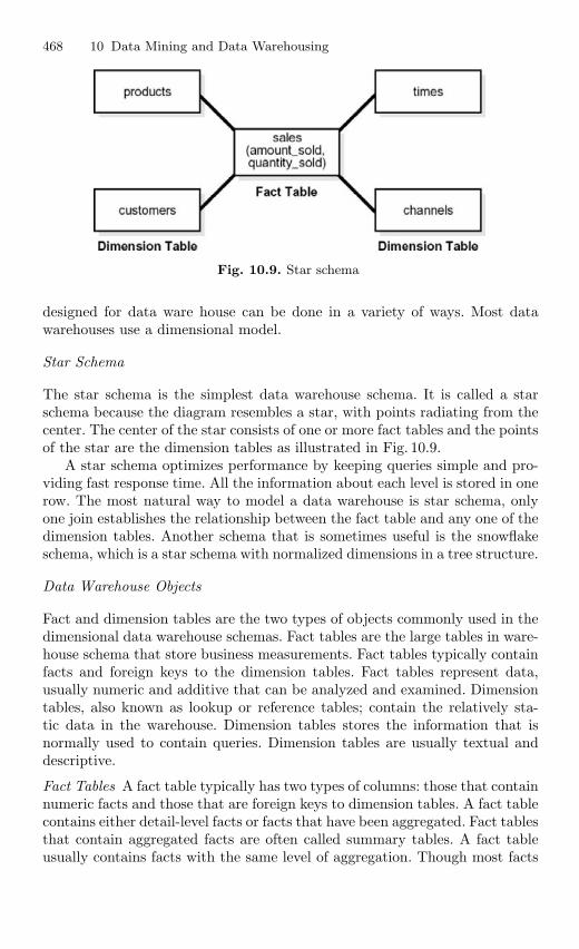
468 10 Data Mining and Data Warehousing
Fig. 10.9. Star schema
designed for data ware house can be done in a variety of ways. Most datawarehouses use a dimensional model.
Star Schema
The star schema is the simplest data warehouse schema. It is called a starschema because the diagram resembles a star, with points radiating from thecenter. The center of the star consists of one or more fact tables and the pointsof the star are the dimension tables as illustrated in Fig. 10.9.
A star schema optimizes performance by keeping queries simple and pro-viding fast response time. All the information about each level is stored in onerow. The most natural way to model a data warehouse is star schema, onlyone join establishes the relationship between the fact table and any one of thedimension tables. Another schema that is sometimes useful is the snowflakeschema, which is a star schema with normalized dimensions in a tree structure.
Data Warehouse Objects
Fact and dimension tables are the two types of objects commonly used in thedimensional data warehouse schemas. Fact tables are the large tables in ware-house schema that store business measurements. Fact tables typically containfacts and foreign keys to the dimension tables. Fact tables represent data,usually numeric and additive that can be analyzed and examined. Dimensiontables, also known as lookup or reference tables; contain the relatively sta-tic data in the warehouse. Dimension tables stores the information that isnormally used to contain queries. Dimension tables are usually textual anddescriptive.
Fact Tables A fact table typically has two types of columns: those that containnumeric facts and those that are foreign keys to dimension tables. A fact tablecontains either detail-level facts or facts that have been aggregated. Fact tablesthat contain aggregated facts are often called summary tables. A fact tableusually contains facts with the same level of aggregation. Though most facts
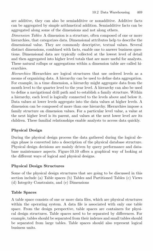
10.2 Data Warehousing 469
are additive, they can also be semiadditive or nonadditive. Additive factscan be aggregated by simple arithmetical addition. Semiadditive facts can beaggregated along some of the dimensions and not along others.Dimension Tables A dimension is a structure, often composed of one or morehierarchies, that categorizes data. Dimensional attributes help to describe thedimensional value. They are commonly descriptive, textual values. Severaldistinct dimensions, combined with facts, enable one to answer business ques-tions. Dimensional data are typically collected at the lowest level of detailand then aggregated into higher level totals that are more useful for analysts.These natural rollups or aggregations within a dimension table are called hi-erarchies.Hierarchies Hierarchies are logical structures that use ordered levels as ameans of organizing data. A hierarchy can be used to define data aggregation.For example, in a time dimension, a hierarchy might aggregate data from themonth level to the quarter level to the year level. A hierarchy can also be usedto define a navigational drill path and to establish a family structure. Withina hierarchy, each level is logically connected to the levels above and below it.Data values at lower levels aggregate into the data values at higher levels. Adimension can be composed of more than one hierarchy. Hierarchies impose afamily structure on dimension values. For a particular level value, a value atthe next higher level is its parent, and values at the next lower level are itschildren. These familial relationships enable analysts to access data quickly.
Physical Design
During the physical design process the data gathered during the logical de-sign phase is converted into a description of the physical database structure.Physical design decisions are mainly driven by query performance and data-base maintenance aspects. Figure 10.10 offers a graphical way of looking atthe different ways of logical and physical designs.
Physical Design Structures
Some of the physical design structures that are going to be discussed in thissection include (a) Table spaces (b) Tables and Partitioned Tables (c) Views(d) Integrity Constraints, and (e) Dimensions
Table Spaces
A table space consists of one or more data files, which are physical structureswithin the operating system. A data file is associated with only one tablespace. From the design perspective, table spaces are containers for physi-cal design structures. Table spaces need to be separated by differences. Forexample, tables should be separated from their indexes and small tables shouldbe separated from large tables. Table spaces should also represent logicalbusiness units.
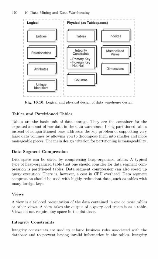
470 10 Data Mining and Data Warehousing
Fig. 10.10. Logical and physical design of data warehouse design
Tables and Partitioned Tables
Tables are the basic unit of data storage. They are the container for theexpected amount of raw data in the data warehouse. Using partitioned tablesinstead of nonpartitioned ones addresses the key problem of supporting verylarge data volumes by allowing you to decompose them into smaller and moremanageable pieces. The main design criterion for partitioning is manageability.
Data Segment Compression
Disk space can be saved by compressing heap-organized tables. A typicaltype of heap-organized table that one should consider for data segment com-pression is partitioned tables. Data segment compression can also speed upquery execution. There is, however, a cost in CPU overhead. Data segmentcompression should be used with highly redundant data, such as tables withmany foreign keys.
Views
A view is a tailored presentation of the data contained in one or more tablesor other views. A view takes the output of a query and treats it as a table.Views do not require any space in the database.
Integrity Constraints
Integrity constraints are used to enforce business rules associated with thedatabase and to prevent having invalid information in the tables. Integrity
10.2 Data Warehousing 471
constraints in data warehousing differ from constraints in OLTP environ-ments. In OLTP environments, they primarily prevent the insertion of invaliddata into a record, which is not a big problem in data warehousing environ-ments because accuracy has already been guaranteed. In data warehousingenvironments, constraints are only used for query rewrite. NOT NULL con-straints are particularly common in data warehouses. Under some specificcircumstances, constraints need space in the database. These constraints arein the form of the underlying unique index.
Indexes and Partitioned Indexes
Indexes are optional structures associated with tables or clusters. In addi-tion to the classical B-tree indexes, bitmap indexes are very common in datawarehousing environments. Bitmap indexes are optimized index structures forset-oriented operations. Additionally, they are necessary for some optimizeddata access methods such as star transformations.
Dimensions
A dimension is a schema object that defines hierarchical relationships betweencolumns or column sets. A hierarchical relationship is a functional dependencyfrom one level of a hierarchy to the next one. A dimension is a container oflogical relationships and does not require any space in the database. A typicaldimension is city, state (or province), region, and country.
10.2.6 The User Interface
In this section, we provide a brief introduction to contemporary interfaces fordata warehouses. A variety of tools are available to query and analyze datastored in data warehouses. These tools can be classified as follows:
(a) Traditional query and reporting tools(b) On-line analytical processing, MOLAP, and ROLAP tools(c) Data-mining tools(d) Data-visualization tools
Traditional Query and Reporting Tools
Traditional query and reporting tools include spreadsheets, personal computerdatabases, and report writers and generators
OLAP Tools
On-Line Analytical Processing is the use of a set of graphical tools thatprovides users with multidimensional views of their data and allows themto analyze the data using simple windowing techniques. The term on-line
472 10 Data Mining and Data Warehousing
analytical processing is intended to contrast with the more traditional termon-line transaction processing. OLAP is a general term for several categoriesof data warehouse and data mart access tools. Relational OLAP (ROLAP)tools use variations of SQL and view the database as a traditional relationaldatabase, in either a star schema or other normalized or denormalized set oftables. ROLAP tools access the data warehouse or data mart directly. Multidi-mensional OLAP (MOLAP) loads data into an intermediate structure usuallya three or higher dimensional array.
Data-Mining Tools
Data mining is knowledge discovery using a sophisticated blend of techniquesfrom traditional statistics, artificial intelligence, and computer graphics. Asthe amount of data in data warehouses is growing exponentially, the usersrequire automated techniques provided by data-mining tools to mine theknowledge in these data.
Data Visualization Tools
Data-visualization is the representation of data in graphical and multimediaformats for human analysis. Benefits of data visualization include the abilityto better observe trends and patterns, and to identify correlations and clusters.
Summary
Data mining is a form of knowledge discovery that uses a sophisticated blendof techniques from traditional statistics, artificial intelligence, and computergraphics. In this chapter, a brief introduction to data mining is given whichincludes need for data mining, data mining functionalities, and classificationof data mining systems. This chapter also discusses major issues in data min-ing, data mining primitives, and data mining tasks, and gives syntax for datamining query language. The data mining architecture, data mining associationrules for large database, and multilevel database for transaction are discussedin depth in this chapter. This chapter also discusses the concepts of classifi-cation and prediction, which are two forms of data analysis that can be usedto extract models describing important data classes or predict future datatrends. The different types of classification methods are explain in detail.
The process of grouping a set of physical or abstract objects into classesof similar objects is called clustering. A cluster is a collection of data objectsthat are similar to one another within the same cluster and are dissimilarto the objects in other clusters. This chapter gives brief idea about cluster
Review Questions 473
analysis. This chapter also gives an idea of how to choose data mining system,applications and trends in data mining.
The purpose of data warehouse is to consolidate and integrate data from avariety of sources, and to format those data in a context for making accuratebusiness decisions. A data warehouse is an integrated and consistent storeof subject-oriented data obtained from a variety of sources and formattedinto a meaningful context to support decision making in an organization.This chapter discusses the goals of data warehousing, characteristics of datain a data warehouse, and different types of data warehouse architectures.Two types of data warehouse design like logical and physical data warehousedesign are discussed in depth. Finally, the user interface which gives a briefintroduction to contemporary interfaces for data warehouses is discussed.
Review Questions
10.1. What is the need for data mining?
Data mining is the process of discovering interesting knowledge from largeamounts of data stored in databases, data warehouses, or other informationrepositories. The volume of data in an organization increases day by day, inorder to extract useful information from huge volume of data, data mining isnecessary.
10.2. What are the functionalities of data mining system?
Functionalities of data mining are used to specify the kind of patterns to befound in data mining tasks. It can be classified into two categories such asDescriptive and Predictive. Descriptive mining task characterize the generalproperties of data in the database, whereas predictive mining task performinference on the current data in order to make predictions.
10.3. Explain the “binning” method of data cleaning?
Binning method smoothen the sorted data value by consulting its “neighbor-hood” that is, the values around it. The sorted values are distributed intonumber of “buckets,” or bins:
– Smoothing by bin means each value in a bin is replace by the mean valueof the bin.
– Smoothing by bin medians means each bin value replaces bin median.
10.4. What are the performance issues in data mining?
The performance issues in data mining include efficiency, scalability, andparallelization of data mining algorithms.
474 10 Data Mining and Data Warehousing
10.5. Explain the concept of classification and prediction with respect to datamining?
Databases are rich with hidden information that can be used for makingintelligent business decisions. Classification and prediction are two forms ofdata analysis that can be used to extract models describing important dataclasses or predict future data trends. Whereas classification predicts categor-ical labels, prediction models continuous-valued functions.
10.6. What are the factors to be considered in designing data mining querylanguage?
Designing a comprehensive data mining language is challenging because datamining covers wide spectrum of task, from data characterization to miningassociation rules, data classification and evaluation analysis.
Designing the data mining query language is specified by the followingprimitives:
– The kind of knowledge to be mined.– The background knowledge to be used in the discovery process.– The Interestingness measures and threshold or pattern evaluation.
10.7. Mention the challenges involved in mining spatial data?
A crucial challenge to spatial data mining is the exploration of efficient spa-tial data mining techniques due to the huge amount of spatial data and thecomplexity of spatial data types and spatial access methods. Spatial datamining allows the extension of traditional spatial analysis method by placingemphasis on efficiency, scalability, and co-operation with database systems,improved interaction with the user and discovery of new types of knowledge.
10.8. What is the need for Data Warehousing in an organization?
The need for Data Warehousing in most organizations is:
– A business requires an integrated, company-wide view of high-quality in-formation.
– The information systems department must separate informational fromoperational systems in order to dramatically improve performance in man-aging company data.
10.9. Define the term “data mart”?
A data mart is a data warehouse that is limited in scope, whose data areobtained by selecting and summarizing data from a data warehouse or fromseparate extract, transform, and load processes from source data systems.
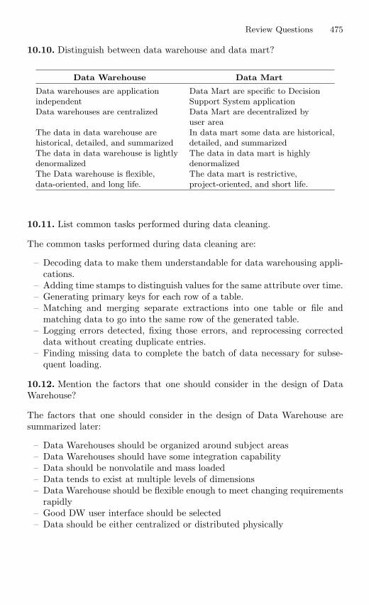
Review Questions 475
10.10. Distinguish between data warehouse and data mart?
Data Warehouse Data Mart
Data warehouses are application Data Mart are specific to Decisionindependent Support System applicationData warehouses are centralized Data Mart are decentralized by
user areaThe data in data warehouse are In data mart some data are historical,historical, detailed, and summarized detailed, and summarizedThe data in data warehouse is lightly The data in data mart is highlydenormalized denormalizedThe Data warehouse is flexible, The data mart is restrictive,data-oriented, and long life. project-oriented, and short life.
10.11. List common tasks performed during data cleaning.
The common tasks performed during data cleaning are:
– Decoding data to make them understandable for data warehousing appli-cations.
– Adding time stamps to distinguish values for the same attribute over time.– Generating primary keys for each row of a table.– Matching and merging separate extractions into one table or file and
matching data to go into the same row of the generated table.– Logging errors detected, fixing those errors, and reprocessing corrected
data without creating duplicate entries.– Finding missing data to complete the batch of data necessary for subse-
quent loading.
10.12. Mention the factors that one should consider in the design of DataWarehouse?
The factors that one should consider in the design of Data Warehouse aresummarized later:
– Data Warehouses should be organized around subject areas– Data Warehouses should have some integration capability– Data should be nonvolatile and mass loaded– Data tends to exist at multiple levels of dimensions– Data Warehouse should be flexible enough to meet changing requirements
rapidly– Good DW user interface should be selected– Data should be either centralized or distributed physically
11
Objected-Oriented and Object RelationalDBMS
Learning Objectives. This chapter provides an overview of object oriented andobject relational database management system. The need for object oriented con-cepts in DBMS, OODBMS, and ORDBMS are discussed elaborately in this chapter.The evaluation criteria and targets with respect to OODBMS and comparison ofOODBMS with ORDBMS are also dealt with. After completing this chapter thereader should be familiar with the following concepts:
– Object oriented programming language– Availability of OO Technology and applications– Overview of OODBMS Technology– Evaluation Criteria for OODBMS– Evaluation targets– Overview of ORDBMS– ORDBMS Design– Aggregation and Composition in UML– Comparison of ORDBMS and OODBMS
11.1 Objected oriented DBMS
11.1.1 Introduction
This chapter provides a simple view about the Object-Oriented DatabaseManagement Systems (OODBMS). Each OODBMS will be architected basedon a set of assumptions which make it more or less suited for particularapplication domains and usage patterns. Thus, a single OODBMS will notbe the best in all situations. This chapter will also be used as an introductionto object-oriented database technology.
An evaluation of OODBMS must include analysis in four areas:
– Functionality– Usability– Platform– Performance
S. Sumathi: Objected-Oriented and Object Relational DBMS, Studies in Computational
Intelligence (SCI) 47, 477–558 (2007)
www.springerlink.com c© Springer-Verlag Berlin Heidelberg 2007
478 11 Objected-Oriented and Object Relational DBMS
Functionality
An analysis of functional capabilities is performed to determine if a givenOODBMS provides sufficient capabilities to meet the current and future needsof a given development effort. Functional capabilities include basic databasefunctionality, such as concurrency control and recovery as well as object-oriented database features, such as inheritance and versioning. Each evalu-ation will have to identify and weight a set of functional requirements to bemet by the candidate OODBMS. Weighting is an important considerationsince application workarounds may be possible for missing functionality.
Usability
Usability deals with the application development and maintenance process. Is-sues include development tools and the ease with which database applicationscan be developed and maintained. How a developer perceives the databaseand the management of persistent objects might also be considered underthe category of usability. Other issues to be considered are database admin-istration, product maturity, and vendor support. Evaluation of usability islikely to be highly subjective. Perhaps the most easily measurable evalua-tion criterion is platform. An OODBMS is either available or not on theapplication’s target hardware and operating system. Heterogeneous targetenvironments require that the OODBMS transparently interoperates withinthat environment.
Platform
An OODBMS is typically a multiprocessed software system communicatingover a local area network. Platforms upon which database server processes,client application processes, additional administration processes (e.g., lockservers), and development tools can be hosted must be considered. Networkrequirements should also be evaluated. Performance may represent the mostimportant evaluation criteria. The University of Wisconsin has performed abenchmarking of OODBMS, known as the 007 benchmark. A general purposebenchmark is only effective in predicting the performance of an OODBMS foran application which closely mirrors the behavior of that benchmark.
Performance
An effective benchmark must consider the number of interactive users, therate of database updates and accesses, the size of the databases, the hardwareand network configurations, and the general access patterns of the databaseapplications. Thus, in order to provide useful information, a benchmark mustbe modeled to closely mimic the expected behavior of the application being
11.1 Objected oriented DBMS 479
developed. Providing a fair and substantive evaluation of OODBMS is a dif-ficult task. Issues regarding accuracy of marketing information and technicaldocumentation, completeness of implementation, usability of implementation,performance, and feature interaction (regarding completeness, usability, andperformance) must be considered when performing the evaluation. The objec-tive of this chapter is to perform the first part of this evaluation process byperforming an extensive analysis based on technical product documentation.In particular:
– Functional capabilities have been identified by examination of theproduct’s technical manuals as supplied by the vendor. Discussions withtechnical representatives of the vendor have been used to clarify ourunderstandings and descriptions of the evaluated products.
– Usability has been derived by analyzing the documentation for the vendorsupplied tools and by reviewing the application programming interface inorder to understand how an application interacts with the database.
– Information regarding platform and heterogeneous operation has beensupplied by the product vendors.
– Performance is not addressed as part of this evaluation.
Benefits of Object Oriented Programming
There are several benefits of adopting OOP. The following three benefits,although subjective, are considered by many to be major reasons for adoptingOOP:
– Programs reflect reality.– The model is more stable than functionality.– Subclassing and virtuals improve the reusability of code.
11.1.2 Object-Oriented Programming Languages (OOPLs)
The following is a list of some popular OOPLs:
– C++ Language System– C Talk– Smalltalk– Smalltalk-80– Actor– Enfin– Prokappa– Eiffel– KnowledgePro– Classic-Ada with Persistence– Objective-C– Trellis/Owl
480 11 Objected-Oriented and Object Relational DBMS
– Flavors– CLOS– Common Loops
Most OOPLs can trace their origins to Simula. The concepts of Objectsand Classes are employed by most of these languages.
Comparing OOPLs
Different OOPLs are appropriate for different environments. For corporateenvironments Smalltalk is better than C++. Smalltalk is a higher level lan-guage and will be COBOL of the OO world in the future.
Smalltalk, Flavors, and Objective-C allows free access to inherited instancevariables by descendant classes. Other OOPLs, like C++, restrict accessto inherited instance variables. Where access to inherited instance vari-ables is needed, it should be provided in the form of operations. OnlyCLOS permits specific instances of classes to have behavior independent oftheir classes.
Objective-C
Objective-C is considered by some researchers to be a cross between C andSmalltalk. It is possible to precompile Objective-C code to produce standardC as output. Objective-C incorporates the concept of an object identifier, id,which is a handle for referring to an object in a message expression. Object-Cis a compiled language, unlike Smalltalk and CLOS.
C++:
C++ is the most popular OOPL. It is an object-oriented extension to C,developed at AT&T Bell Laboratories. C++ supports the OOP concepts ofobjects, classes, inheritance, polymorphism, and parameterized types. TheC++ class concept can be considered as a generalization of the C feature ofa “struct.”
C++ has been evolving since it was released by AT&T as version of Cwith classes in 1984. The latest release is version 3.1, and it provides multi-ple inheritance, type-safe linkages, abstract classes, and a form of exceptionhandling.
C++ provides an access control mechanism for the operations on objects.The operations are called member functions. Member functions can have oneof the following three modes of access:
– Public– Private– Protected
11.1 Objected oriented DBMS 481
Public member functions are accessible by all clients of the object. Privatemember functions are accessible only by other member functions of the class.Protected member functions are accessible only by other member functions ofclass derived from that class.
11.1.3 Availability of OO Technology and Applications
Some of the OO technologies that are being used to develop software appli-cation products are:
– Case tools based on OOT– Analysis and design tools, some with OO capabilities– Knowledge-based systems– Hypermedia, Hypertext– GUI front ends– Object DBMS– Radial application development environments
In the commercial CASE environments, vendors are employing OOT forall their products. GUI tools are mostly designed using OO concepts, andclasses of GUI tools are widely available.
Transition to OOT
OOT has the reputation of requiring a learning curve. This is not only dueto the necessity of learning a new language, but also due to the necessity ofunlearning process oriented programming techniques. Because of the differ-ence between the top–down structured programming and the OO techniques,the transition from a traditional structured programming environment to theobject oriented environment requires a high investment of time and energy.
Containing Relationships Between Objects
Quite often, objects that contain other objects need to be represented in sucha way that they are logically regarded as a single object. It is important toprovide for containing relationships by which the composite logical object canrefer to the contained objects. Typically, the contained objects are treated asprivate objects of enclosing object. This encapsulation might not be appro-priate if such a tight coupling is not desired.
Modeling Relationships in C++
Interactions between objects can be captured during OOD by appropriaterelationships. At the implementation level, C++ provides the following mech-anisms for implementing object relationships:
1. Global Objects2. Function arguments
482 11 Objected-Oriented and Object Relational DBMS
3. Constructors4. Base classes5. Templates
Using Relationship Between Objects
Objects interacting in a system make use of the services offered by otherobjects. The using relationship can be used to express a subset of such inter-actions. Booch and Vilot have identified three roles that each object may playin using relationships:
Actor objects can operate upon other objects, but are never operated uponby other objects. Such objects make use of services offered by other objectsbut do not themselves provide any service to the objects they make use of.
Server objects never operate upon objects, but are operated upon by otherobjects.
Agent objects can both operate upon other objects and be operated uponby other objects.
Relationships Among Classes
Rumbaugh has identified three types of class relationships:
1. Generalization or “kind-of”2. Aggregation or “part-of”3. Association, implying some semantic connection.
Booch and Vilot have identified two more types of relationships betweenclasses
1. Instantiation relationships2. Metaclass relationships
Booch and Vilot suggest the following rule of thumb for identifying rela-tionships: “If an abstraction is more than the sum of its component parts,then using relationships are more appropriate. If an abstraction is a kind ofsome other abstraction or if that abstraction is exactly equal to the sum ofits components, then inheritance is a better approach.”
11.1.4 Overview of OODBMS Technology
This section deals with Need, Evolution, Characteristics, and Applications ofObject Oriented Databases Technology.
The Need for Object-Oriented Databases
The increased emphasis on process integration is a driving force for the adop-tion of object-oriented database systems. For example, the Computer Inte-grated Manufacturing (CIM) area is focusing heavily on using object-orienteddatabase technology as the process integration framework. Advanced office
11.1 Objected oriented DBMS 483
automation systems use object-oriented database systems to handle hyperme-dia data. Hospital patient care tracking systems use object-oriented databasetechnologies for ease of use. All of these applications are characterized by hav-ing to manage complex, highly interrelated information, which is strength ofobject-oriented database systems.
Clearly, relational database technology has failed to handle the needsof complex information systems. The problem with relational database sys-tems is that they require the application developer to force an informationmodel into tables where relationships between entities are defined by values.Mary Loomis, the architect of the Versant OODBMS compares relational andobject-oriented databases. “Relational database design is really a process oftrying to figure out how to represent real-world objects within the confinesof tables in such a way that good performance results and preserving dataintegrity is possible. Object database design is quite different. For most parts,object database design is a fundamental part of the overall application designprocess. The object classes used by the programming language are the classesused by the ODBMS. Because their models are consistent, there is no need totransform the program’s object model to something unique for the databasemanager.
An initial area of focus by several object-oriented database vendors hasbeen the Computer Aided Design (CAD), Computer Aided Manufacturing(CAM), and Computer Aided Software Engineering (CASE) applications. Aprimary characteristic of these applications is the need to manage very com-plex information efficiently. Other areas where object-oriented database tech-nology can be applied include factory and office automation. For example, themanufacture of an aircraft requires the tracking of millions of interdependentparts that may be assembled in different configurations. Object-oriented data-base systems hold the promise of putting solutions to these complex problemswithin reach of users.
Object-orientation is yet another step in the quest for expressing solutionsto problems in a more natural, easier to understand way. Michael Brodie inhis book On Conceptual Modeling states “the fundamental characteristic ofthe new level of system description is that it is closer to the human con-ceptualization of a problem domain. Descriptions at this level can enhancecommunication between system designers, domain experts and, ultimately,system end-users.”
The study of database history is centered on the problem of data modeling.“A data model is a collection of mathematically well defined concepts thathelp one to consider and express the static and dynamic properties of dataintensive applications.”
A data model consists of:– Static properties such as objects, attributes and relationships– Integrity rules over objects and operations– Dynamic properties such as operations or rules defining new database
states based on applied state changes
484 11 Objected-Oriented and Object Relational DBMS
Object-oriented databases have the ability to model all three of these com-ponents directly within the database supporting a complete problem/solutionmodeling capability. Prior to object-oriented databases, databases were ca-pable of directly supporting points 1 and 2 above and relied on applicationsfor defining the dynamic properties of the model. The disadvantage of del-egating the dynamic properties to applications is that these dynamic prop-erties could not be applied uniformly in all database usage scenarios sincethey were defined outside the database in autonomous applications. Object-oriented databases provide a unifying paradigm that allows one to integrateall three aspects of data modeling and to apply them uniformly to all usersof the database.
The Evolution of Object-Oriented Databases
Object-oriented database research and practice dates back to the late 1970sand had become a significant research area by the early 1980s, with initial com-mercial product offerings appearing in the late 1980s. Today, there are manycompanies marketing commercial object-oriented databases that are secondgeneration products. The growth in the number of object-oriented databasecompanies has been remarkable. As both the user and vendor communitiesgrow there will be a user pull to mature these products to provide robust datamanagement systems.
OODBMS’s have established themselves in niches such as e-commerce,engineering product data management, and special purpose databases inareas such as securities and medicine. The strength of the object modelis in applications where there is an underlying needed to manage complexrelationships among data objects. Today, it is unlikely that OODBMS are athreat to the stranglehold that relational database vendors have in the marketplace. Clearly, there is a partitioning of the market into databases that arebest suited for handling high volume low complexity data and databases thatare suited for high complexity, reasonable volume, with OODBMS filling theneed for the latter.
Object-oriented databases are following a maturation path similar torelational databases. Figure 11.1 depicts the evolution of object-orienteddatabase technologies. On the left, we have object-oriented languages thathave been extended to provide simple persistence allowing application objectsto persist between user sessions. Minimal database functionality is providedin terms of concurrency control, transactions, recovery, etc. At the mid-point,we have support for many of the common database features mentioned earlier.Database products at the mid-point are sufficient for developing reasonablycomplex data management applications. Finally, database products withdeclarative semantics have the ability to greatly reduce development efforts,as well to enforce uniformity in the application of these semantics. OODBMSproducts today are largely in the middle with a few products exhibiting declar-ative semantics, such as constraints, referential integrity rules, and security
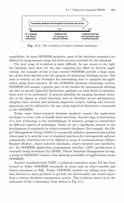
11.1 Objected oriented DBMS 485
Fig. 11.1. The evolution of object-oriented databases
capabilities. In most OODBMS products, most of the database semantics aredefined by programmers using low-level services provided by the database.
The next stage of evolution is more difficult. As one moves to the rightthe database does more for the user requiring less effort to develop appli-cations. An example of this is that current OODBMS provide a large num-ber of low-level interfaces for the purpose of optimizing database access. Theonus is entirely on the developer for determining how to optimize his appli-cation using these features. As the OODBMS database technology evolves,OODBMS will assume a greater part of the burden for optimization allowingthe user to specify high-level declarative guidance on what kinds of optimiza-tions need to be performed. A general guideline for gauging database matu-rity is the degree to which functions such as database access optimization,integrity rules, schema and database migration, archive, backup and recoveryoperations can be tailored by the user using high-level declarative commandsto the OODBMS.
Today, most object-oriented database products require the applicationdeveloper to write code to handle these functions. Another sign of maturationof a new technology is the establishment of industry groups to standardizeon different aspects of technology. Today we see a significant interest in thedevelopment of standards for object-oriented databases. For example, the Ob-ject Management Group (OMG) is a nonprofit industry sponsored associationwhose goal is to provide a set of standard interfaces for interoperable softwarecomponents. Interfaces are to be defined in areas of communications (ObjectRequest Broker), object-oriented databases, object-oriented user interfaces,etc. An OODBMS application programmers interface (API) specification iscurrently being developed (by ODMG, Object Database Management Group,a group of OODBMS vendors) thus allowing portability of applications acrossOODBMS.
Another standards body X3H7, a technical committee under X3, has beenformed to define OODBMS standards in areas such as object-models andobject-extensions to SQL. Today, OODBMS vendors are adding more data-base features to their products to provide the functionality one would expectfrom a mature database management system. This evolution moves us to themid-point of the evolutionary scale shown in Fig. 11.1.
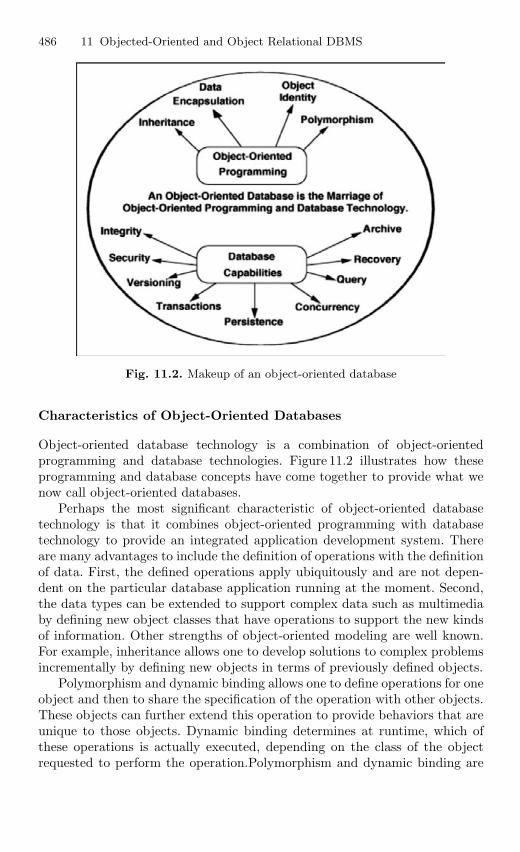
486 11 Objected-Oriented and Object Relational DBMS
Fig. 11.2. Makeup of an object-oriented database
Characteristics of Object-Oriented Databases
Object-oriented database technology is a combination of object-orientedprogramming and database technologies. Figure 11.2 illustrates how theseprogramming and database concepts have come together to provide what wenow call object-oriented databases.
Perhaps the most significant characteristic of object-oriented databasetechnology is that it combines object-oriented programming with databasetechnology to provide an integrated application development system. Thereare many advantages to include the definition of operations with the definitionof data. First, the defined operations apply ubiquitously and are not depen-dent on the particular database application running at the moment. Second,the data types can be extended to support complex data such as multimediaby defining new object classes that have operations to support the new kindsof information. Other strengths of object-oriented modeling are well known.For example, inheritance allows one to develop solutions to complex problemsincrementally by defining new objects in terms of previously defined objects.
Polymorphism and dynamic binding allows one to define operations for oneobject and then to share the specification of the operation with other objects.These objects can further extend this operation to provide behaviors that areunique to those objects. Dynamic binding determines at runtime, which ofthese operations is actually executed, depending on the class of the objectrequested to perform the operation.Polymorphism and dynamic binding are
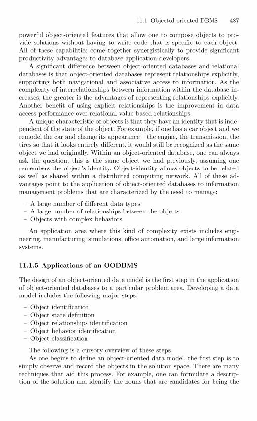
11.1 Objected oriented DBMS 487
powerful object-oriented features that allow one to compose objects to pro-vide solutions without having to write code that is specific to each object.All of these capabilities come together synergistically to provide significantproductivity advantages to database application developers.
A significant difference between object-oriented databases and relationaldatabases is that object-oriented databases represent relationships explicitly,supporting both navigational and associative access to information. As thecomplexity of interrelationships between information within the database in-creases, the greater is the advantages of representing relationships explicitly.Another benefit of using explicit relationships is the improvement in dataaccess performance over relational value-based relationships.
A unique characteristic of objects is that they have an identity that is inde-pendent of the state of the object. For example, if one has a car object and weremodel the car and change its appearance – the engine, the transmission, thetires so that it looks entirely different, it would still be recognized as the sameobject we had originally. Within an object-oriented database, one can alwaysask the question, this is the same object we had previously, assuming oneremembers the object’s identity. Object-identity allows objects to be relatedas well as shared within a distributed computing network. All of these ad-vantages point to the application of object-oriented databases to informationmanagement problems that are characterized by the need to manage:
– A large number of different data types– A large number of relationships between the objects– Objects with complex behaviors
An application area where this kind of complexity exists includes engi-neering, manufacturing, simulations, office automation, and large informationsystems.
11.1.5 Applications of an OODBMS
The design of an object-oriented data model is the first step in the applicationof object-oriented databases to a particular problem area. Developing a datamodel includes the following major steps:
– Object identification– Object state definition– Object relationships identification– Object behavior identification– Object classification
The following is a cursory overview of these steps.As one begins to define an object-oriented data model, the first step is to
simply observe and record the objects in the solution space. There are manytechniques that aid this process. For example, one can formulate a descrip-tion of the solution and identify the nouns that are candidates for being the
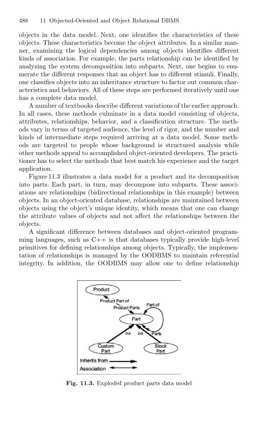
488 11 Objected-Oriented and Object Relational DBMS
objects in the data model. Next, one identifies the characteristics of theseobjects. These characteristics become the object attributes. In a similar man-ner, examining the logical dependencies among objects identifies differentkinds of association. For example, the parts relationship can be identified byanalyzing the system decomposition into subparts. Next, one begins to enu-merate the different responses that an object has to different stimuli. Finally,one classifies objects into an inheritance structure to factor out common char-acteristics and behaviors. All of these steps are performed iteratively until onehas a complete data model.
A number of textbooks describe different variations of the earlier approach.In all cases, these methods culminate in a data model consisting of objects,attributes, relationships, behavior, and a classification structure. The meth-ods vary in terms of targeted audience, the level of rigor, and the number andkinds of intermediate steps required arriving at a data model. Some meth-ods are targeted to people whose background is structured analysis whileother methods appeal to accomplished object-oriented developers. The practi-tioner has to select the methods that best match his experience and the targetapplication.
Figure 11.3 illustrates a data model for a product and its decompositioninto parts. Each part, in turn, may decompose into subparts. These associ-ations are relationships (bidirectional relationships in this example) betweenobjects. In an object-oriented database, relationships are maintained betweenobjects using the object’s unique identity, which means that one can changethe attribute values of objects and not affect the relationships between theobjects.
A significant difference between databases and object-oriented program-ming languages, such as C++ is that databases typically provide high-levelprimitives for defining relationships among objects. Typically, the implemen-tation of relationships is managed by the OODBMS to maintain referentialintegrity. In addition, the OODBMS may allow one to define relationship
Fig. 11.3. Exploded product parts data model
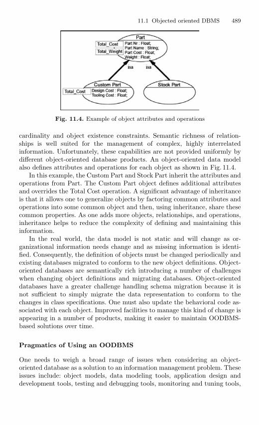
11.1 Objected oriented DBMS 489
Fig. 11.4. Example of object attributes and operations
cardinality and object existence constraints. Semantic richness of relation-ships is well suited for the management of complex, highly interrelatedinformation. Unfortunately, these capabilities are not provided uniformly bydifferent object-oriented database products. An object-oriented data modelalso defines attributes and operations for each object as shown in Fig. 11.4.
In this example, the Custom Part and Stock Part inherit the attributes andoperations from Part. The Custom Part object defines additional attributesand overrides the Total Cost operation. A significant advantage of inheritanceis that it allows one to generalize objects by factoring common attributes andoperations into some common object and then, using inheritance, share thesecommon properties. As one adds more objects, relationships, and operations,inheritance helps to reduce the complexity of defining and maintaining thisinformation.
In the real world, the data model is not static and will change as or-ganizational information needs change and as missing information is identi-fied. Consequently, the definition of objects must be changed periodically andexisting databases migrated to conform to the new object definitions. Object-oriented databases are semantically rich introducing a number of challengeswhen changing object definitions and migrating databases. Object-orienteddatabases have a greater challenge handling schema migration because it isnot sufficient to simply migrate the data representation to conform to thechanges in class specifications. One must also update the behavioral code as-sociated with each object. Improved facilities to manage this kind of change isappearing in a number of products, making it easier to maintain OODBMS-based solutions over time.
Pragmatics of Using an OODBMS
One needs to weigh a broad range of issues when considering an object-oriented database as a solution to an information management problem. Theseissues include: object models, data modeling tools, application design anddevelopment tools, testing and debugging tools, monitoring and tuning tools,
490 11 Objected-Oriented and Object Relational DBMS
and database maintenance tools. A database application, like any softwaresystem, has a life cycle and requires a complete set of life cycle support tools.The following is a brief overview of the kinds of capabilities one needs to lookfor in these areas.
First, one needs to construct an object model of the information prob-lem to be solved by the database. With current object-oriented databases,there are significant variations in the modeling capabilities of these prod-ucts. For example, relationships in some databases are supported by high-leveldeclarative capabilities that allow one to define self-maintaining properties ofrelationships. In other database products, one must program the semanticsof relationships explicitly.
Some database products support a significantly richer data model provid-ing powerful data management services that are defined as part of the datamodel. For example, one may define the existence of some objects to be de-pendent on a particular relationship. When one retracts the relationship, thenthe related object is also deleted. Other examples of more advanced databasesemantics include relationship cardinality constraints, attribute value con-straints, uniqueness properties of attribute values, initial and default values,object versioning, and composite objects. All these data model issues affecthow easily one can define the data model using tools provided by the databasevendor. Another benefit is that the richer the data modeling facilities the lesswork that is required implementing the database application.
An area that many OODBMS evaluators overlook is the tools to supportthe development of the database applications. Since an OODBMS includes alanguage for specifying object behaviors, one needs to understand how suchbehaviors are developed and tested for a given OODBMS. Testing is particu-larly important since one need to integrate the compiler testing and debuggingtools with the database persistent object storage manager.
During database maintenance, one often needs to introduce incrementalchanges into the database and the database applications. This is one of themost difficult areas since existing objects must be migrated to a new stateconforming to the new schema definitions. This is a common problem withall database applications and needs to be anticipated in the design of thedatabase and its applications. Today most OODBMS provide low level servicesfor migrating databases, making the process of changing the schema a majorchallenge for database developers.
Finally, the problem of optimizing a database implementation for a par-ticular application is a difficult one. First, there is little experience withOODBMS on which to base optimization strategies. Second, many of theoptimization features are at a low level, requiring the application developer todesign the application around these features. Both database instrumentationand monitoring tools are needed, as well as facilities for tuning an existingapplication. As with relational databases, object-oriented database systemsalso require extensive monitoring and tuning to extract the maximum perfor-mance for a given application.
11.1 Objected oriented DBMS 491
11.1.6 Evaluation Criteria
This section is a detailed discussion of evaluation criteria that may be con-sidered when evaluating OODBMS. These criteria are broken into three mainareas:
– Functionality– Application Development Issues– Miscellaneous Criteria
Functionality
Functionality, defines evaluation criteria based on functional capabilities pro-vided by the OODBMS. Subsections include Basic Object-Oriented Mod-eling, Advanced Object-Oriented Database Topics, Database Architecture,Database Functionality, Application Programming Interface, and Queryingan OODBMS. The topics discussed in the Basic Object-Oriented Model-ing subsection are those functions that are expected to be similar in allOODBMS products, such as the ability to define complex objects using classes,attributes, and behaviors. In fact, these topics are the object-oriented fea-tures found in most OO technologies (e.g., languages, design methods). TheAdvanced Object-Oriented Database Topics subsection describes functional-ity that is somewhat unique to object-oriented databases. It is expected thatOODBMS products will differ significantly in these areas. The Database Func-tionality subsection describes the features that distinguish a database from apersistent storage manager (e.g., concurrency control and recovery).
Application Development Issues
Application Development Issues considers issues regarding the developmentof applications on top of an OODBMS. Miscellaneous Criteria, identifies afew nonfunctional and nondevelopmental evaluation issues. These issues dealwith vendor and product maturity, vendor support, and current users of theOODBMS product.
Although the evaluation criteria identified in this chapter will be animportant part of any OODBMS selection process, the issues of platform andperformance will most likely dominate the selection process. Although miss-ing functionality can often be managed at the application level, inadequateperformance cannot be overcome (assuming optimal use of database facilitiesand features).
Miscellaneous Criteria
The list of evaluation criteria defined in this chapter is quite extensive. Thislist was developed as a means of covering the spectrum of issues that might
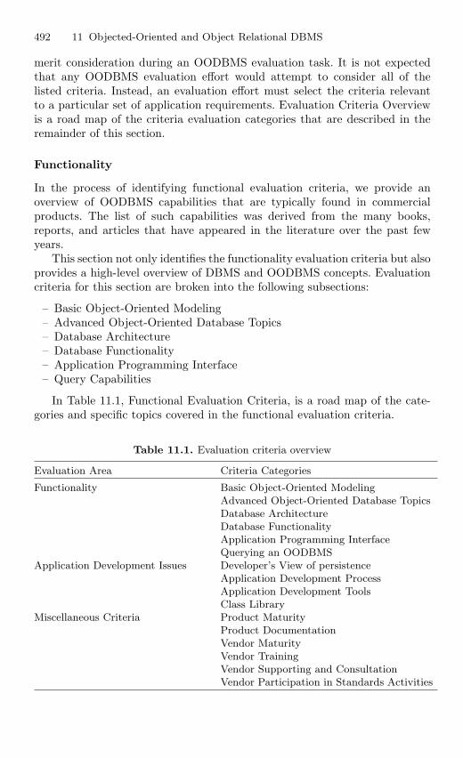
492 11 Objected-Oriented and Object Relational DBMS
merit consideration during an OODBMS evaluation task. It is not expectedthat any OODBMS evaluation effort would attempt to consider all of thelisted criteria. Instead, an evaluation effort must select the criteria relevantto a particular set of application requirements. Evaluation Criteria Overviewis a road map of the criteria evaluation categories that are described in theremainder of this section.
Functionality
In the process of identifying functional evaluation criteria, we provide anoverview of OODBMS capabilities that are typically found in commercialproducts. The list of such capabilities was derived from the many books,reports, and articles that have appeared in the literature over the past fewyears.
This section not only identifies the functionality evaluation criteria but alsoprovides a high-level overview of DBMS and OODBMS concepts. Evaluationcriteria for this section are broken into the following subsections:
– Basic Object-Oriented Modeling– Advanced Object-Oriented Database Topics– Database Architecture– Database Functionality– Application Programming Interface– Query Capabilities
In Table 11.1, Functional Evaluation Criteria, is a road map of the cate-gories and specific topics covered in the functional evaluation criteria.
Table 11.1. Evaluation criteria overview
Evaluation Area Criteria Categories
Functionality Basic Object-Oriented ModelingAdvanced Object-Oriented Database TopicsDatabase ArchitectureDatabase FunctionalityApplication Programming InterfaceQuerying an OODBMS
Application Development Issues Developer’s View of persistenceApplication Development ProcessApplication Development ToolsClass Library
Miscellaneous Criteria Product MaturityProduct DocumentationVendor MaturityVendor TrainingVendor Supporting and ConsultationVendor Participation in Standards Activities
11.1 Objected oriented DBMS 493
Basic Object-Oriented Modeling
The evaluation criteria in this section distinguish database as an object-oriented database. Topics in this section cover the basic object-oriented (OO)capabilities typically supported in any OO technology (e.g., programming lan-guage, design method). These basic capabilities are expected to be supportedin all commercial OODBMS. The topics are given a cursory overview here asshown in Table 11.2 for readers new to OO technology.
Complex Objects. OO systems and applications are unique that the infor-mation being maintained is organized in terms of the real-world entities be-ing modeled. This differs from relational database applications that requirea translation from the real-world information structure to the table formatsused to store data in a relational database. Normalizations upon the relationaldatabase tables result in further perturbation of the data from the user’sperceptual viewpoint. OO systems provide the concept of complex objects toenable modeling of real-world entities. A complex object contains an arbitrarynumber of fields, each storing atomic data values or references to other objects(of arbitrary types). A complex object exactly models the user perception ofsome real-world entity.
Object Identity. OO databases (and programming languages) provide the con-cept of an object identifier (OID) as a means of uniquely identifying a partic-ular object. OIDs are system generated. A database application does not havedirect access to the OID. The OID of an object never changes, even acrossapplication executions. The OID is not based on the value stored within theobject. This differs from relational databases, which use the concept of pri-mary keys to identify a particular table row (i.e., tuple). Primary keys arebased upon data stored in the identified row. The concept of OIDs makes iteasier to control the storage of objects (e.g., not based on value) and to buildlinks between objects (e.g., they are based on the never changing OID). Com-plex objects often include references to other objects, directly or indirectlystored as OIDs.
The size of an OID can substantially affect the overall database sizedue to the large number of inter object references typically found withinan OO application. When an object is deleted, its OID may or may not bereused. Reuse of OIDs reduces the chance of running out of unique OIDs butintroduces the potential for invalid object access due to dangling references.A dangling reference occurs if an object is deleted, and some other objectretains the deleted object’s OID, typically as an interobject reference. Thissecond object may later use the OID of the deleted object with unpredictableresults. The OID may be marked as invalid or may have been reassigned.Typically, an OODBMS will provide mechanisms to ensure dangling refer-ences between objects are avoided.
Classes. OO modeling is based on the concept of a class. A class definesthe data values stored by, and the functionality associated with, an object
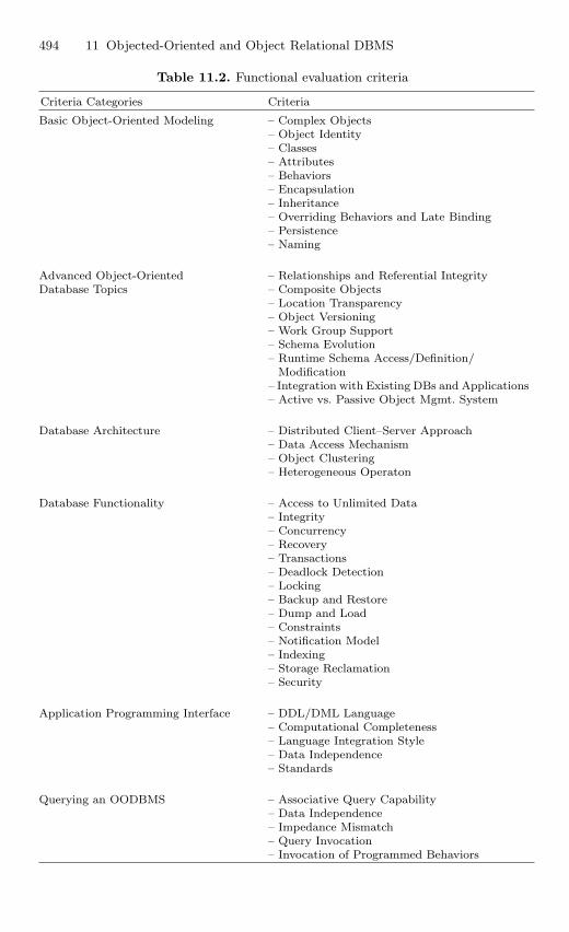
494 11 Objected-Oriented and Object Relational DBMS
Table 11.2. Functional evaluation criteria
Criteria Categories Criteria
Basic Object-Oriented Modeling – Complex Objects– Object Identity– Classes– Attributes– Behaviors– Encapsulation– Inheritance– Overriding Behaviors and Late Binding– Persistence– Naming
Advanced Object-Oriented – Relationships and Referential IntegrityDatabase Topics – Composite Objects
– Location Transparency– Object Versioning– Work Group Support– Schema Evolution– Runtime Schema Access/Definition/
Modification– Integration with Existing DBs and Applications– Active vs. Passive Object Mgmt. System
Database Architecture – Distributed Client–Server Approach– Data Access Mechanism– Object Clustering– Heterogeneous Operaton
Database Functionality – Access to Unlimited Data– Integrity– Concurrency– Recovery– Transactions– Deadlock Detection– Locking– Backup and Restore– Dump and Load– Constraints– Notification Model– Indexing– Storage Reclamation– Security
Application Programming Interface – DDL/DML Language– Computational Completeness– Language Integration Style– Data Independence– Standards
Querying an OODBMS – Associative Query Capability– Data Independence– Impedance Mismatch– Query Invocation– Invocation of Programmed Behaviors
11.1 Objected oriented DBMS 495
of that class. One of the primary advantages of OO data modeling is thistight integration of data and behavior through the class mechanism. Eachobject belongs to one, and only one, class. An object is often referred to asan instance of a class. A class specification provides the external view of theinstances of that class. A class has an extent (sometimes called an extension),which is the set of all instances of the class. Implementation of the extentmay be transparent to an application, but minimally provides the ability tovisit every instance of the class. Within an OODBMS, the class construct isnormally used to define the database schema. Some OODBMS use the termtype instead of class. The OODBMS schema defines what objects may bestored within the database.
Attributes. Attributes represent data components that make up the contentof a class. Attributes are called data members in the C++ programminglanguage. Instance attributes are data components that are stored by eachinstance of the class. Class attributes (static data members in C++) are datavalues stored once for all instances of the class. Attributes may or may not bevisible to external users of the class. Attribute types are typically a subset ofthe basic data types supported by the programming language that interfaces tothe OODBMS. Typically this includes enumeration types such as charactersand booleans, numeric types such as integers and floats, and fixed lengtharrays of these types such as strings. The OODBMS may allow variable lengtharrays, structures (i.e., records), and classes as attribute types.
Pointers are normally not good candidates for attribute types since pointervalues are not valid across application executions.
An OODBMS will provide attribute types that support interobject ref-erences. OO applications are characterized by a network of interconnectedobjects. Object interconnections are supported by attributes that referenceother objects. Other types that might be supported by an OODBMS includetext, graphic, and audio. Often these data types are referred to as BinaryLarge OBjectS (BLOBS). Derived attributes are attributes that are not ex-plicitly stored but instead calculated on demand. Derived attributes requirethat attribute access be indistinguishable from behavior invocation.
Behaviors. Behaviors represent the functional component of a class. Abehavior describes how an object operates upon its attributes and how itinteracts with other related objects. Behaviors are called member functionsin the C++ programming language. Behaviors hide their implementationdetails from users of a class.
Encapsulation. Classes are said to encapsulate the attributes and behaviorsof their instances. Behavior encapsulation shields the clients of a class (i.e.,applications or other classes) from seeing the internal implementation of abehavior. This shielding provides a degree of data independence so that clientsneed not be modified when behavior implementations are modified (they willhave to be modified if behavior interfaces change).
496 11 Objected-Oriented and Object Relational DBMS
A class’s attributes may or may not be encapsulated. Attributes that aredirectly accessible to clients of a class are not encapsulated (public data mem-bers in C++ classes). Modifying the definition of a class’s attributes thatare not encapsulated requires modification of all clients that access them.Attributes that are not accessible to the clients of a class are encapsulated(private or protected data members in C++ classes). Encapsulated attributestypically have behaviors that provide clients some form of access to theattribute. Modifications to these attributes typically do not require modifi-cation to clients of the class.
Inheritance. Inheritance allows one class to incorporate the attributes andbehaviors of one or more other classes. A subclass is said to inherit from oneor more superclasses. The subclass is a specialization of the superclass in thatit adds additional data or behaviors, or overrides behaviors of the superclass.Superclasses are generalizations of their subclasses. Inheritance is recursive.A class inherits the attributes and behaviors from its superclasses, and fromits superclass’s superclasses, etc. In a single inheritance model, a class maydirectly inherit from only a single other class. In a multiple inheritance modela class may directly inherit from more than one other class. Systems support-ing multiple inheritance must specify how inheritance conflicts are handled.Inheritance conflicts are attributes or behaviors with the same name in a classand its superclass, or in two superclasses.
Inheritance is a powerful OO modeling concept that supports reuse and ex-tensibility of existing classes. The inheritance relationships between a groupsof classes define a class hierarchy. Class hierarchies improve the ability of usersto understand software systems by allowing knowledge of one class (a super-class) to be applicable to other classes (its subclasses).
Overriding Behaviors and Late Binding. OO applications are typically struc-tured to perform work on generic classes (e.g., a vehicle) and at runtimeinvoke behaviors appropriate for the specific vehicle being executed upon(e.g., Boeing 747). Applications constructed in such a manner are more eas-ily maintained and extended since additional vehicle classes may be addedwithout requiring modification of application code. Overriding behaviors isthe ability for each class to define the functionality unique to itself for a givenbehavior. Late binding is the ability for behavior invocation to be selected atruntime based on the class of an object (instead of at compile time).
Persistence. Persistence is the characteristic that makes data available acrossexecutions. The objective of an OODBMS is to make objects persistent. Per-sistence may be based on an object’s class, meaning that all objects of a givenclass are persistent. Each object of a persistent class is automatically madepersistent. An alternative model is that persistence is a unique characteristicof each object (i.e., it is orthogonal to class). Under this model, an object’s per-sistence is normally specified when it is created. A third persistence model isthat any object reachable from a persistent object is also persistent. Such sys-tems require some way of explicitly stating that a given object is persistent
11.1 Objected oriented DBMS 497
(as a means of starting the network of interconnected persistent objects).Related to the concept of persistence is object existence. OODBMS may pro-vide a means by which objects are explicitly deleted. Such systems must ensurethat references to deleted objects are also removed. An alternative strategyis to maintain an object as long as references to the object exist. Once allreferences are removed, the object can be safely deleted.
Naming. OO applications are characterized as being composed of a networkof interconnected objects. An application begins by accessing a few known ob-jects and then traverses to additional objects via relationships from the knownobjects. As objects are created they are linked (i.e., related) to other existingobjects. Given this scenario, the database must provide some mechanism foridentifying one or more objects at application start-up without using relationsfrom existing objects. This is typically accomplished by allowing objects to benamed and providing a retrieval mechanism based upon name. An applicationbegins by loading one or two “high-level” objects that it knows by name andthen traverses to other reachable objects. Object names apply within somename scope. Within a given scope, names must be unique (i.e., the same namecan not refer to two objects). The simplest scope model is for the entire data-base to act as a single name scope. An alternative scope model is for theapplication to identify name scopes. Using multiple name scopes will reducethe chance for name conflicts.
Advanced Object-Oriented Database Topics
Functional capabilities identified in this section are those that are somewhatunique to object-oriented database systems. We expect that these topics rep-resent the most interesting evaluation topics and will provide the greatestdiversity among the evaluated OODBMS.
Relationships and Referential Integrity Relationships are an essential compo-nent of the object-oriented modeling paradigm. Relationships allow objects torefer to each other and result in networks of interconnected objects. Relation-ships are the paths used to perform navigation-based data access typical ofprogrammed functionality. The ability to directly and efficiently model rela-tionships is one of the major improvements of the object-oriented data modelover the relational data model.
Conceptually, relationships can be thought of as abstract entities thatallow objects to reference each other. An OODBMS may choose to representrelationships as attributes of the class (from which the relationships emanate),as independent objects (in which case relationships may be extensible andallow attributes to be added to a relationship), or as hidden data structuresattached to the owning object in some fashion.
Relationships are often referred to as references, associations, or links.Sometimes the term relation is used to mean the schema definition of thepotential for interconnections between objects, and the term relationshipis used to mean actual occurrences of an interconnection between objects.
498 11 Objected-Oriented and Object Relational DBMS
In this document we will use the term relationship interchangeably for boththe schema definition and the object level existence for connections betweenobjects. Relationships can be characterized by a number of different indepen-dent parameters, leading to a large number of different relationship behaviors:
– Relationships may be unidirectional or bidirectional. A unidirectional re-lationship exists in only a single direction, allowing a traversal from oneobject to another but no traversal in the reverse direction. A bidirectionalrelationship allows traversal in both directions. When a relationship isestablished along a bidirectional relationship, that relationship is auto-matically created in both directions (i.e., the application explicitly cre-ates the relationship in one direction and the OODBMS implicitly setsthe relationship in the opposite direction).
– Relationships have a cardinality, typically either one-to-one, one-to-many,or many-to-many. A one-to-one relationship allows one object to be relatedto another object (e.g., spouse might typically be modeled as a one-to-onerelationship). Setting a one-to-one relationship deletes any previously ex-isting relationship. A one-to-many relationship allows a single object to berelated to many objects in one direction, in the reverse direction an objectmay be related to only a single object (e.g., when modeling a house, thehouse might be composed of many rooms, each room is part of a singlehouse). One-to-one and one-to-many relationships may be unidirectionalor bidirectional. A many-to-many relationship, which must be bidirec-tional, allows each object to be related to many objects in both directionsof the relationship (e.g., modeling the relationship between parents andchildren might use a many-to-many bidirectional relationship. A personmay have many children; children may have more than one parent.).
– Relationships may have ordering semantics. Ordered relationships are typ-ically considered as lists (the objects are ordered by the operations thatbuild the relations, not by the values stored in the related objects). Un-ordered relationships are either sets or bags. Sets do not allow duplication;bags do.
– Relationships may support the concept of composite objects.
The existence of relationships gives rise to the need for referential integrity.Referential integrity ensures that objects do not contain references to deletedobjects. Referential integrity can be automatically provided for bidirectionalrelationships. Given a bidirectional relationship, when an object is deleted,all related objects can be found and have their relationships to the deletedobject removed. Unidirectional relationships cannot be assured of referentialintegrity (short of performing complete scans of the database). If an objectwhich is the target of a unidirectional relationship is deleted, there is noefficient mechanism to identify all objects that reference the deleted object(and delete the relationships to the deleted object). Application level solutions
11.1 Objected oriented DBMS 499
to this problem exist (e.g., maintenance of existence dependency lists), butmay result in poor performance and are effectively duplicating much of thework done by bidirectional relationships.
Alternatively, if the OODBMS does not reuse object identifiers, then adeleted object may be tomb-stoned, meaning a mark is left denoting that theobject has been deleted. When a reference to a deleted object is made it canthen be trapped as an error, or simply ignored, with an appropriate updateof the referencing object’s relationship (to no longer relate to the deletedobject). Some OODBMS products provide a similar capability by keepingreference counts to objects, and only deleting an object when all referenceshave been removed.
Relationship implementation provides a major differentiator betweenOODBMS products. On disk, relationships are typically modeled using ob-ject identifiers. Once brought into memory, relationships may remain as objectidentifiers or be swizzled into virtual memory pointers. Swizzling is a processthat converts disk-based relationship representations into memory pointersfor all related objects that are in memory. This may be done on object loador on demand when a particular relationship is traversed. Swizzling tradesthe overhead of performing the conversion to a memory-based pointer tra-versal in the hopes that multiple future accesses across the relationship willresult in an overall speed improvement. Systems that do not swizzle requirean object identifier lookup for all relationship traversal. This lookup can beperformed efficiently through the use of lookup tables. Hybrid approachesare also possible. Each application will have to consider its expected objectaccess and relationship traversal patterns to determine if a swizzled or objectidentifier-based relationship approach will best suit its needs.
Composite Objects Composite objects are groupings of interrelated objectsthat can be viewed logically as a single object. Composite objects are typi-cally used to model relationships that have the semantic meaning is-part-of(e.g., rooms are part of a house). Composite objects are connected by therelationship mechanisms provided by the OODBMS. Operations applied tothe “root” object of such a grouping can be propagated to all objects withinthat group. Operations that might be applied on composite objects include:
– Copy– Delete– Lock
Here we are defining Identifier-Equality, Shallow-Equality, and Deep-Equality operations. These three different forms of equality checks compareobject identifiers, attribute values, and attribute values of component ob-jects, respectively. Also defined are Shallow-Copy and Deep-Copy operations.A Shallow-Copy makes a new object and copies attribute values. A Deep-Copy
500 11 Objected-Oriented and Object Relational DBMS
makes a new object, copying nonrelationship attribute values, and then recur-sively creates new objects for related objects (recursively applying the Deep-Copy operation). Deep-Copy is an example of an operation being propagatedacross a composite object. Propagation of delete and lock operations meansthat if the root object is deleted or locked all of its component objects arealso deleted or locked.
Location Transparency Location transparency is the concept that an objectcan be referenced (i.e., can use the same syntactic mechanism) regardless ofwhat database it resides in and where on the network that database is located.Objects should be able to be moved programmatically and have all referencesto the object remain intact (a form of referential integrity). (The ability tomove an object to a new database location will also be considered as part ofdatabase administration capabilities.).
Object Versioning Object versioning is the concept that a single object maybe represented by multiple versions (i.e., instances of that object) at one time.We can define two forms of versioning, each driven by particular requirementsof the applications which are driving the need for OODBMS products:
– Linear Versioning is the concept of saving prior versions of objects asan object changes. In design-type applications (e.g., CASE, CAD) priorversions of objects are essential to maintain the historical progression ofa design and to allow designers to return to earlier design points afterinvestigating and possibly discarding a given design path. Under linearversioning, only a single new version can be created from each existingversion of an object.
– Branch Versioning supports concurrency policies where multiple users mayupdate the same data concurrently. Each user’s work is based upon a con-sistent, nonchanging base version. Each user can modify his version of anobject (as he proceeds along some design path in a CAD application forexample). At some future point in time, under user/application support,the multiple branch versions are merged to form a single version of theobject. Branch versioning is important in applications with long transac-tions so that users are not prevented from access to information for longperiods of time. Under branch versioning, multiple new versions may becreated for an object.
Associated with the idea of versioning is that of configuration. A configu-ration is a set of object versions that are consistent with each other. In otherwords, it is a group of objects whose versions all belong together. OODBMSneeds to provide support so that applications access object versions that be-long to the same conceptual configuration. This may be achieved by control-ling the relationships that are formed for versioned objects (i.e., they may beduplicated in the new object or replaced with relationships to other objects).
An OODBMS may provide low level facilities which application developersuse to control the versioning of objects. Alternatively, the OODBMS may
11.1 Objected oriented DBMS 501
implement a specific versioning policy such as automatically creating a newobject version with each change. An automatic policy may result in rapid andunacceptable expansion of the database and requires some automated meansof controlling this growth.
Work Group Support In addition to versioning, an OODBMS might supportgroup applications in other manners. The ability is to designate shared andprivate databases with the concept of checking data in and out of these dataspaces. Some databases may allow segments of the database to be taken off-line, perhaps on a portable computer, used autonomously, and then broughtback on-line at a later time. Long transactions are another mechanism on topof which group applications can be built.
Schema Evolution Schema evolution is the process by which existing data-base objects are brought into line with changes to the class definitions ofthose objects (i.e., schema changes require all instances of the changed classto be modified so as to reflect the modified class structure). Schema evolutionis helpful although not essential during system development (as a means ofretaining test data, for example). Schema evolution is essential for mainte-nance and/or upgrades of fielded applications. Once an application is in thefield (and users are creating large quantities of information), an upgrade orbug fix cannot require disposal of all existing user databases. Schema evolu-tion is also essential for applications that support user-level modeling and/orextension of the application.
Here we have given a framework for schema modifications in an object-oriented database. Included in this framework are invariants which must bemaintained at all times (e.g., all attributes of a class must have a distinctname), rules for performing schema modifications (e.g., changing the typeof an attribute in a given class must change the type of that attribute inall classes which inherit that attribute), and a set of schema changes thatshould be supported by an object-oriented database. This set of schema changeoperations is:
1. Changes to Definition of a Class:(a) Changes to an Attribute of a Class (applies to both instance and class
attributes):– Add an attribute to a class.– Remove an attribute from a class.– Change the name of an attribute.– Change the type of an attribute.– Change the default value of an attribute.– Alter the relationship properties for relationship attributes.
(b) Changes to a Behavior of a Class:– Add a new behavior to the class.– Remove a behavior from the class.– Change the name of a behavior.– Change the implementation of a behavior.
502 11 Objected-Oriented and Object Relational DBMS
2. Changes to the Inheritance of a Class:– Add a new superclass to a class.– Remove a superclass for a given class.– Change the order of superclasses for a class (it is expected that su-
perclass ordering will be used to handle attribute and behavior inher-itance conflicts).
3. Changes to the Existence of a Class:– Add a new class.– Remove an existing class.– Change the name of a class.
Schema changes will require modification of instances of the changed classas well as applications that referenced the changed class. Some of these changescannot be performed automatically by the OODBMS. Deleting attributes andsuperclasses are examples of schema changes that could be performed auto-matically. Adding attributes and superclasses can only be performed if de-fault values are acceptable for the initial state of new attributes. This is notlikely, especially for relationship attributes. An OODBMS should provide toolsand/or support routines for aiding programmed schema evolution.
A manual evolution approach requires instance migration to be performedoff-line, probably through a dump of the database and a reload of the datathrough an appropriate transformation filter. Systems may perform an ag-gressive update by automatically adjusting each instance after each schemachange. This approach may be slow due to the overhead of performing theupdate on all instances at a single time. This approach is the easiest for anapplication to implement since multiple versions of the schema need not bemaintained indefinitely.
Schema changes may be performed in background mode, thus spreadingthe update overhead over a longer period of time. A lazy evaluation approachdefers updating objects until they are accessed and found to be in an in-consistent state. Both the background and lazy approaches require extendedperiods where multiple versions of the schema exist and will be complicatedby multiple schema modifications. Applications and stored queries will haveto be updated manually as a result of schema changes. Some forms of schemachanges will not require updates to applications and queries due to dataindependence and encapsulation of a class’s data members.
It is expected that all OODBMS products will support some form ofschema evolution for static schema changes. By static, we mean the schema ischanged by manipulations of class definitions outside of application process-ing (i.e., by reprocessing database schema definitions and modifying applica-tion programs). Dynamic schema modification, meaning modification of theschema by the application, is more complex and potentially inconsistent withthe basic C++ header file approach used for schema definitions in many cur-rent commercial products. Dynamic schema modification is only needed inapplications that require user definable types.
11.1 Objected oriented DBMS 503
Runtime Schema Access/Definition/Modification An OODBMS typicallymakes use of a database resident representation of the schema for the data-base. The existence of such a representation, and a means of accessing it,provides applications with direct access to schema information. Access toschema information might be useful in building custom tools which browsethe structure and contents of a database. Modification and definition of theschema at runtime allows the development of dynamically extensible appli-cations. Users of this modeling system define the classes, attributes, andbehaviors of the information that they wish to model. Once defined, instancesof these classes may be created and manipulated.
The idea of dynamic schema definition is foreign to the C++ programminglanguage. In C++, class definitions are defined statically in header files. Anapplication may not alter these class definitions at runtime. OODBMS canprovide access and modification of their schemata by storing the schema asinstances of predefined classes and then allowing applications to create, mod-ify, and query the instances which model the schema. An application mightwish to modify the schema in order to extend an application to store newinformation or to display information in alternative presentations.Integration with Existing DBs and Applications Numerous papers have ap-peared in the literature describing the need for integration of object-orientedand relational database technologies. Newly developed object-oriented appli-cations will need to access existing relational databases. Data stored in object-oriented databases must be accessible to existing Standard Query Language(SQL) applications. Some applications will require access to both relationaland object-oriented databases.
The process of accessing a relational database from an object program isgiven as follows. Defining a mapping of the relational schema into an objectmodel is the first task. A simple approach is to represent each relation by aclass and replace foreign key fields (in the relational schema) by relationships(in the object-oriented schema). Given a mapping of tables to classes, a meansof invoking SQL operations from the object program must be defined. This canbe provided by defining methods on the mapped classes for creating, updating,and deleting instances. These methods are responsible for interacting with therelational database. Additional methods are required to provide an interfaceto query operations that translate the tuples returned from a query into aset of objects accessible by the object program. Database interface generatorproducts, providing automated support for interfacing object programs torelational databases, are currently being developed. These products may workfrom a user-developed set of class definitions, or from the relational database’sdata definitions language (DDL). In either case, the result is a set of methodspecifications and implementations that provide access to a relational databasefrom an object program.
OODBMS vendors are moving to support the need for SQL access to theirdatabases. This need arises due to the large experience base of SQL users andthe desire for existing applications to be continually supported, as OODBMS
504 11 Objected-Oriented and Object Relational DBMS
systems become part of the information infrastructure. The basic approachto this task is to incorporate an SQL interface in the OODBMS applicationprogramming interface (API) and to provide an SQL query processing capa-bility.
Active vs. Passive Object Management System. OODBMS may be character-ized as being an active or a passive object management system. A passiveOODBMS means that the database does not store the implementation ofthe methods defined for a class. Applications built on a passive OODBMSprovide in their executable image the code for each method defined in thesystem. Application execution results in each object, that is accessed duringthat execution, being moved from the database server process to the clientapplication process. Once the object resides in the application’s address space,a message may be sent to that object resulting in the object executing one ofits methods. Note that the process of moving the object from the databaseserver to the application’s address space is typically transparent to the ap-plication programmer. An active OODBMS means that the database storesthe implementation of object behaviors (i.e., methods) in the database. Thisallows objects to execute those behaviors (i.e., respond to messages) in thedatabase server process. Advantages of an active data model include:
– Objects may be accessed and manipulated by nonobject-oriented pro-grams. These programs may access objects in the database through astandard programming language interface. Each such access may result ina long series of messages being sent between many different objects thatare cooperating to provide some useful service on behalf of the requestingapplication.
– Object behaviors are stored in a single location (the database), whichmakes it easier to be sure that all applications have the latest version ofthose behaviors. This also tends to isolate those applications from changesto the object behaviors.
– Each object accessed by the application need not be transferred to theapplication’s address space.
– Consistency checks (i.e., constraints) can be automatically maintained bythe database. As an object’s state is changed, the database server processcan automatically execute consistency checks to ensure that the new statedoes not violate some constraint.
One of the significant differences between an active and a passiveOODBMS becomes apparent when considering the implications of traversing10,000 objects as part of a query or other database operation. Using a passivedatabase requires that each of those 10,000 objects be moved from the data-base server to the client application prior to invoking the methods that accessthe objects. An active database can be programmed so that the traversaland method invocation occurs in the database server process, eliminating theneed to transfer each object across the network to the application process.
11.1 Objected oriented DBMS 505
Database Architecture
This section provides an overview of architectural issues relevant to anOODBMS. Many papers has been published which will describe an imple-mentation of a persistent memory system upon which object-oriented data-bases may be built and describes an implementation of shared database serverarchitecture suitable as a back-end for an object-oriented database.
Distributed Client–Server Approach Advances in local area network andworkstation technology have given rise to group design type applicationsdriving the need for OODBMS (e.g., CASE, CAD, and Electronic Offices).OODBMS typically execute in a multiple process distributed environment.Server processes provide back-end database services, such as management ofsecondary storage and transaction control. Client processes handle applica-tion specific activities, such as access and update of individual objects. Theseprocesses may be located on the same or different workstations. Typicallya single server will be interacting with multiple clients servicing concurrentrequests for data managed by that server. A client may interact with multipleservers to access data distributed throughout the network.
The evaluations and benchmarks are the three alternative workstation-server architectures that have been proposed for use with OODBMS:
– Object server approach. The unit of transfer from server to client is anobject. Both machines cache objects and are capable of executing methodson objects. Object-level locking is easily performed. The major drawbackof this approach is the overhead associated with the server interactionrequired to access every object and the added complexity of the serversoftware which must provide complete OODBMS functionality (e.g., beable to execute methods). Keeping client and server caches consistent mayintroduce additional overheads.
– Page server approach. The unit of transfer from server to client is a page(of objects). Page-level transfers reduce the overhead of object access sinceserver interaction is not always required. Architecture and implementationof the server is simplified since it needs only to perform the backend data-base services. A possible drawback of this approach is that methods canbe evaluated only on the client, thus all objects accessed by an applicationmust be transferred to the client. Object-level locking will be difficult toimplement.
– File server approach. The OODBMS client processes interact with anetwork file service (e.g., Sun’s NFS) to read and write database pages.A separate OODBMS server process is used for concurrency controland recovery. This approach further simplifies the server implementationsince it need not manage secondary storage. The major drawback of thisapproach is that two network interactions are required for data access,one to the file service and one to the OODBMS server.
506 11 Objected-Oriented and Object Relational DBMS
Many scientists have identified no clear winner when benchmarking thethree approaches. The page server approach seemed best with large bufferpools and good clustering algorithms. The object server approach performedpoorly if applications scanned lots of data, but was better than the pageserver approach for applications performing lots of updates and running onworkstations with small buffer pools.
Data Access Mechanism. An evaluation of OODBMS products should con-sider the process necessary to move data from secondary storage into a clientapplication. Typically this requires communication with a server process, pos-sibly across a network. Objects loaded into a client’s memory may require fur-ther processing, often referred to as swizzling, to resolve references to otherobjects which may or may not already be loaded into the client’s cache. Theoverhead and process by which locks are released and updated objects arereturned to the server should also be considered.
Object Clustering. OODBMS which transfer units larger than an object do sounder the assumption that an application’s access to a given object implies ahigh probability that other associated objects may also be accessed. By trans-ferring groups of objects, additional server interaction may not be necessaryto satisfy these additional object accesses. Object clustering is the ability foran application to provide information to the OODBMS so that objects whichit will typically access together can be stored near each other and thus benefitfrom bulk data transfers.
Heterogeneous Operation. An OODBMS provides a mechanism for applica-tions to cooperate, by sharing access to a common set of objects. A typicalOODBMS will support multiple concurrent applications executing on multi-ple processors connected via a local area network. Often, the processors willbe from different computer manufacturers; each having its own data represen-tation formats. For applications to cooperate in such an environment, datamust be translated to the representation format suitable for the processorupon which that data is stored (both permanently by a server and temporarilyby a client wishing to access the data). To be an effective integration mecha-nism, an OODBMS must support data access in a heterogeneous processingenvironment.
Database Functionality
The primary benefit an application derives from a database is that applica-tion data persists across application executions. Additional benefits offeredby a database are the ability to share data between applications, provisionof concurrent access to the data by multiple applications, and providing anapplication the access to a data space larger than its process address space.This section reviews the issues that distinguish an OODBMS from a languagewith persistence (e.g., Smalltalk). A language with persistence typically pro-vides for data to exist across executions but does not provide the additionalbenefits outlined earlier.
11.1 Objected oriented DBMS 507
Within this section we provide a brief overview of the database topic withadditional issues relevant to object-oriented databases.
Access to Unlimited Data. A database provides an application, the ability toaccess a virtually unlimited amount of data. In particular, the application canaddress more data than would fit within the application process address space.Some databases may support the notion of transient data that is maintainedduring program execution but not saved in the database. This is useful forproviding access to very large transient data objects that do not map easilyinto the application’s address space.
Integrity. A database is required to maintain both structural and logical in-tegrity. Structural integrity ensures that the database contents are consistentwith its schema. Logical integrity ensures that constraints specifying logicalproperties of the data are always true. Many papers describe new concerns forintegrity in OODBMS. A major concern is that OODBMS architectures mapdata directly into the applications address space (unlike a typical relationaldatabase that provided direct access to the data only in a separate databaseserver process).
Mapping data into the application’s address space yields significant perfor-mance improvements over server-only data access, especially for the applica-tion areas being targeted by OODBMS. However, once data is mapped into anapplication’s address space there is no way to guarantee it is not inadvertentlyor maliciously tampered with. This limits a database’s ability to guaranteeintegrity of the data. Structural integrity mechanisms include assurances thatreferences to deleted objects do not exist and that all instances are consistentwith their class definitions. Logical integrity can be supported by encapsu-lating all the data members of a class and providing access to informationcontent of an object only through behaviors defined by the class.
Additional integrity constraints can be supported if the database providesa mechanism for specifying application-level constraints and for ensuringthe execution of those constraints before and/or after behavior invocation.Constraints executed before a behavior can test the consistency of the req-uest and the input parameters. Constraints executed after a behavior cantest for logical consistency of the resulting state of the object and anyoutput parameters.
Concurrency. Databases provide concurrency control mechanisms to ensurethat concurrent access to data does not yield inconsistencies in the databaseor in applications due to invalid assumptions made by seeing partially up-dated data. The problems of lost updates and uncommitted dependencies arewell documented in the database literature. Relational databases solve thisproblem by providing a transaction mechanism that ensures atomicity andserializability. Atomicity ensures that within a given logical update to thedatabase, either all physical updates are made or none are made. This en-sures the database is always in a logically consistent state, with the DB beingmoved from one consistent state to the next via a transaction. Serializability
508 11 Objected-Oriented and Object Relational DBMS
ensures that running transactions concurrently yields the same result as ifthey had been run in some serial (i.e., sequential) order.
Relational databases typically provide a pessimistic concurrency controlmechanism. The pessimistic model allows multiple processes to read data aslong as none update it. Updates must be made in isolation, with no otherprocesses reading or updating the data. This concurrency model is sufficientfor applications that have short transactions, so that applications are notdelayed for long periods due to access conflicts.
For applications being targeted by OODBMS (e.g., multiperson designapplications), the assumption of short transactions is no longer valid. Opti-mistic concurrency control mechanisms are based on the assumptions thataccess conflicts will rarely occur. Under this scenario, all accesses are allowedto proceed and, at transaction commit time, conflicts are resolved. OODBMShave incorporated the idea of optimistic concurrency control mechanisms forbuilding applications that will have long transaction times.
Handling of conflicts at committed time cannot simply abort a transaction,however, since one designer may be losing days or weeks of work. OODBMSmust provide techniques to allow multiple concurrent updates to the samedata and support for merging these intermediate results at an appropriatetime (under application control). Most systems use some form of versioningsystem in order to handle this situation.
An alternative policy is to allow reading and a single update to occurin parallel. Readers are made aware that the data they are reading may bein the midst of an update. Thus readers may be viewing slightly outdatedinformation. Implementation of this approach fits well in the client–serverarchitecture typical for an OODBMS. Each client application gets its ownlocal copy of the data. If an update is made to the data, the server doesnot permanently store it until all concurrent read transactions are completed.Thus, all read transactions execute seeing a consistent data set, albeit onethat is in the process of being updated.
Once all readers have completed, the write transaction is allowed to com-plete modifying the permanent copy of the data. Some OODBMS may, attransaction commit, inform reading clients that the data they just read is inthe process of being updated.Recovery. Recovery is the ability for a database to return to a consistent stateafter a software or hardware failure. Similar to concurrency, the transactionconcept is used to implement recovery and to define the boundaries of recoveryactivity. One or more forms of database journaling, backup, check-pointing,logging, shadowing, and/or replication are used to identify what needs to berecovered and how to perform a recovery.
Databases must typically respond to application failures, system failures,and media failures. Application failures are typically trapped by the transac-tion mechanism and recovery is implemented by rolling back the transaction.System failures, such as loss of power, may require log and/or checkpoint sup-ported rollback of uncommitted transactions and rollforward of transactions
11.1 Objected oriented DBMS 509
that were committed but not completely flushed to disk. Media failures, suchas a disk head crash, require restoration of the database from a backup version,and replaying of transactions that have been committed since the backup.
The ability of a database to recover from failures results in a heavy process-ing and storage overhead. In the process of evaluating an OODBMS, its abilityto recover from faults, and the overhead incurred to provide that recovery ca-pability, must be carefully considered. Applications envisioned for OODBMS(e.g., CASE tools) often do not have the same strict recovery requirements asdo relational database applications (e.g., banking systems). In addition, theamount of data stored in such systems may result in unacceptable storageoverheads for many forms of recovery. For these reasons, an OODBMS eval-uation effort must carefully select the recovery capabilities needed based onboth the functional and performance requirements of the application.
Transactions. Transactions are the mechanism used to implement concur-rency and recovery. Within a transaction, data from anywhere in the (dis-tributed) database must be accessible. A feature found in many OODBMSproducts is to commit a transaction but to allow the objects to remain in theclient cache under the expectation that they will soon be referenced again.
Some OODBMS have incorporated the concept of long and/or nestedtransactions. A long transaction allows transactions to last for hours or dayswithout the possibility of system generated aborts (due to lock conflicts forexample). System generated aborts must be avoided for applications targetingOODBMS since a few hours or days of work cannot be simply discarded. Longtransactions may be composed of nested transactions for purposes of recovery.Nested transactions allow a single (root) transaction to be decomposed intomultiple subtransactions.
Each subtransaction can be committed or aborted independently of theother subtransactions contained in the scope of the root transaction. Eachsubtransactions commit is dependent upon its immediate superior commit-ting and the root transaction committing. Nested transactions improve uponthe basic transaction mechanism by providing finer-grained control over thefailure properties of software. Using nested transactions, a portion of a com-putation can fail and be retried without affecting other parts of that samecomputation. Nested transactions were developed to provide concurrency con-trols for distributed computing systems. Again, an OODBMS evaluation mustcarefully consider whether the target application requires nested transactionsand the performance and/or storage impacts of using this facility.
Deadlock Detection. Database systems use deadlock detection algorithms todetermine when applications are deadlocked due to conflicting lock requests.Relational DBMS typically select an arbitrary transaction and abort it in anattempt to let the remaining transactions complete. The aborted transactionis normally restarted automatically by the system. This scheme works wellfor the class of applications supported by relational DBMS. As described inthe previous section, applications being targeted by OODBMS cannot afford
510 11 Objected-Oriented and Object Relational DBMS
a system-aborted transaction resulting in the potential loss of hours, days, orweeks of work. OODBMS provide alternative concurrency control and trans-action mechanisms to reduce or avoid the possibility of deadlocks. Regardlessof concurrency control protocol, an OODBMS must still detect and resolvedeadlocks.
Locking. Locking of database entities is the typical approach to implementingtransactions. OODBMS may provide locking at the object and/or the pagelevel. Object-level locking may result in high overheads due to lock manage-ment. Page-level locking may reduce concurrency, especially for write locks,since not all objects on a page may be used in the transaction that holds thelock. OODBMS clustering facilities will aid in reducing the loss of concurrencydue to page-level locking.
An OODBMS will implicitly acquire and release locks as data is accessedby an application. Application support may be necessary for specifying thelock mode (e.g., all locks may be acquired in read mode by default and theapplication must specify that write access to the object is necessary). TheOODBMS may also provide an interface for explicitly locking data.
Backup and Restore. Backup is the process of copying the state of the data-base to some other storage medium in case of subsequent failure or simplyfor historical record. Ideally backups can be performed while the database isin use. Backups may be performed only on specific sections of the database.Incremental backup capabilities reduce the amount of information that mustbe saved by storing only changes since a prior backup. Obviously, a databasemust be able to be restored from a backup.
Dump and Load. A database may be dumped into a human readable ASCIIformat. Specific segments of the database may be dumped. A database maybe recreated by loading from a dump file.
Constraints. Constraints are application-specific conditions that must alwayshold true for a database. Logical database integrity can be supported by pro-viding the application developer with the ability to define constraints andfor those constraints to be automatically executed at the appropriate times.Although constraints can be directly encoded in behaviors, having a sepa-rate constraint mechanism reduces duplication and ensures execution of theconstraints. Some OODBMS define a model for constraint definition and invo-cation but require applications to explicitly invoke the constraint executions.
Constraints executed at behavior invocation can test for validity of theinput parameters and the requested operation. Constraints executed atthe completion of a behavior invocation can test for logical consistency ofthe result values and resulting database state.
Notification Model. An OODBMS may provide a passive and/or an activenotification model. A notification model allows an application to be informedwhen an object is modified or when some other database event occurs. Passivenotification systems require that the application query the database for state
11.1 Objected oriented DBMS 511
changes. A passive system minimally provides the logic that determines if anobject has changed state or if an event has occurred.
The application is responsible for informing the database of the objectsand events in which it is interested and for periodically querying the databaseto see if those objects have been updated or if particular events have occurred.
An active notification system is one in which application routines are in-voked automatically as a result of some object being updated or some data-base event was occurring. Active notification systems are similar to databasetriggers and constraint systems (whereby constraints are executed when oneof their operands changes state). Presently there is no clear indication thatsuch mechanisms can be efficiently supported in general purpose databasemanagement systems.
Indexing. Databases make use of indexing to provide optimized data retrievalbased on some aspect of that data. In particular, query evaluations can bedramatically improved by the presence of indexes. Query optimizers mustdynamically determine if an index is present and, if so, use that index toprovide an efficient query execution.
Indexes in an OODBMS are typically built to provide lookup of all objectsof a given class and its subclasses based on one or more data members of thatclass. Indexes may be segregated to some segment of a database or may spanthe entire database.
Different indexing implementations result in different time and space per-formance. Hashing and b-trees are two common index implementation tech-niques. Indexing add to the overhead associated with creating, deleting, andmodifying objects and thus must be used judiciously.
Storage Reclamation. Data stored within a database is dynamically createdand destroyed by the applications that access that database. Data that isno longer accessible, whether determined implicitly by the system or as theresult of an explicit delete by an application, results in storage space that isno longer in use. Reclamation of unused space must be performed so that adatabase does not continuously grow. Space reclamation should be performedincrementally or as a background activity so that performance hiccups are notencountered by the applications.
Security. Secure database systems protect their data from malicious misuse.Security requirements are similar to data integrity requirements that protectdata from accidental misuse. Secure databases typically provide a multilevelsecurity model where users and data are categorized with a specific securitylevel. Mandatory security controls ensure that users can access data only attheir level and below. Discretionary security controls provide access controlbased on explicit authorization of a user’s access to data.
Applications targeted by OODBMS often do not require strict securitycontrols, although discretionary access controls seem desirable for work-groupdesign type applications. Little work has been done to add security mecha-nisms to OODBMS.
512 11 Objected-Oriented and Object Relational DBMS
Application Programming Interface
A major distinction between an object-oriented database application and arelational database application is the relation between the data manipula-tion language (DML) and the application programming language. Large scalecommercial database applications are developed in a standard programminglanguage (e.g., C, C++). In a relational database, SQL is used as the DML,providing the means to create, update, query, and delete data from the data-base. Thus, in a relational database application, a significant amount of effortis spent transforming data between the two different languages.
Critics claim that this impedance mismatch adds to the complexity ofbuilding relational database applications. In an object-oriented databaseapplication, the DML is typically very near to a standard programming lan-guage. For example, many OODBMS support C++ as their DML, with theresult that C++ can be used for building the entire application. OODBMSproponents claim that by using a single language, the impedance mismatch isremoved (or significantly reduced) and application development is simplified.The OODBMS approach is not without its critics. OODBMS applicationstraverse the network of interconnected objects to discover information. Thishand-coded navigation of the schema cannot automatically take advantage ofindexes that might be added and requires modification of the application codeas the schema changes.
SQL, on the other hand, is an associative retrieval language, not requiringany information describing how information is to be found. SQL statementscan be recompiled and/or optimized at runtime to find the best access pathto the requested data.
It is clear that both relational and object-oriented database approacheshave merit and will used for developing particular classes of applications. It isinteresting to note that relational vendors are currently adding object-orientedfeatures to their products and those OODBMS vendors are adding SQL-likequery capabilities to theirs. In addition, third party companies are developingautomated integration tools that allow SQL applications to access OODBMSand OODBMS to access relational databases.
This section covers issues relevant to the application programming inter-face of an OODBMS. As described earlier, OODBMS aim to provide a tightintegration between the data definition/manipulation language and a stan-dard programming language in an attempt to ease the application develop-ment task.
DDL/DML Language. An OODBMS provides one or more languages in whichdata definitions can be specified and applications can be constructed. A com-mon example is to use C++ header files for describing the class structures(i.e., schema) and then to implement the behaviors of those classes and theremainder of the application in C++. The data description component of thelanguage often is an extension of some standard programming language tosupport specification of relationships and other object-oriented features.
11.1 Objected oriented DBMS 513
Computational Completeness. Relational database query languages, such asSQL, are typically not computationally complete, meaning general purposecontrol and computation structures are not provided. For this reason, appli-cations are built by embedding the query language statements in a standardprogramming language. OODBMS that use a standard programming language(or an extension of one) for data definition and data manipulation providethe application developer with a computationally complete language in whichdatabase manipulations and general purpose processing can be accomplished.
Language Integration Style. A number of mechanisms may be used for pro-viding access to the database from the programming language. These includelibrary interfaces, language extensions, or for true object-oriented languages,definition of behaviors for construction, destruction, and access via memberfunctions. Most authors define loose language integration as one where thedatabase operations are explicitly programmed, for example by library calls.This is common for OODBMS interfaces from the C programming language.Tight language integration makes the database operations transparent, typi-cally through inherited behaviors in a class hierarchy. For example, C++ in-tegration might use the standard class constructor and destructor constructsto create and delete objects from the database. Even in a tight integration,additional parameters will often be added to control database activity (e.g.,clustering) and some database operations will be provided by library calls.
Data Independence. Data independence is the ability for the schema of thedatabase to be modified without impacting the external (i.e., application) viewof that schema. As described earlier, encapsulation is accomplished by theschema definition language encapsulating the internals of data members andbehaviors. Applications that rely only on the public interfaces of classes willbe protected from changes to the private portions and the implementationsof those classes.
The concept of derived attributes also adds to data independence. Aderived attribute is one that is not stored, but instead calculated on demand.An application cannot determine whether an attribute is derived or not (i.e., ifit is stored or computed), thus changes to the schema do not affect the appli-cation. Typically, programming languages do not easily support the concept ofderived attributes. In C++ for example, a function call is syntactically differ-ent than an attribute reference, so providing transparent derived attributes isnot possible. Eiffel is an object-oriented programming language that directlysupports the concept of a derived attribute.
Standards. Applications can be portable across OODBMS products if allsuch products agree on a standard application programming interface (API).The Object Database Management Group (ODMG) is a working groupof OODBMS vendors tasked with defining a set of interface specificationsaimed at ensuring application portability and interoperability. All membersof OODBMS vendors have agreed to support the standard specification onceit is developed (initial version expected in the fall of 1993). One of these
514 11 Objected-Oriented and Object Relational DBMS
specifications will be a C++ binding for object definition, manipulation, andquery. Currently no standard exists and all OODBMS have a custom API, thusapplication programs are not portable across databases. A concern is that anyexisting applications will have to be modified when a standard is defined andimplemented by the OODBMS vendors. OODBMS typically integrate witha standard programming language such as C, C++, or Smalltalk. One issueis whether the OODBMS works with a standard version of a programminglanguage (e.g., ANSI C, AT&T compatible C++). A second is whether theOODBMS uses a custom-built compiler or can use any third party compiler(e.g., from a compiler vendor).
Querying an OODBMS
Query languages provide access to data within a database without having tospecify how that data is to be found. Thus, query languages provide a level ofdata independence. An application or user need not understand the structuresstoring the data in order to access the data. This is in strong contrast tonetwork and hierarchical databases that require programmed navigation ofthe database.
Included in these requirements are a flexible-type system, inheritance, as-sociation of behaviors with data, and the use of rules or constraints. In partic-ular, hand-coded navigational access has been shown to be less optimal thanan optimized query approach, and changes to schema and indexing requirechanges to the navigational segments of application code. In light of this, it isclearly important for OODBMS to provide a declarative query language thatis closely integrated with an object-oriented programming language.
Associative Query Capability. Standard Query Language (SQL), as definedby the ANSI X3H2 committee is being revised to incorporate object-orientedfeatures. In the short term, OODBMS vendors are providing their own object-oriented extensions to SQL in order to provide reasonable access to their objectdatabases from an SQL like language.
A range of query capabilities for OODBMS:
– No query language support. All data access must be via programmed data-base navigation.
– Collection-based queries. Queries operate on some predefined collection ofobjects, selecting individual objects based on some predicate, yielding aresulting collection of objects.
– General queries. Which can have a result of any type (e.g., value, object,or collection). An additional capability is for a query to return textualinformation that is suitable for report generation.
Data Independence. The basic motivation for using a declarative query lan-guage is to support data independence. Query implementations are expectedto make optimal use of schema associations and indexes at runtime.
11.1 Objected oriented DBMS 515
Impedance Mismatch. One of the main criticisms of relational database pro-gramming is the impedance mismatch between the data manipulation lan-guage (DML), normally SQL, and the application programming language,typically some general purpose language such as C. Relational database ap-plications have an impedance mismatch, in that database access via the querylanguage is table-based while application programming is individual value-based. Extra code and intellectual hurdles are required to translate betweenthe two.
A presumed benefit of OODBMS is that the application programminglanguage and the DML are the same. However, as noted earlier, critics claimthis eliminates data independence. Declarative query capabilities, which arebeing added to OODBMS, will support the concept of data independence. Howwell these query capabilities are integrated with the application programminglanguage will dictate the level of impedance mismatch between the applicationprogramming language and the use of associative queries.
A range of techniques for integrating queries within an OODBMS:
– Supply a Select method on all persistent classes– Extend the object programming language to include SQL like predicates
for filtering selection operations– Embed the SQL Select statement into the object programming language,
providing a preprocessor which translates these statements into an appro-priate set of runtime calls
A tight integration of query invocation and query result with the selectedOODBMS application language will decrease the impedance mismatch typicalof database applications.
Query Invocation. As described throughout this section, the major emphasisis to provide an associative query capability from within programmed appli-cations. An additional requirement is to provide a means for ad hoc queryinvocation, possibly from within a database browser tool.
Invocation of Programmed Behaviors. The query language should be able toinvoke object behaviors as part of their predicates. Whether this can be donefrom programmed queries and/or ad hoc queries must be investigated.
Application Development Issues
Functionality directly affects application development, for example, languageintegration affects how developers perceive the use of the database. Anotherfunctional issue that is extremely important to the application developmentprocess is schema migration. The ability to migrate schema (i.e., to updateobjects in response to schema changes) affects the testing process and theability to upgrade fielded versions of the software.
This section identifies more specific application development issues. Eval-uation of application development issues is not as straightforward as that for
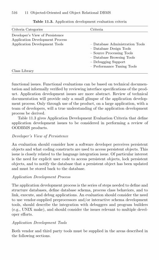
516 11 Objected-Oriented and Object Relational DBMS
Table 11.3. Application development evaluation criteria
Criteria Categories Criteria
Developer’s View of PersistenceApplication Development ProcessApplication Development Tools – Database Administration Tools
– Database Design Tools– Source Processing Tools– Database Browsing Tools– Debugging Support– Performance Tuning Tools
Class Library
functional issues. Functional evaluations can be based on technical documen-tation and informally verified by reviewing interface specifications of the prod-uct. Application development issues are more abstract. Review of technicaldocumentation will provide only a small glimpse of the application develop-ment process. Only through use of the product, on a large application, with ateam of developers, will a true understanding of the application developmentprocess be derived.
Table 11.3 gives Application Development Evaluation Criteria that defineapplication development issues to be considered in performing a review ofOODBMS products.
Developer’s View of Persistence
An evaluation should consider how a software developer perceives persistentobjects and what coding constructs are used to access persistent objects. Thisissue is closely related to the language integration issue. Of particular interestis the need for explicit user code to access persistent objects, lock persistentobjects, and to notify the database that a persistent object has been updatedand must be stored back to the database.
Application Development Process
The application development process is the series of steps needed to define andstructure databases, define database schema, process class behaviors, and tolink, execute, and debug applications. An evaluation should consider the needto use vendor-supplied preprocessors and/or interactive schema developmenttools, should describe the integration with debuggers and program builders(e.g., UNIX make), and should consider the issues relevant to multiple devel-oper efforts.
Application Development Tools
Both vendor and third party tools must be supplied in the areas described inthe following sections.
11.1 Objected oriented DBMS 517
Database Administration Tools. Database administration tools are used forcreating, deleting, and reorganizing (e.g., moving) databases. Database admin-istration tasks should be available to applications (i.e., through a programmedinterface) in order to allow applications to hide database administration tasksfrom the user.
Database Design Tools. Database design tools are used for interactively defin-ing the schema or classes which are to be stored within a database. Third partyobject-oriented modeling tools may be available which generate source codesuitable for use with the OODBMS.
Source Processing Tools. Source processing tools perform the transformationof textual descriptions of applications programs into executable code. Theseinclude preprocessors specific to the OODBMS as well as standard languagecompilers. Also included might be tools to aid in controlling the process ofapplication building (e.g., UNIX make facilities). Integration with applicationdevelopment environments should also be considered.
Database Browsing Tools. Interactive browsing tools allow database schemaand contents to be viewed graphically and possibly modified.
Debugging Support. An OODBMS vendor should supply tools and or utili-ties that are useful during the debugging process. These facilities should beinviolable from third party debugging environments.
Performance Tuning Tools. An OODBMS should provide utilities which en-able a developer to understand the performance parameters of an applicationand a means by which performance can be adjusted as a result of this analy-sis. In addition, any specific design considerations that can affect performancemust be considered.
Class Library
Object-oriented development is based on building a reusable set of classes or-ganized into a class hierarchy. The class hierarchy mechanism supports reuseof general data and behaviors in specialized classes. As described earlier,Language Integration Style, some OODBMS may provide their applicationinterface through a class library. Inherited behaviors provide support for per-sistence, object creation, deletion, update, and reference traversal.
In addition to the possibility of providing database interface through theclass library, an OODBMS may deliver application support classes. Suchclasses typically provide data abstractions such as sets, lists, dictionaries, etc.These classes should be extensible just like any other user-defined class. Ide-ally source code would be provided for these classes. Source is needed sincedocumentation is often insufficient for determining the effect of invoking eachmethod under each possible condition. Source is also useful in understand-ing performance characteristics and in repairing errors that may be found inthe code.
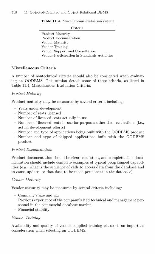
518 11 Objected-Oriented and Object Relational DBMS
Table 11.4. Miscellaneous evaluation criteria
Criteria
Product MaturityProduct DocumentationVendor MaturityVendor TrainingVendor Support and ConsultationVendor Participation in Standards Activities
Miscellaneous Criteria
A number of nontechnical criteria should also be considered when evaluat-ing an OODBMS. This section details some of these criteria, as listed inTable 11.4, Miscellaneous Evaluation Criteria.
Product Maturity
Product maturity may be measured by several criteria including:
– Years under development– Number of seats licensed– Number of licensed seats actually in use– Number of licensed seats in use for purposes other than evaluations (i.e.,
actual development efforts)– Number and type of applications being built with the OODBMS product– Number and type of shipped applications built with the OODBMS
product
Product Documentation
Product documentation should be clear, consistent, and complete. The docu-mentation should include complete examples of typical programmed capabil-ities (e.g., what is the sequence of calls to access data from the database andto cause updates to that data to be made permanent in the database).
Vendor Maturity
Vendor maturity may be measured by several criteria including:
– Company’s size and age– Previous experience of the company’s lead technical and management per-
sonnel in the commercial database market– Financial stability
Vendor Training
Availability and quality of vendor supplied training classes is an importantconsideration when selecting an OODBMS.
11.1 Objected oriented DBMS 519
Vendor Support and Consultation
It is expected that significant support will be required during the OODBMSevaluation process and to overcome the initial learning curve. OODBMS ven-dors should provide a willing and capable support staff. Support should beavailable via phone and electronically. Consulting support might also be ap-pealing where the OODBMS vendor provides expert, hands-on assistance inproduct use, object-oriented application design (especially in regards to data-base issues), and in maximizing database application performance.
Vendor Participation in Standards Activities
The vendor should be active in standards efforts in the object-oriented, lan-guage, CASE, open software, and data exchange areas. In particular:
– Object Management Group (OMG). An organization funded by over80 international information systems corporations whose charter is todevelop standards for interoperation and portability of software. TheOMG is focusing on object-oriented integration technologies such asObject Request Broker (ORB), OODBMS interfaces, and object inter-faces for existing applications.
– Object Database Management Group (ODMG). An organization ofOODBMS vendors chartered to define a standard interface to OODBMSthat will allow application portability and interoperability. Standardsdefined by the ODMG will be provided to OMG, ANSI, STEP, PCTE,etc. to aid in their respective standardization efforts.
– ANSI standardization efforts in languages (C, C++, Smalltalk), SQL, andobject-oriented databases.
– Standards such as Portable Common Tool Environment (PCTE) andCASE Data Interchange.
– Format (CDIF) providing for common data representations, dataexchange formats, and interoperation of tools.
– PDES/STEP. An effort aimed at standardizing an exchange format forproduct model data (product model data, such as CAD data, representsa prime application area for OODBMS).
11.1.7 Evaluation Targets
This chapter identifies the commercial OODBMS that were evaluated as partof this effort. For each evaluation target we identify:
– The platforms upon which that OODBMS is hosted– The level of heterogeneous operation supported by the OODBMS– The application interface languages provided by the OODBMS– Third party products that interoperate in some way with the OODBMS
Information provided in this section was provided directly by each vendor.
520 11 Objected-Oriented and Object Relational DBMS
Objectivity/DB
Objectivity/DB is an object-oriented database product developed and mar-keted by Objectivity, Inc., 800 El Camino Real, Menlo Park, CA 94025, (415)688-8024. Evaluation information provided in this report was obtained fromthe technical documentation set for Objectivity/DB Version 2.0 and fromdiscussions with technical representatives of Objectivity, Inc.
Objectivity/DB may be executed by client applications hosted in a hete-rogeneous network of:
– DECstation under Ultrix 4.2– Sun4/SPARC under SunOS 4.1, Solaris 2.0 or Solaris 2.1– VAX under Ultrix 4.2 or VMS– Hewlett Packard 9000 series 300 under HP/UX 8.0– Hewlett Packard 9000 series 700 or 800 under HP/UX 8.0 or HP/UX 9.0– IBM RISC System/6000 under AIX– Silicon Graphics Iris under IRIX 4.0– NCR System 3300 (i386) under SVR4 Version 2.0
Applications running on any of the earlier platforms, connected via a localarea network, may share access to a single database. Objectivity, Inc., hasannounced and released a Beta test subset version of Objectivity/DB forWindows NT. A version running on DEC/ALPHA under OSF 1.0 is also inBeta testing.
Objectivity/DB provides application interfaces for:
– AT&T compatible C++– ANSI C
Objectivity/DB was designed as an open product and is advertised to workwith any ANSI C or AT&T compatible C++ compiler. Objectivity, Inc., haspartnership agreements to develop tool integrations and/or be compatiblewith the following products:
1. Program Development Environments:– SoftBench from Hewlett-Packard– ObjectCenter from CenterLine Software– FUSE from DEC– WorkBench 6000 from IBM– ObjectWorks from ParcPlace
2. RDBMS Gateways:– Persistence Software
3. Object-oriented GUIs:– UIM/X from Visual Software, Ltd.– XVT from XVT Software, Inc.– Integrated Computer Solutions, Inc.– Objective, Inc.– Micram Classify/DB.
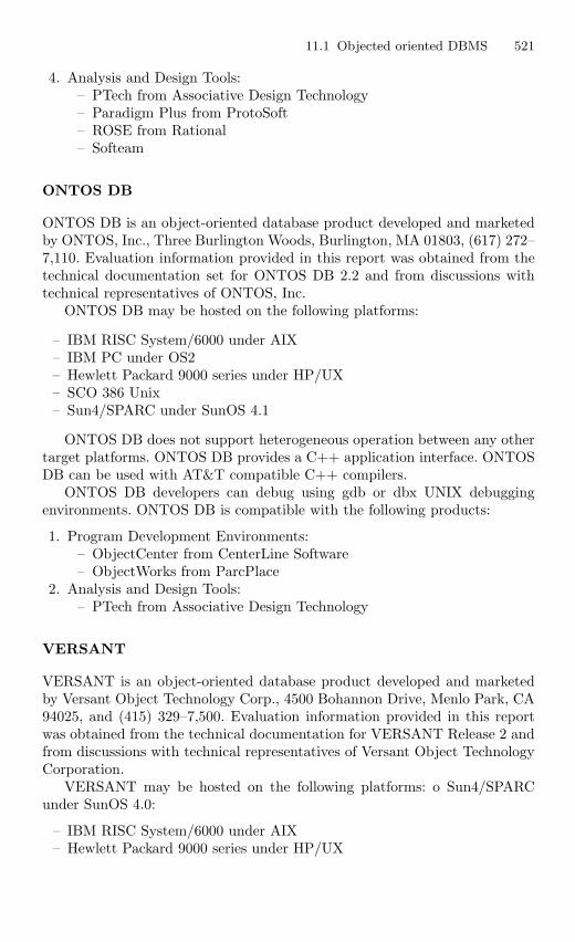
11.1 Objected oriented DBMS 521
4. Analysis and Design Tools:– PTech from Associative Design Technology– Paradigm Plus from ProtoSoft– ROSE from Rational– Softeam
ONTOS DB
ONTOS DB is an object-oriented database product developed and marketedby ONTOS, Inc., Three Burlington Woods, Burlington, MA 01803, (617) 272–7,110. Evaluation information provided in this report was obtained from thetechnical documentation set for ONTOS DB 2.2 and from discussions withtechnical representatives of ONTOS, Inc.
ONTOS DB may be hosted on the following platforms:
– IBM RISC System/6000 under AIX– IBM PC under OS2– Hewlett Packard 9000 series under HP/UX– SCO 386 Unix– Sun4/SPARC under SunOS 4.1
ONTOS DB does not support heterogeneous operation between any othertarget platforms. ONTOS DB provides a C++ application interface. ONTOSDB can be used with AT&T compatible C++ compilers.
ONTOS DB developers can debug using gdb or dbx UNIX debuggingenvironments. ONTOS DB is compatible with the following products:
1. Program Development Environments:– ObjectCenter from CenterLine Software– ObjectWorks from ParcPlace
2. Analysis and Design Tools:– PTech from Associative Design Technology
VERSANT
VERSANT is an object-oriented database product developed and marketedby Versant Object Technology Corp., 4500 Bohannon Drive, Menlo Park, CA94025, and (415) 329–7,500. Evaluation information provided in this reportwas obtained from the technical documentation for VERSANT Release 2 andfrom discussions with technical representatives of Versant Object TechnologyCorporation.
VERSANT may be hosted on the following platforms: o Sun4/SPARCunder SunOS 4.0:
– IBM RISC System/6000 under AIX– Hewlett Packard 9000 series under HP/UX
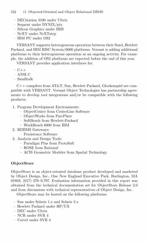
522 11 Objected-Oriented and Object Relational DBMS
– DECstation 3100 under Ultrix– Sequent under DYNIX/ptx– Silicon Graphics under IRIS– NeXT under NeXTstep– IBM PC under OS2
VERSANT supports heterogeneous operation between their Sun4, HewlettPackard, and IBM RISC System/6000 platforms. Versant is adding additionalplatforms to their heterogeneous operation as an ongoing activity. For exam-ple, the addition of OS2 platforms are expected before the end of this year.
VERSANT provides application interfaces for:
– C++– ANSI C– Smalltalk
C++ compilers from AT&T, Sun, Hewlett Packard, Glockenspiel are com-patible with VERSANT. Versant Object Technologies has partnership agree-ments to develop tool integrations and/or be compatible with the followingproducts:
1. Program Development Environments:– ObjectCenter from CenterLine Software– ObjectWorks from ParcPlace– SoftBench from Hewlett-Packard– WorkBench 6000 from IBM
2. RDBMS Gateways:– Persistence Software
3. Analysis and Design Tools:– Paradigm Plus from ProtoSoft– ROSE from Rational– ACIS Geometric Modeler from Spatial Technology
ObjectStore
ObjectStore is an object-oriented database product developed and marketedby Object Design, Inc., One New England Executive Park, Burlington, MA01803, (617) 270–9,797. Evaluation information provided in this report wasobtained from the technical documentation set for ObjectStore Release 2.0and from discussions with technical representatives of Object Design, Inc.
ObjectStore may be hosted on the following platforms:
– Sun under Solaris 1.x and Solaris 2.x– Hewlett Packard under HP/UX– DEC under Ultrix– NCR under SVR 4– Univel under SVR 4
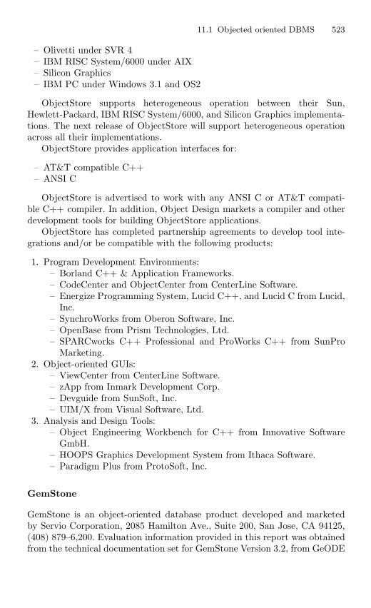
11.1 Objected oriented DBMS 523
– Olivetti under SVR 4– IBM RISC System/6000 under AIX– Silicon Graphics– IBM PC under Windows 3.1 and OS2
ObjectStore supports heterogeneous operation between their Sun,Hewlett-Packard, IBM RISC System/6000, and Silicon Graphics implementa-tions. The next release of ObjectStore will support heterogeneous operationacross all their implementations.
ObjectStore provides application interfaces for:
– AT&T compatible C++– ANSI C
ObjectStore is advertised to work with any ANSI C or AT&T compati-ble C++ compiler. In addition, Object Design markets a compiler and otherdevelopment tools for building ObjectStore applications.
ObjectStore has completed partnership agreements to develop tool inte-grations and/or be compatible with the following products:
1. Program Development Environments:– Borland C++ & Application Frameworks.– CodeCenter and ObjectCenter from CenterLine Software.– Energize Programming System, Lucid C++, and Lucid C from Lucid,
Inc.– SynchroWorks from Oberon Software, Inc.– OpenBase from Prism Technologies, Ltd.– SPARCworks C++ Professional and ProWorks C++ from SunPro
Marketing.2. Object-oriented GUIs:
– ViewCenter from CenterLine Software.– zApp from Inmark Development Corp.– Devguide from SunSoft, Inc.– UIM/X from Visual Software, Ltd.
3. Analysis and Design Tools:– Object Engineering Workbench for C++ from Innovative Software
GmbH.– HOOPS Graphics Development System from Ithaca Software.– Paradigm Plus from ProtoSoft, Inc.
GemStone
GemStone is an object-oriented database product developed and marketedby Servio Corporation, 2085 Hamilton Ave., Suite 200, San Jose, CA 94125,(408) 879–6,200. Evaluation information provided in this report was obtainedfrom the technical documentation set for GemStone Version 3.2, from GeODE
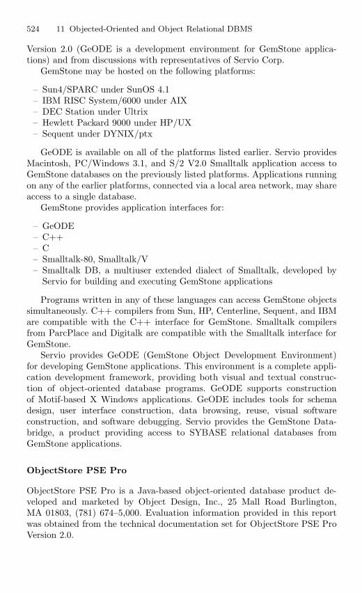
524 11 Objected-Oriented and Object Relational DBMS
Version 2.0 (GeODE is a development environment for GemStone applica-tions) and from discussions with representatives of Servio Corp.
GemStone may be hosted on the following platforms:
– Sun4/SPARC under SunOS 4.1– IBM RISC System/6000 under AIX– DEC Station under Ultrix– Hewlett Packard 9000 under HP/UX– Sequent under DYNIX/ptx
GeODE is available on all of the platforms listed earlier. Servio providesMacintosh, PC/Windows 3.1, and S/2 V2.0 Smalltalk application access toGemStone databases on the previously listed platforms. Applications runningon any of the earlier platforms, connected via a local area network, may shareaccess to a single database.
GemStone provides application interfaces for:
– GeODE– C++– C– Smalltalk-80, Smalltalk/V– Smalltalk DB, a multiuser extended dialect of Smalltalk, developed by
Servio for building and executing GemStone applications
Programs written in any of these languages can access GemStone objectssimultaneously. C++ compilers from Sun, HP, Centerline, Sequent, and IBMare compatible with the C++ interface for GemStone. Smalltalk compilersfrom ParcPlace and Digitalk are compatible with the Smalltalk interface forGemStone.
Servio provides GeODE (GemStone Object Development Environment)for developing GemStone applications. This environment is a complete appli-cation development framework, providing both visual and textual construc-tion of object-oriented database programs. GeODE supports constructionof Motif-based X Windows applications. GeODE includes tools for schemadesign, user interface construction, data browsing, reuse, visual softwareconstruction, and software debugging. Servio provides the GemStone Data-bridge, a product providing access to SYBASE relational databases fromGemStone applications.
ObjectStore PSE Pro
ObjectStore PSE Pro is a Java-based object-oriented database product de-veloped and marketed by Object Design, Inc., 25 Mall Road Burlington,MA 01803, (781) 674–5,000. Evaluation information provided in this reportwas obtained from the technical documentation set for ObjectStore PSE ProVersion 2.0.
11.1 Objected oriented DBMS 525
ObjectStore PSE Pro may be hosted on the following platforms that sup-port Java VMs:
– Windows 95– Windows NT– OS/2– Macintosh– Unix
ObjectStore PSE Pro supports JDK 1.1 or higher.
IBM San Francisco
IBM San Francisco is an object-oriented framework developed and marketedby IBM. Evaluation information provided in this report was obtained from thetechnical documentation set for IBM San Francisco Version 1.2, along withdiscussions with technical representatives of IBM, San Francisco division.
The IBM San Francisco framework may be used to develop client andserver Java-based applications hosted in a heterogeneous network of:
– Windows 95 (client)– Windows NT Workstation 4.0– Windows NT Server 4.0– AIX 3.1– OS/400
Server applications can interface to ODBC-JDBC supported databases, ordirectly through object-relational mapping to:
– Microsoft SQL Server 6.5– IBM DB2
11.1.8 Object Relational DBMS
In spite of the impact of relational databases in last decades, this kind ofdatabases has some limitations to support data persistence required byactual applications. Due to recent hardware improvements more sophis-ticated applications have emerged, such as CAD/CAM (Computer-AidedDesign/Computer-Aided Manufacturing), CASE (Computer-Aided SoftwareEngineering), GIS (Geographic Information System), etc. These applicationscan be characterized as consisting of complex objects related by complex rela-tionships. Representing such objects and relationships in the relational modelimplies that the objects must be decomposed into a large number of tuples.
Thus, a considerable number of joins is necessary to retrieve an objectand, when tables are too deeply nested, performance is significantly reduced.A new generation of databases has appeared to solve these problems: theobject-oriented database generation, which includes the object-relational andobject databases. This new technologyis well suited for storing and retrieving
526 11 Objected-Oriented and Object Relational DBMS
complex data because it supports complex data types and relationships, mul-timedia data, inheritance, etc. Nonetheless, good technology is not enough tosupport complex objects and applications. It is necessary to define method-ologies that guide designers in the object database design task, in the sameway traditionally has been done with relational databases.
Unfortunately, none of these proposals can be considered as “the method,”neither for object-relational nor for object databases. On the one hand, theydo not consider last versions of the representative standards for both tech-nologies: ODMG 3.0 for object databases and SQL: 1999 for object-relationaldatabases. And, on the other hand, some of them are based on techniques asOMT or, even, on the E/R model. So, they have to be updated consideringUML, SQL: 1999, and ODMG 3.0 as their reference models. Object data-bases are well suited for storing and retrieving complex data by allowing theuser to navigate through data. However, object-relational technology, that is,relational technology extended with new capabilities, such as triggers, meth-ods, user defined types, etc., presents two advantages compared with objectdatabases: it is compatible with relational technology and provides a bettersupport for complex applications. Therefore, object-relational databases areexpected to have a bigger impact in the market than object databases. Forthese reasons in this section we focus on object-relational databases design.
In this chapter we propose a methodology for object-relational databasedesign. As conceptual modeling technique we have chosen the UML class dia-gram. UML, as a Universal Modeling Language is every day more accepted. Italso presents the advantage of being able to model the full system, includingthe database model, in a uniform way. Besides, as UML is an extensible lan-guage, it is possible to define the required stereotypes for specific applications.The methodology provides some guidelines to translate a conceptual schema(in UML notation) into a logical schema.
As logical model we use the SQL: 1999 object-relational model so thatthe guidelines were not dependent of the different implementations of object-relational products. We use Oracle8i as an implementation example. In thissection, we focus on aggregation and composition design. In the frameworkof our methodology, we propose specific guidelines to design aggregations andcompositions in an object-relational model. Although the methodology, aswe have explained earlier, is mainly based in SQL: 1999, in this section, wefocus on the aggregation and composition implementation in Oracle8i. Thereason is that this product supports a collection data type, the nested table,which is specially appropriated to implement aggregations and compositions.This collection data type is not provided neither by SQL: 1999 nor by otherproducts, such as Informix Universal Server.
11.1.9 Object-Relational Model
In this section we summarize the object model of the current standard forobject-relational databases, SQL: 1999, as well as the main characteristics
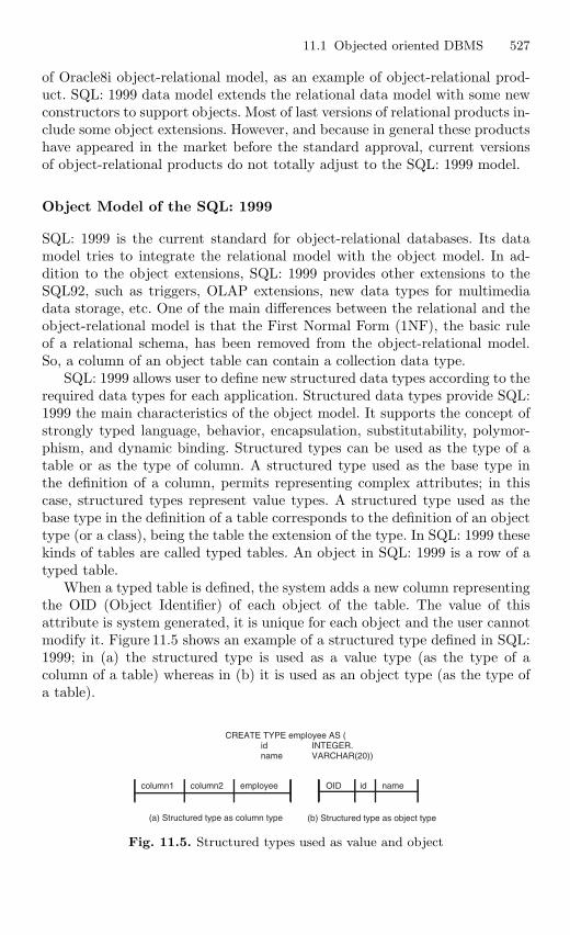
11.1 Objected oriented DBMS 527
of Oracle8i object-relational model, as an example of object-relational prod-uct. SQL: 1999 data model extends the relational data model with some newconstructors to support objects. Most of last versions of relational products in-clude some object extensions. However, and because in general these productshave appeared in the market before the standard approval, current versionsof object-relational products do not totally adjust to the SQL: 1999 model.
Object Model of the SQL: 1999
SQL: 1999 is the current standard for object-relational databases. Its datamodel tries to integrate the relational model with the object model. In ad-dition to the object extensions, SQL: 1999 provides other extensions to theSQL92, such as triggers, OLAP extensions, new data types for multimediadata storage, etc. One of the main differences between the relational and theobject-relational model is that the First Normal Form (1NF), the basic ruleof a relational schema, has been removed from the object-relational model.So, a column of an object table can contain a collection data type.
SQL: 1999 allows user to define new structured data types according to therequired data types for each application. Structured data types provide SQL:1999 the main characteristics of the object model. It supports the concept ofstrongly typed language, behavior, encapsulation, substitutability, polymor-phism, and dynamic binding. Structured types can be used as the type of atable or as the type of column. A structured type used as the base type inthe definition of a column, permits representing complex attributes; in thiscase, structured types represent value types. A structured type used as thebase type in the definition of a table corresponds to the definition of an objecttype (or a class), being the table the extension of the type. In SQL: 1999 thesekinds of tables are called typed tables. An object in SQL: 1999 is a row of atyped table.
When a typed table is defined, the system adds a new column representingthe OID (Object Identifier) of each object of the table. The value of thisattribute is system generated, it is unique for each object and the user cannotmodify it. Figure 11.5 shows an example of a structured type defined in SQL:1999; in (a) the structured type is used as a value type (as the type of acolumn of a table) whereas in (b) it is used as an object type (as the type ofa table).
CREATE TYPE employee AS ( id INTEGER. name VARCHAR(20))
column1 column2
(a) Structured type as column type (b) Structured type as object type
employee OID id name
Fig. 11.5. Structured types used as value and object
528 11 Objected-Oriented and Object Relational DBMS
A structured type can include associated methods representing its behav-ior. A method is an SQL function, whose signature is defined next to thedefinition of the structured type. The body specification is defined separatelyon the signature of the method.
SQL: 1999 supports simple inheritance for structured types and for typedtables. A subtype inherits the attributes and the behavior of the supertype.A subtable inherits the columns, restrictions, triggers, and methods of thesupertable. A row of a typed table is an object and differs from the rest ofobjects by its OID. The value of the OID is generated by the system whena new object is inserted in the table. The type of this column is a referencetype (REF). Therefore, each typed table has a column that contains the OIDvalue. There are different REF types, one for each object type; that is, theREF type is a constructor of types rather than a type itself. An attributedefined as reference type holds the OID of the referred object. So, the REFtype permits implementing relationships without using foreign keys. SQL:1999 supports another structured type: the ROW type. The ROW type is astructured type defined by the user. It has neither extension nor OID. So, itcannot be used as an object type.
SQL: 1999 only supports a collection type ARRAY. The ARRAY can beused whenever another type can be placed (as the type of an attribute ofa structured type, as the type of a column, etc.). The ARRAY type allowsrepresenting multivolume attributes not forcing tables to be in 1NF.
Object Model of Oracle8i
As well as SQL: 1999, Oracle8i supports structured data types that can bedefined by the user (although, with a different syntax). A structured type canbe used, as in SQL: 1999, as a column type or as a type of a table. A structuredtype used as a column type represents a value type and a structured type usedas the type of a table represents an object type, being the table the extensionof the type. Each row of this kind of tables is an object and, in the same wayas in SQL: 1999, they have a special column of reference type (REF) thatallows identifying each object (OID). It is also possible to define an attributeas a reference to an object type. Oracle8i allows associating behavior to objecttypes, defining the signature of the methods as part of the type definition. Thebody of the method is defined separately.
Oracle8i supports two kinds of collections: VARRAYS, equivalent to theSQL: 1999 ARRAY and the nested table. A nested table is a table that isembedded in another table. It is possible to define a table data type andto use this type as a column type in a table. So, this column contains atable (called nested table) with a collection of values, objects, or references.Figure 11.6 shows an example of nested table (C Table).
One of the main differences between Oracle8i and SQL: 1999 object-relational model is that Oracle8i does not support inheritance, neither of typesnor of tables. There exist, however, some relational products, as for example,
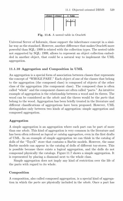
11.1 Objected oriented DBMS 529
Fig. 11.6. A nested table in Oracle8i
Universal Server of Informix, those support the inheritance concept in a simi-lar way as the standard. However, another difference that makes Oracle8i morepowerful than SQL: 1999 is related with the collection types. The nested tablenot supported by SQL: 1999, allows to represent an object collection embed-ded in another object, that could be a natural way to implement the UMLaggregation.
11.1.10 Aggregation and Composition in UML
An aggregation is a special form of association between classes that representsthe concept of “WHOLE PART.” Each object of one of the classes that belongto the aggregation (the composed class) is composed of objects of the otherclass of the aggregation (the component class). The composed class is oftencalled “whole” and the component classes are often called “parts.” An intuitiveexample of aggregation is the relationship between a wood and its threes. Thewood can be considered as the whole and the threes would be the parts thatbelong to the wood. Aggregation has been briefly treated in the literature anddifferent classifications of aggregations have been proposed. However, UMLdistinguishes only between two kinds of aggregation: simple aggregation andcomposed aggregation.
Aggregation
A simple aggregation is an aggregation where each part can be part of morethan one whole. This kind of aggregation is very common in the literature andhas been often refereed as logical or catalog aggregation, even in the first draftsof UML. As an example of simple aggregation we can think in the catalog ofdolls of the “ToysX” store that contains n Barbie models. However, the sameBarbie models can appear in the catalog of dolls of different toy-stores. Thisis possible because there exists a logical aggregation, and the dolls do notcompound physically the catalogs. Figure 11.7 shows a simple aggregation. Itis represented by placing a diamond next to the whole class.
Simple aggregation does not imply any kind of restriction over the life ofthe parts with regard to its whole.
Composition
A composition, also called composed aggregation, is a special kind of aggrega-tion in which the parts are physically included in the whole. Once a part has
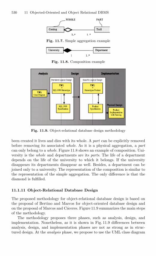
530 11 Objected-Oriented and Object Relational DBMS
Fig. 11.7. Simple aggregation example
Fig. 11.8. Composition example
Fig. 11.9. Object-relational database design methodology
been created it lives and dies with its whole. A part can be explicitly removedbefore removing its associated whole. As it is a physical aggregation, a partcan only belong to a whole. Figure 11.8 shows an example of composition. Uni-versity is the whole and departments are its parts. The life of a departmentdepends on the life of the university to which it belongs. If the universitydisappears its departments disappear as well. Besides, a department can bejoined only to a university. The representation of the composition is similar tothe representation of the simple aggregation. The only difference is that thediamond is fulfilled.
11.1.11 Object-Relational Database Design
The proposed methodology for object-relational database design is based onthe proposal of Bertino and Marcos for object-oriented database design andon the proposal of Marcos and Caceres. Figure 11.9 summarizes the main stepsof the methodology.
The methodology proposes three phases, such as analysis, design, andimplementation. Nonetheless, as it is shown in Fig. 11.9 differences betweenanalysis, design, and implementation phases are not as strong as in struc-tured design. At the analysis phase, we propose to use the UML class diagram
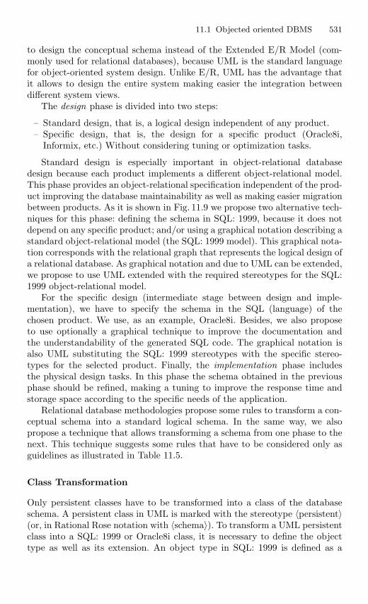
11.1 Objected oriented DBMS 531
to design the conceptual schema instead of the Extended E/R Model (com-monly used for relational databases), because UML is the standard languagefor object-oriented system design. Unlike E/R, UML has the advantage thatit allows to design the entire system making easier the integration betweendifferent system views.
The design phase is divided into two steps:
– Standard design, that is, a logical design independent of any product.– Specific design, that is, the design for a specific product (Oracle8i,
Informix, etc.) Without considering tuning or optimization tasks.
Standard design is especially important in object-relational databasedesign because each product implements a different object-relational model.This phase provides an object-relational specification independent of the prod-uct improving the database maintainability as well as making easier migrationbetween products. As it is shown in Fig. 11.9 we propose two alternative tech-niques for this phase: defining the schema in SQL: 1999, because it does notdepend on any specific product; and/or using a graphical notation describing astandard object-relational model (the SQL: 1999 model). This graphical nota-tion corresponds with the relational graph that represents the logical design ofa relational database. As graphical notation and due to UML can be extended,we propose to use UML extended with the required stereotypes for the SQL:1999 object-relational model.
For the specific design (intermediate stage between design and imple-mentation), we have to specify the schema in the SQL (language) of thechosen product. We use, as an example, Oracle8i. Besides, we also proposeto use optionally a graphical technique to improve the documentation andthe understandability of the generated SQL code. The graphical notation isalso UML substituting the SQL: 1999 stereotypes with the specific stereo-types for the selected product. Finally, the implementation phase includesthe physical design tasks. In this phase the schema obtained in the previousphase should be refined, making a tuning to improve the response time andstorage space according to the specific needs of the application.
Relational database methodologies propose some rules to transform a con-ceptual schema into a standard logical schema. In the same way, we alsopropose a technique that allows transforming a schema from one phase to thenext. This technique suggests some rules that have to be considered only asguidelines as illustrated in Table 11.5.
Class Transformation
Only persistent classes have to be transformed into a class of the databaseschema. A persistent class in UML is marked with the stereotype 〈persistent〉(or, in Rational Rose notation with 〈schema〉). To transform a UML persistentclass into a SQL: 1999 or Oracle8i class, it is necessary to define the objecttype as well as its extension. An object type in SQL: 1999 is defined as a
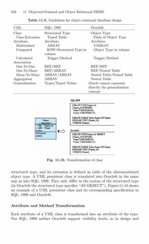
532 11 Objected-Oriented and Object Relational DBMS
Table 11.5. Guidelines for object-relational database design
UML SQL: 1999 Oracle8i
Class Structured Type Object TypeClass Extension Typed Table Table of Object Type
Attribute Attribute AttributeMultivalued ARRAY VARRAYComposed ROW/Structured Type in
columnObject Type in column
Calculated Trigger/Method Trigger/MethodAssociation
One-To-One REF/REF REF/REFOne-To-Many REF/ARRAY REF/Nested TableMany-To-Many ARRAY/ARRAY Nested Table/Nested Table
Aggregation ARRAY Nested TableGeneralization Types/Typed Tables Oracle cannot represent
directly the generalizationconcept
Fig. 11.10. Transformation of class
structured type, and its extension is defined as table of the aforementionedobject type. A UML persistent class is translated into Oracle8i in the sameway as into SQL: 1999. They only differ in the syntax of the structured type(in Oracle8i the structured type specifies “AS OBJECT”). Figure 11.10 showsan example of a UML persistent class and its corresponding specification inSQL: 1999 and Oracle8i.
Attribute and Method Transformation
Each attribute of a UML class is transformed into an attribute of the type.Nor SQL: 1999 neither Oracle8i support visibility levels, so in design and
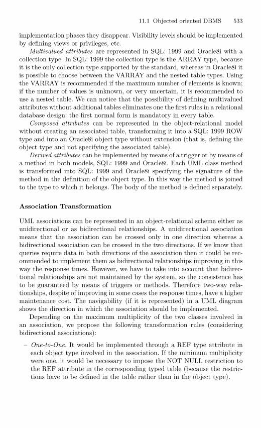
11.1 Objected oriented DBMS 533
implementation phases they disappear. Visibility levels should be implementedby defining views or privileges, etc.
Multivalued attributes are represented in SQL: 1999 and Oracle8i with acollection type. In SQL: 1999 the collection type is the ARRAY type, becauseit is the only collection type supported by the standard, whereas in Oracle8i itis possible to choose between the VARRAY and the nested table types. Usingthe VARRAY is recommended if the maximum number of elements is known;if the number of values is unknown, or very uncertain, it is recommended touse a nested table. We can notice that the possibility of defining multivaluedattributes without additional tables eliminates one the first rules in a relationaldatabase design: the first normal form is mandatory in every table.
Composed attributes can be represented in the object-relational modelwithout creating an associated table, transforming it into a SQL: 1999 ROWtype and into an Oracle8i object type without extension (that is, defining theobject type and not specifying the associated table).
Derived attributes can be implemented by means of a trigger or by means ofa method in both models, SQL: 1999 and Oracle8i. Each UML class methodis transformed into SQL: 1999 and Oracle8i specifying the signature of themethod in the definition of the object type. In this way the method is joinedto the type to which it belongs. The body of the method is defined separately.
Association Transformation
UML associations can be represented in an object-relational schema either asunidirectional or as bidirectional relationships. A unidirectional associationmeans that the association can be crossed only in one direction whereas abidirectional association can be crossed in the two directions. If we know thatqueries require data in both directions of the association then it could be rec-ommended to implement them as bidirectional relationships improving in thisway the response times. However, we have to take into account that bidirec-tional relationships are not maintained by the system, so the consistence hasto be guaranteed by means of triggers or methods. Therefore two-way rela-tionships, despite of improving in some cases the response times, have a highermaintenance cost. The navigability (if it is represented) in a UML diagramshows the direction in which the association should be implemented.
Depending on the maximum multiplicity of the two classes involved inan association, we propose the following transformation rules (consideringbidirectional associations):
– One-to-One. It would be implemented through a REF type attribute ineach object type involved in the association. If the minimum multiplicitywere one, it would be necessary to impose the NOT NULL restriction tothe REF attribute in the corresponding typed table (because the restric-tions have to be defined in the table rather than in the object type).
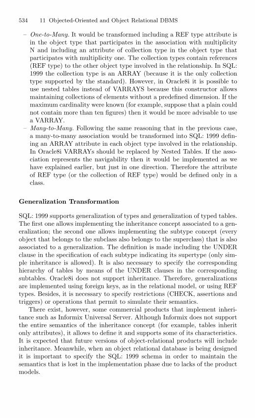
534 11 Objected-Oriented and Object Relational DBMS
– One-to-Many. It would be transformed including a REF type attribute isin the object type that participates in the association with multiplicityN and including an attribute of collection type in the object type thatparticipates with multiplicity one. The collection types contain references(REF type) to the other object type involved in the relationship. In SQL:1999 the collection type is an ARRAY (because it is the only collectiontype supported by the standard). However, in Oracle8i it is possible touse nested tables instead of VARRAYS because this constructor allowsmaintaining collections of elements without a predefined dimension. If themaximum cardinality were known (for example, suppose that a plain couldnot contain more than ten figures) then it would be more advisable to usea VARRAY.
– Many-to-Many. Following the same reasoning that in the previous case,a many-to-many association would be transformed into SQL: 1999 defin-ing an ARRAY attribute in each object type involved in the relationship.In Oracle8i VARRAYs should be replaced by Nested Tables. If the asso-ciation represents the navigability then it would be implemented as wehave explained earlier, but just in one direction. Therefore the attributeof REF type (or the collection of REF type) would be defined only in aclass.
Generalization Transformation
SQL: 1999 supports generalization of types and generalization of typed tables.The first one allows implementing the inheritance concept associated to a gen-eralization; the second one allows implementing the subtype concept (everyobject that belongs to the subclass also belongs to the superclass) that is alsoassociated to a generalization. The definition is made including the UNDERclause in the specification of each subtype indicating its supertype (only sim-ple inheritance is allowed). It is also necessary to specify the correspondinghierarchy of tables by means of the UNDER clauses in the correspondingsubtables. Oracle8i does not support inheritance. Therefore, generalizationsare implemented using foreign keys, as in the relational model, or using REFtypes. Besides, it is necessary to specify restrictions (CHECK, assertions andtriggers) or operations that permit to simulate their semantics.
There exist, however, some commercial products that implement inheri-tance such as Informix Universal Server. Although Informix does not supportthe entire semantics of the inheritance concept (for example, tables inheritonly attributes), it allows to define it and supports some of its characteristics.It is expected that future versions of object-relational products will includeinheritance. Meanwhile, when an object relational database is being designedit is important to specify the SQL: 1999 schema in order to maintain thesemantics that is lost in the implementation phase due to lacks of the productmodels.
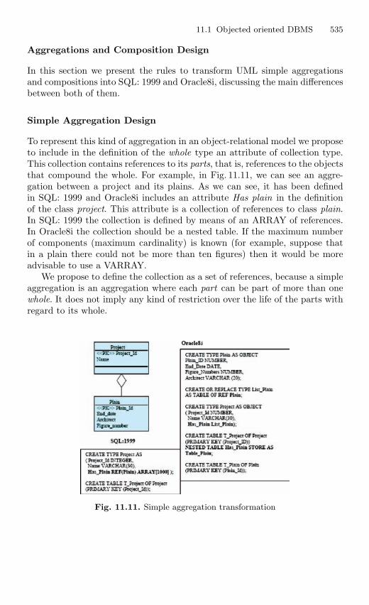
11.1 Objected oriented DBMS 535
Aggregations and Composition Design
In this section we present the rules to transform UML simple aggregationsand compositions into SQL: 1999 and Oracle8i, discussing the main differencesbetween both of them.
Simple Aggregation Design
To represent this kind of aggregation in an object-relational model we proposeto include in the definition of the whole type an attribute of collection type.This collection contains references to its parts, that is, references to the objectsthat compound the whole. For example, in Fig. 11.11, we can see an aggre-gation between a project and its plains. As we can see, it has been definedin SQL: 1999 and Oracle8i includes an attribute Has plain in the definitionof the class project. This attribute is a collection of references to class plain.In SQL: 1999 the collection is defined by means of an ARRAY of references.In Oracle8i the collection should be a nested table. If the maximum numberof components (maximum cardinality) is known (for example, suppose thatin a plain there could not be more than ten figures) then it would be moreadvisable to use a VARRAY.
We propose to define the collection as a set of references, because a simpleaggregation is an aggregation where each part can be part of more than onewhole. It does not imply any kind of restriction over the life of the parts withregard to its whole.
Fig. 11.11. Simple aggregation transformation
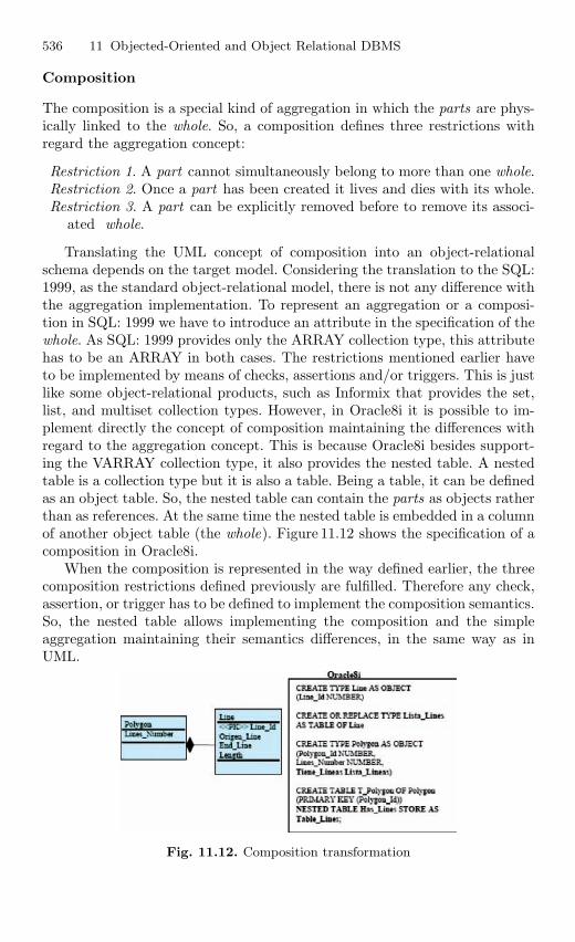
536 11 Objected-Oriented and Object Relational DBMS
Composition
The composition is a special kind of aggregation in which the parts are phys-ically linked to the whole. So, a composition defines three restrictions withregard the aggregation concept:
Restriction 1. A part cannot simultaneously belong to more than one whole.Restriction 2. Once a part has been created it lives and dies with its whole.Restriction 3. A part can be explicitly removed before to remove its associ-
ated whole.
Translating the UML concept of composition into an object-relationalschema depends on the target model. Considering the translation to the SQL:1999, as the standard object-relational model, there is not any difference withthe aggregation implementation. To represent an aggregation or a composi-tion in SQL: 1999 we have to introduce an attribute in the specification of thewhole. As SQL: 1999 provides only the ARRAY collection type, this attributehas to be an ARRAY in both cases. The restrictions mentioned earlier haveto be implemented by means of checks, assertions and/or triggers. This is justlike some object-relational products, such as Informix that provides the set,list, and multiset collection types. However, in Oracle8i it is possible to im-plement directly the concept of composition maintaining the differences withregard to the aggregation concept. This is because Oracle8i besides support-ing the VARRAY collection type, it also provides the nested table. A nestedtable is a collection type but it is also a table. Being a table, it can be definedas an object table. So, the nested table can contain the parts as objects ratherthan as references. At the same time the nested table is embedded in a columnof another object table (the whole). Figure 11.12 shows the specification of acomposition in Oracle8i.
When the composition is represented in the way defined earlier, the threecomposition restrictions defined previously are fulfilled. Therefore any check,assertion, or trigger has to be defined to implement the composition semantics.So, the nested table allows implementing the composition and the simpleaggregation maintaining their semantics differences, in the same way as inUML.
Fig. 11.12. Composition transformation
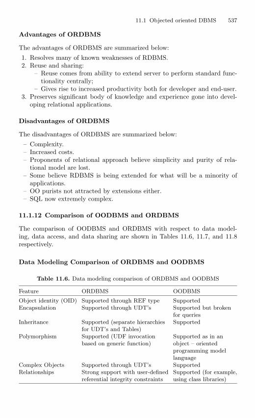
11.1 Objected oriented DBMS 537
Advantages of ORDBMS
The advantages of ORDBMS are summarized below:1. Resolves many of known weaknesses of RDBMS.2. Reuse and sharing:
– Reuse comes from ability to extend server to perform standard func-tionality centrally;
– Gives rise to increased productivity both for developer and end-user.3. Preserves significant body of knowledge and experience gone into devel-
oping relational applications.
Disadvantages of ORDBMS
The disadvantages of ORDBMS are summarized below:– Complexity.– Increased costs.– Proponents of relational approach believe simplicity and purity of rela-
tional model are lost.– Some believe RDBMS is being extended for what will be a minority of
applications.– OO purists not attracted by extensions either.– SQL now extremely complex.
11.1.12 Comparison of OODBMS and ORDBMS
The comparison of OODBMS and ORDBMS with respect to data model-ing, data access, and data sharing are shown in Tables 11.6, 11.7, and 11.8respectively.
Data Modeling Comparison of ORDBMS and OODBMS
Table 11.6. Data modeling comparison of ORDBMS and OODBMS
Feature ORDBMS OODBMS
Object identity (OID) Supported through REF type SupportedEncapsulation Supported through UDT’s Supported but broken
for queriesInheritance Supported (separate hierarchies Supported
for UDT’s and Tables)Polymorphism Supported (UDF invocation Supported as in an
based on generic function) object – orientedprogramming modellanguage
Complex Objects Supported through UDT’s SupportedRelationships Strong support with user-defined Supported (for example,
referential integrity constraints using class libraries)
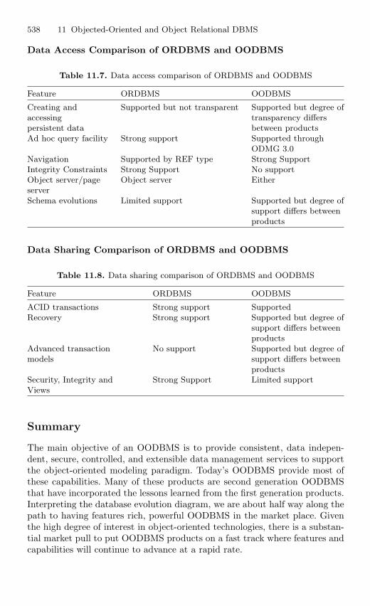
538 11 Objected-Oriented and Object Relational DBMS
Data Access Comparison of ORDBMS and OODBMS
Table 11.7. Data access comparison of ORDBMS and OODBMS
Feature ORDBMS OODBMS
Creating and Supported but not transparent Supported but degree ofaccessing transparency differspersistent data between productsAd hoc query facility Strong support Supported through
ODMG 3.0Navigation Supported by REF type Strong SupportIntegrity Constraints Strong Support No supportObject server/page Object server EitherserverSchema evolutions Limited support Supported but degree of
support differs betweenproducts
Data Sharing Comparison of ORDBMS and OODBMS
Table 11.8. Data sharing comparison of ORDBMS and OODBMS
Feature ORDBMS OODBMS
ACID transactions Strong support SupportedRecovery Strong support Supported but degree of
support differs betweenproducts
Advanced transaction No support Supported but degree ofmodels support differs between
productsSecurity, Integrity and Strong Support Limited supportViews
Summary
The main objective of an OODBMS is to provide consistent, data indepen-dent, secure, controlled, and extensible data management services to supportthe object-oriented modeling paradigm. Today’s OODBMS provide most ofthese capabilities. Many of these products are second generation OODBMSthat have incorporated the lessons learned from the first generation products.Interpreting the database evolution diagram, we are about half way along thepath to having features rich, powerful OODBMS in the market place. Giventhe high degree of interest in object-oriented technologies, there is a substan-tial market pull to put OODBMS products on a fast track where features andcapabilities will continue to advance at a rapid rate.
11.1 Objected oriented DBMS 539
A major strength of the OODBMS technology is its ability to representcomplex behaviors directly. By incorporating behaviors into the database, onesubstantially reduces the complexity of applications that use the database. Inthe ideal scenario, most of the application code will deal with data entry anddata display. All the functionality associated with data integrity and datamanagement would be defined within the basic object model. The advantagesof this approach are:
– All operations are defined once and reused by all applications.– Changes to an operation affect all applications, simplifying database main-
tenance (although most databases require the applications to be recom-piled).
The benefits of object-oriented database applications development are anincrease in productivity resulting from the high degree of code reuse and anability to cope with greater complexity resulting from incremental refinementof problems. One also gets increased design flexibility due to polymorphismand dynamic binding. Finally, both developers and users will experience ben-efits resulting from the naturalness and simplicity of representing data asobjects.
These strengths need to be weighed against the organizational changesintroduced by this new and different way of engineering solutions. Differentengineering considerations contribute to performance and reliability than forrelational DBMS’s. Projects need to be managed differently. Clearly, one needsto approach this new technology with eyes open, recognizing that the benefitswill be realized after a considerable investment has been made to learn howto use it effectively.
In this chapter we have summarized a methodology for object-relationaldatabase design focused on the aggregation and composition implementation.The methodology proposes three phases: analysis, design and implementation.As conceptual modeling technique we have chosen the UML class diagram.As logical model we have used the SQL: 1999 object-relational model, sothat the guidelines are not dependent of the different implementations ofeach object-relational product. As a product example we have used Oracle8i.We have briefly explained the rules to transform a UML aggregation into anobject-relational model considering the differences between aggregation andcomposition.
We have focused on the implementation in Oracle8i because this productsupports a collection data type, the nested table that is specially appropri-ated to implement aggregations and compositions. This collection data typeis not provided neither by SQL: 1999 nor by other products. In the method-ology we have proposed two alternative techniques for the standard designphase: defining the schema in SQL: 1999, because it does not depend ona specific product; and/or using a graphical notation describing a standardobject-relational model (the SQL: 1999 model).
540 11 Objected-Oriented and Object Relational DBMS
This graphical notation corresponds with the relational “graph” that rep-resents the logical design of a relational database. Although there are someproposals of UML stereotypes for database design, they are focusing on therelational model. The next step will be completing the methodology takinginto account the UML use cases diagrams to design the behavior of the classes.
Review Questions
11.1. State the benefits of OOP.
There are several benefits of adopting OOP. The following three benefits,although subjective, are considered by many to be major reasons for adoptingOOP:
– Programs reflect reality.– The model is more stable than functionality.– Subclassing and virtuals improve the reusability of code.
11.2. List some OOPLs. Compare different OOP languages.
The following is a list of some popular OOPLs:
– C++ Language System– C Talk– Smalltalk– Smalltalk-80– Actor– Enfin– Prokappa– Eiffel– KnowledgePro– Classic-Ada with Persistence– Objective-C– Trellis/Owl– Flavors– CLOS– Common Loops
Most OOPLs can trace their origins to Simula. The concepts of Objectsand Classes are employed by most of these languages.
11.3. Explain different modeling relationships in C++?
Interactions between objects can be captured during OOD by appropriaterelationships. At the implementation level, C++ provides the following mech-anisms for implementing object relationships:
Review Questions 541
1. Global Objects2. Function arguments3. Constructors4. Base classes5. Templates
11.4. Compare and contrast the different definitions of Object-oriented datamodels.
A data model consists of:
– Static properties such as objects, attributes, and relationships.– Integrity rules over objects and operations.– Dynamic properties such as operations or rules defining new database
states based on applied state changes.
Object-oriented databases have the ability to model all three of these com-ponents directly within the database supporting a complete problem/solutionmodeling capability. Prior to object-oriented databases, databases were capa-ble of directly supporting points 1 and 2 above and relied on applications fordefining the dynamic properties of the model. The disadvantage of delegat-ing the dynamic properties to applications is that these dynamic propertiescould not be applied uniformly in all database usage scenarios since they weredefined outside of the database in autonomous applications. Object-orienteddatabases provide a unifying paradigm that allows one to integrate all threeaspects of data modeling and to apply them uniformly to all users of thedatabase.
11.5. How did the need arise for Object-oriented databases?
The increased emphasis on process integration is a driving force for the adop-tion of object-oriented database systems. For example, the Computer Inte-grated Manufacturing (CIM) area is focusing heavily on using object-orienteddatabase technology as the process integration framework. Advanced officeautomation systems use object-oriented database systems to handle hyperme-dia data. Hospital patient care tracking systems use object-oriented databasetechnologies for ease of use. All of these applications are characterized by hav-ing to manage complex, highly interrelated information, which is strength ofobject-oriented database systems.
Clearly, relational database technology has failed to handle the needs ofcomplex information systems. The problem with relational database systems isthat they require the application developer to force an information model intotables where relationships between entities are defined by values. For the mostpart, object database design is a fundamental part of the overall applicationdesign process. The object classes used by the programming language are theclasses used by the ODBMS. Because their models are consistent, there is no
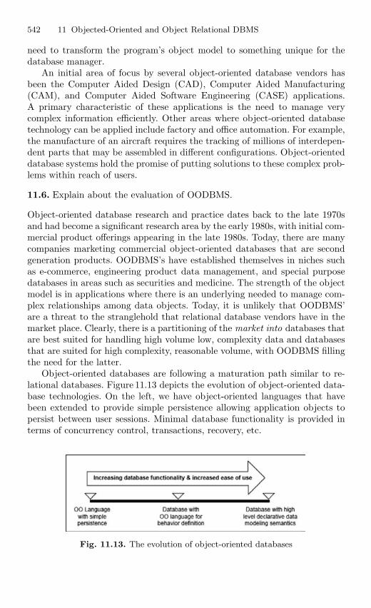
542 11 Objected-Oriented and Object Relational DBMS
need to transform the program’s object model to something unique for thedatabase manager.
An initial area of focus by several object-oriented database vendors hasbeen the Computer Aided Design (CAD), Computer Aided Manufacturing(CAM), and Computer Aided Software Engineering (CASE) applications.A primary characteristic of these applications is the need to manage verycomplex information efficiently. Other areas where object-oriented databasetechnology can be applied include factory and office automation. For example,the manufacture of an aircraft requires the tracking of millions of interdepen-dent parts that may be assembled in different configurations. Object-orienteddatabase systems hold the promise of putting solutions to these complex prob-lems within reach of users.
11.6. Explain about the evaluation of OODBMS.
Object-oriented database research and practice dates back to the late 1970sand had become a significant research area by the early 1980s, with initial com-mercial product offerings appearing in the late 1980s. Today, there are manycompanies marketing commercial object-oriented databases that are secondgeneration products. OODBMS’s have established themselves in niches suchas e-commerce, engineering product data management, and special purposedatabases in areas such as securities and medicine. The strength of the objectmodel is in applications where there is an underlying needed to manage com-plex relationships among data objects. Today, it is unlikely that OODBMS’are a threat to the stranglehold that relational database vendors have in themarket place. Clearly, there is a partitioning of the market into databases thatare best suited for handling high volume low, complexity data and databasesthat are suited for high complexity, reasonable volume, with OODBMS fillingthe need for the latter.
Object-oriented databases are following a maturation path similar to re-lational databases. Figure 11.13 depicts the evolution of object-oriented data-base technologies. On the left, we have object-oriented languages that havebeen extended to provide simple persistence allowing application objects topersist between user sessions. Minimal database functionality is provided interms of concurrency control, transactions, recovery, etc.
Fig. 11.13. The evolution of object-oriented databases
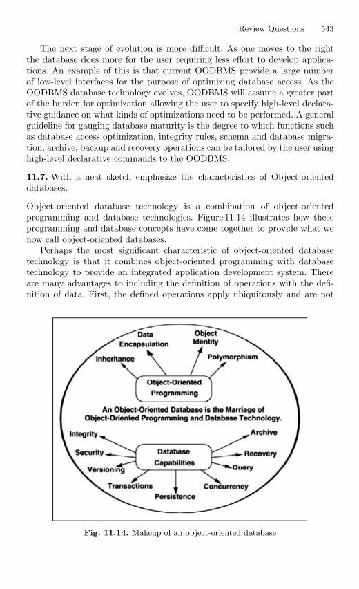
Review Questions 543
The next stage of evolution is more difficult. As one moves to the rightthe database does more for the user requiring less effort to develop applica-tions. An example of this is that current OODBMS provide a large numberof low-level interfaces for the purpose of optimizing database access. As theOODBMS database technology evolves, OODBMS will assume a greater partof the burden for optimization allowing the user to specify high-level declara-tive guidance on what kinds of optimizations need to be performed. A generalguideline for gauging database maturity is the degree to which functions suchas database access optimization, integrity rules, schema and database migra-tion, archive, backup and recovery operations can be tailored by the user usinghigh-level declarative commands to the OODBMS.
11.7. With a neat sketch emphasize the characteristics of Object-orienteddatabases.
Object-oriented database technology is a combination of object-orientedprogramming and database technologies. Figure 11.14 illustrates how theseprogramming and database concepts have come together to provide what wenow call object-oriented databases.
Perhaps the most significant characteristic of object-oriented databasetechnology is that it combines object-oriented programming with databasetechnology to provide an integrated application development system. Thereare many advantages to including the definition of operations with the defi-nition of data. First, the defined operations apply ubiquitously and are not
Fig. 11.14. Makeup of an object-oriented database
544 11 Objected-Oriented and Object Relational DBMS
dependent on the particular database application running at the moment.Second, the data types can be extended to support complex data such asmultimedia by defining new object classes that have operations to supportthe new kinds of information. Other strengths of object-oriented modelingare well known. For example, inheritance allows one to develop solutions tocomplex problems incrementally by defining new objects in terms of previouslydefined objects.
Polymorphism and dynamic binding allows one to define operations forone object and then to share the specification of the operation with otherobjects. These objects can further extend this operation to provide behaviorsthat are unique to those objects. Dynamic binding determines at runtime,which of these operations is actually executed, depending on the class of theobject requested to perform the operation. Polymorphism and dynamic bind-ing are powerful object-oriented features that allow one to compose objects toprovide solutions without having to write code that is specific to each object.All of these capabilities come together synergistically to provide significantproductivity advantages to database application developers.
11.8. Describe how relationships can be modeled in an OODBMS.
Using Relationship Between Objects
Objects interacting in a system make use of the services offered by otherobjects. The using relationship can be used to express a subset of such inter-actions. Booch and Vilot have identified three roles that each object may playin using relationships:
Actor objects can operate upon other objects, but are never operated uponby other objects. Such objects make use of services offered by other objectsbut do not themselves provide any service to the objects they make use of.
Server objects never operate upon objects, but are operated upon by otherobjects.
Agent objects can both operate upon other objects and be operated uponby other objects.
Relationships among Classes
Rumbaugh has identified three types of class relationships:
1. Generalization or “kind-of”2. Aggregation or “part-of”3. Association, implying some semantic connection4. Booch and Vilot have identified two more types of relationships between
classes5. Instantiation relationships6. Metaclass relationships
Review Questions 545
Booch and Vilot suggests the following rule of thumb for identifyingrelationships: “If an abstraction is more than the sum of its component parts,then using relationships are more appropriate. If an abstraction is a kind ofsome other abstraction or if that abstraction is exactly equal to the sum ofits components, then inheritance is a better approach.”
11.9. What functionality would typically be provided by an ORDBMS?
Due to recent hardware improvements more sophisticated applications haveemerged, such as CAD/CAM (Computer-Aided Design/Computer-AidedManufacturing), CASE (Computer-Aided Software Engineering), GIS (Geo-graphic Information System), etc. These applications can be characterized asconsisting of complex objects related by complex relationships. Representingsuch objects and relationships in the relational model implies that the objectsmust be decomposed into a large number of tuples.
Thus, a considerable number of joins is necessary to retrieve an objectand, when tables are too deeply nested, performance is significantly reduced.A new generation of databases has appeared to solve these problems: theobject-oriented database generation, which includes the object-relational andobject databases. This new technology is well suited for storing and retrievingcomplex data because it supports complex data types and relationships, mul-timedia data, inheritance, etc. Nonetheless, good technology is not enough tosupport complex objects and applications. It is necessary to define method-ologies that guide designers in the object database design task, in the sameway traditionally has been done with relational databases.
The object model of the current standard for object-relational databases,SQL: 1999, as well as the main characteristics of Oracle8i object-relationalmodel, as an example of object-relational product. SQL: 1999 data modelextends the relational data model with some new constructors to supportobjects. Most of last versions of relational products include some objectextensions. However, and because in general these products have appeared inthe market before the standard approval, current versions of object-relationalproducts do not totally. Adjust to the SQL: 1999 model.
11.10. Discuss about the various criteria used to evaluate OODBMS
These criteria are broken into three main areas:
– Functionality– Application Development Issues– Miscellaneous Criteria
Functionality, defines evaluation criteria based on functional capabilitiesprovided by the OODBMS. Subsections include Basic Object-Oriented Mod-eling, Advanced Object-Oriented Database Topics, Database Architecture,Database Functionality, Application Programming Interface, and Queryingan OODBMS.
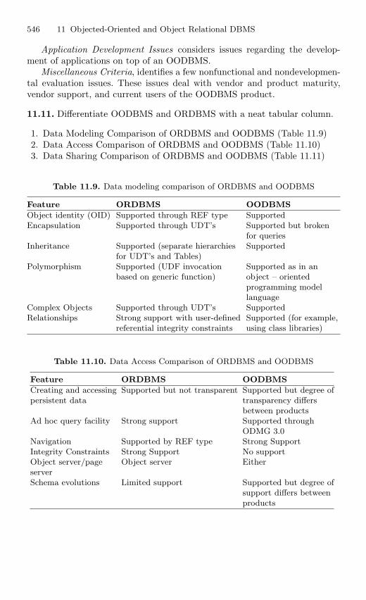
546 11 Objected-Oriented and Object Relational DBMS
Application Development Issues considers issues regarding the develop-ment of applications on top of an OODBMS.
Miscellaneous Criteria, identifies a few nonfunctional and nondevelopmen-tal evaluation issues. These issues deal with vendor and product maturity,vendor support, and current users of the OODBMS product.
11.11. Differentiate OODBMS and ORDBMS with a neat tabular column.
1. Data Modeling Comparison of ORDBMS and OODBMS (Table 11.9)2. Data Access Comparison of ORDBMS and OODBMS (Table 11.10)3. Data Sharing Comparison of ORDBMS and OODBMS (Table 11.11)
Table 11.9. Data modeling comparison of ORDBMS and OODBMS
Feature ORDBMS OODBMS
Object identity (OID) Supported through REF type SupportedEncapsulation Supported through UDT’s Supported but broken
for queriesInheritance Supported (separate hierarchies Supported
for UDT’s and Tables)Polymorphism Supported (UDF invocation Supported as in an
based on generic function) object – orientedprogramming modellanguage
Complex Objects Supported through UDT’s SupportedRelationships Strong support with user-defined Supported (for example,
referential integrity constraints using class libraries)
Table 11.10. Data Access Comparison of ORDBMS and OODBMS
Feature ORDBMS OODBMS
Creating and accessing Supported but not transparent Supported but degree ofpersistent data transparency differs
between productsAd hoc query facility Strong support Supported through
ODMG 3.0Navigation Supported by REF type Strong SupportIntegrity Constraints Strong Support No supportObject server/page Object server EitherserverSchema evolutions Limited support Supported but degree of
support differs betweenproducts
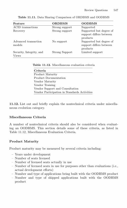
Review Questions 547
Table 11.11. Data Sharing Comparison of ORDBMS and OODBMS
Feature ORDBMS OODBMS
ACID transactions Strong support SupportedRecovery Strong support Supported but degree of
support differs betweenproducts
Advanced transaction No support Supported but degree ofmodels support differs between
productsSecurity, Integrity, and Strong Support Limited supportViews
Table 11.12. Miscellaneous evaluation criteria
Criteria
Product MaturityProduct DocumentationVendor MaturityVendor TrainingVendor Support and ConsultationVendor Participation in Standards Activities
11.12. List out and briefly explain the nontechnical criteria under miscella-neous evolution category.
Miscellaneous Criteria
A number of nontechnical criteria should also be considered when evaluat-ing an OODBMS. This section details some of these criteria, as listed inTable 11.12, Miscellaneous Evaluation Criteria.
Product Maturity
Product maturity may be measured by several criteria including:
– Years under development– Number of seats licensed– Number of licensed seats actually in use– Number of licensed seats in use for purposes other than evaluations (i.e.,
actual development efforts)– Number and type of applications being built with the OODBMS product– Number and type of shipped applications built with the OODBMS
product
548 11 Objected-Oriented and Object Relational DBMS
Product Documentation
Product documentation should be clear, consistent, and complete. Thedocumentation should include complete examples of typical programmedcapabilities (e.g., what is the sequence of calls to access data from thedatabase and to cause updates to that data to be made permanent in thedatabase).
Vendor Maturity
Vendor maturity may be measured by several criteria including:
– Company’s size and age.– Previous experience of the company’s lead technical and management per-
sonnel in the commercial database market.– Financial stability.
Vendor Training
Availability and quality of vendor supplied training classes is an importantconsideration when selecting an OODBMS.
Vendor Support and Consultation
It is expected that significant support will be required during the OODBMSevaluation process and to overcome the initial learning curve. OODBMS ven-dors should provide a willing and capable support staff. Support should beavailable via phone and electronically. Consulting support might also be ap-pealing where the OODBMS vendor provides expert, hands-on assistance inproduct use, object-oriented application design (especially in regards to data-base issues), and in maximizing database application performance.
Vendor Participation in Standards Activities
The vendor should be active in standards efforts in the object-oriented, lan-guage, CASE, open software, and data exchange areas. In particular:
– Object Management Group (OMG). An organization funded by over 80 in-ternational information systems corporations whose charter is to developstandards for interoperation and portability of software. The OMG is fo-cusing on object-oriented integration technologies such as Object RequestBroker (ORB), OODBMS interfaces, and object interfaces for existingapplications.
– Object Database Management Group (ODMG). An organization ofOODBMS vendors chartered to define a standardinterface to OODBMS
Review Questions 549
that will allow application portability and interoperability. Standardsdefined by the ODMG will be provided to OMG, ANSI, STEP, PCTE,etc. to aid in their respective standardization efforts.
– ANSI standardization efforts in languages (C, C++, Smalltalk), SQL, andobject-oriented databases.
– Standards such as Portable Common Tool Environment (PCTE) andCASE Data Interchange
– Format (CDIF) providing for common data representations, data ex-change formats and interoperation of tools.
– PDES/STEP. An effort aimed at standardizing an exchange format forproduct model data (product model data, such as CAD data, representsa prime application area for OODBMS).
11.13. What are the advantages and disadvantages of extending the relationaldata model?
Advantages of ORDBMS
1. Resolves many of known weaknesses of RDBMS.2. Reuse and sharing:
– Reuse comes from ability to extend server to perform standard func-tionality centrally.
– Gives rise to increased productivity both for developer and end-user.3. Preserves significant body of knowledge and experience gone into devel-
oping relational applications.
Disadvantages of ORDBMS
– Complexity.– Increased costs.– Proponents of relational approach believe simplicity and purity of rela-
tional model are lost.– Some believe RDBMS is being extended for what will be a minority of
applications.– OO purists not attracted by extensions either.– SQL now extremely complex.
11.14. Analyze the concept OODBMS in fundamental four areas
OODBMS can be analyzed in the following four areas:
– Functionality– Usability– Platform– Performance
550 11 Objected-Oriented and Object Relational DBMS
An analysis of functional capabilities is performed to determine if a givenOODBMS provides sufficient capabilities to meet the current and future needsof a given development effort. Functional capabilities include basic databasefunctionality such as concurrency control and recovery as well as object-oriented database features such as inheritance and versioning. Each evaluationwill have to identify and weight a set of functional requirements to be metby the candidate OODBMS. Weighting is an important consideration sinceapplication workarounds may be possible for missing functionality.
Usability deals with the application development and maintenance process.Issues include development tools and the ease with which database applica-tions can be developed and maintained. How a developer perceives the data-base and the management of persistent objects might also be considered underthe category of usability. Other issues to be considered are database adminis-tration, product maturity, and vendor support. Evaluation of usability is likelyto be highly subjective. Perhaps the most easily measurable evaluation crite-rion is platform. An OODBMS is either available or not on the application’starget hardware and operating system. Heterogeneous target environmentsrequire that the OODBMS transparently interoperates within that environ-ment.
11.15. Explain concept of Object Versioning
Object versioning is the concept that a single object may be represented bymultiple versions (i.e., instances of that object) at one time. We can define twoforms of versioning, each driven by particular requirements of the applicationswhich are driving the need for OODBMS products:
– Linear Versioning is the concept of saving prior versions of objects asan object changes. In design-type applications (e.g., CASE, CAD) priorversions of objects are essential to maintain the historical progression ofa design and to allow designers to return to earlier design points afterinvestigating and possibly discarding a given design path. Under linearversioning, only a single new version can be created from each existingversion of an object.
– Branch Versioning supports concurrency policies where multiple usersmay update the same data concurrently. Each user’s work is based upon aconsistent, nonchanging base version. Each user can modify his version ofan object (as he proceeds along some design path in a CAD application forexample). At some future point in time, under user/application support,the multiple branch versions are merged to form a single version of theobject. Branch versioning is important in applications with long transac-tions so that users are not prevented access to information for long periodsof time. Under branch versioning, multiple new versions may be createdfor an object.
Associated with the idea of versioning is that of configuration. A configu-ration is a set of object versions that are consistent with each other. In other
Review Questions 551
words, it is a group of objects whose versions all belong together. OODBMSneed to provide support so that applications access object versions that belongto the same conceptual configuration. This may be achieved by controlling therelationships that are formed for versioned objects (i.e., they may be dupli-cated in the new object or replaced with relationships to other objects).
An OODBMS may provide low level facilities which application developersuse to control the versioning of objects. Alternatively, the OODBMS mayimplement a specific versioning policy such as automatically creating a newobject version with each change. An automatic policy may result in rapid andunacceptable expansion of the database and requires some automated meansof controlling this growth.
11.16. Explain about the concept Basic Object-Oriented modeling.
Basic Object-Oriented Modeling
The evaluation criteria in this section distinguish database as an object-oriented database. Topics in this section cover the basic object-oriented (OO)capabilities typically supported in any OO technology (e.g., programming lan-guage, design method). These basic capabilities are expected to be supportedin all commercial OODBMS. The topics are given a cursory overview here forreaders new to OO technology.
Complex Objects
OO systems and applications are unique that the information being main-tained is organized in terms of the real-world entities being modeled. Thisdiffers from relational database applications that require a translation fromthe real-world information structure to the table formats used to store datain a relational database. Normalizations upon the relational database tablesresult in further perturbation of the data from the user’s perceptual viewpoint.OO systems provide the concept of complex objects to enable modeling of real-world entities. A complex object contains an arbitrary number of fields, eachstoring atomic data values or references to other objects (of arbitrary types).A complex object exactly models the user perception of some real-world entity.
Object Identity
OO databases (and programming languages) provide the concept of an objectidentifier (OID) as a means f uniquely identifying a particular object. OIDsare system generated. A database application does not have direct accessto the OID. The OID of an object never changes, even across applicationexecutions. The OID is not based on the value stored within the object. Thisdiffers from relational databases, which use the concept of primary keys toidentify a particular table row (i.e., tuple). Primary keys are based upon
552 11 Objected-Oriented and Object Relational DBMS
data stored in the identified row. The concept of OIDs makes it easier tocontrol the storage of objects (e.g., not based on value) and to build linksbetween objects (e.g., they are based on the never changing OID). Complexobjects often include references to other objects, directly or indirectly storedas OIDs.
Classes
OO modeling is based on the concept of a class. A class defines the data valuesstored by, and the functionality associated with, an object of that class. Oneof the primary advantages of OO data modeling is this tight integration ofdata and behavior through the class mechanism. Each object belongs to one,and only one, class. An object is often referred to as an instance of a class.A class specification provides the external view of the instances of that class.A class has an extent (sometimes called an extension), which is the set of allinstances of the class. Implementation of the extent may be transparent toan application, but minimally provides the ability to visit every instance ofthe class. Within an OODBMS, the class construct is normally used to definethe database schema. Some OODBMS use the term type instead of class. TheOODBMS schema defines what objects may be stored within the database.
Attributes
Attributes represent data components that make up the content of a class.Attributes are called data members in the C++ programming language. In-stance attributes are data components that are stored by each instance of theclass. Class attributes (static data members in C++) are data values storedonce for all instances of the class. Attributes may or may not be visible toexternal users of the class. Attribute types are typically a subset of the ba-sic data types supported by the programming language that interfaces to theOODBMS. Typically this includes enumeration types such as characters andbooleans, numeric types such as integers and floats, and fixed length arrays ofthese types such as strings. The OODBMS may allow variable length arrays,structures (i.e., records), and classes as attribute types.
Pointers are normally not good candidates for attribute types since pointervalues are not valid across application executions.
An OODBMS will provide attribute types that support interobject ref-erences. OO applications are characterized by a network of interconnectedobjects. Object interconnections are supported by attributes that referenceother objects. Other types that might be supported by an OODBMS includetext, graphic, and audio. Often these data types are referred to as binarylarge objects (BLOBS). Derived attributes are attributes that are not explic-itly stored but instead calculated on demand. Derived attributes require thatattribute access be indistinguishable from behavior invocation.
Review Questions 553
Behaviors
Behaviors represent the functional component of a class. A behavior describeshow an object operates upon its attributes and how it interacts with otherrelated objects. Behaviors are called member functions in the C++ program-ming language. Behaviors hide their implementation details from users of aclass.
Encapsulation
Classes are said to encapsulate the attributes and behaviors of their instances.Behavior encapsulation shields the clients of a class (i.e., applications or otherclasses) from seeing the internal implementation of a behavior. This shieldingprovides a degree of data independence so that clients need not be modifiedwhen behavior implementations are modified (they will have to be modifiedif behavior interfaces change).
A class’s attributes may or may not be encapsulated. Attributes that aredirectly accessible to clients of a class are not encapsulated (public data mem-bers in C++ classes). Modifying the definition of a class’s attributes thatare not encapsulated requires modification of all clients that access them.Attributes that are not accessible to the clients of a class are encapsulated(private or protected data members in C++ classes). Encapsulated attributestypically have behaviors that provide clients some form of access to theattribute. Modifications to these attributes typically do not require modifi-cation to clients of the class.
Inheritance
Inheritance allows one class to incorporate the attributes and behaviors of oneor more other classes. A subclass is said to inherit from one or more super-classes. The subclass is a specialization of the superclass in that it adds addi-tional data or behaviors, or overrides behaviors of the superclass. Superclassesare generalizations of their subclasses. Inheritance is recursive. A class inheritsthe attributes and behaviors from its superclasses, and from its superclass’ssuperclasses, etc. In a single inheritance model, a class may directly inheritfrom only a single other class. In a multiple inheritance model a class maydirectly inherit from more than one other class. Systems supporting multipleinheritance must specify how inheritance conflicts are handled. Inheritanceconflicts are attributes or behaviors with the same name in a class and itssuperclass, or in two superclasses.
Inheritance is a powerful OO modeling concept that supports reuse andextensibility of existing classes. The inheritance relationships between a groupof classes define a class hierarchy. Class hierarchies improve the ability of usersto understand software systems by allowing knowledge of one class (a super-class) to be applicable to other classes (its subclasses).
554 11 Objected-Oriented and Object Relational DBMS
Overriding Behaviors and Late Binding
OO applications are typically structured to perform work on generic classes(e.g., a vehicle) and at runtime invoke behaviors appropriate for the specificvehicle being executed upon (e.g., Boeing 747). Applications constructed insuch a manner are more easily maintained and extended since additional vehi-cle classes may be added without requiring modification of application code.Overriding behaviors is the ability for each class to define the functionalityunique to itself for a given behavior. Late binding is the ability for behaviorinvocation to be selected at runtime based on the class of an object (insteadof at compile time).
Persistence
Persistence is the characteristic that makes data available across executions.The objective of an OODBMS is to make objects persistent. Persistence maybe based on an object’s class, meaning that all objects of a given class arepersistent. Each object of a persistent class is automatically made persistent.An alternative model is that persistence is a unique characteristic of eachobject (i.e., it is orthogonal to class). Under this model, an object’s persistenceis normally specified when it is created. A third persistence model is thatany object reachable from a persistent object is also persistent. Such systemsrequire some way of explicitly stating that a given object is persistent (as ameans of starting the network of interconnected persistent objects). Relatedto the concept of persistence is object existence. OODBMS may provide ameans by which objects are explicitly deleted. Such systems must ensure thatreferences to deleted objects are also removed. An alternative strategy is tomaintain an object as long as references to the object exist. Once all referencesare removed, the object can be safely deleted.
Naming
OO applications are characterized as being composed of a network of inter-connected objects. An application begins by accessing a few known objectsand then traverses to additional objects via relationships from the knownobjects. As objects are created they are linked (i.e., related) to other existingobjects. Given this scenario, the database must provide some mechanism foridentifying one or more objects at application start-up without using relationsfrom existing objects. This is typically accomplished by allowing objects to benamed and providing a retrieval mechanism based upon name. An applicationbegins by loading one or two “high-level” objects that it knows by name andthen traverses to other reachable objects. Object names apply within somename scope. Within a given scope, names must be unique (i.e., the same namecan not refer to two objects). The simplest scope model is for the entire data-base to act as a single name scope. An alternative scope model is for the
Review Questions 555
application to identify name scopes. Using multiple name scopes will reducethe chance for name conflicts.
11.17. Describe the features of Schema Evolution.
Schema Evolution
Schema evolution is the process by which existing database objects are broughtinto line with changes to the class definitions of those objects (i.e., schemachanges require all instances of the changed class to be modified so as toreflect the modified class structure). Schema evolution is helpful although notessential during system development (as a means of retaining test data, forexample). Schema evolution is essential for maintenance and/or upgrades offielded applications. Once an application is in the field (and users are creatinglarge quantities of information), an upgrade or bug fix cannot require disposalof all existing user databases. Schema evolution is also essential for applica-tions that support user-level modeling and/or extension of the application.
Here we have given a framework for schema modifications in an object-oriented database. Included in this framework are invariants which must bemaintained at all times (e.g., all attributes of a class must have a distinctname), rules for performing schema modifications (e.g., changing the typeof an attribute in a given class must change the type of that attribute inall classes which inherit that attribute), and a set of schema changes thatshould be supported by an object-oriented database. This set of schema changeoperations is:
1. Changes to Definition of a Class:(a) Changes to an Attribute of a Class (applies to both instance and class
attributes):– Add an attribute to a class.– Remove an attribute from a class.– Change the name of an attribute.– Change the type of an attribute.– Change the default value of an attribute.– Alter the relationship properties for relationship attributes.
(b) Changes to a Behavior of a Class:– Add a new behavior to the class.– Remove a behavior from the class.– Change the name of a behavior.– Change the implementation of a behavior.
2. Changes to the Inheritance of a Class:– Add a new superclass to a class.– Remove a superclass for a given class.– Change the order of superclasses for a class (it is expected that
superclass ordering will be used to handle attribute and behavior in-heritance conflicts).
556 11 Objected-Oriented and Object Relational DBMS
3. Changes to the Existence of a Class:– Add a new class.– Remove an existing class.– Change the name of a class.
Schema changes will require modification of instances of the changed classas well as applications that referenced the changed class. Some of these changescannot be performed automatically by the OODBMS. Deleting attributesand superclasses are examples of schema changes that could be performedautomatically. Adding attributes and superclasses can only be performed ifdefault values are acceptable for the initial state of new attributes. This isnot likely, especially for relationship attributes. An OODBMS should providetools and/or support routines for aiding programmed schema evolution.
A manual evolution approach requires instance migration to be performedoff-line, probably through a dump of the database and a reload of thedata through an appropriate transformation filter. Systems may perform anaggressive update by automatically adjusting each instance after each schemachange. This approach may be slow due to the overhead of performing theupdate on all instances at a single time. This approach is the easiest for anapplication to implement since multiple versions of the schema need not bemaintained indefinitely.
Schema changes may be performed in background mode, thus spreadingthe update overhead over a longer period of time. A lazy evaluation approachdefers updating objects until they are accessed and found to be in an in-consistent state. Both the background and lazy approaches require extendedperiods where multiple versions of the schema exist and will be complicatedby multiple schema modifications. Applications and stored queries will haveto be updated manually as a result of schema changes. Some forms of schemachanges will not require updates to applications and queries due to data in-dependence and encapsulation of a class’s data members.
It is expected that all OODBMS products will support some form ofschema evolution for static schema changes. By static, we mean the schema ischanged by manipulations of class definitions outside of application process-ing (i.e., by reprocessing database schema definitions and modifying applica-tion programs). Dynamic schema modification, meaning modification of theschema by the application, is more complex and potentially inconsistent withthe basic C++ header file approach used for schema definitions in manycurrent commercial products. Dynamic schema modification is only neededin applications that require user definable types.
11.18. What are the architecture issues relevant to the OODBMS
Database Architecture
1. Distributed Client–Server ApproachAdvances in local area network and workstation technology have givenrise to group design type applications driving the need for OODBMS
Review Questions 557
(e.g., CASE, CAD, and Electronic Offices). OODBMS typically executein a multiple process distributed environment. Server processes provideback-end database services, such as management of secondary storage andtransaction control. Client processes handle application specific activities,such as access and update of individual objects. These processes may belocated on the same or different workstations. Typically a single serverwill be interacting with multiple clients servicing concurrent requests fordata managed by that server. A client may interact with multiple serversto access data distributed throughout the network.The evaluations and benchmarks are the three alternative workstation-server architectures that have been proposed for use with OODBMS:
– Object server approach. The unit of transfer from server to client isan object. Both machines cache objects and are capable of execut-ing methods on objects. Object-level locking is easily performed. Themajor drawback of this approach is the overhead associated with theserver interaction required to access every object and the added com-plexity of the server software which must provide complete OODBMSfunctionality (e.g., be able to execute methods). Keeping client andserver caches consistent may introduce additional overheads.
– Page server approach. The unit of transfer from server to client is apage (of objects). Page-level transfers reduce the overhead of objectaccess since server interaction is not always required. Architectureand implementation of the server is simplified since it needs only toperform the backend database services. A possible drawback of thisapproach is that methods can be evaluated only on the client, thus allobjects accessed by an application must be transferred to the client.Object-level locking will be difficult to implement.
– File server approach. The OODBMS client processes interact with anetwork file service (e.g., Sun’s NFS) to read and write database pages.A separate OODBMS server process is used for concurrency controland recovery. This approach further simplifies the server implementa-tion since it need not manage secondary storage. The major drawbackof this approach is that two network interactions are required for dataaccess, one to the file service and one to the OODBMS server.
Many scientists have identified no clear winner when benchmarking thethree approaches. The page server approach seemed best with large bufferpools and good clustering algorithms. The object server approach per-formed poorly if applications scanned lots of data, but was better thanthe page server approach for applications performing lots of updates andrunning on workstations with small buffer pools.
2. Data Access MechanismAn evaluation of OODBMS products should consider the process neces-sary to move data from secondary storage into a client application. Typi-cally this requires communication with a server process, possibly acrossa network. Objects loaded into a client’s memory may require further
558 11 Objected-Oriented and Object Relational DBMS
processing, often referred to as swizzling, to resolve references to otherobjects which may or may not already be loaded into the client’s cache.The overhead and process by which locks are released and updated objectsare returned to the server should also be considered.
3. Object ClusteringOODBMS which transfer units larger than an object do so under the as-sumption that an application’s access to a given object implies a highprobability that other associated objects may also be accessed. By trans-ferring groups of objects, additional server interaction may not be neces-sary to satisfy these additional object accesses. Object clustering is theability for an application to provide information to the OODBMS so thatobjects which it will typically access together can be stored near eachother and thus benefit from bulk data transfers.
4. Heterogeneous OperationAn OODBMS provides a mechanism for applications to cooperate, bysharing access to a common set of objects. A typical OODBMS will sup-port multiple concurrent applications executing on multiple processorsconnected via a local area network. Often, the processors will be from dif-ferent computer manufacturers; each having its own data representationformats. For applications to cooperate in such an environment, data mustbe translated to the representation format suitable for the processor uponwhich that data is stored (both permanently by a server and temporar-ily by a client wishing to access the data). To be an effective integrationmechanism, an OODBMS must support data access in a heterogeneousprocessing environment.
12
Distributed and Parallel DatabaseManagement Systems
Learning Objectives. This chapter is dedicated to distributed and paralleldatabase management system. The distributed database design, architecture,concurrency control, and reliability concepts are discussed in this chapter. Thischapter also deals with parallel database architecture; components and benefits ofparallel processing. After completing this chapter the reader should be familiar withthe following concepts:
1. Distributed database management system2. Distributed DBMS architecture3. Distributed database design4. Semantic data control5. Distributed concurrency control6. Distributed DBMS reliability7. Parallel database management system
12.1 Distributed Database
Distributed database provides a number of advantages of distributedcomputing to the DBMS domain. A distributed computing system consistsof a number of processing elements that are interconnected by a computernetwork, and that cooperate in performing certain application tasks. Thedistributed database is a collection of multiple logically interrelated databasesdistributed over a computer network. Parallel processing divides a complextask into many smaller tasks, and executes the smaller tasks simultaneouslyin several tasks. Thus the complex task is completed with better performanceand also quickly. The parallel database system makes use of the parallelism inDBMS and achieves high performance and high availability database serversat much lower price.
A distributed database is a collection of data which belong logically tothe same system but are spread over the sites of a computer network. Thisdefinition emphasizes two equally important aspects of a distributed databaseas follows:
S. Sumathi: Distributed and Parallel Database Management Systems, Studies in Computational
Intelligence (SCI) 47, 559–609 (2007)
www.springerlink.com c© Springer-Verlag Berlin Heidelberg 2007
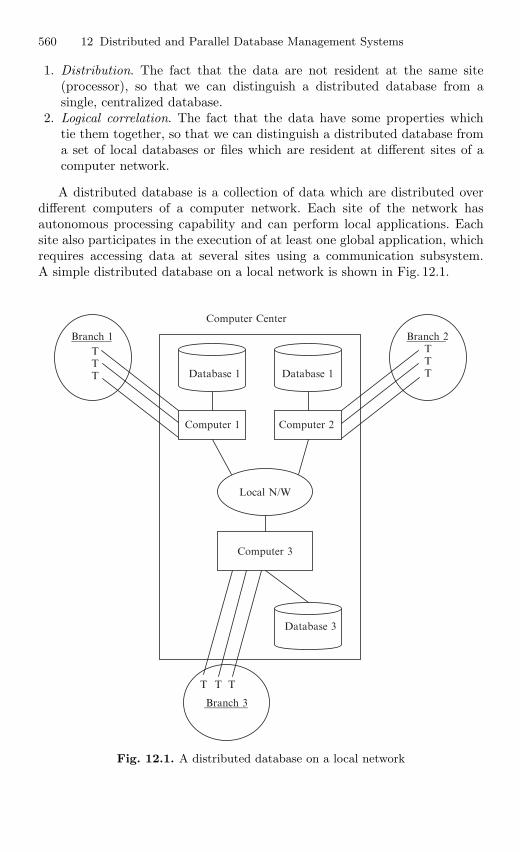
560 12 Distributed and Parallel Database Management Systems
1. Distribution. The fact that the data are not resident at the same site(processor), so that we can distinguish a distributed database from asingle, centralized database.
2. Logical correlation. The fact that the data have some properties whichtie them together, so that we can distinguish a distributed database froma set of local databases or files which are resident at different sites of acomputer network.
A distributed database is a collection of data which are distributed overdifferent computers of a computer network. Each site of the network hasautonomous processing capability and can perform local applications. Eachsite also participates in the execution of at least one global application, whichrequires accessing data at several sites using a communication subsystem.A simple distributed database on a local network is shown in Fig. 12.1.
Database 1 Database 1
Computer 1 Computer 2
Local N/W
Branch 2TTT
Branch 1TTT
Computer 3
Database 3
T T T
Branch 3
Computer Center
Fig. 12.1. A distributed database on a local network
12.1 Distributed Database 561
12.1.1 Features of Distributed vs. Centralized Databases
The features which characterize the traditional database approach are cen-tralized control, data independence, and reduction of redundancy, complexphysical structures for efficient access, integrity, recovery, concurrency control,privacy, and security.
– Centralized control. The possibility of providing centralized control of theinformation resources of a whole enterprise or organization was consideredas one of the strongest motivations for introducing databases; they weredeveloped as the evolution of information systems in which each applica-tion had its own private files.
In general, in distributed databases it is possible to identify a hierar-chical control structure based on a global database administrator, whohas the central responsibility of the whole database, and on local data-base administrators, who have the responsibility of their respective localdatabases.
– Data independence. It means that the actual organization of data istransparent to the application programmer. Programs are written havinga conceptual view of the data, the so-called conceptual schema. The mainadvantage of data independence is that programs are unaffected bychanges in the physical organization of data.
– Reduction of redundancy. In traditional databases, redundancy wasreduced as far as possible for two reasons: first, inconsistencies amongseveral copies of the same logical data are automatically avoided byhaving only one copy, and second, storage space is saved by eliminatingredundancy. In distributed databases, however, there are several reasonsfor considering data redundancy as desirable features. First, the localityof applications can be increased if the data are replicated at all siteswhere applications need it, and second, the availability of the systemcan be increased, because a site failure does not stop the execution ofapplications at other sites if the data are replicated.
– Complex physical structures and efficient access. In distributed data-bases, complex accessing structures are not the right tool for efficientaccess. Therefore, while efficient access is a main problem in distrib-uted databases, physical structures are not a relevant technological issue.Efficient access to a distributed database cannot be provided by usingintersite physical structures, because it is very difficult to build and main-tain such structures and because it is not convenient to navigate at arecord level in distributed databases.
The software components which are typically necessary for building adistributed database in this case are:
1. The database management component (DB)2. The data communication component (DC)
562 12 Distributed and Parallel Database Management Systems
3. The data dictionary (DD), which is extended to represent informationabout distribution of data in the network
4. The distributed database component (DDC)
An important property of distributed database management systems(DDBMSs) is whether they are homogeneous or heterogeneous. HomogeneousDDBMS refers to a DDBMS with the same DBMS at each site, even if thecomputers and/or the operating systems are not the same. A heterogeneousDDBMS uses instead at least two different DBMSs. Heterogeneous DDBMSadds the problem of translating between the different data models of thedifferent local DBMSs to the complexity of homogeneous DDBMSs.
12.2 Distributed DBMS Architecture
The architecture of a system defines its structure. This means that thecomponents of the system are identified, the function of each component isspecified, and the interrelationships and interactions among these componentsare defined.
12.2.1 DBMS Standardization
The standardization efforts related to DBMSs because of the close relationshipbetween the architecture of a system and the reference model of that system,which is developed as a precursor to any standardization activity. It is definedas “a conceptual framework whose purpose is to divide standardization workinto manageable pieces and to show at a general level how these pieces arerelated with each other.” A reference model can be described according tothree different approaches:
1. Based on components. The components of the system are defined togetherwith the interrelationships between components. Thus a DBMS consists ofa number of components, each of which provides some functionality. Theirorderly and well-defined interaction provides total system functionality.
2. Based on functions. The different classes of users are identified and thefunctions that the system will perform for each class are defined. Thesystem specifications within this category typically specify a hierarchicalstructure for user classes. This results in hierarchical system architecturewith well-defined interfaces between the functionalities of different layers.
3. Based on data. The different types of data are identified, and an architec-tural framework is specified which defines the functional units that willrealize or use data according to these different views. Since data are thecentral resource that a DBMS manages, this approach is claimed to be thepreferable choice for standardization activities. The advantage of the dataapproach is the central importance it associates with the data resource.
12.2 Distributed DBMS Architecture 563
12.2.2 Architectural Models for Distributed DBMS
Let us consider the possible ways in which multiple databases may be puttogether for sharing by multiple DBMSs. We use a classification that organizesthe systems as characterized with respect to (1) the autonomy of local systems,(2) their distribution, and (3) their heterogeneity.
Autonomy
It refers to the distribution of control, not of data. It indicates the degreeto which individual DBMS can operate independently. Autonomy is a func-tion of a number of factors such as whether they can independently executetransactions, and whether one is allowed to modify them. Requirements of anautonomous system have been specified in a variety of ways.
1. The local operations of the individual DBMSs are not affected by theirparticipation in the multidatabase system.
2. The manner in which the individual DBMSs process queries and optimizethem should not be affected by the execution of global queries that accessmultiple databases.
3. System consistency or operation should not be compromised when indi-vidual DBMSs join or leave the multidatabase confederation.
The dimensions of autonomy are specified as follows:
1. Design autonomy. Individual DBMSs are free to use the data models andtransaction management techniques that they prefer.
2. Communication autonomy. Each of the individual DBMSs is free to makeits own decision as to what type of information it wants to provide to theother DBMSs or to the software that controls their global execution.
3. Execution autonomy. Each DBMS can execute the transactions that aresubmitted to it in any way that it wants to do.
Distribution
There are a number of ways DBMSs can be distributed. We abstract thealternatives into two classes: client/server distribution and peer-to-peerdistribution. The client/server distribution concentrates data managementduties at servers while the clients focus on providing the application envi-ronment including the user interface. The communication duties are sharedbetween the client machines and servers. Client/server DBMSs represent thefirst attempt at distributing functionality. There are a variety of ways of struc-turing them, each providing a different level of distribution. In peer-to-peersystems, there is no distinction of client machines vs. servers. Each machinehas full DBMS functionality and can communicate with other machines toexecute queries and transactions.
564 12 Distributed and Parallel Database Management Systems
Heterogeneity
It may occur in various forms in distributed systems, ranging from hard-ware heterogeneity and differences in networking protocols to variations indata managers. Heterogeneity in query languages not only involves the use ofcompletely different data access paradigms in different data models, but alsocovers difference in languages even when the individual systems use the samedata model. Different query languages that use the same data model oftenselect very different methods for expressing identical requests.
12.2.3 Types of Distributed DBMS Architecture
The distributed DBMS architecture types namely client server and peer-to-peer systems are discussed below.
Client/Server Systems
The general idea of this architecture is simple and elegant: distinguish thefunctionality that needs to be provided and divide these functions into twoclasses as server functions and client functions. This provides a two levelarchitecture which makes it easier to manage the complexity of modernDBMSs and the complexity of distribution.
As with any highly popular term, client/server has been much abused andhas come to mean different things. If one takes a process-centric view, thenany process that requests the services of another process is its client and viceversa. In this sense, “client/server computing” and “client/server DBMS,” asit is used in its more modern context, do not refer to processes, but to actualmachines.
The architecture shown in Fig. 12.2 is quite common in relational systemswhere the communication between the clients and the server without trying tounderstand or optimize them. The server does most of the work and returnsthe result relation to the client. There are a number of different types ofclient/server architecture. The simplest is the case where there is only oneserver which can be accessed by multiple clients. We call this as “multipleclient–single server.” From a data management perspective, this is not muchdifferent from centralized databases since the database is stored on only onemachine (the server) which also hosts the software to manage it.
There are two management strategies in multiple client–multiple server:either each client manages its own connection to the appropriate server oreach client knows of only its “home server” which then communicates withthe other servers as required. The former approach simplifies server code, butloads the client machines with additional responsibilities. This leads to whathas been called as “heavy client” systems. The latter approach, on the otherhand, concentrates the data management functionality at the servers. Thus,the transparency of data access is provided at the server interface, leading to“light clients.”
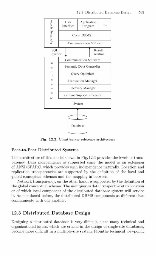
12.3 Distributed Database Design 565
SQLqueries
Resultrelation
Ope
rating
sys
tem User
InterfaceApplicationProgram …
Client DBMS
Communication Software
Communication Software
Semantic Data Controller
Query Optimizer
Transaction Manager
Recovery Manager
Runtime Support Processor
System
Database
Op
er
at
in
g
Fig. 12.2. Client/server reference architecture
Peer-to-Peer Distributed Systems
The architecture of this model shown in Fig. 12.3 provides the levels of trans-parency. Data independence is supported since the model is an extensionof ANSI/SPARC, which provides such independence naturally. Location andreplication transparencies are supported by the definition of the local andglobal conceptual schemas and the mapping in between.
Network transparency, on the other hand, is supported by the definition ofthe global conceptual schema. The user queries data irrespective of its locationor of which local component of the distributed database system will serviceit. As mentioned before, the distributed DBMS components at different sitescommunicate with one another.
12.3 Distributed Database Design
Designing a distributed database is very difficult, since many technical andorganizational issues, which are crucial in the design of single-site databases,become more difficult in a multiple-site system. Fromthe technical viewpoint,
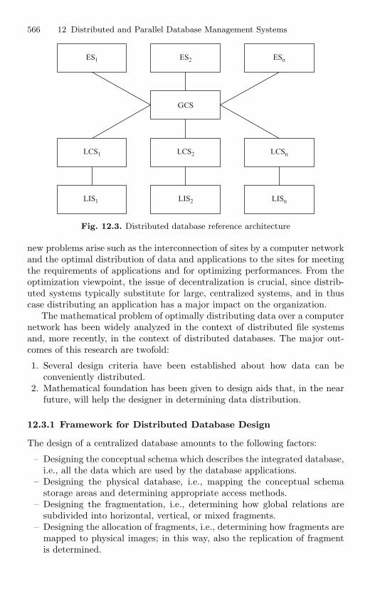
566 12 Distributed and Parallel Database Management Systems
ES1 ES2 ESn
GCS
LCS1 LCS2 LCSn
LIS1 LIS2 LISn
Fig. 12.3. Distributed database reference architecture
new problems arise such as the interconnection of sites by a computer networkand the optimal distribution of data and applications to the sites for meetingthe requirements of applications and for optimizing performances. From theoptimization viewpoint, the issue of decentralization is crucial, since distrib-uted systems typically substitute for large, centralized systems, and in thuscase distributing an application has a major impact on the organization.
The mathematical problem of optimally distributing data over a computernetwork has been widely analyzed in the context of distributed file systemsand, more recently, in the context of distributed databases. The major out-comes of this research are twofold:
1. Several design criteria have been established about how data can beconveniently distributed.
2. Mathematical foundation has been given to design aids that, in the nearfuture, will help the designer in determining data distribution.
12.3.1 Framework for Distributed Database Design
The design of a centralized database amounts to the following factors:
– Designing the conceptual schema which describes the integrated database,i.e., all the data which are used by the database applications.
– Designing the physical database, i.e., mapping the conceptual schemastorage areas and determining appropriate access methods.
– Designing the fragmentation, i.e., determining how global relations aresubdivided into horizontal, vertical, or mixed fragments.
– Designing the allocation of fragments, i.e., determining how fragments aremapped to physical images; in this way, also the replication of fragmentis determined.
12.3 Distributed Database Design 567
The distinction between these two problems (related to fragmentation) isconceptually relevant, since the first one deals with the logical criteria whichmotivate the fragmentation of a global relation, while the second one dealswith the physical placement of data at various sites. However, this distinctionmust be introduced with extreme care.
The application requirements include:
1. The site from which the application is issued (also called site of origin ofapplication).
2. The frequency of activation of the application (i.e., the number of activa-tion requests in the unit time); in the general case of applications whichcan be issued at multiple sites, we need to know the frequency of activationof each application at each site.
3. The number, type, and the statistical distribution of accesses made byeach application to each required data “object.”
12.3.2 Objectives of the Design of Data Distribution
– Processing locality. Distributing data to maximize processing localitycorresponds to the simple of placing data as close as possible to the appli-cations with which use them. Designing data distribution for maximizingprocessing locality (or, conversely, for minimizing remote references) canbe done by adding the number of local and remote references correspond-ing to each candidate fragmentation and fragment allocation, and selectingthe best solution among them.
– Availability and reliability of distributed data. A high degree of availabilityfor read-only application is achieved by storing multiple copies of the sameinformation. Reliability is also achieved by storing multiple copies of thesame information since it is possible to recover from crashes or from thephysical destruction of one of the copies by using the other, still availablecopies.
– Workload distribution. Distributing the work load over the sites is animportant feature of distributed computer systems. Workload is done inorder to take advantage of the different powers or utilizations of compu-ters at each site, and to maximize the degree of parallelism of executionof applications.
– Storage costs and availability. Database distribution should reflect thecost and availability of storage at the different sites. It is possible to havespecialized sites in the network for data storage, or conversely to havesites which do not support mass storage at all. Typically, the cost of datastorage is not relevant compared with CPU, I/O, and transmission costsof applications, but the limitation of available storage at each site mustbe considered.
568 12 Distributed and Parallel Database Management Systems
12.3.3 Top-Down and Bottom-Up Approaches to the Designof Data Distribution
In the top-down approach, we start by designing the global schema, and weproceed by designing the fragmentation of the database, and then by allocat-ing the fragments to the sites, creating the physical images. The approach iscompleted fragments by performing, at each site, the physical design of thedata which are allocated to it.
When the distributed database is developed as the aggregation of existingdatabases, it is not easy to follow the top-down approach. In fact, in thiscase the global schema is often produced as a compromise between existingdata descriptions. It is even possible that each pair of existing databases isindependently interfaced using a different translation schema, without thenotion of a global schema.
When existing databases are aggregated, a bottom-up approach to thedesign of data distribution can be used. This approach is based on the inte-gration of existing schemata into a single global schema. By integration, wemean the merging of common data definitions and the resolution of conflictsamong different representations given to the same data.
A heterogeneous system adds to the complexity of data integration theneed for a translation between different representations. In this case, it ispossible to make a one-to-one translation between each pair of differentDBMSs; however, the approach which is mostly used in the prototypes ofheterogeneous systems is to select a common data model, and then to trans-late into this unique representation all the different schemata of the involvedDBMSs.
12.3.4 Design of Database Fragmentation
The design of fragmentation is the first problem that must be solved in thetop-design of data distribution. The purpose of fragmentation design is todetermine nonoverlapping fragments which are “logical units of allocation,”i.e., that are appropriate start points for the following data allocation problem.
Horizontal Fragmentation
Determining the horizontal fragmentation of a database amounts to deter-mining both “logical” properties of data, such as the number of references ofapplications to fragments; this coordination of logical and statistical aspectsis rather difficult.
Primary Horizontal Fragmentation
The primary horizontal fragments are defined using selections on globalrelations. The correctness of primary fragmentation requires that each tuple
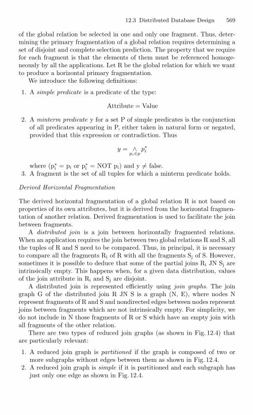
12.3 Distributed Database Design 569
of the global relation be selected in one and only one fragment. Thus, deter-mining the primary fragmentation of a global relation requires determining aset of disjoint and complete selection prediction. The property that we requirefor each fragment is that the elements of them must be referenced homoge-neously by all the applications. Let R be the global relation for which we wantto produce a horizontal primary fragmentation.
We introduce the following definitions:
1. A simple predicate is a predicate of the type:
Attribute = Value
2. A minterm predicate y for a set P of simple predicates is the conjunctionof all predicates appearing in P, either taken in natural form or negated,provided that this expression or contradiction. Thus
y = ∧pi∈p
p∗i
where (p∗i = pi or p∗
i = NOT pi) and y = false.3. A fragment is the set of all tuples for which a minterm predicate holds.
Derived Horizontal Fragmentation
The derived horizontal fragmentation of a global relation R is not based onproperties of its own attributes, but it is derived from the horizontal fragmen-tation of another relation. Derived fragmentation is used to facilitate the joinbetween fragments.
A distributed join is a join between horizontally fragmented relations.When an application requires the join between two global relations R and S, allthe tuples of R and S need to be compared. Thus, in principal, it is necessaryto compare all the fragments Ri of R with all the fragments Sj of S. However,sometimes it is possible to deduce that some of the partial joins Ri JN Sj areintrinsically empty. This happens when, for a given data distribution, valuesof the join attribute in Ri and Sj are disjoint.
A distributed join is represented efficiently using join graphs. The joingraph G of the distributed join R JN S is a graph (N, E), where nodes Nrepresent fragments of R and S and nondirected edges between nodes representjoins between fragments which are not intrinsically empty. For simplicity, wedo not include in N those fragments of R or S which have an empty join withall fragments of the other relation.
There are two types of reduced join graphs (as shown in Fig. 12.4) thatare particularly relevant:
1. A reduced join graph is partitioned if the graph is composed of two ormore subgraphs without edges between them as shown in Fig. 12.4.
2. A reduced join graph is simple if it is partitioned and each subgraph hasjust only one edge as shown in Fig. 12.4.
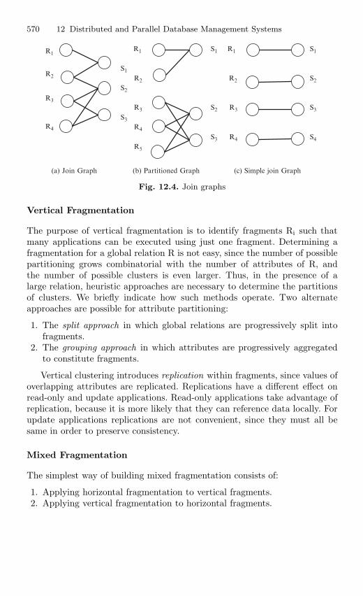
570 12 Distributed and Parallel Database Management Systems
R2
R1
R3
R4
R1
R2
S2
S1
R3
S3
R4
R5
S1 R1
R2
S2 R3
S3 R4
S1
S2
S3
S4
(a) Join Graph (b) Partitioned Graph (c) Simple join Graph
Fig. 12.4. Join graphs
Vertical Fragmentation
The purpose of vertical fragmentation is to identify fragments Ri such thatmany applications can be executed using just one fragment. Determining afragmentation for a global relation R is not easy, since the number of possiblepartitioning grows combinatorial with the number of attributes of R, andthe number of possible clusters is even larger. Thus, in the presence of alarge relation, heuristic approaches are necessary to determine the partitionsof clusters. We briefly indicate how such methods operate. Two alternateapproaches are possible for attribute partitioning:
1. The split approach in which global relations are progressively split intofragments.
2. The grouping approach in which attributes are progressively aggregatedto constitute fragments.
Vertical clustering introduces replication within fragments, since values ofoverlapping attributes are replicated. Replications have a different effect onread-only and update applications. Read-only applications take advantage ofreplication, because it is more likely that they can reference data locally. Forupdate applications replications are not convenient, since they must all besame in order to preserve consistency.
Mixed Fragmentation
The simplest way of building mixed fragmentation consists of:
1. Applying horizontal fragmentation to vertical fragments.2. Applying vertical fragmentation to horizontal fragments.
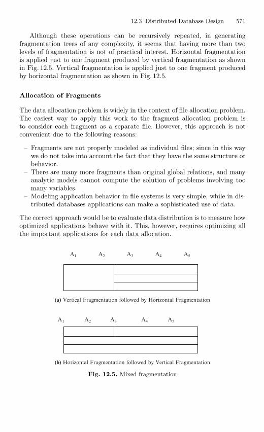
12.3 Distributed Database Design 571
Although these operations can be recursively repeated, in generatingfragmentation trees of any complexity, it seems that having more than twolevels of fragmentation is not of practical interest. Horizontal fragmentationis applied just to one fragment produced by vertical fragmentation as shownin Fig. 12.5. Vertical fragmentation is applied just to one fragment producedby horizontal fragmentation as shown in Fig. 12.5.
Allocation of Fragments
The data allocation problem is widely in the context of file allocation problem.The easiest way to apply this work to the fragment allocation problem isto consider each fragment as a separate file. However, this approach is notconvenient due to the following reasons:
– Fragments are not properly modeled as individual files; since in this waywe do not take into account the fact that they have the same structure orbehavior.
– There are many more fragments than original global relations, and manyanalytic models cannot compute the solution of problems involving toomany variables.
– Modeling application behavior in file systems is very simple, while in dis-tributed databases applications can make a sophisticated use of data.
The correct approach would be to evaluate data distribution is to measure howoptimized applications behave with it. This, however, requires optimizing allthe important applications for each data allocation.
A1
A2 A3 A4 A5A1
A2 A3 A4 A5
(a) Vertical Fragmentation followed by Horizontal Fragmentation
(b) Horizontal Fragmentation followed by Vertical Fragmentation
Fig. 12.5. Mixed fragmentation
572 12 Distributed and Parallel Database Management Systems
General Criteria for Fragment Allocation
Determining a nonredundant final allocation is easier. The simplest methodis “best-fit” approach; a measure is associated with each possible allocation,and the site with best measure is selected. Replication introduces furthercomplexity in the design, because of the following reasons:
– The degree of replication of each fragment becomes a variable of theproblem.
– Modeling read applications is complicated by the fact that the applicationscan now select among several alternatives sites for accessing fragments.
For determining the redundant allocation of fragments, either of the followingtwo methods can be used:
– Determine the set of all sites where the benefit of allocating one copy ofthe fragment is higher than the cost, and allocate a copy of the fragmentto each element of this set; this method selects “all beneficial sites.”
– Determine first the solution of the nonreplicated problem, and thenprogressively introduce replicated copies starting from the most beneficial;the process is terminated when no “additional replication” is beneficial.
Both methods have some disadvantages. In the “all beneficial sites”method, quantifying costs and benefits for each individual fragment allocationis more critical than in the nonredundant case. The “additional replication”method is a typical heuristic approach; with this method, it is possible to takeinto account that the increase in the degree of redundancy is progressively lessbeneficial.
12.4 Semantic Data Control
An important requirement of a centralized or a distributed DBMS is the abilityto support data control. Data control typically includes view management,security control, and semantic integrity control. Informally, these functionsmust ensure that authorized users perform correct operations on the data-base, contributing to the maintenance of database integrity. There are severalways to store data control definitions, according to the way the directoryis managed. Directory information can be stored differently according to itstype; in other words, some information might be fully duplicated whereasother information might be distributed.
12.4.1 View Management
One of the main advantages of the relational model is that it provides fulllogical data independence. External schemas enable user groups to have their
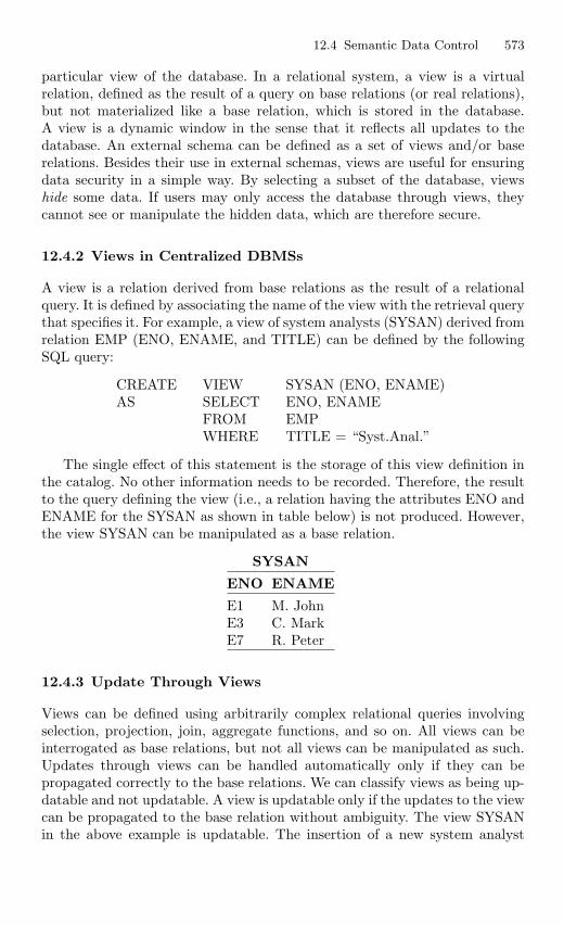
12.4 Semantic Data Control 573
particular view of the database. In a relational system, a view is a virtualrelation, defined as the result of a query on base relations (or real relations),but not materialized like a base relation, which is stored in the database.A view is a dynamic window in the sense that it reflects all updates to thedatabase. An external schema can be defined as a set of views and/or baserelations. Besides their use in external schemas, views are useful for ensuringdata security in a simple way. By selecting a subset of the database, viewshide some data. If users may only access the database through views, theycannot see or manipulate the hidden data, which are therefore secure.
12.4.2 Views in Centralized DBMSs
A view is a relation derived from base relations as the result of a relationalquery. It is defined by associating the name of the view with the retrieval querythat specifies it. For example, a view of system analysts (SYSAN) derived fromrelation EMP (ENO, ENAME, and TITLE) can be defined by the followingSQL query:
CREATE VIEW SYSAN (ENO, ENAME)AS SELECT ENO, ENAME
FROM EMPWHERE TITLE = “Syst.Anal.”
The single effect of this statement is the storage of this view definition inthe catalog. No other information needs to be recorded. Therefore, the resultto the query defining the view (i.e., a relation having the attributes ENO andENAME for the SYSAN as shown in table below) is not produced. However,the view SYSAN can be manipulated as a base relation.
SYSAN
ENO ENAME
E1 M. JohnE3 C. MarkE7 R. Peter
12.4.3 Update Through Views
Views can be defined using arbitrarily complex relational queries involvingselection, projection, join, aggregate functions, and so on. All views can beinterrogated as base relations, but not all views can be manipulated as such.Updates through views can be handled automatically only if they can bepropagated correctly to the base relations. We can classify views as being up-datable and not updatable. A view is updatable only if the updates to the viewcan be propagated to the base relation without ambiguity. The view SYSANin the above example is updatable. The insertion of a new system analyst
574 12 Distributed and Parallel Database Management Systems
<101, John> will be mapped into the new employee <101, John, Syst.Anal>.If attributes other than TITLE were hidden by the view, they would beassigned null values.
12.4.4 Views in Distributed DBMS
The definition of a view is similar in a distributed DBMS and in a centralizedsystem. However, a view in a distributed system may be derived from fragmentrelations stored at different sites. When a view is defined, its name and itsretrieval query are stored in the catalog. Since views may be used as baserelations by application programs, their definitions should be stored in thedirectory in the same way as the base relation descriptions. Depending onthe degree of site autonomy offered by the system, view definitions can becentralized at one site, partially duplicated, or fully duplicated. If the viewdefinition is not present at the site where query is issued, remote access to theview definition site is necessary.
Views derived from distributed relations may be costly to evaluate. Sincein a given organization it is likely that many users access the same views, someproposals have been made to optimize view derivation. The view derivationis done by merging the view qualification with the query qualification. Analternate solution is to avoid view derivation by maintaining actual versionsof the views, called snapshots. A snapshot represents a particular state of thedatabase and is therefore static, meaning that it does not reflect updates tobase relations. Snapshots are useful when users are not particularly interestedin seeing the most recent version of the database.
12.4.5 Data Security
It is an important function of a database system that protects data againstunauthorized access. Data security includes two aspects: data protection andauthorization control.
Data protection is required to prevent unauthorized users from under-standing the physical content of data. This function is typically provided byfile systems in the context of centralized and distributed operating systems.The main data protection approach is data encryption, which is useful forboth information stored on a disk and information exchanged on a network.Encrypted (encoded) data can be decrypted (decoded) only by authorizedusers who “know the code.”
Authorization control must guarantee that only authorized users performoperations they are allowed to perform on the database. Many different usersmay have access to a large collection of data under the control of a singlecentralized or distributed system. In relational systems, authorizations can beuniformly controlled by database administrators using high-level constructs.For example, controlled objects can be specified by predicates in the sameway as a query qualification.
12.4 Semantic Data Control 575
12.4.6 Centralized Authorization Control
Three main aspects are involved in authorization control: the users, whotrigger the execution of the application programs; the operations, which areembedded in application programs; and the database objects, on which theoperations are performed. Authorization control consists of checking whethera given triple can be allowed to proceed (i.e., the user can execute the oper-ation of the object). An authorization can be viewed as a triple (user, opera-tion type, and object definition) which specifies that the user has the right toperform an operation of operation type on an object. To control authorizationsproperly, the DBMS requires users, objects, and rights to be defined.
In a relational system, objects can be defined by their type (view, relation,tuple, and attribute) as well as by their content using selection predicates.A right expresses a relationship between a user and an object for a particularset of operations. In a SQL-based relational DBMS, an operation is a high-level statement such as SELECT, INSERT, UPDATE, or DELETE, and rightsare defined (granted or revoked) using the following statements:
GRANT <operation type(s)> ON <object> TO <user(s)>REVOKE<operation type(s)> FROM<object> TO<user(s)>
The keyword public can be used to mean all users. Authorization controlcan be characterized based on who (the grantors) can grant the rights. Inits simplest form, the control is centralized: a single user or user class, thedatabase administrators have all privileges on the database objects and arethe only one allowed to use the GRANT and REVOKE statements.
A more flexible but complex form of control is decentralized; the creatorof an object becomes its owner and is granted all privileges on it. In partic-ular, there is the additional operation type GRANT. Granting the GRANTprivilege means that all rights of the grantor performing the statement aregiven to the specified users. Therefore the person receiving the right (thegrantee) may subsequently grant privileges on that object. The main diffi-culty with this approach is that the revoking process must be recursive.
12.4.7 Distributed Authorization Control
The additional problem of authorization control is a distributed environmentsystem from the fact that the objects and subjects are distributed. Theseproblems are remote user authentication, management of distributed autho-rization rules, as well as handling of views and of user groups. Remote userauthentication is necessary since any sites of a distributed DBMS may acceptprograms initiated, and authorized, at remote sites. Two solutions are possiblein preventing unauthorized users in remote accessing as follows:
1. The information for authenticating users (user name and password) isreplicated at all sites in the catalog. Local programs, initiated at a remotesite, must also indicate the user name and password.
576 12 Distributed and Parallel Database Management Systems
2. All sites of the distributed DBMS identify and authenticate themselvessimilarly to the way users do. Intersite communication is thus protectedby the use of the site password.
Distributed authorization rules are expressed in the same way as centralizedones. They can be either in fully replicated at each site or stored at the sites ofthe reference objects. The main advantage of fully replicated approach is thatauthorization can be processed by query modification at compile time. How-ever, directory management is more costly because of data duplication. Thesecond solution is better if locality of reference is high. However, distributedauthorization cannot be controlled at compile time.
12.4.8 Semantic Integrity Control
Another important and difficult problem for a database system is how toguarantee database consistency. A database state is said to be consistentif the database satisfies a set of constraints, called semantic integrity con-straints. Maintaining a consistent database requires various mechanisms suchas concurrency control, reliability, protection, and semantic integrity control.Semantic integrity control ensures database consistency by rejecting updateprograms which lead to inconsistent database states, or by activating specificactions on the database state, which compensate for the effects of the updateprograms.
Semantic integrity constraints are rules that represent the knowledge aboutthe properties of an application. They define static or dynamic applicationproperties which cannot be directly captured by the object and operationconcepts of a data model. Thus the concept of an integrity rule is stronglyconnected with that of a data model in the sense that more semantic infor-mation about the application can be captured by means of these rules.
Two main types of integrity constraints can be distinguished: structuralconstraints and behavioral constraints. Structural constraints express basicsemantic properties inherent to a model. Examples of such constraints areunique key constraints in the relational model, or one-to-many associationsbetween objects in the network model. Behavioral constraints, on the otherhand, regulate the application behavior. Thus they are essential in the data-base design process. They can express associations between objects, such asinclusion dependency in the relational model, or describe object propertiesand structures. The increasing variety of database applications and the recentdevelopment of database design aid tools call for powerful integrity constraintswhich can enrich the data model.
The main problem in supporting automatic semantic integrity control isthat the cost of checking assertions can be prohibitive. Enforcing integrityassertions is costly because it generally requires access to a large amount ofdata which are not involved in the database updates. The problem is moredifficult when assertions are defined over a distributed database.
12.4 Semantic Data Control 577
12.4.9 Distributed Semantic Integrity Control
The method obviously works with replicated directories. The two main prob-lems of designing an integrity subsystem for a distributed DBMS are thedefinition and storage of assertions, and the enforcement of these assertions.
Definition of Distributed Integrity Assertions
An integrity assertion is supposed to be expressed in tuple relational calculus.Each assertion is seen as a query qualification which is either true or falsefor each tuple in the Cartesian product of the relations determined by tuplevariables. Since assertions can involve data stored at different sites, their stor-age must be decided so as to minimize the cost of integrity checking. Thereis a strategy based on integrity assertions that distinguishes three classes ofassertions:
1. Individual assertions. Single-relation single-variable assertions. They referonly to tuples to be updated independently of the rest of the database.
2. Set-oriented assertions. Includes single-relation multivariable constraintssuch as functional dependency and multirelation multivariable constraints.
3. Assertions involving aggregates. Requires special processing because of thecost of evaluating the aggregates.
Enforcement of Distributed Integrity Assertions
Enforcing distributed integrity assertions is more complex than needed incentralized DBMSs. The main problem is to decide where to enforce the in-tegrity assertions. The choice depends on the class of the assertion, the typeof update, and the nature of the site where the update is issued:
1. Individual assertions. Two cases are considered. If the update is an insertstatement, all the tuples to be inserted are explicitly provided by the user.In this case, all individual assertions can be enforced at the site where theupdate is submitted. If the update is a qualified update (delete or modifystatements), it is sent to the sites storing the relation that will be updated.
2. Assertions involving aggregates. These assertions are among the mostcostly to test because they require the calculation of the aggregate func-tions. The aggregate functions generally manipulated are MIN, MAX,SUM, and COUNT. Each aggregate function contains a projection partand a selection part. To enforce these assertions efficiently, it is possibleto produce compiled assertions that isolate redundant data which can bestored at each site storing the associated relation. This data are calledviews.
578 12 Distributed and Parallel Database Management Systems
12.5 Distributed Concurrency Control
Distributed concurrency control mechanism of a distributed DBMS ensuresthe consistencies of the database. It is maintained in a multiuser distrib-uted environment. If transactions are internally consistent, the simplest wayof achieving this objective is to execute each transaction alone, one afteranother. It is obvious that such an alternate is only of theoretical interest andcannot be implemented in practical systems, since it minimizes the systemthroughput. The level of concurrency is probably that most important para-meter in distributed systems. Therefore, the concurrency control mechanismsattempts to find a suitable trade-off between maintaining the consistency ofthe database and maintaining a high-level of concurrency.
The distributed system is fully reliable and does not experience any failureseven though this is an entirely unrealistic assumption; there is a reason formaking it. It permits as to delineate the issues related to the managementof concurrency from those related to the operation of the reliable distributedsystem.
12.5.1 Serializability Theory
If the concurrent execution of transactions leaves the database in a state thatcan be achieved by their serial execution in some order, problems such aslast updates will be resolved. This is exactly that the point of serializabilityargument. A schedule S is defined over a set of transaction T = (T1,T2 . . .Tn)and specifies an interleaved order of execution of this transaction operations.Two operations Oij(X) and Ojk(X) accessing the same database entity X aresaid to be in conflict if at least is a right. From this definition, first, readoperations do not conflict each other. Therefore, the two types of conflicts areread–write and write–write.
12.5.2 Taxonomy of Concurrency Control Mechanism
There are number of ways that the concurrency control approaches can beclassified. One obvious classification criterion is the mode of database distri-bution. Some algorithms that have been proposed require a fully replicateddatabase, while others can operate on partially replicated or partitioned data-base. The concurrency control algorithms may also be classified according tothe network topology, such as those requiring a communication subnet withbroadcasting capability or those working in a star type network or circu-larly connected network. The most common classification criterion, however,is synchronization primitives. The corresponding breakdown of concurrencycontrol algorithms results in two classes, algorithms that are based onmutually exclusive access to shared data and those that attempt to order theexecution of transactions according to the set of rules.
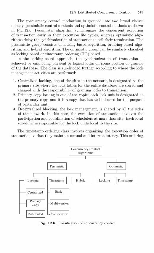
12.5 Distributed Concurrency Control 579
The concurrency control mechanism is grouped into two broad classesnamely, pessimistic control methods and optimistic control methods as shownin Fig. 12.6. Pessimistic algorithm synchronizes the concurrent executionof transaction early in their execution life cycles, whereas optimistic algo-rithms delay the synchronization of transactions until their termination. Thepessimistic group consists of locking-based algorithm, ordering-based algo-rithm, and hybrid algorithm. The optimistic group can be similarly classifiedas locking based or timestamp ordering (TO) based.
In the locking-based approach, the synchronization of transaction isachieved by employing physical or logical locks on some portion or granuleof the database. The class is subdivided further according to where the lockmanagement activities are performed:
1. Centralized locking, one of the sites in the network, is designated as theprimary site where the lock tables for the entire database are stored andcharged with the responsibility of granting locks to transaction.
2. Primary copy locking is one of the copies each lock unit is designated asthe primary copy, and it is a copy that has to be locked for the purposeof particular unit.
3. Decentralized blocking, the lock management, is shared by all the sidesof the network. In this case, the execution of transaction involves theparticipation and coordination of schedulers at more than site. Each localscheduler is responsible for the lock units local to the site.
The timestamp ordering class involves organizing the execution order oftransaction so that they maintain mutual and interconsistency. This ordering
Concurrency ControlAlgorithms
Pessimistic Optimistic
Locking Timestamp Hybrid Locking Timestamp
Basic Centralized
Multi-versionPrimary Copy
Distributed Conservative
Fig. 12.6. Classification of concurrency control
580 12 Distributed and Parallel Database Management Systems
is maintained by assigning timestamps to both the transactions and the dataitems that are stored in the database.
12.5.3 Locking-Based Concurrency Control
The main idea of this control is to ensure that the data that are sharedby conflicting operations are accessed by one operation at a time. This isaccomplished by associating a “lock” with each lock unit. This lock is set bya transaction before it is accessed and is reset at the end of its use. Obviouslythe lock unit cannot be accessed by an operation if it is locked by another.Thus, a lock request by a transaction is granted only if the associated lockis not being held by any other transaction. The distributed DBMS not onlymanages locks but also handles the lock management responsibilities behalfof the transaction. In other words, the users do not need to specify when dataneed to be locked, the distributed DBMS takes care of the every time thetransaction issues read or write operations.
In a locking-based system, the scheduler is a lock manager. The transac-tion manager (TM) passes to the lock manager, the database operation andassociated information. The lock manager then checks if the lock unit thatcontains the data item is already locked. If so, and if the existing lock modeis incompatible with that of the current transaction, the current operation isdelayed. Otherwise, the lock is set to desired mode and database operation ispassed on to the data processor for actual database access. The transactionmanager is then informing of the results of the operations. The termination oftransaction results in the release of its locks and initiation of another trans-action that might be waiting for the access to be same data item.
Centralized 2PL Algorithm
These algorithm can be easily extended (replicated or partitioned) to thedistributed database environment. One way of doing this is to delegate lockmanagement responsibility to a single site only. This means that only of thesites has a lock manager, the transaction manager at the other sites commu-nicates with rather than with the own lock managers. This is also known asprimary site 2PL algorithm. The communication between the operating sitesin order to execute a transaction according to a centralized 2PL is shown inFig. 12.7. This communication between transaction manager at the site wherethe transaction is initiated, the lock manager at the central site, and the dataprocessor at other participating sites are those at which the operation is tobe carried out.
An important difference between the centralized TM algorithm and theTM algorithm of locking is that the distributed TM has to implement thereplica control protocol if the database is replicated. The central lock managerdoes not send the operations to the respective data processors; that is doneby the coordinating TM.
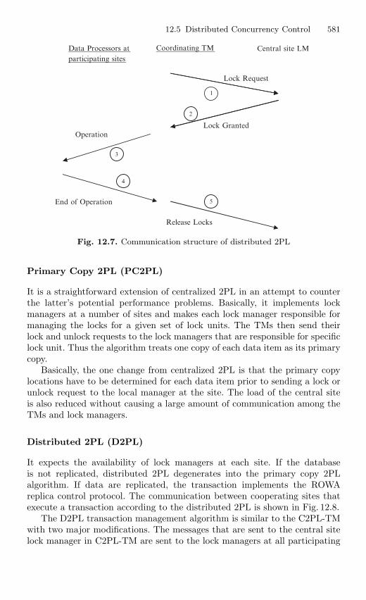
12.5 Distributed Concurrency Control 581
Data Processors at participating sites
Coordinating TM Central site LM
1
Lock Request
Lock Granted
2
3
4
5
Operation
End of Operation
Release Locks
Fig. 12.7. Communication structure of distributed 2PL
Primary Copy 2PL (PC2PL)
It is a straightforward extension of centralized 2PL in an attempt to counterthe latter’s potential performance problems. Basically, it implements lockmanagers at a number of sites and makes each lock manager responsible formanaging the locks for a given set of lock units. The TMs then send theirlock and unlock requests to the lock managers that are responsible for specificlock unit. Thus the algorithm treats one copy of each data item as its primarycopy.
Basically, the one change from centralized 2PL is that the primary copylocations have to be determined for each data item prior to sending a lock orunlock request to the local manager at the site. The load of the central siteis also reduced without causing a large amount of communication among theTMs and lock managers.
Distributed 2PL (D2PL)
It expects the availability of lock managers at each site. If the databaseis not replicated, distributed 2PL degenerates into the primary copy 2PLalgorithm. If data are replicated, the transaction implements the ROWAreplica control protocol. The communication between cooperating sites thatexecute a transaction according to the distributed 2PL is shown in Fig. 12.8.
The D2PL transaction management algorithm is similar to the C2PL-TMwith two major modifications. The messages that are sent to the central sitelock manager in C2PL-TM are sent to the lock managers at all participating
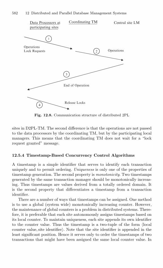
582 12 Distributed and Parallel Database Management Systems
Data Processors at participating sites
Coordinating TM Central site LM
1
Operations2
3
4
OperationsLock Requests
End of Operation
Release Locks
Fig. 12.8. Communication structure of distributed 2PL
sites in D2PL-TM. The second difference is that the operations are not passedto the data processors by the coordinating TM, but by the participating localmanagers. This means that the coordinating TM does not wait for a “lockrequest granted” message.
12.5.4 Timestamp-Based Concurrency Control Algorithms
A timestamp is a simple identifier that serves to identify each transactionuniquely and to permit ordering. Uniqueness is only one of the properties oftimestamp generation. The second property is monotonicity. Two timestampsgenerated by the same transaction manager should be monotonically increas-ing. Thus timestamps are values derived from a totally ordered domain. Itis the second property that differentiates a timestamp from a transactionidentifier.
There are a number of ways that timestamps can be assigned. One methodis to use a global (system wide) monotonically increasing counter. However,the maintenance of global counters is a problem in distributed systems. There-fore, it is preferable that each site autonomously assigns timestamps based onits local counter. To maintain uniqueness, each site appends its own identifierto the counter value. Thus the timestamp is a two-tuple of the form 〈localcounter value, site identifier〉. Note that the site identifier is appended in theleast significant position. Hence it serves only to order the timestamps of twotransactions that might have been assigned the same local counter value. In
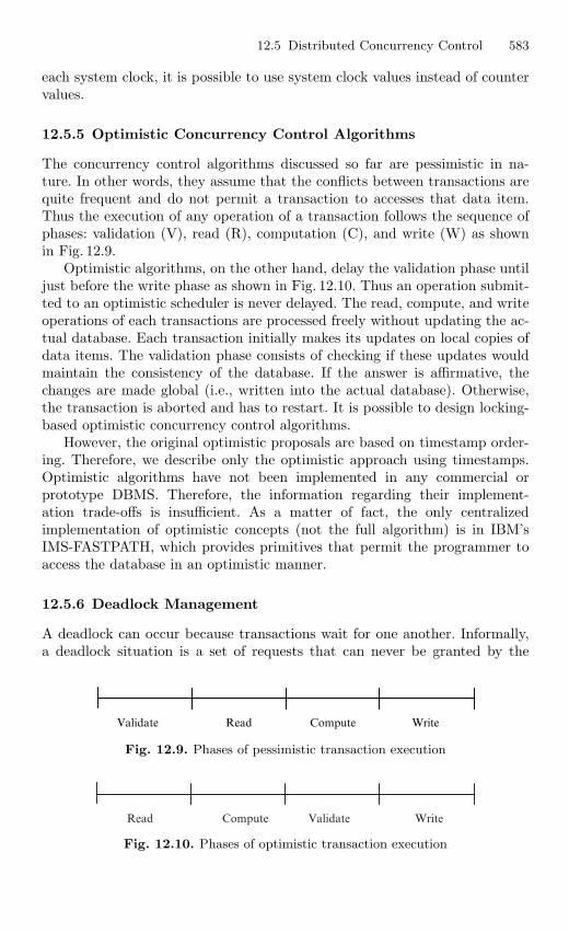
12.5 Distributed Concurrency Control 583
each system clock, it is possible to use system clock values instead of countervalues.
12.5.5 Optimistic Concurrency Control Algorithms
The concurrency control algorithms discussed so far are pessimistic in na-ture. In other words, they assume that the conflicts between transactions arequite frequent and do not permit a transaction to accesses that data item.Thus the execution of any operation of a transaction follows the sequence ofphases: validation (V), read (R), computation (C), and write (W) as shownin Fig. 12.9.
Optimistic algorithms, on the other hand, delay the validation phase untiljust before the write phase as shown in Fig. 12.10. Thus an operation submit-ted to an optimistic scheduler is never delayed. The read, compute, and writeoperations of each transactions are processed freely without updating the ac-tual database. Each transaction initially makes its updates on local copies ofdata items. The validation phase consists of checking if these updates wouldmaintain the consistency of the database. If the answer is affirmative, thechanges are made global (i.e., written into the actual database). Otherwise,the transaction is aborted and has to restart. It is possible to design locking-based optimistic concurrency control algorithms.
However, the original optimistic proposals are based on timestamp order-ing. Therefore, we describe only the optimistic approach using timestamps.Optimistic algorithms have not been implemented in any commercial orprototype DBMS. Therefore, the information regarding their implement-ation trade-offs is insufficient. As a matter of fact, the only centralizedimplementation of optimistic concepts (not the full algorithm) is in IBM’sIMS-FASTPATH, which provides primitives that permit the programmer toaccess the database in an optimistic manner.
12.5.6 Deadlock Management
A deadlock can occur because transactions wait for one another. Informally,a deadlock situation is a set of requests that can never be granted by the
Validate Read Compute Write
Fig. 12.9. Phases of pessimistic transaction execution
Read Compute Validate Write
Fig. 12.10. Phases of optimistic transaction execution
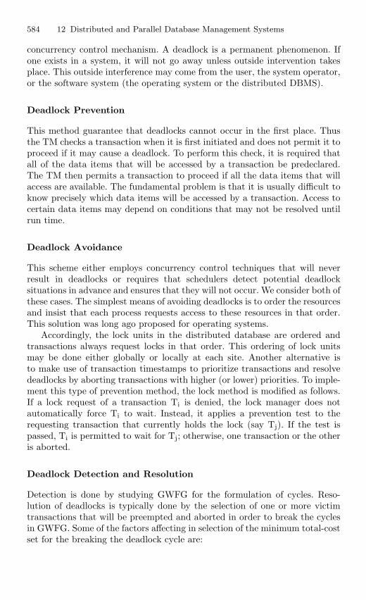
584 12 Distributed and Parallel Database Management Systems
concurrency control mechanism. A deadlock is a permanent phenomenon. Ifone exists in a system, it will not go away unless outside intervention takesplace. This outside interference may come from the user, the system operator,or the software system (the operating system or the distributed DBMS).
Deadlock Prevention
This method guarantee that deadlocks cannot occur in the first place. Thusthe TM checks a transaction when it is first initiated and does not permit it toproceed if it may cause a deadlock. To perform this check, it is required thatall of the data items that will be accessed by a transaction be predeclared.The TM then permits a transaction to proceed if all the data items that willaccess are available. The fundamental problem is that it is usually difficult toknow precisely which data items will be accessed by a transaction. Access tocertain data items may depend on conditions that may not be resolved untilrun time.
Deadlock Avoidance
This scheme either employs concurrency control techniques that will neverresult in deadlocks or requires that schedulers detect potential deadlocksituations in advance and ensures that they will not occur. We consider both ofthese cases. The simplest means of avoiding deadlocks is to order the resourcesand insist that each process requests access to these resources in that order.This solution was long ago proposed for operating systems.
Accordingly, the lock units in the distributed database are ordered andtransactions always request locks in that order. This ordering of lock unitsmay be done either globally or locally at each site. Another alternative isto make use of transaction timestamps to prioritize transactions and resolvedeadlocks by aborting transactions with higher (or lower) priorities. To imple-ment this type of prevention method, the lock method is modified as follows.If a lock request of a transaction Ti is denied, the lock manager does notautomatically force Ti to wait. Instead, it applies a prevention test to therequesting transaction that currently holds the lock (say Tj). If the test ispassed, Ti is permitted to wait for Tj; otherwise, one transaction or the otheris aborted.
Deadlock Detection and Resolution
Detection is done by studying GWFG for the formulation of cycles. Reso-lution of deadlocks is typically done by the selection of one or more victimtransactions that will be preempted and aborted in order to break the cyclesin GWFG. Some of the factors affecting in selection of the minimum total-costset for the breaking the deadlock cycle are:
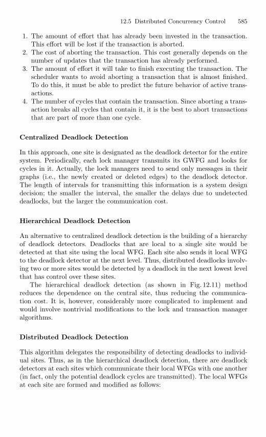
12.5 Distributed Concurrency Control 585
1. The amount of effort that has already been invested in the transaction.This effort will be lost if the transaction is aborted.
2. The cost of aborting the transaction. This cost generally depends on thenumber of updates that the transaction has already performed.
3. The amount of effort it will take to finish executing the transaction. Thescheduler wants to avoid aborting a transaction that is almost finished.To do this, it must be able to predict the future behavior of active trans-actions.
4. The number of cycles that contain the transaction. Since aborting a trans-action breaks all cycles that contain it, it is the best to abort transactionsthat are part of more than one cycle.
Centralized Deadlock Detection
In this approach, one site is designated as the deadlock detector for the entiresystem. Periodically, each lock manager transmits its GWFG and looks forcycles in it. Actually, the lock managers need to send only messages in theirgraphs (i.e., the newly created or deleted edges) to the deadlock detector.The length of intervals for transmitting this information is a system designdecision; the smaller the interval, the smaller the delays due to undetecteddeadlocks, but the larger the communication cost.
Hierarchical Deadlock Detection
An alternative to centralized deadlock detection is the building of a hierarchyof deadlock detectors. Deadlocks that are local to a single site would bedetected at that site using the local WFG. Each site also sends it local WFGto the deadlock detector at the next level. Thus, distributed deadlocks involv-ing two or more sites would be detected by a deadlock in the next lowest levelthat has control over these sites.
The hierarchical deadlock detection (as shown in Fig. 12.11) methodreduces the dependence on the central site, thus reducing the communica-tion cost. It is, however, considerably more complicated to implement andwould involve nontrivial modifications to the lock and transaction manageralgorithms.
Distributed Deadlock Detection
This algorithm delegates the responsibility of detecting deadlocks to individ-ual sites. Thus, as in the hierarchical deadlock detection, there are deadlockdetectors at each sites which communicate their local WFGs with one another(in fact, only the potential deadlock cycles are transmitted). The local WFGsat each site are formed and modified as follows:
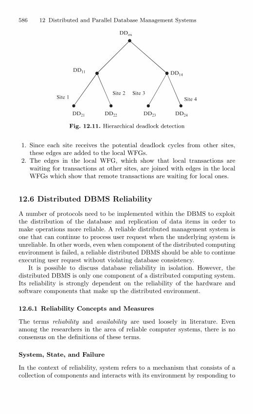
586 12 Distributed and Parallel Database Management Systems
Site 2 Site 3Site 1 Site 4
DDox
DD14 DD11
DD21 DD22 DD23 DD24
Fig. 12.11. Hierarchical deadlock detection
1. Since each site receives the potential deadlock cycles from other sites,these edges are added to the local WFGs.
2. The edges in the local WFG, which show that local transactions arewaiting for transactions at other sites, are joined with edges in the localWFGs which show that remote transactions are waiting for local ones.
12.6 Distributed DBMS Reliability
A number of protocols need to be implemented within the DBMS to exploitthe distribution of the database and replication of data items in order tomake operations more reliable. A reliable distributed management system isone that can continue to process user request when the underlying system isunreliable. In other words, even when component of the distributed computingenvironment is failed, a reliable distributed DBMS should be able to continueexecuting user request without violating database consistency.
It is possible to discuss database reliability in isolation. However, thedistributed DBMS is only one component of a distributed computing system.Its reliability is strongly dependent on the reliability of the hardware andsoftware components that make up the distributed environment.
12.6.1 Reliability Concepts and Measures
The terms reliability and availability are used loosely in literature. Evenamong the researchers in the area of reliable computer systems, there is noconsensus on the definitions of these terms.
System, State, and Failure
In the context of reliability, system refers to a mechanism that consists of acollection of components and interacts with its environment by responding to
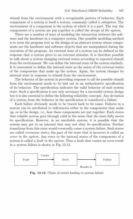
12.6 Distributed DBMS Reliability 587
stimuli from the environment with a recognizable pattern of behavior. Eachcomponent of a system is itself a system, commonly called a subsystem. Theenvironment of a component is the system of which it is a part. The way thecomponents of a system are put together is called the design of the system.
There are a number of ways of modeling the interaction between the soft-ware and the hardware in a computer system. One possible modeling methodis to treat the program text as the design of an abstract system whose compo-nents are the hardware and software objects that are manipulated during theexecution of the program. An external state of a system can be defined as theresponse that a system gives to an external stimulus. It is therefore possibleto talk about a system changing external states according to repeated stimulifrom the environment. We can define the internal state of the system similarly.It is convenient to define the internal state as the union of the external statesof the components that make up the system. Again, the system changes itsinternal state in response to stimuli from the environment.
The behavior of the system in providing response to all the possible stimulifrom the environment needs to be laid out in an authoritative specificationof its behavior. The specification indicates the valid behavior of each systemstate. Such a specification is not only necessary for a successful system designbut it is also essential to define the following reliability concepts. Any deviationof a system from the behavior in the specification is considered a failure.
Each failure obviously needs to be traced back to its cause. Failures in asystem can be attributed to deficiencies either in the components that makeup, or in the design, i.e., how these components are put together. Each statesthat reliable system goes through valid in the sense that the state fully meetsits specification. However, in an unreliable system, it is possible that thesystem may get to an internal that may not obey its specification. Furthertransitions from this state would eventually cause a system failure. Such statesare called erroneous states ; the part of the state that is incorrect is called anerror in the system. Any error in the internal states of the components of asystem is called a fault in the system. Thus a fault that causes an error resultin a system failure is shown in Fig. 12.12.
Fault Error Failure
Causes
Results in
Fig. 12.12. Chain of events leading to system failure
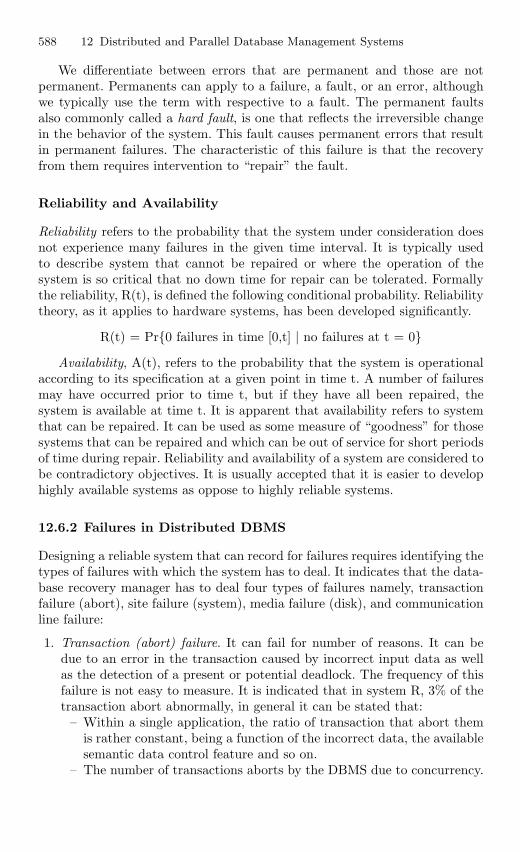
588 12 Distributed and Parallel Database Management Systems
We differentiate between errors that are permanent and those are notpermanent. Permanents can apply to a failure, a fault, or an error, althoughwe typically use the term with respective to a fault. The permanent faultsalso commonly called a hard fault, is one that reflects the irreversible changein the behavior of the system. This fault causes permanent errors that resultin permanent failures. The characteristic of this failure is that the recoveryfrom them requires intervention to “repair” the fault.
Reliability and Availability
Reliability refers to the probability that the system under consideration doesnot experience many failures in the given time interval. It is typically usedto describe system that cannot be repaired or where the operation of thesystem is so critical that no down time for repair can be tolerated. Formallythe reliability, R(t), is defined the following conditional probability. Reliabilitytheory, as it applies to hardware systems, has been developed significantly.
R(t) = Pr0 failures in time [0,t] | no failures at t = 0
Availability, A(t), refers to the probability that the system is operationalaccording to its specification at a given point in time t. A number of failuresmay have occurred prior to time t, but if they have all been repaired, thesystem is available at time t. It is apparent that availability refers to systemthat can be repaired. It can be used as some measure of “goodness” for thosesystems that can be repaired and which can be out of service for short periodsof time during repair. Reliability and availability of a system are considered tobe contradictory objectives. It is usually accepted that it is easier to develophighly available systems as oppose to highly reliable systems.
12.6.2 Failures in Distributed DBMS
Designing a reliable system that can record for failures requires identifying thetypes of failures with which the system has to deal. It indicates that the data-base recovery manager has to deal four types of failures namely, transactionfailure (abort), site failure (system), media failure (disk), and communicationline failure:
1. Transaction (abort) failure. It can fail for number of reasons. It can bedue to an error in the transaction caused by incorrect input data as wellas the detection of a present or potential deadlock. The frequency of thisfailure is not easy to measure. It is indicated that in system R, 3% of thetransaction abort abnormally, in general it can be stated that:
– Within a single application, the ratio of transaction that abort themis rather constant, being a function of the incorrect data, the availablesemantic data control feature and so on.
– The number of transactions aborts by the DBMS due to concurrency.
12.6 Distributed DBMS Reliability 589
2. Site (system) failure. It can be traced back to a hardware failure (proces-sor, main memory, etc.) or to a software failure (bug in the operatingsystem or in the DBMS code). The important point from the perspec-tive is that a system failure is always assumed to result in the loss of mainmemory contents. In distributed database terminology, system failures aretypically referred to as site failure, since they result in the failed site beingunreachable from other sites in the distributed system.
3. Media (disk) failures. It refers to the failures of the secondary storagedevices that store the database. Such failures may be due to operatingsystem errors, as well as to hardware faults such as head crashes orcontroller failures. The important feature from the perspective of DBMSreliability is that all or part of the database that is on the secondarystorage is considered to be destroyed and inaccessible. These failures arefrequently treated as problems local to one site and therefore not specifi-cally addressed in the reliability mechanisms of distributed DBMSs.
4. Communication failures. The communication failures are unique to dis-tributed DBMS (not centralized DBMS). Lost or undeliverable messagesare typically the consequence of communication line failures or site fail-ures. If a communication line fails, in addition to losing messages in transit,it may also divide the network into two or more disjoint groups. This iscalled network partitioning. If the network is partitioned, the sites in eachpartition may continue to operate.
The detection of undeliverable massages is facilitated by the use oftimers and a timeout mechanism that keeps track of how long it hasbeen since the sender site has not received any confirmation from thedestination site about the receipt of the message. The term for the failureof the communication network to deliver messages and the confirmationswithin this period is performance failure. It needs to be handled withinthe reliability protocols for distributed DBMSs.
Reasons for Failures in Distributed Systems
Soft failures make up more than 90% of all hardware system failures. It isinteresting note that this percentage has not changed significantly since theearly days of computing. More recent studies indicate that the occurrenceof soft failures is significantly higher than that of hard failures. Most of thesoftware failures are transient hence a dump and restart may be sufficient torecover without any need to repair the software. Software failures are mostdifficult to discuss because there is no agreement on a classification scheme.The software failures due to communication and database are by far thedominant causes. These are followed by operating system failures, whichare then followed by failures in the application code and in the transactionmanagement software.
590 12 Distributed and Parallel Database Management Systems
When one investigates hardware causes of failures, 49% of hardwarefailures are disk failures, 23% are due to communication, 17% due to processorfailure, 9% due to wiring, and 1% due to the failure of spares.
12.6.3 Basic Fault Tolerance Approaches and Techniques
The two fundamental approaches to constructing a reliable system are faulttolerance and fault prevention. Fault tolerance refers to a system designapproach which recognizes that faults will occur; it tries to build mechanismsinto the system so that the faults can be detected and removed or compen-sated for before they can result in a system failure. Fault prevention has twoaspects. The first is fault avoidance, which refers to the techniques used tomake sure that faults are not introduced into the system. These techniquesinvolve detailed design methodologies and quality control. The second aspectis fault removal, which refers to the techniques that are employed to detectany faults that might have been remained in the system despite the applica-tion of fault avoidance and removes these faults. The fault removal techniquescan be applied only during the system implementation prior to field use ofthe system.
Fault detection techniques are not coupled with fault tolerance features,they issue a warning when a failure occurs but do not provide any meansof tolerating the failure. Therefore, it might be appropriate to separate faultdetection from strictly fault tolerant approaches.
12.6.4 Distributed Reliability Protocols
Similar to local reliability protocols, the distribution versions aim to maintainthe atomicity and durability of distributed transactions that execute over anumber of databases. To facilitate the description of the distributed reliabilityprotocols, we resort to a commonly used abstraction. We assume that at theoriginating site of a transaction there is a process that executes its operations.This process is called the coordinator. The coordinator communicates with theparticipant processes at the other sites which assist in the execution of thetransaction’s operations.
Components of Distributed Reliability Protocols
The reliability techniques in distributed database systems consist of commitand recovery protocols. Recall from the preceding section that the commit andrecovery protocols specify how the commit and the recover commands areexecuted. Both of these commends need to be executed differently in adistributed DBMS than in a centralized DBMS. The primary requirementof commit protocols is that they maintain the atomicity of distributedtransactions. This means that even though the execution of the distributedtransaction involves multiple sites, some of whichmight fail while executing,
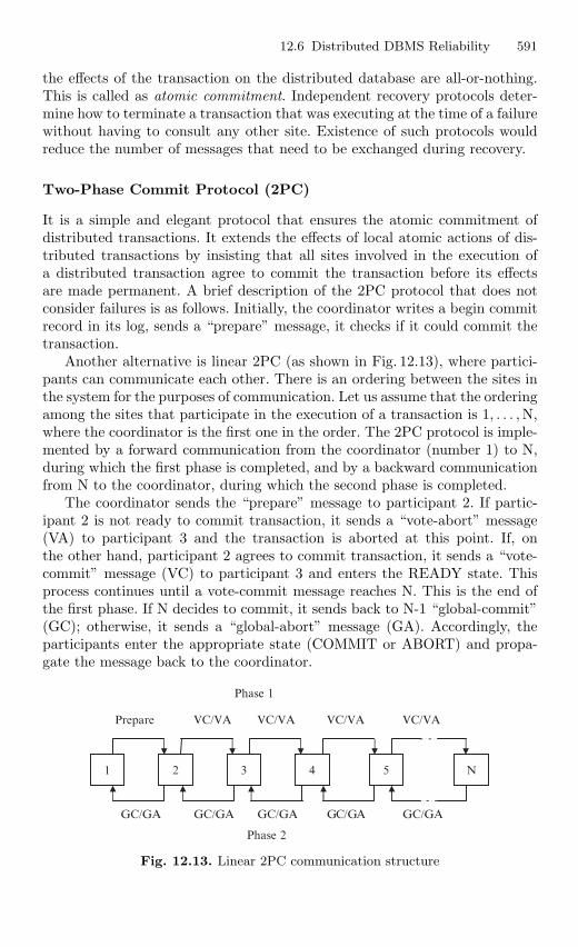
12.6 Distributed DBMS Reliability 591
the effects of the transaction on the distributed database are all-or-nothing.This is called as atomic commitment. Independent recovery protocols deter-mine how to terminate a transaction that was executing at the time of a failurewithout having to consult any other site. Existence of such protocols wouldreduce the number of messages that need to be exchanged during recovery.
Two-Phase Commit Protocol (2PC)
It is a simple and elegant protocol that ensures the atomic commitment ofdistributed transactions. It extends the effects of local atomic actions of dis-tributed transactions by insisting that all sites involved in the execution ofa distributed transaction agree to commit the transaction before its effectsare made permanent. A brief description of the 2PC protocol that does notconsider failures is as follows. Initially, the coordinator writes a begin commitrecord in its log, sends a “prepare” message, it checks if it could commit thetransaction.
Another alternative is linear 2PC (as shown in Fig. 12.13), where partici-pants can communicate each other. There is an ordering between the sites inthe system for the purposes of communication. Let us assume that the orderingamong the sites that participate in the execution of a transaction is 1, . . . ,N,where the coordinator is the first one in the order. The 2PC protocol is imple-mented by a forward communication from the coordinator (number 1) to N,during which the first phase is completed, and by a backward communicationfrom N to the coordinator, during which the second phase is completed.
The coordinator sends the “prepare” message to participant 2. If partic-ipant 2 is not ready to commit transaction, it sends a “vote-abort” message(VA) to participant 3 and the transaction is aborted at this point. If, onthe other hand, participant 2 agrees to commit transaction, it sends a “vote-commit” message (VC) to participant 3 and enters the READY state. Thisprocess continues until a vote-commit message reaches N. This is the end ofthe first phase. If N decides to commit, it sends back to N-1 “global-commit”(GC); otherwise, it sends a “global-abort” message (GA). Accordingly, theparticipants enter the appropriate state (COMMIT or ABORT) and propa-gate the message back to the coordinator.
1 2 3 N54
Prepare VC/VA VC/VA VC/VA VC/VA
GC/GA GC/GA GC/GA GC/GA GC/GA
Phase 1
Phase 2
Fig. 12.13. Linear 2PC communication structure
592 12 Distributed and Parallel Database Management Systems
Architectural Considerations
Here the protocols are implemented within the framework of our architecturalmodel. This involves specification of the interface between the concurrencycontrol algorithms and the reliability protocols. It is quite difficult to specifyprecisely the execution of these commands. The difficulty is twofold. First,a significantly more detailed model of the architecture than the one we havepresented needs to be considered for correct implementation of these com-mands. Second, the overall scheme of implementation is quite dependent onthe recovery procedures that the local recovery manager implements.
One possible implementation of the commit protocols within our architec-tural model is to perform both the coordinator and participant algorithmswithin the transaction managers at each site. This provides some uniformityin executing the distribution commit operations. However, it entails unnec-essary communication between the participation transaction manager and itsscheduler; this is because the scheduler has to decide whether a transactioncan be committed or aborted.
Storing the commit protocol records in the database log maintained by theLRM and the buffer manager requires some changes to the LRM algorithms.This is the third architectural issue we address. Unfortunately, these changesare dependent on the type of the algorithm that the LRM uses. The LRMhas to determine whether the failed site is the host of the coordinator or ofa participant. This information can be stored together with the begin trans-action record. The LRM then has to search for the last record written in thelog record during execution of the commit protocol.
12.7 Parallel Database
The distribution database implies a number of computers connected by a widearea or a local area network. The increasing use of powerful personal comput-ers, work stations, and parallel computers in distributed systems has a majorimpact on distributed database technology. The integration of workstationsin a distributed environment enables a more efficient function distribution inwhich application programs run on workstations, called application servers,while database functions are handled by dedicated computers, called databaseservers.
A parallel computer, or multiprocessor, is itself a distributed system madeof a number of nodes connected by a fast network within a cabinet. Distrib-uted database technology can be naturally revised and extended to implementparallel database systems. It exploits the parallelism data management in or-der to deliver high performance and high availability. Database serves at muchlower price than equivalent main frame computers.
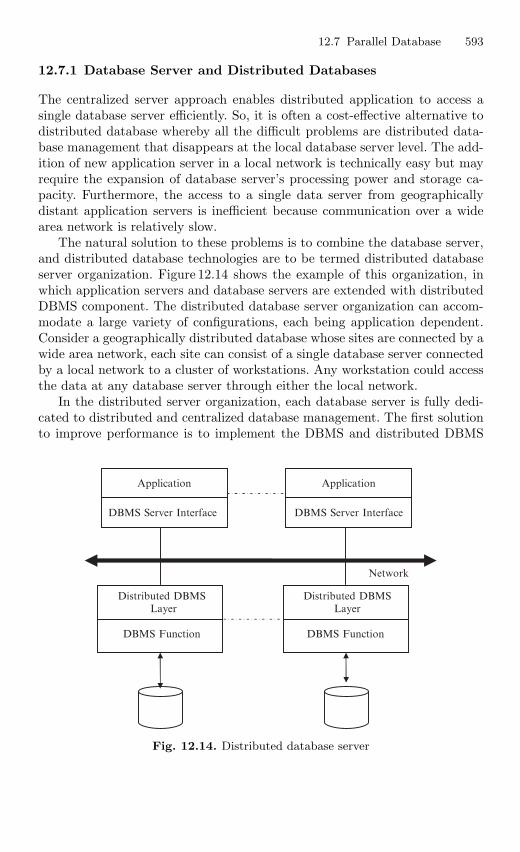
12.7 Parallel Database 593
12.7.1 Database Server and Distributed Databases
The centralized server approach enables distributed application to access asingle database server efficiently. So, it is often a cost-effective alternative todistributed database whereby all the difficult problems are distributed data-base management that disappears at the local database server level. The add-ition of new application server in a local network is technically easy but mayrequire the expansion of database server’s processing power and storage ca-pacity. Furthermore, the access to a single data server from geographicallydistant application servers is inefficient because communication over a widearea network is relatively slow.
The natural solution to these problems is to combine the database server,and distributed database technologies are to be termed distributed databaseserver organization. Figure 12.14 shows the example of this organization, inwhich application servers and database servers are extended with distributedDBMS component. The distributed database server organization can accom-modate a large variety of configurations, each being application dependent.Consider a geographically distributed database whose sites are connected by awide area network, each site can consist of a single database server connectedby a local network to a cluster of workstations. Any workstation could accessthe data at any database server through either the local network.
In the distributed server organization, each database server is fully dedi-cated to distributed and centralized database management. The first solutionto improve performance is to implement the DBMS and distributed DBMS
Application
DBMS Server Interface
Application
DBMS Server Interface
Distributed DBMS Layer
DBMS Function
Network
Distributed DBMSLayer
DBMS Function
Fig. 12.14. Distributed database server
594 12 Distributed and Parallel Database Management Systems
modules on top of a distributed database operating system running on a tradi-tional computer. Another solution is to go one step further and use a paralleldatabase system.
Parallel processing exploits multiprocessor computers to run applicationprograms by using several processors cooperatively, in order to improveperformance. Its prominent use has long been in scientific computing byimproving the response time of numerical applications. Recent develop-ment in both the general purpose MIMD parallel computers using standardmicroprocessors and parallel programming techniques has enabled parallelprocessing to increase performance and availability.
The problem faced by conventional database management has long beenknown as “I/O bottleneck,” induced by high disk access time with respectto main memory access time (typically hundreds of thousands times faster).Initially, DBM designers tackled this problem by introducing the data filteringdevices within the disk. They too failed due to poor price/performance whencompared to the software solution which can easily benefit from hardwareprogress in silicon technology.
An important result of DBM research is in the general solution of the I/Obottleneck. If we store a database of size D on a single disk with throughput T,the system throughput is bounded by T. On the contrary, if we partition thedatabase across n disks, each with capacity D/n and throughput T′ (nearlyequivalent to T), we get an ideal throughput of n * T′ which can be betterconsumed by multiple processors. Note that main memory database systemsolution which tries to maintain the database in main memory is complimen-tary rather than alternative.
Parallel database system designers strived to develop software-orientedsolutions in order to exploit multiprocessor hardware. The objective of par-allel database system can be achieved by extending distributed databasetechnology.
Parallel database software must effectively deploy the system’s processingpower to handle diverse applications, online transaction processing (OLTP)applications, decision support system (DSS) applications, as well as a mixedOLTP and DSS workload. OLTP applications are characterized by shorttransactions, which have low CPU and I/O usage. DSS applications arecharacterized by long transactions, with high CPU and I/O usage.
Parallel database software is often specialized usually to serve as queryprocessors. Since they are designed to serve a single function, however,specialized servers do not provide a common foundation for integrated opera-tions. These include online decision support, batch reporting, data warehous-ing, OLTP, distributed operations, and high availability systems. Specializedservers have been used most successfully in the area of very large databases.
Consider the versatile parallel software should offer excellent price/perfor-mance on open systems hardware, and be designed to serve a wide variety ofenterprise computing needs. Features such as online backup, data replication,portability, interoperability, and support for a wide variety of client tools can
12.7 Parallel Database 595
enable a parallel to support application integration, distributed operations,and mixed application workloads.
There are a number of hardware architectures allow multiple computersto share access to data, software, or peripheral devices. A parallel databaseis designed to take advantage of such architectures by running multiple in-stances, which share a single physical database. In appropriate applications,a parallel server can allow access to single database by users on multiple ma-chines with increased performance. A parallel server processes transaction inparallel by servicing a stream of transactions using multiple CPUs on differ-ent nodes, and each CPU processes an entire transaction. This is an efficientapproach because many applications consist of online insert and update trans-actions that tend to have short data access requirements.
12.7.2 Main Components of Parallel Processing
The main components of parallel processing are speedup and scale-up, syn-chronization, locking, and messaging.
Speedup and Scale-up
Speedup is the extent to which more hardware can perform the same task inless time than the original system. With added hardware, speedup holds thetask constant and measures the time saved. With good speedup, additionalprocessors reduce system response time. You can measure speedup by usingthe following formulae:
Speedup =Original Processing TimeParallel Processing Time
The original processing time is the elapsed time spent by a small system onthe given task and parallel processing time is the elapsed time spent by alarger, parallel system on the given task. For example, if the original systemtook 100 s to perform a task, and two parallel systems took 50 s, then thevalue of speedup would be equal to 2.
Scale-up is the ability of a system n times larger to perform a job n timeslarger, in the same period as the original system. With good scale-up, if trans-action volumes grow, you can keep response time constant by adding hardwareresources such as CPUs. We can measure the scale-up by using the formulae:
Scale-up =Parallel Processing VolumeOriginal Processing Volume
The original processing volume is the transaction volume processed in a givenamount of time on a small system. The parallel processing volume is thetransaction volume processed in a given amount of time on a parallel system.If the value of scale-up is 2, then it indicates the ideal of linear scale-up, i.e.,twice as much as the hardware can process twice the data volume in the sameamount of time.
596 12 Distributed and Parallel Database Management Systems
Synchronization
Coordination of concurrent tasks is called synchronization. Synchronization isnecessary for correctness. The key to successful parallel processing is to divideup tasks so that very little synchronization is necessary. If the synchronizationnecessary is less, then the speedup and scale-up are better.
In parallel processing between nodes, a high-speed communication net-works are required among the parallel processors. The overhead of thissynchronization can be very expensive if a great deal of internode commu-nication is necessary. For parallel processing within a node, messaging is notrequired instead a shared-memory can be used. A task, in fact, may requiremultiple messages. If tasks must continually wait to synchronize, then severalmessages may be needed per task. In most database management systems,messaging and locking between nodes are handled by the distributed lockmanager (DLM).
The amount of synchronization depends on the amount of resources andthe number of users and tasks working on the resources. Little synchronizationmay be needed to coordinate a small number of concurrent tasks, but lots ofsynchronization may be necessary to coordinate many concurrent tasks.
A great deal of time spent in synchronization indicates high contention forresources. Too much time spent in synchronization can diminish the benefitsof parallel processing. With less time spent in synchronization, better speedupand scale-up can be achieved.
Locking
Locks are fundamentally a way of synchronizing tasks. Many different lockingmechanisms are necessary to enable the synchronization of tasks required byparallel processing. External locking facilities as well as mechanisms internalto the database are necessary. A DLM is the external locking facility used bymany parallel databases. A DLM is an operating software, which coordinatesresource sharing between nodes running a parallel server.
The instances of a parallel server use the DLM to communicate witheach other and coordinate the modification of database resources. Each nodeoperates independently of other nodes, except when contending for the samesource. The DLM allows applications to synchronize access to resource suchas data, software, and peripheral devices, so that concurrent requests forthe same resource are coordinated between applications running on differentnodes. The DLM performs the following services for applications:
1. Keeps track of the current ownership of a resource.2. Accepts lock requests for resources from application process.3. Notifies the requesting process when a lock on a resource is available.4. Gets access to a resource for a process.
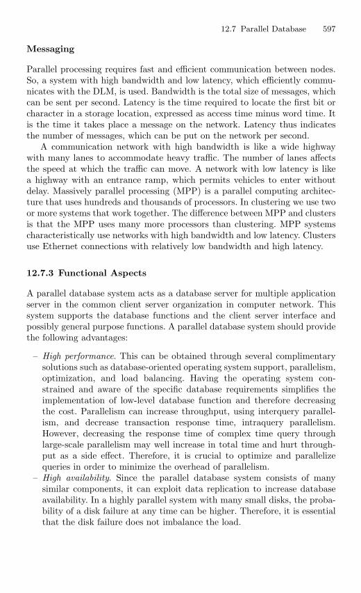
12.7 Parallel Database 597
Messaging
Parallel processing requires fast and efficient communication between nodes.So, a system with high bandwidth and low latency, which efficiently commu-nicates with the DLM, is used. Bandwidth is the total size of messages, whichcan be sent per second. Latency is the time required to locate the first bit orcharacter in a storage location, expressed as access time minus word time. Itis the time it takes place a message on the network. Latency thus indicatesthe number of messages, which can be put on the network per second.
A communication network with high bandwidth is like a wide highwaywith many lanes to accommodate heavy traffic. The number of lanes affectsthe speed at which the traffic can move. A network with low latency is likea highway with an entrance ramp, which permits vehicles to enter withoutdelay. Massively parallel processing (MPP) is a parallel computing architec-ture that uses hundreds and thousands of processors. In clustering we use twoor more systems that work together. The difference between MPP and clustersis that the MPP uses many more processors than clustering. MPP systemscharacteristically use networks with high bandwidth and low latency. Clustersuse Ethernet connections with relatively low bandwidth and high latency.
12.7.3 Functional Aspects
A parallel database system acts as a database server for multiple applicationserver in the common client server organization in computer network. Thissystem supports the database functions and the client server interface andpossibly general purpose functions. A parallel database system should providethe following advantages:
– High performance. This can be obtained through several complimentarysolutions such as database-oriented operating system support, parallelism,optimization, and load balancing. Having the operating system con-strained and aware of the specific database requirements simplifies theimplementation of low-level database function and therefore decreasingthe cost. Parallelism can increase throughput, using interquery parallel-ism, and decrease transaction response time, intraquery parallelism.However, decreasing the response time of complex time query throughlarge-scale parallelism may well increase in total time and hurt through-put as a side effect. Therefore, it is crucial to optimize and parallelizequeries in order to minimize the overhead of parallelism.
– High availability. Since the parallel database system consists of manysimilar components, it can exploit data replication to increase databaseavailability. In a highly parallel system with many small disks, the proba-bility of a disk failure at any time can be higher. Therefore, it is essentialthat the disk failure does not imbalance the load.
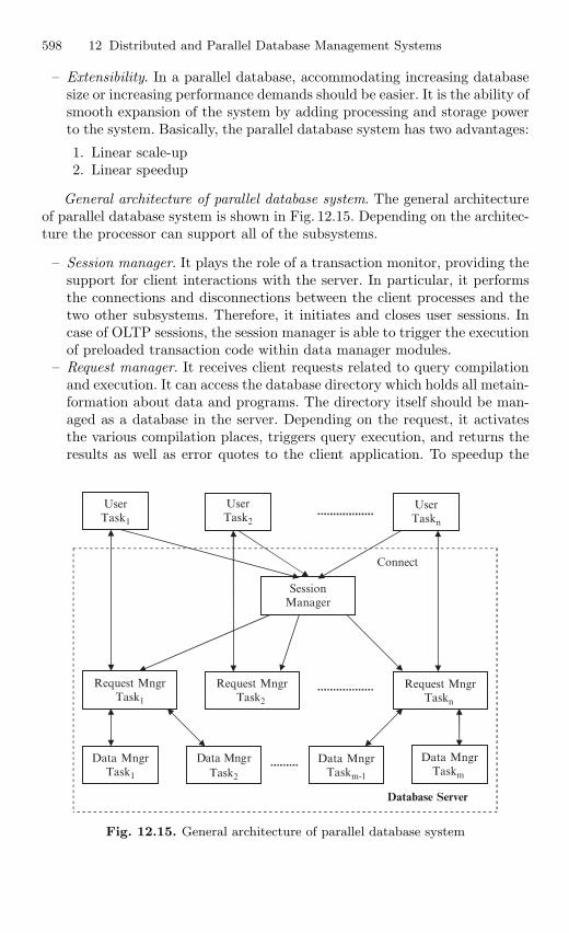
598 12 Distributed and Parallel Database Management Systems
– Extensibility. In a parallel database, accommodating increasing databasesize or increasing performance demands should be easier. It is the ability ofsmooth expansion of the system by adding processing and storage powerto the system. Basically, the parallel database system has two advantages:
1. Linear scale-up2. Linear speedup
General architecture of parallel database system. The general architectureof parallel database system is shown in Fig. 12.15. Depending on the architec-ture the processor can support all of the subsystems.
– Session manager. It plays the role of a transaction monitor, providing thesupport for client interactions with the server. In particular, it performsthe connections and disconnections between the client processes and thetwo other subsystems. Therefore, it initiates and closes user sessions. Incase of OLTP sessions, the session manager is able to trigger the executionof preloaded transaction code within data manager modules.
– Request manager. It receives client requests related to query compilationand execution. It can access the database directory which holds all metain-formation about data and programs. The directory itself should be man-aged as a database in the server. Depending on the request, it activatesthe various compilation places, triggers query execution, and returns theresults as well as error quotes to the client application. To speedup the
User Task1
Request MngrTask1
UserTask2
Request MngrTask2
UserTaskn
Request MngrTaskn
SessionManager
Data MngrTask1
Data Mngr Task2
Data MngrTaskm-1
Data MngrTaskm
Database Server
Connect
Fig. 12.15. General architecture of parallel database system
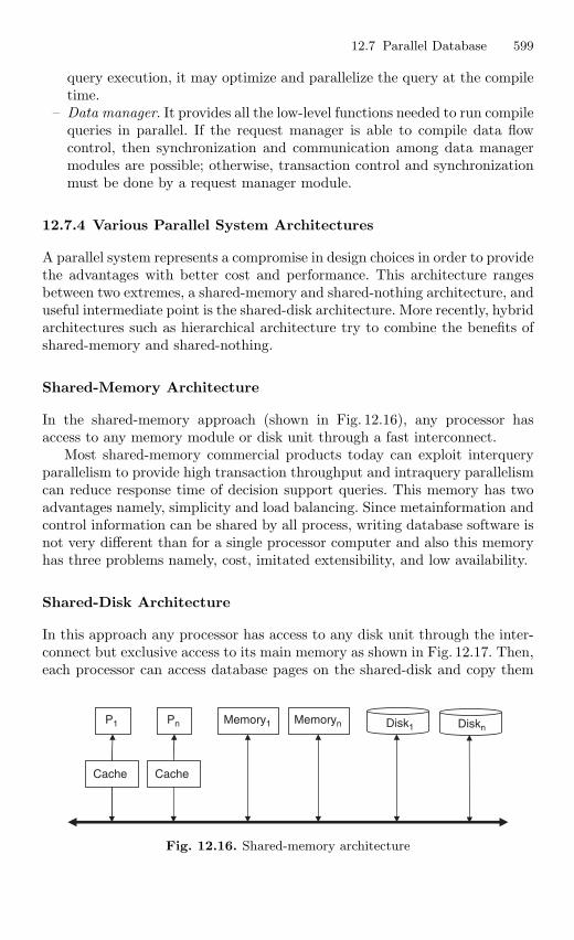
12.7 Parallel Database 599
query execution, it may optimize and parallelize the query at the compiletime.
– Data manager. It provides all the low-level functions needed to run compilequeries in parallel. If the request manager is able to compile data flowcontrol, then synchronization and communication among data managermodules are possible; otherwise, transaction control and synchronizationmust be done by a request manager module.
12.7.4 Various Parallel System Architectures
A parallel system represents a compromise in design choices in order to providethe advantages with better cost and performance. This architecture rangesbetween two extremes, a shared-memory and shared-nothing architecture, anduseful intermediate point is the shared-disk architecture. More recently, hybridarchitectures such as hierarchical architecture try to combine the benefits ofshared-memory and shared-nothing.
Shared-Memory Architecture
In the shared-memory approach (shown in Fig. 12.16), any processor hasaccess to any memory module or disk unit through a fast interconnect.
Most shared-memory commercial products today can exploit interqueryparallelism to provide high transaction throughput and intraquery parallelismcan reduce response time of decision support queries. This memory has twoadvantages namely, simplicity and load balancing. Since metainformation andcontrol information can be shared by all process, writing database software isnot very different than for a single processor computer and also this memoryhas three problems namely, cost, imitated extensibility, and low availability.
Shared-Disk Architecture
In this approach any processor has access to any disk unit through the inter-connect but exclusive access to its main memory as shown in Fig. 12.17. Then,each processor can access database pages on the shared-disk and copy them
P1
Cache
Pn
Cache
Memory1 Memoryn Disk1 Diskn
Fig. 12.16. Shared-memory architecture
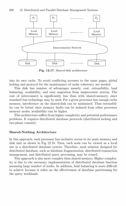
600 12 Distributed and Parallel Database Management Systems
Interconnection Network
P1 P2 Pn
Local Memory
Local Memory
Local Memory
Disk Disk Disk
Fig. 12.17. Shared-disk architecture
into its own cache. To avoid conflicting accesses to the same pages, globallocking and protocol for the maintenance of cache coherency are needed.
This disk has number of advantages namely, cost, extensibility, loadbalancing, availability, and easy migration from uniprocessor system. Thecost of interconnect is significantly less than with shared-memory, sincestandard bus technology may be used. For a given processor has enough cachememory, interference on the shared-disk can be minimized. Thus extensibil-ity can be better since memory faults can be isolated from other processormemory nodes, availability can be higher.
This architecture suffers from higher complexity and potential performanceproblems. It requires distributed database protocols (distributed locking andtwo-phase commit).
Shared-Nothing Architecture
In this approach, each processor has exclusive access to its main memory anddisk unit as shown in Fig. 12.18. Then, each node can be viewed as a localsite in a distributed database system. Therefore, most solution designed fordistributed database, such as database fragmentation, distributed transactionmanagement, and distributed query processing, may be reused.
This approach is also more complex than shared-memory. Higher complex-ity is due to the necessary implementation of distributed database functionassuming large number of nodes. In addition, load balancing is more difficultto achieve because it relies on the effectiveness of database partitioning forthe query workloads.
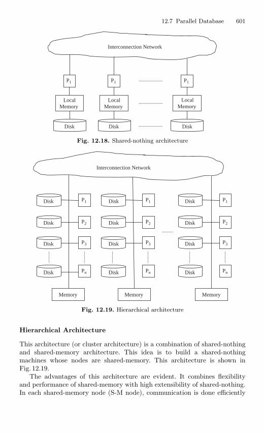
12.7 Parallel Database 601
Local
Memory
Disk
P1 P1 P1
Local
Memory
Interconnection Network
Disk
Local
Memory
Disk
Fig. 12.18. Shared-nothing architecture
Disk
Disk
Disk
Disk
P1
P2
P3
Pn
P1
P2
P3
Pn
P1
P2
P3
Pn
Memory Memory Memory
Disk
Interconnection Network
Disk
Disk
Disk
Disk
Disk
Disk
Disk
Fig. 12.19. Hierarchical architecture
Hierarchical Architecture
This architecture (or cluster architecture) is a combination of shared-nothingand shared-memory architecture. This idea is to build a shared-nothingmachines whose nodes are shared-memory. This architecture is shown inFig. 12.19.
The advantages of this architecture are evident. It combines flexibilityand performance of shared-memory with high extensibility of shared-nothing.In each shared-memory node (S-M node), communication is done efficiently
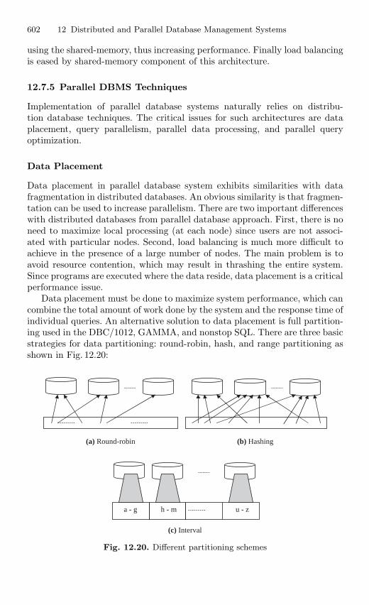
602 12 Distributed and Parallel Database Management Systems
using the shared-memory, thus increasing performance. Finally load balancingis eased by shared-memory component of this architecture.
12.7.5 Parallel DBMS Techniques
Implementation of parallel database systems naturally relies on distribu-tion database techniques. The critical issues for such architectures are dataplacement, query parallelism, parallel data processing, and parallel queryoptimization.
Data Placement
Data placement in parallel database system exhibits similarities with datafragmentation in distributed databases. An obvious similarity is that fragmen-tation can be used to increase parallelism. There are two important differenceswith distributed databases from parallel database approach. First, there is noneed to maximize local processing (at each node) since users are not associ-ated with particular nodes. Second, load balancing is much more difficult toachieve in the presence of a large number of nodes. The main problem is toavoid resource contention, which may result in thrashing the entire system.Since programs are executed where the data reside, data placement is a criticalperformance issue.
Data placement must be done to maximize system performance, which cancombine the total amount of work done by the system and the response time ofindividual queries. An alternative solution to data placement is full partition-ing used in the DBC/1012, GAMMA, and nonstop SQL. There are three basicstrategies for data partitioning: round-robin, hash, and range partitioning asshown in Fig. 12.20:
a - g h - m u - z
(a) Round-robin (b) Hashing
(c) Interval
Fig. 12.20. Different partitioning schemes
12.7 Parallel Database 603
1. Round-robin partitioning. It is the simplest strategy, it ensures uniformdata distribution. With n partitions, the ith tuple in insertion order isassigned to partition (I mod n). This strategy enables the sequential accessto a relation to be done in parallel. Direct access of individual tuplesrequires accessing the entire relation.
2. Hash partitioning. It applies a hash function to some attribute which yieldsthe partition number. This strategy allows exact match queries on theselection attribute to be processed by exactly one node and all otherqueries to be processed by all the nodes in parallel.
3. Range partitioning. It distributes tuples based on the value intervals(ranges) of some attribute. In addition to supporting exact match queriesas with hashing, it is well suited for range queries. This partitioning resultsin high variation in partition size.
The performance of full partitioning is compared to that of the clusteringthe relations on a single disk. The results indicate that for a wide variety ofmultiuser workloads, partitioning is consistently better. However, clusteringmay dominate in processing the complex queries. So, the solution to dataplacement is variable partitioning. It is defined as the degree of partitioning,or, the number of nodes over which a relation is fragmented, is a functionof the size and access frequency of the relation. This strategy is much moreinvolved than either clustering or full partitioning because changes in datadistribution may result in reorganization.
In a highly parallel system with variable partitioning, periodic reorgani-zations for load balancing are essential and should be frequent unless theworkload is fairly static and experiences only a few updates. Such reorga-nizations should remain transparent to compiled programs that run on thedatabase server.
Query Parallelism
– Intraoperator parallelism. Intraoperator parallelism is based on the decom-position of one operator in a set of independent suboperators, calledoperator instances. This decomposition is done using static and/ordynamic partitioning of relations. Each operator instance will thenprocess one relation partition also called bucket. The operator decom-position frequently benefits from the initial partitioning of the data. Theselect operator can be directly decomposed into several select operators,each on a different partition and no redistribution is required. Figure 12.21shows that if the relation is partitioned on the select attribute, partition-ing properties can be used to eliminate some select instances.
The partitioning function is independent of local algorithm which is usedto join operator. For instance, a hash join using a hash partitioning needs twohash functions.
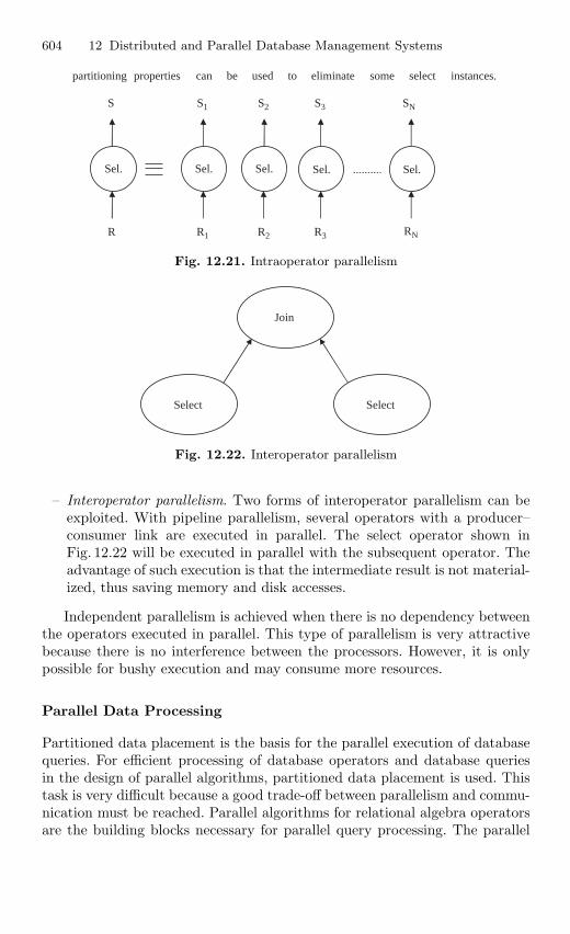
604 12 Distributed and Parallel Database Management Systems
partitioning properties can be used to eliminate some select instances.
Sel. Sel. Sel. Sel. Sel.
S S1 S2 S3 SN
R R1 R2 R3 RN
Fig. 12.21. Intraoperator parallelism
Join
Select Select
Fig. 12.22. Interoperator parallelism
– Interoperator parallelism. Two forms of interoperator parallelism can beexploited. With pipeline parallelism, several operators with a producer–consumer link are executed in parallel. The select operator shown inFig. 12.22 will be executed in parallel with the subsequent operator. Theadvantage of such execution is that the intermediate result is not material-ized, thus saving memory and disk accesses.
Independent parallelism is achieved when there is no dependency betweenthe operators executed in parallel. This type of parallelism is very attractivebecause there is no interference between the processors. However, it is onlypossible for bushy execution and may consume more resources.
Parallel Data Processing
Partitioned data placement is the basis for the parallel execution of databasequeries. For efficient processing of database operators and database queriesin the design of parallel algorithms, partitioned data placement is used. Thistask is very difficult because a good trade-off between parallelism and commu-nication must be reached. Parallel algorithms for relational algebra operatorsare the building blocks necessary for parallel query processing. The parallel

12.7 Parallel Database 605
processing of join is significantly more involved than that of select. The distrib-uted join algorithms designed for high-speed networks can be applied success-fully in a partitioned database context. However, the availability of a globalindex at run time provides more opportunities for efficient parallel execution.
Parallel Query Optimization
Parallel query optimization takes the advantage of both interoperator andintraoperator parallelism. This can be achieved by some of the techniquesused for distributed DBMSs. Parallel query optimization refers to the processof producing an execution plan for a given query that minimizes an objectivecost function. A query optimizer contains three components, they are searchspace, cost model, and search strategy.
The search space is the set of alternative execution plans to represent theinput query. These plans give same result but differ on the execution orderof operators and the way these operators are implemented. The cost modelpredicts the cost of given execution plan. To be accurate, the cost modelshould have good knowledge about the parallel execution environment.
– Search space. Execution plans are abstracted, as usual, by means ofoperator trees, which define the order in which the operators are executed.Operator trees are enriched with annotations, which indicate additionalexecution aspects, such as the algorithm of each operator. An importantexecution aspect to be reflected by annotations is the fact that two sub-sequent operators can be executed in pipeline. Pipeline and store annota-tions constrain the scheduling of execution of execution plans. They splitan operator tree into nonoverlapping subtrees, called phases. Pipelinedoperators are executed in same phase, whereas a storing indication estab-lishes the boundary between one phase and the subsequent phase.
– Cost model. The optimizer cost model is responsible for estimating thecost of a given execution plan. It is viewed by two parts: architecturedependent and architecture independent. The architecture-independentpart is constituted by the cost functions for operator algorithms. If weignore the concurrency issues, only the cost functions for data repartition-ing a relation’s tuples in a shared-nothing system imply transfers of dataacross the interconnect, whereas it reduces to hashing in shared-memorysystems. Memory consumption in the shared-nothing case is complicatedby interoperator parallelism.
– Search strategy. This does not need to be different from either central-ized or distributed query optimization. However, the search space tendsto be much larger because there are more alternative parallel executionplans. Thus, randomized search strategies generally outperform determin-istic strategies in parallel query optimization.
606 12 Distributed and Parallel Database Management Systems
Benefits of Parallel Processing and Parallel Database
Parallel processing can benefit certain kinds of application by providingenhanced throughput (scale-up) and improved response time (speedup).Improved response time can be achieved either by breaking up a largertask into smaller components or by reducing wait time. Parallel databasetechnology can benefit in numerous applications by:
– Higher performance– Higher availability– Greater flexibility– More users
Summary
In this chapter, we discussed the distributed databases and parallel databasesarchitecture and some of the basic techniques involved. First, we have seenthat distributed database is having a number of advantages over centralizedsystems. We then discussed the various fragmentation involved in distributeddatabases. In semantic data control, we discussed the view management,security control, and semantic integrity control. The two main issues forefficiently performing data control are the definition and storage of rules.Concurrency control provides the isolation and consistency properties oftransaction, and then we discussed various algorithms in locking. Finally, indistributed database we discussed reliability and availability. The variousfailures in distributed database are listed and the different protocols used toovercome the failures are discussed. In parallel database, better performanceand high availability are achieved. Various architectures and techniques ofparallel database are discussed and finally the benefits are also listed.
Review Questions
12.1. What is meant by distributed databases?
A distributed database is a collection of data which belong logically to thesame system but are spread over the sites of a computer network. Thisdefinition emphasizes two equally important aspects of a distributed data-base as follows:
– Distribution. The fact that the data are not resident at the same site(processor), so that we can distinguish a distributed database from a sin-gle, centralized database.
Review Questions 607
– Logical correlation. The fact that the data have some properties whichtie them together, so that we can distinguish a distributed database froma set of local databases or files which are resident at different sites of acomputer network.
12.2. What are special features of distributed database over the centralizeddatabase?
The features, which characterize the traditional database approach, arecentralized control, data independence, and reduction of redundancy, complexphysical structures for efficient access, integrity, recovery, concurrency control,privacy, and security.
12.3. Explain primary horizontal fragmentation?
The primary horizontal fragments are defined using selections on globalrelations. The correctness of primary fragmentation requires that each tuple ofthe global relation be selected in one and only one fragment. Thus, determin-ing the primary fragmentation of a global relation requires determining a setof disjoint and complete selection prediction. The property that we require foreach fragment is that the elements of them must be referenced homogeneouslyby all the applications.
12.4. What are the methods to prevent unauthorized users in remote access-ing in distributed database?
Two solutions are possible in preventing unauthorized users in remote access-ing as follows:
1. The information for authenticating users (user name and password) isreplicated at all sites in the catalog. Local programs, initiated at a remotesite, must also indicate the user name and password.
2. All sites of the distributed DBMS identify and authenticate themselvessimilarly to the way users do. Intersite communication is thus protectedby the use of the site password.
12.5. Explain the concurrency control mechanisms?
The concurrency control mechanism is grouped into two broad classes aspessimistic control methods and optimistic control methods. Pessimisticalgorithm synchronizes the concurrent execution of transaction early in theirexecution life cycles, whereas optimistic algorithms delay the synchroniza-tion of transactions until their termination. The pessimistic group consists oflocking-based algorithm, ordering-based algorithm, and hybrid algorithm. Theoptimistic group can, similarly, be classified as locking based or timestampordering based.
608 12 Distributed and Parallel Database Management Systems
12.6. Explain distributed 2PL algorithm?
It expects the availability of lock managers at each site. If the databaseis not replicated, distributed 2PL degenerates into the primary copy 2PLalgorithm. If data are replicated, the transaction implements the ROWAreplica control protocol. The communication between cooperating sites thatexecute a transaction according to the distributed 2PL.
12.7. Define the terms reliability and availability?
Reliability refers to the probability that the system under consideration doesnot experience many failures in the given time interval. It is typically used todescribe system that cannot be repaired or where the operation of the systemis so critical that no down time for repair can be tolerated. Availability refersto the probability that the system is operational according to its specificationat a given point in time t. A number of failures may have occurred prior totime t, but if they have all been repaired, the system is available at time t. Itis apparent that availability refers to system that can be repaired. It can beused as some measure of “goodness” for those systems that can be repairedand which can be out of service for short periods of time during repair.
12.8. What are the reasons for failure in distributed DBMS?
Designing a reliable system that can record for failures requires identifying thetypes of failures with which the system has to deal. It indicates that the data-base recovery manager has to deal four types of failures namely, transactionfailure (abort), site failure (system), media failure (disk), and communicationline failure.
12.9. What is meant by parallel processing and what are the benefits ofparallel processing?
Parallel processing divides a complex task into many smaller tasks, andexecutes the smaller tasks simultaneously in several tasks. Thus the complextask is completed with better performance and also quickly. Parallel process-ing can benefit certain kinds of application by providing enhanced throughput(scale-up) and improved response time (speedup).
12.10. Explain hierarchical architecture in parallel databases?
This architecture (or cluster architecture) is a combination of shared-nothingand shared-memory architecture. This idea is to build a shared-nothingmachine whose nodes are shared-memory. It combines flexibility and perform-ance of shared-memory with high extensibility of shared-nothing. In eachshared-memory node (S-M node), communication is done efficiently using theshared-memory, thus increasing performance. Finally load balancing is easedby shared memory component of this architecture.
Review Questions 609
12.11. Need for parallel databases?
Parallel processing exploits multiprocessor computers to run applicationprograms by using several processors cooperatively, in order to improveperformance. Its prominent use has long been in scientific computing byimproving the response time of numerical applications. Recent develop-ment in both the general purpose MIMD parallel computers using standardmicroprocessors and parallel programming techniques has enabled parallelprocessing to increase performance and availability.
12.12. What are the main components of parallel processing? Explainspeedup?
The main components of parallel processing are speedup and scale-up,synchronization, locking, and messaging. Speedup is the extent to whichmore hardware can perform the same task in less time than the originalsystem. With added hardware, speedup holds the task constant and measuresthe time saved. With good speedup, additional processors reduce systemresponse time. You can measure speedup by using the following formulae:
Speedup =Original Processing TimeParallel Processing Time
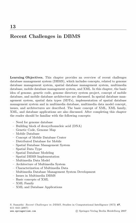
13
Recent Challenges in DBMS
Learning Objectives. This chapter provides an overview of recent challengesdatabase management system (DBMS), which includes concepts, related to genomedatabase management system, spatial database management system, multimediadatabase, mobile database management system, and XML. In this chapter, the basicidea of genome, genetic code, genome directory system project, concept of mobiledatabase, and mobile database architecture are discussed. In spatial database man-agement system, spatial data types (SDTs), implementation of spatial databasemanagement system and in multimedia database, multimedia data model concept,issues, and architectures are described. The basic concept of XML, XML family,XML, and database applications are also discussed. After completing this chapterthe reader should be familiar with the following concepts:
– Need for genome database– Building block of deoxyribonucleic acid (DNA)– Genetic Code, Genome Map– Mobile Database– Concept of Mobile Database Center– Distributed Database for Mobile– Spatial Database Management System– Spatial Data Type– Spatial Database Modeling– Spatial DBMS Implementation– Multimedia Data Model– Architecture of Multimedia System– Characterization of Multimedia Data– Multimedia Database Management System Development– Issues in Multimedia DBMS– Basic concepts of XML– XML Family– XML and Database Applications
S. Sumathi: Recent Challenges in DBMS, Studies in Computational Intelligence (SCI) 47,
611–643 (2007)
www.springerlink.com c© Springer-Verlag Berlin Heidelberg 2007
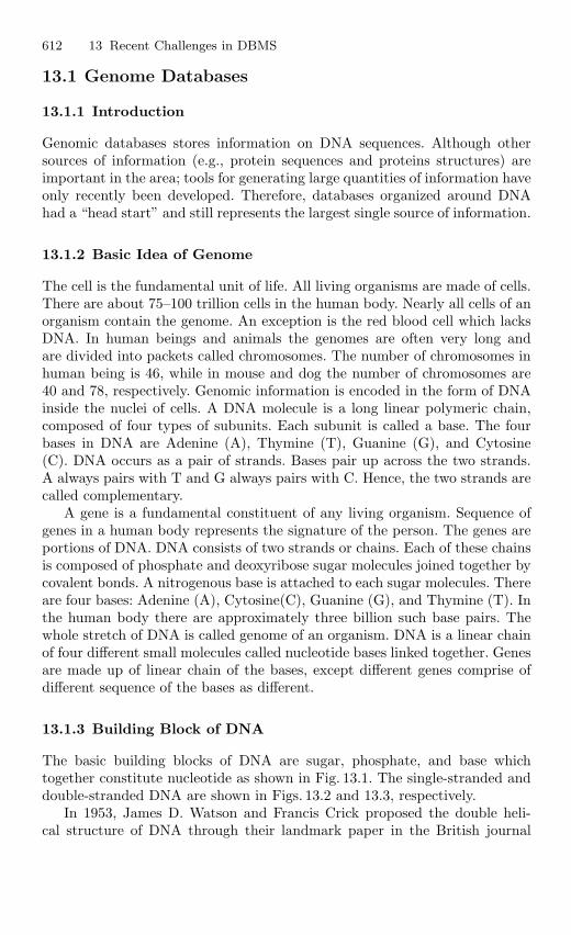
612 13 Recent Challenges in DBMS
13.1 Genome Databases
13.1.1 Introduction
Genomic databases stores information on DNA sequences. Although othersources of information (e.g., protein sequences and proteins structures) areimportant in the area; tools for generating large quantities of information haveonly recently been developed. Therefore, databases organized around DNAhad a “head start” and still represents the largest single source of information.
13.1.2 Basic Idea of Genome
The cell is the fundamental unit of life. All living organisms are made of cells.There are about 75–100 trillion cells in the human body. Nearly all cells of anorganism contain the genome. An exception is the red blood cell which lacksDNA. In human beings and animals the genomes are often very long andare divided into packets called chromosomes. The number of chromosomes inhuman being is 46, while in mouse and dog the number of chromosomes are40 and 78, respectively. Genomic information is encoded in the form of DNAinside the nuclei of cells. A DNA molecule is a long linear polymeric chain,composed of four types of subunits. Each subunit is called a base. The fourbases in DNA are Adenine (A), Thymine (T), Guanine (G), and Cytosine(C). DNA occurs as a pair of strands. Bases pair up across the two strands.A always pairs with T and G always pairs with C. Hence, the two strands arecalled complementary.
A gene is a fundamental constituent of any living organism. Sequence ofgenes in a human body represents the signature of the person. The genes areportions of DNA. DNA consists of two strands or chains. Each of these chainsis composed of phosphate and deoxyribose sugar molecules joined together bycovalent bonds. A nitrogenous base is attached to each sugar molecules. Thereare four bases: Adenine (A), Cytosine(C), Guanine (G), and Thymine (T). Inthe human body there are approximately three billion such base pairs. Thewhole stretch of DNA is called genome of an organism. DNA is a linear chainof four different small molecules called nucleotide bases linked together. Genesare made up of linear chain of the bases, except different genes comprise ofdifferent sequence of the bases as different.
13.1.3 Building Block of DNA
The basic building blocks of DNA are sugar, phosphate, and base whichtogether constitute nucleotide as shown in Fig. 13.1. The single-stranded anddouble-stranded DNA are shown in Figs. 13.2 and 13.3, respectively.
In 1953, James D. Watson and Francis Crick proposed the double heli-cal structure of DNA through their landmark paper in the British journal
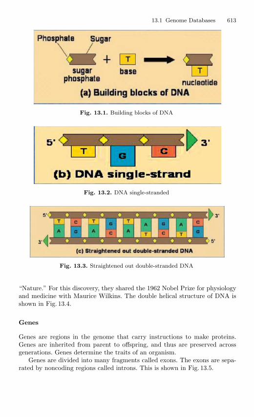
13.1 Genome Databases 613
Fig. 13.1. Building blocks of DNA
Fig. 13.2. DNA single-stranded
Fig. 13.3. Straightened out double-stranded DNA
“Nature.” For this discovery, they shared the 1962 Nobel Prize for physiologyand medicine with Maurice Wilkins. The double helical structure of DNA isshown in Fig. 13.4.
Genes
Genes are regions in the genome that carry instructions to make proteins.Genes are inherited from parent to offspring, and thus are preserved acrossgenerations. Genes determine the traits of an organism.
Genes are divided into many fragments called exons. The exons are sepa-rated by noncoding regions called introns. This is shown in Fig. 13.5.
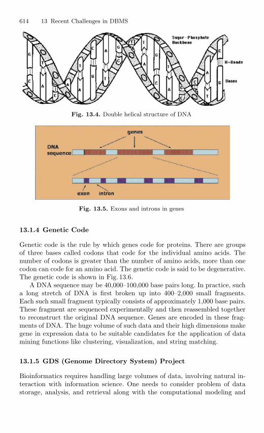
614 13 Recent Challenges in DBMS
Fig. 13.4. Double helical structure of DNA
Fig. 13.5. Exons and introns in genes
13.1.4 Genetic Code
Genetic code is the rule by which genes code for proteins. There are groupsof three bases called codons that code for the individual amino acids. Thenumber of codons is greater than the number of amino acids, more than onecodon can code for an amino acid. The genetic code is said to be degenerative.The genetic code is shown in Fig. 13.6.
A DNA sequence may be 40,000–100,000 base pairs long. In practice, sucha long stretch of DNA is first broken up into 400–2,000 small fragments.Each such small fragment typically consists of approximately 1,000 base pairs.These fragment are sequenced experimentally and then reassembled togetherto reconstruct the original DNA sequence. Genes are encoded in these frag-ments of DNA. The huge volume of such data and their high dimensions makegene in expression data to be suitable candidates for the application of datamining functions like clustering, visualization, and string matching.
13.1.5 GDS (Genome Directory System) Project
Bioinformatics requires handling large volumes of data, involving natural in-teraction with information science. One needs to consider problem of datastorage, analysis, and retrieval along with the computational modeling and
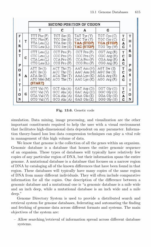
13.1 Genome Databases 615
Fig. 13.6. Genetic code
simulation. Data mining, image processing, and visualization are the otherimportant constituents required to help the user with a visual environmentthat facilitates high-dimensional data dependent on any parameter. Informa-tion theory-based loss less data compression techniques can play a vital rolein management of this high volume of data.
We know that genome is the collection of all the genes within an organism.Genomic database is a database that houses the entire genomic sequenceof an organism. These types of databases will typically have relatively fewcopies of any particular region of DNA, but their information spans the entiregenome. A mutational database is a database that focuses on a narrow regionof DNA by cataloging all of the known differences that have been found in thatregion. These databases will typically have many copies of the same regionof DNA from many different individuals. They will often include comparativeinformation for all the copies. One description of the difference between agenomic database and a mutational one is “a genomic database is a mile wideand an inch deep, while a mutational database is an inch wide and a miledeep.”
Genome Directory System is used to provide a distributed search andretrieval system for genome databases, federating and automating the findingand fetching of genome data across different formats and systems. The mainobjectives of the system are:
– Allow searching/retrieval of information spread across different databasesystems.
616 13 Recent Challenges in DBMS
– Facilitate bulk retrieval of large data sets that are selected by customerneeds through query, in a quick and easy manner.
– Development will be focused on life science genome databases but it willdraw on and interoperate with general information technology standardsand common practices.
– Include flexible adaptors for different data storage and management sys-tems.
– Utilize existing standards, technologies, and available bioinformatics datasystems while keeping the licensing as open as possible.
– Implement use of the life science identifier (LSID) for genome, gene, andrelated object naming and retrieval.
A large collaboration of model organism databases around the academiccommunity is called the Generic Model Organism Database (GMOD). Thepurpose of GMOD is to develop reusable components suitable for creatingnew community databases of biology. The Genome Directory System (GDS)project has come about because of the need to query multiple organism data-bases without worrying about where the data reside or what format it existsin. Although GDS is being developed with model organism genome databasesin mind it can also be used with other life science databases where a need forfederated queries exist. This document will briefly outline the overall layoutof the GDS system and describe each components purpose and technologiesused at each level. An overview of the data flow for the GDS project is shownin Fig. 13.7.
Data Provider Layer
The Data Provider Layer is comprised of the components that hold the rawdata and can utilize multiple systems for data access to each of the data types.The data types most commonly encountered in the life sciences include flat file,relational database management systems (RDBMS), and XML. In addition toexisting in different data management systems, the format of the data itselfcan vary between data sources. To get around this, the Data Provider Layeralso includes some external packages.
Data Directory Layer
This layer is the most important piece in the system as it bridges the disparatedata sources and the client. The purpose of this layer is to accept queriesfrom clients, manage the federation of the queries if needed, and know howand where to retrieve the information from the various data sources. Theresults from these queries will be returned in the form of data objects thatcan be further manipulated by the clients. The Data Directory Layer will beresponsible for all communication going to the Data Provider Layer.
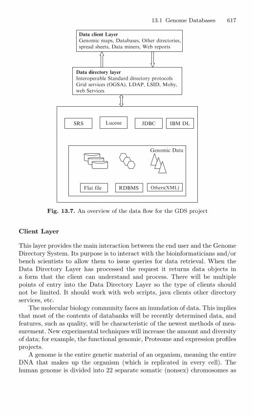
13.1 Genome Databases 617
Data client LayerGenomic maps, Databases, Other directories,spread sheets, Data miners, Web reports
Data directory layerInteroperable Standard directory protocolsGrid services (OGSA), LDAP, LSID, Moby,web Services
SRS Lucene JDBC IBM DL
Genomic Data
Flat file Others(XML)RDBMS
Fig. 13.7. An overview of the data flow for the GDS project
Client Layer
This layer provides the main interaction between the end user and the GenomeDirectory System. Its purpose is to interact with the bioinformaticians and/orbench scientists to allow them to issue queries for data retrieval. When theData Directory Layer has processed the request it returns data objects ina form that the client can understand and process. There will be multiplepoints of entry into the Data Directory Layer so the type of clients shouldnot be limited. It should work with web scripts, java clients other directoryservices, etc.
The molecular biology community faces an inundation of data. This impliesthat most of the contents of databanks will be recently determined data, andfeatures, such as quality, will be characteristic of the newest methods of mea-surement. New experimental techniques will increase the amount and diversityof data; for example, the functional genomic, Proteome and expression profilesprojects.
A genome is the entire genetic material of an organism, meaning the entireDNA that makes up the organism (which is replicated in every cell). Thehuman genome is divided into 22 separate somatic (nonsex) chromosomes as
618 13 Recent Challenges in DBMS
well as the X and Y chromosomes. Within the genome are genes – regionsof chromosomes that serve as templates for the production of proteins. Thusgenes code for proteins. A dysfunctional gene and/or gene product can havea harmful effect on the organism (e.g., Duchenne Muscular Dystrophy). How-ever, the entire genome of higher organisms is not dedicated only to encodingfor proteins. In fact, only a small portion (genes) is used as a template forprotein production. Much of the intervening areas are still of use for analysisthrough the use of genetic markers. A genetic marker is a unique site withinthe genome that can be used to determine the “state” of a region of thegenome, known as the “genotype.”
Genome, this is referred to as “linkage,” i.e., the disease gene is “linked”to a region (genetic marker) on a chromosome. Linkage analysis requires a setof genetically related subjects (a family), the phenotypes of the subjects withrespect to a disease, and the genotypes of the subjects for a genetic marker.The likelihood that the data (family structure, phenotypes, and genotypes)correlates with a model of inheritance for the disease and with the actualinheritance patterns (observed by genotypes) provides a measure of the evi-dence for “linkage.” Thus, a linkage analysis calculates the likelihood that thedisease-causing gene is located near a genetic marker based on the given setof subjects, phenotypes, and genotypes.
Geno Map
Geno Map is a suite of independent, yet inter-related tools primarily devel-oped in Java. These tools manipulate data from a domain-specific networkeddatabase, allowing sharing of information among multiple distributed clientswithout replication and coherency problems. The main goal of Geno Map is toprovide a portable, intuitive interface for managing the information associatedwith the gene location/discovery process.
The Geno Map system is designed to support a diverse collection of usersin a wide-area network environment. The data objects being managed areof the most sensitive nature – usually identifying family relationships amongmembers, some of who may carry stigmatizing genetic diseases. The GenoMap Database is an essential component and is used to form an administra-tive domain; i.e., only users belonging to that domain can access the data.Database access requires a separate level of authentication.
Geno Map is a large-scale, distributed, heterogeneous, client/server appli-cation to support the systematic exploration of the genome to narrow, andultimately identify, the locus of a particular gene (or set of genes) involved ina disease or trait. In contrast to many applications developed in support ofthe Human Genome Project (HGP).
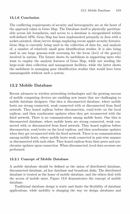
13.2 Mobile Database 619
13.1.6 Conclusion
The conflicting requirements of security and heterogeneity are at the heart ofthe approach taken in Geno Map. The Database itself is physically partition-able across lab boundaries, and access to a database is encapsulated withinwell-defined APIs. Geno Map has been implemented primarily in Java with asocket-oriented, client/server design employing recent applet security features.Geno Map is currently being used in the collection of data for, and analysisof, a number of relatively small gene identification studies. It is also beingused in one large genome-wide screening for the locus (loci) of the gene(s)involved in autism. The former shows its usefulness in supporting users whowant to employ the analysis features of Geno Map, while not needing thelarge-scale data collection and management facilities, while the latter showsthe usefulness in managing gene identification studies that would have beenunmanageable without such a system.
13.2 Mobile Database
Recent advances in wireless networking technologies and the growing successof mobile computing devices are enabling new issues that are challenging tomobile database designers. One idea is disconnected database, where mobilehosts are strong connected, weak connected with or disconnected from fixednetwork. They hoard replicas before disconnection, read/write on the localreplicas, and then synchronize updates when they get reconnected with thefixed network. There is no communication among mobile hosts. One idea isdisconnected database, where mobile hosts are strong connected, weak con-nected with or disconnected from fixed network. They hoard replicas beforedisconnection, read/write on the local replicas, and then synchronize updateswhen they get reconnected with the fixed network. There is no communicationamong mobile hosts, where mobile hosts weak connected in pair-wise manneror disconnected with each other. They hoard replicas from their peers and syn-chronize updates upon connection. When disconnected, local data accesses areperformed.
13.2.1 Concept of Mobile Database
A mobile database should be defined as the union of distributed database,disconnected database, ad hoc database and broadcast disks. The distributeddatabase is treated as the home of mobile database, and the others deal withthe access of mobile users. Figure 13.8 demonstrates the concept of mobiledatabase.
Traditional database design is static and limits the flexibility of databaseapplications, while mobility is changing the way we design databases and
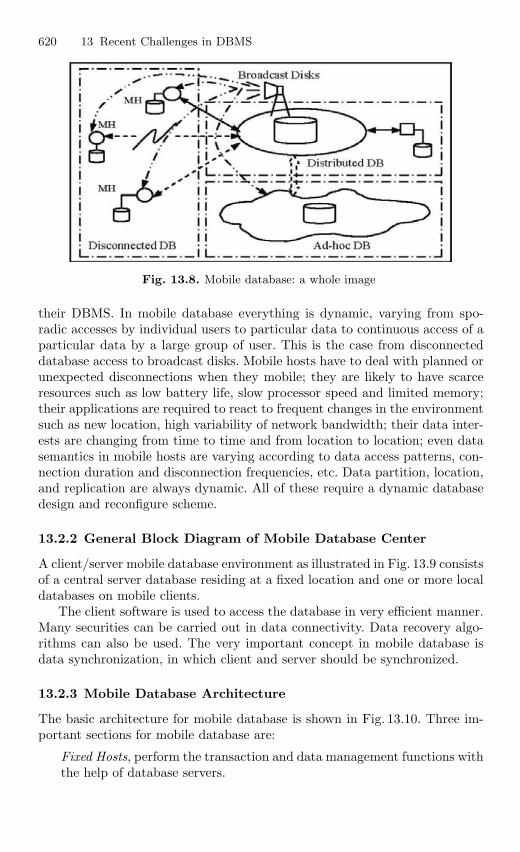
620 13 Recent Challenges in DBMS
Fig. 13.8. Mobile database: a whole image
their DBMS. In mobile database everything is dynamic, varying from spo-radic accesses by individual users to particular data to continuous access of aparticular data by a large group of user. This is the case from disconnecteddatabase access to broadcast disks. Mobile hosts have to deal with planned orunexpected disconnections when they mobile; they are likely to have scarceresources such as low battery life, slow processor speed and limited memory;their applications are required to react to frequent changes in the environmentsuch as new location, high variability of network bandwidth; their data inter-ests are changing from time to time and from location to location; even datasemantics in mobile hosts are varying according to data access patterns, con-nection duration and disconnection frequencies, etc. Data partition, location,and replication are always dynamic. All of these require a dynamic databasedesign and reconfigure scheme.
13.2.2 General Block Diagram of Mobile Database Center
A client/server mobile database environment as illustrated in Fig. 13.9 consistsof a central server database residing at a fixed location and one or more localdatabases on mobile clients.
The client software is used to access the database in very efficient manner.Many securities can be carried out in data connectivity. Data recovery algo-rithms can also be used. The very important concept in mobile database isdata synchronization, in which client and server should be synchronized.
13.2.3 Mobile Database Architecture
The basic architecture for mobile database is shown in Fig. 13.10. Three im-portant sections for mobile database are:
Fixed Hosts, perform the transaction and data management functions withthe help of database servers.
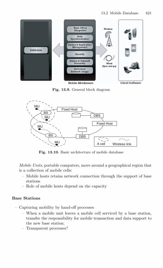
13.2 Mobile Database 621
Fig. 13.9. General block diagram
A cell Wireless link
MU
MU
MU
MU
BSFixed Host
DBS
Fixed Host
DBSBS
Fig. 13.10. Basic architecture of mobile database
Mobile Units, portable computers, move around a geographical region thatis a collection of mobile cells:
– Mobile hosts retains network connection through the support of basestations
– Role of mobile hosts depend on the capacity
Base Stations
– Capturing mobility by hand-off processes– When a mobile unit leaves a mobile cell serviced by a base station,
transfer the responsibility for mobile transaction and data support tothe new base station.
– Transparent processes?
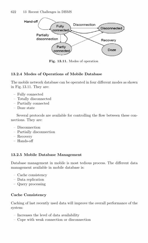
622 13 Recent Challenges in DBMS
Fig. 13.11. Modes of operation
13.2.4 Modes of Operations of Mobile Database
The mobile network database can be operated in four different modes as shownin Fig. 13.11. They are:
– Fully connected– Totally disconnected– Partially connected– Doze state
Several protocols are available for controlling the flow between these con-nections. They are:
– Disconnection– Partially disconnection– Recovery– Hands-off
13.2.5 Mobile Database Management
Database management in mobile is most tedious process. The different datamanagement available in mobile database is:
– Cache consistency– Data replication– Query processing
Cache Consistency
Caching of last recently used data will improve the overall performance of thesystem:
– Increases the level of data availability– Cope with weak connection or disconnection
13.2 Mobile Database 623
Data Replication
The data replication or data duplication will reduce redundancy and minimizethe amount of memory space needed. It increases the level of data availabilityand performance.
Query Processing
The efficient processing of user queries is very important in data management.It is of two types:
– Involve only the context of the database– Locate dependent query
13.2.6 Mobile Transaction Processing
A mobile transaction is a transaction where at least one mobile host is in-volved. Mobile database involves lot of transaction traffic. Efficient methodshould be employed for controlling data traffic. Some of the characteristics ofmobile transaction processing are:
– Split computations among mobile hosts and stationary hosts– Due to disconnection and mobility, mobile transactions shares their state
and partial results to other transactions– Mobile transactions require support from stationary hosts in computations
and communications– Movement of mobile hosts during the execution of mobile transactions– Movement of transaction states and accessed data– Long-lived transactions due to mobility and frequent disconnections– Support concurrency, recovery, disconnection, etc.
Requirements for Mobile Transaction
The basic requirements of mobile transaction are summarized:
– Accommodate the limitations of mobile computing environments– Minimize aborts due to disconnections– Correctness of distributed transaction processing– Minimize blocking of ongoing transactions– Support local autonomy– Disconnection processing– Ability to distribute the transaction’s processing– Share the state and the partial results– Capture the movement of mobile transactions– Support long-lived transactions– Support long disconnection periods– Support partial failure and provide different recovery strategies
624 13 Recent Challenges in DBMS
Dynamic Data/Currency Protocol for Mobile Database Design
Traditional database design is static and limits the flexibility of database app-lications, while mobility is changing the way we design databases and theirDBMS. In mobile database everything is dynamic, varying from sporadic acc-esses by individual users to particular data to continuous access of a particulardata by a large group of users. This is the case from disconnected databaseaccess to broadcast disks. Mobile hosts have to deal with planned or unex-pected disconnections when they are mobile; they are likely to have scarceresources such as low battery life, slow processor speed, and limited memory;their applications are required to react to frequent changes in the environ-ment such as new location, high variability of network bandwidth; their datainterests are changing from time to time and from location to location; evendata semantics in mobile hosts vary according to data access patterns, con-nection duration and disconnection frequencies, etc. Data partition, location,and replication are always dynamic. All of these require a dynamic databasedesign and reconfigure scheme.
13.2.7 Distributed Database for Mobile
A distributed database is a single logical database that is spread physicallyacross computers in multiple locations that are connected by a data communi-cations network. We emphasize that a distributed database is truly a databaseand not a loose collection of files. The distributed database is still centrallyadministered, work must allow the users to share the data; thus a user orprogram at location A must be able to access (and perhaps update) data atlocation B.
The distributed database requires multiple database management systems,running at each remote site. The degree to which these different DBMSs co-operate, to work in partnership, and whether there is master site that coor-dinated request involving data from multiple sites distinguish different typesof distributed database environments.
Distributed database framework for mobile environments is made entirelyby mobile components. Mobile hosts communicate together in an ad hoc man-ner. Communication networks are formed on demand.
Modes of Operation of Distributed Database
There are four modes of operation of distributed database. They are:
– Sign-off mode– Check-out mode
– DB partition– Check-out with mobile read– Check-out with system read
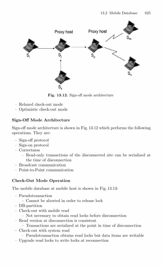
13.2 Mobile Database 625
Fig. 13.12. Sign-off mode architecture
– Relaxed check-out mode– Optimistic check-out mode
Sign-Off Mode Architecture
Sign-off mode architecture is shown in Fig. 13.12 which performs the followingoperations. They are:
– Sign-off protocol– Sign-on protocol– Correctness
– Read-only transactions of the disconnected site can be serialized atthe time of disconnection
– Broadcast communication– Point-to-Point communication
Check-Out Mode Operation
The mobile database at mobile host is shown in Fig. 13.13:
– Pseudotransaction– Cannot be aborted in order to release lock
– DB-partition– Check-out with mobile read
– Not necessary to obtain read locks before disconnection– Read version at disconnection is consistent
– Transactions are serialized at the point in time of disconnection– Check-out with system read
– Pseudotransaction obtains read locks but data items are writable– Upgrade read locks to write locks at reconnection
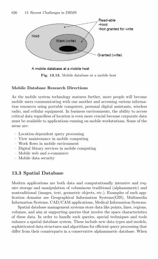
626 13 Recent Challenges in DBMS
Fig. 13.13. Mobile database at a mobile host
Mobile Database Research Directions
As the mobile system technology matures further, more people will becomemobile users communicating with one another and accessing various informa-tion resources using portable computers, personal digital assistants, wirelessradio, and cellular equipment. In business environments, the ability to accesscritical data regardless of location is even more crucial because corporate datamust be available to applications running on mobile workstations. Some of theareas are:
– Location-dependent query processing– View maintenance in mobile computing– Work flows in mobile environment– Digital library services in mobile computing– Mobile web and e-commerce– Mobile data security
13.3 Spatial Database
Modern applications are both data and computationally intensive and req-uire storage and manipulation of voluminous traditional (alphanumeric) andnontraditional (images, text, geometric objects, etc.). Examples of such app-lication domains are Geographical Information Systems(GIS), MultimediaInformation Systems, CAD/CAM applications, Medical Information Systems.
Spatial database management systems store data like points, lines, regions,volumes, and aim at supporting queries that involve the space characteristicsof these data. In order to handle such queries, special techniques and toolsenhance a spatial database system. These include new data types and models,sophisticated data structures and algorithms for efficient query processing thatdiffer from their counterparts in a conservative alphanumeric database. When
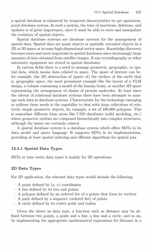
13.3 Spatial Database 627
a spatial database is enhanced by temporal characteristics we get spatiotem-poral database system. In such a system, the time of insertions, deletions, andupdates is of great importance, since it must be able to store and manipulatethe evolution of spatial objects.
Spatial database systems are database systems for the management ofspatial data. Spatial data are point objects or spatially extended objects in a2D or 3D space or in some high-dimensional vector space. Knowledge discoverybecomes more and more important in spatial databases since increasingly largeamounts of data obtained from satellite images, X-ray crystallography or otherautomatic equipment are stored in spatial databases.
In various fields there is a need to manage geometric, geographic, or spa-tial data, which means data related to space. The space of interest can be,for example, the 2D abstraction of (parts of) the surface of the earth thatis, geographic space, the most prominent example like the layout of a VLSIdesign, a volume containing a model of the human brain, or another 3D spacerepresenting the arrangement of chains of protein molecules. At least sincethe advent of relational database systems there have been attempts to man-age such data in database systems. Characteristic for the technology emergingto address these needs is the capability to deal with large collections of rela-tively simple geometric objects, for example, a set of 100,000 polygons. Thisis somewhat different from areas like CAD databases (solid modeling, etc.)where geometric entities are composed hierarchically into complex structures,although the issues are certainly related.
A spatial database system is a database system which offers SDTs in itsdata model and query language. It supports SDTs in its implementation,providing at least spatial indexing and efficient algorithms for spatial join.
13.3.1 Spatial Data Types
SDTs or time series data types is mainly for 2D operations.
2D Data Types
For 2D application, the relevant data types would include the following:
– A point defined by (x, y) coordinates– A line defined by its two end points– A polygon defined by an ordered list of n points that form its vertices– A path defined by a sequence (ordered list) of points– A circle defined by its center point and radius
Given the above as data type, a function such as distance may be de-fined between two points, a point and a line, a line and a circle, and so on,by implementing the appropriate mathematical expressions for distance in a
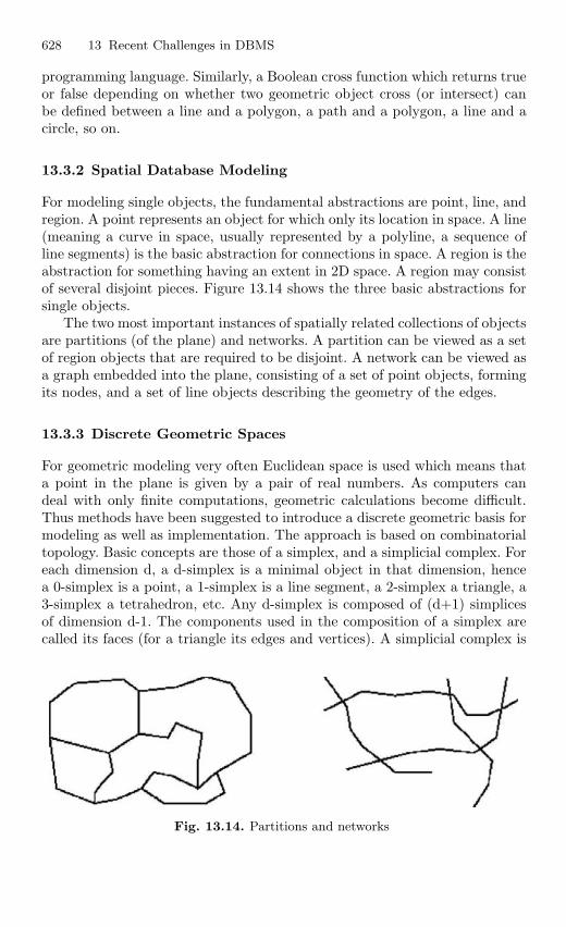
628 13 Recent Challenges in DBMS
programming language. Similarly, a Boolean cross function which returns trueor false depending on whether two geometric object cross (or intersect) canbe defined between a line and a polygon, a path and a polygon, a line and acircle, so on.
13.3.2 Spatial Database Modeling
For modeling single objects, the fundamental abstractions are point, line, andregion. A point represents an object for which only its location in space. A line(meaning a curve in space, usually represented by a polyline, a sequence ofline segments) is the basic abstraction for connections in space. A region is theabstraction for something having an extent in 2D space. A region may consistof several disjoint pieces. Figure 13.14 shows the three basic abstractions forsingle objects.
The two most important instances of spatially related collections of objectsare partitions (of the plane) and networks. A partition can be viewed as a setof region objects that are required to be disjoint. A network can be viewed asa graph embedded into the plane, consisting of a set of point objects, formingits nodes, and a set of line objects describing the geometry of the edges.
13.3.3 Discrete Geometric Spaces
For geometric modeling very often Euclidean space is used which means thata point in the plane is given by a pair of real numbers. As computers candeal with only finite computations, geometric calculations become difficult.Thus methods have been suggested to introduce a discrete geometric basis formodeling as well as implementation. The approach is based on combinatorialtopology. Basic concepts are those of a simplex, and a simplicial complex. Foreach dimension d, a d-simplex is a minimal object in that dimension, hencea 0-simplex is a point, a 1-simplex is a line segment, a 2-simplex a triangle, a3-simplex a tetrahedron, etc. Any d-simplex is composed of (d+1) simplicesof dimension d-1. The components used in the composition of a simplex arecalled its faces (for a triangle its edges and vertices). A simplicial complex is
Fig. 13.14. Partitions and networks
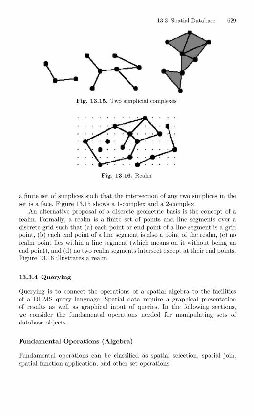
13.3 Spatial Database 629
Fig. 13.15. Two simplicial complexes
Fig. 13.16. Realm
a finite set of simplices such that the intersection of any two simplices in theset is a face. Figure 13.15 shows a 1-complex and a 2-complex.
An alternative proposal of a discrete geometric basis is the concept of arealm. Formally, a realm is a finite set of points and line segments over adiscrete grid such that (a) each point or end point of a line segment is a gridpoint, (b) each end point of a line segment is also a point of the realm, (c) norealm point lies within a line segment (which means on it without being anend point), and (d) no two realm segments intersect except at their end points.Figure 13.16 illustrates a realm.
13.3.4 Querying
Querying is to connect the operations of a spatial algebra to the facilitiesof a DBMS query language. Spatial data require a graphical presentationof results as well as graphical input of queries. In the following sections,we consider the fundamental operations needed for manipulating sets ofdatabase objects.
Fundamental Operations (Algebra)
Fundamental operations can be classified as spatial selection, spatial join,spatial function application, and other set operations.
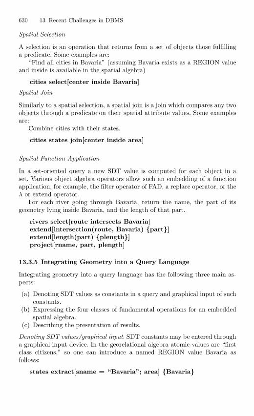
630 13 Recent Challenges in DBMS
Spatial Selection
A selection is an operation that returns from a set of objects those fulfillinga predicate. Some examples are:
“Find all cities in Bavaria” (assuming Bavaria exists as a REGION valueand inside is available in the spatial algebra)
cities select[center inside Bavaria]
Spatial Join
Similarly to a spatial selection, a spatial join is a join which compares any twoobjects through a predicate on their spatial attribute values. Some examplesare:
Combine cities with their states.
cities states join[center inside area]
Spatial Function Application
In a set-oriented query a new SDT value is computed for each object in aset. Various object algebra operators allow such an embedding of a functionapplication, for example, the filter operator of FAD, a replace operator, or theλ or extend operator.
For each river going through Bavaria, return the name, the part of itsgeometry lying inside Bavaria, and the length of that part.
rivers select[route intersects Bavaria]extend[intersection(route, Bavaria) part]extend[length(part) plength]project[rname, part, plength]
13.3.5 Integrating Geometry into a Query Language
Integrating geometry into a query language has the following three main as-pects:
(a) Denoting SDT values as constants in a query and graphical input of suchconstants.
(b) Expressing the four classes of fundamental operations for an embeddedspatial algebra.
(c) Describing the presentation of results.
Denoting SDT values/graphical input. SDT constants may be entered througha graphical input device. In the georelational algebra atomic values are “firstclass citizens,” so one can introduce a named REGION value Bavaria asfollows:
states extract[sname = “Bavaria”; area] Bavaria
13.3 Spatial Database 631
Expressing the four classes of fundamental operations. Spatial function appli-cation, although not possible in classical relational algebra, is also in practiceprovided by query languages (in SQL by allowing expressions in the SELECTclause).
SELECT * FROM rivers WHERE route intersects Window
13.3.6 Spatial DBMS Implementation
From the point of view of the spatial algebra implementation which is done insome programming language, most likely the DBMS implementation language,the representation:
– Is a value of some programming language data type, e.g., region– Is some arbitrary data structure which is possibly quite complex– Supports efficient computational geometry algorithms for spatial algebra
operations– Is not geared only to one particular algorithm but is balanced to support
many operations well enough
To fulfill the requirements of the DBMS, the representation must be apaged data structure compatible with the DBMS support for long fields orlarge attribute values. To support efficient loading and storing on disk, itshould consist of a single contiguous byte block as long as it is small enoughto fit into one page or implement a more complex paging strategy to accessthe value. For the case that a value representation happens to be large, a goodstrategy is to split it into a small info part. The info part might be containedin the DBMS object representation and contain a logical pointer to a separatepage sequence holding the exact geometry part. The generic operations neededby the DBMS may concern, for example, transforming from/to a textual orgraphic representation for input/output at the user interface, or transformingfrom/to an ASCII format for bulk loading or external data exchange. Morespecifically, for SDTs, generic approximations may be needed to interface withspatial access methods, for example, each data type must provide access to abounding box (also called minimum bounding rectangle (MBR)).
From the spatial algebra and also the programming language point of view,the representation should be such that it is mapped by the compiler into asingle or perhaps a few contiguous areas (to support the DBMS loading). Therepresentation can support operations as follows:
Plane Sweep Sequence . Very often, algorithms on the exact geometry use aplane-sweep. The sweep needs the components of the object (e.g., the vertices)in some fixed order.
Approximations . The implementation of many operations starts with a roughtest on an approximation of the object as that of the bounding box. Hencethese should be part of the representation.
632 13 Recent Challenges in DBMS
Stored Unary Function Values . Some operations of the spatial algebra com-pute properties of a spatial value, e.g., the area or perimeter of a region. Theyare computed after the creation of the value and then stored with it.
13.4 Multimedia Database Management System
13.4.1 Introduction
A database management system (DBMS) is a general-purpose software sys-tem that facilitates the processes of defining, constructing, and manipulatingdatabases for various applications. DBMSs, and in particular those based onthe relational data model, have been very successful at the management of ad-ministrative data. However, handling large collections of digitized multimediadata is still a major challenge. Current database systems are not equipped torepresent the entire multimedia data flow, nor may it be desirable for them tosupport the plethora of retrieval types required to support multimedia data.Thus, continuous media data must be parsed into represent able segments,which we term media objects. In order to represent the original data streamto users, synchronization constraints among media objects must be specifiedand maintained.
A multimedia database management system (MMDBMS) must supportmultimedia data types in addition to providing facilities for traditional DBMSfunctions like database creation, data modeling, data retrieval, data access andorganization, and data independence. The area and applications have experi-enced tremendous growth. Especially with the rapid development of networktechnology, multimedia database system gets more tremendous developmentand multimedia information exchange becomes very important.
13.4.2 Multimedia Data
Multimedia data refers to the simultaneous use of data in different mediaforms, including images, audio, video, text, and numerical data. Many mul-timedia applications, such as recording and playback of motion video andaudio, slide presentations, and video conferencing, require continuous presen-tation of a media data stream and the synchronized display of multiple mediadata streams. Such synchronization requirements are generally specified byeither spatial or temporal relationships among multiple data streams. For ex-ample, a motion video and its caption must be synchronized spatially at theappropriate position in a movie, and, in a slide presentation, a sequence ofimages and speech fragments must be temporally combined and presented tocompose one unified and meaningful data stream.
13.4 Multimedia Database Management System 633
Characterization of Multimedia Data
Multimedia systems are able to deal with multimedia data like audio, stillimages, graphics, animation, text, etc. The most significant features ofmultimedia data come from the observation that its representation canbe much closer to the physical or a virtual physical reality that the usualalphanumeric data which in general is used to represent symbolic information.For example, a video is a recording of the visual information over a period oftime at a point in space. The classification of multimedia data can be madeas time-dependent data like audio, video, and animation or time-independentdata which includes data types like text, still images, and alphanumericdata types. Time-dependent data has only a meaningful interpretation withrespect to a constantly progressing time scale. A timescale is needed to asso-ciate with a time-dependent data its correct interpretation at each point oftime expressed by the atomic constituents of the data. Due to the closenessto physical reality a further characteristic of multimedia data is its highdensity of information in one datum. Due to high density of information inmultimedia data the amounts of data can be huge. As long as data is staticin time and size like symbols, pictures, or images no serious problems interms of processing speed are imposed on networks, on storage devices, andon main memories of current computer technology. Also dynamic data in sizecan be handled efficiently by suing the abstraction of files as provided byoperating systems. Serious problems with such data occur only in connectionwith applications where extreme high numbers of data elements are involved,example, processing of satellite images for weather forecast.
When dealing with huge amount of data under real time constraints it maybe convenient or even necessary to perform the processing not on the datavalues themselves but on the references to the values. A good example for thisis video script editing. Certain applications of dynamic data may need oper-ations which cannot be performed over references, for example, copying. Inthis case some form of dynamic data management has to be provided, which akind of spreads the process over time such that at each distinct moment only alimited amount of physical resources needed. When processing dynamic data,typically parallel tasks occur. This comes from the nature of this data sincein contrast to processing static data operations taken nonnegligible periods oftime. Also it often is necessary to process data in parallel.
13.4.3 Multimedia Data Model
A multimedia data stream consists of a set of data upon which some timeconstraints are defined. The time constraints may specify discrete, continuous,or stepwise constant time flow relationships among the data. For example,some multimedia streams, such as audio and video, are continuous in nature, inthat they flow across time; other data streams, such as slide presentations andanimation, have discrete or stepwise time constraints. The multimedia streams
634 13 Recent Challenges in DBMS
may not have convenient boundaries for data representation. To facilitateretrieval of such data in databases, we must break each media stream into a setof media objects. Each media object represents a minimum chunk of the mediastream that bears some semantic meaning. Media objects in different mediastreams may have different internal structures. For example, a continuousvideo stream can be segmented into a set of media objects, each of whichcontains a set of video frames with specific semantic meaning. Similarly, acontinuous audio stream can be segmented into a set of media objects, each ofwhich contains a set of audio samples with specific semantic meaning. Withoutloss of generality, we assume that basic data elements delivered from thetransportation layer are media objects.
Media objects from different data streams may need to be linked throughtime constraints to specify their synchronization. For example, in slide pre-sentation applications, an audio object must be played along with a slideobject. We define a multimedia unit Oi, to be the composition of a set ofmedia objects O1i,...,Oni, where Oni represents ith media object of the nthmedia stream participating in the synchronized stream. Thus, a compositedata stream made up of multiple media streams consists of a set of multi-media units, where each multimedia unit unifies media objects from multiplemedia streams. Such multimedia units may also be considered as compositeobjects. Furthermore, a collection of objects from either a single data streamor a composite data stream may be conceptually modeled as a hierarchicalstructure. At each increasing level, a set of media objects may be consideredto be a super class object which may then, in turn, be a component of anothersuper class at a higher level.
Constraints on Media Objects
We will now address the synchronization requirements that need be placedon media data streams. There are two types of constraints that need to bespecified on media objects, intra- and interstream constraints. Intrastreamconstraints specify the synchronization requirements to be placed on a singlemedia stream and interstream constraints specify the synchronization require-ments to be placed on more than one media stream.
Let mi be a single media stream which consists of a set of media objectsOi1,...Oil. Intrastream constraints on Oi1,...Oil define time flow relationshipsamong these objects. The intrastream constraints may be continuous, dis-crete, or stepwise constant. Unlike temporal constraints, media objects arenot typically statically associated with independent time constraints. Owingto the sequential character of media objects in a single media stream, eachmedia object must be associated with a relative start time and a time inter-val which specifies the duration of its retrieval, assuming that the first mediaobject in the media stream starts at time zero. The actual start time of amedia object is usually dynamically determined. Once a media stream is in-voked, it is associated with an actual start time; the start time of each media
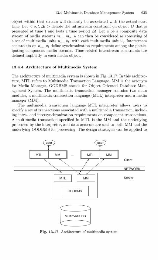
13.4 Multimedia Database Management System 635
object within that stream will similarly be associated with the actual starttime. Let < o, t,∆t > denote the intrastream constraint on object O that ispresented at time t and lasts a time period ∆t. Let u be a composite datastream of media streams m1,...mn. u can then be considered as consisting ofa set of multimedia units u1,...ul, with each multimedia unit ui. Interstreamconstraints on u1,...ul define synchronization requirements among the partic-ipating component media streams. Time-related interstream constraints aredefined implicitly in each media object.
13.4.4 Architecture of Multimedia System
The architecture of multimedia system is shown in Fig. 13.17. In this architec-ture, MTL refers to Multimedia Transaction Language, MM is the acronymfor Media Manager, OODBMS stands for Object Oriented Database Man-agement System. The multimedia transaction manager contains two mainmodules, a multimedia transaction language (MTL) interpreter and a mediamanager (MM).
The multimedia transaction language MTL interpreter allows users tospecify a set of transactions associated with a multimedia transaction, includ-ing intra- and intersynchronization requirements on component transactions.A multimedia transaction specified in MTL is the MM and the underlyingprocessed by the interpreter, and data accesses are sent to both MM and theunderlying OODBMS for processing. The design strategies can be applied to
user
MTL
MTL
OODBMS
Multimedia DB
MTLMM
MM
MM
Client
NETWORK
Server
user
Fig. 13.17. Architecture of multimedia system
636 13 Recent Challenges in DBMS
any OODBMS environment that support a C++ interface. Currently existingobject-oriented database systems that fit into this category include Object-Store and ODE.
13.4.5 Multimedia Database Management System Development
The first MMDBMS rely mainly on the operating system for storing andquerying files. These were ad hoc systems that served mostly as reposito-ries. The first multimedia database system ORION was developed in 1987.In the mid 1990s, some of the commercial MMDBMS developed are Media-DB, JASMINE, and ITASCA that is the commercial successor of ORION.They were all able to handle diverse kind of data and provided mechanismsfor querying, retrieving, inserting, and updating data. Most of these productsdisappeared from the market after some years of existence, and only someof them continued and adapted themselves successfully to the hardware andsoftware advances as well as application changes.
From 1996 to 1998, commercial systems were proposed which handle mul-timedia content by providing complex object types for various kinds of media.The object-oriented style provides the facility to define new data types andoperators appropriate for the new kinds of media, such as video, image, andaudio. Therefore, broadly used commercial MMDBMSs are extensible Object-Relational DBMS.
The most advanced solutions are marketed by Oracle 10g, IBM DB2,and IBM Informix. They propose a similar approach for extending the basicsystem. DB2 Image Extender defines the distinct data type DB2IMAGEwith associated user-defined functions for storing and manipulating imagefiles. MIRROR, an acronym for Multimedia Information Retrieval ReducingInformation Overload developed at the University of Twente, is a researchMMDBMS that is developed to better understand the kind of data manage-ment that is required in the context of multimedia digital libraries. MARS, anacronym for Multimedia Analysis and Retrieval System is a project carriedout at the University of Illinois. MARS realizes an integrated multimediainformation retrieval and database management system, that supports multi-media information as first class object suited for storage and retrieval basedon their semantic content. The MPEG-7 Multimedia Data Cartridge is a sys-tem extension of the Oracle 9i DBMS providing a multimedia query language,access to media, processing and optimization of queries, and indexingcapacities relying on multimedia database schema derived from MPEG-7.
13.4.6 Issues in Multimedia DBMS
The key issue in a multimedia database is how to access and how to exchangemultimedia information effectively. The key to retrieval process is similar-ity between two objects. The content of the object is analyzed and used to
13.5 XML 637
evaluate specified selection predicates which are termed as content-based ret-rieval. In order to have an accurate representation of the multimedia objectsin the database and the query object, different features like texture, shape,and color have to be combined. The results are high dimensional vectors. Theefficiency of the similarity search must be supported by the use of multidi-mensional indexing structures and by dimension reduction methods.
In order to retrieve multimedia data from a database system, a querylanguage must be provided. A multimedia query language must have abili-ties to handle complex spatial and temporal relationships. A powerful querylanguage should have to deal with keywords, index on keywords, and seman-tic contents of multimedia objects. The key to efficient communication is torely on standards for communicating metadata and associated media data. Inmultimedia database management system, there is a need to retrieve compos-ite objects. In addition, the multimedia database system should use multiplerepresentations of data for different users and profiles.
13.5 XML
13.5.1 Introduction
Extensible Markup Language (XML) is a simplified version of SGML (Stan-dard Generalized Markup Language defined by ISO 8879) designed for WebApplications. It retains all SGML advantages of extensibility, structure, andvalidation in a language that is designed to be vastly easier to learn, use,and implement than full SGML. The World Wide Web Consortium, thestandards body for all web technologies, describes XML as a “method forputting structured data in a text file.” XML is a standard for the defini-tion of markup languages for the Web. XML was designed to describe data.XML uses a Document Type Definition (DTD) or an XML Schema to de-scribe the data. It is not itself the successor to HTML as the language ofthe web, but successors will follow the XML standard. Like HTML, XML isbuilt on the SGML standard, but as a refinement of the standard, not a setof tags. That is a key distinction that gives XML particular value. XML is aW3C recommendation.
13.5.2 Origin of XML
XML was developed by an XML Working Group (originally known as theSGML Editorial Review Board) formed under the auspices of the WorldWide Web Consortium (W3C) in 1996. It was chaired by Jon Bosak ofSun Microsystems with the active participation of an XML Special Inter-est Group (previously known as the SGML Working Group) also organizedby the W3C.
638 13 Recent Challenges in DBMS
13.5.3 Goals of XML
The design goals for XML are:
1. XML shall be straightforwardly usable over the Internet.2. XML shall support a wide variety of applications.3. XML shall be compatible with SGML.4. It shall be easy to write programs which process XML documents.5. The number of optional features in XML is to be kept to the absolute
minimum, ideally zero.6. XML documents should be human-legible and reasonably clear.7. The XML design should be prepared quickly.8. The design of XML shall be formal and concise.9. XML documents shall be easy to create.
10. Terseness in XML markup is of minimal importance.
13.5.4 XML Family
XML is actually family of standards and technologies which are given inTable 13.1. XML 1.0 defines what elements, attributes, and entities are. Otherstandards include:
– XLink describes a standard way to add hyperlinks to an XML file.– XPointer is a syntax in development for pointing to parts of an XML
document. An XPointer is a bit like a URL, but instead of pointing todocuments on the Web, it points to pieces of data inside an XML file.
– CSS (Cascade Style Sheets) describes formatting rules, same as it doesfor HTML.
– XSL is the advanced language for expressing stylesheets.– XML Namespaces describes a facility for including tags from different
tagsets in a single document.– XML Schemas describes an alternative to the DTD for defining the ele-
ments and attributes in a document. XML Schemas help developers toprecisely define the structures of their own XML-based formats.
– DOM (Document Object Model) is a standard set of function calls formanipulating XML files from a programming language.
13.5.5 XML and HTML
XML is not a replacement for HTML. XML and HTML were designed withdifferent goals. XML was designed to describe data and to focus on what datais. HTML was designed to display data and to focus on how data looks. HTMLis about displaying information, while XML is about describing information.
XML tags are not predefined. The user must invent their own tags. On theother hand, the tags used to mark up HTML documents and the structure of
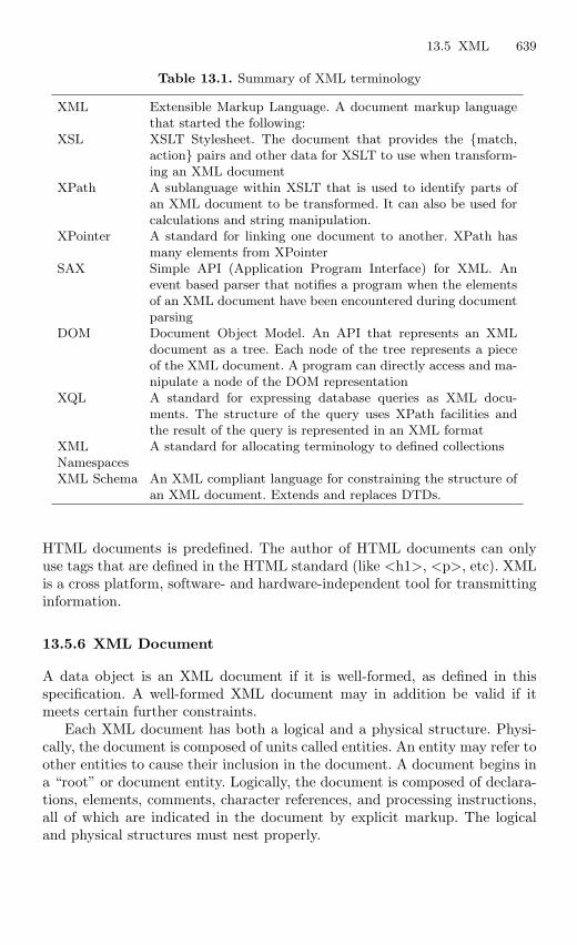
13.5 XML 639
Table 13.1. Summary of XML terminology
XML Extensible Markup Language. A document markup languagethat started the following:
XSL XSLT Stylesheet. The document that provides the match,action pairs and other data for XSLT to use when transform-ing an XML document
XPath A sublanguage within XSLT that is used to identify parts ofan XML document to be transformed. It can also be used forcalculations and string manipulation.
XPointer A standard for linking one document to another. XPath hasmany elements from XPointer
SAX Simple API (Application Program Interface) for XML. Anevent based parser that notifies a program when the elementsof an XML document have been encountered during documentparsing
DOM Document Object Model. An API that represents an XMLdocument as a tree. Each node of the tree represents a pieceof the XML document. A program can directly access and ma-nipulate a node of the DOM representation
XQL A standard for expressing database queries as XML docu-ments. The structure of the query uses XPath facilities andthe result of the query is represented in an XML format
XML A standard for allocating terminology to defined collectionsNamespacesXML Schema An XML compliant language for constraining the structure of
an XML document. Extends and replaces DTDs.
HTML documents is predefined. The author of HTML documents can onlyuse tags that are defined in the HTML standard (like <h1>, <p>, etc). XMLis a cross platform, software- and hardware-independent tool for transmittinginformation.
13.5.6 XML Document
A data object is an XML document if it is well-formed, as defined in thisspecification. A well-formed XML document may in addition be valid if itmeets certain further constraints.
Each XML document has both a logical and a physical structure. Physi-cally, the document is composed of units called entities. An entity may refer toother entities to cause their inclusion in the document. A document begins ina “root” or document entity. Logically, the document is composed of declara-tions, elements, comments, character references, and processing instructions,all of which are indicated in the document by explicit markup. The logicaland physical structures must nest properly.
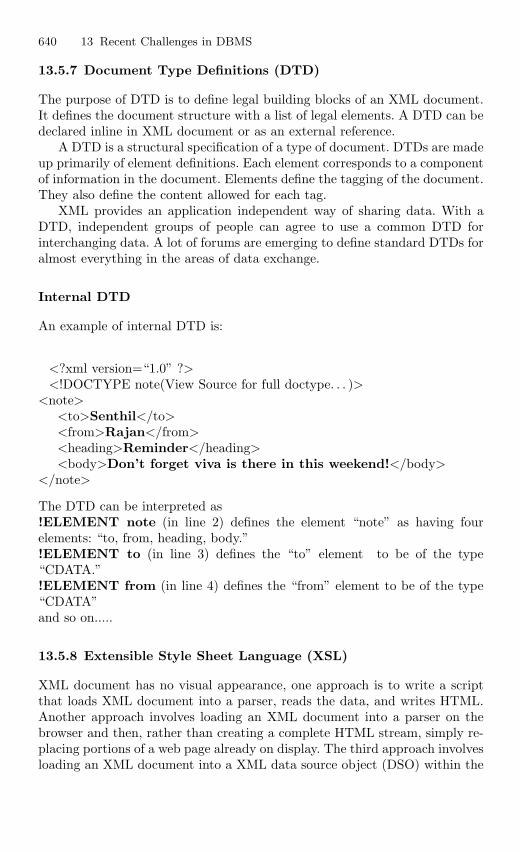
640 13 Recent Challenges in DBMS
13.5.7 Document Type Definitions (DTD)
The purpose of DTD is to define legal building blocks of an XML document.It defines the document structure with a list of legal elements. A DTD can bedeclared inline in XML document or as an external reference.
A DTD is a structural specification of a type of document. DTDs are madeup primarily of element definitions. Each element corresponds to a componentof information in the document. Elements define the tagging of the document.They also define the content allowed for each tag.
XML provides an application independent way of sharing data. With aDTD, independent groups of people can agree to use a common DTD forinterchanging data. A lot of forums are emerging to define standard DTDs foralmost everything in the areas of data exchange.
Internal DTD
An example of internal DTD is:
<?xml version=“1.0” ?><!DOCTYPE note(View Source for full doctype. . . )>
<note><to>Senthil</to><from>Rajan</from><heading>Reminder</heading><body>Don’t forget viva is there in this weekend!</body>
</note>
The DTD can be interpreted as!ELEMENT note (in line 2) defines the element “note” as having fourelements: “to, from, heading, body.”!ELEMENT to (in line 3) defines the “to” element to be of the type“CDATA.”!ELEMENT from (in line 4) defines the “from” element to be of the type“CDATA”and so on.....
13.5.8 Extensible Style Sheet Language (XSL)
XML document has no visual appearance, one approach is to write a scriptthat loads XML document into a parser, reads the data, and writes HTML.Another approach involves loading an XML document into a parser on thebrowser and then, rather than creating a complete HTML stream, simply re-placing portions of a web page already on display. The third approach involvesloading an XML document into a XML data source object (DSO) within the
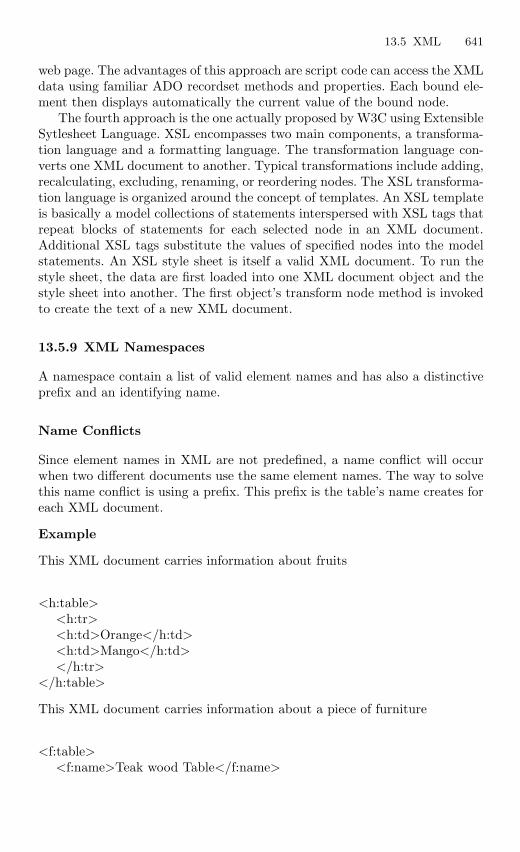
13.5 XML 641
web page. The advantages of this approach are script code can access the XMLdata using familiar ADO recordset methods and properties. Each bound ele-ment then displays automatically the current value of the bound node.
The fourth approach is the one actually proposed by W3C using ExtensibleSytlesheet Language. XSL encompasses two main components, a transforma-tion language and a formatting language. The transformation language con-verts one XML document to another. Typical transformations include adding,recalculating, excluding, renaming, or reordering nodes. The XSL transforma-tion language is organized around the concept of templates. An XSL templateis basically a model collections of statements interspersed with XSL tags thatrepeat blocks of statements for each selected node in an XML document.Additional XSL tags substitute the values of specified nodes into the modelstatements. An XSL style sheet is itself a valid XML document. To run thestyle sheet, the data are first loaded into one XML document object and thestyle sheet into another. The first object’s transform node method is invokedto create the text of a new XML document.
13.5.9 XML Namespaces
A namespace contain a list of valid element names and has also a distinctiveprefix and an identifying name.
Name Conflicts
Since element names in XML are not predefined, a name conflict will occurwhen two different documents use the same element names. The way to solvethis name conflict is using a prefix. This prefix is the table’s name creates foreach XML document.
Example
This XML document carries information about fruits
<h:table><h:tr><h:td>Orange</h:td><h:td>Mango</h:td></h:tr>
</h:table>
This XML document carries information about a piece of furniture
<f:table><f:name>Teak wood Table</f:name>
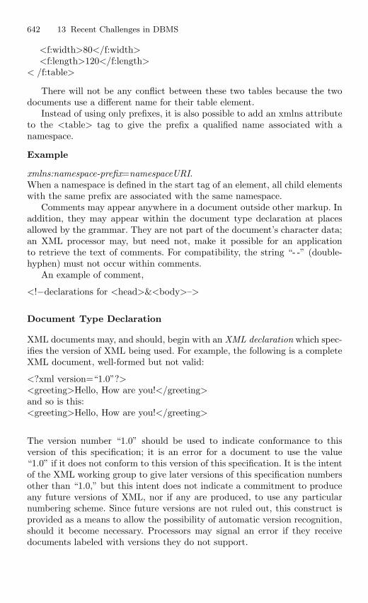
642 13 Recent Challenges in DBMS
<f:width>80</f:width><f:length>120</f:length>
< /f:table>
There will not be any conflict between these two tables because the twodocuments use a different name for their table element.
Instead of using only prefixes, it is also possible to add an xmlns attributeto the <table> tag to give the prefix a qualified name associated with anamespace.
Example
xmlns:namespace-prefix=namespaceURI.When a namespace is defined in the start tag of an element, all child elementswith the same prefix are associated with the same namespace.
Comments may appear anywhere in a document outside other markup. Inaddition, they may appear within the document type declaration at placesallowed by the grammar. They are not part of the document’s character data;an XML processor may, but need not, make it possible for an applicationto retrieve the text of comments. For compatibility, the string “- -” (double-hyphen) must not occur within comments.
An example of comment,
<!−declarations for <head>&<body>–>
Document Type Declaration
XML documents may, and should, begin with an XML declaration which spec-ifies the version of XML being used. For example, the following is a completeXML document, well-formed but not valid:
<?xml version=“1.0”?><greeting>Hello, How are you!</greeting>and so is this:<greeting>Hello, How are you!</greeting>
The version number “1.0” should be used to indicate conformance to thisversion of this specification; it is an error for a document to use the value“1.0” if it does not conform to this version of this specification. It is the intentof the XML working group to give later versions of this specification numbersother than “1.0,” but this intent does not indicate a commitment to produceany future versions of XML, nor if any are produced, to use any particularnumbering scheme. Since future versions are not ruled out, this construct isprovided as a means to allow the possibility of automatic version recognition,should it become necessary. Processors may signal an error if they receivedocuments labeled with versions they do not support.
13.5 XML 643
The function of the markup in an XML document is to describe its storageand logical structure and to associate attribute-value pairs with its logicalstructures. XML provides a mechanism, the document type declaration, todefine constraints on the logical structure and to support the use of predefinedstorage units. An XML document is valid if it has an associated documenttype declaration and if the document complies with the constraints expressedin it.
13.5.10 XML and Datbase Applications
XML Schema provides a standardized way of representing domains. The ben-efits of XML are:
Tagged Information. Structured documents allow the user to specify uniqueand specific content tags that makes it possible to retrieve any piece of taggedinformation. A format tag would not allow a user to access the structureof the document. For example, if the format tag for the abstract was italic,the format tag for a glossary entry might also be italic. There would be noway to retrieve the information because the format tags were not unique andidentifiable. However, the structural tag would allow a user to retrieve theabstract or a series of abstracts.
Reusable Components. It is possible to tag the information based on theuse of the individual pieces of information or components. Components arepieces of information that can be used individually or combined to form largercomponents. Components include: paragraphs, chapters, warnings, notes, in-structions, introductions, and examples.
Structured Documentation. Structured documentation provides a greatdeal of power in organizing a document:
– Consistent organization and structure across documents.– Reusability of segments (modules).– Increased accessibility.
Separation of Content and Formatting. The separation of content fromformatting makes it very easy to create multiple outputs from a single XMLfile. The format is defined in style sheets that can be linked to the file.
14
Projects in DBMS
Learning Objectives. Here we have given list of projects which we haveimplemented using Oracle as the back-end and Visual Basic as the front-endand the concepts from DBMS. The projects described in this chapter are generallysimpler than real-life projects but complex enough to illustrate common problemsthat the students will encounter.
14.1 List of Projects
1. Bus Transport Management System2. Course Administration System3. Election Voting System4. Hospital Management System5. Library Management System6. Railway Management System
14.2 Overview of the Projects
14.2.1 Front-End: Microsoft Visual Basic
Visual Basic was derived from BASIC, and is an event-driven programminglanguage. Programming in Visual Basic is done visually, which means that aswe design we will know how our application will look on execution. We can,therefore, change and experiment with the design to meet our requirement.
The Visual Basic Professional edition provides the features like:
– Allows creating powerful 32-bit applications for Microsoft Windows 9xand Windows NT.
– Includes intrinsic controls, as well as grid, tab, and data-bound controls.
S. Sumathi: Projects in DBMS, Studies in Computational Intelligence (SCI) 47, 645–697 (2007)
www.springerlink.com c© Springer-Verlag Berlin Heidelberg 2007
646 14 Projects in DBMS
– Includes Microsoft Developer Network CDs containing full online docu-mentation.
– Active X controls, including Internet control.– Internet Information Server Application Designer.– Dynamic HTML Page Designer.
14.2.2 Back-End: Oracle 9i
Oracle is the first DBMS language that supported SQL in 1979. It is anobject-relational database. A relational database is an extremely simple wayof managing data in the form of a collection of tables. An object-relationaldatabase supports all the features of a relational database while also support-ing object-oriented concepts and features. This language generally follows acooperative approach.
Organized data can be called information. Oracle is also a means of easilyturning data into information. Oracle will sort through and manipulate dataand their relationships with each other.
A relational database management system such as Oracle basically doesthe following three things:
1. Acquire data2. Store the data3. Retrieve the data
Oracle supports this in-keep-out approach and provides tools that allowsophistication in how data are captured, edited, modified, and put in; howto maintain security; and how to manipulate. An object-relational databasemanagement system (ORDBMS) extends the capabilities of the RDBMS tosupport object-oriented concepts. Thus Oracle is used as an RDBMS to takeadvantage of its object-oriented features.
Oracle follows a familiar language used in everyday conversations. Theinformation stored in Oracle is kept in tables. Also Oracle is a shared language.
Oracle was the first company to release a product that used the English-based Structured Query Language (SQL). Oracle’s query language has struc-ture and a set of rules and syntax that are basically the normal rules that canbe easily understood.
14.2.3 Interface: ODBC
Open Database Connectivity (ODBC) is an industry standard programminginterface that enables applications to access a variety of database manage-ment system residing on many different platforms. ODBC provides a largedegree of database independence through a standard SQL syntax, which canbe translated by database-specific drivers to the native SQL of the DBMS.
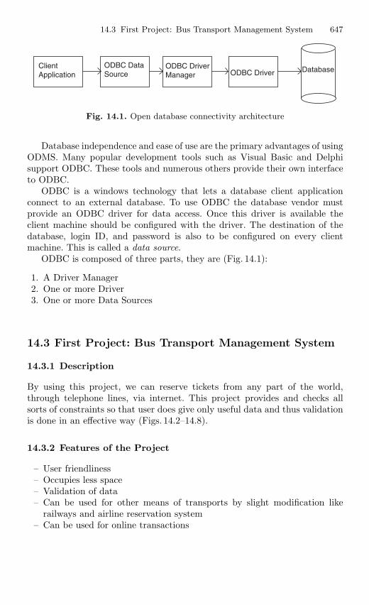
14.3 First Project: Bus Transport Management System 647
ClientApplication
ODBC DataSource
ODBC DriverManager ODBC Driver Database
Fig. 14.1. Open database connectivity architecture
Database independence and ease of use are the primary advantages of usingODMS. Many popular development tools such as Visual Basic and Delphisupport ODBC. These tools and numerous others provide their own interfaceto ODBC.
ODBC is a windows technology that lets a database client applicationconnect to an external database. To use ODBC the database vendor mustprovide an ODBC driver for data access. Once this driver is available theclient machine should be configured with the driver. The destination of thedatabase, login ID, and password is also to be configured on every clientmachine. This is called a data source.
ODBC is composed of three parts, they are (Fig. 14.1):
1. A Driver Manager2. One or more Driver3. One or more Data Sources
14.3 First Project: Bus Transport Management System
14.3.1 Description
By using this project, we can reserve tickets from any part of the world,through telephone lines, via internet. This project provides and checks allsorts of constraints so that user does give only useful data and thus validationis done in an effective way (Figs. 14.2–14.8).
14.3.2 Features of the Project
– User friendliness– Occupies less space– Validation of data– Can be used for other means of transports by slight modification like
railways and airline reservation system– Can be used for online transactions
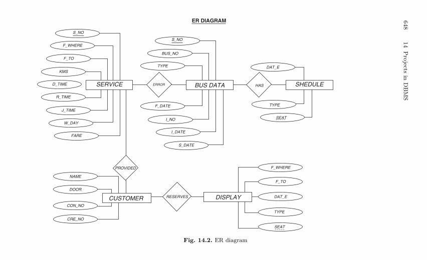
648
14
Pro
jectsin
DB
MS
S_NO
F_WHERE
BUS_NO
TYPE
F_DATE
I_NO
I_DATE
S_DATE
F_TO
KMS
D_TIME
R_TIME
J_TIME
W_DAY
FARE
S_NO
SERVICE
CUSTOMER DISPLAY
BUS DATA SHEDULE
DAT_E
TYPE
SEAT
F_WHERE
F_TO
DAT_E
TYPE
SEAT
RESERVES
PROVIDED
ER DIAGRAM
NAME
DOOR
CON_NO
CRE_NO
ERROR HAS
Fig. 14.2. ER diagram
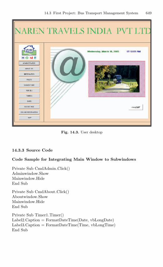
14.3 First Project: Bus Transport Management System 649
Fig. 14.3. User desktop
14.3.3 Source Code
Code Sample for Integrating Main Window to Subwindows
Private Sub CmdAdmin Click()Adminwindow.ShowMainwindow.HideEnd Sub
Private Sub CmdAbout Click()Aboutwindow.ShowMainwindow.HideEnd Sub
Private Sub Timer1 Timer()Label2.Caption = FormatDateTime(Date, vbLongDate)Label3.Caption = FormatDateTime(Time, vbLongTime)End Sub
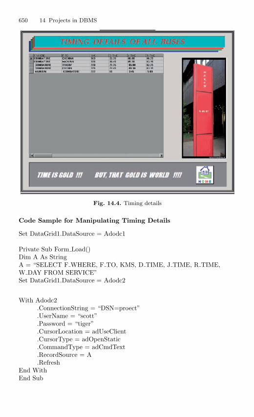
650 14 Projects in DBMS
Fig. 14.4. Timing details
Code Sample for Manipulating Timing Details
Set DataGrid1.DataSource = Adodc1
Private Sub Form Load()Dim A As StringA = “SELECT F WHERE, F TO, KMS, D TIME, J TIME, R TIME,W DAY FROM SERVICE”Set DataGrid1.DataSource = Adodc2
With Adodc2.ConnectionString = “DSN=proect”.UserName = “scott”.Password = “tiger”.CursorLocation = adUseClient.CursorType = adOpenStatic.CommandType = adCmdText.RecordSource = A.Refresh
End WithEnd Sub
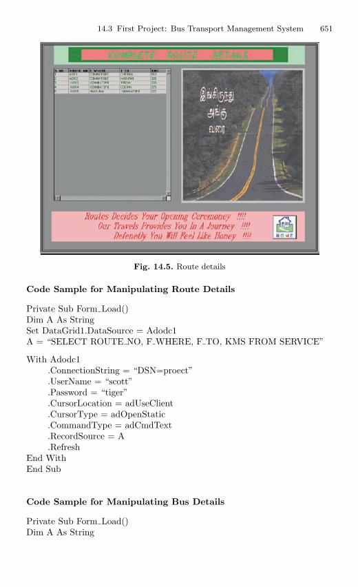
14.3 First Project: Bus Transport Management System 651
Fig. 14.5. Route details
Code Sample for Manipulating Route Details
Private Sub Form Load()Dim A As StringSet DataGrid1.DataSource = Adodc1A = “SELECT ROUTE NO, F WHERE, F TO, KMS FROM SERVICE”
With Adodc1.ConnectionString = “DSN=proect”.UserName = “scott”.Password = “tiger”.CursorLocation = adUseClient.CursorType = adOpenStatic.CommandType = adCmdText.RecordSource = A.Refresh
End WithEnd Sub
Code Sample for Manipulating Bus Details
Private Sub Form Load()Dim A As String
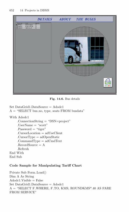
652 14 Projects in DBMS
Fig. 14.6. Bus details
Set DataGrid1.DataSource = Adodc1A = “SELECT bus no, type, seats FROM busdata”
With Adodc1.ConnectionString = “DSN=project”.UserName = “scott”.Password = “tiger”.CursorLocation = adUseClient.CursorType = adOpenStatic.CommandType = adCmdText.RecordSource = A.Refresh
End WithEnd Sub
Code Sample for Manipulating Tariff Chart
Private Sub Form Load()Dim A As StringAdodc1.Visible = FalseSet DataGrid1.DataSource = Adodc1A = “SELECT F WHERE, F TO, KMS, ROUNDKMS*.40 AS FAREFROM SERVICE”
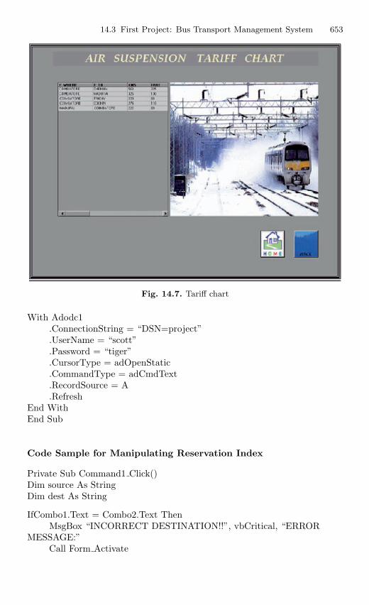
14.3 First Project: Bus Transport Management System 653
Fig. 14.7. Tariff chart
With Adodc1.ConnectionString = “DSN=project”.UserName = “scott”.Password = “tiger”.CursorType = adOpenStatic.CommandType = adCmdText.RecordSource = A.Refresh
End WithEnd Sub
Code Sample for Manipulating Reservation Index
Private Sub Command1 Click()Dim source As StringDim dest As String
IfCombo1.Text = Combo2.Text ThenMsgBox “INCORRECT DESTINATION!!”, vbCritical, “ERROR
MESSAGE:”Call Form Activate
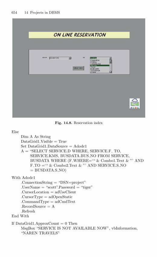
654 14 Projects in DBMS
Fig. 14.8. Reservation index
ElseDim A As StringDataGrid1.Visible = TrueSet DataGrid1.DataSource = Adodc1A = “SELECT SERVICE.D WHERE, SERVICE.F TO,
SERVICE.KMS, BUSDATA.BUS NO FROM SERVICE,BUSDATA WHERE (F WHERE=‘“ & Combo1.Text & ”’ ANDF TO =‘“ & Combo2.Text & ”’ AND SERVICE.S NO= BUSDATA.S NO)
With Adodc1.ConnectionString = “DSN=project”.UserName = “scott”.Password = “tiger”.CursorLocation = adUseClient.CursorType = adOpenStatic.CommandType = adCmdText.RecordSource = A.Refresh
End With
If DataGrid1.ApproxCount = 0 ThenMsgBox “SERVICE IS NOT AVAILABLE NOW”, vbInformation,“NAREN TRAVELS”
14.3 First Project: Bus Transport Management System 655
Combo1.Visible = TrueCombo2.Visible = TrueLabel1.Visible = TrueLabel2.Visible = TrueLabel3.Visible = TrueCommand1.Visible = TrueCommand3.Visible = FalseOption1.Visible = FalseOption2.Visible = FalseOption3.Visible = FalseOption4.Visible = FalseCommand4.Visible = FalseShape1.Visible = TrueDataGrid1.Visible = False
Elsesource = Combo1.Textdest = Combo2.Textcn.ConnectionString = “DSN=project”cn.Open “DSN=project”, “scott”, “tiger”rs.Open “UPDATE DEST SET F WHERE=‘“ & dest & ”’;”, cn,
adOpenDynamic, adLockOptimistic, adCmdTextrs.Open “UPDATE SOURCE SET F TO=‘“ & source & ”’;”,cn, adOpenDynamic,
adLockOptimistic, adCmdText rs.Open “COMMIT;”,cn, adOpenDynamic, adLockOptimistic, adCmdTextcn.CloseOption1.Visible = TrueOption2.Visible = TrueOption3.Visible = TrueOption4.Visible = TrueOption1.Value = FalseOption2.Value = FalseOption3.Value = FalseOption4.Value = FalseCommand4.Visible = TrueCommand4.Enabled = FalseCombo1.Visible = FalseCombo2.Visible = FalseLabel1.Visible = FalseLabel2.Visible = FalseLabel3.Visible = FalseCommand1.Visible = FalseCommand3.Visible = TrueShape1.Visible = False
End If
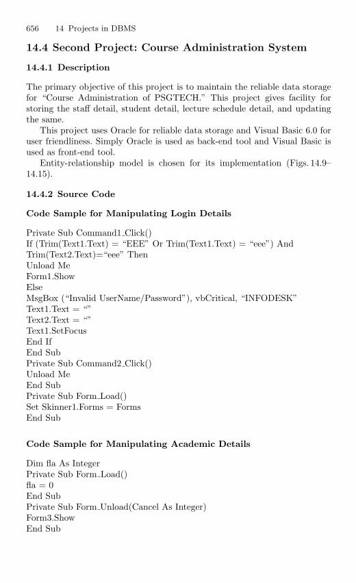
656 14 Projects in DBMS
14.4 Second Project: Course Administration System
14.4.1 Description
The primary objective of this project is to maintain the reliable data storagefor “Course Administration of PSGTECH.” This project gives facility forstoring the staff detail, student detail, lecture schedule detail, and updatingthe same.
This project uses Oracle for reliable data storage and Visual Basic 6.0 foruser friendliness. Simply Oracle is used as back-end tool and Visual Basic isused as front-end tool.
Entity-relationship model is chosen for its implementation (Figs. 14.9–14.15).
14.4.2 Source Code
Code Sample for Manipulating Login Details
Private Sub Command1 Click()If (Trim(Text1.Text) = “EEE” Or Trim(Text1.Text) = “eee”) AndTrim(Text2.Text)=“eee” ThenUnload MeForm1.ShowElseMsgBox (“Invalid UserName/Password”), vbCritical, “INFODESK”Text1.Text = “”Text2.Text = “”Text1.SetFocusEnd IfEnd SubPrivate Sub Command2 Click()Unload MeEnd SubPrivate Sub Form Load()Set Skinner1.Forms = FormsEnd Sub
Code Sample for Manipulating Academic Details
Dim fla As IntegerPrivate Sub Form Load()fla = 0End SubPrivate Sub Form Unload(Cancel As Integer)Form3.ShowEnd Sub
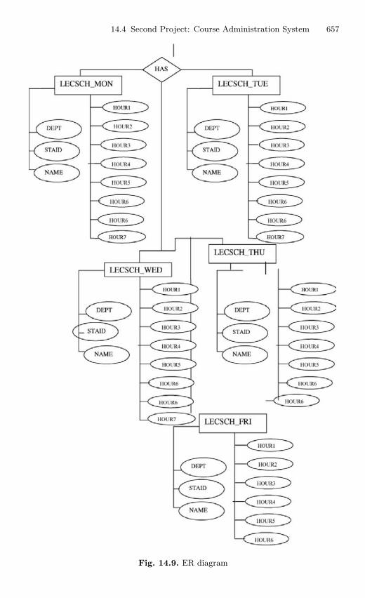
14.4 Second Project: Course Administration System 657
Fig. 14.9. ER diagram
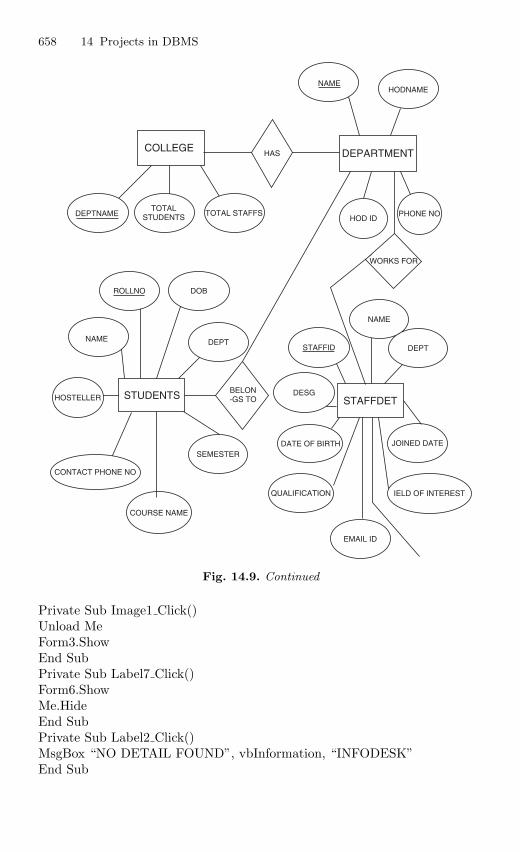
658 14 Projects in DBMS
COLLEGE
NAME
HAS
HOD ID
WORKS FOR
NAME
DEPT
STAFFDET
STAFFID
JOINED DATE
DESG
DATE OF BIRTH
QUALIFICATION IELD OF INTEREST
EMAIL ID
PHONE NO
DEPARTMENT
HODNAME
DEPTNAME
ROLLNO DOB
SEMESTER
BELON-GS TO
NAME
STUDENTS
COURSE NAME
CONTACT PHONE NO
HOSTELLER
DEPT
TOTALSTUDENTS TOTAL STAFFS
Fig. 14.9. Continued
Private Sub Image1 Click()Unload MeForm3.ShowEnd SubPrivate Sub Label7 Click()Form6.ShowMe.HideEnd SubPrivate Sub Label2 Click()MsgBox “NO DETAIL FOUND”, vbInformation, “INFODESK”End Sub
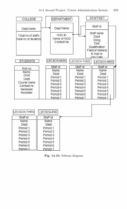
14.4 Second Project: Course Administration System 659
Fig. 14.10. Schema diagram
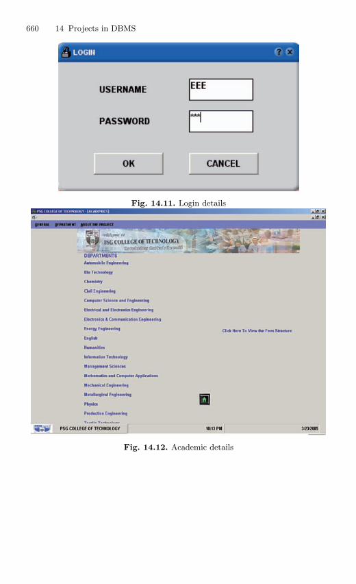
660 14 Projects in DBMS
Fig. 14.11. Login details
Fig. 14.12. Academic details
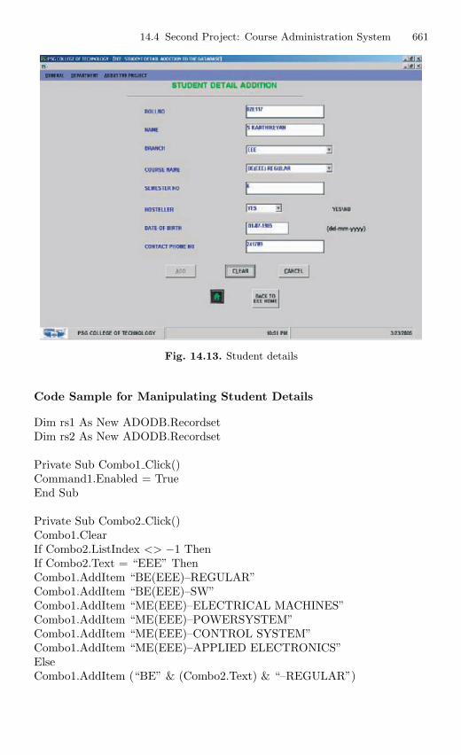
14.4 Second Project: Course Administration System 661
Fig. 14.13. Student details
Code Sample for Manipulating Student Details
Dim rs1 As New ADODB.RecordsetDim rs2 As New ADODB.Recordset
Private Sub Combo1 Click()Command1.Enabled = TrueEnd Sub
Private Sub Combo2 Click()Combo1.ClearIf Combo2.ListIndex <> −1 ThenIf Combo2.Text = “EEE” ThenCombo1.AddItem “BE(EEE)–REGULAR”Combo1.AddItem “BE(EEE)–SW”Combo1.AddItem “ME(EEE)–ELECTRICAL MACHINES”Combo1.AddItem “ME(EEE)–POWERSYSTEM”Combo1.AddItem “ME(EEE)–CONTROL SYSTEM”Combo1.AddItem “ME(EEE)–APPLIED ELECTRONICS”ElseCombo1.AddItem (“BE” & (Combo2.Text) & “–REGULAR”)
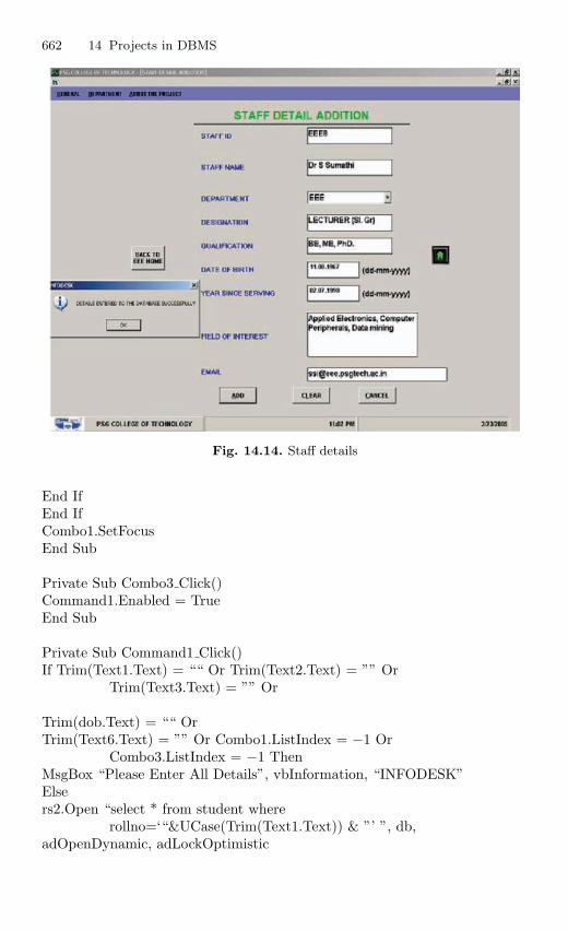
662 14 Projects in DBMS
Fig. 14.14. Staff details
End IfEnd IfCombo1.SetFocusEnd Sub
Private Sub Combo3 Click()Command1.Enabled = TrueEnd Sub
Private Sub Command1 Click()If Trim(Text1.Text) = ““ Or Trim(Text2.Text) = ”” Or
Trim(Text3.Text) = ”” Or
Trim(dob.Text) = ““ OrTrim(Text6.Text) = ”” Or Combo1.ListIndex = −1 Or
Combo3.ListIndex = −1 ThenMsgBox “Please Enter All Details”, vbInformation, “INFODESK”Elsers2.Open “select * from student where
rollno=‘“&UCase(Trim(Text1.Text)) & ”’ ”, db,adOpenDynamic, adLockOptimistic
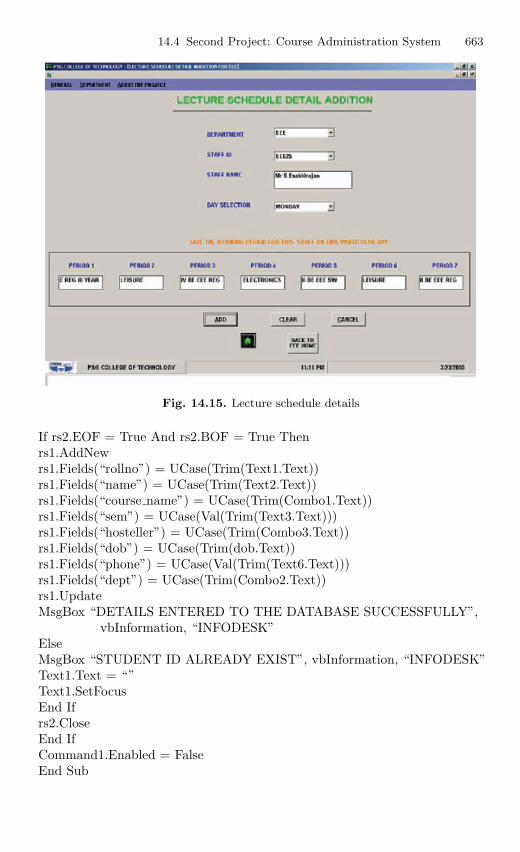
14.4 Second Project: Course Administration System 663
Fig. 14.15. Lecture schedule details
If rs2.EOF = True And rs2.BOF = True Thenrs1.AddNewrs1.Fields(“rollno”) = UCase(Trim(Text1.Text))rs1.Fields(“name”) = UCase(Trim(Text2.Text))rs1.Fields(“course name”) = UCase(Trim(Combo1.Text))rs1.Fields(“sem”) = UCase(Val(Trim(Text3.Text)))rs1.Fields(“hosteller”) = UCase(Trim(Combo3.Text))rs1.Fields(“dob”) = UCase(Trim(dob.Text))rs1.Fields(“phone”) = UCase(Val(Trim(Text6.Text)))rs1.Fields(“dept”) = UCase(Trim(Combo2.Text))rs1.UpdateMsgBox “DETAILS ENTERED TO THE DATABASE SUCCESSFULLY”,
vbInformation, “INFODESK”ElseMsgBox “STUDENT ID ALREADY EXIST”, vbInformation, “INFODESK”Text1.Text = “”Text1.SetFocusEnd Ifrs2.CloseEnd IfCommand1.Enabled = FalseEnd Sub
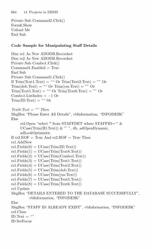
664 14 Projects in DBMS
Private Sub Command2 Click()Form6.ShowUnload MeEnd Sub
Code Sample for Manipulating Staff Details
Dim rs1 As New ADODB.RecordsetDim rs2 As New ADODB.RecordsetPrivate Sub Combo1 Click()Command1.Enabled = TrueEnd SubPrivate Sub Command1 Click()If Trim(Text1.Text) = ““ Or Trim(Text2.Text) = ”” OrTrim(dob.Text) = ““ Or Trim(yss.Text) = ”” OrTrim(Text5.Text) = ““ Or Trim(Text6.Text) = ”” OrCombo1.ListIndex = −1 OrTrim(ID.Text) = ““ Or
Text8.Text = ”” ThenMsgBox “Please Enter All Details”, vbInformation, “INFODESK”Else
rs2.Open “select * from STAFFDET where STAFFID=‘“ &UCase(Trim(ID.Text)) & ”’ ”, db, adOpenDynamic,adLockOptimistic
If rs2.EOF = True And rs2.BOF = True Thenrs1.AddNewrs1.Fields(0) = UCase(Trim(ID.Text))rs1.Fields(1) = UCase(Trim(Text8.Text))rs1.Fields(2) = UCase(Trim(Combo1.Text))rs1.Fields(3) = UCase(Trim(Text1.Text))rs1.Fields(4) = UCase(Trim(Text2.Text))rs1.Fields(5) = UCase(Trim(dob.Text))rs1.Fields(6) = UCase(Trim(yss.Text))rs1.Fields(7) = UCase(Trim(Text5.Text))rs1.Fields(8) = UCase(Trim(Text6.Text))rs1.UpdateMsgBox “DETAILS ENTERED TO THE DATABASE SUCCESSFULLY”,
vbInformation, “INFODESK”ElseMsgBox “STAFF ID ALREADY EXIST”, vbInformation, “INFODESK”rs2.CloseID.Text = “”ID.SetFocus
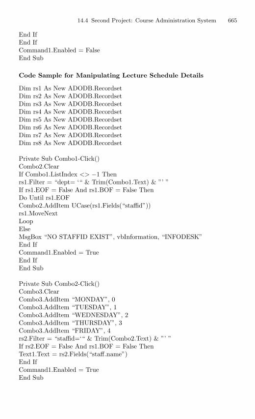
14.4 Second Project: Course Administration System 665
End IfEnd IfCommand1.Enabled = FalseEnd Sub
Code Sample for Manipulating Lecture Schedule Details
Dim rs1 As New ADODB.RecordsetDim rs2 As New ADODB.RecordsetDim rs3 As New ADODB.RecordsetDim rs4 As New ADODB.RecordsetDim rs5 As New ADODB.RecordsetDim rs6 As New ADODB.RecordsetDim rs7 As New ADODB.RecordsetDim rs8 As New ADODB.Recordset
Private Sub Combo1-Click()Combo2.ClearIf Combo1.ListIndex <> −1 Thenrs1.Filter = “dept= ‘“ & Trim(Combo1.Text) & ”’ ”If rs1.EOF = False And rs1.BOF = False ThenDo Until rs1.EOFCombo2.AddItem UCase(rs1.Fields(“staffid”))rs1.MoveNextLoopElseMsgBox “NO STAFFID EXIST”, vbInformation, “INFODESK”End IfCommand1.Enabled = TrueEnd IfEnd Sub
Private Sub Combo2-Click()Combo3.ClearCombo3.AddItem “MONDAY”, 0Combo3.AddItem “TUESDAY”, 1Combo3.AddItem “WEDNESDAY”, 2Combo3.AddItem “THURSDAY”, 3Combo3.AddItem “FRIDAY”, 4rs2.Filter = “staffid=‘“ & Trim(Combo2.Text) & ”’ ”If rs2.EOF = False And rs1.BOF = False ThenText1.Text = rs2.Fields(“staff name”)End IfCommand1.Enabled = TrueEnd Sub
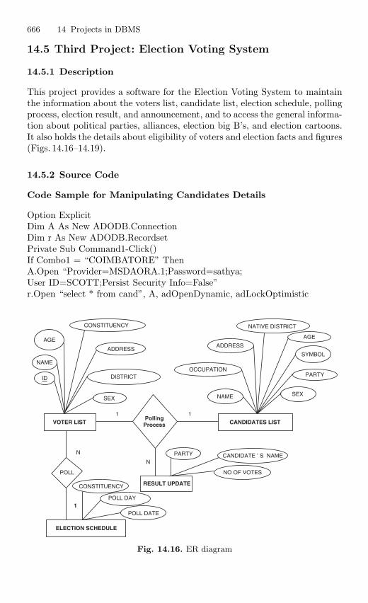
666 14 Projects in DBMS
14.5 Third Project: Election Voting System
14.5.1 Description
This project provides a software for the Election Voting System to maintainthe information about the voters list, candidate list, election schedule, pollingprocess, election result, and announcement, and to access the general informa-tion about political parties, alliances, election big B’s, and election cartoons.It also holds the details about eligibility of voters and election facts and figures(Figs. 14.16–14.19).
14.5.2 Source Code
Code Sample for Manipulating Candidates Details
Option ExplicitDim A As New ADODB.ConnectionDim r As New ADODB.RecordsetPrivate Sub Command1-Click()If Combo1 = “COIMBATORE” ThenA.Open “Provider=MSDAORA.1;Password=sathya;User ID=SCOTT;Persist Security Info=False”r.Open “select * from cand”, A, adOpenDynamic, adLockOptimistic
PARTY
POLL
VOTER LIST CANDIDATES LIST
AGE
SEX
DISTRICT
ADDRESS
CONSTITUENCY
NAME
ID
NAME SEX
SYMBOL
AGE
ADDRESS
OCCUPATIONPARTY
NATIVE DISTRICT
ELECTION SCHEDULE
RESULT UPDATE
POLL DATE
CONSTITUENCY
POLL DAY
NO OF VOTES
CANDIDATE ’ S NAME
Polling Process
1
N
N
1
1
Fig. 14.16. ER diagram
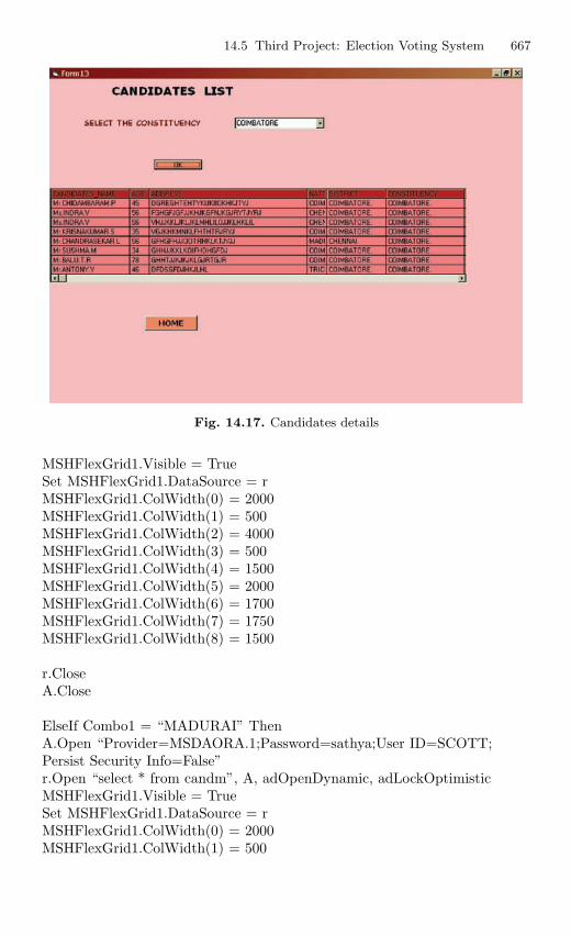
14.5 Third Project: Election Voting System 667
Fig. 14.17. Candidates details
MSHFlexGrid1.Visible = TrueSet MSHFlexGrid1.DataSource = rMSHFlexGrid1.ColWidth(0) = 2000MSHFlexGrid1.ColWidth(1) = 500MSHFlexGrid1.ColWidth(2) = 4000MSHFlexGrid1.ColWidth(3) = 500MSHFlexGrid1.ColWidth(4) = 1500MSHFlexGrid1.ColWidth(5) = 2000MSHFlexGrid1.ColWidth(6) = 1700MSHFlexGrid1.ColWidth(7) = 1750MSHFlexGrid1.ColWidth(8) = 1500
r.CloseA.Close
ElseIf Combo1 = “MADURAI” ThenA.Open “Provider=MSDAORA.1;Password=sathya;User ID=SCOTT;Persist Security Info=False”r.Open “select * from candm”, A, adOpenDynamic, adLockOptimisticMSHFlexGrid1.Visible = TrueSet MSHFlexGrid1.DataSource = rMSHFlexGrid1.ColWidth(0) = 2000MSHFlexGrid1.ColWidth(1) = 500
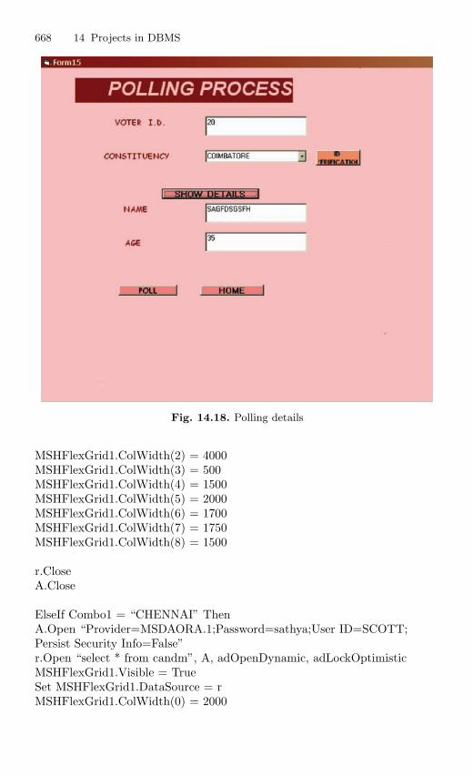
668 14 Projects in DBMS
Fig. 14.18. Polling details
MSHFlexGrid1.ColWidth(2) = 4000MSHFlexGrid1.ColWidth(3) = 500MSHFlexGrid1.ColWidth(4) = 1500MSHFlexGrid1.ColWidth(5) = 2000MSHFlexGrid1.ColWidth(6) = 1700MSHFlexGrid1.ColWidth(7) = 1750MSHFlexGrid1.ColWidth(8) = 1500
r.CloseA.Close
ElseIf Combo1 = “CHENNAI” ThenA.Open “Provider=MSDAORA.1;Password=sathya;User ID=SCOTT;Persist Security Info=False”r.Open “select * from candm”, A, adOpenDynamic, adLockOptimisticMSHFlexGrid1.Visible = TrueSet MSHFlexGrid1.DataSource = rMSHFlexGrid1.ColWidth(0) = 2000
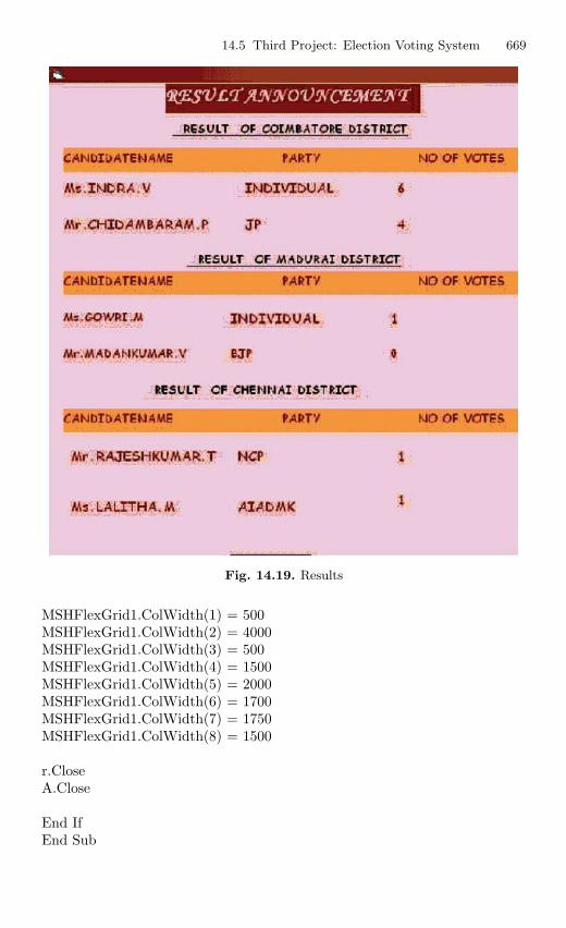
14.5 Third Project: Election Voting System 669
Fig. 14.19. Results
MSHFlexGrid1.ColWidth(1) = 500MSHFlexGrid1.ColWidth(2) = 4000MSHFlexGrid1.ColWidth(3) = 500MSHFlexGrid1.ColWidth(4) = 1500MSHFlexGrid1.ColWidth(5) = 2000MSHFlexGrid1.ColWidth(6) = 1700MSHFlexGrid1.ColWidth(7) = 1750MSHFlexGrid1.ColWidth(8) = 1500
r.CloseA.Close
End IfEnd Sub
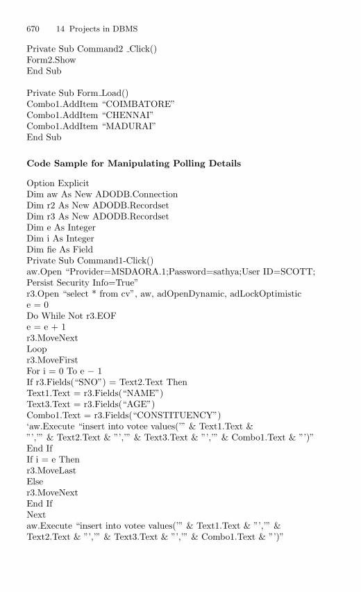
670 14 Projects in DBMS
Private Sub Command2 Click()Form2.ShowEnd Sub
Private Sub Form Load()Combo1.AddItem “COIMBATORE”Combo1.AddItem “CHENNAI”Combo1.AddItem “MADURAI”End Sub
Code Sample for Manipulating Polling Details
Option ExplicitDim aw As New ADODB.ConnectionDim r2 As New ADODB.RecordsetDim r3 As New ADODB.RecordsetDim e As IntegerDim i As IntegerDim fie As FieldPrivate Sub Command1-Click()aw.Open “Provider=MSDAORA.1;Password=sathya;User ID=SCOTT;Persist Security Info=True”r3.Open “select * from cv”, aw, adOpenDynamic, adLockOptimistice = 0Do While Not r3.EOFe = e + 1r3.MoveNextLoopr3.MoveFirstFor i = 0 To e − 1If r3.Fields(“SNO”) = Text2.Text ThenText1.Text = r3.Fields(“NAME”)Text3.Text = r3.Fields(“AGE”)Combo1.Text = r3.Fields(“CONSTITUENCY”)‘aw.Execute “insert into votee values(’” & Text1.Text &”’,’” & Text2.Text & ”’,’” & Text3.Text & ”’,’” & Combo1.Text & ”’)”End IfIf i = e Thenr3.MoveLastElser3.MoveNextEnd IfNextaw.Execute “insert into votee values(’” & Text1.Text & ”’,’” &Text2.Text & ”’,’” & Text3.Text & ”’,’” & Combo1.Text & ”’)”
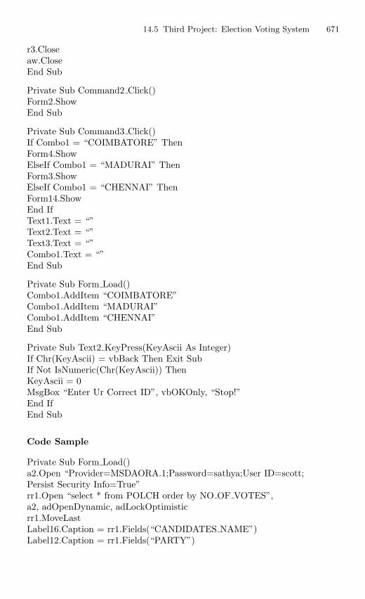
14.5 Third Project: Election Voting System 671
r3.Closeaw.CloseEnd Sub
Private Sub Command2 Click()Form2.ShowEnd Sub
Private Sub Command3 Click()If Combo1 = “COIMBATORE” ThenForm4.ShowElseIf Combo1 = “MADURAI” ThenForm3.ShowElseIf Combo1 = “CHENNAI” ThenForm14.ShowEnd IfText1.Text = “”Text2.Text = “”Text3.Text = “”Combo1.Text = “”End Sub
Private Sub Form Load()Combo1.AddItem “COIMBATORE”Combo1.AddItem “MADURAI”Combo1.AddItem “CHENNAI”End Sub
Private Sub Text2 KeyPress(KeyAscii As Integer)If Chr(KeyAscii) = vbBack Then Exit SubIf Not IsNumeric(Chr(KeyAscii)) ThenKeyAscii = 0MsgBox “Enter Ur Correct ID”, vbOKOnly, “Stop!”End IfEnd Sub
Code Sample
Private Sub Form Load()a2.Open “Provider=MSDAORA.1;Password=sathya;User ID=scott;Persist Security Info=True”rr1.Open “select * from POLCH order by NO OF VOTES”,a2, adOpenDynamic, adLockOptimisticrr1.MoveLastLabel16.Caption = rr1.Fields(“CANDIDATES NAME”)Label12.Caption = rr1.Fields(“PARTY”)
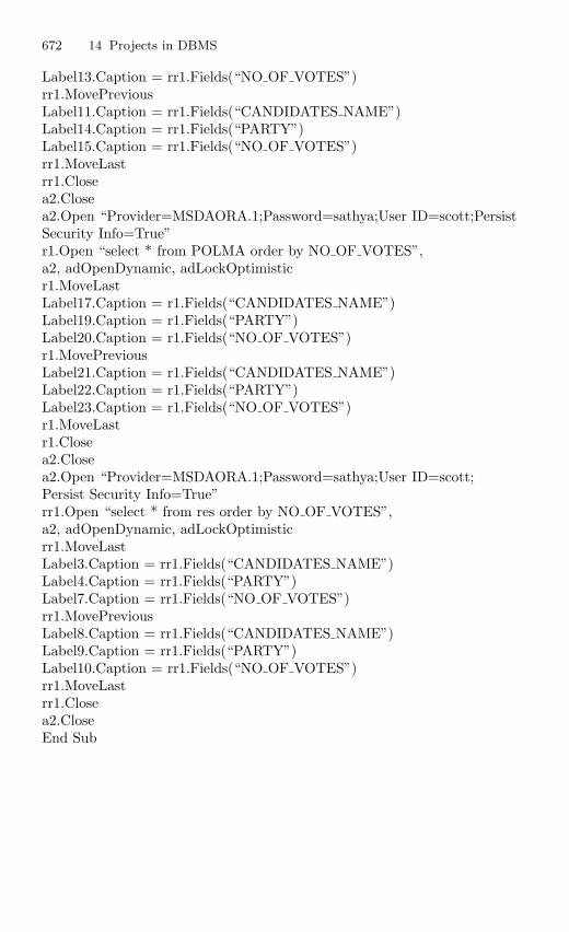
672 14 Projects in DBMS
Label13.Caption = rr1.Fields(“NO OF VOTES”)rr1.MovePreviousLabel11.Caption = rr1.Fields(“CANDIDATES NAME”)Label14.Caption = rr1.Fields(“PARTY”)Label15.Caption = rr1.Fields(“NO OF VOTES”)rr1.MoveLastrr1.Closea2.Closea2.Open “Provider=MSDAORA.1;Password=sathya;User ID=scott;PersistSecurity Info=True”r1.Open “select * from POLMA order by NO OF VOTES”,a2, adOpenDynamic, adLockOptimisticr1.MoveLastLabel17.Caption = r1.Fields(“CANDIDATES NAME”)Label19.Caption = r1.Fields(“PARTY”)Label20.Caption = r1.Fields(“NO OF VOTES”)r1.MovePreviousLabel21.Caption = r1.Fields(“CANDIDATES NAME”)Label22.Caption = r1.Fields(“PARTY”)Label23.Caption = r1.Fields(“NO OF VOTES”)r1.MoveLastr1.Closea2.Closea2.Open “Provider=MSDAORA.1;Password=sathya;User ID=scott;Persist Security Info=True”rr1.Open “select * from res order by NO OF VOTES”,a2, adOpenDynamic, adLockOptimisticrr1.MoveLastLabel3.Caption = rr1.Fields(“CANDIDATES NAME”)Label4.Caption = rr1.Fields(“PARTY”)Label7.Caption = rr1.Fields(“NO OF VOTES”)rr1.MovePreviousLabel8.Caption = rr1.Fields(“CANDIDATES NAME”)Label9.Caption = rr1.Fields(“PARTY”)Label10.Caption = rr1.Fields(“NO OF VOTES”)rr1.MoveLastrr1.Closea2.CloseEnd Sub
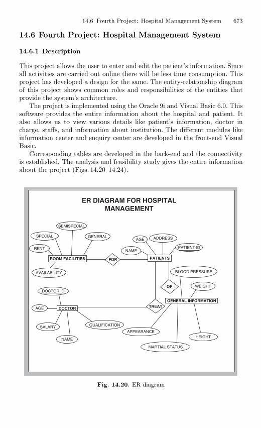
14.6 Fourth Project: Hospital Management System 673
14.6 Fourth Project: Hospital Management System
14.6.1 Description
This project allows the user to enter and edit the patient’s information. Sinceall activities are carried out online there will be less time consumption. Thisproject has developed a design for the same. The entity-relationship diagramof this project shows common roles and responsibilities of the entities thatprovide the system’s architecture.
The project is implemented using the Oracle 9i and Visual Basic 6.0. Thissoftware provides the entire information about the hospital and patient. Italso allows us to view various details like patient’s information, doctor incharge, staffs, and information about institution. The different modules likeinformation center and enquiry center are developed in the front-end VisualBasic.
Corresponding tables are developed in the back-end and the connectivityis established. The analysis and feasibility study gives the entire informationabout the project (Figs. 14.20–14.24).
ER DIAGRAM FOR HOSPITALMANAGEMENT
SEMISPECIAL
SPECIAL GENERAL
SALARY QUALIFICATION
APPEARANCE
AVAILABILITY
DOCTOR ID
MARTIAL STATUS
ADDRESS
PATIENTS
GENERAL INFORMATION
FORROOM FACILITIES
DOCTOR
OF
TREAT
AGE
AGE
NAME
NAME
PATIENT ID
BLOOD PRESSURE
WEIGHT
HEIGHT
RENT
Fig. 14.20. ER diagram
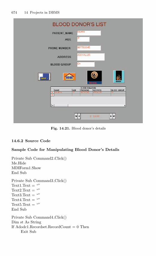
674 14 Projects in DBMS
Fig. 14.21. Blood donor’s details
14.6.2 Source Code
Sample Code for Manipulating Blood Donor’s Details
Private Sub Command2 Click()Me.HideMDIForm1.ShowEnd Sub
Private Sub Command3 Click()Text1.Text = “”Text2.Text = “”Text3.Text = “”Text4.Text = “”Text5.Text = “”End Sub
Private Sub Command4 Click()Dim st As StringIf Adodc1.Recordset.RecordCount = 0 Then
Exit Sub
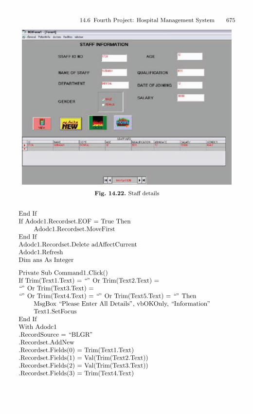
14.6 Fourth Project: Hospital Management System 675
Fig. 14.22. Staff details
End IfIf Adodc1.Recordset.EOF = True Then
Adodc1.Recordset.MoveFirstEnd IfAdodc1.Recordset.Delete adAffectCurrentAdodc1.RefreshDim ans As Integer
Private Sub Command1 Click()If Trim(Text1.Text) = “” Or Trim(Text2.Text) =“” Or Trim(Text3.Text) =“” Or Trim(Text4.Text) = “” Or Trim(Text5.Text) = “” Then
MsgBox “Please Enter All Details”, vbOKOnly, “Information”Text1.SetFocus
End IfWith Adodc1.RecordSource = “BLGR”.Recordset.AddNew.Recordset.Fields(0) = Trim(Text1.Text).Recordset.Fields(1) = Val(Trim(Text2.Text)).Recordset.Fields(2) = Val(Trim(Text3.Text)).Recordset.Fields(3) = Trim(Text4.Text)
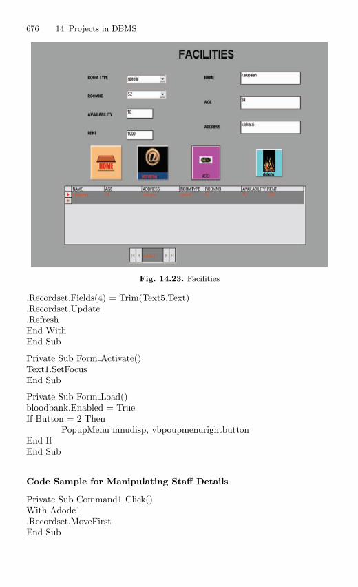
676 14 Projects in DBMS
Fig. 14.23. Facilities
.Recordset.Fields(4) = Trim(Text5.Text)
.Recordset.Update
.RefreshEnd WithEnd Sub
Private Sub Form Activate()Text1.SetFocusEnd Sub
Private Sub Form Load()bloodbank.Enabled = TrueIf Button = 2 Then
PopupMenu mnudisp, vbpoupmenurightbuttonEnd IfEnd Sub
Code Sample for Manipulating Staff Details
Private Sub Command1 Click()With Adodc1.Recordset.MoveFirstEnd Sub
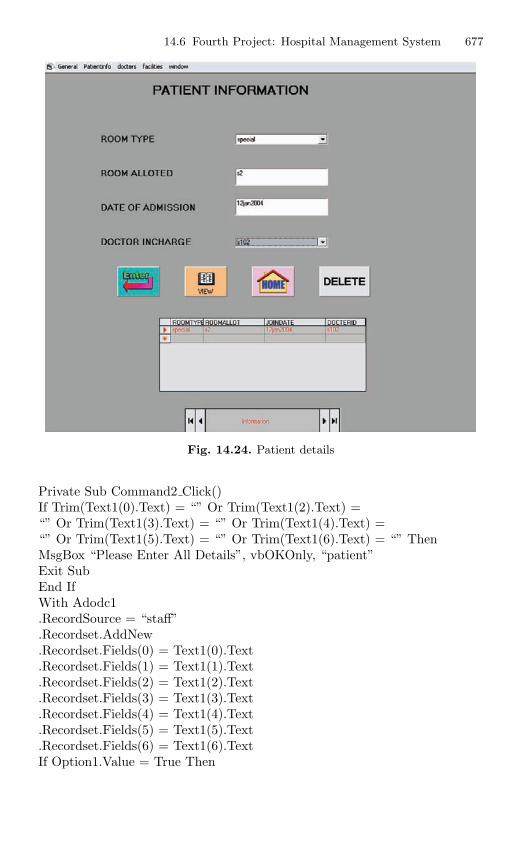
14.6 Fourth Project: Hospital Management System 677
Fig. 14.24. Patient details
Private Sub Command2 Click()If Trim(Text1(0).Text) = “” Or Trim(Text1(2).Text) =“” Or Trim(Text1(3).Text) = “” Or Trim(Text1(4).Text) =“” Or Trim(Text1(5).Text) = “” Or Trim(Text1(6).Text) = “” ThenMsgBox “Please Enter All Details”, vbOKOnly, “patient”Exit SubEnd IfWith Adodc1.RecordSource = “staff”.Recordset.AddNew.Recordset.Fields(0) = Text1(0).Text.Recordset.Fields(1) = Text1(1).Text.Recordset.Fields(2) = Text1(2).Text.Recordset.Fields(3) = Text1(3).Text.Recordset.Fields(4) = Text1(4).Text.Recordset.Fields(5) = Text1(5).Text.Recordset.Fields(6) = Text1(6).TextIf Option1.Value = True Then
678 14 Projects in DBMS
.Recordset.Fields(7) = “MALE”Else.Recordset.Fields(7) = “FEMALE”End If.Recordset.UpdateEnd WithEnd Sub
Private Sub Command3 Click()With Adodc1.RecordSource = “staff”.Recordset.Delete adAffectCurrent.Recordset.UpdateEnd WithEnd Sub
Private Sub Command4 Click()Me.HideMDIForm1.ShowEnd Sub
Private Sub Command5 Click()With Adodc1.Recordset.MovePreviousEnd Sub
Private Sub Command6 Click()With Adodc1.Recordset.MoveNextEnd Sub
Code Sample for Manipulating Facilities
Private Sub Form Load()db.ConnectionString = “DSN=patient”db.Open “DSN=patient”, “scott”, “tiger”rs.Open “roomlist”, db, adOpenDynamic, adLockOptimistic,
adCmdTableCombo1.Text = “”Combo1.AddItem “special”Combo1.AddItem “semi-special”Combo1.AddItem “general ward”Combo1.ListIndex = 0
End Sub
Private Sub Command1 Click()If Trim(Text2.Text) = “” Or Trim(Text3.Text) =
14.6 Fourth Project: Hospital Management System 679
“” Or Trim(Text4.Text) = “” ThenMsgBox “Please Enter All Details”, vbExclamation,“Information”Text2.SetFocusExit SubEnd IfWith Adodc1.RecordSource = “roomlist”.Recordset.AddNew.Recordset.Fields(0) = Trim(Text2.Text).Recordset.Fields(1) = Val(Trim(Text3.Text)).Recordset.Fields(2) = Trim(Text4.Text).Recordset.Fields(3) = Combo1.Text.Recordset.Fields(4) = Combo2.Text.Recordset.Fields(5) = Val(Trim(Text1.Text)).Recordset.Fields(6) = Trim(Text5.Text).Recordset.Update.RefreshEnd WithEnd Sub
Private Sub Form Unload(Cancel As Integer)rs.CloseSet rs = Nothingdb.CloseSet db = NothingEnd Sub
Code Sample for Manipulating Patient Details
Private Sub Form Load()cn.ConnectionString = “DSN=patient”cn.Open “DSN=bulletin”, “scott”, “tiger”rs.Open “stin”, cn, adOpenDynamic, adLockOptimistic, adCmdTableDo While Not rs.EOFCombo2.AddItem rs.Fields(0)rs.MoveNextLoopCombo1.AddItem “special”Combo1.AddItem “general”
End Sub
Private Sub Form Unload(Cancel As Integer)rs.Closecn.CloseSet cn = Nothing
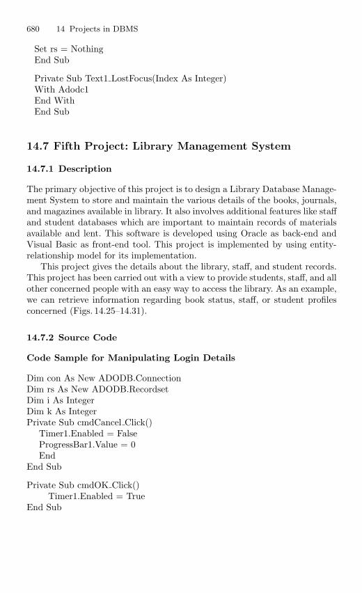
680 14 Projects in DBMS
Set rs = NothingEnd Sub
Private Sub Text1 LostFocus(Index As Integer)With Adodc1End WithEnd Sub
14.7 Fifth Project: Library Management System
14.7.1 Description
The primary objective of this project is to design a Library Database Manage-ment System to store and maintain the various details of the books, journals,and magazines available in library. It also involves additional features like staffand student databases which are important to maintain records of materialsavailable and lent. This software is developed using Oracle as back-end andVisual Basic as front-end tool. This project is implemented by using entity-relationship model for its implementation.
This project gives the details about the library, staff, and student records.This project has been carried out with a view to provide students, staff, and allother concerned people with an easy way to access the library. As an example,we can retrieve information regarding book status, staff, or student profilesconcerned (Figs. 14.25–14.31).
14.7.2 Source Code
Code Sample for Manipulating Login Details
Dim con As New ADODB.ConnectionDim rs As New ADODB.RecordsetDim i As IntegerDim k As IntegerPrivate Sub cmdCancel Click()
Timer1.Enabled = FalseProgressBar1.Value = 0End
End Sub
Private Sub cmdOK Click()Timer1.Enabled = True
End Sub
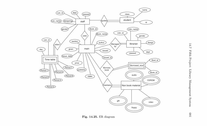
14.7
Fifth
Pro
ject:Lib
rary
Managem
ent
System
681
Lec_id
Lec_name designing
deptpasswd
staff
gender
Lec_id
refers
day
Time table
Period 1
Period 2
Period 5
Period 4
Period 3
Period 6
Period 7publisher
price
Issue_date
given
section
uses
Book_id
class
student
Libn_name
Libn_id
Managedby
librarian
passwd
Borrowed_stud
audio
Non book material
gift
floppy
video
CDROM
Book_id
Stud_id
dept
design
gender
id
name
Book_name
author
issued
Issued_id
Borrowsbook
main
ISBN
guides
maintains
Fig. 14.25. ER diagram
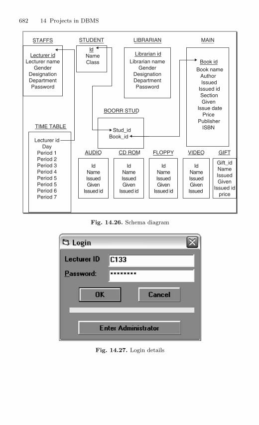
682 14 Projects in DBMS
IdNameClass
Librarian id
Librarian nameGender
DesignationDepartmentPassword
Book id
Book nameAuthorIssued
Issued idSectionGiven
Issue datePrice
PublisherISBNTIME TABLE
Lecturer id Day
Period 1 Period 2 Period 3 Period 4 Period 5 Period 5 Period 6 Period 7
BOORR STUD
Stud_idBook_id
AUDIO
Id NameIssuedGiven
Issued id
CD ROM FLOPPY VIDEO GIFT
Gift_idNameIssuedGiven
Issued idprice
Lecturer idLecturer name
GenderDesignationDepartmentPassword
STAFFS STUDENT LIBRARIAN MAIN
Id NameIssuedGiven
Issued id
Id NameIssuedGiven
Issued id
Id NameIssuedGivenIssued
Fig. 14.26. Schema diagram
Fig. 14.27. Login details
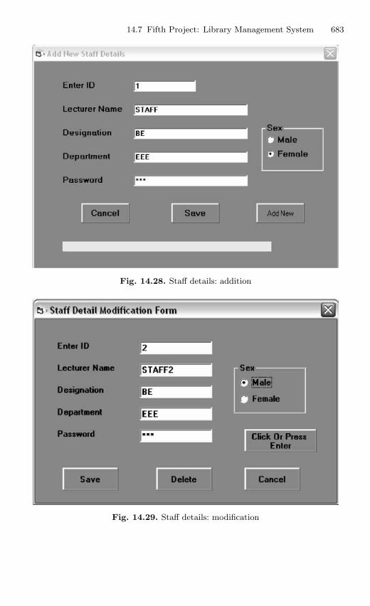
14.7 Fifth Project: Library Management System 683
Fig. 14.28. Staff details: addition
Fig. 14.29. Staff details: modification
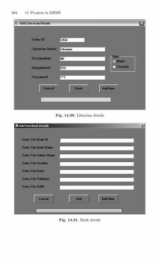
684 14 Projects in DBMS
Fig. 14.30. Librarian details
Fig. 14.31. Book details
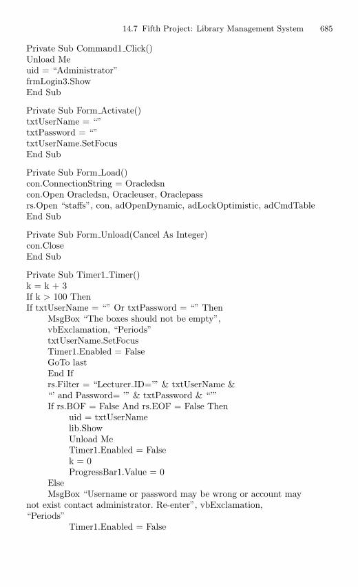
14.7 Fifth Project: Library Management System 685
Private Sub Command1 Click()Unload Meuid = “Administrator”frmLogin3.ShowEnd Sub
Private Sub Form Activate()txtUserName = “”txtPassword = “”txtUserName.SetFocusEnd Sub
Private Sub Form Load()con.ConnectionString = Oracledsncon.Open Oracledsn, Oracleuser, Oraclepassrs.Open “staffs”, con, adOpenDynamic, adLockOptimistic, adCmdTableEnd Sub
Private Sub Form Unload(Cancel As Integer)con.CloseEnd Sub
Private Sub Timer1 Timer()k = k + 3If k > 100 ThenIf txtUserName = “” Or txtPassword = “” Then
MsgBox “The boxes should not be empty”,vbExclamation, “Periods”txtUserName.SetFocusTimer1.Enabled = FalseGoTo lastEnd Ifrs.Filter = “Lecturer ID=’” & txtUserName &“’ and Password= ’” & txtPassword & “’”If rs.BOF = False And rs.EOF = False Then
uid = txtUserNamelib.ShowUnload MeTimer1.Enabled = Falsek = 0ProgressBar1.Value = 0
ElseMsgBox “Username or password may be wrong or account may
not exist contact administrator. Re-enter”, vbExclamation,“Periods”
Timer1.Enabled = False
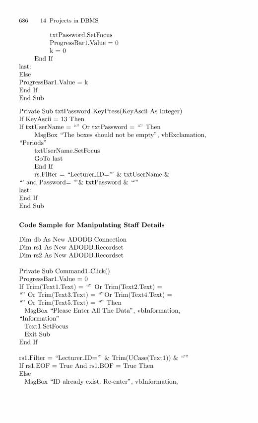
686 14 Projects in DBMS
txtPassword.SetFocusProgressBar1.Value = 0k = 0
End Iflast:ElseProgressBar1.Value = kEnd IfEnd Sub
Private Sub txtPassword KeyPress(KeyAscii As Integer)If KeyAscii = 13 ThenIf txtUserName = “” Or txtPassword = “” Then
MsgBox “The boxes should not be empty”, vbExclamation,“Periods”
txtUserName.SetFocusGoTo lastEnd Ifrs.Filter = “Lecturer ID=’” & txtUserName &
“’ and Password= ’”& txtPassword & “’”last:End IfEnd Sub
Code Sample for Manipulating Staff Details
Dim db As New ADODB.ConnectionDim rs1 As New ADODB.RecordsetDim rs2 As New ADODB.Recordset
Private Sub Command1 Click()ProgressBar1.Value = 0If Trim(Text1.Text) = “” Or Trim(Text2.Text) =“” Or Trim(Text3.Text) = “”Or Trim(Text4.Text) =“” Or Trim(Text5.Text) = “” Then
MsgBox “Please Enter All The Data”, vbInformation,“Information”
Text1.SetFocusExit Sub
End If
rs1.Filter = “Lecturer ID=’” & Trim(UCase(Text1)) & “’”If rs1.EOF = True And rs1.BOF = True ThenElse
MsgBox “ID already exist. Re-enter”, vbInformation,
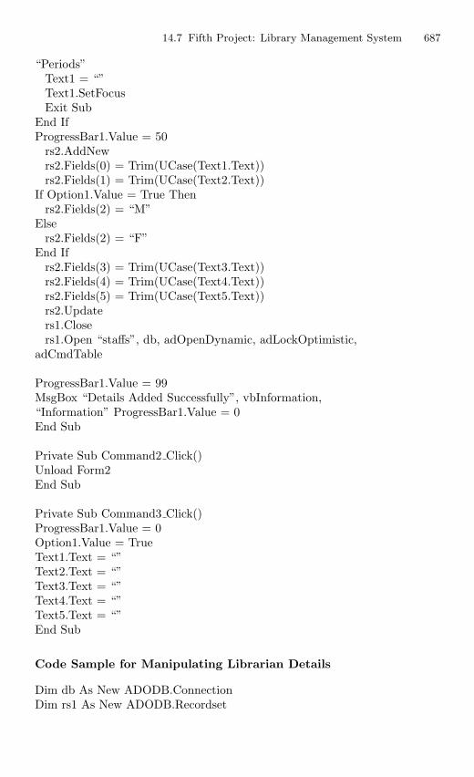
14.7 Fifth Project: Library Management System 687
“Periods”Text1 = “”Text1.SetFocusExit Sub
End IfProgressBar1.Value = 50
rs2.AddNewrs2.Fields(0) = Trim(UCase(Text1.Text))rs2.Fields(1) = Trim(UCase(Text2.Text))
If Option1.Value = True Thenrs2.Fields(2) = “M”
Elsers2.Fields(2) = “F”
End Ifrs2.Fields(3) = Trim(UCase(Text3.Text))rs2.Fields(4) = Trim(UCase(Text4.Text))rs2.Fields(5) = Trim(UCase(Text5.Text))rs2.Updaters1.Closers1.Open “staffs”, db, adOpenDynamic, adLockOptimistic,
adCmdTable
ProgressBar1.Value = 99MsgBox “Details Added Successfully”, vbInformation,“Information” ProgressBar1.Value = 0End Sub
Private Sub Command2 Click()Unload Form2End Sub
Private Sub Command3 Click()ProgressBar1.Value = 0Option1.Value = TrueText1.Text = “”Text2.Text = “”Text3.Text = “”Text4.Text = “”Text5.Text = “”End Sub
Code Sample for Manipulating Librarian Details
Dim db As New ADODB.ConnectionDim rs1 As New ADODB.Recordset
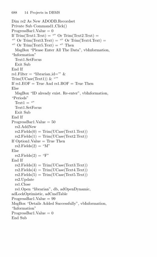
688 14 Projects in DBMS
Dim rs2 As New ADODB.RecordsetPrivate Sub Command1 Click()ProgressBar1.Value = 0If Trim(Text1.Text) = “” Or Trim(Text2.Text) =“” Or Trim(Text3.Text) = “” Or Trim(Text4.Text) =“” Or Trim(Text5.Text) = “” Then
MsgBox “Please Enter All The Data”, vbInformation,“Information”
Text1.SetFocusExit Sub
End Ifrs1.Filter = “librarian id=’” &Trim(UCase(Text1)) & “’”If rs1.EOF = True And rs1.BOF = True ThenElse
MsgBox “ID already exist. Re-enter”, vbInformation,“Periods”
Text1 = “”Text1.SetFocusExit Sub
End IfProgressBar1.Value = 50
rs2.AddNewrs2.Fields(0) = Trim(UCase(Text1.Text))rs2.Fields(1) = Trim(UCase(Text2.Text))
If Option1.Value = True Thenrs2.Fields(2) = “M”
Elsers2.Fields(2) = “F”
End Ifrs2.Fields(3) = Trim(UCase(Text3.Text))rs2.Fields(4) = Trim(UCase(Text4.Text))rs2.Fields(5) = Trim(UCase(Text5.Text))rs2.Updaters1.Closers1.Open “librarian”, db, adOpenDynamic,
adLockOptimistic, adCmdTableProgressBar1.Value = 99MsgBox “Details Added Successfully”, vbInformation,“Information”ProgressBar1.Value = 0End Sub
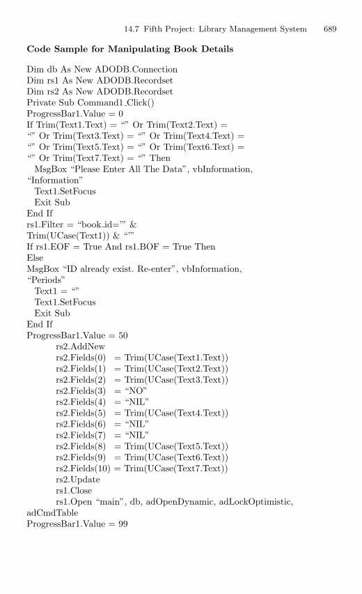
14.7 Fifth Project: Library Management System 689
Code Sample for Manipulating Book Details
Dim db As New ADODB.ConnectionDim rs1 As New ADODB.RecordsetDim rs2 As New ADODB.RecordsetPrivate Sub Command1 Click()ProgressBar1.Value = 0If Trim(Text1.Text) = “” Or Trim(Text2.Text) =“” Or Trim(Text3.Text) = “” Or Trim(Text4.Text) =“” Or Trim(Text5.Text) = “” Or Trim(Text6.Text) =“” Or Trim(Text7.Text) = “” Then
MsgBox “Please Enter All The Data”, vbInformation,“Information”
Text1.SetFocusExit Sub
End Ifrs1.Filter = “book id=’” &Trim(UCase(Text1)) & “’”If rs1.EOF = True And rs1.BOF = True ThenElseMsgBox “ID already exist. Re-enter”, vbInformation,“Periods”
Text1 = “”Text1.SetFocusExit Sub
End IfProgressBar1.Value = 50
rs2.AddNewrs2.Fields(0) = Trim(UCase(Text1.Text))rs2.Fields(1) = Trim(UCase(Text2.Text))rs2.Fields(2) = Trim(UCase(Text3.Text))rs2.Fields(3) = “NO”rs2.Fields(4) = “NIL”rs2.Fields(5) = Trim(UCase(Text4.Text))rs2.Fields(6) = “NIL”rs2.Fields(7) = “NIL”rs2.Fields(8) = Trim(UCase(Text5.Text))rs2.Fields(9) = Trim(UCase(Text6.Text))rs2.Fields(10) = Trim(UCase(Text7.Text))rs2.Updaters1.Closers1.Open “main”, db, adOpenDynamic, adLockOptimistic,
adCmdTableProgressBar1.Value = 99
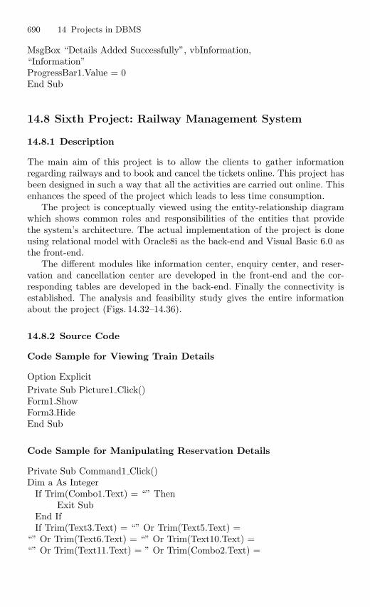
690 14 Projects in DBMS
MsgBox “Details Added Successfully”, vbInformation,“Information”ProgressBar1.Value = 0End Sub
14.8 Sixth Project: Railway Management System
14.8.1 Description
The main aim of this project is to allow the clients to gather informationregarding railways and to book and cancel the tickets online. This project hasbeen designed in such a way that all the activities are carried out online. Thisenhances the speed of the project which leads to less time consumption.
The project is conceptually viewed using the entity-relationship diagramwhich shows common roles and responsibilities of the entities that providethe system’s architecture. The actual implementation of the project is doneusing relational model with Oracle8i as the back-end and Visual Basic 6.0 asthe front-end.
The different modules like information center, enquiry center, and reser-vation and cancellation center are developed in the front-end and the cor-responding tables are developed in the back-end. Finally the connectivity isestablished. The analysis and feasibility study gives the entire informationabout the project (Figs. 14.32–14.36).
14.8.2 Source Code
Code Sample for Viewing Train Details
Option ExplicitPrivate Sub Picture1 Click()Form1.ShowForm3.HideEnd Sub
Code Sample for Manipulating Reservation Details
Private Sub Command1 Click()Dim a As Integer
If Trim(Combo1.Text) = “” ThenExit Sub
End IfIf Trim(Text3.Text) = “” Or Trim(Text5.Text) =
“” Or Trim(Text6.Text) = “” Or Trim(Text10.Text) =“” Or Trim(Text11.Text) = ” Or Trim(Combo2.Text) =
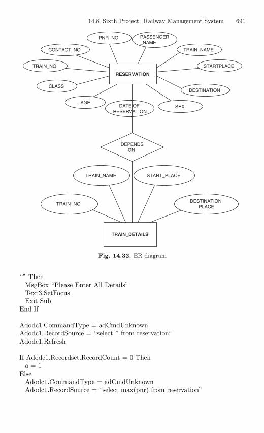
14.8 Sixth Project: Railway Management System 691
RESERVATION
PNR_NO
TRAIN_NAME
STARTPLACE
DESTINATION
SEX AGE
CONTACT_NO
CLASS
DATE OF RESERVATION
PASSENGER_NAME
TRAIN_NO
TRAIN_DETAILS
TRAIN_NO
TRAIN_NAME START_PLACE
DESTINATION PLACE
DEPENDSON
Fig. 14.32. ER diagram
“” ThenMsgBox “Please Enter All Details”Text3.SetFocusExit Sub
End If
Adodc1.CommandType = adCmdUnknownAdodc1.RecordSource = “select * from reservation”Adodc1.Refresh
If Adodc1.Recordset.RecordCount = 0 Thena = 1
ElseAdodc1.CommandType = adCmdUnknownAdodc1.RecordSource = “select max(pnr) from reservation”
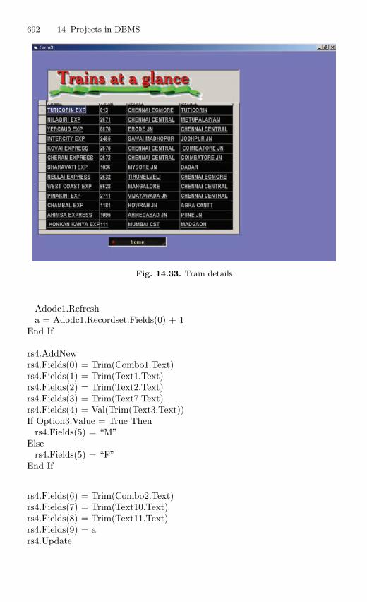
692 14 Projects in DBMS
Fig. 14.33. Train details
Adodc1.Refresha = Adodc1.Recordset.Fields(0) + 1
End If
rs4.AddNewrs4.Fields(0) = Trim(Combo1.Text)rs4.Fields(1) = Trim(Text1.Text)rs4.Fields(2) = Trim(Text2.Text)rs4.Fields(3) = Trim(Text7.Text)rs4.Fields(4) = Val(Trim(Text3.Text))If Option3.Value = True Then
rs4.Fields(5) = “M”Else
rs4.Fields(5) = “F”End If
rs4.Fields(6) = Trim(Combo2.Text)rs4.Fields(7) = Trim(Text10.Text)rs4.Fields(8) = Trim(Text11.Text)rs4.Fields(9) = ars4.Update
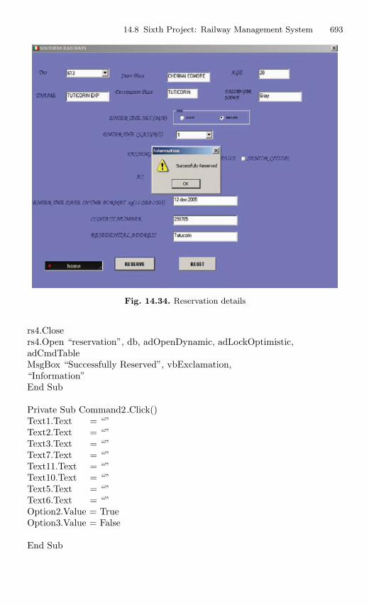
14.8 Sixth Project: Railway Management System 693
Fig. 14.34. Reservation details
rs4.Closers4.Open “reservation”, db, adOpenDynamic, adLockOptimistic,adCmdTableMsgBox “Successfully Reserved”, vbExclamation,“Information”End Sub
Private Sub Command2 Click()Text1.Text = “”Text2.Text = “”Text3.Text = “”Text7.Text = “”Text11.Text = “”Text10.Text = “”Text5.Text = “”Text6.Text = “”Option2.Value = TrueOption3.Value = False
End Sub
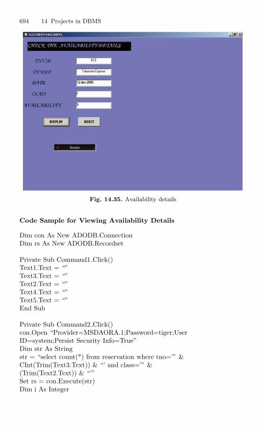
694 14 Projects in DBMS
Fig. 14.35. Availability details
Code Sample for Viewing Availability Details
Dim con As New ADODB.ConnectionDim rs As New ADODB.Recordset
Private Sub Command1 Click()Text1.Text = “”Text3.Text = “”Text2.Text = “”Text4.Text = “”Text5.Text = “”End Sub
Private Sub Command2 Click()con.Open “Provider=MSDAORA.1;Password=tiger;UserID=system;Persist Security Info=True”Dim str As Stringstr = “select count(*) from reservation where tno=’” &CInt(Trim(Text3.Text)) & “’ and class=’” &(Trim(Text2.Text)) & “’”Set rs = con.Execute(str)Dim i As Integer
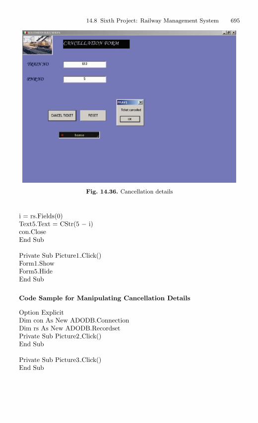
14.8 Sixth Project: Railway Management System 695
Fig. 14.36. Cancellation details
i = rs.Fields(0)Text5.Text = CStr(5 − i)con.CloseEnd Sub
Private Sub Picture1 Click()Form1.ShowForm5.HideEnd Sub
Code Sample for Manipulating Cancellation Details
Option ExplicitDim con As New ADODB.ConnectionDim rs As New ADODB.RecordsetPrivate Sub Picture2 Click()End Sub
Private Sub Picture3 Click()End Sub
696 14 Projects in DBMS
Private Sub Command1 Click()rs.Filter = “pnr = ’” &Trim(Text2.Text) & “’”If rs.EOF = False And rs.BOF = False Thenrs.Deleters.UpdateMsgBox “Ticket canceled”End IfEnd Sub
Private Sub Command2 Click()Text1.Text = “”Text2.Text = “”Text3.Text = “”End Sub
Private Sub Form Load()con.Open “DSN=railway”, “system”, “tiger”rs.Open “reservation”, con, adOpenDynamic, adLockOptimistic,adCmdTableEnd SubPrivate Sub Picture1 Click(Index As Integer)Form8.HideForm1.ShowEnd Sub
14.9 Some Hints to Do Successful Projects in DBMS
Class projects are slightly different from real-world applications, but they havemany features in common. One of the most challenging aspects is that anyproject contains a level of uncertainty and ambiguity. In real-life situations, theproblems are solved through experience and discussions with project manager.With class projects, the students can get some advice from the faculty members,but they need to make their own decisions and interpretations many times.
The desired steps that students should take during the initial phase of theprojects are:
– Identify the goals and objectives of the proposed project.– Additional research of the industry and similar firms will help to get an
overall idea of the project.– After collecting sufficient details develop the conceptual idea of the project
by developing the ER model of the project.– The ER model will help to analyze individual forms and reports. It is
also necessary to identify the overall purpose of each form. The studentsshould be able to describe the purpose of each form.
14.9 Some Hints to Do Successful Projects in DBMS 697
The following steps the students should consider during the implementationphase:
– After collecting sufficient details about the project the next step in theimplementation phase is to select proper front-end, the back-end, andsuitable interface.
– Some of the front-end the students can opt for is Visual Basic and PowerBuilder.
– As the back-end, the students can select either SQL or ACCESS. Thestudents can also go for Oracle forms and reports.
– The students should try to develop good normalized list before creatingtables using SQL or ACCESS.
– Start with an initial set of tables and keys that correct. Add columnsand tables as you need them. If your initial tables are correct then youshould be able to add new columns and tables without altering the existingdesign.
– While developing forms, take care that the forms are user-friendly. At thesame time, the user should not alter important data (secret data). Forthis, make use of the concept of “views” wherever necessary.
– Do not forget to take backup copy of your work periodically. Always keepbackup copy of your project on a different disk.
A
Dictionary of DBMS Terms
Access Plan
Access plans are generated by the optimization component to implementqueries submitted by users.
ACID Properties
ACID properties are transaction properties supported by DBMSs. ACID isan acronym for atomic, consistent, isolated, and durable.
Address
A location in memory where data are stored and can be retrieved.
Aggregation
Aggregation is the process of compiling information on an object, therebyabstracting a higher-level object.
Aggregate Function
A function that produces a single result based on the contents of an entire setof table rows.
Alias
Alias refers to the process of renaming a record. It is alternative name usedfor an attribute.
700 A Dictionary of DBMS Terms
Anomaly
The inconsistency that may result when a user attempts to update a tablethat contains redundant data.
ANSI
American National Standards Institute, one of the groups responsible for SQLstandards.
Application Program Interface (API)
A set of functions in a particular programming language is used by a clientthat interfaces to a software system.
ARIES
ARIES is a recovery algorithm used by the recovery manager which is invokedafter a crash.
Armstrong’s Axioms
Set of inference rules based on set of axioms that permit the algebraic mani-pulation of dependencies. Armstrong’s axioms enable the discovery of minimalcover of a set of functional dependencies.
Associative Entity Type
A weak entity type that depends on two or more entity types for its primarykey.
Attribute
The differing data items within a relation. An attribute is a named column ofa relation.
Authorization
The operation that verifies the permissions and access rights granted to auser.
Base Table
Base table is a named relation corresponding to an entity in the conceptualschema, whose tuples (rows) are physically stored in the database.
A Dictionary of DBMS Terms 701
Bitmap Index
A compact, high speed indexing method where the key values and the condi-tions are compressed to a small size that can be stored and searched rapidly.
BLOB
BLOB is an acronym for Binary Large Object. BLOB is a data type for fieldscontaining large binary data such as images.
Boyce–Codd Normal Form
A relation in third normal form in which every determinant is a candidatekey.
Bucket
With reference to hash file, Bucket is the unit of a file having a particularaddress.
Buffer
Buffer an area in main memory containing physical database records trans-ferred from disk.
Candidate Key
Any data item or group of data items which identify uniquely tuples in arelation.
Cardinality
The number of tuples in a relation.
Cartesian Product
All of the possible combinations of the rows from each of the tables involvedin a join operation.
CASE Tool
CASE is an acronym for computer-aided software engineering. CASE toolssupport features for drawing, analysis, prototyping, and data dictionary.CASE tool facilitate database development.
702 A Dictionary of DBMS Terms
Chasm Trap
A chasm trap exists where a model suggests the existence of relationshipbetween entity types, but the pathway does not exist between certain entityoccurrences.
Client
An individual user workstation that represents the front end of a DBMS.
Client/Server Architecture
Client/Server architecture is an arrangement of components among computersconnected by a network.
Clustered Index
An index in which the logical or indexed order of the key values is the sameas the physical stored order of the corresponding rows.
CODASYL
Conference on Data System Languages.
Concurrent Access
Performing two or more operations on the same data at the same time.
Concurrency Control
Concurrency control is the control on the database and transactions whichare executed concurrently to ensure that each transaction completed healthy.
Composite Key
A candidate key comprising more than one attribute
Composite Index
An index that uses more than one column in a table to index data.
COMMIT
To control transactions, SQL provides this command to save recent DMLchanges to the database.
A Dictionary of DBMS Terms 703
Condition Box
A special box used by QBE to store logical conditions that are not easilyexpressed in the table skeleton.
Constraints
Constraints are conditions that are used to impose rules on the table.
Conceptual View
The logical database description in ANSI/SPARC DBMS architecture.
Concurrent Access
Two or more users operating on the same rows in a database table at thesame time.
Correlated Subquery
In SQL, a sub query in which processing the inner query depends on datafrom the outer query.
COUNT
An aggregate function that returns the number of values in a column.
Cursor
An SQL feature that specifies a set of rows, an ordering of those rows and acurrent row within that ordering.
Data
Data is a representation of facts, concepts or instructions in a formalizedmanner suitable for communication, interpretation or processing by humansor automatic means.
Data Abstraction
Data abstraction means the storage details of the data are hidden from theuser and the user is provided with the conceptual view of the database.
704 A Dictionary of DBMS Terms
Database
Database is the collection of interrelated data.
Data Definition Language (DDL)
The language component of a DBMS that is used to describe the logicalstructure of a database.
Data Manipulation Language (DML)
A language component of a DBMS that is used by a programmer to accessand modify the contents of a database.
Database Instance
The actual data stored in a database at a particular moment in time.
Database State
Database state refers to the content of a database at a moment in time.
Database Management System
General purpose software used to maintain the database.
Database System
A database system means both a DBMS plus a database.
Database Administrator
A person or group of people responsible for the design and supervision of adata base.
Database Recovery
The process of restoring the database to a correct state in the event of afailure.
Database Security
Protection of the database against accidental or intentional loss, destruction,or misuse.
A Dictionary of DBMS Terms 705
Data Mining
Data mining is the process of discovering implicit patterns in data storedin data warehouse and using those patterns for business advantage such aspredicting future trends.
Data Model
Collection of conceptual tools for describing data and relationship betweendata.
Data Dictionary
Centralized store of information about database.
Data Warehouse
Data warehouse is a central repository for summarized and integrated datafrom operational databases and external data sources.
DB2
An IBM relational database system.
DBTG
Database Task Group.
Deadlock
The situation where each of two transactions are waiting indefinitely for theother transaction to release the resources it requests.
Degree of a Relation
The number of attributes in the relation.
Denormalization
Denormalization is the process of combining tables so that they are easier toquery. Denormalization is opposite to normalization. Denormalization is doneto improve query performance.
706 A Dictionary of DBMS Terms
Derived Attribute
Derived attributes are the attributes whose values are derived from otherrelated attribute.
Determinant
An attribute or set of attributes on which the value of one or more attributesdepend.
Distributed Database
A database located at more than one site.
Domain
The set of all possible values for a given data item.
Domain Integrity
Data integrity that enforces valid entries for a given column
Domain Relational Calculus
Domain Relational Calculus is a calculus that was introduced by Edgar F.Codd as a declarative database query language for the relational data model.
DDL
Data Definition Language is used to define the schema of a relation.
DML
Data Manipulation Language is basically used to manipulate a relation.
Dual
A virtual table automatically created by Oracle along with the data dictionary.It has one column, DUMMY, defined to be VARCHAR2(1), and contains onerow with a value of “X”.
Embedded SQL
An application structure in which SQL statements are embedded within pro-grams written in a host language like C, JAVA.
A Dictionary of DBMS Terms 707
Encapsulation
Hiding the representation of an object is encapsulation.
Entity
An object that exist and is distinguishable from other objects.
Entity Class
A set of entities of the same type.
Entity Instance
Entity instance is a particular occurrence of an entity.
Entity Integrity (Table Integrity)
Integrity that defines a row as a unique entity for a particular table andensures that the column cannot contain duplicate values.
Equijoin
A join operator where the join condition involves equality.
ER Model
ER stands for Entity-Relationship model. ER Model is based on a perceptionof a real world that consists of collection of basic objects called entities andrelationships among these objects.
EER Model
EER stands for Enhanced ER model. EER model is the extension of origi-nal model with new modeling constructs. The new modeling constructs aresupertype, subtype.
Exclusive Lock
A lock that prevents other users from accessing a database item. Exclusivelocks conflict with all other kids of locks such as shared locks.
708 A Dictionary of DBMS Terms
Fantrap
A fantrap exists where a model represents a relationship between entity typesbut the pathway between certain entity occurrences is ambiguous.
File
A file is a collection of records of the same type.
File Organization
Methods used in organizing data for storage and retrieval such as sequential,indexed sequential, or direct.
First Normal Form
A relation is in first normal form if it contains no repeating groups.
Flat File
A file in which the fields of records are simple atomic values.
Foreign Key
Attribute or set of attributes that identifies the entity with which anotherentity is associated.
Fourth Normal Form
A relation is in fourth normal form if it is in BCNF and contains no multi-valued dependencies.
Function
A set of instructions that operates as a single logical unit.
Functional Dependency
A constraint between two attributes or two sets of attributes in a relation.
Generalization
In extended ER model (EER model), generalization is a structure in whichone object generally describes more specialized objects.
A Dictionary of DBMS Terms 709
GRANT
An SQL command for granting privileges to a user/users.
Graphical User Interface (GUI)
An interface that uses pictures and graphic symbols to represent commandsand actions.
Hashing
A mathematical technique for assigning a unique number to each record in afile.
Hash Function
A function that maps a set of keys onto a set of addresses.
Hierarchical Database
A DBMS type that organizes data in hierarchies that can be rapidly searchedfrom top to bottom.
Identifier
An attribute or collection of attributes that uniquely distinguishes an entity.
Index
A data structure used to decrease file access time.
Inheritance
Object-oriented systems have a concept of inheritance which permits class Xto derive much of its code and attributes from another class Y. Class X willcontain the data attributes and operations of class Y.
Intersection
A relational algebra operation performed on two union-compatible relationsso as to produce a relation which contains rows that appear in both the union-compatible relations.
710 A Dictionary of DBMS Terms
ISA Relationship
The relationship between each subtype and its supertype.
ISO
ISO stands for International Standards Organization. ISO in conjuction withANSI to provide standard SQL for relational databases.
JOIN
An operation that combines data from more than one table.
JDBC
JDBC stands for Java Database Connectivity. A standard interface betweenJava applet or application and a database.
Key
Key is a data item that helps to identify individual occurrences of an entitytype.
Leaf
In a tree structure, an element that has no subordinate elements.
Lock
A procedure used to control concurrent access to data.
Log
A file containing a record of database changes.
Logical Database Design
A part of database design that is concerned with modeling the business re-quirements and data.
Logical Data Independence
Application programs and terminal activities remain logically unimpairedwhen information preserving changes of any kind that theoretically permitunimpairment are made to the base tables.
A Dictionary of DBMS Terms 711
Meta Data
Data about data is meta data. In other words, metadata is the data aboutthe structure of the data in a database.
Mirrored Disk
Set of disks that are synchronized as follows: **each write to one disk goes toall disks in the mirrored set; reads can access any of the disk.
Mobile Database
A database that is portable and physically separate from a centralized data-base server but is capable of communicating with that server from remotesites.
Modification Anomaly
An unexpected side effect that occurs when changing the data in a table withexcessive redundancies.
Multivalued Attribute
A multivalued attribute is an attribute to which more than one value is asso-ciated.
Multiple Tier Architecture
A client/server architecture with more than three layers a PC client, databaseserver an intervening middleware server and application servers. The applica-tion servers perform business logic and manage specialized kinds of data suchas images.
Multivalued Dependency
A type of dependency that exists when there are at least three attributes (forexample X, Y, and Z) in a relation, and for each value of X there is a well-defined set of values for Y and a well-defined set of values for Z, but the setof values of Y is independent of set Z.
Natural Join
In a natural join, the matching condition is equality condition; one of thematching columns is discarded in the result table.
712 A Dictionary of DBMS Terms
Normal Form
A set of conditions defined on entity specification.
Normalization
The design process for generating entity specifications to minimize both dataredundancy and update anomalies.
NULL Value
A value that is either unknown or not applicable.
Object
An object is a collection of data, an identity, and a set of operations sometimescalled methods.
Object-Oriented Database
An object-oriented database combines database capabilities with an objectoriented analysis and design.
Object-Relational Database
Object-relational database combines RDBMS features with object-orientedfeatures like inheritance and encapsulation.
ODBC
ODBC stands for Open Data Base Connectivity. A standard interface bywhich application programs can access and process SQL databases in a DBMSindependent manner.
OLAP
Online Analytical Processing systems, contrary to the regular, conventionalonline transaction processing systems, are capable of analyzing online a largenumber of past transactions or large number of data records (ranging frommega bytes to gigabytes and terabytes).
OLTP
OLTP stands for Online Transaction Processing which supports large numberof concurrent transactions without imposing excessive delays.
A Dictionary of DBMS Terms 713
One-to-Many Relationship
A relationship between two tables in which a single row in the first table canbe related to one or more rows in the second table, but a row in the secondtable can be related only to one row in the first table.
One-to-One Relationship
A relationship between two tables in which a single row in the first table canbe related to only one row in the second table, and a row in the second tablecan be related to only one row in the first table.
Oracle
A relational database management system marketed by Oracle Corporation.
Outer Join
Outer join is a relational algebra operator which combines two tables. In anouter join, the matching and nonmatching rows are retained in the result.
Overflow
Overflow occurs when an insertion is attempted into a bucket or node that isfull.
Partial Functional Dependency
A dependency in which one or more nonkey attributes are functionally depen-dent on part (but not all) of the primary key.
Physical Data Independence
Application programs and terminal activities remain logically unimpairedwhenever any changes are made in either storage representation or accessmethods.
Polymorphism
Polymorphism is a principle of object-oriented computing in which a com-puting system has the ability to choose among multiple implementations of amethod.
714 A Dictionary of DBMS Terms
Primary Key
An attribute or set of attributes that uniquely identifies a tuple in a relation.
Procedural Language Interface
Procedural Language Interface is a method to combine a nonprocedural lan-guage such as SQL with programming language such as Visual Basic. Embed-ded SQL is an example for procedural language interface.
QBE
QBE stands for Query By Example. QBE uses a terminal display with at-tribute names as table headings for queries.
Query
Query is a request to extract useful data.
Query Plan
The plan produced by an optimizer for processing a query
Query Processing
The activities involved in retrieving data from the database are called as queryprocessing.
Query Optimization
The activity of choosing an efficient execution strategy for processing a queryis called as Query optimization.
RAID
RAID is an acronym for Redundant Array of Independent Disks. RAID is acollection of disks that operates as a single disk.
Range Query
Range query refers to selection on an interval. For example, select the nameof players whose age is between thirty and thirty five.
A Dictionary of DBMS Terms 715
Recursive Relationship
A relationship type where the same entity type participates more than oncein different roles.
Redundant Data
Redundant data refers to the same data that is stored in more than onelocation in the database.
Referential Integrity
The referential integrity imposes the constraint that if a foreign key exists ina relation, either the foreign key value must match a candidate key value ofsome tuple in its home relation or the foreign key value must be wholly null.
Relation
A relation is a table with rows and columns.
Relationship Type
Relationship type is a set of meaningful associations among entity types.
Relational Algebra
Procedural language based on algebraic concepts. It consists of collection ofoperators that are defined on relations, and that produce relations as results.
Relational Calculus
A query language based on first order predicate calculus.
Relational Database
A database that organizes data in the form of tables.
Relational Database Management System (RDBMS)
Software that organizes manipulates and retrieves data stored in a relationaldatabase.
Recursive Relationship
A relationship in which one entity references itself.
716 A Dictionary of DBMS Terms
Repository
A repository is a collection of resources that can be accessed to retrieve in-formation. Repositories often consist of several databases tied together by acommon search engine.
REVOKE
An SQL statement for removing privileges from a user/users.
ROLLBACK
A DBMS recovery technique that aborts active applications and attempts toreinstate the state of the database prior to initiating the applications activeat the time the database failed.
Root
The top record, row, or node in a tree. A root has no parent.
Schema
Schema is the collection of named object.
Scalar Function
A function operating on a single value. Scalar functions return a single value.
Second Normal Form (2NF)
A relation schema R is in 2 NF if every nonprime attribute A in R is fullyfunctionally dependent on the primary key of R.
Self Join
A join that merges data from a table with data in the same table, based oncolumns in a table that are related to one another.
Semantic Data Model
Semantic data model provides a vocabulary for expressing the meaning as wellas the structure of database data.
A Dictionary of DBMS Terms 717
Semijoin
A dyadic relational operator yielding the tuples of one operand that con-tributes to the join of both.
Sequential File Organization
The records in the file are stored in sequence according to a primary key value.
SGML
SGML stands for Standard Generalized Markup Language. A standard meansfor tagging and marking the format, structure, and content of documents.HTML is a subset of SGML.
Shared Lock
Lock that allows concurrent transactions to read a resource.
Sparse Index
Index in which the underlying data structure contains exactly one pointer toeach data page.
Stripe
Stripping is an important concept for RAID storage. Stripping involves theallocation of physical records to different disks.
Structured Query Language (SQL)
A standard language used to manipulate data in a database.
Subquery
Query within a query.
Subtype
A subtype represents a subset or subgroup of super class entity type’s ins-tances. Subtype inherit the attributes and relationships associated with theirsuper type.
718 A Dictionary of DBMS Terms
SUM
An aggregate function that returns the sum of all values. Sum can be usedwith numeric columns only. NULL values are ignored.
Super Type
Super type is a generic entity type that has a relationship with one or moresubtype.
Table
Table is a 2D arrangement of data. The table consists of rows and columns.
Ternary Relationship
A relationship which involves three entity types. It is a simultaneous relation-ship among the instances of three entity types.
Three-Tier Architecture
Three-Tier architecture is client/server architecture with three layers: a PCclient, database server and an application server.
Transaction
Transaction is the execution of user program in DBMS. In other words it canbe stated as the various read and write operations done by the user programon the DBMS, when it is executed in DBMS environment.
Transaction Log
File that records transactional changes occurring in a database, providing abasis for updating a master file and establishing an audit trail.
Transitive Dependency
If the attribute X is dependent on Y and the attribute Y is dependent on Zthen the attribute X is transitively dependent on Z
Trigger
Action that causes a procedure to be carried out automatically when a userattempts to modify data.
A Dictionary of DBMS Terms 719
Trivial Dependency
The dependency of an attribute on itself.
Tuple
A row in the tabular representation of the relation.
Tuple Relational Calculus
The tuple relational calculus is based on specifying a number of tuple vari-ables. Each tuple variable usually ranges over a particular database relation,meaning that the variable may take as its value any individual tuple fromthat relation.
Two Phase Locking
A locking scheme with two distinct phases. During the first phase the DBMSmay set licks, during the second it is allowed only to release locks.
Two Phase Commit
Process that ensures transactions applying to more than one server are com-pleted on either all servers or none.
Two-Tier Architecture
Two-Tier architecture is a client/server architecture in which a PC client anda database server interact directly to request and transfer data. The PC clientcontains the user interface code, the server contains the data access logic, andthe PC client and the server share the validation and business logic.
Union
A relational algebra operation performed on two union-compatible relationsto produce a third relation which contains every row in the union-compatiblerelations minus any duplicate rows.
Union Compatible
Two relations are union compatible if they have same number of attributesand the attributes in the corresponding columns arise from the same domain.
720 A Dictionary of DBMS Terms
Update Anomaly
An undesirable side effect caused by an insertion, deletion, or modification.
Updatable View
When the rows of an updatable view is modified then DBMS translates theview modifications into the modifications to the rows of the base tables.
Variable
A location in memory used to hold temporary values. Variables have a scopeand a lifetime depending on where they are created and how they are defined.
View
A virtual table which is derived from base table using a query.
Visual Basic (VB)
A product of Microsoft that is used to develop applications for the windowsenvironment. The professional version supports database connections.
Volatile Storage
Volatile storage loses its state when the power is disconnected.
VSAM
VSAM stands for Virtual Storage Access Method. It is IBM’s implementationof the B-tree concept.
Weak Entity
An entity whose existence depends on other entity.
Write–write Conflict
The situation in which two write actions operate on the same data item.
World Wide Web (WWW)
A first attempt to set up an international database of information.
XML
A language for defining the structure and the content of documents on theWorld Wide Web.
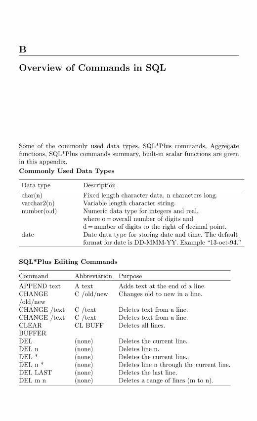
B
Overview of Commands in SQL
Some of the commonly used data types, SQL*Plus commands, Aggregatefunctions, SQL*Plus commands summary, built-in scalar functions are givenin this appendix.Commonly Used Data Types
Data type Description
char(n) Fixed length character data, n characters long.varchar2(n) Variable length character string.number(o,d) Numeric data type for integers and real,
where o = overall number of digits andd = number of digits to the right of decimal point.
date Date data type for storing date and time. The defaultformat for date is DD-MMM-YY. Example “13-oct-94.”
SQL*Plus Editing Commands
Command Abbreviation Purpose
APPEND text A text Adds text at the end of a line.CHANGE/old/new
C /old/new Changes old to new in a line.
CHANGE /text C /text Deletes text from a line.CHANGE /text C /text Deletes text from a line.CLEARBUFFER
CL BUFF Deletes all lines.
DEL (none) Deletes the current line.DEL n (none) Deletes line n.DEL * (none) Deletes the current line.DEL n * (none) Deletes line n through the current line.DEL LAST (none) Deletes the last line.DEL m n (none) Deletes a range of lines (m to n).
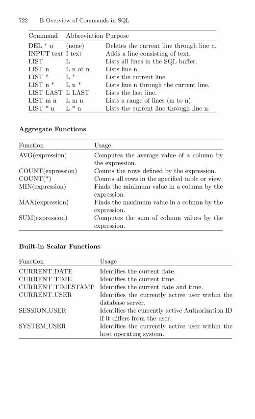
722 B Overview of Commands in SQL
Command Abbreviation Purpose
DEL * n (none) Deletes the current line through line n.INPUT text I text Adds a line consisting of text.LIST L Lists all lines in the SQL buffer.LIST n L n or n Lists line n.LIST * L * Lists the current line.LIST n * L n * Lists line n through the current line.LIST LAST L LAST Lists the last line.LIST m n L m n Lists a range of lines (m to n).LIST * n L * n Lists the current line through line n.
Aggregate Functions
Function Usage
AVG(expression) Computes the average value of a column bythe expression.
COUNT(expression) Counts the rows defined by the expression.COUNT(*) Counts all rows in the specified table or view.MIN(expression) Finds the minimum value in a column by the
expression.MAX(expression) Finds the maximum value in a column by the
expression.SUM(expression) Computes the sum of column values by the
expression.
Built-in Scalar Functions
Function Usage
CURRENT DATE Identifies the current date.CURRENT TIME Identifies the current time.CURRENT TIMESTAMP Identifies the current date and time.CURRENT USER Identifies the currently active user within the
database server.SESSION USER Identifies the currently active Authorization ID
if it differs from the user.SYSTEM USER Identifies the currently active user within the
host operating system.
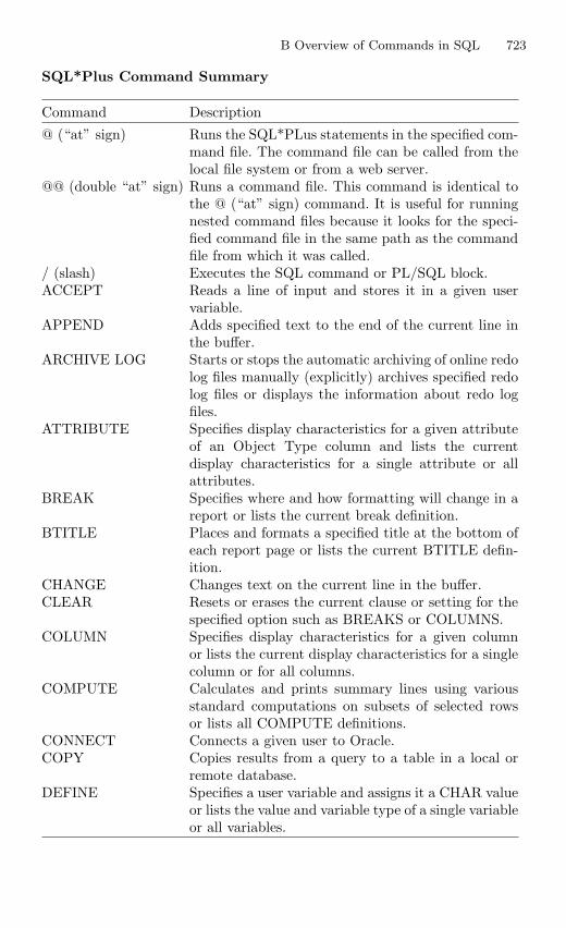
B Overview of Commands in SQL 723
SQL*Plus Command Summary
Command Description
@ (“at” sign) Runs the SQL*PLus statements in the specified com-mand file. The command file can be called from thelocal file system or from a web server.
@@ (double “at” sign) Runs a command file. This command is identical tothe @ (“at” sign) command. It is useful for runningnested command files because it looks for the speci-fied command file in the same path as the commandfile from which it was called.
/ (slash) Executes the SQL command or PL/SQL block.ACCEPT Reads a line of input and stores it in a given user
variable.APPEND Adds specified text to the end of the current line in
the buffer.ARCHIVE LOG Starts or stops the automatic archiving of online redo
log files manually (explicitly) archives specified redolog files or displays the information about redo logfiles.
ATTRIBUTE Specifies display characteristics for a given attributeof an Object Type column and lists the currentdisplay characteristics for a single attribute or allattributes.
BREAK Specifies where and how formatting will change in areport or lists the current break definition.
BTITLE Places and formats a specified title at the bottom ofeach report page or lists the current BTITLE defin-ition.
CHANGE Changes text on the current line in the buffer.CLEAR Resets or erases the current clause or setting for the
specified option such as BREAKS or COLUMNS.COLUMN Specifies display characteristics for a given column
or lists the current display characteristics for a singlecolumn or for all columns.
COMPUTE Calculates and prints summary lines using variousstandard computations on subsets of selected rowsor lists all COMPUTE definitions.
CONNECT Connects a given user to Oracle.COPY Copies results from a query to a table in a local or
remote database.DEFINE Specifies a user variable and assigns it a CHAR value
or lists the value and variable type of a single variableor all variables.
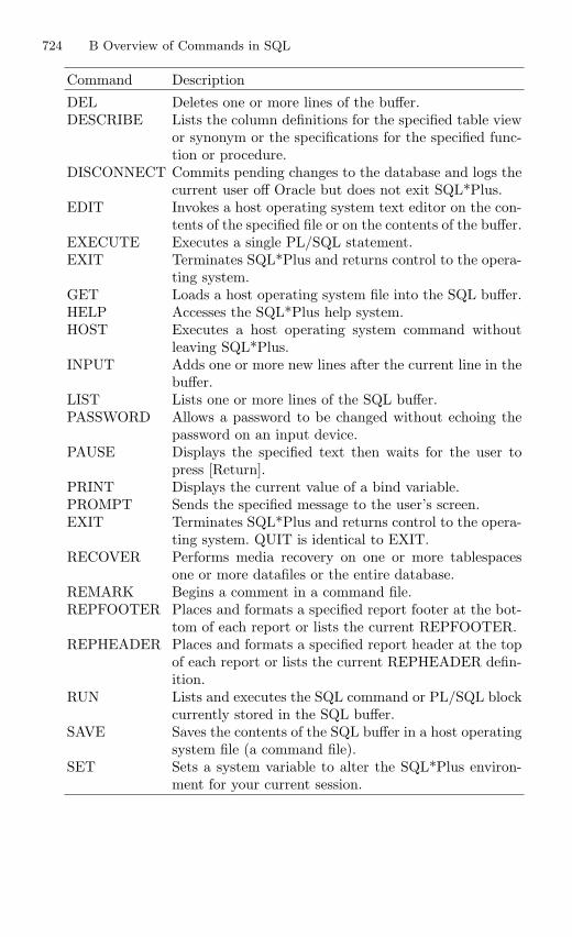
724 B Overview of Commands in SQL
Command Description
DEL Deletes one or more lines of the buffer.DESCRIBE Lists the column definitions for the specified table view
or synonym or the specifications for the specified func-tion or procedure.
DISCONNECT Commits pending changes to the database and logs thecurrent user off Oracle but does not exit SQL*Plus.
EDIT Invokes a host operating system text editor on the con-tents of the specified file or on the contents of the buffer.
EXECUTE Executes a single PL/SQL statement.EXIT Terminates SQL*Plus and returns control to the opera-
ting system.GET Loads a host operating system file into the SQL buffer.HELP Accesses the SQL*Plus help system.HOST Executes a host operating system command without
leaving SQL*Plus.INPUT Adds one or more new lines after the current line in the
buffer.LIST Lists one or more lines of the SQL buffer.PASSWORD Allows a password to be changed without echoing the
password on an input device.PAUSE Displays the specified text then waits for the user to
press [Return].PRINT Displays the current value of a bind variable.PROMPT Sends the specified message to the user’s screen.EXIT Terminates SQL*Plus and returns control to the opera-
ting system. QUIT is identical to EXIT.RECOVER Performs media recovery on one or more tablespaces
one or more datafiles or the entire database.REMARK Begins a comment in a command file.REPFOOTER Places and formats a specified report footer at the bot-
tom of each report or lists the current REPFOOTER.REPHEADER Places and formats a specified report header at the top
of each report or lists the current REPHEADER defin-ition.
RUN Lists and executes the SQL command or PL/SQL blockcurrently stored in the SQL buffer.
SAVE Saves the contents of the SQL buffer in a host operatingsystem file (a command file).
SET Sets a system variable to alter the SQL*Plus environ-ment for your current session.
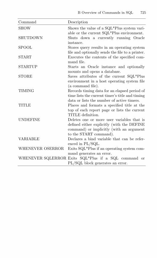
B Overview of Commands in SQL 725
Command Description
SHOW Shows the value of a SQL*Plus system vari-able or the current SQL*Plus environment.
SHUTDOWN Shuts down a currently running Oracleinstance.
SPOOL Stores query results in an operating systemfile and optionally sends the file to a printer.
START Executes the contents of the specified com-mand file.
STARTUP Starts an Oracle instance and optionallymounts and opens a database.
STORE Saves attributes of the current SQL*Plusenvironment in a host operating system file(a command file).
TIMING Records timing data for an elapsed period oftime lists the current timer’s title and timingdata or lists the number of active timers.
TITLE Places and formats a specified title at thetop of each report page or lists the currentTITLE definition.
UNDEFINE Deletes one or more user variables that isdefined either explicitly (with the DEFINEcommand) or implicitly (with an argumentto the START command).
VARIABLE Declares a bind variable that can be refer-enced in PL/SQL.
WHENEVER OSERROR Exits SQL*Plus if an operating system com-mand generates an error.
WHENEVER SQLERROR Exits SQL*Plus if a SQL command orPL/SQL block generates an error.
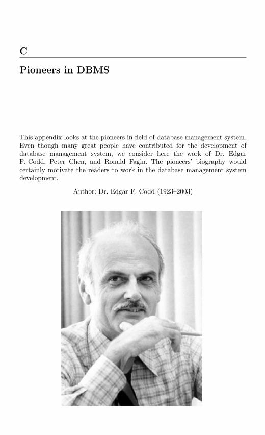
C
Pioneers in DBMS
This appendix looks at the pioneers in field of database management system.Even though many great people have contributed for the development ofdatabase management system, we consider here the work of Dr. EdgarF. Codd, Peter Chen, and Ronald Fagin. The pioneers’ biography wouldcertainly motivate the readers to work in the database management systemdevelopment.
Author: Dr. Edgar F. Codd (1923–2003)
728 C Pioneers in DBMS
C.1 About Dr. Edgar F. Codd
Ted Codd was a genuine computing pioneer. He was also an inspiration toall of us who had the fortune to know him and work with him. He beganhis career in 1949 as a programming mathematician for IBM on the SelectiveSequence Electronic Calculator. He subsequently participated in the devel-opment of several important IBM products, including its first commercialelectronic computer (IBM 701) and the STRETCH machine, which led toIBM’s 7090 mainframe technology. Then, in the 1960s, he turned his atten-tion to the problem of managing large commercial databases – and over thenext few years he created, single handed, the invention with which his namewill forever be associated: the relational model of data.
The relational model is widely recognized as one of the great technicalinnovations of the twentieth century. Codd described it and explored itsimplications in a series of research papers – staggering in their origina-lity – which he published throughout the period 1969–1979. The effect of thosepapers was twofold: they changed for good the way the Information Technol-ogy (IT) world (including the academic component of that world in particular)perceived the database management problem; and they laid the foundationfor an entire new industry, the relational database industry, now worth manybillions of dollars a year. In fact, not only did Codd’s relational model set theentire discipline of database management on a solid scientific footing, but italso formed the basis for a technology that has had, and continues to have,a major impact on the very fabric of our society. It is no exaggeration to saythat Ted Codd is the intellectual father of the modern database field.
Codd’s supreme achievement with the relational model should not beallowed to eclipse the fact that he made major original contributions in severalother important areas as well, including multiprogramming, natural languageprocessing, and more recently Enterprise Delta (a relational approach to busi-ness rules management), for which he and his wife were granted a US patent.The depth and breadth of his contributions were recognized by the long list ofhonors and elected positions that were conferred on him during his lifetime:including IBM Fellow, elected ACM Fellow, elected Fellow of the Britain Com-puter Society, elected member of the National Academy of Engineering, andelected member of the American Academy of Arts and Sciences. In 1981 he re-ceived the ACM Turing Award, the most prestigious award in the field of Com-puter Science. He also received an outstanding recognition award from IEEE:the very first annual achievement award from the international DB2 UsersGroup, and another annual achievement award from DAMA in 2001. Com-puterworld, in celebration of the 25th anniversary of its publication, selectedhim as one of 25 individuals in or related to the field of computing who havehad the most effect on our society. And Forbes magazine, which in December2002 published a list of the most important innovations and contributionsfor each of the 85 years of its existence, was selected for the year 1970 therelational model of data by E.F. Codd.
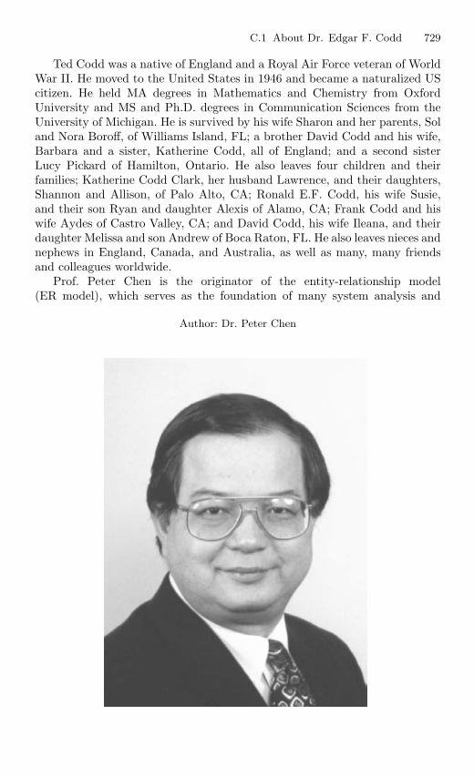
C.1 About Dr. Edgar F. Codd 729
Ted Codd was a native of England and a Royal Air Force veteran of WorldWar II. He moved to the United States in 1946 and became a naturalized UScitizen. He held MA degrees in Mathematics and Chemistry from OxfordUniversity and MS and Ph.D. degrees in Communication Sciences from theUniversity of Michigan. He is survived by his wife Sharon and her parents, Soland Nora Boroff, of Williams Island, FL; a brother David Codd and his wife,Barbara and a sister, Katherine Codd, all of England; and a second sisterLucy Pickard of Hamilton, Ontario. He also leaves four children and theirfamilies; Katherine Codd Clark, her husband Lawrence, and their daughters,Shannon and Allison, of Palo Alto, CA; Ronald E.F. Codd, his wife Susie,and their son Ryan and daughter Alexis of Alamo, CA; Frank Codd and hiswife Aydes of Castro Valley, CA; and David Codd, his wife Ileana, and theirdaughter Melissa and son Andrew of Boca Raton, FL. He also leaves nieces andnephews in England, Canada, and Australia, as well as many, many friendsand colleagues worldwide.
Prof. Peter Chen is the originator of the entity-relationship model(ER model), which serves as the foundation of many system analysis and
Author: Dr. Peter Chen
730 C Pioneers in DBMS
design methodologies, computer-aided software engineering (CASE) tools,and repository systems including IBM’s Repository Manager/MVS andDEC’s CDD/Plus. After years of efforts of many people in developingand implementing the ideas, now “entity-relationship model (ER model),”“entity-relationship diagram (ER diagram),” and “Peter Chen” have becomecommonly used terms in “online” dictionaries, books, articles, web pages,course syllabi, and commercial product brochures.
Dr. Peter Chen’s original paper on the ER model is one of the most citedpapers in the computer software field. Prof. Peter Chen was honored by theselection of his original ER model paper as one of the 38 most influentialpapers in Computer Science. Based on one particular citation database,Chen’s paper is the 35th most cited article in Computer Science. It is thefourth most downloaded paper from the ACM Digital Library in January2005 (Communications of ACM, March 2005).
The ER model was adopted as the metamodel for the American NationalStandards Institute (ANSI) Standard in Information Resource Directory Sys-tem (IRDS), and the ER approach has been ranked as the top methodologyfor database design and one of the top methodologies in systems developmentby several surveys of FORTUNE 500 companies.
Dr. Chen’s work is a cornerstone of software engineering, in particularCASE. In the late 1980s and early 1990s, IBM’s Application DevelopmentCycle (AD/Cycle) framework and DB2 repository (RM/MVS) were based onthe ER model. Other vendors’ repository systems such as Digital’s CDD+were also based on the ER model. Prof. Chen has made significant impacton the CASE industry by his research work and by his lecturing around theworld on structured system development methodologies. Most of the majorCASE tools including Computer Associates’ ERWIN, Oracle’s Designer/2000,and Sybase’s PowerDesigner (and even a general drawing tool like Microsoft’sVISIO) are influenced by the ER model.
The ER model also serves as the foundation of some of the recent workon object-oriented analysis and design methodologies and Semantic Web. TheUML modeling language has its roots in the ER model.
The hypertext concept, which makes the World Wide Web extremely pop-ular, is very similar to the main concept in the ER model. Dr. Peter Chenis currently investigating this linkage as an invited expert of several XMLworking groups of the World Wide Web Consortium (W3C).
Prof. Peter Chen’s work is cited heavily in a book published in 1993 forgeneral public called Software Challenges published by Time-Life Books as apart of the series on “Understanding Computers.”
Dr. Chen is a Fellow of the IEEE, the ACM, and the AAAS. He is amember of the European Academy of Sciences. He has been listed in Who’sWho in America and Who’s Who in the World for more than 15 years. He isthe recipient of prestigious awards in several fields of IT: data management,information management, software engineering, and general informationscience/technology:
C.1 About Dr. Edgar F. Codd 731
– The Data Resource Management Technology Award from the DataAdministration Management Association (NYC) in 1990.
– The Achievement Award in Information Management in 2000 from DAMAInternational, an international professional organization of data manage-ment professionals, managers, and Chief Information Officers (CIOs).Dr. E.F. Codd (the inventor of the relational data model) is the winnerof the same award in 2001.
– Inductee, the Data Management Hall of Fame in 2000.– The Stevens Award in Software Method Innovation in 2001, and the award
was presented at IEEE International Conference on Software Maintenancein Florence, Italy on 8 November 2001.
– The IEEE Harry Goode Award at the IEEE-CS Board of Governors Meet-ing in San Diego, February 2003. The previous winners of the Harry GoodeAward include the inventors of computers, core memory, and semiconduc-tors.
– The ACM/AAAI Allen Newell Award at the ACM Award Banquet inSan Diego, June 2003. He was introduced at the opening ceremony in the2003 International Joint Conference on Artificial Intelligence (IJACI-03)on 11 August 2003 in Acapulco, Mexico. The previous seven winners ofthe Allen Newell Award include a Nobel Prize and National Medal ofScience winner, two National Medal of Technology winners (one of them isalso an ACM Turing Award winner), and other very distinguished scien-tists who either have made significant contributions to several disciplinesin computer science or have bridged computer science with other disci-plines.
– The Pan Wen-Yuan Outstanding Research Award in 2004. Starting 1997,the awards have been given to usually three individuals each year (onein Taiwan, one in Mainland China, and one in “overseas” – outside ofTaiwan and Mainland China) in the high-tech fields (including elec-tronics, semiconductors, telecommunications, computer science, computerhardware/software, IT, and IS). In 2003, the overseas winner was Prof.Andrew C.C. Yao of Princeton University, who is also a winner of theACM Turing Award.
Dr. Peter Chen was recognized as a “software pioneer” in the “SoftwarePioneers” Conference, Bonn, Germany, 27–28 June 2001, together with agroup of very distinguished scientists including winners of President’s Medalsof Technology, ACM Turing Awards, ACM/AAAI Allen Newell Awards, orIEEE distinguished awards such as Harry Goode Awards. The streamed videoand slides of the talks in the “Pioneers” Conference may be available at theconference website. All the speeches in the conference are documented in abook (with four DVDs) published by Springer, and how to order the book canbe found in the section on Papers Online.
Prof. Peter Chen is a member of the Advisory Committee of the Computerand Information Science and Engineering (CISE) Directorate of the National
732 C Pioneers in DBMS
Science Foundation (NSF). He was a member of the Airlie Software Coun-cil, which consists of software visionaries/gurus and very-high-level softwareorganization executives, organized by US Department of Defense (DoD). Hewas an advisor to the President of Taiwan’s largest R&D organization, Indus-trial Technology Research Institute (ITRI), with over 6,000 employees, whichhas been the driving force of Taiwan’s high-tech growth in the past threedecades.
Dr. Peter Chen was one of five main US delegates to participate in thefirst IEEE USA–China International Conference, which was held in Beijing,in 1984 and to meet with PRC leaders and government officers in the Scienceand Technology fields and the Education area. Since 1984, he has been anHonorary Professor of Huazhong University of Science and Technology inWuhan, China.
Dr. Peter Chen is also the Editor-in-Chief of Data & Knowledge Engi-neering, the Associate Editor for the Journal of Intelligent Robotic Systems,Electronic Government, and other journals. In the past, he was the AssociateEditor for IEEE Computer, Information Sciences, and other journals.
At MIT, UCLA, and Harvard, Prof. Peter Chen taught various courses inInformation Systems and Computer Science. At LSU, he has been doingresearch and teaching on Information Modeling, Software Engineering,Data/Knowledge Engineering, Object-Oriented Programming, Internet/Web,Java, XML, Data Warehousing, E-commerce (B2B and B2C), HomelandSecurity, Identity Theft, System Architecture, Digital Library, and IntelligentSystems for Networking (Sensors Networks, Wi-Fi, and Cellular).
Prof. Peter Chen is the Principal Investigator of a large NSF-funded mul-tidisciplined project on profiling of terrorists and malicious cyber transac-tions for counter terrorisms and crimes. Dr. Peter Chen is also the ExecutiveDirector of the China–US Million Book Project (funded by NSF through CMUand the Ministry of Education of PRC), which is in the process of creatinga large digital library of over one million books in English and Chinese. Hehas been the Principal Investigator of various research projects in systemarchitecture, information/knowledge management, software engineering, andperformance analysis sponsored by many government agencies and commer-cial companies.
Dr. Peter Chen holds the position of M.J. Foster Distinguished Chair Pro-fessor of Computer Science in Louisiana State University since 1983.
Charles W. Bachman attended Michigan State College and graduated in1948 with a Bachelor’s degree in Mechanical Engineering (Tau Beta Phi). Hegraduated in 1950 with a Master’s degree in Mechanical Engineering fromUniversity of Pennsylvania. He attended Wharton School of Business in theUniversity of Pennsylvania at the same time and completed three quarters ofthe requirements for an MBA.
He worked for the Dow Chemical Company in Midland Michigan. Hestarted in Engineering Department working on engineering economics prob-lems (operation research). In 1962 he transferred to the Finance Department
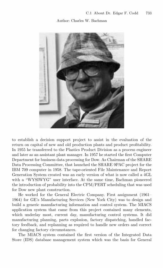
C.1 About Dr. Edgar F. Codd 733
Author: Charles W. Bachman
to establish a decision support project to assist in the evaluation of thereturn on capital of new and old production plants and product profitability.In 1955 he transferred to the Plastics Product Division as a process engineerand later as an assistant plant manager. In 1957 he started the first ComputerDepartment for business data processing for Dow. As Chairman of the SHAREData Processing Committee, that launched the SHARE 9PAC project for theIBM 709 computer in 1958. The tape-oriented File Maintenance and ReportGeneration System created was an early version of what is now called a 4GLwith a “WYSIWYG” user interface. At the same time, Bachman pioneeredthe introduction of probability into the CPM/PERT scheduling that was usedfor Dow new plant construction.
He worked for the General Electric Company. First assignment (1961–1964) for GE’s Manufacturing Services (New York City) was to design andbuild a generic manufacturing information and control system. The MIACSapplication system that came from this project contained many elements,which underlay most, current day, manufacturing control systems. It didmanufacturing planning, parts explosion, factory dispatching, handled fac-tory feedback, and replanning as required to handle new orders and correctfor changing factory circumstances.
The MIACS system contained the first version of the Integrated DataStore (IDS) database management system which was the basis for General
734 C Pioneers in DBMS
Electrics IDS and IDS II, Cullinet’s IDMS, and a host of other DBMS basedon Bachman’s Network Data Model. IDS was the first disk-based databasemanagement system used in production. It seized a number of new oppor-tunities available at that time and created a unique product. It was builtupon a “virtual memory” system that was being applied to the storage andretrieval of dynamic and permanent data. It provided a page-turning buffermanagement system that provided almost instantaneous access to the datamost recently accessed. It provided for the declaration and processing dataorganized in application-specific network structures. It fully integrated its,record-at-a-time, STORE, RETRIEVE, MODIFY, and DELETE languagestatements into the GE GECOM programming language. IDS created a newparadigm for the application programmers. It changed their I/O vantage pointfrom data fowing “IN and OUT of the program” to the program moving “INand OUT of the database.” Once a record was stored, it remained available inthe database, forever, unless it was explicitly deleted. IDS was characterizedas a “network model” database management system, because it provided forthe direct construction and navigation of the semantic graphs that underliemost business applications systems.
The MIACS system also contained a transaction-oriented operating systemthat accepted the input of new “problem control cards,” with their associateddata cards, and stored them until they could be dispatched. It dispatched eachsuch problem in priority sequence, following the completion of the prior prob-lem. It loaded the required program blocks into the buffer area, allocated allunneeded buffer blocks to the IDS page-turning system, and then dispatchedthe computer to the program. The solving of one problem might engender thecreation of one or more new problem statements with their associated datarecords. The storage and retrieval of problem statements and their associateddata were handled by the IDS database management system, along with allof the application requirements.
Bachman developed data structure diagrams (ER diagrams), commonlyknown as Bachman diagrams, as a graphical representation of semantic struc-tures within the data.
In 1964, Bachman transferred to GE’s Computer Department in Phoenix,Arizona with assignment to convert the GE 225 version of IDS to a commercialproduct for GE’s 400 and 600 computer lines. At the same time, Bachmanworked with the ANSI SPARC Study Group on DBMS, in creating theirreport of Network Databases. This task group was responsible for creatingthe specification for the integration of IDS into the COBOL programminglanguage. This report formed the basis for GE’s IDS II and many other DBMSbased on the specification.
Later Bachman started the GE-Weyerhaeuser project team that createdfirst “nonstop” operating system (WEYCOS) for the GE 600 computer. Thisteam also created the first multiprogramming version of IDS, which allowedmany programs to access to a common database with transparent locking,deadlock (interference) detection, recovery, and restart.
C.1 About Dr. Edgar F. Codd 735
Bachman developed a database-oriented version (dataBASIC) of theBASIC programming language. Its integrated database facility was based onthe “universal relation” concept (before the concept was formerly described).The product was shipped for both the GE 400 and 600 product lines. TheCity of Tulsa, OK used dataBASIC to construct their public safety and policesystem.
Honeywell Information Systems, Inc. acquired the General Electric’s Com-puter Division. Bachman’s first assignment was to manage a group to specifyand implement a version of IDS for Honeywell’s advanced product line, to bebuilt by the newly merged company. In 1973 Bachman transferred to Honey-well’s Advanced System Project as Chief Staff Engineer.
He has given the Association of Computer Machinery’s Alan M. TuringAward in 1973 for pioneering work in database management systems. TheTuring Award is the software industry’s equivalent of the Nobel Prize. The1973 Turing Lecture by Bachman was entitled “The Programmer as Naviga-tor.” He published the “extended network” data model in 1973.
He served as Vice Chairman with the ANSI SPARC’s Study Group onDBMS, to explore the possible standardization database management lan-guages. Group report spelled out the first architectural statement about thevarious interfaces and protocols required to support the data independenceconcept and established what is now broadly known as the “three schemaapproach.” He elected a “Distinguished Fellow” of the British ComputerSociety in 1978 for database research. Only 22 people have been so honoredtoday. He published the “role” data model in 1978.
He began work in 1976 as leader of Honeywell’s Distributed System Archi-tecture Project. This work served as the prototype of the later ANSI SPARCStudy Group – Distributed System Architecture and the International Stan-dard Organization’s (ISO) Open System Interconnection Project. He becameChairman of the ANSI Study Group in 1978 and Chairman of the ISO OpenSystems Interconnection Subcommittee in 1979.
In 1980 he began working on concepts more recently called computer-aidedsoftware engineering. He was awarded 16 US patents while at Honeywell fordatabase inventions and one British patent for pioneering work on model-driven development (executable functional specifications).
In Cullinane (Cullinet) Database Systems, he joined Cullinet as Vice Presi-dent of Product Management, while retaining responsibility as Chairman forthe ISO Open Systems Interconnection Subcommittee. He also continued workon prototype CASE systems. Cullinet’s IDMS system is a direct copy ofBachman’s original IDS DBMS. During the 2 years with Cullinet, the roledata model, which had been developed at Honeywell, was enhanced to facili-tate its integration with the existing Cullinet IDMS software. The result wasthe “Partnership” Data Model which was published in 1983 and which wasawarded a software patent in the US.
Bachman Information Systems, Inc. was created on 1 April 1983 to pro-ductize the CASE concepts, which had been developed while at Honeywell
736 C Pioneers in DBMS
and Cullinet. Key concepts’ use included the establishment of a clear sepa-ration between the specification of the business level (logical) rules charac-terized as the business model and the specification of the physical level rulescharacterized by existing database languages, communication languages, andprogramming languages.
This distinction between logical and physical levels became very importantas the implementation rules from existing COBOL, PL/I, IDMS, IMS, andRelational DBMS could be “reverse engineered” into an enhanced data modelbased on the Partnership Data Model, extended with some object-orientedconcepts.
Bachman Information Systems received it first round of venture capitalfunding in 1986, and after several additional rounds went public in 1990.Bachman Information Systems did business on a worldwide basis and washighly respected for its products supporting data modeling and databaseadministrator professionals. In this period, a number of patents were awardedto Bachman Information Systems dealing with aspects of the CASE products.Mr. Bachman was a co-inventor on six of these.
Bachman Information Systems, Inc. of Boston, MA and Cadre Technology,Inc. of Providence, RI merged to form a new company, named “Cayenne Soft-ware, Inc.” Bachman and Cadre developed and marketed similar products,i.e., CAD/CAM products to help the software professionals in carryingout their tasks. The largest difference in the two former companies isthat Bachman marketed its products to the commercial market and Cadremarketed theirs to the engineering/scientific market.
In June 1996, Charlie was given a Life Achievement Award by the Massa-chusetts Software Council. In August 1996, he and his wife, Connie, moved toTucson, Arizona. In the fall of 1997, Charlie was showcased as one of the“wizards” in the Association of Computer Machinery and The ComputerMuseums exhibition, “The Wizards and Their Wonders.” This was a photo-graphic exhibit and its contents were published in a book of the same name.That same fall, Mr. Bachman retired as an employee and the Chairman of theBoard of Cayenne Software (formerly Bachman Information Systems) after14 years service.
Mr. Bachman lives with his wife of 52 years, Connie Hadley, and continueshis consulting work. He has worked on metamodeling and software engineer-ing projects with Constellar Corp. and The Webvan Group. He is currentlyworking on the story of the development of IDS.
C.2 Ronald Fagin
Ronald Fagin’s article: “A normal form for relational databases that is basedon domains and keys” published in ACM Transactions on Database Systems(volume 6, issue 3, September 1981).

C.2 Ronald Fagin 737
C.2.1 Abstract of Ronald Fagin’s Article
A new normal form for relational databases, called “domain–key normal form(DK/NF),” is defined. Also, formal definitions of insertion anomaly and dele-tion anomaly are presented. It is shown that a schema is in DK/NF if and onlyif it has no insertion or deletion anomalies. Unlike previously defined normalforms, DK/NF is not defined in terms of traditional dependencies (functional,multivalued, or join). Instead, it is defined in terms of the more primitiveconcepts of domain and key, along with the general concept of a “constraint.”We also consider how the definitions of traditional normal forms might bemodified by taking into consideration, for the first time, the combinatorialconsequences of bounded domain sizes. It is shown that after this modifica-tion, these traditional normal forms are all implied by DK/NF. In particular,if all domains are infinite, then these traditional normal forms are all impliedby DK/NF.
D
Popular Commercial DBMS
Some of the popular commercial DBMS like System R, DB2, and Informix,their features and applications are given in this appendix.
D.1 System R
D.1.1 Introduction to System R
SYSTEM R is a Database Management System which implements theconcept of Relational Data Architecture. It is introduced by Codd in 1970as an approach toward providing solution to various problems in databasemanagement systems. The system provides a high-level data independenceby isolating the end user as much as possible from underlying storage struc-tures. The system permits definition of a variety of relational views oncommon underlying data. Data control features are provided including autho-rization, integrity assertions, triggered transactions, a logging and recoverysubsystem, and facilities for maintaining data consistency in a shared-updateenvironment.
D.1.2 Keywords Used
Database
Database is an ordered collection of useful information in such a way thatstoring and retrieval of information is more easy, accurate, and much efficient.
Data Model
A data model is a collection of high-level data description constructs that hidemany low-level storage details.
740 D Popular Commercial DBMS
Relational Model
In this model a database is a collection of one or more relations, where eachrelation is a table with rows and columns.
The main construct for representing data in the relational model is arelation. A relation consists of a relation schema and a relation instance.The relation instance is a table, and the relation schema describes the columnheads for the table.
RSI
It is the abbreviation of Relational Storage Interface. It is the external inter-face which handles access to single tuples of base relations.
RSS
It is the abbreviation of Relational Storage System. It is a complete storagesubsystem of RSI. It manages devices, space allocation, storage buffers,transaction consistency and locking, deadlock detection, back out, transactionrecovery, system recovery and it maintains indexes on selected fields of baserelations, and pointer chains across relations.
RDI
It is the abbreviation of Relational Data Interface. It is the external interfacewhich can be called directly from a programming language, or used to supportvarious emulators and other interfaces.
RDS
It is the abbreviation of Relational Data System. It supports RDI, providesauthorization, integrity enforcement, and support for alternative views ofdata.
D.1.3 Architecture and System Structure
Architecture and system structure includes major interfaces and componentsas illustrated in Fig. D.1. They are:
1. RSI (Relational Storage Interface)2. RDI (Relational Data Interface)3. SEQUEL4. VM (Virtual Machines)
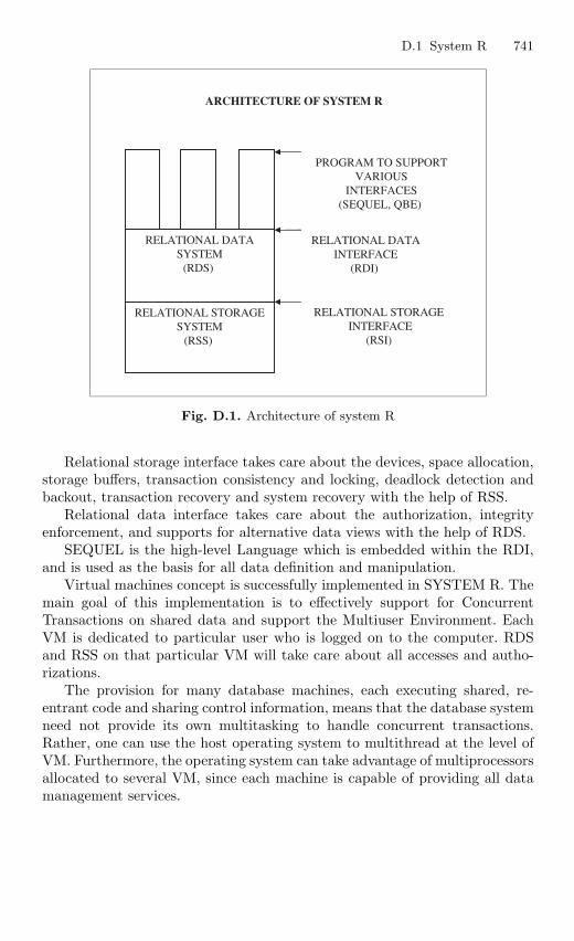
D.1 System R 741
RELATIONAL DATASYSTEM
(RDS)
RELATIONAL STORAGE INTERFACE
(RSI)
RELATIONAL DATAINTERFACE
(RDI)
PROGRAM TO SUPPORTVARIOUS
INTERFACES(SEQUEL, QBE)
ARCHITECTURE OF SYSTEM R
RELATIONAL STORAGESYSTEM
(RSS)
Fig. D.1. Architecture of system R
Relational storage interface takes care about the devices, space allocation,storage buffers, transaction consistency and locking, deadlock detection andbackout, transaction recovery and system recovery with the help of RSS.
Relational data interface takes care about the authorization, integrityenforcement, and supports for alternative data views with the help of RDS.
SEQUEL is the high-level Language which is embedded within the RDI,and is used as the basis for all data definition and manipulation.
Virtual machines concept is successfully implemented in SYSTEM R. Themain goal of this implementation is to effectively support for ConcurrentTransactions on shared data and support the Multiuser Environment. EachVM is dedicated to particular user who is logged on to the computer. RDSand RSS on that particular VM will take care about all accesses and autho-rizations.
The provision for many database machines, each executing shared, re-entrant code and sharing control information, means that the database systemneed not provide its own multitasking to handle concurrent transactions.Rather, one can use the host operating system to multithread at the level ofVM. Furthermore, the operating system can take advantage of multiprocessorsallocated to several VM, since each machine is capable of providing all datamanagement services.
742 D Popular Commercial DBMS
D.1.4 Relational Data Interface
Query Facilities in RDI
Similar to other Database Sublanguages SEQUEL also provides most of thedata manipulation facilities as described earlier.
EXAMPLE 1:Consider the following block of query.SELECT NAMEFROM EMP
WHERE ID= ‘1234’;
Explanation
This is the simple query which will give the Names of the employees who havethe ID as 1234. This query has no problem in execution. It is efficient too.But consider the following Nested Query:
Example 2:SELECT NAMEFROM EMPWHERE SAL >SELECT SALFROM EMP
WHERE EMPNO = B1.MGR
Explanation
This query is formed by combining two simple queries. Experience has shownthat this block label notation has three disadvantages:
– It is not possible to select quantities from the inner block, such as: “Forall employee who earn more than their manager, list the employee’s nameand his manager’s name.”
– Since the query is asymmetrically expressed, the optimizer is biasedtoward making an outer loop for the first block and an inner loop for thesecond block. Since this may not be the optimum method for interpretingthe query, the optimization process is made difficult.
– Human factors studies have shown that the block label notation is hardfor nonprogrammers to learn.
Because of these disadvantages, the block label notation has been replacedby the following more symmetrical notation, which allows several tables to belisted in the FROM clause and optionally referred to by variable names.
D.1 System R 743
EXAMPLE 3:SELECT DNOFROM EMPWHERE JOB = ‘CLERK’GROUP BY DNOHAVING COUNT (*) > 10
Explanation
In the above block of statements three new terms are used they are GROUPBY, HAVING, and COUNT().
GROUP BY is used to grouping the selected tuples according to particularfield value.HAVING is used to select the tuples which satisfy the give condition formthe grouped tuples.COUNT will provide number of tuples in each group.
D.1.5 Data Manipulation Facilities in SEQUEL
The RDI facilities for insertion, deletion, and update of tuples are alsoprovided via the SEQUEL data sublanguage. SEQUEL can be used to mani-pulate either one tuple at a time or a set of tuples with a single command.The current tuple of a particular cursor may be selected for some operation bymeans of the special predicate CURRENT TUPLE OF CURSOR. The valuesof a tuple may be set equal to constants, or to new values computed from theirold values, or to the contents of a program variable suitably identified by aBIND command. These facilities will be illustrated by a series of examples.Since no result is returned to the calling program in these examples, no cursorname is included in the calls to SEQUEL.
EXAMPLE 4:CALL SEQUEL (‘UPDATE EMP SET SAL = SAL * 1.1
WHERE DNO = 50’);
Explanation
This command will update the salary value of the employees who are havingID as 50 to 1.1 times of his salary. This type of update is called as ORIENTEDUPDATE.
Example 5:CALL BIND (‘PVSAL’, ADDR (PVSAL));CALL SEQUEL (‘UPDATE EMP SET SAL = PVSAL WHERE
CURRENT TUPLE OF CURSOR C3’);
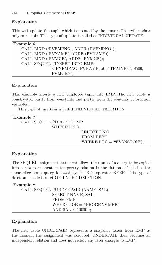
744 D Popular Commercial DBMS
Explanation
This will update the tuple which is pointed by the cursor. This will updateonly one tuple. This type of update is called as INDIVIDUAL UPDATE.
Example 6:CALL BIND (‘PVEMPNO’, ADDR (PVEMPNO));CALL BIND (‘PVNAME’, ADDR (PVNAME));CALL BIND (‘PVMGR’, ADDR (PVMGR));CALL SEQUEL (‘INSERT INTO EMP:
< PVEMPNO, PVNAME, 50, “TRAINEE”, 8500,PVMGR>’);
Explanation
This example inserts a new employee tuple into EMP. The new tuple isconstructed partly from constants and partly from the contents of programvariables.
This type of insertion is called INDIVIDUAL INSERTION.
Example 7:CALL SEQUEL (‘DELETE EMP
WHERE DNO =SELECT DNOFROM DEPTWHERE LOC = “EVANSTON”);
Explanation
The SEQUEL assignment statement allows the result of a query to be copiedinto a new permanent or temporary relation in the database. This has thesame effect as a query followed by the RDI operator KEEP. This type ofdeletion is called as set ORIENTED DELETION.
Example 8:CALL SEQUEL (‘UNDERPAID (NAME, SAL)
SELECT NAME, SALFROM EMPWHERE JOB = “PROGRAMMER”AND SAL < 10000’);
Explanation
The new table UNDERPAID represents a snapshot taken from EMP atthe moment the assignment was executed. UNDERPAID then becomes anindependent relation and does not reflect any later changes to EMP.
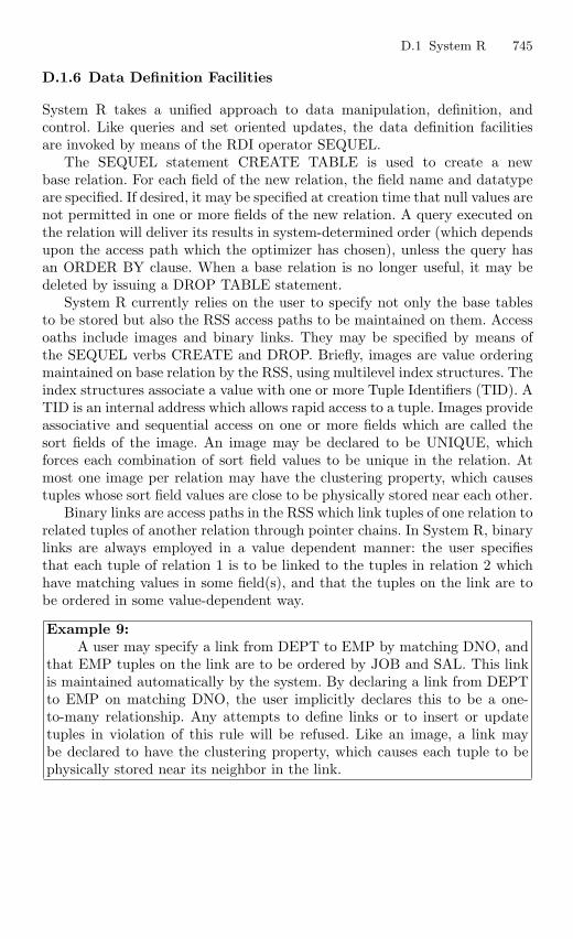
D.1 System R 745
D.1.6 Data Definition Facilities
System R takes a unified approach to data manipulation, definition, andcontrol. Like queries and set oriented updates, the data definition facilitiesare invoked by means of the RDI operator SEQUEL.
The SEQUEL statement CREATE TABLE is used to create a newbase relation. For each field of the new relation, the field name and datatypeare specified. If desired, it may be specified at creation time that null values arenot permitted in one or more fields of the new relation. A query executed onthe relation will deliver its results in system-determined order (which dependsupon the access path which the optimizer has chosen), unless the query hasan ORDER BY clause. When a base relation is no longer useful, it may bedeleted by issuing a DROP TABLE statement.
System R currently relies on the user to specify not only the base tablesto be stored but also the RSS access paths to be maintained on them. Accessoaths include images and binary links. They may be specified by means ofthe SEQUEL verbs CREATE and DROP. Briefly, images are value orderingmaintained on base relation by the RSS, using multilevel index structures. Theindex structures associate a value with one or more Tuple Identifiers (TID). ATID is an internal address which allows rapid access to a tuple. Images provideassociative and sequential access on one or more fields which are called thesort fields of the image. An image may be declared to be UNIQUE, whichforces each combination of sort field values to be unique in the relation. Atmost one image per relation may have the clustering property, which causestuples whose sort field values are close to be physically stored near each other.
Binary links are access paths in the RSS which link tuples of one relation torelated tuples of another relation through pointer chains. In System R, binarylinks are always employed in a value dependent manner: the user specifiesthat each tuple of relation 1 is to be linked to the tuples in relation 2 whichhave matching values in some field(s), and that the tuples on the link are tobe ordered in some value-dependent way.
Example 9:A user may specify a link from DEPT to EMP by matching DNO, and
that EMP tuples on the link are to be ordered by JOB and SAL. This linkis maintained automatically by the system. By declaring a link from DEPTto EMP on matching DNO, the user implicitly declares this to be a one-to-many relationship. Any attempts to define links or to insert or updatetuples in violation of this rule will be refused. Like an image, a link maybe declared to have the clustering property, which causes each tuple to bephysically stored near its neighbor in the link.
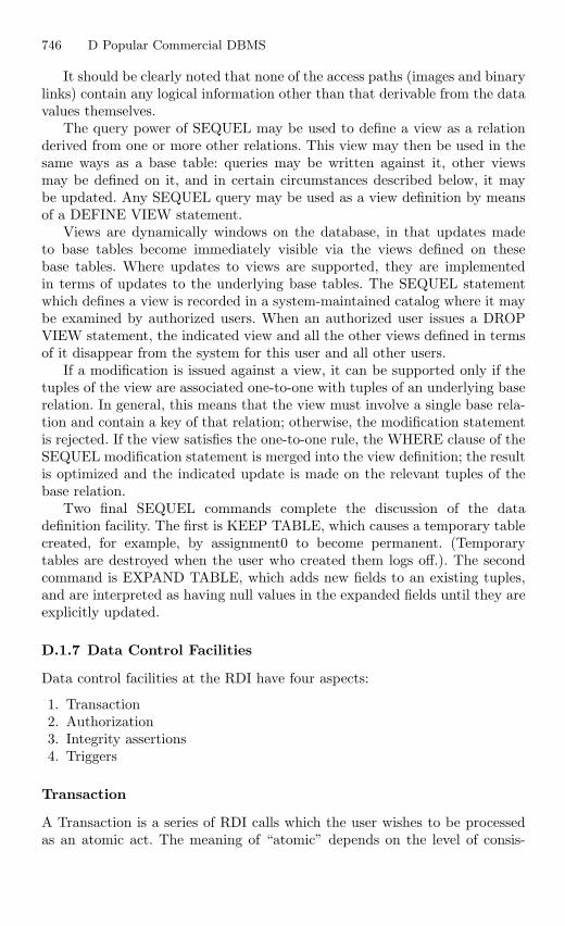
746 D Popular Commercial DBMS
It should be clearly noted that none of the access paths (images and binarylinks) contain any logical information other than that derivable from the datavalues themselves.
The query power of SEQUEL may be used to define a view as a relationderived from one or more other relations. This view may then be used in thesame ways as a base table: queries may be written against it, other viewsmay be defined on it, and in certain circumstances described below, it maybe updated. Any SEQUEL query may be used as a view definition by meansof a DEFINE VIEW statement.
Views are dynamically windows on the database, in that updates madeto base tables become immediately visible via the views defined on thesebase tables. Where updates to views are supported, they are implementedin terms of updates to the underlying base tables. The SEQUEL statementwhich defines a view is recorded in a system-maintained catalog where it maybe examined by authorized users. When an authorized user issues a DROPVIEW statement, the indicated view and all the other views defined in termsof it disappear from the system for this user and all other users.
If a modification is issued against a view, it can be supported only if thetuples of the view are associated one-to-one with tuples of an underlying baserelation. In general, this means that the view must involve a single base rela-tion and contain a key of that relation; otherwise, the modification statementis rejected. If the view satisfies the one-to-one rule, the WHERE clause of theSEQUEL modification statement is merged into the view definition; the resultis optimized and the indicated update is made on the relevant tuples of thebase relation.
Two final SEQUEL commands complete the discussion of the datadefinition facility. The first is KEEP TABLE, which causes a temporary tablecreated, for example, by assignment0 to become permanent. (Temporarytables are destroyed when the user who created them logs off.). The secondcommand is EXPAND TABLE, which adds new fields to an existing tuples,and are interpreted as having null values in the expanded fields until they areexplicitly updated.
D.1.7 Data Control Facilities
Data control facilities at the RDI have four aspects:
1. Transaction2. Authorization3. Integrity assertions4. Triggers
Transaction
A Transaction is a series of RDI calls which the user wishes to be processedas an atomic act. The meaning of “atomic” depends on the level of consis-
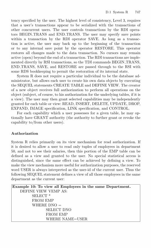
D.1 System R 747
tency specified by the user. The highest level of consistency, Level 3, requiresthat a user’s transactions appear to be serialized with the transactions ofother concurrent users. The user controls transactions by the RDI opera-tors BEGIN TRANS and END TRANS. The user may specify save pointswithin a transaction by the RDI operator SAVE. As long as a transac-tion is active, the user may back up to the beginning of the transactionor to any internal save point by the operator RESTORE. This operatorrestores all changes made to the data transaction. No cursors may remainactive (open) beyond the end of a transaction. The RDI transactions are imple-mented directly by RSI transactions, so the TDI commands BEGIN TRANS,END TRANS, SAVE, and RESTORE are passed through to the RSI withsome RDS bookkeeping to permit the restoration of its internal state.
System R does not require a particular individual to be the database ad-ministrator, but allows each user to create his own data objects by executingthe SEQUEL statements CREATE TABLE and DEFINE VIEW. The creatorof a new object receives full authorization to perform all operations on theobject (subject, of course, to his authorization for the underlying tables, if it isa view). The user may then grant selected capabilities may be independentlygranted for each table or view: READ, INSERT, DELETE, UPDATE, DROP,EXPAND, IMAGE specification, LINK specification, and CONTROL.
For each capability which a user possesses for a given table, he may op-tionally have GRANT authority (the authority to further grant or revoke thecapability to/from other users).
Authorization
System R relies primarily on its view mechanism for read authorization. Ifit is desired to allow a user to read only tuples of employees in department50, and not to see their salaries, then this portion of the EMP table can bedefined as a view and granted to the user. No special statistical access isdistinguished, since the same effect can be achieved by defining a view. Tomake the view mechanism more useful for authorization purposes, the reservedword USER is always interpreted as the user-id of the current user. Thus thefollowing SEQUEL statement defines a view of all those employees in the samedepartment as the current user:
Example 10: To view all Employees in the same Department.DEFINE VIEW VEMP AS:
SELECT *FROM EMPWHERE DNO =
SELECT DNOFROM EMPWHERE NAME=USER
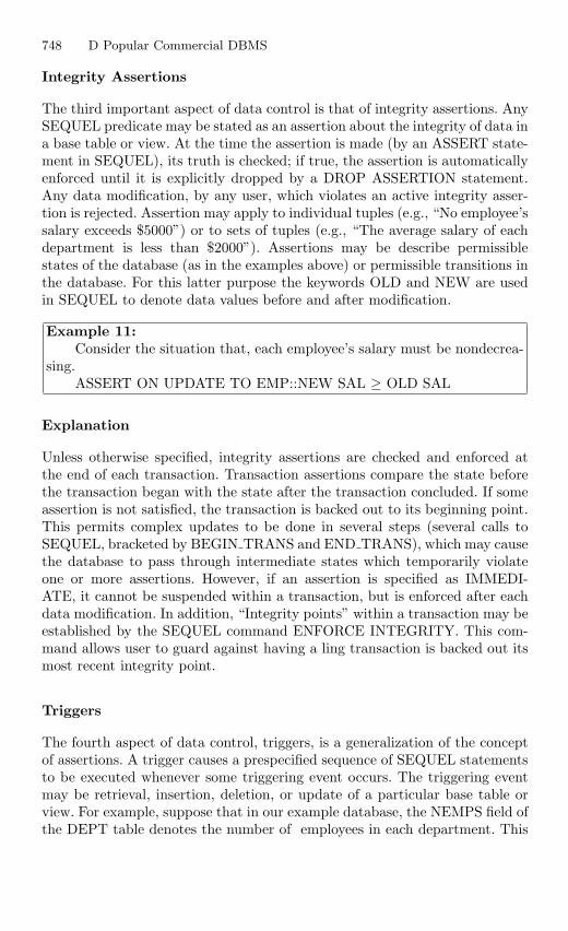
748 D Popular Commercial DBMS
Integrity Assertions
The third important aspect of data control is that of integrity assertions. AnySEQUEL predicate may be stated as an assertion about the integrity of data ina base table or view. At the time the assertion is made (by an ASSERT state-ment in SEQUEL), its truth is checked; if true, the assertion is automaticallyenforced until it is explicitly dropped by a DROP ASSERTION statement.Any data modification, by any user, which violates an active integrity asser-tion is rejected. Assertion may apply to individual tuples (e.g., “No employee’ssalary exceeds $5000”) or to sets of tuples (e.g., “The average salary of eachdepartment is less than $2000”). Assertions may be describe permissiblestates of the database (as in the examples above) or permissible transitions inthe database. For this latter purpose the keywords OLD and NEW are usedin SEQUEL to denote data values before and after modification.
Example 11:Consider the situation that, each employee’s salary must be nondecrea-
sing.ASSERT ON UPDATE TO EMP::NEW SAL ≥ OLD SAL
Explanation
Unless otherwise specified, integrity assertions are checked and enforced atthe end of each transaction. Transaction assertions compare the state beforethe transaction began with the state after the transaction concluded. If someassertion is not satisfied, the transaction is backed out to its beginning point.This permits complex updates to be done in several steps (several calls toSEQUEL, bracketed by BEGIN TRANS and END TRANS), which may causethe database to pass through intermediate states which temporarily violateone or more assertions. However, if an assertion is specified as IMMEDI-ATE, it cannot be suspended within a transaction, but is enforced after eachdata modification. In addition, “Integrity points” within a transaction may beestablished by the SEQUEL command ENFORCE INTEGRITY. This com-mand allows user to guard against having a ling transaction is backed out itsmost recent integrity point.
Triggers
The fourth aspect of data control, triggers, is a generalization of the conceptof assertions. A trigger causes a prespecified sequence of SEQUEL statementsto be executed whenever some triggering event occurs. The triggering eventmay be retrieval, insertion, deletion, or update of a particular base table orview. For example, suppose that in our example database, the NEMPS field ofthe DEPT table denotes the number of employees in each department. This
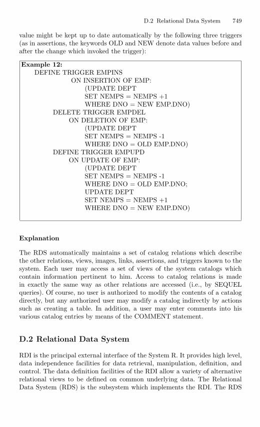
D.2 Relational Data System 749
value might be kept up to date automatically by the following three triggers(as in assertions, the keywords OLD and NEW denote data values before andafter the change which invoked the trigger):
Example 12:DEFINE TRIGGER EMPINS
ON INSERTION OF EMP:(UPDATE DEPTSET NEMPS = NEMPS +1WHERE DNO = NEW EMP.DNO)
DELETE TRIGGER EMPDELON DELETION OF EMP:
(UPDATE DEPTSET NEMPS = NEMPS -1WHERE DNO = OLD EMP.DNO)
DEFINE TRIGGER EMPUPDON UPDATE OF EMP:
(UPDATE DEPTSET NEMPS = NEMPS -1WHERE DNO = OLD EMP.DNO;UPDATE DEPTSET NEMPS = NEMPS +1WHERE DNO = NEW EMP.DNO)
Explanation
The RDS automatically maintains a set of catalog relations which describethe other relations, views, images, links, assertions, and triggers known to thesystem. Each user may access a set of views of the system catalogs whichcontain information pertinent to him. Access to catalog relations is madein exactly the same way as other relations are accessed (i.e., by SEQUELqueries). Of course, no user is authorized to modify the contents of a catalogdirectly, but any authorized user may modify a catalog indirectly by actionssuch as creating a table. In addition, a user may enter comments into hisvarious catalog entries by means of the COMMENT statement.
D.2 Relational Data System
RDI is the principal external interface of the System R. It provides high level,data independence facilities for data retrieval, manipulation, definition, andcontrol. The data definition facilities of the RDI allow a variety of alternativerelational views to be defined on common underlying data. The RelationalData System (RDS) is the subsystem which implements the RDI. The RDS
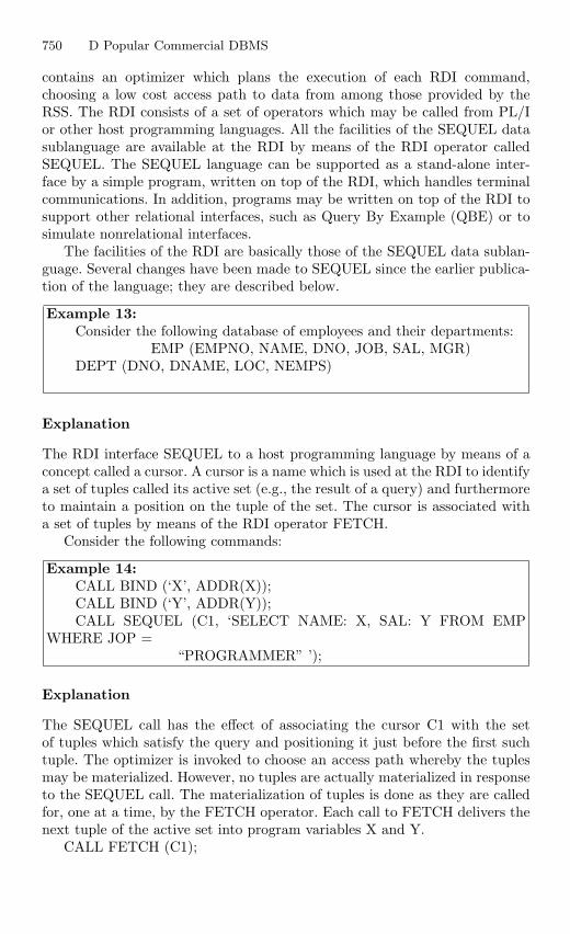
750 D Popular Commercial DBMS
contains an optimizer which plans the execution of each RDI command,choosing a low cost access path to data from among those provided by theRSS. The RDI consists of a set of operators which may be called from PL/Ior other host programming languages. All the facilities of the SEQUEL datasublanguage are available at the RDI by means of the RDI operator calledSEQUEL. The SEQUEL language can be supported as a stand-alone inter-face by a simple program, written on top of the RDI, which handles terminalcommunications. In addition, programs may be written on top of the RDI tosupport other relational interfaces, such as Query By Example (QBE) or tosimulate nonrelational interfaces.
The facilities of the RDI are basically those of the SEQUEL data sublan-guage. Several changes have been made to SEQUEL since the earlier publica-tion of the language; they are described below.
Example 13:Consider the following database of employees and their departments:
EMP (EMPNO, NAME, DNO, JOB, SAL, MGR)DEPT (DNO, DNAME, LOC, NEMPS)
Explanation
The RDI interface SEQUEL to a host programming language by means of aconcept called a cursor. A cursor is a name which is used at the RDI to identifya set of tuples called its active set (e.g., the result of a query) and furthermoreto maintain a position on the tuple of the set. The cursor is associated witha set of tuples by means of the RDI operator FETCH.
Consider the following commands:
Example 14:CALL BIND (‘X’, ADDR(X));CALL BIND (‘Y’, ADDR(Y));CALL SEQUEL (C1, ‘SELECT NAME: X, SAL: Y FROM EMP
WHERE JOP =“PROGRAMMER” ’);
Explanation
The SEQUEL call has the effect of associating the cursor C1 with the setof tuples which satisfy the query and positioning it just before the first suchtuple. The optimizer is invoked to choose an access path whereby the tuplesmay be materialized. However, no tuples are actually materialized in responseto the SEQUEL call. The materialization of tuples is done as they are calledfor, one at a time, by the FETCH operator. Each call to FETCH delivers thenext tuple of the active set into program variables X and Y.
CALL FETCH (C1);
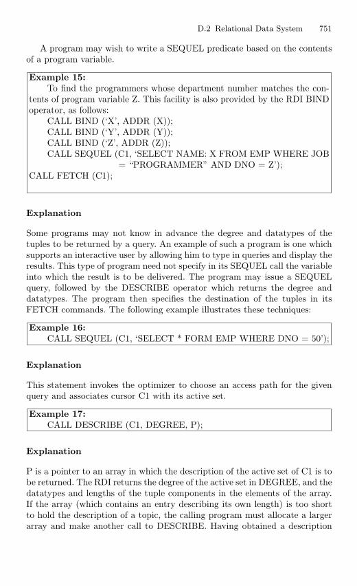
D.2 Relational Data System 751
A program may wish to write a SEQUEL predicate based on the contentsof a program variable.
Example 15:To find the programmers whose department number matches the con-
tents of program variable Z. This facility is also provided by the RDI BINDoperator, as follows:
CALL BIND (‘X’, ADDR (X));CALL BIND (‘Y’, ADDR (Y));CALL BIND (‘Z’, ADDR (Z));CALL SEQUEL (C1, ‘SELECT NAME: X FROM EMP WHERE JOB
= “PROGRAMMER” AND DNO = Z’);CALL FETCH (C1);
Explanation
Some programs may not know in advance the degree and datatypes of thetuples to be returned by a query. An example of such a program is one whichsupports an interactive user by allowing him to type in queries and display theresults. This type of program need not specify in its SEQUEL call the variableinto which the result is to be delivered. The program may issue a SEQUELquery, followed by the DESCRIBE operator which returns the degree anddatatypes. The program then specifies the destination of the tuples in itsFETCH commands. The following example illustrates these techniques:
Example 16:CALL SEQUEL (C1, ‘SELECT * FORM EMP WHERE DNO = 50’);
Explanation
This statement invokes the optimizer to choose an access path for the givenquery and associates cursor C1 with its active set.
Example 17:CALL DESCRIBE (C1, DEGREE, P);
Explanation
P is a pointer to an array in which the description of the active set of C1 is tobe returned. The RDI returns the degree of the active set in DEGREE, and thedatatypes and lengths of the tuple components in the elements of the array.If the array (which contains an entry describing its own length) is too shortto hold the description of a topic, the calling program must allocate a largerarray and make another call to DESCRIBE. Having obtained a description
752 D Popular Commercial DBMS
of the tuples to be returned, the calling program may proceed to allocate astructure to hold the tuples and may specify the location of this structure inits FETCH command:
Example 18:CALL FETCH (C1, Q);
Explanation
Q is a pointer to an array of pointers which specify where the individualcomponents of the tuple are to be delivered. If this “destination” parameter ispresent in a FETCH command, it overrides any destination which may havebeen specified in the SEQUEL command which defined the active set of C1.
A special RDI operator Open is provided as a shorthand method to asso-ciate a cursor with an entire relation. For example, the command:
Example 19:CALL OPEN (C1, ‘EMP’);is exactly equivalent toCALL SEQUEL (C1, ‘SELECT * FROM EMP’);
Explanation
The use of OPEN is slightly preferable to the use of SEQUEL to open a cursoron a relation, since OPEN avoids the use of the SEQUEL parser.
D.3 DB2
D.3.1 Introduction to DB2
DB2 is a strategic product from IBM. It is available on all of IBM’s keyplatforms. IBM’s Information Warehouse architecture employs DB2 as a keycomponent. DB2 is a relational database management system. The relationalmodel is founded on the mathematics of set theory, thereby providing a solidtheoretical base for the management of data. Relational databases are typi-cally easier to use and maintain than databases based on nonrelational tech-nology. An IBM relational database management system that is available asa licensed program on several operating systems. Programmers and users ofDB2 can create, access, modify, and delete data in relational tables using avariety of interfaces.
DB2’s foundation in the relational model also provides it with improveddata availability, data integrity, and data security because the relational modelrigorously defines as part of the database. Programmers and users of DB2 cancreate, access, modify, and delete data in relational tables using a varietyof interfaces. Because DB2 is a relational database management system, it is
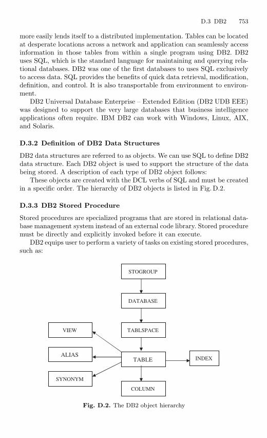
D.3 DB2 753
more easily lends itself to a distributed implementation. Tables can be locatedat desperate locations across a network and application can seamlessly accessinformation in those tables from within a single program using DB2. DB2uses SQL, which is the standard language for maintaining and querying rela-tional databases. DB2 was one of the first databases to uses SQL exclusivelyto access data. SQL provides the benefits of quick data retrieval, modification,definition, and control. It is also transportable from environment to environ-ment.
DB2 Universal Database Enterprise – Extended Edition (DB2 UDB EEE)was designed to support the very large databases that business intelligenceapplications often require. IBM DB2 can work with Windows, Linux, AIX,and Solaris.
D.3.2 Definition of DB2 Data Structures
DB2 data structures are referred to as objects. We can use SQL to define DB2data structure. Each DB2 object is used to support the structure of the databeing stored. A description of each type of DB2 object follows:
These objects are created with the DCL verbs of SQL and must be createdin a specific order. The hierarchy of DB2 objects is listed in Fig. D.2.
D.3.3 DB2 Stored Procedure
Stored procedures are specialized programs that are stored in relational data-base management system instead of an external code library. Stored proceduremust be directly and explicitly invoked before it can execute.
DB2 equips user to perform a variety of tasks on existing stored procedures,such as:
STOGROUP
DATABASE
TABLSPACE
COLUMN
TABLE INDEX
VIEW
ALIAS
SYNONYM
Fig. D.2. The DB2 object hierarchy
754 D Popular Commercial DBMS
ALIAS A locally defined name for a table or view in the same local DB2subsystems or in a remote DB2 subsystem.
COLUMN A single, nondecomposable data element in a DB2 table.DATABASE A logical grouping of DB2 objects related by common
characteristics such as logical functionality, relation to anapplication system or subsystem, or type of data.
INDEX A DB2 object that consist of one or more VSAM data sets.STOGROUP A series of DASD volumes assigned a unique name and used to
allocate VSAM data sets for DB2 objects.TABLE A DB2b object that consists of columns and rows that define the
physical characteristics of the data to be stored.TABLE SPACE A DB2 object that defines the physical structure of the data sets
used to house the DB2 table data.VIEW A virtual table consisting of a SQL SELECT statement that
accesses data from one or more tables or views.
– Viewing– Modifying– Running and testing– Copying and pasting stored procedures across connections– Building, in one step, stored procedures on target databases– Customizing settings to enable remote debugging of installed procedures.
Stored procedures run in a separate DB2 address space known as the storedprocedure address space. To execute a stored procedure, a program must issuethe SQL call statement. When the call is issued, the name of the stored proce-dure and its list of parameters are send to DB2. DB2 searches SYSIBM.SYSPROCEDURES for the appropriate row that 1 defines the stored procedureto be executed.
DB2 Stored Procedure Builder provides a single development environ-ment that supports multiple languages – including Java and SQL procedurelanguage – and the entire DB2 Universal DatabaseTM. DB2 Stored ProcedureBuilder can launch from the DB2 Program Group or from add-in menus onIBM VisualAge R© for Java, Microsoft R© Visual C++, and Microsoft VisualBasic. After start-up, the wizards in DB2 Stored Procedure Builder take userthrough each task, one step at a time. The first step is to define user project.Simply follow the wizards, which will ask user to provide a project name anddecide how user want to connect to the database. User also will be asked fora logon name and password. Once user project is defined, users are ready tocreate a new stored procedure or work on an existing one. Launching a newprocedure, The Stored Procedure Builder Project View window, gives usera picture of all users existing stored procedures and their connections. Thisis the window where user can select existing procedures for modification or,using the menu or toolbar command, create a new stored procedure.
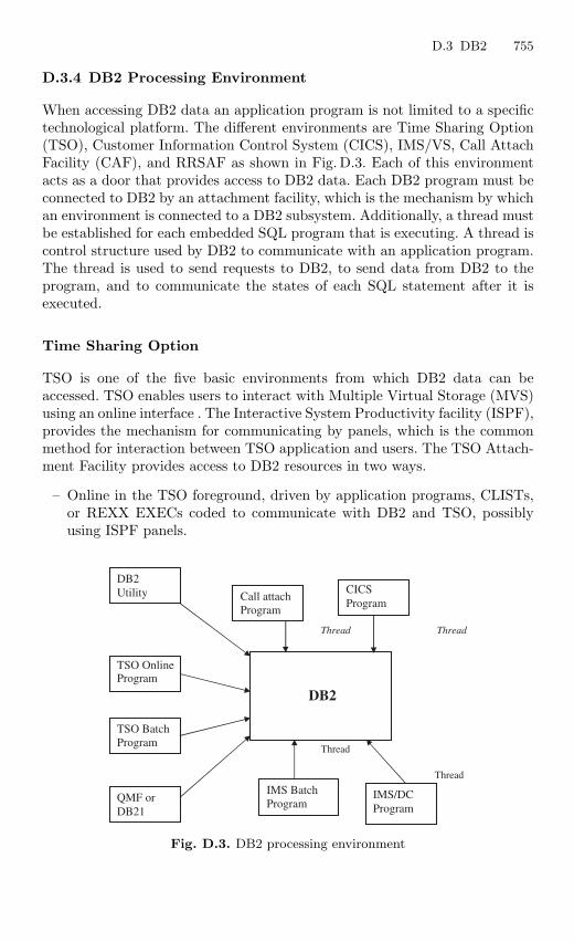
D.3 DB2 755
D.3.4 DB2 Processing Environment
When accessing DB2 data an application program is not limited to a specifictechnological platform. The different environments are Time Sharing Option(TSO), Customer Information Control System (CICS), IMS/VS, Call AttachFacility (CAF), and RRSAF as shown in Fig. D.3. Each of this environmentacts as a door that provides access to DB2 data. Each DB2 program must beconnected to DB2 by an attachment facility, which is the mechanism by whichan environment is connected to a DB2 subsystem. Additionally, a thread mustbe established for each embedded SQL program that is executing. A thread iscontrol structure used by DB2 to communicate with an application program.The thread is used to send requests to DB2, to send data from DB2 to theprogram, and to communicate the states of each SQL statement after it isexecuted.
Time Sharing Option
TSO is one of the five basic environments from which DB2 data can beaccessed. TSO enables users to interact with Multiple Virtual Storage (MVS)using an online interface . The Interactive System Productivity facility (ISPF),provides the mechanism for communicating by panels, which is the commonmethod for interaction between TSO application and users. The TSO Attach-ment Facility provides access to DB2 resources in two ways.
– Online in the TSO foreground, driven by application programs, CLISTs,or REXX EXECs coded to communicate with DB2 and TSO, possiblyusing ISPF panels.
Thread Thread
Thread
Thread
QMF orDB21
TSO OnlineProgram
TSO BatchProgram
IMS/DCProgram
IMS Batch Program
DB2
DB2Utility Call attach
Program
CICS Program
Fig. D.3. DB2 processing environment
756 D Popular Commercial DBMS
– In batch mode using the TSO Terminal Monitor Program, IKJEFT01 (orIKJEFT1B), to invoke the DSN command and run a DB2 applicationprogram.
Customer Information Control System
CICS is a teleprocessing monitor that enables programmers to develop online,translation-based programs. By means of Basic Mapping Support (BMS) andthe data communications facilities of CICS, programs can display formatteddata on screens and receive formatted data from users. When DB2 data areaccessed using CICS, multiple threads can be active simultaneously, givingmultiple users concurrent access to a DB2 subsystems of a single CICS region.
Information Management System
Information Management System (IMS) is IBM’s prerelational database man-agement system offering. It is based on the structuring of related data itemsin inverted tree or hierarchies. IMS is combination of two components:
– IMS/DB the database management systems– IMS/TM, the transaction management environment, also known as
IMS/DC.
IMS programs are categorized, based on the environment in which they runand the types of databases they can access. The four types of IMS programsare batch programs, batch message processors, message processing programs,and fast path programs.
Query Management Facility
IBM’s Query Management Facility (QMF) is an interactive query tool usedto produce formatted query output. QMF forms enable user to perform thefollowing:
– Code a different column heading– Specify control breaks– Code control-break heading and footing text– Specify edit codes to transform column data– Compute averages, percentages, standard deviations, and totals for spe-
cific columns.– Display summary results across a row, suppressing the supporting detail
rows– Omit columns in the query from the report.
D.3 DB2 757
Call Attach Facility
CAF is used to manage connections between DB2 and batch and online TSOapplication programs. CAF programs can be executed as one of the following:
– An MVS batch job– A started task– A TSO batch job– An online TSO application
CAF is used to control a program’s connection to DB2. The DB2 programcommunicates to DB2 through the CAF language interface, DSNALI. FiveCAF calls are used to control the connections.
CONNECT Establishes a connection between the programs MVSaddress space and DB2
DISCONNECT Eliminates the connection between the programs MVSaddress space and DB2
OPEN Establishes a thread for the program to communicate withDB2
CLOSE Terminates the threadTRANSLATE Provides the program with DB2 error message information,
placing it in the SQLCA
D.3.5 DB2 Commands
DB2 commands are operator issued request that administer DB2 resourcesand environments. There are six categories of DB2 commands, which aredelineated by the environment from which they are issued. These are:
– DB2 environment command– DSN commands– IMS commands– CICS commands– TSO commands– IRLM commands
DB2 Environment Command
There are three types of environment commands:
– Information gathering command. It is used to monitor DB2 objects andresources.
758 D Popular Commercial DBMS
– Administrative commands. These are provided to assist the user with theactive administration, resources specification, and environment modifica-tion of DB2 sub systems.
– Environment control commands. These commands affect the status of theDB2 subsystem and the distributed data facility.
All DB2 environment commands have a common structure as follows:cp command operand
DSN Commands
DSN commands are actually the subcommands of the DSN command proces-sor. DSN is a control program that enables users to issue DB2 environmentcommands, plan management commands, and commands to develop and runapplication development programs.
IMS Commands
IMS commands affect the operation of DB2 and IMS/TM. IMS commandsmust be issued from a valid terminal connected to IMS/TM and the issuermust have the appropriate IMS authority.
CISS Command
The CICS commands affect the operation of DB2 and CICS. CICS commandsmust be issued from a valid terminal connected to CICS and the issuer musthave the appropriate CICS authority.
TSO Command
The DB2 TSO commands are CLISTS that can be used to help compile andrun DB2 programs or build utility JCL. There are two TSO commands:
DSNH Can be used to precompiled, translate, compile, link, bind, and runDB2 application programs.
DSNU Can be used to generate JCL for any online DB2 utility.
IRLM Commands
The IRLM commands affect the operation of the IRLM defined to a DB2subsystem. IRLM commands must originate from an MVS console, and theissuer must have the appropriate security.
D.3 DB2 759
D.3.6 Data Sharing in DB2
DB2 data sharing allows applications running on multiple DB2 subsystemsto concurrently read and write to the same data set. Data sharing enablesmultiple DB2 subsystems to behave as one. DB2 data sharing provides manybenefits. The primary benefit of data sharing is to provide increased avail-ability to data. An additional benefit is expanded capacity. Each data-sharinggroup may consist of multiple members, application programs are providedwith enhanced data availability. Data sharing increases the flexibility of con-figuring DB2.
DB2 and the INTERNET
There are two main reasons for DB2 professionals to use the Internet:
– To develop applications that allow for Web-based access to DB2 data– To search for DB2 product, technical, and training information
IBM provides two options for accessing DB2 data over the web: DB2WWWand Net.Data.
DB2 WWW
DB2 WWW is an IBM product for connecting DB2 databases to the Web.Using a Web browser and DB2 WWW, companies can use the Internet as afront end to DB2 databases. Using DB2 WWW, data stored in DB2 tables ispresented to users in style of a Web page. DB2WWW provides two-tier andthree-tier client/server environment.
Net. Data
Net. Data, another IBM product, is an upwardly compatible follow-on versionof DB2 WWW. DB2 WWW applications are compatible with Net. Data.
Data Warehousing with DB2
A data warehouse is best defined by the type and the manner of data stored init and the people who use the data. Data warehousing enable the end users tohave the access to corporate operational data to follow and respond to busi-ness trends. Data warehousing enables an organization to make informationavailable for analytical processing and decision making.
A data warehouse is a collection of data that are
– Separate from operational systems– Accessible and available for queries– Subject oriented by business
760 D Popular Commercial DBMS
– Integrated and consistently named and defined– Associated with defined period of time– Static, or nonvolatile, such that updates are not made
The data warehouse defines the manner in which data
– Are systematically constructed and cleansed– Are transformed in to a consistent view– Are distributed wherever it is needed– Are made easily accessible– Are manipulated for optimal access by disparate processes
DB2’s hardware-based data compression techniques are optimal for the data-warehousing environment.
D.3.7 Conclusion
Today’s competitive business climate dictates that companies derive moreinformation out of their databases. Analysts looking for business trends intheir company’s database pose increasingly complex queries, often throughquery generator front-end tools. Businesses must extract as much usefulinformation as possible from the large volumes of data that they keep,making parallel database technology a key component of such business intelli-gence applications. Enterprises and independent software vendors continue torequire support for more application productivity and capability. And manygrowing enterprises have data stored in many systems, often both tile systemsand database systems from a variety of vendors. All of these areas contributeto high performance at low cost. Being able to access and manage these datawith high performance, fast response time and low total cost of ownership isa compelling advantage in business today.
D.4 Informix
D.4.1 Introduction to Informix
In 1980, Roger Sippl and Laura King founded Relational Database Systems(RDS) in Sunnyvale, California. In February 1988, RDS merged with Innov-ative Software of Overland Park, Kansas, which had been founded by MikeBrown and Mark Callegari in 1979. The 1988 merger, which was the firstmajor acquisition by Informix, was an effort to broaden platform coveragefor the Informix DBMS and add needed end-user tools. The tools (initiallyMacintosh-based) never did exactly meet the executives’ expectations, but theacquisition could be interpreted as a welcome gesture of support for the enduser.
D.4 Informix 761
Roger Sippl and Laura King founded Relational Database Systems at atime when both relational database management and the UNIX operatingsystem were just beginning to be encountered on mini- and micro-computers:Rather than tailoring the DBMS for mainframe hardware and proprietaryoperating systems, RDS built a product that used an open operating system,ran on small, general-purpose hardware, used a standard programming inter-face (SQL), and supplied a number of end-user tools and utilities. RDS wasamong the first companies to bring enterprise-level database management outof the computer room and onto the desktop.
Informix based its relational database management products on opensystems and standards such as industry-standard Structured Query Lan-guage (SQL) and the UNIX operating system. Two notable innovationshave propelled Informix to an industry-leading position in database man-agement technology: the parallel processing capabilities of Informix DynamicScalable Architecture (DSA) and the ability to extend relational databasemanagement to new, complex datatypes using the object-relational powersof INFORMIX-Universal Server. Informix introduced its first RDBMSs –INFORMIX-Standard Engine and INFORMIX-OnLine.
There are four major types of Informix RDBMS product users. These usersinclude the database administrator or DBA, the system administrator or SA,the application developer, and the application user. The DBA is the persongenerally responsible for keeping the Informix RDBMS running. The SA isresponsible for the operating system and the machine on which the RDBMSis running. An application developer builds the applications that access theInformix RDBMS. Finally, the application user is the person who runs theapplication to access the data in the Informix RDBMS and performs specifictasks on that data.
All user applications that access the Informix RDBMS are consideredclients, and the actual Informix RDBMS is considered the server. Theclient/server process is natural in the RDBMS world because the RDBMS isits own software process, running throughout the day and waiting for tasksto perform. A client can have the Informix RDBMS server to perform one offour basic tasks. These tasks are select, insert, update, or delete. A select isconsidered a query because it looks at a specific set of data. An insert actuallyadds new information, usually an entire row, into the database. An updatetask changes existing data. A delete actually removes an entire row of data;consider it the opposite of an insert.
D.4.2 Informix SQL and ANSI SQL
The SQL version that Informix products support is compatible with standardSQL (it is also compatible with the IBM version of the language). However, itdoes contain extensions to the standard; that is, extra options or features forcertain statements, and looser rules for others. Most of the differences occur
762 D Popular Commercial DBMS
in the statements that are not in everyday use. For example, few differencesoccur in the SELECT statement, which accounts for 90% of the SQL use for atypical person. However, the extensions do exist and create a conflict. Thou-sands of Informix customers have embedded Informix-style SQL in programsand stored procedures. They rely on Informix to keep its language the same.Other customers require the ability to use databases in a way that conformsexactly to the ANSI standard. They rely on Informix to change its languageto conform.
– Informix resolves the conflict with the following compromise: The Informixversion of SQL, with its extensions to the standard, is available by default.
– User can ask any Informix SQL language processor to check the use ofSQL and post a warning flag whenever user use an Informix extension.
D.4.3 Software Dependencies
IBM Informix Dynamic Server TM 9.30 (IDS) delivers a first-in-class data-base that combines the robustness, high performance, and scalability of theIBM Informix flagship relational database management system (RDBMS)with advanced object-relational technology to store, retrieve, and managerich data intelligently and efficiently. IBM IDS is built on the IBM InformixDynamic Scalable Architecture TM (DSA) – the goal of which is to providethe most effective parallel database architecture available – to help manage in-creasingly large and complex databases while substantially improving overallsystem performance and scalability. IBM IDS delivers proven technology thatefficiently integrates new and complex data directly into the server. It handlestime-series, geospatial, geodetic, XML, video, image, and other user-defineddata – side by side with traditional legacy data – to meet the most rigorousdata and business demands. IBM IDS allows user to lower the total-cost-of-ownership by leveraging existing standards for development tools, systemsinfrastructure, and customer skill sets as well as its development-neutral envi-ronment and comprehensive array of application development tools for rapiddeployment of applications under Linux, Windows, and UNIX (Fig. D.4).
The dynamic scalable architecture of IBM IDS provides the ability to fullyexploit the processing power available in SMP environments by performingdatabase activities in parallel (such as I/O, complex queries, index builds, logrecovery, inserts, and backups and restores). It was designed from the groundup to provide built-in multithreading and parallel processing capabilities, thusproviding the most efficient use of all available system resources.
Virtual processors and multithreading. IBM IDS gives user the unique abil-ity to scale user database system by employing a dynamically configurablepool of database server processes (virtual processors) and dividing large tasksinto subtasks for rapid processing. The virtual processors schedule and man-age user requests and parallel subtasks using multiple concurrent threads.
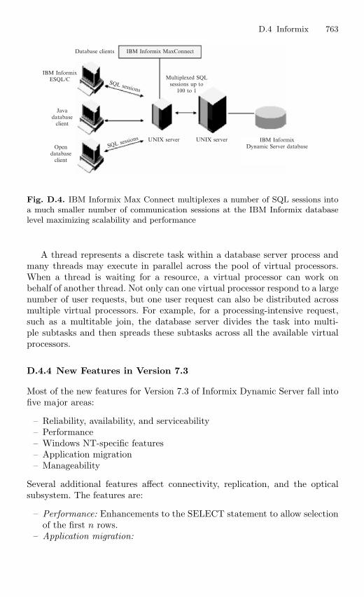
D.4 Informix 763
IBM Informix MaxConnectDatabase clients
Multiplexed SQLsessions up to
100 to 1
UNIX server UNIX server IBM InformixDynamic Server database
SQL sessions
SQL sessions
IBM InformixESQL/C
Javadatabase
client
Opendatabase
client
Fig. D.4. IBM Informix Max Connect multiplexes a number of SQL sessions intoa much smaller number of communication sessions at the IBM Informix databaselevel maximizing scalability and performance
A thread represents a discrete task within a database server process andmany threads may execute in parallel across the pool of virtual processors.When a thread is waiting for a resource, a virtual processor can work onbehalf of another thread. Not only can one virtual processor respond to a largenumber of user requests, but one user request can also be distributed acrossmultiple virtual processors. For example, for a processing-intensive request,such as a multitable join, the database server divides the task into multi-ple subtasks and then spreads these subtasks across all the available virtualprocessors.
D.4.4 New Features in Version 7.3
Most of the new features for Version 7.3 of Informix Dynamic Server fall intofive major areas:
– Reliability, availability, and serviceability– Performance– Windows NT-specific features– Application migration– Manageability
Several additional features affect connectivity, replication, and the opticalsubsystem. The features are:
– Performance: Enhancements to the SELECT statement to allow selectionof the first n rows.
– Application migration:
764 D Popular Commercial DBMS
1. New functions for case-insensitive search (UPPER, LOWER, INITCAP)2. New functions for string manipulations (REPLACE, SUBSTR, LPAD,
RPAD)3. New CASE expression4. New NVL and DECODE functions5. New date-conversion functions (TO CHAR and TO DATE)6. New options for the DBINFO function7. Enhancements to the CREATE VIEW and EXECUTE PROCEDURE
statements
New Features in Version 8.2
Following are new features that have been implemented in Version 8.2 ofDynamic Server with AD and XP Options:
– Global Language Support (GLS)– New aggregates: STDEV, RANGE, and VARIANCE– New TABLE lock mode for the LOCK MODE clause of ALTER TABLE
and CREATE TABLE statement– Support for specifying a lock on one or more rows for the Cursor Stability
isolation level
Following features, which were introduced in Version 8.1 of Dynamic Serverwith AD and XP Options:
– The CASE expression in certain Structured Query Language (SQL) state-ments
– New join methods for use across multiple computers– Nonlogging tables– External tables for high-performance loading and unloading
Command-Line Conventions
This section defines the format of commands that are available in Informixproducts. These commands have their own conventions, which might includealternative forms of a command, required and optional parts of the command,and so forth. Each diagram displays the sequences of required and optionalelements that are valid in a command. A diagram begins at the upper-leftcorner with a command. It ends at the upper-right corner with a vertical line.Between these points, user can trace any path that does not stop or back up.Each path describes a valid form of the command. User must supply a valuefor words that are in italics.
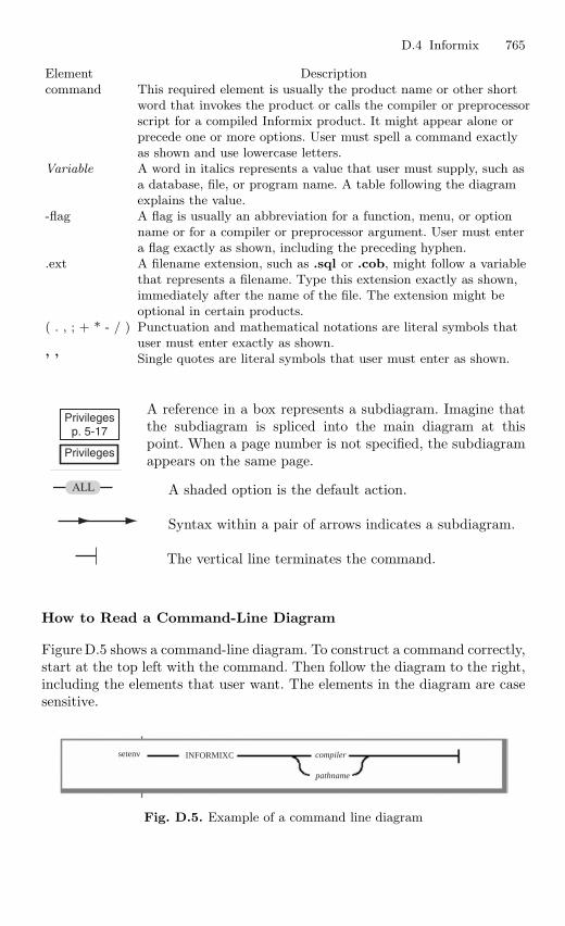
D.4 Informix 765
Element Descriptioncommand This required element is usually the product name or other short
word that invokes the product or calls the compiler or preprocessorscript for a compiled Informix product. It might appear alone orprecede one or more options. User must spell a command exactlyas shown and use lowercase letters.
Variable A word in italics represents a value that user must supply, such asa database, file, or program name. A table following the diagramexplains the value.
-flag A flag is usually an abbreviation for a function, menu, or optionname or for a compiler or preprocessor argument. User must entera flag exactly as shown, including the preceding hyphen.
.ext A filename extension, such as .sql or .cob, might follow a variablethat represents a filename. Type this extension exactly as shown,immediately after the name of the file. The extension might beoptional in certain products.
( . , ; + * - / ) Punctuation and mathematical notations are literal symbols thatuser must enter exactly as shown.
’ ’ Single quotes are literal symbols that user must enter as shown.
Privilegesp. 5-17
Privileges
A reference in a box represents a subdiagram. Imagine thatthe subdiagram is spliced into the main diagram at thispoint. When a page number is not specified, the subdiagramappears on the same page.
A shaded option is the default action.
Syntax within a pair of arrows indicates a subdiagram.
ALL
The vertical line terminates the command.
How to Read a Command-Line Diagram
Figure D.5 shows a command-line diagram. To construct a command correctly,start at the top left with the command. Then follow the diagram to the right,including the elements that user want. The elements in the diagram are casesensitive.
setenv INFORMIXC compiler
pathname
Fig. D.5. Example of a command line diagram
766 D Popular Commercial DBMS
To construct a command correctly, start at the top left with the command.Then follow the diagram to the right, including the elements that user want.The elements in the diagram are case sensitive.
These are the steps to be followed:
1. Type the word setenv.2. Type the word INFORMIXC.3. Supply either a compiler name or pathname. After user choose compiler
or pathname, user come to the terminator. User command is complete.4. Press RETURN to execute the command.
Informix’s current application development products, are INFORMIX-NewEra and INFORMIX-4GL, have been incorporated into the UniversalTools Strategy announced in March of 1997. The Universal Tools Strategygives application developers a wide choice of application development toolsfor Informix database servers, permitting developers to take a modular,component-based, open tools approach. The INFORMIX-Data Director fam-ily of plug-in modules lets developers extend, manage, and deploy applicationsfor INFORMIX-Universal Server using their choice of Informix and otherindustry-standard tools.The following products are included under the Universal Tools Strategy:
INFORMIX-Data Director for Visual BasicINFORMIX-Data Director for Java (formerly J works)INFORMIX-New EraINFORMIX-4GLINFORMIX-Java Object Interface (JOI) (formerly Java API)INFORMIX-JDBCINFORMIX-C++ Object Interface (COI)INFORMIX-CLIINFORMIX-ESQL/CINFORMIX-Developer SDK
D.4.5 Conclusion
The powerful and extensible IBM Informix Database Server is designed todeliver breakthrough scalability, manageability, and performance. IBM IDSenables user to manage business logic, create and access rich data, and definecomplex database functions in an integrated, intelligent information manage-ment system. With IBM IDS, user benefit from the performance and scala-bility offered by the proven Dynamic Server Architecture, while gaining allthe advantages of object-oriented technology and unlimited extensibility –resulting in an immense capacity to grow and adapt to ever-changing needs.
Bibliography
1. Abiteboul, S., Hull, R., and Vianu, V., Foundations of Databases, Addison-Wesley, Reading, MA, 1995
2. Aho, A., Beeri, C., and Ullman, J., The Theory of Joins in Relational Data-bases, ACM Transactions on Database Systems, 4:3, 1979
3. Aho, A., Sagiv, Y., and Ullman, J., Efficient Optimization of a Class of Rela-tional Expressions, ACM Transactions on Database Systems, 4:4, 1979
4. Aho, A., and Ullman, J., Universality of Data Retrieval Languages, Proceedingsof the POPL Conference, San Antonio, TX, ACM, 1979
5. Albano, A., De Antonellis, V., and Di Leva, A. (Eds.), Computer-Aided Data-base design: The DATAID Project, North-Holland, Amsterdam, 1985
6. Atzeni, P., and De Antonellis, V., Relational Database Theory, Benjamin-Cummings, Menlo Park, CA, 1993
7. Atzeni, P., Mecca, G., and Merialdo, P., To Weave the Web, Proceedings of 23rdInternational Conference on Very Large Data Bases, Athens, Greece, MorganKaufmann, San Francisco, 1997
8. Atzeni, P., Mecca, G., and Merialdo, P., Design and Maintenance of Data-Intensive Web Sites, Proceedings of 6th International Conference on ExtendingDatabase Technology, Valencia, Spain, Lecture Notes in Computer Science, Vol.1377, pp. 436–450, Springer, Berlin Heidelberg New York, 1998
9. Astrahan, M., et al., System R: A Relational Approach to Data Base Manage-ment, ACM Transactions on Database Systems, 1:2, 1976
10. Armstrong, W., Dependency Structures of Data Base Relationships, Proceed-ings of the IFIP Congress, 1974
11. Arkinson, M., and Buneman, P., Types and Persistence in Database Program-ming Languages, ACM Computing Surveys, 19:2, 1987
12. Atzeni, P., and De Antonellis, V., Relational Database Theory, Benjamin/Cummings, Menlo Park, CA, 1993
13. ANSI, American National Standards Institute: The Database Language SQL,Document ANSI X3.135, 1986
14. Bachman, C., The Data Structure Set Model. In: Rustin (Ed.), Proceedingsof 1974 ACM-SIGMOD Workshop on Data Description, Access and Control,Ann Arbor, MI, May 1–3, 1974
15. Baeza-Yates, R., and Larson, P.A., Performance of B1-trees with Partial Ex-pansions, IEEE Transactions on Knowledge and Data Engineering, 1:2, 1989
768 Bibliography
16. Baeza-Yates, R., and Ribero-Neto, B., Modern Information Retrieval, Addison-Wesley, Reading, MA, 1999
17. Bancilhon, F., Delobel, C., and Kanellakis, P. (Eds.), Building an Object-Oriented Database System: The Story of O2, Morgan Kaufmann, San Mateo,CA, 1992
18. Batini, C., Ceri, S., and Navathe, S.B., Conceptual Database Design, an Entity-Relationship Approach, Benjamin-Cummings, Menlo Park, CA, 1992
19. Bernstein, P.A., Hadzilacos, V., and Goodman, N., Concurrency Control andRecovery in Database Systems, Addison-Wesley, Reading, MA, 1987
20. Bernstein, P.A., Middleware: A Model for Distributed System Services. Com-munications of the ACM, 39:2, 89–98, 1996
21. Bertino, E., and Martino, L., Object-oriented Database Systems: Concepts andArchitectures, Addison-Wesley, Reading, MA, 1993
22. Brodie, M.L., and Stonebraker, M., Legacy Systems: Gateways, Interfaces &the Incremental Approach, Morgan Kaufmann, San Mateo, CA, 1995
23. Bachman, C., Data Structure Diagrams, Data Base (Bulletin of ACM SIG-FIDET), 1:2, 1969
24. Bachman, C., The Programmer as a Navigator, The California Association ofCommunity Managers, 16:1, 1973
25. Bachman, C., The Data Structure Set Model. In: Rustin (Ed.), Proceedingsof 1974 ACM-SIGMOD Workshop on Data Description, Access and Control,Ann Arbor, MI, 1974
26. Bachman, C., and Williams, S., A General Purpose Programming System forRandom Access Memories, Proceedings of the Fall Joint Computer Conference,AFIPS, 26, 1964
27. Cannan, S.J., and Otten. G.A.M., SQL-The Standard Handbook, McGraw-Hill,New York, 1992
28. Cattel, R.G.G., Object Data Management – Object Oriented and Extended Re-lational Database Systems, revised edition, Addison-Wesley, Reading, MA, 1994
29. Ceri, S. (Ed.), Methodology and Tools for Database Design, North-Holland,Amsterdam, 1983
30. Ceri, S., and Fraternali, P., Designing Database Applications with Objects andRules: The IDEA Methodology, Addison-Wesley, Reading, MA, 1997
31. Ceri, S., Fraternali, P., and Paraboschi, S., Design Principles for Data-IntensiveWeb Sites, ACM SIGMOD Record, 28:1, 1999
32. Ceri, S., Gottlob, G., and Tanea, L., Logic Programming and Data Bases,Springer, Berlin Heidelberg New York, 1989
33. Ceri, S., and Pelagatti, G., Distributed Databases: Principles and Systems,McGraw-Hill, New York, 1984
34. Ceri, S., and Widom, J., Deriving Production Rules for Constraint Mainte-nance, Proceedings of the International Conference on Very Large Data Bases,Brisbane, Australia, pp. 566–577, Morgan Kaufmann, San Francisco, 1990
35. Chamberlin, D.D., A Complete Guide to DB2 Universal Database, MorganKaufmann, San Francisco, CA, 1998
36. Chamberlin, D.D., Astrahan, M.M., Eswaran, P.P., Lorie, R.A., Mehl, J.W.,Reisner, P., and Wade, B.W., SEQUEL 2: A Unified Approach to Data Defini-tion, Manipulation and Control, IBM Journal of Research and Development,20:6, 97–137, 1976
37. Chamberlin, D.D., and Boyce, R.F., SEQUEL: A Structured English QueryLanguage, Proceedings of ACM Sigmoid Workshop, 1, 249–264, 1974
Bibliography 769
38. Chakravarthy, S., Active Database Management Systems: Requirements, State-of-the-Art, and an Evaluation. In: Entity-Relationship Approach: The Core ofConceptual Modeling 1991
39. Chakravarthy, S., Divide and Conquer: A Basis for Augmenting a ConventionalQuery Optimizer with Multiple Query Processing Capabilities, Proceedings ofthe Seventh International Conference on Data Engineering, 1991
40. Chakravarthy, S., Anwar, E., Maugis, L., and Mishra, D., Design of Sentinel:An Object-oriented DBMS with Event-based Rules, Information and SoftwareTechnology, 36:9, 1994
41. Chakravarthy, U., Grant, J., and Minker, J., Logic-Based Approach to Seman-tic Query Optimization, ACM Transactions on Database Systems, 15:2, 1990
42. Chen, P.P., The Entity-Relationship Model: Toward a Unified View of Data,ACM Transactions on Database Systems, 1:1, 9–36, 1976
43. Cheng, J., and Malaika, S. (Eds.), Web Gateway Tools: Connecting IBM andLotus Applications to the Web, Wiley, New York, 1997
44. Cochrane, R., Pirahesh, H., and Mattos, N., Integrating Triggers and Declara-tive Constraints in SQL Database Systems, Proceedings of the InternationalConference on Very Large Data Bases, Mumbai (Bombay), pp. 567–578,Morgan Kaufmann, San Francisco, 1996
45. Codd, E.F., A Relational Model for Large Shared Data Banks, Communica-tions of the ACM, 13:6, 377–387, 1970
46. Codd, E.F., Further Normalization of the Data Base Relational Model. In:Rustin, R. (Ed.), Database Systems, pp. 33–64, Prentice Hall, Eaglewood Cliffs,NJ, 1972
47. Codd, E.F., Relational Competencies of Database Sublanguages. In: Rustin,R. (Ed.), Database Systems, pp. 65–98, Prentice Hall, Eaglewood Cliffs, NJ,1972
48. Codd, E.F., Extending the Database Relational Model to Capture More Mean-ing, ACM Transactions on Database Systems, 4:4, 397–434, 1979
49. Codd, E.F., Relational Database: A practical Foundation for Productivity,Communications of the ACM, 25:2, 109–117, 1982
50. Codd, E.F., Twelve Rules for On-Line Analytical Processing, Computerworld,April 1995
51. Comer, D.E., Internetworking with TCP/IP, Volume 1: Principles, Protocols,and Architecture, 3rd edition, Prentice Hall, Eaglewood Cliffs, NJ, 1995
52. Date, C.J., An Introduction to Database Systems, 6th edition, Addison-Wesley,Reading, MA, 1995
53. Date, C.J., and Darwen, H., A Guide to the SQL Standard, 3rd edition,Addison-Wesley, Reading, MA, 1993
54. Date, C., A Critique of the SQL Database Language, ACM SIGMOD Record,14:3, 1984
55. Date, C., and White, C., A Guide to DB2, 3rd edition, Addison-Wesley, Read-ing, MA, 1989
56. Date, C., and White, C., A Guide to SQL/DS, Addison-Wesley, Reading, MA,1988
57. Davies, C., Recovery Semantics for a DB/DC System, Proceedings of the ACMNational Conference, 1973
58. Davis, W., System Analysis and Design, Addison-Wesley, Reading, MA, 198359. Dhavan, C., Mobile Computing, McGraw-Hill, New York, 1997
770 Bibliography
60. Dittrich, K., Object-Oriented Database Systems: The Notion and the Issues.In: Dittrich and Dayal (Eds.), Proceedings of the International Workshop onObject-Oriented Database Systems, 1986
61. Dittrich, K., and Dayal, U., (Eds.), Proceedings of the International Workshopon Object-Oriented Database Systems, IEEE CS, Pacific Grove, CA, September1986
62. Dittrich, K., Kotz, A., and Mulle, J., An Event/Trigger Mechanism to EnforceComplex Consistence Constraints in Design Databases. In: SIGMOD Record,15:3, 1986
63. Eisenberg, A., and Melton, J., Standards in Practice, ACM SIGMOD Record,27:3, 53–58, 1998
64. Elmagarmid, A.K. (Ed.), Database Transaction Models for Advanced Applica-tions, Morgan Kauffmann, San Mateo, CA, 1992
65. Elmagarmid, A., Leu, Y., Litwin, W., and Rusinkiewicz, M., A MultidatabaseTransaction Model for Interbase. In: International Conference on Very LargeData Bases, 1990
66. Elmasri, R., James, S., and Kouramajian, V., Automatic Class and MethodGeneration for Object-Oriented Databases, Proceedings of the Third Interna-tional Conference on Database and Object-Oriented Databases (DOOOD-93),Phoenix, AZ, December 1993
67. Elmasri, R., Kouramajian, V., and Fernando, S., Temporal Database Modeling:An Object-Oriented Approach, International Conference on Information andKnowledge Management, November 1993
68. Elmasri, R., Larson, J., and Navathe, S., Schema Integration Algorithms forFederated Databases and Logical Database Design, Honeywell CSDD, TechnicalReport CSC-86-9:8212, January 1986
69. Elmasri, R.A., and Navathe, S.B., Fundamentals of Database Systems, 2ndedition, Benjamin-Cummings, Menlo Park, CA, 1994
70. Fairly, R., Software Engineering Concepts, McGraw-Hill, New York, 198571. Fagin, R., Multivalued Dependencies and a New Normal Form for Relational
Databases, ACM Transactions on Database Systems, 2:3, 197772. Fagin, R., Normal Forms and Relational Database Operators, Proceedings of
the 1979 ACM SIGMOD International Conference on Management of Data,1979
73. Fagin, R., A Normal Form for Relational Databases That is Based on Domainsand Keys, ACM Transactions on Database Systems, 6:3, 1981
74. Fagin, R., Nievergelt, J., Pippenger, N., and Strong, H., Extendible Hashing-A Fast Access Method for Dynamic Files, ACM Transactions on DatabaseSystems, 4:3, 1979
75. Fayyad, U.M., Piatetsky-Shapiro, G., Smyth, P., and Uthurusamy, R. (Eds.),Advances in Knowledge Discovery and Data Mining, AAAI /MIT, Cambridge,MA, 1996
76. Fleming, C.C., and von Halle, B., Handbook of Relational Database Design,Addison-Wesley, Reading, MA, 1989
77. Florescu, D., Levy, A., and Mendelzon, A., Database Techniques for the World-Wide Web: A Survey. ACM SIGMOD Record, 27:3, 59–74, 1998
78. Gogolla, M., and Hohenstein, U., Towards a Semantic View of an ExtendedEntity-Relationship Model, ACM Transactions on Database Systems, 16:3,1991
Bibliography 771
79. Goldberg, A., and Robson, D., Smalltalk-80: The Language and Its Implemen-tation, Addison-Wesley, Redaing, MA, 1983
80. Goldfine, A., and Konig, P., A Technical Overview of the Information ResourceDictionary System (IRDS), 2nd edition, NBS IR 88-3700, National Bureau ofStandards, 1988
81. Gotlieb, L., Computing Joins of Relations. In: Proceedings of the ACM SIG-MOD International Conference on Management of Data, 1975
82. Graham, I.S., HTML Sourcebook, 2nd edition, Wiley, New York, 199683. Gray, J., and Anderton, M., Distributed Computer Systems: Four Case Studies,
IEEE Proceedings, 75:5, 719–726, 198784. Gray, J., Chaudhuri, S., Bosworth, A., Layman, A., Reichart, D., Venkatrao, M.,
Fellow, F., and Pirahesh, H., Data Cube: A Relational Aggregation OperatorGeneralizing Group-by, Cross-Tab, and Sub Totals, Data Mining and KnowledgeDiscovery, 1:1, 29–53, 1997
85. Gray, J., and Reuter, A., Transaction Processing Concepts and Techniques,Morgan Kauffmann, San Mateo, CA, 1994
86. Greenspun, P., Philip & Alex’s Guide to Web Publishing, Morgan Kaufmann,San Mateo, CA, 1999
87. Hamilton, G., Catteli, R., and Fisher, M., JDBC Database Access with Java-ATutorial and Annotated Reference, Addison Wesley, Reading, MA, 1997
88. Hammer, M., and McLeod, D., Semantic Integrity in a Relational DatabaseSystem, Proceedings of 23rd International Conference on Very Large DataBases 1975
89. Hammer, M., and McLeod, D., Database Descriptions with SDM: A SemanticData Model, ACM Transactions on Database Systems, 6:3, 1981
90. Hammer, M., and Sarin, S., Efficient Monitoring of Database Assertions. In:Proceedings of the 1978 ACM SIGMOD International Conference on Manage-ment of Data, 1978
91. Harald Kosh, Distributed Multimedia Database Technologies supported byMPEG-7 and MPEG-21, CRC, West Palm Beach, FL, 2003
92. Hull, R., and King, R., Semantic Database Modeling: Survey, Applications andResearch Issues, ACM Computing Surveys, 19:3, 201–260, 1987
93. Inmon, B., Building the Data Warehouse, Wiley, New York, 199694. Ioannidis, Y., and Kang, Y., Randomized Algorithms for Optimizing Large Join
Queries. In: Proceedings of the 1990 ACM SIGMOD International Conferenceon Management of Data 1990
95. Ioannidis, Y., and Kang, Y., Left-Deep vs. Bushy Trees: An Analysis of Strat-egy Spaces and Its Implications for Query Optimization. In: Proceedings of the1991 ACM SIGMOD International Conference on Management of Data, 1991
96. Ioannidis, Y., and Wong, E., Transforming Nonlinear Recursion to Linear Re-cursion. In: International Conference on Expert Database Systems, 1988
97. Irani, K., Purkayastha, S., and Teorey, T., A Designer for DBMS-ProcessableLogical Database Structures, Proceedings of 23rd International Conference onVery Large Data Bases, 1979
98. Isakowitz, T., Bieber, and M., Vitali, F. (Guest Eds.), Web Information Sys-tems, Communications of the ACM, 41:7, 78–117, 1998
99. Ju, P., Databases on the Web: Designing and Programming for Network Access,IDG Books Worldwide, Foster City, CA, 1997
100. Kim, W., Object-Oriented Databases: Definition and Research Directions,IEEE Transactions on Knowledge and Data Engineering, 2:3, September 1990
772 Bibliography
101. Kim, W. (Ed.), Modern Database Systems: the Object Model, Interoperability,and Beyond, ACM and Addison-Wesley, New York, 1995
102. Kimball, R., The Data Warehouse Toolkit: Practical Techniques for BuildingDimensional Data Warehouses, Wiley, New York, 1996
103. Kumar, A., and Segev, A., Cost and Availability Tradeoffs in Replicated Con-currency Control, ACM Transactions on Database Systems, 18:1, 1993
104. Kumar, A., and Stonebraker, M., Semantics Based Transaction ManagementTechniques for Replicated Data, in Proceedings of the 1987 ACM SIGMODInternational Conference on Management of Data, 1987
105. Kumar, V., and Hsu, M., Database Recovery, Kluwer Academic, Dordrecht1998
106. Kung, H., and Robinson, J., Optimistic Concurrency Control, ACM Transac-tions on Database Systems, 6:2, 1981
107. Lacroix, M., and Pirotte, A., Domain-Oriented Relational Languages, Proceed-ings of 23rd International Conference on Very Large Data Bases, 1977
108. Lacroix, M., and Pirotte, A., ILL: An English Structured Query Languagefor Relational Data Bases. In: Nijssen (Ed.), Proceedings of the IFIP TC-2Working Conference on Modelling in Data Base Management Systems, 1977
109. Lamport, L., Time, Clocks and the Ordering of Events in a Distributed System,Communications of the ACM, 21:7, 558–565, 1978
110. Liu, C., Peek, J., Jones, R., Buus, B., and Nye, A., Managing Internet Infor-mation Services, O’Reilly & Associates, Sebastopol, CA, 1994
111. Loomis, M.E.S., Object Databases: the Essentials, Addison-Wesley, Reading,MA, 1995
112. Lucyk, B., Advanced Topics in DB2, Addison-Wesley, Reading, MA, 1993113. Lum, V.Y., Ghosh, S.P., Schkolnik, M., Taylor, R.W., Jefferson, D., Su. S., Fry,
J.P., Teorey, T.J., Yao, B., Rund, D.S., Kahn, B., Navathe, S.B., Smith, D.,Aguilar, L., Barr, W.J., and Jones, P.E., 1978 New Orleans Data Base DesignWorkshop Report, Proceedings of the International Conference on Very LargeData Bases, Rio de Janeiro, Brazil, 328–339, 1979
114. Maier, D., Stein, J., Otis, A., and Purdy, A., Development of an Object-Oriented DBMS, Object-Oriented Programming, Systems, Languages, and Ap-plications, 1986
115. Maier, D., The Theory of Relational Databases, Computer Science Press,Potomac, MD, 1983
116. Mannila, H., and Raiha, K.J., The Design of Relational Databases, Addison-Wesley, Reading, MA, 1992
117. McFadden, F.R., and Hoffer, J.A., Modern Database Management, 4th edition,Benjamin Cummings, Menlo Park, CA, 1994
118. Melton, J., SQL3 Update, Proceedings of the IEEE International Conferenceon Data Engineering 1996, 566–672, 1996
119. Melton, J., and Simon, A.R., Understanding the New SQL, Morgan Kaufmann,San Mateo, CA, 1993
120. Mohan, C., and Narang, I., Algorithms for Creating Indexes for Very LargeTables without Quiescing Updates, in Proceedings of the 1992 ACM SIGMODInternational Conference on Management of Data, 1992
121. Mohan, C. et al., ARIEL: A Transaction Recovery Method Supporting Fine-Granularity Locking an Partial Rollbacks Using Write-Ahead Logging, ACMTransactions on Database Systems, 17:1, March, 1992
Bibliography 773
122. Moss, J., Nested Transactions and Reliable Distributed Computing, Proceed-ings of the Symposium on Reliability in Distributed Software and DatabaseSystems, IEEE CS, July 1982
123. Mylopolous, J., Bernstein, P., and Wong, H., A Language Facility for DesigningDatabase-Intensive Applications, ACM Transactions on Database Systems, 5:2,1980
124. Ng, P., Further Analysis of the Entity-Relationship Approach to DatabaseDesign, IEEE Transactions on Software Engineering, 7:1, 1981
125. Nievergelt, J., Binary Search Trees and File Organization, ACM ComputingSurveys, 6:3, 1974
126. Nijssen, G. (Ed.), Modelling in Data Base Management Systems, North-Holland, Amsterdam, 1976
127. Nijssen, G. (Ed.), Architecture and Models in Data Base Management Systems,North-Holland, Amsterdam, 1977
128. Obermarck, R., Distributed Deadlock Detection Algorithm, ACM Transactionson Database Systems, 7:2, 1982
129. Olle, T., The CODASYL Approach to Data Base Management, Wiley, 1978130. O’Neil, P., Database Principles, Programming, Performance, Morgan
Kaufmann, Sun Mateo, CA, 1994131. Oracle, RDBMS Database Administrator’s Guide, Oracle, 1992132. Oracle, Performing Tuning Guide, Version 7.0, Oracle, 1992133. Oracle, Oracle 8 Server Concepts, Vols. 1 and 2, Release 8.0, Oracle Corpora-
tion, 1997134. Oracle Corporation, Oracle 8 Server: Concepts Manual, Redwood City, CA,
1998135. Oracle Corporation, Oracle 8 Server: SQL Language Reference Manual,
Redwood City, CA, 1998136. Ozsu, M.T., and Valduriez, P., Principles of Distributed Database Systems, 2nd
edition, Prentice Hall, Eaglewood Cliffs, NJ, 1999137. Papadimitriou, C., The Serializability of Concurrent Database Updates, Jour-
nal of the ACM, 26:4, 1979138. Papadimitriou, C., The Theory of Database Concurrency Control, Computer
Science Press, New York, 1986139. Papazoglou, M., and Valder, W., Relational Database Management: A Systems
Programming Approach, Prentice-Hall, Englewood Cliffs, NJ, 1989140. Paredaens, J., De Bra, P., Gysses, M., and Van Gucht, D., The Structure of
the Relational Database Model, Springer, Berlin Heidelberg New York, 1989141. Pazandak, P., and Srivatsava, J., Evaluating Object DBMSs for Multimedia,
IEEE Multimedia, 4:3, 34–49, 1997142. Pressman, R.S., Software Engineering, a Practitioner’s Approach, 3rd edition,
McGraw-Hill, New York, 1992143. Ramakrishnan, R. (Ed.), Applications of Logic Databases, Kluwer Academic,
Dordrecht, 1995144. Ramakrishnan, R., Database Management Systems, McGraw-Hill, New York,
1997145. Reisner, P., Human Factors Studies of Database Query Languages: A Survey
and Assessment, ACM Computing Surveys, 13:1, 1981146. Rosenfeld, L., and Morville, P., Information Architecture for the World Wide
Web, O’Reilly and Associates, Sebastopol, CA, 1998
774 Bibliography
147. Rumbaugh, J., Blaha, M., Premerlani, W., Eddy, F., and Lorensen, W., ObjectOriented Modelling and Design, Prentice Hall, Eaglewood Cliffs, NJ, 1991
148. Rustin, R. (Ed.), Data Base Systems, Prentice-Hall, Englewood Cliffs, NJ, 1972149. Rustin, R. (Ed.), Proceedings of the BJNAV2, 1974150. Samaras, G., Britton, K., Citton, A., and Mohan, C., Two-Phase Optimizations
in a Commercial Distributed Environment, Journal of Distributed and ParallelDatabases, 3:4, 325–360, 1995
151. Samet, H., The Design and Analysis of Spatial Data Structures, Addison-Wesley, Reading, MA, 1989
152. Selinger, P. et al., Access Path Selection in a Relational Database ManagementSystem. In: Proceedings of the 1979 ACM SIGMOD International Conferenceon Management of Data, 1979
153. Senko, M., Specification of Stored Data Structures and Desired Output inDIAM II with FORAL, Proceedings of 23rd International Conference on VeryLarge Data Bases, 1975
154. Senko, M., A Query Maintenance Language for the Data Independent Access-ing Model II, Information Systems, 5:4, 1980
155. Senn, J.A., Analysis & Design of Information Systems, 2nd edition, McGraw-Hill, New York, 1989
156. Shasha, D., Database Tuning: A Principled Approach, Morgan Kaufmann, SanMateo, CA, 1994
157. Shasha, D., and Goodman, N., Concurrent Search Structure Algorithms, ACMTransactions on Database Systems, 13:1, 1988
158. Sheth, A.P., and Larson, J.A., Federated Database Systems for Managing Dis-tributed, Heterogenous, and Autonomous Databases, ACM Computing Sur-veys, 22:3, 183–236, 1990
159. Siegel, J. (Ed.), CORBA: Fundamentals and Programming, Wiley, New York,1996
160. Silberschatz, A., Korth, H.F., and Sudarshan, S., Database System Concepts,McGraw-Hill, New York, 1996
161. Stonebraker, M., Object-Relational DBMSs – The Next Great Wave, MorganKauffmann, San Mateo, CA, 1994
162. Stonebraker, M. (Ed.), Readings in Database Systems, 2nd edition, MorganKauffmann, San Mateo, CA, 1994
163. Stonebraker, M., Rowe, L.A., Lindsay, B.G., Gray, J., Carey, M.J., Brodie,M.L., Bernstein, P.A., and Beech, D., Third-Generation Database SystemManifesto, ACM SIGMOD Record, 19:3, 31–44, 1990
164. Smith, J.M., and Smith, D.C.P., Database Abstractions: Aggregation andGeneralization, Proceedings of the 1977 ACM Transactions on Database Sys-tems, 2:1, 105–133, 1977
165. Subrahmanian, V.S., Principles of Multimedia Database Systems, MorganKaufmann, San Mateo, CA, 1998
166. Tansel, A., et al., (Eds.) Temporal Databases: Theory, Design, and Implemen-tation, Benjamin Cummings, Menlo Park, CA, 1993
167. Teorey, T., Database Modeling and Design: The Fundamental Principles, 2ndedition, Morgan Kauffmann, Los Altos, CA, 1994
168. Teorey, T., Yang, D., and Fry, J., A Logical Design Methodology for RelationalDatabases Using the Extended Entity-Relationship Model, ACM ComputingSurveys, 18:2, 1986
Bibliography 775
169. Teorey, T.J., Database Modeling and Design: the E-R Approach, MorganKaufmann, San Mateo, CA, 1990
170. Teorey, T.J., and Fry, J.P., Design of Database Structures, Prentice Hall,Eaglewood Cliffs, NJ, 1982
171. Teorey, T.J., Yang, D., and Fry, J.P., A Logical Design Methodology for Rela-tional Databases Using the Extended Entity-Relational Approach, ACM Com-puting Surveys, 18:2, 201–260, 1986
172. Tsichritzis, D., and Lochovsky, F.H., Data Models, Prentice Hall, EaglewoodCliffs, NJ, 1982
173. Tsou, D.M., and Fischer, P.C., Decomposition of a Relation Scheme into BoyceCodd Normal Form, SIGACT News, 14:3, 23–29, 1982
174. Ullman, J., Implementation of Logical Query Languages for Databases, ACMTransactions on Database Systems, 10:3, 1985
175. Ullman, J.D., Principles of Database and Knowledge Base Systems, Vol. 1,Computer Science Press, Potomac, MD, 1988
176. Ullman, J.D., Principles of Database and Knowledge Base Systems, Vol. 2,Computer Science Press, Potomac, MD, 1989
177. Ullman, J.D., and Widom, J., A First Course in Database Systems, PrenticeHall, Upper Saddle River, NJ, 1997
178. Valduriez, P., and Gardarin, G., Analysis and Comparison of Relational Data-base Systems, Addison-Wesley, Reading, MA, 1989
179. Vassiliou, Y., Functional Dependencies and Incomplete Information, Proceed-ings of 23rd International Conference on Very Large Data Bases, 1980
180. Verheijen, G., and VanBekkum, J., NIAM: An Information Analysis Method.In: Olle et al. (Eds.), Proceedings of the CRIS Conference, 1982
181. Verhofstadt, J., Recovery Techniques for Database Systems, ACM ComputingSurveys, 10:2, 1978
182. Vielle, L., Recursive Axioms in Deductive Databases: The Query-Subquery Ap-proach. In: Proceedings International Conference on Expert Database Systems,1986
183. Vossen, G., Data Models, Database Languages, and Database Management Sys-tems, Addison-Wesley, Reading, MA, 1990
184. Wang, Y., and Madnick, S., The Inter-Database Instance Identity Problem inIntegrating Autonomous Systems. In: Proceedings of the Fifth IEEE Interna-tional Conference on Data Engineering, 1989
185. Wang, Y., and Rowe, L., Cache Consistency and Concurrency Control in aClient/Server DBMS Architecture. In: Proceedings of the 1991 ACM SIGMODInternational Conference on Management of Data, 1991
186. Wallace, D., William Allan Award Address: Mitochondrial DNA Variation inHuman Evolution, Degenerative Disease, and Aging, American Journal of Hu-man Genetics, 1994
187. Weddell, G., Reasoning About Functional Dependencies Generalized for Se-mantic Data Models, ACM Transactions on Database Systems, 17:1, 1992
188. Weikum, G., Principles and Realization Strategies of Multilevel TransactionManagement, ACM Transactions on Database Systems, 16:1, 1991
189. Widom, J., Research Problems in Data Warehousing, Proceedings of the 4thInternational Conference on Information and Knowledge Management, Novem-ber 1995
190. Widom, J.,and Ceri, S., Active Database Systems, Morgan Kauffmann, SanMateo, CA, 1996
776 Bibliography
191. Wiederhold, G., Database Design, McGraw-Hill, New York, 1983192. Wiorkowski, G., and Kull, D., DB2-Design and Development Guide, 3rd edi-
tion, Addison-Wesley, Reading, MA, 1992193. Wong, E., and Youssefi, K., Decomposition-A Strategy for Query Processing,
ACM Transactions on Database Systems, 1:3, 1976194. Yannakakis, Y., Serializability by Locking, Journal of the ACM, 31:2, 1984195. Yao, S., Optimization of Query Evaluation Algorithms, ACM Transactions on
Database Systems, 4:2, 1979196. Yao, S. (Ed.), Principles of Database Design, Vol. 1: Logical Organizations,
Prentice-Hall, Englewood Cliffs, NJ, 1985197. Youssefi, K., and Wong, E., Query Processing in a Relational Database Man-
agement System, Proceedings of 23rd International Conference on Very LargeData Bases, 1979
198. Zaniolo, C., Analysis and Design of Relational Schemata for Database Systems,Ph.D. dissertation, University of California, LA, 1976
199. Zaniolo, C., Design and Implementation of a Logic Based Language for DataIntensive Applications, MCC Technical Report#ACA-ST-199-88, June, 1988
200. Zaniolo, C., Database Relations with Null Values, Journal of Computer andSystem Science, 28:1, 142–166, 1984
201. Zaniolo, C., Ceri, S., Faloutsos, C., Snodgrass, R.T., Subrahmanian, V.S., andZicari, R., Introduction to Advanced Database Systems, Morgan Kaufmann,San Mateo, CA, 1997
202. Zaniolo, C. et al., Advanced Database Systems, Morgan Kaufmann, San Mateo,CA, 1997
203. Zloof, M., Query by Example, Proceedings of the National Computer Confer-ence, American Federation of Information Processing Societies, 44, 1975
204. Zobel, J., Moffat, A., and Sacks-Davis, R., An Efficient Indexing Technique forFull-Text Database Systems, Proceedings of 23rd International Conference onVery Large Data Bases, 1992
Related Documents