Spontaneous symmetry breaking and proper-time flow equations

arX

iv:h

ep-t

h/04

0317

6v1

17

Mar

200

4

Spontaneous Symmetry Breaking and Proper-Time

Flow Equations

Alfio Bonanno

INAF - Osservatorio Astrofisico, Via S.Sofia 78, I-95123 Catania, Italy

INFN Sezione di Catania, Via S.Sofia 64, I-95123 Catania, Italy

Giuseppe Lacagnina

Institut fur Theoretische Physik, Universitat Regensburg,

D-93040 Regensburg, Germany

Abstract

We discuss the phenomenon of spontaneous symmetry breaking by means of

a class of non-perturbative renormalization group flow equations which employ a

regulating smearing function in the proper-time integration. We show, both an-

alytically and numerically, that the convexity property of the renormalized local

potential is obtained by means of the integration of arbitrarily low momenta in

the flow equation. Hybrid Monte Carlo simulations are performed to compare the

lattice Effective Potential with the numerical solution of the renormalization group

flow equation. We find very good agreement both in the strong and in the weak

coupling regime.

1 Introduction

The mechanism of spontaneous symmetry breaking is one of the most important nonper-

turbative phenomena in quantum field theory and statistical mechanics. Unfortunately,

due to its strong nonperturbative character, many of its aspects are not yet well under-

stood mainly because of the lack of reliable computational tools even in simple physical

situations. For example, in the liquid-vapor phase transition, the system undergoes a

first-order phase transition below the critical temperature, but the presence of long-range

fluctuations renders the mean-field description inadequate. The well-known Maxwell con-

struction [1] reproduces the flat isotherms in the two-phase region but does not provide

the correct critical exponents near the critical region.

In quantum field theory the situation is even more dramatic because the perturbative

calculation of the Effective Potential (EP) generates an imaginary part whose physical

meaning is not entirely clear. In fact, the EP should be a convex function of the fields

by construction, since it is the Legendre transform of the generating functional of the

connected Green’s functions [2].

An important result was obtained in [3] within the framework of the Effective Average

Action, for a continuous O(N)-symmetric scalar theory: it was shown that in order to

correctly reproduce the convexity property of the free energy a non-trivial saddle point

(spin wave solution) must be chosen in the loop-expansion [4]. This result has opened the

possibility of using the Wilsonian RG approach in discussing non-perturbative issues of

this kind.

Quite generally the possibility of applying renormalization group (RG) methods to

the description of first order phase transition has frequently been matter of discussion in

the recent years. Although the question is still not completely settled, several works have

shown that the Wilsonian RG approach is a promising tool for such kind of investigations.

In particular it has been shown [5] that the Wegner-Houghton (WH) RG equation (a sharp

cut-off momentum-space wilsonian-type of RG flow equation) already in the simple local

potential approximation (LPA) reproduces the convexity property of the free energy as

a result of the integration of arbitrarily low momenta without resorting to any ad hoc

Maxwell construction, or saddle point approximation. Moreover, the RG transformation

is always well defined below the critical line.

1

The essential ingredient of their analysis was the use of a robust and very accurate

numerical method for handling the RG equation without resorting to polynomial trun-

cations. Similar results have also been obtained with a smooth cutoff RG flow equation,

in the framework of the exact RG equation for the effective average action [6]. In [7] an

alternative method which combines the RG flow equation approach with the non-trivial

saddle point expansion method has been presented.

The wilsonian RG transformation [9], as opposed to the more conventional RG trans-

formation based on the rescaling properties of the Green’s functions, preserves all the

infinite number of interactions generated in the low-energy action by “averaging-out” the

small-scale physics defined at some high-energy scale Λ, and for this reason is a power-

ful tool in order to investigate situations where infinitely many length scales are coupled

together. Quite generally, the Wilsonian action can be defined as

e−SΩ(Φ) =

∫

Dϕδ(Φ − C(ϕ)) e−S(ϕ) (1.1)

where Φ is a low frequency field which is in turn a function of the fundamental field

ϕ via Φ = C(φ) and C is some averaging operator. If the effective theory is defined on a

lattice Λ0, then

δ(Φ − C(ϕ)) =∏

x∈Λ0

δ(Φ(x) − C(ϕ)(x))

For computational purposes, a continuous wilsonian RG transformation is defined in

the momentum-space representation where the definition (1.1) becomes

e−Sk(Φ) =

∫

Dζe−S(ζ+Φ) (1.2)

ζ being the high-frequency part of the fundamental field with momenta p greater than

some infrared cutoff p > k, and Φ the low-frequency one, with momenta p ≤ k. If we

choose

C(ϕ) =1

Ω

∫

Ω

ϕ (1.3)

where Ω is a characteristic volume over which the field is averaged, in the limit Ω → ∞

(equivalently, vanishing infrared cutoff k in Eq.(1.2) ) the blocked action gives precisely the

EP, namely the non-derivative part of the Effective Action Γ[φ], defined as the Legendre

transform of W [J ], the generator of the connected Green’s functions in the presence of

an external current J [8].

2

In practice, the wilsonian RG transformation obtained from explicit calculation of

(1.2) is strongly non-linear, and only by retaining infinitely many interactions generated

by integrating out the “fast” variable, the RG transformation can be well defined below

the critical line. Therefore, a numerical treatment of the full non-linear partial differential

equation is necessary even in the simplest LPA approximation of the Wilsonian Action.

In recent years, in an attempt of calculating (1.2) non-perturbatively, a new type of

RG flow equations has been proposed [?] and further developed [10, 11, 12]. It is based on

Schwinger’s proper time regulator, and it is therefore well suited for a direct application

to gauge theories.

The proper time renormalization group equation (PTRG) does not belong to the class

of exact-RG flows which can be formally derived from the Green’s functions generator

without resorting to any truncation or approximation [14, 15, 16]. Nevertheless the flow

equation has the property of preserving the symmetries of the theory and, in addition,

it has a quite simple and manageable structure. Moreover the PTRG flow, although

it can not fully reproduce perturbative expansions beyond the one loop order [17], still

does provide excellent results when used to evaluate the critical properties such as the

critical exponents of the three dimensional scalar theories at the non-gaussian fixed point

[18, 19]. In particular the determination is optimized when one takes the “sharp” limit

of the cutoff function on the proper time and it turns out to be much more accurate

than the one corresponding to a smoother regulator. The PTRG also provides excellent

determinations of the energy levels of the quantum double well [20]. In fact, the use of

the special type of PT regulator described in this paper and already discussed in [18, 20]

realizes an localized integration over the “fast” variables at a given infrared running

momentum k and, for this reason, it shows an impressive numerical convergence stability

in the calculations of the critical exponents.

In this paper we shall instead be mainly concerned with the study of a a strong non-

perturbative phenomenon like the SSB, for which the validity of PTRG equations has

not been tested yet. In particular, the relevant question we would like to address in this

paper is to analytically and numerically study the approach to the convexity for the EP

obtained by means of a class of PTRG flow equations in the limit of vanishing infrared

cutoff. A smeared type of proper-time regulator will be used which selects a localized

integration in the “fast” variables in the path-integral. The resulting flow equation can

3

be thought of as an interpolation of a “smooth” modification of the LPA approximation of

the Wegner-Houghton (WH) [13] “exact” flow equation, and the exponentially ultraviolet

(UV) converging flow discussed in [14, 19]. It will be shown that the PTRGs can correctly

describe the approach to convexity as k → 0, and that give results which are completely

consistent with the analysis performed in [5] for the WH equations, and in [4] for the

“exact” evolution equation for the effective average action. The additional advantage is

that below the upper critical dimension the PTRG flow equation predicts the expected

discontinuity of the inverse compressibility, whereas the “exact” WH equation fails to do

so.

In order to strengthen our analysis, we compare the result of our numerical investiga-

tion with the standard EP computed on a lattice by means of a Hybrid Monte Carlo ap-

proach. Our main conclusion is that lattice EP and PTRG flow equation agree extremely

well even for relatively small lattices, both in the perturbative and non-perturbative

regime.

2 Flow equations from proper-time regulators

Let us now review the basic assumptions in the derivation of the PTRG flow equation.

We first calculate the wilsonian action in (1.2) in the one-loop approximation as

S1−loopk (Φ) = −

1

2

∫

∞

0

ds

sfk(s, Λ)Tr

(

e−s

δ2SΛ

δϕ2

∣

∣

∣

ϕ=Φ − e−s

δ2SΛ

δϕ2

∣

∣

∣

ϕ=0

)

(2.1)

where, following [21, 22, 23], we have introduced an heat-kernel smooth regulator fk

in the Schwinger proper time representation for the one-loop expression and we have

subtracted the UV divergent contribution of a vanishing background field. The following

prescription apply to the choice of fk:

• fk(s = 0, Λ) = 0 in order to regularize the UV divergences as s → 0

• fk=0(s → ∞, Λ) = 1 in order to leave the IR physics unchanged by the regulator

• fk=Λ(s, Λ) = 0 in order to recover the original bare theory at the cutoff scale k = Λ.

The flow equation for the Wilsonian action Sk results from considering Eq.(2.1) in the

infinitesimal momentum shell k, k + δk and then RG-improving the resulting expression,

4

which amounts to substitute the bare action SΛ with the running one SΛ → Sk in the

RHS of Eq.(2.1),

k∂Sk(Φ)

∂k= −

1

2

∫

∞

0

ds

sk∂fk(s, Λ)

∂kTr

(

e−sS′′

k (Φ) − e−sS′′

k (0))

. (2.2)

where primes indicate functional derivatives with respect to ϕ. At this point, one

should stress that although the fast momentum integration in (2.1) has been obtained by

assuming a trivial saddle point in the path-integral, the RG-improved flow equation (2.2)

is instead a functional differential flow equation which is valid for a general average action

Sk(Φ).

If we then project Eq.(2.2) onto its non-derivative part, the anomalous dimension η is

set to zero, and the resulting flow equation for the local potential reads

k∂Uk(Φ)

∂k= −

Kd

2

∫

∞

0

ds

s1+d/2k∂fk(s, Λ)

∂k

(

e−U ′′

k (Φ)s − e−U ′′

k (0)s)

. (2.3)

where Kd = 2/(4π)d/2Γ(d/2). For actual calculations we shall employ the following class

of proper-time smearing functions

fnk (s, Λ) =

Γ(n, sk2) − Γ(n, sΛ2)

Γ(n)(2.4)

where Γ(a, z) =∫ z

0dt tα−1e−t is the incomplete Gamma function and n a positive real

number. Note that limn→∞ = fnk (ns, Λ) = θ(s − k2) − θ(s − Λ2).

Since k∂Γ(n, sk2)/∂k = −2(sk2)ne−sk2

the s-integration in (2.3) can be explicitly

performed, having at last

k∂Uk(Φ)

∂k= −

Kd

2kd ln

(

1 +U ′′

k (Φ)

k2

)

n =d

2(2.5)

k∂Uk(Φ)

∂k=

Mdn

(4π)d/2kd

(

1 +U ′′

k (Φ)

nk2

)d/2−n

n >d

2(2.6)

k∂Uk(Φ)

∂k=

1

(4π)d/2kd exp

(

−U ′′

k (Φ)

k2

)

n → ∞ (2.7)

where Mdn = nd/2Γ(n − d/2)/Γ(n), and in particular Md

∞= 1. In order to simplify the

notation we have not explicitly written in the RHS of the equations the field independent

contributions which correspond to a trivial shift of the vacuum energy at k = 0. Eq.(2.5)

5

is obtained from the n = d/2 limit by performing the trivial rescaling k →√

d/2k of the

infrared cutoff. It coincides with the LPA approximation of the “exact” WH sharp cut-off

equation [22]. Eq.(2.6) converges to Eq.(2.7) as n → ∞. In other words, the n-dependence

in the cutoff interpolates between a WH type of equation and the “exponential” RG

equation (2.7).

3 Analytical and numerical results

We shall now analytically and numerically study the RG flow below the critical line.

Eq.(2.2) is in principle an evolution equation for a generic Wilsonian action Sk(Φ) and

already in the simplest LPA approximation described in (2.5-2.7) it directly exhibits the

approach to convexity as k → 0. In other words, the non-perturbative features like spin

waves, kinks or instantons are already included in Eq.(2.2). This result should not come

entirely as a surprise since we already stressed that (2.5) obtained for n = d/2, is the LPA

approximation of the “exact” Wegner-Houghton equation studied in [5]. In this respect,

Eq.(2.6) and Eq.(2.7) can be thought of as smooth-cutoff modifications of the sharp cutoff

WH equation, and it is then important to understand their IR behaviour below the critical

temperature. In particular, the location of the polar singularity in Eq.(2.6) in the (Φ, k2)

plane seems to be n-dependent:

nk2 + U ′′

k (Φ) = 0 (3.1)

so that in the limit n → ∞, it becomes an essential singularity at k = 0 in Eq.(2.7). The

relevant question, is to understand how the convexity of the free energy is recovered in

the k → 0 limit in these cases.

Our discussion will be mainly concerned with n > d/2, because the n = d/2 case has

extensively discussed by [5] and the n → ∞ case can be often extrapolated as a large n

regime of (2.6). (numerically one does not see any relevant difference between (2.6) and

(2.7) already for n ∼ 20).

In order to study the behavior of the solution of Eq.(2.6) near Φ = 0 it is convenient

to introduce the rescaled potential and field

Vk = Mdn/(4π)d/2Uk φ =

√

Mdn/(4π)d/2Φ. (3.2)

6

It is then convenient to take the second derivative of Eq.(2.6) with respect to φ and

to define a new variable Wk(φ) through

Wk(φ) =(

1 +V ′′

k

nk2

)d/2−n

(3.3)

which becomes large and positive in the broken phase near φ = 0 for k → 0. In terms of

this new variable Eq.(2.6) becomes

W ′′

k = −2k−d+2n(1 − W−

1n−d/2

k ) −nk−d+2

n − d/2W

−n+1−d/2

n−d/2

k k∂Wk

∂k(3.4)

and prime means now derivative wrt φ. In Eq.(3.4), when Wk is large and positive, we

can neglect terms which are suppressed as inverse power of Wk and obtain the solution

Wk = n k−d+2(φ20 − φ2) (3.5)

with |φ| < φ0, which is well behaved for any value of k > 0, being φ0 an integration

constant. Since our approach breaks down at φ = φ0, we can thus identify φ0 as the value

of the field at the coexistence.

By inserting solution (3.5) back in (3.3) and solving for U ′′

k (Φ) we have the well-known

behavior

Uk(φ) = −nk2

2φ2 + O(k2φ2) (3.6)

which is consistent with the analysis of [3, 4]. Incidentally, we note that (3.6) shows

that the approach to the flat bottom is slower for larger values of n.

For the sake of completeness we notice that the n → ∞ limit of (3.4) reads

W ′′

k = 2k−d+2 ln Wk −k−d+2

Wkk∂Wk

∂k(3.7)

while if we instead define Wk(φ) = ln(1 + V ′′

k /k2), Eq.(2.5) implies

W ′′

k = 4k−d+2 − 2eWk k∂Wk

∂k. (3.8)

Although no simple analytical solution is available in the broken phase near φ = 0 for

Eq.(3.7) we can still understand how the regulator affects the approach to the spinoidal

line.

7

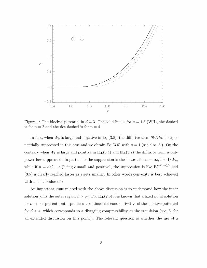
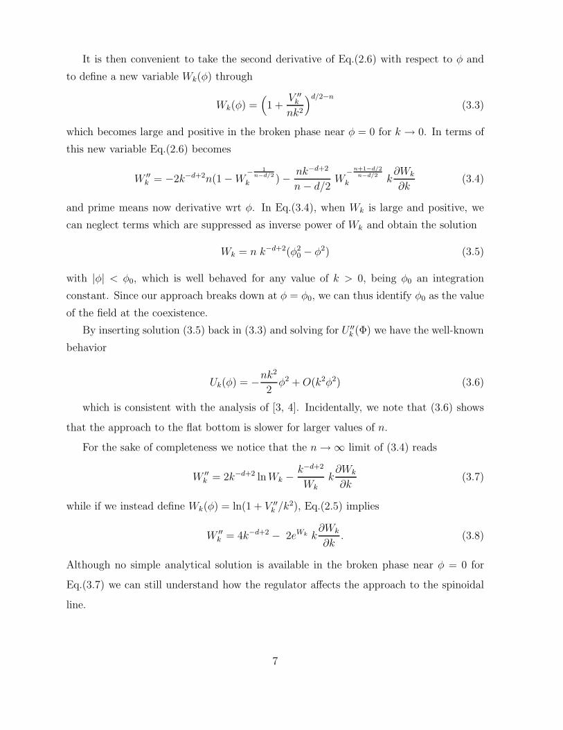
Figure 1: The blocked potential in d = 3. The solid line is for n = 1.5 (WH), the dashedis for n = 2 and the dot-dashed is for n = 4

In fact, when Wk is large and negative in Eq.(3.8), the diffusive term ∂W/∂k is expo-

nentially suppressed in this case and we obtain Eq.(3.6) with n = 1 (see also [5]). On the

contrary when Wk is large and positive in Eq.(3.4) and Eq.(3.7) the diffusive term is only

power-law suppressed. In particular the suppression is the slowest for n → ∞, like 1/Wk,

while if n = d/2 + ǫ (being ǫ small and positive), the suppression is like W−(1+ǫ)/ǫk and

(3.5) is clearly reached faster as ǫ gets smaller. In other words convexity is best achieved

with a small value of ǫ.

An important issue related with the above discussion is to understand how the inner

solution joins the outer region φ > φ0. For Eq.(2.5) it is known that a fixed point solution

for k → 0 is present, but it predicts a continuous second derivative of the effective potential

for d < 4, which corresponds to a diverging compressibility at the transition (see [5] for

an extended discussion on this point). The relevant question is whether the use of a

8

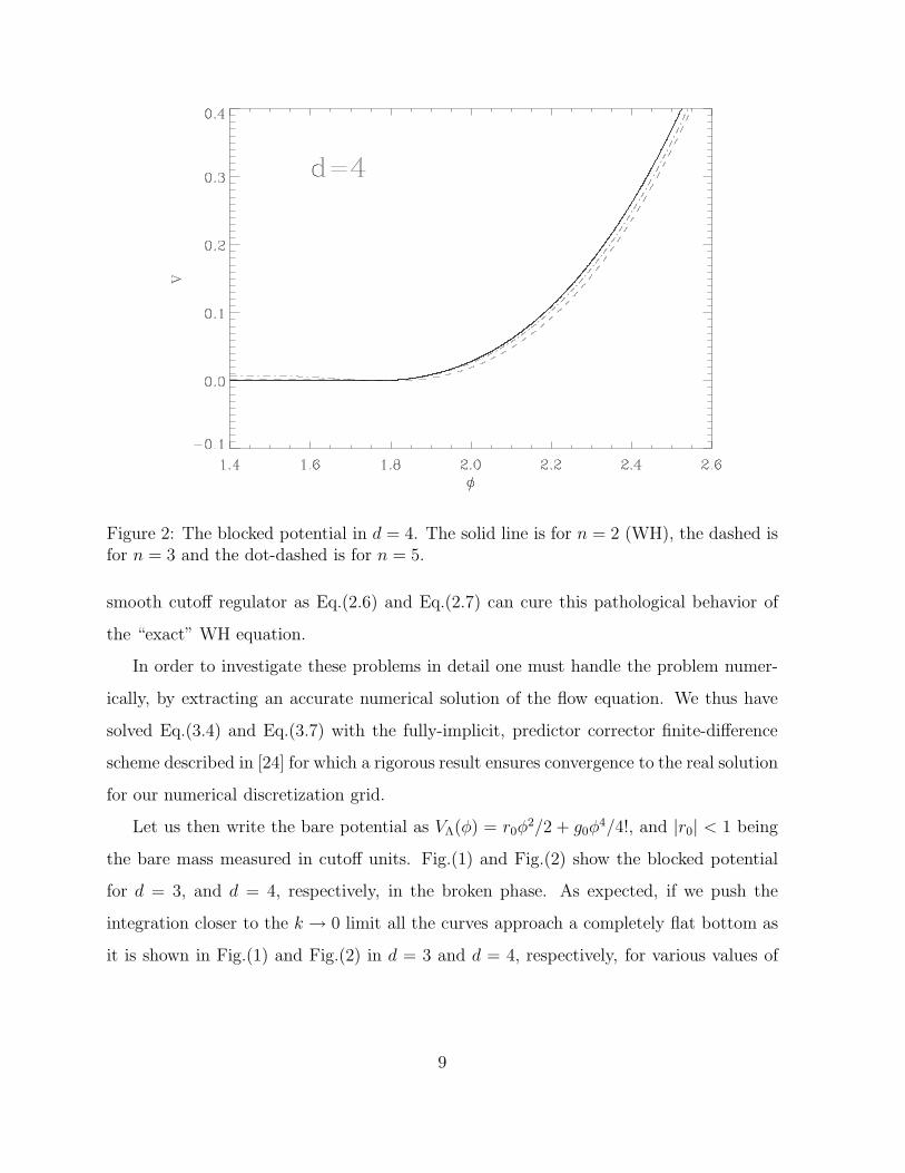
Figure 2: The blocked potential in d = 4. The solid line is for n = 2 (WH), the dashed isfor n = 3 and the dot-dashed is for n = 5.

smooth cutoff regulator as Eq.(2.6) and Eq.(2.7) can cure this pathological behavior of

the “exact” WH equation.

In order to investigate these problems in detail one must handle the problem numer-

ically, by extracting an accurate numerical solution of the flow equation. We thus have

solved Eq.(3.4) and Eq.(3.7) with the fully-implicit, predictor corrector finite-difference

scheme described in [24] for which a rigorous result ensures convergence to the real solution

for our numerical discretization grid.

Let us then write the bare potential as VΛ(φ) = r0φ2/2 + g0φ

4/4!, and |r0| < 1 being

the bare mass measured in cutoff units. Fig.(1) and Fig.(2) show the blocked potential

for d = 3, and d = 4, respectively, in the broken phase. As expected, if we push the

integration closer to the k → 0 limit all the curves approach a completely flat bottom as

it is shown in Fig.(1) and Fig.(2) in d = 3 and d = 4, respectively, for various values of

9

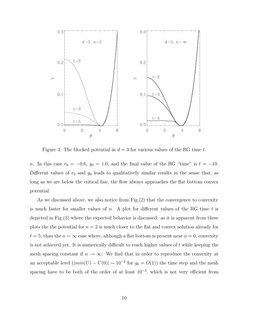
Figure 3: The blocked potential in d = 3 for various values of the RG time t.

n. In this case r0 = −0.6, g0 = 1.0, and the final value of the RG “time” is t = −10.

Different values of r0 and g0 leads to qualitatively similar results in the sense that, as

long as we are below the critical line, the flow always approaches the flat bottom convex

potential.

As we discussed above, we also notice from Fig.(2) that the convergence to convexity

is much faster for smaller values of n. A plot for different values of the RG time t is

depicted in Fig.(3) where the expected behavior is discussed: as it is apparent from these

plots the the potential for n = 2 is much closer to the flat and convex solution already for

t = 5, than the n = ∞ case where, although a flat bottom is present near φ = 0, convexity

is not achieved yet. It is numerically difficult to reach higher values of t while keeping the

mesh spacing constant if n → ∞. We find that in order to reproduce the convexity at

an acceptable level (|min(U) − U(0)| ∼ 10−2 for g0 = O(1)) the time step and the mesh

spacing have to be both of the order of at least 10−3, which is not very efficient from

10

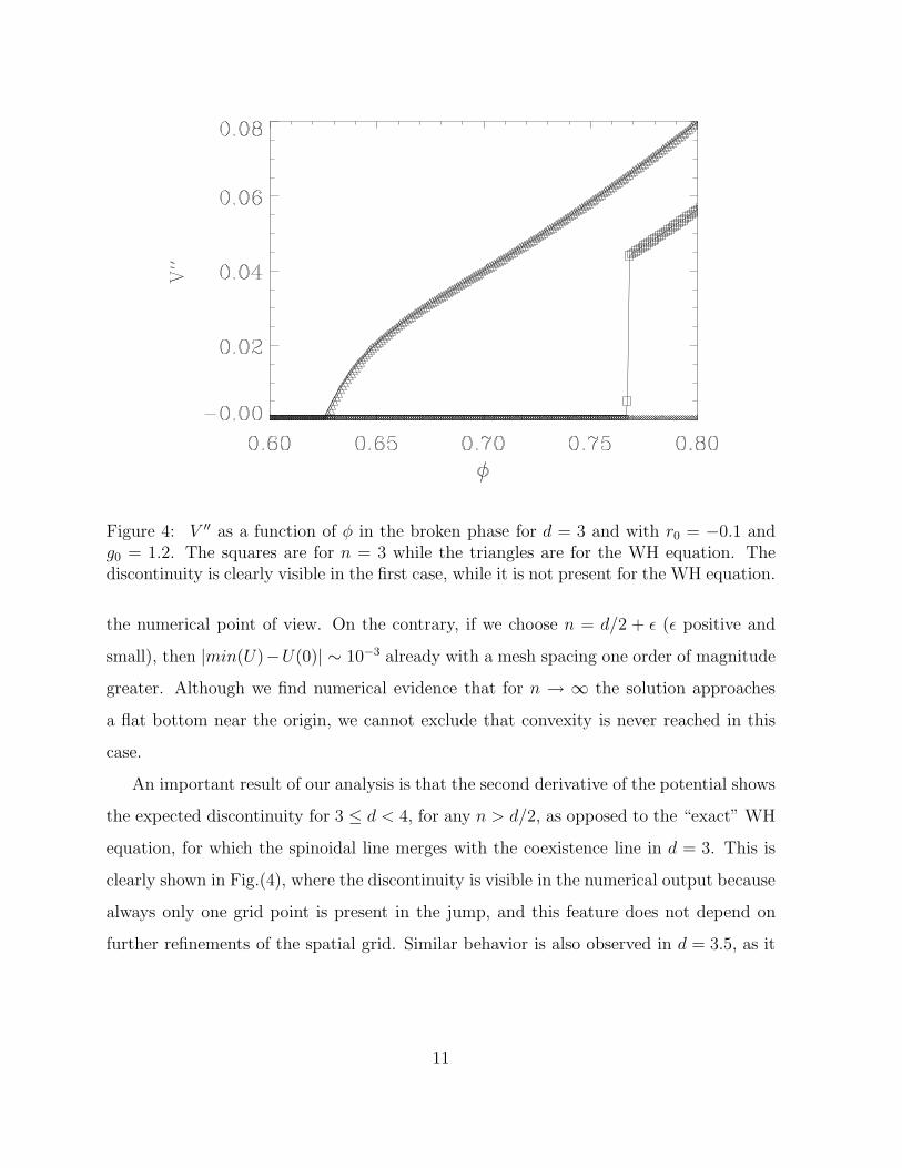
Figure 4: V ′′ as a function of φ in the broken phase for d = 3 and with r0 = −0.1 andg0 = 1.2. The squares are for n = 3 while the triangles are for the WH equation. Thediscontinuity is clearly visible in the first case, while it is not present for the WH equation.

the numerical point of view. On the contrary, if we choose n = d/2 + ǫ (ǫ positive and

small), then |min(U)−U(0)| ∼ 10−3 already with a mesh spacing one order of magnitude

greater. Although we find numerical evidence that for n → ∞ the solution approaches

a flat bottom near the origin, we cannot exclude that convexity is never reached in this

case.

An important result of our analysis is that the second derivative of the potential shows

the expected discontinuity for 3 ≤ d < 4, for any n > d/2, as opposed to the “exact” WH

equation, for which the spinoidal line merges with the coexistence line in d = 3. This is

clearly shown in Fig.(4), where the discontinuity is visible in the numerical output because

always only one grid point is present in the jump, and this feature does not depend on

further refinements of the spatial grid. Similar behavior is also observed in d = 3.5, as it

11

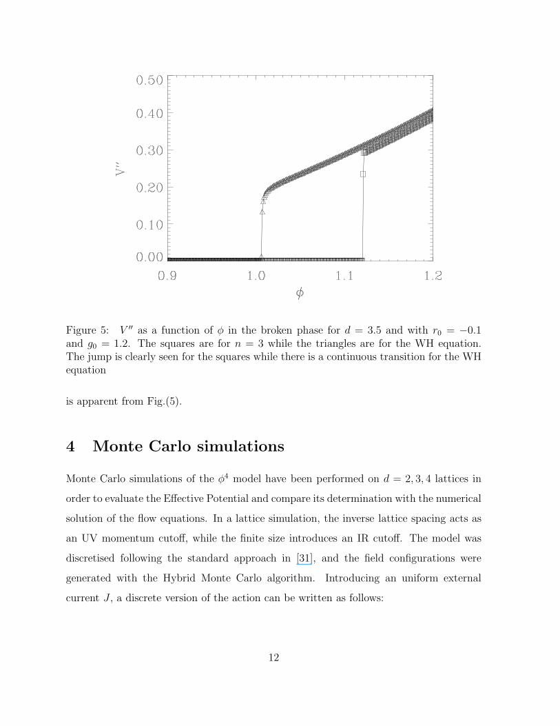
Figure 5: V ′′ as a function of φ in the broken phase for d = 3.5 and with r0 = −0.1and g0 = 1.2. The squares are for n = 3 while the triangles are for the WH equation.The jump is clearly seen for the squares while there is a continuous transition for the WHequation

is apparent from Fig.(5).

4 Monte Carlo simulations

Monte Carlo simulations of the φ4 model have been performed on d = 2, 3, 4 lattices in

order to evaluate the Effective Potential and compare its determination with the numerical

solution of the flow equations. In a lattice simulation, the inverse lattice spacing acts as

an UV momentum cutoff, while the finite size introduces an IR cutoff. The model was

discretised following the standard approach in [31], and the field configurations were

generated with the Hybrid Monte Carlo algorithm. Introducing an uniform external

current J , a discrete version of the action can be written as follows:

12

0 50 100 150 200configuration

1.25

1.5

1.75

2

2.25

2.5

2.75

3

3.25

Φ

J = 0J = 0.25J = 0.5

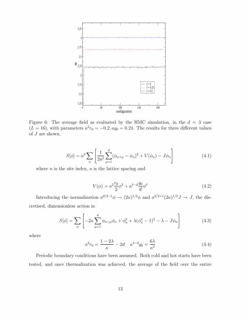
Figure 6: The average field as evaluated by the HMC simulation, in the d = 3 case(L = 16), with parameters a2r0 = −0.2, ag0 = 0.24. The results for three different valuesof J are shown.

S[φ] = ad∑

n

[

1

2a2

d∑

µ=1

(φn+µ − φn)2 + V (φn) − Jφn

]

(4.1)

where n is the site index, a is the lattice spacing and

V (φ) = a2 r0

2φ2 + a4−dg0

4!φ4 (4.2)

Introducing the normalization ad/2−1φ → (2κ)1/2φ and ad/2+1(2κ)1/2J → J , the dis-

cretised, dimensionless action is:

S[φ] =∑

n

[

−2κd

∑

µ=1

φn+µφn + φ2n + λ(φ2

n − 1)2 − λ − Jφn

]

(4.3)

where

a2r0 =1 − 2λ

κ− 2d a4−dg0 =

6λ

κ2(4.4)

Periodic boundary conditions have been assumed. Both cold and hot starts have been

tested, and once thermalization was achieved, the average of the field over the entire

13

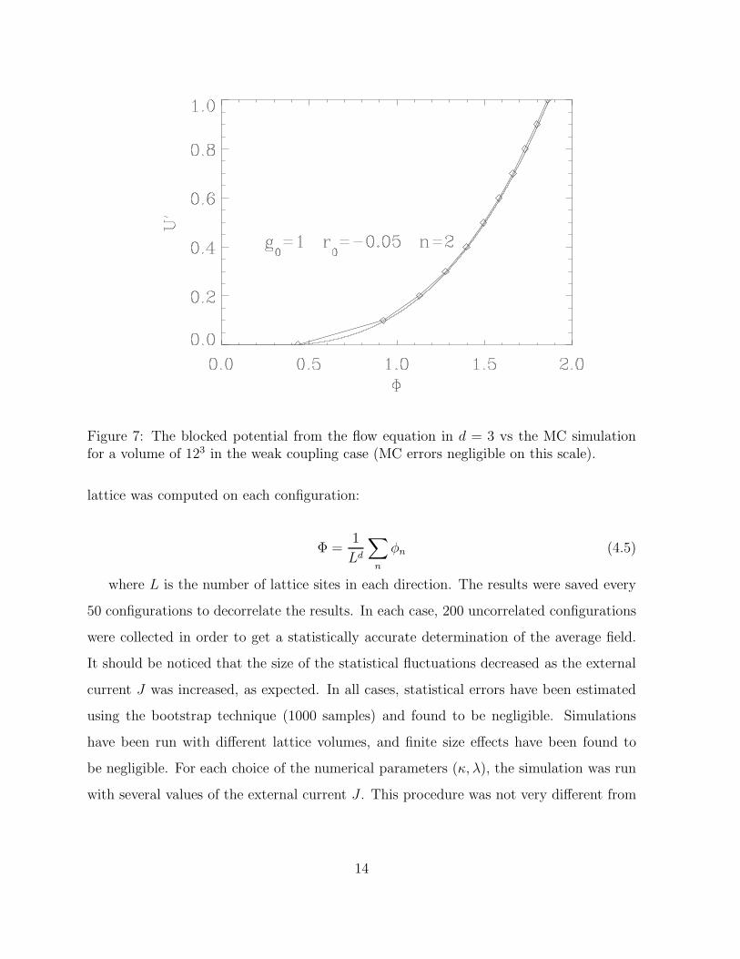
Figure 7: The blocked potential from the flow equation in d = 3 vs the MC simulationfor a volume of 123 in the weak coupling case (MC errors negligible on this scale).

lattice was computed on each configuration:

Φ =1

Ld

∑

n

φn (4.5)

where L is the number of lattice sites in each direction. The results were saved every

50 configurations to decorrelate the results. In each case, 200 uncorrelated configurations

were collected in order to get a statistically accurate determination of the average field.

It should be noticed that the size of the statistical fluctuations decreased as the external

current J was increased, as expected. In all cases, statistical errors have been estimated

using the bootstrap technique (1000 samples) and found to be negligible. Simulations

have been run with different lattice volumes, and finite size effects have been found to

be negligible. For each choice of the numerical parameters (κ, λ), the simulation was run

with several values of the external current J . This procedure was not very different from

14

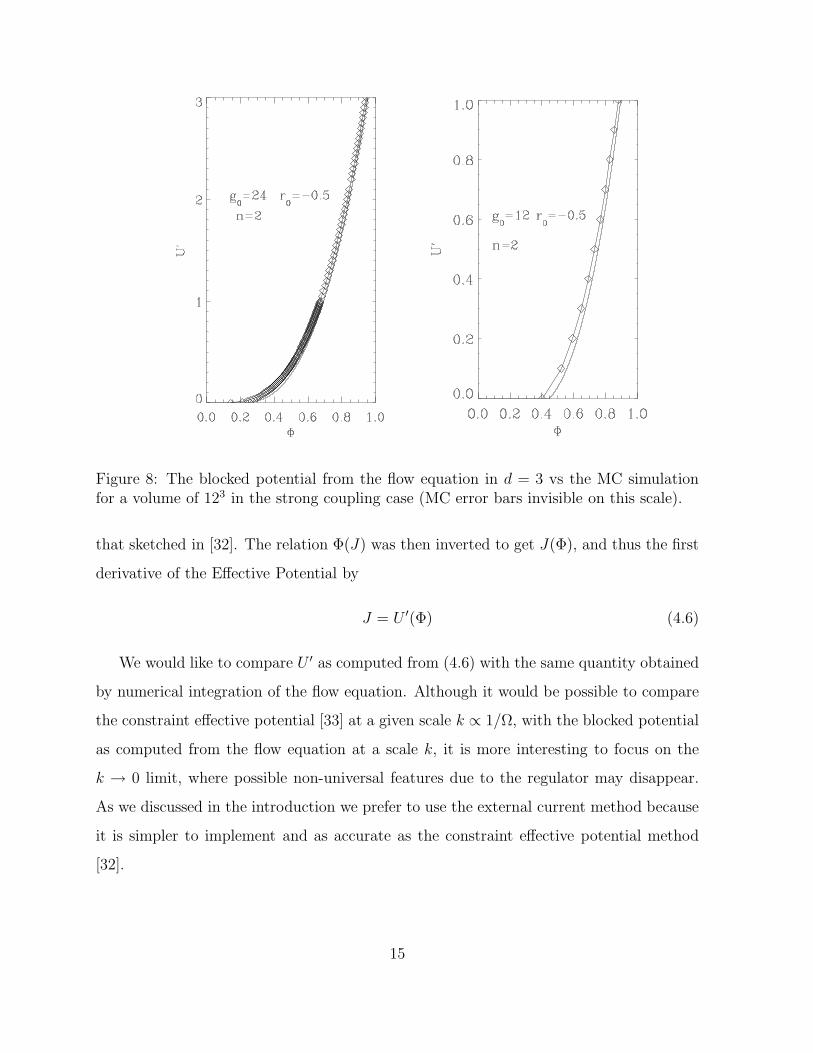
Figure 8: The blocked potential from the flow equation in d = 3 vs the MC simulationfor a volume of 123 in the strong coupling case (MC error bars invisible on this scale).

that sketched in [32]. The relation Φ(J) was then inverted to get J(Φ), and thus the first

derivative of the Effective Potential by

J = U ′(Φ) (4.6)

We would like to compare U ′ as computed from (4.6) with the same quantity obtained

by numerical integration of the flow equation. Although it would be possible to compare

the constraint effective potential [33] at a given scale k ∝ 1/Ω, with the blocked potential

as computed from the flow equation at a scale k, it is more interesting to focus on the

k → 0 limit, where possible non-universal features due to the regulator may disappear.

As we discussed in the introduction we prefer to use the external current method because

it is simpler to implement and as accurate as the constraint effective potential method

[32].

15

We explore a set of parameters which is not close to the critical line, so that finite-

size effects can be neglected, and we are able to compare the result of the flow equation

directly to the lattice determination of the effective potential. In particular we find that

it is was not necessary to construct a lattice version of the RG flow equation as discussed

in [34]. We have integrated Eq.(3.4) rewriting all the relevant quantities in units of the

UV cut-off and then we have followed the evolution down to t → ∞ with the help of the

numerical integrator. In order to show the predictive power of our approach we have not

fine-tuned the bare parameters in the RG flow equations to reproduce renormalized mass

and coupling constant obtained in the lattice calculation as done in [34]. Instead, we have

decided to set the same bare mass and coupling constant in the lattice bare potential

(4.2) and in the bare potential of the RG equation. Moreover we have rescaled back

our potential and field according to (3.2) so that we get U ′

k=0(Φ) out of the numerical

computation. According to the analysis of the previous session we have considered n ∈

(d/2, d] where the numerical stability is best achieved.

The results are shown in Fig.(7) and Fig.(8) for n = 2 and d = 3, where it is apparent

that there is already a very good agreement with the MC data both in the weak and in

the strong coupling regime. Better agreement could probably be achieved by including

the wave-function renormalization function, but this is not our main concern in this

investigation.

5 Conclusions

We have discussed the PTRG flow equation below the critical line in a scalar theory. In

particular we have shown that the convexity property of the free energy is recovered by

integration of the LPA flow equation in the k → ∞ limit. Within a class of n-dependent

proper time regulator, the approach to the correct flat bottom potential is faster when

n = d/2 + ǫ being ǫ positive and small. The expected discontinuity of the U ′′ at the

transition is correctly reproduced for any value of ǫ > 0 as opposed to the “exact” WH

16

flow (ǫ = 0), which does not show this feature. We have performed an extensive MC

investigation of the EP in d = 3 in order to discuss the numerical predictions and we

found very good agreement both the strong coupling and weak coupling phase without

resorting to a fine-tuning procedure between the bare parameters in the MC and in the

RG flow equation. We anticipate that our result can be relevant in gauge theory where the

presence of the PT regulator is an essential tool deriving a non-perturbative flow equation

[23].

Acknowledgements

We acknowledge Martin Reuter and Dario Zappala for useful comments. G. Lacagnina

acknowledges the financial support by the DFG-Forschergruppe “Lattice Hadron Phe-

nomenology” and wishes to thank V. Braun, A. Schafer and M. Gockeler for useful dis-

cussions.

References

[1] P.C. Hemmer, J.L. Lebowitz, in Phase Transitions and Critical Phenomena, edited

by C. Domb and M.S.Green (Academic, New York, 1976), Vol 5b.

[2] E.J. Weinberg, Ai-qun Wu, Phys. Rev. D36 (1987), 2474.

[3] A. Ringwald, C. Wetterich, Nucl. Phys. B353 (1991), 303.

[4] N.Tetradis, C. Wetterich, Nucl. Phys. B383 (1992), 197.

[5] A. Parola, D. Pini, L. Reatto, Phys. Rev. E48 (1993), 3321; A. Parola, L. Reatto,

Phys. Rev. Lett. 53 (1984), 2417; Phys. Rev. A31 (1985), 3309; Adv. in Phys. 44

(1995), 211; J. Phys. Cond. Matter 8 (1996), 9221.

17

[6] J. Berges, N. Tetradis, C. Wetterich, Phys. Rep. 363 (2002), 223 and

hep-ph/0005122.

[7] J. Alexandre, V. Branchina, J. Polonyi, Phys. Lett. B445 (1999), 351.

[8] L. O’Raifeartaigh, A. Wipf, H. Yoneyama, Nucl. Phys. B271 (1986), 273.

[9] K.G. Wilson, M.E. Fisher, Phys. Rev. Lett. 28 (1972), 240; K.G. Wilson,J. Kogut,

Phys. Rep. 12C (1974), 75.

[10] G. Papp, B.J. Schafer, H.J. Pirner, J. Wambach, Phys. Rev. D61 (2000), 096002.

[11] B.J. Schafer, H.J. Pirner, Nucl. Phys. A627 (1997), 481; Nucl. Phys. A660 (1999),

439; J. Meyer, G. Papp, H.J. Pirner, T. Kunihiro, Phys. Rev. C61 (2000), 035202.

[12] O. Bohr, B.J. Schafer, J. Wambach, Renormalization group flow equations and the

phase transition in O(N) models, Preprint July 2000, and hep-ph/0007098.

[13] F. J. Wegner, A. Houghton, Phys. Rev A8 (1972) , 401.

[14] D. F. Litim, Phys. Rev. D 64 (2001) , 105007; JHEP, 0111, 059, (2001).

[15] D. F. Litim, J. M. Pawlowski, Phys. Lett. B 516 (2001), 197.

[16] D. F. Litim, J. M. Pawlowski, Phys. Rev. D 65 (2002), 081701(R); Phys. Rev. D 66

(2002), 025030; Phys. Lett. B 546 (2002), 279.

[17] D. Zappala, Phys. Rev. D 66 (2002), 105020.

[18] A. Bonanno, D. Zappala, Phys. Lett. B504 (2001), 181.

[19] M. Mazza, D. Zappala, Phys. Rev. D 64 (2001), 105013.

[20] D. Zappala, Phys. Lett. A 290 (2001), 35.

[21] M. Oleszczuk, Z. Phys. C64, (1994), 533.

18

[22] S.-B. Liao, Phys. Rev. D53, (1996), 2020.

[23] S.-B. Liao, Phys. Rev. D56, (1997), 5008.

[24] W.F. Ames, Numerical methdos for Partial Differential Equations (Academic, Lon-

don, 1977).

[25] J. Zinn-Justin, Quantum Field Theory and Critical Phenomena, (3rd ed., Oxford

University Press, 1996).

[26] P. Butera, M. Comi, Phys. Rev. B56 (1997), 8212.

[27] B.G. Nickel, J.J. Rehr, J. Stat. Phys. 61 (1990), 1.

[28] C.F. Baillie, R. Gupta, K.A. Hawick, G.S. Pawley, Phys. Rev. B45 (1992), 10438,

and references therein.

[29] H.G. Ballesteros, L.A. Fernandez, V. Martin-Mayor, A. Munoz Sudupe, Phys. Lett.

B387 (1996), 125.

[30] M. Hasenbush, J. Phys. A32 (1999), 4851.

[31] I. Montvay, G. Munster, Quantum Fields on a Lattice, (Cambridge University Press,

1994).

[32] A. Ardekani, A.G. Williams, Phys. Rev. E 57 (1998), 6140.

[33] O’Raifeartaigh, A.Wipf, H.Yoneyama Nucl.Phys. B 271 (1986), 653.

[34] J.R. Shepard, V. Dmitrasinovic, Phys. Rev. D51 (1995), 7017.

19