Split-beam echosounder observations of natural methane ...

University of New Hampshire University of New Hampshire

University of New Hampshire Scholars' Repository University of New Hampshire Scholars' Repository

Center for Coastal and Ocean Mapping Center for Coastal and Ocean Mapping

3-2015

Split-beam echosounder observations of natural methane seep Split-beam echosounder observations of natural methane seep

variability in the northern Gulf of Mexico variability in the northern Gulf of Mexico

Kevin W. Jerram University of New Hampshire, Durham, [email protected]

Thomas C. Weber University of New Hampshire, Durham, [email protected]

Jonathan Beaudoin University of New Hampshire, Durham

Follow this and additional works at: https://scholars.unh.edu/ccom

Part of the Geochemistry Commons, and the Geophysics and Seismology Commons

Recommended Citation Recommended Citation Jerram, K., T. C. Weber, and J. Beaudoin (2015), Split-beam echo sounder observations of natural methane seep variability in the northern Gulf of Mexico, Geochem. Geophys. Geosyst., 16, 736–750, doi:10.1002/ 2014GC005429.

This Journal Article is brought to you for free and open access by the Center for Coastal and Ocean Mapping at University of New Hampshire Scholars' Repository. It has been accepted for inclusion in Center for Coastal and Ocean Mapping by an authorized administrator of University of New Hampshire Scholars' Repository. For more information, please contact [email protected].

RESEARCH ARTICLE10.1002/2014GC005429

Split-beam echo sounder observations of natural methaneseep variability in the northern Gulf of MexicoKevin Jerram1, Thomas C. Weber1, and Jonathan Beaudoin1

1Center for Coastal and Ocean Mapping, University of New Hampshire, Durham, New Hampshire, USA

Abstract A method for positioning and characterizing plumes of bubbles from marine gas seeps usingan 18 kHz scientific split-beam echo sounder (SBES) was developed and applied to acoustic observations ofplumes of presumed methane gas bubbles originating at approximately 1400 m depth in the northern Gulfof Mexico. A total of 161 plume observations from 27 repeat surveys were grouped by proximity into 35clusters of gas vent positions on the seafloor. Profiles of acoustic target strength per vertical meter of plumeheight were calculated with compensation for both the SBES beam pattern and the geometry of plumeensonification. These profiles were used as indicators of the relative fluxes and fates of gas bubbles acousti-cally observable at 18 kHz and showed significant variability between repeat observations at time intervalsof 1 h–7.5 months. Active gas venting was observed during approximately one third of the survey passes ateach cluster. While gas flux is not estimated directly in this study owing to lack of bubble size distributiondata, repeat surveys at active seep sites showed variations in acoustic response that suggest relativechanges in gas flux of up to 1 order of magnitude over time scales of hours. The minimum depths of acous-tic plume observations at 18 kHz averaged 875 m and frequently coincided with increased amplitudes ofacoustic returns in layers of biological scatterers, suggesting acoustic masking of the gas bubble plumes inthese layers. Minimum plume depth estimates were limited by the SBES field of view in only five instances.

1. Introduction

Marine methane gas seeps support diverse biological communities on the seafloor; indicate locations ofpotentially exploitable hydrocarbon deposits; increase localized concentrations of dissolved methane in thewater column; and, in cases of free gas ebullition and bubble ascent through the water column, may con-tribute directly to the atmospheric quantity of this potent greenhouse gas [Judd, 2003, 2004; Greinert andN€utzel, 2004; Hovland et al., 2012; Mienert, 2012]. Accordingly, interest from public, scientific, environmental,and governmental groups in marine methane gas seeps has increased significantly in recent decades [Juddet al., 2002; Hovland et al., 2012]. Of widespread and long-term interest are the locations of gas vent areas,the quantities and fates of free gas bubbles in the water column, and the variability of seep activity at sitesof active venting such that long-term averages of gas flux can be estimated [Naudts et al., 2006; Greinert,2008; Hovland et al., 2012; Kannberg et al., 2013]. In this study, we present a method for georeferencing andcharacterizing the acoustic responses of natural marine gas bubble plumes observed with a widely installedfishery research echo sounder. This method is capable of positioning gas vent areas on the seafloor withaccuracies near those of a multibeam echo sounder used for bathymetric mapping. The acoustic scatteringstrengths of plumes are compared after isolation from effects of the observational platform and environ-ment, such as the echo sounder pulse length and orientation as well as the plume shape due to currents.This method is employed to identify and to evaluate the temporal variability of gas vent sites during twoseries of ship-based acoustic surveys in the northern Gulf of Mexico in 2011 and 2012.

1.1. Acoustic Observations of Marine Gas BubblesShip-based acoustic methods have been demonstrated to be suitable for detecting midwater plumes of gasbubbles [e.g., Greinert et al., 2006], locating corresponding vent sites on the seafloor [e.g., Artemov, 2006],and estimating the shallowest depths of bubble survival. Acoustic methods offer advantages over gas fluxmeasurement systems requiring in situ bubble monitoring or collection equipment [e.g., Hornafius et al.,1999] in that echo sounders may be readily applied over large spatial scales and do not affect gas or waterflow at the seafloor [Judd, 2003]. Natural methane seeps have been detected and investigated with acoustic

Key Points:� A split-beam scientific echo sounder

is used to profile methane bubbleplumes� Repeat observations suggest order-

of-magnitude gas flow variabilityover hours� One third of known seep sites in the

survey area are detected during eachpass

Supporting Information:� ms_similarity_data

Correspondence to:K. Jerram,[email protected]

Citation:Jerram, K., T. C. Weber, and J. Beaudoin(2015), Split-beam echo sounderobservations of natural methane seepvariability in the northern Gulf ofMexico, Geochem. Geophys. Geosyst.,16, 736–750, doi:10.1002/2014GC005429.

Received 13 JUN 2014

Accepted 21 JAN 2015

Accepted article online 28 JAN 2015

Published online 19 MAR 2015

JERRAM ET AL. VC 2015. American Geophysical Union. All Rights Reserved. 736

Geochemistry, Geophysics, Geosystems

PUBLICATIONS

techniques in every major ocean on Earth [Judd, 2003] using various combinations of split-beam scientificecho sounders (SBES) [e.g., Naudts et al., 2006; Weber et al., 2012a], multibeam echo sounders (MBES) [Niko-lovska et al., 2008; Weber et al., 2012c], side-scan sonars [e.g., Jones et al., 2010], subbottom profilers [e.g.,Naudts et al., 2006], and acoustic Doppler current profilers [e.g., Holland et al., 2006]. SBES systems have alsobeen used for detecting and monitoring anthropogenic seeps including methane gas and oil released intothe water column from leaking wells and pipelines [Johansen et al., 2003; Hickman et al., 2012; Weber et al.,2012b]. While the source of gas on the seafloor might truly include many small point sources, we are limited(as in all investigations) in the resolution of the instrument. In this study, we consider a seep or gas vent tobe a region on the seafloor that produces a plume of gas bubbles occupying a small range of target angles(angles from the sonar to the acoustic scatterer of interest) within the larger echo sounder field of view ateach range. That is, the horizontal extent of the train of bubbles near the seafloor is approximately an orderof magnitude smaller than the beam width footprint at that depth. Several terms are used in the literatureto describe acoustic observations of bubbles in the water column, including ‘‘flares,’’ ‘‘seeps,’’ and ‘‘plumes.’’In this study, the phrase ‘‘plume observation’’ refers to acoustic data indicating a train of free gas bubblesascending through the water column from a seep area on the seafloor.

In this study, an 18 kHz Simrad EK60 SBES was utilized for detection, georeferencing, and target strength(TS) characterization of marine gas seeps in the northern Gulf of Mexico. SBES systems have been tradition-ally employed in fishery research, for which standard methods of in situ beam pattern measurements havebeen developed that enable calibrated TS measurements [Foote et al., 1987]. Calibrated TS measurementsfor gas bubbles are necessary to accurately calculate the bubbles’ acoustic scattering cross sections, whichdepend primarily on gas composition, bubble radius, and ambient conditions [Clay and Medwin, 1977].Given information or assumptions about gas composition, distribution of bubble radii, and ambient condi-tions, calibrated TS measurements facilitate calculation or estimation of gas flux [e.g., Artemov et al., 2007;Ostrovsky et al., 2008; Weber et al., 2014]. Though no estimates of gas flux are made in this study owing tothe lack of direct bubble composition and size distribution data, the calibrated TS measurements possiblewith SBES systems represent a significant advantage over noncalibrated echo sounders for this purposewhere bubble composition and size distribution data are available.

Some of the advantages of using a SBES for seep investigation were identified by Artemov [2006] andaddressed in part for studies with a Simrad EK500, a precursor to the EK60, in the Black Sea. The methoddescribed herein is similar to that described by Artemov [2006] but also incorporates several distinct fea-tures with regard to georeferencing seep targets, characterizing the scattering strength profiles of plumes,and establishing the limits of the echo sounder field of view (FOV). This method was applied to data col-lected during repeat surveys in an area of active venting in 2011 and 2012 (Figure 1) to evaluate the vari-ability in acoustic scattering strengths of gas bubbles and bubble fates, including the presence and absenceof plumes with consideration for the echo sounder FOV. These factors have significant implications forlong-term average flux estimates. While variability has been studied previously [e.g., Leifer et al., 2004; Grei-nert, 2008; Schneider von Deimling et al., 2011], this study adds to the body of research by examining vari-ability in gas flow over a relatively large region (8 km survey lines with an approximately 290 m diameterecho sounder footprint on the seafloor) during repeat survey passes spanning a comparatively long-timescale (up to 7.5 months). The results of this study confirm the applicability of SBES systems for georeferenc-ing of seep sites and calibrated TS monitoring for gas flow, and also demonstrate acceptable gas vent posi-tioning accuracy with the SBES compared to MBES. Calibrated TS data are further compensated in thisstudy for the effects of echo sounder pulse length, vessel orientation, and plume axis deformation due tocurrents; the resulting scattering strength is normalized by the vertical extent of plume ensonification andreferred to as Sz, z being the vertical axis of interest for bubble transport. For a given frequency, Sz facilitatesunbiased comparison of plume scattering strengths along the vertical axis across observational platforms(e.g., different echo sounder pulse lengths and orientations) and environmental conditions (e.g., currentswhich deform the plumes during ascent). These factors are not considered completely in other scatteringstrength values used in the literature, such as volume scattering (Sv), area scattering (Sa), or TS. For instance,holding all other parameters constant, a change in echo sounder pulse length from 1 to 4 ms between sur-veys would result in a 6 dB increase in TS. Of interest for future seep mapping efforts, our observationsshow large variability in plume presence and scattering strength, suggesting that long-term flux estimatesin the Gulf of Mexico would benefit from repeat surveys because single-pass surveys do not identify all vent

Geochemistry, Geophysics, Geosystems 10.1002/2014GC005429

JERRAM ET AL. VC 2015. American Geophysical Union. All Rights Reserved. 737

sites along a survey track line, capture the variability in plume scattering strengths at known vent sites, orestablish relationships in gas flow between nearby vent sites which may be linked by subbottom gas migra-tion pathways.

2. Methods

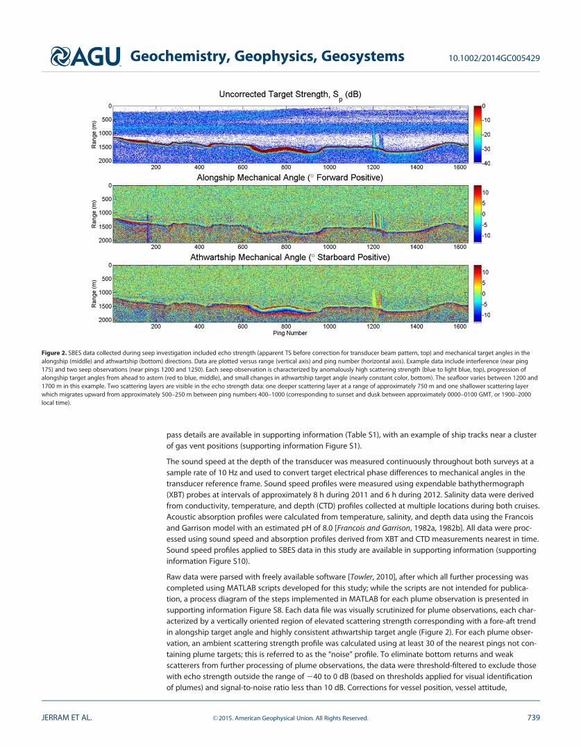
An 18 kHz Simrad EK60 SBES with 4 ms transmit pulse length and one-way 23 dB total angular beam widthof 12� was used to collect water column backscatter data during repeat seep mapping surveys aboardNOAA ship Okeanos Explorer over the southwest edge of the Biloxi Dome in the northern Gulf of Mexico(Figure 1), a region well known for gas venting [Judd et al., 2002; MacDonald et al., 2003; Weber et al., 2014].Unless specified otherwise, all echo sounder descriptions and data discussed in this text refer to the SimradEK60 SBES and the FOV refers to the 12� cone representing the echo sounder beam width. The transducerwas mounted adjacent to the vessel’s Kongsberg EM302 MBES on a hull ‘‘blister’’ designed for acoustic sen-sors at approximately 4.6 m depth. Data collected include echo strength (apparent target strength prior tocompensation for transducer beam pattern) and digitized electrical phase differences in the alongship(bow-to-stern) and athwartship (port-to-starboard) directions (Figure 2). Vessel position and attitude weremeasured with an Applanix POS/MV 320 motion sensor receiving position corrections from a C-NAV 2050differential global positioning system (GPS), yielding position and attitude uncertainties of 1.3 m (horizontaldilution of precision) and 0.02� (one standard deviation), respectively.

Twenty-seven acoustic survey passes over the Biloxi Dome were conducted on NNW and SSE headings inlate August and early September 2011 and April 2012 (Figure 1 and supporting information Table S1). Timeintervals between passes varied from less than an hour to over a week during the 2011 survey. Survey oper-ations in 2012 were broken into two sessions separated by approximately 12 h, with mean time intervalsbetween survey passes of 1.2 and 1.7 h for the first and second sessions, respectively. In order to improvecoverage of known vent sites during the 2012 survey, the mean survey orientation (course over ground)was adjusted from 152�–332� in 2011 to 147�–327� in 2012. Additionally, to increase the number of pingscontaining plume data at each known vent site, mean vessel speed during survey operations was reducedfrom 11.3 kn in 2011 to 10.0 kn and 7.0 kn during the first and second sessions, respectively, in 2012. Survey

Figure 1. Seep study area on the southwest edge of the Biloxi Dome in the northern Gulf of Mexico. Projection is Universal TransverseMercator (UTM, zone 16 North) referenced to the WGS84 ellipsoid. Bathymetric data were collected with a 30 kHz Kongsberg EM302 MBESaboard NOAA Ship Okeanos Explorer during SBES data collection in 2011. The survey lines represent the mean ship tracks during data col-lection in 2011 and 2012. Clusters are numbered sequentially from northwest to southeast and indicated by circles with radii of 145 m torepresent the approximate SBES beam width footprint on the seafloor. Circles are centered at the means of seep positions for each cluster.Gulf of Mexico maps on left adapted from NOAA image (http://www.ngdc.noaa.gov/mgg/image/gom_hillshade.jpg).

Geochemistry, Geophysics, Geosystems 10.1002/2014GC005429

JERRAM ET AL. VC 2015. American Geophysical Union. All Rights Reserved. 738

pass details are available in supporting information (Table S1), with an example of ship tracks near a clusterof gas vent positions (supporting information Figure S1).

The sound speed at the depth of the transducer was measured continuously throughout both surveys at asample rate of 10 Hz and used to convert target electrical phase differences to mechanical angles in thetransducer reference frame. Sound speed profiles were measured using expendable bathythermograph(XBT) probes at intervals of approximately 8 h during 2011 and 6 h during 2012. Salinity data were derivedfrom conductivity, temperature, and depth (CTD) profiles collected at multiple locations during both cruises.Acoustic absorption profiles were calculated from temperature, salinity, and depth data using the Francoisand Garrison model with an estimated pH of 8.0 [Francois and Garrison, 1982a, 1982b]. All data were proc-essed using sound speed and absorption profiles derived from XBT and CTD measurements nearest in time.Sound speed profiles applied to SBES data in this study are available in supporting information (supportinginformation Figure S10).

Raw data were parsed with freely available software [Towler, 2010], after which all further processing wascompleted using MATLAB scripts developed for this study; while the scripts are not intended for publica-tion, a process diagram of the steps implemented in MATLAB for each plume observation is presented insupporting information Figure S8. Each data file was visually scrutinized for plume observations, each char-acterized by a vertically oriented region of elevated scattering strength corresponding with a fore-aft trendin alongship target angle and highly consistent athwartship target angle (Figure 2). For each plume obser-vation, an ambient scattering strength profile was calculated using at least 30 of the nearest pings not con-taining plume targets; this is referred to as the ‘‘noise’’ profile. To eliminate bottom returns and weakscatterers from further processing of plume observations, the data were threshold-filtered to exclude thosewith echo strength outside the range of 240 to 0 dB (based on thresholds applied for visual identificationof plumes) and signal-to-noise ratio less than 10 dB. Corrections for vessel position, vessel attitude,

Figure 2. SBES data collected during seep investigation included echo strength (apparent TS before correction for transducer beam pattern, top) and mechanical target angles in thealongship (middle) and athwartship (bottom) directions. Data are plotted versus range (vertical axis) and ping number (horizontal axis). Example data include interference (near ping175) and two seep observations (near pings 1200 and 1250). Each seep observation is characterized by anomalously high scattering strength (blue to light blue, top), progression ofalongship target angles from ahead to astern (red to blue, middle), and small changes in athwartship target angle (nearly constant color, bottom). The seafloor varies between 1200 and1700 m in this example. Two scattering layers are visible in the echo strength data: one deeper scattering layer at a range of approximately 750 m and one shallower scattering layerwhich migrates upward from approximately 500–250 m between ping numbers 400–1000 (corresponding to sunset and dusk between approximately 0000–0100 GMT, or 1900–2000local time).

Geochemistry, Geophysics, Geosystems 10.1002/2014GC005429

JERRAM ET AL. VC 2015. American Geophysical Union. All Rights Reserved. 739

orientation of the transducer in the vessel reference frame, and refraction of the acoustic raypath wereapplied to georeference all threshold-filtered plume targets. These georeferenced plume targets were thenused to estimate the associated gas vent positions on the seafloor, calculate plume TS profiles, and estimatethe minimum depths reached by bubbles acoustically observable at 18 kHz. More detailed descriptions ofthe methods for TS calibration, target positioning, timing corrections, and determination of transducerangular offsets are available in supporting information S1.1–S1.4.

2.1. Seep ClusteringTo identify repeat observations of unique seep sites across surveys, plume observations were grouped byfinding clusters of their associated gas vent position estimates in which all were separated by no more thana given ‘‘linking distance’’ of 65 m from at least one other gas vent. The linking distance approximates thelargest expected horizontal positioning uncertainty in the survey area according to the split-aperture corre-lation method employed by the echo sounder for target angle calculation (supporting information S1.5).This linking method relies on georeferenced plume data in the water column to identify spatial relation-ships among gas vent areas on the seafloor; accordingly, even if linked by subbottom gas migration path-ways, seep sites separated by more than 65 m may be treated as separate clusters using this criterion.

Based on simultaneous 2011 multibeam echo sounder observations, in which plumes near nadir typicallysubtended angles far less than the SBES beam width, each seep site was expected to have an areal extentmuch smaller than the SBES beam width footprint on the seafloor (approximately 290 m diameter at1400 m depth). Because no seep sites were observed in 2011 with areal extents exceeding the split-beamecho sounder beam width footprint (which would be termed ‘‘diffuse’’ seeps in the view of this echosounder), every plume observation was expected to capture the entire areal extent of the associated gasventing area on the seafloor. Plumes from gas vent areas of this nature occupy less than the beam width-limited ensonified volume and are hereafter described as ‘‘discrete’’ plumes in this study.

2.2. TS of Seep TargetsMidwater gas bubbles of radii much smaller than the acoustic wavelength scatter incident acoustic energyisotropically by damped harmonic oscillation (supporting information S1.6). Figure S2 (supporting informa-tion) presents the frequency and radius dependencies of TS for single bubbles of free methane gas in sea-water; in this figure, bubble resonance conditions are characterized by a TS peak for each bubble radius.The smaller radii used in this example (1–5 mm) are representative of methane gas bubbles observed usingremotely operated vehicles equipped with high-definition cameras and visual bubble sizing apparatus dur-ing the 2012 data collection period in the vicinity of the study area [Weber et al., 2014] and by other marinegas investigations in the Gulf of Mexico [Leifer and MacDonald, 2003] and at other deep water gas vent sitesin the Barents Sea [Sauter et al., 2006], Black Sea [Sahling et al., 2009], and Arabian Sea [R€omer et al., 2012].Based on the depth and radius dependencies of TS for methane bubbles depicted in Figure S2, it isexpected that changes in TS profiles represent changes to parameters of the ensonified bubbles acousti-cally observable at 18 kHz. For instance, changes in TS during bubble ascent may reflect changes in thenumbers of bubbles acoustically observable at 18 kHz, changes in the bubble size distribution, changes inthe scattering strengths of acoustically observable bubbles, or a combination thereof. Without knowledgeof the bubble size distribution in an ensonified target volume, ambiguity exists in the relationship betweenTS at any single frequency and the total volume of gas ensonified.

2.3. Sz for Single Discrete PlumesThough gas flux estimation is not possible for bubbles ensonified at a single frequency without knowledgeof bubble size distribution, temporal variability in scattering strength may be indicative of relative changesin gas flux for a single source with constant bubble size distribution. Likewise, scattering strength variabilityalong a plume axis in the vertical direction may indicate changes to net vertical gas flux and bubble behav-ior or survival during ascent [e.g., Rehder et al., 2002; McGinnis et al., 2006]. However, TS does not accountfor the geometry of intersection between the transmit pulse and the plume axis. This geometry of intersec-tion directly affects the number of bubbles ensonified for a given plume and depends on transmit pulselength, echo sounder orientation, and depth-dependent plume deformation due to water current structure.These parameters vary significantly between plume observations and among echo sounder configurationsfor seep studies. To isolate a scattering strength value independent from these variations, a quantity, Sz (dBre 1 m21) describing TS per unit of vertical extent of plume ensonification is suggested as

Geochemistry, Geophysics, Geosystems 10.1002/2014GC005429

JERRAM ET AL. VC 2015. American Geophysical Union. All Rights Reserved. 740

Sz5TS 2 10 log10 dz; (1)

where dz is the vertical extent (m) of plume axis ensonification (supporting information Figure S3). Theinherent assumption in this definition is that the range of target angles subtended by a discrete plume issmall compared to the beam width, as required for split-aperture target angle calculation. Further, TS is nor-malized by the vertical extent of the plume within each sample because it is assumed that the vertical fluxof gas is the quantity of interest. From Figure S3, dz is calculated as

dz5 L cos h; (2)

where L is the length of intersection between the transmit pulse and the plume axis. Angle h is measuredfrom vertical to the plume axis unit vector, u

*

p, along which all bubbles are assumed to have the samedirection of ascent. L is calculated as

L5cs

2 cos /; (3)

where c is sound speed (m/s) at the target estimated from sound speed profile data and s is the transmitpulse length (s). / is the angle between u

*

p and u*

r calculated from the dot product definition

cos /5u*

r � u*

p

ju*rjju*

pj; (4)

where u*

r is the unit vector aligned with the refraction-corrected path of the incident planar acoustic wave.For observations of single discrete plumes, the quantity Sz isolates TS from effects of transducer orientation,plume deformation, and changes in pulse length to facilitate comparison of acoustic scattering strengths of bub-bles along the vertical dimension of interest for gas flux. Figure 3 compares TS and Sz profiles for a single plumeobservation, showing a fairly consistent difference between the profile amplitudes. The apparent consistency ofthe difference between TS and Sz in this example is due to the relatively uniform vertical orientations of the echosounder and plume axes and the single transmission pulse length (4 ms) used in this study. As Sz normalizes TSfor the effects of these survey parameters to facilitate comparison of scattering strengths across studies, the dif-ference between TS and Sz would be expected to vary for other survey configurations and plume orientations.

2.4. Diffuse and Multiple Discrete PlumesCharacterization of relative gas flux by Sz is appropriate for single discrete plume observations, as the collec-tive backscattering strength for a single stream of bubbles in each echo sounder sample volume is expectedto be the only significant contributor to TS at each sample range. Because the beam pattern compensationfor TS calculation depends on accurate target angle calculation, which is confounded by the presence ofstrong scatterers at different target angles at each range, observations of multiple discrete plumes or diffuseplumes within the echo sounder field of view are likely plagued by erroneous target positioning, TS correc-tion, and Sz calculation.

The single discrete natures of plumes were verified using simultaneous multibeam echo sounder data proc-essed in the commercial water column mapping software QPS Fledermaus FMMidwater (supporting infor-mation Figure S4); any multiple discrete or diffuse plumes apparent in the multibeam data that also fellwithin the split-beam echo sounder field of view were flagged during further analyses (Figure 5, doubleexclamation points). In studies where simultaneous multibeam data are not available, identification of dif-fuse or multiple discrete plumes is problematic. It may be possible to identify the presence of diffuseplumes by examining the coherence of the target angle data, but this possibility was not explored here. Incases of diffuse plumes, volume scattering strength (Sv) is a more appropriate measure of collective scatter-ing strength for randomly spaced, noninteracting bubbles [Clay and Medwin, 1977].

3. Results

3.1. Seep Observations and PositionsTo identify repeat observations of unique seep sites at similar locations throughout the study area, seeparea position estimates calculated from SBES plume data were grouped (or ‘‘clustered’’) using a linking dis-tance of 65 m. This method yielded 35 clusters (Figure 1 and supporting information Table S2), each

Geochemistry, Geophysics, Geosystems 10.1002/2014GC005429

JERRAM ET AL. VC 2015. American Geophysical Union. All Rights Reserved. 741

including between 1 and 25 SBES observations on repeat survey lines, with a total of 161 seep area positionestimates among all clusters. Additional cluster data are available in supporting information Table S2. Foreach cluster, the mean of SBES gas vent position estimates was taken as the cluster center. Nine clusterscontained SBES observations from both 2011 and 2012, whereas eight clusters contained only 2011 dataand 18 clusters contained only 2012 data. These differences in plume counts per cluster between years arerelated primarily to realignment of the survey track line from 2011 to 2012. Among clusters containing twoor more plume observations, the horizontal differences between estimated gas vent positions and clustercenters on the seafloor averaged 35 m with a standard deviation of 19 m.

To examine the SBES seep positioning accuracy, SBES gas vent position estimates were compared to‘‘benchmark’’ positions from simultaneous MBES observations in 2011 (supporting information Figure S5).Results suggest SBES seep positioning accuracy on the order of MBES positioning capability for most casesof single discrete plumes. Additional information regarding SBES gas vent positioning results relative toMBES benchmarks is available in supporting information S2.1.

3.2. Sz Profiles and Plume DepthsProfiles of Sz versus depth were created for all plume observations (supporting information S2.2). The mini-mum acoustically observable plume depth was estimated for every plume observation by visual scrutiny of

Figure 3. TS and Sz profiles for an example SBES plume observation (Figure 2, near ping 1200). Dashed lines are noise profiles based on 30 pings immediately neighboring the plumeobservation. Green points represent scattering strengths of targets after threshold-filtering to exclude the seafloor (thick black horizontal line) and very weak scatterers, as well as forminimum signal-to-noise ratio of 10 dB. Each profile is constructed from binned data with depth bin widths of 20 m and a minimum count of 10 samples. The TS and Sz profiles sharesimilar shapes with approximately a 5 dB difference. This consistency stems from normalization for vertical extent of plume ensonification of approximately 5 dB for all samples basedon the fixed echo sounder pulse length and near-vertical plume and echo sounder orientations. TS would have likely shown more variation with increased plume deformation or chang-ing echo sounder configuration. The intent of Sz calculation is to isolate TS (and changes in TS) from effects on scattering strength related to the observational platform (echo sounderconfiguration and vessel motion) as well as plume deformation such as that which may result from currents.

Geochemistry, Geophysics, Geosystems 10.1002/2014GC005429

JERRAM ET AL. VC 2015. American Geophysical Union. All Rights Reserved. 742

TS and target angle data, yield-ing minimum plume depthestimates with a mean of875 m. The shallowestobserved plume depth wasapproximately 360 m, with 32plumes (20% of all observa-tions) rising to depths shal-lower than 600 m (Figure 4).Most acoustic plume observa-tions appeared to terminatebelow 600–800 m, one of sev-eral depth ranges character-ized by increased densities ofbiological acoustic scatterersknown collectively as the‘‘deep scattering layer’’ [Urick,1975] (Figures 2, 3, supportinginformation S4, and supportinginformation S6). For example,two distinct depth rangeswithin the deep scatteringlayer are visible in Figure 2(top), with two plume observa-tions appearing to terminate inthe deeper layer between 800and 1200 m depth.

In general, reduced signal-to-noise ratio in the deep scatter-ing layer between 600 and900 m depth tended to dividethe estimated minimumdepths of bubble plumesacoustically observable at

18 kHz into a bimodal distribution, with 34 plumes (21% of all observations) appearing to extend shallowerthan 700 m and the remainder appearing to terminate deeper than 750 m (Figure 4); no estimates fellbetween 700 and 750 m. This dividing effect of the deep scattering layer contributes to the relatively largestandard deviation of 191 m among all estimates of the shallowest depths attained by bubbles acousticallyobservable at 18 kHz. Importantly, the bubble plumes detected in this study may have physically reachedshallower waters than the minimum depths observed in the acoustic data collected at a single frequency; inthese cases, ensonification at other frequencies (perhaps closer to the frequency of bubble resonance) mayhave yielded different estimates of the minimum depths of acoustically observable bubbles [e.g., Greinertet al., 2010]. Limitations of the SBES FOV did not appear to impact a significant portion of minimum plumedepth estimates. Of 161 plume observations, 156 (97%) were observed to terminate within the SBES FOVand five were likely ‘‘cutoff’’ by the FOV. Four of the five FOV-limited minimum plume depth estimates fellwithin the depth range of 1020–1200 m, with one estimate at 550 m.

Mean Sz values were calculated from all targets in the deepest 200 m of each plume observation for relativecomparison of temporal changes of gas flow activity at the gas vent sites, including apparent starting andstopping of bubble release acoustically observable at 18 kHz (Figure 5). The depth range of the deepest200 m of plume targets was selected to include targets in the 10 Sz profile depth bins nearest the seafloor;each depth bin has a width of 20 m to achieve a typical count of at least 10 samples in each bin. Mean Sz

values in the deepest 200 m were calculated for all but one observation, at which the Sz profile containedinsufficient data for averaging in the deepest 200 m (‘‘X,’’ Figure 5). In one case, two separate SBES plume

Figure 4. Distribution of minimum plume depths observed acoustically at 18 kHz based onmanual scrutiny of echo strength and trends in alongship and athwartship mechanicalangles. Of 161 plumes originating at approximately 1400 m depth in the seep study area,156 appeared to terminate within the echo sounder FOV. Minimum depth estimates fell out-side the echo sounder FOV on five occasions and were likely limited (or ‘‘cutoff’’) by theecho sounder FOV. Four of these five minimum observed plume depths fell between 1000and 1200 m and one was estimated at approximately 550 m.

Geochemistry, Geophysics, Geosystems 10.1002/2014GC005429

JERRAM ET AL. VC 2015. American Geophysical Union. All Rights Reserved. 743

observations during one survey pass satisfied the seep clustering proximity criterion and were assigned to aunique cluster; Figure 5 includes both mean Sz values in the deepest 200 m as a diagonally split cell. Cover-age for the echo sounder FOV on the seafloor was estimated for each survey pass to determine whether aplume at each cluster position would have fallen inside or outside the horizontal range of plume positionsexpected to be visible. In cases of no plume observation within a cluster during a survey pass, an indicationis made in Figure 5 for whether the cluster position fell within the echo sounder FOV on the seafloor andwas expected to be visible. Means of plotted values for each cluster across all passes and each pass acrossall clusters are plotted on the right side and bottom of Figure 5, respectively.

Figure 5. Variability in presence and acoustic scattering strength of plume observations at cluster locations over surveys in 2011 and 2012.Survey pass times are listed in Table S1. Color represents the mean Sz in the deepest 200 m. White indicates that the cluster position wasexpected to pass within the echo sounder field of view but no plume was observed; black indicates passes during which the cluster posi-tion was not expected to be visible due to ship position and orientation of the echo sounder field of view. In one instance, two separateseep observations on a single survey pass (22) satisfied the cluster linking distance criterion and were associated with the same cluster 27;these observations are represented by a split cell with the upper and lower triangle colors pertaining to the first and second seep observa-tions, respectively. The ‘‘X’’ for cluster 26 during pass 6 indicates that a seep was observed but the Sz profile contained insufficient data forcalculation of mean Sz in the deepest 200 m. For the 55 SBES plume observations in 2011, MBES data suggest that two distinct plumes areincluded within the SBES FOV on three occasions; these instances are marked by double exclamation points. 2012 MBES data have notbeen reviewed for similar instances. Means of the plotted values for each cluster and each survey pass are shown in the right column andbottom row, respectively.

Geochemistry, Geophysics, Geosystems 10.1002/2014GC005429

JERRAM ET AL. VC 2015. American Geophysical Union. All Rights Reserved. 744

4. Discussion

4.1. Seep Positioning and ClusteringFor seep areas separated by more than the SBES beam width footprint on the seafloor, the developmentand application of processing steps for georeferencing plume targets observed with the SBES has beenshown to yield seep positioning accuracy commensurate with that of the MBES calibrated for bathymetricand midwater mapping used in this study. These results suggest that plumes detected with SBES and tracedto similar seafloor positions correspond to repeat observations of unique seep areas within the positioningresolution of the SBES, thus facilitating comparison of scattering strength profiles based on repeat measure-ments of calibrated TS for plumes originating at unique seep areas on the seafloor. Likewise, barring otherfactors which may inhibit the detection of plumes, such as excessive ship noise or interference from otherecho sounders, the SBES positioning capability demonstrated here increases confidence in the conclusionsof absence of bubbles acoustically observable at 18 kHz when the echo sounder FOV includes a knownseep site but no plume is observed.

Though plumes were observed repeatedly during survey passes conducted on two narrow ranges ofheadings (NNW and SSE), MBES gas vent position benchmarks are distributed in all directions relative tosimultaneous SBES position estimates. The MBES and SBES gas vent positions typically differ by an orderof magnitude less than the SBES footprint diameter (Figure S5). These results suggest that the errone-ous SBES timing data and unknown SBES transducer angular offsets, the most likely contributors tolarge and systemic positioning errors have been substantially resolved. Timing correction and angularoffset estimation appear to be practical and worthwhile steps for georeferencing SBES data in futurestudies.

The disadvantages of seep positioning with SBES are related to beam width and availability of targetangle data within the beam width-limited FOV. Of primary consequence, the SBES beam width of 12� pro-vided limited athwartship FOV coverage compared to MBES. Second, the ability to distinguish among sep-arate plumes rising simultaneously within the FOV is limited by the SBES split-aperture correlationmethod, which produced one pair of alongship and athwartship target angles per range sample pertransmit-receive cycle (e.g., Figure 2). This second concern of coincident echoes from separate plumesmay be addressed in future studies by closer examination of target angle data which cannot be readilydistinguished visually. For instance, data selected for a plume observation may contain threshold-filteredtargets associated with multiple plumes originating from distinct seep areas on the seafloor. This causesdifficulties in target angle estimation using split-aperture correlation, which is based on an assumption ofa single target at any given range. No attempt was made in this study to examine changes in target angledata trends between single discrete, multiple discrete, and diffuse seep sites. All threshold-filtered targetswithin each SBES plume observation were attributed to a single-seep location, limiting the distinction ofdiscrete gas vent areas falling within the SBES beam width and requiring scrutiny of MBES data to identifyinstances of multiple plumes. MBES data from 2011 showed two distinct plumes for 3 out of the 55 con-current SBES plume observations, suggesting that the assumption of contributions from a single gas ventarea to SBES TS data and target angle measurements is applicable to the large majority of plumeobservations.

Plume observations were clustered for evaluation of temporal variability based on the proximities of theirestimated seep site locations to each other within the SBES horizontal positioning uncertainty of 65 m for asingle plume target passing the minimum signal-to-noise ratio threshold filter. The resulting cluster loca-tions were typically separated by at least several hundred meters (Figure 1) and the horizontal distributionof seep area positions in each cluster typically spanned no more than the SBES beam width footprint on theseafloor. As expected for clusters of distinct seep sites, a maximum of one plume observation per surveypass was made at each cluster during almost all passes. On only one occasion, two unique plumes and theirassociated distinct seep position estimates observed on a single pass were later assigned to the same clus-ter. This ‘‘dual-seep’’ observation was recognized as an artifact of the clustering method, which otherwisesucceeded in identifying and assigning a maximum of one plume observation per pass to each clusterbased on proximity alone. It is important to note that cluster boundaries had no typical shape, as the linkingdistance had no directional component and was applied with the sole intent of grouping seep area positionestimates by proximity. The absence of any general trends in cluster shapes suggests that seep locationswere not consistently distributed within each cluster. This distribution of seep positions within a cluster

Geochemistry, Geophysics, Geosystems 10.1002/2014GC005429

JERRAM ET AL. VC 2015. American Geophysical Union. All Rights Reserved. 745

may be a result of random measurement error, changes in the activities of closely spaced but separate bub-ble sources on the seafloor, or a combination of these factors.

Clustering of plume observations was performed based on proximity of estimated seep locations on theseafloor within the maximum expected split-beam echo sounder horizontal positioning uncertainty of 65 min 1400 m water depth. However, the results of this method may not have completely captured the geologi-cal links between gas vent sites. For instance, though identified and isolated as distinct clusters by the link-ing distance of 65 m, several of the 20 clusters containing only one seep area lend themselves toconsideration alongside other nearby clusters that also contained one or more seeps. This is evident primar-ily where the clustering process has produced multiseep clusters that are extended in the along-track direc-tion but excluded nearby isolated seep areas that did not meet the linking distance criterion. For example,single-seep cluster 5 falls within the along-track extent of multiseep cluster 4, which itself has a distributionof seep positions roughly equal to the separation between clusters 4 and 5 (approximately 120 m, or lessthan the SBES beam width footprint radius at 1400 m). The single seep observation in cluster 5 was madeduring pass 19, corresponding with plume absence in cluster 4 and raising the possibility that plume obser-vations in clusters 4 and 5 are related and may originate from the same subbottom network of gas migra-tion pathways belonging to one broad seep area. Similar consideration may be applied for the pairs ofsingle-seep clusters 6 and 9 with multiseep clusters 7 and 8, respectively. There are also instances of closelyspaced but distinctly numbered multiseep clusters containing plume observations which may be related.For example, cluster 27 contains 19 seeps which satisfy the linking distance criterion but are spread alongtrack over approximately 250 m. This along-track distance overlaps that of cluster 28, which is centered lessthan 100 m from the center of cluster 27 and includes two plumes observed on passes with no observationsat cluster 27. Though these clusters were identified and separated based on proximity of individual seepobservations, the spacing and timing of those observations suggest that gas vents in clusters 27 and 28 areclosely related. These examples raise the possibility that the simple linking distance clustering method maynot adequately capture temporal relationships between nearby seep sites and may yield cluster dimensionsmuch larger than the beam width footprint. Additional consideration for the timing of seep observations inclose proximity during the clustering process may prove useful in grouping vent sites which exhibit relatedgas flow even if physically separated by more than the linking distance. Likewise, timing criteria would aidin delineating among seep areas which satisfy a given proximity criterion but are not related in their flowbehaviors. In this study, the linking distance of 65 m was applied as a simple grouping criterion and gener-ally produced well-separated clusters containing one repeat plume observation per pass. This method couldbe readily applied to future seep studies, with adjustment of the linking distance appropriate for the echosounder beam width.

4.2. Plume Observations and Sz ProfilesThe SBES FOV coverage of clusters 1, 4–12, 14–16, 18, 23–24, 26, and 35 was limited during 2011 due toalignment of the survey track line, which was adjusted by approximately 5� heading in 2012 to providemore consistent coverage of all clusters (Figure 1). Clusters 2–3, 13, 17, 29, and 32 included only single seepposition estimates in locations that fell just beyond the expected FOV coverage for most passes duringboth surveys; as such, coverage did not improve at these clusters from 2011 to 2012. Despite the surveytrack line realignment and associated change in FOV coverage, no appreciable difference was notedbetween 2011 and 2012 in the variability of plume observation rates. For instance, the ratio of total plumeobservations to number of cluster locations within the echo sounder FOV varied from low ratios of 3:12(three plumes observed over 12 clusters within the FOV during one pass) during passes 5 and 7 in 2011 and5:27 during pass 17 in 2012 to highs of 3:6 and 6:12 during passes 8 and 9 in 2011 and 10:28 in passes 22 in2012. Per-pass rates of plume observation in 2011 and 2012 averaged 0.35 and 0.27, respectively. Theseresults suggest that an average of approximately one third of known seep areas in this study were observedto be venting gas during any given survey pass and that there was no appreciable change in plume pres-ence across the entire survey area during the 2011 and 2012 data collection periods.

Though a general trend in gas flow activity is not evident for the entire survey area, individual clusters var-ied widely in the rates of plume observations across all passes within the FOV. These rates ranged fromlows of 1:26 (one plume observed at one cluster within the FOV in 26 passes) at cluster 31 and 1:23 at clus-ter 21 to a high of 25:27 at cluster 33, with each cluster typically falling within the SBES FOV during 2011and 2012. Average plume observation rates at each cluster, accounting for FOV coverage for all passes,

Geochemistry, Geophysics, Geosystems 10.1002/2014GC005429

JERRAM ET AL. VC 2015. American Geophysical Union. All Rights Reserved. 746

resembled per-pass rates across all clusters with a mean of 0.31; the standard deviation of 0.29 in rate ofplume observation at each cluster reflects the wide variability in total plume observations at each clusterlocation across surveys. Importantly, there was no single cluster that exhibited gas flow on every surveypass, nor was there any single survey pass which observed plumes at all of the cluster locations. Conversely,no survey pass included zero plume observations. Taken together, these results suggest that the rates ofplume observations at clusters falling within the SBES FOV are indicators of plume presence or absencewhich are independent of survey track line orientation and dependent primarily on the activity of gas vent-ing at each cluster location. These results depend heavily on the SBES seep site positioning method andappropriate consideration of the FOV limitations in identifying observations of plumes originating from sim-ilar sources on the seafloor; other acoustic survey platforms or data collection environments may presentadditional challenges for identifying repeat plume observations.

Sz profiles for plumes observed at cluster 22 (supporting information Figure S7) show that plume observa-tions in the upper water column were significantly limited by reverberation in the deep scattering layerbetween 600 and 900 m depth. That is, the actual plume may extend upward from the top of the acousticobservation. This limit applied to most plume observations, as evidenced by the sharply decreasing fre-quency of minimum plume depths in the depth range of 600–900 m (Figure 4). The widespread and con-sistent reductions of bubbles detectable at 18 kHz at depths shallower than 600 m likely correspond withreductions in bubble size due to gas transfer out of the bubbles during ascent [Rehder et al., 2002; McGinniset al., 2006]. In these cases, it is possible that the seeps would remain detectable at shallower depths in thewater column using different acoustic frequencies [Greinert et al., 2010].

For 32 plume observations, gas transfer out of the bubbles was sufficiently slow to enable survival of bub-bles detectable at 18 kHz to depths shallower than 600 m. In one case, a plume reached as shallow as360 m, though no plume observations extended shallower than this depth. Only one plume observationreaching a depth shallower than 600 m was limited by the echo sounder FOV (at approximately 550 m),suggesting that bubbles which had been consistently acoustically observable at 18 kHz during the 800 mascent from the seafloor to a depth of 600 m dissipated rapidly over the subsequent 250 m. These observa-tions suggest enhanced survival of bubbles for a small number of plumes, followed by rapid reduction ofdetectable bubbles at depths shallower than 600 m. Formation of methane hydrate shells on the bubbleshas been suggested as a mechanism which may inhibit gas transfer and increase the duration of bubblesurvival for methane bubbles originating at the depth of the survey area and ascending through the depthrange over which methane hydrates are stable [Rehder et al., 2002; Leifer and MacDonald, 2003; Judd, 2004;Greinert et al., 2006; McGinnis et al., 2006; Chen et al., 2014]. The shallow (minimum) depth limit of thehydrate stability zone, above which hydrates will dissociate at shallower depths, typically falls between 500and 600 m in the Gulf of Mexico [Milkov et al., 2000; Tishchenko et al., 2005; Weber et al., 2014] and is calcu-lated according to Tishchenko et al. [2005, equation (24)] at 610 m for a typical temperature-depth profile inthe study region. This shallow limit of the hydrate stability zone coincides with the depth range containingmost of the shallowest depths of detectable bubble survival during this study, suggesting rapid dissolutionof methane gas bubbles after dissociation of their hydrate shells. The acoustic effects of methane hydrateshells on TS for bubbles are areas of active research and were not considered here, apart from this discus-sion of shallow plume observations related to the reduced dissolution of acoustically observable bubblesduring ascent through the hydrate stability zone.

4.3. Sz Base VariabilityAs shown in Figure 5, a wide range of mean Sz in the deepest 200 m was observed throughout the 2011 and2012 surveys. Assuming constant distributions of bubble sizes at each cluster (though unlikely for largechanges in flux), fluctuations in mean Sz of 63 dB re 1 m21 would correspond to doubling or halving, respec-tively, of the numbers of bubbles per vertical meter. In general, mean Sz values for clusters on the NNW endof the survey line (e.g., clusters 1 and 4–9) appear consistently 2–4 dB re 1 m21 higher than those for clusterscloser to the middle of the survey line (e.g., clusters 10–26). Survey pass 12 includes the only 2011 plumeobservations on the NNW end of the survey line at clusters which were also observed with seeps in 2012;these clusters (4 and 7) show relatively consistent agreement in mean Sz between surveys in 2011 and 2012.

A greater number of plumes were observed during the seven NNW-heading passes (61 plumes) than theseven SSE-heading passes (45 plumes) in 2012. This pattern is most obvious in plume detections at cluster

Geochemistry, Geophysics, Geosystems 10.1002/2014GC005429

JERRAM ET AL. VC 2015. American Geophysical Union. All Rights Reserved. 747

34 (Figure 5), for which plume presence is directly correlated with ship heading in 2012. The unlikelihood ofa correlation between gas flow at a cluster and ship heading suggests a difference between estimated FOV cov-erage and the practical limits of plume target detection during SBES data processing and threshold filtering. Clus-ter 34 was investigated as a primary example of possible ‘‘false positive FOV coverage’’ estimates in 2012 (Figure5, cluster 34, odd-numbered passes 15–27). To investigate FOV coverage at cluster 34, the closest approach ofthe ship to the cluster center during each pass was calculated for comparison to the FOV footprint on the sea-floor. The athwartship FOV coverage differs to port and to starboard due to transducer roll offset and vessel roll,which is affected primarily by vessel loading, wind, and sea state. Except for three passes in 2011 (black boxes,Figure 5), the ship passed within 100 m athwartship of cluster 34 on all passes in 2011 and 2012. These athwart-ship pass distances fell well within the expected FOV coverage of 160 m in the port direction (the bearing to clus-ter 34 during NNW-heading survey passes in 2012). This is in agreement with plume observation patterns in thisdata collection period. During SSE-heading passes in 2012, FOV coverage to starboard was reduced to approxi-mately 100 m by a combination of transducer roll offset and vessel roll (Table S1). Closer comparison of the clus-ter position relative to FOV coverage during these SSE-heading passes showed that cluster 14 typically fell within30 m of the limit of the expected FOV coverage, or approximately 1� of the 23 dB beam width.

The FOV was defined in this study by the 23 dB beam width of the SBES, and every plume observationincluded threshold-filtered targets within this angular range. Plume targets were also frequently detected atangles outside the 23 dB beam width. These targets were not included in TS calculations due to limitedbeam pattern correction data beyond the 23 dB beam width but suggest capability for plume detectionoutside the beam width-limited FOV coverage estimate. One related concern would be detection of plumeswith targets exclusively outside the 23 dB beam width. In this case, a plume would have been detected butnot represented in the seep position estimates or TS calculations. However, the careful visual scrutiny of theTS data echograms (similar to Figures 2 and S6) during plume selection and subsequent confirmation thatall plume observations included targets inside the 23 dB beam width suggest that the physical presenceand absence of plumes during survey passes are faithfully represented in the positioning and TS results.

Periods of consistent plume presence or absence were noted to change for several clusters between 2011 and2012 (Figure 5). For example, a plume was observed at cluster 19 during all survey passes within the FOV in2011 but only two passes (on both NNW and SSE headings) in 2012. The practical athwartship limit for plumedetection at this cluster was not expected to be a factor in this observed change, as the two observations in2012 were made on different headings and cluster 19 fell well within the FOV coverage estimate for all passes.Similarly, no plumes were observed at cluster 25 in 2011 but were frequently observed starting with pass 21 in2012. These patterns suggest that gas flow at several clusters switches between ‘‘on’’ and ‘‘off’’ over time scalesvarying within and between each survey. Among consecutive plume observations at individual clusters withconsistently detectable gas flow, the mean Sz values in the deepest 200 m appear to remain generally within61 dB re 1 m21 from pass to pass over time scales of 1 h to 7 months (e.g., Figure 5, cluster 4, passes 22–27;cluster 27, passes 12–18). Less frequently, larger Sz variations up to 10 dB re 1 m21 were observed between sub-sequent passes separated by less than 2 h (e.g., Figure 5, cluster 11, passes 22–24). These observations suggest ahigh degree of variability in active gas flow at the seep study sites across all surveys.

At several locations along the survey lines there are groups of consecutively numbered clusters falling withina beam width footprint on the seafloor of each other, from which a maximum of one plume is observed pergroup per survey pass. These groups include clusters (4 and 5), (6 and 7), (8 and 9), (10 and 11), (21 through24), (27 and 28), and (31 through 33). The general pattern of plume observations at only one cluster in eachgroup per survey pass suggests possible connections of subseafloor gas migration pathways feeding the sep-arately clustered seep sites in each group, by which gas tends to flow at only one of the clusters within eachgroup at any given time. Likewise, instances of no plume observation during a pass over each group may beassociated with gas flow at nearby gas vent sites outside the FOV coverage or a temporarily halt in gas flowwhile pressure builds sufficiently in a subseafloor gas pocket to restart acoustically observable bubble release;these scenarios cannot be explored further without additional water column and subbottom survey data.

5. Conclusions

A method for bubble plume detection and positioning has been demonstrated with a split-beam scientificecho sounder (SBES) employed for repeat surveys over a region of natural methane gas bubble venting at

Geochemistry, Geophysics, Geosystems 10.1002/2014GC005429

JERRAM ET AL. VC 2015. American Geophysical Union. All Rights Reserved. 748

approximately 1400 m depth in the northern Gulf of Mexico. Though gas flux cannot be established fromTS measurements at a single frequency without knowledge of the bubble size distribution, a unit Sz equalto the TS normalized for the vertical extent of plume axis ensonification was employed to facilitate relativecomparison of gas flux under the assumption of constant bubble size distribution. Sz also enables compari-son of acoustic scattering strengths of plumes observed in other studies with different echo sounder config-urations, such as transducer orientations and pulse lengths. In this study, plume behavior at known ventsites was observed to vary from apparently steady gas flow during surveys 8 months apart to multiple appa-rent starts and stops in gas flow on time scales of hours. Plumes were observed at an average of approxi-mately one third of the known vent sites during each survey pass, indicating large spatial and temporalvariability and suggesting that single-pass surveys do not adequately capture the nature of gas flow overlarge regions of the seafloor. Following the bubble plumes upward from the seafloor, only 20% of plumeswere observed to reach depths of 600 m or shallower, where scattering from biological organisms in thedeep scattering layer may have masked the acoustic returns from gas bubbles. The survival of bubblesdetectable at 18 kHz during the 800 m ascent from 1400 to 600 m depth is followed by rapid extinction,suggesting inhibition of gas transfer during initial ascent by methane hydrate coatings on bubbles deeperthan the shallow limit of the hydrate stability zone at approximately 600 m. With knowledge of bubble sizedistribution, Sz data incorporating reduced uncertainties of positioning and backscattering strength offer astep toward standardized gas flux calculation across seep investigations and echo sounder configurations.

ReferencesArtemov, Y. G. (2006), Software support for investigation of natural methane seeps by hydroacoustic method, Mar. Ecol. J., 5, 57–71.Artemov, Y. G., V. N. Egorov, G. G. Polikarpov, and S. B. Gulin (2007), Methane emission to the hydro- and atmosphere by gas bubble

streams in the Dnieper paleo-delta, the Black Sea, Mar. Ecol. J., 6(3), 5–26.Chen, L., E. D. Sloan, C. A. Koh, and A. K. Sum (2014), Methane hydrate formation and dissociation on suspended gas bubbles in water, J.

Chem. Eng. Data, 59, 1045–1051.Clay, C. S., and H. Medwin (1977), Acoustical Oceanography, John Wiley, N. Y.Foote, K. G., H. P. Knudsen, and G. Vestnes (1987), Calibration of Acoustic Instruments for Fish Density Estimation: A Practical Guide, Interna-

tional Council for the Exploration of the Sea, Copenhagen.Francois, R. E., and G. R. Garrison (1982a), Sound absorption based on ocean measurements. Part I: Pure water and magnesium sulfate con-

tributions, J. Acoust. Soc. Am., 72(3), 896–907.Francois, R. E., and G. R. Garrison (1982b), Sound absorption based on ocean measurements. Part II: Boric acid contribution and equation

for total absorption of sound, J. Acoust. Soc. Am., 72(6), 1879–1890.Greinert, J. (2008), Monitoring temporal variability of bubble release at seeps: The hydroacoustic swath system GasQuant, J. Geophys. Res.,

113, C07048, doi:10.1029/2007JC004704.Greinert, J., and B. N€utzel (2004), Hydroacoustic experiments to establish a method for the determination of methane bubble fluxes at cold

seeps, Geo Mar. Lett., 24(2), 75–85, doi:10.1007/s00367-003-0165-7.Greinert, J., Y. Artemov, V. Egorov, M. Debatist, and D. Mcginnis (2006), 1300-m-high rising bubbles from mud volcanoes at 2080 m in the

Black Sea: Hydroacoustic characteristics and temporal variability, Earth Planet. Sci. Lett., 244(1–2), 1–15, doi:10.1016/j.epsl.2006.02.011.Greinert, J., K. B. Lewis, J. Bialas, I. A. Pecher, A. Rowden, D. A. Bowden, M. De Batist, and P. Linke (2010), Methane seepage along the Hikur-

angi Margin, New Zealand: Overview of studies in 2006 and 2007 and new evidence from visual, bathymetric and hydroacoustic investi-gations, Mar. Geol., 272(1–4), 6–25, doi:10.1016/j.margeo.2010.01.017.

Hickman, S. H., P. A. Hsieh, W. D. Mooney, C. B. Enomoto, P. H. Nelson, L. A. Mayer, T. C. Weber, K. Moran, P. B. Flemings, and M. K. McNutt(2012), Scientific basis for safely shutting in the Macondo Well after the April 20, 2010 Deepwater Horizon blowout, Proc. Natl. Acad. Sci.U. S. A., 109(50), 20,268–20,273, doi:10.1073/pnas.1115847109.

Holland, C. W., T. C. Weber, and G. Etiope (2006), Acoustic scattering from mud volcanoes and carbonate mounds, J. Acoust. Soc. Am.,120(6), 3553–3565, doi:10.1121/1.2357707.

Hornafius, J. S., D. Quigley, and B. P. Luyendyk (1999), The world’s most spectactular marine hydrocarbon seeps (Coal Oil Point, Santa Bar-bara Channel, California): Quantification of emissions, J. Geophys. Res., 104(C9), 20,703–20,711.

Hovland, M., S. Jensen, and C. Fichler (2012), Methane and minor oil macro-seep systems—Their complexity and environmental signifi-cance, Mar. Geol., 332–334, 163–173, doi:10.1016/j.margeo.2012.02.014.

Johansen, Ø., H. Rye, and C. Cooper (2003), DeepSpill—Field study of a simulated oil and gas blowout in deep water, Spill Sci. Technol. Bull.,8(5–6), 433–443, doi:10.1016/S1353–2561(02)00123-8.

Jones, A. T., J. Greinert, D. A. Bowden, I. Klaucke, C. J. Petersen, G. L. Netzeband, and W. Weinrebe (2010), Acoustic and visual characterisa-tion of methane-rich seabed seeps at Omakere Ridge on the Hikurangi Margin, New Zealand, Mar. Geol., 272(1–4), 154–169,doi:10.1016/j.margeo.2009.03.008.

Judd, A. G. (2003), The global importance and context of methane escape from the seabed, Geo Mar. Lett., 23(3–4), 147–154, doi:10.1007/s00367-003-0136-z.

Judd, A. G. (2004), Natural seabed gas seeps as sources of atmospheric methane, Environ. Geol., 46(8), 988–996, doi:10.1007/s00254-004-1083-3.

Judd, A. G., M. Hovland, L. I. Dimitrov, S. G. Gil, and V. Jukes (2002), The geological methane budget at Continental Margins and its influ-ence on climate change, Geofluids, 2, 109–126.

Kannberg, P. K., A. M. Tr�ehu, S. D. Pierce, C. K. Paull, and D. W. Caress (2013), Temporal variation of methane flares in the ocean aboveHydrate Ridge, Oregon, Earth Planet. Sci. Lett., 368, 33–42, doi:10.1016/j.epsl.2013.02.030.

Leifer, I., and I. MacDonald (2003), Dynamics of the gas flux from shallow gas hydrate deposits: Interaction between oily hydrate bubblesand the oceanic environment, Earth Planet. Sci. Lett., 210(3–4), 411–424, doi:10.1016/S0012-821X(03)00173-0.

AcknowledgmentsEcho sounder data used in this paperwere collected during NOAA ShipOkeanos Explorer cruises EX1105 (2011)and EX1202 Leg 3 (2012) and arepublically available by variousmethods. MBES and sound speedprofile data are available through theNOAA OER Digital Atlas. A direct link isunder development for access to SBESdata through the NOAA OER DigitalAtlas. At the time of submission, SBESdata are available by request using theNOAA OER Program Data AccessRequest Form. This work wassupported by the NOAA grantsNA05NOS4001153 andNA10NOS4000073. We thank thecaptain, crew, and scientific personnelof NOAA Ship Okeanos Explorer fortheir efforts during data collection.Additionally, we thank Dezhang Chufor providing software to calculatecalibration sphere target strength andLarry Mayer, Brian Calder, JensGreinert, Helen Czerski, and oneanonymous reviewer for their helpfulcomments on this manuscript.

Geochemistry, Geophysics, Geosystems 10.1002/2014GC005429

JERRAM ET AL. VC 2015. American Geophysical Union. All Rights Reserved. 749

Leifer, I., J. R. Boles, B. P. Luyendyk, and J. F. Clark (2004), Transient discharges from marine hydrocarbon seeps: Spatial and temporal vari-ability, Environ. Geol., 46(8), 1038–1052, doi:10.1007/s00254-004-1091-3.

MacDonald, I. R., W. W. Sager, and M. B. Peccini (2003), Gas hydrate and chemosynthetic biota in mounded bathymetry at mid-slope hydro-carbon seeps: Northern Gulf of Mexico, Mar. Geol., 198(1–2), 133–158, doi:10.1016/S0025-3227(03)00098-7.

McGinnis, D. F., J. Greinert, Y. Artemov, S. E. Beaubien, and A. W€uest (2006), Fate of rising methane bubbles in stratified waters: How muchmethane reaches the atmosphere?, J. Geophys. Res., 111, C09007, doi:10.1029/2005JC003183.

Mienert, J. (2012), Signs of instability, Nature, 490, 491–492.Milkov, A. V., R. Sassen, I. Novikova, and E. Mikhailov (2000), Gas hydrates at minimum stability water depths in the Gulf of Mexico: Signifi-

cance to geohazard assessment, Trans. Gulf Coast Assoc. Geol. Soc., 50, 217–224.Naudts, L., J. Greinert, Y. Artemov, P. Staelens, J. Poort, P. Van Rensbergen, and M. De Batist (2006), Geological and morphological setting

of 2778 methane seeps in the Dnepr paleo-delta, northwestern Black Sea, Mar. Geol., 227(3–4), 177–199, doi:10.1016/j.margeo.2005.10.005.

Nikolovska, A., H. Sahling, and G. Bohrmann (2008), Hydroacoustic methodology for detection, localization, and quantification of gas bub-bles rising from the seafloor at gas seeps from the eastern Black Sea, Geochem. Geophys. Geosyst., 9, Q10010, doi:10.1029/2008GC002118.

Ostrovsky, I., D. F. McGinnis, L. Lapidus, and W. Eckert (2008), Quantifying gas ebullition with echosounder: The role of methane transportby bubbles in a medium-sized lake, Limnol. Oceanogr. Methods, 6, 105–118, doi:10.4319/lom.2008.6.105.

Rehder, G., P. W. Brewer, E. T. Peltzer, and G. Friederich (2002), Enhanced lifetime of methane bubble streams within the deep ocean, Geo-phys. Res. Lett., 29(15), 1731, doi:10.1029/2001GL013966.

R€omer, M., H. Sahling, T. Pape, G. Bohrmann, and V. Spieß (2012), Quantification of gas bubble emissions from submarine hydrocarbonseeps at the Makran continental margin (offshore Pakistan), J. Geophys. Res., 117, C10015, doi:10.1029/2011JC007424.

Sahling, H., et al. (2009), Vodyanitskii mud volcano, Sorokin trough, Black Sea: Geological characterization and quantification of gas bubblestreams, Mar. Pet. Geol., 26(9), 1799–1811, doi:10.1016/j.marpetgeo.2009.01.010.

Sauter, E. J., S. I. Muyakshin, J. Charlou, and M. Schl€uter (2006), Methane discharge from a deep-sea submarine mud volcano into the upperwater column by gas hydrate-coated methane bubbles, Earth Planet. Sci. Lett., 243, 354–365.

Schneider von Deimling, J., G. Rehder, J. Greinert, D. F. McGinnnis, A. Boetius, and P. Linke (2011), Quantification of seep-related methanegas emissions at Tommeliten, North Sea, Cont. Shelf Res., 31(7–8), 867–878, doi:10.1016/j.csr.2011.02.012.

Tishchenko, P., C. Hensen, K. Wallmann, and C. S. Wong (2005), Calculation of the stability and solubility of methane hydrate in seawater,Chem. Geol., 219(1–4), 37–52, doi:10.1016/j.chemgeo.2005.02.008.

Towler, R. (2010), readEKRaw EK/ES60 ME/MS70 MATLAB toolkit, rel. 4/16/10. [Available at http://hydroacoustics.net/viewtopic.php?f536&t5131.]

Urick, R. J. (1975), Principles of Underwater Sound, 2nd ed., McGraw-Hill, N. Y.Weber, T. C., K. Jerram, and L. Mayer (2012a), Acoustic sensing of gas seeps in the deep ocean with split-beam echosounders, in Proceed-

ings of Meetings on Acoustics, 17(1), Acoustical Society of America. [Available at http://scitation.aip.org/content/asa/journal/poma/17/1/10.1121/1.4772948.]

Weber, T. C., A. De Robertis, S. F. Greenaway, S. Smith, L. Mayer, and G. Rice (2012b), Estimating oil concentration and flow rate with cali-brated vessel-mounted acoustic echo sounders, Proc. Natl. Acad. Sci. U. S. A., 109(50), 20,240–20,245, doi:10.1073/pnas.1108771108.

Weber, T. C., L. Mayer, J. Beaudoin, K. Jerram, M. Malik, B. Shedd, and G. Rice (2012c), Mapping gas seeps with the deepwater multibeamechosounder on Okeanos Explorer, Oceanography, 25(1), suppl., 54–55.

Weber, T. C., L. Mayer, K. Jerram, J. Beaudoin, and Y. Rzhanov (2014), Acoustic estimates of methane gas flux from the seabed in a6000 km2 region in the Northern Gulf of Mexico, Geochem. Geophys. Geosyst., 15, 1911–1925, doi:10.1002/2014GC005271.

Geochemistry, Geophysics, Geosystems 10.1002/2014GC005429

JERRAM ET AL. VC 2015. American Geophysical Union. All Rights Reserved. 750