Old Dominion University ODU Digital Commons Physics eses & Dissertations Physics Winter 2009 Spin Structure of the Deuteron Nevzat Guler Old Dominion University Follow this and additional works at: hps://digitalcommons.odu.edu/physics_etds Part of the Elementary Particles and Fields and String eory Commons , and the Nuclear Commons is Dissertation is brought to you for free and open access by the Physics at ODU Digital Commons. It has been accepted for inclusion in Physics eses & Dissertations by an authorized administrator of ODU Digital Commons. For more information, please contact [email protected]. Recommended Citation Guler, Nevzat. "Spin Structure of the Deuteron" (2009). Doctor of Philosophy (PhD), dissertation, Physics, Old Dominion University, DOI: 10.25777/nrrh-de51 hps://digitalcommons.odu.edu/physics_etds/40

Welcome message from author
This document is posted to help you gain knowledge. Please leave a comment to let me know what you think about it! Share it to your friends and learn new things together.
Transcript
Old Dominion UniversityODU Digital Commons
Physics Theses & Dissertations Physics
Winter 2009
Spin Structure of the DeuteronNevzat GulerOld Dominion University
Follow this and additional works at: https://digitalcommons.odu.edu/physics_etds
Part of the Elementary Particles and Fields and String Theory Commons, and the NuclearCommons
This Dissertation is brought to you for free and open access by the Physics at ODU Digital Commons. It has been accepted for inclusion in PhysicsTheses & Dissertations by an authorized administrator of ODU Digital Commons. For more information, please contact [email protected].
Recommended CitationGuler, Nevzat. "Spin Structure of the Deuteron" (2009). Doctor of Philosophy (PhD), dissertation, Physics, Old Dominion University,DOI: 10.25777/nrrh-de51https://digitalcommons.odu.edu/physics_etds/40

SPIN STRUCTURE OF THE DEUTERON
by
Nevzat Guler M.S. June 2002, University of Texas at Arlington
A Dissertation Submitted to the Faculty of Old Dominion University in Partial Fulfillment of the
Requirement for the Degree of
DOCTOR OF PHILOSOPHY
PHYSICS
OLD DOMINION UNIVERSITY December 2009
Approved by:
Sebastian E. Kuhn (Director)
Gail Dodge
Ian Balitsky
Charles I. Siikenik
John Adam
ABSTRACT
SPIN STRUCTURE OF THE DEUTERON
Nevzat Guler
Old Dominion University, 2009
Director: Dr. Sebastian E. Kuhn
Double spin asymmetries for the proton and the deuteron have been measured
in the EG lb experiment using the CLAS detector at Jefferson Lab. Longitudinally
polarized electrons at energies 1.6, 2.5, 4.2 and 5.7 GeV were scattered from longitudi
nally polarized NH3 and ND3 targets. The double spin asymmetry A\\ for the proton
and the deuteron has been extracted from these data as a function of W and Q2 with
unprecedented precision. The virtual photon asymmetry Ai and the spin structure
function g\ can be calculated from these measurements by using parametrization to
the world data for the virtual photon asymmetry A^ and the unpolarized structure
functions F\ and R. The large kinematic coverage of the experiment (0.05 GeV2 <
Q2 < 5.0 GeV2 and 1.08 GeV < W < 3.0 GeV) helps us to better understand the
spin structure of the nucleon, especially in the transition region between hadronic
and quark-gluon degrees of freedom. The results on A\, g± and the first moment T\,
as well as the higher moments Tf and Tf, using the entire data set for the deuteron,
are presented in this thesis. The moments are compared to theoretical and phe-
nomenological calculations. In addition, parameterizations of the world data on the
asymmetries and the spin structure functions are studied to create and refine the
models on these quantities that can be used in various applications. Finally, the neu
tron asymmetries are extracted from the combined proton and deuteron data and
the preliminary results are demonstrated.

©Copyright, 2010, by Nevzat Guler, All Rights Reserved
in

ACKNOWLEDGMENTS
I would like to thank my advisor Sebastian Kuhn for his support, encouragement and
patience throughout this work. His directions and dedication made the completion
of this thesis possible. Also special thanks goes to Gail Dodge for her continued
support from the very beginning. In addition, I have a great appreciation for Peter
Bosted, who played a very important part in this analysis and saved the day many
times. Ralph Mineheart was always there for us in every meeting and his dedication
gave me a driving force. Many thanks goes to Keith Griffioen for his continuous
support. Being a student under the care of all these people was a great pleasure and
valuable experience. I want to thank them for giving me the opportunity to work on
the EG lb experiment.
I would also like to thank Ian Balitsky, Charles Sukenik and John Adam for
being in my thesis committee. Moreover, the other ODU professors Mark Havey,
Larry Weinstein and Moskov Amarian, Lepsha Vuskovic, and many others, made
the experience worthwhile with their help and teachings.
My fellow students, Robert Fersch, Josh Pierce and Sharon Careccia made this
journey possible with their great work and support. I would like to thank Harut
Avagyan, Alexander Deur and Stepan Stepanyan for being there whenever we need
their help and for their valuable contributions. Many thanks to Volker Burkert for
supporting us all the way. Moreover, thanks to Tony Forest, Angela Biselli, Mark
Ito for their contributions on this experiment as well as on our analysis. I would also
like to express my appreciation to Alexander Deur, Karl Slifer, Oscar Rondon and
Patricia Solvignon for their help in collecting the world data for our fits and sharing
their data with us.
I want to thank Stephan Bueltmann for his continuous support. He was always
there as a friend and a humble mentor whenever he is needed. I also want to thank
Yelena Prok and Vipuli Dharmawardane for defining a solid path for us with their
earlier work on this experiment. Thank you very much Yelena also for the delicious
food and dinner invitations.
I would like to thank my ODU fellows, Jixie Zhang, Svyatoslav Tkachenko, Ho-
vanes Bagdasaryan, Khrishna Adhikari and Mike Mayer, Serkan Golge, Mustafa
Canan and many others for their friendship and support. Special thanks to Jixie for
being there whenever I need to discuss various programming issues.
IV

Finally, I would also like to thank my parents and my wife for their patience
during this work. Without their continuous support and love, none of these would
be possible. Also, I appreciate many of my friends that came into my life, bring their
love and provide me with their support and encouragement to continue on my path.
There are also many nameless heroes that I cannot thank enough because of their
work on this experiment, which made this work possible. This research was supported
by the US Department of Energy, thus, I would like to thank the taxpayers and the
US Government for creating research opportunities for curious minds.
v

TABLE OF CONTENTS
VI
Page LIST OF TABLES xi LIST OF FIGURES xv
CHAPTERS
I Introduction 1 1.1 Lepton Hadron Scattering 5
II Theoretical Background 14 11.1 The Structure Functions 14
II. 1.1 Polarized Inclusive Deep-Inelastic Scattering 15 II.1.2 Photo-Absorption Cross Sections 19 II. 1.3 Asymmetries 22 II.1.4 Extension to Spin 1 Target 24
11.2 Interpretation in the Quark-Parton Model 25 11.3 Q2 Evolution of the Structure Functions 28
11.3.1 QCD corrections to the probability distribution functions . . . 30 11.3.2 Q2 dependence of gx(x, Q2) in the DIS region 32 11.3.3 The operator product expansion and moments of gi(x,Q2) . . 33 11.3.4 Nucleon resonance region 37 11.3.5 Quark-hadron duality 40
11.4 Sum Rules and Theoretical Models 42 11.4.1 Vector and Axial Vector Coupling Constants 44 11.4.2 pQCD Corrections 47 11.4.3 The Ellis-Jaffe Sum Rule 48 11.4.4 The Bjorken Sum Rule 50 11.4.5 The Gerasimov-Drell-Hearn (GDH) Sum Rule 51 11.4.6 Generalized Forward Spin Polarizabilities 59 11.4.7 Phenomenological Models 61
11.5 The Deuteron, A Closer Look 63 II.5.1 Extraction of Neutron Information from A Deuteron Target . 67
11.6 Summary 69 III Experimental Setup 71
III. 1 Continuous Electron Beam Accelerator Facility 71 111.2 Hall B Beam-Line 72 111.3 CEBAF Large Acceptance Spectrometer 75
111.3.1 Torus Magnet 76 111.3.2 Drift Chambers 78 111.3.3 Time of Flight System 81 111.3.4 Cherenkov Counters 83 111.3.5 Electromagnetic Calorimeter 85
111.4 The Trigger And The Data Acquisition System 89

vii
III.5 EGlb Targets 91 IV Data Analysis 94
IV.l Eglb Runs 95 IV.2 Data reconstruction and calibration 96
IV.2.1 Event reconstruction 99 IV.2.2 Calibrations 100
IV.3 DST Files 108 IV.4 Helicity pairing 109 IV.5 Quality checks and pre-analysis corrections I l l
IV.5.1 Event rates 112 IV.5.2 Beam charge quality 113 IV.5.3 Effects of beam charge asymmetry 113 IV.5.4 Polarizations and asymmetry check 115 IV.5.5 Faraday cup corrections 115 IV.5.6 Additional comments 116
IV.6 Data Binning 118 IV.7 Electron Identification 120
IV.7.1 Status Flag 121 IV.7.2 Trigger Bit 121 IV.7.3 Vertex Cuts 122 IV.7.4 Cherenkov Counter Cuts 122 IV.7.5 Electromagnetic Calorimeter Cuts 124 IV.7.6 Additional kinematic cuts 127
IV.8 Geometric and Timing Cuts on the CC 128 IV.8.1 Geometric cuts 130 IV.8.2 Timing cuts 132 IV.8.3 Left-Right PMT cut 134 IV.8.4 Final Comments 134
IV.9 Fiducial Cuts 136 IV.lOKinematic Corrections 141
IV. 10.1 Raster Correction 143 IV. 10.2Average Vertex Position 146 IV.10.3Torus Current Scaling Correction 148 IV.10.4Beam Energy Correction 149 IV.10.5Multiple Scattering and Magnetic Field Corrections 153 IV.10.6Energy Loss Correction 155 IV.10.7Momentum Correction 158 IV.10.8Patch Correction 171 IV. 10.90verall Results of the Kinematic Corrections 174
IV.llDilution Factor 185 IV. 11.1 Calculation of Total Target Length L 190 IV. 11.2Modeling 15N from 12C Data and Calculation of lN 195 IV. 11.3Calculation of Ammonia Target Length lA 202 IV.11.4Dilution Factor Results 211

V l l l
IV.12Background Analysis 215 IV.12.1Pion Contamination 216 IV.12.2Pair Symmetric Electron Contamination 225
IV.13Beam and Target Polarization 235 IV.13.1Theoretical Asymmetry For Quasi-Elastic Scattering from the
Deuteron 236 IV. 13.2Extraction of Quasi-Elastic Asymmetry from the Data . . . . 237 IV.13.3Final PbPt Values 242 IV.13.4P(,Pt for Weighting Data from Different Helicity Configurations 246
IV.14Polarized Background Corrections 254 IV.15Radiative corrections 258 IV.16Model Input 259
IV.16.1Models of the unpolarized structure functions for the deuteron 260 IV.16.2Modelsof Ax and A2 in the DIS region 262
IV. 17Combining Data from Different Configurations 265 IV. 17.1 Combining runs 265 IV. 17.2Weighting of Asymmetries 267 IV.17.3t-Test 267 IV.17.4Combining opposite target polarizations 268 IV. 17.5Combining data with slightly different beam energies 270 IV.17.6Combining data sets with opposite torus polarities 271 IV. 17.7Combining data sets with different beam energies 272 IV.17.8Combining W bins for plotting 273
IV.18Physics Quantities and Propagation of the Statistical Errors 274
IV.19Systematic Error Calculations 277 IV.19.1Pion and pair-symmetric backgrounds 279 IV.19.2Dilution factor 280 IV.19.3Beam and target polarizations 280 IV.19.4Polarized background 281 IV. 19.5Radiative corrections 281 IV.19.6Systematic errors due to models 282
V Physics Results 283 VI Modeling the World Data 301
VI. 1 Parametrization of A\ 302 VI.2 Parametrization of A\ 305 VI.3 Parametrization of A% 309 VI.4 Parametrization of A™ by using the deuteron data 312 VI.5 Additional Comments 315
VII Conclusion 319
APPENDICES
A DST Variables 321 B Fiducial Cuts 325

ix
B.l Inbending Fiducial Cuts 325 B.2 Outbending Fiducial Cuts 325
C Additional Tables 328 C.l Pion and pair symmetric contamination parameters 328 C.2 Systematic Errors 328 C.3 Kinematic Regions for Model usage in T\ integration 328
BIBLIOGRAPHY 342
VITA 352

X
LIST OF TABLES
Page 1 Quark flavors 5 2 Contribution of various channels to the GDH integral 56 3 CLAS Parameters 92 4 EG lb run sets by beam energy and torus current 96 5 Run Summary Table 97 6 Helicity error codes I l l 7 Helicity pairing table example 112 8 Faraday Cup normalization factors for beam divergence 117 9 Q2 bins for the EGlb experiment 119 10 Parameters to translate the raster ADC to the beam position in trans
verse coordinate system 144 11 The "nominal" (from MCC) and "true" (from Hall-A) beam energies
for the EGlb 152 12 Parameter definitions in Bethe-Bloch Formula 156 13 Electron cuts applied for the momentum correction data sample. . . . 163 14 Proton cuts applied for the momentum correction data sample 164 15 Elastic event cuts applied for the momentum correction data sample. 165 16 Second iteration cuts for the elastic events 166 17 Pion cuts applied for the momentum correction data sample 168 18 First iteration epTr+7r~ cuts for the momentum correction data sample. 169 19 Second iteration cuts for the epn+ir~ events 169 20 Number of events in each data sample for the momentum correction fit. 170 21 Sector-dependent momentum correction parameters in EGlb 170 22 Beam energy and torus current dependent parameters, Tset, for out-
bending data sets 171 23 Forward angle momentum correction parameters for the EGlb exper
iment 173 24 Polar angle 9 bins for the kinematic correction plots 175 25 Azimuthal angle </> bins for the kinematic correction plots 175 26 Target parameter definitions 187 27 The EGlb target material properties 189 28 The EGlb target material properties 190 29 Target parameter values 191 30 Calculated total target length L for different data sets in the EGlb
experiment 196 31 Parameters a and b for 15N/12C cross-section ratios 199 32 The 15N target length lN for different data sets 203 33 Frozen ammonia effective target lengths I A for each data configuration. 211 34 Momentum bins used for the pion contamination analysis 218 35 Polar angle bins used for the pion contamination analysis 219 36 Pion selection cuts for the pion contamination analysis 219

xi
37 Cuts on Positron 226 38 Form factor GE(Q2) and GM(Q2) fit parameters 236 39 W limits for elastic event selection 238 40 Electron cuts for PbPt calculation with the inclusive method 238 41 Electron cuts for P\,Pt calculation with the exclusive method 243 42 Cuts for the selection of quasi-elastic events for P\,Pt calculation. . . . 243 43 Q2 limits in GeV for the PbPt average 246 44 Pf,Pt values from different methods for all data sets with ND3 target. 252 45 PbPt values averaged over opposite target polarizations 255 46 t-Test results for combining sets with opposite target polarizations. . 269 47 z-Test results for combining data with slightly different beam energies. 271 48 z-Test results for combining sets of opposite torus polarity. 272 49 z-Test results for combining data sets with different beam energies. . 273 50 Systematic error index 279 51 Final parameters for the first step A\ fit 305 52 Final parameters for the second step A\ fit 307 53 Final parameters for the A\ fit 309 54 Final parameters for the A2 fit 312 55 DST variables: particle ID. SEB is the standard particle ID used in
RECSIS, whereas pJd(DST) is the DST equivalent 321 56 DST event headers 321 57 DST scaler variables and run information 322 58 DST particle variables 323 59 DST particle variables (added later to use the geometric and timing
cuts) 324 60 DST variables: helicity flag 324 61 Fiducial cuts parameters for the inbending data 326 62 Loose fiducial cut parameters for the inbending data 326 63 Fiducial cuts parameters for the outbending data 327 64 Standard ir~/e~ ratio parameters a and b 329 65 Standard ir~ je~ ratio parameters c and d 330 66 Total 7r~/e~ ratio parameters a and b 331 67 Total 7r~/e - ratio parameters c and d 332 68 e + / e _ ratio parameters a and b 333 69 e+ /e~ ratio parameters c and d 334 70 Systematic errors on A\ + r\A2 1 GeV data 335 71 Systematic errors on Ax + r]A2 for 2 GeV data 336 72 Systematic errors on A\ + r\A2 for 4 GeV data 337 73 Systematic errors on A\ + r]A2 for 5 GeV data 338 74 Systematic errors on A\ 339 75 Systematic errors on A\ for different W regions 340 76 W regions (in GeV) used for Ti calculation. Model was used where
data is not available 341

xii
LIST OF FIGURES
Page 1 Electron scattering from nucleon 6 2 Polarized electron-nucleon scattering 15 3 Electron-nucleon scattering in QPM 26 4 Scaling behavior of spin-flip transitions 27 5 Dependence of the resolution of nucleon's internal structure on Q2. . 29 6 Vertices that are used in the calculation of splitting functions 31 7 Higher Twist contributions to the first moment of g\ for the neutron. 36 8 Resonance states appearing in the total cross section 37 9 Path of integration for Cauchy's integral formula 52 10 Phenomenological models for the Q2 evolution of I y and r : . . . 64 11 Deuteron spin states as a combination of the proton and the neutron
spins 65 12 A schematic view of the CEBAF accelerator 72 13 A schematic view of Hall B and beam line monitoring devices 73 14 Schematic of Moller polarimeter 74 15 Comparison of the beam charge asymmetry measurements from the
Faraday Cup and the Synchrotron Light Monitor 76 16 Three dimensional view of CLAS 77 17 Configuration of the torus coils 78 18 CLAS magnetic field 79 19 Schematic of a section of drift chambers showing two super-layers . . 80 20 CLAS drift chamber for one sector 80 21 The four panels of TOF scintillator counters for one of the sectors . . 82 22 Array of CC optical modules in one sector 84 23 One optical module of the CLAS Cherenkov detector 85 24 View of one of the six CLAS electromagnetic calorimeter modules . . 87 25 Schematic side view of the fiber-optic readout unit of the calorimeter
module 88 26 Electron signal in the Electromagnetic Calorimeter 90 27 Data flowchart of the CLAS DAQ 91 28 A schematic of the target insert strip 93 29 Kinematic coverage of the EG lb experiment 97 30 RF offset from run 28405 102 31 RF bunch timing offsets 102 32 Time-of-flight reconstructed mass spectrum 104 33 Electromagnetic Calorimeter timing calibration 105 34 Time-based tracking in the CLAS drift chamber 107 35 Residual average of the time based tracking (TBT) 107 36 Helicity pulses in the EGlb 110 37 Quality check plot for beam charge asymmetry. 114 38 Quality check plot for polarizations and asymmetry check 114
xiii
39 Vertex positions before and after raster corrections 123 40 Cherenkov Counter signal 123 41 ECin vs. ECtot for negative charged particles 125 42 EC^ for negative charged particles 125 43 Particle identification by energy deposited to the EC 126 44 ECtot IP vs. P plots for negative charged particles 126 45 Cut on Sector 5 polar angle 128 46 The CC projective plane 129 47 Polar angle cut on the CC signal 131 48 Timing cut on the CC signal 133 49 Left-right PMT cut on the CC signal 135 50 Results of the geometric and timing cuts on the CC 136 51 Pion to electron ratio plots before and after geometric and time cuts. 137 52 Effects of the magnetic field of the polarized target on the scattering
angle measurements for all 6 sectors 139 53 The fiducial cuts for inbending data at low and high momentum bins. 140 54 The fiducial cuts for outbending data 141 55 Loose fiducial cuts on inbending data for asymmetry measurement . . 142 56 Front view schematic of raster correction geometry 145 57 Side view schematic of raster correction geometry. 145 58 Azimuthal angle vs. vertex position before and after raster corrections 147 59 Raster pattern for run 28110 148 60 Elastic peak positions before correction 150 61 Elastic peak positions before correction 151 62 Artistic visualization of the effect of multiple scattering 154 63 At proton 164 64 Distribution in 9ei and <pei of elastic ep events 166 65 Missing energy and momentum distributions for the elastic events. . . 167 66 Difference between electron and proton azimuthal angles for elastic
scattering 167 67 At proton 169 68 Low 9 elastic peak positions prior to final corrections 173 69 Missing energy for different sectors 176 70 (j) vs. AE'/E' before and after the kinematic corrections for the 1.606
and 1.723 GeV data sets 177 71 4> v s- AE'/E' before and after the kinematic corrections for the 2.561
and 4.238 GeV data sets 178 72 Elastic W peak for various </> bins before and after the kinematic cor
rections for 1.606 and 2.286 GeV data sets 179 73 Elastic W peak for various 0 bins before and after the kinematic cor
rections for 2.561 and 4.238 GeV data sets 180 74 Elastic W peak improvement by the kinematic corrections 181 75 Elastic W peak improvement by the kinematic corrections 182 76 Elastic W peak improvement by the kinematic corrections 183

xiv
77 Elastic W peak improvement by the kinematic corrections 184 78 Target length L measurement from data 193 79 Target length L measurement from model 195 80 15N/12C count rate ratios for the 2.3 GeV data set 201 81 Measurement of 15N target length by using the radiated cross section
model 203 82 Measurement of the effective ammonia target length I A from data. . . 207 83 Measurement of the effective ammonia target length l^ for different
helicity states 208 84 Measurement of ammonia target length l& from the radiated cross
section model 210 85 Dilution factors plotted vs. W 213 86 Dilution factors (from data) plotted vs. Q2 214 87 Cherenkov spectrum for electrons and pions 217 88 Cherenkov spectrum for electrons and pions 221 89 Pion to electron ratio as a function of momentum for two polar angle
bins 222 90 Dependence of the exponential parameters on the polar angle 223 91 Total and standard contaminations as a function of momentum for a
single polar angle bin before the geometric and timing cuts 225 92 7r+ contamination on positrons 228 93 7r+ to positron ratio as a function of momentum for two 9 bins. . . . 229 94 7r+ contamination of positron 229 95 positron to electron ratio for a single polar angle bin 230 96 exponential fit parameter 231 97 Positron asymmetry as a function of momentum for a single 9 bin in
various data sets 233 98 e+/e~ ratio for two opposite torus polarity data 234 99 The exponential fit parameters for the e+/e~ ratio as a function of 9. 234 100 W distributions from inclusive events for the background removal pro
cedure in the ND3 target 240 101 W distributions from inclusive events for the background removal pro
cedure in the NH3 target 241 102 Distributions of azimuthal angle difference between the electron and
the proton in exclusive quasi-elastic events for different data sets with the ND3 target 244
103 W distributions for exclusive ep quasi-elastic events for different data sets, showing the background removal for the ND3 target 245
104 Pt,Pt values for different data sets for ND3 target 247 105 PbPt values for different data sets for ND3 target 248 106 PfyPt values for different data sets for ND3 target 249 107 PbPt values for different data sets for ND3 target 250 108 P^Pt values for different data sets for ND3 target 251 109 Models of R and Fi for the deuteron 263
XV
110 The A\ fits in the DIS region for the proton and neutron 264 111 t-Test between data sets with opposite target polarizations 268 112 Ai+r]A2 versus final invariant mass W for different beam energy settings. 286 113 Ai+rjA2 versus final invariant mass W for different beam energy settings. 287 114 Ai + 77 2 versus W together with different sources of systematic error. 288 115 Virtual photon asymmetry A\ versus W for a few Q2 bins 289 116 Ai for the deuteron versus the final state invariant mass W for various
Q2 bins 290 117 Ai of the deuteron versus the final state invariant mass W for various
Q2 bins 291 118 g\ for the deuteron versus the final state invariant mass W for various
Q2 bins 292 119 gi for the deuteron versus the final state invariant mass W for various
Q2 bins 293 120 g\ for the deuteron versus the Bjorken variable x for various Q2 bins. 294 121 gi for the deuteron versus the Bjorken variable x for various Q2 bins. 295 122 F{ for the deuteron versus Q2 from data and data+model . 296 123 r} for the deuteron versus Q2 from data and data+model 297 124 T} versus Q2, EG lb current and previous analysis 298 125 r? and Tf versus Q2 299 126 Forward Spin Polarizability (70) versus Q2 300 127 A\ parametrization 306 128 A\ parametrization for various Q2 bins 307 129 The A\ parametrization 310 130 The A% parametrization 313 131 The A% parametrization 314 132 The model and data for gi/Fi for the deuteron 316 133 The parametrized A? 317 134 gi/Fi for the neutron and its parametrized calculation 318

1
CHAPTER I
INTRODUCTION
Understanding the fundamental structure of matter is a longstanding quest of science.
Since the discovery of the atom, human beings have traveled a long distance toward
a deeper understanding of the universe. Mass, spin and charge have been determined
to be the three most basic properties of matter. However, we still don't know the
source of these properties or how they are carried on to the higher level structures of
matter. Different theories like Quantum Electrodynamics, Quantum Chromodynam-
ics or String Theory dedicate themselves to investigate and explain these properties.
But their foundation and continuation require experimental confirmation.
Scattering of charged particles has been used as a tool to study the structure of
matter for a long time. In the years 1909—1911, Ernest Rutherford and his students,
Hans Geiger and Ernest Marsden, conducted an experiment in which a thin gold foil
was bombarded with a-particles. Rutherford showed that the angular distribution
of the scattered a-particles was evidence for a sub-structure of the atom. Rutherford
interpreted the atom as a positively charged nucleus with negatively charged electron
cloud around it creating electrically neutral atoms. In 1918 Rutherford noticed that
when alpha particles were shot into nitrogen gas, his scintillation detectors showed
the signatures of hydrogen nuclei. Rutherford determined that this hydrogen could
only have come from the nitrogen. He suggested that the hydrogen nucleus, which
was known to have an atomic number of 1, was an elementary particle that makes
up the nucleus of other atoms. Gradually, this concept of a fundamental particle
that makes up the nucleus was accepted widely and later these particles were called
protons.
On the other hand, the atomic mass of most elements was greater than the atomic
number, the number of protons inside the nucleus. Contribution of the electrons to
the atomic weight was negligibly small. For a neutral atom, the number of protons
in the nucleus and the number of electrons should be equal. In order to account
for the discrepancy between the atomic number and the atomic mass, Rutherford
suggested that there were electrons as well as protons in the nucleus, canceling out
some of the positive charge. However, this model had many problems. According to
This dissertation follows the style of Physical Review D.

2
the uncertainty principle formulated by Heisenberg in 1926, it would require a huge
amount of energy to confine electrons inside a nucleus and that kind of energy has
never been observed in any nuclear process. An even more striking puzzle involved
the spin of the nitrogen-14 nucleus, which had been experimentally measured to be 1
in basic units of angular momentum. According to Rutherford's model, nitrogen-14
nucleus would be composed of 14 protons and 7 electrons to give it a charge of +7
but a mass of 14 atomic mass units. However, it was also known that both protons
and electrons carried an intrinsic spin of 1/2 unit of angular momentum, and there
was no way to arrange 21 particles in one group, or in groups of 7 and 14, to give a
spin of 1. All possible pairings gave a net spin of 1/2.
Later in 1930, Bothe and Becker observed that bombardment of beryllium with
alpha particles from a radioactive source produced neutral radiation which was pene
trating but non-ionizing. At first this radiation was thought to be gamma radiation,
although it was more penetrating than any gamma rays known. Then in 1932, an
experiment by Irene Joliot-Curie and Frederic Joliot showed that if this unknown ra
diation fell on paraffin or any other hydrogen-containing compound it ejected protons
of very high energy. This was not in itself inconsistent with the assumed gamma ray
nature of the new radiation, but detailed quantitative analysis of the data became
increasingly difficult to reconcile with such a hypothesis. Finally, in 1932 the physi
cist James Chadwick performed a series of experiments showing that the gamma ray
hypothesis was untenable. He suggested that in fact the new radiation consisted of
uncharged particles of approximately the mass of the proton, and he performed a
series of experiments verifying his suggestion. These uncharged particles were called
neutrons.
The discovery of the neutron immediately explained the nitrogen-14 spin puz
zle. When nitrogen-14 was proposed to consist of 3 pairs of protons and 3 pairs of
neutrons, with an additional unpaired proton and neutron each contributing a spin
of 1/2 in the same direction for a total spin of 1, the model became viable. Soon,
nuclear neutrons were used to naturally explain spin differences in many different
nuclides in the same way, and the neutron as a basic structural unit of atomic nu
clei was accepted. Later, protons and neutrons were called under a common name,
nucleon. The force that keeps the nucleons together in the nucleus is called the
strong force. It turned out that apart from nucleons, there were many other strongly
interacting particles called baryons, which are fermions with half-integer spin, and

3
mesons, which are bosons with integer spin. Baryons and mesons together are called
hadrons.
History repeatedly proved that scattering of charged particles from nuclei is a
strong tool to study the structure of matter. After the development of accelerators,
the same approach was used to study the nucleon. In the 1960s high energy elec
tron beams were used at the Stanford Linear Accelerator Center (SLAC) to probe
the hadronic structure of proton and deuterium targets. In the experiment, 20 GeV
electrons scattered on protons showed evidence for substructure of the proton. Sim
ilar experiments at CERN confirmed that the nucleon (proton or neutron) is not an
elementary particle but made of so-called partons.
In 1964, the quarks were introduced by M. Gell-Mann and G. Zweig as the con
stituents of the hadrons. Quarks are fractionally charged fermions with spin 1/2.
They come in six flavors, which are described in Table 1, in terms of their electrical
charge Q, strangeness quantum number S and isospin ( / , / s ) . The non-relativistic
Constituent Quark Model (CQM) has been developed to describe the internal struc
ture of the nucleon in terms of the quarks. In the naive approach of the CQM,
a nucleon contains three spin 1/2 valence quarks. The proton is formed by two u
quarks and one d quark. The neutron, on the other hand, has two d quarks and
one u quark. The CQM became very successful in explaining the hadronic states
as well as predicting the anomalous magnetic moment of the nucleon. Relativistic
quantum mechanics predicts the magnetic moment of a pointlike particle with charge
Z, spin S and mass MN to be ji = Z^N2S, where /J,N — e/2MN is the nuclear mag
neton. Experiments, on the other hand, indicate that the nucleon has a magnetic
moment fi = (Z + KN)^N2S, where Z = 1 for the proton and Z = 0 for the neu
tron. The quantity K^ is called the anomalous magnetic moment of the nucleon.
Experiments measured the anomalous magnetic moment of the proton KP = 1.79
and that of the neutron Kn = —1.91. This was a strong indication of the composite
structure of the nucleon. The CQM predicts that /J,P = 2.85/J.N, yielding KP = 1.85,
and \xn = — 1.90/i/v, giving a perfectly good agreement with the measured nn.
The CQM can also calculate the ratio of the axial vector coupling constant and
the vector coupling constant QA/QV = 5/3. However, the experiment gives QAI9v =
1.2695 ± 0.0029. There is a 25% disagreement between the experimental value and
the prediction of the CQM. In this prediction, however, the CQM assumes that
the valence quarks inside the nucleon have no orbital angular momenta, being in

4
the L = 0 state. According to relativistic quantum mechanics, non-zero orbital
angular momentum contributions will reduce the value of the axial vector coupling
and provide a better agreement with the measurements. These considerations led
to the development of the relativistic CQM, which, in general, does a better job of
explaining the static properties of the nucleon. However, it was obvious that a more
rigorous theory was needed. We encourage the reader to look into [1] and [2] for the
successes and failures of the CQM.
Later in 1972, Quantum Chromodynamics (QCD) was postulated as a way to
explain the interactions between quarks. Today, the CQM is historically considered
as a possible bridge between QCD and the experimental data. In the more rigorous
approach by QCD, the valence quarks in either nucleon are surrounded by a sea
of quark-antiquark pairs of uu, dd and ss as well as gluons that act as the force
carriers between the quarks. The other quarks listed in Table 1, which are generally
referred to as heavy quarks, do not play an important part in the nucleon. In addition
to flavor, spin and electrical charge, quarks also possess another quantum number
called color charge. The color charge can take different values: red (r), green (g) and
blue (b). The antiquarks carry the corresponding anti-colors, namely anti-red, anti-
green and anti-blue. All bound states of quarks, hadrons or mesons, are colorless,
which means they either carry all three color charges together or posses both color
and anti-color. Gluons are electrically neutral particles with spin 1 but they also
carry color. Gluons are mixtures of two colors, such as red and antigreen, which
constitutes their color charge. According to Quantum Chromodynamics, the gluons
are the gauge bosons of the strong interaction. Therefore, the quarks are bound
together by the gluons. In addition, gluons can interact with each other since they
also carry color charge. In field theories, the strength of the interaction is represented
by a dimensionless quantity called the coupling constant. In QED, the fine structure
constant a serves as the coupling constant of the electromagnetic interactions. In
QCD, on the other hand, the coupling constant strongly depends on the energy
scale of the interaction and increases with the distance between the quarks. As a
result, the strong force diminishes at small distances so that the quarks are able to
move freely within the hadron. This phenomenon is called Asymptotic Freedom. On
the other hand, as the distance between the quarks increases, the strong coupling
constant gets bigger, confining the quarks inside the hadron. This phenomenon is
called Confinement, which is the basic reason why we cannot observe quarks outside

5
the hadrons. As a result of Asymptotic Freedom (a small coupling constant at small
scales), QCD can be solved using perturbative calculations in the domain where the
distances probed are small. In this domain, quarks can be observed as almost free
particles. As the scale increases, however, the strong interaction increases and all
quarks begin to react coherently so that what we observe is the collective response of
all quarks and gluons inside the hadron. When the energy of the probe is increased,
a quark can be knocked out of the hadron by means of deep inelastic scattering. Part
of the energy is converted into quark-antiquark pairs as a result of Confinement and
a "jet" of hadrons is formed.
TABLE 1: Known quark flavors (F) with their electrical charge Q, strangeness quantum number S and isospin (I,h)-
F
u d s c t b
Q 2/3 -1/3 -1/3 2/3 2/3 -1/3
S 0 0 -1 0 0 0
/
1/2 1/2 0 0 0 0
h 1/2 -1/2 0 0 0 0
1.1 LEPTON H A D R O N SCATTERING
According to Quantum Electrodynamics (QED), the electromagnetic force between
the electron and the proton is mediated via a virtual photon. In order to observe the
internal structure of hadrons, a probe which has a wavelength smaller than the size
of the hadron is required. In scattering high energy electrons, the four-momentum
transfer to the proton is generally large. This provides a virtual photon with a small
enough wavelength to probe the internal structure of the proton. In addition to the
energy transfer, there is an additional degree of freedom in this interaction, that is
spin.
A typical electron-nucleon interaction e + N —» e' + X is shown in Fig. 1, where
an incoming electron emits a virtual photon which is then absorbed by a nucleon.
In inclusive measurements only the scattered lepton is detected, whereas additional
final state particles are detected for exclusive measurements.

6
FIG. 1: Electron scattering from a nucleon.
A typical lepton-nucleon scattering can be analyzed in three different regimes
according to the energy transferred, u, during the interaction. If the transferred
energy from lepton to nucleon is small during the interaction, the process can be
described as an elastic collision. The energy transfer (recoil energy) is uniquely
determined by the three-momentum q transferred. The wavelength of the exchange
particle during the interaction, the virtual photon, provides the resolution of the
nucleon's interior but do not cause any internal excitation. In this way, we can
resolve the electric and magnetic form factors of the nucleon, which contribute to
the differential cross section. The form factors depend on the wavelength of the
virtual photon, which is inversely proportional to the four momentum transferred,
Q2 = if — v2, and this reflects that nucleon is not a point like particle but it has a
finite spatial extent1.
If the transferred energy is increased, the energy of the virtual photon increases
and begins to create excitations in the inner state of the nucleon. These excited
states of the nucleon (the so-called resonances) have more mass since the changes in
the inner structure of the nucleon require energy, which is absorbed from the virtual
photon. Therefore, the mass, W, of a resonance can be found by calculating the
square of the total four-momentum of the final state after the electron scattering,
W2 = M2 + 2Mv - Q2, (1)
where M is the nucleon mass. These resonance states are not stable. Therefore 1See for example Particles and Nuclei by B. Povh and K. Rith

7
they will break down and decay after a short time. In some experiments, we ob
serve the decay particles and reconstruct their vertex and total mass to learn more
about the resonance state that has been formed during the scattering. By plotting
the cross section versus the transferred energy or the final state mass W, different
resonances can be observed. These resonances will show themselves as preferred fi
nal states, in other words as peaks in the spectrum, in the differential cross section
versus W distributions. Standard notation for naming resonances is I212j, where
I = 0(S), 1(P), 2(D), 3(F) is the orbital angular momentum, I = 1/2 or 3/2 is the
isospin and J = | / ± 1/2| is the total angular momentum of the final state. The
P33(1232), commonly known as the A resonance, the Pn(1440), £>13(1520), 5n(1535)
and the Fi5(1680) are just a few examples.
At high energies, elastic scattering becomes relatively unlikely. Elastic form fac
tors fall rapidly with the total four-momentum transferred, Q2, revealing the internal
structure of the nucleon. As the transferred energy increases, the resonance states
disappear from the cross section distributions versus final-state invariant mass W.
The virtual photon interacts with a single parton and breaks the nucleon into differ
ent hadronic states. This region is called deep inelastic region (DIS).
Lepton-nucleon scattering experiments yield a lot of information about the in
ternal structure of the nucleon depending on the resolution of the probe, the virtual
photon. Apart from obtaining information about the momentum distribution of
quarks inside the nucleon, it also reveals information on the spin polarizations of
the quarks and their contribution to the overall spin of the nucleon. The virtual
photon absorption cross section is sensitive to the quark spin polarization because
the spin of the quark must be anti-parallel to the spin of the virtual photon for the
quark to absorb the virtual photon and still remain in a spin 1/2 state. Therefore,
by measuring the virtual photon absorption cross sections for different helicities, we
can measure the spin contributions of different quark flavors.
When the nucleon is probed at high Q2, the wavelength of the virtual photon
is small enough to interact with individual quarks. At these energies, quark-quark
and quark-gluon interactions can be neglected on the basis of Asymptotic Freedom.
Bjorken predicted that the structure functions, which describe the momentum and
spin distributions of the nucleon, show a scaling behavior in the region of high momen
tum transfer. This behavior actually reveals the existence of point like constituents
inside the nucleon because scaling is expected when an electron scatters off a point
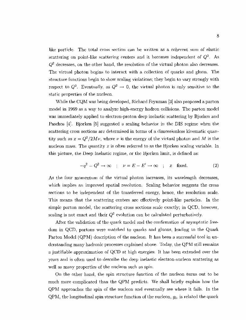
8
like particle. The total cross section can be written as a coherent sum of elastic
scattering on point-like scattering centers and it becomes independent of Q2. As
Q2 decreases, on the other hand, the resolution of the virtual photon also decreases.
The virtual photon begins to interact with a collection of quarks and gluon. The
structure functions begin to show scaling violations; they begin to vary strongly with
respect to Q2. Eventually, as Q2 —> 0, the virtual photon is only sensitive to the
static properties of the nucleon.
While the CQM was being developed, Richard Feynman [3] also proposed a parton
model in 1969 as a way to analyze high-energy hadron collisions. The parton model
was immediately applied to electron-proton deep inelastic scattering by Bjorken and
Paschos [4]. Bjorken [5] suggested a scaling behavior in the DIS regime when the
scattering cross sections are determined in terms of a dimensionless kinematic quan
tity such as x = Q2/2Mu, where v is the energy of the virtual photon and M is the
nucleon mass. The quantity x is often referred to as the Bjorken scaling variable. In
this picture, the Deep Inelastic regime, or the Bjorken limit, is defined as:
-q2 = Q2 _> oo ; v = E - E' -» oo ; x fixed. (2)
As the four momentum of the virtual photon increases, its wavelength decreases,
which implies an improved spatial resolution. Scaling behavior suggests the cross
sections to be independent of the transferred energy, hence, the resolution scale.
This means that the scattering centers are effectively point-like particles. In the
simple parton model, the scattering cross sections scale exactly; in QCD, however,
scaling is not exact and their Q2 evolution can be calculated perturbatively.
After the validation of the quark model and the confirmation of asymptotic free
dom in QCD, partons were matched to quarks and gluons, leading to the Quark
Parton Model (QPM) description of the nucleon. It has been a successful tool in un
derstanding many hadronic processes explained above. Today, the QPM still remains
a justifiable approximation of QCD at high energies. It has been extended over the
years and is often used to describe the deep inelastic electron-nucleon scattering as
well as many properties of the nucleon such as spin.
On the other hand, the spin structure function of the nucleon turns out to be
much more complicated than the QPM predicts. We shall briefly explain how the
QPM approaches the spin of the nucleon and eventually see where it fails. In the
QPM, the longitudinal spin structure function of the nucleon, gi, is related the quark
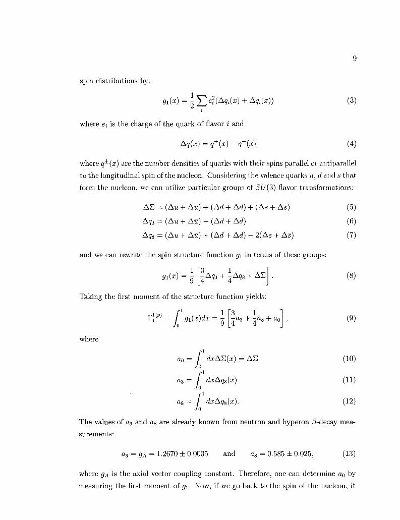
9
spin distributions by:
9i(x) = « E ei ( A ^ ( X ) + A9i(x)) (3)
where e$ is the charge of the quark of flavor i and
Aq(x) =q+(x) -q~{x) (4)
where q±{x) are the number densities of quarks with their spins parallel or antiparallel
to the longitudinal spin of the nucleon. Considering the valence quarks u, d and s that
form the nucleon, we can utilize particular groups of SU(3) flavor transformations:
A S = (Au + Au) + {Ad + Ad) + (As + As)
Aq3 = (Au + Au) - (Ad + Ad)
Aq8 = (Au + Au) + (Ad + Ad) - 2(As + As)
and we can rewrite the spin structure function g\ in terms of these groups:
1 si 0*0 = 9
3 1 -Aq3 + -Aq8 + AS
(5)
(6)
(7)
(8)
Taking the first moment of the structure function yields:
/
l 1 To 1
gi(x)dx = - - a 3 + - a 8 + a0 where
a0
az
a%
= I dxAZ(x) = AS Jo
= / dxAq3(x) Jo
= / dxAq8(x). Jo
(9)
(10)
(11)
(12)
The values of a3 and a& are already known from neutron and hyperon /3-decay mea
surements:
a3 =gA = 1.2670 ±0.0035 and a8 = 0.585 ± 0.025, (13)
where gA is the axial vector coupling constant. Therefore, one can determine a0 by
measuring the first moment of g-y. Now, if we go back to the spin of the nucleon, it

10
can be written as the sum of the quark spins Sg, the gluon spins AG and the orbital
angular momenta of the sea quarks and the gluons Lz:
l- = Sq + /\G + Lz (14)
where the quark spin contribution Sq can be written as the sum of individual flavors
each carrying momentum fraction x with spin components ± | along the direction of
motion of the nucleon:
~<lHx) - nil (x) + ~<li+(x) + nQi (x) (15) SQ= dxJ2 Jo i
= \ I dxJ^AftM + AgKx)) (16) *Jo i
= l-f dxAE(x) = iAE = \a0. (17)
In the simple QPM, AG and Lz are expected to vanish, therefore AE = ao alone
should be responsible for the total spin of the nucleon and be equal to 1. Relativistic
corrections require some of the spin of the nucleon to be carried by the orbital angular
momentum of the quarks since the quarks should have relativistic speeds in the
confined space of the nucleon because of Heisenberg's uncertainty principle. As a
result 60% of the nucleon spin should be carried by the spins of the quarks. In this
approach, strange sea quark and gluon contributions are still not taken into account.
Therefore the model fails to explain the spin content correctly. Indeed, that is exactly
the outcome of the EMC experiment at CERN [6]. According to the experimental
results of the EMC AE = ao = 0.12 ± 0.17 was reported, which means only a very
small fraction of the proton's spin is carried by its constituent quarks. Moreover, by
using Eqs. (10 - 12), we can evaluate that:
a0 = AE = as + 3(As + As) (18)
If one could ignore the contribution from the strange quarks as Ellis and Jaffe sug
gested in 1974, a0 should be close to a8 = 0.585. The result of the EMC experiment
contradicts this prediction of the QPM. This failure of the QPM is often referred to
as the spin crisis.
As briefly mentioned, in the DIS region, the interaction cross section displays
a phenomena called scaling, scattering centers are pointlike and free particles. If
scaling is correct, the measured quantities should be independent of Q2, which de
termines the resolution of the probe, a virtual photon. The predictions of the QPM
11
do not depend on the resolution of the probe in the DIS region and hence it exhibits
scaling. However, there are many experimental observations on scaling violations as
the resolution of the scattering probe is increased. Therefore, the QPM also fails to
explain these scaling violations: the Q2 dependence of the measured quantities such
as cross sections and structure functions of the nucleon. The spin structure function
gi of the nucleon given in Eq. (3) also exhibits scaling violation, hence, it becomes
also a function of Q2 as well as the momentum fraction x.
Later, it was realized that the situation can be explained in the framework of
QCD, in which the structure of the nucleon becomes much more complicated than
the QPM anticipated. The scaling violations are actually predicted by perturbative
QCD (pQCD). What appears to be quarks at a particular resolution turns out to
be a collection of quarks, antiquarks and gluons at a higher resolution. Therefore
pQCD can describe the change of the apparent distributions when the nucleon is
probed at a different resolution. In the QCD framework, the ultra-violet divergences
are taken care of by renormalization. Other divergences, which are called collinear
divergences, arise because of small quark masses and are attended by using a scheme
called factorization [7]. In this scheme, the interaction of virtual photons with a
nucleon is broken up into long (soft) and short (hard) distance interactions. The point
at which this separation is made is called factorization scale fi2. The long distance
interactions cannot be calculated analytically. They can only be parametrized and
studied experimentally. Therefore, the infinite terms can be absorbed into the long
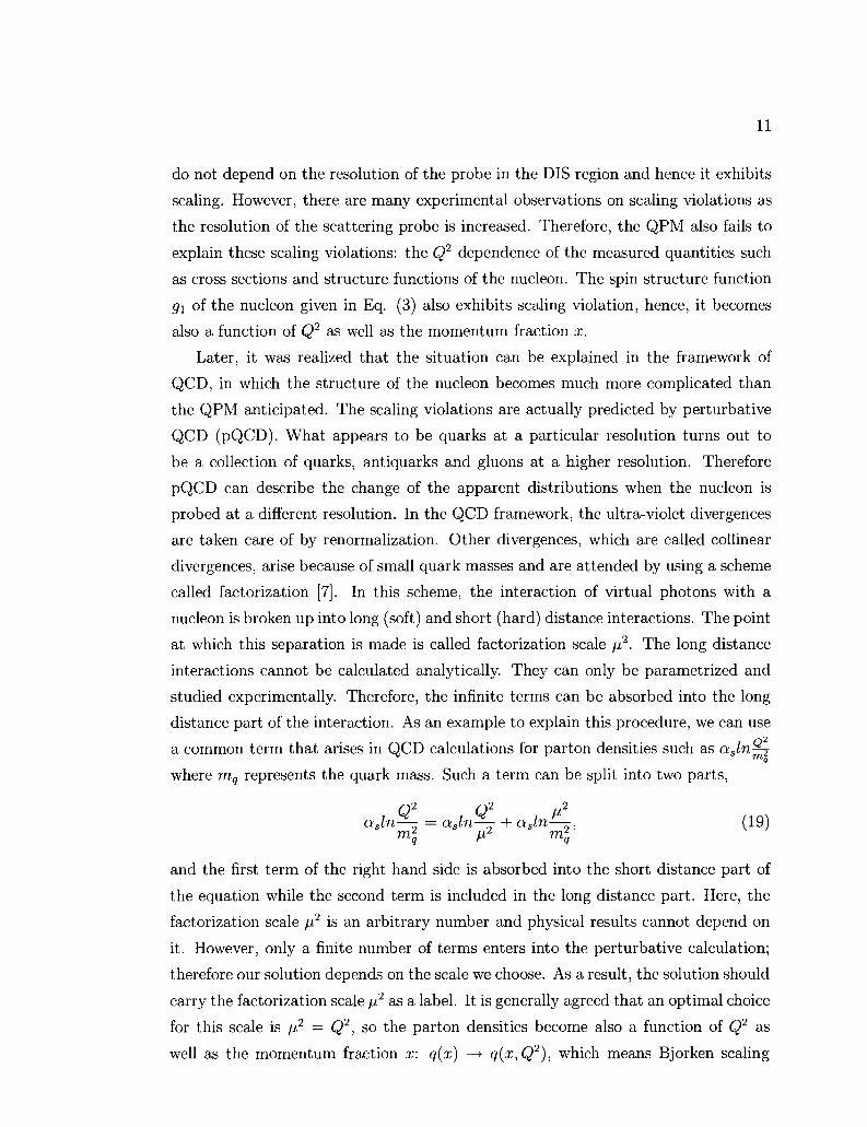
distance part of the interaction. As an example to explain this procedure, we can use
a common term that arises in QCD calculations for parton densities such as asln^2
where mq represents the quark mass. Such a term can be split into two parts,
OLsln— = asln— + asln—, (19)
and the first term of the right hand side is absorbed into the short distance part of
the equation while the second term is included in the long distance part. Here, the
factorization scale ft2 is an arbitrary number and physical results cannot depend on
it. However, only a finite number of terms enters into the perturbative calculation;
therefore our solution depends on the scale we choose. As a result, the solution should
carry the factorization scale ji2 as a label. It is generally agreed that an optimal choice
for this scale is /i2 = Q2, so the parton densities become also a function of Q2 as
well as the momentum fraction x: q(x) —> q(x,Q2), which means Bjorken scaling

12
is broken. Therefore, QCD is able to handle the scaling violations observed in the
unpolarized and polarized structure functions. The QPM turns out to be a zero
order approximation to pQCD. The parton densities q(x) and Aq(x) become just the
zeroth order members of QCD calculations. However, the momentum distributions
of quarks, antiquarks and gluons cannot be fully calculated from first principles of
QCD and they have to be measured experimentally.
The predictions of QCD and the progress in theoretical work triggered many
experimental efforts. The spin structure functions became the center of interest.
Especially the longitudinal spin structure function of the nucleon g± and its moments
are strong tests and complements of the QCD calculations. The Bjorken sum rule,
which is explained in section II.4.4, is considered to be an important test for QCD
in the DIS region at high Q2. At the opposite end of the kinematic region, the
Gerasimov-Drell-Hearn (GDH) sum rule, which is explained in section II.4.5, plays
an important role to understand the non-perturbative QCD region. The GDH sum
rule is valid at the real photon point (Q2 = 0) and connects spin observables to
the static properties of the nucleon. Additional theoretical work, for example by Ji
and Osborn (see section II.4.5), provided an extension of the GDH sum rule into
the resonance and DIS regions. This work unified the two fundamental sum rules:
The Bjorken sum rule in the DIS regime and the GDH sum rule at the real photon
point. The connection between the two kinematic end points provides a theoretical
tool to explore the transition region between the perturbative and non-perturbative
QCD regimes. This is very important to understand the structure of the nucleon.
However, this goal requires precise measurement of the spin observables in a large
kinematic region.
The EGlb experiment, carried out at Jefferson Lab, measured the virtual photon
asymmetry A\ and the longitudinal spin structure function gi of the proton and the
deuteron in an unprecedented kinematical range. As well as exploring the resonance
contributions to A\ and gi, the data will enable us to test different theoretical and
phenomenological calculations of the Q2 evolution of Ti for both targets. Experimen
tal verification of chiral perturbation theory and future Lattice QCD calculations,
which are valid in the intermediate Q2 regions, will also be possible by using the
EGlb results. In addition, higher twist effects, which reveal information on quark-
gluon interactions, can be explored and the validity of the quark-hadron duality in
the spin sector can be tested by using this data. In this thesis, we present the results

13
on the deuteron. In addition, the deuteron, apart from being intrinsically interesting,
can also be used as an effective source of information for the neutron spin structure
functions when combined with proton measurements. Therefore, the methodology to
extract the neutron spin structure function is also explained and preliminary results
are presented in this thesis.
Chapter II introduces the theoretical background and explains the formalism of
the nucleon spin structure functions. Chapter III describes the experimental appa
ratus. Chapter IV covers the data analysis and chapter V presents the final results.
Chapter VI explains the parameterizations of the physics quantities and concluding
remarks are presented in chapter VII.

14
CHAPTER II
THEORETICAL BACKGROUND
In this chapter, the nucleon structure functions will be introduced as an effective
description of deep-inelastic scattering (DIS) between an electron and a nucleon or
a nuclear target. The cross sections for such interactions will be evaluated. These
cross sections can be expressed in terms of the structure functions and thus will
give us a better understanding of the internal structure of the nucleon. Later, the
interpretation of the structure functions in the QPM will be provided and it will
be compared to the QCD interpretation, which explains the kinematical evolutions
of the structure functions in a more rigorous way. Later, the moments of the spin
dependent structure functions will be introduced and the resulting sum rules that
play an important role for the test of QCD and many theoretical frameworks will be
analyzed. Finally, the methods that can be used to obtain the neutron spin structure
functions from the combined proton and deuteron spin structure functions will be
explained together with required corrections.
II. 1 T H E S T R U C T U R E F U N C T I O N S
The structure functions naturally rise from the formulation of deep-inelastic scatter
ing (DIS) between a lepton and a nucleon in QED. In this section, the cross section for
DIS will be calculated and expressed in terms of the structure functions. Emphasis
will be given to the case of longitudinal polarization where the incoming electron and
the target nucleon are both polarized parallel or anti-parallel to the direction of the
electron beam. The cross section differences for certain polarization states during the
interaction lead to experimentally observable asymmetries. These asymmetries can
be used to isolate certain spin dependent and independent structure functions. The
connection between the experimental asymmetries and the actual physical processes
that take place during the polarized lepton-nucleon scattering will be established by
introducing virtual photon asymmetries, that are evaluated from photo-absorption
cross sections and give direct insight for the internal structure of the nucleon. This
will give us a deeper understanding of the structure functions in terms of the virtual
photon asymmetries.
15
k'
* x
polarized beam
k, $1
polarized target
P T S W
S
lifrz spin
final . hadronic
"•*• state X
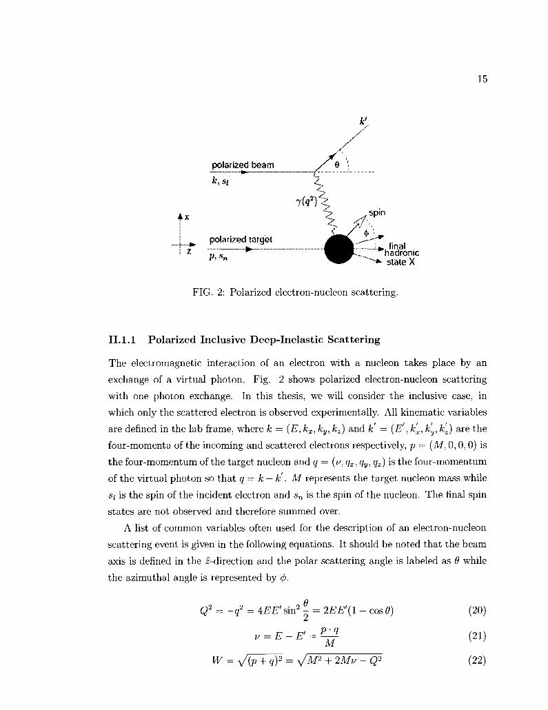
FIG. 2: Polarized electron-nucleon scattering.
II. 1.1 Polarized Inclusive Deep-Inelastic Scattering
The electromagnetic interaction of an electron with a nucleon takes place by an
exchange of a virtual photon. Fig. 2 shows polarized electron-nucleon scattering
with one photon exchange. In this thesis, we will consider the inclusive case, in
which only the scattered electron is observed experimentally. All kinematic variables
are defined in the lab frame, where k = (E, kx, ky, kz) and k = (E , kx, ky, kz) are the
four-momenta of the incoming and scattered electrons respectively, p = (M, 0,0,0) is
the four-momentum of the target nucleon and q = (v, qx, qy, qz) is the four-momentum
of the virtual photon so that q = k — k . M represents the target nucleon mass while
si is the spin of the incident electron and sn is the spin of the nucleon. The final spin
states are not observed and therefore summed over.
A list of common variables often used for the description of an electron-nucleon
scattering event is given in the following equations. It should be noted that the beam
axis is denned in the ^-direction and the polar scattering angle is labeled as 0 while
the azimuthal angle is represented by 4>.
Q2 = -q2 = 4EE' sin2 | = 2EE'(1 - cosfl)
u = E-E' = M
W = y/{p + qf = y/M2 + 2Mv - Q2
(20)
(21)
(22)

16
Q2 Q2
2p-q 2Mv v ;
y p-k E E K '
'Q
e = (1 + 2(1+ r) tan 2(0/2)) * (27)
ex/Q2
E-eE' (28)
D = TT§ (29)
where Q2 is the squared four-momentum and v is the energy of the virtual photon,
W is the mass of final hadronic state, x is the Bjorken scaling variable and e is the
relative flux of the two polarization states of the virtual photon (ratio of longitudinal
polarization to the transverse polarization). D is the depolarization factor that
represents how much of the incoming lepton's polarization is transferred to the virtual
photon. R is the ratio of longitudinal to transverse virtual photo absorbtion. More
information is given on these factors in section II. 1.3.
Assuming one photon exchange, the differential cross section for detecting the
scattered electron in the solid angle dQ, and energy range (E , E + dE ) is given by:
d2° * E ' L ^ (30) dttdE' 2MqA E ""
where a is the fine structure constant, L^ is the leptonic tensor and W^u is the
hadronic tensor. The leptonic tensor, which describes the emission of the virtual
photon by the electron, can be calculated from QED. It is written in terms of Dirac
spinors (u) and the gamma matrix (7^) as:
L^(k,si;k') = '^2^u(k',s'l)qftlu(k,si) * u(k\ st)^vu{k, st) (31)
where we summed over the final spin states st of the electron. It has symmetric (S)
and anti-symmetric (A) parts under //, v interchange:
L^ik, Sl; k') = 2L$(k; k') + 2iL$(k, s,; k') (32)
17
where
and
L$(k; k') = kX + k',K - g^k.k' - m2)
LlJ)(k,sr,k') = e^a0s?(k-k'y
(33)
(34)
where m is the electron mass, e^a/g is the Levi-Civita antisymmetric tensor and
g^ = diag(l, — 1 , - 1 , - 1 ) is the metric tensor.
The hadronic tensor describes the interaction between the virtual photon and the
nucleon. Since we don't know the internal structure of the nucleon, it is not possible
to calculate it analytically. For the nucleon with spin 1/2, the hadronic tensor can be
written in terms of symmetric and anti-symmetric parts just like the leptonic tensor.
W^(k,Sl;k') = W$\q;p) + iWJ£\q;p,Sn) (35)
with
WW(q;p) =
+
Qfj-Qu
r,2 L 9
v»-
9iiv J
p.q -#%
2F1(x,Q2)
p.q Vv 2"*/
T
(36)
Mv F2(x,Q2)
and
W^H^P.Sn) = e^af3qa
1M
PQ L £9l(x,(?)+(fn-JjPB)92(x,Cf) (37)
The coefficients Fi and F2 are unpolarized structure functions and gi and g2 are
polarized structure functions. The differential cross section in Eq. (30) can be
written in the following form separating the symmetric and antisymmetric parts
d2a a2 E PS)W^{S) _ L(A)W^(A)^ (38) dtldE' 2MQA E
When we consider the spin averaged cross section (summing over all possible spin
orientations where electron and nucleon spins are either parallel or anti-parallel),
only the symmetric part of the hadronic tensor, W^^ contribute yielding:
d2an d2an Aa2Ea ,Q I = COS I —
dQ.dE' dQdE' Q4 V2 M tan
1 ^ Fl{x,Q2) + -F2{x,Q2) (39)
The first and the second arrows indicate the electron and the nucleon spin orientations
respectively. If we consider the difference between the cross sections with the two
18
possible spin orientations of the longitudinally polarized electron and the nucleon
being parallel or anti-parallel, then only the anti-symmetric part of the hadronic
tensor, W^A) contribute:
d V * d2a^ 4a2 E' 1 T,„ _ „, , ^ 2 , „ „ , , ^ 2 , , ,An. XUZ-lmW= Q^^M-u [(E + E'CosO)9l{x,Q
2) - 2Mx92(x,Q2)] (40)
Since we have the structure functions as a function of (x,Q2), it is desirable
to express the differential cross sections also in terms of these variables. By using
dfl = 2ir sin 6d9 where we assumed azimuthal symmetry, which is usually the case in
the inclusive scattering experiments, and the kinematical relations
Q2 = 2EE'(l-cos6) = 4EE'sin2-, (41)
u = E-E' = Q2/2Mx, (42)
the conversion factor between the two different sets of the kinematical variables can
be obtained, d2a n v d2o ( 4 3 )
d9.dE' EE' x dQ2dx
and the differential cross section equations can be written in a more convenient way
in terms of x and Q2,
a = 47TQ2 r Q4 ,, , ^ A Q2 Q2
Q4X ,M2E2xF^Q)+V-2^x-fE2^F^Q^
4na2 1 ACTH = Q2x ME
where we used notations
Q2 Q2\ 2 2Mx 2 "
2MEx 2E2 r x ' E
(44)
(45)
= riV* d2a^
° ~ dQ2dx + dQ2dx [ '
_ rfV* _ d2a^ a]] ~ dQ2dx dQ2dx ( '
These cross section differences are useful for isolating specific structure functions or
their combinations. Since they are experimentally accessible quantities, the above
relations form the basis of most experiments trying to measure the unpolarized and
polarized structure functions of the nucleon. In the following sections, we will define
experimental asymmetries in terms of these cross section differences and establish
their connections to a deeper understanding of physical processes that take place
during the lepton-nucleon scattering events.

19
The limit Q2 —> oo and v —> oo, where x is fixed, determines the Bjorken regime.
In this region, the structure functions F i 2 and g^^ are observed to approximately
scale, i.e., they almost become independent of Q2. This behavior of the structure
functions in the DIS region actually reveal the existence of point like constituents
inside the nucleon because scaling is expected when electrons scatter off point like
particles. As explained in chapter 1, the simple QPM predicts exact scaling for
these functions. On the other hand, as the wavelength of the exchanged virtual
photon increases, hence, the resolution of the probe decreases, the structure functions
begin to show scaling violations and begin to vary strongly with respect to Q2.
These scaling violations are handled in pQCD. However, QCD cannot predict any
value for the structure functions, which makes them basic subjects of experimental
measurements and models.
II. 1.2 Photo-Absorption Cross Sections
As explained in the previous section, the interaction of the the electron with the
nucleon can be viewed as a two step process described separately by leptonic and
hadronic tensors. Eventually, the contraction of these tensors yields the differen
tial cross sections which can be defined in terms of the polarized and unpolarized
structure functions. When we concentrate on the photon-nucleon vertex of this inter
action, the process can be viewed as forward Compton scattering of a virtual photon
off a nucleon. The optical theorem states that the total cross section of an incident
plane wave (the rate at which flux is removed from the incident plane wave by the
processes of scattering and absorption) is proportional to the imaginary part of the
forward scattering amplitude.
atot = ^Im[M(9 = 0)] (48)
where 9 is the scattering angle and \jK is a factor associated with the incoming
photon flux. For a real photon beam (Q2 —*0), the flux is inversely proportional to
the energy of the photon (represented by v, given in Eq. (21)), therefore the flux
factor is \/v. If we consider the invariant mass of the final state (given in Eq. (22))
and apply it for real photon case where Q2 = 0 and K = v we get:
W2 = M2 + 2Mu = M2 + 2MK (49)
For a virtual photon (Q2 > 0), flux is somewhat arbitrary. By using the so-called
Hand convention, Eq. (49), evaluated for a real photon, could also be used for a
20
virtual photon, which yields for K [8]
K=W*-ti>=v_§L (50) 2M 2M K '
M in Eq. (48) represents the forward Compton scattering amplitude, which depends
on the helicity states of the virtual photon and the nucleon before and after the scat
tering process. The scattering amplitudes for different helicity combinations of the
virtual photon and the nucleon can be referred as helicity amplitudes. The forward
scattering amplitude can be decomposed into different forward helicity amplitudes.
We can write these helicity amplitudes with defining indices for corresponding helicity
states as Aiitj-i>j>, where i,j are the spin projections of the incident photon and nu
cleon and i', f are that of the scattered photon and nucleon respectively. The nucleon,
being a spin 1/2 particle, has two possible helicity states, m = 1/2, —1/2. The vir
tual photon, being a spin 1 particle and which may attain mass unlike a real photon,
can have 3 possible polarization states, namely m = 1,0, — 1. If the virtual photon is
polarized in the m = ±1 states, it is called transversely (or circularly) polarized. If it
is polarized in the m = 0 state, it is called longitudinally (or linearly) polarized. As
a result, there are 10 possible helicity combinations for the scattering amplitude. By
employing the parity conservation Mij-yji = Ai-it-j--i't-f and invariance of time
reversal Mij-^ji = Aii'j'^j , these 10 combinations can be reduced to 4 indepen
dent forward helicity amplitudes: A / t 1 _ i . 1 _ i , M.i±.i I , A ^ 0 I . 0 I , . M 0 i 0 i. These
helicity amplitudes can be computed in terms of the hadronic tensor W^.
A W J ' ^ ' ^ W W (51)
where & is the polarization vector of the virtual photon, which can either be trans
verse or longitudinal [9]. Indeed, the parameter introduced in Eq. (27) corresponds
to the relative strength of these two polarization states and solely depends on the
kinematics of the scattered lepton (that emitted the virtual photon being discussed).
At this point, we can formulate the virtual photon-nucleon interaction by using the
optical theorem and calculate the total photo-absorption cross sections for different
helicity states in terms of the forward helicity amplitudes, which are indeed express
ible in terms of the polarized and unpolarized structure functions introduced earlier.
21
As a result, the four independent virtual photon-nucleon cross sections can be ex
pressed as [9] [10]:
T 4-7ra , _, 47r2a , _ 9 x
°\= -jrM^-\*> -\ = ~KM (Fl ~9l+192) (53)
/• 47ra , d 4ir2a ( ,_, 1 + 72 \ ,r A.
TL Ana A-K2a °lL = - 7 r ^ o , i ; 0 . -k = 17777 (01 + 32) (55)
The cross sections, a j , are labeled by the total initial helicity of the virtual photon-
nucleon system, J and the polarization of the virtual photon, P. The polarization
states include transverse (T) and longitudinal (L) polarizations as well as the inter
ference term (TL).
It is clear that certain combinations of the photo-absorption cross sections given
above lead to specific structure functions or their combinations. We can define total
absorption cross sections for transverse and longitudinal virtual photon polarization
as aT=UaT + aT\ ( 5 6 )
2 \ 2 2 /
and
aL = ok (57) 2
The unpolarized structure functions can be written in terms of these cross sections,
* - ^ <«)
KM x , r Tx . _ F 2 = « 2 IO. 2 °" + a ) 5 9
oir'a 1 + Y The ratio of the two cross sections give rise to the unpolarized structure function R, that was used earlier in Eq. (29),
R = ^ = <1 + ^ 1 - 1 < 6 0 )
Also, the spin structure function g\ can be calculated from these cross sections:
91 = 8^+ 72) ( ^ 2 " *W + 2 7 ^ 2 ) ( 6 1 )

22
II. 1.3 Asymmetries
Now we can define the virtual photon asymmetries A\ and A2 in terms of the virtual
photon absorption cross sections given above
A.ix, Q2) = -+—* = w*>-'"W (62)
T T
2 2 _
ol + ol 2 2
2a\L
2 _
a-T + <rj
g1(x,Q2)-12g2(x,Q2)
Fi(x,Q*)
l[gi(x,Q2) + g2(x,Q2)} Fi(x,Q2) Mx,?)-^-"""-'}^-*" (63)
2 2
By using these equations, we can express the spin dependent structure functions in
terms of the virtual photon asymmetries:
1 + 72 gl(x,Q2) = r\^^,(A1 + 1A2) (64)
Fi(x,Q2) ( A, g2(x,Q2) = \\^> [-Al + -±\ (65)
The asymmetries A\ and A2 have straight forward physical meanings but they
are not experimentally accessible quantities except that A\ can be measured with
real photons in principle. Therefore, we define an experimental asymmetry Ay by
using the differential lepton-nucleon cross sections defined in the Eqs. (44) and (45).
A{](x,Q2) = ^ - (66)
Working in terms of asymmetries instead of cross sections allows us to disregard the
geometric acceptance of the detector since the acceptance from the numerator and
the denominator cancels out. By substituting the Eqs. (64) and (65) for gx and g2
into (66), A\\ can be expressed in terms of A\ and A2
A\\ = D(Ai + r]A2) (67)
where e, r\ and D are defined in Eqs. (27), (28) and (29), respectively. In polarized
deep inelastic scattering experiments with longitudinally polarized leptons and nu-
cleons, the spins of the incoming lepton and the nucleon are aligned in the direction
of the lepton's propagation axis. When the virtual photon is emitted, its propagation
axis can be different than the propagation axis of the incoming lepton. The spin of
the virtual photon is either parallel or perpendicular to its own propagation axis.
23
Therefore, the polarization of the lepton is not fully transferee! to the virtual photon.
The depolarization factor takes this loss into account.
We can analyze the the expressions for A\ and A2 a little bit to estimate their
boundaries. The photo-absorption cross sections aj,2 and aj,2 are always positive,
therefore, the absolute value of the ratio defining Ai is bound to be less than or equal
to 1. For elastic scattering A\ = 1. The cross section term aTL is an interference
term between aL and aT, therefore we can deduce an orthogonality relation
\aTL\ < V^r (68)
which yields
\A*\ = aTL
aT < \ - F = V/? (69)
In elastic scattering, aTL oc TGEGM and aT oc TG2M, where r = I / 7 and GE and GM
are electric and magnetic form factors of the nucleon [1], so that A2 = ^GE/GM =
\/R. There is even a more specific boundary requirement, that is often used, on A2,
which states that
\A2\ < y/Ril + AJ/2 (70)
This requirement is called Soffer limit [11]. It follows directly from Eqs. (62) and
(63), together with the fact the \aTL\ < JjoLo\i2 and R = oL /(aj,2 + crj,2).
Let's focus on the virtual photon asymmetry Ai and the spin structure function
g\. Ai can be evaluated as:
Ai = ^ ~ r)A2 (71)
and by putting this into Eq. (64), g\ can be evaluated as:
0i = ^ + (7 - V)A2 (72) I + 72
The kinematical factors rj and 7 in front of A2 are typically small in high energy
experiments. In the Bjorken limit, where x is fixed, they both go to 0. According
to the kinematical range of the experiment, one can measure A\ and g\ by either
assuming the second term on the right hand side of the Eqs. (71) and (72) is negligibly
small and can be treated as a systematic error or using measured results or models
of A2 in the corresponding kinematics. In any case, we need to know the structure
functions Fi and R, which have been measured by several experiments [12][13].

24
II. 1.4 Extension to Spin 1 Target
In this thesis, our analysis is focused on the deuteron target, which is a spin 1
nuclear object. So far, our derivations for the relationships between the photo-
absorption cross sections and the structure functions assumed a spin 1/2 nucleon
target. In case of the deuteron, there are three different helicity states, m = ± 1 ,
when the third component of the deuteron's spin is aligned or anti-aligned in the
direction (z) of the incoming lepton, and m — 0, when the spin component along
z is zero. As a result, the number of independent helicity amplitudes, hence the
photo-absorption cross sections become 8 instead of 4. This requires four additional
structure functions, usually referred to as 6i_4; for a complete definition of the process
see [14] [15]. These additional structure functions are called tensor structure functions
and all arise because of the binding effects between the proton and the neutron that
form the deuteron. When we approximate the deuteron as a combination of a proton
and a neutron in a relative S-state, hence, with no interaction between them, the
helicity amplitudes for the deuteron can be expressed as a sum of the individual
helicity amplitudes from the proton and the neutron such that
-Mi,o;i,o = ^M^rM + Mu-ix-0 ( 7 3)
and therefore the additional independent helicity amplitudes vanish, leaving us with
the same definitions for the asymmetries and structure functions for the spin 1
deuteron as we obtained for a spin 1/2 nucleon target.
In case we need to take the nuclear binding effects and D-state of the deuteron
into account, we need to consider the additional structure functions. In the DIS
limit, however, the the kinematical factors in front of 62_4 structure function become
essentially zero, therefore their effects can be neglected, but &i can make a small
contribution. The structure function b\ describes the difference in the cross sections
between the helicity-0 and the averaged non-zero helicity contributions. In case of the
deuteron, we can define two types of polarizations: a vector polarization Pz = (n+ —
n~)/{n+ + n~ + n°) and a tensor polarization Pzz = (n+ + n~ — 2n°)/(n+ + n~ + n°).
Here n+,n~,n° are the atomic populations with positive, negative and zero spin
projections on the beam direction, respectively. For a spin 1/2 target the vector
polarization is defined as Pz = (n+ —n~)/\n++n~) while tensor polarization vanishes.
Existence of the tensor polarization for spin 1 target leads to the structure function
6i.
25
It should be pointed out that the probability of finding the deuteron in a D-state
is already small, on the order of 5%, which makes the the structure function bx a
small quantity in general. Indeed, the results of HERMES [15] experiment on the
measurement of the b\ structure function of the deuteron confirms that. Especially in
the kinematic range of the EGlb experiment it is consistent with zero. Moreover, in
the EGlb experiment, the tensor polarization is small, on the order of 10%, making
the contribution of the 6i structure function even smaller. In addition to these, since
we take the difference of the cross sections, the tensor polarization, hence, the 6i
contribution cancels out in the numerator of the expression (40), only contributing
to the denominator. As a result, the contribution of the b\ structure function is
three-fold small in the EGlb experiment, therefore, we can safely neglect its effect
on the other structure functions measured in the experiment. This leaves us with
the same definitions for the structure functions of the deuteron that we previously
obtained for the nucleon.
II.2 I N T E R P R E T A T I O N IN T H E Q U A R K - P A R T O N MODEL
The Quark-Parton Model (QPM) [8] [16] describes the nucleon as a composition of
partons, pointlike objects, which are later identified as elementary quarks. The
structure we observe by probing the nucleon with a virtual photon depends on the
resolution of the probe, that is the four-momentum transferred Q2. This is also called
virtuality of the photon since Q2 —> 0 for real photons. The partonic structure is
observed if the virtuality of the photon is high. In a so-called infinite momentum
frame, where the the energy and the four-momentum of the virtual photon are large,
the virtual photon scatters off the pontlike partons, i.e., elementary quarks. This
provides us with the structure of the nucleon described in the Bjorken limit and the
Bjorken variable x becomes the fraction of the nuclear momentum carried by the
struck quark. The scattering cross section of the nucleon can then be computed from
the incoherent sum over the quark contributions. In the Bjorken limit, quarks are
essentially non-interacting free particles because the strong coupling constant goes
to 0 as Q2 —> co, which leads to asymptotic freedom. Fig. 3 shows a simple image
of the scattering process in the QPM.
In this regime, the unpolarized structure functions can be evaluated by using
the impulse approximation [17], where the nucleon matrix element in the hadronic
tensor W^ can be replaced by a sum of quark matrix elements weighted by their

26
lepton
proton
i hadrons
mass W
FIG. 3: Electron-nucleon scattering in QPM.
distribution functions. The result for the unpolarized structure functions yields
KM = IT,*M*)+*(*)] (74) i
and
F2{x) = 2xF1 (75)
where et is the charge of the quark i and qi{x) is the probability density for the quark i
to carry a fraction x of the nucleon's momentum. q~i(x) corresponds to the probability
density for the anti-quark i. Therefore, Fi(x) at a given x can be interpreted as
the sum of the distribution of quark (and anti-quark) flavors carrying a momentum
fraction x of the nucleon, weighted by their squared charges. F2, integrated over all
x, indicates the total four-momentum fraction carried by all the quarks (and anti-
quarks), weighted by squares of their charges. It can be understood as a spatial
current density of the nucleon. Similarly, the polarized structure functions in the
QPM can be written as:
ftW = ^E e '[A*( i)+ A*(x)]
with
g2(x) = 0
Aq(x) = q+(x) - q (x)
(76)
(77)
(78)

27
(a) Initial Spins Parallel (b) Initial Spins Antiparallel
FIG. 4: Interpretation of the spin-transitions in the scaling region for a longitudinally polarized electron scattering off a longitudinally polarized nucleon. Valence quarks with their spin directions are shown inside the nucleon. (i) Incoming electron and target nucleon are shown. (ii)The electron emits a virtual photon and flips its spin. The virtual photon can only interact with the quarks that carries an opposite spin with respect to the photon, (iii) The quark flips its spin and the resulting final state has either spin 3/2 or 1/2 depending on the initial spin configurations.
where q±(x) are the number densities of quarks with their spin parallel or antipar
allel to the longitudinal spin of the nucleon. When we put these expressions for the
structure functions into Eqs. (52) and (53), we find that o\,2 ~ ^2(q+ + q+) and cr3/2 ~ XX? - + Q~)- The virtual photon absorption cross sections are, therefore,
sensitive to the quark spin polarizations because the quark with spin 1/2 can only
absorb the virtual photon if its spin is anti-parallel to the spin of the photon. There
fore, in the QPM, which actually holds in the Bjorken limit, one can get the spin
contributions of different quark flavors to the overall spin of the nucleon by mea
suring the virtual photon absorption cross sections for different nucleon helicities.
Therefore, A\ defined as [p\,2 — a^,2)/2aT can be interpreted as the asymmetry in
quark distributions with with their spins aligned and anti-aligned with that of the
nucleon (see Fig. 4).
Another implication of the QPM is that the structure function R goes to zero in
the Bjorken limit. In this frame, the transverse components of the quark momentums
can be neglected because the nucleon momentum is large. In this limit, longitudinally

28
polarized quarks can only absorb transversely polarized virtual photons, so that
aL in Eq. (54) becomes essentially 0 making R = 0. The same argument leads
to the conclusion that the virtual photon asymmetry A<± is also 0 in this regime.
Then we can approximate g\ ~ A\F\. Therefore, the structure function pi can
be interpreted as the distribution of quarks inside the nucleon multiplied by their
spin asymmetries with respect to the absorbed virtual photon. So, it reveals the
polarization distribution of the quarks inside the nucleon.
Finally, the most important implication of this picture is that the polarized and
unpolarized structure functions are independent of Q2. This is called scaling in-
variance, which was initially observed in SLAC experiments performed in the DIS
region, but ruled out by later experiments performed over larger Q2 ranges. This
shows that in the kinematic regions where the four-momentum transfer is finite, the
simple partonic interpretation is not valid anymore. The scaling violations can be
explained by perturbative QCD (pQCD). What appears to be quarks at a particular
resolution turns out to be a collection of quarks, antiquarks and gluons at a different
resolution.
II.3 Q2 EVOLUTION OF T H E S T R U C T U R E F U N C T I O N S
There are various different calculation methods to express the Q2 dependence of the
structure functions. At high Q2 regions, perturbative QCD (pQCD) gives a rigorous
approach by adding higher order correction terms to the parton distribution functions
defined in the simple QPM. The zeroth order approximation of pQCD is equivalent
to the QPM definitions. However, pQCD expansions require small coupling constant,
therefore, the expansions break down in the region where Q2 < 1 GeV2. There are
also resonance contributions that begin to strongly affect the structure functions in
the intermediate Q2 regions (Q2 a few GeV) and cannot be incorporated into the
pQCD methods. Therefore pQCD is only efficient for the DIS region where Q2 is
large and W > 2 GeV. In the medium Q2 regions, a method called Operator Product
Expansion is generally used to express the Q2 dependence of the structure functions.
At even lower Q2 regions lattice QCD and effective theories like Chiral Perturbation
Theories come into play.
As we mentioned in the previous section, probing the nucleon with photons at
different energies results in different pictures of the nucleon. At low Q2 what appears
to be a valence quark with momentum fraction x begins to look like combination

29
t t
)
" T l
Q 2 increases
FIG. 5: Dependence of the resolution of nucleon's internal structure on Q2 due to a finer resolution of the nucleon's internal structure with increasing Q2.
of quarks, antiquarks and gluons at higher Q2. Or, we can say, each quark itself is
surrounded by a cloud of partons and as we increase our resolution, we begin to see
inside the cloud. Therefore, the probability distribution functions that describe the
probability of finding a quark with flavor i and momentum fraction x, varies with Q2.
We can make a simple analogy to explain this behavior by considering appearance
of an image on a computer screen. If the pixel size of the screen is smaller or at
least equal to the pixel size of the image, we see the net image. If the pixel size of
the image is smaller than that of the screen, which means screen resolution is not
high enough, the image begins to appear blurry because a few pixel in the image
are blended together. As the resolution of the screen decreases, which corresponds
to the Q2 in our definition, more and more pixels of the image will be combined on
the screen. By zooming out the image, eventually the whole image can be fit into
a single pixel on the screen. Then, only the average color of whole image will be
visible to us. Of course, the dynamic properties of the nucleon makes this analogy
too simple to describe the whole situation.
In the range of Q2 <C 1 GeV2, the resolved distance is compatible with the nu
cleon size. As Q2 increases, the internal quark-gluon and gluon-gluon substructures
begin to effect the scattering cross section. These interactions reduce the observed
momentum of the valence quarks because the nucleon's momentum is distributed be
tween many partons (number of resolved partons that share the nucleon's momentum
increases with Q2). Therefore, the valence quark probability distribution functions
(PDF), qi(x), decrease with increasing Q2 in the high x region while they increase
with increasing Q2 in the low x region. As a result, the probability distribution
functions, thus, the structure functions become functions of both x and Q2.
'/?!
&f

30
II.3.1 QCD corrections to the probability distribution functions
QCD is able to give a rigorous approach to explain the Q2 dependencies of the struc
ture functions. The evolution of the probability distribution functions with respect
to Q2 is formalized by Dokshitzer-Gribov-Lipatov-Altarelli-Parisi (DGLAP) equa
tions [18] [19]. A pedagogical introduction to the derivation of these equations can
be found in [8]. The main mechanisms that can change the momentum distribution
of the quarks and gluons are categorized in three basic interactions: Quarks can
loose momentum by radiating gluons, gluons can generate quark-antiquark pairs and
gluons can decompose into gluon-gluon pairs. The amplitude for these processes are
given in terms of so-called splitting functions Pij(x/y), which describes the probabil
ity to find a parton i carrying a momentum fraction y to split into two partons, one of
which (j), that later interacts with the virtual photon, carries a momentum fraction
x. The partons can either be quarks or gluons and there are no flavor dependencies.
There are 4 splitting functions, two of which, Pqq and Pqo, contribute only to the
evolution of the quark distribution functions qi(x,Q2) and the other two, Pcq and
PGG, contribute only to the gluon distribution function G(x,Q2).
The Q2 evolution of the distribution function for a quark or a gluon with mo
mentum fraction x can be written as a sum of the distribution functions of possible
parent partons with momentum fraction y weighted by corresponding probabilities
of the processes required for the creation of the quark or gluon at hand. Finally this
sum is integrated over the full range of momentum fraction y (> x). The integration
covers the whole range of possible momentum fractions for the parent partons above
x (For a parent parton with momentum fraction y to be able to create a quark with
momentum fraction x, y > x should be satisfied). The resulting equations show
a logarithmic dependence on Q2. The final DGLAG evolution equations for spin
averaged quark and gluon distributions are written as:
dqi(x,Q2)
dlnQ
dG(x,Q2) as f1 dy
dlnQ2
Os_ fl dy 2TT JX y qi(y,Q2)pgq[-)+G(y^Q)p^(-
= g / 1 7 E^Q2)Pog(^)+G(y,Q2)PGG
(79)
(80)
Therefore, Eq. (79) mathematically expresses the fact that the quark with momen
tum fraction x, the one that interacts with the virtual photon, [qi{x,Q2) on the

31
z - x Paa(x/Z) Gq GG
FIG. 6: The processes related to the lowest order QCD splitting functions. Each splitting function Pij(x/z) gives the probability that a parton of type i converts into a parton of type j , carrying a fraction x/z of the momentum of parton i.
left hand side] could have come from a parent quark qi(y,Q2), which has radiated a
gluon or could also have come from a parent gluon G(y,Q2) that created a quark-
antiquark pair. The probabilities for each of these processes are described by the
splitting kernels Pij(x/y).
Similarly, the spin dependent case can be written [20],
dAqi{x,Q2
d\nQ2 ~2nJx
1dy_
y
2 \ A D l X \ , A / - < / . . /->2- • - >X
Aqi(y,Q2)APqq ( - 1 + AG(y,Q')APqG ( - (81)
dAG(x,Q2)
d l n Q 2
with
= S!L f 2 W X
ldy_
y V Aft(y, Q2) APGq (-)+ AG(y, Q2)APGG ' X
AG(x) = AG+{x) - AG~{x)
(82)
(83)
where G±(x) are the number densities of gluons with their spin parallel or antipar-
allel to the longitudinal spin of the nucleon. Also, APy = Pi i+j+ Pi+j- where +
and — representing the corresponding parton helicities. Parity conservation requires
Pi-j± = Pi+j^- It is customary to separate the polarized quark distribution function
in Eq. (81) for singlet AE and non-singlet qNS quark distributions since they evolve
independently from each other. The second term in Eq. (81) does not contribute to
evolution of qNS.

32
Pij Funct ions
The splitting functions used in Eqs. (81-82) also depend on the strong coupling
constant as(Q2). In pQCD, the polarized splitting function APij(x) can be expanded
in a power series of as(Q2),
2TT A P y ( x , a a ) = A P f (x) + ^^AP^(x) + ... (84)
where the subscripts (0) and (1) refer to leading order (LO) and next to leading
order (NLO) contributions. The splitting function that appear in Eqs. (81-82)
correspond to the LO term. The crucial point is that the strong coupling constant
as(Q2) enters as a coefficient for each term, therefore, this procedure works only
in the kinematic regions where the strong coupling constant is small enough for
perturbative expansion, i.e. in the regime where pQCD is applicable.
Q2 evolution of the probability distribution functions imply that the structure
functions defined in Eqs. (74-76) now become functions of Q2 as well. In the next
section we will focus on the structure function gx and explain its dependence on Q2.
II.3.2 Q2 dependence of gi(x,Q2) in t h e DIS region
In perturbative QCD the Q2 dependence of the g\ structure function is given by [19]:
nf
9i(x, Q2) = \j2 e« [C«(x> a") ® A ( ^ x ' ^ ) + CG(X> a«) ® AG(X> <?2)] (85)
i
where sum over all quark flavors n/ is taken. The convolution ® is denned as
Cg(x, a„) ® Aq(x, Q2) = f ^Cq (-,aa) q(x, Q2) (86) Jx y \y )
The coefficients Cq(x, as) and CG(X, a„) are called Wilson coefficients and correspond
to photon-quark and photon-gluon hard scattering cross sections respectively. The
Wilson coefficients can be expanded perturbatively in powers of as,
Gix, a.) = Cf\x) + ^±C?\x) + ... (87)

33
The LO terms are given as Cq(x) = 5(1 — x) and CqG(x) = 0, therefore, we can write
the gi structure function up to the NLO term as
<&(*, Q2) = \ E 4 [Ag(x, Q2) + Aq(x, Q2)] i
+ \ Ee* f v c ' f^)[A?(y'Q2) + A^ Q2)] (88) ^ J X y \ a /
The spin dependent probability distribution functions Aq(x,Q2) and AG(x,Q2) can
be calculated by using DGLAP equations given in the previous section. Calculation
of the Wilson coefficients and the probability distribution functions beyond leading
order (LO) depends on the renormalization scheme used. For information on the
different schemes commonly used, the reader is referred to [7].
II.3.3 The operator product expansion and moments of gi(x,Q2)
In order to understand the quark confinement in QCD, one needs to understand the
dynamics of quark-gluon interactions at large distances. This requires the study of
structure functions at intermediate and low Q2 values. This is a transition region
between the DIS and the resonance regions. In these kinematics, pQCD corrections
break down while contributions from the resonance states of the nucleon and multi-
parton correlations, known as higher twists, come into play. The Operator Product
Expansion (OPE) [21] [22] [23] method is used in this regime to express the structure
functions in terms of short distance effects that are calculable by pQCD, and long
distance effects that can only be measured experimentally.
The OPE analysis of the spin structure function g\ expresses the nth moment
of <7i as a power series expansion of the nucleon matrix elements M™ by using the
Wilson coefficients E™(Q2/fi2,as) as expansion parameters:
r 7 ( Q 2 ) = [1dxxn-1g1(x,Q2)= f^ M?(n2)E?(%,as) (89) J° T=2,4,.. ^ ^
for n — 1,3, 5 , . . . and // is the factorization scale. The explanations that follow are
made by considering the first moment, n = 1. The sum in (89) is ordered according
to the twist r = (dimension - spin) of the current operators, beginning with the
34
lowest twist r = 2. The lowest twist corresponds to the largest contribution to the
expansion. Each additional unit of r produces a factor of order AQCD/Q, which
makes their contribution less important at high Q2 region.
The Wilson coefficients E™ are calculable by pQCD. The nucleon matrix elements
M™(/j2) are local operators which describe the quark-gluon structure of the nucleon.
The term r = 2 (twist-2) in Eq. (89) is known as the leading twist and can be
decomposed into flavor triplet (a3 = g^), octet (a8) and singlet (a0 = AS) axial
charges [24] [25]:
$n(Q2) = cNS(Q2)
where CMS and Cs are the non-singlet and singlet Wilson coefficients. The flavor
triplet axial charge can be obtained from neutron /3-decay, g^ = 1.2670 ± 0.0035
while the octet axial charge is determined from hyperon decay, a8 = 0.579 ± 0.025.
The singlet axial charge, AS, is defined in the Bjorken limit (Q2 —> oo) as,
nf
A S = £ [ A f t ( x , Q2) + Aqt(x, Q2)] (91)
i=i
and contains information about the contribution of quarks to the total spin of the
nucleon or nuclei. More information is given on the axial charges in section II.4.2.
The other terms (r > 2) in Eq. (89) are known as the higher twist corrections.
Higher twist corrections to the first moment of gi(x,Q2)
According to OPE, T\, the first moment of g1, can be expressed in powers of \jQ2:
T\iQ2) = j\X9l{X,Q2)= £ ^ = MQ2) + ^ + ^ f P + ... 02)
where /xr contains specific nucleon matrix elements. The lowest order term, known as
twist-2, is a direct measure of the single parton behavior while the higher order terms
come from quark-quark and quark-gluon correlations. The higher twist contribution
to the first moment of g\ is obtained by subtracting the leading twist term from the
total:
Ar{(Q2) EE T\(Q2) - »2{Q2) = ^ £ ± + f ^ l + 0{±) (93)
We can write the coefficient of the 1/Q2 term as:
M2
M Q 2 ) = - g - M l n Q 2 ) + 4d2(\nQ2) + 4/2(lnQ2)] (94)
± k9A + ha* + CS(Q2)~AE (90)
35
where a2 is a twist-2 operator (also called kinematical higher twist), entering here
due to target mass correction [27], which can be calculated as [1]:
a2 = 2 / dxx2g1(x,Q2) (95) Jo
The coefficient d2, which is a twist-3 operator, can be calculated by:
d2 = 3 f dx x2[g2(x, Q2) - g™w(x, Q2)} (96) Jo
where
g^ix,Q2) = -9l(x,Q2) + I *H9l(y,Q2) (97) J x y
is the Wandzura-Wilczek form of the spin structure function g2. Therefore, d2 shows
the deviation of g2 from the Wandzura-Wilczek form.
The coefficient f2 is a twist-4 operator. It cannot be measured directly but it can
be extracted from data as a fit parameter. The analysis performed on the neutron
in [24] can be studied as an example for f2 extraction. Data from all available
experiments were analyzed to determine the total higher twist effects, Ar™, on the
first moment of g™ for the neutron. Fig. 7 shows A r " versus l/Q2 for various
experiments. Known values for gA, a8 together with AE = 0.35 are used to calculate
/z£ according to Eq. (90). Also, the values for a™ = -0.0031 ± 0.0020 and d$ =
0.0079±0.0048, evaluated from world data at Q2 = 5GeV2, are used in the analysis.
A two parameter fit, using f2 and //" as parameters, in the range of Q2 > 0.5 GeV2,
and a one parameter fit, using only f2 as parameter, in the range of Q2 > 1 GeV2,
were performed on the data. Any possible Q2 dependence of /ig is neglected. The
solid curve shows the result of the two parameter fit while the dashed curve shows
the result of the one parameter fit. The values of f2 and /ig determined from this fit
are:
/2" = 0.034 ± 0.043 ^ = M 4(-0.019 ± 0.017) (98)
where M is the nucleon mass. By using this value of f2, it is obtained that //£ =
M2(0.019 ± 0.024). Combining this with y% obtained from the fit, A r ? becomes
exactly 0 at Q2 = 1 GeV2.
The twist-3 and twist-4 operators, d2 and f2, are thought to be related to the
color electric XE and color magnetic \B polarizabilities of the nucleon:
XE = \{2d2 + f2) (99)

36
0.08 cJLabEMOlO "6LACE142
HERMES SLACE143 A SMC ?8LACE154
0.5 1
FIG. 7: Higher Twist contributions to the first moment of gi for the neutron [24]. Total higher twist effects, Ar™, calculated from various experiments and plotted versus 1/Q2- Two parameter \ 2 minimization fit to the Ar™ used to extract ji-More information is given in the text.
XB = g(4d2 - /2) (100)
Different models for the nucleon give different values for these color polarizabilities,
which makes the determination of higher twist contributions to the first moment of
gi important to distinguish between those nucleon models. Two groups performed
higher twist analysis on the neutron [24] and the proton [25] [26] g± structure functions
and calculated the color magnetic and color electric polarizabilities from higher twist
contributions and found consistent values within statistical and systematic errors.
Both results seem to favor the MIT bag model [27]. Unfortunately, the lack of
available data, especially on the neutron, makes this analysis more difficult at low and
intermediate Q2 regions where the higher twist effects become relatively important.
Hopefully the data from EG lb experiment will contribute to the solution of this
problem. Moreover, the current world data show that higher twist contributions to
the first moment of g± are almost zero for Q2 = 1 GeV2, which is a strong indication
of quark-hadron duality in this kinematic region. We will cover this topic in the
following sections.
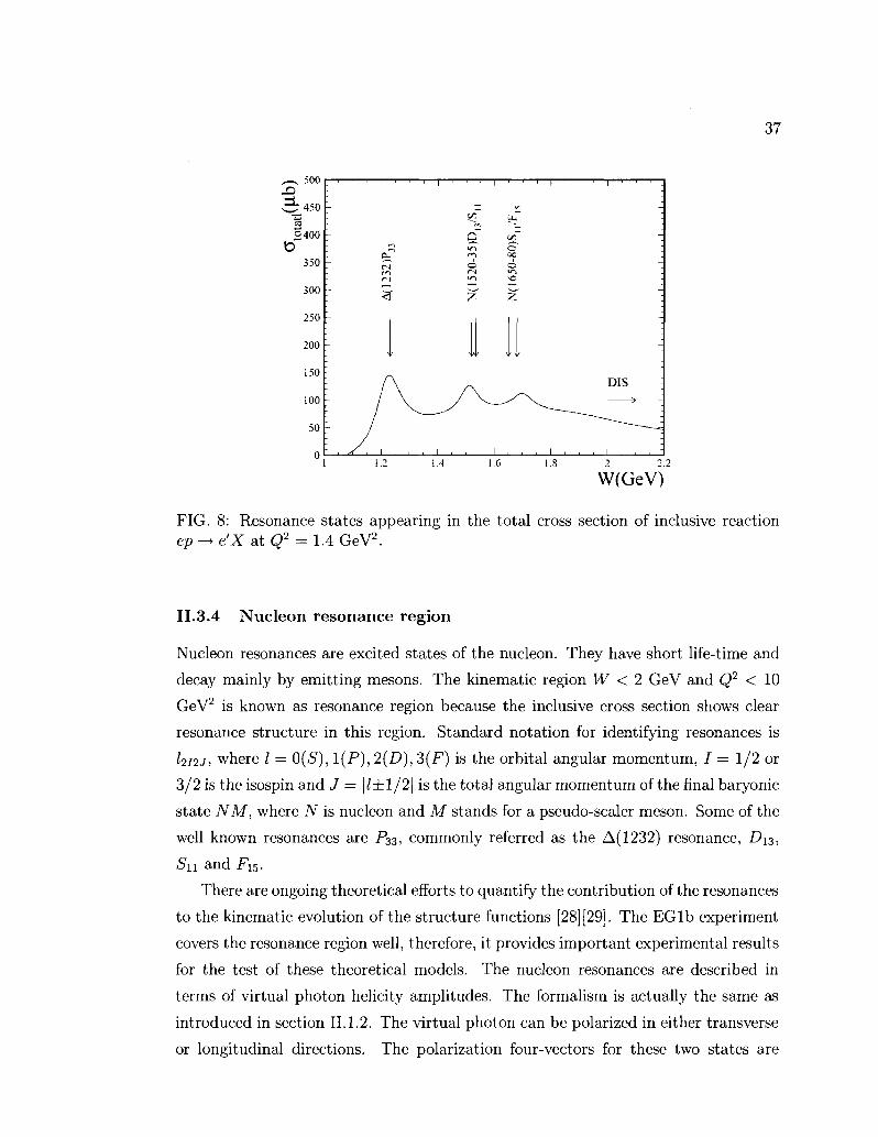
37
r-v 500
w . 4 5 0 ca §400
O
350
300
250
200
150
100
50
0
FIG. 8: Resonance states appearing in the total cross section of inclusive reaction ep - • e'X at Q2 = 1.4 GeV2.
II.3.4 Nucleon resonance region
Nucleon resonances are excited states of the nucleon. They have short life-time and
decay mainly by emitting mesons. The kinematic region W < 2 GeV and Q2 < 10
GeV2 is known as resonance region because the inclusive cross section shows clear
resonance structure in this region. Standard notation for identifying resonances is
^2/27, where I = 0(5), 1(P), 2(D), 3(F) is the orbital angular momentum, / = 1/2 or
3/2 is the isospin and J = | /±1/2 | is the total angular momentum of the final baryonic
state NM, where N is nucleon and M stands for a pseudo-sealer meson. Some of the
well known resonances are P33, commonly referred as the A(1232) resonance, Di3,
Sn and Fi5 .
There are ongoing theoretical efforts to quantify the contribution of the resonances
to the kinematic evolution of the structure functions [28] [29]. The EGlb experiment
covers the resonance region well, therefore, it provides important experimental results
for the test of these theoretical models. The nucleon resonances are described in
terms of virtual photon helicity amplitudes. The formalism is actually the same as
introduced in section II. 1.2. The virtual photon can be polarized in either transverse
or longitudinal directions. The polarization four-vectors for these two states are
W(GeV)

38
written respectively as:
4 = -^=(0, ±1 , -7 ,0 ) (101)
e£ = l ( M , 0 , 0 , i / ) (102)
The corresponding components for the electromagnetic current JM„ are
J± = &,„, = ± - 7 | ( J * + iJy) (1 0 3)
Jo = eft-V = ^Jz (104)
Conventionally, three transition amplitudes, connecting a nucleon iVi ms with a spin
projection m s , with any nucleon resonance N*m. with spin j and projection rrij, are
written as follows [30]:
Ah = w{w^w{NU^Ni-i> ( 1 0 5 » Ai = ii\lw^W I^WM) (106)
M <Ar,|Jo|JV.i> (107) J>5 ' ' 2 > 2 ' 3 2M\ W2- M2
The transition amplitudes ^4^2 and A3/2 correspond to transversly polarized photons
leading to final state helicities 1/2 and 3/2 respectively while Si/2 corresponds to
longitudinally polarized photons. The transverse and longitudinal virtual photon
cross sections can be written in terms of these amplitudes,
T ,, r»\ _ ^M n A 12 vi/2(vR,Q2) = 7^r(\Ah\
2) (108) 1 RMR 2
*Z/2(»R,Q2) = ^r(\Al\2) (109)
1 RMR 2
^ / 2 ( ^ Q 2 ) = ^ - ( | 5 i | 2 ) (no) 1 RMR 2
while the interference term is
«T\^Q2) = ^r(\A±/ + \sif) (in) 1 RMR
2 2
where MR is the invariant mass of the resonance state, TR is the decay width and
vR = (MR - M2 + Q2) /2M.

39
The total transverse cross section, aT = (aJ,2 + aJ,2)/2, and the interference cross
section, aTL, can be written in terms of the structure functions:
47r2a / „ 2Mx
MK <rI,2{"R,<?) = T717(^ + 9i- —92 ) (112)
T / ^ 2 N 4 7 r 2 « f r, 2Mx \ ,110>
<rI,2("R,Q2) = W<{ '~9l + ~1T92) ( U 3 )
^ L K , Q 2 ) = ^ f ( 9 i + 32). (H4)
The transition amplitudes in Eqs. (105—107) are related to photon asymmetry Ai,
Al~\All^ + \ A ^ ( U 5 )
When we consider the A(l232) resonance (with spin-3/2), calculation of the transi
tion amplitudes in terms of multipoles (see Ref. [30]) reveals that A3/2 ~ V3Ai/2 at
small Q2. Therefore, Ai ~ —0.5 is expected for the electromagnetic excitation of the
A(1232) resonance. At large Q2, on the other hand, A3/2 amplitude tends to vanish
and A1/2 transition dominates, hence, Ai approaches to + 1 . In case of the _D13(1520)
resonance, Ai/2 amplitude becomes zero at Q2 = 0 [30], which yields A± = — 1 at
the real photon point. At large Q2, however, Ai/2 is expected to dominate over A3/2
as Q2 —>• oo, yielding A\ = + 1 . In addition, electromagnetic excitation of spin-1/2
resonances, such as 5n(1535), will have an asymmetry A± = 1 since the amplitude
A3/2 cannot contribute. By studying the Q2 variation of the photon asymmetries
for different mass ranges, one can understand the relative strength of the transition
amplitudes contributing to different resonance states.
Electron-nucleon scattering in the DIS and resonance regions follow two seemingly
different mechanisms. In the DIS region, electrons scatter from quarks in relative
isolation (asymptotically free) and the cross section is given by the incoherent sum
over the individual quark contributions. Interpretations utilize quark-gluon degrees
of freedom in these kinematics. In the resonance region, on the other hand, the entire
nucleon responds to the probe coherently, and the interaction is best described by
utilizing hadronic degrees of freedom. An intriguing observation, first made by Elliot
Bloom and Fred Gilman [31], is that there is a similarity between the data from the
two different kinematic regions. In fact, the structure functions measured in the reso
nance region are found to be approximately equivalent to the deep inelastic structure
functions if a proper scaling variable that connects the two kinematic regions is used.
This phenomena is known as quark-hadron duality, which will be described next.
40
II.3.5 Quark-hadron duality
Quark hadron duality explores the connection between the hadronic and partonic
descriptions of the nucleon. It states that the smooth scaling curve seen at high
momentum transfer should be an accurate average of resonance bumps seen at low
momentum transfer for the same values of Bjorken x variable. If duality holds after
averaging over all kinematical regions (a concept known as global duality), single
quark interactions should successfully describe lepton-nucleon interactions even for
low energy and small Q2 values. Then, perturbative calculations by QCD should
approximately yield the average of hadronic observables over a large kinematical
region. Moreover, the same concept can also be tested for a limited kinematic range
within the resonance region to understand the contribution of different resonance
states to the global duality. Duality limited to certain resonances is known as local
duality. The data from EGlb for 4.2 and 2.4 GeV will clarify the situation for
resonance states around the P33 region, where preliminary results show a breakdown
of local duality. A more detailed study of duality for polarized structure functions
at low and intermediate Q2 regions is definitely required to understand the spin
of the nucleon in terms of quarks and gluons. It is arguable that manifestation of
the strong force might be hidden under the aspects of duality because it creates
a relationship between single quark interactions, which govern the short distance
dynamics, and resonance electro-production, where the long distance dynamics of
the nucleon become important. A detailed review about the current standing of
duality can be found in [7] [32] [33].
For kinematic regions where Q2 ^> M2 , the Bjorken x variable can be interpreted
as the momentum fraction carried by the struck quark. But at low Q2 regions, a kine
matic correction that arises due to the non-zero target mass is needed. Introduction
of the Nachtmann scaling variable £ = 2x/( l + y/l + AM2x2 /Q2) partly takes care
of the target mass effects. Explicit target mass corrections have also been derived
under the QCD framework [34].
There are experimental confirmations for duality in the structure function F2 of
the proton [35]. It has been shown that duality holds for the unpolarized struc
ture functions integrated over the entire resonance region (global duality) for Q2 >
1.5 GeV2. A more careful investigation for the intermediate and low Q2 regions is
important in the sense that breakdown of duality might be observed.
Duality also needs to be studied for the polarized structure functions, which are

41
given by the differences of cross sections, rather than the sum, therefore, they are not
positive-definite like the unpolarized structure functions. This brings up a question if
duality still holds for the asymmetries or is it only good for the cross sections? Recent
results [36] [37] confirmed that global duality for the <?i structure function is indicated
by the data for Q2 values larger than 1.7 GeV2 for the proton and 2 GeV2 for the
deuteron. Hence, a general preliminary conclusion can be made that the description
of the spin asymmetry of the nucleon in terms of quark degrees of freedom is also
valid in the resonance region. However, an exception is the spin structure function
#i in the region of AP33(1232) resonance, where (local) duality seems to break down
[37].
According to OPE, a partonic description of the moments of the structure func
tions at intermediate Q2 should be always possible if one accounts for the contribution
of higher twist corrections at sufficient level. Indeed, Ref. [38] showed how duality
can be understood under the OPE framework. In this framework, global duality
implies suppression of the higher twist effects, leaving mainly the leading twist con
tribution dominant. Therefore, experimental observation of higher twist effects in the
resonance region is an important tool to study global duality. On the other hand,
understanding local duality in the QCD framework is more subtle since there is no
clear understanding how the cancellations of the higher twist effects can take place
in limited kinematic regions.
There is also an interpretation of duality in the constituent quark model in [39].
The authors argue that duality may be explained in terms of the cancellations of
resonance contributions with opposite parities. Ref. [39] also suggests that global
duality must fail at Q2 where electric and magnetic multipoles have comparable
strengths. Calculations with simplistic models predicted that this would be Q2 ~
0.5 GeV2. Indeed, duality is expected to eventually break down as Q2 —> 0.
In addition to local vs. global and polarized vs. unpolarized aspects of duality, it
is also important to investigate proton vs. neutron cases. The unpolarized structure
function in DIS region is proportional to the sum of the squares of the constituent
quark charges ~ ^e2 Coherent excitation of the resonances, on the other hand, is
driven by the square of the sum of the constituent quark charges ~ (^2 e9)2 [39]. In
the constituent quark model, these two quantities are the same for the proton but
not for the neutron, which creates a curiosity if there are different aspects of duality
for the proton and the neutron.

42
II .4 S U M R U L E S A N D T H E O R E T I C A L M O D E L S
Since QCD cannot be solved analytically, we don't have a complete description of
the spin structure functions in order to understand the behavior of the quarks inside
the nucleon. However, integrals over the spin structure functions can be compared
to rigorous theoretical results, like sum rules, lattice QCD calculations and chiral
perturbation theory, providing a powerful tool to study the spin structure of the
nucleon. Sum rules are precise predictions of the behavior of the spin structure
functions in certain kinematic limits. Experimental data can be used to test these
predictions and extract information.
In this section, we will explain some of the sum rules that are specifically related
to the first moment of gi(x, Q2),
Jo dx9l(x,Q2), (116)
which can be expressed in terms of the nucleon matrix elements of current operators
via the Operator Product Expansion (OPE) as shown in Eq. (92). It should be noted
that, the OPE is valid only if the moments include the elastic contribution at x = 1.
However, in the DIS region, the elastic contribution is completely negligible. For that
reason, the experimentally measured moments at high Q2 often excludes the elastic
term from the upper limit of the integral. On the other hand, at low Q2, especially in
the resonance region, elastic contribution becomes large, hence, cannot be neglected
for a complete description of the moments in terms of the nucleon matrix elements.
Therefore, moments in these kinematics are distinguished according to their inclusion
or exclusion of the elastic contribution. This distinction becomes important for the
sum rules that specifically apply to the low Q2 regions.
Before defining the sum rules related to the first moment of gi, let's visit the
QPM that preserves its validity in the limit Q2 —» oo. In the QPM, the spin structure
function g\ can be written as in Eq. (76). Therefore, the first moment of g\ simplifies
in the case of free quark fields to:
T\= J dx9l =l-J £e?(A9i(x) + Aq^dx (117)
Assuming three quark flavors (it, d, s), we get for the proton

43
and for the neutron U(n) 1 / 1 . . 4 . , . 1
r ; w = - - A « + - A r f + - A 5 ) (119)
where A ^ represents the integrated quark distributions defined by
Aqi = f (Aft(x) + Aqi(x))dx, (120) ./o
which is the fraction of the nucleon spin carried by the quark flavor q^.
The transition currents between baryons made out of three quark types are de
scribed in terms of the octet axial vector currents,
J£ = ^ - y V ( y ) ^ (* = 1,. . . ,8) (121)
where A& are the SU(3) Gell-Mann flavor matrices and ip is a column vector for three
quark fields (u,d, s):
4 = (122)
\i>s J At this point, it is convenient to introduce the nucleon axial charge ak defined in
terms of the matrix elements of the nucleon state vector [30] [20]:
2MakS>l = (P,S\Jg\P,S) (123)
where M is the nucleon mass and |P, S) is the state vector of the nucleon with spin S.
Assuming SU(3) symmetry holds exact, the non-singlet vector currents are conserved.
This leads to the ak (k = 1 , . . . ,8) to be independent of Q2 and conserved to any
order in as. The singlet current is not conserved because it requires factorization to
deal with divergences that arise and it is convenient to choose Q2 as the factorization
scale. Its exact value depends on the factorization scheme utilized. In commonly
used factorization schemes [7], a^ depends on Q2 when we go beyond the Leading
Order calculations.
The relevant matrix elements to this analysis are a0, a3 and a8. The singlet
element, a0, represents the net spin carried by the quarks, AS , in the DIS mea
surements. Based on the assumption that SU(3) is a good symmetry, the other two
matrix elements of the axial vector currents can be expressed in terms of the weak
decay constants F and D [40], which are constrained by the neutron and hyperon

44
/3-decay measurements. As a result, the three matrix elements can be written as:
a0 = Au + Ad + As = AE (124)
a3 = Au- Ad = F + D = 1.26 (125)
a8 = Au + Ad- 2As = 3F - £> = 0.58 (126)
Finally, by combining Eqs. (118) and (119) with (124-126), we can write the first
moment of g\ in terms of the axial charges for the proton,
-^ [9F - D + 6As] (127) 18
- ! - [6F-4 .D + 6As] (128) 18
It should be noted that the above relations between the quark spin distributions
and the weak decay constants are only valid in the limit that Q2 —> oo. For finite
Q2, corrections provided by pQCD, should be utilized
II.4.1 Vector and Axial Vector Coupling Constants
In order to understand the relations between the quark spin distributions and the
weak decay constants mentioned above, let's look at weak charged current transitions,
such as neutron /?-decay, in the framework of the Constituent Quark Model (CQM)
[1], in which we assume that nucleon contains three constituent quarks, UUD for
the proton and UDD for the neutron. The constituent quarks are labeled with
capitol letters to distinguish them from the current quarks u and d used in the QPM
earlier. The neutron /3-decay can be visualized as electron capture by a proton under
the assumption of time reversal invariance in physical processes. The weak charged
current transitions contain vector (V) and axial vector (A) parts.
At low energies, as in the case of nuclear /3-decay, the vector part of the hadronic
current can be written as V = gv(n\r~\p), w n e r e \n) a n d \p) represents the neutron
and proton states while r~ is the isospin lowering operator, which turns the proton
into a neutron. The matrix element (n\T~\p) is simply equal to 1. The vector coupling
constant gv accounts for the fact that the weak interaction acts on the individual
quarks, not the whole nucleon. In the case of electron capture by the proton, one of
the U quarks is converted into a D quark, with simultaneous emission of an electron
vr=j\l{x)dx=\ "3 1 -a3 + -a8 + a0
and for the neutron
-I
r ^ = jf gi(x)dx = I " 3 1 -ja3 + T°8 + a0

45
neutrino. As a result, we can write the vector part as V = (n\ ^ T~\p), in which sum
goes over all quarks in the nucleon and r~\U) = \D) and T~\D) = 0. By utilizing
SU(2) symmetry we can write [1],
? q
which simply states that matrix element of any isospin lowering operator r~ between
two members of iso-doublet (e.g., the proton and the neutron or the U and D quarks)
is the same as the matrix element of the operator r 3 between two 1$ = + 1/2 states.
The operator r 3 behaves as T3\U) = + 1 , T3\D) = — 1, which means the right hand
side of the above equation is equal to 1. Therefore, gv(n\T~\p) — 1> indicating that
gv = 1. The experimentally measured [41] value is gy = 1.000 ± 0.003. Hence, the
vector weak charge is conserved. So, it can be said that just like the electric charge,
the vector charge is also protected by conservation laws. This is often referred to as
Conserved Vector Current (CVC).
In the case of the axial vector, we can write the three spatial components as
A = 9A(Wj s\r~al\p, s), where a1 are the Pauli spin matrices that act on the spin
wave function in the same way the r ' s act on isospin. \p, s) and |n, s) are the proton
and neutron states with spin s = f or [. The axial vector coupling constant g^
accounts for the quark level interaction. At the quark level, the matrix elements
can be written as At = (n, s\ ^2qT~alq\p, s). Again by utilizing the SU(2) group
symmetry, the z component of the axial vector current Az can be written as:
gA(n,s\T-a3\p,s) = (p,s\ ^rzqa
zq\p, s) (130)
Q
The left hand side gives g&. The operator combination T3<73 at the right hand side
behaves on the individual quarks as:
rXW T) = +W T) , ryq\U I) = -\U |) (131)
ryq\D T) = - | D T) , ryq\D [) = +\D |> (132)
Summing over all possible flavor and spin states, the Eq. (130) eventually yields,
gA = AU- AD (133)
where AU = \U | ) - \U | ) and AD = \D ]) - \D | ) . This relation derived by
using the CQM also holds for the QPM once we apply the same idea to the current

46
quarks instead of the constituent quarks and take also the anti-quark polarizations
into account. Therefore, gA = Au — Ad, in which the definition of Aq is now changed
to Eq. (120). This relation holds its validity at the limit Q2 —»• oo, where quarks are
asymptotically free. However, in this approach, the orbital angular momentum of
the quarks are assumed to be zero, which is not exactly true. Therefore, relativistic
corrections are required. This simple calculation gives an idea for the connection
between the quark spin distributions and the QA coupling constant.
The axial vector coupling constant was measured from neutron /3-decay. It can
be written in terms of the weak decay constants F and D, which describe the anti
symmetric and symmetric SU(3) couplings respectively. This, however, is based on
the assumption that SU(3) symmetry of baryon octet is exact and the strange quarks
in the nucleon are unpolarized. The most up to date value of gA is [7]:
gA = F + D = 1.2670 ±0.0035 (134)
Hence, the axial vector charge, unlike the vector charge, is not exactly conserved by
the strong interactions.
Another weak decay we need to consider is the /3-decay of a A-hyperon into a
proton by emitting electron and electron anti-neutrino [1]. In this process, the s
quark changes into a u quark. Again, one can define vector and axial vector parts
of this transition. By utilizing SU(3) group symmetry of isospin and strangeness,
the axial vector coupling constant of the transition, g\ can be related to the quark
spin distributions in the framework of the QPM: g\ = Au + Ad — 2As. Under the
assumption that SU(3) symmetry is exact, this quantity is often written in terms of
the weak decay constants as:
g\ = 3 F - D = 0.585 ± 0.025 (135)
The experimental value is obtained by a global fit to the world data [7]. In the
CQM, in which there is no strange quark inside the nucleon, g\ must be equal to
1. Therefore, the experimental result indicates that the s quark polarization is non-
negligible or SU(3) symmetry is not exact. pQCD corrections address some of the
issues and provide an extension of these definitions, that are only valid in the Q2 —• oo
limit, for a finite Q2.

47
II.4.2 p Q C D Correc t ions
Following the prescriptions given in section II.3, the structure functions can be
evolved to finite Q2. By using DGLAP equations to take radiative effects into ac
count and utilizing the OPE for higher twist corrections, the Q2 dependency of the T\
can be evaluated. However, divergences arise in pQCD corrections. The ultra-violet
divergences are taken care of by renormalization. Collinear divergences that arise be
cause of masslessness of quarks are attended by using a scheme called factorization.
The interaction of the virtual photon with a nucleon is visualized as a combination of
long (soft) and short (hard) distance interactions. The point this separation is made
is called factorization scale /i2. The long distance interactions cannot be calculated
analytically. They can only be parametrized and studied experimentally. Therefore,
the infinite terms can be absorbed into the long distance part of the interaction. For
instance, we can use a common term that arises in pQCD calculations for parton
densities such as asln^ where mq represents quark mass. Such a term can be split
into two parts as:
asln—-z = asln—r- + ajn—r (136)
then the first term of the right hand side is absorbed into the short distance part of the
equation and the second term is into the long distance part. Here, the factorization
scale /x2 is an arbitrary number and physical results cannot depend on it. However,
only a finite number of terms enters into the analytic calculation, therefore, our
solution depends on the scale we choose. As a result, the solution should carry the
factorization scale /J,2 as a label. It is generally agreed that an optimal choice for this
scale is /J,2 = Q2, so the parton densities become also a function of Q2 as well as the
momentum fraction x: q(x) —>• q(x,Q2). There are different factorization schemes in
use. In the Modified-Minimal-Subtraction (MS) scheme, a3 and a8 are independent
of Q2 and ao = AS. The correction term CQ in Eq. (88) vanishes, so that AG does
not contribute to T\. By utilizing Eqs. (89), (90) and (92), the expression for the Ti
up to twist-4 correction can be written as:
r\{p'n)(Q2) = ^2 ±a3 + ±a8] CNS(Q2) + \aQ{Q2)Cs(Q
2) + ^ (137)
where Hi{Q2) is given in (94) and the non-singlet (NS) and singlet (S) Wilson coef
ficients are given by:
CNS(Q2) = 1 - ( ^ ) - 3.58 ( ^ ) 2 - 20.22 ( ^ ) * . . . (138)
48
CS(Q2) = 1 - ( ^ ) - 1.096 ( ^ ) . . . (139)
The QPM turns out to be a zero order approximation to pQCD. The parton densities
q{x) and Aq(x) becomes just the leading order members of QCD calculations. These
perturbative corrections are small for DIS experiments such as the EMC experiment
that triggered the so called spin crises. Next, we will define a few sum rules that are
initially based on the quark parton model, compare their results with experiments
and analyze their implications after the pQCD corrections are applied.
II.4.3 The Ellis-Jaffe Sum Rule
By using the SU(3) flavor symmetry and assuming the strange sea quark is unpo-
larized, As = 0, Ellis and Jaffe predicted a value for the first moment of g[ in the
framework of the QPM. Starting from Eq. (127) and using measured values of the
weak decay constants, they found T^ = 0.186 and T1 = —0.024. It should be
stated that this prediction also assumes net gluon polarization AG = 0. Later, in the
EMC experiment, however, r } ( p ) = 0.128 ±0.013 ±0.019 was measured at Q2 = 10.7
GeV2. The experimental value is much lower than the prediction made by Ellis-Jaffe.
This discrepancy is what triggered the so-called spin crisis. This low value of the
r \ was also confirmed by later experiments.
The assumption As = 0 made in the Ellis-Jaffe sum rule implies that oto = a8.
Therefore, in the regime of the QPM, a0 = 3F — D = 0.585, as known from the
hyperon decay. Remember that in the QPM (at the limit Q2 —> oo), a^ corresponds
to the total spin carried by the quarks. In a non-relativistic model, it is expected
that all of the proton's spin is carried by the valence quarks, which means a0 = 1.
Relativistic corrections consider the orbital angular momentums of the quarks and
decrease this value to a0 ~ 0.6. Ellis-Jaffe prediction is in good agreement with the
relativistic model. However, if one tries to extract the value of ao by using Eq. (127)
and the measured value of the T1 ,
a0 = 9r j ( p ) - | a3 - j a8 = 0.05 ± 0.12 ± 0.17, (140)
which is much smaller than the Ellis-Jaffe prediction. Indication of the EMC exper
iment is that the contribution of the quark spins to the overall spin of the proton is
very small.
One can argue that the EMC regime, Q2 = 10.7 GeV2, is not high enough for the
QPM equations to be valid, therefore, one must apply the pQCD corrections. This
49
is done by using the Eq. (137). However, the perturbative corrections turn out to be
small for the EMC data. The corrected value becomes [42] a0 = 0.17 ± 0.12 ± 0.17
evaluated at Q2 = 10 GeV2. Hence, the QCD-improved corrections do not resolve
the question why the value of ao is much smaller than the expected. Later, several
more precise experiments were performed in order to measure T1 , I \ and I \ (
[43] [44] [45] [46] [47] [48] [49]. It should be noted that the experimental verification of
the sum rule requires inclusion of the elastic peak at x = 1. However, for the DIS
experiments, the elastic peak contribution is very small. Hence, most experimental
results in the DIS regime do not include the elastic peak. But, the importance of
the elastic peak increases as we get to lower Q2 regions, where the results should be
handled carefully. In addition, low x extrapolation while calculating the T\ integral is
an important factor. The HERMES and COMPASS experiments used different and
more precise low x extrapolation than the previous experiments did. By using the
recent measurements on the deuteron, these experiments estimated the most precise
singlet axial charge a0, yielding a0 = 0.33 ± 0.04 for HERMES evaluated at Q2 = 5
GeV2 and aQ = 0.35 ± 0.06 for COMPASS at Q2 = 3 GeV2.
Gluon Polarization and Axial Anomaly
Several schemes have been developed to incorporate a non-zero gluon polarization in
order to explain the low ao measured in the experiments. It has been shown in [51]
that there is an anomalous contribution to the axial current, which breaks the axial
current conservation and causes a gluonic contribution to ao such that [52]
a0 = AZ-^-as(Q2)AG(Q2), (141)
where A S represents the net spin carried by the quarks. However, this actually
depends on the factorization scheme. In the MS scheme, the gluonic contribution
turns out to be zero, thus AE = ao(Q2), which means AE becomes Q2 dependent
thus cannot be directly interpreted as the net spin carried by the quarks. In the
other factorization schemes, AB and JET, AE is Q2 independent and therefore,
corresponds to the net spin carried by the quarks. However, in these factorization
schemes the gluonic contribution to a0 is non-zero. As a result, a small a0 does not
necessarily mean that the quarks carry a small fraction of the total spin as long as
there is also a gluon polarization contributing. In order to explain the small a0, a
gluon polarization as large as AG ~ 1.7 is required at Q2 = 1 GeV2. Unfortunately,

50
the recent experimental results pretty much ruled out such a large gluon polarization
[7], which brings us back to the question why a$ is small.
As a conclusion, the Ellis-Jaffe sum rule is important because its violation implies
that the strange quark polarization and the gluonic contributions should be taken
into account seriously. The reader is strongly encouraged to look into Ref. [7] for
these ongoing efforts and recent experimental results on this subject. In addition,
determining the orbital angular momentum contributions from both quarks and the
gluon is also an important ingredient to understand the spin content of the nucleon.
II.4.4 The Bjorken Sum Rule
By using Eqs. (118) and (119), we obtain:
rl(p) _ pl(") = h A u _ A ( f) ( U 2 )
According to Eq. (133), the right hand side of (142) is directly related to the ax
ial vector coupling constant g&- This is, however, only valid in the QPM frame.
Therefore, we can write in the QPM that
r l W _ pit-) = 1 gA ( 1 4 3 )
This is the celebrated Bjorken sum rule, which was derived before QCD was invented.
Its validity can be extended into a finite Q2 region by applying the QCD corrections
to the structure functions as prescribed earlier. By using Eq. (137), the most general
form of the Bjorken sum rule can be written as
pl(p) _ pl(n) = CNS£A + h i g h e r t w . s t ) ( M 4 )
where CNS is the non-singlet Wilson coefficient as given in Eq. (138).
The strength of the Bjorken sum rule comes from the fact that all additional spin
contributions from the gluon and the strange sea quarks are canceled in the difference,
leaving only the contributions from the up and the down quarks. There is no model
dependency or any underlying assumption in the Bjorken sum rule, other than QCD
and isospin symmetry. It completely relies on QCD assumptions. Therefore it is
considered as one of the most important tests of QCD. In the region 2 < Q2 < 10
GeV2, the Bjorken sum rule has been verified at the level of 10% accuracy [30].
Taking as(M2) = 0.119 ± 0.002 , which yields a s(5 GeV2) = 0.29 ± 0.02, gives,
pl(p) _ pl(n) = a l g 2 ± Q 0 Q 5 a). Q2 = 5 G e y 2 ( M 5 )

51
The El55 experiment measured [7] [47]
pl(p) _ pl(n) = Q 1 ? 6 ± Q Q 0 8 a t Q2 = 5 G e y 2 (14gj
At this point, we can also look at the sum of the first moments for the proton and
the neutron. In the first approximation (by neglecting nuclear effects as well as the
higher twist contributions), the first moment for the deuteron can be expressed by
summing the proton and neutron such that I y = | ( r i( p ) + T^ )(1 — 1.5w£>) where
WD is a probability that deuteron is in a D state and the factor 1/2 is introduced to
express the value "per nucleon" (see section II.5 for details). From Eq. (137), we can
immediately conclude that the 03 term has no effect on I \ and the do term will
dominate. Therefore, I \ ( is especially sensitive to AE (without the interference of
a3), and via its Q2 evolution, to gluons.
II.4.5 The Gerasimov-Drell-Hearn (GDH) Sum Rule
When the momentum transfer of the photon becomes smaller, at low Q2, perturbative
QCD cannot be utilized because the strong coupling constant approaches 1. There
are phenomenological models that incorporate the photo-absorption cross sections in
order to predict the low Q2 evolution of the structure functions.
As explained in section II.3.4, the photo-absorption cross sections can be related
to the helicity transition amplitudes and expressed in terms of the structure functions.
The Gerasimov-Drell-Hearn (GDH) sum rule relates the difference between the two
real photo-absorption cross sections a[,2 and oj to the anomalous magnetic moment
of the nucleon K [53] [54],
1(0) = j T ±[al/2(u) - <%,2(y)\ = -44?S«2 = - ^ <1 4 7> where UQ marks the inelastic (pion production) threshold, S = 1/2 is the spin of the
nucleon, M is the nucleon mass and a is the fine structure constant. The anomalous
magnetic moment for the proton is KP = +1.79 and for the neutron it is Kn = —1.91.
Therefore, the numerical results for the GDH sum rule for the proton /p(0) = —205 fib
and the neutron 7„(0) = —233/^6.
The GDH integral was originally derived for real photons at Q2 = 0. Derivation of
the sum rule exclusively relies on very general principles such as Lorentz invariance,
Gauge invariance, crossing symmetry and the low energy theorem. The details on
the derivation can be found in [55] and [56]. Here, we can briefly outline the steps

52
flm v'
FIG. 9: Path of integration for Cauchy's integral formula.
involved. The spin dependent Compton forward scattering amplitude for real photons
with energy v can be written as,
T(U, e = o) = ?; • ei fT(u) + id • (?; x ro gTT{v) (148)
where fr and grr are scalar functions, 1 a is the vector of Pauli spin matrices and
tij label the initial and final polarization of the photon. The above scattering ampli
tude is a simplified case of the full scattering amplitude by fulfilling the transversity
condition for real photons, t- k = 0, where k represents the nucleon momentum.
The Compton scattering is symmetric under the exchange of in and outgoing
photons (e*j <-> e^*). This symmetry is called crossing symmetry and is exact for all
orders of electromagnetic coupling. As a result of this symmetry we have:
T(-v,6 = 0)=T*(v,6 = 0), M-v) = mv), 9TT(-V) = - / 2 » (149)
We can compute the Compton amplitude for different spin orientations of the
photon and the nucleon. For this analysis, we only need to focus our attention
to two cases where the spins are either aligned, which yields an amplitude /3/2 , or
anti-aligned, which yields / i / 2 :
/3/2W = frW ~ grr(v), /1/2O) = fr(v) + 9TT{V) (150)
fz/2 and /1/2 are associated to the helicity amplitudes described in section II.1.2. By
using the optical theorem, the forward scattering amplitudes for different helicity
1 / r (^ ) represents the spin independent amplitude while grriv) is the spin-flip amplitude. Sometimes fr(y) a n d grri^) may be referred to as fi(v) and /2(^) respectively.

53
combinations can be related to the total cross sections,
Im f(u) = ^-a(u). (151)
Then, we can write the amplitudes fa and grr as:
Im fT(u) = ^ ( f f l / 2 ( i / ) + a3/2(u)) = £ aT{u) (152)
Im gTT(u) = ~-(a1/2(u) - cr3/2(u)) = — aTT{u) (153) 07T 47T
At this point, we are ready to use the Cauchy's integral formula to evaluate the
scattering amplitudes. The Cauchy's integral is written as:
f{u) = J_Idu'fi!iL (154) M ' 2-KiJc {u'-u) V ;
The path of integration is shown in Fig. 9. In terms of different segments of the
integration, we can rewrite the Cauchy's integral:
/w = ip/_ oo
du
1 f A> fly) ,• i /" w' / ( O ( 1 5 5 )
+ / du . , x + lim / du / , \ 2™ iic+(0,oo) \y -V) 8^0 2*1 JK_{v<5) \V -V)
where V denotes the principal value integral. The important point here is that the in
tegral along the path K+(0, oo) vanishes according to the No-subtraction hypothesis.
It should be noted that there is no strong reason why the No-subtraction hypothesis
should hold. This remains as one of the assumptions that the GDH sum rule just
relies on. The No-subtraction itself relies on other fundamental assumptions like
Lorentz and gauge invariance and causality. The integral above is reduced to:
f(u) = ±V r du'J^l- (156) ™ J-oo {V - U)
Recalling the crossing symmetry properties of the scattering amplitudes, we can write
the above integral as:
fW) = lv r d , (fML + n ^ ) (157)
Considering only the real part, this integral simplifies to Kramers-Kronig dispersion
relation: ,
Re /(„) = ^V J™ du Im f(u') (~i^-ji) (1 5 8)

54
By incorporating the results of the optical theorem for the scattering amplitudes
/ r (^ ) and gTTW)jv given in Eqs. (152 - 153) into the Kramers-Kronig dispersion
relation we get,
Re w=& r *'™ (A) = hl d"' " V ) S {~T (159)
n=0 L , / u J
where we used Binomial expansion for the terms in v in the integration. Similarly,
for grr/v we have,
~ 2n~\
^ = ^ 1 I T i"/»<" > - *»^ »l (7 ) n=0 LJU
(160)
Now, we will compare these equations for fr and QTTJV with their expansion based
on the low energy theorems and deduce the GDH sum rule.
The Low energy theorem
The Low energy theorem in Compton scattering, first suggested by Thirring and
then generalized by Low, Gell-Mann and Goldberger, provides an expansion of the
Compton scattering amplitudes in terms of the photon energy v up to the the lowest
non-trivial order in electromagnetic coupling. The expansion yields:
/TM = ~ + K + f c ^ + o M (Mi)
^ = - ^ " 2 + ^ 2 + 0 M ( 1 6 2 )
where M is the nucleon mass. Note that fr is even and grr is an odd function of v
as a result of the crossing symmetry, as is the electric and /3M is the magnetic dipole
polarizabilities. The leading term in the spin-flip amplitude grr/^ is determined by
the anomalous magnetic moment K of the nucleon while the quadratic terms in v is
governed by the forward spin polarizability 70.
By comparing the dispersion relations with the low energy theorem expansions
for the scattering amplitudes, we obtain our basic sum rules. The Baldin's sum rule
for the electric and magnetic polarizabilities,
i r ^ v ) = a * + / ? M (i63)

55
the GDH sum rule,
if^M-')-^.rt = - ^ , ("4) and the forward spin polarizability,
-73 kl/2(" ') - ^3/2^')] = 70 (165)
In the Eq. (164), the lower limit of integration is often replaced with pion production
threshold v0 because the cross-sections for real photon are zero below this threshold,
which means the GDH sum rule has no elastic contribution due to kinematic con
straint. This convention brings us the original GDH sum rule written in Eq. (147)
at the beginning of this section.
The G D H Sum Rule for the Deuteron
The GDH sum rule can also be established for the deuteron because the low energy
theorem holds its validity for composite systems such as the deuteron. The deuteron
anomalous magnetic moment K& = —0.143 is relatively small, which yields a small
value for the GDH sum rule ld{0) = —0.65 fib. Because of its small binding energy,
the deuteron has a quite extended spatial structure. Its anomalous magnetic moment
is small because of an almost complete cancellation of proton and neutron anomalous
magnetic moments in the deuteron. When we consider the small GDH sum for the
deuteron, we expect some cancellations to occur in the deuteron GDH integral as
well. Different production channels contributing to the integral must be analyzed
separately to understand the overall value of the sum. For example, there is a photo-
disintegration process 7 + d —» n + p as well as some meson production channels
that contribute to the GDH sum of the deuteron. The same meson production
channels also contribute to the GDH sum of the nucleon. Table 2 shows the estimated
contributions of various production channels to the deuteron (d) and the neutron +
proton (n+p) GDH integrals. If one considers only the meson production channels,
In+P ~ —476.74 /ib is relatively close to Id ~ —408.83 \xb. However, if we include the
photo-disintegration channel contribution for the deuteron, we get Id ~ —27.31 fib.
The remaining discrepancy can be attributed to additional final state channels that
were neglected in these calculations. Nevertheless, a strong anti-correlation between
the low energy photo-disintegration process and the high energy meson production
channels is the main reason of the small GDH integral for the deuteron.
4TT2 L

56
TABLE 2: Estimated contributions of various channels to the GDH integral (in jib) for the neutron+proton In+P and for the deuteron Id- The photo-disintegration channel 7 + of —> n + p is integrated up to v = 0.8 GeV, the single pion and eta production channels are integrated up to v — 1.5 GeV and the double pion channel is integrated up to v = 2.2 GeV [57].
Channel np 7T
7T7T
V Sum
GDH Sum
J-n+p
0 -315.33 -175.95 14.54
-476.74 -437.94
h 381.52 -263.44 -159.34 13.95 -27.31 -0.65
At high energies, especially above pion production threshold, the contribution
from the photo-disintegration channel completely vanishes. In that case, the deuteron
GDH integral can be approximated by the sum of the proton and neutron integrals
plus nuclear corrections. This is the situation in the kinematic regime of the EGlb
experiment. One straightforward correction comes from the D-state. In the DIS
experiments, a valid approximation for the deuteron GDH integral can be written as
Id = (Ip + In)(l — l-5u>£)) with WD ~ 0.056. However, higher order nuclear corrections
are required for better comparison between the GDH integral of the deuteron and
the sum of the integrals of the nucleons, see section II.5 for those details.
Generalization of the G D H integral for virtual photons
As explained earlier, for the low Q2 regions, it is important to distinguish between
the moments with elastic contribution at x = 1 either included or excluded. The
relations between the moments of the structure functions and the matrix elements
of operators are only valid if the moments include the elastic contribution. In the
DIS region, the elastic contribution is negligible and generally excluded. But, at low
Q2, the contribution becomes important. Therefore, we will label the moments with
elastic contribution included as F\, while we will use F{ for the moments with no
elastic contribution. Experimentally tabulated moments generally exclude the elastic
contribution. From now on, we will use the same labeling convention for the integrals
as well.

57
The GDH integral can be generalized for virtual photons, hence, for Q2 > 0. The
most straightforward method is to assume that real photon cross sections connect
smoothly to the virtual photon cross sections. Therefore, we can simply replace the
real photo-absorption cross sections with the corresponding virtual photo-absorption
cross sections and write the generalized integral with no elastic contribution as:
f°° du HQ2) = / - [ * ? > , Q2) ~ " ? > , Q2)] (166)
By using Eqs. (52) and (53), the integral is often written in terms of the spin structure
functions: I ^ = 8TF r-^i(x,Q2)-7292(x,Q2)] (167)
M J0 x K
where 7 = Q/u, x is the Bjorken variable and K is the flux factor. In the commonly
used Hand's convention K = v(l — x). Another convention is that of Gilman's, in
which K = vy/T+i*. The upper limit of the integration is determined by:
Q2
X° = Q2 + m7T(2M + m7T) ( 1 6 8 )
where mn = 0.137 GeV is the lightest pion mass. In the high energy limit, when
7 <C 1, the integral becomes
rtril\ 1 6 ? r a fX° 1 rV\j 1 6 7 r asi/^2\
^ = ~Q*~J gi(x,Q2)dx = -^-T\{Q2) (169)
The above equation provides a connection between the GDH integral and experi
mental observables. This connection can be established in a more rigorous way by
introducing an integral related to the moment T\,
2 M 2 . , , ^ 2M2 rX0
W) • - 2M2 rxo
g 2-r |(Q2) = - ^ - y o 9i(x,Q2)dx (170)
using Eqs. (52), (53) and Hand's convention for the flux factor K, this integral can
be expressed in terms of the cross sections,
f , _ 2 , M2 [°°l-Q2/2Mv 2
J ^ = ^ l 0 T T W ^ [ C T l / 2 M ) ( m )
-a3/2(u,Q2) + 2-^aTL(u,Q2)}^
It is clear that the integral h(Q2) is only an approximation to the GDH integral
I{Q2) because of the interference cross section aTL(u,Q2). However, when we take
the limit as Q2 —• 0 on the Ti(Q2), we recover the generalized GDH integral:
M2 f°°r rr , „ 0 , r , _ , „ d,U M2 -,
Q2 W*W = r^U^Q2)-°U"><?)] ~ = s^W) (172) ?2^o Q-Kza JVo v onza

58
Hence, we can write the GDH sum rule in terms of the first moment:
ton 7lW>) - 4 , Bm 1 W ) = - ^ (173)
The anomalous magnetic moment of nucleon is a precisely measured quantity. There
fore, the generalized GDH sum rule becomes a strong argument to constrain the first
moment of gi as Q2 approaches to 0. The form of Eq. (173) is interesting in the
sense that f \ approaches 0 from negative value as Q2 —> 0. But, T\ is expected to
be positive in the DIS region. This means it must change its sign in the resonance
region and converge to 0 at Q2 = 0 with a slope of — K2/8M2.
Another method to generalize the GDH sum rule was developed by Ji and Osborne
[58] by generalizing the Compton scattering amplitude in Eq. (148), which was given
for real photons, to a virtual photon case by introducing an additional longitudinal
polarization vector. They begin by defining a time-ordered forward virtual-photon
Compton scattering tensor and express its spin dependent (antisymmetric) part in
terms of two new scaler functions Si(v, Q2) and 52(v, Q2), which are spin-dependent
Compton amplitudes. These amplitudes satisfy crossing relations:
S1(v,Q2)=S1(-v,Q2), S2(v,Q2) = -S2(-v,Q2) (174)
By optical theorem, these Compton amplitudes are connected to the spin structure
functions,
Si{v,Q2) = 2vGi{v,Q2) (175)
with M2vGl(v, Q2) = gx{x,Q2) and Mv2G2{v,Q2) = g2(x,Q2). The dispersion
relation for Si is given by:
Si(u,Q) = 4 — — r — — — (176)
JMQ2) (V ~ v )
Here, Gi is difficult to calculate analytically but it can be measured while Si is hard
to measure but it can be calculated. At least in principle, by taking v = 0 in Eq.
(176), Ref. [58] arrives at a possible candidate for a generalized <52-dependent sum
rule:
51(0,Q2) = 4 / ° ° ^ d K Q 2 ) JMQ2) v
= ikfW) (177)
- w«Q2)

59
where f \(Q2) is the inelastic portion of the first moment F\(Q2) and we have Eq.
(173) for the integral Ii(Q2). It should be noted that, when Q2 ^ 0, the Compton
amplitude receives a contribution Sf (0, Q2) from elastic scattering. This contribution
can be calculated by using Dirac and Pauli elastic form factors Ff2(Q2) [58][7]:
Sf(0,Q2) = ±F?(Q2)[F?(Q2) + F?(Q2)} (178)
then, by using Eq. (177), the full moment with elastic contribution, yields,
M2 K2
glim W ) = -^F?(Q2)[F?(Q2) + FI\Q2)] - ^ (179)
Theoretical predictions can be made for the Compton amplitude S\(0,Q2). For
Q2 > 1 GeV2, the operator product expansion can be utilized by expanding the first
moment in powers of 1/Q2 using the twist coefficients. In this approach, including
the elastic contribution to the first moment is vital. For Q2 < 0.1 GeV2, on the other
hand, chiral perturbation (xPT) theories can be used. The details on x ? T calcula
tions can be found in [58] [59][60]. In the region 0.1 < Q2 < 0.5 GeV2, Lattice QCD
has been suggested in [58]. There are several different schemes each yielding slightly
different generalized GDH integrals. A nice review for these various definitions of
integrals and their comparisons to each other can be found in [61].
II.4.6 Generalized Forward Spin Polarizabilities
In the previous section, we mentioned the forward spin polarizability 70 for real pho
tons, deduced from the comparison of the dispersion relations with the low energy
theorem. Several different methods have been used to generalize the dispersion re
lations to the virtual photon case [61]. Generalization of all amplitudes in virtual
Compton scattering is given in [56]. As mentioned in the previous section, one can
generalize the Compton scattering amplitude for real photons in Eq. (148) to dou
bly virtual Compton scattering (VVCS) by introducing an additional longitudinal
polarization vector g:
T > , Q 2 , <9 = o) = r; • c; fT(u, Q2) + i t • {rf x ?,) 9TT{v, Q2) (180)
+ hiy, Q2) + ia • [(?/ - ti) x q] gTL(v, Q2)
JT and gxr are now functions of v and Q2. fL(v,Q2) is the amplitude for the
longitudinal polarization of the virtual photon while grhiy-, Q2) is the amplitude for

60
the interference between the transverse and the longitudinal polarizations. In the
limit Q2 = 0, fT and gTr coincide with those in Eq. (148) while fa and gn vanish.
While taking the limit Q2 —> 0, it is important to send v —>• 0 limit first so that
elastic contributions can be accounted for. In case of elastic scattering, We need to
preserve the virtuality of the photon in order not to loose the elastic contribution
to the virtual Compton scattering off a nucleon. The inelastic contributions, on the
other hand, are independent of the order of the limits.
These amplitudes are related to the cross sections via the optical theorem.
Im fa(u) = J £ aL(u, Q2) , Im fTL{u) = £ aTL(u, Q2) (181)
Note that, we are now using the flux factor K while incorporating the optical theo
rem for virtual photons. These Compton amplitudes minus their corresponding Born
terms (subtracting the elastic contribution) can be expanded in powers of v2 accord
ing to the low energy theorem. The leading term in the expansion of grr yields the
generalized GDH integral:
2 M2 rXo
IA(Q2) = - ^ J dx[9l(x,Q2)-72g2(x,Q2)] (182)
with
IA(0) = - ^ (183)
The advantage of this definitions is that the factor K for the photon flux, which
depends on the choice of convention, hence, arbitrary, disappears.
The next-to-leading term in the expansion of grr yields the generalized forward
spin polarizability 70:
16aM2 r ° 7o(Q2) = ^ P / *2 9i{x,Q2) ^—92(x,Q2) dx (184)
Similarly, the expansion of the amplitude grL yields yet another generalized forward
spin polarizability STL'
IfirvM2 fx° 5TL(Q2) = ^ - J x2[gi(x,Q2) + g2(x,Q2)]dx (185)
Note the factor Q~6 in the definitions. This means, unlike some of the other gen
eralized integrals, 70 and STL still manage to preserve quantifiable values at very
small Q2. The forward spin polarizabilities exploit soft, non-perturbative aspects of
the nucleon structure. Therefore, they provide an excellent ground for testing x ? T
theories, which are only valid at Q2 < 0.1 GeV2.

61
II.4.7 Phenomenological Models
In the kinematic region below Q2 « 0.1 GeV2 the generalized GDH Sum Rule and
XPT theory should be applicable. Above Q2 = 1 GeV2, one can utilize OPE, pQCD
and the modified Bjorken Sum Rule. Constraints enforced by the sum rules govern
the Q2 evolution of T\ in these regions. In the low Q2 region, T\ is expected to be
negative and approach to 0 as Q2 —> 0. In the high Q2 region, on the other hand,
T{ should asymptotically approach a constant positive value. This indicates that
r j should cross zero somewhere in the range of 0.2 < Q2 < 1.0 GeV2. This region
is known to be dominated by the nucleon resonances, where we don't have a good
theoretical understanding of the Q2 dependence of the structure functions. For that
reason, experimental data in the resonance region are very important. This is one
of the main goals of the EGlb experiment. There are Lattice QCD calculations and
some phenomenological models that try to describe the Q2 behavior of the structure
functions in this kinematic region. In this section, we will discuss two models, with
which we compare our results.
The Q2 evolution of the GDH integral was parametrized by Anselmino [62] and
later refined by Burkert and Ioffe [63] by splitting the quantity into resonant and
non-resonant parts:
9M2 -IGDH(Q2) = -QT^Q2) = Ires(Q2) + I\Q2) (186)
where Ires is the contribution from the resonant states and decreases rapidly with
increasing Q2. This contribution is of course also unknown a priori, but can be
approximated by the amplitudes for j*N —»• N* —• NIT, which are reasonably well
known from phase shift analysis of it (virtual) photo-production. The integral IGDH
in this equation satisfies IGDH(Q2 = 0) = —n2/4. The term I has the following form,
inspired by vector meson dominance models [64] of photon-nucleon interaction,
" 1 c//2 2-pas I (Q2) = 2 M T (187)
Q2 + /x2 (Q2 + fi2)2\
where Tas is the asymptotic value of T\(Q2 —> oo), used as a constraining parameter,
and // is a mass parameter that characterizes the scale of the Q2 variation and is
taken at the p o r w mass. The variable c is determined by using the GDH sum rule
at the real photon point,
IGDH(Q2 = 0) = Ires(0) + / '(0) = - - K \ (188)

62
yielding 1 /I2 1
c = l + -K2 + res(o) 4
(189) 2 M 2 ras
This parametrization predicts a change of sign for r\(Q2) at Q2 ~ 0.3 GeV2. This
occurs due to the contribution of the A(1232) resonance, which has a large negative
contribution to F\ at small Q2.
Another parametrization of T\ is provided by Soffer and Teryaev [65]. They
considered the sum,
r{+2(Q2) = r[(Q2) + rl(Q2) (190)
where
r^(Q2)= [1g2(x,Q2)dx (191) Jo
is the first moment of the spin structure function g2. Therefore, the GDH integral
can be calculated as
2 M2 2 M2
IGDH(Q2) = -~n(Q2) = ^ r [ f \AQ2) ~ n(Q2)] (192)
with IGDH(Q2 = 0) = —K 2 / 4 . For all Q2, T\ is constrained by the Burkhardt-
Cottingam sum rule (BCSR) [66],
r 2 = / £ g2{x,Q2)dx = 0, (193) Jo
where the integral includes the elastic contribution. At large Q2 —> oo, f \ « T^ =
0, which means at large Q2, the main contribution to T\+2(Q2) comes from the
asymptotic value of T\(Q2), thus f \+2(Q2) is known for large Q2. On the other
hand, at the real photon point, Q2 = 0, it follows from the BCSR that [65]
r*(0) = r£(0) - elastic contribution = ^ T ^ ( « 2 + en) (194)
r}(0) = - ^ « 2 (GDH sum rule) (195)
where e is the nucleon charge and K, is the anomalous magnetic moment of the
nucleon. Therefore we have,
f i+2(0) = ^-2en (196)
Therefore, since T\+2(Q2) is known for both large Q2 and at Q2 = 0, and it is positive
at both limits, a smooth parametrization can be performed between the two limits.
Parameterizing the positive f}+2((52) is an advantage over parameterizing F\(Q2)

63
because it avoids a sign change. Unfortunately, this approach will not work for the
neutron since its charge is 0, implying ^ ^ ( O ) = 0. For the proton case, on the other
hand, [65] suggests the following parametrization:
f 1+2(Q2) = 0(Ql - Q2) 1 i+2W ) = °Wo - V )
with
AKp QlTl{Q } + 0(Q20 - Q2)t\{Q2) (197)
Ql = l^LfH?) „ i G e V 2 (198)
The value of T^ = 0.128 was initially taken from the EMC experiment. This
choice of Ql ensures the continuity of the function and its derivative. Once T\+2(Q2)
is parametrized, T\(Q2) can be deduced from T\(Q2) = T\+2(Q2) - T\(Q2). This,
however, requires the Q2 dependence of T\(Q2), which is provided by the Schwinger
sum rule,
rl(Q2) = mf+2Q2 »GM(Q2) [»GM(Q2) - GE{Q2)] (199)
where GE and GM are the electric and magnetic form factors of the nucleon and fi
is the nucleon magnetic moment. In the latest model from Soffer and Teryaev, I \
crosses zero is at Q2 ~ 0.25 GeV2.
Experimental verification of all these models and calculations is crucial in order
to understand the dynamics of the spin variables inside the nucleon or nuclei. Fig. 10
shows the expected Q2 evolution of F\ for the proton and the deuteron from different
calculation methods and previous experiments. Filling the missing kinematic regions
and mapping the entire Q2 range in the resonance region and beyond is one of the
biggest motivations of the EG lb experiment.
II.5 T H E D E U T E R O N , A CLOSER LOOK
In previous sections, we explained how the asymmetries, the GDH integral and some
other quantities that are related to nucleon structure can also be applied to a deuteron
with modifications that arise from nuclear effects. In this section, we will take a closer
look at the deuteron.
The deuteron is a stable nucleus, composed of a proton and a neutron with a
binding energy of ~ 2.2 MeV. It has a mass of 1875.6 MeV. It is the only bound
system of two nucleons found in nature. Since they are both fermions, the total
wave function of both the proton and neutron must be antisymmetric. The deuteron
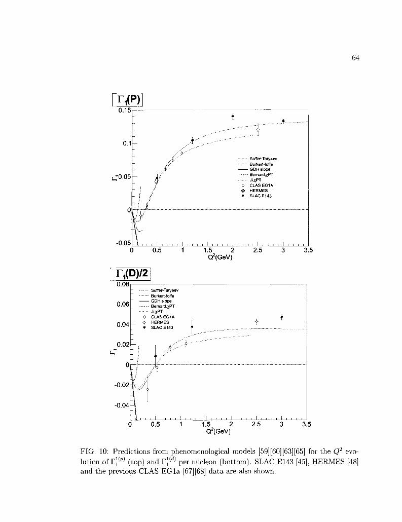
64
r,(P) 0.15
0.1
ro.os
-0.05
-
•i ~i
\
§
• > • •
i
> ' ' " ' . ' . ' - • •
*
, , , i
: I
I !
0*»
I
{
Soffer-Taryaev Burkert-lofle GDH slope Bernard.xPT Ji.XPT CLAS EG1A HERMES SLACE143
, , ! , ! , , I , , , ,
0-?
0.5 1.5 2.5 CT(GeV)
r,(D)i2 0.08
0.06
0.04
0.02
0
-0.02
-0.04
- Soffer-Taryaev Burkert-loffe GDH slope Bernard.xPT
........ J i i XpT
0 CLAS EG1A * HERMES ¥ SLAC E143
#
::•.•• 6
0.5 1 1.5 2.5 CT(GeV)
3.5
3.5
FIG. 10: Predictions from phenomenological models [59] [60] [63] [65] for the Q2 evolution of T\{p) (top) and r j ( d ) per nucleon (bottom). SLAC E143 [45], HERMES [48] and the previous CLAS EG la [67] [68] data are also shown.

65
L = 2 D state
s ,= i
FIG. 11: Deuteron spin states as a combination of the proton and neutron spins. Two possible angular momentum states are shown: L = 0 (S-state) and L = 1 (D-state).
is an isospin singlet state (antisymmetric under the exchange of the proton and
the neutron). Apart from their isospin, the two nucleons have also their spins and
spatial distributions (locations). The symmetry for the exchange of the locations
of the member nucleons is called parity, often denoted by P. If the exchange is
symmetric, the parity is said to be even or positive. If it is antisymmetric, the parity
is odd or negative. The parity is determined by the total orbital angular momentum
L of the two nucleons by P = (—1)L. Being an isospin singlet state, the deuteron
must be symmetric under the double exchange of the spins and the locations of the
member nucleons. Therefore, the deuteron can either be in a symmetric spin and even
parity or an antisymmetric spin and odd parity states. The former case forms a spin
triplet state with total spin S = 1. The even parity requires the total orbital angular
momentum L = 0 , 2 , . . . The ground state prefers the lowest possible orbital angular
momentum. The latter case forms a spin singlet state with total spin 5 = 0. However,
the spin singlet state does not lead to a bound state for the deuteron. Somehow,
the nuclear force prefers the spin triplet state while the singlet state is just (barely)
unbound. Therefore, at first approximation, the deuteron ground state has S = 1,
L = 0 (even parity), which means the total angular momentum J = 1. This is called
the S-state of the deuteron. However, the L — 2 state is also possible, which is called
the D-state. Indeed, the sum of the magnetic moments for the member nucleons,

66
//(proton) + /i(neutron) = 0.8797, is slightly different than the precisely measured
magnetic moment of the deuteron, /z(deuteron) = 0.8574. This deviation indicates
that the higher orbital angular momentum states are contributing to the deuteron
wave function. The deuteron also has a non-zero electric quadrupole moment, which
means the electric charge inside the deuteron is not spherically distributed. That is
another indication that the deuteron is not a simple spherically symmetric S-state
with L = 0 but it is a mixture of the S and D states. The S-state can be written as:
| J = 1, Jz = 1) = \L = 0, Lz = 0) |5 = 1, Sz = 1). (200)
Therefore, the spins of the proton and the neutron are both aligned with the spin
of the deuteron. In the D-state, however, the z projection of the nucleon spins is
not always aligned with the total angular momentum. Both nucleons can have their
spins oriented in opposite direction to the spin of the deuteron (see Fig. 11) . The
D-state is written as:
\J = 1,JZ = 1) = ^ \ L = 2,LZ = 0)\S = 1,SZ = 1)
^\L = 2,LZ = 1)\S=1,SZ = 0) (201)
+ ^ \L = 2,LZ = 2)\S = 1,SZ = -1).
The probability of finding the deuteron in the D-state is W£> « 0.056. Therefore, the
likelihood of finding a nucleon with spin down is \WD (see Fig. 11). If we ignore
nuclear effects, which will be explained later, the following relations between the
deuteron and nucleon cross sections can be derived:
= [1- -^DJ < + -wDa^ (202)
a\] = (l - - ^ a%, +\wDa^ (203)
where the first arrow indicates the electron beam helicity while the second arrow is
the spin direction of the target with respect to the electron. If we normalize the
deuteron cross section ad as "per nucleon", the nucleon cross section above is given
by <7/v = (<7p + crn)/2. By substituting these into Eq. (62), we obtain,
A\=[l-\wD 'alAl + alAJ
(204)
67
By using Eqs. (52 - 53), the cross sections can be replaced by the structure functions
so that <?i can be written as
^ , Q ^ ( i - ^ P ) [ ^ - Q i ) ; ^ - 9 2 )
where the factor 1/2 is introduced by convention because the deuteron structure
functions are typically given "per nucleon". The correction factor represents the ratio
of the polarization PN of the member nucleon to the polarization of the deuteron,
PD [69] (see Eqs. (202 - 203)).
II.5.1 Extraction of Neutron Information from A Deuteron Target
One of our purposes is to extract neutron information from the deuteron and proton
data. In order to extract the nucleon structure function from a measurement on a
nucleus, we need to understand the effects of the nuclear medium on the nucleon
structure. Once we understand these effects, we can make the necessary corrections
on the deuteron structure function and extract the neutron information by using
deuteron and proton data. Moreover, by comparing our results to the available
neutron data from 3He targets [70], for example, we can justify our understanding
of the nuclear medium and its effects on the nucleon structure. The EGlb data
will make an important contribution to the neutron spin structure and reduce the
uncertainties substantially over a good kinematic range of x and Q2.
In the resonance region, for spin structure functions, the most important nuclear
effects are considered to be the Fermi motion and the depolarizing effect of the D-
wave [71]. The correction for the depolarizing effect of the D-wave is described in
the previous section in Eqs. (204) and (205). Although this is the most important
correction for x < 0.7, the additional corrections are required, especially for larger
x [72], the most important of which being the Fermi motion. There are additional
effects such as off-shell mass effect and the EMC effect that should be considered.
However, those are found to be relatively small corrections [71]. In the following
sections, we summarize the corrections required to extract neutron information from
deuteron and proton data.
Fermi Motion
Bound nucleons are moving inside the nucleus, causing kinematic shifts and Doppler
broadening of peaks in the cross section. If we assume that the proton and neutron
(205)
68
spin structure functions have similar behavior in the resonance region, the positions
of the nucleon resonances should be the same for both nucleons. However, in case
of the deuteron, the resonance peaks may be smeared and shifted because of the
Fermi motion of the nucleons. If one tries to extract the neutron structure functions
by subtracting the proton from the deuteron, the maximum of the proton structure
function may become the minimum of the neutron structure function. This turns
the Fermi smearing into an important effect to consider while extracting neutron
information from the deuteron and proton data.
Recently it was suggested by [73] that a convolution method can be used itera-
tively to take these effects into account and extract the neutron structure functions
from nuclear data. The method uses convoluted proton and neutron structure func
tions (SFs) to model the deuteron and relies on the knowledge of the proton and
deuteron to iteratively extract the neutron SFs. A predefined input function for
the neutron is evolved iteratively until the function becomes stable. Currently, the
convolution only corrects for the Fermi motion and the D-state of the deuteron and
disregards other nuclear effects. Still, the method is suitable to incorporate other
corrections as they are modeled. It has been successfully tried on the unpolarized
structure functions. However, the convolution method is only well proven for func
tions with no sign change. On the other hand, the spin structure function gi has
several sign changes in the resonance region. This causes the iterative method to fail
in some kinematic regions. This mainly happens if one uses data with errors for the
proton and deuteron. Using parameterizations of the structure functions, instead,
makes the method more reliable. The results of the EG lb experiment, with both the
proton and the deuteron data, provides a perfect environment to test this method.
More information on this together with parameterizations of the world asymmetry
data are given in chapter VI.
Off-Mass Shell Effects
The deuteron is made up of a proton and a neutron. But because of the negative
contribution coming from the binding energy to the overall mass of deuterium, M^ =
Mp + Mn — 2.2 MeV, both nucleons cannot be on the mass shell at the same time.
Moreover, the nucleons will also have relativistic motion and their total energy should
be calculated by y/M£ + p2 + \JM% + p2n ^> M^, therefore, the mass of a bound
nucleon is much smaller than that of a free one in this picture. Various corrections

69
for this off-shell effect have been proposed.
EMC Effect
This effect can be summarized as the observed dependence of the cross section per
nucleon on the nuclear medium. It was first observed by the EMC Collaboration
[42]. It is due to the distortion of the free-nucleon structure function by the nuclear
medium. The effect has a strong kinematical dependence being most pronounced
at large x > 0.5. However, currently we don't have a reliable model of the EMC
effect in the deuteron, thus, this effect is not included into our method to extract
the neutron SF from the deuteron data. More information on the EMC effect can be
found in [6] [74] [75].
Effects of non-nucleonic states
Effects of nucleonic resonance states and pions (meson exchange currents) as part
of the structure of the deuteron should also be considered. According to the six
quark bag model of the deuteron, one should include direct correlations between
quarks and gluons in the proton and neutron. Finally, one could consider nuclear
shadowing, which is re-scattering of the lepton from both nucleons in the deuteron or
from the meson cloud within the nucleus. However, there is no universally accepted
quantitative model for the deuteron which corrects for these effects.
II. 6 S U M M A R Y
We described the theoretical background and purpose of the EGlb experiment. Since
the " spin crisis", many experimental data have been collected to explain the spin of
the nucleon. More data are still needed to understand the full picture. The EGlb
experiment covered a very important kinematic range that has not been explored
by previous experiments. The data generated by the experiment will help to put
further constraints on the contribution of different quark flavors to the total spin of
the nucleon. EGlb is one of the very few experiments with high statistics and very
large kinematic coverage. The data will map the dependence of the spin structure
functions on the four-momentum transferred and the momentum fraction carried by
the struck quark. Moreover, the results will provide new information on resonance

70
excitations, duality, higher twist coefficients and the approach to Q2 = 0, especially
for the neutron.
The analysis presented in this thesis is mainly focused on the deuteron data for
all beam energies. The proton data are also analyzed in parallel with the deuteron
data. The combined analysis will utilize the large statistics of the experiment at full
extend. This will be very useful to extract the neutron information by using the
fact that a deuteron is a bound state of a proton and a neutron. Since they have
no electric charge, manipulating and polarizing free neutrons is very difficult with
the technology at hand. Moreover, a neutron is radioactive and decays into a proton
when it is not in a bound state. As a result, we have a very limited information on the
neutron spin structure. The EG lb experiment will be one of the major contributers
to the scientific information on the spin structure function of the neutron.

71
CHAPTER III
EXPERIMENTAL SETUP
III. l C O N T I N U O U S ELECTRON B E A M ACCELERATOR FACILITY
The EG lb experiment has been carried out using the electron beam provided by the
Continuous Electron Beam Accelerator Facility (CEBAF) at the Thomas Jefferson
National Accelerator Facility (TJNAF). A schematic of the machine is shown in Fig.
12. CEBAF is composed of two linear accelerators joined by two 180° arcs with a
radius of 80 meters. Each recirculating arc is composed of five separate beam line
sections. There is also a 45 MeV injector delivering polarized electrons obtained
from a strained GaAs photocathode source by inducing excitations using a circularly
polarized laser beam. Another component that should be mentioned at this point
is the half wave plate (HWP) that can be inserted in the laser beam to change the
polarization phase of the produced electron beam by 180°. The status of the HWP
(in or out) was changed periodically during the experiment to make sure no polarity
dependent bias was created on the asymmetry. If the HWP is in, the beam helicity
requires an extra negative sign.
The accelerator is based on 338 superconducting radio-frequency (SRF) cavities
that boost the beam with radio-frequency waves. Eight SRF cavities are grouped
together to make a cryomodule. In each linear accelerator, there are twenty cry-
omodules. In order to maintain the superconductivity, all cryomodules are cooled to
2 Kelvin by liquid helium, produced at the Lab's Central Helium Liquefier.
The beam has a 1.497 GHz micro bunch structure. Connected by two recirculating
arcs, the two parallel linacs can accelerate the beam up to five times boosting the
beam energy up to 1.2 GeV for each turn. The accelerator can provide a high
luminosity continuous electron beam with energies ranging between 800 MeV and
5.8 GeV. There are quadrupole and dipole magnets in the tunnel to steer and focus
the beam as it passes through each arc. More than 2,200 magnets are necessary to
keep the beam on a precise path and tightly focused. The energy spread of the beam
is around AE/E < 10"4.
CEBAF is designed to deliver polarized or unpolarized electron beam to three
experimental areas simultaneously. These experimental areas are called Hall—A,
B and C. Beam is directed into each experimental hall's transport channel using
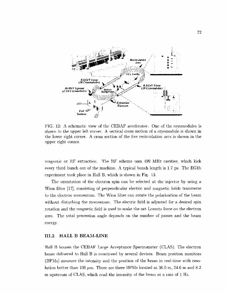
72
FIG. 12: A schematic view of the CEBAF accelerator. One of the cryomodules is shown in the upper left corner. A vertical cross section of a cryomodule is shown in the lower right corner. A cross section of the five recirculation arcs is shown in the upper right corner.
magnetic or RF extraction. The RF scheme uses 499 MHz cavities, which kick
every third bunch out of the machine. A typical bunch length is 1.7 ps. The EGlb
experiment took place in Hall B, which is shown in Fig. 13.
The orientation of the electron spin can be selected at the injector by using a
Wien filter [17], consisting of perpendicular electric and magnetic fields transverse
to the electron momentum. The Wien filter can rotate the polarization of the beam
without disturbing the momentum. The electric field is adjusted for a desired spin
rotation and the magnetic field is used to make the net Lorentz force on the electron
zero. The total precession angle depends on the number of passes and the beam
energy.
III.2 HALL B BEAM-LINE
Hall B houses the CEBAF Large Acceptance Spectrometer (CLAS). The electron
beam delivered to Hall B is monitored by several devices. Beam position monitors
(BPMs) measure the intensity and the position of the beam in real-time with reso
lution better than 100 /um. There are three BPMs located at 36.0 m, 24.6 m and 8.2
m upstream of CLAS, which read the intensity of the beam at a rate of 1 Hz.

73
FIG. 13: A schematic view of Hall B and the beam line monitoring devices: Beam position monitors (BPM), harps and the Moller polarimeter. The Faraday cup is also shown downstream. These components are explained throughout the text.
A "Harp" is located upstream from the center of the CLAS detector to measure
the beam profile. The Harp is a system of thin wires. The beam position in the
x and y direction is measured by moving the wires through the beam by using
stepper motors while no physics data are taken. Cerenkov light produced by scattered
electrons is measured in photomultiplier tubes to obtain x and y distributions of the
beam. The acceptable width of the beam distribution is typically less than 200 //m.
The EGlb experiment used longitudinally polarized beam. The polarization of
the beam was monitored by a Moller polarimeter at the entrance of Hall B. Separate
Moller runs had to be taken periodically in order to measure the beam polarization.
A typical Moller measurement carries a statistical uncertainty of about 1% and takes
around 30 minutes. Fig. 14 shows the diagram of the Moller polarimeter as viewed
from above. It consists of a target chamber, two quadrupole magnets and two de
tectors. The target chamber encapsulates a permendur foil (alloy of 49% cobalt,
49% iron and 2% vanadium), oriented at ± 20 degrees with respect to the beam
line and magnetized by a coil system. The two quadrupoles are used to separate the
scattered electrons from the unscattered beam. These electrons are later detected
and the number of coincidences for each helicity state are recorded to calculate the
asymmetry. The interaction between the electron beam and the polarized permendur

74
Low Energy: focusing High energy: defocusing
Target chamber
n - m - ---IB •••"
»»—70 cm-
-::i
Quadrupole
TOP VIEW always defocusing _,
Quadrupole
beam nine
_ v _ i \
^ Effective field reg
_ t_ _ 7
ion'
' - •
. , ueiecior particle
exit flange , , - [ " j | 5 * " «
/ 37.5 cnr C r ' . i l
- - NV-- 1 - - -) )—" '":'
* 15.6 cmf J ^ a a
h -* - 25 cm
FIG. 14: Top view schematic diagram of the Hall B Moller polarimeter [76].
target can be expressed in terms of the beam (Pb) and the target (Pf) polarizations
as [77]:
da
dn oc(l+ £ PfAvlA (206)
where, the parameters A^ are defined as:
_ A —A _
^T-22
sin4 6CM
(3 + cos2f5CM)2
(7 + cos2 9CM) sin2 0CM
A J « O
(3 + cos20C M)2
for i ^ j
(207)
(208)
(209)
The electron beam is in the z direction, 9 CM represents the scattering angle in the
center of mass frame. Therefore, knowing the differential cross section, the target po
larization and the scattering parameters, one can calculate the beam polarization. In
the EGlb experiment, the beam polarization was around 70%. Although the beam
polarization was monitored during the experiment, the results of Moller measure
ments were only used for a consistency check. In the EGlb experiment, the beam
times the target polarization is deduced from the elastic scattering events, which is
explained in section IV. 13.
At the very end of the beam line, the Faraday cup (FC) measures and records
the accumulated beam charge. This is used to determine the flux of the beam, which
is later used for normalization purposes while calculating the cross sections. The
Faraday cup signal is gated with respect to the beam helicity so that it is recorded

75
separately for each beam helicity (+ or —) and used to measure the beam charge
asymmetry defined by, f?C+ — PC~
Abeam = F £ + + pQ- ' (2 1 0)
The FC is the final stop for the electron beam. It is made of 4 tons of lead and is
70 radiation lengths deep. During the experiment, the FC reading was halted when
the readout electronics were busy. This is known as the live-time gated FC. Ungated
FC readings, which measure the total accumulated beam charge, were also taken
for both helicities. By using the ungated FC readings, the beam charge asymmetry
was calculated for all data files and monitored for data quality (see section IV.5).
Another way of measuring the beam charge asymmetry is by using the readings from
the Synchrotron Light Monitor (SLM), which is located at the beam injector. SLM
ungated and live-time gated readings are also available in the EGlb data for each
beam helicity. Comparing the beam charge asymmetry at the SLM (at the start of
the beam) and the FC (at the stop of the beam) can be an interesting way of deducing
the beam quality. Fig. 15 shows the comparison of the beam charge asymmetry from
both sources.
III.3 CEBAF LARGE ACCEPTANCE SPECTROMETER
CLAS is a unique detector, with almost 47r coverage, that can be used to investigate
reaction mechanisms of electron scattering because it allows detection of almost all
charged particles as well as neutrons and photons emitted after the absorption of a
virtual photon during the scattering. Superconducting coils separate the detector
into six equivalent sectors.
Each sector in CLAS acts as an independent spectrometer. In each sector there
are three units of Drift Chamber (DC) assemblies to determine the trajectories and
momenta of charged particles, Cherenkov Counters (CC) for electron identification,
Scintillation Counters (SC) for time-of-flight (TOF) measurements, and an Electro
magnetic Shower Calorimeter (EC) to identify showering particles such as electrons
and photons and to detect neutral particles such as neutrons (see Fig. 16). Combi
nations of any of these detectors may be used to build a desired trigger configuration
for the reaction of interest. The polar angle coverage in CLAS varies from 8° to 140°
for the DC, 8° to 142° for the SC, and 8° to 45° for the CC and EC detectors. In
the following sections, brief descriptions will be given for each of these components
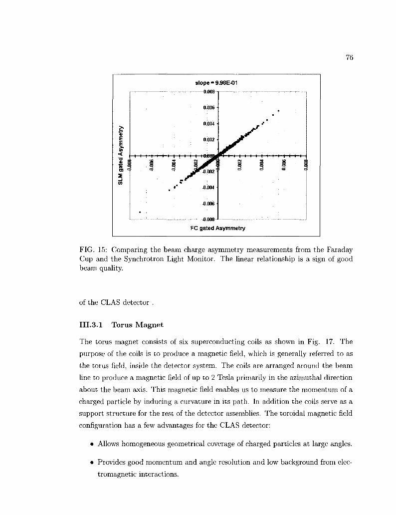
76
E E >. in < •a a •s
v>
slope = 9.98E-01
(hBBft-
0.006 4
i i i i i i i i i
I 41.004 J
4.006
-OvOOB-
1—!—!—I—I—t—t—l—l—(—•—t-
FC gated Asymmetry
FIG. 15: Comparing the beam charge asymmetry measurements from the Faraday Cup and the Synchrotron Light Monitor. The linear relationship is a sign of good beam quality.
of the CLAS detector .
III.3.1 Torus Magnet
The torus magnet consists of six superconducting coils as shown in Fig. 17. The
purpose of the coils is to produce a magnetic field, which is generally referred to as
the torus field, inside the detector system. The coils are arranged around the beam
line to produce a magnetic field of up to 2 Tesla primarily in the azimuthal direction
about the beam axis. This magnetic field enables us to measure the momentum of a
charged particle by inducing a curvature in its path. In addition the coils serve as a
support structure for the rest of the detector assemblies. The toroidal magnetic field
configuration has a few advantages for the CLAS detector:
• Allows homogeneous geometrical coverage of charged particles at large angles.
• Provides good momentum and angle resolution and low background from elec
tromagnetic interactions.

77
FIG. 16: Three dimensional view of CLAS. Three layers of DC are shown in purple, CC in dark blue, SC in red and EC in green.
• Leaves a field free region at the center of the detector around the target, which
is a very useful feature for implementing polarized targets there.
The direction of the beam line defines the z coordinate of the detector system.
Then the horizontal and vertical directions are the x and y coordinates respectively.
The polar angle 9 is the angle between a scattered particle and the z coordinate. The
azimuthal angle 0 is the angle of scattering projected on the x-y plane. The reference
angle for <f> is taken as the center of sector 1. Each coil consists of 4 layers of 54 turns of
aluminum-stabilized NbTi/Cu conductor. The coils are surrounded by cooling tubes
that constantly circulate liquid helium so that the coils are kept at superconducting
temperature of 4.5 K. The maximum design current of the coil is 3860 A, which
creates a magnetic field of 2.5 Tesla-meters integrated along the forward direction
and the field drops to 0.6 Tesla-meters at a polar angle of 90 degrees. Operation of
the torus, on the other hand, has been limited to 3375 A to avoid any failure. A

78
FIG. 17: Configuration of the torus coils is shown. This configuration effects the placement of the drift chambers creating three different regions.
contour plot .of the magnetic field of CLAS in the mid-plane between two coils is
shown in Fig. 18. The direction of the current can be changed in the coils, thus
creating different configurations for the magnetic field. In one configuration, called
inbending, the negative particles are curved toward the beam-line. In the outbending
configuration, negative particles are curved away from the beam-line.
III .3.2 Drift C h a m b e r s
In the EGlb experiment, the trajectories and momenta of the charged particles
are measured by the drift chambers (DC) [78]. A drift chamber is a detector for
particles of ionizing radiation. It operates on the principle that a charged particle
traveling through a carefully chosen gas will ionize surrounding atoms/molecules. If
one introduces wires with positive electric potential into such an environment, the
resulting electrons from ionization will be accelerated toward the nearest wires by
the electric field created between the wires. If the electric field is high enough, the
electrons will reach a point where they have enough kinetic energy to liberate other
electrons and ions in collisions with surrounding atoms/molecules in the gas. The
resulting cascade of ionization is eventually collected on the wire and creates a flow of
current. This current is later detected by electronic sensors. The location of the wire
gives an idea about the path of the ionizing particle. If one also precisely measures
the timing of the signal on the wire and takes into account that the electrons need

79
-300 -200 -tOO 0 100 200 300 400 cm
FIG. 18: A contour magnetic field of the CLAS torus magnet in the mid-plane between two coils.
some time to drift to the nearest wire, one can infer the distance at which the particle
passed the wire. This greatly increases the accuracy of the path reconstruction. The
electric signal passes through a preamplifier, an amplifier, a discriminator and 2:1
multiplexer and then starts a TDC. The TDCs are stopped by the event trigger.
More details on the DC and their calibration are given in section IV.2.2.
The CLAS has multi-layers of drift chamber assemblies in each sector that can
be grouped into three main regions. Region 1 is the closest one to the target and it
resides in a low magnetic field region inside the torus bore. It is used to determine
the initial direction of charged particle tracks. Region 2 is located between the coils,
where there is a high magnetic field up to 2 Tesla. Region 3 is the outermost layer,
located outside the coils (see Figs. 16 and 17).
Each region of drift chamber has two super-layers. In each super-layer, there
are 6 layers of hexagonal cells, except for the first super-layer of the region 1 drift
chamber, which has 4 layer of cells. Each hexagonal cell has six field wires at the
corners of the hexagon, which work as cathode. At the center, there is the sense wire
which is the anode (see Fig. 19). The hexagonal shape is the most cost-effective
shape to minimize the error in drift time to drift distance conversion. In each region
of drift chambers, there is one axial and one stereo super-layer. Axial wires follow
the direction of the torus magnetic field (perpendicular to the direction of the beam).
Stereo wires, on the other hand, are oriented at an angle of 6 degrees relative to the

80
FIG. 19: Cross-sectional picture of a drift chamber with two super-layers. The sense wires (anode) are located at the center of hexagonal cells created by the surrounding field wires (cathode). The arrow shows a charged particle passing through the drift chamber and the shadowed hexagons represent the cells that give a signal.
FIG. 20: CLAS drift chamber for one sector.
81
axial wires. This combination in each region allows one to determine the azimuthal
angle 0 of the particle. Fig. 20 shows a single sector drift chamber box in the shape
of an onion slice. Wires extend from end plate to end plate, on which the circuit
boards are mounted. The beam direction is also shown in the picture. The box is
filled with a gas mixture of 88% argon and 12% carbon dioxide. This mixure provides
a drift velocity of typically 4 cm/fisec. The radius of the hexagonal cells increases
semi-uniformly from region 1 to region 3. It is 0.7 cm in region 1, 1.5 cm in region
2 and 2 cm in region 3. Each of the sense wires, made from gold plated tungsten,
has a diameter of 20 /im, while the field wires, which are aluminium, are 140 /xm
in diameter. The drift chambers can detect charged particles with momenta greater
than 200 MeV/c over the polar angle range from 8° to 140° with a spatial resolution
of ~ 400 fim [79]. The resulting momentum resolution is ~ 0.5—1.5%. More about
the CLAS drift chambers will be explained in section IV.2.2.
III.3.3 Time of Flight System
In addition to the tracking information and momentum determined by the DC, we
also need to determine the velocity of the particle in order to find its mass. The
Time-of-Flight (TOF) system of CLAS is designed to precisely measure the time
of flight of charged particles [80], which allows us to determine the velocity of the
particle. Therefore, its mass, which explicitly identifies the particle, can be calculated
according to:
m = . (211)
The TOF detectors are made from scintillator material. In general, we can de
scribe a scintillator as a material that emits fluorescence photons when struck by a
high-energy charged particle. Scintillators have characteristic values for their light
output (absorbed energy vs. number of emitted photons) and decay times (how long
the photon emission lasts). The shorter the decay time of a scintillator, the less dead
time the detector will have, and therefore the more ionizing events per unit of time
it will be able to detect. Because of their relatively short decay time, scintillators
are used for high resolution timing information. Moreover, the light output enables
us to determine the amount of energy deposited into the scintillator, which later
becomes useful for particle identification. The fluorescence light emitted by the scin
tillator is collected by photomultiplier tubes (PMTs), which are extremely sensitive

82
FIG. 21: Time of flight scintillator counters for one of the sectors. It is built in 4 panels to accommodate the CLAS geometry.
light detectors. These detectors multiply the signal produced by incident light by
as much as 108. Therefore, even a single photon can be detected. Incident photons
induce emission of photo-electrons on the surface of the cathode of the tube, which is
coated with a material that has a low work function. Emitted photo-electrons from
the photo cathode are directed toward an electron multiplier. In the electron mul
tiplier, electrons are multiplied by the process of secondary emission. Basically, the
multiplier consists of several electrodes with increasing positive voltage. Each time
an electron hits the electrode, more electrons are released and accelerated toward
the next electrode. This creates an avalanche effect and produces more electrons,
amplifying the signal. Then this signal is transferred to electronic circuits and can
be used as timing and trigger information. Their high frequency response makes
PMTs a natural choice for timing measurements.
The TOF counter unit for one sector includes 57 scintillator strips (BC-408)
mounted as four panels combined together (see Fig. 21). The width and length of
the scintillators vary according to their location. Forward angle scintillators, which
cover up to 45 degrees, are 15 cm wide while the rest are 22 cm. The length of the
strips vary from 30 to 450 cm. All scintillator strips have a thickness of 5.08 cm.
They are perpendicular to the beam direction with angular coverage of 2 degrees
each. They are positioned within a sector in such a way that particles will always
pass through the strips along the normal line. The total geometric coverage of a
TOF unit is 8 to 142 degrees of the polar angle and 100% of the azimuthal angle,
83
except the angles occupied by the torus coils.
The signals from the scintillators are collected in PMTs and transferred to time-to-
digital converters (TDC) and analog-to-digital converters (ADC) to convert the signal
into a digital information and stored. The TDC keeps track of timing information
while the ADC stores the amplitude of the signal, which is proportional to the energy
released by the incident particle. The last 18 scintillators in the back angles are
grouped into 9 pairs and each pair is connected to a single TDC and ADC channel
to reduce the number of converters used. Therefore 48 channels of scintillator strip
are being read out for each sector. The timing resolution of the scintillator counters
varies with the length and width of the strip. The CLAS TOF detector is designed
such that pions and kaons can be separated and identified up to 2 GeV/c. As a
result, the time resolution is « 120 ps for the forward counters, which are shorter,
and ~ 250 ps for polar angles above 90 degrees. The average time resolution is about
140 ps.
I I I .3 .4 Cherenkov Coun te r s
Between the Drift Chambers and the Time Of Flight Counters, a Cherenkov detector
is positioned within each sector. These detectors are called the Cherenkov counters
(CC). They are designed to discriminate between electrons and hadrons, specifically
negative pions [81]. The Cherenkov detector uses the fact that a charged particle
traveling through the medium with a speed exceeding the local phase velocity of light
in that medium emits electromagnetic radiation called Cherenkov light. This light is
emitted in a cone about the direction in which the particle is moving. In the Ring
Imaging Cherenkov detectors, the angle of the cone can be used as a direct measure
of the particle's velocity by utilizing the relation:
cosGc = — . (212) nv
In the EG lb experiment, however, the Cherenkov counters are used as a threshold
detector, which only tells if a particle is detected or not. The primary purpose of
the CC is to identify electrons and discriminate negative pions. Therefore, a medium
was chosen such that only electrons should be able to travel above the speed of light
in that medium. The velocity threshold for Cherenkov light emission is /3=l/n where
n is the refraction index of the medium. The Cherenkov material that was chosen
for this purpose is perfluorobutane C4F10, which has n=l.00153. That corresponds

84
FIG. 22: Array of CC optical modules in one sector.
to a threshold in energy of the particle:
E= m =J-^—m= 18.1m, (213) y/l^W \n-l
where m is a mass of the particle. This provides an acceptably high pion momentum
threshold (pn > 2.5 GeV/c).
The Cherenkov Counter of CLAS consists of six independent identical Cherenkov
optical units (one unit per sector). One of these units is shown in Fig. 22. One
Cherenkov unit contains 18 segments each covering a different region of polar angle.
The whole unit with 18 segments extends from 8° to 45° in the polar direction. Each
segment is divided into two optical modules along the symmetry plane of each sector.
These modules, which looks like wings, are named left and right modules. Therefore,
each Cherenkov unit in each sector consists of 36 optical modules (see Fig. 22). Each
optical module has three mirrors - elliptical, hyperbolic and cylindrical - to direct
the light into a light collecting Winston cone (see Fig. 23). One PMT is connected
to the end of each module. The mirrors are aligned to optimize the light collection
by the PMTs.
The amount of light collected in the PMTs is measured and stored for each par
ticle in the event. The Cherenkov counter is one of the detectors that is generally
used in the event trigger for electron scattering experiments with CLAS. Typically,
a Cherenkov threshold for the acceptance of the particle as an electron or not is

85
Cylindrical
Mirror Cylindrical
Minor
Electron Track
FIG. 23: A schematic of one optical segment of the CLAS Cherenkov detector. Cherenkov light is reflected from the hyperbolic and elliptical mirrors into the Winston Cone (WC), which is surrounded by a Magnetic Shield. The light is then collected by the Photomultiplier Tubes (PMTs).
determined later in the analysis software (see section IV.7.4). As mentioned above,
the Cherenkov counters are useful to discriminate pions from electrons up to the pion
momentum of 2.5 GeV/c. Pions that exceed this momentum can emit Cherenkov
radiation that is comparable to the radiation produced by the electrons. In order
to identify these more energetic pions, the other detectors are used. In addition, it
should be noted that pions below 2.5 GeV/c are also able to create some Cherenkov
radiation through primary and secondary ionization of atomic electrons in the gas
and surrounding environment. This, however, occurs for around 1% of the pions.
The electron efficiency within the fiducial acceptance of the CC from the measured
photo-electron yield exceeds 99% (see [81]). Outside of the fiducial region the effi
ciency drops rapidly and varies strongly. Therefore the non-fiducial region is usually
excluded from the data analysis. The limiting factor in the acceptance of CLAS mea
surements mainly comes from the Cherenkov Counter efficiency, which is discussed
extensively in section IV. 9.
I I I .3 .5 E lec t romagne t ic Ca lor imete r
The last component of the CLAS detector system is the Electromagnetic Calorime
ter (EC). A Calorimeter is a detector used to identify particles by measuring their
energy deposition in matter and determining the method of deposition. An incident
86
particle deposits energy in the absorber material of the calorimeter, which is gener
ally a high density material (with a high electric charge Z in its nucleus) like lead
or steel, and the deposited energy is measured by a collector material layered with
the absorber material1. The collector material is generally some kind of scintillator
material connected to photomultiplier tubes. Based on the pattern of energy deposi
tion, the calorimeters are used to distinguish between electrons and hadrons and to
detect neutral particles.
At energies up to a few MeV, the dominant interaction of photons with matter is
through Compton scattering and the photoelectric effect. Above the 10 MeV range,
pair-production becomes the dominant method of interaction for photons within
material with high—Z nuclei. Low energy electrons interact with matter by creating
excitations within atoms. High energy electrons, on the other hand, lose their energy
mostly by bremsstrahlung. The electron is deflected by the Coulomb field of the
nucleus, because it has a very small mass, and emits a photon. These high energy
photons interact with matter and create high energy electron-positron pairs. The
resulting electrons again create photons via bremsstrahlung. The sequence of these
processes result in an electromagnetic shower. The sequence continues until the e+e-
pairs are not energetic enough to produce bremsstrahlung radiation. The energy of
the shower is converted into light by the scintillator strips, which is finally collected
by PMTs.
On the other hand, massive particles, for example hadrons, have very small
bremsstrahlung cross-sections at energies at which CLAS operates. The main energy
loss mechanism for these particles is ionization. Ionization and radiation produce dif
ferent signals in the EC. The Coulomb field of an atom extends over regions far larger
in radius than the nucleus of the atom. As a result, the probability of an electron
being deflected by the Coulomb field of an atom is much larger than the probability
that a hadron creates ionization within an atom. Therefore, electromagnetic showers
begin within a much shorter distance into the calorimeter than the hadronic show
ers. Electrons deposit a constant fraction of their total energy mostly in the first
half of the EC. Energy deposition of hadrons, on the other hand, is independent of
beam energy and peaks around the minimum ionizing energy of the particle in that
material. In CLAS, the EC signal produced by electrons is much stronger than, and
1 There are also calorimeters made from one type of material, which is both high density and scintillating, such as lead-glass calorimeters.

87
Scintillator bars
I.ead sheets
Fiber Ught (>uideK (front)
Fiber Light Guides (rear)
FIG. 24: View of one of the six CLAS electromagnetic calorimeter modules.
distinguishable from, the signal produced by hadrons. Separating pions from elec
trons becomes particularly important when the pion momentum exceeds 2.5 GeV/c
because they too begin to create a signal in the CC. Hence, the EC becomes vital
to identify electrons correctly at high energies. For this reason, the EC is a part of
the trigger scheme of the CLAS detector. The Electromagnetic Calorimeter of CLAS
has the following basic functionalities [82]:
• Detection of electrons above 0.5 GeV.
• Detection of photons above 0.2 GeV.
• Reconstruction of 7r° nd r\ by measuring their 27 decays.
• Detection of neutrons and separation of neutrons from photons based on their
time-of-flight.
In the CLAS detector, there are 6 modules, one for each sector, of Electromagnetic
Calorimeters, which are commonly known as the Forward Angle Calorimeter (EC)
and cover polar angles from 8 to 45 degrees. There are also two extra modules in the
first and second sectors to cover angles from 50 to 75 degrees. These two are called
the Large Angle Calorimeter (LAC). Even if they are based on the same principles,
the design specifications of the EC and the LAC are slightly different from each
other. Here, only the design specifications of the EC are explained because the LAC
is not actively used in our experiment. However, full specifications for the LAC can
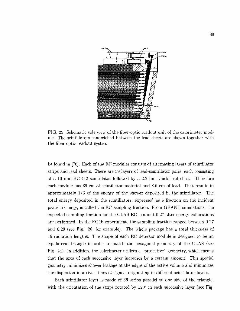
88
nwr-^ J-LO
FIG. 25: Schematic side view of the fiber-optic readout unit of the calorimeter module. The scintillators sandwiched between the lead sheets are shown together with the fiber optic readout system.
be found in [76]. Each of the EC modules consists of alternating layers of scintillator
strips and lead sheets. There are 39 layers of lead-scintillator pairs, each consisting
of a 10 mm BC-412 scintillator followed by a 2.2 mm thick lead sheet. Therefore
each module has 39 cm of scintillator material and 8.6 cm of lead. That results in
approximately 1/3 of the energy of the shower deposited in the scintillator. The
total energy deposited in the scintillators, expressed as a fraction on the incident
particle energy, is called the EC sampling fraction. From GEANT simulations, the
expected sampling fraction for the CLAS EC is about 0.27 after energy calibrations
are performed. In the EGlb experiment, the sampling fraction ranged between 0.27
and 0.29 (see Fig. 26, for example). The whole package has a total thickness of
16 radiation lengths. The shape of each EC detector module is designed to be an
equilateral triangle in order to match the hexagonal geometry of the CLAS (see
Fig. 24). In addition, the calorimeter utilizes a "projective" geometry, which means
that the area of each successive layer increases by a certain amount. This special
geometry minimizes shower leakage at the edges of the active volume and minimizes
the dispersion in arrival times of signals originating in different scintillator layers.
Each scintillator layer is made of 36 strips parallel to one side of the triangle,
with the orientation of the strips rotated by 120° in each successive layer (see Fig.
89
24). This creates three orientations or views, which are labeled as U, V and W.
Each of these specific orientations contain 13 layers of the 39 layers in one detector
module. This arrangement provides stereo information on the location of energy
deposition. The first 5 layers of each view, the first 15 layers of the module, are
grouped together to form an inner stack, referred to as the inner calorimeter. The
inner calorimeter has total of 36x3 strips. The remaining 8 layers are also grouped
to form an outer stack in the module, referred to as the outer calorimeter, which
also has total of 36x3 strips. This separation enhances longitudinal sampling of
the shower for improved hadron identification. Therefore, the whole module has
36(strips)x3(views)x2(stacks) = 216 strips. One PMT module is connected to each
strip via a fiber-optic light readout system that transmits the scintillator light to the
PMTs. Fig. 25 displays a schematic side view of the fiber-optic readout unit of the
calorimeter module. These fibers were bent in a controlled way to form semi-rigid
bundles originating at the ends of the scintillator strips and terminating at a plastic
mixing light-guide adapter coupled to a PMT.
The EC is the main detector to separate electrons from pions above 2.5 GeV/c.
The total energy deposited in the calorimeter is readily available at the trigger level to
reject minimum ionizing particles or to select a particular range of scattered electron
energy. Triggering on the correct particle is very important for timing information
of all particles detected. Pion events are largely suppressed by setting the EC total
energy threshold Etotai in the CLAS hardware trigger. From the detector performance
under running conditions, it is determined that the overall position resolution is
a = 2.3 cm. The time resolution is about r = 3 ns. Neutral hits, photon and neutron,
in the EC are determined by the absence of a corresponding DC track. The neutrons
and photons can further be discriminated by their time-of-flight information. The
7T° and rj are identified by requiring two neutral hits whose reconstructed energies
combine to the mass of n° or 77.
III.4 T H E T R I G G E R A N D T H E DATA ACQUISITION SYSTEM
The event trigger is formed by a combination of the signals from different components
of the CLAS detector. The CLAS detector has several trigger levels. For the EG lb
experiment, the level-1 trigger was used, which is based on a coincidence between the
EC and the CC detectors. The level-2 trigger also includes information from the DC
as well, but it was not used in the EGlb experiment. During the experiment, the

90
18000
16000
14000
12000
10000
8000
6000
4000
2000
FIG. 26: The plot shows the total energy deposited in the EC (inner and outer combined) divided by the momentum for the electrons. 29% of the energy deposited is observed by the scintillators of the EC. This quantity is usually called the EC sampling fraction.
thresholds of the detectors used for the trigger were adjusted to specifically accom
modate each beam/torus configuration. The signals from the detector subsystems
are sent to a pre-trigger logic module, where the bit patterns from the subsystems are
compared against patterns preloaded in memory tables. If the pre-trigger conditions
are satisfied, the signal is submitted to the level-1 trigger. If there is a trigger in the
event, the signal is passed to the Trigger Supervisor (TS), which communicates with
the Readout Controllers (ROCs). TS has 12 trigger inputs, 8 of which are used by
the level-1 trigger. It also has a level-2 trigger confirmation input so that the TS
can be configured only to require level-1 input or to require level-1 input and level-2
confirmation. Level-2 confirmation was not required in the EGlb experiment. If the
level-1 trigger is satisfied, then the data are read out, digitized and transferred to
the Event Builder (EB). Finally the Event Recorder (ER) receives the information
from the Event Builder through the Data Distribution (DD) shared memory. The
data are written to the disk and later transferred to the tape SILO for permanent
storage. The data flowchart of the CLAS DAQ system is shown in Fig. 27.
The DAQ system was initially designed for an event rate of 2 kHz. During the
EGlb experiment, the event rate was about 4 kHz and the data rate was 25 MB/s.
Nowadays, the DAQ can reach up to 5 kHz in event rate. The live time was about
90%. The DAQ system for CLAS uses software called CODA (CEBAF Online Data
Acquisition). CODA provides specific configurations of the DAQ components for
Entries 1001431 Mean 0.2877 RMS 0.03201
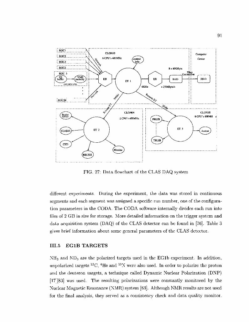
91
FIG. 27: Data flowchart of the CLAS DAQ system
different experiments. During the experiment, the data was stored in continuous
segments and each segment was assigned a specific run number, one of the configura
tion parameters in the CODA. The CODA software internally divides each run into
files of 2 GB in size for storage. More detailed information on the trigger system and
data acquisition system (DAQ) of the CLAS detector can be found in [76]. Table 3
gives brief information about some general parameters of the CLAS detector.
III.5 EG1B TARGETS
NH3 and ND3 are the polarized targets used in the EG lb experiment. In addition,
unpolarized targets 12C, 4He and 15N were also used. In order to polarize the proton
and the deuteron targets, a technique called Dynamic Nuclear Polarization (DNP)
[17] [83] was used. The resulting polarizations were constantly monitored by the
Nuclear Magnetic Resonance (NMR) system [83]. Although NMR results are not used
for the final analysis, they served as a consistency check and data quality monitor.

92
TABLE 3: Some useful CLAS Parameters
Capability
Coverage
Resolution
Particle ID
Luminosity
DAQ
Quantity polar angle momentum
momentum (9 < 30°) momentum (9 > 30°)
polar angle azimuthal angle
time 7r/K separation 7r/p separation electron beam
event rate data rate
Range 8° < 9 < 140°
p > 0.2 GeV/c ap/p ss 0.5% ap/p w 1-2% OQ ~ 1 mrad o$ RS 4 mrad
er4 « 100-250 ps p < 2 GeV/c
p < 3.5 GeV/c L « 1034 nucleon cm~2sec_1
4 kHz 25 MB/s
In this section, we will describe the target system of the EGlb experiment.
The EGlb targets are located on the symmetry axis of CLAS and are surrounded
by a pair of superconducting Helmholtz coils. The coils produce a 5 Tesla magnetic
field around the target cell. The magnet was kept at 4.2 K through a liquid Helium
reservoir located outside the CLAS. The target itself was kept at 1 K by a refrigeration
system. The target cells were attached to a target insert as shown in Fig. 28. Each
cell is 1 cm in length and 1.5 cm in diameter. The entrance window of each cell
is sealed by a thin aluminum foil of 71/im thickness (aluminum was chosen for its
strength) while the exit window is sealed by a thin kapton foil. A stepping motor
connected to the insert moves the insert in the vertical direction so that targets can be
switched mechanically. The ND3 and NH3 target cells are surrounded by NMR coils
for polarization measurements. Part of the target stick remained immersed in a mini-
cup filled by liquid Helium in order to keep the targets at low (1 K) temperature.
This was necessary to maintain the polarization of the target materials. Another
target insert very similar to the one shown in Fig. 28 was also used for 15N runs and
contained only two target cells, 12C and frozen 15N. 15NH3 and 15ND3 were chosen as polarized target materials in the EGlb experi
ment because of their high content of polarizable nucleons: 16.7% for the 15NH3 and
28.6% for the 15ND3. They also have high resistance to radiation damage. Moreover,

93
Electrical feed-thru (1 of 4)
Target cells
Vacuum flange
, ___ Gear head connection •* ^ X ^ to stepping motor
Vertical drive shaft
Brass heat sink
\ Horizontal ..--"' alignment pins
FIG. 28: A schematic of the target insert strip showing the four target cells used for the EGlb experiment: ND3, 12C, NH3 and Empty. NMR coils surround the ND3
and NH3 target cells.
it is easy to correct the measured asymmetry of the proton or the deuteron for the 15N polarization contribution. The spin of the 15N is carried by a single valence
proton and the required corrections to the measured asymmetries due to the 15N
polarization are well understood. More information about the target materials is
given in section IV. 11.

94
CHAPTER IV
DATA ANALYSIS
Handling data from complex experiments like EG lb requires certain precautions and
corrections. In this chapter, we are going to focus on the analysis techniques we used
to extract physics results from the EG lb data. The raw data from the experiment
includes a wide range of events representing many different physical processes. The
events relevant to a specific analysis goal must be determined. The data should be
calibrated and corrected according to the detector behavior and experimental con
ditions. We followed certain procedures to convert the raw data into descriptions of
physical properties that can be interpreted and compared to theoretical calculations.
The following list summarizes the most important procedures in a chronological or
der:
• Data calibration and reconstruction
• Creating Data Summary Tape (DST) files
• Helicity pairing
• Quality checks and data selection
• Particle identification
• Precision (geometric and timing) cuts
• Fiducial cuts
• Kinematic corrections
• Dilution factors
• Pion and pair symmetric background corrections
• Extraction of the beam x target polarization
• Polarized background correction
• Radiative corrections
• Combining data

95
• Models
• Systematic errors
• Extraction of the neutron structure functions from the combined proton and
deuteron data
Some of these procedures include many sub-steps. Throughout this chapter, we will
give detailed descriptions of these procedures and provide a layout for the analysis
of the EG lb data.
The double spin asymmetry A\\ is obtained from the measured experimental asym
metry Araw via,
4i = -r- {-FTT Cb^k ~ C2) + ARC (214)
JRC \^D^b^t J
where Pf,Pt is the product of beam and target polarizations, FQ is the dilution factor,
which accounts for the scattering from the unpolarized components of the target,
Cback represents the pion and pair symmetric background corrections, fnc and ARC
take care of the radiative effects while C\ and C2 corrects for the contributions from
the polarized background. The experimental asymmetry Araw is defined by:
Araw = ; T (215)
where n~ and n+ are determined by counting the inclusive scattering events for each
helicity state and normalizing with the accumulated (live-time gated) beam charge
(Ne) for that helicity state:
ATU + _ iVTT
W ; n ~N!
with arrows indicating the relative spin orientations of the electron and the target
nucleus (or nucleon). The quantity Araw is extracted for certain kinematic bins in
Q2 and W in the resonance region and above, for each beam energy and detector
setting separately.
I V . l EG1B R U N S
During the experiment, a longitudinally polarized electron beam of various energies
ranging from 1.6 GeV to 5.7 GeV was incident on longitudinally polarized proton
(NH3) and deuteron (ND3) targets. This ensures a good coverage of the entire reso
nance region and above: 1.08 GeV < W < 3.0 GeV; 0.05 GeV2 < Q2 < 5.0 GeV2.
n~ = —1T ; n + = — n (216)

96
In order to increase the kinematic coverage, the torus current was also switched be
tween inbending and outbending settings for some beam energies. In addition to the
NH3 and ND3 targets, data on the 12C target and the empty target (with only liquid
Helium) were also collected for each beam energy and torus setting. These runs were
used to estimate the unpolarized background contribution to the data. Occasional
runs were also taken on pure 15N target and used to monitor the effectiveness of the
background removal procedure using the 12C runs. Table 4 provides a simple sum
mary of all runs taken together with corresponding target, beam and torus settings.
Fig. 29 shows the kinematic coverage of the entire experiment. Coverage of different
beam energies are shown in different colors. Based on Table 4, we separated the
data into different configurations and analyzed each set separately. We analyzed 11
different data sets for both ND3 and NH3 targets, which are listed in Table 5. At the
end, the results from these sets were combined with specific guidelines.
TABLE 4: EGlb run sets by beam energy and torus current.
Run Numbers
25488-25559; 25669-26221 26222-26359 28512-28526
27644-27798; 28527-28532 27205-27351 28001-28069
27799-27924; 27942-27995 27936-27941
28074-28277; 28482-28494; 28506-28510 28280-28479; 28500-28505 27356-27364; 27386-27499
27366-27380 27069-27198 26874-27068
26468-26722; 26776-26851
Beam Energy(GeV)
1.606 1.606 1.723 1.723 2.286 2.561 2.561 2.792 4.238 4.238 5.615 5.615 5.725 5.725 5.743
Torus Current (A)
+ 1500 -1500 + 1500 -1500 +1500 +1500 -1500 -1500 +2250 -2250 +2250 -2250 +2250 -2250 -2250
IV.2 DATA R E C O N S T R U C T I O N A N D CALIBRATION
During the experiment, the data was stored in segments and each segment was as
signed a specific run number. The DAQ software internally divides each run into files

97
TABLE 5: Analyzed data sets by target, listing the beam energy EB and the torus current IT- Throughout each data set, there are also occasional 12C and empty target runs, used for background analysis.
ND3[£B(GeV), /T(A)]
1.606, +1500
1.606, -1500
1.723, -1500
2.561, +1500
2.561, -1500
4.238, +2250
4.238, -2250
5.615, +2250
5.725, +2250
5.725, -2250
5.743, -2250
NH3[£5(GeV), /r(A)]
1.606, +1500
1.606, -1500
1.723, -1500
2.386, +1500
2.561, -1500
4.238, +2250
4.238, -2250
5.615, +2250
5.725, +2250
5.725, -2250
5.743, -2250
FIG. 29: Kinematic coverage of the EG lb experiment for all beam energies. The solid and dotted lines mark the inelastic threshold at W = 1.08 GeV and the DIS threshold at W = 2.0 GeV, respectively.
98
of 2G B for storage. Each run took approximately 2 hours and consists of 20-30 files.
These files were stored on tapes for further processing. The data were written in a
special format based on the BOS bank system. The BOS banks are logical records
for the data file that consist of a four word header (1 word = 4 bytes) followed by
various data words. This system allows programs reading the tapes to skip unknown
or uninteresting headers altogether. The format also provides a robust error han
dling system. If the reading software encounters faulty parts in the file, it can parse
the file for the next valid BOS header and continue reading. Information in the raw
data files consist of TDC and ADC values from detector components as well as beam
related information. The next step is data reconstruction. During the reconstruction
process, the simple event builder (SEB) [84] is used. The SEB incorporates geometric
parameters and calibration constants for the CLAS detector and converts the raw
data into physics quantities like particle IDs, positions, energies and momenta, etc.
The standard package for the reconstruction of the CLAS data is called REC-
SIS, which communicates via log messages that appear both on the screen and in a
log file. RECSIS executes a set of programs called ana and user-ana, FORTRAN
based reconstruction software for the CLAS detector. The libraries for this soft
ware can be checked out from CVS repository and executables can be created from
the libraries. One also needs to set environmental parameters to choose a specific
calibration database for the experiment as well as to set other CLAS parameters.
The user-ana program is configured by using a tcl script, i.e., rec-eglsql.tcl. The tcl
script sets the names for input and output files, torus magnet current values and the
number of events to process for each file. It basically determines a small subset of a
large number of run control parameters required for the process of reconstruction. It
also manages which BOS banks should be used for the output file so that one would
be able to choose only the interesting BOS banks for the analysis. Once everything
is set, the reconstruction can be initiated by using a command line: user-ana -t
rec-eglsql.tcl, which reconstructs a specified raw data file in the tcl script for the
specified BOS banks.
There are more than 40,000 files in the EG lb experiment. The reconstruc
tion procedure is semi-automated by using other sets of scripts, run-a-run.pl and
run-a-file.pl. The template form of these scripts can be found under jlab cue
"/u/home/clasegl/eglb/scripts/". They must be modified for each data set with
different beam energy and torus current. These scripts launch the reconstruction of

99
each file as a batch job to make use of the computing power of the Jefferson Lab
batch farm [85].
IV.2.1 Event reconstruction
Event reconstruction consists of identification of particles in the event together with
calculation of their momenta in the CLAS coordinate system. In this coordinate sys
tem, the z-component points along the beam axis while the x and y-components are
in the horizontal and vertical directions, respectively. Charged particles are expected
to give signals in all detector components while neutral particles give signals only
in the Scintillator Counter (SC) and the Electromagnetic Calorimeter (EC). Tracks
are reconstructed in a two-step process. Hit-based tracking is used for preliminary
identification. After the trigger start time is determined, calibrations on the DC are
performed to establish time-based tracking, which is explained in the last part of
section IV.2.2.
Charged particles
Track reconstruction begins by identifying hit-based tracks in the DC. In this stage,
only the sense wires at the center of each DC cell that had a signal are used to
create a preliminary trajectory for the particle. The momentum and the charge of
the particle is determined from the curvature of the trajectory obtained from the
DC. This is called hit-based tracking, which provides a preliminary production angle
and momentum for the particle. The code cycles through each particle in the event
to verify coinciding signals in the CC and EC for electron identification. The signals
must agree with the trajectory of the particle within the time of flight window. If all
signals register for a negative charged particle, the particle is accepted as an electron
candidate. If there are more than one electron candidates, the one with the highest
momentum is selected as an electron.
After the electron is identified, its time of flight information is obtained from the
SC signal. Then, the trigger start time can be determined by tracing the electron
back to the vertex along its geometrical path and assuming the electron travels with
the speed of light. In case there is no negative particle track in the event, the
positive particle with the highest momentum is used to establish the start time.
This is generally a positron that comes from pair production.1 The reconstruction
1Positive trigger events are only used for pair symmetric contamination analysis.

100
of the start time requires calibration of the SC for time delays and synchronization
of individual scintillators. These calibrations are described in section IV.2.2 in more
detail.
Once the start time is established from the trigger particle, usually an electron,
the time of flight for the other particles in the event can be determined from their
signals in the SC by subtracting the start time. If the SC signal is not available for
a particle, the EC signal is used instead. Then, the velocity of the particles in the
event, other than the electron, can be calculated by using their path lengths from
the vertex to the hit location in the SC. The mass of the particle is calculated from
its velocity and momentum by m = p//3j.2
Neutral particles
Neutral particles are identified by energy clusters in the EC that do not match any of
the tracks. The photons create electromagnetic showers and deposit all their energy
in the EC. The signal amplitude from the EC ADC is used to calculate the energy
of the photons. Neutrons may deposit energy in the EC, mostly by proton recoil
followed by ionization. The energy deposition clusters from neutrons usually appear
in the outer parts of the EC. Neutrons can be identified from a hit in the calorimeter
that does not satisfy any of the requirements for a charged particle. Neutrons are
distinguished from photons by their time of flight to the EC. Neutral particles are not
affected by the toroidal magnetic field, so they follow a straight path to the location
they are first observed. The angle of their trajectory is determined from the position
of the energy cluster at the surface of the calorimeter. Particles like ir° and r] mesons
can be identified from their decay products [82]. A ir° decays into two photons with
98.8% probability while r\ mesons have additional decay channels. Neverthless, by
applying kinematic requirements to the decay products, one can establish a missing
mass spectrum and identify some of these neutral mesons.
IV.2.2 Calibrations
For the correct reconstruction of the events in the detector, the response of each
detector component should be parametrized according to experimental conditions.
This procedure is called calibration. The reconstruction and calibration procedures
2Natural units with c = 1 were chosen.

101
go together in an iterative manner. During the data acquisition, once a trigger is
detected, the TDCs in each detector component start measuring the time until a sig
nal is received to stop them, at which point the data is recorded. Calibration of the
detectors is required to synchronize their timing with the beam radio frequency (RF)
time. An energy calibration is also required for the EC. The calibration procedure
produces certain parameters, ADC and TDC offsets, for different detector compo
nents. These parameters are often referenced as calibration constants. Afterward,
these constants are written into the CLAS calibration database [86] allocated to the
EG lb experiment. The reconstruction code reads this database and reconfigures
the response of the detector components to each event according to the parameters
provided.
Time of flight calibration and reconstruction of the start time
The time of flight information is obtained from the SC with 48 paddles for each sector
and two PMTs on each paddle. During the reconstruction, TDC and ADC values
from the PMTs are converted into time and energy. The leading edge discriminator
registers the signal pulse when the amplitude passes a certain threshold. However,
the timing of this threshold depends on the amplitude of the pulse, which affects
the steepness of the rising edge of the pulse. This creates a dependence of the TDC
signal on the ADC amplitude, a known phenomena called time-walk. The PMTs
are calibrated to take the time-walk corrections into account. The ADC vs. TDC
(pulse height vs. time) signal is fitted for each PMT and the time-walk correction
parameters are obtained to calibrate the PMTs.
Each scintillator paddle has two PMTs attached, one at either end, referred to
as the left (L) and right (R) PMTs. The signal generated at any location in the
scintillator paddle takes different times, t^ and £R, to travel to each of these PMTs.
The crucial point is that for a signal generated at the center of the paddle, ti, = tR
must always be true. For some paddles, this requirement necessitates the introduction
of a left-right calibration offset. The offset is determined by using cosmic ray runs or
data runs. More information about these calibrations can be found in [87] and [88].
After the above calibrations are performed on the SC, the trigger start time can
be calculated by using,
tstart = tsc 7T~, (217)
pc
where tsc is the time recorded at the SC when an electron is registered. (3 = 1 for
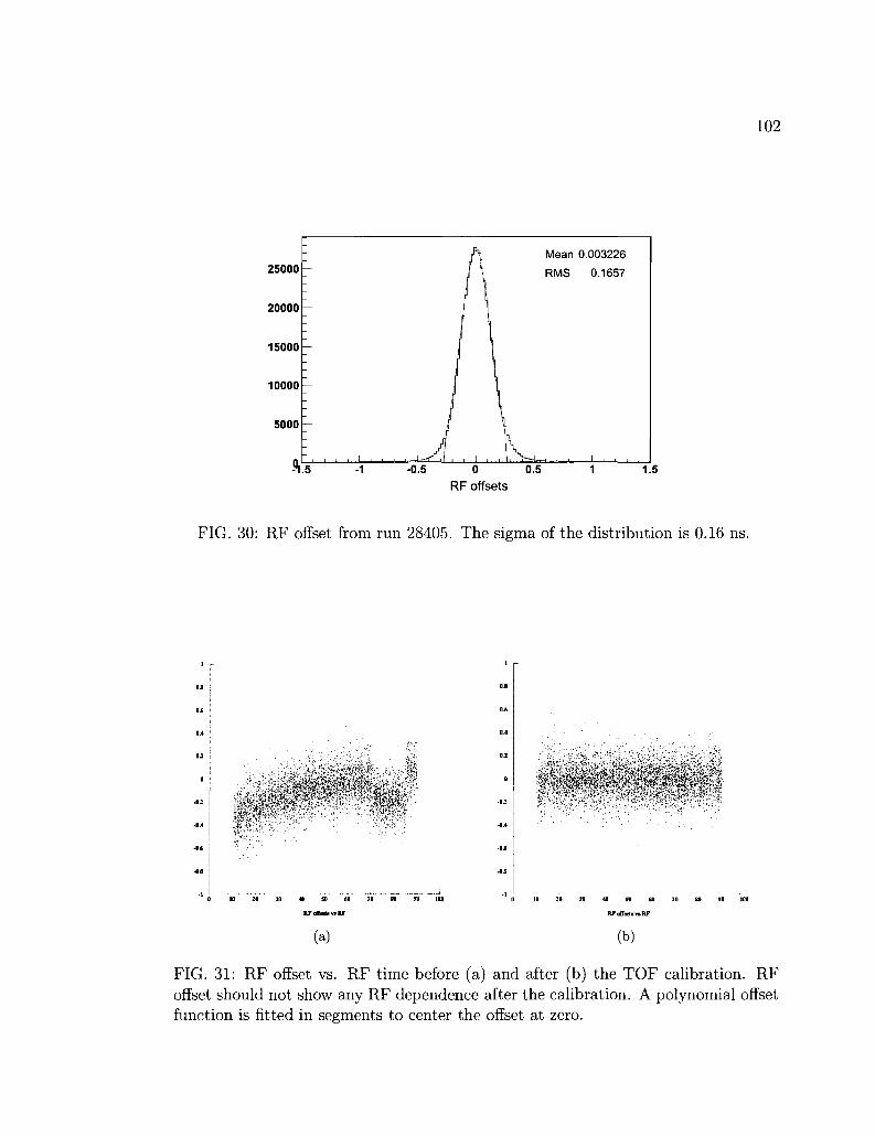
102
25000
20000
15000
10000
5000
X
Mean 0.003226
RMS 0.1657
-0.5 0 0.5 RF offsets
1.5
FIG. 30: RF offset from run 28405. The sigma of the distribution is 0.16 ns.
*-,*VJ4
mm mm.
0 10 20 30 4 * 60 ?• SO TO 100
RI-ttfsdsvsRF
(a)
10 2 1 3S SB U 70 SO
RFcfiadsvsRF
(b)
FIG. 31: RF offset vs. RF time before (a) and after (b) the TOF calibration. RF offset should not show any RF dependence after the calibration. A polynomial offset function is fitted in segments to center the offset at zero.

103
the electrons and lpath is the path length obtained by tracing the electron back to
the vertex along its track. As shown in Fig. 30, the reconstructed start time shows a
Gaussian distribution around the RF time provided by the accelerator. The electron
beam is delivered to the experimental hall in bunches with a 499 MHz frequency.
The bunch period is At = 2.0039 ns. Ideally, the reconstructed start time should
coincide with the arrival of one of the bunches. However, the finite resolution of
the reconstructed start time creates a Gaussian distribution centered around the RF
time (see Fig. 30). The width of the distribution corresponds to the time resolution,
which is generally around 0.16 - 0.20 ns. If the mean of the start time distribution
is different than the RF time of the beam, the start time should be corrected for the
offset,
tRFoff — tstart ~ t-RF- (218)
The start time with the RF correction, therefore, is written as,
tstart = tsc 7j h tRFoff. (219)
The phase of the RF signal may sometimes change after a long run period. Therefore,
each run period might require a calibration of the RF offset. Normally, the RF offset
distribution vs. RF time should not show any dependence on the RF time. If it is
not the case, the RF offset is fitted by a third degree polynomial in four different
regions of the RF time. The resulting parameters readjust the RF offset distribution
to make it independent of the RF time in all regions. These parameters are written
into the calibration database and applied to the other runs within the same run
period. Fig. 31 shows the RF offset vs. RF time before and after the RF calibration.
In some part of the EG lb experiment, however, the RF signal was not available and
this calibration was not performed.
The final step is a paddle to paddle delay calibration of all SC units. The idea
is to synchronize the timing of all scintillators to the same RF signal so that they
behave as a coherent unit. The paddle to paddle delay effects show themselves in the
reconstructed time of flight (TOF) mass of the secondary particles plotted against
the paddle ID. In addition, if certain paddles have their timing off with respect to
the others, expected minus measured TOF of the secondary particles, which should
be around zero, is disturbed for those paddles. TOF Mass vs. paddle ID and At
vs. paddle ID plots are monitored during the calibration to make sure there are no
bad paddles which give a wrong mass or TOF information for protons and pions.

104
-
-
- J]
LJ. { _ ^ 0 0.5 1 1.5 2 2.5 3 3.5 4
TOF mass
FIG. 32: TOF mass spectrum for secondary particles for an EGlb data run. Mass is given in GeV. The pion and proton peaks are clearly visible. The deuteron peak can also be resolved at 1.876 GeV.
In case there is no RF signal available from the accelerator, the reconstructed start
time is used as a reference to determine the TOF information for the secondary
particles. Fig. 32 shows the reconstructed time of flight mass spectrum after proper
calibrations are made.
Electromagnetic calorimeter calibration
Once the SC calibrations are done, the EC timing signal is calibrated to the SC
signal. The average difference between the EC and SC timing is minimized by using
a 5-parameter fit. A sample plot of the overall time resolution is shown in Fig. 33.
In addition, the PMTs in the EC require calibration of the ADC pedestals [82] [89].
The EC sampling fraction, the energy from the electromagnetic shower detected by
the scintillator material in the EC and divided by the energy of the incident particle,
should normally be a distribution around 0.27-0.29 with a ~ 0.03. This quantity is
monitored during the calibration procedure. File to file variation of the EC sampling
fraction should be minimal for the same run period if the calibration is successful.

105
S1 ECt-SCt, electrons
FIG. 33: Difference between EC and SC times (in ns) for reconstructed electron events after EC timing calibrations. The plot is from run 28079 sector 1.
Drift chamber calibration
Initially, the track reconstruction is performed by using only the location of the
sense wires in the DC (hit-based tracking). If one precisely measures the timing of the
current pulses of the wire and takes into account that the induced ions/electrons need
some time to drift to the nearest wire, one can infer the distance at which the particle
passed the wire. This greatly increases the accuracy of the path reconstruction.
Therefore, after the start time is determined, a more accurate path for the particle
can be calculated by taking the drift time in each DC cell into account. The drift
time is converted to the drift distance, which is called the distance of closest approach
(DOCA). By using the calculated DOCA, a more accurate track of the particle is
obtained as shown in Fig. 34. This is called time-based tracking (TBT) [76] [78] [90].
During the DC calibration, first the drift time, thrift, needs to to be determined,
tdrift — tstart + tcable + ^TDC — t flight ~~ t; prop ''walk} (220)
where tstart is the event start time, tcab\e is the time-delay from the cable, tTDC is the
time measured by the TDC, tfught is the flight time of the particle from the event
vertex to the sense wire and twaik is the time-walk correction (see section IV.2.2).
The next step is to parametrize the drift distance as a function of the drift time.

106
This parametrization may have different forms for different drift chamber regions.
For example, the Region 3, was parametrized by the following functional form [78],
v x(param) = v0t + r\ I 1 + K I I , (221)
J V ''max
where v0 is the drift velocity (at t = 0), t = thrift, tmax is the maximum drift time for
the ions created at the edge of the drift cell and r], K, p and q are the fit parameters.
Then the parametrized DOCA, x(param), is used to minimize the difference
E \Xi{param) - Xj{trial)\'
where x^trial) is the DOCA from a global trial track, often referred as fitted DOCA,
including all superlayers and initially obtained from the hit based track (HBT),
and Giitrial) is the corresponding error for the fitted DOCA. The parameters are
determined for each superlayer for a best fit to a global track with all superlayers.
The difference between the calculated DOCA and the fitted DOCA is called the
residual and should be around zero after going from HBT to TBT. This quantity is
monitored separately for each superlayer and sector to ensure the quality of the DC
calibration. The residual for superlayer 3 for all sectors combined is shown in Fig.
35. The sigma of the residual is monitored for all files and kept around 0.05 to ensure
the quality of the DC calibration. It should never exceed 0.06 for any file.
The drift distance is the radial distance of the track from the wire but does
not predict which side of the wire the track is. This ambiguity is resolved by a
separate fit within each superlayer. A straight line fit is made to various choices
within each superlayer, trying all possible left-right combinations and selecting the
one with the highest probability. A more detailed explanation on the time based
track reconstruction can be found in [76].
Final comments on data reconstruction
The reconstruction code produces ntuple files and monitoring histograms as well
as BOS files. The monitoring histograms are used to determine the success of the
calibration procedure. The calibration is normally performed on a sample data set,
which is often referred to as the passO calibration. Sometimes a few iterations are
required to establish a good calibration. Then the calibration constants are applied
to the entire data set and the resulting monitoring histograms are investigated to

107
a' 'v~ 'v' 'v' 'd> \ T '
or- --«r' \ - *V ' '•r* v ' 1 "V" "w
9. ,0 ,
Particle Track
FIG. 34: A track through one DC superlayer showing the the calculated distance of closest approach (DOCA) for each sense wire. The accuracy of the particle track can be increased by using the DOCA, which is called time-based tracking [76] [90].
TBT residual SL3
Entries 1384297 Mean 0.003779 RMS 0.05745
0.05 0.1 0.15 0.2 0.25
FIG. 35: Residual average of the time based tracking (TBT) from run 28079 for superlayer 3, all sectors combined. The sigma of the residual is monitored for all files and kept around 0.05 to ensure the quality of the DC calibrations.
108
make sure that the calibration is successful on the entire set. The final stage is
referred to as the passl calibration. The data sets for different beam energy and
torus current configurations are calibrated independently.
Normally, the ntuple files produced by the reconstruction code are used for the
analysis of the data. Only the events that pass a set of basic criteria (e.g. one good
electron in the event) are written into these files in a simpler format, so, they are
already well compressed compared to the original BOS files. However, the EG lb
experiment was one of the largest experiments at the time with an unprecedented
amount of data. Limited disk space at the time of the experiment required further
compression of the data. This led to data summary tapes (DST).
IV.3 D S T FILES
The DST files reduced the amount of stored data for the analysis by changing the
data format. For the main analysis of the EG lb experiment, we used the DST files.
The ntuple files were briefly used for a few data sets for comparison purposes. Only
certain variables were written into the DST files with certain precision. Detailed
information on the variables and their precision in the DST files can be found in
Tables 55-60 under Appendix A.
After the reconstruction code created the calibrated data in BOS format [91],
another code called "HelP.cc" [92] was used to read the BOS files and create the
DST files. "HelP" was executed by a script called "makeDST.pl", which is lo
cated under the "/u/home/nguler/eglb/upg_egl_dst/HelP/" directory in the Jef
ferson Lab CUE3 system. Another program called "DSTMaker_byRun.pl",located
under "/u/home/nguler/eglb/upg_egl_dst/makeDST/", was written in order to
automate the DST file creation procedure. It automatically finds the files for
a specific beam energy and torus configuration, pulls them from the silo tapes,
checks if the file is copied fully without error4, executes "HelP" to create the
DST files and puts the created files back into the silo for storage. All the DST
files are stored under "/mss/home/nguler/dst/" for electron triggered events and
"/mss/home/nguler/dstp/" for positron triggered events (with no negative track
3CUE is the Common User Environment, which encompasses all of the managed systems by the Jefferson Lab Computer Center and various other hosts at the lab
4The script compares the crc32 (Cyclic Redundancy Check with 32 bits) checksum of the file in the silo and the file copied into the work disk and proceeds only if the comparison is successful and creates a list of failed files for a second trial.

109
found), which are called DSTp files. The DSTp files are used later only for pair
symmetric contamination analysis.
Another useful program called "LinkDATA.pl" organizes all the DST (and DSTp)
files that belong to different beam energy and torus current configurations and creates
an easy to manage database. The script caches the DST files (and/or the DSTp files
based on the options given to the code) and creates links into a directory specified
by the user (or the default directory, DATA). Since it uses soft links to the cache
directory, the file storage database created by the "LinkDATA.pl" does not use any
disk space, and it can be created anywhere that can access the cache disks of the
Jefferson Lab farm machines. The user can also tell the script to re-cache certain
files, create a list of missing files, link files of specific criteria based on the quality
checks and link the DST files only if the corresponding DSTp file also exists. This
script can be found under the "/u/home/nguler/eglb/egl_dst/makeDST/" directory
in the Jefferson Lab CUE system.
IV.4 HELICITY PAIRING
In order to determine the experimental asymmetry Araw, given in Eq. (215), it is
important to distinguish between different helicity states. The helicity of the beam is
pseudo-randomly alternated at the injector with a frequency of 30 Hz. This is called
the original state. The original state is always followed by a complement state. The
information about the helicity state and the total integrated charge for that helicity
state are stored in the data stream after each helicity flip (sometimes the information
was injected after 2 helicity flips depending on the DAQ throughput). A sync pulse,
with twice the frequency of the helicity pulse, is also delivered to the experimental
hall and stored in the data stream. The sync pulse is used to identify the helicity flips
and detect missing helicity bits. The original helicity state is always labeled with 1
or 2, while the complement state is labeled with 3 or 4. The original helicity pulse
labeled with 1 should always be followed by a complement helicity pulse labeled with
4. Similarly, 2 should always be followed by 3. The flip should always coincide with
the rising edge of every other sync pulse. Fig. 36 shows the flow of helicity states
together with corresponding helicity bits labeled with + or —.
Knowing the order of helicity labels, one can identify if any helicity state was
missed due to dead time problems in the DAQ system. A broken sequence leads to
unpaired helicity states, which would introduce a false asymmetry. It was determined
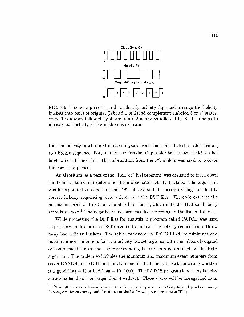
110
Clock Sync Bit
Helicity Bit
Original/Complement state
FIG. 36: The sync pulse is used to identify helicity flips and arrange the helicity buckets into pairs of original (labeled 1 or 2)and complement (labeled 3 or 4) states. State 1 is always followed by 4, and state 2 is always followed by 3. This helps to identify bad helicity states in the data stream.
that the helicity label stored in each physics event sometimes failed to latch leading
to a broken sequence. Fortunately, the Faraday Cup scaler had its own helicity label
latch which did not fail. The information from the FC scalers was used to recover
the correct sequence.
An algorithm, as a part of the "HelP.cc" [92] program, was designed to track down
the helicity states and determine the problematic helicity buckets. The algorithm
was incorporated as a part of the DST library and the necessary flags to identify
correct helicity sequencing were written into the DST files. The code extracts the
helicity in terms of 1 or 0 or a number less than 0, which indicates that the helicity
state is suspect.5 The negative values are encoded according to the list in Table 6.
While processing the DST files for analysis, a program called PATCH was used
to produces tables for each DST data file to monitor the helicity sequence and throw
away bad helicity buckets. The tables produced by PATCH include minimum and
maximum event numbers for each helicity bucket together with the labels of original
or complement states and the corresponding helicity bits determined by the HelP
algorithm. The table also includes the minimum and maximum event numbers from
scaler BANKS in the DST and finally a flag for the helicity bucket indicating whether
it is good (flag = 1) or bad (flag = 10,-1000). The PATCH program labels any helicity
state smaller than 1 or larger than 4 with -10. These states will be disregarded from
5The ultimate correlation between true beam helicity and the helicity label depends on many factors, e.g. beam energy and the status of the half wave plate (see section III.l).

I l l
TABLE 6: Helicity error codes.
Err Code Reason -1 ROC out of sync -2 Helicity mismatch -3 Sync mismatch -5 Scaler physics helicity mismatch
-10 Skip in TGBI helicity scaler -20 Skip in HLS scaler -50 Other pair failed helicity test
-100 Smaller than usual number of triggers -200 No beam current in FC
further analysis. The program also examines the order of the helicity states and
determines the buckets that are out of sequence. It also compares minimum and
maximum event numbers from the trigger banks with the output of the scaler banks
and labels unmatched helicity buckets. The label for these two latter cases is -
1000. In addition, PATCH takes care of suspicious helicity states at the end of some
DST files that occur during file closing. Whenever a bad helicity bucket is found,
the original and the complement states are always thrown away together until the
correct sequence is recovered. This ensures that the removal of problematic buckets
will not bias any particular helicity state. During the analysis process, the PATCH
program is executed first and its output table is used by the DST reader to determine
problematic helicity buckets. A segment from its output is shown in Table 7.
IV.5 QUALITY CHECKS A N D PRE-ANALYSIS CORRECTIONS
First level quality checks were performed during data reconstruction. The time of
flight information from SC, EC sampling fractions, DC residuals and EC-SC time
differences were monitored for each file after full reconstruction of each data set.
This ensures the applied calibration constants, determined by using sample runs, are
successfully calibrating the full data set. After the reconstruction, there are about
40,000 DST files. Some of these files are not usable for physics analysis due to
experimental conditions or DAQ errors during the data taking process. Therefore,
a second level quality check is required to determine corrupted or bad files. The
quality checks are performed on a file by file basis and separately executed for each

112
TABLE 7: A short segment from tables produced by the PATCH program. The table is from file dst28237_00.B00. Columns show minimum and maximum events in the helicity bucket, the corresponding helicity state and the resulting helicity bit. Event numbers from a different BOS bank, SCLR, are also listed for error check. The last column is the final flag, 1 meaning an acceptable bucket. The fraction of problematic buckets that show up in one file is less than 1%.
evmin
73779
73893
73996
74169
74269
75023
75197
75306
75406
75562
75665
evmax
73889
73994
74164
74261
74351
75196
75305
75402
75559
75663
75764
state
2 3 1 4 2 -1000
2 3 2 3 2
bit 0 1 1 0 0 -1000
0 1 0 1 0
evmin_SCLR
73779
73893
73996
74169
74269
75023
75197
75306
75406
75562
75665
evmax.SCLR
73889
73994
74164
74261
74351
75196
75305
75402
75559
75663
75764
flag
1 1 1 1 -1000
-10 1 1 1 1 1
data set (Target, Beam Energy, Torus Current). In this section, the general outline
for these quality checks will be described.
IV.5 .1 Event r a t e s
Count rates, normalized by the integrated beam charge, for inclusive events were
monitored. The normalization was done by using the gated Faraday cup information.
The event selection procedure includes standard electron cuts, which are used for the
analysis of the data. As well as the inclusive count rates, we also monitored proton
and pion count rates by using the standard ID cuts in the DST files. The count rates
are monitored separately for each sector. The files with different count rates from
the average were identified for all sectors. We checked the entries in the logbook
while monitoring the count rates, especially the inclusive rates. If the count rate fell
within 8% (sometimes 5% according to the sigma of the distibution) of the average
count rate, the file was accepted as a good file. In order to do this correctly, the
rates were monitored separately for each sector as well so that quality checks would
not give a wrong decision because of a specific sector failure which effects the total

113
count rate. A group of files that fail the 8% requirement for three or more sectors
are reported in the bad file list. On the other hand, if the group of files show lower
count rates for only one or two sectors, they are reported in the warning file list. A
single file that fails, even for a single sector, is directly eliminated. If the files fail
the 8% percent requirement for all sectors, a sector independent failure, we look for
reasons in the logbook entries and report them if there is an obvious reason. This
practice helps to find out if any mistake has been made in labeling the files for their
target. Rates for proton counts as well as for 7r+ and TT~ counts were also monitored
for each sector. If these exclusive counts fail for any file or segment of files while
their inclusive rates look good, we report them in the warning file list. The final fate
of a file with a warning label is determined after a group discussion. In addition, we
require the helicity bit, from PATCH, in the DST to be either 1 or 0.
IV.5.2 Beam charge quality
When measuring asymmetry, it is important to eliminate false asymmetries caused
by experimental conditions. For example, we checked to make sure that the same
amount of beam charge was delivered to the target in both helicity states. The
integrated beam charge asymmetry was determined by using un-gated Faraday cup
values, FC+ - FC~
•n-beam — p^i+ , pr<- ' \A60)
where, + and — represent the corresponding helicity states. The distribution of beam
charge asymmetry for all DST files was monitored to determine files with unusually
high beam charge asymmetry. A Gaussian fit to its distribution was used in order
to to make a proper cut (see Fig. 37). The files that remain outside the cut are
eliminated. Our final beam charge asymmetry cut was ±0.005, using the ungated
Faraday cup asymmetry value.
IV.5.3 Effects of beam charge asymmetry
During the quality checks we also looked at the effect of the beam charge asymmetry
on the inclusive asymmetry. This study led to a more detailed investigation on the
dependence of the inclusive asymmetry on the beam charge asymmetry. The over
all conclusion was that the data behave as expected and our normalization scheme
(normalizing the counts with the gated Faraday cup values) works well to remove
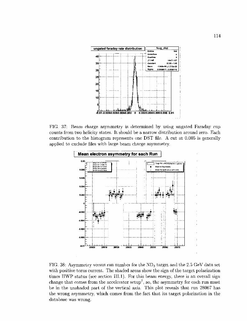
114
ungated faraday rate distribution | fcug dist Entries
Underflow 4 Overflow 0
J^/ndf 144.7/127
Constant 32.95 ± 1.65
Mean -1.942e-05± 1.713S-0S Sigma 0.0004817±0.0000172
(.01-0.00&0.006-0.004-0.002 0 0.0020.0040.0060.008 0.01
FIG. 37: Beam charge asymmetry is determined by using ungated Faraday cup counts from two helicity states. It should be a narrow distribution around zero. Each contribution to the histogram represents one DST file. A cut at 0.005 is generally applied to exclude files with large beam charge asymmetry.
Mean electron asymmetry for each Run
j TargetPat K K«P(rilled lor nefl/posi
Electron Asymmetry
Mean for each group with
28000 28010 28020 20030 28040 28050 28060 28070
FIG. 38: Asymmetry versus run number for the ND3 target and the 2.5 GeV data set with positive torus current. The shaded areas show the sign of the target polarization times HWP status (see section III.l). For this beam energy, there is an overall sign change that comes from the accelerator setup7, so, the asymmetry for each run must be in the unshaded part of the vertical axis. This plot reveals that run 28067 has the wrong asymmetry, which comes from the fact that its target polarization in the database was wrong.

115
unphysical asymmetry from the data. More detailed information on this specific
study can be found among the CLAS notes archive [93].
IV.5.4 Polarizations and asymmetry check
It is important to determine the correct sign for the product of beam and target
polarization since a wrong sign would dilute the asymmetry. Electron asymmetry
plots were generated for groups of runs from the same data set. These are plots of
electron asymmetry versus the run number. An example of such a plot is shown
in Fig. 38. The products of the half wave plate (HWP) sign (1 for in, -1 for out)
and the target polarization sign for each run are also shown in this plot. There are
various ways to show the overall polarization state properly. We decided to shows
only the multiplication of the HWP sign and the target polarization sign by creating
a shaded area on the positive or negative side of the plot according to the result.
The primary purpose is to understand if there were any runs with the wrong sign
of the electron asymmetry. In case it should occur, we examined these specific runs
more carefully to find out if any mistake was made in recording the HWP state
or the target polarization during the data taking. In the plot shown, for example,
run 28067 was determined to have the wrong target polarization in the database.
Logbook investigation reveals that its target polarization should be the same as the
subsequent runs. The runs determined to have the wrong sign for the HWP or the
target polarization were corrected during the data analysis process.
IV.5.5 Faraday cup corrections
The Faraday cup is located 29.5 m downstream from the CLAS target cell. Its diam
eter is 15 cm. We get the integrated beam charge information from the Faraday cup.
However, while the beam passes through the target, multiple scattering causes an
overall spread of the beam. If the spread angle of the beam is larger than 0.146°, some
of the beam charge will be lost outside the Faraday cup, leading to an unaccounted
beam charge. The beam divergence can be calculated by the Moliere distribution
[95] [94] but the target magnet complicates the situation, causing an additional diver
gence. Therefore, a detailed study was conducted by R. Minehart et al. measuring
the current at the upstream Beam Position Monitors (BPMs) and comparing it to
the Faraday cup values for different targets and beam energies. It was assumed that
no correction was needed for 5.7 GeV beam, which has a small divergence. This

116
energy was used to establish the exact correspondence between the BPMs and the
Faraday cup. Then, for each beam energy and target, the ratio of the BPM value
to the Faraday cup value was recorded. It was determined that no correction was
required for any target from the 4.X and 5.X GeV data sets. However, correction
factors for other data sets were determined as given in Table 8. The Faraday Cup
value should be divided by the normalization factor to get the true integrated beam
charge to normalize the counts. These factors are recorded in a run information
table that is used by the DST reader during the analysis. Note that the correction
is largest for the lowest beam energy, as expected.
Another correction for the Faraday cup information comes from the fact that for
Empty target runs, the Faraday cup recorded at half the rate it did for other targets.
This was intentionally done by removing one bit from FC response rate to be able to
accommodate a higher beam current during the experiment. Since the empty target
has a much shorter radiation length, it could accommodate a higher beam current
without increasing the dead time for the DAQ. However, this results in only half the
FC count for the empty target runs. Therefore, a factor of 2 must be multiplied with
the FC counts for empty targets. The quality checks revealed that there are also a
few other runs with missing FC bit, so their FC values must also be multiplied by 2.
The FC multiplicative factor is also incorporated into the run information table and
used by the DST reader during the analysis process. The run information table can
be consulted for detailed information and correction factors for each run.
It should be noted that the Faraday Cup corrections above do not affect the raw
asymmetry calculations but become important only for background analysis where
we need to divide normalized counts from different targets, with differing radiation
lengths. Therefore, these corrections are applied for cases like dilution factor studies
only but they are not applied while calculating the raw asymmetries, where FC
corrections cancel out. In this way, we avoid possible type conversion and precision
loss problems that may arise when dividing a large integer number, like Faraday cup
values, by a normalization factor.
IV.5.6 Additional comments
During the quality checks, some of the runs were determined to have the wrong torus
current encoded (with value -1 A) in the DST file. In particular runs 26256-26276
from the 1.6 GeV data set, 27248-27256, 27270-27275 from the 2.3 GeV data set and

117
TABLE 8: Faraday Cup normalization factors correcting for angular beam divergence.
Vbeam (GeV) 1.606 1.723 2.286 2.561
NH3
0.846 0.856 0.951 0.986
ND3
0.828 0.840 0.951 0.986
i 2 C
0.850 0.860 0.962 0.986
Empty(LHe)
0.965 0.967 1.000 1.000
26591-26598, 26723-26775 from the 5.8 GeV data set had the wrong torus current
of -1 A in the database. We made sure that the torus currents for these runs were
set manually in the tcl script during the data reconstruction. The torus currents are
also corrected during data analysis by replacing the encoded torus current with the
corrected torus current in the DST file.
There are also files which crash the DST reader program or give empty or unusual
outputs. These files are flagged and removed from the final list. Finally, we always
checked the logbook for specific runs we labeled as bad. We briefly went over the
logbook entries for each run and marked the bad or problematic runs. In summary,
we compared the logbook entries with our results as a consistency check.
In addition, detailed investigations were made on the raster patterns for each
run. Some runs show elevated count rates in certain parts of the target material,
which usually means that the beam is scraping the target edge or there may be an
interfering material in front of the target. More information about this study as well
as some additional concerns about the quality checks can be found in [95].
At the end of the quality check procedure, a list of bad files and a complete
run information table are produced. The table includes a flag for each run together
with corresponding target, energy, torus and polarization information as well as the
Faraday Cup correction factors. The script LinkDATA.pl, described in section IV.3,
is used to organize the files and exclude the bad files from the final list. Missing
files from storage or cache disks are determined and recovered if they are good files.
The DST reader consults with the bad file list and the run information table while
processing each file for analysis. More information and detailed monitoring plots for
quality checks can be found in [96] and [97]. At this point, we begin to describe the
higher level analysis.

118
IV.6 DATA B I N N I N G
The goal of our experiment is to determine asymmetries as a function of at least
two kinematic variables. The kinematic variables have been defined and explained
in earlier sections. Among these variables, we choose to use the squared four-
momentum transfer Q2 and invariant mass W as our official variables. Once we have
the cross section distributions for different helicities with respect to these variables,
da(AQ2,AW), we can express them as a function of any other pair of kinematic
variables as well. Another common pair is (Q2,x), where x is the Bjorken scaling
variable. While converting the {Q2,W) pair into (Q2,x), we used kinematic values
directly obtained from data, which are averaged over the amount of data observed for
that specific kinematic bin. In order to go into details, we first need to explain our
data binning method. We divided the Q2 and W range of the data into finite bins.
The W bins are simply generated as 10 MeV bins. Binning in Q2 is logarithmically
calculated by using the formula:
Bin Number = n = int (13 log10 ( ^ l O 2 7 7 1 3 J J , (224)
where, (1 + 10"1/13)
C = [-^ 1 . (225)
From these equations, we can calculate Q2min and Q2
max for each bin by using the
following definitions:
Q2min = C x 10(-2 7)/1 3 (226)
Q2max = C x l O ^ 1 " 2 7 ) / 1 3 (227)
Table 9 show the Q2 bins of the EG lb data together with the minimum and
maximum value for each bin. The table also shows the arithmetic and geometric
average of each bin. For our analysis, we did not use a simple average for the bin
centers but determined the central values directly from the data itself. This was done
by calculating the Q2 and W values of each data point in the bin and then averaging
all data for a single bin by using the corresponding counts in each bin. The kinematic
centers of the bins do not always peak at the arithmetic or geometric bin centers.

TABLE 9: Q2 bins for EG lb experiment
Bin 1 2 3 4 5 6 7 8 9 10 11 12 13 14 15 16 17 18 19 20 21 22 23 24 25 26 27 28 29 30 31 32 33 34 35 36 37 38 39 40
Q2min 0.009188388 0.010968883 0.013094397 0.015631785 0.01866086 0.022276898 0.026593641 0.031746867 0.037898668 0.045242545 0.054009494 0.064475272 0.076969073 0.091883882 0.109688832 0.130943966 0.156317848 0.186608595 0.222768982 0.265936407 0.317468671 0.378986684 0.452425451 0.540094935 0.644752718 0.769690734 0.91883882 1.096888321 1.309439656 1.563178475 1.86608595 2.227689819 2.659364071 3.17468671 3.789866839 4.524254507 5.400949352 6.447527179 7.696907344 9.1883882
Q2max 0.010968883 0.013094397 0.015631785 0.018660860 0.022276898 0.026593641 0.031746867 0.037898668 0.045242545 0.054009494 0.064475272 0.076969073 0.091883882 0.109688832 0.130943966 0.156317848 0.186608595 0.222768982 0.265936407 0.317468671 0.378986684 0.452425451 0.540094935 0.644752718 0.769690734 0.918838820 1.096888321 1.309439656 1.563178475 1.866085950 2.227689819 2.659364071 3.174686710 3.789866839 4.524254507 5.400949352 6.447527179 7.696907344 9.188388200 10.968883209
geoAve 0.0100 0.0120 0.0143 0.0171 0.0204 0.0243 0.0291 0.0347 0.0414 0.0494 0.0590 0.0704 0.0841 0.100 0.120 0.143 0.171 0.204 0.243 0.291 0.347 0.414 0.494 0.590 0.704 0.841 1.00 1.20 1.43 1.71 2.04 2.43 2.91 3.47 4.14 4.94 5.90 7.04 8.41 10.0
ariAve 0.0101 0.0120 0.0144 0.0171 0.0205 0.0244 0.0292 0.0348 0.0416 0.0496 0.0592 0.0707 0.0844 0.101 0.120 0.144 0.171 0.205 0.244 0.292 0.348 0.416 0.496 0.592 0.707 0.844 1.01 1.20 1.44 1.71 2.05 2.44 2.92 3.48 4.16 4.96 5.92 7.07 8.44 10.1

120
IV.7 ELECTRON IDENTIFICATION
During the EG lb experiment, the event trigger used a combination of the Electro
magnetic Calorimeter and the Cherenkov counter signals and accepted all events
above the threshold, which was determined specifically for each electron beam con
figuration. The off-line reconstruction code (RECSIS) creates a second filter of events
by requiring more strict particle definitions and uses the Simple Event Builder (SEB)
to identify particles. The RECSIS identification of particles is primarily based on
the time of flight information from Scintillator Counters (SC) and the track recon
struction by the Drift Chamber (DC). More detailed information on the off-line data
reconstruction can be found in section IV.2. At high energies, as in the case of the
EGlb experiment, the SEB method is not reliable because all particles are very fast
and the time of flight (TOF) information does not reliably distinguish electrons from
pions. The inclusive analysis requires a very careful selection of electrons, which was
accomplished by requiring a negative track with matching signals in the TOF scin
tillators, the Cherenkov Counters (CC), and the Electromagnetic Calorimeter (EC).
If more than one track was found satisfying this condition, the track with the short
est flight time was selected as the electron candidate. The primary contamination
for electrons comes from negatively charged pions. The EC and the CC detectors
were specifically used to separate pions and other negatively charged particles from
electrons. After the completion of the reconstruction by the RECSIS code, the list
of cuts below were applied for the inclusive analysis to identify electrons:
1. Charge = -1
2. Status Flag selection
3. Trigger Bit selection
4. Helicity selection
5. Vertex cut
6. Cherenkov photo-electron cut
7. Electromagnetic Calorimeter cut
8. First electron candidate (with shortest flight time)

121
9. Additional kinematic cuts
• Momentum cut
• Polar angle cut
• Energy transfer cut
• Polar angle cut for sector 5
10. Geometric and Timing cuts on the Cherenkov Counter
11. Fiducial cut
The following sections will provide more detailed information on some of these cuts.
IV.7.1 Status Flag
Each identified particle in the DST carries a status flag. If the particle status flag is in
the [0,5] range, the reconstruction is time-based and the event is acceptable. Particles
with status flag > 5 are reconstructed from hit-based tracking only and should be
eliminated. In addition, if a particle is detected in all 3 superlayers of the DC and its
trajectory is reconstructed accurately, 10 is added to the status flag variable, which
carries some of the time based tracks into a range of [10,15]. Therefore, the status
flag selection criteria is:
0 < status flag < 5 OR 10 < status flag < 15
IV.7.2 Trigger Bit
Each event in the DST carries a trigger bit information. It is an integer value that
represents a 16 digit binary number. We call this value a trigger word. Each bit
corresponds to a specific trigger response. We will call these bits as trigger bits and
they can either be on or off (1 or 0). The very first bit (the least significant bit) is
trigger bit 1. Trigger bits 1 to 6 correspond to our standard triggers, one for each
sector, based on CC and EC signals. Trigger bit 7 requires a hit in EC and CC
anywhere, while trigger bit 8 requires a hit only in the EC with a lower threshold (no
CC hit). Trigger bit 8 is mainly used for minimally biased pion selection. Trigger
bits 9 to 14 are not used for any purpose. Trigger bits 15 and 16 record the value
of the helicity bucket (redundantly). The trigger bits are combined to yield trigger

122
words. If only trigger bit 1 is fired, the trigger word would be 1, which corresponds
to an event in sector 1. If trigger bit 3 is fired (event in sector 3), the trigger word
is 4. For an event observed in sector 1 and 3, the trigger bit configuration (only
considering the first 6 digits) would be 000101, giving a trigger word of 5. Our event
selection criteria is based on signals in trigger bits 1 through 6. If none of these bits
were on for the event, it is discarded. If any of the bits from 1 to 6 were signaled, we
accept the event regardless of the higher bit values.
IV.7.3 Vertex Cuts
It is important that the scattered electrons come from the target, not the surrounding
material. Therefore, the interaction vertex should be within certain boundaries. By
looking at the vertex distribution of the electron, we determined global values for the
minimum and maximum position of the interaction vertex in the z coordinate (along
the beam direction). In CLAS coordinates, the target center is at z = -55.0 cm.
The minimum z position was chosen to be -58.0 cm while the maximum z position
is -52.0 cm,
-58 <vz< -52.
Interactions that come from outside of this region are rejected for all particles. Of
course, before applying the vertex cut, proper vertex corrections are applied (see
Fig. 39). These corrections are described in section IV. 10.1 in detail. It should be
noted that the target configuration makes it impossible to cut out the target window
material with a vertex cut since the resolution of the event vertex reconstruction
is not fine enough to resolve distinct scattering peaks within the ~2.3 cm distance
of the target banjo length. In order to eliminate contributions from the aluminum,
Kapton and liquid helium on either side of the target material, other background
subtraction methods, such as dilution factor calculations, are used.
IV.7.4 Cherenkov Counter Cuts
The Cherenkov counter (CC) is designed primarily to separate electrons from pions.
The threshold for the electrons is 9 MeV while for pions it is 2.5 GeV8. Identification
of pions in the CC is quite successful as long as the pion energy is below the threshold
value, in which case the pion peak can easily be distinguished from the electron 8These are momentum thresholds and natural units are used with c = 1.
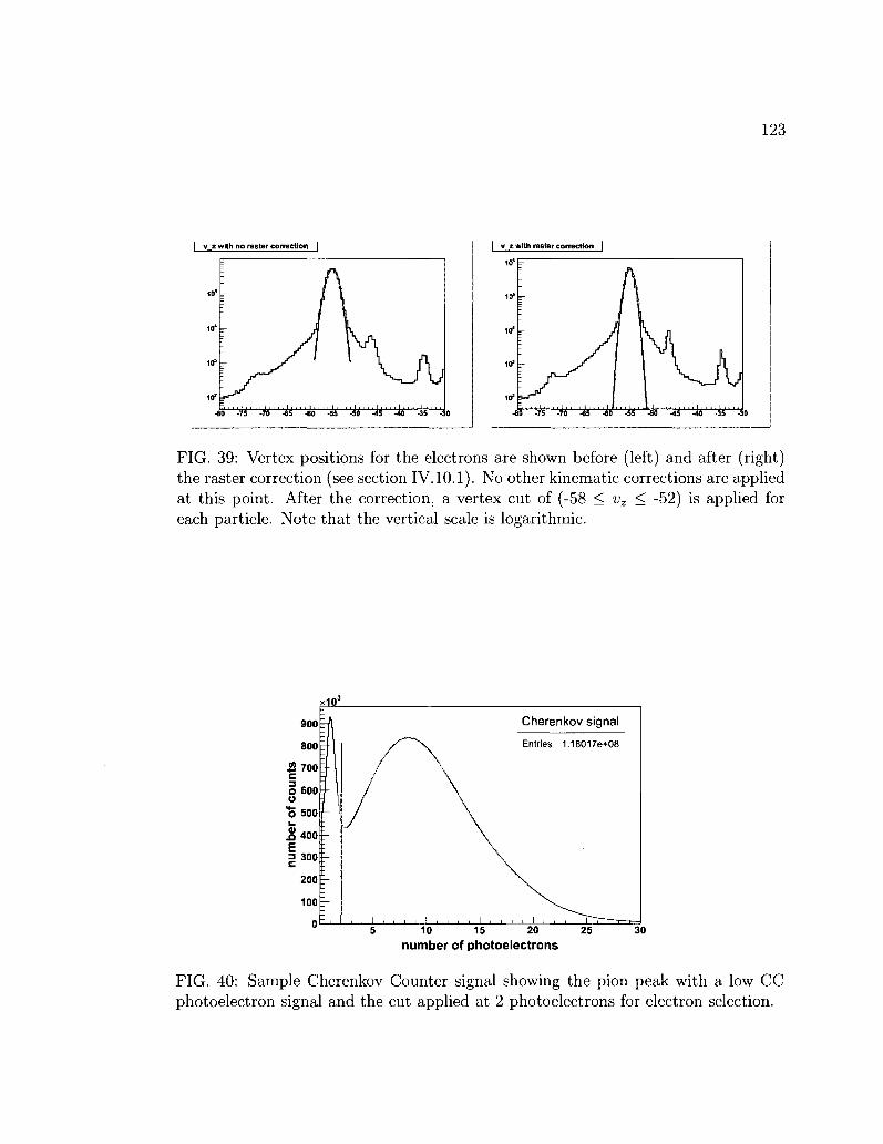
123
| v_z with no raster correction |
-80 -75 -70 -65
j v 2 with raster correction I
10"
10"
10*
10?
10=
r
-80 -75 -70 -65 -60 -55 -50 -45 -40 -35 -3 ;0
FIG. 39: Vertex positions for the electrons are shown before (left) and after (right) the raster correction (see section IV.10.1). No other kinematic corrections are applied at this point. After the correction, a vertex cut of (-58 < vz < -52) is applied for each particle. Note that the vertical scale is logarithmic.
Cherenkov signal
Entries 1.18017e+08
10 15 20
number of photoelectrons 25 30
FIG. 40: Sample Cherenkov Counter signal showing the pion peak with a low CC photoelectron signal and the cut applied at 2 photoelectrons for electron selection.

124
signal. However, the signal from high energy pions above the thereshold becomes
indistinguishable from the electron signal, making the Cherenkov detectors inefficient
to separate high energy pions from electrons. Fig. 40 shows a sample signal from CC
together with the applied cut at 2 photoelectrons to identify the electrons. This cut
is applied for momenta less than 3.0 GeV. Since the CC efficiency is relatively low
at higher momenta, a cut requiring that the number of photoelectrons exceed 0.5 for
momenta above 3.0 GeV is used. Any remaining pion contamination is taken care of
by other cuts that will be defined in the following sections.
IV.7.5 Electromagnetic Calorimeter Cuts
When we plot the energy deposition in the inner calorimeter (ECin) versus the total
energy deposition in the EC (ECtot), we see a clear separation between the electron
and pion signals. The total energy deposited by an electron in the EC is proportional
to its momentum (p). This ratio is called a sampling fraction, which is ~0.29 for
this experiment (see Fig. 44). The pions, on the other hand, are minimum ionizing
particles, hence, their energy deposition mechanism is different than that of the
electrons. Details about this are given in section III.3.5. The energy loss for a pion
in the calorimeter is mostly independent of its momentum. The localized events in
the bottom left corner of each plot in Figs. 41 and 43 represent the pions detected
by the EC. As the momentum of the particles increase, the distinction between the
electrons and the pions in the calorimeter become more evident because ECinjp and
ECtot/v for the pions decrease rapidly while ECtot/p for the electrons remains as a
Gaussian distribution around the sampling fraction as shown in Fig. 44. In order to
select the electrons, we applied the following cuts:
• ECtot I p > 0.20 for p < 3 GeV
• ECtot IP > 0.24 for p > 3 GeV
• ECin > 0.06
E C sum correction
The Electromagnetic Calorimeter records three different signals for the energy de
posited by an incident particle. These signals correspond to the inner calorimeter
(ECin), outer calorimeter (ECout) a n d total energy deposited (ECtot) in both layers.

125
0.5
0.45
0.4
0.35
0.3
fjifo.25
0.2
0.15
0.1
0.05
I ECin vs ECtol for negative charged particles
~ '-
'-
'-
.: ili* j j T
- ^
: . . . ? » i , , , , i 0.1 0.2 0.3
EC.., 0.4 0.5 0.6
xi<r
7000
6000
5000
4000
-3000
2000
1000
'o
FIG. 41: ECin vs. EC t o t for negative charged particles. -ECjn > 0.06 is required to select the electrons. These events are from the 4.2 GeV outbending data.
30
25
20
15
10
5
. . E I ECin all negative particles |
~n
-" 1 ~^^^-;- ^
- . . ' i i , , , , i , , , , i 0.1 0.2 0.3 0.4 0.5 0.6 0.7
EC,.
FIG. 42: The energy deposition of negative charged particles in the inner layer of the EC (energy spectrum of the ECin). Edn > 0.06 is required to select the electrons and separate them from negative pions. These events are from the 4.2 GeV outbending data.

126
I E<V
0.35
0.3
0.25
6 s 0.2
0.15
0.1
0.05
vs ECtat/P for negative charged particles I
r
~r
v /£ * /
* " " * •
- . . . " "• ;
: : i . . . . i . . . . i . . . . i . . . . i . . . . i . . . . i i. 0.05 0.1 0.15 0.2 0.25 0.3 0.35 0.4 0.45 0.5
EC„/P .. .
(a) EB = 1.6 GeV; IT =
ECin/P vs EC10t/P for negative charged particles
-1500 A
0.4
0.35
0.3
0.25
O" 0.2 UJ
0.15
0.1
0.05
~ r
I ^
t , •^i-.-rT. i . . . , i . . . . i .
,**7\ m y % •
0.05 0.1 0.15 0.2 0.25 0.3 0.35 0.4 0.45 0.5 E C J P
(c) EB = 4.2 GeV; IT = -2250 A
ECJPvs
0.4
0.35
0.3
0.25 0. if 0.2 UJ
0.15
0.1
0.05
r
-~r
'T
-r
EClot/P for negative charged particles I
r,>" ,--
j *
i"
9 :*- J S*r
its*
0.05 0.1 0.15 0.2 0.25 0.3 0.35 0.4 0.45 0.5 ECtJP
x10? '1401
000,
600
400
200
o !
(b) EB = 2.5 GeV; IT =
ECin/P vs ECtDt/P for negative charged particles I
-1500 A
0.3
0.25
o £ 0.2 ui
0.15
0.1
S
x10'
600
500'
400:
300!
0.05 0.1 0.15 0.2 0.25 0.3 0.35 0.4 0.45 0
.... „. ttJI, .
(d) EB = 5.7 GeV; IT = -2250 A
FIG. 43: ECin/p vs. ECtot/p for 4 different beam energies (EB) with outbending torus currents (IT)- The beam energies increase from the top left to the bottom right plot. The events concentrated in the left bottom corner of each picture are pions, which become more visible with increasing beam energy.
0.5 fr
0.45;
0.4 z
0.35^
0.3^
,"*0.25 J
0.2
0.15
0.1
0.05
ECtet/P vs P for negative charged particles
SflWrtm
K*
. i i . i — i — i _ i 0.5 1 1.5 2 2.5 3 3.5 4 4.5 5
P(GeV)
X10 ;
1200
1000
800 >
; 600
400
200
0
14
12
10
8
6
4
2
on
FIG. 44: ECtot/p vs. p distribution (left) and ECtot/p spectrum for negative charged particles (right). The applied cut is shown with the straight lines and explained in the text.
127
Normally, ECtot = ECin + ECout should always be true. However, the readout for
these three signals did not always fulfill this condition. Even if the event is good,
sometimes a few channels in the EC failed to record the deposited energy leading
to a mismatch. These occasional failures required an additional correction for the
energy deposited in the EC such that:
ECtot = MAX(ECtot, (ECin + ECout)). (228)
This correction makes sure that the total measured energy in the EC was employed
in the PID cuts described above.
IV.7.6 Additional kinematic cuts
The event reconstruction becomes unreliable when scattered particles get too close
to the edge of the geometric acceptance of the detector. Also, the detector effi
ciency becomes unpredictable in case of very low momentum particles. Therefore,
we employed the following additional cuts on the data:
E' y = 1 - — < 0.80;
7.5° < 6DC < 49°,
where O^c is the polar angle measured at Drift Chamber region 1. The upper angle
limit comes from the interference of the target magnet coils with the detector. The
lower angle limit is employed to make sure the data is within the acceptance of the
CLAS detector. It is also smaller than the usual DC coverage because the target
was shifted back during the experiment. In addition, we also applied a cautionary
requirement on the transferred energy such that:
v = E - E' > 0. (229)
Sector 5 Cut
Sector by sector inspection of the data revealed a problematic kinematic region in
sector 5, where the event reconstruction failed for unknown reasons resulting in a
discrepancy between the calculated and measured polar angles. This was observed in
the DST files as well as the original ntuple files, which means the reconstruction failed
at the SEB level. The problem becomes more obvious if one plots the reconstructed

128
F . . . . i . . • . i • . . . i • i i , i , , i I -58 .57 -56 .55 -54 -53 -52
ThetaDCI vs vz
FIG. 45: Reconstructed vertex position versus doc for electrons in sector 5. A polar angle cut in sector 5 was necessary to remove the part of data with bad vertex definition. The kinematic region 18 < Que < 21 for this sector was excluded from analysis.
z-vertex position vs. 9DC, as shown in Fig. 45. This kinematic region is excluded
from further analysis by applying the following cut on the data:
9DC < 18° and 6DC > 21° (Sector 5 only) (230)
There are other cuts we used on the data to identify the electrons even more pre
cisely. Since these additional cuts require a thorough analysis of the data and detailed
explanations, we prefer to dedicate an entire section to them. The following sections
describe the additional cuts for precise electron identification and minimization of
pion contamination.
IV.8 GEOMETRIC A N D TIMING CUTS ON T H E CC
Geometrical and timing cuts on Cherenkov Counter signals, first developed by
M.Osipenko et al. [98], were applied to the EGlb data for the first time. The
original set of parameters determined by Osipenko did not work very efficiently for
our data because they greatly reduced the electron sample while clearing up the pi-
ons. We extensively studied the data to develop a new set of parameters that worked
better for us. This section provides some explanations of these cuts.
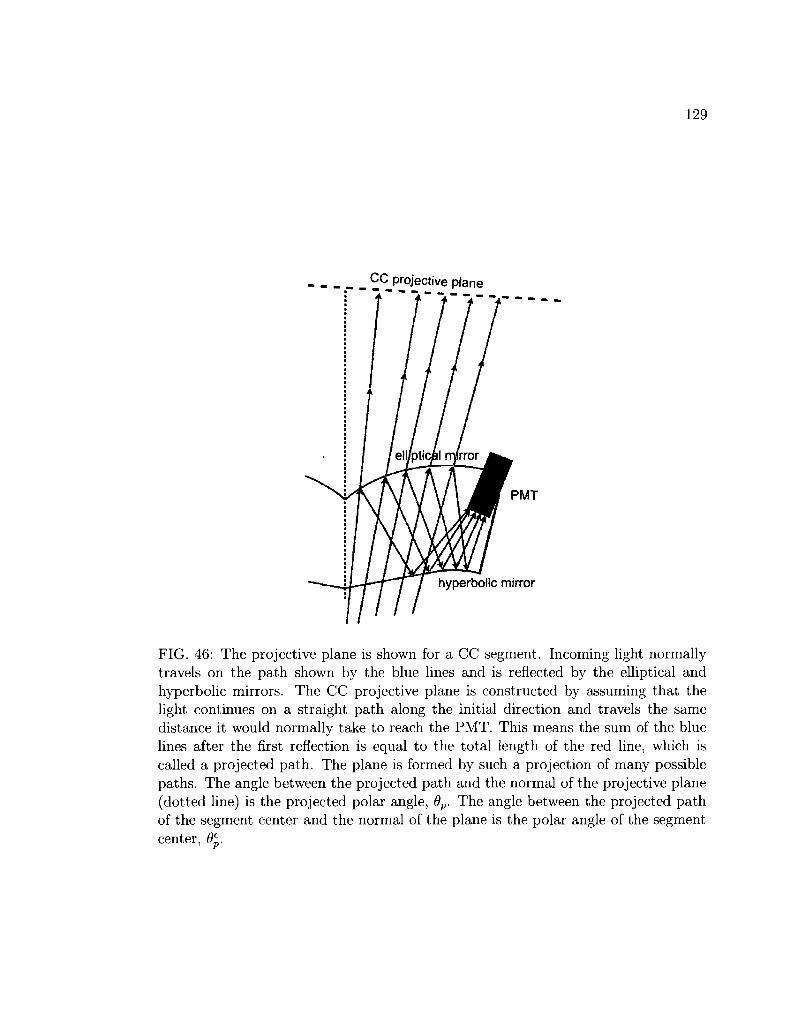
129
CC projective plane
FIG. 46: The projective plane is shown for a CC segment. Incoming light normally travels on the path shown by the blue lines and is reflected by the elliptical and hyperbolic mirrors. The CC projective plane is constructed by assuming that the light continues on a straight path along the initial direction and travels the same distance it would normally take to reach the PMT. This means the sum of the blue lines after the first reflection is equal to the total length of the red line, which is called a projected path. The plane is formed by such a projection of many possible paths. The angle between the projected path and the normal of the projective plane (dotted line) is the projected polar angle, 9p. The angle between the projected path of the segment center and the normal of the plane is the polar angle of the segment center, Qc
v.

130
Each sector in the CLAS detector contains 18 CC segments. Each of these seg
ments has two photomultiplier tubes (PMT), one at right and one at left. These
PMTs have a certain rate of noise that has been measured to be around 42 kHz
and each noise pulse may have an amplitude around one photo-electron. The main
purpose of the CC is to distinguish between the electron and pion tracks. It has been
determined that if a noise pulse in the CC and a negative pion track measured in
the DC coincides within the same trigger time window of the CLAS detector, which
is 150 ns, the pion can be registered as an electron by the analysis code. This is
apparently the biggest source of pion contamination for the inclusive data. In order
to eliminate the coincidences between the CC noise and a pion track, the geometric
and time matching requirements between the CC signal and a measured track were
implemented into our data selection criteria.
IV.8.1 Geometric cuts
An imaginary CC projective plane is constructed behind the CC detector at a dis
tance traveled by the CC radiation from the emission point to the PMT but without
doing any reflections in the mirror system. The resulting CC projective plane is
shown in Fig. 46 and is given in terms of the CLAS coordinate system as:
1 - 7.840784063 x 10 - 4 x - 1.681461571 x 10 - 3 z = 0 (231)
where x is the radial distance along the sector center and z is the direction along the
beam line. Then, for each CC segment, the polar angle of the segment is constructed
by connecting the points from the center of CLAS to the center of the image of the
CC segment at the projective plane. The polar angle of each electron candidate is
also determined by using the SC impact point of the track and projecting it to the
CC projective plane. This quantity will be referred as the projected polar angle. Fig.
46 shows the construction of this polar angle.
Distributions of the particles' polar angles, 9P, are monitored for each segment.
They should show a Gaussian distribution around the polar angle of the segment
center, Qc. For some segments, however, slight offsets have been observed. After
correcting the distribution for these offsets, we can apply a cut to remove the tails of
the distribution. In order to determine where to apply the cuts exactly, we plotted
the electron and pion (iv~) distributions together on a logarithmic scale, as shown in
Fig. 47. It is clear that the tails of the electron polar angle distributions are actually

131
I electron polar angle sed_seg10 |
-20 -15 -10
| electron polar angle sed_seg12 \ Entries 9450341 Mean -0.07189
-20 -15 -10 -5
FIG. 47: Distribution of the projected polar angels of the electrons (black lines) and the pions (green lines) for a few segments in sector 1. There are 6 sectors and each sector contains 18 segments. Similar plots are produced for each segment and fitted by a Gaussian function to determine the mean value of the distribution. Comparison of the electron distribution to the pion distribution proves that most of the particles that "pretend" to be electrons and stay 3cr away from the mean value of the electron distribution are actually pions. These particles are eliminated from the electron sample by applying the cuts shown by the blue lines. Note that the y scale is logarithmic.

132
mislabeled pions. By looking at the distributions for each segment, we determined
an appropriate polar angle cut for each segment in all sectors.
IV.8.2 T iming cu t s
After the geometrical cuts applied on polar angles, we still need to apply time match
ing between the CC signal and the passage of the particle. To determine the timing
of the electron candidate, we use the SC signal. If the particle is a real electron, the
SC and CC signals should be produced by the same particle. We assume the electron
travels with the speed of light. Therefore, the time difference between the SC and
CC signals should be given by:
Atsc-cc = r_ r { m )
c/3
where rsc — rcc is the track distance between the SC paddle and the CC projective
plane. These variables exist in the DST files as "sc_r" and "cc_r". The time of hits
also recorded as "sc_time" and "cc_time".
It should be pointed out that the original DST files, produced during the calibra
tion and reconstruction process, did not have these variables, although they existed
in the original BOS files. We had to change the DST structure to implement the
variables into the DST libraries and reproduce all the DST files again in order to
complete this analysis. This procedure took a substantial amount of time. After
completing the new DST production, we compared the old DST results with the
new ones to ensure the success of the implemented changes. Finally, by using the
recorded times and the track distances from the SC and CC detectors, it is possible
to determine the difference between the expected time and the observed time, At,
a s : c^ r " j (233)
The At distribution should normally peak around zero. Again, we plotted the elec
tron and pion At distributions together in a logarithmic scale, as shown in Fig. 48.
The tails of the electron distributions are clearly mostly pions. However, if one looks
at the positive side of the electron peak, around the 60 ns region, there is another
peak that begins to appear for the electron candidates in some segments. Pion can
didates do not have any peak in that region. This shows that this strange peak
actually represents true electrons and should not be cut out. Because of that, we

133
| electron At SC-CC sec1_seg06 |
10s
104
103
10J
10
r E
r ! r ^ - s ^ s ' ^ ^ 2 ^ ^ ^
f r
/ i,
\ , fcZzzz&z^
Entries 1689595
Constant 6.454e+05
Mean -0.324
Sigma 0.7532
' L ^ 1 \ 1
....Mw 40
electron At SC-CC sec1_seg10 | Entries 816937 Constant 3.27e+05 Mean -0.2238 Sigma 0.671
Entries 1615474 Constant 5.8e+05 Mean -0.3787 Sigma 0.7722
FIG. 48: Distribution of the At given in Eq. (233) for electrons (black lines) and pions (green lines) for some segments in sector 1. Similar plots are produced for all sectors and segments and electron distributions are fitted by a Gaussian function to determine the mean value of the distribution. Comparison of the electron distribution to the pion distribution proves that most of the particles that "pretend" to be electrons but stay at the tails of the electron distributions are actually pions. These particles are eliminated from the electron sample by applying the cuts shown by the blue lines. Note that the y scale is logarithmic. The cut is applied only on the left side since there are electron peaks that appear around the 60 ns region. Those extra peaks are clearly not pions so they were kept.

134
applied the timing cut only to the left side of the distribution. In rare cases, espe
cially for outbending runs, a similar peak appears also on the negative side of the
electron distribution, around the -60 ns region. In those cases, we moved the cut
even below the range of that peak in order not to lose those electrons. Each segment
was carefully examined to determine the best location of the cut to eliminate most of
the pions but still keep the electron sample intact. Finally, a table of cut parameters
was produced for the main analysis program.
IV.8.3 Left-Right P M T cut
One last geometrical cut we applied on the electron candidates was the left-right PMT
cut. For this cut, we observed the projected azimuthal angle distribution for each
segment and kept track of the source PMT for the CC signal. If the azimuthal angle
is negative, the left PMT should give a signal and if the azimuthal angle is positive,
the right PMT should give the signal. If the the track is close to the sector center,
both PMTs may give signal for the same track. By plotting the azimuthal angle
distributions separately for left and right PMTs, we can see in Fig. 49 that sometimes
the wrong PMT is being fired, which we interpret as an accidental coincidence and
we eliminate that particle from the final electron sample. See Fig. 49 for details.
IV.8.4 Final Comments
The impact of the geometric and timing cuts on the analysis is explained in section
IV. 12 in more detail. Fig. 50 shows how these cuts greatly eliminate the pions
from the electron sample. In these plots, all electron cuts, except the CC cuts, were
applied. Using these cuts, on the other hand, causes the loss of some electrons,
around 5 to 10% at most, from our analysis sample, especially for the outbending
data. However, the amount of electrons we lose will not increase our statistical errors
considerably while the pions we clear up by these cuts will reduce our systematic error
substantially. This can be seen from Fig. 51, which shows pion to electron ratios as
a function of momentum for various polar angle bins before and after the cuts were
applied. This ratio directly enters into our systematic error, which only becomes
small after the cleanup procedure. Similar plots for various momentum and polar
angle bins are also shown in section IV. 12 as well as in [99].

135
x10J
electron azimuthal angle, PMT hit sec2_seg06 I electron azimuthal angle, PMT hit sec2_seg07 I
30 -20 -10 10 20 30
electron azimuthal angle, PMT hit sec2_seg10
x10 electron azimuthal angle, PMT hit sec2_seg11 I
10 20 30
250
200
150
100
10 20 30
FIG. 49: Azimuthal angle ((f)) distributions of electron candidates for a few segments in sector 2. The azimuthal angles of the electrons coming from the left PMT of the CC segment are plotted in red. The ones coming from the right PMT are plotted in blue. If both PMTs have a signal, the distribution is plotted in black. Electrons that have a signal in both PMTs should be coming from the region around the segment center, at <j> = 0. The left PMT should fire for electrons with 0 < 0, while the right PMT should fire for electrons with <j> > 0. Particles with positive 4> angle that had a signal only in the left PMT and vice versa cannot be true electrons. They are assumed to be accidental coincidences and eliminated from the inclusive sample.
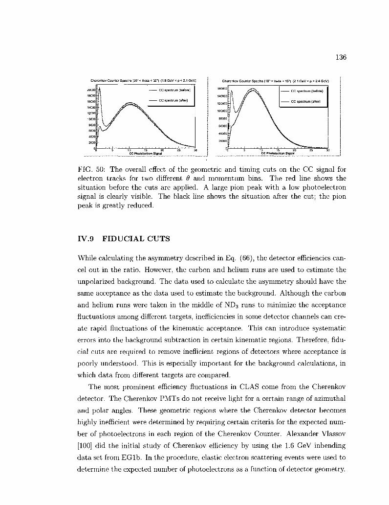
136
Cherenkov Counter Spectra (25° < ttieta < 30°) (1.8 GeV < p < 2.1 GeV)
FIG. 50: The overall effect of the geometric and timing cuts on the CC signal for electron tracks for two different 0 and momentum bins. The red line shows the situation before the cuts are applied. A large pion peak with a low photoelectron signal is clearly visible. The black line shows the situation after the cut; the pion peak is greatly reduced.
IV.9 FIDUCIAL CUTS
While calculating the asymmetry described in Eq. (66), the detector efficiencies can
cel out in the ratio. However, the carbon and helium runs are used to estimate the
unpolarized background. The data used to calculate the asymmetry should have the
same acceptance as the data used to estimate the background. Although the carbon
and helium runs were taken in the middle of ND3 runs to minimize the acceptance
fluctuations among different targets, inefficiencies in some detector channels can cre
ate rapid fluctuations of the kinematic acceptance. This can introduce systematic
errors into the background subtraction in certain kinematic regions. Therefore, fidu
cial cuts are required to remove inefficient regions of detectors where acceptance is
poorly understood. This is especially important for the background calculations, in
which data from different targets are compared.
The most prominent efficiency fluctuations in CLAS come from the Cherenkov
detector. The Cherenkov PMTs do not receive light for a certain range of azimuthal
and polar angles. These geometric regions where the Cherenkov detector becomes
highly inefficient were determined by requiring certain criteria for the expected num
ber of photoelectrons in each region of the Cherenkov Counter. Alexander Vlassov
[100] did the initial study of Cherenkov efficiency by using the 1.6 GeV inbending
data set from EGlb. In the procedure, elastic electron scattering events were used to
determine the expected number of photoelectrons as a function of detector geometry.
Cherenkov Counter Spectra (10° < theta < 15°) (2.1 GeV < p< 2.4 GeV)
160000
140000
120000
100000
80000
6OO00
40000
20000
°0
CC spectrum (before)
CC spectrum (after)
5 10 15 20 25 30 CC Pholelectron Signal

137
O.ODB
0.007
0.006
0.005
V
"0.004
0.003
0.002
0.001
theta [20.0, 25.0]
theta [25.0, 30.0]
theta [30.0, 35.0]
theta [35.0, 40.0]
momentum(GeV)
(a) 1.6 GeV before
0.0018
0.0016
0.0014
^ 0 . 0 0 1
0.0008
0.0006
0.0004
0.0002
"
Q Q
£
A theta [20.0, 25.0]
v theta [25.0, 30.0]
c theta (30.0, 35.0]
D theta [35.0, 40.0]
momentum (GeV)
(b) 1.6 GeV after
0.06
0.05
' 0.03
0.02
: r
L
-r
r
G
A
D
A
¥
, ?
A
, T , , ,
A theta [20.0, 25.0]
? theta [25.0, 30.0]
O theta [30.0, 35.0]
a theta [35.0,40.0]
A
• i i , i
momentum(GeV)
(c) 2.5 GeV before
0.02
0.015
0.01
0.005
;
A
9 A
£ §
A
A theta [20.0, 25.0]
i theta [25.0, 30.0)
c theta [30.0, 35.0]
G theta [35.0, 40.0]
<?
momentum(GeV)
(d) 2.5 GeV after
0 06
0.05
0.04
0.03
0.02
0.01
t , l
u
•o
A
s
!3
h
* 1
0 theta [15.0, 2D.0]
A theta [20.0, 25.0]
T theta [25.0, 30.0]
0 theta [30.0, 35.0]
u theta [35.0,40.0]
B
$ f A
momentum (GeV)
(e) 4.2 GeV before
0.02
0.018
0.016
0.014
0.012
r- 0.01 K
0.008
0.006
0.004
0.002
m theta [15.0, 20.0]
A theta [20.0, 25.0]
•<t theta [25.0, 30.0]
C theta [30.0, 35.0]
• theta [35.0, 40.0]
momentum(GeV)
(f) 4.2 GeV after
0.06
0.05
K 0.03
0.02
0.01
C
: -r
~r
T
~
T
1 ' ' 'o!5'
m
a
m theta [15.0, 20.0]
A theta [20.0, 25.0]
v theta [25.0, 30.0]
o theta [30.0, 35.0]
• theta [35.0, 40.0]
B
* u » 1 1.5 2 2.5 3 3.5
momentum(( 3eV)
0.02
0.015 (D
0.01
0.005
1
" " 7
; '-
-;
0 , 5
• thela [15.0, 20.0]
A theta [20.0, 25.0]
» theta [25.0, 30.0]
n theta [30.0, 35.0]
• theta [35.0, 40.0]
% |
» ! i. • ; 1 1.5 2 2.5 3 3.5 A
momentum) GeV)
(g) 5.7 GeV before (h) 5.7 GeV after
FIG. 51: 7r~/e ratio versus momentum for various polar angle bins, before and after the CC geometric and timing cuts. ND3 inbending data are shown. Note that the vertical scale of the after-cut plots is smaller.

138
The event selection criteria include cuts on the missing mass (W), vertex and the
energy deposited in the EC. In addition, geometrical matching of the track's x and
y coordinates from the EC and CC detectors were also required by putting a reason
able limit on the deviation. The Cherenkov efficiency function is assumed to obey
Poisson distribution. The main idea behind Vlassov's work was to determine the
mean number of photoelectrons as a function of projective angles 6 and 0 measured
at the SC/EC plane. Once the expected number of photoelectrons is known, the
Poisson distribution can be used to calculate the Cherenkov efficiency for each 9 and
<\> bin. Therefore, the efficiency of a specific detector location can be written as:
efficiency = ^ ^ - (234) n > c
where /J, is the expected number of photoelectrons and c is the minimum cutoff. In
order to eliminate pions from the electron sample, a lower limit of 2.0 photoelec
trons was used as the minimum electron detection threshold. In order to determine
inefficient CC regions, an 80% efficiency requirement was employed. Then events
were collected for each 9 and <j) D m that satisfies this efficiency threshold. When
the distribution of these events were plotted with respect to each geometric region
of the detector (different sectors and 9 and 4> bins), certain geometric regions of the
detector showed no events. These were determined as inefficient regions.
For fiducial cuts, the polar angle is reconstructed from the momentum of the
particle by using 9 — arctan(p2/p r). The azimuthal angle is measured at the drift
chamber layer 1. Due to the magnetic field around the polarized target, which is along
the z direction, the trajectory of the scattered particle experiences a </>-kick, which
causes the angle at the vertex and the angle reconstructed by the drift chambers to
be slightly different. As a result, the azimuthal angle shows some distortions with
respect to the polar angle 9 if it is calculated at the vertex. The distortion can be
seen in Fig. 52. Therefore, the more symmetric 4>DC values are used to determine
the fiducial geometry.
The study to determine the geometric values of the fiducial cut was made by
R. Fersch [95]. After carefully studying the efficiency map of 9 vs. </> for different
electron momenta (0.15 GeV bins used), parametrized functions of (p, 9 and pe with 6
parameters (inbending) and 10 parameters (outbending) were produced. The values
for the parameters were determined empirically as a function of momentum and kept
constant for momenta larger than 4.0 GeV. Curves drawn on top of inclusive data

139
0 vs. 9 (reconstructed <j>) | | | <\> vs. 8 (<j) measured at inner DC) |
e(°) e(°)
FIG. 52: Distribution of the scattered electrons in the 9 vs. 0 plane. The samples are taken from the 2.3 GeV data set. The left plot shows the <fi angle reconstructed at the vertex. The plot at the right shows the angle measured by the layer 1 drift chamber. The azimuthal angle reconstructed at the vertex shows some distortion with respect to the azimuthal angle. The drift chamber measurement is more reliable for fiducial cut determination. The plot is courtesy of Robert Fersch [95].
using the final equations are shown in Figs. 53 and 54. Data remaining outside of
these curves are eliminated by the fiducial cuts. Fig. 53 shows inbending data for low
and high momentum bins. The inbending data are relatively easier to handle since
fiducial regions don't show much dependence on sectors. Therefore, the same fiducial
cuts were used for all sectors in the case of inbending data. For the outbending data,
however, the sector by sector variation is too much. Parameters were produced
independently for each sector. Fig. 54 shows the situation for outbending data for
sectors 1 and 3. In this figure, only electron events that meet the 80% requirement
are shown. The fiducial region at the sector center is clearly different for sector 1
and 3. It should also be noted that the empty vertical strip on the sector 3 plot is
because of an inactive SC paddle. Also, the "eyebrow" structures observed in the
inbending data in Fig. 53 do not appear for outbending data because of different
electron projection angles.
The fiducial cuts are a set of "restrictive" cuts that remove the part of data coming
from the inefficient regions of the CC. Acceptance in these regions of the detector is
not well understood so it may vary between different data configurations and targets.

140
Sector 5: All events in * vs. 9 (1.20 GeV < p < 1.35 GeV)
ou
50
40
$ 3 0
20
10
a
• 1 , , | i r . ' 1
^:Pffi^ 1 KtJm/ rfJ^HH'
1" ' ^ f c ' «i—^^^^^Bff
"nErJ^Bfr * i •^^•(^B^^^^^P^*
I ^ ^ F T t ^ r T . 1 , , , , 1 , : • , I , i , , 1 , : ,
m 160 - 50
40
n30
20
1 1 • 0
Sector 5: CC efficient events in i|i vs. e (1.20 GeV < p <1.35 GeV)
en
Sector 4: All events in $ vs. 6 (4.65 GeV < p < 4.80 GeV) Sector 4: CC efficient events in 41 vs. 8 (4.65 GeV < p < 4.80 GeV)
FIG. 53: 4> v s- 0 f° r inclusive inbending data (torus current 2250) at low (top) and high (bottom) momentum bins. The fiducial cuts are shown as black lines. The top row is for the momentum bin 1.20 GeV < p < 1.35 GeV and sector 5. The bottom row is for a the momentum bin 4.65 GeV < p < 4.80 GeV and sector 4. The figures on the left column show all electron events. The right column figures show electrons that meet the 80% efficiency criteria. The two are shown together to create an idea on the effect of the fiducial cuts on the data statistics. In the second plot, the so called "eyebrow" structures represent direct impacts on the CC PMT. The fiducial cut excludes those data from further analysis. The plots are courtesy of Robert Fersch [95].

141
60
50
40
r 3 0
20
10
Sector 1: CC efficient events in $ vs. G (1.50 GeV< p < 1.65 GeV)
°0
* r ^ * \ • •
' i ' • • • i • i I • • »• • I \ i m H " ! • - • • I i • • i I . i i i I i i i i I
35 60
10 15 20 25 30 35 40
en
30
25
20
15
10
5
0
50
40
—30
20
10h
Sector 3: CC efficient events in $ vs. e (1.50 GeV< p < 1.65 GeV)
, , l {.,•, , - , . | .TV. , f . , , , I , , . , I
50
H40
30
20
t 5 10 15 20 25 30 35 40
en
FIG. 54: Fiducial cuts for outbending data from two different sectors (1 and 3) in the same momentum bin (1.50 GeV < p < 1.65 GeV) are shown. Detailed explanations are in the text.
This requires the use of the fiducial cuts for the background calculations, in which
data from different targets are compared to estimate the background contribution to
the total count. So, the restrictive fiducial cuts are mainly used for the dilution factor
and the pion and pair symmetric contamination calculations. The raw asymmetry,
on the other hand, was measured without applying these restrictive cuts in order to
gain more statistics. However, in Fig. 53, the "eyebrow" structure, which represents
particles directly impacting the Cherenkov PMT, still presents an obvious concern.
A set of loose fiducial cuts were created just to exclude these events, the direct PMT
hits. These events only show up for the inbending data. Therefore, loose fiducial
cuts were used for inbending data and no fiducial cuts were used for the outbending
data in order to measure the asymmetry. An example of a loose fiducial cut is shown
for momentum bin 3.45 GeV < p < 3.60 GeV in Fig. 55. The parameterizations for
the fiducial cuts together with the final parameters can be found in Appendix B.
IV.10 KINEMATIC CORRECTIONS
In all CLAS experiments, it is necessary to correct the measured momenta and
scattering angles of all identified final state particles. The 4-momentum of the particle

142
Sector 4: CC Efficient hits (3.45 GeV < p < 3.60 GeV)
60
50
40
©*>
20
10
FIG. 55: Loose fiducial cut for a single momentum bin and sector on inbending data used for the asymmetry measurement. The loose cuts specifically target the direct PMT hits in the CC.
is assumed to be influenced by different factors that arise from the experimental
setup. These factors distort the reconstructed path of the particle giving rise to
miscalculation of its 4-momentum by the reconstruction code. The distortions can
be monitored by looking at certain distributions of data. One of the most important
ones is the position of the missing mass W peak for the elastic events. For inclusive
data, the centroid for the W distribution of the elastic peak should be at the proton
mass Mp = 0.9382 GeV. Moreover, the width of the distribution should be small
enough to be compatible with the momentum resolution of the CLAS detector. In
our data, we saw a clear dependence of the W peak position on azimuthal angle
4>. In order to show the <j> dependence, we plotted the difference between expected
and observed electron momenta of the elastic events. The plot shows a strong 0
dependence of this difference. We also observed broader distributions than expected.
The peak position, integrated over all kinematics, was also significantly shifted from
its expected value.
The main idea behind the kinematic corrections lies in the minimization of miss
ing 4-momentum for events with well understood kinematics. These mainly include

143
elastic ep —> ep and inelastic ep —> ep7r+7r~ events. In order to correct the kinemat
ics of all final state particles, it is necessary to apply various corrections in a certain
order. These corrections include: raster correction, torus scaling, beam energy cor
rection, multiple scattering correction, stray magnetic field correction, energy loss
correction and finally momentum correction. Since the momentum correction is per
formed by fitting elastic and inelastic events and minimizing the missing energy and
momentum, all other corrections need to be applied first in order to correct for all
known and calculable effects. After that, the momentum correction will take care of
the remaining unquantifiable effects. We developed a kinematic correction package
for the EG lb experiment. This stand-alone package includes all various types of
correction functions and it applies the individual corrections in the correct order. In
the following parts, we will describe each of these functions in detail in the order of
application.
IV. 10.1 R a s t e r Cor rec t ion
The electron beam does not always pass through the center of the target. Indeed, the
beam position is constantly changed by raster magnets so that the radiation damage
on the target material (because of constant beam exposure) can be minimized. This
procedure is called rastering of the beam. Generally a spiral pattern is followed.
Two pairs of magnets, one for the horizontal (X) and the other for the vertical (Y)
movement of the beam position, are used for this purpose. The current that goes into
the raster magnets are recorded by analog-to-digital converters (ADCs). The exact
(rx,ry) coordinates of the beam position can be determined by using these ADC
values. The procedure to translate the ADC values (XADC and YADC) into beam
position coordinates (rx,ry) was developed by Peter Bosted [101]. The calibration
procedure assumes a linear relationship between ADC values and the beam position,
therefore expressing the beam coordinates (rx,ry) as:
rx =(XADC - Xo)cx (235)
rv ={YADC - Y0)cy (236)
We define the corrected vertex position zcorr as:
+ x'/tan{6) (237)
where zmeas is the vertex position determined by the tracking code assuming x=y=0,
6 is the polar angle of the particle, as measured at the vertex, and x' is transverse

144
displacement of the vertex position along the particle track from the center of the
target, defined as:
x' = [rxcos((j)s) + rysin((f)s)]/cos(<i> - 4>s) (238)
where 4> is the particle's azimuthal angle (in degrees), calculated via <j> = tan_ 1(px , py),
where px and py are the momentum components in the x and y directions in the
detector coordinate system and <ps is the sector angle given by <f>s= (S -1)*60, where
S is the sector number from 1 to 6. Fig. 56 shows the geometry of these variables.
The valus X0, Y0, cx and cy are determined for each beam energy by minimizing the
X2 defined by: N
X2 = J2(Z™rr ~ Z0)2 (239)
i=0
where z0 is another fit parameter which defines the center of the target and the sum is
taken over all tracks. The final values of the parameters are listed in Table 10. Vertex
and azimuthal angle corrections for each particle in the event can be performed once
the final parameters are obtained. The vertex is corrected by using Eq. (237). The
typical geometry can be seen in Fig. 57.
TABLE 10: Parameters to translate the raster ADC to the beam position in the transverse coordinate system. Data sets are given in energy (GeV) and torus sign
(+/-)•
Data Set
1.6+; 1.6-
1.7+; 1.7-
2.3+
2.5+; 2.5-
4.2+; 4.2-
5.6+; 5.6-
5.73+; 5.73-; 5.76-
X0
3800
3900
3900
3900
3900
3900
4250
C-x
-0.000175
-0.00060
-0.00048
-0.00041
-0.00026
-0.00019
-0.000195
YQ
5600
4000
4000
4000
4000
4000
6360
Cy
-0.00018
-0.00060
-0.00048
-0.00041
-0.00026
-0.00019
-0.00019
The transverse displacement x' of the vertex position also requires azimuthal angle
correction. The raster correction changes the calculated distance that a particle trav
els in the magnetic field of the target. Since the magnetic field creates an additional
(f) deflection, the RECSIS code automatically corrects for this deflection assuming
the original (uncorrected) vertex position. Once the true vertex is determined, the

145
Target Front View
X ^
/ Fy
target" \ center
t r u e \ vertex/
/ « . , • • • < > > ;
\ s = x'cos(q> - <ps)
X s = rxcosq>s + rysin<ps
'9-"" X
/#X**
<r
FIG. 56: Raster correction geometry, as viewed from the upstream of the beam. The dotted red line (s) is the mid-plane of the triggered sector, which is defined at an angle <j>a from the horizontal axis. The raster coordinates (rx, ry, the solid red lines) are projected onto the sector mid-plane. This projection is used to express the vertex displacement x' along the particle track in radial direction.
Target Side View
Beam
Target center
FIG. 57: Raster correction geometry, as viewed from the side of the target. Longitudinal displacement of the vertex position is determined by using its transverse displacement and the polar angle from DC1. The RECSIS code assumes all events come from the central line (solid black line). We first apply the transverse displacement correction x'. Then the longitudinal displacement correction x' jtan9 brings the vertex position to its true place.

146
azimuthal angle is corrected by:
0C = </>„-(<? x 5 0 ) ( - ^ - ) ( - ) (240) 100 pt
where pt stands for the transverse component of the particle's momentum, q is the
charge (±1), 50 is the strength of the 5 Tesla magnetic field in kGauss, c is the speed
of light and x' is the radial displacement of the vertex. The final correction in the
subroutine after appropriate unit conversions is:
4>c = 0o - (q x 5 0 ) ( - ^ - ) ( - i - ) ( i ) (241) 100 33.356 pt
Fig. 58 shows the azimuthal angle vs. the vertex position before and after applying
the raster corrections. It can be seen that the correction provided a better vertex
resolution and mostly removed the phi dependence of the vertex position.
Having the proper values for raster coordinates rx and ry, a target image can
be constructed by plotting the number of events as a function of rx and ry. Fig.
59 shows such a plot from run number 28110. These raster patterns are useful to
understand what went on during that run. If the density of events is low, it might
indicate a hole in the target material in that region, or if too many scattering events
are coming from a certain region of the target, it might indicate strange material
or a wire shadowing the target. These raster patterns are generated and carefully
monitored for each run during the quality check procedure.
IV. 10.2 Average Vertex Position
After applying the raster correction to each particle in the event, the average vertex
position is calculated by using the vertex position of charged particles that come from
the interaction. At this point, we also apply reasonable cuts to eliminate particles
that come from the target windows (see Fig. 39). By using the GEANT simulation
package for the CLAS detector (GSIM) [102], it was shown that using the weighted
average of vertex positions from all charged particles in the event improves the accu
racy of the determination of the event vertex [103]. From the GSIM studies, which
will be explained more in the next section, a vertex resolution, az, is assigned to
each particle as oz = 0.1/(/3pt) where pt is the transverse momentum of the scattered
particle and (3 — p/E, where p is the total momentum and E is the total energy of
the particle. The vertex position of the event is determined by summing over the

147
Azimuthal angle vs. longitudinal vertex position
| Azimuthal angle vs. longitudinal vertex position
ten '^^P&glVStMM&l 150 &*&£&ss%m
1 0 0 ^ S s | ^ ^ f e H
-80 -75 -70 -65 -60 -55 -50 -45 -40 -35 -30 v2 (cm)
FIG. 58: Azimuthal angle (in degrees) vs. vertex position (in cm) before (top plot) and after (bottom plot) raster corrections. The plot is from 1.6 GeV inbending data set. No other kinematic corrections are applied at this point. After the correction, a vertex cut of (-58 < vz < -52) is applied for each particle.

148
1 Raster Pattern Run 28110 ~|
70(
60(
501
401
301
201
10(
•"*.8 -0.6 -0.4 -0.2 -0 0.2 0.4 0.6 0.8 ° Raster X
FIG. 59: Raster pattern for run 28110. The circular shape of the target is clearly distinguishable. A homogeneous distribution of scattered events is an indication of good run. The "cross shaped" pattern is an artifact of the ADC readout.
vertex positions of all particles, weighted by the vertex resolution
Zave=i>i • i
IV. 10.3 Torus C u r r e n t Scaling Cor rec t ion
Data reconstruction of the EGlb experiment for 2.3, 2.5 and 4.2 GeV beam energies
was done using the values for the torus current from the EG 2000 database. These
values fluctuate up to 0.5 percent while the true current is constant. The fluctuations
may affect the reconstructed momentum of the particles. Indeed, the position of the
elastic peak from the data clearly revealed that data reconstruction was affected by
the wrong values of the torus current provided from the EG2000 database.
The data reconstruction routine actually checks the value of the torus current for
each run and corrects it if the fluctuation is within 0.2 percent of the correct value
[104] by replacing the torus current with the default value. However, the program
does not correct larger fluctuations. In order to correct for fluctuations larger than
0.2 percent we multiplied each component of a particle's momentum by a scaling
(242)

149
factor. The scaling factor is equal to the ratio of the database torus current value to
the correct torus current value.
Ptrue = "7 Pmeas
(243) •Lmeas
We monitored the changes in the position of the elastic peak before and after the
correction for each run. The top plot in Fig. 60 shows the position of the elastic
peak for several runs from the 4.2 GeV data before any correction. The bottom plot
in the figure shows the same data after the torus scaling correction is applied.
We also calculated a grand average of elastic peak positions for all runs with the
same torus current value. The top plot in Fig. 61 shows these grand averages with
respect to the corresponding torus currents before the scaling correction is applied.
The data are from the 4.2 GeV inbending set. As can be seen in the top figure, there
is a clear correlation between the torus current deviation from its nominal value and
the elastic peak position. The main purpose of this correction is to remove this
correlation. The bottom plot shows the situation after the correction is applied. By
comparing the two figures before and after the correction, we concluded that the
dependency of the elastic peak position on the value of the torus current fluctuations
is removed by the scaling correction. It should be noted that no other kinematic
corrections have been applied yet on these plots. The offset of the elastic peak
position from its expected value even after the scaling correction is clearly a problem
but may come from other sources or even from a poor fitting function to find the
elastic peak. The main point of this correction is to scale all elastic peak positions and
make them independent of the torus current value. The other kinematic corrections
will take care of the offset. The effect for the 2.3 GeV data is much smaller compared
to the 4.2 GeV data set simply because the fluctuations are smaller. This correction
is applied only to the 2.3, 2.5 and 4.2 GeV data sets. The other data sets were
reconstructed with the correct torus value.
IV. 10.4 Beam Energy Correction
The electron beam comes with a predefined energy from the accelerator and hits the
target nucleus or nuclei after it traverses some matter in the target material. Knowing
the energy of the electron just before the interaction occurs is critical to determine
the kinematic observables accurately. During the experiment, nominal beam energy
measurements were supplied from the MCC (Machine Control Center) based on

150
Elastic Peak Position For Different Runs |
8200 28210 28220 28230 28240 28250 28260 28270 28280 Run Number
Elastic Peak Position For Different Runs I
0.99 —
0.98 ~—
0.97^
0 .96^
0 .95^
0.94 '-..
0.93 '-
0 .92^
0.91^
M
•*.*«• * %H*M**i * * V * I # ^ . * ^ * T •*.*.*
200 28210 28220 28230 28240 28250 28260 28270 28280 Run Number
FIG. 60: Elastic peak positions for different runs before (top) and after (bottom) torus current scaling correction. The dotted red line represents the expected location of the elastic peak at 0.938 GeV.

151
I Elastic Peak Position For Different Torus Current Values I
1
0.99
0.98
0.97
0.96
0.95
0.94
0.93
0.92
0.91
°22
E-
E-
~
E-
z~ 9 z • -_ •
--
- , , , I , , , I . , . I , , , I , ,
54 2256 2258 2260 2262 Torus Current
I Elastic Peak Position For Different Torus Current Values I
1
0.99
0.98
0.97
0.96
0.95
0.94
0.93
0.92
0.91
°22
L • • • . »
: , , , i , , , i , , , i , , , i , ,
54 2256 2258 2260 2262 Torus Current
, i ,
2264
, I ,
2264
»
2266
»
22 66
FIG. 61: Average elastic peak positions for group of runs with respect to their torus current value before (top) and after (bottom) torus current scaling correction. The dotted red line represents the expected location of the elastic peak at 0.938 GeV. The scatter of these positions with run number is clearly reduced. The overall shift is later corrected by the remaining kinematic corrections.
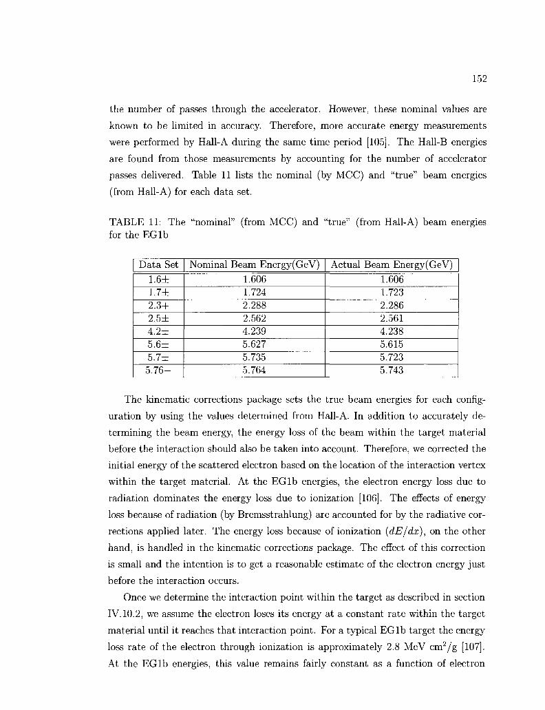
152
the number of passes through the accelerator. However, these nominal values are
known to be limited in accuracy. Therefore, more accurate energy measurements
were performed by Hall-A during the same time period [105]. The Hall-B energies
are found from those measurements by accounting for the number of accelerator
passes delivered. Table 11 lists the nominal (by MCC) and "true" beam energies
(from Hall-A) for each data set.
TABLE 11: The "nominal" (from MCC) and "true" (from Hall-A) beam energies for the EG lb
Data Set
1.6± 1.7± 2.3+ 2.5± 4.2± 5.6± 5.7± 5.76-
Nominal Beam Energy(GeV)
1.606 1.724 2.288 2.562 4.239 5.627 5.735 5.764
Actual Beam Energy(GeV)
1.606 1.723 2.286 2.561 4.238 5.615 5.723 5.743
The kinematic corrections package sets the true beam energies for each config
uration by using the values determined from Hall-A. In addition to accurately de
termining the beam energy, the energy loss of the beam within the target material
before the interaction should also be taken into account. Therefore, we corrected the
initial energy of the scattered electron based on the location of the interaction vertex
within the target material. At the EGlb energies, the electron energy loss due to
radiation dominates the energy loss due to ionization [106]. The effects of energy
loss because of radiation (by Bremsstrahlung) are accounted for by the radiative cor
rections applied later. The energy loss because of ionization (dE/dx), on the other
hand, is handled in the kinematic corrections package. The effect of this correction
is small and the intention is to get a reasonable estimate of the electron energy just
before the interaction occurs.
Once we determine the interaction point within the target as described in section
IV. 10.2, we assume the electron loses its energy at a constant rate within the target
material until it reaches that interaction point. For a typical EGlb target the energy
loss rate of the electron through ionization is approximately 2.8 MeV cm2/g [107].
At the EGlb energies, this value remains fairly constant as a function of electron

153
momentum. Moreover, the dE/dx corrections can safely be generalized for all targets
in the experiment because it basically depends of the ratio of the atomic number over
the mass number (Z/A), which is roughly the same for all the EGlb targets. Energy
loss is calculated by:
Therefore,
A£[MeV] = 2.8 \pJoalJoa + pHelHe + PAUSZ] (245)
where pfoidfoU, PHelHe and PA^A represent the mass thickness for the window foils,
the liquid Helium and the ammonia target respectively while Sz is the fraction of the
target length the electron traveled within the ammonia target. In this correction, we
used typical values (estimated from the previous analysis of 1.6 and 5.7 GeV data
sets [17] [77]) for these parameters: pfoiilfoii = 0.1 g/cm2 ; pHelHe = 0.3 g/cm2 ; pAlA
= 0.6 g/cm2 ; Sz = (zave — zc + 0.5)/LA where LA = 1 cm (physical length of the
ammonia target) and zc = -55.1 (the target center position). It should also be noted
that vertex positions zave and zc are negative numbers. The average energy loss of
the electron because of ionization varies around 2-3 MeV depending on the vertex
position zave. The energy loss determined from Eq. (245) is subtracted from the true
beam energy, listed in Table 11, for each event.
IV.10.5 Multiple Scattering and Magnetic Field Corrections
Two additional effects that are known to affect the momentum reconstruction are:
• The possible angular distortions that may come from multiple scattering expe
rienced by the detected particles.
• The effects of the target magnetic field that extend into the far regions of the
detector.
While the scattered particles travel through the material in their path, they expe
rience multiple scattering within that material. The net result of these multiple
scatterings can distort the angular distribution of the particles when they are de
tected because the reconstruction code (RECSIS) does not account for these effects.
Moreover, the angular distortion can cause the reconstructed vertex position for each
particle to shift from its true place. Fig. 62 shows an artistic visualisation of this

154
FIG. 62: Artistic visualization of the effect of multiple scattering on the angular distributions and the vertex positions of each scattered particles (by R. Fersch). The black arrows show the true angles while the blue dotted lines show the apparent angles that the reconstruction code would supply.
situation for two scattered particles. In addition to the multiple scattering, the ef
fect of the target magnetic field beyond Region 1, which will be referred to as stray
magnetic field, was not incorporated into the RECSIS code during the EGlb data
reconstruction. The reconstruction code only accounted for the target magnetic field
in the vicinity of the target.
The GEANT simulation package for the CLAS detector (GSIM) [102] was used
in order to understand the overall results of these effects on the kinematics of the
detected particles and determine the necessary corrections. The GSIM package was
updated to incorporate a reasonably accurate model of the EGlb target. A large
random sample of particles was generated by using the GSIM package and recon
structed with the same version of the RECSIS code that was used for the EGlb
data reconstruction. The original and the reconstructed quantities were compared to
isolate the effects of the multiple scattering and the stray magnetic field on the kine
matics of some detected particles, mainly electrons and protons. It was realized that
the required corrections could be parametrized by simple formulas and eventually
applied to all charged particles. The details of this study can be found in [103].
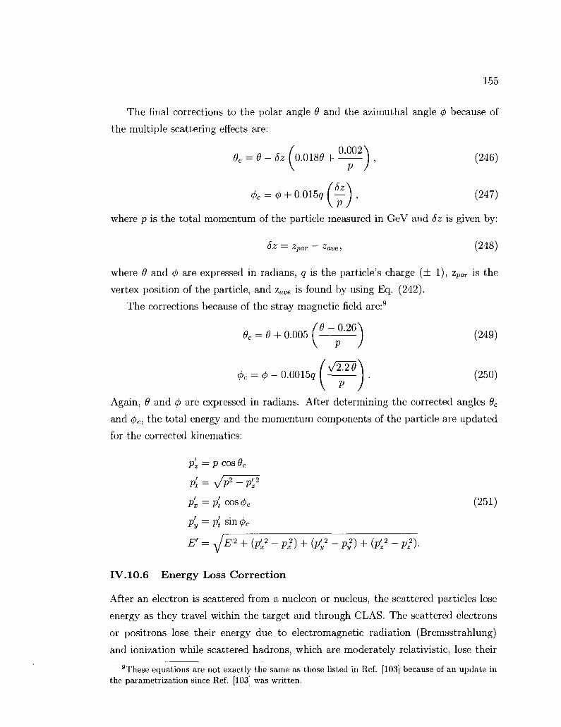
155
The final corrections to the polar angle 9 and the azimuthal angle 0 because of
the multiple scattering effects are:
9C = 9 - 5z (o.Ol89 + ™®\ ; (246)
4>c = 0 + 0 . 0 1 5 g ( — V (247)
where p is the total momentum of the particle measured in GeV and 5z is given by:
oz Zpar Zdye, ^z toj
where 9 and <f> are expressed in radians, q is the particle's charge (± 1), zpar is the
vertex position of the particle, and zave is found by using Eq. (242).
The corrections because of the stray magnetic field are:9
9C = 9 + 0.005 ^ ~ 0 " 2 6 ) (249)
{¥) 4>c = 4>- 0.0015q ^—— . (250)
Again, 9 and </> are expressed in radians. After determining the corrected angles 9C
and <fic, the total energy and the momentum components of the particle are updated
for the corrected kinematics:
p'z = p cos 9C
Pt = VP2 ~ P'z2
Px = Pt c o s 4>c (251)
P'y = P't s i n <t>c
E'=^E* + ( ^ - px2) + (P;2 - p%) + (p'z
2 - pi).
IV. 10.6 Energy Loss Correction
After an electron is scattered from a nucleon or nucleus, the scattered particles lose
energy as they travel within the target and through CLAS. The scattered electrons
or positrons lose their energy due to electromagnetic radiation (Bremsstrahlung)
and ionization while scattered hadrons, which are moderately relativistic, lose their
9These equations are not exactly the same as those listed in Ref. [103] because of an update in the parametrization since Ref. [103] was written.

156
energy primarily due to ionization and atomic excitations. The energy loss of the
electron due to radiation is handled by the radiative corrections, which are applied
later in the analysis. The mean rate of energy loss due to ionization (also called
stopping power) is best described by the Bethe-Bloch formula [108]:
TABLE 12: Parameter definitions in Bethe-Bloch Formula
Symbol
c
P 7 mec
2
re
NA
''max
K
P
z Z A I
Definition
Speed of light v/c of the incident particle
i/Vi - P2
Electron mass x c2
Classical electron radius Avogadro's number Maximum energy transfer AnNArl mec
2
Density of absorbing material Charge of incident particle Atomic number of absorber Atomic mass of absorber Mean excitation energy
Unit or Value
299 792 458 m/s
0.510998 918(44) MeV e2/47re0mec
2 = 2.817940 325(28) 6.0221415(10) x 1023 mol"1
MeV 0.307075 MeV g-1 cm2
gr/mol
electron charge (e)
g/mol MeV
fm
dx = P K A/32
1. (2mec2f32
12Wmax
2 l n P 01 (252)
The definitions and values of the variables in the Bethe-Bloch formula are given in
Table 12. In the equation we used the following approximations:
Wmax = 2mec2/327
2,
Z/A = 0.5,
7 = 90 xlO"6 MeV.
(253)
Therefore, we can write Eq. (252) in its final form that we used in the kinematic
corrections package:
dx
0.5 0.307 x — x In
2^,2 2 x 0.511/j27:
90 x 10-6 I? (254)
Since the correction is applied only to charged particles of q = ± 1 , we used z = 1.
The energy loss AE can be calculated by approximating dE/dx = AE/Ax, which is

157
a safe approximation for high energies and thin target. Therefore, we can write Eq.
(254) as:
-AE[MeV] = PAxRE (255)
where RE represents the rate of collisional energy loss and is given by the (3 dependent
factor in square bracket in Eq. (254) while pAx is given by:
pAx[g/cm2} = [pfoulfou + pHelne + PAUSZ]/ cos 9 (256)
where pfoulfou = 0.1 g/cm2 is the mass thickness of the window foils, pne^He = 0.3
g/cm2 is the mass thickness of the liquid Helium and PAIA = 0.6 g/cm210 represents
the mass thickness of the ammonia target while 6z, the fraction of a distance the
electron traveled within the ammonia target, is 5z = (zave — zc + 0.5)/L^ where L^ =
1 cm (physical length of the ammonia target), zc = -55.1 (the target center position)
and zave is calculated by Eq. (242).n All the lengths should be divided by cos#
because the scattered particle traverses the target material with an angle of 9, which
increases the effective length by a factor of l /cos#. For electrons and positrons we
assumed a constant rate of energy loss at RE = 2.8 MeV cm2/g. For hadrons, RE
is calculated by using the expression in Eq. (254). Once — AE is calculated, the
absolute value of the energy loss needs to be added to the measured energy so that
the true scattering energy can be determined. Therefore, we determined the final
corrected kinematics (£", p'x, p'y, p'z) of the scattered particle at the scattering point
in terms of the uncorrected kinematics (E, px, py, pz) as:
E' = E + | - AE\
12 j-i/2 m2 , 2 , 2 , 2
P =E ~E +PX+Py+PZ
P'X=PX>< p'/p (257)
Py = Py X P/P
p'z=pzx p'/p
where p represents the measured total vector momentum of the particle. At this
point, the kinematics of the scattered charged particles are corrected for all quantifi
able effects at the first order. Now we are ready to apply the minimization of missing
energy and momentum to determine the final part of the kinematic corrections.
10The average density of 15NH3 and 15ND3 targets is PA ~ 1 g/cm3 and the average effective length for the ammonia targets is ~ 0.6 cm
nBecause of resolution limits, the average vertex occasionally ended up outside the target window. In that case, the vertex was assumed to be on the target edge for purposes of the dE/dx calculations.

158
IV. 10.7 Momentum Correction
The purpose of the corrections described in the previous sub-sections is to obtain
the best possible information for the kinematics of the scattered particles. After
these corrections are applied, there are still unaccounted effects that will change
the reconstructed kinematics of the detected particles from their true values. These
effects include:
1. Misalignment of the drift chamber wires or drift chambers themselves relative
to their nominal positions, or wire sag.
2. Incomplete map of all drift chamber wires passed to the tracking code
3. Wrong or incomplete magnetic field map used by the reconstruction code.
Unfortunately, there is no exact way to account for such effects. Therefore, we need
to rely on the data to understand the cumulative results of the unknown effects and
correct them based on available information.
There are many different momentum correction schemes for the CLAS detector.
For the EGlb experiment we used the technique developed by Sebastian Kuhn and
Alexei Klimenko [109]. This technique is based on the selection of well-identified
elastic ep —> ep events as well as at least one channel of multi-particle final states and
utilizes four-momentum conservation. Having multi-particle final states in the data
sample helps to cover lower hadron momenta and avoids strong kinematic correlation
between angle and momentum in the elastic events. We chose ep7r+7r~ as our multi-
particle final state. Once the data were obtained and corrected for all the effects
described earlier, we went over all events one by one to determine the four-momentum
of each particle in the event and applied a parametrized correction to it. By summing
over all particles in the event, we determined the total final four-momentum of the
event. We also calculated the total initial four-momentum of each scattering event
by using the corrected beam energy and the target mass, for which, we used the
proton mass because our data for the fit was obtained from NH3 runs. By taking
the difference between the total initial and final four-momentum of the scattering
event, we determined the total missing four-momentum of the event. Ideally the
missing four-momentum for each event should exactly be zero. However, for each
component of the missing four-momentum (E[miss], px[miss], py[miss], Pz[miss]), we get a
Gaussian distribution. These distributions can be minimized by optimizing the value
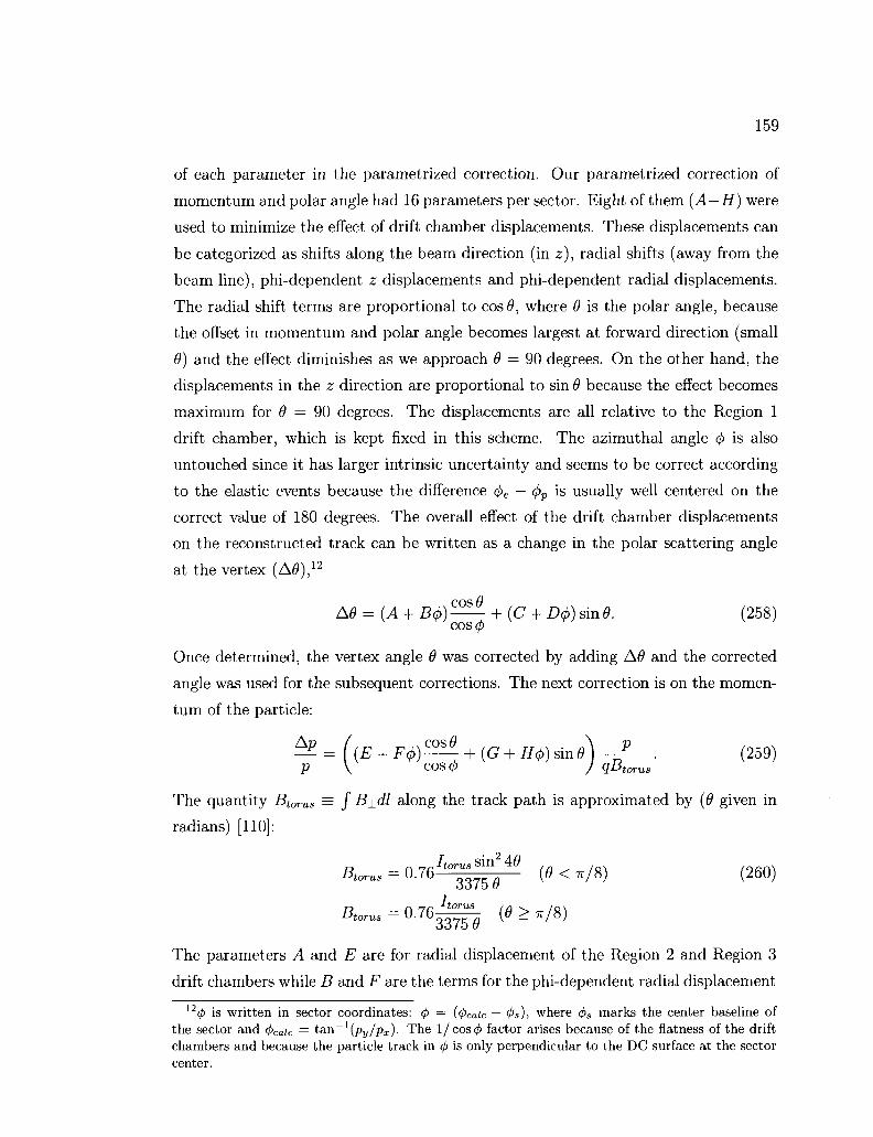
159
of each parameter in the parametrized correction. Our parametrized correction of
momentum and polar angle had 16 parameters per sector. Eight of them (A—H) were
used to minimize the effect of drift chamber displacements. These displacements can
be categorized as shifts along the beam direction (in z), radial shifts (away from the
beam line), phi-dependent z displacements and phi-dependent radial displacements.
The radial shift terms are proportional to cos#, where 8 is the polar angle, because
the offset in momentum and polar angle becomes largest at forward direction (small
6) and the effect diminishes as we approach 8 = 90 degrees. On the other hand, the
displacements in the z direction are proportional to sin 8 because the effect becomes
maximum for 8 = 90 degrees. The displacements are all relative to the Region 1
drift chamber, which is kept fixed in this scheme. The azimuthal angle (j) is also
untouched since it has larger intrinsic uncertainty and seems to be correct according
to the elastic events because the difference cj)e — <pp is usually well centered on the
correct value of 180 degrees. The overall effect of the drift chamber displacements
on the reconstructed track can be written as a change in the polar scattering angle
at the vertex (A8),n
cos 0 A8 = (A + B(t>) - + (C + D<f>) sin 8. (258)
COSip
Once determined, the vertex angle 8 was corrected by adding A8 and the corrected
angle was used for the subsequent corrections. The next correction is on the momen
tum of the particle:
^ = ((E + F</>)^- + (G + H<t>)sme)-?—. (259) P V COS(P / Q&torus
The quantity Bt(yrus = J B±dl along the track path is approximated by (8 given in
radians) [110]:
Btorus = 0 - 7 6 J t o 3 3 ^ ( 0 < T T / 8 ) (260)
Btorus = °-76^58 ^ - ^
The parameters A and E are for radial displacement of the Region 2 and Region 3
drift chambers while B and F are the terms for the phi-dependent radial displacement
12 (ft is written in sector coordinates: 4> = (<t>caic — 0s )> where <f>s marks the center baseline of the sector and <j>ca.ic = tan-1(py/'px). The l /cos0 factor arises because of the flatness of the drift chambers and because the particle track in 4> is only perpendicular to the DC surface at the sector center.
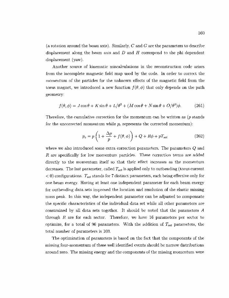
160
(a rotation around the beam axis). Similarly, C and G are the parameters to describe
displacement along the beam axis and D and H correspond to the phi dependent
displacement (yaw).
Another source of kinematic miscalculations in the reconstruction code arises
from the incomplete magnetic field map used by the code. In order to correct the
momentum of the particles for the unknown effects of the magnetic field from the
torus magnet, we introduced a new function /(#,</>) that only depends on the path
geometry:
/ ( M ) = J cos 9 + K sin 9 + L/63 + {M cos 9 + N sin 9 + 0/93)<f). (261)
Therefore, the cumulative correction for the momentum can be written as (p stands
for the uncorrected momentum while pc represents the corrected momentum):
Pc = p (l + ^ + f(9,<f>)\+Q + R<j) + PTset (262)
where we also introduced some extra correction parameters. The parameters Q and
R are specifically for low momentum particles. These correction terms are added
directly to the momentum itself so that their effect increases as the momentum
decreases. The last parameter, called Tset is applied only to outbending (torus current
< 0) configurations. Tset stands for 7 distinct parameters, each being effective only for
one beam energy. Having at least one independent parameter for each beam energy
for outbending data sets improved the location and resolution of the elastic missing
mass peak. In this way, the independent parameter can be adjusted to compensate
the specific characteristics of the individual data set while all other parameters are
constrained by all data sets together. It should be noted that the parameters A
through R are for each sector. Therefore, we have 16 parameters per sector to
optimize, for a total of 96 parameters. With the addition of Tset parameters, the
total number of parameters is 103.
The optimization of parameters is based on the fact that the components of the
missing four-momentum of these well identified events should be narrow distributions
around zero. The missing energy and the components of the missing momentum were

161
calculated for the elastic events,
Px[miss] Px[e] Px[p]
Py[miss) Py[e] Py\p]
Pz\miss\ — EB ~ Pz[e] ~ Pz[p] (263)
E[miSS] = EB + Mp — Ee — Ep
where EB is the beam energy, Mp is proton mass, E'e, •, is the energy of the scattered
electron (proton) and px[e{p))i Py[e(p)], Pz[e(p)] a r e the x, y and z components of the
momentum of the electron (proton). Similarly for the epir+ir~ events, the components
of the missing four-momentum were calculated by:
Px[miss] = Px[e] Px\p] Px[tr~] Px[w+]
Py[miss] = — Py[e] ~ Py\p] ~ Py\-n~] ~ Py[ir+]
Pz[miss] = EB - pz[e] - pz[p] - p z [ 7 r - ] - p 2 [ 7 r+] (264)
E[miss] = EB + Mp — E'e — E'p - E'n- — E'n+.
Then the x2 of the fit was evaluated by adding the squares of each component,
normalized to the expected resolution of that component,
( v2 v2 v2 E2 \
rx[miss] fy[miss} ^zjmiss] [miss] \ C2651 aL aPy al aE J
The expected resolutions for the missing four-momentum components were set to
aPx = aPy = 0.014 GeV and oVz = aE = 0.020 GeV. We used MINUIT [111] to
minimize the x2 a n d optimize all the parameters in the correction formula. For each
elastic event, we also added another term to the total \2'-
A 2 v - ({Wcalc-Mpf\ A X = £ (,(0.020GeV)2J
(266)
elas-events x
where Mp is proton mass and Wcaic is the missing mass of the inclusive elastic event.
After looping over all events (elastic and multi-particle final states for both inbending
and outbending configurations), an additional term was added to the total \ 2 f° r e a c h
parameter:
parm=0 °Vo.rm

162
The reason of the last addition is to limit the parameters to reasonable ranges and
avoid run-away solutions in some corner of the parameter space. An intrinsic un
certainty of 0.01 was used for parameters F and H. For parameters Q and R, the
uncertainty was set to 0.003. For the rest of the parameters, the intrinsic uncertainty
was set to 0.001.
It should be noted that the momentum correction fit is an iterative procedure.
Initially we begun with all parameters set to zero and ran the minimization rou
tine. We determined the parameter values that minimized the x2- Then we used
those parameters as initial parameters and ran the minimization again. We contin
ued the iteration until the parameter values were stabilized. During the iteration,
we also tightened the data sample by applying the intermediate correction. Once
we determined the optimal values of all parameters that minimized the overall x2>
the parameters were frozen together with all applied corrections. Since this data
driven correction absorbs all unknown effects that previous corrections missed, the
parameters really belong not only to the momentum correction part of the kinematic
corrections package but also to all previous corrections applied before this stage.
Data selection for the momentum correction fit
The data selection is very important for the success of the momentum correction
scheme. As we mentioned earlier, we used elastic ep —> ep and inelastic ep —> epir+Tr~
events. Of course, the elastic events are the most reliable events in terms of correctly
identifying the final state and they do a good job of fixing the kinematics around
the elastic peak. However, we also needed to incorporate some inelastic events into
the data sample in order to ensure a reasonable fit for all kinematics including the
resonance and the DIS regions. The next final state we have in the EGlb data with
enough statistics that can be used for this purpose is ep —> epn+ir~ events. While
determining these events, particle identifications should be made carefully.
For electrons, we applied the cuts listed in Table 13. The cuts for proton iden
tification can be found in Table 14. One element in the table, the proton ID cut,
is a cut specially applied only for hadrons based on the time of flight information
of the particle. When the particle is found in the event and if it is not an electron,
its expected time of flight {TOFcaic) is calculated by using the start time, the path

163
TABLE 13: Electron cuts applied for the momentum correction data sample.
particle charge = -1 good helicity selection one electron per event
p > 0MEB
P<EB
0 < flag < 5 or 10 < flag < 15 triggerbit cut (see section IV.7.2)
^Cnphe > 2.0 ECtot/p > 0.21
ECin > 0.06 -58.0 < zvertex < -52.0
5° < 9 < 49°
length and the momentum of the particle:
TOFcalc = StartTime + PathLength
(268) c^p2/{p2 + M2)
The TOFcaic is calculated by assuming the hadron is a proton, pion, kaon or deuteron
and using the corresponding mass values. Then the calculated TOF for each particle
is compared to the time of flight registered by the TDC during the experiment. The
hadron type that gives the smallest difference between the calculated TOF and the
measured value is tagged to that particle. This is a preliminary method to determine
the hadron type.
After the preliminary cuts that include charge, helicity and ID cuts, the initial
kinematic corrections were applied to the particle and more precise cuts were applied
afterward. The difference between the measured and calculated TOF (see Eq. (268))
is calculated again for the particle and a cut is applied on At. The At distribution
for the proton can be seen in Fig. 63.
The cuts applied to select the elastic ep —»• ep events are listed in Table 15. In the
table, (f)p — (pe represents the difference between the azimuthal angles of the electron
and proton while 0P — 6Q is the difference between the polar angles of the proton and
the virtual photon, where 6Q was calculated by:
EL sin 6P 9Q = tan l
E- E'ecos9e (269)

164
300
250
200
150
100
50
x103
- \ dt_prot |
r
'-
j-
j-
" . , , , i , , , , i
°-2 -1.5 -1 i T. i . .
-0.5 , I ,
0
\ \
Entries 2.5946S4e+07
Mean 0.112
RMS D.2995
\
\
\
I
0.5 1 1.5 2
FIG. 63: Difference between measured and expected time of flight (in ns) for protons in EGlb. The plot shown has cuts for regular proton selections (see section IV.13). For the momentum correction data sample, a slightly tighter cut on the positive side, At < 0.6 ns, was applied.
TABLE 14: Proton cuts applied for the momentum correction data sample.
particle charge = +1 good helicity selection
electron found in the event
one proton per event proton ID cut (see text)
not the first particle in the event -0.8 < At < 0.6
0 < 49° -58.0 < vz < -52.0
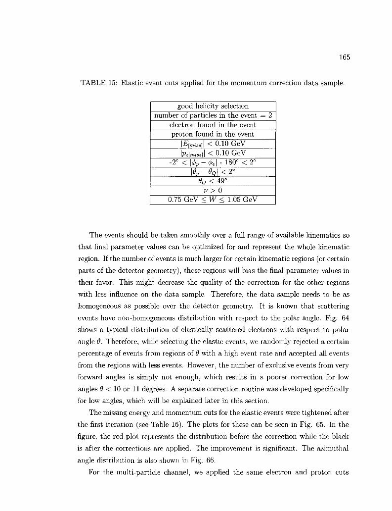
165
TABLE 15: Elastic event cuts applied for the momentum correction data sample.
good helicity selection number of particles in the event = 2
electron found in the event proton found in the event
\Elmiss]\ < 0.10 GeV
\Pz\misa]\ < 0-10 GeV -2° < \4>p-<f>e\ - 180° < 2°
\0P — BQ\ < 2° 9Q < 49°
v > 0 0.75 GeV < W < 1.05 GeV
The events should be taken smoothly over a full range of available kinematics so
that final parameter values can be optimized for and represent the whole kinematic
region. If the number of events is much larger for certain kinematic regions (or certain
parts of the detector geometry), those regions will bias the final parameter values in
their favor. This might decrease the quality of the correction for the other regions
with less influence on the data sample. Therefore, the data sample needs to be as
homogeneous as possible over the detector geometry. It is known that scattering
events have non-homogeneous distribution with respect to the polar angle. Fig. 64
shows a typical distribution of elastically scattered electrons with respect to polar
angle 9. Therefore, while selecting the elastic events, we randomly rejected a certain
percentage of events from regions of 6 with a high event rate and accepted all events
from the regions with less events. However, the number of exclusive events from very
forward angles is simply not enough, which results in a poorer correction for low
angles 9 < 10 or 11 degrees. A separate correction routine was developed specifically
for low angles, which will be explained later in this section.
The missing energy and momentum cuts for the elastic events were tightened after
the first iteration (see Table 16). The plots for these can be seen in Fig. 65. In the
figure, the red plot represents the distribution before the correction while the black
is after the corrections are applied. The improvement is significant. The azimuthal
angle distribution is also shown in Fig. 66.
For the multi-particle channel, we applied the same electron and proton cuts

166
15 20 25 Theta DC1
30 35 40 15 20 25 30 35 Phi DC1
40 45 50
FIG. 64: Distribution in 6 (left) and <f> (right) of elastic ep events for the 4.2 GeV outbending data. The 9 distribution has a strong kinematic dependence while the (f> distribution is flat.
TABLE 16: Second iteration cuts for the elastic events.
\Px[miss]
\Py[miss]
\Pz[miss]
1 P1
\J-J\miss\
- 1 ° < \<f>p -
< 0.055 GeV < 0.055 GeV < 0.060 GeV < 0.060 GeV
- <j>e\ - 180° < 1°

167
P„(miss) electron for all sectors |
10000
8000
6000
4000
2000
Entries 88745
Mean -0.0003785
RMS 0.03637
Entries B8745
Mean -0.001239
RMS 0.03205
).3 -0.2 -0.1 0 0.1 0.2 0.3
I Py(miss) electron for all sectors
10000
8000
6000
4000
2000
;
I
= 1
l
I -%.3 -0.2 -0.1 0 0.1
Entries 88745
Mean 4.001028
RMS 0.03376
I Entries 88745
Mean 0.0003S8B
RM5 0.03049
0.2 0.3
Pz(miss) electron for all sectors |
6000
5000
4000
3000
2000
1000
4
Entries 8874S
Mean -0.01447
RIMS 0.05087
Entries 88745
Mean 0.006911
RMS 0.0453E
3 -0.2 -0.1 0.1 0.2 0.3
E(miss) electron for all sectors |
5000
4000
3000
2000
1000
4
- J
~ J
\.J , I7 !7J
3 -0.2 -0.1 0 0.1
Entries 88745
Mean -0.01127
RMS 0.0S5S9
I
Entries 8874S
Mean 0.012
RMS 0.0496
0.2 0.3
FIG. 65: Missing energy and momentum distributions from elastic events in the EGlb data. Beam energy = 4.2 GeV; Torus = -2250 A; Target is NH3. The red line is before and the black line is after the correction.
4000
3500
3000
2500
2000
1500
1000
500
z j phi_elas | .FL,
j j \
'- / \
Entries 285606
Mean -0.07185
RMS 2.257
FIG. 66: The difference between electron and proton azimuthal angles for elastic scatterings after subtracting 180 degrees. (Beam energy = 4.2 GeV; Torus = -2250 A; Target is NH3).
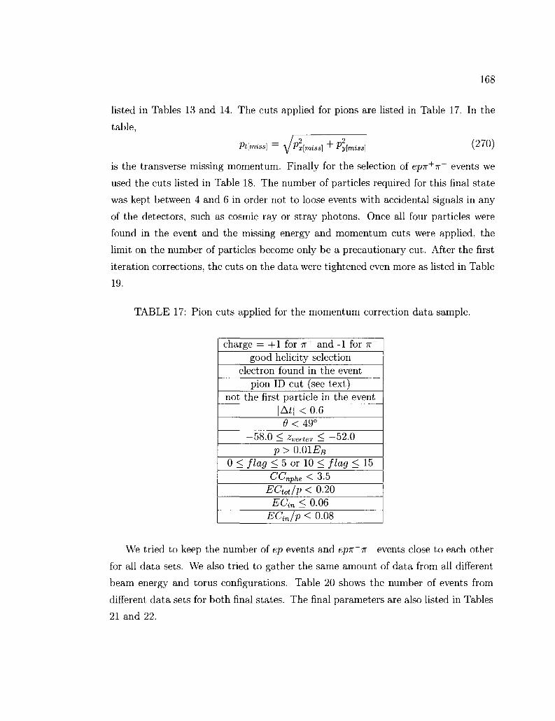
168
listed in Tables 13 and 14. The cuts applied for pions are listed in Table 17. In the
table,
Pt[miss] = yPx[miss] + Py[miss] (2^)
is the transverse missing momentum. Finally for the selection of epir+ir~ events we
used the cuts listed in Table 18. The number of particles required for this final state
was kept between 4 and 6 in order not to loose events with accidental signals in any
of the detectors, such as cosmic ray or stray photons. Once all four particles were
found in the event and the missing energy and momentum cuts were applied, the
limit on the number of particles become only be a precautionary cut. After the first
iteration corrections, the cuts on the data were tightened even more as listed in Table
19.
TABLE 17: Pion cuts applied for the momentum correction data sample.
charge = +1 for TT+ and -1 for TT~ good helicity selection
electron found in the event pion ID cut (see text)
not the first particle in the event ~ \At\ < 0.6
e < 49° —58.0 < zvertex < —52.0
p > 0.01EB
0 < flag < 5 or 10 < flag < 15
(st'nphe < "J.5 ECtot/p < 0.20 ~
ECin < 0.06 ECin/p < 0.08
We tried to keep the number of ep events and ep7r+7r~ events close to each other
for all data sets. We also tried to gather the same amount of data from all different
beam energy and torus configurations. Table 20 shows the number of events from
different data sets for both final states. The final parameters are also listed in Tables
21 and 22.

35000
30000
25000
20000
15000
10000
5000
0
-1 dt_pim | f\
- . . . i , , , r . , i , , , i . , , i , , , i , , , i
Entries 4137833 Mean -0.0104 RMS 0 2145
r~n 1 -0.8 -0.6 -0.4 -0.2 0 0.2 0.4 0.6 0.8 1
90000
eoooo
70000
60000
50000
40000
30000
20000
10000
0
: ! "t_pip |
L
------
L *S
: , , , ! , , , , 1 -0.8 -0.6 -0.4 -0.2 , | , 0 0.2
Entries 1.295625e+07
Moan -0.005951
RMS 0.2307
0.4 0.6 0.8
( a ) 7T- ( b ) TT-t
FIG. 67: Difference between the measured and expected time of flight for -n and 7r+
TABLE 18: First iteration ep7r+7r cuts for the momentum correction data sample.
good helicity selection 4 < number of particles < 6
electron found proton found
7r+ found 7r found
\Eu < 0.12 GeV
IP. < 0.12 GeV \Pt[miss}\ < 0-10 GeV
TABLE 19: Second iteration cuts for the epir+ir events.
\Pt\miss)\ < 0.055 GeV |p*M„ll < 0.060 GeV \E{miss]\ < 0.060 GeV
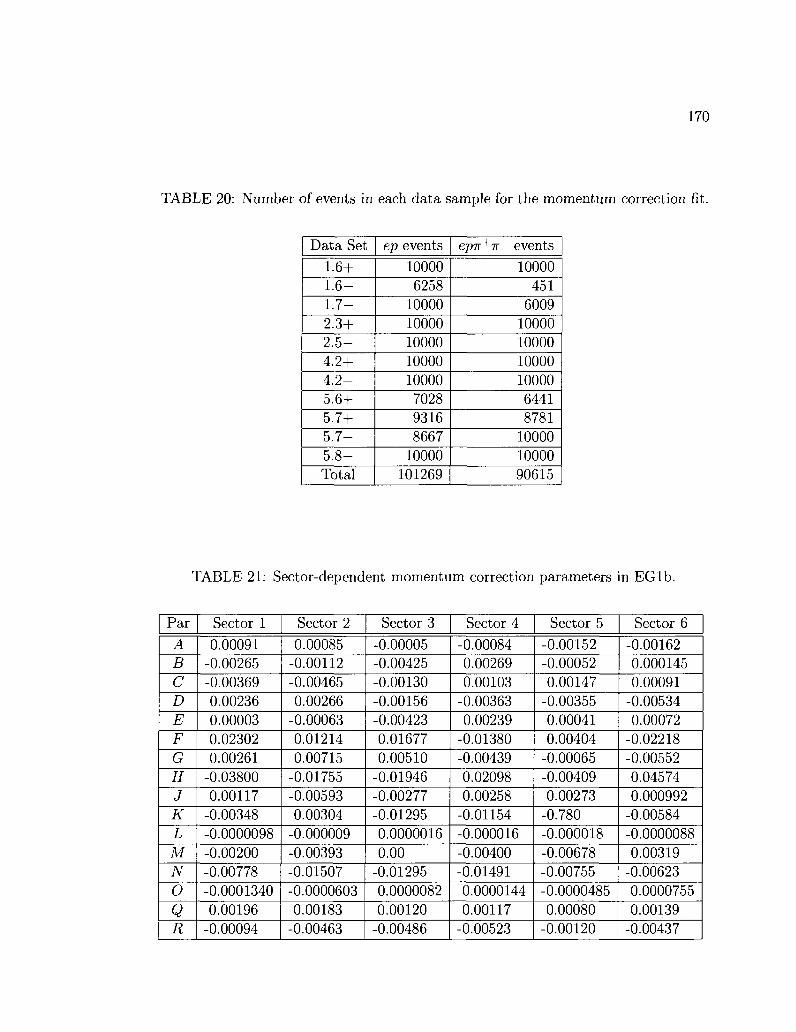
170
TABLE 20: Number of events in each data sample for the momentum correction fit.
Data Set
1.6+ 1.6-
1.7-2.3+ 2.5-4.2+
4.2-5.6+ 5.7+
5.7-5.8-Total
ep events
10000 6258 10000 10000 10000 10000 10000 7028 9316 8667 10000 101269
ep7r+7r events
10000 451 6009 10000 10000 10000 10000 6441 8781 10000 10000 90615
TABLE 21: Sector-dependent momentum correction parameters in EGlb.
Par
A B C D E F G H J K L M N O Q R
Sector 1
0.00091 -0.00265 -0.00369 0.00236 0.00003 0.02302
0.00261 -0.03800 0.00117 -0.00348 -0.0000098 -0.00200 -0.00778 -0.0001340 0.00196 -0.00094
Sector 2
0.00085 -0.00112 -0.00465 0.00266 -0.00063 0.01214 0.00715 -0.01755 -0.00593 0.00304 -0.000009 -0.00393 -0.01507 -0.0000603 0.00183 -0.00463
Sector 3
-0.00005 -0.00425 -0.00130 -0.00156 -0.00423 0.01677 0.00510 -0.01946 -0.00277 -0.01295 0.0000016
0.00 -0.01295 0.0000082
0.00120 -0.00486
Sector 4
-0.00084 0.00269 0.00103 -0.00363 0.00239 -0.01380 -0.00439 0.02098 0.00258 -0.01154
-0.000016 -0.00400 -0.01491 0.0000144 0.00117 -0.00523
Sector 5
-0.00152 -0.00052
0.00147 -0.00355 0.00041 0.00404 -0.00065 -0.00409 0.00273 -0.780 -0.000018 -0.00678 -0.00755
-0.0000485 0.00080 -0.00120
Sector 6
-0.00162 0.000145 0.00091 -0.00534 0.00072 -0.02218 -0.00552 0.04574 0.000992 -0.00584 -0.0000088
0.00319 -0.00623 0.0000755 0.00139 -0.00437

171
TABLE 22: Beam energy and torus current dependent parameters, Tset, for outbend-ing data sets.
Data set
1.6-1.7-2 . 5 -4 . 2 -5 .6-
5.73-5.76-
Tset
-0.000159 0.000705 0.000308 0.003203
-1.64xl0"1 2
0.000854 -0.000589
IV. 10.8 Patch Correction
The momentum correction relies on the elastic and inelastic events in the data for
minimization of missing four-momentum. The amount of those events at extremely
small angles is rather limited. Moreover, there is a complex magnetic field around
the target that mainly affects scattered particles at small angles. Therefore, even
after the momentum corrections were applied, we still saw a deviation of the elastic
peak in the W spectrum from its true value and also a strong dependence of the
elastic peak position on the azimuthal angle in this angular range. This means that
because of the lack of sample events at these small angles, the momentum correction
has failed to account for the complex magnetic field which is especially important
at small angles. Even if there are not many ep and epTT+Tr~ events at these forward
angles (this is mainly an acceptance problem for protons), there are many inclusive
e~ events that can be used for our analysis.
A patch correction that can be applied on top of the momentum correction was
developed by Peter Bosted to correct specifically the scattering events at small angles.
The correction simply utilizes the linear dependence of the elastic peak position on
the azimuthal angle and uses a fit function to minimize that dependence over selected
events in the range of small polar angles. The fit function also includes a 0 dependent
term to smoothly merge the small angle correction and large angle correction. The
functional form of the correction is:
Ap = 0.02 u+w + x^t-vrMf (271)

172
where U, V and X are the fit parameters that should be determined separately for
each sector and torus current configuration. The latter depends on the sign of the
product of the torus polarity and particle's charge. If torus x charge is positive,
the particle's configuration is outbending (particle's trajectory is bent away from the
beam line), otherwise it is inbending (toward the beam line). The polar (9) and
the azimuthal (</)) angles were taken from the Region 1 drift chamber. In order to
determine the parameter values, the data were separated into 9 and <j> bins for each
sector. For 9, 1° bins and for (j> 10° bins were used during the fit procedure. The elastic
peak W position was determined for each bin. The correction requires the elastic peak
position to be calculated as precisely as possible with all background contributions
removed. Since we have NH3 and ND3 data together for all beam energies (except
2.3 GeV data13), the ratio of NH3 to ND3 scattering events were used to obtain a
more precise elastic peak distribution. In the ratio, the 15N background cancels out
leaving the ratio of the free proton elastic peak to the deuteron quasi-elastic peak.
The resulting elastic peak is narrower and the position is more precise. Fig. 68
shows an example of this peak ratio for 6 </> bins in sector 1 before the corrections
were made.
Once the elastic peak position was determined for each sector, 6 and 0 bin, the
MINUIT minimization package was used to minimize the difference between the
elastic peak position and the proton mass and determine the fit parameters in Eq.
(271). The fit was made separately for each sector and for inbending and outbending
torus configurations. The patch correction is designed to be only effective in the
forward angle region; its effect quickly diminishes as we go to higher angles and the
standard momentum correction takes over there. The effectiveness of this correction
depends on the abundance of inclusive NH3 and ND3 data at small polar angels.
Therefore, the correction was good for outbending data and low beam energies. The
patch correction was applied only to the 1.6 GeV inbending and outbending data
sets and the 1.7, 2.5 and 4.2 GeV outbending data sets. The final values of these
parameters are listed in Table 23.
13Since ND3 data is not available for 2.3 GeV beam energy, 12C was used to remove the background contribution. However, in the end, the patch correction was not applied to this data set.

173
0,85 ~~ " " 0.90 ' 0.95 1.00" 1.05 W IGeVS
FIG. 68: Ratios of NH3/ND3 spectra for six different (f> bins in Sector 1 for 6 < 13°, separated by an arbitrary offset for visibility. Corrections are needed in this angular range to remove the dependence of the peak position on the azimuthal angle and center the peak at the proper elastic value of W = 0.938 GeV. Plot courtesy P. Bosted.
TABLE 23: Forward angle momentum correction parameters for the EG lb experiment. The sign of torus x charge determines which set (inbending or outbending) should be applied for the particle.
Parameter
Outbending U V X
Inbending U V X
Sector 1 Sector 2 Sector 3 Sector 4 Sector 5 Sector 6
-0.0472 -0.2235 -0.2730
-0.0378 -0.1650 -0.1789
-0.2485 -0.0532 -0.4687
-0.0066 -0.2370 -0.1929
0.0257 -0.2588 -0.1733
-0.5182 0.1406 -0.2743
-0.2238 0.2786 -0.963
-0.2621 0.3348 -0.748
-0.0024 -0.4065 0.713
-0.1918 0.3624 0.591
-0.1217 0.2378 -0.032
-0.1203 0.1846 -1.070

174
IV. 10.9 Overall Results of the Kinematic Corrections
In order to evaluate the overall effect of the kinematic correction package, we mon
itored various different dependencies. The missing energy and momentum distribu
tions for each sector before and after each correction were monitored. In addition,
the AE'/E' vs. 4> and W versus <f) behaviors of the elastic peak from the inclusive
events were examined in different 9 bins. Tables 24 and 25 list the polar and az-
imuthal angle bins used to generate these plots. AE'/E' is the difference between
the expected and measured energy of the scattered electron,
A C 1 ' nv zpi L±I-J ^theo rneas (079}
E' Etheo
The expected energy E'theo for the electron in elastic scattering was calculated by
_ MEB
&theo- M + £ B ( 1 _ C O S 0 ) W
where we used Eqs. (20), (21) and (22), with W = M for the elastic events. Finally
AE'/E' was plotted with respect to <f>.
In the remainder of this section, we will present these monitored distributions
before and after the kinematic corrections were applied. Fig. 69 shows the change
in the missing energy distribution of the elastic events separately for different sec
tors. Similar plots were also shown in Fig. 65 for missing momentums and energy
integrated over all sectors. The results also show a clear improvement of the elastic
peak location and width for most data sets. The dependence of the elastic peak on
the azimuthal angle is shown in Figs. 72 and 73. In addition, Figs. 74 through 77
show the distributions of the invariant mass W for inclusive counts after the proper
background subtractions were made by using the 12C data. In these plots, the elas
tic (or the quasi-elastic) peak before and after the kinematic corrections are shown
together, for both NH3 and ND3 targets and various data sets.

175
TABLE 24: Polar angle 9 bins used to plot the monitoring histograms for the kinematic corrections.
bin 1 2 3 4 5 6 7 8 9 10 11 12
min° 7.0 8.0 9.0 10.0 11.0 12.0 14.0 16.0 18.0 22.0 26.0 32.0
max° 8.0 9.0 10.0 11.0 12.0 14.0 16.0 18.0 22.0 26.0 32.0 49.0
TABLE 25: Azimuthal angle 0 bins used to plot the monitoring histograms for the kinematic corrections. The bins are selected to maximize and equally distribute events in each bin.
bin 1 2 3 4 5 6 7
min° 1.0
15.0 20.0 25.0 30.0 35.0 40.0
max0
15.0 20.0 25.0 30.0 35.0 40.0 50.0

176
E(miss) electron for sector 1 |
1200
1000
800
600
400
200
4l 3 -0.2 -0.1
Entries 17708
Mean 0.01253
RMS 0.0507
Entries 17708
Mean 0.01276
RMS 0.04981
0.3
E(miss) electron for sector 2
1000P Entries 166B5
Mean 0.004051
RMS 0.04862
| Entries 16685
Mean 0.01137
RMS 0.04853
| E(miss) electron for sector 3 |
1000F Entr ies 15388
Mean -0.03086
RMS 0.05776
I
Entries 15388
Mean 0.004448
RMS 0.04783
E(miss) electron for sector 4 |
1000
800
600
400
200
: r H f
:
: \\
1
Entries 16716
Mean -0.01525
RMS 0.04838
I Entries 16716
Mean 0.0101
RMS 0.04564
0.1 0.2 0.3
E(miss) electron for sector 6 |
Entr ies 12852
Mean -0.02959
RMS 0.05804
! Entries 12852
Mean 0.02261
RMS 0.05215
FIG. 69: Missing energy Eymiss-\ for elastic events in different sectors. The red line is before the kinematic corrections are applied while the black line represents the final situation. The plots shown are from the 4.2 GeV outbending data set.

177
hMoni2D_DE_el_bc_sec1_lh10
60
- f'
z~ ~ ^ a ^ c
hMoni2D DE el ac seel th10
60
;
- • ! • '
", , , . I , , , . I , , . , I , , . , I , . . . . . . , ! . . , . 1 , . , , ! , . , , ! , , , . -0.05-0.04-0.03-0.02 -0.01 0 0.010.02 0.03 0.04 0.05 J.OS-0.04-0.03-0.02-0.01 0 0.01 0.02 0.03 0.04 0.05
hMoni2D_DE_el_bc_sec4_th06 |
so r
hMonl2D_DE_el_ac_sec4_thQ6 |
ff.05-0.04-0.03-0.02-0.01 0 0.010.02 0.03 0.04 0.05 -0.05-0.04-0.03-0.02-0.01 0 0.01 0.02 0.03 0.04 O.OS
FIG. 70: (f) vs. AE'/E' before (the left panel) and after (right panel) the kinematic corrections (see Eq. (272)). The pictures are randomly selected among more than thousand plots for different beam energy, torus, sector and polar angle 9. The top row is from the 1.606 GeV inbending data set while the bottom row is from the 1.723 GeV outbending set. The dependency of AE'/E' on the azimuthal angle is removed successfully for most kinematic regions.

178
hMoni2DJ)E_el,_bc_sec3_th04 |
60
hMoni2D_DE_el_ac_sec2_th05~j
601
5 0 k
. . I . . . . I . . . . 11
n n r * m v f
' ' • ' • • ' • • • ' i • • • ' i ' * •
-0.05-0.04-0.03-0.02 -0.01 0 0.01 0.02 0.03 0.04 0.05
FIG. 71: Same as Fig. 70 except the top row is for the 2.561 GeV data and the bottom row is for the 4.238 GeV outbending data sets.
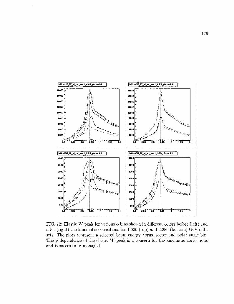
179
hMoni1D_W_el_bc_sec1Jh09_phisec04
18 0.85 0.9 0.95
| hMoni1O_W_el_bc_sec1_th09_phisecQ3 |
hMoni1D_W_el_ac_see1_th09_phlsec04
.8 0.85 0.9 0.95 1 1.05 1.1
| hMoni1D_W_el_ac_see1_ai09_phisec03 |
4000 R
FIG. 72: Elastic W peak for various 0 bins shown in different colors before (left) and after (right) the kinematic corrections for 1.606 (top) and 2.286 (bottom) GeV data sets. The plots represent a selected beam energy, torus, sector and polar angle bin. The (f> dependence of the elastic W peak is a concern for the kinematic corrections and is successfully managed.
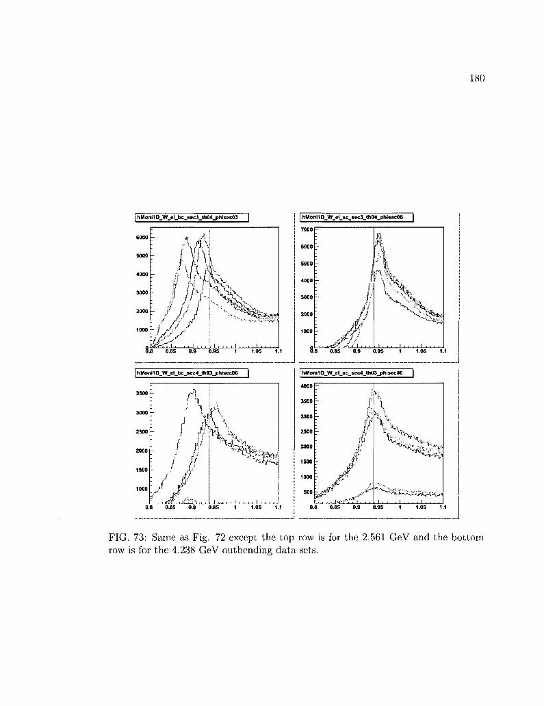
| hMoni1O_W_el_bcjsec3_t»i04jphlsec03 |
6000
5000
4000
3000
2000
1000
8
r A/A
i M T /-^"""V
ij^' * f e ? ? K , . . i , . .
i
\>x xSfe
i , , . , i i , 8 0.8S 0.9 0.9S 1
. . 1 . , . , 1.0S 1 1
I h Monil D_W_el_bc_sec4_ttiO3_phisec06 |
| hMoni1D_W_el_ac_sec3.Jh04_phlsec06 |
0.8 O.BS 0.9 0.95 1 1.05 1.1
.8 0.85 0.9 0.95 1 1.05 1.1
| hMoni1D_W_el_ac_sec4_th03_phisec06 |
x y j ^
i i i n i i i i i
FIG. 73: Same as Fig. 72 except the top row is for the 2.561 GeV and the bottom row is for the 4.238 GeV outbending data sets.

181
1800
1600
1400
1200
c 1000 3 O
° 800
600
400
200
x103
: • Aft.Mom.Corl
; • Aft.Mom.Coijr
1606i
^IH3
ND3
Const 1 81e+06±3.19e+04
Mean 0.938810.00
Sigma 0.0128 + 0.00
Const 7.531e+05±
Mean 0.9427 ± 0.001
Sigma 0.02558 ±0.001
• •
I . . . . I . . . . I . . . . 1 . . . . 1 . . . .
12632
I2968
2525
1808
2684
1800
1600
1400
1200
c 1000 3 O
° 800
600
400
200
x103
— I • Bef.Mom.Cor
\ • Bef.Mom.CcJ-
— .*• .• .
1606i
NH3
1 i*ND3
Const 1 ,65e+0S + 2.69e+04
Mean 0.937 i 0.00 I2622
Sigma 0 01379*0.0 10304
Const 7.262e+05i 1976
Mean 09411+0 00 11334
Sigma 0 02592 1 0.00 12183
0.95 1 1.05 W(GeV)
0.95 1 1.05 W(GeV)
x10"
800
700
600
: • Aft.Mom.Cori?NH3
Aft.Mom.CorMD3
1606o 8.32e+CS±2.O7e+04
0 10293 Mean 09418 ±00
Sigma 0.01003 ±0.00 )3097
Const 7.01e+05
Mean 0 9435 ±0.01
7567
b0306
Sigma 0.01743 + 0.0003547
--.. "•••••,•••••••' ,~*~" ,-•"•"
W»A«bA*«»ft*n*ifl
0.95 1 1.05 W(GeV)
x10 800
700
600
500
c
O 400 u
300
: • Bef.Mom.Corf NH3
• Bef.Mom.CoS ND3
1606o Const 6.86e+05 J. 1 82e+04
]!3799 Mean
Sigma
0 9342 ±0 00i
0.01249+0.01
Const 6.60e+05 +
Mean 0.9355 ±0.00(
Sigma 0 021141:0.001
...~."-' 1 • ' • • ' • • • • I • • • • I • • • • ' •
7100
2975
4843
0.95 1 1.05 W(GeV)
FIG. 74: Inclusive number of counts versus invariant mass W distributions after proper background subtractions are made by using the 12C data. Each row represents a different data set. The left plot is after all kinematic corrections are applied while the right plot is before the corrections, except the raster correction. The brown curves (with the higher peak) are for NH3 and the blue curves are for ND3 targets. Each plot representing a different data set is labeled with the beam energy in MeV and the torus configuration i (inbending) or o (outbending). After the kinematic corrections, the invariant mass peak for the elastic events should be centered around the proton mass (0.938 GeV) and the sigma of the distribution should be smaller.

182
17230
Aft.Mom.Corf
Aft.Mom.CorjililD3
Const 1.30G+06 i 2.49C+04
Mean 0.939910.00)2273
Sigma 0.01031 i 0.00
Consi 7 2e+05
Mean 0.9422 i 0.00(
Sigma 0.01859 + 0
3877
1542
11941
9.8 0.85 0.9 0.95 1 1.05 1.1 W(GeV)
1200
1000
800
600
400
200
X103
_ •
'•_•
Bef.Mom.Cor
Bef.Mom.Cor
17230
NH3
I 4ND3
Cons!
Mean
Sigma
Const
Mean
Sigma
!•
1.17O+06±3.09G+04
0.9385 ± 0 00
0.011251.0.00
6.758+05 ±
0.9403 ±0.00(
0.02042 ± 0.00(
.TrrrrrT?,, i . , , ,
13459
53654
4753
2147
306S
0.95 1 1.05 W(GeV)
400
300
200
100
*10 3
-
, , I . ,
A "7 !
\
2286J
JH3
I
i . . . . i . . . . i
Const
Mean
Sigma
" . . . 1
4.957e+05i
0.9365 :tO 00
0.0175810.00
••
, I , 1 I , I ,
7874
13201
13571
500
400
300
200
100
x103
J
" f
/
-^J*-** . . I . . .
2286i
( 1NH3
Const 4.66e+051
Mean 0.93721 0.00<
Sigma 0 01948 ±0.00(
\ • #«<
. I I . . , , I . . . . I . . . . I . . . .
582
2825
3304
0.95 1 1.05 W(GeV)
0.95 1 1.05 W(GeV)
x103
- • Aft.Mom.Con
I - • Aft.Mom.Corn
25610
NH3
1_ ND3
• •
I . , . , I . . . . I
Const 1.23e+06±1.39e+04
Mean 0.944 + 0.00
Sigma 0.01694 ± 0.00
Const 7.136e+05±
Mean 0.94671 0.0(
Sigma 0.0272510.001
. . . 1 . . . . 1 . . . .
)2276
J2591
4914
0323
4036
W(GeV) 1.15 1.2
103 25610
Bef.Mom.Cor[ NH3
i
Bef.Mom.CorrND3
Mean 0.9298 ± 0.001)4779
Sigma 0.02335 100006315
Const 5 4 2 1 e + 0 5 + 3231
Mean 0 . 9 2 8 6 1 0 . 0 0 ( 2 9 9 3
Sigma 0.03226 • 0.00 14801
0.95 1 1.05 W(GeV)
FIG. 75: Continuation of Fig. 74 for other data sets.

183
40000
35000
30000
25000
c
520000 u
15000
10000
5000
4238i
: • Aft.Mom.Corf«toH3
: • Aft.Mom.CqmNb3
[ J\\
Const
Mean
Sigma
S!i
~if'3L"r', . 1 . , , . i i
3950+04
0.9397 ±0.0
0.02604 i 0.00
1499
J03S9
!4479
1.4578+04 L147
0.9491 0.0( 1447
0.05489 + 0.0(2015
40000
35000
30000
25000
c
520000 u
15000
10000
5000
4238i
— i : • Bef.Mom.CorJ NH3
i
: • Bef.Mom.Corr ND3
L 1 \ : l i\ - • ! \
Const
Mean
Sigma
Const
Mean
Sigma
l ' . ' " ' • > • • , , , 1
3.118+04
0.9172 iO.OOt
±471
7522
0.035410.00)9811
1.3258+04 : 147
0.9278 5:0.01 1135
0.061581 0.0(
V
*\.v
, , , ! . , , ,
2656
0.95 1 1.05 W(GeV)
0.95 1 1.05 W(GeV)
250
200
150
100
50
, 4 2 3 8 0 x10
'_ • Af t .Mom.Co^H3
- • Aft.Mom.C«niM33
: M
! S - ~ f T T . . . I . . . . I . . . . I
Const 2.68e*05 i
Mean 0.9374 + 0.0
Sigma 0 02613 ±0.00
Const 2.18e+05
Mean 0.9439 1: 0.00
Sigma 0.04309 1 0.81
•• .• .*
•• • •• •"
, . . 1 . , , , 1
2476
1C282
13223
= 646
12201
0304
250
200
150
100
50
X1P3 4 2 3 8 0
• Bef.Mom.Corj NH3
•
Bef.Mom.Corr ND3 • • •
M •
A: ! \
• V..
Const
Mean
Sigma
Const
Mean
Sigma
1 766e+05 i
0.905110.01
0 0396910
1.621e+05
0.91091 0.001
2640
1387
0015
:804
7508
0.056871 0.Q11079
.••'
. . . I . . . . 0.85 0.9 0.95 1 1.05
W(GeV) 1.8 0.85 0.9 0.95 1 1.05
W(GeV)
= 3000
5615i
I • Aft.Mom.Corr NH3
- • Aft.Mom.CornND3
Ji i • • • •
• • •
'•"-v : V . . . i i . . . . i i
Const 38071
Mean 0 9449 ± 0 00C
Sigma 0 03718 * 0.0
Const 24171
Mean 0.95510 0
Sigma 0.07514 1 0.01
• • .•?:'• •• •• V
66.26
8366
1086
>7.59
15521
9307 = 3000
o
5615i
'. ' Bef.Mom.Corr NH3
- • Bef.Mom.Corr ND3
! - ^**
- f^V^ fyt i
_ • • " *- •". *- I » .% • {
•••••
, i , . ,
Const
Mean
Sigma
Const
Mean
Sigma
'••.»' '.'.' "• .*"*'
, i i
30031
0.9356+0.00(
0.0514510.01
2297 ±
0.951 ±0.01
007863 + O.t
. 1 '
. '?'• . . . r. *
.
37.7
8918
1588
58.91
5486
1085
0.95 1 1.05 1.1 1.15 1.2 W(GeV)
0.9 0.95 1 1.05 W(GeV)
FIG. 76: Continuation of Fig. 75 for other data sets.

184
8000
7000
6000
„ 5000
8 4000
3000
2000
1000
: .
r
,.!..
Wt i m
Aft.Mom.Corr NH3 •
Aft.Mom.CornND3 • • •
•ft M
J 1 / ' / 1
7 i / •
* f ' '
„ • • i 1 1 1 1 1 1 1 1 1 1 • 1 1 •
57251
"
* • i *
, . i . . , , i
Const
Mean
Sigma
Const
Mean
Sigma
5619 ±
0.9536 ±0.(
87.7
0102
0.03977 ±0.01 1229
22841
0.964 • 0.0(
50.11
5802
0.06888+0 0H7119
,
„ • • • • •
. , . 1 —
8000
7000
6000
„ 5000
c 3
8 4000
3000
2000
1000
5725i
L • Bef.Mom.Corr NH3
- • Bef.Mom.Corr ND3
: ;
/ i \
- ,is~*• !
r, . . . 1 . . . . I . . . . I . . . . I . . . . I
Consi
Mean
Sigma
Const
Mean
Sigma
4632 ±
0.9478 1 0.0'
0.05183 ± 0 0(
2227 ±
0.9697 ± 0 . {
0.08443 + 0
, , , i , i i . I . . i .
107.1
2047
3152
16.06
1634
3206
S.8 0.85 0.9 0.95 1 1.05 W(GeV)
0.85 0.9 0.95 1 1.05 W(GeV)
5725o
1 • Aft.Mom.Co/rjwH3
. • Aft.Mom.OorriNB3
[ / \ 1 m !• i •*• •»
Cons! 3.096e+04::
Mean 0.9355 * 0 00
Sigma 0.03939 ± 0.001
Const 1.342e+04 ±
Mean 0.9438 ±0.00<
Sigma 0.06162 + 0 01
•• • •• •• •• • • • • ' • • « • • "
, . , 1 . . . , 1 . . . .
175.1
12731
3816
109.1
8712
1703
25000
-_ .
-
,,, I,
ptf
57250
Bef.Mom.Corr NH3
Bef.Mom.Corr ND3
/ ! \ ft\ !
!
Const
Mean
Sigma
Const
Mean
Sigma
2 159e+04±
0.9377 + 0 00(
0 0515+0.0<
1.007e+04±
0.9482+ 0.01
2177
7242
1292
161.2
2576
0.0715±0.0115118
.„
• : ' . . i . . . . i . . . 1 . . . .
0.85 0.9 0.95 1 1.05 W(GeV)
1.1 1.15 1.2 1.8 0.85 0.9 0.95 1 1.05 1.1 W(GeV)
35000
30000
25000
c 320000 u
15000
10000
5000
5743o
: • Aft.Mom.CoMNH3
~ J '\ • ' Aft.Mom.OornNko
Cons! 3.829e+04:t
Mean 0.9348 ± 0.001
Sigma 0.03724 ± 0.001
; / j \ r / ' \
/ ' \
Consi 1.415e+04:i:
Mean 0 9469 ± 0.0(
Sigma 0 06109 ±0.C
i i \
: / ' V
~ :/ : -v^. . v'-"' :•' • • ••• .••••„••••• •
3468
4062
5426
I62.9
1338
0239
35000
30000
25000
320000 o
15000
10000
5000
: .
r
r :
z_
--—.• &
57430
Bef.Mom.Cor[ NH3 1
Bef.Mom.Corr ND3 i
•
y>\ f '"A
7 * \ / ( V
/ ' V I T
•* • V 1 1
'•* v ^ • • • • • * • •
~.~- : • •
, i — i , . , : i . . .
•• \**»
.••k.:-
"• . i . . . . i
Const
Mean
Sigma
Const
Mean
Sigma
•••«.?•« •* . . . i
2.511e+04±
0.9268 i 0.00!
0.05154 ±0.0(
1.0058+04 +
0.9421 ±0.01
0.07357 i 0.1
'%'
• •„ • •, •iT..-
*~ •
. . , I , , , ,
322.5
9929
1665
I45.3
2061
10481
0.95 1 1.05 W(GeV)
0.95 1 1.05 W(GeV)
FIG. 77: Continuation of Fig. 76 for the remaining data sets.

185
IV. 11 DILUTION FACTOR
Since we are interested in scattering events from polarized nucleons, the asymmetries
must be corrected for the contributions from unpolarized background. These contri
butions mainly come from the nearly unpolarized 15N nucleus in the target material
(ND3), the liquid helium bath that surrounds it for cooling and the target windows
that keep the whole apparatus together. For this purpose, we define a quantity called
dilution factor, which is the fraction of events scattered from the polarized deuteron
target. First we define the raw asymmetry as:
Araw = ~ n , (274) n~ + n+
In this equation, n~ and n+ are determined by counting the inclusive scattering
events for each helicity and normalizing with the accumulated beam charge. During
the counting procedure, we have no way to know if the event is coming from the
polarized target or from the unpolarized background. However, since the unpolarized
contribution is the same for both helicities, it cancels out in the numerator. The
denominator, on the other hand, is heavily diluted by the background contribution.
Therefore, we need to correct the denominator such that:
Aundii = ; — T (275)
where UB stands for the count of the background events. Based on this approach,
we can define a dilution factor (FJJ) to correct the asymmetry for the background
contribution: rr + n+ -nB nA-nB .. nB
tD = — — - — = = 1 , {l(<o) n + n+
UA nA
where TIA represents the total count of events from all sources in the beam path.
Then we can write the undiluted asymmetry in terms of the diluted asymmetry and
the dilution factor defined in Eq. (276) as:
AUndu = —^—• (277) I'D
In a naive approach, when we consider the 15ND3 target, we see that there are 3 po
larized deuterons (6 polarized nucleons) for every 21 nucleons. Therefore, the dilution
factor, which was defined as the fraction of events scattered from polarized target
nucleons, would be 6/21. For a more precise approach, this number would be slightly
modified by the difference in cross section for scattering off proton versus scattering

186
off neutron, and nuclear effects. However, the additional material in the beam path,
mainly the target windows and the liquid helium bath, makes the determination of
the dilution factor more complicated. The ideal way to determine the dilution factor
would be to take 15N runs under the exact same conditions as the 15ND3 runs and
subtract the scattering events of the former case from the latter after scaling them
with appropriate normalization to make them comparable. However, due to technical
difficulties with 15N targets [112], taking frequent 15N runs in between 15ND3 runs
was not an option. Another way would be to simulate the 15N contribution by taking
data on on a material with a structure close to 15N. One possible choice for that is
a 12C target. However, scattering from 12C is not exactly the same as scattering
from 15N because of the different number of nucleons in these targets and the extra
neutron in the 15N. In order to overcome this obstacle, limited 15N runs were taken
at some beam energies together with 12C runs taken regularly for all beam conditions
and 15N runs were simulated by using the cross section ratio of 12C to 15N targets. In
addition, empty target runs, in which the target slot was filled only with the liquid
helium, were also taken regularly for each beam condition. By using these runs, the
liquid helium contribution to the scattering events was determined. From now on,
we will refer to these liquid helium runs as the empty target (E) runs. The required
quantities14 that will be used throughout this section are denned in Table 26.
Two different methods were used to calculate the dilution factor and their results
were compared. In a chronological order, the first method was developed by Sebastian
Kuhn and is based on the parametrization of data and the neutron-to-deuterium cross
section ratios to simulate the 15N background in terms of 12C. The second method
was developed by Peter Bosted and Robert Fersch and is based on the radiated cross
section model described in Ref. [112].
Method 1: dilution factors from parametrization of data
In order to calculate Fo by using the first method, we need to determine the amount
of background events n# in Eq. (276). In terms of the quantities described in Table
26, we can define rig as:
nB = nE + —- nc-lAnHe, (278) pcic crc
4Note that cross sections are in terms of cm2 per nucleus.

187
TABLE 26: Target parameter definitions. The subscript X represents different target types used during the experiment. The following acronyms are used for different target types throughout this section: N for nitrogen; A for ammonia; T (or D) for deuteron; C for carbon and He for liquid helium. In addition, Al is aluminum, K is kapton and F represents all kapton and aluminum foils. All counts (represented by rix) are normalized to the corresponding total integrated beam charge for each target. The quantity / is introduced for convenience. It assumes o> « oc so that the foil mass thickness can be expressed as a fraction of carbon mass thickness. This quantity is used in later sections while calculating the target lengths.
Parameter
L
lx Px ox nx n'c = Pck^c nHe = PHe&He nN = PNIN^N
n'A = PAUCTA
f = PFh/pch
Definition
Total length of the target cell Length of target X Density of target X Cross section of target X Measured counts from target X Expected counts scattered only from 12C Expected counts per 1 cm length of liquid 4He Expected counts scattered only from 15N Expected counts scattered from ammonia Contribution to count rate from all Aluminium (Al) and Kapton (K) foils combined, expressed as a fixed fraction of the contribution from 12C
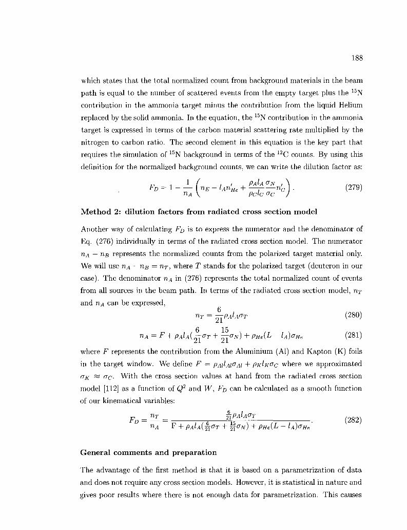
188
which states that the total normalized count from background materials in the beam
path is equal to the number of scattered events from the empty target plus the 15N
contribution in the ammonia target minus the contribution from the liquid Helium
replaced by the solid ammonia. In the equation, the 15N contribution in the ammonia
target is expressed in terms of the carbon material scattering rate multiplied by the
nitrogen to carbon ratio. The second element in this equation is the key part that
requires the simulation of 15N background in terms of the 12C counts. By using this
definition for the normalized background counts, we can write the dilution factor as:
FD = l - - ( n E - lAn'He + ^ ^ n ' c ) . (279) nA \ Pdc oc J
Method 2: dilution factors from radiated cross section model
Another way of calculating Fp is to express the numerator and the denominator of
Eq. (276) individually in terms of the radiated cross section model. The numerator
nA — riB represents the normalized counts from the polarized target material only.
We will use nA — n# = nT, where T stands for the polarized target (deuteron in our
case). The denominator nA in (276) represents the total normalized count of events
from all sources in the beam path. In terms of the radiated cross section model, TIT
and nA can be expressed,
nT = WTPAUOT (280)
6 15 nA = F + PJA(—(TT + I^N) + PHe{L - lA)crHe (281)
where F represents the contribution from the Aluminium (Al) and Kapton (K) foils
in the target window. We define F = pA\lAioAi + PKIK&C where we approximated
OK ~ oc- With the cross section values at hand from the radiated cross section
model [112] as a function of Q2 and W, FQ can be calculated as a smooth function
of our kinematical variables:
nT _ §ipAlA&T
nA F + pAlA(^aT + Ifcriv) + pHe(L - lA)aHe FD = ~^ = „ , _ , , « _ 2\:_ , . ,r , x _ • (282)
General comments and preparation
The advantage of the first method is that it is based on a parametrization of data
and does not require any cross section models. However, it is statistical in nature and
gives poor results where there is not enough data for parametrization. This causes

189
TABLE 27: Densities of the target materials in the EGlb experiment. Values are fromRefs. [113] and [114].
Target Material
ammonia (NH3) ammonia (ND3)
carbon (12C) nitrogen-15 (15N)
liquid helium (He) kapton (K)
aluminum (Al)
Density (g/cm3)
0.917 1.056 2.17 1.1
0.145 1.42 2.69
Density (mol/cm3)
0.0508 0.0502 0.180 0.073
0.0362 0.00371 0.0997
artificially large bin by bin statistical fluctuations, which causes large errors on FD
and therefore on the undiluted asymmetry. The advantage of the second method
is that FD is obtained as a smooth function of Q2 and W. Therefore, the results
can easily be extrapolated into regions where there is not enough data for the first
method. FD was calculated by both methods and it was confirmed that the second
method behaves exactly as the parametrization of the first method. In the end, the
first method was only used for the calculation of systematic errors and in the quasi-
elastic region. The second method was used to determine the dilution factors for
asymmetry measurements.
After defining the dilution factor and the methods to calculate it, we can now
determine what we need to carry out the necessary calculations in both methods.
When we examine Eq. (279) closely, we see that we need to determine the densities
and the lengths for the ammonia and the carbon targets to carry out the method
1 calculation. We also need the nitrogen cross section, which we will simulate by
using the carbon data. That will require the knowledge of the target length for the
carbon as well as the nitrogen. From the Eq. (282), we see that we need the target
density and the length for the ammonia as well as the total target length L. For the
cross sections we will use the radiated cross section model. The target densities are
already known and they are written in Table 27.
Approximate target lengths from physical measurements are given in Table 28.
The value for the window foil material changes after the run 27997 because of the
addition of a Kapton (K) piece after this run. The true length of the ammonia

190
TABLE 28: Lengths of the target materials in the EG lb experiment. Values are from Refs. [113] and [114].
Target Material
total (L) ammonia (NH3) ammonia (ND3)
carbon (12C) carbon (12C)
nitrogen-15 (15N) liquid helium (He)
kapton (K) kapton (K)
aluminum (Al)
Approximate Length (cm)
1.9 0.6 0.6 0.23
0.22 (for 15N target runs) 0.5
L minus solid target material 0.0304(0.0384 after 27997)
0.0354 (for 15N target runs) 0.0167
targets (15NH3 or 15NDs), which is represented by I A , depends on the packing fraction
(the percentage of volume occupied by ammonia beads in the total target volume).
Therefore, it should be studied explicitly. The same situation is also valid for the 15N target. The liquid Helium exists in all target types since it is used to keep the
target at low temperature. Its length depends on how much of the liquid Helium was
displaced by the other target material that it is hosting. The length of the Kapton
(K) and the Aluminum (Al) targets are known from physical measurements during
the experiment. Since the dilution factor is very sensitive to these values, the target
lengths for the ammonia and the nitrogen targets were studied explicitly to determine
the correct FQ. Next we will describe how the target lengths are determined. Table
29 shows the values of some target parameters defined earlier in Table 26. These
values will be used for the calculations of other quantities.
IV. 11.1 Calculation of Total Target Length L
The total target length L includes the length of the mini-cup that includes the target
cell itself and the liquid Helium around it as well as the foil materials for the win
dows. The nominal value for L is 1.9 cm. However, this length may change slightly
according to experimental conditions because of varying pressure that causes the
window material to change its shape, liquid Helium overflow or the beam position
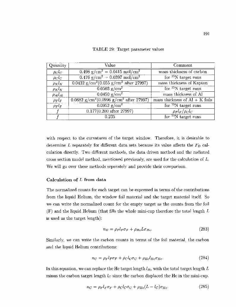
191
TABLE 29: Target parameter values
Quantity
Pch Pch PKIK
PK\K
PAI^AI
PFIF
pFlF
f f
Value
0.498 g/cm2 = 0.0415 mol/cm2
0.476 g/cm2 = 0.0397 mol/cm2
0.0432 g/cm2(0.055 g/cm2 after 27997) 0.0503 g/cm2
0.0450 g/cm2
0.0882 g/cm2(0.0996 g/cm2 after 27997) 0.0952 g/cm2
0.177(0.200 after 27997) 0.235
Comment
mass thickness of carbon for 15N target runs
mass thickness of Kapton for 15N target runs
mass thickness of Al mass thickness of Al + K foils
for 15N target runs
PFIF/PCIC
for 15N target runs
with respect to the curvatures of the target window. Therefore, it is desirable to
determine L separately for different data sets because its value affects the FQ cal
culation directly. Two different methods, the data driven method and the radiated
cross section model method, mentioned previously, are used for the calculation of L.
We will go over these methods separately and provide their comparison.
Calculation of L from data
The normalized counts for each target can be expressed in terms of the contributions
from the liquid Helium, the window foil material and the target material itself. So
we can write the normalized count for the empty target as the counts from the foil
(F) and the liquid Helium (that fills the whole mini-cup therefore the total length L
is used as the target length):
UE = PFh°F + pHeL(JHe- (283)
Similarly, we can write the carbon counts in terms of the foil material, the carbon
and the liquid Helium contributions:
nc = PFIF&F + Pch^C + PHehe^He- (284)
In this equation, we can replace the He target length ljje with the total target length L
minus the carbon target length IQ since the carbon displaced the He in the mini-cup.
nc = PFIF°F + Pclc°C + PHe(L - lc)&He- (285)

192
However, an extra correction is needed for the liquid Helium target because of
its larger radiation length (X0(g/cm2)) compared to the other targets. All solid
targets in the experiment were designed to be around the same mass thickness
t = pxlx(g/cm2). However, the count rate from a target is affected by its radiation
thickness, defined by t/X0. Since the radiation thickness of He is smaller compared
to carbon, its count rate should be corrected by adding an extra length to it. Then
fully radiated cross sections for the He are calculated by using two different target
lengths. The ratio of these cross sections was determined for each kinematical bin of
the experiment and used as a multiplication factor for any liquid He count whenever
the counts were obtained from the data. In addition, an extra raster cut was applied
to the empty target counts. More detailed information on the corrections on the
empty target can be found in [95].
At this point, we can use the convenience factor / introduced in the previous
section to simplify Eqs. (283) and (285) as:
nE = fpchvc + pHeLoHe (286)
nc = (1 + f)pclc<?c + pHe(L - lc)oHe (287)
The ratio TEC = nE/nc is employed and oc = 3o#e is assumed to determine the
total target length for each kinematical bin Lun:
'3pclc[(l + f)rEc-f} Lhj' bin = 0 PHe
-TEclcj/iX-TEc)- (288)
Then the error weighted average of Lbm is taken to determine the average total target
length L for each data set. For this purpose, we also need to calculate the statistical
error on Lun- This statistical error is calculated with respect to rEc as:
J-1 bin
where
dL
orEc
N(l + f)-lc | N[(l + f)rEC - f] - TECIC
1 - rEc (1 - TEC)2
N = 3pClc/PHe,
'TEC1
and
which yields
&TEC ~
1(drEc\2 , (drEC
U7J n*+Ur'nci
rEC v
(289)
(290)
(291)
(292)

193
I Total target length (L). 0.009 < Q2 < 10.970 I 3 5
2.8
2.6
2.4
_ 2-2
E a 2
1.8
1.6
1.4
1.2
1.2 1.4 1.6 1.8 2 2.2 2.4 2.6 W(GeV)
FIG. 78: Total target length, L, calculated using the EGlb data, shown as a function of W averaged over Q2 bins. A W cut of 1.40 GeV is incorporated for the final value of L to remove the effects of the A-resonance. Plot is courtesy of R. Fersch.
Therefore, the error weighted average of the total target length is calculated as:
5 1 Yl Lbin/°2Lun L = Q ' " (293)
Q2 W
The statistical error on L is not used anywhere else since it underestimates the real
error on the target length. Instead, we used the systematic errors which are explained
in [95]. In averaging L, specific W and Q2 ranges were used for the validity of the
model. In order to remove the A(1232) region, where L^ does not show a flat
behavior, only the W > 1.40 GeV was used for average L. There are also upper W
cuts that change for different Q2 bins and can be found in [95]. The final results
of L from this method are listed in Table 30 under "Method 1". The plot of L as
a function of W (without the W cut incorporated for the final value), with error-
weighted average taken over Q2 bins, is also shown in Fig. 78 for the 5.76 GeV
outbending data set.
Calculation of L from models
The second method of calculation of L incorporates the radiated cross section model.
Detailed explanation of this model can be found in [112]. The measured 12C count
rate can be expressed in terms of the radiated cross section model (derived by using
the carbon data, which is expressed by the square brackets after the cross section

194
terms) of the individual contributions from the foils, the liquid helium and the ni
trogen target itself as:
nc = PAIIAI<?AI[C] + PKIK°C\C} + Pclc<?c[c] + PHe{L - lc)°He\c}, (294)
with OK ~ cfc- Similarly, the measured count rate for the empty target is:
nE = PAIIAI&AI\E} + PK^K^C[E] + PHeLaHe[E]. (295)
The model ratio of the count rates of the carbon and empty targets is given by:
nc
Solving this equation for the target length L gives us:
, rEcF[c\ - F[E] + rEcPclcOc[c\ - rECpHelccrHe[C] ,o n„N
PHe&He[E\ ~ rEcPHe^He[C]
where the foil contribution from Al and Kapton are combined under the term F =
PAIIAI&AI + PK\K&C- The error on L^n can be estimated (assuming the foil contri
butions are small (F —>0) and <JHe\c] ~ &He[E}) by its variation with respect to the
ratio rEc'-
°Lhin = -~-—<?rEC = ——z M—:—^5—> ( 2 9 8 ) dLun _ Pclc&C[C] - pHeh^He[C]
drEC TEC pHeVHe[c](l ~ rECy
with oTEC given in Eq. (292). The error weighted average of the total target length is
calculated by summing over all Q2 and W bins as described in the previous section.
Since the model cross sections already have the corrections for nuclear EMC effects,
the W cut can be reduced to W > 1.10 GeV for this calculation. Also, Q2 dependent
upper W cuts are used, which are described in [95] in detail. This is a direct cal
culation of L from models, in which the cross sections, unlike the previous method,
are determined by a fit to the world data. However, for the radiated cross section
model, the total target length must be known first. Therefore, an iterative method
is used by beginning from an initial value of L = 1.90 cm. Radiated cross sections
are calculated from initial value and L is recalculated with the method described.
Then the cross sections are recalculated from the new L. The iteration is continued
until L stabilizes, which is usually after 2 iterations for most data sets. An additional
iteration was always performed to make sure the length was absolutely stable. Fig.
79 shows the final L from method 2 as a function of W, averaged over Q2 bins (0.317
< Q2 < 0.645) for the 4.2 GeV inbending data set.

195
1 Total target length (L modeled), 0.317 < tf < 0.645 I 3
2.6
2.6
2.4
2.2 E 2. 2
1.8
1.6
1.4
1.2
1
--~-'-
^\s^®\^^^^^^f*^^\^f
1 1.2 1.3 1.4 1.5 1.6 1.7 1.8 1.9 2 W(GeV)
FIG. 79: Total target length, L, calculated using the radiated cross-section models, shown as a function of W, averaged over Q2 bins (0.317 < Q2 < 0.645) for the 4.2 GeV inbending data set. Plot is courtesy of R. Fersch.
The two methods are compared carefully and their results agree very well. The
final results of both methods can be seen in Table 30. For the final analysis, the
results from the radiated cross section model (method 2) was used. The method
just described for the calculation of L stands as a general outline for all target
length calculations, which we will describe in the following sections. Even though
the calculation methods are similar or the same, there are still slight differences that
should be explained.
IV.11.2 Modeling 1 5N from 12C Data and Calculation of I N
As already mentioned, the best way to remove the 15N contribution from the ammonia
(15NH3 and 15NDs) target counts is to take data on the 15N with the same beam
conditions. Since it was not possible because of technical difficulties, instead we took
data on a 12C target as the closest possible approximation of 15N. However, scattering
from 12C is not identical to scattering from 15N because of a different number of
nucleons. Even if this can be taken care of by parametrization and scaling of the 12C data, there is also an extra neutron in the 15N target, which has to be accounted
for. There are, fortunately, some 15N target runs during the EGlb experiment, at
least for some of the beam configurations. These data were used to express the 15N
cross section in terms of the 12C cross section. Two different methods, explained in
the previous section, were used to create a good fit for the 15N cross section. The
first method used a parametrized definition of the 15N cross section in terms of the
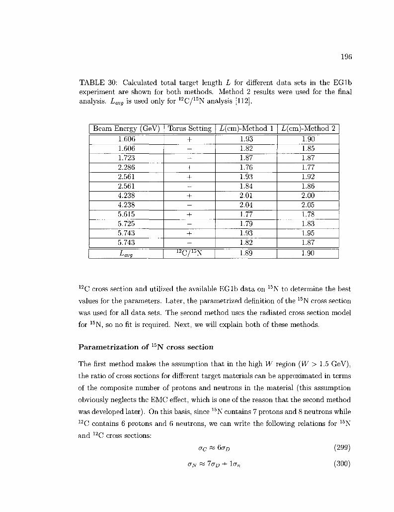
196
TABLE 30: Calculated total target length L for different data sets in the EG lb experiment are shown for both methods. Method 2 results were used for the final analysis. Lavg is used only for 12C/15N analysis [112].
Beam Energy (GeV)
1.606 1.606 1.723 2.286 2.561 2.561 4.238 4.238 5.615 5.725 5.743 5.743
l^avg
Torus Setting
+ — —
+ + —
+ —
+ -
+ —
1 2 C / 1 5 N
L(cm)-Method 1
1.93 1.82 1.87 1.76 1.93 1.84 2.01 2.04 1.77 1.79 1.93 1.82
1.89
L(cm)-Method 2
1.90 1.85 1.87 1.77 1.92 1.86 2.00 2.05 1.78 1.83 1.95 1.87
1.90
12C cross section and utilized the available EG lb data on 15N to determine the best
values for the parameters. Later, the parametrized definition of the 15N cross section
was used for all data sets. The second method uses the radiated cross section model
for 15N, so no fit is required. Next, we will explain both of these methods.
Parametrization of 15N cross section
The first method makes the assumption that in the high W region (W > 1.5 GeV),
the ratio of cross sections for different target materials can be approximated in terms
of the composite number of protons and neutrons in the material (this assumption
obviously neglects the EMC effect, which is one of the reason that the second method
was developed later). On this basis, since 15N contains 7 protons and 8 neutrons while 12C contains 6 protons and 6 neutrons, we can write the following relations for 15N
and 12C cross sections:
ac « 6aD (299)
aN « 7cr£) + \an (300)

197
a»~(l + l— )°c, (301) \ 6 6(7/3/
where an and o^ are the neutron and the deuteron cross sections respectively, given
in cm2 per nucleus. The nominal values 7/6 and 1/6 can be turned into parameters a
and 6, respectively, and fit to the the nitrogen data for the beam energies where they
are available, so that small deviations from these nominal values can be determined.
Therefore, we can write the above equation as:
aN= (a + b~\ ac (302)
The world data parametrization by S. Kuhn [113] is used for the neutron to deuteron
cross section ratio onjao- Following the same prescription given in the previous
sections, we can express the count rates for the carbon and the empty targets as:
nc = (1 + f)n'c + (L- lc)n'He (303)
nE = fn'c + Ln'He, (304)
where n'c and n'He are the expected count rates for the carbon and helium targets
as given in Table 26. The expected count rates can be expressed in terms of the
measured count rates by using the above equations:
n'c = TTJTcnc + TTjtc
nE (305)
and
nHe = TT7TnE + Yinrnc ( 3 0 6 )
L + Jlc L + Jlc
By using a similar approach, the measured nitrogen count rate can be expressed in
terms of the foils, the liquid helium and the 15N contribution:
nN = fpclc&c + PHe(L - lN)&He + PN^N^N (307)
And again using the definitions given in Table 26:
nN = fn'c + {L- lN)n'He + n'N (308)
By using the defined parametrization of the nitrogen cross section in terms of the
carbon cross section, we can write:
nN = fn'c + {L- lN)n'He + ^ - ( a + b^) n'c. (309) Pch \ VD)
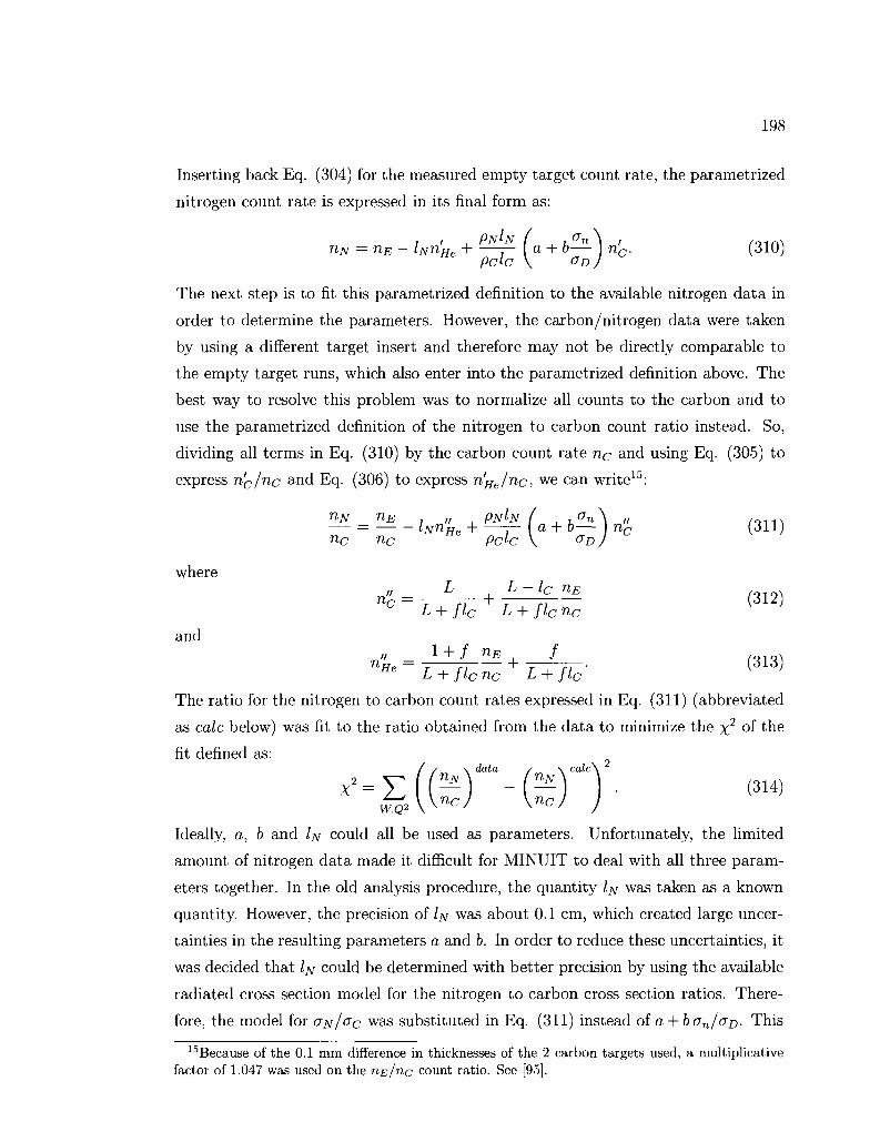
198
Inserting back Eq. (304) for the measured empty target count rate, the parametrized
nitrogen count rate is expressed in its final form as:
nN = nE- lNn'He -\ — ( a + b— I n'c. (310) pch \ &DJ
The next step is to fit this parametrized definition to the available nitrogen data in
order to determine the parameters. However, the carbon/nitrogen data were taken
by using a different target insert and therefore may not be directly comparable to
the empty target runs, which also enter into the parametrized definition above. The
best way to resolve this problem was to normalize all counts to the carbon and to
use the parametrized definition of the nitrogen to carbon count ratio instead. So,
dividing all terms in Eq. (310) by the carbon count rate nc and using Eq. (305) to
express n'c/nc and Eq. (306) to express n'He/nc, we can write15:
lNn%e + P-^f- (a + b^-) n'c (311) WJV _n£ , _„ , PNIN (_ , LC:
nc nc
where
and
„" L t L-lc nE , „ 1 0 ,
nc = TTTc + LTTc^ <312)
nHe = r , r, — + r , n • V 3 1 3 J 1 + / nE | /
L + flcnc L + flc
The ratio for the nitrogen to carbon count rates expressed in Eq. (311) (abbreviated
as cole below) was fit to the ratio obtained from the data to minimize the x2 °f the
fit defined as:
( / \ data / \ calc\
,. m -(a )• Ideally, a, b and IN could all be used as parameters. Unfortunately, the limited
amount of nitrogen data made it difficult for MINUIT to deal with all three param
eters together. In the old analysis procedure, the quantity IN was taken as a known
quantity. However, the precision of IN was about 0.1 cm, which created large uncer
tainties in the resulting parameters a and b. In order to reduce these uncertainties, it
was decided that IN could be determined with better precision by using the available
radiated cross section model for the nitrogen to carbon cross section ratios. There
fore, the model for CTJV/CC was substituted in Eq. (311) instead of a + ban/ao- This
15Because of the 0.1 mm difference in thicknesses of the 2 carbon targets used, a multiplicative factor of 1.047 was used on the n.E/nc count ratio. See [95].

199
leaves us with a single parameter IN to determine from the fit in Eq. (314). The x2
minimization was performed separately for each data set. Then the final values of
Zjv were used in the original form of Eq. (311) to determine the parameters a and b.
The resulting values for these parameters are listed in Table 31 together with their
uncertainties. The average values of the parameters are very close to their nominal
values a = 7/6 and b = 1/6. It should be pointed out that these values for a and b
are only used in systematic error calculations. The final values for the target length
IN are also listed in Table 32 under "Method 1".
TABLE 31: Values of the parameters a and b for different data sets for which there is available nitrogen data. These parameters are used to express the nitrogen cross section in terms of the carbon cross section.
Data Beam (GeV) Torus 1.723 + 1.723 -2.286 + 4.238 + 4.238 -5.615 + 5.615 -average
a 1.12 ± 0.0030 1.08 ± 0.0019 1.18 ± 0.0015 1.12 ± 0.0187 1.20 ± 0.0014 1.04 ± 0.0186 1.24 ± 0.0070 1.16 ± 0.0008
b 0.27 ± 0.0073 0.37 ± 0.0047 0.12 ± 0.0036 0.28 ± 0.0452 0.07 ± 0.0031 0.47 ± 0.0461 -0.01 ± 0.0155 0.15 ± 0.0019
Modeling the 1 5N from radiated cross sections to determine IN
There are 7 carbon-nitrogen data sets taken with different beam energy and torus
configurations as part of the EGlb experiment. Among these data sets, the 2.286
GeV inbending set is used to create a reliable model for the cross section ratios of 15N/12C and 4He/12C targets. Detailed explanations of this analysis can be seen in
[112] and it is beyond the content of this thesis. Once the model was generated, it
was successfully tested by using the other available data sets on the nitrogen and
carbon.
The 15N count rate can be expressed in terms of radiated cross sections (derived
by using the nitrogen data, which is expressed by the square brackets after the cross
section terms) of the individual contributions from the foils, the liquid helium and

200
the nitrogen target itself as:
n>N = PAIIAI&AI[N} + pK^K^C[N] + PNIN&N[N] + pHe{L - lN)&He[N} (315)
In the same way, the 12C count rate can also be written in terms of radiated cross
sections (derived by using the carbon data):
nc = PA\IAIOAI\C\ + PKIK&C\C\ + Pclc<?C[C] + PHe(L - lc)&He[C]- (316)
The model for the count rate ratio of the nitrogen and carbon is written as:
rmodel = ^ ( 3 1 7 )
and this count rate ratio (abbreviated as model) is fit to the real data count rate
ratio (abbreviated as data) to minimize the x2 of the fit:
(318) x2 =
where aTNC is given by
arNC = )
which yields
. \ "* j^data model\2 / 2 • / ,, VNC ~rNC ) larNci
W,Q2
l(drNC\ n (drNC\2
]] V dnN J h \ dnc J (319)
al^ = Jn-Nl + n-c\ (320)
TNC V
This fit uses an iterative method to determine the total target length L for these run
sets, which used a different target insert. After getting the fit results from 2.286 GeV
data, the model is extrapolated to other kinematic regions by using the available data
from other beam energies. Some additional corrections are also needed to account
for the beam charge normalization of the count rates because of the discrepancy
between the true beam charge and the measured beam charge due to the spread
of the beam aperture, through multiple scattering, that exceeded the faraday cup
radius. In addition, the model for the 4.2 GeV data needed an additional scaling.
More information about these additional corrections for this analysis, as well as the
description of the systematic errors applied, can be found in [95]. Fig. 80 shows the
count rate ratios 15N/12C and the resulting fit for the 2.286 GeV data set. The model
represents the data very well in most kinematic regions.

201
| Charge
1.2
1.15
1.1
1.05
1
0.95
0.85
norm allied co „,„•.,(
1 1
' N / " C ) , 1 . 2 0 0 < W «
m m -
1.130 |
. - . A i ^
| Charge norm
1.1
1.15
1.1
1.0S
1
0.95
... 0.SS
allied count ratio
X i
•
("Ml U C) , 1.210 < W «; 1 .2<l«|
?B « B t IB
1 1 T
... .„ .
1
. . • . 1
|-„ — . r - ^ , - . . . . - !
,., --r
- ¥ » .... w «s», s
r *
" ~
[charge normalized co
1.15
1.1
1.05
O.SS
0.9
O.SS
0.8
T
r
i-1-
lor1
nl ratios
h
'w"ci.ii9o<w<i
tf(0*1 _
ilJ
"'if
1
| Charge nonnallied count ratios ('N/^C), 1 . 3 8 K W < 1.3511 |
e - _ - _ . » - _ < <
| Charge normalized co
1.2
1.15
1.05
0.95
0.9
0.85
0.8
j-
L L
:— r
r
r
, 10"'
nt ratio. ['
''ti Zj
W - C l . 1 J » < W < 1 3 B i |
.« 1
, tfiavl
(a) 1 5 N/ C count rate ratios vs. Q2 for various W bins.
|chargs normalized
1.2
1.15
1.1
1.05
0.9
0.85
L
ount ratios ( "M;"C),
1
,18T<0 * < 0 .266 |
^ , i s^rW^>y
[Charge normalize
1.15
1.05
0.95
0.9
0.S5
•
r
-
count ratios
hJ& F ^
f V ' q , o.2ee <a'< O.ITB |
^ £ £ 3 a j £ a c a a S ^ a a S B k k & I f l
^ a
.
|charge normalized count ra
1.15
1.1
1.05
0.95
0.9
0.85
i-
I-0" t i
los ( " W " C ) , 0 .379 < Q1 « 0.5401
l " T — ' • • - - ^ ^ 1 | , - ^ ^ ^ , ^ , . . . , . , . B |
(b) 1 5 N/ 1 2 C count rate ratios vs. W for various Q2 bins.
FIG. 80: 15N/12C count rate ratios for the 2.3 GeV data set are shown together with the final model for different kinematic regions. Plots are courtesy of R. Fersch.
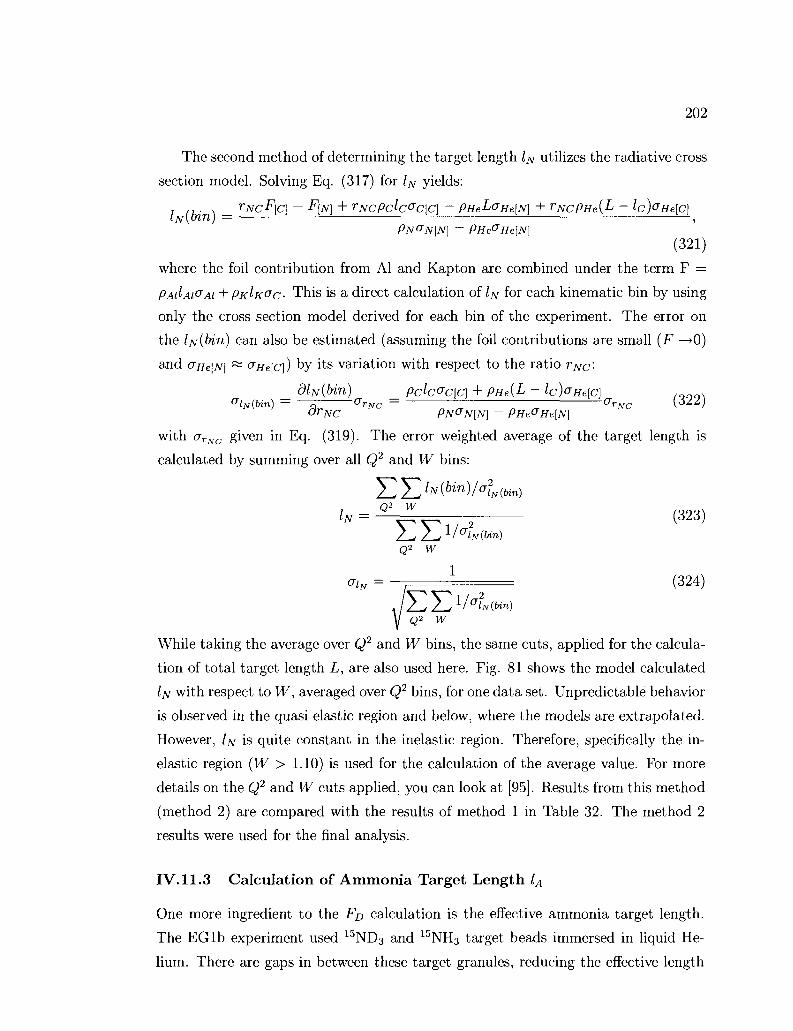
202
The second method of determining the target length IN utilizes the radiative cross
section model. Solving Eq. (317) for lN yields:
, /> • \ _ rNcF\C] - F[N] + rNCPclc^C[C] — PHeL(THe[N] + rNCPHe{L - lc)vHe\C) 'TVI / — i
PN&N\N\ — PHe&He{N]
(321)
where the foil contribution from Al and Kapton are combined under the term F =
PAIIAI&AI + PKIK&C- This is a direct calculation of IN for each kinematic bin by using
only the cross section model derived for each bin of the experiment. The error on
the IN (bin) can also be estimated (assuming the foil contributions are small (F —>0)
and (7He[N] ~ 0"He[c]) by its variation with respect to the ratio TNC'-dlN(bin) _ Pclc<?C[C\ + pHe{L - lc)<7He[C] ,„nns
&lN(bin) - —^Z ^rjvc - — " OrNC \6ll) OTNC PN&N[N] - PHe°He[N]
with urNC given in Eq. (319). The error weighted average of the target length is
calculated by summing over all Q2 and W bins:
(bin) O2 W Q (323)
(324)
lfi(bin)
While taking the average over Q2 and W bins, the same cuts, applied for the calcula
tion of total target length L, are also used here. Fig. 81 shows the model calculated
IN with respect to W, averaged over Q2 bins, for one data set. Unpredictable behavior
is observed in the quasi elastic region and below, where the models are extrapolated.
However, IN is quite constant in the inelastic region. Therefore, specifically the in
elastic region (W > 1.10) is used for the calculation of the average value. For more
details on the Q2 and W cuts applied, you can look at [95]. Results from this method
(method 2) are compared with the results of method 1 in Table 32. The method 2
results were used for the final analysis.
IV. 11.3 Calculation of Ammonia Target Length I A
One more ingredient to the Fo calculation is the effective ammonia target length.
The EG lb experiment used 15ND3 and 15NH3 target beads immersed in liquid He
lium. There are gaps in between these target granules, reducing the effective length

203
1 Nitroqen target length(15N). 0.009 <Q 2 < 10.970 I 0.9
0.8
0.7
- * 0.6
0.5
0.4
_ r
'r
r i
• , i i . . . i , . , i , . . i . 0.6 0.8 1 1.2 1.4 1.6 1.8 2
W (GeV) 2
FIG. 81: The 15N target length l^, calculated from the radiated cross section model is shown for different W bins. The value in each W bin is averaged over Q2 bins. For the final value, lower (W > 1.10) and upper [95] W cuts are applied as in the case of the L calculation. The plot is for the 2.286 GeV data set.
TABLE 32: Values of the 15N target length ZJV for different data sets from two methods. There are 7 data sets with nitrogen data. More explanations on the methods are in the text.
Data set
1.723 + 1.723 -2.286 + 4.238 + 4.238 -5.615 + 5.615 -average
/jv(cm)-Method 1 0.44 ± 0.00039 0.45 ± 0.00033 0.45 ± 0.00015 0.47 ± 0.00086 0.47 ± 0.00008 0.43 ± 0.00066 0.45 ± 0.00028 0.46 ± 0.00007
Zjv(cm)-Method 2
0.45 ± 0.00057 0.45 ± 0.00056 0.46 ± 0.00023 0.48 ± 0.00103 0.47 ± 0.00022 0.44 ± 0.00119 0.46 ± 0.00043 0.46 ± 0.00014

204
of the target. The design length of the ammonia target cell is about 1 cm. The
fraction of this length that contains only the target material (ammonia) is called the
packing fraction and is approximately 60%, which gives an effective length of 0.6 cm.
Accurate calculation of FD requires a precise value for the packing fraction. The
packing fraction can vary according to the beam configuration as well as the geomet
ric location within the target cell. An overall effective value of the packing fraction
will be determined for each beam configuration. In this section, we will introduce
two methods, the same ones used for the other quantities, for the calculation of the
packing fraction.
Calculation of I A. from data
Following the same prescription developed for the nitrogen target length calculation,
we begin by parameterizing the ammonia cross section in terms of the carbon cross
section by using the number of protons and neutrons in each material. The same
procedure is used for both 15ND3 and 15NH3 targets, but in this analysis, we will go
over the 15ND3 calculations, so, the abbreviation A will refer to 15ND3.
ac ~ 6oD (325)
oN ~ 7CT£> + ltfn (326)
<TA~VN + 3aD (327)
It should be pointed out that the above equations are only approximate for large
W. Also, the EMC effect is neglected with these approximation, which is one of the
basic disadvantages of this method. By using the previous parametrization for the
nitrogen cross section given in Eq. (302), we can parametrize the ammonia cross
section in terms of carbon:
aA = (a + b^ + 3^-) ac (328) V °D 0C}
Also using the initial assumption given in Eq. (325) that ac = 6CT.D, we have:
aA = f a + b— + 0.5 J ac (329)
For the neutron to deuteron cross section ratio on/o£>, the parametrization by S.
Kuhn [113] is used, which is given as a function of beam energy, Q2 and W. Now

205
we can express the ammonia target count in terms of the contributions from the foil
material, the liquid Helium and the ammonia itself:
nA = fpckvc + PHe{L - lA)aHe + PAU^A, (330)
using the same expressions for the carbon and helium counts as given in Eqs. (305)
and (306) as well as the definitions given in Table 26:
nA = fn'c + {L- lA)n'He + n'A, (331)
where
n'A = PAU^A (332)
is normalized counts scattered only from ammonia. Inserting the ammonia cross
section parametrization into Eq. (329):
nA = fn'c + {L- lA)n'He + ^ ( a + b^ + Q.h] n'c (333) pch \ oD )
and using Eq. (304) for the measured empty target count, we obtain the final
parametrized form of the ammonia target count as:
nA = nE — lAn'Hp -\ — I a + b— + 0.5 I nr. (334) pdc \ °D J
From Eq. (334), the ammonia target length lA(bin) can be expressed for each kine
matic bin as:
lA(bin) = (nA - nE) ' ' a + 6— + 0.5 CTD
nc - nHe . (335) .Pdc
Figs. 82 and 83 show the final distribution of the effective ammonia target length (in
cm) over different kinematic bins. The latter figure shows the results for individual
helicity states separately in different colors for various Q2 bins. The error on this
quantity can be estimated by taking its variation with respect to each measured
count rate.
ai*™=v (SOnA+(M)nc+(lb)nE (336)
Partial derivatives are calculated with the help of Eqs. (305) and (306) that relate the
expected carbon and helium count rates to the measured carbon and empty target
count rates. We define the quantities:
P = a + 6— + 0.5 (337) 0£>

206
Therefore:
R = -^-Rn'c - n'He (338)
| ^ = l/R (339) dnA
dnc ~ R2 [6m)
L-lc + 1+/ ))
(341) d h {R+(nA-nE)(^^ + ^ ) )
dnE R2
While determining the final lA for each data set, the error weighted average of
lA(bin) is taken and the same Q2 and W cuts are used as before, i.e., W >1.4 GeV
(to exclude the A(1232) resonance) up to a maximum value that differs for each Q2
bin. These upper W cuts can be found in [95]. The high W regions are avoided
because systematic errors (i.e. pion contamination, radiative corrections) dominate.
The average lA for each data set and the errors are calculated as:
Z^Q2 Z^W ^/alA(bin) (342)
°U = , 1 2 = (343)
Table 33 shows the final values of the ammonia target length calculated with this
method (method 1).
Calculation of lA from radiated cross-section models
Calculating the packing fraction from the parametrization as described above has
certain drawbacks. In this method, the main assumption is that the cross sections
for different target materials can be expressed in terms of the composite number of
protons and neutrons in the material. This assumption obviously neglects the EMC
effect. Therefore, the parametrization method requires W cuts in order to exclude
regions where the EMC effect can have a big impact as well as to exclude regions
where systematic errors can dominate the result. This issue becomes important
especially for the data sets taken with low beam energies since it leaves a narrow W
region to average over. These issues required the development of the second method,
in which the radiated cross section model can be used safely in all W regions. In
this section, we will present the results of the calculation of lA from the cross section

207
Ammonia target length (ND ), 0.187 < Q2 < 0.223
0.8
0.5
I , ^ • 5 " I I » • * S i ,
I . . . I , , , , I
Ammonia target length (ND.), 1.310 < Qz < 1.560
0.8
H
0.7 -
1.6 1.8 2 W (GeV)
2.2 2.4
FIG. 82: ND3 effective target length in cm (calculated from method 1) as a function of W for the 1.6 GeV inbending (top) and 4.2 GeV inbending (bottom) data sets are shown.

208
Ammonia target length (NO ). 0.156 < Q' < 0.1B7
0.8
0.7
0.6
0.5
0.4
" r b -
%^yW^i^f^& I
° f 2 1.25 1.3 1.35 1.4 1.45 1.5 1.55 1.6 1.65 W(GeV)
0f2'V25''l3'"35''l4'V45''l5'l55'T.'l.65
W(GeV)
Ammonia target length (ND ). 0.223 < QJ < 0.266
» 08 3 . .
0.7 3 - *
J - -
0.6
0.5
0.4
" " ^ n ^ P i r utHS.
2 1.25 1.3 1.35 1.4 1.45 1.5 1.55 1.6 1.65
Ammonia target length (ND ). 0.379 < Q
0.8
0.7
0.6
0.5
0.4
N
I ** r
t- ^ £ ^
-
< 0.452
6 0
IR . W (GeV)
Ammonia target length (NO ). 0.919 < Q1
0.8
0.7
0.6
0.5
0.4
] • -
S - •
3 - -
&&j&
. . . I . . . 1 . . . 1 . . . 1
< 1.100 I
. . . i . . . i . . ,
W (GeV)
Ammonia target length (ND ), 1.560 < Q' < 1.870
W (GeV)
FIG. 83: ND3 effective target length (in cm) as a function of W for the 1.6 GeV (top) and 4.2 GeV (bottom) inbending data sets. Different colors represent different helicity configurations. The calculations were made by using method 1.

209
lA(bin) =
model. The same prescription, already described above for the calculation of the
nitrogen target length, can also be applied to this case. First we write
n>A = PAIIAIVAI\A) + PKIK<TC[A] + PNIN&A[A] + pHe(L — lA)PHe[A]- (344)
In the same way, the 12C count rate can also be written in terms of radiated cross
sections (derived by using the carbon data) as:
n>C = PAIIAI&AI[C} + PK^K^C\C\ + Pch^C[C] + PHe(L - lc)^He[C] (345)
The model for the count rate ratio of the nitrogen and carbon is written as:
rmodel = ^A ( 3 4 g)
Solving for I A and describing the foil terms by F = PAIIAI&AI + PK^K^C yields:
rAcF[c] - F\A] + rACpclcVC[C} ~ pHeLc?He\A} + TACpHejL — lc)^He[C\
PA&A\A\ - PHe°He{A] (347)
where the square brackets are inserted after the cross section terms to indicate which
targets are used to generate the radiated cross section model. At this point, we can
describe the ammonia cross section in terms of individual parts as:
15 6 OA = gjOJv + -^°D (348)
where the constant multiplication factors 15/21 and 6/21 are the ratios of the atomic
masses of 15N and D3 to that of 15ND3, respectively. They account for the molar
masses of the constituents in the ammonia target. This weighting is necessary because
the unit of the mass thickness in the radiated cross section model is g/cm2, not
moles/cm2. Therefore, we can rewrite Eq. (347):
, / , . N rAcF[C]-F[A] + rAcPclccrc[C}~ PHeLaHe[A}+rAcPHe(L-lc)crHelc} lA[oin) = -^ —g .
PA\2l^N[A} + 21 VD[A}) - PHe&He[A]
(349)
The error on the target length is: dlA(bin) _ pch°c[c] + PHe{L - lc)vHe[c]
OlA{Un) = —£ LCTrAc = „Yl5~ " " I i s "" ' ^ " ' " " ' " ' V ^ + "A^C-Or AC PA{2iaN[A] + 2ia D[A]) ~ PHe^He[A] V
(350)
The average value for I A is calculated the same way as described in the case of method
1. However, since the radiated cross section model was used for this method, which
accounts internally for the EMC effect, the lower W cut is safely reduced to W = 1.10
GeV. The final results for IA from this method are shown in Fig. 84. In addition,
the final values of IA from both methods are shown in Table 33 for each data set.

Ammonia target length (ND ), 0.919 < Q2 < 1.100
0.8
0.7
0.6
0.5
0.4
0.3
A i j i ii
i i V H i " , , , , , , " i « ' • . , . . V . . i . , , v ' i i * i i i i i i
i
r i , , , i , , , i , , , i . , , i . , , i , , 1 1.2 1.4 1.6 1.8 2 2.2 2.4 2.6 2.8
W(GeV)
FIG. 84: ND3 target length shown as a function of W for the 2.5 GeV inbending and the 5.8 GeV outbending data sets. These values are calculated using the radiated cross section model. Plot is courtesy of R. Fersch.

211
TABLE 33: Values of the effective ammonia target length {IA) , using the two different methods described in the text. The error bars reflect only the error on the statistical fit, not the true uncertainty on the value.
Beam E
1.606
1.606
1.723
2.561
2.561
4.238
4.238
5.615
5.725
5.725
5.743
Torus
+ -
-
+ -
+ —
+ + -
-
ZA(cm)-Method 1
0.6611 ± 0.0005
0.6394 ± 0.0022
0.5926 ± 0.0008
0.5887 ± 0.0009
0.6179 ± 0.0003
0.5977 ± 0.0009
0.6084 ± 0.0003
0.6045 ± 0.0011
0.5947 ± 0.0013
0.5719 ± 0.0005
0.7226 ± 0.0006
/A(cm)-Method 2)
0.6865 ± 0.0002
0.6755 ± 0.0005
0.6262 ± 0.0002
0.5974 ± 0.0004
0.6314 ± 0.0002
0.5978 ± 0.0004
0.6130 ± 0.0001
0.6049 ± 0.0005
0.5897 ± 0.0006
0.5703 ± 0.0003
0.7232 ± 0.0003
IV. 11.4 Dilution Factor Results
As we have all the ingredients now, we can resume our original Eqs. (279) and (282)
for the dilution factor calculation with method 1 and method 2, respectively. Fig.
85 shows the dilution factor with respect to W for different Q2 bins as calculated
from the first method by parametrization of the data. The Fo peaks at the quasi-
elastic region as expected because most of the elastic scatterings come from the free
polarized deuterons (or protons in case of the 15NH3) in this region, reducing the
background contributions. The results from method 2 are also shown in Fig. 85 as
blue lines together with the method 1 results, shown as red points. The errors on the
dilution factors for each kinematic bin were determined systematically by varying the
contributions from each ingredient one at a time, obtaining the final result of Fp and
summing over all variations. More details on the systematic errors on the dilution
factor are given in section IV. 19.2. In addition, Ref. [95] gives a full description of
the method by which the systematic errors were calculated. None of the statistical
errors in method 1 were used anywhere except for determining the error weighted
FD over all kinematic bins for each data set.
Comparison of the results from the two different approaches confirms the validity
of our analysis method. While both methods have their advantages and drawbacks,
212
calculating FD from the radiated cross section model has a certain advantage over
the parametrization method. It creates a continuous function as well as an opportu
nity for extrapolation into kinematic bins where the data are not enough for a good
parametrization. Moreover, the parametrization method creates statistical fluctua
tions in the final results, while the model method avoids these fluctuations creating
much smoother FD over different kinematic bins. For these reasons, the results from
the method 2 were used for the final analysis of A1 measurement. On the other hand,
the drawback of the cross section model method comes in the elastic region, where
it overestimates the dilution factor. Fig. 85 shows the inadequacy of this method at
the elastic peak.
The only place where FD for the quasi-elastic region was used was for the extrac
tion of target times beam polarization (PbPt ) from the elastic scattering data. Since
the parametrization results in this kinematic range are quite precise, those results
were used for the PbPt calculations. Moreover, as it is explained in section IV. 13,
PbPt was calculated by various methods. The PbPt results for which the dilution
factors were used agrees statistically well with the results obtained from the other
methods for most data sets (see section IV. 13). In addition, the PbPt values obtained
by using the dilution factors were only used for the 1.6 and 1.7 GeV outbending data
sets. The FD results for the elastic region were not used anywhere else throughout
this analysis.
After full consideration of all advantages and drawbacks of both methods in cal
culating FD , it was decided that the parametrization method will be used in the W <
1.08 GeV region while the radiated cross section method will be used for the W >
1.08 GeV. When an integration of FD results over kinematic bins was needed, the
two methods were averaged separately and kept separate across the W boundary.
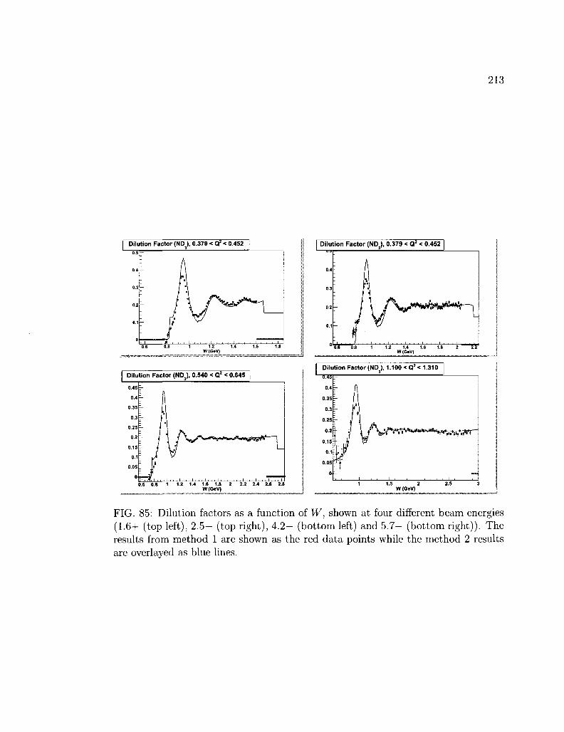
213
I Dilution Factor (ND3), 0.379 < Q2 < 0.452
Dilution Factor (ND3), 0.540 < Q2 < 0.645 |
0.45
0.4
0.35
0.3
0.25
0.2
0.15
0.1
0.05
0 =H"
• I 7 \^if^^t~^j'*^i^^^~'''fftj^fM^t I
F f,.., i,, 0.6 0.8 1 1.2 1.4 1.6 1.8 2 2.2 2.4 2.6 2.8
W(GeV)
•""•'• '• '""w-Vi'iHWr
1.5 2 W(GeV)
FIG. 85: Dilution factors as a function of W, shown at four different beam energies (1.6+ (top left), 2 . 5 - (top right), 4 . 2 - (bottom left) and 5 .7- (bottom right)). The results from method 1 are shown as the red data points while the method 2 results are overlayed as blue lines.

214
stmSt-
1 Dilution Factor (ND3), 1.500 < W < 1.650
0.5
0.45
0.4
0.35
0.3
0.25
0.15
0.1
0.05
-r
" " ° " ~ Q'lO.>aU_
I Dilution Factor (ND ), 1.650 <W< 1.800 |
SLlf&) I Dilution Factor (ND,), 2.100 < W < 2.250 I
0.5
0.45
0.4
0.35
0.3
0.25
0.2
0.15
0.1
0.05
0
s_Q !(Gey !)_ 1
I Dilution Factor (ND3). 1.350 <W< 1.500 |
0.5r
Dilution Factor
0.5
0.45
0.4
0.35
0.3
0.25
0.2
0.15
0.1
0.05
(NDj) 1.500 <W< 1.650
, • • • • • "
I
I
• %
I
^ _ ___rfwgl__ I Dilution Factor (ND3), 1.950 <W<2.100 J
[ Dilution Factor
0.45
0.4
0.35
0.3
0.25
0.2
0.15
0.1
0.05
0
---_ : r
L
--»*»«•!
(NDj), 1.650 <W< 1.800 1
« . . . • • • • • * *
FIG. 86: Dilution factors as a function of Q2, shown for several W bins, for the 4.2— (top) and 5.7— (bottom) data sets. There is a slight Q2 dependence of the dilution factor for some W regions.

215
IV.12 B A C K G R O U N D ANALYSIS
Electron rates measured in the EG lb experiment are contaminated by misidenti-
fied pions and pair symmetric electrons. This contamination affects the measured
asymmetry, and therefore an extra correction should be applied to account for this
effect. The correction to the asymmetry comes from the fact that the count rates
used to calculate the asymmetry are changed by the amount of misidentified parti
cles. Therefore, when we calculate the raw asymmetry in terms of the electron count
rates for positive (N+) and negative (N~) helicities,
N~ - N+
Araw = N- + N+ ' (351)
the count rates should be corrected by the amount of corresponding contaminations
N+ and N~ for both helicities:
_ (iV- - N-) - (iV+ - iV+)
where (N~ — N~) and (iV+ — N+) are the uncontaminated count rates for the two
helicity states. Let's assign for total counts iV = N+ + N~ and Nc = N* + N~, and
re-arrange the terms to isolate the contamination:
_ (N~ - N+) - (N- - JV+) corr~ (N-Nc) • [ '
By dividing the numerator and the denominator by N, we can write
N--N+ _ Af~-iVc+
Acorr = \ - Nc/N • ( 3 5 4 )
With the ratio of the contaminant to the contaminated count R = Nc/N, the above
expression can be written as:
A _ NC-N+ •fT-raw Nc/R
•A-corr = Z ~ • (odd) 1 — it
Defining Ac = (N~ — N+)/Nc, which is the raw asymmetry of the contaminant,
yields Ar - RA
•Acorr = - — (oob)
1 — K
or we can write: •f*-corr ^back-^raw V " " ' /

216
where 1 — HAC/Araw foc.Q\
(-'back — -. _ „ • [600)
Therefore, in order to correct the raw asymmetry, we need to know the ratio R and
also the asymmetry of the contaminating particle in the corresponding kinematics.
In a more generalized form, the background correction to the asymmetry can be
written as:
• ^raw •™corr -firaw . > \OOif)
i
where Ri are the fractions of events coming from a given background and A{ are the
asymmetries of the contributing background processes.
There are mainly two distinct sources of such background in the EG lb analy
sis. The first one is pions misidentified as electrons and the second one is secondary
electrons that mostly come from the pair production process. In the following sub
sections, we investigate these backgrounds separately and come up with a method of
correction.
IV.12.1 Pion Contamination
In the EG lb experiment the main tool to separate pions from electrons is the
Cherenkov counter (CC). The CC can separate pions from electrons up to 2.5 GeV. A
pion in this energy range can have a CC signal around 0-1 photoelectrons. When we
examine the signal from the CC, we see a huge pion peak around 1 photoelectrons.
The tail of this peak contaminates the electron sample up to the 4 or 5 photoelectron
range. Above 2.5 GeV, on the other hand, pions also begin to produce a Cherenkov
signal in the detector material. It is not possible to separate these high energy pions
from electrons at all using the CC alone. Therefore, we need to correct the resulting
asymmetry for contamination. To remove pions up to 2.5 GeV from the electron
sample, we apply a CC signal cut to the electrons. We need to optimize the place
of this cut to remove most of the pions and not to reduce the electron statistics too
much at the same time. If we increase the strictness of the Cherenkov cut too much
to remove more pions, we lose too many electrons, hence causing a larger statistical
uncertainty in our results. Therefore, we need to apply an optimum cut to remove
the pion peak from our electron sample and deal with the rest of the pions by other
methods.
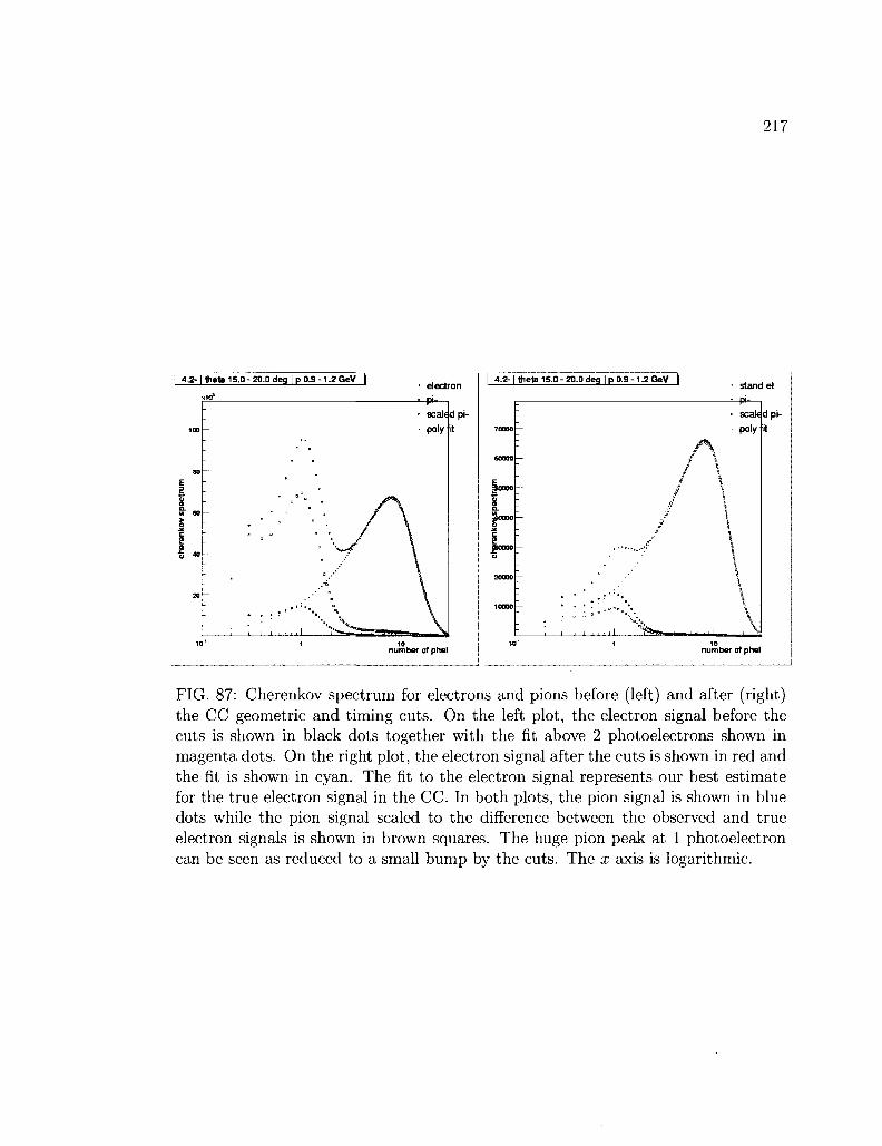
217
4.2- | theta 1S.0 - 20.0 deg | p 0.9 -1.2 GeV
xigl electron
- p k
scaled pi
poly it
number of phel
4.2-|theta15.D-2D.0deg jp 0.9-1.2 GeV | stand el
number of phel
FIG. 87: Cherenkov spectrum for electrons and pions before (left) and after (right) the CC geometric and timing cuts. On the left plot, the electron signal before the cuts is shown in black dots together with the fit above 2 photoelectrons shown in magenta dots. On the right plot, the electron signal after the cuts is shown in red and the fit is shown in cyan. The fit to the electron signal represents our best estimate for the true electron signal in the CC. In both plots, the pion signal is shown in blue dots while the pion signal scaled to the difference between the observed and true electron signals is shown in brown squares. The huge pion peak at 1 photoelectron can be seen as reduced to a small bump by the cuts. The x axis is logarithmic.

218
TABLE 34: Momentum bins (in GeV) used for the pion contamination analysis.
bin 1 2 3 4 5 6 7 8 9 10 11 12 13 14
min 0.03 0.30 0.60 0.90 1.20 1.50 1.80 2.20 2.60 3.00 3.40 3.90 4.40 4.90
max 0.30 0.60 0.90 1.20 1.50 1.80 2.20 2.60 3.00 3.40 3.90 4.40 4.90 5.40
Applying geometrical and temporal cuts to remove pion contamination from the
electron sample was a breakthrough in our pion contamination analysis (see Fig.
51). The huge pion peak shown in the left plot of Fig. 87 is reduced by these
cuts as shown on the right. The remaining contamination was carefully analyzed to
determine the pion to electron ratio in the CC region above the photoelectron cut
and in the full CC region. The ratio above the 2 photoelectrons cut is called standard
contamination and the ratio in the full CC region is called total contamination. The
standard contamination is used for pions below 2.5 GeV. The total contamination is
used to determine contamination above 3.0 GeV. A linear combination of standard
and total contamination is used between 2.5 and 3.0 GeV.
The main idea behind the pion contamination analysis lies with the assumption
that the pion to electron ratio must be a smooth function of momentum and polar
angle. Once we determine the form of this function, we can determine the ratio for
any given kinematics. By using carefully determined momentum and polar angle bins
shown in Tables 34 and 35, we examined the data bin by bin to determine pion to
electron ratios and extract the functional dependence of the ratio R^ on momentum
and 0. The ratio for a specific momentum and polar angle bin is determined by
scaling a pion sample with small photoelectron signal to the pion peak in the electron
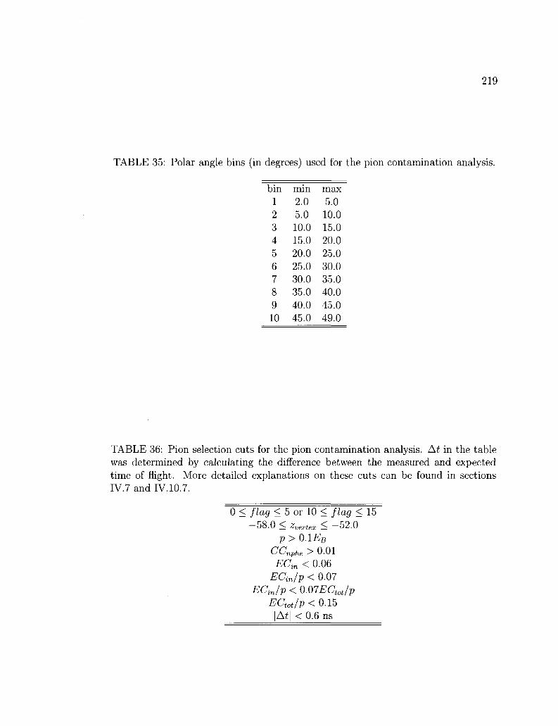
219
TABLE 35: Polar angle bins (in degrees) used for the pion contamination analysis.
bin 1 2 3 4 5 6 7 8 9 10
min 2.0 5.0 10.0 15.0 20.0 25.0 30.0 35.0 40.0 45.0
max 5.0 10.0 15.0 20.0 25.0 30.0 35.0 40.0 45.0 49.0
TABLE 36: Pion selection cuts for the pion contamination analysis. At in the table was determined by calculating the difference between the measured and expected time of flight. More detailed explanations on these cuts can be found in sections IV.7 and IV. 10.7.
0 < flag < 5 or 10 < flag < 15 — 58.0 < ^vertex 5: — 52.0
p > 0.1EB
CCnphe > 0.01 ECin < 0.06
ECin/p < 0.07 ECjp < 0.07ECtot/p
ECtat/p < 0.15 |At| < 0.6 ns
220
sample. Electromagnetic calorimeter signals and timing cuts are used to extract the
best pion selection for our purpose. Table 36 summarizes all major detector cuts we
applied to select pions. For the 1.6 GeV data we also applied an additional trigger
bit cut because this data set required a more precise selection of pions to get a clean
sample. Trigger bits 1 to 6 correspond to our standard triggers based on the CC and
EC signals and they are used for electrons. Trigger bit 7 requires a hit in EC and
CC anywhere, while trigger bit 8 requires a hit only in EC with a lower threshold
(no CC hit). Trigger bit 8 is mainly used for minimally biased pion selection (see
IV.7.2) but since it is pre-scaled it also reduces the sample size a great deal. For the
1.6 GeV set it was very difficult to get a clean sample by just applying the EC and
timing cuts, so, we used trigger bits 7 and 8 to select pions in addition to the regular
cuts described in Table 36.
It is probably best to explain our method of finding the pion to electron ratio by
using Fig. 88. The plot shows the Cherenkov spectrum after all cuts for electrons
(red) and pions (blue). The horizontal axis is a logarithmic scale and represents
the number of photoelectrons produced by the particle in the Cherenkov counter.
The cyan points represent a fit to the electron spectrum and approximates the true
electron sample without pion contamination. It is a simple combination of 3 r d and 7th
degree polynomial fits in the region of the spectrum above the pion peak. The fit can
be thought as a simulation of electrons with the same kinematics in the Cherenkov
counter. The difference between the red and cyan distributions is assumed to all come
from pions that are misidentified as electrons by the detector. We can call these pions
extracted pions. The "true" pions from our pion sample (blue points), are scaled to
the extracted pions. The resulting spectrum is shown with the brown points (hollow
squares) and represents our best guess for the pion contamination. By summing all
pions and electrons above our photoelectron threshold, which is 2 photoelectrons, we
determined their ratio. This ratio is called the standard contamination. We also took
the pion to electron ratio in the full spectrum, above and below our photoelectron
threshold, which gave us the total contamination. This procedure was repeated for
each momentum and polar angle bin where enough data for a clean fit and extraction
were available.
When we examine the distribution of pion to electron ratio with respect to mo
mentum for a single polar angle bin, we see an exponential dependence. Fig. 89
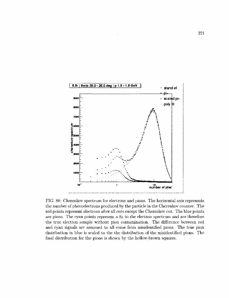
221
5.8- [ theta 20.D - 25.0 deg | p 1.5 -1.8 GeV |
10 number of phei
FIG. 88: Cherenkov spectrum for electrons and pions. The horizontal axis represents the number of photoelectrons produced by the particle in the Cherenkov counter. The red points represent electrons after all cuts except the Cherenkov cut. The blue points are pions. The cyan points represent a fit to the electron spectrum and are therefore the true electron sample without pion contamination. The difference between red and cyan signals are assumed to all come from misidentified pions. The true pion distribution in blue is scaled to the the distribution of the misidentified pions. The final distribution for the pions is shown by the hollow-brown squares.

222
0.02
0.018
0.016
.0
J 0.01 c
3>O08
i.OOS
0.004
0.002
C -i i i i i
0.5
X2/ndf 1.2!4(3
Constant -3836±0 4754
Slop* -1178 ±0 3379 : I
* theta [20.0, 25.0]
\ !
\ 1 •• -rH^H , , , i , , , , i , , , , i , , , , i
1 1 •I ;
, , , i , 1 1.5 2 2.5 3
momentum(GeV)
I I i I 3.5 4
0.02
0.018
0.016
^1.014 O •3)012 c
J 0.01
&.008 •
0.006
0.004
0.002
t
7
-'
XJ'nilf 0.46I8/3
Constant -3.221+ 0B474
Slops -t.858± 0 6821
theta |25 0, 30.0J
;I
! ':! | ! i -• I . \
0.5 1 1.5 2 2.5 momentum(GeV)
, L ,, , i , ,,, 3 3.5 4
FIG. 89: Pion to electron ratio as a function of momentum for polar angle bins for 20-25 (left) and 25-30 (right) degrees.
shows the distribution of ratios for different momentum bins and the overall expo
nential fit to the points. The ratio follows a smooth function up to a momentum
of 2.5 GeV, where the Cherenkov counter is no longer able to distinguish between
electrons and pions. Below 2.5 GeV, we can write the pion to electron ratio as:
Rn = eCn+s,P (360)
where p is momentum of the particle (electron). In the above equation, C„ and 5V
actually depend on 6. Therefore, we can write the equation in the form:
R = ec*(e)+SA0)p (361)
We need to find the form of C1[{6) and S%{6). When we examine the dependence of
the parameters Cw and 5W on polar angle, we see, according to Fig. 90, that they are
both linear functions of the polar angle. Therefore,
Cv{0) = a + b0
S7T{6) = c + d0
(362)
(363)
As a result, we can write the overall functional form of the pion to electron ratio in
the following form: ^> _ eC*(6)+S*(9)p _ ea+b0+cp+Mp (364)

223
c o o E "5. •a c CO
(A - -2
a x o>
2h
E £2 CO
a.
i
XJAndf 0.3044/2
P<> -4.192 ± 1-009
P1 0.02694 ± 0.0)4948
I.70: 5 X2 / ndf 0.
PO -0.6489 + 0.
P1 -0.03031 +0.43741
12
7856
theta (deg)
FIG. 90: Dependence of the exponential parameters on the polar angle. In the plot, the red data points represent C7!{6) (the constant factor in the equation) and the blue points represent S„(8) (the slope factor of the equation). The resulting parameters from the fit to CV(#) give a and b (in the upper box), while the parameters from the fit to Sir(0) give c and d (in the lower box) according to Eq. (364).
224
By using momentum and polar angle bins where data are available, we can de
termine all parameters a, b, c and d with good precision for each energy and torus
current configuration. It should be noted that these parameters depend on the beam
energy and the torus polarity, hence, a separate fit must be done for each data set.
Once these parameters are determined, it is possible to calculate the ratio Rv for any
momentum and polar angle value. Once we parametrized the ratio Rn, we can fix
our raw asymmetry for pion contamination according to:
AT = Aei1 ~ ^J^1 where Rn = - (365) 1 — Kn e
However, since our pion contamination was reduced significantly after the geometric
and timing cuts, mentioned in section IV.8, we decided to use the contamination
itself as an estimate of the systematic error. Some final typical values for the ratio
Rv can be seen in Fig. 89 for two different 9 bins. In addition, more values of Rv
for various data sets and kinematics are also shown at the right hand side of Fig.
51. The maximum value of the ratio is generally around 0.5% for low momentum
range and it rapidly decreases with increasing momentum. Consequently, we do not
need to determine the pion asymmetry at all. We can simply take it to be practically
zero16 and correct the electron asymmetry according to
^ r = r^k K = ~e- (366)
The difference between the corrected asymmetry and the uncorrected asymmetry is
then taken as a systematic error on the final asymmetry.
As we mentioned earlier, this whole procedure is valid for electrons up to 2.5
GeV. At higher energies, pions also begin to give a strong signal in the CC and
those pions contaminate the electron sample in a different way. To determine the
amount of contamination in the high energy region, we followed a similar approach
but we used an electron sample which was not cleaned by the geometric and timing
cuts. Moreover, we used the full CC spectrum to determine total pion contamination.
Again this analysis was done as explained earlier for each momentum and polar angle
bins and the functional form of the total pion contamination was determined. Of
course, the functional form is the same as the standard contamination except that
the parameters are different. Fig. 91 shows the standard and total contamination
before the geometric and timing cuts were applied for a single 9 bin. Extrapolation 16 This corresponds to a limit — 1 < A„/Aei < 1.

225
0.2
0.18
0.16
c 0 . 1 4 O
"5 0.12 C
| 0.1 c 8 0.08
a 0 . 0 6
0.04
0.02
_ ~
" i i i i
|V
Xa /ndf 0.3931/3
Constant 0.3871 ± 0
S!PP# -21137 + 0
X J / *d f
Constant -i;W
Slope -2 0!
3742
2795
0.21 13/3
S9 ± 0 4884
54 ± 0 3618
» theta (20.0, 25,0)
i i i i I i i i i I i i i T T T T ? - * - J I i i i I i ' i l l i i i
0.5 1.5 2 2.5 momentum(GeV)
3.5
FIG. 91: Total and standard contaminations as a function of momentum for a single polar angle bin. This analysis was done by using an electron sample that was not cleaned by the geometric and timing cuts (see section IV. 8). The total contamination on the full CC spectrum and the standard contamination above the photoelectron threshold are shown together. The total contamination is larger than the standard contamination.
of the total contamination was used to find the pion to electron ratio above 3.0 GeV.
In between 2.5 and 3.0 GeV, a simple linear combination of standard contamination
and total contamination was used.
IV.12.2 Pair Symmetric Electron Contamination
Another source of background contamination in the EG lb experiment is secondary
electrons. The secondary electrons mainly come from electron-positron pair produc
tion inside the detector. There is no way to tell if the detected electron is a primary
electron from the scattering off the target or a secondary electron from the pair pro
duction process. The system simply accepts the first electron as the trigger particle.
The number of electrons that come from pair production is very small but we still

226
TABLE 37: Cuts on Positrons
0 < flag < 5 or 10 < flag < 15 —58.0 < zvertex < —52.0
triggerbit cut (see section IV.7.2) p > 0.15EB
CCnphe > 0.01 ECin > 0.06
ECtot/p > 0.20 for p < 3.0 ECtat/p > 0.24 for p > 3.0
need to correct the asymmetry for the contamination caused by these electron, which
are referred to as the pair symmetric electrons.
Electron-positron pair production has two main sources inside the CLAS detector:
The decay 7r° —» e + e _ 7 (also known as the Dalitz decay) plays the leading role with
a 1.2% branching ratio. The other possible source is 7r° —• 77 and 7 —> e+e~. Other
sources of e+e~ pair creation such as Bremstrahlung photons are all very small and
hence negligeble. More detailed information about pair production rates in the EG lb
experiment can be found in CLAS note Ref. [115].
Since we cannot distinguish pair symmetric electrons from the original scattered
electrons, the only way to estimate the contribution from electrons coming from pair
creation is to monitor the corresponding positrons because every pair symmetric elec
tron should be accompanied by a positron with the same kinematics. Normally, the
positron to electron ratio would automatically give us the amount of pair symmetric
contamination. However, there is a strong magnetic field inside the CLAS detec
tor which bends the particle's trajectory according to its charge. This affects the
acceptance of the detector depending on the charge of the particle. Therefore, the
acceptance is not the same for electrons and positrons since they will be bent in op
posite directions by the torus field. In order to get the same acceptance, we actually
need to compare electrons to positrons from opposite torus polarity configurations.
In the EGlb experiment, we have DST files, where the electron is the trigger
particle, and also DSTp files where no electron was found and therefore the trigger
particle was a positron. The DSTp files are stored separately. There are a few
positron counts in the DST files but most positrons are in the DSTp files. We

227
processed both file types to get the total count of positrons in each kinematic bin.
The electron and positron cuts are the same except for the charge requirement.
Table 37 lists the cuts applied to select positrons. In addition to those shown in
the table, we also applied fiducial cuts as well as geometrical and timing cuts. We
cleaned the positron and electron samples from pion contamination. We performed
the 7r+ contamination analysis on positrons exactly the same way we performed the
7T~ contamination analysis on the electrons.
Fig. 92 shows the CC spectra for positrons and ir+ for a single polar angle and
momentum bin. The positron peak shown is already cleaned from most misidentified
7r+ by applying the geometric and teming cuts. Still, a huge 7r+ contamination dis
torts the shape of the positron spectrum. Our goal is to obtain the uncontaminated
positron spectrum and find the difference between contaminated and uncontaminated
spectra to determine the amount of n+ in the positron rate. For this purpose, we
used the fact that the positron and electron CC spectra should be exactly the same
as long as we have the same acceptance. Therefore, we used a fit to the correspond
ing electron spectrum (with the reduced pion contamination, i.e., after geometric
and timing cuts), with the same acceptance to estimate the true (uncontaminated)
positron distribution. This was done by scaling the electron spectrum to the positron
spectrum above 7 photoelectrons, and fitting the resulting electron spectrum, thus
obtaining the estimated positron spectrum. The cyan colored fit in Fig. 92 shows
our best estimate for the final true positrons in the CC. It should be noted that,
while creating the true positron spectrum by using the electrons from the opposite
torus current data, both of the samples should be normalized to the corresponding
total beam charge before the scaling is done.
Afterward, the amount of ir+ contamination on positrons can be estimated by
looking at the difference between the true and observed positron distributions (note
that the observed positron distributions must have the geometric and timing cuts
applied to them). Once the spectrum for this difference was generated, the true
(or scaled) pion distribution, the brown-triangle data in Fig. 92, was obtained by
scaling the observed pion distribution17 to this difference. Then we summed the
number of pions in the true (scaled) pion distribution to determine the integrated pion
rate. Similar summation was also made for the positrons by using the the observed
positron distribution, in the same range of number of photoelectrons in the CC. The
17The observed n+ peak is much too big to fit on the scale of that plot.
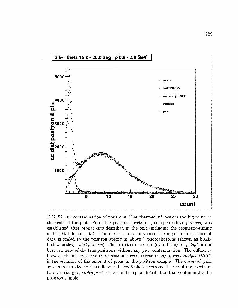
228
2.5- | theta 15.0 - 20.0 deg | p 0.6 - 0.9 GeV |
5000
4000
+ '5.
£ 3 0 0 0 ^
"<5 o a .
+•»
.S2000 TJ
o
IOOOH
• pLrepos
a scaledpLrepos
* pos -s1an( 30E DIFF
» scaledpH-
- poly 11
count
FIG. 92: 7r+ contamination of positrons. The observed n+ peak is too big to fit on the scale of the plot. First, the positron spectrum (red-square dots, purepos) was established after proper cuts described in the text (including the geometric-timing and tight fiducial cuts). The electron spectrum from the opposite torus current data is scaled to the positron spectrum above 7 photoelectrons (shown as black-hollow circles, scaled purepos). The fit to this spectrum (cyan-triangles, polyfit) is our best estimate of the true positrons without any pion contamination. The difference between the observed and true positron spectra (green-triangle, pos-standpos DIFF) is the estimate of the amount of pions in the positron sample. The observed pion spectrum is scaled to this difference below 6 photoelectrons. The resulting spectrum (brown-triangles, scaled pi+) is the final true pion distribution that contaminates the positron sample.

229
0.9
0.8
0.7
0.6
0.5
0.4
0.3
0.2
0.1
; :
= -:
; r
Mil
K , , ,
! ! - l ^ -J 1
i V:1
1 :
I7 : [ ? • • • •
' : 1 1
; m. : r:-;
f
X2/ndl 1.499/3
Constant -1.436± Sope
X Indl
0160410
1.169
1285
1.1 "1/3
Cmstart -3,329 ±0 Sops 1.204 + 0
3432
2615
iheta [25 0. 30.0|
1.5 2 2.5 3 momentum(GeV)
1.5 2 2.5 3 momentum(GeV)
FIG. 93: 7r+ to positron ratio as a function of momentum is shown for the 8 bins 20° < 9 < 25° (left) and 25° < d < 30° (right). As in the case of electrons, this ratio follows an exponential form and can be considered as a smooth function of momentum.
c o o O. 0
d
a x a> <*-o E S CO
a
-2
-6H
1
X2/ndf 0.2757/2
pO
Pi
-2.602+D.675
-0.02257 ±0.03104
1—4
_L ± 15 20 25 30 35 40 45
theta(deg)
FIG. 94: 7i+ contamination of positron. The points show the 6 dependence of the exponential fit parameters, the slope Se(9) and the constant factor Ce(6).

230
0.25
0.2
r to.
0.05
I I I I I I I I I 1 I I I I I 11*1-1 A I I I A I I I J, I I I JL I I I IJJ I I
0 0.5 1 1.5 2 2.5 3 3.5 4 momentum(GeV)
FIG. 95: e + / e ratio as a function of momentum for a single polar angle bin. It follows an exponential function as in the previous cases.
ratio of the integrated pion and positron (from the observed positron distribution)
rates for each kinematic bin determines the amount of pion contamination in the
positron sample. The ratio of the integrated rates in the full CC range gives the
total contamination, while the ratio above a CC threshold of 2 photoelectrons gives
the standard contamination. Fig. 93 shows the pion to positron ratio as a function
of momentum. It is fitted by an exponential function. In the figure, the total
contamination (the larger ratio) and the standard contamination are shown together.
It should be noted that this plot is for a single polar angle bin. The fit parameters
should be a smooth function of polar angle as well. Fig. 94 shows the exponential fit
parameters (Ce and Se) for each 9 bin as a function of 9. Therefore, Figs. 93 and 94
together actually confirms our basic assumption that the contamination should be a
smooth function of momentum and polar angle.
The amount of pair symmetric electrons contaminating the true electron sample
is estimated by using the true positron spectrum from opposite torus polarity data

231
4
2
tio
ID k.
4> o +
1 1 -2
a 0> o jm - 4
s a a.
-6
i
-
-
i*-*0**'^
—
1 1 1 1 1 1 1
0 15
^ ^ • " • " " a
i i I i i i i I i i i i I i i
20 25 30
theta(deg)
Z2/ndf 249.4/2
P0 -2.419 ±0.02602
P1 0.1206 ±0.001269
X2/m|fc»-'*"' 88.B/2
"pO .1.191 ±0.12219
p1 4.08465 ±0.0(1051
• const • slope
i i I i i i i I i i i i
35 40 4 5
FIG. 96: The exponential fit parameters Ce(6) (blue, labeled as const) and Se(8) (red, labeled as slope) for each 6 bin are plotted as a function of 9. They follow a linear dependence as expected.

232
(after n+ contamination is removed from the sample). Therefore, the ratio of the
integrated true (uncontaminated) positron spectrum (from opposite torus polarity)
over the integrated electron spectrum (after minimizing the TT~ contamination by
geometric and timing cuts) gives us the contamination caused by the pair symmetric
electrons. The integrations for both spectra were done above 7 photoelectrons so
that the remaining IT~ contamination in the electron sample (that persists in the
low photoelectron region but it is very small in general) does not propagate into the
e+/e~ ratio. Note that both data samples were first normalized to their corresponding
beam charge before taking their ratio. Fig. 95 shows and example of such a ratio as
a function of momentum for a single 9 bin. As expected, it follows an exponential
form: Re = eCeW+st(e)P ( 3 6 7 )
Ce and Se are fit parameters that depend on the polar angle 8. Fig. 96 shows the
dependence of these parameters on 6. In the end, the pair symmetric contamination
is also a smooth function of momentum and polar angle in the form:
Re — eCe(e)+Se{d)p = ea+be+cP+d9p (ggg)
Once we determine the parameters from available data, we can determine the ratio
Re — e + /e~ for any kinematics and correct the asymmetry by applying the correction
formula: Araw
1 - Re^a Ar?w - RPAraw
Acorr _ Araw nel _ el ±l-e-"-poS Cicc\\ Aei ~Aei 1-/L ~ rni [dW)
Araw Araw
<"r = V - p - « . ) ' " (370)
In order to correct the asymmetry, we need the raw asymmetry of the contami
nant electrons as well as the ratio. By definition, the asymmetry of pair symmetric
electrons is the same as the asymmetry of positrons for the opposite torus polar
ity. Therefore, we determined the positron asymmetry from data for each of our
momentum and polar angle bins and wrote the values into a table. The analysis
program reads in this table to find the corresponding positron asymmetry for a given
momentum and polar angle. Fig. 97 shows the positron asymmetries as a function
of momentum for a single 6 bin. A few data sets are shown to give a general idea. In
most kinematics, the positron asymmetry is consistent with zero. This correction is,
in general, very small, on the order of 0.2% of the statistical error in most bins, less
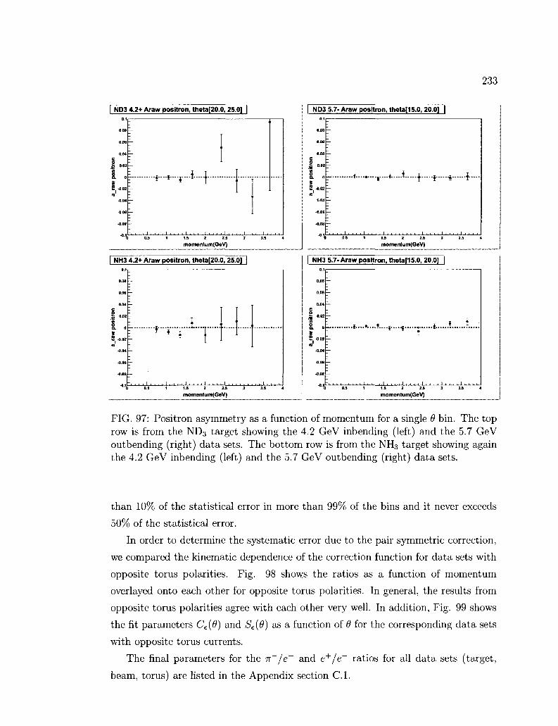
233
ND3 4.2* Araw positron, theta[20.0,25.0] |
momentum(GeV)
NH3 4.2* Araw positron, theta[20.0, 25.0]
momentum(GeV)
| ND3 5.7-Araw positron, theta[15.0, 20.0] |
" 0.08
O.Ofi
0.04 c o £ 0.02
& o S 2-0.02
«' -0.04
-0.06
-0.08
•°\
-r
r
:_
r * s - -*-J i * s-
-r r
0.5 1 1.S 2 2.5 3
momenta m(GeV)
•-i
. 1 . . . . 3.5 A
NH3 5.7-Araw positron, theta[15.0, 20.0] |
momentum(GeV)
FIG. 97: Positron asymmetry as a function of momentum for a single 6 bin. The top row is from the ND3 target showing the 4.2 GeV inbending (left) and the 5.7 GeV outbending (right) data sets. The bottom row is from the NH3 target showing again the 4.2 GeV inbending (left) and the 5.7 GeV outbending (right) data sets.
than 10% of the statistical error in more than 99% of the bins and it never exceeds
50% of the statistical error.
In order to determine the systematic error due to the pair symmetric correction,
we compared the kinematic dependence of the correction function for data sets with
opposite torus polarities. Fig. 98 shows the ratios as a function of momentum
overlayed onto each other for opposite torus polarities. In general, the results from
opposite torus polarities agree with each other very well. In addition, Fig. 99 shows
the fit parameters Ce(6) and Se(8) as a function of 9 for the corresponding data sets
with opposite torus currents.
The final parameters for the ir~/e~ and e+ /e~ ratios for all data sets (target,
beam, torus) are listed in the Appendix section C.l.

234
| 4.2 GeV | theta 20.0 -
0.2
.20.15
| +
* 0.1
0.05
0
25.0 deg
; \
0.5 1.5 f *5.5
i - iJndl 333.8/G
Constant 6^562 ± 0.01082
Slope -3-JM ± 0.COM65
1 O inb(+) D oub(-)
" ' ^ " j . s 0 " ^
4.2 GeV | theta 25.0 - 30.0 deg I>'"'•" ««<e Constant 0.M39 i 0 01M5
-3 543 ± 0.013O5
O inb(+) D oub(-)
momentum(GeV) 0 0.5 1 1.5 2
momentum(GeV)
FIG. 98: e + / e ratio for opposite torus polarity data for two 6 bins.
• s h
X2/radl
pO
p1
6.643/2
'1.743 ±0.05786
fp3Sm ± 0.002*66
57 ndl
pO
p1
15.99/2
-1.94.3 ± 0.04415
-0.05115 ± 0jd* i7 i i
H^/ndl 2S3.3i'2
pD -2.419 ± 0.02574
p1 0.120* ± 0.001257
J ! 2 /ndf 90 .13*2
pO -1.169 ± O-OHflt
p1 -0.0447 ± 0.001037
I i i i i I i i i i I i i i i I i i i i I I I I I I I I 15 20 25 30 35 40
theta(deg) 45
FIG. 99: The exponential fit parameters Ce (const) and Se (slope) for 4.2 GeV inbending and outbending data sets are shown together as a function of 6.
235
IV.13 B E A M A N D TARGET POLARIZATION
In order to determine the double spin asymmetry, the raw asymmetry from the count
rates needs to be corrected for the net polarization. Therefore the product of the
beam and target polarization is required. During the experiment, the beam polar
ization was measured by using the Moller Polarimeter and the target polarization
was monitored by the Nuclear Magnetic Resonance (NMR) system. In the EG lb
experiment, the electron beam polarization was very stable and the measurements
from the Moller Polarimeter are dependable. On the other hand, the target polariza
tion was not quite stable. Moreover, the NMR coils are located outside the target,
and are therefore more sensitive to the outer layers of the target material. However,
the polarization of the target can change within the target volume, especially since
the regions of the target exposed to the beam are depolarized more quickly. To pre
vent quick and local depolarization of the target material, the beam is rastered over
the target area in a spiral motion. However, the rastering is not always perfect and
especially the outer layer of the target, to which the NMR is most sensitive, is not effi
ciently rastered. Therefore, it is generally expected that NMR values are superficially
higher than the true polarization of the target. Moreover, there are other technical
uncertainties on the NMR readings that are not well understood. As a result, we
need a reliable method of determining the true beam x target polarization.
The most reliable method to determine the polarization is to extract the infor
mation from the data itself. This extraction is based on the fact that the theoretical
asymmetry for elastic and quasi-elastic events is well determined. Once the theo
retical asymmetry is known, the beam and target polarization can be determined
according to: A quasi—el
p p = meas ( 3 - ^
*D Aheo
where Fp stands for the dilution factor to remove the effect of scattering from un-
polarized nucleons in the target. Therefore, what we need to do is to extract the
asymmetry by using quasi-elastic scattering from the deuteron, correct it for the
background contributions and then divide it by the theoretical prediction. For the
EGlb experiment, this was done separately for each Q2 bin. Then, the PbPt values
from all Q2 bins with reasonable statistical error were averaged to determine the final
value.

236
IV.13.1 Theoretical Asymmetry For Quasi-Elastic Scattering from the
Deuteron
The double-spin asymmetry A\\ can be calculated by using the electric and magnetic
form factors GE and GM in the elastic region. The virtual photon asymmetries for
elastic scattering are simply [1]:
Ax = 1 (372)
and /Q* GE(Q2)
A2 = y/R (el) v GM(Q2)'
(373)
i?(ei) represents the structure function R in the elastic region. It can be shown from
Eqs. (20), (21) and (22) that Q2 = IMv for the elastic events. Hence, the double
spin asymmetry for elastic scattering can be calculated by using Eqs. (26-29) and
(67) such that [17]:
, 2 r G [ f + G ( r f + (1 + r) tan2(fl/2))] A|1 = 1 + G2 r/e ' ( 3 ? 4 )
where r = Q2/AM2, G = GM/GE, E is the beam energy, M is the mass of the
nucleon and 6 is the polar scattering angle of the electron. For the electromagnetic
form factors we used the latest parametrization by J. Arrington [116]:
GE(Q2) = [l + P2Q2 + P4Q4+p6Q6 + .- +P12Q12] l
GM{Q2) = nP [l + P2Q2 +P4Q4 +P6Q
6 + ... +P12Q1 2]"1
where the coefficients P2-P12 are given in Table 38.
(375)
(376)
TABLE 38: Fit parameters for the Rosenbluth form factors GE and GM [116].
Parameter
P2
Pi
Pe Ps Pw P12
GE
3.226 1.508
-0.3773 0.611
-0.1853 0.01596
GM
3.19 1.355 0.151
-0.0114 5.33xl0"4
-9.00xl0"6
The double spin asymmetries of the proton and the neutron were calculated
according to Eq. (374) using the parameterization given by Arrington. After that,

237
the deuteron quasi-elastic asymmetry was determined from that of the proton and
the neutron as the weighted average:
n aeJAeJ + ofAi ( 3 \ , , AD = _P_JL nn / j _ o \ g^
II rf + a* V 2 D) y > where WD is the probability of finding deuteron in D-state. However, this procedure
was later replaced with a more advance calculations of the theoretical asymmetries by
Sebastian Kuhn, which included the proper momentum distribution of the nucleons
inside the deuteron as well as radiative effects. Not much difference was observed for
the proton; however, for the deuteron we found that it is important to account for the
nuclear and radiative effects. For the final results, the theoretical elastic asymmetries
from S. Kuhn were used to calculate PbPt for the deuteron.
IV. 13.2 Extraction of Quasi-Elastic Asymmetry from the Data
There are two methods for the extraction of the quasi-elastic asymmetries from data.
In the first method, quasi-elastic events are selected by detecting only the scattered
electrons. This is called the inclusive method. The final state mass W is recon
structed and a specific cut on W depending on the data configuration (beam energy
and torus settings) is applied to select the quasi-elastic events. Table 39 lists the
applied cuts for each configuration. After subtracting the background contributions,
the elastic asymmetry is evaluated in the elastic W region. In the second method,
the scattered electron and a knock-out proton are both detected in the final state
and their azimuthal angle correlation is used as an additional constraint to select the
quasi-elastic events. This method is known as the exclusive method. Both methods
have their own advantages and drawbacks. Below, we will explain both methods in
more detail.
Inclusive Method
The first step is to identify the electrons. The set of cuts we used for this purpose
is shown in Table 40. The advantage of the inclusive method is its statistical power.
The amount of the quasi-elastic events determined from inclusive scattering is very
high compared to the exclusive method. However, the higher statistics comes with a
price: more background contribution. The main challenge of this method is to isolate
the elastic peak by correctly removing the background. We developed two methods
to remove the background from inclusive elastic events.

TABLE 39: W limits in GeV for (quasi-)elastic event selection in the inclusive (incl) and exclusive (excl) methods.
^beam
1.606 1.723 2.286 2.561 4.238 5.615 5.725 5.743
incl Wmin
0.90 0.90 0.90 0.90 0.90 0.88 0.88 0.88
incl Wmax
0.98 0.98 0.99 0.99 0.99 1.00 1.00 1.00
excl Wmin
0.88 0.88 0.87 0.87 0.86 0.84 0.84 0.84
excl Wmax
0.98 0.98 0.99 0.99 1.02 1.02 1.02 1.02
TABLE 40: Electron cuts for PbPt calculation with the inclusive method.
particle charge = -1 good helicity selection one electron per event
p > O.OIEB ~~
P<EB
0 < flag < 5 or 10 < flag < 15 triggerbit cut (section IV.7.2)
CCnphe > 2.0 if p < 3.0 GeV or CCnphe > 0.5 if p > 3.0 GeV " ECtot/p > 0-20 if p < 3.0 GeV or ECtot/p > 0.24 if p > 3.0 GeV
ECin > 0.06 -58.0 < Zyertex < -52.0
7.5° < 9 < 49° v > 0 GeV
sector 5 cut (section IV.7) loose fiducial cuts
geometric-timing cuts on the CC (section IV.8) W cut (see Table 39)

239
The first one is based on the carbon data and referred to as the carbon subtraction
method. In this method we assume that counts from the 12C target can be used to
simulate the 15N counts in the elastic region. We also assume that the lower tail of the
W distribution mainly comes from background. Therefore in the low W tail, beam
charge normalized ND3 counts and 12C counts should be exactly the same apart from
a scaling factor. The scaling factor accounts for the difference in the mass thickness of
the nitrogen in the ammonia and the carbon targets. Therefore, the total background
in the ND3 counts is determined by normalizing the carbon counts to the ND3 counts
in the low W region to evaluate the scaling factor and then multiplying the carbon
counts with this scaling factor in all W regions. The difference between the ND3 and
the scaled 12C counts yields the true (quasi-)elastic events. The crucial point in this
approach is to evaluate the scaling factor correctly, hence, to determine the low W
region where only the background counts contribute. We systematically studied this
Wiow region and monitored the resulting scaling factor. At the end, we determined
0.50 < W < 0.65 to be the optimal region. Below this region, we don't have enough
events for a reliable calculation. Above this region the quasi-elastic tail begins to
interfere. Figs. 100 and 101 show the background removal procedure by using the
carbon data.
The second method for background subtraction is to simply use the previously
determined dilution factor values. This method became superior to the carbon sub
traction method especially after the radiated cross section models were developed
for 15N/12C ratios, which enabled us to reliably determine the dilution factors in
the elastic region. After this accomplishment, we abandoned the carbon subtraction
method and used the dilution factors instead while determining Pb?t with the in
clusive method. However, in the exclusive method, which is explained next, carbon
subtraction remained as the main method to remove the background from elastic ep
events.
Another crucial point was to define the quasi-elastic region. We varied the W
cuts and monitored the resulting PbPt values and their statistical errors. We began
with a tight cut, which results in a large statistical error and then we loosened the
cut step by step until the Pj,Pt value stabilized. Then we also moved the cut region
by an offset and monitored the PbPt values in order to choose the region where the
values are most stable. We performed this procedure for each data configuration.
Table 39 lists the final W cuts for different beam energies.

240
W distributions from target and background scatterings W distributions from target and background scatterings
FIG. 100: W distributions from inclusive events are shown for the background removal procedure. The top row is from the 1.6 GeV ND3 positive (left) and negative (right) target polarizations. The bottom row is the same for the 2.5 GeV ND3 data set. The red solid line {Target) is the raw inclusive data from the ND3 target. The blue solid line (Backg) represents the 12C data, which is scaled to the ND3 data (green dots) and subtracted from it. The final quasi-elastic distribution is shown with black dots (Diff).

241
W distributions from target and background scatterings
Target
Backg
Backg scaled
Diff Tar-Backg
X' / ndf 4 239o.07 / 7
Constar*.279e'04 13.928a*06
Mean 0.9352 ± 3 025
Sigma 0 03264 ± 3.597
^3^Range 0.6«v- 0.770
""*•.«„„,<..•*"""**•« \
• ^ ^ v / X \ \
„.-'""""—.. \*.
90000
80000
70000
60000
|oooo u 40000
30000
20000
10000
W distributions from target and background scatterings
— Target
Backg
\ > Backg scaled
\« Diff Tar-Backg
* " " . / \ ^ S*
X'tnM
Consta
Mean
Sigma
0.64
6. 3 5 9 B+07 1 7
* . 5 2 1 e * 0 4 ± 5.869e*06
0.935113.304
0.02254 ± 3.844
ange fc,- 0.770
W distributions from target and background scatterings W distributions from target and background scatterings
3.6 0.7 0.8 0.9
FIG. 101: Same as Fig. 100 for the NH3 data sets. The top row is from the 1.6 and the bottom is from the 2.3 GeV data sets. Background removal for the NH3 target is much cleaner than for the ND3 target.
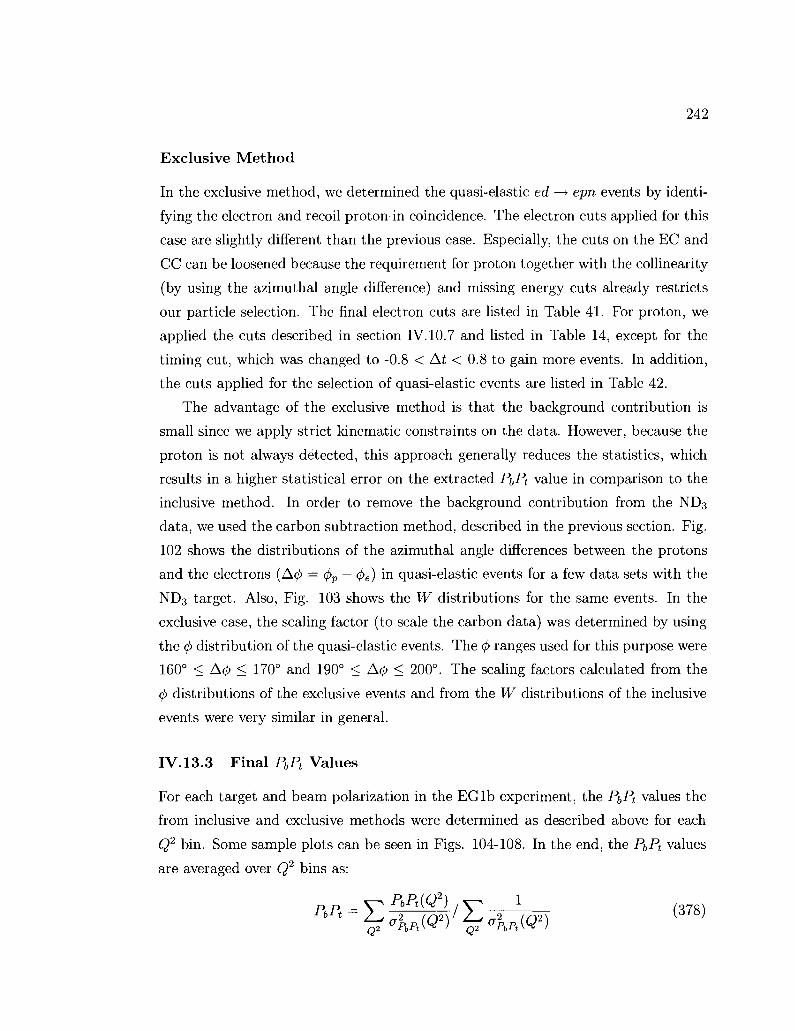
242
Exclusive M e t h o d
In the exclusive method, we determined the quasi-elastic ed —> epn events by identi
fying the electron and recoil proton in coincidence. The electron cuts applied for this
case are slightly different than the previous case. Especially, the cuts on the EC and
CC can be loosened because the requirement for proton together with the collinearity
(by using the azimuthal angle difference) and missing energy cuts already restricts
our particle selection. The final electron cuts are listed in Table 41. For proton, we
applied the cuts described in section IV. 10.7 and listed in Table 14, except for the
timing cut, which was changed to -0.8 < At < 0.8 to gain more events. In addition,
the cuts applied for the selection of quasi-elastic events are listed in Table 42.
The advantage of the exclusive method is that the background contribution is
small since we apply strict kinematic constraints on the data. However, because the
proton is not always detected, this approach generally reduces the statistics, which
results in a higher statistical error on the extracted PbPt value in comparison to the
inclusive method. In order to remove the background contribution from the ND3
data, we used the carbon subtraction method, described in the previous section. Fig.
102 shows the distributions of the azimuthal angle differences between the protons
and the electrons (A<> = <pp — (f>e) in quasi-elastic events for a few data sets with the
ND3 target. Also, Fig. 103 shows the W distributions for the same events. In the
exclusive case, the scaling factor (to scale the carbon data) was determined by using
the 4> distribution of the quasi-elastic events. The (f> ranges used for this purpose were
160° < Acj) < 170° and 190° < A0 < 200°. The scaling factors calculated from the
<f> distributions of the exclusive events and from the W distributions of the inclusive
events were very similar in general.
IV. 13.3 Final PbPt Values
For each target and beam polarization in the EG lb experiment, the PbPt values the
from inclusive and exclusive methods were determined as described above for each
Q2 bin. Some sample plots can be seen in Figs. 104-108. In the end, the PbPt values
are averaged over Q2 bins as:

243
TABLE 41: Electron cuts for PbPt calculation with the exclusive method.
particle charge = -1 good helicity selection one electron per event
P<EB
0 < flag < 5 or 10 < flag < 15 triggerbit cut (section IV.7.2)
(s(snphe ~> 1-0
ECtot/p > 015 if p < 3.0 GeV or ECtot/p > 0.20 if p > 3.0 GeV -58.0 < zvertex < -52.0
8.5° < 6 < 49° sector 5 cut (section IV.7)
v > 0 GeV
TABLE 42: Cuts for the selection of quasi-elastic events for PbPt calculation. An electron and a proton were required with at most one neutral particle in the event in order not to loose events with accidental signals in any of the detectors (by a cosmic ray or a stray photon). E[miss] and 9Q were calculated according to Eqs. (264) and (269), respectively.
good helicity selection particles in the event = 2 (or 3 with one neutral particle)
electron found in the event proton found in the event
\E[miss]\ < 0-08 GeV \0P — 0Q\ < 2°
9Q < 49° -3° < 10P - cf)e\ - 180° < 3°
W cut (see Table 39)

244
2000
1000
ft
distributions from target and background scatterings
Target
Backg
• Backg scaled
• Diff Tar-Backg
Q2 Range 0.770-0.919
$ distributions from target and background scatterings
40 150 160 170 180 190 200 210 220 * . i - * i » ( D e s >
6000
5000
„4000
c 3 O
•>3000
2000
1000
Target
Backg
• Backg scaled
• Diff Tar-Backg
Q2 Range 0.770-0.919
?40 150 " 160 T70 180 190 200 210 220
d> distributions from target and background scatterings
§1500 o o
1000
Target
Backg
« Backg scaled
• Diff Tar-Backg
<ji distributions from target and background scatterings
3000
2500
2000
c O1500
1000
500
— Target
Backg
• Backg scaled
• Diff Tar-Backg
170 180 190 200 210 220 * „ , - * p , (Deg )
170 180 190 200 210 220 «., -opr(Deg)
FIG. 102: Distribution of azimuthal angle difference between the electron and the proton (Acj) = 4>p — <fie) in exclusive quasi-elastic events for different data sets with the ND3 target. The top row is from the 1.6 GeV positive (left) and negative (right) target polarizations. The bottom row is the same for the 2.5 GeV data set. The red solid line (Target) is the raw inclusive data from the ND3 target. The blue solid line (Backg) represents the 12C data, which is scaled to the ND3 data (green dots) and subtracted from it. The final quasi-elastic distribution is shown with black dots (Diff). The range -3° < \cj>p - 4>e\ - 180° < 3° was selected for the calculation of PbPt.

245
260U
2000
1500
1000
500
W distributions from
-:
" . i . i i • - -
target
L<P K I ,
and backqround scatterinqs
V— Target
\— Backg
\* Backg scaled
\ l Diff Tar-Backg
X'/ndf 1.846e+04/7
Constant 2395± 1427
Mean 0.9451± 0.02617
Sigma 0.03317 ± 0.03243
Q2 Range l \ 0.770-0.919
*%** \
, , i , , t .« i Z ^ ^ . . , „ | , . . , i , , . ,
W distributions from target and background scatterings
3000
2500
_2000
S
O1500
1000
500
1 1.1 W(GeV)
Target
Backg
Backg scaled
Diff Tar-Backg
X' /ndl 4.743e*04/7
Constant 2676 ± 3671
Mean 0.3455± 0.06089
Sigma 0.03316 ± 0 07475
Cr Range
0.770-0.919
1 1.1 1.2 W(GeV)
W distributions from target and background scatterings
1.982e*04/7
Conslant 842.7 ± 1496
Mean 0.9441± 0.09324
Sigma 0.0377 ± 0.1273
Q2 Range 1.097-1.309
W distributions from target and background scatterings
o 600
Target
Backg
Backg scaled
Diff Tar-Backg
X ! /ndf l.367e*04/7
Conslanl 923 6± 1017
Mean 0.9482± 0.06175
Sigma 0.0422± 0.09945
Cr Range
1.097-1.309
W(GeV)
FIG. 103: W distributions for exclusive ep quasi-elastic events for different data sets, showing the background removal for the ND3 target. The top row is from the 1.6 GeV positive (left) and negative (right) target polarizations. The W cut applied on this data set to calculate Pf,Pt was 0.88 < W < 0.98. The bottom row is the same for the 2.5 GeV data. The W cut was 0.87 < W < 0.99. The explanations for the curves and data points are provided in the caption of Fig. 102.
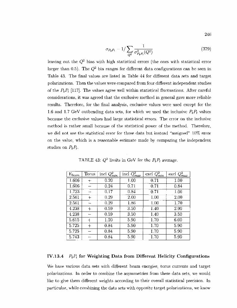
246
ff^ = 1 / E ^ J 7 ^ T (379) Q2 aPbPtW I
leaving out the Q2 bins with high statistical errors (the ones with statistical error
larger than 0.5). The Q2 bin ranges for different data configurations can be seen in
Table 43. The final values are listed in Table 44 for different data sets and target
polarizations. Then the values were compared from four different independent studies
of the Pt,Pt [117]. The values agree well within statistical fluctuations. After careful
considerations, it was agreed that the exclusive method in general gave more reliable
results. Therefore, for the final analysis, exclusive values were used except for the
1.6 and 1.7 GeV outbending data sets, for which we used the inclusive PbPt values
because the exclusive values had large statistical errors. The error on the inclusive
method is rather small because of the statistical power of the method. Therefore,
we did not use the statistical error for those data but instead "assigned" 10% error
on the value, which is a reasonable estimate made by comparing the independent
studies on PbPt-
TABLE 43: Q2 limits in GeV for the PbPt average.
f-'beam
1.606 1.606 1.723 2.561 2.561 4.238 4.238 5.615 5.725 5.725 5.743
Torus
+ —
—
+ —
+ -
+ + —
—
i n c l Qmin
0.20 0.24 0.17 0.29 0.29 0.59 0.59 1.20 0.84 0.84 0.84
incl Q2max
1.00 0.71 0.84 2.00 1.86 3.50 3.50 5.90 5.90 5.90 5.90
e x c l Qmin
0.71 0.71 0.71 1.00 1.00 1.40 1.40 1.70 1.70 1.70 1.70
excl Qmax
1.00 0.84 1.00 2.00 1.70 2.90 3.50 6.00 5.90 5.90 5.90
IV.13.4 PbPt for Weighting Data from Different Helicity Configurations
We have various data sets with different beam energies, torus currents and target
polarizations. In order to combine the asymmetries from these data sets, we would
like to give them different weights according to their overall statistical precision. In
particular, while combining the data sets with opposite target polarizations, we know

247
0.6
0.4
0.2
^ 0 Q.
-0.2
PBPT vs. Q2 for Target: ND3(+) Energy (MeV): 2561.0 Torus: 1500
- 0 . 4 h
-0.6
0.6
0.4
0.2
[ # _ * * • : # ; : a • • • B^p B B • • £ B B B B B£VJ •
•f • - • * • • - • - - T •
Excl (Method) Z2 /ndf 1.97/4
p0 0.2616 ±0.01677
e Incl (Dilution) X2 / ndf 5.391/8
p0 0.2282 ± 0.008498
Relative Weight 0.2061 ±0.0061
0.5 1.5 Q2(GeV2)
2.5
PBPT vs. Q2 for Target: ND3(-) Energy (MeV): 2561.0 Torus: 1500
°«, o Q.
• 0 . 2 h
-0.4
-0.6
Excl (Method) X21 ndf 1.809 / 4
p0 -0.2041± 0.01566
Incl (Dilution) X2/ndf 8.811/8
p0 -0.2075 ± 0.007885
i^fa:i y .-*; .-Ai.-il"-.'.'!'.
Relative Weight -0.1886 ±0.0056
_l I I l_ 0.5 1.5
Q2(GeV2) 2.5
FIG. 104: PbPt values for the 2.5 GeV inbending data sets for ND3 target. The plot shows the resulting PbPt values for the Q2 bins with available data. The results from the exclusive (blue square) and the inclusive (brown circle) methods are shown. The corresponding linear fits to the data are also shown as lines: the solid blue line is for the exclusive and the dashed brown line is for the inclusive methods. The results of the linear fits are shown. Note that these results from the linear fits are not the actual PbPt values but they are practically the same up to 3rd significant figure. In addition, the relative weighting factor described in section IV. 13.4 is also written on each plot.
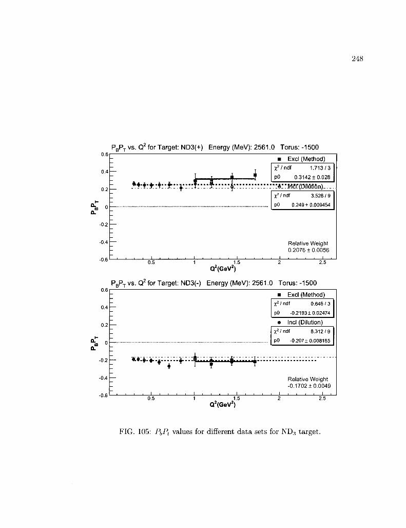
0.6
0.4
0.2
0.2
0.4
0.6
0.6
0.4
PBPT vs. Q2 for Target: ND3(+) Energy (MeV): 2561.0 Torus: -1500
i—|—*—i
• Excl (Method) Z2/ndf 1.713/3
p0 0.3142 ±0.028
::#"M(Si:poofi6n.).... X21 ndf 3.528 / 9
p0 0.24910.009454
Relative Weight 0.2076 1 0.0056
_1 I I I I I I L_ 0.5 1.5
Q2(GeV2) 2.5
PBPT vs. Q2 for Target: ND3(-) Energy (MeV): 2561.0 Torus: -1500
Excl (Method) X21 ndf 0.646 / 3
p0 -0.2193 ±0.02474
0.2—
0.2
0.4—
» Incl (Dilution) X2/ndf 8.312/9
p0 -0.207 ±0.008165
& # . $ . ^ . a . ««*«*^»»- -M A M ± -
0.6 _ i i i_
Relative Weight -0.170210.0049
I I I I I I I I I I I I I I I I ' 1 I I I L_
0.5 1 1.5 2 2.5 Q2(GeV2)
FIG. 105: PbPt values for different data sets for ND3 target.
0.4
0.3
0.2
0.1
-0.1
0.2
0.3
0.4
n c
P B P T v s . Q 2 for T a r g e t : N D 3 ( + ) E n e r g y ( M e V ) : 1 6 0 6 . 0 T o r u s : 1 5 0 0
-T
r # =_ » » . - . . - * r .-».- r v .- r .- (h -.- ^.••- .-.- 9 .-.- - . - . - . - 1 . . . .
^
• Excl (Method)
x'lmtf 1.216/2
pO 0.2318 + 0.01133
• Incl (Dilution)
X'lntll 4.121/9
pO 0.2111± 0.003708
= Relative Weight — 0 .1970+0 .0030
- 1 , , 1 , , , 1 I 1 1 1 1 1 1 1 , , I 1 , , , 1 I , 1 1 1 1 1 0.8
Q2(GeV2)
PBPT vs. Q2 for Target: ND3(-) Energy (MeV): 1606.0 Torus: 1500
Q. to a.
§-
E • * * •
=
. « . * * . * * * . * . • . . 4 ^ 1 . *1.1<a-|.Vfcb-fcfc>t.
• Excl (Method)
X11 ndf 3.257 / 2
pO -0.1799 + 0.01074
• Incl (Dilution)
Z !/ndf 12.13/9
pO -0.162610.003552
Relative Weight -0.1528 ±0 .0029
Q2(GeV2)
U.4
0.3
0.2
0.1
-0.1
0.2
0.3
0.4
P B P l
E-
vs . Q 2 for T a r g e t : N D 3 ( + ) E n e r g y ( M e V ) :
+*..A*.*..ir..i....l....-i
* • - • • • * Y — i - -
. i . . . i i . . . i . . .
1 7 2 3 . 0 T o r u s : - 1 5 0 0
• Excl (Method)
X ! /nd f 1.677/2
pO 0.1524 + 0.03381
• Incl (Dilution)
X! 1 ndf 6.981/9
pO 0.1673+0.006736
Relative Weight 0.1410 + 0.0045
0.2 0.4 0.6 0.8 1 1.2 Q2(GeV2)
PEA
§-
\-
vs . Q 2 for T a r g e t : N D 3 ( - ) E n e r g y ( M e V ) :
w»T+"*"r"i" t * ]
i
1 7 2 3 . 0 T o r u s : - 1 5 0 0
• Excl (Method)
X11 ndf 0.5241 / 2
pO -0.2564 + 0.03516
• Incl (Dilution)
X2 / ndf 15.21/9
pO -0.173210.006889
Relative Weight -0 .1598+0.0046
, I , i , 1 i i , 1 , 0.2 0.4 0.6 0.8
Q2(GeV2]
FIG. 106: PbPt values for different data sets for ND3 target.

250
PBPT vs. Q2 for Target: ND3(+) Energy (MeV): 4238.0 Torus: 2250
•:|:^-.4:-j-:|r-:ri-:r.-|-.-
Excl (Method) X21 ndt 0.566 / 4
pO 0.2368 ± 0.0283
y .v.'-*.v*'T*JI,-e!'iPJl,u-ti.9-r!).... J Jt'/ndf 3.269/8
pO 0.2203 ± 0.02096
Relative Weight 0.1886 + 0.0087
2 2.5 Q2(GeV2)
0.4
0.2
0.4
PBPT vs. Q' for Target: ND3(-)
* i i T'rf1-
• • • • • ! • < •
Energy (MeV) 4238.0 Toms: 2250
J. T
• Excl (Method) X2 / ndf 6.447 / 4
pO -0.1787 ± 0.0285
• Incl (Dilution) X21 ndf 9.998 / 8
pO -0.1539 ±0.02089
T ^ " Relative Weight -0.1684 + 0.0086
i , , , , i 2.5
Q2(GeV2)
PBPT vs. Q2 for Target: ND3(+) Energy (MeV): 4238.0 Toms: -2250
**.fr*.y,A..f..jfc
Excl (Method) %' I ndf 8.042 / 5
pO 0.1572+0.02054
Incl (Dilution) Z2/ndf 8.265/10
pO 0 .158910 .009903
Relative Weight 0.1432 + 0.0048
2 3 Q2(GeV2)
PBPT vs. Q2 for Target: ND3(-) Energy (MeV): 4238.0 Torus: -2250
o. m
0 .
n i...fr.^...j..'....
T
• Excl (Method) X21 ndf 5.707 / 5
pO -0.1794+0.03564
Incl (Dilution) i ( ! /ndf 7.227/10
pO -0.1702+0.01731
Relative Weight -0.1306 + 0.0085
2 3 tflGeV2)
FIG. 107: P\)Pt values for different data sets for ND3 target.
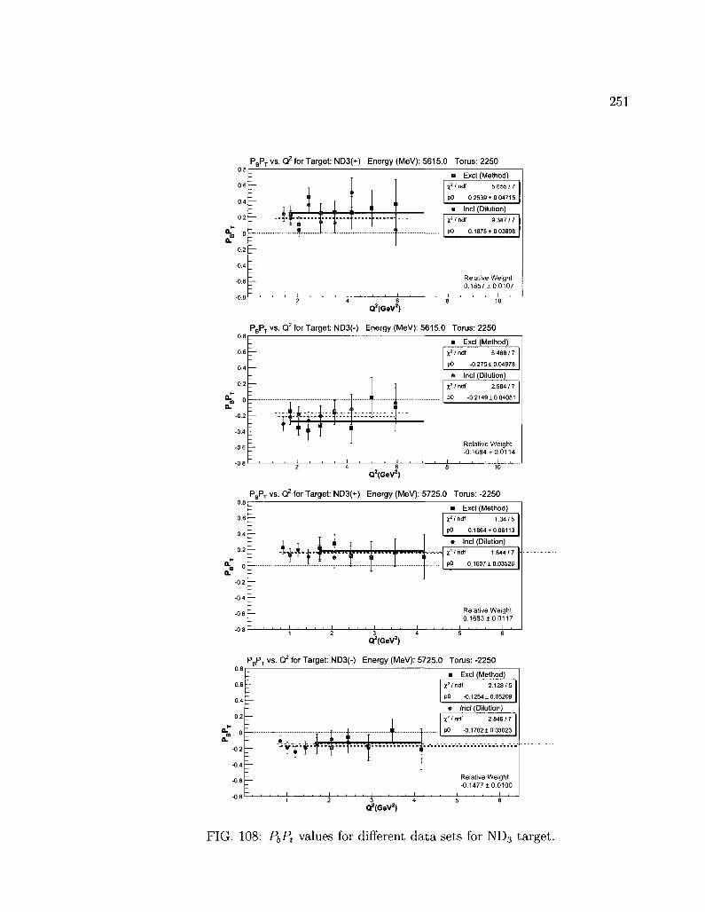
PBPT vs. Q2 for Target: ND3(+) Energy (MeV): 5615.0 Torus: 2250
0.6
0.2
°-m " 0 .
-0.2
-0.4
~-
~
id— J.J. . . . . . . X . . . . . . .
J I
-I
II
... <•
• Excl (Method) jr.2/ndf 5.655/7
p0 0.2539 + 0.04715
• Incl (Dilution)
X2 /ndf 9.347/7
p0 0.1878 ±0.03898
Relative Weight 0 .185710 .0107
. , i . . . i , , , i ,
Q2(GeV2)
PBPT vs. Q2 for Target: ND3(-) Energy (MeV): 5615.0 Torus: 2250
a. m
a.
Excl (Method)
X21 ndf 5.486 / 7
pO -0.275 ±0.04978
t m Incl (Dilution)
X21 ndf 2.584 / 7
pO -0.2149± 0.04081
Relative Weight -0.1684 ±0.0114
Q2(GeV2)
PBPT vs. Q2 for Target: ND3(+) Energy (MeV): 5725.0 Torus: -2250
0.6 ;
0.4 '—
0.2 |
, °: -0.2 ;
-0.4 —
-0.6
-0.8
L. t'l y^
Excl (Method)
X'lndl 1.34/5
pO 0.1864 ±0.06113
Incl (Dilution) X2/ndf 1.644/7
pO 0.1607 ±0.03526
Relative Weight 0.1683±0.0117
3 Q2(GeV2)
PBPT vs. Q2 for Target: ND3(-) Energy (MeV): 5725.0 Torus: -2250 0.8
0.6 h
0.4 ;
0.2 \
i o—-
-0.2 ;
-0.4^-
-0.6
-0.8
Excl (Method)
X2lndf 2.128/5
pO -0.1254± 0.05209
L n _ j _ ^ _
Incl (Dilution)
X21 ndf 2.846/7
pO -0.1702 ±0.03023
Relative Weight -0.147710.0100
Q 2 ( G e V 2 )
FIG. 108: PbPt values for different data sets for ND3 target.
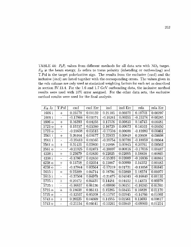
252
TABLE 44: PbPt values from different methods for all data sets with ND3 target. EB is the beam energy, IT refers to torus polarity (inbending or outbending) and T.Pol is the target polarization sign. The results from the exclusive {excl) and the inclusive (incl) are listed together with the corresponding errors. The values given in the rela column are only used as statistical weighting factors for each set as described in section IV.13.4. For the 1.6 and 1.7 GeV outbending data, the inclusive method results were used with 10% error assigned. For the other data sets, the exclusive method results were used for the final analysis.
EB IT
1606 i
1606 i
1606 o
1723 o
1723 o
2561 i
2561 i
2561 o
2561 o
4238 i
4238 i
4238 o
4238 o
5615 i
5615 i
5725 i
5725 i
5725 o
5725 o
5743o
5743 o
T.Pol
+ -
+ + -
+ -
+ -
+ -
+ -
+ -
+ -
+ -
+ -
excl
0.23178
-0.17988
0.16393
0.15237
-0.25638
0.26164
-0.20413
0.31421
-0.21925
0.23679
-0.17867
0.15718
-0.17944
0.25389
-0.27504
0.20472
-0.16837
0.18639
-0.12537
0.20225
-0.21154
excl Err
0.01132
0.01074
0.04255
0.03380
0.03515
0.01677
0.01565
0.02800
0.02473
0.02830
0.02850
0.02054
0.03564
0.04714
0.04978
0.04431
0.06136
0.06113
0.05208
0.04369
0.06641
incl
0.21105
-0.16261
0.17576
0.16729
-0.17316
0.22823
-0.20754
0.24898
-0.20697
0.22025
-0.15393
0.15887
-0.17019
0.18794
-0.21475
0.14481
-0.09890
0.15285
-0.15797
0.14955
-0.10261
incl Err
0.00370
0.00355
0.00835
0.00673
0.00688
0.00849
0.00788
0.00945
0.00816
0.02095
0.02089
0.00990
0.01731
0.03860
0.04043
0.04412
0.06151
0.03435
0.02945
0.02561
0.03849
rela
0.19703
-0.15276
0.14743
0.14103
-0.15980
0.20608
-0.18859
0.20761
-0.17016
0.18858
-0.16836
0.14322
-0.13058
0.18574
-0.16840
0.14373
-0.16245
0.16828
-0.14766
0.13693
-0.09903
rela Err
0.00297
0.00285
0.00481
0.00450
0.00461
0.00608
0.00564
0.00562
0.00487
0.00865
0.00864
0.00483
0.00845
0.01072
0.01135
0.00978
0.01365
0.01170
0.01002
0.00817
0.01224

253
that the two sets can have a rather significant difference in the magnitude of their
target polarizations. An optimal strategy requires us to include this information in
our statistical weighting. However, our method of determining the product of beam
and target polarization PbPt (using elastic or quasi-elastic scattering) will not yield
sufficient statistical accuracy over a single "group" to make this feasible. Therefore,
we need a more precise method at least to estimate the relative magnitude of PbPt
for a given data set.
The main purpose is to extract an estimate of PbPt using our model of the existing
spin structure function data together with the already determined asymmetries for
each bin for a given group. This does not have to be too precise (and of course may
be off by an overall scale factor, since we don't know whether our existing model has
the correct overall scale). However, it is sufficient to give us a relative magnitude of
PbPt, that we will call Pre\.
This requires to use the "models" to determine a "predicted" A\\ for each bin
where the group under investigation has data. Above W = 1.08 GeV this was done
with a simple code that uses the A\, A2 and R from "models" and combines them
into All10*2' = D(Ai + rjA2), using the correct beam energy and electron scattering
angle for each bin to calculate the required kinematic quantities like e, r\ and D, given
in Eq. (29). For kinematic bins below W = 1.08 GeV, we used the (quasi-)elastic
inclusive asymmetries instead. These were calculated according to Eqs. (374) and
(377). It should be noted that, bins below W = 0.9 GeV are not used in this process
since the data in these bins are largely unpolarized and/or have large random errors.
At this point, we can calculate an estimate for Prei for each bin in W > 0.9 GeV
and Q2 for a given data set (G) as follows:
PrdW,^) = ^ ^ \ (380)
where A^aw represents the raw asymmetry of the data set (all runs combined) and
FD is the dilution factor for the bin in question. The error on this quantity, for just
one kinematic bin, is
rel fp Amodel' \ '
We can then combine the information from all [Q2,W] bins with W > 0.90 GeV by

254
the usual statistically weighted mean:
E P™l/aPrel bins J* , = " " , , , (382)
bins
rrel
with statistical error
o>pG = • (383) rel E V4rei bins
From Eqs. (380) and (381), we can deduce that
P , AG
rel J? Amodel ^1™ — = FDA^odei-f^, (384) TPrel aAG
ret ; Lraw
so, the last equation can also be written as
Y,FDA^lA?aw/o\oaw
pG _ bins C385) rel E(^)2(^re/)2M?a.'
bins
which avoids any need to divide by (potentially) small (zero) numbers.
While combining the two different data sets with opposite target polarizations,
we multiply the total count for each set with the square of its relative PbPt, given
by P^el, to determine its weight. Then this weight is divided by the sum from both
data sets to determine the scaling factor associated with each set. Then, this scaling
factor is used whenever we need to sum quantities from the two data sets. The raw
asymmetries and the true P^Pt values are summed in this way while combining the
data sets with opposite target polarizations. More detailed explanations on the data
combining procedure is given in section IV. 17.
IV. 14 POLARIZED B A C K G R O U N D CORRECTIONS
The dilution factor corrects for scattering off unpolarized "non-target" nucleons or
nuclei in the target material. However, some of these might be polarized and, there
fore, affect the observed asymmetry. This section explains the corrections required
to account for the effects of the polarized background on the measured asymmetry.
The proton and deuteron targets are embedded in 15NH3/15ND3 molecules. As
the targets are polarized by the DNP process, surrounding nucleons from 15N can

255
TABLE 45: P\,Pt values for the ND3 target averaged over opposite target polarizations, from three different methods. EQ is the beam energy, IT refers to torus polarity (inbending or outbending).
EB IT
1606 i
1606 o
1723o
2561 i
2561 o
4238 i
4238 o
5615 i
5725 i
5725 o
5743 o
excl 1
0.2112
0.1639
0.2096
0.2332
0.2694
0.2109
0.1619
0.2628
0.1903
0.1551
0.2040
Err
0.0080
0.0425
0.0246
0.0114
0.0188
0.0201
0.0178
0.0344
0.0361
0.0400
0.0376
excl 2
0.2236
0.2244
0.2241
0.2439
0.2616
0.1852
0.1608
0.2383
0.1802
0.1814
0.1775
Err
0.0067
0.0346
0.0192
0.0101
0.0152
0.0179
0.0165
0.0309
0.0303
0.0373
0.0338
incl
0.1918
0.1757
0.1705
0.2180
0.2291
0.1907
0.1613
0.1992
0.1266
0.1554
0.1407
Err
0.0026
0.0083
0.0048
0.0058
0.0063
0.0148
0.0086
0.0280
0.0361
0.0225
0.0220
also become polarized. In addition, there is an approximately 2% contamination of 14N, which is also polarizable. Moreover, a small percentage of residual nuclei such
as NH3 and ND2H! also indroduce polarizable nucleons. Although the effect of the
polarized background on the measured asymmetry is small, it should be considered
as one of the correction factors. In order to correct for the polarized background, we
followed the prescription developed by [118]. The general form of the correction can
be written as:
Aff" = d (Ay - C2) , (386)
where Ajjorr is the asymmetry due only to the polarized deuterons (or protons) in the
target material. A\\ represents the asymmetry after the dilution factor and the beam
x target polarization corrections were applied. At this point, radiative corrections
have not yet been applied to A\\. The multiplicative factor C\ stands as a weight
factor for additional polarized nucleons of the same type as the intended target. The
additive factor C2 corrects for the asymmetry introduced by nucleons of a type other
than the intended target.
256
Corrections on the deuteron target
In case of the deuteron, the correction factors in Eq. (386) can be written as [118]:
Cf = 77 r W 1.02, (387) 1 l-Vp + Dn/(l-l.5wD) ' l }
C$ = ^(Dn- DP)AP « -0.03A,, (388)
where Ap is the proton asymmetry, A\\(Q2, W), with all corrections applied, except
for the radiative correction. The term wp corrects for the D-state contribution to
the deuteron. The remaining terms are defined as:
number of protons p number of protons + number of deuterons
n PN 9EMC /Qnnx Dn = r]N-E 7T- (3 9°)
Pd » n Pp i tn -,\PN 9EMC /oni\
DP = VP-^ + (2r?jv - 1)-= 7T- (391) "d rd y VN = : TTJ^ ; TTTTT « 0.02, (392)
number of 14N
number o/14N + number o/15N
where the values of the r\p and r\^ comes from general expectations for a typical
target. The r]p, for example, assumes approximately 4.5% of the ND3 molecules are
actually ND2Hi, giving rise to proton impurities in the target. The factor QEMC is
the correction for the EMC effect,
15JV ^_ 14N _ ^ 1 / o n o \ 9 EMC ~ 9EMC = 9EMC ~ 1, {6\)6)
which is just a crude approximation but its uncertainty, together with the uncertainty
of the other factors, is considered in the systematic error calculations. The factors
Pd, Pp, PN represent the corresponding polarizations of the deuteron, proton and
nitrogen targets respectively. The nitrogen polarizations are given by,
while the proton polarization is:
(
-RAN = PN = -0.40Pd . (394)
PP= < 0.191 + 0.683Pd for Pd > 0.16
1.875P* for Pd < 0.16
Although the effect of the factor Cd is very minor, the factor C | becomes im
portant since it is multiplied by the proton asymmetry. The overall correction is

257
approximately 3 to 5% of the asymmetry. The uncertainites in the values of the
correction factors, Cf and C^-, are considered as part of our systematic error cal
culations. For the proton asymmetries, initially the radiated asymmetries from the
EG lb NH3 target were used since for each beam energy for the deutron, there is a
corresponding data set on the proton and they are analyzed together in parrallel. On
the other hand, using the data has the disadvantage that the statistical error on the
proton measurements directly propagate into the statistical error on the deuteron
measurements. Even though this is a very small effect, instead of using data, we also
tried using the model for the proton aymmetry. When using the model, the error on
the proton asymmetry is set to zero, therefore the statistical error on the deuteron
data is not affected by the statistical uncertainity of the proton measurements. Since
the final model inputs agree with the proton data at a very good level, we eventu
ally decided to use the model values for the proton asymmetry while applying the
polarized background correction to the deuteron.
Corrections on the proton target
In the case of the NH3 target, the main contribution to the measured proton asym
metry comes from the unpaired "quasi-free" protons in the 15N nuclei. Because of its
negative magnetic moment, the 15N nucleus polarizes in the opposite direction of the
target-protons. But the unpaired proton in the 15N is expected to be "anti-alligned"
with the nuclear spin with a relative polarization of-1/3. Therefore, the polarization
of the quasi-free proton in the 15N adds positively to the total polarization of the
target-protons.
The correction factors in Eq. (386) can be written explicitly for the NH3 target
as18,
C\ = 11-fV
3 3 PP j C\ « 0, (395)
where P/v and Pp represent nitrogen and target-proton polarizations, respectively.
The term —1/3 in the C\ is the Clebsch-Gordan coefficient, representing the relative
polarization of the quasi-free proton in 15N. The second 1/3 term is there because
the ammonia target has three hydrogen atoms for each nitrogen molecule. Other
polarized nucleons might enter from the small amount of 14N present in the target
material. This would enter via a Cf term; however, in our case this contribution was
18The factor gEMc(x) for EMC effect is neglected, since its effect is negligible for this correction.
258
negligible and its estimated effect is considered as a systematic error.
In order to calculate Cf, we need to know the nitrogen polarization. A fit was
developed by the E143 collaboration [118] to express the 15N polarization, P/v, in
terms of the proton polarization, Pp, in the NH3 target:
p15N = -(0.136Pp - 0.183Pp2 + 0.335Pp
3). (396)
In order to obtain the quantitative form of the correction, we express A\\ in terms of
the raw asymmetry divided by the dilution factor and the beam x target polarization,
4l = = % - (397)
Using this for the uncorrected asymmetry in Eq. (386), and expressing the C\ term
as given in Eq. (395), the corrected proton asymmetry can be written as
Ar=FP(praWiipy W
^D^byrp — 33 / i vJ
which means that the effective target polarization is increased by the amount | | |P/v | -
For the implementation of this corrections, we used Pp = PbPt/Pb, where P^Pt values
were obtained as described in section IV. 13 and Pb is the M0ller polarization averaged
over all runs within the same data set. In general, this correction is on the order
of the statistical errors on the extracted PbPt values. Detailed information on the
polarized background corrections for the proton target is given in [95].
IV. 15 R A D I A T I V E CORRECTIONS
In the experiment, our goal is to extract asymmetries for a single photon exchange
process, which is also called Born scattering. However, there are higher order QED
processes contributing to the measured asymmetries. These contributions are re
moved by the radiative corrections. The corrections can be examined in two main
categories: internal and external radiative corrections.
The internal radiative corrections account for higher order QED processes that
may occur during the interaction. These include internal Bremsstrahlung, where
the incoming or the scattered electron emits a photon; vertex correction, in which
a photon exchange occurs between the incoming and the scattered electron; and
vacuum polarization of the virtual exchange photon. The correction for the internal

259
radiative effects can be calculated by adding the cross sections of each higher order
process to the Born cross section [119].
The external radiative corrections [120] account for the energy loss of the elec
tron while passing through the detector field and the target material mainly by the
Bremsstrahlung process. As an electron traverses the target it can radiate a real
photon, which changes the energy of the scattering process. The resulting energy
loss may affect the kinematic calculations. The effect becomes especially important
for elastic scattering because the elastic cross section grows rapidly as the beam en
ergy decreases, which increases the probability for radiation of a high energy photon
followed by elastic scattering. This creates a radiative elastic tail extending from the
elastic peak into the inelastic region. The corrections depend on the experimental
conditions.
For the radiative corrections in the EGlb experiment, an iterative, model de
pendent program called RCSLACPOL was used. For detailed information on the
incorporation of the internal and external radiative effects into this software, the
reader is referred to [119][120][121]. The program creates a multiplicative and an
additive correction term, 1/JRC and ARC- These correction terms were generated
for each beam energy in our standard (Q2,W) bins. The correction is applied to
the asymmetry A\\, as the last correction before the calculation of the virtual photon
asymmetries, Acorr
Aforn = -$— + ARC. (399) JRC
The additive term, ARC, corrects for the quasi-elastic radiative tail as well as the
inelastic tail and is negative for the big majority of our kinematics. The multiplicative
term, 1/JRC, which is always larger than 1, corrects for the radiative elastic tail
underneath the inelastic region. Since 0 < JRC < 1, we can interpret the measured
asymmetry consisting of a fraction JRC of the true asymmetry and a fraction 1 — JRC of
the contaminating asymmetry. Therefore, this term takes into account the additional
dilution caused by the internal and external radiations. Using a multiplicative factor
also provides a way to properly propagate the statistical errors.
IV.16 MODEL I N P U T
Knowledge of the structure functions F\ and R as well as the virtual photon asym
metry A<i is necessary to extract the physics quantities of interest, namely A\ and
260
<7i, from the EG lb data. Moreover, the deep inelastic contributions to the integral
over 0i are required for a full evaluation of the moments. Eqs. (447-452) provide a
brief summary of these calculations and the usage of these quantities.
Parameterizations based on the existing world data were used for these quantities
that are required but not measured in this experiment. A package program, devel
oped by S. Kuhn et al., generates models of all physics quantities of interest based on
world data parameterizations and current theoretical knowledge. This program was
used to generate the models for A2, F\ and R as well as Ax and gx, which are mainly
used for comparisons to the our final experimental results. Then, the experimental
results, in an iterative approach, can be used to refine these models.
The models are under continues development as new data come to exist on the
asymmetries and the structure functions. Especially the models on A\ and A2 in
the resonance region went through rigorous upgrade with the inclusion of many
experiments, including EGlb. Studies on the parameterizations of the virtual photon
asymmetries in the resonance region are provided in chapter VI. The first part of this
section describes the models of the unpolarized structure functions. In the second
part, we will give the current status of the virtual photon asymmetries in the DIS
region.
IV.16.1 Models of the unpolarized structure functions for the deuteron
The F\ model is used for the calculation of g\ from the virtual photon asymmetries,
according to Eq. (64). The model for R = aL/aT, the ratio of longitudinal to
transverse cross-sections for unpolarized scattering (see Eqs. (60) and (70)), is used
for calculation of the depolarization factor D, given in Eq. 29. Also, the same
models are used, while processing the data, for the parametrization studies on the
spin structure functions and asymmetries in chapter VI.
The most detailed information on the models for the unpolarized structure func
tions of the deuteron can be found in [122]. The calculations of R, F\ and F2 all
follow from fits to the world data for the total transverse (aT) and longitudinal (aL)
cross sections (see Eqs. (56 - 60)). Inelastic electron scattering on the deuteron can
be divided into two distinct contributions: quasi-elastic and inelastic scattering. The
unpolarized structure functions were modeled separately for these two regimes.
In the quasi-elastic region, PWIA Fermi smearing based on the pre-integrated
Paris wave function was used by replacing the continuous inelastic cross-section with

261
a S-function elastic cross section at W = Mp. The elastic cross-section was calcu
lated using the nucleon form factors modified for off-shell effects and taking Pauli
suppression into account.
In the inelastic region, a fit was performed by using the world data for the electro-
production cross section measurements and minimizing \2 defined by [122]
X2 = itfoiWuQ2) - oKWtftfttSaiiWuCfi)]2 (400)
where the sum is over all experimental points with transverse inelastic cross section
&i(Wi,Q2) and total statistical and systematic error 5<Ti(Wi,Q2). Since the fit was
performed for inelastic scattering only, the quasi elastic contribution was subtracted
from data prior to the fit. In addition, because of limited kinematics of the longitu
dinal cross section measurements on the deuteron, the fit was performed only to the
transverse portion of the cross section. The transverse cross section was extracted
from data by using
al = arD/(l + eRD), (401)
where e is the relative polarization of the virtual photon and oTD is reduced cross
section defined as
ar = aT(W, Q2) + eaL(W, Q2). (402)
An assumption was made that Rp = Rn and Rp was evaluated by Fermi smearing
(Tp and Op, which were obtained from proton model [123]. It was concluded that the
effect of Fermi smearing is small for most kinematics of interest and RD = Rp to a
good approximation. The model cross section crJ)(W, Q2) was defined in terms of the
average free nucleon transverse cross section, ajf = (<rj + a^)/2, with Fermi motion
taken into account in the Plane Wave Impulse Approximation [122]:
<?1{W,Q2) = adip(W,Q2) + Jal(W, (Q2)')®2(k)d3k (403)
where the integral is over the Fermi momentum k and integrates the deuteron wave
function Q2(k) times the average free nucleon transverse cross section (?Jj(W,Q2).
The term a dip is an additional parametrization for the dip region between the quasi-
elastic peak and the A(1232) resonance. This dip region had to be treated with extra
parameters to account for meson exchange currents and final state interactions.
In the DIS region, the parametrization from the NMC collaboration was used
[124], which is a 15 parameter fit to F2, by using inclusive muon scattering in the

262
kinematic range 0.006 < x < 0.6 and Q2 from 0.5 to 75 GeV2 together with existing
world data at that time. As a reference, plots for R and Fi models of the deuteron
are shown for various Q2 bins in Fig. 109.
IV.16.2 Models of Ax and A2 in the DIS region
The proton and neutron models for Ai in the DIS region were produced by pa
rameterizing the world data. The A\ parametrization included data from EMC [6],
SMC [44], E143 [45], E155 [47], HERMES [48], EGla [68] and EGlb [17]. The Anx
parametrization included data from measurements on 3He targets (E142 [43], E154
[46], HERMES [48] and Hall-A [70]) as well as ND3 targets (E143 [45], E155 [47],
HERMES [48], SMC [44], COMPASS [49], EGla [67] and EGlb [50]). We also used
real photon data from ELSA [125] [126] and MAMI [127] for both parameterizations
to constrain the fit as Q2 —> 0. The data on A\ were used as presented by the experi
ments with the 3He target. In order to extract neutron data from ND3 measurements,
we used the simplified assumption:
A\ = {\- \JbwD)
and solved the equation for A\ using models for A\ and the unpolarized structure
functions Ff'n. In the end, the A\ fit utilized the following parametrization:
AP = £P1+P2tan-i(P32<?2)[i + (p4 + p 5 t a n - ^ F l Q 2 ) ) sin(7r£P7)], (405)
while the parametrization for A\ was
A\ = ZPl[(P2 + P3tan-\P2Q2)) s i n « P 5 ) - cos(7r£P6)], (406)
where Pi represents parameter i. We also allowed the overall scale of each experiment
to vary within the stated systematic error by employing additional parameters for
each experiment. The kinematic variable £ in the parameterizations was defined by
= Q2 + (M + Mn)2-M2
Miy + ^/v2 + Q2) '
where M is the nucleon mass and Mw is the mass of the 7r° = 0.135 GeV/c2. The error
on the fit was calculated by using the error matrix E3k determined by the minimization
routine such that 5Ai — djE3kd
k, where di = dA\jdPi is the derivative of A\ with
respect to parameter Pi, and summation is implied over repeating indexes. Fig. 110
FlA\ + FfAf
Ff + F? (404)

R for the deuteron in low Q range R for the deuteron in low Q range
1.2 1.4 1.6 1.8 2 2.2 2.4 2.6 2.8 W(GeV)
0.7
0.6
0.5h
• - • Q 2 = 0 . 35
— Q2 = 0.50
- - - Q 2 = 0.71
— Q2 = 1.01
— - - Q2 = 1.44
— Q2 = 2.05
Ql I I I I • 1 I I I I I I I I I I I 1 I I I I I I I I I I I I I I I I • I
1 1.2 1.4 1.6 1.8 2 2.2 2.4 2.6 2.8 3 W(GeV)
F, for the deuteron in low Q range F^ for the deuteron in high Q range
3.5-
3
2.5
2
1.5
1
0.5
0
j-
~ I - I \ j !_ 1
\ 1 - I • 1 "- 1
J ' n i l
ffl/ 1 / / / A/* / * / * / a* / ' / * /
U* / ' / * * Ki / * / * /
mf * / * /
i J&^r / ' / * / l *. » " / * / * /
1 wS&f - * / * / 1 fev*-/* / * / 1 w*>*f ** /
1 I/O *-'' / —Q2 = 0.01 1 Mj-.'-y ---Q2 = 0.02 \J$!/^y — Q2 = 003 vj* / - - - Q 2 = 0.04 V . Q2 = 0 Q 6
- - - Q 2 = 0 . 0 8
— Q 2 = 0 . 1 2
- - - Q 2 = 0 . 1 7
— Q 2 = 0 . 2 4
• i i I i i i I i i i I i i i I i i i I i i i I i i i I i i i t i i i
3.5
- - - Q 2 = 0.35
— Q2 = 0.50
•CT = 0.71
1.2 1.4 1.6 1.8 2 2.2 2.4 2.6 2.8
W(GeV)
1 1.2 1.4 1.6 1.8 2 2.2 2.4 2.6 2.8 3 W(GeV)
FIG. 109: The models for R (top) and Fi (bottom) for the deuteron are shown for various Q2 bins.

264
0.8
0.6
0.4 C O 0.2
9 n a <f-02
-0.4
-0.6
-0.8
x distribution of A1 for a Q2 bin
L • A., data
L - A 1 fit
Q2Rangfi_— ^H86S~^228
0.1 0.2 0.3 0.4 0.5 0.6 0.7 0.8 0.9 1
x Bjorken
: distribution of A1 for a Q2 bin
0.1 0.2 0.3 0.4 0.5 0.6 0.7 0.8 0.9
x Bjorken
: distribution of A1 for a Q2 bin
0.1 0.2 0.3 0.4 0.5 0.6 0.7 0.8 0.9 1 x Bjorken
: distribution of A1 for a tf bin
0.1 0.2 0.3 0.4 0.5 0.6 0.7 0.8 0.9
x Bjorken
FIG. 110: The Ai fits in the DIS region for the proton (top) and neutron (bottom).
shows some results for both A\ and A™ fits. Afterwards, the deuteron model was
obtained by using Eq. (404), with the corresponding error calculated by
6A* = V W [ ( F [ ) 2 ( K ) 2 + ™2^211 / 2 ' (408)
A2 in the DIS region was calculated by employing the Eq. (63) and using the the
Wandzura-Wilczek [7] relation for g\vw, which yields
A2 = l nww
(409)
where F\ comes from our model and g^w was calculated by solving
= / ' * * ' Jx y
WW 9T
(410)
iteratively in terms of our A\ and F\ models, without considering the higher twist
contributions. The higher twist contributions were taken into account for the sys
tematic error on the model by including twist-3 calculations. After the calculations

265
of both A\ and A^, the asymmetry A\ for the deuteron was determined as a weighted
sum of the two by using F\ as a weight factor (similar to Eq. (404)).
In order to ensure a smooth transition between the resonance and the DIS re
gions, the parameterizations for A\ and A2 in the DIS region were later used for
parameterizations in the resonance region by employing their extrapolation. This
will be described in chapter VI in more detail.
IV. 17 COMBINING DATA FROM D I F F E R E N T CONFIGURATIONS
Extraction of the most precise information on the asymmetries and the structure
functions from a set of heterogeneous runs in the EG lb data requires a solid method
ology to combine the data sets from different configurations. During the experiment,
several runs of data were taken with each possible combination of a set of parameters
that determine the kinematic reach and the overall scale of the measured asymme
tries. We want to combine all this information into the quantities of interest (e.g.,
A\ + 77^2) for each of our standard W and Q2 bins, while minimizing the final sta
tistical error. The parameters that can possibly vary from one run to the next are:
1. Beam energy
2. Torus polarity
3. Target material and polarization (including direction of polarization, along (+)
or opposite (—) to the beam direction)
4. A/2-plate status (in = 1 or out = 0)
It should be noted that even a small change in the beam energy can correspond to
a different setting of injector optics, resulting potentially in a reversal of beam polar
ization. After considering various possibilities on how to combine runs with different
run parameters, the following scheme was selected for the double-spin asymmetry
analysis of the EGlb data.
IV.17.1 Combining runs
All runs belonging to the same beam energy, torus current (including sign) and
target polarization (including sign) should be combined to calculate the first set
of raw asymmetries, Araw(W, Q2), for each kinematic bin. This means summing
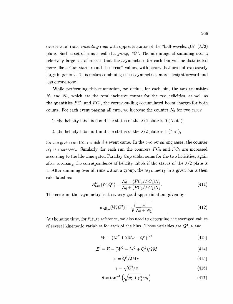
266
over several runs, including runs with opposite status of the "half-wavelength" (A/2)
plate. Such a set of runs is called a group, "G". The advantage of summing over a
relatively large set of runs is that the asymmetries for each bin will be distributed
more like a Gaussian around the "true" values, with errors that are not excessively
large in general. This makes combining such asymmetries more straightforward and
less error-prone.
While performing this summation, we define, for each bin, the two quantities
iV0 and Ni, which are the total inclusive counts for the two helicities, as well as
the quantities FC0 and FCi, the corresponding accumulated beam charges for both
counts. For each event passing all cuts, we increase the counter N0 for two cases:
1. the helicity label is 0 and the status of the A/2 plate is 0 ("out")
2. the helicity label is 1 and the status of the A/2 plate is 1 ("in"),
for the given run from which the event came. In the two remaining cases, the counter
Ni is increased. Similarly, for each run the counters FCQ and FC\ are increased
according to the life-time gated Faraday Cup scalar sums for the two helicities, again
after reversing the correspondence of helicity labels if the status of the A/2 plate is
1. After summing over all runs within a group, the asymmetry in a given bin is then
calculated as:
A- (W Q2) = No ' ( ^ / r c ^ (411)
The error on the asymmetry is, to a very good approximation, given by
^.we2> = V^Tiv (412)
At the same time, for future reference, we also need to determine the averaged values
of several kinematic variables for each of the bins. Those variables are Q2, v and
W = (M2 + 2Mv - Q2)1'2 (413)
E' = E - (W2 - M2 + Q2)/2M (414)
x = Q2/2Mu (415)
7 = VO*/v (416)
9 = tan"1 (^Pl+p2y/pz) (417)
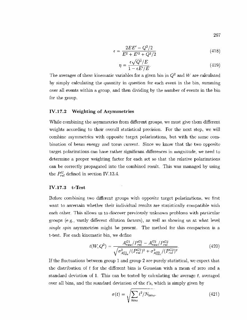
267
2EE' - QV2
£ 2 + £ ' 2 + Q2 /2 J
= e^QVE V l-eE'/E' { }
The averages of these kinematic variables for a given bin in Q2 and W are calculated
by simply calculating the quantity in question for each event in the bin, summing
over all events within a group, and then dividing by the number of events in the bin
for the group.
IV.17.2 Weighting of Asymmetries
While combining the asymmetries from different groups, we must give them different
weights according to their overall statistical precision. For the next step, we will
combine asymmetries with opposite target polarizations, but with the same com
bination of beam energy and torus current. Since we know that the two opposite
target polarizations can have rather significant differences in magnitude, we need to
determine a proper weighting factor for each set so that the relative polarizations
can be correctly propagated into the combined result. This was managed by using
the Pfel defined in section IV. 13.4.
IV. 17.3 t-Test
Before combining two different groups with opposite target polarizations, we first
want to ascertain whether their individual results are statistically compatible with
each other. This allows us to discover previously unknown problems with particular
groups (e.g., vastly different dilution factors), as well as showing us at what level
single spin asymmetries might be present. The method for this comparison is a
t-test. For each kinematic bin, we define
\G\ I pGl _ AG2 lpG2 t(\A/ Cfi\ raw! rel raw/ rel (Ar)()\
' McJ(PrGJ)2 + °2
Ac2/(PrGJ)2'
y •r%raw -^raw
If the fluctuations between group 1 and group 2 are purely statistical, we expect that
the distribution of t for the different bins is Gaussian with a mean of zero and a
standard deviation of 1. This can be tested by calculating the average t, averaged
over all bins, and the standard deviation of the i's, which is simply given by
<?{t) = | ^ 2 / J V h , (421) y bins
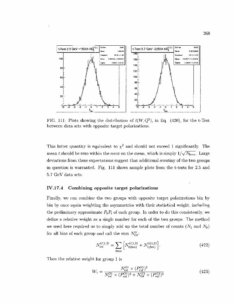
268
t-Test 2.5 GeV +1500A N[£ )H Entries 2486
Mean 0.00539
Constant 97.82 ± 2.48
Mean 0.00931610.020403
Sigma 0.9956 ±0.0155
Entries 4028
Mean -0.0003849
Constant 1 6 1 . 3 ± 3 . 2
Mean 0.00571± 0.01575
Sigma 0 .9824±0 .0116
FIG. I l l : Plots showing the distribution of t(W,Q2), in Eq. (420), for the t-Test between data sets with opposite target polarizations.
This latter quantity is equivalent to \ 2 a n d should not exceed 1 significantly. The
mean t should be zero within the error on the mean, which is simply l/yWbms- Large
deviations from these expectations suggest that additional scrutiny of the two groups
in question is warranted. Fig. I l l shows sample plots from the t-tests for 2.5 and
5.7 GeV data sets.
IV. 17.4 Combining opposite target polarizations
Finally, we can combine the two groups with opposite target polarizations bin by
bin by once again weighting the asymmetries with their statistical weight, including
the preliminary approximate P^Pt of each group. In order to do this consistently, we
define a relative weight as a single number for each of the two groups. The method
we used here required us to simply add up the total number of counts (iVi and JV0)
for all bins of each group and call the sum N^ot:
N: G(l,2) tot
- V [jvG(1-2) + JVG ( U ) (422) bins
Then the relative weight for group 1 is
Wx = Ngl x {Pg}f
Nst >< (p%)2+N% >< ra2 (423)
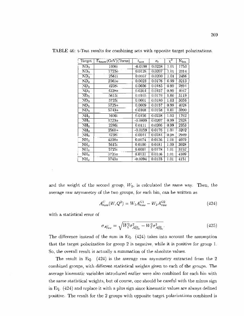
269
TABLE 46: t-Test results for combining sets with opposite target polarizations.
Target
ND3
ND3
ND3
ND3
ND3
ND3
ND3
ND3
ND3
ND3
NH3
NH3
NH3
NH3
NH3
NH3
NH3
NH3
NH3
NH3
Ebeam(GeV) (Torus)
1606i 1723o
2561i 2561o
42381 4238o
5615i 5725i 5725o
5743o
1606i 1723o 22861 2561o
4238i 4238o
5615i 5725i 5725o 5743o
^ave
-0.0198 0.0128 0.0057
0.0023
0.0036 0.0364
0.0105
0.0001 0.0009 0.0168
0.0156 -0.0099
0.0111 -0.0159 0.0044 0.0074
0.0100
0.0001 0.0131 -0.0094
°t 0.0238 0.0207 0.0200
0.0176 0.0185
0.0157 0.0179
0.0180 0.0157 0.0158
0.0238 0.0207 0.0206
0.0176 0.0184
0.0156 0.0181
0.0178 0.0156 0.0155
x> 1.01
1.01 1.01
0.99 0.99
0.99 1.00 1.03
0.99 1.01
1.02
0.99 0.99 1.01
0.98 1.01 1.00 1.01 1.01 1.01
^bin
1753 2314
2486
3213 2894
4047
3119 3056
4028 3990
1762
2328 2353 3202
2949
4079 3028 3152
4109 4151
and the weight of the second group, W2, is calculated the same way. Then, the
average raw asymmetry of the two groups, for each bin, can be written as
A?aw(W, Q2) = WXA^W - W2Afaw (424)
with a statistical error of
°Acaw = Jw?a\G1 + Wlo\G2 . (425) raw y -^raw -^raw
The difference instead of the sum in Eq. (424) takes into account the assumption
that the target polarization for group 2 is negative, while it is positive for group 1.
So, the overall result is actually a summation of the absolute values.
The result in Eq. (424) is the average raw asymmetry extracted from the 2
combined groups, with different statistical weights given to each of the groups. The
average kinematic variables introduced earlier were also combined for each bin with
the same statistical weights, but of course, one should be careful with the minus sign
in Eq. (424) and replace it with a plus sign since kinematic values are always defined
positive. The result for the 2 groups with opposite target polarizations combined is
270
referred to as a "set" in the following. The only difference between the sets is their
beam energy and torus currents. Table 46 shows the results for the t-tests for all
data sets.
Before continuing any further in combining runs, at this stage we converted the
raw asymmetries by dividing out Pi,Pt and FD for each set. In addition, the correc
tions for pion and pair-symmetric contaminations as well as the polarized background
and the radiative corrections were all applied at this stage. Finally, the resulting val
ues for AEorn(W, Q2) were converted to values for A\ + rjA2(W, Q2) by dividing with
the averaged D results (obtained from models) for each bin. All of these manipula
tions in principle depend on the beam energy and in case of contaminations, also on
the torus polarity (see section IV. 12). The values for A\ + 77A2, for each bin, as well
as the averaged kinematic variables and the count rates are propagated into the next
step.
IV.17.5 Combining data with slightly different beam energies
At this stage we have 11 data sets for both targets. These sets are given in Table 5.
Among these, there are sets with slightly different beam energies but the same torus
current. These sets are:
• 1.606 GeV, -1500A ; 1.723 GeV, -1500A
• 5.615 GeV, +2250A ; 5.725 GeV, +2250A
• 5.725 GeV, -2250A ; 5.743 GeV, -2250A
The values for Ai + r]A2 = A\2 are combined for these sets by taking their error
weighted average for each kinematic bin,
-^12 ° AGI ~^~ -^12 /aAG2
A—{w^ Q2} = *» *» , (426)
aATrn(W, Q2) = ( ] ) . (427)
The kinematic factor 77 does depend on the beam energy, however, it is very small for
our kinematic region, which makes the combination of Ai + rfA2 for slightly different
beam energies possible. Moreover, we applied a z-test in order to make sure that
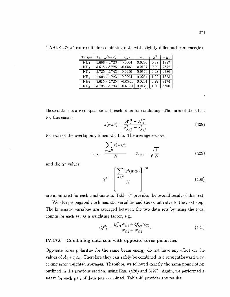
271
TABLE 47: z-Test results for combining data with slightly different beam energies.
Target
ND3
ND3
ND3
NH3
NH3
NH3
E(,eam(GeV)
1.606- 1.723 5.615- 5.725 5.725 - 5.743
1.606- 1.723 5.615- 5.725 5.725 - 5.743
zave 0.0004 -0.0561 0.0950
0.0294 -0.0544 -0.0179
Oz
0.0230 0.0197 0.0169
0.0234 0.0201 0.0172
x2
0.98 0.99 0.98
1.02 0.98 1.00
™bin
1887 2572 3486
1825 2474 3366
these data sets are compatible with each other for combining. The form of the z-test
for this case is AGI _ AG2
Z(W,Q2) = — ^ H-nl2 /112
for each of the overlapping kinematic bin. The average z-score,
(428)
^ 2 Z(W<Q2) W,Q2
N (429)
and the \2 values
X
Y^ z2(w'Q2) W,Q2
N
1/2
(430)
are monitored for each combination. Table 47 provides the overall result of this test.
We also propagated the kinematic variables and the count rates to the next step.
The kinematic variables are averaged between the two data sets by using the total
counts for each set as a weighting factor, e.g.,
(Q2) = QGINGI + QG2NG2
NG1 + NG2 (431)
IV.17.6 Combining data sets with opposite torus polarities
Opposite torus polarities for the same beam energy do not have any effect on the
values of A\ + r]A2- Therefore they can safely be combined in a straightforward way,
taking error weighted averages. Therefore, we followed exactly the same prescription
outlined in the previous section, using Eqs. (426) and (427). Again, we performed a
z-test for each pair of data sets combined. Table 48 provides the results.

272
TABLE 48: z-Test results for combining sets of opposite torus polarity.
Target ND3
ND3
ND3
ND3
NH3
NH3
NH3
NH3
E6eam(GeV) (Torus)
1.6(4-)- 1.6(-) 2.5(+) - 2.5(-) 4.2(+) - 4.2(-) 5.7(+) - 5.7(-)
1.6(+) - 1.6(-) 2.4(+) - 2.5(-) 4.2(+) - 4.2(-) 5.7(+) - 5.7(-)
Zave
-0.0468 -0.0290 -0.0256 -0.0268 0.1492 -0.0722 -0.0143 0.1240
°z 0.0276 0.0237 0.0215 0.0193 0.0281 0.0237 0.0222 0.0196
x2
0.97 0.98 0.99 0.98 1.05 1.04 1.00 1.02
^bin
1310 1778 2162 2683 1258 1768 2028 2585
At this point, before combining data sets with different beam energies, we need
to extract A\ and g\ by using models for A2 and F\,
MW, Q2) = [A, + r1A2](W, Q2) - WA^iW, Q2)
9i(W,Q2) = ^ _ F^odel(W,Q2)
~ 1 + {Q2)/{u)2 A1(W,Q2) + y/W) I model
M (W,Q2)
(432)
(433)
These values, again, together with the kinematic variables, averaged according to Eq.
(431), and the count rates for each bin are propagated to the next level of analysis.
IV.17.7 Combining data sets with different beam energies
At this point we have 4 independent data sets, which we can label E1, E2, E4 and
E5, corresponding to 1.x, 2.x, 4.x and 5.x GeV data sets. In each set, we have
Ai, <ji, kinematic variables and the count rates for each bin. The A\ and the g\
values from different sets can be combined by taking their error weighted averages.
The kinematic variables are, again, combined by weighting them with corresponding
count rates in each bin. In this way, the data sets were combined, two at a time: first
combining E1 and E2, then combining £^1:2) with E4 and finally combining E^1:2'A^
with E5. We performed a z-test between each individual data set, as well as between
the combined and the individual data sets. The results are given in Table 49.
As a result, all data are combined into a single set, consisting of A\ and g\ values,
as well as the properly averaged kinematic variables and the count rates, for W
and Q2 bins. In the next section, we will summarize the corrections applied on
the asymmetries and describe how we propagated the statistical errors after each

273
TABLE 49: z-Test results for combining data sets with different beam energies.
Target
ND3
ND3
ND3
ND3
ND3
ND3
ND3
NH3
NH3
NH3
NH3
NH3
NH3
NH3
Beam Sets
El-E2
E2-E4
E4-E5
E2-Eb
E^E* £(l:2)_£4
EW-V-E* E^-E2
E2-Ei
E*-Eb
E2-E5
El-E"-£(l:2)_£4
E^-V-E5
Zave j °~z
0.126 -0.021 0.093 0.095 0.104 0.003 0.093
0.105 -0.055 0.161 0.125 0.098 -0.045 0.151
0.024 0.024 0.019 0.031 0.035 0.024 0.019 0.024 0.025 0.019 0.033 0.037 0.025 0.019
x> 1.01 1.00 0.99 1.02 1.03 1.00 0.96
1.10 1.10 1.03 1.06 1.16 1.07 1.01
P*bin
1666 1727 2699 1033 788 1732 2719
1616 1519 2593 871 729 1524 2639
correction. Then we will outline the systematic errors and the final results for these
quantities, as well as the other quantities of interest, are presented in chapter V.
IV. 17.8 Combin ing W b ins for p lo t t ing
Our final results are created as a function of Q2 and W. Section IV. 6 explains
the kinematic values of our standard Q2 and W bins. On the other hand, while
demonstrating the results for various quantities, it is generally better to combine
a few W bins and plot the average result in a larger kinematic range for better
visibility. Therefore, we combined data in standard W bins within a AW = 40 MeV
range and plot the average results. For this purpose, the data from standard W bins
were combined by taking their error weighted average:
x = (434)
cr= E1/-,2 (435)
where summation is performed within AW = 40 MeV range. It should be pointed
out that this kind of combination was only made for the data and its statistical error.

274
We utilized a different method for the systematic errors, which will be explained in
section IV. 19.
IV. 18 PHYSICS QUANTITIES A N D PROPAGATION OF
T H E STATISTICAL ERRORS
The raw asymmetry is calculated from the count rates:
where N+ and N~ are total inclusive counts, for each bin, corresponding to the
positive and negative helicity configurations, respectively. The quantity Rpc is the
normalization factor, FC+
RFC = j^z (437)
which is the ratio of accumulated Faraday cup charges for these helicity configura
tions. The statistical error on the raw asymmetry is given by
2RFCN+N- / 1 1 , .
Later, pion and pair symmetric contaminations are determined. Since the pion
contamination is small, it is only treated as a systematic error in the final results.
The pair symmetric correction is applied to the raw asymmetry,
A — A r -A 1 - RApos/Araw _ Araw - RApos
where R is the e+je~ ratio and Apos is the positron raw asymmetry. The error on
this quantity propagates as
AAmr = ^r+_*f»-r (440)
The next step in the analysis is to determine the dilution factor, Fp, and the beam
x target polarization, P\,Pt- The asymmetry corrected for these effects is
AT-^f- (441)
Although extraction of these quantities have their own statistical and systematic
uncertainties, they are treated as part of our systematic error calculations. Thus,

275
their uncertainties do not enter into the statistical error of the final results. The
error on the Aruaw is written as
Then we apply the polarized background corrections,
Afr = d {A\aw - C2AP) (443)
where Ap is the un-radiated proton asymmetry. The statistical error becomes
AAf r r = d (AA\aw - d^Ap) (444)
with the factors C\ and d described in section IV. 14. Finally, radiative corrections
are applied in the following form,
Acorr
Af°rn = -$— + ARC, (445) JRC
and the statistical error becomes:
AABorn = II (4 4 6)
JRC
After all corrections described in the preceding sections, the final form of the corrected
asymmetry, A\\ = A$orn, can be written as:
M = T~ (-T^p Cback - d) + ARC. (447) JRC \^D^b^t J
In the next stage, we can calculate the virtual photon asymmetry A\.
A1 = ^-r,A2, (448)
where D is the depolarization factor described earlier. The statistical error on the
virtual photon asymmetry is calculated as:
AAx = ^ . (449)
The spin structure function g\ is given by
F1 0i
1 + 72 11 , (450)

276
The statistical error associated with the gt is
A#i = Fi
D (451)
1 + 72
Finally, we can calculate the moments of the spin structure function. The nth moment
is written as,
r?(<22)= / 0i(x,Q2)xn_1<fc. (452) Jo
The integral can be divided into infinitesimal ranges and expressed as a summation rxi+i nw
N -x.
i=0 JXi
gi{x,Qz)xn-'dx
Then the infinitesimal integral can be evaluated by parts fXi+1
9 l ( x , Q 2 ) x n - V x = 5 l (x ,Q 2 ) n
--d(9l(x,Q2)). n
(453)
(454)
Since our bin sizes are small and we have a single gi value per bin, hence g\ is constant
within the infinitesimal range of the integration, d(gi(x, Q2)) = 0. Therefore, the
second term in the right hand side vanishes, leaving us with
N
r?(Q2) = £ 'i+\
i=0 n -9i(x,Q2)- (455)
The small bin sizes we have validates this as a good approximation to a continuous
integration. However, our data is in (W,Q2) bins, so we need to determine the
corresponding x for each bin. We used experimentally determined kinematic averages
for xav in each (W, Q2) bin and calculated the nth moment of g\ as: rn vlaw
TUQ2) = J2 w
xhigh Xt.
n -9i(W,Q'),
with
Xhigh — \Xav [w] + xav[w-i])/2
{xav[W\ + Xav[W+l\)/2
for a constant Q2. The statistical error on this quantity is given by
Ar?(Q2) = ]T w L
xhigh x low
n
2 \ V 2
x[A9l(W,Q2)]2)
(456)
(457)
(458)
(459)
where Agi(W, Q2) is the statistical error on gi(W, Q2). The final results on these
quantities are presented in chapter V. However, before presenting the final results, we
need to estimate the systematic uncertainties on the measurement of these quantities.
In the following sections, we will describe how we handled systematic errors.

277
IV. 19 SYSTEMATIC ERROR CALCULATIONS
All applied corrections to the asymmetries and the structure functions as well as the
model inputs required to calculate the final results are summarized in Eqs. (447-
451). However, each of the correction factors as well as the model inputs for the
A2, F\ and D19 have their uncertainties. The only way to understand the effects
of these uncertainties on the measured quantity is to evaluate that quantity with
the standard value of all corrections and model input and with the boundary value
(including uncertainties) of every one of these factors. Then the difference between
these two measurements can be considered as the systematic error, due to that specific
factor, on the quantity of interest. Therefore, the first step in the systematic error
calculation is to determine the range of uncertainty for each factor that enters into
the calculations. The analysis is first performed by using the standard values, which
we can call standard measurement. Then it is repeated again by changing only one of
the factors by the amount of its uncertainty while keeping all other quantities at their
standard values. Similarly, the full analysis is repeated for each uncertain factor and
several different systematic variations are obtained for each measured quantity. For
example, if Ai(W, Q2) is the standard value for a given (W,Q2) bin mA A<i\w,Q2) is the value obtained by changing a factor i by its uncertainty, the systematic error
on .<4i(W, Q2) due to the uncertainty of i is calculated by
5A?{W,Q2) = \A[S\W,Q2)-4\W,Q2)\ (460)
The total systematic error 5A\° (W, Q2), is then calculated by adding all the sys
tematic uncertainties in quadrature:
5A?ot\\V,Q2) = (52[6A?(W,Cf)A (461)
The main factors that enter into the systematic error calculations are:
1. Pion and pair symmetric background
2. Dilution factor
3. Beam x target polarization
4. Polarized background
19The depolarization factor D internally depends on the structure function R.

278
5. Radiative correction
6. Errors on model asymmetries and structure functions
However, it should be noted that, for each item on this list, there may be several
sub-parameters varied during the analysis. Overall there are 27 parameters as listed
in Table 50. In order to make this procedure quick and automatic, an error index
array was used in the analysis program. Each subprocess in the program looks for the
status of the index in the array corresponding to its specific correction and decides
whether the correction should be applied at the standard value or the boundary
value of the parameter. Each index in the array is turned on or off, "on" meaning
the systematic change should be applied to that parameter. Then, the whole analysis
code is put into a loop over all values of the index array. For each repetition, one
element of the index array is turned on to create the systematic results of the analysis.
Table 50 lists the elements of the error index array and describes the corresponding
variations. In addition, Appendix section C.2 provides detailed tables of systematic
errors for individual Q2 bins as a percentage of the statistical errors. This quantity is
calculated as the quadratic mean of the ratio of the systematic error to the statistical
error,
<v:cent(Q2) = Y^olat{Q\W)Xm (462)
where TV is the number of W bins entering into the summation. Tables 70-73 summa
rize the systematic errors on A\ + rjA2 for each data set with different beam energy
settings and provides the individual contributions from different sources. Also, Table
74 gives the total systematic errors on Ai, together with the different sources, and
Table 75 provides the systematic errors evaluated in different W regions.
The following sections describe the different systematic variations in more detail.
Before continuing to the individual systematic error definitions, it should also be
noted that the systematic errors were evaluated independently for standard W bins
of 10 MeV and the combined W bins of 40 MeV. While the data and the statistical
errors from standard bins were combined within W = 40 MeV range as explained in
section IV. 17.8, the systematic errors cannot be combined in that fashion. Therefore,
the full analysis was performed for the combined bins the same way it was done for the
standard bin size by running over all systematic variations and adding the systematic
differences in quadrature for the combined data.

279
TABLE 50: Systematic error index and corresponding variations to each index element.
Error Index
0 1 2 3 4
5 - 16 17- 22 2 3 - 25 2 6 - 28
Variation
Standard analysis Pion background correction
Pair symmetric correction varied Dilution factor varied
Radiative corrections varied PbPt varied for each beam energy
Model inputs Place holder for further model inputs
Polarized background corrections
IV. 19.1 Pion and pair-symmetric backgrounds
Most of the pion background was removed by precise identification of electrons and
using the geometric-time cuts described in section IV.8. Studies on the remaining
pion background revealed a very small amount of pion contamination in the electron
sample. The results of that analysis can be seen in section IV. 12.1. Since it is very
small, the total amount of this contamination was treated as a systematic error. The
effect of the remaining pion contamination on the raw asymmetry can be quantified
as A -"-raw J I T T ^ 1 I ACO\
A-corr = \ o V4 6 3)
1 — tin
where i?w = ir~ je~ ratio and A" K, 0 is the pion asymmetry. The difference between
the corrected value and the standard value was used to estimate the systematic error
due to the remaining pion contamination.
In order to determine the systematic uncertainty in the pair-symmetric contam
ination, the average contamination over all 0 and momentum bins, weighted by the
errors on the fit parameters, were compared for opposing torus polarities for the same
beam energy. Half of that difference was added to the e+/e~ ratio and the asymme
try was corrected by using the new value. In case there were not data for both torus
polarities for a particular beam energy, such as the 1.7 and 5.6 GeV data sets, the
comparison was made with the closest beam energy. The total systematic error due
to the pion and pair symmetric backgrounds is less than 1% of the asymmetry.
280
IV. 19.2 Dilution factor
The dilution factor analysis was performed by R. Fersch, who precisely determined
the overall systematic uncertainty on this quantity. The main source of error in
determining the dilution factor was the target model parameters, namely, the un
certainties in the physical measurements of the various materials in the target: the
lengths and the densities of the carbon, Kapton and aluminum as well as the frozen
ammonia target. In order to estimate the systematic error on the dilution factors,
these parameters were changed by a reasonable amount [95].
The dilution factor was obtained by two independent methods, first one relying
on data and the second one relying on a model, as described in section IV. 11. This
model used a world data parametrization of unpolarized cross sections. Eventually,
the results obtained by using the model were used for the final analysis. However, the
systematic errors from the model were not determined. Therefore, in addition to the
systematic uncertainties on the target parameters, model uncertainties should also
be considered in the systematic error calculation. This was done by comparing the
dilution factors obtained from the two different methods. However, the results from
the first method had bin to bin statistical fluctuations, so a direct comparison would
result in an error dominated by these statistical fluctuations, which are not char
acteristic for systematic error. Also, that approach would not be possible for some
kinematic regions, where we had poor data but the model dependent dilution factors
were determined by extrapolation. Therefore, a fit to the dilution factors obtained
from the data was generated and a comparison between this fit and the model-based
dilution factors were used as part of the systematic error on this quantity. For more
detailed information, the reader is encouraged to look at [95].
IV.19.3 Beam and target polarizations
As described in section IV. 13, the product of beam and target polarization was
extracted using data. The main source of error on this quantity is of a statistical
nature. However, the error was not propagated as a statistical error. Instead, the
statistical error on PbPt was added to the value of the polarization used for the
standard analysis, for one data set at a time, keeping others unchanged. The full
analysis was repeated 12 times, each corresponding to systematic results due to a
change in the polarization of one data set. Then the differences between the standard
281
analysis and the systematic analysis were added in quadrature to determine the total
systematic error due to the uncertainties in the P^Pt extraction. The Pf,Pt extraction
was done by using the exclusive method for all data sets except the 1.6 and 1.7 GeV
ND3 sets with negative torus polarity. For these specific data sets, the inclusive
method of extraction was used with a 10% error on the value, which is twice and
three times larger than the statistical error obtained from the inclusive method,
respectively. For the inclusive method, dilution factors were used but because of the
overestimated statistical errors on these data sets, the correlation in the systematic
errors between the dilution factor and PbPt can be safely neglected.
IV.19.4 Polarized background
The correction factors C\ and C2, described in section IV. 14, have uncertainties
that are not well defined. For the standard correction, the values C\ = 1.02 and
C2 = —0.03Ap were used, where Ap is the proton asymmetry. Then the value of
C\ — 1.01 was used for one systematic result and C\ = —0.02^4P used as another
variation. For the ND3 target, C\ corrects for 14N impurities while C2 corrects for
proton and 15N impurities in the target. The residual 14N amount is less than 2%,
which makes the error on C\ negligeble. C2, on the other hand, includes the proton
asymmetry and has considerable effect on the measured asymmetry. Its contribution
to the total systematic error changes, depending on the kinematics, between 1% to
6% of the statistical error of A\ + 7/A2.
IV.19.5 Radiative corrections
A proper way to estimate the systematic error on the radiative correction is to run
RCSLACPOL for different models and target parameterizations. But, this was not
possible at this point. However, it is known from a previous analysis that radiative
corrections are reliable within 5%. Therefore, to obtain systematic errors on radiative
corrections, the values of ARC and (1 — fac) were increased by 5%. It should be
noted that fee ranges as 0 < fee < 1- The effect of this quantity, and its systematic
uncertainty, increases as the value of the fuc decreases. (1 — fuc) can be interpreted
as the fraction of the contaminating asymmetry while fnc is the fraction of the true
asymmetry that contributes to the measured asymmetry. Therefore, the amount of
the contamination factor was increased by 5% of its value to estimate the systematic
error.
282
IV.19.6 Systematic errors due to models
Systematic errors due to models are obtained by varying the model choices as well
as changing the fit parameters to the world data by a standard deviation.
In the derivation of Ax + r/A2 = A\\/D, the depolarization factor D includes the
structure function ratio R (see Eqs. (29) and (60)). To get the systematic error due
to R, one standard deviation was subtracted from the fit parameters for R.
For extraction of A\, we had to use modeled values of A2. Unfortunately A2 is not
well known due to very limited data. In the DIS region, the standard A2 model was
derived from Eq. (63) by using the Wandzura-Wilczek [7] relation for g^w, without
considering higher twist terms. For systematic errors, the A2 model varied by taking
into account the twist-3 part, g2J', in addition to g^w• In the resonance region,
A2 was determined by parameterizing the world data for the proton and neutron
and combining them with a smearing function that takes care of the nuclear effects
because of the Fermi motion of the nucleons and the D-state correction [73]. More
detailed information about A2 in the resonance region is provided in chapter VI. The
systematic error from A2 model was determined by varying the model between the
current and old parameterizations.
The structure function F\ was used in the derivation of g\. Its systematic error
was determined by varying the fit parameters for Fi by one standard deviation and
using the i*\ with errors added.
283
C H A P T E R V
PHYSICS RESULTS
The results from the analysis are presented in this section by showing comprehensive
plots of the physics quantities extracted. The main goal of the analysis is to measure
the double spin asymmetry A\\ with all corrections given in Eq. (447) and extract
A\ + r]A2, Ai, gi and r \ for the deuteron. It should be noted that the quantities in
the following figures are averaged over the final state invariant mass W in 40 MeV
bins. The systematic errors for the averaged results were obtained with the usual
procedure by independently running the whole analysis on each quantity for each
systematic uncertainty.
After measuring A\\, A\ + r\A2 was calculated according to Eq. (67) by using
the model values for D. Figs. 112 and 113 show the results for selected Q2 bins for
various beam energy settings. Fig. 114 explicitly provides the systematic errors on
this quantity from different contributing elements. Once A\ + 7]A2 is calculated, we
can extract the virtual photon asymmetry A\, by using model inputs for A2. Fig. 115
shows this quantity together with different sources of systematic errors. In addition,
Figs. 116 and 117 show the final Ai versus final state invariant W mass for all Q2
bins in our kinematic coverage. At low Q2, the effect of the AP33(1232) resonance
is clearly visible which proves that the Az/2 transition is dominant in this region as
expected, causing the asymmetry to be negative. As we go to higher values of W,
the transition A\/2 becomes dominant leading to resonances such as Z?i3(1520) and
5n(1535).
By using Eq. (450) and taking Fi and A2 from models, the spin structure function
gf is evaluated for each bin. Figs. 118 and 119 show its behavior with respect to
W. In addition, gf versus Bjorken x for each Q2 bin are also presented in Figs. 120
and 121. The red curve on each plot comes from the our "Models". g\ is deeply
affected by the resonance structure, again the A(1232) being the most prominent
one, making gi negative in this region. When we go to higher Q2, the effect of the
resonances diminishes and g\ approaches zero toward the quasi-elastic region.
The moments of the structure functions are calculated by integrating the structure
functions over the full kinematic region from x = 0.001 up to the quasi elastic

284
threshold x at W = 1.08 GeV. By using the relation,
W = y/M2 + Q2/x - Q2 (464)
the maximum W values for the kinematic point x = 0.001 were determined for each
Q2 bin from Q2 = 0.01 to 10 GeV2.
Experimental limitations prevent us from exploring the region where x —> 0 since
it would require a very high beam energy. At the limit x = 0.001, the invariant mass
reaches up to 100 GeV. Moreover, the extrapolation of the integral is not well known
below x = 0.001. Therefore, this kinematic region was excluded from the integration.
The minimum W value was always kept at 1.08 GeV, which is the quasi-elastic
threshold. Convention for the evaluation of the moments generally excludes the
quasi-elastic region. The low Q2 behavior of I \ is more interesting without the
elastic contribution since the effect of the A resonance becomes more obvious.
The described limits of the integration require model input since the EG lb results
do not cover the full kinematic region. Therefore, the model values for gi were used
where data are not available. The regions for which we use either the data or the
model were determined by scanning through the quality of the data for different W
regions in each Q2 bin. Data with large statistical errors were excluded from the
integration. The EGlb data for the structure function gx starts at W = 1.15 GeV,
since below that region the radiative effects overwhelm the real data. However, we
have a reliable model that can be used for the integration. Above this value, we have
data up to W = 3 GeV depending on the Q2 bin. Figs. 120 - 121 show the behavior
of gfi data for all Q2 bins used in the integration. Also, there are some gaps in our
data that correspond to uncovered regions because of discrete beam energies. These
gaps appear only for a few Q2 bins and model values were used for the integration
in those regions. Table 76 in Appendix C.3 summarizes the W regions in which
the values from the model or the data were used for the integration. An additional
constraint can also be put on the data by considering the average kinematic points
we have extracted from the data and propagated up to this point. These kinematic
variables include e, r\ and 7 for each bin, so that one can calculate a cut parameter
y such that,
y = ^ = T]^lAv (465)
Then, a requirement y < 0.80 can be used to select the regions for which data can
be used for the integration. If data with large statistical errors are used in the

285
integration, these statistical errors will clearly be visible in the relevant Q2 values of
the moments.
With above considerations, the integral can be divided into measured and un
measured regions such that,
r i ( Q 2 ) = / 9i{x,Q2) model
+ / 9i{^,Q2) data (or model for gaps) (466) Jx(Wdata)
/•i(W=1.08)
+ / gi(x,Q2) model Jx(W1.15)
and each integration is performed according to Eqs. (456) and (459). For comparison
purposes, the plots of T™ will usually show the results of the integration using only
the data and using the data and model together. Of course the result obtained by
only using the data will deviate from the true value since the integral is not complete.
However, there are Q2 regions where the overall model contribution to the integral is
very small and the data alone gives a good approximation to the full integral. In those
kinematic points, the results obtained from the data alone and from the data + model
together come very close to each other. These Q2 regions that model contribution to
the overall integral is minimal can be used to test the model. Figs. 122 - 124 show
the Q2 evolution of the first moment as measured by the EG lb experiment and also
the current status of the world data on this quantity. The higher moments T\ and
T\ are also calculated in the same way by using Eq. (456) with appropriate powers
n = 3,5. Fig. 125 shows the results for the third moment T\ and the fifth moment
Y\ of #1 as extracted from the EG lb data.
Fig. 126 shows the forward spin polarizability 70 for the deuteron, which was
calculated according to Eq. (184). Values calculated are also multiplied by 15.134
for unit conversion to [10-4 fm4]. The figure also shows the integral part of 70 without
the kinematic factor. Detailed information on 70 is provided in section II.4.6. Its
calculation heavily depends on the knowledge of the structure function #2, as well as
g\. Indeed, the largest systematic error on 70 comes from #2 as shown in Fig. 126.

286
A ^ A (D) for Q2 [0.19, 0.22] GeV2
o o o
< -0
-0
-0
-0
• A, + TI A data A! + TI A mode
B l Sys error TI A model
1.2 1.4 1.6 W(GeV)
1.8
(a) 1.6 GeV
A,+TI A (D) for Q2 [0.32, 0.38] GeV2
1.4 1.6 1.8 2 W(GeV)
(c) 2.5 GeV
1
0.8
0.6
0.4
f« <" 0
-0.2
-0.4
-0.6
-0.8
A ^ A? (D) for Q 2 [0.38, 0.45] GeV 2
. A + n A A, + ri A2data A,+ 71A model
H i Sys error 71A model
1.2 1.4 1.6 1.8 W(GeV)
(b) 1.6 GeV
A ^ T I AJD) for Q 2 [0.45, 0.54] GeV2
1.6 1.8 W(GeV)
(d) 2.5 GeV
FIG. 112: Ai + r)A2 versus final invariant mass W for 1.6 and 2.5 GeV beam energy settings. The Q2 bin is given at the top of each plot. The red-solid and brown-dotted curves are A\ + 77A2 and 77^2 parameterizations, respectively. The green shade represents the total systematic error on Ax + r)A2.

287
A ^ T I A? (D) for Q2 [0.54, 0.64] GeV2
1.2 1.4 1.6 1.8 2 2.2 2.4 2.6 2.8 W(GeV)
(a) 4.2 GeV
A ^ A (D) for Q 2 [1.10, 1.31] GeV2
1.2 1.4 1.6 1.8 2 2.2 2.4 2.6 2.8 W(GeV)
(c) 5.7 GeV
A ^ T I A?(D) for Q2 [0.92, 1.10] GeV2
• A , + TIA data — A, +11A mode| US Sys error
r\ A model
1.2 1.4 1.6 1.8 2 2.2 2.4 2.6 2.8 W(GeV)
(b) 4.2 GeV
A ^ A (D) for Q2 [1.56, 1.87] GeV2
1.2 1.4 1.6 1.8 2 2.2 2.4 2.6 2.8 3 W(GeV)
(d) 5.7 GeV
FIG. 113: Ai + rjA2 versus final invariant mass W for 4.2 and 5.7 GeV beam energy settings. The Q2 bin is given at the top of each plot. The red-solid and brown-dotted curves are A± + 77^2 and r]A2 parameterizations, respectively. The green shade represents the total systematic error on Ai + 77^2.

288
A ^ A (D) for Q2 [0.16, 0.19] GeV
1.4 1.6 W(GeV)
(a) 1 GeV
A^ri A (D) for Q 2 [0.64, 0.77] GeV2
• A , + i\ A data
A , + n A mode
E l Sys error
| f ^ + i J t i ^±A f f
1 1.2 1.4 1.6 1.8 2 2.2 2.4 2.6 2.8 3 W(GeV)
(c) 4 GeV
Ay+Ti A?(D) for Q 2 [0.45, 0.54] GeV2
1
0.5
-1
-1.5
• A . + n A data ' ' 2
— A, + T I A mode
[fV^| Sys error
i , t^_.
$m&*»
1.2 1.4 1.6 1.8 2 2.2 2.4 W(GeV)
(b) 2 GeV
A^TI A?(D) for Q 2 [1.10, 1.31] GeV2
e A , + T I A data
— A. + r i A mode i i 2
Sys error
1.2 1.4 1.6 1.8 2 2.2 2.4 2.6 2.8 3 W(GeV)
(d) 5 GeV
FIG. 114: Ai + r]A2 versus W together with different sources of systematic error. The central shade (green) is the total systematic error. The other systematic errors are offset to the following vertical scales, from top to bottom: pion and pair symmetric contamination (-0.4); dilution factor (-0.6); radiative correction (-0.8); P(,Pt (-1-0); models (-1.2); polarized background (-1.4). At this point, the biggest source of our systematic error comes from the PfcPj extraction.
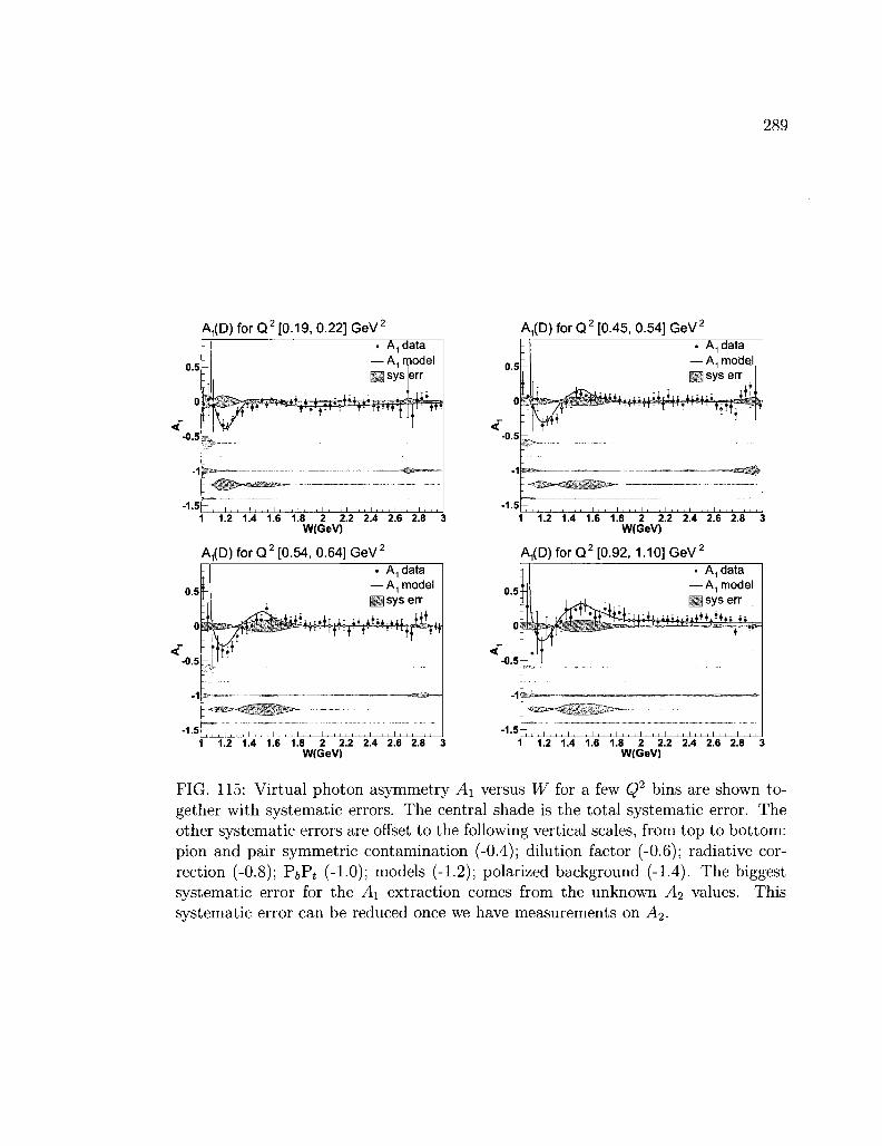
289
A^D) for Q2 [0.19, 0.22] GeV
0.5
-0.5
-1
• A, data — A^ model Ssyserr
o W^^^^^i^i^fi^^Tp^f *jffiflj
-1.3h •o*
1 1.2 1.4 1.6 1.8 2 2.2 2.4 2.6 2.8 3 W(GeV)
A/D) for Q 2 [0.54, 0.64] GeV2
-0.5
• A, data — A, model ££] sys err
i
1 1.2 1.4 1.6 1.8 2 2.2 2.4 2.6 2.8 3 W(GeV)
A^D) for Q2 [0.45, 0.54] GeV
1 1.2 1.4 1.6 1.8 2 2.2 2.4 2.6 2.8 3 W(GeV)
A^D) for Q2 [0.92, 1.10] GeV2
-0.5
-1.5
• A1 data — A., model (§§ sys err
+&+Hi^*iii+!i±i-i*J
1 1.2 1.4 1.6 1.8 2 2.2 2.4 2.6 2.8 3 W(GeV)
FIG. 115: Virtual photon asymmetry A\ versus W for a few Q2 bins are shown together with systematic errors. The central shade is the total systematic error. The other systematic errors are offset to the following vertical scales, from top to bottom: pion and pair symmetric contamination (-0.4); dilution factor (-0.6); radiative correction (-0.8); PfcPt (-1-0); models (-1.2); polarized background (-1.4). The biggest systematic error for the A\ extraction comes from the unknown A2 values. This systematic error can be reduced once we have measurements on A2.
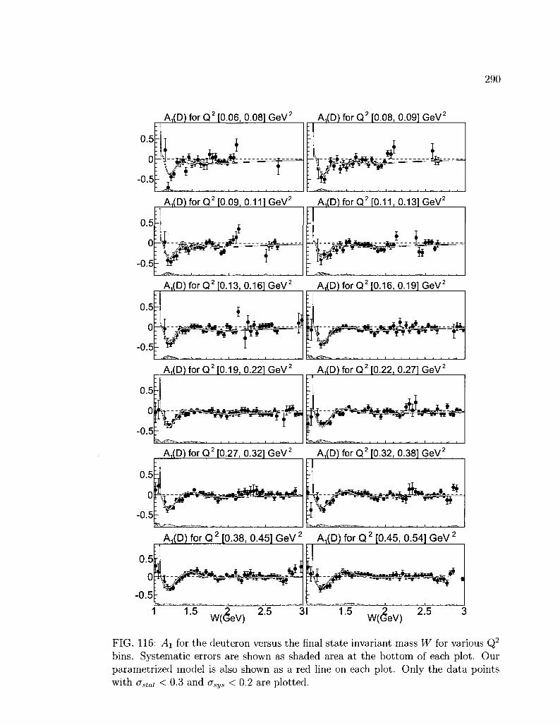
290
A,(D) for Q2 [0.06, 0.081 GeV2 A1(D)for Q2 [0.08, 0.091 GeV2
A1(D)forQ2r0.09, 0.111 GeV2 A1(D)for Q2 rO.11. 0-131 GeV2
A^D) for Q2 [0.13, 0.161 GeV2 A^D) for Q2 [0.16, 0.191 GeV2
A1(D)forQ2r0.19, 0.221 GeV2 A1(D)for Q2 r0.22, 0.271 GeV2
A,(D) for CT [0.27, 0.321 GeV" A^D) for CT [0.32, 0.381 GeV
A.,(D) for Q 2 [0.38, 0.451 GeV 2 A^D) for Q 2 [0.45, 0.54] GeV 2
1-5 iA„2 %„ 2.5 W(GeV)
FIG. 116: Ai for the deuteron versus the final state invariant mass W for various Q2
bins. Systematic errors are shown as shaded area at the bottom of each plot. Our parametrized model is also shown as a red line on each plot. Only the data points with astat < 0.3 and asys < 0.2 are plotted.
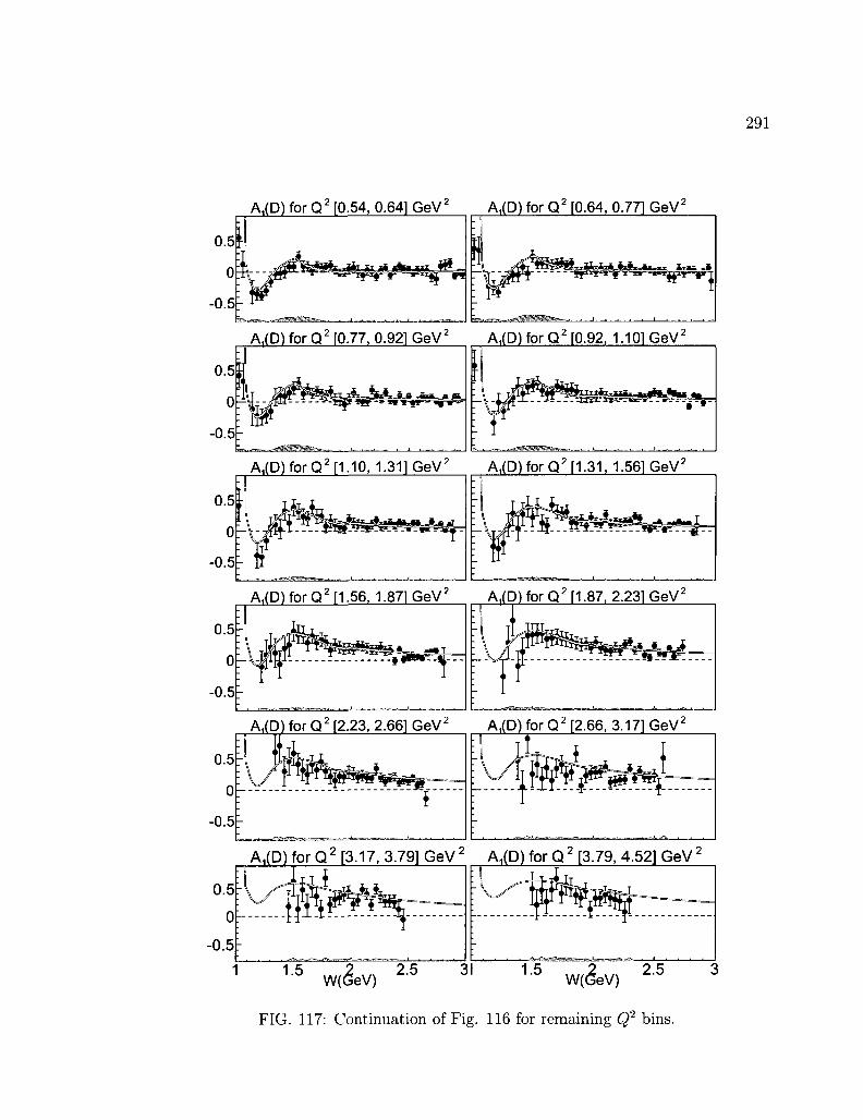
291
A,(D) for Q2 fO.54, 0.641 GeV2 A,(D) for Q2 fO.64, 0.771 GeV
A^D) for Q2 [0.77, 0.921 GeV2 A1(D)forQ2 [0.92, 1.101 GeV
A1(D)forQ2n.10, 1.311 GeV2 A1(D)for Q2 M-31, 1.561 GeV2
A,(D) for Q2M.56, 1.871 GeV2 A^D l fo rQ 2 [1.87, 2.231 GeV
A,(D) for Q2 f2.23, 2.661 GeV2 A,(D) for Q2 T2.66, 3.171 GeV2
Aj(D) for Q 2 [3.17, 3.79] GeV 2 A,(D) for Q 2 f3.79, 4.52] GeV'
FIG. 117: Continuation of Fig. 116 for remaining Q2 bins.

292
g vs. W(GeV) for Q2 (0.06, 0.08) g vs. W(GeV) for Q2 (0.08, 0.09)
g vs. W(GeV) for Q2 (0.09, 0.11) g vs. W(GeV) for Q2 (0.11, 0.13)
g vs. W(GeV) for CT (0.13, 0.16) g vs. W(GeV) for CT (0 16, 0.19)
Q g | vs. W(GeV) for Q2 (027, 032) gt vs. W(GeV) for Q2 (0.32, 038)
0.4
0.2
0
-0.2
-0.4
g vs. W(GeV) for Q 2 (0.38, 0.4S g vs. W(GeV) for Q 2 (0.45, 0.54)
AaL 1.5 2 2.5
W(GeV) 1 5 W<JeV) 2 5
FIG. 118: g\ for the deuteron with respect to the final state invariant mass W for many Q2 bins. The shaded area at the bottom of each plot represents the systematic errors. Model for <?i is shown as a red line on each plot. Only data points with &stat < 0.2 are plotted.
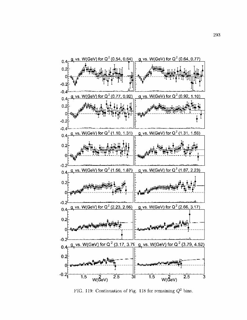
293
0.4 g vs. W(GeV) for Q2 (0.54, 0.64) g vs. W(GeV) for Q2 (0.64, 0.77)
•MWL, I
- 0 . 4 1 —
w^^uki WfW M
«2,o-7-7 n no\ _ ..„ > A ; / / - „ \ / \ f „ - r\ 2 , g, vs. W(GeV) for CT (0.77. 0.92) g, vs. W(GeV) for CT (0.92, 1.10)
Q 4 g vs. W(GeV) for 0 / (1.56, 1.87) g vs. W(GeV) for CT (1.87, 2.23)
g | vs. W(GeV) for CT (2.23, 2.66) g, vs. W(GeV) for CT (2.66 3.17)
-0.21
FIG. 119: Continuation of Fig. 118 for remaining Q2 bins.

294
g vs. x for Q2 (0.06, 0.08) g, vs. x for Q2 (0.08, 0.09)
g,vs. x for Q2 (0.09, 0.11) g vs. x for Q2 (0.11. 0.13)
g, vs. x for Q2 (0.13, 0.16) g vs. x for Q2 (0.16, 0.19)
g vs. x for Q2 (0.19, 0.22) g vs. x for Q2 (0.22, 0.27)
-0.5
Q 4 g vs. x for Q2 (0.27, 0.32) g vs. x for Q2 (0.32, 0.38)
. g i vs. x for Q 2 (0.38, 0.45) g i vs. x for Q 2 (0.45, 0.54)
FIG. 120: #i with respect to the Bjorken variable x for many Q2 bins together with model shown as red lines on each plot. The shaded area at the bottom of each plot represents the systematic error. DIS curve for Q2 = 10 GeV is also shown as blue dashed line.
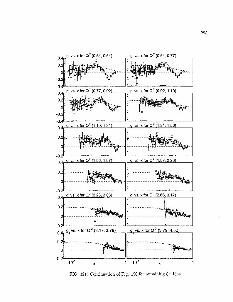
295
0.4 _g, vs. x for Q2 (0.54, 0.64) g vs. x for Q2 (0.64, 0.77)
-0.2-
-0.4
g vs. x for CT (1.87, 2.23)
fl|vs. x forQ' (2.23, 2.66) g | vs. x for CT (2.66, 3.17)
0.2
0
-0.2 g i vs. x for Q 2 (3.17, 3.79) q} vs. xfor Q 2 (3.79, 4.52)
—fcsir*—3
10"' X 1 10" x
FIG. 121: Continuation of Fig. 120 for remaining Q2 bins.
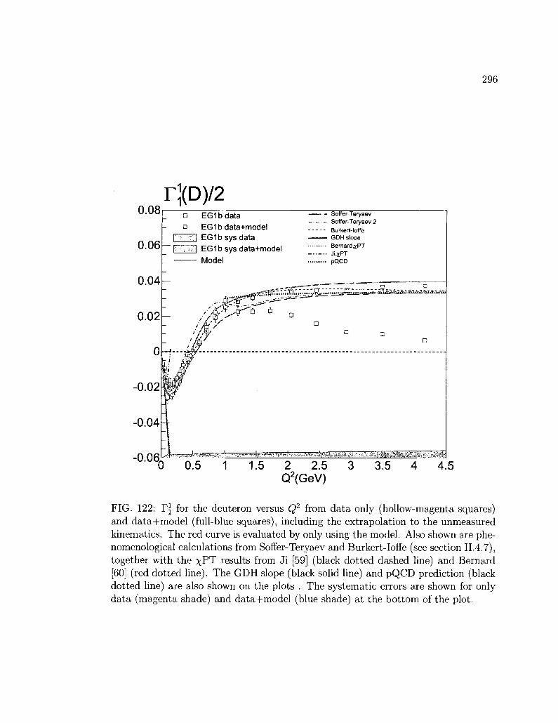
296
0.08
0.06
0.04
r](D)/2
-0.02
-0.04
-0.06.
• EG 1b data • EG1bdata+model
r"7n EGlbsysdata ;;\-ir::| EG1 b sys data+model
Model
Soffer-Teryaev Soffer-Teryaev 2 Burkert-loffe GDH slope Bernard,xPT
• • - • • Ji .xPT
pQCD
2 2.5 Q2(GeV)
4.5
FIG. 122: T\ for the deuteron versus Q2 from data only (hollow-magenta squares) and data+model (full-blue squares), including the extrapolation to the unmeasured kinematics. The red curve is evaluated by only using the model. Also shown are phe-nomenological calculations from Soffer-Teryaev and Burkert-loffe (see section II.4.7), together with the x ? T results from Ji [59] (black dotted dashed line) and Bernard [60] (red dotted line). The GDH slope (black solid line) and pQCD prediction (black dotted line) are also shown on the plots . The systematic errors are shown for only data (magenta shade) and data+model (blue shade) at the bottom of the plot.

297
0.03 r](D)/2
0.2 0.3 0.4 Q2(GeV)
r](D)/2 a EG1bdata+model
l i ' 'M :'•! EG1bsysdata+model
Model
? | _ 0 EG1a
* HERMES
* SLAC E143
Soffer-Teryaev
— Soffer-Teryaev 2
• - - Burkert-loffe GDH slope Bernard,zPT
— Ji,ZPT pQCD
>£l."." .^., .X.WMMJ <^m£&u&?' aMffli" wu&ii «tiow -Til^itJMfiavWiJ
-0.06, 0 0.5 1 1.5 2 2.5 3 3.5 4 4.5
Q2(GeV)
FIG. 123: The top plot is the same as Fig. 122 only zoomed into the low Q2 region. Results from other experiments are also shown in the bottom plot, including E143 [45], HERMES [48] and EGla [67].

298
0.08
0.06
0.04
r](D)/2 • EGlbdata
• EG1bdata+model
^ H EGlbsysdata
^ H EG1b sys data+model
Model
A EGlbprev data+model
• Soffer-Teryaev Soffer-Teryaev 2 Burkert-loffe
• GDH slope Bernard ,xPT
• Ji.JCPT
p Q C D
2 2.5 Q2(GeV)
0.03
0.02
0.01
-0.01
-0.02
-0.03
-0.04
r](D)/2 E G l b d a t a EG1b data+model EG1b sys data EG1b sys data+model Model EG1b prev data+model
• Soffer-Teryaev
Soffer-Teryaev 2
Burkert-loffe
• GDH slope
Bemard,;(PT
• Ji.XPT
pQCD
CT(GeV)
FIG. 124: Comparison of this analysis and the previous one on the T\ extraction from EGlb. The red triangles represent the previous analysis, which was done by only using the 1.6 and 5.7 GeV data. For clear visibility, those points are shifted to a slightly higher Q2 by adding an offset factor. The two independent analysis results complement each other well within statistical errors. Addition of the 2.5 and 4.2 GeV data clearly improves the medium Q2 region and the overall statistics.

299
0.01
0.008
0.006
r?(D)/2
-0.002
• r3 data+model a r3 data
tljgl;j r3 sys data+model r3 model
1 1.5 2 Q2(GeV)
0.003
D.0025
0.002
r*(D)/2
D.0005
D r5 data+model • r5 data
" P H r5 sys data+model r5 model
3.5
Q2(GeV)
FIG. 125: Higher moments of gi extracted from the EGlb data are shown with respect to Q2, the third moment Tf (top), and the fifth moment Tl (bottom). The hollow squares were calculated with no model contribution while the filled squares have model input for the kinematic regions with no available data.

300
Y* (D)/2 '0
2
^ 1
1 T ° 0 o
-1
-2
7 <
®
a Y data+model O Y0
d a t a
^ g y sys data+model
i — i Y° s y s 92
Y model
my ® ® * """"'§r
0.1 0.2 0.3 0.4 0.5 0.6 0.7 Q2(GeV)
Yn (0)12
• Q .
0.01
_J>.005
M 5 a
CO
-0.005
-0.01
-0.015
_ &<&&&%
# Y data+model O V0data
m | Y sys data+model 1 1 V° sys g2
Y model , ^
ft «@
# i
10"1
Q2(GeV)
FIG. 126: Forward spin polarizability (70) for the deuteron is shown versus Q2. The hollow circles represent the calculation by using only data and the full circles are data + model results. The green shaded area is the total systematic error. The systematic error that comes from g2, by taking g2 = 0, is shown with the gray shade overlapped on the total systematic error. The model curve is also shown as a line through data points. The top plot shows values also multiplied by 15.134 for unit conversion to [10~4 fm4]. The bottom plot is just the integral part, without the kinematic factor taken into account.

301
C H A P T E R VI
MODELING T H E WORLD DATA
As new data are generated on the structure functions, our knowledge in different
kinematic regions improves, which enables us to upgrade the models on interesting
physics quantities such as Ai and A2 for the proton, the neutron and the deuteron.
This chapter presents the latest efforts for fitting the world data to produce reliable
models, specifically for A\ and A2 for the proton and neutron. Moreover, since data
are rare on the neutron target, existing deuteron and proton data, especially with
the help of the EG lb results, provide us a platform to extract information on the
neutron spin structure functions.
The behavior of the spin structure functions and the asymmetries in the resonance
region is especially interesting because it is the region where theoretical efforts mostly
fail. Thus, we don't have a rigorous method to describe this region. Therefore,
parametrization of the existing data in the resonance region remains the only reliable
option. These parameterizations are needed to extract other physics quantities, study
radiative effects and even learn about the effects of nuclear medium on the structure
of the nucleon.
The general procedure for the fits includes collection of the world data on the
specific quantities and utilization of a least-square fitting routine to determine the
optimal parameters that describe the data best by minimizing the x2 of the fit, which
is defined by
x W ' w ) = E {oAdata{Q\w)y (467)
where the sum is taken over all data points. Adata(Q2, W) is the value of the data for
the specific quantity, A\ or A2, and A^lt(Q2, W) is the output of the fit function at the
kinematic point of the data. The a^data(Q2, W) is generally taken as the statistical
error of the data point, but for some experiments, statistical and systematic errors
were added in quadrature.
Minimization of the \ 2 was performed by using the MINUIT package from CERN
[111], which provides various different minimization routines. The most widely used
is MIGRAD, which is regarded as "the most efficient and complete single method,
recommended for general functions" [111]. We tried MIGRAD as well as MINOS,
to evaluate parameter errors. Also, the MINIMIZE scheme uses MIGRAD unless it

302
gets into trouble, in which case it switches to SIMPLEX, which is another multi
dimensional minimization routine, and then calls MIGRAD again. In the end, we
decided to use the MINIMIZE routine. However, we did not observe, in any of the
final fits we used, a failure with MIGRAD and a switch to SIMPLEX.
Various parameterizations were tried and compared to each other. The final
functional forms are given in the following sections. The parametrized functions, in
general, also utilize other existing models such as MAID 2007 [128] as well as an
older parameterization of the same kind performed on the more limited data set of
the time. MAID is a unitary isobar model for pion photo- and electroproduction on
the nucleon. It describes the world data on the j*N —> A transition and threshold
7r° production. These existing models provided us a method to extrapolate the fit
successfully into the kinematic regions with no available data, which is the case
specifically with A\ and A% parameterizations..
In the following sections, information is given on the specific parameterizations of
the existing world data on the virtual photon asymmetries A\ and A2 in the resonance
region for the proton and the neutron. We should point out that all data shown in
this chapter were averaged over AW = 40 MeV for plotting purposes by taking
their error weighted averages. However, fitting was performed on the individual data
points at their true kinematic values. Once the models for the spin structure functions
of the proton and the neutron were created, the deuteron models in the resonance
region were obtained by smearing the nucleon structure functions and combining
them according to Eq. (205). For this purpose, the smearing procedure developed
in Ref. [73] was used.
VI. 1 PARAMETRIZATION OF A\
The EG lb experiment measured A\ in the resonance region with an unprecedented
precision. Therefore, the largest amount of data for this fit comes from the EGlb
experiment, in the kinematic region 0.05 GeV2 < Q2 < 5.0 GeV2. The next exper
iment is from MIT BATES [129] and has precision data in the A resonance region
for Q2 = 0.123, 0.175, 0.240 and 0312 GeV2. Then the RSS experiment [130][131],
performed in Hall-C of the Jefferson Lab, provides precision data in the region 1.0
< Q2 < 1.4 GeV2 and 1.08 GeV < W < 2.0 GeV. We also used the results from the
EGla experiment [68], which measured A\ in the Q2 region from 0.15 to 1.6 GeV2.

303
The fit was performed in two separate steps. The first step employed a 16 param
eter fit function. In this function, some of the parameters were used to specifically
treat certain W regions to describe the resonant structure better. Also, MAID model
and an extrapolation of the DIS model into the resonance region were utilized to en
sure the resulting parametrization smoothly continues in the high and low W regions.
The resulting parameters from this step were fixed and the function was used as a
static quantity in the second step fit. The second step employed a 12 parameter fit
function. In this step, we also used an older parametrization and made use of its
strength in some kinematic regions. This two-step approach created a good method
to treat and fine tune certain kinematic regions and describe the resonant structure
better. The fit function for the first step can be written as:
E1 = P0 + Pi tan-1[((52 - P22) Pi]
E2 = P4 + P5 t an" 1 [ (g 2 - P 2) P2]
E3 = 1 — E\ — E2
E4 = P8 + P9 tan-1[(Q2 - P20) P 2J
E5 = Pu + Pis tan"1[(Q2 - Px24) P2
5]
^ , . /IT \W -1.08' Gi = 1 — sin
d = G\
C3 = cos
1.08
W-1.08'
C4 =
M
Ac^ = I
2 - 1.08
[ - M S ) ] 2 w>i.g 0 W<1.9
0 W> 1.35
Eid + E2d + E3d + E4d + E5C5
' MAf + {1-M)A?IS W<2
A°IS W > 2
(468)
where Pj represents parameter i, A^ is the MAID 2007 model of A\ and A±IS is
the DIS extrapolation. A1' ' represents the final calculated fit from the first step.

304
The final parametrization for Ax is used in the second step fit function, which is
described by
Q2Ph = {
Wnh = 7T
0 Q2 < 0.01 GeV2
^ ( ^ + 2 ) Q 2 > 0.01 GeV2
1 Q2 > 10 GeV2
(W - 1.08) ph ~ " (2.04 - 1.08)
Do = P0 + Pi cos (Q2ph) + P2 cos (2Q2
ph)
D1 = Pi + P4 cos (Q2ph) + P5 cos (2Q2
ph) (469)
D2 = Pe + P7 cos (Q2ft) + P8 cos (2Q2
ph)
D3 = P9 + Pw cos (Q2ph) + P „ cos (2Q2
h)
' Do sin (12Wpfc) + £>i sin (Wpft)
>B = < + D 2 sin (2Wph) + D3 sin {4Wph) W < 2.04 GeV
[0 W < 2.04 GeV
Acx = (I - B) A?l] + BA° \OM
where AfM represents an older parametrization and Af is the final parametrized
model. The total number of parameters for the whole fit is 28. During each fit
step, the minimization was performed iteratively, generally two iterations were used,
automatically passing the results of the first iteration as the starting parameters of
the second one. In the first iteration, an initial step size of 0.00001 was used on all
parameters. After the first evaluation of the x2> MINUIT decides on the step size
values based on the first derivatives. In the second iteration, we let MINUIT continue
to decide the step sizes internally. We observed that the final step sizes are generally
very close to zero, on the order of 10~10. Also, no restrictions were employed on the
parameter limits.
Tables 51 and 52 give the initial and final values of the parameters together with
estimated errors and the first derivatives. No user defined derivatives were supplied,
in which case, MINUIT uses its own method by evaluating the finite differences over
the step size. The small step sizes we observe ensures the reliability of these first
derivatives, which in turn yields the reliability of the parameter errors. The resulting

305
first derivatives are generally small or practically zero for some of the parameters.
However, the parameter errors were not used to determine the final errors on the
actual model. The errors on the model were determined systematically by evaluating
the differences between the new fit and various different parameterizations from old
fits.
Total number of data points for the A\ fit was 4325. For the step 1 fit with 16
parameters, the initial \2 value was 22898. After the fit, a \2 °f 5231.94 was reached.
For the second step with 12 parameters, the initial x2 was 5331.92 and the final value
became 4500.08, which results x2/n-d-f ~ 1-04. Figs. 127 and 128 show the resulting
fit together with the data and the other models for various Q2 regions.
TABLE 51: Final parameters for the first step A\ fit (version number 20S1 [132]). The fit function is given in Eq. (468). The total number of data points used in the fit was 4325. The final x2/n.d.f ~ 1.209 was reached at the end of the fit.
ParNo
1 2 3 4 5 6 7 8 9 10 11 12 13 14 15 16
Initial
0.4 0.1 0.5 1.0 0.4 0.1 0.5 1.0 0.1 0.1 0.5 1.0 1.0 0.1 1.0 1.0
Final
-1.01616e-01 -2.97618e+00 -3.23456e-01 2.74645e+00 1.21003e+00 3.10913e+00 4.56491e-05 2.17872e+00 5.08220e-01
-5.99465e-01 -1.09332e+01 -2.03878e+03 3.42967e-01 4.38685e-01 1.28403e-07 1.01192e+00
Error
8.42531e-01 7.93359e-01 2.68590e-02 4.96660e-01 8.04876e-01 7.00746e-01 3.39639e-04 4.27999e-01 8.64463e-01 5.56410e-01 5.46744e+01 1.44157e+04 8.05711e-02 1.43131e-01 1.17306e+00 4.94477e-01
First Derivatives
2.01952e-03 2.89470e-03
-7.30760e-03 -2.24628e-03 2.13005e-03 2.83534e-03 4.65342e-03 2.32311e-03
-6.65403e-03 1.04521e-02
-6.88992e-14 -1.98474e-12 1.32518e-02 5.90950e-03 1.07202e-06 2.97119e-03
VI.2 PARAMETRIZATION OF M
A similar method as described in the previous section was used to fit the A\ data.
Again, there were no restrictions on the parameter limits and the same initial step
sizes with two consecutive iterations were employed for MINUIT.

306
W distribution of A, for a Q bin
0.8
0.6
0.4
0.2
< " Ob
-0.2 F
- 0 . 4 :
- 0 . 6 ;
-0.8 ;
z-
-\
\-
\
Q2 Range 0.077 - 0.092
• i W i N f i '.* *• • t i u lh+* i ^_ i »•
| ^ — ' ^ — ^ c a l c - J ^ ' s$ — A, maid . . .
A , . -A, data
i . . . i .1 . . i . , .
W distribution of A, for a Q2 bin
1.2 1.4 1.6 1.8
w
W distribution of A, for a Q2 bin
Q2 Range 0.187-0.223
•*5»*t"
A, maid . , , . 1 . , • A, data A., o d 1
- A i d ' s , _
w
0.8
0.6
0.4
0.2
< ° -0.2
-0.4
-0.6
-0.8
W distribution of
L
r w j _ /
— \ t /
i l
*f?f
, , i ,
A, for a Q2 bin
Q2 Range 0.379 - 0.452
»si-, j i i jf
"i**vv
—A^alc
. 1 . . -A. data A, old 1
—A,dis . i .1 i , , , i ,
Q2 Range 0.131 -0.156
1
0.8
0.6
0.4
0.2
< " 0
-0.2
-0.4
-0.6
-0.8
- 1 U
W distribution of A. for a Q bin
Q2 Range 0.223 - 0.266
^calc A. maid A , . A
1 , . -A-data A, old 1
A..dis i .1 . . i . . . i . . . i
1.2 1.4 1.6 1.S
w
0.8
0.6
0.4
0.2
< " 0
-0.2
-0.4
-0.6
-0.8
W distribution of A, for a Q2 bin
Q2 Range 0.452 - 0.540
r / ~ N
r
r
r
^ ^ ^ - - - j f W i S i l , $_ '+«****
% • * / ~ ^ ^ c a ' c
\J —A. maid A . . A
1 . . .A . data A, o d 1
" - A . i dis 1.6 1.S
w 1.6 1.8
w
FIG. 127: Apx parametrization for various Q2 bins. The final fit is shown with the
red curve. Other curves are MAID 2007, old parametrization and the DIS extrapolation into the resonance region. For only plotting purposes, the data from different contributing experiments were combined over AW = 40 MeV, by taking their error weighted averages (fitting was performed on the individual data points at their true kinematic values).
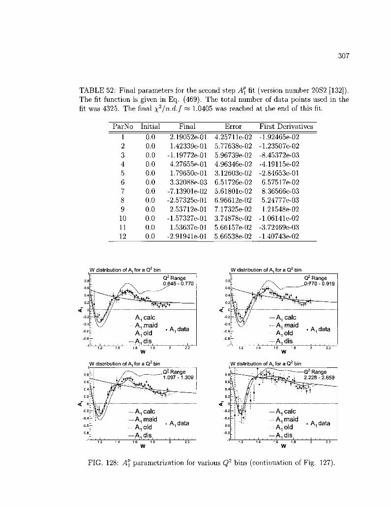
307
TABLE 52: Final parameters for the second step A\ fit (version number 20S2 [132]). The fit function is given in Eq. (469). The total number of data points used in the fit was 4325. The final \2/n.d.f ~ 1.0405 was reached at the end of this fit.
ParNo
1 2 3 4 5 6 7 8 9 10 11 12
Initial
0.0 0.0 0.0 0.0 0.0 0.0 0.0 0.0 0.0 0.0 0.0 0.0
Final
2.19052e-01 1.42339e-01
-1.19772e-01 4.27655e-01 1.79650e-01 3.32088e-03
-7.13901e-02 -2.57325e-01 2.53712e-01
-1.57327e-01 1.53637e-01
-2.91941e-01
Error
4.25711e-02 5.77638e-02 5.96739e-02 4.96346e-02 3.12603e-02 6.51726e-02 5.61801e-02 6.96612e-02 7.17325e-02 3.74878e-02 5.66157e-02 5.66538e-02
First Derivatives
-1.92465e-02 -1.23507e-02 -8.45372e-03 -4.191156-02 -2.84653e-01 6.57517e-02 8.36566e-03 5.24777e-03 1.21548e-02
-1.06141e-02 -3.72469e-03 -1.40743e-02
1
O.i
0.6F
0.4 5
0.2 ;
<" oE -0.2 F
- 0 . 4 ;
-0.6:
-0.8 :
W distribution of A, for a Q2 bin
L
r
:
Q2 Range s~^ 0645 - 0.770
^ ^ ^ ^ w _ _ _ _ }••/ ^"^^***^if(*r
fcy —A1 calc V / —A. maid . . .
. 1 . . • A. data A., old 1
—A^dis . i . , , i . . . i . i , .
W distribution of A, for a Q2 bin
Q2 Range _j0r770-0.919
W
W distribution of A, for a Q2 bin
2 2 2
1r
0.8 5
0.6 3
0 . 4 :
0 . 2 :
< °l - 0 . 2 :
- 0 . 4 :
- 0 . 6 :
- 0 . 8 :
-1
W distribution of A, for a Q bin
I <>
^fjTj Q2 Range * i r i 3 s . * . 2.228 - 2.659
^ — —
—A, calc —A, maid . . .
. 1 . , -A. data A., old 1
—A^is
w 2 2.2
FIG. 128: A\ parametrization for various Q2 bins (continuation of Fig. 127).

308
Data on A\ is sparse, which makes the fit difficult. Mainly, the RSS [133], BATES
[129] and the latest EGlb [95] results were used for this fit. The EGlb results were
obtained by linear regression between Ai + r]A2 values and rj from varying beam
energies. After various trials with different fit functions, the following form was
employed:
^3 = P 02 ( | - t a n - 1 ( Q 2 P 1
2 + P 2 ) )
P2 + tan"1 (Q2Pi + P5) E2
E4 =
- 4- P2 2 ^ r3
E2 — E%
P2
d = l -
C2
C3
(log (Q2) - P7f + P2 + 0.0001
w -im' 2-
1 — sin
1.08
cos 7T
7T
2
W -
T y - 1 . 0 8
2 - 1.08
1.08"
a
Ac2=<
(470)
2 - 1.08
skMSS! ] ) 1-3<W<1.8 0 otherwise
M = EXCX + E2C2 + E3C3
MA™ + {1-M) A°IS + E4C4 W < 2
A?IS W>2
Similar to the previous section, Pt represents parameter i and A^ represents the final
calculated fit, while A^ is the MAID model and A%IS is the DIS extrapolation. The
Wandzura-Wilczek relation and the Burkhardt-Cottingham Sum Rule [7] were used
to estimate the DIS extrapolation of A2 into the resonance region and were used as a
constraint in the fit. A smooth transition between the resonance region and the DIS
region was required. In addition, another constraint, the Soffer limit (see Eq. (70))
provided a general estimate and a boundary on the fit results. A penalty was applied
to the x2 f° r cases when the calculated fit exceeded the Soffer limit such that:
{\Aflt{Q2, W)\ - As°"er(Q2, W)f X\Q\W) = YJ 0.005
(471)

309
The fit was performed in several iterations. In the first iteration, the values of
parameters P6, P7 and P8 were kept constant, and in the second iteration, they were
released. The resulting final parameters from these first calculations were used as the
starting parameters for the next round and the same fit was repeated twice, again
first fixing parameters PQ, P7, Ps and releasing them after the first 6 parameters
reached their optimal values.
The total number of data points for the A\ fit was 344. The final x2 °f the fit
was 418.8, resulting in a x2/n-d-f ~ 1.21. Table 53 shows the resulting parameter
values and Fig. 129 shows the fit results together with the available data for various
Q2 regions.
TABLE 53: Final parameters for the A\ fit given in Eq. (470). The final x2/n.d.f ss 1.21 was reached at the end of this fit. The total number of data points used in the fit was 344.
ParNo
1 2 3 4 5 6 7 8 9
Final
5.92348e-01 1.66989e+02
-2.79601e+04 -1.80099e+00 3.66274e+00
-7.7621 le+04 2.72528e-01
-1.77948e-01 4.72596e-01
Error
1.97150e-01 4.89463e-01 1.62278e+02 4.56000e-01 7.98533e+02 4.47812e+06 5.91656e-02 9.76423e-02 1.06130e-01
First Derivatives
9.30561e-04 -2.21883e-04 -2.99000e-07 2.26247e-04 5.63709e-10 3.92323e-15 1.13762e-02 4.03108e-03
-2.63065e-03
VI.3 PARAMETRIZATION OF A*
It is not possible to make a direct measurement on a polarized neutron target to
extract the asymmetries and structure functions of the neutron. The best approx
imates to a polarized neutron target are polarized 3He and deuterium targets. In
both cases, the nuclear effects smear the nucleon structure, making it difficult to
isolate the information from a single nucleon. Currently, there are limited data on
a transversely polarized deuteron target [130]. However, smearing makes it difficult
to extract neutron information for AV^ from deuteron because proton dominates. In
the resonance region, there are also two other experiments that took measurements
on a polarized 3He target. The first experiment was E94-107, which took place in

310
W distribution of / ^ for a Q2 bin W distribution of Aj for a Q bin
W distribution of A^ for a Q2 bin W distribution of fi^ for a Q bin
0.8
0.6 :
0.4 -
0.2 i s ^ ^ ^ f e S S
-0 2 • — A , calc
-0.4
-0.6
-0.8
?
I I . I
: — A2 maid A 2 o l d
— A2 dis i iSpffer ,
Q2 Range 0.223 - 0.266
r r^r .
•! A2 bates 4 A 2 e g 1 b *i A2 rss »j A2e143 *i A2 e155 • A2e155X l
0.8
0.6
0.4
0.2
-0.2
-0.4
-0.6
-0.8
" I I I ! <l :
* 0 I
3 2 Range 3.^66-0.317
I
• 1 ^ s f ^ ^ ' J - ^ * ^ 1 '• ^ — ^ " " " ^ '• •
1 — A 2 c a l c 1 | - ' — A 2 maidt '
A2 old i
^ — A 2 dis | [i , . , i goffer i ' , ,
• A2 bates o A2eg1b » A2 rss . A2e143 o A2e155 . A2e155X,
w 1.2 1.4
w
0.8
0.6
0.4
0.2
J1 n < ° -0.2
-0.4
-0.6
-0.8
W distribution of A,
~T
\
r
.-• ^ \ \
for
-h
a Q
s • - v ^
- A ,
" A 2
A 2
- A 2
£p
a m ol di ff«
2 bin f
&1 \2-*t 1
lie aid d s
r i ,
Qf Range 1.J097-1.309
c
• A2 bates o A2eg1b » A2rss . A2e143 © A2 e155 • A2e155X,
W distribution of A; for a Q2 bir^
W
FIG. 129: Final AF2 parametrization (red line) for various Q2 bins, for which there are available data, are shown together with other models described in the text. The shaded area represents the Soffer limit. The RSS (red), BATES (blue) and EGlb (green circle) data are also plotted.

311
Hall-A at Jefferson Lab [134][135]. The experiment measured the spin-dependent
cross section for the inclusive scattering of polarized electrons from a polarized 3He
target in the quasi-elastic and resonance regions for 0.1 < Q2 < 0.9 GeV2. By using
both the transverse and longitudinally polarized targets, the experiment extracted
the spin structure functions g\ and g% for 3He. The second experiment, E01-012, also
took place in Hall-A at Jefferson Lab to measure the quark-hadron duality on the
neutron by using a polarized 3He target [136][137]. This experiment also extracted
the spin structure functions g\ and g2 for 3He by measuring the cross section for
inclusive electron scattering off longitudinally and transversely polarized targets.
Since we are merely trying to model the general behavior of A% in the resonance
region, we decided to use these data on 3He to extract some A% data for our fits. We
first applied simple nuclear corrections to get the polarized structure function of the
neutron from the 3He data by using our latest model for the proton,
rf=g!- + 2 ^ x 0 . 0 2 7 ^ ( 4 7 2 )
°« = GST ^ _ g?* + 2.0 x 0.027<gN
92 ~ 0.87 { ]
<7„He
°* = 557 <475)
where the factor 0.87 is for the effective neutron polarization in 3He while 0.027 is
that of the proton, with two protons. Then we calculated the corresponding virtual
photon asymmetries A\ and A2 for the neutron by using these results,
A, = 9-^^ (476)
< = ( "91 /C92 ) (477) a<n - 7 ^ 2
^2 = ^ ( 5 1 + 52) (478) Fr
2 ( 1 t , • aA2 = I yya9i +a92.
(479)
where we used the existing models for Fi, which are described in section IV. 16. Once
we have the relevant data, we utilized our fit function given in (470), which was also
used to fit the proton data on A\. The total number of data points we had for this
case was 161. The initial x2 °f the fit with the starting parameters was 350.55 while

312
the final x2 after the minimization was 190.23, yielding x2/n.d.f = 1.18. Table 54
shows the initial and the final parameters of the A% fit. Figs. 130 and 131 show the
fit together with the experimental data for various Q2 values with available data.
TABLE 54: Final parameters for the A% fit given in Eq. 470. The final x2'/n.d.f « 1.18 was reached at the end of this fit. The total number of data points used in the fit was 161.
ParNo
1 2 3 4 5 6 7 8 9
Initial
0.7 1.0
-2.0 1.0 1.0
-1.0 0.07 0.0 0.2
Final
-4.56143e-08 -3.56573e+00 6.91149e+01 4.64862e-01
-1.64811e+01 -8.14488e+02 6.24803e-01
-5.58762e-01 1.36991e+00
Error
5.79134e+00 1.41421e+00 1.41421e+00 9.00620e-02 3.09743e-02 3.06294e+00 2.07558e-02 1.21758e-01 5.60160e-02
First Derivatives
-2.72043e-09 0.00000e+00 0.00000e+00 8.86916e-05 2.48725e-03
-1.08100e-05 -1.21569e-03 9.07721e-05 2.78096e-04
VI.4 PARAMETRIZATION OF A\ B Y USING T H E D E U T E R O N
DATA
The main ingredients for a fit of A\ for the neutron are the data on the deuteron
spin structure function gi and the convolution procedure described in Refs. [73] [138]
and section II.5. Extraction of the neutron information requires a careful study of
the nuclear effects, especially the Fermi motion, which is primarily considered in the
convolution procedure. Of course, the D-wave correction was also applied. Moreover,
creating the best possible fits to the proton and deuteron data is essential for the
best results with this method. Since the EG lb experiment took data on both of
these targets, we have a unique opportunity to extract the neutron asymmetries and
structure functions by using the final results from EGlb.
The fitting mechanism for this case is quite different than in the previous cases.
The fitted data come from the deuteron spin structure function gi measurements.
The results of the EGlb experiment, described in this thesis, were used as well as
the measurements from the RSS [130] and E143 [45] experiments. A fit function
was employed to determine A\ and the parametrized A\ was used in the smearing
procedure, together with the final A\ parametrization described in section VI. 1.

313
W distribution of Aj for a Q2 bin W distribution of A; for a Q2 bin
W distribution of fi^ for a Q bin
-0.2
-0.4
-0.6
-0.8
A2 init — A2 calc — A2 maid
r - A2old - — A2 dis
. i . . . i , . . £Q"<?r .
. A2E94
. A2E01012
, i . . . i
w W distribution of A , for a Q2 bin
0.8
0.6
0.4
0.2
-0.2
-0.4
-0.6
-0.8
Q2 Range 0.223 - 0.266
— A2 init — A2 calc — A2 maid — A2 old — A2 dis
. A , E94
1.6
1
0.8
0.6
0.4
0.2
< ° -0.2
-0.4
-0.6
-0.8
-1
w W distribution of A . for a Q bin
- A2 init — A2 calc — A2 maid -•• A2old — A2 dis
Q2 Range 0.540 - 0.645
. A , E94
A , E01012
w 1.i
W distribution of Aj for a Q2 bin
0.8
0.6
0.4
0.2
< ° -0.2
-0.4
-0.6
-0.8
r
[-
: r
-:, , i
jffi^S^&Z A2 init
— A2calc — A2 maid — A2old — A2 dis
, , i , , , P P ^ i ' , i
Q2 Range 0.770-0.919
^ T t * ™ " • • • . A2 E94
• A2E01012
i
w
FIG. 130: Final A1^ parametrization for various Q2 bins with available data. The red line represents the final fit. Blue data points are from the E94-107 experiment. The MAID model (green), the DIS extrapolation (brown) and older parametrization (cyan) are also plotted. The shaded region is the Soffer limit.

314
W distribution of A; for a Q bin
0.8
0.6
0.4
0.2
-0.2
-0.4
-0.6
-0.8
w
Cr Range 1.097-1.309
•
: ~ L
:, , i , . ,
— A2 init — A2 calc — A2 maid
A2old — A2dis
, , , iSpffqr , |
• A2E94
. A2E01012
i . , , i
W distribution of A; for a Q bin
0.8
0.6
0.4
0.2
<f ° -0.2
-0.4
-0.6
-0.8
-1
Q2 Range 1.563-1.866
• A 2 init
— A2 calc — A2 maid
A2old — A , dis > A , E01012
£Qffqr .
w
FIG. 131: Final AV^ parametrization for various Q2 bins with available data. The red line represents the final fit. The data from E01-012 is also shown (red) together with the MAID model (green), the DIS extrapolation (brown) and an older parametrization (cyan). The shaded region is the Softer limit.
The smearing function combines the information for the proton and neutron by
taking nuclear effects like Fermi motion into account and calculates the deuteron
spin structure function gf, which was compared to data to calculate the \2 of the fit
according to Eq. (467). After the minimization of the x2, the resulting parameters
were used in the fit function for the neutron to determine the final parametrized
values of A\.
For the fit function, the parameterizations of A\ and A\, described in Eqs. (468)
and (470), were both tried. Eventually, the A\ parametrization in Eq. (470), which
was also used for A^, seemed to described the data best. The total number of data
points for this fit was 3175. The final x2 w a s 2503.41, which yields x2/n.d.f ~ 1.26.
We should point out that this fit will be improved by employing a second step fit as
we did for the case of proton. However, the current results describe the data well in
most kinematics as can be seen in Fig. 132. The model for A" obtained by using the
final parameters is also shown in Fig. 133.
Finally, once we have reliable models for the proton and neutron structure func
tions, we can determine the deuteron model by properly smearing the proton and
neutron. As a result, we have experimental data on deuteron spin structure function
(?i as well as its model obtained by the smearing procedure [73]. We can extract the
neutron structure function data by
1 nldata]
01 1 — 1.5WD
I d[data] d[model]
) + 9i n[model]
(480)

315
where Wn stands for D-state probability. The statistical and systematic errors prop
agate as stat _ stat fA8~\\
an[data] ~ \ _ \ §w ad\data] l 4 0 i i
sys _ •*• sys (AR9\ un[data] ~ \ — \ §w d[data}- \WA)
However, since this extraction depends on the model choice, we need to vary both
the neutron and deuteron models and add the differences coming from model choices
to the total systematic error in quadrature
x 21 1/2
systot n[data\
sys ^2 j _ I \ " ^ f o n [ d a t a j _ n[i «W2 + $>r (483)
where summation is over different model choices and g" represents the extracted
result for model choice i. The results for this extraction are shown in Fig. 134 for a
few Q2 bins.
VI.5 A D D I T I O N A L C O M M E N T S
The work on modeling the world data is a continuous and iterative procedure. Some
of the results have certain model dependencies. For example, the EGlb results
for Ai have a slight dependence on the A2 models (see Ref. [95]). By getting
a better parametrization for A2, the A\ model can be improved and in turn, the
A2 parametrization can be re-visited to create a better model on this quantity. In
addition, the data on these quantities are constantly improving in different kinematic
ranges. The efforts will continue as these new data come into existence. In particular,
the EG4 experiment [139] will allow us to extend our parameterizations of A\, A™
into the lower Q2 range and give us opportunity to resume our efforts.

316
W distribution of g^ for a Q2 bin
Q2 Range 0.156-0.187
-g.jdis*' . g ^ g l b ^ m a i d . g i rss -gcalc . g e143 i . i . . i . . . i i , , i ,
W distribution of gd for a Q2 bin
1.6 1i
w W distribution of g* for a Q2 bin
A, i
Q2 Range 0.452 - 0.540
g^ i s . g ^ g l b
g1 maid . g1 rss
gcalc , g e143 , i, , i , . . i , i , . i ,
w
1.2 1.4 1.6 1.S
w distribution of gd for a Q2 bin
Q2 Range 1.097-1.309
- g ^ i s . ^ e g l b —g maid . g i rss - g c a l c . g e143 . i . i , , i , . . i i . . i .
Q2 Range 0.266-0.317
—9, dis . g.,eg1b —g„ maid . g rss
1 i - g c a l c . g e143 . i . i . . i . , , i . » . . i .
w W distribution of g'J for a Q2 bin
Q2 Range 0.770-0.919
^ d i s . g ^ g l b g_ maid . g. rss
1 i gcalc . g e143 , i . . i . , , i i , , i ,
w
1.6 1.S
w distribution of gd for a Q bin
Q2 Range 1.309-1.563
^ d i s . g ^ g l b
g i maid . g i rss
gcalc . g e143 . i . . i . . . i . i . . i .
w w
FIG. 132: The model for gi/F^ for the deuteron (red solid line), which was calculated from the parametrized A" and A\ by applying the smearing procedure, is plotted together with the experimental data points for various Q2 bins. Together with the EGlb experiment (blue), the RSS (red) and E143 (green) data are also shown. As usual, the green line represents MAID and the brown line is the DIS extrapolation.
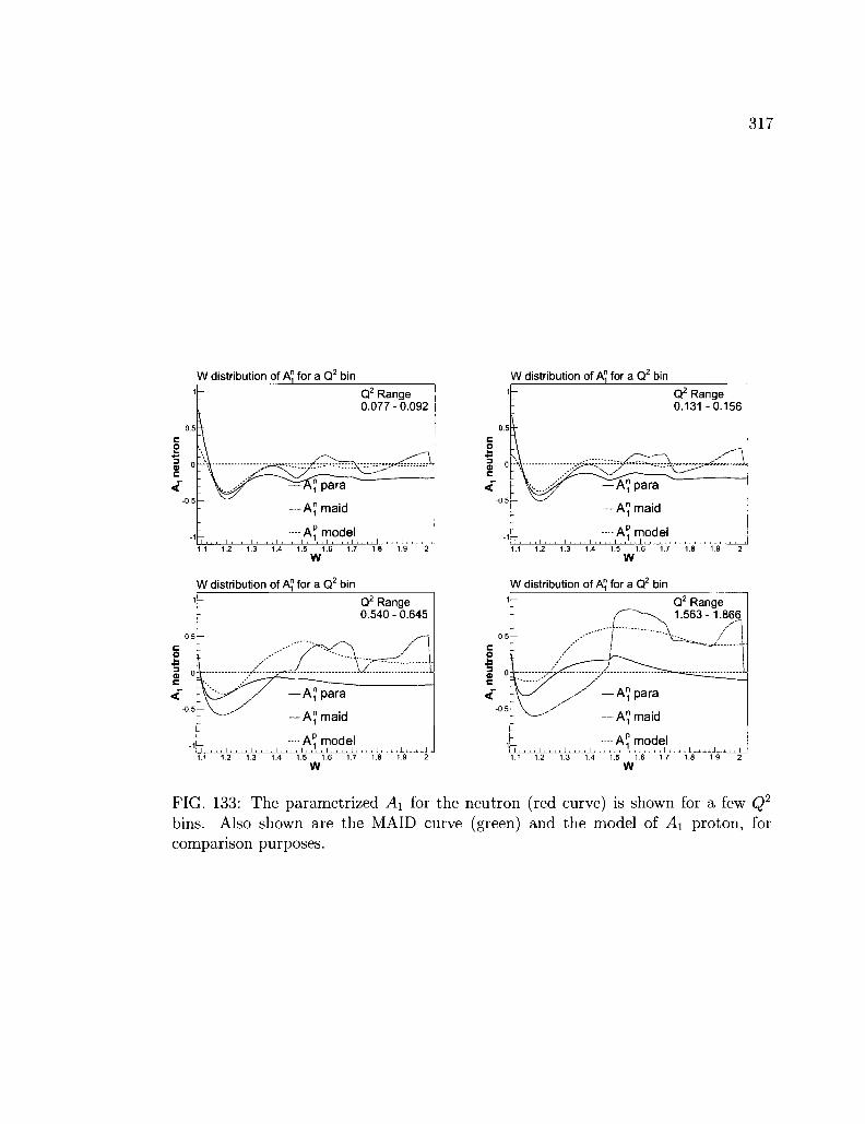
1
0.5
0
0.5
-1
W distribution of A? for a Q2 bin
Q2 Range - 0.077 - 0.092
\
i ^:2^^^^^a - V J ^ ' "^A" para
— A" maid
-_ - A ^ model 1.1 1.2 1.3 1.4 1.5 1.6 1.7 1.8 1.9 2
w W distribution of A" for a Q2 bin
Q2 Range 0.540 - 0.645
A" para
A" maid
A? model i • i i
1
0.5
0
0.5
-1
W distribution of A" for a Q bin
Q2 Range 0.131-0.156
\
A /---—\ /"""I p.L ^^y^^^ - \^>f —A" para
— A" maid
L -A^ model 1.1 1.2 1.3 1.4 1.5 1.6 1.7 1.8 1.9 2
w W distribution of A!J for a Q2 bin
1.1 1.2 1.3 1.4 1.5 1.6 1.7 1.8 1.9 2
w
Q2 Range 1.563-1.866
— A" para
— A" maid
—-A? model 1.1 1.2 1.3 1.4 1.5 1.6 1.7 1.8 1.9 2
w
FIG. 133: The parametrized A\ for the neutron (red curve) is shown for a few Q2
bins. Also shown are the MAID curve (green) and the model of Ai proton, for comparison purposes.

318
W distribution of g"IF" for a Q2 bin
0.8
0.6
°>-0.4
-0.6
-0.8
-1'
Q2 Range 0.156-0.187
. g ^ E G I b
•— 9j'F? model
1.1 1.2 1.3 1.4 1.5 1.6 1.7 1.8 1.9 2
w W distribution of g7F" for a Q2 bin
0.8
0.6
C 0.4 O
£ 0 2
S o t l T - 0 2
°>-0.4
-0.6
-0.8
Q2 Range 0 .317-0.379
^ > r j ' ' tTfH-.u..LU4..fl. r--+' :-7 : 'f-i-:i-:.*:-i"t"f"ft-
—- 9""1! model
. g-VFJEGIb
gp/F; model « , " ,
1.1 1.2 1.3 1.4 1.5 1.6 1.7 1.8 1.9 2
w W distribution of g7F? for a Q2 bin
0.8
0.6
C 0.4 O i 0.2 3 « o
l lT-0.2
°>~-OA
-0.6
-0.8
-1
Q2 Range 0.770-0.919
•=f-r i - - t j i J . •
g^/P model | 1 '•
. g7F?EG1t
1.1 1.2 1.3 1.4 1.5 1.6 1.7 1,8 1.9 2
w
W distribution of g"IF" for a Q2 bin 1 , 1 — •
0.8
0.6
! :
°>-0.4
-0.6
-0.8
-1
;sj....
Q2 Range 0.266-0.317
. g#!JEG1b
--gP/F; model
1.1 1.2 1.3 1.4 1.5 1.6 1.7 1.8 1.9 2
w W distribution of g7F!; for a Q2 bin
Q2 Range 0.452 - 0.540
. g'VF'JEGIb
iS5!fi model
1.1 1.2 1.3 1.4 1.5 1.6 1.7 1.8 1.9 2
w W distribution of g7F? for a Q2 bin
1
o.8;
0.6
0.4
0.2
o t -
"-0.2
-0.4
-0.6
-0.8
Q2 Range 1.563-1.866
[- g"/F; njiodel
••" ^'fLfflSl61
g-VFJEGIb
1.1 1.2 1.3 1.4 1.5 1.6 1.7 1.8 1.9 2
w
FIG. 134: Parametrized gi/Fi (red dashed line) for the neutron is plotted together with gi/Fi neutron (blue data points) extracted from the EGlb deuteron data according to Eq. (480). The systematic errors are shown as green shades at the bottom of each plot. The same quantity for proton is also shown for comparison purposes (blue dashed line).
319
C H A P T E R VII
CONCLUSION
The EGlb experiment measured the double spin asymmetry for the deuteron (and
the proton) over a large kinematic range that covers the resonance region and the
onset of the DIS region. Although the results from the 1.6 and 5.7 GeV data have
been available before, these data have been reanalyzed for full statistics by adding
the remaining data sets with 2.5 and 4.2 GeV beam energies. This extended the kine
matic coverage and reduced the errors on the measured quantities significantly. The
measurements from EGlb enabled the extraction of the virtual photon asymmetry
Ai for 0.05 GeV2 < Q2 < 5.0 GeV2 with unprecedented precision. The statisti
cal precision of the data enabled us to see clear resonant behavior at low Q2. The
largest systematic error on A\ comes from model input for A2. The studies on A2
parametrization is an ongoing process and with its completion, the systematic errors
on Ai, and thus gi, will decrease.
At low Q2, the structure function g( is also deeply affected by the resonance
structure in our kinematic range. As a result, its first moment, T\, as well as the
higher moments, have a strong Q2 dependence. As we go to higher Q2, the resonant
structure is less explicit and the Q2 dependence of the first moment slowly diminishes.
The experimental data confirm the Q2 evolution of the first moment envisioned by
the phenomenological studies, described in chapter II. At low Q2, F\ is negative and
expected to approach the GDH slope. The data from EGlb do not cover a low enough
Q2 region to put the GDH slope under a robust test. However, the overall tendency in
that region obeys the constraints enforced by the GDH slope. The next generation
experiments [139] will cover a lower Q2 range in order to test the GDH slope as
well as xPT theory in this region. T\ being negative at low Q2 is attributed to the
AP33(1232) resonance, which is also evident from the g\ versus x plots that become
negative in this region. It should be pointed out that the plots of the moments shown
in this analysis all exclude the quasi-elastic peak. Its inclusion would smear out the
effects of the resonances. As we go to higher Q2, F\ for the deuteron experiences its
minima around 0.10 < Q2 < 0.15 GeV2 and attains a positive slope, then crossing
zero around 0.45 < Q2 < 0.50 GeV2. As we go above Q2 ~ 2 GeV2, T\ becomes
almost flat approaching the Bjorken limit. In the intermediate and high Q2 regions,
the data and phenomenological calculations agree well. The data from the EGlb
320
experiment will create opportunities to test different versions of the generalized GHD
integrals and modified Bjorken Sum Rule. Moreover, the results will create a robust
ground for studies on duality and calculations of the higher twist coefficients.
Parametrization of the world data on the virtual photon asymmetries is an impor
tant basis for calculations of radiative corrections to cross sections. Moreover, these
parameterizations are also crucial for the extraction of spin structure functions from
future asymmetry measurements as well as providing inputs for phenomenological
calculations. In addition, the extraction of the neutron structure functions from the
proton and deuteron data by comprehensively taking the nuclear effects into account
gives us a more reliable parametrization for the neutron. In addition, this kind of
work can provide a different environment to study and test the nuclear effects inside
the deuteron.
Although its effect on the final results will be small, the radiative corrections
applied to A\\ still require an update after the completion of the parameterizations
on the symmetries. After that, the final official data from this analysis will be
available in the CLAS database [140].

321
A P P E N D I X A
DST VARIABLES
In the DST tables, the range (R) of a variable is defined in terms of the offset (o),
the multiplier (m), the sign (s), that determines whether the variable is signed (1)
or not (0), and the number of bits (n) for the variable,
R = 2™ — -m
\ -o] J
1 *s ; (2n
— \m
(484)
This is the scheme used in the DST libraries to determine the maximum and minimum
acceptable values for the variables.
TABLE 55: DST variables: particle ID. SEB is the standard particle ID used in RECSIS, whereas pJd(DST) is the DST equivalent.
SEB ID pid(DST) particle 11
2212 2112
211 -211 321
-321 45 49 47 22
-11
1 2 3 4 5 6 7 8 9
10 11 12
electron proton neutron 7T+
7T~
K+
K~ deuteron 3He 4 ife photon positron
TABLE 56: DST event headers
name event n_part start_time raster _x raster_y trigbits
offset 0.0 0.0 0.0 0.0 0.0 0.0
multiplier 1.0 1.0
100.0 1.0 1.0 1.0
signed 0 0 1 0 0 0
bits 27
5 14 16 16 16
definition event number from BOS file number of particles in the event event start_time x coordinate of the raster position y coordinate of the raster position trigger bit

322
TABLE 57: DST scaler variables and run information
name CLOCK.UG CLOCK_G FC_UG FC_G EVMin EVmax clockug clockg fcupug fcupg synchug synchg PMTTop PMTBottom PMTBeamRight PMTBeamLeft BeamE BeamI TorusI Targetl BeamPol TargetPol BadRun Target PolPlate
offset 0.0 0.0 0.0 0.0 0.0 0.0 0.0 0.0 0.0 0.0 0.0 0.0 0.0 0.0 0.0 0.0 0.0 0.0 0.0 0.0 0.0 0.0 0.0 0.0 0.0
multiplier 1.0 1.0 1.0 1.0 1.0 1.0 1.0 1.0 1.0 1.0 1.0 1.0 1.0 1.0 1.0 1.0 1.0
10.0 1.0 1.0
100.0 100.0
1.0 1.0 1.0
signed 0 0 0 0 0 0 0 0 0 0 0 0 0 0 0 0 0 0 1 1 1 1 0 0 0
bits 31 31 31 31 27 27 19 19 12 12 16 16 10 10 10 10 16 10 12 12 7 7
32 7 2
definition live time ungated clock live time gated clock live time ungated faraday cup live time gated faraday cup first event of the helicity state last event of the helicity state ungated clock gated clock ungated faraday cup gated faraday cup ungated SLM gated SLM PMT output PMT output PMT output PMT output Beam energy Beam current Torus current Target current Beam polarization Target polarization Run flag Target type Half-wave plate status
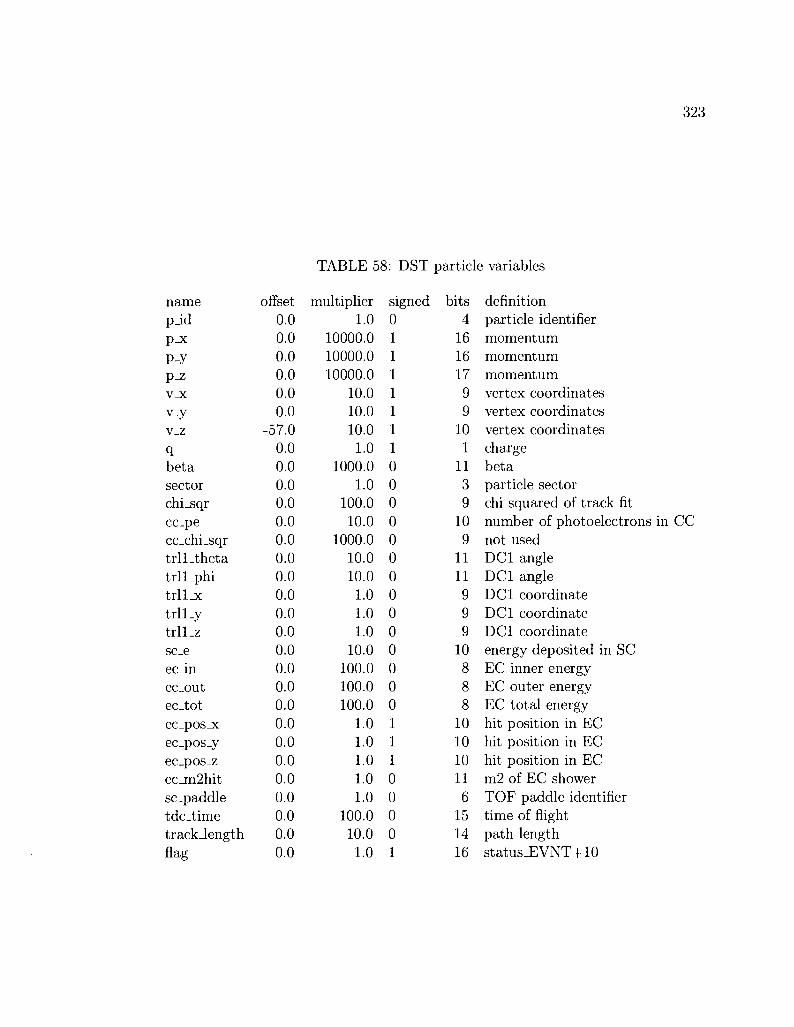
TABLE 58: DST particle variables
name pJd p j x
p-y p_z v_x
v-y v_z
q beta sector chLsqr cc-pe cc_chi_sqr tr l l . theta trll_phi trll_x trll-y trll_z sc_e ec_in ec_out ec_tot ec_pos-x ec_pos_y ec_pos_z ec_m2hit sc_paddle tdc_time trackJength nag
offset 0.0 0.0 0.0 0.0 0.0 0.0
-57.0 0.0 0.0 0.0 0.0 0.0 0.0 0.0 0.0 0.0 0.0 0.0 0.0 0.0 0.0 0.0 0.0 0.0 0.0 0.0 0.0 0.0 0.0 0.0
multiplier signed bits 1.0
10000.0 10000.0 10000.0
10.0 10.0 10.0
1.0 1000.0
1.0 100.0 10.0
1000.0 10.0 10.0
1.0 1.0 1.0
10.0 100.0 100.0 100.0
1.0 1.0 1.0 1.0 1.0
100.0 10.0
1.0
0 1 1 1 1 1 1 1 0 0 0 0 0 0 0 0 0 0 0 0 0 0 1 1 1 0 0 0 0 1
4 16 16 17 9 9
10 1
11 3 9
10 9
11 11 9 9 9
10 8 8 8
10 10 10 11 6
15 14 16
definition particle identifier momentum momentum momentum vertex coordinates vertex coordinates vertex coordinates charge beta particle sector chi squared of track fit number of photoelectrons in not used DC1 angle DC1 angle DC1 coordinate DC1 coordinate DC1 coordinate energy deposited in SC EC inner energy EC outer energy EC total energy hit position in EC hit position in EC hit position in EC m2 of EC shower TOF paddle identifier time of flight path length status_EVNT+10

TABLE 59: DST particle variables (added later to use the geometric and timing cuts).
name SCJX
sc.y sc_z sc_cx sc_cy sc_cz cc_time cc_status cc_r cc_sec sc.time scstatus sc_r sc_sec
offset 0.0 0.0 0.0 0.0 0.0 0.0 0.0 0.0 0.0 0.0 0.0 0.0 0.0 0.0
multiplier 1.0 1.0 1.0
1000.0 1000.0 1000.0
100.0 1.0
10.0 1.0
100.0 1.0
10.0 1.0
signed 1 1 1 1 1 1 0 0 0 0 0 0 0 0
bits 10 10 10 10 10 10 15 15 15 3
15 15 15 3
definition sc position sc position sc position sc direction cosine sc direction cosine sc direction cosine cc time cc status flag cc radial distance cc sector sc time sc status flag sc radial distance sc sector
TABLE 60: DST variables: helicity flag
helicity flag 1 2 3 4
-1 -2
true 1 0 1 0 1 0
helicity state first state of the pair first state of the pair second state of the pair second state of the pair bad helicity flag bad helicity flag
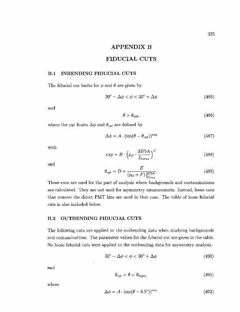
325
APPENDIX B
FIDUCIAL CUTS
B . l I N B E N D I N G FIDUCIAL CUTS
The fiducial cut limits for 0 and 6 are given by:
30° - A<f> < (f>< 30° + Acf) (485)
and
0 > Qcuu (486)
where the cut limits Acf) and 9cut are defined by
Acf) = A • (sin(0 - 6^))^ (487)
with
„ / 3375A\^ , ,„„. exp = B- [Vei--T (488)
and
^ = g+ (Pe ,J )PA- (489)
These cuts are used for the part of analysis where backgrounds and contaminations
are calculated. They are not used for asymmetry measurements. Instead, loose cuts
that remove the direct PMT hits are used in that case. The table of loose fiducial
cuts is also included below.
B.2 O U T B E N D I N G FIDUCIAL CUTS
The following cuts are applied to the outbending data when studying backgrounds
and contaminations. The parameter values for the fiducial cut are given in the table.
No loose fiducial cuts were applied to the outbending data for asymmetry analysis.
30° - A<t>< <j>< 30° + Acp (490)
and
Ocut <0< ehigh, (491)
where
Acf> = A • (sin(0 - 6.5°))exp (492)

326
"n.nm. 35
(GeV/c)
exp = B- {^PeiJ
cut = D + E • ( 1 — -Pscale)
Qhigh = min(40o,<9„om)
r l / 3375A o c r , „ . \ i 17^- rlPei-Tj r + 2.5GeV/c)
Pscale Pel
3375A
l Torus
1500A
•l Torus
3
(493)
(494)
(495)
(496)
(497)
TABLE 61: Fiducial cut parameters for the inbending data. Momentum is in GeV and angles are in degrees. These cuts are not used for asymmetry measurements.
Parameter
A B C D E F
4>lim
p <3 GeV
36 0.28 0.30 10
16.72 0.06 20
p >3 GeV
36 0.25 0.30 10
16.72 0.06 20
TABLE 62: Loose fiducial cut parameters for the inbending data. These cuts remove the direct PMT hits only. They can be applied in case of asymmetry measurements but cannot be applied to any acceptance dependent measurements.
Parameter
A B C D E F
4>lim
p <3 GeV
41 0.26 0.30
9 16.72 0.06 21.5
p >3 GeV
41 0.26 0.30
8 16.72 0.06 21.5
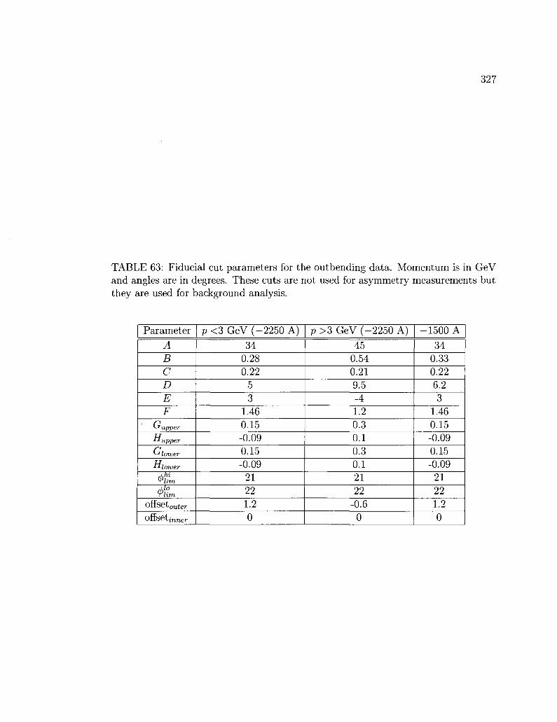
327
TABLE 63: Fiducial cut parameters for the outbending data. Momentum is in GeV and angles are in degrees. These cuts are not used for asymmetry measurements but they are used for background analysis.
Parameter
A B C D E F
L"upper
Hupper
Slower
•"lower
filim
4>Hm Onset outer
ortseLiriTier
p <3 GeV (-2250 A)
34 0.28 0.22
5 3
1.46 0.15 -0.09 0.15 -0.09
, 21 22 1.2 0
p >3 GeV (-2250 A)
45 0.54 0.21 9.5 -4 1.2 0.3 0.1 0.3 0.1 21 22
-0.6 0
-1500 A
34 0.33 0.22 6.2 3
1.46 0.15 -0.09 0.15 -0.09
21 22 1.2 0
328
A P P E N D I X C
ADDITIONAL TABLES
C.l PION AND PAIR SYMMETRIC CONTAMINATION PARAME
TERS
C.2 SYSTEMATIC ERRORS
C.3 KINEMATIC REGIONS FOR MODEL USAGE IN T\ INTEGRA
TION

329
TABLE 64: Standard IT je ratio parameters a and b in Eq. (364).
Target ND3 ND3 NH3 NH3 ND3 NH3 NH3 ND3 ND3 NH3 ND3 ND3 NH3 NH3 ND3 NH3 ND3 ND3 NH3 NH3 ND3 NH3
E 1606 1606 1606 1606 1723 1723 2286 2561 2561 2561 4238 4238 4238 4238 5615 5615 5725 5725 5725 5725 5743 5743
Torus 1500
-1500 1500
-1500 -1500 -1500 1500 1500
-1500 -1500 2250 ^2250 2250 -2250 2250 2250 2250 -2250 2250 -2250 -2250 -2250
a -14.27 ± 2.968 -11.06 ± 2.600 -17.27 ± 3.112 -11.62 ± 3.205 -11.06 ± 2.600 -11.62 ± 3.205 -4.946 ± 1.314 -5.190 ± 1.229 -4.250 ± 0.775 -4.373 ± 0.815 -4.637 ± 2.096 -4.192 ± 1.008 -5.051 ± 1.897 -4.656 ± 1.266 -3.791 ± 1.577 -4.143 ± 2.004 -2.859 ± 1.584 -4.322 ± 0.996 -3.631 ± 1.482 -4.272 ± 0.872 -4.695 ± 1.022 -4.333 ± 0.844
b 0.211 ± 0.092 0.217 ± 0.118 0.289 ± 0.092 0.270 ± 0.146 0.217 ± 0.118 0.270 ± 0.146 0.006 ± 0.042 0.022 ± 0.040 -0.009 ± 0.035 -0.003 ± 0.037 0.036 ± 0.080 0.026 ± 0.049 0.043 ± 0.073 0.045 ± 0.062 0.023 ± 0.060 0.030 ± 0.076 -0.005 ± 0.060 0.046 ± 0.047 0.017 ± 0.057 0.042 ± 0.042 0.064 ± 0.049 0.040 ± 0.040
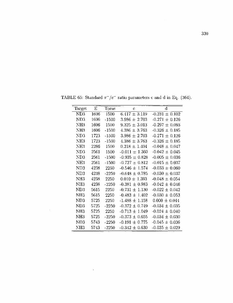
TABLE 65: Standard -K /e ratio parameters c and d in Eq. (364).
Target ND3 ND3 NH3 NH3 ND3 NH3 NH3 ND3 ND3 NH3 ND3 ND3 NH3 NH3 ND3 NH3 ND3 ND3 NH3 NH3 ND3 NH3
E 1606 1606 1606 1606 1723 1723 2286 2561 2561 2561 4238 4238 4238 4238 5615 5615 5725 5725 5725 5725 5743 5743
Torus 1500
-1500 1500
-1500 -1500 -1500 1500 1500
-1500 -1500 2250 -2250 2250 -2250 2250 2250 2250 -2250 2250 -2250 -2250 -2250
c 6.417 ± 3.119 3.986 ± 2.703 9.325 ± 3.013 4.386 ± 3.763 3.986 ± 2.703 4.386 ± 3.763 0.218 ± 1.404 -0.011 ± 1.360 -0.935 ± 0.828 -0.727 ± 0.812 -0.546 ± 1.574 -0.648 ± 0.785 0.010 ± 1.393 -0.381 ± 0.983 -0.731 ± 1.130 -0.483 ± 1.402 -1.488 ± 1.158 -0.372 ± 0.749 -0.713 ± 1.049 -0.373 ± 0.655 -0.191 ± 0.775 -0.342 ± 0.630
d -0.231 ± 0.102 -0.271 ± 0.126 -0.297 ± 0.093 -0.326 ± 0.185 -0.271 ± 0.126 -0.326 ± 0.185 -0.048 ± 0.047 -0.042 ± 0.045 -0.005 ± 0.036 -0.015 ± 0.037 -0.033 ± 0.060 -0.030 ± 0.037 -0.048 ± 0.054 -0.042 ± 0.046 -0.022 ± 0.042 -0.030 ± 0.053 0.000 ± 0.044 -0.034 ± 0.035 -0.024 ± 0.040 -0.034 ± 0.030 -0.045 ± 0.036 -0.035 ± 0.029

331
TABLE 66: Total TT /e ratio parameters a and b in Eq. (364).
Target ND3 ND3 NH3 NH3 ND3 NH3 NH3 ND3 ND3 NH3 ND3 ND3 NH3 NH3 ND3 NH3 ND3 ND3 NH3 NH3 ND3 NH3
E 1606 1606 1606 1606 1723 1723 2286 2561 2561 2561 4238 4238 4238 4238 5615 5615 5725 5725 5725 5725 5743 5743
Torus 1500
-1500 1500
-1500 -1500 -1500 1500 1500
-1500 -1500 2250 -2250 2250 -2250 2250 2250 2250 -2250 2250 -2250 -2250 -2250
a -5.851 ± 1.378 -2.563 ± 1.299 -6.057 ± 1.484 -2.703 ± 1.699 -2.563 ± 1.299 -2.703 ± 1.699 -2.423 ± 0.761 -2.675 ± 0.663 -2.728 ± 0.563 -2.628 ± 0.600 -0.394 ± 0.914 -1.112 ± 0.651 -0.584 ± 0.881 -1.204 ± 0.711 0.087 ± 0.516 -0.043 ± 0.585 0.176 ± 0.516 -0.907 ± 0.411 0.037 ± 0.510 -0.921 ± 0.404 -1.012 ± 0.427 -1.078 ± 0.414
b 0.117 ± 0.042 0.015 ± 0.065 0.118 ± 0.045 0.019 ± 0.086 0.015 ± 0.065 0.019 ± 0.086 0.043 ± 0.023 0.055 ± 0.020 0.052 ± 0.022 0.046 ± 0.023 0.039 ± 0.031 0.063 ± 0.026 0.043 ± 0.029 0.063 ± 0.029 0.016 ± 0.017 0.019 ± 0.020 0.014 ± 0.017 0.051 ± 0.016 0.018 ± 0.017 0.050 ± 0.016 0.055 ± 0.017 0.053 ± 0.016

TABLE 67: Total -K je ratio parameters c and d in Eq. (364).
Target ND3 ND3 NH3 NH3 ND3 NH3 NH3 ND3 ND3 NH3 ND3 ND3 NH3 NH3 ND3 NH3 ND3 ND3 NH3 NH3 ND3 NH3
E 1606 1606 1606 1606 1723 1723 2286 2561 2561 2561 4238 4238 4238 4238 5615 5615 5725 5725 5725 5725 5743 5743
Torus 1500 -1500 1500 -1500 -1500 -1500 1500 1500
-1500 -1500 2250 -2250 2250 -2250 2250 2250 2250 -2250 2250 -2250 -2250 -2250
c 0.692 ± 1.889 -0.334 ± 1.517 0.950 ± 2.034 -0.243 ± 1.995 -0.334 ± 1.517 -0.243 ± 1.995 -1.415 ± 0.947 -1.281 ± 0.788 -0.875 ± 0.738 -0.933 ± 0.789 -1.846 ± 0.705 -1.066 ± 0.502 -1.671 ± 0.678 -1.013 ± 0.552 -1.535 ± 0.364 -1.466 ± 0.418 -1.558 ± 0.363 -0.767 ± 0.293 -1.472 ± 0.360 -0.783 ± 0.288 -0.707 ± 0.306 -0.681 ± 0.294
d -0.106 ± 0.057 -0.088 ± 0.078 -0.110 ± 0.062 -0.092 ± 0.104 -0.088 ± 0.078 -0.092 ± 0.104 -0.026 ± 0.029 -0.025 ± 0.024 -0.039 ± 0.027 -0.037 ± 0.029 -0.014 ± 0.023 -0.041 ± 0.019 -0.019 ± 0.022 -0.044 ± 0.022 -0.001 ± 0.012 -0.004 ± 0.014 0.000 ± 0.012 -0.026 ± 0.011 -0.003 ± 0.012 -0.026 ± 0.011 -0.030 ± 0.012 -0.030 ± 0.011
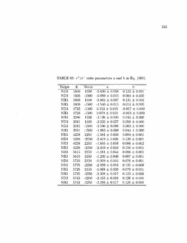
333
TABLE 68: e + / e ratio parameters a and b in Eq. (368).
Target ND3 ND3 NH3 NH3 ND3 NH3 NH3 ND3 ND3 NH3 ND3 ND3 NH3 NH3 ND3 NH3 ND3 ND3 NH3 NH3 ND3 NH3
E 1606 1606 1606 1606 1723 1723 2286 2561 2561 2561 4238 4238 4238 4238 5615 5615 5725 5725 5725 5725 5743 5743
Torus 1500
-1500 1500
-1500 -1500 -1500 1500 1500 -1500 -1500 2250 -2250 2250 -2250 2250 2250 2250 -2250 2250 -2250 -2250 -2250
a -5.630 ± 0.058 -0.959 ± 0.015 -5.962 ± 0.067 -1.540 ± 0.015 0.152 ± 0.015 0.079 ± 0.015 -2.126 ± 0.030 -2.225 ± 0.027 -2.596 ± 0.008 -1.983 ± 0.009 -1.591 ± 0.050 -2.419 ± 0.026 -1.645 ± 0.058 -2.449 ± 0.024 -1.181 ± 0.044 -1.230 ± 0.040 -0.929 ± 0.044 -2.299 ± 0.018 -1.068 ± 0.039 -2.308 ± 0.017 -2.453 ± 0.018 -2.289 ± 0.017
b 0.122 ± 0.001 0.004 ± 0.000 0.131 ± 0.002 0.014 ± 0.000 -0.017 ± 0.000 -0.015 ± 0.000 0.044 ± 0.000 0.056 ± 0.000 0.063 ± 0.000 0.044 ± 0.000 0.084 ± 0.001 0.120 ± 0.001 0.086 ± 0.002 0.118 ± 0.001 0.086 ± 0.001 0.087 ± 0.001 0.076 ± 0.001 0.125 ± 0.000 0.079 ± 0.001 0.123 ± 0.000 0.126 ± 0.000 0.128 ± 0.000

334
TABLE 69: e + / e ratio parameters c and d in Eq. (368).
Target ND3 ND3 NH3 NH3 ND3 NH3 NH3 ND3 ND3 NH3 ND3 ND3 NH3 NH3 ND3 NH3 ND3 ND3 NH3 NH3 ND3 NH3
E 1606 1606 1606 1606 1723 1723 2286 2561 2561 2561 4238 4238 4238 4238 5615 5615 5725 5725 5725 5725 5743 5743
Torus 1500
-1500 1500
-1500 -1500 -1500 1500 1500 -1500 -1500 2250 -2250 2250 -2250 2250 2250 2250 -2250 2250 -2250 -2250 -2250
c -4.707 ± 0.090 -6.743 ± 0.029 -4.221 ± 0.104 -6.397 ± 0.028 -6.663 ± 0.028 -6.564 ± 0.027 -3.952 ± 0.042 -3.538 ± 0.038 -3.269 ± 0.013 -3.908 ± 0.015 -1.899 ± 0.039 -1.190 ± 0.022 -1.885 ± 0.045 -1.208 ± 0.020 -1.079 ± 0.033 -1.025 ± 0.030 -1.169 ± 0.033 -0.415 ± 0.015 -1.097 ± 0.029 -0.434 ± 0.014 -0.417 ± 0.015 -0.438 ± 0.014
d -0.032 ± 0.002 0.016 ± 0.001 -0.046 ± 0.003 0.004 ± 0.001 0.025 ± 0.001 0.021 ± 0.001 -0.003 ± 0.001 -0.013 ± 0.001 -0.025 ± 0.000 -0.013 ± 0.000 -0.052 ± 0.001 -0.084 ± 0.001 -0.053 ± 0.001 -0.083 ± 0.000 -0.065 ± 0.001 -0.068 ± 0.001 -0.061 ± 0.001 -0.090 ± 0.000 -0.063 ± 0.001 -0.089 ± 0.000 -0.089 ± 0.000 -0.093 ± 0.000

335
TABLE 70: Systematic errors <JpSy
rscent for each Q2 bin as a percentage of statistical
errors on Ai + 77 2 for the deuteron are listed for 1 GeV data. The percentage values are calculated according to Eq. (462) and evaluated in 1.15 < W < 2.60 GeV.
Q2 bin Total Back. Dilution Radiative P6P t Model Pol. Back. 1 2 3 4 5 6 7 8 9 10 11 12 13 14 15 16 17 18 19 20 21 22 23 24 25 26
16 21 21 17 12 14 9 11 12 15 18 21 18 17 13 15 15 15 17 19 18 20 17 15 11 10
0.04
0.05
0.1 0.09
0.06
0.08
0.04
0.05
0.06
0.09
0.1 0.1 0.1 0.1 0.07
0.08
0.1 0.2 0.1 0.2 0.2 0.3 0.2 1 0.1 0.1
3 4 4 4 2 4 3 3 3 4 6 7 5 5 4 5 6 5 7 7 7 8 7 6 5 4
14 18 16 13 7 9 5 6 5 5 6 6 5 5 4 4 5 5 5 5 5 5 5 5 5 4
7 11 12 9 10 11 7 9 9 13 15 18 16 15 11 12 10 10 12 12 12 14 11 10 7 7
1 2 2 2 1 2 1 2 2 3 3 3 3 3 3 5 7 6 8 9 8 9 8 7 5 4
0
2 2 2 2 2 2 2 4 4 5 6 7 7 6 5 3 2

336
TABLE 71: Systematic errors CTsyrscent(Q2) on A\ + 77A2 for the deuteron are listed
for 2 GeV data. The percentage values are calculated according to Eq. (462) and evaluated in 1.15 < W < 2.60 GeV.
Q2bin
1 2 3 4 5 6 7 8 9 10 11 12 13 14 15 16 17 18 19 20 21 22 23 24 25 26 27 28 29 30
Total
45 20 25 25 13 12 10 15 8 7 10 9 11 13 13 14 11 13 13 13 15 16 15 18 21 22 19 16 14 7
Back.
0.9 0.5 0.7 0.8 0.5 0.5 0.4 0.7 0.4 0.3 0.5 0.5 0.6 0.8 0.6 0.7 0.4 0.5 0.4 0.4 0.6 0.6 0.6 0.7 1 1 0.8 0.7 0.5 0.2
Dilution
3 2 3 3 2 2 2 3 2 2 3 2 3 4 4 5 4 4 4 4 5 6 5 7 7 8 7 6 5 3
Radiative
44 20 24 24 12 10 7 11 5 4 5 4 5 6 4 5 4 4 3 4 4 4 4 4 4 3 3 3 3 2
PhPt
8 5 7 7 5 6 5 9 5 4 7 6 9 10 10 11 9 10 10 10 10 12 10 12 15 16 14 13 11 6
Model
5 3 4 4 2 2 2 3 2 2 3 3 3 4 4 5 4 5 5 5 7 7 7 8 9 10 8 6 5 2
Pol 1 0.7 1 1 0.7 0.8 0.8 1 0.8 0.7 1 1 1 2 2 2 2 2 3 3 4 5 6 7 7 8 7 6 4 2

337
TABLE 72: Systematic errors < ™ * ( Q 2 ) on Ax + r)A2 for the deuteron are listed for 4 GeV data. The percentage values are calculated according to Eq. (462) and evaluated in 1.15 < W < 2.60 GeV.
Q2bin
7 8 9 10 11 12 13 14 15 16 17 18 19 20 21 22 23 24 25 26 27 28 29 30 31 32 33 34 35
Total
15 11 19 11 12 13 13 9 11 15 11 9 12 13 12 16 12 18 17 19 21 23 23 23 24 20 16 13 9
Back.
0.7 0.5 0.9 0.5 0.5 0.4 0.6 0.4 0.5 0.6 0.5 0.4 0.4 0.7 0.4 0.6 0.5 0.7 0.6 0.7 0.8 0.9 0.9 0.8 0.7 0.5 0.6 0.3 0.2
Dilution
2 1 3 1 2 2 2 1 2 3 2 2 2 2 2 3 2 3 3 4 5 6 6 6 6 5 4 3 3
Radiative
11 7 10 5 4 3 3 2 2 2 2 2 2 1 2 1 2 2 2 1 2 2 1 0.9 1 0.9 0.7 0.7 0.3
PbP* 10 8 14 8 10 10 11 7 10 13 10 8 11 12 11 14 11 17 15 17 19 21 20 21 22 18 14 12 8
Model
5 4 8 4 6 6 5 4 5 6 4 3 4 5 5 5 4 6 5 7 7 7 7 6 7 5 3 2 2
Pol 0.9 0.8 1 0.8 1 1 1 0.8 1 1 1 0.9 1 2 2 2 2 3 4 4 5 5 5 5 5 4 3 2 1

338
TABLE 73: Systematic errors o-^yTscent(Q2) on A1 + riA2 for the deuteron are listed
for 5 GeV data. The percentage values are calculated according to Eq. (462) and evaluated in 1.15 < W < 2.60 GeV.
Q 2 b in 16 17 18 19 20 21 22 23 24 25 26 27 28 29 30 31 32 33 34 35 36 37
Total 13 14 23 20 23 17 20 19 24 24 25 25 25 28 27 30 30 29 29 24 21 18
Back. 0.8 0.5 3 2 2 2 1 1 2 1 1 2 1 2 2 2 2 2 1 0.9 0.6 0.3
Dilution 1 0.6 2 2 2 1 2 2 3 3 3 4 4 5 5 6 6 5 5 4 4 5
Radiative 0.9 0.4 1 0.7 0.6 0.7 0.8 0.7 0.7 0.9 1 0.9
0.8 0.6 0.5 0.4 0.5
PbPt 12 14 22 19 21 15 20 18 23 23 24 24 24 26 25 28 28 27 27 23 21 17
Model 3 2 5 5 8 6 4 3 4 4 4 4 5 6 7 6 6 5 4 3 2 2
Pol. Back. 0.6 0.4
2 3 3 4 5 5 6 6 6 6 5 4 3 1

339
TABLE 74: Systematic errors on A\ deuteron for each Q2 bin as a percentage of the statistical errors, as given in Eq. (462). The percentage values are evaluated in 1.15 < W < 2.60 GeV.
Q2 bin Total Back. Dilution Radiative PbP t Model Pol. Back. 1 2 3 4 5 6 7 8 9 10 11 12 13 14 15 16 17 18 19 20 21 22 23 24 25 26 27 28 29 30 31 32 33 34 35 36 37
26 21 22 21 13 13 11 14 13 14 16 18 20 22 25 33 43 50 55 56 51 47 45 51 53 51 39 29 25 23 26 25 27 28 24 21 18
0.4 0.3 0.4 0.5 0.3 0.3 0.4 0.5 0.4 0.4 0.5 0.4 0.6 0.7 0.5 0.7 0.4 0.3 0.3 0.3 0.4 0.7 0.5 0.7 0.8
0.8 0.6 0.3
3 3 4 4 2 3 2 3 3 3 4 3 4 4 3 4 4 4 4 4 4 4 3 4 4 4 4 4 5 5 6 5 5 5 4 4 5
25 18 19 18 9 9 7 10 7 6 6 5 5 5 4 4
- 4 3 3 3 3 3 3 3 2 2 2 2 1 1 1 1 0.8 0.6 0.5 0.4 0.5
7 9 11 9 8 9 7 9 10 10 11 12 12 12 10 11 9 7 9 9 8 9 8 10 11 12 14 16 18 19 23 23 25 26 23 21 17
3 2 3 3 2 2 2 3 5 7 9 12 15 17 22 30 41 49 54 55 50 45 44 50 51 49 36 23 16 11 8 6 5 5 3 2 2
0.9 1 1 1 0.9 1 0.8 1 1 1 2 2 2 2 2 2 2 3 3 4 3 4 4 4 4 5 5 5 5 6 6 6 6 5 4 3 1

340
TABLE 75: Systematic errors on A\ deuteron for Q2 bins, as a percentage of statistical errors, calculated according to Eq. (462). The percentage values are evaluated in three different regions: Total (1.15 < W < 2.60 GeV); Regionl (1.15 < W < 1.25 GeV); Region2 (1.25 < W < 1.80 GeV); Region3 (1.80 < W < 2.60 GeV).
Q2 bin
1 2 3 4 5 6 7 8 9 10 11 12 13 14 15 16 17 18 19 20 21 22 23 24 25 26 27 28 29 30 31 32 33 34 35 36 37
Total
26 21 22 21 13 13 11 14 13 14 16 18 20 22 25 33 43 50 55 56 51 47 45 51 53 51 39 29 25 23 26 25 27 28 24 21 18
Regionl
0.0052
0 23 7 8 11 5 6 10 24 37 50 59 63 68 89 117 130 134 135 108 84 59 46 38 26 22 18 13 13 13 12 13 11 18 9 26
Region2
18 22 21 19 12 16 10 13 13 12 14 16 16 19 25 36 50 61 71 72 69 66 67 79 82 80 59 39 30 24 22 21 18 22 24 22 17
Reg:
38 19 24 25 15 10 12 16 13 13 14 13 15 15 15 17 14 11 13 13 13 13 12 12 13 15 18 20 22 22 29 29 32 33 23 22 0.04
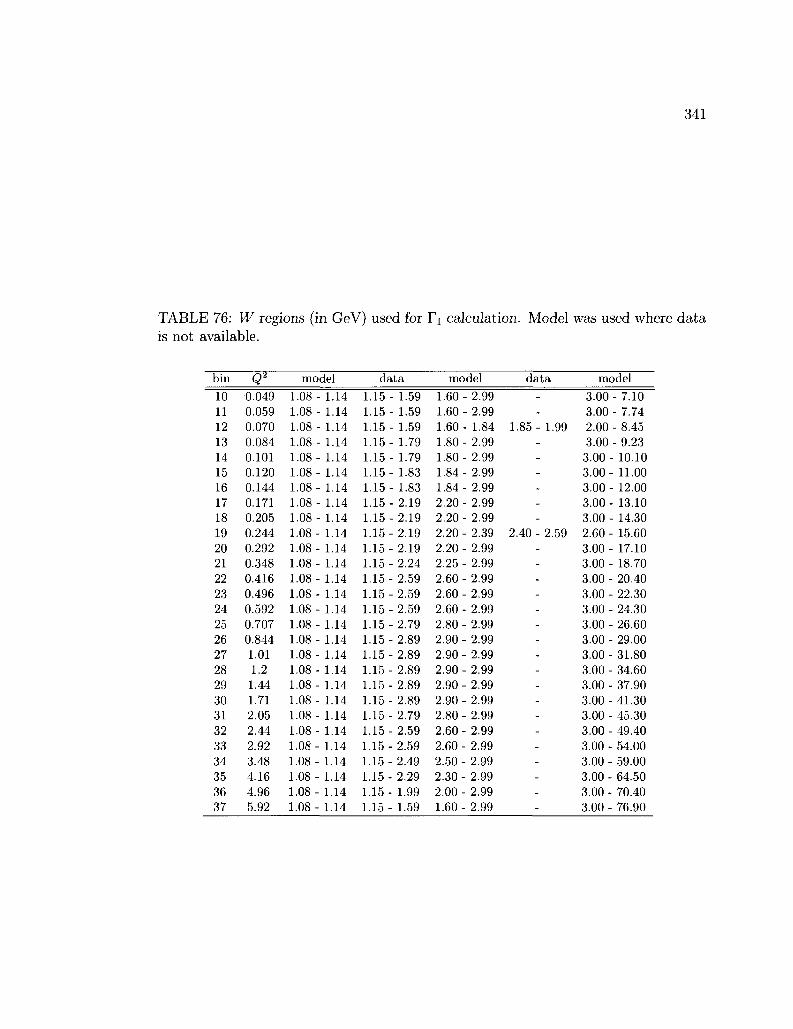
341
TABLE 76: W regions (in GeV) used for Tx calculation. Model was used where data is not available.
bin Q model data model data model 10 11 12 13 14 15 16 17 18 19 20 21 22 23 24 25 26 27 28 29 30 31 32 33 34 35 36 37
0.049 0.059 0.070 0.084 0.101 0.120 0.144 0.171 0.205 0.244 0.292 0.348 0.416 0.496 0.592 0.707 0.844 1.01 1.2 1.44 1.71 2.05 2.44 2.92 3.48 4.16 4.96 5.92
1.08 1 1 1 1 1 1 1 1 1 1 1 1 1 1 1 1 1 1 1 1 1 1 1 1 1 1 1
08 08 08 08-08-08-08-08-08-08-08-08-08-08-08-08-08-08-08-08-08-08-08-08-08-08-08-
- 1.14 - 1.14 - 1.14 - 1.14 - 1.14 1.14 1.14 1.14 1.14 1.14 1.14 1.14 1.14 1.14 1.14 1.14 1.14 1.14 1.14 1.14 1.14 1.14 1.14 1.14 1.14 1.14 1.14 1.14
1.15 1.15 1.15 1.15-1.15 1.15-1.15-1.15 -1.15-1.15-1.15-1.15-1.15-1.15-1.15-1.15-1.15-1.15-1.15-1.15-1.15-1.15-1.15 -1.15-1.15-1.15-1.15 -1.15-
- 1.59 - 1.59 - 1.59 - 1.79 1.79 1.83 1.83 2.19 2.19 2.19 2.19 2.24 2.59 2.59 2.59 2.79 2.89 2.89 2.89 2.89 2.89 2.79 2.59 2.59 2.49 2.29 1.99 1.59
1.60 1.60 1.60-1.80-1.80-1.84-1.84-2.20-2.20-2.20-2.20-2.25-2.60-2.60-2.60-2.80-2.90-2.90-2.90-2.90-2.90-2.80-2.60-2.60-2.50-2.30-2.00-1.60-
- 2.99 - 2.99 1.84 1.85 2.99 2.99 2.99 2.99 2.99 2.99 2.39 2.40 2.99 2.99 2.99 2.99 2.99 2.99 2.99 2.99 2.99 2.99 2.99 2.99 2.99 2.99 2.99 2.99 2.99 2.99
3.00 3.00
- 1.99 2.00 3.00 3.00 -3.00 -3.00 -3.00 -3.00 -
-2.59 2.60-3.00 -3.00 -3.00-3.00-3.00-3.00-3.00-3.00-3.00-3.00-3.00-3.00-3.00-3.00-3.00-3.00-3.00-3.00-
- 7.10 - 7.74 -8.45 -9.23 10.10 11.00 12.00 13.10 14.30 15.60 17.10 18.70 20.40 22.30 24.30 26.60 29.00 31.80 34.60 37.90 41.30 45.30 49.40 54.00 59.00 64.50 70.40 76.90

342
BIBLIOGRAPHY
[1] S.E. Kuhn. "Nucleon Structure Functions: Experiments and Models," Lecture
notes from HUGS (Hampton University Graduate Studies at JLab) lectures
(1997).
[2] H. Fritzsch and G. Eldahoumi, "Constituent Quarks and the Spin of the Proton,"
arXiv:hep-ph/0906.1139 (2009).
[3] R. P. Feynman, "Proceedings of the 3rd Topical Conference on High Energy
Collision of Hadrons," Stony Brook, N. Y. (1969).
[4] J. D. Bjorken and E. A. Paschos, "Inelastic Electron-Proton and 7—Proton
Scattering and the Structure of the Nucleon," Phys. Rev. 185, 1975 (1969).
[5] J. D. Bjorken, "Asymptotic Sum Rules at Infinite Momentum," Phys. Rev. 179,
1547 (1969).
[6] J.J. Aubert et al, Phys. Lett. B 123, 275 (1983).
[7] S. E. Kuhn, J. P. Chen and E. Leader, "Spin Structure of the Nucleon - Sta
tus and Recent Results," Prog. Part. Nucl. Phys. 63, 1 (2009) [arXiv:hep-
ph/0812.3535].
[8] F. Halzen and A. D. Martin, Quarks and Leptons, New York: John Wiley k.
Sons (1979).
[9] E. Leader and E. Predazzi, An introduction to gauge theories and the "new
physics", Cambridge university Press (1982).
[10] T. Pussieux and R. Windmolders, A collection of formulas for spin dependent
deep inelastic scattering, (Unpublished).
[11] J. Softer and O. V. Teryaev, hep-ph/9906455.
[12] M. Osipenko et al. [CLAS Collaboration], "The deuteron structure function F2
with CLAS", arXiv:hep-ex/0507098 (2005).
[13] C.S. Armstrong, et al, Phys. Rev. D 63 094008 (2001). [hep-ph/0104055].
[14] P. Hoodbhoy, R. L. Jaffe and A. Manohar, Nucl. Phys. B 312, 571 (1989).
343
[15] A. Airapetian et al., Phys. Rev. Lett. 95 242001 (2005) [arXiv:hep-ex/0506018]
[16] F. E. Close, An Introduction to Quarks and Partons, London: Academic Press
(1984). [ISBN 0-12-175150-3]
[17] Y. Prok, "Measurement of the Spin Structure Function gi(x, Q2) of the Proton
Measured in the Resonance Region," Ph.D. diss., University of Virginia, 2004.
[18] V. N. Gribov and L.N. Lipatov, Sov. J. Nucl. Phys. 15, 138 (1972); Y.L.
Dokahitzer, Sov. Phys. JETP. 16, 161, (1977); G. Altarelli and G. Parisi, Nucl.
Phys. B 126, 298 (1977).
[19] B. W. Filippone and X. Ji, Adv. Nucl. Phys. 26, 1 (2001).
[20] E. Leader, Spin in particle physics, Cambridge Monogr. Part. Phys. Nucl. Phys.
Cosmol. 15 (2001).
[21] W. Melnitchouk and W. Weise, arXiv:hep-ph/0006170 (2000).
[22] B. Lampe and E. Reya, "Spin physics and polarized structure functions," Phys.
Rep. 332 1 (2000).
[23] K. Wilson, Phys. Rev. 179, 1499 (1969); R. A. Brandt and G. Preparata, Nucl.
Phys. B 27, 541 (1971); O. Nachtmann, Nucl. Phys. B 63, 237 (1973).
[24] Z.E. Meziani, arXiv:hep-ph/0404066 (2004).
[25] M. Osipenko, arXiv:hep-ph/0404195 (2004).
[26] A. Deur, "Higher-twist analysis of moments of spin structure function,"
arXiv:nucl-ex/0508022 (2005).
[27] X. Ji and P. Unrau, Phys. Lett. B 333, 228 (1994).
[28] C. E. Carlson and N. C. Mukhopadhyay, Phys. Rev. D 58, 094029 (1998).
[29] J. Edelmann, G. Piller, N. Kaiser and W. Weise, Nucl. Phys. A 665, 125 (2000).
[30] A. Thomas and W. Weise, The structure of the nucleon, Wiley-VCH, Berlin
(2001).

344
[31] E.D. Bloom and F.J. Gilman, "Scaling, Duality, and the Behavior of Resonances
in Inelastic electron-Proton Scattering," Phys. Rev. Lett. 25 1140 (1970).
[32] W. Melnitchouk, R. Ent, and C. Keppel, Phys. Rep. 406, 127 (2005).
[33] F.E. Close and W. Melnitchouk, "Symmetry breaking and quark-hadron duality
in structure functions," Phys. Rev. C 68 035210 (2003).
[34] J. Blmlein and A. Tkabladze, Nucl. Phys. B 553, 427 (1999).
[35] I. Niculescu et al, Phys. Rev. Lett. 85, 1186 (2000).
[36] P.E. Bosted et al, "Quark-hadron duality in spin structure functions g{ and
gf,n Phys. Rev. C 75, 035203 (2007).
[37] T.A. Forest, GDH 2004 Proceedings, p84, World Scientific (2004).
[38] De Rujula, H. Georgi and H.D. Politzer, Ann. Phys. 103, 315 (1977).
[39] F. E. Close and N. Isgur, Phys. Lett. B 509, 81 (2001).
[40] Z. Dziembowski and J. Franklin, Nucl. Part. Phys. 17 213, (1991).
[41] David Griffiths, Introduction to Elementary Particles, New York: John Wiley &
Sons (1987).
[42] M. Anselmino, A. Efremov, E. Leader, CERN Reports TH/7216/94 (1994).
[43] P. L. Anthony et al., E142 Collaboration, Phys. Rev. D 54, 6620 (1996).
[44] B. Adeva et al., Spin Muon Collaboration, Phys. Rev. D 58, 112001 (1998).
[45] K. Abe et al, E143 Collaboration, Phys. Rev. D 58, 112003 (1998) [arXiv:hep-
ph/9802357].
[46] K. Abe et al., E154 Collaboration, Phys. Lett. B 405, 180 (1997).
[47] P. L. Anthony et al., E155 Collaboration, Phys. Lett. B 493, 19 (2000);
arXiv:hep-ex/9904002.
[48] A. Airapetian et al, HERMES Collaboration, Phys. Rev. D 75, 012007 (2007);
Phys. Lett. B 404, 383 (1997).

345
[49] V. Y. Alexakhin et al., COMPASS Collaboration, Phys. Lett. B 647, 8 (2007).
[50] K. V. Dharmawardane et al. [CLAS Collaboration], Phys. Lett. B 641, 11 (2006)
[arXiv:nucl-ex/0605028].
[51] S. L. Adler, Phys. Rev. 177, 2426 (1969).
[52] R. D. Carlitz, J. C. Collins and A. H. Mueller, Phys. Lett. B 214, 229 (1988).
[53] S.B. Gerasimov, Sov. J. of Nucl. Phys. 2, 430 (1966).
[54] S.D. Drell and A.C. Hearn, Phys. Rev. Lett. 16, 908 (1966).
[55] K. Helbing, "The Gerasimov-Drell-Hearn sum rule," Prog. Part. Nucl. Phys. 57,
405 (2006) [arXiv:nucl-ex/0603021].
[56] D. Drechsel, B. Pasquini,.and M. Vanderhaeghen, Phys. Rep. 378, 99 (2003).
[57] H. Arenhovel et al, GDH 2004 Proceedings, p294, World Scientific (2004).
[58] X. Ji and J. Osborne, J. Phys. G 27, 127 (2001) [arXiv:hep-ph/9905410].
[59] X. Ji, C. Kao, and J. Osborne, Phys. Lett. B 472, 1 (2000).
[60] V. Bernard, T.R. Hemmert, and U.G. Meisner, Phys. Lett. B 545, 105 (2002).
[61] Drechsel, D., S. S. Kamalov, and L. Tiator, Phys. Rev. D 63, 114010 (2001).
[62] M. Anselmino, B.L. Ioffe and E. Leader, Sov. J. Nucl. Phys. 49, 136 (1989).
[63] V. D. Burkert and B. L. Ioffe and E. Leader, Phys. Lett. B 296, 223 (1992).
[64] J. J. Sakurai, Currents and Mesons, University of Chicago Press, Chicago (1969).
[65] J. Soffer and O. V. Teryaev, Phys. Rev. D 51, 25 (1995); J. Soffer and O. V.
Teryaev, Phys. Rev. D 56, 7458 (1997).
[66] H. Burkhardt and W.N. Cottingham, Ann. Phys. (NY) 56, 453 (1970).
[67] J. Yun et al., Phys. Rev. C 67, 055204 (2003).
[68] R. Fatemi et al, "Measurement of the Proton Spin Structure Function gi{x,Q2)
for Q2 from 0.15 to 1.6 GeV2 with CLAS," Phys. Rev. Lett. 91, 2220022 (2003).
346
[69] O.A. Rondon, Phys. Rev. C 60, 035201 (1999).
[70] X. Zheng, GDH 2004 Proceedings, p73, World Scientific (2004); X. Zheng et al.,
Phys. Rev. Lett. 92, 012004 (2004).
[71] C. Ciofi degli Atti, L. P. Kaptari, S. Scopetta and A. Y. Umnikov, "The Neutron
Spin Structure Function from the Deuteron Data in the Resonance Region,"
Phys. Lett. B 376, 309 (1996) [arXiv:nucl-th/9601045].
[72] W. Melnitchouk, Nucl. Phys. A 631, 296C (1997) [arXiv:hep-ph/9708484].
[73] Y. Kahn, W. Melnitchouk and S. A. Kulagin, "New method for extracting neu
tron structure functions from nuclear data," Phys. Rev. C 79, 035205 (2009)
[arXiv:nucl-th/0809.4308].
[74] D. F. Geesaman, K. Saito and A.W. Thomas, Annu. Rev. Nucl. Part. Sci. 45
337 (1995).
[75] W. Bentz, I. C. Cloet and A. W. Thomas, "The polarized EMC effect," AIP
Conf. Proc. 892, 248 (2007).
[76] B. A. Mecking, et al, "The CEBAF large acceptance spectometer (CLAS),"
Nucl. Instr. Meth. A 503, 513 (2003).
[77] V. Dharmawardane, "Spin Structure Functions of the Deuteron Measured with
CLAS In and Above the Resonance Region," Ph.D. diss., Old Dominion Uni
versity (2004).
[78] M. D. Mestayer et al, Nucl. Instr. and Meth. A 449, 81 (2000).
[79] L. Qin et al, CLAS-NOTE 1996-018 JLAB (1996).
[80] E. S. Smith et al, Nucl. Instr. and Meth. A 432, 265 (1999).
[81] G. Adams et al, Nucl. Instr. and Meth. A 465, 414 (2001).
[82] M. Amarian et al, Nucl. Instr. and Meth. A 460, 239 (2001).
[83] C. D. Keith et al., "A polarized target for the CLAS detector," Nucl. Instr. and
Meth. A 501, 327 (2003).
[84] S. Stepanyan, "Simple Event Builder (SEB) in the framework of RECSIS,"

347
ht tp: / /www.j lab.org/~stepanya/seb_man.html
[85] Jefferson Lab Computing,
h t t p s : / / w i k i . j l a b . o r g / c c / e x t e r n a l / w i k i / i n d e x . p h p / S c i e n t i f i c _ C o m p u t i n g
[86] Harut Avagyan, et ai, "The CLAS Calibration Database," CLAS-NOTE 2001-
003 JLAB (2001).
[87] E.S. Smith et ai, "The time-of-fhght system for CLAS," Nucl. Instr. Meth. A
432, 265 (1999).
[88] E.S. Smith, V.Dharmawardane, et ai, "Calibration of the CLAS TOF System,"
CLAS-NOTE 1999-011 JLAB (1999). (Updated in 2001).
[89] C. Smith, EC Energy Calibration,
h t tp : / /www.j lab .org/~lcsmith/EC_Energy_Cal ibra t ion.html
[90] L.M. Qin et al, "Prototype studies and design considerations for the CLAS
Region 2 drift chambers," Nucl. Instr. Meth. A 411, 265 (1998).
[91] Dieter Cords et ai, "CLAS Event Format with BOS," CLAS-NOTE 1994-005
JLAB (1994).
[92] "HELicity Physics analysis for EGlb,"
h t t p : / /www. j l ab .o rg /~ c l a s eg l / ana l y s i s / eg l b /He lP .h t m l
[93] S. Kuhn and N. Guler, "False Asymmetry Studies for EGlb Experiment,"
CLAS-NOTE 2005-005 JLAB (2005).
[94] W.M. Yao et ai, (Particle Data Group), "The Review of Particle Physics," J.
Phys. G33, 1 (2007).
[95] Robert Fersch, "Measurement of Inclusive Proton Double-Spin Asymmetries and
Polarized Structure Functions in the CLAS EG1B Experiment," Ph.D. diss., The
College of William and Marry (2008).
[96] "Quality Checks for the EGlb 4.2 and 2.5 GeV data sets,"

348
http://www.jlab.org/Hall-B/secure/egl/EG2000/nevzat/QUALITY_CHECKS/
[97] "Quality Checks for the EGlb experiment,"
http://www.jlab.org/Hall-B/secure/egl/EG2000/fersch/QUALITY_CHECKS/
[98] M. Osipenko, A. Vlassov and M. Taiuti, "Matching between the electron can
didate track and the Cherenkov counter hit," CLAS-NOTE 2004-020 JLAB
(2004).
[99] "Geometric and Timing Cuts for EGlb,"
http://www.jlab.org/Hall-B/secure/egl/EG2000/nevzat/GE0M_CC_CUTS/
[100] A. Vlassov, "CLAS Cherekov Counter study,"
h t tp : / /www. j l ab .o rg /~v las sov /cc / index .h tml
[101] Peter Posted, S. Kuhn, Y. Prok, "Raster Corrections for EG1B," CLAS-NOTE
2003-008 JLAB (2003).
[102] M. Bellis, "Reliability and Limitations of GSIM," CLAS-NOTE 2002-016
JLAB (2002).
[103] P. Bosted and H. Avakian, "Multiple Scattering and Stray Magnetic Field
Corrections for Tracking in the Presence of Target Field," CLAS-NOTE 2006-
006 JLAB (2006). (The magnetic field correction is updated later.)
[104] H. Avakian, personal correspondence.
[105] "Hall A Absolute Beam Energy Measurements,"
h t tp : / /ha l laweb. j lab .org /equipment /beam/energy/absolu te_beam_energy.h tml
[106] Glenn F. Knoll, Radiation Detection and Measurement, New York: John Wiley
k Sons (2000).
[107] W.M. Yao et al., (Particle Data Group), "The Review of Particle Physics," J.
Phys. G33, 1 (2007).

349
[108] William R. Leo, Techniques for Nuclear and Particle Physics Experiments,
Berlin: Springer-Verlag (1994)
[109] S.E. Kuhn, A.V. Klimenko, "Momentum corrections for E6," CLAS-NOTE
2003-005 JLAB (2003).
[110] CEBAF Hall B Conceptual Design Report (1990).
[Ill] F. James, "MINUIT Function Minimization and Error Analysis Reference Man
ual," .
http://wwwasdoc.web.cern.ch/wwwasdoc/minuit/minmain.html
[112] P. Bosted and R. Fersch et al, "Ratios of 15N/12C and 4He/12C inclusive elec-
troproduction cross-sections in the nucleon resonance region," Phys. Rev. C 78
015202 (2008) [arXiv:nucl-ex/0712.2438v3].
[113] S. Kuhn, "Data Analysis for EG 1" (analysis document),
ht tp: / /www.j lab.org/Hall-B/secure/egl /AnalysisDoc/EG2000DataAnalyis .pdf
[114] D.R. Lide, ed. CRC Handbook of Chemistry and Physics, 78th Ed. Boca Raton,
FL: CRC Press (1997).
[115] Peter Posted, "Pair Symmetric and Pion Backgrounds for EG1B," CLAS-
NOTE 2004-005 JLAB (2004).
[116] J. Arrington, "Implications of the discrepancy between proton form factor mea
surements," Phys. Rev. C 69, 022201 (2004).
[117] "PbPt studies for EGlb,"
ht tp: / /www.jlab.org/Hall-B/secure/egl/EG2000/nevzat/PBPT/Comparisons
[118] K. Abe et al, Phys. Rev. D 58, 112003 (1998).
[119] T.V. Kuchto and N.M. Shumeiko, "Radiative Effects in Deep Inelastic Scatter
ing of Polarized Leptons by Polarized Nucleons," Nucl. Phys. B219, 412 (1983).
[120] L.W. Mo and Y.S. Tsai, "Radiative Corrections to Elastic and Inelastic ep and
lip Scattering," Rev. Mod. Phys. 41 , 205 (1969).

350
[121] F.R. Wesselmann, "Precision Measurement of the Spin Structure of the Proton
and the Deuteron in the." Ph.D. diss., Old Dominion University (2000).
[122] P.E. Bosted and M.E. Christy, "Empirical Fit to Inelastic Electron-Deuteron
and Electron-Neutron Resonance Region Transverse Cross Sections," Phys. Rev.
C 77, 065206 (2008).
[123] M.E. Christy and P.E. Bosted, "Empirical Fit to Precision Inclusive Electron-
Proton Cross Sections in the Resonance Region," arXiv:0712.3731 (2007).
[124] M. Arneodo et al, Phys. Lett. B 364, 107 (1995).
[125] H. Dutz et al, Phys. Rev. Lett. 91, 192001 (2003).
[126] H. Dutz et al, Phys. Rev. Lett. 94, 162001 (2005).
[127] H. Dutz et al, Phys. Rev. Lett. 93, 032003 (2004)
[128] http://wwwkph.kph.uni-mainz.de/MAID//maid2007/
129] Octavian Florin Filoti, Ph.D. diss., pages 190-194, University of New Hamp
shire (2007).
130] K. Slifer et al [Resonance Spin Structure Collaboration], "Spin Structure Mo
ments of the Proton and Deuteron," arXiv:0812.0031 [nucl-ex].
131] O. A. Rondon, AIP Conf. Proc. 842, 395 (2006).
132] http:/ /www.jlab.org/Hall-B/secure/egl/EG2000/nevzat/M0DELS/
133] Oscar A. Rondon and Karl Slifer, personal correspondence.
134] M. Amarian et al, "The Q2 Evolution of the Neutron Spin Structure Moments
using a 3He Target", Phys. Rev. Lett. 92 022301 (2004).
135] K. Slifer et al, (The Jefferson Lab E94-010 Collaboration), "He-3 Spin-
Dependent Cross Sections and Sum Rules", Phys. Rev. Lett. 101, 022303 (2008)
[arXiv:nucl-ex/0803.2267].
136] P. Solvignon et al. [Jefferson Lab E01-012 Collaboration], Phys. Rev. Lett. 101,
182502 (2008) [arXiv:nucl-ex/0803.3845].

351
[137] Patricia Solvignon, "Measurement of the 3He Spin Structure Functions in the
Resonance Region: A Test of Quark-Hadron Duality on the Neutron," Ph.D.
diss., Temple University (2006).
[138] S. A. Kulagin and W. Melnitchouk, Phys. Rev. C 77, 015210 (2008) [arXivmucl-
th/0710.1101].
[139] M. Anghinolfi et al. "The GDH Sum Rule with Nearly-Real Photons and the
Proton gi Structure Function at Low Momentum Transfer," CLAS Proposal
PR-03-006 (2003).
[140] h t t p : / / c l a s w e b . j l a b . o r g / p h y s i c s d b /
[141] K. Abe et al, "Measurements of R = aL/aT for 0.03< x <0.1 and fit to world
data." Phys. Lett. B452 194 (1999).
[142] S. Kuhn, "Model for the Asymmetry A2.n Technical note (2001).
h t tp : / /www. j lab .o rg /Hal l -B/secure /eg l /Models /A2technote .ps
[143] G. Adams et al, "CLAS detector", Preprint submitted to Elsevier Science,
July 15, (2002).
[144] R.M Gibbons, D.I Nathan, "Thermodynamic Data of Helium-3", Tech. Report
AFML-TR-67-175, Air Force Materials Laboratory, October 1967, Reproduced
by U.S. Department of Commerce.
[145] D. Lawrence, M.D. Mestayer, "CLAS Drift Chamber Calibration Procedures,"
CLAS-NOTE 1999-011 JLAB (1999).
[146] A.V. Klimenko "Electron Scattering from a High Momentum Neutron in Deu
terium," Ph.D. diss., Old Dominion University (2004)
[147] J.M. Musolf et al, Phys. Rep. 239, 1 (1994).
[148] Peter Renton, Electroweak Interactions: An Introduction to the Physics of
Quarks and Leptons Cambridge University Press, 1990.

352
VITA
Nevzat Guler
Department of Physics
Old Dominion University
Norfolk, VA 23529
EDUCATION:
• Ph.D. Physics, Old Dominion University, Norfolk, Virginia anticipated 2009,
"Spin Structure of the Deuteron and the Neutron", advised by Sebastian Kuhn.
• M.Sc. Physics, University of Texas at Arlington, Arlington, Texas, 2002, "De
velopment and Test of Silicon Microstip Detector Package for pp2pp experiment
at RHIC at BNL", advised by Kaushik De.
• B.Sc. Physics, Midle East Technical University, Ankara, Turkey, 1998, "Neu
trino Oscillations", advised by Perihan Tolun.
EXPERIENCE:
• 2002 - Present: Research Assistant, Old Dominion University, Norfolk, VA
• 2000 - 2002: User Scientist, Brookhaven National Laboratory, Upton, NY
• 1999 - 2002: Research Assistant, Univ. of Texas at Arlington, Arlington, TX
• 1999 Summer: Summer Student, CERN, Geneva, Switzerland
• 1998 - 1999: Teaching Assistant, Midle East Technical Univ., Ankara, Turkey
Typeset using LJTgX.
Related Documents