Spin states of Dirac equation and Rashba spin-orbit interaction

arX

iv:1

408.

6078

v1 [

cond

-mat

.mes

-hal

l] 2

6 A

ug 2

014

Spin states of Dirac equation

and Rashba spin-orbit interaction

A. A. Eremko,1, ∗ L. S. Brizhik,2, † and V. M. Loktev2, 3, ‡

1Bogolyubov Institute for Theoretical Physics,

Metrolohichna str., 14b, Kyiv, 03680, Ukraine

2Bogolyubov Institute for Theoretical Physics,

Kyiv, Ukraine

3National Technical University of Ukraine ”KPI”,

Kyiv, Ukraine

(Dated: August 27, 2014)

Abstract

The problem of the spin states corresponding to the solutions of Dirac equation is studied. In

particular, the three sets of the eigenfunctions of Dirac equation are obtained. In each set the

wavefunction is at the same time the eigenfunction of one of the three spin operators, which do

not commute with each other, but do commute with the Dirac Hamiltonian. This means that the

eigenfunctions of Dirac equation describe three independent spin states. The energy spectrum is

calculated for each of these sets for the case of quasi-two-dimensional electrons in a quantum well.

It is shown that the standard Rashba spin-orbit interaction takes place in one of such states only.

In another one this interaction is not formed at all, and for the third one it leads to the band

spectrum which is anisotropic in the plane domain of the propagation of a free electron and is

different from the isotropic spectrum of Rashba type.

PACS numbers: 03.65.Pm, 03.65.Ta, 73.20.At

Keywords: Dirac equation, spin states, Rashba spin-orbit interaction, quantum well, two-dimensional elec-

trons

1

INTRODUCTION

Exploiting the spin degree of freedom of charge carriers (electrons or holes) seemed im-

possible up to relatively recent times. At present it is the main aim of the new branch

of electronics, called ”spintronics” [1]. Controlling particle spin is possible because of the

spin-orbit interaction (SOI), which binds the spin and momentum of a particle in an ex-

ternal inhomogenous potential. Theoretical and experimental study of this problem is very

important, in particular, for the study of layered semiconducting heterostructures, or quan-

tum wells (QW), in which charge carriers captured by the potential of some narrow layer,

represent practically two-dimensional (2D) electron gas. In the presence of the anisotropy

determined by the applied electric field and/or special configuration of the heterostructure,

when the anisotropy is transversal to this layer, SOI removes spin the degeneracy of the 2D

conducting or valent band. This phenomenon is known as Rashba effect [2, 3].

A plane potential well is one of the mostly used models to study the properties of quasi-2D

electron gas. Nonrelativistic problem is solved for the electron propagation in the external

potential which is inhomogenous in one direction and homogenous in two other directions,

taking into account the potential relief. If the potential has the form of the well (in the

simplest case of the rectangular potential box) in the direction of inhomogenuity, electrons

are captured by this potential layer. They preserve the momentum in the plane of the layer

and fill in discrete energy levels of the spacial quantization, whose number is determined by

the depth of the potential well. In the result, such layer (interface) is characterized by the

set of the 2D electron bands. In the nonrelativistic approximation the dispersion laws of

these bands are determined by the solutions of the Schrodinger equation which contains SOI.

As it was mentioned above, SOI determines spin orientation. In the case of an asymmetric

QW, it determines Rashba dispersion law, or band splitting in the k-space depending on

spin direction.

It is well known that the existence of the electron spin is a natural consequence of the

relativistic Dirac equation (DE) [4], and that SOI in Shrodinger equation results from the

expansion of DE with respect to the degrees of 1/c [5–7]. A particle wavefunction Ψ(r) in

Dirac quantum theory is a four-component coordinate function which is represented in the

form of a matrix which contains one-column (bispinor) coordinate functions. In this theory

the operators related to the spin of a particle, are sixteen 4×4 Dirac matrices, including the

2

unit matrix. In the nonrelativistic approximation bispinor wavefunction is approximated

by a spinor one. In this case the operators of the spin projections are given by the three

Pauli matrices. Usually it is assumed that Shrodinger equation which includes SOI, takes

into account all possibilities of DE. Nevertheless, the question, how completely and exactly

nonrelativistic approximation describes the spin degree of freedom, remains open. This

problem is of special importance at present when the perspectives of exploring particle spin

in the processes of information storage and transfer, become realistic.

In the present paper we solve DE with asymmetric rectangular potential which models a

QW. Dirac equation with rectangular (step-like or box-like) potential was studied in various

papers starting with the famous paper of Klein [8]. Mostly, these papers studies 1D electron

propagation, perpendicular to the rectangular step, with the main attention to the role of

the relativistic effects [8–10] or to the role of specific potentials which capture particles. In

particular, in [11] this potential was represented in the form of a spatial dependence of a

mass of a relativistic particle, and in [12] a quaternion potential was studied.

Below we study the spin states of quasi-2D, due to the presence of a QW, electrons and

calculate their energies as functions of their 2D wave vectors. The corresponding solutions

are analyzed for the values of energies relevant to important problems of solid state physics,

and compared with the results of nonrelativistic model. For the readers convenience and

completeness of the paper we give some known results from the theory of DE.

DIRAC EQUATION

Stationary DE for a particle in the absence of the magnetic field has the form [4–6]

[

cαp+ V (r) + βmc2]

Ψ = EΨ . (1)

Here c is the speed of the light, m is the mass of a particle, p = −i~∇ is its momentum

operator, α =∑

j ejαj, αj (j = x, y, z) and β are Dirac matrices, V (r) is the external po-

tential, and Ψ(r) is a four-component coordinate function introduced above. Dirac matrices

satisfy the following conditions [5–7]

α2j = β2 = I ,

αj β + βαj = 0, (2)

αjαk + αkαj = 0 (j 6= k),

3

where I is a unit 4×4 matrix. Using Dirac matrices, it is possible to form sixteen independent

matrices which form the group in the sense that the product of any two matrices is a matrix

which belongs to this set, with the accuracy of the constant coefficient equal to ±1 or ±i(see [5, 6]). Below we write down these Hermitian conjugate Dirac matrices in the standard

representation, which we will use below:

I =

I2 0

0 I2

, ρ1 =

0 I2

I2 0

, ρ2 =

0 −iI2iI2 0

, ρ3 =

I2 0

0 −I2

,

α =

0 σ

σ 0

, Σ =

σ 0

0 σ

, (3)

Γ =

0 −iσiσ 0

, Ω =

σ 0

0 −σ

.

Here I2 is a unit 2× 2 matrix, σj (j = x, y, z) are Pauli matrices which satisfy the following

relations:

σxσy = iσz, σzσx = iσy, σyσz = iσx, σ2j = I2.

Pauli matrices are usually written in the form

σx =

0 1

1 0

, σy =

0 −ii 0

, σz =

1 0

0 −1

, (4)

where z-axis defines a chosen direction. In (3) the notations of ρj matrices are used as in

[13] with ρ3 ≡ β, as it is used in the relativistic electron theory.

The very notion of the spin degree of freedom is related to the eigen momentum of a

particle, called ’spin’. Spin is the consequence of the fact that, according to DE, in an

isotropic space an integral of motion is the total momentum

J = L+ S . (5)

Here L = r×p is the operator of the orbital momentum, and S = (~/2)Σ is the spin operator

with the projections of the vector Σ defined in (3). The square of the modulus of the spin

S2 is an integral of motion and corresponds to the eigenvalue s = 1/2. Therefore, the spin

projection ~ms on some chosen direction takes two values which correspond to the magnetic

quantum number ms = ±1/2. Nevertheless, it is impossible to relate eigen spinors to this

4

quantum number since the operator S does not commute with the Hamiltonian, and, hence,

does not have a system of eigenfunctions which is joint with it. Therefore, to define the spin

eigenstates of relativistic particles, one has to find such spin operators which commute with

the corresponding Hamiltonian.

The choice of the spin operator which determines spin eigenstates, is not unique in the

case of a free particle, since there are several operators that commute with the Hamiltonian.

One of them is the operator of the spin momentum projection parallel to the momentum or

to the direction of motion:

S‖ = Σp . (6)

Operators of vector momentum, p, and of total momentum, J, are integrals of free motion,

as well as some other vector operators, which commute with the Hamiltonian of Eq. (1):

ǫ = Ω× p , (7)

µ = Σ+Γ× p

mc, (8)

S = Ω+ ρ1p

mc. (9)

In [13] the components of the vector (7) are treated as the components of electric spin polar-

ization, of the vector (8) – as components of magnetic spin polarization, and the 3D vector

(9) together with the value (6) as the components of 4-pseudovector of spin polarization.

For a free motion of a particle one can also introduce the operator of spin polarization

s0 =pS‖ +

[

p[

Sp]]

p2.

The latter allows to describe spin projections on the arbitrary direction e · s0 where e is an

arbitrary unit vector.

Quantum well potential

Below we consider the simplest case of a 1D potential, or QW. Let us choose the direction

of z-axis along the normal to the QW plane. The potential created by such a well, depends

on one coordinate only, V (r) = V (z). In this case the state of a particle with a given value

of a 2D momentum in the xy-plane, k = (kx, ky), is described by the function

Ψk(r) = ei(kxx+kyy)Ψ (z) . (10)

5

Substituting (10) in DE (1), we can rewrite it in the form

[

−i~cαzd

dz+ ~ckα+ V (z)I +mc2β

]

Ψ (z) = EΨ (z) .

Representing the bispinor Ψ (z) in the form

Ψ (z) =

(

ψ(z)

ϕ(z)

)

, (11)

we transform Eq. (1) to the following system of equations:

−i~cσzd

dzϕ+ ~ckσϕ+

[

mc2 + V (z)]

ψ = Eψ ,

−i~cσzd

dzψ + ~ckσψ −

[

mc2 − V (z)]

ϕ = Eϕ . (12)

It is easy to see that in the case of an inhomogenous potential V (z) 6= const not all spin

operators (6)-(9) commute with the Hamiltonian. Only the following components of the

vector operators (8)-(9) are conserved:

ǫz = Ωxpy − Ωypx , (13)

µz = Σz +1

mc

(

Γxpy − Γypx

)

, (14)

Sx = Ωx + ρ1pxmc

, Sy = Ωy + ρ1pymc

. (15)

Since these operators commute with the Hamiltonian but do not commute with each other,

the system of the eigenfunctions of the Hamiltonian can be joint with one of them, only.

Therefore, the solution of Eqs. (12) can be represented in the form of the three sets of

eigen wavefunctions, with different physical meaning of the spin quantum numbers. Worth

mentioning also that since the projections Sx and Sy do not commute, the anisotropy in the

originally isotropic xy-plane automatically appears with an arbitrary axis of the anisotropy.

Eigenfunctions of the operator of the electric spin polarization projection

First, let us consider the case when the eigenfunctions of DE are also the eigenfunctions of

the operator (7). This means that we search the solution of the system of equations (12),

which is joint with the equation

ǫzΨk(r) = ǫΨk(r) .

6

Substituting in it the function (10) and taking into account Eq. (11), the explicit form of

the operator ǫz and the corresponding Dirac matrices (3), we get the equation

−~k

ΛR 0

0 −ΛR

(

ψ(z)

ϕ(z)

)

= ǫ

(

ψ(z)

ϕ(z)

)

, (16)

where according to the definition, k =√

k2x + k2y and

ΛR =

0 −ie−iφ

ieiφ 0

=

0 e−i(φ+π/2)

ei(φ+π/2) 0

, tanφ =kykx. (17)

Here the projections of the 2D wavevector are kx = k cosφ, ky = k sinφ, and the matrix ΛR,

defined as ΛR = (kxσy − kyσx)/k, determines Rashba SOI in the nonrelativistic approach

(see [1, 2]).

Let us represent the eigenvalue as ǫ = −~kσ. They can be obtained from Eq. (16) which

takes the form:

ΛRψ(z) = σψ(z) , ΛRϕ(z) = −σϕ(z) .

This means that functions ψ(z) and ϕ(z) are proportional to the eigen spinors of the matrix

ΛR, which are orthonormalized spinor

χ+ =1√2

(

e−i(φ/2+π/4)

ei(φ/2+π/4)

)

, χ− =1√2

(

e−i(φ/2+π/4)

−ei(φ/2+π/4)

)

, χ†σχσ′ = δσ,σ′ , (18)

that correspond to the eigenvalues σ = ±1, respectively, so that ΛRχ± = ±χ±. Therefore,

the bispinor Ψ (z) is characterized by the quantum number σ = ±1:

Ψσ(z) =

(

f(z)χσ

g(z)χ−σ

)

, (19)

where f(z) and g(z) are arbitrary functions. We can assign the quantum number σ to the

bispinor (19) as the quantum number that corresponds to the upper component of (19).

To find these functions, we have to substitute this bispinor into Eqs. (12), which contain

matrices σz and

kσ = kxσx + kyσy = kΛ(φ) , Λ(φ) =

0 e−iφ

eiφ 0

. (20)

Taking into account the action of these matrices on the spinors (18), namely, σzχσ = χ−σ

and Λ(φ)χσ = iσχ−σ, we see that Eqs. (12) are transformed into the system of equations

7

for functions f(z) and g(z):

−i~c(

df

dz− σkf

)

=[

E − V (z) +mc2]

g ,

−i~c(

dg

dz+ σkg

)

=[

E − V (z)−mc2]

f . (21)

Below we consider the QW of the form

V (z) =

VL and z < a,

VC and a ≤ z ≤ b,

VR and z > b,

(22)

where VL ≥ VR > VC and d = b− a is the width of the QW. In other words, we assume that

the space in z-direction is divided into three regions in each of which the potential takes

constant value Vj = const (j = L,C,R). Equations (21) in each of these regions are reduced

to a single equation for the function fj(z):

−~2c2

d2fjdz2

=[

(E − Vj)2 − ε2⊥

]

fj . (23)

Here the notation is introduced

ε⊥ =√m2c4 + ~2c2k2 . (24)

The function gj(z) is determined from the second equation in (21) at the given energy

gj(z) = −i ~c

E − Vj +mc2(

f ′j − σkfj

)

. (25)

Here and below the prime means z-derivative of the corresponding function.

Eigenfunctions of the operator of magnetic spin polarization projection

Let us now find solutions of the system (12), which are joint with the equation

µzΨk(r) = µΨk(r) .

Substituting function (10) into the latter equation and taking into account Eq. (11), the

explicit form of the operator µz (8) and the corresponding Dirac matrices, we obtain the

equation

σz i ~kmc

ΛR

−i ~kmc

ΛR σz

(

ψ(z)

ϕ(z)

)

= µ

(

ψ(z)

ϕ(z)

)

, (26)

8

where matrix ΛR is defined in (17).

To solve Eq. (26), let us chose the spinors ψ(z) and ϕ(z) in the form

ψ(z) =

(

e−iφ/2ψ1(z)

eiφ/2ψ2(z)

)

, ϕ(z) =

(

e−iφ/2ϕ1(z)

eiφ/2ϕ2(z)

)

(27)

and rewrite Eq. (26) as follows:

(µ− 1)ψ1(z)−~k

mcϕ2(z) = 0 ,

− ~k

mcψ1(z) + (µ+ 1)ϕ2(z) = 0 ,

(µ+ 1)ψ2(z) +~k

mcϕ1(z) = 0 ,

~k

mcψ2(z) + (µ− 1)ϕ1(z) = 0 .

From above we find the eigenvalues µ = ±µ0, µ0 =√

1 + (~k/mc)2. The corresponding

solutions can be represented as:

ψ2(z) = −λϕ1(z), ϕ2(z) = λψ1(z), (28)

at µ = µ0, and as

ψ1(z) = −λϕ2(z), ϕ1(z) = λψ2(z), (29)

at µ = −µ0, with two arbitrary functions for every value of µ. Namely, ψ1 and ϕ1 at µ = µ0,

and ψ2 and ϕ2 at µ = −µ0. The coefficient λ in these relations is defined as

λ =~k

mc (µ0 + 1)=

~ck

ε⊥ +mc2, (30)

where ε⊥ is defined in (24). Therefore, the spinors incoming into the bispinor with the given

spin quantum number µ = ±µ0, take the final form

ψ+(z) =

(

e−iφ/2ψ(z)

−eiφ/2λϕ(z)

)

, ϕ+(z) =

(

e−iφ/2ϕ(z)

eiφ/2λψ(z)

)

, (31)

ψ−(z) =

(−e−iφ/2λϕ

eiφ/2ψ(z)

)

, ϕ−(z) =

(

e−iφ/2λψ(z)

eiφ/2ϕ

)

. (32)

Substituting the above expressions for the spinors (31) or (32) into (12), we derive four

equations for the two unknown functions ψ(z) and ϕ(z). Let us introduce the spin quantum

number σ, which takes two values σ = ±1 and which defines the eigenvalues of the magnetic

9

spin polarization (14): µ = σµ0. Then four equations (12) can be written in the form

i~cσdϕ

dz= ~ckλψ −

(

E − V −mc2)

ψ ,

i~cσλdϕ

dz= ~ckψ −

(

E − V +mc2)

λψ ,

i~cσdψ

dz= −~ckλϕ−

(

E − V +mc2)

ϕ ,

i~cσλdψ

dz= −~ckϕ−

(

E − V −mc2)

λϕ .

Multiplying the first equation by λ and extracting from it the second equation, we get the

identity 0 = 0. Similarly, multiplying the third equation by λ and extracting from it the

fourth one, we again get the same identity. Therefore, we have two equations for the two

unknown functions. Let us rewrite them by adding the second equation with the first one,

multiplied by λ, and, respectively, the fourth with the third one multiplied also by λ. In the

result we have

−i~cσdψdz

= [E − V (z) + ε⊥]ϕ ,

−i~cσdϕdz

= [E − V (z)− ε⊥]ψ . (33)

where the definition (30) is used.

In the case of a rectangular QW (22), Eqs. (33) in each region are reduced to the same

equation (23) for function ψj(z) (j = L,C,R). The function ϕj(z) corresponding to the

solution, has the form

ϕj(z) = −i ~cσ

E − Vj + ε⊥ψ′j , (34)

which is different from (25).

Eigenfunctions of the operator of the spin polarization projection S

As it was mentioned above, in the given configuration of the potential V (z), the pro-

jections of this operator in the xy-plane are conserved. Since the operators of these pro-

jections do not commute between themselves, the Hamiltonian can have the joint system

of eigenfunctions, generally speaking, with any component of the operator S, with arbi-

trary direction in xy-plane. In the general case this direction can be defined by a unit vector

e0 = ex cos φ0+ey sin φ0. This means that we have to find the eigenfunctions of the following

10

operator:

Se0≡ S0 = e0S = Ωx cos φ0 + Ωy sin φ0 + ~ρ1

kx cosφ0 + ky sin φ0

mc. (35)

Here matrices Ωj and ρ1 are defined in (3). Acting by the operator (35) on function (10) and

taking into account (11) and explicit form of Dirac matrices, gives us the following equation

Λ(φ0)~k0mcI2

~k0mcI2 −Λ(φ0)

(

ψ(z)

ϕ(z)

)

= s

(

ψ(z)

ϕ(z)

)

. (36)

Here the operator Λ(φ0) is defined in (20) at φ = φ0, and, therefore, it has the following

explicit form Λ(φ0) = cosφ0σx + σy sinφ0. Let us represent the vector k using parallel

and orthogonal components of the vector e0: k = k0e0 + k⊥e⊥, where e⊥ = e0 × ez =

ex sinφ0 − ey cosφ0:

k0 = kx cosφ0 + ky sinφ0 , k⊥ = kx sinφ0 − ky cosφ0. (37)

To solve Eq. (36), let us write the spinors ψ(z) and ϕ(z) in the form, similar to Eq. (27):

ψ(z) =

(

e−iφ0/2ψ1(z)

eiφ0/2ψ2(z)

)

, ϕ(z) =

(

e−iφ0/2ϕ1(z)

eiφ0/2ϕ2(z)

)

. (38)

In the result, we derive the system of equations

sψ1(z)−~k0mc

ϕ1(z) = ψ2(z) ,

sψ2(z)−~k0mc

ϕ2(z) = ψ1(z) ,

sϕ1(z)−~k0mc

ψ1(z) = −ϕ2(z) ,

sϕ2(z)−~k0mc

ψ2(z) = −ϕ1 .

Similarly to above, adding and extracting the first two equations, and repeating this proce-

dure for the last ones, we obtain the system which is more convenient for analysis:

(s− 1) (ψ1 + ψ2)−~k0mc

(ϕ1 + ϕ2) = 0 ,

−~k0mc

(ψ1 + ψ2) + (s + 1) (ϕ1 + ϕ2) = 0 ,

(s+ 1) (ψ1 − ψ2)−~k0mc

(ϕ1 − ϕ2) = 0 ,

−~k0mc

(ψ1 − ψ1) + (s− 1) (ϕ1 − ϕ2) = 0 .

11

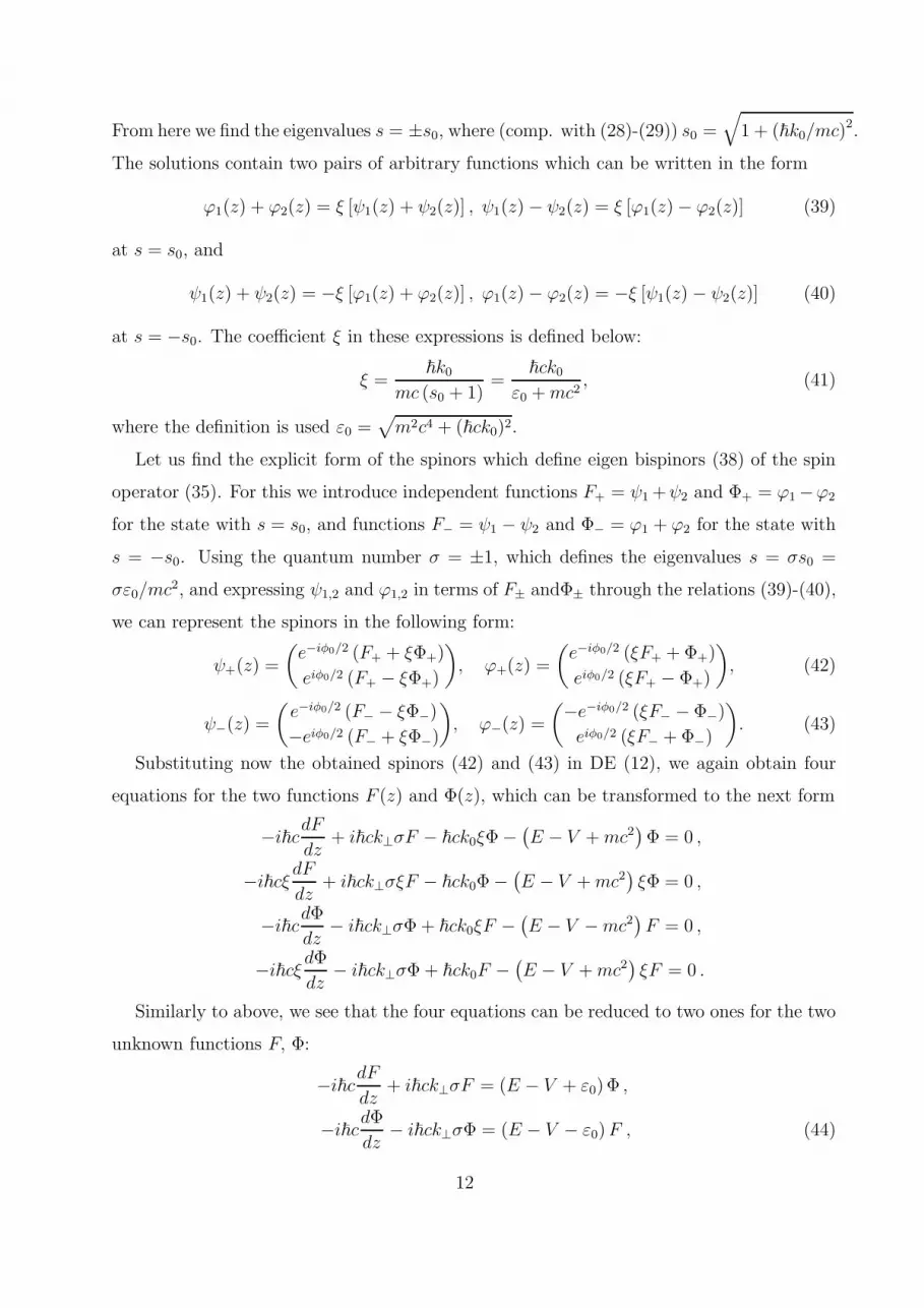
From here we find the eigenvalues s = ±s0, where (comp. with (28)-(29)) s0 =√

1 + (~k0/mc)2.

The solutions contain two pairs of arbitrary functions which can be written in the form

ϕ1(z) + ϕ2(z) = ξ [ψ1(z) + ψ2(z)] , ψ1(z)− ψ2(z) = ξ [ϕ1(z)− ϕ2(z)] (39)

at s = s0, and

ψ1(z) + ψ2(z) = −ξ [ϕ1(z) + ϕ2(z)] , ϕ1(z)− ϕ2(z) = −ξ [ψ1(z)− ψ2(z)] (40)

at s = −s0. The coefficient ξ in these expressions is defined below:

ξ =~k0

mc (s0 + 1)=

~ck0ε0 +mc2

, (41)

where the definition is used ε0 =√

m2c4 + (~ck0)2.

Let us find the explicit form of the spinors which define eigen bispinors (38) of the spin

operator (35). For this we introduce independent functions F+ = ψ1+ψ2 and Φ+ = ϕ1−ϕ2

for the state with s = s0, and functions F− = ψ1 − ψ2 and Φ− = ϕ1 + ϕ2 for the state with

s = −s0. Using the quantum number σ = ±1, which defines the eigenvalues s = σs0 =

σε0/mc2, and expressing ψ1,2 and ϕ1,2 in terms of F± andΦ± through the relations (39)-(40),

we can represent the spinors in the following form:

ψ+(z) =

(

e−iφ0/2 (F+ + ξΦ+)

eiφ0/2 (F+ − ξΦ+)

)

, ϕ+(z) =

(

e−iφ0/2 (ξF+ + Φ+)

eiφ0/2 (ξF+ − Φ+)

)

, (42)

ψ−(z) =

(

e−iφ0/2 (F− − ξΦ−)

−eiφ0/2 (F− + ξΦ−)

)

, ϕ−(z) =

(−e−iφ0/2 (ξF− − Φ−)

eiφ0/2 (ξF− + Φ−)

)

. (43)

Substituting now the obtained spinors (42) and (43) in DE (12), we again obtain four

equations for the two functions F (z) and Φ(z), which can be transformed to the next form

−i~cdFdz

+ i~ck⊥σF − ~ck0ξΦ−(

E − V +mc2)

Φ = 0 ,

−i~cξ dFdz

+ i~ck⊥σξF − ~ck0Φ−(

E − V +mc2)

ξΦ = 0 ,

−i~cdΦdz

− i~ck⊥σΦ+ ~ck0ξF −(

E − V −mc2)

F = 0 ,

−i~cξ dΦdz

− i~ck⊥σΦ + ~ck0F −(

E − V +mc2)

ξF = 0 .

Similarly to above, we see that the four equations can be reduced to two ones for the two

unknown functions F, Φ:

−i~cdFdz

+ i~ck⊥σF = (E − V + ε0)Φ ,

−i~cdΦdz

− i~ck⊥σΦ = (E − V − ε0)F , (44)

12

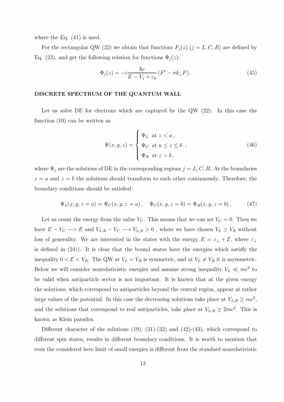
where the Eq. (41) is used.

For the rectangular QW (22) we obtain that functions Fj(z) (j = L,C,R) are defined by

Eq. (23), and get the following relation for functions Φj(z):

Φj(z) = −i ~c

E − Vj + ε0(F ′ − σk⊥F ) . (45)

DISCRETE SPECTRUM OF THE QUANTUM WALL

Let us solve DE for electrons which are captured by the QW (22). In this case the

function (10) can be written as

Ψ(x, y, z) =

ΨL at z < a ,

ΨC at a ≤ z ≤ b

ΨR at z > b ,

, (46)

where Ψj are the solutions of DE in the corresponding regions j = L,C,R. At the boundaries

z = a and z = b the solutions should transform to each other continuously. Therefore, the

boundary conditions should be satisfied:

ΨL(x, y, z = a) = ΨC(x, y, z = a) , ΨC(x, y, z = b) = ΨR(x, y, z = b) . (47)

Let us count the energy from the value VC . This means that we can set VC = 0. Then we

have E − VC −→ E and VL,R − VC −→ VL,R > 0 , where we have chosen VL ≥ VR without

loss of generality. We are interested in the states with the energy E = ε⊥ + E , where ε⊥is defined in (24)). It is clear that the bound states have the energies which satisfy the

inequality 0 < E < VR. The QW at VL = VR is symmetric, and at VL 6= VR it is asymmetric.

Below we will consider nonrelativistic energies and assume strong inequality VL ≪ mc2 to

be valid when antiparticle sector is not important. It is known that at the given energy

the solutions, which correspond to antiparticles beyond the central region, appear at rather

large values of the potential. In this case the decreasing solutions take place at VL,R ≥ mc2,

and the solutions that correspond to real antiparticles, take place at VL,R ≥ 2mc2. This is

known as Klein paradox.

Different character of the solutions (19), (31)-(32) and (42)-(43), which correspond to

different spin states, results in different boundary conditions. It is worth to mention that

even the considered here limit of small energies is different from the standard nonrelativistic

13

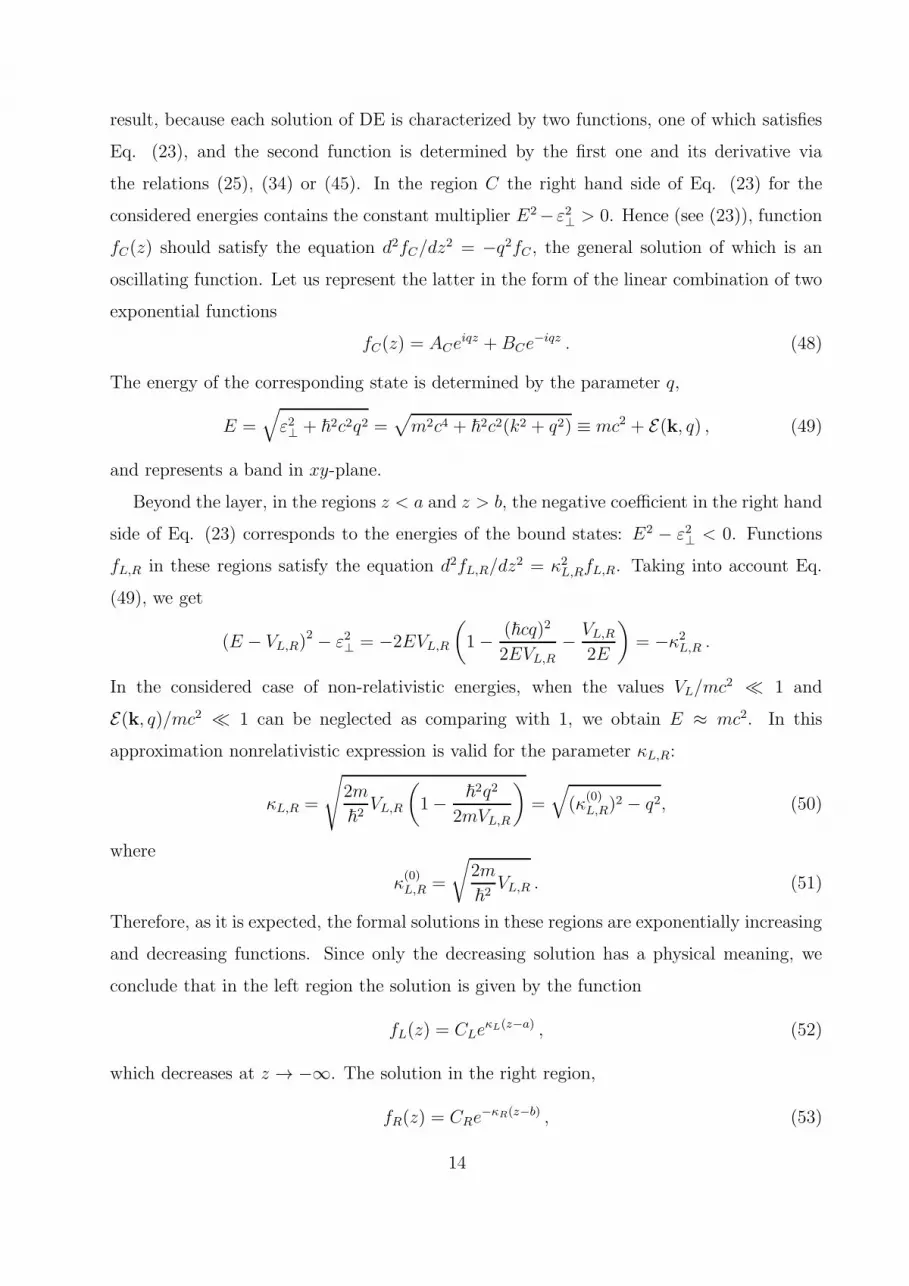
result, because each solution of DE is characterized by two functions, one of which satisfies

Eq. (23), and the second function is determined by the first one and its derivative via

the relations (25), (34) or (45). In the region C the right hand side of Eq. (23) for the

considered energies contains the constant multiplier E2−ε2⊥ > 0. Hence (see (23)), function

fC(z) should satisfy the equation d2fC/dz2 = −q2fC , the general solution of which is an

oscillating function. Let us represent the latter in the form of the linear combination of two

exponential functions

fC(z) = ACeiqz +BCe

−iqz . (48)

The energy of the corresponding state is determined by the parameter q,

E =√

ε2⊥ + ~2c2q2 =√

m2c4 + ~2c2(k2 + q2) ≡ mc2 + E(k, q) , (49)

and represents a band in xy-plane.

Beyond the layer, in the regions z < a and z > b, the negative coefficient in the right hand

side of Eq. (23) corresponds to the energies of the bound states: E2 − ε2⊥ < 0. Functions

fL,R in these regions satisfy the equation d2fL,R/dz2 = κ2L,RfL,R. Taking into account Eq.

(49), we get

(E − VL,R)2 − ε2⊥ = −2EVL,R

(

1− (~cq)2

2EVL,R− VL,R

2E

)

= −κ2L,R .

In the considered case of non-relativistic energies, when the values VL/mc2 ≪ 1 and

E(k, q)/mc2 ≪ 1 can be neglected as comparing with 1, we obtain E ≈ mc2. In this

approximation nonrelativistic expression is valid for the parameter κL,R:

κL,R =

√

2m

~2VL,R

(

1− ~2q2

2mVL,R

)

=

√

(κ(0)L,R)

2 − q2, (50)

where

κ(0)L,R =

√

2m

~2VL,R . (51)

Therefore, as it is expected, the formal solutions in these regions are exponentially increasing

and decreasing functions. Since only the decreasing solution has a physical meaning, we

conclude that in the left region the solution is given by the function

fL(z) = CLeκL(z−a) , (52)

which decreases at z → −∞. The solution in the right region,

fR(z) = CRe−κR(z−b) , (53)

14

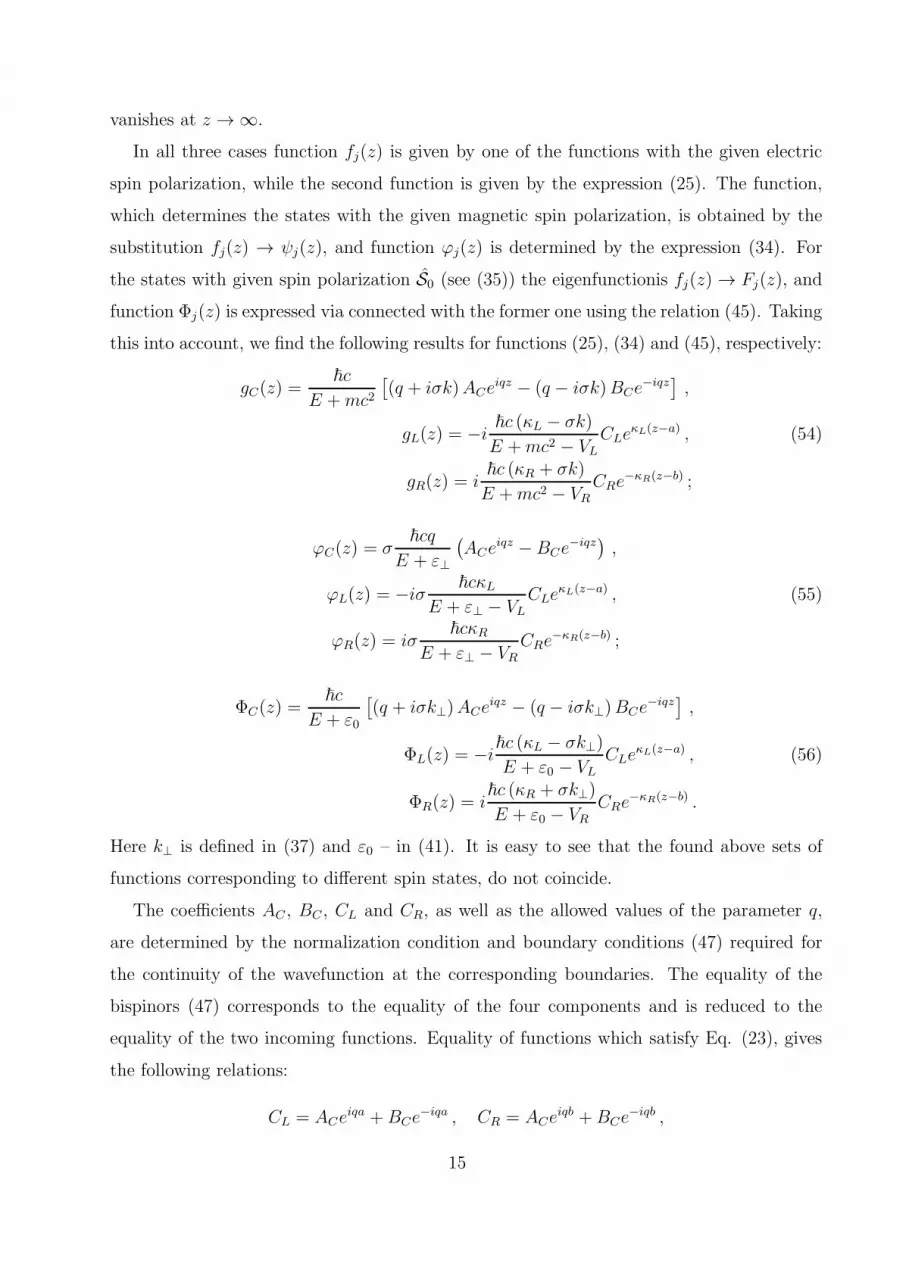
vanishes at z → ∞.

In all three cases function fj(z) is given by one of the functions with the given electric

spin polarization, while the second function is given by the expression (25). The function,

which determines the states with the given magnetic spin polarization, is obtained by the

substitution fj(z) → ψj(z), and function ϕj(z) is determined by the expression (34). For

the states with given spin polarization S0 (see (35)) the eigenfunctionis fj(z) → Fj(z), and

function Φj(z) is expressed via connected with the former one using the relation (45). Taking

this into account, we find the following results for functions (25), (34) and (45), respectively:

gC(z) =~c

E +mc2[

(q + iσk)ACeiqz − (q − iσk)BCe

−iqz]

,

gL(z) = −i ~c (κL − σk)

E +mc2 − VLCLe

κL(z−a) , (54)

gR(z) = i~c (κR + σk)

E +mc2 − VRCRe

−κR(z−b) ;

ϕC(z) = σ~cq

E + ε⊥

(

ACeiqz −BCe

−iqz)

,

ϕL(z) = −iσ ~cκLE + ε⊥ − VL

CLeκL(z−a) , (55)

ϕR(z) = iσ~cκR

E + ε⊥ − VRCRe

−κR(z−b) ;

ΦC(z) =~c

E + ε0

[

(q + iσk⊥)ACeiqz − (q − iσk⊥)BCe

−iqz]

,

ΦL(z) = −i~c (κL − σk⊥)

E + ε0 − VLCLe

κL(z−a) , (56)

ΦR(z) = i~c (κR + σk⊥)

E + ε0 − VRCRe

−κR(z−b) .

Here k⊥ is defined in (37) and ε0 – in (41). It is easy to see that the found above sets of

functions corresponding to different spin states, do not coincide.

The coefficients AC , BC , CL and CR, as well as the allowed values of the parameter q,

are determined by the normalization condition and boundary conditions (47) required for

the continuity of the wavefunction at the corresponding boundaries. The equality of the

bispinors (47) corresponds to the equality of the four components and is reduced to the

equality of the two incoming functions. Equality of functions which satisfy Eq. (23), gives

the following relations:

CL = ACeiqa +BCe

−iqa , CR = ACeiqb +BCe

−iqb ,

15

from which we can express the coefficients CL and CR via the coefficients AC and BC .

Substituting this result into the condition of the equality of functions (54), (55) or (56), we

get the system of two homogenous equations for the coefficients AC and BC :

F ∗Le

iqaAC + FLe−iqaBC = 0 ,

FReiqbAC + F ∗

Re−iqbBC = 0 . (57)

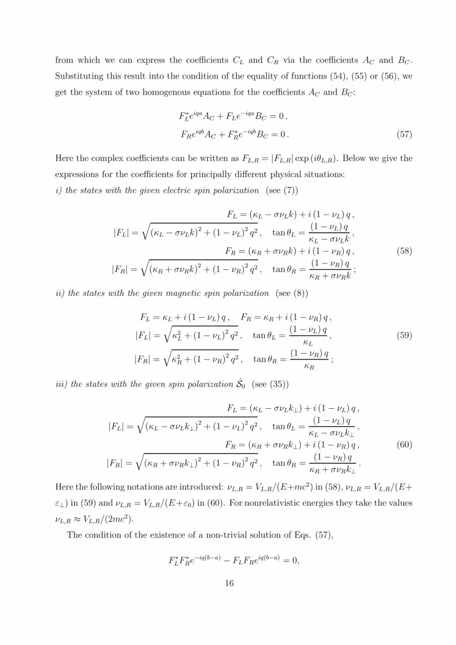
Here the complex coefficients can be written as FL,R = |FL,R| exp (iθL,R). Below we give the

expressions for the coefficients for principally different physical situations:

i) the states with the given electric spin polarization (see (7))

FL = (κL − σνLk) + i (1− νL) q ,

|FL| =√

(κL − σνLk)2 + (1− νL)

2 q2 , tan θL =(1− νL) q

κL − σνLk,

FR = (κR + σνRk) + i (1− νR) q , (58)

|FR| =√

(κR + σνRk)2 + (1− νR)

2 q2 , tan θR =(1− νR) q

κR + σνRk;

ii) the states with the given magnetic spin polarization (see (8))

FL = κL + i (1− νL) q , FR = κR + i (1− νR) q ,

|FL| =√

κ2L + (1− νL)2 q2 , tan θL =

(1− νL) q

κL, (59)

|FR| =√

κ2R + (1− νR)2 q2 , tan θR =

(1− νR) q

κR;

iii) the states with the given spin polarization S0 (see (35))

FL = (κL − σνLk⊥) + i (1− νL) q ,

|FL| =√

(κL − σνLk⊥)2 + (1− νL)

2 q2 , tan θL =(1− νL) q

κL − σνLk⊥,

FR = (κR + σνRk⊥) + i (1− νR) q , (60)

|FR| =√

(κR + σνRk⊥)2 + (1− νR)

2 q2 , tan θR =(1− νR) q

κR + σνRk⊥.

Here the following notations are introduced: νL,R = VL,R/(E+mc2) in (58), νL,R = VL,R/(E+

ε⊥) in (59) and νL,R = VL,R/(E+ε0) in (60). For nonrelativistic energies they take the values

νL,R ≈ VL,R/(2mc2).

The condition of the existence of a non-trivial solution of Eqs. (57),

F ∗LF

∗Re

−iq(b−a) − FLFReiq(b−a) = 0,

16

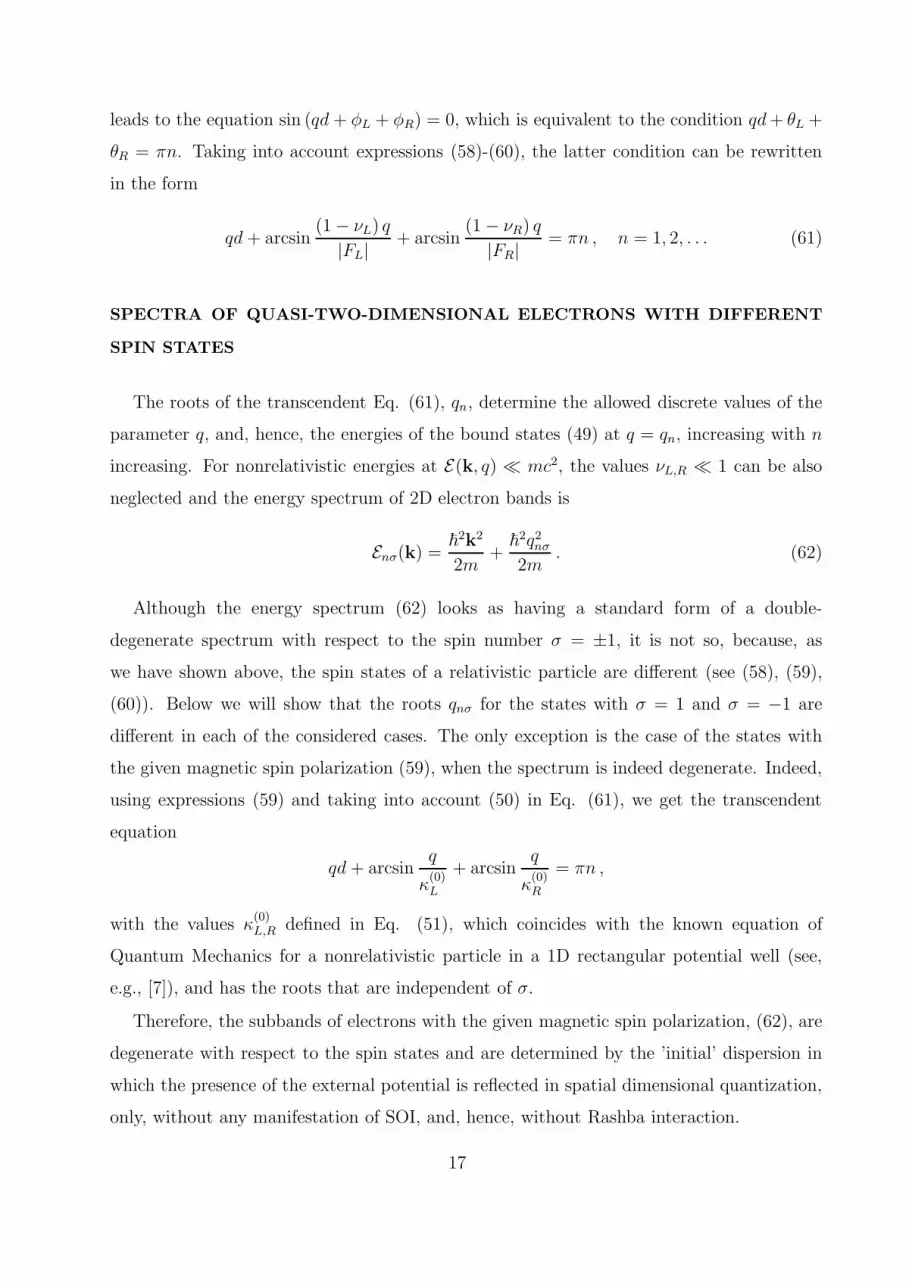
leads to the equation sin (qd+ φL + φR) = 0, which is equivalent to the condition qd+ θL +

θR = πn. Taking into account expressions (58)-(60), the latter condition can be rewritten

in the form

qd+ arcsin(1− νL) q

|FL|+ arcsin

(1− νR) q

|FR|= πn , n = 1, 2, . . . (61)

SPECTRA OF QUASI-TWO-DIMENSIONAL ELECTRONS WITH DIFFERENT

SPIN STATES

The roots of the transcendent Eq. (61), qn, determine the allowed discrete values of the

parameter q, and, hence, the energies of the bound states (49) at q = qn, increasing with n

increasing. For nonrelativistic energies at E(k, q) ≪ mc2, the values νL,R ≪ 1 can be also

neglected and the energy spectrum of 2D electron bands is

Enσ(k) =~2k2

2m+

~2q2nσ2m

. (62)

Although the energy spectrum (62) looks as having a standard form of a double-

degenerate spectrum with respect to the spin number σ = ±1, it is not so, because, as

we have shown above, the spin states of a relativistic particle are different (see (58), (59),

(60)). Below we will show that the roots qnσ for the states with σ = 1 and σ = −1 are

different in each of the considered cases. The only exception is the case of the states with

the given magnetic spin polarization (59), when the spectrum is indeed degenerate. Indeed,

using expressions (59) and taking into account (50) in Eq. (61), we get the transcendent

equation

qd+ arcsinq

κ(0)L

+ arcsinq

κ(0)R

= πn ,

with the values κ(0)L,R defined in Eq. (51), which coincides with the known equation of

Quantum Mechanics for a nonrelativistic particle in a 1D rectangular potential well (see,

e.g., [7]), and has the roots that are independent of σ.

Therefore, the subbands of electrons with the given magnetic spin polarization, (62), are

degenerate with respect to the spin states and are determined by the ’initial’ dispersion in

which the presence of the external potential is reflected in spatial dimensional quantization,

only, without any manifestation of SOI, and, hence, without Rashba interaction.

17

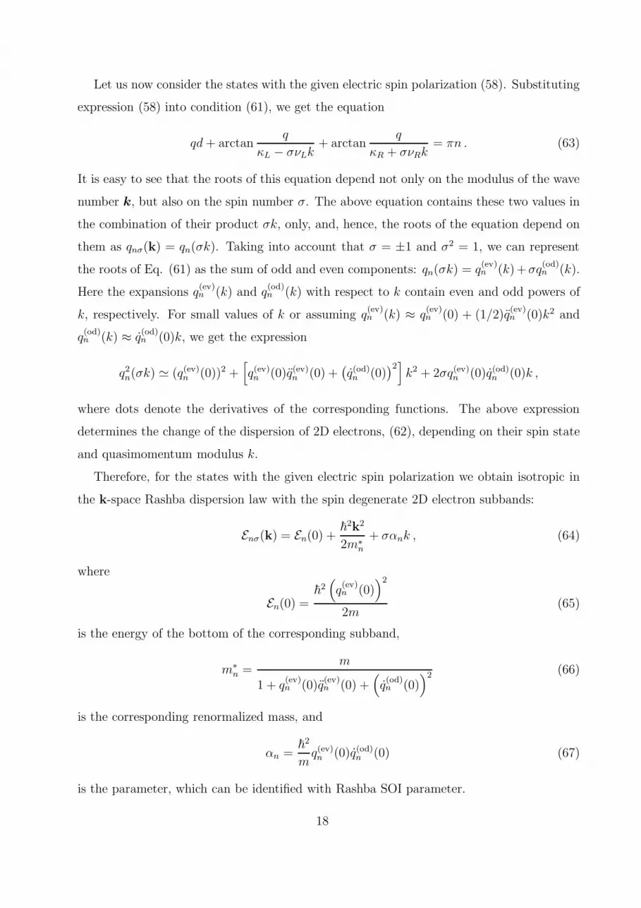
Let us now consider the states with the given electric spin polarization (58). Substituting

expression (58) into condition (61), we get the equation

qd+ arctanq

κL − σνLk+ arctan

q

κR + σνRk= πn . (63)

It is easy to see that the roots of this equation depend not only on the modulus of the wave

number k, but also on the spin number σ. The above equation contains these two values in

the combination of their product σk, only, and, hence, the roots of the equation depend on

them as qnσ(k) = qn(σk). Taking into account that σ = ±1 and σ2 = 1, we can represent

the roots of Eq. (61) as the sum of odd and even components: qn(σk) = q(ev)n (k)+σq

(od)n (k).

Here the expansions q(ev)n (k) and q

(od)n (k) with respect to k contain even and odd powers of

k, respectively. For small values of k or assuming q(ev)n (k) ≈ q

(ev)n (0) + (1/2)q

(ev)n (0)k2 and

q(od)n (k) ≈ q

(od)n (0)k, we get the expression

q2n(σk) ≃ (q(ev)n (0))2 +[

q(ev)n (0)q(ev)n (0) +(

q(od)n (0))2]

k2 + 2σq(ev)n (0)q(od)n (0)k ,

where dots denote the derivatives of the corresponding functions. The above expression

determines the change of the dispersion of 2D electrons, (62), depending on their spin state

and quasimomentum modulus k.

Therefore, for the states with the given electric spin polarization we obtain isotropic in

the k-space Rashba dispersion law with the spin degenerate 2D electron subbands:

Enσ(k) = En(0) +~2k2

2m∗n

+ σαnk , (64)

where

En(0) =~2(

q(ev)n (0)

)2

2m(65)

is the energy of the bottom of the corresponding subband,

m∗n =

m

1 + q(ev)n (0)q

(ev)n (0) +

(

q(od)n (0)

)2 (66)

is the corresponding renormalized mass, and

αn =~2

mq(ev)n (0)q(od)n (0) (67)

is the parameter, which can be identified with Rashba SOI parameter.

18

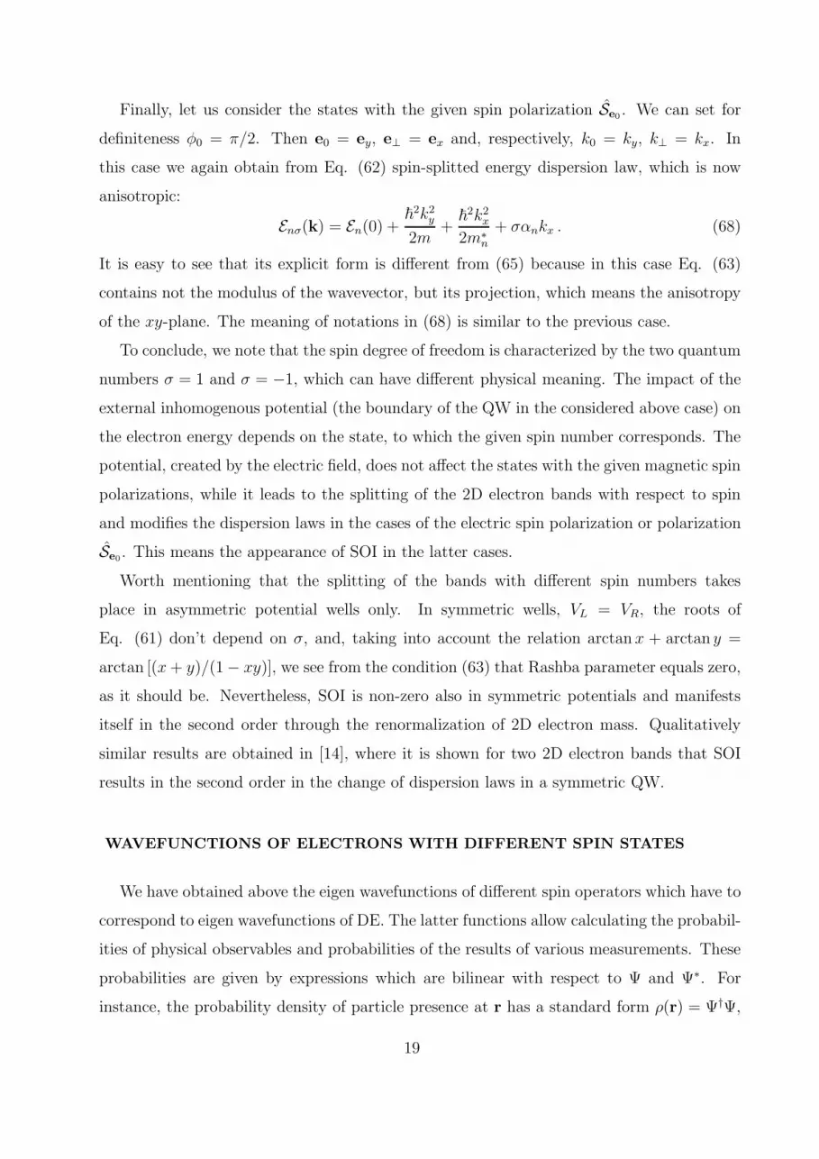
Finally, let us consider the states with the given spin polarization Se0. We can set for

definiteness φ0 = π/2. Then e0 = ey, e⊥ = ex and, respectively, k0 = ky, k⊥ = kx. In

this case we again obtain from Eq. (62) spin-splitted energy dispersion law, which is now

anisotropic:

Enσ(k) = En(0) +~2k2y2m

+~2k2x

2m∗n

+ σαnkx . (68)

It is easy to see that its explicit form is different from (65) because in this case Eq. (63)

contains not the modulus of the wavevector, but its projection, which means the anisotropy

of the xy-plane. The meaning of notations in (68) is similar to the previous case.

To conclude, we note that the spin degree of freedom is characterized by the two quantum

numbers σ = 1 and σ = −1, which can have different physical meaning. The impact of the

external inhomogenous potential (the boundary of the QW in the considered above case) on

the electron energy depends on the state, to which the given spin number corresponds. The

potential, created by the electric field, does not affect the states with the given magnetic spin

polarizations, while it leads to the splitting of the 2D electron bands with respect to spin

and modifies the dispersion laws in the cases of the electric spin polarization or polarization

Se0. This means the appearance of SOI in the latter cases.

Worth mentioning that the splitting of the bands with different spin numbers takes

place in asymmetric potential wells only. In symmetric wells, VL = VR, the roots of

Eq. (61) don’t depend on σ, and, taking into account the relation arctan x + arctan y =

arctan [(x+ y)/(1− xy)], we see from the condition (63) that Rashba parameter equals zero,

as it should be. Nevertheless, SOI is non-zero also in symmetric potentials and manifests

itself in the second order through the renormalization of 2D electron mass. Qualitatively

similar results are obtained in [14], where it is shown for two 2D electron bands that SOI

results in the second order in the change of dispersion laws in a symmetric QW.

WAVEFUNCTIONS OF ELECTRONS WITH DIFFERENT SPIN STATES

We have obtained above the eigen wavefunctions of different spin operators which have to

correspond to eigen wavefunctions of DE. The latter functions allow calculating the probabil-

ities of physical observables and probabilities of the results of various measurements. These

probabilities are given by expressions which are bilinear with respect to Ψ and Ψ∗. For

instance, the probability density of particle presence at r has a standard form ρ(r) = Ψ†Ψ,

19

the current density probability is j = cΨ†αΨ, the probability density of the eigen spin mo-

mentum which is proportional to the vector, is S = Ψ†ΣΨ, and so on. To calculate these

values, we find below the explicit form of the wavefunctions.

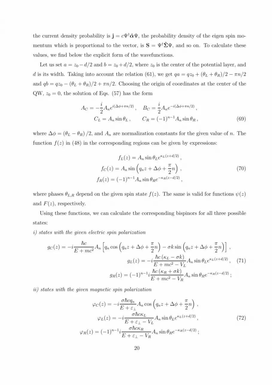
Let us set a = z0−d/2 and b = z0+d/2, where z0 is the center of the potential layer, and

d is its width. Taking into account the relation (61), we get qa = qz0 + (θL + θR)/2− πn/2

and qb = qz0 − (θL + θR)/2 + πn/2. Choosing the origin of coordinates at the center of the

QW, z0 = 0, the solution of Eqs. (57) has the form

AC = − i

2Ane

i(∆φ+πn/2) , BC =i

2Ane

−i(∆φ+πn/2) ,

CL = An sin θL , CR = (−1)n−1An sin θR , (69)

where ∆φ = (θL − θR) /2, and An are normalization constants for the given value of n. The

function f(z) in (48) in the corresponding regions can be given by expressions:

fL(z) = An sin θLeκL(z+d/2) ,

fC(z) = An sin(

qnz +∆φ+π

2n)

, (70)

fR(z) = (−1)n−1An sin θRe−κR(z−d/2) ,

where phases θL,R depend on the given spin state f(z). The same is valid for functions ψ(z)

and F (z), respectively.

Using these functions, we can calculate the corresponding bispinors for all three possible

states:

i) states with the given electric spin polarization

gC(z) = −i ~c

E +mc2An

[

qn cos(

qnz +∆φ+π

2n)

− σk sin(

qnz +∆φ +π

2n)]

,

gL(z) = −i ~c (κL − σk)

E +mc2 − VLAn sin θLe

κL(z+d/2) , (71)

gR(z) = (−1)n−1i~c (κR + σk)

E +mc2 − VRAn sin θRe

−κR(z−d/2) ;

ii) states with the given magnetic spin polarization

ϕC(z) = −i σ~cqnE + ε⊥

An cos(

qnz +∆φ+π

2n)

,

ϕL(z) = −i σ~cκLE + ε⊥ − VL

An sin θLeκL(z+d/2) , (72)

ϕR(z) = (−1)n−1iσ~cκR

E + ε⊥ − VRAn sin θRe

−κR(z−d/2) ;

20

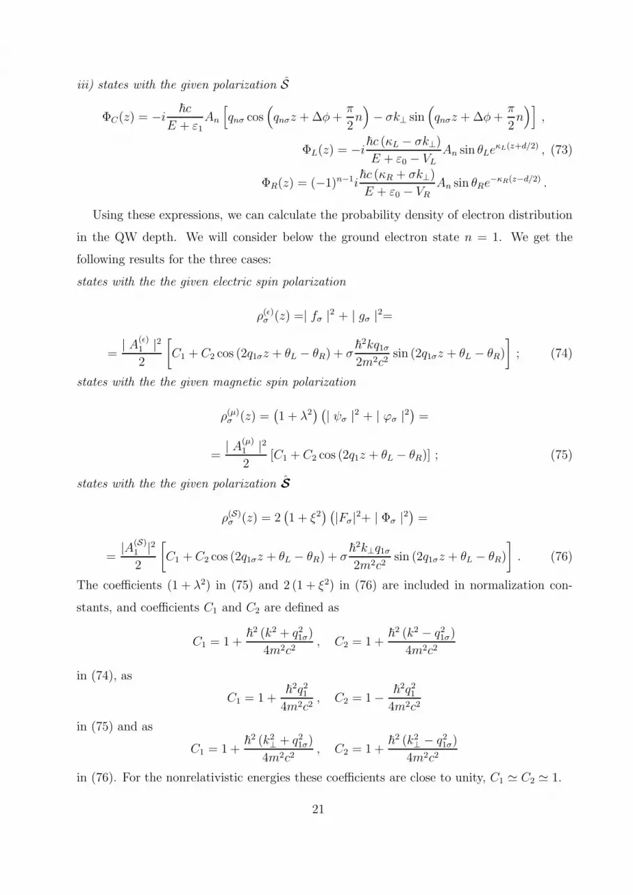
iii) states with the given polarization S

ΦC(z) = −i ~c

E + ε1An

[

qnσ cos(

qnσz +∆φ+π

2n)

− σk⊥ sin(

qnσz +∆φ+π

2n)]

,

ΦL(z) = −i~c (κL − σk⊥)

E + ε0 − VLAn sin θLe

κL(z+d/2) , (73)

ΦR(z) = (−1)n−1i~c (κR + σk⊥)

E + ε0 − VRAn sin θRe

−κR(z−d/2) .

Using these expressions, we can calculate the probability density of electron distribution

in the QW depth. We will consider below the ground electron state n = 1. We get the

following results for the three cases:

states with the the given electric spin polarization

ρ(ǫ)σ (z) =| fσ |2 + | gσ |2=

=| A(ǫ)

1 |22

[

C1 + C2 cos (2q1σz + θL − θR) + σ~2kq1σ2m2c2

sin (2q1σz + θL − θR)

]

; (74)

states with the the given magnetic spin polarization

ρ(µ)σ (z) =(

1 + λ2) (

| ψσ |2 + | ϕσ |2)

=

=| A(µ)

1 |22

[C1 + C2 cos (2q1z + θL − θR)] ; (75)

states with the the given polarization S

ρ(S)σ (z) = 2(

1 + ξ2) (

|Fσ|2+ | Φσ |2)

=

=|A(S)

1 |22

[

C1 + C2 cos (2q1σz + θL − θR) + σ~2k⊥q1σ2m2c2

sin (2q1σz + θL − θR)

]

. (76)

The coefficients (1 + λ2) in (75) and 2 (1 + ξ2) in (76) are included in normalization con-

stants, and coefficients C1 and C2 are defined as

C1 = 1 +~2 (k2 + q21σ)

4m2c2, C2 = 1 +

~2 (k2 − q21σ)

4m2c2

in (74), as

C1 = 1 +~2q21

4m2c2, C2 = 1− ~

2q214m2c2

in (75) and as

C1 = 1 +~2 (k2⊥ + q21σ)

4m2c2, C2 = 1 +

~2 (k2⊥ − q21σ)

4m2c2

in (76). For the nonrelativistic energies these coefficients are close to unity, C1 ≃ C2 ≃ 1.

21

It follows from above that SOI does not affect the probability density of electron distri-

bution inside the QW in the case of electrons with the given magnetic spin polarization.

Distribution probability density of electrons with the given electric spin polarization or with

the given polarization S do depend on the spin number. In particular, electrons with oppo-

site spin numbers are shifted towards the opposite boundaries of the QW.

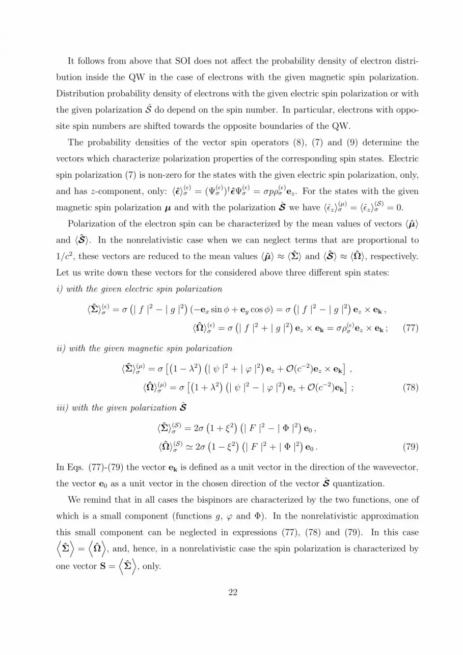
The probability densities of the vector spin operators (8), (7) and (9) determine the

vectors which characterize polarization properties of the corresponding spin states. Electric

spin polarization (7) is non-zero for the states with the given electric spin polarization, only,

and has z-component, only: 〈ǫ〉(ǫ)σ = (Ψ(ǫ)σ )†ǫΨ

(ǫ)σ = σpρ

(ǫ)σ ez. For the states with the given

magnetic spin polarization µ and with the polarization S we have 〈ǫz〉(µ)σ = 〈ǫz〉(S)σ = 0.

Polarization of the electron spin can be characterized by the mean values of vectors 〈µ〉and 〈S〉. In the nonrelativistic case when we can neglect terms that are proportional to

1/c2, these vectors are reduced to the mean values 〈µ〉 ≈ 〈Σ〉 and 〈S〉 ≈ 〈Ω〉, respectively.Let us write down these vectors for the considered above three different spin states:

i) with the given electric spin polarization

〈Σ〉(ǫ)σ = σ(

| f |2 − | g |2)

(−ex sin φ+ ey cosφ) = σ(

| f |2 − | g |2)

ez × ek ,

〈Ω〉(ǫ)σ = σ(

| f |2 + | g |2)

ez × ek = σρ(ǫ)σ ez × ek ; (77)

ii) with the given magnetic spin polarization

〈Σ〉(µ)σ = σ[(

1− λ2) (

| ψ |2 + | ϕ |2)

ez +O(c−2)ez × ek]

,

〈Ω〉(µ)σ = σ[(

1 + λ2) (

| ψ |2 − | ϕ |2)

ez +O(c−2)ek]

; (78)

iii) with the given polarization S

〈Σ〉(S)σ = 2σ(

1 + ξ2) (

| F |2 − | Φ |2)

e0 ,

〈Ω〉(S)σ ≃ 2σ(

1− ξ2) (

| F |2 + | Φ |2)

e0 . (79)

In Eqs. (77)-(79) the vector ek is defined as a unit vector in the direction of the wavevector,

the vector e0 as a unit vector in the chosen direction of the vector S quantization.

We remind that in all cases the bispinors are characterized by the two functions, one of

which is a small component (functions g, ϕ and Φ). In the nonrelativistic approximation

this small component can be neglected in expressions (77), (78) and (79). In this case⟨

Σ⟩

=⟨

Ω⟩

, and, hence, in a nonrelativistic case the spin polarization is characterized by

one vector S =⟨

Σ⟩

, only.

22

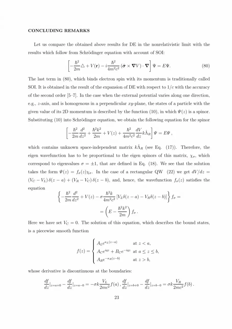
CONCLUDING REMARKS

Let us compare the obtained above results for DE in the nonrelativistic limit with the

results which follow from Schrodinger equation with account of SOI:

[

− ~2

2m+ V (r)− i

~2

4m2c2(σ ×∇V ) ·∇

]

Ψ = EΨ. (80)

The last term in (80), which binds electron spin with its momentum is traditionally called

SOI. It is obtained in the result of the expansion of DE with respect to 1/c with the accuracy

of the second order [5–7]. In the case when the external potential varies along one direction,

e.g., z-axis, and is homogenous in a perpendicular xy-plane, the states of a particle with the

given value of its 2D momentum is described by the function (10), in which Ψ (z) is a spinor.

Substituting (10) into Schrodinger equation, we obtain the following equation for the spinor

[

− ~2

2m

d2

dz2+

~2k2

2m+ V (z) +

~2

4m2c2dV

dzkΛR

]

Ψ = EΨ ,

which contains unknown space-independent matrix kΛR (see Eq. (17)). Therefore, the

eigen wavefunction has to be proportional to the eigen spinors of this matrix, χσ, which

correspond to eigenvalues σ = ±1, that are defined in Eq. (18). We see that the solution

takes the form Ψ (z) = fσ(z)χσ. In the case of a rectangular QW (22) we get dV/dz =

(VC − VL) δ(z − a) + (VR − VC) δ(z − b), and, hence, the wavefunction fσ(z) satisfies the

equation

− ~2

2m

d2

dz2+ V (z)− σ

~2k

4m2c2[VLδ(z − a)− VRδ(z − b)]

fσ =

=

(

E − ~2k2

2m

)

fσ .

Here we have set VC = 0. The solution of this equation, which describes the bound states,

is a piecewise smooth function

f(z) =

ALeκL(z−a) at z < a,

ACeiqz +BCe

−iqz at a ≤ z ≤ b,

ARe−κR(z−b) at z > b,

whose derivative is discontinuous at the boundaries:

df

dz|z=a+0 −

df

dz|z=a−0 = −σk VL

2mc2f(a) ,

df

dz|z=b+0 −

df

dz|z=b−0 = σk

VR2mc2

f(b) .

23

The incoming parameters κL,R in the nonrelativistic approximation are defined in Eq. (50).

Matching conditions for the function at the boundaries a and b lead to the condition (63),

from which the bound states can be determined, and to Rashba dispersion law (64) for 2D

electron bands and spin vector S, which are determined in Eq. (77). In this case the upper

spinor (large component) of the bispinor (19) plays the role of the wavefunction.

Therefore, Schrodinger equation (80) gives only the solution, which corresponds to the

given electric spin polarization, while, according to DE, 2D electrons, captured by the QW,

can have different spin states, which differ by the energy spectrum and by the electron spin

orientation. At the given electric spin polarization the vector S lies in the plane of the po-

tential layer and is ’bound’ to the direction of the electron momentum, being perpendicular

to it. In the states with the given magnetic spin polarization electron spins are oriented

perpendicular to the layer, and, finally, in the states with the given spin polarization S

they lie in the plane of the potential layer and are oriented along the chosen direction. The

difference of the energy spectra of these three states, which is absent in the homogenous

isotropic space, is, in fact, a sequence of the ’spin-orbit interaction’. Realization (’prepara-

tion’) of one of these states is determined by external conditions, such as presence of electric

and/or magnetic field, external pressure, interface properties, etc., and, therefore, should be

manifested in various physical experiments.

The reason for the origin of SOI is determined by the fact that DE, unlike its nonrel-

ativistic limit, does not admit separation of spatial and spin coordinates. This conclusion

follows not only from the circumstance that even in the homogenous isotropic space spin

operator S is not an integral of motion, but also from the fact that spin operators (6)-(9),

which allow to classify the states by their spin degree of freedom, include also coordinate

dependence since they contain the momentum operator.

In conclusion, we stress that the joint procedure of the transition to the nonrelativistic

limit is performed without the preliminary classification of the spin eigenstates and is based

on the assumption that the down spinor is a small component of the bispinor for the states

with positive energy [5–7]. As we have shown above, such assumption is valid for the states

with the given electric spin polarization determined by the bispinor in Eq. (19), only. In

the general case the large and small components can belong to all four components of the

bispinor, as it is in the case of spinors (31)-(32) and (42)-(43). Probably, because of this

fact the solution of Eq. (80) coincides with the solution of DE for the given electric spin

24

polarization, but does not have the solutions corresponding to the given magnetic spin

polarization µ, or spin polarization S. Derivation of the nonrelativistic equations which

take these facts into account, is a subject of a separate study and will be done elsewhere.

Acknowledgement The work is done within the Fundamental Research Programme of

the National Academy of Sciences of Ukraine.

∗ [email protected]

† [email protected];

‡ [email protected]

[1] J. Fabian, A. Matos-Abiague, C. Ertler, P. Stano, and I. Zutic, Acta Phys. Slov. 57, 565

(2007)).

[2] E. I. Rashba, Fiz. Tverd. Tela 2, 1224 (1960) [Sov. Phys. Solid State 2, 1109 (1960)].

[3] Y. A. Bychkov and E. I. Rashba, Pisma Zh. Eksp. Teor. Fiz. 39, 66 (1984) [Sov. Phys. JETP

Lett. 39, 78 (1984)] .

[4] P. A. M. Dirac, Proc. Roy. Soc., A 117, 610 (1928).

[5] Hans A. Bete. Intermediate Quantum Mechanics, W. A. Benjamin, Inc. New York-Amsterdam,

1964.

[6] V.B. Berestetskiy, E.M. Lifshitz, L.P. Pitaevskiy, Relativistic Quantum Theory, part I (in

Russian). Moscow, Nauka, 1968.

[7] O.S. Davydov. Quantum Mechanics (in Ukrainian), Vydavnychyi Dim Akademperiodyka,

Kyiv, 2012.

[8] O. Klein, Z. Phys. 53, 157 (1929).

[9] A. Calogeracos, N. Dombey, Int. J. Mod. Phys. A, 14, 631 (1999).

[10] P. Krekora, Q. Su, and R. Grobe, Phys. Rev. Lett. 92, 040406 (2004); 93, 043004 (2004).

[11] P. Alberto, C. Fiolhais, and V. M. S. Gil, Eur. J. Phys. 17, 19-24 (1996).

[12] S. De Leo and S. Giardino, J. Math. Phys. 55, 022301 (2014).

[13] A.A. Sokolov, I.M. Ternov, Relativistic Electron (in Russian), Moscow, Nauka, 1974

[14] E.S. Bernardes, J. Schliemann, M. Lee, J.C. Egues, and D. Loss, Phys. Rev. Lett. 99, 076603

25

(2007).

26