arXiv:0807.1580v2 [quant-ph] 19 Dec 2008 EPJ manuscript No. (will be inserted by the editor) Spin squeezing in a bimodal condensate: spatial dynamics and particle losses Yun Li 1,2 , P. Treutlein 3 , J. Reichel 1 and A. Sinatra 1 1 Laboratoire Kastler Brossel, ENS, UPMC and CNRS, 24 rue Lhomond, 75231 Paris Cedex 05, France 2 State Key Laboratory of Precision Spectroscopy, Department of Physics, East China Normal University, Shanghai 200062, China 3 Max-Planck-Institut f¨ ur Quantenoptikand Fakult¨at f¨ ur Physikder Ludwig-Maximilians-Universit¨at, Schellingstrasse 4, 80799 M¨ unchen, Germany Received: date / Revised version: date Abstract. We propose an analytical method to study the entangled spatial and spin dynamics of interacting bimodal Bose-Einstein condensates. We show that at particular times during the evolution spatial and spin dynamics disentangle and the spin squeezing can be predicted by a simple two-mode model. We calculate the maximum spin squeezing achievable in experimentally relevant situations with Sodium or Rubidium bimodal condensates, including the effect of the dynamics and of one, two and three-body losses. PACS. PACS-03.75.Gg Entanglement and decoherence in Bose-Einstein condensates – PACS-42.50.Dv Quantum state engineering and measurements – PACS-03.75.Kk Dynamic properties of condensates; col- lective and hydrodynamic excitations, superfluid flow – PACS-03.75.Mn Multicomponent condensates; spinor condensates 1 Introduction In atomic systems effective spins are collective variables that can be defined in terms of orthogonal bosonic modes. In this paper the two modes we consider are two different internal states of the atoms in a bimodal Bose-Einstein condensate. States with a large first order coherence be- tween the two modes, that is with a large mean value of the effective spin component in the equatorial plane of the Bloch sphere, can still differ by their spin fluctua- tions. For an uncorrelated ensemble of atoms, the quan- tum noise is evenly distributed among the spin compo- nents orthogonal to the mean spin. However quantum cor- relations can redistribute this noise and reduce the vari- ance of one spin quadrature with respect to the uncorre- lated case, achieving spin squeezing [1,2]. Spin-squeezed states are multi-particle entangled states that have prac- tical interest in atom interferometry, and high precision spectroscopy [3]. Quantum entanglement to improve the precision of spectroscopic measurements has already been used with trapped ions [4] and it could be used in atomic clocks where the standard quantum limit has already been reached [5]. A promising all-atomic route to create spin squeez- ing in bimodal condensates, proposed in [6], relies on the Kerr-type non linearity due to elastic interactions between atoms. Quite analogously to what happens to a coherent state in a nonlinear Kerr medium in optics [7], an initial “phase state” or coherent spin state, where all the effective spins point at the same direction, dynamically evolves into a correlated spin-squeezed state. A straightforward way to produce the initial phase state in a bimodal condensate is to start with one atomic condensate in a given internal state a and perform a π/2-pulse coupling coherently the internal state a to a second internal state b [8]. However, as the strength of the interactions between two atoms a − a, b − b and a − b are in general different, the change in the mean field energy excites the spatial dynamics of the con- densate wave functions. In the evolution subsequent to the pulse, the spin dynamics creating squeezing and the spa- tial dynamics are entangled [6,9,10,11] and occur on the same time scale set by an effective interaction parameter χ. This makes it a priori more difficult to obtain simple analytical results. In this paper we develop a simple formalism which al- lows us to calculate analytically or semi analytically the effect of the spatial dynamics on spin squeezing. In Sec- tion 2 we present our dynamic model. Using our treatment we show that at particular times in the evolution the spa- tial dynamics and the spin dynamics disentangle and the dynamical model gives the same results as a simple two- mode model. We also identify configurations of parameters in which the simple two mode-model is a good approxi- mation at all times. Restricting to a two-mode model, in Section 3 we generalize our analytical results of [12] on op- timal spin squeezing in presence of particle losses to the case of overlapping and non-symmetric condensates.

Welcome message from author
This document is posted to help you gain knowledge. Please leave a comment to let me know what you think about it! Share it to your friends and learn new things together.
Transcript

arX
iv:0
807.
1580
v2 [
quan
t-ph
] 1
9 D
ec 2
008
EPJ manuscript No.(will be inserted by the editor)
Spin squeezing in a bimodal condensate: spatial dynamics andparticle losses
Yun Li1,2, P. Treutlein3, J. Reichel1 and A. Sinatra1
1 Laboratoire Kastler Brossel, ENS, UPMC and CNRS, 24 rue Lhomond, 75231 Paris Cedex 05, France2 State Key Laboratory of Precision Spectroscopy, Department of Physics, East China Normal University, Shanghai 200062,
China3 Max-Planck-Institut fur Quantenoptik and Fakultat fur Physik der Ludwig-Maximilians-Universitat, Schellingstrasse 4, 80799
Munchen, Germany
Received: date / Revised version: date
Abstract. We propose an analytical method to study the entangled spatial and spin dynamics of interactingbimodal Bose-Einstein condensates. We show that at particular times during the evolution spatial and spindynamics disentangle and the spin squeezing can be predicted by a simple two-mode model. We calculatethe maximum spin squeezing achievable in experimentally relevant situations with Sodium or Rubidiumbimodal condensates, including the effect of the dynamics and of one, two and three-body losses.
PACS. PACS-03.75.Gg Entanglement and decoherence in Bose-Einstein condensates – PACS-42.50.DvQuantum state engineering and measurements – PACS-03.75.Kk Dynamic properties of condensates; col-lective and hydrodynamic excitations, superfluid flow – PACS-03.75.Mn Multicomponent condensates;spinor condensates
1 Introduction
In atomic systems effective spins are collective variablesthat can be defined in terms of orthogonal bosonic modes.In this paper the two modes we consider are two differentinternal states of the atoms in a bimodal Bose-Einsteincondensate. States with a large first order coherence be-tween the two modes, that is with a large mean valueof the effective spin component in the equatorial planeof the Bloch sphere, can still differ by their spin fluctua-tions. For an uncorrelated ensemble of atoms, the quan-tum noise is evenly distributed among the spin compo-nents orthogonal to the mean spin. However quantum cor-relations can redistribute this noise and reduce the vari-ance of one spin quadrature with respect to the uncorre-lated case, achieving spin squeezing [1,2]. Spin-squeezedstates are multi-particle entangled states that have prac-tical interest in atom interferometry, and high precisionspectroscopy [3]. Quantum entanglement to improve theprecision of spectroscopic measurements has already beenused with trapped ions [4] and it could be used in atomicclocks where the standard quantum limit has already beenreached [5].
A promising all-atomic route to create spin squeez-ing in bimodal condensates, proposed in [6], relies on theKerr-type non linearity due to elastic interactions betweenatoms. Quite analogously to what happens to a coherentstate in a nonlinear Kerr medium in optics [7], an initial“phase state” or coherent spin state, where all the effective
spins point at the same direction, dynamically evolves intoa correlated spin-squeezed state. A straightforward way toproduce the initial phase state in a bimodal condensate isto start with one atomic condensate in a given internalstate a and perform a π/2-pulse coupling coherently theinternal state a to a second internal state b [8]. However, asthe strength of the interactions between two atoms a− a,b− b and a− b are in general different, the change in themean field energy excites the spatial dynamics of the con-densate wave functions. In the evolution subsequent to thepulse, the spin dynamics creating squeezing and the spa-tial dynamics are entangled [6,9,10,11] and occur on thesame time scale set by an effective interaction parameterχ. This makes it a priori more difficult to obtain simpleanalytical results.
In this paper we develop a simple formalism which al-lows us to calculate analytically or semi analytically theeffect of the spatial dynamics on spin squeezing. In Sec-tion 2 we present our dynamic model. Using our treatmentwe show that at particular times in the evolution the spa-tial dynamics and the spin dynamics disentangle and thedynamical model gives the same results as a simple two-mode model. We also identify configurations of parametersin which the simple two mode-model is a good approxi-mation at all times. Restricting to a two-mode model, inSection 3 we generalize our analytical results of [12] on op-timal spin squeezing in presence of particle losses to thecase of overlapping and non-symmetric condensates.

2 Please give a shorter version with: \authorrunning and \titlerunning prior to \maketitle
In Sections 4 and 5, we apply our treatment to cases ofpractical interest. We first consider a bimodal 87Rb con-densate. Rb is one of the most common atoms in BECexperiments and it is a good candidate for atomic clocksusing trapped atoms on a chip [13]. Restricting to stateswhich are equally affected by a magnetic field to first or-der, the most common choices are |F = 1,m = −1〉 and|F = 2,m = 1〉 which can be magnetically trapped, or|F = 1,m = 1〉 and |F = 2,m = −1〉 that must be trappedoptically but for which there exists a low-field Feshbachresonance which can be used to reduce the inter-speciesscattering length [14,15]. Indeed a particular feature ofthese Rb states is that the three s-wave scattering lengthscharacterizing interactions between a− a, b− b and a− batoms are very close to each other. A consequence is thatthe squeezing dynamics is very slow when the two conden-sates overlap. The inter-species Feshbach resonance can beused to overcome this problem and speed up the dynamics[15].
In schemes involving the |F = 2,m = ±1〉 of Rubid-ium, the main limit to the maximum squeezing achievableis set by the large two-body losses rate in these states. Asa second case of experimental interest we then considerNa atoms in the |F = 1,mF = ±1〉 states [6]. Althoughtheses states have opposite shifts in a magnetic field, theypresent the advantage of negligible two-body losses. Usingour analytical optimization procedure, we calculate themaximum squeezing achievable in this system includingthe effect of spatial dynamics and particle losses.
In Section 5 we examine a different scenario for Rbcondensates in which, instead of changing the scatteringlength, one would spatially separate the two condensatesafter the mixing π/2 pulse and hold them separately dur-ing a well chosen squeezing time. An interesting featureof this scheme is that the squeezing dynamics acts onlywhen the clouds are spatially separated and it freezes outwhen the two clouds are put back together so that onecould prepare a spin squeezed state and then keep it fora certain time [12]. State-selective potentials for 87Rb in|F = 1,m = −1〉 and |F = 2,m = 1〉 [13] have recentlybeen implemented on an atom chip, and such scheme couldbe of experimental interest.
2 Dynamical spin squeezing model
In this section we develop and compare dynamical modelsfor spin squeezing. No losses will be taken into account inthis section.
2.1 State evolution
We consider the model Hamiltonian
H =
∫
d3r
∑
ε=a,b
[
ψ†εhεψε +
1
2gεεψ
†εψ
†εψεψε
]
+ gabψ†b ψ
†aψaψb (1)
where hε is the one-body hamiltonian including kineticenergy and external trapping potential
hε = −~2∆
2m+ U ext
ε (r ) . (2)
The interactions constants gεε′ are related to the corre-sponding s-wave scattering lengths gεε′ = 4π~
2aεε′/Mcharacterizing a cold collision between an atom in stateε with an atom in state ε′ (ε, ε′ = a, b), and M is themass of one atom.
We assume that we start from a condensate with Natoms in the internal state a; the stationary wave functionof the condensate is φ0(r ). After a π/2 pulse, a phase stateis created, which is our initial state:
|Ψ(0)〉 =1√N !
[
Caa†|φ0〉
+ Cbb†|φ0〉
]N
|0〉 (3)
where Ca, Cb are mixing coefficients with |Ca|2+|Cb|2 = 1
and the operator a†|φ0〉creates a particle in the internal
state a with wave function φ0. To describe the entangledevolution of the spin dynamics and the external dynamicsof the wave functions, it is convenient to introduce Fockstates with well defined number of particles in |a〉 and|b〉, these numbers being preserved during time evolutionsubsequent to the mixing pulse. Expanded over the Fockstates, the initial state (3) reads:
|Ψ(0)〉 =
N∑
Na=0
(
N !
Na!Nb!
)1/2
CNaa CNb
b |Na : φ0, Nb : φ0〉,
(4)where Nb = N −Na, and
|Na : φa, Nb : φb〉 =
[
a†|φa(Na,Nb)〉
]Na
√Na!
[
b†|φb(Na,Nb)〉
]Nb
√Nb!
|0〉 .(5)
Within an Hartee-Fock type ansatz for the N -bodystate vector, we calculate the evolution of each Fock statein (4). We get [9]:
|Na : φ0, Nb : φ0〉 → e−iA(Na,Nb; t)/~
×|Na : φa(Na, Nb; t), Nb : φb(Na, Nb; t)〉 , (6)
where φa(Na, Nb; t) and φb(Na, Nb; t) are solutions of thecoupled Gross-Pitaevskii equations:
i~∂tφε =[
hε + (Nε − 1)gεε|φε|2 +N ′εgεε′ |φε′ |2
]
φε (7)
here with the initial conditions
φa(0) = φb(0) = φ0 , (8)
and the time dependent phase factor A solves:
d
dtA(Na, Nb; t) = −
∑
ε=a,b
Nε(Nε − 1)gεε
2
∫
d3r|φε|4
− NaNbgab
∫
d3r|φa|2|φb|2 . (9)
Please give a shorter version with: \authorrunning and \titlerunning prior to \maketitle 3
With this treatment we fully include the quantum dynam-ics of the two condensate modes a and b, as one does forthe simple two modes model, but also including the spa-tial dynamics of the two modes and their dependence onthe number of particles. The approximation we make isto neglect all the other modes orthogonal to the conden-sates which would be populated thermally. An alternativemethod is to use a number conserving Bogoliubov theorythat explicitly includes the operators of the condensatesas in [10]. In that case all the modes are present but themodes orthogonal to the condensates are treated in a lin-earized way. In [10], the author compares the number con-serving Bogoliubov approach to our approach using manyGross-Piaevskii equations, also used in [6], and he findsvery similar result for the spin squeezing. He also findsthat within the Bogoliuobov approximation the thermallyexcited modes strictly do not affect the squeezing in thescheme we consider here. If the number conserving Bogoli-ubov has the advantage of being systematic, our approach,supplemented with a further approximation (the modulus-phase approximation introduced in Sect. 2.3) allows us toget some insight and obtain simple analytical results.
2.2 Calculation of spin squeezing
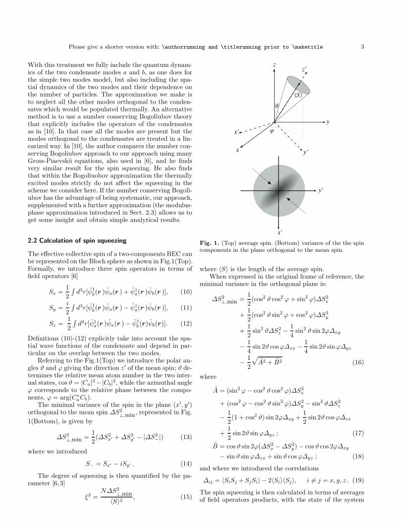
The effective collective spin of a two-components BEC canbe represented on the Bloch sphere as shown in Fig.1(Top).Formally, we introduce three spin operators in terms offield operators [6]
Sx =1
2
∫
d3r[ψ†b(r )ψa(r ) + ψ†
a(r )ψb(r )], (10)
Sy =i
2
∫
d3r[ψ†b(r )ψa(r ) − ψ†
a(r )ψb(r )], (11)
Sz =1
2
∫
d3r[ψ†a(r )ψa(r ) − ψ†
b(r)ψb(r)]. (12)
Definitions (10)-(12) explicitly take into account the spa-tial wave functions of the condensate and depend in par-ticular on the overlap between the two modes.
Referring to the Fig.1(Top) we introduce the polar an-gles ϑ and ϕ giving the direction z′ of the mean spin; ϑ de-termines the relative mean atom number in the two inter-nal states, cosϑ = |Ca|2−|Cb|2, while the azimuthal angleϕ corresponds to the relative phase between the compo-nents, ϕ = arg(C∗
aCb).The minimal variance of the spin in the plane (x′, y′)
orthogonal to the mean spin ∆S2⊥,min, represented in Fig.
1(Bottom), is given by
∆S2⊥,min =
1
2(∆S2
x′ +∆S2y′ − |∆S2
−|) (13)
where we introduced
S− = Sx′ − iSy′ . (14)
The degree of squeezing is then quantified by the pa-rameter [6,3]
ξ2 =N∆S2
⊥,min
〈S〉2 , (15)
x'
y
x
z
y'
z'
ϑ
ϕ
⟨ S⟩
x'
y'
Fig. 1. (Top) average spin. (Bottom) variance of the the spincomponents in the plane orthogonal to the mean spin.
where 〈S〉 is the length of the average spin.When expressed in the original frame of reference, the
minimal variance in the orthogonal plane is:
∆S2⊥,min =
1
2(cos2 ϑ cos2 ϕ+ sin2 ϕ)∆S2
x
+1
2(cos2 ϑ sin2 ϕ+ cos2 ϕ)∆S2
y
+1
2sin2 ϑ∆S2
z − 1
4sin2 ϑ sin 2ϕ∆xy
− 1
4sin 2ϑ cosϕ∆zx − 1
4sin 2ϑ sinϕ∆yz
− 1
2
√
A2 + B2 (16)
where
A = (sin2 ϕ− cos2 ϑ cos2 ϕ)∆S2x
+ (cos2 ϕ− cos2 ϑ sin2 ϕ)∆S2y − sin2 ϑ∆S2
z
− 1
2(1 + cos2 ϑ) sin 2ϕ∆xy +
1
2sin 2ϑ cosϕ∆zx
+1
2sin 2ϑ sinϕ∆yz ; (17)
B = cosϑ sin 2ϕ(∆S2x −∆S2
y) − cosϑ cos 2ϕ∆xy
− sinϑ sinϕ∆zx + sinϑ cosϕ∆yz ; (18)
and where we introduced the correlations
∆ij = 〈SiSj + SjSi〉 − 2〈Si〉〈Sj〉, i 6= j = x, y, z . (19)
The spin squeezing is then calculated in terms of averagesof field operators products, with the state of the system

4 Please give a shorter version with: \authorrunning and \titlerunning prior to \maketitle
at time t, obtained by evolving equation (4) with equation(6). To calculate the averages one needs to compute the
action of the field operators ψa ψb on the Fock states (5)[16],
ψa(r) |Na : φa(Na, Nb), Nb : φb(Na, Nb)〉= φa(Na, Nb, r)
√
Na
× |Na − 1 : φa(Na, Nb), Nb : φb(Na, Nb)〉, (20)
ψb(r) |Na : φa(Na, Nb), Nb : φb(Na, Nb)〉= φb(Na, Nb, r)
√
Nb
× |Na : φa(Na, Nb), Nb − 1 : φb(Na, Nb)〉. (21)
The explicit expressions of the averages needed to calcu-late the spin squeezing parameter are given in AppendixA. These quantum averages correspond to an initial statewith a well-defined number of particles N . In case of fluc-tuations in the total number of particles where the densitymatrix of the system is a statistical mixture of states witha different number of particles, a further averaging of Nover a probability distribution P (N) is needed [9,17].
2.3 Dynamical modulus-phase approach
In principle, equations (7)-(9) can be solved numericallyfor each Fock state in the sum equation (4), and the squeez-ing can be computed as explained in the previous section.However, for a large number of atoms and especially inthree dimensions and in the absence of particular symme-tries (e.g. spherical symmetry) this can be a very heavynumerical task. To overcome this difficulty, in order todevelop an analytical approach, we can exploit the factthat for large N in the initial state (4) the distributions ofthe number of atoms Na and Nb are very peaked aroundtheir average values with a typical width of order
√N .
Moreover, assuming that possible fluctuations in the totalnumber of particles are described by a distribution P (N)having a width much smaller than the average of the totalnumber of particles N , we can limit to Na and Nb closeto Na = |Ca|2N and Nb = |Cb|2N . We then split thecondensate wave function into modulus and phase
φε = |φε| exp(iθε) ε = a, b , (22)
and we assume that the variation of the modulus over thedistribution of Nε can be neglected while we approximatethe variation of the phase by a linear expansion aroundNε [9]. The approximate condensate wave functions read
φε(Na, Nb) ≃ φε exp
i∑
ε′=a,b
(Nε′ − Nε′)(∂Nε′θε)Na,Nb
(23)where φε ≡ φε(Na = Na, Nb = Nb).
The modulus phase approximation takes into account,in an approximate way, the dependence of the condensatewave functions on the number of particles. It is precisely
this effect that is responsible of entanglement between spa-tial dynamics and spin dynamics.
As explained in Appendix B, all the relevant averagesneeded to calculate spin squeezing can then be expressedin terms of φε and of three time and position dependentquantities:
χd(r) =1
2[(∂Na
− ∂Nb)(θa − θb)]Na,Nb
, (24)
χs(r) =1
2[(∂Na
+ ∂Nb)(θa − θb)]Na,Nb
, (25)
χ0(r) =1
2[(∂Na
− ∂Nb)(θa + θb)]Na,Nb
. (26)
In some cases (see Sect. 2.4) these quantities can be ex-plicitly calculated analytically. To calculate the squeezingin the general case, it is sufficient to evolve a few coupledGross-Pitaevskii equations (7) for different values of Na,Nb, to calculate numerically the derivatives of the phasesappearing in (24)-(26). Although we do not expect a per-fect quantitative agreement with the full numerical modelfor all values of parameters, we will see that the analyticalmodel catches the main features and allows us to interpretsimply the results.
In the particular case of stationary wave functions ofthe condensates, the parameters χd, χs and χ0 becomespace-independent:
χstd = −
[(∂Na− ∂Nb
)(µa − µb)]Na,Nb
2~t (27)
χsts = −
[(∂Na+ ∂Nb
)(µa − µb)]Na,Nb
2~t (28)
χst0 = χst
s . (29)
In this case we recover a simple two-mode model. Equa-tions (27)-(28) will be used in section 3. In that contestwe will rename χst
d /t = −χ and χsts /t = −χ to shorten the
notations.To test our modulus-phase dynamical model, in Fig. 2,
we consider a situation in which the external dynamics issignificantly excited after the π/2 pulse which populatesthe state b. Parameters correspond to a bimodal Rb con-densate in |F = 1,mF = 1〉 and |F = 2,mF = −1〉 withNa = Nb = 5 × 10⁴ and where a Feshbach resonance isused to reduce aab by about 10% with respect to its barevalue [14,15]. The considered harmonic trap is very steepω = 2π × 2 kHz. In the figure we compare our modulus-phase approach (dashed line) with the full numerical so-lution (solid line) and with a stationary calculation using(27)-(28) (dash-dotted line) which is equivalent to a two-mode model. The oscillation of the squeezing parameterin the two dynamical calculations (dashed line and solidline) are due to the fact that the sudden change in themean-field causes oscillations in the wave functions whoseamplitude and the frequency are different for each Fockstate. From the figure, we find that our modulus-phaseapproach obtained integrating 5 Gross-Pitaevskii equa-tions (dashed line) reproduces the main characteristics ofthe full numerical simulation using 3000 Fock states (solidline). The stationary two mode model on the other hand is

Please give a shorter version with: \authorrunning and \titlerunning prior to \maketitle 5
0 0.5 1 1.5 2 2.5 3 3.5 4 4.510
−4
10−3
10−2
10−1
100
t [ms]
ξ2
Two−mode stationaryModulus−phase 5 GPEFull numerical simulation
Fig. 2. Spin squeezing as a function of time. Comparison of themodulus-phase model (red dashed line) with a full numericalcalculation with 3000 Fock states (blue solid line) and with astationary two-mode model (violet dash-dotted line). Spatialdynamics is strongly excited after the π/2-pulse populating asecond internal state. ω = 2π × 2 kHz, Na = Nb = 5 × 10⁴,m=87 a.m.u., aaa = 100.44 rB, abb = 95.47 rB, aab = 88.28 rB .No particle losses. rB is the Bohr radius.
not a good approximation in this case. Only for some par-ticular times the three curves almost touch. At these timesthe wave functions of all the Fock states almost overlapand, as we will show in our analytical treatment, spatialdynamics and spin dynamics disentangle.
In Fig.3 we move to a shallow trap and less atoms. Wenote that in this case both the modulus-phase curve andthe numerical simulation are very close to the stationarytwo-mode model which is then a good approximation atall times.
2.4 Squeezing in the breathe-together solution
In this section we restrict to a spherically symmetric har-monic potential Uext = mω2r2/2 identical for the twointernal sates. For values of the inter particle scatteringlengths such that
aab < aaa, abb (30)
and for a particular choice of the mixing angle such thatthe mean field seen by the two condensates with Na andNb particles is the same:
Nagaa + Nbgab = Nbgbb + Nagab ≡ Ng , (31)
the wave functions φa and φb solve the same Gross-Pitaevskiiequation. In the Thomas-Fermi limit, the wave functionsφa and φb share the same scaling solution φ [18,19] and“breathe-together” [9].
φa = φb = φ(r, t) ≡ e−iη(t)
L3/2(t)eimr2L(t)/2~L(t)φ0(r/L(t) )
(32)
0 0.1 0.2 0.3 0.4 0.510
−3
10−2
10−1
100
t [s]
ξ2
Two−mode stationaryModulus−phase 5 GPEFull numerical simulation
0 0.1 0.2 0.3 0.4 0.5-1
0
1
t [s]
j
×π
Fig. 3. (Top) spin squeezing as a function of time in a case inwhich the spatial dynamics is weakly excited. Blue solid line:full numerical calculation with 1000 Fock states. Red dashedline: modulus-phase model. Violet dash-dotted line: station-ary two-mode model. (Bottom) angle giving the direction ofthe mean spin projection in the equatorial plane of the Blochsphere. Parameters: ω = 2π × 42.6 Hz, Na = Nb = 1 × 10⁴,m=87 a.m.u., aaa = 100.44 rB , abb = 95.47 rB, aab = 88.28 rB.No particle losses. rB is the Bohr radius.
with
η =g
gaa
µ
L3~(33)
d2Ldt2
=g
gaa
ω2
L4− ω2L ; (34)
φ0(r ) =
(
15
8πR30
)1/2 [
1 − r2
R20
]1/2
(35)
µ is the chemical potential of the stationary condensatebefore the π/2 pulse, when all the N atoms are in state a,
and R0 =√
2µ/mω2 is the corresponding Thomas-Fermiradius. The initial conditions for (34) are L(0) = 1 and
L(0) = 0.Note that the scaling solution identical for the two
modes a and b is valid only for Na = Na, Nb = Nb anddoes not apply to all the wave functions φa(Na, Nb) andφb(Na, Nb) in the expansion equation (4). Nevertheless,an advantage of choosing the mixing angle in order to sat-isfy the breathe-together condition equation (31), is thatthe mean spin has no drift velocity. In Fig.4 we calculatethe spin squeezing (Top) and the angle ϕ giving the direc-tion of the mean spin projection on the equatorial plane ofthe Bloch sphere (Bottom), for the same parameters as inFig.3 except for the mixing angle that we now choose sat-
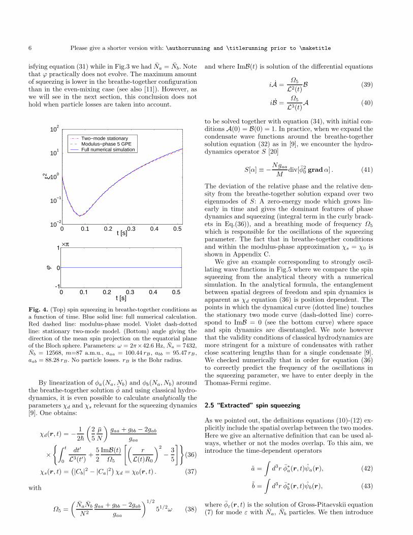
6 Please give a shorter version with: \authorrunning and \titlerunning prior to \maketitle
isfying equation (31) while in Fig.3 we had Na = Nb. Notethat ϕ practically does not evolve. The maximum amountof squeezing is lower in the breathe-together configurationthan in the even-mixing case (see also [11]). However, aswe will see in the next section, this conclusion does nothold when particle losses are taken into account.
0 0.1 0.2 0.3 0.4 0.510
−2
10−1
100
101
102
t [s]
ξ2
Two−mode stationaryModulus−phase 5 GPEFull numerical simulation
0 0.1 0.2 0.3 0.4 0.5-1
0
1
t [s]
j
×π
Fig. 4. (Top) spin squeezing in breathe-together conditions asa function of time. Blue solid line: full numerical calculation.Red dashed line: modulus-phase model. Violet dash-dottedline: stationary two-mode model. (Bottom) angle giving thedirection of the mean spin projection on the equatorial planeof the Bloch sphere. Parameters: ω = 2π×42.6 Hz, Na = 7432,Nb = 12568, m=87 a.m.u., aaa = 100.44 rB , abb = 95.47 rB ,aab = 88.28 rB. No particle losses. rB is the Bohr radius.
By linearization of φa(Na, Nb) and φb(Na, Nb) aroundthe breathe-together solution φ and using classical hydro-dynamics, it is even possible to calculate analytically theparameters χd and χs relevant for the squeezing dynamics[9]. One obtains:
χd(r, t) = − 1
2~
(
2
5
µ
N
)
gaa + gbb − 2gab
gaa
×
∫ t
0
dt′
L3(t′)+
5
2
ImB(t)
Ω5
[
(
r
L(t)R0
)2
− 3
5
]
(36)
χs(r, t) =(
|Cb|2 − |Ca|2)
χd = χ0(r, t) . (37)
with
Ω5 =
(
NaNb
N2
gaa + gbb − 2gab
gaa
)1/2
51/2ω (38)
and where ImB(t) is solution of the differential equations
iA =Ω5
L2(t)B (39)
iB =Ω5
L3(t)A (40)
to be solved together with equation (34), with initial con-ditions A(0) = B(0) = 1. In practice, when we expand thecondensate wave functions around the breathe-togethersolution equation (32) as in [9], we encounter the hydro-dynamics operator S [20]
S[α] ≡ −Ngaa
Mdiv[φ2
0 gradα] . (41)
The deviation of the relative phase and the relative den-sity from the breathe-together solution expand over twoeigenmodes of S: A zero-energy mode which grows lin-early in time and gives the dominant features of phasedynamics and squeezing (integral term in the curly brack-ets in Eq.(36)), and a breathing mode of frequency Ω5
which is responsible for the oscillations of the squeezingparameter. The fact that in breathe-together conditionsand within the modulus-phase approximation χs = χ0 isshown in Appendix C.
We give an example corresponding to strongly oscil-lating wave functions in Fig.5 where we compare the spinsqueezing from the analytical theory with a numericalsimulation. In the analytical formula, the entanglementbetween spatial degrees of freedom and spin dynamics isapparent as χd equation (36) is position dependent. Thepoints in which the dynamical curve (dotted line) touchesthe stationary two mode curve (dash-dotted line) corre-spond to ImB = 0 (see the bottom curve) where spaceand spin dynamics are disentangled. We note howeverthat the validity conditions of classical hydrodynamics aremore stringent for a mixture of condensates with ratherclose scattering lengths than for a single condensate [9].We checked numerically that in order for equation (36)to correctly predict the frequency of the oscillations inthe squeezing parameter, we have to enter deeply in theThomas-Fermi regime.
2.5 “Extracted” spin squeezing
As we pointed out, the definitions equations (10)-(12) ex-plicitly include the spatial overlap between the two modes.Here we give an alternative definition that can be used al-ways, whether or not the modes overlap. To this aim, weintroduce the time-dependent operators
a =
∫
d3r φ∗a(r, t)ψa(r), (42)
b =
∫
d3r φ∗b (r, t)ψb(r), (43)
where φε(r, t) is the solution of Gross-Pitaevskii equation(7) for mode ε with Na, Nb particles. We then introduce

Please give a shorter version with: \authorrunning and \titlerunning prior to \maketitle 7
0 0.2 0.4 0.6 0.8 1 1.2 1.4 1.610
−4
10−3
10−2
10−1
100
t [ms]
ξ2
Two−mode stationaryAnalytical solutionModulus−phase 5 GPEFull numerical sumulation
0 0.2 0.4 0.6 0.8 1.0 1.2 1.4 1.6-2
0
2
t [ms]
Im
Fig. 5. (Top) test of the analytical formula equation (36) inthe deep Thomas-Fermi regime. Spin squeezing as a functionof time. Blue solid line: full numerical calculation. Red dashedline: modulus-phase model. Black dotted line: analytical curveusing equation (36). Violet dash-dotted line: stationary two-mode model using (27)-(28). (Bottom) function ImB(t). Spatialand spin dynamics disentangle when ImB(t) = 0. Parameters:Na = Nb = 5×10⁵, ω = 2π×2 kHz, m=87 a.m.u., aaa = abb =0.3 aho, aab = 0.24 aho. aho is the harmonic oscillator length:aho =
p
~/Mω. No particle losses.
the spin operators:
Sx =1
2(b†a+ a†b), (44)
Sy =i
2(b†a− a†b), (45)
Sz =1
2(a†a− b†b). (46)
In the new definition of spin squeezing calculated by thespin operators defined in equations (44)-(46), which wecall the “extracted” spin squeezing, we still take into ac-count entanglement between external motion and spin dy-namics, but we give up the information about the over-lap between the two modes. In Appendix D, we give thequantum averages useful to calculate the extracted spinsqueezing within the modulus-phase approach describedin Section 2.3. We will use this extracted spin squeezingin Section 5.
Comparing the expressions given in Appendix D withthose of Appendix F (in the absence of losses), one real-izes that in the stationary case, where χd, χs and χ0 arespace independent, the extracted spin squeezing dynami-cal model reduces to a two-mode model that we study indetail in the next section.
3 Two-mode model with Particle losses
In this section we generalize our results of [12] to possiblyoverlapping and non-symmetric condensates. In subsec-tion 3.1 we address the general case, while in subsection3.2 we restrict to symmetric condensates and perform an-alytically an optimization of the squeezing with respectto the trap frequency and number of atoms. In the wholesection, as in [12], we will limit to a two-mode stationarymodel and we do not address dynamical issues.
3.1 Spin squeezing in presence of losses
We consider a two-component Bose-Einstein condensateinitially prepared in a phase state, that is with well definedrelative phase between the two components,
|Ψ(0)〉 = |ϕ〉 ≡(
|Ca|e−iϕ/2a† + |Cb|eiϕ/2b†)N
√N !
|0〉 . (47)
When expanded over Fock states, the state (47) shows bi-nomial coefficients which, for large N , are peaked aroundthe average number of particles in a and b, Na and Nb. Inthe same spirit as the “modulus-phase” approximation ofsubsection 2.3, we can use this fact to expand the Hamil-tonian of the system to the second order around Na andNb
H0 ≃ E(Na, Nb) +∑
ε=a,b
µε(Nε − Nε) +1
2∂Nε
µε(Nε − Nε)2
+1
2(∂Nb
µa + ∂Naµb) (Na − Na)(Nb − Nb) (48)
where the chemical potentials µε and all the derivativesof µε should be evaluated in Na and Nb. We can write
H0 = fN + ~vN (Na − Nb) +~χ
4(Na − Nb)
2 (49)
with
vN =1
2~
[
(µa − µb) − ~χ(Na − Nb) + ~χ(N − N)]
(50)
χ =1
2~(∂Na
µa + ∂Nbµb − ∂Nb
µa − ∂Naµb)Na,Nb
(51)
χ =1
2~(∂Na
µa − ∂Nbµb)Na,Nb
. (52)
The function f of the total number of particles, N =Na + Nb, commutes with the density operator of the sys-tem and can be omitted. The second term in equation(49) proportional to Sz describes a rotation of the aver-age spin vector around the z axis with velocity vN . Thethird term proportional to S2
z provides the nonlinearityresponsible for spin squeezing. It also provides a secondcontribution to the drift of the relative phase between thetwo condensates in the case Na 6= Nb.
In presence of losses, the evolution is ruled by a masterequation for the density operator ρ of the system. In the
8 Please give a shorter version with: \authorrunning and \titlerunning prior to \maketitle
interaction picture with respect to H0, with one, two, andthree-body losses, we have:
dρ
dt=
3∑
m=1
∑
ε=a,b
γ(m)ε
[
cmε ρc†mε − 1
2c†mε cmε , ρ
]
+ γab
[
cacbρc†ac
†b −
1
2c†ac†bcacb, ρ
]
(53)
where ρ = eiH0t/~ρe−iH0t/~, ca = eiH0t/~ae−iH0t/~, andsimilarly for b,
γ(m)ε =
K(ε)m
m
∫
d3r|φε(r)|2m , (54)
γab =Kab
2
∫
d3r|φa(r)|2|φb(r)|2 . (55)
K(ε)m is the m-body rate constant (m = 1, 2, 3) and φε(r)
is the condensate wave function for the ε component withNa = Na and Nb = Nb particles. Kab is the rate constantfor a two-body loss event in which two particles comingfrom different components are lost at once.
In the Monte Carlo wave function approach [21] we de-fine an effective Hamiltonian Heff and the jump operators
J(m)ε (J
(2)ab )
Heff = − i~2
3∑
m=1
∑
ε=a,b
γ(m)ε c†mε cmε − i~
2γabc
†ac
†bcacb ;(56)
J (m)ε =
√
γ(m)ε cmε , J
(2)ab =
√γabcacb (57)
We assume that a small fraction of particles will be lost
during the evolution so that we can consider χ, γ(m)ε and
γab as constant parameters of the model. The state evolu-tion in a single quantum trajectory is a sequence of ran-dom quantum jumps at times tj and non-unitary Hamil-tonian evolutions of duration τj :
|Ψ(t)〉 = e−iHeff(t−tk)/~J (mk)εk
(tk)e−iHeffτk/~J (mk−1)εk−1
(tk−1)
. . . J (m1)ε1
(t1)e−iHeffτ1/~|Ψ(0)〉 , (58)
where now εj = a, b or ab. Application of a jump J(mj)εj (tj)
to the N -particle phase state at tj yields
J (mj)εj
(tj)|φ〉N ∝ |φ+∆jtj〉N−mj, (59)
∆j = 2χδεj ,ab + (χ+ χ)mjδεj ,a + (χ− χ)mjδεj ,b .(60)
After a quantum jump, the phase state is changed into anew phase state, with m particle less and with the relativephase between the two modes showing a random shift∆jtjwith respect to the phase before the jump. Note that inthe symmetrical case χ = 0 and no random phase shiftoccurs in the case of a jump of ab. Indeed we will findthat at short times in the symmetrical case theses kind ofcrossed ab losses are harmless to the the squeezing.
In presence of one-body losses only, also the effectiveHamiltonian changes a phase state into another phase
state and we can calculate exactly the evolution of thestate vector analytically, as we did in [12] for symmetricalcondensates. When two and three-body losses enter intoplay, we introduce a constant loss rate approximation [22]
Heff ≃ − i~2
3∑
m=1
∑
ε=a,b
γ(m)ε Nm
ε − i~
2γabNaNb ≡ − i~
2λ
(61)valid when a small fraction of particles is lost at the timeat which the best squeezing is achieved. In this approxi-mation, the mean number of particles at time t is
〈N〉 = N
1 −
∑
ε=a,b
∑
m
Γ (m)ε + Γab
t
(62)
Γ (m)ε ≡ Nm−1
ε mγ(m)ε ; Γab = γab
√
NaNb (63)
where for example Γ(m)ε t is the fraction of lost particles
due to m-body losses in the ε condensate. Let us presentthe evolution of a single quantum trajectory: Within theconstant loss rate approximation, we can move all thejump operators in (58) to the right. We obtain:
|Ψ(t)〉 = e−λt/2k
∏
j=1
J (mj)εj
(tj)|Ψ(0)〉
= e−λt/2e−iTk |αk||ϕ+ βk〉N−N(k) (64)
where
|αk|2 =
k∏
j=1
∑
m′=1,2,3
∑
ε′=a,b
δmj ,m′δεj ,ε′Nm′ |Cε′ |2m′
γ(m′)ε′
+ N2|Ca|2|Cb|2γabδεj ,ab
(65)
βk =
k∑
j=1
tj
2χδεj ,ab +∑
m′=1,2,3
m′δmj,m′
× [(χ+ χ)δεj ,a − (χ− χ)δεj ,b]
(66)
N(k) =
k∑
j=1
∑
m′=1,2,3
m′δmj,m′(δεj ,a + δεj ,b) + 2δεj ,ab , (67)
and Tk is a phase which cancels out when taking the av-erages of the observables [23].
The expectation value of any observable O is obtainedby averaging over all possible stochastic realizations, thatis all kinds, times and number of quantum jumps, eachtrajectory being weighted by its probability
〈O〉 =∑
k
∫
0<t1<t2<···tk<t
dt1dt2 · · ·dtk∑
εj ,mj
〈Ψ(t)|O|Ψ(t)〉 . (68)
Note that the single trajectory (64) is not normalized. Theprefactor will provide its correct “weight” in the average.
We report in Appendix E and F the averages neededto calculate the spin squeezing for one-body losses only

Please give a shorter version with: \authorrunning and \titlerunning prior to \maketitle 9
(exact solution) and for one, two and three-body losses(constant loss rate approximation) respectively. The ana-lytical results are expressed in terms of the parameters χand χ defined in equations (51) and (52) respectively andof the drift velocity
v =1
2~
[
(µa − µb) − ~χ(Na − Nb) + ~χ(N − N)]
, (69)
where N is the total initial number of atoms.
3.2 Symmetrical case: optimization of spin squeezing
If we restrict to symmetrical condensates which may ormay not overlap, we can carry out analytically the opti-mization of squeezing in presence of losses. In the symmet-ric case and constant loss rate approximation it turns outthat ∆S2
z = 〈N〉/4. This allows to express ξ2 in a simpleway:
ξ2 =〈a†a〉〈b†a〉2
(
〈a†a〉 + A−√
A2 + B2)
, (70)
with
A =1
2Re
(
〈b†a†ab− b†b†aa〉)
(71)
B = 2 Im(
〈b†b†ba〉)
. (72)
An analytical expression for spin squeezing is calculatedfrom (70) with
〈b†a〉 =e−λt
2cosN−1(χt)NF1 (73)
A =e−λt
8N(N − 1)
[
F0 − F2 cosN−2(2χt)]
(74)
B =e−λt
2cosN−2(χt) sin(χt)N(N − 1)F1 (75)
where the operator N = (N − ∂σ) acts on the functions
Fβ(σ) = exp
[
3∑
m=1
2γ(m)teσm sin(mβχt)
mβχt cosm(βχt)
+γabte
2σ
cos2(βχt)
]
, (76)
with β = 0, 1, 2 and all expressions should be evaluated inσ = ln N .
We want now to find simple results for the best squeez-ing and the best squeezing time in the large N limit. Inthe absence of losses [1] the best squeezing and the bestsqueezing time in units of 1/χ scale as N−2/3. We thenset N = ε−3 and rescale the time as χt = τε2. We expand(70) for ε≪ 1 up to order 2 included, keeping Γ (m)/χ con-stant. The key point is that in this expansion, for large Nand short times, the crossed losses ab do not contribute.As in [12], introducing the squeezing ξ20(t) in the no-losscase, we obtain:
ξ2(t) = ξ20(t)
[
1 +1
3
Γsqt
ξ20(t)
]
. (77)
with:
Γsq =∑
m
Γ (m)sq and Γ (m)
sq = mΓ (m) . (78)
The result (77) very simply accesses the impact of losseson spin squeezing. First it shows that losses cannot be ne-glected as soon as the lost fraction of particles is of theorder of ξ20 . Second it shows that in the limit N → ∞and ξ20(tbest) → 0, the squeezing in presence of losses is ofthe order of the lost fraction of particles at the best time:ξ2(tbest) ∼ Γsqtbest/3. This also sets the limits of validityof our constant loss rate approximation. For our approx-imation to be valid, the lost fraction of particle, hencesqueezing parameter at the best squeezing time, shouldbe small.
From now on, the optimization of the squeezing in thelarge N limit proceeds much as in the case of spatiallyseparated condensates [12]. The only difference is in thestationary wave functions in the Thomas-Fermi limit. Foroverlapping condensates we consider a stable mixture with
aab < aaa = abb , (79)
and we introduce the sum and difference of the intra andinter-species s-wave scattering lengths:
as = aaa + aab (80)
ad = aaa − aab . (81)
In the symmetric case considered here we have
µa = µb =1
2~ω
[
15
2
Nas
aho
]2/5
, (82)
χ =23/532/5
53/5
(
~
M
)−1/5
ω6/5N−3/5 ad
a3/5s
(83)
Γ (1) = K1 (84)
Γ (2) =152/5
27/57π
(
~
M
)−6/5
ω6/5N2/5a−3/5s K2 (85)
Γ (3) =54/5
219/531/57π2
(
~
M
)−12/5
ω12/5N4/5
a−6/5s K3 , (86)
where aho =√
~/Mω is the harmonic oscillator length, ωis the geometric mean of the trap frequencies. We recoverthe case of spatially separated condensates [12] settingaab = 0 in (80)-(81).
The squeezing parameter for the best squeezing timeξ2(tbest, ω) is minimized for an optimized trap frequency
ωopt =219/1275/12π5/6
151/3
~
M
a1/2s
N1/3
(
K1
K3
)5/12
. (87)
Note however that this optimization concerns one- andthree-body losses only. The effect of decoherence due twotwo-body losses quantified by the ratio Γ (2)/χ is indepen-dent of the trap frequency.
10 Please give a shorter version with: \authorrunning and \titlerunning prior to \maketitle
Once the trap frequency is optimized, ξ2(tbest, ωopt)
is a decreasing function of N . The lower bound for ξ2,reached for N → ∞ is then
inft,ω,N
ξ2 =
[
5√
3M
28π~
]2/3 [√
7
2
K1K3
a2d
+K2
ad
]2/3
. (88)
A simple outcome of this analytic study is that, for pos-itive scattering lengths aaa, aab, the maximum squeezingis obtained when aab = 0 that is for example for spatiallyseparated condensates. Another possibility is to use a Fes-chbach resonance to decrease the inter-species scatteringlength aab [14,15], knowing that the crossed a − b lossesdo not harm the squeezing at short times.
4 Results for overlapping condensates
In this and the next section we give practical examples ofapplication of the analysis led in the two previous sections.
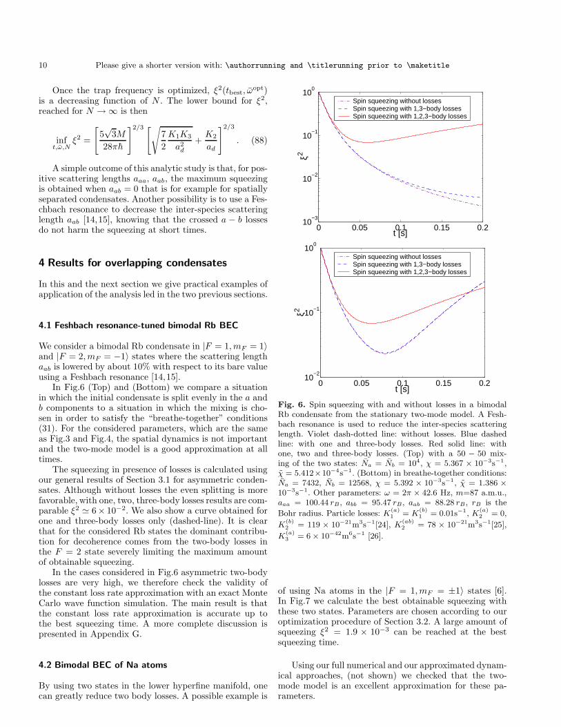
4.1 Feshbach resonance-tuned bimodal Rb BEC
We consider a bimodal Rb condensate in |F = 1,mF = 1〉and |F = 2,mF = −1〉 states where the scattering lengthaab is lowered by about 10% with respect to its bare valueusing a Feshbach resonance [14,15].
In Fig.6 (Top) and (Bottom) we compare a situationin which the initial condensate is split evenly in the a andb components to a situation in which the mixing is cho-sen in order to satisfy the “breathe-together” conditions(31). For the considered parameters, which are the sameas Fig.3 and Fig.4, the spatial dynamics is not importantand the two-mode model is a good approximation at alltimes.
The squeezing in presence of losses is calculated usingour general results of Section 3.1 for asymmetric conden-sates. Although without losses the even splitting is morefavorable, with one, two, three-body losses results are com-parable ξ2 ≃ 6× 10⁻². We also show a curve obtained forone and three-body losses only (dashed-line). It is clearthat for the considered Rb states the dominant contribu-tion for decoherence comes from the two-body losses inthe F = 2 state severely limiting the maximum amountof obtainable squeezing.
In the cases considered in Fig.6 asymmetric two-bodylosses are very high, we therefore check the validity ofthe constant loss rate approximation with an exact MonteCarlo wave function simulation. The main result is thatthe constant loss rate approximation is accurate up tothe best squeezing time. A more complete discussion ispresented in Appendix G.
4.2 Bimodal BEC of Na atoms
By using two states in the lower hyperfine manifold, onecan greatly reduce two body losses. A possible example is
0 0.05 0.1 0.15 0.210
−3
10−2
10−1
100
t [s]
ξ2
Spin squeezing without lossesSpin squeezing with 1,3−body lossesSpin squeezing with 1,2,3−body losses
0 0.05 0.1 0.15 0.210
−2
10−1
100
t [s]
ξ2
Spin squeezing without lossesSpin squeezing with 1,3−body lossesSpin squeezing with 1,2,3−body losses
Fig. 6. Spin squeezing with and without losses in a bimodalRb condensate from the stationary two-mode model. A Fesh-bach resonance is used to reduce the inter-species scatteringlength. Violet dash-dotted line: without losses. Blue dashedline: with one and three-body losses. Red solid line: withone, two and three-body losses. (Top) with a 50 − 50 mix-ing of the two states: Na = Nb = 104, χ = 5.367 × 10⁻³s−1,χ = 5.412×10⁻⁴s−1. (Bottom) in breathe-together conditions:Na = 7432, Nb = 12568, χ = 5.392 × 10⁻³s−1, χ = 1.386 ×10⁻³s−1. Other parameters: ω = 2π × 42.6 Hz, m=87 a.m.u.,aaa = 100.44 rB, abb = 95.47 rB, aab = 88.28 rB, rB is the
Bohr radius. Particle losses: K(a)1 = K
(b)1 = 0.01s−1, K
(a)2 = 0,
K(b)2 = 119 × 10−21m3s−1[24], K
(ab)2 = 78 × 10−21m3s−1[25],
K(a)3 = 6 × 10−42m6s−1 [26].
of using Na atoms in the |F = 1,mF = ±1〉 states [6].In Fig.7 we calculate the best obtainable squeezing withthese two states. Parameters are chosen according to ouroptimization procedure of Section 3.2. A large amount ofsqueezing ξ2 = 1.9 × 10⁻³ can be reached at the bestsqueezing time.
Using our full numerical and our approximated dynam-ical approaches, (not shown) we checked that the two-mode model is an excellent approximation for these pa-rameters.

Please give a shorter version with: \authorrunning and \titlerunning prior to \maketitle 11
0 0.04 0.08 0.12 0.1610
−4
10−3
10−2
10−1
100
t [s]
ξ2
Spin squeezing without lossesSpin squeezing with 1,3−body losses
Fig. 7. Spin squeezing with and without losses in a bimodal Nacondensate from the stationary two-mode model. Violet dash-dotted line: without losses. Blue dashed line: with one andthree-body losses. Optimized parameters: Na = Nb = 4 × 10⁴
ω = 2π × 183 Hz, m=23 a.m.u., aaa = abb = 51.89 rB, aab =48.25 rB, rB is the Bohr radius. χ = 5.517 × 10⁻³s−1, χ = 0.
Particle losses: K(a)1 = K
(b)1 = 0.01s−1, K
(a)2 = K
(b)2 = 0,
K(a)3 = K
(b)3 = 2 × 10−42m6s−1 [27].
5 Dynamically separated Rb BEC
In this subsection we consider a bimodal Rb condensatein |F = 1,mF = −1〉 and |F = 2,mF = 1〉 states. Ratherthan using a Feshbach resonance to change gab, we con-sider the possibility of suddenly separating the two cloudsright after the mixing π/2 pulse using state-selective po-tentials [28], and recombining them after a well choseninteraction time. A related scheme using Bragg pulses inthe frame of atom interferometry was proposed in [29]. Weconsider disc shaped identical traps for the two states aand b with ωz > ωx,y ≡ ω⊥, that can be displaced inde-pendently along the z axes. In order to minimize center-of-mass excitation of the cloud, we use a triangular rampfor the displacement velocity, as shown in Fig.8 (Bottom),with total move-out time 2τ = 4π/ωz [30]. In Fig.8 (Top)we show the z-dependence of densities of the clouds, in-tegrated in the perpendicular xy plane, as the clouds areseparated and put back together after a given interactiontime.
We use our dynamical modulus-phase model in 3 di-mensions to calculate the spin squeezing in this scheme.As the spatial overlap between the two clouds reducesa lot as they are separated, in Fig.9 we calculate boththe spin squeezing obtained from the definitions (10)-(12)of spin operators (dashed line), and the “extracted spinsqueezing” introduced in Section 2.5 based on the “instan-taneous modes” (42)-(43) (solid line). The oscillations inthe dashed line are due to tiny residual center of mass os-cillations of the clouds that change periodically the smalloverlap between the two modes. They are absent in theextracted spin squeezing curve (solid line) as they do notaffect the spin dynamics. When the clouds are put backtogether and the overlap between the modes is large again,the spin squeezing and the extracted spin squeezing curves
0 4 8 12 16-2
0
2x 10
-3
t [ms]
δz [m
/s]
.
Fig. 8. (Top) |φa(z, t)|2 and |φb(z, t)|2 in arbitrary units as
the clouds are separated and put back together after an inter-action time of about 15 ms. The harmonic potential for thea-component does not move, while that for the b-componentis shifted vertically with a speed δz. The distance between thetwo trap centers when they are separated is δz = 4
p
~/Mωz.
(Bottom) variation in time of δz. Parameters: Na = Nb =5 × 10⁴, ωx,y = 2π × 2.31 Hz, ωz = 2π × 1 kHz, m=87 a.m.u.,aaa = 100.44 rB, abb = 95.47 rB , aab = 98.09 rB , rB is the Bohrradius. No particle losses.
give close results (not identical as the overlap of the twoclouds is not precisely one).
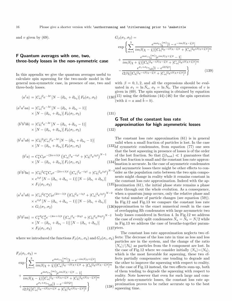
In Fig.10 (Top) we compare the extracted spin squeez-ing curve of Fig.9 (solid line) with a two-mode stationarycalculation (dash-dotted line) assuming stationary con-densates in separated wells. We notice that the squeezingprogresses much more slowly in the dynamical case. In-deed when we separate the clouds, the mean field changessuddenly for each component exciting a breathing modewhose amplitude and frequency is different for each of theFock states involved. In the quasi 2D configuration con-sidered here, the breathing of the wave functions is welldescribed by a scaling solution in 2D for each condensateseparately [18,19] adapted to the case in which the trapfrequency is not changed, but the mean-field is changedsuddenly after separating the two internal states:
φε(r⊥, t) =e−iηε(t)
Lε(t)eimr2
⊥Lε(t)/2~Lε(t)φ0
(
r⊥
Lε(t)
)
(89)
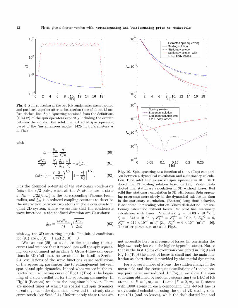
12 Please give a shorter version with: \authorrunning and \titlerunning prior to \maketitle
0 2 4 6 8 10 12 14 16 1810
−2
100
102
104
t [ms]
ξ2
Fig. 9. Spin squeezing as the two Rb condensates are separatedand put back together after an interaction time of about 15 ms.Red dashed line: Spin squeezing obtained from the definitions(10)-(12) of the spin operators explicitly including the overlapbetween the clouds. Blue solid line: extracted spin squeezingbased of the “instantaneous modes” (42)-(43). Parameters asin Fig.8.
with
ηε =gεε
gaa
µ
L2ε~
(90)
d2Lε
dt2=Nε
N
gεε
gaa
ω2⊥
L3ε
− ω2⊥Lε ; (91)
φ0(r⊥) =
(
2
πR20
)1/2 [
1 − r2⊥R2
0
]1/2
. (92)
µ is the chemical potential of the stationary condensatebefore the π/2 pulse, when all the N atoms are in state
a, R0 =√
2µ/mω2⊥ is the corresponding Thomas-Fermi
radius, and gεε is a reduced coupling constant to describethe interaction between two atoms in the ε condensate inquasi 2D system, where we assume that the condensatewave functions in the confined direction are Gaussians:
gεε =4π~
2aεε
M
√
Mωz
2π~(93)
with aεε the 3D scattering length. The initial conditionsfor (91) are Lε(0) = 1 and Lε(0) = 0.
We can use (89) to calculate the squeezing (dottedcurve) and we note that it reproduces well the spin squeez-ing curve obtained integrating 5 Gross-Pitaevskii equa-tions in 3D (full line). As we studied in detail in Section2.4, oscillations of the wave functions cause oscillationsof the squeezing parameter due to entanglement betweenspatial and spin dynamics. Indeed what we see in the ex-tracted spin squeezing curve of Fig.10 (Top) is the begin-ning of a slow oscillation for the squeezing parameter. InFig.10 (Bottom) we show the long time behavior. Thereare indeed times at which the spatial and spin dynamicsdisentangle, and the dynamical curve and the steady statecurve touch (see Sect. 2.4). Unfortunately these times are
0 2 4 6 8 10 12 14 16 1810
−2
10−1
100
t [ms]
ξ2
Extracted spin squeezingScaling solutionStationary solutionStationary solution with1,2,3−body losses
0 0.05 0.1 0.15 0.2 0.2510
−4
10−3
10−2
10−1
100
t [s]
ξ2
Scaling solutionStationary solutionStationary solution with1,2,3−body losses
Fig. 10. Spin squeezing as a function of time. (Top) compari-son between a dynamical calculation and a stationary calcula-tion. Blue solid line: extracted spin squeezing in 3D. Blackdoted line: 2D scaling solution based on (91). Violet dash-dotted line: stationary calculation in 3D without losses. Redsolid line: stationary calculation in 3D with losses. Spin squeez-ing progresses more slowly in the dynamical calculation thanin the stationary calculation. (Bottom) long time behavior.Black doted line: scaling solution. Violet dash-dotted line: sta-tionary calculation without losses. Red solid line: stationarycalculation with losses. Parameters: χ = 5.003 × 10⁻³s−1,
χ = 1.342 × 10⁻⁴s−1, K(a)1 = K
(b)1 = 0.01s−1 , K
(a)2 = 0,
K(b)2 = 119 × 10−21m3s−1[24], K
(a)3 = 6 × 10−42m6s−1 [26].
The other parameters are as in Fig.8.
not accessible here in presence of losses (in particular thehigh two-body losses in the higher hyperfine state). Noticethat in the first 15 ms of evolution considered in Fig.9 andFig.10 (Top) the effect of losses is small and the main lim-itation at short times is provided by the spatial dynamics.
For a lower number of atoms, the sudden change in themean field and the consequent oscillations of the squeez-ing parameter are reduced. In Fig.11 we show the spinsqueezing obtained by suddenly separating two BEC of Rbatoms in |F = 1,mF = −1〉 and |F = 2,mF = 1〉 stateswith 1000 atoms in each component. The dotted line isa dynamical calculation using the quasi 2D scaling solu-tion (91) (and no losses), while the dash-dotted line and

Please give a shorter version with: \authorrunning and \titlerunning prior to \maketitle 13
0 0.01 0.02 0.03 0.0410
−3
10−2
10−1
100
t [s]
ξ2
Scaling solutionStationary solutionStationary solution with1,2,3−body losses
Fig. 11. Spin squeezing as a function of time in two smallRb condensates. Black doted line: scaling solution based on(91). Violet dash-dotted line: stationary calculation withoutlosses. Red solid line: stationary calculation with losses. Pa-
rameters: K(a)1 = K
(b)1 = 0.01s−1, K
(a)2 = 0, K
(b)2 = 119 ×
10−21m3s−1[24],K(a)3 = 6×10−42m6s−1 [26]. The other param-
eters: Na = Nb = 103, ωx,y = 2π× 11.82 Hz, ωz = 2π× 2 kHz,m=87 a.m.u., aaa = 100.44 rB, abb = 95.47 rB, aab = 98.09 rB ,rB is the Bohr radius. χ = 0.213s−1 , χ = 2.763 × 10⁻³s−1.
the solid line are stationary calculations without and withlosses respectively. Note that around t = 0.02s, where thedynamical curve and the stationary curve touch, a squeez-ing of about ξ2 ∼ 2 × 10⁻² could be reached despite thehigh losses in the F = 2 state [31].
6 Conclusions
In conclusion we developed a method to study the en-tangled spatial and spin dynamics in binary mixtures ofBose-Einstein condensates. The method, which is the nat-ural extension of our work [9] to the case of spin squeezing,allows a full analytical treatment in some cases and canbe used in the general case to study a priori complicatedsituations in 3D without the need of heavy numerics. In-cluding the effect of particle losses and spatial dynamics,we have calculated the maximum squeezing obtainable ina bimodal condensate of Na atoms in |F = 1,mF = ±1〉states when the two condensates overlap in space, and wehave calculated the squeezing in a bimodal Rb conden-sate in which a Feshbach resonance is used to reduce theinter-species scattering length as recently realized experi-mentally [15]. For Rb we also propose an original schemein which the two components are spatially separated us-ing state-dependent potentials, recently realized for the|F = 1,mF = −1〉 and |F = 2,mF = 1〉 states, and thenrecombined after a well chosen squeezing time. With thismethod we show that ξ2 ∼ 2 × 10⁻² could be reachedin condensates of 1000 atoms, despite the high two-bodylosses in the higher hyperfine state.
Yun Li acknowledges support from the ENS-ECNUprogram, and A.S. acknowledges stimulating discussions
with M. Oberthaler, J. Esteve and K. Mølmer. Our groupis a member of IFRAF.
A Quantum averages of the field operators
Using equations (20)-(21), the averages needed to calcu-late squeezing parameter can be written in terms of thewave functions φa, φb and the phase factor A solution ofequation (9):
〈ψ†b(r)ψa(r)〉
=
N∑
Na=1
N !
(Na − 1)!Nb!|Ca|2(Na−1)|Cb|2NbC∗
bCa
×φ∗b(Na − 1, Nb + 1, r)φa(Na, Nb, r)
× expi[A(Na − 1, Nb + 1) −A(Na, Nb)]/~×[〈φa(Na − 1, Nb + 1)|φa(Na, Nb)〉]Na−1
×[〈φb(Na − 1, Nb + 1)|φb(Na, Nb)〉]Nb . (94)
〈ψ†b(r)ψ†
a(r′)ψa(r)ψb(r′)〉
=
N−1∑
Na=1
N !
(Na − 1)!(Nb − 1)!|Ca|2Na |Cb|2Nb
×φ∗b(Na, Nb, r)φ∗a(Na, Nb, r′)φa(Na, Nb, r)
×φb(Na, Nb, r′) . (95)
〈ψ†b(r)ψ†
b(r′)ψa(r)ψa(r′)〉
=
N∑
Na=2
N !
(Na − 2)!Nb!|Ca|2(Na−2)|Cb|2NbC∗2
b C2a
×φ∗b (Na − 2, Nb + 2, r)φ∗b (Na − 2, Nb + 2, r′)
×φa(Na, Nb, r)φa(Na, Nb, r′)
× expi[A(Na − 2, Nb + 2) −A(Na, Nb)]/~×[〈φa(Na − 2, Nb + 2)|φa(Na, Nb)〉]Na−2
×[〈φb(Na − 2, Nb + 2)|φb(Na, Nb)〉]Nb . (96)
〈ψ†b(r)ψ†
b(r′)ψb(r)ψa(r′)〉
=
N−1∑
Na=1
N !
(Na − 1)!(Nb − 1)!|Ca|2(Na−1)|Cb|2NbC∗
bCa
×φ∗b(Na − 1, Nb + 1, r)φ∗b (Na − 1, Nb + 1, r′)
×φb(Na, Nb, r)φa(Na, Nb, r′)
× expi[A(Na − 1, Nb + 1) −A(Na, Nb)]/~×[〈φa(Na − 1, Nb + 1)|φa(Na, Nb)〉]Na−1
×[〈φb(Na − 1, Nb + 1)|φb(Na, Nb)〉]Nb−1 . (97)

14 Please give a shorter version with: \authorrunning and \titlerunning prior to \maketitle
〈ψ†a(r)ψ†
a(r′)ψa(r)ψb(r′)〉
=
N−1∑
Na=1
N !
(Na − 1)!(Nb − 1)!|Ca|2Na |Cb|2(Nb−1)C∗
aCb
×φ∗a(Na + 1, Nb − 1, r)φ∗a(Na + 1, Nb − 1, r′)
×φa(Na, Nb, r)φb(Na, Nb, r′)
× expi[A(Na + 1, Nb − 1) −A(Na, Nb)]/~×[〈φa(Na + 1, Nb − 1)|φa(Na, Nb)〉]Na−1
×[〈φb(Na + 1, Nb − 1)|φb(Na, Nb)〉]Nb−1 . (98)
We use these averages to calculate the squeezing in our fulldynamical model. In practice we do not sum over all theFock states but over a “large enough width” (typically
> 6√N) around the average number of atoms Na, Nb.
The spin squeezing is obtained by equation (15) using thedefinitions (10)-(12) for the spin operators.
B Quantum averages in the modulus-phase
approach
Within the modulus-phase approximation, the scalar prod-uct of the wave vectors can be written as
〈φa(Na − β,Nb + β)|φa(Na, Nb)〉= expiβ
∫
d3r|φa(r)|2[χ0(r) + χd(r)] (99)
〈φb(Na − β,Nb + β)|φb(Na, Nb)〉= expiβ
∫
d3r|φb(r)|2[χ0(r) − χd(r)] (100)
〈φb(Na − β,Nb + β)|φa(Na, Nb)〉=
∫
d3rφ∗b (r)φa(r) exp[i(Na − β)χd(r) − iNbχd(r)]
× exp[i(N − N)χs(r) − iN(|Ca|2 − |Cb|2)χd(r)]
× exp[iβχ0(r)] (101)
〈φa(Na + β,Nb − β)|φb(Na, Nb)〉=
∫
d3rφ∗a(r)φb(r) exp[−iNaχd(r) + i(Nb − β)χd(r)]
× exp[−i(N − N)χs(r) − iN(|Ca|2 − |Cb|2)χd(r)]
× exp[−iβχ0(r)] (102)
where β ∈ Z, and we have used the relation
∫
d3r|φε|2 exp[i(∂Na− ∂Nb
)θε(Na, Nb)]
≃ exp[ i∫
d3r|φε|2(∂Na− ∂Nb
)θε(Na, Nb)] . (103)
By using the Gross-Pitaevskii equations (7) for φε(Na, Nb)and for φε(Na, Nb), one obtains
i~∂t
[
(Na − Na)∂θε
∂Na+ (Nb − Nb)
∂θε
∂Nb
]
Na,Nb
= (Nε − Nε)gεε|φε|2 + (Nε′ − Nε′)gεε′ |φε′ |2 , (104)
where ε 6= ε′ = a, b. Using (104) together with the initialcondition (8), we obtain for the phase factor A in Eq. (9)
[A(Na − 1, Nb + 1) −A(Na, Nb)]/~
= −(Na − 1)∫
d3r|φa(r)|2[χ0(r) + χd(r)]
−Nb
∫
d3r|φb(r)|2[χ0(r) − χd(r)] (105)
[A(Na − 2, Nb + 2) −A(Na, Nb)]/~
= −2(Na − 2)∫
d3r|φa(r)|2[χ0(r) + χd(r)]
−2Nb
∫
d3r|φb(r)|2[χ0(r) − χd(r)]
−∫
d3r|φa(r)|2[χ0(r) + χd(r)]
+|φb(r)|2[χ0(r) − χd(r)] (106)
The averages and variances of the spin operators equa-tions (10)-(12) are obtained by equations (94)-(98) afterspatial integration. We get:
∫
d3r〈ψ†b(r)ψa(r)〉
= NC∗bCa
∫
d3rφ∗b (r)φa(r)[|Ca|2eiχd(r) + |Cb|2e−iχd(r)]N−1
× exp[i(N − N)χs(r)] exp[−iN(|Ca|2 − |Cb|2)χd(r)]
× exp[iχ0(r)] . (107)
∫
d3rd3r′〈ψ†b(r)ψ†
a(r′)ψa(r)ψb(r′)〉
= N(N − 1)|Ca|2|Cb|2∫
d3rd3r′φ∗b(r)φa(r)φ∗a(r′)φb(r′) .
(108)∫
d3rd3r′〈ψ†b(r)ψ†
b(r′)ψa(r)ψa(r′)〉
= N(N − 1)C∗2b C2
a
∫
d3rd3r′φ∗b(r)φa(r)φ∗b (r′)φa(r′)
×[|Ca|2eiχd(r)+iχd(r′) + |Cb|2e−iχd(r)−iχd(r′)]N−2
× exp−iN(|Ca|2 − |Cb|2)[χd(r) + χd(r′)] exp2i[χ0(r)
+χ0(r′)] expi(N − N)[χs(r) + χs(r
′)]× exp−i
∫
d3r′′(|φa|2[χ0(r′′) + χd(r
′′)]
+|φb|2[χ0(r′′) − χd(r
′′)]) . (109)
∫
d3rd3r′〈ψ†b(r)ψ†
b(r′)ψb(r)ψa(r′)〉
= N(N − 1)C∗bCa|Cb|2
∫
d3r′φ∗b(r′)φa(r′)[|Ca|2eiχd(r′)
+|Cb|2e−iχd(r′)]N−2 exp[−iN(|Ca|2 − |Cb|2)χd(r′)]
× exp[iχ0(r′) − iχd(r
′)] exp[i(N − N)χs(r′)] . (110)
∫
d3rd3r′〈ψ†a(r)ψ†
a(r′)ψa(r)ψb(r′)〉
= N(N − 1)C∗aCb|Ca|2
∫
d3r′φ∗a(r′)φb(r′)[|Ca|2e−iχd(r′)
+|Cb|2eiχd(r′)]N−2 exp[iN(|Ca|2 − |Cb|2)χd(r′)]
× exp[−iχ0(r′) − iχd(r
′)] exp[−i(N − N)χs(r′)] . (111)
In the above expressions χd, χs and χ0 are the space andtime dependent functions defined in equations (24), (25)and (26). In practice it is sufficient to evolve five wavefunctions φa(r, t), φb(r, t) for (Na, Nb ± δNb) and (Na ±δNa, Nb) with δNa,b 6= 0 (to calculate numerically χd χs
χ0), and with δNa,b = 0 (to calculate the central wavefunctions φa,b). The spin squeezing is obtained by equation(15) using the definitions (10)-(12) for the spin operators.

Please give a shorter version with: \authorrunning and \titlerunning prior to \maketitle 15
C Equality of χs
and χ0 in the
breathe-together configuration
Evaluating (104) for ε = a, Na = Na; ε = b, Nb = Nb andsubtracting the two relations, on obtains
∂t
( ¯∂θa
∂Nb−
¯∂θb
∂Na
)
= 0 (112)
where we used the fact that in breathe-together conditions|φa| = |φb|. Equation (112) implies that the time deriva-tive of χs − χ0 is zero. As for t = 0 χs = χ0 = 0, weconclude that χs = χ0 at all times.
D Extracted spin squeezing quantum
averages
By using the instantaneous modes (42)-(43) and withinthe modulus-phase approach, the quantum averages usefulto calculate spin squeezing are expressed in terms of thefunctions:
χexd (r, r′) =
1
2(∂Na
− ∂Nb)[θa(r) − θb(r
′)](Na, Nb) (113)
χexs (r, r′) =
1
2(∂Na
+ ∂Nb)[θa(r) − θb(r
′)](Na, Nb) (114)
χex0 (r, r′) =
1
2(∂Na
− ∂Nb)[θa(r) + θb(r
′)](Na, Nb) .(115)
We obtain:
〈b†a〉 = NC∗bCa
∫
d3r1d3r2|φb(r1)|2|φa(r2)|2
×[|Ca|2eiχex
d (r2,r1) + |Cb|2e−iχex
d (r2,r1)]N−1
× exp[i(N − N)χexs (r2, r1) + iχex
0 (r2, r1)]
× exp[−iN(|Ca|2 − |Cb|2)χexd (r2, r1)] (116)
〈b†a†ab〉 = N(N − 1)|Ca|2|Cb|2 (117)
〈b†b†aa〉 = N(N − 1)C∗2b C2
a
∫
d3r1d3r2d
3r3d3r4
×|φb(r1)|2|φb(r2)|2|φa(r3)|2|φa(r4)|2
×|Ca|2ei[χex
d (r4,r2)+χex
d (r3,r1)]
+|Cb|2e−i[χex
d (r4,r2)+χex
d (r3,r1)]N−2
× exp2i[χex0 (r4, r2) + χex
0 (r3, r1)]× exp−iN(|Ca|2 − |Cb|2)[χex
d (r4, r2) + χexd (r3, r1)]
× expi(N − N)[χexs (r4, r2) + χex
s (r3, r1)]× exp−i
∫
d3r5(|φa(r5)|2[χex0 (r5, r5) + χex
d (r5, r5)]
+|φb(r5)|2[χex0 (r5, r5) − χex
d (r5, r5)]) (118)
〈b†b†ba〉 = N(N − 1)C∗bCa|Cb|2
∫
d3r1d3r2|φb(r1)|2|φa(r2)|2
×[|Ca|2eiχex
d (r2,r1) + |Cb|2e−iχex
d (r2,r1)]N−2
× exp[iχex0 (r2, r1) − iχex
d (r2, r1)]
× exp[−iN(|Ca|2 − |Cb|2)χexd (r2, r1)]
× exp[i(N − N)χexs (r2, r1)] (119)
〈a†a†ab〉 = N(N − 1)C∗aCb|Ca|2
∫
d3r1d3r2|φa(r1)|2|φb(r2)|2
×[|Cb|2eiχex
d (r1,r2) + |Ca|2e−iχex
d (r1,r2)]N−2
× exp[−iχex0 (r1, r2) − iχex
d (r1, r2)]
× exp[iN(|Ca|2 − |Cb|2)χexd (r1, r2)]
× exp[−i(N − N)χexs (r1, r2)] (120)
In case the wave functions φa, φb are stationary we re-cover the stationary two-mode model averages given inthe next appendix in the particular case of no losses. Thespin squeezing is obtained by equation (15) using the def-initions (44)-(46) for the spin operators.
E Quantum averages with one-body losses:
Exact solution in the non symmetric case
In this appendix we give the exact result for quantumaverages needed to calculate spin squeezing in the caseof a two-mode model with one-body losses only, in thegeneral non-symmetric case.
〈a†a〉 = |Ca|2N exp(−γat) (121)
〈a†a†aa〉 = |Ca|4N(N − 1) exp(−2γat) (122)
〈b†b†bb〉 = |Cb|4N(N − 1) exp(−2γbt) (123)
〈b†a†ab〉 = |Cb|2|Ca|2N(N − 1) exp[−(γa + γb)t] (124)
〈b†a〉 = C∗bCbe
−2ivtN exp
[
−1
2(γa + γb)t
]
LN−11 (125)
〈b†b†ba〉 = |Cb|2C∗bCae
−2ivtN(N − 1)eiχt
× exp
[
−1
2(γa + 3γb)t
]
LN−21 (126)
〈a†a†ab〉 = |Ca|2C∗aCbe
2ivtN(N − 1)eiχt
× exp
[
−1
2(3γa + γb)t
]
LN−2−1 (127)
〈b†b†aa〉 = C∗2b C2
ae−4ivtN(N − 1)
× exp [−(γa + γb)t]LN−22 (128)
where we introduced the function Lβ with β = −1, 1, 2
Lβ =|Ca|2
γa + iβ(χ+ χ)
[
γaeiβχt + iβ(χ+ χ)e−(γa+iβχ)t
]
+|Cb|2
γb − iβ(χ− χ)
[
γbeiβχt − iβ(χ− χ)e−(γb−iβχ)t
]
(129)
16 Please give a shorter version with: \authorrunning and \titlerunning prior to \maketitle
and v given by (69).
F Quantum averages with one, two,
three-body losses in the non-symmetric case
In this appendix we give the quantum averages useful tocalculate spin squeezing for the two-mode model in thegeneral non-symmetric case, in presence of one, two andthree-body losses.
〈a†a〉 = |Ca|2e−λt [N − (∂σ1+ ∂σ2
)]F0(σ1, σ2) (130)
〈a†a†aa〉 = |Ca|4e−λt [N − (∂σ1+ ∂σ2
− 1)]
× [N − (∂σ1+ ∂σ2
)]F0(σ1, σ2) (131)
〈b†b†bb〉 = |Cb|4e−λt [N − (∂σ1+ ∂σ2
− 1)]
× [N − (∂σ1+ ∂σ2
)]F0(σ1, σ2) (132)
〈b†a†ab〉 = |Cb|2|Ca|2e−λt [N − (∂σ1+ ∂σ2
− 1)]
× [N − (∂σ1+ ∂σ2
)]F0(σ1, σ2) (133)
〈b†a〉 = C∗bCbe
−(2iv+λ)t(
|Ca|2e−iχt + |Cb|2eiχt)N−1
× [N − (∂σ1+ ∂σ2
)]F1(σ1, σ2) (134)
〈b†b†ba〉 = |Cb|2C∗bCae
−(2iv+λ)t(
|Ca|2e−iχt + |Cb|2eiχt)N−2
× eiχt [N − (∂σ1+ ∂σ2
− 1)] [N − (∂σ1+ ∂σ2
)]
× F1(σ1, σ2) (135)
〈a†a†ab〉 = |Ca|2C∗aCbe
(2iv−λ)t(
|Cb|2e−iχt + |Ca|2eiχt)N−2
× eiχt [N − (∂σ1+ ∂σ2
− 1)] [N − (∂σ1+ ∂σ2
)]
× G1(σ1, σ2) (136)
〈b†b†aa〉 = C∗2b C2
ae−(4iv+λ)t
(
|Ca|2e−2iχt + |Cb|2e2iχt)N−2
× [N − (∂σ1+ ∂σ2
− 1)] [N − (∂σ1+ ∂σ2
)]
× F2(σ1, σ2) (137)
where we introduced the functions Fβ(σ1, σ2) andGβ(σ1, σ2)
Fβ(σ1, σ2) =
exp
3∑
m=1
emσ1γ(m)a [1 − e−imβ(χ+χ)t]
imβ(χ+ χ)[|Ca|2e−iβ(χ+χ)t + |Cb|2eiβ(χ−χ)t]m
+emσ2γ
(m)b [eimβ(χ−χ)t − 1]
imβ(χ− χ)[|Ca|2e−iβ(χ+χ)t + |Cb|2eiβ(χ−χ)t]m
+eσ1+σ2γab[1 − e−i2βχt]
i2βχ[|Ca|2e−iβ(χ+χ)t + |Cb|2eiβ(χ−χ)t]2
(138)
Gβ(σ1, σ2) =
exp
3∑
m=1
emσ2γ(m)b [1 − e−imβ(χ−χ)t]
imβ(χ− χ)[|Cb|2e−iβ(χ−χ)t + |Ca|2eiβ(χ+χ)t]m
+emσ1γ
(m)a [eimβ(χ+χ)t − 1]
imβ(χ+ χ)[|Cb|2e−iβ(χ−χ)t + |Ca|2eiβ(χ+χ)t]m
− eσ1+σ2γab[1 − ei2βχt]
i2βχ[|Cb|2e−iβ(χ−χ)t + |Ca|2eiβ(χ+χ)t]2
(139)
with β = 0, 1, 2, and all the expressions should be eval-uated in σ1 = ln Na, σ2 = ln Nb. The expression of v isgiven in (69). The spin squeezing is obtained by equation(15) using the definitions (44)-(46) for the spin operators
(with a = a and b = b).
G Test of the constant loss rate
approximation for high asymmetric losses
The constant loss rate approximation (61) is in generalvalid when a small fraction of particles is lost. In the caseof symmetric condensates, from equation (77) one seesthat the best squeezing in presence of losses is of the orderof the lost fraction. So that ξ(tbest) ≪ 1 guarantees thatthe lost fraction is small and the constant loss rate approx-imation is accurate. In the case of asymmetric condensatesand asymmetric losses there might be other effects to con-sider as the population ratio between the two spin compo-nents might change in reality while it remains constant inthe constant loss rate approximation. Indeed with the ap-proximation (61), the initial phase state remains a phasestate through out the whole evolution. As a consequence,when a quantum jump occurs, only the relative phase andthe total number of particle changes (see equation (59)).In Fig.12 and Fig.13 we compare the constant loss rateapproximation to the exact numerical result in the caseof overlapping Rb condensates with large asymmetric twobody losses considered in Section 4. In Fig.12 we addressthe case of evenly split condensates Na = Nb = N/2 whilein Fig.13 we address the case of breathe-together param-eters.
The constant loss rate approximation neglects two ef-fects: The decrease of the loss rate in time as less and lessparticles are in the system, and the change of the ratio〈Na〉/〈Nb〉 as particles from the b component are lost. Inthe case of Fig.12 where we consider initially 〈Na〉=〈Nb〉,which is the most favorable for squeezing, these two ef-fects partially compensates: one tending to degrade andthe other to improve the squeezing with respect to reality.In the case of Fig.13 instead, the two effects sum-up, bothof them tending to degrade the squeezing with respect toreality. Note however that even for such large and com-pletely non-symmetric losses, the constant loss rate ap-proximation proves to be rather accurate up to the bestsqueezing time.

Please give a shorter version with: \authorrunning and \titlerunning prior to \maketitle 17
0 0.05 0.1 0.15 0.210
−2
10−1
100
t [s]
ξ2
Approximate analytical solutionFull numerical simulation
0 0.05 0.1 0.15 0.21.6
1.8
2x 10⁴
Nto
t
0 0.05 0.1 0.15 0.2−1
0
1x 10⁴
t [s]
(Na−
Nb)/
2
Fig. 12. (Top) Spin squeezing with two-body losses in a bi-modal Rb condensate as a function of time for symmetricallysplit condensates. Blue solid line: exact numerical simulationwith 4000 realizations. Red dash-dotted line: analytical solu-tion with constant loss rate approximation. (Bottom) Corre-sponding total number of particles and 〈Sz〉 as a function oftime. Parameters: Na = Nb = 104, ω = 2π × 42.6 Hz, m=87a.m.u., aaa = 100.44 rB, abb = 95.47 rB, aab = 88.28 rB , rB isthe Bohr radius, χ = 5.367×10⁻³s−1, χ = 5.412×10⁻⁴s−1, v =
13.758 s−1. Particle losses: K(a)2 = 0, K
(b)2 = 119×10−21m3s−1.
References
1. M. Kitagawa and M. Ueda, Phys. Rev. A 47, 5138 (1993).2. J. Hald, J. L. Sørensen, C. Schori, and E. S. Polzik, Phys.
Rev. Lett. 83, 1319 (1999); A. Kuzmich, L. Mandel, andN. P. Bigelow, Phys. Rev. Lett. 85, 1594 (2000).
3. D. J. Wineland, J. J. Bollinger, W. M. Itano, and D. J.Heinzen, Phys. Rev. A 50, 67 (1994).
4. D. Leibfried, M. D. Barrett, T. Schaetz, J. Britton, J. Chi-averini, W. M. Itano, J. D. Jost, C. Langer, D. J. WinelandScience 304, 1476 (2004).
5. G. Santarelli, Ph. Laurent, P. Lemonde, A. Clairon, A. G.Mann, S. Chang, and A. N. Luiten, and C. Salomon Phys.Rev. Lett. 82, 4619 (1999).
6. A. Sørensen, L. M. Duan, I. Cirac, and P. Zoller, Nature409, 63 (2001).
7. B. Yurke, D. Stoler, Phys. Rev. Lett. 57, 13 (1986).8. D. S. Hall, M. R. Matthews, J. R. Ensher, C. E. Wieman,
and E. A. Cornell, Phys. Rev. Lett. 81, 1539 (1998).
0 0.05 0.1 0.15 0.210
−2
10−1
100
t [s]
ξ2
Approximate analytical solutionFull numerical simulation
0 0.05 0.1 0.15 0.21.4
1.7
2x 10⁴
Nto
t
0 0.05 0.1 0.15 0.2−1
0
1x 10⁴
t [s]
(Na−
Nb)/
2
Fig. 13. (Top) Spin squeezing with two-body losses in a bi-modal Rb condensate as a function of time in breathe-togetherconfiguration. Blue solid line: exact numerical simulation with4000 realizations. Red dash-dotted line: analytical solutionwith constant loss rate approximation. (Bottom) Correspond-ing total number of particles and 〈Sz〉 as a function of time.Parameters: Na = 7432, Nb = 12568, χ = 5.392 × 10⁻³s−1,χ = 1.386 × 10⁻³s−1, v = 13.850 s−1. The other parametersare the same as in Fig.12.
9. A. Sinatra and Y. Castin, Eur. Phys. J. D 8, 319 (2000).10. A. Sørensen, Phys. Rev. A 65, 043610 (2002).11. S. Thanvanthri, and Z. Dutton, Phys. Rev. A 75, 023618
(2007).12. Y. Li, Y. Castin, and A. Sinatra, Phys. Rev. Lett. 100,
210401 (2008).13. P. Treutlein, P. Hommelhoff, T. Steinmetz, T. W. Hasch,
and J. Reichel, Phys. Rev. Lett. 92, 203005 (2004).14. M. Erhard, H. Schmaljohann, J. Kronjager, K. Bongs, and
K. Sengstock, Phys. Rev. A 69, 032705 (2004).15. A. Widera, S. Trotzky, P. Cheinet, S. Folling, F. Gerbier,
I. Bloch, V. Gritsev, M. D. Lukin, and E. Demler, Phys.Rev. Lett. 100, 140401 (2008).
16. We can write the field operators as ψa(r) = a〈r|, ψb(r) =b〈r| and use the commutation relations:
[a〈r|, a†|φa(Na,Nb)〉] = 〈r|φa(Na, Nb)〉 = φa(Na, Nb, r)
[ b〈r|, b†|φb(Na,Nb)〉 ] = 〈r|φb(Na, Nb)〉 = φb(Na, Nb, r) .
18 Please give a shorter version with: \authorrunning and \titlerunning prior to \maketitle
17. A. Sinatra and Y. Castin, Eur. Phys. J. D 4, 247 (1998)18. Yu. Kagan, E. L. Surkov, and G. V. Shlyapnikov, Phys.
Rev. A 54, R1753 (1996).19. Y. Castin and R. Dum, Phys. Rev. Lett. 77, 5315 (1996).20. S. Stringari, Phys. Rev. Lett. 77, 2360 (1996).21. K. Mølmer, Y. Castin, J. Dalibard, J. Opt. Soc. Am. B 10,
524 (1993); H. J. Carmichael, An Open Systems Approach
to Quantum Optics Springer, (1993).22. A. Sinatra and Y. Castin, Eur. Phys. J. D 4, 247 (1998).23. In the expression (65) of |αk|
2 we replaced N with N con-sistently with the constant loss rate approximation.
24. K. M. Mertes, J. W. Merrill, R. Carretero-Gonzalez, D. J.Frantzeskakis, P. G. Kevrekidis, and D. S. Hall, Phys. Rev.Lett. 99 190402 (2007).
25. As we are pretty far from the Feshbach resonance, we as-sume for the crossed ab two-body loss rate the same valuemeasured in [24] for the |F = 1,mF = −1〉, |F = 2,mF =1〉 states.
26. E. A. Burt, R. W. Ghrist, C. J. Myatt, M. J. Holland, E.A. Cornell, and C. E. Wieman, Phys. Rev. Lett. 79, 337(1997).
27. D. M. Stamper-Kurn, M. R. Andrews, A. P. Chikkatur, S.Inouye, H.-J. Miesner, J. Stenger, and W. Ketterle, Phys.Rev. Lett. 80 2027 (1998).
28. P. Treutlein, T. W. Hasch, J. Reichel, A. Negretti, M. A.Cirone, and T. Calarco Phys. Rev. A 74 022312 (2006).
29. Uffe V. Poulsen and Klaus Mølmer, Phys. Rev. A 65
033613 (2002).30. A. Couvert, T. Kawalec, G. Reinaudi, and D. Guery-
Odelin, arXiv: 0708.4197v1.31. We checked that similar result can be obtained with differ-
ent geometry where we prepare the condensate in a cigarshape and separate them along the longitudinal compo-nent.
Related Documents


![Vocabulario bimodal[1]](https://static.cupdf.com/doc/110x72/55b317ebbb61ebef478b46c4/vocabulario-bimodal1.jpg)


