Spin Qubits for Quantum Information Processing · Chapter 14 Spin Qubits for Quantum Information Processing In this chapter we will review the basic principles of manipulating spin

Chapter 14

Spin Qubits for QuantumInformation Processing

In this chapter we will review the basic principles of manipulating spin qubits for quantuminformation processing. The history of spin manipulation (magnetic resonance) techniquesfor nuclear spins and electron spins in solids and liquids was dated back to early 1940s [1].The first nuclear magnetic resonance (NMR) experiments were performed independentlyby E.M. Purcell’s group at Harvard [2] and by F. Bloch’s group at Stanford [3] in 1946.The first electron spin resonance (ESR) experiment was performed by E. Zavoisky in1945 [4]. After those breakthrough experiments, people quickly recognized that the newlydeveloped experimental techniques provide an indispensable ultra-small probe inside solidsand liquids. Today, magnetic resonance techniques have many application areas in physics,chemistry, biology, medicine and engineering [5]. More recently, a single electron spin ora single nuclear spin is expected to play as a robust qubit for quantum computing. Thisis because the quantum state of a spin is relatively stable against external perturbations,compared to other degrees of freedom such as an electric charge.

In particular, an electron spin is suitable for a qubit in quantum processor, because anelectron spin can be manipulated and also can be coupled to other electron spins with amuch shorter time scale than a nuclear spin. On the other hand, a nuclear spin is suitablefor a qubit in quantum memory, because a nuclear spin has a much longer coherencetime than an electron spin. We will describe in this chapter haw to manipulate a singleelectron spin and nuclear spin with an alternating magnetic field and also how to interfacean electron spin and a nuclear spin, i.e. transferring a qubit of information between thetwo, using a hyperfine coupling.

14.1 Simple magnetic resonance theory

A nucleus (or electron) possesses a magnetic moment(vector operator),

µ = hγI , (14.1)

where γ is a gyromagnetic ratio and I is a dimension-less angular momentum operator(J = hI is a standard angular momentum operator).

1

A magnetic interaction Hamiltonian for a spin in a dc magnetic field H0 (along z-axis)is

H = −µ · −→k H0 = −hγH0Iz , (14.2)

where −→k is a unit vector along z-axis.The squared total angular momentum I2 and the z-component of the total angular

momentum Iz commute [6]: [I2, Iz

]= 0 . (14.3)

Therefore, a simultaneous eigenstate of I2 and Iz exists and can be defined by

I2|I, m〉 = I(I + 1)|I, m〉 , (14.4)

Iz|I, m〉 = m|I, m〉 . (14.5)

The eigenvalues take I = 12 , 1, 3

2 , · · · and m = I, I − 1, · · · − I, respectively. The eigen-energies corresponding to (14.2) for such eigenstates are given by

E = −hγH0m . (14.6)

Figure 14.1 shows the Zeeman spectrum of the eigen-energies for an electron spin withI = 1/2 and Cu nuclear spin with I = 3

2 . The gyromagnetic ratio γ for an electron spin isnegative so that m = −1/2 state is the ground state as shown in (a), while that of a Cunuclear spin is positive so that m = 3/2 state is the ground state as shown in (b).

(a) (b)(a) (b)

Figure 14.1: The eigen-energies of an electron spin (a) and a Cu nuclear spin (b).

If we apply an alternating magnetic field H1 cosωt along a perpendicular direction, forinstance x-axis, in addition to the static field H0, the new Hamiltonian is

HI = −hγH1 cosωtIx . (14.7)

The x-component Ix of the angular momentum operator is expressed as

Ix =12

(I+ + I−

), (14.8)

where I+ and I− are called a rasing and lowering operator because of the following recursionrelation:

I+|I,m〉 =√

I(I + 1)−m(m + 1)|I, m + 1〉 , (14.9)

2

I−|I,m〉 =√

I(I + 1)−m(m− 1)|I, m− 1〉 . (14.10)

From the above argument, we understand the transverse ac magnetic field H1 cosωt hasthe capability to change the eigenvalue m, if the frequency ω is close to the resonance withthe Zeeman splitting,

ω ' |γ|H0 . (14.11)

The change of the eigenvalue m by ±1, of course, must accompany the absorption oremission of a single photon at frequency ω to satisfy energy conservation law. This is theprinciple of magnetic resonance.

14.2 Gyromagnetic ratio and g-factor

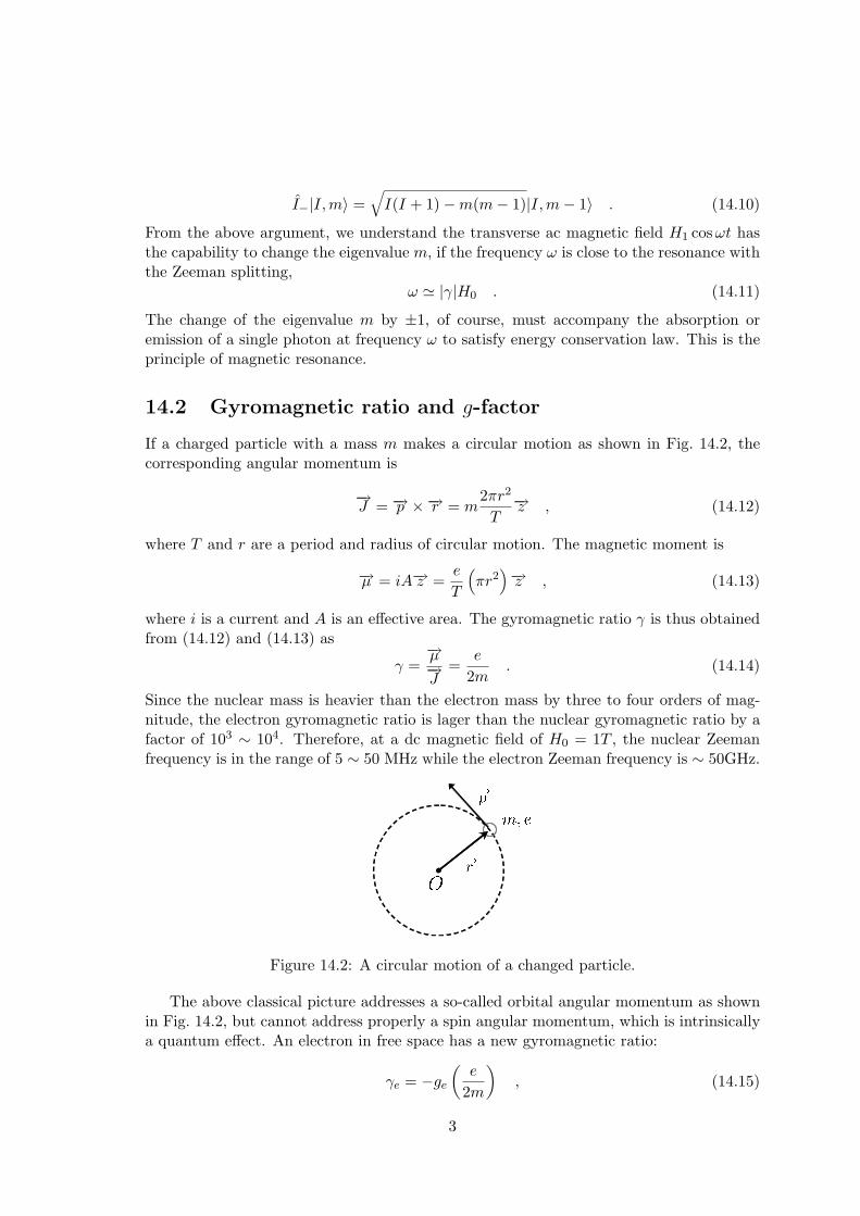
If a charged particle with a mass m makes a circular motion as shown in Fig. 14.2, thecorresponding angular momentum is

−→J = −→p ×−→r = m

2πr2

T−→z , (14.12)

where T and r are a period and radius of circular motion. The magnetic moment is

−→µ = iA−→z =e

T

(πr2

)−→z , (14.13)

where i is a current and A is an effective area. The gyromagnetic ratio γ is thus obtainedfrom (14.12) and (14.13) as

γ =−→µ−→J

=e

2m. (14.14)

Since the nuclear mass is heavier than the electron mass by three to four orders of mag-nitude, the electron gyromagnetic ratio is lager than the nuclear gyromagnetic ratio by afactor of 103 ∼ 104. Therefore, at a dc magnetic field of H0 = 1T , the nuclear Zeemanfrequency is in the range of 5 ∼ 50 MHz while the electron Zeeman frequency is ∼ 50GHz.

Figure 14.2: A circular motion of a changed particle.

The above classical picture addresses a so-called orbital angular momentum as shownin Fig. 14.2, but cannot address properly a spin angular momentum, which is intrinsicallya quantum effect. An electron in free space has a new gyromagnetic ratio:

γe = −ge

(e

2m

), (14.15)

3

where ge = 2.002319 · · · is an electron g-factor [6]. An electron is solids acquires a differentvalue for a g-factor due to the presence of spin-orbit coupling [5, 6]. The gyromagneticratio of a nuclear spin is defined by

µn = gne

2MphI = γnhI , (14.16)

where Mp is a proton mass. The gyromagnetic ratio γn = gne

2Mp(> 0) is independent of

environments and a universal value for a nucleus, because the nuclear wavefunction is sotiny and protected by surrounding valence electrons that the environment hardly affectsit.

14.3 Thermal population and saturation

In a magnetic resonance experiment, a spin system continuously absorbs a photon froman alternating magnetic field and dissipates its energy to thermal reservoirs, as shown inFig. 14.3. The steady state (thermal equiliblium) populations of the two spin states, N−and N+, and those of the two reservoir states, Na and Nb, satisfy the detailed balance:

spin system external reservoir

Figure 14.3: Absorption of photon and energy dissipation of a spin system.

N−NbW−b→+a = N+NaW+a→−b , (14.17)

where the two transition matrix elements are identical, since

W−b→+a =2π

h

∣∣∣〈+, a|HI |−, b〉∣∣∣2

(14.18)

=2π

h

∣∣∣〈−, b|HI |+, a〉∣∣∣2

= W+a→−b.

Therefore, the spin population ratio is identical to the reservoir population ratio (Boltzmanfactor) as it should be at thermal equilibrium:

N−N+

=Na

Nb= e−E/kBT . (14.19)

If we begin with a non-thermal population, the transient behavior is descried by thefollowing rate equation:

d

dtN+ = N−W↓ −N+W↑ , (14.20)

4

d

dtN− = N+W↑ −N−W↓ , (14.21)

where W↓ = NbW−b→+a > W↑ = NaW+a→−b. The population difference n = N+ −N− isgoverned by the rate equation:

d

dtn = −n− n0

T1. (14.22)

Here n0 = NW↓−W↑W↓+W↑

is a thermal equilibrium population difference and T1 = (W↓ + W↑)−1

is a spin relaxation time. Equation (14.22) indicates that any departure of n from n0 canbe removed with a time constant T1 due to the coupling of the spin system to externalreservoirs.

The rate equation for photon absorption and emission processes is given by

d

dtN+ = W−→+N− −W+→−N+ , (14.23)

d

dtN− = W+→−N+ −W−→+N− . (14.24)

The two transition matrix elements are also identical with each other, W−→+ = W+→− =W , so that the population difference n is governed by

d

dtn = −2Wn . (14.25)

Equation (14.25) means that the population difference n disappears (population satura-tion) if only absorption and emission of photons from the alternating magnetic field istaken into account and the dissipation to external reservoirs is neglected.

If we combine the two effects, we have a complete rate equation:

d

dtn = −2Wn− n− n0

T1. (14.26)

The steady state solution of the above equation is

n =n0

1 + 2WT1. (14.27)

The energy absorption rate per second is now calculated as

d

dtE = hωnW =

hωn0W

1 + 2WT1=

hωn0W(W ¿ 1

2T1

)

hωn02T1

(W À 1

2T1

) . (14.28)

The energy absorption rate dEdt initially increases with the incident field energy W but

saturates at the value determined by T1 time constant. A short T1 is essential to detect aweak absorption signal.

5

14.4 Manipulation of a single spin

14.4.1 Heisenberg equation of motion

The motion of an isolated spin in a static magnetic field is governed by the ZeemanHamiltonian,

H = −hγH0Iz . (14.29)

Using the commutation relations,[Ix, Iy

]= iIz , (14.30)

[Iy, Iz

]= iIx , (14.31)

[Iz, Ix

]= iIy , (14.32)

we obtain the Heisenberg equations of motion:

d

dtIx =

1ih

[Ix, H

]= γH0Iy , (14.33)

d

dtIy = γH0Ix , (14.34)

d

dtIz = 0 . (14.35)

Combining (14.33), (14.34) and (14.35), we have the famous operator torque equation:

d

dtI = −→

idIx

dt+−→

jdIy

dt+−→

kdIz

dt= γH0I ×−→k , (14.36)

or equivalentlyd

dtµ = γH0µ×−→k , (14.37)

where −→i ,−→j ,−→k are the unit vectors along x, y, z directions and µ = γhI is the magnetic

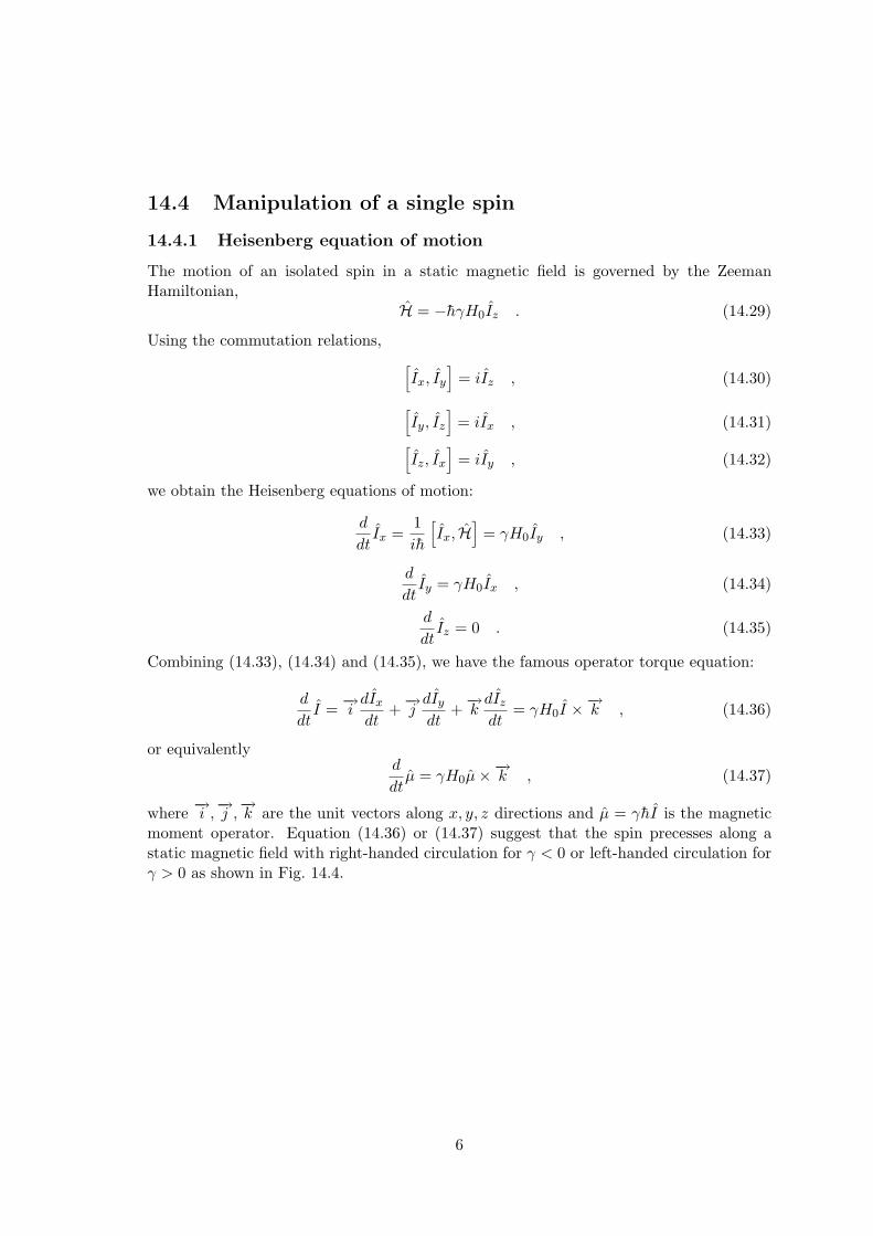
moment operator. Equation (14.36) or (14.37) suggest that the spin precesses along astatic magnetic field with right-handed circulation for γ < 0 or left-handed circulation forγ > 0 as shown in Fig. 14.4.

6

Figure 14.4: Spin precession about a static magnetic field with a Larmor frequency ωL =|γ|H0.

14.4.2 Rotating reference frame

Suppose a fictitious frame (−→i ,−→j ,−→k ) rotates along z-axis (or−→k ) with an angular frequency−→Ω, their dynamics are described by

d

dt

−→i = −→Ω ×−→i , (14.38)

d

dt

−→j = −→Ω ×−→j , (14.39)

d

dt

−→k = −→Ω ×−→k , (14.40)

Then a dynamical variable −→F = −→i Fx +−→

j Fy +−→k Fz follows the equation,

d

dt

−→F = −→

idFx

dt+−→

jdFy

dt+−→

kdFz

dt+ Fx

d−→i

dt+ Fy

d−→j

dt+ Fz

d−→k

dt(14.41)

=∂−→F

∂t+−→Ω ×−→F .

Here d−→Fdt and ∂

−→F∂t are considered as the time rates of change of −→F with respect to a (fixed)

laboratory frame and (rotating) fictitious frame (−→i ,−→j ,−→k ), respectively.

If we substitute −→F = µ in (14.41) and use (14.37), we have

d

dtµ =

∂µ

∂t+−→Ω × µ = γH0µ×−→k . (14.42)

The above result leads to the Heisenberg equation of motion for µ in a rotating frame:

∂µ

∂t= µ×

(γH0

−→k +−→Ω

)(14.43)

= γHeff µ×−→k ,

7

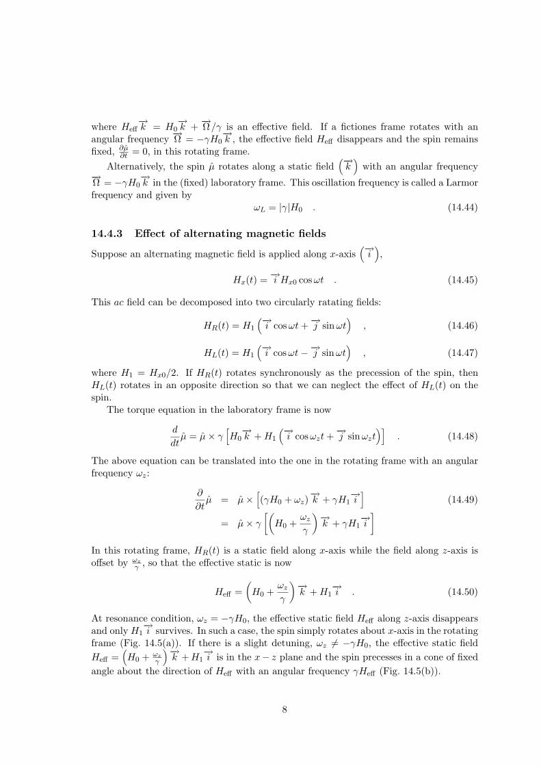
where Heff−→k = H0

−→k + −→Ω/γ is an effective field. If a fictiones frame rotates with an

angular frequency −→Ω = −γH0−→k , the effective field Heff disappears and the spin remains

fixed, ∂µ∂t = 0, in this rotating frame.

Alternatively, the spin µ rotates along a static field(−→

k)

with an angular frequency−→Ω = −γH0

−→k in the (fixed) laboratory frame. This oscillation frequency is called a Larmor

frequency and given byωL = |γ|H0 . (14.44)

14.4.3 Effect of alternating magnetic fields

Suppose an alternating magnetic field is applied along x-axis(−→

i),

Hx(t) = −→i Hx0 cosωt . (14.45)

This ac field can be decomposed into two circularly ratating fields:

HR(t) = H1

(−→i cosωt +−→

j sinωt)

, (14.46)

HL(t) = H1

(−→i cosωt−−→j sinωt

), (14.47)

where H1 = Hx0/2. If HR(t) rotates synchronously as the precession of the spin, thenHL(t) rotates in an opposite direction so that we can neglect the effect of HL(t) on thespin.

The torque equation in the laboratory frame is now

d

dtµ = µ× γ

[H0−→k + H1

(−→i cosωzt +−→

j sinωzt)]

. (14.48)

The above equation can be translated into the one in the rotating frame with an angularfrequency ωz:

∂

∂tµ = µ×

[(γH0 + ωz)

−→k + γH1

−→i

](14.49)

= µ× γ

[(H0 +

ωz

γ

)−→k + γH1

−→i

]

In this rotating frame, HR(t) is a static field along x-axis while the field along z-axis isoffset by ωz

γ , so that the effective static is now

Heff =(

H0 +ωz

γ

)−→k + H1

−→i . (14.50)

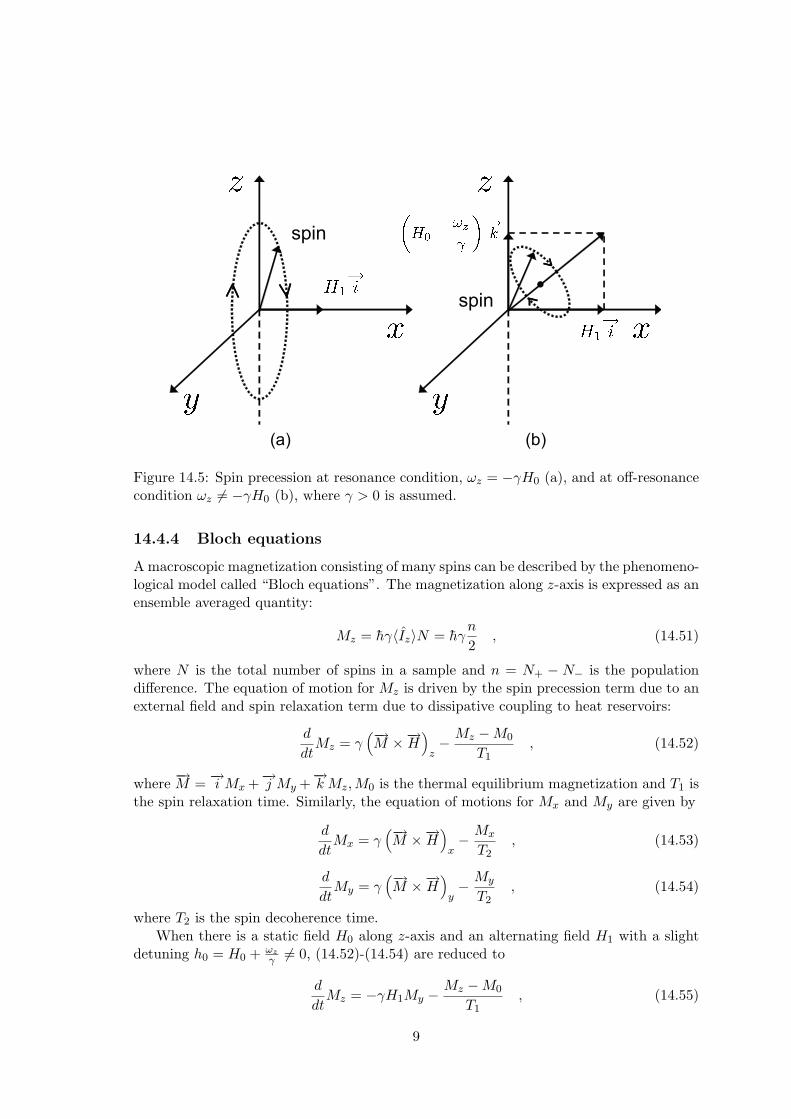
At resonance condition, ωz = −γH0, the effective static field Heff along z-axis disappearsand only H1

−→i survives. In such a case, the spin simply rotates about x-axis in the rotating

frame (Fig. 14.5(a)). If there is a slight detuning, ωz 6= −γH0, the effective static fieldHeff =

(H0 + ωz

γ

)−→k + H1

−→i is in the x− z plane and the spin precesses in a cone of fixed

angle about the direction of Heff with an angular frequency γHeff (Fig. 14.5(b)).

8

spin

spin

(a) (b)

Figure 14.5: Spin precession at resonance condition, ωz = −γH0 (a), and at off-resonancecondition ωz 6= −γH0 (b), where γ > 0 is assumed.

14.4.4 Bloch equations

A macroscopic magnetization consisting of many spins can be described by the phenomeno-logical model called “Bloch equations”. The magnetization along z-axis is expressed as anensemble averaged quantity:

Mz = hγ〈Iz〉N = hγn

2, (14.51)

where N is the total number of spins in a sample and n = N+ − N− is the populationdifference. The equation of motion for Mz is driven by the spin precession term due to anexternal field and spin relaxation term due to dissipative coupling to heat reservoirs:

d

dtMz = γ

(−→M ×−→H

)z− Mz −M0

T1, (14.52)

where −→M = −→i Mx +−→j My +−→k Mz,M0 is the thermal equilibrium magnetization and T1 is

the spin relaxation time. Similarly, the equation of motions for Mx and My are given by

d

dtMx = γ

(−→M ×−→H

)x− Mx

T2, (14.53)

d

dtMy = γ

(−→M ×−→H

)y− My

T2, (14.54)

where T2 is the spin decoherence time.When there is a static field H0 along z-axis and an alternating field H1 with a slight

detuning h0 = H0 + ωzγ 6= 0, (14.52)-(14.54) are reduced to

d

dtMz = −γH1My − Mz −M0

T1, (14.55)

9

d

dtMx = γh0My − Mx

T2, (14.56)

d

dtMy = γH1Mz − γh0Mx − My

T2, (14.57)

in the rotating frame.If H1 is small so that saturation along x-axis is negligible (weak probing case), we have

the approximate solution for Mz:Mz ' M0 . (14.58)

We now introduceM+ = Mx + iMy = hγ〈I+〉N , (14.59)

which satisfies the equation of motion

d

dtM+ = −

(iγh0 +

1T2

)M+ + iγH1M0 . (14.60)

The steady state solution of (14.60) is given by

M+ =γM0

γh0 − i 1T2

H1 . (14.61)

The in-phase and quadrature-phase responses to the small external probe field H1 are nowexpressed as

Mx = χ0ω0T2(ω0 − ω) T2

1 + (ω0 − ω)2 T 22

H1 , (14.62)

My = χ0ω0T21

1 + (ω0 − ω)2 T 22

H1 , (14.63)

where χ0 = M0/H0 is the magnetic susceptibility at dc and ω0 = γH0 is the spin Larmorfrequency. Equations (14.62) and (14.63) represent the linear dispersion and absorptionspectrum for a small external probe field.

14.5 Optical manipulation of semiconductor spin qubits

S.M. Clark et al., PRL 99, 040501 (2007)D. Press et al., Nature 456, 218 (2008)

14.6 Double resonance

14.6.1 Hyperfine interaction

Let us consider a magnetic coupling between two spins, say a nuclear spin and an electronspin, as shown in Fig. 14.6

Suppose a nucleus with a magnetic moment µn at −→r = 0 has a finite radius ρ0, thereexist two kinds of magnetic fields: uniform internal field Hi inside the nucleus and externaldipole field He outside the nucleus, as shown in Fig. 14.7. The continuity of magnetic flux

10

(nuclear spin)

(electron spin)

Figure 14.6: A magnetic coupling between a nuclear spin I and electron spin S.

requires the integrated magnetic fields inside and outside the nucleus exactly cancel witheach other out:

φi (ρ0) + φe (ρ0) = 0. . (14.64)

The internal flux is given byφi (ρ) = πρ2

0Hi , (14.65)

while the external flux is

φe (ρ) = 2π∫ ∞

ρ0

(−µn

r3

)rdr (14.66)

= −µn2π

ρ0.

From (14.64), (14.65) and (14.66), we have the internal field

Hi =2µn

ρ20

. (14.67)

If an electron wavefunction overlaps with a nuclear wavefunction, the effective nuclearmagnetic field which an electron spin feels is given by

Hz = Hi

(43πρ3

0

)|ue(0)|2 , (14.68)

where |ue(0)|2 is the electron density at −→r = 0 and thus(

43πρ3

0

)|ue(0)|2 is the probability

of finding an electron inside the nucleus. The magnetic interaction between the nucleus andthe electron outside the nucleus is identically equal to zero, when the electron wavefunctionspreads isotropically to a much larger space than the nuclear wavefunction, which is thecase for a s-wave symmetry electron wavefunction. Then, the space integration cancelsout exactly due to the continuity of magnetic flux. Form (14.67) and (14.68), the effectiveinteraction Hamiltonian.

H = −µeHz = −8π

3µe · µn|ue(0)|2 (14.69)

=8π

3γeγnh2I · S|ue(0)|2 ,

11

Figure 14.7: The internal and external magnetic fields created by a single nuclear spinwith a magnetic moment µn.

where µe = −hγeS and µn = hγnI are used. The Hamiltonian (14.69) is called a con-tact Hyperfine interaction, which exists only for the case that the electron and nucleuswavefunctions overlap.

If an electron is distant from a nucleus or an electron and a nucleus are co-located butthe electron wavefunction is a p-wave, d-wave or other symmetries with non-zero angularmomentum, the space integration for an external dipole field He is non-zero. We have anew interaction Hamiltonian [6]:

H =µe · µn

r3− 3 (µe · −→r ) (µn · −→r )

rs(14.70)

=γeγn

r3h2

3

(S · −→r

) (I · −→r

)

r2− S · I

,

The Hamiltonian (14.70) has the terms such as −γeγn

r3 h2SxIx and γeγn

r5 h2SxIyxy. If

Ix = 12

(I+ + I−

)and Iy = 1

2i

(I+ − I−

)and similar expressions for Sx and Sy are used

in (14.70) and we introduce a polar coordinate (r, θ, ϕ) as shown in Fig. 14.8, we have thenew expression:

H = −γeγn

r3h2(A + B + C + D + E + F ) , (14.71)

whereA = Sz Iz

(1− 3 cos2 θ

), (14.72)

B = −14

(S+I− + S−I+

) (1− 3 cos2 θ

), (14.73)

C = −32

(S+Iz + Sz I+

)sin θ cos θe−iφ , (14.74)

D = −32

(S−Iz + Sz I−

)sin θ cos θe−iφ , (14.75)

E = −34S+I+ sin2 θe−2iφ , (14.76)

12

F = −34S−I− sin2 θe2iφ . (14.77)

Figure 14.8: A polar coordinate for an electron spin and a nuclear spin.

If there is a strong static field H0 along z-axis, the Zeeman Hamiltonian

Hz = −γnhH0Iz + γehH0Sz , (14.78)

dominates over the hyperfine interaction Hamiltonian. In this case we can solve the Zee-man problem first and then treat the hyperfine coupling as a perturbation. The eigenen-ergy of the unperturbed state is

Ez = −γnhH0mI + γehH0ms , (14.79)

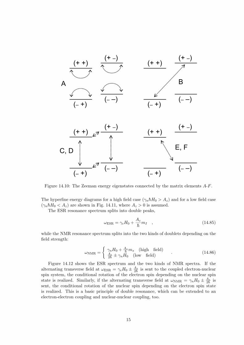
where mI and ms are the eigenvalues of Iz and Sz. The energy level diagram is shownin Fig. 14.9 for mI = ±1/2 and ms = ±1/2. The matrix elements A to F connect theseZeeman eigenstates, as shown in Fig. 14.10

13

(+ +)(+ –)

(– +)(– –)

Figure 14.9: The Zeeman energy level diagram for a pair of nuclear and election spins(mI = ±1/2,ms = ±1/2)

14.6.2 Spin Hamiltonian and hyperfine spectrum

When a nucleus is located at −→r = 0 and an electron wavefunction χ(r) is located at anarbitrary position, both contact and dipolar hyperfine coupling terms are non-negligible,the over-all electron-nuclear interaction Hamiltonian is given by

HIS =∫|ψ(r)|2

8π

3γeγnh2I · Sδ(r) +

γeγn

r3h2 (14.80)

×3

(I · −→r

) (S · −→r

)

r2− I · S

= AxSxIx + AySy Iy + AzSz Iz .

In most cases of interst, the electron Zeeman energy γehH0 is much larger than thehyperfine interaction energy Ax, Ay, Az. Therefore, the z-component of the electron spinoperator commutes with the spin Hamiltonian:

[H, Sz

]' 0. . (14.81)

This fact leads to a reduced spin Hamiltonian

H = γnhH0Iz + γehH0Sz + AzSz Iz . (14.82)

The eigenstates and corresponding eigen-energies of the above Hamiltonian are

|ms〉|mI〉 (ms = ±1/2,mI = ±1/2) , (14.83)

E = −γnhH0mI + γehH0ms + AzmsmI . (14.84)

14

(+ +)

(– +)(– –)

(+ –)

E, F

(+ +)

(– +)(– –)

(+ –)

(+ +)

(– +)(– –)

(+ –)(+ +)

(– +)(– –)

(+ –)

C, D

A B

Figure 14.10: The Zeeman energy eigenstates connected by the matrix elements A-F .

The hyperfine energy diagrams for a high field case (γnhH0 > Az) and for a low field case(γnhH0 < Az) are shown in Fig. 14.11, where Az > 0 is assumed.

The ESR resonance spectrum splits into double peaks,

ωESR = γeH0 +Az

hmI , (14.85)

while the NMR resonance spectrum splits into the two kinds of doublets depending on thefield strength:

ωNMR =

γnH0 + Az

h ms (high field)Az2h ± γnH0 (low field)

. (14.86)

Figure 14.12 shows the ESR spectrum and the two kinds of NMR spectra. If thealternating transverse field at ωESR = γeH0 ± Az

2h is sent to the coupled electron-nuclearspin system, the conditional rotation of the electron spin depending on the nuclear spinstate is realized. Similarly, if the alternating transverse field at ωNMR = γnH0 ± Az

2h issent, the conditional rotation of the nuclear spin depending on the electron spin stateis realized. This is a basic principle of double resonance, which can be extended to anelectron-electron coupling and nuclear-nuclear coupling, too.

15

(+ +)

(– +)

(– –)

(+ –)

(a)

(+ +)

(– +)

(– –)

(+ –)(b)

Figure 14.11: The hyperfine energy diagrams for (a) high field case (γnhH0 > Az) and (b)low field case (γnhH0 < Az) .

14.6.3 Optical control of two semiconductor spins

T.D. Ladd and Y. Yamamoto, arXiv:0910.4988v1 (2009)

16

(a)

(b)

(c)

Figure 14.12: The ESR and two kinds of NMR spectra for a hyperfine coupling electron-nuclear spin system.

17

Bibliography

[1] C.J. Gorter et al., Physica 9, 591 (1942).

[2] E.M. Purcell et al., Phys. Rev. 69, 37 (1946).

[3] F. Bloch et al., Phys. Rev. 69, 127 (1946).

[4] E. Zavoicky, Fiz. Zh 9, 211, 245 (1945).

[5] P. Schlichter, Principles of Magnetic Resonance, Springer, Berlin (1990).

[6] C. Cohen-Tannoudji, B. Diu, and F. Laoe, Quantum Mechanics John Wiley & Sons,New York (1977).

18