Spin networks and quantum gravity

gr-q

c/95

0500

6 4

May

199

5

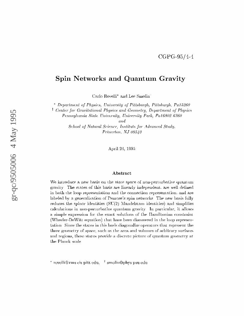
CGPG-95/4-4Spin Networks and Quantum GravityCarlo Rovelli� and Lee Smoliny� Department of Physics, University of Pittsburgh, Pittsburgh, Pa15260y Center for Gravitational Physics and Geometry, Department of PhysicsPennsylvania State University, University Park, Pa16802-6360andSchool of Natural Science, Institute for Advanced Study,Princeton, NJ 08540April 24, 1995AbstractWe introduce a new basis on the state space of non-perturbative quantumgravity. The states of this basis are linearly independent, are well de�nedin both the loop representation and the connection representation, and arelabeled by a generalization of Penrose's spin networks. The new basis fullyreduces the spinor identities (SU(2) Mandelstam identities) and simpli�escalculations in non-perturbative quantum gravity. In particular, it allowsa simple expression for the exact solutions of the Hamiltonian constraint(Wheeler-DeWitt equation) that have been discovered in the loop represen-tation. Since the states in this basis diagonalize operators that represent thethree geometry of space, such as the area and volumes of arbitrary surfacesand regions, these states provide a discrete picture of quantum geometry atthe Planck scale.� [email protected], y [email protected]

1 IntroductionThe loop representation [1, 2] is a formulation of quantum �eld theory suit-able when the degrees of freedom of the theory are given by a gauge �eld,or a connection. This formulation has been used in the context of contin-uum and lattice gauge theory [3], and it has found a particularly e�ectiveapplication in quantum gravity [2, 4], because it allows a description of thedi�eomorphism invariant quantum states in terms of knot theory [2, 5], and,at the same time, because it partially diagonalizes the quantum dynamics ofthe theory, leading to the discovery of solutions of the dynamical constraints[2, 6]. Recent results in quantum gravity based on the loop representationinclude the construction of a �nite physical Hamiltonian operator for puregravity [7] and fermions [8], the computation of the physical spectra of area[9] and volume [10], and the developement of a perturbation scheme thatmay allow transition amplitudes to be explicitely computed [7, 11, 12]. Amathematically rigorous formulation of quantum �eld theories whose con�g-uration space is a space of connections, inspired by the loop representation,has been recently developed [13, 14] and the kinematics of the theory is nowon a level of rigor comparable to that of constructive quantum �eld theory[15]. This approach has also produced interesting mathematical spin-o�'ssuch as the construction of di�eomorphism invariant generalised measureson spaces of connections [14] and could be relevant for a constructive �eldtheory approach to non-abelian Yang-Mills theories.Applications of the loop representation, however, have been burdened bycomplications arising from two technical nuisances. The �rst is given by theMandelstam identities, because of which the loop states are not independentand form an overcomplete basis. The second is the presence of a certain signfactor in the de�nition of the fundamental loop operators T n for n > 1. Thissign depends on the global connectivity of the loops on which the operatoracts and obstructs a simple local graphical description of the operator'saction. In this work, we describe an elegant way to overcome both of thesecomplications. This comes from using a particular basis, which we denoteas spin network basis, since it is related to the spin networks of Penrose [16].The spin network basis has the following properties.� i. It solves the Mandelstam identities.� ii. It allows a simple and entirely local graphical calculus for the T noperators. 2

� iii. It diagonalises the area and volume operators.The spin network basis states, being eigenstates of operators that correspondto measurement of the physical geometry, provide a physical picture of thethree dimensional quantum geometry of space at the Planck-scale level.The main idea behind this construction, long advocated by R. Loll [17],is to identify a basis of independent loop states in which the Mandelstamidentities are completely reduced. We achieve such a result by exploiting thefact that all irreducible representations of SU(2) are built by symmetrizedpowers of the fundamental representation. We will show that in the looprepresentation this translates into the fact that we can suitably antisym-metrize all loops overlapping each other, without loosing generality. Moreprecisely, the (suitably) antisymmetrized loop states span, but do not overspan, the kinematical state space of quantum gravity.The independent basis states constructed in this way turn out to belabelled by Penrose's spin networks [16], and by a direct generalization ofthese. A spin network is a graph whose links are \colored" by integers sat-isfying simple relations at the intersections. Roger Penrose introduced spinnetworks in a context unrelated to the present one; remarkably, however,his aim was to explore a quantum mechanical description of the geometryof space, which is the same ambition that underlies the loop representationconstruction.The idea of using a spin network basis has appeared in other contexts inwhich holonomy of a connection plays a role, including lattice gauge theory,[18, 19] and topological quantum �eld theory [20, 21, 22, 23, 24, 25]. Theuse of this basis in quantum gravity has been suggested previously [26], butits precise implementation had to await resolution of the sign di�cultiesmentioned above. Here, these di�culties are solved by altering a sign inthe relation between the graphical notation of a loop and the correspondingquantum state. This modi�ed graphical notation for the loop states allowsus to reduce the loop states to the independent ones by simply antisym-metrizing overlapping loops.The spin-network construction has already suggested several directionsof investigation, which are being pursued at the present time. The fact thatit diagonalizes the operator that measures the volume of a spatial slice [10]gives us a physical picture of a discrete quantum geometry and also makesthe spin network basis useful for perturbation expansions of the dynamics ofgeneral relativity, as described in [7, 11, 12]. It has also played a role in themathematically rigorous investigations of refs. [15, 27]. Another intriguing3

suggestion is the possibility of considering q deformed spin-networks, onwhich we will comment in the conclusion.The details of the application of the spin network basis to the diagonal-ization of the volume and area operators have been described in an earlierpaper [10]. The primary aim of this paper is to give an introduction tothe spin network basis and to its use in nonperturbative quantum gravity.We emphasize the details of its construction, at a level of detail and rigorthat we hope will be useful for practical calculations in quantum gravity.No claims are made of mathematical rigor; for that we point the reader tothe recent works by Baez [28] and Thiemann [27], where the spin networkbasis is put in a rigorous mathematical context. Finally, we note that in thispaper we work with SL(2; C) (or SU(2)) spinors, which are relevant for theapplication to quantum gravity, but a spin network basis such as the one wedescribe exists for all compact gauge groups [28].This paper is organized as follows. In the next section we brie y explainthe two problems that motivate the use of the spin network basis. This leadsto section 3, in which we provide the de�nition of spin network states in theloop representation. In section 4, we describe the spin network states asthey appear in the connection representation [29]. The proof that the spinnetwork states do form a basis of independent states may then be given insection 5. Following this, in section 6, we review the general structure of thetransformation theory (in the sense of Dirac) between the loop representa-tion and the connection representation. The use of the spin network basisconsiderably simpli�es the transformation theory, as we show here. Simi-larly, old results on the existence of solutions to the hamiltonian constraintand exact physical states of quantum gravity may be expressed in a simplerway in terms of the spin network basis. Its use makes it unnecessary toexplicitly compute the extensions of characteristic states of nonintersectingknots to intersecting loops, as described in [2, 26]1.Finally, an important side result of the analysis above is that it indicateshow to modify the graphical calculus in loop space in order to get rid of theannoying non-locality due to the dependence on global rooting. The newnotation that allows a fully local calculus is de�ned in section 7. The papercloses with a brief summary of the results in section 8, and with a short1These characteristic states were previously de�ned to be equal to one on the knotclass of a non-intersecting loop, zero on all other non-intersecting loops, with an extensionto the classes of intersecting loops de�ned by solving the Mandelstam identities [2, 26].Now they may be succinctly described as being equal to one on one element of the spinnetwork basis and zero on all the others. 4

appendix in which we discuss the details of the construction of higher thantrivalent vertices.2 De�nition of the problemThe loop representation is de�ned by the choice of a basis of bra states h�jon the state space of the quantum �eld theory. These states are labelled byloops �. By a loop, we mean here a set of a �nite number of single loops;by a single loop, we mean a piecewise smooth map from the circle S1 intothe space manifold. The loop basis is characterised (de�ned) by the actionon this basis of a complete algebra of observables [2]. A quantum states j iis represented in this basis by the loop space function (�) = h�j i: (1)For detailed introductions and notation we refer to [26, 29, 30]. As shown in[1, 2], the functions (�) that represent states of the system must satisfy aset of linear relations, which we denote as the Mandelstam relations. Thesecode, among other things, the structure group of the Ashtekar's connection[31] A of the classical theory. Let U�(A) = expR�A be the parallel propa-gator matrix, or holonomy, of the connection A along the curve �, and letT [A;�] = TrU�(A) be its trace. Then the Mandelstam relations are de�ned,for the present purposes, as follows[13]. For every set of loops �1; :::�N andcomplex numbers c1; :::; cN such thatXk ck T [A;�k] = 0 (2)holds for all (smooth) connections A, the states (�) must satisfyXk ck (�k) = 0: (3)It follows that the states of the bra basis h�j are not independent (as linearfunctionals on the ket state space), but satisfy the identitiesXk ckh�kj = 0: (4)The basis h�j is therefore overcomplete. Let us from now on concentrateon the SL(2; C) case. There are two cases of the relation (4) that are5

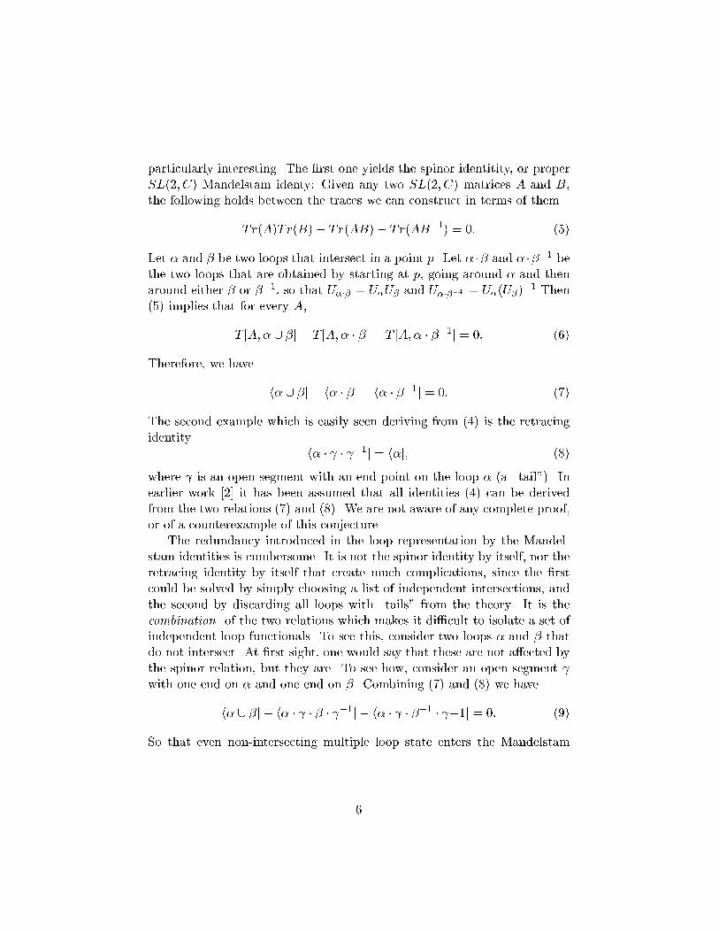
particularly interesting. The �rst one yields the spinor identitity, or properSL(2; C) Mandelstam identy: Given any two SL(2; C) matrices A and B,the following holds between the traces we can construct in terms of them.Tr(A)Tr(B)� Tr(AB)� Tr(AB�1) = 0: (5)Let � and � be two loops that intersect in a point p. Let � �� and � ���1 bethe two loops that are obtained by starting at p, going around � and thenaround either � or ��1, so that U��� = U�U� and U����1 = U�(U�)�1 Then(5) implies that for every A,T [A;� [ �]� T [A;� � �]� T [A;� � ��1] = 0: (6)Therefore, we have h� [ �j � h� � �j � h� � ��1j = 0: (7)The second example which is easily seen deriving from (4) is the retracingidentity h� � � �1j = h�j; (8)where is an open segment with an end point on the loop � (a \tail"). Inearlier work [2] it has been assumed that all identities (4) can be derivedfrom the two relations (7) and (8). We are not aware of any complete proof,or of a counterexample of this conjecture.The redundancy introduced in the loop representation by the Mandel-stam identities is cumbersome. It is not the spinor identity by itself, nor theretracing identity by itself that create much complications, since the �rstcould be solved by simply choosing a list of independent intersections, andthe second by discarding all loops with \tails" from the theory. It is thecombination of the two relations which makes it di�cult to isolate a set ofindependent loop functionals. To see this, consider two loops � and � thatdo not intersect. At �rst sight, one would say that these are not a�ected bythe spinor relation, but they are. To see how, consider an open segment with one end on � and one end on �. Combining (7) and (8) we haveh� [ �j � h� � � � � �1j � h� � � ��1 � �1j = 0: (9)So that even non-intersecting multiple loop state enters the Mandelstam6

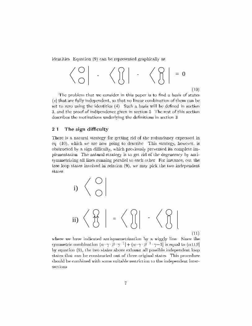
identities. Equation (9) can be represented graphically as- - = 0. (10)The problem that we consider in this paper is to �nd a basis of stateshsj that are fully independent, so that no linear combination of them can beset to zero using the identities (4). Such a basis will be de�ned in section3, and the proof of indipendence given in section 5. The rest of this sectiondescribes the motivations underlying the de�nitions in section 3.2.1 The sign di�cultyThere is a natural strategy for getting rid of the redundancy expressed ineq. (10), which we are now going to describe. This strategy, however, isobstructed by a sign di�culty, which previously prevented its complete im-plementation. The natural strategy is to get rid of the degeneracy by anti-symmetrizing all lines running parallel to each other. For instance, out thetree loop states involved in relation (9), we may pick the two independentstates

ii)

i)

= - , (11)where we have indicated antisymmetrization by a wiggly line. Since thesymmetric combination h� � �� � �1j+ h� � � ��1 � �1j is equal to h�[�jby equation (9), the two states above exhaust all possible independent loopstates that can be constructed out of three original states. This procedureshould be combined with some suitable restriction to the independent inter-sections. 7

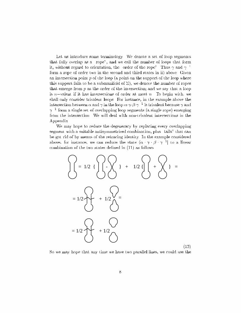
Let us introduce some terminology. We denote a set of loop segmentsthat fully overlap as a \rope", and we call the number of loops that formit, without regard to orientation, the \order of the rope". Thus and �1form a rope of order two in the second and third states in ii) above. Givenan intersection point p of the loop (a point on the support of the loop wherethis support fails to be a submanifold of �), we denote the number of ropesthat emerge from p as the order of the intersection; and we say that a loopis n�valent if it has intersections of order at most n. To begin with, weshall only consider trivalent loops. For instance, in the example above theintersection between � and in the loop �� ��� �1 is trivalent because and �1 form a single set of overlapping loop segments (a single rope) emergingfrom the intersection. We will deal with non-trivalent intersections in theAppendix.We may hope to reduce the degeneracy by replacing every overlappingsegment with a suitable antisymmetrized combination, plus \tails" that canbe got rid of by means of the retracing identity. In the example consideredabove, for instance, we can reduce the state h� � � � � �1j to a linearcombination of the two states de�ned in (11) as follows

= 1/2 + 1/2

= 1/2 { - } + 1/2 { + } =

= 1/2 + 1/2 =

. (12)So we may hope that any time we have two parallel lines, we could use the8

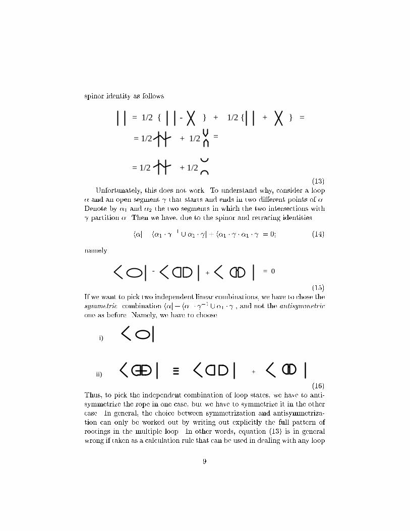
spinor identity as follows= 1/2 { - } + 1/2 { + } =

= 1/2 + 1/2 =

= 1/2 + 1/2 . (13)Unfortunately, this does not work. To understand why, consider a loop� and an open segment that starts and ends in two di�erent points of �.Denote by �1 and �2 the two segments in which the two intersections with partition �. Then we have, due to the spinor and retracing identitiesh�j � h�1 � �1 [ �1 � j+ h�1 � � �1 � j = 0; (14)namely= 0- + . (15)If we want to pick two independent linear combinations, we have to chose thesymmetric combination h�j+ h�1 � �1 [�1 � j, and not the antisymmetricone as before. Namely, we have to choose

+ii)

i) .(16)Thus, to pick the independent combination of loop states, we have to anti-symmetrize the rope in one case, but we have to symmetrize it in the othercase. In general, the choice between symmetrization and antisymmetriza-tion can only be worked out by writing out explicitly the full pattern ofrootings in the multiple loop. In other words, equation (13) is in generalwrong if taken as a calculation rule that can be used in dealing with any loop9

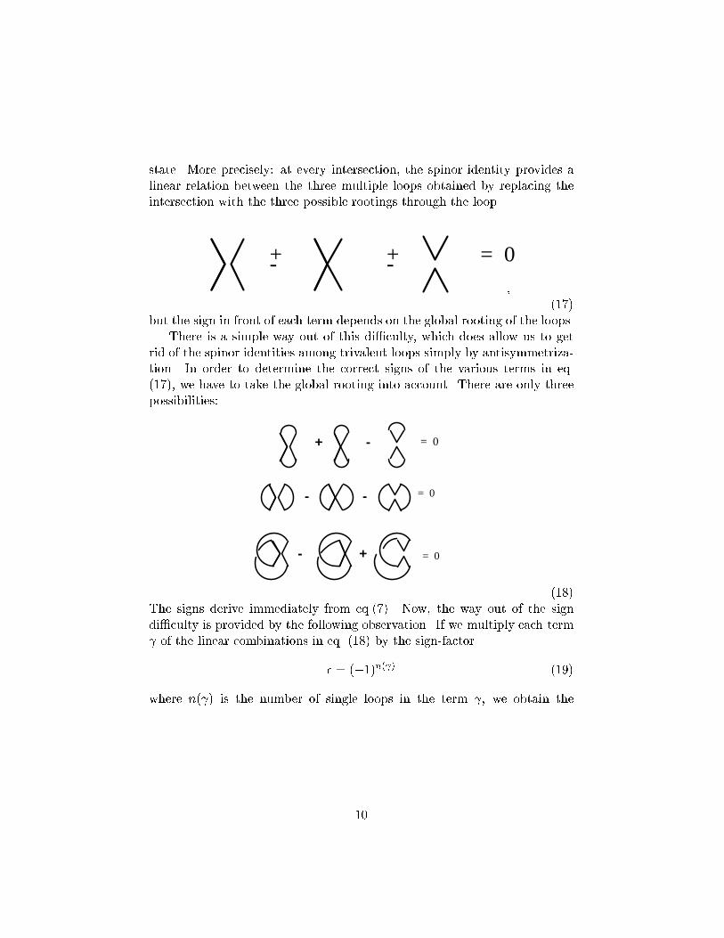
state. More precisely: at every intersection, the spinor identity provides alinear relation between the three multiple loops obtained by replacing theintersection with the three possible rootings through the loop+- +- = 0, (17)but the sign in front of each term depends on the global rooting of the loops.There is a simple way out of this di�culty, which does allow us to getrid of the spinor identities among trivalent loops simply by antisymmetriza-tion. In order to determine the correct signs of the various terms in eq.(17), we have to take the global rooting into account. There are only threepossibilities:

= 0

= 0

= 0

+

+

-

- -

- . (18)The signs derive immediately from eq.(7). Now, the way out of the signdi�culty is provided by the following observation. If we multiply each term of the linear combinations in eq. (18) by the sign-factor� = (�1)n( ) (19)where n( ) is the number of single loops in the term , we obtain the10

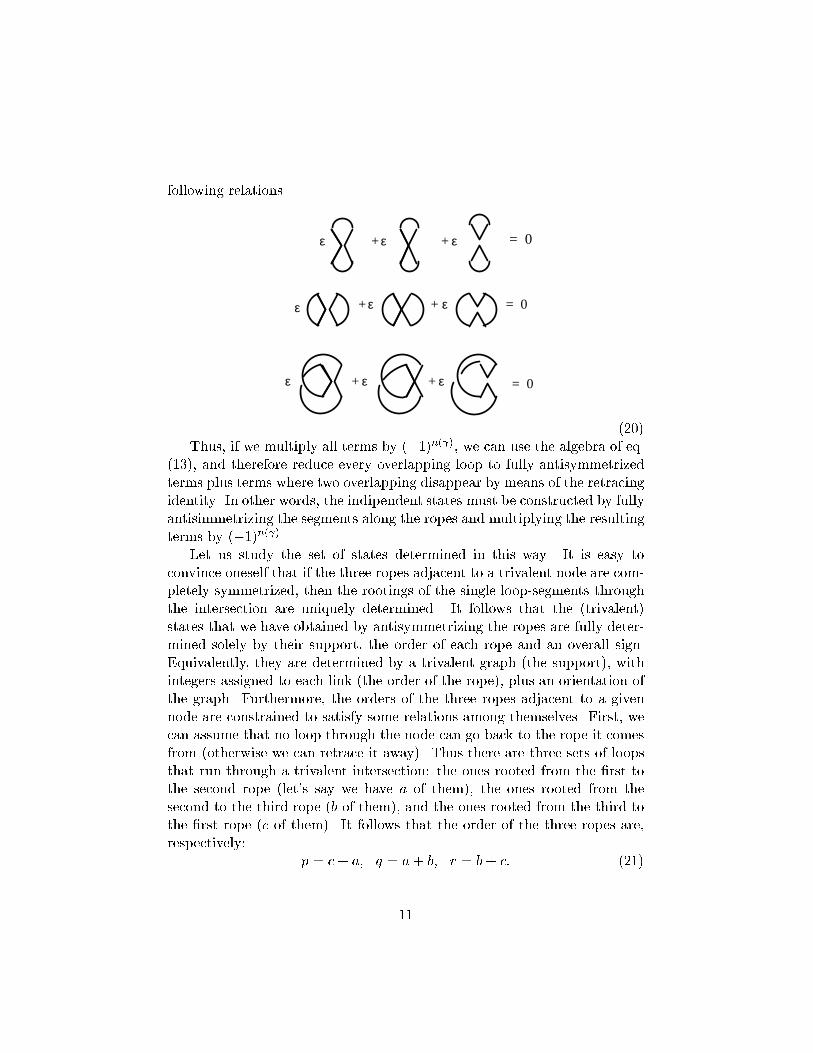
following relations.ε+

ε+ ε+

ε+ε+

ε+

= 0

= 0

= 0

ε

ε

ε

. (20)Thus, if we multiply all terms by (�1)n( ), we can use the algebra of eq.(13), and therefore reduce every overlapping loop to fully antisymmetrizedterms plus terms where two overlapping disappear by means of the retracingidentity. In other words, the indipendent states must be constructed by fullyantisimmetrizing the segments along the ropes and multiplying the resultingterms by (�1)n( ).Let us study the set of states determined in this way. It is easy toconvince oneself that if the three ropes adjacent to a trivalent node are com-pletely symmetrized, then the rootings of the single loop-segments throughthe intersection are uniquely determined. It follows that the (trivalent)states that we have obtained by antisymmetrizing the ropes are fully deter-mined solely by their support, the order of each rope and an overall sign.Equivalently, they are determined by a trivalent graph (the support), withintegers assigned to each link (the order of the rope), plus an orientation ofthe graph. Furthermore, the orders of the three ropes adjacent to a givennode are constrained to satisfy some relations among themselves. First, wecan assume that no loop through the node can go back to the rope it comesfrom (otherwise we can retrace it away). Thus there are three sets of loopsthat run through a trivalent intersection: the ones rooted from the �rst tothe second rope (let's say we have a of them), the ones rooted from thesecond to the third rope (b of them), and the ones rooted from the third tothe �rst rope (c of them). It follows that the order of the three ropes are,respectively: p = c+ a; q = a+ b; r = b+ c: (21)11

The three numbers a; b and c are arbitrary positive integers, but not so theorders p; q and r of the adjacent ropes. It follows immediately from (21)that they satisfy two relations:� i. Their sum is even,� ii. None is larger than the sum of the other two;and that these two conditions on p; q and r are su�cient for the existenceof a; b and c. We conclude that our states are labelled by oriented trivalentgraphs, with integers pl associated to each links l, such that at every nodethe relations i. and ii. are satis�ed. By de�nitions, these are Penrose's spinnetworks [16]. Thus, a linear combination of trivalent loops with the samesupport, in which every rope is fully antisymmetrized is uniquely determinedby an an imbedded, oriented, trivalent spin network. We shall denote thesefully antisymmetrized states as spin-network states. From the discussion wehave just had we can see that they comprise an independent basis.Using the above discussion as motivation, in the next section we providea complete de�nition of spin networks and spin network quantum states.3 Spin-network states in the loop representationIn this section we de�ne the spin network states and their correspondingdi�eomorphism invariant knot states. As de�ned by Penrose, a spin networkis a trivalent graph, �, in which the links l are labled by positive integerspl, denoted \the color of the link", such that the sum of the colors of threelinks adjacent to a node is even and none of them is larger than the sum ofthe other two. To each spin network we may associate an orientation, +1or �1, determined by assigning a cyclic ordering to the three lines emergingfrom each node. In particular, an orientation is determined by a planarrepresentation of the graph (by the clockwise ordering of the lines), andgets reversed by redrawing one of the intersection with two lines emergingin inverted order. Here we consider imbedded, oriented, spin networks,and we denote such objects by the capitalized latin letters S; T;R::: . Animbedded spin network is a spin network plus an immersion of its graphin the three-dimensional manifold �. Later, in discussing the solution ofthe di�eomorphism constraint, we will consider equivalence classes of thesespin networks under di�eomorphisms; these will be called \s-knots" andindicated by lower case latin letters s; t; r; ::: .12

Given a trivalent imbedded oriented spin network (from now on, just spinnetwork) S, we can construct a quantum state of the loop representation asfollows. First we replace every link l of the spin network by a rope of degreep, where p is the color of the link l. Then, at every intersection we join thesegments that form the rope pairwise, in such a way that each segment isjoined with one of the segments of a di�erent rope. As illustrated in theprevious section, the constraints on the coloring turn out to be preciselythe necessary and su�cient conditions for the matching to be possible. Thematching produces a (multiple) loop, which we denote as S1 . Then, weconsider the M = Ql pl! loops Sm;m = 1; :::;M that can be obtained from S1 by permutations of the loops along each rope. (Each rope of color plproduces pl! terms.) We assign to each of these loops a sign factor (�1)c(m)which is positive/negative for even/odd permutations of the loops in S1 .(Equivalently, one can identify c(m) with the number of crossings alongropes, in a planar representation of the loops.) Finally we de�ne the statehSj �Xm (�1)c(m)(�1)n(m)h Smj (22)(here and in he following we write n( Sm) as n(m) for short; we recall thatn( ) is the number of single loops forming the multiple loop ). We denotethe state hSj de�ned by equation (22) as spin network state, or the quantumstate associated with the spin network S.Notice that, up to the overall sign, the linear combinaton that de�nes hSjis independent on the particular rooting through the intersections chosen inconstructing S1 , because every other rooting is produced by the permuta-tions. The overall sign is �xed by the orientation of the spin network. Forconcreteness, let us assign an orientation to the spin network by projectingit on a plane, and assign (�1)c(m) = 1 to the (unique) loop S1 among the Sm that can be drawn without crossings the segments (c(1) = 0) along theropes and in the nodes. We will show in section 4 that the states hSj wehave de�ned form a basis of independent states for the trivalent quantumstates.We represent spin network states simply by drawing their graphs andlabeling the edges with the corresponding colors, and, if necessary, withthe name of the loop or segment they correspond to. As an example, andin order to illustrate how the signs are taken into account by the above13

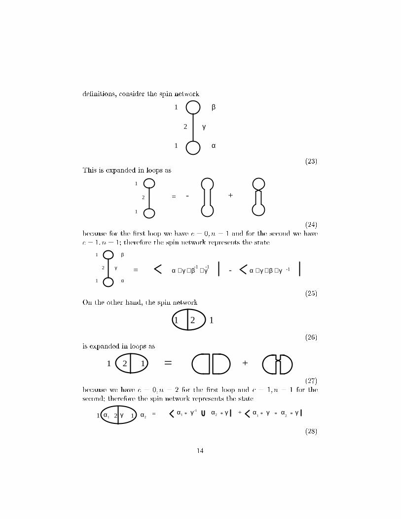
de�nitions, consider the spin network1

1

β

α

2 γ . (23)This is expanded in loops as=

1

1

2 - + (24)because for the �rst loop we have c = 0; n = 1 and for the second we havec = 1; n = 1; therefore the spin network represents the state-1-1

α ∗ γ ∗ β ∗ γ -1α ∗ γ ∗ β ∗ γ-=

1

1

β

α

2 γ .(25)On the other hand, the spin network2 11 (26)is expanded in loops as

1 =2 1 + (27)because we have c = 0; n = 2 for the �rst loop and c = 1; n = 1 for thesecond; therefore the spin network represents the stateα 1 * * γγ-1 α2 + *α

1 * γ * γα22 1γ1 =α2α 1 . (28)14

Notice the plus sign, contrary to the minus sign of the previous example.The construction above can be easilly extended to loops with intesectionsof valence higher than 3. This is done by means of a simple generalizationof the spin networks, obtained by considering non-trivalent graphs coloredon the vertices al well as on the links. Or, equivalently, by trivalent spinnetworks in which sets of nodes are located in the same spacial point. Thisis worked out in detail in the Appendix.Now, since the spin network states hSj span the loop state space, itfollows that any ket state j i is uniquely determined by the values of thehSj functionals on it. Namely, it is uniquely determined by the quantities (S) := hSj i: (29)Furthermore, since, as we shall prove later, the bra states hSj are linearlyindependent, any assignement of quantities (S) corresponds to some ketj i. Therefore, quantum states in the loop representation can be representedby spin network functionals (S). By doing so, we can forget the di�cultiesdue to the Mandelstam identities, which the loop states (�) must satisfy.In particular, we can consider spin networks characteristic states T (S),de�ned by T (S) = �T;S . We will later see that the Ashtekar-Lewandowskimeasure induces a scalar product in the loop representation under which thespin network states are orthonormal; then we can identify the characteristicstates as the Hilbert duals of the spin network bra states. On the otherhand, this identi�cation depends on the scalar product, and thus in generalone should not confuse the spin network characteristic states (kets) with thespin network states (bras).It is easy to see that the calculations of the action of the Hamiltonianconstraint C, presented in [2] imply immediately that if (S) vanishes onall spin networks S which are not regular (formed by smooth and non self-intersecting loops), then C (S) = 0. Notice that this follows from thecombination of two results: the �rst is that hSjC = 0 for all regular S; thesecond is that C (S) = 0 if S is not regular; both these results are dis-cussed in [2]. Thus, states (S) with support on regular spin networks solvethe Hamiltonian constraint, and, at the same time, satisfy the Mandelstamidentities. Indeed, they are precisely the extensions of the loop states withsupport on regular loops de�ned implicitely in [2] and discussed in detailin [26]. The spin network basis allows these solutions to be exhibited in amuch more direct form.The same conclusion may be reached using the form of the hamiltonian15

constraint described in [7], in which we consider the classically equivalentform of the constraint R� fp�C, where f are smooth functions on �.3.1 Di�eomorphism invariance and spin networks in knotspaceOne of the main reasons of interest of the loop representation of quantumgravity is the possibility of computing explicitely with di�eomorphism in-variant states. These are given by the knot states. A knotK is an equivalentclass of loops under di�eomorphisms. We recall from [2] that a knots state,which we denote as K , or simply as jKi in Dirac notation, is a state ofthe quantum gravitational �eld with support on all the loops that are in theequivalence class K K(�) = h�jKi = ( = 1 if � 2 K;= 0 otherwise: (30)Clearly, the same idea works for the spin network states. Let us considerthe equivalent classes of embedded oriented spin networks under di�eomor-phisms. Such equivalence classes are entirely identi�ed by the knottingproperties of the embedded graph forming the spin network and by its col-oring. We call these equivalence classes knotted spin networks, or s-knotsfor short, and indicate them with a lower case Latin letter as s; t; r::: . Ans-knot s can therefore be thought of as an abstract topological object inde-pendent of a particular imbedding in space, in the same fashion as knots.Then, for every knotted spin network s we can de�ne a quantum state jsi(a ket!) of the gravitational �eld by s(S) = hSjsi = ( = 1 if S 2 s;= 0 otherwise: (31)Notice that in general a knot state jKi does not satisfy the Mandelstamrelations. Di�eomorphism invariant loop functionals representing physicalstates should be constructed by suitable linear combination of the elemen-tary knot states jKi. This must be done by �nding suitable extensions ofthe states from their values on regular knots to intersecting knots, using theMandelstam identities, as described in [26]. However, these constructionsare rather cumbersome, in spite of the fact that the rigorous results basedon the use of di�eomorphism invariant measures on loop space [14] ensureus of the existence of such states. The spin network construction provides16

a way to circumvent this di�culty. Indeed, the s-knot state form a com-plete set of solutions of the di�eomorphism constraint; and the s-knot statescorresponding to regular spin networks are solutions of all the constraintscombined.The space of the trivalent s-knots is numerable, for the same reason forwhich the set of the knots without intersections is numerable. However, werecall that di�eomorphism classes of graphs with intersections of order higherthan �ve are continuous. To construct a separable basis for di�eomorphisminvariant states including spin networks of all valences, a seperable basismust be selected for functions on each of these moduli spaces. As thesespaces are �nite dimensional, this can be accomplished. For a classi�cationof the resulting moduli spaces of higher intersections, see [32].This concludes the construction of the spin network states and of thes-knot states in the loop representation. To set the stage for the demon-stration of their independence, we �rst de�ne the spin network states in theconnection representation.4 The connection representationWe recall that in the connection representation one may consider a loop state �, or j�i, de�ned by the trace2 of the holonomy of the Ashtekar SL(2; C)connection A along �, �(A) = hAj�i = T [A;�] = Tr(U�) (32)Consider a spin network S. We can mimic the construction of the looprepresentation, and de�ne the quantum state S(A) = hAjSi =Xm (�1)c(m)+n(m)T [A; Sm]; (33)where, we recall, n is the number of single loops and c counts the termsof the symmetrization. Let us analyse this state in some detail. For everyevery link l with color pl, there are p parallel propagators Ul(A) along thelink l, each one in the spin 1=2 representation, that enter the de�nition2Note that here we do not use the factor of 1=2 that has been conventional since thework of Ashtekar and Isham [13], but return to the original convention of ref. [2]. Thischoice is substantally more convenient for the present formalism, because otherwise wehave to keep track of a factor of 1=2 for every trace, and these factors come into therelations between the spin networks and the loop states.17

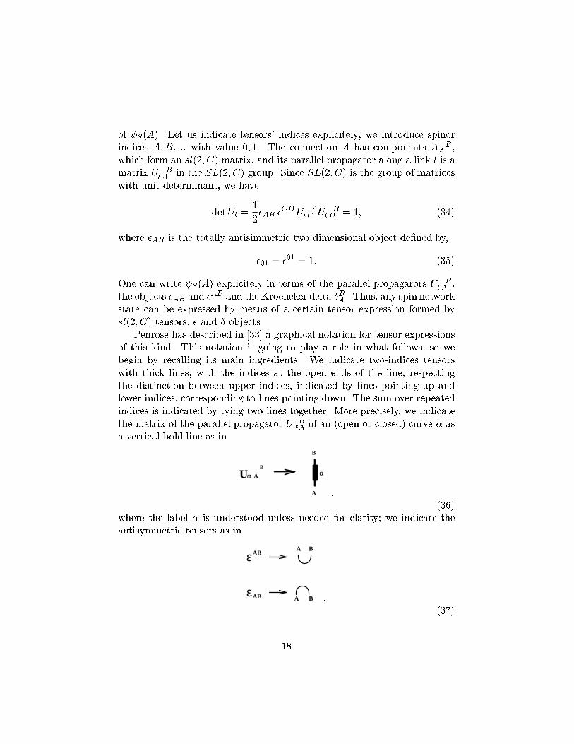
of S(A). Let us indicate tensors' indices explicitely; we introduce spinorindices A;B; ::: with value 0; 1. The connection A has components A BA ,which form an sl(2; C) matrix, and its parallel propagator along a link l is amatrix U BlA in the SL(2; C) group. Since SL(2; C) is the group of matriceswith unit determinant, we havedetUl = 12�AB �CD U AlC U BlD = 1; (34)where �AB is the totally antisimmetric two dimensional object de�ned by,�01 = �01 = 1: (35)One can write S(A) explicitely in terms of the parallel propagarors U BlA ,the objects �AB and �AB and the Kroeneker delta �BA . Thus, any spin networkstate can be expressed by means of a certain tensor expression formed bysl(2; C) tensors, � and � objects.Penrose has described in [33] a graphical notation for tensor expressionsof this kind. This notation is going to play a role in what follows, so webegin by recalling its main ingredients. We indicate two-indices tensorswith thick lines, with the indices at the open ends of the line, respectingthe distinction between upper indices, indicated by lines pointing up andlower indices, corresponding to lines pointing down. The sum over repeatedindices is indicated by tying two lines together. More precisely, we indicatethe matrix of the parallel propagator U�BA of an (open or closed) curve � asa vertical bold line as inUα A

Bα

A

B , (36)where the label � is understood unless needed for clarity; we indicate theantisymmetric tensors as inεAB

εABA B

A B , (37)18

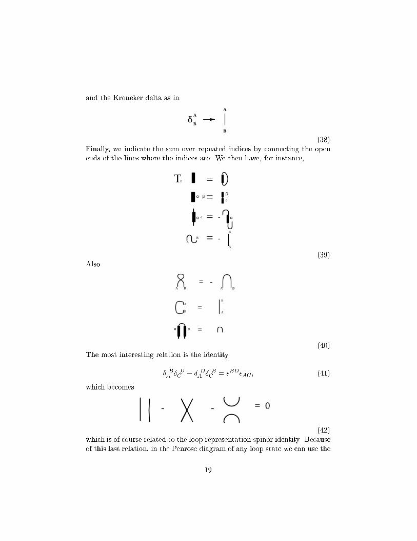
and the Kroneker delta as inA

B

δA

B . (38)Finally, we indicate the sum over repeated indices by connecting the openends of the lines where the indices are. We then have, for instance,Tr =

=

= -

= -

β

α α

B

A

α

BA

-1

α β

. (39)Also=

= -

=A

B

B

A

α α

A B A B

. (40)The most interesting relation is the identity� BA � DC � � DA � BC = �BD�AC ; (41)which becomes= 0- - (42)which is of course related to the loop representation spinor identity. Becauseof this last relation, in the Penrose diagram of any loop state we can use the19

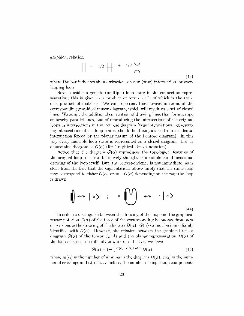
graphical relation= 1/2 + 1/2 (43)where the bar indicates simmetrization, on any (true) intersection, or over-lapping loop.Now, consider a generic (multiple) loop state in the connection repre-sentation; this is given as a product of terms, each of which is the traceof a product of matrices. We can represent these traces in terms of thecorresponding graphical tensor diagram, which will result as a set of closedlines. We adopt the additional convention of drawing lines that form a ropeas nearby parallel lines, and of reproducing the intersections of the originalloops as intersections in the Penrose diagram (true intersections, represent-ing intersections of the loop states, should be distinguished from accidentalintersection forced by the planar nature of the Penrose diagram). In thisway every multiple loop state is represented as a closed diagram. Let usdenote this diagram as G(�) (for Graphical Tensor notation).Notice that the diagram G(�) reproduces the topological features ofthe original loop �; it can be naively thought as a simple two-dimensionaldrawing of the loop itself. But, the correspondence is not immediate, as isclear from the fact that the sign relations above imply that the same loopmay correspond to either G(�) or to �G(�) depending on the way the loopis drawn.

α α - α; (44)In order to distinguish between the drawing of the loop and the graphicaltensor notation G(�) of the trace of the corresponding holonomy, from nowon we denote the drawing of the loop as D(�). G(�) cannot be immediatelyidenti�ed with D(�). However, the relation between the graphical tensordiagram G(�) of the tensor �(A) and the planar representation D(�) ofthe loop � is not too di�cult to work out. In fact, we haveG(�) = (�1)m(�)+c(�)+n(�)D(�) (45)where m(�) is the number of minima in the diagram D(�), c(�) is the num-ber of crossings and n(�) is, as before, the number of single loop components20

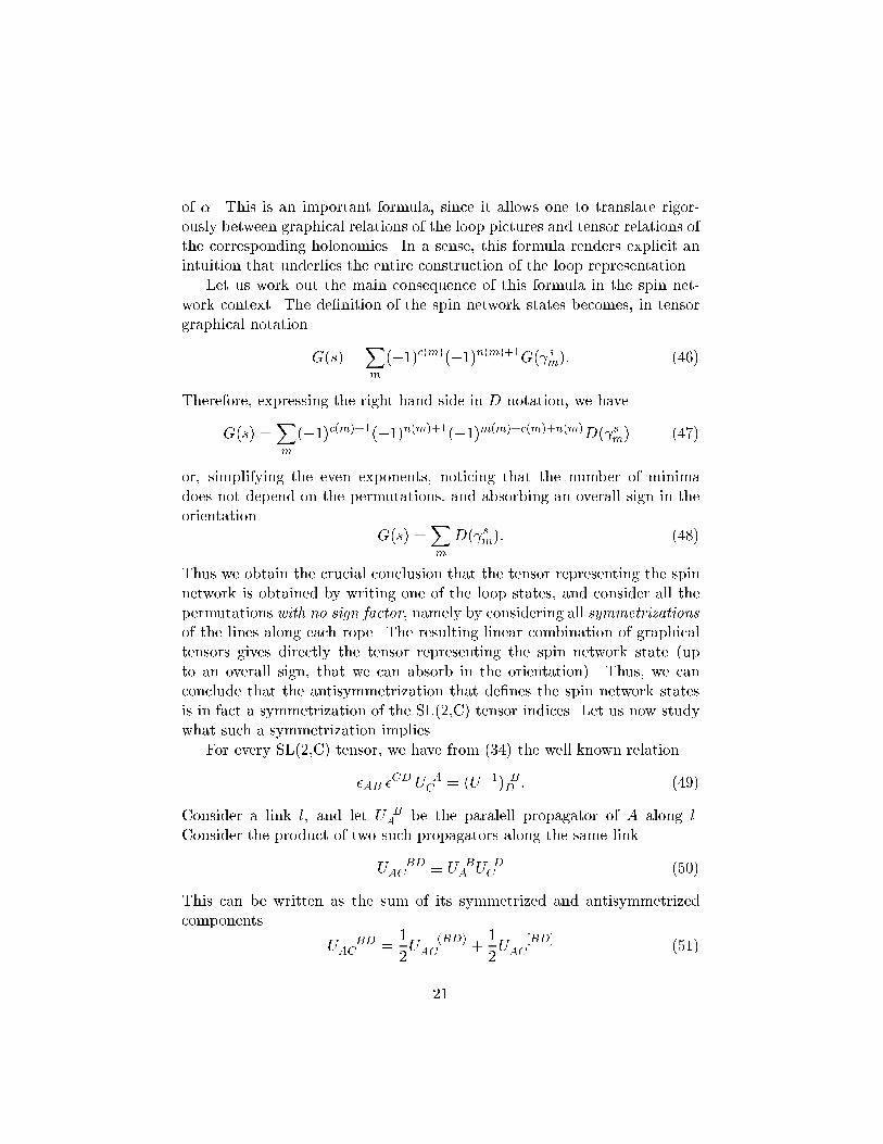
of �. This is an important formula, since it allows one to translate rigor-ously between graphical relations of the loop pictures and tensor relations ofthe corresponding holonomies. In a sense, this formula renders explicit anintuition that underlies the entire construction of the loop representation.Let us work out the main consequence of this formula in the spin net-work context. The de�nition of the spin network states becomes, in tensorgraphical notation G(s) =Xm (�1)c(m)(�1)n(m)+1G( sm): (46)Therefore, expressing the right hand side in D notation, we haveG(s) =Xm (�1)c(m)+1(�1)n(m)+1(�1)m(m)+c(m)+n(m)D( sm) (47)or, simplifying the even exponents, noticing that the number of minimadoes not depend on the permutations, and absorbing an overall sign in theorientation G(s) =Xm D( sm): (48)Thus we obtain the crucial conclusion that the tensor representing the spinnetwork is obtained by writing one of the loop states, and consider all thepermutations with no sign factor, namely by considering all symmetrizationsof the lines along each rope. The resulting linear combination of graphicaltensors gives directly the tensor representing the spin network state (upto an overall sign, that we can absorb in the orientation). Thus, we canconclude that the antisymmetrization that de�nes the spin network statesis in fact a symmetrization of the SL(2,C) tensor indices. Let us now studywhat such a symmetrization impliesFor every SL(2,C) tensor, we have from (34) the well known relation�AB �CD U AC = (U�1) BD : (49)Consider a link l, and let U BA be the paralell propagator of A along l.Consider the product of two such propagators along the same linkU BDAC � U BA U DC (50)This can be written as the sum of its symmetrized and antisymmetrizedcomponents U BDAC = 12U (BD)AC + 12U [BD]AC (51)21

However, it is straightforward to show from the properties of two componentspinors that U [BD]AC = �AC�BD: (52)so that we have the identityU BA U DC = 12U (BA U D)C + 12�AC�BD (53)If we write this in graphical tensor notation we have precisely equation (13).Following the same procedure, it is easy to show that a product of matricesU A1B1 U A2B2 :::U AnBn can be decomposed in a sum of terms, each one formedby totally symmetrized terms U (A1B1 U A2B2 :::U Ak)Bk times a product of epsilonmatrices.Of course what is going on here has a direct interpretation in termsof SU(2) representation theory. Each matrix U BA lives in the spin 1=2representation of SU(2); the product of n of these matrices lives in the n-thtensor power of the spin 1=2 representation, and this tensor product canbe decomposed in the sum of irreducible representations. The irreduciblerepresentations are simply obtained by symmetrizing on the spin 1/2 indices.The reason we have reconstructed the details of the decomposition, is thatthis leads us to the precise relation between the tensorial expression of theconnection representation states and the loop representation notation.In fact, a fully antisymmetrized rope of degree p is represented in matrixnotation by a fully symmetrized tensor product of p parallel propagatorsin the fundamental spin 1=2 representation. Therefore a rope of degree pcorresponds in the connection representation to a propagator in the spinp=2 representation. The result that every loop can be uniquely expandedin the spin network basis is equivalent to statements that the symmetrizedproducts of the fundamental representation of SL(2; C) gives all irreduciblerepresentations.4.1 Nodes and 3j symbols: Explicit relationsThe trivalent intersections between three ropes de�ne an SL(2; C) invariantproduct of three irreducible representations. Clearly the fact that there is aunique trivalent intersection in the loop representation is the re ection of thefact that there is a unique way of combining three irreducible representationsto get the singlet representation, or, equivalently, that there is a uniquedecomposition of the tensor product of two irreducible representations. In22

this subsection we make the relation between the two formalisms explicit,for the sake of completeness.Consider a triple intersection with adjacent lines colored p; q and r.These correspond to the representations with angular momenta lp = p=2,lq = q=2 and lr = r=2. The restriction on p; q and r that p + q + r is evenand none is larger than the sum of the other two corresponds to the basictensor algebra relations of the algebra of the irreducible representations ofSL(2; C), namely the angular momentum addition rules. In fact, the twoconditions are equivalent to the following familiar condition on lr once lpand lq are �xed:lr = jlp � lqj; jlp � lqj+ 1; ::::; (lp + lq)� 1; lp + lq: (54)Now, let p; q, and r be �xed, and let us study the corresponding intersectionin the connection representation. This is given by a summation over thesymmetrized indices of the three products of parallel propagators. Let usraise all the indices of the propagators adjacent to the node. Let us denoteby U AB the spin 1=2 propagator along the link colored p, and by V AB andW AB the propagators along the links colored q and r, where the propagatorsare oriented towards he intersection, so that the upstairs indices refer to theend on the intersection. Since the other index of each matrix is not going toplay any role, we drop it, and write simply UAV A and WA. We must haveat the intersectionUA1 :::UApV B1 :::V BqWC1 :::WCrKA1:::Ap;B1:::Bq;C1:::Cr (55)where KA1:::Ap;B1:::Bq;C1:::Cr is an invariant tensor, symmetric in the �rst pentries, the middle q and the last r. Since the only invariant tensor is �AB ,KA1:::Ap;B1:::Bq ;C1:::Cr must be a sum of products of �AB's. None of the �AB'scan have both indices among the �rst p indices ofKA1:::Ap;B1:::Bq ;C1:::Cr , since�AB is antisymmetric and the �rst p indices are symmetrised. Similarly forthe middle q and the last r. Thus we have �AB's with an A index and aB index (let's say we have a of them) �AB 's with a B index and a C index(b of them) �AB's with a C index and an A index (c of them). Clearly wemust have a+ b = p; b+ c = q and c+a+ r. Thus KA1:::Ap;B1:::Bq;C1:::Cr maycontain a term of the form�Ac+1B1 :::�ApBa �Ba+1C1 :::�BqCb �Cb+1A1 :::�BrAc (56)We have to symmetrize this in each of the three set of indices. We obtainp!q!r! terms, and it is not di�cult to see that this sum is the only invariant23

tensor with the required properties. ThusKA1:::Ap;B1:::Bq;C1:::Cr =X �Ac+1B1 :::�ApBa�Ba+1C1 :::�BqCb�Cb+1A1 :::�BrAc(57)where the sum is over all the symmetrizations of the A;B and C indices.Now, notice that, if we read the graphical representation of the tensor asrepresenting the loops, each of the terms in the sum corresponds preciselyto the rooting of a individual loops between the p and the q links, and soon. Thus, we obtain precisely the spin network vertex. On other hand, therelation between the matrix KA1:::Ap;B1:::Bq ;C1:::Cr and the 3j symbols is alsoclear. For every representation with spin lp, let us introduce the index mpthat takes the (2lp + 1) values mp = �lp; :::; lp. And in the basis vmp in therepresentation space related to the fully symmetrized tensor product of 2lpspinors A1 ::: Ap , we writevmp = (A1 ::: Ap)�A1:::Apmp (58)Then we can write the vertex in this basis asKmpmqmr = �A1:::Apmp �B1:::Bqmq �C1:::Crmr KA1:::Ap;B1:::Bq;C1:::Cr (59)By uniqueness this must be proportional to the 3j symbols of SU(2):Kmpmqmr � lp lq lrmp mq mr ! : (60)5 Demonstration of the independence of the spinnetwork basisWe are �nally in the position to prove the independence of the spin networkstates jsi. We will do this in the connection representation. The indepen-dence of these states is a linear property, and it should therefore be possibleto prove it using only the linear structure of the space. However, it is mucheasier to construct a proof using an (arbitrary) inner product structure onthe state space. Since linear independence is a linear property, once we haveproven independence using a speci�c inner product, the result is independentfrom the inner product used.Ashtekar and Lewandowski [14] have recently studied calculus on thespace of connections, and have de�ned a measure d�AL(A) on (a suitable24

extension of) the space of connections, or, equivalently, a generalized mea-sure on the space of connections [28]. Loop states, and their products are allmeasurable in this measure (in fact, the measure is de�ned using the tech-nology of cylindrical measures, where the cylindrical functions are preciselythe loop states.) Thus, the measure de�nes a quadratic form, or a scalarproduct, on the linear span of the loop states, which is �nite as long aswe consider only �nite linear combination. For our purposes, the measured�AL(A) is convenient for several reasons. First because it is di�eomor-phism invariant. Second, because it is under good control, so calculationswith it are easy. Here, we will use the original Ashtekar Lewandowski mea-sure de�ned for SU(2) connections. The extension to SL(2; C) connections,is discussed in refs. [15]. In the present context, since loop states, as func-tionals on SL(2; C) connections are holomorphic (functions of A and not �A)they are determined by their restriction on the SU(2) connections; thus, theSU(2) measure that we employ de�nes an Hilbert space structure on thesefunctionals, and this is all we need here. In any case, we refer the reader toreference refs. [15] for a much more accurate treatement of this point.Let us thus consider functionals f(A) of the connection of the formf(A) = f(U�1(A); :::; U�n (A)); (61)where f(g1; :::; gn) is a function on the n�th power of SL(2; C), and thus,in particular on the n�th power of SU(2). An example is provided by theloop states �(A). The AL measure can be characterised as follows byZ d�AL(A)f(A) = Z f(g1; :::; gn) dH(g1; :::; gn) (62)where dH is the Haar measure on the n-th power of SU(2). The measurede�nes an inner product between loop states via( �; �) = Z d�AL(A) � �(A) �(A): (63)Now, what we want to prove is that the spin network states s arelinearly independent. Suppose that we can prove that they are all orthogonalwith respect to this scalar product, namely( s; s) 6= 0 (64)for every s, and ( s; s0) = 0 for every s0 6= s: (65)25

Then their linear independence follows, because if there were a linear com-bination of spin network states such that s =Xm cm sm (66)we would have, taking the scalar product of the above equation with sitself, a vanishing right hand side and a non-vanishing left hand side. Thus,to prove independence, we have to prove (64) and (65).Let us consider a given spin network s. We have, using de�nitions( s; s) = Z d�AL(A) � s(A) s(A): (67)The spin network state is a sum (over permutations m) of products (overthe single loops in the multiple loop sm ) of traces of products (over thesingle links ljim covered by the loop �im ) of holonomies of Aa. Then s =Xm (�1)n(m)+c(m)Yi TrYj Uljim (68)Therefore, using the de�nition of the Ashtekar-Lewandowski measure, wehave ( s; s0) = Z dH(g(1):::g(L))Xm (�1)n(m)+c(m)�Yi TrYj g(ljim)Xm0 (�1)n(m0)+c(m0)Yi0 TrYj0 g(lj0i0m0) (69)where we have labelled as 1::::L the links of the spin network. Now we haveto use properties of the SU(2) Haar measure. The main properties we needare Z dH(g) = 1Z dH(g) U(g) BA = 0Z dH(g) U(g) BA U(g) DC = 12 �AC�BD (70)See reference [35] for a detailed discussion.Let us analyze the e�ect of the integration graphically. Pick a link l,and consider the corresponding group integration R dH(g(l)). Let the colors26

of this link be p and p0 for s and s0. Then the integration over g(l) is theintegration over the product of 2p U 's. The result is the product of �AB'sdescribed above. Notice, however, that only the terms in which all the �AB'shave one index coming from one of the spin networks and one index fromthe other can survive, because the others vanish due to the symmetry in thespin network indices and the antisymmetry in the result of the integration.Therefore, in each of the links involved in the integration there should beprecisely the same number of segments in s and s0. This is su�cient to seethat any two spin network states corresponding to di�erent spin networksare orthogonal.Let us now take s = s0. Then, integrating the link l gives a set ofepsilons that connects the two copies of s one with the other. We obtainthus terms in which, at every end of l the two other adjacent links can simplybe retraced back, plus terms which will vanish upon the next integration.Thus the two copies of s get completely retraced back, leaving, at the endjust products of integrations over the identity, each giving 1. Thus, we haveshown that all spin network states are normalized. This completes the prooffor trivalent states. The extension to higher valence intersections is simple;see also [28]. We may note that this result parallels the discussion of theindependence of the spin network basis for hamiltonian lattice gauge theory,given, for example, in Furmanski and Kowala [19]. Given that the Ashtekar-Lewandowski measure is built from the projective limit of inner products forlattice gauge theories, for all analytic embeddings of lattices in �, it is notsurprising that the result extends from lattice gauge theory to this case.6 Relationship between the connection and theloop representationIn this section we review the relation between the loop representation Rland the connection representation Rc, which was introduced in [2]. Thisrelation is simpler in the light of the spin network basis. To see this, we mayrecall from [2] that there exists a third relevant representation. This is therepresentation �Rc dual to the connection representation. The (ket) states in�Rc are, by de�nition, the bra-states of the connection representation, namelythey are linear functionals on the space of functionals (A). Equivalently,we may think of these states as measures on the space of the connections.We denote the states in Rc by jd�i. The operators de�ning in Rc areimmediately de�ned also in Rc, by their dual action.27

In the absence of an inner product there is no canonical map between thestate space of �Rc and the state space ofRc. On the other hand, however, therepresentation �Rc is directly related to the loop representation Rl. In fact,by double duality, any functional of the connection (A) de�nes a linearmap on the state space of �Rc, viah jd�i = hd�j i = Z d�(A) (A): (71)In particular, each loop state j �i, which is de�ned in the connection rep-resentation Rc by hAj �i = T [A;�], determines a dual state h �j in Rc,via h �jd�i = hd�j �i = Z d�(A) T [A;�] (72)By de�nition of the loop representation [2], these bra states h �j in Rc areto be identi�ed precisely with the loop states h�j:h�j = h �j; (73)In other words, the loop representation state (�) is the state that is repre-sented in the dual connection representation Rc by the measure d�, where (�) = Z d�(A)T [A;�]: (74)This construction depends only on the linear structure of the quantumtheory, namely it does not depend on a speci�c scalar product ( ; ) which mayor may not be de�ned on the state space. In the absence of a scalar productthere is no canonical map between ket-space and bra-space, and therefore nocanonical association of a dual state (a measure) d�(A) to a given connectionrepresentation state (A); nor, equivalently, there is any canonical mappingbetween the connection representation Rc and loop representation Rl.If a scalar product is given, then we can map connection representationstates into loop representation states, because, given a connection represen-tation functional (A), there is a unique dual state d� (A) such that, forevery y0, hd� j 0i = ( ; 0) (75)And the loop state (�) corresponding to the connection representationstate (A) is then given by (�) = h �jd� i: (76)28

In particular, a scalar product in the connection representation can be as-signed by �xing a measure d�(A) on the space of connections, so that( ; 0) = Z d�(A) (A) 0(A): (77)Then, the induced map between the connection representation and the looprepresentation is the known expression for the loop transform (�) = Z d�(A) T (A;�) 0(A): (78)To implement this relation explicitely we must use a measure d�(A) whichrespects the invariances of the theory. Non-trivial gauge-invariant and di�eo-morphism-invariant (generalised) measures on the space of connection haverecently being constructed[14], and the Ashtekar-Lewandowski measure weused above is the simplest of these. The existence of this measure allowsus to establish a de�nite linear map between the connection and the looprepresentation. Let us do so, and study its consequences. We will discusslater the extent to which we can take the resulting scalar product, and thusthe resulting identi�cation of the two representations, as the \physicallycorrect" one.For every ket state (A) in the connection representation, the Ashtekar-Lewandowski scalar product associates to it the bra state (or measure)d� (A) = d�AL(A) (A). Let us consider a spin network state s(A). Thecorresponding bra state state is d�s(A) = d�AL(A) s(A). By the propertyof the spin network states under the Ashtekar-Lewandowski integration, wehave then the remarkable result( s; s0) = hd�sj s0i = �ss0 : (79)The loop representation state bra state hsj corresponding to s is de�nedsolely in terms of the linear properties of the representation. The looprepresentation ket state jsi, on the other hand, is de�ned by s(�) = Z d�s(A)T [A;�]: (80)and it follows immediately that it is the adjoint of hsj. Thus, the AshtekarLewandowski inner product becomes, in the loop representation:hsjs0i = �ss0 ; (81)29

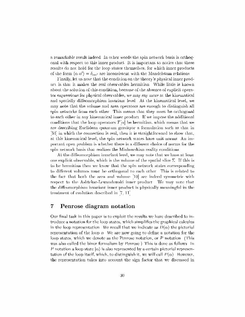
a remarkable result indeed. In other words the spin network basis is orthog-onal with respect to this inner product. It is important to notice that theseresults do not hold for the loop states themselves, for which inner productsof the form h�j�0i = ���0 are inconsistent with the Mandelstam relations.Finally, let us note that the condition on the theory's physical inner prod-uct is that it makes the real observables hermitian. While little is knownabout the solution of this condition, because of the absence of explicit opera-tor expressions for physical observables, we may say more at the kinematicaland spatially di�eomorphism invariant level. At the kinematical level, wemay note that the volume and area operators are enough to distinguish allspin networks from each other. This means that they must be orthogonalto each other in any kinematical inner product. If we impose the additionalconditions that the loop operators T [�] be hermitian, which means that weare describing Euclidean quantum gravityor a formulation such as that in[34] in which the connection is real, then it is straightforward to show that,at this kinematical level, the spin network states have unit norms. An im-portant open problem is whether there is a di�erent choice of norms for thespin network basis that realizes the Minkowskian reality conditions.At the di�eomorphism invariant level, we may note that we have at leastone explicit observable, which is the volume of the spatial slice �. If this isto be hermitian then we know that the spin network states correspondingto di�erent volumes must be orthogonal to each other. This is related tothe fact that both the area and volume [10] are indeed symmetric withrespect to the Ashtekar-Lewandowski inner product. We may note thatthe di�eomorphism invariant inner product is physically meaningful in thetreatment of evolution described in [7, 11]7 Penrose diagram notationOur �nal task in this paper is to exploit the results we have described to in-troduce a notation for the loop states, which simpli�es the graphical calculusin the loop representation. We recall that we indicate as D(�) the pictorialrepresentation of the loop �. We are now going to de�ne a notation for theloop states, which we denote as the Penrose notation, or P notation. (Thiswas also called the binor formalism by Penrose.) This is done as follows. InP notation a loop state j�i is also represented by a certain pictorial represen-tation of the loop itself, which, to distinguish it, we will call P (�). However,the representation takes into account the sign factor that we discussed in30

previous sections. Thus, we choose the convention that the diagram of aloop, P (�) in P notation is related to the loop state j�i by (�1)n(�)+1j�i,where n(�), we recall, indicates the number of single loops, or components,of the multiple loop �. In other words, the P notation P (�) of a loop statej�i is de�ned by P (�) = (�1)n(a)+1D(�): (82)The important aspect of the P notation is that with these conventions thethe spinor identy is now local. In fact it now reads as+ + = 0. (83)Therefore equation (13) holds rigorously whithin this notation. Thus cansolve the spinor identity (on trivalent states) by restricting to the states inwhich every rope is (in P notation) fully antisymmetrized. It is importantto note that the P notation is completely topological, in that a diagramcorresponds to the same loop state no matter how it is oriented ot drawn.This is a great advantage in calculations.For completeness we mention a variant of the P notation, has been usedin some published work [10]. The variant, which we may denote SymmetricPenrose notation, corresponds to what Penrose called the spinor calculus,as opposed to binor calculus. In this notation, which we will refer to as SPnotation, the diagram that corresponds to a loop � will be labled S(�). Itis de�ned by, S(�) = (�1)n(�)+c(�)+m(�)+1D(�): (84)We recall that c(�) and m(�) are the number of crossings and the numberof minima in D(�). Notice that the SP notation is not "topological", in thesense that the way the loop a is drawn matters for the determination of thesign: adding a minumun and a maximum is equiavelent to change the signof the state. Notice that the permutations of the loops along a rope changethe number of crossings therefore the antisimmetrization in the P notationcorresponds to a symmetrization in SP notation (hence the name). Whileit is more cumbersome for calculation, the signi�cance of the SP notation isthat it has an immediate interpretation in terms of Penrose graphical tensorcalculus, which we de�ned earlier in the connection representation. Indeed,31

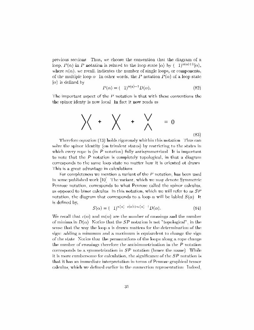
we have immediately that SP (�) = G(�): (85)Finally, we mention the fact that the P notationcan be obtained fromthe graphical tensor notation by adding the immaginary unit to each �, andadding a minus one for every crossing.7.1 Loop operators in Penrose notationA most valuable aspect of the Penrose diagram notation we have introducedis the simpli�cation it allows in the calculus with the loop operators. Inthis section we describe the action of the loop operators on the loop statesexpressed in Penrose notation.We recall [2] that in terms of the standard loop notation the action ofthe loop operators T 1 and T 2 is given byh�jT a[�](s) = �a[�; �(s)](h� � �j � h� � ��1j) (86)h�jT ab[�](s; t) = �a[�; �(s)]�b[�; �(t)]Xi (�1)r(i)h(� �st �)ij (87)The distributional factor �a[�; �(s)] (which doesn't play any role in thediagramatics) is de�ned in [2]. The geometrical part of the action of theseoperators can be coded in the \grasping" action shown inα β

( )a2p

-l (88)However, as is well known by anybody who attempted to perform complexcomputations with these operators, the local graphical action expressed ineq. (88) does not su�ce to compute the correct linear combination appearingin the r.h.s of eq. (87). The di�culty is given by the signs in front of thevarious terms. These signs are dictated by the global rooting properties ofthe loop that are being grasped. In particular the sign is determined in(87) by r(i), which is de�ned [2] as the number of segments that have tobe reversed in order to obtain a consistent orientation of the loop after thererooting. While complete, this way of determining the sign is cumbersome,and in computing the action of operators as the area, the Hamiltonian, or thevolume, the determination of the signs is the hardest part of the calculation.This di�culty disappears using the Penrose diagram notation.32

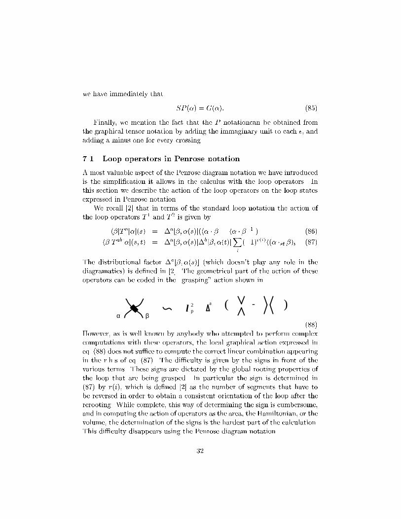
Let us begin by considering the action of T 1 on a loop state.β

a [T α ] s( ) . (89)To compute this we express the r.h.s of in Penrose notation. The result isa β β

α α

+( )2pl . (90)Notice the plus sign, due to the change of sign

β

α

-1= α ∗ β . (91)This suggests that we indicate the operator T a[�](s) by

β

a

[ ]β s( )Ta (92)To notate the action of the operator we may then introduce the followingfundamental \grasping" rule

= 2pl

a

a . (93)33

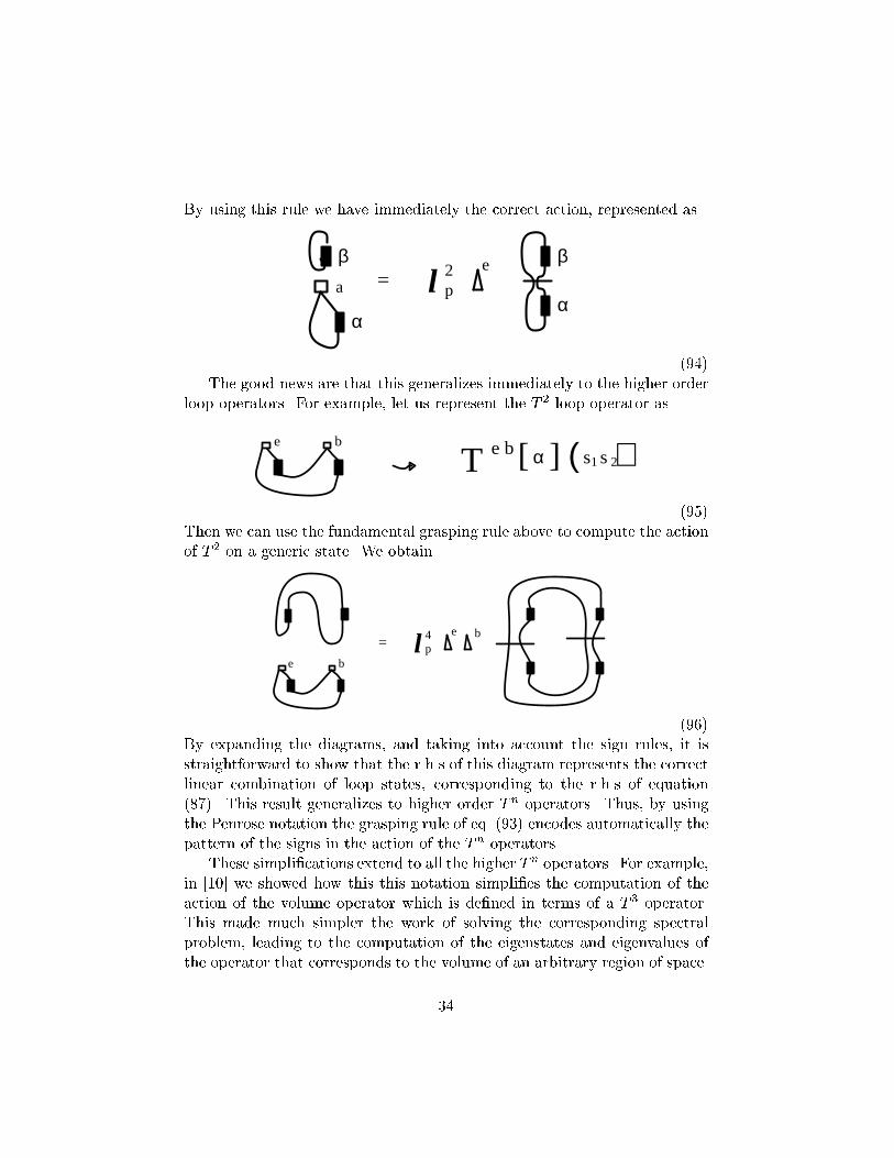
By using this rule we have immediately the correct action, represented asβ

α

a

β

α= 2

p

el . (94)The good news are that this generalizes immediately to the higher orderloop operators. For example, let us represent the T 2 loop operator as

[ ] (α s s )T e b1 2

be . (95)Then we can use the fundamental grasping rule above to compute the actionof T 2 on a generic state. We obtaine

ep=4

b

bl . (96)By expanding the diagrams, and taking into account the sign rules, it isstraightforward to show that the r.h.s of this diagram represents the correctlinear combination of loop states, corresponding to the r.h.s of equation(87). This result generalizes to higher order T n operators. Thus, by usingthe Penrose notation the grasping rule of eq. (93) encodes automatically thepattern of the signs in the action of the T n operators.These simpli�cations extend to all the higher T n operators. For example,in [10] we showed how this this notation simpli�es the computation of theaction of the volume operator which is de�ned in terms of a T 3 operator.This made much simpler the work of solving the corresponding spectralproblem, leading to the computation of the eigenstates and eigenvalues ofthe operator that corresponds to the volume of an arbitrary region of space.34

8 ConclusionWe have de�ned a basis of independent states in the loop and in the connec-tion representations of quantum gravity which solves the Mandelstam iden-tities. This basis is labelled by a generalization of Penrose spin networks. Itis orthonormal in the scalar product de�ned by the Asktekar-Lewandowskimeasure, and provides a simple relation between the connection and theloop representation. We have introduced a notation for the loop states ofquantum gravity based on Penrose's graphical tensor notation. In this no-tation, the action of the loop operators becomes local, and can be expressedin terms of the simple graphical rule given in equation (93).An intriguing suggestion on the possibility of modifying the frameworkwe have presented in this paper follows from the following observation. Be-cause of the short-scale discretness of the geometry [10], the only remain-ing divergences in nonperturbative quantum gravity must be infrared diver-gences, analogous to the spikes, or the uncontrolled proliferation of \babyuniverses" seen in nonperturbative numerical calculations employing dy-namical triangulations [36] in both two and four dimensions. In the presentcontext, a source of such divergences may be the sum over the coloringsof the spin networks, which label the representations of SU(2). This sug-gests that a natural invariant regularization of the theory could be providedby replacing SU(2) with the quantum group SL(2)q . Such a strategy hasbeen successfully implemented in 3 dimensions by Turaev and Viro [21],and there have been attempts to extend it to four dimensional di�eomor-phism invariant theories [23]. The use of q-deformed spin networks in theloop representation of quantum gravity is presently under investigation [37].Furthermore, spin networks may make it possible to de�ne quantum gravityon manifolds with a �nite boundary [38], and to use the methods of topolog-ical �eld theory to describe the structure of the physical quantum gravitystate space in the presence of boundaries. In this context, the level q ofSL(2)q turns out to be related to the inverse of the cosmological constant[38]. These investigations reinforce the conjecture that the q deformationcould play the role of infrared regulator. The possible relevance of q defor-mations of the gauge group SU(2)L in quantum gravity is also suggested bythe important role quantum groups play in knot theory [39], as well as bythe possibility of quantum-gravity induced, quantum-group deformations ofthe space-symmetries [40].Finally, we remark that the existence of a spin network basis for thespace of di�eomorphism invariant states of the quantum gravitational �eld,35

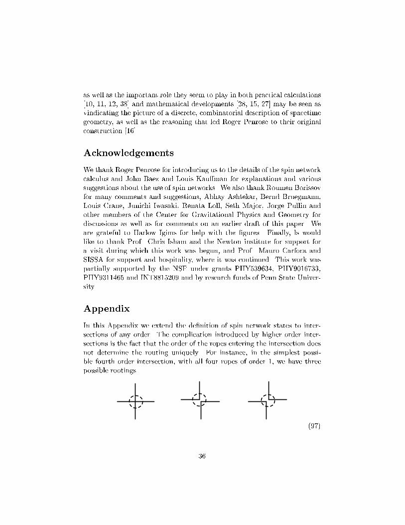
as well as the important role they seem to play in both practical calculations[10, 11, 12, 38] and mathematical developments [28, 15, 27] may be seen asvindicating the picture of a discrete, combinatorial description of spacetimegeometry, as well as the reasoning that led Roger Penrose to their originalconstruction [16].AcknowledgementsWe thank Roger Penrose for introducing us to the details of the spin networkcalculus and John Baez and Louis Kau�man for explanations and varioussuggestions about the use of spin networks. We also thank Roumen Borissovfor many comments and suggestions, Abhay Ashtekar, Bernd Bruegmann,Louis Crane, Junichi Iwasaki, Renata Loll, Seth Major, Jorge Pullin andother members of the Center for Gravitational Physics and Geometry fordiscussions as well as for comments on an earlier draft of this paper. Weare grateful to Harlow Igims for help with the �gures. Finally, ls wouldlike to thank Prof. Chris Isham and the Newton institute for support fora visit during which this work was begun, and Prof. Mauro Carfora andSISSA for support and hospitality, where it was continued. This work waspartially supported by the NSF under grants PHY539634, PHY9016733,PHY9311465 and INT8815209 and by research funds of Penn State Univer-sity.AppendixIn this Appendix we extend the de�nition of spin network states to inter-sections of any order. The complication introduced by higher order inter-sections is the fact that the order of the ropes entering the intersection doesnot determine the routing uniquely. For instance, in the simplest possi-ble fourth order intersection, with all four ropes of order 1, we have threepossible rootings(97)36

out of which two are independent, due to the spinor identity. Neverthe-less, with a small amount of additional technical machinery, it is possibleto extend the spin network basis to include arbitrary intersections. Thisis because given the order n of an intersection i, and given the coloringp1; :::; pn of the n ropes adjacent to i, there is only a �nite number of waysof rootings the loops through the intersection, and therefore a (smaller) �-nite number k(p1; :::; pn) of independent rootings. For completeness, we putk(p1; :::; pn) = 0 if a consistent rooting through the intersection does notexist for n ropes of orders p1; :::; pn; this is for instance the case if Pj pjis odd. In the particular case of trivalent intersections (n = 3) we havek(p1; :::; p3) = 1 if the sum of three colors pj is even and none of the threeis larger than the sum of the other two, and k(p1; :::; p3) = 0 otherwise.In order to extend the de�nition of spin network states to non-trivalentloops, it is su�cient to choose a unique way of labeling the k(p1; :::; pn)independent rootings through an intersection i, by means of an integer vi =1; :::; k(p1; :::; pn). Once this is done, we de�ne a generalized spin network sas an oriented imbedded graph �, with positive integers, or colors, pl andvi assigned to each link l and to each of node i; satisfying the relationsvi � k(p1; :::; pn), p1; :::; pn being the colors of the links adjacent to the nodei. The construction of the corresponding spin network quantum states hsjis then as before.The task of labeling independent spin networks can be achieved as fol-lows. For every n, we choose a unique trivalent graph �(n) with n free ends,and no closed loop; for instance, we may choose(98)Such a graph will have n links adjacent to the free ends, and (n�3) internallinks, which we denote as \virtual" links. For every n, and every set of colorsp1; :::; pn we consider the possible colorings q1; :::; q(n�3) of the virtual linksof �(n) which are compatible with the colorings p1; :::; pn of its external links(under the spin networks vertex conditions). We obtain in this way a familyof colored trivalent spin networks �(n)1 ; :::;�(n)k(p1;:::;pn) with n external linkscolored p1; :::; pn. It is not di�cult to see that these are linear combinationsof rootings through the intersection which exhaust all possibilities, up to the37

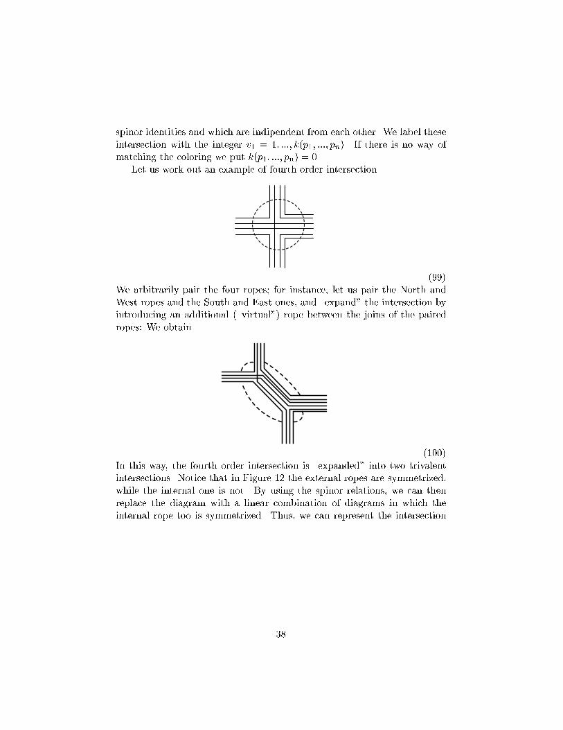
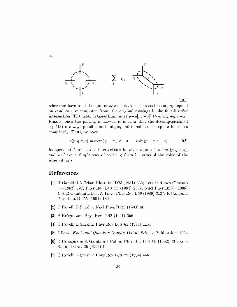
spinor identities and which are indipendent from each other. We label theseintersection with the integer v1 = 1; :::; k(p1; :::; pn). If there is no way ofmatching the coloring we put k(p1; :::; pn) = 0.Let us work out an example of fourth order intersection.. (99)We arbitrarily pair the four ropes; for instance, let us pair the North andWest ropes and the South and East ones, and \expand" the intersection byintroducing an additional (\virtual") rope between the joins of the pairedropes: We obtain

. (100)In this way, the fourth order intersection is \expanded" into two trivalentintersections. Notice that in Figure 12 the external ropes are symmetrized,while the internal one is not. By using the spinor relations, we can thenreplace the diagram with a linear combination of diagrams in which theinternal rope too is symmetrized. Thus, we can represent the intersection38

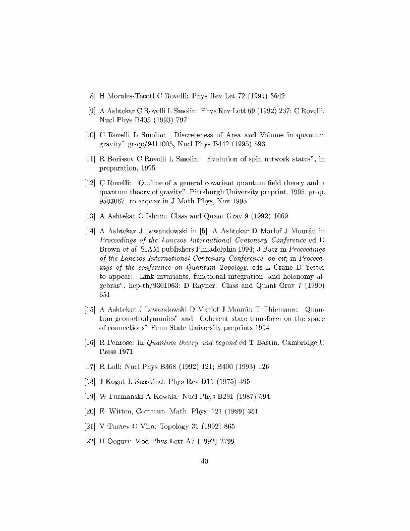
asq

p

s

r

ii

c iq s

r

p

= . (101)where we have used the spin network notation. The coe�cients ci dependon (and can be computed from) the original rootings in the fourth orderintersection. The index i ranges from max(jp�qj; jr�sj) to min(p+q; r+s).Finally, once the pairing is chosen, it is clear that the decomposition ofeq. (13) is always possible and unique, and it reduces the spinor identitiescompletely. Thus, we havek(p; q; r; s) = max(jp� qj; jr � sj)�min(p+ q; r + s) (102)independent fourth order intersections between ropes of orders (p; q; r; s),and we have a simple way of ordering them in terms of the color of theinternal rope.References[1] R Gambini A Trias: Phys Rev D23 (1981) 553; Lett al Nuovo Cimento38 (1983) 497; Phys Rev Lett 53 (1984) 2359; Nucl Phys B278 (1986)436; R Gambini L Leal A Trias: Phys Rev D39 (1989) 3127; R Gambini:Phys Lett B 255 (1991) 180[2] C Rovelli L Smolin: Nucl Phys B133 (1990) 80[3] B Br�ugmann: Phys Rev D 43 (1991) 566[4] C Rovelli L Smolin: Phys Rev Lett 61 (1988) 1155[5] J Baez: Knots and Quantum Gravity, Oxford Science Publications 1994[6] B Bruegmann R Gambini J Pullin: Phys Rev Lett 68 (1992) 431: GenRel and Grav 25 (1993) 1[7] C Rovelli L Smolin: Phys Rev Lett 72 (1994) 44639

[8] H Morales-Tecotl C Rovelli: Phys Rev Let 72 (1994) 3642[9] A Ashtekar C Rovelli L Smolin: Phys Rev Lett 69 (1992) 237; C Rovelli:Nucl Phys B405 (1993) 797[10] C Rovelli L Smolin: \Discreteness of Area and Volume in quantumgravity" gr-qc/9411005, Nucl Phys B442 (1995) 593[11] R Borissov C Rovelli L Smolin: \Evolution of spin network states", inpreparation, 1995[12] C Rovelli: \Outline of a general covariant quantum �eld theory and aquantum theory of gravity", Pittsburgh University preprint, 1995, gr-qc9503067, to appear in J Math Phys, Nov 1995[13] A Ashtekar C Isham: Class and Quant Grav 9 (1992) 1069[14] A Ashtekar J Lewandowski in [5]. A Ashtekar D Marlof J Mour~au inProceedings of the Lanczos International Centenary Conference ed DBrown et al SIAM publishers Philadelphia 1994; J Baez in Proceedingsof the Lanczos International Centenary Conference, op cit; in Proceed-ings of the conference on Quantum Topology, eds L Crane D Yetterto appear; \Link invariants, functional integration, and holonomy al-gebras", hep-th/9301063; D Rayner: Class and Quant Grav 7 (1990)651[15] A Ashtekar J Lewandowski D Marlof J Mour~au T Thiemann: \Quan-tum geometrodynamics" and \Coherent state transform on the spaceof connections" Penn State University preprints 1994[16] R Penrose: in Quantum theory and beyond ed T Bastin, Cambridge UPress 1971[17] R Loll: Nucl Phys B368 (1992) 121; B400 (1993) 126[18] J Kogut L Susskind: Phys Rev D11 (1975) 395[19] W Furmanski A Kowala: Nucl Phys B291 (1987) 594[20] E. Witten, Commun. Math. Phys. 121 (1989) 351[21] V Turaev O Viro: Topology 31 (1992) 865[22] H Ooguri: Mod Phys Lett A7 (1992) 279940

[23] L Crane D Yetter: in Quantum Topology, eds L H Kau�man RA Baad-hio, World Scienti�c Press, (1993) 120; L Crane IB Frenkel: J MathPhys 35 (1994) 5136; L Crane D Yetter: On algebraic structures implicitin topological quantum �eld theories, Kansas preprint 1994[24] TJ Foxon: \Spin networks, Turaev-Viro theory and the loop represen-tation" Class and Quant Grav, to appear 1995, gr-qc/9408013.[25] C Rovelli: Phys Rev D48 (1993) 2702[26] L Smolin: in Quantum Gravity and Cosmology, eds J P�erez-Mercaderet al, World Scienti�c, Singapore 1992[27] T Thiemann: unpublished[28] J Baez : \ Spin Network States in Gauge Theory", Advances inMathematics, to appear 1995, gr-qc/941107; \Spin Networks in non-perturbative quantum gravity", gr-qc 9504036[29] A Ashtekar: Non perturbative canonical gravity, World scienti�c, Sin-gapore 1991[30] C Rovelli: Class Quant Grav 8 (1991) 1613[31] A Ashtekar: Phys Rev Lett 57 (1986) 2244; Phys Rev D36 (1987) 1587[32] N Grott C Rovelli: \Moduli spaces of intersecting knots", in prepara-tion[33] R Penrose W Rindler: Spinors and Spacetime, Cambridge U Press 1984[34] JF Barbero: \Real variables for Lorentz signature spacetimes", PennState preprint CGPG-94/11-3, gr-qc/9410014[35] M Creutz: J Math Phys 19 (1978) 2043[36] ME Agishtein AA Migdal: Mod Phys Lett A7 (1992) 1039; Nucl PhysB385 (1992) 395; J Ambjorn J Jurkiewicz: Phys Lett B278 (1992) 42; HHamber: Phys Rev D50 (1994) 3932; BV de Bakker J Smit: \Two pointfunctions in 4d dynamical triangulations", ITFA-95-1, gr-qc/9503004;J Ambjorn J Juriewicz Y Watabiki, to appear in JMP, Nov 1995[37] S Major L Smolin: in preparation41

[38] L Smolin: Linking quantum gravity and topological quantum �eld theoryto appear in J Math Phys, Nov 1995[39] L Kau�man: Knots and Physics , World Scienti�c Singapore 1991[40] M Pillin WB Schmidke J Wess: Nucl Phys B403 (1993) 223

42