Spin dephasing in quantum wires

Spin dephasing in quantum wires

S. Pramanik and S. Bandyopadhyay

Department of Electrical Engineering, Virginia Commonwealth University, Richmond, Virginia 23284

M. Cahay

Department of Electrical and Computer Engineering and Computer Science, University of Cincinnati,

Cincinnati, Ohio 45221

Abstract

We study high-field spin transport in a quantum wire using a semiclassical approach.

Spin dephasing (or spin depolarization) in the wire is caused by D’yakonov-Perel’ re-

laxation associated with bulk inversion asymmetry (Dresselhaus spin-orbit coupling)

and structural inversion asymmetry (Rashba spin-orbit coupling). The depolariza-

tion rate is found to depend strongly on the initial polarization of the spin. If the

initial polarization is along the axis of the wire, the spin depolarizes 100 times

slower compared to the case when the initial polarization is transverse to the wire

axis. We also find that in the range 4.2 K - 50 K, temperature has a weak influence

and the driving electric field has a strong influence on the depolarization rate. The

steady state distribution of the spin components parallel and transverse to the wire

axis also depend on the initial polarization. If the initial polarization is along the wire

axis, then the steady state distribution of both components is a flat-topped uniform

distribution, whereas if the initial polarization is transverse to the wire axis, then the

distribution of the longitudinal component resembles a Gaussian, and the distribution

of the transverse component is U-shaped.

Corresponding author. e-mail: [email protected]

1

Keywords: A. Spin dephasing, A. Spin transport

72.25.Dc, 72.25.Mk, 72.25.Hg, 72.25.Rb

Typeset using REVTEX

2

I. INTRODUCTION

There is considerable current interest in spin transport in quantum confined structures because

of the advent of the field of spintronics [1–4]. A number of device proposals advocate the use of

the spin degree of freedom of an electron (as opposed to the charge degree of freedom) to realize

electronic devices such as transistors [5], diodes [6], solar cells [7], filters [8] and stub tuners [9].

Additionally, spin is nowadays preferred to charge for encoding qubits in quantum logic gates

[10–13] because of the much longer spin coherence time in semiconductors [14,15] compared to

charge coherence time [16].

In this paper, we study electron spin transport in quasi one-dimensional structures. In the past,

single particle ballistic models [9,17–19] were employed to study spin transport. They are fully

quantum mechanical, but do not account for any scattering or spin dephasing. More recently, Ca-

hay and Bandyopadhyay have treated spin dephasing via elastic impurity scattering within a fully

quantum mechanical model [20]. However, they do not account for spin dephasing via inelastic

(phase-breaking) scattering mechanisms which are important at elevated temperatures and high

electric fields.

As far as classical models are concerned, a number of studies used a drift-diffusion type ap-

proach to model spin transport and spin dephasing at elevated temperatures and moderate electric

fields [21–23]. “Spin-up” and “spin-down” electrons are treated similar to electrons and holes in

conventional bipolar transport. Spin dephasing is treated by a spin relaxation term that describes

coupling between the “spin-up” and “spin-down” electrons similar to the generation-recombination

term describing coupling between electrons and holes in bipolar transport. The inadequacy of these

models has been pointed out by Saikin et. al. [24]. Apart for the fact that a relaxation time approx-

imation does not fully capture the physics of spin dephasing (even if different relaxation times are

used to describe different processes [25]), the drift-diffusion formalism is invalid at relatively high

electric fields when transport non-linearities become important [26]. Non-linearities in spin trans-

port have been observed experimentally [27,28]. Furthermore, these models cannot treat coherence

effects arising from superposition of spin-up and spin-down states. Recently, such superpositions

were treated in a Bloch equation approach [29] and a generalized drift-diffusion type approach

3

derived from the Boltzmann transport equation [30]. These later models are still somewhat inade-

quate in that they do not treat the momentum dependence of the spin-orbit coupling (the primary

cause of spin dephasing) self-consistently.

In reality, the temporal evolution of spin and the temporal evolution of the momentum of an

electron cannot be separated. The dephasing (or depolarization) rates are functionals of the electron

distribution function in momentum space which continuously evolves with time when an electric

field is applied to drive transport. Thus, the dephasing rate is a dynamic variable that needs to

be treated self-consistently in step with the dynamic evolution of the electron’s momentum. Such

situations are best treated by Monte Carlo simulation, which has been recently adopted by a num-

ber of groups to study spin transport in quasi-two-dimensional structures [31,24]. In this paper,

we extend this approach to quasi one-dimensional structures using a multi-subband Monte Carlo

simulator.

This paper is organized as follows: in the next section, we describe the theory followed by

results and discussions in Section 3. Finally, we conclude in Section 4.

II. THEORY

Consider a quasi one-dimensional semiconductor structure shown in Fig. 1. An electric field

Ex is applied along the axis of the quantum wire to induce charge flow. In addition, there is another

transverse electric field Ey that causes Rashba spin-orbit interaction. This configuration mimics the

configuration of a spin interferometer proposed in ref. [5].

Electrons are injected into this wire (from a half-metallic contact) with a specific spin polariza-

tion. We are interested in finding how the injected spin decays with time as the electron traverses

the quantum wire under the action of the electric fields Ex and Ey while being subjected to elastic

and inelastic scattering events.

Following Saikin, et. al. [24], we treat the spin using the standard spin density matrix [32]:

ρσ(t) =

264 ρ""(t) ρ"#(t)

ρ#"(t) ρ##(t)

375 ; (1)

4

which is related to the spin polarization component as Sn(t) = Tr(σnρσ(t)) (n = x;y;z). Over a

small time interval δt, we will assume that no scattering takes place and that the electron’s mo-

mentum changes slowly enough due to the driving electric field (in other words Exδt is small

enough) that transport can be described by a constant (time-independent) momentum or wavevec-

tor. We take this wavevector to be the average of the wavevector at the beginning and end of the

time interval:

k = (kinitial + k f inal)=2 = kinitial +qExδt=2h (2)

During this interval, the spin density matrix undergoes a unitary evolution according to

ρσ(t+δt) = eiHso(k)δt=hρσ(t)eiHso(k)δt=h ; (3)

where Hso(k) is the momentum dependent spin-orbit interaction Hamiltonian that has two main

contributions due to the bulk inversion asymmetry (Dresselhaus interaction) [33]

HD(k) =βk2

y

kσx (k kx) (4)

and the structural inversion asymmetry (Rashba interaction) [34]

HR(k) =ηkσz (5)

The Rashba term is present only if inversion symmetry in the structure is broken by some external

agent such as the external electric field Ey. The constants β and η depend on the material and, in

the case of η, also on the external electric field Ey breaking inversion symmetry.

Equation (3) describes a rotation of the spin vector about an effective magnetic field determined

by the magnitude of the average wavevector during the time interval δt. Note that during this

time interval, the spin dynamics is coherent and there is no “dephasing” since the evolution is

unitary. However, there are two agents that ultimately cause dephasing. The first is the electric

field Ex that changes the “average wavevector” from one time interval δt to the next. The second is

the stochastic scattering that changes the “average wavevector” between two successive intervals

(separated by a scattering event) randomly. These two causative agents produce a distribution of

spin states that results in effective dephasing. The evolution of the spin polarization vector S (=

5

Sxux + Syuy + Szuz; where un is the unit vector along the n-direction) can be viewed as coherent

motion (rotation) and dephasing/depolarization (reduction in magnitude). This type of dephasing

is the D’yakonov-Perel’ relaxation [35] which is the dominant mechanism for dephasing in one-

dimensional structures.

Generally, there are many causes of spin dephasing – interactions with local magnetic fields

caused by magnetic impurities, nuclei and spin orbit interaction. In our work, we have considered

only the D’yakonov-Perel’ dephasing due to spin-orbit interaction since it is, by far, the dominant

mechanism in quantum wires of technologically important semiconductors such as GaAs (which

is the material we consider in Section 3). In addition to D’yakonov-Perel’, another type of de-

phasing mechanism associated with spin-orbit coupling is the Elliott-Yafet relaxation [36] that

causes a spin to flip randomly during a momentum relaxing collision. It comes about because in

a compound semiconductor like GaAs, which lacks inversion asymmetry, the Bloch states in the

crystal are not eigenstates of the spin operator. Therefore, a “spin-up” state has some “spin-down”

component and vice versa. Consequently, a momentum relaxing scattering event can flip spin.

Fortunately, in a quantum wire structure, the momentum relaxing events are strongly suppressed

because of the one-dimensional constriction of the phase space for scattering [37]. Accordingly,

the Elliott-Yafet mechanism is considerably weaker than the D’yakonov-Perel’ mechanism in quasi

one-dimensional structures, and therefore can be ignored as a first approximation. Finally, there is

one last important dephasing mechanism known as the Bir-Aronov-Pikus mechanism [38] accruing

from exchange coupling between electrons and holes. This mechanism is absent in unipolar trans-

port. In our simulations, we have considered only the D’yakonov-Perel’ mechanism, but inclusion

of the Elliott-Yafet mechanism is a relatively easy extension and is reserved for future work.

Returning to Equation (3), the unitary evolution in time can be recast in the following equation

for the temporal evolution of the spin vector [31]:

dSdt

= ~ΩS (6)

where the so-called “precession vector”~Ω has two contributions ΩD(k) and ΩR(k) due to the bulk

inversion asymmetry (Dresselhaus interaction) and the structural inversion asymmetry (Rashba

interaction) respectively:

6

ΩD(k) =2a42

h

π

Wy

2

k

ΩR(k) =2a46

hEyk ; (7)

where a42 and a46 are material constants.

Christensen and Cardona [39] calculated a42 to be equal to 2.9 1029 eV-m3 in GaAs whereas

Richards and Jusserand [40] deduced its value to be 1.6 1029 eV-m3 from Raman experiments.

In our simulations, we take the value to be 2 1029 eV-m3. The value of a46 is taken to be 4

1038 C-m2 [31]. In our simulations, we assumed Ey = 100 kV/cm.

As stated before, we assume that over the short time interval δt, the electron’s wavevector is

time-invariant and given by the average wavevector in Equation (2). Consequently, the Ω-s are

constant and independent of time in the interval δt. Accordingly, the solution of Equation (6) for

the spin components yields:

Sx(t+δt) =ΩR

ΩT

Sy(t)sin(ΩTδt)+

ΩD

ΩTSz(t)

ΩR

ΩTSx(t)

cos(ΩT δt)

+

ΩD

ΩT

2

Sx(t)+ΩDΩR

Ω2T

Sz(t)

Sy(t+δt) = Sy(t)cos(ΩTδt)+

ΩR

ΩTSx(t)

ΩD

ΩTSz(t)

sin(ΩT δt)

Sz(t+δt) =ΩD

ΩT

Sy(t)sin(ΩTδt)+

ΩD

ΩTSz(t)

ΩR

ΩTSx(t)

cos(ΩT δt)

+

ΩR

ΩT

2

Sz(t)+ΩDΩR

Ω2T

Sx(t) (8)

where ΩT =q

Ω2R+Ω2

D. All Ω-s are calculated at the average value of the wavevector in the

interval δt given by Equation (2). It is easy to verify from the above equations that spin is conserved

for every individual electron, i.e.

S2x(t+δt)+S2

y(t+δt)+S2z (t+δt) = S2

x(t)+S2y(t)+S2

z(t) = jSj2 (9)

A. Monte Carlo simulation

From Equation (8), we see that the temporal evolution of the spin in any time interval δt is

governed by the spin precession vector. This vector changes from one time interval to the next

7

because it depends on the electron wavevector (Equation (7)) that dynamically evolves during

transport. The time evolution of the wavevector is found from a Monte Carlo solution of the

Boltzmann Transport Equation in a quantum wire [41–43]. Equation (8) is solved directly in the

Monte Carlo simulator in each time interval δt. If a scattering event takes place in the middle of

any such interval, the evolution of the spin according to Equation (8) is immediately terminated,

the wavevector state is updated depending on the type of scattering event that took place, the Ω-s

are recalculated based on the new wavevector, and the evolution of the spin is continued according

to Equation (8) for the remainder of the interval δt. At the end of every time interval δt, we collect

statistics about the spin components.

The following scattering mechanisms are included in the Monte Carlo simulator: surface opti-

cal phonons, polar and non-polar acoustic phonons, and confined polar optical phonons. A multi-

subband simulation is employed; six subbands are considered in the z-direction and only one in the

y-direction. This is justified since the width of the wire (z-dimension) is assumed to be 30 nm and

the thickness (y-dimension) is only 4 nm. The energy separation between the closest two subbands

is 6 meV (corresponding to a temperature of 52 K). At the highest lattice temperature (50 K) and

electric field (4 kV/cm) considered in our simulations, we find that the lowest four subbands are

occupied while the highest two subbands do not contain any electron. No intervalley transfer (from

the Γ valley to the L-valley takes place). The details of the simulator can be found in ref. [42,43].

Equations (8) are solved directly in the Monte Carlo simulator. We use a time step δt of

10 femtoseconds and a 1,000 - 10,000 electron ensemble to collect spin statistics. We find the

magnitude of the spin vector S as a function of time, as well as the components Sx, Sy and Sz as

functions of time. At the end of the simulation, we find the distribution of Sx, Sy and Sz calculated

over the electron ensemble.

III. RESULTS AND DISCUSSION

We consider two cases: electrons are injected with their spins initially (i) polarized along the

axis of the quantum wire, and (ii) polarized transverse to the axis of the quantum wire. We call

these two cases x-polarized injection and y- (or z-) polarized injection, respectively. In the results

8

to follow, we show that the spin dynamics is drastically different for the two cases. In other words,

there is significant anisotropy.

A. X-polarized injection

We first consider the case of x-polarized injection. All electrons are injected with their spins

completely polarized along the axis of the wire.

1. Effect of driving electric field

In Fig. 1, we show how the magnitude of the average (ensemble averaged over all electrons)

spin vector S decays with time for four different values of the longitudinal electric field Ex applied

along the axis of the wire. This field drives transport. The lattice temperature is 30 K.

From Fig. 1, we see that the decay is nearly exponential. Therefore, we will define the spin

dephasing time as the time it takes for j< S > j to decay to 1=e times its initial value of 1. Table I

shows the spin dephasing time as a function of electric field.

As expected, the dephasing time decreases with increasing electric field. There are two con-

tributing factors for this trend. First, the average wavevector k given by Equation (2) changes

more rapidly from one time interval to another with increasing electric field Ex. Hence the preces-

sion vector ΩT which depends on k changes more rapidly from one time interval to another at a

higher electric field. Now consider the random effect of scattering which results in different initial

wavevector kinitial for different electrons in a given time interval. This results in different k (and

hence different Ω-s, or different precession rates) for different electrons in the same time inter-

val. Ensemble averaging over the electrons therefore causes the magnitude of the spin vector S to

decay, resulting in effective spin dephasing (or depolarization). Since the difference between the

precession rates for different electrons will be larger at a stronger electric field Ex, the dephasing

rate increases with increasing electric field. The second factor that contributes to this trend is that

the frequency of scattering itself increases with increasing electric field. Scattering randomizes the

Ω-s since it randomizes k. This also results in faster dephasing at stronger electric fields.

9

At first glance, it may be troubling to assimilate the fact that the magnitude of the ensemble

averaged S (= j < S > j) can decay with time. One should remember that the magnitude of S (=

jSj) is conserved only for an individual electron as shown by Equation (9), but the magnitude is

not invariant when we ensemble average over many electrons. It is this ensemble averaging that

results in effective spin dephasing, as mentioned before.

2. Temporal decay of spin components

In Fig. 2 we show how the average (ensemble averaged over all electrons) x-, y- and z-

components of the spin decay with time. The driving electric field Ex = 2 kV/cm and the lattice

temperature is 30 K. Since, initially the spin was polarized along the x-direction, the ensemble

averaged y- and z-components remain near zero and the ensemble averaged x-component decays

with time. The decay of the ensemble averaged x-component is indistinguishable from the decay

of j< S > j shown in Fig. 1, as expected.

3. Spin distribution

In Fig. 3(a)-3(c), we show the distribution of the x-, y- and z-components of the spins in the

electron ensemble once steady state is reached. Again, the driving electric field is 2 kV/cm and

the lattice temperature is 30 K. There is a slight depletion at the extremities of the distribution

function (Sx;Sy;Sz = 1), but otherwise, these are uniform flat-topped distributions showing that

all values of spin components are equally likely. Of course, the non-steady-state (transient) dis-

tribution does not behave like this. To illustrate this point, we show in Fig. 3(d), the distribution

of the x-component 10 nanoseconds after injection. The electric field in this case is 0.1 kV/cm

and obviously (as can be seen from Fig. 1) steady state has not been reached. In this case, the

distribution is still skewed heavily towards the initial distribution at time t = 0 when all electrons

had an x-component equal to +1. When steady state is reached, j< S > j will decay nearly to zero

and the distribution will become more or less uniform and flat-topped.

10

4. Effect of temperature

In Fig. 4, we show how the dephasing rate and the decay characteristic of j < S > j depends

on the lattice temperature. Increasing lattice temperature results in increasing phonon scattering

that randomizes k and Ω-s more rapidly. This results in faster dephasing. In the temperature range

considered here (4.2 K - 30 K), most of the scattering is due to spontaneous emission of phonons

(which is temperature independent), as opposed to stimulated emission or absorption (which are

temperature dependent). Therefore, it is no surprise that the decay rate and characteristics are

weakly sensitive to temperature in this range.

In Fig. 5(a) - 5(c), we show the steady state distributions of the spin components at a lattice

temperature of 4.2 K. The driving electric field is 2 kV/cm. Comparing with Fig. 3, we see

that the steady state distributions look very similar so that the temperature does not significantly

affect them. Additionally, although not shown, we have found that the shape of the steady state

distribution is independent of the driving electric field.

B. Y- or z-polarized injection

We now consider injection with the initial spins polarized transverse to the wire axis. There is a

slight difference between injecting spins polarized along the y-direction versus the z-direction since

the structure is both geometrically asymmetric (z-dimension is larger than the y-dimension) and

also electrically asymmetric (there is an electric field Ey along the y-direction to induce Rashba spin

orbit coupling). Indeed these differences result in slight differences between y- and z-polarized

injections, but they are small.

1. Effect of driving electric field

In Fig. 6(a), we show the temporal dephasing characteristics of j < S > j for six different

electric fields when electrons are initially polarized along the z-direction. The lattice temperature

is 30 K as before. Again, the spin dephases faster at higher electric fields as expected. But now,

comparison of Figures 1 and 6 reveal that the dephasing rates are very “anisotropic” in the sense

11

that the dephasing rates are different by more than an order of magnitude depending on whether

the spins are initially polarized along the wire or transverse to the wire. The dephasing rate is faster

when the initial spins are polarized transverse to the wire axis. One obvious reason for this is that

in a quasi one-dimensional structure, the Dresselhaus spin orbit interaction is inoperative on spin

polarized along the axis of the wire. Therefore, x-polarized spin dephases only due to the Rashba

interaction in the quantum wire, while the y- and z-polarized spins dephase due to both the Rashba

and the Dresselhaus interactions. Consequently, y- and z-polarized spins dephase faster. The spin

dephasing times for various electric fields are shown in Table II.

In Fig. 6(b), we show the spin dephasing characteristics when the spins are initially polarized

along the y-direction. The dephasing time at an electric field of 2 kV/cm is now 0.25 nanoseconds

compared to 0.1 nanoseconds when the initial polarization is along the z-direction. This difference

(a factor of 2.5) is expected since the structure is both geometrically and electrically asymmetric

with respect to y and z, as stated before.

From Figures 1 and 6, we find that the electric field dependence of the spin dephasing rate is

stronger when the spins are initially injected with polarization transverse to the wire axis. Compar-

ing Tables I and II, the difference between the dephasing rates at fields of 0.1 kV/cm and 2 kV/cm

is a factor of 7 when spins are initially polarized along the wire axis, while it is a factor of 50

when the initial polarization is transverse to the wire axis. This difference too can be attributed to

the fact that both Rashba and Dresselhaus interactions are operative on the initial spin for trans-

verse injection (while only the former is operative for longitudinal injection) so that the electric

field is more effective for the transverse case.

In Fig. 6, there is a nearly discrete change in the value of j < S > j at t = 0 (it is even more

pronounced in Fig. 10; see later). This is a numerical artifact. Our model is based on the assump-

tion that the Ω-s are constant in the time interval δt and correspond to the average k within that

time interval (as given by Equation (2)). This is a good assumption when δt is small enough. If δt

is too large, the assumption is no longer reasonable and artificial features can be manifested in the

simulation results such as the discrete jump at t = 0. We have verified that this artifact diminishes

when we make δt smaller. We have used δt = 10 femtoseconds in our simulations. Using a smaller

12

value of δt reduces the artifact, but increases the computational time. Therefore, we have chosen a

value of δt that is a compromise between accuracy and computational resources.

2. Decay of spin components

In Fig. 7(a) we show how the average (ensemble averaged over all electrons) x-, y- and z-

components of the spin decay with time for z-polarized injection. The driving electric field Ex =

2 kV/cm and the lattice temperature is 30 K. Since, initially the spin was polarized along the z-

direction, the ensemble averaged x-component remains near zero since the Dresselhaus interaction

does not couple (see Equation (8)) y- or z-polarized spins to the x-polarized spins. Only the Rashba

interaction couples to the x-polarized spins (if the Rashba interaction were absent, the x-component

of the spin will remain identically zero for every electron). Any non-zero value of the x-component

at any time is only because of the Rashba interaction. Since this interaction is weak in our case,

the x-component remains near zero. The y- and z-components of the spin oscillate with time (in

accordance with Equation (8)) with a slowly decaying envelope. They start out with a π=2 phase

shift between them initially which quickly changes owing to dephasing (or ensemble averaging

over electrons).

In Fig. 7(b), we show the same characteristics for y-polarized injection. There are slight

differences between Figs. 7(a) and 7(b), again owing to the fact that the structure is geometrically

and electrically asymmetric with respect to y and z.

It is interesting to note that the temporal decay of the x-component in Figs. 1 and 2 is monotonic

(with no hint of any oscillatory component), while the temporal decay of the y- and z-components

in Fig. 7 is clearly oscillatory. The oscillatory component is a manifestation of the coherent dy-

namics (spin rotation) while the monotonic decay is a result of the incoherent dynamics (spin

dephasing or depolarization). There is a competition between these two dynamics determined by

the relative magntitudes of the rotation rate (Ω) and the dephasing rate. For the x-component, the

rotation rate is weak because it is solely due to the Rashba interaction which is weak. Hence the

dephasing dynamics wins handsomely resulting in no oscillatory component. In contrast, the rota-

tion rate for the y- and z-components is much larger since it is the result of both Dresselhaus (bulk

13

inversion asymmetry) and Rashba (structural inversion asymmetry) interactions. Consequently,

the oscillatory component is visible in the decays characteristics of the y- and z-components, but

not in the case of the x-component.

3. Spin distributions

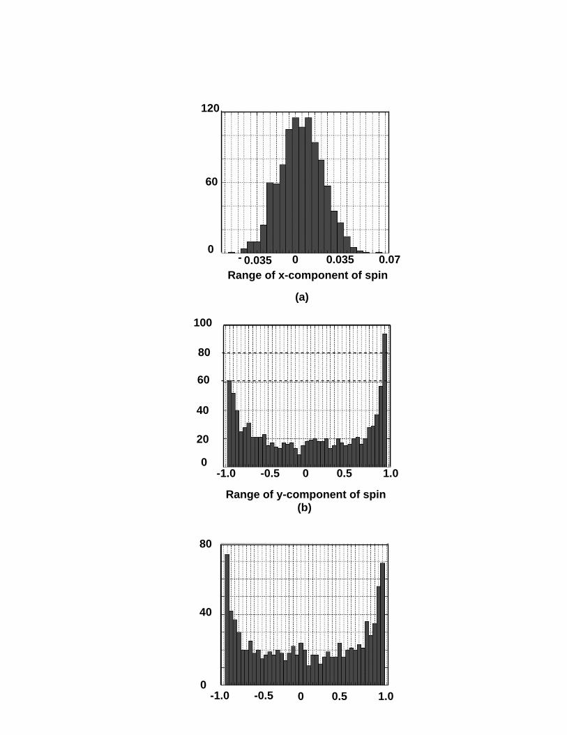
In Fig. 8(a)-8(c), we show the distribution of the x-, y- and z-components of the spins in

the electron ensemble once steady state is reached. We define steady state as the condition when

j < S > j approaches zero in Fig. 7. Again, the driving electric field is 2 kV/cm and the lattice

temperature is 30 K. Comparing these figures to Figs. 3(a) - 3(c), we find that the steady state dis-

tributions are vastly and qualitatively different for injection with transverse polarization compared

to injection with longitudinal polarization. The distributions in Fig. 8 are not uniform flat topped

distributions at all.

The x-component shows a very narrow Gaussian-type distribution with zero mean and a stan-

dard deviation less than 0.03. This is expected since the x-component should be ideally zero (the

distribution would be a delta function at zero) in the absence of the Rashba interaction. The Rashba

interaction causes some spread about the zero value, but the Rashba interaction is weak and there-

fore the spread is small.

The y- and z-components show a U-shaped distribution weighted towards the extreme values

of -1 and +1. This U-shape is a consequence of the oscillatory nature of the decay characteristics

for y- and z-components seen in Fig. 7. Note that the slopes of the decay characteristics are zero

at the peaks and valleys when the spins have close to their extremal values. Hence the spins spend

more time near their extremal values. Consequently, more spins in the ensemble will have values

close to -1 and +1 than any other intermediate value.

In Fig. 9(a)-9(c), we show the steady state spin distributions when spins are initially polarized

along the y-direction. There is a slight difference between the distributions in Figs. 8 and 9 because

of the geometric and electrical asymmetry between x and y. Otherwise, the qualitative features are

the same.

For both y- and z-polarized injections, we have found that the shapes of the steady state distri-

14

butions are fairly independent of temperature and driving electric field.

4. Effect of temperature

Finally, in Fig. 10, we show the effect of temperature on the dephasing (or depolarization)

characteristics of j< S > j when spins are initially polarized along the z-direction. Once again, the

driving electric field is 2 kV/cm. There is a very weak temperature dependence in the range 10 K

- 50 K for essentially the same reason as alluded to in Section 3.1.4.

IV. CONCLUSION

In this paper, we have studied spin dephasing in a quasi one dimensional structure. The dephas-

ing rate was found to be strongly anisotropic in the sense that it depends sensitively on whether the

spins are initially polarized along the wire axis, or perpendicular to the wire axis. A somewhat dif-

ferent type of anisotropy in the spin relaxation rates was discussed in ref. [44] and was attributed to

interference between various types of spin-orbit interactions. In our case, the anisotropy is primar-

ily due to the fact that the Dresselhaus interaction operates only on spins polarized transverse to

the wire axis and not on spins polarized along the wire axis. This anisotropy can be exploited in the

design of spintronic devices such as the gate controlled spin interferometer where the suppression

of spin dephasing is a critical issue. We have also shown that the steady state spin distributions are

strongly a function of the initial polarization. The dephasing rate has a very weak dependence on

temperature and a moderately strong dependence on the driving electric field.

The work of S. P and S. B. were supported by the National Science Foundation under grant

ECS-0196554.

15

REFERENCES

[1] G. Prinz and K. Hathaway, Phys. Today, 48, 24 (1995); G. Prinz, Science, 270, 1660 (1998).

[2] S. A. Wolf, D. D. Awschalom, R. A. Buhrman, J. M. Daughton, S. von Molnar, M. L. Roukes,

A. Y. ChtChelkanova and D. M. Treger, Science, 294, 1488 (2001).

[3] D. D. Awschalom, M. E. Flatte and N. Samarth, Sci. Am., 286, 66 (2002).

[4] S. Das Sarma, Am. Sci., 89, 516 (2001).

[5] S. Datta and B. Das, Appl. Phys. Lett., 56, 665 (1990).

[6] M. E. Flatte and G. Vignale, Appl. Phys. Lett., 78, 1273 (2001).

[7] I. Zutic, J. Fabian and S. Das Sarma, Appl. Phys. Lett., 79, 1558 (2001).

[8] T. Koga, J. Nitta, H. Takayanagi and S. Datta, Phys. Rev. Lett., 88, 126601 (2002).

[9] X. F. Wang, P. Vasilopoulos and F. M. Peeters, Phys. Rev. B, 65, 165217 (2002).

[10] S. Bandyopadhyay and V. P. Roychowdhury, Superlattices Microstruct., 22, 411 (1997).

[11] V. Privman, I. D. Vagner and G. Kventsel, Phys. Lett. A, 239, 141 (1998).

[12] B. E. Kane, Nature (London), 393 133 (1998).

[13] S. Bandyopadhyay, Phys. Rev. B, 61, 13813 (2000).

[14] G. Feher, Phys. Rev., 114, 1219 (1954).

[15] J. M. Kikkawa and D. D. Awschalom, Phys. Rev. Lett., 80, 4313 (1998).

[16] P. Mohanty, J. M. Q. Jariwalla and R. A. Webb, Phys. Rev. Lett., 78, 3366 (1997).

[17] F. Mireles and G. Kirczenow, Phys. Rev. B, 64, 024426 (2001).

[18] Th. Schapers, J. Nitta, H. B. Heersche and H. Takayanagi, Physica E, 13, 564 (2002).

[19] T. Matsuyama, C.-M. Hu, D. Grundler, G. Meier, and U. Merkt, Phys. Rev. B, 65, 155322

(2002).

16

[20] M. Cahay and S. Bandyopadhyay (preprint).

[21] J. Fabian, I. Zutic and S. Das Sarma, Phys. Rev. B, 66, 165301 (2002).

[22] G. Schmidt and L. W. Molenkamp, Semicond. Sci. Tech., 17, 310 (2002).

[23] Z. G. Yu and M. E. Flatte, Phys. Rev. B, 66, 235302 (2002).

[24] S. Saikin, M. Shen, M. C. Cheng and V. Privman, www.arXiv.org/cond-mat/0212610; M.

Shen. S. Saikin, M. C. Cheng and V. Privman, www.arXiv.org/cond-mat/0302395

[25] W. H. Lau, J. T. Olesberg and M. E. Flatte, Phys. Rev. B, 64, 161301 (2001).

[26] M. S. Lundstrom, Fundamentals of Carrier Transport, Modular Series on Solid State Devices,

Vol. X, (Addison-Wesley, Reading, Massachusetts, 1990).

[27] G. Schmidt, C. Gould, P. Grabs, A. M. Lunde, G. Richter, A. Slobodsky and L. W.

Molenkamp, www.arXiv.org/cond-mat/0206347.

[28] H. Sanada, Y. Arata, Y. Ohno, Z. Chen, K. Kayanuma, Y. Oka, F. Matsukura and H. Ohno,

Appl. Phys. Lett., 81, 2788 (2002).

[29] M. Q. Weng and M. W. Wu, J. Appl. Phys., 93, 410 (2003).

[30] Y. Qi and S. Zhang, Phys. Rev. B., 67, 052407 (2003).

[31] A. Bournel, P. Dollfus, S. Galdin, F-X Musalem and P. Hesto, Solid State Commun., 104, 85

(1997); A. Bournel, P. Dollfus, P. Bruno and P. Hesto, Mat. Sci. Forum, 297-298, 205 (1999);

A. Bournel, V. Delmouly, P. Dollfus, G. Tremblay and P. Hesto, Physica E, 10, 86 (2001).

[32] K. Blum, Density Matrix Theory and Applications, (Plenum, New York, 1996).

[33] G. Dresselhaus, Phys. Rev., 100, 580 (1955).

[34] E. I. Rashba, Sov. Phys. Semicond., 2, 1109 (1960); Y. A. Bychkov and E. I. Rashba, J. Phys.

C, 17, 6039 (1984).

[35] M. I. D’yakonov and V. I. Perel’, Sov. Phys. Solid State, 13, 3023 (1972).

17

[36] R. J. Elliott, Phys. Rev., 96, 266 (1954).

[37] H. Sakaki, Jpn. J. Appl. Phys., 19, L735 (1980).

[38] G. L. Bir, A. G. Aronov and G. E. Pikus, Sov. Phys. JETP, 42, 705 (1976).

[39] N. E. Christensen and M. Cardona, Solid State Commun., 51, 491 (1984).

[40] D. Richards and B. Jusserand, Phys. Rev. B, 59, R2506 (1999).

[41] D. Jovanovich and J-P Leburton, in Monte Carlo Device Simulation: Full Band and Beyond

Ed. K. Hess (Kluwer Academic, Boston, 1991) pp. 191-218.

[42] N. Telang and S. Bandyopadhyay, Appl. Phys. Lett., 66, 1623 (1995).

[43] N. Telang and S. Bandyopadhyay, Phys. Rev. B, 51, 9728 (1995).

[44] N. S. Averkiev, L. E. Golub and M. Willander, Fizika i Tekhnika Poluprovodnikov, 36, 97

(2002) [Semiconductors, 36, 91 (2002).]

18

FIGURES

FIG. 1. Temporal dephasing of the ensemble average spin vector with time in a GaAs quantum wire of

dimension 4 nm 30 nm at a lattice temperature of 30 K. The results are shown for various driving electric

fields E§. The spins are injected with their polarization initially aligned along the wire axis. The geometry

of the wire and the axes designation are shown above.

FIG. 2. Temporal dephasing of the x-, y- and z-components of spin in the same GaAs wire at 30 K. The

driving electric field is 2 kV/cm and the spins are injected with their polarization initially aligned along the

wire axis.

FIG. 3. Distribution of the spin components in the GaAs wire. The driving electric field is 2 kV/cm

and the lattice temperature is 30 K. Spins are injected with their polarization initially aligned along the wire

axis. (a) steady state distribution of the x-component, (b) steady state distribution of the y-component, (c)

steady state distribution of the z-component and (d) transient distribution (after a time of 10 nanoseconds)

of the x component when the driving electric field is 0.1 kV/cm.

FIG. 4. Temperature dependence of the spin dephasing in the GaAs wire when the driving electric field

is 2 kV/cm. Spins are injected with their polarization initially aligned along the wire axis.

FIG. 5. Steady state istribution of the spin components in the GaAs wire. The driving electric field is 2

kV/cm and the lattice temperature is 4.2 K. Spins are injected with their polarization initially aligned along

the wire axis. (a) distribution of the x-component, (b) distribution of the y-component, and (c) distribution

of the z-component.

FIG. 6. Temporal dephasing of the ensemble average spin vector with time in a GaAs quantum wire

of dimension 4 nm 30 nm at a lattice temperature of 30 K. The results are shown for various driving

electric fields E§. (a) The spins are injected with their polarization initially aligned along the z-axis which

is mutually perpendicular to the wire axis and the direction of the electric field Ey used to induce the Rashba

spin orbit coupling; (b) spins are injected with their polarization initially aligned along the y-axis which is

the direction of the electric field Ey used to induce the Rashba spin orbit coupling.

19

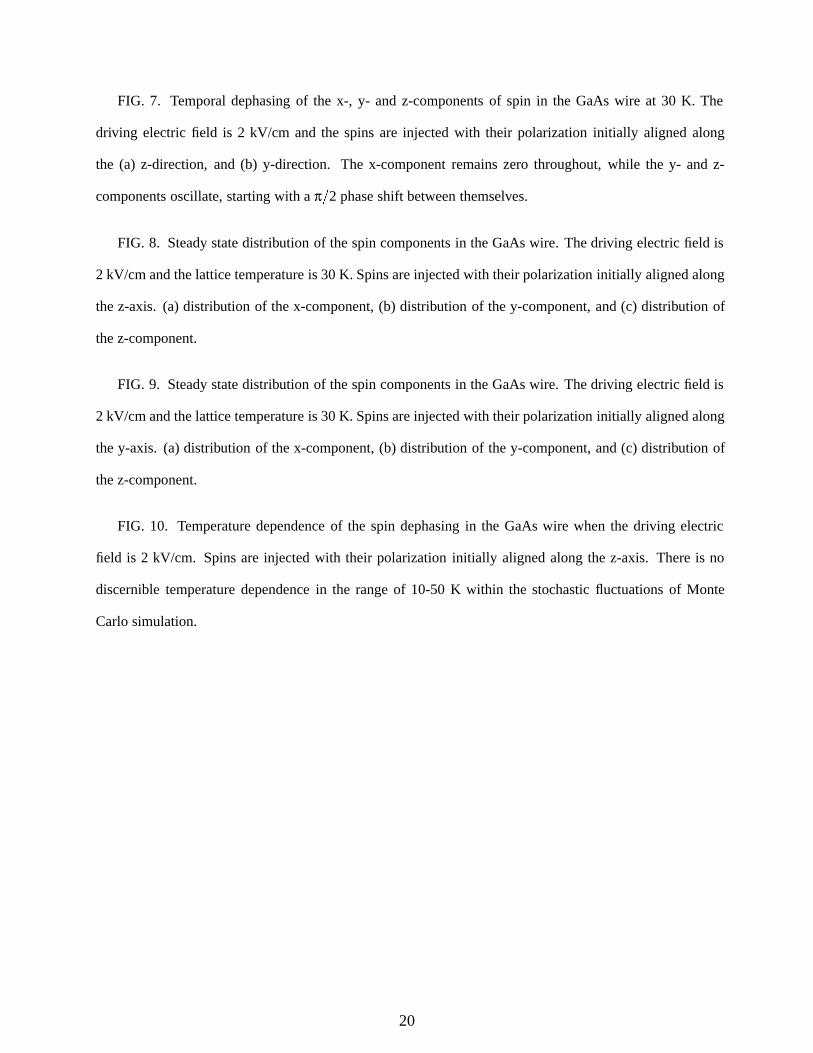
FIG. 7. Temporal dephasing of the x-, y- and z-components of spin in the GaAs wire at 30 K. The

driving electric field is 2 kV/cm and the spins are injected with their polarization initially aligned along

the (a) z-direction, and (b) y-direction. The x-component remains zero throughout, while the y- and z-

components oscillate, starting with a π=2 phase shift between themselves.

FIG. 8. Steady state distribution of the spin components in the GaAs wire. The driving electric field is

2 kV/cm and the lattice temperature is 30 K. Spins are injected with their polarization initially aligned along

the z-axis. (a) distribution of the x-component, (b) distribution of the y-component, and (c) distribution of

the z-component.

FIG. 9. Steady state distribution of the spin components in the GaAs wire. The driving electric field is

2 kV/cm and the lattice temperature is 30 K. Spins are injected with their polarization initially aligned along

the y-axis. (a) distribution of the x-component, (b) distribution of the y-component, and (c) distribution of

the z-component.

FIG. 10. Temperature dependence of the spin dephasing in the GaAs wire when the driving electric

field is 2 kV/cm. Spins are injected with their polarization initially aligned along the z-axis. There is no

discernible temperature dependence in the range of 10-50 K within the stochastic fluctuations of Monte

Carlo simulation.

20

TABLES

TABLE I. Spin dephasing times as a function of driving electric field in a GaAs quantum wire of

dimensions 30 nm 4 nm at a temperature of 30 K. The spins are initially polarized along the wire axis.

Electric field (kV/cm) Spin dephasing time (sec)

0.1 1.7 108

0.5 5.0 109

1.0 3.5 109

2.0 2.5 109

21

TABLE II. Spin dephasing times as a function of driving electric field in a GaAs quantum wire of

dimensions 30 nm 4 nm at a temperature of 30 K. The spins are initially polarized transverse to the wire

axis (z-axis).

Electric field (kV/cm) Spin dephasing time (sec)

0.1 5.0 109

0.5 9.0 1010

1.0 3.0 1010

2.0 1.0 1010

3.0 6.0 1011

4.0 4.0 1011

22

0 2 4 6 8 10

Time (nanosecond)

Mag

nit

ud

e o

f av

erag

e sp

in v

ecto

r |<

S>|

30 nm

4 nm

y

z

x

T = 30K

0.1 kV/cm

2 kV/cm

1 kV/cm

0.5 kV/cm

T = 30 K

X = |<S>|

0 = <S >x

= <S >

= < S >

y

z

Time (nanoseconds)

0 2 4 6 8 10

Sp

in c

om

po

nen

ts

0

10

20

30

40

50

60

Co

un

t

-1 -0.8 -0.6 -0.4 -0.2 0.0 0.2 0.4 0.6 0.8 1.0 0

x-component of spin (S )x

(a)

Co

un

t

-1 -0.8 -0.6 -0.4 -0.2 0.0 0.2 0.4 0.6 0.8 1.0

Co

un

t

-1 -0.8 -0.6 -0.4 -0.2 0.0 0.2 0.4 0.6 0.8 1.0

y-component of spin (S )

0

10

20

30

40

50

60

70

y(b)

Co

un

t

0

10

20

30

40

50

60

70

80

(c)

Co

un

t

-1 -0.8 -0.6 -0.4 -0.2 0.0 0.2 0.4 0.6 0.8 1.0

x

-1 -0.8 -0.6 -0.4 -0.2 0.0 0.2 0.4 0.6 0.8 1.0

(d)

Co

un

t

0

20

40

60

80

100

120

140

160

-1 -0.8 -0.6 -0.4 -0.2 0.0 0.2 0.4 0.6 0.8 1.0

z-component of spin (S )z

non-steady-state x-component of spin (S )x

Electric field

2 kV/cm

0 2 4 6 8 10

Mag

nit

ud

e o

f en

sem

ble

ave

rag

ed s

pin

vec

tor

|<S

>|

0

0.2

0.4

0.6

0.8

1.0

Time (nanoseconds)

T=30K

T=4.2K

-0.5 0 0.5 1.0-1.0

-0.5 0 0.5 1.0-1.0

-0.5 0 0.5 1.0-1.0

Range of x-component of spin

Range of y-component of spin

Range of z-component of spin

(a)

(b)

(c)

0.1 kV/cm

0.5 kV/cm

1.0 kV/cm2.0 kV/cm

4.0 kV/cm

3.0 kV/cm

Time (nanoseconds)

0

0 0.1 0.2 0.3 0.4

0.2

0.4

0.6

0.8

1.0

Mag

nit

ud

e o

f en

sem

ble

aver

age

of

the

spin

vec

tor

|<S

>|

0.2 kV/cm

2.0 kV/cm

0

0.2

0.4

0.6

0.8

1.0

Mag

nit

ud

e o

f en

sem

ble

aver

age

of

the

spin

vec

tor

|<S

>|

Time (nanoseconds)

0 0.05 0.10 0.15 0.20 0.25 0.3

(a)

|<S>|

<S >z

<S >y-1

-0.5

0

0.5

1

0 0.1 0.2 0.3Time (nanoseconds)

Sp

in

(a)

-1

0

1

Sp

in

Time (nanoseconds)

<S >

<S >

|<S>|z

y

0 0.08 0.16 0.24

0 0.035 0.070.035-

Range of x-component of spin

0

60

120

(a)

0 0.5 1.0 -1.0 -0.50

20

40

60

80

100

Range of y-component of spin(b)

0

40

80

-1.0 -0.5 0 0.5 1.0

0 0.015 0.030-0.045 -0.03 -0.0150

20

40

60

80

100

120

Co

un

t

0 0.5 1.0-1.0 -0.5

Co

un

t

0

40

80

(a)

Range of x-component of spin

Range of y-component of spin(b)

Co

un

t

40

80

0 0.5 1.0-1.0 -0.5

Range of y-component of spin

0

(c)

T=10K

T=50K

T=30K

T=20K

0 0.02 0.04 0.06 0.08 0.10

0.2

0.4

0.6

0.8

Time (nanoseconds)

Mag

nit

ud

e o

f th

e en

sem

ble

av

erag

ed s

pin

vec

tor

|<S

>|