Speed Sensor Less Field-Oriented Control of IM With Interconnected Observers Experimental Tests on Low Frequencies Benchmark

8/14/2019 Speed Sensor Less Field-Oriented Control of IM With Interconnected Observers Experimental Tests on Low Frequen…

http://slidepdf.com/reader/full/speed-sensor-less-field-oriented-control-of-im-with-interconnected-observers 1/12

Speed sensorless field-oriented control of inductionmotor with interconnected observers: experimentaltests on low frequencies benchmark

D. Traore, J. De Leon, A. Glumineau and L. Loron

Abstract: Field-oriented speed control of induction motors (IMs) without mechanical sensors(speed sensor and load torque sensor) are considered. The methodology is divided into two parts. First, interconnected high-gain observers are designed to estimate the mechanical and mag-netic variables from the only measurement of stator current. Secondly, the speed and flux esti-mation are used by a controller to achieve the speed /flux tracking. The flux regulation problemis simple and the traditional approach is followed by using proportional integral (PI) controller.For the speed-regulation problem, it is stated that flux regulation quickly happens by using a high-gain PI controller to regulate the q-axis current to its reference. Stability analysis based onLyapunov theory is proved to guarantee the ‘observer þ controller’ stability. To test and validatethe controller–observer by considering the sensorless control problem of IM at low frequency, asignificant benchmark is implemented. The trajectories of this benchmark are designed to validate

the controller and observer under three operating conditions: low speed, high speed and very lowspeed. Furthermore, robustness tests with respect to parameter variations are given in order to showthe performance of the proposed observer–controller scheme.

1 Introduction

Because of its reliability, ruggedness and relatively lowcost, induction motor (IM) is the most widely used in indus-trial applications. However, the IM presents a challengingcontrol problem. This is mainly due to the following four factors:

† The IM is a complex highly coupled nonlinear system.† Two of the state variables (rotor fluxes and mechanicalspeed) are not usually measurable.† Because of heating, the rotor and stator resistances varyconsiderably with a significant impact on the systemdynamics.† The load torque is generally unknown.

For direct field-oriented control of IM drives, for example, the speed knowledge is crucial, and generallysensors are used to measure it. The minimisation of thenumber of sensors contributes to simplify the installationand decreases the cost of both control and maintenance.Consequently, during the last decade, there has been a con-siderable interest in IM drives without mechanical sensors

(sensorless). A major difficulty is the estimation of thestate variable at low frequencies. Another difficulty is toensure the robustness against parameter variations. In theliterature, several approaches have been proposed to esti-mate the rotor velocity and load torque from the measure-ments, such as the stator current or voltage, for example,[1–8].

In [1], two types of observers are investigated. To increasethe robustness of the speed sensorless IM drives for high- performanceapplication, the authors proposed a second obser-ver which is an adaptive uncertain observer. This observer iscombined with an integral-proportional (IP) controller for speed tracking. The direct torque control and space vector modulation schemes for the sensorless IM drives based oninput–output feedback linearisation control are addressed in[8]. In [4], an algorithm for simultaneous estimation of motor speed and rotor resistance is presented. This observer is combined with a state feedback controller which is load torque-adaptive. The sensorless control scheme and a rotor

fluxobserver, which is adaptivewithrespectto rotor resistanceat constant rotor speed, have been proposed in [5].Field-oriented controller using a singular perturbationapproach with on-line stator resistance estimation for speed sensorless has been addressed in [2]. A high-gain observer is proposed in [3]. This observer is associated to field-oriented feedback with PI controller. In [6] a speed sensorless control-ler for IM, based on a high-gain speed observer, has been proposed. To improve the performance of the control law at lowspeed, the authors add a stator resistance adaptationmechanism.

In the literature, the stability analysis for speed sensorless isnot available except in [7, 9]. In [9], the global exponentialspeed flux tracking was proved. The global asymptotic stab-ility of the closed loop has been guaranteed in [7]. However,the authors assume that the load torque and vector flux areknown which is not realistic in an industrial situation.

# The Institution of Engineering and Technology 2007

doi:10.1049/iet-cta:20060453

Paper first received 26th October 2006 and in revised form 11th June 2007

D. Traore and A. Glumineau are with IRCCyN: Institut de Recherche enCommunications et Cybernetique de Nantes, Ecole Centrale de Nantes, BP92101, 1 Rue de la Noe, 44312 Nantes Cedex 3, France

J. De Leon is with the Department of Electrical Engineering, Universidad Autonoma de Nuevo Leon, PO Box 148-F, San Nicolas de Los Garza 66450,

N.L, Mexico

L. Loron is with IREENA: Institut de Recherche en Electronique etElectrotechnique de Nantes Atlantique, Bd de l’universite, BP 406, Saint-

Nazaire Cedex 44602, France

E-mail: [email protected]

IET Control Theory Appl., 2007, 1, (6), pp. 1681– 1692 1681



Canudas et al . [10] and Ibarra-Rojas et al. [11], demon-strate that the main conditions to lose the observability of IM are: the excitation voltage frequency is zero and therotor speed is constant. Yet, in the literature, the sensorlessalgorithms are usually tested and evaluated at high and lowspeed [6, 9, 12]. However, a few studies have highlighted this problem of unboservability [9]. In [9] the ‘observer þcontroller’ was tested on a ‘sensorless control benchmark’.The trajectories of this benchmark are chosen to evaluatethe IM sensorless algorithm in observable and unobservable

conditions. Unfortunately, when the load torque is.

20% of the nominal load torque the ‘observer þ controller’ becomes unstable.

The purpose of this paper is to propose a traditionalfield-oriented control using an interconnected high-gainobserver that achieves a good speed /flux tracking for IMcontrol without mechanical sensors. Then to test and evalu-ate the performance of our sensorless controller on aspecific benchmark defined in [9]. This benchmark iscalled sensorless control benchmark. Three operating con-ditions are considered in this benchmark: (1) low speed with nominal load, (2) high speed with nominal load, (3)unobservable conditions (low frequencies). In this region(unobservable condition), we define the value of speed

and the stator pulsation by using the inobservability con-ditions [10] of the IM. In our case, the value of the speed is V ¼20.5 rad /s. The load torque in this region is thenominal torque (8 N m), so that the speed and the developed torque are in opposite directions.

The paper is organised as follows. Section 2 is devoted tothe description of the IM model. The interconnected obser-vers design is introduced in Section 3. In Section 4, theLyapunov stability analysis of these observers is given.The flux-oriented control is presented in Section 5. TheLyapunov stability analysis of the observersþ controller is given in Section 6. Experimental results are given and dis-cussed in Section 7.

2 IM model

The IM model, described in this paper, is based on the motor equation in a rotating frame d and q-axes [13]. The dynamicequation can be described by

isd

isq

f r d

f r q

_V

0BBBBBB@

1CCCCCCA

¼

baf r d þ bpVf r q À g isd þ v sisq

baf r q À bpVf r d À g isq À v sisd

Àaf r d þ (v s À pV)f r q þ aM sr isd

Àaf r q À (v s À pV)f r d þ aM sr isq

m(f r d isq À f r qisd ) À cVÀ 1

J T l

0BBBBBBB@

1CCCCCCCA

þ

m1 0

0 m1

0 0

0 0

0 0

0BBBBBB@

1CCCCCCA

usd

usq

(1)

where isd , isq, f r d , f r q, usd , usq, V and Tl denote, respect-ively, the stator currents, the rotor fluxes, the stator voltage inputs, the angular speed and the load torque. Thesubscripts s and r refer to the stator and rotor. The par-ameters a, b, c, g , s , m and m1 are defined by: a ¼ Rr / Lr ,

b¼

M sr /s Ls Lr , c¼

f v/ J , g ¼

( Lr

2

Rsþ M sr 2

Rr )/s Ls Lr

2

,s ¼ 12 ( M sr 2 / Ls Lr ), m ¼ pM sr / JLr , m1 ¼ 1/s Ls. Rs and

Rr are the resistances, Ls and Lr the self-inductances, M sr the mutual inductance between the stator and rotor

windings, p the number of pole-pair, J the inertia of thesystem (motor and load) and f v the viscous dampingcoefficient.

Furthermore, the operation domain D of IM is defined bythe set of values

D ¼ { X [ R6jjf r d j Fmaxd , jf r qj Fmax

q

jisd j I maxd , jisqj I

maxq , jVj Vmax, T l T l

max}

where X ¼ (f r d , f r q, isd , isq, V, Tl), Fd max, Fq

max, I d max, I q

max,Vmax and T l

max are the actual maximum values for thefluxes, currents, speed and torque load, respectively.

The control inputs are the stator voltages. Only stator cur-rents and stator voltages are measured.

3 Interconnected observers design

In this section, we propose the design of two interconnected observers for the sensorless IM. Consider IM model (1)

rewritten in form (2)

X NL

:_ x ¼ f ( x) þ g ( x)u

y ¼ h( x)

&(2)

where x ¼ (isd isq f r d f r q V T l)T, u ¼ (usd usq)T, y ¼ (h1,

h2)T ¼ (isd , isq)T

f ( x) ¼

baf r d þ bpVf r q À g isd þ v sisq

baf r q À bpVf r d À g isq À v sisd

Àaf r d

þ(v s

À pV)f r q

þaM sr isd

Àaf r q À (v s À pV)f r d þ aM sr i sq

m(f r d isq À f r qisd ) À cVÀ 1

J T l

0

0

BBBBBBBBB@

1

CCCCCCCCCA

and g ( x) ¼

m1 0

0 m1

0 0

0 0

0 0

0BBBBBB@

1CCCCCCA

In this paper, the unknown load torque is considered con-stant; thus, the IM model (2) may be seen as the intercon-nection between subsystems (3) and (4). Then we supposethat each subsystem satisfies some required properties to build an observer and we assume that, for each of this sep-arate observer, the state of the other is available

isd

_V

_T l

0B@

1CA ¼

0 bpf r q 0

0 0 À1

J 0 0 0

0BB@

1CCA

isd

V

T l

0B@

1CA

þ Àg isd þ abf r d þ m1usd þ v sisq

m(f r d isq À f r qisd ) À cV

0

0B@ 1CA (3)

IET Control Theory Appl., Vol. 1, No. 6, November 2007 1682





Then, assuming that Assumption 2 is verified, a nominalobserver for interconnected systems (5) is given by

O:

_Z 1 ¼ A1(Z 2)Z 1 þ g 1(u, y, Z 2, Z 1)

þ(GS À11 C

T1 þ B2(Z 2))( y1 À ^ y1)

þ( B1(Z 2) þ KC T2 )( y2 À ^ y2)

_S 1 ¼ Àu 1S 1 À AT1 (Z 2)S 1 À S 1 A1(Z 2) þ C

T1 C 1

^ y1 ¼ C 1Z 1_Z 2 ¼ A2(Z 1)Z 2 þ g 2(u, y, Z 1, Z 2) þ S

À12 C

T2 ( y2 À ^ y2)

_S 2

¼ Àu 2S 2

À AT

2 (Z 1)S 2

ÀS 2 A2(Z 1)

þC T2 C 2

^ y2 ¼ C 2Z 2

8>>>>>>>>>><>>>>>>>>>>:

(10)

Remark 5: It is worth noticing that kS 1k and kS 2k are bounded for u 1 and u 2 large enough due to the persistency property of inputs; more details can be found in [9].

4 Stability analysis of observer underparameters uncertainties

Defining the estimation errors as

e1

¼ X 1

ÀZ 1 and e2

¼ X 2

ÀZ 2

the estimation error dynamics is given by

_e1 ¼ [ A1(Z 2) À GS À11 C T1 C 1 À B2(Z 2)C 1]e1

þ g 1(u, y, X 2, X 1) À g 1(u, y, Z 2, Z 1)

þ [ A1( X 2) À A1(Z 2)] X 1

À ( B1(Z 2)C 2 þ KC T2 C 2)e2 (11)

_e2 ¼ [ A2(Z 1) À S À12 C T2 C 2]e2

þ [ A2( X 1) À A2(Z 1)] X 2

þ[ g 2(u, y, X 1, X 2)

À g 2(u, y, Z 1, Z 2)] (12)

Now we consider that the motor parameters are knownwith uncertainties. So (11) and (12) become

_e1 ¼ [ A1(Z 2) À GS À11 C

T1 C 1 À B2C 1]e1

þ g 1(u, y, X 2, X 1) þ D g 1(u, y, X 2, X 1)

À g 1(u, y, Z 2, Z 1) þ [ A1( X 2) þ D A1( X 2) À A1(Z 2)] X 1

À ( B1C 2 þ KC T2 C 2)e2 (13)

_e2 ¼ [ A2(Z 1) À S À12 C

T2 C 2]e2

þ [ A2( X 1) þ D A2( X 1) À A2(Z 1)] X 2

þ g 2(u, y, X 1, X 2)

þD g 2(u, y, X 1, X 2)

À g 2(u, y, Z 1, Z 2)

where the terms D A1( X 2), D A2( X 1), D g 1(u, y, X 2, X 1) and D g 2(u, y, X 1, X 2) represent the uncertain terms of A1( X 2),

A2( X 2), g 1(u, y, X 2, X 1) and g 2(u, y, X 1, X 2), respectively.

Assumption 3: We assume that the uncertain terms satisfythe following inequalities

kD A1( X 2)k r 1, kD A2( X 1)k r 2, kD g 1(u, y, X 2, X 1)k r 3

kD g 2(u, y, X 1, X 2)k r 4

with r i . 0, for i

¼1, . . . , 4.

Theorem 1: Let us consider system (5) and assume thatAssumptions 1– 3 are satisfied. Then, system (10) is aninterconnected observer for system (5). The parameters u 1

and u 2 can be selected from (16). Furthermore, theestimation error converges asymptotically to zero if weknow exactly the motor parameters. Otherwise, the conver-gence of the complete observer admits a small upper bound.

Remark 6: When the persistence condition is not satisfied (in the unobservable area), we will prove the stability of the observer in Section 6.1.

Proof: Let us define V o ¼ V 1 þ V 2 a candidate Lyapunovfunction where V 1 and V 2 are, respectively, the candidateLyapunov function for each dynamics (11), (12) given byV 1 ¼ eT

1 S 1e1 and V 2 ¼ eT2 S 2e2. Next, taking the time deriva-

tive of V o and replacing the suitable expressions, (13) and (10) we have

_V o ¼ eT1 Àu 1S 1 À (2S 1GS À1

1 À 1)C T1 C 1 À 2S 1 B02

È Ée1

þ 2eT1 S 1 A1( X 2) À A1(Z 2)

È É X 1 þ 2eT

1 S 1 D A1( X 2)È É

X 1

þ 2eT 1 S 1 g 1(u, y, X 2, X 1) À g 1(u, y, Z 2, Z 1)

È Éþ 2eT

1 S 1 D g 1(u, y, X 2, X 1)È Éþ eT

2 Àu 2S 2 À C T2 C 2È É

e2

þ2eT

2 S 2 A2( X 1)

À A2(Z 1)È É X 2

þ2eT

2 S 2 D A2( X 1)È É X 2

þ 2eT2 S 2 g 2(u, y, X 1, X 2) À g 2(u, y, Z 1, Z 2)

È Éþ 2eT

2 S 2 D g 2(u, y, X 1, X 2)È ÉÀ 2eT

1 S 1( B01 þ K 0)e2

where B01 ¼ B1(Z 2)C 1, B0

2 ¼ B2(Z 2)C 2 and K 0 ¼ KC T2 C 2.

From Assumption 2, the following inequalities hold

kS 1k k 1, kS 2k k 5, k X 1k k 3, k X 2k k 7k g 1(u, y, X 2, X 1) À g 1(u, y, Z 2, Z 1)È Ék k 4ke2k þ k 9ke1k

k A1( X 2) À A1(Z 2)È Ék k 2ke2kk A2( X 1) À A2(Z 1)È Ék k 6ke1k

k g 2(u, y, X 1, X 2) À g 2(u, y, Z 1, Z 2)È Ék k 8ke1k þ k 10ke2kk B01k k B1, k B02k k B2, k K 0k k k 0

Using the norm, from Assumptions 1 and 3, and byregrouping with respect to ke1k and ke2k, the time deriva-tive of V o can be rewritten as follows

_V o À(u 1 þ 2k B1 À 2k 1k 9)eT1 S 1e1 þ 2m1ke1kke2k

þ 2m2ke1kke2k À (u 2 À 2k 10k 5)eT2 S 2e2

þ 2m3ke2kke1k þ 2m4ke2kke1k þ m5ke1kþ m6ke2k (14)

where m1

¼k 1k 2k 3

Àk B2k 1

Àk k 0k 1, m2

¼k 1k 4, m3

¼k 5k 6k 7,

m4 ¼ k 5k 8, m5 ¼ 2(k 1k 3r 1þ k 1r 3) and m6 ¼ 2(k 5k 7r 2þ k 5r 4): Now, consider that the following inequalities are satisfied

lmin(S i)keik2 keik2S i lmax(S i)keik2, i ¼ 1, 2

where lmin(S i) and lmax(S i) are minimal and maximal eigen-values of S i independently to u

keik2S i¼ e

Ti S iei, i ¼ 1, 2

Inequality (14) can be rewritten in terms of functions V 1and V 2

_V o À(u 1 þ 2k B1 À 2k 1k 9)V 1 À (u 2 À 2k 10k 5)V 2

þ 2 ˜ m ffiffiffiffiffi

V 1p ffiffiffiffiffi

V 2p

þ m5ke1k þ m6 ke2k (15)




where

˜ m ¼X4

i¼0

˜ m i, min(S ) ¼ ffiffiffiffiffiffiffiffiffiffiffiffiffiffiffiffi

min(S 1)p ffiffiffiffiffiffiffiffiffiffiffiffiffiffiffiffi

min(S 2)p

˜ m i ¼mi ffiffiffiffiffiffiffiffiffiffiffiffiffiffiffi

min(S )p , i ¼ 1, 2, 3, 4

Using the following inequality, ffiffiffiffiffi

V 1p ffiffiffiffiffi

V 2p (e =2)V 1þ

(1=2e )V 2, 8e [ ]0, 1[

_V o À(u 1 þ 2k B1 À 2k 1k 9)V 1 þ ˜ me V 1

þ ˜ m

e V 2 À (u 2 À 2k 10k 5)V 2 þ m5ke1k þ m6ke2k

Consequently

_V o À(u 1 þ 2k B1 À 2k 1k 9 À ˜ me )V 1

À u 2 À 2k 10k 5 À˜ m

e

V 2 þ m5ke1k þ m6ke2k

with d ¼ min(d 1, d 2) and m ¼ max(m5, m6), where

d 1 ¼ u 1 þ 2k B1 À 2k 1k 9 À ˜ me . 0 and d 2 ¼ u 2 À 2k 10k 5À ˜ m=e . 0.So that

u 1 . 2k 1k 9 þ ˜ me À 2k B1, u 2 . 2k 10k 5 þ˜ m

e (16)

Then it follows that

_V o Àd (V 1 þ V 2) þ m( ffiffiffiffiffi

V 1p

þ ffiffiffiffiffi

V 2p

) Àd V o þ mc ffiffiffiffiffi

V op

(17)

where c . 0, such that c p ðV 1 þ V 2Þ . ffiffiffiffiffiV 1p þ ffiffiffiffiffiV 2p .

If the motor parameters are exactly known, then m ¼ 0and _V o Àd V o. This system (10) is an exponential observer for system (5).

Otherwise, if m= 0, inequality (17) can be rewritten as

_V o À(1 À 6 )d V o À 6 V o þ mc kek, 1 . 6 . 0 (18)

Finally, we have

_V o À(1 À 6 )d V o, 8kek ! mc

6d (19)

By choosing u 1 and u 2, inequality (19) shows that in spiteof perturbations due to motor parameters variations, the

observation errors will converge to a small upper bound.A

Remark 7: Inequality (16) depends on the Lipschitz con-stants introduced in Assumption 2. From Lipschitz con-stants, we can calculate the minimum value of u 1 and u 2.Then we tune u 1 and u 2 in order to accelerate the conver-gence of the observer.

5 Flux-oriented control

In order to easily design the flux-oriented control, let usdenote by VÃ and f Ã the smooth bounded reference

signals for the output variables to, respectively, controlthe speed V and the rotor flux modulus p ðf 2r d þ f 2r qÞ.Following the strategy of field-oriented control

(f r d ¼p ðf 2r d þ f 2r qÞ, f r q ¼ 0), the new dynamic model of

IM is given by

_V

f r d

r

isd

isq

0BBBBBB@

1CCCCCCA

¼

mf r d isq À cV

Àaf r d þ aM sr isd

pVþ a M sr

f r d

isq

Àg isd þ abf r d þ pVisq þ a M sr

f r d

i2sq

Àg isq À bpVf r d À pVisd À a

M sr

f r d isd isq

0BBBBBBBBBBB@

1CCCCCCCCCCCA

þ

0 0 À1

J 0 0 0

0 0 0

m1 0 0

0 m1 0

0BBBBBBB@

1CCCCCCCA

V sd

V sq

T l

0B@

1CA (20)

where isd , isq and V sd , V sq are the stator currents and stator voltages in axes of dq frame, respectively, and r the fluxangle.

Note that the electromagnetic torque is

T e ¼ pM sr

Lr

f r d isq (21)

For the new model (20), by holding constant the magni-tude of the rotor flux, there is a linear relationship between isq and the speed dynamic.

Moreover, to eliminate the nonlinear terms effect, a poss-ible strategy is to force a current-control mode using high-gain feedback [13].

That is, one uses PI current loops of the form

V sd ¼ Kivd

ð t

0

(iÃsd À isd ) d t þ Kpvd (iÃsd À isd ) (22)

V sq ¼ Kivq

ð t

0

(iÃsq À isq) d t þ Kpvq(i

Ãsq À isq) (23)

to force isd and isq to, respectively, track their correspondingreferences i

Ãsd and i

Ãsq. The PI current loops result in fast

responses by using large feedback gain. As a result, iÃsd

and iÃsq are considered as the new inputs and the system

reads

_Vf r d

¼ mf r d iÃsq À cVÀT l J

Àaf r d þ aM sr iÃsd

0@ 1A (24)

and r ¼ pV þ a( M sr =f r d )isq.Before carrying on the design of the controllers, let us first

examine how to estimate the stator frequency (v s). For theflux-oriented field f r q ; 0, so that v s ¼ pVþa( M sr =f r d )isq.

To avoid the uncertainties of IM parameters in the obser-ver and achieve our goal (f r q ; 0), we define

˜ v s ¼ pVþ aM sr

f r d

isq À(isq À isq)

b 1f r d

k v s (25)

where ˜ v s is an estimate stator frequency, b 1 ¼ M sr =s Ls Lr

and k v s . 0.




5.1 Flux controller design

The field-oriented control is

iÃsd ¼ Kif r d

ð t

0

(f Ã À f r d )(t ) d t þ Kpf r d (f Ã À f r d )

þ 1

aM sr

f Ã þ 1

M sr

f Ã (26)

where the error flux tracking is ef ¼ f Ã À f r d .

In (24), we replace iÃsd by (26), then the dynamic of ef is

_ef ¼ (À aÀ aM sr Kpf r d )ef À aM sr Kif r d

ð t

0

ef (t ) d t (27)

By choosing the change of coordinates

x f ¼ T f (ef ) ¼Ð t

0ef (t ) d t , ef

T

(28)

(27) can be written, in a state-space representation, asfollows

x f ¼ ¯ Af x f (29)

where Af ¼ 0 1a1f a2f

with a1f ¼ ÀaM sr Kif rd

and

a2f ¼ Àa À M sr Kpf r d .

5.2 Speed controller design

If the flux controller forces f r d to its reference f Ã and weassume that the flux is properly established in the motor,the electromagnetic torque (21) reads

T e ¼ K T isq (30)

where K T is K T ¼ ( pM sr = Lr )f Ã. Thus, there is a linear

relationship between isq and V.

Considering that the reference current iÃsq is given by

iÃsq(t ) ¼ 1

K T

[ KiV

ð t

0

(VÃ ÀV)(t ) d t þ KpV(VÃ ÀV)]

þ 1

mf r d

_VÃ þ cVþ T l

J

" #(31)

the error speed tracking is eV(t ) ¼ VÀVÃ. In (24), wereplace iÃsq by its expression (31), then the dynamic of eVis given by

_eV

¼ À

KpV

J

eV

À

KiV

J ð

t

0

eV(t ) d t (32)

Defining the following change of coordinates

x V ¼ T V(eV) ¼ Ð t

0eV(t ) d t , eV

T

(33)

It follows that (32) can be written in a state-space rep-resentation as follows

x V ¼ ¯ AVx V (34)

where AV ¼ 0 1

a1V a2V

with a1V ¼ Àð KiV= J Þ and

a2f ¼ Àð KpV= J Þ.

Remark 8: [ KiVÐ t

0 (VÃ ÀV)(t ) d t þ KpV(VÃ ÀV)] isequivalent to PI controller. For the simulation and exper-imental tests, the PI controller is replaced by an IP control-ler to limit transient phenomena. We defined w max, and v q

the coefficients to calculate the IP regulator by the classicalsymmetric optimum method.

Proposition 1: Let us consider IM model (24) and assumethat under the action of flux controller (26) and speed con-troller (31), the rotor speed and the flux track the desired references. Then, the tracking errors converge to zero expo-nentially as t tends to 1.

Proof: Let us consider the following candidate Lyapunovfunction

V c ¼ x Tf Pf x f þ x TV PVx V (35)

By taking the time derivative of (35) and using (29) and (34), yield

_V c ¼ x Tf ( Pf Af þ A

T

f Pf )x f þ x TV( PV AV þ A

T

V PV)x V

¼ Àx Tf Qf x f À x TVQVx V

where Qf . 0, Pf . 0, QV . 0, PV . 0 such that Pf Af þ

AT

f Pf ¼ ÀQf , PV AV þ A

T

V PV ¼ ÀQV.

This implies

_V c Àh f x Tf Pf x f À h Vx TV PVx V

where h f ¼ lminQf =lmax Pf and h V ¼ lminQV=lmax PV.By taking d c ¼ min(h f , h V), then

_V c Àd cV c

It follows that the tracking error converges asymptoti-cally to zero. A

Remark 9: The assumptions of input persistence and bound-ness of ‘inputs’ u(.) are only used for observer design. For the controller design, these assumptions are not required.We know that, u(.) becomes a function of the state for the

‘observer-based control’. Our controller is a classical ahigh-gain PI controller with additional terms [(26) and (31)]. This choice is made to improve the tracking errors performance and to prove its convergence independentlyto the observer (Proposition 1). So that, the controller is astabilising control and its purpose is to guarantee the bound-edness of the state. Then, the assumption that the IM state is bounded is not required for the closed-loop system.

6 Stability analysis of the observer-controllerscheme

For the IM sensorless control, the speed and the flux arenot measurable. The load torque is considered as an

unknown perturbation. Thus, it is necessary to replacethe speed and the flux measures by their estimations incontrollers (26) and (31). Now, the new controllers aregiven by

iÃsd ¼ Kif r d

ð t

0

(f Ã À f r d )(t ) d t þ Kpf r d (f Ã À f r d )

þ 1

aM sr

f Ã þ 1

M sr

f Ã (36)

iÃsq(t ) ¼ 1

K T

KiV ð t

0

(VÃ À V)(t ) d t þ KpV(VÃ À V)

!þ 1

mf r d

_VÃ þ cVþ T l

J

" #(37)




The reduced model of IM (24) can be rewritten in closed loop as

_Vf r d

¼ mf r d i

Ãsq(V, f r d ) À cVÀ T l

J

Àaf r d þ aM sr iÃsd (f r d )

0@

1A (38)

Note that (38) is rewritten in the following form

_V¼

mf r d iÃsq(V, f r d )

ÀcV

ÀT l

J þmf r d [i

Ãsq(V, f r d ) À i

Ãsq(V, f r d )]

f r d ¼ À af r d þ aM sr iÃsd (f r d )

þ aM sr [iÃsd (f r d ) À i

Ãsd (f r d )]

8>>>>><>>>>>:

(39)

Remark 10: In order to avoid a singularity problem in (37),we initialise the observer with a flux initial condition differ-ent from zero, such that controller (37) is well defined. Thiscondition is a physical condition of IM (no flux implies notorque!) [16]. Moreover the flux controller (36) allows toguarantee that f

r d reaches its reference f Ã. Before the

motor is fluxed, (i.e. f r d ¼ f Ã) the speed reference is keptzero. We will prove that singularities of controller (37)are avoided for all t ! 0.

Considering (26), (31), (36), (37) and (39), [for more

details, iÃsd (f r d ) and iÃsd (f r d ) are, respectively, given by

(26) and (36) and iÃsq(V, f r d ) and iÃsq(V, f r d ) are, respect-

ively, given by (31) and (37)], the tracking error dynamicsof flux and speed defined in (27) and (32) become

_ef ¼ (Àa À aM sr Kpf r d )ef

À aM sr Kif r d

Ð t

0ef (t ) d t

ÀaM sr [ Kif

r d Ð t

0e f (t ) d t

þ Kpf

r d

e f ]

_eV ¼ À KpV J

1 þ e f ˆ f r d

eV

À KiV J

1 þ e f ˆ f r d

ð t

0

eV(t ) d t

þ KpV J

1 þ e f ˆ f r d

À c

" #e V

þ KiV J

1 þ e f ˆ f r d

ð t

0

e V(t ) d t

þe f

ˆ f r d

VÃþ

cVþ

eT l

J h i

8>>>>>>>>>>>>>>>>>>>>>>>>>>>><>>>>>>>>>>>>>>>>>>>>>>>>>>>>:

(40)

where e f ¼ f r d À f r d and e V ¼ VÀ V. Using (28) and (33), (40) becomes

x f ¼ Af x f þ Bf Gf (e f )

x V ¼ AVx V þ BVGV(e V)(41)

where

Gf (e f ) ¼ ÀaM sr Kpf r d e f þ K I f

ð t

0

e f (t ) d t

!

GV ¼

G1

(e V

)þG

2

(e f

)þG

3

(e V

, e f

)

G1(e V) ¼ KiV J

ð t

0

e V(t ) d t þ KpV J

À c

!e V

G2(e f ) ¼e f

f r d

VÃ þ cVþ eT l

J

h iÀ KpV

J

e f

f r d

Â eV À KiV

J

e f

f r d

ð t

0

eV(t ) d t

G3(e V, e f ) ¼e f

f r d

KpV J

e V þ KiV

J

ð t

0

e V(t ) d t

!

Bf ¼ BV ¼0

1

With e1 ¼ e 1 and e2 ¼ e 2, the error dynamics of theobserver–controller (13) and (41) is

x f ¼ ¯ Af x f þ Bf G f (e f )

x V ¼ ¯ A0Vx V þ BVG V(e V)

e 1 ¼ [ A1(Z 2) À S À11 G C T

1 C 1 À B1C 1]e 1 þ g 1(u, y, X 2)

þ D g 1(u, y, X 2, X 1) À g 1(u, y, Z 2, Z 1) þ [ A1( X 2)

þ D A1( X 2) À A1(Z 2)] X 1 À ( B2C 2 þ KC T2 C 2)e 2

e 2

¼[ A2(Z 1)

ÀS À1

2 C T2 C 2]e 2

þ[ A2( X 1)

þD A2( X 1)

À A2(Z 1)] X 2 þ g 2(u, y, X 1, X 2)

þ D g 2(u, y, X 1, X 2) À g 2(u, y, Z 1, Z 2) (42)

Lemma 1: Consider (a) system (5) satisfying Assumptions1– 3 for which an interconnected observer (10) can bedesigned and (b) system (24) controlled by (36) and (37).Then, by using the speed and flux estimations given byobserver (10), these controllers track the speed and theflux to the desired references, that is, the tracking errorsof speed and flux converge asymptotically to zero.

Proof: Let us define the Lyapunov function candidate for the overall error dynamics (42)

V oc ¼ V o þ V c

¼ e T1 S 1e 1 þ e T2 S 2e 2 þ x Tf Pf x f þ x TV PVx V (43)

From (19), with d o ¼ (1 À 6 )d , we know that_V o À(1 À 6 )d V o Àd oV o.

Taking the time derivative of (43) and considering (42)yield

_V oc Àd oV o þ x Tf ( Pf Af þ A

T

f Pf )x f þ 2x Tf Pf Bf Gf (e f )

þ x TV( PV AV þ AT

V PV)x V þ 2x TV PV BVGV(e V)

or

_V oc Àd oke k2S u À x Tf Qf x f þ 2l 1kx f k Pf

ke kS u

À x TVQVx V þ 2l 2kx Vk PVke kS u

where kGf (e f )k l 1ke kS u , kGV(e V)k l 2ke kS u

, l 1 . 0,l 2 . 0:

Using the following inequalities

ke

kS u

kx f

k Pf

j 1

2 kx f

k2

Pf

þ

1

2j 1 ke

k2S u

ke kS u kx Vk PV

j 22kx Vk2

PVþ 1

2j 2ke k2

S u




8j 1, j 2 [ ]0, 1[, we have

_V oc Àd oke k2S u À h f kx f k2

Pf þ l 1j 1kx f k2

Pf þ l 1j 1ke k2

S u

À h Vkx Vk2 PV

þ l 2j 2kx Vk2 PV

þ l 2j 2ke k2

S u

or

_V oc À d o À l 1j 1À l 2j 2

ke k2

S u À (h f À l 1j 1)kx f k2

Pf

À (h V À l 2j 2)kx Vk2 PV

Let us define q 1 ¼ (h f À l 1j 1) . 0, q 2 ¼ (h VÀl 2j 2) . 0, q 3 ¼ (d À l 1=j 1 À l 2=j 2) . 0 and takeq ¼ min(q 1, q 2, q 3), it follows that

_V oc Àq V oc

Hence, the estimations and the tracking errors of the aug-

mented overall system converge asymptotically to zero as t tends to 1.Proof that controller (37) are well defined for all t ! 0.

Our goal here is to prove that f r d is different to zero att 1. Let us define

e comf ¼ f Ã À f r d )f r d ¼ f Ã À e comf

e obsf ¼ f r d À f r d ) f r d ¼ f r d À e obsf

f r d ¼ f Ã À (e comf þ e obsf

)

where e comf and e obsf

are flux tracking and estimation

errors.f r d ¼ 0 implies

f Ã ¼ e comf þ e obsf

(44)

Equation (29) is the dynamic of flux tracking error, bychoosing Kpf r d and Kif r d so that A

f is Hurwitz thene comf

0 at t 1. Next, consider (17) and the following change of variable

v ¼ 2p

V o. The time derivative of v is given by

_v Àd v þ cm (45)

where the solutions of (45) are

v(t ) v(t 0)eÀd (t Àt 0) þ cm

d (1 À eÀd (t Àt 0)) (46)

By taking into account that the reference flux isf Ã ¼ 0.595, it follows that if e obsf = 0.595, then thisimplies f ˆ r d = 0 at all t . 0. A

6.1 Stability of the observer – controller under unobservability area

Our goal here is to prove the stability of the observer þcontroller when the inputs are not persistent (i.e. unobservability area).

Observer O1 is defined in (8), where

A1(Z 2) ¼0 bpf r q 0

0 0 À 1 J

0 0 0

0B@

1CA

g 1(u, y, Z 2, Z 1) ¼Àg isd þ abf r d þ m1usd þ ˜ v sisq

m(f r d isq À f r qisd ) À cV

0

0B@

1CA

For flux-oriented control, we have f r q¼ 0. Let us definee f r q ¼ f r q2f ˆ r q ) f ˆ r q¼2e 2f r q, e f r d ¼ f r d 2f ˆ r d ) f r d ¼

f r d ¼ f r d 2f ˆ r d ) f r d ¼ e 2 f

r d þ f ˆ r d v ˜ s ¼ 2e v

s þ v s , e T

l ¼

T l 2 T ^ l , B 2 ( Z 2 ) ¼ 2km L2 e f

r q

Consequently, (11) becomes

e isd ¼ Àge isd

À a1

det(S 1)e isd

þ k c1e isqþ abe f r d

þ v se isq

þ e v s isq þ bpVe f r q

e V ¼ Àce V Àd 1

det(S 1)e isd

À 1

J e T l

þ k c1e isq

þ me f r d isq þ mf r d e isq

þ me f r qisd

e T l¼ À g 1a

det(S 1)e isd

À kmf r d e isqÀ kme f r q

e isd

(47)

The coefficients of Riccati equation (S 1) defined in (8) aresolutions of

_S 11 ¼ Àu 1S 11 þ 1

_S 12 ¼ Àu 1S 12 þ bpe f r qS 11

_S 13 ¼ Àu 1S 13 þ S 12

J

_S 22 ¼ Àu 1S 22 þ bpe f r qS 12

_S 23 ¼ Àu 1S 23 þS 22

J þ bpe f r q

S 13

_S 33 ¼ Àu 1S 33 þ2S 23

J

(48)

So that a1 ¼ S 22S 332 S 232 , d 1 ¼ S 13S 232 S 12S 33, g 1 ¼

S 12S 232 S 13S 22 and det(S 1) ¼ S 11* a1þ S 12* d 1þ S 13* g 1.From (48), we note that S 11 not tends to zero at t 1,

even if u 1 . 0,)

det(S 1)= 0. At t

) 1, the other coeffi-

cients (S ij ) are very small because they depend to e f r q. Inunobservability area, v s ¼ 0 and V is constant (V :¼ k V,in our case k V ¼20.5). Consequently, observer O1 (8)may be seen as an estimator. Equation (47) becomes

e isd ¼ Àge isd

þ k c1e isqþ abe f r d

þ e v s isq þ bpk Ve f r q

e V ¼ Àce V À1

J e T l

þ k c1e isqþ me f r d

isq

þ mf r d e isqþ me f r q

isd

e T l¼ Àkmf r d e isq

À kme f r qe isd

(49)

From (1), with V constant, we have

T e ¼ f vk V þ T l (50)




where T e ¼ Jmf r d isq ¼ Jm(f ˆ r d þ e 2f r d )isq (f r q ¼ 0).

mf r d ¼ f vk V þ T l

Jisq

À me f r d þ e T l

Jisq

(51)

Using (51), (49) can be rewritten as

e isd ¼ À

ge isd þ

k c1e isq þ

abe f r d þ

e v s

isq

þbpk Ve f

r q

e V ¼ Àce V À1

J e T l

þ k c1e isqþ me f r d

isq

þ mf r d e isqþ me f r q

isd

e T l¼ À

k e isq

Jisq

e T lÀ

k e isq

Jisq

( f vk V þ T l) þ km(e isqe f r d

À e f r qe isd

)

(52)

Equation (52) shows that the estimation errors dynamic isfirst-order stable dynamics with small excitation.

The observer O2 is given by (9), where

A2(Z 1) ¼Àg ÀbpV ab

0 Àa À pV

0 pV Àa

0B@

1CA

g 2(u, y, Z 1, Z 2) ¼À ~ v sisd þ m1usq

~ v sf r q þ aM sr isd

À ~ v sf r d þ aM sr isq

0B@

1CA

If V= 0 (in unobservability area), then matrix A2(Z 1) isconstant; thus, observer O2 is well defined and the error dynamics (12) is stable. If V ¼ 0 and IM is in the unobser-vability area, we have V ¼2e V, the coefficients of (S 2)

satisfy the equation

_S 11 ¼ (2g À u 2)S 11 þ 1

_S 12 ¼ (g þ a À u 2)S 12 À bpe VS 11 À pe VS 13

_S 13 ¼ (g þ a À u 2)S 13 þ abS 11 þ pe VS 12

_S 22 ¼ (2a À u 2)S 22 þ 2bpe VS 12 À 2 pe VS 23

_S 23

¼(2a

Àu 2)S 23

þbpe VS 13

À pe VS 33

þ pe VS 22

ÀabS 12

_S 33 ¼ (2a À u 2)S 33 À 2abS 13 þ 2 pe VS 23

(53)

and (25) becomes

~ v s ¼ À pe V þ aM sr

f r d

isq Àe isq

b 1f r d

k v s (54)

Remark 11: At t 1, all of the coefficients in (53) aresmall. In this case, observer (9) can be seen as an estimator.

We chose k v s so that v ˜ s= 0 to stabilise the observer.

That is why we have defined v ˜ s by (25). A similar approachis used in [16].

7 Experimental results

The experimental results of the observer þ controller,respectively, defined in Section 3 and 5 are now given.The motor parameters values of the set-up are as follows.

nominal rate power 1.5 kW

nominal angular speed 1430 rpm

number of pole pairs 2nominal voltage 220 V

nominal current 6.1 A

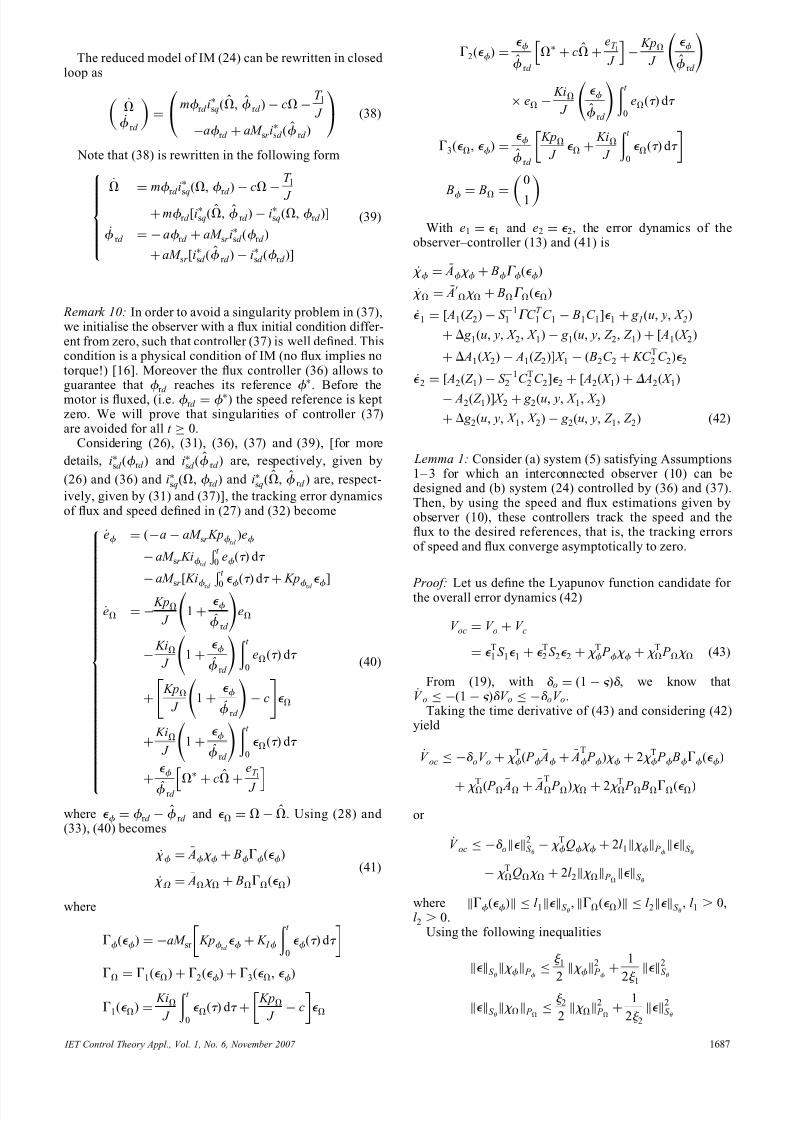
Fig. 1 Experimental result in nominal case




The identified parameters values of the motor are asfollows.

R s 1.47 V

R r 0.79 V

Ls 0.105 H

Lr 0.094 H

M sr 0.094 H

J 0.0077 kg m2

f v 0.0029 N m/rad/s

The parameters are chosen as follows: a ¼ 0.82,k ¼ 0.14, k c1 ¼ 300, k c2 ¼ 0.5, Kif r d ¼ 0.12, Kpf r d ¼ 200,

Kivd ¼ 0.03, Kpvd ¼ 15, Kivq ¼ 0.03, Kpvq ¼ 10,w max ¼ p /3, v q ¼ 950, K v s ¼ 200, u 1 ¼ 3000 and u 2 ¼ 7000 to satisfy the convergence conditions.

The experimental sampling time T is equal to 200 ms.For our experiment, to test robustness in hot conditions,

we take Rs nominal þ30% for the design of the observer and the controller. For the experiment only, the stator cur-rents are measured. The speed and the flux amplitude are provided by the observer.

The experimental results of the nominal case for other

parameters (except stator resistance) are shown in Fig. 1.These figures show the good performance of both systemobserver þ controller in trajectory tracking and perturbationrejection. In terms of trajectory tracking, we note that the

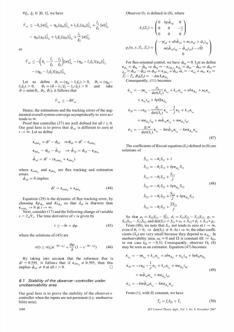
Fig. 2 Experimental result with rotor resistance variation ( þ50%)

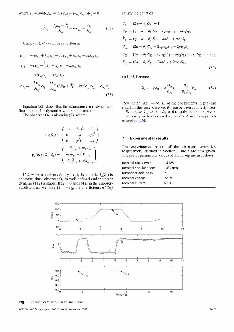
Fig. 3 Experimental result with rotor resistance variation ( 250%)




estimated motor speed (Fig. 1b) converges to the measured speed (Fig. 1a) near and under unobservable conditions. It isthe same conclusion for estimated flux (Fig. 1 f ) with respectto reference flux (Fig. 1e). The estimated load torque(Fig. 1d ) converges to the measured load torque (Fig. 1c),except under unobservable conditions (between 7 and 9 s). Nevertheless, it appears a small static error when themotor speed increases (between 3 and 6 s). In terms of per-turbation rejection, we have noted that the load torque iswell rejected excepted at the time when it is applied ((Fig. 1a, b, e and f ) at time 1.5 and 5 s) and when it isremoved (Figs. 1a, b, e and f at time 2.5 s).

The robustness of the observer þ

controller is confirmed by the result obtained with rotor resistance variation(þ50%) applied to the observer and controller parameters(Fig. 2).

These figures display similar experimental results for therotor resistance nominal case under observable conditions.

It appears a static error when the motor is under unobservable condition (between 7 and 9 s) (Figs. 2a and b). However,the static error increases a little when the load torque isapplied at time 1.5 and 5 s (Figs. 2a and b). In conclusion,we can say that the increase in the rotor resistance valueslightly affects the performance of the speed trajectoriestracking.

A second test is made with a 250% variation on rotor resistance value. The experimental results are shown inFig. 3. For the speed, flux and load torque estimation, theconclusion is the same as þ50% variation case (Fig. 2).But for this robustness test, the control induces noise.This can be seen on the measured torque (Fig. 3c).

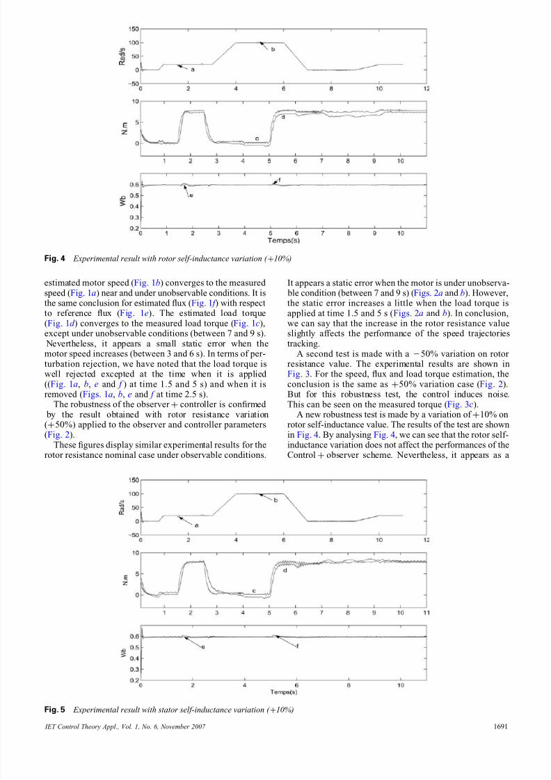
A new robustness test is made by a variation of þ10% onrotor self-inductance value. The results of the test are shownin Fig. 4. By analysing Fig. 4, we can see that the rotor self-inductance variation does not affect the performances of theControl þ observer scheme. Nevertheless, it appears as a

Fig. 4 Experimental result with rotor self-inductance variation ( þ10%)

Fig. 5 Experimental result with stator self-inductance variation ( þ10%)




small oscillation when the load torque is applied (Figs. 4aand b) at time 5 s.

A last robustness test is a þ10% variation of stator self-inductance value. The results of this test are shown in Fig. 5.Comparing this result with rotor self-inductance variationyields the same conclusion except that the oscillations become important at time 5 s when the load torque isapplied (Figs. 5a and b).

8 Conclusion

This paper investigates the field-oriented control of IMwithout mechanical sensors (speed sensor, load torquesensor). The first contribution of the paper is to design aninterconnected observer that well estimates the load evenwhen nominal load torque is applied. The second contribution is to propose a complete field-oriented control withhigh-gain PI controller that achieves a good speed and fluxtracking for IM without mechanical sensorless. The third contribution is to test and evaluate our observers þ controller on experimental set-up with a significant sensorless control benchmark. The trajectories of this benchmark are defined to include operation region where the speed and developed

torque are in opposite directions (generating). The stabilityof the controller þ observers scheme is proved byLyapunov theory even on unobservable conditions.

The robustness of the controller and observer is con-firmed by significant parameter variations. To improve theresult, it will be interesting in the future to build a moresophisticated control law such as sliding-mode controller or backstepping controller.

9 References

1 Faa, J.L., Rong, J.W., and Pao, C.L.: ‘Robust speed sensorlessinduction motor drive’, IEEE Trans. Aerosp. Electron. Syst., 1999,35, (2), pp. 566–578

2 Guiseppe, G., and Hidetoshi, U.: ‘A novel stator resistance estimationmethod for speed-sensorless induction motor drives‘’, IEEE Trans. Ind. Appl., 2000, 36, (6), pp. 1619–1627

3 Hassan, K.K., and Elias, G.S.: ‘Sensorless speed control of inductionmotors’. Proc. 2004 ACC, Boston, 30 June–July 2004, pp. 1127–1131

4 Kubota, H., and Matsuse, K.: ‘Speed sensorless filed-oriented controlof induction motor with rotor resistance adaptation‘’, IEEE Trans. Ind. Appl., 1994, 30, (5), pp. 344–348

5 Montanari, M., Peresada, S., Tilli, A., and Tonielli, A.: ‘Speed sensorless control of induction motor based on indirectfield-orientation’. Conf. Record of the 2000 IEEE IndustryApplications Conf., 2000, vol. 3, pp. 1858–1865

6 Montanari, M., and Tilli, A.: ‘Sensorless control of induction motors based on high-gain Speed Estimation one-line stator resistanceadaptation’. The 32nd Annual Conf. IECON, Paris, 7–10 November 2006, pp. 1263–1268

7 Marino, R., Tomei, P., and Verrelli, C.M.: ‘A global tracking controlfor speed-sensorless induction motors’, Automatica, 2004, 40, pp. 1071–1077

8 Soltani, J., Arab Makadeh, G.R., and Hosseiny, S.H.: ‘A new adaptivedirect torque control (DTC) scheme based-on SVW for adjustablespeed sensorless induction motor drive’. The 30th Annual Conf.IEEE Industrial Electric Society, November 2004, pp. 1111–1115

9 Ghanes, M., Jesus, D.L., and Glumineau, A.: ‘Novel controller for induction motor without mechanical sensor and experimentalvalidation’. Proc. 45th IEEE CDC, San Diego, 13– 15 December 2006, pp. 4008–4013

10 Canudas, D.W.C., Youssef, A., Barbot, J.P., Martin, Ph., and Malrait,

F.: ‘Observability conditions of induction motors at low frequencies’.IEEE CDC, Sydney, December 200011 Ibarra-Rojas, S., Moreno, J., and Espinosa, G.: ‘Global observability

analysis of sensorless induction motor’, Automatica, 2004, 40, (6), pp. 1079–1085

12 Gregor, E., and Karel, J.: ‘Low-speed sensorless control of inductionmachine’, IEEE Trans. Ind. Appl., 2006, 53, (1), pp. 120–128

13 Chiasson, J.: ‘Non linear controllers for induction motors’. IFACConf. System Structure and Control, Nantes, 5–7 July 1995

14 Besancon, G., and Hammouri, H.: ‘On observer design for interconnected systems’, J. Math. Syst. Estim. Control , 1998, 8, (4), pp. 377–397

15 Besancon, G., and Hammouri, H.: ‘Observer synthesis for class of nonlinear control systems’, Eur. J. Control , 1996, 2, (3), pp. 176–192

16 Marino, R., Sergei, P., and Tomei, P.: ‘Global adaptive outputfeedback control of induction motors with uncertain rotor resistance’, IEEE Trans. Autom. Control , 1999, 44, (5), pp. 967–983


Speed Sensor Less Field-Oriented Control of IM With Interconnected Observers Experimental Tests on Low Frequencies Benchmark

Documents