Speech encoding by coupled cortical theta and gamma oscillations

elifesciences.org

RESEARCH ARTICLE

Speech encoding by coupled cortical thetaand gamma oscillationsAlexandre Hyafil1*, Lorenzo Fontolan1,2, Claire Kabdebon1, Boris Gutkin1,3,Anne-Lise Giraud2

1INSERM U960, Group for Neural Theory, Departement d’Etudes Cognitives, EcoleNormale Superieure, Paris, France; 2Department of Neuroscience, University ofGeneva, Geneva, Switzerland; 3Centre for Cognition and Decision Making, NationalResearch University Higher School, Moscow, Russia

Abstract Many environmental stimuli present a quasi-rhythmic structure at different timescales

that the brain needs to decompose and integrate. Cortical oscillations have been proposed as

instruments of sensory de-multiplexing, i.e., the parallel processing of different frequency streams in

sensory signals. Yet their causal role in such a process has never been demonstrated. Here, we used

a neural microcircuit model to address whether coupled theta–gamma oscillations, as observed in

human auditory cortex, could underpin the multiscale sensory analysis of speech. We show that, in

continuous speech, theta oscillations can flexibly track the syllabic rhythm and temporally organize

the phoneme-level response of gamma neurons into a code that enables syllable identification. The

tracking of slow speech fluctuations by theta oscillations, and its coupling to gamma-spiking activity

both appeared as critical features for accurate speech encoding. These results demonstrate that

cortical oscillations can be a key instrument of speech de-multiplexing, parsing, and encoding.

DOI: 10.7554/eLife.06213.001

IntroductionThe physical complexity of biological and environmental signals poses a fundamental problem to the

sensory systems. Sensory signals are often made of different rhythmic streams organized at multiple

timescales, which require to be processed in parallel and recombined to achieve unified perception.

Speech constitutes an example of such a physical complexity, in which different rhythms index

linguistic representations of different granularities, from phoneme to syllables and words (Rosen,

1992; Zion Golumbic et al., 2012). Before meaning can be extracted from continuous speech, two

critical pre-processing steps need to be carried out: a de-multiplexing step, i.e., the parallel analysis of

each constitutive rhythm, and a parsing step, i.e., the discretization of the acoustic signal into

linguistically relevant chunks that can be individually processed (Stevens, 2002; Poeppel, 2003;

Ghitza, 2011). While parsing is presumably modulated in a top-down way, by knowing a priori

through developmental learning (Ngon et al., 2013) where linguistic boundaries should lie, it is likely

largely guided by speech acoustic dynamics. It has recently been proposed that speech de-

multiplexing and parsing could both be handled in a bottom-up way by the combined action of

auditory cortical oscillations in distinct frequency ranges, enabling parallel computations at syllabic

and phonemic timescales (Ghitza, 2011;Giraud and Poeppel, 2012). Intrinsic coupling across cortical

oscillations of distinct frequencies, as observed in electrophysiological recordings of auditory cortex

(Lakatos et al., 2005; Fontolan et al., 2014), could enable the hierarchical combination of syllabic-

and phonemic-scale computations, subsequently restoring the natural arrangement of phonemes

within syllables (Giraud and Poeppel, 2012).

The most pronounced energy fluctuations in speech occur at about 4 Hz (Zion Golumbic et al.,

2012) and can serve as an acoustic guide for signalling the syllabic rhythm (Mermelstein, 1975).

*For correspondence: alexandre.

[email protected]

Competing interests: The

authors declare that no

competing interests exist.

Funding: See page 19

Received: 23 December 2014

Accepted: 28 May 2015

Published: 29 May 2015

Reviewing editor: Hiram

Brownell, Boston College, United

States

Copyright Hyafil et al. This

article is distributed under the

terms of the Creative Commons

Attribution License, which

permits unrestricted use and

redistribution provided that the

original author and source are

credited.

Hyafil et al. eLife 2015;4:e06213. DOI: 10.7554/eLife.06213 1 of 23

http://elifesciences.org/

http://en.wikipedia.org/wiki/Open_access

https://creativecommons.org/

http://dx.doi.org/10.7554/eLife.06213.001

mailto:[email protected]

mailto:[email protected]

http://creativecommons.org/licenses/by/4.0/

http://creativecommons.org/licenses/by/4.0/

http://dx.doi.org/10.7554/eLife.06213

Since the syllabic rate coincides with the auditory cortex theta rhythm (3–8 Hz), syllable boundaries

could be viably signalled by a given phase in the theta cycle. The relevance of speech tracking by

the theta neural rhythm (Henry et al., 2014) is highlighted by experimental data showing that

speech intelligibility depends on the degree of phase-locking of the theta-range neural activity in

auditory cortex (Ahissar et al., 2001; Luo and Poeppel, 2007; Peelle et al., 2013; Gross et al.,

2013). By analogy with the spatial and mnemonic oscillatory processes that take place in the

hippocampus (Jensen and Lisman, 1996; Lisman and Jensen, 2013; Lever et al., 2014), the theta

oscillation may orchestrate gamma neural activity to facilitate its subsequent decoding (Canolty

et al., 2007): the phase of theta-paced neural activity could regulate faster neural activity in the low-

gamma range (>30 Hz) involved in linguistic coding of phonemic details (Ghitza, 2011; Giraud and

Poeppel, 2012). The control of gamma by theta oscillations could hence both modulate the

excitability of gamma neurons to devote more processing power to the informative parts of syllabic

sound patterns, and constitute a reference time frame aligned on syllabic contours for interpreting

gamma-based phonemic processing (Shamir et al., 2009; Ghitza, 2011; Kayser et al., 2012;

Panzeri et al., 2014).

Compelling as this hypothesis may sound, direct evidence for neural mechanisms linking speech

constituents and oscillatory components is still lacking. One way to address a causal role of oscillations

in speech processing is computational modelling, as it permits to directly test the efficiency of cross-

coupled theta and gamma oscillations as an instrument of speech de-multiplexing, parsing, and

encoding. Previous models of speech processing involved only gamma oscillations in the context of

isolated speech segments (Shamir et al., 2009) or did not involve neural oscillations at all (Gutig and

Sompolinsky, 2009; Yildiz et al., 2013). On the other hand, previous models of cross-frequency

coupled oscillations did not address sensory functions as parsing and de-multiplexing (Jensen and

Lisman, 1996; Tort et al., 2007). Here, we examined how a biophysically inspired model of coupled

theta and gamma neural oscillations can process continuous speech (spoken sentences). Specifically,

we determined: (i) whether theta oscillations are able to accurately parse speech into syllables, (ii)

whether syllable-related theta signal may serve as a reference time frame to improve gamma-based

decoding of continuous speech; (iii) whether this decoding requires theta to modulate the activity of

the gamma network. To address the last two points, we compared speech decoding performance of

the model with two control versions of the network, in which we removed the neural connection

entraining the theta neurons by speech fluctuations or the link that couples them to the gamma

neurons.

eLife digest Some people speak twice as fast as others, while people with different accents

pronounce the same words in different ways. However, despite these differences between speakers,

humans can usually follow spoken language with remarkable ease.

The different elements of speech have different frequencies: the typical frequency for syllables,

for example, is about four syllables per second in speech. Phonemes, which are the smallest elements

of speech, appear at a higher frequency. However, these elements are all transmitted at the same

time, so the brain needs to be able to process them simultaneously.

The auditory cortex, the part of the brain that processes sound, produces various ‘waves’ of

electrical activity, and these waves also have a characteristic frequency (which is the number of bursts

of neural activity per second). One type of brain wave, called the theta rhythm, has a frequency of

three to eight bursts per second, which is similar to the typical frequency of syllables in speech, and

the frequency of another brain wave, the gamma rhythm, is similar to the frequency of phonemes. It

has been suggested that these two brain waves may have a central role in our ability to follow

speech, but to date there has been no direct evidence to support this theory.

Hyafil et al. have now used computer models of neural oscillations to explore this theory. Their

simulations show that, as predicted, the theta rhythm tracks the syllables in spoken language, while

the gamma rhythm encodes the specific features of each phoneme. Moreover, the two rhythms work

together to establish the sequence of phonemes that makes up each syllable. These findings will

support the development of improved speech recognition technologies.

DOI: 10.7554/eLife.06213.002


Research article Computational and systems biology | Neuroscience



Results

Model architecture and spontaneous behaviourThe model proposed here (Figure 1A) is inspired from cortical architecture (Douglas and Martin,

2004; da Costa and Martin, 2010) and function (Lakatos et al., 2007) as well as from previous

biophysical models of cross-frequency coupled oscillation generation (Tort et al., 2007; Kopell et al.,

2010; Vierling-Claassen et al., 2010). We used the well documented Pyramidal Interneuron Gamma

(PING) model for implementing a gamma network: bursts of inhibitory neurons immediately follow

bursts of excitatory neurons (Jadi and Sejnowski, 2014), creating the overall spiking rhythm. Given

that gamma and theta oscillations are both locally present in superficial cortical layers (Lakatos et al.,

2005), we assume similar local generation mechanisms for theta and gamma with a direct connection

between them. Direct evidence for a local generation of theta oscillations in auditory cortex is still

scarce (Ainsworth et al., 2011) and we cannot completely rule out that they might spread from

remote generators (e.g., in the hippocampus; Tort et al., 2007; Kopell et al., 2010). Yet, we built the

case for local generation from the following facts: (1) neocortical (somatosensory) theta oscillations are

observed in vitro (Fanselow et al., 2008), (2) MEG, EEG, and combined EEG/FMRI recordings in

humans show that theta activity phase-locks to speech amplitude envelope in A1 and immediate

association cortex—but not beyond—(Ahissar et al., 2001; Luo and Poeppel, 2007; Cogan and

Poeppel, 2011; Morillon et al., 2012), and (3) theta phase-locking to speech is not accompanied by

power increase, arguing for a phase restructuring of a local oscillation (Luo and Poeppel, 2007). We

assumed a similar generation mechanism for theta and gamma oscillations, with slower excitatory and

inhibitory synaptic time constants for theta (Kopell et al., 2010; Vierling-Claassen et al., 2010). The

distinct dynamics for the two modules reflect the diversity of inhibitory synaptic timescales observed

experimentally, with Martinotti cells displaying slow synaptic inhibition (Ti neurons), and basket cells

showing faster inhibition decay (Gi neurons) (Silberberg and Markram, 2007). We refer to the theta

network as Pyramidal Interneuron Theta (PINTH), by analogy with PING. The full model is hence

composed of a theta-generating module with interconnected spiking excitatory (Te) and inhibitory (Ti)

neurons that spontaneously synchronize at theta frequency (6–8 Hz) through slow decaying inhibition;

and of a gamma-generating module with excitatory (Ge) and inhibitory (Gi) neurons that burst at

a faster rate (25–45 Hz) synchronized by fast decaying inhibition (PING; Figure 1B) (Borgers and

Kopell, 2005). The firing pattern of our simulated neurons is sparse and weakly synchronous at rest,

consistent with the low spiking rate of cortical neurons (Brunel and Wang, 2003) (Figure 1—figure

supplement 1D). Unlike the classical 50–80 Hz PING seen in in vitro preparations of rat auditory

cortex (Ainsworth et al., 2011), our network produced a lower gamma frequency around 30 Hz, as

observed in human auditory cortex in response to speech (Nourski et al., 2009; Pasley et al., 2012).

At rest the PINTH population activity synchronizes at the theta timescale, and the PING population

at the gamma time scale. Both the Te and Ge populations receive projections from a ‘subcortical’

module that mimics the nonlinear filtering of acoustic input by subcortical structures, which primarily

includes a signal decomposition into 32 auditory channels (Chi et al., 2005). Individual excitatory

neurons in the theta module received channel-averaged input while those in the gamma module

received frequency selective input. Such a differential selectivity was motivated by experimental

observations from intracranial recordings (Morillon et al., 2012; Fontolan et al., 2014) suggesting

that unlike the gamma one, the theta response does not depend on the input spectrum. It also mirrors

the dissociation in primate auditory cortex between a population of ’stereotyped’ neurons responding

very rapidly and non-selectively to any acoustic stimulus (putatively Te neurons) and a population of

’modulated’ neurons responding selectively to specific spectro-temporal features (putatively Ge

neurons) (Brasselet et al., 2012). Each Ge neuron receives input from one specific channel, preserving

the auditory tonotopy, so that the whole Ge population represents the rich spectral structure of the

stimulus. Each Te neuron receives input from all the channels, i.e., the Te population conveys a widely

tuned temporal signal capturing slow stimulus fluctuations. Importantly, the two oscillating modules

are connected through all-to-all connections from Te neurons to Ge neurons allowing the theta

oscillations to control the activity of the faster gamma oscillations. This structure enables syllable

boundary detection (through the theta module) to constrain the decoding of faster phonemic

information. The output of the network is taken from the Ge neurons as we assume that the Ge

neurons provide the input to higher-level cortical structures performing operations like phoneme




categorization and providing access to lexicon. Accordingly, in the model the Ge neurons receive

more spectral details about speech than the Te neurons (Figure 1B). Ge spiking is then referenced

with respect to timing of theta spikes, and submitted to decoding algorithms.

Model dynamics in response to natural sentencesWe first explored the dynamic behaviour of the model. As expected from its architecture and

biophysical parameters (see ‘Materials and methods’), the neural network produced activity in theta

(6–8 Hz) and low gamma (25–45 Hz) ranges, both at rest and during speech presentation. Consistent

with experimental observations (Luo and Poeppel, 2007) there was no notable increase in theta

Figure 1. Network architecture and dynamics. (A) Architecture of the full model. Te excitatory neurons (n = 10) and Ti inhibitory neurons (n = 10) form the

PINTH loop generating theta oscillations. Ge excitatory neurons (n = 32) and Gi inhibitory neurons (n = 32) form the PING loop generating gamma

oscillations. Te neurons receive non-specific projections from all auditory channels, while Ge units receive specific projection from a single auditory

channel, preserving tonotopy in the Ge population. PING and PINTH loops are coupled through all-to-all projections from Te to Ge units. (B) Network

activity at rest and during speech perception. Raster plot of spikes from representative Ti (dark green), Te (light green), Gi (dark blue), and Ge (light blue).

Simulated LFP is shown on top and the auditory spectrogram of the input sentence "Ralph prepared red snapper with fresh lemon sauce for dinner" is

shown below. Ge spikes relative to theta burst (red boxes) form the output of the network. Gamma synchrony is visible in Gi spikes. (C) Evoked potential

(ERP) and Post-stimulus time histograms (PSTH) of Te and Ge population from 50 simulations of the same sentence: ERP (i.e., simulated LFP averaged over

simulations, black line), acoustic envelope of the sentence (red line, filtered at 20 Hz), PSTH for theta (green line) and gamma (blue line) neurons. Vertical

bars show scale of 10 spikes for both PSTH. The theta network phase-locks to speech slow fluctuations and entrains the gamma network through the

theta–gamma connection. (D) Theta/gamma phase-amplitude coupling in Ge spiking activity. Top panel: LFP gamma envelope follows LFP theta phase in

single trials. Bottom-Left panel: LFP phase-amplitude coupling (measured by Modulation Index) for pairs of frequencies during rest, showing peak in

theta–gamma pairs. Bottom-right panel: MI phase-amplitude coupling at the spiking level for the intact model and a control model with no theta–gamma

connection (red arrow on A panel), during rest (blue bars) and speech presentation (brown bars).

DOI: 10.7554/eLife.06213.003

The following figure supplement is available for figure 1:

Figure supplement 1. Spectral analysis.

DOI: 10.7554/eLife.06213.004






spiking during speech presentation, but sentence onsets induced a phase-locking of theta oscillations

as shown by the Post-stimulus time histograms of theta neurons, which was further enhanced by all

edges in speech envelope. Consequently, the resulting global evoked activity followed the acoustic

envelope of the speech signal (Figure 1C) (Abrams et al., 2008). Local Field Potential (LFP) indexes

the global synaptic activity over the network (excitatory neurons of both networks) and its dynamics

closely followed spiking dynamics. Unlike the LFP theta power pattern, the LFP theta phase pattern

was robust across repetitions of the same sentence (Figure 1—figure supplement 1A,C,E),

replicating LFP behaviour from the primate auditory cortex (Kayser et al., 2009), and human MEG

data (Luo and Poeppel, 2007; Luo et al., 2010). In line with other empirical data from human auditory

cortex (Nourski et al., 2009) gamma oscillations followed the onset of sentences (Figure 1C). Owing

to the feed-forward connection from the theta to the gamma sub-circuits, the gamma amplitude was

coupled to the theta phase both at rest and during speech (Figure 1D). The coupling was visible both

in the spiking (Figure 1—figure supplement 1B) and LFP signal (Figure 1D). Critically, this coupling

disappeared when the theta/gamma connection was removed, showing that a common input to Te

and Ge cells is not sufficient to couple the two oscillations.

Syllable boundary detection by theta oscillationsBefore testing the speech decoding properties of the model, we explored whether syllable

boundaries could reliably be detected at the cortical level by a theta network (see Methods). This first

study was based on a corpus consisting of 4620 phonetically labelled English sentences (TIMIT

Linguistic Data Consortium, 1993). The acoustic analysis of these sentences confirmed a correspon-

dence between the dominant peak of the speech modulation spectrum and the mean syllabic rate

(3–6 Hz) (Figure 2—figure supplement 1A), whereby syllabic boundaries correspond to trough in

speech slow fluctuations (Peelle et al., 2013). The theta network in the model (Figure 2—figure

supplement 1B) was explicitly designed to exploit such regularities and infer syllable boundaries.

When presenting sentences to the theta module, we observed a consistent theta burst within 50 ms

following syllable onset followed by a locking of theta oscillations to theta acoustic fluctuations in the

speech signal (Figure 2—figure supplement 1C,D). More importantly, neuronal theta bursts closely

aligned to the timing of syllable boundaries in the presented sentences (Figure 2A). We compared

the performance of the theta network to that of two alternative models also susceptible to predict

syllable boundaries: a simple linear-nonlinear acoustic boundary detector (Figure 2—figure

supplement 1E) and Mermelstein algorithm, a state-of-the-art model which, unlike the model

developed here, only permits ‘off-line’ syllable boundary detection (Mermelstein, 1975). The theta

network performed better than both the linear model and the Mermelstein algorithm (Figure 2B, all

p-values <10−12). Similar to results from behavioural studies of human perception (Miller et al., 1984;

Nourski et al., 2009; Mukamel et al., 2011) the theta network could adapt to different speech rates.

The model performed better than other algorithms, with a syllabic alignment accuracy remaining well

above chance levels (p < 10−12) in the twofold and threefold time compression conditions. (Figure 2B).

This first study demonstrates that theta activity provides a reliable, syllable-based, internal time

reference that the neural system could use when reading out the activity of gamma neurons.

Decoding of simple temporal stimuli from output spike patternsOur next step was to test whether the theta-based syllable chunks of output spike trains (Ge neurons)

for the different input types could be properly classified. We first quantified the model’s ability to

encode stimuli designed as simple temporal patterns. We used 50 ms sawtooth stimuli whose shape

was parametrically varied by changing the peak position (Figure 3A), with interstimulus interval

between 50 and 250 ms. This toy set of stimuli was previously used in a gamma-based speech

encoding model and argued to represent idealized formant transitions (Shamir et al., 2009). We

extracted spike patterns from all the Ge (output) neurons from −20 ms before each sawtooth onset to

20 ms after its offset. This procedure is referred to as ‘stimulus timing’ since it uses the stimulus onset

as time reference. Using a clustering method (see ‘Materials and methods’), we observed that the

identity of the presented sawtooth could be decoded from the output spike patterns (Figure 3A) with

over 60% accuracy (Figure 3C, light grey bar). We also computed the decoding performance when we

used an internal time reference provided by the theta timing rather than by the stimulus timing. When

spike patterns were analysed within a window defined by two successive theta bursts (Figure 3C, dark




grey bar), sawtooth decoding was still possible and even relatively well preserved (mean decoding

rate of 41.7%). Noise in the theta module allows the alignment of theta bursts to stimulus onset and

thus improves detection performance by enabling consistent theta chunking of spike patterns.

We then compared the decoding performance from the full model with that of two control models:

one in which the theta module was not driven by the stimulus (undriven theta model) and one in which

the theta module was not connected with the gamma module (uncoupled theta/gamma model)

(Figure 3B, green and blue). Decoding performance of both control models, as revealed by the mean

performance (Figure 3C) and confusion matrices (Figure 3E), was degraded for either neural code

(theta onset and stimulus timing, all p-values <10−9). The details of the raw confusion matrices show

that the temporal patterns are decoded correctly or as a neighbouring temporal shape only in the

intact version of the model (Figure 3E). Furthermore, the intact model achieved better signal vs rest

discrimination than the two control models, notably avoiding false alarms (Figure 3D). In summary,

these analyses show that gamma-spiking neurons within theta bursts provide a reliable internal code

for characterizing simple temporal patterns, and that this ability is granted by the time-locking of

theta neurons (Te units) to stimulus and the modulation they exert on the fast-scale output (Ge) units.

Continuous speech encoding by model output spike patternsThe overarching goal of this theoretical work was to assess whether coupled cortical oscillations can

achieve on-line speech decoding from continuous signal. We therefore set out to classify syllables

from natural sentences. To decode Ge spiking, we used similar procedures as for the encoding/

decoding of simple temporal patterns. Output Ge spikes were parsed into spike patterns based on

the theta chunks, and the decoding analysis was used to recover syllable identity (Figure 4A). To

evaluate the importance of the precise spike timing of gamma neurons, we compared decoding (see

‘Materials and methods’) using spike patterns (i.e., spikes labelled with their precise timing w.r.t.

chunk onset) vs those obtained from plain spike counts (i.e., unlabelled spikes). When using spike

patterns syllable decoding reached a high level of accuracy in the intact model: 58% of syllables were

correctly classified within a set of 10 possible (randomly chosen) syllables (Figure 4B). Syllable

Figure 2. Theta entrainment by syllabic structure. (A) Theta spikes align to syllable boundaries. Top graph shows the

activity of the theta network at rest and in response to a sentence, including the LFP traces displaying strong theta

oscillations, and raster plots for spikes in the Ti (light green) and Te (dark green) populations. Theta bursts align well

to the syllable boundaries obtained from labelled data (vertical black lines shown on top of auditory spectrogram in

graph below). (B) Performance of different algorithms in predicting syllable onsets: Syllable alignment score indexes

how well theta bursts aligned onto syllable boundaries for each sentence in the corpus, and the score was averaged

over the 3620 sentences in the test data set (error bars: standard error). Results compare Mermelstein algorithm

(grey bar), linear-nonlinear predictor (LN, pink) and theta network (green), both for normal speed speech

(compression factor 1) and compressed speech (compression factors 2 and 3). Performance was assessed on

a different subsample of sentences than those used for parameter fitting.

DOI: 10.7554/eLife.06213.005


Figure supplement 1. TIMIT corpus and models used for syllable boundary detection.

DOI: 10.7554/eLife.06213.006






decoding dropped when using spike counts instead of spike patterns (p < 10−12). Critically, decoding

was poor in both control models (undriven theta and uncoupled theta/gamma) using either spike

counts or spike patterns (significantly lower than decoding using spike patterns in the full model, all

p-values < 10−12, and non-significantly higher than decoding using spike counts in the full model, all

p-values > 0.08 uncorrected).

Figure 3. Sawtooth classification. (A) Gamma spiking patterns in response to simple stimuli. The model was presented with 50 ms sawtooth stimuli, where

peak timing was parameterized between 0 (peak at onset) and 1 (peak at offset). Spiking is shown for different Ge neurons (y axis) in windows phase-

locked to theta bursts (−20 to +70 ms around the burst, x-axis). Neural patterns are plotted below the corresponding sawtooths. (B) Simulated networks.

The analysis was performed on simulated data from three distinct networks: ‘Undriven-theta model’ (no speech input to Te units, top), ‘Uncoupled theta/

gamma model’ (no projection from Te toGe units, middle), full intact model (bottom). (C) Classification performance using stimulus vs. theta timing for the

three simulated networks. The stimulus timing (light bars) is obtained by extracting Ge spikes in a fixed-size window locked to the onset of the external

stimulus; the theta timing (dark bars) is obtained by extracting Ge spikes in a window defined by consecutive theta bursts (theta chunk, see Figure 3A).

Classification was repeated 10 times for each network and neural code, and mean values and standard deviation were extracted. Average expected

chance level is 10%. (D) Stimulus detection performance, for the intact and control models. Rest neural patterns were discriminated against any of the 10

neural patterns defined by the 10 distinct temporal shapes. (E) Confusion matrices for stimulus- and theta-timing and the two control models (using theta-

timing code). The colour of each cell represents the number of trials where a stimulus parameter was associated with a decoded parameter (blue: low

numbers; red: high numbers). Values on the diagonal represent correct decoding.

DOI: 10.7554/eLife.06213.007





We also explored the model performance for encoding syllables spoken by different speakers. We

used a similar decoding procedure as above, but here the classifier was trained on different speakers

pronouncing the same two sentences. Theta chunks were classified into syllables based on the

network response to the two sentences uttered by 99 other speakers. The material included sentences

spoken by 462 speakers of various ethnic and geographical origins, showing a marked heterogeneity

in phonemic realization and syllable durations (as labelled by phoneticians). The syllable duration

distribution was skewed with the median at 200 ms and tail values ranging from a few ms to over 800

ms (Figure 4—figure supplement 1A). Given that theta activity is meant to operate in a 3–9 Hz range,

i.e., integrate speech chunks of about 100–300 ms (Ghitza, 2011, 2014), we did not expect the model

Figure 4. Continuous speech parsing and syllable classification. (A) Decoding scheme. Output spike patterns were

built by extracting Ge spikes occurring within time windows defined by consecutive theta bursts (red boxes) during

speech processing simulations. Each output pattern was then labelled with the corresponding syllable (grey bars).

(B) Syllable decoding average performance for uncompressed speech. Performance for the three simulated models

(Figure 3B) using two possible neural codes: spike count and spike pattern. (C) Syllable decoding average

performance across speakers, using the spike pattern code. Syllable decoding was optimal when syllable duration

was within the 100–300 ms range, i.e., corresponded to the duration of one theta cycle. The intact model performed

better than the two controls irrespective of syllable duration range. Chance level is 10%. Colour code same as B.

(D) Syllable decoding performance for compressed speech for the intact model using the spike pattern code (same

speaker, as in B). Compression ranges from 1 (uncompressed) to 3. Average chance level is 10% (horizontal line in

the right plot).

DOI: 10.7554/eLife.06213.008


Figure supplement 1. Syllable classification across speakers.

DOI: 10.7554/eLife.06213.009






to perform equally well along the whole syllable duration range. Accordingly, decoding accuracy was

not uniform across the whole syllable duration range. When decoding from spike pattern, the intact

model allowed 24% accuracy (chance level at 10%). It showed a peak in performance in the range in

which it is expected to operate, i.e., for syllables durations between 100 and 300 ms. Given the cross-

speaker phonemic variability such a performance is fairly good. Critically, the intact model

outperformed control models both within the 100 to 300 ms range (p < 0.001), and throughout the

whole syllable duration span (p < 0.001). These analyses overall show that the model can flexibly track

syllables within a physiological operating window, and that syllable decoding relies on the integrity of

the model architecture.

Lastly, we tested more directly the resilience of the spike pattern code to speech temporal

compression and found that while degrading the decoding performance remained above chance for

compression rates of 2 and 3 (Figure 4D), mimicking humans decoding performance (Ahissar et al.,

2001). Altogether, the decoding of syllables from continuous speech showed that coupled theta and

gamma oscillations provide a viable instrument for syllable parsing and decoding, and that its

performance relies on the coupling between the two oscillation networks.

Encoding properties of model neuronsWe finally assessed the physiological plausibility of the model by comparing the encoding properties

of the simulated neurons, without further parameter fitting, with those of neurons recorded from

primate auditory cortex (Kayser et al., 2009; 2012). The first analysis of neural encoding properties

consisted of comparing the ability to classify neural codes from the model into arbitrary speech

segments of fixed duration (as opposed to classification into syllables as in previous section). We

simulated data using natural speech and studied the spiking activity of Ge neurons by implementing

the same methods of analysis as in the original experiment. We extracted fixed-size windows of spike

patterns activity for individual Ge neurons, and assessed neural encoding characteristics using

different neural codes. Speech encoding was first evaluated using a nearest-mean classifier and then

using mutual information techniques (Kayser et al., 2009).

Classifier analysisIn this analysis, neural patterns were classified not into syllables as above or into any linguistic

constituent but into arbitrary segments of speech, allowing for a-theoretical insight into the encoding

properties of neurons. We extracted a subset of 25 sentences from the TIMIT corpus and exposed the

network to 50 presentations of each sentence from the subset. We defined 10 stimuli as 10 distinct

windows of a given size (from 80 to 480 ms) randomly extracted from the 25 sentences, and then

assessed the capacity to decode the identity of a stimulus from the activity of individual Ge neurons

within that window (Kayser et al., 2012). Three different codes were used (Figure 5A): a simple spike

count was used as reference code; a time-partitioned code where spikes were assigned to one of 8

bins of equal duration within the temporal window; a phase-partitioned code where spikes were

labelled with the phase of LFP theta at the timing of spike (the spikes were then assigned into one of 8

bins according to their phase).

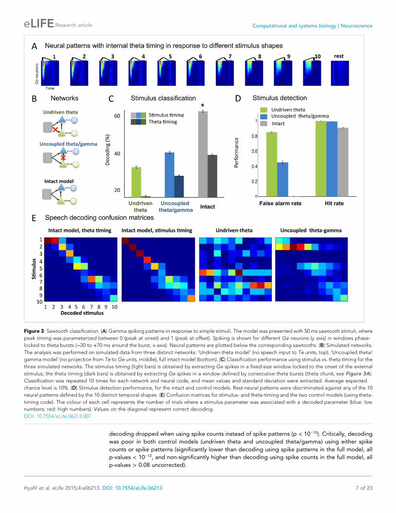
We observed that for 80 to 240 ms windows (within one theta cycle), decoding was almost as

good for the phase-partitioned code as for the time-partitioned code (Figure 5B, left). In other

words, stimulus decoding using theta timing was nearly as good as when using stimulus timing.

Performance using the spike count was considerably lower (p < 10−12 for all 6 window sizes).

Overall, there was a qualitative and even quantitative match between the results from simulated

data and the original experimental results (Figure 5B, right). When we removed either the input-

to-theta (undriven theta model) or the theta-to-gamma connection (uncoupled theta/gamma

model) in the network, the performance of the phase-partitioned code dropped to just above that

of the spike count code (Figure 5—figure supplement 1A; significantly lower increase in

decoding performance using phase-partitioned instead of spike count code compared to full

model, p < 10−12 for all 6 window sizes and both control models), and the simulations no longer

predicted the experimental results. Finally, experimental data and simulations from the

intact model also matched when we investigated the dependence of decoding accuracy on the

number of bins, which was not the case for any of the control models (Figure 5—figure

supplement 1B).




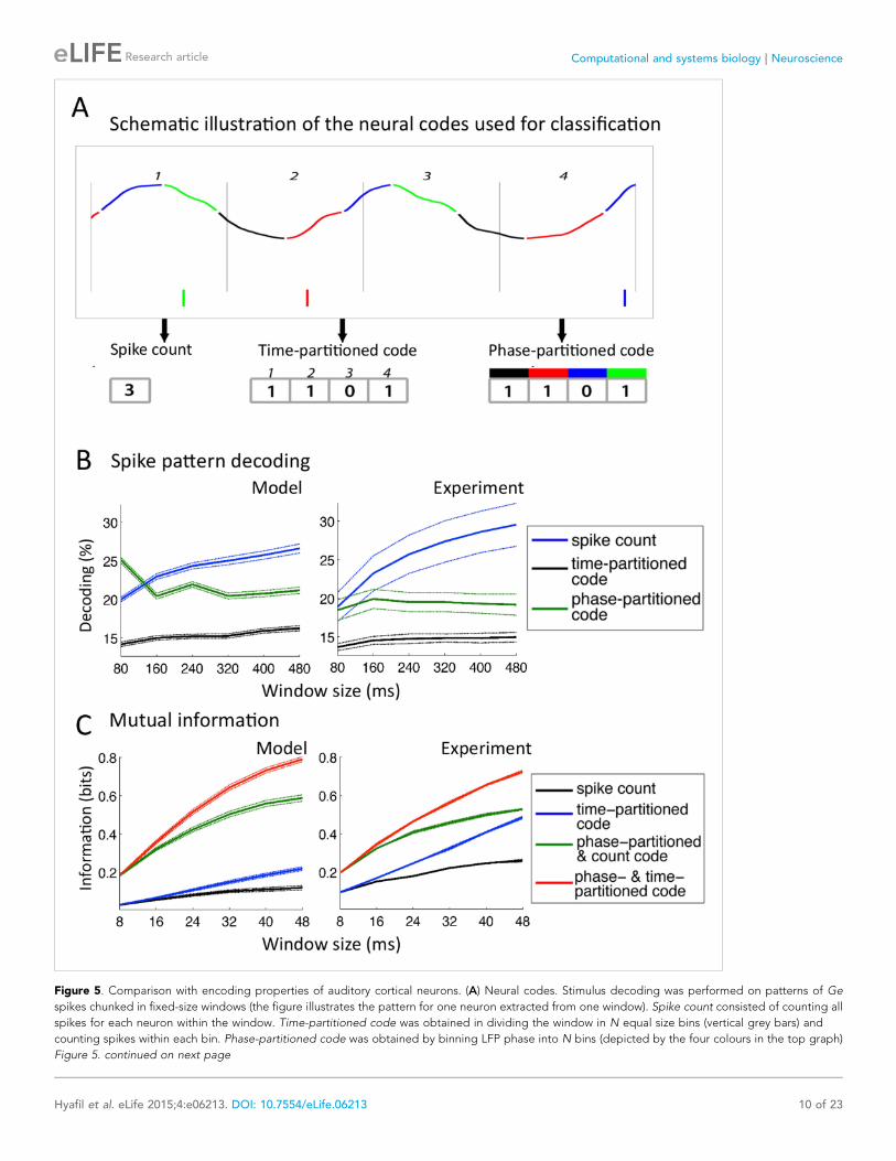
Figure 5. Comparison with encoding properties of auditory cortical neurons. (A) Neural codes. Stimulus decoding was performed on patterns of Ge

spikes chunked in fixed-size windows (the figure illustrates the pattern for one neuron extracted from one window). Spike count consisted of counting all

spikes for each neuron within the window. Time-partitioned code was obtained in dividing the window in N equal size bins (vertical grey bars) and

counting spikes within each bin. Phase-partitioned code was obtained by binning LFP phase into N bins (depicted by the four colours in the top graph)

Figure 5. continued on next page




Mutual information (MI) analysisMI between the input (acoustic stimulus) and the output (neural pattern) provides an alternative

measure for how well stimuli are encoded in the output pattern (see ‘Materials and methods’). We

used the same simulation data as for the classification procedure, but the sentences were subdivided

into shorter chunks using a non-overlapping time window (length T: 8–48 ms) (Kayser et al., 2009).

We compared the MI between the stimulus and neural activity in individual Ge neurons as a function of

the length of stimulus window, using four neural codes: spike count, time-partitioned code, phase-

partitioned code combined with spike count and finally combined phase- and time-partitioned codes.

These codes are qualitatively equivalent to the decoding strategies used in the previous classifier

analysis. Figure 5C shows that taking into account the spike phase boosts the MI carried by the Spike

count code or the Time-partitioned code alone (p < 10−12 for all 6 window sizes). In other words, spike

phase provided additional rather than redundant information to more traditional codes. The gain

provided by spike phase increased when enlarging the window and when combined with either spike

count or spike pattern (Spike Count vs Time-partitioned; Spike count and Phase-partitioned code vs

Time- and Phase-partitioned code). These results replicate the original experimental data from

monkey auditory cortex (Kayser et al., 2009). Such a pattern was not reproduced using any of the

control models (Figure 5—figure supplement 1C). These results hence show that in addition to

enhancing the reliability of the spike phase code, the theta–gamma connection enhanced the

temporal precision of Ge neurons spiking in response to speech stimuli.

Critically, results from both classifier and mutual information analyses demonstrate that the full

network architecture of the model provides an efficient way of boosting the encoding capacity of

neurons in a way that bears remarkable similarities to actual neurons from primate auditory cortex.

DiscussionLike most complex natural patterns, speech contains rhythmic activity at different scales that conveys

different and sometimes non-independent categories of information. Using a biophysically inspired

model of auditory cortex function, we show that cortical theta–gamma cross-frequency coupling

provides a means of using the timing of syllables to orchestrate the readout of speech-induced

gamma activity. The current modelling data demonstrate that theta bursts generated by a theta

(PINTH) network can predict ‘on-line’ syllable boundaries at least as accurately as state-of-the-art

offline syllable detection algorithms. Syllable boundary detection by a theta network hence provides

an endogenous time reference for speech decoding. Our simulated data further show that a gamma

biophysical network, receiving a spectral decomposition of speech as input, can take advantage of the

theta time reference to encode fast phonemic information. The central result of our work is that the

gamma network could efficiently encode temporal patterns (from simple sawtooths to natural

speech), as long as it was entrained by the theta rhythm driven by syllable boundaries. The proposed

theta/gamma network displayed sophisticated spectral and encoding properties that compared both

qualitatively and quantitatively to existing neurophysiological evidence including cross-frequency

coupling properties (Schroeder and Lakatos, 2009) and theta-referenced stimulus encoding

(Kayser et al., 2009; 2012). The projections from the Te to Ge neurons endowed the network with

phase-amplitude and phase-frequency coupling between gamma and theta oscillations, at both the

spike and the LFP levels (Jensen and Colgin, 2007). This closely reproduces the theta/gamma

Figure 5. Continued

and assigning each spike with the corresponding phase bin. (B) Spike pattern decoding. (Left) Decoding performance across Ge neurons for the intact

model using N = 8 bins for each code: spike count (black curve), time-partitioned (blue curve), and phase-partitioned codes (green curve). (Right) Data

from the original experiment. Adapted from Kayser et al., 2012. (C) Mutual information (MI). (Left) Mean MI between stimulus and individual output

neuron activity during sentence processing in the intact model for spike count (black curve), time-partitioned (blue line), combined count and phase-

partitioned (green line) and combined time- and phase-partitioned codes (red line). (Right) Comparison with experimental data from auditory cortex

neurons (adapted from Kayser et al., 2009).

DOI: 10.7554/eLife.06213.010


Figure supplement 1. Speech decoding performance and MI (control models).

DOI: 10.7554/eLife.06213.011






phase-amplitude coupling observed from intracortical recordings (Giraud and Poeppel, 2012;

Lakatos et al., 2005). Importantly, due to the dissociation of excitatory populations we obtained

denser gamma spiking immediately after the theta burst evoked by the syllable onset. This validates

a critical point of theta/gamma parsing system, namely that a more in-depth encoding is carried-out

by the auditory cortex during the early phase of syllables, when more information needs to be

extracted (Schroeder and Lakatos, 2009; Giraud and Poeppel, 2012).

The human auditory system, like other sensory systems, is able to produce invariant responses to

different physical presentations of the same input. Importantly, it is relatively insensitive to the speed

at which speech is being produced. Speech can double in speed from one speaker to another and yet

remain intelligible up to an artificial compression factor of 3 (Ahissar et al., 2001). In the current

model, theta bursts could still signal syllable boundaries when speech was compressed by a factor 2

and this alignment deteriorated for higher compression factors. Syllable decoding was significantly

degraded for compressed speech, yet remained twice as accurate as chance. Our network is purely

bottom-up and does not include high level linguistic processes and representations, which in all

likelihood plays an important role in speech perception (Davis et al., 2011; Peelle et al., 2013;

Gagnepain et al., 2012): its relative resilience to speech compression is thus a fairly good

performance. A previous model (Gutig and Sompolinsky, 2009) proposed a neural code that was

robust to speech warping, based on the notion that individual neurons correct for speech rate by their

overall level of activity. While this model achieved very good speech categorization performance, it

relied on extremely precise spiking behaviour (neurons spiked only once, when their associated

channel reached a certain threshold), for which neurophysiological evidence is scarce. Another model

developed by Hopfield proposes that a low gamma external current provides encoding neurons with

reliable timing and dynamical memory spanning up to 200 ms, a long enough window to integrate

information over a full syllable (Hopfield, 2004). The utility of gamma oscillations for precise spiking is

arguably similar in both Hopfield’s model and ours, whereas the syllable integration process is

irregularly ensured by intermittent traces of recent (∼200 ms) neural activity in Hopfield’s, and in ours

by regularly spaced theta bursts that are locked to the speech signal. The advantage of our model is

that integration over long speech segments is permanently enabled by the phase of output spikes

with respect to the ongoing theta oscillation. Our approach shows that accurate encoding can be

achieved using a system that does not require explicit memory processes, and in which the temporal

integration buffer is only emulated by a slow neural oscillator aligned to speech dynamics.

In the current combined theta/gamma model, theta oscillations do not only act as a syllable-scale

integration buffer, but also as a precise neural timer. Because syllabic contours are reflected in the

slow modulations of speech, the theta oscillator can flexibly entrain to them (3–7 Hz, Figure 2—figure

supplement 1A) and signal syllable boundaries. The spiking behaviour of theta neurons parallels

experimental observations that a subset of neurons in A1 respond to the onset of naturalistic sounds

(Fishbach et al., 2001; Phillips et al., 2002; Wang et al., 2008), providing an endogenous time

reference that serves as a landmark to decode from other neurons (Kayser et al., 2012; Brasselet

et al., 2012; Panzeri and Diamond, 2010; Panzeri et al., 2014). This parallels the dissociation

between Ge and Te units in our model: while Ge units are channel specific, Te units cover the whole

acoustic spectrum, which allow them to respond quickly and reliably to the onset of all auditory stimuli

(Brasselet et al., 2012). In the model, however, theta neurons did not only discharge at stimulus onset

but at regular landmarks along the speech signal, the syllable boundaries (Zhou and Wang, 2010).

These neurons, hence, tie together the fast neural activity of gamma excitatory neurons into strings of

linguistically relevant chunks (syllables), acting like punctuation in written language (Lisman and

Buzsaki, 2008). This mechanism for segmentation is conceptually similar to the segmentation of

neural codes by theta oscillations in the hippocampus during spatial navigation (Gupta et al., 2012).

From an evolutionary viewpoint, because the theta rhythm is neither auditory- nor human-specific,

it might have been incorporated as a speech-parsing tool in the course of language evolution.

Likewise, human language presumably optimized the length of its main constituents, syllables, to the

parsing capacity of the auditory cortex. As a result, syllables have the ideal temporal format to

interface with, e.g., hippocampal memory processes, or with motor routines reflecting other types of

rhythmic mechanical constrains, e.g., the natural motion rate of the jaw (4Hz) (Lieberman, 1985).

Although conceptually promising, syllable tracking and speech encoding by a theta/gamma

network, as proposed here, also show some limitations. While our current model is purely bottom-up,

top-down predictions play a significant role in guiding speech perception (Arnal and Giraud, 2012;




Gagnepain et al., 2012; Poeppel et al., 2008) presumably across different frequency channels and

processing timescales (Wang, 2010; Bastos et al., 2012; Fontolan et al., 2014). How these

predictions interplay with theta- and gamma-parsing activity remain unclear (Lee et al., 2013).

Experimental findings suggest that theta activity might be at the interface of bottom-up and top-

down processes (Peelle et al., 2013). Theta auditory activity is better synchronized to speech

modulations when speech is intelligible, irrespective of its temporal or spectral structure (Luo and

Poeppel, 2007; Peelle et al., 2013). In the present model, theta activity bears an intrinsic temporal

predictive function: it is driven by speech modulations, but is also resilient enough to syllable length

variations to stay tuned to the global statistics of speech (average syllable duration). The model

performed well above chance level when decoding syllables from a new speaker, showing flexibility in

syllable tracking within a 3 to 9 Hz range. A natural follow-up of this work will hence be to explore how

the intrinsic dynamics of theta and gamma activity interact not only with sensory input but also with

linguistic top-down signals, e.g., word, sentence level predictions (Gagnepain et al., 2012), and even

cross-modal predictions (Arnal et al., 2009). The trade-off between the autonomous functioning of

theta and gamma oscillatory activity on one hand and their entrainment to sensory input on the other

hand are at the core of future experimental and theoretical challenges.

In conclusion, our model provides a direct evidence that theta/gamma coupled oscillations can be

a viable instrument to de-multiplex speech, and by extension to analyse complex sensory scenes at

different timescales in parallel. By tying the gamma-organized spiking to the syllable boundaries,

theta activity allows for decoding individual syllables in continuous speech streams. The model

demonstrates the computational value of neural oscillations for parsing sensory stimuli based on their

temporal properties and offers new perspectives for syllable-based automatic speech recognition (Wu

et al., 1997) and brain-machine interfaces using oscillation-based neuromorphic algorithms.

Materials and methods

Architecture of the full modelThe model is composed of 4 types of cells: theta inhibitory neurons (Ti, 10 neurons), theta excitatory

cells (Te, 10 neurons), gamma inhibitory neurons (Gi, 32 neurons), and gamma excitatory neurons (Ge,

32 neurons) also called output neurons. All neurons were modeled as leaky integrate-and-fire neurons,

where the dynamics of the membrane potential Vi of the neurons followed:

CdVi

�dt =gLðVL −ViÞ+ ISYNi ðtÞ+ IINP

i ðtÞ+ IDCi + ηðtÞ;

where C is the capacitance of the membrane potential; gL and VL are the conductance and equilibrium

potential of the leak current; ISYN, IINP and IDC are the synaptic and constant currents, respectively; η(t) is

a Gaussian noise term of σi variance.

Whenever Vi reached the threshold potential VTHR, the neuron emitted a spike and Vi was turned

back to VRESET.

ISYN is the sum of all synaptic currents from all projecting neurons in the network:

ISYNi ðtÞ=∑jgijsijðtÞ�VSYNj −ViðtÞ

�;

where gij is the synaptic conductance of the j-to-i synapse, sij(t) is the corresponding activation

variable, and VSYN is the equilibrium potential of synaptic current (0 mV for excitatory neurons, −80 mV

for inhibitory neurons). The activation variable sij(t) varies as follow:

dxRj�dt =−1

�τRj + δ

�t − tSPKj

�;

dsij�dt =−1

�τDj ;

where τRj and τDj are the time constants for synaptic rise and synaptic decay, respectively.

The connectivity among the cells is the following:

1. Te and Ti are reciprocally connected with all-to-all connections, generating the PINTH rhythm.There were also all-to-all connections within Ti cells.

2. Ge and Gi are also reciprocally connected with all-to-all connections, generating the PING rhythm.3. Te projected with all-to-all connections to Ge cells, enabling cross-frequency coupling.




Input current IiINP(t) is non-null only for Te and Ge cells and follows the equation:

IINPi ðtÞ=∑cωcixcðtÞ;

where xc(t) is the signal from channel c and ωci is the weight of the projection from channel c to unit i.Input to Te units is computed by filtering the auditory spectrogram by an optimized 2D spectro-

temporal kernel (see section LN model below). LFP signal was simulated by summing the absolute

values of all synaptic currents to all excitatory cells (both Ge and Te), as in Mazzoni et al. (2008). All

simulations were run on Matlab. Differential equations were solved using Euler method with a time

step of 0.005 ms. Values for all parameters are provided in Tables 1 and 2.

StimuliWe used oral recordings of English sentences produced by male and female speakers from the TIMIT

database (Linguistic Data Consortium, 1993). The sentences were first processed through a model of

subcortical auditory processing (Chi et al., 2005) to the sentences. The model decomposes the auditory

input into 128 channels of different frequency bands, reproducing the cochlear filterbank (http://www.isr.

umd.edu/Labs/NSL/Software.htm). The frequency-decomposed signals undergo a series of nonlinear

filters reflecting the computations taking place in the auditory nerve and other subcortical nuclei. We then

reduced the number of channels from 128 to 32 by averaging the signal of each group of four consecutive

channels, and used these 32 channels as input to the network. Each channel projected onto a distinct Ge

cell (i.e., specific connections, ωci =0:25δðc; iÞ). As for Te input, each channel was convolved by the

temporal filter and projected to all Te cells (all-to-all connections). Such a convolution can be implemented

by a population of relay neurons that transmit their input with a certain delay, here between 0 and 50 ms.

Phoneme identity and boundaries have been labelled by phoneticians in every sentence of the

corpus. We used the Tsylb2 program (Fisher, 1996) that automatically syllabifies phonetic

transcriptions (Kahn, 1976) to merge these sequences of phonemes into sequences of syllables

according to English grammar rules and thus get a timing for syllable boundaries.

To address the resilience of the model to speech compression, we produced compressed sentences

by applying a pitch-synchronous, overlap and add (PSOLA) procedure implemented by PRAAT,

a speech analysis and modification software (http://www.fon.hum.uva.nl/praat/). The procedure retains

all spectral properties from the original speech data in the compressed process. The same precortical

filters were then applied as for uncompressed data before feeding into the network.

Syllable boundary prediction algorithmsSyllable boundaries triggered average (STAs) were computed as follow: for each syllable boundary

(syllable onsets excluding the first of each sentence), we extracted a 700 ms window of the

corresponding locked to the syllable boundary and averaged over all syllable boundaries. STAs were

computed for speech envelope and for each channel of the Chi et al. (2005) model.

Predictive modelsWe compared the performance of four distinct families of models to predict the timing of syllable

boundaries based on speech envelope or speech audiogram: the Mermelstein algorithm, a Linear–

Nonlinear (LN) model (a simplified integration-to-threshold algorithm), the entrained theta neural

oscillator and a purely rhythmic control model. The four algorithms are presented in the sections below.

Mermelstein algorithmThe Mermelstein algorithm is a standard algorithm that predicts syllable boundaries by identifying

troughs in the power of the speech signal (Mermelstein, 1975; Villing et al., 2004). The predicted

Table 1. Full network parameter set

Parameter C VTHR VRESET VK VL gL gGe;Gi gGi;Ge gTe;Ge

Value 1 F/cm2 −40 mV −87 mV −100 mV −67 mV 0.1 5/NGe 5/NGi 0.3/NTe

Parameter τRGe τRTe τRGi τRTi τDGe τDGi IDCGe IDCGi

Value 0.2 ms 4 ms 0.5 ms 5 ms 2 ms 20 ms 3 1

DOI: 10.7554/eLife.06213.012



http://www.isr.umd.edu/Labs/NSL/Software.htm

http://www.isr.umd.edu/Labs/NSL/Software.htm

http://www.fon.hum.uva.nl/praat/



boundaries are computed according to the

following steps. First, extract the power of

speech signal in the 500–4000 Hz range (grossly

corresponding to formants) and low-pass filter at

40 Hz to remove fast fluctuations, defining a so-

called loudness function. Second, for each

sentence, compute the convex hull of the

loudness signal and extract the maximum of the difference between the loudness signal and its

convex hull. If that difference exceeds a certain threshold Tmin and if the peak intensity of the interval

of no more than Pmax smaller than the peak intensity of the whole sentence, then that time of maximal

difference is defined as a predicted boundary and the same procedure is applied recursively to the

intervals to the left and right of that boundary. Parameters Tmin and Pmax were optimized to yield

minimum prediction distance (see below), yielding Tmin = 0.152 dB and Pmax = 15.85 dB.

Note that this algorithm cannot be run online since the convex hull at a given time depends on the

future value of speech power. Thus syllable boundaries can only be predicted after a certain delay,

which makes it impractical for online speech comprehension as occurring in the human brain.

LN model and variationsTo evaluate the capacity of a simplified neural system to predict syllable boundaries, we trained

a generalized linear point process model on the syllable data set. The model (Figure 2—figure

supplement 1D) does not incorporate full neural dynamics but simply comprises a linear stimulus

kernel followed by nonlinear function. The process issues a ‘spike’ or ‘syllable boundary signal’

whenever the output reaches a certain threshold (Pillow et al., 2008). This signal is fed back into the

nonlinear function (another kernel Ih is used here): such negative feedback loop implements a relative

refractory period. This model is a generalization of the Linear–Nonlinear Poisson model, hence we

refer to it simply as LN model. We used the 32 auditory channels as input to the model and trained it

to maximize its syllable boundary prediction performance.

We looked for a linear filter that is separable in its temporal and spectral component. We first

computed the Spike Triggered Average (or rather ‘Syllable Boundary Triggered Average’) for all 32

channels from 600 ms to 0 ms prior to the actual boundary in 10 ms time steps. Yet STA provides the

optimal estimate for the linear kernel in a LN model only when stimulus consists of uncorrelated white

noise (Chichilnisky, 2001). To get the optimal values out of the white noise condition, we looked at

the separable filter H that yields best prediction of the output, i.e., ðÆ|YðtÞ− Yðt|HÞ|2æÞ, where:c Y(t) is a binary output equal to 1 if there is a syllabic boundary in the 10 ms interval, 0 otherwise,c H is a separable spectro-temporal filter (i.e., H(ω, u) = S(ω)T(u) for all orders u and all frequencies ω. Sand T are, respectively, the spectral and temporal component of filter H.

c Yðt|HÞ=∑u;wHðw; uÞXðω; t− uÞ; where Xðω; tÞ is the value of auditory channel ω at time step t.

Optimal solutions of the system verify:

∑uTðuÞRðω; uÞ= ∑

u;v;ξSðξÞTðuÞTðvÞMðω; ξ; u; vÞ ∀ω;

∑ωSðωÞRðω; uÞ= ∑

v;ω;ξSðωÞSðξÞTðvÞMðω; ξ; u; vÞ ∀u;

where Rðω; uÞ= ÆYðtÞXðω; tÞæt (i.e., R is the Spike Triggered Average)andM is the covariance tensor for

X, i.e., Mðω; ξ; u; vÞ= covðXðω; t − uÞ;Xðξ; t − vÞÞ.Solutions to T and S for that system of equations can be approximated numerically using the

following iterative procedure:

S0ðωÞ=1 ∀ω;T0ðuÞ=1 ∀u;

Sn+1 =

T0R

∑u;vTnðuÞTnðvÞMðu;v;:;:Þ

!T

;

Tn+1 =

RS0

∑ω;ξSn+1ðωÞSn+1ðξÞMðω; ξ; :; :Þ

!;

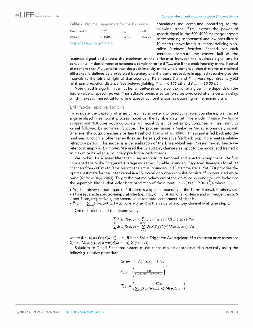
Table 2. Optimal parameters for the LN model

Parameter tnextsp τIh DC

Value 0.0748 1.433 0.4672

DOI: 10.7554/eLife.06213.013





and then stopping when the resulting square error ‖RS0−∑ω;ξSn+1ðωÞSn+1ðξÞTnðvÞMðω; ξ; :; :vÞ‖2ugoes

below a minimum value (we used a threshold of 10−4). The first 6 components (i.e., time bins) of the

temporal kernel (i.e., 0–50 ms) were also used for input convolution in the theta model. We did not

integrate further components (60–400 ms) since their weight was much lower and its implementation

by relay neurons seemed less realistic.

To retrieve the optimal value for all parameters of the model, we used the GLM matlab toolbox

developed in the Pillow lab (http://pillowlab.cps.utexas.edu/code_GLM.html), using as input the one-

dimensional signal UðtÞ=∑ωSðωÞXðω; tÞ. Other parameters of the LN model including the self-

inhibition temporal kernel Ih were optimized using the gradient descent implemented in the toolbox.

This method provides estimation for a stochastic generalized LN model. We were interested in

assessing the performance of a deterministic LN model. We then run a deterministic model with the

same parameters as the stochastic model plus one new free parameter describing the normalized

time to next spike (in the stochastic model, that time is drawn from an exponential distribution). The

value of tnextsp was optimized using the same minimization procedure used for others models (see

Optimisation section below). Two other parameters were also optimized again, since this procedure

minimized a different score than the GLM toolbox score: time scale of self-inhibition τIh and constant

input to the model DC (Table 2).

We made one last modification to this LN model. We optimized the model such that it would

maximally fire not at the time of syllable boundaries but 10 ms posterior to that time (de facto, we

simply slid the STA window by 10 ms). This provides a delayed signal but likely more reliable since it

can use more information (notably the rebound in the auditory spectrogram that is present right after

a syllable boundary).

Theta modelThe theta model is composed of the Te and Ti cells from the full network model described above, with

the exact same parameter set. 11 parameters were optimized in the full model, 10 in the control

model (see values in Table 3).

Control modelThe control model was used to provide a baseline for assessing the performance of other models.

Under these control conditions, predicted syllable boundaries were generated rhythmically at a fixed

time interval, irrespective of the stimulus. The rate of the rhythmic process was varied from 1 Hz to 15

Hz in 0.5 Hz intervals. Such control model yielded better performance than another control model

consisting of a homogeneous Poisson process. It thus provides a more stringent control for estimating

the efficiency of other algorithms.

Model performance evaluationWe evaluated how well syllable boundaries predicted by any model matched with the boundaries derived

from labelled speech data. As an evaluation metrics, we used a point process distance that is used to

compare distance between spike trains (Victor and Purpura, 1997). Shift cost was set to 20 s−1 (in other

words, a predicted and an actual boundary could be matched if they were no more than 50 msec apart).

To draw comparison between different models, for each level of compression, we computed the

(non-normalized) distance measure for the theta model summed over all sentences in the test data set,

as well as the average number of predicted boundaries per sentence. We then matched the theta model

to a control rhythmic model with the same predicted syllabic rate, and computed the difference

between the non-normalized distance for the theta model and for that matched rhythmic model.

OptimisationWe optimized the parameters from all models to get the minimal normalized point process distance

between predicted and actual boundaries in each sentence. Optimization was made using global

Table 3. Optimal parameters for the theta model

Pars σTe σTi = σGe = σGi τDTe τDTi IextTe IDCTe τDCTi gTi;Ti gTi;Te gLTe

Value 0.282 Affiffiffiffiffiffiffiffiffiffiffiffiffiffiffiffiffiffims=cm2

p2.028 A

ffiffiffiffiffiffiffiffiffiffiffiffiffiffiffiffiffiffims=cm2

p24.3 30.36 15 1.25 0.0851 0.432 0.207 0.264

DOI: 10.7554/eLife.06213.014



http://pillowlab.cps.utexas.edu/code_GLM.html



gradient descent (function fminsearch in Matlab) and repeated with many initial points to avoid

retaining a local minimum. Although both the theta model and the control model are intrinsically

stochastic, the sample size was large enough for the objective function over the entire sample to be

nearly deterministic, allowing for convergence of the gradient descent algorithm. The list of optimized

parameters for each type of model is provided in the related model sections above. We split the entire

TIMIT TRAIN data set (4620 sentences) into two data sets: a first data set of 1000 sentences was used

to compute optimal parameters; final assessment of an algorithm performance with its optimal

parameters was done on a separate set of 3620 sentences.

Analysis of model behaviour

LFP spectral analysisSimulated LFP was downsampled to 1000 Hz before applying a time-frequency decomposition using

complex Morlet wavelet transform, with all frequencies between 2 and 100 Hz with a 0.5 Hz precision.

Coherence between stimulus and LFP signal was then computed for each time point t and each

frequency f over 100 simulations using 100 distinct sentences sen, using the formula from Mitra and

Pesaran (1999). Synchronized bursts of the PING or PINTH were detected using spike timings in Gi

and Ti populations since spikes of inhibitory neurons were more synchronized than those of excitatory

neurons. Synchronous bursts of spikes were detected within a given population whenever more than

10% of neurons in the population spikes within a 6 ms interval (15 ms for Ti cells).

Cross-frequency couplingWe computed cross-frequency coupling from 50 simulations of the model, each with a different TIMIT

sentence preceded by 1000–1500 ms rest.

For the LFP phase-amplitude coupling, we extracted phase and amplitude from all frequencies

from 2 Hz to 70 Hz in 1 Hz interval, and computed the Modulation Index for all pairs of frequencies

(Tort et al., 2010). Data from all trials were concatenated (separately for spontaneous and speech-

related activity) across all trials beforehand. To compute Modulation Index, in each condition, signal

amplitude values x(famp,t,sen) were binned in N = 18 different bins according to the simultaneous

phase of x(fphase,t,sen). For spike phase-amplitude coupling, we defined spike gamma amplitude as

the number of Gi neurons spiking at a given gamma burst, and the spike theta phase was defined by

linear interpolation from −π for a theta spike burst to +π for the subsequent theta burst.

Simple temporal patterns decodingWe first explored the model’s performance using simple sawtooth signals (Shamir et al., 2009),

representing prototypical realizations of formant transitions in a given frequency band. Each stimulus

consisted of a rising component between 0 and 1, followed by a decay component from 1 back to 0. The

overall length of the sawtooth was 50 ms, and the relative position of the maximal point tMAX between

the starting point tSTART and end point tEND was defined by a variable a = (tMAX − tSTART)/(tEND − tSTART).

The input connectivity had to be slightly modified since sawtooths are one-dimensional signals in

contrast to the multi-dimensional channel signals that we have to use for speech stimuli: for Te units,

we used IEXTTe = 20; and for the connections to Ge units in line with the original model (Shamir et al.,

2009), we used different input levels across the population, ranging from 0.125 to 4 in 0.125 intervals.

The rest of the model remained unchanged.

We simulated the response of the network to a series of 500 sawtooths with parameter a taking

one of 10 equally spaced values within the [0 1] interval. Interstimulus interval varied randomly

between 50 and 250 ms.

We compared the model’s performance for different neural codes. For the ‘stimulus timing’ code

(see ‘Results’ section), we extracted the spike pattern of output (Ge) neurons between 20 ms before

and 70 ms after of each sawtooth onset. We computed the distance between all output spike patterns

using a spike train distance measure (Victor and Purpura, 1997), implemented in the Spike Train

Analysis Toolkit (http://neuroanalysis.org/toolkit/). We used a shift cost of 200 s−1 corresponding to

a timing resolution of 5 ms. We decoded the peak parameter using the simple leave-one-out

clustering procedure of the STA toolkit, using a clustering exponent of −10. By comparing the

‘decoded parameter’, i.e., the parameter corresponding to the closest cluster, to the input sawtooth

parameter, we built confusion matrices and computed decoding performance.



http://neuroanalysis.org/toolkit/


In the ‘theta-timing’ code, we extracted the spike pattern of output neuron in windows starting 20

before a theta burst and finishing 20 ms after the next theta burst (‘theta chunks’, Figure 4A). Spike

times within each chunk were referenced with respect to the onset of the window. Each spike pattern

was labelled with the corresponding value of the stimulus if the theta burst occurred during the

presentation of the stimulus, or with the label ‘rest’ if the theta burst occurred during an interstimulus

interval. The same decoding analysis was applied on such internally referenced neural patterns,

yielding a 11 × 11 confusion matrix (10 stimulus shapes and rest). Detection theory measures (hits,

misses, correct rejections, and false alarms) were computed by summing values in blocks of the

confusion matrix (of size 10 × 10, 10 × 1, 1 × 10, and 1 × 1, respectively). A classification confusion

matrix was obtained by removing the last row and last column of that confusion matrix.

We run the same decoding analysis on variants of the network: the full network; a control model

where Te units do not receive the sawtooth input (undriven theta network) and another control where

theta–gamma connections were removed (uncoupled theta–gamma network).

Syllable decoding from sentencesThe classification procedure was similar for syllable decoding, where we tried to decode the identity

of syllables within continuous stream of speech (full sentences) from the activity of output neurons. We

stimulated the network by presenting 25 sentences from the TIMIT corpus repeated 100 times each.

We extracted theta chunks of Ge spike patterns as explained previously. Each chunk was labelled with

the identity of the syllable being presented at the time of the first theta burst of the chunk. We

randomly selected 10 syllables from the whole set of syllables within the 25 sentences. As in some

cases there were several consecutive theta chunks corresponding to the same syllable, we equated

the total number of theta chunks per syllable by randomly selecting 100 theta chunks labelled with

each of the 10 syllables. Syllable classification of theta-chunked Ge spike patterns was performed

using two different neural codes. For the spike pattern code, we applied the same procedure as for

sawtooth classification, using a smaller value of spike shift cost corresponding to a timing resolution of

60 ms. For the spike count code, we measured the number of spikes emitted by each Ge neuron

within a theta chunk. We then ran a simple nearest-mean classification procedure to decode syllable

identity corresponding to each theta chunk from the spike counts of all Ge neurons (see ‘Classification

analysis’ below). Both methods relied on the leave-one-out procedure that consists in identifying

a chunk after the decoder was trained on all chunks but the to-be-decoded one. Decoding was

repeated 200 times using each time a different set of 10 random syllables, and the analysis was

performed over all three variants of the network.

For syllable classification across speakers, we used the two sentences from the TIMIT corpus that

have been recorded for each of the 462 speakers (’She had your dark suit in greasy wash water all

year’ and ’Don’t ask me to carry an oily rag like that’) and trained the network to classify syllables

based on the neural output from other speakers, thus testing generalization across speakers. There is

a wide variability of pronunciations over speakers as attested by the variability of chain of phonemes

labelled of phoneticians, but the two sentences could nonetheless be parsed into 25 syllables overall

for each speaker. We simulated the network presenting these 924 sentences and used the theta-

chunked output to decode syllable identity. The method used was very similar to the syllable

decoding analysis, where we classified theta-chunked neural patterns into one of 10 possible syllables

(drawn randomly from the set of 25 syllables), with the only difference that here the classifier was

based on theta chunks coming from different speakers. The classification was repeated 100 times for

different subsets of syllables.

Neural encoding properties: classification analysisThe first analysis of neural encoding properties consisted in comparing the ability to classify neural

codes from the model into arbitrary speech segments (as opposed to syllables as in previous section).

The methods, as detailed below, were inspired by the decoding of neural auditory cortical activity

recorded in monkeys in response to naturalistic sounds (Kayser et al., 2012). We simulated the

network by presenting 25 different sentences from the TIMIT corpus repeated 50 times each. For

a given window size (ranging from 80 to 480 ms in 80 ms intervals), we randomly extracted 10

windows (defined as stimuli) from the overall set of 25 sentences. We then retrieved stimulus identity

based on the activity of a neuron that was randomly drawn from the Ge population using three




different neural codes. In the neural count code, we counted the number of spikes emitted by that

neuron within each window. In the time-partitioned code, we divided each window into N equally size

bins, and computed the number of spikes for each of the 8 bins separately. In the phase-partitioned

code, we divided the window based on theta-phase- rather time-intervals: each spike was labelled

with the phase of the theta oscillation at the corresponding spike time, and we computed the number

of spikes falling into each of the N subdivisions of the [−π;π] interval.We then used a nearest-mean template matching procedure to decode the stimuli. To classify each

stimulus exemplar using each neural code, we averaged the vectors over all presentations of each

stimulus using a leave-one-out procedure; we then computed the Euclidian distance from the current

vector to each of the 10 stimulus-averaged template. Finally, we ‘decoded’ the neural code by assigning

it to the stimulus class with minimal distance to template. A more detailed explanation of the procedure

is provided in the original experiment article (Kayser et al., 2012). The procedure was repeated 1000

times, each time with a different set of 10 random stimuli, and performed the 3 variants of network.

Neural encoding properties: mutual information analysisWe complemented the stimulus classification with a similar analysis using mutual information between

the acoustic ‘stimulus’ and response of individual Ge neurons to further characterize the encoding

properties of the network. Mutual Information (MI) estimates the reduction of uncertainty about the

acoustic ‘stimulus’ that is obtained from the knowledge of a single trial of neural response. The data

set was identical to the one previously used for stimulus classification analysis, where each stimulus

was again segmented into non-overlapping windows of length T (here 8 to 48 ms) (Kayser et al.,

2009; de Ruyter van Steveninck et al., Strong, 1997).

Mutual Information was computed for the same neural codes as in Kayser et al. (2009). We used

Spike count code and Time-partitioned code as described above (for the Time-partitioned code the

size of the bins was kept constant to 8 bins; the number of bins in a window hence increased with

window size. As slow LFP phase was more reliable over sentence repetitions than power, we

combined spike count and LFP theta phase to get a Spike count & Phase-partitioned code

(Montemurro et al., 2008). For this code, the phase of slow LFP was divided into N = 4 bins, and the

firing rate in each window was labelled according to the phase at which the first spike occurred.

Finally, we explored the influence of slow LFP phase on MI when combined with temporal spiking

patterns. Thus, in the Time- & Phase-partitioned code spikes carry two distinct tags, the first one

referring to the position of the spike inside one of the four subdivisions of the stimulus window, the

second indicating the phase of the underlying LFP at the moment of the spike occurrence.

We corrected for sampling bias (Kayser et al., 2009) first by using a shuffling method (Panzeri

et al., 2007), then the quadratic extrapolation method (Strong et al., 1998). We further reduced the

residual bias using a bootstrapping technique (200 resampled data) (Montemurro et al., 2008).

AcknowledgementsThis work was funded by the European Research Council (Compuslang project; Grant agreement

260347), the Swiss National Fund (grant 320030-149319), the Agence National de la Recherche, the

CNRS. We warmly thank Oded Ghitza for stimulating discussions, Maoz Shamir and Andy Brughera for

sharing elements of code with us, Adrien Wohrer for help with the mathematical analysis and Jean-

Paul Haton for his input from the perspective of automatic speech recognition. BSG gratefully

acknowledges partial support from the National Research University Higher School of Economics.

Additional information

Funding

Funder Grant reference Author

European Research Council (ERC) CompusLang 260347 Lorenzo Fontolan

Schweizerische Nationalfonds zurForderung der WissenschaftlichenForschung

320030-149319 Anne-Lise Giraud




Funder Grant reference Author

Agence Nationale de laRecherche

Boris Gutkin

Centre National de la RechercheScientifique

Anne-Lise Giraud

The funders had no role in study design, data collection and interpretation, or thedecision to submit the work for publication.

Author contributions

AH, Conception and design, Acquisition of data, Analysis and interpretation of data, Drafting or

revising the article; LF, Acquisition of data, Analysis and interpretation of data, Drafting or revising

the article; CK, Acquisition of data, Analysis and interpretation of data; BG, A-LG, Conception and

design, Analysis and interpretation of data, Drafting or revising the article

Additional files

Major datasetThe following previously published dataset was used:

Author(s) Year Dataset titleDataset IDand/or URL

Database, license, andaccessibility information

Linguistic DataConsortium (LDC)

1993 TIMIT Acoustic-PhoneticContinuous SpeechCorpus

https://catalog.ldc.upenn.edu/LDC93S1

Available from theLinguistic DataConsortium (registrationrequired).

ReferencesAbrams DA, Nicol T, Zecker S, Kraus N. 2008. Right-hemisphere auditory cortex is dominant for coding syllablepatterns in speech. The Journal of Neuroscience 28:3958–3965. doi: 10.1523/JNEUROSCI.0187-08.2008.

Ahissar E, Nagarajan SS, Ahissar M, Protopapas A, Mahncke H, Merzenich MM. 2001. Speech comprehension iscorrelated with temporal response patterns recorded from auditory cortex. Proceedings of the NationalAcademy of Sciences of USA 98:13367–13372. doi: 10.1073/pnas.201400998.

Ainsworth M, Lee S, Cunningham MO, Roopun AK, Traub RD, Kopell NJ, Whittington MA. 2011. Dual gammarhythm generators control interlaminar synchrony in auditory cortex. The Journal of Neuroscience 31:17040–17051. doi: 10.1523/JNEUROSCI.2209-11.2011.

Arnal LH, Giraud AL. 2012. Cortical oscillations and sensory predictions. Trends in Cognitive Sciences 16:390–398.doi: 10.1016/j.tics.2012.05.003.

Arnal LH, Morillon B, Kell CA, Giraud AL. 2009. Dual neural routing of visual facilitation in speech processing. TheJournal of Neuroscience 29:13445–13453. doi: 10.1523/JNEUROSCI.3194-09.2009.

Bastos AM, Usrey WM, Adams RA, Mangun GR, Fries P, Friston KJ. 2012. Canonical microcircuits for predictivecoding. Neuron 76:695–711. doi: 10.1016/j.neuron.2012.10.038.

Borgers C, Kopell NJ. 2005. Effects of noisy drive on rhythms in networks of excitatory and inhibitory neurons.Neural Computation 17:557–608. doi: 10.1162/0899766053019908.

Brasselet R, Panzeri S, Logothetis NK, Kayser C. 2012. Neurons with stereotyped and rapid responses providea reference frame for relative temporal coding in primate auditory cortex. The Journal of Neuroscience 32:2998–3008. doi: 10.1523/JNEUROSCI.5435-11.2012.

Brunel N, Wang XJ. 2003. What determines the frequency of fast network oscillations with irregular neuraldischarges? I. Synaptic dynamics and excitation-inhibition balance. Journal of Neurophysiology 90:415–430.doi: 10.1152/jn.01095.2002.

Canolty RT, Soltani M, Dalal SS, Edwards E, Dronkers NF, Nagarajan SS, Kirsch HE, Barbaro NM, Knight RT. 2007.Spatiotemporal dynamics of word processing in the human brain. Frontiers in Neuroscience 1:185–196. doi: 10.3389/neuro.01.1.1.014.2007.

Chi T, Ru P, Shamma SA. 2005. Multiresolution spectrotemporal analysis of complex sounds. The Journal of theAcoustical Society of America 118:887–906. doi: 10.1121/1.1945807.

Chichilnisky EJ. 2001. A simple white noise analysis of neuronal light responses. Network 12:199–213. doi: 10.1080/713663221.

Cogan GB, Poeppel D. 2011. A mutual information analysis of neural coding of speech by low-frequency MEGphase information. Journal of Neurophysiology 106:554–563. doi: 10.1152/jn.00075.2011.

da Costa NM, Martin KA. 2010. Whose cortical column would that be? Frontiers in Neuroanatomy 4:16. doi: 10.3389/fnana.2010.00016.





http://dx.doi.org/10.1523/JNEUROSCI.0187-08.2008

http://dx.doi.org/10.1073/pnas.201400998


http://dx.doi.org/10.1016/j.tics.2012.05.003


http://dx.doi.org/10.1016/j.neuron.2012.10.038

http://dx.doi.org/10.1162/0899766053019908


http://dx.doi.org/10.1152/jn.01095.2002

http://dx.doi.org/10.3389/neuro.01.1.1.014.2007

http://dx.doi.org/10.3389/neuro.01.1.1.014.2007

http://dx.doi.org/10.1121/1.1945807

http://dx.doi.org/10.1080/713663221

http://dx.doi.org/10.1080/713663221

http://dx.doi.org/10.1152/jn.00075.2011

http://dx.doi.org/10.3389/fnana.2010.00016

http://dx.doi.org/10.3389/fnana.2010.00016


Davis MH, Ford MA, Kherif F, Johnsrude IS. 2011. Does semantic context benefit speech understanding through“top-down” processes? Evidence from time-resolved sparse fMRI. Journal of Cognitive Neuroscience 23:3914–3932. doi: 10.1162/jocn_a_00084.

de Ruyter van Steveninck RR, Lewen GD, Strong SP, Koberle R, Bialek W. 1997. Reproducibility and variability inneural spike trains. Science 275:1805–1808. doi: 10.1126/science.275.5307.1805.

Douglas RJ, Martin KA. 2004. Neuronal circuits of the neocortex. Annual Review of Neuroscience 27:419–451.doi: 10.1146/annurev.neuro.27.070203.144152.

Fanselow EE, Richardson KA, Connors BW. 2008. Selective, state-dependent activation of somatostatin-expressing inhibitory interneurons in mouse neocortex. Journal of Neurophysiology 100:2640–2652. doi: 10.1152/jn.90691.2008.

Fishbach A, Nelken I, Yeshurun Y. 2001. Auditory edge detection: a neural model for physiological andpsychoacoustical responses to amplitude transients. Journal of Neurophysiology 85:2303–2323.

Fisher WM. 1996. tsylb2. National Institute of Standards and Technology. http://www.nist.gov/speech/tools.Fontolan L, Morillon B, Liegeois-Chauvel C, Giraud AL. 2014. The contribution of frequency-specific activity tohierarchical information processing in the human auditory cortex. Nature Communications 5:4694. doi: 10.1038/ncomms5694.

Gagnepain P, Henson RN, Davis MH. 2012. Temporal predictive codes for spoken words in auditory cortex.Current Biology 22:615–621. doi: 10.1016/j.cub.2012.02.015.

Ghitza O. 2011. Linking speech perception and neurophysiology: speech decoding guided by cascaded oscillatorslocked to the input rhythm. Frontiers in Psychology 2:130. doi: 10.3389/fpsyg.2011.00130.

Ghitza O. 2014. Behavioral evidence for the role of cortical θ oscillations in determining auditory channel capacityfor speech. Frontiers in Psychology 5:652. doi: 10.3389/fpsyg.2014.00652.

Giraud AL, Poeppel D. 2012. Cortical oscillations and speech processing: emerging computational principles andoperations. Nature Neuroscience 15:511–517. doi: 10.1038/nn.3063.

Gross J, Hoogenboom N, Thut G, Schyns P, Panzeri S, Belin P, Garrod S. 2013. Speech rhythms and multiplexedoscillatory sensory coding in the human brain. PLOS Biology 11:e1001752. doi: 10.1371/journal.pbio.1001752.

Gupta AS, van der Meer MA, Touretzky DS, Redish AD. 2012. Segmentation of spatial experience by hippocampaltheta sequences. Nature Neuroscience 15:1032–1039. doi: 10.1038/nn.3138.

Gutig R, Sompolinsky H. 2009. Time-warp-invariant neuronal processing. PLOS Biology 7:e1000141. doi: 10.1371/journal.pbio.1000141.

Henry MJ, Herrmann B, Obleser J. 2014. Entrained neural oscillations in multiple frequency bands comodulatebehavior. Proceedings of the National Academy of Sciences of USA 111:14935–14940. doi: 10.1073/pnas.1408741111.

Hopfield JJ. 2004. Encoding for computation: recognizing brief dynamical patterns by exploiting effects of weakrhythms on action-potential timing. Proceedings of the National Academy of Sciences of USA 101:6255–6260.doi: 10.1073/pnas.0401125101.

Jadi MP, Sejnowski TJ. 2014. Cortical oscillations arise from contextual interactions that regulate sparse coding.Proceedings of the National Academy of Sciences of USA 111:6780–6785. doi: 10.1073/pnas.1405300111.

Jensen O, Colgin LL. 2007. Cross-frequency coupling between neuronal oscillations. Trends in Cognitive Sciences11:267–269. doi: 10.1016/j.tics.2007.05.003.

Jensen O, Lisman JE. 1996. Theta/gamma networks with slow NMDA channels learn sequences and encodeepisodic memory: role of NMDA channels in recall. Learning & Memory 3:264–278. doi: 10.1101/lm.3.2-3.264.

Kahn D. 1976. Syllable-based generalizations in English phonology. http://seas3.elte.hu/szigetva/courses/syllable/kahn76-pres-szpsyllableracz.pdf.

Kayser C, Ince RA, Panzeri S. 2012. Analysis of slow (theta) oscillations as a potential temporal reference frame forinformation coding in sensory cortices. PLOS Computational Biology 8:e1002717. Edited by Tim Behrens. doi: 10.1371/journal.pcbi.1002717.

Kayser C, Montemurro MA, Logothetis NK, Panzeri S. 2009. Spike-phase coding boosts and stabilizes informationcarried by spatial and temporal spike patterns. Neuron 61:597–608. doi: 10.1016/j.neuron.2009.01.008.

Kopell NJ, Borgers C, Pervouchine DD, Malerba P. 2010. Gamma and theta rhythms in biophysical models ofhippocampal circuits. In: Cutsuridis V, editor. Hippocampal microcircuits: Springer. p. 423–57.

Lakatos P, Chen CM, O’Connell MN, Mills A. 2007. Neuronal oscillations and multisensory interaction in primaryauditory cortex. Neuron 53:279–292. doi: 10.1016/j.neuron.2006.12.011.

Lakatos PP, Shah AS, Knuth KH, Ulbert I, Karmos G, Schroeder CE. 2005. An oscillatory hierarchy controllingneuronal excitability and stimulus processing in the auditory cortex. Journal of Neurophysiology 94:1904–1911.doi: 10.1152/jn.00263.2005.

Lee JH, Whittington MA, Kopell NJ. 2013. Top-down beta rhythms support selective attention via interlaminarinteraction: a model. PLOS Computational Biology 9:e1003164. Edited by Stephen Coombes. doi: 10.1371/journal.pcbi.1003164.

Lever C, Kaplan R, Burgess N. 2014. In: Derdikman D, Knierim JJ, editors. Space,Time and Memory in theHippocampal Formation. Vienna: Springer Vienna. doi: 10.1007/978-3-7091-1292-2.

Lieberman P. 1985. On the evolution of human syntactic ability. Its pre-adaptive Bases—Motor control and speech.Journal of Human Evolution 14:657–668. doi: 10.1016/S0047-2484(85)80074-9.

Linguistic Data Consortium. 1993. TIMIT acoustic-phonetic continuous speech corpus. https://catalog.ldc.upenn.edu/LDC93S1.

Lisman JE, Buzsaki G. 2008. A neural coding scheme formed by the combined function of gamma and thetaoscillations. Schizophrenia Bulletin 34:974–980. doi: 10.1093/schbul/sbn060.



http://dx.doi.org/10.1162/jocn_a_00084

http://dx.doi.org/10.1126/science.275.5307.1805

http://dx.doi.org/10.1146/annurev.neuro.27.070203.144152

http://dx.doi.org/10.1152/jn.90691.2008

http://dx.doi.org/10.1152/jn.90691.2008

http://www.nist.gov/speech/tools

http://dx.doi.org/10.1038/ncomms5694

http://dx.doi.org/10.1038/ncomms5694

http://dx.doi.org/10.1016/j.cub.2012.02.015

http://dx.doi.org/10.3389/fpsyg.2011.00130


http://dx.doi.org/10.1038/nn.3063

http://dx.doi.org/10.1371/journal.pbio.1001752

http://dx.doi.org/10.1038/nn.3138







http://dx.doi.org/10.1016/j.tics.2007.05.003

http://dx.doi.org/10.1101/lm.3.2-3.264

http://seas3.elte.hu/szigetva/courses/syllable/kahn76-pres-szpsyllableracz.pdf

http://seas3.elte.hu/szigetva/courses/syllable/kahn76-pres-szpsyllableracz.pdf

http://dx.doi.org/10.1371/journal.pcbi.1002717




http://dx.doi.org/10.1152/jn.00263.2005



http://dx.doi.org/10.1007/978-3-7091-1292-2

http://dx.doi.org/10.1016/S0047-2484(85)80074-9



http://dx.doi.org/10.1093/schbul/sbn060


Lisman JE, Jensen O. 2013. The theta-gamma neural code. Neuron 77:1002–1016. doi: 10.1016/j.neuron.2013.03.007.Luo H, Liu Z, Poeppel D. 2010. Auditory cortex tracks both auditory and visual stimulus dynamics using low-frequency neuronal phase modulation. PLOS Biology 8:e1000445. Edited by Robert Zatorre. doi: 10.1371/journal.pbio.1000445.

Luo H, Poeppel D. 2007. Phase patterns of neuronal responses reliably discriminate speech in human auditorycortex. Neuron 54:1001–1010. doi: 10.1016/j.neuron.2007.06.004.

Mazzoni A, Panzeri S, Logothetis NK, Brunel N. 2008. Encoding of naturalistic stimuli by local field potentialspectra in networks of excitatory and inhibitory neurons. PLOS Computational Biology 4:e1000239. Edited byKarlJ Friston. doi: 10.1371/journal.pcbi.1000239.

Mermelstein P. 1975. Automatic segmentation of speech into syllabic units. The Journal of the Acoustical Societyof America 58:880–883. doi: 10.1121/1.380738.

Miller JL, Grosjean F, Lomanto C. 1984. Articulation rate and its variability in spontaneous speech: a reanalysis andsome implications. Phonetica 41:215–225. doi: 10.1159/000261728.

Mitra PP, Pesaran B. 1999. Analysis of dynamic brain imaging data. Biophysical Journal 76:691–708. doi: 10.1016/S0006-3495(99)77236-X.

Montemurro MA, Rasch MJ, Murayama Y, Logothetis NK, Panzeri S. 2008. Phase-of-firing coding of natural visualstimuli in primary visual cortex. Current Biology 18:375–380. doi: 10.1016/j.cub.2008.02.023.

Morillon B, Liegeois-Chauvel C, Arnal LH, Benar CG, Giraud AL. 2012. Asymmetric function of theta and gammaactivity in syllable processing: an Intra-cortical study. Frontiers in Psychology 3:1–9. doi: 10.3389/fpsyg.2012.00248.

Mukamel EA, Wong KF, Prerau MJ, Brown EN, Purdon PL. 2011. Phase-based measures of cross-frequencycoupling in brain electrical dynamics under general anesthesia. Conference Proceedings: Annual InternationalConference of the IEEE Engineering in Medicine and Biology Society 2011:1981–1984. doi: 10.1109/IEMBS.2011.6090558.

Ngon C, Martin A, Dupoux E, Cabrol D, Dutat M, Peperkamp S. 2013. (Non)words, (non)words, (non)words:evidence for a protolexicon during the first year of life. Developmental Science 16:24–34. doi: 10.1111/j.1467-7687.2012.01189.x.

Nourski KV, Reale RA, Oya H, Kawasaki H, Kovach CK, Chen H, Howard MA, Brugge JF. 2009. Temporal envelopeof time-compressed speech represented in the human auditory cortex. The Journal of Neuroscience 29:15564–15574. doi: 10.1523/JNEUROSCI.3065-09.2009.

Panzeri S, Diamond ME. 2010. Information carried by population spike times in the whisker sensory cortex can bedecoded without knowledge of stimulus time. Frontiers in Synaptic Neuroscience 2:17. doi: 10.3389/fnsyn.2010.00017.

Panzeri S, Ince RA, Diamond ME, Kayser C. 2014. Reading spike timing without a clock: intrinsic decoding of spiketrains. Philosophical Transactions of the Royal Society of London. Series B, Biological Sciences 369:20120467.doi: 10.1098/rstb.2012.0467.

Panzeri S, Senatore R, Montemurro MA, Petersen RS. 2007. Correcting for the sampling bias problem in spike traininformation measures. Journal of Neurophysiology 98:1064–1072. doi: 10.1152/jn.00559.2007.

Pasley BN, David SV, Mesgarani N. 2012. Reconstructing speech from human auditory cortex. PLOS Biology 10:e1001251. Edited by Robert Zatorre. doi: 10.1371/journal.pbio.1001251.

Peelle JE, Gross J, Davis MH. 2013. Phase-locked responses to speech in human auditory cortex are enhancedduring comprehension. Cerebral Cortex 23:1378–1387. doi: 10.1093/cercor/bhs118.

Phillips DP, Hall SE, Boehnke SE. 2002. Central auditory onset responses, and temporal asymmetries in auditoryperception. Hearing Research 167:192–205. doi: 10.1016/S0378-5955(02)00393-3.

Pillow JW, Shlens J, Paninski L, Sher A, Litke AM, Chichilnisky EJ, Simoncelli EP. 2008. Spatio-temporal correlationsand visual signalling in a complete neuronal population. Nature 454:995–999. doi: 10.1038/nature07140.

Poeppel D. 2003. The analysis of speech in different temporal integration windows: cerebral lateralization as‘asymmetric sampling in time’. Speech Communication 41:245–255. doi: 10.1016/S0167-6393(02)00107-3.

Poeppel D, Idsardi WJ, van Wassenhove V. 2008. Speech perception at the interface of neurobiology andlinguistics. Philosophical Transactions of the Royal Society of London. Series B, Biological Sciences 363:1071–1086. doi: 10.1098/rstb.2007.2160.

Rosen S. 1992. Temporal information in speech: acoustic, auditory and linguistic aspects. PhilosophicalTransactions of the Royal Society of London. Series B, Biological Sciences 336:367–373. doi: 10.1098/rstb.1992.0070.

Schroeder CE, Lakatos P. 2009. The gamma oscillation: master or slave? Brain Topography 22:24–26. doi: 10.1007/s10548-009-0080-y.

Shamir M, Ghitza O, Epstein S, Kopell NJ. 2009. Representation of time-varying stimuli by a network exhibitingoscillations on a faster time scale. PLOS Computational Biology 5:e1000370. doi: 10.1371/journal.pcbi.1000370.

Silberberg G, Markram H. 2007. Disynaptic inhibition between neocortical pyramidal cells mediated by Martinotticells. Neuron 53:735–746. doi: 10.1016/j.neuron.2007.02.012.

Stevens KN. 2002. Toward a model for lexical access based on acoustic landmarks and distinctive features. TheJournal of the Acoustical Society of America 111:1872. doi: 10.1121/1.1458026.

Strong SP, Koberle R, van Steveninck RRR, Bialek W. 1998. Entropy and information in neural spike trains. PhysicalReview Letters 80:197–200. doi: 10.1103/PhysRevLett.80.197.

Tort AB, Komorowski R, Eichenbaum H, Kopell N. 2010. Measuring phase-amplitude coupling between neuronaloscillations of different frequencies. Journal of Neurophysiology 104:1195–1210. doi: 10.1152/jn.00106.2010.








http://dx.doi.org/10.1121/1.380738

http://dx.doi.org/10.1159/000261728

http://dx.doi.org/10.1016/S0006-3495(99)77236-X

http://dx.doi.org/10.1016/S0006-3495(99)77236-X

http://dx.doi.org/10.1016/j.cub.2008.02.023



http://dx.doi.org/10.1109/IEMBS.2011.6090558

http://dx.doi.org/10.1109/IEMBS.2011.6090558

http://dx.doi.org/10.1111/j.1467-7687.2012.01189.x

http://dx.doi.org/10.1111/j.1467-7687.2012.01189.x


http://dx.doi.org/10.3389/fnsyn.2010.00017

http://dx.doi.org/10.3389/fnsyn.2010.00017

http://dx.doi.org/10.1098/rstb.2012.0467

http://dx.doi.org/10.1152/jn.00559.2007


http://dx.doi.org/10.1093/cercor/bhs118

http://dx.doi.org/10.1016/S0378-5955(02)00393-3

http://dx.doi.org/10.1038/nature07140

http://dx.doi.org/10.1016/S0167-6393(02)00107-3




http://dx.doi.org/10.1007/s10548-009-0080-y

http://dx.doi.org/10.1007/s10548-009-0080-y



http://dx.doi.org/10.1121/1.1458026

http://dx.doi.org/10.1103/PhysRevLett.80.197

http://dx.doi.org/10.1152/jn.00106.2010


Tort AB, Rotstein HG, Dugladze T, Gloveli T, Kopell NJ. 2007. On the formation of gamma-coherent cellassemblies by oriens lacunosum-moleculare interneurons in the hippocampus. Proceedings of the NationalAcademy of Sciences of USA 104:13490–13495. doi: 10.1073/pnas.0705708104.

Victor J, Purpura K. 1997. Metric-space analysis of spike trains: theory, algorithms and application. Network 8:127–164. doi: 10.1088/0954-898X/8/2/003.

Vierling-Claassen D, Cardin JA, Moore CI, Jones SR. 2010. Computational modeling of distinct neocorticaloscillations driven by cell-type selective optogenetic drive: separable resonant circuits controlled by low-threshold spiking and fast-spiking interneurons. Frontiers in Human Neuroscience 4:198. doi: 10.3389/fnhum.2010.00198.

Villing R, Timoney J, Ward T, Costello J. 2004. Automatic blind syllable segmentation for continuous speech.Electronic Engineering.

Wang XJ. 2010. Neurophysiological and computational principles of cortical rhythms in cognition. PhysiologicalReviews 90:1195–1268. doi: 10.1152/physrev.00035.2008.

Wang X, Lu T, Bendor D, Bartlett E. 2008. Neural coding of temporal information in auditory thalamus and cortex.Neuroscience 157:484–494. doi: 10.1016/j.neuroscience.2008.07.050.

Wu SL, Shire ML, Greenberg S, Morgan N. 1997. Integrating syllable boundary information into speechrecognition. Acoustics, Speech, and Signal Processing, 1997. ICASSP-97., 1997 IEEE International Conference on,2. IEEE. p. 987–990. http://ieeexplore.ieee.org/xpls/abs_all.jsp?arnumber=596105.

Yildiz IB, von Kriegstein K, Kiebel SJ. 2013. From birdsong to human speech recognition: bayesian inference ona hierarchy of nonlinear dynamical systems. PLOS Computational Biology 9:e1003219. Edited by Viktor K Jirsa.doi: 10.1371/journal.pcbi.1003219.

Zhou Y, Wang X. 2010. Cortical processing of dynamic sound envelope transitions. Journal of Neuroscience 30:16741–16754. doi: 10.1523/JNEUROSCI.2016-10.2010.

Zion Golumbic EM, Poeppel D, Schroeder CE. 2012. Temporal context in speech processing and attentionalstream selection: a behavioral and neural perspective. Brain and Language 122:151–161. doi: 10.1016/j.bandl.2011.12.010.




http://dx.doi.org/10.1088/0954-898X/8/2/003

http://dx.doi.org/10.3389/fnhum.2010.00198

http://dx.doi.org/10.3389/fnhum.2010.00198

http://dx.doi.org/10.1152/physrev.00035.2008

http://dx.doi.org/10.1016/j.neuroscience.2008.07.050

http://ieeexplore.ieee.org/xpls/abs_all.jsp?arnumber=596105



http://dx.doi.org/10.1016/j.bandl.2011.12.010

http://dx.doi.org/10.1016/j.bandl.2011.12.010


Speech encoding by coupled cortical theta and gamma oscillations

Documents