Speech Coding Techniques (I) Introduction to Quantization Scalar quantization Uniform quantization Nonuniform quantization Waveform-based coding Pulse Coded Modulation (PCM) Differential PCM (DPCM) Adaptive DPCM (ADPCM) Model-based coding Channel vocoder Analysis-by-Synthesis techniques Harmonic vocoder

Welcome message from author
This document is posted to help you gain knowledge. Please leave a comment to let me know what you think about it! Share it to your friends and learn new things together.
Transcript
Speech Coding Techniques (I) Introduction to Quantization
Scalar quantization Uniform quantization Nonuniform quantization
Waveformbased coding Pulse Coded Modulation (PCM) Differential PCM (DPCM) Adaptive DPCM (ADPCM)
Modelbased coding Channel vocoder AnalysisbySynthesis techniques Harmonic vocoder
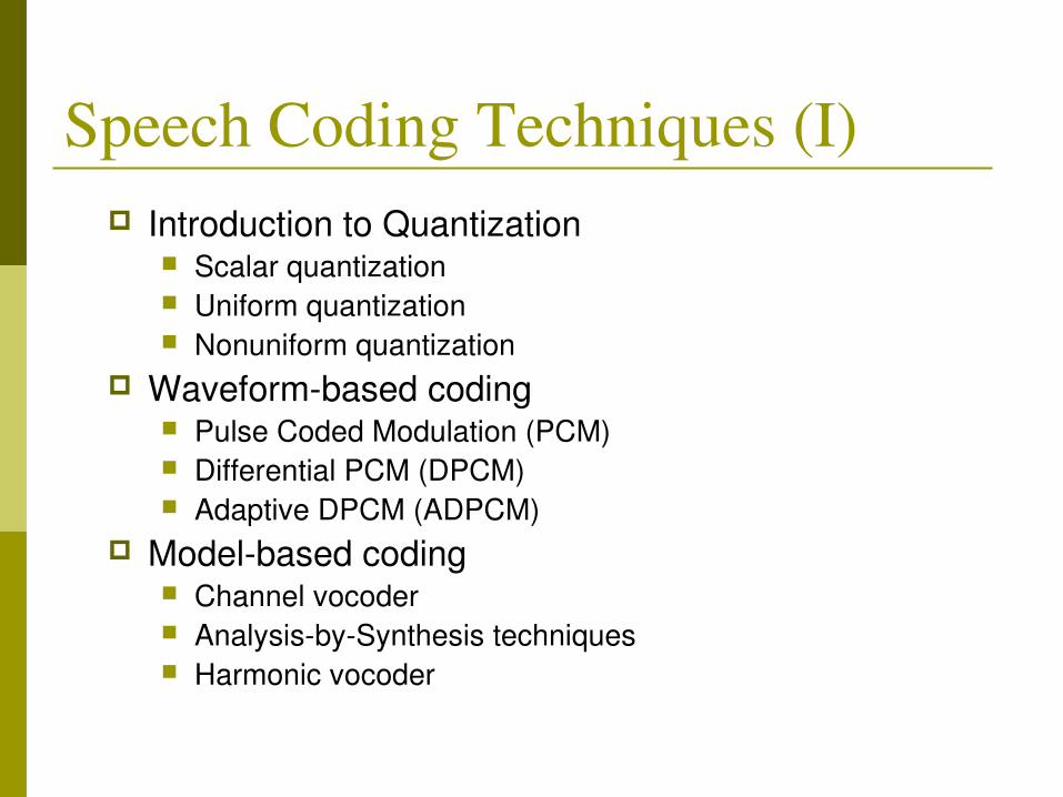
Origin of Speech Coding“Watson, if I can get a mechanism which will make a current of electricity vary its intensity as the air variesin density when sound is passing through it, I cantelegraph any sound, even the sound of speech.”
A. G. Bell’1875analog communication
HX =−∑i=1
N
pi log2pi (bits/sample)or bps
digital communication C. E. Shannon’1948
Entropy formulaof a discrete source
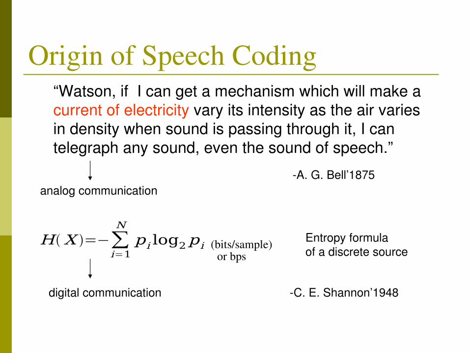
Digitization of Speech Signals
Sampler Quantizerxc(t) x(n)=xc(nT) x(n)
continuoustimespeech signal
discrete sequencespeech samples

Sampling Sampling Theorem
when sampling a signal (e.g., converting from an analog signal to digital), the sampling frequency must be greater than twice the bandwidth of the input signal in order to be able to reconstruct the original perfectly from the sampled version.
Sampling frequency: >8K samples/second (human speech is roughly bandlimited at 4KHz)

Quantization In Physics
To limit the possible values of a magnitude or quantity to a discrete set of values by quantum mechanical rules
In speech coding To limit the possible values of a speech sample or
prediction residue to a discrete set of values by information theoretic rules (tradeoff between Rate and Distortion)

Quantization Examples Examples
Continuous to discrete a quarter of milk, two gallons of gas, normal temperature is 98.6F,
my height is 5 foot 9 inches Discrete to discrete
Round your tax return to integers The mileage of my car is about 60K.
Play with bits Precision is finite: the more precise, the more bits you need (to
resolve the uncertainty) Keep a card in secret and ask your partner to guess. He/she can
only ask Yes/No questions: is it bigger than 7? Is it less than 4? ... However, not every bit has the same impact
How much did you pay for your car? (two thousands vs. $2016.78)
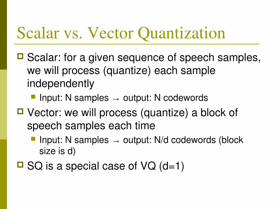
Scalar vs. Vector Quantization Scalar: for a given sequence of speech samples,
we will process (quantize) each sample independently Input: N samples → output: N codewords
Vector: we will process (quantize) a block of speech samples each time Input: N samples → output: N/d codewords (block
size is d) SQ is a special case of VQ (d=1)

Scalar Quantization
x f f 1 xs∈S
original value
quantizationindex
quantized value
Quantizer
x Q x
In SQ, quantizing N samples is not fundamentally different from Quantizing one sample (since they are processed independently)
A quantizer is defined by codebook (collection of codewords) and mapping function (straightforward in the case of SQ)

RateDistortion Tradeoff Rate: How many
codewords (bits) are used? Example: 16bit audio vs.
8bit PCM speech Distortion: How much
distortion is introduced? Example: mean absolute
difference(L1), mean square error (L2) Rate (bps)
Distortion
SQVQ
Question: which quantizer is better?

Uniform QuantizationUniform Quantization
A scalar quantization is called uniform quantization (UQ) if all its codewords are uniformly distributed (equallydistanced)
24 408 ... 248
Example (quantization stepsize ∆=16)∆ ∆∆ ∆
Uniform Distribution
f x ={12A
x∈[−A, A ]
0 else A A
1/2A
x
f(x)denoted by U[A,A]

6dB/Bit Rule
∆/2 ∆/2
1/ ∆
e
f(e)
Note: Quantization noise of UQ on uniform distribution is also uniformly distributed
For a uniform source, adding one bit/sample can reduce MSE or increase SNR by 6dB
(The derivation of this 6dB/bit rule will be given in the class)
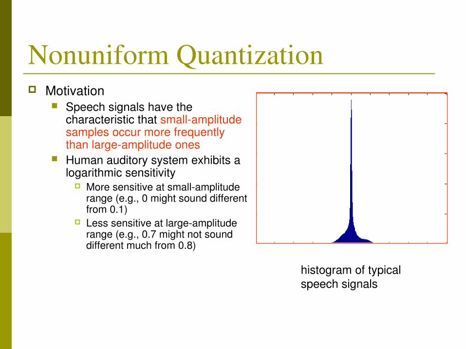
Nonuniform Quantization Motivation
Speech signals have the characteristic that smallamplitude samples occur more frequently than largeamplitude ones
Human auditory system exhibits a logarithmic sensitivity
More sensitive at smallamplitude range (e.g., 0 might sound different from 0.1)
Less sensitive at largeamplitude range (e.g., 0.7 might not sound different much from 0.8)
histogram of typical speech signals
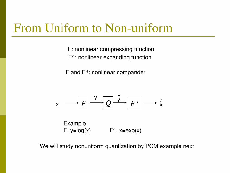
From Uniform to Nonuniform
x Q xF F1
Example F: y=log(x) F1: x=exp(x)
y y
F: nonlinear compressing functionF1: nonlinear expanding function
F and F1: nonlinear compander
We will study nonuniform quantization by PCM example next
Speech Coding Techniques (I) Introduction to Quantization
Scalar quantization Uniform quantization Nonuniform quantization
Waveformbased coding Pulse Coded Modulation (PCM) Differential PCM (DPCM) Adaptive DPCM (ADPCM)
Modelbased coding Channel vocoder AnalysisbySynthesis techniques Harmonic vocoder
Pulse Code Modulation Basic idea: assign smaller quantization stepsize
for smallamplitude regions and larger quantization stepsize for largeamplitude regions
Two types of nonlinear compressing functions Mulaw adopted by North American
telecommunications systems Alaw adopted by European telecommunications
systems
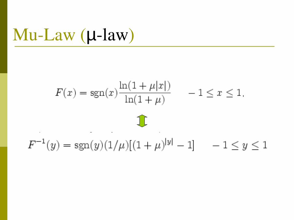
MuLaw (µlaw)

MuLaw Examples
x
y

ALaw

x
y
ALaw Examples
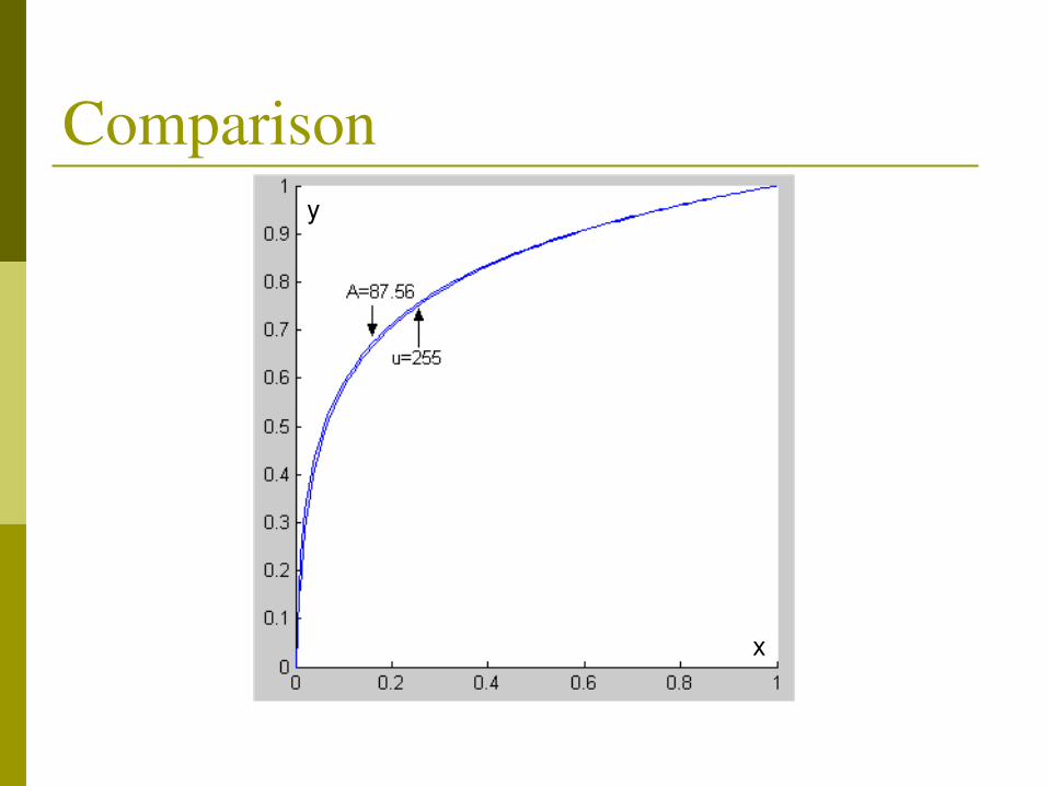
Comparison
x
y

PCM Speech
Mulaw(Alaw) compresses the signal to 8 bits/sample or 64Kbits/second (without compandor, we would need 12bits/sample)

A Look Inside WAV Format
MATLAB function [x,fs]=wavread(filename)

Change the Gear Strictly speaking, PCM is merely digitization of
speech signals – no coding (compression) at all By speech coding, we refer to representing
speech signals at the bit rate of <64Kbps To understand how speech coding techniques
work, I will cover some basics of data compression
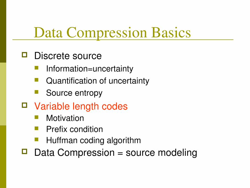
Data Compression Basics Discrete source
Information=uncertainty Quantification of uncertainty Source entropy
Variable length codes Motivation Prefix condition Huffman coding algorithm
Data compression = source modeling
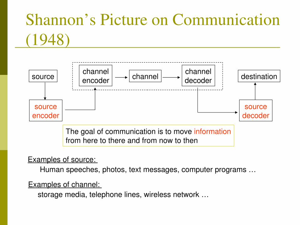
Shannon’s Picture on Communication (1948)
sourceencoder
channel
sourcedecoder
source destination
Examples of source: Human speeches, photos, text messages, computer programs …
Examples of channel: storage media, telephone lines, wireless network …
channelencoder
channeldecoder
The goal of communication is to move informationfrom here to there and from now to then
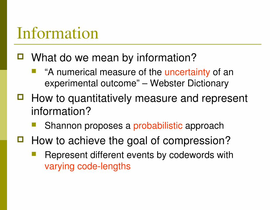
Information What do we mean by information?
“A numerical measure of the uncertainty of an experimental outcome” – Webster Dictionary
How to quantitatively measure and represent information? Shannon proposes a probabilistic approach
How to achieve the goal of compression? Represent different events by codewords with
varying codelengths
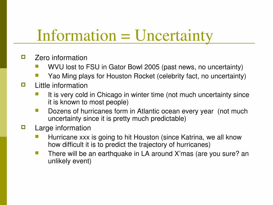
Information = Uncertainty Zero information
WVU lost to FSU in Gator Bowl 2005 (past news, no uncertainty) Yao Ming plays for Houston Rocket (celebrity fact, no uncertainty)
Little information It is very cold in Chicago in winter time (not much uncertainty since
it is known to most people) Dozens of hurricanes form in Atlantic ocean every year (not much
uncertainty since it is pretty much predictable) Large information
Hurricane xxx is going to hit Houston (since Katrina, we all know how difficult it is to predict the trajectory of hurricanes)
There will be an earthquake in LA around X’mas (are you sure? an unlikely event)
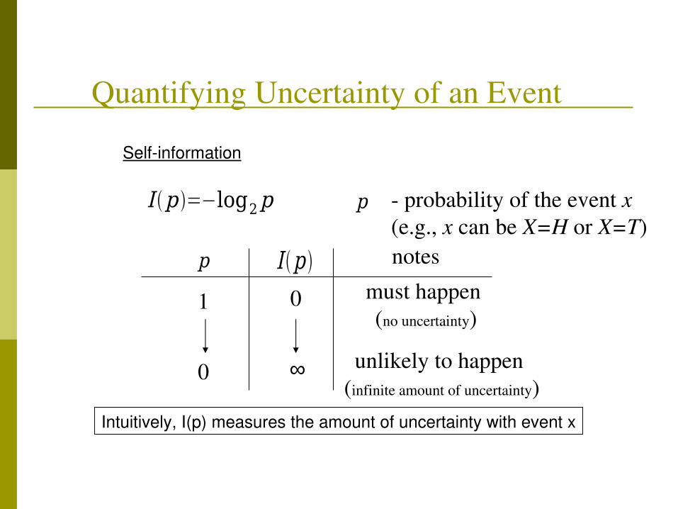
Quantifying Uncertainty of an Event
I p =−log2p p probability of the event x (e.g., x can be X=H or X=T)
p
1
0
I p
0
∞
notesmust happen (no uncertainty)
unlikely to happen (infinite amount of uncertainty)
Selfinformation
Intuitively, I(p) measures the amount of uncertainty with event x

Discrete Source A discrete source is characterized by a
discrete random variable X Examples
Coin flipping: P(X=H)=P(X=T)=1/2 Dice tossing: P(X=k)=1/6, k=16 Playingcard drawing:
P(X=S)=P(X=H)=P(X=D)=P(X=C)=1/4
How to quantify the uncertainty of a discrete source?
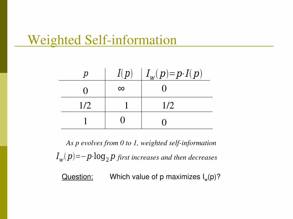
Weighted Selfinformation
p
0
1
I p
0
∞
1/2 1
0
0
1/2
Iw p =−p⋅log2p
Question: Which value of p maximizes Iw(p)?
Iw p =p⋅I p
As p evolves from 0 to 1, weighted selfinformation
first increases and then decreases

p=1/e
Iw p =1
e ln2
Maximum of Weighted Selfinformation

x∈{1,2,. . . ,N}
pi=probx=i , i=1,2,. . . ,N ∑i=1
N
pi=1
• To quantify the uncertainty of a discrete source, we simply take the summation of weighted selfinformation over the whole set
X is a discrete random variable
Uncertainty of a Discrete Source
• A discrete source (random variable) is a collection (set) of individual events whose probabilities sum to 1

Shannon’s Source Entropy Formula
HX =∑i=1
N
Iwpi
HX =−∑i=1
N
pi log2pi (bits/sample)or bps

Source Entropy Examples
• Example 1: (binary Bernoulli source)
p=probx=0 ,q=1−p=probx=1 HX =−plog2pq log2q
Flipping a coin with probability of head being p (0<p<1)
Check the two extreme cases:
As p goes to zero, H(X) goes to 0 bps → compression gains the most
As p goes to a half, H(X) goes to 1 bps → no compression can help
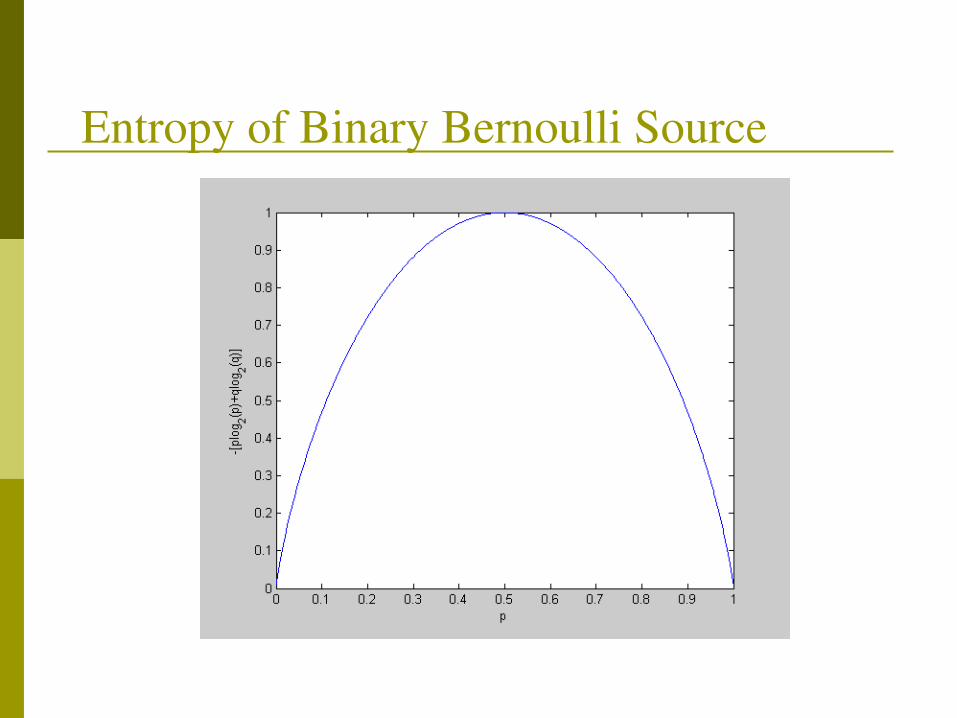
Entropy of Binary Bernoulli Source
Source Entropy Examples
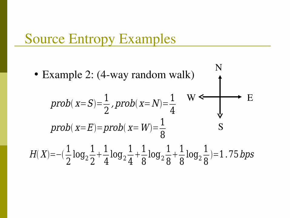
• Example 2: (4way random walk)
prob x=S =12,probx=N =
14
HX =−12log2
1214log2
1418log2
1818log2
18=1.75bps
N
E
S
W
prob x=E =prob x=W =18
Source Entropy Examples (Con’t)
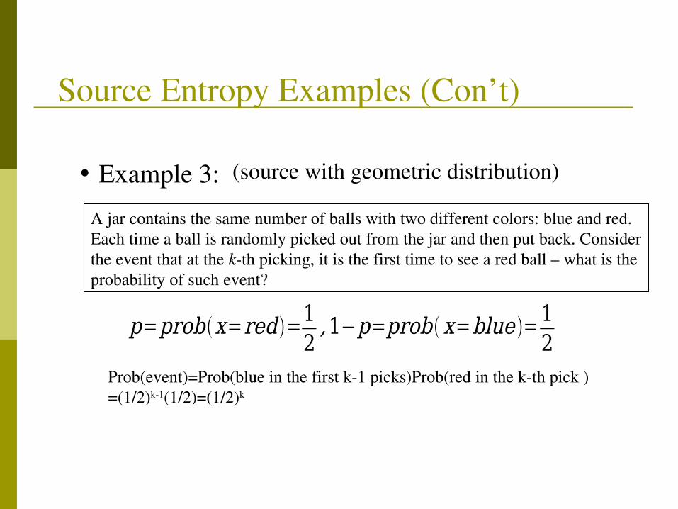
• Example 3:
p=probx=red =12,1−p=prob x=blue =1
2
A jar contains the same number of balls with two different colors: blue and red.Each time a ball is randomly picked out from the jar and then put back. Considerthe event that at the kth picking, it is the first time to see a red ball – what is the probability of such event?
Prob(event)=Prob(blue in the first k1 picks)Prob(red in the kth pick )=(1/2)k1(1/2)=(1/2)k
(source with geometric distribution)
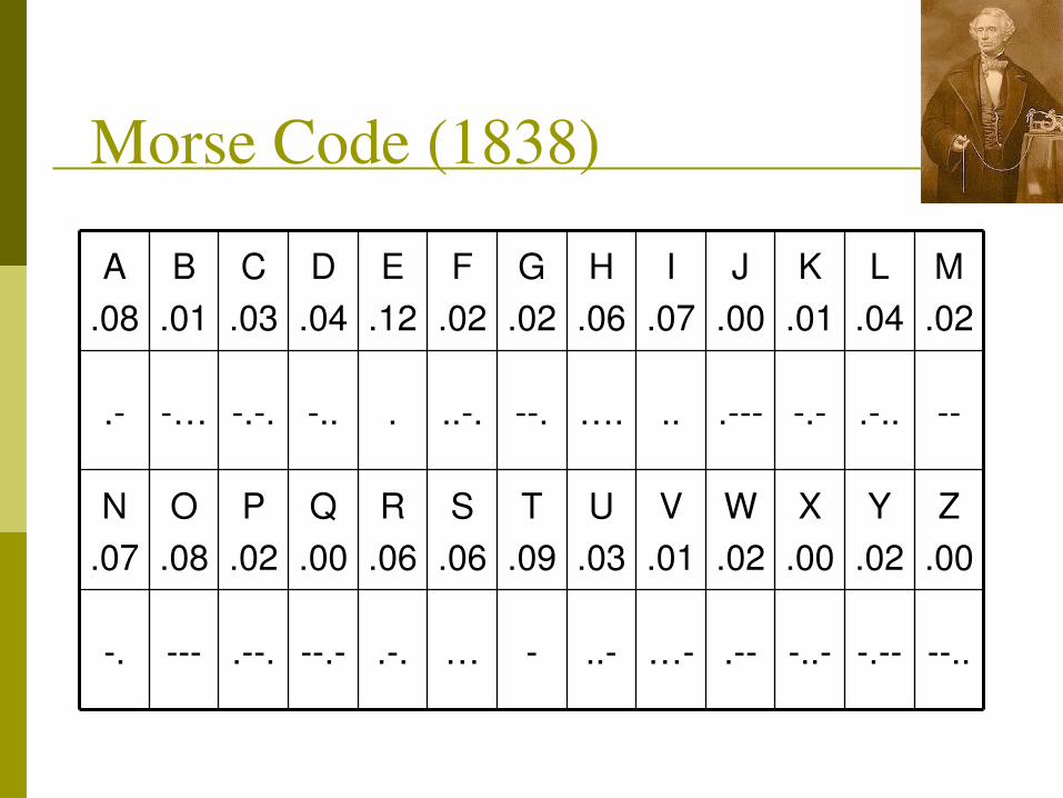
Morse Code (1838)
......…..…......
Z.00
Y.02
X.00
W.02
V.01
U.03
T.09
S.06
R.06
Q.00
P.02
O.08
N.07
.......…..........….
M.02
L.04
K.01
J.00
I.07
H.06
G.02
F.02
E.12
D.04
C.03
B.01
A.08

Average Length of Morse Codes Not the average of the lengths of the letters:
(2+4+4+3+…)/26 = 82/26 3.2≈ We want the average a to be such that in a typical
real sequence of say 1,000,000 letters, the number of dots and dashes should be about a∙1,000,000
The weighted average: (freq of A)∙(length of code for A) + (freq of B)∙(length of code for B) + …
= .08∙2 + .01∙4 + .03∙4 + .04∙3+… 2.4≈
Question: is this the entropy of English texts?
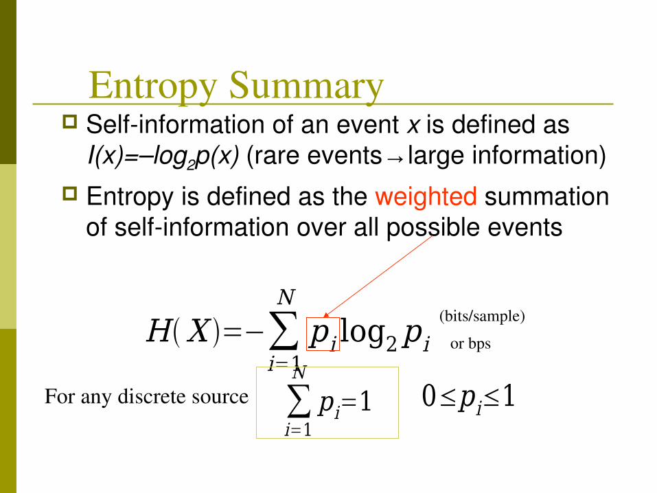
Entropy Summary Selfinformation of an event x is defined as
I(x)=–log2p(x) (rare events→large information) Entropy is defined as the weighted summation
of selfinformation over all possible events
∑i=1
N
pi=1
HX =−∑i=1
N
pi log2pi(bits/sample)
or bps
0≤pi≤1For any discrete source

How to achieve source entropy?
Note: The above entropy coding problem is based on simplified assumptions are that discrete source X is memoryless and P(X) is completely known. Those assumptions often do not hold forrealworld data such as speech and we will recheck them later.
entropycoding
discretesource X
P(X)
binary bit stream
Data Compression Basics Discrete source
Information=uncertainty Quantification of uncertainty Source entropy
Variable length codes Motivation Prefix condition Huffman coding algorithm
Data Compression = source modeling
Recall:
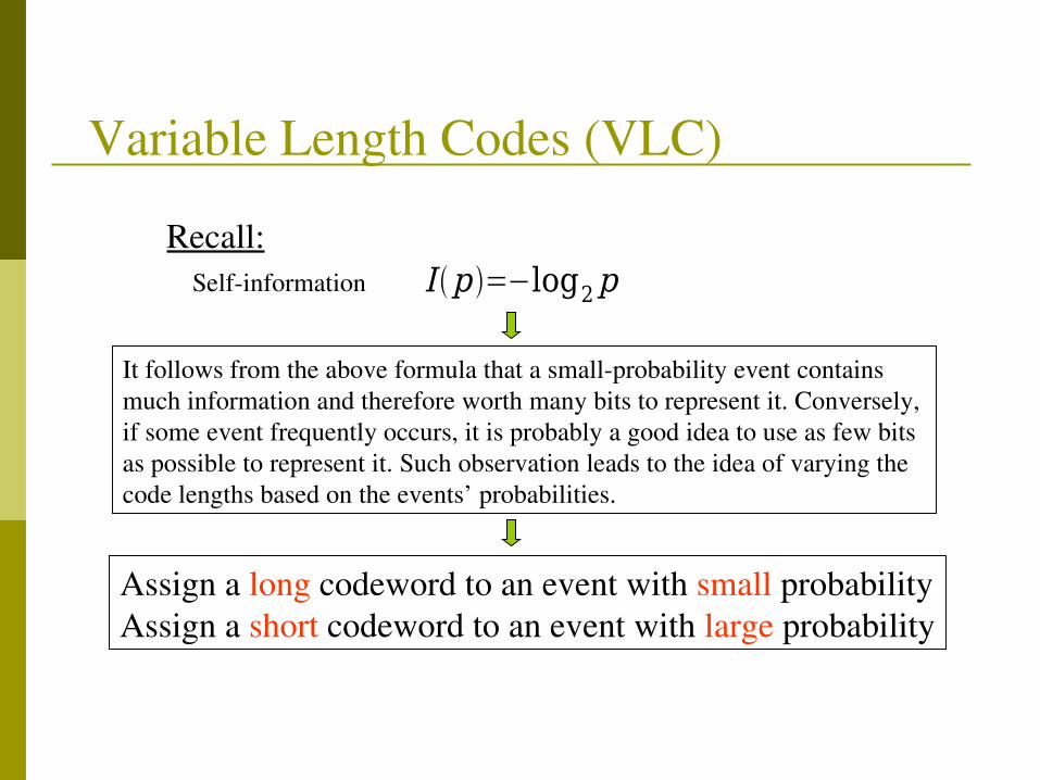
Variable Length Codes (VLC)
Assign a long codeword to an event with small probabilityAssign a short codeword to an event with large probability
I p =−log2pSelfinformation
It follows from the above formula that a smallprobability event containsmuch information and therefore worth many bits to represent it. Conversely, if some event frequently occurs, it is probably a good idea to use as few bits as possible to represent it. Such observation leads to the idea of varying thecode lengths based on the events’ probabilities.

symbol k pk
S
W
NE
0.50.250.125
fixedlengthcodeword
0.125
00011011
variablelengthcodeword010110111
4way Random Walk Example
symbol stream : S S N W S E N N N W S S S N E S Sfixed length: variable length:
00 00 01 11 00 10 01 01 11 00 00 00 01 10 00 000 0 10 111 0 110 10 10 111 0 0 0 10 110 0 0
32bits28bits
4 bits savings achieved by VLC (redundancy eliminated)

=0.5×1+0.25×2+0.125×3+0.125×3=1.75 bits/symbol
• average code length:
Toy Example (Con’t)
• source entropy:HX =−∑
k=1
4
pk log2pk
l=Nb
Ns
Total number of bits
Total number of symbols(bps)
l=2bpsHX fixedlength variablelength
l=1.75bps=H X

Problems with VLC When codewords have fixed lengths, the
boundary of codewords is always identifiable. For codewords with variable lengths, their
boundary could become ambiguous
symbolS
W
NE
VLC
011011
S S N W S E …
0 0 1 11 0 10…
0 0 11 1 0 10… 0 0 1 11 0 1 0…
S S W N S E … S S N W S E …
e
d d

Uniquely Decodable Codes To avoid the ambiguity in decoding, we need to
enforce certain conditions with VLC to make them uniquely decodable
Since ambiguity arises when some codeword becomes the prefix of the other, it is natural to consider prefix condition
Example: p ∝ pr ∝ pre ∝ pref ∝ prefi ∝ prefix
a∝b: a is the prefix of b

Prefix condition
No codeword is allowed to be the prefix of any other codeword.
We will graphically illustrate this condition with the aid of binary codeword tree
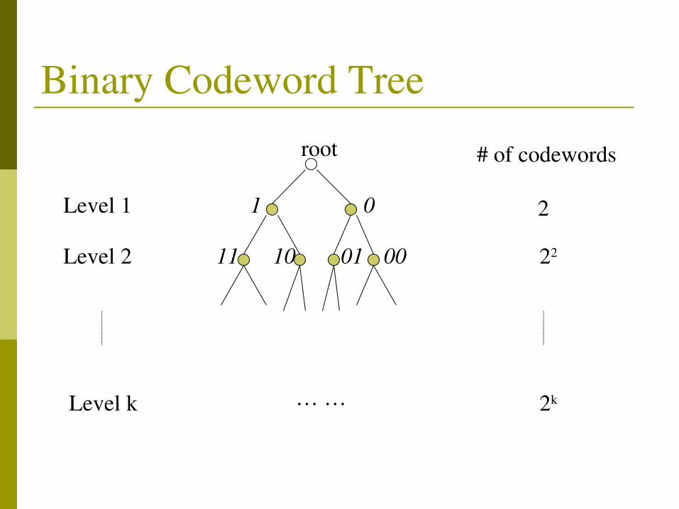
Binary Codeword Tree
1 0
… …
1011 01 00
root
Level 1
Level 2
# of codewords
2
22
2kLevel k
Prefix Condition Examplessymbol x
WE
SN
011011
codeword 1 codeword 2010110111
1 0
… …
1011 01 00
1 0
… …
1011
codeword 1 codeword 2
111 110
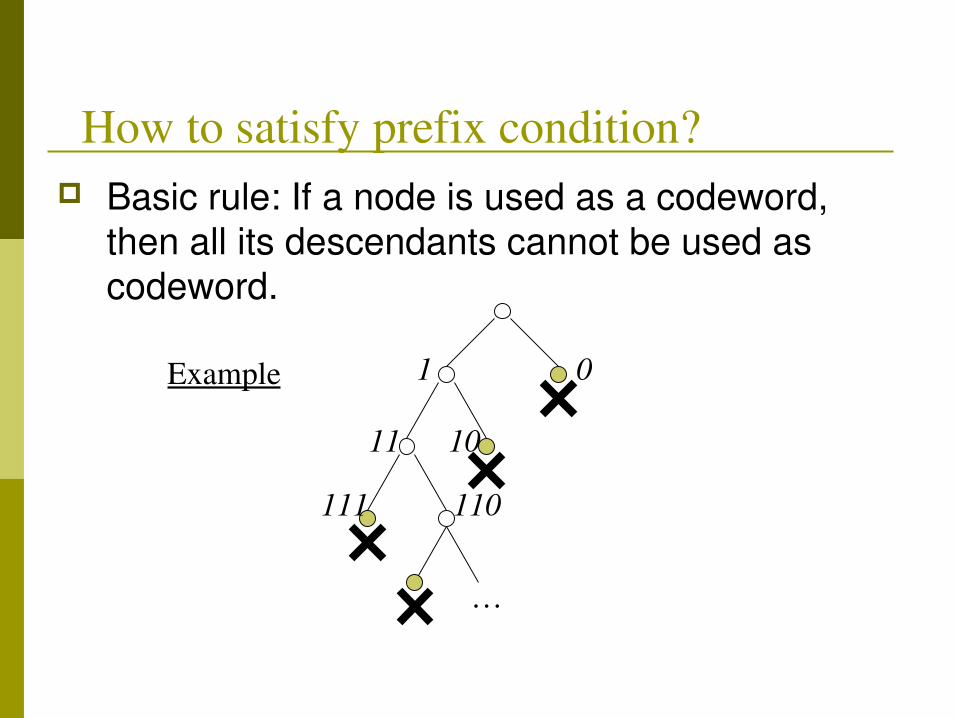
How to satisfy prefix condition? Basic rule: If a node is used as a codeword,
then all its descendants cannot be used as codeword.
1 0
1011
111 110
Example
…

VLC Summary Rule #1: short codeword – large probability
event, long codeword – small probability event Rule #2: no codeword can be the prefix of any
other codeword Question: given P(X), how to systematically
assign the codewords that always satisfy those two rules? Answer: Huffman coding, arithmetic coding
Entropy Coding

Huffman Codes (Huffman’1952) Coding Procedures for an Nsymbol source
Source reduction List all probabilities in a descending order Merge the two symbols with smallest probabilities into a
new compound symbol Repeat the above two steps for N2 steps
Codeword assignment Start from the smallest source and work backward to the
original source Each merging point corresponds to a node in binary
codeword tree
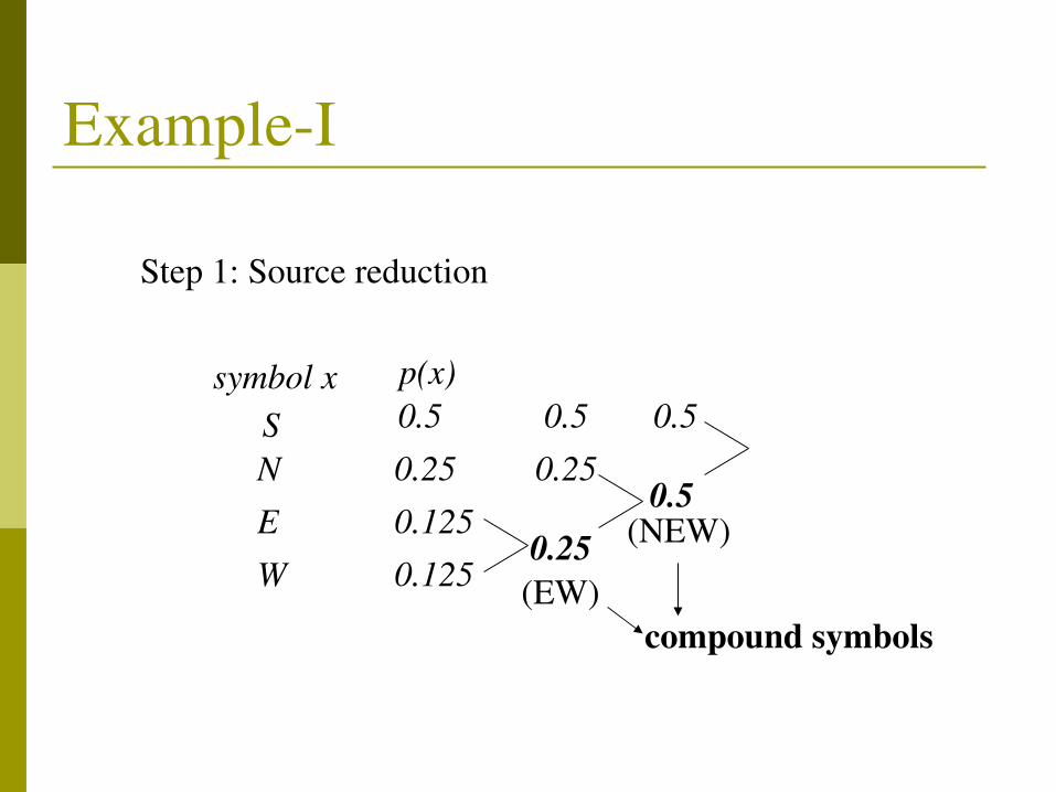
symbol x p(x)S
W
NE
0.50.250.1250.125
0.25
0.250.5 0.5
0.5
ExampleI
Step 1: Source reduction
(EW)
(NEW)
compound symbols

p(x)0.50.250.1250.125
0.25
0.250.5 0.5
0.5 1
0
1
0
1
0
codeword010110
111
ExampleI (Con’t)
Step 2: Codeword assignment
symbol xS
W
NE
NEW 0
10EW
110EW
N
S
01
1 0
1 0111
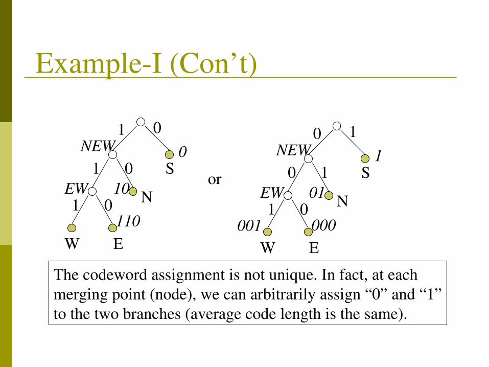
ExampleI (Con’t)
NEW 0
10EW
110EW
N
S
01
1 0
1 0
NEW 1
01EW
000EW
N
S
10
0 1
1 0001
The codeword assignment is not unique. In fact, at eachmerging point (node), we can arbitrarily assign “0” and “1”to the two branches (average code length is the same).
or

symbol x p(x)e
o
ai
0.40.20.20.1
0.40.2
0.4 0.6
0.4
ExampleII
Step 1: Source reduction
(iou)
(aiou)
compound symbolsu 0.10.2(ou)
0.40.20.2
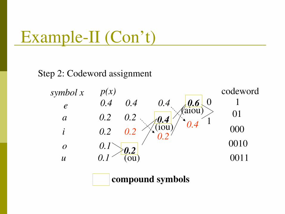
symbol x p(x)e
o
ai
0.40.20.20.1
0.40.2
0.4 0.6
0.4
ExampleII (Con’t)
(iou)
(aiou)
compound symbols
u 0.10.2(ou)
0.40.20.2
Step 2: Codeword assignment
codeword0
1
10100000100011
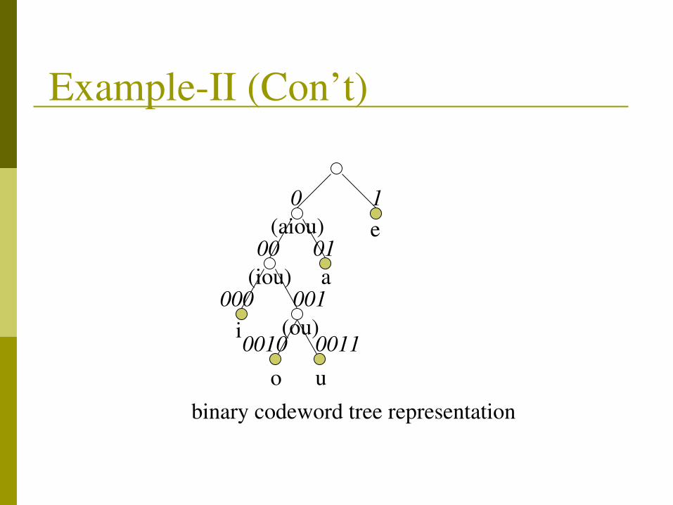
ExampleII (Con’t)
0 1
0100
000 001
0010 0011
e
o u
(ou)i
(iou) a
(aiou)
binary codeword tree representation

Data Compression Basics Discrete source
Information=uncertainty Quantification of uncertainty Source entropy
Variable length codes Motivation Prefix condition Huffman coding algorithm
Data Compression = source modeling

What is Source Modelingentropycoding
discretesource X
P(X)
binary bit stream
ModelingProcess
entropycoding
discretesource X
binarybit stream
probabilityestimation
P(Y)
Y
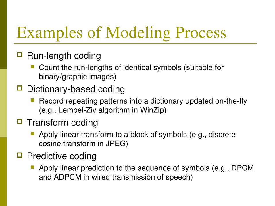
Examples of Modeling Process Runlength coding
Count the runlengths of identical symbols (suitable for binary/graphic images)
Dictionarybased coding Record repeating patterns into a dictionary updated onthefly
(e.g., LempelZiv algorithm in WinZip) Transform coding
Apply linear transform to a block of symbols (e.g., discrete cosine transform in JPEG)
Predictive coding Apply linear prediction to the sequence of symbols (e.g., DPCM
and ADPCM in wired transmission of speech)
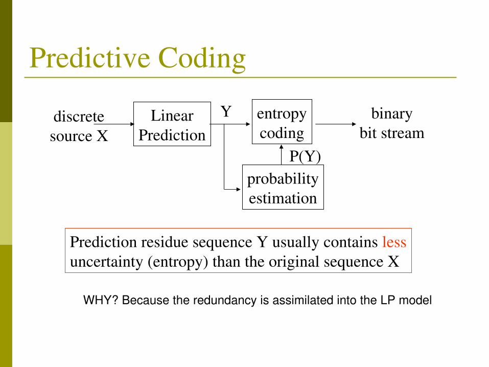
Predictive Coding
LinearPrediction
entropycoding
discretesource X
binarybit stream
probabilityestimation
P(Y)
Y
Prediction residue sequence Y usually contains lessuncertainty (entropy) than the original sequence X
WHY? Because the redundancy is assimilated into the LP model
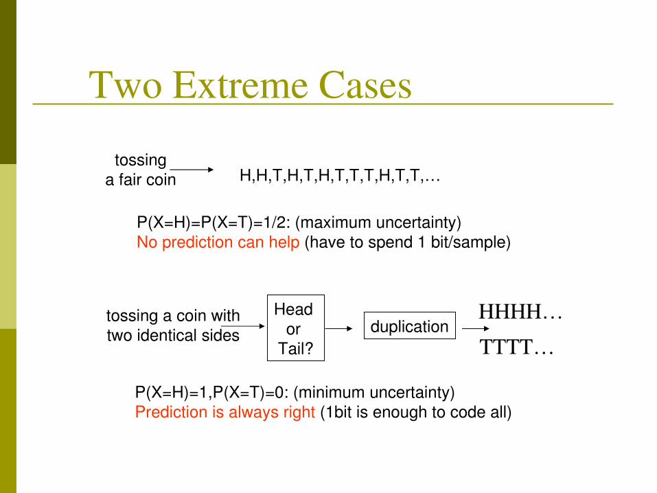
Two Extreme Cases tossing
a fair coin
Head or
Tail?duplicationtossing a coin with
two identical sides
P(X=H)=P(X=T)=1/2: (maximum uncertainty) No prediction can help (have to spend 1 bit/sample)
P(X=H)=1,P(X=T)=0: (minimum uncertainty) Prediction is always right (1bit is enough to code all)
HHHH…TTTT…
H,H,T,H,T,H,T,T,T,H,T,T,…

Differential PCM Basic idea
Since speech signals are slowly varying, it is possible to eliminate the temporal redundancy by prediction
Instead of transmitting original speech, we code prediction residues instead, which typically have smaller energy
Linear prediction Fixed: the same predictor is used again and again Adaptive: predictor is adjusted onthefly
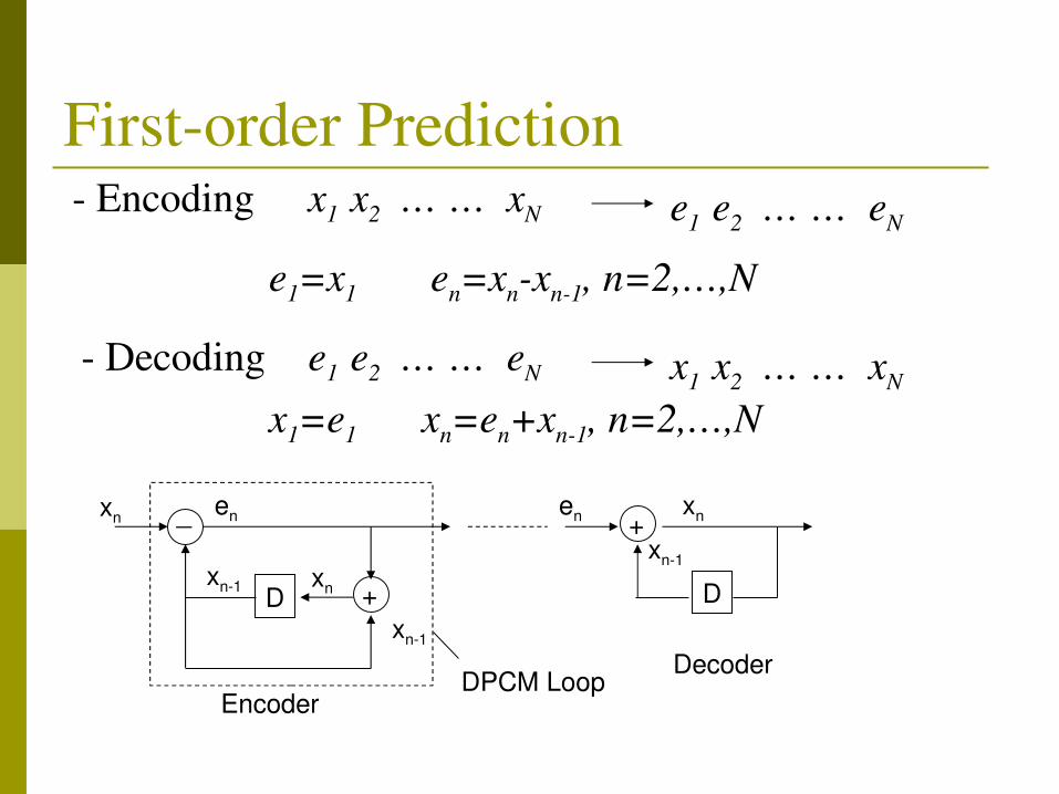
Firstorder Prediction Encoding
Decoding
e1=x1 en=xnxn1, n=2,…,N
x1 x2 … … xN e1 e2 … … eN
e1 e2 … … eN x1 x2 … … xN
x1=e1 xn=en+xn1, n=2,…,N
_
+D
xn
xnxn1
en
xn1
+xn1
en xn
D
EncoderDecoderDPCM Loop

Prediction Meets Quantization Openloop
Prediction is based on unquantized samples Since decoder only has access to quantized samples,
we run into a socalled drifting problem which is really bad for compression
Closedloop Prediction is based on quantized samples Still suffers from error propagation (i.e., quantization
errors of the past will affect the efficiency of prediction), but no drifting is involved
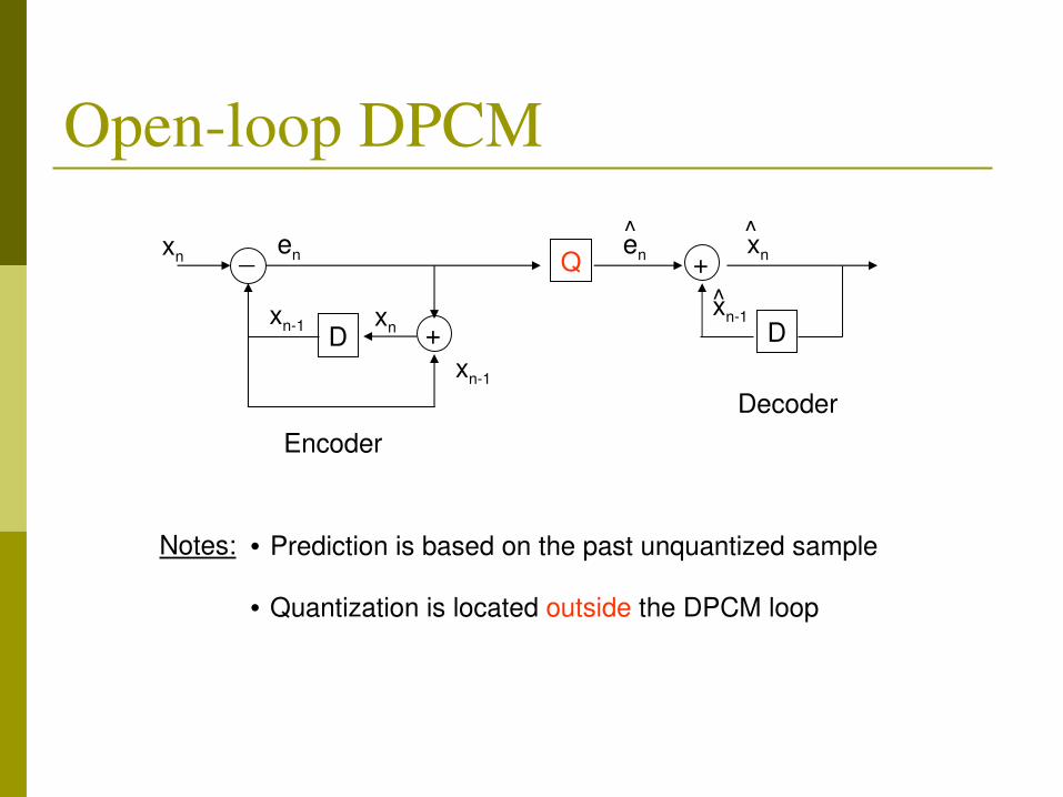
Openloop DPCM
_
+D
xn
xnxn1
en
xn1
+xn1
en xn
D
EncoderDecoder
Q^ ^
^
Notes: • Prediction is based on the past unquantized sample
• Quantization is located outside the DPCM loop
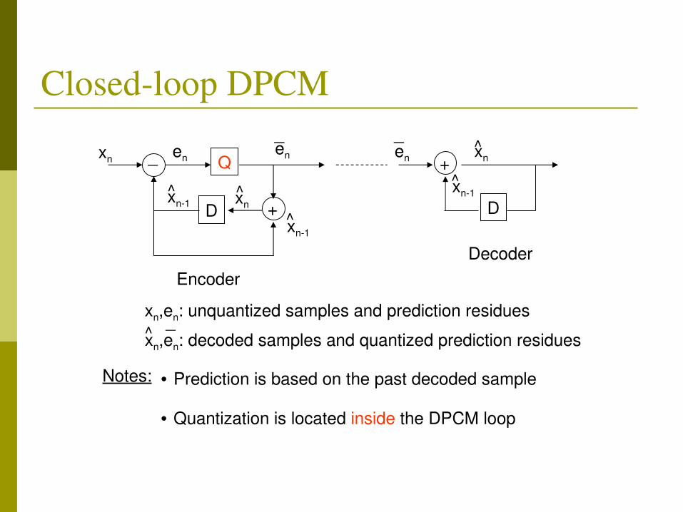
Closedloop DPCM
_
+D
xn
xnxn1
en
xn1
+en xn
D
EncoderDecoder
Q_
en
_
^^
^
xn1^
^
xn,en: unquantized samples and prediction residuesxn,en: decoded samples and quantized prediction residues^ _
Notes: • Prediction is based on the past decoded sample
• Quantization is located inside the DPCM loop

Numerical Example
90xn
en
xn
92 91 93 93 95 …
90 2 2 3 0 2
90 93 90 93 93 96 …
en_
^
90 3 3 3 0 3Q Q x =[ x3 ]⋅3
a
bab
a
b a+b

Closedloop DPCM Analysis_
+D
xn
xnxn1
en
xn1
Qen
_
^^^
en=xn− xn−1xn=en xn−1
xn− xn=en−enA:
B:
A B
The distortion introduced to prediction residue en is identical to that introduced to the original sample xn
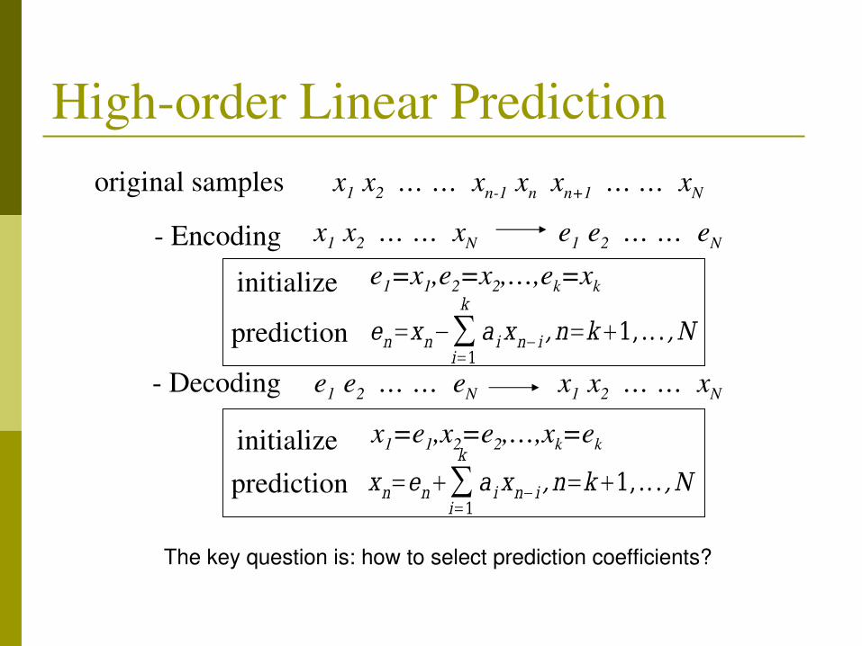
x1 x2 … … xn1 xn xn+1 … … xN original samples
Encoding
Decoding
e1=x1,e2=x2,…,ek=xkinitialize
prediction
x1 x2 … … xN e1 e2 … … eN
e1 e2 … … eN x1 x2 … … xN
initializeprediction
en=xn−∑i=1
k
a ixn−i ,n=k1,.. . ,N
x1=e1,x2=e2,…,xk=ek
xn=en∑i=1
k
a ixn−i ,n=k1,.. . ,N
Highorder Linear Prediction
The key question is: how to select prediction coefficients?
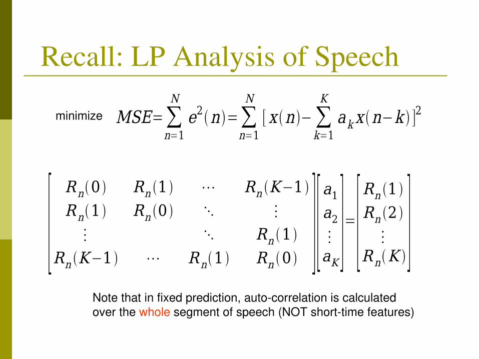
Recall: LP Analysis of Speech
[Rn0 Rn 1 ⋯ Rn K−1
Rn1 Rn 0 ⋱ ⋮
⋮ ⋱ Rn 1
Rn K−1 ⋯ Rn1 Rn 0 ][a1a2⋮
aK]=[
Rn 1
Rn 2
⋮
RnK ]
MSE=∑n=1
N
e2n =∑n=1
N
[x n −∑k=1
K
akx n−k ]2minimize
Note that in fixed prediction, autocorrelation is calculatedover the whole segment of speech (NOT shorttime features)
Quantized Prediction Residues Further entropy coding is possible
Variable length codes: e.g., Huffman codes, Golomb codes Arithmetic coding
However, the current practice of speech coding assign fixedlength codewords to quantized prediction residues The assigned codelengths are already nearly optimal for
achieving the firstorder entropy Good for the robustness to channel errors
DPCM can achieve compression of two (i.e., 32kbps) without noticeable speech quality degradation

Adaptive DPCM
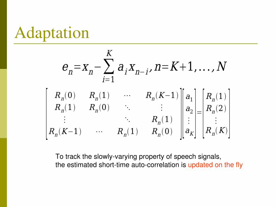
Adaptation
en=xn−∑i=1
K
a ixn−i ,n=K1,.. . ,N
[Rn0 Rn 1 ⋯ Rn K−1
Rn1 Rn 0 ⋱ ⋮
⋮ ⋱ Rn 1
Rn K−1 ⋯ Rn1 Rn 0 ][a1a2⋮
aK]=[
Rn 1
Rn 2
⋮
RnK ]
To track the slowlyvarying property of speech signals,the estimated shorttime autocorrelation is updated on the fly

Prediction Gain
K
Gp
Gp=10log10
σx2
σe2dB

Forward and Backward Adaptation Forward adaptation
The autocorrelation is estimated from the current frame and the quantized prediction coefficients are transmitted to the decoder as side information (we will discuss how to quantize such vector in the discussion of CELP coding)
Backward adaptation The autocorrelation is estimated from the causal past
and therefore no overhead is required to be transmitted; decoder will duplicate the encoder’s operation

Illustration of Forward Adaptation
F1 F2 F3 F4 F5
For each frame, a set of LPCs are transmitted
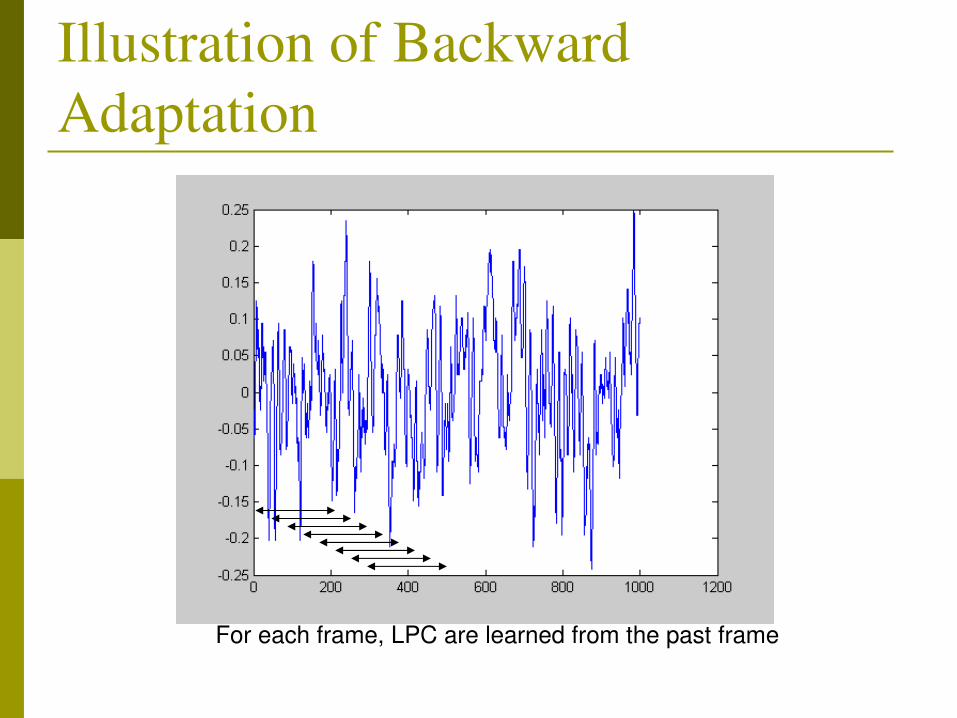
Illustration of Backward Adaptation
For each frame, LPC are learned from the past frame
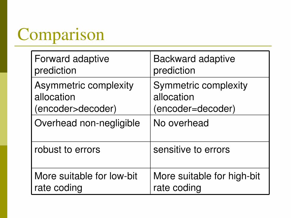
Comparison
More suitable for highbit rate coding
More suitable for lowbit rate coding
sensitive to errorsrobust to errors
No overheadOverhead nonnegligible
Symmetric complexity allocation (encoder=decoder)
Asymmetric complexity allocation (encoder>decoder)
Backward adaptive prediction
Forward adaptive prediction
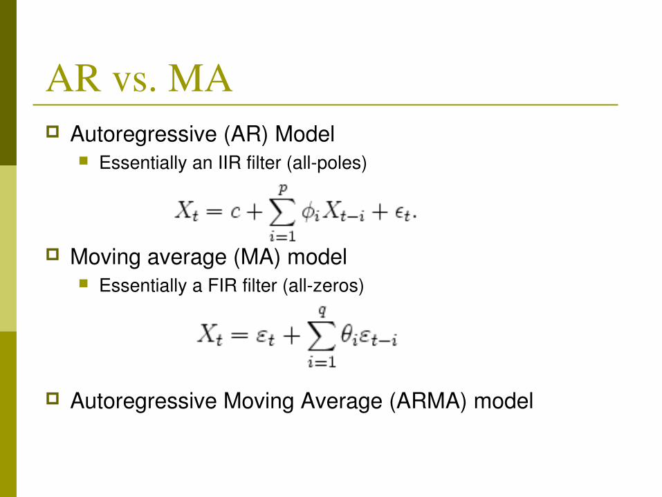
AR vs. MA Autoregressive (AR) Model
Essentially an IIR filter (allpoles)
Moving average (MA) model Essentially a FIR filter (allzeros)
Autoregressive Moving Average (ARMA) model
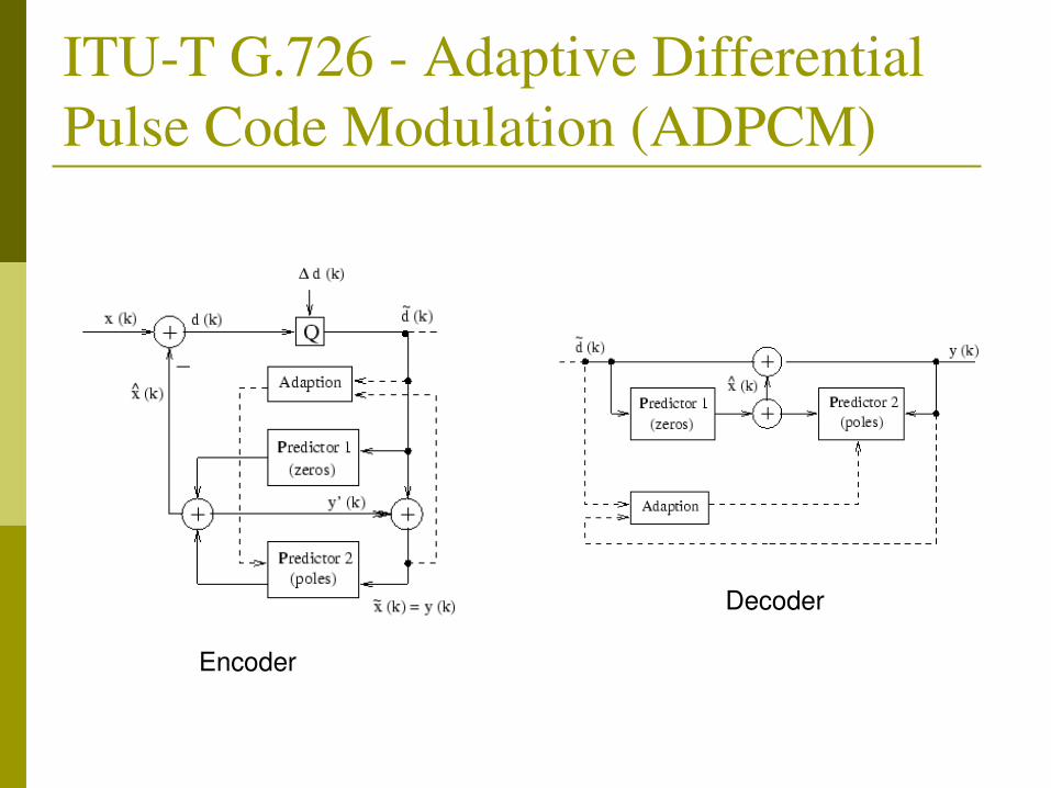
ITUT G.726 Adaptive Differential Pulse Code Modulation (ADPCM)
Encoder
Decoder

Waveform Coding Demo
http://wwwlns.tf.unikiel.de/demo/demo_speech.htm

Data Compression Paradigm
ModelingProcess
entropycoding
discretesource X
binarybit stream
probabilityestimation
P(Y)
Y
Question: Why do we call DPCM/ADPCM waveform coding?
Answer: Because Y (prediction residues) is also a kind ofwaveform just like the original speech X – they have the same dimensionality
Speech Coding Techniques (I) Introduction to Quantization
Scalar quantization Uniform quantization Nonuniform quantization
Waveformbased coding Pulse Coded Modulation (PCM) Differential PCM (DPCM) Adaptive DPCM (ADPCM)
Modelbased coding Channel vocoder AnalysisbySynthesis techniques Harmonic vocoder
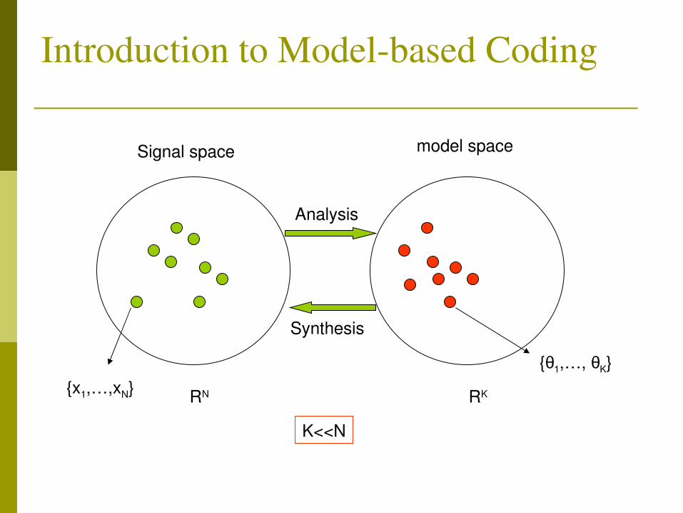
Introduction to Modelbased Coding
RN
Signal space model space
RK
K<<N
{x1,…,xN}{θ1,…, θK}
Analysis
Synthesis

Toy Example
xn=sin 2πfnφ ,n=1,2,. .. ,NModelbased coding of sinusoid signals
θ1=f θ2=φ
Input signal{x1,…,xN} analysis synthesis Reconstructed
signal
Question (test your understanding about entropy)If a source is produced by the following model: x(n)=sin(50n+p), n=1,2,…,100 where p is a random phase with equal probabilities of being 0,45,90,135,180,225,270,315. What is the entropy of this source?
Building Models for Human Speech Waveform coders can also viewed as a kind of
models where K=N (not much compression) Usually modelbased speech coders target at
very high compression ratio (K<<N) There is no free lunch
High compression ratio comes along with severe quality degradation
We will see how to achieve a better tradeoff in part II (CELP coder)

Channel Vocoder: Encoding
Bandpassfilter
Bandpassfilter
Voicingdetector
Pitchdetector
rectifier
rectifier
Lowpassfilter
Lowpassfilter
A/Dconverter
A/Dconverter
ENCODER
1bit
6bits
34bits/channel
Frame size: 20ms Bit rate=24003200bps
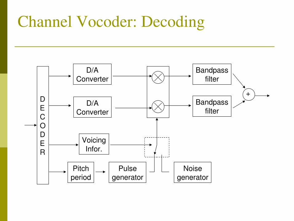
Channel Vocoder: Decoding
DECODER
D/AConverter
D/AConverter
VoicingInfor.
Pitchperiod
Pulsegenerator
Noisegenerator
Bandpassfilter
Bandpassfilter
+
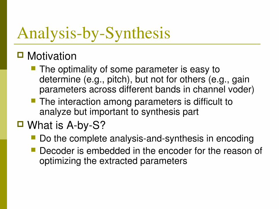
AnalysisbySynthesis Motivation
The optimality of some parameter is easy to determine (e.g., pitch), but not for others (e.g., gain parameters across different bands in channel voder)
The interaction among parameters is difficult to analyze but important to synthesis part
What is AbyS? Do the complete analysisandsynthesis in encoding Decoder is embedded in the encoder for the reason of
optimizing the extracted parameters
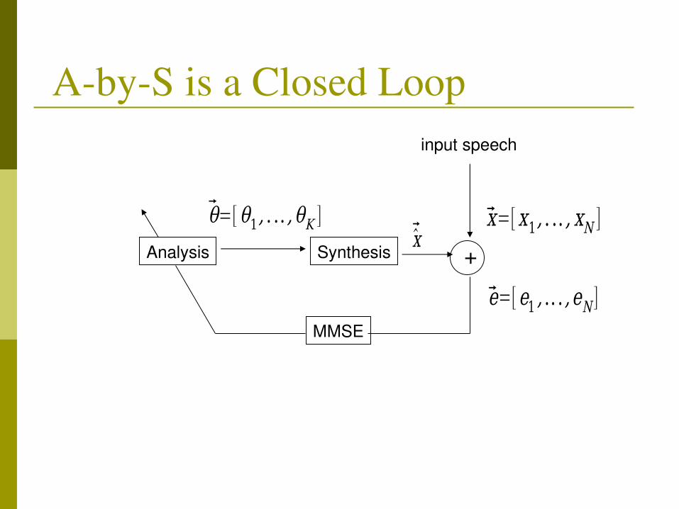
AbyS is a Closed Loop
+Analysis Synthesis
input speech
x=[x1, . .. , xN ]
e=[e1 , .. . ,eN ]
xθ=[θ1, . .. ,θK ]
MMSE
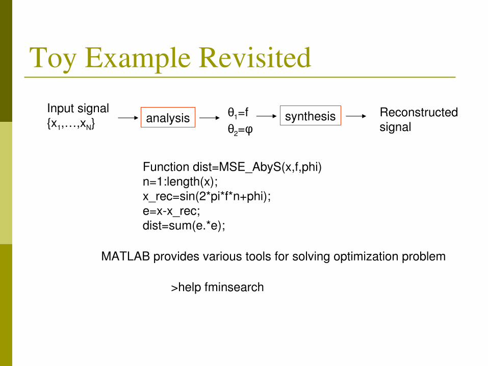
Toy Example Revisitedθ1=f θ2=φ
Input signal{x1,…,xN} analysis synthesis Reconstructed
signal
Function dist=MSE_AbyS(x,f,phi)n=1:length(x);x_rec=sin(2*pi*f*n+phi);e=xx_rec;dist=sum(e.*e);
>help fminsearch
MATLAB provides various tools for solving optimization problem
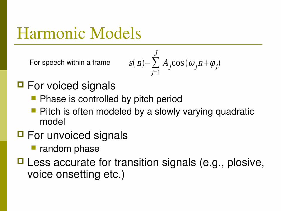
Harmonic Models
For voiced signals Phase is controlled by pitch period Pitch is often modeled by a slowly varying quadratic
model For unvoiced signals
random phase Less accurate for transition signals (e.g., plosive,
voice onsetting etc.)
sn =∑j=1
J
A jcos ω jnφ j For speech within a frame

AbyS Harmonic Vocoder
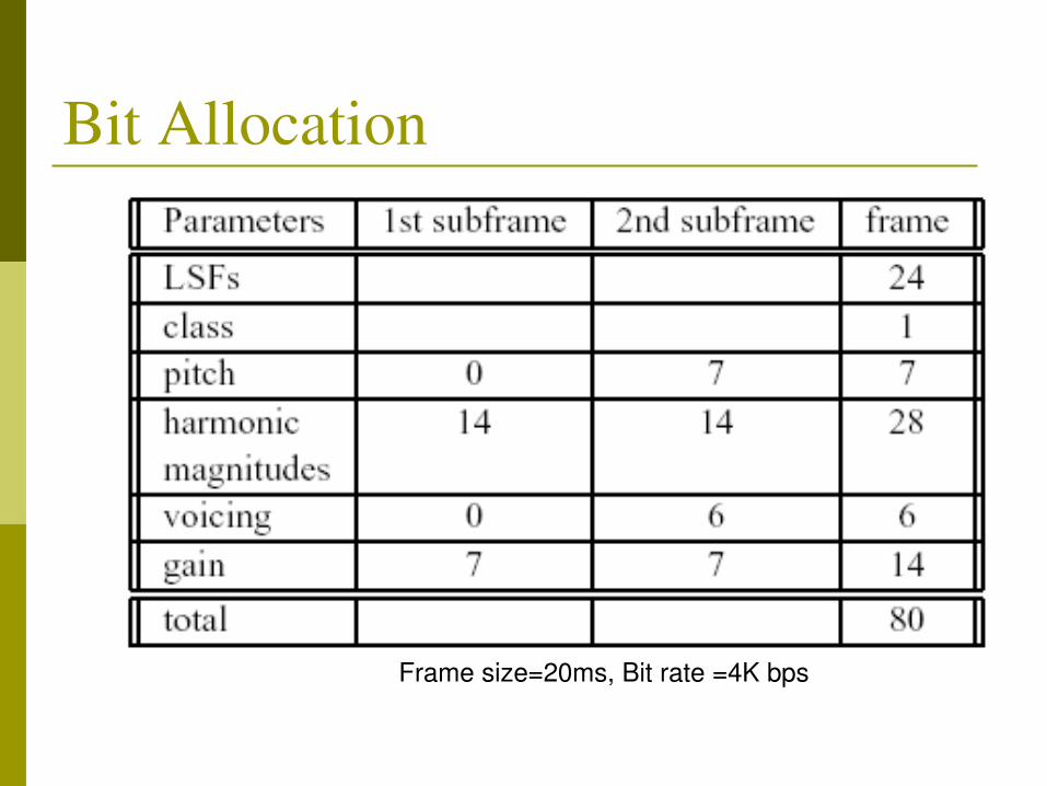
Bit Allocation
Frame size=20ms, Bit rate =4K bps

Towards the Fundamental Limit How much information can one convey in one
minute? It depends on how fast one speaks It depends on which language one speaks It surely also depends on the speech content
Modelbased speech coders Can compress speech down to 300500 bits/second,
can’t tell who speaks it, no intonation or stress or gender difference
A theoretically optimal approach: speech recognition + speaker recognition + speakerdependent speech synthesis
Related Documents