Spectrum Sharing Systems for Improving Spectral Efficiency in Cognitive Cellular Network Deepak G.C. School of Computing and Communications Lancaster University A thesis submitted in partial fulfillment for the degree of Doctor of Philosophy September 2016 brought to you by CORE View metadata, citation and similar papers at core.ac.uk provided by Lancaster E-Prints

Welcome message from author
This document is posted to help you gain knowledge. Please leave a comment to let me know what you think about it! Share it to your friends and learn new things together.
Transcript

Spectrum Sharing Systems for
Improving Spectral Efficiency in
Cognitive Cellular Network
Deepak G.C.
School of Computing and Communications
Lancaster University
A thesis submitted in partial fulfillment for the degree of
Doctor of Philosophy
September 2016
brought to you by COREView metadata, citation and similar papers at core.ac.uk
provided by Lancaster E-Prints

Declaration of Authorship
I, Deepak G.C., declare that this thesis titled “Spectrum Sharing
Systems for Improving Spectral Efficiency in Cognitive Cel-
lular Network” and the work presented in it are my own. I therefore
confirm that:
• Where I have consulted the published work of others, thesis al-
ways clearly attributed.
• Where I have quoted from the work of others, the source is always
given. With the exceptions of such quotations, this thesis is
entirely my own work.
• I have acknowledged all main source of help while preparing this
Thesis.
• Where the thesis is based on work done by myself jointly with
others, I have made clear what was done by others and what I
have contributed myself.
• Detailed breakdown of the publications is presented in the first
Chapter of this Thesis.
Signed:
Date:
i

Acknowledgements
First of all, I would like to show my sincere gratitude to my academic
supervisor Dr. Keivan Navaie for his care, support and excellent
supervision throughout the duration of my PhD. His guidance and im-
mense inspiration have greatly encouraged me in the last four years
of my PhD. I wish to express my appreciation to Prof. Qiang Ni
for his continuous support and engaging in my research works. In ad-
dition, the continuous help from the staff at Lancaster University and
Infolab21, especially the head of the school Prof. Jon Whittle and
postgraduate coordinator Debbie Stubs, are also highly appreciated.
Moreover, I felt so special with everyone in our generous and vibrant
Communications System research group at the Lancaster University.
This modest work would not have been possible without the support
that I have always been receiving from my family. More precisely, I
would like to thank my better half, Mrs. Mamata Koirala, whom
I have always considered as my infinite source of inspiration in all
the battles and endeavours of my life. Her help, care and support in
every moment have a special place in my life. I would also like to
dedicate this work to my son, Mr. Bivaan G.C., whose presence
always motivated me to pursue my aim. I would also like to thank
my mother Radha G.C., Mina G.C., father Dhan Bahadur G.C., my
brother and sisters, my parents-in-law, who were always behind me
with a huge support.
A big thank you to all the British and non-British friends whom I
met during my stay at Lancaster, who made my stay here as if I were
at my home. At last but not the least, special thanks to European
Union Marie Curie grant and my academic supervisor who provided
the research funding to become true this personal goal that I have
been dreaming for half of my life.
ii

Abstract
Since spectrum is the invisible infrastructure that powers the wire-
less communication, the demand has been exceptionally increasing in
recent years after the implementation of 4G and immense data re-
quirements of 5G due to the applications, such as Internet-of-Things
(IoT). Therefore, the effective optimization of the use of spectrum is
immediately needed than ever before.
The spectrum sensing is the prerequisite for optimal resource allo-
cation in cognitive radio networks (CRN). Therefore, the spectrum
sensing in wireless system with lower latency requirements is pro-
posed first. In such systems with high spatial density of the base
stations and users/objects, spectrum sharing enables spectrum reuse
across very small regions. The proposed method in this Thesis is a
multi-channel cooperative spectrum sensing technique, in which an in-
dependent network of sensors, namely, spectrum monitoring network,
detects the spectrum availability. The locally aggregated decision in
each zone associated with the zone aggregator (ZA) location is then
passed to a decision fusion centre (DFC). The secondary base station
(SBS) accordingly allocates the available channels to secondary users
to maximize the spectral efficiency. The function of the DFC is for-
mulated as an optimization problem with the objective of maximizing
the spectral efficiency. The optimal detection threshold is obtained
for different cases with various spatial densities of ZAs and SBSs. It is
further shown that the proposed method reduces the spectrum sensing
latency and results in a higher spectrum efficiency.
Furthermore, a novel power allocation scheme for multicell CRN is
proposed where the subchannel power allocation is performed by in-
corporating network-wide primary system communication activity. A
iii

collaborative subchannel monitoring scheme is proposed to evaluate
the aggregated subchannel activity index (ASAI) to indicate the ac-
tivity levels of primary users. Two utility functions are then defined to
characterize the spectral efficiency (SE) and energy efficiency (EE) as
a function of ASAI to formulate a utility maximization problem. The
optimal transmit power allocation is then obtained with the objective
of maximizing the total utility at the SBS, subject to maximum SBS
transmit power and collision probability constraint at the primary re-
ceivers. Since optimal EE and SE are two contradicting objectives to
obtain the transmit power allocation, the design approach to handle
both EE and SE as a function of common network parameter, i.e.,
ASAI, is provided which ultimately proves the quantitative insights
on efficient system design. Extensive simulation results confirm the
analytical results and indicate a significant improvement in sensing
latency and accuracy and a significant gain against the benchmark
models on the rate performance, despite the proposed methods per-
form with lower signalling overhead.
iv

List of Abbreviations
3GPP third generation partnership project
ASAI aggregated subchannel activity index
AWGN additive white Gaussian noise
BPSK binary phase shift keying
CCT Charnes-Cooper Transformation
CDF cumulative distribution function
CoMP coordinate multipoint
CRN cognitive radio network
D2D device to device
dB decibels
DFC decision fusion centre
DSA dynamic spectrum access
ED energy detection
EE energy efficiency
EPA Equal Power Allocation
FFT fast Fourier transform
GD Geolocation database
GSM global system of mobile
IoT internet of things
KKT KarushKuhnTucker
LoS line of sight
LTE-A long term evolution - advance
M2M machine to machine
MAC medium access control
MIMO multiple input multiple output
v

MTC machine type communication
NOMA non-orthogonal multiple access
OFDMA orthogonal frequency division multiple access
OSA opportunistic spectrum access
PDF probability density function
PBS primary base station
PCU Perfect Channel Utilization
PU primary users
QoS quality of service
QPSK quadrature phase shift keying
REM radio environment mapping
ROC receiver operating characteristics
SAI subchannel activity index
SBS secondary base station
SDR software defined radio
SE spectral efficiency
SNIR signal to noise and interference ratio
SON self organizing network
SU secondary users
TDMA time division multiple access
TDD time division duplexing
UHF ulta high frequency
UMTS Universal Mobile Telecommunications System
VHF very high frequency
WRAN wireless regional area networks
WSDB white space database
ZA zone aggregator
vi

Contents
List of Tables xi
List of Figures xii
1 Introduction 1
1.1 Cognitive Radio Networks . . . . . . . . . . . . . . . . . . . . . . 4
1.1.1 Cognitive cycle . . . . . . . . . . . . . . . . . . . . . . . . 5
1.1.2 Journey of Cognitive Radio Networks . . . . . . . . . . . . 7
1.2 Research Problems . . . . . . . . . . . . . . . . . . . . . . . . . . 9
1.3 Motivation . . . . . . . . . . . . . . . . . . . . . . . . . . . . . . . 12
1.3.1 Spectrum Sensing in Practice: Observation in Lancaster Area 13
1.4 Thesis Outline . . . . . . . . . . . . . . . . . . . . . . . . . . . . . 17
1.5 List of Publications . . . . . . . . . . . . . . . . . . . . . . . . . . 18
2 Spectrum Sensing for Cognitive Radio 20
2.1 Spectrum Sensing Techniques . . . . . . . . . . . . . . . . . . . . 21
2.1.1 Energy detection . . . . . . . . . . . . . . . . . . . . . . . 22
2.1.2 Matched Filter Detection . . . . . . . . . . . . . . . . . . . 25
2.1.3 Cyclostationary Detection . . . . . . . . . . . . . . . . . . 26
2.2 Cooperative Spectrum Sensing . . . . . . . . . . . . . . . . . . . . 27
2.2.1 Centralized Sensing . . . . . . . . . . . . . . . . . . . . . . 29
2.2.1.1 Soft Combining . . . . . . . . . . . . . . . . . . . 30
2.2.1.2 Hard Combining . . . . . . . . . . . . . . . . . . 30
2.2.2 Distributed Sensing . . . . . . . . . . . . . . . . . . . . . . 31
2.3 Challenges in Spectrum Sensing . . . . . . . . . . . . . . . . . . . 32
vii

CONTENTS
2.4 Conclusions . . . . . . . . . . . . . . . . . . . . . . . . . . . . . . 33
3 System Model 35
3.1 Network Modelling . . . . . . . . . . . . . . . . . . . . . . . . . . 35
3.2 Channel Modelling . . . . . . . . . . . . . . . . . . . . . . . . . . 36
3.3 Frame Structures . . . . . . . . . . . . . . . . . . . . . . . . . . . 39
3.4 Cognitive Radio Standard: IEEE 802.22 . . . . . . . . . . . . . . 41
3.5 Conclusions . . . . . . . . . . . . . . . . . . . . . . . . . . . . . . 44
4 Low-Latency Zone-Based Cooperative Multichannel Spectrum
Sensing 46
4.1 Sensor Network Enabled Spectrum Sensing . . . . . . . . . . . . . 49
4.2 Network Model . . . . . . . . . . . . . . . . . . . . . . . . . . . . 52
4.2.1 Spectrum Monitoring Network . . . . . . . . . . . . . . . . 52
4.2.2 Sensing Devices . . . . . . . . . . . . . . . . . . . . . . . . 54
4.3 Zone-Based Cooperative Spectrum Sensing . . . . . . . . . . . . . 56
4.3.1 Offloading and Sensing Latency . . . . . . . . . . . . . . . 59
4.4 Sensing Design . . . . . . . . . . . . . . . . . . . . . . . . . . . . 60
4.4.1 Spectrum Sensing Accuracy . . . . . . . . . . . . . . . . . 60
4.4.2 Optimal Sensing to Improve Spectral Efficiency . . . . . . 62
4.4.3 Optimal Detection Threshold . . . . . . . . . . . . . . . . 66
4.4.3.1 Scenario 1 (Z = 1,M = 1) . . . . . . . . . . . . . 69
4.4.3.2 Scenario 2 (Z = 2,M = 1) . . . . . . . . . . . . . 69
4.4.3.3 Scenario 3 (Z = 3,M = 1) . . . . . . . . . . . . . 70
4.4.3.4 Scenario 4 (Z = 1,M = 2) . . . . . . . . . . . . . 70
4.4.3.5 Scenario 5 (Z = 1,M = 3) . . . . . . . . . . . . . 71
4.4.4 Unified Detection Threshold . . . . . . . . . . . . . . . . . 71
4.4.5 An Algorithm for Estimating ε∗ . . . . . . . . . . . . . . . 73
4.5 Simulation Results and Analysis . . . . . . . . . . . . . . . . . . . 74
4.5.1 Comparative Study of Sensing Accuracy . . . . . . . . . . 74
4.5.2 Tradeoff Between Sensing Latency and Detection Threshold 78
4.5.3 Performance Evaluation with Optimal Detection . . . . . . 78
4.5.4 System Throughput Analysis . . . . . . . . . . . . . . . . 80
4.6 Conclusions . . . . . . . . . . . . . . . . . . . . . . . . . . . . . . 84
viii

CONTENTS
5 Resource Allocation in Multicell Collaborative Cognitive Radio
Networks 87
5.1 System Model . . . . . . . . . . . . . . . . . . . . . . . . . . . . . 92
5.1.1 Spectrum Sensing . . . . . . . . . . . . . . . . . . . . . . . 94
5.1.2 Subchannel Activity Index . . . . . . . . . . . . . . . . . . 95
5.2 Inter-Cell Collaborative Spectrum Monitoring . . . . . . . . . . . 98
5.2.1 Collaborative Spectrum Access . . . . . . . . . . . . . . . 99
5.2.2 Optimal Power Allocation for 0 < δi < 1 . . . . . . . . . . 101
5.2.2.1 Rayleigh Distributed Interference Link . . . . . . 103
5.2.2.2 Optimal Power Allocation in SBS . . . . . . . . . 104
5.3 Energy Efficient Power Allocation . . . . . . . . . . . . . . . . . . 106
5.4 Simulation Results . . . . . . . . . . . . . . . . . . . . . . . . . . 109
5.4.1 Simulation Settings . . . . . . . . . . . . . . . . . . . . . . 110
5.4.2 Impact of Maximum Transmit Power . . . . . . . . . . . . 112
5.4.3 Impact of Collision Probability Constraint . . . . . . . . . 112
5.4.4 Impact of Primary Network Activity . . . . . . . . . . . . 113
5.4.5 Comparison with EPA and PCU . . . . . . . . . . . . . . 115
5.4.6 Impact of Primary Network Traffic on Energy Efficiency . 117
5.4.7 Energy Efficiency and Total Spectral Efficiency . . . . . . 118
5.5 Conclusions . . . . . . . . . . . . . . . . . . . . . . . . . . . . . . 120
6 Conclusions and Future Works 122
6.1 Summary of the Thesis . . . . . . . . . . . . . . . . . . . . . . . . 122
6.2 Future Research . . . . . . . . . . . . . . . . . . . . . . . . . . . . 125
A Proof of Lemma 4.1 129
B Proof of Lemma 4.2 131
C Proof of Lemma 4.3 132
D Proof of Lemma 4.4 133
E Proof of Corollary 4.1 134
ix

CONTENTS
References 156
x

List of Tables
1.1 The historical development trend of cognitive radio networks . . . 7
2.1 The comparison and summary of three spectrum sensing methods. 28
3.1 The physical and medium access control layer parameters set for
IEEE 802.22 WRAN standard. . . . . . . . . . . . . . . . . . . . 42
3.2 The secondary users spectrum sensing sensitivity requirements for
IEEE 802.22 standard. . . . . . . . . . . . . . . . . . . . . . . . . 43
4.1 The optimal SNR threshold for different scenarios . . . . . . . . . 68
5.1 Simulation Parameters . . . . . . . . . . . . . . . . . . . . . . . . 110
xi

List of Figures
1.1 The received signal power in dBm in the radio spectrum of 400
MHz to 670 MHz. . . . . . . . . . . . . . . . . . . . . . . . . . . . 14
1.2 The received signal power in dBm in the radio spectrum of GSM. 15
1.3 The received signal power in dBm in the radio spectrum of 900 MHz. 16
1.4 The OFDM subcarriers of LTE signal captured at the central fre-
quency 891 MHz in time and frequency axis. . . . . . . . . . . . . 16
2.1 Receiver operating characteristics curve for energy detection method
through AWGN channel for various received SNR. . . . . . . . . . 24
3.1 The considered cellular cognitive raido network as a reference sys-
tem model. . . . . . . . . . . . . . . . . . . . . . . . . . . . . . . 37
3.2 The frame structure of the considered reference system model with
distinct sensing sub-slots and data transmission duration. . . . . . 40
4.1 The system model for zone-based cooperative spectrum sensing
technique. . . . . . . . . . . . . . . . . . . . . . . . . . . . . . . . 53
4.2 The signalling diagram of the proposed zone-based cooperative
spectrum sensing technique. . . . . . . . . . . . . . . . . . . . . . 58
4.3 The time frame in the proposed method consists of the query dura-
tion (Tq), and transmission duration (T −Tq). In the conventional
sensing, a frames consists of the sensing duration, Ts,i, and trans-
mission duration (T − Ts,i). . . . . . . . . . . . . . . . . . . . . . 59
4.4 Normalized throughput vs. different values of Z and M . . . . . . 76
4.5 Probability of correctly detecting the subchannels vs. average re-
ceived SNR when false alarm rate is fixed. . . . . . . . . . . . . . 77
xii

LIST OF FIGURES
4.6 Optimal spectrum detection threshold vs. sensing duration (la-
tency) for various miss detection constraints. . . . . . . . . . . . . 79
4.7 Probability of miss detection and false alarm of the first eight sub-
channels for different values of Ts. . . . . . . . . . . . . . . . . . . 80
4.8 The average throughput per subchannel vs. number of SBS. . . . 81
4.9 Average system throughput per subchannel vs. the primary sub-
channel activity for various detection probability constraints. . . . 82
4.10 Average system throughput per subchannel vs. the probability of
detection for various false alarm probability constraints. . . . . . . 83
5.1 A schematic of the considered cognitive cellular network. . . . . . 93
5.2 Probability of false alarm vs. the received SNR to estimate the
idle (or busy) primary channels. . . . . . . . . . . . . . . . . . . . 98
5.3 Total achievable spectral efficiency at the secondary system vs.
aggregated subchannel activity index for various transmit power
constraints. . . . . . . . . . . . . . . . . . . . . . . . . . . . . . . 113
5.4 Total achievable spectral efficiency of SBS vs. collision probability
threshold for PT = 10, 30 dBm for the proposed method and the
PCU for δ = 0.6. . . . . . . . . . . . . . . . . . . . . . . . . . . . 114
5.5 The total achievable spectral efficiency of the SBS vs. the number
of SUs, S, for PT = 10, 30 dBm, δ = 0.001, 0.6 and η = 0.05. . . . 115
5.6 Total achievable spectral efficiency of the secondary system vs. the
total number of the secondary users for different scenarios and PT
values. . . . . . . . . . . . . . . . . . . . . . . . . . . . . . . . . . 116
5.7 Energy efficiency vs. normalized interference from primary system
for various primary network traffic. . . . . . . . . . . . . . . . . . 117
5.8 Achievable spectral and energy efficiency vs. primary user activity
index for various total power constraints. . . . . . . . . . . . . . . 119
xiii

Chapter 1
Introduction
We have experienced a substantial wireless data traffic growth in the last decade
due to the rapidly growing number of mobile users and data hungry applications,
e.g., video streaming, and voice over internet protocol (VoIP). It is expected that
the wireless data traffic will increase exponentially until next decade due to the
emerging applications of internet of things (IoT) [1], machine-to-machine (M2M)
communications [2] in addition to the traditional use of cellular communication
for voice and data traffic.
The IP traffic is expected to increase nearly 100-fold from 2005 to 2020 when
11 billion smart devices are connected to the internet virtually creating the infor-
mation superhighway, according to recent Cisco virtual networking index (VNI)
report [3]. Similarly, the smartphone traffic generated by mobile and wireless
terminals will account for 66 percent of the total IP traffic by 2020. For in-
stance, M2M devices will have a huge contribution on it with the impressive
traffic growth rate by 44 percent during the same period. To manage such a
high level of demand, fifth generation (5G) of wireless communication has been
recently proposed with the aim of implementing it by 2020 [4].
The aim of 5G is to provide the 1 to 10 Gbps connections to the end users
with 1 ms of round trip delay, i.e., latency, on the data packet. Such type of con-
nections are expected to be provided with 100 percent network coverage, however
it also targets to reduce the energy consumption by 90 percent simultaneously [5].
A huge technical shift in current wireless protocol stack is necessary to simultane-
ously achieve the majority of targets put forward by 5G community. As a result,
1

various new technologies have been proposed in recent years by both industry
and academia as possible candidate technologies for 5G, for instance, mmWave
communication, non-orthogonal multiple access (NOMA), massive multiple input
multiple output (MIMO), cognitive radio networks (CRN) including many others
[6], [7].
As a matter of fact, there is no need of a complete generational shift in tech-
nologies innovation to achieve the targets set for 5G. One of the views in the
research community is that the next generation telecommunication technologies
should have a backward compatibility with the existing network infrastructure
from economic as well as user experience perspectives. We come to this conclusion
just by observing the technology development trends from beginning of mobile
communication to the fourth generation (4G) in recent years. Therefore, even
in the case of transition from 4G to 5G, many 5G services should be provided
through the existing technologies of 4G wireless communication. However, one of
the exceptions could be the data transmission with latency in the range of 1 ms.
This is a very challenging task in the current telecoms infrastructure, therefore a
huge technology transformation may be needed to achieve it [8].
The third generation partnership project (3GPP) Release-11, and subsequent
releases, provide the most promising wireless technology platforms, which is re-
ferred as long term evolution advanced (LTE-A) [9]. It aims to provide better
peak/average spectral efficiency, improved coverage and better cell-edge through-
put. The Release-11 introduces new capabilities, e.g., self-organized network
(SON), carrier aggregation (CA), machine type communication (MTC), coordi-
nated multi-point (CoMP) transmission and reception, among many other can-
didate technologies.
As a matter of fact, to achieve the target set by 3GPP, all of the proposed tech-
nologies that build a complete LTE-A platform include the ad-on features which
ultimately create a complex and large network, which if not properly managed,
defeats the benefits of the developed system. Therefore, 3GPP developed SON
solutions to handle, for instance, coverage and capacity optimization, handover
management, energy saving features, among many other [10]. The functions of
SON is divided into three broad categories: self-configuration, self-optimization
and self-healing.
2

The concept of CoMP transmission/reception is to improve the coverage of
cellular network, and has been regarded as a key technology of LTE-A. It is easy
to maintain the higher system throughput when the user is close to the trans-
mitter, however cell edge users receive a fraction of throughput due to the path
loss and channel fading in addition to the interference from neighbour base sta-
tions. In CoMP scheme, the transmitters and receivers dynamically coordinate
to provide joint scheduling and transmissions as well as joint processing of the
received signals. In this way, a user at the edge of a cell is able to be served
by two or more base stations to improve signals reception and transmission and
increase throughput particularly under cell edge conditions [11]. It mainly fo-
cuses on transmission schemes, channel state information reporting, interference
measurement, and reference signal design.
The 4G in terms of LTE-A also introduces the MTC enhancements such that
the communication involves no or little human interactions among large number
of low data rate devices with longer battery life. Here, MTC is also expected
to virtually extend the WiFi into the LTE-A and optimize LTE-A for M2M
communications [12]. Some of the enhanced features identified by 3GPP for
MTC are remote management, congestion control, security, low device cost, and
many other features are still being investigated.
The carrier aggregation feature enables a flexible way of frequency-bandwidth
allocation to different users to support varying high data rate and wide bandwidth
on a different basis [13]. Therefore, CA is the technical solution to overcome the
spectrum fragmentation, where up to five carriers can be aggregated, each with a
bandwidth of 1.4, 3, 5, 10, 15, or 20 MHz, thereby allowing for overall bandwidth
of 100 MHz. For instance, in the UK, two 20 MHz carriers are combined in
1800/2600 MHz band to provide the maximum downlink speed of 300 Mbps [14].
Moreover, CA is supported for both frequency division duplex (FDD) and time
division duplex (TDD) with all carriers using the same duplex scheme.
The technique of carrier aggregation is an important contribution from 3GPP
in the LTE-A platform to achieve greater capacity from the large number of
fragmented spectrum. There have been a number of field tests and commercial
implementations of CA to date by various service providers around the globe.
Based on its technical aspect and commercial success, it can be argued that CA
3

1.1 Cognitive Radio Networks
is a very first step along the long road to implement cognitive radio networks in
future wireless communication system. Spectrum availability in various band is
highly variable and may include long idle periods. This fact encouraged spectrum
sharing concept which is one of the prominent features of CRN.
In the next section, the detail explanation, opportunities and challenges asso-
ciated to the CRN will be briefly discussed.
1.1 Cognitive Radio Networks
The Federal Communication Commission (FCC) studied and published a report
in 2002 that about one fourth of allocated spectrum in the USA is not fully utilized
[15], and similar study was published in the UK by Office of Communication
(OfCom). There is also a similar trend in many developed or developing nations
around the globe. In the current practice, spectrum for cellular communication
is exclusively allocated to licensed users which cannot be accessed by other users
or service providers even if the channels are not partially or fully being utilized.
When the demand of wireless technologies and services increases dramatically as
predicted by Cisco VNI report [3], the static spectrum allocation policy will be
obsolete. As a result, there is an immediate need of the dynamic spectrum access
(DSA) technologies [16] and new spectrum regulatory policies.
The dynamic nature of the wireless communication has put forward many
challenges to the system designers, e.g., inter and intra-cell interference, hidden
terminals, path loss and fading effects. Therefore, a reliable and feasible technique
has to be developed to exploit the spectrum opportunities in time, space and
frequency in such a way that licensed users are always protected from any harmful
interference and the possible degradation in quality of service (QoS). Therefore,
one of the highly anticipated technologies to solve the spectrum scarcity issue is
the cognitive radio [17].
A cognitive radio is defined, in [18], as an intelligent wireless communication
system capable of changing its transceiver parameters based on interaction with
external environments in which it operates. Therefore, it is intuitive that CRN is
an enabling technology to implement the important features of DSA. The ideal
DSA approach therefore allocates spectrum, transmit power, and other wireless
4

1.1 Cognitive Radio Networks
communication parameters proportionally to the secondary systems in such a way
that every secondary user (SU) not only receives equal share of resources but also
sacrifices the QoS equally in cases of system misconfiguration [19]. Therefore, in
literature, DSA and CRN are sometimes interchangeably used.
In CRN, unlicensed users of the spectrum, also known as SUs, are allowed to
access the licensed bands under the condition that licensed users of the spectrum,
also known as primary users (PU), are protected from the harmful interferences
[20]. Broadly speaking, two types of CRN have been proposed based on the way
SUs access the spectrum [21]. In first case, the CRN adopts opportunistic spec-
trum access (OSA), where SUs opportunistically operate on the channel which
is originally allocated to the PUs. In this case, the SUs must ensure the status
of the primary channels are accurately observed. Therefore, in OSA based CRN
the accuracy of the observation strategy is exceptionally critical. Secondly, the
spectrum sharing (SS) based CRN allows SUs to transmit simultaneously with
the PUs over the same spectrum even in cases the PU transmission is active as
long as the QoS degradation in primary system due to the SU interference is
tolerable. The first type of spectrum sharing is called as overlay spectrum access,
whereas the second type is broadly known as underlay spectrum access [22].
1.1.1 Cognitive cycle
It is now very important to understand the cognitive radio cycle to develop the
efficient resource allocation methods in CRN. The cycle consists of four funda-
mental stages, which are spectrum sensing, spectrum decision, spectrum sharing
and spectrum handoff, a.k.a, spectrum mobility [23].
• Spectrum sensing : The very first stage of CRN is the spectrum sensing
which involves the real-time identification of the unused subchannels by
the primary systems. Such subchannels, in literature, are also referred as
spectrum holes. The details about various sensing methods are found in
[24], and some of them will be explained in detail in chapter 3 as well. This
stage also includes the identification, with minimum delay, of the arrival
5

1.1 Cognitive Radio Networks
of licensed users on the subchannel(s). Such kind of sensing delay is gen-
erally defined by primary systems as a threshold value depending on their
interference suppressing capability.
• Spectrum decision: The second stage of the cognitive cycle is the spec-
trum decision based on the spectrum sensing results in the first stage. In
this stage, SUs have to select the best available subchannels which must
satisfy the minimum throughput requirements on both primary as well as
secondary systems. This is achieved by means of spectrum characteriza-
tion, selection and SU reconfiguration [25]. This, in general, involves the
analysis of continuous or discrete statistical information about the primary
user activity on the subchannels [26].
• Spectrum sharing : The stage of spectrum sharing has gained much attention
in the research community right from the beginning of research in cogni-
tive radio. It basically refers the management of coordinated access to the
selected (or available) subchannels by the SUs [27], [28]. The access mecha-
nism could be underlay, overlay or combination of them [29]. Therefore, in
this stage, it is not only about the spectrum sharing but also involves the
transmission power control, time-slot allocation among the SUs.
• Spectrum handoff : The spectrum handoff, as a last stage of the cognitive
cycle, is the ability of the secondary system to vacate the subchannel(s) as
immediately as it is reclaimed by the licensed user and access the new best
available subchannel(s) which satisfied the QoS requirements [30]. Although
it is very important aspect of CRN, it has gained very limited attention in
research community until the recent time. It can be further categorized
into proactive handoff and reactive handoff depending on when the handoff
process is supposed to be initiated [31].
After introducing the basics of cognitive radio, a brief historical notes on the
development of cognitive radio and communication will be presented in the next
section.
6

1.1 Cognitive Radio Networks
Table 1.1: The historical development trend of cognitive radio networks
1999 One of the earliest concept paper published in IEEE Com-
munication Magazine
2000 A detail and comprehensive version of cognitive radio pub-
lished as a PhD dissertation by Joseph Mitola
2002 FCC release the report
2003 Published CRT proceeding (FCC ET Docket No. 03−108)
2004 One of the pioneering paper published by Simon Haykin in
IEEE JSAC
2004 The IEEE 802.22 WRAN standard committee established
2005 IEEE P1900 committee was established
2008/2009 FCC and OfCom opened up the TV white spaces for unli-
censed access.
2012 The IEEE802.22 WRAN final report published
2013 Proof-of-concept and experiment testbeds on cognitive ra-
dio network appeared
2016 Huge database of research journals in IEEE explorer in
spectrum sharing and cognitive radio.
1.1.2 Journey of Cognitive Radio Networks
The adaptability with the dynamic radio environment is one of the important
features of spectrum sharing system. This capability was highly discussed in a
platform known software-defined radio (SDR) in mid-nineties as a convergence of
digital radio and computer software. It is obvious to say that SDR is the turning
point to explore the potentials of the cognitive radio as a disruptive technology
for next generation of wireless communication. A brief historical development of
cognitive radio has been summarized in Table 1.1.
The term cognitive radio and software-defined radio were firstly framed by
J. Mitola in one of his pioneering paper [32] and later in his PhD dissertation
[33] in 1999 and 2000, respectively. In fact, the cognitive cycle was described
7

1.1 Cognitive Radio Networks
as a means to enhance the flexibility of future wireless communication, however
no solutions and possible applications were proposed by those works. The work
published by Simon Haykin [17] in 2004 actually elaborated the signal processing
aspect of cognitive radio and opened the window of various research problems
and potentials in dynamic spectrum sharing system to apply in the cellular and
heterogeneous networks.
Until 2004, the standard committee, in FCC and IEEE, initiated the work
towards the dynamic spectrum sharing system. Moreover, a special credit should
be given to FCC’s Spectrum-Policy Task Force report [15], published in 2002,
which concluded that spectrum access is a more significant problem than the
actual physical scarcity of spectrum. In addition, the unused and underused
portion of spectrum were defined and the concept of spectrum hole was branded
for the first time which attracted the attention of wireless communication research
community. In 2003, FCC also published the proceeding in cognitive radio for
open discussion [18].
To speed up the implementation of dynamic sharing system in reality, a stan-
dard protocol was necessary so that the industry, academia and various telecom
service providers can work together. In 2004, IEEE established the 802.22 com-
mittee to make standards for sharing the unused portion of radio spectrum in
very-high frequency (VHF) and ultra-high frequency (UHF) band, i.e., 52 MHz
to 862 MHz, which are primarily used for analog and digital TV signal trans-
mission. In 2005, IEEE P1900 Committee1 was formed to enable the radio and
spectrum management for spectrum sharing system. The primary purpose has
been defined as to initiate the standardization of cognitive radio for the real-time
adjustment of spectrum utilization when the network circumstances and objec-
tives are changed.
The research and innovation activities in cognitive radio was encouraged by
various government and regulation agencies. The important decision taken by
FCC in the USA in 2009 and OfCom in the UK in 2010 to open up TV white
1P1900 committee was later reorganized as Standard Coordinating Committee 41 (SCC 41),
which later expanded as dynamic spectrum access network (DySPAN) Standards Committee.
Various P1900 committee, which are P1900.1 to P1900.7 Working Group, are actively working
for a range of specific research areas in cognitive radio.
8

1.2 Research Problems
spaces, i.e., unused portion of TV band in particular time and location, for unli-
censed users implied very long term impact [34]. The final report on medium ac-
cess control and physical layer specifications for cognitive radio wireless regional
area networks (WRAN) was published in 2012 [35]. It defines the operational
policies and procedures that allow spectrum sharing where the communications
devices may opportunistically operate in the spectrum of the primary services.
Due to enormous potentials in the next generation mobile communication as
well as extensive industrial interests, many testbeds are being designed to enhance
the research and applicability of cognitive radio. One of the reasons is, of course,
WRAN 802.22 standard available which defines various standards for cognitive
radio operations. Few examples of such testbeds are Cognitive Radio Experi-
ments World (CREW) project conducted by EU ICT-2009 and Ghent University,
Cognitive Radio Network Testbed (CORNET) in Virginia Tech, CorteXLab in
France to shape the future IoT, Cognitive Radio Testbed (CoREX) in UCLA
among many others. In addition, there are more than 3,000 journal articles and
10,000 conference articles in IEEE database alone until 2016. The immense inter-
ests and dedication by academia, industry and government ultimately resulted the
cognitive radio communications as one of the important candidate technologies
for 5G and beyond [36].
1.2 Research Problems
In the modern cellular systems, one of the scarce resources for wireless data
transmission is the radio spectrum. The management of crowded radio spectrum
is more important due to the fact that large parts of spectrum are either unused or
underused at a given time and geographical location. Therefore, at first hand, the
problem domain must be properly identified to find the best strategy of resource
allocation. The problem domain, broadly speaking, constitutes spectrum sensing,
subchannel allocation and transmission power control in CRN. They are briefly
described in this section.
• The spectrum sensing is basically the stage of obtaining the usage pattern
of spectrum which significantly embeds the primary users activity on the
9

1.2 Research Problems
subchannels in a given time and geographical locations. There are var-
ious methods to achieve this information, e.g., accessing the geolocation
database, using beacons and using the local spectrum sensing methods [37].
The geolocation database, which is authorized and administrated by regu-
latory authorities, is one of the latest prominent works to access the unused
subchannels in TV band that can be used for rural broadband access where
received SNR at the user terminal is minimum [38].
A number of different techniques of spectrum sensing are being proposed
to identify the presence or absence of primary user in the subchannel. Par-
ticularly considering the CRN scenario, energy detection, cyclostationary
feature detection, matched filter, waveform based sensing along with many
other are proposed in recent years [39], [40]. Some of them are also con-
sidered to be the candidate technology to enable cognitive communication,
e.g., WRAN in TV band using cognitive radio technique. In energy detec-
tion, the output of the energy detector is compared with a threshold which
heavily depends in the noise floor [41]. Moreover, the cooperative detection
methods are also getting a huge attention in research community because
it can suppress the effects of noise uncertainty, fading and shadowing in the
wireless channels [42].
As a matter of fact, whatever sensing methods are used, the performance
of sensing devices improves when high sampling rate, high resolution of
analog-to-digital converters(ADC) and high speed processors are provided.
In addition, the sensing devices should be able to detect relatively large band
of spectrum for identifying the spectrum opportunities. On the other hand,
the sensing duration is a very small fraction of the total frame duration.
In cases when the sensing duration is maintained higher which ultimately
increases the sensing accuracy, the data transmission duration gets smaller
which directly affects the throughput performance of the secondary system
[43]. This indicates that an stringent tradeoff do always exist in the CRN.
Therefore, the spectrum sensing methods need to identify and then solve
such a strict tradeoff into more flexible tradeoff for system designers.
10
1.2 Research Problems
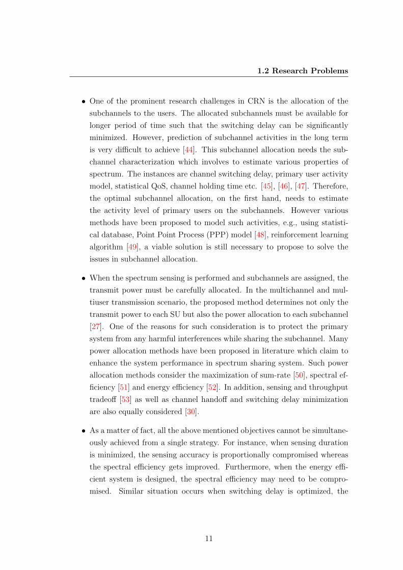
• One of the prominent research challenges in CRN is the allocation of the
subchannels to the users. The allocated subchannels must be available for
longer period of time such that the switching delay can be significantly
minimized. However, prediction of subchannel activities in the long term
is very difficult to achieve [44]. This subchannel allocation needs the sub-
channel characterization which involves to estimate various properties of
spectrum. The instances are channel switching delay, primary user activity
model, statistical QoS, channel holding time etc. [45], [46], [47]. Therefore,
the optimal subchannel allocation, on the first hand, needs to estimate
the activity level of primary users on the subchannels. However various
methods have been proposed to model such activities, e.g., using statisti-
cal database, Point Point Process (PPP) model [48], reinforcement learning
algorithm [49], a viable solution is still necessary to propose to solve the
issues in subchannel allocation.
• When the spectrum sensing is performed and subchannels are assigned, the
transmit power must be carefully allocated. In the multichannel and mul-
tiuser transmission scenario, the proposed method determines not only the
transmit power to each SU but also the power allocation to each subchannel
[27]. One of the reasons for such consideration is to protect the primary
system from any harmful interferences while sharing the subchannel. Many
power allocation methods have been proposed in literature which claim to
enhance the system performance in spectrum sharing system. Such power
allocation methods consider the maximization of sum-rate [50], spectral ef-
ficiency [51] and energy efficiency [52]. In addition, sensing and throughput
tradeoff [53] as well as channel handoff and switching delay minimization
are also equally considered [30].
• As a matter of fact, all the above mentioned objectives cannot be simultane-
ously achieved from a single strategy. For instance, when sensing duration
is minimized, the sensing accuracy is proportionally compromised whereas
the spectral efficiency gets improved. Furthermore, when the energy effi-
cient system is designed, the spectral efficiency may need to be compro-
mised. Similar situation occurs when switching delay is optimized, the
11

1.3 Motivation
primary users may be highly affected by the higher interference which ulti-
mately forces the SUs to terminate the transmission on cognitive subchan-
nel. Therefore, a new method for CRN must be proposed to put spectrum
sensing, spectrum allocation and transmit power control together with a
common network parameter such that a better as well as practically achiev-
able tradeoff can be obtained.
1.3 Motivation
The research presented in this thesis is highly motivated by the issues raised in
the previous section. Furthermore, the research in the field of spectrum sens-
ing and resource allocation, a low complexoty but highly efficient methods are
immediately required. The objective of my research is to bridge the gap in this
area.
With the revolution in wireless communication technologies and the cost of
wireless devices as well as services falling down dramatically in last two decades,
radio spectrum has become the extremely scarce resource for wireless networks to
provide the required QoS to the end users. The current static spectrum allocation
policy is one of the barriers to increase the spectrum utilization efficiency. Cog-
nitive radio, in parallel, emerged into the wireless communication framework as
a tool to solve the spectrum shortage and underutilization problems. Moreover,
to fulfil the requirements of 5G such as low latency, high throughput, high spec-
tral and energy efficiency, a very intelligent wireless communication technique is
needed. Therefore, the main motivation for this research emerged form finding
the best possible techniques which help to achieve the goals with minimum system
complexity and lower implementation cost.
The spectrum sensing methods in the literature, whether cooperative or non-
cooperative, deal with the tradeoff between sensing and transmission duration.
However, a few sensing methods do not work under low signal to noise ratio
(SNR), e.g., energy detection, or they are vulnerable to interference due to the
sampling clock offset, i.e., cyclostationary detection. Similarly, cooperative spec-
trum sensing method needs higher computational complexity to achieve an accu-
rate sensing information, whereas wideband sensing increases the hardware design
12

1.3 Motivation
complexity. Therefore, the research works presented in this thesis are highly mo-
tivated to find a low complexity but high sensing accuracy tradeoff in spectrum
sensing in CRN.
Similarly, various schemes have been proposed in subchannel allocation and
transmit power control in CRN. Many of the proposed methods tend to optimize
one network parameter, such as spectral efficiency, energy efficiency and switching
delay considering other parameters in the ideal range. In practice however, such
flexibility is not always possible to achieve. Therefore, the combined framework
was immediately realized to optimize the spectral efficiency, energy efficiency
and the primary user activities in which the sensing parameters can be tuned at
secondary system to control them. The research presented in this thesis also got
motivation from such requirement.
As a motivational work at the beginning of the research, a spectrum sensing
tasks were performed at various spectrum range to study the diversity of spectrum
usage and availability which will be discussed next.
1.3.1 Spectrum Sensing in Practice: Observation in Lan-
caster Area
Once spectrum sensing techniques and issues of cognitive radio communication
have been discussed, it is very important to elaborate how the idle as well as
under-utilized portion of the spectrum are distributed in real wireless communi-
cation scenario. For instance, the observation of primary signals in some cellular
and TV band in Lancaster City area have been presented in this section to further
understand the general concept of cognitive radio for cellular communication.
Depending on the nature of the available subchannel, i.e., both the unused
as well as under-utilized, different accessing modes can be used, for instance,
overlay and underlay mode of spectrum access. The recent announcement by
Ofcom assures the creation of White Spaces Databases (WSDBs) on UHF TV
band which is operated by selected organizations that have been qualified by
Ofcom to operate in the United Kingdom and they provide the WSDB Services
to white space devices (WSDs) [54]. However, similar concept is not feasible in
13

1.3 Motivation
the cellular communication due to the dynamic nature of users. Therefore, a real
time spectrum sensing result is needed to exploit the available subchannels.
As mentioned previously, cognitive radio concept can be implemented within
the TV band in VHF and UHF spectrum, typically in 54 MHz to 790 MHz [55], to
cellular communication in 900/1600 MHz, LTE in 800 MHz, UMTS in 2100 MHz
[56] and even most recently proposed in mmWave band. In this section, the
field based spectrum sensing results are presented showing the TV white spaces,
various cellular bands including 3G and 4G/LTE signals.
The software defined radio platform is used to find the spectrum availability
map using the device originally designed as a receiver for digital video broadcasting-
terrestrial (DVB-T). The frequency tuner uses the micro coaxial antenna port
with omnidirectional antenna. The received radio frequency signal at the tuner
are down-converted to intermediate frequency and then to the baseband signal.
The sampling rate in this spectrum sensing is set to 2.4 MHz and antenna gain
is 40.
480 500 520 540 560 580 600 620 640 660
−15
−10
−5
0
5
10
15
Frequency (MHz)
Pow
er R
atio
(dB
m)
Figure 1.1: The received signal power in dBm in the radio spectrum of 400 MHz
to 670 MHz.
14
1.3 Motivation
880 890 900 910 920 930 940 950 960 970−30
−25
−20
−15
−10
−5
0
Frequency (MHz)
PowerRatio(d
Bm)
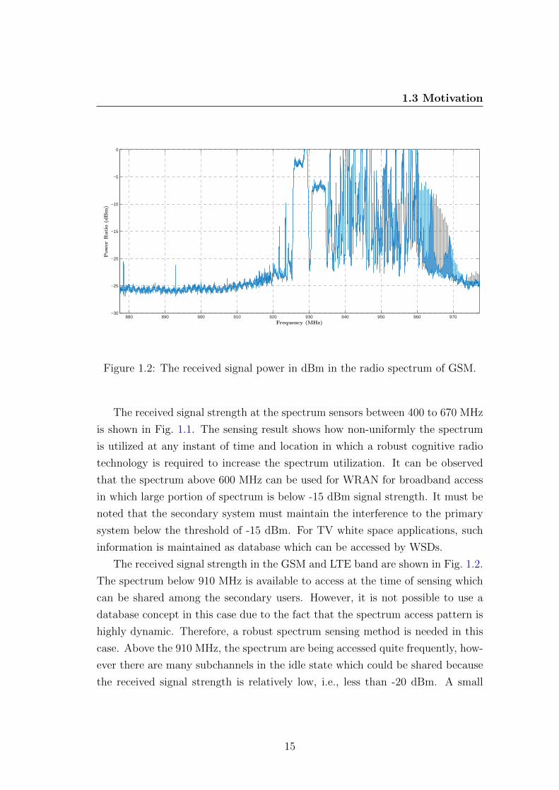
Figure 1.2: The received signal power in dBm in the radio spectrum of GSM.
The received signal strength at the spectrum sensors between 400 to 670 MHz
is shown in Fig. 1.1. The sensing result shows how non-uniformly the spectrum
is utilized at any instant of time and location in which a robust cognitive radio
technology is required to increase the spectrum utilization. It can be observed
that the spectrum above 600 MHz can be used for WRAN for broadband access
in which large portion of spectrum is below -15 dBm signal strength. It must be
noted that the secondary system must maintain the interference to the primary
system below the threshold of -15 dBm. For TV white space applications, such
information is maintained as database which can be accessed by WSDs.
The received signal strength in the GSM and LTE band are shown in Fig. 1.2.
The spectrum below 910 MHz is available to access at the time of sensing which
can be shared among the secondary users. However, it is not possible to use a
database concept in this case due to the fact that the spectrum access pattern is
highly dynamic. Therefore, a robust spectrum sensing method is needed in this
case. Above the 910 MHz, the spectrum are being accessed quite frequently, how-
ever there are many subchannels in the idle state which could be shared because
the received signal strength is relatively low, i.e., less than -20 dBm. A small
15

1.3 Motivation
935 940 945 950 955 960−30
−25
−20
−15
−10
−5
0
5
10
15
20
Frequency (MHz)
PowerRatio(d
Bm)
Figure 1.3: The received signal power in dBm in the radio spectrum of 900 MHz.
portion of 900 MHz band is shown in Fig. 1.3. The spectrum is usually averaged
over many samples, the observed sequences are just an instantaneous observa-
tion. However it has been observed similar distribution of spectrum access, it can
Frequency (MHz)
Tim
e H
isto
ry (
ms)
→
−1.5 −1 −0.5 0 0.5 1 1.50
10
20
30
40
dBm−80 −70 −60 −50 −40 −30 −20 −10 0 10 20
Figure 1.4: The OFDM subcarriers of LTE signal captured at the central fre-
quency 891 MHz in time and frequency axis.
16

1.4 Thesis Outline
be argued that channel access distribution will follow similar pattern in average.
When closely observed the spectrum, subchannels are available to be accessed by
the secondary system, under strict interference constraint, even though they are
not contiguous.
In Fig. 1.4, the individual subcarrier have been identified at the baseband
central frequency 891 MHz and the bandwidth is 2.8 MHz. The red and yellow
vertical lines indicate the individual OFDM subcarrier where red line indicates
the higher received signal strength. Therefore, OFDM is considered as a ideal
candidate for multiplexing in CRN because the subcarriers allocation to users
can be done adaptively.
1.4 Thesis Outline
This thesis is organized into six different chapters, which covers spectrum sensing
and resource allocation strategies for cognitive radio networks.
In Chapter 2, various aspects of spectrum sensing for cognitive radio com-
munication will be presented. It will firstly describe the requirements of spectrum
sensing in cognitive radio along with the very important tradeoff between sens-
ing and transmission duration. Secondly, various spectrum sensing methods are
described that are available in the literature as a foundation of the proposed spec-
trum sensing methods later in the thesis. The cooperative and non-cooperative
spectrum sensing are also described with their respective advantages and disad-
vantages. The challenges of spectrum sensing methods for cognitive radio will also
be described. Thirdly, the spectrum sensing results obtained from the specially
designed spectrum sensors for TV band and GSM band, i.e., 500 MHz, 800 MHz
and 1600 MHz will be presented to show the nature of spectrum availability in
real network.
In Chapter 3, the considered system model will be described in detail.
The multi-cellular and multi-carrier system with primary and secondary service
providers collocated in the same geographical region for spectrum sharing system
will be presented. The subchannel division, orthogonal frequency division multi-
ple access (OFDMA) as modulation scheme and various channel and interference
17

1.5 List of Publications
models are described to justify their usage in the considered system of spectrum
sensing and resource management.
In Chapter 4, the proposed spectrum sensing scheme will be exclusively
described. It is basically the sensor-enabled cognitive radio system where the
dedicated sensing devices replace the spectrum sensing task from the secondary
system. As a result, the secondary users can have more slot duration to transmit
the data packets in addition to the lower power consumption due to skipping the
sensing task. This chapter will also present design criteria of sensing devices such
that the tradeoff among the sensing accuracy, system throughput and sensing
network cost can be explained both mathematically and through the simulation
results. The detail communication protocol among secondary system and the
sensing devices will also be presented.
In Chapter 5, the proposed resource allocation method will be presented.
Firstly, a reliable method of estimating the activities of primary users on the
subchannels are explained defining a parameter called subchannel activity index.
This parameter will be later obtained in the multiple cell scenario which indicates
the best possible subchannel in the vicinity of the cell at a particular time and
location. Furthermore, the transmit power allocation problem is defined and
solved to find the optimal transmit power. While formulating the optimization
problem, both spectral efficiency and energy efficiency will be considered. Later in
the chapter, the integrated method of analysis is presented which shows a better
system design approach to maintain the balanced energy and spectral efficiency
by changing the sensing parameters in the secondary system.
Finally, Chapter 6 presents the conclusions of the thesis by briefly reviewing
the contributions of the proposed methods and associated challenges while imple-
menting them in real network scenario. Based on the recent research activities,
the future directions of resource allocation in cognitive radio in terms of 5G and
its standardization are also discussed.
1.5 List of Publications
Deepak, G.C., Keivan Navaie, and Qiang Ni, “Power allocation in multicell col-
laborative cognitive radio networks,” Under review on IEEE Transaction
18

1.5 List of Publications
(The content presented in Chapter 5 is based on this paper.)
Deepak G.C., and Keivan Navaie, “A low latency zone-based cooperative spec-
trum sensing,” IEEE Sensor Journal, vol. 16, no. 15, pp. 6028-6042, Aug. 2016.
(The content presented in Chapter 4 is based on this paper.)
Deepak G.C., and Keivan Navaie, “On the collaborative cognitive radio net-
works,” IEEE InfoCom Student Seminar, San Francisco, USA, 10-15 April, 2016.
(The content presented in Chapter 5 is based on this paper.)
Diky Siswonto, Li Zhang, Keivan Navaie, and Deepak G.C., “Weighted Sum
Throughput Maximization in Heterogeneous OFDMA Networks,” IEEE VTC-
Spring conference, Nanjing, China, 15-18 May, 2016.
(The content presented in Chapter 4 is based on this paper.)
Deepak, G.C., Keivan Navaie, and Qiang Ni “Inter-cell collaborative spectrum
monitoring for cognitive cellular networks in fading environment,” Proc of IEEE
Int. Conf. on Comm. (ICC), IEEE pp. 7498-7503, 2015.
(The content presented in Chapter 5 is based on this paper.)
Deepak G.C., and Keivan Navaie “On the sensing time and achievable through-
put in sensor-enabled cognitive radio networks,” Proc. of Tenth Int. Symp. on
Wireless Commun. Systems (ISWCS), IEEE, pp. 1-5, 2013.
(The content presented in Chapter 4 is based on this paper.)
19

Chapter 2
Spectrum Sensing for Cognitive
Radio
Spectrum sensing is the mechanism to identify the fully or partially unoccupied
spectrum by primary users at a particular time and geographical location. The
fully unoccupied spectrum are also defined as the spectrum holes. In more gen-
eral cognitive radio term, spectrum sensing techniques result the spectrum usage
characteristics in terms of multiple dimension of frequency, time and space [24].
Spectrum sensing has been considered to be the fundamental requirement for
spectrum sharing in cognitive radio framework.
The primary users (or primary systems) and secondary users (or secondary
systems) are frequently used while discussing the cognitive radio and spectrum
sensing. Primary users are the mobile terminals who have the exclusive right to
access the specific part of the spectrum as soon as there is data packet to transmit.
It means, in cellular system, the primary users are the incumbent licensee of the
spectrum for which they pay the cost to get access. On the other hand, secondary
users have the lower right to access the same spectrum which they have to exploit
in such a way that they do not cause any harmful interference to the primary
system.
The spectrum sensing task is generally performed by the secondary users. As
a result, the secondary users must have a reliable and accurate cognitive radio
capabilities to exploit the unused part of radio spectrum. However, in some
latest advancements, the database service provider may disseminate the accurate
20
2.1 Spectrum Sensing Techniques
status of the target frequency band. One of the examples is the geolocation
database (GD) of TV white spaces to be used for broadband access when the TV
transmitter is not using a particular band [57]. This has been proposed in the
IEEE 802.22 standard and it is partially implemented with wireless regional area
network (WRAN) in practice. The basic information about this standard will be
discussed in the next chapter.
The wideband spectrum sensing is necessary in some cognitive radio applica-
tions where large band of spectrum is to be opportunistically accessed. However,
wideband spectrum sensing requires higher power consumption for analog-to-
digital conversation in addition to high sampling rate [40]. To avoid such prob-
lems, the wideband can be divided into the narrowband subchannels which is also
known as the multiband spectrum sensing. They can be sensed either sequen-
tially or in parallel depending on the availability of number of sensing antennas.
The advantage of multiband sensing is that the subchannels are assumed to be
independent and the narrowband spectrum problems becomes a binary hypoth-
esis test. In the following section, we will present various multiband spectrum
sensing techniques that are in practice.
2.1 Spectrum Sensing Techniques
The output of spectrum sensing decides whether a particular subchannel is avail-
able or being occupied. Therefore, the problem, in its simplest form, can be
modelled as binary hypothesis test at the secondary users, or spectrum sensors
if sensing is done at the separate entity. The null hypothesis is denoted by H0
when a particular subchannel is idle. In this case, the received signal is of course
only the random channel noise. In contrast, the alternative hypothesis is denoted
by H1 when a particular subchannel is occupied by primary users. In this case,
the received signal is both the noise and signal transmitted by primary system.
To define the spectral sensing techniques, various discrete signals are defined
from mathematical and signal processing perspectives. Let the received signal at
the secondary users receiving antenna is denoted by y = [y[0], y[1], . . . , y[K − 1].
Here y[k] denotes the kth sample in the sequence for k = 0, 1, . . . , K − 1. The
sampled signal is y[k] , y(kTs) where fs = 1Ts
is the sampling rate. The digitally
21

2.1 Spectrum Sensing Techniques
modulated signal samples transmitted by the primary system is represented by
x = [x[0], x[1], . . . , x[K − 1], where kth element of the sequence is denoted by
x[k] , x(kTs). The noise vector is denoted by w = [w[0], w[1], . . . , w[K−1] where
the kth sample in the sequence is denoted by w[k] , w(kTs). For mathematical
tractability, the channel gain between primary transmitter and secondary receiver
is considered to be unit, though this assumption is practically not feasible. This
channel gain will be considered in the next chapter onwards when more advance
form of spectrum sensing and resource allocation methods are presented.
The spectrum sensing technique should be able to differentiate between the
following two contrast hypotheses.
y[k] =
{w[k], : H0,
x[k] + w[k], : H1,(2.1)
where, w(k) is considered to be circulatory symmetric zero mean complex Gaus-
sian random variables with variance σ2.
2.1.1 Energy detection
The energy detection, also known as radiometer, is one of the well known spec-
trum sensing methods due to its low computational complexity and easy to im-
plement [58], [59]. This is due to the fact that it does not involve any complex
signal processing techniques. The energy detectors, i.e., secondary users unless
otherwise stated, measures the energy received during the finite sensing duration
which is then compared against the predetermined threshold which depends on
the noise floor [60]. This is a popular spectrum sensing technique because the
detectors do not need a priori knowledge of signal transmitted by the primary
system, but it is assumed that large number of signal samples are available at the
detector.
The energy detection spectrum sensing method comes with various challenges,
for instance, selection of the energy detection threshold. If the detection threshold
is not properly obtained, the spectrum sensing efficiency needs to be highly com-
promised. In addition, energy detectors are also unable to differentiate between
22

2.1 Spectrum Sensing Techniques
the channel noise and the interference signal from primary users. Therefore, this
method provides relatively poor performance when received SNR is very low [61].
In order to identify whether particular subchannel is idle or busy, the test
statistics in the form of decision metric, i.e., Λ[y], is first calculated by averaging
the energy received over a period of N observed samples as following.
Λ[y] =1
K
K−1∑
k=0
|y[k]|2. (2.2)
In the next stage, the decision metric is compared against the detection threshold
εth to make the decision about whether the subchannel is idle, i.e., in favour of
hypothesis H0, or occupied, i.e., in favour of hypothesis H1. Therefore, the energy
detector decides that H1 is true under the condition Λ[y] > εth and secondary
users are not allowed to use the subchannel. Similarly, H0 is true in all other
cases in which the subchannel is allowed to be accessed by secondary users to
transmit their data.
Two parameters are very important to measure the performance of energy
detection method, which are probability of false alarm, denoted by Pf, and prob-
ability of detection, denoted by Pd. Moreover, the probability of miss detection,
Pm, refers to the case when detection of subchannel is failed and they are related
as Pd + Pm = 1. The Pf is the probability that the spectrum sensors incorrectly
decide that a particular subchannel is occupied by primary users when actually
the hypothesis H0 is true, i.e., the subchannel is idle. The probability of false
alarm is then formulated as below.
Pf = Pr{Λ[y] > εth|H0}. (2.3)
Similarly, the Pd is the probability that the spectrum sensors correctly decide
that a particular subchannel is occupied by primary users when actually the
hypothesis H1 is true, i.e., the subchannel is busy. The probability of detection
is then formulated as below.
Pd = Pr{Λ[y] > εth|H1}. (2.4)
From the very basic definition of Pf and Pd, it is easy to say that the larger
Pd is always expected whereas Pf is expected to be smaller. When Pd is lower,
23

2.1 Spectrum Sensing Techniques
0 0.2 0.4 0.6 0.8 10
0.1
0.2
0.3
0.4
0.5
0.6
0.7
0.8
0.9
1
Probability of false alarm (Pfa)
Probabilityofdetection(P
d)
SNR 0 dBSNR 4 dBSNR 6 dBSNR 8 dB
Figure 2.1: Receiver operating characteristics curve for energy detection method
through AWGN channel for various received SNR.
the primary user transmission in the subchannel is missed which ultimately cause
undesired interference to the primary users. Similarly, when Pf is higher, many
opportunistic spectrum accesses on the subchannels are missed which causes lower
spectrum utilization. Therefore, it is very important to restrict them within a
acceptable values. The general concept on the spectrum sensing design is to
minimize the Pf while Pd is kept above the minimum level to protect the primary
system from the interference. However, various advanced methods have been
proposed in the literature to achieve this tradeoff.
When Pd is plotted against the Pf, the resulting plot is known as the receiver
operating characteristics (ROC) curve. At a particular instance of sensing, a pair
of (Pf, Pd) can be obtained which lies in the ROC curve as shown in Fig. 2.1. It
shown how Pf and Pd are achieved for various received signal SNR from 0 dB to 8
dB. It can be observed that when Pf is relaxed to the higher value, the detection
accuracy can be improved with higher Pd. Moreover, when the received SNR is
24

2.1 Spectrum Sensing Techniques
higher, the better (Pf, Pd) pair is achieved.
The performance of energy detection varies according to the fading channels.
This method highly depends on the sensing threshold which merely depends on
the noise variance. In practice however, such noise variance cannot be predicted
in advance. Due to this uncertainties, accurate subchannel detection is impossible
below certain SNR, which is also known as SNR wall [61].
2.1.2 Matched Filter Detection
The matched filter technique to obtain the subchannel information requires per-
fect knowledge of signalling features on the data transmitted by the primary
systems [62], [63]. The features include the operating frequency, bandwidth,
modulation type, frame format or pulse shaping. Therefore, for a known de-
terministic signal, matched filter detector acts as a replica correlator. The test
statistic simply correlates the nth sample of the observed sequence y[n] at the
receiver of the spectrum sensors to the replica of primary user signal x[n]. The
null hypothesis (H0) and alternative hypothesis (H1) are then tested as following.
Λ[y] = R
[N−1∑
n=0
y[n]x∗[n]
]> εth : H1,
Λ[y] = R
[N−1∑
n=0
y[n]x∗[n]
]≤ εth : H0,
(2.5)
where εth is the detection threshold1, R[·] denotes the real part of complex number
whereas ()∗ denotes the complex conjugate.
The advantage of using the matched filter is that it takes low sensing duration
to meet the Pf and Pd requirements set by primary system [64]. It is due to the
fact that the smaller number of samples are required to detect the subchannel
in comparison to the energy detection. As a result, the matched filter detector
may acquire the higher transmission duration, and therefore improved system
throughput. In this method, the required number of samples grows according to
1Just for simplicity, the same threshold symbol is used as in the energy detection, however
they are characteristically different parameters.
25

2.1 Spectrum Sensing Techniques
O(1/SNR) which indicates that higher the variance of channel noise, larger num-
ber of samples must be processed to meet the required level of Pf. However, the
beauty of matched filter detection cannot be achieved without sacrificing some-
thing. firstly, secondary users may require to demodulate or decode the signal
transmitted from primary system which consumes more energy while sensing the
subchannels. Secondly, the implementation complexity is relatively higher due to
the requirements of dedicated receiver for every known signal type [59].
2.1.3 Cyclostationary Detection
The information bearing signal in communication system exhibit a form of pe-
riodicity, for instance, symbol rate, chip rate, channel code or cyclic prefix [65],
[66]. The noise presents no correlation due to the wide sense stationary whereas
the modulated signals exhibit the correlation due to the redundancy of signal
periodicities. This feature of periodic pattern on the transmitted signal can be
exploited for spectrum sensing by cyclostationary detection. One of the features
that make cyclostationary detection method a very attractive option is that it
has ability to differentiate the primary user signal not only from the channel noise
but also from another primary user signal or interference [67].
The orthogonal frequency division multiplexing (OFDM) signals can be con-
sidered which are embedded with the cyclic prefix to protect the signals from
intersymbol interference. The cyclic prefix basically means each OFDM symbol
preceded by replica of end part of the same symbol. Therefore cyclic prefix can be
easily exploited for spectrum sensing using cyclostationary detection. When the
cyclic frequency is considered to be α, the cyclic spectral density (CSD) function
of received signal y[n] is calculated as following [68].
S(f, α) =∞∑
l=−∞
Rαy (l)e−j2πfl, (2.6)
where,
Rαy (l) = E[y[k + l]y∗[k − l]e2παk]. (2.7)
The peak value of CSD is attained when the fundamental frequency and cyclic
frequency of y[k] are matched which merely indicates the hypothesis H1 is correct.
26
2.2 Cooperative Spectrum Sensing
In all other cases, the hypothesis H0 is correct. If the cyclic frequency is unknown,
it can be easily extracted from the received signal. The drawbacks of this detec-
tion technique is that it reduces the system capacity due to signalling overhead
because the same information has to transmit twice within a frame. Moreover,
the computational complexity is very high in comparison to the matched filter
and energy detector because it has to cope with the effect of sampling frequency
offset in the system.
Many other spectrum sensing techniques have been proposed in the literature,
for instance, blind sensing, filter-bank based sensing, multi-taper sensing, com-
pressive sensing. All of them have a set of advantages and disadvantages and the
choice depends on the network scenario and the sensing hardware available.
2.2 Cooperative Spectrum Sensing
The primary and secondary systems may not be in the line-of-sight (LoS) com-
munication due to the mobility of the users. This results the noise uncertainty,
path loss, channel fading and shadowing on the received signal. Therefore, the
spectrum sensors receive very low primary signal and may incorrectly detect the
presence or absence of primary users on subchannels. This condition is also
referred as hidden terminal problem of spectrum sensing. On the other hand,
the secondary users must sense the channels as correctly as possible to maintain
the sensing reliability even in worst fading scenario to mange the interference to
primary system below the predefined threshold.
To improve the sensing accuracy, i.e., sensitivity, of cognitive radio spectrum
sensors and to make it more robust against the hidden terminal problem and
channel fading irrespective of the sensing methods in use, cooperative spectrum
sensing has been considered as an appropriate solution [69]. The concept of
spectrum sensing with cooperation is to use multiple sensors distributed across
the coverage area and combine their individual measurements into one common
decision. The probability of miss detection and probability of false alarm would
be considerably minimized when cooperative sensing technique is used [70] in
addition to solve the hidden primary terminal problem and it may also lower the
sensing duration [71].
27

2.2 Cooperative Spectrum Sensing
Table 2.1: The comparison and summary of three spectrum sensing methods.
Energy Detector Matched Filter Cyclostationary
Detector
Test statistics The total energy
of received
signal at the CR
receivers
Correlation with the
received signal at CR
receiver and a replica
of the signal
The cyclic
spectrum
density function
of the received
signal
Sensing
accuracy
Low with no
prior
information of
the PUs
High: It is optimum
detection method
with a short sensing
time (It needs a prior
information of the
PU’s signal).
Medium: It can
differentiate
between
different PU
signals.
Implementation
complexity
Low: It is
simple and
easier to
implement in
practice.
High if the SU
receivers need to
estimate different
types of PU signals,
however pre-stored
information can be
used to reduce this
complexity.
High but in less
extent to that of
the Matched
Filter
Robustness
against low
SNR
low: The energy
detector is very
sensitive to
noise power
mismatch.
High: It offers good
detection in very
noisy scenarios.
Medium: Its
performance in
the low SNR is
better than the
energy detector.
When the cooperative sensing is performed among large number of secondary
users or cooperative sensors, the sensing performance as well as the sensing re-
liability are significantly improved. In contrast, the complexity of the system
28

2.2 Cooperative Spectrum Sensing
design also increases simultaneously due to the flooding of large number of con-
trol signals. Such control signals are possibly transmitted through the ISM band,
dedicated band or even an underlay system such as ultra wide band. Therefore,
an efficient information sharing algorithm is required to achieve the maximum
benefits of the cooperation in cognitive radio enabled wireless communication.
When the distributed sensing devices detect the subchannel state, they are
either shared among them or forwarded to the central processing unit depending
on the mode of operation. Once the final decision is made, the spectrum sensing as
well as channel sharing information are shared among the multiple users through
the control channel. In many cooperative sensing method, the cognitive radio
network is divided into the clusters and the decision information is transmitted
to the cluster head in an assigned frame/slot [72]. While executing this task,
the coordination algorithm should be designed such that the minimum delay
is achieved [46]. The cooperative sensing is performed either centrally or in
distributed fashion depending on where the sensing results are processed.
2.2.1 Centralized Sensing
In centralized spectrum sensing, individual spectrum sensors or secondary users
sense the subchannel in its geographical location which are then collected at the
central processing unit, also known as decision fusion centre (DFC). The available
subchannels are identified at the DFC using various decision fusion rules which
are being proposed in literature with their own pros and cons. The information
is then multicasted through the dedicated control channel to the secondary users
[73]. The obstructions in between primary and secondary systems may cause
multipath fading and shadowing, however another user in its vicinity may have
good channel condition which helps the cooperative detection process to be more
robust than the case when single user is sensing the subchannel. Even the control
channel could be under deep fading, however they are assumed to be a perfect
channel in the network design.
Depending on the nature of sensing results obtained at the local sensors and
the processing of information at the DFC, centralized sensing method are cate-
gorised as the soft combining and hard combining methods.
29

2.2 Cooperative Spectrum Sensing
2.2.1.1 Soft Combining
In soft combining method, the locally sensed subchannel information is forwarded
to the DFC without taking any local decision or hypothesis test [74]. The decision
is made at the DFC by combining those unprocessed data using the appropriate
methods. One of the conventionally used rule is the square law combining of
received data from the individual sensing data. In this method, the estimated
energy level is reported back to the DFC and all energy levels from secondary
users are combined with square law which is then compared against the threshold
value to decide the status of the subchannel. However, there are various methods
to combine soft data together, such as correlation based soft combining [75].
Let us consider that there are z = 1 . . . Z sensors or secondary users to co-
operatively sense the subchannels. By assuming the noise vector wz and signal
vector xz are independent for each sensors, the received signal vector from z sen-
sors is obtained as y = [yT1 ,yTz . . .y
TZ ]. The log-likelihood ratio provides the test
statistics as following.
log
(Pr(y|H1)
Pr(y|H0)
)=
Z∑
z=1
||yz||2σ2z
=Z∑
z=1
Λz, (2.8)
where, Λz is the log-likelihood ratio from the zth sensor. The statistics ||yz ||2
σ2z
is the soft decision from z secondary users. The weighted sum in (2.8) is then
compared against the threshold value to decide the status of the subchannels.
The soft combining cooperative technique provides accurate estimation of the
subchannel status, however it need a relatively huge bandwidth due to embedding
much information in control packets. On the other hand, if one of Z number of
the secondary users is untrustworthy, it severely degrades the cooperative gain
and therefore the spectrum sensing efficiency [76].
2.2.1.2 Hard Combining
The soft combining potentially require the complex structure of signal processing
hardware because DFC may receive large amount of data to process. The best
alternative of this technique is that the sensing devices take decision from the
locally sensing data and quantize the decision in binary format, which are, in
30

2.2 Cooperative Spectrum Sensing
general terms, known as hard decision bits. Therefore, in hard combining, the
DFC is just to process the received bits and take the decision using various logic
fusion rules; for instance, AND-logic rule, OR-logic rule, majority-count-login
rule amongst others are proposed in literature [77].
When the individual sensing device z take local decision, the individual test
statistics are quantized into a single bit such that Λ(z) ∈ {0, 1} are the hard deci-
sion bits. It indicates that when local test statistics is greater than the predefined
threshold, the decision is taken as 1 which indicates the subchannel is busy. In
other cases, the decision is taken as 0 which indicates the subchannel is idle.
When there are Z number of sensors, the test statistic at the DFC using simple
voting rule decides in favour of the hypothesis H1 when the following condition
is satisfied.
Z−1∑
z=0
Λ(z) ≥ C, (2.9)
where, 1 ≤ C ≤ Z. The fusion AND, OR and majority count rules are the special
cases when C is fixed at a particular value [40]. In cases when C = Z, the fusion
rule is known as AND fusion rule in which all the local sensors must unanimously
agree on the status of the subchannel. When C = 1, the fusion rule is known
as OR-logic where even one of the sensing devices decides the channel to be idle,
the channel is declared to be available to use by cognitive users. Finally, when
C = Z/2, the decisions are fused using majority count rule where majority of the
sensing devices must agree on the channel status. The detail of each method is
skipped here, however they will be briefly described when they are used in the
following chapters.
2.2.2 Distributed Sensing
When the number of secondary users are increased in centralized cooperation,
the cooperation complexity is simultaneously increased. In the distributed coop-
erative sensing method, the sensing devices act as relay and share the subchannel
status information with each other rather than sensing to the centralized DFC
[78]. In this case, the secondary users according to their detection performance
31

2.3 Challenges in Spectrum Sensing
may form a logical cluster on a temporary basis. Such cluster may be dynamically
forming depending on the distribution of the sensing devices. However in some
cases, the secondary users may share subchannel information to each other on an
ad hoc manner where information is forwarded to its one hop neighbour using
the amplify-and-forward technique.
The obvious advantage of distributed sensing is that no deployment of DFC is
needed which reduces the implementation cost. However, the signalling overhead
could be higher than in centralized system due to flooding of control signal among
the sensors if the cluster is not perfectly formed. The sensing and reporting time
is significantly reduced due to the decentralized decision taking procedure which
helps to increase the system throughput [79]. The detail of this method will also
be explained in next chapters when the proposed methods are presented in detail.
2.3 Challenges in Spectrum Sensing
Despite the spectrum sharing system is the solution to solve the spectrum scarcity
problem, there are many impediments to achieve a balance tradeoff. The factors,
for instance, interference protection, spectrum efficiency, energy efficiency, sensing
duration, implementation cost etc., depend among each other and finding the
optimal operating point is a challenging task in CRN.
The probabilities of false alarm and miss detection always maintain a funda-
mental tradeoff in spectrum sensing. The false alarm probability is related to the
implementation cost in CRN whereas probability of miss detection is responsible
for the performance of the sensing system. The higher the false alarm, the lesser
is the spectrum opportunity, whereas, higher miss detection increases the inter-
ference to the primary system. In practice, unfortunately, both of them cannot be
minimized simultaneously with a single detection algorithm or hardware. In the
recently proposed methods, one probability is kept fixed and another probability
is minimized. From primary system point of view, probability of miss detection
is expected to be minimum, whereas from secondary system point of view, the
probability of false alarm should be kept minimum. Therefore, the balance of
both of them is an interesting as well as a challenging task.
32

2.4 Conclusions
The management of sensing accuracy and data transmission duration tradeoff
is another challenging task in spectrum sensing. As a matter of fact, when the
large number of samples are received at the secondary system receiver, the higher
accuracy in spectrum sensing is achieved. However, in doing so, secondary users
have to spend more slot duration to the sensing task which causes the shorter
duration for data transmission [80]. As a result, the achievable spectral efficiency
at the secondary system is minimized. Some solutions have been proposed in [81],
[82] where the optimal sensing duration is possible to obtain which maximizes the
secondary user throughput and, at the same time, the interference to primary
system can be kept at minimum. However, a perfect tradeoff between sensing
duration and throughput is very difficult to handle in practice.
When the cooperative method of spectrum sensing is used, irrespective of
the decision fusion methods, the energy consumption of the secondary system
increases when the number of cooperative users grows. Therefore, the energy
efficient design of cooperative sensing method is always a challenging task. The
methods such as censoring [83], sleeping [84], clustering [85], amongst others, have
been proposed to solve energy consumption problems, however optimal sensing
and energy tradeoff is difficult to achieve in cooperative CRN.
2.4 Conclusions
In this chapter, the spectrum sensing techniques for cognitive radio were described
considering both advantages and disadvantages of predominant spectrum sensing
methods. The energy detection method has been concluded to be the simplest
one from the system design point of view, however it does not perform well
under low receive SNR. The cyclostationary and matched filter based sensing
have better sensing efficiency but they have higher system complexity due to
the requirements of advance digital signal processors. The cooperative sensing
method and various decision fusion methods have also been presented along with
their merits and challenges. The cooperative sensing can reduce the probabilities
of miss detection and false alarm while sensing the subchannels but the system
complexity increases due to large number of control signals. The associated hard
combining and soft combining methods were also discussed in detail.
33

2.4 Conclusions
The spectrum sensing for real signals in various radio spectrum, ranging from
TV transmission in UHF and VHF to cellular and LTE bands, have also been
discussed. The results demonstrated that the unused and under-utilized spectrum
can be exploited to build a complete spectrum sharing system. The OFDMA
subcarriers were also captured to show how OFDMA subcarriers can be allocated
to the secondary users to realize the cognitive radio communication.
The fundamental limitations with non-cooperative sensing, which at the end
when it comes to the sensing accuracy, could be addressed by means of cooper-
ation among sensing devices. However in this case the sensing complexity needs
to be addressed simultaneously. The problem with the current spectrum sensing
method is that they do not exploit the network structure to reduce the signalling
overhead without compromising the sensing accuracy of secondary system. This
highly motivates to investigate a sensing method by means of distributed sensing
network which would balance the tradeoff between sensing accuracy and signalling
overhead.
34

Chapter 3
System Model
The generic system model is presented in this chapter which is going to be referred
in the subsequent chapters with the required add-on features and functions where
it is necessary. The system model in general accommodates the cellular network
structure, channel model, frame structure in addition to other physical (PHY)
and medium access control (MAC) layer technologies.
3.1 Network Modelling
The considered system model consists of a cellular network that is enabled with
the cognitive radio functionality. The specific reason to focus on the cellular sys-
tem for dynamic spectrum allocation is that cellular systems are in use through-
out the world and many devices and data applications for the spectrum used for
cellular communication are comprehensively researched, understood and imple-
mented. On the other hand, the usage pattern of cellular spectrum is much more
dynamic in comparison to the recently developed cognitive radio in TV spectrum
for rural broadband in which spectrum identification is relatively simple because
the spectrum is idle over the longer period of time [86]. Therefore, a robust, effi-
cient and less complex system must be designed for cellular systems to efficiently
utilize the idle or under-utilized portion of scarce cellular spectrum.
The reference system model is an autonomous cellular network where each
secondary user (or distributed and independent sensing device) performs the spec-
trum sensing task and the subchannels are accessed if and only if the received
35

3.2 Channel Modelling
power on the channel is less than the threshold value. The considered cellular
network is characterized by the fact that the intercell interference is inevitable
due to the universal frequency reuse scheme. Therefore, the identical frequency
bands can be allocated between two adjacent cells. As a result, a dynamic trans-
mit power control at each base station is required in such systems to minimize
the interference.
The cellular cognitive radio network can possibly be represented as an au-
tonomous cellular network where primary system and secondary system are con-
sidered into the same geographical location sharing the common set of resources.
Therefore, in a such autonomous cellular system, the role of adaptation in efficient
resource allocation becomes increasingly important [87].
The considered system model is an infrastructure-based cellular CRN, also
referred to as the secondary system, collocated with a legacy primary cellular
network. The schematic of the considered network scenario is shown in Fig. 3.1.
The primary users communicate with the primary base station and secondary
users communicate with the cognitive radio base stations on the allocated time
slots and frequency subchannels. The primary and secondary users are served by
a single primary and secondary base station, respectively as considered in [88].
The transmit power control algorithm is executed in the secondary system
and the primary system’s transmit power is considered to be fixed, i.e., no power
control mechanism is considered on the primary transmitter. Without loss of
generality, all the transmitters and receivers in the system are equipped with the
single omnidirectional antenna unless otherwise stated. The analysis however can
be easily extended into sectorized cell by considering each sector as a cell with a
single antenna. There is no direct signalling between the primary system and the
secondary system.
3.2 Channel Modelling
The total frequency band of B Hz is licensed to the primary system which serves
primary users for voice and data communications. The primary users are indexed
by j ∈ {1, . . . , J}. The spectrum of the primary system is shared with a secondary
system for downlink transmission. The CRN is a multicell network with M
36

3.2 Channel Modelling
SecondaryBase Station
PrimaryBase Station
gsi
gsigsigpi
gpi
gji
PU
PU
PU
SU
SU
SU
Figure 3.1: The considered cellular cognitive raido network as a reference system
model.
secondary base stations (SBSs). In the central cell, SBS serves secondary users
indexed by s ∈ {1, . . . , S}. In addition, the radio spectrum is divided into N
non-overlapping Bi = B/N Hz subchannels which are indexed by i ∈ {1, . . . , N}.The communication link between the secondary transmitter to the secondary
receivers, for subchannel i ∈ {1, . . . , N}, referred to as secondary channel which is
denoted by gsi(ν). Similarly, the secondary transmitter to the primary receivers,
for subchannel i ∈ {1, . . . , N}, is referred to as interference channel which is de-
noted by gji(ν). The parameter ν denotes the joint fading state which is dropped
hereafter for brevity. Due to the small-scale frequency-dependent multipath prop-
agation characteristics, each SU may experience different channel gains across
different subchannels, i = {1, . . . , N}, each with bandwidth of Bi Hz. Depending
on the PU activity and its required QoS at a specific time and location, secondary
users may have access to x number of subchannels where 0 ≤ x ≤ N .
To sense the subchannels by secondary users and dynamically adjust their op-
erating parameters, the physical layer of the secondary system needs to be highly
37
3.2 Channel Modelling
flexible as well as adaptable. The method of accessing the subchannels in multi-
carrier transmission, also known as orthogonal frequency division multiple access
(OFDMA), has the potential to fulfil the requirements [89]. Therefore, OFDMA
has been highly anticipated to realize the cognitive radio concept to provide
an scalable and adaptive technology for air interface. In the considered system
model, the secondary system utilizes OFDMA to access N non-overlapping sub-
channels.
When OFDMA is used, the subcarriers are grouped together into a cluster
which are assigned to the individual user. This flexibility and adaptability makes
this the best candidate transmission technology for cognitive radio. Such appli-
cations of OFDMA in cognitive radio have been considered in significant number
of previous works as in [90], [91], [92]. The advantages of OFDMA in cognitive
radio as summarized below.
• Since the spectrum sensing may be required to achieve the benefits of cog-
nitive radio communication, the computational complexity of sensing algo-
rithm is significantly lowered when OFDMA is implemented. It is due to
the fact that the received signal is passed through the fast Fourier transform
(FFT) circuitry in OFDMA system to convert time domain signal into the
frequency domain. The primary signal detection can be performed on the
received signal in frequency domain since the signal of primary system is
spread over a group of range of FFT output samples.
• The improvement in spectrum utilization using the waveform shaping tech-
nique where some subcarriers can be turned off depending on the existence
of primary users.
• The interoperability associated with OFDMA makes it a good choice for
cognitive radio. Since OFDMA has been used in both long-range as well
as short-range communication systems, cognitive radio networks equipped
with OFDMA can be used with various technologies including WiMAX,
IEEE 802.11x, IEEE 802.22, amongst others.
38

3.3 Frame Structures
• Its adaptability to the changing environment is very good. For instance, it
can adaptively change the transmit power, channel coding or modulation
order based on the channel quality as well as the user requirements.
The objective in this system model is to maximize the parameters such as
spectral efficiency or energy efficiency. The optimization problem is thus in the
form of a utility function in terms of secondary system throughput and weighting
factor, which, in its simplest form, could be formed as a linear combination as
shown below:
max∑
s∈S
∑
i∈N
αsiRsi, (3.1)
where Rsi is the average rate for user s while accessing subchannel i. Also, S is the
set of secondary users which access the available subchannels N whereas α is the
weighting factor which maintains fairness among the primary and secondary users
due to the fact that the gain at secondary system comes at the expense of primary
throughput because the interference is introduced at primary receivers [93]. Here,
α is the set of weights which is based on predefined QoS requirements and the
primary users activity. The total transmit power and maximum interference to
primary system constraints will also be considered in the proposed spectrum
sensing and resource allocation methods.
3.3 Frame Structures
The frame structure of the considered spectrum sensing and sharing model is
depicted in Fig. 3.2. Each frame consists of the sensing time slot which is
followed by the data transmission slot. The secondary users have to sense a
set of subchannels within the sensing duration using the energy detection as
mentioned in chapter 2. The decisions are then shared among other cellular base
stations or clusters within a cell depending on the system design. The information
then provides whether the subchannel is idle or occupied by the primary users
at particular time and location. If a particular subchannel is found to be idle,
the secondary base station allows particular user to access the subchannel with
39

3.3 Frame Structures
Frame n Frame n+ 1 - - - - - - - Frame K
1 2 3 4 - - n∗ T − Ts
Ts∗(n ≤ N)
Sensingduration
Sensingsub-slot
Data transmissionduration
Figure 3.2: The frame structure of the considered reference system model with
distinct sensing sub-slots and data transmission duration.
allocated maximum transmit power. When the subchannel is found to be busy
due to possible arrival of primary user, a new subchannel is provided if one is
currently available. The secondary user will have to immediately trigger the
channel switching algorithm. If the subchannel is busy, the spectrum sensing
technique is repeated again.
The sensing slot is allocated for the spectrum sensing in addition to execute
many other cognitive radio related functions, for instance, decision taking, sub-
channel allocation and subchannel handoff whenever they are necessary. The
frame duration is denoted as T out of which Ts, where Ts ≤ T , is the sensing
duration. Therefore, the data transmission duration is T−Ts. The secondary sys-
tems may be able to sense the multiple subchannels within the sensing duration
in which case sensing duration is divided into the sub-slots. One sensing sub-slot
is considered as the duration to sense a single subchannel. Therefore, there are
maximum of N sensing sub-slots in which case the sensing slot is denoted as
Ts = {Ts1, Ts2, . . . , Tsk}k≤N .
In the considered system model, a very important tradeoff appears between
the sensing duration and the data transmission duration, thus the throughput on
the secondary system. In cases the Shannon capacity of the channel is considered
as Rc = log2(1+SNIR) where SNIR is the received signal to noise and interference
ratio, the effective throughput on the data transmission duration is achieved to
40

3.4 Cognitive Radio Standard: IEEE 802.22
be (T − Ts)Rc. When the sensing duration is increased to enhance the sensing
accuracy by receiving the larger number of samples for energy detection (or for
any other detection methods), the transmission duration is significantly reduced
which directly degrades the secondary system throughput. In other words, for any
two sensing durations T 1s and T 2
s such that T 1s < T 2
s , then (T−T 1s )Rc > (T−T 2
s )Rc
which is described as a sensing-throughput tradeoff in CRN.
There have been series of proposed methods to find the optimal sensing
time and transmit power allocation scheme with the aim of achieving maximum
throughput. The CRN framework in [82] demonstrated that better achievable
throughput is achieved when average power constraint, instead of instantaneous
power constraint, is taken. Similarly, the design of optimal sensing time and
ergodic throughput on secondary system in wideband sensing based spectrum
sharing is presented in [53]. The auction based spectrum sensing and subchannel
allocation is also presented in [94] with the underlay and overlay spectrum ac-
cessing schemes. However, the spectrum accuracy and the achievable throughput
in CRN can never be attained simultaneously with any of the proposed meth-
ods. This is due to the fundamental limits of the available spectrum sensing
mechanisms. To solve this issue, a fundamental change is necessary to design the
spectrum sensing and throughput tradeoff from a unique and different perspective
of system design. The instance considered here, which is described in the next
chapter, is the independent sensing network model to achieve both with reduced
signalling overhead.
3.4 Cognitive Radio Standard: IEEE 802.22
The discussion of spectrum sensing and resource allocation in cognitive radio
enabled cellular network becomes incomplete without describing the IEEE 802.22
WRAN standard. It is also important to briefly mention it here because the
standard will be frequently used in the subsequent chapters when the cellular
CRN parameters have to be chosen while proposing new methods of spectrum
sensing and resource allocation as well as for the comparison purpose.
The first worldwide wireless standard to realize the cognitive radio commu-
nication in practice is IEEE 802.22 which was released in July 2011. Therefore,
41

3.4 Cognitive Radio Standard: IEEE 802.22
Table 3.1: The physical and medium access control layer parameters set for IEEE
802.22 WRAN standard.
FFT size 1024, 2048, 4096
Cyclic Prefix size Variable
Bits per symbol 2, 4, 6
Pilots 96, 192, 384
Bandwidth 6, 7 and 8 MHz
Multiple access OFDMA/TDMA
Code rate 12, 2
3, 3
4, 5
6
Modulation schemes BPSK, QPSK, 16-QAM, 64-QAM
Duplex TDD
Frame size Super-frame: 160 ms, frame: 10 ms
this is the milestone for future CRN technology because it employs a number of
cognitive features such as spectrum sensing, subchannels allocation and transmit
power control. It provides network access for users within a cell by sharing a
vacant TV white spaces (TVWS) which has excellent radio propagation char-
acteristics to improve the wireless broadband connectivity in rural areas [95].
Various technologies in PHY and MAC layers are considered in this standard,
which defines the typical operating range of 17 to 30 km and up to maximum of
100 km is targeted in a particular geographical location with a maximum data
rate up to 22Mbps [96]. All other PHY and MAC layer parameters set for IEEE
802.22 WRAN standard are shown in Table 3.1.
The PHY layer of this standard is based on the OFDMA in which 1680 subcar-
riers are grouped into the 60 subchannels. The modulation schemes are defined
as binary phase shift keying (BPSK), quaternary phase shift keying (QPSK), 16-
quadrature amplitude modulation (16-QAM) and 64-QAM. The MAC layer is
responsible for the resource allocation in IEEE 802.22 standard in which a point-
to-multipoint mode is adopted. Therefore, the proposed cellular topology consists
42
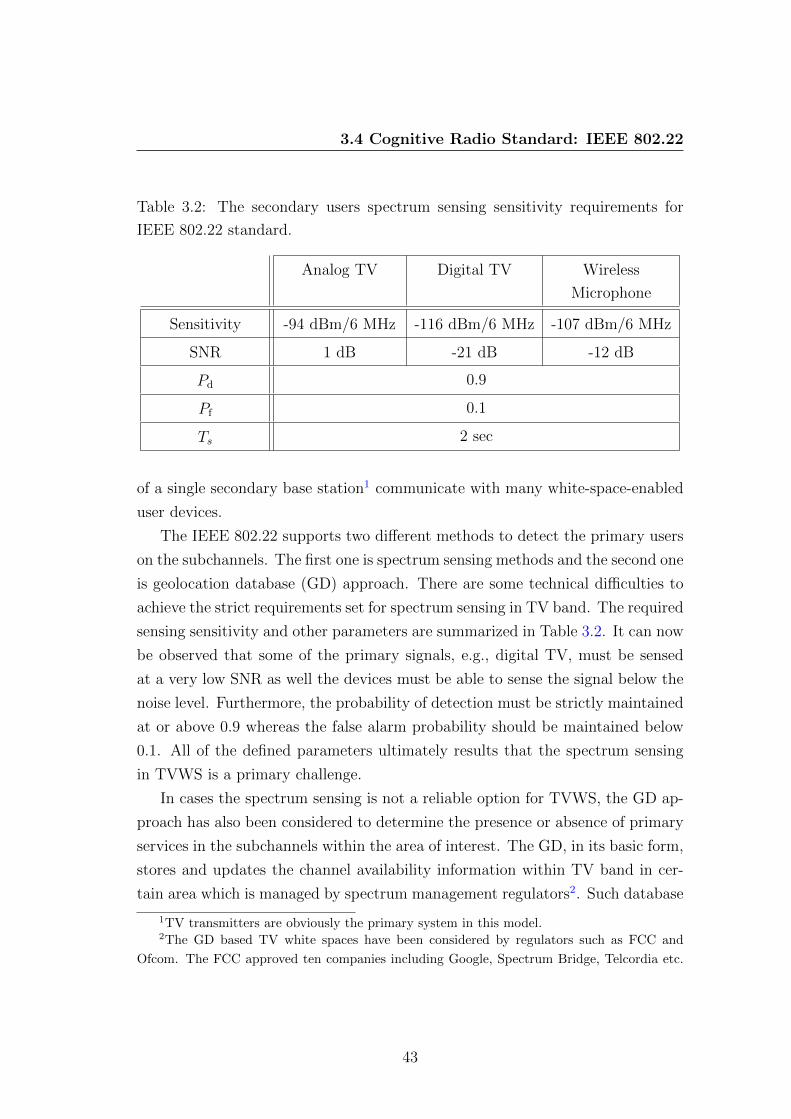
3.4 Cognitive Radio Standard: IEEE 802.22
Table 3.2: The secondary users spectrum sensing sensitivity requirements for
IEEE 802.22 standard.
Analog TV Digital TV Wireless
Microphone
Sensitivity -94 dBm/6 MHz -116 dBm/6 MHz -107 dBm/6 MHz
SNR 1 dB -21 dB -12 dB
Pd 0.9
Pf 0.1
Ts 2 sec
of a single secondary base station1 communicate with many white-space-enabled
user devices.
The IEEE 802.22 supports two different methods to detect the primary users
on the subchannels. The first one is spectrum sensing methods and the second one
is geolocation database (GD) approach. There are some technical difficulties to
achieve the strict requirements set for spectrum sensing in TV band. The required
sensing sensitivity and other parameters are summarized in Table 3.2. It can now
be observed that some of the primary signals, e.g., digital TV, must be sensed
at a very low SNR as well the devices must be able to sense the signal below the
noise level. Furthermore, the probability of detection must be strictly maintained
at or above 0.9 whereas the false alarm probability should be maintained below
0.1. All of the defined parameters ultimately results that the spectrum sensing
in TVWS is a primary challenge.
In cases the spectrum sensing is not a reliable option for TVWS, the GD ap-
proach has also been considered to determine the presence or absence of primary
services in the subchannels within the area of interest. The GD, in its basic form,
stores and updates the channel availability information within TV band in cer-
tain area which is managed by spectrum management regulators2. Such database
1TV transmitters are obviously the primary system in this model.2The GD based TV white spaces have been considered by regulators such as FCC and
Ofcom. The FCC approved ten companies including Google, Spectrum Bridge, Telcordia etc.
43

3.5 Conclusions
information contains operating channels, duration of use, device transmit power,
user location and such other relevant information. In this scheme, the secondary
devices first send a query to the database server to know the available frequency
channels in TV band within their location. It is obvious that such devices must
be equipped with global positioning system (GPS) to find the precise location
of the user. The devices then receive the list of unoccupied subchannels before
initiating the communication [97].
The further step taken to enable GD is the radio environment mapping (REM)
which can be considered as advance knowledge base which keeps record of multi-
domain information about the subchannels and networks as well as the historical
information. The optimal scheme to access such database information is still
in the early research phase. However, recently proposed methods to choose the
database access strategy are the probabilistic decision process [98] and Markov
decision process [99], amongst others. In any accessing method, the existing rules
must be properly addressed and at the same time they have to maximize the
overall communication opportunities through the on-demand access.
3.5 Conclusions
In this chapter, the reference system model has been highlighted such that it will
be easier in the next two chapters where system model is discussed with some
add-on features. The network architecture is considered as infrastructure based
multi-cellular network where independent primary and secondary cellular systems
share the scarce radio spectrum. The network design has also been considered
keeping in mind the multi-tier small cell network, i.e., heterogeneous network, as
a network scenario for 5G and beyond. Therefore, the considered system model
and the proposed methods of spectrum sensing and resource allocation in the next
chapters are equally applicable to the next generation networks with minimum
level of modification.
Since there are primary and secondary cellular systems, there are communi-
cation links, i.e. secondary transmitter to secondary receivers and primary trans-
mitter to primary receivers, as well as interference links, i.e., from secondary
as a GD administrator and some of them have already completed the tests by 2015.
44

3.5 Conclusions
transmitter to primary receivers. The stochastic behaviour of such channel gains
plays a vital role in system performance because they are random in nature and
difficult to predict in real time. Therefore, assumptions are frequently made
about the channel gains, such as channel reciprocity and probability distribution
function with known parameters when they have to be modelled in practice. The
basic channel property as well as some physical layer technologies have been also
discussed in this chapter. In addition, OFDMA plays vital role to realize CRN
which makes spectrum sensing task less computationally complex due to the FFT
circuitry available in OFDMA. It also maintains higher spectrum utilization and
is compatible with many existing systems and hardware.
The frame structure of the proposed system model is also discussed in this
chapter. The sensing duration and data transmission duration together form a
strict tradeoff in practice, also known as sensing and throughout tradeoff. There-
fore, it is very important to implement the optimal sensing method to find the
optimal sensing duration which maximizes the secondary system throughput by
keeping interference to the primary system below the threshold level. The cur-
rent work is highly inspired with this requirement by designing a novel technique
of spectrum sensing to realize the cognitive radio in practice. Moreover, a brief
working principle of first cognitive radio standard, i.e., IEEE 802.22, has been
also discussed which is available in the TV band where the spectrum holes can
be exploited to provide the remote broadband services.
45

Chapter 4
Low-Latency Zone-Based
Cooperative Multichannel
Spectrum Sensing
In wireless communications, data is often transmitted within the allocated time
frames. The number of data bits transmitted in each time frame is directly re-
lated to the the system throughput. To enable the dynamic spectrum access
(DSA) in cognitive radio communication, part of each time frame is allocated
to spectrum sensing thus no transmission is allowed in this duration [22]. By
increasing the sensing duration the sensing accuracy is also increased, however
the remaining time for transmission thus the system throughput is also corre-
spondingly decreased. This results in a fundamental trade-off between sensing
accuracy and system throughput [43]. As a consequence, choosing the optimal
value of sensing duration is a challenging task [53]. Therefore, a unique method
of spectrum sensing is needed in CRN to achieve the better sensing-throughput
tradeoff deal without increasing the sensing complexity and signalling overhead.
In this chapter, the details of such spectrum sensing technique will be presented
as one of the proposed methods.
Conventionally, the spectrum availability is sensed at the SUs which are ran-
domly distributed over space and time. Fundamental characteristics of multiuser
wireless environment including multipath fading, user mobility and hidden termi-
nal problem, as well as limited sensing duration result in reducing the spectrum
46

sensing accuracy. Therefore, in such environments conventional sensing mecha-
nisms are not able to efficiently sense the spectrum availability with an accept-
able level of accuracy required for protecting the PUs from inevitable interference
[100].
To address the sensing accuracy issue, cooperative spectrum sensing tech-
niques have been introduced in literature, e.g., [101], [102], [103], [104]. In co-
operative spectrum sensing, SUs sense the spectrum availability and share this
information with other network entities. Spectrum availability decision is then
made by combining the collected sensing information based on a rule, e.g., AND,
OR or K-out-of-N1 [43]. The advantages and challenges associated with the coop-
erative spectrum sensing are already discussed in Section 2.2 and Section 2.3. In
such methods, the spectrum availability information obtained from multiple SUs
can also be processed using more sophisticated techniques. Instances include
weighting [41], multidimensional correlation [42] and minimizing the collision
probability at the PUs [100]. In weighting, the share of the provided information
by each sensor in the final decision is determined by a weighting vector which
is a system design parameter. Further, [42] leverages the spatio-temporal corre-
lations between spectral observations among various nodes and across different
time instants to minimize the sensing cost and maximize its accuracy.
Various settings have been proposed for implementing cooperative spectrum
sensing, e.g., [105] and references therein present the detail survey. The cooper-
ative spectrum sensing proposed in [103] divides the coverage area into clusters,
where the SUs perform spectrum sensing and base station acts as a decision fusion
centre. The users considered as the cluster heads then make spectrum availability
decisions. In such a cooperative sensing model, a higher sensing duration results
in a shorter data transmission duration which results degradation in achievable
data rate. In addition, the signalling overhead is also higher in the secondary sys-
tem and the performance is highly sensitive to the reporting channel conditions.
The logical cluster formation proposed in [106] has been designed to tackle
the issues due to the imperfect reporting channel conditions. In [107], the cluster
formation is proposed based on the heterogeneous characteristics of primary and
1K-out-of-N rule is also mentioned as majority count rule in literature when K ≤ N/2,
however both can be used interchangeably in theory.
47
secondary users such that users in the same cluster sense the identical set of
channels to increase the sensing accuracy. The cluster heads however act locally
therefore unable to incorporate their location information into the network wide
channel allocation. In addition, various decentralized cooperative schemes are
proposed, e.g., [108], where no decision fusion entity exists and therefore the SUs
themselves diffuse the received decisions.
In addition to the centralized and decentralized cooperative schemes, a relay-
based multiple hops cooperative sensing is proposed in [109], where source to
destination spectrum information is forwarded by the relay nodes, where either
amplify-and-forward or decode-and-forward method is implemented. This tackles
the issues of erroneous report channel by increasing the cooperation footprint.
A two channel sensing technique under imperfect spectrum sensing based on
the independent set of access and backup subchannels is also proposed in [110],
where both subchannels are sensed in a single time slot to improve the system per-
formance by jointly considering spectrum sensing and spectrum access. Although
cooperative sensing often improves the sensing accuracy, the corresponding sig-
nalling overhead further reduces the overall system throughput.
As a matter of fact, whether it is centralized, decentralized or relay-assisted
cooperative model mentioned in [101]-[109], the formation of clusters is very chal-
lenging due to the time varying nature of the wireless channels and mobility of
users. The merits of incorporating the location information are recognized in
conventional cognitive radio [111] as well as in advance cooperative communi-
cation [105]. However, embedding the location information in the CRN design
might increase the signalling overhead. The dynamic cluster formation algorithm
also causes very high signalling overhead. Therefore, an independent spectrum
monitoring network has been proposed in this chapter to improve the cooperative
sensing efficiency with reduced complexity.
In majority of the available cluster based cooperative sensing approaches, in
addition to the signalling overhead due to the cluster head selection, cooperative
spectrum sensing also introduces extra spectrum sensing latency. This is due to
the fact that the SUs need to allocate an extra part of their fixed time frame to
transmit the sensing information to a fusion centre and then wait for the sensing
decision to be made and received back. To address this issue, the sensor selection
48

4.1 Sensor Network Enabled Spectrum Sensing
algorithms have been proposed in [112], [113]. However, cooperative sensing fails
to provide required low-latency access which is of an immense importance in use
cases including M2M communications [114]. Also, M2M plays an important role
in the structure of the Internet-of-Things (IoT) which will be mainly connected
through wireless communications.
4.1 Sensor Network Enabled Spectrum Sensing
The framework to offload the cooperative sensing to an independent monitor-
ing network has been proposed in [115] to tackle the latency issues due to the
sensing durations. It comprises of sensors deployed within the coverage area of
cellular network and continuously monitor the spectrum availability. The sensing
information is then communicated by the sensors to a central entity on sepa-
rate signalling channels. In this setting, by careful design of system parameters,
the same level of accuracy is achieved without reducing the system throughput.
There is, of course, cost associated with building the monitoring network, which
is justified in [115] considering extraordinary price of radio spectrum in mobile
communication bands. An independent network of sensors is further considered
in [116],[117] for nomadic cognitive networks in urban and sub-urban areas. The
advantages of considering a separate monitoring network are twofold. Firstly, it
lowers the corresponding sensing latency due to the reduced sensing duration,
thus the spectral efficiency is increased by offloading the spectrum sensing task
to an independent monitoring network. Secondly, the spectrum sensing accuracy
is significantly improved due to cooperative sensing.
The above mentioned techniques improve the sensing accuracy and the as-
sociated latency, however they ignore the location information of sensors. Due
to very high number of objects in the coverage area, incorporating the location
information into sensing is capable of enabling spectrum reuse across very small
regions in the network coverage area which is, in the proposed method, is re-
ferred as micro-spectrum-reuse. Incorporating the exact location of the sensors
however might introduce a new dimension to the spectrum sensing complexity
and increases its associated costs. Instead in this chapter a simple Zone-Based
Cooperative Spectrum Sensing will be proposed. The sensing architecture in the
49
4.1 Sensor Network Enabled Spectrum Sensing
proposed method is based on dividing the coverage area into zones and defining a
zone aggregator (ZA) as an intermediate entity. A general case is considered here
in which the spectrum is divided into number of channels (i.e., subchannels in
multicarrier systems). The ZAs then process the sensing outcome of the sensors
for each subchannel located in their corresponding zone. The aggregated decision
for each zone is then passed to a fusion centre. In the proposed scheme, to ad-
dress the overhead issue it is further devised a one-bit-per-subchannel signalling
scheme between the ZAs and the fusion centre.
In the proposed method, a central decision fusion centre located, e.g., in
the secondary base station then utilizes the aggregated sensing information in
the network zones. The SBS accordingly allocates the available subchannels to
maximize the spectral efficiency and keep the interference at the PUs below the
system required threshold. The corresponding function of the DFC is formulated
as an optimization problem and show that it is a convex optimization problem.
The optimal detection threshold is then obtained for different cases with various
spatial densities of ZAs and SBSs. We further obtain a close form for the optimal
sensing threshold based on a weight-based approach.
Various factors are involved in the efficiency of the proposed method in this
chapter, including number of zones and base stations, the spatial distribution of
the sensing devices and the zone size. The impacts of these factors are deeply
investigated on the system performance and propose techniques for efficient de-
sign of the corresponding parameters. This provides extra degrees of freedom
in designing the spectrum monitoring network and provides quantitative insight
on deployment of such networks. In the analysis of the proposed method, it is
focused on energy detection as the main spectrum sensing method at the sensors.
The analysis presented here can be extended to design the parameters for cases
where other spectrum sensing techniques are utilized in the sensors.
In the proposed method, the latency associated with the spectrum sensing is
the time required for signalling between the SUs and the DFC. For a given re-
quired spectrum sensing accuracy, it is also shown that the the proposed method
ultimately provides a lower latency in comparison with conventional sensing meth-
50

4.1 Sensor Network Enabled Spectrum Sensing
ods1. Therefore, the proposed method provides enabling techniques and protocols
for adopting DSA in low latency M2M communications.
The analyses presented here are unique as they provide quantitative insight
on the achievable gain on the spectral efficiency using cooperative sensing based
on an independent monitoring network.
Using simulations the investigation on the accuracy of spectrum sensing in
the proposed method is performed as a function of the distributed sensing in-
formation. The achieved throughput gains of the proposed method for various
network parameters, e.g., sensing duration, detection threshold, primary user ac-
tivities, are also investigated. In addition, the proposed zone-based cooperative
spectrum sensing method is compared against the reference model where there is
no cooperation among the clusters or SBS. Moreover, the comparisons are also
made with the cases where the spectrum sensing information is combined using
only OR/AND method.
The contributions presented in this chapter are summarized as following.
1. A novel spectrum sensing method is proposed based on an independent
spectrum monitoring network and devise the associated system, algorithms
and signalling protocols which incorporate zone location information in the
spectrum sensing. The proposed method in this chapter enables micro-
spectrum-reuse and results in higher spectral efficiency, lower signalling
overhead, and thus the lower latency in comparison to the cases where
no subchannel monitoring network is implemented.
2. An analytical framework is developed with the objective of maximizing
system throughput under various monitoring network scenarios subject to
spectrum sensing accuracy and maximum tolerable imposed interference at
the primary systems.
3. Extensive simulations confirm the analytical results and indicate the through-
put performance and sensing latency improvement using the proposed sens-
ing method. The simulation results also outline the parameter design ex-
1Hereafter, conventional sensing is referred to any spectrum sensing technique in SUs in
which the time frames are divided into sensing, and transmission durations.
51

4.2 Network Model
plain the role of various factors including spatial density of ZAs, and SBSs,
primary system activity, and sensing threshold on the sensing performance.
4.2 Network Model
The general concepts of the system model, which consists of multi-cellular multi-
carrier CRN, has been already presented in chapter 3 and further details and
add-on features associated with the proposed techniques will be discussed in this
chapter. A schematic of the system is shown in Fig. 4.1 in which a primary base
station (PBS) provides service to the PUs which are randomly distributed within
the coverage area. The secondary system is also a cellular network which utilizes
OFDMA, where the frequency spectrum is divided into N non-overlapping chan-
nels. The detail of OFDMA in terms of cellular CRN is described in Section 3.2.
The channel model and the frame format are also the same as described previ-
ously. The add-on components in this case are the distributed sensing devices for
spectrum sensing purpose. Therefore, in addition to the cellular architecture, the
concept of clusters is also designed for sensing purpose as shown in Fig. 4.1.
4.2.1 Spectrum Monitoring Network
The spectrum sensors are distributed uniformly within the coverage area. In
practice, their locations can be engineered by the service providers. For simplicity,
a homogeneous network of sensors is further assumed, where sensing parameters of
all the sensor nodes are the same. Unlike the conventional sensing methods, where
SUs sense the subchannels sequentially before accessing them, in the proposed
method, the sensing task is offloaded to a spectrum monitoring network. In this
setting, each sensing device detects the primary spectrum activity on a subset of
channels, i ∈ {1, . . . , N}, within a circular region with radius, rsen and reports
their availability to the SBS. As a result of the proposed independent sensing
network, the sensing order of multiple subchannels becomes irrelevant due to the
sufficiently longer sensing duration available. During transmitting the subchannel
availability reports to the zone aggregators, the sensing function is stopped. The
52

4.2 Network Model
Zone 2
Zone 1
SBS/DFC
SU
PBS
PU
: Zone Aggregator
: Sensing Devices
Figure 4.1: The system model for zone-based cooperative spectrum sensing tech-
nique.
connectivity of the sensing network therefore depends on rsen and distribution of
sensing devices.
To associate the sensing information with the location, the coverage area
is then divided into the overlapped zones. The zones are chosen assuming a
uniform distribution of sensing devices. In each zone, there is a zone aggregator
(ZA) which receives the sensing information from sensors located in its circular
sensing zone with radius rZA. The sensing devices and ZAs collectively form a
monitoring network which is designed for cooperative spectrum sensing in the
secondary network. Each ZA is associated to the location of its covered zone and
53

4.2 Network Model
broadcast a pilot signal including a zone identification (ZID). Monitoring network
utilizes a narrow band pre-allocated spectrum independent from the primary and
secondary systems.
The received information in the ZAs is then processed and forwarded to the
DFC located, e.g., in the SBS indexed by m = 1, . . . ,M . Based on the sensing
information provided by the corresponding ZAs, DFC then decides the availability
of each channels in that particular zone. Here, ZAs are indexed by z = 1, . . . , Z,
where Z is the number of zone aggregators in the system.
4.2.2 Sensing Devices
Sensors utilize energy detection technique for detecting the availability of the
channels. Energy sensing has been considered here due to its simplicity and
tractability as it does not need a priori channel information [84], [118] as explained
in chapter 2.
The sampled signals received at the sensor during the sensing duration are
yi[k] = wi[k], and yi[k] = gi[k]xi[k] + wi[k], under hypothesis H0 and H1, respec-
tively, where H0 (H1) represents the absence (presence) of the primary signals.
In addition, yi[k] is the k-th received sample over subchannel i and gi[k] is the
channel gain from primary transmitter to the secondary receiver, i.e., the interfer-
ence link, which is assumed to be fixed during the signalling period. Noise signal,
wi(k), is independent and identically distributed circularly symmetric complex
Gaussian with zero mean and variance of E[|wi[k]|2] = σ2w. The detail of energy
detection is same as explained in Section 2.1.1.
Time is slotted into frames in which the frame duration and the sensing du-
ration for each sensing device are denoted by T , and Ts,i, respectively. The
sampling frequency is fs, thus the number of samples during the sensing duration
is K = Ts,ifs. The received signal energy is
Ei[y] =1
K
K∑
k=1
|yi[k]|2. (4.1)
In cases where the PUs are communicating with the PBS, the transmitted
signal is also being received by the sensing devices which are located within the
54

4.2 Network Model
transmission range of the PU. Therefore, the sensors periodically sense subchan-
nel i and obtain the corresponding test statistics, i.e., energy levels, and the
hypothesis test is then performed based on the measured parameters and the sys-
tem defined parameters. The performance of the spectrum sensing techniques,
similar as mentioned previously, is characterized by false alarm and miss detec-
tion probabilities. For a subchannel i, the probability of false alarm, and miss
detection are represented by Pf,i, and Pm,i, respectively, and detection probability
is defined as Pd,i = 1 − Pm,i. The lower the detection probability, the higher
is the chance of collision between PU and SU transmission; thus lower is the
the system spectral efficiency. Similarly, having a higher false alarm results in
under-utilization of the practically available primary spectrum by the SUs [22].
The miss detection and false alarm probabilities are obtained as Chi-squared
distribution with 2K degrees of freedom, however it is shown, according to the
central limit theorem, that for a large number of independent and identically
distributed (i.i.d) samples (K > 40) obtained from primary transmitter, the
cumulative density function (CDF) of the estimated energy can also be approx-
imated by a normal distribution, see, e.g., [119]. In such cases, the false alarm
and detection probabilities are as following [43].
Pf,i(εi, Ts,i) = Pr(Ei[y] > εi|H0)
, Q
((εiσ2w
− 1
)√Ts,ifs
), (4.2)
and
Pd,i(εi, Ts,i) = Pr(Ei[y] > εi|H1)
, Q
((εiσ2w
− γi − 1
)√Ts,ifs
2γi + 1
), (4.3)
where
γi =E[|xi|2]|gi|2
σ2w
is the average received SNR of the PUs signal on subchannel i. Here, εi and Ts,i
are the energy detection threshold and sensing duration for the sensing devices.
55

4.3 Zone-Based Cooperative Spectrum Sensing
Moreover, εi and Ts,i are the design parameters and they represent the trade-off
between Pf,i(εi, Ts,i), and Pm,i(εi, Ts,i) = 1 − Pd,i(εi, Ts,i) which is often referred
to as receiver operating characteristics (ROC) curve [120]. One of the instances
of ROC curve is described in Fig. 2.1. The sensing results and therefore the
Pf,i(εi, Ts,i), and Pm,i(εi, Ts,i) are obtained from the individual ROC curve for
each subchannel, therefore the subscript i can also be removed in this chapter for
brevity to subsequently represent them as Pf(εi, Ts,i), Pd(εi, Ts,i) and Pm(εi, Ts,i),
respectively.
4.3 Zone-Based Cooperative Spectrum Sensing
In the proposed method, spectrum sensors report the locally sensed subchannel
decisions to their corresponding ZAs. ZAs then transmit their aggregated decision
to the SBS. In cases when the SUs request for the new channel, an available
subchannel from {1, . . . , N} is granted to the SU. Therefore, the efficiency of the
proposed method depends on the accurate detection of the PU activity on each
subchannel rather than sensing duration, since in the proposed method, sensors
are, in fact, independent from the secondary network.
The logical AND rule is implemented at the ZAs which is applied on the
sensing information collected from individual sensors in its corresponding zone.
Based on AND rule, for a subchannel to be available in a zone all sensors located
in a zone must unanimously agree on the subchannel availability. In other words,
if any sensor in a given zone observes subchannel i as busy, then subchannel i
is considered busy thus the SUs located in that zone are not granted access to
subchannel i by the SBS. This rather pessimistic strategy is designed to best
protect the active PUs within the zone. As a result, the achievable spectral
efficiency in this case acts as a lower bound to the maximum achievable spectral
efficiency. Other techniques, e.g., k-out-of-N, can be applied depending on the
interference suppression capability of the primary system. In addition, using
this fusion method maintains the mathematical tractability to obtain the sensing
thresholds later in the paper. Here, SBS may also act as ZA in cases where the
cell size is small such that sensors have direct communication with the SBS.
56
4.3 Zone-Based Cooperative Spectrum Sensing
Corresponding to each subchannel, one bit information is generated by each
sensor, where 0 indicates the subchannel is available and, 1 otherwise. For in-
stance, if there are 10 sensors in a zone monitoring a total of 128 subchannels,
for each sensing period, a total 1280 bits of signalling is transmitted in that zone.
ZA then feeds back the subchannel availability to the DFC as a binary vector,
where each entry shows the availability of the corresponding subchannel in that
zone. DFC then allocates channels to maximize micro-spectrum-reuse.
The signalling diagram for the proposed zone-based cooperative sensing tech-
niques is shown in Fig. 4.2. The sensing devices are synchronized and they sense
the subchannels periodically. Therefore, every sensing device is programmed to
sense the spectrum and reports its sensing decisions back to its corresponding ZA.
The proposed protocol in this chapter is based on providing best-effort service
to the SUs. The SU which requires access to the subchannel transmits a request
message (REQ) to the SBS including its required bandwidth (B) as well as its
corresponding ZIDs (Zk). The received ZIDs by each SU act as a location pointer
by enabling location pointer in the channel information field.
The DFC then allocates subchannels, i ∈ {1, . . . , N}, to the SU in that zone
(if any) as well as corresponding thresholds, Ith. Here, Ith is a system defined
parameter and it is set by primary system according to their capacity to sup-
press the inter-zone interference, via a response message (RES). Furthermore,
the DFC is able to incorporate other information in its decision making, such
as subchannel and traffic variations. Thus DFC has a potential to act as a
knowledge-based/expert entity which keeps record of relevant primary channel
information such as traffic activities and load variations, transmission power, and
subchannel power gain.
The SUs then start communicating on the allocated subchannels while con-
stantly checking the ZIDs. Here, the coexistence beacon protocol is adopted as
in [35] in which the subchannel information is embedded in the transmission. In
the proposed method and later in the simulations, a unique identity is set for the
PUs and SUs which is also embedded in their transmitted signal. As soon as a
PU starts transmission, then using this unique identity field, the sensing devises
are capable of recognizing that the detected signal is in fact from a PU transmit-
ter. The monitoring network continuously senses the subchannels. Therefore, if
57

4.3 Zone-Based Cooperative Spectrum Sensing
Sensing Devices ZAs DFCs SUsChannel Info + LOC(i,s,l)
(i,s,l)
(D,Z1)AND(D,Z2)AND(D,Z3)AND
REQ(B,Zk)
RES(i, Ith)INT (i)NEWChannel(i, Ith)
TER(i, Zk)
Tq
OneCoop
erativeTs,i
START
END
START
END
i → Channels → Statusl → Location
D → DecisionZk → Zones
→ Fusion
Figure 4.2: The signalling diagram of the proposed zone-based cooperative spec-
trum sensing technique.
a PU starts transmitting on a given subchannel, the SUs transmission on that
subchannel is immediately stopped and other available subchannels, if any, will
be allocated to that SU. Similarly, if a SU moves into another zone, i.e., its
corresponding ZID is changed, the allocated subchannel in its original zone is
released and a new subchannel, if available, is allocated to the SU in its new
zone. Alternatively, to identify whether a detected signal is from a PU transmit-
ter, inter-frame quiet period (IFQP) protocol [35] can also be implemented. In
such cases, the DFC sends an interrupt message (INT) to the SU to immediately
release the allocated subchannel(s). If SU still requires access and previously al-
located subchannels are no longer available, a NEW message is sent by the DFC
allocating new subchannel(s) (if available), where NEW message has same param-
eters as RES message. In cases, where the SU does not require access anymore,
a terminating message (TER) is sent to the DFC to release the corresponding
subchannels i ∈ {1, . . . , N} within zone Zk.
58
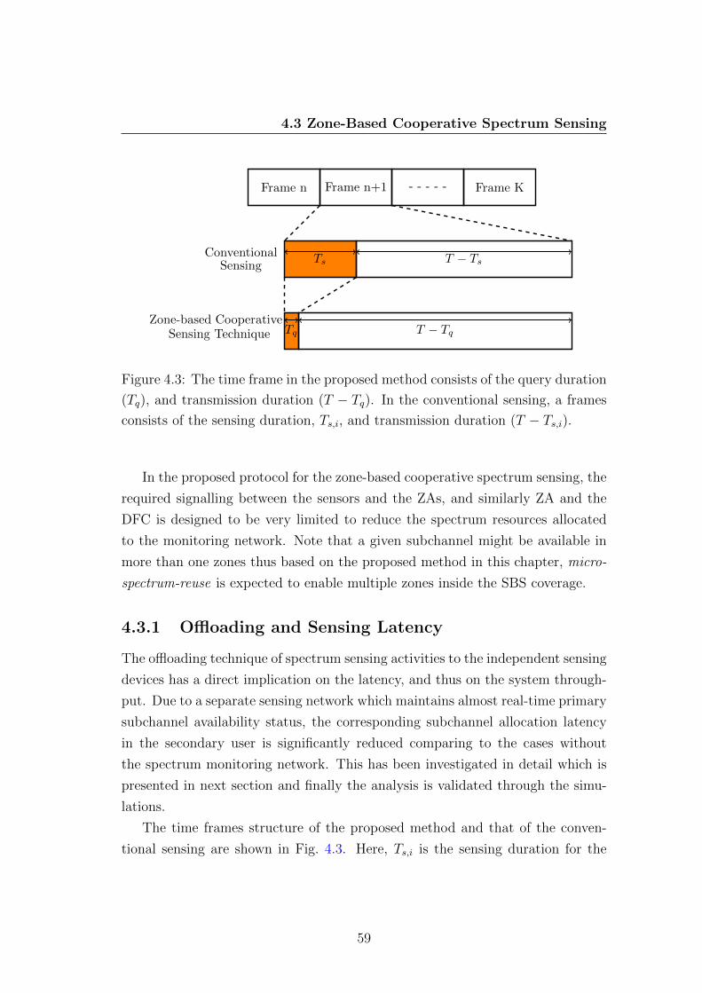
4.3 Zone-Based Cooperative Spectrum Sensing
Frame n Frame n+1 - - - - - Frame K
Ts T − Ts
Tq T − Tq
ConventionalSensing
Zone-based CooperativeSensing Technique
Figure 4.3: The time frame in the proposed method consists of the query duration
(Tq), and transmission duration (T − Tq). In the conventional sensing, a frames
consists of the sensing duration, Ts,i, and transmission duration (T − Ts,i).
In the proposed protocol for the zone-based cooperative spectrum sensing, the
required signalling between the sensors and the ZAs, and similarly ZA and the
DFC is designed to be very limited to reduce the spectrum resources allocated
to the monitoring network. Note that a given subchannel might be available in
more than one zones thus based on the proposed method in this chapter, micro-
spectrum-reuse is expected to enable multiple zones inside the SBS coverage.
4.3.1 Offloading and Sensing Latency
The offloading technique of spectrum sensing activities to the independent sensing
devices has a direct implication on the latency, and thus on the system through-
put. Due to a separate sensing network which maintains almost real-time primary
subchannel availability status, the corresponding subchannel allocation latency
in the secondary user is significantly reduced comparing to the cases without
the spectrum monitoring network. This has been investigated in detail which is
presented in next section and finally the analysis is validated through the simu-
lations.
The time frames structure of the proposed method and that of the conven-
tional sensing are shown in Fig. 4.3. Here, Ts,i is the sensing duration for the
59
4.4 Sensing Design
conventional spectrum sensing and Tq is the duration of the required communica-
tion between the secondary system and the secondary base station. Hereafter, we
refer to Tq as the query time, where Tq << Ts,i. The low latency of the proposed
signalling method is due to substituting the sensing duration Ts,i with Tq. The
extra transmission time, Ts,i − Tq, results in increasing the total system spectral
efficiency and its corresponding cost is deploying the spectrum monitoring net-
work. Therefore, careful analysis is required to evaluate whether the gain on the
spectral efficiency dominates the costs of deploying the monitoring network.
Without sensing devices, a portion of the frame duration, i.e., Ts,i, must be
sacrificed for spectrum sensing by the SUs. As a result, a shorter time is available
to the SUs for data transmission. Therefore, offloading the sensing task to the
sensing devices significantly increases transmission durations without reducing
the sensing accuracy. The optimal sensing duration, Ts,i is not defined in WRAN
standard [35], however it is shown in [43] that the optimalTs,iT
is 4% to 5%. In
the proposed method, TqTs,i
is chosen to be less than 1%.
Because of the independent spectrum sensing network, the sensing devices are
able to sense the subchannel throughout the frame duration. Therefore, using
the zone-based cooperative sensing protocol enables simultaneous sensing, in the
monitoring network, and data transmission at the secondary system. In this case,
the only time interval required for obtaining the availability of the subchannel is
Tq which is the duration of signalling between REQ messages sent by the SU and
RES message sent by the DFC. The signalling duration in the proposed method is
a very small fraction of sensing duration of the conventional approach of spectrum
sensing.
4.4 Sensing Design
4.4.1 Spectrum Sensing Accuracy
Inaccurate sensing either negatively affects the primary system performance through
creating interference (in cases of miss detection), or results in a lower spectral effi-
ciency in the secondary network by missing an actual access opportunity (in cases
60
4.4 Sensing Design
of false alarm). To investigate the sensing accuracy, here it is simply assumed
that the sensors are uniformly distributed in the network coverage area.
Lemma 4.1. In a monitoring network with Z ZAs/cell indexed by z = 1, . . . , Z
and M cooperative SBS indexed by m = 1, . . . ,M , the probability of accurate
sensing for equiprobable hypotheses subchannels [121], i ∈ {1, . . . , N}, at the SBS
is:
P(SBS)cs,i
∆= 1−
[{1− Pd(εi, Ts,i)
}Z+
{Pf(εi, Ts,i)
}Z]M,∀i. (4.4)
Proof. See Appendix A.
Remark 4.1. The probabilities for hypotheses H0, and H1 are denoted by PH0,
and PH1, respectively. Equiprobable subchannel assumption indicates that half
of the channels are busy at any observation window. However, the analytical
and simulation results in the next sections in this paper are equally credible for
other scenarios, for instance, unutilized, i.e., PH0 << 0.5, underutilized, i.e.,
PH0 > 0.5, and crowded, i.e., PH0 > 0.9 subchannels. This assists obtaining
analytical solutions in terms of detection threshold, and normalized throughput
later in this Thesis.
Here, Lemma 1 indicates that Pcs,i depends on probabilities of miss detection
and false alarm, as well as the number of ZAs and sensors in each zone. This
provides two new degrees of freedom which could be exploited to improve the
sensing accuracy. In practical systems, the summation of the two terms inside
the bracket in (4.4) constitutes a small value for a given sensing device. This is due
to the fact that miss detection and false alarm probabilities cannot independently
adopt arbitrary values as they follow the corresponding sensors’ ROC.
Note that in (4.4), Pcs,i ∈ [0, 1] which can be obtained by varying the operating
points in ROC curve within the limits, i.e., Pm(εi, Ts,i) ≤ 0.5, and Pf(εi, Ts,i) ≤0.5. These cases will be considered as constraints while formulating the optimiza-
tion problem P1. By applying these constraints, it is assured that the probability
of correctly sensing the subchannel stays within the feasible range and therefore
61
4.4 Sensing Design
value of Pcs,i stays within 0 and 1. This also ensures the protection from sys-
tem failure due to the bad detectors. Therefore, the worst detection cases, e.g.,
Pf(εi, Ts,i) ≥ 0.5 and Pm(εi, Ts,i) ≥ 0.5, are excluded in the proposed method. As
a result, if a subchannel is badly detected, the resources will not be allocated by
the SBS to any user to protect the primary users from probable interference.
4.4.2 Optimal Sensing to Improve Spectral Efficiency
Here, the system function as an optimization problem is formulated with the
objective of maximizing the spectral efficiency at the secondary system. In ad-
dition, R00i , and R01
i are the SUs’ throughput conditioned over hypotheses H0,
and H1, respectively. Therefore, based on conditional probability of correctly
sensing the subchannel and [43], [53], the achievable throughput is obtained
asT−Ts,iT
(Pcs,i|H0PH0R
00i + Pcs,i|H1PH1R
01i
). Assuming equiprobable hypothesis in
which PH0 = PH1 as in [121], the secondary system throughput for subchannel i
is reduced as following.
R(εi, Ts,i) =T − Ts,i
TPH1
[Pcs,iR
00i + Pcs,iR
01i
],∀i. (4.5)
Here, Pcs,i represents the measure of spectral efficiency of the secondary system.
A higher sensing accuracy contributes towards a higher spectral efficiency thus
improves the system throughput.
For a special case of Z = M = 1, using (4.4) and (4.5) the total secondary
system throughput, R(εi, Ts,i), is
T − Ts,iT
PH1
[(1− Pf)R
00i + (1− Pf)R
01i −KL
], (4.6)
where, KL = PH1 [(1− Pd)R00i + (1− Pd)R01
i )] is the throughput loss due to the
miss detection (Pm > 0). Note that if Pm → 0, then KL → 0.
For given values of Z and M , the optimal sensing parameters are obtained
via the following optimization problem.
62

4.4 Sensing Design
Problem P1:
maxεi,Ts,i
R(εi, Ts,i), (4.7a)
s.t. Ip(εi, Ts,i) ≤ Ith, (4.7b)
Pm(εi, Ts,i) ≤ Pm, (4.7c)
Pf(εi, Ts,i) ≤ Pf, ∀i, (4.7d)
where
Ip(εi, Ts,i) =∑
i
Pm,i(εi, Ts,i)Pt,s gi (4.8)
is the aggregated interference received at the PUs. For subchannel i, (4.7b)
ensures that the received interference remains below the given threshold level, I th.
This will protect the PUs against the potential sensing errors [122]. In addition,
the minimum detection probability of “spectrum holes” is enforced by (4.7c) and
(5.17a). In P1, Pt,s is the SU’s maximum transmit power, gi is the channel gain
between the secondary transmitter and the primary receiver, and Pm, and Pf are
the maximum miss detection, and false alarm probabilities, respectively. These
parameters are provided by the related communication standards, see, e.g., [35].
In P1, PH0R00i +PH1R
01i is constant during a time frame duration, T . Moreover,
in the proposed method, Ts,i = Tq � T , thereforeT−Ts,iT
is almost constant (See
Fig. 4.3) which is referred to as TTx throughout this Thesis. Consequently, the
only optimization parameter in P1 is Pcs,i, which is a function of εi, and Ts,i.
Based on the above, P1 is then reduced to the following optimization problem.
Problem P2:
maxεi,Ts,i
1−[{
1− Pd(εi, Ts,i)
}Z+
{Pf(εi, Ts,i)
}Z]M, (4.9a)
s.t.∑
i
Pm(εi, Ts,i)Pt,sgi ≤ Ith, (4.9b)
Pm(εi, Ts,i) ≤ Pm, (4.9c)
Pf(εi, Ts,i) ≤ Pf , ∀i. (4.9d)
The following set of Lemmas are needed for further analysis to obtain the
solutions of P2. It is also due to the fact that (4.9c) and (5.17b) are the proba-
bilistic constraints which make the optimization problem difficult to handle, thus
63

4.4 Sensing Design
difficult to obtain the closed form solution. Therefore, it is necessary to find the
equivalent approximation with the deterministic nature with the help of following
Lemmas.
Lemma 4.2. If Pm(εi, Ts,i) ≤ 0.5, and Pf(εi, Ts,i) ≤ 0.5, then σ2w ≤ εi ≤ (1 +
γi)σ2w.
Proof. See Appendix B.
Here, the necessary conditions to maximize the system throughput are there-
fore Pd(εi, Ts,i) ≥ 0.5 and Pm(εi, Ts,i) ≤ 0.5 must be maintained at the cognitive
radio system. Moreover, they also exactly follow the requirements of one of the
cognitive radio standards, i.e., IEEE 802.22, in practice.
Lemma 4.3. For a fixed, Ts,i, and εi ≥ σ2w, Pf(εi, Ts,i) is a decreasing and convex
function of εi.
Proof. See Appendix C.
Lemma 4.4. For a fixed Ts,i, εi ≤ (1 + γi)σ2w, Pm(εi, Ts,i) is an increasing and
convex function of εi.
Proof. See Appendix D.
Using Lemmas 4.2 - 4.4, the probabilistic constraints in (5.17b) and (4.9c) are
approximated by σ2w ≤ εi ≤ (1 + γi)σ
2w.
Using Lemmas 4.2, 4.3 and 4.4 it is straightforward to prove the following
Lemma.
Lemma 4.5. For a given Ts,i, if Pm(εi, Ts,i) ≤ 0.5, and Pf(εi, Ts,i) ≤ 0.5, then
Pm(εi, Ts,i), and Pf(εi, Ts,i) are both convex functions of εi.
It is now important to examine the convexity of the constraints defined in P2
to further generalize the problem [123]. Therefore, the following Lemma is also
needed for further simplification of P2.
64

4.4 Sensing Design
Lemma 4.6. Lemma 6: For σ2w ≤ εi ≤ (1 + γi)σ
2w, Pm(εi, Ts,i) and Pf(εi, Ts,i)
are decreasing convex functions of Ts,i.
Based on Lemmas 4.2 - 4.5, it can be easily concluded that both Pm(εi, T s,i)
and Pf(εi, T s,i) are convex functions of εi, where sensing duration is fixed at
T s,i under the conditions to protect the PUs. Here, the conditions to maximize
the throughput are: Pd(εi, Ts,i) ≥ 0.5, and Pm(εi, Ts,i) ≤ 0.5, which are the
requirements of IEEE 802.22 standards [35].
Based on the above, P2 is approximated as the following.
Problem P3:
maxεi
1−[{
1− Pd(εi)
}Z+
{Pf(εi)
}Z]S, (4.10a)
s.t.∑
i
Pm(εi, Ts,i)Pt,sgi ≤ I th, (4.10b)
σ2w ≤ εi ≤ (1 + γi)σ
2w, ∀i. (4.10c)
In P3, (4.10c) is convex under the stated conditions in Lemmas presented
above. The interference constraint at the PU, (4.10b), is due to the imperfect
channel sensing, where |gi|2 is the gain of subchannel i. Here, Pt,s > 0 is the
transmission power of the SU and Pm,i(εi, T s,i) is a convex function of εi under
the condition given in Lemma 4.2. Since non-negative sum of convex functions
is a convex function in the same domain, the interference constraint is also a
convex function of εi. To show the convexity of P3, it is further needed to inves-
tigate (4.10a). Note that throughout this chapter Pm(f)(εi, T s,i) and Pm(f)(εi) are
interchangeably used for brevity.
Corollary 4.1. In the zone-based cooperative spectrum sensing, for any combi-
nation of M and Z, the throughput, (4.10a), is a concave function of εi .
Proof. See Appendix E.
Based on the above, P3 is a convex optimization problem.
65

4.4 Sensing Design
4.4.3 Optimal Detection Threshold
When the spectrum sensing problem is a linear programming problem, several
established methodologies to solve such problems, such as simplex and interior
point methods, do exist. However, even when the optimization problem is non-
linear but its convexity could be established, as explained in the previous sections
for the current system model, several known methods can be employed to solve
such problems. One of the examples is of course to use the Lagrangian duality
method, where local optimal is also the global optimal solution, usually with
the application of Karush-Kuhn-Tucker (KKT) conditions [124]. Therefore, the
Lagrangian method is implemented here to find the solutions of P3 and the La-
grange duality property is applied as described in [125]. The Lagrangian function
corresponding to P3 is
L(εi, λ1,λ2,λ3) =1−[{
1− Pd(εi)
}Z+
{Pf(εi)
}Z]M
+ λ1(Ith −N∑
i=1
PmPt,s gi) +N∑
i=1
λ2i(εmax − εi)
+N∑
i=1
λ3i(εi − εmin),
(4.11)
where, εmax = (1+γi)σ2w, εmin = σ2
w, and λ1, λ2, λ3 are non-negative Lagrangian
dual variables corresponding to the constraints. Here, λ1 is scalar because sub-
channel i accessed exclusively by only one PU. The interference constraint pro-
tects the PUs on subchannel i = 1, . . . , N in case of miss detection. Similarly,
λ2 and λ3 are the Lagrangian multipliers associated with detection threshold
constraints. Throughput this Thesis, vectors are presented using bold fonts.
The corresponding duality gap is expected to be zero as P3 is convex and the
Slater’s condition [125] is satisfied. The KKT conditions for any set of ε∗i , λ1, λ2,
66

4.4 Sensing Design
λ3 are [125]:
∇L(ε∗i , λ∗1,λ
∗2,λ
∗3) = 0, (4.12a)
I(ε∗i ) ≤ Ith, (4.12b)
λ∗1 > 0,λ∗2 � 0,λ∗
3 � 0, (4.12c)
λ∗1(Ith −N∑
i=1
Pm,iPtx gi) = 0, (4.12d)
N∑
i=1
λ2i(εmax − ε∗i ) = 0, (4.12e)
N∑
i=1
λ3i(ε∗i − εmin) = 0, ∀i. (4.12f)
Here, a similar approach as in [122] is followed to obtain the solutions. If the
condition σ2w < εi < (1 + γi)σ
2w holds, the constraint (4.12b) becomes linear, i.e.,
I(ε∗i ) = Ith. Therefore, for any λ∗1 ≥ 0, λ∗1(Ith − I(ε∗i )) = 0.
The complementary slackness conditions in (4.12e) and (4.12f) are further
analysed. From (4.12e), for λ∗2i > 0 for any subchannel, εmax − ε∗i = 0, the
optimal detection value, ε∗i , is equal to εmax. For cases where λ∗2i = 0 for any
subchannel i, then (εmax − ε∗i ) > 0, therefore ε∗i < εmax. Similar observation on
(4.12f) results in ε∗i > εmin. Under the same condition, λ∗3i = 0 for any channel,
i = {1, . . . , N}. However, this assumption may not be correct anymore in case
of ε∗ /∈ [εmin, εmax], since the optimization problem is exclusively convex within
this interval.
In the considered multi-channel scenario, it is now assumed that the subchan-
nels are identically distributed and sensed similarly, thus the results obtained are
valid for all subchannels, i ∈ {1, . . . , N}. Therefore, the subchannel index i is
dropped hereafter for brevity. From the Lagrangian stationary point, (4.12a), is
∂L(ε∗, λ∗1,λ∗2,λ
∗3)
∂ε= 0. (4.13)
If both Z and M vary, then it is not easy to obtain a closed form solution for
P3. Instead, this problem is solve separately for different numbers of Z and M
67

4.4 Sensing Design
Table 4.1: The optimal SNR threshold for different scenarios
Scenario 1
(Z = 1, M = 1)
εX = σ2w
2γ
[γc + 2
fsTsln(
TTx
TTx+λ1Pt,s g
)]
Scenario 2
(Z = 2, M = 1)
εX = σ2w
2γ
[γc + 2
fsTsln
(2PfTTx
2PmTTx+λ1Pt,s g
)]
Scenario 3
(Z = 3, M = 1)
εX = σ2w
2γ
[γc + 2
fsTsln
(3P
2
fTTx
3P2
mTTx+λ1Pt,s g
)]
Scenario 4
(Z = 1, M = 2)
εX = σ2w
2γ
[(γ + 1)2 − 1 + 2
fsTs× ln
(2(Pm+Pf)TTx
2(Pm+Pf)TTx+λ1Pt,s g
)]
Scenario 5
(Z = 1, M = 3)
εX = σ2w
2γ
[(γ + 1)2 − 1 + 2
fsTs× ln
(3(Pm+Pf)
2TTx
3(Pm+Pf)2TTx+λ1Pt,s g
)]
similar to the approach used in proving Corollary 4.1. Here, εM is obtained which
is defined as sensing detection threshold for all subchannels, where M is constant.
Similarly, εZ is then obtained which is defined as sensing detection threshold for
all subchannels, where Z is constant. The optimal detection threshold will be
shown to be a linear combination of εM and εZ .
The optimal detection threshold for various design scenario has been summa-
rized in Table 4.1 where εX is either εZ or εM . In the following, each scenario
shown in the table will be investigate in detail for further analysis and to obtain
the closed form optimal solution.
68

4.4 Sensing Design
4.4.3.1 Scenario 1 (Z = 1,M = 1)
In this case, (4.13) is rewritten as
∂L1(ε∗, λ∗1)
∂ε=∂
∂ε
(TTx
[1− (Pm(ε) + Pf(ε))
]
+ λ1(Ith − Pm(ε)Pt,s g)
)= 0,
(4.14)
which results in the following equation.
TTx∂Pd(ε)
∂ε+ λ1Pt,s
∂Pd(ε)
∂ε= TTx
∂Pf(ε)
∂ε. (4.15)
To derive the solution in terms of detection threshold, ∂Pd(ε)∂ε
and ∂Pf(ε)∂ε
are
utilized which have been obtained in Lemma 4.3, and Lemma 4.4, respectively.
For a given Ts, straightforward mathematical derivations result in a closed form
expression for the optimal SNR threshold for all subchannels.
ε∗M(Z) =σ2w
2γ
[γc +
2
fsTsln
(TTx
TTx + λ1Pt,s g
)], (4.16)
where γc = (γ + 1)2 − 1.
4.4.3.2 Scenario 2 (Z = 2,M = 1)
In this case, similar to (4.14) and (4.15) and straight mathematical derivation,
following is easily obtained.
∂L2(ε∗i , λ∗1)
∂εi=
∂
∂εi
(TTx[1− (P2
m(εi) + P2f (εi))
]+ λ1(Ith − Pm(εi)Pt,s gi)
)= 0,
(4.17)
∂L2(ε∗, λ∗)
∂ε=∂
∂ε
(TTx[1− (P2
m(ε) + P2f (ε))
]
+ λ1(Ith − Pm(ε)Pt,s g)
)= 0,
(4.18)
69

4.4 Sensing Design
ε∗M =σ2w
2γ
[(γ + 1)2 − 1 +
2
fsTsln
(ZPZ−1
f TTx
ZPZ−1m TTx + λ1Pt,s g
)]. (4.17)
ε∗Z =σ2w
2γ
[(γ + 1)2 − 1 +
2
fsTsln
(M(Pm + Pf)
M−1TTx
M(Pm + Pf)M−1TTx + λ1Pt,s g
)]. (4.18)
which results in the following equation.
TTx
[− 2Pm
∂Pd(ε)
∂ε+ 2Pf
∂Pf(ε)
∂ε
]= λ1Pt,s g
∂Pf(ε)
∂ε. (4.19)
Following the same line of argument as in deriving (4.16), the optimum SNR
threshold is then obtained for any subchannel as following.
ε∗M =σ2w
2γ
[γc +
2
fsTsln
(2PfTTx
2PmTTx + λ1Pt,s g
)]. (4.20)
Here, ε∗M is the optimum SNR threshold valid for the frame duration T .
4.4.3.3 Scenario 3 (Z = 3,M = 1)
Similar to the above, it can be obtained as
ε∗M =σ2w
2γ
[γc +
2
fsTsln
(3P2
f TTx
3P2mTTx + λ1Pt,s g
)]. (4.21)
Finally based on the results above, and following the same line of argument
as in Corollary 4.1, for a fixed M and any number of ZAs, i.e., z = 1, . . . , Z, the
optimal SNR threshold can be generalized as shown in (4.17).
4.4.3.4 Scenario 4 (Z = 1,M = 2)
In this case, at a particular time and location, a SBS may receive sensing in-
formation from more than one ZAs. In this scenario, similar to the case where
70
4.4 Sensing Design
Z is variable, Lagrangian stationary point is used as mentioned in (4.12a). For
M = 2, it is simple to show that
ε∗Z =σ2w
2γi
[(γ + 1)2 − 1 +
2
fsTs× ln
(2(Pm + Pf)TTx
2(Pm + Pf)TTx + λ1Pt,s g
)]. (4.19)
4.4.3.5 Scenario 5 (Z = 1,M = 3)
Similar to the previous cases, the optimal threshold can be obtained for different
values of M , for instance M = 3. Finally, following the same steps as in obtaining
(4.17), the generalized optimal solution for any number of SBSs as shown in (4.18).
Note that in (4.16)-(4.19), the miss detection and false alarm maximum tol-
erable values are selected such that Pm < 0.5, and Pf < 0.5 as described in the
previous Section.
4.4.4 Unified Detection Threshold
As it is seen above, the optimal values of detection thresholds, ε∗M and ε∗Z , both
depend on Z and M . In addition, due to the random nature of wireless channel
the exact number of sensing devices that their sensing information received at
ZA cannot be considered fixed. For instance, some sensing devices may fail to
communicate with the ZAs and apparently with SBS. In some cases, the commu-
nication channel between sensing devices may also undergo deep fading in which
the sensing network scenario is changed. Therefore, a unified detection mode
is necessary so that the proposed technique works for any possible scenario and
various combinations of Z and M . Here, a linear combination of ε∗M and ε∗Z is
proposed as described below.
ε∗ = αε∗M + (1− α)ε∗Z , (4.20)
where α is directly related to the network structure, i.e., Z and M : if Z < M then
α is 0 < α < 0.5 to emphasize on the contribution of ε∗Z comparing to ε∗M in (4.20).
This is simply because ε∗Z is the detection threshold for cases, where Z < M . In
contrast, where Z > M , system sets 0.5 < α < 1, so ε∗M contributes more than
ε∗Z in ε∗. However, in cases where Z and M are equal, system sets α = 0.5 and
71
4.4 Sensing Design
apparently ε∗M and ε∗Z contribute equally in (4.20). In the simulations presented
later in this chapter, system selects α within the ranges mentioned above based
on the densities of Z and M , for instance, when Z � M , α is selected on the
lower range of 0.5 < α < 1. For the cases where M = 0, and Z = 0, the system
sets α = 1, and α = 0, respectively.
In cases where due to the random time varying nature of wireless communi-
cation, such as channel fading, interference, hidden terminal problem, etc., either
or both of Z and M are equal to zero, then the optimal detection threshold is
undefined because ε∗M and ε∗Z are −∞. As a matter of fact, this situation does
not normally occur in the proposed model of zone-based cooperative spectrum
sensing but should be considered as a special case to avoid singularities. Here
the proposed method has a specific treatment to tackle such issues as described
in the following.
According to (4.17) and (4.18), M = 0, and Z = 0 indicate ε∗Z → −∞, and
ε∗M → −∞, respectively. At the same time, the sensing system controls α to avoid
such a condition. Therefore, for M → 0, sensing system sets α ≈ 1. Therefore,
limM→0
ε∗Z(M).(1− α) ≈ 0, (4.21)
which indicates that optimal detection threshold solely depends on the ε∗M in
(4.20). Similarly, if Z → 0, the sensing system selects α ≈ 0, thus,
limZ→0
ε∗M(Z).(α) ≈ 0, (4.22)
i.e., the optimal detection threshold solely depends on the ε∗Z in (4.20). Using
this method, it is now possible to obtain a unified version of optimal spectrum
sensing threshold.
In the next section, a step by step algorithm is discussed for obtaining an
estimation for ε∗ based on the above analysis. In obtaining the optimal detec-
tion threshold which maximizes the system throughput, the bisection method is
implemented.
72
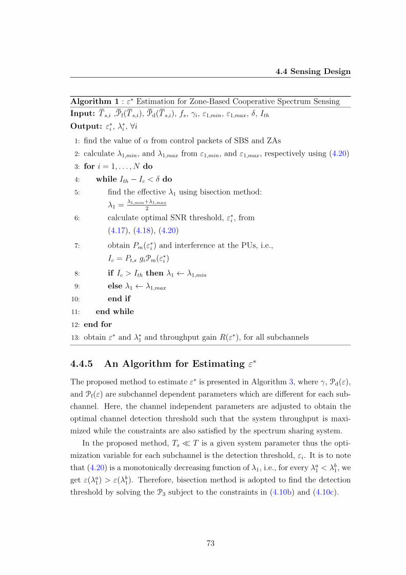
4.4 Sensing Design
Algorithm 1 : ε∗ Estimation for Zone-Based Cooperative Spectrum Sensing
Input: T s,i ,Pf(T s,i), Pd(T s,i), fs, γi, ε1,min, ε1,max, δ, Ith
Output: ε∗i , λ∗i , ∀i
1: find the value of α from control packets of SBS and ZAs
2: calculate λ1,min, and λ1,max from ε1,min, and ε1,max, respectively using (4.20)
3: for i = 1, . . . , N do
4: while Ith − Ic < δ do
5: find the effective λ1 using bisection method:
λ1 =λ1,min+λ1,max
2
6: calculate optimal SNR threshold, ε∗i , from
(4.17), (4.18), (4.20)
7: obtain Pm(ε∗i ) and interference at the PUs, i.e.,
Ic = Pt,s giPm(ε∗i )
8: if Ic > Ith then λ1 ← λ1,min
9: else λ1 ← λ1,max
10: end if
11: end while
12: end for
13: obtain ε∗ and λ∗1 and throughput gain R(ε∗), for all subchannels
4.4.5 An Algorithm for Estimating ε∗
The proposed method to estimate ε∗ is presented in Algorithm 3, where γ, Pd(ε),
and Pf(ε) are subchannel dependent parameters which are different for each sub-
channel. Here, the channel independent parameters are adjusted to obtain the
optimal channel detection threshold such that the system throughput is maxi-
mized while the constraints are also satisfied by the spectrum sharing system.
In the proposed method, Ts � T is a given system parameter thus the opti-
mization variable for each subchannel is the detection threshold, εi. It is to note
that (4.20) is a monotonically decreasing function of λ1, i.e., for every λa1 < λb1, we
get ε(λa1) > ε(λb1). Therefore, bisection method is adopted to find the detection
threshold by solving the P3 subject to the constraints in (4.10b) and (4.10c).
73

4.5 Simulation Results and Analysis
4.5 Simulation Results and Analysis
In this section, the performance of the proposed zone-based cooperative spec-
trum sensing is evaluated under various network settings and parameters with
the help of the simulation tools. Further comparisons will be presented regard-
ing the performance of the proposed method against the benchmark systems.
The first benchmark model is the case where there is no cooperation among the
clusters/SBS, and the second benchmark network setting is when the decisions
are diffused at the central entity using the OR/AND rule. The corresponding
resource allocation framework in terms of latency, detection probability, commu-
nication activity of primary systems etc. are then compared. The considered
system is a cognitive radio system, where N = 16 and T = 100 ms. The mean
signalling duration for each SU, E[Ts,i], is maintained at 2 ms. The sampling rate
is fs = 20 kSample/Second and therefore the sampling overhead is fsTs,i = 60
and σ2w = 1 is also considered.
It is further assumed that the subchannels are equiprobable such that PH0 =
0.5. The traffic on the subchannels is randomly generated and SUs always have
data packets ready to be transmitted unless otherwise stated. The subchannels
between primary and secondary systems are modelled as Rayleigh fading with
scale parameter of 1. The primary channel protection and spectrum utilization
level are defined according to the IEEE 802.22 standard [35] as Pd ≥ 0.9, and
Pf ≤ 0.1, respectively. The parameters have been chosen following the available
standards for cognitive radio standard as explained in Section 3.4.
4.5.1 Comparative Study of Sensing Accuracy
The proposed zone-based cooperative spectrum sensing, as defined in (4.4), is
validated by considering the appropriate value of probability of detection which
fulfils the requirement of constraint (4.7c) as well as the cognitive radio standard
for WRAN, i.e., IEEE 802.22. Moreover, the false alarm probability is obtained
from the corresponding ROC curve which is the basis of the performance indicator
in spectrum sensing. Therefore, the instantaneous Pd and Pf pair is chosen for
74

4.5 Simulation Results and Analysis
a given combination of M and Z to test the spectrum sensing accuracy of the
proposed method.
For comparison, Z = 1 is considered as the conventional cooperative spectrum
sensing based on Lemma 4.1 at the SBSs and therefore there is no subchannel
reusability. The case of higher Z represents the special scenario that the multiple
antennas are transmitting at the BSs and the cell is divided into sectors. In this
case, each sector can be considered as a single antenna cell and therefore number of
ZAs and SBSs are increased. The case Z = 1 will be considered as a benchmarking
scenario for comparison. In Fig. 4.4, the normalized system throughput, which
is directly related to the system spectral efficiency, is plotted versus the number
of zone aggregators for different number of SBSs. Here, it is seen for the case
Z = 1 that the normalized throughput is 0.6 whereas in a zone-based cooperative
spectrum sensing method as indicated by Z ≥ 2, it is significantly improved from
0.9 to 0.96 when ZAs are set to 2 and 3, respectively. This is due to the fact that
the proposed method has better spectrum sensing accuracy due to the higher
number of locally sensing decisions obtained from distributed spectrum sensors
than majority of the conventional cooperative channel sensing techniques.
The higher sensing accuracy ensures that no access to that particular subchan-
nel is granted by the SBS to protect the PUs. The result also provides insight
on the rate of spectral efficiency increased by increasing M as a result of the
proposed micro-spectrum-reuse technique. Here, it is also confirmed in Fig. 4.4
that the increase of normalized throughout from 0.9 to 0.96 when cooperative
SBSs are increased from 2 to 3.
As it is further observed, in cases where there are larger number of ZAs, the
spectral efficiency is relatively higher. It is due to the fact that the number
of spectrum sensors per ZA becomes lower in this scenario. As a result, the
probability of unanimous agreement of subchannels to be available in a zone
is higher due to the implementation of AND rule among less number sensing
devices. It can also be concluded from Fig. 4.4 that when higher number of ZAs
are installed, the number of cooperative SBS does not necessarily need to increase
to achieve better system throughput. This helps to find the optimal number of
zones and SBS to set up within the cell to achieve the objective.
75

4.5 Simulation Results and Analysis
1 2 3 4 5 60.6
0.65
0.7
0.75
0.8
0.85
0.9
0.95
1
Number of ZAs within the transmission range of SBS.
Normalized
system
throughput
Cooperative SBS=2
Cooperative SBS=3
Cooperative SBS=4
Cooperative SBS=5
Figure 4.4: Normalized throughput vs. different values of Z and M .
Fig. 4.5 compares the spectrum sensing accuracy of the proposed method
against the non-cooperative technique as well as the subchannel assignment with
cooperative sensing [126] in which the OR fusion method is implemented for vari-
ous received SNR. It is obvious that the performance gain in terms of the sensing
accuracy is achieved with the expense of installing new sensing infrastructure,
however it brings multiple advantages in the proposed network scenario. In ad-
dition to sensing accuracy as shown in Fig 4.5, it also increases the transmission
duration for the SUs which contributes to achieve higher aggregated throughput
at the secondary system with reduced system complexity.
In this particular case, the simulation is performed for AWGN channel using
QPSK modulation with sampling overhead Ts,ifs = 100 and Pf is no more than
0.1. The sensing network has been created by setting Z = 3 and M = 2 for the
proposed method. In addition, there are 3 cooperative sensors installed for OR
76

4.5 Simulation Results and Analysis
−14 −12 −10 −8 −6 −4 −2 0 20
0.1
0.2
0.3
0.4
0.5
0.6
0.7
0.8
0.9
1
Average received SNR (dB) at the spectrum sensors
Pro
babilitiesofco
rrectsensing(ordetection)
Correct sensing(Pcs)-proposed
Detection-OR combining
Detection-single sensor
Figure 4.5: Probability of correctly detecting the subchannels vs. average received
SNR when false alarm rate is fixed.
fusion method. It can be observed in figure that the correctly sensing probability
of the proposed method is improved to 0.99 in comparison to 0.6 in case of non-
cooperation sensing technique and 0.85 in case of hard decisions are aggregated
with OR fusion method at −4 dB received SNR.
However the sensing performance at higher SNR, i.e., greater than 0 dB in
the considered scenario, is observed to be similar in all three cases, this situation
cannot be guaranteed in wireless communication due to the severe fading and
hidden terminal problems. Moreover, energy detection performs better in such
ideal case of higher SNR. Therefore, the sensing efficiency of the proposed method
is higher than other two references cases in low received SNR regimes.
77

4.5 Simulation Results and Analysis
4.5.2 Tradeoff Between Sensing Latency and Detection
Threshold
In Fig. 4.6, the optimal spectrum detection threshold, ε∗, is plotted versus sensing
duration at the spectrum sensors for different values of maximum acceptable miss
detection probability, where one ZA aggregates subchannel availability informa-
tion from four spectrum sensing devices. The threshold in fact determines the Pm
and Pf pair for the proposed sensing method and thus the system performance.
As it is seen, for long sensing duration in the secondary system, obtaining the
optimal detection threshold deems irrelevant and not related to the maximum
acceptable miss detection probability. However in the proposed method, the
sensing duration is represented by the short signalling duration, i.e., less than
2 ms in Fig. 4.6, the optimal detection threshold must be obtained to improve
the system throughput. Therefore, the length of transmission duration does not
need to be compromised whilst latency is significantly reduced.
The obvious tradeoff is to relax the sensing duration (Ts > 2 ms) in which the
transmission duration is shorter, but higher will be the latency associated with
the spectrum sensing. In contrast, the sensing duration, thus the latency, can be
reduced (Ts < 2 ms), where a higher complexity is expected as the appropriate
sensing threshold must be evaluated through the proposed algorithm. Note that
in the proposed method the latency associated with the sensing is very small and
the cost is limited to the corresponding computational complexity required for
evaluating the optimal detection threshold.
4.5.3 Performance Evaluation with Optimal Detection
Here, the performance of the proposed cooperative spectrum sensing method
in terms of probabilities of false alarm and miss detection, thus probability of
correct sensing, is further examined as a function of sensing duration, Ts, i.e.,
equivalently Tq in the proposed method. In the simulation settings, the conditions
in Lemma 4.2 to Lemma 4.5 are strictly held. This means that for the simulated
system, optimization problem P3 is convex thus (4.17) and (4.18) are the optimal
solutions.
78

4.5 Simulation Results and Analysis
0 2 4 6 8 10 12−0.5
0
0.5
1
1.5
2
Sensing duration (msec)
Spectrum
dete
ction
thre
shold
(dBm)
Pm Constraint=0.05Pm Constraint=0.10Pm Constraint=0.15Pm Constraint=0.20Pm Constraint=0.25
Figure 4.6: Optimal spectrum detection threshold vs. sensing duration (latency)
for various miss detection constraints.
In the proposed method, the sensing duration, Ts, is significantly smaller
compared to the frame duration, T , therefore it is independent of the optimization
procedure. However, in the conventional spectrum sharing methods, where SUs
sense and utilize the ideal subchannels, optimal choice of Ts is crucial. Under the
scenario mentioned above, Pm(ε∗), and Pf(ε∗) for an optimal value of detection
threshold have been obtained as shown in Fig. 4.7. While obtaining Pm(ε∗) for an
optimal detection threshold, Pf(ε∗i ) is kept fixed and vice versa. As expected, the
longer the signalling duration, the lower will be the miss detection and false alarm
probabilities. In addition, lowering Ts,i from 9 ms to 6 ms significantly reduces
Pm(ε∗) and Pf (ε∗) for all subchannels. On the other hand, reduction of Ts from
6 ms to 3 ms does not reduce sensing accuracy in the same proportion. This
suggests a way to adjust the signalling duration based on the required spectrum
79
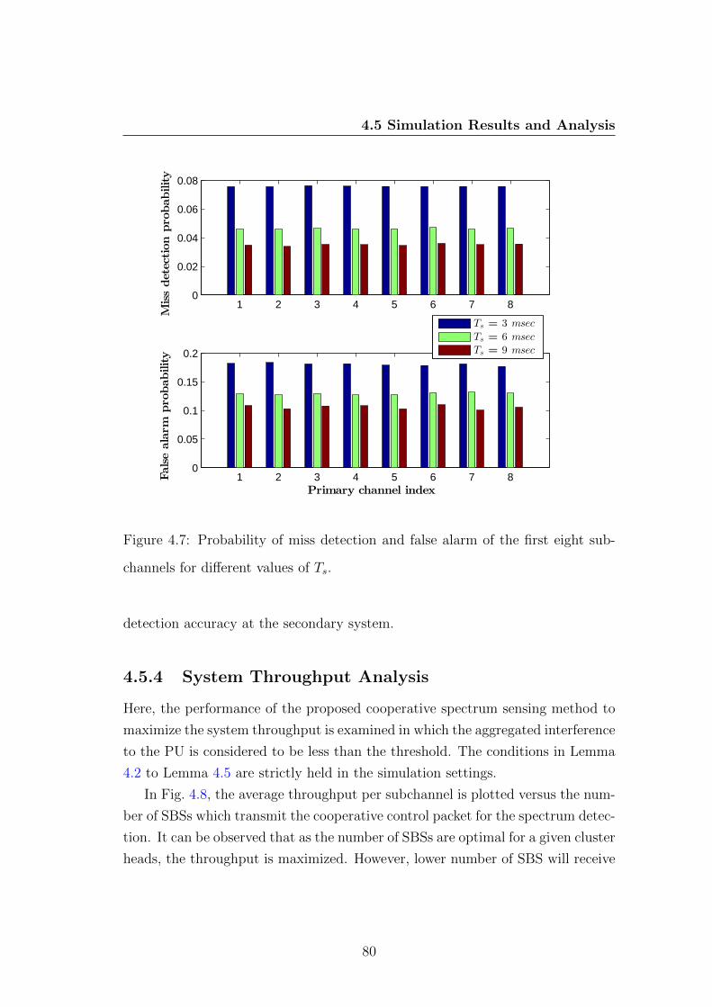
4.5 Simulation Results and Analysis
1 2 3 4 5 6 7 80
0.02
0.04
0.06
0.08
Missdetectionprobability
1 2 3 4 5 6 7 80
0.05
0.1
0.15
0.2
Falsealarm
probability
Primary channel index
Ts = 3 msec
Ts = 6 msec
Ts = 9 msec
Figure 4.7: Probability of miss detection and false alarm of the first eight sub-
channels for different values of Ts.
detection accuracy at the secondary system.
4.5.4 System Throughput Analysis
Here, the performance of the proposed cooperative spectrum sensing method to
maximize the system throughput is examined in which the aggregated interference
to the PU is considered to be less than the threshold. The conditions in Lemma
4.2 to Lemma 4.5 are strictly held in the simulation settings.
In Fig. 4.8, the average throughput per subchannel is plotted versus the num-
ber of SBSs which transmit the cooperative control packet for the spectrum detec-
tion. It can be observed that as the number of SBSs are optimal for a given cluster
heads, the throughput is maximized. However, lower number of SBS will receive
80

4.5 Simulation Results and Analysis
1 2 3 4 5 6 7 83
4
5
6
7
8
9
Number of SBSs transmitting subchannel information (S) to its neighbours
Averagesystem
thro
ughputper
subch
annel
(kbps)
Operating ZAs = 1
Operating ZAs = 3
Operating ZAs = 5
Figure 4.8: The average throughput per subchannel vs. number of SBS.
less information about the subchannel availability and, as a result, the through-
put per subchannel decreases. In addition, when the number of signalling bits
at the SBS increases, secondary system has to perform logical AND operation
among large decision variables which results in detecting less opportunities to
access the primary subchannel.
Furthermore the higher the number of ZAs, the higher is the accuracy of
spectrum sensing. Therefore, the system throughput is increased accordingly.
For a given simulation setup, the increment of ZAs from 1 to 3 significantly
increases per subchannel throughput in comparison to increment from 3 to 5. As
shown in Fig. 4.8, for a network setup of 3 SBSs, the subchannel throughput is
achieved to be 7 kbps which can be increased to 8 kbps by increasing ZAs by 2
within a SBS region. However, further increase in ZAs to 5 does not improve the
throughput at the same rate, i.e., it is just increased by 0.2 kbps by increasing
ZAs to 5. It proves that finding the optimal number of SBSs and ZAs is more
81
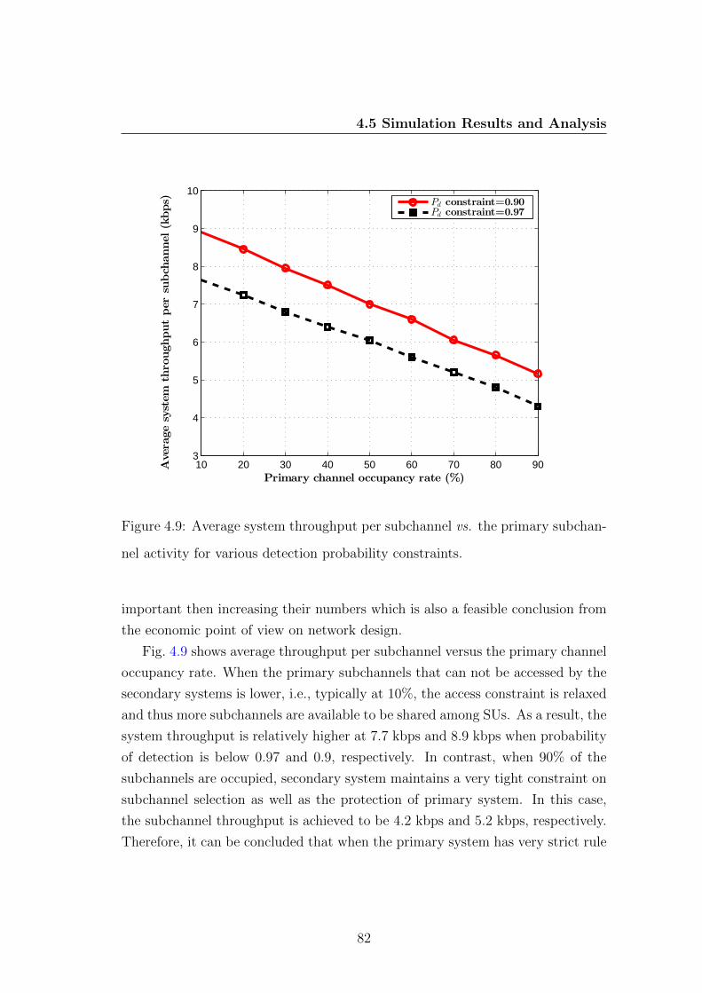
4.5 Simulation Results and Analysis
10 20 30 40 50 60 70 80 903
4
5
6
7
8
9
10
Primary channel occupancy rate (%)
Averagesystem
thro
ughputper
subch
annel
(kbps)
Pd constraint=0.90Pd constraint=0.97
Figure 4.9: Average system throughput per subchannel vs. the primary subchan-
nel activity for various detection probability constraints.
important then increasing their numbers which is also a feasible conclusion from
the economic point of view on network design.
Fig. 4.9 shows average throughput per subchannel versus the primary channel
occupancy rate. When the primary subchannels that can not be accessed by the
secondary systems is lower, i.e., typically at 10%, the access constraint is relaxed
and thus more subchannels are available to be shared among SUs. As a result, the
system throughput is relatively higher at 7.7 kbps and 8.9 kbps when probability
of detection is below 0.97 and 0.9, respectively. In contrast, when 90% of the
subchannels are occupied, secondary system maintains a very tight constraint on
subchannel selection as well as the protection of primary system. In this case,
the subchannel throughput is achieved to be 4.2 kbps and 5.2 kbps, respectively.
Therefore, it can be concluded that when the primary system has very strict rule
82

4.5 Simulation Results and Analysis
0.8 0.82 0.84 0.86 0.88 0.9 0.92 0.94 0.96 0.983
4
5
6
7
8
9
10
Threshold value of probability of detection (Pd)
Averagesystem
thro
ughputper
subch
annel
(kbps)
Pf constraint=0.10Pf constraint=0.20
Figure 4.10: Average system throughput per subchannel vs. the probability of
detection for various false alarm probability constraints.
of interference the secondary systems have to sacrifice a portion of throughput
which can be compensated with the proposed spectrum sensing network.
On further analysis, it can be observed that when the probability of detec-
tion constraint is relaxed, for instance, from 0.97 to 0.9, there is a higher chance
to access the subchannels. In both cases, the subchannel occupancy rate is lin-
early decreased with the increasing primary channel activities. Therefore, for a
particular cellular network scenario, the secondary system throughout cannot be
increased beyond a certain limit depending on nature of primary system.
The subchannel throughput versus the probability of detection constraint, i.e.,
Pd, is given in Fig. 4.10 for various false alarm probabilities. When Pd is main-
tained at the lower value, e.g., at ≈ 0.8, there is higher chance of miss detection
of the subchannel status and therefore the throughput is relatively lower than the
83

4.6 Conclusions
case where Pd is constrained at ≈ 0.9. However, by increasing Pd from 0.9 to 0.97,
the throughput falls down quickly because the detection constraint becomes tight
and smaller number of primary subchannels are available for secondary users. It
has also been observed that as long as Pf remains within the maximum limit
defined in the simulation setup for a given optimal Pd, the throughput is not
significantly degraded even if the false alarm constraint is relaxed from Pf = 0.1
to 0.2. Therefore, along with selection of optimal detection threshold (ε), the
optimal choices of Pd and Pf are always important for the accurate sensing of
the subchannels and efficiently utilizing them. The proposed spectrum sensing
network approach thus helps not only to enhance the performance but also to
choose the accurate network parameters for cellular cognitive radio design and
implementation.
4.6 Conclusions
In this chapter, a new method for multichannel spectrum sensing through an
independent monitoring network has been presented in which the location of the
sensor is partly incorporated into the subchannel allocation. It was also shown
that the proposed zone-based cooperative spectrum sensing method increases
the sensing accuracy which facilitates higher spectrum reusability. The detail
description of spectrum sensing algorithms and signalling protocols which incor-
porate zone location information in the spectrum sensing has been also presented
which enables the micro-spectrum-reuse and results in higher system throughput,
lower signalling overhead, and thus the lower latency. It is obvious that the cost
involved in designing overlaid spectrum sensing network is higher, however the
advantages of spectrum sensing accuracy and subchannels reusability outnumbers
the disadvantages.
An analytical framework is also developed with the objective function to max-
imize the secondary system throughput under various monitoring network scenar-
ios subject to the spectrum sensing accuracy and maximum tolerable interference
imposed at the primary system. Moreover, various required conditions have been
identified and derived mathematically to achieve the optimal solution in the form
84

4.6 Conclusions
of detection threshold. The spectrum sensing accuracy has been derived for vari-
ous configurations of ZAs and SBSs and shown that the optimization problem is
convex under all possible configurations. As a result, a closed form solution for
the optimal sensing threshold value has been successfully determined. Similarly,
the obtained solutions would be linearly combined based on allocated weights to
make the optimal detection threshold valid for possible configurations. It has
been also shown that the proposed method outperforms many conventional coop-
erative sensing techniques in terms of sensing accuracy with the help of numerical
analysis and simulations results.
Higher system throughput is partly due to the extra subchannel reusability
created by exploiting location information of the spectrum sensors through the
micro-spectrum-reuse. In addition, it provided the concept of spectrum sens-
ing network collocated with the cellular CRN system and its design aspect for
next generation network. Using simulations, the sensing accuracy and system
throughput have been evaluated against various network parameters to prove
the efficiency of the proposed method of spectrum sensing. The simulations also
demonstrated the improvement on the spectrum sensing accuracy due to the
proposed method with significantly lower latency and higher system through-
put comparing to the cases without zoning. Furthermore, it is also shown that
when the sensing duration is lowered as described in the proposed method, it
is very important to find the optimal sensing threshold to improve the system
throughput. In addition, there are always optimal numbers of sensing devices to
be installed inside the cellular region in which maximum system throughput is
achieved. The optimal choice of probabilities of miss detection and false alarm
are equally important in the considered spectrum sensing method as described in
this chapter.
This chapter dealt with the spectrum sensing techniques by deploying the
spectrum sensing network to maximize the secondary system throughput. How-
ever, the issues that are frequently faced in CRN, such as modelling the primary
user activity in the subchannels, are not considered in this model. As a matter
of fact, such issue is equally important to be considered in the problem domain
because the activity of primary users put the limitations on the cognitive radio
network due to the imposed interference constraint as well as transmit power
85

4.6 Conclusions
constraint. In the next chapter, a detail mathematical modelling of primary user
activity for the proposed optimal resource allocation techniques will be discussed.
In addition, spectral efficiency and energy efficiency are important measures of
CRN performance. The detail study of such parameters is lacking in this chapter,
which are particularly considered in terms of primary user activity model in the
next chapter. Also, few interesting analytical results and simulations will also be
presented to validate the proposed resource allocation methods.
86

Chapter 5
Resource Allocation in Multicell
Collaborative Cognitive Radio
Networks
When the spectrum sensing is executed by the secondary system to obtain the
channel availability information, they must be efficiently utilized with a minimum
level of transmit power to achieve higher spectral and energy efficiencies. In cog-
nitive radio enabled wireless communications, a secondary network, i.e., cognitive
radio networks, opportunistically accesses the available spectrum initially licensed
to the primary network. As mentioned in the previous chapters, cognitive radio
technique is one of the solutions that has been considered to improve the spectral
efficiency (SE), which is defined as the total capacity normalized by the avail-
able bandwidth measured in bps/Hz, in the cellular band [127]. However, the
main challenge in spectrum sharing is to efficiently exploit the underutilized por-
tions of the primary spectrum without compromising the QoS requirements in
the primary system.
The level of underutilized radio resources available to the cognitive multicell
networks depends on the nature of users communication activities in the primary
system. Several spectrum sharing methods have been defined for the CRNs in-
87

cluding overlay, underlay and a combination of both [22],[128]. In the overlay
spectrum sharing, the secondary system accesses the subchannel only when it
is in idle state. In the underlay method, the secondary system simultaneously
utilizes the subchannel subject to keeping the aggregated interference at the pri-
mary receiver below a predefined threshold. This threshold is a system parameter
which depends on the primary system characteristics [29]. Ideally, to assure the
QoS in the primary system, in overlay (underlay) access, accurate information of
spectrum sensing (perfect channel state information for the channel between the
secondary transmitters and the primary receivers) is a prerequisite. In practice
however, attaining such parameters is very challenging because there is generally
no or very limited resources for inter-system signalling.
On the other hand, the research on energy efficiency (EE) has attracted sig-
nificant attention because of the environmental concern as well as the device
requirements of longer battery life [129]. The impact of the proposed primary
subchannel activity profile on the EE is further investigated on the considered
multicell system. Here, EE measures how efficiently the available energy is uti-
lized to maintain the QoS in the end-to-end communications [130]. The EE metric
can take various forms such as energy-per-bit to noise power spectral density ra-
tio, i.e., Eb/N0, bit per Joule capacity, rate per energy, or Joule per bit, however
they are essentially equivalent and mutually convertible [131]. Both EE and SE
are required to study in a single framework because there is a very strict tradeoff
exist between them such that improvement of one may deteriorate the other [132].
In the considered multicarrier multicell CRN, the coordination among the
neighbouring secondary base stations plays a paramount role in efficient de-
sign of the network-wide optimal assignment of the scarce radio resources [133].
Network-wide resource allocation significantly reduces the impact of intra-system
interference on the overall secondary system performance. It also enables the
secondary system to exploit the temporal variations in the idle or underutilized
spectrum due to the stochastic nature of primary system communication activ-
ity on the subchannels. Exploiting the real-time primary subchannel behaviour,
which is temporal and nondeterministic, can enhance the performance of the radio
resource allocation in the secondary system [94].
88

To characterize the primary users communication activity, Poisson Point Pro-
cess (PPP) based models have been proposed in [134]. However, due to the
dynamic but unpredictable nature of the primary traffic, such models often fail
to apprehend instantaneous primary subchannel activity [86]. Other researchers
propose schemes which are designed to exploit the primary service activity, how-
ever it is usually assumed that the activity information is available to the sec-
ondary system, either through signalling or a priori knowledge, see, e.g., [29]. Yet,
this assumption may not always be valid in practical scenarios where multicell
networks are considered.
In this chapter, the activity levels of primary users on the subchannels are in-
corporated into the transmission power allocation at SBS such that the maximum
possible SE can be achieved. The higher signalling level is expected when sub-
channel activities are necessary to broadcast to the centralized system. However,
the proposed method simplifies the power allocation method in CRN thereby
significantly reducing the signalling overhead. Moreover, when the SE and sub-
channel activity profile are integrated, the objective function is characterized as
a utility function.
On the other hand, the EE as an objective function depends directly on the
level of accuracy of the channel state information (CSI), however such information
may not be available to the SU transmitter [135]. The proposed method in
this chapter addresses the problems due to the unknown channel gain by means
of incorporating the estimated primary users’ activity level on the subchannels
with the minimum signalling overhead. An energy per received bits has been
considered as a metric in [136] as the basis for a resource allocation approach that
adopts the spectrum sharing along with soft-sensing information by adaptively
setting the sensing threshold. Irrespective of the proposed method, the energy
and spectral efficient design for CRN is studied in [137],[138] to optimize one of
them at a time which remains valid for a frame duration.
The accurate prediction of the primary system activity on subchannels is a
function of arrival and departure rate of the PUs in addition to the allocated trans-
mitted power and channel gains, which are random in nature and very difficult to
obtain, if not impossible, in practice. Instead, the subchannel activity index (SAI)
as a new parameter is now defined, which indicates the level of communication
89

activity within the primary subchannels. Therefore, SAI is a probabilistic metric
which is based on the sensing outcomes using energy detection by a limited num-
ber of spectrum decision makers. In this chapter, a novel scheme to evaluate the
aggregated SAI (ASAI) among the SBSs will be presented. The ASAI parameter
is then utilized in an optimal and efficient design of the SU’s transmission power
allocation strategy which maintains better achievable SE and EE such that the
best possible scenario can be obtained from both energy and spectrum utilization
perspectives.
The purpose of the SAI (or ASAI when all the neighbour cells are considered)
is to address the signalling overhead issue in multicell CRN. When the subchan-
nels are found to be underutilized, there is still room, subject to careful and
controlled power allocation, to accommodate secondary users due to low primary
system activity. In a secondary cell covered by a SBS, ASAI carries dual informa-
tion, i.e., firstly, activity of the primary users located in that cell, and secondly,
the primary users accessing the subchannels in the adjacent cells. A combination
of both is utilized in this case to design the efficient resource allocation scheme.
It is therefore proposed a simple, yet efficient, collaborative spectrum monitoring
scheme with very low signalling overhead to estimate the ASAI based on one bit
per subchannel feedback transmitted by the neighbour SBSs as a control packet.
Depending on the ASAI estimation, a very important tradeoff occurs which
has a significant impact on the optimal subchannel and transmit power allo-
cations. In cases where the SBS allocates a higher transmission power to the
subchannels with a higher ASAI, the minimum QoS requirements to the primary
services may be compromised along with significant degradation on EE. On the
other hand, a low utilization of the available spectrum is achieved by allocating a
lower power to a subchannel with a lower ASAI. To model this tradeoff, A notion
of utility function is adopted [139],[140]. For each SU communicating over the
subchannel, two utility functions are then formulated as a decreasing function
of the ASAI and, first, increasing function of the achievable rate and, second,
increasing function of EE for each cognitively utilized subchannel.
At first, optimal power allocation method is formulated in which the objective
is to maximize the total SBS utility, in terms of the SE, subject to total available
transmit power at the SBS and primary system collision probability constraints.
90
Secondly, under the same system settings, the optimal power allocation will be
formulated with the objective of maximizing the total SBS utility, in terms of EE,
subject to the similar constraints described above. The first optimization prob-
lem is non-convex, and the second case is a fractional optimization problem which
can be approximated as quasi-convex under certain assumptions. The formulated
problems are the instances of weighted sum-rate maximization which have been
substantially studied in the related literature, see, e.g., [27],[133],[141],[142] al-
though most of the previous works require accurate channel state information
and/or spectrum sensing, thus need direct inter-system and heavy intra-system
signalling. A unique feature of our proposed method is its very low signalling
overhead which uses only one bit per sunchannel.
The detail comparison of the system performance is discussed in terms of EE
against a cognitive cellular network when there is no signalling among the SBSs
in which the SBS executes equal subchannel power allocation. The significant
sum-rate improvement is confirmed by the simulation results. The sum-rate per-
formance of the proposed method will also be compared with a scenario in which
the combination of underlay and overlay access techniques are adopted, where
perfect knowledge of interference channel state and spectrum sensing information
are available at the SBS. Finally, the energy efficient CRN design under the sim-
ilar network settings will be discussed and obtain the practical network scenario
in which both EE and SE can be optimized. Simulation results also show that the
proposed method closely follows the ideal spectrum access with a slightly lower
achievable rate although the required signalling overhead is significantly reduced.
The major contributions of this chapter are summarised as following.
• The subchannel activity index is first defined and characterized as an in-
dicator of activities level of the primary users in their corresponding sub-
channels. It is then followed by a simple yet efficient collaborative spectrum
monitoring among the base stations to obtain the aggregated SAI (ASAI)
for efficient transmit power allocation at the SBSs which also maintains a
very low signalling overhead among the cellular systems.
• A utility function is defined to incorporate the ASAI into the corresponding
spectral efficiency for all subchannels. The joint efficient transmit power
91

5.1 System Model
and subchannel allocation schemes are then formulated as an optimization
problem in the SBS to maximize the total SBS utility function.
• The further investigation is presented to examine the impact of ASAI into
the energy efficiency on the similar system settings. This case is also handled
in a similar approach to that of the previous one by defining utility function
in terms of energy efficiency to find the efficient transmission power profile.
The obtained solutions can be easily extended to many practical cellular
network scenarios with relevant modifications.
• Finally, a suboptimal subchannel and transmit power allocation schemes
are studied considering both spectral and energy efficiencies using various
mathematical and optimization tools. Moreover, the design technique to
achieve the near optimal spectral and energy efficiencies based on ASAI by
varying the spectrum sensing parameters will be elaborated. The obtained
SE and EE relation based on ASAI in the proposed method is practically
more efficient than the conventional EE and SE tradeoff which is, in most
cases, based on the transmit power. The results are then validated through
the extensive simulations.
In the next section, a brief description of the considered system model in this
chapter will be presented.
5.1 System Model
The considered system includes a cellular CRN which is collocated with a legacy
cellular primary system which is the same as presented in chapter 3 and chapter
4 with some add-on features which are described in this Section. A schematic
of the considered network is presented in Fig. 5.1. In this system model how-
ever, the independent sensing network is optional and therefore the clusters are
not presented. In addition, the subchannel activity information is shared among
the base stations to achieve the parameter known as ASAI. Here, a B Hz fre-
quency band is licensed to the primary system which serves primary users in-
dexed by j ∈ {1, . . . , J}. The spectrum of the primary system is shared with
92

5.1 System Model
SBS0
SBS1
SBS2
PBS
[ δ]T
[ δ ] T
[ δ ]T
gsi
gsi
gji
PU
SU
SU
Figure 5.1: A schematic of the considered cognitive cellular network.
secondary system for downlink transmission. The CRN is a multi-cell network
with M base stations. In the central cell, SBS serves secondary users indexed
by s ∈ {1, . . . , S}. The secondary system utilizes orthogonal frequency division
multiple access (OFDMA), as mentioned in Section 3.2, where the radio spectrum
is divided into N non-overlapping Bi = B/N Hz subchannels which are indexed
by i ∈ {1, . . . , N}.The communication link between the secondary transmitter to the secondary
receivers and secondary transmitter to the primary receivers, for subchannel
i ∈ {1, . . . , N}, are referred to as secondary channel, and interference channel,
and denoted by gsi(ν), and gji(ν), respectively. Parameter ν denotes the joint
93

5.1 System Model
fading state which is dropped hereafter for brevity. The value of gsi is updated
through the measurement in each time frame by the CRN user. Making gji avail-
able at the secondary system is a challenging task because there is often no direct
signalling between primary and secondary systems. Here, similar to [142], the ba-
sic assumption is that it is estimated through the aggregated interference received
at the SUs due to the primary transmission.
In this setting, the spectral efficiency for SU, s, accessing subchannel i is:
rsi = log2(1 + Psihsi) bps/Hz, (5.1)
where, hsi is the subchannel gain to interference plus noise ratio which is a random
variable, and Psi is the allocated transmission power on subchannel i at the SBS
corresponding to secondary user s. Here, rs = [rs1 . . . rsi . . . rsN ]T is defined as the
rate vector for secondary user s, where [.]T indicates vector transpose operator.
The optimal transmit power vector in the central SBS, P∗i = [P ∗1i . . . P∗s,i . . . P
∗Si]
T ,
is directly related to the primary network communication activity on subchannel
i as well as the associated constraints for protecting PU’s QoS.
Time is slotted into frames and SBSs are synchronized in the frame level.
There is no signalling between the primary system and the CRN. The secondary
service either adopts underlay or overlay spectrum access technique based on each
subchannel status. In underlay access the secondary service can always access to
the subchannel subject to the interference constraint for the primary system. In
overlay access, the secondary service senses the subchannel status and conducts
transmission if the corresponding frequency band is idle. While implementing
OFDMA in CRN, the inter-channel interference is negligible due to high spectral
distance and sharp bandpass filter in the secondary system [29].
5.1.1 Spectrum Sensing
The energy detection based spectrum sensing has been described in detail in
previous chapters, however a brief review is presented here. In the considered
energy detector spectrum sensing technique, spectrum sensing is performed in
each sensing slot at the SUs to determine whether the subchannel is idle or busy.
94

5.1 System Model
Therefore, when the subchannel status is estimated, it is either a correct estima-
tion or embedded with a sensing errors. It is further assumed that subchannel i’s
status remains unchanged during a sensing slot, Ts,i. The actual state of the sub-
channel i ∈ {1 . . . N} is represented by hypothesis {H0,i, H1,i}, where H0,i (H1,i)
indicates the idle (busy) state of the subchannel i. The probabilities of H0,i, H1,i
are denoted by PH0, and PH1, respectively.
In energy detection, the SUs receive Ts,ifs baseband complex samples during
the sensing slot, Ts,i, where sampling rate is fs. Let yi[k] denote the kth sampled
signals received at the SU during the sensing duration are
yi[k] =
{wi[k], : H0,
gi[k]xi[k] + wi[k], : H1,(5.2)
where xi[k] is the received signal from PUs and wi[k] is the additive white Gaus-
sian noise (AWGN) with variance σ2w = E[|wi[k]|2], and gi[k] is the channel gain
which is assumed to be constant during the signalling duration. The test statistic
of the received signal is thus obtained as
Ei[y] =1
Ts,ifs
Ts,ifs∑
k=1
|yi[k]|2. (5.3)
For each subchannel i, the test statistic is then compared with the threshold
energy level, εi, to locally obtain the status of subchannel i. In practice, εi is
a system parameter which mainly depends on the primary system requirements,
such as their interference suppression capability [27].
5.1.2 Subchannel Activity Index
For a subchannel i ∈ {1, . . . , N}, the outcomes of detection are: idle (Ei[y] <
εi|H0,i), busy (Ei[y] ≥ εi|H1,i), miss detection (Ei[y] < εi|H1,i), and false alarm
(Ei[y] ≥ εi|H0,i). A necessary condition for the SUs to access the subchannel i is
Pr(idle) + Pr(miss detection) > Pr(busy) + Pr(false alarm). Here for brevity
equiprobable subchannels are generally assumed in which the probability of a
subchannel being idle is equal to that of being busy as in [121]. The above
95

5.1 System Model
necessary condition for subchannel being available thus reduced to the following
probability ratio.
Ψi ,Pr(Ei[y] < εi|H0,i) + Pr(Ei[y] < εi|H1,i)
Pr(Ei[y] ≥ εi|H1,i) + Pr(Ei[y] ≥ εi|H0,i)> 1. (5.4)
The parameter δi is now defined as a measure of the primary system activity
as following.
δi ,
1, ifPr(Ei[y]<εi|H0,i)+Pr(Ei[y]<εi|H1,i)
Pr(Ei[y]≥εi|H1,i)+Pr(Ei[y]≥εi|H0,i)< 1,
0, ifPr(Ei[y]<εi|H0,i)+Pr(Ei[y]<εi|H1,i)
Pr(Ei[y]≥εi|H1,i)+Pr(Ei[y]≥εi|H0,i)> 1,
either 0 or 1, otherwise.
(5.5)
It is straightforward to express Ψi in terms of miss detection and false alarm
for the outcomes of subchannel detection method as Ψi =1−Pf,i+Pm,i
1+Pf,i−Pm,i, where for
subchannel i ∈ {1, . . . , N}, Pm,i and Pf,i are the probabilities of miss detection
and false alarm, respectively.
In cases δi , 0, the activity of primary system on subchannel i is most likely
low. In such cases, the SUs can access subchannel i with a low risk of interference.
Conversely, when δi , 1, it is likely that the subchannel is in use by the primary
system, and thus SUs are not allowed to access the subchannel without proper
transmit power control mechanism.
When the probability ratio, Ψi in (5.4) is equal to 1, although it occurs with
a low probability, δi randomly selects either 0 or 1, which is basically a decision
deadlock situation. If this decision does not fall towards the correct state of the
subchannel, the interference to the primary transmission system is likely to be
unavoidable. This situation occurs if and only if Ψi = 1 thus Pm,i = Pf,i,∀i. For
a given energy detector, such cases are less likely which can be concluded from
the complementary receiver operating characteristic (CROC) curve, i.e., the plot
of Pm,i against Pf,i in a cognitive radio environment.
In the following, the cases δi = 0 and δi = 1 are further investigated to find
the optimal resource allocation among users. In addition, Ψi = 1 is a less likely
event and therefore further exploration is irrelevant for the considered system.
For the sensing duration, Ts,i, and sampling frequency, fs, Pd,i for energy de-
tection is [143]: Q((
εiσ2w− γi − 1
)√Tif0
2γi+1
), where Q(z) := (1/
√2π)
∫ +∞z
e−(τ2/2)dτ ,
96

5.1 System Model
and εi, σ2w, and γi are energy detection threshold, variance of the additive white
Gaussian noise at the spectrum sensors, and the average received signal to noise
ratio (SNR) of primary system signal received at the spectrum sensors, respec-
tively. The sensing parameters are assumed to be fixed during the sensing dura-
tion. Noting (5.4), Ψi ≷ 1 reduces to Pm,i ≷ Pf,i, thus
Pf,i ≷ 1−Q
((εiσ2w
− γi − 1
)√Tif0
2γi + 1
), ∀i. (5.6)
Pf,i is thus obtained from (5.6) as
Q−1(1− Pf,i)√Ts,ifs
≷
(εiσ2w
− 1
)1√
2γi + 1− γi√
2γi + 1, ∀i. (5.7)
Setting Θ1i = εiσ2w− 1, Θ2i =
Q−1(1−Pf,i)√Ts,ifs
, (5.7) is further reduced to
γi ≷ Θ1i + Θ22i ±Θ2i
√Θ2
2i + 2Θ1i + 1, ∀i. (5.8)
Using (5.7) as an equation, the maximum tolerable false alarm probability, i.e.,
Pf, is obtained along with its corresponding received SNR, γi. In Fig. 5.2, the
Pf,i is shown versus the received SNR. The SNR threshold is obtained at γi = γi,
where δi is randomly chosen, thereby introducing the interference due to imperfect
decision. Here, γi is in fact the SNR threshold based on which the subchannel
availability is detected. Furthermore, when the condition γi > γi (γi < γi) is
satisfied, the interference to the primary system due to the imperfect decision
is very low. The plot in Fig. 5.2 is presented while other sensing parameters
including sensing overhead, frame duration etc. are kept constant.
In cases where a lower Pf,i is set, which ultimately enhances the spectrum
utilization, the subchannel is available only in high received SNR regime. However
when the constraint is relaxed, the condition γi > γi is achieved even for lower
SNR. Therefore, more subchannels become available to be accessed by the SUs.
Note that in Fig. 5.2, Pm,i = Pf,i, or γ = γ, is the region in CROC curve around
which the maximum interference occurs because of the uncertainty in decision
made on the availability of subchannel i. In the considered system, having γi = γi
is however always less likely than γi ≷ γi. Therefore in the proposed method, the
interference due to the random subchannel decision would be negligible.
97

5.2 Inter-Cell Collaborative Spectrum Monitoring
−0.5 0 0.5 1 1.5 2 2.5 30
0.1
0.2
0.3
0.4
0.5
0.6
0.7
0.8
0.9
Received SNR, γi, (dB)
Pro
bability
offalsealarm
(Pfa,i)
γi > γi
γi = γi
γi < γi
Pfa,i
Figure 5.2: Probability of false alarm vs. the received SNR to estimate the idle
(or busy) primary channels.
5.2 Inter-Cell Collaborative Spectrum Monitor-
ing
The SBSs perform the spectrum sensing and estimate the status of the subchan-
nels. Corresponding to subchannel i in SBS m, where m = 1, . . . ,M , spectrum
sensing returns a decision variable δm,i. If subchannel i is busy (idle), then δm,i = 1
(δm,i = 0). Sensing vector, δm = [δm,1, . . . , δm,N ]T , indicates the status of the sub-
channels in SBS m.
The cooperative detection technique on δm,i|{m=1...M, i∈{1...N}} is then imple-
mented among the SBSs to obtain the aggregated SAI (ASAI). The subchannel
sensing however is not perfect, which results the subchannel status, e.g., idle or
busy, is likely subject to sensing errors. Therefore, when the subchannel is busy
98

5.2 Inter-Cell Collaborative Spectrum Monitoring
(idle), there are two possible statuses, i.e., either in the idle state or busy state
in which only one of them is correct.
For subchannel i in a SBS with M − 1 neighbouring SBSs, the ASAI is then
obtained as following.
δi =1
M
M∑
m=1
wmδm,i, ∀i, (5.9)
where wm is the weight associated with δm,i provided by SBS m ∈ {1, . . . ,M}which primarily depends on the priority given to the decision, e.g., depending
on the distance of the neighbour SBSs. Here, we simply consider unit weights,
wm = 1, m = 1, . . . ,M to ensure the equal contributions from all the SBSs.
The weights could be also assigned based on the level of interference from the
neighbouring SBSs, or depending on the nature of traffic in the neighbour base
stations. The aggregated activity index vector for an SBS is then defined as
following.
δ =[δ1, . . . , δN
]T, (5.10)
where according to (5.9), 0 ≤ δi ≤ 1, ∀i.To obtain ASAI, each SBS only needs to transmit 1-bit of information per sub-
channel to the neighbouring SBSs. In the proposed method, each SBS broadcasts
its corresponding δi at the beginning of each time frame which is received and rec-
ognized by all its neighbouring SBSs. Therefore, in a SBS obtaining ASAI for all
N subchannels in a SBS with M−1 neighbouring cells only requires (M−1)×Nbits of feedback.
5.2.1 Collaborative Spectrum Access
In a given SBS, the availability of subchannel i is then evaluated based on the
value of δi. The SBS then adopts an appropriate access technique for each sub-
channel based on its corresponding ASAI.
In this section, a power allocation scheme is proposed in which incorporating
δi, the transmit power of the SBS is obtained to maximize the achievable rate of
99

5.2 Inter-Cell Collaborative Spectrum Monitoring
Algorithm 2 Inter-Cell Collaborative Spectrum Monitoring Scheme at SBS0
1: Neighboring SBSs, feedback δm = [δm1, . . . , δmN ]T , to SBS0,
2: for each subchannel i, do
3: SBS0, obtains δi, using (5.9)
4: if δi = 1, then
5: the subchannel is not allocated in SBS0.
6: else if δi = 0, then
7: overlay access is adopted by the SBS0 on
subchannel i,
8: obtain optimal transmit power,P∗a, and maximize
spectral efficiency,
9: go to step (12),
10: else if 0 < δi < 1, then
11: SBS0 adopts underlay access on subchannel i and
allocates power based on scheme in Section III.D.
12: obtain optimal transmit power,P∗bbased on the
scheme in Section IV.
13: end if
14: end for
the secondary system subject to the maximum SBS transmit power and the QoS
constraints in the primary network. The proposed spectrum access method at
the SBS based on ASAI is summarized in Algorithm 2.
There are three possible cases: i) δi = 0, ii) δi = 1, and iii) 0 < δi < 1. For
δi = 0, there is no PU transmission detected on subchannel i both within the
SBS and in the neighbouring cells. Therefore, overlay spectrum access is adopted
for transmission over subchannel i. In cases where δi = 1, subchannel i is busy
both in the SBS and its neighbouring cells, therefore secondary transmission
on this subchannel is not allowed. In cases where 0 < δi < 1 which is most
100

5.2 Inter-Cell Collaborative Spectrum Monitoring
likely to occur, underlay spectrum access technique is adopted by the secondary
system. The larger the δi, the higher will be the chance of imposing interference on
subchannel i, thus the transmit power at the SBS should be adjusted accordingly
to protect the primary system communication activity. In the following section,
the detail analytical solution of the proposed subchannel power allocation for the
case 0 < δi < 1 is presented.
5.2.2 Optimal Power Allocation for 0 < δi < 1
Here, an analytical framework is proposed to obtain the optimal subchannel power
allocation based on δi. As it is seen in (5.1), the achievable rate for user s on
subchannel i, rsi, is a function of hsi, where hsi = |gsi|2/(N0 + Ipi), N0 is the
power of AWGN at the secondary receiver, and Ipi is the aggregated interference
due to simultaneous transmissions by the PUs. It is assumed that the primary
transmitters follow a non-adaptive and constant transmission power. On the
other hand, the higher the value of δi, the higher is the activity of the primary
system over subchannel i. Therefore, a higher Psi is required to keep rsi at the
same level to maintain the QoS.
It is again considered that for a SU s, two subchannels i, k, provide the same
achievable rate, rsi = rsk. If δi < δk, then Ipi < Ipk. Therefore, according to (5.1)
a higher transmit power is required to provide the same rate, i.e., Psi < Psk. In
other words, the “cost” of providing the same rate to user s on subchannel i is
lower than that of subchannel k.
Since there are multiple network parameters in the objective function, one way
to incorporate them in an optimization problem is by defining a utility function.
Here the purpose is to quantify the impact of δi on the system performance at the
SBS when deciding for the access method, and the transmit power on subchannel
i, Psi. Thus corresponding to SU s, transmitting on subchannel i, the utility
function, usi, is defined as following. The utility based resource allocation for
OFDMA system has been considered in many previous work, see, e.g, [140].
usi ,rsi
δiαsi, (5.11)
101

5.2 Inter-Cell Collaborative Spectrum Monitoring
where αsi is a weight parameter assigned by the secondary system for the user
fairness and prioritize the traffic. The larger the value of usi, the lower is the
cost of transmission on subchannel i. Total secondary system utility, Ua, is then
defined as
Ua =S∑
s=1
N∑
i=1
usi. (5.12)
If 0 < δi < 1, the SBS adopt underlay spectrum access. Thus interference
is introduced at the primary receivers. Transmission collision may then occur at
the primary receiver if the inflicted interference by the secondary transmission,
Iji =∑S
s=1 Psi gji,∀i, j, which is the interference at primary user due to secondary
transmission, gets higher than a predefined threshold βji,∀j, i. To protect the
QoS in the primary system, a radio resource allocation is devised so that the
probability of collision in the primary system is kept below a threshold, ηji, which
is a primary system parameter related to the primary QoS [142]. The optimal
radio resource allocation is then formulated as following.
A1 : maxP
Ua, (5.13a)
s.t.S∑
s=1
N∑
i=1
Psi ≤ PT , (5.13b)
Pr
{S∑
s=1
Psi gji > βji
}≤ ηji, ∀j, i, (5.13c)
where Psi is the allocated transmission power for SU s on subchannel i, P is
a S × N matrix, P = [P1| . . . |PS], and Ps = [Ps1, . . . , PsN ]T . Constraint in
(5.13b) ensures that the total transmit power in the SBS is always smaller than
its maximum transmit power, PT . Furthermore, (5.13c) is to keep the collision
probability for the primary users below ηji. Hereafter, for brevity it is assumed
that the same QoS requirements for all users and over all subchannels, thus
βji = β, and ηji = η.
The probabilistic constraint in (5.13c) is difficult to be handled analytically.
Instead, similar to [142], the constraint is transformed into a convex approxima-
102

5.2 Inter-Cell Collaborative Spectrum Monitoring
tion, assuming that the channel distribution information (CDI) of the interference
channel, gji, is known to the SBS. The constraint in (5.13c) is then reduced to
Pr
{gji >
β∑Ss=1 Psi
}= 1− Pr
{gji ≤
β∑Ss=1 Psi
},
= 1− Fgji
[β∑S
s=1 Psi
],
≤ η, ∀j, i, (5.14)
where, FX(x) represents the cumulative distribution function (CDF) of a random
variable X.
5.2.2.1 Rayleigh Distributed Interference Link
If gji follows a Rayleigh distribution with parameter r, then (5.14) is further
reduced as following.
exp
(−β
2r2∑S
s=1 Psi
)≤ η, ∀i. (5.15)
For Rayleigh distributed gji, using (5.15), (5.13c) is then reduced to
S∑
s=1
Psi ≤β
2r2(
ln 1η
) , ∀i. (5.16)
Therefore, under Rayleigh fading interference channels, A1 is reduced to the fol-
lowing optimization problem.
A2 : maxP
S∑
s=1
N∑
i=1
rsi
δiαsi, (5.17a)
s.t.S∑
s=1
N∑
i=1
Psi ≤ PT , (5.17b)
S∑
s=1
Psi ≤β
2r2(
ln 1η
) , ∀i. (5.17c)
Hereafter, for brevity, we assume αsi = 1 ∀i, s.
103

5.2 Inter-Cell Collaborative Spectrum Monitoring
5.2.2.2 Optimal Power Allocation in SBS
It can be observed that the optimization problem A2 is non-convex due to its non-
convex feasible power allocation set, P. Here, the dual decomposition approach
[125] is adopted to obtain a sub-optimal solutions. There is a duality gap between
the obtained solutions which are obtained using the dual decomposition method
and the actual optimal solutions. However, it is shown in [144] that if the number
of subchannels is sufficiently large, the duality gap becomes very small. Note
that the obtained Ua using dual decomposition is in fact a lower bound on the
maximum achieved total secondary system utility.
Lagrange function, L, corresponding to A2 is obtained as following.
L(P, λ,µ) =N∑
i=1
1
δ i
∑
s∈S
log2
(1 +|gsi|2Psi(δi)N0 + Ipi
)+ λ
(S∑
s=1
N∑
i=1
Psi ≤ PT
)
+N∑
i=1
µi
S∑
s=1
Psi(δi) ≤β
2r2(
ln 1η
)
, (5.18)
where, λ ≥ 0 is the Lagrangian multiplier associated with the constraint (5.17b),
and µ ≥ 0 is the Lagrangian vector associated with the constraints in (5.17c).
Here, Ipi is the aggregated interference observed at secondary system. The dual
function is accordingly defined as:
D(λ,µ) = maxP
La(P, λ,µ). (5.19)
Therefore, the corresponding dual function is:
D(λ,µ) = maxP
N∑
i=1
1
δi
∑
s∈S
log2
(1 +|gsi|2Psi(δi)N0 + Ipi
)
− λN∑
i=1
S∑
s=1
Psi(δi)−N∑
i=1
µi
S∑
s=1
Psi(δi), (5.20)
and thus the corresponding dual optimization problem is
104

5.2 Inter-Cell Collaborative Spectrum Monitoring
min D(λ,µ),
s.t. λ ≥ 0, µ ≥ 0. (5.21)
The optimal transmission power obtained from (5.21) maximizes the total system
utility, however it needs to adjust λ,µ, which are in fact the prices associated
with the constraints in A2.
Here, the Lagrangian multipliers (λ,µ) are iteratively estimated using the sub-
gradient method [145], where the suitable direction of (λ,µ) is obtained. This
reduces the computational complexity of finding the solution of the optimization
problem. The value of λ and µ are calculated through the following iterations.
λ(l + 1) =
(λi(l) + ∆s(l)
(PT −
S∑
s=1
N∑
i=1
Psi
))+
, (5.22)
µi(l + 1) =
µi(l) + ∆s(l)
β
2r2(
ln 1η
) −S∑
s=1
Psi(δi)
+
, (5.23)
where, (a)+ = max{0, a} and ∆s(l) is the step size at the lth iteration. The step
size is initialized as ∆s(l) ≥ 0, where∑∞
l=1 ∆2s(l) <∞, and
∑∞l=1 ∆s(l)→∞.
The optimal power allocation for each subchannel which maximizes the total
utility in the SBS is a classic water-filling problem [125], thus, after few mathe-
matical manipulations, the transmit power profile is obtained as following.
P ∗si =
(1/ln(2)
δi(λ+∑
i µi)− N0 + Ipi|gsi|2
)+
. (5.24)
As it is seen, (5.24) returns P ∗si = 0 for subchannel i ifN0+Ipi|gsi|2 > 1/ln2
δi(λ+∑
i µi),∀s.
Note that P ∗si is independent from η and β. Therefore, the constraint in (5.17c)
needs to be re-evaluated as a further requirement of optimum transmit power
allocation.
In OFDMA based cognitive radio systems only one SU, s∗, accesses subchannel
i , therefore the maximum transmission power for the case where there is a free
105

5.3 Energy Efficient Power Allocation
subchannel is calculated as the maximum value of the constraint in (5.17c) as
following.
P ∗s∗i =β
2r2(
ln 1η
) . (5.25)
Therefore, the optimum transmission power is
P optsi = min {max(0, P ∗si),max(P ∗s∗i, 0)} ,∀s, i, (5.26)
which maintains the collision probability requirement for all the PUs as well as
the transmission power constraint for the SBSs. Here, (5.26) is in fact the mini-
mum value of (5.24) and (5.25), which is considered as the optimal transmission
power because this does not violate other constraints and also fulfils the QoS
requirements of the primary system.
5.3 Energy Efficient Power Allocation
In this section, the efficient transmission power allocation method is investigated
from the energy efficiency (EE) perspective. As mentioned in the previous section,
the ASAI provided an extra degree of freedom in system design to achieve the
optimal spectral efficiency. Here, the implication of δi on the energy efficiency
(EE) of the CRN is studied as a new design criteria. Furthermore, the concept of
EE is extended and accordingly defined as the achievable utility per unit power
consumption. Similar to the case of spectral efficiency, the total interference
constraints is considered to guarantee the minimum QoS to the PUs. Therefore,
a utility function Ub is further defined to characterize the energy efficiency of the
system as following.
Ub =
N∑i=1
1
δi
∑s∈S
log2
(1 + |gsi|2Psi(δi)
N0+Ipi
)
k1 + k2
N∑i=1
S∑s=1
Psi(δi)
αsi, (5.27)
where, k1 and k2 are the circuit operation power and power amplifier consump-
tions, respectively. For brevity, hereafter it is assumed that αsi = 1, ∀i, s.
106

5.3 Energy Efficient Power Allocation
The maximum achievable EE is obtained through the following optimization
problem.
A3 : ξ∗ = maxP
N∑i=1
1
δi
∑s∈S
log2
(1 + |gsi|2Psi(δi)
N0+Ipi
)
k1 + k2
N∑i=1
S∑s=1
Psi(δi)
, (5.28a)
s.t.S∑
s=1
Psi gji < βji, (5.28b)
Psi ≥ 0 ∀s, i. (5.28c)
The optimization problem A3 needs to be approximated to be transformed
into a convex optimization problem. Therefore, the fractional function in (5.28a)
requires further analysis to show that it is quasi-concave. Since the global optimal
and local optimal solutions match when it satisfied the KKT conditions, it can be
concluded that P ∗s,i(δi) is an optimal solution if it satisfies the KKT conditions,
see, e.g., [136] and references therein.
The results in [146] can be used here in which it is shown that utilizing
Charnes-Cooper Transformation (CCT), a quasi-concave fractional optimization
can be further reduced to a concave optimization problem. Therefore, to further
simplify A3, here y = tP is set, i.e., P = yt, where t = 1
k1+k2N∑i=1
S∑s=1
Psi(δi)
, and
y , {ysi}{s=1...S, i=1...N}.
By following further analytical manipulation, A3 is then reduced to
A4 : maxy,t>0
t
N∑
i=1
1
δi
∑
s∈S
log2
(1 +
y
t
|gsi|2N0 + Ipi
), (5.29a)
s.t.S∑
s=1
ysi gji − β t ≤ 0, (5.29b)
t
(k1 + k2
N∑
i=1
S∑
s=1
ysi(δi)
)= 1, (5.29c)
ysi ≥ 0 ∀s, i. (5.29d)
107

5.3 Energy Efficient Power Allocation
A4 can be further reduced as following.
A5 : maxy,t>0
N∑
i=1
t1
δi
∑
s∈S
log2
(1 +
y
t
|gsi|2N0 + Ipi
)−
S∑
s=1
tlog2(t), (5.30a)
s.t. (5.29b), (5.29c), (5.29d), (5.30b)
which has been now converted to the convex optimization problem. The La-
grangian function corresponding to A5 is then obtained as:
L(y, t, λ, µ, φ, υ) =N∑
i=1
t1
δi
∑
s∈S
log2
(1 +
y
t
|gsi|2N0 + Ipi
)−
S∑
s=1
t · log2(t)−N∑
i=1
λi
(S∑
s=1
ysi gji − β t)−
µ
(t · k1 + k2
N∑
i=1
S∑
s=1
ysi(δi)− 1
)+
S∑
s=1
φsys + υ · t, (5.31)
where λ, µ, φ and υ are Lagrangian coefficients associated with the correspond-
ing constraints in A5. In addition, ξ can also be defined as EE and we find
optimal transmission power profile which maximizes ξ. Following the same line
of arguments as in the chapter 4, by taking the complimentary slackness of KKT
condition and noting that 0 ≤ P ≤ PT , the optimal transmission power is ob-
tained as P ∗ = y∗
t∗which ultimately is reduced as following.
P ∗si = min
[ 1
ln(2)
δi (∑
i λigji + µ)− N0 + Ipi|gsi|2
]+
, PT
. (5.32)
A new optimization problem can also be obtained by adding a new constraint
to the total transmission power in A5. The closed form solution of the optimal
transmission power can be obtained similar to (5.32). Therefore, PT has been
considered as maximum range of P ∗si which is similar analysis as in [147] and
references therein.
For further observation, fractional utility function, Ub, in (5.27) can be written
as ξ = XN(P,δi)
XD(P,δi). Dinkenlbach’s theorem [148], [149] is then utilized to obtain the
optimal ξ and transmit power as shown in Theorem 5.1.
108

5.4 Simulation Results
Algorithm 3 Iterative power allocation algorithm and EE optimization
Input: error tolerance: ε > 0, maximum iterations: Imax, iteration index: n,
λ(0) =λ(0), µ(0) =µ(0), initial EE: ξ(0) = ξ(0)
Output: ε-optimal power profile: P∗, optimal EE: ξ∗
1: while (n ≤ Imax AND XN(P∗, δi)− ξ∗XD(P∗, δi) ≥ 0) do
2: obtain P(n) from (5.32) for a given (or obtained) ξ(n)
3: obtain λ(n), and µ(n) using subgradient method
4: set n = n+ 1, and ξ(n) = XN(P∗,δi)
XD(P∗,δi)
5: end while
6: return the ε-optimal power allocation profile P∗ = P(n), and ξ∗ = ξ(n).
Theorem 5.1. The optimal energy efficiency, ξ∗, is achieved in A3 when the
condition maxPXN(P, δi)−ξ∗XD(P, δi) = XN(P∗, δi)−ξ∗XD(P∗, δi) = 0 is satisfied
for XN(P, δi) ≥ 0 and XD(P, δi) > 0.
The iterative power allocation algorithm is adopted to obtain the optimal
power allocation profile, P∗ based on (5.32), to resolve the EE optimization prob-
lem. According to Theorem 5.1, the iteratively calculated transmission power pro-
file is optimal if and only if, in Algorithm 3, XN(P∗, δi) − ξ∗XD(P∗, δi) becomes
equal to zero after n iterations. In other cases, the ε-optimal transmission power
and energy efficiency, XN(P∗, δi) − ξ∗XD(P∗, δi) < ε is achieved, where ε > 0
is an error tolerance which is a very small positive number. The convergence
of Algorithm 3 depends on the associated constraints, channel gain information,
error tolerance factors etc.
5.4 Simulation Results
In this Section, the analytical results of the proposed techniques are simulated
and then compared against the reference models for validation.
109

5.4 Simulation Results
5.4.1 Simulation Settings
Table 5.1: Simulation Parameters
Channel Model Rayleigh with r = 1.
Number of Subchannels (N) 32
Subchannel Bandwidth (Bi) 125 KHz
Number of The Secondary Users (S) 6
Interference Threshold (β) 0.15
Collision Probability Threshold (η) 0.1-0.6
Maximum SBS Transmit Power (PT ) 10-30 dBm
Probability of Idle Subchannel (PH0) 0.5
Noise Spectral Density (N0) -174 dBm/Hz1
Location of SUs Random around SBS0 (origin)
In this Section, the simulation is performed considering an OFDMA based
cellular cognitive radio network, where primary system is collocated with the
secondary system, as shown in Fig. 5.1. Firstly, one secondary base station is
considered, e.g., SBS0, which implements the proposed Algorithm 2 presented in
Section 5.2. Both primary and secondary users are randomly dispersed within the
transmission range of SBS0. In each time frame, ASAI, i.e., 0 < δi ≤ 1, where i ∈{1, . . . , N}, is estimated using the low complexity collaborative spectrum sensing
approach. As mentioned in the previous sections, ASAI in all subchannels are
independently estimated through the energy detection method. The simulation
parameters are shown in Table 5.1, unless otherwise stated.
At first, the investigation results on the impact of system parameters on the
performance of the proposed method is presented which will be briefly discussed
later in this Section. The system performance of the proposed method is then
compared against two benchmark system models. Various schemes have been
1The noise power in the considered subchannel is 4.976× 10⁻¹³ mW.
110

5.4 Simulation Results
proposed in literature to measure the performance of channel and power alloca-
tion technique, e.g., [29], [47], [150], [151]. Based on them, several benchmark
models have been developed for comparison, therefore they will be referenced
in this chapter as well. The concepts of equal power allocation, perfect channel
utilization, and bursty primary traffic are some of the designs from the previous
works for comparison purpose in this chapter.
The first one is branded as Equal Power Allocation (EPA). Here, EPA is the
scenario under which standalone SBS0 with no signalling among the adjacent
SBSs is considered. As a result, the base station does not have a priori knowl-
edge of ASAI which ultimately forces to allocate equal transmit power in all the
subchannels. Therefore, in such cases, the SBS has to allocate the equal transmit
power to users even when the channel gain is measured to be the lower bound.
Moreover, Perfect Channel Utilization (PCU) is considered as a second reference
model for comparison. This ideal scenario is the upper-bound benchmark, which
may not be generally available in practice. Here, PCU is a scenario in which
an ideal spectrum sharing system is considered, where both accurate spectrum
sensing information and perfect interference channel state are available on the
secondary system. Therefore, depending on the subchannel access rate, PCU
utilizes overlay spectrum sharing for idle subchannels, and underlay spectrum
sharing method for underutilized subchannels.
For underlay spectrum access method, the secondary system utility is maxi-
mized for a proposed power allocation method subject to aggregated interference
constraint and maximum SBS transmit power constraint. Moreover, EPA can be
considered as a worst case scenario due to the lack of knowledge about primary
user activity and interference channel status, whereas PCU is considered as the
best case scenario due to the availability of interference channel and primary user
activity information. The investigated performance metric is the total achievable
spectral efficiency defined as∑S
s=1
∑Ni=1 rsi which is the sum-rate normalized over
the system bandwidth.
111

5.4 Simulation Results
5.4.2 Impact of Maximum Transmit Power
Here, it is examined how primary traffic load and total transmit power constraint
at SBS affect the total achievable spectral efficiency of secondary system. When
the PUs are more active by accessing subchannels more frequently, i.e., higher
δi, the achievable rate at SBS is decreased as shown in Fig. 5.3. Interestingly
however, it is observed that when the rate of PUs accessing their subchannel is
less frequent, e.g., δi < 0.5, increasing PT does not significantly help to achieve
better system throughput. As it can be further observed that the increase in PT
from 10 dBm to 30 dBm, the maximum SE achievement is below 1 bps/Hz. This
is due to the fact that, for lower δ where a large number of subchannels are avail-
able for secondary systems, even by allocating a higher PT , the transmit power
per subchannel at SBS remains almost constant due to the imposed interference
constraint.
5.4.3 Impact of Collision Probability Constraint
The total achievable spectral efficiency at the SBS versus the interference con-
straint at the primary system (η) is plotted in Fig. 5.4 for the proposed power
allocation scheme as well as the system settings for PCU. As it can be observed,
allocating a higher maximum transmission power results in a higher spectral effi-
ciency which can be considered as an obvious case. However, it is further observed
that increasing PT from 10 to 30 dBm results in an improvement of 1 bps/Hz on
the spectral efficiency mostly in all considered interference constraints from 0.01
to 0.12. Corresponding to a larger PT , a relatively greater throughput improve-
ment is observed for larger values of η. Since a primary system with a larger
η demonstrates a higher tolerance against the secondary interference, the SBS
is able to allocate a higher transmission power, thus achieves a higher spectral
efficiency.
Fig. 5.4 further indicates that the spectral efficiency performance of the pro-
posed method closely follows the scenario of PCU where the underlay and overlay
method of cognitive radio channel access is implemented. Note that comparing
to PCU, the proposed method requires a significantly lower signalling overhead.
112

5.4 Simulation Results
0.2 0.3 0.4 0.5 0.6 0.7 0.83
3.5
4
4.5
5
Primary aggregated subchannel activity index (δ)
Totalach
ievable
spectraleffi
cien
cy
(bps/Hz)
PT is at 10 dBmPT is at 20 dBmPT is at 30 dBm
Figure 5.3: Total achievable spectral efficiency at the secondary system vs. ag-
gregated subchannel activity index for various transmit power constraints.
In other words, the lower level of required signalling in the proposed method is
associated with a reasonable cost on throughput.
5.4.4 Impact of Primary Network Activity
In this Section, the total achievable spectral efficiency obtained through the pro-
posed method for two distinct primary network load conditions are compared.
The first scenario is the case in which the primary service transmitter has very
limited amount of data to transmit. This situation is modelled by setting very
low duty cycle which apparently simulates the low traffic intensity at primary
transmitter. This will result in a very low ASAI which is typically obtained with
average value of δ = 0.001. The next is a case when moderately loaded primary
service is considered, where subchannel activity index is achieved to be δ = 0.6.
113

5.4 Simulation Results
0 0.02 0.04 0.06 0.08 0.1 0.120
0.5
1
1.5
2
2.5
3
3.5
4
4.5
5
Interference constraint (η)
Totalach
ievable
spectraleffi
cien
cy(b
ps/Hz)
Proposed Method, PT=10 dBm
Proposed Method, PT=30 dBm
PCU, PT=10 dBm
PCU, PT=30 dBm
Figure 5.4: Total achievable spectral efficiency of SBS vs. collision probability
threshold for PT = 10, 30 dBm for the proposed method and the PCU for δ = 0.6.
When the network scenario is set such that δ is achieved to be 0.001, the power
allocation in Section 5.2 acts very approximately to an overlay method of spec-
trum access. Therefore, the comparison presented here indicates how efficient
is the proposed power allocation scheme in exploiting the load variations in the
primary network.
The total achievable spectral efficiency at the secondary system is plotted in
Fig. 5.5 when the number of SUs (S) varies in the range of 4 to 10, and total
transmit power (PT ) varies from 10 to 30 dBm. Also the network scenario is
maintained such that ASAI is achieved to be at δ = 0.001, 0.6, 0.999 to simulate
three different network load conditions and η is set to be 0.05. As it is observed in
Fig. 5.5, when the ASAI (δi) in the primary network is increased, the achievable
spectral efficiency at secondary system simultaneously decreases. Surprisingly
however, the achievable spectral efficiency of the proposed method is very close
114
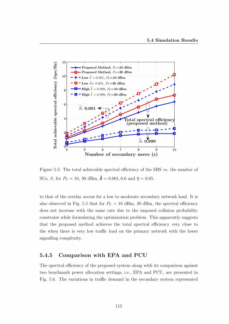
5.4 Simulation Results
4 5 6 7 8 9 100
2
4
6
8
10
12
Number of secondary users (s)
Totalach
ievable
spectraleffi
cien
cy(b
ps/Hz)
δ: 0.001
δ: 0.999
Total spectral efficiency(proposed method)
Proposed Method, PT=10 dBm
Proposed Method, PT=30 dBm
Low δ = 0.001, PT=10 dBm
Low δ= 0.001, PT=30 dBm
High δ = 0.999, PT=10 dBm
High δ = 0.999, PT=30 dBm
Figure 5.5: The total achievable spectral efficiency of the SBS vs. the number of
SUs, S, for PT = 10, 30 dBm, δ = 0.001, 0.6 and η = 0.05.
to that of the overlay access for a low to moderate secondary network load. It is
also observed in Fig. 5.5 that for PT = 10 dBm, 30 dBm, the spectral efficiency
does not increase with the same rate due to the imposed collision probability
constraint while formulating the optimization problem. This apparently suggests
that the proposed method achieves the total spectral efficiency very close to
the when there is very low traffic load on the primary network with the lower
signalling complexity.
5.4.5 Comparison with EPA and PCU
The spectral efficiency of the proposed system along with its comparison against
two benchmark power allocation settings, i.e., EPA and PCU, are presented in
Fig. 5.6. The variations in traffic demand in the secondary system represented
115

5.4 Simulation Results
4 5 6 7 8 9 101
2
3
4
5
6
7
8
9
10
11
Number of secondary users (s)
Totalach
ievable
spectraleffi
cien
cy(b
ps/Hz)
Proposed Method, PT=10 dBm
Proposed Method, PT=30 dBm
PCU, PT=10 dBm
PCU, PT=30 dBm
EPA, PT=10 dBm
EPA, PT=30 dBm
Figure 5.6: Total achievable spectral efficiency of the secondary system vs. the
total number of the secondary users for different scenarios and PT values.
by the number of secondary users, S, when maximum transmit power is kept at
10 dBm, 30 dBm. As expected, PCU achieves the highest system utility due to
ideally utilizing the subchannels, whereas EPA has the lowest due to the absence
of subchannel activity profile at the primary system which enforces system to
allocate equal transmit power. The proposed resource allocation scheme however
achieves a significantly higher spectral efficiency than that of the EPA. This
is due to the fact that the primary system activity provided by incorporating
ASAI is exploited in the subchannel power allocation. It is further observed that
the proposed method closely follows the ideal subchannel access, i.e., PCA with a
slightly lower spectral efficiency but significantly lower signalling overhead among
the secondary base stations.
116

5.4 Simulation Results
0.1 0.2 0.3 0.4 0.5 0.6 0.70
5
10
15
20
25
30
Normalized Interference from Primary System
Ach
ievable
Energy
Efficien
cy
(b/Hz/Joule)
δ estimated 0.7δ estimated 0.5δ estimated 0.3Bursty primary traffic
Figure 5.7: Energy efficiency vs. normalized interference from primary system
for various primary network traffic.
5.4.6 Impact of Primary Network Traffic on Energy Effi-
ciency
The performance of the proposed method in terms of energy efficiency is inves-
tigated against the case when the ASAI is not estimated. When the impact of
interference from primary system increases, the achievable energy efficiency de-
teriorates due to the higher transmit power requirement at the secondary system
to suppress the interference. The lowest energy efficiency is achieved when the
primary network traffic is of bursty nature in which the variation of δ becomes
high. Therefore, even in the lower interference regime, the energy efficiency is not
significantly higher. For instance, energy efficiency is achieved to be four times
higher (≈ 20 b/Hz/Joule) when δ = 0.7 than the case of bursty primary network
117

5.4 Simulation Results
traffic (≈ 5 b/Hz/Joule). Therefore, it can be concluded that the δ estimation
enables the improved resource allocation to achieve higher energy efficiency as
shown in Fig. 5.7. Moreover, when the primary users activity is higher and is
considered to be accurately estimated, there are more opportunities available
to access the subchannels such that the system energy is significantly utilized
for data transmission to achieve improved energy efficiency. However when the
interference from the primary system is higher, energy efficiency cannot be sig-
nificantly improved in the same way. For instance, at the normalized interference
of 0.6, the energy efficiency is improved just from 4 to 6 b/Hz/Joule, in cases of
bursty primary traffic and δi = 0.3, respectively.
5.4.7 Energy Efficiency and Total Spectral Efficiency
Here, further analysis is presented regarding the optimal energy and spectral
efficiencies as a unified model for the real-time measurement of the subchannel
activity index, δ, since both EE and SE depend on optimal transmit power and
QoS requirements imposed by the primary system. In addition, the ASAI is
used in the proposed analytical models to design the optimal transmit power
allocation. Such an articulated analysis is possible to design due to the proposed
system model and utility functions presented in previous sections.
The optimal spectral efficiency and energy efficiency as a function of δi for the
proposed method, for a range of total transmit power, is shown in Fig. 5.8. The
proposed methods improve the performance in various range of ASAI, i.e., δi. It
is shown in Fig. 5.8, for instance, that when subchannels are busy, as indicated
by δi in the range of [0.65, 0.9], the transmission power is controlled in such a
way that the EE is improved whereas the SE does not degrade significantly when
maximum PT is 30 dBm. Also in the lower ASAI, as indicated by δi in the range
of [0.1, 0.3], EE remains in the same level of around 15 b/Hz/Joule without signif-
icant decrease in the spectral efficiency. Moreover, when the primary subchannels
are moderately occupied, i.e., δi in the range of [0.4, 0.6], the secondary system
can achieve acceptable levels of both EE and SE simultaneously. In this case, the
maximum PT does not play a vital role on the system performance.
118

5.4 Simulation Results
0.1 0.2 0.3 0.4 0.5 0.6 0.7 0.8 0.9
20
The sub-channel activity index (δi)
Totalach
ievable
spectralefficiency
(bps/Hz)
EE AnalysisSE Analysis
0.1 0.2 0.3 0.4 0.5 0.6 0.7 0.8 0.92
4
6
Ach
ievable
energy
efficien
cy(b
/Hz/Joule)
15 dBm20 dBm25 dBm
10 dBm20 dBm30 dBm
Figure 5.8: Achievable spectral and energy efficiency vs. primary user activity
index for various total power constraints.
In a conventional EE and SE optimization, the improvement in EE as well as
SE is obtained either by considering a linear combination of EE and SE objectives
[129], or defining an objective function based on the transmit power as discussed
in [138]. In such cases, when the transmit power is increased, improved SE is
obtained with the sacrifice on the EE and vice-versa. The major concern in such
models of CRN design is that there is a limited range of transmit power for SUs
due to the interference constraints imposed by primary system. For instance, the
higher the transmit power, larger will be the interference to the primary system
which puts the limitations on the secondary system. In the proposed model
however, by relaxing (or tightening) the constraint in (5.8), larger (or smaller)
number of subchannels could be available for SUs such that δi slightly moves to
the higher (or lower) range. Therefore, depending on the requirements, i.e., either
better EE or better SE is anticipated, system parameters can be optimized to
119

5.5 Conclusions
achieve the target without compromising the primary system QoS in the proposed
method.
Therefore, the proposed method provides an entirely new perspective on cogni-
tive radio and communication system design where the operating point in terms
of ASAI, as shown in x-axis in the Fig. 5.8, can be dynamically obtained by
adjusting the sensing parameters, e.g., sensing duration, sensing threshold, and
detection probability threshold.
5.5 Conclusions
At the beginning of this chapter, the reference system model with the add-on
features considered for the proposed method of resource allocation has been pre-
sented. In addition, the essentials of energy detection method for spectrum sens-
ing and the associated hypothesis testing are reviewed. Based on the conditional
probabilities of hypotheses tests, the decisions parameters are identified which ul-
timately provides information about the primary subchannels. This resulted the
parameter subchannel activity index which has been defined and characterized
to incorporate the communication activity associated with the PUs in efficient
resource allocation. Moreover, a simple yet efficient intercell collaborative spec-
trum monitoring scheme has been proposed with very low signalling overhead to
evaluate the activities level of users in the subchannels, i.e., aggregated subchan-
nel activity index, as an indicator of network wide activities level of PUs on the
subchannels.
The efficient power allocation profile is then obtained at the SBS with the
objective of maximizing total SBS utility and total primary users interference
constraint as well as the total transmit power constraint. The SBS utility has
been defined based on ASAI and system throughput. In addition, the impact
of ASAI into the energy efficiency is also investigated by defining the utility
function and obtained the efficient transmit power profile with the associated
constraints. In the cognitive radio network, the energy and spectral efficiencies
contradict each other due to the fact that both cannot be maximized at the same
time. A general practice is that one of them is maximized keeping another at
120

5.5 Conclusions
a certain level. However in the proposed method, a novel and practically viable
design between spectral and energy efficiencies has been successfully achieved
considering the primary communication activity on the allocated subchannels.
The simulation results have further confirmed that the proposed scheme ex-
ploits the variations in the primary system communication activity to improve
the secondary system achievable rate. It is also confirmed the slight decrease of
the rate comparing to the ideal case in which both underlay and overlay methods
of spectrum sensing are implemented, however it is greater than the case when
no optimal power allocation algorithm is implemented, i.e., the equal power allo-
cation method. Further investigation has been executed to measure the impact
of ASAI into the energy efficiency and concluded that the proposed method is
a better design approach to obtain the optimal energy efficiency and/or spec-
tral efficiency concurrently by adjusting the spectrum sensing parameters at the
secondary system.
121

Chapter 6
Conclusions and Future Works
6.1 Summary of the Thesis
In Chapter 1, the very beginning picture of cognitive radio networks has been
discussed. The requirements of cognitive radio is basically due to the current con-
vergence of various wireless communication technologies, the exponential growth
of user densities and the data-hungry applications. In addition, the require-
ments for M2M and Internet-of-Everything also demanded more data transmis-
sion through the wireless channel. On this context, software-defined network and
cognitive radio communication have been studied for last one and half decade. A
detail study of cognitive cycle to enable the cognitive radio concept has also been
discussed in this chapter. The journey of cognitive radio networks has come long
way to make it worldwide acceptable by industry, government and academia.
Various organizations, for instance the IEEE, have worked together to make a
global standard for cognitive radio, such as IEEE 802.22 to be used in TV band,
in this period. The journey of cognitive radio has been briefly described in this
chapter. Since the research domain of cognitive radio networks is very wide, there
are even many challenges to implement them in practice. Such research challenges
in terms of spectrum sensing, resource allocation, energy efficiency etc. have also
been described along with the relevant examples. The factors that motivated
122

6.1 Summary of the Thesis
to conduct this research, which apparently produced this Thesis, have also been
included in this chapter.
In Chapter 2, a brief description of various spectrum sensing techniques pro-
posed for cognitive radio networks has been presented. The spectrum sensing task
is obviously one of the first requirements to enable the cognitive radio communi-
cation in current cellular network architecture. Therefore, based on the outcome
of sensing technique, an efficient resource allocation method could be designed,
i.e., higher the spectrum sensing accuracy, better will be the resource allocation
strategy. Nevertheless, a very important tradeoff between sensing duration and
transmission duration do exist in cognitive radio communication. Such issues
have been clearly identified and described in this chapter. Moreover, various
spectrum sensing methods have been described that are available in the liter-
ature as a foundation of the proposed spectrum sensing methods proposed in
this Thesis. Specifically, the cooperative and non-cooperative spectrum sensing
also have been described with their respective advantages and disadvantages. In
a cooperative spectrum sensing method where local information about the sub-
channel availability is diffused at a centralized system, soft combining and hard
combining methods are, in general, used in such cases. The benefit have been
described in this chapter, such as the hard combining method has less complexity
with lower accuracy on the spectrum sensing results. The challenges of spectrum
sensing methods for cognitive radio have been briefly discussed. At last but not
the least, the spectrum sensing results obtained from the specially designed spec-
trum sensors for TV band and GSM band, i.e., 500 MHz, 800 MHz and 1600 MHz
have been collected in the Lancaster City area to show the nature of spectrum
availability in real network. The rest of the chapters discussed to exploit the
available spectrum as shown on the obtained spectrum sensing results.
In Chapter 3, a brief introduction of the considered system model has been
presented. The concepts of multi-cellular and multi-carrier system with pri-
mary and secondary service providers collocated in the same geographical re-
gion for spectrum sharing have been discussed with the appropriate network dia-
grams. The concept of subchannels, orthogonal frequency division multiple access
(OFDMA) as an optimal modulation scheme for cognitive radio in addition to
the interference models have also been described to justify their usage in the
123

6.1 Summary of the Thesis
considered system of spectrum sensing and resource management. Furthermore,
the channel models, frame structure where spectrum sensing and transmission
durations are embedded have also been discussed. The features presented in this
chapter is the basis for the follow-up chapters with some add-on features when
they are needed. The last part of the chapter discussed one of the available cog-
nitive radio standards for the TV band, i.e, IEEE 802.22 standard, to explain
the strict requirements to implement cognitive radio in practice. The purpose
of this subsection is that the rest of the proposed methods would follow such
requirements to choose the appropriate cognitive radio parameters.
In Chapter 4, the proposed low-latency zone-based cooperative spectrum
sensing scheme in a multicell network has been exclusively described. It was
basically the sensor-enabled cognitive radio system where the dedicated sensing
devices took control the spectrum sensing task from the secondary system. In
conventional cognitive radio however, the secondary users have to consume the
precise resource of time frame in terms of the sensing duration. As a result of
the proposed methods, the secondary users can have more frame duration to
transmit the data packets which apparently improves the system throughout. In
addition, the proposed method significantly improves the power consumption in
the secondary system due to skipping the bulky spectrum sensing task. This
chapter also presented the design criteria of sensing devices such that the trade-
off among the sensing accuracy, system throughput and sensing network cost can
be explained both mathematically and through the simulation results. The de-
tail communication protocol among secondary system and the sensing devices
have also been presented. However offloading the sensing task to an independent
network is a good idea, the design of such a network is equally a challenging
task. In this chapter, various combination of spectrum sensing devices and base
stations have been considered and it has been shown mathematically that the op-
timization problem is a convex optimization problem under some specific network
parameters. Such conditions have been explained and solved the problem to find
the optimal design of such network. Finally, the simulation results demonstrated
the improved sensing accuracy and thus the system throughput in the proposed
network scenarios.
124
6.2 Future Research
In Chapter 5, the proposed method of subchannels and transmit power al-
location have been presented. It is obvious to believe that the communication
activities of primary users on the subchannels highly affect the resource allocation
strategy in secondary system. As a result, a reliable method of estimating the
activities of primary users on the subchannels was explained by defining a param-
eter called the subchannel activity index. This parameter was later obtained in
the multiple cell scenario such that the aggregated version is obtained by incorpo-
rating such decision vectors from the neighbouring cells. This parameter literally
indicates the best possible subchannel in the vicinity of the cell at a particular
time and location. Furthermore, the transmit power allocation problem is defined
as an optimization problem with the primary system interference constraint and
total transmit power constraint. The problem was then solved using dual decom-
position method to find the optimal transmit power profile. While formulating
the optimization problem, both spectral efficiency and energy efficiency have been
considered. Therefore, the energy efficiency also has been defined as a utility
function in terms of the subchannel activity index. The fractional optimization
problem has been defined with the similar constraints mentioned above. Later
in the chapter, the obtained results from the optimization problem have been
analysed together which concluded that the proposed method maintains a better
system design approach to maintain the balanced between energy efficiency and
spectral efficiency by changing the sensing parameters in the secondary system.
Finally, in this Chapter 6, the summary and contributions of this Thesis have
been presented. Based on the recent research activities, the future directions of
radio resource allocation in cognitive radio in terms of the requirements of 5G
are also discussed.
6.2 Future Research
It is in fact too early to predict the features of 5G telecommunication system.
Nevertheless, the early prediction shows that the data volume has to be 1000
times higher per area with up to 100 times higher data rate and 10 times longer
125

6.2 Future Research
battery life of devices [152]. Such services must be available with the millisec-
onds of end-to-end delay. Therefore, it can be anticipated that a single technology
alone cannot fulfil such a vibrant requirements. Therefore, there must be diverse
technologies which converge together with appropriate protocols to achieve the
targets. Some of the recently proposed technologies for 5G are mmWave, NOMA,
heterogeneous network (HetNet), massive MIMO etc. [153]. The cognitive radio
enabled M2M communication has gained huge attention recently to solve spec-
trum scarcity and energy efficiency issues in M2M communications [154]. However
it is needless to say that one of the highly celebrated and matured technologies in
5G and beyond is cognitive radio network. It is due to the fact that the scarcity
of spectrum will be the key challenge to provide the services in 5G and cognitive
radio is capable of tackling such issues. Therefore, a further research work is
to obtain the reliable and robust spectrum sensing and radio resource allocation
methods to make cognitive radio as one of the inevitable candidate technologies of
5G. One of the solutions to solve the spectrum scarcity problem is to use mmWave
in 35 GHz or 70 GHz where huge amount of bandwidth is available. However, it
is too immature to expect mmWave communication in near future because the
early stage of channel modelling has just been undertaken. Also, microwave band
is very attractive for wireless communication among service providers because it
travels longer distance and its channel properties are well understood. As a result,
more effort should be devoted to make cognitive radio an important technology
at early stage of 5G and beyond.
Since cellular mobile communication system from 1G to 4G were basically
human oriented, such as they carry audio, video and data generated by users.
On the other hand, in case of 5G, the things oriented communication system is
considered to be enabled [155]. The recent research and development efforts in
D2D and M2M to enable IoT are the early signs of future wireless communica-
tion system [156],[157]. These are the short range radio communication systems
where peer devices are close to each other with line-of-sight (LOS) or non-LOS
communication range. In such cases, the cognitive radio technique could be im-
plemented using the underlay access mode such that they do not interfere, or with
minimum interference, to the primary system. Therefore, finding the appropriate
126

6.2 Future Research
protocols and techniques for such communication systems is another important
future research.
The important milestone of cognitive radio to make it commercially available
is by drifting the IEEE 802.22 standard in TV bands to solve connectivity issue
such as in the rural broadband services. The recent announcement by FCC and
Ofcom to enable spectrum occupancy database temporarily solves the spectrum
sensing requirements, so the key issues now have to do with cognitive networks,
particularly of the integration of space-time-spectrum databases into cognitive
networks. A further research is needed to make such database to be useful in real-
time as well as enabled with context-aware functionality. One of the important
issue in this approach is the security in the database system. Although some
recent research provides the theory on how a cognitive radio can be inherently
secure, including smart enough to examine uploads to accept trustable updates
from the local spectrum sensors and to reject that are potentially malicious, the
foundations have yet to be embraced by the cognitive radio community. Similarly,
the access mechanism to such spectrum database by the authentic users is another
unsolved research problem which needs further research to propose the robust
solution.
The concept of NOMA at the first hand emerged from the concept of dy-
namic spectrum access in cognitive radio, such as the underlay spectrum sharing
scheme between secondary and primary systems. In NOMA, distinct power lev-
els are allocated among the multiple users depending on the channel gain, where
communication takes place at the same time frame and frequency subchannels
[158]. This concept is similar to the concept of underlay spectrum access where
the secondary users transmit even when primary system is using subchannels with
the constraint of interference to the primary system is below threshold. There-
fore, it can be argued that the advancement in cognitive radio not only improves
the spectrum utilization but also assists to initiate new technologies which ulti-
mately enforce to achieve the target of 5G. Further research must be conducted
in NOMA implying the similar concepts proposed for CRN.
There are also various research issues to make CRN as an enabling technology
for next generation networks. The instances are LTE over CRN to improve the
QoS of LTE users and the spectrum handoff mechanism [159] to minimize the
127

6.2 Future Research
switching delay when secondary system has to communicate (or terminate) on the
next available subchannel. Furthermore, the accurate and real-time estimation
of primary user activities such that opportunities are not missed by secondary
users. The concept of Kalman filter is also considered to be a future work to
evaluate the temporal characteristics in the cognitive network, for instance, the
primary users activities, for optimal resource allocation. Nevertheless, the future
research direction is not only limited to the above mentioned areas but also to
explore further as an multi-disciplinary research area.
128

Appendix A
Proof of Lemma 4.1
Proof. In this proof, equiprobable hypotheses, i.e., the probability of the chan-
nel being in idle or busy states are equal, is being considered. Therefore, the
probability of accurate channel sensing in the sensing devices is,
Pcs,i(εi, Ts,i)∆= 1−
{Pm,i(εi, Ts,i) + Pf,i(εi, Ts,i)
},∀i. (A.1)
The cases with no sensing errors, i.e., Pf,i(εi, Ts,i) = 0, and Pm,i(εi, Ts,i) = 0, are
referred to as perfect channel sensing, in such cases Pcs,i(εi, Ts,i) = 1. However,
practically Pcs,i(εi, Ts,i) ∈ [0, 1] which can be obtained by varying the operating
points in ROC curve within the range, Pm(εi, Ts,i) ≤ 0.5, and Pf(εi, Ts,i) ≤ 0.5,
which is also described in detail in (4.7c), (5.17a), and Lemmas 4.6-4.4. In the
maximally inaccurate sensing case, i.e., Pm(εi, Ts,i) = 0.5, (or Pd(εi, Ts,i) = 0.5),
and Pf(εi, Ts,i) = 0.5, we get Pcs,i(εi, Ts,i) = 0. Similarly in the perfect sensing
case, i.e., Pm(εi, Ts,i) = 0, (or Pd(εi, Ts,i) = 1), and Pf(εi, Ts,i) = 0, we get
Pcs,i(εi, Ts,i) = 1.
The logical AND rule is implemented in the ZAs, based on the sensing infor-
mation collected from sensing devices. Therefore, the aggregated information is
129

Pag,i =∏N
i=1 Px,i, where Px,i is either miss detection or false alarm probability.
Therefore, for any channel i,
P(ZA)cs,i (εi, Ts,i) = 1−
{Z∏
z=1
Pm,i(εi, Ts,i) +Z∏
z=1
Pf,i(εi, Ts,i)
}. (A.2)
The ZAs then make the spectrum sensing decision for each channel in its
corresponding zone based on applying AND rule on the sensing decisions provided
by the sensor in their corresponding zone. The obtained information is combined
at the SBS such that one channel can be utilized by multiple users within the
transmission range of SBS but no adjacent zones are permitted to access the same
channels.
Therefore, for possible micro-spectrum-reuse, the aggregate information is
Pag,i = 1 − ∏Ni=1(1 − Py,i), where Py,i is either miss detection or false alarm
probability for channel i. Consequently, Pag,i = 0 for Py,i = 0, ∀i thus (A.2) is
written as
P(SBS)cs,i = 1−
M∏
m=1
1−[1−
Z∏
z=1
Pm,i(εi, Ts,i)−Z∏
z=1
Pf,i(εi, Ts,i)
]. (A.3)
Straightforward mathematical manipulations for independent decisions from ZAs
result in the following
P(SBS)cs,i = 1−
[{1− Pd(εi, Ts,i)
}Z+
{Pf(εi, Ts,i)
}Z]M,∀i (A.4)
which completes the proof.
130

Appendix B
Proof of Lemma 4.2
Proof. Starting from Pf(εi, Ts,i) ≤ 0.5 along with (4.2), we write:
(εiσ2w
− 1
)√Ts,ifs ≥ Q−1(0.5) = 0. (B.1)
Since Ts,ifs > 0, then εiσ2w− 1 ≥ 0, therefore, εi ≥ σ2
w.
Similarly, substituting (4.3) in Pm(εi, Ts,i) ≤ 0.5, results in:
(εiσ2w
− γi − 1
)√Ts,ifs
2γi + 1≤ Q−1(0.5) = 0. (B.2)
SinceTs,ifs2γi+1
> 0, then εiσ2w− γi − 1 ≤ 0. Therefore, εi ≤ (1 + γi)σ
2w.
131

Appendix C
Proof of Lemma 4.3
Proof. Starting from (4.2), the first derivative of Pf(εi, Ts,i) is
∂Pf(εi, Ts,i)
∂εi= −
√Ts,ifs√2πσ2
w
exp
(−(εiσ2w
− 1
)2Ts,ifs
2
), (C.1)
which is always negative; thus, Pf(εi, Ts,i) is a decreasing function of εi. The
second derivative of Pf(εi, Ts,i) is
∂2Pf(εi, Ts,i)
∂2εi=
Ts,ifs√2πσ4
w
exp
(−C2
1
Ts,ifs2
)(εiσ2w
− 1
), (C.2)
where C1 = εiσ2w− 1. Since σ2
w ≤ εi, the second derivation is always positive;
therefore, Pf(εi, Ts,i) is a convex function of εi.
132

Appendix D
Proof of Lemma 4.4
Proof. Starting from (4.3), the first derivative of Pd(εi, Ts,i) is
∂Pd(εi, Ts,i)
∂εi= −
√Ts,ifs
2π(2γi + 1)
1
σ2w
exp
(−C2
Ts,ifs2
), (D.1)
where, C2 =(εiσ2w− γi − 1
)2
. Since∂Pd(εi,Ts,i)
∂εi< 0, and Pm(εi, Ts,i) = 1 −
Pd(εi, Ts,i), it can be shown by substitution that∂Pm(εi,Ts,i)
∂εi> 0. This also shows
that Pm(εi, Ts,i) is an increasing function of εi.
The second derivative of Pd(εi, Ts,i) is
∂2Pd(εi, Ts,i)
∂2εi=
√Ts,ifs
2π(2γi + 1)
1
σ4w
exp (−C3)
(εiσ2w
− γi − 1
), (D.2)
where, C3 =(εiσ2w− γi − 1
)2Ts,ifs
2. Here, all the terms are positive except εi
σ2w−
γi − 1. However, the inequality εiσ2w− γi − 1 ≤ 0 holds under the condition
εi ≤ (1 + γi)σ2w. Therefore,
∂2Pd(εi,Ts,i)
∂2εi< 0 holds and Pm(εi, Ts,i) = 1−Pd(εi, Ts,i)
proves that∂2Pm(εi,Ts,i)
∂2εi> 0. Consequently, Pm(εi, Ts,i) is an increasing and convex
function of εi. This completes the proof.
133

Appendix E
Proof of Corollary 4.1
Proof. To prove Corollary 4.1, the probability of channel accurate sensing in
(4.10a) is shown to be concave. We start with the scenario, where Z = M = 1.
Scenario 1 : For Z = 1, M = 1, and a fixed signalling duration, T s,i, and
frame duration, T , under the stated conditions in Lemma 4.6-Lemma 4.4, the
probability of accurate sensing of channel i is a concave function of εi.
In this scenario, Pcs,i(εi) = 1− ((1− Pd(εi)) + Pf(εi)). The second derivative
of Pcs,i is
∂2Pcs,i(εi, T s,i)
∂2εi= −∂
2Pm(εi, T s,i)
∂2εi− ∂2Pf(εi, T s,i)
∂2εi. (E.1)
It was already shown that∂2Pm(εi,T s,i)
∂2εi> 0, and
∂2Pf(εi,T s,i)
∂2εi> 0, therefore
∂2Pcs,i(εi,T s,i)
∂2εi< 0.
Therefore, the second derivative of Pcs,i is negative ∀i, thus it is a concave
function of εi for which the maximum occurs at optimal detection threshold, ε∗i .
Scenario 2 : Following the same line of argument as in Scenario 1, the proba-
bility of accurate sensing of channel i is a concave function of εi, for Z = 2 and
134

M = 1.
In this scenario, Pcs,i(εi) = 1− ((1− P2d(εi)) + P2
f (εi)). The second derivative
of Pcs,i is
∂2Pcs,i(εi, T s,i)
∂2εi= −∂
2P2m(εi, T s,i)
∂2εi− ∂2P2
f (εi, T s,i)
∂2εi. (E.2)
Now the second derivative of P2f,i(εi) is
∂2P2f (εi, Ts,i)
∂ε2i
=− 2
√Ts,ifs√2πσ2
w
[exp
(−A2
)∂Pf(εi, Ts,i)
∂εi
+ Pf∂
∂εi
(exp
(−A2
))],
(E.3)
where A = Ts,ifs
(εiσ2w− 1)2
. According to Lemma 4.3,∂Pf(εi,Ts,i)
∂εi< 0; we further
notice that for Pf > 0 and any x 6= 0, ∂e−x
∂x< 0. Using (E.3), we conclude that
∂2P2f (εi,Ts,i)
∂ε2i> 0.
Following the same line of argument as in (E.3), it is straightforward to show
that∂2P2
d(εi,Ts,i)
∂ε2i> 0. Substituting P2
d,i(εi) = (1− Pm,i(εi))2, we then get:
∂2P2d(εi, Ts,i)
∂ε2i
=
(−2
∂2Pm(εi, Ts,i)
∂ε2i
+∂2P2
m(εi, Ts,i)
∂ε2i
)> 0. (E.4)
According to Lemma 4.4, we also have∂2Pm(εi,Ts,i)
∂ε2i> 0, therefore we conclude
∂2P2m(εi,Ts,i)
∂ε2i> 0.
From (E.3) and noting that the positive sum of two concave functions is also a
concave function, one can conclude that∂2Pcs,i(εi,Ts,i)
∂ε2i< 0. It means the probability
of accurate sensing is a concave and decreasing function of εi.
Scenario 3 : Similar to Scenario 1 and 2, the probability of accurate sensing
of channel i is concave for Z = 1 and M = 2. In this case, the probability of
135
accurate sensing is calculated as below.
Pcs,i(εi) = 1−[Pm(εi) + Pf(εi)
]2
= 1− P2m(ε1)− 2Pm(ε1)Pf(ε1)− P2
f (ε1).
(E.5)
The second order derivative of (E.5) is
∂2P2cs,i(εi)
∂ε2i
=− ∂2P2m(εi)
∂ε2i
− 2Pm∂2Pf(εi)
∂ε2i
− 2Pf∂2Pm(εi)
∂ε2i
− ∂2P2f (εi)
∂ε2i
. (E.6)
For a fixed signalling duration T s,i, we already showed that ∂2Pf(εi)
∂ε2i> 0 in
Lemma 4.3, ∂2Pm(εi)
∂ε2i> 0 in Lemma 4.4, and ∂2P2
m(εi)
∂ε2i> 0, and
∂2P2f (εi)
∂ε2i> 0 in
Scenario 2. Moreover, we note that the maximum acceptable probability of miss
detection, and false alarm are bounded as 0 ≤ Pf ≤ 0.5, and 0 ≤ Pm ≤ 0.5,
respectively. Therefore, we can conclude that∂2P2
cs,i(εi)
∂ε2i< 0 and is concave function
of εi, and the maximum value occurs at εi = ε∗i which has been obtained in
Section 4.4.4.
Scenario 4 : Following the same line of argument as in Scenarios 1-3, the
probability of accurate sensing of channel i is a concave function of εi for Z = 1,
M = 3, as well as Z = 3, M = 1.
We then argue that the function is concave for the combination of ZAs, i.e.,
n1 = 2 and n2 = n1 + 1 and SBSs, i.e., n3 = 2 and n4 = n3 + 1 and it also
holds for n1 = 1 and n3 = 1. It means that it must be also true for any possible
combination of natural numbers of ZAs and SBSs according to the principal of
mathematical induction.
136

References
[1] A. Al-Fuqaha, M. Guizani, M. Mohammadi, M. Aledhari, and M. Ayyash,
“Internet of things: A survey on enabling technologies, protocols, and ap-
plications,” IEEE Communications Surveys Tutorials, vol. 17, no. 4, pp.
2347–2376, Fourthquarter 2015. (Page 1).
[2] M. Weyrich, J. P. Schmidt, and C. Ebert, “Machine-to-machine communi-
cation,” IEEE Software, vol. 31, no. 4, pp. 19–23, July 2014. (Page 1).
[3] Cisco Inc., “Cisco virtual networking index,” White Paper at
www.cisco.com, Feb 2014. (Pages 1, 4).
[4] W. H. Chin, Z. Fan, and R. Haines, “Emerging technologies and research
challenges for 5G wireless networks,” IEEE Wireless Communications,
vol. 21, no. 2, pp. 106–112, April 2014. (Page 1).
[5] J. G. Andrews, S. Buzzi, W. Choi, S. V. Hanly, A. Lozano, A. C. K. Soong,
and J. C. Zhang, “What will 5G be?” IEEE Journal on Selected Areas in
Communications, vol. 32, no. 6, pp. 1065–1082, June 2014. (Page 1).
[6] F. Boccardi, R. W. Heath, A. Lozano, T. L. Marzetta, and P. Popovski,
“Five disruptive technology directions for 5G,” IEEE Communications
Magazine, vol. 52, no. 2, pp. 74–80, February 2014. (Page 2).
[7] V. Jungnickel, K. Manolakis, W. Zirwas, B. Panzner, V. Braun, M. Los-
sow, M. Sternad, R. Apelfrojd, and T. Svensson, “The role of small cells,
coordinated multipoint, and massive MIMO in 5G,” IEEE Communications
Magazine, vol. 52, no. 5, pp. 44–51, May 2014. (Page 2).
137

REFERENCES
[8] E. Hossain, M. Rasti, H. Tabassum, and A. Abdelnasser, “Evolution to-
ward 5G multi-tier cellular wireless networks: An interference management
perspective,” IEEE Wireless Communications, vol. 21, no. 3, pp. 118–127,
2014. (Page 2).
[9] T. 3rd Generation Partnership Project, “Lte-advanced,” Release-
11, 2013, (Accessed on: April-2014). [Online]. Available: http:
//www.3gpp.org/technologies/keywords-acronyms/97-lte-advanced (Page
2).
[10] A. A. Atayero, O. I. Adu, and A. A. Alatishe, “Self organizing networks for
3GPP LTE,” in International Conference on Computational Science and
Its Applications. Springer, 2014, pp. 242–254. (Page 2).
[11] S. Sun, Q. Gao, Y. Peng, Y. Wang, and L. Song, “Interference manage-
ment through CoMP in 3GPP LTE-advanced networks,” IEEE Wireless
Communications, vol. 20, no. 1, pp. 59–66, February 2013. (Page 3).
[12] Qualcomm Inc., “LTE MTC: Optimizing LTE Ad-
vanced for machine-type communications,” White Paper at
www.qualcom.com, Feb 2014, (Accessed on: 10-Dec-
2015). [Online]. Available: https://www.qualcomm.com/documents/
lte-mtc-optimizing-lte-advanced-machine-type-communications (Page 3).
[13] C. S. Park, L. Sundstrm, A. Walln, and A. Khayrallah, “Carrier aggregation
for LTE-advanced: design challenges of terminals,” IEEE Communications
Magazine, vol. 51, no. 12, pp. 76–84, December 2013. (Page 3).
[14] Qualcomm Inc., “LTE advanced carrier aggregation,” White Pa-
per at www.qualcom.com, 2016, (Accessed on: 24-Mar-2016). [On-
line]. Available: https://www.qualcomm.com/invention/technologies/lte/
lte-carrier-aggregation (Page 3).
[15] Federal Communications Commission, “Spectrum policy task force report,”
FCC 02-155, 2002. (Pages 4, 8).
138

REFERENCES
[16] Q. Zhao and B. M. Sadler, “A survey of dynamic spectrum access,” IEEE
signal processing magazine, vol. 24, no. 3, pp. 79–89, 2007. (Page 4).
[17] S. Haykin, “Cognitive radio: brain-empowered wireless communications,”
IEEE Journal on Selected Areas in Communications, vol. 23, no. 2, pp.
201–220, 2005. (Pages 4, 8).
[18] FCC ET, “Docket no 03-222 notice of proposed rule making and order,”
2003. (Pages 4, 8).
[19] R. Menon, R. Buehrer, and J. Reed, “On the impact of dynamic spec-
trum sharing techniques on legacy radio systems,” IEEE Transactions on
Wireless Communications, vol. 7, no. 11, pp. 4198–4207, 2008. (Page 5).
[20] A. Ghasemi and E. Sousa, “Fundamental limits of spectrum-sharing in fad-
ing environments,” IEEE Transactions on Wireless Communications, vol. 6,
no. 2, pp. 649–658, 2007. (Page 5).
[21] X. Kang, R. Zhang, Y.-C. Liang, and H. K. Garg, “Optimal power alloca-
tion strategies for fading cognitive radio channels with primary user outage
constraint,” IEEE Journal on Selected Areas in Communications, vol. 29,
no. 2, pp. 374–383, 2011. (Page 5).
[22] M. Khoshkholgh, K. Navaie, and H. Yanikomeroglu, “Access strategies for
spectrum sharing in fading environment: Overlay, underlay, and mixed,”
IEEE Transactions on Mobile Computing, vol. 9, no. 12, pp. 1780–1793,
2010. (Pages 5, 46, 55, 88).
[23] M. T. Masonta, M. Mzyece, and N. Ntlatlapa, “Spectrum decision in cog-
nitive radio networks: A survey,” IEEE Communications Surveys & Tuto-
rials, vol. 15, no. 3, pp. 1088–1107, 2013. (Page 5).
[24] T. Yucek and H. Arslan, “A survey of spectrum sensing algorithms for
cognitive radio applications,” IEEE Communications Suevey & Tutorials,
vol. 11, no. 1, pp. 116–130, 2009. (Pages 5, 20).
139

REFERENCES
[25] I. F. Akyildiz, W.-Y. Lee, M. C. Vuran, and S. Mohanty, “Next
generation/dynamic spectrum access/cognitive radio wireless networks:
A survey,” Computer Networks, vol. 50, no. 13, pp. 2127 – 2159,
2006. [Online]. Available: http://www.sciencedirect.com/science/article/
pii/S1389128606001009 (Page 6).
[26] D. T. Ngo, C. Tellambura, and H. H. Nguyen, “Resource allocation for
OFDMA-based cognitive radio multicast networks with primary user ac-
tivity consideration,” IEEE Transactions on Vehicular Technology, vol. 59,
no. 4, pp. 1668–1679, May 2010. (Page 6).
[27] L. Zhang, Y. Xin, Y.-C. Liang, and H. Poor, “Cognitive multiple access
channels: optimal power allocation for weighted sum rate maximization,”
IEEE Transactions on Communications, vol. 57, no. 9, pp. 2754–2762, 2009.
(Pages 6, 11, 91, 95).
[28] D. Xu, E. Jung, and X. Liu, “Efficient and fair bandwidth allocation in mul-
tichannel cognitive radio networks,” IEEE Transactions on Mobile Comput-
ing, vol. 11, no. 8, pp. 1372–1385, 2012. (Page 6).
[29] G. Bansal, M. Hossain, V. Bhargava, and T. Le-Ngoc, “Subcarrier and
power allocation for ofdma-based cognitive radio systems with joint overlay
and underlay spectrum access mechanism,” IEEE Transactions on Vehic-
ular Technology, vol. 62, no. 3, pp. 1111–1122, 2013. (Pages 6, 88, 89, 94,
111).
[30] F. Sheikholeslami, M. Nasiri-Kenari, and F. Ashtiani, “Optimal probabilis-
tic initial and target channel selection for spectrum handoff in cognitive
radio networks,” IEEE Transactions on Wireless Communications, vol. 14,
no. 1, pp. 570–584, 2015. (Pages 6, 11).
[31] L. C. Wang, C. W. Wang, and C. J. Chang, “Optimal target channel se-
quence design for multiple spectrum handoffs in cognitive radio networks,”
IEEE Transactions on Communications, vol. 60, no. 9, pp. 2444–2455,
September 2012. (Page 6).
140

REFERENCES
[32] J. Mitola and G. Q. Maguire, “Cognitive radio: making software radios
more personal,” IEEE Personal Communications, vol. 6, no. 4, pp. 13–18,
Aug 1999. (Page 7).
[33] J. Mitola, “Cognitive radio-an integrated agent architecture for software
defined radio,” Royal Institute of Technology (KTH), 2000. (Page 7).
[34] M. Nekovee, “A survey of cognitive radio access to TV white spaces,” in
2009 International Conference on Ultra Modern Telecommunications Work-
shops, Oct 2009, pp. 1–8. (Page 9).
[35] “IEEE 802.22 WRAN WG,” http://www.ieee802.org/22/, 2012, (Accessed
on: October-2013). (Pages 9, 57, 58, 60, 63, 65, 74).
[36] X. Hong, J. Wang, C. X. Wang, and J. Shi, “Cognitive radio in 5G: a
perspective on energy-spectral efficiency trade-off,” IEEE Communications
Magazine, vol. 52, no. 7, pp. 46–53, July 2014. (Page 9).
[37] A. Ghasemi and E. S. Sousa, “Spectrum sensing in cognitive radio net-
works: requirements, challenges and design trade-offs,” IEEE Communica-
tions Magazine, vol. 46, no. 4, pp. 32–39, April 2008. (Page 10).
[38] A. B. Flores, R. E. Guerra, E. W. Knightly, P. Ecclesine, and S. Pandey,
“Ieee 802.11af: a standard for tv white space spectrum sharing,” IEEE
Communications Magazine, vol. 51, no. 10, pp. 92–100, October 2013. (Page
10).
[39] P. Paysarvi-Hoseini and N. Beaulieu, “On the benefits of multichan-
nel/wideband spectrum sensing with non-uniform channel sensing dura-
tions for cognitive radio networks,” IEEE Transactions on Communica-
tions, vol. 60, no. 9, pp. 2434–2443, September 2012. (Page 10).
[40] E. Axell, G. Leus, E. G. Larsson, and H. V. Poor, “Spectrum sensing for
cognitive radio: State-of-the-art and recent advances,” IEEE Signal Pro-
cessing Magazine, vol. 29, no. 3, pp. 101–116, 2012. (Pages 10, 21, 31).
141

REFERENCES
[41] E. Peh, Y.-C. Liang, Y. L. Guan, and Y. Zeng, “Cooperative spectrum
sensing in cognitive radio networks with weighted decision fusion schemes,”
IEEE Transactions on Wireless Communications, vol. 9, no. 12, pp. 3838–
3847, December 2010. (Pages 10, 47).
[42] D. Xue, E. Ekici, and M. C. Vuran, “Cooperative spectrum sensing in cog-
nitive radio networks using multidimensional correlations,” IEEE Trans-
actions on Wireless Communications, vol. 13, no. 4, pp. 1832–1843, April
2014. (Pages 10, 47, 47).
[43] Y.-C. Liang, Y. Zeng, E. Peh, and A. T. Hoang, “Sensing-throughput trade-
off for cognitive radio networks,” IEEE Transactions on Wireless Commu-
nications, vol. 7, no. 4, pp. 1326–1337, 2008. (Pages 10, 46, 47, 55, 60,
62).
[44] K. W. Choi and E. Hossain, “Estimation of primary user parameters in
cognitive radio systems via hidden markov model,” IEEE Transactions on
Signal Processing, vol. 61, no. 3, pp. 782–795, 2013. (Page 11).
[45] B. Canberk, I. Akyildiz, and S. Oktug, “Primary user activity modeling
using first-difference filter clustering and correlation in cognitive radio net-
works,” IEEE/ACM Transactions of Networking, vol. 19, no. 1, pp. 170–
183, 2011. (Page 11).
[46] M. Ashour, A. A. El-Sherif, T. ElBatt, and A. Mohamed, “Cognitive radio
networks with probabilistic relaying: stable throughput and delay trade-
offs,” IEEE Transactions on Communications, vol. 63, no. 11, pp. 4002–
4014, 2015. (Pages 11, 29).
[47] Y. Wang, P. Ren, F. Gao, and Z. Su, “A hybrid underlay/overlay trans-
mission mode for cognitive radio networks with statistical quality-of-service
provisioning,” IEEE Transactions on Communications, vol. 13, no. 3, pp.
1482–1498, March 2014. (Pages 11, 111).
[48] H. ElSawy, E. Hossain, and M. Haenggi, “Stochastic geometry for modeling,
analysis, and design of multi-tier and cognitive cellular wireless networks:
142

REFERENCES
A survey,” IEEE Communications Surveys & Tutorials, vol. 15, no. 3, pp.
996–1019, 2013. (Page 11).
[49] I. Macaluso, D. Finn, B. Ozgul, and L. A. DaSilva, “Complexity of spec-
trum activity and benefits of reinforcement learning for dynamic channel
selection,” IEEE Journal on Selected Areas in Communications, vol. 31,
no. 11, pp. 2237–2248, November 2013. (Page 11).
[50] E. E. Yaacoub and Z. Dawy, “Centralized multicell scheduling with interfer-
ence mitigation,” Resource Allocation in Uplink OFDMA Wireless Systems:
Optimal Solutions and Practical Impl., pp. 173–201, 2012. (Page 11).
[51] F. Haider, C.-X. Wang, H. Haas, E. Hepsaydir, X. Ge, and D. Yuan,
“Spectral and energy efficiency analysis for cognitive radio networks,” IEEE
Transactions on Wireless Communications, vol. 14, no. 6, pp. 2969–2980,
2015. (Page 11).
[52] F. Zhou, N. C. Beaulieu, Z. Li, J. Si, and P. Qi, “Energy-efficient optimal
power allocation for fading cognitive radio channels: Ergodic capacity, out-
age capacity, and minimum-rate capacity,” IEEE Transactions on Wireless
Communications, vol. 15, no. 4, pp. 2741–2755, 2016. (Page 11).
[53] S. Stotas and A. Nallanathan, “Optimal sensing time and power allocation
in multiband cognitive radio networks,” IEEE Transactions on Communi-
cations, vol. 59, no. 1, pp. 226–235, 2011. (Pages 11, 41, 46, 62).
[54] Ofcom, “Digital dividend: cognitive access statement on licence-exempting
cognitive devices using interleaved spectrum,” Ofcom Statement, July 2009,
(Accessed on: July-2013). [Online]. Available: http://stakeholders.ofcom.
org.uk/binaries/consultations/cognitive/statement/statement.pdf (Page
13).
[55] ——, “TV white spaces: A consultation on white space device
requirements,” Ofcom Statement, November 2012, (Accessed on: August-
2013). [Online]. Available: http://stakeholders.ofcom.org.uk/binaries/
consultations/whitespaces/summary/condoc.pdf (Page 14).
143

REFERENCES
[56] Huawei Inc., “Mitigating interference between LTE and GSM/UMTS
networks,” Huawei Report, 2012, (Accessed on: 10-Nov-2013). [Online].
Available: http://www1.huawei.com/enapp/198/hw-079474.htm (Page
14).
[57] H. N. Tran, K. Ishizu, and F. Kojima, “Evaluation of channel availability for
mobile device by using a TV white space database qualified by the ofcom,”
in 2015 IEEE 81st Vehicular Technology Conference (VTC Spring), May
2015, pp. 1–6. (Page 21).
[58] H. Urkowitz, “Energy detection of unknown deterministic signals,” Pro-
ceedings of the IEEE, vol. 55, no. 4, pp. 523–531, 1967. (Page 22).
[59] D. Cabric, S. M. Mishra, and R. W. Brodersen, “Implementation issues in
spectrum sensing for cognitive radios,” in Signals, systems and computers,
2004. Conference record of the thirty-eighth Asilomar conference on, vol. 1.
IEEE, 2004, pp. 772–776. (Pages 22, 26).
[60] E. Axell and E. G. Larsson, “Optimal and sub-optimal spectrum sensing of
OFDM signals in known and unknown noise variance,” IEEE Journal on
Selected Areas in Communications, vol. 29, no. 2, pp. 290–304, 2011. (Page
22).
[61] R. Tandra and A. Sahai, “SNR walls for signal detection,” IEEE Journal
of selected topics in Signal Processing, vol. 2, no. 1, pp. 4–17, 2008. (Pages
23, 25).
[62] F. Salahdine, H. E. Ghazi, N. Kaabouch, and W. F. Fihri, “Matched filter
detection with dynamic threshold for cognitive radio networks,” in Wire-
less Networks and Mobile Communications (WINCOM), 2015 International
Conference on, Oct 2015, pp. 1–6. (Page 25).
[63] X. Zhang, F. Gao, R. Chai, and T. Jiang, “Matched filter based spectrum
sensing when primary user has multiple power levels,” China Communica-
tions, vol. 12, no. 2, pp. 21–31, Feb 2015. (Page 25).
144

REFERENCES
[64] R. Tandra and A. Sahai, “Fundamental limits on detection in low SNR
under noise uncertainty,” in 2005 International Conference on Wireless
Networks, Communications and Mobile Computing, vol. 1. IEEE, 2005,
pp. 464–469. (Page 25).
[65] P. D. Sutton, J. Lotze, K. E. Nolan, and L. E. Doyle, “Cyclostationary
signature detection in multipath rayleigh fading environments,” in 2007 2nd
International Conference on Cognitive Radio Oriented Wireless Networks
and Communications. IEEE, 2007, pp. 408–413. (Page 26).
[66] J. Lunden, V. Koivunen, A. Huttunen, and H. V. Poor, “Collaborative cy-
clostationary spectrum sensing for cognitive radio systems,” IEEE Trans-
actions on Signal Processing, vol. 57, no. 11, pp. 4182–4195, 2009. (Page
26).
[67] J. K. Tugnait and G. Huang, “Cyclic autocorrelation based spectrum sens-
ing in colored gaussian noise,” in 2012 IEEE Wireless Communications and
Networking Conference (WCNC), April 2012, pp. 731–736. (Page 26).
[68] W. A. Gardner, “Exploitation of spectral redundancy in cyclostationary
signals,” IEEE Signal Processing Magazine, vol. 8, no. 2, pp. 14–36, 1991.
(Page 26).
[69] M. Feng, T. Jiang, D. Chen, and S. Mao, “Cooperative small cell networks:
High capacity for hotspots with interference mitigation,” IEEE Wireless
Communications, vol. 21, no. 6, pp. 108–116, 2014. (Page 27).
[70] J. Shen, S. Liu, L. Zeng, G. Xie, J. Gao, and Y. Liu, “Optimisation of coop-
erative spectrum sensing in cognitive radio network,” IET communications,
vol. 3, no. 7, pp. 1170–1178, 2009. (Page 27).
[71] D. Cabric, A. Tkachenko, and R. W. Brodersen, “Spectrum sensing mea-
surements of pilot, energy, and collaborative detection,” in MILCOM 2006-
2006 IEEE Military Communications conference. IEEE, 2006, pp. 1–7.
(Page 27).
145

REFERENCES
[72] C. Sun, W. Zhang, and K. B. Letaief, “Cluster-based cooperative spectrum
sensing in cognitive radio systems,” in 2007 IEEE International Conference
on Communications. IEEE, 2007, pp. 2511–2515. (Page 29).
[73] R. Gao, Z. Li, P. Qi, and H. Li, “A robust cooperative spectrum sens-
ing method in cognitive radio networks,” IEEE Communications Letters,
vol. 18, no. 11, pp. 1987–1990, 2014. (Page 29).
[74] D. Teguig, B. Scheers, and V. L. Nir, “Data fusion schemes for cooperative
spectrum sensing in cognitive radio networks,” in Communications and In-
formation Systems Conference (MCC), 2012 Military, Oct 2012, pp. 1–7.
(Page 30).
[75] D. M. S. Bhatti and H. Nam, “Correlation based soft combining scheme for
cooperative spectrum sensing in cognitive radio networks,” in 2014 IEEE
79th Vehicular Technology Conference (VTC Spring), May 2014, pp. 1–5.
(Page 30).
[76] S. M. Mishra, A. Sahai, and R. W. Brodersen, “Cooperative sensing among
cognitive radios,” in 2006 IEEE International Conference on Communica-
tions, vol. 4, June 2006, pp. 1658–1663. (Page 30).
[77] L. Lu, X. Zhou, U. Onunkwo, and G. Y. Li, “Ten years of research in
spectrum sensing and sharing in cognitive radio,” EURASIP Journal on
Wireless Communications and Networking, vol. 2012, no. 1, p. 1, 2012.
(Page 31).
[78] Q. Wu, G. Ding, J. Wang, X. Li, and Y. Huang, “Consensus-based
decentralized clustering for cooperative spectrum sensing in cognitive radio
networks,” Chinese Science Bulletin, vol. 57, no. 28, pp. 3677–3683, 2012.
[Online]. Available: http://dx.doi.org/10.1007/s11434-012-5074-6 (Page
31).
[79] B. Wang and K. J. R. Liu, “Advances in cognitive radio networks: A sur-
vey,” IEEE Journal of Selected Topics in Signal Processing, vol. 5, no. 1,
pp. 5–23, Feb 2011. (Page 32).
146

REFERENCES
[80] W.-Y. Lee and I. Akyildiz, “Optimal spectrum sensing framework for cog-
nitive radio networks,” IEEE Transactions on Wireless Communications,
vol. 7, no. 10, pp. 3845–3857, 2008. (Page 33).
[81] W. Han, J. Li, Z. Tian, and Y. Zhang, “Dynamic sensing strategies for effi-
cient spectrum utilization in cognitive radio networks,” IEEE Transactions
on Wireless Communications, vol. 10, no. 11, pp. 3644–3655, 2011. (Page
33).
[82] Y. Pei, Y.-C. Liang, K. Teh, and K. H. Li, “How much time is needed for
wideband spectrum sensing?” IEEE Transactions on Wireless Communi-
cations, vol. 8, no. 11, pp. 5466–5471, 2009. (Pages 33, 41).
[83] Y. Chen, “Analytical performance of collaborative spectrum sensing using
censored energy detection,” IEEE Transactions on Wireless Communica-
tions, vol. 9, no. 12, pp. 3856–3865, 2010. (Page 33).
[84] S. Maleki, A. Pandharipande, and G. Leus, “Energy-efficient distributed
spectrum sensing for cognitive sensor networks,” IEEE Sensors Journal,
vol. 11, no. 3, pp. 565–573, 2011. (Pages 33, 54).
[85] E. Pei, H. Han, Z. Sun, B. Shen, and T. Zhang, “LEAUCH: low-energy
adaptive uneven clustering hierarchy for cognitive radio sensor network,”
EURASIP Journal on Wireless Communications and Networking, vol. 2015,
no. 1, pp. 1–8, 2015. (Page 33).
[86] D. Willkomm, S. Machiraju, J. Bolot, and A. Wolisz, “Primary users in
cellular networks: A large-scale measurement study,” in New frontiers in
dynamic spectrum access networks, 2008. DySPAN 2008. 3rd IEEE sympo-
sium on. IEEE, 2008, pp. 1–11. (Pages 35, 89).
[87] B. Golkar and E. S. Sousa, “Resource allocation in autonomous cellular net-
works,” IEEE Transactions on Wireless Communications, vol. 12, no. 11,
pp. 5572–5583, 2013. (Page 36).
147
REFERENCES
[88] M. Monemi, M. Rasti, and E. Hossain, “On joint power and admission
control in underlay cellular cognitive radio networks,” IEEE Transactions
on Wireless Communications, vol. 14, no. 1, pp. 265–278, 2015. (Page 36).
[89] H. A. Mahmoud, T. Yucek, and H. Arslan, “OFDM for cognitive radio:
merits and challenges,” IEEE wireless communications, vol. 16, no. 2, pp.
6–15, 2009. (Page 38).
[90] J. Mao, G. Xie, J. Gao, and Y. Liu, “Energy efficiency optimization for
OFDM-based cognitive radio systems: A water-filling factor aided search
method,” IEEE Transactions on Wireless Communications, vol. 12, no. 5,
pp. 2366–2375, 2013. (Page 38).
[91] K. G. M. Thilina, E. Hossain, and M. Moghadari, “Cellular ofdma cogni-
tive radio networks: Generalized spectral footprint minimization,” IEEE
Transactions on Vehicular Technology, vol. 64, no. 7, pp. 3190–3204, July
2015. (Page 38).
[92] M. E. Sahin, I. Guvenc, and H. Arslan, “Opportunity detection for ofdma-
based cognitive radio systems with timing misalignment,” IEEE Transac-
tions on Wireless Communications, vol. 8, no. 10, pp. 5300–5313, October
2009. (Page 38).
[93] Z. Wang, L. Jiang, and C. He, “Optimal price-based power control algo-
rithm in cognitive radio networks,” IEEE Transactions on Wireless Com-
munications, vol. 13, no. 11, pp. 5909–5920, 2014. (Page 39).
[94] J. Zou, H. Xiong, D. Wang, and C. W. Chen, “Optimal power allocation
for hybrid overlay/underlay spectrum sharing in multiband cognitive radio
networks,” IEEE Transactions on Vehicular Technology, vol. 62, no. 4, pp.
1827–1837, 2013. (Pages 41, 88).
[95] H. Shi, R. V. Prasad, V. S. Rao, I. Niemegeers, and M. Xu, “Spectrum-and
energy-efficient D2DWRAN,” IEEE Communications Magazine, vol. 52,
no. 7, pp. 38–45, 2014. (Page 42).
148

REFERENCES
[96] C.-S. Sum, G. P. Villardi, M. A. Rahman, T. Baykas, H. N. Tran, Z. Lan,
C. Sun, Y. Alemseged, J. Wang, C. Song et al., “Cognitive communication
in TV white spaces: An overview of regulations, standards, and technology
[accepted from open call],” IEEE Communications Magazine, vol. 51, no. 7,
pp. 138–145, 2013. (Page 42).
[97] H. B. Yilmaz, T. Tugcu, F. Alagz, and S. Bayhan, “Radio environment map
as enabler for practical cognitive radio networks,” IEEE Communications
Magazine, vol. 51, no. 12, pp. 162–169, December 2013. (Page 44).
[98] M. Caleffi and A. S. Cacciapuoti, “Database access strategy for TV white
space cognitive radio networks,” in Sensing, Communication, and Network-
ing Workshops (SECON Workshops), 2014 Eleventh Annual IEEE Inter-
national Conference on, June 2014, pp. 34–38. (Page 44).
[99] ——, “Optimal database access for TV white space,” IEEE Transactions
on Communications, vol. 64, no. 1, pp. 83–93, 2016. (Page 44).
[100] M. Khoshkholgh, K. Navaie, and H. Yanikomeroglu, “Optimal design of
the spectrum sensing parameters in the overlay spectrum sharing,” IEEE
Transactions on Mobile Computing, vol. PP, no. 99, pp. 1–1, 2013. (Page
47, 47).
[101] A. Ghasemi and E. Sousa, “Collaborative spectrum sensing for opportunis-
tic access in fading environments,” in New Frontiers in Dynamic Spectrum
Access Networks, 2005. DySPAN 2005. 2005 First IEEE International Sym-
posium on, Nov 2005, pp. 131–136. (Pages 47, 48).
[102] H. Zhuang, Z. Luo, J. Zhang, and Y. Li, “Cooperative sensor solution to
enhancing the performance of spectrum sensing,” in Communications and
Networking in China (CHINACOM), 2010 5th International ICST Conf.
on, Aug 2010, pp. 1–6. (Page 47).
[103] H. Yu, W. Tang, and S. Li, “Optimization of multiple-channel cooperative
spectrum sensing with data fusion rule in cognitive radio networks,” Journal
of Electronics (China), vol. 29, no. 6, pp. 515–522, 2012. (Page 47, 47).
149

REFERENCES
[104] Y. Abdi and T. Ristaniemi, “Joint local quantization and linear cooperation
in spectrum sensing for cognitive radio networks,” IEEE Transactions on
Signal Processing, vol. 62, no. 17, pp. 4349–4362, Sept 2014. (Page 47).
[105] I. F. Akyildiz, B. F. Lo, and R. Balakrishnan, “Cooperative spectrum sens-
ing in cognitive radio networks: A survey,” Physical Communication, vol. 4,
no. 1, pp. 40–62, Mar. 2011. (Pages 47, 48).
[106] W. Lin, Y. Wang, and W. Ni, “Cluster-based cooperative spectrum sensing
in two-layer hierarchical cognitive radio networks,” in Global Comm. Conf.
(GLOBECOM), 2013 IEEE, Dec 2013, pp. 1082–1087. (Page 47).
[107] W. Zhang, Y. Yang, and C. K. Yeo, “Cluster-based cooperative spectrum
sensing assignment strategy for heterogeneous cognitive radio network,”
IEEE Transactions on Vehicular Technology, vol. 64, no. 6, pp. 2637–2647,
June 2015. (Page 47).
[108] C. G. Tsinos and K. Berberidis, “Decentralized adaptive eigenvalue-based
spectrum sensing for multiantenna cognitive radio systems,” IEEE Trans-
actions on Wireless Communications, vol. 14, no. 3, pp. 1703–1715, March
2015. (Page 48).
[109] Y. Han, S. H. Ting, and A. Pandharipande, “Cooperative spectrum sharing
protocol with secondary user selection,” IEEE Transactions on Wireless
Communications, vol. 9, no. 9, pp. 2914–2923, September 2010. (Page 48,
48).
[110] J. Lai, E. Dutkiewicz, R. Liu, and R. Vesilo, “Opportunistic spectrum access
with two channel sensing in cognitive radio networks,” IEEE Transactions
on Mobile Computing, vol. PP, no. 99, pp. 1–1, 2013. (Page 48).
[111] I. Nevat, G. W. Peters, and I. B. Collings, “Location-aware coopera-
tive spectrum sensing via gaussian processes,” in Communications Theory
Workshop (AusCTW), 2012 Australian, Jan 2012, pp. 19–24. (Page 48).
150

REFERENCES
[112] M. Monemian and M. Mahdavi, “Analysis of a new energy-based sensor
selection method for cooperative spectrum sensing in cognitive radio net-
works,” IEEE Sensors Journal, vol. 14, no. 9, pp. 3021–3032, Sept 2014.
(Page 49).
[113] Y. Selen, H. Tullberg, and J. Kronander, “Sensor selection for cooperative
spectrum sensing,” in New Frontiers in Dynamic Spectrum Access Net-
works, DySPAN 2008. 3rd IEEE Symposium on, Oct 2008, pp. 1–11. (Page
49).
[114] Y. Li, K. K. Chai, Y. Chen, and J. Loo, “Duty cycle control with
joint optimisation of delay and energy efficiency for capillary machine-to-
machine networks in 5G communication system,” Transactions on Emerg-
ing Telecomm. Tech., vol. 26, no. 1, pp. 56–69, 2015. (Page 49).
[115] B. Mercier, V. Fodor, R. Thobaben, M. Skoglund, V. Koivunen, S. Lindfors,
J. Ryynanen, E. G. Larsson, C. PetriolI, G. Bongiovanni et al., “Sensor net-
works for cognitive radio: Theory and system design,” ICT mobile summit,
2008. (Page 49, 49).
[116] O. Grondalen, M. Lahteenoja, and P. Gronsund, “Evaluation of business
cases for a cognitive radio network based on wireless sensor network,” in
New Frontiers in Dynamic Spectrum Access Networks (DySPAN), 2011
IEEE Symposium on, May 2011, pp. 242–253. (Page 49).
[117] N. Hasan, W. Ejaz, S. Lee, and H. Kim, “Knapsack-based energy-efficient
node selection scheme for cooperative spectrum sensing in cognitive ra-
dio sensor networks,” IET Communications, vol. 6, no. 17, pp. 2998–3005,
November 2012. (Page 49).
[118] K. Letaief and W. Zhang, “Cooperative communications for cognitive radio
networks,” Proceedings of the IEEE, vol. 97, no. 5, pp. 878–893, May 2009.
(Page 54).
[119] H. Cramer, Mathematical methods of statistics. Princeton university press,
1999, vol. 9. (Page 55).
151

REFERENCES
[120] S. Atapattu, C. Tellambura, and H. Jiang, “Analysis of area under the
ROC curve of energy detection,” IEEE Transactions on Wireless Commu-
nications, vol. 9, no. 3, pp. 1216–1225, March 2010. (Page 56).
[121] A. Singh, M. Bhatnagar, and R. Mallik, “Cooperative spectrum sensing in
multiple antenna based cognitive radio network using an improved energy
detector,” IEEE Communications Letters, vol. 16, no. 1, pp. 64–67, 2012.
(Pages 61, 62, 95).
[122] P. Paysarvi-Hoseini and N. Beaulieu, “Optimal wideband spectrum sens-
ing framework for cognitive radio systems,” IEEE Transactions on Signal
Processing, vol. 59, no. 3, pp. 1170–1182, March 2011. (Pages 63, 67).
[123] R. Fan and H. Jiang, “Optimal multi-channel cooperative sensing in cog-
nitive radio networks,” IEEE Transactions on Wireless Communications,
vol. 9, no. 3, pp. 1128–1138, March 2010. (Page 64).
[124] Z.-Q. Luo and W. Yu, “An introduction to convex optimization for com-
munications and signal processing,” IEEE Journal on Selected Areas in
Communications, vol. 24, no. 8, pp. 1426–1438, Aug 2006. (Page 66).
[125] S. P. Boyd and L. Vandenberghe, Convex optimization. Cambridge uni-
versity press, 2004. (Pages 66, 66, 67, 104, 105).
[126] W. Wang, B. Kasiri, J. Cai, and A. S. Alfa, “Channel assignment schemes
for cooperative spectrum sensing in multi-channel cognitive radio net-
works,” Wireless Communications and Mobile Computing, vol. 15, no. 10,
pp. 1471–1484, 2015. (Page 76).
[127] M. Khoshkholgh, K. Navaie, and H. Yanikomeroglu, “Achievable capac-
ity in hybrid DS-CDMA/OFDM spectrum-sharing,” IEEE Transactions
on Mobile Computing, vol. 9, no. 6, pp. 765–777, June 2010. (Page 87).
[128] K. Shashika Manosha, N. Rajatheva, and M. Latva-aho, “Overlay/underlay
spectrum sharing for multi-operator environment in cognitive radio net-
works,” in Vehicular Technology Conference (VTC Spring), 2011 IEEE
73rd, 2011, pp. 1–5. (Page 88).
152

REFERENCES
[129] H. Hu, H. Zhang, and Y. Liang, “On the spectrum- and energy-efficiency
tradeoff in cognitive radio networks,” IEEE Transactions on Communica-
tions, vol. 64, no. 2, pp. 490–501, Feb 2016. (Pages 88, 119).
[130] C. Han, T. Harrold, S. Armour, I. Krikidis, S. Videv, P. M. Grant, H. Haas,
J. Thompson, I. Ku, C.-X. Wang, T. A. Le, M. Nakhai, J. Zhang, and
L. Hanzo, “Green radio: radio techniques to enable energy-efficient wireless
networks,” IEEE Transactions on Communications, vol. 49, no. 6, pp. 46–
54, June 2011. (Page 88).
[131] X. Hong, J. Wang, C. X. Wang, and J. Shi, “Cognitive radio in 5G: a
perspective on energy-spectral efficiency trade-off,” IEEE Transactions on
Communications, vol. 52, no. 7, pp. 46–53, July 2014. (Page 88).
[132] R. Amin, J. Martin, J. Deaton, L. A. DaSilva, A. Hussien, and A. Eltawil,
“Balancing spectral efficiency, energy consumption, and fairness in future
heterogeneous wireless systems with reconfigurable devices,” IEEE Journal
on Selected Areas in Communications, vol. 31, no. 5, pp. 969–980, 2013.
(Page 88).
[133] L. Liu, R. Zhang, and K.-C. Chua, “Achieving global optimality for
weighted sum-rate maximization in the K-user gaussian interference channel
with multiple antennas,” IEEE Transactions on Wireless Communications,
vol. 11, no. 5, pp. 1933–1945, 2012. (Pages 88, 91).
[134] X. Tan, H. Zhang, and J. Hu, “Achievable transmission rate of the sec-
ondary user in cognitive radio networks with hybrid spectrum access strat-
egy,” IEEE Communications Letters, vol. 17, no. 11, pp. 2088–2091, 2013.
(Page 89).
[135] L. Wang, M. Sheng, Y. Zhang, X. Wang, and C. Xu, “Robust energy effi-
ciency maximization in cognitive radio networks: The worst-case optimiza-
tion approach,” IEEE Transactions on Communications, vol. 63, no. 1, pp.
51–65, Jan 2015. (Page 89).
153

REFERENCES
[136] A. Alabbasi, Z. Rezki, and B. Shihada, “Energy efficient resource allocation
for cognitive radios: A generalized sensing analysis,” IEEE Transactions on
Wireless Communications, vol. 14, no. 5, pp. 2455–2469, May 2015. (Pages
89, 107).
[137] S. Wang, W. Shi, and C. Wang, “Energy-efficient resource management in
OFDM-based cognitive radio networks under channel uncertainty,” IEEE
Transactions on Communications, vol. 63, no. 9, pp. 3092–3102, Sept 2015.
(Page 89).
[138] W. Zhang, C. Wang, D. Chen, and H. Xiong, “Energy-spectral efficiency
tradeoff in cognitive radio networks,” IEEE Transactions on Vehicular
Technologies, vol. PP, no. 99, pp. 1–1, 2015. (Pages 89, 119).
[139] F. Kelly, “Charging and rate control for elastic traffic,” European Transac-
tions on Telecommunication, vol. 8, no. 1, pp. 33–37, 1997. (Page 90).
[140] M. Katoozian, K. Navaie, and H. Yanikomeroglu, “Utility-based adaptive
radio resource allocation in OFDM wireless networks with traffic prioritiza-
tion,” IEEE Transactions on Wireless Communications, vol. 8, no. 1, pp.
66–71, Jan 2009. (Pages 90, 101).
[141] J. Kaleva, A. Tolli, and M. Juntti, “Weighted sum rate maximization for in-
terfering broadcast channel via successive convex approximation,” in Proc.
IEEE GLOBECOM 2012, 2012, pp. 3838–3843. (Page 91).
[142] N. Mokari, K. Navaie, and M. Khoshkholgh, “Downlink radio resource al-
location in ofdma spectrum sharing environment with partial channel state
information,” IEEE Transactions on Wireless Communications, vol. 10,
no. 10, pp. 3482–3495, 2011. (Pages 91, 94, 102, 102).
[143] W. Zhang, C. K. Yeo, and Y. Li, “A MAC sensing protocol design for data
transmission with more protection to primary users,” IEEE Transactions
on Mobile Computing, vol. 12, no. 4, pp. 621–632, April 2013. (Page 96).
154

REFERENCES
[144] W. Yu and R. Lui, “Dual methods for nonconvex spectrum optimization
of multicarrier systems,” IEEE Transactions on Communications, vol. 54,
no. 7, pp. 1310–1322, July 2006. (Page 104).
[145] D. Palomar and M. Chiang, “A tutorial on decomposition methods for
network utility maximization,” IEEE Journal on Selected Areas in Com-
munications, vol. 24, no. 8, pp. 1439–1451, 2006. (Page 105).
[146] A. Charnes and W. W. Cooper, “Programming with linear fractional
functionals,” Naval Research Logistics Quarterly, vol. 9, no. 3-4, pp. 181–
186, 1962. [Online]. Available: http://dx.doi.org/10.1002/nav.3800090303
(Page 107).
[147] L. Wang, M. Sheng, X. Wang, Y. Zhang, and X. Ma, “Mean energy ef-
ficiency maximization in cognitive radio channels with PU outage con-
straint,” IEEE Communications Letters, vol. 19, no. 2, pp. 287–290, Feb
2015. (Page 108).
[148] D. Ng, E. Lo, and R. Schober, “Energy-efficient resource allocation in multi-
cell OFDMA systems with limited backhaul capacity,” IEEE Transactions
on Wireless Communications, vol. 11, no. 10, pp. 3618–3631, October 2012.
(Page 108).
[149] W. Dinkelbach, “On nonlinear fractional programming,” Management
Science, vol. 13, no. 7, pp. pp. 492–498, 1967. [Online]. Available:
http://www.jstor.org/stable/2627691 (Page 108).
[150] H. Peng and T. Fujii, “Hybrid overlay/underlay resource allocation for cog-
nitive radio networks in user mobility environment,” in Vehicular Technol-
ogy Conference (VTC Fall), 2013 IEEE 78th, Sept 2013, pp. 1–6. (Page
111).
[151] S. Senthuran, A. Anpalagan, and O. Das, “Throughput analysis of oppor-
tunistic access strategies in hybrid underlay/overlay cognitive radio net-
works,” IEEE Transactions on Communications, vol. 11, no. 6, pp. 2024–
2035, June 2012. (Page 111).
155

REFERENCES
[152] Q. C. Li, H. Niu, A. T. Papathanassiou, and G. Wu, “5G network capac-
ity: key elements and technologies,” IEEE Vehicular Technology Magazine,
vol. 9, no. 1, pp. 71–78, 2014. (Page 126).
[153] C. X. Wang, F. Haider, X. Gao, X. H. You, Y. Yang, D. Yuan, H. M. Ag-
goune, H. Haas, S. Fletcher, and E. Hepsaydir, “Cellular architecture and
key technologies for 5G wireless communication networks,” IEEE Commu-
nications Magazine, vol. 52, no. 2, pp. 122–130, February 2014. (Page 126).
[154] A. Aijaz and A. H. Aghvami, “Cognitive machine-to-machine communica-
tions for internet-of-things: A protocol stack perspective,” IEEE Internet
of Things Journal, vol. 2, no. 2, pp. 103–112, April 2015. (Page 126).
[155] Z. Ma, Z. Zhang, Z. Ding, P. Fan, and H. Li, “Key techniques for 5G
wireless communications: network architecture, physical layer, and MAC
layer perspectives,” Science China Information Sciences, vol. 58, no. 4, pp.
1–20, 2015. (Page 126).
[156] M. N. Tehrani, M. Uysal, and H. Yanikomeroglu, “Device-to-device com-
munication in 5G cellular networks: challenges, solutions, and future direc-
tions,” IEEE Communications Magazine, vol. 52, no. 5, pp. 86–92, 2014.
(Page 126).
[157] A. Alexiou, “Wireless World 2020: Radio interface challenges and tech-
nology enablers,” IEEE Vehicular Technology Magazine, vol. 9, no. 1, pp.
46–53, 2014. (Page 126).
[158] H. Tabassum, M. S. Ali, E. Hossain, M. Hossain, D. I. Kim et al., “Non-
orthogonal multiple access (NOMA) in cellular uplink and downlink: Chal-
lenges and enabling techniques,” arXiv preprint arXiv:1608.05783, 2016.
(Page 127).
[159] C. Zhang and K. G. Shin, “What should secondary users do upon in-
cumbents’ return?” IEEE Journal on Selected Areas in Communications,
vol. 31, no. 3, pp. 417–428, 2013. (Page 127).
156
Related Documents