SPECTRE Short Packet Communication Toolbox Version 0.2 Contributors (alphabetic order): Austin Collins, Giuseppe Durisi, Tomaso Erseghe, Victoria Kostina, Johan ¨ Ostman, Yury Polyanskiy, Ido Tal, Wei Yang e-mail: [email protected] July 25, 2016 Abstract Shannon theory describes fundamental limits of communication and compression systems. Classic closed-form results (such as the well known log(1 + SNR) formula) apply only to the regime of infinite blocklength (infinite packet size/delay). For finite blocklengths, no closed-form results are usually obtainable, but there exist tight upper and lower bounds, as well as approximations. This manual describes numerical routines for computing these bounds and approximations for some popular channel and source models. The toolbox is under development and the participation of additional members of the information and communication theory communities in this endeavor is warmly welcomed! 1

Welcome message from author
This document is posted to help you gain knowledge. Please leave a comment to let me know what you think about it! Share it to your friends and learn new things together.
Transcript

SPECTREShort Packet Communication Toolbox
Version 0.2
Contributors (alphabetic order):Austin Collins, Giuseppe Durisi, Tomaso Erseghe, Victoria Kostina,
Johan Ostman, Yury Polyanskiy, Ido Tal, Wei Yang
e-mail: [email protected]
July 25, 2016
Abstract
Shannon theory describes fundamental limits of communication andcompression systems. Classic closed-form results (such as the well knownlog(1 + SNR) formula) apply only to the regime of infinite blocklength(infinite packet size/delay). For finite blocklengths, no closed-form resultsare usually obtainable, but there exist tight upper and lower bounds, aswell as approximations. This manual describes numerical routines forcomputing these bounds and approximations for some popular channeland source models.
The toolbox is under development and the participation of additionalmembers of the information and communication theory communities inthis endeavor is warmly welcomed!
1

Contents
Contents 2
1 Motivation 5
2 The real AWGN channel 72.1 Summary plot: plot v3() . . . . . . . . . . . . . . . . . . . . . 72.2 Achievability: shannon ach2() . . . . . . . . . . . . . . . . . . 82.3 Achievability: kappabeta ach() . . . . . . . . . . . . . . . . . 82.4 Achievability: gallager ach() . . . . . . . . . . . . . . . . . . 82.5 Converse: converse() . . . . . . . . . . . . . . . . . . . . . . . 92.6 Normal approximation: normapx awgn(), normapx biawgn() . 92.7 Code database: plot universe() . . . . . . . . . . . . . . . . 9
3 Block-memoryless Rayleigh fading (no CSI) 113.1 Achievability bounds . . . . . . . . . . . . . . . . . . . . . . . . 123.2 Converse helper functions . . . . . . . . . . . . . . . . . . . . . 123.3 Converse bound . . . . . . . . . . . . . . . . . . . . . . . . . . . 133.4 Alamouti . . . . . . . . . . . . . . . . . . . . . . . . . . . . . . 133.5 Outage capacity . . . . . . . . . . . . . . . . . . . . . . . . . . 133.6 Ergodic capacity . . . . . . . . . . . . . . . . . . . . . . . . . . 14
4 Quasi-static fading channel 154.1 Summary plot: plot all() . . . . . . . . . . . . . . . . . . . . 164.2 Achievability: ach simo csir() . . . . . . . . . . . . . . . . . . 164.3 Achievability: ach simo nocsi() . . . . . . . . . . . . . . . . . 174.4 Achievability: mimo iso ach() . . . . . . . . . . . . . . . . . . 174.5 Converse: converse simo() . . . . . . . . . . . . . . . . . . . . 174.6 Converse: mimo iso conv() . . . . . . . . . . . . . . . . . . . . 174.7 Normal approximation . . . . . . . . . . . . . . . . . . . . . . . 17
5 Quasi-static fading channel (long-term power constraint) 195.1 The AWGN channel (H = 1) . . . . . . . . . . . . . . . . . . . 205.2 Quasi-static fading channel with perfect CSIT . . . . . . . . . . 20
6 Block-memoryless Rayleigh Fading (CSIR) 216.1 Summary plot: plot all() . . . . . . . . . . . . . . . . . . . . 226.2 Achievability Bound: MIMO achievability CSIR() . . . . . . . 226.3 Normal Approximation: MIMO csir normapx() . . . . . . . . . 23
2

CONTENTS 3
7 Energy-per-bit under vanishing spectral efficiency 257.1 Summary plot . . . . . . . . . . . . . . . . . . . . . . . . . . . . 267.2 The AWGN channel (Hj = 1) . . . . . . . . . . . . . . . . . . . 267.3 Rayleigh fading: CSIR case . . . . . . . . . . . . . . . . . . . . 277.4 Rayleigh fading: noCSI case . . . . . . . . . . . . . . . . . . . . 27
8 Fixed-length source coding under a distortion criterion 298.1 Binary memoryless source . . . . . . . . . . . . . . . . . . . . . 308.2 Gaussian memoryless source . . . . . . . . . . . . . . . . . . . . 318.3 Binary erased source . . . . . . . . . . . . . . . . . . . . . . . . 32
9 Variable-length compression allowing errors 359.1 Binary memoryless source . . . . . . . . . . . . . . . . . . . . . 36
10 Joint source-channel coding under a distortion criterion 3710.1 Binary memoryless source transmitted over a binary symmetric
channel . . . . . . . . . . . . . . . . . . . . . . . . . . . . . . . 3810.2 Gaussian source transmitted over an AWGN channel . . . . . . 39
11 The binary-symmetric channel (BSC) 4111.1 Summary plot: plot all() . . . . . . . . . . . . . . . . . . . . 4111.2 Achievability: dt ach() . . . . . . . . . . . . . . . . . . . . . . 4211.3 Achievability: rcu ach() . . . . . . . . . . . . . . . . . . . . . 4211.4 Achievability: gallager ach() . . . . . . . . . . . . . . . . . . 4211.5 Converse: converse() . . . . . . . . . . . . . . . . . . . . . . . 4211.6 Normal approximation: normapx() . . . . . . . . . . . . . . . . 43
12 The binary-erasure channel (BEC) 4512.1 Summary plot: plot all() . . . . . . . . . . . . . . . . . . . . 4512.2 Achievability: dt ach() . . . . . . . . . . . . . . . . . . . . . . 4612.3 Achievability: gallager ach() . . . . . . . . . . . . . . . . . . 4612.4 Converse: converse() . . . . . . . . . . . . . . . . . . . . . . . 4612.5 Normal approximation: normapx() . . . . . . . . . . . . . . . . 47
13 The binary-AWGN channel (BI-AWGN) 4913.1 Converse: converse mc() . . . . . . . . . . . . . . . . . . . . . 4913.2 Example 1: example speff.m . . . . . . . . . . . . . . . . . . . 5013.3 Example 2: example per.m . . . . . . . . . . . . . . . . . . . . 51
Bibliography 53


Chapter 1
Motivation
In his 1948 landmark paper, Claude E. Shannon demonstrated that communi-cation with arbitrarily small probability of error is feasible if, and only if, thecommunication rate is below the so called channel capacity. To achieve thisresult, codes with large packet size (blocklength) must be employed. Shannon’schannel capacity has served as a useful guideline to design wireless communica-tion systems.
In some applications, however, a more refined analysis of the interplay be-tween packet-error probability, communication rate, and packet size is required.This may occur in emerging applications, such as massive machine-to-machinecommunication for metering, traffic safety, and telecontrol of industrial plants,together with real-time data transfer to enable remote wireless control (tactileinternet), which may require the exchange of short packets, sometimes understringent latency and reliability constraints.
Finite-blocklength information theory, a subfield of information theory thatbenefitted from seminal contributions from Shannon, Strassen, and Dobrushin,among others, is currently a very active field of research. Nonasymptoticachievability and converse bounds on the maximum coding rate achievable fora given packet size and packet error probability are now available for severalchannel models that are relevant for wireless communication systems, such asthe AWGN channel, the quasi-static Rayleigh fading channel, and the Rayleighblock-fading channel. The purpose of this toolbox is to provide numericalroutines for the computation of these bounds. In the next chapters, we providea bare-bone manual, which describes the routines available in this toolbox.
5


Chapter 2
The real AWGN channel
General info:
• Maintainer: Y. Polyanskiy <[email protected]>
• Main references: [1]
• Example: See Fig. 2.1
• Channel model:Yj = Xj + Zj , j = 1, . . . , n
– Codewords are real: xj ∈ R, j = 1, . . . , n
– Noise: Zj ∼ N (0, 1) iid.
– Power constraints: Each codeword xn satisfies
n∑j=1
|xj |2 ≤ nP
• Common input/output arguments:
1. P – input argument; parameter of the power constraint (so P = 10is SNR = 10 dB).
2. epsil – block probability of block error.
3. lm or Lms – output argument; log2M , log-size of codebook (base-2information units).
4. n – input argument; blocklength.For slow functions that do not support vectorized arguments.
5. Ns – input argument; vector of blocklengths.
2.1 Summary plot: plot v3()
Definition:
function [Ns lb ub feinst gal wlfz] = plot_v3(P, epsil)
This function plots various bounds on the same figure. See Fig. 2.1.
7

8 CHAPTER 2. THE REAL AWGN CHANNEL
> plot_v3(10, 0.001, 1, 100:20:1000)
0 100 200 300 400 500 600 700 800 900 10000
0.2
0.4
0.6
0.8
1
1.2
1.4
1.6
1.8
Blocklen, n
Rat
e, R
Bounds for AWGN, SNR = 10 dB, Pe = 0.001
Capacity
Converse (|X|2 = nP)
Normal approximationkappa−beta achievabilityGallager random coding
Figure 2.1: Code and resulting picture for AWGN bounds
2.2 Achievability: shannon ach2()
Definition:
function lm = shannon_ach2(n, epsil, P)
Function computes Shannon’s cone-packing achievability bound, see [1, (41)].
2.3 Achievability: kappabeta ach()
Format:
function Lms = kappabeta_ach(Ns, epsil, P, hack)
This computes the κβ achievability bound, see left-hand inequality in [1,(218)]. If hack 6= 0, then we use asymptotic approximation for κ. This increasesthe speed dramatically and is very precise already at n = 10, see [1, (217)]. Ifhack is not set, it defaults to 1.
2.4 Achievability: gallager ach()
Format:
function lm = gallager_ach(n, epsil, P)
Computes Gallager’s achievability bound, see [1, (44)].

2.5. CONVERSE: CONVERSE() 9
2.5 Converse: converse()
Format:
function Lms = converse(Ns, epsil, P)
This computes the meta-converse lower bound with QY n = N (0, 1 + P )n,see right-hand inequality in [1, (218)].
2.6 Normal approximation: normapx awgn(),
normapx biawgn()
Format:
function Lms = normapx_awgn(Ns, epsil, P);
Fast and frequently very precise approximation to both achievability andconverse:
logM ≈ nC −√nV Q−1(ε) +
1
2log n
2.7 Code database: plot universe()
Code in universe/plot_universe() compiles a comparative plot of normalizedrate for different codes. See [1, Section IV.D].


Chapter 3
Block-memoryless Rayleighfading channel, no CSI
General info:
• Maintainer: G. Durisi <[email protected]>
• Contributors: G. Durisi, J. Ostman, W. Yang
• Main reference: [2]
• Example: See Fig. 3.1.
• Channel model: Rayleigh block-fading channel with mt transmit antennasand mr receive antennas that stays constant for nc channel uses. Theblocklength n is an integer multiple of the coherence time nc, i.e., n = lnc;here l denotes the number of independent time-frequency branches:
Yk = XkHk + Wk , k = 1, . . . , l , (3.1)
where Yk,Wk ∈ Cnc×mr , Xk ∈ Cnc×mt and Hk ∈ Cmt×mr . The noiseWk and the channel gain Hk are independent and have independentCN (0, 1) entries. Neither the transmitter nor the receiver are aware ofthe realizations of the fading matrix Hk.
The power constraint is defined per coherence interval, i.e., each codewordC consists of l subcodewords C1, . . . ,Cl that must satisfy:
trCHk Ck
= ncρ, k = 1, . . . , l.
Here, ρ denotes the SNR.
• Common input, output arguments:
– snrdB – SNR in dB
– T – channel coherence time (expressed in channel uses)
– L – number of independent fading realizations spanned by eachcodeword
– Mt – number of tranmsmit antennas
11

12 CHAPTER 3. BLOCK-MEMORYLESS RAYLEIGH FADING (NO CSI)
168 84 42 24 12 8 6 4
coherence interval nc (log scale)
1 2 4 7 14 21 28 420
0.5
1
1.5
2
2.5
3
Alamouti
Cout(ρ, ε)
Cerg(ρ) (approx.)
time-frequency diversity branches l (log scale)
bit/chan
nel
use
MC upper boundDT lower bound
R∗(nc, l, ε, ρ)
Figure 3.1: Maximum coding rate R∗(nc, l, ε, ρ) for 2×2 MIMO system operatingover a Rayleigh block-fading channel with coherence time nc. Each packetspans l coherence intervals. The packet size is 168 channel uses. The packeterror rate is ε = 10−3. The SNR is ρ = 6 dB.
– Mr – number of receve antennas
– epsilon – packet error rate (block error rate)
– prec – log2 of the number of samples used in the Monte-Carlo step;this parameter should be set so that 2prec 100/epsilon
– filename – data file in which the samples of the information densityare saved for possible future refinements (provided that the flag SAVE
is set)
– R – estimate of the maximum coding rate
– current_eps – actual bound on the packet error rate (it may deviatefrom epsilon if prec is not chosen appropriately)
3.1 Achievability bounds: DT USTM NxM(), DT USTM MxM()
Format:
function [R,current_eps]
=DT_USTM(snrdB,T,L,Mt,Mr,epsilon,prec,filename);
This function computes the USTM-DT achievability bound [2, Th. 3] for thecase mt ≤ mr.
3.2 Converse helper functions: MC USTM 2x2 q1x2(),MC USTM 2x2 q 2x2(), MC USTM 4x4 q Mx4
Format

3.3. CONVERSE BOUND 13
function [R,current_eps,current_prec]
=MC_USTM_2x2(snrdB,T,L,Mtalt,epsilon,prec,pow_all,filename)
function [R,current_eps,current_prec]
=MC_USTM_4x4(snrdB,Mtalt,T,L,epsilon,prec,pow_all,filename)
These two functions compute the right-hand side of [2, Eq. (41)] for fixed inputdiagonal matrices Σklk=1 and fixed auxiliary output distribution (which isparameterized by the number of effectively used transmit antennas Mtalt thatresult in this distribution), for the case mt = mr = 2 and mt = mr = 4. Toobtain the actual converse bound, a further optimization over these parametersneed to be performed. This is discussed in the next section. The parameterpow_all is related to the diagonal entries of the matrices Σklk=1. For themt = mr = 2 case, pow_all is an l-dimensional vector, whose entries are in[0, 0.5]. Indeed, the particular formulation of the power constraint in [2, Eq. (41)]implies that the other entry is uniquely determined from the first one. For the4 × 4 case, the code provided assumes that the optimization in [2, Eq. (41)]is restricted only to Σklk=1 of the form Σ1 = · · · = Σl = Σ. In this case,pow_all is a 4-dimensional vector that contains the diagonal entries of Σ.
3.3 Converse bound: compute MC 2x2 telatar
Format
function R=compute_MC_2x2_telatar(snrdB,T,L,epsilon)
Compute the metaconverse upper bound [2, Eq. (41)] by invoking the functionMC USTM 2x2() and by optimizing over the input diagonal matrices Σklk=1
and the number of effectively used transmit antennas. The optimization overthe Σklk=1 is restricted to 2× 2 diagonal matrices whose diagonal entries areeither [SNR/2, SNR/2] or [SNR, 0] according to the generalized form of Telatarconjecture reported in [2, Eq. (42)]. NOTE: this function may be very slow if Lis large or epsilon is small.
3.4 Alamouti: DT USTM Alamouti(), MC USTM Alamouti()
Format
function [R,current_eps]
=MC_USTM_Alamouti(snrdB,T,L,epsilon,prec,filename)
function [R,current_eps]
=DT_USTM_Alamouti(snrdB,T,L,epsilon,prec,filename)
These functions compute achievability and converse bounds for a 2× 2 MIMOsystem with Alamouti used as inner code
3.5 Outage: outage mi(), outage alamouti(),outage 2x2 telatar()
function [Cout,current_eps]
=outage_mi(snrdB,epsilon,Mt,Mr,L,pow_all,prec)

14 CHAPTER 3. BLOCK-MEMORYLESS RAYLEIGH FADING (NO CSI)
function [Cout,current_eps]
=outage_alamouti(snrdb,epsilon,L,prec,filename)
function R=outage_2x2_telatar(L,prec,epsilon,snrdb)
The first two functions compute the outage mutual information Iε for a givenset of diagonal input covariance matrices, and the outage mutual informationwith Alamouti, respectively:
P[E[ı(X l;Yl)|Hl] ≤ Iε] = ε ,
where in the first case, the covariance structure of X l = (X1, . . . , Xl) is specifiedby pow_all and
ı(X l;Yl) =
l∑k=1
logdPYk|Xk
dPYk
.
The outage_mi function evaluates the outage mutual information correspondingto a given input covariance matrix, whose eigenvalues are specified in pow_all.Specifically, pow_all is a Mt-1 x L matrix containing the first Mt−1 eigenvaluesof the input covariance matrices corresponding to each coherence interval. Thelast eigenvalue follows from the power constraint. To obtain the outage capacityone has to optimize over all possible choices of pow_all.
The function outage_2x2_telatar provides an example on how to performthis optimization for the 2×2 MIMO case. The optimization is restricted to inputcovariance matrices that satisfy the generalized Telatar conjecture [2, Eq. (42)]according to which in the eigenvalues of the input covariance matrix in eachcoherence interval satisfy the following property: k out the Mt eigenvalues areequal to SNR/k and the remaining Mt−k eigenvalues are equal to zero. Thevalue of k may change across the coherence intervals.
3.6 Ergodic capacity: ergodic USTM()
function RergUSTM=ergodic_USTM(snrdB,T,Mt,Mr,prec)
This function computes a lower bound on the ergodic capacity (no CSIR),obtained by evaluating the mutual information for a USTM input distribution.It is assumed that mt ≤ mr.

Chapter 4
Quasi-static fading channel
General info:
• Maintainer: W. Yang <[email protected]>
• Main references: [3]
• Example: See Fig. 6.1
• Channel model: a quasi-static MIMO fading channel with mt transmitand mr receive antennas. The channel input-output relation within nchannel uses is given by
Y = XH + Z (4.1)
where X ∈ Cn×mt is the signal transmitted over n channel uses; Y ∈ Cn×mr
is the corresponding received signal; the matrix H ∈ Cmt×mr contains thecomplex fading coefficients, which are random but remain constant overthe n channel uses; Z ∈ Cn×mr denotes the additive noise at the receiver,which is independent of H and has iid CN (0, 1) entries. Power constraints:each codeword xn satisfies
‖X‖2F ≤ nP.
In the code, we also assume that the entries of H are iid Rician-distributed,i.e.,
Hij ∼ CN (√K/(K + 1), 1/(K + 1))
where K is the Rician K-factor.
• The code for the MIMO case (mt > 1) is built under the additionalassumption that all codewords X are “isotropic”, i.e., (see [3, Sec. III])
1
nXHX =
P
mtImt
. (4.2)
Currently, we do not have code for MIMO achievability and conversebounds that hold without the assumption (4.2).
• Input/output arguments:
1. nn – input argument; vector of blocklengths.
15

16 CHAPTER 4. QUASI-STATIC FADING CHANNEL
0 100 200 300 400 500 600 700 800 900 10000
0.2
0.4
0.6
0.8
1
XLabel
YLa
bel
EpsilonCapacity
NormalApproximation
KappaBetaBound
AchNocsi
MetaConverse
Figure 4.1: Achievability and converse bounds for a quasi-static SIMO Rician-fading channel withK-factor equal to 20 dB, two receive antennas, SNR = −1.55dB, and ε = 10−3.
2. error – input argument; block error probability.
3. tx, rx – input arguments; number of transmit and receive antennas.
4. P – input argument; parameter of the power constraint (linear scale).
5. K – input argument; Rician K-factor. If K is not set, it defaults to 0,in which case the entries of H follow a Rayleigh distribution.
6. rate_a, rate_c, rate_na – output arguments; lower (achievabil-ity) bound, upper (converse) bound, and normal approximation of(log2M)/n, channel coding rate (base-2 information units).
4.1 Summary plot: plot all()
Format:
[C_e, rate_a, rate_c, rate_na] = plot_all(nn, P, error, tx, rx, K);
This function plots capacity/achievability/converse/normal approximationcurves on the same figure. See Fig. 6.1.
4.2 Achievability: ach simo csir()
Format:
function rate_a = ach_simo_csir(nn, P, error, rx, K);
This function computes the κβ achievability bound over a single-inputmultiple-output (SIMO) channel with perfect CSIR, see [3, Footnote 7].

4.3. ACHIEVABILITY: ACH SIMO NOCSI() 17
4.3 Achievability: ach simo nocsi()
Format:
function rate_a = ach_simo_nocsi(nn, P, error, rx, K);
This function computes the achievability bound over a SIMO channel withno CSI, see [3, Eq. (67)].
4.4 Achievability: mimo iso ach()
Format:
function rate_a = mimo_iso_ach(nn, P, error, tx, rx, K);
This function computes the achievability bound over a MIMO channel withno CSI, where all input codewords satisfy XHX = nP
mtImt , see [3, Eq. (65)].
4.5 Converse: converse simo()
function rate_c = converse_simo(nn,P, error, rx, K);
This function computes the converse bound over a single-input multiple-output (SIMO) channel with CSIRT, see [3, Eq. (76)].
4.6 Converse: mimo iso conv()
function rate_c = mimo_iso_ach(nn, P, error, tx, rx, K);
This function computes the converse bound over a MIMO channel withCSIRT, where all input codewords satisfy XHX = nP
mtImt
, see [3, Eq. (78)].
4.7 Normal approximation: normapprox simo(),normapprox mimo iso()
Format:
function rate_na = normapprox_simo(nn,P, error, rx, K)
function rate_na = normapprox_mimo_iso(nn, P, error, tx, rx, K);
These two functions compute the normal approximation RN (ε, n) to bothachievability and converse, obtained by solving the following equation
ε = E
[Q
(C(H)−RN (ε, n)√
nV (H)
)]where
C(H) , log2 det
(Imt
+P
mtHHH
)and
V (H) , m log22 e−
m∑i=1
log22 e
(1 + Pλi/mt)
with m , minmt,mr and λi being the eigenvalues of HHH.


Chapter 5
Quasi-static fading channel(long-term power constraint)
General info:
• Maintainer: W. Yang <[email protected]>
• Main references: [4]
• Channel model:
Yi = HXi + Zi, i = 1, . . . , n (5.1)
where
– Xi, Yi ∈ C are the channel input and output, respectively
– H ∈ C is the complex channel coefficient
– Zi ∼ CN (0, 1) is the i.i.d. white Gaussian noise
• An (n,M, ε)lt code for the channel (5.1) consists of
– an encoder f : 1, . . . ,M × C → Cn that maps the messageW ∈ 1, . . . ,M and the channel coefficient H to a codeword xn =f(W,H) satisfying the long-term (i.e., averaged-over-all-codeword)power constraint
EW,H[‖f(W,H)‖2
]≤ nP (5.2)
where W is equiprobable on 1, . . . ,M– a decoder g : Cn × C → 1, . . . ,M satisfying the average error
probability constraint
P[g(Y n, H) 6= W ] ≤ ε (5.3)
where Y n is the channel output induced by the transmitted codewordxn = f(W,H) according to (5.1).
• Remark: for comparison, a code is said to satisfy a short-term (i.e.,per-codeword) power constraint if the encoder satisfies
‖f(W,H)‖2 ≤ nP (5.4)
with probability one, see Chapter 4.
19

20CHAPTER 5. QUASI-STATIC FADING CHANNEL (LONG-TERM
POWER CONSTRAINT)
• Common input/output arguments:
– snr_db – input argument; SNR in dB
– nn – input argument; blocklength
– error – input argument; block error probability
– rate_ach_lt/rate_conv_lt/rate_na_lt – output arguments; lower(achievability) bound, upper (converse) bound, and normal approxi-mation of (log2M)/n, maximal achievable rate (in bits/ch. use).
5.1 The AWGN channel (H = 1)
Format
function rate_ach_lt=awgn_ach_lt(snr_db, nn, error);
function rate_conv_lt=awgn_conv_lt(snr_db, nn, error);
function rate_na_lt = awgn_na_lt(snr_db,nn,error);
These functions compute achievability/converse/normal approximation of(log2M)/n, maximal achievable rate (in bits/ch. use). The bounds are from [4,Section II.C] .
5.2 Quasi-static fading channel with perfect CSIT
Under construction.

Chapter 6
Block-memoryless RayleighFading (CSIR)
General info:
• Maintainer: A. Collins <[email protected]>
• Main references: Coming Soon
• Example: See Figure 6.1
• Channel Model: with nt transmit antennas, nr receive antennas, andcoherence time T , the model is given by
Yj = HjXj + Zj , j = 1, . . . , n
Where F is either R or C, and
– Xj ∈ Fnt×T is channel input
– Hj ∈ Fnr×nt is fading matrix, iid Rayleigh per block
– Zj ∈ Fnr×T is the i.i.d. (circularly symmetric) Gassian noise matrix.
– Yj ∈ Fnr×T is output matrix
The input must satisfy the per-codeword power constraint
n∑j=1
‖xj‖2F ≤ nP
• Input / output arguments
– P – Power constraint
– n – number of coherent blocks (for nT total channel uses)
– n_t – number of transmitter antennas
– n_r – number of receiver antennas
– T – channel coherence time (in number of channel uses)
– epsilon – average probability of error
– real_or_complex – specifies real or complex channel (set to ’real’
or ’complex’, respectively)
21

22 CHAPTER 6. BLOCK-MEMORYLESS RAYLEIGH FADING (CSIR)
6.1 Summary plot: plot all()
Format:
function log_M = plot_all(P,n_t,n_r,T,epsilon)
This will plot the achievability bound, the normal approximation, and thecapacity as in Figure 6.1. To change the plot range, the n_vec vector can bechanged to include the desired points.
Figure 6.1: Achievability (blue), normal approximation (red), and capacity forthe real MIMO CSIR block fading channel with nt = nr = T = 2, P = 10,ε = 10−3.
6.2 Achievability Bound: MIMO achievability CSIR()
Format:
function log_M = MIMO_achievability_CSIR(n,epsilon,n_t,n_r,T,P,real_or_complex)
This function computes the following average probability of error achievabil-ity bound:
logM ≥ sup0<τ<ε
supQY
βτ (PY , QY )
β1−ε+τ (PXY , PXQY )
Where PY is the output distribution through the channel when the input PXhas the following distribution (Xn iid N (0, P/nt))
Xn
√nTP
‖Xn‖F

6.3. NORMAL APPROXIMATION: MIMO CSIR NORMAPX() 23
And QY is the output distribution when the input is iid Gaussian N (0, P/nt).Both of these are fairly easily adjustable in the code.
Note that the iter variable in the code sets the number of Monte Carloiterations. The sampling loop uses parfor, which attempts to distribute thecomputation. The number of Monte Carlo iterations should be taken < 100/ε.For small ε (e.g. 10−3, you may want to let the code run overnight.
6.3 Normal Approximation: MIMO csir normapx()
Format:
function logM = MIMO_csir_normapx(n,epsilon,n_t,n_r,T,P,real_or_complex)
This function computes the normal approximation up to the O(√n) term,
i.e.
logM ≈ nTC −√nTV Q−1(ε)
It utilizes one of two functions to compute the capacity C and dispersion V :
function [C,V] = capacity_and_dispersion(n_t,n_r,T,P)
or
function [C,V] = capacity_and_dispersion_mc(n_t,n_r,T,P,real_or_complex)
The capacity_and_dispersion function computes C and V via numerical inte-gration for the complex MIMO channel, while capacity_and_dispersion_mc
compute these quantities using Monte Carlo. The Monte Carlo computation isalso useful it’s flexibility, e.g. it’s simple to change the fading distribution tocompute the capacity and dispersion of non-Rayleigh fading channels.

Chapter 7
Energy-per-bit under vanishingspectral efficiency
General info:
• Maintainer: Y. Polyanskiy <[email protected]>
• Main references: [5, 6]
• Example: See Fig. 7.1
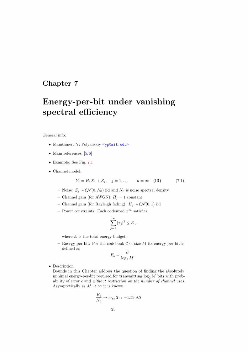
• Channel model:
Yj = HjXj + Zj , j = 1, . . . n =∞ (!!!) (7.1)
– Noise: Zj ∼ CN (0, N0) iid and N0 is noise spectral density
– Channel gain (for AWGN): Hj = 1 constant
– Channel gain (for Rayleigh fading): Hj ∼ CN (0, 1) iid
– Power constraints: Each codeword x∞ satisfies
∞∑j=1
|xj |2 ≤ E ,
where E is the total energy budget.
– Energy-per-bit: For the codebook C of size M its energy-per-bit isdefined as
Eb =E
log2M.
• Description:Bounds in this Chapter address the question of finding the absolutelyminimal energy-per-bit required for transmitting log2M bits with prob-ability of error ε and without restriction on the number of channel uses.Asymptotically as M →∞ it is known:
EbN0→ loge 2 ≈ −1.59 dB
25

26CHAPTER 7. ENERGY-PER-BIT UNDER VANISHING SPECTRAL
EFFICIENCY
> energy-per-bit/plot_all()
100
101
102
103
104
105
106
−2
−1
0
1
2
3
4
5
6
7
8
Information bits, k
Eb/
No,
dB
Energy per bit vs. length of the message (AWGN channel); ε=0.001
AchievabilityNormal approximationConverseShannon limit, −1.59 dB
100
101
102
103
104
105
−2
0
2
4
6
8
10
Information bits, k
Eb/
No,
dB
Energy per bit vs. length of the message (Rayleigh fading); ε=0.001
noCSI: Achievability (ach_ht)noCSI: Normal approximationnoCSI: ConverseCSIR: Normal approximationShannon limit, −1.59 dB
Figure 7.1: Example figures generated by the energy-per-bit code
• Real/Complex: In the regime of infinite bandwidth as here, there is nodifference between real/complex channel inputs (but noise variance in thereal case should be taken Zj ∼ N (0, N0
2 )).
• MIMO and block-fading: Surprisingly, having multiple transmit antennasor block-constant fading makes no difference for energy-per-bit, see [6].Having mr > 1 receive antennas is equivalent to scaling N0 → N0
mrand
thus again does not require any special treatment.
• Remark: These bounds correspond to allowing no feedback link. Even amodicum of feedback significantly improves the energy-per-bit tradeoff atfinite length, see [5].
• Remark: The tradeoff Eb
N0vs. log2M can also be interpreted as the
rate-blocklength tradeoff for the power-constrained infinite-bandwidthcontinunuous-time channel, see [5, (50)-(51)].
• Common input/output arguments:
1. epsil – block probability of block error.
2. lm or Lms – input or output argument; log2M , log-size of codebook(base-2 information units).
3. en0 or EE – input/output argument; total energy budget availableEE= E
N0(to get Eb
N0divide by lm).
7.1 Summary plot
plot_all()
This script generates two figures, shown on Fig. 7.1.Note: Script takes several hours to finish.
7.2 The AWGN channel (Hj = 1)
Here Hj = 1 in the channel model (7.1).Format:

7.3. RAYLEIGH FADING: CSIR CASE 27
function En0 = energy_awgn_ach(Lms, epsil);
function lm = energy_awgn_conv(en0, epsil);
function lm = energy_awgn_normapx(en0, epsil);
These functions return achievability/converse/normal approximation. Thebounds are from [5, Theorems 2 and 3].
7.3 Rayleigh fading: CSIR case
Format:
function lm = energy_csir_conv(EE, epsil);
This function computes the converse (upper) bound on the number ofinformation bits, lm, that a Rayleigh fading channel with perfect CSIR cantransmit under a total energy budget EE= E
N0; see [6, Theorem 11]. Note that
for CSIR case we can use energy_aegn_ach() and energy_awgn_normapx()
for achievability and normal approximation, see [6, Section III.D].
Note: vector EE should be in ascending order.
7.4 Rayleigh fading: noCSI case
Format:
function lm = energy_nocsi_ach_ht(EE, epsil);
function lm = energy_nocsi_ach_ml(EE, epsil);
These are two achievability bounds [6, Corollary 4 and 5] with the secondone, _ml(), being typically better.
function lm = energy_nocsi_conv(EE, epsil);
function lm = energy_nocsi_normapx(EE, epsil);
The converse bound is [6, Theorem 6]. The normal approximation is com-puted by maximizing over A in [6, (64)].
Note: Vector EE should be in ascending order.Note: Functions energy_nocsi_ach_ml() and energy_nocsi_conv() arevery slow.


Chapter 8
Fixed-length source coding undera distortion criterion
• Maintainer: V. Kostina <[email protected]>
• Main references: [7]
• Performance criterion - excess distortion probability:
P[d(S,Z) > d] ≤ ε,
where S is the source and Z is its representation.
• The code uses auxiliary functions contained in lib/. This directorycan to be added to Matlab path by running the following command:path(path, ’../../lib’);
• To speed up calculations, some functions use the so-called ‘persistent’variables whose values are retained during multiple calls to those functions.This helps to choose the starting positions for various optimizationswisely. For example, if the function is computed for blocklength 510 afterblocklength 500, it takes advantage of the previous computation to choosea starting position for various optimizations. To avoid problems, usecommand clear all to clear the values of all persistent variables whenmaking a computation unrelated to the previous computation.
• Recommended usage:
path(path, ’../../lib’);
clear all;
N = 10:10:1000;
out = NaN(1, length(N));
for k = 1:length(N)
n = N(k);
try
out(k) = Rstar(..., n, ...);
save(’mydatafile’);
catch ME
29

30CHAPTER 8. FIXED-LENGTH SOURCE CODING UNDER A
DISTORTION CRITERION
> cd sc/GMS
> plot_all(0.1, 0.01, 10:5:500)
0 50 100 150 200 250 300 350 400 450 5001.6
1.8
2
2.2
2.4
2.6
2.8
3
3.2
3.4
3.6
Blocklength, n
Com
pres
sion
rat
e, b
it / s
ourc
e sa
mpl
e
Lossy compression of iid standard normal source. Distortion=0.1 at excess=1%
Rogers (achievability)Normal approximationSphere covering + HT (converse)
Figure 8.1: Lossy compression bounds for the memoryless Gaussian source.
fprintf(’Error: %s\n’, getReport(ME));
out(k) = NaN;
end
end
• For an example plot (produced via sc/GMS/plot_all.m) see Fig. 8.1.
8.1 Binary memoryless source
Source model
S1, S2, . . . are i.i.d Bernoulli with bias p.
Distortion measure
Bit error rate
d(sk, zk) =1
k
k∑i=1
1si 6= zi.
Matlab code
sc/BMS/
Main functions
Rstar(d, n, e, p, fun): Compression rate compatible with a given excessdistortion.
Dstar(R, n, e, p, fun): Distortion threshold compatible with a given excessprobability and a given rate.

8.2. GAUSSIAN MEMORYLESS SOURCE 31
Input arguments
d: distortion threshold.
R: compression rate.
n: blocklength.
e: excess distortion probability.
p: source bias.
fun: alias for the function to be computed. Acceptable values:
‘shannon’ : Shannon’s achievability bound [7, Theorem 1].
‘normal’ : Gaussian approximation [7, Theorem 12].
‘spherecoveringc’ : Converse via sphere covering and hypothesis testing [7,Theorem 8].
‘generalc’ : General converse via d-tilted information [7, Theorem 7].
‘spherecoveringa’ : Achievability via covering with random spheres [7,Theorem 21].
‘permutationa’ : Achievability via permutation coding (i.e. all code-words are of the same type, namely, the type that achieves therate-distortion function) [7, Theorem 22].
‘martona’ : Converse via Marton’s bound [7, Theorem 5].
8.2 Gaussian memoryless source
Source model
S1, S2, . . . are i.i.d N (0, 1).
Distortion measure
Squared error
d(sk, zk) =1
k
k∑i=1
(si − zi)2
Matlab code
sc/GMS/
Main functions
Rstar(d, n, e, fun): Compression rate compatible with a given excess dis-tortion.
Dstar(R, n, e, fun): Distortion threshold compatible with a given excessprobability and a given rate.

32CHAPTER 8. FIXED-LENGTH SOURCE CODING UNDER A
DISTORTION CRITERION
Input arguments
d: distortion threshold.
R: compression rate.
n: blocklength.
e: excess distortion probability.
fun: alias for the function to be computed. Acceptable values:
‘shannon’ : Shannon’s achievability bound [7, Theorem 1].
‘normal’ : Gaussian approximation [7, Theorem 12].
‘spherecoveringc’ : Converse via sphere covering and hypothesis testing [7,Theorem 8].
‘spherecoveringa’ : Achievability via covering with random spheres [7,Theorem 37].
The following fun values are accepted only by Rstar(...).
‘generalc’ : General converse via d-tilted information [7, Theorem 7].
‘rogersa’ : Achievability using a result by Rogers [7, Theorem 39].
8.3 Binary erased source
Source model
S1, S2, . . . are i.i.d fair coin flips. However, the encoder does not observeS1, S2, . . .. Instead, it observes an erased version of the source: X1, X2, . . .,where Xi = Si with probability 1− α, and Xi = ? with probability α.
Distortion measure
Bit error rate with respect to the original source
d(sk, zk) =1
k
k∑i=1
1si 6= zi, si, zi ∈ 0, 1.
Matlab code
sc/BES/
Main functions
Rstar(d, n, e, alpha, fun): Compression rate compatible with a given ex-cess distortion.

8.3. BINARY ERASED SOURCE 33
Input arguments
d: distortion threshold.
n: blocklength.
e: excess distortion probability.
alpha: erasure probability.
fun: alias for the function to be computed. Acceptable values:
‘spherecoveringa’ : Achievability via covering with random spheres [7,Theorem 33].
‘spherecoveringc’ : Converse via sphere covering (hypothesis testing) [7,Theorem 32].
‘normal’ : Gaussian approximation [7, Theorem 12].
‘aeq’ : Achievability via covering with random spheres for a surrogaterate-distortion problem which negates the stochastic variability ofthe erasure channel [8].
‘ceq’ : Converse via sphere covering (hypothesis testing) for the surrogateproblem [8].
‘normaleq’ : Gaussian approximation for the surrogate problem [8].


Chapter 9
Variable-length compressionallowing errors
• Maintainer: V. Kostina <[email protected]>
• Main references: [9].
• Fixed probability of error:
P[S 6= Z] ≤ ε,
where S is the source and Z is its reconstruction after the (almost lossless)encoding.
• Performance criterion: average length of the compressed representation.
• Performance criterion - excess distortion probability:
P[d(S,Z) > d] ≤ ε,
where S is the source and Z is its reconstruction after the transmissionover a noisy channel.
• The code uses auxiliary functions contained in lib/. This directoryneeds to be added to Matlab path by running the following command:path(path, ’../../lib’);
• To speed up calculations, some functions use the so-called ‘persistent’variables whose values are retained during multiple calls to those functions.This helps to choose the starting positions for various optimizationswisely. For example, if the function is computed for blocklength 510 afterblocklength 500, it takes advantage of the previous computation to choosea starting position for various optimizations. To avoid problems, usecommand clear all to clear the values of all persistent variables whenmaking a computation unrelated to the previous computation.
• Recommended usage:
path(path, ’../../lib’);
clear all;
35

36CHAPTER 9. VARIABLE-LENGTH COMPRESSION ALLOWING
ERRORS
N = 10:10:1000;
out = NaN(1, length(N));
for k = 1:length(N)
n = N(k);
try
out(k) = Rstar(..., n, ...);
save(’mydatafile’);
catch ME
fprintf(’Error: %s\n’, getReport(ME));
out(k) = NaN;
end
end
9.1 Binary memoryless source
Source model
S1, S2, . . . are i.i.d Bernoulli with bias p.
Matlab code
sc/varrate/
Main function
Rstar(p, e, n, fun): Compression rate compatible with a given excess dis-tortion.
Input arguments
p: source bias.
e: error probability.
n: blocklength.
fun: alias for the function to be computed. Acceptable values:
‘approx’ : Gaussian approximation [9, Theorem 4].
‘exact’ : Exact minimum average rate [9, (26)].
‘exacti’ : Exact value of the Erokhin function [9, (40)].
‘ie’ : Exact value of the expectation of the ε-cutoff of information inSk [9, (11),(13)].

Chapter 10
Joint source-channel codingunder a distortion criterion
• Maintainer: V. Kostina <[email protected]>
• Main references: [10]
• Performance criterion - excess distortion probability:
P[d(S,Z) > d] ≤ ε,
where S is the source and Z is its reconstruction after the transmissionover a noisy channel.
• The code uses auxiliary functions contained in lib/. This directoryneeds to be added to Matlab path by running the following command:path(path, ’../../lib’);
• To speed up calculations, some functions use the so-called ‘persistent’variables whose values are retained during multiple calls to those functions.This helps to choose the starting positions for various optimizationswisely. For example, if the function is computed for blocklength 510 afterblocklength 500, it takes advantage of the previous computation to choosea starting position for various optimizations. To avoid problems, usecommand clear all to clear the values of all persistent variables whenmaking a computation unrelated to the previous computation.
• Recommended usage:
path(path, ’../../lib’);
clear all;
N = 10:10:1000;
out = NaN(1, length(N));
for k = 1:length(N)
n = N(k);
try
out(k) = Rstar(..., n, ...);
save(’mydatafile’);
37

38CHAPTER 10. JOINT SOURCE-CHANNEL CODING UNDER A
DISTORTION CRITERION
catch ME
fprintf(’Error: %s\n’, getReport(ME));
out(k) = NaN;
end
end
10.1 Binary memoryless source transmitted over abinary symmetric channel
Source model
S1, S2, . . . are i.i.d Bernoulli with bias p.
Channel model
Yi = Xi +Ni, where Ni are i.i.d. Bernoulli with bias δ.
Distortion measure
Bit error rate
d(sk, zk) =1
k
k∑i=1
1si 6= zi.
Matlab code
jscc/BMS-BSC/
Main functions
Rstar(p, delta, d, e, n, fun): Compression rate compatible with a givenexcess distortion.
Dstar(R, n, e, p, delta, fun): Distortion threshold compatible with agiven excess probability and a given rate.
Input arguments
p: source bias.
delta: channel crossover probability.
d: distortion threshold.
e: excess distortion probability.
R: compression rate.
n: blocklength.
fun: alias for the function to be computed. Acceptable values:
‘approx’ : Gaussian approximation [10, Theorem 10].

10.2. GAUSSIAN SOURCE TRANSMITTED OVER AN AWGN CHANNEL39
‘clistdecoding’ : Converse via list decoding and hypothesis testing [10,Theorem 4].
‘ajoint’ : Achievability via joint source-channel coding [10, Theorem 8].
‘aseparate’ : Achievability via separation [10, Theorem 6].
The following fun values are accepted only by Rstar(...).
‘cgeneral’ : General converse via d-tilted information [10, Theorem 2].
‘approxseparate’ : Gaussian approximation for the separation architecture[10, (126)].
‘arcu’ : For the almost lossless transmission, achievability via RCUbound [10, Theorem 9].
The following fun values are accepted only by Dstar(...).
‘random’ : Achievability via random coding for fair coin flip source [10,Theorem 6].
‘nocoding’ : Achievability via no coding. [10, Theorem 23].
10.2 Gaussian source transmitted over an AWGNchannel
Source model
S1, S2, . . . are i.i.d N (0, 1).
Channel model
Yi = Xi +Ni, where Ni are i.i.d. N (0, 1).
Distortion measure
Squared error
d(sk, zk) =1
k
k∑i=1
(si − zi)2.
Matlab code
jscc/GMS-AWGN/
Main functions
Rstar(P, d, e, n, fun): Transmission rate compatible with a given excessdistortion (nats).
Dstar(R, n, e, P, fun): Distortion threshold compatible with a given excessprobability and a given rate.

40CHAPTER 10. JOINT SOURCE-CHANNEL CODING UNDER A
DISTORTION CRITERION
Input arguments
P: maximum allowable transmit power, or SNR.
d: distortion threshold.
e: excess distortion probability.
R: transmission rate.
n: blocklength.
fun: alias for the function to be computed. Acceptable values:
‘approx’ : Gaussian approximation [10, Theorem 10].
‘cht’ : Converse via list decoding and hypothesis testing [10, Theorem 4].
‘ajoint’ : Achievability via joint source-channel coding [10, Theorem 8].
‘aseparate’ : Achievability via separation [10, Theorem 6].
The following fun values are accepted only by Dstar().
‘nocoding’ : Achievability via no coding [10, Theorem 24].
‘approxnocoding’ : Gaussian approximation for the uncoded system [10,(129), (208)].
The following fun values are accepted only by Rstar().
‘cgeneral’ : General converse via d-tilted information [10, Theorem 2].
‘approxseparate’ : Gaussian approximation for the separation architecture[10, (126)].

Chapter 11
The binary-symmetric channel(BSC)
General info:
• Maintainer: Y. Polyanskiy <[email protected]>
• Main references: [1]
• Example: See Fig. 11.1
• Channel model:
Yj = Xj + Zj mod 2, j = 1, . . . , n
– Codewords are 0/1: xj ∈ 0, 1, j = 1, . . . , n
– Noise: Zj ∼ Ber(δ) iid.
• Common input/output arguments:
1. delta – input argument; crossover probability δ.
2. epsil – block probability of block error. Warning: All code in thissection is tailored to maximal probability of error.
3. lm or Lms – output argument; log2M , log-size of codebook (base-2information units).
4. n – input argument; blocklength.For slow functions that do not support vectorized arguments.
5. Ns – input argument; vector of blocklengths.
11.1 Summary plot: plot all()
Definition:
function [Ns ach_rcu ach_dt ach_gal conv normapx_val] = plot_all(delta, epsil);
This function computes and plots various bounds on the same figure. SeeFig. 11.1.
41

42 CHAPTER 11. THE BINARY-SYMMETRIC CHANNEL (BSC)
> plot_all()
0 200 400 600 800 1000 1200 1400 1600 1800 20000
0.05
0.1
0.15
0.2
0.25
0.3
0.35
0.4
0.45
0.5
Blocklen, n
Rat
e, R
Bounds for the BSC(0.11), Pe,max
= 0.001
CapacityConverseNormal approximationRCU achievabilityDT achievabilityGallager achievability
Figure 11.1: Code and resulting picture for BSC bounds
11.2 Achievability: dt ach()
Definition:
function Lms = dt_ach(Ns, delta, epsil)
Function computes DT achievability bound, see [1, (166)].
11.3 Achievability: rcu ach()
Format:
function lm = rcu_ach(n, delta, epsil)
This computes the RCU achievability bound, see [1, (162)].Warning: This function only takes scalar value of n.
11.4 Achievability: gallager ach()
Format:
function Lms = gallager_ach(Ns, delta, epsil)
Computes Gallager’s achievability bound, see [1, (44)].
11.5 Converse: converse()
Format:

11.6. NORMAL APPROXIMATION: NORMAPX() 43
function Lms = converse(Ns, delta, epsil)
This computes the sphere-packing lower bound. Equivalently, this is thebest possible meta-converse bound with QY n = Ber(1/2)n, see [1, Theorem 35].
11.6 Normal approximation: normapx()
Format:
function Lms = normapx(Ns, delta, epsil);
Fast and frequently very precise approximation to both achievability andconverse:
logM ≈ nC −√nV Q−1(ε) +
1
2log n
where C = log 2− δ log 1δ − (1− δ) log 1
1−δ and V = δ(1− δ) log2 1−δδ .


Chapter 12
The binary-erasure channel(BEC)
General info:
• Maintainer: Y. Polyanskiy <[email protected]>
• Main references: [1]
• Example: See Fig. 11.1
• Channel model:
Yj =
Xj , with prob.1− δe, with prob.δ
j = 1, . . . , n
Codewords are 0/1: xj ∈ 0, 1, j = 1, . . . , n
• Common input/output arguments:
1. delta – input argument; crossover probability δ.
2. epsil – block probability of block error. Warning: All code in thissection is tailored to maximal probability of error.
3. lm or Lms – output argument; log2M , log-size of codebook (base-2information units).
4. n – input argument; blocklength.For slow functions that do not support vectorized arguments.
5. Ns – input argument; vector of blocklengths.
12.1 Summary plot: plot all()
Definition:
function [Ns ach_dt ach_gal conv normapx_val] = plot_all(delta, epsil);
This function computes and plots various bounds on the same figure. SeeFig. 12.1.
45

46 CHAPTER 12. THE BINARY-ERASURE CHANNEL (BEC)
> plot_all()
0 100 200 300 400 500 600 700 800 900 10000
0.05
0.1
0.15
0.2
0.25
0.3
0.35
0.4
0.45
0.5
Blocklen, n
Rat
e, R
Bounds for the BSC(0.5), Pe,max
= 0.001
CapacityConverseNormal approximationDT achievabilityGallager achievability
Figure 12.1: Code and resulting picture for BEC bounds
12.2 Achievability: dt ach()
Definition:
function Lms = dt_ach(Ns, delta, epsil)
Function computes DT achievability bound, see [1, (183)].
Note: The RCU bound is weaker for the BEC, so we do not need to evaluateit.
12.3 Achievability: gallager ach()
Format:
function Lms = gallager_ach(Ns, delta, epsil)
Computes Gallager’s achievability bound, see [1, (44)].
12.4 Converse: converse()
Format:
function Lms = converse(Ns, delta, epsil)
This computes the special converse bound for the BEC, see [1, Theorem38]. Later, it was found that it corresponds to the meta-converse bound with anon-product distribution QY n , see [11, Section VI.D].

12.5. NORMAL APPROXIMATION: NORMAPX() 47
12.5 Normal approximation: normapx()
Format:
function Lms = normapx(Ns, delta, epsil);
Fast and frequently very precise approximation to both achievability andconverse:
logM ≈ nC −√nV Q−1(ε) ,
where C = (1− δ) log 2 and V = δ(1− δ) log2 2.


Chapter 13
The binary-AWGN channel(BI-AWGN)
General info:
• Maintainer: T. Erseghe <[email protected]>
• Main references: [12]
• Example: See Fig. 13.1
• Channel model:
Yj =√
ΩXj + Zj , j = 1, . . . , n
– Codewords are 0/1: xj ∈ ±1, j = 1, . . . , n
– Noise: Zj ∼ N (0, 1) iid
– Ω is the signal to noise ratio (SNR).
• Common input/output arguments:
1. n – blocklength.
2. Pe – block probability of block error, or packet error rate. Warning:All code in this section is tailored to average probability of error.
3. R – code rate.
4. SNRdB – signal to noise ratio in dB.
13.1 Converse: converse mc()
Definition #1:
R = converse_mc(N,Pe,SNRdB,’approx’)
returns the metaconverse Polyanskiy-Poor-Verdu (PPV) upper bound on ratefor a codeword of length N, a packet error rate of Pe, and a signal to noiseratio of SNRdB (in dB). Multiple bound values can be obtained by ensuring thatN, Pe, and SNRdB have the same length. The specific approximation used forcalculating the bound is specified by ’approx’:
49

50 CHAPTER 13. THE BINARY-AWGN CHANNEL (BI-AWGN)
• ’normal’ normal approximation, the O(n−1) approximation availablefrom [12, Fig. 6, 3rd block]; this is a very fast algorithm, but may providea weak approximation.
• ’On2’ (default) the O(n−2) approximation derived from [12, Fig. 6, 2ndblock]; at low Pe this is much more reliable than the ’normal’ option.
• ’On3’ the O(n−3) approximation derived from [12, Fig. 6, 2nd block];at high Pe this is much more unrealiable than ’On2’. It can be used toidentify the region where ’On2’ is a reliable solution, namely the regionwhere ’On2’ and ’On3’ closely match.
• ’full’ (this option will be available soon) the full bound derived numer-ically from [12, Fig. 6, 1st block].
Definition #2:
SNRdB = converse_mc(N,Pe,R,’approx’,’error’)
for a codeword of length N, and code rate R, the function returns the signal tonoise ration SNRdB (in dB) at which the PPV metaconverse lower bound onerror rate is equal to Pe. Multiple bound values can be obtained by ensuringthat N, Pe, and R have the same length. The specific approximation used forcalculating the bound is specified by ’approx’ (see above).
13.2 Example 1: example speff.m
In example_speff.m we use the converse_mc function in order to derive anupper bound on rate, R, and then plot a bound on spectral efficiency, namelyρ = 2R. We also recall the relation
Ω = ρEbN0
with Ω the SNR, and Eb the energy spent per bit of information. The exampleis built on a codeword of length n=1000 for which the bounds at Pe=1e-5 arederived according to the following code:
n = 1e3;
Pe = 1e-5;
SNRdB = -15:10; % SNR Omega
uno = ones(size(SNRdB)); % vector of ones
% normal approximation - expected execution time 2 sec
rhoNA = 2*converse_mc(n*uno,Pe*uno,SNRdB,’normal’);
EbN0NA = SNRdB-10*log10(rhoNA);
% O(n^-2) approximation - expected execution time 90 sec
rhoPPV = 2*converse_mc(n*uno,Pe*uno,SNRdB,’On2’);
EbN0PPV = SNRdB-10*log10(rhoPPV);

13.3. EXAMPLE 2: EXAMPLE PER.M 51
% O(n^-3) approximation - expected execution time 120 sec
rhoPPVb = 2*converse_mc(n*uno,Pe*uno,SNRdB,’On3’);
EbN0PPVb = SNRdB-10*log10(rhoPPVb);
and then the results is plotted by using
figure
set(0,’defaulttextinterpreter’,’latex’)
semilogy(EbN0PPV,rhoPPV,’-’,EbN0PPVb,rhoPPVb,’--’,...
EbN0NA,rhoNA,’-.’)
xlabel(’SNR $E_b/N_0$’)
ylabel(’spectral efficiency $\rho$ [bit/s/Hz]’)
grid
The result is given in the plot on the left in Fig. 13.1
0 5 10 1510
−3
10−2
10−1
100
101
SNR E b/N 0
spectralefficiency
ρ[b
it/s/
Hz]
n = 1000, Pe = 1e - 05
O (n − 2) approx
O (n − 3) approx
normal approx
−0.5 0 0.5 1 1.5 210
−7
10−6
10−5
10−4
10−3
10−2
10−1
100
SNR E b/N 0
errorpro
bability
Pe
n = 1000, R = 0.5
Figure 13.1: Examples of BI-AWGN metaconverse bounds
13.3 Example 2: example per.m
In example_per.m we use the converse_mc function in order to derive a lowerbound on the packet error rate, Pe. The example is built on a codeword oflength n=1000 and rate R=0.5 for which bounds are derived according to thefollowing code:

52 CHAPTER 13. THE BINARY-AWGN CHANNEL (BI-AWGN)
n = 1e3;
R = 1/2;
Pev = 10.^([-0.5:-0.25:-1.75,-2:-0.5:-7]);
uno = ones(size(Pev));
% normal approximation - expected execution time 15 sec
SNRdBNA = converse_mc(n*uno,Pev,R*uno,’normal’,’error’);
% O(n^-2) approximation - expected execution time 120 sec
SNRdBPPV = converse_mc(n*uno,Pev,R*uno,’On2’,’error’);
% O(n^-3) approximation - expected execution time 280 sec
SNRdBPPVb = converse_mc(n*uno,Pev,R*uno,’On3’,’error’);
and then the results is plotted by using
figure
set(0,’defaulttextinterpreter’,’latex’)
semilogy(SNRdBPPV,Pev,’-’,SNRdBPPVb,Pev,’--’,...
SNRdBNA,Pev,’-.’)
xlabel(’SNR $E_b/N_0$’)
ylabel(’error probability $P_e$’)
grid
The result is given in the plot on the right in Fig. 13.1
Bibliography
[1] Y. Polyanskiy, H. V. Poor, and S. Verdu, “Channel coding rate in thefinite blocklength regime,” IEEE Trans. Inf. Theory, vol. 56, no. 5, pp.2307–2359, May 2010.
[2] G. Durisi, T. Koch, J. Ostman, Y. Polyanskiy, and W. Yang, “Short-packetcommunications over multiple-antenna Rayleigh-fading channels,” Dec.2014. [Online]. Available: http://arxiv.org/abs/1412.7512
[3] W. Yang, G. Durisi, T. Koch, and Y. Polyanskiy, “Quasi-static multiple-antenna fading channels at finite blocklength,” IEEE Trans. Inf. Theory,vol. 60, no. 7, pp. 4232–4265, Jul. 2014.
[4] W. Yang, G. Caire, G. Durisi, and Y. Polyanskiy, “Optimum power controlat finite blocklength,” IEEE Trans. Inf. Theory, vol. 61, no. 9, pp. 4598–4615, Sep. 2015.
[5] Y. Polyanskiy, H. V. Poor, and S. Verdu, “Minimum energy to send k bitswith and without feedback,” IEEE Trans. Inf. Theory, vol. 57, no. 8, pp.4880–4902, Aug. 2011.
[6] W. Yang, G. Durisi, and Y. Polyanskiy, “Minimum energy to send k bitsover multiple-antenna fading channels,” arXiv:1507.03843v1, Jul. 2015.
[7] V. Kostina and S. Verdu, “Fixed-length lossy compression in the finiteblocklength regime,” IEEE Transactions on Information Theory, vol. 58,no. 6, pp. 3309–3338, June 2012.
[8] ——, “Nonasymptotic noisy lossy source coding,” in Proceedings 2013IEEE Information Theory Workshop, Seville, Spain, Sep. 2013.
[9] V. Kostina, Y. Polyanskiy, and S. Verdu, “Variable-length compressionallowing errors,” IEEE Transactions on Information Theory, vol. 61, no. 9,pp. 4316–4330, Aug. 2015.
[10] V. Kostina and S. Verdu, “Lossy joint source-channel coding in the finiteblocklength regime,” IEEE Transactions on Information Theory, vol. 59,no. 5, pp. 2545–2575, May 2013.
[11] Y. Polyanskiy, “Saddle point in the minimax converse for channel coding,”IEEE Trans. Inf. Theory, May 2012, submitted. [Online]. Available:http://people.lids.mit.edu/yp/homepage
53

54 BIBLIOGRAPHY
[12] T. Erseghe, “Coding in the finite-blocklength regime: Bounds based onlaplace integrals and their asymptotic approximations,” arXiv preprintarXiv:1511.04629, 2015.
Related Documents