Spectral Wave Characteristics over the Head Bay of Bengal

Spectral Wave Characteristics over the Head Bay of Bengal: A Modeling Study

ANINDITA PATRA,1 PRASAD K. BHASKARAN,1 and RAJIB MAITY2

Abstract—Information on spectral wave characteristics is an

essential prerequisite for ocean engineering-related activities and

also to understand the complex wave environment at any given

location. To the best of our knowledge, there are no comprehensive

studies attempted so far to study the wave spectral characteristics

over the head Bay of Bengal, a low-lying deltaic environment. The

present study is an attempt to describe the spectral characteristics of

wave evolution across different locations over this deltaic region

based on numerical simulations. Therefore, it implements a multi-

scale nested modeling approach using two state-of-art wave mod-

els, WAM and SWAN, and forced with ERA-Interim winds

spanning the year of 2016. Model-computed integrated wave

parameters are validated against wave rider buoy data as well as

remotely sensed SARAL/AltiKa and merged altimeter data.

Analysis of the monthly averaged one-dimensional spectrum

reveals a single peak during the southwest monsoon and existence

of double peaks from November to January, and occasionally up to

March. Variance energy density undergoes inter-seasonal variation

and attains its maxima during the month of July. Transformation of

swell wave energy as a function of depth is found to be mostly

associated with physical processes such as wave-bottom interaction

and attenuation by opposing winds during the northeast (NE)

monsoon. Fetch restriction for the evolution of wind seas (from the

NE), modification in wind shear stress by opposing swells, and

bottom effects remarkably contribute to the reduction in wind sea

energy at shallow water depths. This study indicates that the

influence of swells is higher along the eastern side of the basin as

compared to the western side, and marginally higher variance is

also observed over the east except during February–April. The two-

dimensional wave spectra exhibit differential wave systems

approaching from various directions attributed to a reflected swell

system from the south-southeast throughout the year, southwest

swells, reversing wind seas following local winds, and reflected

wind seas from the land boundary.

Key words: Head Bay of Bengal, SWAN, WAM, wave

spectrum, wave transformation.

1. Introduction

Detailed knowledge on ocean wave characteristics

is of paramount importance for the development of

the marine environment, ocean engineering applica-

tions, and sustainable coastal zone management. The

wave spectrum is a standard descriptor of wave

characteristics as it contains information on the dis-

tribution of wave variance over both frequency and

direction domains. The commonly used integrated

parameters such as significant wave height (SWH)

and mean wave period (MWP) provide limited

information on the simultaneous occurrence of dif-

ferent wave systems. Engineering design and

planning calculations that involve complex sea states

are based on accurate wave spectral descriptions. In

the spectral approach, the sea surface is represented

as the superposition of a finite number of harmonic

components with different frequencies and directions.

The spectral components originating from different

physical mechanisms play an important role in the

resultant wave energy balance. The high-frequency

part of the wave spectrum that is the wind-sea regime

governs the exchange of momentum across the air–

sea interface (Cavaleri et al. 2012). On the other

hand, a proper understanding of long-period waves

and their evolution is an essential prerequisite to

address problems related to navigation and offshore

operations, and also important in context to large-

scale motions on the mooring systems (McComb

et al. 2009). The concurrent existence of locally

generated wind seas and remotely forced swells can

lead to complex wave systems that are quite common

in the global oceans. By analyzing the wave spec-

trum, the different wave systems present at a given

location can be identified (Soares 1991; Hanson and

Phillips 2001). Identification of separate wave

Electronic supplementary material The online version of this

article (https://doi.org/10.1007/s00024-019-02292-3) contains sup-

plementary material, which is available to authorized users.

1 Department of Ocean Engineering and Naval Architecture,

Indian Institute ofTechnologyKharagpur,Kharagpur 721 302, India.

E-mail: [email protected]; [email protected] Department of Civil Engineering, Indian Institute of

Technology Kharagpur, Kharagpur 721 302, India.

Pure Appl. Geophys. 176 (2019), 5463–5486

� 2019 Springer Nature Switzerland AG

https://doi.org/10.1007/s00024-019-02292-3 Pure and Applied Geophysics

systems provides a better scope to understand the

specific physical processes that determine the sea

state. For a specific location, the spectral footprint is

unique and depends on the prevailing meteorological

and environmental conditions.

In context of the Indian seas, the Bay of Bengal

and Arabian Sea experience coexistence of wind seas

and swells (Baba et al. 1989; Kumar et al. 2003, 2014;

Aboobacker et al. 2011a, b; Sabique et al. 2012;

Nayak et al. 2013; Sandhya et al. 2016). The wave

characterizations therefore need to be based on the

wave spectrum rather than integral parameters in

order to understand the evolution of wave energy

balance. Unfortunately, there exists no detailed study

on the spectral wave characteristics for the head Bay

of Bengal (north of 20�N) region. The study region

(Fig. 1) located in the North Indian Ocean is a quite

unique region in the world owing to high tidal range,

low-lying topographic features, a large riverine delta

system, excessive sediment loads, numerous tidal

creeks, and the mangrove ecosystems. As stated

above, in order to have a better understanding on the

effect of waves over this highly dynamic nearshore

region, it is necessary to investigate each spectral

component separately. The Bay of Bengal is exposed

to a wind system of high seasonal variability, with

strong winds from the southwest direction during the

southwest monsoon period (June–September), from

the northeast during the northeast (NE) monsoon

period (November–January), and fair weather during

the rest of the months. Due to the reversing wind

system, one can expect intra-annual variability in the

locally generated wind seas. On the other hand, swells

generated from the Southern Ocean are known to

travel over long distances with minimum attenuation

and simultaneously interact with the locally generated

wind waves over the Bay of Bengal basin. The nature

of Southern Ocean swells also varies over a year with

maximum energy during the Southern Hemisphere

winter (June–September) followed by the spring.

Therefore, a detailed analysis covering a period of one

full year can provide vital information on the evolu-

tion of wave spectral characteristics.

Numerical models constitute the basis to charac-

terize the wave conditions when measurements are

not available. The state-of-art third-generation wave

models have gained popularity on the account of their

sophisticated physics and advanced numerics and

have been successfully applied to various regions in

the world by many researchers (Wang and Swail

2002; Shanas et al. 2017; Akpinar et al. 2012, 2016).

With recent developments in computational power,

Figure 1Study region along with locations considered for analysis

5464 A. Patra et al. Pure Appl. Geophys.

the present generation state-of-art models have the

ability to model nearshore regions and complex

coastline geometry with high spatial resolutions.

Wave modeling using the Simulating Waves Near-

shore (SWAN) model was carried out for different

geographical regions such as the Chabahar zone

(Saket et al. 2013), the Persian Gulf (Moeini et al.

2012), Iranian seas (Mazaheri et al. 2013), and the

Black Sea (Akpinar et al. 2012, 2016). Akpinar et al.

(2012) reported on the implementation of the SWAN

model forced by the ECMWF ERA-Interim data set

of reanalyzed 10-m winds over the Black Sea and its

validation with buoy measurements. Stopa et al.

(2011) investigated wave energy resources for the

Hawaiian Islands in the mid-Pacific using WAVE-

WATCH-III and SWAN. The wave climate

variability over the southwest western Australian

shelf and nearshore region and its dependency on

large-scale climate variability was studied using

SWAN by Wandres et al. (2017). Nayak et al. (2013),

Umesh et al. (2017), and Parvathy et al. (2017) have

considered the SWAN model nested with the Wave

Ocean Model (WAM, WAMDIG 1988) for nearshore

wave simulation over different regions in the Bay of

Bengal. Similarly, Sandhya et al. (2014) integrated

two wave models, WAVEWATCH-III (Tolman

1991) and SWAN (Booji et al. 1999), to study the

wave characteristics at coastal Puducherry on the east

coast of India. Therefore, wave information derived

from numerical models is of great importance to the

scientific and engineering community.

There are studies (Patra and Bhaskaran

2016, 2017) that described the wave climate based on

integral wave parameters, such as significant wave

height (SWH) and mean wave period (MWP) over

the head Bay of Bengal region. However, when two

or more wave systems are simultaneously present, the

integral parameters become insufficient to fully rep-

resent the wave climate. Under this condition, the

spectral details are essential for many applications

like climate assessment, navigation, coastal engi-

neering, etc. The purpose of the present study is to

explore the wave spectral features over this region.

To accomplish this, two wave models, viz. WAM and

SWAN, were nested such that the time-varying

boundary spectral information from WAM was pro-

vided to SWAN, and the resultant wave spectrum

obtained from fine-resolution SWAN was used for

further analysis. Accordingly, the model simulation

was carried out for the full year of 2016 in order to

examine the seasonal and intra-annual variability. As

the availability of in situ measured buoy data was

limited for a short period, the model-computed SWH

values have been verified accordingly. The wave

rider buoy data was obtained from the Earth System

Science Organization (ESSO)—Indian National

Centre for Ocean Information Services (INCOIS).

Further, the study also verified the model generated

SWH with the satellite passes of SARAL/AltiKa over

this region. Investigation on the wave evolution

characteristics used the location-specific 1D and 2D

spectrum derived from the model. A detailed inves-

tigation was carried out to examine the monthly

variation in variance density, as well identification of

separate wave systems in the study region. Diurnal

variability and transformation of wave spectra along

various water depths are discussed. In addition, wave

spectra along two longitudinal transects over the

eastern and western side of the study domain are also

compared. This paper is organized as follows: Sect. 2

describes the study area and data sets used; Sect. 3

provides information on the model configuration and

validation exercise, Sect. 4 provides details on the

results and discussion; and, finally, the Sect. 5 dis-

cusses the overall summary and conclusion.

2. Study Area and Data Sets

2.1. Study Area

The study area as shown in Fig. 1 is bounded

between the geographical coordinates 86–93�E and

19.5–23�N and situated at the northward limit of the

Bay of Bengal. The study region is bounded by the

West Bengal coast along the west and the Bangladesh

coast on the east. This area is characterized by

reversing monsoon winds and is also highly prone to

tropical cyclones. The highest tidal range on the east

coast of India exists over this region. Moreover, the

head Bay of Bengal region is encompassed by

numerous riverine networks such as the Ganges,

Brahmaputra and Meghna (GBM) which is known to

be the highest contributor of sediment load discharge

Vol. 176, (2019) Spectral Wave Characteristics over the Head Bay of Bengal: A Modeling Study 5465

in the world. Also, the highly dynamic GBM delta

houses the world’s largest mangrove forest, the

Sundarbans. In a geomorphic sense, the geometry

of this region as a first approximation is a funnel-

shaped bay with a wide continental shelf, numerous

river drainage systems, and shallow bathymetry

protected by mangrove forests.

2.2. Wind Data

Wave models are extremely sensitive to the

quality of input wind forcing, and demand high-

resolution and quality wind data in order to simulate

realistic wave conditions. This study used the wind

data (U and V components) at 10-m height obtained

from the ERA-Interim data set. The ERA-Interim

data set is the most recent global reanalysis data

product produced at the European Centre for

Medium-Range Weather Forecasts (ECMWF). The

quality of the ERA-Interim product is better and

accounts for the recent satellite altimeter data merged

with the built-in ERA-40 data assimilation. Dee et al.

(2011) provides more insight and details on the ERA-

Interim product. This wind data set used in the

present study is well calibrated (Stopa and Cheung

2014) and also widely used for modeling purposes

(Akpinar et al. 2012; Samiksha et al. 2015; Shanas

et al. 2017). The wind fields (U and V components)

are available at every 6-h interval at multiple grid

resolutions dating from 1979 (http://apps.ecmwf.int/

datasets/data/interim-full-daily/levtype=sfc/). The pre-

sent study used six hourly wind fields for the full year

of 2016.

2.3. Wave Data

The present study used the measured wave data

recorded by a moored Datawell directional waverider

(DWR-MkIII) buoy (Barstow and Kollstad 1991)

located off the Digha coast (87.65�E, 21.29�N) in

West Bengal at a water depth of * 15 m (shown in

Fig. 1). This directional wave-rider buoy measures

the heave motion within -20 to ?20 m of surface

elevation with an accuracy of 3%, and wave period

ranging between 1.6 and 30.0 s. The wave direction

measurement using the DWR-MkIII covers the range

between 0� and 360� with a directional resolution of

1.5� and accuracy of 0.5� with respect to magnetic

north. The data sampling duration is about 17 min for

every 30 min at a frequency of 1.28 Hz. A low-pass

filter with a cutoff frequency of 0.58 Hz is applied to

all outputs of the buoy sensors as high-frequency

measurements are prone to noise. Buoy-measured

SWH data was obtained from the Indian National

Centre for Ocean Information Services (INCOIS)

during the period from 21 January to 20 July, 2016.

2.4. Altimeter Data

The present study also used SWH data from

altimetry observations of multi-satellite missions in

order to validate the model-computed wave heights.

The merged satellite altimeter data are available for

download from the French Research Institute for

Exploitation of the Sea/Laboratory of Oceanography

Space website and available from the following URL

link: ftp://ftp.ifremer.fr/ifremer/cersat/products/swath/

altimeters/waves/documentation/publications/. The

raw data was pre-processed using the Basic Radar

Altimetry Toolbox (BRAT) version 3.1.0 (Rosmor-

duc et al. 2011). More details on the data processing

procedures are available in Patra and Bhaskaran

(2016, 2017). Final post-processed data obtained

from the daily records of SWH are then monthly

averaged at a spatial resolution of 0.1� 9 0.1� for

further analysis.

2.5. SAtellite for ARgos and ALtiKa (SARAL/AltiKa)

The SARAL/AltiKa, a joint mission under the

Indian Space Research Organization (ISRO) and

Centre National d’Etudes Spatiales (CNES), France,

uses a Ka-band (35.75 GHz) altimeter system unlike

other altimeters with Ku-band frequencies. The

AltiKa of the SARAL mission has an objective to

provide altimetry measurements to study sea surface

elevation and ocean circulation characteristics pre-

serving the similar accuracy provided by ENVISAT

and JASON missions. The Ka-band altimeter used is

the first oceanographic altimeter that operates using a

high frequency. It is important to note that the Ka

band can provide more accurate measurements in

both spatial and vertical resolutions that enable better

observation of coastal areas, inland water bodies, and


ice cover. The use of high frequency minimizes the

ionospheric perturbations. It has a repeat cycle of

35 days and provides SWH, sea level anomaly, and

wind speed. The data sets are available from ISRO

(http://www.mosdac.gov.in), AVISO (http://www.

aviso.altimetry.fr), and the TUDelft RADS database

(http://www.rads.tudelft.nl/rads/rads.shtml). In this

study, the SWH observations along the track of

SARAL/AltiKa were used to validate the model-

computed wave height. The track data are considered

within a 10-km spatial window for collocation.

Thereafter, the SWHs at these collocation points for a

particular location of interest are averaged.

3. Methodology

3.1. Model Setup

Numerical wave models are tools that can be used

to study the space and time evolution of surface

gravity waves over a given region of interest. This

study used a numerical wave model suitably config-

ured for the head Bay of Bengal region using a multi-

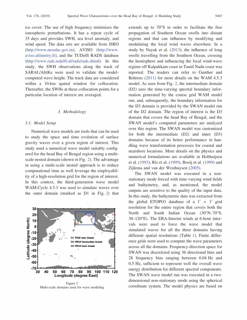
scale nested domain (shown in Fig. 2). The advantage

in using a multi-scale nested approach is to reduce

computational time as well leverage the employabil-

ity of a high-resolution grid for the region of interest.

In this context, the third-generation wave model

WAM-Cycle 4.5.3 was used to simulate waves over

the outer domain (marked as D1 in Fig. 2) that

extends up to 70�S in order to facilitate the free

propagation of Southern Ocean swells into distant

regions and that can influence by modifying and

modulating the local wind waves elsewhere. In a

study by Nayak et al. (2013), the influence of long

swells travelling from the Southern Ocean, crossing

the hemisphere and influencing the local wind-wave

regime off Kalpakkam coast in Tamil Nadu coast was

reported. The readers can refer to Gunther and

Behrens (2011) for more details on the WAM 4.5.3

model. As seen from Fig. 2, the intermediate domain

(D2) uses the time-varying spectral boundary infor-

mation generated by the coarse grid WAM model

run, and, subsequently, the boundary information for

the D3 domain is provided by the SWAN model run

of the D2 domain. The region of interest is the D3

domain that covers the head Bay of Bengal, and the

SWAN model’s computed parameters are analyzed

over this region. The SWAN model was customized

for both the intermediate (D2) and inner (D3)

domains because of its better performance in han-

dling wave transformation processes for coastal and

nearshore locations. More details on the physics and

numerical formulations are available in Holthuijsen

et al. (1993), Ris et al. (1999), Booij et al. (1999) and

Zijlema and van der Westhuysen (2005).

The SWAN model was executed in a non-

stationary mode forced with time-varying wind fields

and bathymetry, and, as mentioned, the model

outputs are sensitive to the quality of the input data.

In this study, the bathymetric data was extracted from

the global ETOPO1 database of a 10 9 10 grid

resolution for the entire region that covers both the

North and South Indian Ocean (30�N–70�S,30–120�E). The ERA-Interim winds at 6-hour inter-

vals were used to force the wave model that

simulated waves for all the three domains having

different spatial resolutions (Table 1). Finite differ-

ence grids were used to compute the wave parameters

across all the domains. Frequency-direction space for

SWAN was discretized using 36 directional bins and

28 frequency bins ranging between 0.04 Hz and

0.5 Hz, sufficient to represent well the overall wave

energy distribution for different spectral components.

The SWAN wave model run was executed in a two-

dimensional non-stationary mode using the spherical

coordinate system. The model physics are based onFigure 2

Multi-scale domains used for wave modeling


third-generation mode for wind input, quadruplet

wave–wave interactions, and white-capping source

functions (more details in the SWAN technical

manual, The SWAN Team 2012). In this study, the

wind input source function based on Janssen

(1989, 1991) for exponential growth and Cavaleri

and Malanotte-Rizzoli (1981) for linear growth was

used. The depth-induced wave breaking was

accounted for using the default options. Bottom

friction was modeled using JONSWAP (Hasselmann

et al. 1973) with a friction coefficient Cf = 0.67

m2s-3 and the triad wave–wave interaction activated

using the default value of the lumped triad approx-

imation (LTA) method (Eldeberky 1996). The first-

order upwind backward space/backward time (BSBT)

numerical scheme was considered for the discretiza-

tion in geographical space. This scheme is

unconditionally stable, monotonic, but rather diffu-

sive and chosen over non-monotone higher-order

linear schemes which produce un-physical results in

the vicinity of sharp gradients in the grid (The SWAN

Team 2012). Model runs were performed from

January to December 2016, and the computed

parameters are saved at 6-h intervals. Spectral

information of wave energy density is computed for

the 16 different locations having varied water depth

as shown in the map (Fig. 1), and details of these

locations are shown in Table 2.

3.1.1 Assessment of Model Performance

The model performance was assessed based on

different statistical measures that compared the

simulated SWH against observed data. The correla-

tion coefficient (CC), bias, normalized bias (NBIAS),

root mean square error (RMSE), normalized standard

deviation (NSTD), and scatter index (SI) are esti-

mated as:

CC ¼Pn

i¼1 ðYmi � �YmÞðYoi � �YoÞffiffiffiffiffiffiffiffiffiffiffiffiffiffiffiffiffiffiffiffiffiffiffiffiffiffiffiffiffiffiffiffiffiffiffiPni¼1 ðYmi � �YmÞ2

q ffiffiffiffiffiffiffiffiffiffiffiffiffiffiffiffiffiffiffiffiffiffiffiffiffiffiffiffiffiffiffiffiffiPni¼1 ðYoi � �YoÞ2

q ;

BIAS ¼ 1

n

Xni¼1

Ymi � Yoið Þ;

NBIAS ¼ BIAS�Yo

� 100;

RMSE ¼ffiffiffiffiffiffiffiffiffiffiffiffiffiffiffiffiffiffiffiffiffiffiffiffiffiffiffiffiffiffiffiffiffiffiffi1

n

Xni¼1

ðYmi � YoiÞ2s

;

NSTD ¼ffiffiffiffiffiffiffiffiffiffiffiffiffiffiffiffiffiffiffiffiffiffiffiffiffiffiffiffiffiffiffiffiffiffiffiffiffi1n

Pni¼1 ðYmi � �YmÞ2

qffiffiffiffiffiffiffiffiffiffiffiffiffiffiffiffiffiffiffiffiffiffiffiffiffiffiffiffiffiffiffiffiffiffiffiffi1n

Pni¼1 ðYoi � �YoÞ2

q ;

Table 1

Study region along with locations considered for analysis

Domain Spatial extent Model used Computational

grid

Input wind Time step

(min)

Frequency Directional

resolution

D1 30�E–120�E, 30�N–70�S WAM 1� 9 1� ERA-Interim

(1� 9 1�)20 0.04–0.41 Hz,

25 frequencies

30�

D2 74�E–97�E, 3�N–25�N SWAN 0.25� 9 0.25� ERA-Interim

(0.125� 9 0.125�)30 0.04–0.50 Hz,

28 frequencies

10�

D3 86�E–93�E, 19.5�N–23�N SWAN 0.01� 9 0.01� ERA-Interim

(0.125� 9 0.125�)30 Same as D2 10�

Table 2

Details of transect locations used for analysis

Locations Longitude and latitude Water depth (m)

L1 (88.00�E, 19.60�N) 1614

L2 (88.00�E, 20.00�N) 1069

L3 (88.00�E, 20.15�N) 558

L4 (88.00�E, 20.25�N) 192

L5 (88.00�E, 20.60�N) 98

L6 (88.00�E, 21.00�N) 48

L7 (88.00�E, 21.20�N) 25

L8 (88.00�E, 21.50�N) 13

L9 (91.50�E, 19.60�N) 1657

L10 (91.50�E, 19.93�N) 1063

L11 (91.50�E, 20.03�N) 541

L12 (91.50�E, 20.08�N) 202

L13 (91.50�E, 20.60�N) 86

L14 (91.50�E, 21.05�N) 54

L15 (91.50�E, 21.20�N) 24

Buoy location (87.65�E, 21.29�N) 15


SI ¼ 1�Yo

ffiffiffiffiffiffiffiffiffiffiffiffiffiffiffiffiffiffiffiffiffiffiffiffiffiffiffiffiffiffiffiffiffiffiffiffiffiffiffiffiffiffiffiffiffiffiffiffiffiffiffiffiffiffiffiffiffiffiffiffiffiffi1

n

Xni¼1

ðYmi � �YmÞ � ðYoi � �YoÞ½ �2s

;

where n represents the number of data pairs; Ymi and

Yoi are the model outputs and observed values,

respectively. �Ym and �Yo are the averaged values cor-

responding to the model and observation,

respectively.

3.2. Model Validation

The directional waverider buoy off the Digha

coast (shown in Fig. 1) is the only source of in situ

observation available in the study region and also

used for the validation of model-computed SWH for a

limited duration (January–July 2016). Model-derived

wave parameters were compared with the measure-

ments at the buoy location to verify the efficacy of the

reanalysis wind-driven model output. Figure 3 a

provides a comparison of the time series of SWH

for the period from 21 January to 20 July barring the

spin-up time. As seen from this figure, the general

agreement between model and measured data looks

reasonable. Table 3 provides the error metrics based

on statistical measures for the model-computed SWH

against buoy measurement off the Digha coast. The

corresponding values of bias, RMSE, and scatter

index for SWH are -0.06 m, 0.24 m, and 0.21,

respectively. The higher correlation coefficient (0.87)

draws attention to the fact that simulated SWH

closely follows the measured SWH across the entire

length of the buoy record. The normalized standard

deviation reveals that model SWH has lower vari-

ability as compared to the observed values. The lower

variability of ERA-Interim data implies a smoother

data set lacking detailed processes and weather

extremes (Stopa and Cheung 2014). Error statistics

of wave height indicate that the model simulations

Figure 3Comparison of significant wave height between a SWAN and wave rider buoy, b SWAN and altimeter, and c SWAN and SARAL/AltiKa


are suitable for further analysis. The discrepancy

evidenced in model outputs may be due to the

limitation in ERA-Interim winds and short duration

of comparison. However, the wave model outputs are

much better than ERA-Interim wave parameters

(which are from a global WAM run) as seen from

Table 2 reported by Patra and Bhaskaran (2017). In

addition, the measured wave spectrum for this

location is not available in the public domain.

Therefore, the model-computed wave spectrum is

the only source available for analyzing the spectral

behavior over this region of interest.

In addition, the model-simulated SWHs are also

compared with altimeter-derived SWHs from differ-

ent missions for the full year of 2016. Time series

comparisons of the monthly averaged values at three

locations (L1, L2, and L9) are shown in Fig. 3b. The

figure clearly shows that model SWHs are fully

consistent with the altimeter records. The high

correlation coefficient (C 0.92), almost no bias

(B 7 cm), and small RMSE are noticeable for all

the three selected locations. In addition to comparison

with altimeter records, the present study also made an

attempt to compare model-computed results with

high-resolution SARAL/AltiKa data (shown in

Fig. 3c). The comparison was made at four different

geographical locations, viz. L1, L8, L12, and the

buoy location. The locations L1 and L12 are at

relatively larger water depths at/off the shelf break

regions, whereas L8 and the buoy locations are in the

coastal waters. Results clearly demonstrate that the

model-computed wave heights match reasonably well

with the high-resolution SARAL/AltiKa data. The

general observation from Fig. 3c is that locations in

the coastal waters (L8 and buoy location) portray a

better match. The error statistics show a higher

correlation coefficient and negligible bias except at

L1 which is far away from the coast. The observed

bias and RMSE at L1 are 0.37 m and 0.42 m,

respectively. The overall observation is that SWHs

from the directional wave rider buoy off the Digha

coast and AltiKa and SWAN model closely follow

each other. Moreover, the AltiKa is a Ka-band

altimeter proven to be much superior as compared

to other satellite missions, and this provides an

opportunity to validate model-computed wave height

at the coastal regions. The validation exercise shows

significant match between model and the satellite

records.

4. Results and Discussions

4.1. Monthly Variability of 1D Wave Spectra

This section analyses the 1D wave spectra

obtained from model simulations. Monthly averaged

1D wave spectra at a deep water location L1 and the

Digha buoy location are presented in Fig. 4. The top

panels in Fig. 4a–c show the monthly energy density

for location L1, and the bottom panels shown in

Fig. 4d–f correspond to the buoy location. The wave

spectrum at L1 consists of multiple peaks during

January 2016 (Fig. 4a). The narrow-banded distinct

mature swells of frequency in excess of 15 s are

present along with one predominant swell peak

(9.81 s) and wind-sea peak (4.64 s). The energy

density corresponding to wind-sea peak is centered at

0.17 m2/Hz, and this diminishes to almost half for the

swell peak. From February to April, the variance

density has magnified gradually rising to 2.46 m2s-1.

The wind-sea peak frequency has shifted towards the

lower lobe with increased energy. Mature swells

persist, but the predominant swell system observed in

January is not seen during this period except March.

The monthly averaged spectrum for May is single-

peaked with a peak value of 2.10 m2/Hz at 9.81 s.

This peak energy is seen reducing during May and

June, although the low-frequency part magnifies as

Table 3

Model-computed error metrics against measured buoy data off the Digha coast during the period January–July 2016

Mean (SWAN) Mean (buoy) CC Bias NBIAS (%) RMSE NSTD SI

SWH 1.04 m 1.10 m 0.87 - 0.06 m - 5.10 0.24 m 0.93 0.21

CC correlation coefficient, NBIAS normalized bias, RMSE root mean square error, NSTD normalized standard deviation, SI scatter index


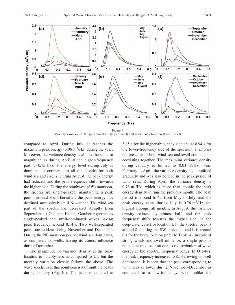
compared to April. During July, it reaches the

maximum peak energy (3.06 m2/Hz) during the year.

Moreover, the variance density is almost the same in

magnitude as during April at the higher-frequency

part ([ 0.15 Hz). The energy level during July is

dominant as compared to all the months for both

wind sea and swells. During August, the peak energy

had reduced, and the peak frequency shifts towards

the higher side. During the southwest (SW) monsoon,

the spectra are single-peaked, maintaining a peak

period around 8 s. Thereafter, the peak energy has

declined successively until November. The wind-sea

part of the spectra has decreased abruptly from

September to October. Hence, October experiences

single-peaked and swell-dominated waves having

peak frequency around 8.14 s. Two well-separated

peaks are evident during November and December.

During the NE monsoon period, wind sea dominates,

as compared to swells, having its utmost influence

during December.

The magnitude of variance density at the buoy

location is notably less as compared to L1, but the

monthly variation closely follows the above. The

wave spectrum at this point consists of multiple peaks

during January (Fig. 4d). The peak is centered at

3.85 s for the higher-frequency side and at 8.94 s for

the lower-frequency side of the spectrum. It implies

the presence of both wind sea and swell components

coexisting together. The maximum variance density

during January is limited to 0.04 m2/Hz. From

February to April, the variance density had amplified

gradually and was also noticed in the peak period of

wind seas. During April, the variance density is

0.76 m2/Hz, which is more than double the peak

energy density during the previous month. The peak

period is around 6–7 s from May to July, and the

peak energy value during July is 0.76 m2/Hz, the

highest amongst all months. In August, the variance

density reduces by almost half, and the peak

frequency shifts towards the higher side. In the

deep-water case (for location L1), the spectral peak is

around 8 s during the SW monsoon, and it is around

6 s for the buoy location (refer to Table 4). In spite of

strong winds and swell influence, a single peak is

noticed at this location due to redistribution of wave

energy in the spectral frequency bands. In October,

the peak frequency increased to 8.14 s owing to swell

dominance. It is seen that the peak corresponding to

wind seas is lower during November–December as

compared to a low-frequency peak, unlike the

Figure 4Monthly variation of 1D spectrum at L1 (upper panel) and at the buoy location (lower panel)


variance density spectrum at L1. The wind-sea

energy is lower because of restricted fetch available

for winds at the buoy location. Consequently, the

wind-sea peak period is less as compared to L1. On

the other hand, the swell period reduces as compared

to L1 following the dispersion of water waves.

The time series analysis of wave spectra enhances

the information on waves as well their physical origin

which includes extreme events, any alteration in

atmospheric forcing, among others. The map of wave

spectral energy density as a function of frequency and

time for each month is shown in Fig. 5. During June–

August, it is mostly around 0.1–0.15 Hz, indicating

the presence of swells. Significant wave spectral

density is noticed for wave periods in excess of 10 s

during this period in distinct patches. During Septem-

ber, the spectral energy density predominantly lies

between 0.1 and 0.15 Hz and occasionally around

0.15–0.2 Hz in the low-frequency side (\ 0.1 Hz).

The spectra are comparatively narrow banded during

the monsoon. Wave spectral density is concentrated

in two separate frequency bands during November–

January. One of the frequency bands lies around

0.2 Hz, due to the presence of wind waves, and the

other is around 0.1 Hz, which represents the presence

of swells. During February–April, the wave spectra

are mainly centered between 0.12 and 0.2 Hz,

indicating the dominance of wind seas. Moreover,

significant wave energy is seen around 0.1 Hz during

10–13 March. During May, very high spectral energy

([ 6 m2/Hz) is seen around 20 May resulting from

cyclone Roanu over the Bay of Bengal. On the other

hand, two dominant bands (0.1–0.15 Hz and

0.15–0.2 Hz) are seen irregularly. In October, signif-

icant energy is noticed around 0.1–0.15 Hz. A

depression during 2–6 November over the head Bay

of Bengal enhanced the variance density around 6

November. The general observation is that wave

spectral density spreads widely over frequencies for

the buoy location as compared to the deep-water

location (Fig. 6). The variance density corresponds to

wind-sea shifts towards higher frequency and lie

centered around 0.25–0.3 Hz during November,

December, and January, but swells are almost in the

same band. During the monsoon, the energy density

concentrates mainly around 0.15–0.2 Hz and occa-

sionally extends to the 0.1–0.15-Hz band. In October,

significant energy is around 0.1–0.15 Hz with a

higher directional spread about 0.15–0.25 Hz during

February and March, and 0.12–0.23 Hz in April. The

signature of depression is clearly seen during May

and November like the case of L1.

4.2. Evolution of Wave Spectra over Varying Depths

In this section, the variation of 1D spectra at

varying water depths along the two longitudinal

transects is studied for each month of 2016. Figure 7

displays the spectral alteration along 88�E, the west

side of the study basin. Distinct peaks corresponding

Table 4

Peak period and energy density for the monthly averaged 1D spectrum at transect locations over the west

Months Deep water location: L1 (1614 m) Shallow water location: L8 (13 m) Buoy location (15 m)

Peak period

(in s)

Peak energy

density (m2/Hz)

Peak period

(in s)

Peak energy

density (m2/Hz)

Peak period

(in s)

Peak energy

density (m2/Hz)

Jan. 9.81/4.64 0.10/0.17 8.94/4.64 0.02/0.02 8.94/3.85 0.03/0.04

Feb. 5.60 0.38 5.10 0.14 5.60 0.17

Mar. 9.81/6.15 0.33/0.67 5.10 0.27 5.60 0.31

Apr. 6.75 2.46 5.60 0.64 6.15 0.76

May 9.81 2.10 8.94/6.15 0.43/0.53 6.15 0.61

June 8.94 2.05 5.60 0.37 6.15 0.53

July 8.14 3.06 5.60 0.59 6.15 0.76

Aug. 7.41 2.02 5.10 0.37 5.10 0.42

Sep. 8.14 1.27 8.14/5.10 0.23/0.27 5.60 0.36

Oct. 8.14 1.10 8.14 0.21 8.14 0.25

Nov. 8.94/5.60 0.27/0.25 8.94/3.51 0.05/0.01 8.94/3.85 0.07/0.03

Dec. 8.94/4.64 0.25/0.39 8.14/2.91 0.04/0.01 8.14/3.51 0.07/0.04


to sea and swell systems are present during the NE

monsoon months at varying water depths examined

for the longitudinal transect at 88�E. The peak energy

for the predominant swell system is almost the same

from L1 to L5 (98-m depth) and decreases thereafter

up to L8. This is attributable to swells propagating

Figure 5Time series of 1D spectra during each month at L1. The color bar indicates variance density (m2/Hz)


from deep water to the shallow water as they seldom

feel the bottom up to a water depth around 100 m,

and thereafter that bottom effect is notable. As

Southern Ocean swells propagate opposite to winds

during the NE monsoon, the attenuation of swells can

be attributed to the effect of opposing wind as well as

Figure 6As Fig. 5 except at the buoy location


Figure 7Comparison of monthly averaged wave spectra at different water depths along the transect at 88�E


the wave-bottom interaction. Longuet-Higgins (1969)

suggests the damping of long waves in case the long

waves and short waves are propagating in opposite

directions, as for wind blowing against a swell. Wind

seas moving away from the coast are stronger for L1–

L5 as sufficient fetch is available for winds (Fig-

ure S1). This is not the case for the nearshore

locations and the wind-sea peak energy is almost half

at L6 than at L5. The wind-sea peak frequency

increases from L5 to L6 and onwards with an

exception during January from L6 to L7. During

December–January, the wind-sea energy is higher

than swells for deep water locations, but is lower for

L6–L8. The opposing swell can intensify the NE

wind sea by increasing wind shear stress towards

offshore. Thus, it also contributes to the reinforce-

ment of wind-sea energy away from the coast. During

the SW monsoon, both wind seas and swells prop-

agate from the south. Energy dissipation due to the

bottom is seen clearly for the locations shallower than

L5. The spectral shape becomes flattened in shallow-

water locations because of deflated spectral density.

The peak frequency of single-peaked spectra is seen

to increase from L6 towards shore. Interestingly,

double peaks are found at L8 for September and not

seen at other locations. During February to April,

wave energy diminishes nearshore crossing L6, and

the peak period changes from L7 to L8. It is

interesting to note that the peak energy is comparable

between L1 and L5 and higher for L2–L4 as wind

blows towards the coast (Figure S1). Accordingly, the

wind seas tend to intensify towards the coast. Peak

frequency remains almost constant from L1 to L8

during October because of swell dominance. This

implies that peak frequency alteration with depth is

mainly manifested for the wind sea part of the

spectrum. The spectral evolution in May is similar to

the SW monsoon months, and two separate peaks are

noticed only for L7 and L8.

Another set of points along the 91.5�E (eastern

side) transect have been considered to study the wave

energy transformation (Fig. 8). During the NE mon-

soon, a drop in variance density is evident from L13

onward which is at the same latitude and almost

similar water depth (86 m) as L5. Moreover, the

wind-sea peak frequency shifts towards higher fre-

quency from L13 onwards. The spectral density is

slightly higher at these points as compared to

locations in the same latitude along 88�E. More

specifically, swells are stronger here than the loca-

tions at 88�E. This is probably associated with the

direction of swell propagation as the Southern Ocean

swells usually propagate from the southwest direc-

tion. In the SW monsoon, similar features as above

such as the dissipation of wave energy, reduction in

peak period, and flattening of wave spectra are seen

from L14 onward for the considered set of points. In

general, the spectral shape is narrower here as

compared to the locations at the western side possibly

due to more swell dominance. In addition, spectral

peaks are higher over the east during the SW

monsoon. The highest variance density (3.04 m2/

Hz) at L9 (Table 5) occurs during June and it is

comparable with peak energy for July at L1. Com-

paring L15 and L7, which are at almost at similar

water depths, the peak period at L15 is higher than

that of L7. During May, the variation along depth is

similar to the SW monsoon. The spectral peak is at

higher energy than for locations on the western side.

Similar features as seen along the western side are

found during October. In contrast, comparably less

wave energy is evident during February–April. The

important thing to note here is the presence of

prominent swell peaks during February and March,

which is absent over the western side of the study

domain. Overall, the analysis agrees with the study by

Patra and Bhaskaran (2016) which showed that

altimeter-derived wave height has increased more

over the eastern side as compared to the western side

of head Bay of Bengal. The SWAN-simulated wave

spectrum for the geographic domain D2 was vali-

dated in a recent separate study by Umesh et al.

(2018). The comparison between the modeled and

measured wave spectra are also presented in Figs. 5

and 6 by Umesh et al. (2018). The present study used

a similar model setup for nesting and wind forcing as

described in Umesh et al. (2018).

4.3. Analysis of 2D Spectra

Two-dimensional wave spectra at L1 averaged

over each month are shown in Fig. 9. Wave systems

present at a location can be distinguished by identi-

fying the frequency-directional behavior of the 2D


Figure 8Comparison of monthly averaged wave spectra at different water depth along the transect at 91.5�E


spectrum. Individual wave systems are energy trans-

formation in the frequency-direction space. The wave

systems can either be locally generated wind sea or a

remotely generated swell system. Wind seas are

defined by high frequency and larger directional

spreading, whereas swells have low frequency and

narrow directional spreading.

The 2D mean spectrum for January consists of

both wind sea and swell components. The prominent

wind seas are from the NE (northeast) direction with

a frequency around 0.2 Hz and higher directional

spread. In addition, another wind-sea system with

lesser directional spread is also noticed from the

west-southwest (WSW) direction. The low-energy

wave system is observed due to waves reflected from

the coastline. Low-frequency swells are evident

approaching from the S (south), SSE (south-south-

east), and SSW (south-southwest) directions. Distinct

swell systems with a peak wave period in excess of

15 s reach from 150�. These swells are possibly

reflected swells from western Australia/Indonesia.

The NE monsoon is dominated by high-frequency

wind seas (0.15–0.25 Hz), and from February

onward, this wave system shifts to a very-high-

frequency region (up to 0.35 Hz). Maximum peak

spectral energy increases gradually from February

onward and attains its maximal value in May. During

February and March, wind seas are from the S (south)

and SW (southwest) with large spreading over

frequency and direction space, and swells arrive

from the SE. During April and May, the wind sea

shifts to lower frequency (0.08–0.25 Hz) with

increased energy levels and less directional width.

During June–October, energy spreading is narrow

over frequency and direction space and concentrates

more towards the lower-frequency side. The spectral

energy propagates from the SW direction with a peak

period of around 10 s. It is noteworthy that a single

peak exists during the SW monsoon which is

characterized by strong SW winds blowing over the

region and swell dominance. The increased swell

propagation from the Southern Ocean to Northern

Indian Ocean basin during the months of June, July,

August, and September can be attributed to the

southern winter. The strong winds are capable of

generating waves with low frequency and high

energy. Thus, wind seas overlap with swells in the

frequency-direction space. However, two distinct

close peaks are seen during July when the wind

reaches its maxima for that year. The energy system

merges into a single peak during the rest of the SW

monsoon months. Waves with the highest peak

energy (0.045 m2/Hz) are found during July. During

November–December, swells are prominent, while

the wind seas dominate. Though the peak energy

corresponding to the swell is high, the total energy is

comparatively more for wind seas by virtue of larger

areal coverage. In addition to the NE direction, wind

seas with low energy are seen radiating from the NW

(northwest). The unidirectional swells arrive from

150� with periods in excess of 10 s almost throughout

the year. Two well-separated wave systems are

Table 5

Peak period and energy density for the monthly averaged 1D spectra at transect locations over the east

Months Deep-water location: L9 (1657 m) Shallow-water location: L15 (24 m)

Peak period (in s) Peak energy density (m2/Hz) Peak period (in s) Peak energy density (m2/Hz)

Jan 11.83/5.10 0.11/0.31 11.83/4.23 0.04/0.09

Feb. 11.83/5.60 0.14/0.24 5.60 0.20

Mar. 9.81/6.15 0.33/0.40 9.81/6.15 0.20/0.35

Apr. 6.75 1.48 6.75 1.13

May 9.81 2.93 9.81 1.71

June 8.94 3.04 8.14 1.34

July 8.94 2.76 8.14 1.51

Aug. 8.14 2.89 8.14 1.69

Sep. 8.94 1.66 8.94 0.94

Oct. 8.14 1.22 8.14 0.73

Nov. 8.94/4.64 0.33/0.35 8.14/3.85 0.26/0.09

Dec. 8.94/5.10 0.32/0.39 8.14/3.85 0.17/0.01


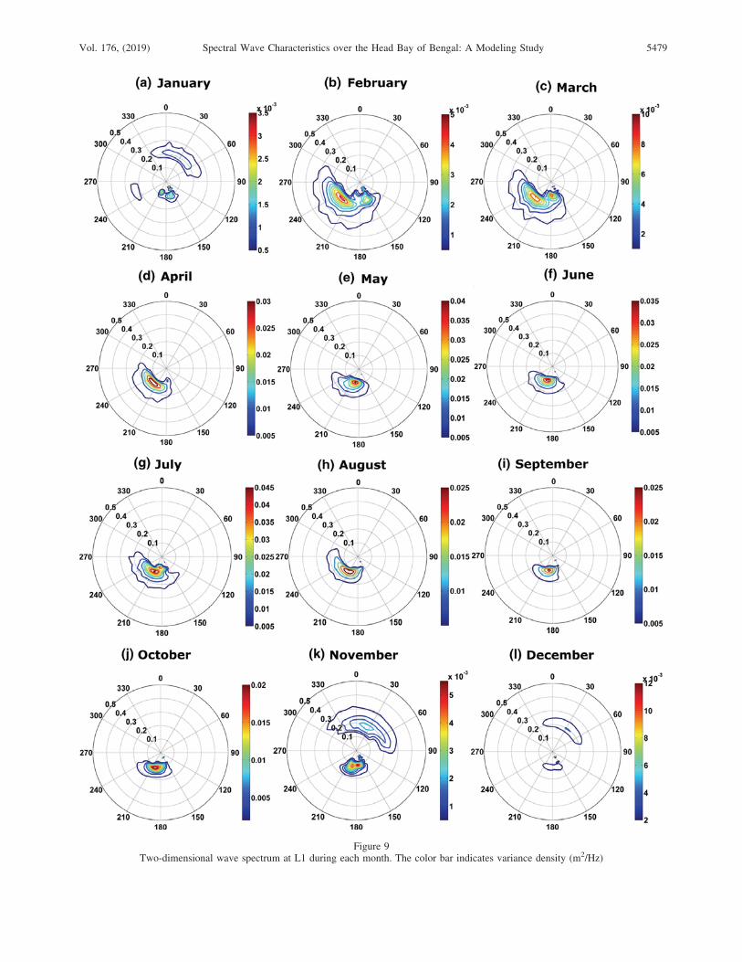
Figure 9Two-dimensional wave spectrum at L1 during each month. The color bar indicates variance density (m2/Hz)


detected during November to April, and that matches

well with the observational evidence reported by

Amrutha and Sanil Kumar (2017).

At the buoy location, the features of 2D spectra

differ in frequency-direction space as compared to

that of the L1 (Fig. 10) location. This is obvious due

to refraction of waves, energy dissipation, and

frequency shift resulting from bottom interaction.

During January, the wind seas from the north are

absent at the buoy location, unlike L1, because of

fetch restriction. Instead, local waves arrive from the

ESE (east-southeast) along with E (east) and NE

directions. Another high-frequency wave system

approaches the buoy location from the SSW direction

with peak energy around 0.2 Hz. This particular wave

system persists thereafter from February to April but

with increase in energy and decrease in peak

frequency. The directional width becomes narrow as

compared to L1 due to confined wave propagation

following the land boundary. During May, the peak

period reaches almost 10 s and the peak energy is

centered around 0.012 m2/Hz. Two distinct closer

peaks are visible at this point during the SW monsoon

months. Waves corresponding to these peaks propa-

gate from the SSE (swells) and SSW (wind seas)

directions with comparatively high energy for wind-

seas. Swell peak frequency is around 10 s and wind-

sea peak frequency is centered around 6–7 s. The

maximum energy observed at the buoy location is

0.012 m2/Hz during July, and that is about four times

less than L1. The month of October follows similar

features like the SW monsoon months but with

narrow directional width and lesser energy levels

resulting from the reversal of wind systems. Though

NE seasonal winds start blowing during November,

waves from the NE are not noticed at this location,

unlike the case seen at the L1 location. This may be

due to limited fetch in the north of this point and

weak winds. A narrow-banded wind-sea system

advances from the NE during December. The wave

spectrum contains two distinct peaks during the SW

and NE monsoon at this location.

Figure 11 shows the diurnal variation of wave

spectra on 8 July 2016 at the Digha buoy location.

Diurnal variation includes the effect attributed due to

local winds (coastal breeze). It is evident at the

nearshore location, unlike the deep-water location.

During early hours of the day, the spectral densities

are low. The wave spectra evolve as wind speed

intensifies over this region and obtain their maxima at

18 h. During July, the SW winds blows from sea to

land which is higher during the afternoon hours. The

peak spectral density at 18 h is almost double as

compared to 00 h. The shift in peak frequency

towards the lower side of the spectrum is seen to

occur during late hours of the day. The peak energy

level of the 1D spectrum at 06 h, 12 h, and 18 h are

0.31 m2/Hz, 0.50 m2/Hz, and 0.75 m2/Hz, respec-

tively. The peak frequency decreases from 0.20 Hz at

00 h to 0.16 Hz at 18 h. Diurnal variability during the

NE monsoon is also clear from Fig. 12. It indicates

the spectral energy variation during 28 December

2016. During December, coastal breeze are stronger

during early hours of the day. Thus, the high-energy

waves approach from a NE direction at 00 h and

06 h. The wind-sea energy is relatively lesser during

the afternoon hours. Also, there is not much vari-

ability noticed in the swell wave system throughout

the day. The wind-sea peak energy decreases and

frequency gets lower during afternoon hours as

evident from the 1D spectra. The wind-sea peak

energy at 00 h is almost thrice as compared to 18 h. It

is seen that the wind system plays a major role in

mature wind-sea conditions during the afternoon

hours. Multiple peaks associated with swells are

consistent during the day.

4.4. Qualitative Case Study of Wave Spectral

Characteristics

The present study is a qualitative analysis of wave

spectral characteristics using a multi-scale nested

modeling approach for the head Bay of Bengal region

which is primarily a data-sparse region. A nested

modeling system using WAM and SWAN models

was adopted to understand the wave characteristics

and spectral evolution of both wind seas and swells

for the study region. To understand the spatio-

temporal evolution of wind waves, an in-depth

qualitative analysis was carried out to better under-

stand the wave spectral evolution characteristics by

carrying out model simulation for one full year. Intra-

seasonal variability of wind waves in a reversing

wind system for the study region has been thoroughly


Figure 10As Fig. 9 except at the buoy location


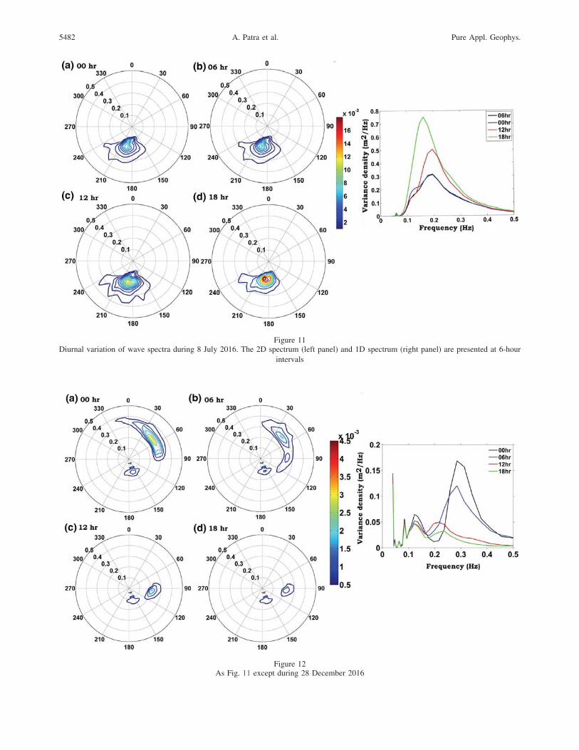
Figure 11Diurnal variation of wave spectra during 8 July 2016. The 2D spectrum (left panel) and 1D spectrum (right panel) are presented at 6-hour

intervals

Figure 12As Fig. 11 except during 28 December 2016


investigated. Monthly averaged wave spectra show

the presence of multiple peaks, indicating the coex-

istence of different wave systems. This study clearly

brings to light transformation of wave spectra in both

wind seas and swell systems for water depths beyond

100 m towards the coast. Qualitative analysis of

wave spectra indicates that during the post-monsoon

season, bottom effects and an opposing wind system

results in lowering the overall swell energy, while

restricted fetch limits evolution of wind seas for the

nearshore regions. The study provides a detailed

overview on the separate wave systems that influ-

ences the local wind-wave climatology of the head

Bay of Bengal region. Interesting features such as the

diurnal variability and transformation of wave spectra

for varying water depths are reported in this study.

The study is qualitative in nature due to lack of high-

resolution wave spectral data, and the authors believe

that this qualitative study is the first information that

provides a comprehensive overview on the spectral

wave evolution characteristics for the head Bay of

Bengal region having wide practical relevance.

A very clear and direct use of this kind of spectral

study is recently brought out by Jiang and Mu (2019).

The wave spectrum at a location contains information

about air-sea interaction at local as well as distant

regions. Time series of wave spectra can detect

ENSO signature at a location in tropical eastern

Pacific Ocean (Portilla et al. 2016; Jiang and Mu

2019). Separate wave system present at a location can

be visualized by spectral analysis which cannot be

understood from integrated wave parameters even if

wind-sea and swell components are partitioned.

Different wave systems approaching from different

direction with different time period have distinct and

specific impact/applications. As aforementioned, high

frequency wave system affect navigation and off-

shore operations and low frequency system find its

application in climate studies influencing air-sea

exchange. Both direction and frequency of wave

systems are must considerable for coastal erosion

estimation studies. Large basin-scale seasonal, inter-

annual wind climate modulation can be captured to

certain extent by wave spectra at a fixed point (Jiang

and Mu 2019). The present analysis could record

signature of cyclone Roanu and distant swells

reflected from western Australia/Indonesia. It is also

believed that wave spectra can track storm activity at

a geographically distant region. When considering

long-term study of wave spectra, climatic influence of

large-scale atmospheric modes like the Southern

Oscillation, the Arctic Oscillation, and the Antarctic

Oscillation on local wave climate can be brought to

light.

5. Summary and Conclusion

The present study made an attempt to explore

the spectral evolution of wave characteristics at

specific locations over the head Bay of Bengal using

a multi-scale nested modeling approach. To

accomplish this, the SWAN model was employed to

simulate the wave conditions over the study domain

using spectral boundary information from WAM for

which the computational grid extends up to 70�S to

incorporate the Southern Ocean swells. The model

simulation was carried out for one complete year of

2016 to have sufficient data to introspect the inter-

seasonal variability. To validate the model output,

measured data were obtained from a buoy off the

Digha coast, and the comparison results in reason-

able fidelity. The merged altimeter products and

SARAL/AltiKa also showed significant agreement

with model’s SWH. The monthly averaged wave

spectra contain multiple peaks throughout the year

emphasizing the coexistence of different wave sys-

tems. The predominant features of 1D wave spectra

at a deep-water location include two distinct peaks

during the post-monsoon, a single peak with higher

energy during the southwest monsoon. Considerably

high spectral density is also noticed during pre-

monsoon season. It attains maximum value during

the month of July. Variance density at the buoy

location is remarkably lower than the aforemen-

tioned location. The time series of 1D spectra at L1

show energy concentration around 0.1–0.15 Hz

during the SW monsoon and over two distinct fre-

quency bands, one around 0.1 Hz and another

around 0.2 Hz during post-monsoon. During Febru-

ary–April, the wave spectra are centered mainly at

0.12–0.2 Hz. The wave spectral density spreads

widely over frequencies for the buoy location

compared to the deep-water location. Moreover,


spectral energy exhibits a shift towards the high-

frequency side. Transformation of wave spectra

along depths at two longitudinal transects has been

scrutinized, and significant attenuation of both wind

sea and swells are found beyond 100-m water depth

towards the coast. During post-monsoon season,

reduction of swell energy is associated with wave-

bottom interaction and opposing winds, while low

wind seas at nearshore result from restricted fetch

available for NE winds. Dissipation caused by bot-

tom friction is the primary wave attenuation

mechanism for aligned wind seas and swells during

the SW monsoon. Higher spectral density, more

specifically, higher swell energy, prevails at a series

of points over east than locations at the west having

similar latitude and almost the same water depths.

The directional spectra convey better information on

the different wave systems based on information in

the spectral space. In addition to S and SSW

directions, swells also arrive from the SE due to

reflection from western Australia/Indonesia at L1.

The direction spread is low during the SW monsoon

as both wind seas and swells reach from the SW

having almost similar peak frequencies. Variance

density associated with wind seas outspreads over

directions during November–March. The study also

traces wind seas reflected from the coastline. The

directional spectra at the buoy location differ from

L1 following limited fetch in the north, coastline

orientation, bottom friction, and refraction by the

bottom. The diurnal variation appears to be signifi-

cant at the buoy location following coastal breezes.

This study thereby develops a preliminary informa-

tion base of wave spectra over the head Bay of

Bengal region. The spectral details can be useful for

several applications like climate studies, sediment

transport, coastal engineering, navigation, etc.

However, there is a need for extensive validation

using measurements before operational use. Fur-

thermore, this work can be extended for several

years to study the inter-annual variability in the

wind-wave system. The identification of wave sys-

tems based on occurrence probability of spectral

peak position following Portilla et al. (2015) can be

undertaken as a separate study with sufficiently long

time series of 2D spectra.

Acknowledgements

The authors sincerely thank the Ministry of Human

Resources Development (MHRD), Government of

India for the financial support. This study is con-

ducted as a part of the Mega Project ‘‘Future of

Cities’’ under the module ‘Effect of Climate change

on local sea level rise and its impact on coastal areas:

Kolkata region as a pilot study’ supported by MHRD

at IIT Kharagpur. The authors are grateful to the

Indian National Centre for Ocean Information Ser-

vices (INCOIS), Ministry of Earth Sciences,

Hyderabad, for providing the waverider buoy data.

Publisher’s Note Springer Nature remains neutral

with regard to jurisdictional claims in published maps

and institutional affiliations.

REFERENCES

Aboobacker, V. M., Rashmi, R., Vethamony, P., & Menon, H. B.

(2011a). On the dominance of pre-existing swells over wind seas

along the west coast of India. Continental Shelf Research, 31,

1701–1712.

Aboobacker, V. M., Vethamony, P., & Rashmi, R. (2011b).

‘‘Shamal’’ swells in the Arabian Sea and their influence along the

west coast of India. Geophysical Research Letters, 38, L03608.

Akpınar, A., Bingolbali, B., & Van Vledder, G. P. (2016). Wind

and wave characteristics in the Black Sea based on the SWAN

wave model forced with the CFSR winds. Ocean Engineering,

126, 276–298.

Akpınar, A., van Vledder, G Ph, Komurcu, MI., & Ozger, M.

(2012). Evaluation of the numerical wave model (SWAN) for

wave simulation in the Black Sea. Continental Shelf Research,

50–51, 80–99.

Amrutha, M. M., & Sanil Kumar, V. (2017). Observation of

dominance of swells over wind seas in the coastal waters of the

Gulf of Mannar, India. Ocean Science, 13, 703–717.

Baba, M., Dattatri, J., & Abraham, S. (1989). Ocean wave spectra

off Cochin, west coast of India. Indian Journal of Marine Sci-

ence, 18, 106–112.

Barstow, S. F., & Kollstad, T. (1991). Field trials of the directional

waverider. Proceedings of the First International Offshore and

Polar Engineering Conference, III, 55–63.

Booji, N., Ris, R. C., & Holthuijsen, L. H. (1999). A third-gener-

ation wave model for coastal regions: 1. Model description and

validation. Journal of Geophysical Research, 104(C4),

7649–7666.

Cavaleri, L., Fox-Kemper, B., & Hemer, M. (2012). Wind-waves in

the coupled climate system. Bulletin of the American Meteoro-

logical Society, 93, 1651–1661.


Cavaleri, L., & Malanotte-Rizzoli, P. (1981). Wind wave predic-

tion in shallow water: theory and applications. Journal of

Geophysical Research, 86(C11), 10961–10973.

Dee, D. P., Uppala, S. M., Simmons, A. J., Berrisford, P., Poli, P.,

Kobayashi, S., et al. (2011). The ERA-Interim reanalysis: con-

figuration and performance of the data assimilation system.

Quarterly Journal Royal Meteorological Society, 137(656),

553–597.

Eldeberky, Y. (1996). Nonlinear transformation of wave spectra in

the nearshore zone (Ph.D. thesis). The Netherlands: The Delft

University of Technology, Department of Civil Engineering.

Gunther, H., & Behrens, A. (2011). The WAM model–validation

document version 4.5.3. Helmholtz-ZentrumGeesthacht (HZG).

Teltow: Centre for Materials and Coastal Research.

Hanson, J. L., & Phillips, O. M. (2001). Automated analysis of

ocean surface directional wave spectra. The Journal of Atmo-

spheric and Oceanic Technology, 18, 277–293.

Hasselmann, K., Barnett, T. P., Bouws, E., Carlson, H., Cartwright,

D. E., Enke, K., et al. (1973). Measurements of wind-wave

growth and swell decay during the Joint North Sea Wave Project

(JONSWAP). Ergnzungsheft zur Deutschen Hydrographischen

Zeitschrift Reihe (p. 95). Hamburg: Deutsches Hydrographisches

Institute.

Holthuijsen, L. H., Booij, N., & Ris, R. C. (1993). A spectral wave

model for the coastal zone. In Proceedings 2nd international

symposiumon ocean wave measurement and analysis, New

Orleans, Louisiana, July 25–28, 1993, NewYork, pp. 630–641.

Janssen, P. A. E. M. (1989). Wave induced stress and the drag of

air flow over sea water. Journal of Physical Oceanography, 19,

745–754.

Janssen, P. A. E. M. (1991). Quasi-linear theory of wind-wave

generation applied to wave forecasting. Journal of Physical

Oceanography, 21, 1631–1642.

Jiang, H., & Mu, L. (2019). Wave climate from spectra and its

connections with local and remote wind climate. Journal of

Physical Oceanography, 49, 543–559.

Kumar, V. S., Anand, N. M., Kumar, K. A., & Mandal, S. (2003).

Multi-peakedness and groupiness of shallow water waves along

Indian coast. The Journal of Coastal Research, 19, 1052–1065.

Kumar, V. S., Dubhashi, K. K., & Nair, T. M. B. (2014). Spectral

wave characteristics off Gangavaram, Bay of Bengal. Journal of

Oceanography, 70, 307–321.

Longuet-Higgins, M. S. (1969). A nonlinear mechanism for the

generation of sea waves. Proceedings of the Royal Society A:

Mathematical, Physical and Engineering Science, 311(1506),

371–389.

Mazaheri, S., Kamranzad, B., & Hajivalie, F. (2013). Modification

of 32 years ECMWF wind field using QuikSCAT data for wave

hindcasting in Iranian Seas. Journal of Coastal Research: Spe-

ciaal Issue, 65, 344–349.

McComb, P., Johnson, D., & Beamsley, B. (2009). Numerical

model study to reduce swell and long wave penetration to Port

Geraldton. In Proceedings of the 2009 pacific coasts and ports

conference, Coasts and ports 2009: In a dynamic environment,

Wellington, September 16–18, 2009, pp. 490–496.

Moeini, M. H., Etemad-Shahidi, A., Chegini, V., & Rahmani, I.

(2012). Wave data assimilation using a hybrid approach in the

Persian Gulf. Ocean Dynamics, 62, 785–797.

Nayak, S., Bhaskaran, P. K., Venkatesan, R., & Dasgupta, S.

(2013). Modulation of local wind–waves at Kalpakkam from

remote forcing effects of Southern Ocean swells. Ocean Engi-

neering, 64, 23–35.

Parvathy, K. G., Umesh, P. A., & Bhaskaran, P. K. (2017). Inter-

seasonal variability of wind–waves and their attenuation char-

acteristics by mangroves in a reversing wind system. The

International Journal of Climatology. https://doi.org/10.1002/

joc.5147.

Patra, A., & Bhaskaran, P. K. (2016). Trends in wind–wave climate

over the head Bay of Bengal region. The International Journal of

Climatology, 36, 4222–4240.

Patra, A., & Bhaskaran, P. K. (2017). Temporal variability in

wind–wave climate and its validation with ESSO-NIOT wave

atlas for the head Bay of Bengal. Climate Dynamics, 49,

1271–1288.

Portilla, J., Cavaleri, L., & Van Vledder, G. (2015). Wave spectra

partitioning and long term statistical distribution. Ocean Mod-

elling, 96, 148–160.

Portilla, J., Salazar, A., & Cavaleri, L. (2016). Climate patterns

derived from ocean wave spectra. Geophysical Research Letters,

43, 11736–11743.

Ris, R. C., Holthuijsen, L. H., & Booij, N. (1999). A third-gener-

ation wave model for coastal regions: 2 verification. Journal of

Geophysical Research, 104(C4), 7667–7681.

Rosmorduc, V., Benveniste, J., Bronner, E., Dinardo, S., Lauret, O.,

Maheu, C., Milagro, M., & Picot, N. (2011). In J. Benveniste and

N. Picot (Eds.), Radar altimetry tutorial. http://www.altimetry.

info. Accessed 20 Mar 2018.

Sabique, L., Annapurnaiah, K., Balakrishnan Nair, T. M., &

Srinivas, K. (2012). Contribution of southern Indian Ocean

swells on the wave heights in the northern Indian Ocean—a

modeling study. Ocean Engineering, 43, 113–120.

Saket, A., Etemad-Shahidi, A., & Moeini, M. H. (2013). Evaluation

of ECMWF wind data for wave hindcast in Chabahar zone. The

Journal of Coastal Research Special Issue, 65, 380–385.

Samiksha, S. V., Polnikov, V. G., Vethamony, P., Rashmi, R.,

Pogarskii, F., & Sudheesh, K. (2015). Verification of model wave

heights with long-term moored buoy data: application to wave

field over the Indian Ocean. Ocean Engineering, 104, 469–479.

Sandhya, K. G., Balakrishnan Nair, T. M., Bhaskaran, P. K.,

Sabique, L., Arun, N., & Jeykumar, K. (2014). Wave forecasting

system for operational use and its validation at coastal Pudu-

cherry, east coast of India. Ocean Engineering, 80, 64–72.

Sandhya, K. G., Remya, P. G., Balakrishnan Nair, T. M., & Arun,

N. (2016). On the co-existence of high-energy low-frequency

waves and locally- generated cyclone waves off the Indian east

coast. Ocean Engineering, 111, 148–154.

Shanas, P. R., Aboobacker, V. M., Albarakati, A. M. A., & Zubier,

K. M. (2017). Superimposed wind-waves in the Red Sea. Ocean

Engineering, 138, 9–22.

Soares, C. G. (1991). On the occurrence of double peaked wave

spectra. Ocean Engineering, 18(1/2), 167–171.

Stopa, J. E., & Cheung, K. F. (2014). Intercomparison of wind and

wave data from the ECMWF Reanalysis Interim and the NCEP

Climate Forecast System Reanalysis. Ocean Modelling, 75,

65–83.

Stopa, J. E., Cheung, K. F., & Chen, Y. L. (2011). Assessment of

wave energy resources in Hawaii. Renewable Energy, 36(2),

554–567.

SWAN Team (2012). SWAN user manual. SWAN Cycle III ver-

sion 40.85. Delft University of Technology, Technical


Documentation, Delft, Netherlands, pp 94. http://www.swan.

tudelft.nl. Accessed 22 Mar 2018.

Tolman, H. L. (1991). A third generation model for wind waves on

slowly varying, unsteady and inhomogeneous depths and cur-

rents. Journal of Physical Oceanography, 21, 782–797.

Umesh, P. A., Bhaskaran, P. K., Sandhya, K. G., & Balakrishnan

Nair, T. M. (2017). An assessment on the impact of wind forcing

on simulation and validation of wave spectra at coastal Pudu-

cherry, east coast of India. Ocean Engineering, 139, 14–32.

Umesh, P. A., Bhaskaran, P. K., Sandhya, K. G., & Balakrishnan

Nair, T. M. (2018). High frequency tail characteristics in the

coastal waters off Gopalpur, Northwest Bay of Bengal: a near-

shore modeling study. Pure and Applied Geophysics, 175,

2351–2379.

WAMDIG. (1988). The WAM model —a third generation ocean

wave prediction model. Journal of Physical Oceanography, 18,

1775–1810.

Wandres, M., Pattiaratchi, C., Hetzel, Y., & Wijeratne, E. M. S.

(2017). The response of the southwest Western Australian wave

climate to Indian Ocean climate variability. Climate Dynamics.

https://doi.org/10.1007/s00382-017-3704-z.

Wang, X. L., & Swail, V. R. (2002). Trends of Atlantic wave

extremes as simulated in a 40-yrwave hindcast using kinematically

reanalyzed wind fields. Journal of Climate, 15(9), 1020–1035.

Zijlema, M., & van der Westhuysen, A. J. (2005). On convergence

behaviour and numerical accuracy in stationary SWAN simula-

tions of nearshore wind wave spectra. Coastal Engineering, 52,

237–256.

(Received August 24, 2018, revised July 26, 2019, accepted July 29, 2019, Published online August 7, 2019)


Spectral Wave Characteristics over the Head Bay of Bengal

Documents