Spectral Lags Obtained by CCF of Smoothed Light Curves

arX

iv:1

202.

2658

v1 [

astr

o-ph

.HE

] 1

3 Fe

b 20

12

Spectral Lags Obtained by CCF of Smoothed Lightcurves

Li, Zhao-sheng, Chen Li, Wang, De-hua

Department of Astronomy, Beijing Normal University, Beijing, BJ 100875

[email protected]

ABSTRACT

We present a new technique to calculate the spectral lags of gamma-ray bursts

(GRBs). Unlike previous processing methods, we first smooth the light curves of

gamma-ray bursts in high and low energy bands using the “Loess” filter, then, we

directly define the spectral lags as such to maximize the cross-correlation function

(CCF) between two smoothed light curves. This method is suitable for various

shapes of CCF; it effectively avoids the errors caused by manual selections for

the fitting function and fitting interval. Using the method, we have carefully

measured the spectral lags of individual pulses contained in BAT/Swift gamma-

ray bursts with known redshifts, and confirmed the anti-correlation between the

spectral lag and the isotropy luminosity. The distribution of spectral lags can

be well fitted by four Gaussian components, with the centroids at 0.03 s, 0.09 s,

0.15 s, and 0.21 s, respectively. We find that some spectral lags of the multi-peak

GRBs seem to evolve with time.

Subject headings: GRB; gamma ray bursts; spectral lag

1. Introduction

Observationally, the shape of a light curve of gamma-ray burst (GRB) is quite complex.

It contains one or several pulses characterized by a fast rise followed by an exponential

decay (FRED) profile (e.g., Fishman et al. 1994; Fenimore 1999). The majority of light

curves do not present periodic variations. Light curves in different energy bands differ in

many aspects, such as the widths. The widths of the pulses in the higher energy bands are

usually smaller than those in the lower ones (Fenimore et al. 1995; Norris et al. 2005). The

time delay among different energy photons is called spectral lag. As has been suspected, the

spectral lags of GRBs and their evolution are vital for probing the physics of GRBs (Schaefer

2007). Lots of statistical works have been done (Band 1997; Norris et al. 2000; Chen et al.

2005). By using cross correlation function, Norris et al. (2000) estimated spectral lags of

– 2 –

six GRBs with known redshifts, concluding that the pulse peak luminosity and the spectral

lag in time τlag are anticorrelated and can be well fitted with a power law L ∼ τ−1.14lag .

Schaefer (2004) explained the relation and also demonstrated that the isotropic luminosity

and the spectral lag should meet L ∼ τ−1lag . Shen et al. (2005) interpreted the spectral lag

as the curvature effect of relativistic motion of GRB shells. Interestingly, Chen et al. (2005)

examined the spectral lags of GRBs with multi-pulse, and found that there seemed to be

no apparent correlation between spectral lags and luminosity in general for pulses within a

given long GRB. Since Swift launched successfully, many GRBs have been measured redshifts

(Gehrels, N. et al. 2004). With larger samples, this anti-correlation was checked carefully.

The results show that the lag-luminosity correlation does exist, but with a larger scatter

(Schaefer 2007; Xiao & Schaefer 2009; Ukwatta et al. 2010). The spectral lags in long and

short GRBs are quite different. Generally, short GRBs have nearly zero lags and long GRBs

have large positive lags (corresponding a temporal lead by higher energy γ-ray photons)

(Band 1997). From this point of view, the spectral lags can be used as one of the observational

parameters to classify the GRBs.

The procedure for estimating spectral lags of GRBs using a cross correlation function

(CCF) has been widely adopted (e.g., Link et al. 1993; Fenimore et al. 1995; Norris et al.

2000). The CCF of x1(t) and x2(t) for a GRB, where x1(t) and x2(t) are the respective light

curves in two different γ-ray photon energy bands, is simply defined as

CCFStd(τ ; ν1, ν2) =〈ν1(t + τ)ν2(t)〉

σν1σν2

, (1)

where νi(t) ≡ xi(t)−〈xi(t)〉 is the light curve of zero mean and σνi = 〈νi2〉1/2 is the standard

deviation from the mean. The spectral lag τlag is defined as such that it maximizes CCF(τ ;

ν1, ν2). Because of the Poisson noise, τlag has to be evaluated through fitting the maximum

of CCF with a polynomial function (Model I) or a Gaussian function with a linear term

representing a background (Model II). For a faint burst, the CCF often displays asymmetry,

or even multiple peaks. Therefore, using Model II to fit the CCF maximum will introduce

a systematic bias. Whereas it is difficult to determine the degree of polynomial to fit CCF

with model I. In both models, fitting interval of CCF will influence the result.

In order to reduce those man-made biases, we introduce a smooth technique. In Sec.2,

we smooth the light curves of different energy bands with “Loess method”, and then calculate

the CCF of two smoothed curves, finally, we directly select the maximum point of CCF as the

spectral lag. The Monto-Carlo simulation is implemented to confirm the smooth factor α.

The algorithm looks simple and reasonable. In Sec.3, we apply this procedure to 121 GRBs

detected by Swift and compare the results with traditional algorithm. The lag-luminosity

correlation and lag-pulse width correlation are also carefully analyzed in the third section.

At last, we analyze the results and give some brief discussions in section 4.

– 3 –

2. Procedure of Analysis

2.1. Smooth the Light Curves First

We use a moving loess (Cleveland 1979; Cleveland & Devlin 1988) filter to smooth the

GRB light curves. The Loess filter is a local regression model, determined by only one

parameter: the smoothing factor, α. α gives a percentage (0 ≤ α ≤ 1), which means to take

α× 100 % of the whole number of data as the smooth-span. For example, supposing a light

curve contains 110 data points, x1, · · · , x110, taking α = 0.1 then a smoothed value of x8 is

generated by a regression using linear least squares with 11 data points x3, x4, · · · , x13 and a

2nd degree polynomial model. Obviously, the α is smaller, the light curve is less smoothed,

and vice versa. Especially, when α = 0, no smooth has been applied. On the other hand,

if α is too large, the smoothed light curve becomes very flat, i.e. α = 1, the smooth-span

is the interval of entire points. Fig. 1 displays the smoothing results of GRB 081222 with

different α. It is easy to see that α = 0.2 has stronger smoothing effect than α = 0.05.

In this paper, the smoothing procedure is as follows: Suppose we have a single pulse

GRB. First, we select an interval to cover the peak of the GRB light curve (e.g., T90, the

duration over which a burst emits from 5% of its total fluence to 95%.) as time range for

calculating spectral lag. Then, we choose an appropriate smooth factor α which is determined

by Monto-Carlo simulations, taking each xi as the center of its smoothing span. We then

use a second order polynomial model to fit all data points in the span, and replace xi by its

fitted value. Obviously, this is a moving average filter.

Ukwatta et al. (2010) suggested that CCFStd sometimes may not recover the artificial

lag. So, in the paper, we adopt the CCF defined by Band (1997),

CCFx,y(d) =

∑min(N,N−d)i=max(1,1−d) xiyi+d√

∑

i x2i

∑

i y2i

. (2)

Here, xi, yi, i = 0, · · · , (N − 1) denote the data of respective smoothed light curves in two

different energy bands. The spectral lag is defined by τlag = d× tb, where d is the maximum

of CCF, tb is the size of a time-bin.

In order to determine a reasonable value of α, we calculated the lags between the

simulated light-curves of high and low energy bands. We selected the following equation

to model a pair of GRB light curves Fh(t) (high energy band) and Fl(t) (low energy band)

(Abdo, A. A. et al. 2009):

F (t) = C0 + p0

{

0, t < t0t−t0ρ

exp(− t−t0ρ), t > t0,

(3)

– 4 –

where C0 is the background counts rate, t0 is the trigger time, p0 and ρ represent the

amplitude and the width of light curves respectively. Since our light curves were background-

subtracted, therefore C0 = 0. The observational facts tell us that the light curves of higher

energy band have smaller p0 and narrower width. In fact, the spectral lag obtained from the

CCF has no relation to p0. So we just need to consider the width ratios between two energy

bands. In this paper, we choose width ratios as 1.05. For a given width, we calculated the

theoretical lags with equation (2). Then, we add a noise X(t) on both Fh(t) and Fl(t), where

X(t) is a normally distributed random variable with expectation 0 and standard deviation

σ. Obviously, a larger σ corresponds to a lower signal-to-noise ratio (S/N). By adjusting

the value of σ, we obtain the light curves with different S/N from 5 to 10. After smoothing,

we achieved the simulation spectral lags of noisy light curves. We shift alpha from 0.01

to 0.1 (step=0.01) to examine which α can fit the theoretical lags best. Fig. 2 illustrates

the simulating results of “lag vs. α”. Each panel of Fig. 2 contains a dashed line and 6

solid curves. The dashed line shows the value of the theoretical lag, while the rest of the

solid curves are the lags obtained from 6 different S/N, with higher S/N indicating shorter

error-bars. All the curves reveal a similar trend: the curves are mildly flattened and shows

little bit spread; all simulated lags are very close to the theoretical lags. When α ranges

between 0.05 and 0.1, the largest relative errors between simulated and theoretical lags are

less than 5%. In order to simplify calculations, our samples take 0.1 and 0.05 as the smooth

factor,respectively.

As a comparison, we perform the CCF for a pair of original light curves. In order to

determine the maximum, we adopt Model II to calculate lags between the light curves:

f(t) = a · exp(−((t− b)/c)2) + d · t+ e, (4)

where a, b, c, d are fitting parameters. The spectral lag is τlag = tmax×tb, where tmax represent

the time corresponding to the maximum of f(t) , and tb is the size of a time-bin.

2.2. Uncertainty Estimation

The Monte Carlo simulation is applied to estimate the uncertainty of spectral lags. For

a pair of given light curves of high and low energy bands,

(

x1, x2, · · · , xn

e1, e2, · · · , en

)

and

(

y1, y2, · · · , ynε1, ε2, · · · , εn

)

,

where, xi and yi are count rates of high and low energy bands, with measurement errors

ei and ǫi, respectively. Based on the data, we constructed a pair of simulated light curves

– 5 –

(x′

1, x′

2, · · · , x′

n) and (y′1, y′

2, · · · , y′

n) by taking x′

i ∼ N(xi, ei2) and y′i ∼ N(yi, εi

2), i = 1, · · · , n.

Here, x′

i is a normally distributed random variable with expectation xi and standard deviation

ei , i = 1, · · · , n. The explanation is similar to y′i. In this work, we constructed 1000 (x′

i , y′

i)

for each pair of observed xi and yi. We simulated 1000 light curves and derived the standard

deviation of 1000 lags as the uncertainty estimate of the lag.

2.3. Determine the S/N and the duration of a GRB pulse

The ratio between the maximum of a pulse and the standard deviation of its background

is defined as the S/N. Here the background is an interval taken before or after the pulse region.

There are many works have been done to determine the duration of GRB (Scargle, J. D.

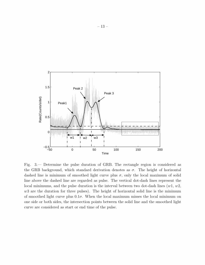
1998; Hakkila et al. 2003). In this work, we still use the smoothing skill. In Fig. 3, we utilize

GRB 061007 as an example to represent the procedure of the duration of GRB pulses. We

smooth the GRB light curve for energy band 15-150 keV with α = 0.1. The smoothed light

curve may contain a few local maximum values. The lags which the pulse peaks exceed 1σ

background are returned. There are two ways to determine the width of individual pulse.

First, when the pulse peak exists local minimums on both sides, the pulse duration is the

interval between the local minimums. Second, when the pulse peak absents local minimum

on one side (or both sides), we drew a horizontal line which height equals to the global

minimum of smoothed light curve with 0.1σ background added, and then the intersection

points between the horizontal line and the smoothed light curve are considered as start or

end point of the pulse.

3. The GRBs sample and the results

3.1. Description of the GRBs sample

Since the successful launch of Swift satellite in November 2004 (Gehrels, N. et al. 2004),

over 600 GRBs have been detected. Swift is a multi-wavelength satellite which can detect

the gamma-ray transitional source and accurately locate the source within less than 100

seconds. Swift observations have played an inconceivably important role in GRB research.

The energy band of BAT/Swift is 15-350 keV. In practice, we only choose photons

between 15 and 150 keV because the BAT is transparent to high energy photons over 150

keV. In previous works, GRBs light curves were extracted by specifying GRBs positions

which were detected by BAT. Here, we use a slightly different method. The XRT can improve

GRB position in both accuracy and precision by using the UVOT to accurately determine

– 6 –

Swift position (Goad et al. 2007; Evans et al. 2009). So, we apply enhanced XRT position

to the procedure ‘batmaskwtevt’ and ‘batbinevt’ and extract background subtracted 15-25

keV and 50-100 keV light curves with a time bin size of 16 ms for spectral lag calculating.

Obviously, when we apply this procedure to a low S/N GRB, it can produce unendurable

error. So, we select the GRBs with S/N larger than 5 in 15-25 keV energy range.

Our sample contains 121 long GRB detected by BAT/Swift from 2004 to 2010, 54 of

them have measured redshifts.

3.2. Results

For a given spectral lag in advance, Ukwatta et al. (2010) simulated a group of light

curves with the profile of a FRED pulse superposed on a background of different noise levels

and fitted the peaks of CCF by a Gaussian function. The calculated lag was consistent with

the value given previously. Through calculation we find that the CCF shows a symmetrical

peak when the simulated light curves have FRED-like pulse shapes. Obviously, Gaussian

curve is appropriate for fitting such maximum. The raw light curves, however, are much more

complicated than the simulated ones, it is hard to get a good fitting with Gaussian function.

As for our samples, the shapes of the CCF can be roughly classified into 3 categories: 1)

Gaussian-like profile; 2) Asymmetric peak and 3) multi-peaks. Not difficult to imagine, it is

easy to fit the first kind of CCF with a Gaussian function but hard for the other two kinds.

We will compare the two methods with various shapes of CCF.

We choose GRB 080413B and GRB 071020 as examples. In Fig. 4, the CCF between 15-

25 keV and 50-100 keV of GRB 080413B shows a Gaussian-like pulse. We fit the maximum

of CCF with a Gaussian function plus a linear function and obtain the spectral lag and error,

τ = 0.14± 0.02 s. Then, using the smooth method, we obtain τ = 0.14± 0.02 s. The results

and figure show that either method can well model the spectral lag of GRB 080413B.

In Fig. 5, the CCF (circle) between 15-25 keV and 50-100 keV of GRB 071020 displays

an asymmetry peak. There is an offset between A and B. If we change the fitting interval,

point A will move, while the location of B is not related to the fitting interval. Although

using a smaller fitting interval that contains the maximum of the CCF may yield similar

lags, it will increase the lag uncertainty. Fig. 5 shows the smooth method (dashed line) is

better for finding the maximum of CCF.

We list 121 spectral lags and pulse widths of GRBs in table 1 and table 2. For GRB

with multiple pulses, we calculate each pulse of spectral lag. In the paper, the spectral lags

– 7 –

with smoothing factor α = 0.1 and α = 0.05 are utilized to analysis.

3.3. The Results Analysis

3.3.1. Comparison between Gaussian Curve Fitting and Smooth Method

From table 1 and table 2, we notice that the correlation coefficient between lagGauss and

lagloess is 0.9, which implies that the result of the two methods have high correlation. The

lagGauss − lagloess relation is fitted by a linear function lagloess(s) = (0.75± 0.05)lagGauss(s) +

(0.005± 0.03). Hence, the lagGauss is systematically larger than lagloess by a factor of 4/3.

3.3.2. The Distribution of Spectral Lags With Smooth Method

Distribution of the lags can be obtained as follows: Assuming each spectral lag obeys

a normal distribution with the mean equals to itself and the standard deviation equals to

its uncertainty. In principle, the uncertainty of a lag should be larger than its temporal

resolution, 0.016 s. Therefore, if a simulated uncertainty is smaller than 0.016 s, we set it

to 0.016 s. In Fig. 7, we add all probability density function (PDF) together, and normalize

the result. As seen in Fig. 7, the PDF of spectral lags has four components which locate at

0.028± 0.001 s, 0.091± 0.003 s, 0.151± 0.01 s, and 0.21± 0.01 s. Obviously, most of GRBs

have positive spectral lags, which is consistent with the high energy photons arriving earlier

than those with low energy photons in long GRBs.

3.3.3. The Relation between the Peak Isotropic Luminosity and the Lag of Primary Peak

Ukwatta et al. (2010) calculated spectral lags within the entire burst region for the

“Gold sample” of GRBs detected by Swift, confirming the correlation between the peak

isotropic luminosity and the lag of primary peak, albeit with a larger scatter in the relation.

Hakkila et al. (2008) argued that it is reasonable to calculate individual pulse spectral lag

instead of a burst range. From table 1 and table 2, our results support that each pulse

spectral lag of multi-pulse GRBs has different delay time. We utilized spectrum and peak

flux data from Bulter (2007) and Ukwatta et al. (2010), and tested the lag-pulse isotropic

luminosity relation. Negative and zero lags were not shown in Fig. 8. The best fit is

logL = (51.4± 0.4)− (0.8± 0.3) log lag/(1+ z). The correlation coefficient R equals to -0.6,

and the slop (0.8±0.3) cover the predicted slop of -1 by Schaefer (2004). Our results support

– 8 –

the lag-luminosity relation.

3.3.4. The Lag-pulse Duration Relation

Hakkila et al. (2008) reported a correlation between the spectral lag and pulse duration

of GRBs with a high correlation coefficient (R=0.97), i.e., the shorter the duration of the

pulse, the smaller the lag and the higher the luminosity and vice versa. We calculated the

time duration and pulse spectral lag of each pulse in the samples. In Fig. 9, the lag-duration

relation in the rest frame of GRBs is still establish but with a smaller correlation coefficient,

R=0.6.

3.3.5. The Evolution of the Lag with Time

Most GRB light curves in the sample have multi-peak structure; we show the lag cor-

responding to each peak in table 1 and table 2. We find that different pulses in one GRB

generally have different spectral lags, meaning that the lags evolve with time. Some GRBs

(GRB 060927, GRB 061222A, GRB 080413A, GRB 080603B, GRB 090404, GRB 100615A)

even have different signs from different pulses, i.e. during a multi-peak burst, one pulse has a

positive lag, while the other may have a negative one. It may be due to the time evolution of

peak energy which can produce negative lags (Peng, Z. Y., et al 2011; Ukwatta et al. 2011).

4. Conclusion

In this work, we develop a new method to calculate the spectral lags. Our method does

not require the choose of fitting function and intervals, thus avoiding the human selection

effects in traditional CCF fitting methods. The M-C simulation is utilized to determine the

smooth factor α. The results show that our method obtains the introduced lags appropriately

as long as taking α between 0.05 and 0.1. Using the method, we assign α = 0.05 and α = 0.1

to calculate the spectral lags of GRBs detected by Swift BAT, respectively. The Gaussian

fitting and smoothing methods spectral lags list in table 1 and table 2. For two smoothing

factors, most of spectral lags cover each other well. From Fig. 6, we see spectral lags fitted

by Model II (i.e. Gauss+line) are strongly correlated with the smooth method results,

that demonstrates our method is reasonable. It is worth noting that lags measured by our

new method are systematically smaller than those calculated by traditional method. Figure

2 shows us that this is not caused by smoothing. We also verify the isotropic luminosity-

– 9 –

spectral lag relation, which is consist with the work of Norris et al. (2000) and Ukwatta et al.

(2010). By calculating multi-peak GRBs spectral lag, we find lags evolve with time with a

weak tendency. Finally, Hakkila et al. (2008) reported the lag-pulse duration relation with

a extremely high correlation coefficient. Our sample does not show this behavior.

We are grateful to the anonymous referee for a careful reading of this manuscript and

for encouragement, constructive criticisms, valuable suggestions and helpful comments to

improve the manuscript. We thank to Yuan Tiantian for careful reading and polishing the

manuscript. This work has been supported by the National Science Foundation of China

(NSFC 10778716, NSFC 11173024 and NSFC 10773034),National Basic Research program

of China 973 Projects (2009CB824800) and the Fundamental Research Funds for the Central

Universities. This work made use of data supplied by the UK Swift Science Data Centre at

the University of Leicester.

REFERENCES

Abdo. A. A., et al. 2009, Nature, Supplementary information, 331, 462

Amati, L., et al. 2002, A&A, 390, 81

Band, D. L. 1997, ApJ, 486, 928

Bulter, N.R. et al. 2007, ApJ, 671,656

Chen, L., Lou, Y.-Q., Wu, M., Qu, J.-L., Jia, S.-M., Yang, X.-J. 2005, ApJ, 619, 983

Cheng, L. X., Ma, Y. Q., Cheng, K. S., Lu, T., Zhou, Y. Y. 1995, A&A, 300, 746

Cleveland, W.S. 1979, Journal of the American Statistical Association 368, 829.

Cleveland, W.S.; Devlin, S.J. 1988, Journal of the American Statistical Association, 403,

596.

Evans et al. 2009, MNRAS, 397, 1177

Fishman, G. J., et al. 1994, in AIP Conf. Proc. 307, Gamma-Ray Bursts, ed.G. J. Fishman

(New York: AIP), 648

Fenimore, E. E. 1999, ApJ, 518, 375

Fenimore, E. E., Ramirez-Ruiz, E. astro-ph/0004176(2000)

– 10 –

Fenimore, E. E., int Zand, J. J. M., Norris, J. P., Bonnell, J. T., Nemiroff, R. J. 1995, ApJ,

448, L101

Gehrels, N., et al. 2004, ApJ, 611, 1005

Goad et al. 2007, A&A, 476, 1401

Hakkila, J., Giblin, T. W., Roiger, R. J., Haglin, D. J., Paciesas, W. S., Meegan, C. A. 2003,

ApJ, 582, 320

Hakkila, J., Giblin, T. W., Norris, J.P., Fragile, P.C., Bonnell, J.T. 2008, ApJ, 677, L81

Link, B., Epstein, R. I., Priedhorsky, W. C. 1993, ApJ, 408, L81

Norris, J. P., et al. 1996, ApJ, 459, 393

Norris, J. P., Marani G. F., Bonnell J. T. 2000, ApJ, 534, 248

2005, Norris, J. P., et al. ApJ, 627, 324

Peng, Z. Y., et al. Astronomische Nachrichten, 332, 92

Reichart D. E. et al. 2000, ApJ, 552, 57

Scargle, J. D. 1998, ApJ, 504, 405

Schaefer, B. E. 2004, ApJ, 602, 306

Schaefer, B. E. 2007, ApJ, 660, 16

Rong-Feng Shen, Li-Ming Song, Zhuo Li. 2005, MNRAS, 362, 59

Ukwatta, T. N., et al. 2010, ApJ, 711, 1073

Ukwatta, T. N., et al. 2011, astro-ph/1109.0666v1(2011)

Xiao L. M., Schaefer B. E. 2009, ApJ, 707, 387

This preprint was prepared with the AAS LATEX macros v5.2.

– 11 –

-5 0 5 10 15 20 25

-0.1

0.0

0.1

0.2

0.3

0.4

Rate(co

unts/s/det)

Time (s)

Light curve=0.05

=0.2

Fig. 1.— Light curve of GRB 081222 with a temporal resolution 16ms. The dotted and solid

lines are the smoothed light curves with α = 0.05 and α = 0.2, respectively.

– 12 –

-0.03

0.00

0.03

0.06

0.09

0.00

0.03

0.06

0.09

0.12

0.15

0.00 0.03 0.06 0.09 0.120.06

0.09

0.12

0.15

0.18

0.00 0.03 0.06 0.09 0.120.18

0.21

0.24

0.27

0.30

Lagth = 32ms Lag

th = 64ms

Lagth = 128ms

Lag

(s)

Lagth = 240ms

Fig. 2.— Lag vs. α. The width ratio is 1.05 and the theoretical lags are 32 ms, 64 ms, 128

ms and 240 ms, respectively. For each panel, the horizontal dotted line shows the theoretical

lag. The horizontal axis represents α, and vertical axis represents lag. The spectral lags and

corresponding error bars of light curves are displayed, with signal-to-noise changing from 5

to 10.

– 13 –

−50 0 50 100 150 200−0.5

0

0.5

1

1.5

2

Time

Rat

e(C

ount

s/s/

det)

w1 w3w2

Peak1

Peak 3

Peak 2

Fig. 3.— Determine the pulse duration of GRB. The rectangle region is considered as

the GRB background, which standard derivation denotes as σ. The height of horizontal

dashed line is minimum of smoothed light curve plus σ, only the local maximum of solid

line above the dashed line are regarded as pulse. The vertical dot-dash lines represent the

local minimums, and the pulse duration is the interval between two dot-dash lines (w1, w2,

w3 are the duration for three pulses). The height of horizontal solid line is the minimum

of smoothed light curve plus 0.1σ. When the local maximum misses the local minimum on

one side or both sides, the intersection points between the solid line and the smoothed light

curve are considered as start or end time of the pulse.

– 14 –

−30 −20 −10 0 10 20 30 40 50

0.7

0.75

0.8

n

CC

F

Gauss Fit

CCF

Smooth first

Fig. 4.— A comparison between Gaussian fitting and loess filter methods for GRB 080413B.

The black points represent the CCF between 15-25 keV and 50-100 keV light curves. The

solid and dashed lines represent the results fitted by traditional Gaussian fitting or smooth

method, respectively.

– 15 –

−40 −30 −20 −10 0 10 20 30 40

0.7

0.75

0.8

0.85

n

CC

F

Gauss Fit

CCF

Smooth First

AB

Fig. 5.— A comparison between Gaussian fitting and loess filter methods for GRB 071020. A

and B indicate the maximums of the CCF smoothed by Gaussian function and loess smooth

method, respectively.

– 16 –

−2 −1 0 1 2 3 4 5−2

−1

0

1

2

3

4

5

Gauss lag (s)

Loe

ss la

g (s

)

Fig. 6.— logGauss -logloess relation. The solid line shows the best fit between logGauss and

logloess. The dashed line displays the diagonal. The 1σ simulation uncertainties are used for

error bars.

– 17 –

-0.5 0.0 0.5 1.0 1.5

0.0

0.5

1.0

1.5

2.0

2.5

3.0

PDF

Spectral lag (s)

PDF Gauss fitting Gauss components 1 Gauss components 2 Gauss components 3 Gauss components 4

Fig. 7.— The PDF of loess spectral lags. The PDF is fitted by four Gauss components which

locate 0.028 ± 0.001 s (dashed line), 0.091 ± 0.003 s (dotted line), 0.15 ± 0.01 s (dash-dot

line), and 0.21± 0.01 s (dash-dot-dot line), respectively.

– 18 –

−4 −3.5 −3 −2.5 −2 −1.5 −1 −0.5 0 0.549.5

50

50.5

51

51.5

52

52.5

53

53.5

54

54.5

Log(lag/(1+z)) (s)

Log

(L)

(erg

/s)

Fig. 8.— The log-log relation between isotropic luminosity and spectral lag. The factor

(1 + z)−1 corrects for the time dilation effect.

– 19 –

−2.5 −2 −1.5 −1 −0.5 0 0.5−0.2

0

0.2

0.4

0.6

0.8

1

1.2

1.4

1.6

Log (lag/(1+z)) (s)

Log

(du

ratio

n/(1

+z)

) (s

)

Fig. 9.— Lag-pulse duration relation in the rest frame of GRBs. Both axes are in units of

second. The factor (1 + z)−1 corrects for the time dilation effect. Each duration error is set

as 10% of its value.

– 20 –

Table 1. The spectral lags of GRB with measured redshift.

GRB Peak No. Start time Stop time lagGauss lagSmooth(s) lagSmooth

α = 0.1 α = 0.05

(s) (s) (s) (s) (s)

(1) (2) (3) (4) (5) (6) (7)

050318 24.52 32.392 0.06 ± 0.05 0 ± 0.05 0.11 ± 0.06

050401 22.968 33.992 0.44 ± 0.1 0.27 ± 0.13 0.14 ± 0.05

050416A -1.648 3.856 0.49 ± 0.1 0.69 ± 0.14 0.64 ± 0.1

050603 -3.24 3.560 0.06 ± 0.02 0.06 ± 0.02 0.05 ± 0.02

050922C -3.624 4.152 0.21 ± 0.02 0.16 ± 0.02 0.27 ± 0.11

051111 -8.88 12.304 1.1 ± 0.4 0.51 ± 0.44 0.48 ± 0.2

060206 -1.976 8.856 0.44 ± 0.07 0.45 ± 0.08 0.43 ± 0.2

060210 -5.032 9.304 0.51 ± 0.2 0.43 ± 0.2 0.34 ± 0.1

060418 23.104 34.848 0.08 ± 0.2 0 ± 0.2 0.02 ± 0.02

060526 -5.040 16.192 0.25 ± 0.06 0.16 ± 0.06 0.21 ± 0.08

060614 -5.360 7.072 0.08 ± 0.02 0.1 ± 0.02 0.08 ± 0.02

060814 1 -0.696 29.704 0.33 ± 0.04 0.16 ± 0.04 0.19 ± 0.09

2 58.6 91.192 -0.49 ± 0.1 -0.34 ± 0.13 -0.6 ± 0.4

060904B -11.488 25.424 0.64 ± 0.1 0.53 ± 0.14 0.58 ± 0.2

060912 -1.2 4.768 0.24 ± 0.03 0.22 ± 0.03 0.22 ± 0.04

060927 1 -1.864 3.896 0.06 ± 0.02 0.05 ± 0.02 0.08 ± 0.02

2 3.48 8.600 -0.02 ± 0.01 0 ± 0.02 0.21 ± 0.1

3 13.16 29.064 -0.67 ± 0.2 -0.62 ± 0.2 -0.74 ± 0.3

061007 1 -4.296 19.768 0.52 ± 0.1 0.19 ± 0.14 0.18 ± 0.05

2 24.072 41.176 0.18 ± 0.06 0.16 ± 0.06 0.11 ± 0.05

3 41.592 65.928 0.17 ± 0.02 0.16 ± 0.02 0.16 ± 0.01

061121 1 -3.112 8.6 0.84 ± 0.2 0.64 ± 0.2 0.82 ± 0.3

2 58.712 82.312 0.02 ± 0.02 0.03 ± 0.02 0.03 ± 0.02

061201 -5.576 7.976 0.2 ± 0.03 0.19 ± 0.03 0.08 ± 0.02

070306 88.944 108.848 0.16 ± 0.06 0.1 ± 0.06 -0.08 ± 0.06

070508 -5.712 29.12 0.09 ± 0.02 0.1 ± 0.02 0.1 ± 0.02

070521 1 7.3520 28.312 0.32 ± 0.06 0.26 ± 0.06 0.18 ± 0.04

2 28.792 33.48 0.29 ± 0.03 0.14 ± 0.03 0.11 ± 0.02

– 21 –

Table 1—Continued

GRB Peak No. Start time Stop time lagGauss lagSmooth(s) lagSmooth

α = 0.1 α = 0.05

(s) (s) (s) (s) (s)

(1) (2) (3) (4) (5) (6) (7)

3 33.416 40.232 0.08 ± 0.01 0.1 ± 0.01 0.14 ± 0.07

070714B -1.728 2.976 0.02 ± 0.02 0.02 ± 0.02 0.02 ± 0.02

070810A -6.872 12.008 0.74 ± 0.2 0.51 ± 0.2 0.5 ± 0.3

071003 -2.656 29.92 0.51 ± 0.09 0.11 ± 0.1 0.11 ± 0.04

071010B -2.264 20.76 0.19 ± 0.02 0.14 ± 0.02 0.14 ± 0.05

071020 -3.808 3.456 -0.02 ± 0.02 0.03 ± 0.02 0.03 ± 0.02

071117 -1.392 6.224 0.75 ± 0.05 0.78 ± 0.05 0.78 ± 0.06

080210 -6.928 23.712 0.64 ± 0.2 0.59 ± 0.2 0.53 ± 0.3

080319B -5.792 62.032 0.2 ± 0.02 0.1 ± 0.01 0.35 ± 0.02

080319C -2.784 15.6 0.23 ± 0.04 0.16 ± 0.04 0.19 ± 0.08

080330 -2.432 15.264 0.16 ± 0.05 0.32 ± 0.05 0.03 ± 0.02

080411 1 14.960 23.36 0.3 ± 0.02 0.21 ± 0.01 0.2 ± 0.02

2 38.720 49.04 0.2 ± 0.02 0.18 ± 0.02 0.18 ± 0.02

3 52.608 62.624 0.29 ± 0.2 0 ± 0.2 0 ± 0.2

4 62.512 72.192 0.23 ± 0.8 0.16 ± 0.1 0.11 ± 0.1

080413A 1 -2.888 10.6 0.2 ± 0.03 0.18 ± 0.03 0.18 ± 0.05

2 12.104 33.72 -0.05 ± 0.03 -0.1 ± 0.03 -0.11 ± 0.06

3 35.032 58.264 0.66 ± 0.3 0.58 ± 0.25 -0.05 ± 0.1

080413B -2.576 7.744 0.14 ± 0.02 0.14 ± 0.02 0.13 ± 0.02

080430 -1.288 14.936 0.42 ± 0.08 0.43 ± 0.08 0.51 ± 0.2

080603B 1 -1.176 6.776 -0.2 ± 0.03 -0.06 ± 0.04 -0.03 ± 0.02

2 6.6 19.688 0.38 ± 0.06 0.27 ± 0.06 0.37 ± 0.1

3 38.872 74.04 0.29 ± 0.08 0.27 ± 0.08 0.19 ± 0.08

080605 -6.84 21.544 0.12 ± 0.02 0.11 ± 0.02 0.11 ± 0.01

080607 -7.296 13.664 0.16 ± 0.02 0.18 ± 0.02 0.14 ± 0.01

080707 -11.864 10.952 0.62 ± 0.2 0.77 ± 0.2 1.12 ± 0.5

080810 -17.824 43.008 -0.03 ± 0.02 0 ± 0.02 0 ± 0.02

080916A -7.568 49.52 1.42 ± 0.3 1.33 ± 0.3 1.25 ± 0.4

– 22 –

Table 1—Continued

GRB Peak No. Start time Stop time lagGauss lagSmooth(s) lagSmooth

α = 0.1 α = 0.05

(s) (s) (s) (s) (s)

(1) (2) (3) (4) (5) (6) (7)

080928 195.432 225.016 -0.08 ± 0.05 0.08 ± 0.05 0.08 ± 0.03

081203A -0.224 47.056 0.68 ± 0.2 0.3 ± 0.2 0.3 ± 0.1

081222 -1.888 16.000 0.31 ± 0.02 0.14 ± 0.03 0.14 ± 0.02

090423 -12.84 30.936 0.39 ± 0.2 0.30 ± 0.2 0.24 ± 0.1

090424 1 -1.784 5.4 0.01 ± 0.02 0.03 ± 0.02 0.03 ± 0.02

2 5.656 26.616 0.08 ± 0.08 0.11 ± 0.08 0.08 ± 0.07

090510 -1.888 6.4 0.03 ± 0.02 0 ± 0.01 0 ± 0.02

090618 1 -7.568 41.776 3.75 ± 0.6 3.42 ± 0.6 3.4 ± 0.9

2 51.2 72.224 0.46 ± 0.03 0.3 ± 0.05 0.3 ± 0.1

3 72.112 99.52 0.001 ± 0.02 0 ± 0.02 0 ± 0.02

4 99.088 140.384 0.55 ± 0.1 0.3 ± 0.1 0.3 ± 0.2

090715B 1 -13.952 34.432 0.87 ± 0.2 0.7 ± 0.2 0.4 ± 0.2

2 48.56 89.2 0.61 ± 0.2 0.38 ± 0.2 0.53 ± 0.3

091018 -1.112 5.688 0.35 ± 0.03 0.32 ± 0.03 0.32 ± 0.05

091127 1 -1.2 3.952 0.02 ± 0.01 0.02 ± 0.02 0.02 ± 0.02

2 4.928 11.856 0.04 ± 0.03 0 ± 0.02 0.03 ± 0.05

091208B 1 -1.088 4.784 0.36 ± 0.1 0.34 ± 0.1 0.34 ± 0.1

2 5.328 17.904 0.07 ± 0.02 0.06 ± 0.02 0.03 ± 0.02

100316B -6.696 12.792 0.81 ± 0.2 0.35 ± 0.2 0.34 ± 0.1

Note. — col.(1): The GRB trigger number. Col.(2): The peak number of GRB. Col.(3):

The start time of individual pulse relative to the GRB trigger time. Col.(4): The stop time

of individual pulse relative to the GRB trigger time. Col.(5): The spectral lags plus errors

between 15-25 keV and 50-100 keV by fitting with Gaussian plus linear equation. Col.(6):The

spectral lags plus errors calculated by smooth method with α = 0.1. Col.(7):The spectral

lags plus errors calculated by smooth method with α = 0.05.

– 23 –

Table 2. The spectral lags of GRB with unknown redshift.

GRB Peak No. Start time Stop time lagGauss lagSmooth(s) lagSmooth

α = 0.1 α = 0.05

(s) (s) (s) (s) (s)

(1) (2) (3) (4) (5) (6) (7)

041220 -2.608 8.096 0.21 ± 0.05 0.08 ± 0.05 0.18 ± 0.08

041224 16.032 41.568 0.49 ± 0.2 0.62 ± 0.2 0.77 ± 0.4

050124 -6.264 6.904 0.03 ± 0.02 0.08 ± 0.02 0.05 ± 0.02

050219B 1 -6.376 5.432 0.23 ± 0.06 0.05 ± 0.06 0.03 ± 0.02

2 -5.976 15.896 0.32 ± 0.05 0.29 ± 0.05 0.10 ± 0.03

050326 1 -2.736 13.392 0.03 ± 0.02 0.02 ± 0.02 0.02 ± 0.02

2 15.52 30.560 0.09 ± 0.02 0.06 ± 0.02 0.06 ± 0.02

050418 -25.416 31.000 0.44 ± 0.09 0.50 ± 0.1 0.42 ± 0.2

050509A -8.664 8.680 0.06 ± 0.03 0.14 ± 0.04 0.06 ± 0.02

050701 2.968 13.384 0.21 ± 0.05 0.14 ± 0.06 0.29 ± 0.2

050717 1 -1.136 16.672 0.01 ± 0.02 0.05 ± 0.02 0.03 ± 0.02

2 16.368 39.408 0.46 ± 0.2 0.13 ± 0.2 0.10 ± 0.03

050801 -2.464 9.9680 0.29 ± 0.08 0.10 ± 0.09 0.00 ± 0.02

050820B 1 -1.608 5.3840 0.42 ± 0.2 0.24 ± 0.2 0.11 ± 0.03

2 5.2240 17.688 -0.40 ± 0.09 -0.11 ± 0.09 -0.21 ± 0.07

051016B 1 -0.584 2.056 0.26 ± 0.08 0.14 ± 0.07 0.13 ± 0.07

2 2.056 7.480 -0.49 ± 0.2 -0.46 ± 0.2 -1.07 ± 0.6

060105 1 -12.00 18.856 0.43 ± 0.09 0.16 ± 0.1 0.16 ± 0.05

2 19.256 43.368 0.55 ± 0.2 0.06 ± 0.2 0.06 ± 0.02

060110 -2.104 14.248 1.09 ± 0.3 1.25 ± 0.3 1.34 ± 0.6

060111A -7.456 18.608 1.53 ± 0.4 1.44 ± 0.4 1.95 ± 0.5

060117 1 -2.776 5.176 0.12 ± 0.02 0.08 ± 0.02 0.08 ± 0.02

2 5.5760 18.936 0.08 ± 0.02 0.03 ± 0.02 0.03 ± 0.02

060223B -7.840 8.400 -1.15 ± 0.5 -0.02 ± 0.5 0.03 ± 0.02

060306 -3.584 8.320 0.18 ± 0.02 0.08 ± 0.03 0 ± 0.02

060313 -3.024 2.048 0 ± 0.02 0 ± 0.02 0 ± 0.02

060428A -3.136 11.904 0.18 ± 0.06 0.00 ± 0.06 0.05 ± 0.02

060708 -1.976 10.392 0.95 ± 0.3 0.29 ± 0.3 0.29 ± 0.1

– 24 –

Table 2—Continued

GRB Peak No. Start time Stop time lagGauss lagSmooth(s) lagSmooth

α = 0.1 α = 0.05

(s) (s) (s) (s) (s)

(1) (2) (3) (4) (5) (6) (7)

060719 1 -0.888 13.352 0.85 ± 0.3 0.51 ± 0.3 0.5 ± 0.2

2 40.136 60.168 0.51 ± 0.1 0.26 ± 0.1 0.32 ± 0.1

060813 -0.888 11.192 -0.01 ± 0.02 0.03 ± 0.02 0.03 ± 0.02

060825 -4.272 8.016 0.54 ± 0.1 0.43 ± 0.1 0.45 ± 0.2

060904A 41.336 81.256 -0.02 ± 0.02 0.1 ± 0.02 0.1 ± 0.04

061004 -0.008 11.512 -0.01 ± 0.03 0.13 ± 0.03 0.13 ± 0.04

061021 0 10.880 0.03 ± 0.02 0 ± 0.02 0 ± 0.02

061126 2.488 14.920 0.14 ± 0.03 0.13 ± 0.03 0.24 ± 0.1

061202 70.648 95.976 -0.14 ± 0.06 0 ± 0.06 0 ± 0.07

061222A 1 23.184 39.984 -0.23 ± 0.06 -0.13 ± 0.06 0.03 ± 0.02

2 45.040 72.672 0.26 ± 0.08 0.00 ± 0.08 -0.1 ± 0.09

3 77.472 99.824 0.14 ± 0.02 0.14 ± 0.02 0.14 ± 0.02

070220 -3.512 27.928 -0.05 ± 0.02 -0.06 ± 0.02 -0.05 ± 0.02

070427 -3.032 17.864 1.62 ± 0.4 0.64 ± 0.4 0.26 ± 0.1

070714A -1.176 8.024 0.34 ± 0.2 0.27 ± 0.2 0.22 ± 0.3

070911 1 7.496 28.984 -0.14 ± 0.08 0 ± 0.08 0 ± 0.02

2 27.768 62.776 0.32 ± 0.03 0.30 ± 0.03 0.24 ± 0.06

070917 -1.128 9.432 0.25 ± 0.02 0.21 ± 0.02 0.21 ± 0.02

080229A 1 -9.240 12.408 1.07 ± 0.31 0.53 ± 0.3 0.45 ± 0.2

2 24.744 52.040 0.30 ± 0.02 0.32 ± 0.02 0.22 ± 0.03

080328 1 -12.176 54.848 0.62 ± 0.26 0.22 ± 0.3 0.16 ± 0.08

2 65.744 101.824 0.70 ± 0.08 0.45 ± 0.09 0.48 ± 0.2

080409 1 -2.088 6.552 0.23 ± 0.05 0.34 ± 0.05 0.35 ± 0.2

2 5.960 13.336 0.09 ± 0.03 0.00 ± 0.03 0.08 ± 0.04

080426 -1.376 3.232 0.10 ± 0.01 0.08 ± 0.02 0.08 ± 0.02

080613B -7.784 34.680 0.05 ± 0.01 0.03 ± 0.02 0.03 ± 0.02

080701 -5.096 7.336 1.34 ± 0.40 1.49 ± 0.4 1.58 ± 0.5

080714 -4.000 6.752 0.53 ± 0.14 0.42 ± 0.1 0.16 ± 0.3

– 25 –

Table 2—Continued

GRB Peak No. Start time Stop time lagGauss lagSmooth(s) lagSmooth

α = 0.1 α = 0.05

(s) (s) (s) (s) (s)

(1) (2) (3) (4) (5) (6) (7)

080727B 1 -0.368 4.928 -0.05 ± 0.02 -0.05 ± 0.02 -0.06 ± 0.02

2 5.408 11.152 0.07 ± 0.02 0.08 ± 0.02 0.06 ± 0.02

080727C -9.032 52.120 0.36 ± 0.1 0.34 ± 0.1 0.37 ± 0.2

080915B -0.768 2.416 -0.04 ± 0.02 -0.05 ± 0.02 -0.05 ± 0.03

081210 6.720 23.120 0.05 ± 0.07 0.10 ± 0.07 0.05 ± 0.02

090113 1 -3.072 3.376 0.20 ± 0.04 0.10 ± 0.04 0.19 ± 0.09

2 3.264 5.328 0.16 ± 0.05 0.02 ± 0.05 0.05 ± 0.02

3 4.928 12.176 0.15 ± 0.1 0.11 ± 0.1 0.19 ± 0.1

090129 -3.472 23.872 0.46 ± 0.08 0.37 ± 0.08 0.30 ± 0.1

090201 -4.256 3.920 0.12 ± 0.2 0.08 ± 0.2 0.13 ± 0.1

090201 4.736 15.888 0.56 ± 0.2 0.50 ± 0.2 0.70 ± 0.3

090301A 1 -6.352 14.336 0.32 ± 0.08 0.11 ± 0.08 0.11 ± 0.02

2 14.464 19.440 0.16 ± 0.04 0.21 ± 0.04 0.22 ± 0.05

3 21.104 28.784 0.15 ± 0.02 0.11 ± 0.02 0.11 ± 0.02

4 29.872 37.584 0.07 ± 0.02 0.06 ± 0.02 0.06 ± 0.02

090401B 1 -0.448 6.288 0.11 ± 0.02 0.06 ± 0.02 0.06 ± 0.02

2 6.192 13.104 0.10 ± 0.02 0.03 ± 0.02 0.03 ± 0.02

090404 1 14.928 36.528 0.19 ± 0.04 0.05 ± 0.05 0.11 ± 0.06

2 33.504 45.600 -0.21 ± 0.1 -0.16 ± 0.1 0.08 ± 0.1

090518 -5.888 3.904 -0.14 ± 0.02 0.13 ± 0.03 0.11 ± 0.03

090530 -3.024 7.808 0.02 ± 0.03 0.10 ± 0.03 0.06 ± 0.03

090709A 1 -21.712 18.512 0.27 ± 0.05 0.27 ± 0.05 0.19 ± 0.06

2 18.032 66.400 0.09 ± 0.02 0.16 ± 0.02 0.16 ± 0.04

090813 1 -0.952 3.208 0.02 ± 0.02 0.00 ± 0.02 0.05 ± 0.02

2 5.384 9.304 0.16 ± 0.1 0.00 ± 0.1 0.06 ± 0.07

090929B -9.064 53.800 0.28 ± 0.08 0.29 ± 0.08 0.18 ± 0.06

091020 -7.136 23.568 -0.02 ± 0.05 0.00 ± 0.05 0.37 ± 0.2

100111A -5.512 11.752 0.27 ± 0.07 0.26 ± 0.08 0.29 ± 0.1

– 26 –

Table 2—Continued

GRB Peak No. Start time Stop time lagGauss lagSmooth(s) lagSmooth

α = 0.1 α = 0.05

(s) (s) (s) (s) (s)

(1) (2) (3) (4) (5) (6) (7)

100423A -3.992 4.552 0.06 ± 0.02 0.03 ± 0.02 0.03 ± 0.02

100522A 1 -2.184 7.752 -0.09 ± 0.02 0.03 ± 0.02 0.03 ± 0.02

2 23.432 39.672 0.56 ± 0.3 0.05 ± 0.3 0.24 ± 0.5

100615A 1 -1.60 9.120 0.62 ± 0.1 0.51 ± 0.1 0.51 ± 0.08

2 8.976 22.784 0.35 ± 0.07 0.16 ± 0.07 0.16 ± 0.04

3 22.496 48.992 -0.49 ± 0.08 -0.34 ± 0.09 -0.5 ± 0.2

100619A 1 -7.824 16.592 0.28 ± 0.05 0.06 ± 0.05 -0.02 ± 0.02

2 79.648 99.792 0.03 ± 0.02 -0.03 ± 0.02 0.06 ± 0.03

100621A -3.288 42.088 1.45 ± 0.1 1.07 ± 0.13 1.07 ± 0.1

100704A -9.032 25.512 1.14 ± 0.2 0.78 ± 0.23 1.04 ± 0.4

100816A -1.360 4.176 0.12 ± 0.02 0.10 ± 0.01 0.10 ± 0.02

100906A 1 -3.248 21.616 0.50 ± 0.04 0.34 ± 0.05 0.27 ± 0.05

2 93.024 131.408 0.72 ± 0.2 0.45 ± 0.18 0.5 ± 0.2

Note. — Each Column represents the same as table 1.