Spectral estimation of the fractional order of a Lévy process

$Page 1: Spectral estimation of the fractional order of a Lévy process$
arX

iv:1

001.

1820

v1 [

mat

h.ST

] 1

2 Ja

n 20

10

The Annals of Statistics

2010, Vol. 38, No. 1, 317–351DOI: 10.1214/09-AOS715c© Institute of Mathematical Statistics, 2010

SPECTRAL ESTIMATION OF THE FRACTIONAL ORDER

OF A LEVY PROCESS

By Denis Belomestny1

Weierstrass-Institute Berlin

We consider the problem of estimating the fractional order of aLevy process from low frequency historical and options data. An esti-mation methodology is developed which allows us to treat both esti-mation and calibration problems in a unified way. The correspondingprocedure consists of two steps: the estimation of a conditional char-acteristic function and the weighted least squares estimation of thefractional order in spectral domain. While the second step is iden-tical for both calibration and estimation, the first one depends onthe problem at hand. Minimax rates of convergence for the fractionalorder estimate are derived, the asymptotic normality is proved anda data-driven algorithm based on aggregation is proposed. The per-formance of the estimator in both estimation and calibration setupsis illustrated by a simulation study.

1. Introduction. Nowadays Levy processes are undoubtedly one of themost popular tool for modeling economic and financial time series [see, e.g.,Cont and Tankov (2004), for an overview]. This is not surprising if onetakes into account their simplicity and analytic tractability on the one handand the ability to reproduce many stylized facts of financial time serieson the other hand. In the last decade, new subclasses of Levy processeshave been introduced and actively studied (mainly in the context of op-tion pricing). Among the best known models are normal inverse Gaussianprocesses (NIG), hyperbolic processes (HP), generalized hyperbolic pro-cesses (GHP) and truncated (or tempered) Levy processes (TLP).Boyarchenko and Levendorskiı (2002) have introduced a general class of reg-ular Levy processes of exponential type (RLE) which contains all abovementioned particular Levy models. This type of processes is characterized

Received August 2008; revised May 2009.1Supported in part by SFB 649 “Economic Risk.”AMS 2000 subject classifications. Primary 62F10; secondary 62J12, 62F25, 62H12.Key words and phrases. Regular Levy processes, Blumenthal–Getoor index, semipara-

metric estimation.

This is an electronic reprint of the original article published by theInstitute of Mathematical Statistics in The Annals of Statistics,2010, Vol. 38, No. 1, 317–351. This reprint differs from the original in paginationand typographic detail.

1

http://arxiv.org/abs/1001.1820v1

http://www.imstat.org/aos/

http://dx.doi.org/10.1214/09-AOS715

http://www.imstat.org

http://www.ams.org/msc/

http://www.imstat.org

http://www.imstat.org/aos/

http://dx.doi.org/10.1214/09-AOS715

2 D. BELOMESTNY

by the requirement that the modulus of the characteristic function of incre-ments behaves like exp(−η|u|α) as |u| →∞ for some 0< α< 2. Parameter αcoincides with the fractional order of the underlying Levy process and playsan important role because it determines the decay of the characteristic func-tion and hence the smoothness properties of the corresponding state pricedensity. Statistical inference for RLE processes is the subject of our paper.

There are basically two types of statistical problems relevant for Levyprocesses: the estimation of parameters of a Levy process Xt from a timeseries of the asset St = exp(Xt) and the calibration of these parameters usingoptions data. Both problems have received much attention recently.

Suppose that a Levy processXt is observed at n time points ∆,2∆, . . . , n∆.SinceX0 = 0, this amounts to observing n increments χi =Xi∆−X(i−1)∆, i=1, . . . , n. If ∆ is small (high-frequency data), then a large increment χi in-dicates that a jump occurred between time ti−1 and ti. Based on this in-sight and the continuous-time observation analogue, inference for the Levymeasure of the underlying Levy process can be conducted. See, for exam-ple, Aıt-Sahalia and Jacod (2006) for a semiparametric problem of estimat-ing volatility of a stable process under the presence of Levy perturbationor Lee and Mykland (2008) and Figueroa-Lopez and Houdre (2006) for thenonparametric problem of testing and estimation for jump diffusion models.For low-frequency observations, however, we cannot be sure to what extentthe increment χi is due to one or several jumps or just to the diffusion partof the Levy process. The only way to draw inference is to use the fact thatthe increments form independent realizations of infinitely divisible probabil-ity distributions. In this setting, a variety of methods have been proposed inthe literature: standard maximum likelihood estimation DuMouchel (1973a,1973b, 1975), using the empirical characteristic function as an estimatingequation [see, e.g., Press (1972), Fenech (1976), Feuerverger and McDun-nough (1981a), Singleton (2001)], maximum likelihood by Fourier inversionof the characteristic function Feuerverger and McDunnough (1981b), a re-gression based on the explicit form of the characteristic function Koutrou-velis (1980) or other numerical approximations Nolan (1997). Some of thesemethods were compared in Akgiray and Lamoureux (1989). Note that all ofthe aforementioned papers deal with the specific parametric (mainly stable)models. A semiparametric estimation problem for Levy models has recentlybeen considered in Neumann and Reiss (2009) and Gugushvili (2008).

The second calibration problem is of special importance for financial appli-cations because pricing of options is performed under an equivalent martin-gale measure, and one can infer on this measure only from options data. Sinceoption data is sparse and the underlying inverse problem is usually ill-posed,we face a rather complicated estimation issue. Different approaches havebeen proposed in the literature to regularize the underlying inverse prob-lem. For example, in Cont and Tankov (2004) and Cont and Tankov (2006),

SPECTRAL ESTIMATION OF THE FRACTIONAL ORDER OF A LEVY PROCESS3

a method based on the penalized least squares estimation with the minimalentropy penalization is proposed. Belomestny and Reiss (2006) developed aspectral calibration method which avoids solving a high-dimensional opti-mization problem and is based on the direct inversion of a Fourier pricingformula with a cut-off regularization in spectral domain. This method essen-tially employees the integrability property of the underlying Levy measure(finite activity Levy processes) that excludes many interesting infinite ac-tivity Levy processes.

In this paper we consider the problem of estimating the fractional or-der of a Levy process from low-frequency historical as well as options data.Our problem is a semiparametric one because we do not assume any spe-cific parametric model for the underlying process but only some asymptoticbehavior. The spectral approach allows us to treat both estimation and cali-bration problems in a unified framework and leads to an efficient data-drivenalgorithm. Moreover, the fractional order estimate delivered by the spectralmethod possesses several interesting optimality properties.

The problem of estimating the degree of activity of jumps in semimartin-gale framework using high-frequency financial data has recently been con-sidered in Aıt-Sahalia and Jacod (2009). On the one hand, small incrementsof the process turn out to be most informative for estimating the activityindex. On the other hand, these small increments are the ones where thecontribution from the continuous martingale part is mixed with the con-tribution from the small jumps. Aıt-Sahalia and Jacod (2009) proposed anestimation procedure which is able to “see through” the continuous part andconsistently estimate the degree of activity for the small jumps under somerestrictions on the structure of the underlying semimartingale. Note that inthe case of Levy processes the degree of activity of jumps is identical to thefractional order of the underlying Levy process. We also stress that the casewhen both diffusion and jump components are presented can be treated inthe framework of spectral estimation as well (see Section 6.9).

Short outline of the paper. In Section 2 we introduce the class of RLEprocesses. Section 3 discusses some aspects of financial modeling with RLEprocesses. Section 4 describes the observational model. In Section 5 meth-ods of estimating the characteristic function of a Levy process from low-frequency historical and options data are presented. Section 6 is devotedto the spectral calibration method of estimating the fractional order α. Wediscuss here the problems of regularization and derive minimax rates of con-vergence for a class of Levy processes. In Section 7 an adaptive procedurefor estimating α is presented, and its properties are discussed. We concludewith some simulation results.

2. Regular Levy processes of exponential type. In this section we recallsome basic properties of Levy processes.

4 D. BELOMESTNY

2.1. Spectral properties of Levy processes. Consider a Levy process Xt

with a Levy measure ν. That is, Xt is cadlag process with independent andstationary increments such that the characteristic function of its marginalsφt(u) is given by

φt(u) := E[eiuXt ](2.1)

= exp

{t

(iuµ− u2a2

2+

∫

R

(eiux − 1− iux1{|x|≤1})ν(dx)

)}.

So, any Levy process Xt is characterized by the so called Levy triple (µ,a, ν)where µ ∈ R is a drift, a > 0 is a diffusion volatility and ν is a Levy mea-sure. Note that the drift µ depends on the type of truncation in (2.1). Infact, this characterization is unique for a fixed truncation function and wecan reconstruct the Levy triple from the characteristic function φt(u). Thisreconstruction may be viewed as consisting of three steps. First, because of

1

|u|2∫

R

(eiux − 1− iux1{|x|≤1})ν(dx)→ 0, |u| →∞,(2.2)

we can find a2/2 as lim|u|→∞|u|−2ψ(u) with

ψ(u) = t−1 log(φt(u)).

Second, note that∫ 1

−1(ψ(u)− ψ(u+w))dw=

∫

R

eiuxρ(dx)

with

ψ(u) = ψ(u) +a2

2u2, ρ(dx) = 2

(1− sinx

x

)ν(dx).

Since ρ is a finite measure (∫(x2 ∧ 1)ν(dx) <∞), one can uniquely recon-

struct it (and hence ν) from ψ(u). Finally, we find µ as limu→∞[ψ(u)/(iu)].So, in principle, we can recover all characteristics of the underlying Levy pro-cess (including the fractional order) provided that φt is completely known. If,however, φt is estimated from data we face an ill-posed estimation problembecause a small perturbation in φt may deteriorate its asymptotic behaviorand lead to the violation of (2.2). In this case using a regularization tech-nique [see, e.g., Cont and Tankov (2004) or Belomestny and Reiss (2006)],we still can get an asymptotically consistent estimates for the whole triple(µ,a, ν) given a consistent estimate of φt.

Remark 2.1. A consistent estimation of ψ(u) from a time series of Xt

is only possible if the number of observations from the distribution with the


cf. φt(u) for some t > 0 increases. This can be either due to a decreasing timestep in a times series of the process X (high frequency data) or due to anincreasing time horizon (low frequency data). While the first type of obser-vational models has received much attention in recent years, there are onlyfew papers dealing with low frequency data [see, e.g., Neumann and Reiss(2009)].

2.2. Fractional order of Levy processes. Let Xt be a Levy process witha Levy measure ν. The value

α := inf

{r≥ 0 :

∫

|x|≤1|x|rν(dx)<∞

}

is called the fractional order or the Blumenthal–Getoor index of the Levyprocess Xt. This index α is related to the “degree of activity” of jumps. AllLevy measures put finite mass on the set (−∞,−ǫ]∪ [ǫ,∞) for any arbitraryǫ > 0, so if the process has infinite jump activity, it must be because of thesmall “jumps,” defined as those smaller than ǫ. If ν([−ǫ, ǫ])<∞ the processhas finite activity and α = 0. But if ν([−ǫ, ǫ]) = ∞, that is, the processhas infinite activity and in addition the Levy measure ν((−∞,−ǫ]∪ [ǫ,∞))diverges near 0 at a rate |ǫ|−α for some α > 0, then the fractional order of Xt

is equal to α. The higher α gets, the more frequent the small jumps become[see Aıt-Sahalia and Jacod (2009) for more discussion].

The Blumenthal–Getoor index is closely related to the notion of the de-gree of jump activity that applies to general semimartingales as shown inAıt-Sahalia and Jacod (2009), and reduces to the Blumenthal–Getoor indexin the special case of Levy processes.

Note also that the Blumenthal–Getoor index coincides with the stabil-ity index for stable processes. Another example of processes having a pre-scribed fractional order α is the class of tempered stable processes of order α.Boyarchenko and Levendorskiı (2002) studied a generalization of temperedstable processes, called regular Levy processes of exponential type (RLE). ALevy process is said to be a RLE process of type [λ−, λ+] and order α ∈ (0,2)if the Levy measure has exponentially decaying tails with rates λ− ≥ 0 andλ+ ≥ 0

∫ −1

−∞eλ−|y|ν(dy)<∞,

∫ ∞

1eλ+yν(dy)<∞(2.3)

and behaves near zero as |y|−(1+α);∫

|y|>ǫν(dy)≍ Π(ǫ)

ǫα, ǫ→+0,

where Π is some positive function on R+ satisfying 0< Π(+0)<∞. Obvi-ously, the fractional order of an RLE process of order α is equal to α. An

6 D. BELOMESTNY

equivalent definition of an RLE process in terms of its characteristic expo-nent ψ(u) can be given as follows. A Levy process is considered to be an RLEprocess of type [λ−, λ+] and order α ∈ (0,2) if the following representationholds:

ψ(u) = iµu+ ϑ(u), µ ∈R,(2.4)

where function ϑ admits a continuation from R into the strip {z ∈C : Imz ∈[−λ+, λ−]} and is of the form

ϑ(u) =−|u|απ(u),(2.5)

where π(u) is a function satisfying

limsup|u|→∞

|π(u)|<∞ and lim inf|u|→∞

|π(u)|> 0

such that

Re[π(u)]> 0, u ∈R \ {0}.(2.6)

As was mentioned in the Introduction, the class of RLE processes includesamong others hyperbolic, normal inverse Gaussian and tempered stable pro-cesses but does not include variance Gamma process. In the sequel we willmainly consider RLE processes without regularity conditions (2.3) (or equiv-alently with λ− = λ+ = 0) since only the behavior of a Levy measure nearzero matters for the fractional order of the corresponding Levy process.

As mentioned before, in this work we are going to consider the problemof estimating the fractional order α of a Levy process Xt from a time seriesof asset prices as well as from option prices. Before turning to this, let usfirst make our modelling and observational framework more precise.

3. Financial modelling. In this section we recall basic facts concerningfinancial modelling with exponential Levy models.

3.1. Asset dynamics. We assume that the asset price St follows an expo-nential Levy model under both historical measure P and risk neutral measureQ. Specifically, we suppose that

St =

{SeXt , under P,Sert+Yt , under Q,

where Xt and Yt are Levy processes, S > 0 is the present value of the asset(at time 0) and r ≥ 0 is the riskless interest rate which is assumed to beknown and constant. Note that the martingale condition for St under Q

entails EQ[eYt ] = 1. The martingale measure Q is in fact not unique underthe presence of jumps. As is standard in the calibration literature, it isassumed to be settled by the market and to be identical for all options


under consideration. Processes Xt and Yt are related by the requirementthat measures P and Q ought to be equivalent: P ∼ Q. Interestingly, thisimplies that if Xt and Yt are RLE process and Xt is of order αP, then Ythas the order αQ = αP. Indeed, the equivalence of the corresponding Levymeasures νP and νQ implies [see Sato (1999)]

∫ ∞

0(√dνQ/dνP − 1)2νP(dx)<∞.(3.1)

Since for RLE processes dνQ(x)/dνP(x)≍ x(αP−αQ) and dνP(x)≍ x−(1+αP) dx

as x→+0, the condition (3.1) can be satisfied only if αP = αQ. This meansthat the fractional order of the underlying Levy process must be the sameunder both historical and risk-neutral measures. This not only indicates theimportance of the fractional order parameter for financial applications butalso suggests that the combination of two estimates of the fractional order αunder P and Q might be useful, for example, to reduce the overall varianceof the resulting combined estimator.

3.2. Option pricing. The risk neutral price at time t= 0 of the Europeancall option with strike K and maturity T is given by

C(K,T ) = e−rTEQ[(ST −K)+].

Using the independence of increments, we can reduce the number of param-eters by introducing the so-called negative log-forward moneyness,

y := log(K/S)− rT,

such that the call price in terms of y is given by

C(y,T ) = SEQ[(eYT − ey)+].

The analogous formula for the price of the European put option is P(y,T ) =SEQ[(ey − eYT )+], and a well-known put-call parity is easily established;

C(y,T )−P(y,T ) = SEQ[eYT − ey] = S(1− ey).

As we need to employ Fourier techniques, we introduce the function

OT (y) :=

{S−1C(y,T ), y ≥ 0,S−1P(y,T ), y < 0.

(3.2)

The function OT records normalized call prices for y ≥ 0 and normalizedput prices for y < 0. It possesses many interesting properties [seeBelomestny and Reiss (2006) for details]; one of them being the followingconnection between the Fourier transform of OT and the characteristic func-tion of YT denoted by φQT :

F[OT ](v) =1− φQT (v − i)

v(v− i), v ∈R.(3.3)

8 D. BELOMESTNY

Another property which directly follows from (3.3) is that∫

R

e−2yOT (y)dy <∞,(3.4)

provided that E[e2YT ] exists and is finite.

4. Observations. We consider two kinds of observational models corre-sponding to two types of statistical problems we are going to tackle. Whilethe first type of models assumes the time series of St is directly available,the second one supposes that only some functionals of St can be observed.

4.1. Time series data. We assume that the values of the log-price processXt = log(St) on equidistant time grid π = {t0, t1, . . . , tn} are observed.

4.2. Option data. As to option data, we assume that we will be given theprices of n call options for a set of forward log-moneynesses y0 < y1 < · · ·< ynand a fixed maturity T corrupted by noise. In terms of the function O, thefollowing sample is available:

OT (yj) =OT (yj) + σ(yj)ξj , j = 1, . . . , n.(4.1)

It is supposed that {ξj} are independent, centered, random variables withE[ξ2j ] = 1 and supj E[ξ

4j ]<∞. Furthermore, we assume that

∫

R

e−2yσ2(y)dy <∞.

This condition is required because we need to transform the original regres-sion model (4.1) to an exponentially weighted one,

OT (yj) = OT (yj) + σ(yj)ξj, j = 1, . . . , n,(4.2)

with OT (y) = e−yOT (y), OT (y) = e−yOT (y) and σ(y) = e−yσ(y).As a matter of fact, a consistent estimation of the fractional order α is

only possible if the amount of data available increases. In our asymptoticanalysis we will therefore assume that the number of time series observationsand the number of available options tend to infinity.

5. Estimation of characteristic functions φP and φQ. The main idea ofthe spectral estimation method (SEM) is to infer on the parameters of theunderlying model using its special structure in the spectral domain. Sincespectral behavior of a RLE process is described explicitly by (2.4) and (2.5),we can apply SEM as soon as an estimate for the corresponding characteristicfunction is available. While estimation of φ under P is rather straightforward,its calibration from option prices under Q requires special treatment.


5.1. Estimation of φ under P. We estimate the characteristic functionφP|π|(u) by its empirical counterpart,

φP|π|(u) =1

n

n∑

j=1

eiu(Xtj−Xtj−1 ).

The empirical characteristic function φP|π| possesses many interesting prop-

erties, and we refer to Ushakov (1999) for a comprehensive overview.

5.2. Estimation of φ under Q. For estimating φQT we employ the Fouriertechnique. So, motivated by (3.3), we define

φQT (u) := 1− u(u+ i)

[n∑

j=1

δjOT (yj)eiuyj

], u ∈R,(5.1)

where δj = yj − yj−1 and OT is defined in (4.2). For more involved methodsof approximating F[OT ](u) see Belomestny and Reiss (2006).

6. Estimation of fractional order. In this section we turn to the problemof estimating the fractional order of a RLE process. To this aim we apply thespectral estimation method accompanied by a spectral cut-off regularization.

6.1. Main idea. Let us consider a RLE process with the characteristicexponent ψ(u) of the form (2.4) and (2.5). In the sequel we assume (mainlyfor the sake of simplicity) that limu→−∞ π(u) = limu→∞ π(u) = η ∈ R+. Inthis case we can rewrite ϑ as

ϑ(u) =−η|u|ατ(u),(6.1)

where Re[τ(u)]> 0 for u ∈R \ {0} and τ(u)→ 1 as |u| →∞. The formula,

Y(u) := log(− log(|φ(u)|2))(6.2)

= log(2η) + α log(u) + log(Re τ(u)), u > 0,

with φ(u) = exp(ψ(u)), suggests how to estimate α from φ. Indeed, in termsof the new “data” Y , we have a linear semiparametric problem with the“nuisance” nonparametric part log(Re τ(u)). Since log(Re τ(u)) tends to 0as |u| →∞, we can get rid of this component by basing our estimation on

Y(u) with large |u|. On the other hand, if we plug-in an estimate φ insteadof φ, the variance of Y(u) will increase exponentially with |u| [because ofthe exponential decay of φ(u)], and we have to regularize the problem bycutting high frequencies. An appropriate weighting scheme would allow totake both effects into account.

10 D. BELOMESTNY

6.2. Truncation. First, we truncate φ to avoid the logarithm’s explosion.Let

Y(u) := log(− log(Tω−,ω+[|φ|2](u))), u ∈R \ {0},where the truncation operator Tω−,ω+ with truncation levels 0< ω− ≤ ω+ <1 is defined via

Tω−,ω+[f ](u) =

ω+, f(u)> ω+,f(u), ω− ≤ f(u)≤ ω+,ω−, f(u)< ω−,

for any real-valued function f .

6.3. Linearization. Truncation allows us to linearize the problem. Set

ω∗±(u) := |φ(u)|2

(1± 2|log |φ(u)||

1 + 2|log |φ(u)||

).

The following lemma holds:

Lemma 6.1. For any u ∈R \ {0} and any ω−(u), ω+(u) satisfying

0< ω− ≤ ω∗− ≤ ω∗

+ ≤ ω+ < 1,

the following inequality holds with probability one:

|Y(u)−Y(u)− ζ1(u)(|φ(u)|2 − |φ(u)|2)| ≤ ζ2(u)(|φ(u)|2 − |φ(u)|2)2,where

ζ1(u) = 2−1|φ(u)|−2 log−1(|φ(u)|)and

ζ2(u) = 2 maxξ∈{ω−(u),ω+(u)}

[1 + |log(ξ)|ξ2 log2(ξ)

].

Using the notation

∆(u) := |φ(u)|2 − |φ(u)|2,Lemma 6.1 can be reformulated as follows:

Corollary 6.2. For any u ∈R \ {0},Y(u)−Y(u) = ζ1(u)∆(u) +Q(u),(6.3)

where

|Q(u)| ≤ ζ2(u)∆2(u)(6.4)

with probability one.


Remark 6.1. Since φ(0) = 1 and φ(u) → 0 as |u| → ∞, the behaviorof truncation levels ω−(u) and ω+(u) in the vicinity of points u = 0 and

u = ∞ becomes important for determining the behavior of Y(u) around

these points. However, the values of Y(u) around 0 will be discarded whileestimating α, and hence we do not need to know ω+(u) for small |u|. As toω−(u) and ω+(u) for large u, they can be constructed if some prior infor-mation on the Blumenthal–Getoor index α and the function π(u) = ητ(u)is available. For instance, if 0< α≤ α≤ α≤ 2 and 0< π− ≤ Re[π(u)]≤ π+for all |u|> u0 with large enough u0 > 0, then one can take

ω−(u) =C1e−2π+|u|α |u|−α, |u|> u0,

ω+(u) =C2e−2π−|u|α, |u|>u0,

with some constants C1 > 0 and C2 depending on π+ and π−, respectively.While a prior upper estimate α for α appears also in the minimax ratesof convergence proved in Section 6.6, a lower estimate α turns out to beirrelevant for the convergence rates.

Note that the slope coefficient ζ1 grows exponentially with |u|. This means

that the variance of Y(u) grows exponentially as well and the values of Y(u)with large |u| and should be discarded when estimating α.

6.4. Spectral cut-off estimation. Taking into account the special semi-

linear structure of (6.2) together with a heteroscedastic variance of Y(u),we apply a weighted least squares method to estimate α. Let w1(u) be afunction supported on [ǫ,1] with some ǫ > 0 that satisfies

∫ 1

0w1(u) log(u)du= 1,

∫ 1

0w1(u)du= 0.(6.5)

For any U > 0 put

wU (u) =U−1w1(uU−1)

and define an estimate αU of α as

αU =

∫ ∞

0wU (u)Y(u)du.(6.6)

It is instructive to see what happens with αU in the case of exact data, thatis, Y = Y . One can see that in this case the following decomposition holds:

αU = log(2η)

∫ ∞

0wU (u)du

︸︷︷︸0

+α

∫ ∞

0wU (u) log(u)du

︸︷︷︸1

+RU

12 D. BELOMESTNY

with

RU :=

∫ ∞

0wU (u) log(Re τ(u))du.(6.7)

So, even in the case of perfect observations we still have the “bias” term RU

induced by model misspecification. Indeed, when applying the least squaresmethod we ignore a nonlinearity caused by RU and treat the problem asbeing linear. This is, however, only justified if RU is small. In fact, RU canbe made small by taking large values of U .

6.5. Further specification of the model class. In order to rigorously studythe complexity of the underlying estimation problem, we have to make fur-ther assumptions about the model class. Let us consider a class of Levymodels A(α,η−, η+,κ) with

ψ(u) = iµu+ ϑ(u), ϑ(u) =−η|u|ατ(u), u ∈R,(6.8)

where 0< α≤ α≤ 2,

0< η− ≤ η ≤ η+ <∞(6.9)

and

|1− τ(u)|. 1

|u|κ , |u| →∞,(6.10)

for some 0< κ ≤ α. We will write

(α,η, τ) ∈A(α,η−, η+,κ)

to indicate that the Levy process with the characteristics (α,η, τ) is inthe class A. The following proposition shows that conditions (6.8), (6.9)and (6.10) can be in fact rephrased in terms of the Levy density of aA(α,η−, η+,κ) process.

Proposition 6.3. Let ν(x) be the Levy density of a Levy process satis-fying (6.8) where the function τ fulfills

τ(u) = 1+D±u−κ + o(|u|−κ), u→±∞,(6.11)

with some constants D+ and D−. Then∫

|x|<ǫx2ν(x)dx= cǫ2−αθ(ǫ),(6.12)

where c > 0 is a constant depending on η and α and the function θ(ǫ) satisfies

|θ(ǫ)− 1|. |ǫ|κ, ǫ→ 0.

As will be shown in the next two sections, even in the class A(α,η−, η+,κ)the problem of estimating α is severely ill-posed, that is, a small perturbationε in data may lead (in worst case) to log−κ/α(1/ε) distance between α andits best estimate. On other hand, it turns out that our estimate αU achievesthe best possible rates of convergence in the class A(α,η−, η+,κ).


6.6. Upper bounds. Let us define

ε :=

n−1, under P,

‖δ‖2 +n∑

j=1

δ2j σ2(yj), under Q,

where ‖δ‖2 =∑nj=1 δ

2j , σ(yj) = e−yjσ(yj) and δj = yj − yj−1. In the case of

calibration ε comprises the level of the numerical interpolation error andof the statistical error simultaneously. In this section we will study theasymptotic behavior of the estimate αU = αU (ε) defined in (6.6) as ε→ 0,A := min{−y0, yn}→∞ and e−A . ‖δ‖2. Thus, it is assumed that the num-ber of historical observations as well as the number of available options tendto infinity. First, we present an upper bound showing that our estimate αU

with the “optimal” choice of the cut-off parameter U converges to α with alogarithmic rate in ε.

Theorem 6.4. For U = U with

U =

[1

2η+log(ε−1 log−β(1/ε))

]1/α

and

β =

{1 + κ/α, under P,(κ + 4)/α− 1, under Q,

it holds

sup(α,η,τ)∈A(α,η−,η+,κ)

E|αU −α|2 .R(ε), ε→ 0,(6.13)

where

R(ε) =

[1

2η+log ε−1

]−2κ/α

.

Remark 6.2. Since the rates are logarithmic it is usual to call the under-lying estimation problem severely ill-posed. From a practical point of view,severely ill-posedness means that more observations are needed to reach thedesired level of accuracy than for well-posed problems.

Remark 6.3. As can be easily seen the convergence rates depend on α,a prior upper bound for α. If there is no prior information on α one maytake α= 2.

14 D. BELOMESTNY

Remark 6.4. For symmetric stable processes we have τ(u) ≡ 1 and itcan be shown that the rates are parametric in this case, that is,

sup(α,η,τ)∈A(α,η−,η+,∞)

E|αU − α|2 . ε, ε→ 0,

for some U depending on ε.

6.7. Lower bounds. Now we show that the rates obtained in the previoussection are the best ones in the minimax sense for the class A(α,η−, η+,κ).

Theorem 6.5. It holds

lims→0

lim infε→0

infα


δ−2n,s(ε)E(|α− α|2) =O(1),(6.14)

where

δn,s(ε) =

[1

2η+log ε−1

]−κ/(α−s)

and the infimum is taken over all estimators α of α.

6.8. Asymptotic behavior. In this section we complete the investigationof asymptotic properties of the estimate α by proving its asymptotic nor-mality. In the case of estimation under P we have the following:

Theorem 6.6. Denote

ς(ε,U) =

[ε

∫ ∞

0wU (u)wU (v)ζ1(u)ζ1(v)S(u, v)dudv

]1/2

with

S(u, v) := Reφ(u− v) + Imφ(u+ v)

− (Reφ(u) + Imφ(u))(Reφ(v) + Imφ(v)).

Let U = U(ε) be a sequence of cutoffs such that ς−1(ε,U(ε))RU(ε) → 0 asε→ 0. Then

ς−1(ε,U(ε))(αU(ε) −α)∼N (0,1), ε→ 0.

Remark 6.5. The choice of U(ε) is based on the following reasoning.On the one hand, we have to require that ς−1(ε,U)RU → 0 in order to ensurethat ς−1(ε,U)(αU − α) has asymptotically zero expectation. On the otherhand, the variance of ς−1(ε,U)αU should converge as ε→ 0, and the limitmust be bounded and nondegenerated.


Remark 6.6. Given an estimate φ of φ and some U = U(ε) such that

|φ(u)| 6= 0 on [−U,U ] and |φ(u)| 6= 1 on [−U,U ] \ {0}, we can estimate thenorming factor ς(ε,U) for αU via

ς(ε,U) :=

[ε

∫ ∞

0wU (u)wU (v)ζ1(u)ζ1(v)S(u, v)dudv

]1/2

with

S(u, v) := Re φ(u− v) + Im φ(u+ v)

− (Re φ(u) + Im φ(u))(Re φ(v) + Im φ(v))

and

ζ1(u) := |φ(u)|−2 log−1(|φ(u)|2).

A similar result can be proved in the case of calibration as well.

6.9. Processes with a nonzero diffusion part. In fact, spectral calibrationalgorithm allows us to treat more general models with a nonzero diffusionpart. Let A(a,α, η−, η+,κ) be a class of Levy processes with the character-istic exponent of the form

ψa(u) = iµu− a2u2/2 + ϑ(u), ϑ(u) =−η|u|ατ(u), u∈R,(6.15)

where 0< a < a and conditions (6.9) and (6.10) are fulfilled. We will write(a,α, η, τ) ∈A(a,α, η−, η+,κ) to indicate that a Levy process with the char-acteristic exponent (6.15) belongs to A(a,α, η−, η+,κ).

Assume first that φa(u) = exp(ψa(u)) is known exactly. Define

L(u) := log(|φa(u)|2) =−a2u2 + 2Re[ϑ(u)]

and

Lξ(u) := ξ2L(u)−L(ξu) = log(|φa(u)|2ξ2/|φa(ξu)|2) =: log(ρξ(u))

for some ξ > 1. It obviously holds

Lξ(u) =−η|u|α(ξ2Re[τ(u)]− ξαRe[τ(ξu)]) =−cξ(α)|u|ατξ(u),where cξ(α) = η(ξ2 − ξα), and τξ(u) fulfills

|1− τξ(u)|.1

|u|κ , |u| →∞.(6.16)

Thus, Lξ(u) has a structure similar to the structure of ϑ(u) in (6.8) and wecan carry over the results of the previous section to a more general model(6.15) by defining

Yξ(u) := log(− log(Tω−,ω+[ρξ](u))),

16 D. BELOMESTNY

where ρξ(u) = |φ(u)|2ξ2/|φ(ξu)|2 with φ being an estimate of φa. Define

αξ,U =

∫ ∞

0wU (u)Yξ(u)du.(6.17)

The following two theorems are extensions of Theorems 6.4 and 6.5, respec-tively, to the case of Levy models with a nonzero diffusion part.

Theorem 6.7. For U = U with

U =

[1

2alog(ε−1 log−β(1/ε))

]1/2

and β = 1+κ/2, it holds

sup(a,α,η,τ)∈A(a,α,η−,η+,κ)

E|αξ,U − α|2 .R(ε), ε→ 0,(6.18)

where

R(ε) = c−1ξ (α)

[1

2alog ε−1

]−κ

.

Theorem 6.8. It holds

lim infε→0

infα

sup(a,α,η,τ)∈A(a,α,η−,η+,κ)

δ−2n (ε)E(|α−α|2) =O(1),(6.19)

where

δn(ε) =

[1

2alog ε−1

]−κ/2

,

and the infimum is taken over all estimators α of α.

As can be seen, the estimate αξ,U is consistent as long as α < 2. The

nearer is α to 2, the closer is the constant cξ(α) to zero and the moredifficult becomes the estimation problem.

7. Adaptive procedure. Minimax results obtained in the previous sec-tions show the complexity of the underlying estimation problem but are notvery helpful in practice. Putting aside the fact that they are related to theperformance of the procedure in the worst situation (worst case scenario)which is not necessarily the case for the given model from A(α,η−, η+,κ),the choice of U suggested there depends on α, is asymptotic and likely tobe inefficient for small sample sizes. In this section we propose an adaptiveprocedure for choosing the cut-off parameter U . First, let us fix a sequenceof cut-off parameters U1 >U2 > · · ·>UK and define

αk =

∫ ∞

0wUk(u)Y(u)du, k = 1, . . . ,K.


We suggest a method based on the combination of multiple testing andaggregation ideas [see Belomestny and Spokoiny (2007)]. Namely, for thesequence of estimates αk consider a sequence of nested hypothesis Hk :α1 =· · ·= αk = α where

αk =

∫ ∞

0wUk(u)Y(u)du, k = 1, . . . ,K.

The hypothesis Hk basically means that RUi= 0 for i= 1, . . . , k. The pro-

cedure is sequential; we put α1 = α1 and start with k = 2 and at each stepk the hypothesis Hk is tested against Hk−1. For testing Hk against Hk−1

we check that the previously constructed adaptive estimate; αk−1 belongsto the confidence intervals built on αk. Then we put

αk = γkαk + (1− γk)αk−1.(7.1)

The mixing parameter γk is defined using a measure of statistical differencebetween αk−1 and αk

γk :=K(Tk/Vk), Tk := (αk − αk−1)2/σ2k,

where σ2k is the variance of αk, K is a kernel supported on [0,1] and {Vk} is aset of critical values. In particular, γk is equal to zero if Hk is rejected; thatis, αk−1 lies outside the confidence interval around αk. The final estimate isequal to αK .

7.1. Choice of the critical values Vk. The critical values V1, . . . ,VK−1

are selected by a reasoning similar to the standard approach of hypothesistesting theory. We would like to provide prescribed performance of the pro-cedure under the simplest (null) hypothesis. In the considered set-up, thenull means that

α1 = · · ·= αK = α.(7.2)

In this case it is natural to expect that the estimate αk coming out of the firststeps of the procedure until index k is close to the nonadaptive counterpartαk.

To give a precise definition we need to specify a loss function. Supposethat the risk of estimation for an estimate α of α is measured by E|α−α|2rfor some r > 0. It is not difficult to show that under the null hypothesis(7.2), each estimate αk asymptotically fulfills

ε−1/2(αk −α)∼N (0, σ2k), ε→ 0.

For example, in the case of estimation under P one can prove (see the proofof Proposition 6.6) that

σ2k =

∫ ∞

0

∫ ∞

0wUk(u)ζ1(u)w

Uk (v)ζ1(v)S(u, v)dudv(7.3)

18 D. BELOMESTNY

with



Therefore,

E0|σ−2k,ε(αk −α)2|r ≈Cr,

where σ2k,ε = εσ2k, Cr =E|ξ|2r , and ξ is the standard normal. We require theparameters V1, . . . ,VK−1 of the procedure to satisfy

E0|σ−2k,ε(αk − αk)

2|r ≤ γCr, k = 2, . . . ,K.(7.4)

Here γ stands for a preselected constant having the meaning of a confidencelevel of the procedure. This gives usK−1 conditions to fixK−1 parameters.

Our definition still involves two parameters γ and r. It is important tomention that their choice is subjective and there is no way for an automaticselection. A proper choice of the power r for the loss function as well asthe “confidence level” γ depends on the particular application and on theadditional subjective requirements of the procedure.

8. Simulations.

8.1. Estimation of the fractional order from a time series. Let us con-sider the generalized hyperbolic (GH) Levy model which was introduced ina series of papers [Eberlein and Keller (1995), Eberlein, Keller and Prause(1998) and Eberlein and Prause (2002)] and emerged from extensive em-pirical investigations of financial time series. See also Eberlein (2001) fora survey on a number of analytical aspects of this model. The character-istic function ΦGH of increments in the GH Levy model with parameters(κ,β, δ, λ) is given by

ΦGH(u) = eiµu(√κ2 + β2)λ

(√κ2 − (β + iu)2)λ

Kλ(δ√κ2 − (β + iu)2)

Kλ(δ√κ2 + β2)

,

where K is the modified bessel function of the second kind. ΦGH has theLevy–Khintchine representation of the form,

ΦGH(u) = exp

(ibu+

∫ ∞

−∞(eiux − 1− iux)g(x)dx

).

Note that this model does not contain a Gaussian component a2u2/2. Func-tion g(x), the density of the corresponding Levy measure, can be represented[see Eberlein (2001)] in an integral form. From this representation the fol-lowing expansion for ρ(x) = x2g(x) can be obtained;

ρ(x) =δ

π+λ+1/2

2|x|+ δβ

πx+ o(|x|), x→ 0.


A direct consequence of this expansion is that∫

|x|>εg(x)dx≍ 1/ε, ε→ 0,

and hence the fractional order of the GH Levy model is equal to 1. In oursimulation study we simulate GH Levy process X with β = 0, λ = 1 anddifferent pairs of κ and δ at n+ 1 equidistant points {0,∆, . . . , n∆}. Uponthat we construct the empirical characteristic function of increments;

φ(u) =1

n

n∑

k=1

eiu(Xk∆−X(k−1)∆).

Following the description of the spectral estimation algorithm, define

Y(u) := log(− log(Tω−,ω+ [|φ|2](u))),where truncation levels ω−, and ω+ are constant in u and are equal to0.01 and 0.95, respectively. In fact, for practical applications with a mediumsample sizes n, the choice of these levels is not crucial. Now consider thefollowing minimization problem:

(lU0 , lU1 ) = argmin

l0,l1

∫ U

0wU (u)(Y(u)− l1 log(u)− l0)

2 du,(8.1)

where wU (u) = U−1w1(U−1u), and w1(u) = u1{ǫ≤u≤1} for some ǫ > 0. An

estimate for the fractional order is defined as αU = lU1 . It is not difficult toshow that αU is of the form,

αU =

∫ ∞

0wU (u)Y(u)du

with wU (u) = U−1w1(U−1u) and w1(u) = w1(u)[A1 log(u) − A2] where A1

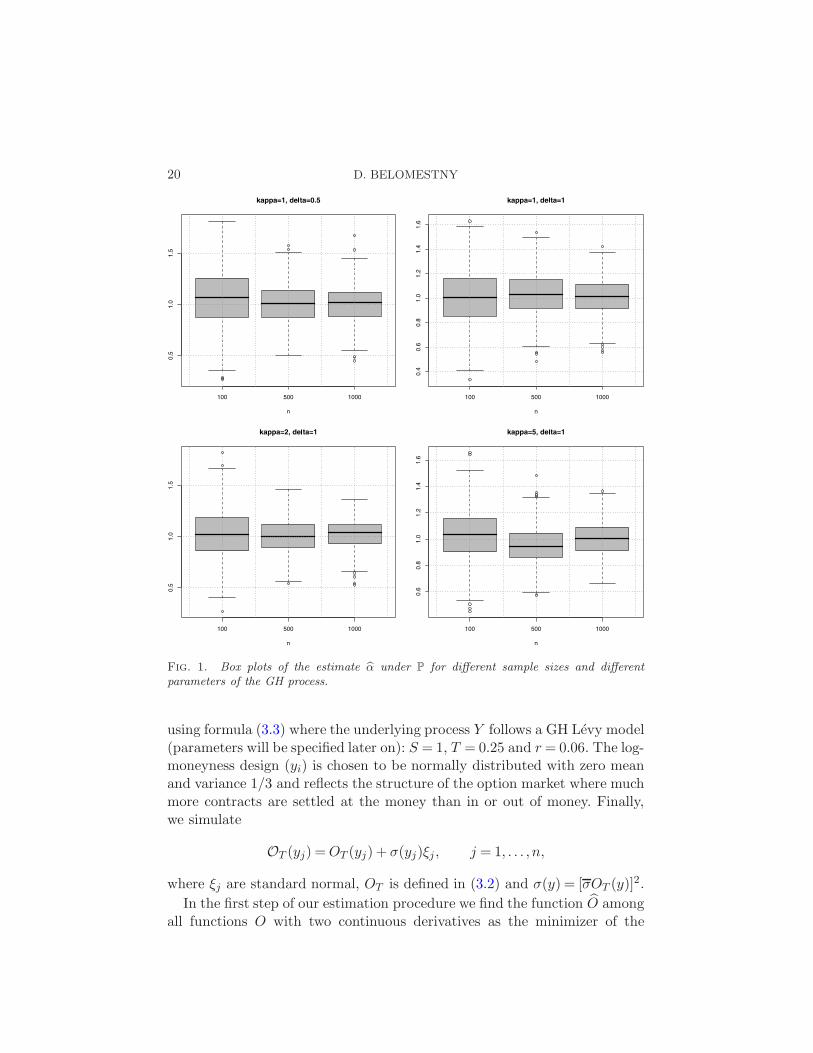
and A2 are two positive constants such that w1(u) satisfies conditions (6.5).Let U1 > U2 > · · · > UK be an exponentially decreasing sequence of cut-offs and α1, . . . , αK be the corresponding sequence of estimates. Following(7.1), we construct a sequence of aggregated estimates α1, . . . , αK using atriangle kernel and a set of critical values V1, . . . ,VK computed by (7.4). Thevariances {σ2k} in (7.3) are estimated from above using a bound for ζ1. Boxplots of α= αK based on 500 trials for different n and different pairs of κand δ are shown in Figure 1.

8.2. Estimation of the fractional order from options data. In the caseof calibration (estimation under Q) we compute first the prices of n calloptions,

C(yk, T ) = SEQ[(eYT − eyk)+], k = 1, . . . , n,

20 D. BELOMESTNY

Fig. 1. Box plots of the estimate α under P for different sample sizes and differentparameters of the GH process.

using formula (3.3) where the underlying process Y follows a GH Levy model(parameters will be specified later on): S = 1, T = 0.25 and r= 0.06. The log-moneyness design (yi) is chosen to be normally distributed with zero meanand variance 1/3 and reflects the structure of the option market where muchmore contracts are settled at the money than in or out of money. Finally,we simulate

OT (yj) =OT (yj) + σ(yj)ξj , j = 1, . . . , n,

where ξj are standard normal, OT is defined in (3.2) and σ(y) = [σOT (y)]2.

In the first step of our estimation procedure we find the function O amongall functions O with two continuous derivatives as the minimizer of the


penalized residual sum of squares

RSS(O,L) =

n+1∑

i=0

(OT (yi)−O(yi))2 +L

∫ yn+1

y0

[O′′(u)]2 du,(8.2)

where y0 ≪ y1 and yn+1 ≫ yn are two extrapolated points with artificial val-ues On+1 = O0 = 0. The first term in (8.2) measures closeness to the data,

while the second term penalizes curvature in the function, and L establishesa trade-off between the two. The two special cases are L= 0 when O interpo-lates the data, and L=∞ when a straight line using ordinary least squares

is fitted. In our numerical example we use the R package p-splines withthe choice of L that minimizes the generalized cross-validation criterion. Itcan be shown that (8.2) has an explicit, finite dimensional, unique minimizerwhich is a natural cubic spline with knots at the values of yi, i = 1, . . . , n.

Since the solution of (8.2) is a natural cubic spline, we can write

O(y) =

n∑

j=1

θjβj(y),

where βj(y), j = 1, . . . , n, is a set of basis functions representing the family

of natural cubic splines. We estimate F[O](v + i) by

F[O](v+ i) =

n∑

j=1

θjF[e−yβj(y)](v).

Although F[e−yβj(y)] can be computed in closed form, we just use the fast

Fourier transform (FFT) and compute F[O](v+ i) on a fine dyadic grid. Onthe same grid one can compute

ψ(v) :=1

Tlog(1 + v(v + i)F[O](v + i)), v ∈R,(8.3)

where log(·) is taken in such a way that ψ(v) is continuous with ψ(−i) =

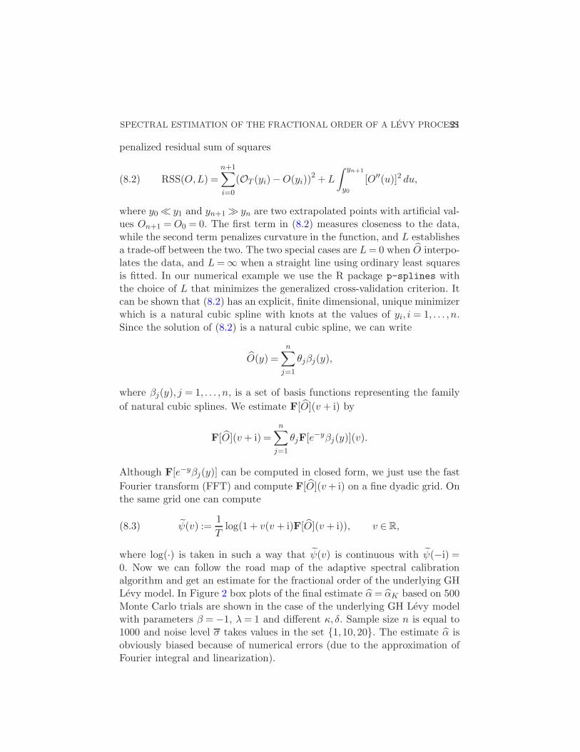
0. Now we can follow the road map of the adaptive spectral calibrationalgorithm and get an estimate for the fractional order of the underlying GHLevy model. In Figure 2 box plots of the final estimate α= αK based on 500

Monte Carlo trials are shown in the case of the underlying GH Levy modelwith parameters β =−1, λ= 1 and different κ, δ. Sample size n is equal to1000 and noise level σ takes values in the set {1,10,20}. The estimate α is

obviously biased because of numerical errors (due to the approximation ofFourier integral and linearization).

22 D. BELOMESTNY

8.3. Processes with a nonzero diffusion part. Turn now to the class ofLevy processes containing a nonzero diffusion part which was treated inSection 6.9. The only algorithmic difference to the case of processes withzero diffusion part is that now we first fix some ξ > 1 and compute

Yξ(u) := log(− log(Tω−,ω+[|ρξ|2](u)))

instead of Y(u) where ρξ(u) = |φ(u)|2ξ2/|φ(ξu)|2 with φ being an estimateof φa. In the estimation procedure we consider only the set of u with|φ(ξu)|> 0. Note that this set is smaller than the set where |φ(u)|> 0 sinceξ > 1. It is also intuitively clear that more observations are needed to esti-mate ρξ with the same quality as |φ(u)|2, and therefore the first problem islikely to be computationally more difficult. This conjecture is supported by

Fig. 2. Box plots of the estimate α under Q for different noise levels and different setsof parameters of the underlying GH Levy process.


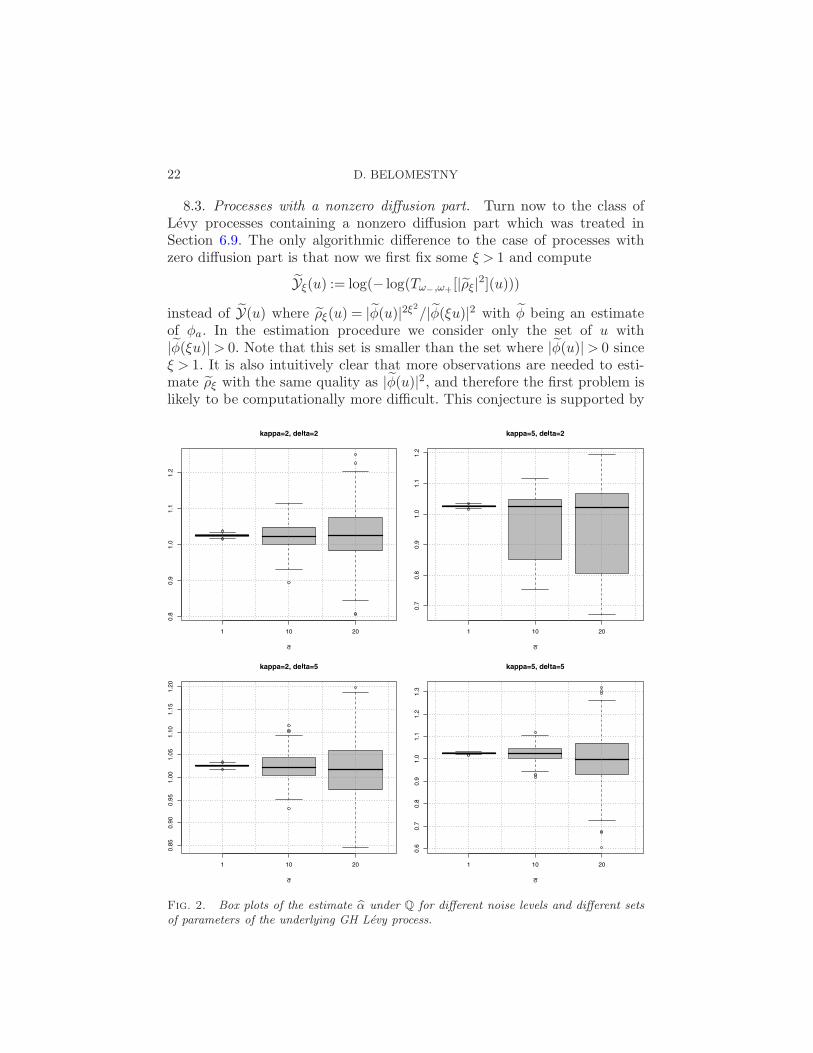
our simulation study as well. Figure 3 shows the boxplots of two estimatesα and αξ based on 500 samples under historical measure P from the GHLevy model with zero diffusion part (left) and with the diffusion parametera equal to 0.1 (right), remaining parameters λ, β, κ and δ being equal to1, 0, 1 and 4, respectively. The estimate αξ is constructed from the esti-mates αU1,ξ, . . . , αUK ,ξ [we use ξ = 2 and w1(u) = u1{ǫ<u≤1} in (8.1)] via thestagewise aggregation procedure as described in Section 7. We took K = 30,Uk = 100(1.25)−(k−1) , k = 1, . . . ,K and K(x) = (1 − x)1{0≤x≤1}. As to thecritical values, they are determined via (7.4) with r = 1, γ = 0.5. Note thatwhile the difference between αξ and α is rather pronounced for small samplesizes, it almost disappears for sample sizes as large as 1000.

APPENDIX

A.1. Proof of Lemma 6.1. For any positive ω− and ω+ satisfying ω−(u)≤|φ(u)|2 ≤ ω+(u), we have

|Y(u)−Y(u)− ζ1(u)(Tω−,ω+[|φ|2](u)− |φ(u)|2)|

≤ ζ2(u)

2(Tω−,ω+[|φ|2](u)− |φ(u)|2)2

≤ ζ2(u)

2(|φ(u)|2 − |φ(u)|2)2.

Furthermore,

||φ(u)|2 − Tω−,ω+[|φ|2](u)| ≤ ||φ(u)|2 − |φ(u)|2|, u ∈Rd,

Fig. 3. Box plots of the estimates α (left) and αξ (right) under P for different samplesizes n.

24 D. BELOMESTNY

and it holds on the set |φ(u)|2 /∈ [ω−, ω+]

||φ(u)|2 − |φ(u)|2| ≥min{|φ(u)|2 − ω−, ω+ − |φ(u)|2}.

Thus,

ζ1(u)||φ(u)|2 − Tω−,ω+[|φ|2](u)| ≤ζ2(u)

2||φ(u)|2 − |φ(u)|2|2

on the set |φ(u)|2 /∈ [ω−, ω+], provided that

2|φ(u)|2|log(|φ(u)|)|min{|φ(u)|2 − ω−, ω+ − |φ(u)|2} ≥ |φ(u)|4 log2(|φ(u)|2)1 + |log(|φ(u)|2)| ,

that is,

min

{1− ω−

|φ(u)|2 ,ω+

|φ(u)|2 − 1

}≥ log(|φ(u)|2)

1 + |log(|φ(u)|2)| .

A.2. Proof of Proposition 6.3. Without loss of generality we can assumethat µ= 0 in (6.8). Denote

ρ(x) =

(1− sinx

x

)ν(x);

then ρ is, up to a scaling factor, the density of some probability distributionwith the characteristic function ζρψ(u) where ζρ is a positive constant and

ψ(u) =

∫ 1

−1(ψ(u)−ψ(u+w))dw.

Due to (6.11) the following asymptotic expansion holds:

ψ(u) = |u|ατ(u)∫ 1

−1

[1−

∣∣∣∣1 +w

u

∣∣∣∣α τ(u+w)

τ(u)

]dw

= C±(α,κ)|u|α−2[1 +O(|u|−κ)], u→±∞,

with some constants C+ and C− depending on α and κ. We consider sepa-rately two cases.

Case 0< α < 1. Note that in this case ψ(u) is integrable on R and theFourier inversion formula implies

ρ(x) =ζρ2π

∫ ∞

−∞(exp(−ixu)− 1)ψ(u)du


since ρ(0) = 0. We have for any positive number a,∫ ∞

−∞(exp(−ixu)− 1)ψ(u)du

=

∫

|u|≤a(exp(−ixu)− 1)ψ(u)du+

∫

|u|>a(exp(−ixu)− 1)ψ(u)du

=: I1 + I2,

where |I1|. |x|. |x|1−α+κ for x→ 0 provided that κ≤ α. Furthermore,

I2 = C±(α,κ)

∫

|u|>a(exp(−ixu)− 1)|u|α−2 du+O(|x|1−α+κ)

= C±(α,κ)|x|1−α[1 +O(|x|κ)], x→±0,

and (6.12) holds.

Case 1 ≤ α < 2. In this case we use the Fourier inversion formula fordistribution functions to get

∫

|x|<ερ(x)dx=

2ζρπ

∫ ∞

0

sin(εu)

uRe[ψ(u)]du.

The representation∫ ∞

0

sin(εu)

uRe[ψ(u)]du

=

∫ a

0

sin(εu)

uRe[ψ(u)]du+

∫ ∞

a

sin(εu)

uRe[ψ(u)]du

=: I1 + I2

and the asymptotic relation

I2 =C+(α,κ)

∫ ∞

a

sin(uε)

uuα−2 du+O(ε2−α+κ)

=C+(α,κ)ε2−α[1 +O(εκ)], ε→+0,

lead now to (6.12) provided that κ≤ α− 1.

A.3. Proof of Theorem 6.4. The representation

αU − α=

∫ ∞

0wU (u)(Y(u)−Y(u))du+RU

26 D. BELOMESTNY

and Lemma 6.1 imply that

E|αU − α|2 ≤ 3E

[∫ ∞

0wU (u)ζ1(u)∆(u)du

]2

(A.1)

+ 3E

[∫ ∞

0wU (u)ζ2(u)∆

2(u)du

]2+ 3|RU |2.

Let us consider the first term in (A.1);

E

[∫ ∞


]2

=

[∫ ∞

0wU (u)ζ1(u)E[∆(u)]du

]2+Var

[∫ ∞


].

Since

ζ1(u) = 2−1|φ(u)|−2 log−1(|φ(u)|) = e2η|u|α Re τ(u)/(2η|u|αRe τ(u)),

we have∫ ∞

0wU (u)ζ1(u)E[∆(u)]du

=

∫ 1

0w1(u)ζ1(Uu)E[∆(Uu)]du(A.2)

=U−α

∫ 1

0

w1(u)e2ηUαuαRe τ(Uu)

2ηuαRe τ(Uu)E[∆(Uu)]du.

Due to the localization principle (Laplace method) and the identity

E[∆(u)] = E|φ(u)|2 − |φ(u)|2 = ε(1− |φ(u)|2),

the integral in (A.2) is asymptotically (as U →∞) less than or equal to

AεU−α

∫ 1

1−δw1(u)u−αe2ηU

αuα

du. εU−αe2ηUα

with arbitrary small δ > 0 and some constant A> 0. Similarly,

Var

[∫ ∞


]

=

∫ ∞

0

∫ ∞

0wU (u)wU (v)ζ1(u)ζ1(v)Cov(∆(u),∆(v))dudv

. εU−2αe2ηUα

+ ε2U−4αe4ηUα

, U →∞,


where again localization principle and the identity,

Cov(|φ(u)|2, |φ(v)|2)= 2ε3(ε−1 − 1)(ε−1 − 2)

× [Re(φ(u)φ(v)φ(−u− v))

+Re(φ(−u)φ(v)φ(u− v))− 2|φ(u)|2|φ(v)|2]+ ε3(ε−1 − 1)[|φ(u+ v)|2 + |φ(−u+ v)|2 − 2|φ(u)|2|φ(v)|2],

are used. Turn now to the second term in (A.1);

E

[∫ ∞

0wU (u)ζ2(u)∆

2(u)du

]2

=

[∫ ∞

0wU (u)ζ2(u)E[∆

2(u)]du

]2+Var

[∫ ∞

0wU (u)ζ2(u)∆

2(u)du

].

Since

ζ2(u).|log |φ(u)|||φ(u)|4 , u→∞,

and

E||φ(u)|2 − |φ(u)|2|2 = E||φ(u)|2 −E|φ(u)|2 +E|φ(u)|2 − |φ(u)|2|2

≤ 2E||φ(u)|2 −E|φ(u)|2|2 + 2|E|φ(u)|2 − |φ(u)|2|2

. ε|φ(u)|2 + ε2, u→∞,

we get an asymptotic estimate;∫ ∞

0wU (u)ζ2(u)E[∆

2(u)]du. εUαe2ηUα

+ ε2Uαe4ηUα

, U →∞.

Similarly, one can prove that

Var

[∫ ∞

0wU (u)ζ2(u)∆

2(u)du

]. ε2U2αe4ηU

α

, U →∞.

Finally, the third term in (A.1),

RU =

∫ ∞

0wU (u) log(Re τ(u))du,

can be can be bounded by

|RU |=∣∣∣∣∫ 1

0w1(u) log(Re τ(uU))du

∣∣∣∣

≤ U−1

∫ A

0|w1(y/U)||log(Re τ(y))|dy

28 D. BELOMESTNY

+U−κ

∫ 1

0|y|−κ |w1(y)|dy . U−κ, U →∞,

for A> 0 large enough. Combining all the previous estimates we get

E|αU − α|2 . εU−2αe2ηUα

+ ε2U2αe4ηUα

+U−2κ

(A.3). εU−2αe2η+Uα

+ ε2U2αe4η+Uα

+U−2κ, U →∞.

Finally the choice

U =

[1


]1/α

with β = 1+ κ/α leads to (6.13).In the case of the calibration problem we have

|φ(u)|2 = 1− 2Re

[u(u+ i)

n∑

j=1

δjO(yj)eiuyj

]

+ u2(1 + u2)

n∑

j,l=1

eiu(yl−yj)δjδlO(yj)O(yl)

and

E|φ(u)|2 = 1− 2Re

[u(u+ i)

n∑

j=1

δjO(yj)eiuyj

]

+ u2(1 + u2)n∑

j 6=l


+ u2(1 + u2)

n∑

j=1

δ2j σ2j .

As was mentioned in Section 3.2, function O(y) = e−yO(y) is nonnegative,Lipschitz and satisfies the Cramer condition,

∫

R

O(y)e−y dy <∞,

provided that E[e2YT ]<∞. Under the condition e−A ≤ ‖δ‖2 we get∣∣∣∣∣

∫

R

eiuyO(y)dy −n∑

j=1

eiuyjδjO(yj)

∣∣∣∣∣. ‖δ‖2, ‖δ‖2 → 0,


as well as∣∣∣∣∣

∣∣∣∣∫

R

eiuyO(y)dy

∣∣∣∣2

−n∑

j,l=1


∣∣∣∣∣. ‖δ‖2, ‖δ‖2 → 0.

Thus,

|E|φ(u)|2 − |φ(u)|2|. u2(1 + u2)n∑

j=1

δ2j (1 + σ2j ).

Further,

|φ(u)|2 −E|φ(u)|2 =−2Re

[u(u+ i)

n∑

j=1

δjσjξjeiuyj

]

+ 2u2(1 + u2)∑

j<l

eiu(yl−yj)δjδlσj σlξjξl

+ u2(1 + u2)

n∑

j=1

δ2j σ2j (ξ

2j − 1)

and

E(|φ(u)|2 −E|φ(u)|2)2 . u2(1 + u2)

n∑

j=1

δ2j σ2j + u4(1 + u2)2

n∑

j=1

δ4j σ4j .

Using these inequalities, the first term in (A.1) can be estimated from aboveas

E

[∫ ∞


]2. U8−2αe4ηU

α‖δ‖4 +U4−2αe4ηUα

[n∑

j=1

δ2j σ2j

]2

. ε2U8−2αe4η+Uα

,

while the second one is asymptotically negligible if ε2U8−2αe4ηUα → 0. Tak-

ing

U =

[1


]1/α

with β = (κ + 4)/α− 1, we get (6.13).

A.4. Proof of Theorem 6.5. For any two probability measures P and Qdefine

χ2(P,Q) =:

∫ (dP

dQ− 1

)2

dQ, if P ≪Q,

+∞, otherwise.

30 D. BELOMESTNY

The following proposition is the main tool for the proof of lower bounds inthe estimation case and can be found in Butucea and Tsybakov (2004).

Proposition A.1. Let PΘ := {Pθ : θ ∈ Θ} be a family of models. As-sume that there exist θ1 and θ2 in Θ with |θ1 − θ2|> 2δn > 0 such that

Pθ1 ≪ Pθ2 , χ2(P⊗nθ1, P⊗n

θ2)≤ κ2 < 1,

then

lim infn→∞

infθn

δ−2n max{Eθ1 |θn − θ1|2,Eθ2 |θn − θ2|2} ≥ (1− κ)2(1−√

κ)2,

where the infimum is taken over all estimators θn (measurable function ofobservations) of the underlying parameter.

Taking Θ=A(α,η−, η+,κ) and θi = (αi, ηi, τi), i= 1,2, we get from Propo-sition A.1,


E(|αε −α|2)≥ δ−2n max{E1(|αε − α1|2),E2(|αε −α2|2)},

provided that |α1 −α2|> 2δn > 0, and

χ2(P⊗nθ1, P⊗n

θ2)≤ κ2 < 1.

Turn now to the construction of models θ1 and θ2. Let us consider a sym-metric stable model,

ψ(u) = iµu+ ϑ(u), ϑ(u) =−η+|u|α, 0< α≤ 1, u ∈R.

For any δ satisfying 0< δ < α and M > 0, define

ψδ(u) = iµu+ ϑδ(u),

where

ϑδ(u) =−η+|u|α1{|u|≤M} −η+M

δ

(1 + cM−κ)|u|α−δ(1 + c|u|−κ)1{|u|>M}.

Then φδ(u) = exp(iµu + ϑδ(u)) is a characteristic function of some Levyprocess and

φδ(u) = φ(u), |u| ≤M,

where φ(u) = exp(iµu+ ϑδ(u)). Indeed, the function ϑδ(u) is a continuous,nonpositive, symmetric function which is convex on R+ for large enoughM and small enough c > 0. According to a well-known Polya criteria [see,e.g., Ushakov (1999)], the function exp(ξϑδ(u)) is a cf. of some absolutelycontinuous distribution for any ξ > 0. In particular, for any natural n the


function exp(ϑδ(u)/n) is a cf. of some absolutely continuous distribution.Hence, exp(ϑδ(u)) is a cf. of some infinitely divisible distribution. Define

θ1 = (α,η+,1), θ2 = (α− δ, η+, τδ,M)(A.4)

and φθ1(u) = φ(u), φθ2(u) = φδ(u) with

τδ,M(u) := |u|δ1{|u|≤M} +M δ

(1 + cM−κ)(1 + c|u|−κ)1{|u|>M}.

If M δ = 1+ cM−κ , that is,

δ = log(1 + cM−κ)/ logM ≍ cM−κ/ logM, M →∞,(A.5)

then

|τδ,M(u)− 1|. |u|−κ, |u| →∞,

and hence θ2 ∈Θ=A(α,η−, η+,κ). Furthermore, it holds

χ2(P⊗nθ1, P⊗n

θ2) = nχ2(pθ1 , pθ2) = n

∫

R

|pθ1(y)− pθ2(y)|2pθ1(y)

dy,

where pθ1 and pθ2 are densities corresponding to cf. φθ1 and φθ2 , respectively.Using the fact that the density of stable law pθ1(y) does not vanish on anycompact set in R and fulfills

pθ1(y)& |y|−(α+1), |y| →∞,

we derive

nχ2(pθ1 , pθ2)≤ nC1

∫

|y|≤A|pθ1(y)− pθ2(y)|2 dy

+ nC2

∫

|y|>A|y|α+1|pθ1(y)− pθ2(y)|2 dy

= nC1I1 + nC2I2

for large enough A> 0 and some constants C1,C2 > 0. Using the fact thatfunction φθ1(u)− φθ2(u) is two times differentiable (it is zero for |u| <M )and Parseval’s identity, we get

I1 ≤1

2π

∫

R

|φθ1(u)− φθ2(u)|2 du

≤ 1

2π

∫

|u|>Me−2η|u|α−δ

du.M1−α+δe−2ηMα−δ

,

I2 ≤1

2π

∫

|u|>M|(φθ1(u)− φθ2(u))

′′|2 du

.

∫

|u|>M|u|6e−2η|u|α−δ

du.M7−α+δe−2ηMα−δ

.

32 D. BELOMESTNY

The choice M ≍ [ 12η+

log(ε−1 log−β(1/ε))]1/(α−δ) with ε= 1/n and some β ≥(7− (α− δ))/2(α− δ) yields

ε−1χ2(pθ1 , pθ2)< 1

for small enough ε. Combining this and (A.5), we arrive at (6.14).For the proof of lower bounds in the case of calibration, one can employ

the fact that the regression model,

OT (yi) = OT (yi) + σ(yi)ξi, δi = yi − yi−1,

E[ξ2i ] = 1, i= 1, . . . , n,

is equivalent to the Gaussian white noise model,

dZ(x) = O(y)dy + ε1/2 dW (y)

with the noise level asymptotics ε→ 0, a two-sided Brownian motion W .Here the noise level ε corresponds to the statistical regression error

∑nj=1 δ

2j σ

2j .

Furthermore, instead of χ2 distance we use the Kullback–Leibler divergence,

KL(Tθ1 ,Tθ2) =1

2

∫

R

|(Oθ1 − Oθ2)(y)|2ε−1 dy,

between two models Tθ1 and Tθ2 corresponding to two Levy processes withcharacteristics θ1 and θ2, respectively [see (A.4)]. Simple calculations leadto the estimate,

KL(Tθ1 ,Tθ2). ε−1Mγe−2η+Mα−δ

with some γ > 0. Hence, for small enough ε > 0 it holds

KL(Tθ1 ,Tθ2)< 1

provided thatM ≍ [ 12η+

log(ε−1 log−β(1/ε))]1/(α−δ) with β ≥ γ/2(α−δ). TheAssouad lemma [see, e.g., Tsybakov (2008)] together with (A.5) implies(6.14).

A.5. Proof of Proposition 6.6. It holds for any fixed U ,

αU −α=

∫ ∞

0wU (u)(Y(u)−Y(u))du

=

∫ ∞


+

∫ ∞

0wU (u)Q(u)du+RU ,

where Q is defined in (6.3). As shown in Lemma A.2, the process ε−1/2∆(u)converges weakly to a Gaussian process Z(u) with E[Z(u)] = 0 and Cov(Z(u),


Z(v)) = S(u, v). Moreover, ε−1/2Q(u)→ 0, almost surely. The representationfor δ(u) in Lemma A.2 and CLT for U -statistics implies that if for some se-quence U(ε), it holds ς−1(ε)RU(ε) → 0 with

ς2(ε) = ε

∫ ∞

0wU(ε)(u)wU(ε)(v)ζ1(u)ζ1(v)S(u, v)dudv,

then ς−1(ε)(αU(ε) −α)→N (0,1).

A.6. Proof of Theorem 6.7. We give only the sketch of the proof. Let ω−

and ω+ be two truncation levels satisfying 0 < ω−(u) < ρξ(u) < ω+(u) < 1and 0 < ω− < ρξ(u)(1 − log(ρξ(u))/(1 + log(ρξ(u)))). First, similar to theproof of Proposition 6.1, one can show that

|Yξ(u)−Y(u)−ζ1,ξ(u)(T0,ω+[ρξ](u)−ρξ(u))| ≤ ζ2,ξ(u)(T0,ω+[ρξ](u)−ρξ(u))2,where

ζ1,ξ(u) =−ρ−1ξ (u) log−1(ρξ(u))

and

ζ2(u) = maxθ∈{ω−(u),ω+(u)}

[1 + |log(θ)|θ2 log2(θ)

].

Furthermore, we have on the set {ρξ(u)≤ ω+(u)}|ρξ(u)− T0,ω+ [ρξ](u)|

≤ ω+(u)||φa(ξu)|2 − |φ(ξu)|2|

|φa(ξu)|2+

||φa(u)|2ξ2 − |φ(u)|2ξ2 ||φa(ξu)|2

,

and on the set {ρξ(u)>ω+(u)} it holds

|ρξ(u)− T0,ω+ [ρξ](u)| ≤ 2ω+(u).

Hence

E|ρξ(u)− T0,ω+ [ρξ](u)|2

≤ 2|φa(ξu)|−4[E||φa(ξu)|2 − |φ(ξu)|2|2

+E||φa(u)|2ξ2 − |φ(u)|2ξ2 |2] + 4ω2

+(u)P(ρξ(u)>ω+(u)).

Without loss of generality one can assume that there exists U0 > 0 such thatρξ(u)/ω+(u)< 1/2 for u >U0. Then it holds for u > U0

P(ρξ(u)> ω+(u))

≤ P(||φa(u)|2ξ2 − |φ(u)|2ξ2 |> ω+(u)|φ(uξ)|2/4)

+P(||φa(uξ)|2 − |φ(uξ)|2|> ω+(u)|φ(uξ)|2/4)≤ 16|φa(ξu)|−4[E||φa(ξu)|2 − |φ(ξu)|2|2 +E||φa(u)|2ξ

2 − |φ(u)|2ξ2 |2].

34 D. BELOMESTNY

In the case of the estimation under P, for instance, we have

E||φa(ξu)|2 − |φ(ξu)|2|2 . ε, E||φa(u)|2ξ2 − |φ(u)|2ξ2 |2 . ε, ε→ 0,

and hence

E|ρξ(u)− T0,ω+ [ρξ](u)|2 . ε|φa(ξu)|−4, ε→ 0.

Now one can follow the proof of Theorem 6.4 and use the fact that

ζ1,ξ(u)≍ c−1ξ (α)|u|−ατ−1

ξ (u) exp(cξ(α)|u|ατξ(u)), u→∞.

A.7. Proof of Theorem 6.8. Instead of Levy models θ1 and θ2, one con-siders models θ1,a and θ2,a with characteristic exponents ψa(u) = iµu −a2u2/2 + ϑ(u) and ψa,δ(u) = iµu − a2u2/2 + ϑδ(u), respectively. The restof the proof is almost identical to the proof of Theorem 6.5.

A.8. Auxiliary results. The following lemma is a basic tool to investigatethe asymptotic behavior of the estimate α under the historical measure P.

Lemma A.2. The process ε−1/2∆(u) with ∆(u) = |φ(u)|2−|φ(u)|2 weaklyconverges to a Gaussian process Z(u) with E[Z(u)] = 0 and Cov(Z(u),Z(v)) =S(u, v) where



Proof. We have

|φ(u)|2 = [Re φ(u)]2 + [Im φ(u)]2 =1

n2

n∑

j=1

n∑

k=1

cos(u(Xj −Xk)).

Put

Hn(u) =

(n2

)−1∑

c

cos(u(Xj −Xk)) =2

n(n− 1)

∑

c

cos(u(Xj −Xk)),

where summation c is over all(n2

)combinations of 2 integers chosen from

(1, . . . , n). Then

ε−1/2(|φ(u)|2 − |φ(u)|2) = ε1/2 + ε−1/2(1− ε)(Hn − |φ(u)|2)− ε1/2|φ(u)|2.The first and third terms on the right-hand side converge to 0. Consider themiddle term. Since Hn(u) is an U -statistic (for each u), ε−1/2(Hn− |φ(u)|2)weakly converges to a Gaussian process with zero mean and covariance

Cov[EX2 cos(u(X1 −X2)),EX2 cos(v(X1 −X2))]


(where EXY denotes the conditional expectation of Y given X). Let uscompute this covariance. For any u, v ∈R it holds

Cov(EX2 [cos(u(X1 −X2))],EX2 [cos(v(X1 −X2))])

= E[(cos(uX2)−Reφ(u))Reφ(u) + (sin(uX2)− Imφ(u)) Imφ(u)]

×[(cos(vX2)−Reφ(v))Reφ(v) + (sin(vX2)− Imφ(v)) Imφ(v)],

where

E(cos(uX2)−Reφ(u))(cos(vX2)−Reφ(v))

=Reφ(u+ v) + Reφ(u− v)

2−Reφ(u)Reφ(v),

E(sin(uX2)− Imφ(u))(sin(vX2)− Imφ(v))

=Reφ(u− v)−Reφ(u+ v)

2− Imφ(u) Imφ(v)

and

E(cos(uX2)−Reφ(u))(sin(vX2)− Imφ(v))

=Imφ(v− u) + Imφ(u+ v)

2−Reφ(u) Imφ(v). �

REFERENCES

Aıt-Sahalia, Y. and Jacod, J. (2009). Estimating the degree of activity of jumps inhigh frequency financial data. Ann. Statist. 37 2202–2244.

Aıt-Sahalia, Y. and Jacod, J. (2006). Volatility estimators for discretely sampled Levyprocesses. Ann. Statist. 35 355–392. MR2332279

Belomestny, D. and Reiss, M. (2006). Spectral calibration of exponential Levy models.Finance Stoch. 10 449–474. MR2276314

Belomestny, D. and Spokoiny, V. (2007). Local-likelihood modeling via stage-wiseaggregation. Ann. Statist. 35 2287–2311. MR2363972

Boyarchenko, S. and Levendorskiı, S. (2002). Barrier options and touch-and-out op-tions under regular Levy processes of exponential type. Ann. Appl. Probab. 12 1261–1298. MR1936593

Akgiray, V. and Lamoureux, C. G. (1989). Estimation of stable-law parameters: Acomparative study. J. Bus. Econom. Statist. 7 85–93.

Butucea, C. and Tsybakov, A. (2004). Sharp optimality for density deconvolution withdominating bias. Theory Probab. Appl. 52 237–249. MR2354572

Cont, R. and Tankov, P. (2004). Nonparametric calibration of jump-diffusion optionpricing models. Journal of Computational Finance 7 1–49.

Cont, R. and Tankov, P. (2006). Retrieving Levy processes from option prices: Regular-ization of an ill-posed inverse problem. SIAM J. Control Optim. 45 1–25. MR2225295

Cont, R. and Tankov, P. (2004). Financial Modelling with Jump Processes 535. Chap-man & Hall/CRC, Boca Raton. MR2042661

DuMouchel, W. H. (1973a). On the asymptotic normality of the maximum-likelihood es-timator when sampling from a stable distribution. Ann. Statist. 1 948–957. MR0339376

http://www.ams.org/mathscinet-getitem?mr=2332279








36 D. BELOMESTNY

DuMouchel, W. H. (1973b). Stable distributions in statistical inference. I. Symmetric

stable distributions compared to other symmetric long-tailed distributions. J. Amer.

Statist. Assoc. 68 948–957. MR0378190

DuMouchel, W. H. (1975). Stable distributions in statistical inference. II. Information

from stably distributed samples. J. Amer. Statist. Assoc. 70 386–393. MR0378191

Eberlein, E. (2001). Application of generalized hyperbolic Levy motions to finance. In:

Levy Processes—Theory and Applications (O. E. Barndorff-Nielsen, T. Mikosch and S.

I. Resnick, eds.) 319–336. Birkhauser Boston, Boston, MA. MR1833703

Eberlein, E. and Keller, U. (1995). Hyperbolic distributions in finance. Bernoulli 1

281–299.

Eberlein, E., Keller, U. and Prause, K. (1998). New insights into smile, mispricing

and value at risk: The hyperbolic model. J. Bus. 71 371–406.

Eberlein, E. and Prause, K. (1998). The generalized hyperbolic model: Financial deriva-

tives and risk measures. In Mathematical Finance-Bachelier Congress 2000 (H. Geman,

D. Madan, S. Pliska and T. Vorst, eds.) 245–267. Springer, Berlin. MR1960567

Fenech, A. P. (1976). Asymptotically efficient estimation oflocation for a symmetric

stable law. Ann. Statist. 4 1088–1100. MR0426260

Feuerverger, A. and McDunnough, P. (1981a). On the efficiency of empirical charac-

teristic function procedures. J. Roy. Statist. Soc. Ser. B 43 20–27. MR0610372

Feuerverger, A. and McDunnough, P. (1981b). On efficient inference in symmetric

stable laws and processes. In Proceedings of the International Symposium on Statistics

and Related Topics (M. Csorgo, D. A. Dawson, J. N. K. Rao and A. K. M. E. Saleh,

eds.) 109–121. North-Holland, Amsterdam. MR0665270

Figueroa-Lopez, E. and Houdre, C. (2006). Risk bounds for the nonparametric estima-

tion of Levy processes. In High Dimensional Probability IV (E. Gine, V. Kolchinskii, W.

Li and J. Zinn, eds.). Institute of Mathematical Statistics Lecture Notes—Monograph

Series 51 96–116. IMS, Beachwood, OH.

Gugushvili, S. (2008). Nonparametric estimation of the characteristic triplet of a dis-

cretely observed Levy process. J. Nonparametr. Stat. 21 321–343. MR2530929

Koutrouvelis, I. A. (1980). Regression-type estimation of the parameters of stable laws.

J. Amer. Statist. Assoc. 75 918–928. MR0600977

Lee, S. and Mykland, P. A. (2008). Jumps in financial markets: A new nonparametric

test and jump dynamics. Review of Financial Studies. 21 2535–2563.

Neumann, M. and Reiss, M. (2009) Nonparametric estimation for Levy processes from

low-frequency observations. Bernoulli 15 223–248.

Nolan, J. P. (1997). Numerical computation of stable densities and distribution func-

tions. Comm. Statist. Stochastic Models 13 759–774. MR1482292

Press, S. J. (1972). Estimation in univariate and multivariate stable distributions. J.

Amer. Statist. Assoc. 67 842–846. MR0362666

Singleton, K. (2001). Estimation of affine asset pricing models using the empirical char-

acteristic function. J. Econometrics 102 111–141. MR1838137

Sato, K. (1999). Levy processes and infinitely divisible distributions. Cambridge Univ.

Press, Cambridge. MR1739520

Tsybakov, A. (2008). Introduction to Nonparametric Estimation. Springer, Berlin.

MR2013911

Ushakov, N. (1999). Selected topics in characteristic functions. VSP, Utrecht. MR1745554

Van der Vaart, A. and Wellner, J. (1996). Weak Convergences and Empirical Pro-

cesses. Springer, New York. MR1385671


















Weierstrass-Institute

Mohrenstr. 39

10117 Berlin

Germany

E-mail: [email protected]

mailto:[email protected]

Spectral estimation of the fractional order of a Lévy process

Documents