Spectral asymmetry of the massless Dirac operator on a 3-torus Article Accepted Version Downes, R. J., Levitin, M. and Vassiliev, D. (2013) Spectral asymmetry of the massless Dirac operator on a 3-torus. Journal of Mathematical Physics, 54 (11). 111503. ISSN 0022- 2488 doi: https://doi.org/10.1063/1.4828858 Available at http://centaur.reading.ac.uk/34885/ It is advisable to refer to the publisher’s version if you intend to cite from the work. See Guidance on citing . To link to this article DOI: http://dx.doi.org/10.1063/1.4828858 Publisher: American Institute of Physics All outputs in CentAUR are protected by Intellectual Property Rights law, including copyright law. Copyright and IPR is retained by the creators or other copyright holders. Terms and conditions for use of this material are defined in the End User Agreement . www.reading.ac.uk/centaur CentAUR Central Archive at the University of Reading

Welcome message from author
This document is posted to help you gain knowledge. Please leave a comment to let me know what you think about it! Share it to your friends and learn new things together.
Transcript
Spectral asymmetry of the massless Dirac operator on a 3torus Article
Accepted Version
Downes, R. J., Levitin, M. and Vassiliev, D. (2013) Spectral asymmetry of the massless Dirac operator on a 3torus. Journal of Mathematical Physics, 54 (11). 111503. ISSN 00222488 doi: https://doi.org/10.1063/1.4828858 Available at http://centaur.reading.ac.uk/34885/
It is advisable to refer to the publisher’s version if you intend to cite from the work. See Guidance on citing .
To link to this article DOI: http://dx.doi.org/10.1063/1.4828858
Publisher: American Institute of Physics
All outputs in CentAUR are protected by Intellectual Property Rights law, including copyright law. Copyright and IPR is retained by the creators or other copyright holders. Terms and conditions for use of this material are defined in the End User Agreement .
www.reading.ac.uk/centaur
CentAUR
Central Archive at the University of Reading

Reading’s research outputs online
Spectral asymmetry of the massless Dirac operator on a 3-torus
Robert J. Downes,1, a) Michael Levitin,2, b) and Dmitri Vassiliev1, c)
1)Department of Mathematics, University College London, Gower Street,
London WC1E 6BT, UK
2)Department of Mathematics and Statistics, University of Reading, Whiteknights,
PO Box 220, Reading RG6 6AX, UK
Consider the massless Dirac operator on a 3-torus equipped with Euclidean metric
and standard spin structure. It is known that the eigenvalues can be calculated explic-
itly: the spectrum is symmetric about zero and zero itself is a double eigenvalue. The
aim of the paper is to develop a perturbation theory for the eigenvalue with smallest
modulus with respect to perturbations of the metric. Here the application of per-
turbation techniques is hindered by the fact that eigenvalues of the massless Dirac
operator have even multiplicity, which is a consequence of this operator commuting
with the antilinear operator of charge conjugation (a peculiar feature of dimension 3).
We derive an asymptotic formula for the eigenvalue with smallest modulus for arbi-
trary perturbations of the metric and present two particular families of Riemannian
metrics for which the eigenvalue with smallest modulus can be evaluated explicitly.
We also establish a relation between our asymptotic formula and the eta invariant.
Keywords: Dirac operator, spectral asymmetry, zero modes, harmonic spinors, eta
invariant
a)Electronic mail: [email protected]; http://www.homepages.ucl.ac.uk/˜zcahc37/b)Electronic mail: [email protected]; http://www.personal.reading.ac.uk/˜ny901965/c)Electronic mail: [email protected]; http://www.homepages.ucl.ac.uk/˜ucahdva/
1
I. INTRODUCTION
Let M be a 3-dimensional connected compact oriented manifold without boundary
equipped with a smooth Riemannian metric gαβ, α, β = 1, 2, 3 being the tensor indices. Let
W be the corresponding massless Dirac operator, see Appendix A in Ref.11 for definition.
There are two basic examples when the spectrum of W can be calculated explicitly. The
first is the unit torus T3 equipped with Euclidean metric. The second is the unit sphere S3
equipped with metric induced by the natural embedding of S3 in Euclidean space R4. In
both examples the spectrum turns out to be symmetric about zero, see Appendix B in Ref.11
for details. Physically, this means that in these two examples there is no difference between
the properties of the particle (massless neutrino) and antiparticle (massless antineutrino).
As pointed out in Refs.4–7, for a general oriented Riemannian 3-manifold (M, g) there is
no reason for the spectrum of the massless Dirac operator W to be symmetric. However,
producing explicit examples of spectral asymmetry is a difficult task. To our knowledge,
the only explicit example was constructed in Ref.20, with the example based on the idea of
choosing a 3-manifold with flat metric but highly nontrivial topology. In our paper we take
a different route: we stick with the simplest possible topology (torus) and create spectral
asymmetry by perturbing the metric.
Further on in this paper we work on the unit torus T3 parameterized by cyclic coordinates
xα, α = 1, 2, 3, of period 2π.
Suppose first that the metric is Euclidean. Then the massless Dirac operator correspond-
ing to the standard spin structure (see formula (A.16) in Ref.11) reads
W = −i
∂∂x3
∂∂x1− i ∂
∂x2
∂∂x1
+ i ∂∂x2
− ∂∂x3
. (I.1)
The operator (I.1) admits separation of variables, i.e. one can seek its eigenfunctions in
the form v(x) = ueimαxα , m ∈ Z3, u ∈ C2, u 6= 0, and calculate the eigenvalues and
eigenfunctions explicitly. The spectrum of the operator (I.1) is as follows.
• Zero is an eigenvalue of multiplicity two.
• For each m ∈ Z3 \ {0} we have the eigenvalue ‖m‖ and unique (up to rescaling)
eigenfunction of the form ueimαxα .
2
• For each m ∈ Z3 \ {0} we have the eigenvalue −‖m‖ and unique (up to rescaling)
eigenfunction of the form ueimαxα .
We now perturb the metric, i.e. consider a metric gαβ(x; ε) the components of which
are smooth functions of coordinates xα, α = 1, 2, 3, and small real parameter ε, and which
satisfies
gαβ(x; 0) = δαβ. (I.2)
One way of establishing spectral asymmetry of the perturbed problem is to compare
the asymptotic distribution of large positive eigenvalues and large negative eigenvalues. As
explained in Section 10 of Ref.10, for a generic first order differential operator this approach
allows one to establish spectral asymmetry. Unfortunately, the massless Dirac operator is
very special in that the second asymptotic coefficient of its counting function is zero, see
formula (1.23) in Ref.11, so in the first two approximations in powers of λ its large positive
eigenvalues are distributed the same way as its large negative eigenvalues. Therefore, in
order to demonstrate spectral asymmetry of the perturbed problem, we will, instead of
dealing with large eigenvalues, deal with small eigenvalues.
II. MAIN RESULT
Let W (ε) be the massless Dirac operator corresponding to the metric gαβ(x; ε). The
difficulty with applying standard perturbation techniques to the operator W (ε) is that all
its eigenvalues have even multiplicity, this being a consequence of the fact that the massless
Dirac operator W (ε) commutes with the antilinear operator of charge conjugation
v =
v1v2
7→−v2v1
=: C(v), (II.1)
see Property 3 in Appendix A of Ref.11. In order to overcome this difficulty we develop
in Sections III–V a perturbation theory for the massless Dirac operator which accounts for
this charge conjugation symmetry. We show that perturbation-wise the double eigenvalues
of the massless Dirac operator can be treated as if they were simple eigenvalues: under
perturbation a double eigenvalue remains a double eigenvalue and all the usual formulae
apply, with only one minor modification. The minor modification concerns the definition
of the pseudoinverse of the unperturbed operator, see formulae (III.8)–(III.12). Namely,
3
in the definition of the pseudoinverse we separate out a two-dimensional eigenspace rather
than a one-dimensional eigenspace. Here, of course, it is important that we don’t have a
magnetic field. A magnetic field would split up a double eigenvalue, see Ref.12. The fact
that the massless Dirac operator and the charge conjugation operator do not commute in
the presence of a magnetic covector potential is well known in theoretical physics: see, for
example, formula (2.5) in Ref.19.
Given a function f : T3 → C, we denote by
f(m) :=1
(2π)3
∫T3
e−imαxαf(x) dx , m ∈ Z3, (II.2)
its Fourier coefficients. Here dx := dx1dx2dx3.
Let λ0(ε) be the eigenvalue of the massless Dirac operator with smallest modulus and let
hαβ(x) :=∂gαβ∂ε
∣∣∣∣ε=0
. (II.3)
Further on we raise and lower tensor indices using the Euclidean metric, which means that
raising or lowering a tensor index doesn’t change anything. A repeated tensor index always
indicates summation over the values 1, 2, 3.
The following theorem is the main result of our paper.
Theorem II.1. We have
λ0(ε) = c ε2 +O(ε3) as ε→ 0, (II.4)
where the constant c is given by the formula
c =i
16εαβγ
∑m∈Z3\{0}
(δµν −
mµmν
‖m‖2
)mα hβµ(m) hγν(m) . (II.5)
Here εαβγ is the totally antisymmetric quantity, ε123 := +1, and the overline stands for
complex conjugation.
Theorem II.1 warrants the following remarks.
• If the constant c defined by formula (II.5) is nonzero, then Theorem II.1 tells us that for
sufficiently small nonzero ε the spectrum of our massless Dirac operator is asymmetric
about zero.
4
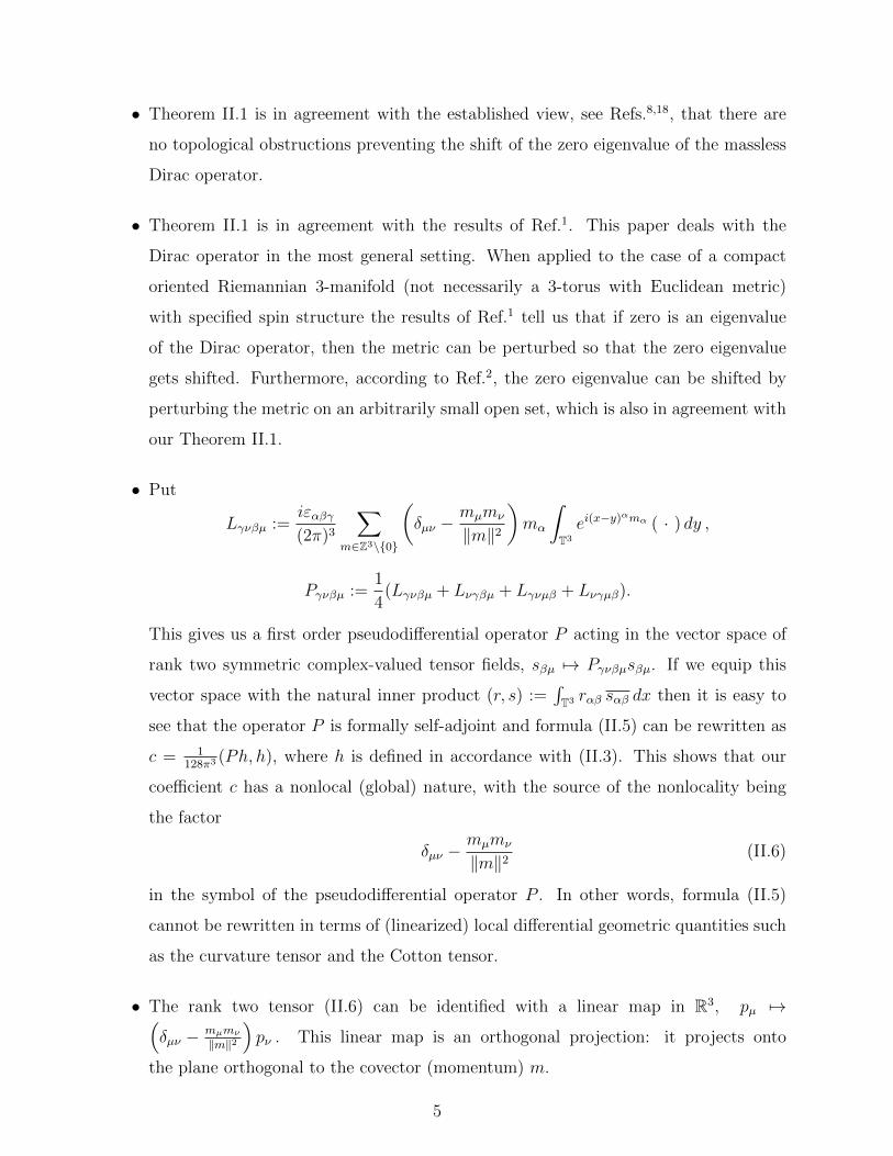
• Theorem II.1 is in agreement with the established view, see Refs.8,18, that there are
no topological obstructions preventing the shift of the zero eigenvalue of the massless
Dirac operator.
• Theorem II.1 is in agreement with the results of Ref.1. This paper deals with the
Dirac operator in the most general setting. When applied to the case of a compact
oriented Riemannian 3-manifold (not necessarily a 3-torus with Euclidean metric)
with specified spin structure the results of Ref.1 tell us that if zero is an eigenvalue
of the Dirac operator, then the metric can be perturbed so that the zero eigenvalue
gets shifted. Furthermore, according to Ref.2, the zero eigenvalue can be shifted by
perturbing the metric on an arbitrarily small open set, which is also in agreement with
our Theorem II.1.
• Put
Lγνβµ :=iεαβγ(2π)3
∑m∈Z3\{0}
(δµν −
mµmν
‖m‖2
)mα
∫T3
ei(x−y)αmα ( · ) dy ,
Pγνβµ :=1
4(Lγνβµ + Lνγβµ + Lγνµβ + Lνγµβ).
This gives us a first order pseudodifferential operator P acting in the vector space of
rank two symmetric complex-valued tensor fields, sβµ 7→ Pγνβµsβµ. If we equip this
vector space with the natural inner product (r, s) :=∫T3 rαβ sαβ dx then it is easy to
see that the operator P is formally self-adjoint and formula (II.5) can be rewritten as
c = 1128π3 (Ph, h), where h is defined in accordance with (II.3). This shows that our
coefficient c has a nonlocal (global) nature, with the source of the nonlocality being
the factor
δµν −mµmν
‖m‖2(II.6)
in the symbol of the pseudodifferential operator P . In other words, formula (II.5)
cannot be rewritten in terms of (linearized) local differential geometric quantities such
as the curvature tensor and the Cotton tensor.
• The rank two tensor (II.6) can be identified with a linear map in R3, pµ 7→(δµν − mµmν
‖m‖2
)pν . This linear map is an orthogonal projection: it projects onto
the plane orthogonal to the covector (momentum) m.
5
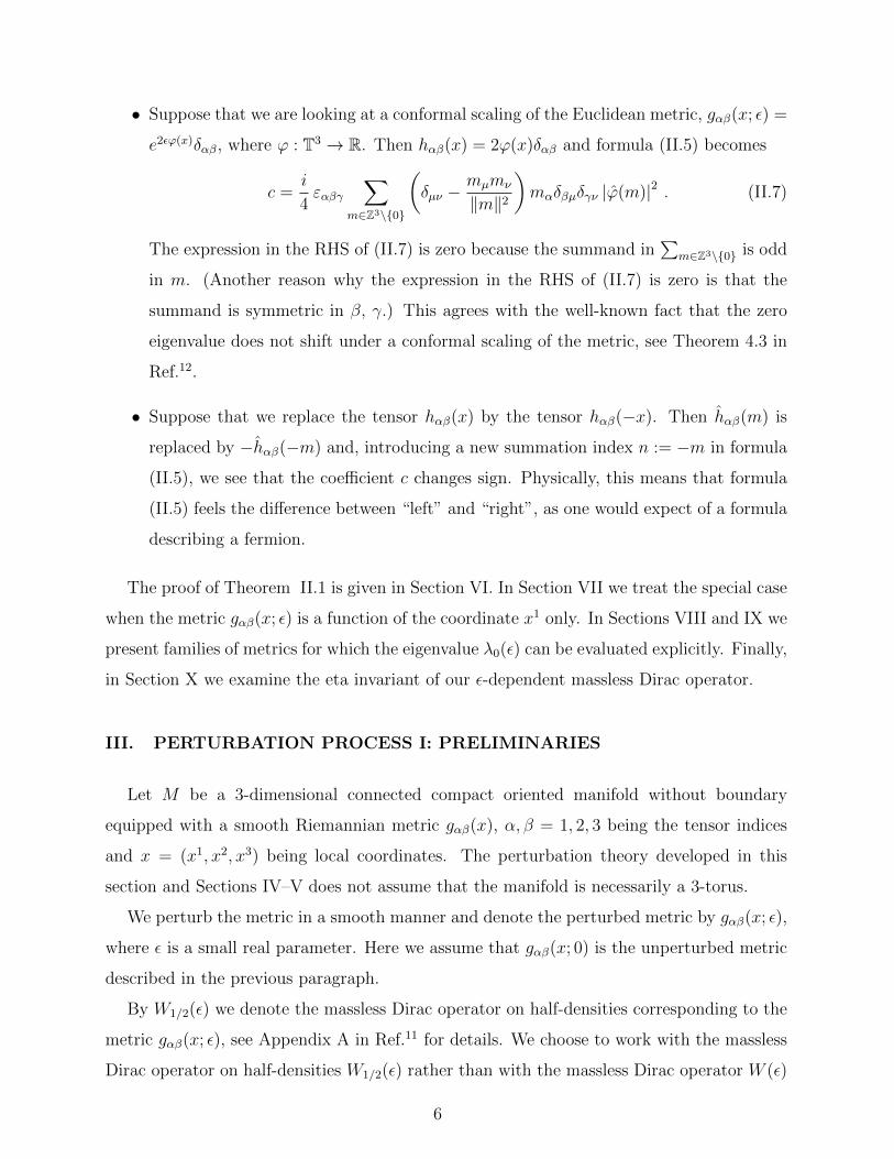
• Suppose that we are looking at a conformal scaling of the Euclidean metric, gαβ(x; ε) =
e2εϕ(x)δαβ, where ϕ : T3 → R. Then hαβ(x) = 2ϕ(x)δαβ and formula (II.5) becomes
c =i
4εαβγ
∑m∈Z3\{0}
(δµν −
mµmν
‖m‖2
)mαδβµδγν |ϕ(m)|2 . (II.7)
The expression in the RHS of (II.7) is zero because the summand in∑
m∈Z3\{0} is odd
in m. (Another reason why the expression in the RHS of (II.7) is zero is that the
summand is symmetric in β, γ.) This agrees with the well-known fact that the zero
eigenvalue does not shift under a conformal scaling of the metric, see Theorem 4.3 in
Ref.12.
• Suppose that we replace the tensor hαβ(x) by the tensor hαβ(−x). Then hαβ(m) is
replaced by −hαβ(−m) and, introducing a new summation index n := −m in formula
(II.5), we see that the coefficient c changes sign. Physically, this means that formula
(II.5) feels the difference between “left” and “right”, as one would expect of a formula
describing a fermion.
The proof of Theorem II.1 is given in Section VI. In Section VII we treat the special case
when the metric gαβ(x; ε) is a function of the coordinate x1 only. In Sections VIII and IX we
present families of metrics for which the eigenvalue λ0(ε) can be evaluated explicitly. Finally,
in Section X we examine the eta invariant of our ε-dependent massless Dirac operator.
III. PERTURBATION PROCESS I: PRELIMINARIES
Let M be a 3-dimensional connected compact oriented manifold without boundary
equipped with a smooth Riemannian metric gαβ(x), α, β = 1, 2, 3 being the tensor indices
and x = (x1, x2, x3) being local coordinates. The perturbation theory developed in this
section and Sections IV–V does not assume that the manifold is necessarily a 3-torus.
We perturb the metric in a smooth manner and denote the perturbed metric by gαβ(x; ε),
where ε is a small real parameter. Here we assume that gαβ(x; 0) is the unperturbed metric
described in the previous paragraph.
By W1/2(ε) we denote the massless Dirac operator on half-densities corresponding to the
metric gαβ(x; ε), see Appendix A in Ref.11 for details. We choose to work with the massless
Dirac operator on half-densities W1/2(ε) rather than with the massless Dirac operator W (ε)
6
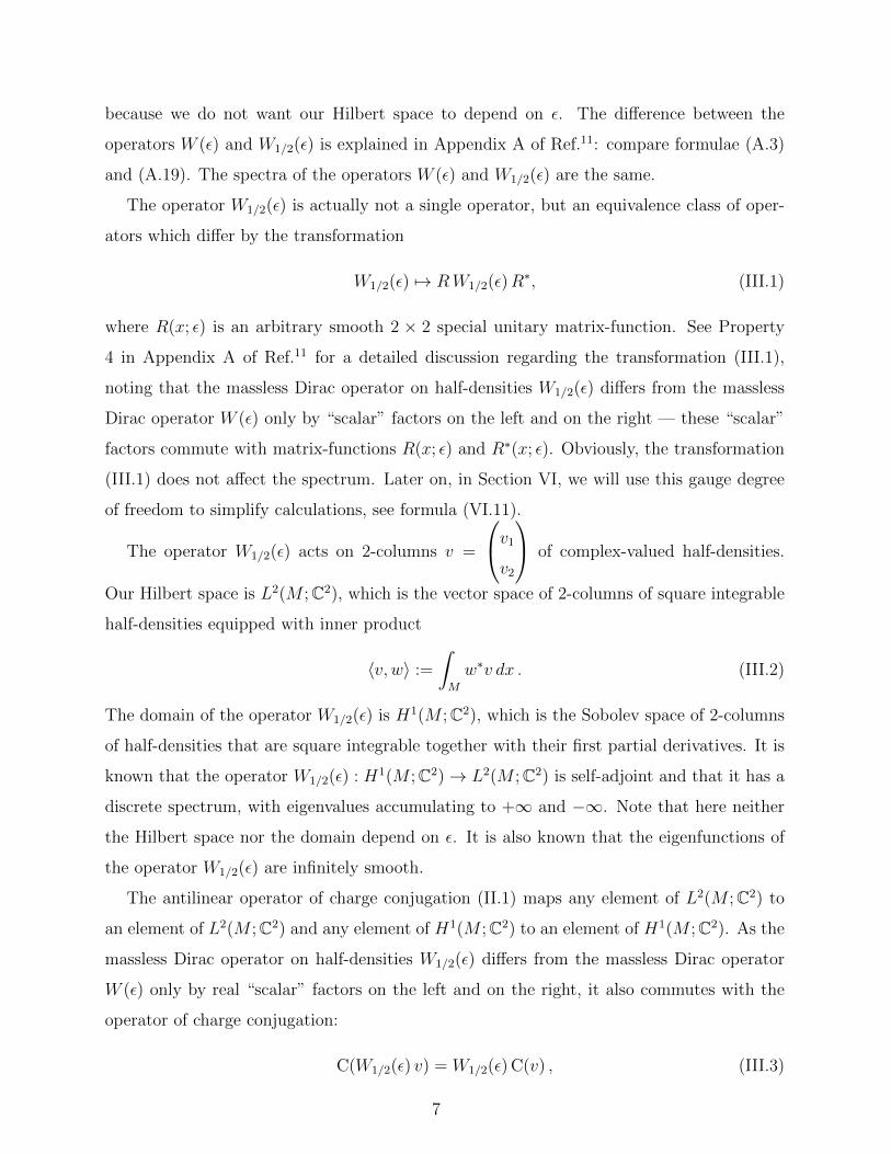
because we do not want our Hilbert space to depend on ε. The difference between the
operators W (ε) and W1/2(ε) is explained in Appendix A of Ref.11: compare formulae (A.3)
and (A.19). The spectra of the operators W (ε) and W1/2(ε) are the same.
The operator W1/2(ε) is actually not a single operator, but an equivalence class of oper-
ators which differ by the transformation
W1/2(ε) 7→ RW1/2(ε)R∗, (III.1)
where R(x; ε) is an arbitrary smooth 2 × 2 special unitary matrix-function. See Property
4 in Appendix A of Ref.11 for a detailed discussion regarding the transformation (III.1),
noting that the massless Dirac operator on half-densities W1/2(ε) differs from the massless
Dirac operator W (ε) only by “scalar” factors on the left and on the right — these “scalar”
factors commute with matrix-functions R(x; ε) and R∗(x; ε). Obviously, the transformation
(III.1) does not affect the spectrum. Later on, in Section VI, we will use this gauge degree
of freedom to simplify calculations, see formula (VI.11).
The operator W1/2(ε) acts on 2-columns v =
v1v2
of complex-valued half-densities.
Our Hilbert space is L2(M ;C2), which is the vector space of 2-columns of square integrable
half-densities equipped with inner product
〈v, w〉 :=
∫M
w∗v dx . (III.2)
The domain of the operator W1/2(ε) is H1(M ;C2), which is the Sobolev space of 2-columns
of half-densities that are square integrable together with their first partial derivatives. It is
known that the operator W1/2(ε) : H1(M ;C2)→ L2(M ;C2) is self-adjoint and that it has a
discrete spectrum, with eigenvalues accumulating to +∞ and −∞. Note that here neither
the Hilbert space nor the domain depend on ε. It is also known that the eigenfunctions of
the operator W1/2(ε) are infinitely smooth.
The antilinear operator of charge conjugation (II.1) maps any element of L2(M ;C2) to
an element of L2(M ;C2) and any element of H1(M ;C2) to an element of H1(M ;C2). As the
massless Dirac operator on half-densities W1/2(ε) differs from the massless Dirac operator
W (ε) only by real “scalar” factors on the left and on the right, it also commutes with the
operator of charge conjugation:
C(W1/2(ε) v) = W1/2(ε) C(v) , (III.3)
7
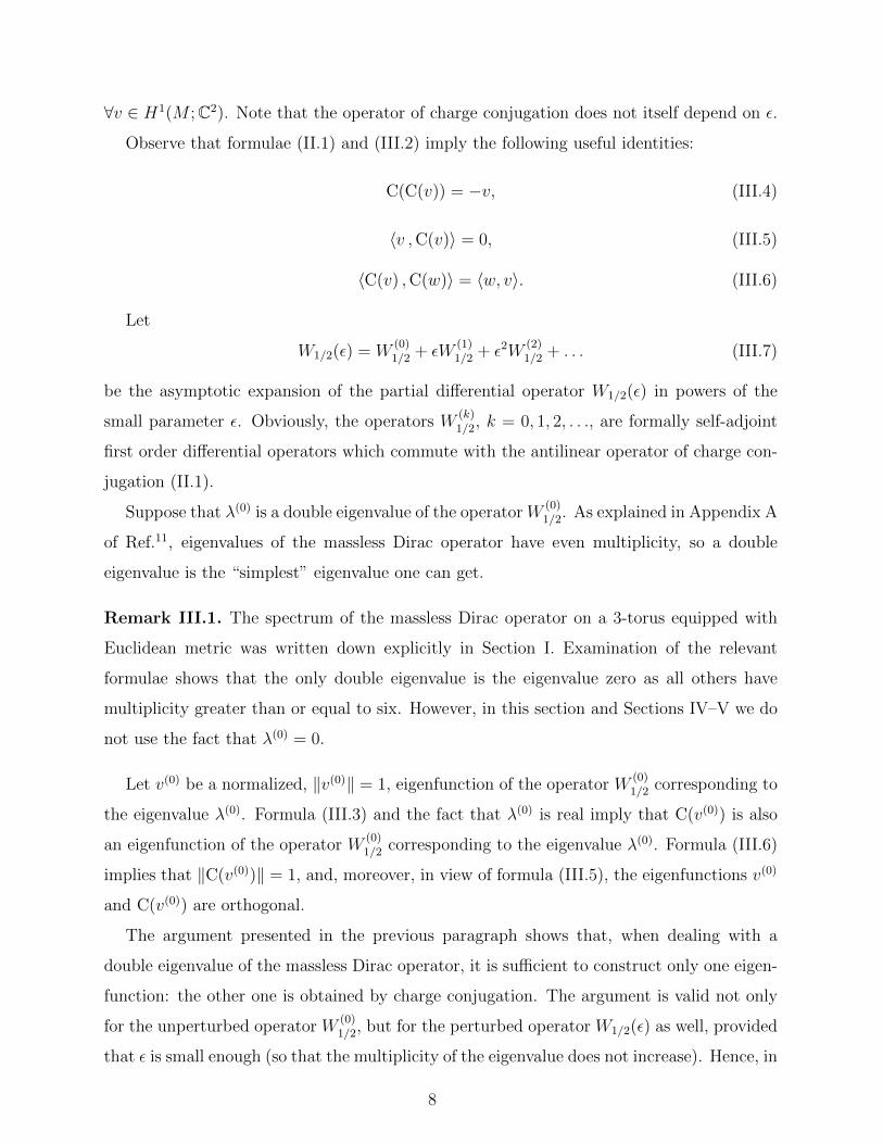
∀v ∈ H1(M ;C2). Note that the operator of charge conjugation does not itself depend on ε.
Observe that formulae (II.1) and (III.2) imply the following useful identities:
C(C(v)) = −v, (III.4)
〈v ,C(v)〉 = 0, (III.5)
〈C(v) ,C(w)〉 = 〈w, v〉. (III.6)
Let
W1/2(ε) = W(0)1/2 + εW
(1)1/2 + ε2W
(2)1/2 + . . . (III.7)
be the asymptotic expansion of the partial differential operator W1/2(ε) in powers of the
small parameter ε. Obviously, the operators W(k)1/2, k = 0, 1, 2, . . ., are formally self-adjoint
first order differential operators which commute with the antilinear operator of charge con-
jugation (II.1).
Suppose that λ(0) is a double eigenvalue of the operator W(0)1/2. As explained in Appendix A
of Ref.11, eigenvalues of the massless Dirac operator have even multiplicity, so a double
eigenvalue is the “simplest” eigenvalue one can get.
Remark III.1. The spectrum of the massless Dirac operator on a 3-torus equipped with
Euclidean metric was written down explicitly in Section I. Examination of the relevant
formulae shows that the only double eigenvalue is the eigenvalue zero as all others have
multiplicity greater than or equal to six. However, in this section and Sections IV–V we do
not use the fact that λ(0) = 0.
Let v(0) be a normalized, ‖v(0)‖ = 1, eigenfunction of the operator W(0)1/2 corresponding to
the eigenvalue λ(0). Formula (III.3) and the fact that λ(0) is real imply that C(v(0)) is also
an eigenfunction of the operator W(0)1/2 corresponding to the eigenvalue λ(0). Formula (III.6)
implies that ‖C(v(0))‖ = 1, and, moreover, in view of formula (III.5), the eigenfunctions v(0)
and C(v(0)) are orthogonal.
The argument presented in the previous paragraph shows that, when dealing with a
double eigenvalue of the massless Dirac operator, it is sufficient to construct only one eigen-
function: the other one is obtained by charge conjugation. The argument is valid not only
for the unperturbed operator W(0)1/2, but for the perturbed operator W1/2(ε) as well, provided
that ε is small enough (so that the multiplicity of the eigenvalue does not increase). Hence, in
8
the perturbation process described in the next section we shall construct one eigenfunction
only.
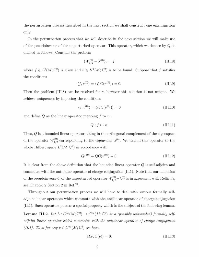
In the perturbation process that we will describe in the next section we will make use
of the pseudoinverse of the unperturbed operator. This operator, which we denote by Q, is
defined as follows. Consider the problem
(W(0)1/2 − λ
(0))v = f (III.8)
where f ∈ L2(M ;C2) is given and v ∈ H1(M ;C2) is to be found. Suppose that f satisfies
the conditions
〈f, v(0)〉 = 〈f,C(v(0))〉 = 0. (III.9)
Then the problem (III.8) can be resolved for v, however this solution is not unique. We
achieve uniqueness by imposing the conditions
〈v, v(0)〉 = 〈v,C(v(0))〉 = 0 (III.10)
and define Q as the linear operator mapping f to v,
Q : f 7→ v. (III.11)
Thus, Q is a bounded linear operator acting in the orthogonal complement of the eigenspace
of the operator W(0)1/2 corresponding to the eigenvalue λ(0). We extend this operator to the
whole Hilbert space L2(M ;C2) in accordance with
Qv(0) = QC(v(0)) = 0. (III.12)
It is clear from the above definition that the bounded linear operator Q is self-adjoint and
commutes with the antilinear operator of charge conjugation (II.1). Note that our definition
of the pseudoinverse Q of the unperturbed operator W(0)1/2−λ(0) is in agreement with Rellich’s,
see Chapter 2 Section 2 in Ref.21.
Throughout our perturbation process we will have to deal with various formally self-
adjoint linear operators which commute with the antilinear operator of charge conjugation
(II.1). Such operators possess a special property which is the subject of the following lemma.
Lemma III.2. Let L : C∞(M ;C2) → C∞(M ;C2) be a (possibly unbounded) formally self-
adjoint linear operator which commutes with the antilinear operator of charge conjugation
(II.1). Then for any v ∈ C∞(M ;C2) we have
〈Lv,C(v)〉 = 0. (III.13)
9
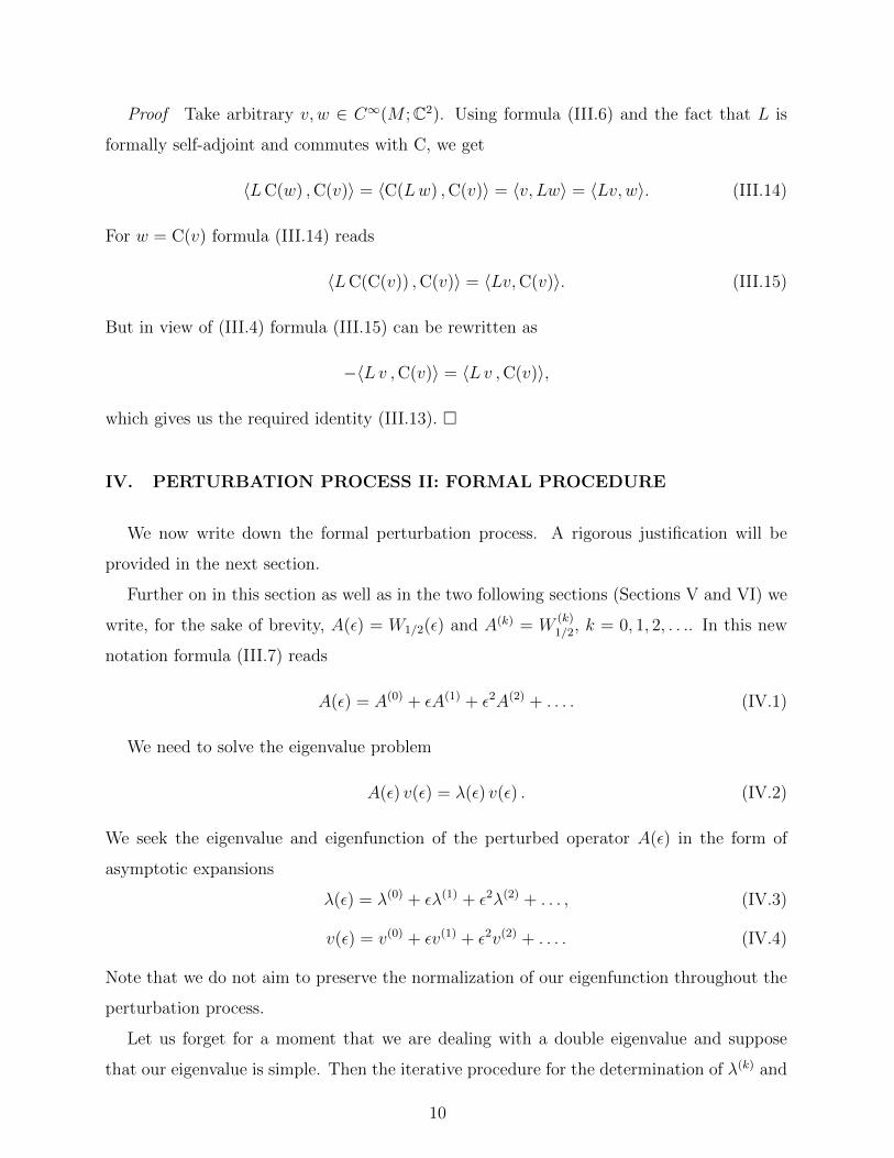
Proof Take arbitrary v, w ∈ C∞(M ;C2). Using formula (III.6) and the fact that L is
formally self-adjoint and commutes with C, we get
〈LC(w) ,C(v)〉 = 〈C(Lw) ,C(v)〉 = 〈v, Lw〉 = 〈Lv,w〉. (III.14)
For w = C(v) formula (III.14) reads
〈LC(C(v)) ,C(v)〉 = 〈Lv,C(v)〉. (III.15)
But in view of (III.4) formula (III.15) can be rewritten as
−〈Lv ,C(v)〉 = 〈Lv ,C(v)〉,
which gives us the required identity (III.13). �
IV. PERTURBATION PROCESS II: FORMAL PROCEDURE
We now write down the formal perturbation process. A rigorous justification will be
provided in the next section.
Further on in this section as well as in the two following sections (Sections V and VI) we
write, for the sake of brevity, A(ε) = W1/2(ε) and A(k) = W(k)1/2, k = 0, 1, 2, . . .. In this new
notation formula (III.7) reads
A(ε) = A(0) + εA(1) + ε2A(2) + . . . . (IV.1)
We need to solve the eigenvalue problem
A(ε) v(ε) = λ(ε) v(ε) . (IV.2)
We seek the eigenvalue and eigenfunction of the perturbed operator A(ε) in the form of
asymptotic expansions
λ(ε) = λ(0) + ελ(1) + ε2λ(2) + . . . , (IV.3)
v(ε) = v(0) + εv(1) + ε2v(2) + . . . . (IV.4)
Note that we do not aim to preserve the normalization of our eigenfunction throughout the
perturbation process.
Let us forget for a moment that we are dealing with a double eigenvalue and suppose
that our eigenvalue is simple. Then the iterative procedure for the determination of λ(k) and
10
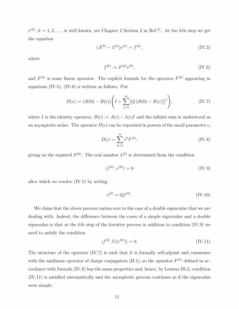
v(k), k = 1, 2, . . ., is well known, see Chapter 2 Section 2 in Ref.21. At the kth step we get
the equation
(A(0) − λ(0))v(k) = f (k), (IV.5)
where
f (k) := F (k)v(0), (IV.6)
and F (k) is some linear operator. The explicit formula for the operator F (k) appearing in
equations (IV.5), (IV.6) is written as follows. Put
D(ε) := (B(0)−B(ε))
(I +
∞∑j=1
[Q (B(0)−B(ε))
]j), (IV.7)
where I is the identity operator, B(ε) := A(ε)− λ(ε)I and the infinite sum is understood as
an asymptotic series. The operator D(ε) can be expanded in powers of the small parameter ε,
D(ε) =∞∑k=1
εkF (k), (IV.8)
giving us the required F (k). The real number λ(k) is determined from the condition
〈f (k), v(0)〉 = 0 (IV.9)
after which we resolve (IV.5) by setting
v(k) = Qf (k). (IV.10)
We claim that the above process carries over to the case of a double eigenvalue that we are
dealing with. Indeed, the difference between the cases of a simple eigenvalue and a double
eigenvalue is that at the kth step of the iterative process in addition to condition (IV.9) we
need to satisfy the condition
〈f (k),C(v(0))〉 = 0. (IV.11)
The structure of the operator (IV.7) is such that it is formally self-adjoint and commutes
with the antilinear operator of charge conjugation (II.1), so the operator F (k) defined in ac-
cordance with formula (IV.8) has the same properties and, hence, by Lemma III.2, condition
(IV.11) is satisfied automatically and the asymptotic process continues as if the eigenvalue
were simple.
11
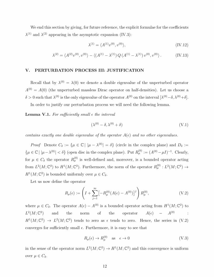
We end this section by giving, for future reference, the explicit formulae for the coefficients
λ(1) and λ(2) appearing in the asymptotic expansion (IV.3):
λ(1) = 〈A(1)v(0), v(0)〉, (IV.12)
λ(2) = 〈A(2)v(0), v(0)〉 − 〈(A(1) − λ(1))Q (A(1) − λ(1)) v(0), v(0)〉 . (IV.13)
V. PERTURBATION PROCESS III: JUSTIFICATION
Recall that by λ(0) = λ(0) we denote a double eigenvalue of the unperturbed operator
A(0) = A(0) (the unperturbed massless Dirac operator on half-densities). Let us choose a
δ > 0 such that λ(0) is the only eigenvalue of the operator A(0) on the interval [λ(0)−δ, λ(0)+δ].
In order to justify our perturbation process we will need the following lemma.
Lemma V.1. For sufficiently small ε the interval
(λ(0) − δ, λ(0) + δ) (V.1)
contains exactly one double eigenvalue of the operator A(ε) and no other eigenvalues.
Proof Denote Cδ := {µ ∈ C | |µ − λ(0)| = δ} (circle in the complex plane) and Dδ :=
{µ ∈ C | |µ−λ(0)| < δ} (open disc in the complex plane). Put R(0)µ := (A(0)−µI)−1. Clearly,
for µ ∈ Cδ the operator R(0)µ is well-defined and, moreover, is a bounded operator acting
from L2(M ;C2) to H1(M ;C2). Furthermore, the norm of the operator R(0)µ : L2(M ;C2)→
H1(M ;C2) is bounded uniformly over µ ∈ Cδ.
Let us now define the operator
Rµ(ε) :=
(I +
∞∑j=1
[−R(0)
µ (A(ε)− A(0))]j)
R(0)µ , (V.2)
where µ ∈ Cδ. The operator A(ε) − A(0) is a bounded operator acting from H1(M ;C2) to
L2(M ;C2) and the norm of the operator A(ε) − A(0) :
H1(M ;C2) → L2(M ;C2) tends to zero as ε tends to zero. Hence, the series in (V.2)
converges for sufficiently small ε. Furthermore, it is easy to see that
Rµ(ε)→ R(0)µ as ε→ 0 (V.3)
in the sense of the operator norm L2(M ;C2)→ H1(M ;C2) and this convergence is uniform
over µ ∈ Cδ.
12
Acting onto (V.2) with the operator A(ε) − µI we see that (A(ε) − µI)Rµ(ε) = I, so
Rµ(ε) = (A(ε)− µI)−1. Put
E(ε) :=1
2πi
∫Cδ
Rµ(ε) dµ . (V.4)
The operator E(ε) is the orthogonal projection onto the span of eigenvectors of the operator
A(ε) corresponding to eigenvalues on the interval (V.1). In particular, E(0) = E(0) is the
orthogonal projection onto the span of eigenvectors of the operator A(0) corresponding to
the double eigenvalue λ(0).
Formulae (V.3) and (V.4) imply
‖E(ε)− E(0)‖op → 0 as ε→ 0, (V.5)
where ‖ · ‖op stands for the operator norm in the Banach space of bounded linear operators
L2(M ;C2)→ L2(M ;C2). Formula (V.5) implies that for sufficiently small ε we have
‖E(ε)− E(0)‖op < 1. (V.6)
Formula (V.6) and the fact that the orthogonal projections E(ε) and E(0) have finite rank
imply that rankE(ε) = rankE(0) = 2 . Thus, the operator A(ε) has two eigenvalues, counted
with multiplicities, on the interval (V.1). We know, see Property 3 in Appendix A of Ref.11,
that the eigenvalues of the operator A(ε) have even multiplicity, so we are looking at one
double eigenvalue on the interval (V.1). �
Let λ(ε) be the unique double eigenvalue of the operator A(ε) from the interval (V.1). De-
note by σ(ε) the spectrum of the operator A(ε) and, for a given µ ∈ R, denote dist(µ, σ(ε)) =
minν∈σ(ε)
|µ− ν|. Obviously, without additional information on µ and on σ(ε) we can only guar-
antee the inequality
dist(µ, σ(ε)) ≤ |µ− λ(ε)|. (V.7)
Choose an arbitrary natural k and denote
λ(ε) = λ(0) + ελ(1) + ε2λ(2) + . . .+ εkλ(k), (V.8)
v(ε) = v(0) + εv(1) + ε2v(2) + . . .+ εkv(k), (V.9)
where the λ(j) and v(j), j = 0, 1, . . . , k, are taken from (IV.3) and (IV.4). We have
‖v(ε)‖ = 1 +O(ε), (V.10)
13
‖(A(ε)− λ(ε))v(ε)‖ = O(εk+1), (V.11)
where ‖ · ‖ stands for the L2(M ;C2) norm (see (III.2) for inner product). As our operator
A(ε) is self-adjoint, formulae (V.10) and (V.11) imply
dist(λ(ε), σ(ε)) ≤ ‖(A(ε)− λ(ε))v(ε)‖‖v(ε)‖
= O(εk+1). (V.12)
Formulae (V.8) and (V.12) and Lemma V.1 imply that for sufficiently small ε,
dist(λ(ε), σ(ε)) = |λ(ε)− λ(ε)|, (V.13)
compare with (V.7). Combining formulae (V.12) and (V.13), we get λ(ε) = λ(ε) +O(εk+1).
This completes the justification of our perturbation process.
VI. PROOF OF THEOREM II.1
The unperturbed massless Dirac operator on half-densities, which we denote by A(0), is
given by the expression in the RHS of (I.1). The unperturbed eigenvalue, λ(0), is zero and
the corresponding normalized eigenfunction is
v(0) =1
(2π)3/2
1
0
. (VI.1)
The pseudoinverse Q of the operator A(0) is given by the formula
Q =1
(2π)3
∑m∈Z3\{0}
eimαxα
m3 m1 − im2
m1 + im2 −m3
−1 ∫T3
e−imαyα ( · ) dy
=1
(2π)3
∑m∈Z3\{0}
eimαxα
‖m‖2
m3 m1 − im2
m1 + im2 −m3
∫T3
e−imαyα ( · ) dy , (VI.2)
where dy := dy1dy2dy3. The operator (VI.2) is a self-adjoint pseudodifferential operator of
order −1.
We have
λ(ε) = ελ(1) + ε2λ(2) +O(ε3), (VI.3)
where the coefficients λ(1) and λ(2) are given by formulae (IV.12) and (IV.13) respectively.
Thus, in order to prove Theorem II.1 we need to write down explicitly the differential
14
operators A(1) and A(2) appearing in the asymptotic expansion of the perturbed massless
Dirac operator on half-densities,
A(ε) = A(0) + εA(1) + ε2A(2) +O(ε3). (VI.4)
In what follows we use terminology from microlocal analysis. In particular, we use the
notions of the principal and subprincipal symbols of a differential operator, see subsection
2.1.3 in Ref.22 for details.
Let L be a first order 2 × 2 matrix differential operator. We denote its principal and
subprincipal symbols by L1(x, ξ) and Lsub(x) respectively. Here ξ = (ξ1, ξ2, ξ3) is the variable
dual to the position variable x; in physics literature the ξ would be referred to as momentum.
The subscript in L1(x, ξ) indicates the degree of homogeneity in ξ.
A first order differential operator L is completely determined by its principal and sub-
principal symbols. Indeed, the principal symbol has the form
L1(x, ξ) = M (α)(x) ξα , (VI.5)
where M (α)(x) are matrix-functions depending only on the position variable x. It is easy to
see that the differential operator L is given by the formula
L = − i2M (α)(x)
∂
∂xα− i
2
∂
∂xαM (α)(x) + Lsub(x) . (VI.6)
Given a first order differential operator L, let us consider the expression 〈Lv(0), v(0)〉,
where v(0) is the constant column (VI.1) and angular brackets indicate the inner product
(III.2). Examination of formula (VI.6) shows that
〈Lv(0), v(0)〉 = 〈Lsubv(0), v(0)〉
because the terms coming from the principal symbol integrate to zero. Consequently for-
mulae (IV.12) and (IV.13) simplify and now read
λ(1) = 〈A(1)subv
(0), v(0)〉, (VI.7)
λ(2) = 〈A(2)subv
(0), v(0)〉 − 〈(A(1) − λ(1))Q (A(1) − λ(1)) v(0), v(0)〉 . (VI.8)
We see that for the purpose of proving Theorem II.1 we do not need to know the full
operator A(2), only its subprincipal symbol A(2)sub.
15
In order to write down explicitly the massless Dirac operator on half-densities A(ε) we
need the concepts of frame and coframe. The differential geometric definition of coframe was
given in Section 3 of Ref.11. However, as in the current paper we are working in a specified
coordinate system, we can adopt a somewhat simpler approach. For the purposes of the
current paper a coframe is a smooth real-valued matrix-function ejα(x; ε), j, α = 1, 2, 3,
satisfying the conditions
gαβ(x; ε) = δjk ejα(x; ε) ekβ(x; ε) , (VI.9)
ejα(x; 0) = δjα . (VI.10)
Here and further on when dealing with matrix-functions we use the convention that the first
index (subscript or superscript) enumerates the rows and the second index (subscript or
superscript) enumerates the columns. Say, in matrix notation the RHS of (VI.9) reads as
“product of coframe transposed and coframe”.
Note that the reason we imposed condition (VI.10) is so that our unperturbed operator
has the form (I.1). See also formula (III.1) and associated discussion.
For a given metric gαβ(x; ε) the coframe ejα(x; ε) is not defined uniquely. We can multiply
the matrix-function ejα(x; ε) from the left by an arbitrary smooth 3× 3 special orthogonal
matrix-function O(x; ε) satisfying the condition O(x; 0) = I, with I denoting the 3 × 3
identity matrix. This will give us a new coframe satisfying the defining relations (VI.9) and
(VI.10). As explained in Appendix A of Ref.11, this freedom in the choice of coframe is
a gauge degree of freedom which does not affect the spectrum. In the current section we
specify the gauge by requiring the matrix-function ejα(x; ε) to be symmetric,
ejα(x; ε) = eαj(x; ε). (VI.11)
Condition (VI.11) makes sense because we are working in a specified coordinate system.
Looking ahead, let us point out the main advantage of the symmetric gauge (VI.11): the
asymptotic expansion of the subprincipal symbol of the massless Dirac operator on half-
densities in powers of ε starts with a quadratic term and, moreover, the coefficient at ε2 has
an especially simple structure, see formulae (VI.16) and (VI.19).
In matrix notation condition (VI.9) now reads “the symmetric positive matrix gαβ(x; ε)
is the square of the symmetric matrix ejα(x; ε)”. Conversely, the symmetric matrix ejα(x; ε)
is the square root of the symmetric positive matrix gαβ(x; ε). We choose the branch of the
square root so that the matrix ejα(x; ε) is positive.
16
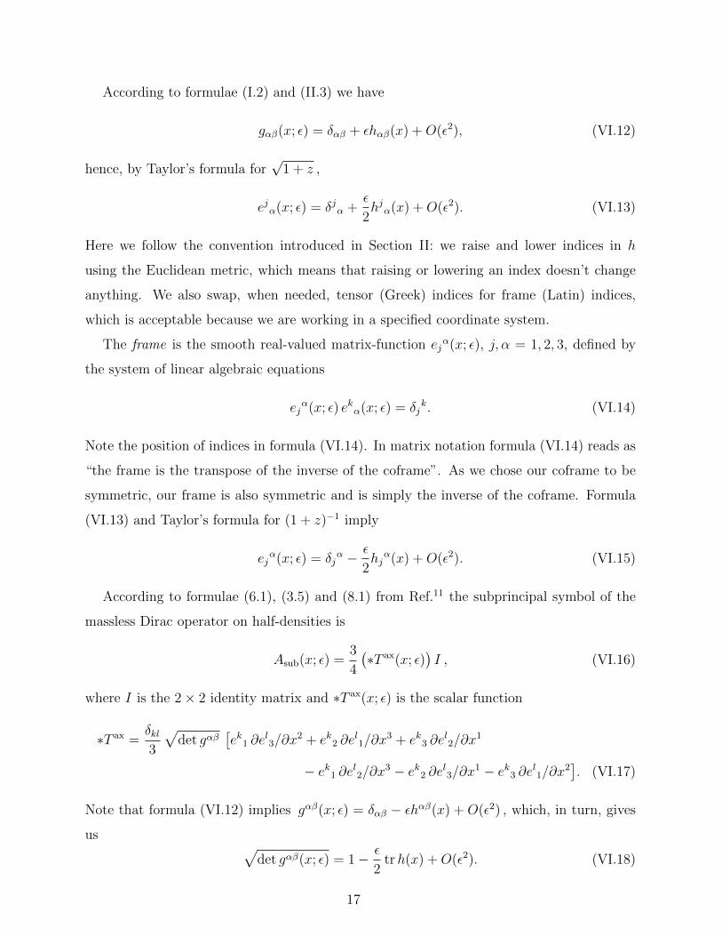
According to formulae (I.2) and (II.3) we have
gαβ(x; ε) = δαβ + εhαβ(x) +O(ε2), (VI.12)
hence, by Taylor’s formula for√
1 + z ,
ejα(x; ε) = δjα +ε
2hjα(x) +O(ε2). (VI.13)
Here we follow the convention introduced in Section II: we raise and lower indices in h
using the Euclidean metric, which means that raising or lowering an index doesn’t change
anything. We also swap, when needed, tensor (Greek) indices for frame (Latin) indices,
which is acceptable because we are working in a specified coordinate system.
The frame is the smooth real-valued matrix-function ejα(x; ε), j, α = 1, 2, 3, defined by
the system of linear algebraic equations
ejα(x; ε) ekα(x; ε) = δj
k. (VI.14)
Note the position of indices in formula (VI.14). In matrix notation formula (VI.14) reads as
“the frame is the transpose of the inverse of the coframe”. As we chose our coframe to be
symmetric, our frame is also symmetric and is simply the inverse of the coframe. Formula
(VI.13) and Taylor’s formula for (1 + z)−1 imply
ejα(x; ε) = δj
α − ε
2hj
α(x) +O(ε2). (VI.15)
According to formulae (6.1), (3.5) and (8.1) from Ref.11 the subprincipal symbol of the
massless Dirac operator on half-densities is
Asub(x; ε) =3
4
(∗T ax(x; ε)
)I , (VI.16)
where I is the 2× 2 identity matrix and ∗T ax(x; ε) is the scalar function
∗T ax =δkl3
√det gαβ
[ek1 ∂e
l3/∂x
2 + ek2 ∂el1/∂x
3 + ek3 ∂el2/∂x
1
− ek1 ∂el2/∂x3 − ek2 ∂el3/∂x1 − ek3 ∂el1/∂x2]. (VI.17)
Note that formula (VI.12) implies gαβ(x; ε) = δαβ − εhαβ(x) + O(ε2) , which, in turn, gives
us √det gαβ(x; ε) = 1− ε
2trh(x) +O(ε2). (VI.18)
17
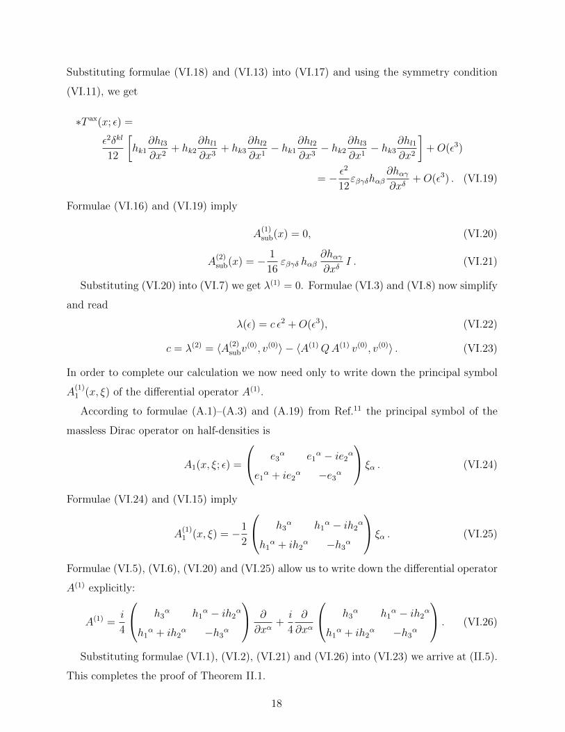
Substituting formulae (VI.18) and (VI.13) into (VI.17) and using the symmetry condition
(VI.11), we get
∗T ax(x; ε) =
ε2δkl
12
[hk1
∂hl3∂x2
+ hk2∂hl1∂x3
+ hk3∂hl2∂x1− hk1
∂hl2∂x3− hk2
∂hl3∂x1− hk3
∂hl1∂x2
]+O(ε3)
= − ε2
12εβγδhαβ
∂hαγ∂xδ
+O(ε3) . (VI.19)
Formulae (VI.16) and (VI.19) imply
A(1)sub(x) = 0, (VI.20)
A(2)sub(x) = − 1
16εβγδ hαβ
∂hαγ∂xδ
I . (VI.21)
Substituting (VI.20) into (VI.7) we get λ(1) = 0. Formulae (VI.3) and (VI.8) now simplify
and read
λ(ε) = c ε2 +O(ε3), (VI.22)
c = λ(2) = 〈A(2)subv
(0), v(0)〉 − 〈A(1)QA(1) v(0), v(0)〉 . (VI.23)
In order to complete our calculation we now need only to write down the principal symbol
A(1)1 (x, ξ) of the differential operator A(1).
According to formulae (A.1)–(A.3) and (A.19) from Ref.11 the principal symbol of the
massless Dirac operator on half-densities is
A1(x, ξ; ε) =
e3α e1
α − ie2α
e1α + ie2
α −e3α
ξα . (VI.24)
Formulae (VI.24) and (VI.15) imply
A(1)1 (x, ξ) = −1
2
h3α h1
α − ih2α
h1α + ih2
α −h3α
ξα . (VI.25)
Formulae (VI.5), (VI.6), (VI.20) and (VI.25) allow us to write down the differential operator
A(1) explicitly:
A(1) =i
4
h3α h1
α − ih2α
h1α + ih2
α −h3α
∂
∂xα+i
4
∂
∂xα
h3α h1
α − ih2α
h1α + ih2
α −h3α
. (VI.26)
Substituting formulae (VI.1), (VI.2), (VI.21) and (VI.26) into (VI.23) we arrive at (II.5).
This completes the proof of Theorem II.1.
18
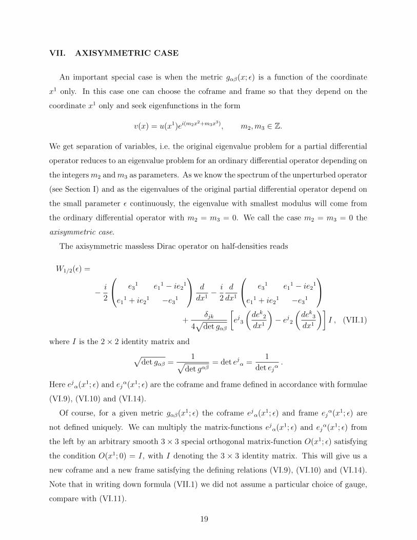
VII. AXISYMMETRIC CASE
An important special case is when the metric gαβ(x; ε) is a function of the coordinate
x1 only. In this case one can choose the coframe and frame so that they depend on the
coordinate x1 only and seek eigenfunctions in the form
v(x) = u(x1)ei(m2x2+m3x3), m2,m3 ∈ Z.
We get separation of variables, i.e. the original eigenvalue problem for a partial differential
operator reduces to an eigenvalue problem for an ordinary differential operator depending on
the integersm2 andm3 as parameters. As we know the spectrum of the unperturbed operator
(see Section I) and as the eigenvalues of the original partial differential operator depend on
the small parameter ε continuously, the eigenvalue with smallest modulus will come from
the ordinary differential operator with m2 = m3 = 0. We call the case m2 = m3 = 0 the
axisymmetric case.
The axisymmetric massless Dirac operator on half-densities reads
W1/2(ε) =
− i
2
e31 e1
1 − ie21
e11 + ie2
1 −e31
d
dx1− i
2
d
dx1
e31 e1
1 − ie21
e11 + ie2
1 −e31
+
δjk
4√
det gαβ
[ej3
(dek2dx1
)− ej2
(dek3dx1
)]I , (VII.1)
where I is the 2× 2 identity matrix and√det gαβ =
1√det gαβ
= det ejα =1
det ejα.
Here ejα(x1; ε) and ejα(x1; ε) are the coframe and frame defined in accordance with formulae
(VI.9), (VI.10) and (VI.14).
Of course, for a given metric gαβ(x1; ε) the coframe ejα(x1; ε) and frame ejα(x1; ε) are
not defined uniquely. We can multiply the matrix-functions ejα(x1; ε) and ejα(x1; ε) from
the left by an arbitrary smooth 3× 3 special orthogonal matrix-function O(x1; ε) satisfying
the condition O(x1; 0) = I, with I denoting the 3 × 3 identity matrix. This will give us a
new coframe and a new frame satisfying the defining relations (VI.9), (VI.10) and (VI.14).
Note that in writing down formula (VII.1) we did not assume a particular choice of gauge,
compare with (VI.11).
19
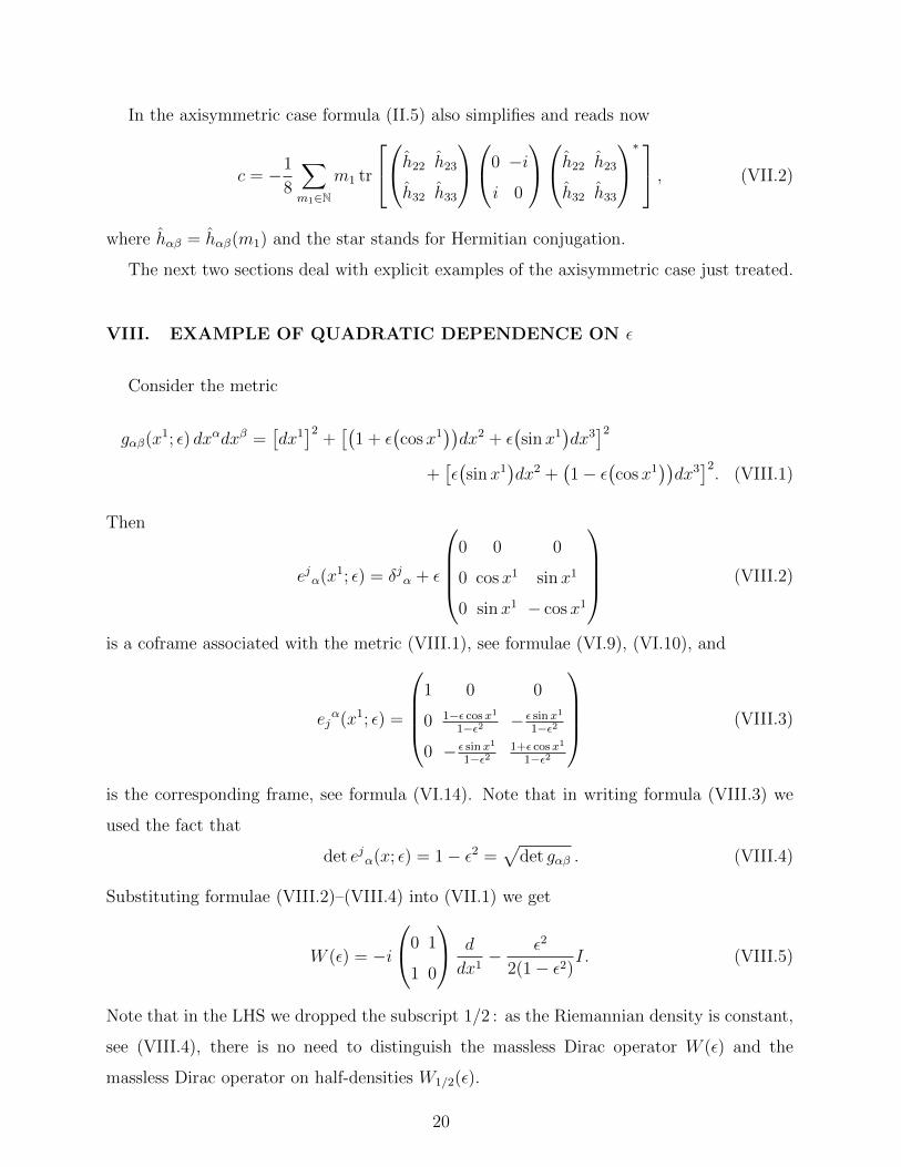
In the axisymmetric case formula (II.5) also simplifies and reads now
c = −1
8
∑m1∈N
m1 tr
h22 h23
h32 h33
0 −i
i 0
h22 h23
h32 h33
∗ , (VII.2)
where hαβ = hαβ(m1) and the star stands for Hermitian conjugation.
The next two sections deal with explicit examples of the axisymmetric case just treated.
VIII. EXAMPLE OF QUADRATIC DEPENDENCE ON ε
Consider the metric
gαβ(x1; ε) dxαdxβ =[dx1]2
+[(
1 + ε(cosx1
))dx2 + ε
(sinx1
)dx3]2
+[ε(sinx1
)dx2 +
(1− ε
(cosx1
))dx3]2. (VIII.1)
Then
ejα(x1; ε) = δjα + ε
0 0 0
0 cosx1 sinx1
0 sin x1 − cosx1
(VIII.2)
is a coframe associated with the metric (VIII.1), see formulae (VI.9), (VI.10), and
ejα(x1; ε) =
1 0 0
0 1−ε cosx11−ε2 − ε sinx1
1−ε2
0 − ε sinx1
1−ε21+ε cosx1
1−ε2
(VIII.3)
is the corresponding frame, see formula (VI.14). Note that in writing formula (VIII.3) we
used the fact that
det ejα(x; ε) = 1− ε2 =√
det gαβ . (VIII.4)
Substituting formulae (VIII.2)–(VIII.4) into (VII.1) we get
W (ε) = −i
0 1
1 0
d
dx1− ε2
2(1− ε2)I. (VIII.5)
Note that in the LHS we dropped the subscript 1/2 : as the Riemannian density is constant,
see (VIII.4), there is no need to distinguish the massless Dirac operator W (ε) and the
massless Dirac operator on half-densities W1/2(ε).
20
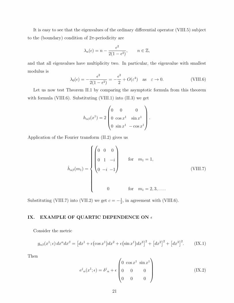
It is easy to see that the eigenvalues of the ordinary differential operator (VIII.5) subject
to the (boundary) condition of 2π-periodicity are
λn(ε) = n− ε2
2(1− ε2), n ∈ Z,
and that all eigenvalues have multiplicity two. In particular, the eigenvalue with smallest
modulus is
λ0(ε) = − ε2
2(1− ε2)= −ε
2
2+O(ε4) as ε→ 0. (VIII.6)
Let us now test Theorem II.1 by comparing the asymptotic formula from this theorem
with formula (VIII.6). Substituting (VIII.1) into (II.3) we get
hαβ(x1) = 2
0 0 0
0 cosx1 sinx1
0 sin x1 − cosx1
.
Application of the Fourier transform (II.2) gives us
hαβ(m1) =
0 0 0
0 1 −i
0 −i −1
for m1 = 1,
0 for m1 = 2, 3, . . . .
(VIII.7)
Substituting (VIII.7) into (VII.2) we get c = −12, in agreement with (VIII.6).
IX. EXAMPLE OF QUARTIC DEPENDENCE ON ε
Consider the metric
gαβ(x1; ε) dxαdxβ =[dx1 + ε
(cosx1
)dx2 + ε
(sinx1
)dx3]2
+[dx2]2
+[dx3]2. (IX.1)
Then
ejα(x1; ε) = δjα + ε
0 cosx1 sinx1
0 0 0
0 0 0
(IX.2)
21
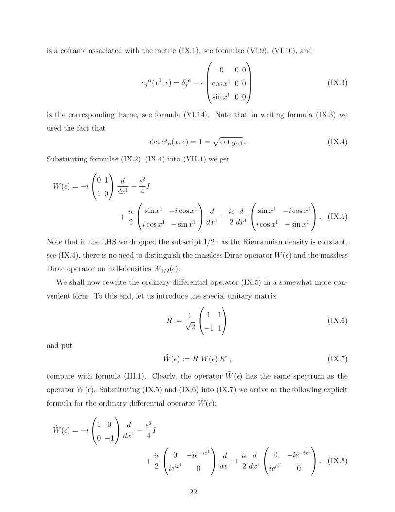
is a coframe associated with the metric (IX.1), see formulae (VI.9), (VI.10), and
ejα(x1; ε) = δj
α − ε
0 0 0
cosx1 0 0
sinx1 0 0
(IX.3)
is the corresponding frame, see formula (VI.14). Note that in writing formula (IX.3) we
used the fact that
det ejα(x; ε) = 1 =√
det gαβ . (IX.4)
Substituting formulae (IX.2)–(IX.4) into (VII.1) we get
W (ε) = −i
0 1
1 0
d
dx1− ε2
4I
+iε
2
sinx1 −i cosx1
i cosx1 − sinx1
d
dx1+iε
2
d
dx1
sinx1 −i cosx1
i cosx1 − sinx1
. (IX.5)
Note that in the LHS we dropped the subscript 1/2 : as the Riemannian density is constant,
see (IX.4), there is no need to distinguish the massless Dirac operator W (ε) and the massless
Dirac operator on half-densities W1/2(ε).
We shall now rewrite the ordinary differential operator (IX.5) in a somewhat more con-
venient form. To this end, let us introduce the special unitary matrix
R :=1√2
1 1
−1 1
(IX.6)
and put
W (ε) := R W (ε)R∗ , (IX.7)
compare with formula (III.1). Clearly, the operator W (ε) has the same spectrum as the
operator W (ε). Substituting (IX.5) and (IX.6) into (IX.7) we arrive at the following explicit
formula for the ordinary differential operator W (ε):
W (ε) = −i
1 0
0 −1
d
dx1− ε2
4I
+iε
2
0 −ie−ix1
ieix1
0
d
dx1+iε
2
d
dx1
0 −ie−ix1
ieix1
0
. (IX.8)
22
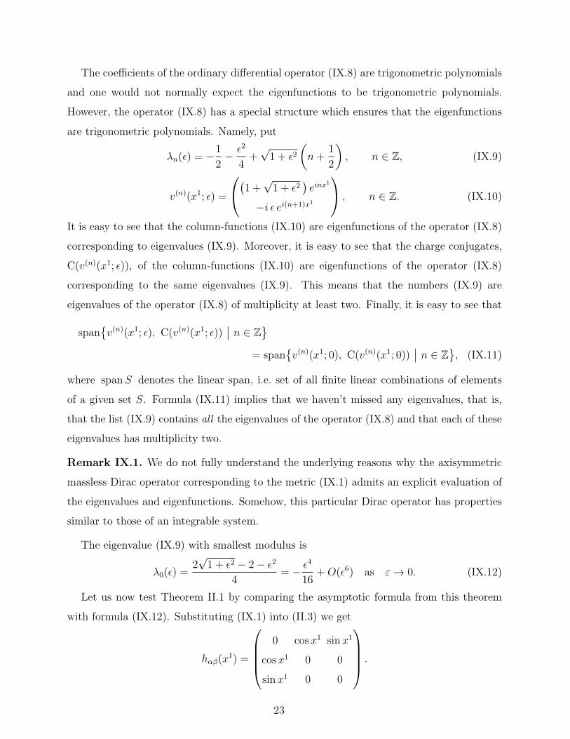
The coefficients of the ordinary differential operator (IX.8) are trigonometric polynomials
and one would not normally expect the eigenfunctions to be trigonometric polynomials.
However, the operator (IX.8) has a special structure which ensures that the eigenfunctions
are trigonometric polynomials. Namely, put
λn(ε) = −1
2− ε2
4+√
1 + ε2(n+
1
2
), n ∈ Z, (IX.9)
v(n)(x1; ε) =
(1 +√
1 + ε2)einx
1
−i ε ei(n+1)x1
, n ∈ Z. (IX.10)
It is easy to see that the column-functions (IX.10) are eigenfunctions of the operator (IX.8)
corresponding to eigenvalues (IX.9). Moreover, it is easy to see that the charge conjugates,
C(v(n)(x1; ε)), of the column-functions (IX.10) are eigenfunctions of the operator (IX.8)
corresponding to the same eigenvalues (IX.9). This means that the numbers (IX.9) are
eigenvalues of the operator (IX.8) of multiplicity at least two. Finally, it is easy to see that
span{v(n)(x1; ε), C(v(n)(x1; ε))
∣∣ n ∈ Z}
= span{v(n)(x1; 0), C(v(n)(x1; 0))
∣∣ n ∈ Z}, (IX.11)
where spanS denotes the linear span, i.e. set of all finite linear combinations of elements
of a given set S. Formula (IX.11) implies that we haven’t missed any eigenvalues, that is,
that the list (IX.9) contains all the eigenvalues of the operator (IX.8) and that each of these
eigenvalues has multiplicity two.
Remark IX.1. We do not fully understand the underlying reasons why the axisymmetric
massless Dirac operator corresponding to the metric (IX.1) admits an explicit evaluation of
the eigenvalues and eigenfunctions. Somehow, this particular Dirac operator has properties
similar to those of an integrable system.
The eigenvalue (IX.9) with smallest modulus is
λ0(ε) =2√
1 + ε2 − 2− ε2
4= − ε
4
16+O(ε6) as ε→ 0. (IX.12)
Let us now test Theorem II.1 by comparing the asymptotic formula from this theorem
with formula (IX.12). Substituting (IX.1) into (II.3) we get
hαβ(x1) =
0 cosx1 sinx1
cosx1 0 0
sinx1 0 0
.
23
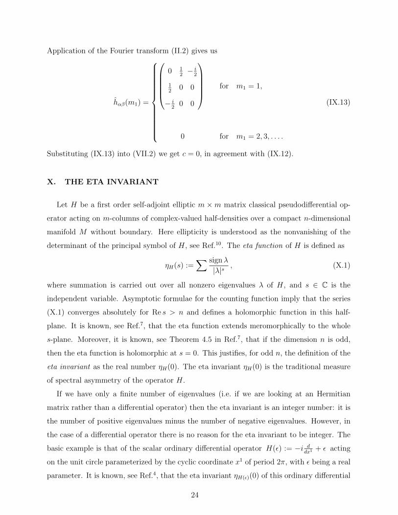
Application of the Fourier transform (II.2) gives us
hαβ(m1) =
0 1
2− i
2
12
0 0
− i2
0 0
for m1 = 1,
0 for m1 = 2, 3, . . . .
(IX.13)
Substituting (IX.13) into (VII.2) we get c = 0, in agreement with (IX.12).
X. THE ETA INVARIANT
Let H be a first order self-adjoint elliptic m ×m matrix classical pseudodifferential op-
erator acting on m-columns of complex-valued half-densities over a compact n-dimensional
manifold M without boundary. Here ellipticity is understood as the nonvanishing of the
determinant of the principal symbol of H, see Ref.10. The eta function of H is defined as
ηH(s) :=∑ signλ
|λ|s, (X.1)
where summation is carried out over all nonzero eigenvalues λ of H, and s ∈ C is the
independent variable. Asymptotic formulae for the counting function imply that the series
(X.1) converges absolutely for Re s > n and defines a holomorphic function in this half-
plane. It is known, see Ref.7, that the eta function extends meromorphically to the whole
s-plane. Moreover, it is known, see Theorem 4.5 in Ref.7, that if the dimension n is odd,
then the eta function is holomorphic at s = 0. This justifies, for odd n, the definition of the
eta invariant as the real number ηH(0). The eta invariant ηH(0) is the traditional measure
of spectral asymmetry of the operator H.
If we have only a finite number of eigenvalues (i.e. if we are looking at an Hermitian
matrix rather than a differential operator) then the eta invariant is an integer number: it is
the number of positive eigenvalues minus the number of negative eigenvalues. However, in
the case of a differential operator there is no reason for the eta invariant to be integer. The
basic example is that of the scalar ordinary differential operator H(ε) := −i ddx1
+ ε acting
on the unit circle parameterized by the cyclic coordinate x1 of period 2π, with ε being a real
parameter. It is known, see Ref.4, that the eta invariant ηH(ε)(0) of this ordinary differential
24
operator is the odd 1-periodic function defined by the formula ηH(ε)(0) = 1−2ε for ε ∈ (0, 1).
In particular, we have ηH(0)(0) = 0 and limε→0±
ηH(ε)(0) = ±1.
The current state of affairs (from an analyst’s perspective) in the subject area of zeta/eta
functions of elliptic operators is described in detail in the two papers Refs.16,17. Let us
highlight a few facts.
• The key results are Theorem 2.7 from Ref.16 and Proposition 2.9 from Ref.17. Arguing
along the lines of Ref.7 one can recover from these results, in a rigorous analytic fashion,
properties of the eta function.
• The eta function is holomorphic at s = 0 in any dimension n ∈ N (i.e. without the
assumption of n being odd). This fact was proved by P. B. Gilkey13.
• The seminal paper of R. T. Seeley23 contained a small mistake: see page 482 in Ref.16
or Remark 2.6 on page 39 in Ref.17 for details.
The more recent survey papers Refs.14,15 provide an overview of the subject.
Let us denote our massless Dirac operator on half-densities by A(ε), where ε ∈ R is
the small parameter appearing in our metric gαβ(x; ε). Theorem II.1 implies the following
corollary.
Corollary X.1. Suppose that the coefficient c defined by formula (II.5) is nonzero. Then
limε→0
ηA(ε)(0) = 2 sign c . (X.2)
Note that we have ηA(0)(0) = 0, so formula (X.2) implies that the function ηA(ε)(0) is
discontinuous at ε = 0.
Proof of Corollary X.1 Put f(ε, t) := Tr[A(ε) e−t(A(ε))
2], where t > 0 and Tr is the
operator (as opposed to pointwise) trace. The paper Ref.9 to which we are about to refer to
actually deals with pointwise estimates, i.e. the trace in Ref.9 is understood as the matrix
trace of the integral kernel on the diagonal at a given point x of the manifold. We do not
need pointwise estimates for the proof of Corollary X.1.
Having fixed ε, let us examine the behaviour of f(ε, t) as t→ 0+. For a generic first order
pseudodifferential operator A(ε) we would have f(ε, t) = O(t−2). However, as explained in
Chapter II of Ref.9, the Dirac operator in odd dimensions is very special and there are a lot
25
of cancellations when one computes the asymptotic expansion for f(ε, t) as t→ 0+. Namely,
it was shown in Ref.9 that
• f(ε, t) = O(√t ) as t→ 0+,
• ηA(ε)(s) is holomorphic in the half-plane Re s > −2 , and
•
ηA(ε)(s) =1
Γ(s+12
) ∫ +∞
0
t(s−1)/2 f(ε, t) dt for Re s > −2 . (X.3)
See also Section 1 in Ref.24.
Formula (X.3) implies
ηA(ε)(0) =1√π
∫ +∞
0
f(ε, t)√t
dt , (X.4)
so in order to prove Corollary X.1 we need to examine the behaviour of the integral (X.4)
as ε→ 0.
Let us denote by λ0(ε) the eigenvalue of the operator A(ε) with smallest modulus and by
E0(ε) the orthogonal projection onto the corresponding 2-dimensional eigenspace. Put
A0(ε) := λ0(ε)E0(ε) , A(ε) := A(ε)− A0(ε),
f0(ε, t) := Tr[A0(ε) e
−t(A0(ε))2]
= 2λ0(ε) e−t(λ0(ε))2 ,
f(ε, t) := Tr[A(ε) e−t(A(ε))
2]
= f(ε, t)− f0(ε, t).
Then formula (X.4) can be rewritten as
ηA(ε)(0) =1√π
∫ 1
0
f(ε, t)√t
dt +1√π
∫ +∞
1
f(ε, t)√t
dt
+2√π
∫ +∞
1
λ0(ε) e−t(λ0(ε))2
√t
dt . (X.5)
The three terms in the RHS of (X.5) are functions of the parameter ε and we shall now
examine how they depend on ε.
The first term in the RHS of (X.5) is continuous at ε = 0 because asymptotic formulae
for f(ε, t) as t→ 0+ are uniform in ε. This follows from the construction of heat kernel type
asymptotics for t→ 0+: the algorithm is straightforward and examination of this algorithm
shows that the asymptotic coefficients and remainder term depend on additional parameters
in a continuous fashion.
26
The second term in the RHS of (X.5) is continuous at ε = 0 because the eigenvalues
of the operator A(ε) depend on ε continuously and because all these eigenvalues, bar one
double eigenvalue, are uniformly separated from zero. The double eigenvalue in question is
identically zero as a function of ε and does not contribute to the second term in the RHS of
(X.5).
Thus, the proof of formula (X.2) reduces to the proof of the statement
2√π
limε→0
∫ +∞
1
λ0(ε) e−t(λ0(ε))2
√t
dt = 2 sign c . (X.6)
But formula (X.6) is an immediate consequence of formula (II.4). �
The geometric meaning of the eta invariant of the Dirac operator acting over a compact
oriented Riemannian manifold of dimension 4k − 1, k ∈ N, has been extensively studied
in Refs.4–7. We are, however, unaware of publications dealing specifically with the Dirac
operator on a 3-torus, though certain 2-torus bundles over a circle were examined in Ref.3.
ACKNOWLEDGMENTS
The authors are grateful to M. F. Atiyah, P. B. Gilkey, G. Grubb and J. D. Lotay for
advice on the eta invariant, and to B. Ammann and M. Hortacsu for drawing our attention
to Refs.1,2,19.
REFERENCES
1B. Ammann, M. Dahl and E. Humbert, Surgery and harmonic spinors, Advances in Math-
ematics 220 (2009), 523–539.
2B. Ammann, M. Dahl and E. Humbert, Harmonic spinors and local deformations of the
metric, Math. Res. Lett. 18 (2011), 927–936.
3M. F. Atiyah, H. Donnelly and I. M. Singer, Eta invariants, signature defects of cusps,
and values of L-functions. Annals of Mathematics 118 (1983), 131–177.
4M. F. Atiyah, V. K. Patodi and I. M. Singer, Spectral asymmetry and Riemannian geom-
etry. Bull. London Math. Soc. 5 (1973), 229–234.
5M. F. Atiyah, V. K. Patodi and I. M. Singer, Spectral asymmetry and Riemannian geom-
etry I. Math. Proc. Camb. Phil. Soc. 77 (1975), 43–69.
27
6M. F. Atiyah, V. K. Patodi and I. M. Singer, Spectral asymmetry and Riemannian geom-
etry II. Math. Proc. Camb. Phil. Soc. 78 (1975), 405–432.
7M. F. Atiyah, V. K. Patodi and I. M. Singer, Spectral asymmetry and Riemannian geom-
etry III. Math. Proc. Camb. Phil. Soc. 79 (1976), 71–99.
8C. Bar, On harmonic spinors. Acta Physica Polonica B 29 (1998), 859–869.
9J.-M. Bismut and D. S. Freed: The analysis of elliptic families. II. Dirac operators, eta
invariants, and the holonomy theorem. Commun. Math. Phys. 107 (1986) 103–163.
10O. Chervova, R. J. Downes and D. Vassiliev, The spectral function of a first order elliptic
system. Journal of Spectral Theory 3 (2013), 317–360.
11O. Chervova, R. J. Downes and D. Vassiliev, Spectral theoretic characterization of the
massless Dirac operator. To appear in Journal of the London Mathematical Society. Avail-
able as preprint http://arxiv.org/abs/1209.3510.
12L. Erdos and J. P. Solovej, The kernel of Dirac operators on S3 and R3. Reviews in Math-
ematical Physics 13 (2001), 1247–1280.
13P. B. Gilkey, The residue of the global η function at the origin. Advances in Mathematics
40 (1981), 290–307.
14G. Grubb, Analysis of invariants associated with spectral boundary problems for elliptic
operators. In AMS Contemp. Math. Proc. 366 “Spectral Geometry and Manifolds with
Boundary and Decomposition of Manifolds”, Amer. Math. Soc., Providence (RI), 2005,
43–64.
15G. Grubb, Remarks on nonlocal trace expansion coefficients. In Analysis, Geometry and
Topology of Elliptic Operators (eds. B. Booss-Bavnbek, S. Klimek, M. Lesch and W.
Zhang), World Scientific, Singapore, 2006, 215–234.
16G. Grubb and R. T. Seeley, Weakly parametric pseudodifferential operators and Atiyah–
Patodi–Singer boundary problems. Invent. Math. 121 (1995), 481–529.
17G. Grubb and R. T. Seeley, Zeta and eta functions for Atiyah–Patodi–Singer operators.
The Journal of Geometric Analysis 6 (1996), 31–77.
18N. Hitchin, Harmonic spinors. Advances in Mathematics 14 (1974), 1–55.
19M. Hortacsu, K. D. Rothe and B. Schroer, Zero energy eigenstates for the Dirac boundary
problem. Nuclear Physics B 171 (1980), 530–542.
20F. Pfaffle, The Dirac spectrum of Bieberbach manifolds. Journal of Geometry and Physics
35 (2000), 367–385.
28
21F. Rellich, Perturbation theory of eigenvalue problems. Courant Institute of Mathematical
Sciences, New York University, 1954.
22Yu. Safarov and D. Vassiliev, The asymptotic distribution of eigenvalues of partial differ-
ential operators. Amer. Math. Soc., Providence (RI), 1997, 1998.
23R. T. Seeley, Complex powers of an elliptic operator. In Proc. Symp. Pure Math. 10,
Amer. Math. Soc., Providence (RI), 1967, 288–307.
24K. P. Wojciechowski, The ζ-determinant and the additivity of the η-invariant on the
smooth, self-adjoint Grassmannian. Commun. Math. Phys. 201 (1999) 423–444.
29
Related Documents