NUSC Technical Report 8887 i 21 May 1991 . IJ AD-A237 388 Spectra and Covariances for "Classical" Nonlinear Signal Processing Problems Involving Class A Non-Gaussian Noise Albert H. Nuttall Surface ASW Directorate David Middleton Consultant/Contractor Naval Underwater Systems Center Newport, Rhode Island / New London, Connecticut Approved for public release; distribution Is unlimited. I I (1111 llii l i; llI I 11(1 Iill l! ~Ii 11l

Welcome message from author
This document is posted to help you gain knowledge. Please leave a comment to let me know what you think about it! Share it to your friends and learn new things together.
Transcript
NUSC Technical Report 8887 i21 May 1991
. IJ
AD-A237 388
Spectra and Covariances for"Classical" Nonlinear SignalProcessing Problems InvolvingClass A Non-Gaussian Noise
Albert H. NuttallSurface ASW Directorate
David MiddletonConsultant/Contractor
Naval Underwater Systems CenterNewport, Rhode Island / New London, Connecticut
Approved for public release; distribution Is unlimited.
I I (1111 llii l i; llI I 11(1 Iill l! ~Ii 11l
PREFACE
This research was conducted under NUSC Project No. A70272,
Subproject No. RROOOO-NO1, Selected Statistical Problems in
Acoustic Signal Processing, Principal Investigator Dr. Albert H.
Nuttall (Code 304). This technical repozt was prepared with
funds provided by the NUSC In-House Independent Research and
Independent Exploratory Development Program, sponsored by the
Office of the Chief of Naval Research. Also, this research is
based in part on work by Dr. David Middleton, supported
originally by Code 10 under ONR Contract N00014-84-C-0417 with
Code 1111.
The techiiical reviewer for this report was Roy L. Deavenport
(Code 3112).
REVIEWED AND APPROVED: 21 MAY 1991
DAVID DENCE
ATD for Surface Antisubmarine Warfare Directorate

S p e c t r a n dT C o v a r a n c e f o r CF o r m A p p r o v e d
i R E Signal PO C ME N gA I PPBP No. OmsE-or1 5PUINI rlD~ltl Jrff frthis collec'tion of intformaiion is estitled to average t hour Def feOnt. including the time for rebviewing instr'ucti ons, Watlching 9-iStttg data source.githefil~l nd ml~llm at a i l nc i.e and monitmg and refviewing th e 4colle< ton of informaio. If d€m e ¢~rhgti tretL~lieo n ~ e'i4LC ft¢otl 'tO ofinf~r ltu ctdn iugt on$ , o red.ciA9 this burden.,to WAshorqtOn headquarters nev~e S wen doe tegfardn Ino tioun tmt o an y Otr so Of efrthis
DaisP Highway. StJhe 1204. Arl tn.v 22202-4302. and to the Office of Manage"In and budget. Paperwork fleduction Project (0704-0 166). Washington, DC 2050]
1. AGENCY USE ONLY (Leave blank) 2. REPORT DATE 3. REPORT TYPE AND DATES COVERED
21 May 1991 Progress4. TJITLE AND SUBTITLE S. FUNDING NUMBERSSpectra and Covariances for "Classical"Nonlinear Signal Processing Problems PE 61152NInvolving Class A Non-Gaussian Noise
6. AUTHOR(S)
Albert H. NuttallDavid Middleton
7. PERFORMING ORGANIZATION NAME(S) AND ADORESS(ES) B. PERFORMING ORGANIZATIONREPORT NUMBER
Naval Underwater Systems Center TR 8887New London LaboratoryNew London, CT 06320
9. SPONSORING / MONITORING AGENCY NAME(S) AND ADDRESS(ES) 10. SPONSORING / MONITORINGAGENCY REPORT NUMBER
Chief of Naval ResearchOffice of the Chief of Naval ResearchArlington, VA 22217-5000
11. SUPPLEMENTARY NOTES
12a. DISTRIBUTION / AVAIL B; .ITY STATEMENT 12b. DISTRIBUTION CODE
Approved for public release;distribution is unlimited.
13. ABSTRACT (Maximum 200 words)
Because of the critical r6le of non-Gaussian noise processesin modern signal processing, which usually involves nonlinearoperations, it is important to examine the effects of the latteron such noise and the extension to added signal inputs. Here,only non-Gaussian (specifically Class A) noise inputs, with anadditive Gaussian component, are considered.
The "classical" problems of zero-memory nonlinear (ZMNL)devices serve to illustrate the approach and to provide avariety of useful output statistical quantities, e.g., mean or"dc" values, mean intensities, covariances, and their associatedspectra. Here, Gaussian and non-Gaussian noise fields areintroduced, and their respective temporal and spatial outputsare described and numerically evaluated for representativeparameters of the noise and the ZMNL devices. Similar
14. SUBJECT TERMS IS. NUMBER OF PAGEScovariance spectranonlinear Clae_ A noise 16. PRICE CODEnon-Gaussian signal processing
17. SECURiTY CLASSIFICATION 18. SECURITY CLASSIFICATION 19. SECURITY CLASSIFICATION 20. LIMITATION OF ABSTRACTOF REPORT OF THIS PAGE OF ABSTRACT
UNCLASSIFIED UNCLASSIFIED UNCLASSIFIED SARNSN 7S401-280-5S00 Standard Form 298 (Rev 2-89)
PVCr*" by Ai Stil IWISM IN~

UNCLASSIFIEDSECURITY CLASSIFICATIONOF THIS PAGE
13. ABSTRACT (continued)
statistics for carriers which are phase or frequencymodulated by Class A (and Gaussian) noise are alsopresented, numerically evaluated, and illustrated in thefigures. A series of appendices and programs provide thetechnical support for the numerical analysis.
14. SUBJECT TERMS (continued)
zero acrary nonlinearity "- law .. tificationfrequency modulation phase modulation
UNCLASSIFIEDSECURITY CLASSIFICATIONOF THIS PAGE

TR 8887
TABLE OF CONTENTS
Page
LIST OF FIGURES iii
LIST OF PRINCIPAL SYMBOLS v
SUMMARY OF NORMALIZING AND NORMALIZED PARAMETEJS vii
PART I. ANALYTIC RESULTS AND NUMERICAL EXAMPLES
1. INTRODUCTION 1
2. ANALYTIC RESULTS: A SUMMARY 2
2.1 THE SECOND-ORDER CLASS A CHARACTERISTIC FUNCTION 3
2.2 PROBLEM I: HALF-WAVE v-TH LAW RECTIFICATION 5
(STATIONARY HOMOGENEOUS FIELDS)
2.2-1 Gauss Processes Alone (A=0) 8
2.2-2 Case B, Figure 2.1 29I. The Intensity E(y 2 ) 10
II. The Mean Value, E(y) 2 2 12
III. The Continuum Intensity, E(y )-E(y) 12
2.2-3 Case A, Figure 2.1 13
2.2-4 Remarks 15
2.2-5 Spectra 16
I. Wavenumber Spectrum 16
II. Frequency Spectrum 18
III. Wavenumber-Frequency Spectrum 19
2.2-6 Frequency and Phase Modulation 20
by Class A and Gaussian NoiseI. Frequency Modulation 22
II. Phase Modulation 23
3. NUMERICAL ILLUSTRATIONS AND DISCUSSION 25
I. Gauss Noise Alone 25
(Figures 3.1 - 3.4)
II. Class A and Gauss Noise 27
(Figures 3.5 - 3.10)
EXTENSIONS , o " 29
-q' I. A0I- I
tr n
-%"l a i F [S !,
| | | | m| n- - -

TR 88R7
Page
PART II. MATHEMATICAL AND COMPUTATIONAL PROCEDURES
4. SOME PROPERTIES OF THE COVARIANCE FUNCTION 43
4.1 Simplification and Evaluation of B (Y) 43
4.2 Limiting Values of the Covariance Function 45
4.3 Value at Infinity 46
4.4 Value at the Origin 48
PART III. APPENDICES AND PROGRAMS
A.1 - EVALUATION OF COVARIANCi FUNCTIONS FOR ZERO SEPARATION 49
(AR=O)
A.2 - EVALUATION OF COVARIANCE FUNCTIONS FOR ZERO DELAY 53
(f,f '0)A.3 - EVALUATION OF TEMPORAL INTENSITY SPECTRUM FOR ZERO 55
SEPARATI'fl (AR=O)
A.4 - EVALUATION OF WAVENUMBER INTENSITY SPECTRUM FOR ZERO 59
DELAY (ff'=O)
A.5 - EVALUATION OF PHASE MODULATION INTENSITY SPECTRUM 63
A.6 - EVALUATION OF FREQUENCY MODULATION INTENSITY SPECTRUM 69
REFERENCES 75
ii
TR 8887
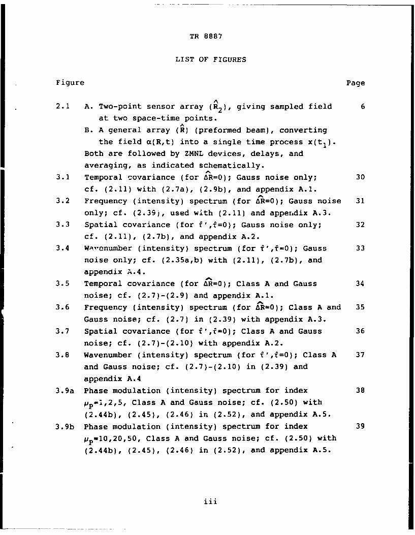
LIST OF FIGURES
Figure Page
2.1 A. Two-point sensor array (R2) , giving sampled field 6
at two space-time points.
B. A general array (R) (preformed beam), converting
the field a(R,t) into a single time process x(t1 ).
Both are followed by ZMNL devices, delays, and
averaging, as indicated schematically.
3.1 Temporal covariance (for AR=0); Gauss noise only; 30
cf. (2.11) with (2.7a), (2.9b), and appendix A.I.3.2 Frequency (intensity) spectrum (for AR=O); Gauss noise 31
only; cf. (2.39), used with (2.11) and apperdix A.3.
3.3 Spatial covariance (for f',f=0); Gauss noise only; 32
cf. (2.11), (2.7b), and appendix A.2.
3.4 W"venumber (intensity) spectrum (for f',f=0); Gauss 33
noise only; cf. (2.35a,b) with (2.11), (2.7b), and
appendix A.4.
3.5 Temporal covariance (for AR=0); Class A and Gauss 34
noise; cf. (2.7)-(2.9) and appendix A.1.
3.6 Frequency (intensity) spectrum (for AR=0); Class A and 35
Gauss noise; cf. (2.7) in (2.39) with appendix A.3.
3.7 Spatial covariance (for f',f=0); Class A and Gauss 36
noise; cf. (2.7)-(2.10) with appendix A.2.
3.8 Wavenumber (intensity) spectrum (for f',f=0); Class A 37
and Gauss noise; cf. (2.7)-(2.10) in (2.39) and
appendix A.4
3.9a Phase modulation (intensity) spectrum for index 38p-M1, 2 ,5, Class A and Gauss noise; cf. (2.50) with
(2.44b), (2.45), (2.46) in (2.52), and appendix A.5.
3.9b Phase modulation (intensity) spectrum for index 39
@p-10,20,50, Class A and Gauss noise; cf. (2.50) with
(2.44b), (2.45), (2.46) in (2.52), and appendix A.5.
iii
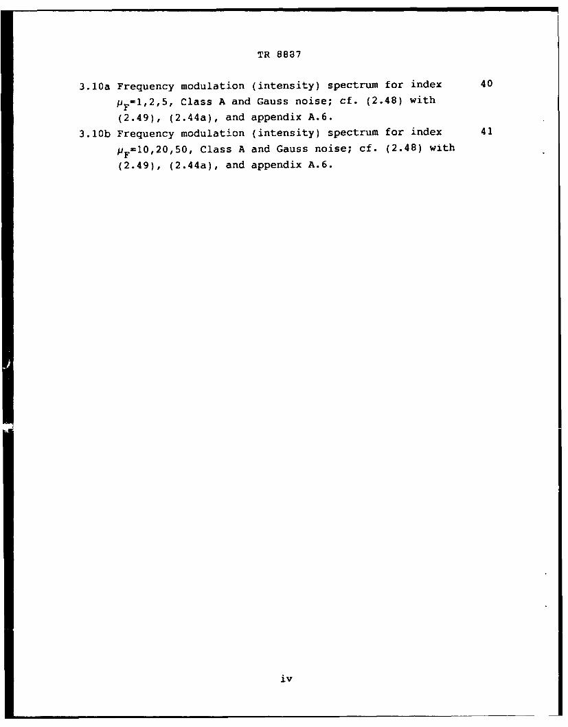
TR 8837
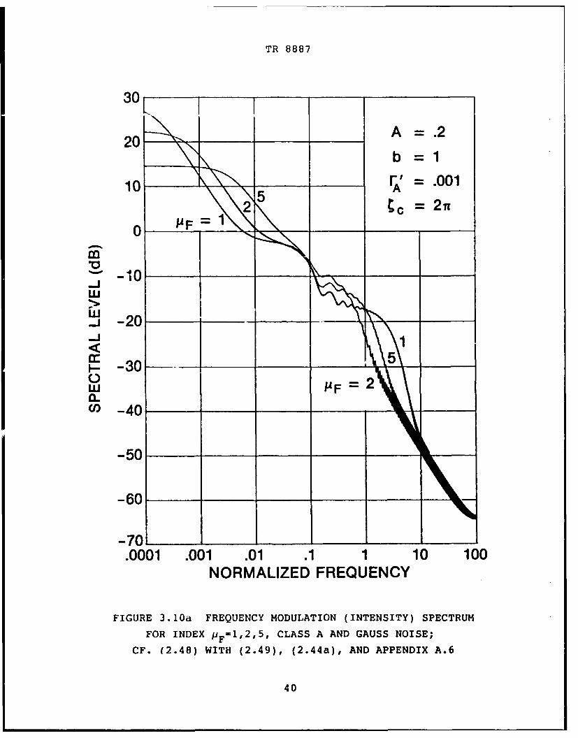
3.10a Frequency modulation (intensity) spectrum for index 40
PF=1,2,5, Class A and Gauss noise; cf. (2.48) with
(2.49), (2.44a), and appendix A.6.
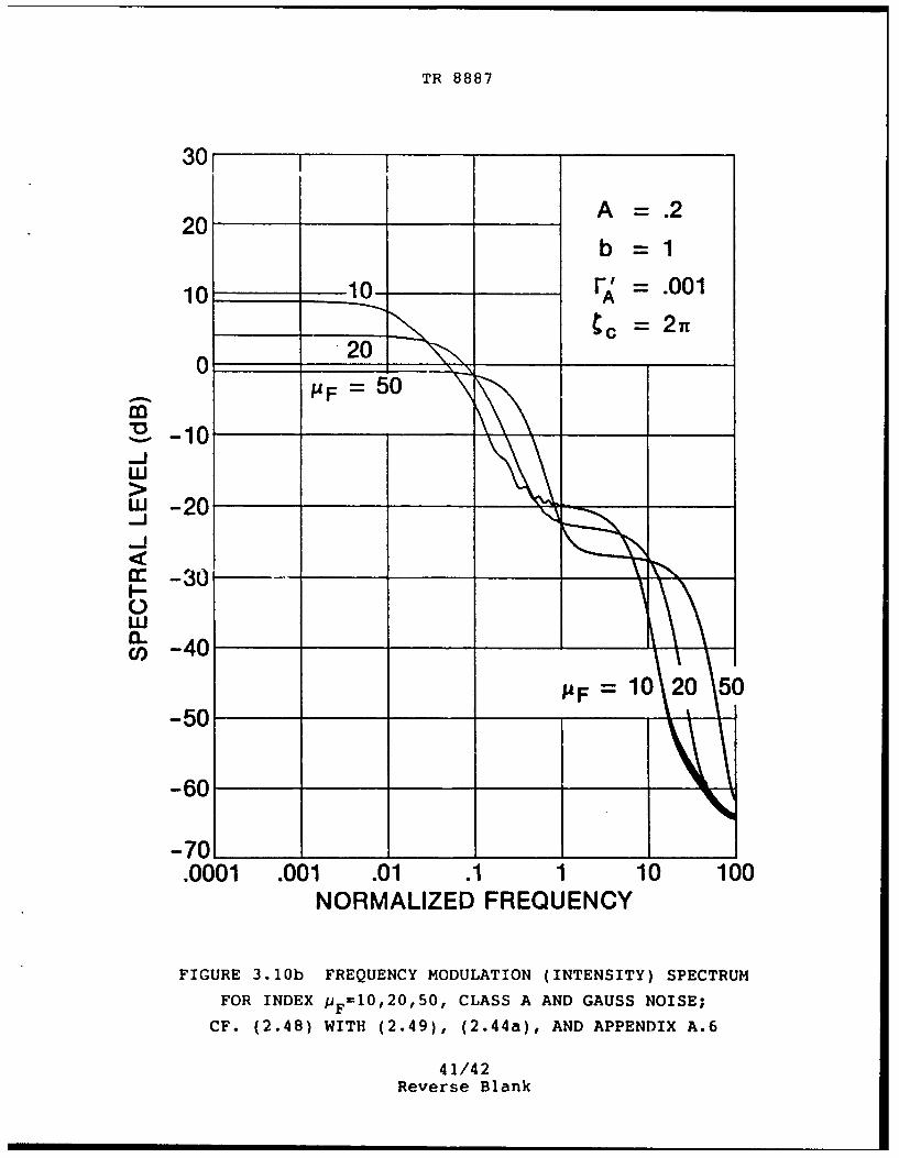
3.10b Frequency modulation (intensity) spectrum for index 41
PF=10,20,50, Class A and Gauss noise; cf. (2.48) with
(2.49), (2.44a), and appendix A.6.
iv
TR 8887
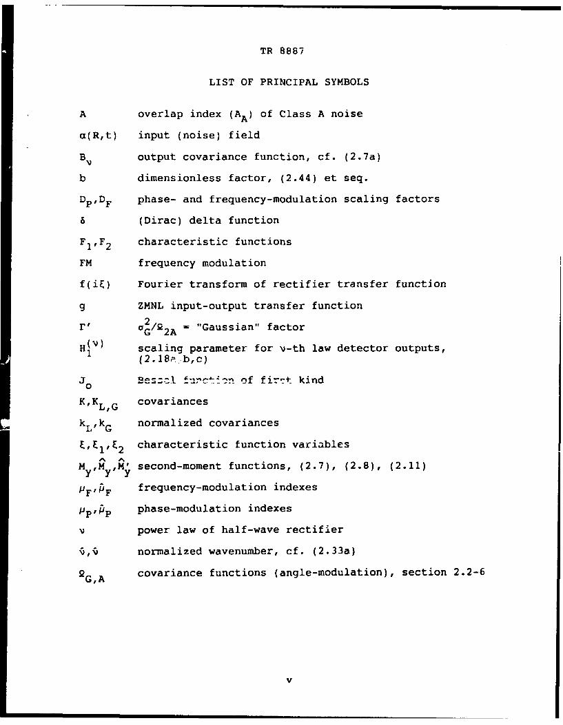
LIST OF PRINCIPAL SYMBOLS
A overlap index (AA) of Class A noise
a(R,t) input (noise) field
B output covariance function, cf. (2.7a)
b dimensionless factor, (2.44) et seq.
Dp,DF phase- and frequency-modulation scaling factors
6 (Dirac) delta function
FI,F 2 characteristic functions
FM frequency modulation
f(i&) Fourier transform of rectifier transfer function
g ZMNL input-output transfer function
' aG/ 2A "Gaussian" factor
H(V) scaling parameter for v-th law detector outputs,H1 (2.189 b,c)
Jo0 Bec'l t o of fir't kind
K,KL,G covariances
kL,kG normalized covariances
characteristic function variables
M y,M y,M second-moment functions, (2.7), (2.8), (2.11)
PFi F frequency-modulation indexes
pip phase-modulation indexes
vpower law of half-wave rectifier
normalized wavenumber, cf. (2.33a)
2G,A covariance functions (angle-modulation), section 2.2-6
v

TR 8887
2 2A intensity of Class A noise
Fo 0spectral parameter in FM, PM, (2.42c)
PM phase modulation
AR,L R spatial correlation distances
AR array operator
Re z real part of z
p"overlap" correlation function, (2.3)
n2 noise variance°m+n
a 2 intensity of Gauss noise componentG
T observation time
T waveform duration of elementary noise source
T t2-tl, delay (correlation) time
f,f' normalized delay parameters
w( ) normalJzed intensity spectrum, (2.52)
W2,W 2 (wavenumber) intensity spectra
W(,W() (frgq,,encv) intensity spectra
x,x(t) array outputs = inputs to ZMNL devices
y,y(t) outputs of ZMNL devices
Ya correlation parameter, cf. (2.7b)
ZMNL zero-memory nonlinear
vi

TR 8887
LIST OF NORMALIZING AND NORMALIZED PARAMETERS
1. 1 - ; ITs; T - t2-t : correlation delayTs = mean duration of typical interfering signal
2. p 1-IflI for IfI < 1, zero otherwise; (2.3): "overlap"
correlation function
3. AR - AR/AL (Z0); AR = IR2-R1I, correlation distance
4. ) w -/= wT s; w - 2nf: normalized (angular) frequency
A5. AwL AL /; normalized (frequency) spectrum bandwidth,
for Class A noise model
A6. AG % wG/A; normalized (frequency) spectrum bandwidth,for Gauss noise component
7. AL = rms spread of spatial covariance of non-Gaussian noise
field component
8. AG = rms spread of spatial covariance of Gaussian noise
field component
9. k - kU L: normalized wavenumber
10. A6 N = spectrum bandwidth of modulating (RC-Gauss) noise;
cf. (2.43) and [1; section 14.1-3]; cf. (11) ff.
11. N Aw N(L) bandwidth of non-Gaussian component ofmodulating noise in PM and FM;
AN > AwN(G) = bandwidth of Gaussian component ofmodulating noise in PM and FM
12. Z - T AWN' correlation variable, cf. (2.43) and (A.6-9)
and figures 3.9a through 3.10b; see (A.6-9) for c
13. f' - f - P(AR/c ), with f - T - AR/cO , cf. (2.3a)
!A- PF - PF(1+r ' ): normalized FM index; (2.53)
15. pp - pp(l+r') : normalized PM index; (2.53)
16. = (W-W 0)/AwN = normalized displaced angular frequency,
cf. (2.49)
vii/viiiReverse Blank

TR 8887
SPECTRA AND COVARIANCES FOR "CLASSICAL" NONLINEAR SIGNAL
PROCESSING PROBLEMS INVOLVING CLASS A NON-GAUSSIAN NOISE
PART I. ANALYTIC RESULTS AND NUMERICAL EXAMPLES
1. INTRODUCTION
Non-Gaussian noise fields play a critical r6le in modern
signal processing because of the frequently dominant effects of
such noise and interference in a wide variety of applications.
Communication theory generally, and specifically telecommunica-
tions, electromagnetic and acoustic scattering, man-made and
natural ambient noise, optics, and underwater acoustics, are
common areas of interest in this respect. In the present report
we are concerned primarily with underwater acoustic noise
phenomena, but the models and results are canonical, that is,
they take forms invariant to the particular physical application
in question.
Specificall), we are concerned with various second-order
statistics of non-Gaussian noise processes and fields after they
have been subjected to different types of nonlinear operations,
such as rectification and modulation. A generic problem here is
the passage of non-Gaussian noise through a zero-memory nonlinear
(ZMNL) device. The desired output statistics are typically the
mean (dc), mean intensity (power), the covariance or correlation
function, and the associated spectra. These last include
wavenumber spectra in the case of noise fields, as well as the
more general frequency-wavenumber spectra obtained by joint
temporal and spatial Fourier transformations. Typical "class-
ical" problems include: (i) rectification, (ii) determination of
output spectra and covariancez, (iii) calculation of (output)
signal-to-noise ratios, (iv) modulation, (v) demodulation, and
(vi) special systems, as for example, the spectrum analyzer.
These and other problems involving ZMNL devices are described in
detail in [1; chapters 5 and 12 - 17]. What is new here is the
TR 8887
use of the approximate second-order probability density functions
and characteristic functions in the above applications when the
noise processes are non-Gaussian.
A full treatment is given in a current study by Middleton,
[2], which is ah. expanded version of his recent paper [3], which
employs some of the results of the present report, namely, the
calculated covariances and spectra. Here, we are content to
summarize the pertinent analytic results, the corresponding
examples of calculated covariances and spectra, and the various
computational procedures associated with their evaluation. The
details of the derivations are provided in [2] and [3]. Included
here, also, is a selection of illustrations of the analytic
results.
2. ANALYTICAL RESULTS: A SUMMARY
In the present study, we address three classical problems
where the goals are the calculation of the covariance and
associated intensity spectrum. Specifically, we consider:
Problem I. The half-wave v-th law rectification of Class A
noise fields and processes;
Problem II. Phase modulation of a carrier by a Class A noise
process; and
Problem III. Frequency modulation of a carrier by a Class A
noise process.
Class A noise, as noted in section 3 of [2], [3], is a
canonical form of interference characterized by a coherent
structure vis-A-vis the (linear) front-end stages of a typical
receiver: negligible transients are produced at the output of
these stages. Class B noise, on the other hand, is incoherent
and highly impulsive, such that the front-end stages of the
receiver generate an output which consists solely of (over-
lapping) transients. Here, the Class A models are tractable in
the required second-order distribution and characteristic
functions, whereas the Class B models are not and must
2
TR 8887
consequently be appropriately approximated in second-order; see
[4] and [5] for additional information. In the present report,
we shall consider examples of Class A noise only.
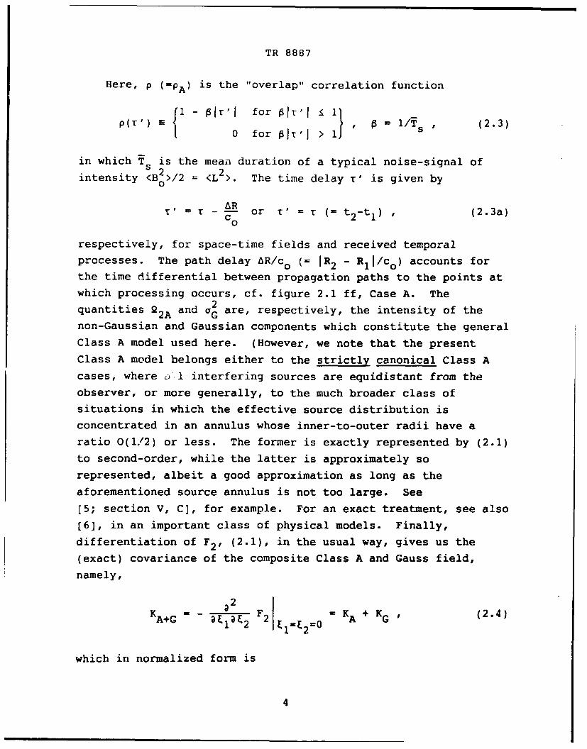
2.1 THE SECOND-ORDSR CLASS A CHARACTERISTIC FUNCTION
In applications [1] - [3], the second-order characteristic
function, F2 (i&l,i&2 ), plays a key r6le: from it, we may obtain
the aforementioned statistics of the outputs of ZMNL devices,
spectra of angle-modulated carriers, and other usually second-
order statistics of various nonlinear operations arising in a
variety of communication and measurement operations.
(See [2], [3] for further discussion.)
Here, we specifically use the approximate Class A noise
characteristic function, F2, including an additive Gaussian
component, given by
CDml1+m 2
F2(i&l,i"Z)A+G = exp[-A(2-p)] T m M2
m ,m2=0
Xmlnexp (2) ( (2.1)n=O n! 2 '
where A (=AA) is the "overlap" index, and where
(2) 2& 2 2 + 2 2 + 2& K(n) (2.2a)S+n,m2+n( ' = m+n +2 m 2 +n 1 2 L+G (
2 (i~ ~1 2 2> 2m+n m_ + A 2 2A; 22A 2 A<Bo> - A<L2>; r, ( G/Q2A, (2.2b)
K(n)L+G = (n kL/A + kG rl 22A; (2.2c)
and kL, kG are the normalized covariances of the non-Gauss and
Gauss components, respectively. Thus, IkL,GI 1 1.
3
TR 8887
Here, p (=PA) is the "overlap" correlation function
{I - PIrI for gIt'I >0 for pit'l > 1J 1/ S (2.3)
in which T sis the mean duration of a typical noise-signal of
intensity <B 0>/2 <L 2>. The time delay T' is given by
' T - c- or T' = r (= t i-ti) , (2.3a)c02
respectively, for space-time fields and received temporalprocesses. The path delay LR/c (= IR2 - RlI/Co) accounts for
the time differential between propagation paths to the points atwhich processing occurs, cf. figure 2.1 ff, Case A. The
quantities 22A and a2 are, respectively, the intensity of the
non-Gaussian and Gaussian components which constitute the general
Class A model used here. (However, we note that the present
Class A model belongs either to the strictly canonical Class A
cases, where o 1 interfering sources are equidistant from the
observer, or more generally, to the much broader class ofsituations in which the effective source distribution is
concentrated in an annulus whose inner-to-outer radii have a
ratio 0(1/2) or less. The former is exactly represented by (2.1)
to second-order, while the latter is approximately so
represented, albeit a good approximation as long as the
aforementioned source annulus is not too large. See
[5; section V, C], for example. For an exact treatment, see also
[6], in an important class of physical models. Finally,
differentiation of F2, (2.1), in the usual way, gives us the
(exact) covariance of the composite Class A and Gauss field,
namely,
a2
KA+G = - l2 F2 0 = KA + KG , (2.4)
which in normalized form is
4

TR 8887
kL + r' kGkA+G(AR'T) - 1 + T' (2.4a)
In practice, A is usually less than unity, say 0(0.1 - 0.3)
typically, so that only a comparatively few terms in A are
needed for numerical evaluation of (2.1) and the statistical
quantities derived from it, cf. section 2.2 ff. Note that when
lITI k 1, p - 0, and r'= 0, we get
c*~
F 2A - IeA ! exp e-A A n exp(-12 2
m=0 n=0
= Fl(i&l)A FI(i 2 )A , (2.4b)
as expected: there is now no correlation between process samples.
With a Gaussian component, these will be correlated, of course,
unless ITJ 4 -, so that kG 4 0, cf. (2.2c).
2.2 PROBLEM I: HALF-WAVE v-TH LAW RECTIFICATION
(STATIONARY AND HOMOGENEOUS FIELDS)
Here we consider the problem of obtaining the second-order
(second-moment) statistics, My, of a sampled noise field, a(R,t),
after passage through a ZMNL device, g, when the noise is
generally non-Gaussian. Various processing configurations are
possible. We show two in figure 2.1, below. Analytically, we
have, for stationary and homogeneous inputs [1; section 2.3-2]
My (R,T) = g(x1 )g(x2 ) = 1 2 f f f(i&) f(i 2)
(2n) i f
x F2 (i&l,i2 ;AR,T)x d 1 d& 2 = yl Y2 ' (2.5)
5
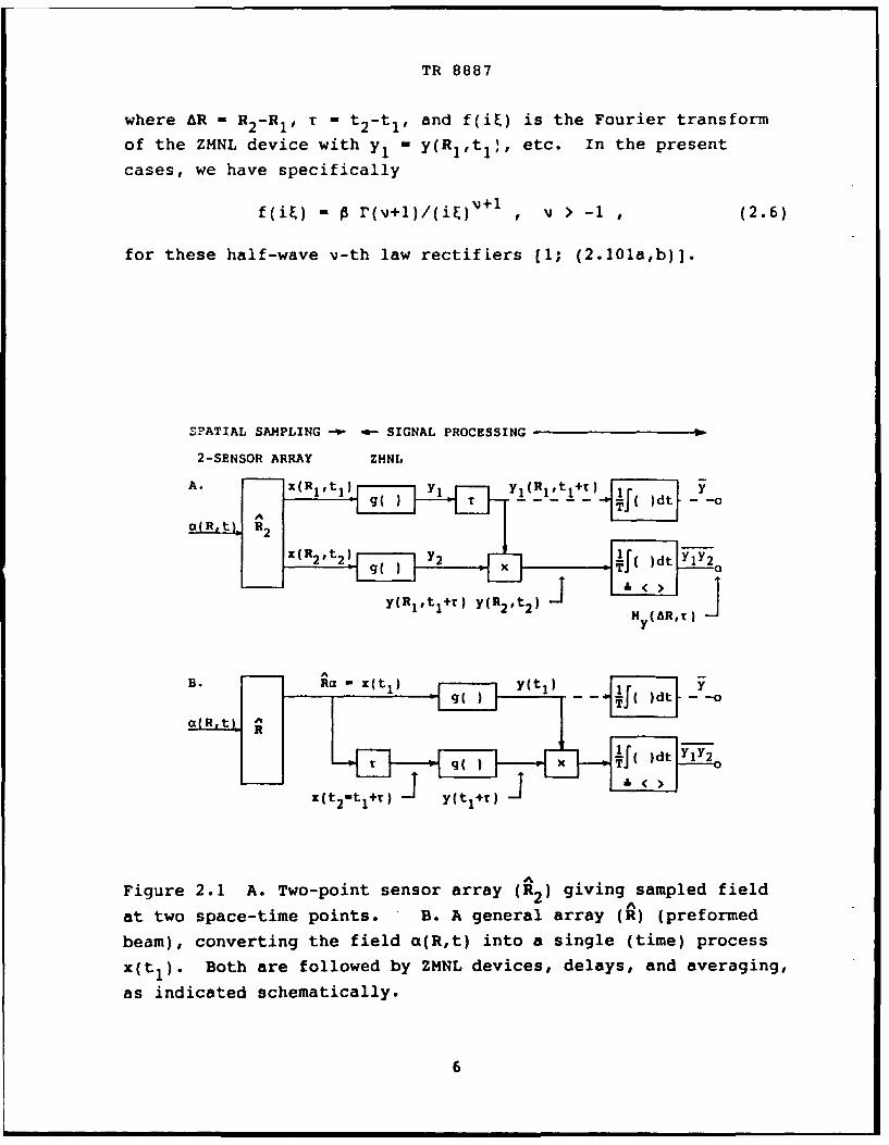
TR 8887
where AR - R 2-Rj, T - t2-t1, and f(i&) is the Fourier transform
of the ZMNL device with y1 y(Rl1tll, etc. In the present
cases, we have specifically
f~i) ~r(v+l)/(i&) V+1 ,V > -1,(2.6)
for these half-wave v-th law rectifiers f1; (2.10la,b)].
SPATIAL SAMPLING SIGNAL PROCESSING
2-SENSOR ARRAY ZMNL
a( 1 t1 r (RRt 2 R4(R
2y
Figure 2. A. Two-pint sensr) array ( 2) giigsmpeJil
attw spc-tm poi t B.A enrl rry ~ (reore
beam), converting tfild a t inosige(time proces
x(tl). Both are followed by ZMNL devices, delays, and averaging,
as indicated schematically.
6

TR 8887
For the Class A non-Gaussian noise inputs of section 2.1
above, we find that the (normalized) second-moment My for the
resulting rectified field is now
00 [A(l-p)]1 12 E (p(A~rwml+m 2
M ylAR,) = exp[-A(2-p)] m m 2 . n
m I m2=0 n=O
/2 n~m2 i/2xnm l + r') /2 _n~m2 + ri] B (2.7)
where we have further postulated the noise field to be isotropic,
AR 4 IARI, and where specifically,
B(YIml'm2 'n) = r( - ) , o.2;)
+ 2Ya r-2 (- +') aF1(JjY ,iV. ;Y2 ) ' (2.7a)
n kL + F' kG
Y ml+n + F' m + ; a = (m Vm 2 ,n) , a' I 1 •
l +r,) (m2.. + r,'I1A A (2.7b)
Specifically, also, we have the following normalized forms
My/2 2 ; ' AT' , A = /T , cf. (2.3)
AR a AR/AL, AL = correlation distance, AR = IR2-R11 . (2.8)
For numerical results, we select the following models for the
space-time covariance functions of the isotropic and stationary
non-Gaussian and Gaussian components of the input noise field:
kL = exp-AR2/ A- T(AWLr'/ 2) = exp(-R2 -A(ARLf') 2 ) , (2.9a)
2/A /A2 2 -- _ % 1 ff
kG exp(-AR2#A -1(AWGT') 2)- exp(-AR2 (A /AG) (AhG'))-) G 2L
7

TR 8887
A A
L G G (2.9b)
Here, AG is a correlation distance, and AwL, AWG are angularfrequency spreads associated with the respective non-Gaussian and
Gaussian components of the input field. Note that if we define
the correlation distance AL as that where kL = l/e (f' - 0),
then AL = R RL, etc.
For the special cases of v considered here, we also observe
(from [1; (A.1-39)]) that B may be expressed in closed form:
B0 (Y) = n + 2 arcsin(Y) , (2.10a)
BI(Y) Y arcsin(Y) + (I Y 2)+ I (.0b)
B2 (Y) [ + y2)[I + arcsin(Y)) + _y2)(.1c)
2.2-1 GAUSS PROCESSES ALONE (A=O)
When only a Gauss noise field is originally present, that is,
A = 0, for example, 22A = 0, (2.7) reduces to the classical
result [1; page 541, (13.4a)]:
A A V VAM'I = M BvM 1,P)M ; Y 4Yo k (.1y YJA=0 Bva-O ;My 4n y a a G* (.1
For comparison with the non-Gaussian cases (A>0), we choose to
have equal input noise intensities. This means that
2 +?+A=0 - uG 2A =2A(l+')
so that
MyIA=0= (1 + I')v B, a=0 ' Yo = kG (2.12)
and MI is then to be compared with My, A > 0. When r' is small,as is usually the case, we can often replace (1 + r')V by unity.
8

TR 8887
At this point, following figure 2.1, we distinguish two
classes of operation. (A), where a pair of point sensors is used
to sample the noise field aid we wish to consider both the space
and temporal correlations of the sampled field at f e two points
(Rlftl), (R2 1t2 ); and iB), where the space-time field is
cc;.verted into a random process, x(t), by the beamforming array
(R), with an associated directionality embodied in the resultant
beam (vide [7; sections IV B and VI A]).
2.2-2 CASE B, FIGURE 2.1
Let us consider the simpler case (Case B) of the time process
first, cf. (B). For this, we set AR = 0 formally in (2.7) et
seq. above, since x = R a(R,t) here and r' - T = t2 -t I, cf.
(2.3a). See also [3; (3.2) et seq. and (3.11a)]. Then our ad
hoc illustrative models of the process covariances kL, kG, are,
from (2.9a,b), at once
kL = kL(t) = exp(- (aL@/ )2 ) = exp(- -!( WLf) 2) (2.13a)
kG= kG(r) = exp(- ( wGf/,) 2 ) - exp(- ( G,) 2) • (2.13b)
Accordingly, (2.7) reduces to
Case B: M y(0,) E My(f)B - (2.7), with Ya = (2.7b),
and (2.13a,b) and AR - 0 therein. (2.14)
We note that when Ifj 1 1, p = 0, and My (O,Ifl 1 1) reduces to asimpler relation [vis-A-vis (2.7)], viz.:
A physically derived model of kG and kL may be made from* ~~~A G dkAa b aefo
[3; (3.11a)] with L - R L, R - (2.9) etc., where L is typically
given by [3; (3.3)], for example.
9
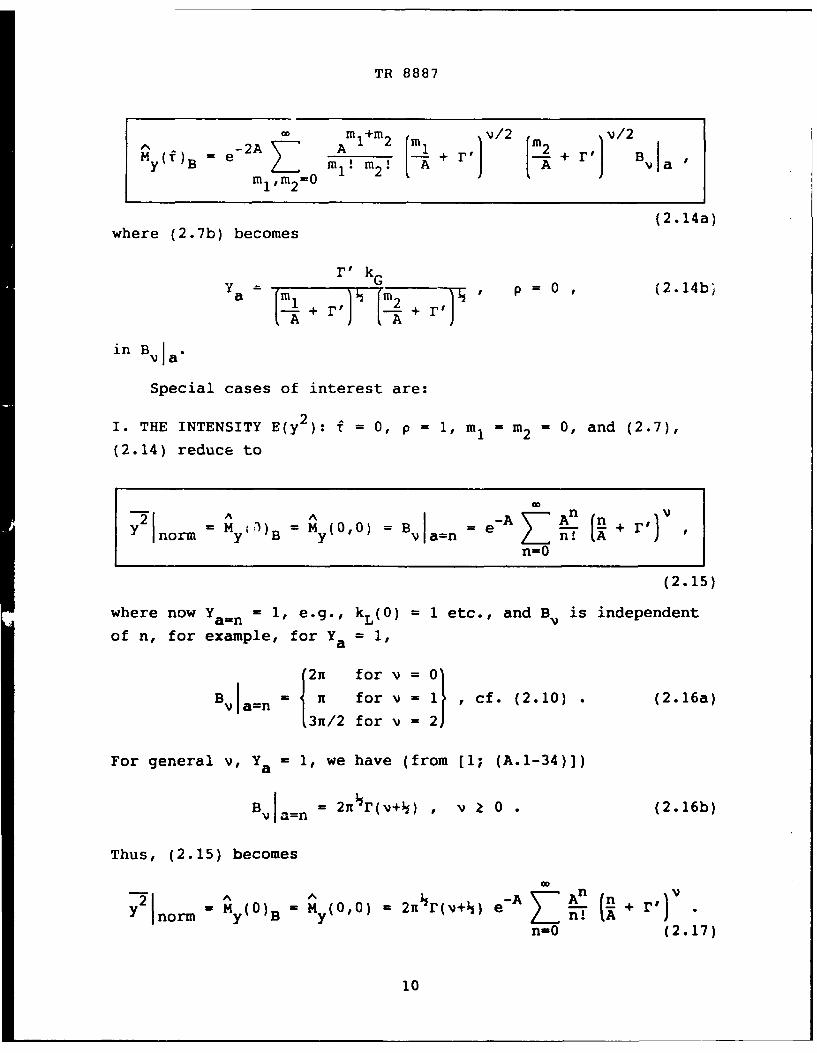
TR 8887
CO mI+m2 v/2 mv/2My(f)B = e2ml, m2:~ + r' m+ ,'Bi
me ,m2=0 + m2 + r B
(2.14a)where (2.7b) becomes
r' kG
1, a p = 0 ,a(2.14b;
in Bva
Special cases of interest are:
I. THE INTENSITY E(y 2): f = 0, p = 1, mI = m 2 = 0, and (2.7),
(2.14) reduce to
21norm My 3)B= M (0,0) = Bv1a=n = eA _ n A
n=0
(2.15)
where now Y a=n = 1, e.g., kL(O) = 1 etc., and B is independent
of n, for example, for Ya = 1,
(2n for v= 0
B vla.n ' T for v 1 ,cf. (2.10) • (2.16a)
13n/2 for v = 2
For general v, Ya = 1, we have (from [1; (A.1-34)])
BIan = 2n7r(v+ ) , z k 0 . (2.16b)
Thus, (2.15) becomes
Y 1 norm My(O)B M y(0,0) = 2n r(v+ ) e-A n An-0 (2.17)
10
TR 8887
The unnormalized form is, from (2.8),
(0)0) 2 v-1
2 2 r(v+) H(v)(Ar .)y S )B '----- M2A 1
with
H v)(A ', ' ) e-A ZI A + r,
n=0
1 for v = 0 , (2.18a)1 ' for v - 1 , (2.18b)
I/A + (1+r') 2 for v = 2 . (2.18c)
For other values of v (>0), we must evaluate H(v) numerically.
II. THE MEAN VALUE, y; If I -
Now p = 0, n - 0, Ya = 0, and (2.7) reduces directly, upon
use of (2.18), io
= yB MM (0,aD) = r 2(2L+1)e-A +
r r2 ( L2.) H( v/2 ) (A,rI) 2
(2.19)
The unnormalized form of (2.19) is, from (2.8),
2 2 V2
y= M( M(0,) = 2 ( )H (v/2 )(A,r') 2 (2.20)
and for v even, we find, from (2.18a,b,c)
H(0) , 1 , H 1 ) = 1 + r' ' H( 2 ) 1 (1 + r' . (2.21)1 1 1 A+
11
TR 8887
_2
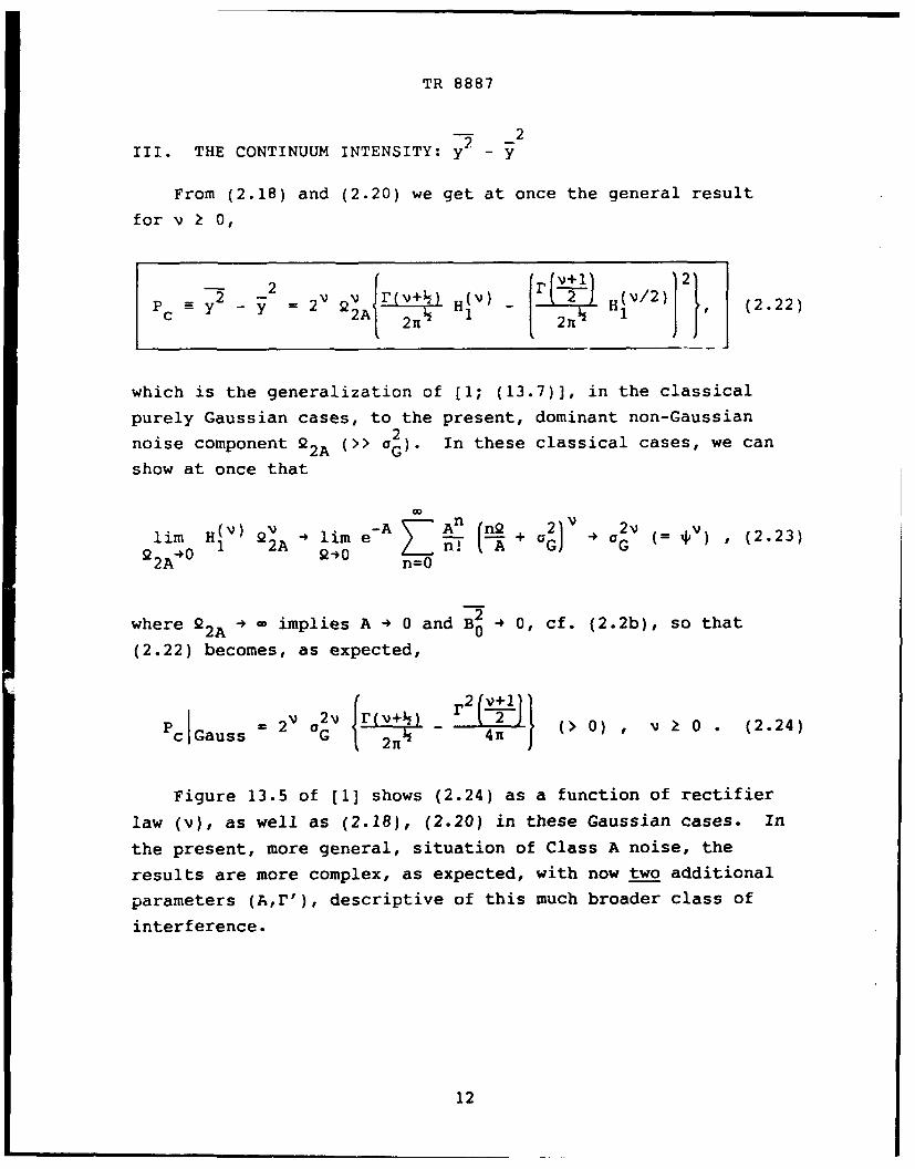
III. THE CONTINUUM INTENSITY: y - y
From (2.18) and (2.20) we get at once the general result
for v k 0,
-P - = 2Q 2A{ lI H(V) - L H(v/2) (2.22)
which is the generalization of [1; (13.7)], in the classical
purely Gaussian cases, to the present, dominant non-Gaussian
noise component 2 ). In these classical cases, we can
show at once that
lim H(v) 2 V 0 lim eA nR0 , .- + °G V _ G (= ,v) , (2.23)2 2A 4 1 2A 240 nO n! A GJ
where 22A O D implies A 4 0 and B2 4 0, cf. (2.2b), so that
(2.22) becomes, as expected,
Pc Gaus = C2 2v {LLv±~.I (> 0) ,v Z 0 .(2.24)Pc Gauss G _2R l- 4n
Figure 13.5 of [1] shows (2.24) as a function of rectifier
law (v), as well as (2.18), (2.20) in these Gaussian cases. In
the present, more general, situation of Class A noise, the
results are more complex, as expected, with now two additional
parameters (A,r'), descriptive of this much broader class of
interference.
12
TR 8887
2.2-3: CASE A, FIGURE 2.1
We turn now to the more general problem of the covariance of
the Class A non-Gaussian random field, sampled according to
procedure (A), shown schematically in figure 2.1 earlier. Here,
x = a(R,t), sensed at (Rl,tl), (R2,t2 ), where L - L, cf. (3.3) in
[3; (3.2)]. Equation (2.7) applies here, with AR P 0 (as well as
for LR - 0), and we use (2.9a,b) for our illustrative examples,
which are discussed in section 3 following. At this point, we
recall from (2.3a) that the proper time delay to use is
T' = r - AR/c o in p = p(r'), and in some of the structural
elements of the noise field covariances, cf. [3; (3.11b,c)].
CASE I: f' = 0
From (2.7), we have p = 1, m = m2 = 1, giving
^ e~-A 7-- An E + B an f R
y(AR,0) - + )' p 1 , :.T = ,(2.25)
n=0
where (2.7b) is specifically
nA
SkL( RO) + r' kG(AR,O)y - . (2.25a)a=n n-- + r'
For calculations, (2.9a,b) are used, with BV given by (2.7a),
where (2.25a) provides Ya" When AR = 0, (2.25) reduces to (2.15)
et seq. for the total intensity of the field observed at R1 m R2.
13
TR 8887
CASE II: AR 4 w, jt' > 1
When &R 4 m, we obtain different results, depending on T'.
Here p - 0, Y a 0, cf. (2.9a,b) in (2.7b), and therefore n - 0.
Accordingly, (2.7) becomes
2Sy, > 1) = y 0 Ynorm (2.19). (2.26)
The fact that AR 4 w ensures that Y 4 0, a behavior similar toathat for Case (B) above, when we consider the purely Gaussian
noise process, section 2.2-i.
CASE III: LR 4 -, 0 < IT'l < 1
Here, p > 0 while Y a 0, so that B , (2.7b), becomes r2(V+ )
once more. The second moment function (2.7) is now
00 m1+m 2My(,') ___ exp-A(2- [A(l-p) 1
-+2 Tm! m2
xn! A A- (2.27)
n-0
which is a minor simplification of (2.7).
CASE IV: AR 4 W, It'I = 0
In this special situation, where T - AR/c 0 w in such a way
that T' = 0 and therefore p = 1, Ya = 0, we obtain directly from
(2.27) the comparatively simple result,
My(C,0) = r (> 0) . (2.28)
14
TR 8887
2.2-4: REMARKS
At first glance, as AR 4 , we might expect M always to-2 -- foYhreduce to y , e.g., K M -y 2 0 for the covariance of the
y yrectified space-time field. This is expectedly the case for the
covariance (and second-moment) function of the input Class A and
Gauss noise field components c(R,t), as we can see directly from
(2.9a,b), or from [3; (3.11b,c)] for example, in the physically
derived cases. However, the process or field y = g(x) here is
the result of a nonlinear operation, cf. (2.5), (2.6), which
severely distorts the input waveform and generates all kinds of
modulation products, associated with the spatial as well as the
temporal variations of the input field. This accounts for the
departures in Cases III, IV of M (Wf') from -2, while certainly-2 ( y
Mx ([,r') + x 0, (since x = 0 initially here).
From the various limiting results above, we see that
M y(0,0) > My (,O) and M y(0,0) > M y(0,) , (2.29a)
and
> (M2 0)bMy(W,0) M y(0,-) depending on A, r', and v ,(2.29b)
with
M y(0,0) - M y(0,-) > 0 , cf. (2.19) and (2,20) , (2.29c)
2M ( = M (0,-) = y , cf. (2.20) and (2.26) , (2.29d)Y Y
whereas
2M x(0,0) > M x(0,-) = Mx (W,0) - x 0 (2.29e)
Finally, we note that (2.11), (2.12) apply here, also, for
the Gauss-alone cases, where now
s2A(1 + a 2 and B (1 + r')V Bvla " 0
15
TR 8887
2.2-5: SPECTRA
The various intensity spectra associated with the output of
the processor (cf. figure 2.1) are important also, as they show
how the energy in this output is distributed. Here, we consider
two types of spectra, respectively, for the rec t ified spatial
field (A) and for the process (B), namely the wavenumber and the
frequency spectrum of y(R,O) and y(O,t). In particular,
wavenumber spectra are useful in the analysis of spatially
distributed phenomena, paralleling the analysis of time-dependent
phenomena.
I: WAVENUMBER SPECTRUM
The wavenumber intensity spectrum is defined here by
W2(k,0)y = W2 (kT)ylr=0 s ff My(AR,O) exp(ik-AR) d(AR) (2.30a)
AR
- 2n f My(AR,O) J0 (kAR) AR d(AR) = W2 (k,O) y , (2.30b)
0
with
k = (k x,k) , fR = IARI k = Ikl (2.30c)
for these isotropic fields, where k is an (angular) vector
wavenumber. Using the normalization of (2.8), we get, with
k kALL,
W2 (k'0)Y AW W = 2n My(X,O) J (kx) x dx (2.31)2(k'y a2 2v 2 /2v,4 f
L 0
for the normalized wavenumber intensity spectrum.
16
TR 8887
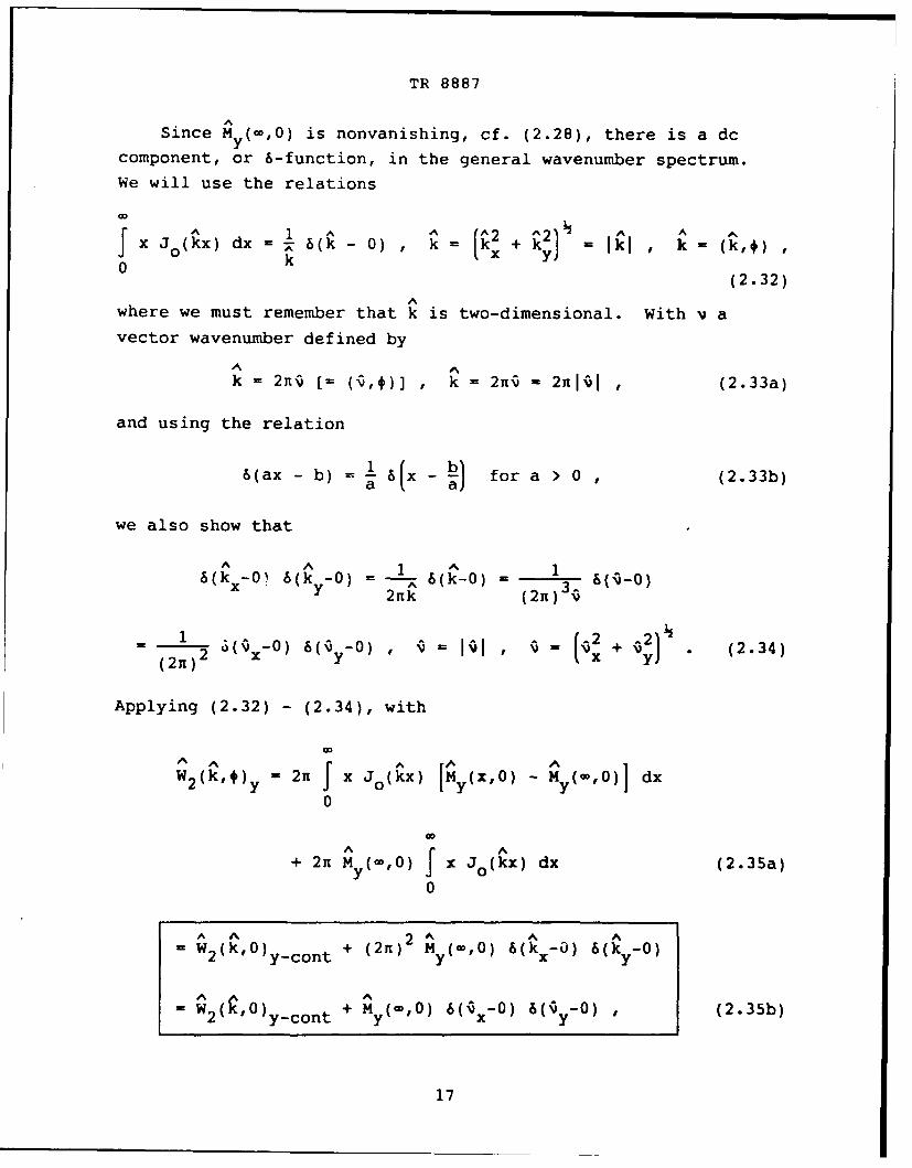
ASince My (,0) is nonvanishing, cf. (2.28), there is a dc
component, or 6-function, in the general wavenumber spectrum.
We will use the relations
J X) 1 A( A (A 2 + ̂ 2) A,oXdx = b(k - 0) , k t + k = Ik, k (k,+)0k
(2.32)
Awhere we must remember that k is two-dimensional. With v avector wavenumber defined by
k = 2ij [= (',)] , k = 2n, - 21tIi, (2.33a)
and using the relation
6(ax - b) = ' 6 x - for a > 0 , (2.33b)
we also show that
-0 -0 1 6(kA) =X Y 2Rk (2n) 3
1 ( -0) 61y-0) , = I, 2 + '2 • (2.34)
(2nT)2 x y y
Applying (2.32) - (2.34), with
A A A1
W2 (k,+) - 2n x J0 (kX) IMy(XO) - M ylO)I dx
0
AA
+ 2R My (,0) x Jolkx) dx (2.35a)
0
A 2 A A A= W2(Ok,0lycont + (2n) My(-,0) 6(kx-0) -(kY-0)
AA A- W2(k,0) nt + M(,) 6( x-0) 6(iy-0) , (2.35b)2 y-cont +y x Y
17
TR 8887
AAwhich defines W 2(kO) ycont' the continuous portion of the
Aspectrum and shows the dc term in k- or v -space, as convenient.
it is W 2 -cont with which we are concerned in the specific
numerical examples of section 3 ff.
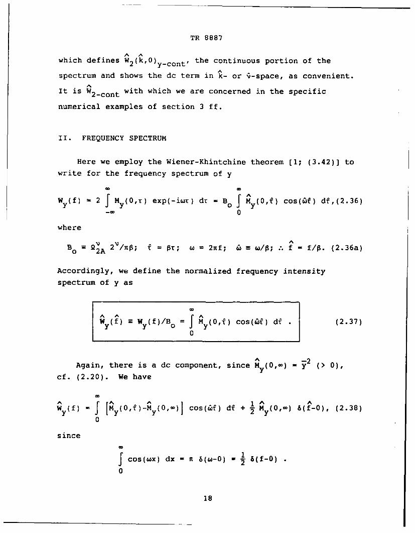
II. FREQUENCY SPECTRUM
Here we employ the wiener-Khintchine theorem [1; (3.42)] to
write for the frequency spectrum of y
(f) 2 fJC M y(0,T) exp(-iwt) dt = B 0 0 M y(O0j) cos(af) df,(2.36)
where
Bo =22A 2 U;f= T 2nf; a =w/t f = f/A. (2.36a)
Accordingly, we define the normalized frequency intensity
spectrum of y as
W y (f) =W Y (f) /B0 f M y(O0j) cos(Qf) df .(2.37)
0
Again, there is a dc component, sinc M2 pO~ =y ( 0),
cf. (2.20). We have
A AA A(f M (O,, (0u- cos(Cof) df + _I 1 (0,-n) 6f0,(2.38)
y f [ y y (1)2y0
since
jcos(wx) dx - i6(w-0) - 6(f-O)
0
18

TR 8887
As in the wavenumber cases above (Case I), we are concerned with
the continuous part of the spectrum, viz.
A I2W y(f) Jot3 IM y(,f) - yIcos(wf) df ,(2.39)
0
which is also illustrated numerically in section 3 ff.
III. WAVENUMBER FREQUENCY SPECTRUM
The wavenumber frequency spectrum is defined by
W2 (k,w)y = f My(ART) exp(ik-AR-iiT) d(AR) d, (2.40)
with w = 2nf. The associated wavenumber spectrum W2 (k,0) used in
(2.30) is obtaincd from W2 (k,r)IT=o. In normalized form, we have
for (2.40), in these isotropic cases,
A A -1W~~ 2 k6 222A a /14no) W 2l(k'wly
M J R,) exp(ik-AR-i~f) d(AR) df ;
W2(k, l) y W 2n f My(Xf) J0(kx) exp(-iGjf) x dx df . (2.41)
00
The various dc components are readily extracted, as in Cases I
and II above. Numerical examples of this joint intensity
spectrum are reserved to a possible subsequent study. The
results of section 3 show the marginal spectra (Cases I, II) of
this more general situation.
19
TR 8887
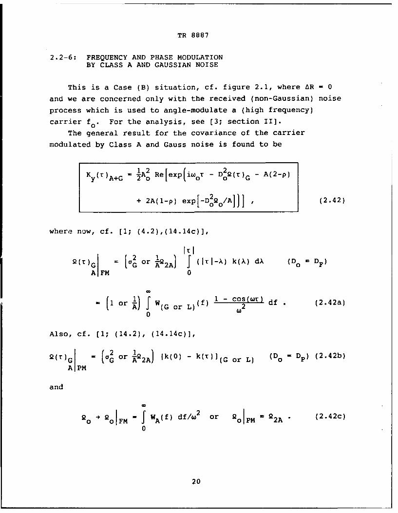
2.2-6: FREQUENCY AND PHASE MODULATIONBY CLASS A AND GAUSSIAN NOISE
This is a Case (B) situation, cf. figure 2.1, where AR = 0
and we are concerned only with the received (non-Gaussian) noise
process which is used to angle-modulate a (high frequency)
carrier f0. For the analysis, see [3; section II].
The general result for the covariance of the carrier
modulated by Class A and Gauss noise is found to be
K2 o exp D22y(t)A+G = Re piwot DoQ(t)G - A(2-p)
+ 2A(l-p) exp1-D22o/A])I , (2.42)
where now, cf. [1; (4.2),(14.14c)],
I II(c)G a G or A22A) J (IrI-k) k(X) dX (Do - DF)
A FM 0
(1 or G Lf ) 1 - cos(WT) df . (2.42a)A) fj( or L)'20
Also, cf. [1; (14.2), (14.14c)],
2(T - (a2 or 12A (k(0) - k(T)I(G or L) (Do = Dp) (2.42b)
APM
and
2 = +2 WA(f) df/w2 or 2 oIPM =22A 2(2.42c)
0
20
TR 8887
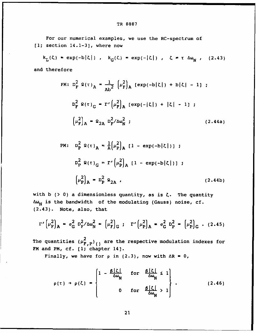
For our numerical examples, we use the RC-spectrum of
[1; section 14.1-3], where now
kL(Z) - exp(-bRI) kG(<) - exp(-ICI) C r A N (2.43)
and therefore
FM: D A -2( 1 FJA [exp(-blCl) + bi - 1]
F 2 (T) r, 2'pl (exp(-RCI) + II 1]
P = 22A DF/&N ; (2.44a)
PM: D 2(T)A _ 2 [I - exp(-bRIC)]
D2 2 (T) r'(,) [1 - exp(-bII)] ;Dp )G )A
(P)A= D 2 2A (2.44b)
with b (> 0) a dimensionless quantity, as is C. The quantity
AWN is the bandwidth of the modulating (Gauss) noise, cf.
(2.43). Note, also, that
r112 a2 D 2/&w 2 _ (P =(2 G D 2 .. P (2.45)VF A - G F N FJG ; 'P)A - G P G "2
The quantities (p Fp() are the respective modulation indexes for
FM and PM, cf. [1; chapter 14].
Finally, we have for p in (2.3), now with AR = 0,
1f- LLL[ f or lA N A Np(T) P (C) .0 f L J (2.46)
0 for ftW 1A2
N
21

TR 8887
Putting the above (2.43), (2.44) in (2.42), we now specialize
our results,
yr)A+G 2o ko(T) cOS(oT) ' with ko(0) - 1 , (2.47)
to the normalized covariance k0 (r), respectively, for FM and PM,
and their associated spectra. We have for these carriers
modulated by a sum of Gaussian and Class A noise:
I. FREQUENCY MODULATION
k(~F - exp[-rfA [ exp(-IJJ) + jij- 1] - A(2-p)
+ Ap exp (- _ FA [exp(-bI~I) + bItI - 1] , (2.48)
with p(T) given by (2.46). Here, 2oIFM 4 - in (2.42). Since
lim ko(C)F M - 0< FM
there is no dc in koFM, and hence all the original carrier power
(-A /2) is distributed into the sideband continuum for this0highly nonlinear modulation, as expected [1; section 14.1-2].
The associated intensity spectrum for koIFM is defined by
W(wIA+GfFM = ko()FM cos(6) dt , o N (2.49)0
which is determined by a direct cosine transform of k o(r)FM . See
appendix A.6 ff.
22
TR 8887
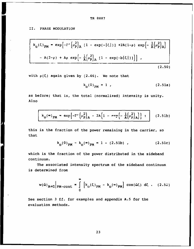
II. PHASE MODULATION
0(Z,) PM-exp[-'(23 [1 - exp(-ItI)] +2A(1-p) exp(- (~A
-A(2-p) + Ap exp(-~~AI exp(-bjVI)])
(2.50)
with p(? ) again given by (2.46). We note that
k ()M= 1 , (2.51a)
as before; that is, the total (normalized) intensity is unity.
Also
k (a-)Pm exp[-P'142 - 2A(l I(IJf2l (2.51b)
this is the fraction of the power remaining in the carrier, so
that
k 0(O)pM - ko -PM = 1 - (2.51b) ,(2.51c)
which is the fraction of the power distributed in the sideband
continuum.
The associated intensity spectrum of the sideband continuum
is determined from
w( 6)A+GIPM-cont f [ [k 0 R1) 1 - ko(a-)PM I cos(CC) dt . (2.52)
0
See section 3 ff. for examples and appendix A.5 for the
evaluation methods.
23

TR 8887
Finally, in the equivalent Gaussian cases. (Gauss noise
modulation of equal intensity and basic spectrum, e.g.,
12). r,('). r, A (1 + r') andk k
we see that (2.48), (2.50) reduce to
[+2MGep-(~l r' [exp(-bjlI) + bIjI 1]/b 2 ]
(A2)" (1 + v')(P24A (2.53a)
k0 R PMGus exp [+2if r' [1 -exp(-bW4)]J
([~A (l + v')(P2A (2.53b)
with spectra obta~ined as before, from (2.49) and (2.52).
24
TR 8607
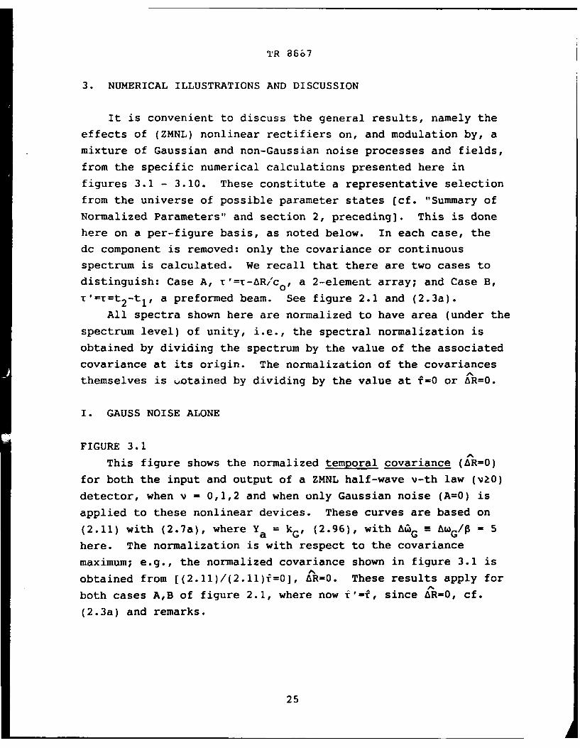
3. NUMERICAL ILLUSTRATIONS AND DISCUSSION
It is convenient to discuss the general results, namely the
effects of (ZMNL) nonlinear rectifiers on, and modulation by, a
mixture of Gaussian and non-Gaussian noise processes and fields,
from the specific numerical calculations presented here in
figures 3.1 - 3.10. These constitute a representative selection
from the universe of possible parameter states [cf. "Summary of
Normalized Parameters" and section 2, preceding]. This is done
here on a per-figure basis, as noted below. In each case, the
dc component is removed: only the covariance or continuous
spectrum is calculated. We recall that there are two cases to
distinguish: Case A, T'=T-AR/'c0 , a 2-element array; and Case B,
T'==t 2-tI, a preformed beam. See figure 2.1 and (2.3a).
All spectra shown here are normalized to have area (under the
spectrum level) of unity, i.e., the spectral normalization is
obtained by dividing the spectrum by the value of the associated
covariance at its origin. The normalization of the covariances
themselves is ouotained by dividing by the value at f=0 or SR=0.
I. GAUSS NOISE ALONE
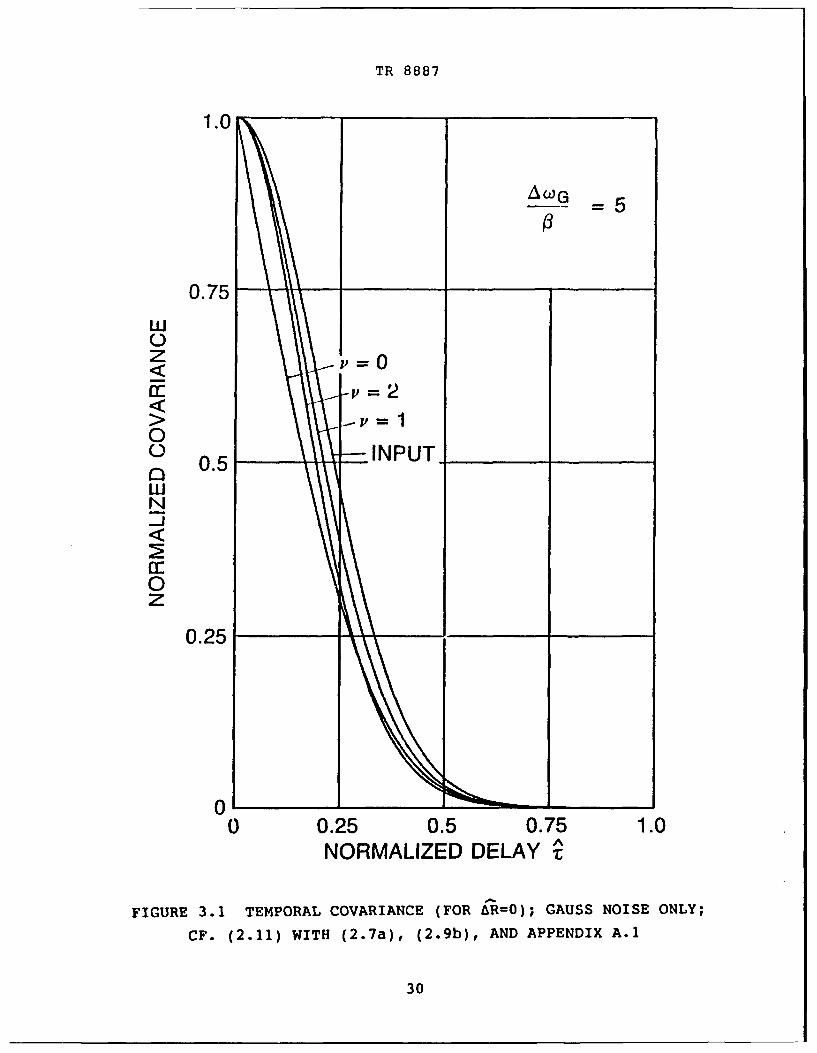
FIGURE 3.1
This figure shows the normalized temporal covariance (AR=0)
for both the input and output of a ZMNL half-wave v-th law (vO)
detector, when v = 0,1,2 and when only Gaussian noise (A=0) is
applied to these nonlinear devices. These curves are based on
(2.11) with (2.7a), where Ya = kG' (2.96), with AG a AG/A - 5
here. The normalization is with respect to the covariance
maximum; e.g., the normalized covariance shown in figure 3.1 is
obtained from [(2.11)/(2.11)f=0], AR=0. These results apply for
both cases A,B of figure 2.1, where now i'-f, since AR=0, cf.
(2.3a) and remarks.
25

TR 8887
As expected (cf. [1; chapter 13]), the general nonlinearity
(2.6), vZO, contracts the covariance, which is equivalent to
spreading the spectrum vis-&-vis the input , cf. figure 3.2,
below. Moreover, the greater the distortion (v=0,2), usually the
greater are these effects. (See appendix A.1.]
FIGURE 3.2
This is the same situation as shown in figure 3.1, except
that the normalized intensity (frequency) spectrum is calculated
now [cf. section 2.2-5, Case II, (2.39)] with My (O,f), (2.11),
used in (2.39). Observe the greatly broadened spectra,
particularly at the low spectral levels, where the greater spread
occurs for the "super-clipper", v=O, cf. remarks, figure 3.1;
also, appendix A.3.
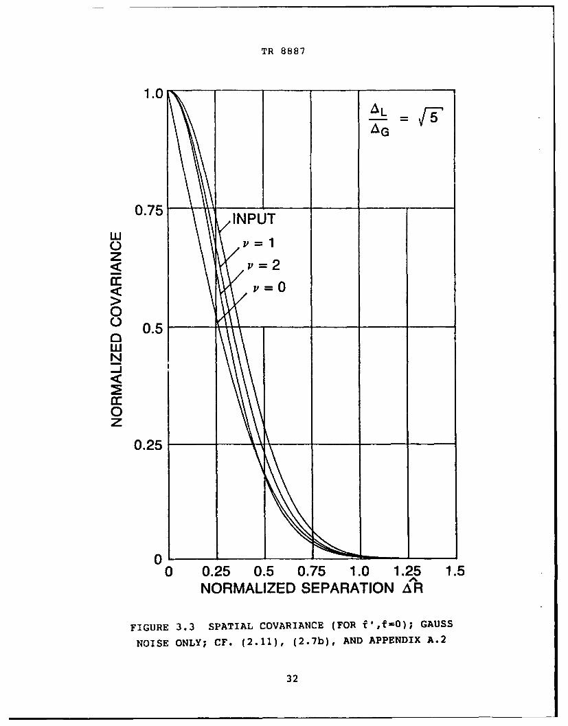
FIGURE 3.3
For the same purely Gaussian field above, cf. (2.11) and
(2.96), with f,'-0, the spatial covarirnce is calculated, with
parameters AL /1G = 5h, using (2.11) as before. The normalization
is with respect to the covariance at AR-0. Again, one observes
the same kind of contraction in the covariance as noted in figure
3.1. [See appendix A.2.]
FIGURE 3.4
This is the wavenumber analogue of the frequency spectrum of
figure 3.2, now with f',f-0, and is obtained from (2.35a,b) with
aL /AG- 5 . The rectification operation similarly spreads the
wavenumber spectrum, with the greatest distortion (v-0) yielding
the greatest wavenumber spread, as expected from the
corresponding contraction of the associated covariance, cf.
figure 3.3 above. [See appendix A.4.]
26
TR 8887
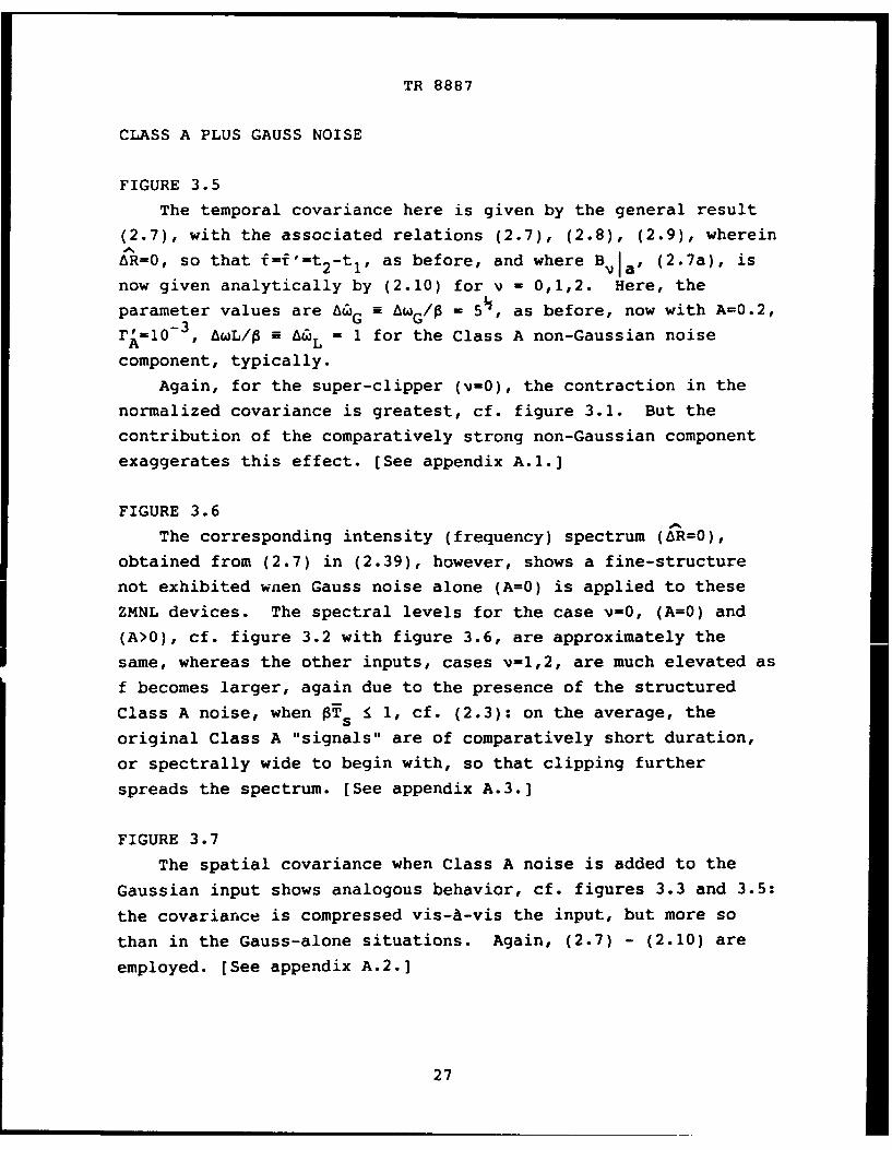
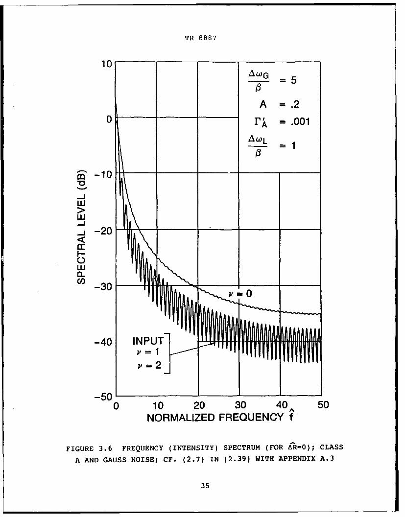
CLASS A PLUS GAUSS NOISE
FIGURE 3.5
The temporal covariance here is given by the general result
(2.7), with the associated relations (2.7), (2.8), (2.9), wherein
AR=0, so that f=f'-t 2-tI , as before, and where B Ia, (2.7a), is
now given analytically by (2.10) for v - 0,1,2. Here, theparameter values are G E G/ 5pramet Gae a = , as before, now with A=0.2,
AI0-3 , AwL/- a* AWL - 1 for the Class A non-Gaussian noise
component, typically.
Again, for the super-clipper (v-0), the contraction in the
normalized covariance is greatest, cf. figure 3.1. But the
contribution of the comparatively strong non-Gaussian component
exaggerates this effect. [See appendix A.1.]
FIGURE 3.6
The corresponding intensity (frequency) spectrum (AR=0),
obtained from (2.7) in (2.39), however, shows a fine-structure
not exhibited wnen Gauss noise alone (A=0) is applied to these
ZMNL devices. The spectral levels for the case v=0, (A=0) and
(A>0), cf. figure 3.2 with figure 3.6, are approximately the
same, whereas the other inputs, cases v=1,2, are much elevated as
f becomes larger, again due to the presence of the structured
Class A noise, when Ts 1 1, cf. (2.3): on the average, the
original Class A "signals" are of comparatively short duration,
or spectrally wide to begin with, so that clipping further
spreads the spectrum. [See appendix A.3.]
FIGURE 3.7
The spatial covariance when Class A noise is added to the
Gaussian input shows analogous behavior, cf. figures 3.3 and 3.5:
the covariance is compressed vis-A-vis the input, but more so
than in the Gauss-alone situations. Again, (2.7) - (2.10) are
employed. [See appendix A.2.]
27
TR 8887
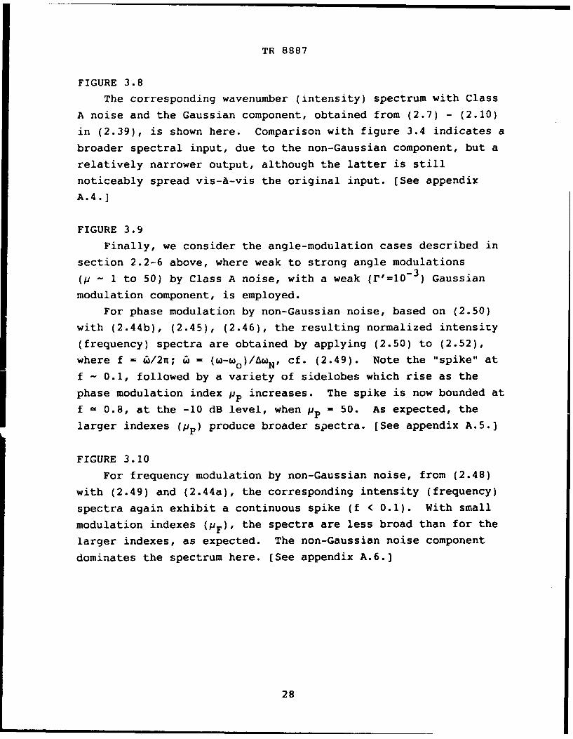
FIGURE 3.8
The corresponding wavenumber (intensity) spectrum with Class
A noise and the Gaussian component, obtained from (2.7) - (2.10)
in (2.39), is shown here. Comparison with figure 3.4 indicates a
broader spectral input, due to the non-Gaussian component, but a
relatively narrower output, although the latter is still
noticeably spread vis-&-vis the original input. [See appendix
A.4.]
FIGURE 3.9
Finally, we consider the angle-modulation cases described in
section 2.2-6 above, where weak to strong angle modulations
( - 1 to 50) by Class A noise, with a weak (r'=0 - 3 ) Gaussian
modulation component, is employed.
For phase modulation by non-Gaussian noise, based on (2.50)
with (2.44b), (2.45), (2.46), the resulting normalized intensity
(frequency) spectra are obtained by applying (2.50) to (2.52),
where f = CB/2n; 6 = (w- 0)/A N, cf. (2.49). Note the "spike" at
f ~ 0.1, followed by a variety of sidelobes which rise as the
phase modulation index pp increases. The spike is now bounded at
f - 0.8, at the -10 dB level, when pp - 50. As expected, the
larger indexes (p) produce broader spectra. [See appendix A.5.]
FIGURE 3.10
For frequency modulation by non-Gaussian noise, from (2.48)
with (2.49) and (2.44a), the corresponding intensity (frequency)
spectra again exhibit a continuous spike (f < 0.1). With small
modulation indexes (PF), the spectra are less broad than for the
larger indexes, as expected. The non-Gaussian noise component
dominates the spectrum here. [See appendix A.6.]
28
TR 8887
EXTENSIONS
Other situations where the second-order Class A probability
density functions may be applied are noted in [2] and [3]. We
list some of the extensions of the analysis to the following
"classical" problems:
1) The inclusion of representative signals, with Gauss and
non-Gauss (Class A) noise, in the problems already treated
here (section 2);
2) The case of the full-wave square-law rectifier, with both
Class A and B noise, as well as Gauss noise;
3) The extension of 2) to include general broadband and
narrowband signals;
4) The calculation of signal-to-noise ratios and deflection
criteria, cf. [1; section 5.3-4].
5) Covariances and spectra for ZMNL system outputs, with
signals as well as non-Gaussian noise inputs;
6) The r6le of the electromagnetic (or acoustic) interference
(EMI or icI) scenario, cf. [5; section 2B,5];
7) Evaluation of the large (FM,PM) indexes, or asymptotically
Gaussiar cases, cf. [12].
Further opportunities to extend the classical theory [2],[3],
now with non-Gaussian noise inputs, are evident from the examples
and methods described in [1; chapters 5, 12 - 16], for instance.
29
TR 8887
1.0
ACLG 5
0.75
w0
00.5 INPUT-____
wN
a:-0
0.25
0 0.25 0.5 0.75 1.0NORMALIZED DELAY
FIGURE 3.1 TEMPORAL COVARIANCE (FOR AR=O); GAUSS NOISE ONLY;
CF. (2.11) WITH (2.7a), (2.9b), AND APPENDIX A.1
30

TR 8887
0ZAWG 5
-10
-20
-30
-1-40-ww
-50
-6 -0--CL
-8
-70-
-1000 10 20 30 4 0 A 50
NORMALIZED FREQUENCY f
FIGURE 3.2 FREQUENCY (INTENSITY) SPECTRUM (FOR A-R-O); GAUSS
NOISE ONLY; CF. (2.39), USED WITH (2.11), AND APPENDIX A.3
31
TR 8887
1.0A L
AG
0.75 INPUTwz 2
00.5-
wN
0
0.25
0 0.25 0.5 0.75 1.0 1.25 1.5NORMALIZED SEPARATION AR
FIGURE 3.3 SPATIAL COVARIANCE (FOR f',f =0); GAUSS
NOISE ONLY; CF. (2.11), (2.7b), AND APPENDIX A.2
32

TR 8887
0
-101 AL y/-
-20
-30-
-- 4 0w
-- 50-
-60'
-80
-90
-10010 20 40 60 80
NORMALIZED WAVENUMBER k
FIGURE 3.4 WAVENUMBER (INTENSITY) SPECTRUM (FOR f',f =0); GAUSS
NOISE ONLY; CF. (2.35a,b) WITH (2.11), (2.7b), AND APPENDIX A.4
33

TR 8887
1.0
A =.2
A .001
0.75 AWOL -1
0
0.
N
p 0
0z
0.25
0l0 0.25 0.5 0.75 1.0
NORMALIZED DELAY
FIGURE 3.5 TEMPORAL COVARIANCE (FOR bR=O); CLASS A
AND GAUSS NOISE; CF. (2.7)-(2.9) AND APPENDIX A.1
34
TR 8887
10AWG 5
A =.2
0 r, .001
AWL
M %-10
ww
-20
0wa-C) 3 0 A
010 20 30 40 A 50NORMALIZED FREQUENCY f
FIGURE 3.6 FREQUENCY (INTENSITY) SPECTRUM (FOR AR=O); CLASS
A AND GAUSS NOISE; CF. (2.7) IN (2.39) WITH APPENDIX A.3
35

TR 8887
AL F
A =.2
INPUT = .001
0.75w
20z
° 0
00.5
wN
0
0.25
00 0.5 1.0 1.5 2.0 2.5 3.0
NORMALIZED SEPARATION A' l
FIGURE 3.7 SPATIAL COVARIANCE (FOR f',f-0); CLASS A
AND GAUSS NOISE; CF. (2.7)-(2.10) WITH APPENDIX A.2
36

TR 8887
10 AL
0_ _ _ A G
-10 A -0
-20-
-1 - 3 0 v=w
-40
I--50w
l -60 1
-70-
-80-
0 10 20 30 40 50 60 70 80NORMALIZED WAVENUMBER k~
FIGURE 3.8 WAVENUMBER SPECTRUM (FOR f',f-O); CLASS A AND
GAUSS NOISE; CF. (2.7)-(2.10) IN (2.38a,b) AND APPENDIX A.4
~37

TR 8887
01
A=.2
-10 b=1
F'; .001
-~-20 1 Vc=2T
w
w
0
cf) -40
-50
-60____ _
.01 .11 10 100NORMALIZED FREQUENCY
FIGURE 3.9a PHASE MODULATION (INTENSITY) SPECTRUM FOR
INDEX pp125 CLASS A AND GAUSS NOISE; CF. (2.50) WITH
(2.44b), (2.45), (2.46) IN (2.52), AND APPENDIX A.5
38

TR 8887
A=.2
-10 b 1
20-202mp 1
-20
w1-30
f-
C')
-50
-60 __ _ _ _ __ _ _ _ __ _ _ _
.01 .1 1 10 100NORMALIZED FREQUENCY
FIGURE 3.9b PHASE MODULATION (INTENSITY) SPECTRUM FOR
INDEX p.p=lO,2O,5O, CLASS A AND GAUSS NOISE; CF. (2.50) WITH
(2.44b), (2.45), (2.46) IN (2.52), AND APPENDIX A.5
39
TR 8887
30
20 A .
b=110 5' .001
20
30--
0=2
-60
-70,_ _ _ _ _ __ _ _ _ _ _ _ _ _
.0001 .001 .01 .1 1 10 100NORMALIZED FREQUENCY
FIGURE 3.10a FREQUENCY MODULATION (INTENSITY) SPECTRUM
FOR INDEX 'PF=l 2 ,5 , CLASS A AND GAUSS NOISE;
CF. (2.48) WITH (2.49), (2.44a), AND APPENDIX A.6
40
TR 8887
20 _ A =.2b =1
1o Fo0' = .001
0c =.22F 50
~-10
wu -20-J
I-
0-CD -40
-50
-60
-70_.0001 .001 .01 .1 1 10 100
NORMALIZED FREQUENCY
FIGURE 3.10b FREQUENCY MODULATION (INTENSITY) SPECTRUM
FOR INDEX PF=10, 2 0 ,5 0 , CLASS A AND GAUSS NOISE;
CF. (2.48) WITH (2.49), (2.44a), AND APPENDIX A.6
41/42Reverse Blank

TR 8887
PART II. MATHEMATICAL AND COMPUTATIONAL PROCEDURES
4. SOME PROPERTIES OF THE COVARIANCE FUNCTION
In this section, we collect some useful relations for the
covariance and auxiliary functions encountered in the numerical
evaluation. These are necessary for rapid computation of the
multiple series involved here and also serve as checks on the
numerical procedures employed.
4.1 SIMPLIFICATION AND EVALUATION OF B (Y)
The function B (Y) is defined by the following combination of
hypergeometric functions:
B (Y) - r 1) F y2) +
2 i2) 1-v 23 y2) f 2or Y 1 or (4.1)
For the upper F function in (4.1), we have [1; (A.1.39b)]
= 0, F(0, 0; 1; Y2) - ;
- 1, F(- , -; ; y 2 ) Y arcsin(Y) + 1 _ Y2)1
V - 2, F( 1, -1; ; 2) = 1 + 2y2 ;(4.2)
where arcsin is the principal value inverse sine function. On
the other hand, for the latter F function in (4.1), we have
[1; (A.1.39a) and (A.1.39c)]
43
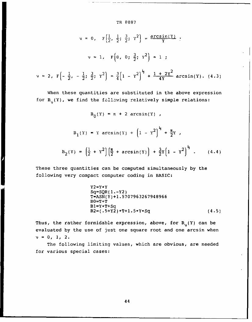
TR 8887
1 1 3 y2) arcsin(Y)v 0, F ';2; Y
v = 1, F(0, 0; i; ) = 1
1_ 2 :( 2)1 + 22, F - y 2 1 4 - y + 2Y arcsin(Y). (4.3)2 2 2' = 1- 4Y
When these quantities are substituted in the above expression
for BV (Y), we find the following relatively simple relations:
B0 (Y) = n + 2 arcsin(Y) ,
B1(Y) = Y arcsin(Y) + 1- y2 +
B2 (Y) = + y 2)(E + arcsin(Y)) + _ Y2) (4.4)
These three quantities can be computed simultaneously by the
following very compact computer coding in BASIC:
Y2=Y*YSq=SQR(I.-Y2)T=ASN(Y)+1.5707963267948966BO=T+TB1=Y*T+SqB2=(.5+Y2)*T+1.5*Y*Sq (4.5)
Thus, the rather formidable expression, above, for B (Y) can be
evaluated by the use of just one square root and one arcsin when
S= 0, 1, 2.
The following limiting values, which are obvious, are needed
for various special cases:
44
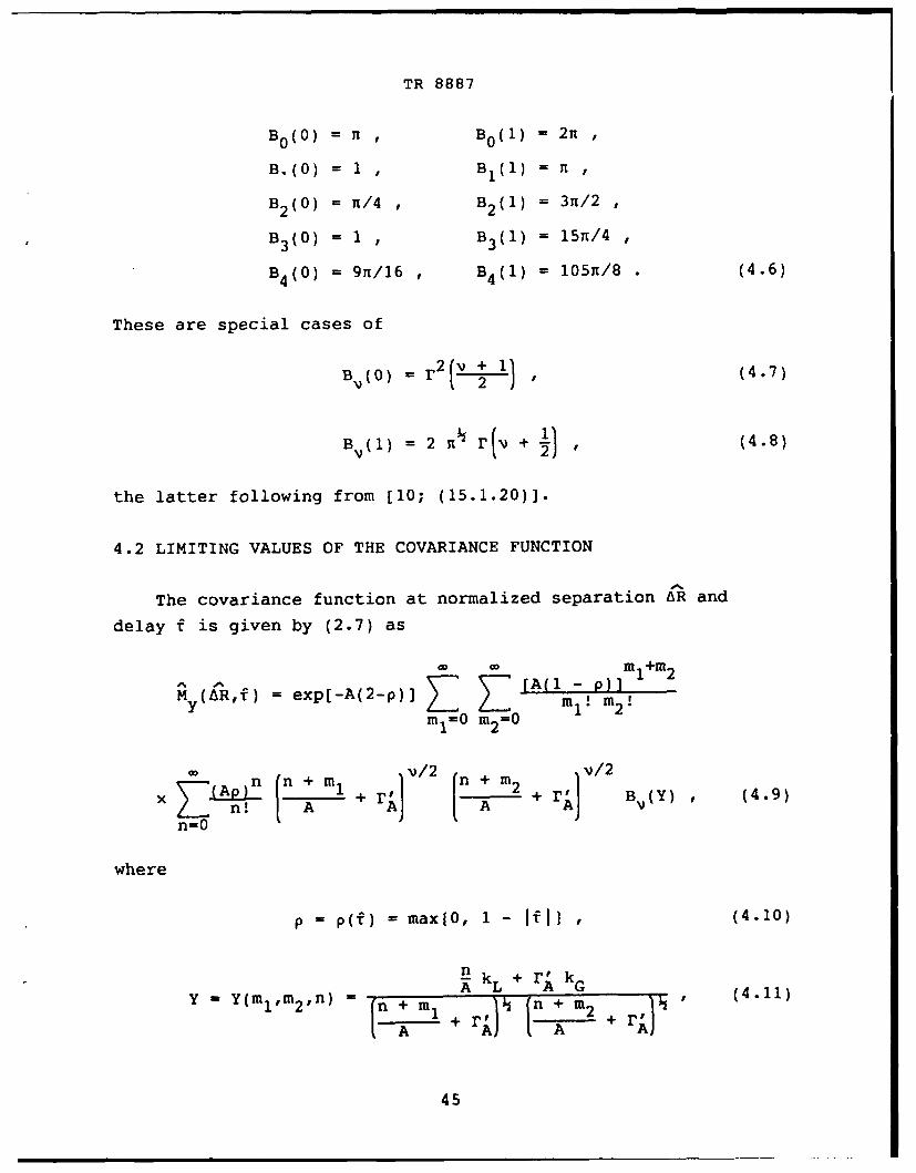
TR 8887
B0 (0) = i B0 (1) = 2n
B,(0) = 1 , BI(1) = Rt
B2 (0) = n/4 , B2 (1) = 3n/2
B3 (0) = 1 , B3 (1) = 15n/4
B4 (0) = 9n/16 , B4 (1) = 105R/8 • (4.6)
These are special cases of
B (0) = r2(, + 1) (4.7)
B (1) = 2 n+ + (4.8)
the latter following from [10; (15.1.20)J.
4.2 LIMITING VALUES OF THE COVARIANCE FUNCTION
The covariance function at normalized separation AR and
delay f is given by (2.7) as
W D A(l - PH m 1+M 2M (tR,f) = exp[-A(2-p)] [ mT ! m2
mI=0 m2=0
-n v/2 v/2
X n + rl [ A + B (Y) , (4.9)
n=0
where
p = p(f) = max{0, 1 - Ili , (4.10)
kL + r, kA L + A n (4.11)
Y - Y(ml'm2'nl)" ' n + m + rj n + m2 + r 4
45
TR 8887
-'2 _1 1Lj 2 f2kL =kL(R,fl = exp - L2_1 , (4.12)
k G kG(ERf) = exp- [(GI a2- 2 i2 . (4.13)
The functions p, kL, kG can be replaced by other functional
dependencies, if desired. The function B (Y) has been
considered earlier and considerably simplified for v = 0, 1, 2.
4.3 VALUE AT INFINITY
As LR or f - ±a, then
p 4 0 , kL 4 0, kG 4 0, Y 4 0 (4.14)
(If IfI remains less than 1 as SR tends to infinity, then p does
not approach zero; this nuance has been discussed elsewhere in
this report.) Then, it follows that
W m 1 +m2 rI v/m2v + r}v/2
M exp(-2A) Lk m+r+ B (0)My T T ml1! m 2! AA
m1=0 m2=0
=B (0) expi(--A) m + r' ) ,/2 (4.15)v )tx~IL m! (EA + AJ
m=0
because the sum on n can be terminated with the n = 0 term.
The sum on m can be effected in closed form, for v = 0, 2, ,
etc., by using the following results:
AmZ ! = exp(A) , (4.16)
m=O
46
TR 8887
- =m 1) A exp(A) , (4.17)
m=O m=l
. AM m2 An (m -i+ 1)m=O m=l
= Am Amnm( - 2)! + - m 1)! (A2 + A) exp(A) . (4.18)
m=2 m=i
There follows
It for v = O'
A 2M(o) = (0+r) for v = 2 (4.19)
9n 4 1 +'2 2)H [- + i + rAJ for v = 4
The case for v = 1 requires a numerical summation, once A and
r' are specified. When these limiting values are subtracted from
the correlation function, we obtain the covariance function.
47
TR 8887
4.4 VALUE AT THE ORIGIN
For AR = 0, f = 0, then
p = 1, kL = 1, kG = 1 , (4.20)
and
A- n ,AA)
M (0,0) = exp(-A) ' + F B (1) (4.21)
2 . n! LA Ak BVl (.1n=0
because the sums on mI and m2 can be terminated with the zero
terms, thereby also leading to Y = 1.
The sum on n can be accomplished in closed form, for
V= 0, 1, 2, etc., by using results given earlier. There follows
2n for v = 0
A
My(0,0) =nj + q for v = 1 (4.22)
3 + (l+r) 2 1 forv=2
48

TR 8887
PART III. APPENDICES AND PROGRAMS
APPENDIX A.1 - EVALUATION OF COVARIANCE FUNCTION
FOR ZERO SEPARATION (AR = 0)
A program for the numerical evaluation of covariance
M y( R,) for AR = 0 is contained in this appendix. Inputsrequired of the user are A, r', (awL/) 2 (AWG/) 2 , 6(f), N(f),
in lines 20 - 70. Since we are generally interested in values of
A less than 1, the series for Ay in (4.9) will not have to be
taken to very large values of mi1, m2 , n; accordingly, the values
of (A /k!] are tabulated once in lines 260 - 300 with a tolerance
of 1E-10 set in line 80.
The values of the covariance at infinity, as given by (4.19),
are computed and subtracted in lines 220 - 240 and 400 - 420;
this is in anticipation of taking a Fourier transform of a
covariance function which decays to zero for large arguments AR.A '
The functions BV(Y) and My (R,f) are available in the two
subroutines stdrting at lines 1010 and 1120, respectively. The
latter subroutine actually calculates the covariance at general
nonzero values of both AR and f, although we only employ it for
AR - 0 in this appendix; see lines 10 and 380. Also, for AR - 0,
the parameter Lg2 - (AL/AG)2 is not relevant and, hence, is
entered as zero in line 380.
The exponential Gaussian forms for kL and kG are used in
lines 1200 and 1210, while the triangular form for p is entered
in line 1240. Any of these can be replaced, if desired, by forms
more appropriate to the user.
The program is written in BASIC for the Hewlett Packard 9000
Computer Model 520. The designation DOUBLE denotes integer
variables, not double precision. The output from the program is
stored in data files AOTO, AOT1, AOT2, for v - 0, 1, 2,
respectively.
49

TR 8887
10 Rc=O. 1DeiR-20 A=.2 I A(subA)30 Cf,. 00 1 IGAMMA' (subA)40 WlIb2=1 I <(DeIW (SUbL )/Beta)A^250 14gb2=25. I(De IW (subC) /Bet a)A260 Dtc=.01 INCREMENT IN TauJA70 Ntc=2Ou NUMBER OF Tau^ VALUESso Tolerance=1.E-109e Cciii AfVO: 40), C(0: SO), ScO: 80)
100 CON DOUBLE J1 INTEGER110 DIM K'ag(200),Tc(0:200),FO(0:200') ,F1 (0:200), F2(l0:20 0)120 DOUBLE Ntc,K IINTEGERS130 FOR K=O TO Ntc140 Tc=K*Dtc T TaUA150 Rho=MAX(0.,1.-ABS(Tc)) IRho160 T2=.5*Tc*Tc170 K1=EXP(-Wlb2*T2)180 'gFVP(-W-gb2*T2)190 K1ag(K')=(Rhio*K1+Gp)*Kg)/(1.+Gp) IINPUT COVARIANCE200 NEXT K210 A=.AA>0 REQUIRED220 F0i nCf=P I230 Fliif=FtFXInC(A,Gp)240 F2inf=.25*PI*( 1.+Gp)*( 1. Gp)250 Af'(0)=1.260 FOR K=1 TO 40270 J=K280 AK)TRK-)AKIA-K./KI290 IF T<Tolerance THEN 320300 NEXT K310 PRINT "40 TERMS IN Af(*)"320 FOR K=0 TO 3*2330 C(K)=TK*A1+Gp340 Sq(K")1.'SQR(T)350 NEXT K360 FOR K=O TO Ntc370 Tc(K)=Tc=K*Dtc ITauA380 CALL Myc(Rc,Tc,A,Gp,'lb2,Wgb2,0. ,FO(K),F1(K),F2(K))390 NEXT K400 MAT FO=FO-(FOinf)410 NAT F1=F1-(Flinf)420 MAT F2=F2-(F2inf)430 MAT FO=FO'(FO(0))440 MAT F1=F1'(F1(0))450 MAT F2=F2/(F2(0))460 PRINT "IN.FINITY: ";F~inf;Flinf;F2inf470 PRINT "MINIMA: " ;MIN(FO(*));MIN(F1 (*));MIN(F2(*) )480 PRINT "AT Ntc: ".;FO(Ntc);F1(Ntc);F2(Ntc)490 CREATE DATA "AIT1",8500 ASSIGN #1 TO "AITI"510 PRINT #1;Kag(*)520 CREATE DATA "AOTO",8530 ASSIGN #1 TO "ACTO"540 PRINT *1;FO(*)550 CREATE DATA "AOTI18
50
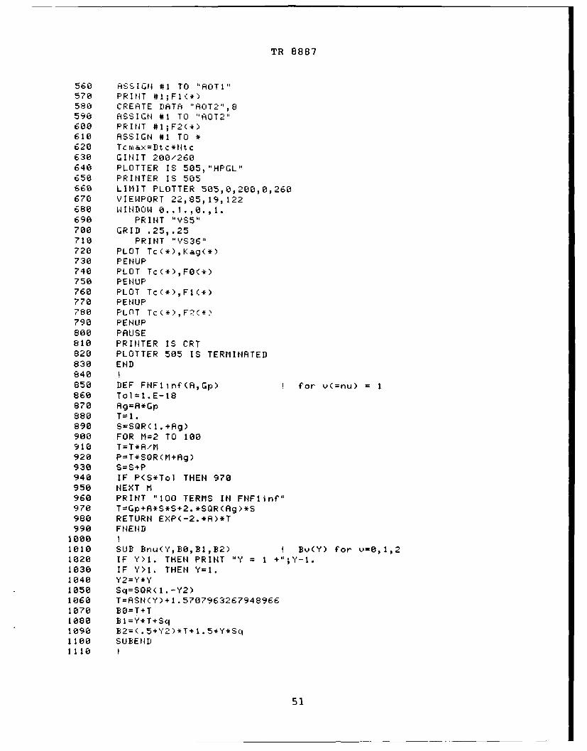
TR 8887
560 ASSIGN #1 TO "ROTI"570 PRINT #I;F1(*)580 CREATE DATA "ROT2",8590 ASSIGN #1 TO "AOT2"600 PRINT #1;F2(*)610 ASSIGN #1 TO *620 Tcrax=Dtc*Ntc630 GINIT 200/260640 PLOTTER IS 505,"HPGL"650 PRINTER IS 505660 LIMIT PLOTTER 505,0,200,0,260670 VIEJPORT 22,85,19,122680 WINDOW 0.1.,0.,1.690 PRINT "'VS5"708 GRID .25,.25710 PRINT "VS36"720 PLOT Tc(*),Kag(*)730 PENUP740 PLOT Tc(*),FO(*)758 PENUP760 PLOT Tc(*),F1(*)770 PENUP780 PLOT Tc(*),F,.'(*)790 PENUP800 PAUSE810 PRINTER IS CRT820 PLOTTER 505 IS TERMINATED838 END84e850 DEF FNFlinf(A,Gp) I for v(=nu) = 1860 Tol=I.E-18870 Ag=A*Gp880 T=I.890 S=SQR(I.+Ag)900 FOR M=2 TO 108910 T=T*A/M920 P=T*SQR(M+Rg)938 S=S+P940 IF P<S*Tol THEN 970958 NEXT M960 PRINT "100 TERMS IN FNF1inC"970 T=Gp+A*S*S+2.*SQR(Ag)*S980 RETURN EXP(-2.*A)*T990 FNEND
18081010 SUB Bnu(Y,BO,BI,B2) I Bv(Y) for v=8,1,21820 IF Y>I. THEN PRINT "Y = I +";Y-1.1030 IF '>1. THEN Y=I.1040 Y2=Y*Y1050 Sq=SQR(1.-Y2)1060 T=ASN(Y)+1.57079632679489661070 BO=T+T1080 BI=Y*T+Sq1090 B2=(.5+Y2)*T+I.5*Y*Sq1100 SUBEND1118
51
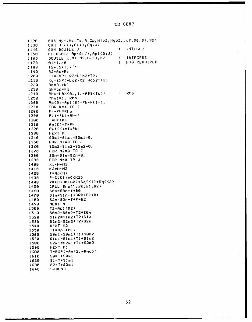
TR 8887
1120 SUB fp1kc (Pc, Tc ,A,G :r, wllb2,1 Ngb2 ,,Lg2, SO, Si, S2)1130 CON AfA*),C(*),Sq(*)1140 CON DOUBLE J INTEGER
1150 ALLOCATE Ap(0:J),Apl(0:J)
1160 DOUBLE K,t11,N2,N,K1,K2 INTEGERS
1170 A1=1.'A ! >O REQUIRED
1180 T2=.5*Tc*Tc1190 R2=Rc*Rc1200 K1=EXP(-R2-W1b2*T2)1210 Kg=EXP(-Lg2*R2-W.gb2*T2)1220 Ak=1A1*K111230 Gk=Gp*Kg1240 RhoMPAY,-(0.,.-ABS(Tc)) Rho1250 Rho1=1.-Rho1260 Ap(0)ARpl(0)=Pk=PklIl.1270 FOR K=1 TO J1280 Pk=Pk*Rho1290 PklI=P1klI*Rlen1300 T=AC(s'1310 Ap(K)=T*Pk1320 Apl(K)=T*Pkl1330 NEXT K1340 S0rn151m15S2m10O.1350 FOR 111=0 TO J1360 66r2=1n2=S2r2=0.1370 FOR M2=0 TO J1380 80n5lnS2n0O.1390 FOR N-=0 TO J1400 K1=N+M111410 K2=1NtM21420 T=Rp(N)1430 P=C(K1)*C(K2)1440 Y=(N*Ak+Gk)*Sq(K1)*Sq(K2)1450 CALL Bnu(Y,BO,D1,B2)1460 SOn=SOn+T*BO1470 Sln=SlntT*SQR(P)*BI1480 S2n=S2n+T*P*B21490 NEXT N1500 T2=Apl(M2)1510 SO2SOm2+T2*SOn1520 Slr,21r2+T2*Sln)1530 52,2=S2rn2tT2*52l1540 NEXT M21550 T1=Apl(Mi)1560 SOnl=SOrltTl*SOf21570 Slui,=Slmnl+T1*S'r21580 S2ra1 =S2rl+T1*S2m21590 NEXT Ill1600 T=EXP(-A*(2.-Rho))1610 S0=T*S~nm11620 51=T*Slnl1630 S2=T*S2,11640 SUBEND
52
TR 8887
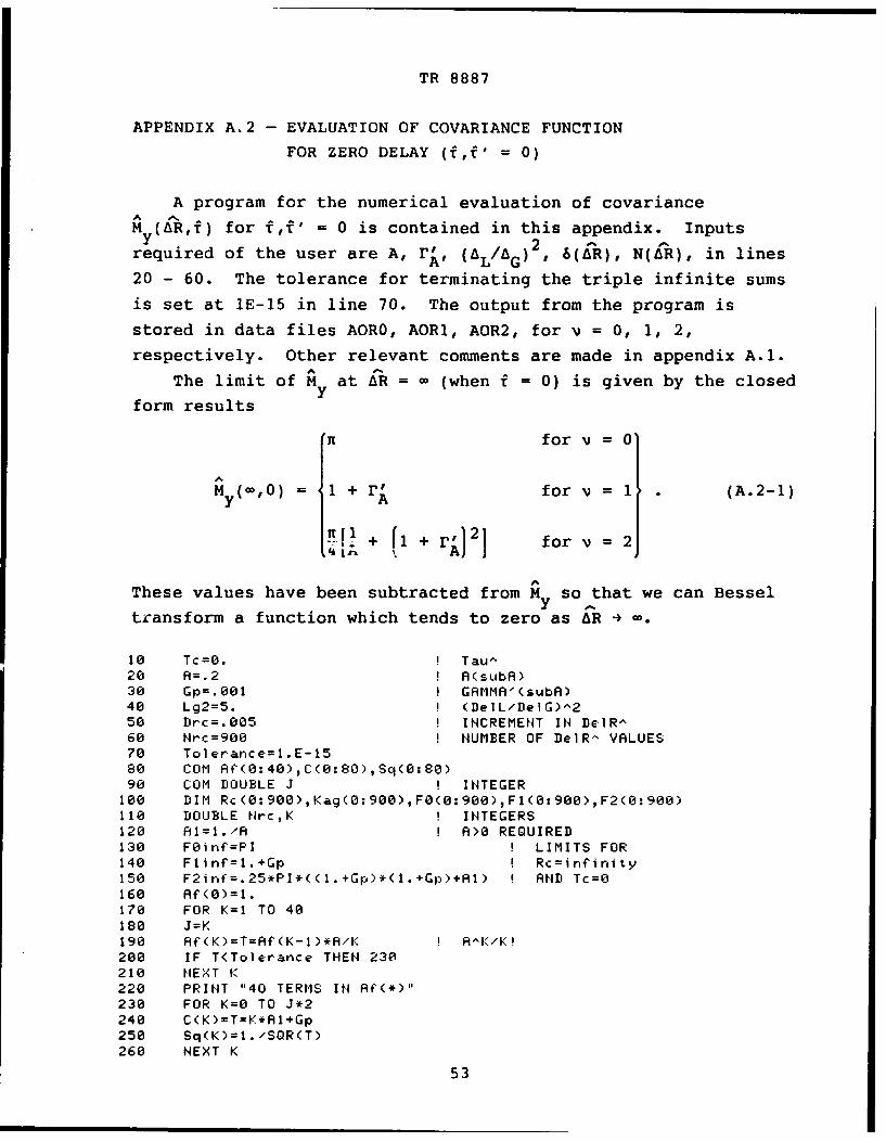
APPENDIX A.2 - EVALUATION OF COVARIANCE FUNCTION
FOR ZERO DELAY (f,f' = 0)
A program for the numerical evaluation of covarianceAM (AR,f) for f,f' 0 is contained in this appendix. Inputs
y 2required of the user are A, r,, (AL/AG) , 6(AR), N(AR), in lines
20 - 60. The tolerance for terminating the triple infinite sums
is set at 1E-15 in line 70. The output from the program is
stored in data files AORO, AOR1, AOR2, for v = 0, 1, 2,
respectively. Other relevant comments are made in appendix A.1.
The limit of M at AR = (when f = 0) is given by the closedyform results
HK for v = 0
y( 0) = A + ' for v = 1 (A.2-1)MyA
+ fi + r,)21 for v = 2A
These values have been subtracted from My so that we can Bessel
transform a function which tends to zero as AR 4 =.
10 Tc=O. Tau ^
20 A=.2 1 A(subA)30 Gp=.001 1 GAMMA'(subR)40 Lg2=5. (De]L/DelG)^250 Drc=.005 1 INCREMENT IN De.R ^
60 Nrc=900 N NUMBER OF DeiR ^ VALUES70 Tolerance=1.E-1580 COM Af(0:40),C(0:80),Sq(0:80)90 COM DOUBLE J ! INTEGER
100 DIM Rc(0:900),Kag(0:900),FO(0:900),F1(0:900),F2(0:900)110 DOUBLE Nrc,K I INTEGERS120 81=1./A 8 R>0 REQUIRED130 FOinf=PI LIMITS FOR140 Flinf=l.+Gp I Rc=infinity150 F2irf=.25*PI*((l.+Gp)*(1.+p)+A1) 1 AND Tc=O160 Af(B)=1.170 FOR K=1 TO 40180 J=K190 Af(K)=T=Af(K-1)*A/K I A^K/K!200 IF T<Tolerance THEN 230210 NEXT K220 PRINT "40 TERMS IN Af(*)"230 FOR K=O TO J*2240 C(K)=T=K*AI+Gp250 Sq(K)=I./SQR(T)260 NEXT K
53
TR 8887
270 FOR K=O TO Nrc280 Rc(K)=Rc=K*Drc DeJRA290 R2=Rc*Rc3uf KI=EXP(-R2)310 Kg=EXP(-Lg2*R2)320 Rho=t-A,(0., 1.-ABS(Tc)) Rho330 Kag(K)=(Rho*K 1 +Gpt*Kg)/( 1. +Gp) I INPUT COVARIANCE340 CALL Myc(Rc,Tc,A,Gp,6.,6.,Lg2,F6(K),FI(K),F2(K)W356 NEXT K360 MAT F6=F-(Fginf)370 MAT FI=Ft-(Flinrf)386 NAT F2=F2-(F2inf)390 MAT F6=F6/(F6(6))460 MAT FI=F1/(FI(6))410 MAT F2=F2/(F2(6))420 PRINT " INFINITY: ";FOinf;Flinf;F2in430 PRINT "MINIMA: " ;MIN(F(*));MIN(F1(*));MIN(F2(*))440 PRINT "AT Nrc: ";FO(t-c);Fl(Nh-rc);F2(Nrc)456 CREATE DATA "AIR",33460 ASSIGN #1 TO "AIRI"476 PRINT #1;Kag(*)480 CREATE DATA "AOR",33490 ASSIGN #1 TO "AOR6"566 PRINT #1;F6(*)516 CREATE DATA "AORI",33526 ASSIGN #1 TO "AORI"536 PRINT #1;F1(t)540 CREATE DATA "AOR2",33556 ASSIGN #1 TO "AOP2"566 PRINT #i;F2(*)576 ASSIGN #1 TO *586 Rcmax=Drc*Nrc590 GINIT 200/260666 PLOTTER IS 565,"HPGL"616 PRINTER IS 565626 LIMIT PLOTTER 565,0,266,6,266636 VIEWPORT 22,85,19,122640 WINDOW 0.,3.,B.,1.656 PRINT "VS5"660 GRID .5,.25676 PRINT "VS36"680 PLOT Rc(*),Kag(*)696 PENUP760 PLOT Rc(*),FO(*)710 PENUP726 PLOT Rc(*),F1(*)736 PENUP746 PLOT Rc(*),F2(*)756 PENUP766 PAUSE776 PRINTER IS CRT786 PLOTTER 505 IS TERMINATED796 END80 I810 SUB Bnu(Y,B,BI,B2) I Bv(Y) for v=r,1,2820 ! SEE APPENDIX A.1906 SUBEtID910 I920 SUB Myc (Rc, Tc, A, Gp, Wl b2, Wgb2, Lg2, $6, Si,52)930 ! SEE APPENDIX A.11440 SUBEND
54

TR 8887
APPENDIX A.3 - EVALUATION OF TEMPORAL INTENSITY
SPECTRUM FOR ZERO SEPARATION (AR = 0)
A program for the numerical evaluation of the Fourier
transform of covariance , (0f) - My () is contained in this
appendix. Inputs required of the user are listed in lines10 - 30. The data input, AOTO or AOT1 or AOT2, as generated bymeans of the program in appendix A.1, is injected by means of
lines 410, 600, and 790.
In order to keep the FFT (fast Fourier transform) size, N inlines 30 and 320, at reasonable values, the data sequence is
collapsed, without any loss of accuracy, according to the method
given in [8; pages 7 - 8] and [9; pages 13 - 16]. The
integration rule documented here is the trapezoidal rule; this
procedure is very accurate and efficient and is recommended for
numerical Fourier transforms.
18 Nt c=280 ! NUMBER OF Tau- VALUES28 Dtc=.81 I ICREMENT IN Tau-38 N=1824 SIZE OF FFT; N > Ntc REQUIRED48 DOUBLE Ntc,N,N4,N2,Ns INTEGERS58 N4=/468 N2=N/278 REDIM Cos(0:N4),X(O:N-1),Y(e:N-I)80 DIM Cos(256),X(123),Y(I023),A(200)90 T=2.,*P I /N
180 FOR Ns=8 TO N4110 Cos(Ns)=COS(T*Ns) QUARTER-COSINE TABLE IN Cos(*)120 NEXT Hs130 GINIT 200/260140 PLOTTER IS 505,"HPGL"158 PRINTER IS 505160 LIMIT PLOTTER 505,0,200,0,260170 VIE1PORT 22,85, 19, 122180 WINDOW 0,N2,-5,1190 PRINT "VS5"200 GRID N/10,1210 PRINT "VS36"220 ASSIGN #1 TO "AITI"230 READ #1;A(*)240 MAT X=(0.)250 MAT Y=(0.)260 X(8)=.5*A(O)270 FOR Ns=1 TO Htc-1280 X(Ns)=A(tls)2:00 11 EXT .1300 X(Ntc)=.5*A(Ntc)
55

TR 8887
310 MAT X=X*(Dtc*4.)320 CALL Fft14(tCo (*,'(*),Y(*))330 FOR Ns=0 TO 12340 Ar=X(Ns)350 IF Ar>0. THEN 380360 PENUP370 GOTO 390380 PLOT tNls,LGT(Ar)390 NEXT Ns400 PENUP410 ASSIGN #1 TO "ROTO"420 READ #1;A(*)430 MAT X=(O.)440 MAT Y=(0.)450 X(O)=.5*A(O)460 FOR Ns=l TO Ntc-1470 X(Nts)=A(Ns)480 NEXT Ns49e X(Ntc)=.S*A(Ntc)500 MAT X=X*(Dtc*4.)510 CALL Fft14(N,Cos(*),X(*),Y(*))520 FOR Ns=O TO N2530 Ar=X(ts)540 IF Ar>0. THEN 570550 PENUP560 GOTO 580570 PLOT Ns,LGT(Ar)580 NEXT Ns590 PENUP600 ASSIGN #1 TO "AOTI"610 READ #1;A(*)620 MAT X=(O.)630 MAT Y=(O.)640 X(O)=.5*A(0)650 FOR Ns=l TO Ntc-1660 X(Ns)=(Ns)670 NEXT Ns680 X(Htc)=.5*A(Ntc)690 MAT X=X*(Dtc*4.)700 CALL FftI4(N,Cos(*),X(*),Y(*))710 FOR Ns'0 TO N2720 Ar=X(Ns)730 IF Ar>0. THEN 760740 PENUP750 GOTO 770760 PLOT Ns,LGT(Ar)770 NEXT Ns780 PENUP790 ASSIGN #1 TO "AOT2"800 READ #1;A(*)810 MAT A=A/(A(0))820 MAT X=(O.)830 MAT Y=(0.)
56
TR 8887
840 X(O)=.5*A(0)850 FOR N=1 TO Ntc-1860 X(t:E )=A 1s)878 NEXT Ns880 X(Nt c)=.5*A(Ntc)898 MAT X=X*(Dtc*4.)900 CALL Fft14(N,Cos(*),X(*),Y(*))910 FOR Ns=O TO N2926 Ar=X(Ns)930 IF Ar>0. THEN 966940 PENUP950 GOTO 970960 PLOT NsLGT(Ar)97A NEXT Ns980 PENUP990 PAUSE1000 END10101020 SUE Fftl4(DOUBLE N,RERL Cos(*),X(*),Y(*)) N t<=2-14=16384; 0 SUBS1030 DOUBLE Log2n,NI,N2,N3,N4,J,K ! INTEGERS < 2'31 = 2,147,483,6481040 DOUBLE 11,12,13,14,15,16, I7,18,19,11 ,II1,112, I13, I14,L(0:13)1050 IF N=1 THEN SUBEXIT1060 IF N>2 THEN 11401070 A=X(0)+X(1)loes X(1)=X(0)-X(1)1090 X()=A1100 R=Y(O)+Y(1)1110 Y(1)=Y(O)-Y(1)1120 Y(O)=R1130 SUBEXIT1140 A=LOG(N)/LOG(2.)1150 Log2n=A1160 IF ABS(A-Log2n)<I.E-8 THEN 11901178 PRINT "N =";N;"IS NOT A PO4ER OF 2; DISALLOWED."1180 PAUSE1190 NI=N/41200 12=N1+11210 N3=N2+11220 N4=N3+N11230 FOR I1=1 TO Log2n1240 12=2A<Log2n-I1)1250 13=2*121260 14=N/131270 FOR 15=1 TO 121280 16=(15-1)*14+11290 IF 16<=N2 THEN 13301300 Al=-Cos(N4-16-1)1310 R2=-Cos(I6-NI-1)1320 GOTO 13501330 AI=Cos(16-1)1340 A2=-Cos(N3-16-1)1350 FOR 17=0 TO N-13 STEP 131360 18=17+I5-11370 19=18+121380 TI=X(I8)1390 T2=X(19)
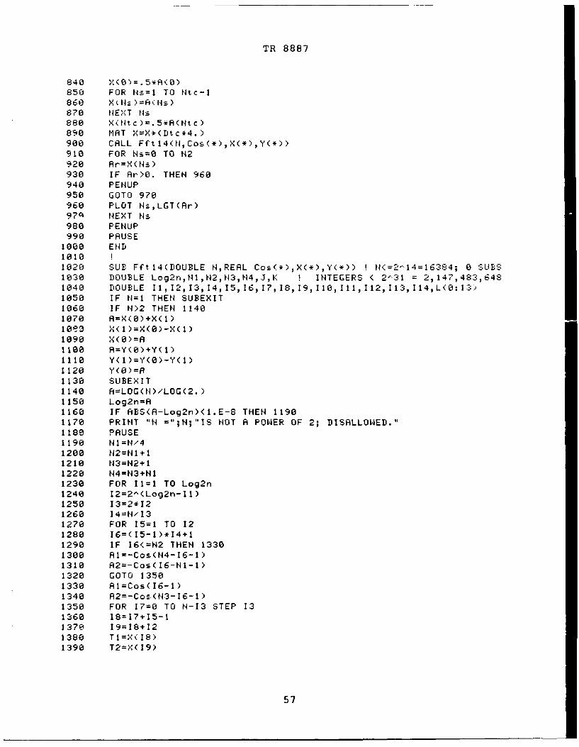
57
TR 8887
1400 T3=Y(I8)1410 T4=Y(19)1420 A3=TI-T21430 R4=T3-T41440 X(I8)=TI+T21450 Y(18)=T3+T41460 X(19)=AI*A3-A2*A41470 Y(19)=AI*A4+R2*R31480 NEXT 171490 NEXT !51500 NEXT 111510 l=Log2n,+1720 FOR 12=1 TO 141530 L(12-1)=11540 IF 12>LWg2n THEN 15681550 L(12-I)r2"(11-12)1560 NEXT 121578 K=O1580 FOR 11=1 TO L(13)1590 FOR 12=11 TO L(12) STEP L(13)1600 FOR 13=I2 TO L(11) STEP L(12)1610 FOR 14=13 TO L(1G) STEP L(11)1620 FOR 15=14 TO L(9) STEP L(10)1630 FOR 16=15 T L3) STEP L(9)1640 FOR 17=I6 TO L(7) STEP L(8)1650 FOR 18=17 TO L(6) STEP L(7)1660 FOR 19=18 TO L(5) STEP L(6)1678 FOR I10=T? TO L(4) STEP L(5)1680 FOR III=Ii TO L(3) STEP L(4)1698 FOR 112=111 TO L(2) STEP L(3)1700 FOR 113=112 TO L(1) STEP L(2)1710 FOR 114=113 TO L(0) STEP L(1)1720 J=114-11738 IF K>J THEN 18081740 F=X(K)1750 X(K)=X(J)1760 X(J)=A1770 A=Y(K)1780 Y(K)=Y(J)1790 Y(J)=R1800 K=K+11810 NEXT 1141820 NEXT 1131830 NEXT 1121840 NEXT III1850 NEXT 1101860 NEXT 191870 NEXT 181880 NEXT 171890 NEXT 161900 NEXT 151910 NEXT 141920 NEXT 131930 NIEXT 121940 NEXT Il1950 SUBEND
58
TR 8887
APPENDIX A.4 - EVALUATION OF WAVENUMBER INTENSITY
SPECTRUM FOR ZERO DELAY (f,f' = 0)
A program for the numerical evaluation of the zeroth-order
Bessel transform of covariance M y(AR,0) - (-o) is contained in
this appendix. Inputs required of the user are listed in lines
10 - 40 and are coupled to appendix A.2, where the data input,
AORO or AOR1 or AOR2, was generated. The numerical Bessel
transform is accomplished by means of Simpson's rule with end
correction [11; pages 414 - 418], and is exceedingly accurate for
the small increment, .005, in AR employed in line 30.
18 Dkc=.4 I INCREMENT IN k"A20 rlkc=208 NUMBER OF k' VALUES38 Drc=.885 INCREMENT IN DelR.40 Nrc=908 NUMBER OF DelR ^ VALUES58 DOUBLE Nrc,-Okc, I,Ns I INTEGERS68 REDIri C(0:Nrc)70 REDIr Ni (8:Nkc), W080:Nk c),1(0:Nkc),W2(8: Nkc)80 DIM C(900),Wi (200 ),,0(200), WI 200),W2(200)90 ASSIGN #1 TO "AIRI"100 READ #I;C(*)118 FOR I=8 TO Nkc120 Kc=I*Dkc 1 k-130 T=Kc*Drc140 Se=So=8.158 FOR Ns=1 TO Nhrc-1 STEP 2160 So=So+tIl.*FN Jo(T*t.ls)*C tls)178 NEXT Ns180 FOR Ns=2 TO Nrc-2 STEP 2190 Se=Se+Ns*FNJo(T*Hs)*C(Ns)200 NEXT Ns210 Wi(I)=C(0)+16.*So+14.*Se220 NEXT I230 MAT Wi=Wi*(Drc*Drc*2.*PI/15.)248 ASSIGN #1 TO "AOR8"250 READ #1;C(*)260 FOR 1=8 TO Nkc270 Kc=I*Dkc280 T=Kc*Drc290 Se=So=.308 FOR Ns=1 TO Nrc-1 STEP 2
310 So=So+N*FNJo(T*N-)*C(Ns)320 NEXT Hs330 FOR Ns=2 TO Nrc-2 STEP 2340 Se=Se+N*FNJo(T*Ns)*C(Ns)350 NEXT Ns360 8( I )=C(8)+ 16.*So+ 14.*Se370 NEXT I380 MAT W0=W0*(Drc*Drc*2.*PI/15.)
59

TR 8887
390 ASSIGN #1 TO "AORi'400 READ #I;Ct*)410 FOR I=O TO Nkc420 Kc=I*Dkc430 T=Kc*Drc440 Se=So=O.450 FOR tNs=l TO Nrc-i STEP 2460 So=SorN-*FNJo(T*Ns)*C(Ns)470 NEXT Ns480 FOR Ns=2 TO Nrc-2 STEP 2490 Se=Se+tls*FtlJo(T*Ns)*C(Ns)500 NEXT Ns510 Wl(I )=C(0)+16. *So+14.*Se520 tEXT I530 MAT W1=1*(Drc*Drc*2*PI/15.)540 ASSIGN #1 TO "AOR2"550 READ #I;C(*)560 ASSIGN #1 TO *570 FOR I=O TO Nkc580 Kc=I*Dkc590 T=Kc*Irc600 Se=So=0.610 FOR Nsl= TO Nrc-I STEP 2620 So=So+ts*FNJo(T*Ns)*C(tls)630 NEXT Ns640 FOR Ns=2 TO Nrc-2 STEP 2
650 Se=Se+Ns-t*:l ;Jo(T*tls)*C (Ns)660 NEXT Ns670 W2I )=C(0)+16.*So+14.*Se680 NEXT I690 MAT W2=W2*(Drc*Drc*2.*PI/15.)700 GINIT 200/260710 PLOTTER IS 505,'HPGL"720 PRINTER IS 505730 LIMIT PLOTTER 505,0,200,0,260740 VIEWPORT 22,85,19,122750 WINDOW 0,Nkc,-9,1760 PRINT "VS5'770 GRID 25,1780 PRINT "VS36"790 FOR 1=0 TO Nkc800 W=Wi(I)810 IF W>O. THEN 840820 PENUP830 GOTO 850840 PLOT I,LGT(W)850 NEXT I860 PENUP
60

TR 8887
870 FOR I=0 TO NI'c880 WWo (I )890 IF 11>0. THEN 920900 PENUP910 COTO 9:30920 PLOT I,LGT(W)930 NEXT I
940 PENLIP950 FOR 1=0 TO IHkc960 WW1,1(I)970 IF 14>0. THEN 1000980 PENUP990 COTO 1010
i000 PLOT 1,LGT(W)1010 NEXT I1020 PENUP1030 FOR 1=0 TO Nkc1040 W=W2(I)1050 IF W>0. THEN 10801060 PENUP1070 COTO 10901080 PLOT I,LCT(W)1090 NEXT I1100 PENUP1110 PAUSE1120 PRINTER IS CRT1130 PLOTTER 505 IS TERMINATED1140 END11501160 DEF FNJo(X) Jo(X) FOR ALL X1170 Y=ABS(X)1180 IF Y>8. THEN 12801190 T=Y*Y HART, #58451200 P=2271490439.5536033-T*(5513584.56477o07522-T*5292.61713o3845574)1210 P=233448917187?869. 7-T*(47?65559442673. 588-T*(4621?2225031 .7180:3-T*P,))1220 P=18596231762189?804.-T*(44145829391815982.-T*P)1230 Q=204251483.52134357+T*(494030.79491813972+T*(884.720367-56175504+T,,1240 Q=2344?50813658996.84T*(15015462449769.7524T*(64398674535. 1332-56+T*Q)J.,1250 Q=18596231762189?733. +T*Q1260 J0 ~P'o1270 RETURN Jo1280 2=8./"? HART, #6546 & 69461290 T=2*Z1300 Pn)2204.5010439651804+T*(128.67758574871419+T*.90047934748026,-*803,:'1310 Pn)8554.8225415066617+T*C8894.4375329606194tT*Pn)1320 Pd=22114.0488519147104+T*(130.88490049992388+T)1330 Pd=8554.8225415066628+T*(8903.8361417095954tT*Pd)1340 0n.13 .990976865960680+T*(1.8497327982345548+T*.009352 59532940319)1350 On=-37.510534954957112-T*(46.093826814625175+T*r-,)1360 Od=921.56697552653090+T*(74.428389741411179+T)1370 Od=2400.6742371172675+T*(2971.9837452084920+T*Od)1380 T='(-. 785398163397448281390 Jo=.28209479177387820*SQR(Z)*(COS(T)*Pti/Pd-SIN.(T )*Z*Onlr/Qd,)1400 RETURN Jo1410 FJElJD
6 1/62Reverse Blank
TR 8887
APPENDIX A.5 - EVALUATION OF PHASE MODULATION INTENSITY SPECTRUM
The normalized covariance function for phase modulation is
given by (2.50) in the main text, namely
k 0 exp[- rA p [1 - exp(- )] - A[2 - p()] + (A5-1)
2
+ 2A [1- p(_)] exp -lp/A) + A p( ) exp(- -- [I - exp(-b )])]
for C Z 0, where C is the time delay and p(C) is the temporal2 2
normalized covariance of the field process. Also Pp = PG
Since (A.5-1) involves an exponential of an exponential of an
exponential, and because a wide range of parameter values are of
interest, care must be taken in numerical evaluation of this
covariance and its transform.
Observe first that
k (0) = 1 since p(O) = I . (A.5-2)
Also, as delay C 4 +-, then p 4 0, giving
ko( ) = exp -rA 1p - 2A + 2A exp -p /A) 0 . (A.5-3)
The spectrum of interest is given by
W0 (w) = 4 f dC cos(wC) ko (C) for w k 0 ; w = 2nf (A.5-4)
0
The nonzero value of (A.5-3) at < = 0 leads to an impulse in
spectrum W0 (w) at w = 0. This limiting value, k0 (), must be
subtracted from covariance (A.5-1) prior to the numerical
Fourier transform indicated by (A.5-4).
63
TR 8887
For FA 2 << 1, the term
expI- r ,p2 [1 - exp(-4)]) (A-5-5)
approaches its limiting value at 4 = +w as follows:
exp (-r , 2 [1 - exp(-4))- exp(- '1) == exp(- 2) [exp(r '2 exp(-t4))- iJ =
- exp (- rA ') rA ,p exp(-4) . (A.5-6)
This is a fairly rapid decay with 4 and will not lead to
numerical difficulty when rA p2 << 1.2For large bp /A, the term
2
exp(- L- [1 - exp(-b4)]) (A.5-7)
is very sharp near 4 = 0; in fact, it is given approximately by
2
exp- -L bt) for 4 near 0 . (A.5-8)
Therefore, we define the sharp component of covariance k (4) as
2
ks (4) = exp[- A + A exp[- - b )J - exp(-A) for all 4 . (A.5-9)
Then
k s(0) = 1 - exp(-A) , k S(-) = 0 . (A.5-10)
64

TR 8887
Now we let
k o() = [k (() - k ()] + k s(0 =
= kf(t) + k s() , (A.5-11)
where kf(t) is a flat function near t - 0. Then we can express
the desired difference as
ko(Z) - k() = [kf(t) - ko(-)] + k s (Z) -
kj j + ks( ) , (A.5-12)
where functions kl(<) and ks (Z) both decay to 0 at Z = . We now
employ two separate FFTs on each of the functions in (A.5-12).
The sharp component, ks (), must be sampled with a very small
increment, A , when bp2/A is large. On the other hand, the flat
component
kl( ) - kf(C) - ko(-) (A.5-13)
can be sampled in a coarser fashion. Finally, if bp2/A is
moderate, we work directly with k0 ) - k0 (-) without breaking
it into any components.
Two programs are furnished in this appendix, one for moderate
bp/A, and the other for the flat component (A.5-13) when b2 /A
is large. For sake of brevity, the Fourier transform of the
sharp -7omponent (A.5-9) is straightforward and is not presented.
The particular covariance p(t) adopted is triangular,
p(K) - 1 - L for IZI < rc 0 otherwise , (A.5-14)
but can easily be replaced. The parameter c is the cutoff value
of covariance p(C).
65
TR 8887
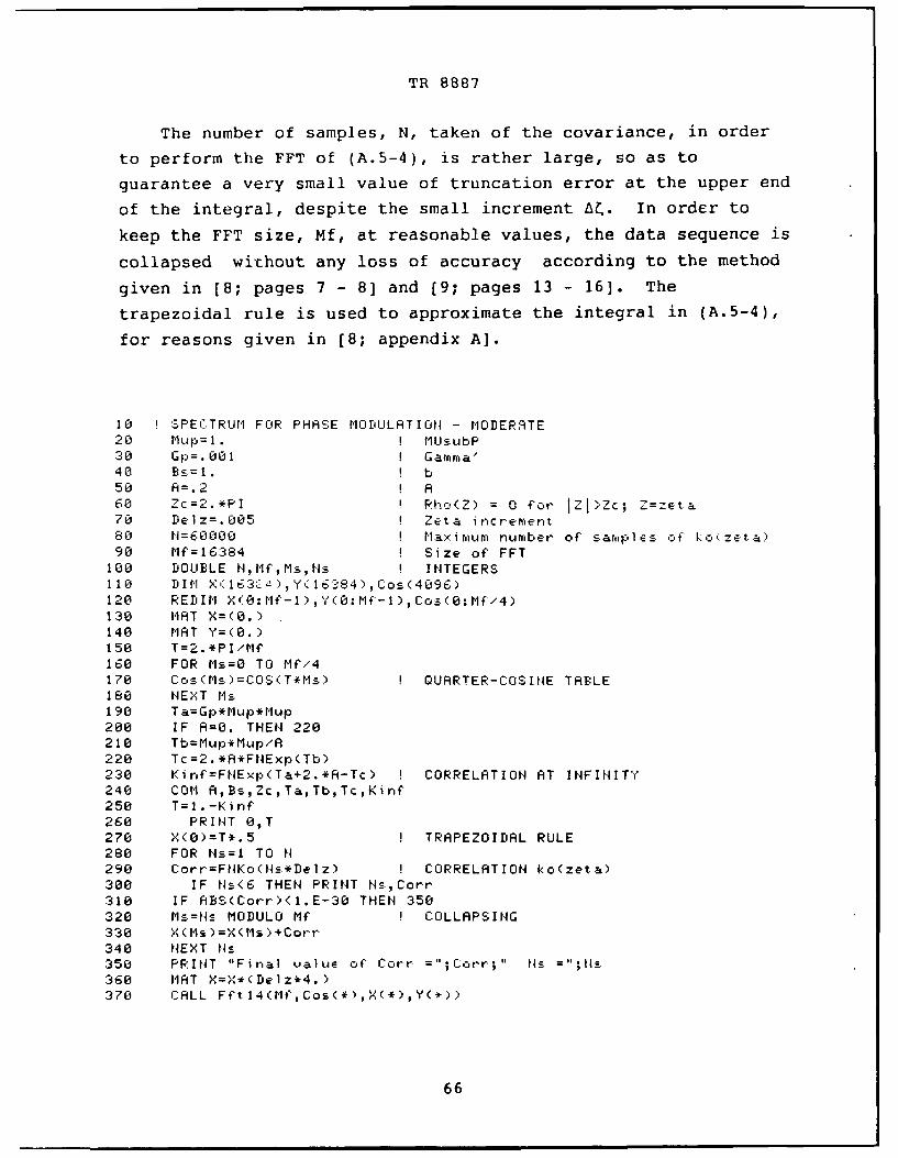
The number of samples, N, taken of the covariance, in order
to perform the FFT of (A.5-4), is rather large, so as to
guarantee a very small value of truncation error at the upper end
of the integral, despite the small increment At. In order to
keep the FFT size, Mf, at reasonable values, the data sequence is
collapsed without any loss of accuracy according to the method
given in [8; pages 7 - 8] and [9; pages 13 - 16]. The
trapezoidal rule is used to approximate the integral in (A.5-4),
for reasons given in [8; appendix A].
10 SPECTRUM FOR PHASE MODULATION - MODER.9TE20 MUI=1. MUSubP30 Gp=. 001 I Gamma'40 BE=1. b50 A=.2 A60 Zc=2.*PI I Rh:(Z) = 0 for IZI>Zc; Z=zeta70 Delz.005 Zeta increment80 H=60000 M axirmum number of samples of Lkokzeta)90 Mf=16:384 Size of FFT100 DOUBLE N, Mf, Ms, Hs INTEGERS110 DIN X< 163,c-_"),Y( 16384),Cos(4096)120 REDIi X(0: Mf"-1), Y(O: Mf-1 ), C:os (0: Mf'4)130 fiAT X=(0.)140 MAT Y=(8.)150 T=2.*PI/Mf160 FOR Ms=0 TO MI/4170 Co-(Ms)=COS(T*Ils) QUARTER-COSINE TABLE180 NEXT Ms190 Ta=Gp*Mup*Mup200 IF A=O. THEN 220210 Tb=Mup*Mup/A220 Tc=2.*A*FHExp(Tb)230 Kirf=FNEx,(Ta+2.*A-Tc) CORRELATION AT INFINITY240 COM A,Bs,ZcTa,Tb,Tc,Kinf250 T=I.-Kinf260 PRINT 0,T270 X(O0=T*.5 TRAPEZOIDAL RULE280 FOR Ns= TO N290 Corr.=FNKo(_1s*DeIz) CORRELATION ko(zeta)300 IF Ns<6 THEN PRINT Ns,Corr310 IF ABS(Corr.)<I.E-30 THEN 350320 'ls=Ns MODULO Mf COLLAPSING330 X(Ms)=X(Ms>+Corr340 NEXT Ns350 PRINT "Final value of Corr =";Corr;" N =";H .
360 MAT X=X*(Delz*4.)370 CALL Fft14(Mf,Cos(*),X(*),Y(*))
66

TR 8887
380 GINIT390 PLOTTER IS "GRAPHICS"400 GRAPHICS ON410 WINDOW -2,2,-60,0420 LINE TYPE 3430 GRID 1,10440 LINE TYPE 1450 Del f=l./(Nf*Delz)460 FOR t1;=i TO Mf-'2470 F=is*Delf FREQUENCY480 PLOT LGT(F),10.*LGT(X(Ms))490 NEXT lMs500 PENUP510 PAUSE520 END530 I540 DEF FNExp(Xminus) I EXP(-X) WITHOUT UNDERFLOW550 IF Xrninus>708.3 THEN RETURN 0.560 RETURN EXP(-Xminus)570 FNEND580590 DEF FNKo(Zeta) I CORRELATION ko(zeta)600 COM A,Bs,Zc,Ta,Tb,Tc,Kinf610 Rho=MAX(0., 1.-Zeta/Zc) TRIANGULAR RHO620 El=Ta*(I.-FNExp(Zeta))630 E2=Tb*(I.-F.Exp(Bs*Zeta))640 E3=A*Rho*FNExp(E2)650 RETURN FNExp(E1+A*(2.-Rho)-Tc*(I.-Rho)-E3)-Kirnf660 FNEND670680 SUB Fft14(DOUBLE N,REAL Cos(*),X(*),Y(*)) ! N<=2"14=16384; 0 SUBS690 ! SEE APPENDIX A.3
10 SPECTRUM FOR PHASE MODULATION - FLAT COMPONENT20 Mup=I. MUsubP30 Gp=.001 I Gamma'40 Bs=l. I b50 A=0. I A60 Zc=2.*PI Rho(Z) = 0 for iZI>Zc; Z=zeta70 Delz=.005 Zeta increment8 N.=60000 Maximum number of sampl-Es of kl(zeta)90 Mf=16384 I Size of FFT
100 DOUBLE N,Mf,Ms,Ns I INTEGERS110 DIM X(16384),Y(16384),Cos(4096)120 REDIM X(O:MC-I1),Y(O: Nf-1),Cos(OaMf/4)130 MAT X=(0.)140 MAT Y=(.)150 T -2. x : -,160 FOR Ms=O TO Mf/4170 Cos(Ms)=COS(T*Ms> I QUARTER-COSINE TABLE
180 NEXT Ms190 Ta=Gp*Mup*Mup200 IF 8=0. THEN 220
67
TR 8887
210 Tb=Miup*l'lUp/'A220 Tc=2. *A*FIIExp( Tb)230 Tb=5.E5524C Ki n=FHExp( Ta+2. *A-Tc) CORRELATION1 AT INFINITY250 Ea=FMExp(A)260 Tbb=Tb*Bs270 COM A, E.s,Zc,Ta, Tb,Tc,KinflEa, Tbb280 T1l-Kinf-(1.-Ea) SUBTRACT SHARP COMPONENT290 PRINT 0,T300 X(O)=T*.5 TRAPEZOIDAL RULE310 FOR Ns=1 TO N320 Corr=FKh1(Ns*Delz) CORRELATIOM k1(zeta)330 IF Ms<6 THEM PRIMT tMs,Corr340 IF ABS(Corr)<1.E-30 THEM 380350 M==s MODULO Mf COLLAPSING360 X(Ms)=XM's)+Corr370 NEXT Ms380 PRINT "Final valJE of Corr =";Corr;" I- ="0N
390 MAT X=X*(Delz*4.)400 CALL Fft 14(M,Cos(*),X,(*),Y(*)>410 GINIT420 PLOTTER IS "GRAPHICS"430 GRAPHICS ON440 WINDOW -2,2,-60,0450 LINE TYPE 3460 GRID 1,10470 LINE TYPE 1480 Derlf:I./(NIf*Delz)490 FOR Ms=1 T'1 MC/2500 F=Ms*Delf FREQUENCY510 T=X(Ms)520 IF T>0. THEN 550530 PENUP540 GOTO 560550 PLOT LGT(F),10.*LGT(T)560 NEXT Ms570 PENUP580 PAUSE590 END600610 DEF FNExp(Xminus) EXP(-X) WITHOUT UNDERFLOW620 IF Xrfitius>708.3 THEN RETURN 0.630 RETURN EXP(-Xminus)640 FNEND650660 DEF FNIK1(Zeta) I CORRELATION kl(zeta)670 COM A, Bs, Zc ,Ta, Tb, Tc, Kinf, Ea, Tbb680 Rho=MAX(0. , 1.-Zeta/Zc) TRIANGULAR RHO690 E1=Ta*(1.-FNExp(Zeta))700 E2=Tb*(1.-FHExp(Bs*Zeta))710 E3=A*Rho*FtlExp(E2)720 E4=FNExp(Tbb*Zeta)730 Sharp=FHExp(A*(1.-E4))-Ea 1 ks(zeta)740 RETURN FNExp(E1+A*(2.-Rho)-Tc*(l.-Rho)-E3)-Kinf-Sharp750 FNEND760770 SUE Fftl4(DOUBLE N,REAL Cos(*),X(*),Y(*)) N .<-214=16384; 0 SUBS780 I SEE APPENDIX A.3
68
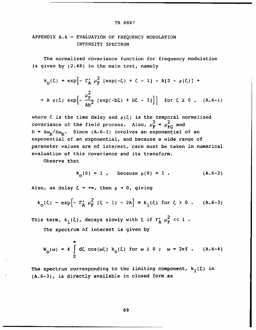
TR 8887
APPENDIX A.6 - EVALUATION OF FREQUENCY MODULATION
INTENSITY SPECTRUM
The normalized covariance function for frequency modulation
is given by (2.48) in the main text, namely
ko(<) = expf- r P4 [exp(-) + < - 1] - A[2 - p(<)] +
2
+ A p(<) exp(_ 2 [exp(-b7) + b - 1] for Z 0 , (A.6-1)Ab
where t is the time delay and p(Z) is the temporal normalized2 2 ncovariance of the field process. Also, pF = FG and
b = A /w . Since (A.6-1) involves an exponential of an
exponential of an exponential, and because a wide range of
parameter values are of interest, care must be taken in numerical
evaluation of this covariance and its transform.
Observe that
k (0) = 1 , because p(O) = 1 . (A.6-2)
Also, as delay i 4 +-, then p 4 0, giving
k0 () - exp(- r 4 (< - 1) - 2A) S kl() for C > 0 . (A.6-3)
This term, kl(), decays slowly with C if rA P << 1
The spectrum of interest is given by
W0 (w) - 4 f dC cos(wC) k0 () for w Z 0 ; w = 2nf . (A.6-4)
0
The spectrum corresponding to the limiting component, kl(C) in
(A.6-3), is directly available in closed form as
69
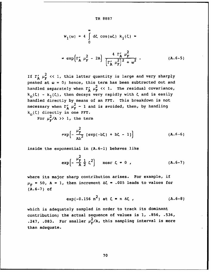
TR 8887
WI(w ) = 4 f d cos(wL) kl(t)
0
2 2'~ , 2~4 rA 2
expi ( F - 2 2 A * (A.6-5)
if q p 2«< 1, this latter quantity is large and very sharply
peaked at w = 0; hence, this term has been subtracted out and
handled separately when FA P << 1. The residual covariance,F
ko(<) - kl(t), then decays very rapidly with r and is easily
handled directly by means of an FFT. This breakdown is not
necessary when rA PF _ 1 and is avoided, then, by handling
k o() directly in one FFT.0 2For pF/A >> 1, the term
2
expA( 2 [exp(-b ) + bi, - 1]) (A.6-6)Ab
inside the exponential in (A.6-1) behaves like
2
exp A 2 near < = 0 ,(A.6-7)
where its major sharp contribution arises. For example, if
PF = 50, A = 1, then increment AZ - .005 leads to values for
(A.6-7) of
exp(-0.156 n2 ) at t - n AC , (A.6-8)
which is adequately sampled in order to track its dominant
contribution; the actual sequence of values is 1, .856, .536,2.247, .083. For smaller p F/A, this sampling interval is more
than adequate.
70

TR 8887
Two programs are furnished in this appendix, one each for the2cases of large and small rA pF The particular covariance p(C)
adopted is triangular,
p(C) = 1 - 10' for I < Cc ' 0 otherwise , (A.6-9)c
but can easily be replaced. The parameter Cc is the cutoff
covariance value and is specified numerically in the examples in
figures 3.9a through 3.10b.
10 I SPECTRUM FOR FREOIUENCY MODULATION - LARGE Gp*Muf-220 Muf=50. MUsubF30 Gp=.001 G am rra'40 Bs=I. b50 A=.2 A60 Zc=2.*PI Rho(Z) = 0 for IZI>Zc Z=zeta70 t'elz=.005 Zeta increment80 N=60000 Max i mum number of s amp e s c k o z t aL90 Mf=16384 Size of FFT
100 DOUBLE N1Pf.,MsNs INTEGERS110 DIM X(16d4),Y(16384),Cos(4096)120 REDIM X(O:MfI-I),Y(O:Mf-1),Cos(O:Mf/4)130 MAT X=(O.)140 MAT Y=(O.)150 T=2.*PI/Mf160 FOR Ms=O TO Mf/4170 Cos(Mc)=COS(TkMs) QUARTER-COSINE TABLE180 NEXT Ms190 Ta=Gp;Muf*Muf200 IF A=0. THEN 220210 Tb=Muf*Muf/(A*Bs*Bs)220 Tc=FNExp(2.*A-Ta)*Ta230 Td=Ta*Ta240 COM H,Bs,Zc,Ta,Tb250 X(0)=.5 I TRAPEZOIDAL RULE260 FOR Ns=1 TO N270 Corr=FNKo(Ns*Delz) I CORRELATION ko(zeta)280 IF Corr<1.E-20 THEN 320290 Ms=Ns MODULO ME COLLAPSING300 X(Ms)=X(1-1s)+Corr310 NEXT NS320 PRINT "Final value of Corr =";Corr;" Ns =';Ns330 MAT X=X*(Delz)340 CALL Ff't 14<Mf,Cos(*))<(*),W*))
71
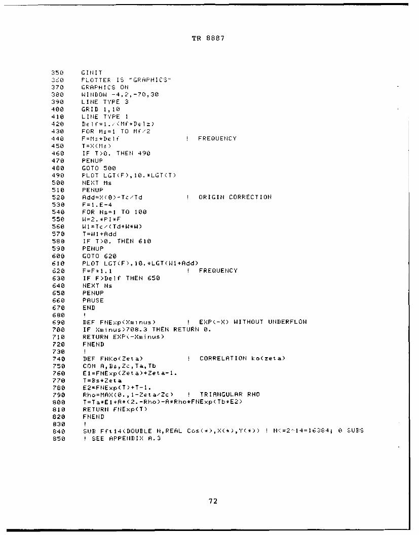
TR 8887
350 GINIT360 PLOTTER IS "GRAPHICS'"
370 GRAPHICS ON380 WINDOW -4,2,-70,30390 LINE TYPE 3400 GRID 1,10410 LINE TYPE I420 DE1C=l."(Mf*De]z)430 FOR M1= TO Mf/2440 F=Ms-*De 1 f FREQUENCY450 T=X(N)460 IF T>O. THEN 490470 PENUP480 GOTO 500490 PLOT LGTtF),1O.*LGT(T)500 NE XT 1MIs510 PENUP520 Add=X(0)-Tc/Td ORIGIN CORRECTION530 F=1.E-4540 FOR Ns=l TO 100550 1=2.*PI*F560 WL=Tc/(Td+W*W)570 T=WI+Add580 IF T>0. THEN 610590 PENUP600 GOTO 620610 PLOT LGT(F),10.*LGT(WI1+Rdd)620 F=F*I. I FREQUENCY630 IF F>Delf THEN 650640 NEXT Ns650 PENUP
660 PAUSE670 END680690 DEF FNExp(Xminus) EXP(-X) WITHOUT UNDERFLOW700 IF Xrninus>708.3 THEN RETURN 0.710 RETURN EXP(-Xminus)720 FNEND730740 DEF FNKo(Zeta) CORRELATION ko(zeta)750 COM A,B s,Zc,Ta,Tb760 EI=FHExp(Zeta)+Zeta-1.770 T=Bs*Zeta780 E2=FNExp(T)+T-1.790 Rho=MAX(0., 1-Zeta/Zc) TRIANGULAR RHO
800 T=T,*E1+R*(2.-Rho )-A*Rho*FNExP (Tb*E2)810 RETURN FNExp(T)820 FNEND830840 SUB Fftl4(DOUBLE N,REAL Cos(*),X(*),Y(*)) ! NI<=2."14=16:384; 0 SU:S
850 SEE APPENDIX A.3
72
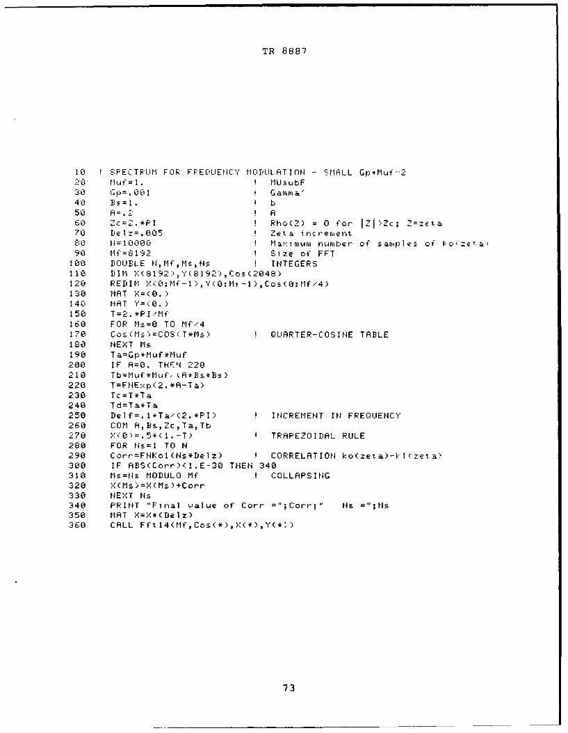
TR 8887
10 SPECTRUM FOR FFEQLIEHCY MOTILLATIONt-i SMALL Gp*Hlui "220 MU f 1IIlU HULbF30 Gp=.O0cl1 G am A)a40 B=1 b50 A=. A60 2c=2.*PI Rho(Z) =0 for, jZI >Zc; Zz.eta70 DelIz=.005 Zeta incr-eiments0 H= I 10000 MaSXI muml turjibe r of sarip 1 E s of ko< zeta90 Mf=6192 ISize of FFT
100 DOLIBLE N, Hlf, Hs , tN INTEGERS110 DIM X(8192), Y(8192) ,Cos(2048)120 REIM X( 0: f - I, Y (0: tlt -1), Cos (0: lf'4)130 MATX=0)140 MAT Y=(0.)150 T =2. * P I/Hlf,160 FOR Hs=0 TO Hf/4170 C's (Mi_) COS( I*Hsc) IQLIARTER-COSINE TABLE180 NEXT M-s190 Ta=Gp*Huf*HUf200 IF A=0. THENA 220210 TbHtLJC *HUf, kA*Bs*BS)220 T=FNExp(2.*A-TaL)230 Tc=T*TaL240 Td=Ta*TaL250 Delf=.1*Ta/(2.*PI) INCREMENT IN FREQUENCY260 COM A,Bs,Zc,Ta,Tb270 Y<(0 =.5*(1.-T) TRAPEZOIDAL RULE280 FOR NslI TO N290 Corrp-FNKol (Ns*tjel z) ICORRELATION ko(zeta)-k I (zet a)300 IF ABS(Corr)<1.E-30 THEN4 340310 Hs=Ns HODULO Hf ICOLLAPSING320 Y"(Ms)=X(Ms)+Corr330 NEXT Ns340 PR INT ' F inalI val ue of Corr ;Corr-; Ns '";Ns350 MAT X=X*(Delz)360 CALL Fft14(H', Cos(*) ,X(*) ,Y(
73

TR 8887
370 GINIT380 PLOTTER IS "GRAPHICS"390 GRAPHICS ON400 WIN1DOW -4,2',-70,30410 LINE TYPE 3420 GRID 1,10
430 LINE TYPE I440 FOR M= TO 2000450 F=M_.-*De 1 f FREQUENCY460 N=2.*PI*F470 I=Tc /(Td+*W) SHARP SPECTRAL COMPONENT480 T=i"f*Delz*F490 Ns=INT(T)500 Fr=T-Ns510 W2=Frt::(l4+1)+(1 -Fr) ,. ( Nl BROAD SPECTRAL COMPONENT520 PLOT LGT\F),10.*LGT(W1+W2)530 NEXT ls540 N MA ..=M ( t.s , I550 FOR tMts=Ns TO rlf/2560 F=M=/ (MCf*De l z) FREQUENCY570 1.=2. *PI*F580 W1 =Tc, (Td+H*N)590 W2=X(Ms600 T= W1 +W2610 IF T>O. THEN 640620 PENUP630 GOTO 650640 PLOT LGT(F),l0.*LGT(T)650 NEXT M'ls660 PENUP670 PAUSE680 ENID6907LO DEF FtNExp( >minu- ) E P(-X) WITHOUT UNDERFLOW710 IF Xrirus>708.3 THEN RETURN 0.720 RETURN EXP(-Xi nus)730 FNEND7407'fl DEF FN4,ol(2ta) CORPELATION ko(zeta)-k1(zeta,760 COM A,Bs,Z,:,Ta, Tb770 E1=FNExo(Zeta) +Zeta-1.780 =Bs*Zcta
790 E2=FtlExp(T. +f-1.900 R ,=MA.(0. , 1-Zet a-Zc ) TRIANGULAR RHO810 T=Ta*EI+A*2.-RV c)-A*Pho*FllExp(Tb*E2)820 RETURN FNE..p T)-FOF xp(Ta*(2eta-1. >+2.*A)630 FNEM'a48850 1UB Fft I'D UBLE H,RE AL CoE(*),X(*,Y(* ) N(2-1416384; i SUBS
SEE AFFEIII!X h. 3
74

TR 8887
REFERENCES
[1) D. Middleton, An Introduction to Statistical Communication
Theory, McGraw-Hill Book Company, Inc., New York, NY, 1960.
Also, Reprint Edition, Peninsula Publishing Co., P.O. Box 867,
Los Altos, CA, 1987.
[2] D. Middleton, "Second-Order Non-Gaussian Probability
Distributions and Their Applications to "Classical" Nonlinear
Signal Processing Problems in Communication Theory," to be
submitted to IEEE Transactions on Information Theory, 1991.
(This is a considerably expanded version of [3] ff.)
[3] D. Middleton, "Second-Order Non-Gaussian Probability
Distributions and Their Applications to Classical Nonlinear
Processing Problems," Proceedings of 20th Conference on
Information Sciences and Systems, pages 394-400, March 19-21,
1986, Princeton University, NJ.
[4] D. Middleton, First- and Second-Order Gauss-Composite
Processes, with Applications to Ambient and Scatter Noise,
in preparation, 1991.
[5] D. Middleton, "Canonical and Quasi-Canonical Probability
Models of Class A Interference," IEEE Transactions on Electro-
magnetic Compatibility, volume EMC-25, number 2, May 1983.
[6] A. H. Nuttall, I. B. Cohen, and D. Middleton, Performance
Parameters for Quasi-Canonical Class A Non-Gaussian Noise;
Source Distribution Law p = 0, Propagation Law y - 2,
NUSC Technical Report 7715, Naval Underwater Systems Center,
New London, CT, 15 June 1986.
75
TR 8887
[7] D. Middleton, "Channel Modeling and Threshold Signal
Processing in Underwater Acoustics: An Analytical Overview,"
IEEE Journal Oceanic Engineering, volume OE-12, number 1, pages
4-28, January 1987.
[8] A. H. Nuttall, Accurate Efficient Evaluation of Cumulative
or Exceedance Probability Distributions Directly From
Characteristic Functions, NUSC Technical Report 7023, Naval
Underwater Systems Center, New London, CT, 1 October 1983.
[9] A. H. Nuttall, "Alternative Forms and Computational
Considerations for Numerical Evaluation of Cumulative Probability
Distributions Directly from Characteristic Functions,"
Proceedings IEEE, volume 58, number 11, pages 1872-1873, November
1970. Also in NUSC Report Number NL-3012, Naval Underwater
Systems Center, New London, CT, 12 Auigust 1970.
[10] Handbook of Mathematical Functions, U. S. Department of
Commerce, National Bureau of Standards, Applied Mathematics
Series Number 55, U. S. Government Printing Office, Washington,
DC, June 1964.
[11] C. Lanczos, Applied Analysis, Third Printing, Prentice-
Hall, Inc., Englewood Cliffs, NJ, 1964.
[12] J. A. Mullen and D. Middleton, "The Rectification of
Non-Gaussian Noise," Quarterly Journal of Applied Mathematics,
volume XV, number 4, pages 395-419, January 1958.
76
Related Documents