Specific Conductance: Theoretical Considerations and Application

Specific Conductance: Theoretical Considerations and Application to Analytical Quality Control

United States Geological SurveyWater-Supply Paper 2311


By RONALD L. MILLER, WESLEY L. BRADFORD, and NORMAN E. PETERS

U.S. GEOLOGICAL SURVEY WATER-SUPPLY PAPER 2311

DEPARTMENT OF THE INTERIOR

DONALD PAUL MODEL, Secretary

U.S. GEOLOGICAL SURVEY

Dallas L. Peck, Director

UNITED STATES GOVERNMENT PRINTING OFFICE: 1988

For sale by the Books and Open-File Reports Section, U.S. Geological Survey, Federal Center, Box 25425, Denver, CO 80225

Library of Congress Cataloging in Publication DataMiller, Ronald LSpecific conductance.(U.S. Geological Survey water-supply paper ; 2311)Bibliography: p.Supt.ofDocs.no.: I 19.13:23111. Water quality Measurement. 2. Water Electric properties-

Measurement. 3. Electric conductivity Measurement. I. Miller, Ronald L. II. Peters, Norman E. III. Title. IV. Series: Geological Survey water-supply paper 2311.

TD370.B69 1986 628.V61 86-600214

CONTENTS

Abstract 1Introduction 1Theory of specific conductance 1

Electrical resistance and conductance 1Definition of conductivity 2Potassium chloride secondary standards 2Temperature effects and instrumental temperature compensation 3Ionic conductance 6

Concentration relationships 7 Temperature relationships 8

Effects of complexation and protonation 9 Applications to analytical quality control 10

An empirical approach in natural waters 10 Tests of the empirical model 11

Adjustments for effects of complexation 11Calculation of the sum of conductance and the exponential correction

factor (f) 11 Evaluation of/ 11

Quality control checks 12Comparison of measured with computed specific conductance and

anions with cations 12 Predicting the sum of anions or cations 13

A special case for seawater and estuarine waters 13 Notes on specific conductance measurements 14

Instrumentation 14 Procedures 14

Summary 15 References 15

FIGURES

1-5. Graphs showing:1. Conductivity-temperature relationships for 0.01 N KG solution and 1 per

mil chlorinity seawater 42. Percentage change in conductivity with temperature for 0.01 N KC1 solu

tion and seawater in 1 °C increments 53. Values of the ratio of specific conductance to conductivity for 0.01 N KG

solution and 1 per mil chlorinity seawater 64. Decreases in equivalent conductance of selected electrolytes with increas

ing concentration 85. Changes in limiting equivalent conductivity of selected ions with

temperature 9

Contents III

TABLES

1. Conductivity of secondary standard potassium chloride (KC1) solutions 32. Comparison of conductivity of 0.01 N KC1 solutions (in jiS/cm) converted to SI

units 33. Comparison of the ratio KS/K predicted by dividing 1410.6 jiS/cm (at 25 °C) by

the conductance calculated using equation 9, equation 10, and calculated using data from Rosenthal and Kidder (1969) and Harned and Owen (1964) 7

4. Values of KS/K for 0.01 N KG solutions in 1 °C increments calculated bydividing 1410.6 jiS/cm (at 25 °C) by the conductance calculated using equation 9 7

5. Limiting equivalent conductances (\°) of selected ions 106. Stability constants (log K,) for ion associations between major inorganic ions in

natural waters at 25 °C 107. Statistical summary of exponential correction factor (f) values 118. One standard-deviation range of estimated KS using (XC, * \°/ 129. Relationship of the/value and anion ratios (p equals the probability of accept

ing the null hypothesis, H0 ; correlation coefficient r=0) 1210. Algorithms for calculating conductivity, specific conductance, chlorinity, and

salinity of seawater and estuarine water 14

IV Contents

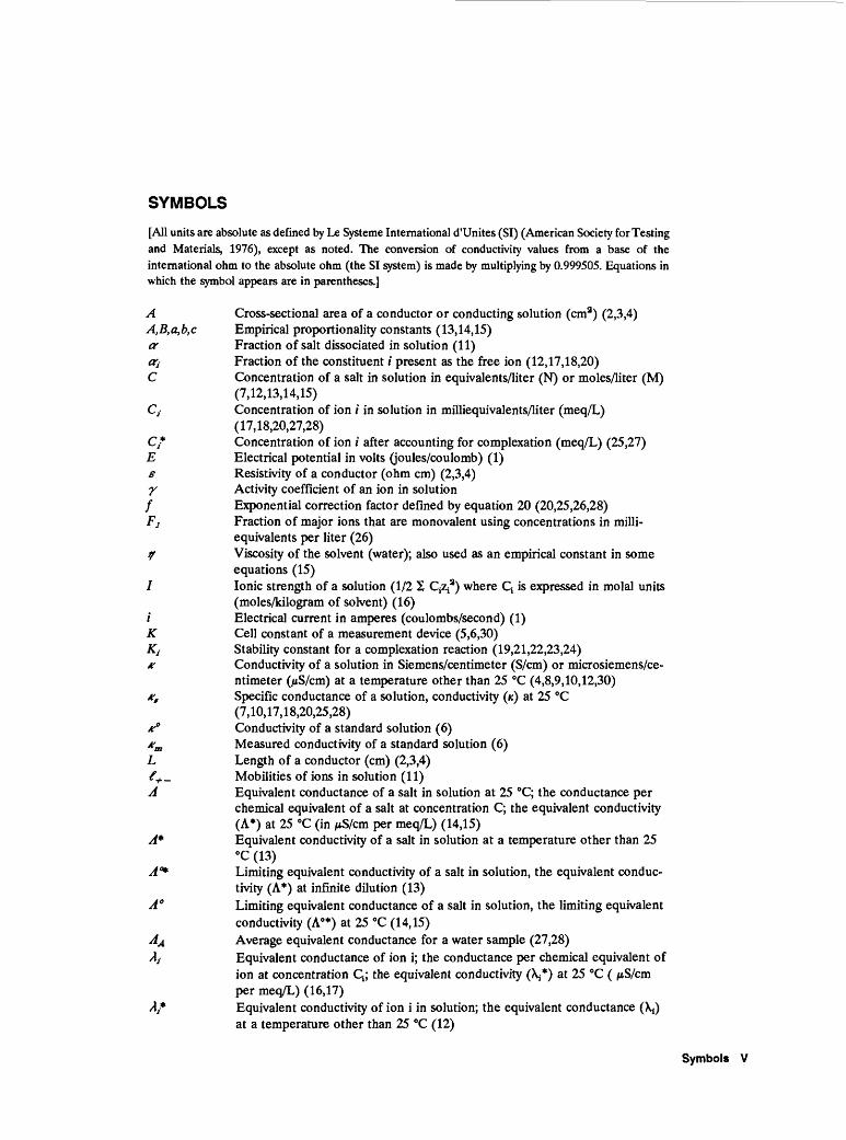
SYMBOLS

[All units are absolute as defined by Le Systeme International d'Unites (SI) (American Society for Testing and Materials, 1976), except as noted. The conversion of conductivity values from a base of the international ohm to the absolute ohm (the SI system) is made by multiplying by 0.999505. Equations in which the symbol appears are in parentheses.]

A Cross-sectional area of a conductor or conducting solution (cm3) (2,3,4)A,B,a,b,c Empirical proportionality constants (13,14,15)or Fraction of salt dissociated in solution (11)or, Fraction of the constituent / present as the free ion (12,17,18,20)C Concentration of a salt in solution in equivalents/liter (N) or moles/liter (M)

(7,12,13,14,15) C, Concentration of ion i in solution in milliequivalents/liter (meq/L)

(17,18,20,27,28)Cy* Concentration of ion i after accounting for complexation (meq/L) (25,27) E Electrical potential in volts (joules/coulomb) (1) ff Resistivity of a conductor (ohm cm) (2,3,4) 7 Activity coefficient of an ion in solution/ Exponential correction factor defined by equation 20 (20,25,26,28) Fj Fraction of major ions that are monovalent using concentrations in milli-

equivalents per liter (26) ^ Viscosity of the solvent (water); also used as an empirical constant in some

equations (15) I Ionic strength of a solution (1/2 2 C^8) where Q is expressed in molal units

(moles/kilogram of solvent) (16)/ Electrical current in amperes (coulombs/second) (1) K Cell constant of a measurement device (5,6,30) Kj Stability constant for a complexation reaction (19,21,22,23,24) x Conductivity of a solution in Siemens/centimeter (S/cm) or microsiemens/ce-

ntimeter (,uS/cm) at a temperature other than 25 °C (4,8,9,10,12,30) /e; Specific conductance of a solution, conductivity (K) at 25 °C

(7,10,17,18,20,25,28)A? Conductivity of a standard solution (6) xm Measured conductivity of a standard solution (6) L Length of a conductor (cm) (2,3,4) /y._ Mobilities of ions in solution (11) A Equivalent conductance of a salt in solution at 25 °C; the conductance per

chemical equivalent of a salt at concentration C; the equivalent conductivity(A*) at 25 °C (in ftS/crn per meq/L) (14,15)

A* Equivalent conductivity of a salt in solution at a temperature other than 25°C (13)

A°* Limiting equivalent conductivity of a salt in solution, the equivalent conduc tivity (A*) at infinite dilution (13)

A° Limiting equivalent conductance of a salt in solution, the limiting equivalentconductivity (A0*) at 25 °C (14,15)

AA Average equivalent conductance for a water sample (27,28) &i Equivalent conductance of ion i; the conductance per chemical equivalent of

ion at concentration Q; the equivalent conductivity (\i*) at 25 °C ( p-S/cmper meq/L) (16,17)

/ly* Equivalent conductivity of ion i in solution; the equivalent conductance (\4)at a temperature other than 25 °C (12)

Symbols V

A/ Limiting equivalent conductance of ion i, the limiting equivalent conductivity(V*) at 25 °C (16,18,20,25,27)

M** Concentration or activity of a divalent metal cation (19,21)R Resistance of a conductor or solution (ohms) (30)R " Resistance of a standard solution (ohms)Rm Measured resistance of a standard solution (ohms)T Temperature in degrees Celsius (°C)X*~ Concentration or activity of a divalent anion (19,21)Zj Charge on the ion i

VI Symbols


£y Ronald L Miller, Wesley L Bradford, and Norman E. Peters

Abstract

This report considers several theoretical aspects and practical applications of specific conductance to the study of natural waters.

A review of accepted measurements of conductivity of secondary standard 0.01 N KCI solution suggests that a widely used algorithm for predicting the temperature varia tion in conductivity is in error. A new algorithm is derived and compared with accepted measurements. Instrumental tem perature compensation circuits based on 0.01 N KCI or NaCI are likely to give erroneous results in unusual or special waters, such as seawater, acid mine waters, and acid rain.

An approach for predicting the specific conductance of a water sample from the analytically determined major ion composition is described and critically evaluated. The model predicts the specific conductance to within ±8 percent (one standard deviation) in waters with specific conductances of 0 to 600 /iS/cm. Application of this approach to analytical quality control is discussed.

INTRODUCTION

Specific conductance is one of the most frequently measured and useful water-quality parameters. Instru mentation now available, appropriate standard solutions, and simple procedures allow measurements to be made easily in the field or laboratory with 95 percent or better accuracy. Specific conductance correlates with the sum of dissolved major-ion concentrations in water and often with a single dissolved-ion concentration (Hem, 1970). Thus, it usefully supplements analytical determination of major ions. Specific conductance can also be used for quality- control checks on laboratory determinations of major ion constituents.

This report discusses several aspects of electrical conductance in aqueous solutions, including variation with temperature and dissolved-ion concentration and the abil ity of current theory to describe these variations. A new algorithm for describing the changes in conductivity with temperature in a standard solution is derived and tested. The report also presents and evaluates an empirical model for estimating the specific conductance from ana

lytically determined concentrations of the major ions. Methods are suggested for use of measured and esti mated specific conductance in analytical quality control. Finally, the report offers suggestions and precautions on the measurement of specific conductance in natural waters.

THEORY OF SPECIFIC CONDUCTANCE

Electrical Resistance and Conductance

Ohm's Law is typically written

E=i R,where

(1)

E electrical potential, in volts (joule/cou lomb),

i= electrical current, in amperes (cou lomb/second), and

R= resistance, in ohms (joule * second/cou lomb2).

The resistance of a conductor is directly propor tional to its length (L) and inversely proportional to its area (A). The proportionality constant is termed the resistivity (e) and is a fundamental physical property of a conductor. Thus,

n- R~and

RA

(2)

(3)

with units of ohm cm.Two types of electrical flow are common: metallic

and electrolytic. Metallic conductance involves valence electrons, which are relatively free to move from atom to atom, rather than electrons that are bound to one atom. Metallic conductance is not of concern in this report. Electrolytic or ionic conduction occurs mainly with salts in the solid, liquid, or dissolved state and involves the

Theory of Specific Conductance 1

migration of ions rather than electrons. In that case, electrons are bound to the atoms, and changes in valence state normally do not occur. An exception occurs in electrolytic cells where electrons are transferred from anode to cathode through a metallic conductor, causing changes in the valence state of ions in solution.

When an electrical potential is applied to an aque ous solution containing ions, positive ions (cations) migrate toward the cathode, and negative ions (anions) migrate toward the anode. The conductivity (ability to conduct an electrical current) of the solution is a function of the rate of movement of charges in the potential field, which, in turn, is a function of the speed of migration of individual ions, the charges and concentrations of the ions, and interactions among individual ions.

Several phenomena occur in aqueous solutions under a potential field that do not occur in metallic conductors; that circumstance necessitates a specific operational definition for conductivity in aqueous solu tions. Ions in solution are surrounded by a sphere of oppositely charged ions and water. When a potential field is imposed on a solution, the migration of the central ion distorts the cosphere of water and oppositely charged ions, and the cosphere itself seeks to move in the opposite direction. The effect may be viewed as a drag on the migrating ion. Both cations and anions experience similar effects, but in opposite directions. Under a constant potential field, the cations and anions accumulate at the electrodes until a solution potential is achieved that bal ances the applied potential; that process is called polar ization.

If allowed to persist, polarization results in cessa tion of transfer of charge in solution, hence an absence of electrical current. The use of alternating potential polarity (alternating current) prevents polarization and reduces the drag effect on the ions. Primarily for those reasons, all standard devices that measure resistivity or conductivity use alternating potential polarity, commonly with a fre quency of 1,000 cycles/second (Hz).

Definition of Conductivity

Conductivity (K) is defined as the reciprocal of the resistivity normalized to a 1-cm cube of a liquid at a specified temperature.

in ohm 1 cm (4)

By common use, the reciprocal of an ohm was formerly called a "mho." Thus, units of conductivity were mhos cm" 1 or, more practically in natural waters, micromhos cm" 1 (jxmho cm" 1 ), for one-millionth of a mho (Rosenthal and Kidder, 1969). Present SI usage is the jiSiemen/cm (pS/cm). The term specific conductance (/*;) is used in this paper when measurements are made at

or corrected to the standard temperature 25 °C. It is not always convenient or practical to design a measurement cell to exact dimensions and a cubic shape; therefore, a cell constant (K) relating the measured conductivity to the conductivity of an accepted standard is determined for a cell. The cell constant is readily determined from a resistance measurement on a Wheatstone bridge (Daniels and Alberty, 1967).

J?« V J? (5,\ K t±Km , \3)

where Rm is the measured resistance, and R "is the known resistance of the standard. By substituting appropriate forms of equation (4), it can be shown that

K,n =KK°, (6)

where K,n and K° are the measured and known conductivity of the standard. The primary standard for determining cell constants is mercury, but because mercury has a high conductivity, aqueous potassium chloride solutions are commonly used as secondary standards (Harned and Owen, 1964).

Potassium Chloride Secondary Standards

Early efforts to develop secondary standard solu tions for conductivity measurements were plagued by ambiguity in the concentration units and methods of measurement. The work of Jones and Bradshaw (1933) as reported by Harned and Owen (1964) provided the first unambiguous set of data on the conductivity of potassium chloride (KG) solutions. Secondary standards now used are based on these data (table 1). To avoid ambiguity, concentrations of KC1 in solutions are listed in two col umns. The first column gives the standard normal con centration (N) and the less used demal concentration (D); the second column gives the actual weight/weight concen tration. Many later works on specific conductance, includ ing this report, use these data as the standard of compar ison.

Below 0.01 molar (M) concentrations, the specific conductance in /-iS/cm of a potassium chloride solution at 25 °C is given by the following equation modified from Lind and others (1959):

where

*,=149,940C-94,650C3/2+58,740C 2logC+198,460C 2 , (7)

Kf = specific conductance (conductivity at 25 °C) in jx,S/cm (based on the interna tional ohm multiply K, by 0.999505 to obtain SI units based on the absolute ohm), and

C= concentration, in moles per liter (M) (equivalent to N for KC1).

2 Specific Conductance: Theoretical Considerations and Application to Analytical Quality Control

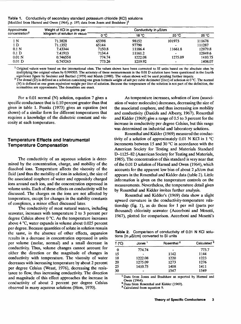
Table 1. Conductivity of secondary standard potassium chloride (KCI) solutions [Modified from Harned and Owen (1964), p. 197; data from Jones and Bradshaw J 1

Approximate concentration2

INID0.1 N0.1 D0.01 N0.01 D

Weight of KCI in grams p< kilogram of solution in vaci

71.382871.1352

7.433447.419130.7465580.745263

jr

J0 0°C

65398651447150.87134.4774.74773.26

Conductivity in pS/cm

18 °C

981529779011186.411161.2

1222.081219.92

20 °C

101973.

11661.8.

1275.09-

25 °C

111678111287

12879.812849.6

1410.751408.07

1 Original values were based on the international ohm. The values shown have been corrected to SI units based on the absolute ohm by multiplying the original values by 0.999505. The accuracy of these measurements in the 0.01 D solution have been questioned in the fourth significant figure by Saulnier and Barthel (1979) and Marsh (1980). The values shown will be used pending further inquiry.

2 The demal (D) is defined as a solution containing one gram formula weight of salt per cubic decimeter (liter) of solution at 0 °C. The normal (N) is defined as one gram equivalent weight per liter of solution. Because the temperature of the solution is not part of the definition, the normalities are approximate. The demalities are exact.

For a 0.01 normal (N) solution, equation 7 gives a specific conductance that is 0.10 percent greater than that given in table 1. Franks (1973) gives an equation (not shown) of a similar form for different temperatures that requires a knowledge of the dielectric constant and vis cosity at each temperature.

Temperature Effects and Instrumental Temperature Compensation

The conductivity of an aqueous solution is deter mined by the concentration, charge, and mobility of the dissolved ions. Temperature affects the viscosity of the fluid (and thus the mobility of ions in solution), the size of the associated cosphere of water and oppositely charged ions around each ion, and the concentration expressed in volume units. Each of these effects on conductivity will be discussed. The charges on the ions are not affected by temperature, except for changes in the stability constants of complexes, a minor effect discussed later.

The conductivity of most natural waters, including seawater, increases with temperature 2 to 3 percent per degree Celsius above 0 °C. As the temperature increases above 4 °C, water expands in volume about 0.025 percent per degree. Because quantities of solute in solution remain the same, in the absence of other effects, expansion results in a decrease in concentration expressed in units per volume (molar, normal) and a small decrease in conductivity. Thus, volume changes cannot account for either the direction or the magnitude of changes in conductivity with temperature. The viscosity of water decreases with increasing temperature by about 2 percent per degree Celsius (Weast, 1976), decreasing the resis tance to flow, thus increasing conductivity. The direction and magnitude of this effect approaches the increase in conductivity of about 2 percent per degree Celsius observed in many aqueous solutions (Hem, 1970).

As temperature increases, solvation of ions (associ ation of water molecules) decreases, decreasing the size of the associated cosphere, and thus increasing ion mobility and conductivity (Daniels and Alberty, 1967). Rosenthal and Kidder (1969) give a range of 0.5 to 3 percent for the increase in conductivity per degree Celsius, but this range was determined on industrial and laboratory solutions.

Rosenthal and Kidder (1969) measured the conduc tivity of a solution of approximately 0.01 N KCI in 1 °C increments between 15 and 30 °C in accordance with the American Society for Testing and Materials Standard D-l 125-82 (American Society for Testing and Materials, 1985). The concentration of this standard is very near that of the 0.01 D solution of Harned and Owen (1964), which accounts for the apparent low bias of about 2 /iS/cm that appears in the Rosenthal and Kidder data (table 2). Little information is given on the temperature controls on the measurements. Nevertheless, the temperature detail given by Rosenthal and Kidder invites further analysis.

Rosenthal and Kidder's (1969) data show a slight upward curvature in the conductivity-temperature rela tionship (fig. 1), as do those for 1 per mil (parts per thousand) chlorinity seawater (Accerboni and Mosetti, 1967), plotted for comparison. Accerboni and Mosetti's

Table 2. Comparison of conductivity of 0.01 N KCI solu tions (in /tS/cm) converted to SI units

T(°C)

01518202530

Jones 1

774.74-

1222.081275.091410.75

-

Rosenthal 2

.11421220127314081547

Calculated 3

773.711441223127614111549

1 Data from Jones and Bradshaw as reported by Harned and Owen (1964).

2 Data from Rosenthal and Kidder (1969). 8 Calculated from equation 9.


3600

2600 -

§1800

^1400

600

200

1 Actual ral*tk>nihlp

First dtrivitivt (Mop*)

S <cUJ { )

10 15 20

TEMPERATURE, IN DEGREES CELSIUS

25

Figure 1 . Conductivity-temperature relationships for 0.01 N KCI solution and 1 per mil chlorinity seawater.

equation1 has been used in this analysis rather than the original measurements obtained by Cox (1966) and Brown and Allentoft (1966), because the equation fits the data extremely well, allowing interpolation between mea surements. The change in conductivity per degree Celsius as a function of temperature (the first derivative) for both 0.01 N KCI and 1 per mil Cl seawater appears to be a linear function of temperature. The plot of conductivity as a function of temperature for 0.01 N KQ fits the equation obtained by least squares regression (r 2 =.825)

^=23.54+0.1536 T. (8)

1 Measurements of conductivity in seawater are based on the international ohm. To convert to a base of the absolute ohm (SI), multiply conductivity by 0.999505.

Integrating and evaluating the constant of integra tion at 18 °C (1222.69 fiS/cm of Harned and Owen's values), the K vs. T relationship becomes

*=774.1+23.54 7+0.07680 T : (9)

Equation 9 agrees to within about 0.13 percent with the four measurements by Harned and Owen (1964) at 0, 18, 20, and 25 °C. It thus appears to be satisfactory over the temperature range of interest in natural waters.

Equation 9 could be used to tabulate another useful parameter the temperature correction factor, or the ratio of *, IK, for 0.01 N KCI.

The percentage change in conductivity with temper ature for 0.01 N KQ is compared with that of 1 per mil Cl and 19 per mil Cl (undiluted) seawater in figure 2. Values for 0.01 N KCI were calculated using equation 9.


10 15 20

TEMPERATURE. IN DEGREES CELSIUS

25 30

Figure 2. Percentage change in conductivity with temperature for 0.01 N KCI solution and seawater in 1 °C increments.

It is apparent that the percentage changes in con ductivity with temperature of the 0.01 N KCI and 1 per mil Cl seawater are significantly different throughout the temperature range studied. Temperature-compensation circuits on most specific-conductance instruments in use today are based on the conductivity vs. temperature functions of 0.01 N KCI or NaCl solutions (J. Cluzel, Beckman Instruments, oral comm., 1985). Thus, they cannot provide accurate compensation in seawater solu tions at measurement temperatures significantly higher or lower than 25 °C. The measurement of specific con ductance in seawater will be discussed later.

It is to be expected also that temperature- compensation circuits based on 0.01 N KCI or NaCl solutions will not compensate accurately in waters with a far different chemical composition (a calcium sulfate-type or an acid mine water, for example), but no systematic study of such effects is known to have been done. Rosenthal and Kidder (1969) point out wide variations in the temperature function of special solutions found in industrial applications. The errors that occur in estuarine

waters are thought to affect the third significant figure of specific conductance (Bradford and Iwatsubo, 1980).

For comparison, values of the ratio (KS IK) for 0.01 N KCI are predicted by dividing the specific conductance (K, equals 1410.6 /nS/cm) calculated at 25 °C using equation 9 by the conductance («) calculated at other temperatures using equation 9. These ratios are plotted in figure 3 along with values calculated directly for 1 per mil Cl seawater from Accerboni and Mosetti (1967). The argument made earlier that temperature-compensation circuits based on the temperature response of 0.01 N KCI or NaCl solutions will lead to significant errors in specific-conductance estimates in seawaterlike solutions is valid here as well. Errors increase to about 2.5 percent at 0 °C.

An equation for computing the ratio is given in "Standard Methods," 15th edition (American Public Health Service, 1981, p. 73). Modified to fit terminology in this paper, it is cited here:

(10)K~l+0.0191(r-25)'


10 15 20


30

Figure 3. Values of the ratio of specific conductance to conductivity for 0.01 N KCI solution and 1 per mil chlorinity seawater.

Ratios predicted from equations 9 and 10 are compared with those calculated from data given by Rosenthal and Kidder (1969) and Harned and Owen (1964) and shown in table 3.

It is apparent that the equation from "Standard Methods" (equation 10) diverges from both actual mea surements and equation 9 at temperatures below 15 °C and is in error by about 5 percent at 0 °C. It also diverges at temperatures above 28 °C.

Because the temperature dependence of the limiting equivalent conductivity of most major ions in natural fresh waters comes closest to that of K+ and CT, the temperature function of 0.01 N KCI secondary standards is generally accepted as a model for the temperature function of most natural waters. (This will be discussed later.)

For convenience in field application, the ratio K S /K for 0.01 N KCI is tabulated (table 4) using equation 9. For example, if a conductance of 1000 is measured at 20 °C,

the specific conductance is 1000X1.106=1106. These ratios are appropriate only for natural fresh waters. Special solutions like seawater, acid mine drainage, and, possibly, acid rain are expected to have significantly different temperature functions, which should be deter mined case by case. Seawater is a well-studied special case discussed later.

Ionic Conductance

In 1883, Arrhenius proposed that all substances that form highly conducting aqueous solutions dissociate into ions capable of transferring charge. The body of theory developed since suggests that the conductivity of an aqueous solution is related to the sum of the concentration and mobility of the free ions. Kortum and Bockris (1951, equation 67) expressed this relation for solutions of a single salt as


Table 3. Comparison of the ratio K.JK predicted by dividing 1410.6 /tS/cm (at 25 °C) by the conductance calculated using equation 9, equation 10, and calculated using data from Rosenthal and Kidder (1969) and Harned and Owen (1964)

T(°C)

05

101518 202528303335

Predicted by equation 9

1.8221.5781.3871.2331.154 1.106 1.0000.9450.9100.8630.834

Predicted by equation 10

1.9141.6181.4021.2361.154 1.106 1.0000.9460.9130.8670.840

Calculated

1.821 1.-

1.2331.154 (1.154) 1 1.106 (1.106) 1 1.0000.9440.910

.-

1 Calculated using Hamed and Owen (1964) values at 25 ° and at 0, 18, and 20 °C.

where(11)

A= equivalent conductance of the salt in solution at concentration C (equiva lents/liter),

a= fraction of the salt dissociated, and +_= ionic mobility of the ions.

By analogy, equation 11 can be generalized for solutions of mixed salts as follows:

= awhere

C, , (12)

K= conductivity of the solution, a,= fraction of the /th constituent present as

the free ion,\*= equivalent conductivity of the /th ion, and C,= concentration of the /th species.

To use equation 12 to compute the conductivity of a solution, the total concentrations of conducting species (C,), the fractions of each species present in ionic form (a,), and the equivalent conductivity of each free ion (X; *) must be known. As will be shown, a, for the major conducting species in natural water can be determined with appropriate accuracy using known stability constants for formation of complexes. The equivalent conductivity, however, varies with the ionic strength and temperature of the solution in ways that theoretical approaches have as yet been unable to describe accurately.

Qassically, the relative mobility or equivalent con ductivity of salts in solution has been studied by the method of Hittorf 2 (summarized by Kortum and Bockris, 1951) in which the rates of change in concentrations around electrodes in solution are determined by the

2 Original work by Hittorf dates from 1853 to 1859. Taylor (1931) gives an extensive bibliography in English of the Hittorf method.

Table 4. Values of K,/K for 0.01 N KCI in 1 °C incrementscalculated by dividing 1410.6 /tS/cm (at 25 °C) by theconductance calculated using equation 9[Values at temperatures above 30 °C have not been verified bymeasurement]

Kf/K

T(°C)

0123456789

0

1.8221.7681.7171.6691.6221.5781.5361.4961.4581.422

10

1.3871.3531.3211.2901.2611.2331.2051.1791.1541.129

20

1.1061.0831.0611.0401.0201.0000.9810.9620.9450.927

30

0.9100.8940.8780.8630.8480.834

----

moving boundary method. The conductance of an indi vidual ion can be determined in absolute units for solu tions of simple salts.

Concentration Relationships

The equivalent conductivity (A*) of a salt in solution decreases with increasing concentration. Various studies have suggested that this relationship takes the form of the square-root law first expressed by Kohlrausch (Harned and Owen, 1964, p. 213):

A*=A°*-aVc, (13)

where A°* is the limiting equivalent conductivity.For convenience of notation and further discussion,

terms will be defined at 25 °C and equation 13 rewritten thus:

A=A°-a VC , (14)

whereA= equivalent conductance of a salt in solu

tion; (A* at 25 °C), A°= limiting equivalent conductance, anda= proportionality constant.

The limiting equivalent conductance is the equiva lent conductance extrapolated to infinite dilution, where interactions between ions in solution disappear and the mobility of individual ions reaches a maximum.

Kohlrausch's square-root law successfully describes the relationship for several single 1:1 salt solutions at concentrations from infinite dilution to 0.03 N. Several extensions of the square-root law have been used with some success at higher concentrations of a single salt:

A=A°-A VC +BC,

A=A°/(1+BA VCA=A°-

/ 1+B VC

(14a)

(14b)

(14c)


-10

1.1.

-20

-25

-300.1 0.2 0.3

VC~<EQUIVALENTSPER LITER) **

Figure 4. Decreases in equivalent conductance of selected electrolytes with increasing concentration. (Data from Harned and Owen, 1964, p.697.)

the general form is

A=A°-ACn (15)

where A, B, and if are empirically determined constants (all from Harned and Owen, 1964). The square-root law and its extensions have proved reasonably successful only in predicting equivalent conductances of dilute single-salt solutions; even in those cases, the linearity of the relation ship fails at concentrations approaching 0.01 N (fig. 4). The equivalent conductance of individual ions in mixed- salt solutions has been shown theoretically by Onsager and Fuoss (as discussed by Harned and Owen, 1964, p. 114) to be a function of the ionic strength, as

(16)

whereX,= equivalent conductance of ion i,

\i°= limiting equivalent conductance of ion /,/ ionic strength, and

f(i) = a function containing \°, the charge on the ion zh temperature, viscosity, the dielectric constant of the solvent, and a series expansion.

Equation 16 has been tested for single-salt solutions only, however, and the expansion of the series in the term

f(i) has proved to be enormously complex for solutions of mixed salts, as in natural waters. Because of this complex ity, the relation between \- and / has not been developed to the point where the specific conductance of a natural water may be calculated from the sum of equivalent conductances; equation 12 is therefore rewritten as

K =S (x- X-C- (17^

In dilute natural waters, however, evidence suggests that the limiting equivalent conductance of ions (table 5) is a good approximation of the equivalent conductance; thus the specific conductance can be closely approximated by equation 17, in the form

K =Z a, V C-t , (18)

with a,-, in most cases, being unity, implying complete dissociation. At total dissolved-solids concentrations above about 10~ 5 N (100 /iS/cm specific conductance), however, significant reductions in equivalent conductance of indi vidual ions occur that invalidate equation 18.

Temperature Relationships

Many measurements have been made of the limiting equivalent conductivity (A0*) of single-salt solutions over the temperature range 0 to 100 °C. Single-ion limiting


140

120

100

80

60

40

20

-20

V)oEC O I -60

.1 -80

-SO

OH" '

Notes:1. The curve for Mfl2+ Is not distinguishable from that

of Ca2*, end the curve for HC03- to not distinguishable from Na+, at this scale.

2. The curve for SO^-ii extended toward the only value available above 25 °C (180»S/cm at 100 °C) and It approximate only.

-100 -

-12010 20 30 40 50 60


Figure 5. Changes in limiting equivalent conductivity of selected ions with temperature. [Data from Robinson and Stokes (1959) p. 465, and for HCO3 from Jacobson and Langmier (1974).]

equivalent conductivity (\°*) has been tabulated by Robin son and Stokes (1959, p. 465). The variations in \°* for selected ions over a temperature range common in natural waters are shown in figure 5. Application of the Onsager and Fuoss equation (equation 16) for prediction of \°* in mixed-salt solutions is complicated by the problems dis cussed earlier. For single-salt solutions, equation 16 reduces to a tractable form (see Harned and Owen, 1964, p. 113), but the theory has apparently not been thor oughly tested even in simple solutions.

Robinson and Stokes (1959) note that \°* increases as much as fivefold from 0 ° to 100 °C for some ions, but that the product r{\°* (where i\ is the fluid viscosity) changes by less than 50 percent at most (for Cl~). As noted earlier, this observation suggests that changes in fluid viscosity account for most of the variation in conductivity of aqueous solutions as a function of temperature.

It may be surmised from the relationships shown in figure 5 that instrument temperature-compensation cir cuits based on the temperature function of a KC1 solution may yield inaccurate measurements of specific conduc tance in aqueous solutions with major ion compositions substantially different from the norm of fresh natural waters (high SO4 2 ~, high pH or low pH, for example) at temperatures more than 15 ° above or below 25 °C.

Effects of Complexation and Protonation

Ion associations or complexes form in natural waters (Stumm and Morgan, 1981) particularly between the alkaline-earth cations (Ca2+ , Mg2 "*", and Sr2+ ) and the sulfate (SO4 2 ~), carbonate(CO3 2 ~), and bicarbonate (HCO3 ~) anions. The conductivity of a solution is reduced by this effect, because the complexes are


Table 5. Limiting equivalent conductances (\/°) of selectedions[Data from Harned and CXven (1964, p. 231), except fluoride ion datafrom Franks (1973, p. 178). Values are based on the international ohmand should be multiplied by 0.999505 to obtain SI units (juS/cm permeg/L)]

CationCaa+H+K+Li+Mg2 "*"Na+NH4,+Sr+

V+

59.50349.8

73.5238.6653.0650.1173.459.46

AnionBr~

crF~

HC03-rNO3 ~OH~so4a-

\°_78.2076.3555.3244.576.971.44

197.880.0

uncharged or less charged than the parent ions and contribute little or nothing to the conductivity of the solution. The extent of complexation in solution may be calculated from known stability constants (K,) for the general reaction

[MX0 ](19)

where the brackets represent activities, M represents a metal cation, and X2 ~ represents an anion. Complexes between alkaline-earth cations and the bicarbonate anion (HCO3 ~) predominantly form compounds with a single plus charge, which contributes to solution conductivity. The reduction in free forms of the parent ions by compl exation needs to be considered. For most dilute natural waters, however, the conductivity of the complex can be ignored because the relative amount of complex formed is small and the mobility of the complex is low compared to that of the free ions. The protonated form of the sulfate anion (HSO4 ~) may also be safely ignored except in highly acidic waters containing sulfate, for example, acid mine drainage.

Table 6 lists stability constants for complexes of interest, including protonated forms of the anions.

APPLICATIONS TO ANALYTICAL QUALITY CONTROL

An Empirical Approach in Natural Waters

From the foregoing theoretical considerations, in particular Kohlrausch's law (equation 17), it is apparent that the sum of the products of the equivalent ionic

Table 6. Stability constants (log K,) for ion associations between major inorganic ions in natural waters at 25 °C [Values from Plummer and others, 1976]

Ion

H+

so4z-2.238 2.309 2.55 2.054

co3z-

2.980 3.153 2.81

10.330

HC<V

1.066 1.015 1.18 6.351

conductances and concentrations (C/X,) of the major ionic constituents determined by chemical analysis should approximate the specific conductance measured in a water sample. But satisfactory models for the equivalent ionic conductances (\) in mixed-salt solutions have not been developed and tested.

Miles and Yost (1982) used the difference between calculated and measured specific conductance coupled with the difference between measured total anion and cation concentrations in an analytical quality-control check that allowed identification of the constituent or measurement most likely in error when agreement was lacking. They were constrained with respect to the specific conductance range of applicability by the need to use limiting equivalent conductances (\°) to approximate ionic equivalent conductances (\). This approximation becomes progressively poorer at specific conductances exceeding 100 fiS/cm. The Miles and Yost (1982) tech nique could be extended to a broader concentration range if a suitable model for the decrease in \ with increasing concentration in a mixed-electrolyte solution were devel oped. The objective of this section of the report is to describe one empirical approach that appears to extend the applicable range to at least 600 |iS/cm . This approach has been used successfully to check analyses of water from the west coast of Florida that had a specific conduc tance of 9000 fiS/cm or less.

Initial attempts to fit actual data to the square-root law (equation 14) and its general extension (equation 15) showed a high degree of scatter, as did attempts to fit a form of equation 16 using ionic strength. The lack of satisfactory fit prompted another approach.

The model proposed and tested here is

K= «, C, (20)

the assumption being that an exponential correction factor (f) would faithfully describe curvature in the relationship between ionic conductance and concentration in natural waters and, on evaluation using a large data base of actual analyses, would prove to have a narrow range of values (approaching a constant) and a low standard deviation over a broad range of concentrations. This approach is also discussed by Miller (written commun.).


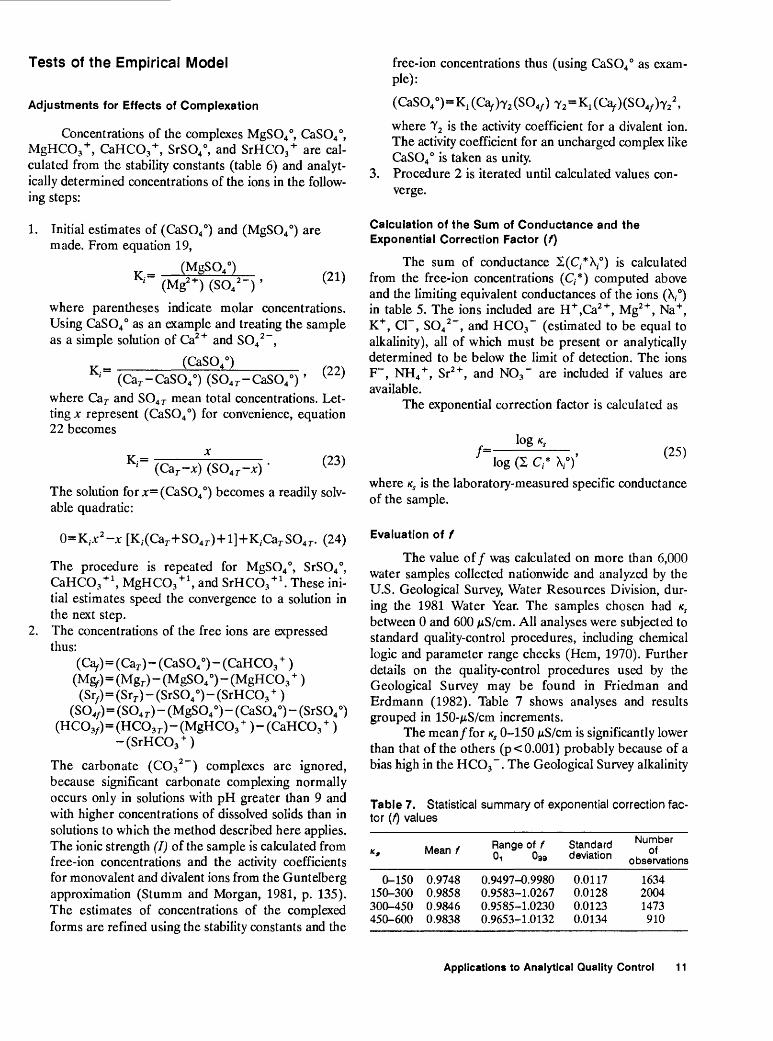
Tests of the Empirical Model

Adjustments for Effects of Complexation

Concentrations of the complexes MgSO4 °, CaSO4 °, MgHCO3 + , CaHCO3 + , SrSO4 °, and SrHCO3 + are cal culated from the stability constants (table 6) and analyt ically determined concentrations of the ions in the follow ing steps:

(21)

1. Initial estimates of (CaSO4 °) and (MgSO4 °) are made. From equation 19,

(MgSQ4 °) ' (Mg2+ ) (SO, 2 ') '

where parentheses indicate molar concentrations. Using CaSO4 ° as an example and treating the sample as a simple solution of Ca2+ and SO4 2 ~,

(CaSQ4 °)m 4 ' (Car -CaS04 °) (SO4r -CaSO4 °) ' ^ '

where Car and SO4r mean total concentrations. Let ting jc represent (CaSO4 °) for convenience, equation 22 becomes

(Car -*) (S04r -*) '(23)

The solution for^=(CaSO4 °) becomes a readily solv able quadratic:

0=K,.jc 2 -jc [K,.(Car+S04r)+l]+K,CarS04r . (24)

The procedure is repeated for MgSO4 °, SrSO4 °, CaHCO3 +1 , MgHCO3 +1 , and SrHCO^ 1 . These ini tial estimates speed the convergence to a solution in the next step.

2. The concentrations of the free ions are expressed thus:

(C3f) = (Car) - (CaSO4 °) - (CaHCO3 + ) (M&/)=(Mgr)-(MgS04 °)-(MgHC03 + ) (Sr/)=(Srr)-(SrS04 °)-(SrHC03 + )

(SO,/)=(S04r)-(MgS04 °)-(CaS04 °)-(SrS04 0) (HC03/)=(HC03r)-(MgHC03 + )-(CaHCO3 + )

-(SrHC03 + )

The carbonate (CO3 2 ~) complexes are ignored, because significant carbonate complexing normally occurs only in solutions with pH greater than 9 and with higher concentrations of dissolved solids than in solutions to which the method described here applies. The ionic strength (I) of the sample is calculated from free-ion concentrations and the activity coefficients for monovalent and divalent ions from the Guntelberg approximation (Stumm and Morgan, 1981, p. 135). The estimates of concentrations of the complexed forms are refined using the stability constants and the

free-ion concentrations thus (using CaSO4 ° as exam- pie):

(CaS04 °)=K1 (Ca/ )T2 (S04/ ) T2 =K1 (Ca/ )(S04/ )T2 2 ,

where 72 is the activity coefficient for a divalent ion. The activity coefficient for an uncharged complex like CaSO4 ° is taken as unity.

3. Procedure 2 is iterated until calculated values con verge.

Calculation of the Sum of Conductance and the Exponential Correction Factor (/)

The sum of conductance ^(C^X,0) is calculated from the free-ion concentrations (C,*) computed above and the limiting equivalent conductances of the ions (X,°) in table 5. The ions included are H+,Ca2+ , Mg2 +, Na+ , K+ , Cl~, SO4 2 ~, and HCO3 ~ (estimated to be equal to alkalinity), all of which must be present or analytically determined to be below the limit of detection. The ions F~, Nt^"1", Sr2+ , and NO3 ~ are included if values are available.

The exponential correction factor is calculated as

j '",log*,

log GS c,.* x,°)' (25)where KS is the laboratory-measured specific conductance of the sample.

Evaluation of 1

The value of/ was calculated on more than 6,000 water samples collected nationwide and analyzed by the U.S. Geological Survey, Water Resources Division, dur ing the 1981 Water Year. The samples chosen had KS between 0 and 600 jiS/cm. All analyses were subjected to standard quality-control procedures, including chemical logic and parameter range checks (Hem, 1970). Further details on the quality-control procedures used by the Geological Survey may be found in Friedman and Erdmann (1982). Table 7 shows analyses and results grouped in 150-jiS/cm increments.

The mean/for KS 0-150 jiS/cm is significantly lower than that of the others (p< 0.001) probably because of a bias high in the HCO3 ~. The Geological Survey alkalinity

Table 7. Statistical summary of exponential correction fac tor (/) values

«,0-150

150-300300-450450-600

Mean /

0.97480.98580.98460.9838

Range of / Oi 099

0.9497-0.99800.9583-1.02670.9585-1.02300.9653-1.0132

Standard deviation

0.01170.01280.01230.0134

Number of

observations

163420041473910

Applications to Analytical Quality Control 11

Table 8. One standard-deviation range of estimated *, using (2 C? X/)'[/=0.9850 and s-0.0128]

2 cr \;150300450600

Mean /-1s

130256380502

Mean f

139275411545

Mean f+ 1 5

148296444592

method involved a fixed-pH endpoint titration to pH 4.5, which is known to overestimate the actual value at low alkalinities (Barnes, 1964). Also, in low-ionic strength samples HCO3 ~ maybe less than the measured alkalinity. Thus, the sum of conductances would be biased high and the/value biased low. The/values in this range also show a small but significant (p < 0.001) positive relation to KS , the value at 150 jtS/cm being 0.9802, very close to the other three mean/ values. Therefore, that mean/value is judged to be in error and rejected in subsequent evalua tions. In part, the problem has been corrected recently for low-ionic strength samples by determining alkalinity through a strong-acid titration and Gran plot analysis (Gran, 1952).

The distributions of/values are normal in all cases, and significantly (p < 0.0001) less than unity. The sample- weighted mean and standard deviations of the remaining three values are/= 0.9850 and 5=0.0128. Because the/ value is used as an exponential, the range of ±1 standard- deviation unit in the estimate of KS is about ±8 percent, as shown in table 8.

The relationship between the / value and major constituent composition was examined by calculating cor relation coefficients between/and anion constituent ratios (table 9). Absolute values of the correlation coefficients are all less than 0.75, those for / vs. SO4 2~/Q~ were significantly different from zero at KS > 150 /tS/cm. The data were highly skewed to low values of the anion ratios, as can be seen by comparing ranges with medians; the correlation coefficients are probably strongly affected by a few high values and are, therefore, suspect. Nevertheless, the persistent recurrence of significant negative correla tion with SO4 2~/Q~ suggests that refinement in the / value may be possible by separating high-sulfate waters for special evaluation. The mean / value for 28 water samples collected in Florida and containing more than 300 mg/1 SO4 2 ~ was 0.9678, for example; that suggests a relationship.

A linear regression of/ vs. the fraction of monovalent ions (Fj) in 326 water samples from Florida had a correlation coefficient (r) of 0.38 and was statistically significant at the 99 percent confidence level.

Table 9. Relationship of the f value and anion ratios (p equals the probability of accepting the null hypothesis, H0 ; correlation coefficient /^O)[Range and median of the constituent ratios are shown only if the correlation coefficient was significantly (p < 0.05) different from zero; if not significant, values are shown by a dash ( )]

«*

0-150

150-300

300-450

450-600

Parameter

rPrP

RangeMedian

rP

Range Median

rP

Range Median

Constituent Ratiosscyci

-0.04330.08

-0.09490.0001 0.005-30 0.730

-0.12880.0001 0.001-59 0.783

-0.71990.0001 0.002-48 0.815

CI/HC03

0.00410.87

0.08100.0003 0.002-47 0.116

0.01880.47

0.06460.05

SCVHCOg

0.00190.94

0.03440.12

-0.02490.34

-0.25750.0001 0.0005-11 0.129

/=0.9687+ 0.01956 (26)

Although the regression equation was determined from data of limited geographical coverage, it strongly suggests that predictions of specific conductance can be improved by adjusting/for water composition.

Results of this evaluation suggest that the exponen tial correction factor / may be used with the limiting equivalent conductances of individual major ions and the analytically determined concentrations of major ions cor rected for complexation to estimate specific conductance for the water sample. This calculated value may be used in a variety of ways as a quality-control check on laboratory analyses and field measurements.

Quality Control Checks

Comparison of Measured with Computed Specific Conductance and Anions with Cations

Use of the exponential correction factor / and calculated adjustments of ion concentrations for com plexation as outlined above allow extension of the Miles and Yost (1982) technique to samples with specific con ductances up to at least 600 /tS/cm, the upper limit of the present evaluation. The technique involves plotting on orthogonal coordinates the difference between measured and computed specific conductance on the abscissa vs. the difference between the anion and cation equivalent con centrations measured in the laboratory on the ordinate. The location of a point representing a given analysis with respect to the origin (the location of a perfect analysis) indicates, in part, which of the several measurements involved may be in error. The plot may be used also as a


control chart with warning limits in concentric circles around the origin.

The technique was adapted in the U.S. Geological Survey Central Laboratories during 1985 for quality control of analyses of samples with specific conductances less than 100

Predicting the Sum of Anions or Cations

A method that supplements the Miles and Yost (1982) technique is to predict the sum of anion or cation equivalent concentrations in a sample and compare the predicted value with the measured value to judge whether one or the other is in error.

An average limiting equivalent conductance (Ax ) with adjustment for complexation is calculated for the water sample by

C,-* \-°

C, 12 (27)

where C* is the concentration of the ion / adjusted for complexation and C, is the analytically determined con centration without adjustment for complexation. Because, restating equation 25,

/=(25)log (2 C,' V)'

equation 27 may be written

log (2 C, /2),=(1// )log K,-log Ax , (28)

where the subscript p designates a predicted value. The differences

(2 C, /2),-2 Cc and (2 C, /2),-2 C., (29)

where subscripts a and c designate analytically deter mined anions and cations, respectively, will suggest whether errors in either the anion or cation determina tions have been made and provide guidance for confirma tory reanalysis.

A Special Case for Seawater and Estuarine Waters

The measurement of specific conductance and its relation to chemical composition in seawater and dilutions of seawater (as in estuaries) where the seawater compo nent dominates the chemical composition represents a well-studied special case. The chemical composition of seawater worldwide is remarkably constant (Cox, 1965). Over the years, a set of algorithms to calculate conduc tivity, specific conductance, density, and chlorinity and salinity (in grams/kilogram or parts per thousand) has been refined to apply to this special case. During the

1970's, the conductivity-salinity-temperature relationships in seawater were extensively reevaluated and refined. The results have been summarized by the Institute of Electri cal and Electronic Engineering (1980).

In the open ocean, variations in salinity are very small, but the differences in density resulting from tem perature and salinity variations determine large-scale oceanic circulation. Thus the measurements from which salinity is determined must be made with far greater accuracy and precision than is common (or usually nec essary) for fresh or estuarine waters, where variations are much larger. Open-ocean salinities normally are deter mined to five significant figures (for example, 35.013 per mil).

In estuarine waters, the relationships between mea surements of interest can be described by a set of algo rithms given in table 10. The algorithm of Accerboni and Mosetti (1967) fits actual measurements by Cox (1966) and Brown and Allentoft (1966) to 35 in 43,000 fiS/cm, or about 0.08 percent, at worst.

The difference between the algorithm of Accerboni and Mosetti (1967) and the algorithm of Pollak (1954), as modified by D.W. Pritchard (written commun., 1978), was evaluated by Bradford and Iwatsubo (1980). They calcu lated the salinity from assumed values of conductivity and temperature using Pollakfc algorithm and the conductivity from the calculated salinity and temperature using Accerboni and Mosetti's algorithm. The differences (assumed conductivity minus calculated conductivity) were < 100 fiS/cm over the salinity range 2 to 33 per mil and temperature range 0 to 30 °C (roughly 2,000 to 56,000 fiS/cm conductivity). The algorithms are adequate for estuarine work and more accurate than common field measurements.

Because of the error likely to occur in instrumental temperature compensation, as discussed earlier, compen sation circuits should not be used in measuring specific conductance in estuaries. Rather, the conductivity and temperature should be measured separately, and the specific conductance, if needed, calculated from Pollack^ algorithm followed by Accerboni and Mosetti's algorithm. Also, the standard solution for calibration of field instru ments should be a secondary standard seawater obtained from an oceanographic institution laboratory. Bradford and Iwatsubo (1980) discuss details of the procedure. Some common field instruments will not perform accu rately at high conductivities. A four-element conductivity probe appears to be preferable to a two-element platinized-platinum (electroplated with platinum black) or carbon-ring cell.

As a quality-control check, the analytically deter mined chloride concentration and the sum of dissolved solids (expressed in per mil) should agree with those predicted by the algorithms in table 10.

Applications to Analytical Quality Control 13

Table 10. Algorithms for calculating conductivity, specificconductance, chlorinity, and salinity of seawater and estua-rine waterAlgorithm to calculate conductivity (K) of seawater and estuarine waterfrom salinity (S) and temperature (T)[After Accerboni and Mosetti, 1967]

where,4 = 2.1923 5=0.12842 k= 0.0320 <r= 0.00290 h =0.1243 0=0.000978

7>20 °C 5=0.0000165

S =35%c

Algorithm to calculate salinity (S) of seawater and estuarine waterfrom conductivity (K) and temperature (T)[Modified from Pollak (1954) by Pritchard, D.W. (written commun.,1978)]Salinity (o/oo)=1.80655Xchlorinity (o/oo)Chlorinity (o/oo)=AXK

A -0.36996

*- 107 -0.7464X10- 3

whereK= conductivity in millisiemens/cmT= temperature in °C

50 =0.13855X101 5 1 =-0.46485668X10~ 1 52 =0.14887785X10~ 2 53 = -0.63083433XlO~4 54 =0.25144517X10-5 55 =-0.59600245X!0~7 56=0.57778085X10~ 9

Note: The conductivity of seawater is based on the international ohm. To convert to a base of the absolute ohm, values obtained from the algorithms above should be multiplied by 0.999505.

NOTES ON SPECIFIC CONDUCTANCE MEASUREMENTS

Instrumentation

The method commonly used to determine the con ductivity of unknown solutions is to measure their resis tance (R) in a cell with a known cell constant (K). The cell constant can be determined using equation 5 with a

standard solution of known conductivity, such as 0.01 N KC1, at the measurement temperature. Resistance of the cell with an unknown solution is then measured on a Wheatstone bridge or other balancing circuit, and con ductivity is calculated as

''KR (30)

Most commercial instruments provide measure ment cells designed with constants of 0.1,1.0, and higher, and a scale designed to show conductivity directly, rather than resistance.

Cells are commonly made of glass or plastic, may be of the dip or cup type, and contain electrodes of platinized platinum, as described by Brown and others (1970). The platinized surface is easily damaged, and carbon or tung sten electrodes are more suitable for field instrumenta tion. A four-element conductivity cell has been used in some field instruments. A constant current is imposed across the outer two elements, and the potential field developed in the solution is measured across the inner two elements, from which the conductivity is obtained. This cell resists corrosion or fouling better than the two- element resistance-measuring type.

In conventional devices using a Wheatstone bridge with alternating current at about 1,000 Hz, the resistance of the sample is balanced by a variable resistor, and the null point is indicated by an electron-ray tube or a needle. Advances in electronics now permit direct-reading tech niques.

Procedures

Some operational details vary from one instrument model to another. In general, the following steps are required to measure the conductivity or specific conduc tance: (1) using the solution to be measured, rinse from the measurement cell any solution or solids remaining from previous sample; (2) allow the temperature of the cell and the solution to equilibrate; (3) compensate for temperature electronically, or mathematically after mea surement using table 4; (4) null the instrument; and (5) record the temperature-corrected measurement (the spe cific conductance).

For natural waters, most instruments apply a 2 percent/°C temperature compensation to readings made at temperatures other than the reference temperature of 25 °C. Automatic temperature-compensation circuits equilibrate a thermistor with a high temperature coeffi cient with the solution to be measured. The appropriate selection of the thermistor and three resistors with low temperature coefficients permits the manufacturers to compensate the temperature effects for a wide range of solutions (Rosenthal and Kidder, 1969). Other instru-


ments require the temperature of the solution to be measured with a thermometer. After the temperature stabilizes, the dial is set to the temperature of the solution, the thermometer is removed, the instrument is nulled, and the specific conductance recorded.

The temperature-compensation circuits of all instruments should be checked for agreement with the 0.01 N KC1 secondary standard as described by equation 9. This may be done by measuring the specific conduc tance of the standard at several temperatures on either side of 25 °C and noting the variations in readings from the instrument, using the temperature-compensation cir cuit. Errors of more than 5 percent are unacceptable; in that event, the temperature-compensation circuit should not be used if it can be avoided. On manual compensation- type meters, the temperature dial may be kept at 25 °C. The instrument will then measure conductivity, and spe cific conductance can be calculated using table 4. If the temperature-compensation circuit cannot be eliminated, a correction graph should be drawn and kept with the instrument.

Before use, instrument calibration should be checked with at least three standard solutions.

SUMMARY

The specific conductance of aqueous solutions, par ticularly natural waters, has proven useful as a quantita tive indicator of the concentration of major ions. However, a review of current theory indicates that the conductivity of individual ions in mixed-salt solutions cannot be accu rately predicted from physical-chemical principles.

A review of accepted measurements of the conduc tivity of secondary standard 0.01 N KC1 solutions suggests that the variation with temperature is a complex function probably not duplicated well by instrument temperature- compensation circuits now available for correcting con ductivity to 25 °C (specific conductance) and that a widely used equation for correcting to 25 °C is in error by as much as 5 percent at 0 °C. A new algorithm has been derived and tested. Also, instrument temperature com pensation is not adequate for use in seawater or estuarine waters where the accuracy of conductivity and salinity measurements must approach 5 significant figures.

This report describes and evaluates an approach to predicting the specific conductance of a water sample from the analytically determined major-ion composition. The method corrects for reduction in free-ion concentra tion resulting from complexation, computes a limiting equivalent conductance for the sample by summing the products of the free-ion concentrations and the limiting equivalent conductances of the ions, and applies an expo nential correction factor to the sum of the products to estimate specific conductance.

The exponential correction factor has been evalu ated on the basis of about 6,000 analyses of water samples collected nationwide with measured specific conductances of 0 to 600 jttS/cm. The correction factor is normally distributed and significantly different from unity and has a mean value of 0.9850 and standard deviation of 0.0128, which predicts measured specific conductances to within ±8 percent (one standard deviation). The method allows extension of the range of the quality-control check (calcu lated specific conductance vs. measured specific conduc tance) on laboratory data beyond the current 100 /u,S/cm to 600 jttS/cm. The report describes a method for narrow ing the possible number of erroneous analyses or mea surements in a quality-control check. Evaluation of the approach at higher specific conductances is called for. Other approaches to adjustment of calculated limiting equivalent conductances to specific conductance should also be critically evaluated.

REFERENCES

Accerboni, Emrico, and Mosetti, F., 1967, A physical relation ship among salinity, temperature, and electrical conductiv ity of sea water: Bollettino di geofisci teorica ed applicata, v. 9, no. 34, p. 87-96.

American Public Health Service, American Water Works Asso ciation and the Water Pollution Control Federation, 1981, Standard methods for the examination of water and waste- water (15th edition): Washington, DC, American Public Health Association, 1134 p.

American Society for Testing and Materials, 1976, Standard for metric practice, E 380-76: ASTM, Philadelphia, PA.

Barnes, Ivan, 1964, Field measurement of alkalinity and pH: U.S. Geological Survey Water-Supply Paper 1535-H, 17 p.

Bradford, W.L., and Iwatsubo, R.T., 1980, Results and evalu ation of a pilot primary monitoring network, San Francisco Bay, California: U.S. Geological Survey Water-Resources Investigation 80-73, 115 p.

Brown, Eugene, Skougstad, M.W., and Fishman, M.J., 1970, Methods for collection and analysis of water samples for dissolved minerals and gases: U.S. Geological Survey Techniques of Water-Resources Investigations, book 5, chapter Al, 160 p.

Brown, N.L., and Allentoft, B., 1966, Salinity, conductivity and temperature relationship of sea water over the range of 0 to 50 p.p.t.: Bissett-Berman Corporation.

Cox, R.A., 1965, The physical properties of sea water, in Chemical Oceanography, v. 1, Riley, J.P., and Skirrow, G. (eds.), New York, Academic Press, p. 73-120.

1966, International oceanographic tables: National Insti tute of Oceanographie of Great Britain and UNESCO.

Daniels, Farrington, and Alberty, R.A., 1967, Physical chemis try (3d ed.): New York, John Wiley, 767 p.

Franks, Felix, 1973, Water, a comprehensive treatise: New York, Plenum Press, v. 3, 472 p.

Friedman, L.C., and Erdmann, D.E., 1982, Quality assurance practices for the chemical and biological analyses of water

References 15

and fluvial sediments: U.S. Geological Survey, Techniques of Water-Resources Investigations, book 5, chapter A6, 181 p.

Gran, Gunar, 1952, Determination of the equivalence point in potentiometric titrations part II: The Analyst, v. 77, p. 661-671.

Harned, H.S., and Owen, B.B., 1964, The physical chemistry of electrolytic solutions (3d ed.): American Chemical Society Monograph Series, New York, Reinhold Publishing, 803 p.

Hem, J.D., 1970, Study and interpretation of the chemical characteristics of natural waters (2d ed.): U.S. Geological Survey Water-Supply Paper 1473, 361 p.

Institute of Electrical and Electronic Engineering, 1980, Spe cial issue on the practical salinity scale: Journal of Oceanic Engineering, v. 5, no. 1, p. 1-65.

Jacobson, R.L., and Langmuir, Donald, 1974, Dissociation constants for calcite and CaHCO3 + from 0 to 50 °C: Geochimica et Cosmochimica Acta, v. 38, p. 301-318.

Jones, Grinnell, and Bradshaw, B.C., 1933, The measurement of the conductance of electrolytes V. A redetermination of the conductance of potassium chloride solutions in absolute units: Journal of the American Chemical Society, v. 55, p. 1780-1800.

Kortum, Georg, and Bockris, J.O., 1951, Textbook of electro chemistry: New York, Elsevier Publishing, v. 1, 351 p.

Lind, J.E., Zwolenik, J.J., and Fuoss, R.M., 1959, Calibration of conductance cells at 25 degrees with aqueous solutions of potassium chloride: Journal of the American Chemical Society, v. 81, p. 1557.

Marsh, K.N., 1980, On the conductivity of an 0.01 D aqueous potassium chloride solution: Journal of Solution Chemis try, v. 9, no. 10, p. 805-807.

Miles, LJ., and Yost, KJ., 1982, Quality analysis of USGS precipitation chemistry data for New York: Atmospheric Environment, v. 16, no. 12, p. 2889-2898.

Plummer, L.N., Jones, B.F., and Truesdale, A.H., 1976, WATEQF A FORTRAN IV version of WATEQ, a computer program for calculating chemical equilibrium of natural waters: U.S. Geological Survey Techniques of Water-Resources Investigation, 76-13, 63 p. (revised, 1978).

Pollak, M J., 1954, The use of electrical conductivity measure ments for chlorinity determination: Journal of Marine Research, v. 13, no. 2, p. 228-231.

Robinson, R.A., and Stokes, R.H., 1959, Electrolyte solutions: London, Butterworths, 571 p.

Rosenthal, Robert, and Kidder, R.J., 1969, Solution conductiv ity handbook: Cedar Grove, NJ, Beckman Instruments, 26P-

Saulnier, P., and Barthel, J., 1979, Determination of electrical conductivity of a 0.01 D aqueous potassium chloride solution at various temperatures by an absolute method: Journal of Solution Chemistry, v. 8, no. 12, p. 847-852.

Stumm, Werner, and Morgan, J.J., 1981, Aquatic chemistry (2d ed.): New York, John Wiley, 780 p.

Taylor, H.S., 1931, A treatise on physical chemistry: New York, Van Nostrand, v. 1, p. 678-683.

Weast, R.C. (ed.), 1976, Handbook of chemistry and physics: Cleveland, CRC Press, 2391 p.


A U S GOVERNMENT FEINTING OFFICE

Specific Conductance: Theoretical Considerations and Application

Documents