1 Western Regional Research Publication W2133 Benefits and Costs of Natural Resources Policies Affecting Public and Private Lands Twenty-Second Interim Report and Proceedings from the Annual Meeting September 2010 Annual Meeting held at: Tanque Verde Ranch Tucson, AZ February 24-26, 2010 Compiled by: Roger H. von Haefen Department of Agricultural and Resource Economics North Carolina State University NCSU Box 8109 Raleigh, NC 27695-8109 [email protected]

Welcome message from author
This document is posted to help you gain knowledge. Please leave a comment to let me know what you think about it! Share it to your friends and learn new things together.
Transcript

1
Western Regional Research Publication
W2133 Benefits and Costs of Natural Resources Policies Affecting
Public and Private Lands
Twenty-Second Interim Report and
Proceedings from the Annual Meeting
September 2010
Annual Meeting held at: Tanque Verde Ranch
Tucson, AZ February 24-26, 2010
Compiled by:
Roger H. von Haefen Department of Agricultural and Resource Economics
North Carolina State University NCSU Box 8109
Raleigh, NC 27695-8109 [email protected]
2
Table of Contents
Introduction 3
W2133 Past and Present Objectives 4
Participating Institutions 6
2010 List of Meeting Attendees 7
2010 Final Program 10
Papers (NOTE: W2133 objectives follow titles in parentheses) 17
"Modeling Spatial Spillover Effects in Willingness to Pay Estimates from 17 Dichotomous Choice Contingent Valuation Surveys: An Example Using the Mexican Spotted Owl" (2b, 3b) Julie Mueller (Northern Arizona) and John Loomis (Colorado State) "Publication Selection Bias in Empirical Estimates of Recreation Demand 29 Own-Price Elasticity: A Meta-Analysis" (2a, 3a) Randall S. Rosenberger (Oregon State) and T.D. Stanley (Hendrix College) "Did the Great Recession Reduce Visitor Spending and Willingness to Pay for 58 Nature-Based Recreation? Evidence from 2006 and 2009" (2b, 3a) John Loomis and Catherine Keske (Colorado State)

3
"Hedonic Valuation, Land Value Capitalization and the Willingness to Pay for Public 81 Goods" (2b, 3b) Nick Kuminoff (Arizona State) and Jaren Pope (Virginia Tech) "Assessing Tradeoffs in Land Use Service Flows within Subdivisions at Multiple Spatial 136 Scales" (1a, 2b, 3b) Joshua Abbott (Arizona State) and Allen Klaiber (Penn State) "Valuing Walkability and Vegetation in Portland, Oregon" (1a, 3b) 173 Niko Drake-McLaughlin and Noelwah R. Netusil (Reed College) "Species Preservation versus Development: An Experimental Investigation under 202 Uncertainty" (1a, 1b, 3b) Douglass Shaw (Texas A&M), Therese Grijalva (Weber State) and Robert Berrens (New Mexico) "What is the Value of a Trip to a National Park? Searching for a Reference 246 Methodology" (2b, 3a) John Duffield, David Paterson and Chris Neher (Montana) "Rounding in Recreation Demand Models: A Latent Class Count Model" (2b, 3a) 277 Keith Evans and Joseph Herriges (Iowa State) "Capturing Preference Uncertainty Under Incomplete Scenarios Using Elicited Choice 292 Probabilities" (1a, 2b, 3a) Subhra Bhattacharjee, Joseph Herriges and Catherine Kling (Iowa State)

4
Introduction These proceedings contain selected research papers presented at the 2010 Annual Meeting of the W2133 Regional Project, "Benefits and Costs of Resource Policies Affecting Public and Private Lands," held in Tucson, AZ, February 24-26, 2010. The annual convergence of W2133 scientists from academia and government took place at the lovely Tanque Verde Ranch. The Ranch was a fantastic gathering spot, attendance was at near-record levels, and the meeting provided an ideal venue for research collaboration, interaction, and exchange. W2133 also celebrated its 42nd anniversary of providing an invaluable outlet for leading research in environmental valuation, policy, and management. The collection of papers included herein illustrate the breadth and depth of research conducted by project members and affiliates. W2133 members and affiliates continue to develop methodologically innovative and policy relevant research in the broad areas of recreation demand analysis, land use, ecosystem service valuation, benefits transfer, stated preference, and climate change. These areas support W2133 objectives and meet future information needs of federal, state, and local resource managers and policy makers. The Annual Meeting ran smoothly thanks to the assistance of several W2133 members, affiliates, and supporters. The efforts of Klaus Moeltner, Brent Sohngen, Kim Rollins, Don Snyder, Fen Hunt and as always, John Loomis and Randy Rosenberger deserve special recognition. I am proud to have served as President for the 2009/2010 project year and look forward to next year's meeting in Albuquerque! Cheers, Roger H. von Haefen North Carolina State University

5
W2133 Past and Present Objectives 2007-2011 (W2133)
1. Natural Resource Management Under Uncertainty a. Economic Analysis of Agricultural Land, Open Space and Wildland-Urban
Interface Issues b. Economic Analysis of Natural Hazards Issues (Fire, Invasive Species, Natural
Events, Climate Change) 2. Advances in Valuation Methods
a. Improving Validity and Efficiency in Benefit Transfers b. Improving Valuation Methods and Technology
3. Valuation of Ecosystem Services a. Valuing Changes in Recreational Access b. Valuing Changes in Ecosystem Services Flows c. Valuing Changes in Water Quality
2002-2006 (W1133)
1. Estimate the Economic Benefits of Ecosystem Management of Forest and Watersheds 2. Calculate the Benefits and Costs of Agro-Environmental Policies 3. Estimate the Economic Value of Changing Recreational Access for Motorized and Non-
Motorized Recreation 4. Estimate the Economic Values of Agricultural Land Preservation and Open Space
1997-2001 (W133)
1. Valuing Ecosystem Management of Forests and Watersheds 2. Benefits and Costs of Agro-Environmental Policies 3. Valuing Changes in Recreational Access 4. Benefits Transfer for Groundwater Quality Programs
1992-1996 (W133)
1. Provide Site-Specific Use and Non-Use Values of Natural Resources for Public Policy Analysis
2. To Develop Protocols for Transferring Value Estimates to Unstudied Areas
1987-1991 (W133) 1. To Conceptually Integrate Market and Nonmarket Based Methods for Application to
Land and Water Resource Base Services 2. To Develop Theoretically Correct Methodology for Considering Resource Quality in
Economic Models and for Assessing the Marginal Value of Competing Resource Base Products
3. To Apply Market and Nonmarket Based Valuation Methods to Specific Resource Base Outputs

6
W2133 Past and Future Objectives (cont.) 1974-1986 (W133)
1. N/A 1967-1972 (WM-59)
1. N/A

7
Participating Institutions
Colorado State University
Cornell University
Iowa State University
Louisiana State University
Michigan State University
North Carolina State University
North Dakota State University
Ohio State University
Oregon State University
Penn State University
Texas A&M University
University of California Statewide Administration
University of California, Berkeley
University of California, Davis
University of Connecticut-Storrs
University of Delaware
University of Georgia
University of Illinois
University of Kentucky
University of Maine
University of Massachusetts
University of New Hampshire
University of Rhode Island
University of Wyoming
Utah State University
Washington State University
West Virginia University

8
2010 List of Attendees
Last Name First Name Affiliation Email
Abbott Josh Arizona State [email protected]
Abidoye Babatunde Iowa State [email protected]
Bergstrom John Georgia [email protected]
Bhattacharjee Subhra Iowa State [email protected]
Boyle Kevin Virginia Tech [email protected]
Braden John Illinois [email protected]
Carson Richard UC San Diego [email protected]
Colby Bonnie Arizona [email protected]
Drake-McLaughlin
Niko Reed College [email protected]
Duffield John Montana [email protected]
Dvarskas Anthony NOAA [email protected]
Evans Keith Iowa State [email protected]
Fletcher Jerry West Virginia [email protected]
Hanemann Michael Berkeley [email protected]
Hansen LeRoy USDA-ERS [email protected]
Herriges Joe Iowa State [email protected]
Hoehn John Michigan State [email protected]
Hoffmann Sandy RFF [email protected]
Hunt Fen NIFA / USDA [email protected]

9
Last Name First Name Affiliation Email
Jakus Paul Utah State [email protected]
Kaplowitz Michael Michigan State [email protected]
Katuwal Hari New Mexico [email protected]
Klaiber Allen Penn State [email protected]
Kobayashi Mimako Nevada-Reno [email protected]
Kuminoff Nick Arizona State [email protected]
Loomis John Colorado State [email protected]
Lupi Frank Michigan State [email protected]
Mansfield Carol RTI [email protected]
McLeod Don Wyoming [email protected]
Moeltner Klaus Nevada-Reno [email protected]
Mueller Julie Northern Arizona [email protected]
Navrud Stale Norwegian University [email protected]
Nepal Naresh New Mexico [email protected]
Netusil Noelwah Reed College [email protected]
Poe Greg Cornell [email protected]
Ready Rich Penn State [email protected]
Rollins Kim Nevada-Reno [email protected]
Rosenberger Randy Oregon State [email protected]
Schnier Kurt Georgia State [email protected]
Shaw Douglass Texas A&M [email protected]

10
Last Name First Name Affiliation Email
Shultz Steven Nebraska-Omaha [email protected]
Siikamäki Juha RFF [email protected]
Smith Kerry Arizona State [email protected]
Snyder Don Utah State [email protected]
Sohngen Brent Ohio State [email protected]
Spiridonov Georgi Delaware [email protected]
Stefanova Stela NECA [email protected]
von Haefen Roger NC State [email protected]
Wandschneider Phil Washington State [email protected]
Weber Matt US EPA - Oregon [email protected]

11
2010 Final Program
Notes:
• Paper presenters are in boldfaced below. • All sessions will be held in the Saguaro Room.
Wednesday, February 24 5:30pm Opening Reception, Cottonwood Grove 6:30pm Group Cookout, Cottonwood Grove Thursday, February 25 7:30am Group Breakfast & Registration, Main Dining Room Session 1 Recreation I 8:30am Frank Lupi (Michigan State) and Min Chen (Michigan State)
“When Site Characteristics in Recreation Demand Models are Endogeneously Supplied, Are Estimated Values Biased?”
8:50am Babatunde Abidoye (Iowa State) and Joseph Herriges (Iowa State) “RUM Models Incorporating Nonlinear Income Effects”
9:10am Juha Siikamäki (RFF) “Use of Time for Outdoor Recreation in the United States, 1965-2007”
9:30am 15-Minute Break Session 2 Hedonics / Land Use I 9:45am Steven Shultz (Nebraska-Omaha) and Nick Schmitz (Minnesota-Mankato)
“Hedonic Estimates of Open-Space and Low Impact Development Sub-Division Designs to Evaluate the Feasibility of Stormwater Management and Flood Control Programs”
10:05am Noelwah R. Netusil (Reed College) and Niko Drake-McLaughlin (Reed College) "Valuing Walkability and Vegetation in Portland, Oregon"
10:25am Don McLeod (Wyoming), Graham McGaffin (Wyoming), Christopher Bastian (Wyoming), Catherine Keske (Colorado State) and Dana Hoag (Colorado State) “Identifying Influential Factors for Colorado and Wyoming Landowners

12
Regarding Conservation Easement Acceptance” 10:45am 15-Minute Break Session 3 Ecosystem Services I 11:00am John Bergstrom (Georgia), Alan Covich (Georgia), Rebecca Moore (Georgia),
James Caudill (Fish and Wildlife Service) and Peter Grigelis (Fish and Wildlife Service) “A Conceptual Framework and Plan for Valuing Ecosystem Goods and Services Provided by U.S. National Wildlife Refuges”
11:20am LeRoy Hansen (ERS), Ronald Reynolds (Fish and Wildlife Service) and Charles Loesch (Fish and Wildlife Service) “Coupling Economic and Ecosystems Models to Better Target Conservation Funds”
11:40am John Hoehn (Michigan State), Michael Kaplowitz (Michigan State) and Frank Lupi (Michigan State) “Valuing Ecosystem Services: Testing the Extent of the Market in Benefits Transfer”
12:00pm Group Lunch, Main Dining Room Session 4 Meta Analysis / Benefits Transfer 1:30pm Randy Rosenberger (Oregon State) and Tom Stanley (Hendrix College)
“Publication Selection Bias in Empirical Estimates of Recreation Demand Own-Price Elasticity: A Meta-Analysis”
1:50pm Stale Navrud (Norwegian University) and Henrik Lindhjem (Norwegian Institute for Nature Research) “Using Meta-Analysis for International Benefit Transfer of Forest Ecosystem Services”
2:10pm John Braden (Illinois), Xia Feng (William and Mary) and DooHwan Won (Sugshen Women’s University) “Waste Sites and Property Values: A Meta-Analysis”
2:30pm 15-Minute Break Session 5 Stated Preference 2:45pm Richard Carson (UC-San Diego), Brett Day (East Anglia), Ian Bateman (East

13
Anglia), Diane Dupont (Brock), Jordan J. Louviere (Technology-Sydney), Sanae Morimoto (Kobe), Riccardo Scarpa (Waikato) and Paul Wang (Technology-Sydney) “Task Independence in Stated Preference Studies: A Test of Order Effect Explanations”
3:05pm John Loomis (Colorado State) and Catherine Keske (Colorado State) “Did the Great Recession Reduce Visitor Spending and Willingness to Pay for Nature-Based Recreation? Evidence from 2006 and 2009”
3:25pm Julie Mueller (Northern Arizona) and John Loomis (Colorado State) “Using Bayesian Estimation to Improve Efficiency in Willingness-to-Pay Estimation: An Example Using the Mexican Spotted Owl”
3:45pm 15-Minute Break Session 6 Recreation II 4:00pm Keith Evans (Iowa State) and Joseph Herriges (Iowa State)
“Rounding in Recreation Demand Models: A Latent Class Count Model” 4:20pm Georgi Spiridonov (Delaware) and George Parsons (Delaware)
“The Effect of Choice Set Formation on Welfare Measures: An Application of Random Utility Models to Beach Recreation in the Mid-Atlantic Region”
4:40pm Carol Mansfield (RTI), Roger von Haefen (NC State), Daniel Phaneuf (NC State) and George Van Houtven (RTI) “Measuring Nutrient Reduction Benefits for Policy Analysis Using Linked Non-Market Valuation and Environmental Assessment Models”
5:00pm Business Meeting w/ Comments from Fen Hunt and Donald Snyder 5:45pm Reception, Rincon Terrace 6:45pm Group Dinner, Main Dining Room Friday, February 26 7:30am Group Breakfast, Main Dining Room Session 7 Stated Preference II 8:30am Sandy Hoffmann (RFF/Alberta), Allen Krupnick (RFF) and Vic Adamowicz
(Alberta) “Who Speaks for the Household: Differences in Spouses' Willingness to Pay and How These are Resolved in a Couple”

14
8:50am Subhra Bhattacharjee (Iowa State), Joseph Herriges (Iowa State) and Catherine Kling (Iowa State) "Capturing Preference Uncertainty Under Incomplete Scenarios Using Elicited Choice Probabilities"
9:10am Kim Rollins (Nevada-Reno) and Mimako Kobayashi (Nevada-Reno) “Risk Preferences of Private Property Owners Facing Wildfire Risks in Nevada: Preliminary Results from the Pilot Survey Data”
9:30am 15-Minute Break Session 8 Hedonics / Land Use II 9:45am Joshua Abbott (Arizona State) and Allen Klaiber (Penn State)
“Assessing Tradeoffs in Land Use Service Flows Within Subdivisions at Multiple Spatial Scales”
10:05am Nick Kuminoff (Arizona State) and Jaren Pope (Virginia Tech) “Hedonic Valuation, Land Value Capitalization and the Willingness to Pay for Public Goods”
10:25am Allen Klaiber (Penn State) and Kerry Smith (Arizona State) “Quasi Experiments, Capitalization, and Estimating Tradeoffs for Changes in Spatially Delineated Amenities”
10:45am 15-Minute Break Session 9 Ecosystem Services II 11:00am Douglass Shaw (Texas A&M), Therese Grijalva (Weber State) and Robert
Berrens (New Mexico) “Species Preservation versus Development: An Experimental Investigation under Uncertainty”
11:20am Matt Weber (EPA) and Joe Marlow (Sonoran Institute) “Public Values Related to the Santa Cruz River in Southern Arizona”
11:40am Brent Sohngen (Ohio State), Sujithkumar Surendran Nair (Ohio State), Kevin King (Ohio State), Norman Fausey (Ohio State), Jonathan Witter (Ohio State), Douglas Southgate (Ohio State) “Integrated Watershed Economic Model for Non-Point Source Pollution Management in Upper Big Walnut Watershed, OH”
12:00pm Group Lunch, Main Dining Room

15
Session 10 Stated Preference and Recreation 1:30pm Greg Poe (Cornell), Antonio Bento (Cornell), Ben Ho (Cornell) and John Taber
(Cornell) “Culpability and Willingness to Pay for Environmental Quality: A Contingent Valuation and Experimental Economics Study”
1:50pm Paul Jakus (Utah State) and Dale Blahna (USDA Forest Service) “The Welfare Effects of Restricting Off-Highway Vehicle Access to Public Lands”
2:10pm John Duffield (Montana), David Paterson (Montana) and Chris Neher (Montana) “What is the Value of a Trip to a National Park? Searching for a Reference Methodology”
2:30pm 15-Minute Break Session 11 Climate Change, State Preference, and Fisheries 2:45pm Rich Ready (Penn State) and Jacqueline Yenerall (Penn State)
“Using a Choice Modeling Framework to Project Land Use Decisions” 3:05pm Kevin Boyle (Virginia Tech), Darla Hatton-MacDonald (CSIRO), Mark
Morrison (Charles Sturt) and John Rose (Sydney) “Untangling Differences in Values from Internet and Mail Stated Preference Studies”
3:25pm Kurt Schnier (Georgia State) “Heterogeneous Spatial Preferences and Mobility Effects in Fisheries: The Case of the Deadliest Catch”
3:45pm 15-Minute Break
Session 12 Stated Preference III 4:00pm Klaus Moeltner (Nevada-Reno), Mimako Kobayashi (Nevada-Reno) and
Kimberly Rollins (Nevada-Reno) “Latent Thresholds Analysis of Choice Data with Multiple Bids and Response Options”
4:20pm Hari Katuwal (New Mexico), Alok Bohara (New Mexico), Jennifer Thacher (New Mexico) and James Price (New Mexico) “Valuing Urban River Water Quality Improvements in Developing Cities: An Application of Choice Experiments”

16
4:40pm Carol Mansfield (RTI) and Roger von Haefen (NC State) “Piping Plovers, Off-Road Vehicles and Beach Closures at Cape Hatteras National Seashore”
5:00pm Adjourn

17
Modeling Spatial Spillover Effects in Willingness to Pay Estimates from Dichotomous Choice Contingent Valuation Surveys: An Example Using the
Mexican Spotted Owl
Julie Mueller Assistant Professor
The W.A. Franke College of Business Northern Arizona University
P.O. Box 15066 Flagstaff, AZ 86011
phone (918) 523-6612 [email protected]
John Loomis
Professor Dept. of Agricultural and Resource Economics
Colorado State University Fort Collins, CO 80523-1172
fax (970) 491-2067 phone (970) 491-2485

18
Abstract We present an application of a Bayesian spatial probit model estimating US residents’ WTP to
protect critical habitat for the endangered Mexican Spotted Owl from a Dichotomous-Choice
Contingent Valuation (DC CV) survey. If respondents’ propensities to vote “yes” on a WTP
question is similar to those in nearby locations, spatial dependence exists within the data, and
traditional probit models will result in biased estimated coefficients and thus biased WTP
estimates. Few studies applying spatial probit models to estimate WTP exist, however, recent
advances in Bayesian estimation through application of Markov Chain Monte Carlo simulations
and Gibbs sampling allow tractable estimation of spatial probit models that explicitly model
spatial dependence. We estimate WTP using a traditional non-spatial probit and a spatial probit.
The spatial autoregressive parameter is statistically significant in the spatial probit, indicating
that spatial spillover effects exist within our data. Values of WTP calculated from the spatial
models are statistically different from the WTP from the non-spatial probit. Therefore, we
conclude that failure to model spatial dependence with our CV data results in underestimation of
WTP.

19
Introduction and Background Mexican Spotted Owls are found in the Southwestern United States and Mexico. In the early
nineties, it was proposed that without habitat protection the Mexican Spotted Owl would be
extinct within 15 years. Therefore, the Mexican Spotted Owl was added to the list of
Endangered Species in 1993. 1 Despite the large amounts of protected critical habitat, the
Mexican Spotted Owl remains threatened today.2 Four million of the designated acres of critical
habitat for the Mexican Spotted Owl are in Arizona. The spotted owl requires old growth forests
for its habitat, and the designation of forests as protected areas has sparked a controversial debate
in the Southwest region of the US about the benefits and costs of endangered species habitat
recovery. In previous studies, the benefits of habitat recovery for the Mexican Spotted Owl were
obtained using Non-market Valuation. Non-market Valuation is a methodology for obtaining
values for environmental goods and services not bought and sold in typical markets. Because no
market “price” exists for preservation of Mexican Spotted Owl habitat, estimation techniques are
employed to determine a value. The most commonly applied method of Non-market Valuation
to obtain values for endangered species habitat is Contingent Valuation (CV). CV is a stated
preference methodology of Non-market Valuation. Stated preference methodologies obtain
values for environmental goods and services from survey data. Empirical methodologies are
used to obtain average Willingness to Pay (WTP) estimates, or values for protecting critical
habitat. Total benefits are calculated by summing average WTP across the relevant geographical
region.
Previous studies on the Mexican Spotted Owl have found average WTP to protect habitat
are approximately $45 per person per year (Loomis and Elkstrand, 1997). Because Spotted Owl
habitats have value beyond the species preservation through recreation and use, it is reasonable 1 http://ecos.fws.gov/speciesProfile/profile/speciesProfile.action?spcode=B074 2 http://www.biologicaldiversity.org/species/birds/Mexican_spotted_owl/index.html

20
to believe that people living closer to the habitat may have a higher WTP for preservation.
While distance to an environmental amenity is a common indicator of an individual’s value, few
studies have examined how WTP varies with distance from protected habitat. This study uses
data already obtained from a Contingent Valuation Survey on the Mexican Spotted Owl,
focusing the empirical analysis to consider how WTP varies with distance to habitat.
Many CV studies apply the dichotomous-choice elicitation format as recommended by Arrow et
al (1993). Dichotomous-choice methodologies involve sampling a large number of respondents
using a WTP question that is in a “voting” or “bid” format. Estimating WTP from a
dichotomous choice survey traditionally involves the use of Maximum Likelihood estimation
techniques. Application of other estimation procedures is uncommon, and to date, few studies
apply alternative methods (Halloway, Shankar and Rahman, 2002).
Yet, it is reasonable to believe that WTP will be similar for respondents living in the
same region, particularly when the non-market good used for valuation has both use and non-use
values. If observations of the dependent variable are similar to those in nearby locations, spatial
dependence exists within the data, and traditional probit models will result in biased estimated
coefficients and therefore biased WTP estimates. Few studies applying spatial probit models
exist and none have been applied to CVM of endangered species habitat. Recent advances in
Bayesian estimation through application of Markov Chain Monte Carlo simulations allow
tractable estimation of spatial probit models that explicitly allow for spatial dependence and
alleviate the possibility of biased estimated coefficients. In this paper, we present an application
of a Bayesian Spatial Probit model to investigate spatial spillover effects on WTP estimates.

21
Method Bayesian estimation of a spatial probit involves repeated sampling using the Gibbs MCMC
method. The spatial dependence in the probit model is represented as follows, where W is an
spatial weights matrix, ρ is the spatial autoregressive parameter, y is the observed value of
the limited-dependent variable, y* is the unobserved latent (net utility) dependent variable and X
is a matrix of explanatory variables.
1 0 0 0
~ 0,
If ρ is not statistically significant, the spatial model collapses to the standard binary probit model.
We estimate the general model and relax the strict independence assumption used in traditional
probit models by allowing changes in one explanatory variable for one observation to impact the
values of other observations within a neighboring distance as defined by the spatial weights
matrix, W. Intuitively, if the amount of endangered species habitat protected is reduced for an
individual observation, this will likely result in an increased distance to habitat for that
household and neighboring households, resulting in a marginal impact that goes beyond what is
represented in a simple estimated coefficient. LeSage and Pace (2009) label the differing spatial
impacts direct, indirect and total. In a traditional probit, marginal impacts are measured by
| / , (1)
where xr is the rth explanatory variable, is its mean, is a non-spatial probit estimate, and
· is the standard normal density. With a spatial probit,
| / , (2)
22
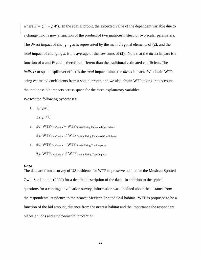
where . In the spatial probit, the expected value of the dependent variable due to
a change in xr is now a function of the product of two matrices instead of two scalar parameters.
The direct impact of changing xr is represented by the main diagonal elements of (2), and the
total impact of changing xr is the average of the row sums of (2). Note that the direct impact is a
function of ρ and W and is therefore different than the traditional estimated coefficient. The
indirect or spatial spillover effect is the total impact minus the direct impact. We obtain WTP
using estimated coefficients from a spatial probit, and we also obtain WTP taking into account
the total possible impacts across space for the three explanatory variables.
We test the following hypotheses:
1. HO: ρ=0
HA: ρ ≠ 0
2. Ho: WTPNon-Spatial = WTP Spatial Using Estimated Coefficients
HA: WTPNon-Spatial ≠ WTP Spatial Using Estimated Coefficients
3. Ho: WTPNon-Spatial = WTP Spatial Using Total Impacts
HA: WTPNon-Spatial ≠ WTP Spatial Using Total Impacts
Data The data are from a survey of US residents for WTP to preserve habitat for the Mexican Spotted
Owl. See Loomis (2000) for a detailed description of the data. In addition to the typical
questions for a contingent valuation survey, information was obtained about the distance from
the respondents’ residence to the nearest Mexican Spotted Owl habitat. WTP is proposed to be a
function of the bid amount, distance from the nearest habitat and the importance the respondent
places on jobs and environmental protection.
23
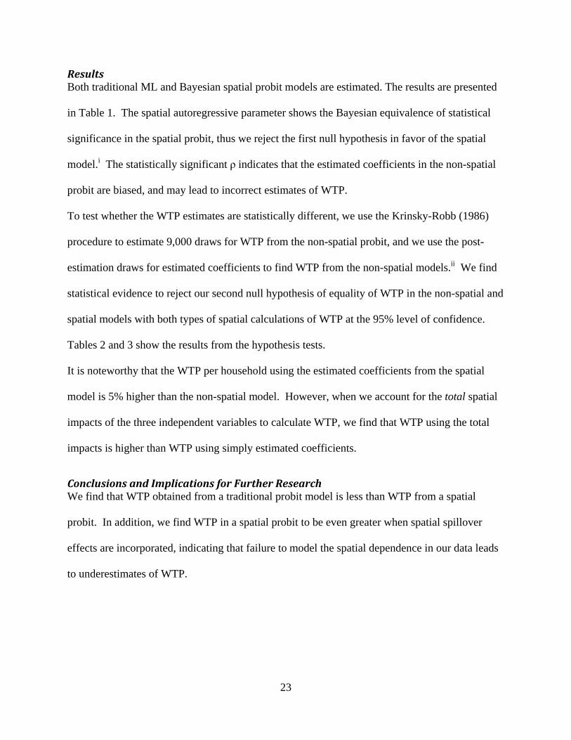
Results Both traditional ML and Bayesian spatial probit models are estimated. The results are presented
in Table 1. The spatial autoregressive parameter shows the Bayesian equivalence of statistical
significance in the spatial probit, thus we reject the first null hypothesis in favor of the spatial
model.i The statistically significant ρ indicates that the estimated coefficients in the non-spatial
probit are biased, and may lead to incorrect estimates of WTP.
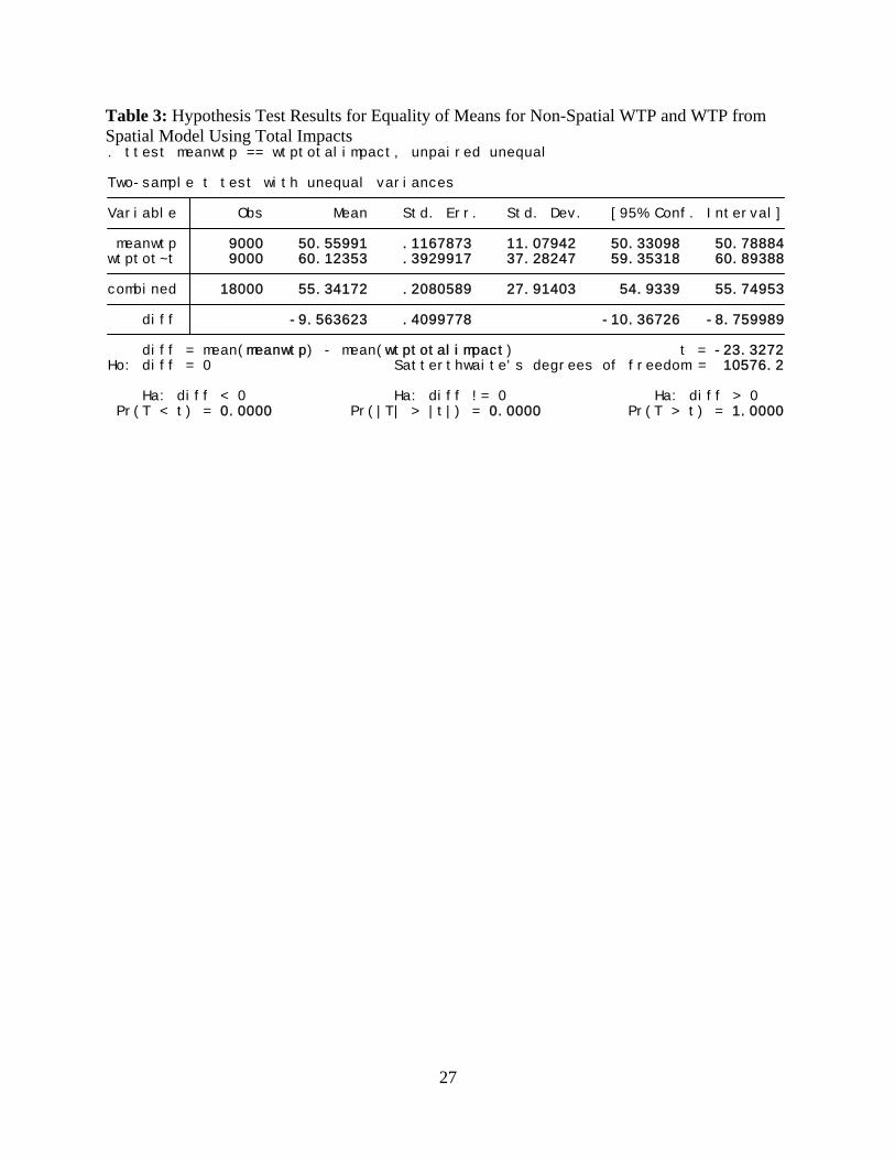
To test whether the WTP estimates are statistically different, we use the Krinsky-Robb (1986)
procedure to estimate 9,000 draws for WTP from the non-spatial probit, and we use the post-
estimation draws for estimated coefficients to find WTP from the non-spatial models.ii We find
statistical evidence to reject our second null hypothesis of equality of WTP in the non-spatial and
spatial models with both types of spatial calculations of WTP at the 95% level of confidence.
Tables 2 and 3 show the results from the hypothesis tests.
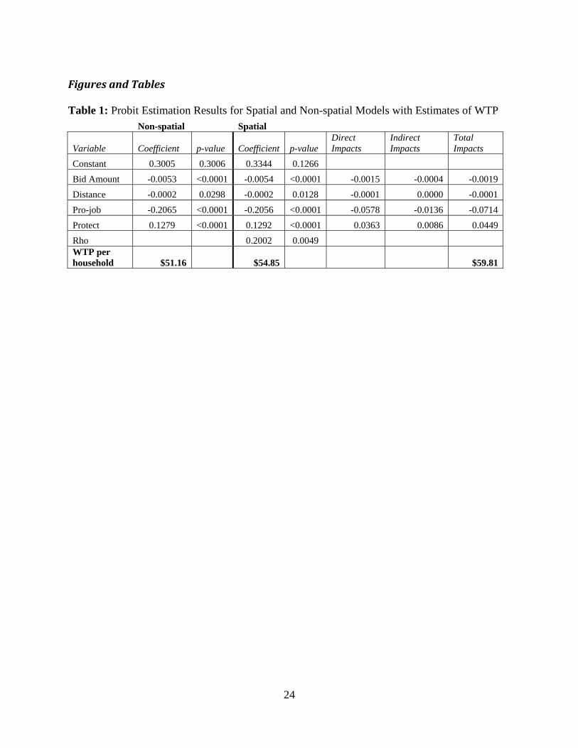
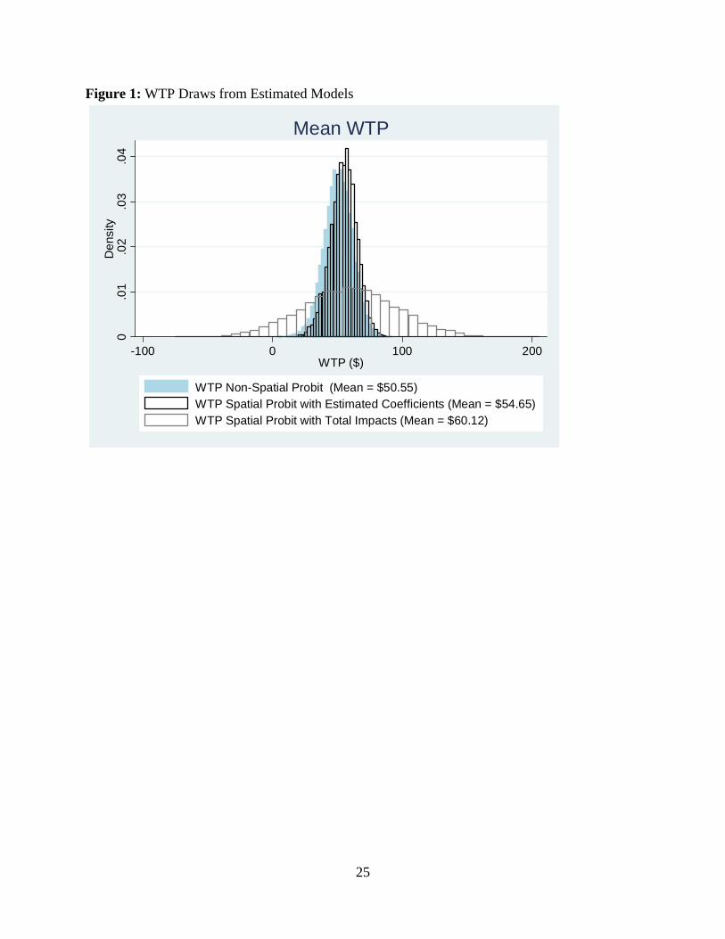
It is noteworthy that the WTP per household using the estimated coefficients from the spatial
model is 5% higher than the non-spatial model. However, when we account for the total spatial
impacts of the three independent variables to calculate WTP, we find that WTP using the total
impacts is higher than WTP using simply estimated coefficients.
Conclusions and Implications for Further Research We find that WTP obtained from a traditional probit model is less than WTP from a spatial
probit. In addition, we find WTP in a spatial probit to be even greater when spatial spillover
effects are incorporated, indicating that failure to model the spatial dependence in our data leads
to underestimates of WTP.
24
Figures and Tables Table 1: Probit Estimation Results for Spatial and Non-spatial Models with Estimates of WTP Non-spatial Spatial
Variable Coefficient p-value Coefficient p-value Direct Impacts
Indirect Impacts
Total Impacts
Constant 0.3005 0.3006 0.3344 0.1266 Bid Amount -0.0053 <0.0001 -0.0054 <0.0001 -0.0015 -0.0004 -0.0019 Distance -0.0002 0.0298 -0.0002 0.0128 -0.0001 0.0000 -0.0001 Pro-job -0.2065 <0.0001 -0.2056 <0.0001 -0.0578 -0.0136 -0.0714 Protect 0.1279 <0.0001 0.1292 <0.0001 0.0363 0.0086 0.0449 Rho 0.2002 0.0049 WTP per household $51.16 $54.85 $59.81
25
Figure 1: WTP Draws from Estimated Models
0.0
1.0
2.0
3.0
4D
ensi
ty
-100 0 100 200WTP ($)
WTP Non-Spatial Probit (Mean = $50.55)WTP Spatial Probit with Estimated Coefficients (Mean = $54.65)WTP Spatial Probit with Total Impacts (Mean = $60.12)
Mean WTP

26
Table 2: Hypothesis Test Results for Equality of Means for Non-Spatial WTP and WTP from Spatial Model Using Estimated Coefficients
Pr(T < t) = 0.0000 Pr(|T| > |t|) = 0.0000 Pr(T > t) = 1.0000 Ha: diff < 0 Ha: diff != 0 Ha: diff > 0
Ho: diff = 0 Satterthwaite's degrees of freedom = 17901 diff = mean(meanwtp) - mean(wtpestcoeff) t = -25.6618 diff -4.090499 .1594006 -4.402939 -3.778058 combined 18000 52.60516 .081143 10.88648 52.44611 52.76421 wtpest~f 9000 54.65041 .1084862 10.2919 54.43775 54.86306 meanwtp 9000 50.55991 .1167873 11.07942 50.33098 50.78884 Variable Obs Mean Std. Err. Std. Dev. [95% Conf. Interval] Two-sample t test with unequal variances
27
Table 3: Hypothesis Test Results for Equality of Means for Non-Spatial WTP and WTP from Spatial Model Using Total Impacts
Pr(T < t) = 0.0000 Pr(|T| > |t|) = 0.0000 Pr(T > t) = 1.0000 Ha: diff < 0 Ha: diff != 0 Ha: diff > 0
Ho: diff = 0 Satterthwaite's degrees of freedom = 10576.2 diff = mean(meanwtp) - mean(wtptotalimpact) t = -23.3272 diff -9.563623 .4099778 -10.36726 -8.759989 combined 18000 55.34172 .2080589 27.91403 54.9339 55.74953 wtptot~t 9000 60.12353 .3929917 37.28247 59.35318 60.89388 meanwtp 9000 50.55991 .1167873 11.07942 50.33098 50.78884 Variable Obs Mean Std. Err. Std. Dev. [95% Conf. Interval] Two-sample t test with unequal variances
. ttest meanwtp == wtptotalimpact, unpaired unequal
28
References Arrow et al. “Report of the NOAA Panel on Contingent Valuation.” Federal Register 58(10)
4602-14. Krinsky, I. & Robb, A. L. (1986) On approximating the statistical properties of elasticities,
Review of Economics and Statistics, 68, pp. 715–719. Holloway, Garth, Shankar, Bhavani and Rahman, Sanzidur. (2002) Bayesian spatial probit
estimation: a primer and an application to HYV rice adoption. Agricultural Economics 27 pp. 383-402.
Li et. Al. (2009) “Public support for reducing US reliance on fossil fuels: Investigating
household willingness-to-pay for energy research and development. Ecological Economics, 68, pp. 731–742.
LeSage, J. and R.K. Pace. Introduction to Spatial Econometrics. 2009. CRC Press. Loomis, John and Elkstrand, Earl. “Economic Benefits of Critical Habitat for the Mexican
Spotted Owl: A Scope Test Using a Multiple-Bounded Contingent Valuation Survey.” Journal of Agriculture and Resource Economics 22(2) 356-366.
Loomis, John B. and White, Douglas S. “Economic Benefits of Rare and Endangered Species:
Summary and Meta-Analysis.” Ecological Economics 18 (1996): 197-126. Loomis, John B. “Vertically Summing Public Good Demand Curves: An Empirical Comparison
of Economic Versus Political Jurisdiction.” (2000). Land Economics 78 (2): 312-321. Smith, Tony E. and LeSage, James P. (2004). “A Bayesian Probit Model with Spatial
Dependencies.” Spatial and Spatiotemporal Econometrics. Advances in Econometrics Volume 18, pp. 127-160.
Yoo, Seung-Hoon. (2004) A Note on a Bayesian Approach to a Dichotomous Choice
Environmental Model, Journal of Applied Statistics, Vol. 31, No. 10, pp.1203–1209. i The “p-values” are calculated using the method described in Gelman et al ***** ii Jeanty, P. Wilner. 2007. "wtpcikr: Constructing Krinsky and Robb Confidence Interval for Mean and Median Willingness to Pay (WTP) Using Stata."North American Stata Users' Group Meetings 2007, 8.
29
Publication Selection Bias in Empirical Estimates of Recreation Demand Own-Price Elasticity: A Meta-Analysis
Randall S. Rosenberger Department of Forest Ecosystems & Society
Oregon State University Corvallis, OR
T. D. Stanley Department of Economics & Business
Hendrix College Conway, AR
Acknowledgments: This research was supported by funds from the U.S. EPA STAR Grant #RD-832-421-01 to Oregon State University and the USDA Forest Service, Rocky Mountain Research Station. Although the research described in this article has been funded wholly or in part by the United States Environmental Protection Agency through grant/cooperative agreement number RD-832-421-01 to Oregon State University, it has not been subjected to the Agency's required peer and

30
policy review and therefore does not necessarily reflect the views of the Agency and no official endorsement should be inferred.

31
Publication Selection Bias in Empirical Estimates of Recreation Demand Own-Price Elasticity: A Meta-Analysis Abstract
A meta-regression analysis of own-price elasticity of recreation demand estimates in the U.S.
shows significant publication selection bias based on simple and multivariate FAT-PET tests.
However, these tests also reveal that there is a genuine empirical elasticity measure. While the
raw average from the data shows elasticity to be unitary (-0.997), this estimate is one-fold to six-
fold too elastic, respectively, when compared to the multivariate PEESE estimate accounting for
heterogeneity (-0.893) and the simple PEESE estimate (-0.158). These results are based on
nearly 600 estimates of own-price elasticity drawn from the recreation demand literature. One
previous MRA was conducted on own-price elasticity estimates (Smith and Kaoru, 1990). We
estimate a similar OLS regression model and find substantial consistency between our model and
Smith and Kaoru’s model according to sign and significance of moderator variables (i.e.,
determinants of elasticities). However, when a multivariate FAT-PET-MRA, which captures
variations in elasticity estimated due to their standard errors and weights the data according to
these standard errors, most of the moderator variables change in sign or significance.
Nonetheless, we confirm Smith and Kaoru’s model and general conclusions that researcher
modeling decisions and assumptions, along with theoretical expectations, do matter. This is
exhibited in the high degree of heterogeneity in the recreation demand literature.
JEL Classifications: C21; C51; Q26; Q51; R22 Keywords: Meta-analysis; Price Elasticity; Publication selection bias; Recreation Demand

32
Introduction
Recreation demand models have been empirically estimated for over a half-century using
an indirect method proposed by Harold Hotelling in 1947. Collectively, there have been over
329 recreation demand studies1 providing over 2,700 empirical estimates of the access value to
recreation resources from 1958 to 2006 (Rosenberger and Stanley 2007). Only one other study
evaluated estimates of own-price elasticity of recreation demand. Smith and Kaoru (1990)
conducted a meta-regression analysis (MRA) of recreation own-price elasticity estimates,
including approximately 77 studies providing 185 own price elasticity estimates from 1970 to
1986. They did not formally test for publication selection bias in their data. This paper tests for
publication selection bias in elasticity estimates from the recreation demand literature.
Own-price elasticity measures the sensitivity of demand to changes in prices. Price
elasticity is typically defined as the percentage change in quantity (e.g., recreation trips) resulting
from a one-percentage change in price (e.g., travel costs). While price elasticities are unitless
measures of demand’s responsiveness to price changes, they are a function of an estimated price
coefficient (δq/δp) and the ratio of prices and quantities (p/q) typically evaluated at their mean
values. If a double-log model is estimated, it can easily be shown that the price coefficient is the
elasticity.
Previous meta-regression analyses have been conducted on elasticity measures, including
private good brands/markets (Tellis 1988), money demand (Knell and Stix 2005), residential
water demand (Espey, Espey and Shaw 1997; Dalhuisen et al. 2003), gasoline demand (Espey
1997, 1998), and cigarette demand (Gallett and List 2003). Dalhuisen et al. (2003) included a
1 This estimate includes only those studies that reported access values for recreation resources. Not included in this total are studies that estimated demand functions without providing consumer surplus estimates and studies providing estimates of marginal values or values per choice occasion.

33
dummy variable identifying unpublished studies and found a significant difference between
elasticity measures in published and unpublished studies, ceteris paribus. Gallett and List (2003)
included a dummy variable identifying the top 36 journals, finding a significant difference in
elasticity estimates for the top journals, ceteris paribus. Stanley (2005a) evaluated the residential
water elasticity data using the funnel asymmetry and precision effect tests (FAT-PET),
uncovering significant publication bias as a function of the standard error of the price elasticity
measures; price elasticities of water demand are exaggerated four-fold through publication
selection bias. However, Knell and Stix (2005) also apply the FAT-PET test on elasticities of
money demand and found small and insignificant publication selection bias.
Publication Selection Bias Tests
Publication selection bias results from a literature of reported estimates that are not an
unbiased sample of the actual empirical evidence.2 Researchers and reviewers often have a
preference for statistically significant results or for results that conform to prior theoretical
expectations, or both. Publication selection has long been recognized as an important problem in
economics (e.g. Card and Krueger 1995; DeLong and Lang 1992; Feige 1975; Leamer 1983;
Leamer and Leonard 1983; Lovell 1983; Roberts and Stanley 2005; Rosenberger and Johnston
2009; Tullock 1959, to cite but a few). The tendency to report only statistically significant
results is greatly bolstered when there is also professional consensus regarding the existence and
direction of an effect—such as the ‘Law’ of demand. When primary survey data are used to
estimate the price coefficient of a demand relation, the first estimated coefficient produced will
2 Some regard ‘publication selection bias’ to be a misnomer, because publication need not be involved. Researchers will learn that there is a preference for statistically significant findings and will tend to selectively report these in any report, published or not. ‘Selection biases’ or ‘reporting biases’ are more descriptive terms for the phenomena discussed in this paper.

34
not necessarily be the one that is reported. Rather, analysts will wish to be sure that the
estimated demand relation is ‘valid.’ Validity will require, at a minimum, that the price
coefficient be negative and in many cases that it be statistically significant as well. Thus, the
sample of reported estimates may not be random, and, if not, any summary of estimates will be
biased. “Publication bias (aka ‘file-drawer problem’) is a form of sample selection bias that
arises if primary studies with statistically weak, insignificant, or unusual results tend not to be
submitted for publication or are less likely to be published” (Nelson and Kennedy 2009, p. 347).
Wide application of MRA in economics suggests that publication biases are often as large
as or larger than the underlying parameter being estimated (Doucouliagos and Stanley 2009;
Hoehn 2006; Krassoi Peach and Stanley 2009; Stanley 2005a, 2008). For example, the negative
sign of own-price elasticity is often required to validate the researcher’s estimated demand
relation. Should a positive coefficient be produced, researchers feel obligated to re-specify the
demand relation, find a different econometric estimation technique, identify and omit outliers, or
somehow expand the dataset. As a result of such publication selection, reported price elasticities
of water demand are exaggerated by a factor of nearly four (Dalhuisen et al. 2003; Stanley
2005a). Needless to say, the water board of a drought-stricken area will be greatly disappointed
to find that a doubling of residential water rates reduces usage by a mere 10% and not the
expected 40%. Because the ‘Law’ of demand is so widely accepted, demand studies will
ironically exhibit the greatest publication bias.
Over the past decade, meta-analysis has become routinely employed to identify and
correct publication selection in economics research (Ashenfelter et al. 1999; Card and Krueger
1995; Coric and Pugh 2008; Doucouliagos 2005; Doucouliagos and Stanley 2009; Egger et al.
35
1997; Gemmill et al. 2007; Görg and Strobl 2001; Knell and Stix 2005; Krassoi Peach and
Stanley 2009; Longhi, Nijkamp and Poot 2005; Mookerjee 2006; Roberts and Stanley 2005;
Rose and Stanley 2005; Stanley 2005a, b, 2008). However, in environmental economics, meta-
analysis has been widely applied but with limited focus on publication selection and other
potential biases (Hoehn 2006; Nelson and Kennedy 2009; Rosenberger and Johnston 2009).
Previous MRAs in environmental economics have treated publication selection bias as arising
from the source of an estimate; a form of systematic heterogeneity among the metadata (Smith
and Huang 1993, 1995; Rosenberger and Stanley 2006). Typically a dummy variable identifying
the publication type is added as an independent variable in the MRA (Rosenberger and Stanley
2006) or a sample selection model is estimated as a form of model specification test (Smith and
Huang 1993, 1995). However, more robust tests of publication selection bias are available.
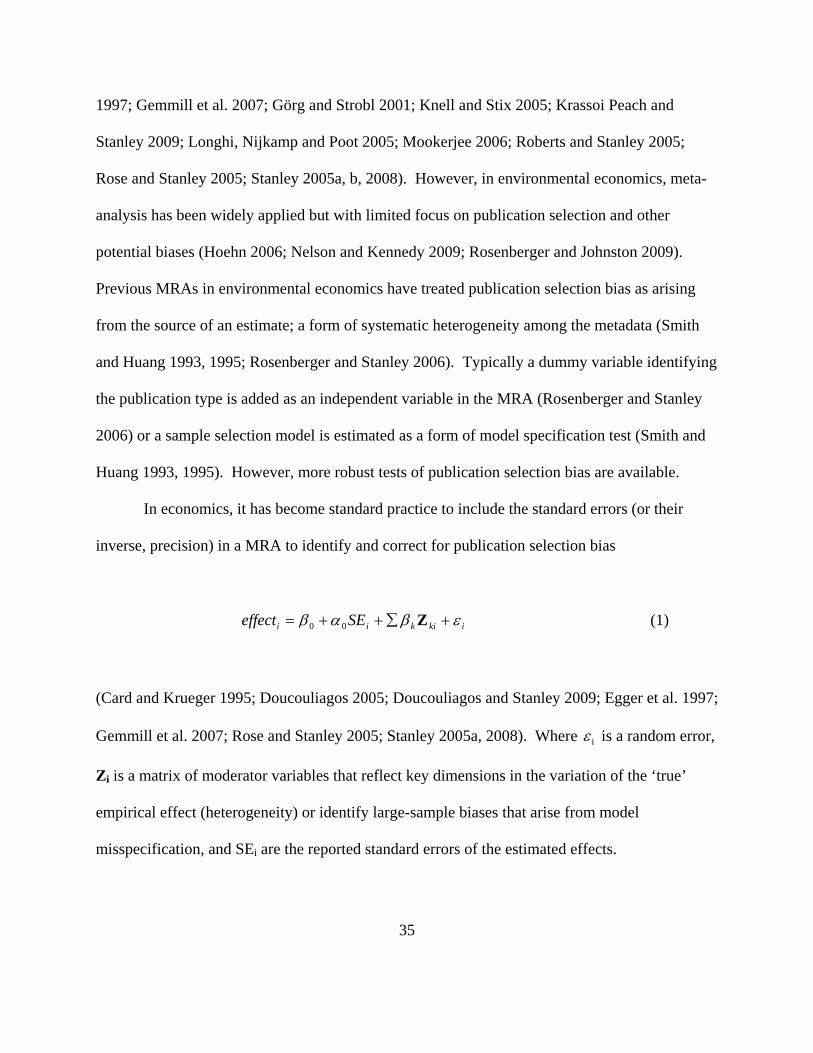
In economics, it has become standard practice to include the standard errors (or their
inverse, precision) in a MRA to identify and correct for publication selection bias
ikikii SEeffect εβαβ +∑++= Z00 (1)
(Card and Krueger 1995; Doucouliagos 2005; Doucouliagos and Stanley 2009; Egger et al. 1997;
Gemmill et al. 2007; Rose and Stanley 2005; Stanley 2005a, 2008). Where iε is a random error,
Zi is a matrix of moderator variables that reflect key dimensions in the variation of the ‘true’
empirical effect (heterogeneity) or identify large-sample biases that arise from model
misspecification, and SEi are the reported standard errors of the estimated effects.
36
Simulations have shown that meta-regression model (1) provides a valid test for
publication bias (H1:α0≠0), called ‘funnel-asymmetry test’ (FAT), and a powerful test for
genuine empirical effect beyond publication selection (H1:β0≠0), called a ‘precision-effect test’
or PET) (Stanley 2008). The reason why this approach works is that the standard error serves as
a proxy for the amount of selection required to achieve statistical significance. Studies that have
large standard errors are at a disadvantage in finding statistically significant effect sizes. Effect
sizes need to be proportionally larger than their standard errors, because statistical significance is
typically determined by a calculated t-value where the standard error is in the denominator. Such
imprecise estimates will likely require further re-estimation, model specification, and/or data
adjustments to become statistically significant. Thus, we expect to see greater publication
selection in estimates with larger SE, ceteris paribus. This correlation between reported effects
and their standard errors has been observed in dozens of different areas of economics research
(Doucouliagos and Stanley 2008).
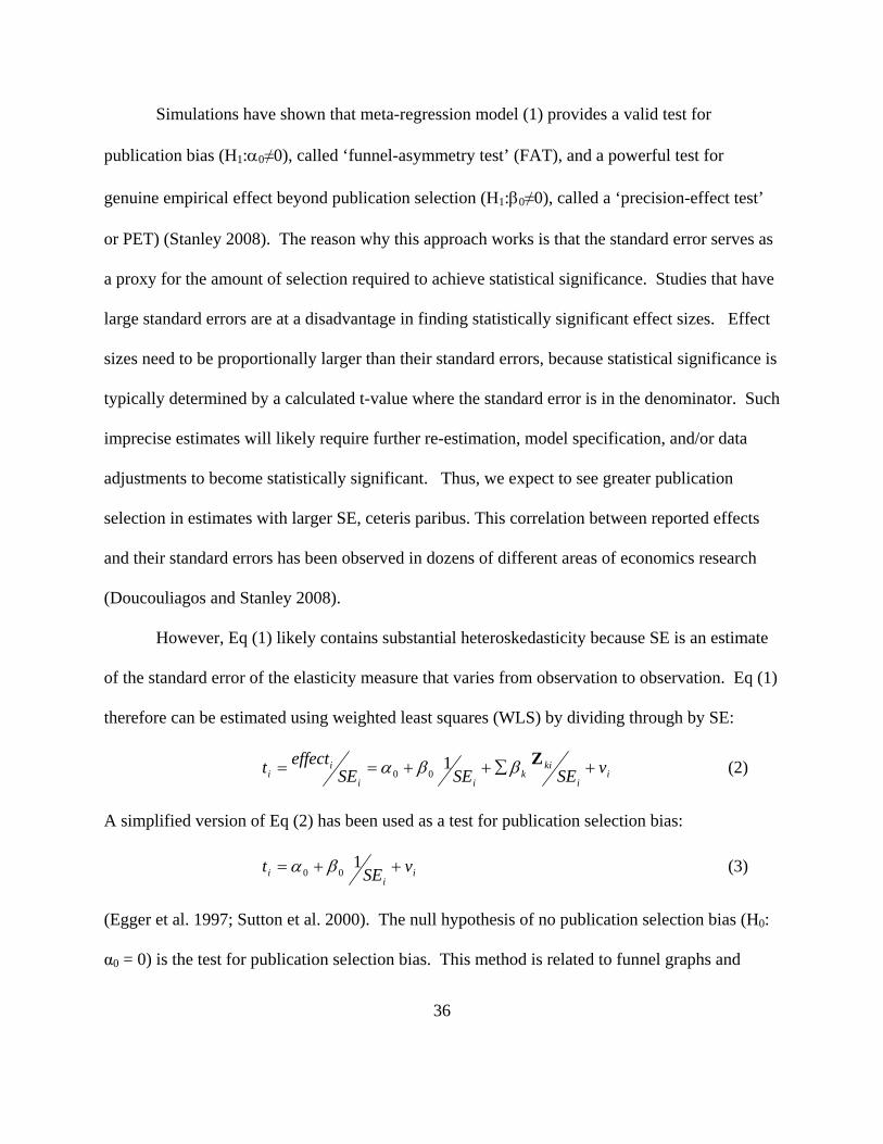
However, Eq (1) likely contains substantial heteroskedasticity because SE is an estimate
of the standard error of the elasticity measure that varies from observation to observation. Eq (1)
therefore can be estimated using weighted least squares (WLS) by dividing through by SE:
ii
kik
ii
ii vSESESE
effectt +∑++== Zββα 100 (2)
A simplified version of Eq (2) has been used as a test for publication selection bias:
ii
i vSEt ++= 100 βα (3)
(Egger et al. 1997; Sutton et al. 2000). The null hypothesis of no publication selection bias (H0:
α0 = 0) is the test for publication selection bias. This method is related to funnel graphs and

37
therefore is called a ‘funnel-asymmetry test’ (FAT) (Stanley 2005a). A funnel graph plots
precision (1/SE) against the elasticity estimate. Figure 1 shows a funnel graph of union-
productivity partial correlations where FAT tests show little sign of publication selection bias
(Stanley 2005a). Compare Figure 1 with Figures 2 and 3 that show asymmetric distributions for
elasticity measures of efficiency wage and residential water demand, respectively. In these latter
two cases, the null hypothesis of no publication selection bias is rejected.
The meta-regression estimate of β0 in Eq (3) is shown to serve as a test for a genuine
empirical effect corrected for publication bias (Stanley 2008). Given 1/SE is a measure of the
precision of the empirical effect, the test (H0: β0 = 0) is called the ‘precision effect test’ (PET),
where the null hypothesis is no genuine empirical effect. Combining these two tests, Eq (3) is
called a FAT-PET-MRA.
FAT (H0: α0 = 0) has low power as a publication selection bias test and PET (H0: β0 = 0)
shows a downward bias in β0 (Stanley and Doucouliagos 2007; Stanley 2008). However, in the
presence of publication selection bias, the observed effect and its standard error have a nonlinear
relationship. This nonlinearity with respect to SE forms the basis for estimating an empirical
effect corrected for publication selection bias, or precision-effect estimate with standard error
(PEESE). A simple power series is used to estimate the nonlinear relationship. Beginning with
the simplest form:
iii SEeffect εαβ ++= 200 (4)
Note, the square of SE (i.e., the variance of each estimated elasticity) is included. A WLS
version of Eq (4) to control for heteroskedasticity is derived by dividing through by SE:
ii
ii vSESEt ++= 100 βα (5)

38
Note that there is no intercept and a second independent variable (SE) is included as compared
with Eq (3). In Eq (5), 0β is the estimate of the effect (elasticity) corrected for publication
selection or the precision-effect estimate with standard error (PEESE). Stanley and
Doucouliagos (2007) provide simulations that show PEESE greatly reduces the potential bias of
publication selection.
Determinants of Elasticity
Several factors are known to affect elasticity estimates, including presence of substitutes,
income effect, necessity of the good, time dimensions of price changes and scope of the affected
resource. These factors give rise to variation in elasticity estimates. For example, a demand
model that evaluates price changes for a particular campground with substitutes will estimate a
more elastic demand than a model that evaluates the demand for camping in general, where
substitution across multiple sites holds demand fairly constant at the activity level with price
changes at a particular site. In addition to these expected variations due to theoretical
considerations, researcher decisions and assumptions regarding experimental design, and
treatment and analysis of data may affect elasticity estimates (Smith and Kaoru 1990). In
previous MRAs of price elasticities (Tellis 1988; Espey, Espey and Shaw 1997), determinants
have been classified as demand model specification factors, environmental characteristics
factors, data characteristics factors, and estimation method factors.
Demand model specification factors include measures of model structure, specification
(omitted variables), functional form, and type of travel cost method. Environmental
characteristics include measures of activity type, geographic region, presence of developed
facilities at the recreation site, and land management agency. Dummy variables identifying the

39
resource type are included, such as lake, river, ocean, etc, as well as differentiating warmwater
and coldwater resources. Data characteristics include measures of survey mode, scope of model,
types of visitors, sample design, and types of trips. Estimation methods include measures of
estimator types such as ordinary least squares (OLS), Poisson and Negative Binomial,
corrections for endogenous stratification, ML-truncation, and censored models.
Data
Empirical estimates of own-price elasticity of recreation demand were derived from the
published literature as part of a larger project (Rosenberger and Stanley 2007). Empirical
recreation demand studies were identified through previous bibliographies, electronic database
searches, and formal requests sent to graduate programs and listservers. Each document was
screened for inclusion in the database using the following criteria―(1) written documentation
must be available; (2) estimate of use value must be provided; (3) use values must be for outdoor
recreation related activities; (4) these use value estimates must be measures of access value (all-
or-nothing, not marginal values); and (5) studies must evaluate recreation resources in Canada or
the United States. Therefore, the selection criteria were not directly targeting demand functions
and elasticity measures; however, the database does cover the majority of recreation demand
studies.
The database currently contains 329 documents that jointly provide 2,705 estimates of
recreation use values. The studies were documented from 1958 to 2006 based on data collected
from 1956 to 2004. Own-price elasticity measures are only derived from travel cost studies,
including individual and zonal, and were either directly coded from estimates provided in the

40
documents, or were calculated when enough information was provided to do so. The price
elasticity database contains 610 estimates from 119 documents from 1960 to 2006.
Table 1 provides variable definitions and descriptive statistics. Own-price elasticity of
recreation demand (P_ELAST) is the dependent variable in all subsequent analyses. ELAST_SE
is the standard error of the elasticity estimate. The independent variables account for potential
factors that affect the variation in price elasticity estimates. Model specification variables
include the presence and number of site characteristic variables in the demand model (SITEVR
and NSITEVAR, respectively); the presence of substitute site price (SUBPRICE) and whether
the value of time was included in the travel cost variable (TIMECOST). Functional form is
captured by a linear-linear (LINLIN) and log-linear (LOGLIN) forms, with double log and
linear-log the omitted category. A dummy variable also identifies whether outliers were
removed from the data prior to model estimation (OUTLIER).
Environmental characteristics factors include several activity types (the omitted category
include all other recreation activities that individually have low sample sizes) and geographic
region (NEAST and SOUTH, with other regions omitted due to correlations with other
variables). These factors also identify sites with developed facilities (DEVREC) and sites
located on national forests (USFS) and state parks (STPARK) (omitted categories include other
public agencies and private lands). Resource types are identified, including LAKE, BAY (or
estuary), OCEAN and RIVER, with land being the omitted category. Water temperature was
also coded as warmwater (WARMWAT) and coldwater (COLDWAT).
Data characteristics include MAIL surveys (all other modes are omitted due to correlation
with other factors) and single site models (SSITE). Visitor type includes resident visitors

41
(RESIDENT) with non-resident and mixed visitors as omitted. ONSITE identifies studies that
derived their sample on-site (other sampling designs such as user list and general population are
omitted). Models that only include single destination trips (SINGDEST) or primary purpose
trips (PRIMARY) are also identified, as well as models based on day trips only (DAYTRIP).
Estimation methods include OLS, Poisson/Negative Binomial count data models
(POISNB), and estimators that corrected for truncation (TRUNC), censoring (CENSOR), and
endogenous stratification (ENDOGST). Other independent variables include a TREND variable
and whether the elasticity measure was calculated (ELASTC), not directly reported in the
primary documents.
Results
Figure 4 plots the funnel graph for elasticity estimates against their precision (1/SE). The
plot is asymmetric with more precise estimates corresponding to inelastic measures. The raw
average elasticity is unitary elasticity (-0.997), while the median elasticity is inelastic (-0.567).
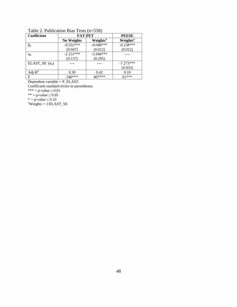
Table 2 reports the simple FAT-PET-MRA and PEESE tests without moderator variables. The
FAT test null hypothesis (H0: α0 = 0) is rejected, signaling publication selection bias. The PET
test null hypothesis (H0: β0 = 0) is also rejected, meaning there is a genuine empirical estimate of
elasticity. The PEESE estimate of empirical elasticity ( 0β ) is significant and -0.158. These
simple FAT-PET and PEESE tests ignore heterogeneity captured by the determinants of
elasticity measures.
Nelson and Kennedy (2009) note that MRAs should account for heteroskedasticity,
dependence and heterogeneity of metadata. Heteroskedasticity is captured through the use of
standard error weights in the models. Hausman tests for dependency among the data emerging

42
as intrastudy correlation among observations derived from the same study reject the classical
regression in favor of a fixed or random effects panel model (Rosenberger and Loomis 2000).
Further, Lagrange Multiplier tests favor a random effects specification that captures intrastudy
dependence in the error term. However, when the standard error weights are used, the WLS
specification is preferred. Therefore, Table 3 reports the fully specified multivariate FAT-PET
and PEESE models.
Four estimated models are provided in Table 3, including an OLS model with White’s
heteroskedastic consistent coefficient standard errors (Model A), an OLS unweighted FAT-PET-
MRA (Model B), a WLS FAT-PET-MRA with standard errors of elasticity measures as weights
(Model C), and a WLS PEESE-MRA with standard errors of elasticity measures as weights
(Model D). Our primary focus will be on Models C and D; however, Models A and B are
provided for general comparisons.
Model C performs best with an adjusted-R2 of 0.78 as compared with Model A (0.54) and
Model B (0.67). Including the FAT-PET measure of publication selection bias improves model
performance, as well as weighting the data by the SE of elasticity measures. Of the 41
moderator variables, over half (21 out of 41) change in sign or significance when accounting for
FAT-PET and weighting the data, signaling substantial heteroskedasticity among the data related
to varying standard errors of elasticity measures (Figure 4). The weighted FAT-PET-MRA,
when accounting for heterogeneity among the data still rejects the FAT null hypothesis (H0: α0 =
0) of no publication selection bias and rejects the PET null hypothesis (H0: β0 = 0) of no genuine
empirical effect, although the magnitude of these coefficients differ from the simple FAT-PET in
Table 2.

43
The estimated coefficients for the moderator variables are interpreted based on the
direction of the effect—a positive sign means more inelastic (i.e., decreases elasticity) while a
negative sign means more elastic (i.e., increases elasticity). Interpretations of elasticity
determinants or moderator effects are restricted to Model C. Seven out of eight demand model
characteristics factors are statistically significant, with five having a positive effect (more
inelastic) and two having a negative effect (more elastic). Including site characteristic measures
(SITEVAR) in the demand model increases the elasticity measure, while increases in the number
of site characteristic variables (NSITEVAR) in the demand model specification decreases the
elasticity measure (each additional site characteristic variable decreases elasticity by 0.186). A
linear-linear (LINLIN) functional form provides more inelastic elasticities than other functional
forms, as does including a price of substitute sites (SUBPRICE) and the value of time in the
travel cost measure (TIMECOST). Individual travel cost models (TCMIND) likewise provide
more inelastic elasticities than zonal travel cost models. Removal of outlier observations from
the data (OUTLIER) increases the elasticity, where these outliers may either be
uncharacteristically large prices or number of trips.
Eleven out of 19 environmental characteristics factors are statistically significant, with
the majority leading to more elastic elasticities. Camping (CAMP) and motorized boating
(MBOAT) provide more elastic elasticities whereas fishing (FISH) and general recreation
(GENREC) studies provide more inelastic measures. Studies conducted in the northeastern U.S.
(NEAST) estimated more price responsive demands. Sites with developed recreation facilities
(DEVREC) showed less price responsive demands. National forest studies (USFS) showed more
elastic demands. Studies of lake (LAKE) and bay/estuary (BAY) resources, in addition to water
44
temperature (warmwater (WARMWAT) and coldwater (COLDWAT)), had more elastic
demands.
Overall, data characteristics factors did not influence elasticity measures with three out of
seven being statistically significant. These statistically significant factors were all negative,
meaning resident visitors only studies (RESIDENT), studies drawing samples onsite (ONSITE),
and studies for primary purpose users (PRIMARY) resulted in more elastic demands.
Estimation method factors were mostly significant in determining elasticity measures
(three out of five). All statistically significant factors led to more inelastic elasticities, including
OLS models (OLS), censored models (CENSOR), and models correcting for endogenous
stratification (ENDOGST). There is a general trend in more elastic elasticity estimates over time
(TREND), with an increase in elasticity of -0.009 per year. Those studies that did not report
elasticities but provided enough information for them to be calculated were from more inelastic
demand models (ELASTC).
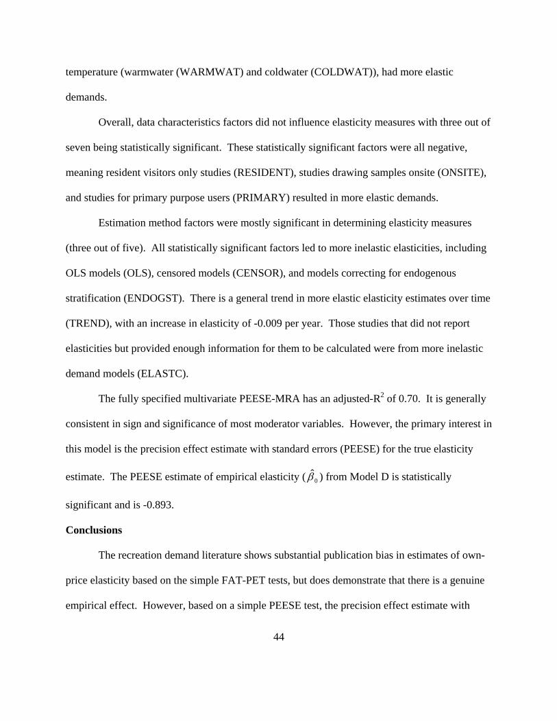
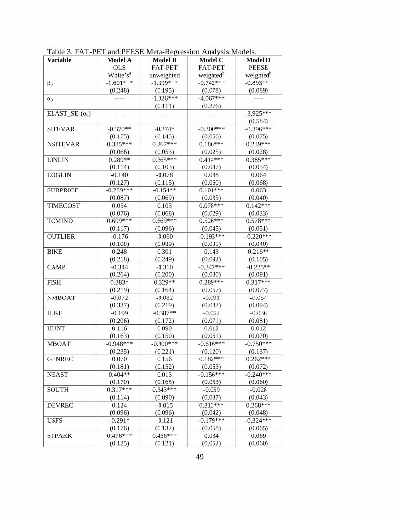
The fully specified multivariate PEESE-MRA has an adjusted-R2 of 0.70. It is generally
consistent in sign and significance of most moderator variables. However, the primary interest in
this model is the precision effect estimate with standard errors (PEESE) for the true elasticity
estimate. The PEESE estimate of empirical elasticity ( 0β ) from Model D is statistically
significant and is -0.893.
Conclusions
The recreation demand literature shows substantial publication bias in estimates of own-
price elasticity based on the simple FAT-PET tests, but does demonstrate that there is a genuine
empirical effect. However, based on a simple PEESE test, the precision effect estimate with

45
standard errors shows the standard error-corrected empirical elasticity is -0.158—recreation
demand is not price responsive (i.e., inelastic). Compared with this PEESE estimate, the raw
average elasticity measure (-0.997) is six-fold more elastic while the raw median elasticity
measure (-0.567) is four-fold too elastic. This means that management decisions or policies
based on central tendency measures based on the raw data will exaggerate the price
responsiveness of recreation demand. For example, pricing decisions based on these raw
measures will underestimate potential revenue from price increases, or will overestimate demand
responses to changes in prices. Accounting for the variation in the standard error of elasticity
measures is important. The standard error weighted average is -0.172, a much more moderate
bias of one-fold higher elasticity.
Even after accounting for the substantial heterogeneity of the recreation demand literature
through determinants of elasticities, there is still substantial publication selection bias and a
genuine empirical effect present in this literature based on the multivariate FAT-PET-MRA.
However, conclusions about the magnitude of publication selection bias when accounting for
heterogeneity of the data is much more modest. The PEESE-MRA estimate of elasticity (-0.893)
is close to the raw average elasticity measure (-0.997), about a one-fold exaggeration similar to
the difference in the simple PEESE estimate and the standard error weighted average.
Smith and Kaoru (1990) estimated a meta-regression analysis of own-price elasticities of
recreation demand for the early literature. Their MRA is consistent with Model A (OLS with
heteroskedastic consistent coefficient standard errors). The demand model, environment and
data characteristics factors were the same in sign and significance for those factors in both
models. However, compared with Model C (FAT-PET-MRA with standard errors as weights),

46
most of the factors changed in sign or significance. For example, the inclusion of substitute site
price in the demand model specification was estimated to be significant and negative in Smith
and Kaoru’s (1990) model, as it was in Model A in this study. However, when the FAT measure
(1/SE) is included and the data are weighted by the standard error of the elasticity measures, the
sign switches to positive and significant (Model C).
Smith and Kaoru’s (1990) general implications still hold, but with different directional
effects of moderator variables. They conclude that “modeling assumptions do matter” (p.271).
With over half of the moderator variables being related to the magnitude of the elasticity
estimated, researcher decisions and assumptions continue to affect this literature beyond what is
theoretically expected.

47
Table 1. Data Description (N = 610) Variable Definition Mean Std Dev Min Max P_ELAST Own price elasticity of demand -0.997 1.040 -5.981 -0.006 ELAST_SE a Std error of elasticity 0.208 0.269 0.003 3.161 SITEVAR 1 = Site characteristics variables in demand model 0.238 0.426 0 1 NSITEVARb # of site characteristics variables in demand model 0.387 0.919 0 5 LINLIN 1 = Linear-linear demand model functional form 0.251 0.434 0 1 LOGLIN 1 = Log-linear demand model functional form 0.359 0.480 0 1 SUBPRICE 1 = Price of substitute site included in demand
model 0.500 0.500 0 1
TIMECOST 1 = Cost of time included in travel cost variable 0.608 0.488 0 1 TCMIND 1 = Individual travel cost model 0.597 0.491 0 1 OUTLIER 1 = Outlier observations removed from data 0.311 0.463 0 1 BIKE 1 = Bicycling 0.034 0.182 0 1 CAMP 1 = Camping 0.046 0.209 0 1 FISH 1 = Fishing 0.323 0.468 0 1 NMBOAT 1 = Non-motorized boating 0.043 0.202 0 1 HIKE 1 = Hiking 0.070 0.256 0 1 HUNT 1 = Hunting 0.090 0.287 0 1 MBOAT 1 = Motorized boating 0.067 0.250 0 1 GENREC 1 = Generalized recreation 0.144 0.352 0 1 NEAST 1 = Northeast region 0.105 0.307 0 1 SOUTH 1 = Southern region 0.236 0.425 0 1 DEVREC 1 = Developed recreation facilities available on-site 0.516 0.500 0 1 USFS 1 = National forest land 0.139 0.346 0 1 STPARK 1 = State park 0.136 0.343 0 1 LAKE 1 = Lake resource 0.306 0.461 0 1 BAY 1 = Estuary or bay resource 0.090 0.287 0 1 OCEAN 1 = Ocean resource 0.044 0.206 0 1 RIVER 1 = River or stream resource 0.148 0.355 0 1 WARMWAT 1 = Warm water resource (lake, river, etc.) 0.128 0.334 0 1 COLDWAT 1 = Cold water resource (lake, river, etc.) 0.090 0.287 0 1 MAIL 1 = Mail survey mode 0.397 0.490 0 1 SSITE 1 = Single site evaluated 0.695 0.461 0 1 RESIDENT 1 = Resident visitors only 0.439 0.497 0 1 ONSITE 1 = Sample drawn on site 0.441 0.497 0 1 SINGDEST 1 = Single destination trips only modeled 0.454 0.498 0 1 PRIMARY 1 = Primary purpose visitors only modeled 0.416 0.493 0 1 DAYTRIP 1 = Day trips only modeled 0.479 0.500 0 1 OLS 1 = Ordinary least squares estimator 0.693 0.461 0 1 POISNB 1 = Poisson/Negative Binomial estimator 0.184 0.387 0 1 TRUNC 1 = Observations truncated in demand model 0.380 0.486 0 1 ENDOGST 1 = Demand model corrected for endogenous
stratification 0.134 0.341 0 1
CENSOR 1 = Censored demand model 0.115 0.319 0 1 TREND Trend (1 = 1960, 2 = 1961,…, 44 = 2003) 25.448 9.355 1 44 ELASTC 1 = Elasticity measure calculated by researcher 0.415 0.493 0 1 aN = 558 bN = 594
48
Table 2. Publication Bias Tests (n=558) Coefficient FAT-PET PEESE
No Weights Weightsa Weightsa
β0 -0.552*** (0.047)
-0.048*** (0.012)
-0.158*** (0.012)
α0 -2.151*** (0.137)
-5.946*** (0.295)
----
ELAST_SE (α0) ---- ---- -7.273*** (0.933)
Adj-R2 0.30 0.42 0.10 F 246*** 407*** 61*** Dependent variable = P_ELAST. Coefficient standard errors in parentheses. *** = p-value ≤ 0.01 ** = p-value ≤ 0.05 * = p-value ≤ 0.10 aWeights = 1/ELAST_SE
49
Table 3. FAT-PET and PEESE Meta-Regression Analysis Models. Variable Model A
OLS White’sa
Model B FAT-PET
unweighted
Model C FAT-PET weightedb
Model D PEESE
weightedb
β0 -1.601*** (0.248)
-1.399*** (0.195)
-0.742*** (0.078)
-0.893*** (0.089)
α0 ---- -1.326*** (0.111)
-4.067*** (0.276)
----
ELAST_SE (α0) ---- ---- ---- -3.925*** (0.584)
SITEVAR -0.370** (0.175)
-0.274* (0.145)
-0.300*** (0.066)
-0.396*** (0.075)
NSITEVAR 0.335*** (0.066)
0.267*** (0.053)
0.186*** (0.025)
0.239*** (0.028)
LINLIN 0.289** (0.114)
0.365*** (0.103)
0.414*** (0.047)
0.385*** (0.054)
LOGLIN -0.140 (0.127)
-0.078 (0.115)
0.088 (0.060)
0.064 (0.068)
SUBPRICE -0.289*** (0.087)
-0.154** (0.069)
0.101*** (0.035)
0.063 (0.040)
TIMECOST 0.054 (0.076)
0.103 (0.068)
0.078*** (0.029)
0.142*** (0.033)
TCMIND 0.699*** (0.117)
0.669*** (0.096)
0.526*** (0.045)
0.578*** (0.051)
OUTLIER -0.176 (0.108)
-0.060 (0.089)
-0.193*** (0.035)
-0.220*** (0.040)
BIKE 0.248 (0.218)
0.301 (0.249)
0.143 (0.092)
0.216** (0.105)
CAMP -0.344 (0.264)
-0.310 (0.200)
-0.342*** (0.080)
-0.225** (0.091)
FISH 0.383* (0.219)
0.329** (0.164)
0.289*** (0.067)
0.317*** (0.077)
NMBOAT -0.072 (0.337)
-0.082 (0.219)
-0.091 (0.082)
-0.054 (0.094)
HIKE -0.199 (0.206)
-0.387** (0.172)
-0.052 (0.071)
-0.036 (0.081)
HUNT 0.116 (0.163)
0.090 (0.150)
0.012 (0.061)
0.012 (0.070)
MBOAT -0.948*** (0.235)
-0.900*** (0.221)
-0.616*** (0.120)
-0.750*** (0.137)
GENREC 0.070 (0.181)
0.156 (0.152)
0.182*** (0.063)
0.262*** (0.072)
NEAST 0.404** (0.170)
0.013 (0.165)
-0.156*** (0.053)
-0.240*** (0.060)
SOUTH 0.317*** (0.114)
0.343*** (0.090)
-0.059 (0.037)
-0.028 (0.043)
DEVREC 0.124 (0.096)
-0.015 (0.096)
0.312*** (0.042)
0.268*** (0.048)
USFS -0.291* (0.176)
-0.121 (0.132)
-0.179*** (0.058)
-0.324*** (0.065)
STPARK 0.476*** (0.125)
0.456*** (0.121)
0.034 (0.052)
0.069 (0.060)

50
Variable Model A OLS
White’sa
Model B FAT-PET
unweighted
Model C FAT-PET weightedb
Model D PEESE
weightedb
LAKE -0.469*** (0.146)
-0.537*** (0.131)
-0.086* (0.044)
-0.150*** (0.050)
BAY 0.002 (0.168)
-0.190 (0.147)
-0.111** (0.052)
-0.172*** (0.060)
OCEAN -0.257 (0.246)
-0.245 (0.212)
0.058 (0.069)
-0.007 (0.080)
RIVER -0.291 (0.184)
-0.580*** (0.152)
0.053 (0.041)
0.006 (0.047)
WARMWAT -0.544** (0.214)
-0.317** (0.154)
-0.179** (0.076)
-0.208** (0.087)
COLDWAT -0.186 (0.256)
0.001 (0.172)
-0.137** (0.067)
-0.092 (0.076)
MAIL 0.399*** (0.123)
0.306*** (0.106)
-0.014 (0.040)
-0.072 (0.045)
SSITE 0.229** (0.116)
0.245** (0.101)
0.008 (0.045)
-0.035 (0.051)
RESIDENT -0.340*** (0.116)
-0.198** (0.090)
-0.101** (0.046)
-0.065 (0.053)
ONSITE -0.209* (0.118)
-0.289*** (0.082)
-0.158*** (0.039)
-0.108** (0.044)
SINGDEST -0.034 (0.206)
-0.030 (0.138)
0.013 (0.062)
0.052 (0.071)
PRIMARY -0.574*** (0.204)
-0.355*** (0.134)
-0.223*** (0.055)
-0.207*** (0.063)
DAYTRIP 0.372*** (0.120)
0.173** (0.088)
0.041 (0.044)
0.031 (0.050)
OLS 0.705*** (0.136)
0.682*** (0.103)
0.234*** (0.062)
0.249*** (0.071)
POISNB 0.510** (0.210)
0.452** (0.178)
0.061 (0.094)
0.178* (0.108)
TRUNC 0.515*** (0.148)
0.499*** (0.097)
-0.011 (0.044)
0.056 (0.050)
ENDOGST -0.086 (0.172)
-0.032 (0.137)
0.150** (0.066)
-0.003 (0.074)
CENSOR -0.146 (0.206)
-0.214 (0.139)
0.308*** (0.077)
0.335*** (0.088)
TREND -0.022*** (0.007)
-0.019*** (0.007)
-0.009*** (0.003)
-0.016*** (0.003)
ELASTC 0.371*** (0.119)
0.299*** (0.100)
0.126*** (0.036)
0.236*** (0.040)
Adj-R2 0.54 0.67 0.78 0.70 F 18*** 27*** 45*** 32*** N 594 542 542 542 Dependent variable = P_ELAST. Coefficient standard errors in parentheses. *** = p-value ≤ 0.01 ** = p-value ≤ 0.05 * = p-value ≤ 0.10 aWhite’s robust heteroskedasticity corrected covariance matrix

51
bWeights = 1/ELAST_SE
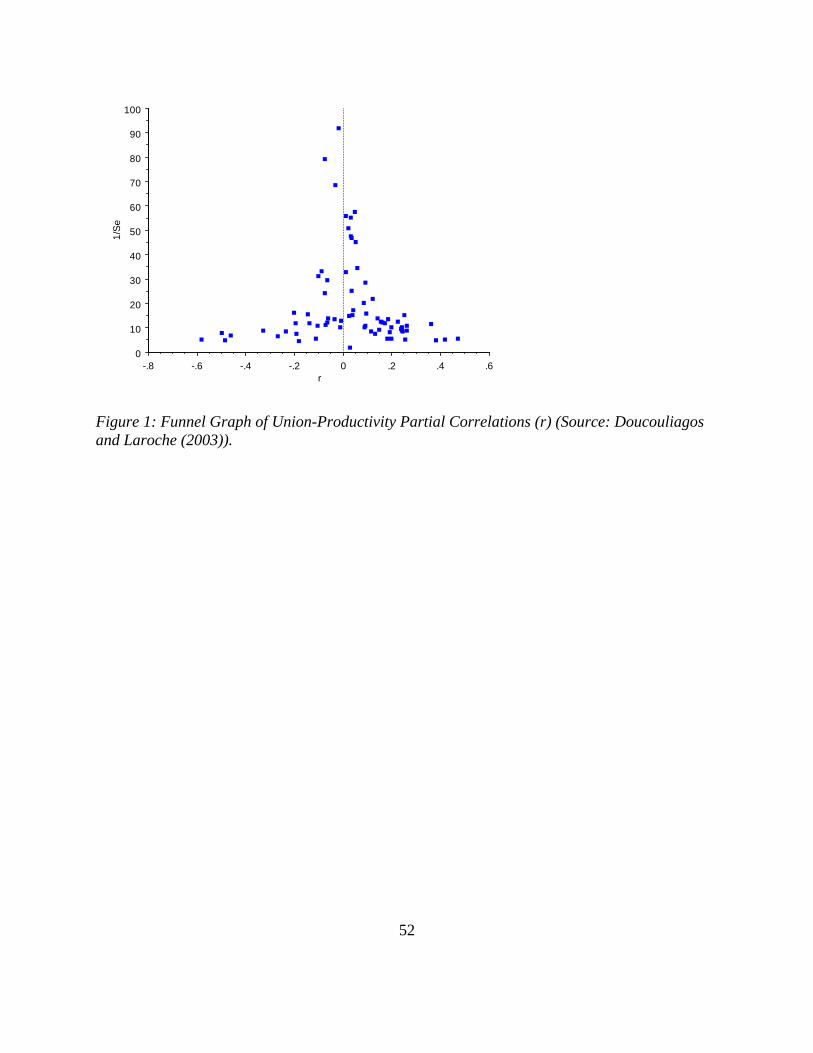
52
Figure 1: Funnel Graph of Union-Productivity Partial Correlations (r) (Source: Doucouliagos and Laroche (2003)).
0
10
20
30
40
50
60
70
80
90
1001/
Se
-.8 -.6 -.4 -.2 0 .2 .4 .6r

53
Figure 2: Funnel Graph of Efficiency Wage Elasticities (Source: Stanley and Doucouliagos (2007)).
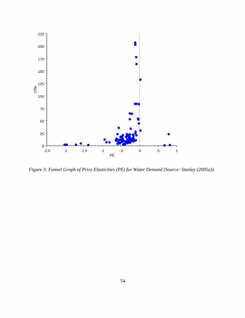
54
Figure 3: Funnel Graph of Price Elasticities (PE) for Water Demand (Source: Stanley (2005a)).
0
25
50
75
100
125
150
175
200
2251/
Se
-2.5 -2 -1.5 -1 -.5 0 .5 1PE
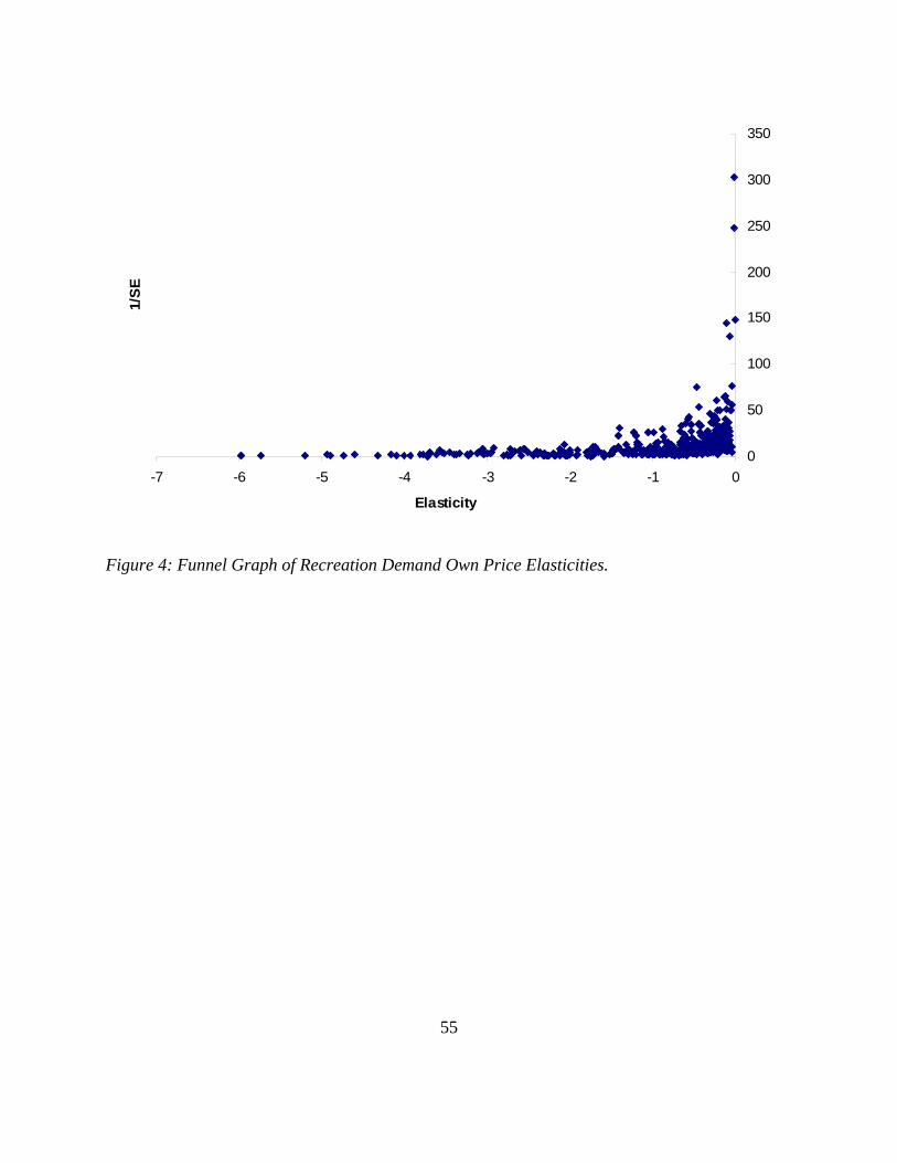
55
Figure 4: Funnel Graph of Recreation Demand Own Price Elasticities.
0
50
100
150
200
250
300
350
-7 -6 -5 -4 -3 -2 -1 0
Elasticity
1/SE

56
References Ashenfelter O, Harmon C, Oosterbeek, H (1999) A review of estimates of the schooling/earnings
relationship, with tests for publication bias. Labour Econ 6(4):453-470. Card D, Krueger AB (1995) Time-series minimum-wage studies: a meta-analysis. Am Econ Rev
85(2):238-243. Coric B, Pugh G (2008) The effects of exchange rate variability on international trade: a meta-
regression analysis. Appl Econ (in press). DOI 10.1080/00036840801964500. Dalhuisen J, Florax RJGM, deGroot HLF, Nijkamp P (2003) Price and income elasticities of
residential water demand: a meta-analysis. Land Econ 79(2):292-308. De Long JB, Lang K (1992) Are all economic hypotheses false? J Polit Econ 100(6):1257-1272. Doucouliagos C (2005) Publication bias in the economic freedom and economic growth
literature. J Econ Surv 19(3):367-388. Doucouliagos C, Laroche P (2003) What do unions do to productivity: a meta-analysis.
Industrial Relations 42(4):650-691. Doucouliagos C, Stanley TD (2008). Theory competition and selectivity. Deakin Working Paper
2008-06. Doucouliagos C, Stanley TD (2009) Publication selection bias in minimum-wage research? A
meta-regression analysis. British J Industrial Relations (in press). Egger M, Davey Smith G, Schneider M, Minder C (1997) Bias in meta-analysis detected by a
simple, graphical test. British Med J 315(7109):629-634. Espey, M (1997) Explaining the variation in elasticity estimates of gasoline demand in the
United States: A meta-analysis. Energy Journal 17:49-60. Espey, M (1998) Gasoline demand revisited: An international meta-analysis of elasticities.
Energy Economics 20:273-295. Espey, M, Espey J and Shaw WD (1997) Price elasticity of residential demand for water: A
meta-analysis. Water Resources Research 33(6):1369-1374. Feige EL (1975) The consequence of journal editorial policies and a suggestion for revision. J
Polit Econ 83(6):1291-1295. Gallett CA, List JA (2003) Cigarette demand: A meta-analysis of elasticities. Health Economics
12(10):821-835. Gemmill MC, Costa-Font J, McGuire A (2007) In search of a corrected prescription drug
elasticity estimate: a meta-regression approach. Health Econ 16(6):627-643. Görg H, Strobl E (2001) Multinational companies and productivity: a meta-analysis. Econ J
111(475):723-739. Hoehn JP (2006) Methods to address selection effects in the meta regression and transfer of
ecosystem values. Ecol Econ 60(2):389-398. Hotelling H (1947) Letter to National Park Service, in: An economic study of the monetary
evaluation of recreation in the National Parks. Washington, DC: U.S. Department of the Interior, National Park Service and Recreational Planning Division.
Knell M, Stix H (2005) The income elasticity of money demand: a meta-analysis of empirical results. J Econ Surv 19(3):513-533.
Krassoi Peach E, Stanley TD (2009) Efficiency wages, productivity and simultaneity: a meta-regression analysis. J Labor Res (in press).
Leamer EE (1983) Let’s take the con out of econometrics. Am Econ Rev 73(1):31-43.

57
Leamer EE, Leonard H (1983) Reporting the fragility of regression estimates. Rev Econ Stat 65(2):306-317.
Longhi S, Nijkamp P, Poot J (2005) A meta-analytic assessment of the effect of immigration on wages. J Econ Surv 19(3):451-477.
Lovell MC (1983) Data mining. Rev Econ Stat 65(1):1-12. Mookerjee R (2006) A meta-analysis of the export growth hypothesis. Econ Letters 91(3):395-
401. Nelson JP, and Kennedy PE (2009) The use (and abuse) of meta-analysis in environmental and
natural resource economics: an assessment. Environ Resour Econ 42(3):345-377. Roberts CJ, Stanley TD (eds) (2005) Meta-regression analysis: issues of publication bias in
economics. Blackwell, Oxford. Rose AK, Stanley TD (2005) A meta-analysis of the effect of common currencies on
international trade. J Econ Surv 19(3):347-365. Rosenberger RS, Johnston RJ (2009) Selection effects in meta-analysis and benefit transfer:
avoiding unintended consequences. Land Econ 85(3):410-428. Rosenberger RS, Loomis JB (2000) Panel stratification in meta-analysis of economic studies: an
investigation of its effects in the recreation valuation literature. J Agric Appl Econ 32(2):459-470.
Rosenberger RS, Stanley TD (2006) Measurement, generalization, and publication: sources of error in benefit transfers and their management. Ecol Econ 60(2):372-378.
Rosenberger RS, Stanley TD (2007) Publication effects in the recreation use value literature: a preliminary investigation. Paper presented at the American Agricultural Economics Association Annual Meeting, Portland, 29 July-1 August 2007. http://purl.umn.edu/9883.
Smith VK, Huang JC (1993) Hedonic models and air pollution: Twenty-five years and counting. Environ Resour Econ 3(4):381-394.
Smith VK, Huang JC (1995) Can markets value air quality? A meta-analysis of hedonic property value models. J Polit Economy 103(1):209-227.
Smith VK, Kaoru Y (1990) What have we learned since Hotelling’s letter: A meta-analysis. Economics Letters 32:267-272.
Stanley TD (2005a) Beyond publication bias. J Econ Surv 19(3):309-345. Stanley TD (2005b) Integrating the empirical tests of the natural rate hypothesis: a meta-
regression analysis. Kyklos 58(4):587-610. Stanley TD (2008) Meta-regression methods for detecting and estimating empirical effect in the
presence of publication selection. Oxford Bull Econ Stat 70(1):103-127. Stanley TD, Doucouliagos H (2007) Identifying and correcting publication selection bias in the
efficiency-wage literature: Heckman meta-regression. School working paper – Economic Series 2007, SWP 2007/11. Victoria, Australia: Deakin University.
Sutton AJ, Abrams KR, Jones DR et al (2000) Methods for meta-analysis in medical research. John Wiley and Sons, Chichester.
Tellis GJ (1988) The price elasticity of selective demand: A meta-analysis of econometric models of sales. Journal of Marketing Research XXV:331-341.
Tullock G (1959) Publication decisions and tests of significance – a comment. J Am Stat Assoc 54(287):593.
58
Did the Great Recession Reduce Visitor Spending and Willingness to Pay for
Nature-Based Recreation? Evidence from 2006 and 2009
Dr. John Loomis, Professor Dept. of Agricultural and Resource Economics
Colorado State University Fort Collins, CO 80523-1172 [email protected]
Dr. Catherine Keske, Assistant Professor Dept. of Soil and Crop Sciences
Colorado State University Fort Collins, CO 80523-1170
July 4, 2010 Acknowledgements: Partial funding for this study came from the Colorado Agricultural Experiment Station project W2133. The Colorado Fourterneer’s Initiative provided support for the data collection.
59
Did the Great Recession Reduce Visitor Spending and Willingness to Pay for Nature-Based
Recreation? Evidence from 2006 and 2009
Abstract
Outdoor recreation is a relatively large industry that can diversify public land based economies
that have traditionally relied upon resource extraction. But what happens to nature-based
recreation visitor spending and benefits during times of national economic recession? To address
this question, we replicate a 2006 high mountain recreation study in the same region, three years
later during the 2009 recession. Results indicate that nature-based public lands recreation in this
area did not experience reductions in total visitor expenditures or total number of visits during
the recession. These results imply that nature-based recreation may represent an economically
stable industry in public land mountain communities. Total benefits to the visitors themselves are
also fairly stable, and there is not a statistically significant decrease in consumer surplus in 2009
compared to 2006.
(JEL Q26)
Keywords: Hiking, consumer surplus, contingent valuation, Colorado, spending, tourism

60
Introduction
The U.S. economy has undergone considerable change from 2006 to 2009. During 2006-2007,
the unemployment rate was under 5%; however, in fall 2009, the national unemployment rate
topped 10% for the first time since 1983 (Bureau of Labor Statistics, 2009). After reaching its
peak of 14,164 in October 2007, the Dow Jones Industrial Average tumbled to below 6,600 in
March 2009. In addition to declines in consumer confidence, the U.S. GDP declined four
consecutive quarters during 2008-2009, marking the longest U.S. recession in 60 years (Bureau
of Economic Analysis, 2009). The grey literature has dubbed this recession the “Great
Recession,” attempting to draw parallels with the Great Depression of the 1930’s (Isidore, 2009).
Many sectors of the U.S. economy, such as the $300 billion domestic automobile industry
(McAlinden, et al.), have been hit hard by the recession. However, there has been little attention
paid to an industry with sales similar to the U.S. domestic automobile manufacturing industry.
This is the active outdoor recreation industry with sales of $290 billion (Outdoor Industry
Foundation, 2006). This industry is an aggregate of outdoor recreation equipment sales and
recreation trip expenditures for camping, fishing, hunting, snow sports, hiking, water-based
recreation and wildlife viewing. Hiker and backpacker spending is one of the largest categories
of the active outdoor recreation industry. Trail-based recreation accounts for $83 billion, or
nearly 30% of the industry (Outdoor Industry Foundation, 2006). Trail-based recreation spending
also supports over 700,000 jobs (Outdoor Industry Foundation, 2006), a figure similar to direct
employment in automobile manufacturing (McAlinden, et al.) The majority of the recreation
spending is trip related spending (e.g., gasoline, hotels, food), rather than purely purchases of
durable equipment. High expenditures and consumer surplus have been documented for nature-

61
based recreation when the economy is at its peak (Outdoor Industry Foundation, 2006; Keske
and Loomis, 2007), but have consumer expenditures and willingness to pay for nature-based
recreation fallen during the Great Recession?
This study focuses on changes in visitation, expenditures and consumer surplus for nature-based,
high mountain recreation during times of macroeconomic change. In this paper, we replicate a
2006 survey design and sampling frame to investigate how visitor use and visitor trip spending
changed between 2006 and 2009 for trail-based recreation in Colorado. Hiking and backpacking
are popular activities nationwide, and results from the Colorado study may be transferrable to
other regions offering these activities. More than one-third of the U.S. population over the age
of 16 participates in hiking or backpacking, representing over 50 million participants (Cordell, et
al., 1999). Greater than one billion days are spent hiking or backpacking in the United States
(Cordell, et al., 1999). Others project that this is a trend that will continue into the future. For
example, Bowker et al. (1999) forecasts that the number of days of hiking is expected to increase
by about 5% a decade between the years 2000 and 2050, for a cumulative increase of 25% over
this time period.
If recreation expenditures are unchanged across periods of economic prosperity and decline, then
recreation has potential to be a stabilizing economic sector in rural economies. Mountain
economies, including our study area, frequently experience competing economic development
interests from energy and mineral extraction industries (Loomis, 2002), which are known for
economic volatility (Davis and Tilton, 2005). Extraction of energy/minerals is a notable driver
of the Colorado economy. One report estimates the 2007 economic contribution of the energy

62
and mineral industry to the Colorado economy to be as high as $11 billion (approximately 5%)
of the state’s gross state product (Corporation for a Skilled Workforce, 2009). However, like
other extraction economies, the western side of Colorado has been quite hard hit by the economic
recession, due in part to the drop in energy and mineral exploration in the region that
encompasses our study area (Bureau of Land Management, 2007).
The economic boom-bust cycles associated with extraction are driven by fluctuations in prices
and spending leakages that result from high rates of commodity exportation. When an economic
structure is heavily export-based, other sectors within the economy may be under-developed,
creating an over-reliance on one industry. This is commonly known as the “Dutch Disease”
(Davis, 1995). The exportation of energy and minerals, combined with the often temporary
workforce, frequently does not generate sustainable regional spending multipliers. The
combination of commodity price volatility and an undiversified, extraction-based economy can
result in a deep economic retraction. Economic diversification is a key component of achieving
economic stability in these resource-based economies (Davis, 1995; Davis and Tilton, 2005;
Iimi, 2007). One avenue toward diversification in resource based economies is to promote
natural resource-based recreational use by outsiders. Of course tourism is also export driven, so
one issue of interest in this paper is whether the tourism sector is able to withstand periods of
significant recession. If so, then promotion of recreation industry in natural resource based
economies may serve to diversify and thus stabilize rural economies that have been traditionally
reliant on extraction. In this paper we test whether visitor recreation expenditures withstood the
“Great Recession” and thus may be used as a strategy to diversify mountain economies.
63
Sales to visitors are only part of the economic picture. The economic efficiency benefits of
outdoor recreation include how much more visitors themselves would pay in excess of their
travel costs (i.e., their consumer surplus). If visitor income falls during the recession, then it is
certainly possible that net willingness to pay (WTP) for recreation opportunities might fall, if the
activity is a normal good. Further, net WTP might be influenced by visitors feeling “poorer” due
to their wealth losses in the stock and housing markets. To investigate this, we implement a
contingent valuation model to test whether willingness to pay changes from 2006 to 2009 in the
same Colorado study area. Knowing whether or not benefit estimates are susceptible to
macroeconomic fluctuations may be useful for long term federal and state agency public land
management planning, including management of recreational areas that have time horizons of
10-15 years. Further, when conducting benefit transfers it is often necessary to combine prior
benefit estimates over one or more decades. Thus, it would be useful to know whether these
benefit estimates are not affected by economic cycles.
The paper proceeds as follows. First, we formalize the economic indicators to be compared.
Next, we introduce the methods used to estimate those indicators during the 2006 boom year and
the Great Recession in summer 2009. We then describe the data, statistical results, and draw
conclusions.

64
Testing for Differences in Visitor Use, Visitor Expenditures and WTP
Sales and Visitor Expenditure Hypothesis Tests
Visitor spending for public land and nature-based recreation can be grouped into several
categories. Transportation (e.g., gasoline, airfare, rental cars) and traveler accommodations (e.g.,
hotels, bed-breakfast) are two of the largest sectors. Other important direct sales to tourists
include food establishments (e.g., restaurants), and retail sales.
We compare hiker expenditures in Colorado for each of the five spending categories, to
determine whether there has been a statistically significant change in the sum of visitor
expenditures between summer 2006 and summer 2009. The general form of our hypothesis test
for each expend category is:
(1) Ho: Expendi2006 = Expendi2009 vs Ha: Expendi2006 ≠Expendi2009
Where Expendi is visitor expenditures of type i, where i= 1,…5.
This hypothesis will be tested using a t-test of difference in means for the two different sample
time periods for each spending category.
Willingness to Pay (WTP)
The net WTP or consumer surplus associated with outdoor recreation on public lands in
Colorado is more difficult to estimate than visitor expenditures. Given the relatively free access
to public lands (Loomis, 2002), there is likely a benefit to visitors from the opportunity to hike
on public lands in the Rocky Mountains in excess of their transportation costs and other trip
related costs.
65
In order to measure net WTP, we utilize the contingent valuation method or CVM (Loomis and
Walsh, 1997). In particular, we estimate WTP using a dichotomous choice CVM model. This
WTP question format asks whether the visitor would pay a specific increase in trip cost, the
magnitude of which is varied across the sample). This model is deemed more market-like and
analogous to the price taking behavior familiar to consumers than asking an open-ended question
of what the maximum amount a visitor would pay (Loomis and Walsh, 1997).
The utility theoretic foundations of the dichotomous choice model have been well developed (see
Hanemann, 1984); and will only be summarized here. We assume that an individual's utility is a
function of a recreation experience at site R and the consumption of all other goods (represented
by income I). The utility function may be represented as:
(1) U = f(R, I)
Utility from visiting a recreation site also depends on an individual's personal preferences which
are known only to that individual, so a portion of the utility function is not observable to the
researcher. Therefore, some components of each individual's utility function are treated as
stochastic, resulting in an indirect utility function and a random term, as follows:
(2) U = f(R, I) = v(R, I) + e
where “e” represents an error term.
With the dichotomous-choice WTP question format, survey respondents are asked whether or
not they would still take their most recent trip to the recreation site if travel costs were $Bid
higher. The respondent is predicted to answer “YES”, if utility from the recreation experience,
along with the associated reduction of $BID in income, is greater than the individual's original
66
utility level without taking the trip. The “YES” respondent would take the trip (R = 1) at the
higher travel cost (I-$Bid), and the "NO" respondent would choose not to take the trip (R = 0).
Therefore, the probability of a “YES” response is represented as follows:
(3) P(YES|$Bid) = P[v(R=1, I-$Bid) + e 1 > v(R= 0, I) + e 2]
where e 1, and e 2 are error terms with means of zero (Hanemann, 1984).
In the random utility framework, a visitor is predicted to respond “Yes”, if the gain in the
deterministic part of the utility function (the indirect utility difference) is larger than the
difference in the stochastic part (e 1- e 2). If the difference of the errors (e 1- e 2) is logistically
distributed, this gives rise to the parametric logit model. The stylized version of the model
estimated is:
(4) Log[(Prob YES)/(1-Prob YES)] = βo –β1($Bid) + β2X2… +βn(Xn) + ε
where $Bid is the increase in trip cost the visitor is asked to pay, X’s are other independent
explanatory variables, and ε is the error term.
WTP Hypotheses Tests
We test for differences in visitor benefits between 2006 and 2009 by using two hypothesis tests.
The first involves a statistical test on the equality of coefficients in the logit willingness to pay
model. The second test is whether mean WTP has changed between the two time periods.
The statistical test is for differences in specific logit coefficients between the two time periods.
In particular, we pool data for the two time periods and include an intercept shift variable,
defined as “2006Dum”, for 2006 responses. We also create an interaction term using this
dummy variable with the other independent variable (Travel Distance) to allow the slope of this

67
coefficient to be different in 2006 than in 2009. This second variable is defined as,
“2006Dum*TravelDistance”. Thus the empirical model is:
(5) Log[(Prob YES)/(1-Prob YES)] =βo –β1($Bid) +β2(2006Dum)+β3(Travel Distance)
+β4 (2006Dum*TravelDistance) +ε
where “2006Dum” =1 if the WTP responses are from 2006, 0 if from 2009.
We included the variable, “Travel Distance,” defined as the distance visitors traveled from their
home to the site. Previous studies found this variable to be a statistically significant explanatory
variable for WTP for Fourteener recreation in 2006 (Keske and Loomis, 2008).
The hypothesis test evaluates whether the coefficients on the dummy variable and the dummy
variable*Travel Distance interaction variable, respectively, are statistically significant:
(6a) Ho: β2=0 vs Ha: β2≠0
(6b) Ho: β4=0 vs Ha: β4≠0
The second test used compares the differences in mean WTP between the years 2006 and 2009.
The formula for mean WTP is given in Hanemann (1989) and adapted here for each of the two
time periods as:
(7) Mean WTP2006 =
[ln(1+Exp(βo+β2(2006Dum)+β3 (MeanTravelDistancei)+β4(2006Dum*MeanTravelDistancei))]/|β1|
Where i is 2006 in Equation (7)
(8) Mean WTP2009 = [ln(1+Exp(βo+β3 (MeanTravelDistancei))]/|β1|
Where i is 2009 in Equation (8).
The hypothesis to be evaluated is whether mean WTP per person per trip is statistically different
in 2009 from 2006. Specifically:
68
(10) Ho: WTP2006 = WTP2009 vs Ha: WTP2006 ≠WTP2009
This will be tested by whether the confidence intervals on the two estimates of mean WTP
overlap (Creel and Loomis, 1991). Confidence intervals are calculated for the mean WTP
(Equation (9)) using the variance-covariance matrix and a procedure adapted to dichotomous
choice CVM by Park, Loomis, and Creel (1991).
Data
Our case study area is Quandary Peak, a recreation area that is southwest of Denver, Colorado,
and approximately ten miles directly south of the resort town of Breckenridge. Surveys were
distributed over three days, on two separate non-holiday weekends during August and September
2006. The mail back survey booklet was designed along the lines of Dillman’s Tailored Design
Method (Dillman, 2000). The 2006 mail back surveys were distributed by two volunteers trained
on survey distribution procedures. Hikers were approached at trailheads and in parking lots at the
conclusion of their recreation activity. There were no refusals to take the survey in 2006. After
providing the visitors with the survey and a postage paid return envelope, names and addresses
were also collected so that a second survey could be mailed to non-respondents. Of the 199 mail
back surveys handed out, 129 surveys were returned, for a response rate of 65%.
The survey included separate sections, described as follows:
Information regarding the specific trip: Seven questions regarding trip purpose and
recreational activities.
Trip expenditures: Five questions addressing trip expenditures on the trip in Colorado.
Respondents were asked to report the amount that they and members of their parties (e.g.,
family, companions) spent in each category. To put expenditures on a per visitor basis,
these expenditures were divided by the number of people in the group. Asking for

69
expenditures from the entire party and then dividing by group size is the preferred
approach to avoid overestimating per person expenditures (Stynes and White, 2006).
Dichotomous Choice Contingent Valuation Question. The WTP question was:
As you know, some of the costs of travel such as gasoline, campgrounds, and hotels often increase. If the total cost of this most recent trip to the recreation area where you were contacted had been $BID higher, would you have made this trip to this Fourteener? Circle one: YES NO
The $BID amount had values ranging from $2 to $950. Fourteener refers to the 14,000 foot peak
that is often the attraction for many of the hikers visiting this area.
The 2009 data collection process, including trailhead location and survey distribution
procedures, mirrored the 2006 data collection process. In 2009, two individuals were trained in
the distribution of surveys: a graduate student, and one of the same volunteers who was
instrumental in the distribution of the surveys in the 2006 study. As with the 2006 study, visitors
were provided with the mail back survey and a postage paid return envelope. Three weeks later,
replacement surveys were mailed to non-respondents. A total of 345 surveys were distributed
over five weekend days during July and August, 2009. A total of 248 surveys were returned for
a response rate of 72%.
2006 and 2009 Visitor Use Estimates Data
Obtaining accurate visitor use estimates for visitation to public lands has been a longstanding
challenge (Loomis, 2000). Until the National Visitor Use Monitoring program (NVUM, see
English et al, 2002), the USDA Forest Service had very inaccurate estimates of overall visitor
use. With the advent of NVUM, the agency now has accurate estimates at the National Forest
level, but not at specific sites within the National Forest as it is not within the project scope for

70
NVUM to go to that level of detail. Thus, we turned to alternative sources of data to estimate
visitor use in 2006 and 2009.
The majority of the USDA Forest Service Fourteener visitor use data has been collected by the
Colorado Fourteeners Initiative (CFI), a non-profit group that receives project direction and
grants from the USDA Forest Service, Rocky Mountain Region. CFI is not viewed as a
traditional activism organization, but rather, it is regarded as a non-profit group that assists the
USDA Forest Service directly with implementing its Fourteener management plans. Visitor use
data gathered by the CFI is mainly the result of a “Peak Stewarding Program”, where volunteers
and staff members approach visitors, primarily from the parking lot or from the summit.
The USDA Forest Service typically adopts CFI data as a measurement of its visitor use, as the
CFI stewardship program provides the most accurate information on visitation use available to
the USDA Forest Service. Longitudinal CFI data indicate that visitor use did not decline
between 2006 and 2009. Data reveal that, if anything, visitor use increased from 2006 to 2009.
In 2006, CFI Peak Steward results recorded 121 contacts over 2 non-holiday weekend days, (for
an average of 60.5 climbers observed per day). Expanding and projecting this data over 32 non-
holiday weekend days from June to September (optimal Fourteener climbing months, due to
weather), the estimated weekend use data were roughly 1,936 visitors. In 2009, CFI Peak
Stewards reported contact with 500 recreators over 6 days, for an average of 83.3 climbers
observed per day, or 2,666 visitors over 32 non-holiday weekends. These observations show an
increase in visitors in 2009, compared to 2006.

71
Survey contact rates from our study also reveals numbers that are consistent with Peak Steward
data. In 2006, we distributed 199 mailback surveys over 3 weekend days, for an average of 66.3
per day (Keske and Loomis, 2008). In 2009, surveys were handed out at a similar rate (345
surveys handed out over 5 weekend days, for an average of 69 surveys per day). Thus our data
confirms that visitor use did not decline during the times of economic recession. If anything,
visits to Fourteeners may have increased, possibly as a result of a tendency for people to visit
their home state, rather than to undertake more expensive travel out of state (e.g., Alaska) or
internationally (Canadian Rockies or the European Alps).
Results
Prior to presenting the expenditure analysis, we wish to note that monetary expenditures in 2009
were converted to 2006 dollars using the Consumer Price Index (CPI).
Expenditure Hypothesis Test Results
Table 1 presents results from the statistical tests for differences between visitor expenditures in
2006 and 2009. In each of the six comparisons, there is no statistical difference between visitor
expenditures in 2006 and 2009 at the 5% level of significance. The only difference that may be
of marginal significance is in gasoline purchases, which is significantly different at the 10%
level. However, some of the difference in gasoline purchases may be a result of fewer miles
driven in 2009, as the price of gasoline increased by a $0.05/gallon according to the American
Automobile Association. As can be seen in the last row of Table 1, our conclusions about each
category are consistent with the lack of statistical difference in total visitor spending across all
categories.

72
Thus, in terms of our hypothesis tests, we fail to reject the null hypothesis of no difference in
visitor expenditures in key tourism sectors. Based on analysis of reported expenditures, hikers in
our sample spent similar amounts in 2006 and 2009. When coupled with our discussion above
that estimated visitor use did not decrease between 2006 and 2009, this suggests that
communities and businesses that rely on nature-based tourism may not have been hard hit by the
Great Recession.
WTP Test Hypothesis Results
Table 2 presents the results of the logit model, which pools visitor WTP responses for 2006 and
2009. As expected, the key price coefficient, the $Bid Amount, is negative and statistically
significant. This serves as a validity check, indicating respondents took the dollar amount they
were asked to pay seriously; the higher the dollar amount respondents were asked to pay, the
lower the probability they would pay. The pooled data model has an intercept dummy variable
for 2006, as well as the dummy interacted with the Travel Distance variable. In terms of our first
hypothesis test, we find that the coefficient on the 2006 intercept dummy is not significant
(p=.5258). The interaction of 2006 dummy*Travel Distance coefficient is also not statistically
significant (p=.8983). Therefore, we fail to reject the null hypothesis that there is no difference
in the 2006 and 2009 coefficients.
Using the coefficients from Table 2, and equations (7) and (8) mean WTP is calculated for year
2006 and 2009, respectively. Table 3 presents the mean WTP estimates obtained from the 2006
and the 2009 data, and the associated 90% confidence intervals. The mean WTP per person per
trip in 2009 is $139 which is 9% below the WTP per person in 2006 ($152). However, as shown
in Table 3, the 90% confidence intervals in 2006 overlap the mean WTP in 2009 and vice versa.
This indicates there is no statistical difference between the WTP per person per trip in 2006 and
73
2009. Thus, we fail to reject the null hypothesis of no difference in mean WTP per visitor
between the two time periods. Since our estimate of visitation in 2006 and 2009 showed no
decrease, it appears there was no statistically significant change in total benefits between 2006
and 2009.
Perhaps one explanation for these results of no statistical difference in visitor spending and
willingness to pay is that hikers visiting these Colorado mountains did not experience a large
reduction in income during this recession in 2009 as compared to 2006. Our data indicates that
average household income from the 2006 study was $108,733, while in 2009 it fell to $102,968
in 2006 dollars. While this is a 5.3% drop in income, the t-test yields a t-statistic of .21, with
associated p-value of .42, indicating no statistical difference in household income in real terms
between the two time periods.
However, income is only one measure of economic prosperity. We might have expected the
large drop in wealth via the fall of the stock market and housing values to cause some retraction
in spending and respondents’ willingness to pay higher trip costs. These drops in the stock
market and housing values would especially be of concern to higher income individuals, as they
typically have substantial holdings in the stock market. Thus they might have felt a
psychological impact on their wealth, which may have reduced their willingness to pay for
recreation in 2009. However, this phenomenon did not manifest itself in nature-based recreation
at this location of Colorado.
74
Conclusions
A comparison of visitor spending data collected from hikers in Colorado using the same survey
questions in 2006 and 2009 demonstrates only one statistically significant reduction in
expenditures in 2009—a reduction in gasoline expenditures. The reduction in gasoline
expenditures may be a reflection of the 50 mile average reduction in distance travelled in 2009
relative to 2006. This drop in mileage appears to explain most of the drop gasoline spending,
from $61 in 2006 to $42 in 2009, because there was only a nickel per gallon difference in
gasoline between the two years. However, this is the only decrease in spending that is
statistically significant at conventional levels, in this case, at 10%.
Other categories of visitor spending showed little or no change from before the recession. When
adjusted for the modest amount of inflation during these years, there was a very slight increase in
visitor spending for trip related equipment ($25 in 2006 vs. $28 in 2009), retail supplies ($13 in
2006 vs. $16 in 2009), and restaurant meals ($78 in 2006 vs. $80 in 2009), none of which were
statistically significant. The greatest change in expenditures was for hotels, which showed an
average increase from $81 in 2006 to $120 in 2009, but this was not significantly different at the
10% level. Further there was no statistically significant (p=0.44) change in overall total visitor
spending summed across all expenditure categories. Thus, we conclude that visitor spending on
nature-based tourism remained remarkably stable during this time period. We also compared two
independent indicators of visitor use of this peak, and these indicators suggest that visitor use has
not decreased between 2006 and 2009, and if anything, visitor use may have increased. The
combined effect of no change in neither visitation nor expenditures per visit leads us to conclude
that, at least in Colorado, nature-based tourism such as high mountain recreation appears to be

75
fairly recession proof. From this finding, we may conclude that rural and public-lands based
communities that have tried to diversify their economies from sole reliance on commodity
extraction to include nature-based recreation appear to have made a smart move.
The benefits to the visitors themselves, as measured by net willingness to pay, showed an 18%
decrease from $162 per person per trip in 2006 to $139 in 2009. However, this difference was
not statistically significant, even at the 10% level. Thus, despite a 250% increase in the
unemployment rate and a 50% drop in the stock market, WTP changed by just 9%. Thus, for
public lands management agencies who are required to develop long term (10-15 year) plans, it
may not be unreasonable for them to presume that recreation benefits over such a long time
period are fairly stable. That is, while there will likely be economic downturns and booms during
a 15 year planning horizon, the economic efficiency benefits to common public lands visitors
such as hikers, will not change significantly during that time period. This stability also bodes
well for benefit transfer, as many of the original empirical studies have often been done at
different points in the business cycle.
Of course there are limitations to any study, and ours is no exception. It would be beneficial to
have such studies before and during the recession for other public lands based recreation to see if
this same pattern is observed. Unfortunately, longitudinal data is rare in recreation studies. While
hiking is one of the most popular public lands based recreation activities, it would be desirable to
have data on other recreation activities such as water-based recreation as well. These limitations
point to important avenues for future research.
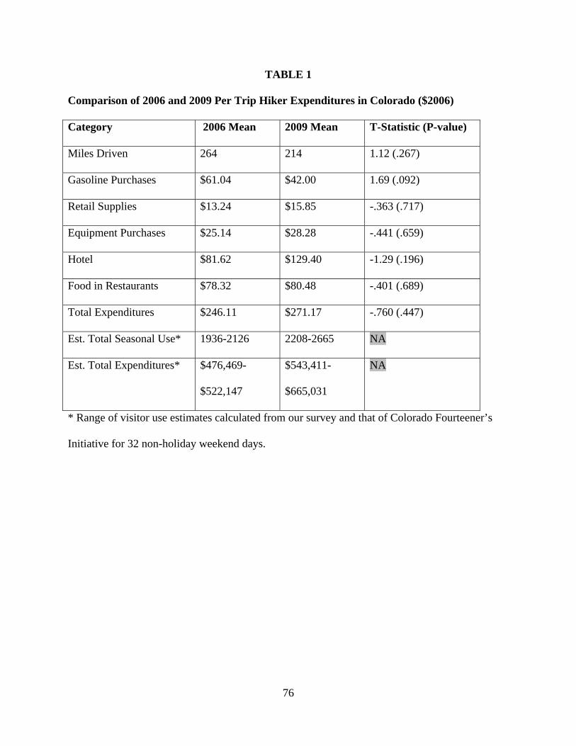
76
TABLE 1
Comparison of 2006 and 2009 Per Trip Hiker Expenditures in Colorado ($2006)
Category 2006 Mean 2009 Mean T-Statistic (P-value)
Miles Driven 264 214 1.12 (.267)
Gasoline Purchases $61.04 $42.00 1.69 (.092)
Retail Supplies $13.24 $15.85 -.363 (.717)
Equipment Purchases $25.14 $28.28 -.441 (.659)
Hotel $81.62 $129.40 -1.29 (.196)
Food in Restaurants $78.32 $80.48 -.401 (.689)
Total Expenditures $246.11 $271.17 -.760 (.447)
Est. Total Seasonal Use* 1936-2126 2208-2665 NA
Est. Total Expenditures* $476,469-
$522,147
$543,411-
$665,031
NA
* Range of visitor use estimates calculated from our survey and that of Colorado Fourteener’s
Initiative for 32 non-holiday weekend days.
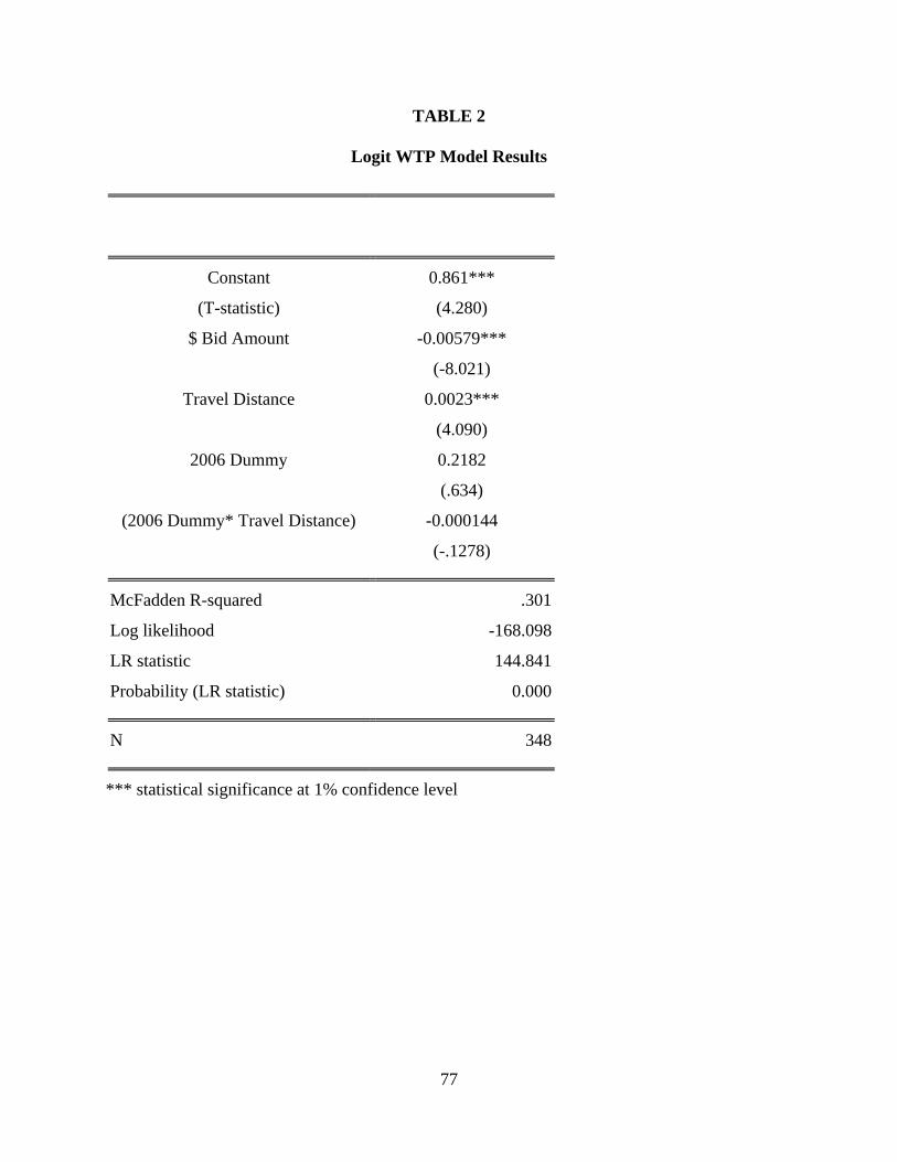
77
TABLE 2
Logit WTP Model Results
Constant
(T-statistic)
0.861***
(4.280)
$ Bid Amount
-0.00579***
(-8.021)
Travel Distance
0.0023***
(4.090)
2006 Dummy
0.2182
(.634)
(2006 Dummy* Travel Distance)
-0.000144
(-.1278)
McFadden R-squared .301
Log likelihood -168.098
LR statistic 144.841
Probability (LR statistic) 0.000
N 348
*** statistical significance at 1% confidence level

78
TABLE 3
Mean WTP Per Person Per Trip and 90% Confidence Intervals
Mean WTP 90% Lower CI 90% Upper CI
2006 data $152 $123 $190
2009 data $139 $119 $167

79
References Bowker, J.M., D. English and K. Cordell. 1999. Projections of Outdoor Recreation Participation to 2050. In Cordell, K. “Outdoor Recreation in American Life” Sagamore Publishing, Champaign, IL. Bureau of Economic Analysis. 2009. National Income Accounts. November 9, 2009. http://www.bea.gov/national/index.htm#gdp. Last Accessed November 9, 2009. Bureau of Labor Statistics. 2009. Employment Situation Summary. November 6, 2009. http://www.bls.gov/news.release/empsit.nr0.htm. Last Accessed November 9, 2009. Bureau of Land Management. 2007. Draft Oil Shale and Tar Sands Resource Management Plan Amendments to Address Land Use Allocations in Colorado, Utah, and Wyoming and Programmatic Environmental Impact Statement. Volumes I, II, and III. December 2007. DES 07-60. Cordell, K., B. McDonald, R.J. Teasley, J. Bergstrom, J. Martin, J. Bason and V. Leeworthy. 1999. Outdoor Recreation Participation Trends. In Cordell, K. “Outdoor Recreation in American Life” Sagamore Publishing, Champaign, IL. Corporation for a Skilled Workforce. 2009. Industry Guidebook: Energy Extraction. Produced for the WEIC Task Force of the Colorado Workforce Development Council by Corporation for a Skilled Workforce. February 2009. Creel, M. and J. Loomis. 1991. Confidence Intervals for Welfare Measures with Application to a Problem of Truncated Counts. Review of Economics and Statistics, Volume 73(2): Davis, G.A. 1995. Learning to Love the Dutch Disease: Evidence from the Mineral Economies. World Development , 23(10): 1765-1779. Davis, G., and J. Tilton, 2005, The Resource Curse. Natural Resources Forum, Aug 29: 233–242. Dillman, D. 2000. Mail and Internet Surveys: The Tailored Design Method. John Wiley and Sons, New York, NY. English, D., Kocis, K., Zarnoch, S., and Arnold, J.R. (2002), ‘Forest Service national visitor use monitoring process’, USDA Forest Service, General Technical Report SRS-57, Southern Research Station, Ashville, NC. Hanemann, M. 1984. “Welfare Evaluations in Contingent Valuation Experiments with Discrete Responses.” American Journal of Agricultural Economics. 66(3): 332-341. Hanemann, M. 1989. “Welfare Evaluations in Contingent Valuation Experiments with Discrete Response Data: Reply.” American Journal of Agricultural Economics. 71(4): 1057-1061.

80
Iimi, A. 2007. Escaping from the Resource Curse: Evidence from Botswana and the Rest of the World. International Monetary Fund Staff Papers 54: 663-699.
Isidore, C. 2009. The Great Recession. CNN Money. March 25, 2009. Keske, C. and J. Loomis. 2008. Regional Economic Contribution and Net Economic Values of Opening Access to Three Colorado Fourteeners. 2008. Tourism Economics 14(2): 249-262. Keske, C.M., and J.B. Loomis. 2007. “High Economic Values from High Peaks of the West”. Western Economics Forum. 4(1): 34-41. Loomis, J. and R. Walsh. 1997. Recreation Economic Decisions: Comparing Benefits and Costs. Venture Publishing Inc., State College, PA. Loomis, J. (2000), ‘Counting on recreation use data: a call for long-term monitoring’, Journal of Leisure Research, 32(1): 93–96. Loomis, J.B. 2002. Integrated Public Lands Management, Second Edition. Columbia University Press. McAlinden, S., K. Hill, B. Swiecki. Economic Contribution of the Automotive Industry to the U.S. Economy—An Updated. Economics and Business Group, Center for Automotive Research. Ann Arbor, Michigan. Outdoor Industry Foundation. 2006. The Active Outdoor Recreation Economy. Available at: http://www.outdoorindustry.org/images/researchfiles/RecEconomypublic.pdf?26 Park, T., J. Loomis, M. Creel. 1991. Confidence intervals for evaluating benefit estimates from dichotomous choice contingent valuation studies. Land Economics 67: 64–73. Stynes, D. and D. White. 2006. Reflections on Measuring Recreation and Travel Spending. Journal of Travel Research 45: 8-16. U.S. Census. Annual Demographic Survey. http://pubdb3.census.gov/macro/032006/hhinc/new06_000.htm. Accessed November 21, 2009.

81
Hedonic Equilibria, Land Value Capitalization,
and the Willingness to Pay for Public Goods†
Nicolai V. Kuminoff Department of Economics Arizona State University
Jaren C. Pope Department of Economics Brigham Young University
This version: May, 2010
First version: December, 2008
† We thank Kelly Bishop, Richard Carson, Tom Downes, Roger von Haefen, Matt Kahn, Mike Keane, Glenn MacDonald, Gilbert Metcalf, Alvin Murphy, Ray Palmquist, Jonah Rockoff, Ed Schlee, V. Kerry Smith, Jeff Zabel, seminar participants at Arizona State University, Brigham Young University, Tufts University, University of Ten-nessee, Utah State University, Virginia Tech, Washington University in St. Louis, and conference participants at AEA and W2133 for valuable comments and suggestions on earlier drafts of this paper. We gratefully acknowledge support from the Lincoln Institute of Land Policy and the National Science Foundation.

82
Abstract
Models of household location choice provide a theoretical foundation for measuring the willing-
ness to pay for public goods. The difficulty is identification. Empirical work was traditionally
believed to suffer from widespread identification problems. Recent studies have revived this
literature by demonstrating that quasi-experiments can provide credible estimates for the rates at
which shocks to public goods are capitalized into land values. In this paper, we develop a uni-
fied framework that relates land value capitalization to the underlying concept of market equili-
brium on which welfare measurement is based. The foundation for our analysis is Rosen’s
description of a differentiated product market with heterogeneous buyers and sellers. First we
define the restrictions on preferences and technology that support a welfare interpretation for the
rate at which an exogenous shock is capitalized into equilibrium prices. Then we translate those
restrictions into testable conditions on micro data sets and on the design of quasi-experiments.
Finally, we use the new framework to analyze the differences between: (i) hedonic estimates of
the willingness to pay for improvements to public school quality from boundary discontinuity
regressions in ten markets and (ii) capitalization rates for changes in test scores that occurred
over the first four years of the federal No Child Left Behind program. We find that hedonic
measures of the average resident’s willingness to pay for improved school quality are four times
as large as capitalization based measures.
Keywords: capitalization, hedonic, identification, welfare, school quality. JEL Codes: C31, D12, L11.

83
I. Introduction
How can we measure the public’s willingness to pay for a public good? This problem has intri-
gued economists for decades.1 Recently, Chay and Greenstone (2005) proposed a novel solu-
tion—use quasi-experiments to identify the rates at which shocks to public goods are capitalized
into land values. The appeal of combining a credible identification strategy with a welfare inter-
pretation of the capitalization effect has led to a resurgence of interest in using markets for pri-
vate property to assess the benefits of public programs.2 Despite the growing importance of this
methodology, the assumptions that enable us to translate capitalization effects into welfare
measures have not been closely examined.
This paper uses the concept of hedonic equilibrium to investigate what land value capita-
lization reveals about the willingness to pay for public goods. We identify problems with using
capitalization to measure willingness to pay, and we propose solutions to those problems. Our
conceptual model builds on Rosen’s (1974) description of the market for a differentiated product.
We consider a market for housing where: (i) a house conveys a bundle of public and private
goods; (ii) heterogeneous buyers and sellers make trades to maximize profits and utility; and (iii)
equilibrium is described by a hedonic price function. Our point of departure from Rosen is to
describe how the price function adjusts following an unexpected shock to a public good influen-
cing the market equilibrium. Depending on the severity of the shock, adjustment may involve a
movement along the hedonic price function or a change in its shape. We express the rate of
change in equilibrium prices (i.e. the capitalization rate) in terms of the reduced form parameters
1 Past proposals have included the median voter model (Bergstrom and Goodman 1973, Rubinfeld, Shapiro, and Roberts 1987) the conventional land value capitalization model (Lind 1973, Starrett 1981), the hedonic model of housing market equilibrium (Scotchmer 1985, 1986, Bartik 1987), and equilibrium sorting models of neighborhood choice (Epple and Sieg 1999, Bayer, Ferreira, and McMillan 2007). 2 For examples see the recent quasi-experimental capitalization studies by Davis (2004), Chay and Greenstone (2005), Greenstone and Gallagher (2008), Linden and Rockoff (2008), Pope (2008), Bin, Landry, and Meyer (2009), Horsch and Lewis (2009), and Cellini, Ferreira, and Rothstein (2010).

84
of the price function which, in turn, depend on market primitives (preferences, income, and
technology). This functional relationship reveals that, in general, capitalization rates do not
identify the willingness to pay for public goods.
The scope for divergence between capitalization and welfare depends on the size of the
shock and the duration of the study period. As both approach zero, the capitalization rate ap-
proaches the marginal willingness to pay (MWTP). In the limit, our model provides a concep-
tual foundation for Chay and Greenstone’s (2005) estimator. As the size of the shock grows, so
does the wedge between capitalization and welfare. The identification problem is intuitive. In a
hedonic demand system, such as Epple (1987), a non-marginal shock to any attribute of a diffe-
rentiated product will change the MWTP for every attribute. All of these changes are condensed
into the same capitalization rate. To isolate the willingness to pay for a single attribute, more
information is needed.
One way to provide the extra information is to place restrictions on the primitives of Ro-
sen’s model. Consider a non-marginal shock to a public good that is capitalized over an interval
when the supply of housing is less than perfectly elastic. We prove three restrictions are both
necessary and sufficient to interpret the capitalization rate as an exact measure of MWTP. First,
preferences, income, and technology must be fixed over the duration of the study period.
Second, utility must be separable in the public good and its demand curve must be perfectly
elastic over the range of the shock. Third, the second derivative of the hedonic price function
with respect to the public good must be zero. If any one of these restrictions is violated, capitali-
zation rates may understate or overstate MWTP.
Restrictions on the primitives of Rosen’s model have testable implications for the evolu-
tion of the hedonic price function. Using a linear-in-parameters specification for the price func-

85
tion, we derive conditions on the data under which capitalization rates will identify the average
consumer’s MWTP. One can identify MWTP in the pre-shock equilibrium if the hedonic gra-
dient is constant over the duration of the study period. If this condition does not hold, one can
still identify MWTP in the post-shock equilibrium if the shock (or an instrument for the shock) is
orthogonal to all other variables. A key point is that randomization of an instrument can provide
the extra information needed to identify post-shock MWTP in lieu of restrictions on market
primitives.
In the second half of the paper, we apply our framework to the problem of measuring the
willingness to pay for improving the quality of public schooling. We have assembled a unique
set of micro data for the analysis. The data describe a quarter of a million individual homes that
sold in the cities and suburbs of Fairfax VA, Portland OR, Detroit MI, Los Angeles CA, and
Philadelphia PA during the 2003 and 2007 school years.3 Each observation includes the sale
price of a home, its structural features, the demographic composition of its neighborhood, the
local public goods available to its residents, and most importantly, measures of academic per-
formance at the public schools to which children living in that home would have been assigned.
Most schools reported significant increases in their students’ math and reading proficien-
cy between 2003 and 2007, with the largest improvements reported by the lowest quality
schools. These trends are consistent with the new incentives that school administrators faced
after the No Child Left Behind Act (NCLB) took effect in 2003 (Dee and Jacob 2009, Neal and
Schanzenbach forthcoming). NCLB required each state to implement a test-based accountability
system for its public schools. Schools that repeatedly failed to meet targets for math and reading
3 After an exhaustive search over potential study regions, we concluded that Fairfax, Portland, Detroit, Los Angeles, and Philadelphia were the only metro areas with public school assignment laws, consistent reporting of test scores, and micro data on recent property sales that would allow us to develop hedonic boundary discontinuity designs at the standards set by Black (1999) and Bayer, Ferreira, and McMillan (2007).

86
proficiency would face a schedule of sanctions. NCLB also required every school to publicly
report the share of its students who achieve proficiency in each subject. We use these data to
compare the willingness to pay for improved school quality with the capitalization of publicly
reported changes in math and reading proficiency.
Our measures of willingness to pay are derived by estimating hedonic price functions in
each of the ten (school year, metro area) pairings. The price functions are identified by boundary
discontinuity designs that exploit the discreteness in each area’s laws for assigning children to
schools. Table 1 compares our main findings to the results from previous boundary discontinuity
studies of Boston (Black 1999) and San Francisco (Bayer, Ferreira, and McMillan 2007). He-
donic estimates for the elasticity of property values with respect to test scores are remarkably
similar across metro areas (column 1). In 2003 our estimates range from 0.12% in Fairfax to
0.27% in Philadelphia. Converting these estimates into constant year 2000 dollars reveals the
average resident would be willing to pay between $422 (Detroit) and $743 (Philadelphia) for a
1% increase in test scores (column 3).
When we repeat the boundary discontinuity analysis for 2007 we find significant changes
in hedonic gradients. These changes drive a wedge between our hedonic measures of willing-
ness to pay in 2003 and estimates based on the capitalization of changes in test scores between
2003 and 2007. Columns 3 and 4 illustrate that the two sets of estimates differ by more than
100% for the average resident in Fairfax, Portland, Detroit, and Philadelphia. Furthermore,
correlation between changes in test scores and other variables drives a wedge between capitaliza-
tion and willingness to pay in 2007. Aggregating our hedonic results over all five study areas
reveals that the average resident’s willingness to pay for a 1% increase in scores increased from
$536 in 2003 to $688 in 2007. These figures are four times as large as our capitalization-based

87
measures. We conclude that researchers must be cautious in using capitalization as the sole basis
for evaluating the benefits of public programs.
Overall, our findings add to three distinct literatures. First, we define the connection be-
tween land value capitalization (Lind 1973, Starrett 1981) and hedonic equilibria (Scotchmer
1985, 1986, Bartik 1987) in the revealed preference literature on using private market outcomes
to predict the willingness to pay for public goods. Second, we establish a conceptual framework
for interpreting evidence on capitalization from the new quasi-experimental literature on policy
evaluation (Davis 2004, Chay and Greenstone 2005, Greenstone and Gallagher 2008, Linden and
Rockoff 2008, Cellini, Ferreira, and Rothstein, 2010). Finally, our boundary discontinuity re-
sults extend the literature on valuing school quality by providing the first consistent evidence on
variation in willingness to pay across time and space (Oates 1969, Kain and Quigley 1975, Black
1999, Figlio and Lucas 2004, Bayer, Ferreira, and McMillan 2007).
The rest of the paper proceeds as follows. Section II briefly reviews the ideas behind he-
donic and capitalization based approaches to valuing public goods. Section III presents our
conceptual model and defines conditions under which capitalization rates identify willingness to
pay. We translate those conditions into testable econometric restrictions in section IV. Section
V describes our data, section VI reports regression results, and section VII analyzes implications
for measuring willingness to pay. Finally, section VIII concludes by summarizing the problems
with capitalization-based benefit measurement and the potential solutions.
II. Hedonic and Capitalization Models for Valuing Public Goods
In his seminal 1956 paper, Tiebout hypothesized that freely mobile households will reveal their
preferences for public goods through the location choices they make. His reasoning influenced
88
the development of two revealed preference techniques: the capitalization model and the hedonic
property value model. Hundreds of applications of these methods over the past 40 years have
contributed much of what we currently know about the willingness to pay for public goods.
Capitalization studies use data before and after a market shock to measure its effect on
property values.4 The power of this technique is the ability to simultaneously measure a change
in asset values and demonstrate that the change was caused by some event. Capitalization mod-
els are routinely used by expert witnesses in litigation over private property externalities (Simons
2006). They are also used to measure the market value of risk and uncertainty (Brookshire et al.
1985). A limitation of the technique is that it lacks a precise welfare interpretation. Lind (1973)
and Starrett (1981) demonstrated that, under the type of sorting behavior Tiebout envisioned,
market capitalization of a large shock may understate or overstate the change in household wel-
fare.5
In contrast, the hedonic property value model based on Rosen (1974) offers a theoretical-
ly consistent approach to welfare measurement. The difficulty is identification. Scotchmer
(1985, 1986) proved that data from a single market are only sufficient to identify marginal val-
ues. To identify a demand curve, one must collect multi-market data on the characteristics of
households and their houses, plus instrumental variables for endogenous characteristics (Bartik
1987, Epple 1987). Unfortunately, barriers to obtaining these data have stymied demand estima-
tion.6 The vast majority of empirical studies only aspire to recover marginal values.7
4 The idea for using panel data to measure how changes in quality characteristics influence housing prices dates back at least to Bailey, Muth, and Nourse (1963). Economic applications begin with Palmquist (1982). 5 While Lind (1973) does not develop a formal utility theoretic framework, he proves that any welfare interpretation of capitalization requires there be zero consumer surplus. This effectively rules out preference-based sorting by heterogeneous agents, as Starrett (1981) later demonstrated. 6 An alternative strategy to identify demand is to provide some information about the structure of consumer prefe-rences. This information may consist of a parametric representation for the utility function (Epple and Sieg 1999, Bajari and Benkard 2005), separability restrictions on preferences (Ekeland, Heckman and Nesheim 2004), an assumption that the populations residing in different cities share a common distribution of unobserved tastes (Bartik
89
Even the seemingly modest task of estimating marginal values is now believed to be pla-
gued by omitted variable bias. Chay and Greenstone (1998, 2005) characterized the problem and
proposed a solution. They replaced the conventional hedonic estimator with an instrumental
variables strategy that isolates how property values are affected by unexpected shocks to public
goods. Their microeconometric model bridged the capitalization and hedonic literatures. It
integrated a quasi-experimental version of the identification strategy from the capitalization
literature with the welfare interpretation of Rosen’s hedonic model.
To illustrate the basic idea, let the price of housing be expressed as ( )ξ,, hgpp = , where
g is the public good of interest, h measures all other public goods and housing characteristics
observed by the analyst, and ξ represents unobserved variables. It is standard practice to specify
a linear-in-parameters price function such as
( )111111 ξεηθ ++= hgp , (1)
where the subscripts indicate the time period. Assuming the specification is correct, the first
order conditions from Rosen (1974) allow us to interpret 1θ as the marginal willingness to pay
(MWTP) for the public good in period 1. However, 1θ is not identified if 1ξ is correlated with
1g or 1h .
Now suppose p, g, and h are also measured after an unexpected shock. First-differencing
the data produces a new estimator,
εγφ Δ+Δ+Δ=Δ hgp , (2)
1987), or an assumption that migration decisions do not arise from changes in individual tastes (Bishop and Tim-mins 2008). 7 That said, the number of studies that aspire to recover marginal values is also vast. To give a rough sense of scale, there are more than 1600 citations of Rosen (1974) in the Social Science Citation Index and approximately 4000 reported by Google Scholar. Property value applications are one of (if not the) most frequent application. See Palmquist (2005) for a review of the literature.

90
where 12 ddd −=Δ for [ ]ε,,, hgpd = . If the bias from omitted variables is purged by differenc-
ing the data, (2) provides an unbiased estimator for φ . Alternatively, if one suspects that
[ ] 0,| ≠ΔΔΔ hgE ε , instrumental variables may be used to develop a consistent estimator.
Interpreted literally, φ is the average rate of change in property values associated with
the shock to g. Chay and Greenstone observe that this capitalization rate will equal MWTP if the
gradient of the price function in (1) is constant over time (i.e. 21 θθ = and 21 ηη = implies
21 θθφ == and 21 ηηγ == ). Recent studies have used this result to estimate the willingness to
pay for changes in cancer risk (Davis 2004), air quality (Chay and Greenstone, 2005), hazardous
waste (Greenstone and Gallagher 2008), crime (Linden and Rockoff 2008, Pope 2008), open
space (Bin, Landry, and Meyer 2009), invasive species (Horsch and Lewis 2009), low income
housing credits (Baum-Snow and Marion 2009), and investment in education (Cellini, Ferreira,
and Rothstein 2010). In all of these studies, the validity of welfare measures rests on the main-
tained assumption that the gradient of the hedonic price function is constant over the duration of
the study. The assumption has been made for periods between 10 and 20 years, for areas ranging
from a single county to the contiguous United States.
Because the price function is an equilibrium outcome generated by interactions between
all of the buyers and sellers in a market, assumptions about its evolution implicitly restrict prefe-
rences and technology.
III. Hedonic Equilibria and the Capitalization of Market Shocks
This section considers the evolution of the hedonic gradient. After introducing the primitives of
the hedonic model and characterizing market equilibrium, we define restrictions on preferences
and technology that are sufficient to assure the gradient will be time-constant. A proof is fol-
91
lowed by brief discussion.
A. Demand, Supply, and Market Equilibrium
Price-taking households are assumed to be free to choose a home with any combination of hous-
ing characteristics (e.g. bedrooms, bathrooms, sqft) in the neighborhood that provides their
desired levels of amenities (e.g. school quality, air quality, racial composition). The utility max-
imization problem is
( ) ( )Θ+= ;,;,,max,,
XgPbytosubjectbXgUbXg
α , (3)
where [ ]ξ,hX = . A household chooses housing characteristics, amenities, and the numeraire
composite commodity (b) to maximize its utility, given its preferences (α ), income ( y ), and the
after-tax price of housing, ( )Θ;, XgP , which is expressed as a general parametric function of g,
X, and a parameter vector, Θ . The first order conditions are
( ) ( )yXgDbUgU
gXgP ,,;;, α≡
∂∂∂∂
=∂
Θ∂ , (4a)
( ) ( )ygXRbUXU
XXgP ,,;;, α≡
∂∂∂∂
=∂
Θ∂ . (4b)
The first equality in (4a) implies that each household will choose a neighborhood that provides a
quantity of g at which their marginal willingness-to-pay for an additional unit exactly equals its
marginal implicit price. Assuming the marginal utility of income is constant, the second equality
observes that as g varies the marginal rate of substitution defines the inverse demand curve,
conditional on X. Equation (4b) states analogous first order conditions for X.
Producers in this market may include developers, contractors, and individuals selling
their homes. Let ( )β;,, XMgC denote a producer’s cost function, where M is the number of

92
type-(g,X) homes they sell and β is a vector of parameters describing the producer.8 Variation
in β captures differences in costs faced by different producers. Following Rosen (1974), we
treat each producer as a price taker who is free to vary the number of units they sell as well as a
subset of the characteristics of each unit. For notational convenience, g is assumed to be ex-
ogenously determined.9 In this case, the profit maximization problem is
( ) ( )βπ ;,,;,max,
XMgCXgPMMX
−Θ⋅= , (5)
with the corresponding first order conditions
( ) ( )M
XMgCXgP∂
∂=Θ
β;,,;, , ( ) ( )X
XMgCMX
XgP∂
∂⎟⎠⎞
⎜⎝⎛=
∂Θ∂ β;,,1;, . (6)
Producers choose M to set the offer price of the marginal home equal to its production costs, and
they choose X to set the marginal per unit cost of each attribute equal to its implicit price.
Equilibrium occurs when the first order conditions in (4) and (6) are simultaneously
satisfied for all households and producers. This system of differential equations implicitly de-
fines the equilibrium hedonic price function that clears the market (Rosen 1974). It will be
useful to rewrite the price function to acknowledge its dependence on model primitives,
( ) ( ) ( )[ ]ΒΑΘΒΑ≡Θ ,,; ,,,;, ggXgPXgP . (7)
Equilibrium levels of X are determined by all of the exogenous variables: g the public good of
interest, ( ) ΑΑ ~,: αyF , a vector of parameters that describes the joint distribution of household
income and preferences, and ( ) ΒΒ ~: βV , a parameter vector describing the distribution of
8 For a developer or contractor, the cost function will reflect the physical, labor, and regulatory costs of building a home. For a homeowner, the cost function will reflect their psychological attachment to the home as well as the cost of renovation. 9 The results of this section are not altered by allowing firms to choose g or by restricting their ability to choose X. The key restriction needed to relate our model to the new empirical capitalization literature is that g may be influ-enced by forces that are exogenous to the model.

93
producer characteristics.10 Naturally, the reduced form parameters describing the shape of the
price function are also functions of the exogenous variables.
B. Necessary Conditions to Interpret the Capitalization Rate as a Measure of MWTP
Now consider two different hedonic equilibria, observed before and after an unexpected shock to
g. The change in the value of a house j depends on the difference in the pre and post-shock price
functions,
( ) ( )[ ] ( ) ( )[ ]1111111122222222 ,,; ,,,,,; ,,, ΒΑΘΒΑ−ΒΑΘΒΑ ggXgPggXgP jjjj , (8)
where the 1 and 2 subscripts denote pre and post-shock equilibria. To isolate the capitalization
rate, we condition on X and divide the change in property value by the change in g,
( )[ ] ( )[ ]
jj
jjjjj gg
XXggPXXggP
12
1111122222 ,,;,,;−
=ΒΑΘ−=ΒΑΘ=φ . (9)
This difference quotient provides a general expression for the capitalization parameter estimated
in the literature.11
Because jφ depends on two (potentially different) price functions, it is not the measure of
MWTP from Rosen (1974). To interpret jφ as the MWTP, we must restrict preferences and
technology to assure that the capitalization rate will equal the partial derivative of the pre-shock
and/or post-shock price functions. Severity of the restriction depends on the size of the shock. If
the change in g is small, we need only restrict 21 Α=Α and 21 Β=Β . Under this condition, the
difference quotient in (9) approaches the partial derivative in (4a) as jj gg 12 − approaches
10 M drops out of the expression for X in (7) because it is a function of model primitives. 11 P and g are typically measured in levels or logs.

94
zero.12 In the limit, pre-shock MWTP equals post-shock MWTP which equals the capitalization
rate. This is intuitive. An infinitesimal change in one hedonic characteristic will not alter the
shape of the price function; equilibrium prices simply increase by MWTP.
In the case of a nonmarginal shock, three restrictions are needed to establish a welfare
interpretation for the capitalization rate. We state this formally as
ASSUMPTION 1.
a. 21 Α=Α and 21 Β=Β .
b. 0=∂Θ∂ g .
c. ( ) ( )Θ=∂Θ∂ ,;, XfgXgP .
Condition a restricts preferences, income, and technology to be constant over the duration of the
study.13 It follows that supply and demand curves for each characteristic are also fixed. The last
two conditions restrict the shapes of those curves. Condition b states that changes in g have no
effect on the shape of the price function. If supply curves are less than perfectly elastic, for
example, condition b is satisfied if demand is perfectly elastic. Condition c further restricts
supply and demand so that the marginal price function for g does not depend on g. If all three
conditions are satisfied, it is straightforward to show that the capitalization rate in (9) must equal
the MWTP in (4a).
THEOREM 1. If assumption 1 holds for a shock to g, then the capitalization rate, φ ,
equals the pre-shock MWTP, which equals the post-shock MWTP.
Proof. Consider any home, j, with characteristics XX j = for which jg changes from
12 Proof of this statement follows immediately from the definition of a derivative. 13 This condition can be relaxed as long as other restrictions are added to guarantee that changes in income, prefe-rences, and technology have no effect on the shape of the equilibrium price function. More precisely, Θ must be invariant to any changes in the elements of Α andΒ .

95
1jg to 2jg . Since 21 Α=Α , 21 Β=Β , and 0=∂Θ∂ g , we know that 21 Θ=Θ . Combining
this result with the assumption that ( ) ( )Θ=∂Θ∂ ,;, XfgXgP implies ( )1,ΘXf ( )2,Θ= Xf .
It follows from the Mean Value Theorem that ( )1, Θ= Xfjφ ( )2,Θ= Xf . The second term
measures pre-shock MWTP and the third term measures post-shock MWTP, as defined by the
first-order conditions from Rosen (1974). QED.
The model proposed by Chay and Greenstone (2005) provides an example. Their linear
price function (1) is consistent with condition c, and their assumption that 21 Θ=Θ implies
conditions a and b are satisfied. Using these restrictions, it is a simple algebraic exercise to
demonstrate that (9) returns the MWTP for g. Alternatively, for models that violate assumption
1 the Mean Value Theorem implies
( ) ( ) gXgPgXgP jjjjj ∂Θ∂≠∂Θ∂≠ 222111 ;,;,φ .
In this case, the direction and magnitude of the bias from misinterpreting the capitaliza-
tion rate as a welfare measure will depend on the correlations in the data and the shapes of
supply and demand curves.14
C. Discussion
We have established that the capitalization rate approaches the partial derivative of the price
function as 12 Α→Α , 12 Β→Β , and 0→Δg . Based on this limiting result, we would expect
the capitalization rate to provide a good approximation to average MWTP for small shocks that
can be tracked over short periods. However, recent studies have focused on large shocks and/or
14 This dependence is easily demonstrated using a closed form expression for the equilibrium price function such as Tinbergen’s (1959) linear-quadratic-normal model. Section IV demonstrates the role of correlations in the data using the standard empirical specification for the hedonic price function.

96
periods of a decade or more. For example, Chay and Greenstone (2005) measure the capitaliza-
tion of large air quality improvements during the 1970s. Davis (2004) tracks the capitalization of
a six-fold increase in pediatric leukemia risk. Greenstone and Gallagher (2008) estimate capita-
lization rates for the cleanup of hazardous waste sites over the first 20 years of the federal “Su-
perfund” program (1980 to 2000).15 We use these studies as examples for two reasons. First
because they develop ingenious identification strategies to provide what are perhaps the most
credible estimates for public good capitalization rates. Second because their exploitation of large
shocks and/or long intervals means the ability to interpret their estimates as measures of average
MWTP rests on the validity of assumption 1.
Consider what assumption 1 implies. At a single point in time, condition c requires the
distribution of marginal prices for g to be degenerate once we condition on X. This is a special
case of a linear marginal price function, which Ekeland, Heckman, and Nesheim (2004) prove is
a nongeneric property of hedonic equilibrium. Even if we invoke the degeneracy restriction with
the idea that it represents a linear approximation to the true price function, conditions a and b
impose deeper restrictions on preferences and technology.
Recall that the hedonic gradient provides a mapping to the distribution of marginal values
in the consumer population (4) and marginal costs in the producer population (6). The only
theoretically-grounded restriction on this mapping that supports 0=∂Θ∂ g is that either the
demand for g or its supply is perfectly elastic.16 Utility must also be separable in g and X. Oth-
15 Unlike the first two examples, the scope of the Superfund shock was small in the sense that only 1% of census tracts contained sites that were cleaned. The key assumptions that enable Greenstone and Gallagher to use the capitalization rate for benefit-cost analysis are that: (i) the MWTP for cleanup does not depend on the degree of contamination, and (ii) the hedonic gradient was invariant to all changes in public goods, housing characteristics, income, preferences, and construction costs that occurred in the United States over their 20-year study period. 16 All else constant, a positive shock to g will decrease MWTP (changing Θ ) if demand is downward sloping. It is possible to offset the change in Θ by a concomitant shock to preferences. While this type of mathematical restric-tion presents a technical possibility, it has no economic content and, in our opinion, does not merit serious consid-

97
erwise, a shock to g could change the implicit prices of the elements of X. If g is the crime rate,
for example, we must be willing to assume that changes in crime do not affect the willingness to
pay for home security systems, fences, or proximity to city parks. These restrictions on own and
cross-price elasticities are not limited to the public good of interest. They also apply to all of the
elements of X that are subject to exogenous shocks. A change in the relative price of any hedon-
ic characteristic violates 0=∂Θ∂ g and drives a wedge between MWTP and the capitalization
rate for any other characteristic. Finally, even if the demand for every characteristic is perfectly
elastic, we must still restrict their relative prices to be unaffected by changes in wealth, prefe-
rences, and construction costs that may occur during the study period.
If assumption 1 is violated, the gradient of the price function may change between the pre
and post-shock observation periods. The bias associated with interpreting the capitalization rate
as a measure of MWTP will depend on: (i) the shape of the price function; (ii) magnitudes of
changes in the reduced-form parameters; and (iii) correlations in the data. Given a parametric
representation for the price function, the capitalization bias can be expressed in terms of
,,,,, 12121 XggΘΘ and 2X . We derive this relationship in the next section and use it to define
testable restrictions on the data that neutralize the capitalization bias.
IV. Sufficient Conditions for Capitalization Based Welfare Measurement
Empirical studies almost always specify the price function to be linear in parameters.17 We
follow this convention and abstract from econometric complications such as measurement error
and approximation error in the choice of functional form. These abstractions allow us to focus
eration. 17 The prevalence of the linearity assumption is partly due to Cropper, Deck, and McConnell (1988). Working with simulated data, they found that linear approximations tended to provide better predictions for MWTP than a more flexible Box-Cox quadratic specification in the presence of unobserved variables and errors in variables.

98
attention on the relationship between capitalization and welfare in the workhorse model of the
empirical literature.18
We begin by repartitioning X into observed (h) and unobserved (ξ ) components. Using
this partition, the linear price functions that describe market equilibria before and after an unex-
pected shock to g are ( )1111111 ξεηθ ++= hgp and ( )2222222 ξεηθ ++= hgp .19 Parameter
subscripts recognize that the shape of the function may have been altered by the shock to g and
by concomitant changes in h, ξ , ( )α,yF , and ( )βV .
Subtracting the old price function from the new one yields a general time-differenced
model,
( ) ( ) εηηθθ Δ+−+−=Δ 11221122 HHggP . (10)
In the special case where 21 θθ = and 21 ηη = , equation (10) reduces to the capitalization estima-
tor from (2), εγφ Δ+Δ+Δ=Δ hgp .
Applying the Frisch-Waugh Theorem, the relationship between the estimated capitaliza-
tion rate (φ ) and MWTP ( 21,θθ ) can be expressed as:
( ) ( )rr
rrrhr
rrgr
′Δ′
+−′′
+−′′
+=εηηθθθφ 12
112
12
ˆ , (11)
where ( ) ghhhhgr Δ′ΔΔ′ΔΔ−Δ= −1 . The estimate forφ is a function of all the parameters of the
true price functions that precede and follow the shock. Put differently, (11) reports what we can
expect to learn about MWTP from estimating (2) when (10) is the true model.
The estimate for the capitalization rate is a function of ex-ante MWTP, ex-post MWTP,
18 That said, one could repeat our analysis in this section under any set of assumptions about the shape of the price function and the sources of error. If the price function lacks a closed form solution, numerical methods could be used to solve for the equilibrium, as in Klaiber and Smith (2009) or Kuminoff and Jarrah (2010). 19 The 1h matrix of control variables may also include a vector of ones so that η includes an intercept.
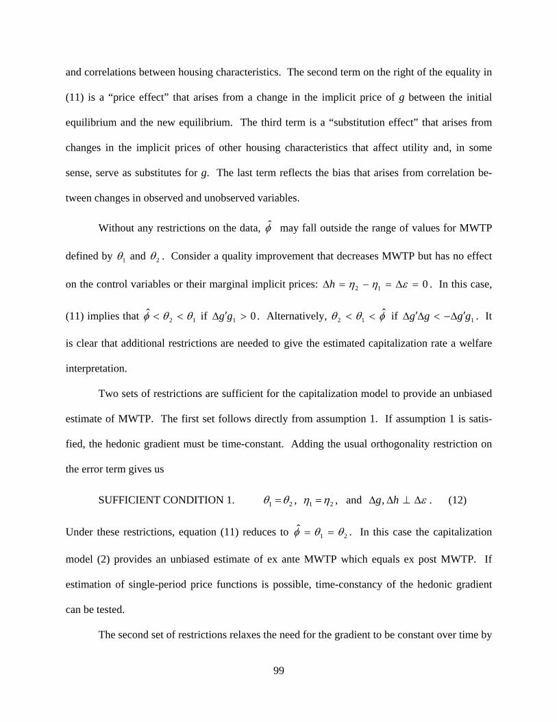
99
and correlations between housing characteristics. The second term on the right of the equality in
(11) is a “price effect” that arises from a change in the implicit price of g between the initial
equilibrium and the new equilibrium. The third term is a “substitution effect” that arises from
changes in the implicit prices of other housing characteristics that affect utility and, in some
sense, serve as substitutes for g. The last term reflects the bias that arises from correlation be-
tween changes in observed and unobserved variables.
Without any restrictions on the data, φ may fall outside the range of values for MWTP
defined by 1θ and 2θ . Consider a quality improvement that decreases MWTP but has no effect
on the control variables or their marginal implicit prices: 012 =Δ=−=Δ εηηh . In this case,
(11) implies that 12ˆ θθφ << if 01 >′Δ gg . Alternatively, φθθ ˆ
12 << if 1gggg ′Δ−<Δ′Δ . It
is clear that additional restrictions are needed to give the estimated capitalization rate a welfare
interpretation.
Two sets of restrictions are sufficient for the capitalization model to provide an unbiased
estimate of MWTP. The first set follows directly from assumption 1. If assumption 1 is satis-
fied, the hedonic gradient must be time-constant. Adding the usual orthogonality restriction on
the error term gives us
SUFFICIENT CONDITION 1. 21 θθ = , 21 ηη = , and εΔ⊥ΔΔ hg, . (12)
Under these restrictions, equation (11) reduces to 21ˆ θθφ == . In this case the capitalization
model (2) provides an unbiased estimate of ex ante MWTP which equals ex post MWTP. If
estimation of single-period price functions is possible, time-constancy of the hedonic gradient
can be tested.
The second set of restrictions relaxes the need for the gradient to be constant over time by

100
adding orthogonality restrictions on the data that exploit the linearity of the model. More pre-
cisely, it can be seen from (11) that 2ˆ θφ = if the following restrictions hold
SUFFICIENT CONDITION 2. ghhg Δ⊥Δ,, 11 and εΔ⊥ΔΔ hg, . (13)
In words: if the shock to g is orthogonal to its initial level, and to the initial levels of the control
variables, and to changes in those variables, then the capitalization rate provides an unbiased
estimate of MWTP in the post-shock equilibrium, even if the gradient changes between the two
observation periods. The data may still contain capitalization bias. If 21 θθ ≠ or 21 ηη ≠ the
price change for any given home may lie above or below the resident’s ex post MWTP. Howev-
er the positive and negative differentials for individual homes cancel out of the first-differenced
estimate for φ due to the linearity of the price function and the orthogonality of the shock.20
If instruments are available, sufficient conditions 1 and 2 can be relaxed. Some authors
have sought to develop instruments for gΔ out of concern for the potential correlation between
changes in observed and unobserved variables. Notably, Chay and Greenstone (2005) and
Greenstone and Gallagher (2008) use discontinuities in the structure of public policies to break
potential correlation between gΔ and εΔ . Equally important is the fact that these “policy dis-
continuity” instruments offer the potential to identify subsets of “treated” and “untreated” homes
that are similar in many other respects. With this in mind, let z denote a set of valid instruments
for gΔ . The instrumental variables analog to the capitalization bias function in (11) simply
replaces gΔ with ( ) gzzzzg Δ′′=Δ −1ˆ . Likewise, (12) and (13) are replaced with (14) and (15).
20 Linearity and orthogonality are both necessary. In the context of assumption 1, we have strengthened condition c such that ( ) ( )Θ=∂Θ∂ fgXgP ;, . Under the original condition c, where the marginal price function may be nonli-near in X, orthogonality restrictions on the data may not be sufficient to identify 2θ .
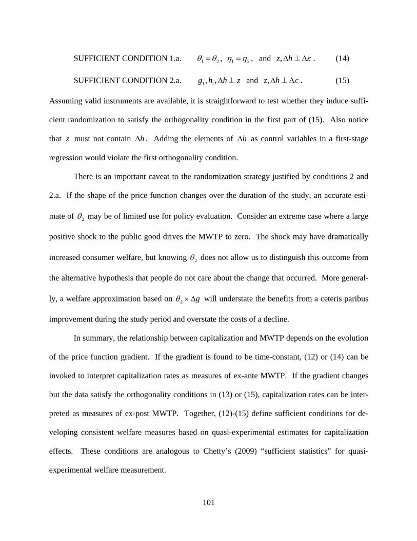
101
SUFFICIENT CONDITION 1.a. 21 θθ = , 21 ηη = , and εΔ⊥Δhz, . (14)
SUFFICIENT CONDITION 2.a. zhhg ⊥Δ,, 11 and εΔ⊥Δhz, . (15)
Assuming valid instruments are available, it is straightforward to test whether they induce suffi-
cient randomization to satisfy the orthogonality condition in the first part of (15). Also notice
that z must not contain hΔ . Adding the elements of hΔ as control variables in a first-stage
regression would violate the first orthogonality condition.
There is an important caveat to the randomization strategy justified by conditions 2 and
2.a. If the shape of the price function changes over the duration of the study, an accurate esti-
mate of 2θ may be of limited use for policy evaluation. Consider an extreme case where a large
positive shock to the public good drives the MWTP to zero. The shock may have dramatically
increased consumer welfare, but knowing 2θ does not allow us to distinguish this outcome from
the alternative hypothesis that people do not care about the change that occurred. More general-
ly, a welfare approximation based on gΔ×2θ will understate the benefits from a ceteris paribus
improvement during the study period and overstate the costs of a decline.
In summary, the relationship between capitalization and MWTP depends on the evolution
of the price function gradient. If the gradient is found to be time-constant, (12) or (14) can be
invoked to interpret capitalization rates as measures of ex-ante MWTP. If the gradient changes
but the data satisfy the orthogonality conditions in (13) or (15), capitalization rates can be inter-
preted as measures of ex-post MWTP. Together, (12)-(15) define sufficient conditions for de-
veloping consistent welfare measures based on quasi-experimental estimates for capitalization
effects. These conditions are analogous to Chetty’s (2009) “sufficient statistics” for quasi-
experimental welfare measurement.

102
To assess the practical importance of conceptual differences between capitalization and
willingness to pay requires tracking how the hedonic gradient evolves over time. The difficulty
lies in identifying single-period price functions. Perhaps the most credible identification strate-
gies to date are the boundary discontinuity designs used to measure the willingness to pay for
improving the quality of public schooling (Black 1999, Bayer, McMillan, and Reuben 2007).
Therefore we focus the remainder of our attention on using this strategy to compare the capitali-
zation of changes in school quality with the willingness to pay for improvements.
V. Capitalization of School Quality Changes and the MWTP for Improvements
Understanding the willingness to pay for school quality is crucial for determining the benefits of
undertaking a wide range of academic reforms. Hedonic property value models offer the most
intuitively appealing method. Because a household’s access to a public school is determined by
whether or not the household lives within the attendance zone for that school, property value
differentials should reflect what parents are willing to pay for their children to attend schools
where students score higher on standardized tests. A large empirical literature evolved around
this idea, beginning with Oates (1969).21
The 40-year history of the literature on valuing school quality is a microcosm for the
broader literature on valuing public goods. Early studies used cross-section models with few or
no controls for omitted variables. Then researchers noted a potential source of confounding—
schools with higher test scores tended to be located in more exclusive neighborhoods. Subse-
quent studies sought to avert the potential bias by developing quasi-experimental identification
strategies. This work began with Black (1999). She noticed that school quality shifts discretely
21 Kain and Quigley (1975) is another early example. Recent applications include Black (1999), Bogart and Crom-well (2000), Downes and Zabel (2002), Gibbons and Machin (2003), Reback (2005), and Bayer, Ferreira, and McMillan (2007). Figlio and Lucas (2004) is an example of a capitalization-based study.

103
as one crosses an attendance zone boundary, but other neighborhood characteristics do not (e.g.
crime rates, air quality, access to the city center). Therefore, the composite price effect of all the
unobserved amenities that are common to homes on both sides of a boundary can be absorbed by
a fixed effect for the “boundary zone”. By focusing on sales that occurred near a boundary and
including fixed effects for each boundary zone, Black forced the identification to come from
price differentials between structurally similar homes located on opposite sides of a boundary.
Bayer, Ferreira, and McMillan (2007) refined Black’s approach to control for correlation
between preferences for schools and preferences for the demographic characteristics of one’s
neighbors. The problem stems from sorting. If preferences for school quality are correlated with
demographic characteristics, such as race or education, then similar “types” of households will
tend to locate in the same attendance zones. This helps to explain why neighborhood demo-
graphics also tend to shift discretely as one crosses an attendance zone boundary. Since prospec-
tive homebuyers may care about the characteristics of their neighbors, one must control for
changes in the demographic composition of the neighborhood in order to isolate the implicit
value of academic performance.
We use the hedonic boundary discontinuity design developed by Black and refined by
Bayer, Ferreira, and McMillan to identify single-period price functions in five metropolitan
areas. Then we calculate the MWTP for school quality, test for time-constancy of the hedonic
gradient, and compare our estimates for MWTP to capitalization rates for the changes in test
scores that occurred during the first four years of the No Child Left Behind Act. The remainder
of this section summarizes the Act, our data, and key features of the research design.

104
A. No Child Left Behind
President George W. Bush announced his “No Child Left Behind” framework for education
reform three days after taking office, and within a year the NCLB act had been passed. NCLB
was one of the most sweeping reforms in the recent history of public education in the United
States. Since its enactment, states have been required to implement accountability systems that
measure student performance in reading and math. Standardized testing is done in grades 3
through 8 and at least once during high school. State test scores are used to determine if each
public school is making “Adequate Yearly Progress” (AYP) toward the goal of having 100% of
its students attain state-specific standards for minimum competency in reading and mathematics
by 2014. Schools that do not meet AYP face a series of repercussions.
Importantly, NCLB established a consistent set of metrics for comparing academic per-
formance across schools and improved accessibility of the information. To obtain a ranking of
schools in their area or to see specific test scores, parents need only visit one of several websites
that collect the information and distribute it freely.22 A low cost of obtaining information should
strengthen the link between property values and the willingness to pay for higher academic
performance.
While test scores have trended up since NCLB was enacted, its impact on the quality of
education has been debated. Advocates argue that school quality will be improved by develop-
ing consistent metrics for tracking school performance, publicizing results, and sanctioning
schools that fail to meet APY. Detractors argue that NCLB creates perverse incentives to “teach
to the test”, to lower state standards, to expel poorly performing students, or even to lie when
reporting scores. Several authors have investigated these issues. Perhaps the most convincing
analyses are those by Neal and Schanzenbach (forthcoming) and Dee and Jacob (2009). These 22 See for example the popular websites: www.greatschools.org and www.schooldigger.com .

105
papers also provide excellent reviews of the literature. Neal and Schanzenbach show that the
introduction of NCLB increased reading and math scores for students in the middle of the
achievement distribution for fifth graders in the Chicago Public School system. Dee and Jacob
(2009) employ a comparative interrupted time series design to identify the impact of NCLB on a
panel of state test scores from the National Assessment of Education Progress (NAEP). The key
feature of their research design is that changes in NAEP scores should be unaffected by the
perverse incentives that critics of NCLB have emphasized. They found that NCLB did indeed
cause large and broad gains in NAEP math achievement scores of 4th and 8th graders, especially
in the bottom decile of the achievement distribution.23 These results suggest that the upward
trend in NCLB scores is consistent with alternative metrics for judging public school quality.
B. Ten Boundary Discontinuity Designs
There have been few applications of the boundary discontinuity methodology to study the wil-
lingness to pay for school quality, and the vintage of data used by Black and Bayer, Ferreira, and
McMillan was early to mid 1990’s. We significantly update and extend the literature by apply-
ing the methodology to 10 new markets: 5 geographic regions (Fairfax County VA, Portland OR,
Philadelphia PA, Detroit MI, and Los Angeles CA) in 2 distinct periods (the 2003 and 2007
school years). After an exhaustive search over prospective study regions, these five areas were
chosen because they each satisfied three key criteria: (i) a sufficient number of boundary zones
to conduct the estimation;24 (ii) a sufficient number of housing transactions available for estima-
23 Mean increases in the National Assessment of Educational Progress math test scores were approximately 1-8 points from the start of NCLB to 2007 for 4th and 8th grade math scores. 24 Boundary discontinuity analysis is extremely data-intensive because it discards housing transactions that occur beyond small distances from the school district boundaries.

106
tion; and (iii) NCLB test scores were reported for the 2003 and 2007 school years.25 Together,
the five regions also provide considerable geographic diversity.
Black (1999) and Bayer, Ferreira, and McMillan (2007) used elementary school atten-
dance zones as the basis for identification. We use this same approach in Fairfax and Portland,
where children are still assigned to elementary schools based on the attendance zones where their
parents live. However, this type of school-specific assignment is no longer the norm. Since the
mid-1990s, there has been an explosion of state and local regulations that mandate open enroll-
ment at the school district level. In an open enrollment area, parents are free to send their child-
ren to any public school that lies within the school district. There is evidence that parents take
advantage of these laws by sending their children to schools outside the elementary attendance
zone where their home is located (Reback 2005, 2008). Philadelphia, Detroit, and Los Angeles
all have open enrollment policies. For these areas, our identification strategy is based on the
relationship between property values and average test scores on opposite sides of the school
district boundary.
Implementing the boundary discontinuity design at the school district level requires tak-
ing a weighted average over the test scores in each district. This has the advantage of smoothing
over idiosyncratic variability in annual school-specific scores. Yet, it also requires extra caution.
Property tax rates often vary discretely across school districts, and district boundaries may be
more likely than attendance zone boundaries to overlap with features of the landscape. There-
fore, we are careful to control for property tax rates and to drop all district boundaries that over-
lap with discernable landscape features such as rivers and highways.
25 States were not required to start reporting test scores until 2006 and so many states did not have test score data available early enough for the analysis.

107
C. Data and Summary Statistics
We collected detailed information on test scores, neighborhood demographics, and homes that
were sold during the 2003 and 2007 school years. The 2003 school year is defined as October 1,
2003 through September 30, 2004, and the 2007 school year is defined as October 1, 2007
through September 30, 2008.26 The test scores that we use are combined rates of math and read-
ing proficiency reported by states under NCLB. Scores are reported at the school and school
district levels. We matched each housing sale with lagged test scores for the relevant school or
school district. Homes that sold during the 2003 school year were matched with math/reading
proficiency scores from the 2002 school year, for example. We will simply refer to the lagged
scores as the “2003 score” and “2007 score” from here on.27 Unlike the NAEP data used by Dee
and Jacob (2009), these scores are not directly comparable across states. We use the state-
specific NCLB scores because they capture variation within metro areas and they contain the
same information that is readily available to prospective homebuyers.
Table 2 reports the 2003 baseline NCLB test scores and 2007-2003 differences for the
10th, 50th, and 90th percentiles of schools within each study area. In Fairfax, for example,
math/reading scores in the bottom 10th percentile of schools increased by an average of 11 points
(or 14%) with a standard deviation of approximately 8 points. The corresponding changes for
the other four metro areas are all positive and typically large. There are smaller gains (and even
losses) at the middle and 90th percentiles. These statistics are consistent with Dee and Jacob’s
(2009) finding that NCLB had the biggest impact on schools that began the program with the
26 These definitions for the school year were chosen because the NCLB test scores and school grades for the preced-ing school year are typically announced at the end of August or the beginning of September. Thus we want to allow time for our proxy for school quality—test scores—to matter in the home buying decisions. 27 The school quality information was obtained from www.schooldatadirect.org. The combined measure of reading and math is an overall measure (calculated by Standard & Poor’s) that provides an average of the proficiency rates achieved across all reading and math tests, weighted by the number of tests taken for each school or school district.

108
lowest scores.
The remaining components of the data were collected from various sources. Sale prices
and structural characteristics of every home sold during the 2003 and 2007 school years were
purchased from a commercial vendor that assembles the data from public records maintained in
the county/counties that comprise each study region. Tax rates were calculated using tax as-
sessment data also available from public records. All other neighborhood characteristics were
collected at the Census block group level, using annual data from Geolytics.28 These block
group data were spatially merged to each home.
Table 3 provides summary statistics for the complete set of data from our Fairfax County,
VA sample. Columns 1-2 report means and standard deviations of all the variables used in the
hedonic and capitalization regressions. In 2003 the average home sold for approximately
$567,000 but by 2007 the price had dropped slightly to $563,000. Over this same period, the
average test score rose from 83.56 to 84.36.29 This seemingly small change masks considerable
heterogeneity across individual schools (table 2). The average home was 34 years old, with 4
bedrooms, 3 baths, and 2,100 square feet of living area on a 0.4 acre lot. It was located in a
block group where 23% of the neighborhood was nonwhite, 24% was under 18 years of age,
85% of homes were owner occupied, 1% of homes were vacant, and 0.37 was the normalized
measure of population density. The average ratio of assessed to taxed value called a “tax rate” in
this area was 112.
Columns 3-5 summarize the sub sample used in the boundary discontinuity analysis.
28 Geolytics combines demographic information from the decennial Census with postal records and actuarial tables of births and deaths to develop an annual series for neighborhood demographics of Census block groups. 29 It should be noted that the mean for the 2003 score levels is slightly different than the 2003 score level reported in Table 2 and the corresponding appendix tables. This is because Table 3 scores are weighted by enrollment whereas Table 2 is weighted by housing transactions. In other words, the difference represents the fact that the spatial distribution of housing transactions is not the same as the spatial distribution of enrollments.

109
Column 3 reports means over sales of homes located within 0.2 miles of a boundary. While this
cuts the sample in half, the characteristics of the average home are virtually the same as in the
full sample (column 1). Column 4 reports the difference in mean characteristics of homes lo-
cated on the “high score” and “low score” sides of a boundary, and column 5 reports T-statistics
on the differences. Differences in test scores are large and statistically significant whereas dif-
ferences in housing characteristics are mostly small and insignificant. Like Bayer, Ferreira, and
McMillan (2007), we find significant differences in the racial composition of homeowners on the
high and low-score sides of a boundary. This underscores the importance of controlling for
demographic characteristics during the estimation.
Columns 6-7 report means and standard deviations for the average home in each Census
block group. These are the data we use to estimate the capitalization rate for changes in test
scores between 2003 and 2007.30 Notice that aggregation does not substantially change the
summary statistics relative to the micro data. Finally, columns 8-9 report correlations between
the change in test scores and levels and changes in all other variables. The orthogonality condi-
tion in (13) is clearly violated.
The Fairfax county data illustrate several features that are common to the data sets for
Portland, Philadelphia, Detroit, and Los Angeles. In particular: (i) variable means are very simi-
lar across the full micro, 0.2 mile micro, and block group samples in each metro area; (ii) test
scores and racial composition both tend to change discretely across the boundary zones; (iii)
changes in test scores are negatively correlated with the baseline level of test scores; and (iv)
changes in test scores are generally correlated with levels and changes in other housing characte-
30 There are insufficient repeated sales of individual homes to implement a micro data analysis as in Davis (2004). Relative to our block-group averages, other recent capitalization studies have used more aggregate data such as census tracts medians or county averages (e.g. Chay and Greenstone 2005, Greenstone and Gallagher 2008, Baum-Snow and Marion 2009).

110
ristics. Complete summary statistics for each metro area are reported in the appendix.
VI. Results
A. Single-Period Hedonic Regressions
Our hedonic estimates of the MWTP for school quality are based on the following specification
for the price function:
εηηθθ +++⋅++⋅+= 070307030703 )ln( BFEBFEhDhtestscoreDtestscoreP . (16)
testscore denotes the log of math and reading proficiencies for the year prior to the housing sale,
D is an indicator for sales that occurred in the 2007 school year, h includes all structural hous-
ing characteristics, neighborhood demographic variables, and the tax rate, and 03BFE , 07BFE
are boundary fixed effects in 2003 and 2007. The boundary regions are 0.2 mile areas that over-
lap adjacent school attendance zones (Fairfax, Portland) or adjacent school districts (Philadel-
phia, Detroit, Los Angeles).31 Under the null hypothesis that the hedonic gradient is constant
over the duration of the study, 00707 ==ηθ .
We begin by using the sample of homes that sold within 0.2 miles of a boundary to assess
the bias from omitted variables. Panels A and B of table 4 report the OLS estimates of 03θ and
07θ from regressions with and without boundary fixed effects. Since test scores are measured in
logs, their coefficients are elasticities. For example, the results in column 2 indicate that the
prices of homes sold in Portland during 2003 were approximately 0.456% higher in school atten-
dance zones where math and reading proficiency was 1% higher. This price elasticity is virtually
the same when we compare school districts in Philadelphia in column 3. Notice that Philadel-
phia is also one of four metro areas to have a significant increase in the price elasticity over the 31 We found similar results for boundary regions of 0.35 and 0.15 miles.

111
first four years of the NCLB program. It increased from 0.481 in 2003 to 0.710 in 2007 (i.e.
0.481 + 0.229). Overall, panel A provides tentative evidence that NCLB test scores matter for
property values and that the functional relationship between them changed over the duration of
our study.
The evidence in panel A is tentative because we have not controlled for possible correla-
tion between school quality and unobserved amenities. Positive correlation seems likely to arise
from the sorting mechanism that underlies hedonic equilibrium. The intuition for this mechan-
ism begins with the observation that household income is a strong predictor of a child’s academ-
ic performance.32 With this in mind, consider the household’s location choice problem. If
homebuyers appreciate low crime rates, access to parks, and scenic views, they will bid up hous-
ing prices in the neighborhoods that provide those (and other) amenities. Wealthier parents who
can afford to live in the higher-amenity neighborhoods will have children who tend to perform
better on standardized tests. Therefore, the inability to control for crime, parks, and views will
produce an upward bias on the OLS estimator for the test score coefficient. The boundary fixed
effects address this problem by absorbing the average price effect of unobserved amenities in the
regions between adjacent school districts or adjacent attendance zones, allowing us to isolate the
property value effect of higher test scores.33
Panel B reports the regression results after adding boundary fixed effects. In each metro
area the coefficient of variation increases and the test score coefficients decrease, consistent with
32 Correlation between household income and academic performance reflects a web of interaction between several underlying factors. Income is correlated with parental education and ability which, in turn, may help to explain the quality of the early parenting environment. Income is also correlated with the education and ability of the parents’ of the child’s peers, and so on. While positive correlation between income and test scores is sufficient to develop intuition for the endogeneity problem in our model, understanding the underlying causal mechanisms is critical to the development of effective education policies. See Heckman (2008) for a summary of the evidence. 33 For more background on this identification strategy see Black (1999) and Bayer, Ferreira, and McMillan (2007).
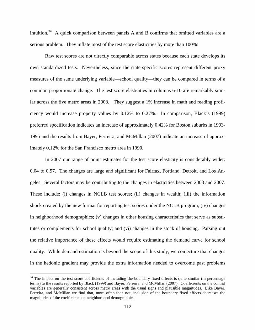
112
intuition.34 A quick comparison between panels A and B confirms that omitted variables are a
serious problem. They inflate most of the test score elasticities by more than 100%!
Raw test scores are not directly comparable across states because each state develops its
own standardized tests. Nevertheless, since the state-specific scores represent different proxy
measures of the same underlying variable—school quality—they can be compared in terms of a
common proportionate change. The test score elasticities in columns 6-10 are remarkably simi-
lar across the five metro areas in 2003. They suggest a 1% increase in math and reading profi-
ciency would increase property values by 0.12% to 0.27%. In comparison, Black’s (1999)
preferred specification indicates an increase of approximately 0.42% for Boston suburbs in 1993-
1995 and the results from Bayer, Ferreira, and McMillan (2007) indicate an increase of approx-
imately 0.12% for the San Francisco metro area in 1990.
In 2007 our range of point estimates for the test score elasticity is considerably wider:
0.04 to 0.57. The changes are large and significant for Fairfax, Portland, Detroit, and Los An-
geles. Several factors may be contributing to the changes in elasticities between 2003 and 2007.
These include: (i) changes in NCLB test scores; (ii) changes in wealth; (iii) the information
shock created by the new format for reporting test scores under the NCLB program; (iv) changes
in neighborhood demographics; (v) changes in other housing characteristics that serve as substi-
tutes or complements for school quality; and (vi) changes in the stock of housing. Parsing out
the relative importance of these effects would require estimating the demand curve for school
quality. While demand estimation is beyond the scope of this study, we conjecture that changes
in the hedonic gradient may provide the extra information needed to overcome past problems
34 The impact on the test score coefficients of including the boundary fixed effects is quite similar (in percentage terms) to the results reported by Black (1999) and Bayer, Ferreira, and McMillan (2007). Coefficients on the control variables are generally consistent across metro areas with the usual signs and plausible magnitudes. Like Bayer, Ferreira, and McMillan we find that, more often than not, inclusion of the boundary fixed effects decreases the magnitudes of the coefficients on neighborhood demographics.

113
with identification. An explanation is saved for section 8. Until then, we continue to focus on
the relationship between marginal effects in the capitalization and hedonic models.
B. Capitalization Regressions and Robustness Checks
Large changes in the hedonic test score coefficients provide the first signal that capitalization
rates are unlikely to identify MWTP. A second indication is the fact that changes in other coeffi-
cients are large enough to reject the hypothesis of a time-constant gradient in each metro area (F-
tests are reported in panel B). Since we lack a randomized instrument for the change in test
scores, there is little hope for circumventing capitalization bias. Measures of correlation in tables
2 and 3 (and appendix tables 1-4) reveal that the orthogonality conditions in (13) are systemati-
cally violated. For example, the changes in NCLB test scores for schools in Fairfax are positive-
ly correlated with some neighborhood characteristics (e.g. percent nonwhite residents in 2003,
percent renting in 2003, population density in 2003) and negatively correlated with others (e.g.
NCLB score in 2003, tax rate, change in percent nonwhite). Thus, it comes as no surprise that
the capitalization-based estimates for the test score elasticity in panel C of table 4 look very
different from their hedonic counterparts in panel B.
The results in panel C were generated by OLS estimation of the first-differenced capitali-
zation model using the full sample of block groups. Notice that Los Angeles is the only place
where the capitalization rate (0.17%) lies within the range defined by the price function parame-
ters from 2003 and 2007 (0.14% to 0.22%). In Fairfax, Portland, Philadelphia, and Detroit, our
capitalization-based estimates for the test score elasticity are far below the lower bound of point
estimates from the hedonic model. The capitalization rate is at least positive and marginally
significant in Philadelphia. In Fairfax and Portland the downward bias is so large that capitaliza-

114
tion rates would imply the willingness to pay for improved school quality is essentially zero. In
Detroit the capitalization rate is negative and marginally significant. This could simply reflect
approximation error in the linear form of the estimating equation, but the hedonic estimates in
column 9 are quite reasonable by contrast.
We consider three alternative explanations for the large differences between our esti-
mates for capitalization rates and hedonic parameters: sample selection, data aggregation, and
unobserved shocks that may be correlated with the change in school quality. Table 5 reports the
results from indirect tests of each hypothesis.
First consider the scope for sample selection bias. Houses located outside the 0.2 mile
boundary zones are included in the capitalization model but excluded from the hedonic regres-
sions. The excluded homes comprise a large share of total housing sales in each metro area,
from 35% in Portland to 92% in Los Angeles. Differences between the capitalization and hedon-
ic results could arise from differences in the distribution of properties located in the excluded and
included areas. To test this possibility, we repeat estimation of the basic hedonic model (without
boundary fixed effects) using all of the micro data that were used to construct the block group
averages for the capitalization model. Results are reported in columns 1-5 of table 5. They
essentially mirror the original hedonic estimates from columns 1-5 of table 4. Given the large
sample sizes, it is remarkable that only two of the ten coefficients are statistically different (Fair-
fax and Detroit in 2003). From this we conclude that sample selection is unlikely to explain the
differences between our baseline results from the hedonic and capitalization models.
A second possibility is that the capitalization results are driven by aggregation bias that
arises from averaging the micro data over Census block groups. The issue is that the “average”
home in a given block group need not correspond to any point on the hedonic price surface. It is

115
difficult to predict the direction and magnitude of the resulting bias. Past studies that have used
Census aggregates have assumed the bias is sufficiently small to ignore (Chay and Greenstone
2005, Greenstone and Gallagher 2008, Baum-Snow and Marion 2009). To test this assumption,
we aggregate the micro data from panel A into block groups and repeat the estimation. Results
are reported in panel B. Comparing the two panels reveals that aggregation does not affect the
general pattern of results. The magnitudes of the coefficients do change a bit, but the differences
are mostly insignificant.
Finally, our estimates for the capitalization rate could be confounded by omitted va-
riables. If changes in unobserved amenities are negatively correlated with changes in school
quality, the first-differenced estimator will be biased downward. To test this possibility we
extend the boundary discontinuity identification strategy to a panel data setting. First, we drop
all houses that do not fall within 0.2 miles of a boundary. Then we aggregate the micro data into
“boundary neighborhoods” on either side of each boundary. Finally, we add fixed effects for
each boundary and estimate the resulting first-differenced model,
εγφ Δ+Δ+Δ+Δ=Δ BFEhtestscoreP )ln( . (17)
These “boundary difference fixed effects” will absorb the capitalization of changes in unob-
served amenities in each boundary region. Results are reported in panel C. While standard
errors on the elasticities are quite large due to the decrease in sample size and the inclusion of
fixed effects, the point estimates are remarkably similar to our baseline results. The point esti-
mates in columns 11-15 of table 5 all fall within the 95% confidence intervals on the correspond-
ing estimates from columns 11-15 of table 4. Thus, omitted variables do not provide much help
in explaining why our baseline estimates for the capitalization rate are so much lower than the
elasticities from the hedonic model. We are left to conclude that the differences we observe are

116
primarily due to changes in the gradient of the hedonic price function.
VII. Summary and Implications of Empirical Results
The results from our boundary discontinuity regressions demonstrate that hedonic gradients can
change significantly over a short period of time. We are not the first to document this type of
instability. Costa and Kahn (2003) found that the implicit price of living in a metropolitan area
with a temperate climate doubled between 1970 and 1980, and then doubled again between 1980
and 1990. In an application that more closely resembles ours, Brookshire et al. (1985) found that
a discrete shock to information about earthquake risk changed the hedonic gradient over a 6-year
period. Other researchers have reported annual changes in the relative prices of structural hous-
ing characteristics (Meese and Wallace 1997, Murphy 2007). However, all of these studies are
vulnerable to the usual concern about confounding from omitted variables. By using a sharp
discontinuity to mitigate the omitted variable pitfall, we have provided the strongest evidence to
date that hedonic gradients do change.
We also find that changes in the hedonic gradient matter for evaluating the benefits of
public education. Table 6 provides a summary comparison between our hedonic and capitaliza-
tion based estimates for the average resident’s willingness to pay for a 1% increase in test scores.
Each column reports the MWTP predicted by a specific econometric model, averaged over the
samples from all five study regions. In columns 1-3 we do not control for omitted variables.
The resulting predictions for MWTP are fairly robust to how we define a data point (house,
Census block group) and how we define the extent of the market (full metro area, 0.2 mile boun-
dary zone). However, these predictions are twice as large as the ones from the model with boun-
dary fixed effects (column 4). This reinforces past evidence on the potential for omitted

117
variables to confound the results from property value studies (Black 1999, Chay and Grenstone
2005, Bayer, Ferreira, and McMillan 2007).
The hedonic boundary discontinuity design in column 4 is our preferred specification. It
controls for omitted variables; it controls for sorting across boundaries on the basis of race; and it
provides a theoretically consistent prediction for MWTP at a single point in time. It implies the
average household would have been willing to pay $536 for a 1% improvement in school quality
during the first year of the NCLB program.35 Over the next four years, there were several
changes. Property values increased by 6% on average, test scores increased by 10%, and there
were smaller changes in the demographic composition of neighborhoods. There was also steady
media coverage of the NCLB program and changes in the broader economy that would have
affected expectations about permanent income (e.g. rapid growth in stock market indices and
personal income per capita). These changes were accompanied by changes in hedonic gradients
which, in turn, increased our prediction for average MWTP to $688 for the 2007 school year.
Relative to our hedonic model, capitalization rates severely understate the willingness to
pay for academic performance. Column 5 reports the average MWTP predicted by our first-
differenced capitalization model ($134 in 2003, $152 in 2007).36 These figures are about ¼ the
size of estimates from our hedonic boundary discontinuity regressions! The difference between
hedonic MWTP and capitalization rates only narrows slightly when we add controls for time-
varying omitted variables to the capitalization regressions (column 6). Placing these results in
the context of our conceptual framework suggests that researchers must be cautious in using
35 This average reflects variation across metro areas, from a low of $422 in Detroit to a high of $743 in Philadelphia. Interestingly, the area with the highest average MWTP, Philadelphia, also ranked third among all U.S. cities in terms of the volume of Google searches on the phrase “No Child Left Behind” in 2004. The top two cities were Pittsburg and Washington D.C. 36 These figures were calculated by combining results from columns 11-15 in table 4 with data on average property values and populations in tables 3 and A1-A4.
118
capitalization rates as the basis for evaluating the benefits of public programs.
VIII. Conclusions
The hedonic property value model and the land value capitalization model are typically viewed
as separate frameworks. We have sought to connect them. By extending Rosen (1974) to de-
scribe how the equilibrium price function adjusts to changes in the supply of a public good, we
were able to express market capitalization as a function of hedonic willingness to pay. This
unified framework provides a welfare theoretic basis for interpreting evidence on capitalization
rates for shocks to public goods.
Our conceptual model produced three insights into the relationship between capitalization
and MWTP. First, the scope for divergence between the two concepts grows with the size of the
shock and the length of the study period. As both dimensions approach zero, the capitalization
rate approaches MWTP. Second, if we want to guarantee that ex-ante MWTP is recoverable
from the capitalization of a non-marginal shock, we must add further assumptions about prefe-
rences and technology to Rosen’s model. These new assumptions have a testable implication.
They imply the hedonic gradient will be constant over time. Finally, if the hedonic gradient
changes over time we can still recover ex-post MWTP as long as the price function is linear in
parameters and the shock (or an instrument for the shock) is randomized.
In the application to school quality, the average difference between capitalization and
MWTP was quite large. To recover MWTP we developed the most comprehensive set of esti-
mates to date on the contribution of academic performance to residential property values, using
hedonic boundary discontinuity designs to control for omitted variables. By analyzing five
metro areas at two points in time, we were able to generate ten separate estimates for the elastici-
119
ty of property values with respect to test scores. We found that these hedonic gradients changed
over time. As a result, our estimates for MWTP were three to four times as large as capitaliza-
tion rates for changes in test scores.
More generally, our framework can guide future research on valuing public goods by il-
lustrating how to overcome problems with capitalization-based welfare measurement. The sim-
plest solution is to avoid interpreting capitalization rates as measures of willingness to pay unless
the data make it possible to track small shocks over brief intervals. If the goal is to recover ex-
post MWTP, a second solution is to find an instrument that randomizes the intensity of the public
good “treatment”. The instrument must be orthogonal to baseline levels of every control variable
and to changes in those variables. This is a tall order which no instrument is likely to satisfy
completely. But some natural experiments and policy discontinuities may come close. The
validity of candidate instruments can be judged from the coefficients on the “price effect” and
“substitution effect” terms in our expression for the capitalization bias (equation 11). For exam-
ple, if 01.01 <′′ rrgr the bias in estimated MWTP that arises from a change in the implicit
price of g will be less than 1% of the change that occurred.
Finally, we conjecture that the same market forces that drive a wedge between capitaliza-
tion and MWTP also have the potential to help us overcome the classic problem with identifying
demand curves. The problem is that the equilibrium price function intersects each household’s
demand curve at exactly one point (Epple 1987; Bartik 1987). To identify the rest of the curve
from market data, we must observe similar households making choices along a different price
surface. Pooling data from different geographic markets, while possible, raises concerns with
selection bias (Rubinfeld, Shapiro, and Roberts 1987). Our conceptual model suggests a differ-
ent solution. We have demonstrated that large shocks to public goods can change the hedonic

120
price surface in a single geographic market. Thus, it may be possible to identify demand curves
from repeated cross-sections of households collected before and after a shock to the distribution
of public goods supplied in a single metro area. We view this quasi-experimental approach to
hedonic demand estimation as a promising direction for future research.

121
TABLE 1 SUMMARY OF HEDONIC AND CAPITALIZATION-BASED ESTIMATES OF THE
WILLINGNESS TO PAY FOR A SMALL IMPROVEMENT IN PUBLIC SCHOOL QUALITY
NOTE.—Children in Boston, San Francisco, Fairfax, and Portland were assigned to elementary schools based on the attendance zones where their parents lived. Children in Philadelphia, Detroit, and Los Angeles were assigned to school districts but free to choose between schools within a district. Each state develops its own standardized tests, which change over time. Assignment laws and test scores are discussed in section V. In cols. 1 and 3, the hedonic estimates are identified by boundary discontinuity designs that use fixed effects to control for omitted variables. In cols. 2 and 4, the capitalization estimates are identified by first-differenced regressions that control for changes in neighborhood demographics and purge omitted variables. All measures of willingness to pay are reported in con-stant year 2000 dollars.
STUDY REGION FOR ESTIMATES
hedonic capitalization hedonic capitalization
(1) (2) (3) (4)
PREVIOUS STUDIES
Black (1999) Boston, MA [1990] 0.42 917 Bayer, Ferreira, McMillan (2007) San Francisco, CA [1993-95] 0.12 372
THIS STUDY Fairfax, VA [2003] 0.12 -0.04 608 -194
Portland, OR [2003] 0.20 0.01 447 16Philadelphia, PA [2003] 0.27 0.12 743 317
Detroit, MI [2003] 0.21 -0.29 422 -587Los Angeles, CA [2003] 0.14 0.17 596 740
All Five Regions [2003] 536 134All Five Regions [2007] 688 152
TEST SCORE ELASTICITY
MEAN WILLINGNESS TO PAY FOR 1% INCREASE
IN TEST SCORES
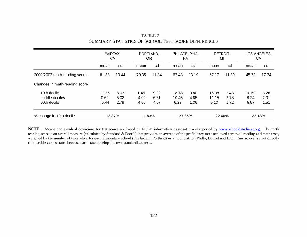
122
TABLE 2
SUMMARY STATISTICS OF SCHOOL TEST SCORE DIFFERENCES
NOTE.—Means and standard deviations for test scores are based on NCLB information aggregated and reported by www.schooldatadirect.org. The math reading score is an overall measure (calculated by Standard & Poor’s) that provides an average of the proficiency rates achieved across all reading and math tests, weighted by the number of tests taken for each elementary school (Fairfax and Portland) or school district (Philly, Detroit and LA). Raw scores are not directly comparable across states because each state develops its own standardized tests.
mean sd mean sd mean sd mean sd mean sd
2002/2003 math-reading score 81.88 10.44 79.35 11.34 67.43 13.19 67.17 11.39 45.73 17.34
Changes in math-reading score
10th decile 11.35 8.03 1.45 9.22 18.78 0.80 15.08 2.43 10.60 3.26middle deciles 0.62 5.02 -4.02 6.61 10.45 4.85 11.15 2.78 9.24 2.0190th decile -0.44 2.79 -4.50 4.07 6.28 1.36 5.13 1.72 5.97 1.51
% change in 10th decile
LOS ANGELES, CA
13.87% 1.83% 27.85% 22.46% 23.18%
FAIRFAX, VA
PORTLAND, OR
PHILADELPHIA, PA
DETROIT, MI
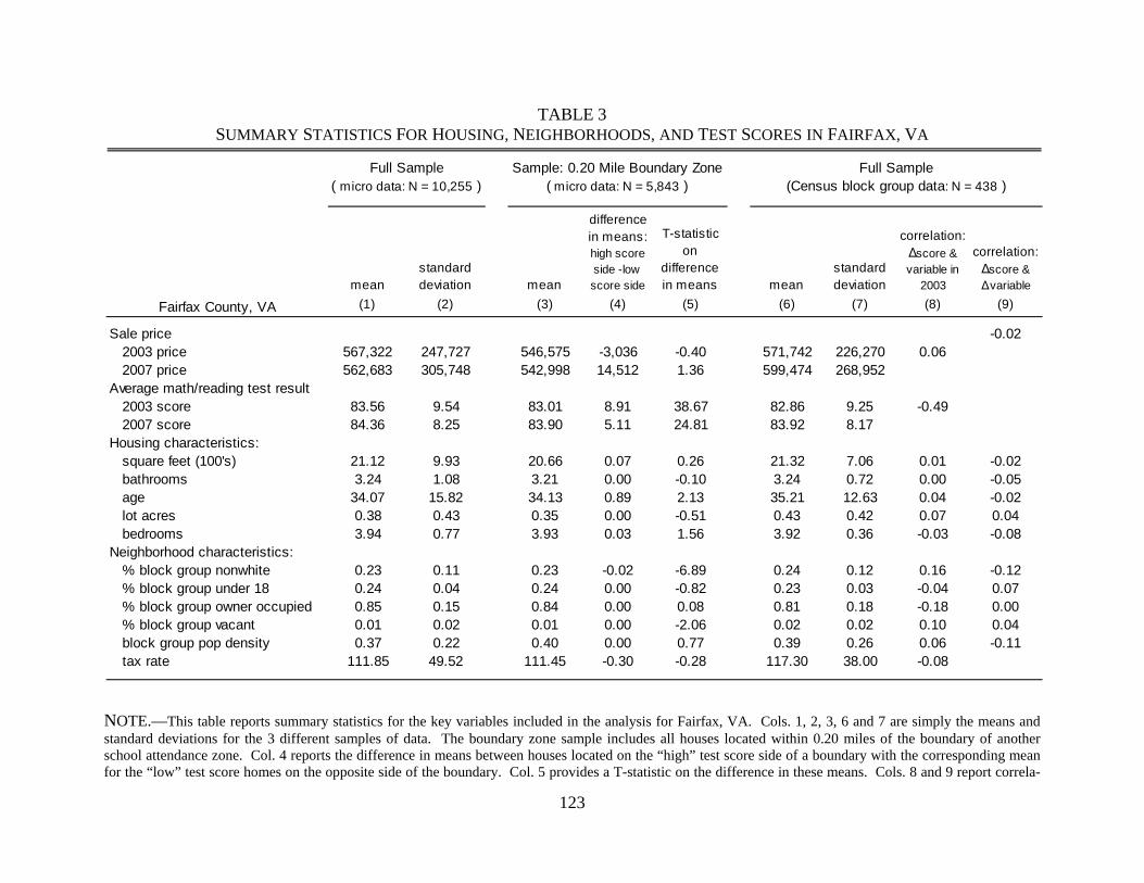
123
TABLE 3 SUMMARY STATISTICS FOR HOUSING, NEIGHBORHOODS, AND TEST SCORES IN FAIRFAX, VA
NOTE.—This table reports summary statistics for the key variables included in the analysis for Fairfax, VA. Cols. 1, 2, 3, 6 and 7 are simply the means and standard deviations for the 3 different samples of data. The boundary zone sample includes all houses located within 0.20 miles of the boundary of another school attendance zone. Col. 4 reports the difference in means between houses located on the “high” test score side of a boundary with the corresponding mean for the “low” test score homes on the opposite side of the boundary. Col. 5 provides a T-statistic on the difference in these means. Cols. 8 and 9 report correla-
meanstandard deviation mean
difference in means: high score side -low score side
T-statistic on
difference in means mean
standard deviation
correlation: ∆score & variable in
2003
correlation: ∆score & ∆variable
(1) (2) (3) (4) (5) (6) (7) (8) (9)
Sale price -0.022003 price 567,322 247,727 546,575 -3,036 -0.40 571,742 226,270 0.062007 price 562,683 305,748 542,998 14,512 1.36 599,474 268,952
Average math/reading test result 2003 score 83.56 9.54 83.01 8.91 38.67 82.86 9.25 -0.492007 score 84.36 8.25 83.90 5.11 24.81 83.92 8.17
Housing characteristics: square feet (100's) 21.12 9.93 20.66 0.07 0.26 21.32 7.06 0.01 -0.02bathrooms 3.24 1.08 3.21 0.00 -0.10 3.24 0.72 0.00 -0.05age 34.07 15.82 34.13 0.89 2.13 35.21 12.63 0.04 -0.02lot acres 0.38 0.43 0.35 0.00 -0.51 0.43 0.42 0.07 0.04bedrooms 3.94 0.77 3.93 0.03 1.56 3.92 0.36 -0.03 -0.08
Neighborhood characteristics: % block group nonwhite 0.23 0.11 0.23 -0.02 -6.89 0.24 0.12 0.16 -0.12% block group under 18 0.24 0.04 0.24 0.00 -0.82 0.23 0.03 -0.04 0.07% block group owner occupied 0.85 0.15 0.84 0.00 0.08 0.81 0.18 -0.18 0.00% block group vacant 0.01 0.02 0.01 0.00 -2.06 0.02 0.02 0.10 0.04block group pop density 0.37 0.22 0.40 0.00 0.77 0.39 0.26 0.06 -0.11tax rate 111.85 49.52 111.45 -0.30 -0.28 117.30 38.00 -0.08
Fairfax County, VA
Full Sample ( micro data: N = 10,255 )
Sample: 0.20 Mile Boundary Zone ( micro data: N = 5,843 )
Full Sample (Census block group data: N = 438 )

124
tions between the change in test scores and levels and changes in all other variables for the full sample of census block group data.
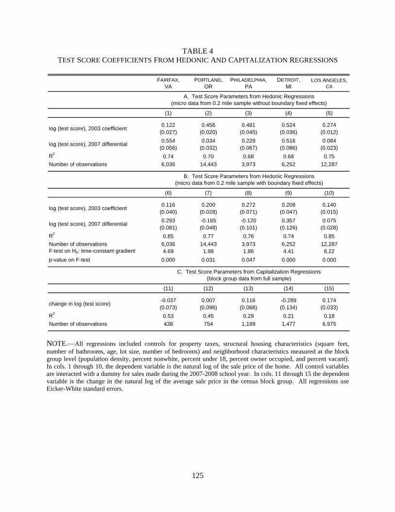
125
TABLE 4 TEST SCORE COEFFICIENTS FROM HEDONIC AND CAPITALIZATION REGRESSIONS
NOTE.—All regressions included controls for property taxes, structural housing characteristics (square feet, number of bathrooms, age, lot size, number of bedrooms) and neighborhood characteristics measured at the block group level (population density, percent nonwhite, percent under 18, percent owner occupied, and percent vacant). In cols. 1 through 10, the dependent variable is the natural log of the sale price of the home. All control variables are interacted with a dummy for sales made during the 2007-2008 school year. In cols. 11 through 15 the dependent variable is the change in the natural log of the average sale price in the census block group. All regressions use Eicker-White standard errors.
FAIRFAX,
VAPORTLAND,
ORPHILADELPHIA,
PADETROIT,
MILOS ANGELES,
CA
(1) (2) (3) (4) (5)
0.122 0.456 0.481 0.524 0.274(0.027) (0.020) (0.045) (0.036) (0.012)0.554 0.034 0.229 0.516 0.084
(0.056) (0.032) (0.067) (0.086) (0.023)R2 0.74 0.70 0.68 0.68 0.75Number of observations 6,036 14,443 3,973 6,252 12,287
(6) (7) (8) (9) (10)
0.116 0.200 0.272 0.208 0.140(0.040) (0.028) (0.071) (0.047) (0.015)0.293 -0.165 -0.120 0.357 0.075
(0.081) (0.048) (0.101) (0.126) (0.028)R2 0.85 0.77 0.76 0.74 0.85Number of observations 6,036 14,443 3,973 6,252 12,287F-test on H0: time-constant gradient 4.69 1.98 1.86 4.41 8.22p-value on F-test 0.000 0.031 0.047 0.000 0.000
(11) (12) (13) (14) (15)
-0.037 0.007 0.116 -0.289 0.174(0.073) (0.096) (0.068) (0.134) (0.033)
R2 0.53 0.45 0.29 0.21 0.18Number of observations 438 754 1,199 1,477 6,975
change in log (test score)
log (test score), 2003 coefficient
log (test score), 2007 differential
A. Test Score Parameters from Hedonic Regressions (micro data from 0.2 mile sample without boundary fixed effects)
B. Test Score Parameters from Hedonic Regressions (micro data from 0.2 mile sample with boundary fixed effects)
C. Test Score Parameters from Capitalization Regressions (block group data from full sample)
log (test score), 2003 coefficient
log (test score), 2007 differential

126
TABLE 5 ROBUSTNESS CHECKS ON TEST SCORE COEFFICIENTS
NOTE.—All regressions included controls for property taxes, structural housing characteristics (square feet, number of bathrooms, age, lot size, number of bedrooms) and neighborhood characteristics measured at the block group level (population density, percent nonwhite, percent under 18, percent owner occupied, and percent vacant). In cols. 1 through 10, the dependent variable is the natural log of the sale price of the home. All control variables are interacted with a dummy for sales made during the 2007-2008 school year. In cols. 11 through 15 the dependent variable is the change in the natural log of the average sale price in the census block group. All regressions use Eicker-White standard errors.
FAIRFAX,
VAPORTLAND,
ORPHILADELPHIA,
PADETROIT,
MILOS ANGELES,
CA
(1) (2) (3) (4) (5)
0.227 0.540 0.546 0.751 0.260(0.023) (0.016) (0.017) (0.019) (0.004)
0.550 0.024 0.396 0.565 0.041(0.044) (0.024) (0.028) (0.042) (0.008)
R2 0.75 0.69 0.72 0.68 0.70Number of observations 10,662 25,294 29,327 32,485 146,783
(6) (7) (8) (9) (10)
0.148 0.388 0.229 0.813 0.321(0.068) (0.045) (0.046) (0.052) (0.012)
0.475 0.086 0.367 0.717 0.082(0.121) (0.070) (0.083) (0.108) (0.022)
R2 0.84 0.82 0.78 0.77 0.73Number of observations 889 1,553 2,647 3,333 14,727
(11) (12) (13) (14) (15)
0.008 -0.025 0.130 -0.445 0.231(0.111) (0.091) (0.180) (0.521) (0.177)
R2 0.83 0.82 0.91 0.87 0.83Number of observations 422 603 176 213 251
change in log (test score)
log (test score), 2003 coefficient
log (test score), 2007 differential
A. Test Score Parameters from Hedonic Regressions (micro data from full sample without boundary fixed effects)
B. Test Score Parameters from Hedonic Regressions (block group data from full sample without boundary fixed effects)
C. Test Score Parameters from Capitalization Regressions (block group data from 0.2 mile sample with boundary fixed effects)
log (test score), 2003 coefficient
log (test score), 2007 differential

127
TABLE 6 IMPACT OF IDENTIFICATION STRATEGY ON ESTIMATES FOR THE AVERAGE
RESIDENT’S WILLINGNESS TO PAY FOR A 1% INCREASE IN TEST SCORES
NOTE.—All measures of willingness to pay are reported in constant year 2000 dollars. Each measure is averaged over the samples from our five study regions, using the elasticities reported in tables 4 and 5. For example, the estimates in col. 4 are based on the elasticities reported in cols. 6 through 10 of table 4.
(1) (2) (3) (4) (5) (6)
Estimates for willingness to pay: 2003 school year 1,238 1,222 1,041 536 134 1692007 school year 1,685 1,572 1,660 688 152 190
Identification strategy: Model hedonic hedonic hedonic hedonic capitalization capitalizationSample full full 0.2 mile 0.2 mile full 0.2 mileData point block group house house house block group block groupSample size 23,149 244,551 42,991 42,991 10,843 1,665
Controls for omitted variables none none none boundary fixed effects differencing
differencing + boundary
fixed effects

128
REFERENCES
Bailey, Martin J., Richard F. Muth, and Hugh O. Nourse. 1963. "A Regression Method for Real
Estate Price Index Construction." Journal of the American Statistical Association, 58(304): 933-42.
Bajari, Patrick and C. Lanier Benkard. 2005. "Demand Estimation with Heterogeneous Consum-
ers and Unobserved Product Characteristics: A Hedonic Approach." Journal of Political Economy, 113(6): 1239-76.
Bartik, Timothy J. 1987. "The Estimation of Demand Parameters in Hedonic Price Models."
Journal of Political Economy 95(1): 81-88. Baum-Snow, Nathaniel, and Justin Marion. 2009. "The Effects of Low Income Housing Tax
Credit Developments on Neighborhoods." Journal of Public Economics 93(5-6): 654-66. Bayer, Patrick, Fernando Ferreira, and Robert McMillan. 2007. "A Unified Framework for Mea-
suring Preferences for Schools and Neighborhoods." Journal of Political Economy, 115(4): 588-638.
Bergstrom, Theodore C., and Robert P. Goodman. 1973. "Private Demands for Public Goods."
American Economic Review 63(3): 280-96. Bin, Okmyung, Craig E. Landry, and Gregory E. Meyer. 2009. "Riparian Buffers and Hedonic
Prices: A Quasi-Experimental Analysis of Residential Property Values in the Neuse Riv-er Basin." American Journal of Agricultural Economics 91(4): 1067-79.
Bishop, Kelly, and Christopher Timmins. 2008. "Simple, Consistent Estimation of the Marginal
Willingness to Pay Function: Recovering Rosen's Second Stage without Instrumental Va-riables." Mimeo.
Black, Sandra E. 1999. "Do Better Schools Matter? Parental Valuation of Elementary Educa-
tion." Quarterly Journal of Economics, 114(2): 577-99. Bogart William T., and Brian A. Cromwell. 2000. "How much is a neighborhood school worth?"
Journal of Urban Economics 47: 280-305. Brookshire, David S., Mark A. Thayer, John Tschirhart, and William D. Schulze. 1985. "A Test
of the Expected Utility Model: Evidence from Earthquake Risks." Journal of Political Economy, 93(2): 369-89.
Cellini, Stephanie Riegg, Fernando Ferreira, and Rothstein Jesse. 2010. "The Value of School
Facility Investments: Evidence from a Dynamic Regression Discontinuity Design." Quarterly Journal of Economics, forthcoming.
Chay, Kenneth Y., and Michael Greenstone. 1998. "Does Air Quality Matter? Evidence from

129
the Housing Market." NBER Working Paper #6826. Chay, Kenneth Y. and Michael Greenstone. 2005. "Does Air Quality Matter? Evidence from the
Housing Market." Journal of Political Economy, 113(2): 376-424. Chetty, Raj. 2009. “Sufficient Statistics for Welfare Analysis: A Bridge Between Structural and
Reduced-Form Methods,” Annual Review of Economics 1: 451-488. Costa, Dora L and Matthew E. Kahn. 2003. "The Rising Price of Nonmarket Goods." American
Economic Review, 93(2): 227-32. Cropper, Maureen L., Leland B. Deck, and Kenenth E. McConnell. 1988. "On the Choice of
Functional Form for Hedonic Price Functions." Review of Economics and Statistics, 70(4): 668-75.
Davis, Lucas. 2004. "The Effect of Health Risk on Housing Values: Evidence from a Cancer
Cluster." American Economic Review, 94(5): 1693-704. Dee, Thomas, and Brian Jacob. 2009. “The Impact of No Child Left Behind on Student
Achievement.” NBER Working Paper 15531. Downes, Thomas A., and Jeffrey E. Zabel. 2002. "The Impact of School Characteristics on
House Prices: Chicago 1987-1991." Journal of Urban Economics 52: 1-25. Ekeland, Ivar, James J. Heckman, and Lars Nesheim. 2004. "Identification and Estimation of
Hedonic Models." Journal of Political Economy, 112(1): S60-S109. Epple, Dennis. 1987. "Hedonic Prices and Implicit Markets: Estimating Demand and Supply
Functions for Differentiated Products." Journal of Political Economy, 95(1): 59-80. Epple, Dennis and Holger Sieg. 1999. "Estimating Equilibrium Models of Local Jurisdiction."
Journal of Political Economy, 107(4): 645-81. Figlio, David N., and Maurice E. Lucas. 2004. "What's in a Grade? School Report Cards and the
Housing Market." American Economic Review 94(3): 591-604. Gibbons, Steve., and Stephen Machin. 2003. "Valuing English Primary Schools." Journal of
Urban Economics 53: 197-219. Greenstone, Michael and Justin Gallagher. 2008. "Does Hazardous Waste Matter? Evidence
from the Housing Market and the Superfund Program." Quarterly Journal of Economics, 123(3): 951-1003.
Heckman, James J. 2008. “Schools, Skills, and Synapses.” Economic Inquiry 46(3): 289-324. Horsch, Eric J., and David J. Lewis. 2009. "The Effects of Aquatic Invasive Species on Property

130
Values: Evidence from a Quasi-Experiment." Land Economics 85(3): 391-409. Kain, John F., and John M. Quigley. 1975. "Housing Markets and Racial Discrimination." New
York: National Bureau of Economic Research. Klaiber, Allen H., and V. Kerry Smith. 2009. “Evaluating Rubin’s Causal Model for Measuring
the Capitalization of Environmental Amenities”. NBER Working Paper 14957. Kuminoff, Nicolai V. and Abdul S. Jarrah. 2010. "A New Approach to Computing Hedonic
Equilibria and Investigating the Properties of Locational Sorting Models." Journal of Ur-ban Economics, 67(3): 322-335.
Linden, Leigh and Jonah E. Rockoff. 2008. "Estimates of the Impact of Crime Risk on Property
Values from Megan's Laws." American Economic Review, 98(3): 1103-27. Lind, Robert C. 1973. "Spatial Equilibrium, the Theory of Rents, and the Measurement of Bene-
fits from Public Programs." Quarterly Journal of Economics, 87(2): 188-207. Meese, Richard A. and Nancy E. Wallace. 1997. “The Construction of Residential Housing
Price Indices: A Comparison of Repeat-Sales, Hedonic-Regression, and Hybrid Ap-proaches.” Journal of Real Estate Economics and Finance. 14: 51-73.
Murphy, Alvin. 2007. “A Dynamic Model of Housing Supply.” Mimeo. Neal, Derek and Diane W. Schanzenbach. forthcoming. "Left Behind By Design: Proficiency
Counts and Test-Based Accountability." The Review of Economics and Statistics. Oates, Wallace. 1969. "The Effects of Property Taxes and Local Public Spending on Property
Values: An Empirical Study of Tax Capitalization and the Tiebout Hypothesis." Journal of Political Economy, 77: 957-971.
Palmquist, Raymond B. 1982. "Measuring Environmental Effects on Property Values without
Hedonic Regressions." Journal of Urban Economics, 33(3): 333-47. Palmquist, Raymond B. 2005. "Property Value Models," in Handbook of Environmental Eco-
nomics, Volume 2. Karl-Göran Mäler and Jeffery Vincent eds. Amsterdam: North Hol-land Press.
Pope, Jaren C. 2008. "Fear of Crime and Housing Prices: Household Reactions to Sex Offender
Registries." Journal of Urban Economics, 64(3): 601-14. Reback, Randall. 2005. "House Prices and the Provision of Local Public Services: Capitalization
under School Choice Programs." Journal of Urban Economics 57: 275-301. Reback, Randall. 2008. "Demand (and supply) in an inter-district public school choice program."
Economics of Education Review 27: 402-416.

131
Rosen, Sherwin. 1974. "Hedonic Prices and Implicit Markets: Product Differentiation in Pure
Competition." Journal of Political Economy, 82(1): 34-55. Rubinfeld, Daniel L., Perry Shapiro, and Judith Roberts. 1987. "Tiebout Bias and the Demand
for Local Public Schooling." Review of Economics and Statistics 69(3): 426-37. Scotchmer, Suzanne. 1985. "Hedonic Prices and Cost/Benefit Analysis." Journal of Economic
Theory 37(1): 55-75. Scotchmer, Suzanne. 1986. "The Short-Run and Long-Run Benefits of Environmental Improve-
ment." Journal of Public Economics, 30(1): 61-81. Simons, Robert. 2006. When Bad Things Happen to Good Property. Washington D.C.: Envi-
ronmental Law Institute. Starrett, David A. 1981. "Land Value Capitalization in Local Public Finance." Journal of Politi-
cal Economy, 89(2): 306-27. Tiebout, Charles. 1956. "A Pure Theory of Local Expenditures." Journal of Political Economy,
64(5): 416-24. Tinbergen, Jan. 1959. "On the Theory of Income Distribution," in Selected Papers of Jan Tin-
bergen. L.H. Klaassen, L.M. Koych and H.J. Witteveen eds. Amsterdam: North Holland.

132
APPENDIX TABLE 1 SUMMARY STATISTICS FOR HOUSING, NEIGHBORHOODS, AND PUBLIC SCHOOLS IN PORTLAND, OR
NOTE.—This table reports summary statistics for the key variables included in the analysis for Portland, OR. Cols. 1, 2, 3, 6 and 7 are simply the means and standard deviations for the 3 different samples of data. The boundary zone sample includes all houses located within 0.20 miles of the boundary of another school attendance zone. Col. 4 reports the difference in means between houses located on the “high” test score side of a boundary with the corresponding mean for the “low” test score homes on the opposite side of the boundary. Col. 5 provides a T-statistic on the difference in these means. Cols. 8 and 9 report correla-tions between the change in test scores and levels and changes in all other variables for the full sample of census block group data.
meanstandard deviation mean
difference in means: high score side -low score side
T-statistic on
difference in means mean
standard deviation
correlation: ∆score & variable in
2003
correlation: ∆score & ∆variable
(1) (2) (3) (4) (5) (6) (7) (8) (9)
Sale price 0.002003 price 241,875 142,991 237,021 2,664 0.91 244,315 127,426 0.002007 price 324,181 173,171 316,236 -4,500 -1.14 336,280 156,920
Average math/reading test result2003 score 79.82 10.93 79.89 7.41 44.93 78.94 10.33 -0.282007 score 76.00 10.83 75.96 4.79 28.77 75.24 10.69
Housing characteristics:square feet (100's) 17.88 7.76 17.75 -0.06 -0.48 17.59 5.18 0.04 -0.06bathrooms 2.22 0.93 2.22 0.04 2.41 2.09 0.59 0.01 -0.03age 39.67 30.16 38.39 -0.56 -1.17 50.17 22.91 0.00 -0.01lot acres 0.20 0.29 0.18 0.00 0.72 0.30 0.43 0.08 0.01bedrooms 3.07 0.94 3.07 -0.01 -0.41 3.03 0.47 0.09 -0.12
Neighborhood characteristics:% block group nonwhite 0.17 0.10 0.17 -0.01 -3.64 0.16 0.11 -0.14 0.00% block group under 18 0.23 0.04 0.24 0.00 -1.14 0.22 0.04 -0.03 -0.02% block group owner occupied 0.66 0.19 0.66 0.00 1.60 0.61 0.22 0.03 -0.06% block group vacant 0.05 0.03 0.05 0.00 -7.41 0.05 0.03 -0.05 0.00block group pop density 0.53 0.29 0.55 -0.01 -1.35 0.56 0.34 -0.08 0.04tax rate 54.62 8.02 54.74 -0.23 -1.86 54.70 9.01 0.13
Portland Metro Area
Full Sample ( micro data: N = 25,294 )
Sample: 0.20 Mile Boundary Zone ( micro data: N = 16,539 )
Full Sample (Census block group data: N = 754 )

133
APPENDIX TABLE 2 SUMMARY STATISTICS FOR HOUSING, NEIGHBORHOODS, AND PUBLIC SCHOOLS IN PHILADELPHIA, PA
NOTE.—This table reports summary statistics for the key variables included in the analysis for Philadelphia, PA. Cols. 1, 2, 3, 6 and 7 are simply the means and standard deviations for the 3 different samples of data. The boundary zone sample includes all houses located within 0.20 miles of the boundary of another school attendance zone. Col. 4 reports the difference in means between houses located on the “high” test score side of a boundary with the corresponding mean for the “low” test score homes on the opposite side of the boundary. Col. 5 provides a T-statistic on the difference in these means. Cols. 8 and 9 report correla-tions between the change in test scores and levels and changes in all other variables for the full sample of census block group data.
meanstandard deviation mean
difference in means: high score side -low score side
T-statistic on
difference in means mean
standard deviation
correlation: ∆score & variable in
2003
correlation: ∆score & ∆variable
(1) (2) (3) (4) (5) (6) (7) (8) (9)
Sale price -0.072003 price 295,845 188,924 285,243 32,498 4.73 273,104 148,829 -0.352007 price 334,662 221,967 324,197 49,222 5.44 316,940 170,204
Average math/reading test result 2003 score 67.88 13.93 69.43 11.05 30.63 64.38 16.84 -0.742007 score 78.61 10.90 79.51 7.20 25.67 75.99 13.23
Housing characteristics:square feet (100's) 20.87 9.48 20.03 1.21 4.21 19.85 5.95 -0.27 0.00bathrooms 2.37 1.00 2.28 0.09 3.02 2.15 0.73 -0.35 -0.02age 42.03 27.85 46.32 3.50 4.23 49.54 21.16 0.03 0.00lot acres 0.49 0.65 0.44 0.02 1.15 0.45 0.46 -0.15 -0.01bedrooms 3.38 0.77 3.33 0.07 2.82 3.40 0.44 -0.04 -0.03
Neighborhood characteristics:% block group nonwhite 0.12 0.14 0.11 -0.01 -1.30 0.14 0.19 0.22 -0.20% block group under 18 0.23 0.04 0.22 0.00 2.54 0.22 0.04 0.01 0.10% block group owner occupied 0.78 0.18 0.79 0.02 3.13 0.74 0.21 -0.12 0.04% block group vacant 0.03 0.03 0.03 0.00 -3.77 0.04 0.03 0.14 -0.02block group pop density 0.34 0.39 0.36 -0.04 -3.83 0.46 0.53 0.28 -0.13tax rate 29.05 14.28 28.38 2.74 6.55 25.47 14.65 -0.30
Philadelphia Metro Area
Full Sample ( micro data: N = 29,333 )
Sample: 0.20 Mile Boundary Zone ( micro data: N = 3,973 )
Full Sample (Census block group data: N = 1,199 )

134
APPENDIX TABLE 3 SUMMARY STATISTICS FOR HOUSING, NEIGHBORHOODS, AND PUBLIC SCHOOLS IN DETROIT, MI
NOTE.— This table reports summary statistics for the key variables included in the analysis for Detroit, MI. Cols. 1, 2, 3, 6 and 7 are simply the means and standard deviations for the 3 different samples of data. The boundary zone sample includes all houses located within 0.20 miles of the boundary of another school attendance zone. Col. 4 reports the difference in means between houses located on the “high” test score side of a boundary with the corresponding mean for the “low” test score homes on the opposite side of the boundary. Col. 5 provides a T-statistic on the difference in these means. Cols. 8 and 9 report correla-tions between the change in test scores and levels and changes in all other variables for the full sample of census block group data.
meanstandard deviation mean
difference in means: high score side -low score side
T-statistic on
difference in means mean
standard deviation
correlation: ∆score & variable in
2003
correlation: ∆score & ∆variable
(1) (2) (3) (4) (5) (6) (7) (8) (9)
Sale price 0.142003 price 219,857 131,658 214,048 14,186 2.92 214,626 123,303 -0.382007 price 166,801 131,839 157,640 11,017 2.44 169,829 104,428
Average math/reading test result2003 score 68.76 12.39 67.91 7.77 27.21 68.01 12.18 -0.602007 score 79.28 10.52 78.51 7.72 32.09 78.80 10.38
Housing characteristics:square feet (100's) 16.57 7.79 16.01 0.66 3.27 16.47 5.93 -0.32 0.02bathrooms 2.06 1.00 2.00 0.08 3.12 2.03 0.73 -0.38 0.08age 46.06 23.24 46.78 0.19 0.36 46.87 18.00 0.26 -0.07lot acres 0.36 0.52 0.30 -0.02 -2.06 0.39 0.46 -0.11 0.01bedrooms 3.15 0.73 3.11 0.03 1.66 3.15 0.45 -0.22 0.00
Neighborhood characteristics:% block group nonwhite 0.13 0.18 0.12 -0.03 -7.53 0.14 0.20 0.04 -0.30% block group under 18 0.23 0.04 0.23 0.01 8.67 0.23 0.04 0.04 0.16% block group owner occupied 0.80 0.18 0.82 0.02 3.79 0.78 0.20 -0.15 -0.01% block group vacant 0.04 0.03 0.03 0.00 0.80 0.04 0.04 0.12 0.02block group pop density 0.40 0.28 0.46 0.01 2.00 0.40 0.28 0.25 -0.07tax rate 27.09 11.25 25.90 -0.61 -2.42 27.70 9.73 -0.11
Detroit Metro Area
Full Sample ( micro data: N =32,486 )
Sample: 0.20 Mile Boundary Zone ( micro data: N = 6,285 )
Full Sample (Census block group data: N = 1,477 )
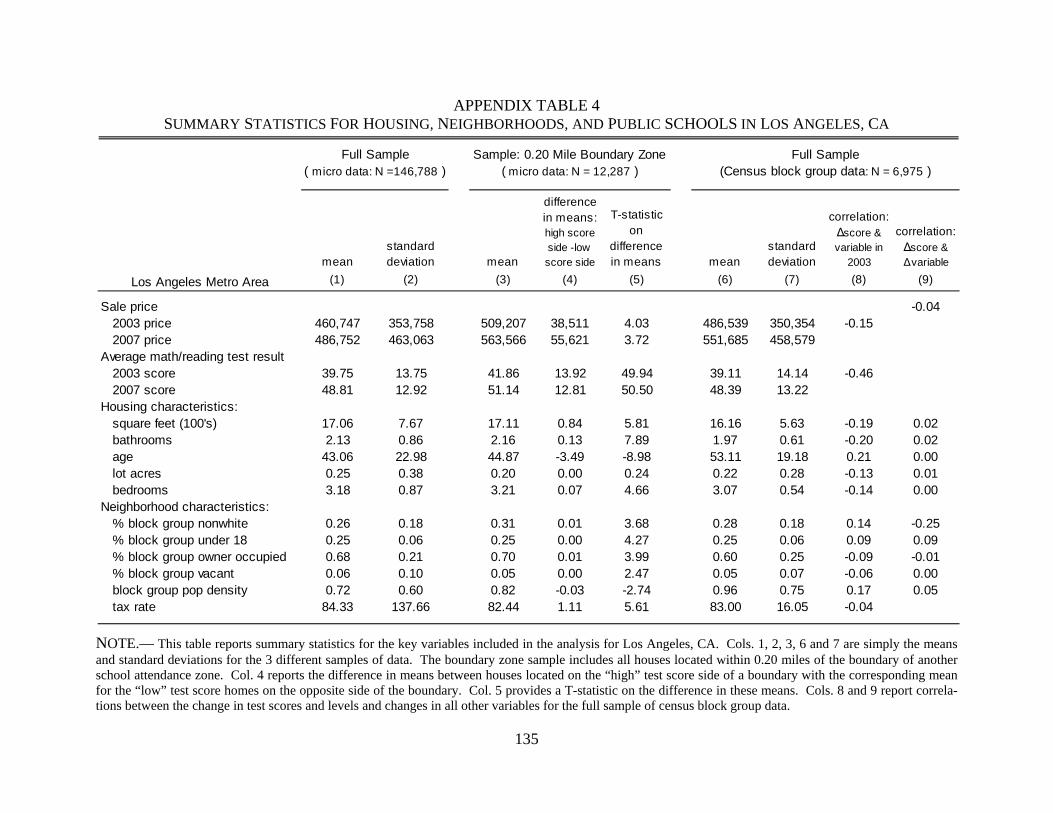
135
APPENDIX TABLE 4 SUMMARY STATISTICS FOR HOUSING, NEIGHBORHOODS, AND PUBLIC SCHOOLS IN LOS ANGELES, CA
NOTE.— This table reports summary statistics for the key variables included in the analysis for Los Angeles, CA. Cols. 1, 2, 3, 6 and 7 are simply the means and standard deviations for the 3 different samples of data. The boundary zone sample includes all houses located within 0.20 miles of the boundary of another school attendance zone. Col. 4 reports the difference in means between houses located on the “high” test score side of a boundary with the corresponding mean for the “low” test score homes on the opposite side of the boundary. Col. 5 provides a T-statistic on the difference in these means. Cols. 8 and 9 report correla-tions between the change in test scores and levels and changes in all other variables for the full sample of census block group data.
meanstandard deviation mean
difference in means: high score side -low score side
T-statistic on
difference in means mean
standard deviation
correlation: ∆score & variable in
2003
correlation: ∆score & ∆variable
(1) (2) (3) (4) (5) (6) (7) (8) (9)
Sale price -0.042003 price 460,747 353,758 509,207 38,511 4.03 486,539 350,354 -0.152007 price 486,752 463,063 563,566 55,621 3.72 551,685 458,579
Average math/reading test result2003 score 39.75 13.75 41.86 13.92 49.94 39.11 14.14 -0.462007 score 48.81 12.92 51.14 12.81 50.50 48.39 13.22
Housing characteristics:square feet (100's) 17.06 7.67 17.11 0.84 5.81 16.16 5.63 -0.19 0.02bathrooms 2.13 0.86 2.16 0.13 7.89 1.97 0.61 -0.20 0.02age 43.06 22.98 44.87 -3.49 -8.98 53.11 19.18 0.21 0.00lot acres 0.25 0.38 0.20 0.00 0.24 0.22 0.28 -0.13 0.01bedrooms 3.18 0.87 3.21 0.07 4.66 3.07 0.54 -0.14 0.00
Neighborhood characteristics:% block group nonwhite 0.26 0.18 0.31 0.01 3.68 0.28 0.18 0.14 -0.25% block group under 18 0.25 0.06 0.25 0.00 4.27 0.25 0.06 0.09 0.09% block group owner occupied 0.68 0.21 0.70 0.01 3.99 0.60 0.25 -0.09 -0.01% block group vacant 0.06 0.10 0.05 0.00 2.47 0.05 0.07 -0.06 0.00block group pop density 0.72 0.60 0.82 -0.03 -2.74 0.96 0.75 0.17 0.05tax rate 84.33 137.66 82.44 1.11 5.61 83.00 16.05 -0.04
Los Angeles Metro Area
Full Sample ( micro data: N =146,788 )
Sample: 0.20 Mile Boundary Zone ( micro data: N = 12,287 )
Full Sample (Census block group data: N = 6,975 )

136
Assessing Tradeoffs in Land Use Service Flows Within Subdivisions at Multiple Spatial Scales
Joshua K. Abbott Arizona State University School of Sustainability
PO Box 875502, Tempe, AZ 85287 USA Email: [email protected]
Phone: 1-480-965-5528
H. Allen Klaiber The Pennsylvania State University
Department of Agricultural Economics and Rural Sociology 208A Armsby Building
University Park, PA 16802 USA Email address: [email protected]
Phone: 1-814-865-0469

137
Assessing Tradeoffs in Land Use Service Flows Within Subdivisions at Multiple Spatial Scales
Abstract
Evaluating the importance of different forms of open space to households requires an evaluation of the
service flows provided by each type of open space. For many non-market goods, these flows occur over
multiple spatial scales and require analysis that simultaneously accounts for capitalization at each scale.
To meet this often overlooked need, we apply a newly developed extension to the Hausman-Taylor model
that treats multiple housing transactions occurring in a spatial location as a panel. This methodology
allows us to account for omitted variables within a subdivision while instrumenting for variables
identified through differences between subdivisions. We measure capitalization of open space at three
distinct spatial scales: adjacency, walkability, and subdivision wide. We find that the interactions
between subdivision open space and private open space in the form of lot size change from
complementarity at small scales to substitutability at large scales. These results confirm much of the
intuition developed by ecologists and public planners on the likely service flows associated with open
space and show how our approach to accounting for multiple spatial scales of capitalization in the
evaluation of non-market goods could be beneficial to other areas of applied research.
Keywords: Open Space; Capitalization; Spatial Scale; Endogeneity; Hedonic; Hausman-Taylor

138
Assessing Tradeoffs in Land Use Service Flows Within Subdivisions at Multiple Spatial Scales
1. Introduction
The increased decentralization and fragmentation of urban development (i.e. sprawl) creates
significant challenges for developers and planners as well as substantial social costs to society (Glaeser
and Kahn 2004). City planners, with finite land supply and limited funds for the extension of
infrastructure to new development, face incentives to increase the density of development within their
communities. Similarly, residential developers must allocate land between housing and undeveloped
open space to maximize their returns on investment – thus providing developers with some incentive to
increase the density of development. Within a given single-family residential development this density
can be accomplished in one of two ways: reduce the size of private lots or the extent of common open
space. Both of these reductions come at a sacrifice, however, as both open space and private lots can
provide a variety of services to subdivision residents such as recreational opportunities, aesthetic
enjoyment, flood mitigation, and privacy and noise buffering. The question of the desired mix of these
uses (whether from the perspective of the developer or the planner) therefore hinges upon the value
accorded to the mix and spatial allocation of these uses by households, or, more precisely, the tradeoffs
between the services associated with this mix and allocation.
A key challenge in assessing the tradeoffs between private lot size and open space is that each is
likely to provide suites of ecosystem services that, while similar in some respects, are also distinct. For
instance, while both private lots and public open space provide recreational opportunities, the nature of
the services provided may differ substantially due to the size, configuration or landscaping of private lots
relative to open space areas. Along with these qualitative differences in service flows (and partly because
of them), the ecosystem services literature suggests that different service flows from a single amenity are
likely to vary substantially in their spatial extent (Daily 1997; Bolund and Hunhammar 1999; Hein, van
Koppen et al. 2006). Furthermore, these multi-scale flows are likely heavily shaped by the completeness
of property rights to private lots versus subdivision open space and the extent to which the associated

139
services take on some of the characteristics of public goods. This interaction of amenities with complex,
institutionally mediated service flows creates the possibility that the contribution of changes in land use
and their interaction will vary depending on the spatial scale at which their capitalization is assessed.
These complexities create both challenges and opportunities for revealed preference methods of
ecosystem service valuation. Challenges arise due to the possibility that failure to properly incorporate all
the appropriate scales of capitalized service flows into model specifications may lead to under or over
valuation of the amenity. However, this realization also creates the opportunity to utilize a priori
knowledge to focus more closely on the capitalization of an amenity’s associated service flows and their
tradeoffs (interactions) with other service flows.
To explore these challenges, we employ a hedonic regression model (Rosen 1974) to examine the
capitalization of subdivision open space and its interactions with potentially substitutable or
complementary land uses within (i.e. private lots) and outside (i.e. city or regional parks) the subdivision
to single family residential property values in the Phoenix metropolitan area.1 We explicitly consider the
latent services that different land uses may provide to residents and utilize a priori information on the
likely scales of these services to create model specifications attuned to the potential zones of
capitalization for each land use. Specifically, we consider that subdivision open space yields services that
may capitalize at three scales: first, at the scale of adjacency to the park; second, to progressively less
“walkable” buffers; and, third, to the neighborhood (subdivision) as a whole so as to capture the overall
provision of surrounding open space. Similarly, we consider that one’s own lot size provides services
that are exclusive to the homeowner and therefore capitalize to individual homes while the overall density
of private space within the neighborhood may yield non-excludable benefits through its impact on density
and its correlates. Through the selective use of interactions we are able to create a flexible model where
the tradeoffs in capitalization from increases in one form of land use or another are allowed to vary across
spatial zones – capturing the idea that land uses may substitute differently for one another depending on
the service flows under consideration.

140
In estimating our model we deal with the potential for omitted neighborhood variable bias
(Palmquist 1992; Irwin and Bockstael 2001) by utilizing a unique feature of our data that lets us identify
the subdivision for each property. By treating our data as a panel of repeated sales within subdivisions we
are able to utilize a recent extension of the Hausman-Taylor instrumental variables (IV) estimator
(Hausman and Taylor 1981) to yield consistent estimates of open space capitalization at all scales (Abbott
and Klaiber 2009). Our first finding is that both subdivision open space and lot size capitalize at a range
of scales with subdivision open space affording considerable capitalization to adjacent properties. The
effects of increased open space provision within “walkable” buffers is, by contrast, relatively small and is
dwarfed in magnitude by the subdivision-wide capitalization of open space, suggesting open space
provision offers valuable services to residents beyond recreational access. Secondly, we find that lot size,
aside from offering benefits to the associated homeowner (as has been thoroughly demonstrated in the
literature), also offers valuable spillovers at the scale of the subdivision. Finally, we find that the
interactions between lot size and subdivision open space at different spatial scales shows that the tradeoffs
between the two land uses vary from complementarity to substitutability depending on the scale of
capitalization – suggesting that these differences occur due to the nature of the services capitalized for
each land use at that particular scale. This suggests that a modeling and estimation approach that is
attuned to multiple scales of capitalization can be enlightening compared to commonly used approaches
and that failure to adopt such an approach may be problematic for both the consistency and interpretation
of the estimated marginal effects from hedonic models.
2. The Literature
The literature on the valuation of various forms of “open space” using hedonic price models is
extensive and varied in its focus.2 Authors have examined a wide range of open space amenities such as
wetlands (Mahan, Polasky et al. 2000), golf courses (Do and Grudnitski 1995), forested lands (Tyrvainen
and Miettinen 2000; Thorsnes 2002), and greenbelts (Correll, Lillydahl et al. 1978; Lee and Linneman
1998). Some authors have focused upon temporal aspects of open space in terms of its protection from
141
eventual development (Irwin and Bockstael 2001; Geoghegan 2002; Smith, Poulos et al. 2002; Klaiber
and Phaneuf 2009). Others have focused upon specific qualitative aspects of parks (i.e. natural areas vs.
urban parks) (Lutzenhiser and Netusil 2001). Finally, there has been an increasing interest in
investigating spatial heterogeneity in the valuation of open space amenities through parametric
(Geoghegan, Wainger et al. 1997; Anderson and West 2006) and locally weighted regression techniques
(Cho, Poudyal et al. 2008; Cho, Clark et al. 2009).
There are a very small number of papers specifically focusing on the question of the valuation of
open space within subdivisions and its interactions with private lots (Peiser and Schwann 1993; Kopits,
McConnell et al. 2007; Towe 2009). Peiser and Schwann (1993) study transactions in a Dallas
subdivision and find little evidence of a price premium for greenbelt alleyways behind houses. Towe
(2009) examines Maryland transactions at the rural-urban fringe with a focus on determining whether the
value of open space in “clustered” subdivisions varies based upon whether it is preserved for agricultural
use or incorporated within the subdivision. While the specification controls for lot size and amount of
subdivision open space, it does not include the interaction between the two, and he ultimately finds no
significant capitalization effect for the quantity of open space. The closest in spirit to our study is that by
Kopits, McConnell and Walls (2007). They utilize data from the urban-rural fringe of Washington, D.C.
and utilize a hedonic model with block group fixed effects in which the acreage of open space in the
subdivision is interacted with the lot size of the house. They find that open space acreage is a weak
substitute for additional lot size. Similarly, they consider whether the capitalization of open space
adjacency to private lots varies in the size of the lot.
While their work does shed light on the nature of tradeoffs between private lots and open space,
there are a number of differences that distinguish our work. First, our data set is substantially different in
that it reflects an urban/suburban environment with relatively dense development, small lots and small
and scattered open space compared to the much more “sprawled” development in their study.3 Second,
while they do consider two scales of capitalization for open space (adjacency and at the subdivision scale),
we add intermediate scales to our model that consider the quantity of open space available to a property

142
within particular distance buffers – therefore accounting for differences of local provision. Third, we
consider the possibility that private lots may have non-excludable effects on property values in a
subdivision (perhaps due to an aversion to density and its correlates) and examine whether the magnitude
of this effect depends on the quantity of open space in and immediately surrounding the subdivision.
Fourth, we control for the presence of various forms of public (non-subdivision) open space in our
estimates (including the possibility of interactions). Finally, our use of the Hausman-Taylor estimator
with subdivision level random effects allows us to demonstrate how this seldom-used tool can parse
between the within and between-neighborhood variation in covariates to consistently estimate the
marginal effects of open space and lot size at all spatial scales in spite of the potential for omitted
variables at the subdivision level (Abbott and Klaiber 2009).
3. Data
The Phoenix metro area provides an ideal laboratory to study subdivision-provided open space
and its interactions with other housing features. The extreme heat in summer, monsoon rains in fall, and
poor soil percolation all create the incentive (often formalized through zoning) for developers to leave
undeveloped land in subdivisions for drainage and heat dissipation. In addition, the high density
development and small lot sizes which distinguish Phoenix from many other urban areas make
subdivision-provided open space a potential amenity to households seeking greater privacy and separation
from neighbors. To explore these issues, we have assembled a detailed database of nearly 620,000 single
family residential transactions occurring over the years 2000 through 2004 obtained from the Maricopa
County assessor and merged with purchased sales data from Dataquick. Unique to our data, the Maricopa
County assessor maintains a detailed inventory of over 20,000 subdivisions located throughout the
Phoenix MSA and indicates the subdivision membership of each parcel. An important feature of the
Phoenix housing market and many other “Sunbelt” markets is that many if not most of the homes within
subdivisions (particularly those built in more recent years) are built by a single builder. This allows us to
characterize observable and unobservable attributes of the housing stock and neighborhood amenities at
143
an economically meaningful scale. The structuring of our data by subdivisions thus serves as the basis for
our analysis of multiple spatial scales of capitalization for subdivision open space and the interactions of
this form of open space with private open space in the form of lot size. We now briefly describe the key
elements of our data in additional detail.
3.1. Transactions
To form our dataset of single family residential transactions, we combine data purchased from a
private data vendor, Dataquick, with data from the Maricopa County assessor and restrict our attention to
2000 to 2004 sales containing a complete list of housing characteristics and a subdivision identifier. The
619,219 transactions in our filtered estimation sample are plotted in figure 1. As is evident from the
figure, these data are widely distributed over virtually the entire metropolitan area . The key housing
characteristics are square footage, lot size, number of bathrooms, number of stories, year built, and
indicator variables for presence of a pool and garage. In addition to these structural characteristics, we
also observe the sales price and sale date of each house as well as a unique identifier which allows us to
link these data to GIS assessor parcel maps. Summary statistics for these data are shown in table 1.
To supplement our transactions data, we obtained information on the location of canals, railways,
and schools as well as spatial data for Census 2000 block groups. We also calculate the distance from
each house to the central business district in Phoenix. Combining these additional spatially defined data
with our residential transactions data we are able to capture socio-demographic characteristics from the
census as well as potential amenities and disamenitites from other land use types.
The most important spatial dimension of our data is an explicit link for each parcel to its
subdivision. These subdivisions range in size from a single house to over 1,100 houses with an average
size of 70 houses. Figure 2 shows the location of residential parcels with subdivision open space indicated
by the darkest shading. After cleaning the data and limiting it to only subdivisions containing a minimum
of 30 houses we are left with a sample of 7,598 subdivisions. These subdivisions will form the basis for
the spatial panel in our Hausman-Taylor specification.

144
3.2. Open Space
Data on open space, including subdivision open space (SOS), was obtained through Arizona
Parks and Recreation and the Maricopa County assessor. In the Phoenix area, SOS is typically
landscaped and well maintained (often by the local homeowner’s association) but has minimal facilities
and typically no public parking. In addition, SOS is often small compared to public parks and is often
integrated within the housing development; however, access is rarely effectively restricted, making the
vast majority of this form of open space non-excludable (at least in principle). Figure 3 provides a
graphical depiction of the four types of open space included in our study: subdivision open space, local
parks, regional parks, and city parks. Due to the similarity in size and characteristics of “destination-
oriented” parks, we combine city and regional parks into a single category of “large park”. Several
cleaning steps were required to isolate subdivision open space parcels, while no cleaning steps were
necessary for the other forms of open space. Summary statistics for each type of open space are shown in
table 1.
We identified subdivision open space using land use codes in the assessor parcel data.
Unfortunately, these codes not only identified true subdivision open space, but also tended to delineate
long slivers of common property only a foot or two wide or highly irregular shapes adjacent to local
streets and sidewalks which are likely public easements. To identify and remove these aberrant parcels
from consideration, we calculated the area and perimeter of each individual subdivision open space
feature and developed cutoffs for minimum area and area/perimeter ratio. We fine tuned these measures
by examining aerial photography of the identified open space parcels to minimize exclusion of “true”
open space while eliminating the majority of the accidental characterization of areas as subdivision open
space. Ultimately we settled on cutoff values of minimum area of 0.25 acres and an area/perimeter ratio
of 40 or greater (in feet).4 The resulting sample contains 3,956 individual subdivision open space parcels
at an average size of 5.2 acres.

145
Using GIS software, we created an adjacency indicator for houses located next to each type of
open space. For the “large park” category, we also calculated the distance to the nearest park from each
house to capture the destination aspect of larger parks. For both local parks and subdivision open space,
we calculated the total acreage of parkland within concentric ring buffers around each residential parcel.
In particular, we used a 2,000 foot buffer to calculate total local park area and used 3 non-overlapping
rings of 1,000, 2,000, and 3,000 feet for calculations of subdivision open space area. To form a
subdivision specific measure of open space, we calculated the average subdivision open space area within
2,000 feet of houses in each subdivision.5
4. Model Specification and Estimation
Households (indexed by k) have heterogeneous preferences for the bundle of attributes associated
with the purchase of a house. These can be characterized by the utility function:
),g,,,,,,(UU kk αOSOSOSOSNX LOTij
SUBij
PUBSMALLij
PUBLARGEijji= , (1)
where Xi is a vector of house specific (represented by subscript i) characteristics like square footage or
number of bathrooms. Nj are “neighborhood” characteristics (indexed by j) that will be perceived as
variable at the scale of a subdivision or a larger spatial unit but not at the resolution of individual houses.
These can include aspects such as the school district, school attendance zone, air quality, aspects
associated with a particular builder or developer (e.g. quality of construction or high-end finishes), or
measurements of the provision of public goods for which local proximity are not important to an
individual’s preferences. The numeraire good is g and heterogeneity across households in preferences for
home/neighborhood characteristics is captured by the parameter vector kα .
PUBLARGEijOS , PUBSMALL
ijOS , SUBijOS , and LOT
ijOS are vectors of varying dimension that contain
measures of the provision and/or proximity of large public open space (i.e. “destination” parks), small
public open space (local parks), privately provided (but collectively owned and managed) subdivision
open space, and “private open space” (i.e. private lots) respectively.6 The use of vectors for each

146
qualitatively distinct form of open space allows different types of open space to impart utility to
households in potentially distinct ways at different scales. Benefits of privacy or noise reduction from the
presence of a greenbelt may accrue exclusively to contiguous properties while the recreational services
provided by the same open space to houses located just across the street may be essentially identical to the
adjacent property. Note as well that the vectors are subscripted by both house (i) and neighborhood (j) in
order to allow for the possibility that consumers may perceive the flow of some classes of services from
some forms of open space as essentially uniform within a neighborhood. This could be the case for many
“destination” parks where proximity by car is essentially invariant at the neighborhood scale or may also
apply to broader “landscape” effects of open space in its effect on neighborhood micro-climate or
homeowners’ perceptions of density and other aesthetic aspects of their subdivision. Finally, we have
included private lots as a form of open space in our model in order to capture their potentially non-
excludable services. For instance, additional private lot acreage to homes in a subdivision may generate
some “public” benefits to the subdivision in a manner similar to explicitly public subdivision open space.
Given sufficient variability and continuity in the supply of housing characteristics and adequate
preference for/against all the characteristics in the population, housing rents will be bid up or down
according to these characteristics and will therefore capitalize into the value of the property. Given
appropriate functional form and separability restrictions on preferences we can specify the following
partially-linear, semi-log hedonic price function:
ii fP εα ++′+′+= ),,,(ln LOTij
SUBij
PUBSMALLij
PUBLARGEijji OSOSOSOSNγXβ . (2)
We choose the semi-log functional form given the interpretability of its marginal effects and the work of
Cropper, Deck and McConnell (1988) suggesting that such simple functional forms tend to outperform
more complex specifications in recovering marginal welfare effects when the hedonic price function is
misspecified. Note that we have avoided choosing an explicit functional form for the effects of the open
space variables at this stage in order to allow for potentially complex interplay in the hedonic price
function between the different forms of open space across different spatial scales. The motivation for this

147
flexibility is to allow for the possibility of interaction across individual open space measures to the extent
that the value of the flow of services from a spatial amenity are enhanced by or substituted for by service
flows from another amenity.
To implement this specification, we specify f( ) as a linear function of measures of open space
proximity and provision along with selected interactions. Table 1 lists each of these variables and their
interactions. The key variables in our specification are those involving private lot size and subdivision
open space. We include private lot variables at two spatial scales, the acreage of one’s own lot (and
acreage squared) and the average lot size within the subdivision. The rationale for lot size as a private
good is well established empirically while mean lot size is included to capture non-excludable spillovers
from the provision of private space within the neighborhood. We include variables for proximity and
provision of subdivision open space at three primary scales. First, we include an indicator variable for
whether a property is adjacent to subdivision open space in order to capture benefits that are excludable to
properties connected to open space (i.e. privacy, noise absorption, view, etc.). Second, we utilize the
aforementioned buffering strategy to consider how much open space is available to individual houses at
1000, 2000, and 3000 feet buffers. This buffering approach allows us to jointly examine both quantity
and proximity of open space, and the buffers are designed to span the range of distances commonly
discussed in the planning literature as “walkable” (Boone, Buckley et al. 2009). These variables can be
viewed as capturing the value of an additional acre at a particular range for recreational and other highly
proximity-dependent use. Third, we include the calculation of the average amount of subdivision open
space within 2000 feet of homes within the subdivision in order to capture the contribution of public
space within and around the subdivision to neighborhood character and other public/club goods.
In addition to these variables, we also consider a select number of interactions based upon
hypotheses of how the services provided by the two land uses (and thus their spatial proxies) may
enhance or substitute for one another. We include an interaction of subdivision open space adjacency
with private lot size to test whether the private benefits from one’s yard are enhanced by adjacency. We
also include an interaction of adjacency with the size of the open space to see if the magnitude of

148
“adjacency services” is influenced by the size of the space. We interact the provision of subdivision open
space acreage within a 2000 foot buffer with the size of the house’s private lot in order to examine
whether the services from open space and own lots are substitutable, complementary or separable at this
scale.7 Finally, to consider the substitutability/complementarity of the two land uses at the subdivision
scale, we interact the subdivision mean levels of lot size and subdivision open space with one another.
While previous models have considered some of these scales and interactions (particularly those
involving adjacency, see Kopits, et al. (2007)), ours is the first study to our knowledge to so extensively
investigate multiple scales of capitalization and their interactions in a hedonic specification; it is also the
first to consider that private lots and open space may provide service flows that capitalize at the
neighborhood or subdivision level as well as to individual properties.
Estimation presents an array of challenges shared by most hedonic price models.8 First, there is
the possibility of endogeneity from the presence of unobserved factors that lower the value of land in
residential development (i.e. high slopes) and therefore selectively increases the proportion of
undeveloped land (open space) in areas of low residential value (Irwin and Bockstael 2001; Irwin 2002).
This concern is likely moot for publically provided open space which is either predetermined with respect
to developer decisions or allocated according to planning goals rather than market forces. It is likely to be
a minor concern for subdivision open space as well given that much of this space is not undeveloped land
but is actually graded and landscaped in a costly manner. Furthermore, zoning requirements for adequate
storm water retention capacity play a strong role in the provision of this form of open space.
An issue of greater concern for our estimation is omitted variables bias. Of particular concern is
the presence of omitted neighborhood variables that are possibly correlated with our open space metrics.
For instance, developers working in areas with unusually high quality local parks with good pedestrian
access may feel less compelled to provide subdivision open space. Areas with good schools may attract
families with children and lead to provision of larger amounts of open space. Alternatively, developers
that utilize high quality finishes in their construction may also provide greater (or more highly improved)
open space. The end result of such unobserved neighborhood variation is a bias of indeterminate sign and

149
magnitude. This problem is well recognized within the literature (Palmquist 1992) and has been dealt
with primarily through the use of extensive proxy variables and spatial fixed effects to approximate
neighborhood indicators and thus absorb any time-constant omitted variables so that the marginal effects
in the regression are identified on the basis of within-neighborhood variation (Anderson and West 2006;
Kopits, McConnell et al. 2007; Cho, Poudyal et al. 2008; Cho, Clark et al. 2009).
The question of the appropriate scale for these spatial fixed effects is a seldom discussed but
important issue. In some cases, spatial fixed effects are included over well-defined areas of neighborhood
heterogeneity such as cities or school districts and attendance zones (Black 1999; Cho, Clark et al. 2009).
However, such coarse indicators leave the potential for substantial inter-neighborhood variation in
omitted characteristics, encouraging the use of finer fixed effects (typically block groups) where data
make them available (Anderson and West 2006). Unfortunately, the elimination of bias that comes with
the use of increasingly fine fixed effects comes at the cost of non-identification or under-identification of
the effects of variables that vary at or above the level of the fixed effect (non-identification) or exhibit
little heterogeneity below the scale of the fixed effect (under-identification). If aspects of an amenity
capitalize approximately evenly across space, then spatial fixed effects approaches run the risk of
identifying a consistent but incomplete marginal effect of the amenity (Abbott and Klaiber 2009).9 This
suggests that the approach to omitted variables bias must be cognizant of the scale of both omitted
variation and the scales of capitalization in the model.
Our first answer to this dilemma is to utilize our ability to identify the subdivision of each
housing parcel to treat our data as repeated cross sections of sales of multiple houses within subdivisions
over time. We can then utilize within-subdivision variation to consistently identify the effects of the open
space variables that vary within subdivisions. This scale of fixed effect is ideal in that it matches
naturally with an intuitively and economically sensible definition of a minimal neighborhood for our
study area – lowering the chance of significant unobservable variation relative to somewhat more
arbitrary and large-scale definitions of neighborhoods (i.e. block groups).10 Nevertheless, the within-
subdivision estimator comes at the cost of our ability to identify the subdivision level open space and lot

150
size variables, yet common approaches like OLS or random effects estimates risk biased estimates for the
open space variables at all scales.
Our answer to this dilemma is to adapt the Hausman-Taylor estimator (Hausman and Taylor
1981) to our spatial, repeated cross-section context. The formal development of this approach is
presented elsewhere (Abbott and Klaiber 2009) so we heuristically develop it here. The Hausman-Taylor
(HT) estimator is a special case of an instrumental variables random effects estimator (Cameron and
Trivedi 2005). The within subdivision varying (henceforth “within-varying”) variables are instrumented
by their deviations from within subdivision means (i.e. they are estimated using the “within” or fixed
effects estimator). Variables that vary at or beyond the scale of the spatial effects (henceforth “between-
varying”) are characterized as either exogenous or (potentially) endogenous. Exogenous between-varying
variables are instrumented by themselves while the endogenous between-varying variables are
instrumented using the subdivision means of any within-varying variables in the model that are presumed
by the analyst to be exogenous.11 There are several notable features of this estimator. First, the HT
estimator achieves identification without external instruments by making dual use of a subset of the
within-varying regressors by essentially treating their within and between subdivision variation as
separate variables. This apparent “something for nothing” comes at the cost of assuming that a sufficient
number of within-varying variables are uncorrelated with the unobserved neighborhood variation that are
also sufficiently correlated with the endogenous between-varying variables to avoid the bias and
inefficiency associated with weak instruments (Bound, Jaeger et al. 1995). While exogeneity may be
difficult to establish a priori, it is possible to test for it empirically by employing a Wald test on an
augmented regression – a robust analog of the Hausman test (Wooldridge 2002; Abbott and Klaiber 2009).
This test works by effectively testing whether the random effects estimates for the coefficients on the
within-varying instruments (inconsistent under violations of the null hypothesis that the variables are
uncorrelated with neighborhood-scale omitted variables) are significantly different from the fixed effects
estimates (which are consistent regardless). The HT estimator therefore provides an attractive alternative
to common estimation techniques in that it makes explicit use of spatial variation within and between

151
neighborhoods to provide consistent identification at all spatial scales while allowing for the falsification
of its identifying assumptions.
5. Results
We are concerned that the subdivision scale measures of private lot acreage and SOS provision
are correlated with unobserved neighborhood characteristics. In the HT framework, we must find two or
more exogenous within-varying regressors to serve as instruments. Using the aforementioned modified
Hausman test, we tested the null hypothesis of exogeneity for a number of candidate instruments and
ultimately settled on the use of adjacency to subdivision open space and its two interactions. Correlation
between these instruments and the endogenous variables are shown in table 2 along with p-value results
from the modified Hausman test.12 We fail to reject the null hypothesis of exogeneity of our instruments
both individually and jointly and the correlations between our instruments and the endogenous variables
are collectively fairly high – suggesting that our instruments have a strong empirical justification.13
Table 3 presents our estimates for the Hausman-Taylor model (where the standard errors are
calculated using a nonparametric bootstrap to allow a less restrictive covariance structure than the
traditional HT estimator). In order to establish the reasonableness of our estimates relative to the
literature, we begin by discussing the non-open space characteristics in our specification before turning
attention to the central results on public and private open space. Examining the structural housing
characteristics identified using within subdivision variation, it is clear that our estimates are congruent
with the literature. We find positive coefficients for square footage, lot size, bathrooms, year built (newer
houses being preferred), presence of a garage, and presence of a pool. The negative coefficient on
number of stories indicates a preference for single story dwellings (holding square footage and lot size
constant), possibly reflecting the preferences of households to limit summer heat buildup in upper stories.
In addition to the linear terms, we also estimate squared terms for square footage, lot size, and year built
and find intuitive negative coefficients for each. The remaining within subdivision control attributes
consist of adjacency measures to various forms of landscape features including schools, railways, and

152
canals. Of these, only adjacency to railways is significant and suggests that railway adjacency reduces the
value of a house by approximately 2.5 percent.
Focusing on characteristics which vary across subdivisions rather than over individual houses we
find that census measures of block group minority racial composition show no significant capitalization
effects relative to the Caucasian base group.14 We find intuitive results that housing prices in areas with
large numbers of children are lower than the omitted class of retired households. In addition, we find that
subdivisions with households containing more working aged adults are associated with higher housing
prices. We find a positive and concave gradient in distance to downtown Phoenix, perhaps reflecting the
overwhelming of any positive effect of proximity to employment or urban amenities (perhaps limited in
this highly polycentric city) by the negative correlates of urban life. We find no significant impact of
having a school located within walkable distance of a subdivision, perhaps reflecting the offsetting of
easy access to the school and its amenities with the associated congestion and noise from school-related
traffic. Lastly, we seem to find that households prefer to distance themselves from large parks. While
unexpected, a glance at figure 3 suggests that this effect may arise from the remote location of large parks
(and in some cases, proximity of these parks to blighted neighborhoods) rather than an actual aversion to
being near large parks. This discussion sounds a more general cautionary note about the interpretation of
the subdivision-varying variables in our model. They are included as control variables to limit the scope
of unobserved heterogeneity in our model. As such they are not instrumented for and should be
interpreted with caution.15
Returning to our focus on open space, we first examine the most immediate spatial scale of
adjacency. Adjacency effects are identified in the HT estimator using within subdivision variation so that
potentially confounding unobserved quality differences across subdivisions are eliminated. We find
positive and significant coefficients associated with adjacency to both local and large public parks but
with substantially larger value accruing to properties adjacent to large public parks. This suggests that
these larger public spaces provided greater services such as noise buffering, aesthetic views, recreational
possibilities, or a feeling of “naturalness” relative to smaller, more dispersed local parks. Continuing this

153
theme, we find that an interaction between subdivision open space adjacency and the size of the open
space is positive so that the capitalization benefits of SOS adjacency are augmented by the size of the
space itself. This is sensible since the flows of spatially attenuated services from open space adjacency
(e.g. privacy and noise buffering) are likely enhanced by the size of the open space. We also find a
positive percentage effect on the capitalization of adjacency from the size of the adjacent private lot (an
addition of 0.1 acres to an adjacent lot increases the benefits from adjacency by 0.4% of the home’s
value). This is congruent with a situation where the services tied to adjacency are enhanced to the degree
that one’s own “private open space” facilitates their consumption through private outdoor activities – as is
likely the case with a larger backyard. Together these findings suggest that both private and public open
space within subdivisions are complementary in their service provision at these small spatial scales.
Our second spatial scale examines the capitalization of open space from close (non-adjacent)
proximity to households. Not surprisingly, we find that capitalization of an additional acre of open space
is substantially larger (approximately 50% larger) within the 1000 foot bound than when relocated at
distances between 1000 to 2000 feet. We find no significant effect for SOS located between 2000 and
3000 feet from a house, suggesting benefits from household-level access to open space are quite localized
in scale. Although statistically significant, the capitalization effect of open space proximity is rather
small; an extra acre of SOS within 1000 feet adds a mere .05% to the value of the house (i.e. $100 for a
$200,000 house).16,17 Similarly, we found no significant effect for provision of local park acreage within
a 2000 foot buffer. One possible (although untestable) explanation for both of these results may lie in the
extreme desert heat that limits daytime recreational use of outdoor areas for a significant portion of the
year. In such a setting, the typical homebuyer may place little premium on walkable access to open space.
Finally, the interaction effect between SOS acreage and a house’s private lot size is highly insignificant.
This seems to indicate that the service flows emanating from SOS proximity and one’s own private lot are
not likely to be substitutable (as would be the case if the interaction was negative). Such separability may
find its explanation in the size and character of private lots in the Phoenix metro. Many private lots are
quite small, limiting their recreational use, and this use may be further curtailed in many areas by the
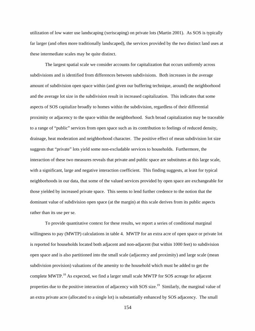
154
utilization of low water use landscaping (xeriscaping) on private lots (Martin 2001). As SOS is typically
far larger (and often more traditionally landscaped), the services provided by the two distinct land uses at
these intermediate scales may be quite distinct.
The largest spatial scale we consider accounts for capitalization that occurs uniformly across
subdivisions and is identified from differences between subdivisions. Both increases in the average
amount of subdivision open space within (and given our buffering technique, around) the neighborhood
and the average lot size in the subdivision result in increased capitalization. This indicates that some
aspects of SOS capitalize broadly to homes within the subdivision, regardless of their differential
proximity or adjacency to the space within the neighborhood. Such broad capitalization may be traceable
to a range of “public” services from open space such as its contribution to feelings of reduced density,
drainage, heat moderation and neighborhood character. The positive effect of mean subdivision lot size
suggests that “private” lots yield some non-excludable services to households. Furthermore, the
interaction of these two measures reveals that private and public space are substitutes at this large scale,
with a significant, large and negative interaction coefficient. This finding suggests, at least for typical
neighborhoods in our data, that some of the valued services provided by open space are exchangeable for
those yielded by increased private space. This seems to lend further credence to the notion that the
dominant value of subdivision open space (at the margin) at this scale derives from its public aspects
rather than its use per se.
To provide quantitative context for these results, we report a series of conditional marginal
willingness to pay (MWTP) calculations in table 4. MWTP for an extra acre of open space or private lot
is reported for households located both adjacent and non-adjacent (but within 1000 feet) to subdivision
open space and is also partitioned into the small scale (adjacency and proximity) and large scale (mean
subdivision provision) valuations of the amenity to the household which must be added to get the
complete MWTP.18 As expected, we find a larger small scale MWTP for SOS acreage for adjacent
properties due to the positive interaction of adjacency with SOS size.19 Similarly, the marginal value of
an extra private acre (allocated to a single lot) is substantially enhanced by SOS adjacency. The small

155
scale MWTP at the household level for private acreage is three orders of magnitude larger than
subdivision open space. This is reasonable given the very different services provided by the two forms of
space, their differential excludability and their relative frequency of use. However, the MWTPs for these
forms of space are not directly comparable for gross welfare calculations since additional open space will
generate services to a number of households while the benefits of additional lot acreage at this small scale
are exclusively private.20
Comparing the MWTP for SOS and lot size at the large (subdivision) scale, we find that the per
household value of an additional acre of SOS is $1,138 compared to the MWTP of $2,918 for private
space (where this subdivision-level change is translated into changes in space per household by dividing
the acre over the mean number of 70 houses in a subdivision). Comparing the marginal household value
for SOS between large scale and small scales reveals the importance of accounting for all scales of
capitalization; the large scale capitalization comprises 70 to 90 percent of household MWTP depending
on whether the house in question is adjacent to the new open space. By contrast, the large scale (public)
effects of private open space, while substantial, are a small portion of household MWTP.
Until now we have only reported results for the Hausman-Taylor estimator. In order to
demonstrate the importance of accounting for omitted variable bias both within and between
neighborhoods and the utility of the HT estimator in this regard, we report results for the identical
specification using the random (subdivision) effects (RE) estimator in table 5. While RE has the
advantage of efficiency in the presence of unobservable subdivision-level heterogeneity, it is inconsistent
if these variables are correlated with the variables of interest in the model. A glance at the RE and HT
estimates reveals that they are quite close in most respects for within-varying variables. The RE estimator,
being a “smart” weighted average of the within and between estimates, strongly favors the within
estimates in our setting because of the long panels created by repeated sales within subdivisions; the bias
in the RE estimates induced by the between estimator is therefore highly limited (Abbott and Klaiber
2009). The similarities end, however, when we examine between-varying characteristics. All three of the
large scale open space estimates are attenuated by nearly the same proportions in the RE estimate relative

156
to the HT estimator, so that subdivision-scale effects of increases in both forms of open space are
understated by the RE estimator (as is the overall MWTP). This highlights the importance of accounting
for the possibility of omitted variables bias at all relevant spatial scales when conducting revealed
preference studies of spatial amenities.21
6. Conclusion
Ecologists have long emphasized the multiplicity of ecosystem services from single spatial
amenities and their heterogeneous spatial transmission via ecosystem structures and processes. Economic
theory – through its focus on private vs. public goods and how people sort themselves in housing markets
according to perceptions of these goods – also has much to say about the spatial characterization of
capitalization gradients from ecosystem services. Nonetheless, explicit characterizations of multiple
scales of capitalization from a single, bundled amenity are extremely rare in hedonic applications, and
attempts to ground these scales in the underlying service flows of the amenity are essentially unheard of.22
Our paper addresses these issues by explicitly considering the scales of capitalization of private and
public open space within subdivisions. Furthermore, we confront the effects of omitted neighborhood
variables on our estimates at all scales by successfully adapting the Hausman-Taylor model to a new
context.
Our finding that both private and public open space exhibit substantial capitalization at the scale
of the neighborhood serves as a cautionary note to the increasingly common use of spatial fixed effects in
hedonic modeling. Indiscriminate use of such estimators may be problematic when an amenity
capitalizes in a broad fashion or (as is likely) the ultimate scale of capitalization is uncertain a priori. At
the very least, analysts must be careful to balance the reduction of bias that comes with a finer
neighborhood fixed effect with the risk of a (potentially more severe) bias from the absorption of the
capitalized service flows into the fixed effects. We believe tools like the Hausman-Taylor estimator have
substantial untapped potential to help analysts more wisely negotiate this tradeoff.
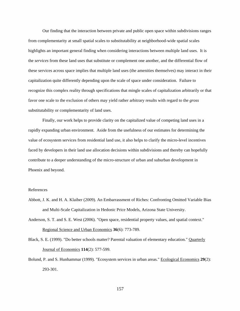
157
Our finding that the interaction between private and public open space within subdivisions ranges
from complementarity at small spatial scales to substitutability at neighborhood-wide spatial scales
highlights an important general finding when considering interactions between multiple land uses. It is
the services from these land uses that substitute or complement one another, and the differential flow of
these services across space implies that multiple land uses (the amenities themselves) may interact in their
capitalization quite differently depending upon the scale of space under consideration. Failure to
recognize this complex reality through specifications that mingle scales of capitalization arbitrarily or that
favor one scale to the exclusion of others may yield rather arbitrary results with regard to the gross
substitutability or complementarity of land uses.
Finally, our work helps to provide clarity on the capitalized value of competing land uses in a
rapidly expanding urban environment. Aside from the usefulness of our estimates for determining the
value of ecosystem services from residential land use, it also helps to clarify the micro-level incentives
faced by developers in their land use allocation decisions within subdivisions and thereby can hopefully
contribute to a deeper understanding of the micro-structure of urban and suburban development in
Phoenix and beyond.
References
Abbott, J. K. and H. A. Klaiber (2009). An Embarrassment of Riches: Confronting Omitted Variable Bias
and Multi-Scale Capitalization in Hedonic Price Models, Arizona State University.
Anderson, S. T. and S. E. West (2006). "Open space, residential property values, and spatial context."
Regional Science and Urban Economics 36(6): 773-789.
Black, S. E. (1999). "Do better schools matter? Parental valuation of elementary education." Quarterly
Journal of Economics 114(2): 577-599.
Bolund, P. and S. Hunhammar (1999). "Ecosystem services in urban areas." Ecological Economics 29(2):
293-301.

158
Boone, C. G., G. L. Buckley, et al. (2009). "Parks and People: An Environmental Justice Inquiry in
Baltimore, Maryland." Annals of the Association of American Geographers 99(4): 767-787.
Bound, J., D. A. Jaeger, et al. (1995). "Problems with Instrumental Variables Estimation When the
Correlation between the Instruments and the Endogenous Explanatory Variable Is Weak." Journal
of the American Statistical Association 90(430): 443-450.
Cameron, A. C. and P. K. Trivedi (2005). Microeconometrics : Methods and Applications. New York,
NY, Cambridge University Press.
Chay, K. Y. and M. Greenstone (2005). "Does air quality matter? Evidence from the housing market."
Journal of Political Economy 113(2): 376-424.
Cho, S. H., C. D. Clark, et al. (2009). "Spatial and Temporal Variation in the Housing Market Values of
Lot Size and Open Space." Land Economics 85(1): 51-73.
Cho, S. H., N. C. Poudyal, et al. (2008). "Spatial analysis of the amenity value of green open space."
Ecological Economics 66(2-3): 403-416.
Correll, M. R., J. H. Lillydahl, et al. (1978). "Effects of Greenbelts on Residential Property-Values -
Some Findings on Political-Economy of Open Space." Land Economics 54(2): 207-217.
Cropper, M. L., L. B. Deck, et al. (1988). "On the Choice of Functional Form for Hedonic Price
Functions." Review of Economics and Statistics 70(4): 668-675.
Daily, G. C. (1997). Nature's services : societal dependence on natural ecosystems. Washington, D.C.,
Island Press.
Do, A. Q. and G. Grudnitski (1995). "Golf-Courses and Residential House Prices - an Empirical-
Examination." Journal of Real Estate Finance and Economics 10(3): 261-270.
Ewing, R., R. Pendall, et al. (2003). Measuring Sprawl and its Impact. Washington, D.C., Smart Growth
America.
Geoghegan, J. (2002). "The value of open spaces in residential land use." Land Use Policy 19(1): 91-98.
Geoghegan, J., L. A. Wainger, et al. (1997). "Spatial landscape indices in a hedonic framework: an
ecological economics analysis using GIS." Ecological Economics 23(3): 251-264.

159
Glaeser, E. and M. Kahn (2004). Sprawl and Urban Growth. Handbook of Regional and Urban
Economics. V. Henderson and J. Thisse. Amsterdam, North Holland. 4: 2481-2527.
Hausman, J. A. and W. E. Taylor (1981). "Panel Data and Unobservable Individual Effects."
Econometrica 49(6): 1377-1398.
Hein, L., K. van Koppen, et al. (2006). "Spatial scales, stakeholders and the valuation of ecosystem
services." Ecological Economics 57(2): 209-228.
Irwin, E. G. (2002). "The effects of open space on residential property values." Land Economics 78(4):
465-480.
Irwin, E. G. and N. E. Bockstael (2001). "The problem of identifying land use spillovers: Measuring the
effects of open space on residential property values." American Journal of Agricultural
Economics 83(3): 698-704.
Kiel, K. A. and K. T. Mcclain (1995). "House Prices during Siting Decision Stages - the Case of an
Incinerator from Rumor through Operation." Journal of Environmental Economics and
Management 28(2): 241-255.
Klaiber, H. A. and D. J. Phaneuf. "Do Sorting and Heterogeneity Matter for Open Space Policy
Analysis? An Empirical Comparison of Hedonic and Sorting Models." American Journal of
Agricultural Economics 91, no. 5(2009): 1312-1318.
Kopits, E., V. McConnell, et al. (2007). "The trade-off between private lots and public open space in
subdivisions at the urban-rural fringe." American Journal of Agricultural Economics 89(5): 1191-
1197.
Lee, C. M. and P. Linneman (1998). "Dynamics of the greenbelt amenity effect on the land market - The
case of Seoul's greenbelt." Real Estate Economics 26(1): 107-129.
Leggett, C. G. and N. E. Bockstael (2000). "Evidence of the effects of water quality on residential land
prices." Journal of Environmental Economics and Management 39(2): 121-144.
Lutzenhiser, M. and N. R. Netusil (2001). "The effect of open spaces on a home's sale price."
Contemporary Economic Policy 19(3): 291-298.

160
Mahan, B. L., S. Polasky, et al. (2000). "Valuing urban wetlands: A property price approach." Land
Economics 76(1): 100-113.
Martin, C. (2001). "Landscape water use in Phoenix, Arizona." Desert Plants 17: 26-31.
McConnell, V. D. and M. A. Walls (2005). The Value of Open Space: Evidence from Studies of
Nonmarket Benefits. Washington, D.C. , Resources for the Future.
Palmquist, R. B. (1992). "Valuing Localized Externalities." Journal of Urban Economics 31(1): 59-68.
Palmquist, R. B. (2005). Property Value Models. Handbook of Environmental Economics. K.-G. Maler
and J. R. Vincent, Elseiver. 2.
Palmquist, R. B., F. M. Roka, et al. (1997). "Hog operations, environmental effects, and residential
property values." Land Economics 73(1): 114-124.
Peiser, R. B. and G. M. Schwann (1993). "The Private Value of Public Open Space within Subdivisions."
Journal of Architectural and Planning Research 10(2): 91-104.
Pope, J. C. (2008). "Buyer information and the hedonic: The impact of a seller disclosure on the implicit
price for airport noise." Journal of Urban Economics 63(2): 498-516.
Rosen, S. (1974). "Hedonic Prices and Implicit Markets - Product Differentiation in Pure Competition."
Journal of Political Economy 82(1): 34-55.
Smith, V. K., C. Poulos, et al. (2002). "Treating open space as an urban amenity." Resource and Energy
Economics 24(1-2): 107-129.
Thorsnes, P. (2002). "The value of a suburban forest preserve: Estimates from sales of vacant residential
building lots." Land Economics 78(3): 426-441.
Towe, C. (2009). "A valuation of subdivision open space by type." American Journal of Agricultural
Economics 91(5): 1319-1325.
Tyrvainen, L. and A. Miettinen (2000). "Property prices and urban forest amenities." Journal of
Environmental Economics and Management 39(2): 205-223.
Wooldridge, J. M. (2002). Econometric Analysis of Cross Section and Panel Data. Cambridge, Mass.,
MIT Press.

161
Table 1. Sum
mary Statistics fo
r Variables Used in Estim
ation
Variable
Obs
Mean
Std. Dev.
Min
Max
Variable
Obs
Mean
Std. Dev.
Min
Max
Price (ln)
619219
12.05413
0.5082354
9.740969
15.90708
Local park area
(<2000 ft.)
619219
3.44556
9.278496
0148.9016
Price
619219
207679.9
307895.7
17000
8097604
Lot size ‐x‐ Local park area
619219
0.626514
1.959936
0195.4796
Subd
. ope
n parcel size
3956
5.22381
10.04932
0.478937
318.4651
Lot size ‐x‐ Sub
d. Ope
n area
(<2000 ft.)
619219
1.819031
4.323193
0453.8388
Subd
ivision parcel cou
nt13783
69.95284
81.27748
11115
Subd
. ope
n area
(<1000 ft.)
619219
2.471076
5.69854
0152.2393
Square fo
otage
619219
18.90922
6.951536
660
Subd
. ope
n area
(<2000 ft.)
619219
6.757736
13.38545
0272.4614
Square fo
otage^2
619219
405.8823
336.8476
363600
Subd
. ope
n area
(<3000 ft.)
619219
9.87486
18.56362
0342.6336
Lot acres
619219
0.1928654
0.135717
0.05
13.93744
Mean subd
. ope
n area
619219
0.085098
0.22284
042.22037
Lot acres^2
619219
0.0556161
0.3748973
0.0025
194.2523
Mean lot size
619219
0.192872
0.124815
0.051291
6.731887
# stories
619219
1.199298
0.3996708
13
Adjacen
t SOS ‐x‐ Lot size
619219
0.011031
0.060206
013.93744
# bathroom
s619219
2.617087
0.8038109
0.5
6Adjacen
t SOS ‐x‐ Sub
d. ope
n parcel size
619219
0.46223
3.083294
0124.8617
Year built
619219
68.87268
15.02397
084
Adjacen
t sub
d. ope
n619219
0.051831
0.221687
01
Year built^2
619219
4969.165
1787.792
07056
Scho
ol619219
0.534509
0.498808
01
Garage
619219
0.9663915
0.1802193
01
Large Park distance
619219
19.071
13.43569
0.115201
58.05552
Pool
619219
0.3505157
0.4771319
01
CBD distance
619219
15.79318
6.032507
0.5202
31.91129
Year=2001
619219
0.1814318
0.3853758
01
CBD distance^2
619219
285.8222
193.883
0.270618
1018.355
Year=2002
619219
0.1901379
0.3924102
01
Pct. Hispanic
619219
0.187009
0.19398
00.977642
Year=2003
619219
0.2078796
0.4057905
01
Pct. Black
619219
0.02721
0.041759
00.817263
Year=2004
619219
0.2584546
0.4377855
01
Pct. Children
619219
0.282785
0.083929
00.589286
Adjacen
t local park
619219
0.0026146
0.0510662
01
Pct. 18 to 35
619219
0.238695
0.092992
01
Adjacen
t large
park
619219
0.0023643
0.0485663
01
Pct. 35 to 55
619219
0.30168
0.077009
00.660194
Adjacen
t schoo
l619219
0.0048658
0.0695855
01
Mean Lot Size ‐x‐ M
ean subd
. ope
n area
619219
0.018997
0.096846
035.23113
Adjacen
t rail
619219
0.0020058
0.0447407
01
Adjacen
t canal
619219
0.0102209
0.1005808
01
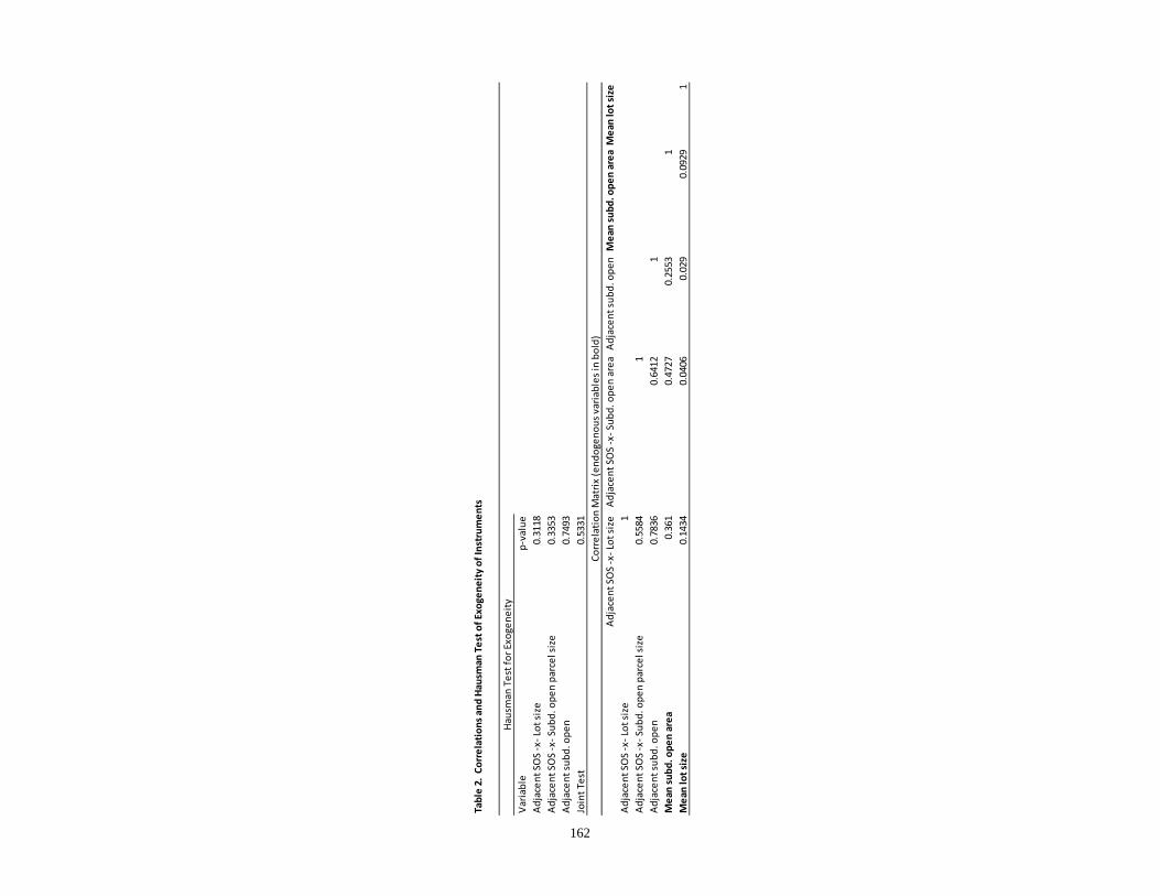
162
Table 2. Correlation
s and Hausm
an Test o
f Exogene
ity of Instrumen
ts
Variable
p‐value
Adjacen
t SOS ‐x‐ Lot size
0.3118
Adjacen
t SOS ‐x‐ Sub
d. ope
n parcel size
0.3353
Adjacen
t sub
d. ope
n0.7493
Joint Test
0.5331
Adjacen
t SOS ‐x‐ Lot size
Adjacen
t SOS ‐x‐ Sub
d. ope
n area
Adjacen
t sub
d. ope
nMean subd
. ope
n area
Mean lot size
Adjacen
t SOS ‐x‐ Lot size
1Adjacen
t SOS ‐x‐ Sub
d. ope
n parcel size
0.5584
1Adjacen
t sub
d. ope
n0.7836
0.6412
1Mean subd
. ope
n area
0.361
0.4727
0.2553
1Mean lot size
0.1434
0.0406
0.029
0.0929
1
Hausm
an Test for Exogene
ity
Correlation Matrix (end
ogen
ous variables in bold)
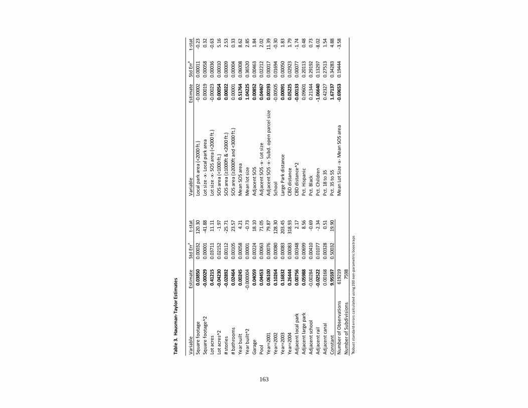
163
Table 3. Hausm
an‐Taylor Estim
ates
Variable
Estimate
Std Erra
t‐stat
Variable
Estimate
Std Erra
t‐stat
Square fo
otage
0.03850
0.00032
120.30
Local park area
(<2000 ft.)
‐0.00002
0.00011
‐0.23
Square fo
otage^2
‐0.00029
0.00001
‐41.88
Lot size ‐x‐ Local park area
0.00019
0.00058
0.32
Lot acres
0.41215
0.03711
11.11
Lot size ‐x‐ SOS area
(<2000 ft.)
‐0.00023
0.00036
‐0.63
Lot acres^2
‐0.04230
0.02152
‐1.97
SOS area
(<1000 ft.)
0.00054
0.00010
5.16
# stories
‐0.02892
0.00112
‐25.71
SOS area
(≥1000ft & <2000 ft.)
0.00022
0.00009
2.53
# bathroom
s0.02464
0.00105
23.57
SOS area
(≥2000ft and
<3000 ft.)
0.00001
0.00004
0.33
Year built
0.00245
0.00058
4.21
Mean SO
S area
0.51764
0.06008
8.62
Year built^2
‐0.000004
0.00001
‐0.73
Mean lot size
1.04225
0.36520
2.85
Garage
0.04059
0.00224
18.10
Adjacen
t SOS
0.00852
0.00463
1.84
Pool
0.04453
0.00063
71.05
Adjacen
t SOS ‐x‐ Lot size
0.04467
0.02212
2.02
Year=2001
0.06100
0.00076
79.87
Adjacen
t SOS ‐x‐ Sub
d. ope
n parcel size
0.00193
0.00017
11.39
Year=2002
0.10264
0.00080
128.30
Scho
ol‐0.00505
0.01694
‐0.30
Year=2003
0.16832
0.00083
203.45
Large Park distance
0.00091
0.00050
1.83
Year=2004
0.26444
0.00083
318.93
CBD distance
0.05225
0.02923
1.79
Adjacen
t local park
0.00756
0.00348
2.17
CBD distance^2
‐0.00133
0.00077
‐1.74
Adjacen
t large
park
0.05988
0.00699
8.56
Pct. Hispanic
0.09601
0.20113
0.48
Adjacen
t schoo
l‐0.00284
0.00410
‐0.69
Pct. Black
0.21344
0.29192
0.73
Adjacen
t rail
‐0.02522
0.01077
‐2.34
Pct. Children
‐1.06640
0.13297
‐8.02
Adjacen
t canal
0.00168
0.00328
0.51
Pct. 18 to 35
0.42327
0.27513
1.54
Constant
9.95597
0.50032
19.90
Pct. 35 to 55
1.67137
0.34283
4.88
Num
ber o
f Observation
s619219
Mean Lot Size ‐x‐ M
ean SO
S area
‐0.69653
0.19444
‐3.58
Num
ber o
f Sub
division
s7598
a Rob
ust stand
ard errors calculated using 20
0 no
n‐pa
rametric bo
ostrap
s
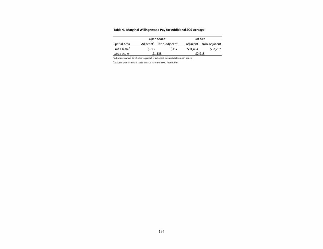
164
Table 4. Marginal Willingness to Pay for Additional SOS Acreage
Spatial Area Adjacenta Non‐Adjacent Adjacent Non‐Adjacent
Small scaleb $513 $112 $91,484 $82,207Large scaleaAdjacency refers to whether a parcel is adjacent to subdivision open spacebAssume that for small scale the SOS is in the 1000 foot buffer
Open Space Lot Size
$1,138 $2,918

165
Table 5. Rando
m Effects Estim
ates
Variable
Estimate
Std Erra
t‐stat
Variable
Estimate
Std Erra
t‐stat
Square fo
otage
0.03856
0.00072
53.61
Local park area
(<2000 ft.)
‐0.00001
0.00015
‐0.10
Square fo
otage^2
‐0.00028
0.00001
‐19.29
Lot size ‐x‐ Local park area
0.00006
0.00064
0.09
Lot acres
0.40296
0.02363
17.05
Lot size ‐x‐ SOS area
(<2000 ft.)
0.00017
0.00059
0.28
Lot acres^2
‐0.04488
0.00825
‐5.44
SOS area
(<1000 ft.)
0.00070
0.00029
2.43
# stories
‐0.03361
0.00279
‐12.03
SOS area
(≥1000ft & <2000 ft.)
0.00034
0.00020
1.70
# bathroom
s0.02727
0.00225
12.14
SOS area
(≥2000f t and
<3000 ft.)
0.00017
0.00008
1.99
Year built
0.00052
0.00096
0.54
Mean SO
S area
0.16993
0.03038
5.59
Year built^2
0.00002
0.00001
2.33
Mean lot size
0.29564
0.03653
8.09
Garage
0.04157
0.00444
9.36
Adjacen
t SOS
0.00541
0.00675
0.80
Pool
0.04515
0.00098
46.17
Adjacen
t SOS ‐x‐ Lot size
0.06431
0.02413
2.66
Year=2001
0.06076
0.00253
24.00
Adjacen
t SOS ‐x‐ Sub
d. ope
n parcel size
0.00184
0.00040
4.59
Year=2002
0.10241
0.00231
44.41
Scho
ol‐0.04945
0.00574
‐8.61
Year=2003
0.16810
0.00328
51.30
Large Park distance
0.00205
0.00021
9.84
Year=2004
0.26415
0.00293
90.07
CBD distance
‐0.02151
0.00283
‐7.61
Adjacen
t local park
0.00730
0.00560
1.30
CBD distance^2
0.00054
0.00009
6.10
Ad jacen
t large
park
0.06350
0.01290
4.92
Pct. Hispanic
‐0.48253
0.02378
‐20.29
Adjacen
t schoo
l‐0.00287
0.01090
‐0.26
Pct. Black
‐0.52199
0.05611
‐9.30
Adjacen
t rail
‐0.02407
0.02700
‐0.89
Pct. Children
‐0.77788
0.05339
‐14.57
Adjacen
t canal
0.00217
0.00680
0.32
Pct. 18 to 35
‐0.22917
0.04846
‐4.73
Constant
11.22154
0.03906
287.30
Pct. 35 to 55
0.83131
0.05744
14.47
Num
ber o
f Observation
s619219
Mean Lot Size ‐x‐ M
ean SO
S area
‐0.20678
0.04598
‐4.50
Num
ber o
f Sub
division
s7598
a Rob
ust stand
ard errors
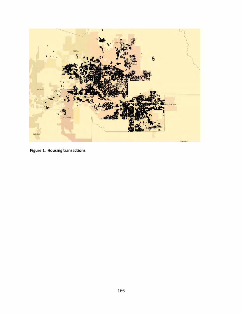
166
Figure 1. Housing transactions
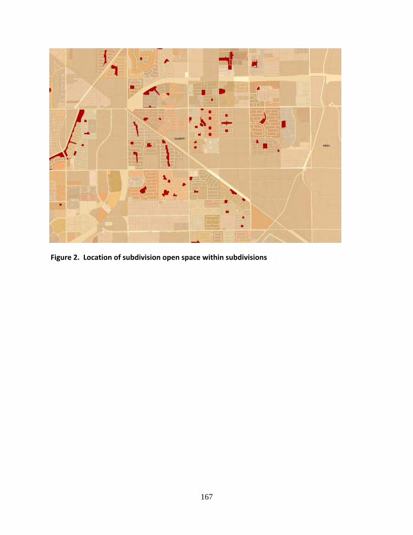
167
Figure 2. Location of subdivision open space within subdivisions
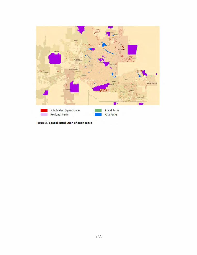
168
169
Endnotes 1 Hedonic regression techniques have been applied to a staggering array of environmental
applications including water quality (Leggett and Bockstael 2000), airport noise (Pope 2008), air
quality (Chay and Greenstone 2005), hazardous waste incinerators (Kiel and Mcclain 1995),
Superfund sites (Cameron 2006; Thorsnes 2002), hog farming operations (Palmquist, Roka et al.
1997), and the presence and qualitative aspects of open space (Irwin 2002; Smith, Poulos and
Kim 2002).
2 We do not attempt a complete survey of this literature. See McConnell and Walls (2005) for a
broad review of both the revealed and stated preference literatures.
3 Despite its reputation to the contrary, residential development in the Phoenix area is actually
relatively compact. One prominent study of 83 MSAs found that only 17 MSAs exhibited
greater residential density than Phoenix (Ewing, Pendall et al. 2003).
4 We later relaxed these measures substantially to include areas filtered out by our criteria and
found no significant difference in our results. These results are available from the authors upon
request.
5 Our buffering strategy for the measurement of subdivision open space intentionally captures
some open space parcels in nearby subdivisions that are nevertheless within a walkable distance
to a particular household. As an alternative to this “non-exclusive” characterization of SOS, we
recalculated subdivision rings and total open space based on an exclusive measure of subdivision
open space that only includes the area of subdivision open space located within the same
subdivision as the house. We found no significant differences between the two approaches and
so we only report results from buffers which potentially overlap neighboring subdivisions.
Given the apparent non-excludability of many services from subdivision open space (including

170
recreational use), we feel this is likely a more accurate representation of the extent of subdivision
open space as perceived by households.
6 This specification can be extended to capture qualitative aspects of open space as well such as
the presence of playground equipment, the average slope, or the percentage of the park in grass
versus other ground cover.
7 The buffer in this case contains all open space up to 2000 feet (i.e. unlike the buffers previously
described, it contains open space up to 1000 feet). The choice to interact a single buffer rather
than all three was made for reasons of parsimony and to avoid collinearity in a highly specified
model.
8 For a current summary of the hedonic price literature see Palmquist (2005)
9 While this dilemma is more apparent for very fine fixed effects, studies employing large scale
fixed effects may not be immune. For instance, highly unpopular land uses (e.g. Superfund sites,
prison facilities) may lend a widespread stigma to entire census tracts or even cities so that
inclusion of fixed effects at these scales could “soak up” some of the capitalized effect of these
land uses beyond their zone of immediate impact.
10 Of course, the potential for bias remains if there are correlated home specific unobservable
variables or time-varying neighborhood characteristics. Our method could be easily extended to
allow for fixed effects for the interaction of year and subdivision to address the second concern.
11 The order condition for identification requires that the number of exogenous within-varying
variables be at least as large as the number of endogenous between-varying variables.
12 The p-values in this table derive from Wald and z-tests based on a robust (sandwich) estimator
of the covariance matrix rather than the more restrictive covariance structure imposed by the
random effects error structure associated with a traditional Hausman test.

171
13 The modified Hausman test rejected the exogeneity of the majority of candidate instruments –
even those whose fixed effects and random effects estimates were virtually identical. That this
same test failed to reject in the case of these three instruments and that the within and between
estimates were essentially identical seems to lend weight to our case for instrument validity.
14 Given the nature of racial segregation in Phoenix neighborhoods, it is possible that our controls
for distance to large parks and the central business district are confounded with these
racial/ethnic variables.
15 The same critique can be levied at numerous hedonic studies employing neighborhood level
variables without regard to their potential for correlation with the error term.
16 One could argue that there is simply insufficient within-subdivision variation in these measures
of SOS provision to permit identification. However, OLS and random effects estimates (which
utilize between subdivision variation) achieved similarly small estimates. Furthermore, the
provision of SOS within 1000 foot buffers does vary substantially within subdivisions so that its
marginal effect in the HT model is precisely estimated, and yet the estimated value of SOS
acreage is quite small.
17 Our analysis is focused on the mean effect of adding SOS acreage in 1000 foot “stair steps” of
varying walkability. It is possible, however, that finer buffers in the sub-1000 foot range could
find larger effects of SOS proximity.
18 For all calculations, we rely on the mean price of housing of $207,680 and use the means of variables
where interaction terms or nonlinearities require the imputation of values into the MWTP calculations.
19 These MWTP calculations do not value the marginal value of adjacency itself (i.e. moving
from non-adjacent to adjacent status). Rather, they consider the marginal value of an acre of
open space for an existing adjacent property.

172
20 To compare MWTP for private and public goods, it is well known that we must sum the
individual MWTPs for the public good.
21 Our comparison of estimators is necessarily terse. Please consult Abbott and Klaiber (2009)
for a much more exhaustive and rigorous comparison in a similar setting.
22 Ideally, we would substitute measurements of all the expected service flows from an amenity
associated with a house into the hedonic price function. It is our inability to clearly map between
spatial location and these service flows that necessitates an approach based on spatial “proxies”
for the flows themselves.

173
Valuing Walkability and Vegetation in Portland, Oregon
Niko Drake-McLaughlin and Noelwah R. Netusil Reed College, Department of Economics
3203 SE Woodstock Blvd. Portland, Oregon 97202-8199

174
Abstract
This study uses the hedonic price method to examine if vegetation on a property, and in
the surrounding neighborhood, and proximity to urban amenities influence the sale price
of single-family residential properties in a highly urbanized part of Portland, Oregon. We
combine structural and location information for 30,786 single-family residential
transactions with high-resolution land cover data and a walkability index developed by
city planners. We estimate multiple models and find evidence of omitted variable bias in
models that do not include both variables and their interactions. A one standard deviation
increase in the walkability index, starting from the mean score, is estimated to increase a
property’s sale price from 1.47% to 6.89%.
JEL codes: Q51, Q24, R14
Keywords: hedonic price method, urban amenities, walkability, vegetation

175
Valuing Walkability and Vegetation in Portland, Oregon
I. Introduction
An urban neighborhood’s desirability depends on many factors including the
amount, type and distribution of vegetation and whether residents have easy access to
parks, shopping, schools and public transit. These factors are also related to broader
environmental concerns. The amount and placement of vegetation can reduce stormwater
runoff, improve water quality and enhance wildlife habitat (Metro 2008), and walkable,
mixed-use neighborhoods have been found to reduce traffic congestion, improve air
quality and reduce greenhouse gas emissions (Bureau of Planning and Sustainability
2009).
Portland, Oregon is ranked as the most sustainable city in the United States
(Haight 2009), but it faces several environmental challenges resulting from a high
percentage of impervious surface area, a sewer system in older neighborhoods that
combines untreated sewage and stormwater runoff, and declines in steelhead trout and
Chinook salmon populations that resulted in their listing as “threatened” under the
Endangered Species Act (Bureau of Environmental Services 1999).
Approximately 35% of the city of Portland is classified as impervious, which
includes “hard” surfaces such as roads, rooftops and driveways. This percentage is a
byproduct of Oregon’s 19 land use planning goals, specifically Goal 14, which requires
urban growth boundaries be “established and maintained by cities, counties and regional
governments to provide land for urban development needs and to identify and separate
urban and urbanizable land from rural land” (Oregon Department of Land Conservation
and Development 2006). While the Portland metropolitan area’s urban growth boundary
176
has contained sprawl, the density of development has resulted in an amount of
impervious surface area that exceeds the level past which water quality is found to
degrade rapidly (Booth, Hartley, and Jackson 2002).
Oregon’s water quality index scores for the Lower Willamette Basin, which
includes the Portland metropolitan area, range from good to very poor. Water quality at a
monitoring site located in downtown Portland is “impacted by high concentrations of
fecal coliform, total phosphates, nitrate and ammonia nitrogen, and biochemical oxygen
demand with additional influence from high total solids” (Oregon Department of
Environmental Quality). The poorest ratings occur during winter when “Portland’s
combined sewer/stormwater system is under the most pressure and overflows are most
likely to occur” (Oregon Department of Environmental Quality).
To reduce the volume of untreated discharges coming from Portland’s combined
sewer system, the city of Portland implemented a series of programs to reduce the
amount of stormwater entering the system and to increase the physical capacity of its
treatment facilities. This “physical capital” approach is complemented by a “natural
capital” approach, the Grey to Green Program, that aims to plant 33,000 yard trees and
50,000 street trees, add 43 acres of ecoroofs, construct 920 green street facilities, and
purchase 419 acres of natural areas over a 5-year period (Bureau of Environmental
Services 2010).
Portland is also exploring, as part of an update to its long-range development
plan, the “20-minute neighborhood” concept which would lead to the redevelopment of
neighborhoods to improve access to urban amenities such as shopping, schools, public
transit and parks. This is expected to decrease residents’ transportation expenditures,

177
reduce pollution, increase safety by having more people on the street, and encourage
healthier lifestyles by promoting walking and biking. Economic benefits include a likely
increase in housing values, reduction in infrastructure costs, ability to attract workers and
new businesses, and an increase in tourism (Bureau of Planning and Sustainability 2009).
The research on walkability and the sale price of single-family residential
properties finds mixed results about factors, such as proximity to bus stops and shopping,
which contribute to walkability. The majority of studies find that vegetation increases the
sale price of single-family residential properties in urban areas, but no research has
included both walkability and vegetation or examined if a synergistic relationship exists
between these variables. Because they are likely to be negatively correlated, studies that
look at just one variable may produce biased estimated coefficients thereby leading to
inaccurate policy recommendations.
Our paper is structured as follows. The following section reviews the literature on
property values, walkability and vegetation. Section III provides background information
about the study area and data used in our analysis. Models are presented in Section IV
with results and key findings in Section V. The final section concludes and offers policy
recommendations.
II. Literature Review
There is a rich literature investigating the effects of vegetation on the sale price of
single-family residential properties in urban areas. Donovan and Butry (2010) estimate
the effect of street trees on the sale price of single-family residential properties on the
east side of Portland, Oregon. In addition to finding a statistically significant increase in
sale price of $8,870 (3% of the median sales price) from the combined effect of street

178
trees in front of a property, and canopy from street trees within 100 feet of a property, the
authors find that street trees reduce a property’s average time on market by 1.7 days.
Numerous studies examine the effect of urban forests on the sale price of
residential properties. While studies find a positive effect from proximity to urban forests
(Mansfield et al. 2005; Tyrvainen and Miettinen 2000), the evidence on forest views is
mixed with studies finding a positive effect (Tyrvainen and Miettinen 2000), a negative
effect (Paterson and Boyle 2002), or effects that vary based on tree type (Garrod and
Willis 1992).
A modeling approach used by several authors includes the amount of the area
surrounding a property classified as forested (Mansfield et al. 2005; Netusil,
Chattopadhyay, and Kovacs 2010; Paterson and Boyle 2002; Payton 2008) or that have
trees, and other kinds of vegetation, as land use categories (Acharya and Bennett 2001;
Geoghegan, Wainger, and Bockstael 1997). Important findings from these studies
include evidence of diminishing returns from tree canopy (Netusil, Chattopadhyay, and
Kovacs 2010) and the superiority of models that incorporate spatial patterns compared to
a more traditional approach that includes straight-line distance to certain land use/land
cover types (Acharya and Bennett 2001).
While research in the Portland metropolitan area has examined if proximity to
specific urban amenities such as open spaces (Lutzenhiser and Netusil 2001), wetlands
(Mahan, Polasky, and Adams 2000), and public transit (Chen, Rufolo, and Dueker 1998)
affect the sale price of single family residential properties, the literature on walkability’s
effect is limited to one study that evaluates the importance of neighborhood design on the
west side of the Portland metropolitan area (Song and Knaap 2003). The authors find

179
mixed results for variables that capture walkability—properties with easier access to
commercial uses, measured as the percentage of land within ¼ mile of a property
classified as commercial, are found to sell for a premium while properties close to bus
stops sell for a discount.
The modeling approach that is closest to the one used in our study is Pivo and
Fisher’s (2010) analysis of how walkability, measured using a value generated by
walkscore.com, affects the market value of office, retail, apartment and industrial
properties. A 10-point increase in walkability, which is measured on a 100-point scale,
is estimated to increase property values by 1 percent for apartments and 9 percent for
office and retail properties. No statistically significant effect was found for industrial
properties.
Pivo and Fisher (2010) note several limitations from using walkscore.com
including its assignment of equal weights to urban amenities such as schools, parks, retail
establishments, etc. that are located within buffers of up to 1 mile from a property.
Barriers to walking, such as highways, rivers and steep slopes, and access to mass transit,
are not taken into account in walkscore’s algorithm, which uses a straight-line distance to
amenities. The walkability index used in our analysis, which is described in detail below,
overcomes these limitations.
III. Data and Study Area
Our data set includes 30,786 single-family residential transactions that occurred
between January 1st, 2005 and December 31st, 2007 in a highly urbanized part of the city
of Portland, Oregon. The data, which are from the Multnomah County Assessor’s office,
were evaluated to make sure that transactions occurred at arms length. Summary

180
statistics, which are broken down by the five areas of Portland (North, Northeast,
Northwest, Southwest and Southeast), are presented in Table 1. Sale price is in 2007
dollars after deflating using the CPI-U.
Table 1: Summary Statistics for House Sales by Area
Land cover information was derived from a 2007 land cover layer that classifies
each 3x3 foot square in the study area as high structure vegetation (trees), low structure
vegetation (grass, shrubs and small trees), impervious surface or open water (rivers,
streams and lakes) (Metro Data Resource Center 2007). The proportion of each land
cover type was computed for each property, within 200 feet of each property, between
200 feet and ¼ mile, and between ¼ mile and ½ mile of each property. Neighborhood
data, such as distance to major arterial roads, distance to highways, slope and elevation
were derived using data layers maintained by the regional government’s data resources
center (Metro Data Resources Center 2009). Median income and proportion white at the
census tract level were derived from the 2000 U.S. Census (U.S. Census Bureau 2009).
A walkability index, which is illustrated in Figure 1, was created by staff at the
Portland Bureau of Planning and Sustainability as part of the “20-minute neighborhood”
concept. The index takes into account several variables, such as the actual walking
distance to full service grocery stores, elementary schools and parks, and if streets are
steeply sloped. Also, the city was divided into ½ mile by ½ mile grid cells and the
number of commercial businesses, the percentage of sidewalk coverage, the number of
intersections and the level of public transit in each grid cell was computed, weighted, and
then incorporated into the index. Scores range from 1-100 for the city of Portland with
the scores for our observations ranging from 1-83.

181
Figure 1: Walkability Index for City of Portland, Oregon
Because data are not consistently available for urban amenities outside the city of
Portland, observations within ½ mile of the city limits may have inaccurate walkability
index values, so these observations were dropped from our analysis. The 30,786 property
sales used in our analysis are shown in Figure 2.
Figure 2: Property Sales in Study Area
The regression specification includes detailed structural, location and
environmental characteristics. The names and descriptions for variables used in the
regression are provided in Table 2.
Table 2: Variable Names and Descriptions
Summary statistics for key variables are provided in Table 3. Lot sizes are small,
averaging around 7,000 square feet; on average, 44% of our lots are covered by
impervious surface area followed by approximately 29% low structure vegetation (grass,
shrubs and small trees), and 27% high structure vegetation (trees). Thirty-two properties
have water on the property itself, so the average lot coverage for this variable is very
small. The land cover percentages remain fairly constant in the buffers (200 feet, 200
feet to ¼ mile and ¼ mile to ½ mile) surrounding our properties. Impervious surface area
in the buffers is approximately 46%, low structure vegetation ranges from around 27% to
28%, and high structure vegetation remains steady at 26%.
Table 3: Summary Statistics
V. Results

182
The theoretical basis for the hedonic price method is firmly established in the
literature. The appropriate functional form for estimation is less clear with most
researchers using the semi-log.
Results of four semi-log models are presented in Table 4. Models 1 and 2 include
just the walkability index and vegetation variables, respectively. Model 3 includes both
variables and Model 4 adds interaction terms. Quadratic terms are included for the
vegetation variables (high structure and low structure) and for the walkability index
because we believe there is some point past which increases in these variables will
decrease a property’s sale price—a modeling approach informed by research in the study
area (Netusil, Chattopadhyay, and Kovacs 2010). We predict that water on a property
will always decrease its sales price due to risks of flooding and other hazards, while water
in the buffers surrounding a property will always increase sale price. Impervious surface
is the excluded variable in both models.
A Breusch-Pagan/Cook-Weisberg test indicates heteroskedasticity in all models,
so robust regressions are run. All of the control variables have the expected sign and
magnitude, and most are statistically significant. Full regression results are available
from the authors.
Table 4: Regression Results (robust standard errors)
Models 1 and 2 are included to compare the effect of modeling these variables
individually with models that include both variables (Model 3) and interaction terms
(Model 4). The estimated coefficient for walkability is statistically significant at the 10%
level in Model 1, but the quadratic term is not significant. The estimated magnitude,
significance, and in the case of the quadratic term, the sign of the estimated coefficient,

183
changes in Model 3 when vegetation is included as a control variable providing strong
evidence of omitted variable bias in Model 1. Interestingly, a comparison of estimated
coefficients for land cover variables Models 2 and 3 does not provide strong evidence of
omitted variable bias.
The estimated coefficients on both walkability terms in Model 3 are statistically
significant, as are many of the land cover variables. Walkability is estimated to have a
positive effect up to 93, which is outside the range of our data (the maximum value is
83), but below the maximum possible value of 100. A one standard deviation increase
(13.11 points) in the walkability index for a property, starting from the mean score of
47.79, is predicted to increase its sale price by $9,942 (3.29%) using the average sale
price in our data set.
The linear and squared terms for on-property high structure vegetation are
statistically significant and predict an optimal on-property high structure vegetation
coverage of 33.74%, which is 8.19 percentage points higher than the average in our data
set. For the average lot, this represents a 20-25 year old oak tree (McPherson et al.
2002). We estimate that increasing high structure vegetation on a property from the
average amount (25.55%), to the amount that maximizes sale price (33.74%) will
increase a property’s sale price by $214 (0.07%).
Increasing high structure vegetation in the 200-foot and 200 foot to ¼ mile buffer
surrounding a property is predicted to always increase a property’s sale price. The
furthest buffer from a property, ¼ mile to ½ mile, shows diminishing returns to high
structure vegetation. The estimated coefficients for low structure vegetation are mixed
ranging from both the linear and quadratic term being significant (200 foot, ¼ mile to ½

184
mile buffers), to only the quadratic term (on property) to neither term (¼ mile to ½ mile
buffer). Water on a property is significantly negative, as expected, and water in the
surrounding buffers is significantly positive, which is also expected.
The fourth model adds interaction terms to Model 3. Nine of the twelve
interaction variables are statistically significant providing evidence of a synergistic
relationship between walkability and land cover.
Table 5 includes predictions of a one standard deviation increase in the
walkability index, from its mean value, evaluated at the 25th, 50th and 75th percentile of
high and low structure vegetation for all buffers. Predicted effects range from 1.47% of
the mean sale price for properties when high and low structure vegetation are at the 25th
percentile to 6.88% when they are at the 75th percentile.
Table 5: Predicted Effect of a One Standard Deviation Increase in Walk Score Evaluated
at Mean Sale Price and Mean Walkability Index
Table 6 holds walkability constant at its 25th, 50th and 75th percentile scores and
shows the predicted effect from increasing on-property high structure vegetation on a
property from the dataset average of 25.55% to the target tree canopy amount (35%-40%)
specified for residential property in the city of Portland’s Urban Forest Action Plan
(Urban Forest Action Plan 2007).
Table 6: Predicted Effect of Increasing On-Property High Structure Vegetation
Evaluated at Mean Sale Price and Mean High Structure Vegetation
The amount of high structure vegetation that maximizes a property’s sale price
varies with its walkability score. Using estimated coefficients from Model 4, the
“optimal” amount of high structure vegetation on a property is 18.44% when the

185
walkability index is at the 25th percentile, 36.60% at the 50th percentile, and 51.12% for
the 75th percentile. This variation in “optimal” amounts of tree canopy explains why
increasing tree canopy, when the walkability index is at the 25th percentile, decreases a
property’s sale price. Predicted effects for the 50th and 75th percentile are positive, but
small.
IV. Policy Implications and Conclusions
This paper has highlighted the importance of two key factors in determining the
sale price of residential properties in an urban area: access to urban amenities, captured
by a walkability index, and land cover on a property and in the surrounding
neighborhood. Models that use one variable or the other likely suffer from omitted
variable bias. Models that include both variables, and interaction terms, show that effects
on sale price that depend on the other variable’s level with increases in high structure
vegetation having a negative predicted effect when walkability is held constant at a low
level (25th percentile). Increases in walkability, holding high and low structure
vegetation constant, is predicted to increase a property’s sale price with the largest effect
occurring for properties with a high amount of low and high structure vegetation (75th
percentile) on the property and in the surrounding buffers.
It is possible that these effects arise from scarcity of walkability and high levels of
high structure vegetation in the same area. If an area is very walkable, it may be further
from parks and closer to retail areas that have more impervious surfaces. Areas with a
high proportion of trees may be less likely to have lots of businesses nearby.
Nevertheless, the data does suggest that increasing both of these factors should have

186
statistically and economically significant effects on a property’s sale price and that the
greatest effect comes from increasing the two in a coordinated effort.
Our results indicate that increasing walkability and vegetation should be pursued,
and that both are beneficial for single-family residential property owners, but neither goal
should be achieved at the expense of the other. How cities accomplish this goal, and
what combination of walkability and vegetation are best for environmental and social
goals, remain questions for further research.
Acknowledgements
We greatly acknowledge assistance from Jonathan Kadish, Gary Odenthal, Carmen
Piekarski, Zach Levin and Minott Kerr.

187
Table 1: Summary Statistics for House Sales by Area
Variable Number of
Observations
Mean Standard
Deviation
Minimum Maximum
realsaleprice
(study area)
30,786 302,118 168,435 53,135 3,408,846
realsaleprice
(N Portland)
5,165 246,825 81,446 64,795 993,354
realsaleprice
(NE
Portland)
9,883 316,248 149,998 53,135 1,572,030
realsaleprice
(NW
Portland)
326 706,618 360,571 107,527 2,750,809
realsaleprice
(SW
Portland)
2,835 462,116 289,284 93,618 3,408,846
realsaleprice
(SE
Portland)
12,577 267,173 119,082 58,921 1,903,024

188
Figure 1: Walkability Index for City of Portland, Oregon
Figure 2: Property Sales in Study Area
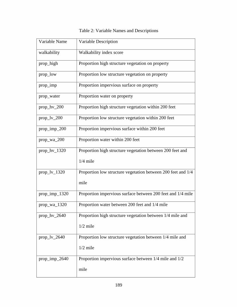
189
Table 2: Variable Names and Descriptions
Variable Name Variable Description
walkability Walkability index score
prop_high Proportion high structure vegetation on property
prop_low Proportion low structure vegetation on property
prop_imp Proportion impervious surface on property
prop_water Proportion water on property
prop_hv_200 Proportion high structure vegetation within 200 feet
prop_lv_200 Proportion low structure vegetation within 200 feet
prop_imp_200 Proportion impervious surface within 200 feet
prop_wa_200 Proportion water within 200 feet
prop_hv_1320 Proportion high structure vegetation between 200 feet and
1/4 mile
prop_lv_1320 Proportion low structure vegetation between 200 feet and 1/4
mile
prop_imp_1320 Proportion impervious surface between 200 feet and 1/4 mile
prop_wa_1320 Proportion water between 200 feet and 1/4 mile
prop_hv_2640 Proportion high structure vegetation between 1/4 mile and
1/2 mile
prop_lv_2640 Proportion low structure vegetation between 1/4 mile and
1/2 mile
prop_imp_2640 Proportion impervious surface between 1/4 mile and 1/2
mile

190
prop_wa_2640 Proportion water between 1/4 mile and 1/2 mile
lotsqft Lot square footage
bldgsqft House square footage
fullbaths Number of full bathrooms
halfbaths Number of half bathrooms
age Year house was sold minus year house was built
numfire Number of fireplaces
N, NE, NW, SW,
SE
Dummy variables for areas of the city
dist_N, dist_NE,
dist_NW,
dist_SW, dist_SE
(feet)
Area variables interacted with distance to CBD
elevation (feet) Elevation of property in feet
medianincome ($) Median income of census tract in dollars
crime Crime index score
proportionwhite Proportion of census tract that is white
prop_slope10% Proportion of property with a slope greater than 10%
Month 1-36 Dummy variables indicating sale month of transaction
maj_art330,
maj_art660,
maj_art1320,
maj_art2640
Dummy variables indicating whether a property is within
330, 660, 1320, or 2640 feet of a major arterial road

191
fwy 330, fwy660,
fwy1320, fwy2640
Dummy variables indicating whether a property is within
330, 660, 1320 or 2640 feet of a freeway
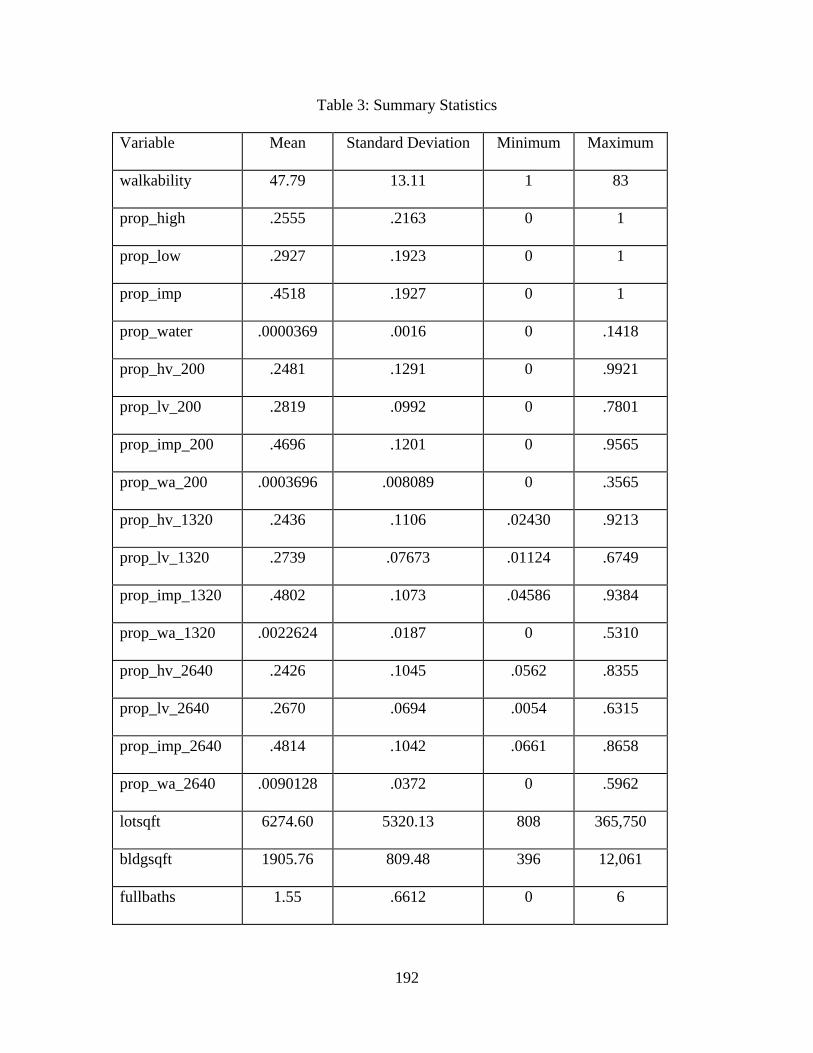
192
Table 3: Summary Statistics
Variable Mean Standard Deviation Minimum Maximum
walkability 47.79 13.11 1 83
prop_high .2555 .2163 0 1
prop_low .2927 .1923 0 1
prop_imp .4518 .1927 0 1
prop_water .0000369 .0016 0 .1418
prop_hv_200 .2481 .1291 0 .9921
prop_lv_200 .2819 .0992 0 .7801
prop_imp_200 .4696 .1201 0 .9565
prop_wa_200 .0003696 .008089 0 .3565
prop_hv_1320 .2436 .1106 .02430 .9213
prop_lv_1320 .2739 .07673 .01124 .6749
prop_imp_1320 .4802 .1073 .04586 .9384
prop_wa_1320 .0022624 .0187 0 .5310
prop_hv_2640 .2426 .1045 .0562 .8355
prop_lv_2640 .2670 .0694 .0054 .6315
prop_imp_2640 .4814 .1042 .0661 .8658
prop_wa_2640 .0090128 .0372 0 .5962
lotsqft 6274.60 5320.13 808 365,750
bldgsqft 1905.76 809.48 396 12,061
fullbaths 1.55 .6612 0 6
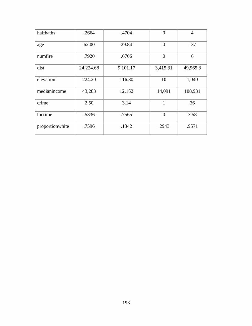
193
halfbaths .2664 .4704 0 4
age 62.00 29.84 0 137
numfire .7920 .6706 0 6
dist 24,224.68 9,101.17 3,415.31 49,965.3
elevation 224.20 116.80 10 1,040
medianincome 43,283 12,152 14,091 108,931
crime 2.50 3.14 1 36
lncrime .5336 .7565 0 3.58
proportionwhite .7596 .1342 .2943 .9571
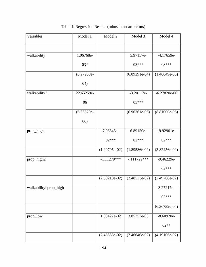
194
Table 4: Regression Results (robust standard errors)
Variables Model 1 Model 2 Model 3 Model 4
walkability 1.06768e-
03*
5.97157e-
03***
-4.17659e-
03***
(6.27958e-
04)
(6.89291e-04) (1.46649e-03)
walkability2 22.65259e-
06
-3.20117e-
05***
-6.27820e-06
(6.55829e-
06)
(6.96361e-06) (8.81000e-06)
prop_high 7.06845e-
02***
6.89150e-
02***
-9.92901e-
02***
(1.90705e-02) (1.89586e-02) (3.82456e-02)
prop_high2 -.111279*** -.111729*** -9.46229e-
02***
(2.50218e-02) (2.48523e-02) (2.49768e-02)
walkability*prop_high 3.27217e-
03***
(6.36739e-04)
prop_low 1.03427e-02 3.85257e-03 -8.60920e-
02**
(2.48553e-02) (2.46640e-02) (4.19106e-02)

195
prop_low2 -7.07229e-02* -6.14550e-02* -7.43739e-
02**
(3.63128e-02) (3.58957e-02) (3.50870e-02)
walkability*prop_low 1.96878e-
03***
(7.35359e-04)
prop_water -7.36746*** -7.18829*** -10.701**
(1.744838) (1.774594) (4.249342)
walkability*prop_water .232681
(0.167586)
prop_hv_200 .159067*** .184108*** -.265058***
(4.07884e-02) (4.05419e-02) (8.10759e-02)
prop_hv2_200 -8.02222e-02 -.102993 6.22763e-02
(6.35825e-02) (6.33478e-02) (6.87583e-02)
walkability*prop_hv_200 7.88557e-
03***
(1.27284e-03)
prop_lv_200 .443899*** .433219*** .289262***
(7.22956e-02) (7.21371e-02) (0.103347)
prop_lv2_200 -.461151*** -.421295*** -.432532***
(0.111749) (0.111743) (0.113157)
walkability*prop_lv_200 3.14192e-03**

196
(1.41205e-03)
prop_wa_200 .846658** 1.06766*** -.563672
(0.385804) (0.363878) (0.641638)
walkability*prop_wa_200 5.59467e-02**
(2.65298e-02)
prop_hv_1320 .253295*** .330514*** .196147
(7.08785e-02) (7.06033e-02) (0.156796)
prop_hv2_1320 .162962 .226176** .352361***
(0.108516) (0.108366) (0.135395)
walkability*prop_hv_1320 2.05930e-03
(2.35815e-03)
prop_lv_1320 .142154 .111889 .410147*
(0.140576) (0.140266) (0.225069)
prop_lv2_1320 -1.55452e-02 .242364 .278726
(0.221011) (0.221076) (0.251169)
walkability*prop_lv_1320 -6.99113e-
03***
(2.56260e-03)
prop_wa_1320 .237102 .345257** 1.1123***
(0.151544) (0.148107) (0.368680)
walkability*prop_wa_1320 -2.29504e-
02***

197
(8.29671e-03)
prop_hv_2640 .651971*** .597983*** .901364***
(7.66755e-02) (7.59835e-02) (0.144002)
prop_hv2_2640 -.859051*** -.651059*** -.976767***
(0.120009) (0.120007) (0.137130)
walkability*prop_hv_2640 -4.34080e-
03**
(2.04546e-03)
prop_lv_2640 .801175*** .606028*** -.712771***
(0.166059) (0.167362) (0.221581)
prop_lv2_2640 -1.03777*** -.681525** -.166792
(0.282672) (0.285593) (0.305121)
walkability*prop_lv_2640 2.23610e-
02***
(2.39760e-03)
prop_wa_2640 .418843*** .470244*** .639733***
(5.16137e-02) (5.13326e-02) (0.189230)
walkability*prop_wa_2640 -4.29048e-03
(3.58124e-03)
Observations 30,786 30,786 30,786 30,786

198
R-squared 0.756 0.763 0.766 0.769
*** p<0.01, ** p<0.05, * p<0.1
Table 5: Predicted Effect of a One Standard Deviation Increase in Walk Score Evaluated
at Mean Sale Price and Mean Walkability Index
High and Low
Structure Vegetation
at 25th Percentile
For All Buffers
High and Low
Structure Vegetation
at 50th Percentile
For All Buffers
High and Low
Structure Vegetation
at 75th Percentile
For All Buffers
Predicted increase
in sale price of a one
standard deviation
increase in
walkability index
$4,431
(1.47%)
$11,746
(3.89%)
$20,801
(6.89%)
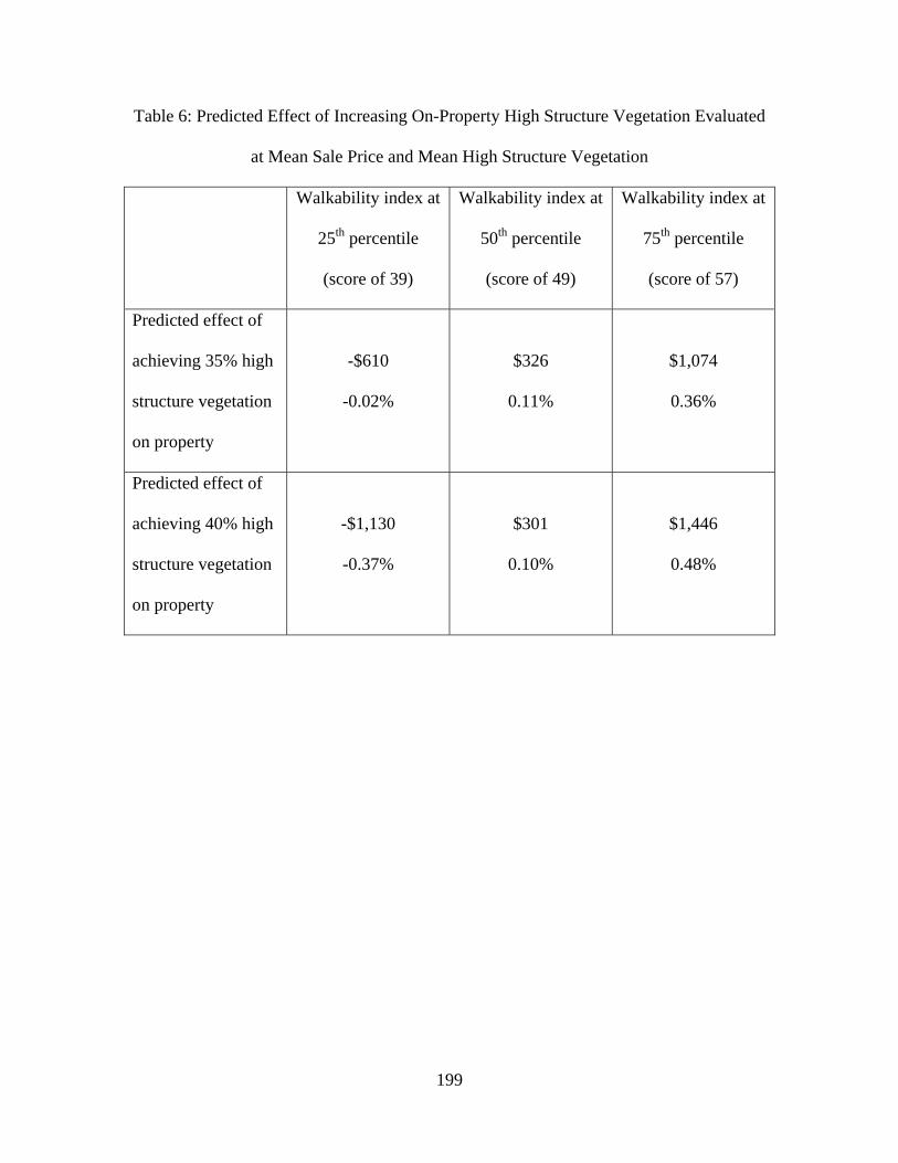
199
Table 6: Predicted Effect of Increasing On-Property High Structure Vegetation Evaluated
at Mean Sale Price and Mean High Structure Vegetation
Walkability index at
25th percentile
(score of 39)
Walkability index at
50th percentile
(score of 49)
Walkability index at
75th percentile
(score of 57)
Predicted effect of
achieving 35% high
structure vegetation
on property
-$610
-0.02%
$326
0.11%
$1,074
0.36%
Predicted effect of
achieving 40% high
structure vegetation
on property
-$1,130
-0.37%
$301
0.10%
$1,446
0.48%

200
References
Acharya, Gayatri, and Lynne Lewis Bennett. 2001. Valuing open space and land‐use patterns in urban watersheds. Journal of Real Estate Finance and Economics 22 (2‐3):221‐237.
Booth, Derek B., David Hartley, and Rhett Jackson. 2002. Forest Cover, Impervious Surface Area, and the Mitigation of Stormwater Impacts. Journal of the American Water Resources Association 38:835‐845.
Bureau, U.S. Census. 2009. American FactFinder. Center, Metro Data Resource. Regional Land Information System 2009. Chen, Hong, Anthony Rufolo, and Kenneth J. Dueker. 1998. Measuring the impact of
light rail systems on single‐family home values ‐ A hedonic approach with geographic information system application. Land Use and Transportation Planning and Programming Applications (1617):38‐43.
Development, Oregon Department of Land Conservation and. 2006. Oregon's Statewide Planning Goals & Guidelines Goal 14: Urbanization. edited by O. D. o. L. C. a. Development.
Donovan, Geoffrey H., and David T. Butry. 2010. Trees in the city: Valuing street trees in Portland, Oregon. Landscape and Urban Planning 94:77‐83.
Garrod, Guy D., and Ken G. Willis. 1992. The Environmental Economic‐Impact of Woodland: A 2‐Stage Hedonic Price Model of the Amenity Value of Forestry in Britain. Applied Economics 24 (7):715‐728.
Geoghegan, J, LA Wainger, and NE Bockstael. 1997. Spatial landscape indices in a hedonic framework: an ecological economics analysis using GIS. Ecological Economics 23 (3):251‐264.
Haight, Abby. 2009. Portland Gets Its Reward: Most Sustainable City. The Oregonian. Lutzenhiser, Margot, and Noelwah R. Netusil. 2001. The Effect of Open Spaces on a
Home's Sale Price. Contemporary Economic Policy 19 (3):291‐298. Mahan, Brent L., Stephen Polasky, and Richard M. Adams. 2000. Valuing Urban
Wetlands: A Property Price Approach. Land Economics 76 (1):100‐113. Mansfield, Carol, Subhrendu K. Pattanayak, William McDow, Robert McDonald, and
Patrick Halpin. 2005. Shades of Green: Measuring the value of urban forests in the housing market. Journal of Forest Economics 11 (3):177‐199.
McPherson, E. Gregory, Scott E. Maco, James R. Simpson, Paula J. Peper, Qingfu Xiao, Ann Marie VanDerZanden, and Neil Bell. 2002. Western Washington and Oregon Community Tree Guide: Benefits, Costs, and Strategic Planting. Center for Urban Forest Research, USDA Forest Service, Pacific Southwest Research Station.
Metro. 2008. State of the Watersheds Monitoring Report, Initial report: Baseline watershed conditions as of Dec. 2006.
Metro Data Resource Center. 2009. 2007 High Resolution Landcover 2007 [cited June 8 2009]. Available from http://rlismetadata.oregonmetro.gov/display.cfm?Meta_layer_id=2303&Db_type=rlislite.

201
Netusil, Noelwah R., Sudip Chattopadhyay, and Kent Kovacs. 2010. Estimating the Demand for Tree Canopy: a Second‐Stage Hedonic Price Analysis in Portland, Oregon. Land Economics.
Paterson, Robert W., and Kevin J. Boyle. 2002. Out of Sight, Out of Mind? Using GIS to Incorporate Visibility in Hedonic Property Value Models. Land Economics 78 (3):417‐425.
Payton, Seth, Greg Lindsey, Jeff Wilson, John R. Ottensmann and Joyce Man. 2008. Valuing the Benefits of the Urban Forest: A Spatial Hedonic Approach. Journal of Environmental Planning and Management 51 (6):717‐736.
Pivo, Gary and Jeffrey D. Fisher. 2010. The Walkability Premium in Commercial Real Estate Investments. In Responsible Property Investesting Center, University of Arizona; Benecki Center for Real Estate Studies, Indiana University.
Quality, Oregon Department of Environmental. Oregon Water Quality Index Report for Lower Willamette, Sandy, and Lower Columbia Basins Water Years 1986‐2995.
Services, Bureau of Environmental. 1999. Steelhead and Chinook Salmon Listing Portland's Response to the Endangered Species Act.
———. 2010. Portland's Green Infrastructure: Quantifying the Health, Energy, and Community Livability Benefits. edited by B. o. E. Services. Portland.
Song, Y., and G. J. Knaap. 2003. New urbanism and housing values: a disaggregate assessment. Journal of Urban Economics 54 (2):218‐238.
Sustainability, City of Portland Bureau of Planning and. 2009. Status Report: Twenty‐Minute Neighborhoods.
———. 2009. Status Report: Twenty‐minute Neighborhoods. Tyrvainen, Liisa, and Antti Miettinen. 2000. Property prices and urban forest
amenities. Journal of Environmental Economics and Management 39 (2):205‐223.
Urban Forest Action Plan. 2007. Portland: Portland Parks & Recreation.

202
Species Preservation versus Development:
An Experimental Investigation under Uncertainty
W. Douglass Shaw Dept.of Agricultural Economics
Texas A&M University [email protected]
Therese Grijalva Department of Economics
Weber State University [email protected]
Robert P. Berrens Department of Economics University of New Mexico

203
Species Preservation versus Development: An Experimental Investigation under Uncertainty
Abstract: The safe minimum standard (SMS) is a decision rule to preserve a renewable resource, unless the social costs of doing so are somehow intolerable. While unpersuasive to many, support for the SMS has been advocated by some economists and policy analysts for settings involving irreversibility and a high degree of uncertainty. The objective of this paper is to explore decision-making involving species preservation versus development within an experimental laboratory setting, and involving a particular type of uncertainty (known payoffs and uncertain probabilities). The experimental design implements a number of prior game-theoretic investigations of the SMS (Bishop 1978; Ready and Bishop 1991; Palmini 1999), involving insurance, lottery or combined games against nature. The choices are between species preservation, which possibly provides a cure for a disease, or developing habitat, leading to irreversible depletion. Econometric results from a random parameters logit (RPL) model, using responses from 117 participants (across both US and Mexican university student samples) and 9 treatment choices, indicate that support for the SMS varies across the type of game, the imposed maximum regret condition concerning the relative magnitude of different costs (e.g., cost of disease) and benefits (e.g., net benefits of development), a constructed measure of respondents’ risk aversion, and other factors. There is also evidence of highly heterogeneous preferences for preservation even within our relatively homogenous student samples. Key Words: Safe Minimum Standard, Uncertainty, Experimental, Game against Nature, Endangered Species

204
Introduction
Choices between species preservation and development are complicated by
potential irreversibility and significant uncertainty (Norton and Toman 1997). The safe
minimum standard (SMS) is a decision rule to preserve a renewable resource, unless the
social costs of doing so are somehow intolerable. While unpersuasive to many, support
for the SMS has been advocated by some economists and policy analysts for settings
involving irreversibility and a high degree of uncertainty. A persistent question, at least
among some environmental and resource economists as well as other scholars, is whether
this potential irreversibility and significant uncertainty justify extraordinary decision
processes, such as advocacy of safe minimum standard (SMS) approaches, relative to
more standard benefit-cost or utilitarian analyses (Ciriacy-Wantrup 1968; Bishop 1978;
Randall and Farmer 1995; Randall 1991 and 2007). Similarly, considerable uncertainty
around possible worst-case scenarios involving global warming have prompted some to
question whether precautionary approaches might be preferred to more traditional
discounted present value approaches to decision making (e.g., Tol 2003; Cole 2008).
The relative merits of SMS-type approaches as preferred decision-making criteria,
versus more standard utilitarian approaches, have been argued from game theoretic
analyses (e.g., Palmini 1999), pluralistic moral philosophy perspectives (Randall and
Farmer 1995), or from the legal theory of trusts (Scott 1999). Randall (2007) argues that
there may be no single rationale for supporting an SMS approach. The SMS may or may
not command consensus in society (Atkinson et al. 2007, p. 6), but from any perspective,
many economists and other analysts have found arguments in support of SMS approaches
unpersuasive (e.g., see Margolis and Naevdal 2008).

205
The objective of this paper is to explore decision-making involving species
preservation versus development within an experimental laboratory setting, and involving
a particular type of uncertainty (known payoffs, but with uncertain probabilities of
events). This investigation implements a number of prior game-theoretic investigations
of the SMS (Bishop 1978; Ready and Bishop 1991), involving “lottery” or “insurance”
games against nature, respectively. Further, we parameterize the basic species
preservation versus development dynamic game of Palmini (1999) with corresponding
regret conditions of making a wrong choice into an experimental framework.
The experimental design also includes treatments varying: (i) information about the
species; and (ii) and the imposed maximum regret condition (regret associated with
making a wrong choice). Multiple sessions of the experiments were run with university
student subjects in the US and Mexico. As part of each session, time (e.g., Coller and
Williams 1999) and risk preferences (e.g., Holt and Laury 2002) were elicited, as both
may affect choices (e.g., Anderson et al. 2008) between preservation and development.
Finally, we also allow the subjects to exhibit heterogeneity in their tastes for preservation.
Econometric results from a random parameters logit (RPL) model, which allows
for individual heterogeneity, demonstrate how support for the SMS preservation choice
varies significantly depending on the format of the game against nature, the imposed
maximum regret condition, the degree of risk aversion as well as both cultural and
individuating factors. While the evidence might be interpreted as supporting the
plausibility of SMS-type policy choices, with an underlying minimax-regret rationale or
logic, it is also clear that such support is neither absolute nor necessarily commanding of
a consensus or majority vote, and might be highly context dependent.

206
Background Literature
Species Preservation and Safe Minimum Standard Approach
Species have value to society for many reasons including: the possibly that they
contain a substance that eventually leads to a cure for a disease; the recognition of their
importance as a critical part of an ecosystem and connections to biodiversity; and the
current or future values they have from harvest, or for passive or extractive recreation
(wildlife viewing, hunting). It has been estimated that one-third of medical prescriptions
given out annually in the United States are based on substances derived from nature or
‘synthesized in imitation of natural substances’ (Lovejoy 1993), and that one-quarter of
the drugs marketed in the United States contain active ingredients derived from plants
(see Farnsworth 1990; Brewer 1993; National Wildlife Federation 2006, and U.S. Fish
and Wildlife Service 2005). Values for many species go beyond use-only related values
(Boyle and Bishop 1987; Loomis and Ekstrand 1997).
Real uncertainty relating to the net benefits of developing habitat, or from
preserving species, arises for many possible reasons. In the case of development, a
developer may not know her benefits from markets that evolve after a development
decision occurs, especially when the time it takes to fully develop a project is lengthy.
For preserving species uncertainty may arise from the: (i) nature of diseases (current and
future unknown ones); (ii) timing of cures, extraction; (iii) future prices and values
related to harvest, or development of the habitat; (iv) discovery of substitute resources;
and (v) exact knowledge of population and population dynamics.

207
Economists have used contingent valuation, and a variety of other stated
preference approaches, to estimate the value of protecting endangered and at-risk species
(e.g. Boyle and Bishop 1987; Loomis and Ekstrand 1997). For example, in an early
study of connections between species preservation and information, Samples et al. (1986)
find that the species’ characteristics and status as endangered as well as features of a
proposed investment program influence willingness-to-pay (WTP) for preservation. In
their heavily-cited, original meta-analysis of studies valuing rare and endangered species,
Loomis and White (1996) find that the annual maximum WTP for 18 species ranges from
$6 to $95 per household. More recently, Richardson and Loomis (2009) have updated the
original meta-analysis (Loomis and White 1996) of threatened, rare and endangered
species. Both the original and the updated meta-analyses present evidence of systematic
information about the social benefits of species preservation. However, both Loomis and
White (1996) and Richardson and Loomis (2009) stopped short of endorsing the use of
such values in strict benefit-cost decision rules, and instead supported SMS approaches in
collective choice rules to protect endangered species.
The SMS was first proposed by Ciriacy-Wantrup in 1952 (see 1968 – a later
edition reference) as a pragmatic policy tool for protecting critical natural resources, at
risk of extinction, rather than any attempt to extend the theory of optimal social choice
(Castle and Berrens 1993; Berrens 2001). The intent was to develop a pragmatic tool for
collective choice in the face of uncertainty, limited scientific information, and irreversible
losses (Castle and Berrens 1993; Castle 1996). However, there have been a number of
attempts to operationalize the SMS in game-theoretic terms.

208
Bishop (1978) originally presented a simple game against nature, referred to as
the “insurance game” where society is uncertain whether or not a disease will occur. The
cure for the disease is known to be found in a natural species, but there is true uncertainty
about whether the disease will occur. Society’s mutually exclusive choices are either
species preservation or development (with the irreversible loss of the species and the
cure). If society follows a minimax decision rule, and minimizes the maximum possible
losses, then the preservation strategy would be chosen.1 Bishop (1978) proposed a
“modified minimax rule” that recognized the opportunity costs of foregone development
and argued for the SMS, unless the social costs of doing so were “unacceptably large.”
Ready and Bishop (1991) presented an alternative to the insurance game known
as the “lottery game” where there is certainty that a disease will occur but uncertainty in
whether the cure will be found in a natural species. In this alternative game, the minimax
decision rule does not lead to the choice of the preservation strategy.
In comparing the insurance and lottery games, Ready and Bishop (1991) argued
that the predictions of game theoretic models are ambiguous because results are highly
sensitive to the framing of the game against nature. They concluded that the SMS may
be without rigorous theoretical foundations, and yet still yield the “right” societal choice.
The implication is that support for the SMS approach can only be based on appeals to
moral arguments or value judgments.
Nevertheless, Ready and Bishop (1991) did note (p. 311) that a minimax regret
criterion (selecting a strategy that minimizes the maximum possible regret of the wrong
choice) would support the SMS preservation choice in both game types (insurance or 1 The mini-max rule is in turn based on early work by Milnor (1964), who suggests that in many cases of risk or uncertainty society wants to minimize the worst that can happen. [In contrast, a maxi-min strategy is one where society tries to get the largest benefits, assuming the worst payoff – the minimum – is drawn.]

209
lottery). Palmini (1999) pursued this and theoretically showed that the minimax regret
criterion provides unambiguous support for the SMS strategy in both types of games in
species preservation choices.
Regret can be thought of as the welfare loss from choosing an action, then
realizing an alternative outcome. Under the minimax regret (MMR) criterion, society
chooses the alternative that costs it the least reduction in welfare if the wrong choice is
made. In the lottery game, if society chooses development and a cure was indeed
available, it would have foregone a cure for a possibly disastrous disease. Alternatively,
the cost of choosing preservation (and then not observing a cure) would be foregone
development benefits minus any preservation benefits (e.g., non-market amenities). The
preferred choice will depend on assumptions embedded in the game about the relative
sizes of the payoffs of different outcomes. But Ciriacy-Wantrup (1968) expected that the
forsaken development benefits would not typically exceed the benefits of preservation,
and there are some endangered species BCA studies that would support this (e.g., Rubin
et al. 1991; Hagen et al. 1992; see Castle and Berrens 1993).
Palmini (1999) develops a schematic as a dynamic game between society and
nature, which combines both the insurance and lottery games (and thus combines both
types of uncertainty in the mutually exclusive choices of preservation or development).
Nature rolls the dice, and the outcomes are determined, and hence, society plays a game
against nature. In reality, the probabilities of events are very often unknown, but the
payoffs are known. In his game-theoretic presentation, Palmini (1999) concludes that a
MMR decision rule yields a consistent outcome for preservation. With the full

210
opportunity cost and regret included in the decision, he theoretically establishes a rational
choice criterion for a risk-averse society.
Simply stated, in situations of considerable uncertainty and potential irreversible
loss, the SMS approach requires that some safe minimum level of a renewable resource
be protected unless the social costs of doing so are somehow intolerable or unacceptably
large. It can be viewed as a burden of proof switching device, favoring preservation
actions, but providing no trump card to preservation (Randall and Farmer 1995). The
determination of what constitutes intolerable is made through the political or
administrative process in any particular case (Castle 1996). Such vagueness has caused
many critics to dismiss the SMS approach. Determination of intolerable costs through a
political process has been likened to the exemption and “God Squad” provision in the
U.S. Endangered Species Act (ESA) of 1973, as amended (Berrens 2001). As such, a
number of authors have roughly equated the logic of the SMS, preserve a species unless
the social costs of doing so are somehow intolerable (Bishop 1978), to preservation
policies like the ESA (Bishop 1980; Castle and Berrens 1993; Woodward and Bishop
1997; Bishop and Woodward 2000, etc.).
Drawing from earlier research on axiomatic rational choice models, Woodward
and Bishop (1997) argued that in cases of true Knightian uncertainty, decision makers
may attach additional weight to avoiding worst case scenarios. There has been a long
period of argument about definitions of uncertainty (e.g. LeRoy and Singell 1987), but
here maintain that uncertainty means unknown probabilities (e.g., Knight 1921). In
contrast, in Woodward and Bishop’s “expert panel problem” there is disagreement within
a panel of experts about some scientific question (e.g., the probability of extinction, or an

211
extreme climate event). Here the experts may believe they know the probabilities, but
disagree, leading the public to experience ambiguity.
In decision settings that involve large and irreversible outcomes, and with no
meaningful way to assign probabilities, it might be quite reasonable to focus on the
endpoints of the outcome space. The implication is that it might be rational for policy
decision makers to adopt precautionary approaches (see Randall 2009; and Weitzman
2007 and 2009), including the SMS (Arrow et al. 2000). Woodward and Bishop (1997)
explicitly identified the SMS as such an approach, and endangered species protection
under the ESA as a relevant policy setting (Berrens 2001).
Species preservation (versus development) decisions and their relationship to like
the ESA of 1973, as amended (in the US), are controversial, and often difficult to explore
empirically (for exceptions see: List et al. 2006; Berrens et al. 1998 and 1999; Greenstone
and Gayer 2009 and Ferraro et al. 2007). Further, Randall (2007) notes that the ESA,
even as amended, may still fall short of the intent of the SMS approach in being largely
reactive or late in the game, rather than representing a truly proactive safety approach.
That is, the SMS should be implemented as an early warning trigger to help keep the
costs of preservation tolerably low (Farmer and Randall 1998; Randall 2007). Here, we
are most interested in empirically exploring the SMS approach and consideration of
information and uncertainty; that is, we are not trying to draw judgment on a complex
piece of legislation (e.g., the ESA) and its implementation. Rather, the results of our
study will help identify factors that explain individual preferences for an SMS approach,
including different levels of social costs of preservation.

212
The Experimental Design
Our full experimental design includes: (i) the insurance game of Bishop (1978);
(ii) the lottery game of Ready and Bishop (1991); and (iii) the combined dynamic game
against nature of Palmini (1999). A simplified form of Palmini’s (1999) extensive,
dynamic overall game with corresponding regrets matrix is shown in Figure 1
(extrapolated from Goodstein 2008).
For preservation benefits, Palmini assumes that all of the benefits are lumped
together as hunting, viewing, etc. These are captured in Bpres (benefits of preservation).
But the assumption is that if society chooses to develop, they will lose the future Bpres, so
there is implied discounting (if future benefits are to be discounted at all). In his game,
Palmini (1999) maintains the following assumptions: (1) the benefits of development are
greater than the benefits of preservation, Bdev > Bpres ; and (2) that the cost of the disease,
Cdisease, will be extremely severe such that Cdisease >> Bdev. Because benefits and costs
occur over time, all figures represent present-valued amounts.
Formally, as noted in the earlier discussion, the rules that decision makers use to
choose between preservation and development depend on whether they are engaged in a
particular strategy. Palmini (1999) argues that in making a decision, the opportunity cost
of a wrong choice is included in the decision-process. For example, suppose an
individual would prefer to develop a unique, irreplaceable resource potentially containing
a cure for a disease. In making this choice, the individual would consider the benefits of
development minus foregone preservation benefits as well as well as the opportunity cost
of making a wrong choice. When choosing development, the opportunity cost of a wrong

213
choice includes the welfare losses from the disease if indeed a cure would have been
available. Including the welfare loss from a wrong choice implies that individuals use a
minimax-regret (MMR) decision rule (Palmini 1999, p.470).
In using a MMR decision rule, a comparison of regrets associated with the
choices to preserve or develop is needed to determine which option yields the greatest
regret so as to minimize that regret. Referring to the regret matrix associated with Figure
1, the maximum regret associated with the decision to develop arises if both a disease
occurs and a cure could have been found; whereas the maximum regret for the decision to
preserve arises when society in spite of preserving the resource still incurs the cost of the
disease (disease and no cure). The optimal choice is to preserve when the maximum
regret associated with the development choice exceeds the maximum regret associated
with the preservation choice, or the following regret condition holds (Palmini 1999):
[( ) ] [( ) ( )]
2 ( )
dev disease pres pres disease dev disease
disease dev pres
B C B B C B C
orC B B
− − > − − −
> ⋅ −. [1]
The full set of nine crossed treatments in our stylized experiments will implement the
insurance, lottery and combined games, and will also vary the relationship between
Cdisease versus 2×(Bdev – Bpres): (i) for Cdisease > 2×(Bdev – Bpres) , maximum development
regret exceeds the maximum preservation regret (labeled hereafter as “COSTGT”); (ii)
for Cdisease = 2×(Bdev – Bpres) , the regret is the same between preservation and
development (labeled hereafter as “COSTEQUAL”); and (iii) for Cdisease < 2×(Bdev –
Bpres), the maximum preservation regret exceeds the maximum development regret
(labeled hereafter as “COSTLT”, and used as our reference case in the logit
specifications). Table 1 presents dollar amounts used in the experiment to represent each

214
of the relationships between the Cdisease , Bdev and Bpres. While in any experiment there
are questions of “parallelism,” the amounts used were within the budget, allowed large
differences in potential earnings, and attempted to characterize the essential SMS setting.
Experimental Methods
Subjects were college students recruited at two universities: the University of
Nayarit (UAN) in Tepic, Mexico, and Weber State University (WSU) in Ogden, Utah.
Nayarit is a Pacific coastal state with a number of unique migratory bird estuaries.
Further, Nayarit is the poorest state in Mexico. We might expect these two groups of
students to be different from one another culturally.
For recruitment all students were told that they would be participating in tasks
with some actual monetary payoffs. All subjects were paid a fixed amount for showing
up ($5 in USA and $7 pesos in Mexico), with the opportunity to earn more based on the
choices they made in the experiment. At the beginning of the experiment, WSU students
were told that they could earn between $11 and $50 (USD), while UAN students could
earn between $21 and $90 (Pesos).
All earnings associated with the experiment exercises were couched in laboratory
dollars (or pesos), where each participant would be paid 10% of laboratory earnings.
Further, because a wrong choice in the SMS exercise could lead to a loss, each student
was given an endowment ($100 laboratory US dollars and $280 laboratory pesos) to
prevent them from losing money (i.e., earning a negative amount). By adjusting the US
laboratory dollar amounts by wage rates in Nayarit (as compared to average wages rates
in Ogden, UT) and current exchange rates, the earnings of the Mexican subjects were
comparable to the earnings of the US subjects. The rounding of these amounts to the

215
nearest tenth figure led to peso amounts that were 1.8 to 2.0 times more than the US
dollar amounts.2
The primary purpose of the experimental design was to test support for the SMS,
within the context of a minimax-regret decision rule. To aid the empirical analysis of
SMS choices, we obtain two additional pieces of information from each individual
participant: (i) the individual’s risk attitude, and (2) their potential rate of discount. There
is no reason to believe that all subjects would have the same risk attitude, same rate of
discount, or the same preference for goods and services in the dimension of time. There is
an expanding literature on ways to obtain both pieces of information in laboratory
settings (e.g., see Andersen et al. 2008; Chetan et al. 2008), and empirically estimate risk
and discount rates jointly. However, as will be seen below, because we use long time
horizons the time elicitation format involved hypothetical choices, and only our risk
preference elicitation involved real payoffs; thus, we cannot pursue the joint estimation
that others have (e.g. Andersen et al. 2008).
The experiment was organized as follows: (1) subjects were first presented with
an introduction about the experiment, instructions, and a practice exercise; (2) utilizing a
split-sample approach, some subjects were provided detailed information on species and
cures found in nature, while others are presented with limited information; (3) subjects
faced a series of paired financial choices over three time horizons (1 year, 5 years and
100 years) (see Table 4); (4) subjects faced the series of risk pairs as shown in Table 2;
(5) subjects participated in nine preservation versus development choice exercises (SMS
2 At the time of the experiment, exchange rates were approximately $14.8 pesos per USD, and wage rates in Nayarit were approximately 1/8 of Ogden wage rates. For example, $100 USD would be presented in pesos as $190 (= $100 ÷ 8 × 14.8 = $185 pesos rounded up to $190 pesos). The calculation of the $280 laboratory peso endowment was based on a $100 laboratory USD endowment plus the $5 participation fee.

216
choices); and (6) subjects were asked a number of debriefing questions and socio-
demographic/economic questions to help explain their choices in (3), (4) or (5).3 The risk
and time exercises are briefly discussed next.
Risk Exercises
We adopt the relatively simple multiple-price list (MPL) approach to elicit risk
attitudes (e.g., see Table 2) following the formats used by several researchers (Holt and
Laury 2002; Andersen et al. 2006 and 2008; Anderson and Mellor, 2008). A MPL
exercise can be used to reveal whether a person is neutral, risk-averse, or risk-loving. In
many, but not all experiments, subjects are paid for their risk choices, depending on the
realization of outcomes. We pay subjects for one of the choices they make, i.e., for their
answer on one of the rows in the MPL (Table 2), which is randomly chosen. To make the
draw, in the presence of students, pre-counted candies (pink and white) were placed in an
opaque bag (e.g., 90 white to correspond with a 90% probability and 10 pink to
correspond to 10% probability), where one student then drew a candy to determine each
students’ earnings for the risk gamble.
Table 2 shows the risk pairs that each subject evaluates. The subjects are
presented with two payments in each: Option A includes $120 and $90; and Option B
includes $210 and $10. The chance of being paid the larger amount in either A or B
increases from 1% to 100%, whereas the chance of being paid the smaller amount in
either A or B decreases from 99% to 0%. The usual interpretation of choices is that if a
person were to choose Option B in the first row, they would have to be especially risk
loving, and if they were to choose Option A at the next to last row, they would be
3 The full set of experiment materials is available at: http://faculty.weber.edu/tgrijalva/experimentalmaterialsforspeciespreservation/materials.htm

217
especially risk averse. For individuals who are risk neutral, the expectation is the usual
one: i.e., that the subject will be indifferent between a gamble and an amount of money
paid with certainty that corresponds to the expected outcome. Risk-averse individuals
require a higher amount of payment under the gamble, and those who seek risk get utility
from the gamble itself, and actually require less of a payment under the gamble than they
would a payment with certainty.
Table 3 presents the expected value of each option and the frequency of choices
made by the participants (both at WSU and UAN). The exercise is constructed such that
expected earnings under A exceed those for B, up until the 7th row, at which point
expected earnings for Option A are less than those for Option B. A risk neutral person
would switch where the expected earnings are approximately equal, which happens
between rows 6 and 7. For Row 12 , one would hope no one would choose column A, but
an odd response does allow identification of those who do not understand the exercise.
The mental process the subject uses may involve expected utility, or expected
earnings calculations, where the subject does a rough calculation of expected earnings,
and decides at what point to switch. There is no law of general human behavior, however,
which dictates this will be so. Other possibilities are that a subject weighs larger risks of
gains more or less heavily, or weighs low risks of gains more or less heavily than
mathematics would dictate, all suggestive of an underlying probability weighting
function (e.g. see discussion of probability weighting functions applied to environmental
contexts in Shaw and Woodward 2008).

218
Time Preference Exercises
Benefits from development might take several years to be realized, but almost
certainly these benefits would be viewed by players of our game as almost immediate,
and accruing to themselves rather than to someone else in the future. In the real world
decisions to develop critical, yet unprotected habitat depend on several factors, including
concerns that potential designation as legally critical habitat under the ESA may impact
the development timing decision (e.g., List et al. 2006).
The benefits from preservation may accrue to future generations. Individuals
certainly may wish to provide goods for people other than themselves, although the
strength of such altruistic behavior has been questioned (e.g. Laury and Taylor 2008). In
any case, discount rates may be important determinants of choice involving trade-offs in
the future. While this likely plays an important role in real-life applications, our SMS
games provided immediate payments (i.e., present value amounts) at the conclusion of
the experiment. As such, the opportunity cost of waiting was not a factor. However,
recognizing that some participants may be thinking about preserving for future
generations, as a first step, we explored the role of time preferences in our empirical
analysis. If our SMS games did involve future payments to participants, a complicated
model would need to be employed (e.g., Rosen 1988; McIntosh et al. 2007).
There are several ways of eliciting discount rates (see early efforts by Fuchs
1986; the extensive review of papers that report on efforts to elicit discount rates and
theoretical and methodological concerns by Frederick et al. 2002), but most rely on
providing individuals with money and time tradeoffs, leaving the researcher to make
inferences about individual discount rates implied by those choices. Table 4 shows the

219
trade-off pairs for a one year time horizon, using a $100 current payment, and varying
annual, and effective annual interest rates. Because of the long time horizons, subjects are
not paid upon realization of these outcomes, and this unfortunately makes this elicitation
approach different from the risk task.
The pairs of choices are quite similar to the paired choices made in the risk
exercise. Coller and Williams (1999) find that choices in the laboratory may actually be
influenced by thoughts about real rates of return in the field and the possibility of earning
a higher rate of return in the field than is offered in the laboratory. As such, subjects
were presented with information about possible field rates of return. The subjects, even if
a random single person is chosen as a winner to be paid, can take their earnings and
invest them outside the laboratory, so this is a concern when real money is involved.
SMS Exercises
In regards to the SMS choices, the treatments consist of a presentation of several
versions of the insurance, lottery, and combined games against nature. The subjects were
presented first with a lottery game with disease certain, but a cure to be uncertain. No
probabilities of diseases or cures were presented to the subjects to characterize risks. In
the second treatment subjects played an insurance game with the disease being uncertain,
but with insurance leading to a certain cure. In the last treatment subjects were presented
with uncertainty for both the disease and the cure. In all games against nature, the costs
of the disease (Cdisease) and the benefits of development or preservation (Bdev and Bpres)
varied to represent cases where Cdisease where either equal, greater than or less than
2×(Bdev – Bpres). The payoff matrix and the corresponding regrets matrix presented to the
subjects reflects Figure 1. As in the risk tasks, students earned money based on one of

220
their choices in the SMS exercises. Similarly, numbers 1 through 9 written on white
ping-pong balls were placed in an opaque bag to determine which of the nine SMS
exercises would be selected for the basis of earnings.
To determine outcomes and to introduce uncertainty for the SMS exercises, we
used opaque bags containing pink and white pieces of candy. The students were told that
a research assistant placed the candies in the bag and that no one knew the exact contents
of each bag, including the instructor. Further, the students were explicitly told that: (1)
an unknown total number of candies was in each bag (e.g., could be 2 or could be 1000);
(2) an unknown number of each color of candy was in each bag; (3) there was at least one
pink and one white candy in each bag; (4) a random student would be selected to choose
the color associated with either a disease or a cure (e.g., cure = pink or white); and (5) a
different random student would be selected to draw a piece of candy from the bag. Thus,
it was hoped that students could see that we could not know what color any student
would choose. Students were informed that at the conclusion of the experiment they
could look inside each bag to confirm the integrity of the experimental design. Prior to
conducting the final version of the experiment, a pretest was conducted at Utah State
University using 8 students. Debriefing of the students indicated that 1 or 2 students did
associate a 50-50 probability with the outcome, while a majority said that they felt
uncertain. Further, these students indicated that they had no preconceived notion of a
cure being associated with the color pink or white.
The full experimental design for this study also includes the following. First, we
have two crossed split-sample treatments: (i) US versus Mexican university students; and
(ii) absence or presence of additional information provided on species preservation

221
benefits. The former tests for cultural differences across distinct populations, as found in
some experimental studies (Cummings et al. 2009). The latter tests for information
effects, as found in the species valuation literature (Samples et al. 1986). Then, each
participant faces nine choices that vary by: (i) the game against nature (lottery, insurance,
combined); and (ii) the relationship between the Cdisease and 2×(Bdev – Bpres) (see equation
[1], which expresses the maximum regret condition of Palmini, 1999).
Econometric Methods and Results
As an initial investigation, a simple comparison of frequencies for the
preservation choice across the nine treatment scenarios is presented in Table 6 (see Table
5 for variable definitions). The top panel in Table 6 is for the full sample, while the
bottom panel is for a restricted sample of 34 participants (9 choices × 34 participants
providing 302 observations) that are the most highly risk averse (measured by
RISKHAT, the risk attitude prediction). For some authors (e.g., Bishop 1978; Palmini
1999), risk aversion is a key assumption for understanding SMS behavior.
All other things equal, one expects that the higher the Cdisease relative to 2×(Bdev –
Bpres), the more likely one will be to preserve. Further, the maximum regret condition [1]
(labeled COSTGT, where Cdisease > 2×(Bdev – Bpres)) is imposed by Palmini (1999) for
expecting the SMS preservation choice under a MMR strategy. Generally, the regret
condition appears to clearly matter. Under the Palmini (1999) regret condition (see
equation [1]), where development imposes the maximum regret, we observe a large
majority (85%) of participants choosing the preservation choice, for both the lottery and
the insurance games. There also appears to be general support, as predicted in the
original Bishop (1978) lottery game work, for an SMS preservation strategy; but, the

222
equivalence of 85% in the two game forms is otherwise unexpected (e.g., Ready and
Bishop 1991), where the preservation choice would be expected to be less likely under
the insurance game against nature. Thus, the Ready and Bishop (1991) rejection of the
original Bishop (1978) argument based on the game against nature (location of the
uncertainty) is not clear in the absence of any significant difference in support for the
SMS choice. This equivalence might appear to be consistent with Palmini’s (1999)
argument for a MMR strategy (and see Bishop 1978, p. 311). However, when we move to
the combined games, with both types of uncertainty present, we see the proportion
choosing the preservation choice dropping significantly to less than a majority. Thus,
even under the most favorable regret condition [1], majority support for the SMS
preservation choice is not always observed.
What happens when we move to our more restrictive sample of the most risk-
averse participants (and risk aversion is emphasized by Palmini 1999)? Here, a more than
80% majority is observed for both the lottery and insurance games, and a 56% (the
average frequency of COSTGT and BOTHGTGT) majority is observed for the combined
game form (Palmini 1999), edging the SMS preservation choice back over a majority.
Finally, as shown in Table 6, while there is sensitivity to the regret condition
(COSTGT, BOTHGTGT, COSTEQUAL, COSTLG), this occurs primarily when the
location of the maximum regret is reversed between development (COSTGT) and
preservation (COSTLT). Some relaxing of the Palmini (1999) maximum regret condition
in equation [1] required to support the SMS preservation choice is possible, as observed
by the COSTEQUAL frequencies that are always relatively closer to the COSTGT

223
condition frequencies. Given this initial picture of the simple frequency of choosing the
preservation option, we turn to more detailed modeling, controlling for other factors.
To further explore preservation choices we estimate several variants of a random
parameters logit (RPL) model to preserve or develop habitat. The RPL allows for taste
heterogeneity in that each parameter estimate can be individual-specific, and is also quite
general in allowing for patterns of correlations that can break the assumption of the
independence of irrelevant alternatives (IIA). Because each subject answers three
questions for three treatments, one would suspect the possibility of correlations over
responses in the error term, presuming that the choices are identical in nature, or at least
strongly similar (i.e. they address the choice for the same good). A panel approach is one
alternative to dealing with possible correlation, but the RPL is another and richer in that it
allows for correlations in the parameters, and heterogeneity in any parameter allowed to
be random as opposed to fixed. Students are sometimes thought to be a fairly
homogenous group of people, but in expressing preferences that relate to environmental
trade-offs they might be quite different from one another. As will be seen, several of the
explanatory variables have influences that indicate heterogeneity exists.
Four model specifications are explored. All model specifications are based on
1000 Halton draws and assuming a normal distribution of parameter estimates. Further,
it is assumed that there are nine periods in the model to represent the nine choices made
by each subject. Variable names and definitions are presented in Table 5. Model I
includes the treatment variables in the experimental design only. Model II includes
treatment variables plus a number of individuating and socio-economic characteristics
(e.g., GENDER, AGE, saving for retirement (RETIREMENT), KIDS, and an income

224
measure (LOG(USPPPY)), as well as a dummy variable indicating whether an individual
believed the outcome of a disease or cure was represented by a 50-50 probability
(FIFTY50). Model III includes all the variables from Model II plus a measure of risk
aversion (RISKHAT).4 Following prior work on the importance of risk aversion in
supporting SMS preservation choices (Bishop 1978; Palmini 1999), we expect the sign
on RISKHAT to be significant and positive. Lastly, Model IV includes all the variables
included in Model III as well as the use of a binary measure of whether or not a
participant exhibited a declining discount rate for longer time horizons, which is proxied
by whether a subject chose a lower discount rate in the 100 year MPL than the 1 year
MPL (referred to as DECLINERATE).
Tables 7A-7D present the results of the four RPL specifications. For each model
specification the estimated coefficients for the set of explanatory variables, the estimated
implied standard deviations to test for evidence of heterogeneous parameters, and the
estimated marginal effects are included. A quick glance at each table shows that several
variables have statistically significant standard deviations, supporting the use of the RPL
(as opposed to the fixed parameter logit), and significant marginal effects.
Across all model specifications, many of the treatment variables are statistically
significant and robust. The results show evidence of a cultural difference between the
two university student samples. The estimated coefficient on MEX is negative and
4 Choices in the risk exercises are used to estimate a modified exponential power (EP) function (e.g., Holt and Laury 2002; and Harrison and Rutsröm 2008). The EP function is given as:
( ) ( )αα rxxv
−−−=
1exp1 for x > 0,
where x represents the income from the experimental choice, or the experimental prize. The terms α and r are parameters to be estimated. See Harrison and Rutsröm 2008 for a full presentation of the utility function estimated by maximum likelihood methods. Using the results of this model, a term RISKHAT representing relative risk aversion (= r + α(1 – r)x(1 – r)) is created and used in the RPL model. A complete description of the model and the results are available upon request from the lead author.

225
significant (at either the 0.01 or 0.05 levels). The information treatment (INFO) variable
tests whether additional details about the species (e.g., Samples et al. 1986) in a
contingent valuation context) affects the probability of choosing preservation. The
results show that INFO does not appear to be a significant determinant of the preservation
choice; however, the implied standard deviation of the random parameter on INFO is
significant across all models, as evidence of a source of heterogeneous preferences.
Consistent with the evidence in Table 6, across all model specifications, both the
game form (location of the uncertainty, i.e., disease or cure) and the imposed regret
condition (Palmini 1999) clearly affect the preservation versus development choice.
Relative to the residual category of the combined game (Palmini 1999) with both types of
uncertainty, participants are significantly more likely to choose the SMS preservation
choice under both the lottery (LOTTERY) and insurance (INSURANCE) games.
Further, participants are significantly more likely to choose preservation, under the case
when development maximizes regret (COSTGT), and the case where the maximum regret
between the preservation and development are equal (COSTEQUAL), relative to the
residual category where preservation maximizes regret (COSTLT). In the game that
contained uncertainty in both the disease happening and whether a cure would be found,
a different cost relationship is additionally explored (BOTHGTGT). In this situation, the
Cdisease is set to be twice the size of Bdev to determine whether the cost of a bad outcome
can significantly offset the perhaps the ‘double’ uncertainty situation. The coefficient on
BOTHGTGT is positive and significant at the 0.01 level.
Across Models II-IV, the coefficients on many of the individual or socioeconomic
factors retain their signs and significance levels. For the full model specification (Model

226
IV) presented in Table 7D, the majority of coefficients in the model have either a
significant estimated coefficient, or implied standard deviation, or both. (The exceptions
are for INFO*MEX, KID, KID2, and DECLINERATE.)
The estimated coefficient for risk aversion (RISKHAT) is significant and positive,
indicating that more risk averse individuals are more likely to support the SMS
preservation choice (as expected, following Palmini 1999).5 Further, there is evidence of
heterogeneity in the significance of the implied standard deviation of the random
parameter for RISKHAT. This is intuitive; the role that risk preference plays in making
the choice to preserve may well be stronger or weaker for certain individuals. Across
Models II-IV, the coefficient on FIFTY50 is positive and significant at the 0.01 level.
In terms of individuating, and socio-economic characteristics of the participants,
the estimated coefficient on gender (MALE) is negative and significant (women are more
likely to support preservation). The estimated coefficient on our income measure,
LOG(USPPPY), for this sample of students, is negative and significant in Models III and
IV, while our measure of far-sightedness, and wealth planning (RETIREMENT) is a
significant positive determinant of preservation. Finally, in terms of the estimated
implied standard deviations, MALE, LOG(USPPPY), and RETIREMENT are shown to
be significant sources of heterogeneity in preservation preferences. Across all students,
these factors vary across individuals in terms of their influence on the choice.
Conclusions and Future Research
The objective of this paper is to examine the support for SMS preservation
choices, given our stylized experimental design (which builds on prior game theoretic
5 Anderson and Mellor (2008) find that risk aversion measures from similar experimental risk elicitation trade-off designs are good predictors for a number of health-related field behaviors.
227
explorations of the SMS) and a particular type of uncertainty (known payoffs and
unknown probabilities). While the evidence might be interpreted as supporting at least
the plausibility of SMS-type policy choices, with an underlying regret rationale, it is also
clear from the results that such support is neither absolute nor necessarily commanding of
a consensus or even majority vote, and might be highly context dependent. As to whether
SMS-type approaches might be likely to garner broad public support, there are certainly a
variety of ways this might be investigated (e.g., large public surveys, etc.).
Our modeling illustrates that there is heterogeneity in making the choice to
preserve species habitat. There may well be other motives than minimizing maximum
regret for making choices such as the ones faced by our subjects. For example, new
explorations consider whether people simply try to avoid feelings of guilt when they
make a decision (e.g. Li et al. 2008; Wubben et al. 2009).6 We cannot rule this out, but
such feelings would likely be more prevalent when decisions are publicly displayed,
rather than private, as in our study. In this experimental case study, we find some mixed
results, but significant heterogeneity. And despite our cultural, split-sample treatment
(which turns out to be significant), our sample of university students is arguably more
homogenous than a large general population sample that includes people of all ages.
Under imposed regret conditions in [1], we find that a large majority of
participants would choose an SMS preservation option for both the lottery and insurance
games. The SMS option would fail a majority-rule referendum when the two types of
uncertainty are combined in the dynamic game form (unless the Cdisease are perhaps
significantly great), although we do observe a small majority in the most highly risk
6 We thank Jay Shogren for drawing our attention to this emerging literature on guilt, but we were not aware of it at the time of study design.

228
averse of our sample. Support for the SMS is shown to be somewhat sensitive to the
imposed regret condition in the game-theoretical developments; that is, we can relax the
regret condition somewhat, but not too much. Support for the SMS-type preservation
option is also shown to be affected by a number of individuating factors, such as the
degree of risk aversion, gender, culture/geographic location, and a number of socio-
economic variables. Finally, there is significant evidence of heterogeneous preferences
for the SMS preservation choice in our RPL model. While it might be argued that under
certain conditions an SMS approach might garner a significant consensus or even
majority support, the evidence from this experimental investigation would appear to
indicate that such a result is highly sensitive to some identifiable factors.
Randall and Farmer (1995) state that society will not always reach consensus
concerning difficult preservation choices, but argue that when consensus does emerge it
will often involve an SMS-type approach. Theoretical arguments for SMS-type
approaches may or may not be persuasive to many economists and policy analysts (see
Gollier et al. 2000; Gollier and Triech 2003), and as shown here, may or may not be able
to capture majority public support, but our initial experimental results add to an
understanding of what likely affects public support, and further add to the debate over
how important extreme/catastrophic outcomes (e.g., as expressed here in our imposed
regret condition) should be counted in social choices with a high degree of uncertainty
(e.g., Randall 2009; Weitzman 2009). That is, there may need to focus more attention in
future research on extreme outcomes (of even a greater magnitude than parameterized in
this experiment) and possible regret scenarios for significant environmental problems that
involve potential irreversibility and uncertainty.

229

230
Table 1: Values of Cdisease, Bdev, and Bpres AmountBOTHGTGT: Cdisease = 2 × Bdev
Cdisease $200Bdev $100Bpres $40
COSTGT: Cdisease > 2 × (Bdev – Bpres) Cdisease $150Bdev $100Bpres $40
COSTEQ: Cdisease = 2 × (Bdev – Bpres) Cdisease $120Bdev $100Bpres $40
COSTLT: Cdisease < 2 × (Bdev – Bpres) Cdisease $100Bdev $100Bpres $40

231
Table 2: Risk Tradeoff Table (English version) Indicate
A or B Below
Option A Option B
1 A B a 1% chance of earning $120 and a 99% chance of earning $90
a 1% chance of earning $210 and a 99% chance of earning $10
2 A B a 5% chance of earning $120 and a 95% chance of earning $90
a 5% chance of earning $210 and a 95% chance of earning $10
3 A B a 10% chance of earning $120 and a 90% chance of earning $90
a 10% chance of earning $210 and a 90% chance of earning $10
4 A B a 20% chance of earning $120 and a 80% chance of earning $90
a 20% chance of earning $210 and a 80% chance of earning $10
5 A B a 30% chance of earning $120 and a 70% chance of earning $90
a 30% chance of earning $210 and a 70% chance of earning $10
6 A B a 40% chance of earning $120 and a 60% chance of earning $90
a 40% chance of earning $210 and a 60% chance of earning $10
7 A B a 50% chance of earning $120 and a 50% chance of earning $90
a 50% chance of earning $210 and a 50% chance of earning $10
8 A B a 60% chance of earning $120 and a 40% chance of earning $90
a 60% chance of earning $210 and a 40% chance of earning $10
9 A B a 70% chance of earning $120 and a 30% chance of earning $90
a 70% chance of earning $210 and a 30% chance of earning $10
10 A B a 80% chance of earning $120 and a 20% chance of earning $90
a 80% chance of earning $210 and a 20% chance of earning $10
11 A B a 90% chance of earning $120 and a 10% chance of earning $90
a 90% chance of earning $210 and a 10% chance of earning $10
12 A B a 100% chance of earning $120
a 100% chance of earning $210
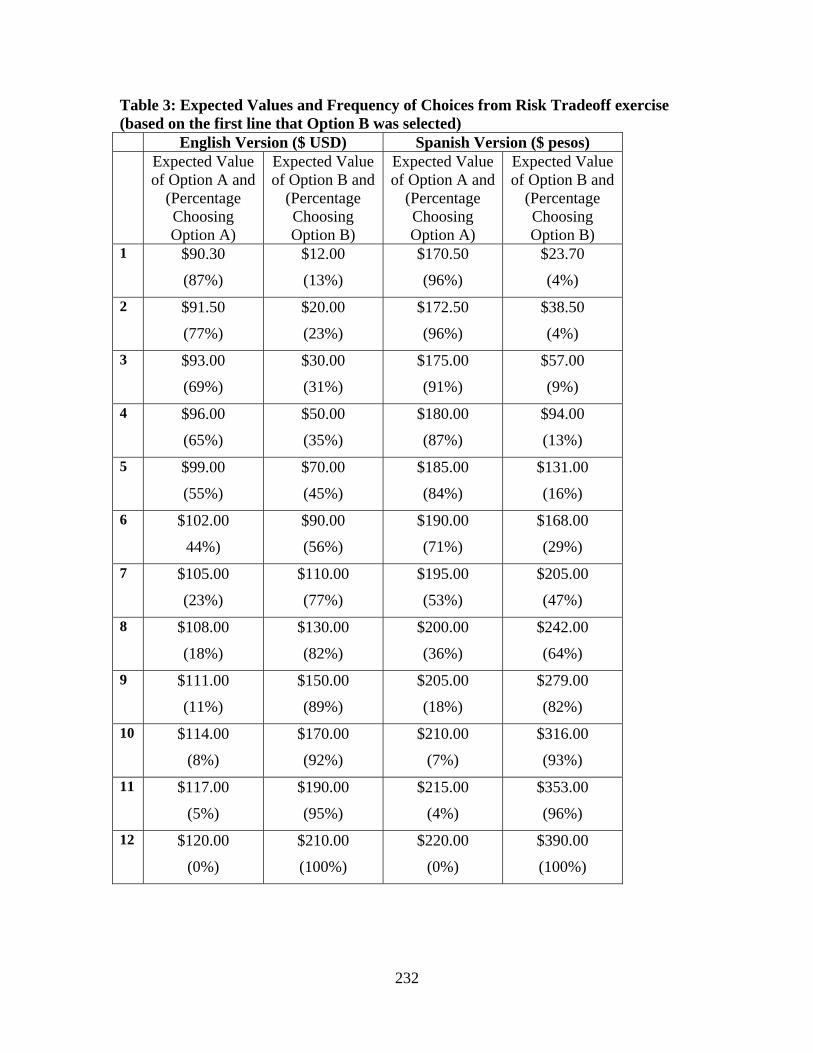
232
Table 3: Expected Values and Frequency of Choices from Risk Tradeoff exercise (based on the first line that Option B was selected) English Version ($ USD) Spanish Version ($ pesos) Expected Value
of Option A and (Percentage Choosing Option A)
Expected Value of Option B and
(Percentage Choosing Option B)
Expected Value of Option A and
(Percentage Choosing Option A)
Expected Value of Option B and
(Percentage Choosing Option B)
1 $90.30
(87%)
$12.00
(13%)
$170.50
(96%)
$23.70
(4%) 2 $91.50
(77%)
$20.00
(23%)
$172.50
(96%)
$38.50
(4%) 3 $93.00
(69%)
$30.00
(31%)
$175.00
(91%)
$57.00
(9%) 4 $96.00
(65%)
$50.00
(35%)
$180.00
(87%)
$94.00
(13%) 5 $99.00
(55%)
$70.00
(45%)
$185.00
(84%)
$131.00
(16%) 6 $102.00
44%)
$90.00
(56%)
$190.00
(71%)
$168.00
(29%) 7 $105.00
(23%)
$110.00
(77%)
$195.00
(53%)
$205.00
(47%) 8 $108.00
(18%)
$130.00
(82%)
$200.00
(36%)
$242.00
(64%) 9 $111.00
(11%)
$150.00
(89%)
$205.00
(18%)
$279.00
(82%) 10 $114.00
(8%)
$170.00
(92%)
$210.00
(7%)
$316.00
(93%) 11 $117.00
(5%)
$190.00
(95%)
$215.00
(4%)
$353.00
(96%) 12 $120.00
(0%)
$210.00
(100%)
$220.00
(0%)
$390.00
(100%)
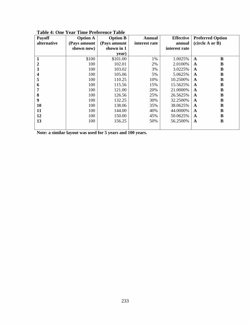
233
Table 4: One Year Time Preference Table Payoff alternative
Option A (Pays amount
shown now)
Option B (Pays amount
shown in 1 year)
Annual interest rate
Effective annual
interest rate
Preferred Option (circle A or B)
1 2 3 4 5 6 7 8 9 10 11 12 13
$100 100 100 100 100 100 100 100 100 100 100 100 100
$101.00 102.01 103.02 105.06 110.25 115.56 121.00 126.56 132.25 138.06 144.00 150.00 156.25
1% 2% 3% 5%
10% 15% 20% 25% 30% 35% 40% 45% 50%
1.0025% 2.0100% 3.0225% 5.0625%
10.2500% 15.5625% 21.0000% 26.5625% 32.2500% 38.0625% 44.0000% 50.0625% 56.2500%
A B A B A B A B A B A B A B A B A B A B A B A B A B
Note: a similar layout was used for 5 years and 100 years.
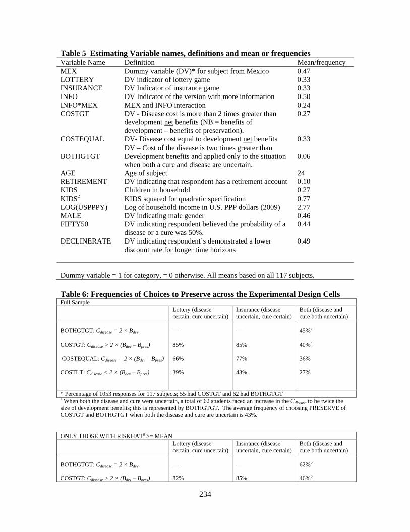
234
Table 5 Estimating Variable names, definitions and mean or frequencies Variable Name Definition Mean/frequency MEX LOTTERY INSURANCE INFO INFO*MEX COSTGT COSTEQUAL BOTHGTGT AGE RETIREMENT KIDS KIDS2 LOG(USPPPY) MALE FIFTY50 DECLINERATE
Dummy variable (DV)* for subject from Mexico DV indicator of lottery game DV Indicator of insurance game DV Indicator of the version with more information MEX and INFO interaction DV - Disease cost is more than 2 times greater than development net benefits (NB = benefits of development – benefits of preservation). DV- Disease cost equal to development net benefits DV – Cost of the disease is two times greater than Development benefits and applied only to the situation when both a cure and disease are uncertain. Age of subject DV indicating that respondent has a retirement account Children in household KIDS squared for quadratic specification Log of household income in U.S. PPP dollars (2009) DV indicating male gender DV indicating respondent believed the probability of a disease or a cure was 50%. DV indicating respondent’s demonstrated a lower discount rate for longer time horizons
0.47 0.33 0.33 0.50 0.24 0.27 0.33 0.06 24 0.10 0.27 0.77 2.77 0.46 0.44 0.49
Dummy variable = 1 for category, = 0 otherwise. All means based on all 117 subjects. Table 6: Frequencies of Choices to Preserve across the Experimental Design Cells Full Sample Lottery (disease
certain, cure uncertain) Insurance (disease uncertain, cure certain)
Both (disease and cure both uncertain)
BOTHGTGT: Cdisease = 2 × Bdev COSTGT: Cdisease > 2 × (Bdev – Bpres) COSTEQUAL: Cdisease = 2 × (Bdev – Bpres) COSTLT: Cdisease < 2 × (Bdev – Bpres)
— 85% 66% 39%
— 85% 77% 43%
45%a
40%a 36%
27%
* Percentage of 1053 responses for 117 subjects; 55 had COSTGT and 62 had BOTHGTGT a When both the disease and cure were uncertain, a total of 62 students faced an increase in the Cdisease to be twice the size of development benefits; this is represented by BOTHGTGT. The average frequency of choosing PRESERVE of COSTGT and BOTHGTGT when both the disease and cure are uncertain is 43%. ONLY THOSE WITH RISKHATa >= MEAN Lottery (disease
certain, cure uncertain) Insurance (disease uncertain, cure certain)
Both (disease and cure both uncertain)
BOTHGTGT: Cdisease = 2 × Bdev COSTGT: Cdisease > 2 × (Bdev – Bpres)
— 82%
— 85%
62%b
46%b
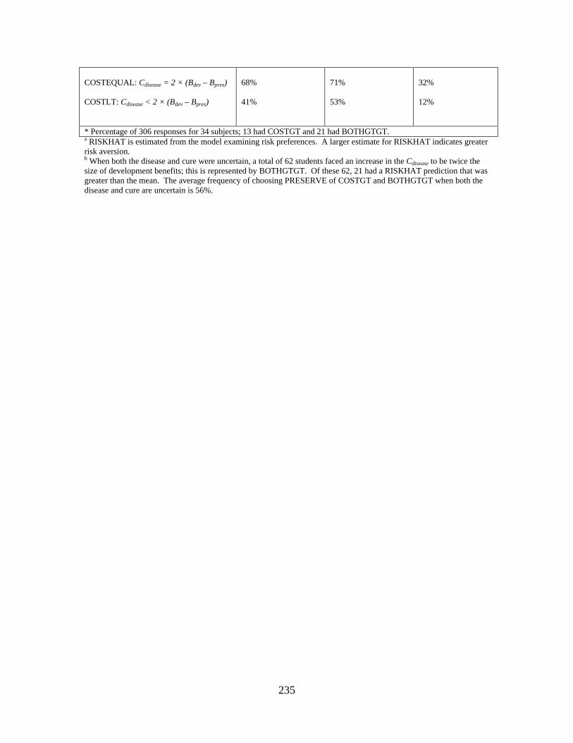
235
COSTEQUAL: Cdisease = 2 × (Bdev – Bpres) COSTLT: Cdisease < 2 × (Bdev – Bpres)
68% 41%
71% 53%
32% 12%
* Percentage of 306 responses for 34 subjects; 13 had COSTGT and 21 had BOTHGTGT. a RISKHAT is estimated from the model examining risk preferences. A larger estimate for RISKHAT indicates greater risk aversion. b When both the disease and cure were uncertain, a total of 62 students faced an increase in the Cdisease to be twice the size of development benefits; this is represented by BOTHGTGT. Of these 62, 21 had a RISKHAT prediction that was greater than the mean. The average frequency of choosing PRESERVE of COSTGT and BOTHGTGT when both the disease and cure are uncertain is 56%.
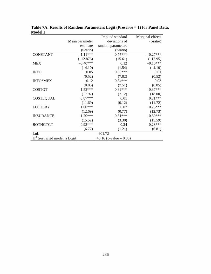
236
Table 7A: Results of Random Parameters Logit (Preserve = 1) for Panel Data, Model I
Mean parameter estimate (t-ratio)
Implied standard deviations of
random parameters (t-ratio)
Marginal effects (t-ratio)
CONSTANT –1.11*** (–12.876)
0.77*** (15.61)
–0.27*** (–12.95)
MEX –0.40*** (–4.10)
0.12 (1.54)
–0.10*** (–4.10)
INFO 0.05 (0.52)
0.60*** (7.82)
0.01 (0.52)
INFO*MEX 0.12 (0.85)
0.84*** (7.51)
0.03 (0.85)
COSTGT 1.52*** (17.97)
0.82*** (7.12)
0.37*** (18.00)
COSTEQUAL 0.87*** (11.69)
0.01 (0.12)
0.21*** (11.72)
LOTTERY 1.00*** (12.69)
0.07 (0.77)
0.25*** (12.73)
INSURANCE 1.20*** (15.52)
0.31*** (3.30)
0.30*** (15.59)
BOTHGTGT 0.93*** (6.77)
0.24 (1.21)
0.23*** (6.81)
LnL –601.72 Π2 (restricted model is Logit) 45.16 (p-value = 0.00)
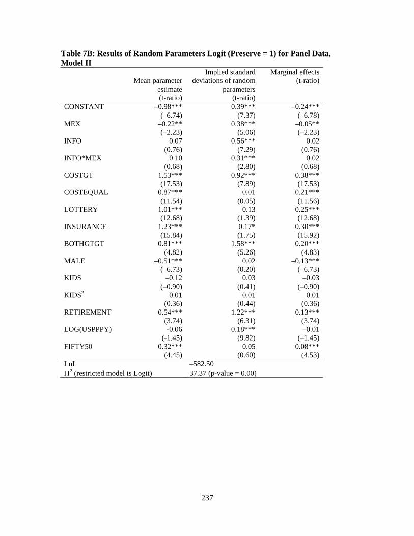
237
Table 7B: Results of Random Parameters Logit (Preserve = 1) for Panel Data, Model II
Mean parameter estimate (t-ratio)
Implied standard deviations of random
parameters (t-ratio)
Marginal effects (t-ratio)
CONSTANT –0.98*** (–6.74)
0.39*** (7.37)
–0.24*** (–6.78)
MEX –0.22** (–2.23)
0.38*** (5.06)
–0.05** (–2.23)
INFO 0.07 (0.76)
0.56*** (7.29)
0.02 (0.76)
INFO*MEX 0.10 (0.68)
0.31*** (2.80)
0.02 (0.68)
COSTGT 1.53*** (17.53)
0.92*** (7.89)
0.38*** (17.53)
COSTEQUAL 0.87*** (11.54)
0.01 (0.05)
0.21*** (11.56)
LOTTERY 1.01*** (12.68)
0.13 (1.39)
0.25*** (12.68)
INSURANCE 1.23*** (15.84)
0.17* (1.75)
0.30*** (15.92)
BOTHGTGT 0.81*** (4.82)
1.58*** (5.26)
0.20*** (4.83)
MALE –0.51*** (–6.73)
0.02 (0.20)
–0.13*** (–6.73)
KIDS –0.12 (–0.90)
0.03 (0.41)
–0.03 (–0.90)
KIDS2 0.01 (0.36)
0.01 (0.44)
0.01 (0.36)
RETIREMENT 0.54*** (3.74)
1.22*** (6.31)
0.13*** (3.74)
LOG(USPPPY) -0.06 (-1.45)
0.18*** (9.82)
–0.01 (–1.45)
FIFTY50 0.32*** (4.45)
0.05 (0.60)
0.08*** (4.53)
LnL –582.50 Π2 (restricted model is Logit) 37.37 (p-value = 0.00)

238
238
Table 7C: Results of Random Parameters Logit (Preserve = 1) for Panel Data, Model III
Mean parameter estimate (t-ratio)
Implied standard deviations of random
parameters (t-ratio)
Marginal effects (t-ratio)
CONSTANT –5.06*** (–2.64)
0.05 (1.01)
–1.25*** (–2.64)
MEX –0.22** (–2.15)
0.15** (2.00)
–0.05** (–2.15)
INFO 0.08 (0.79)
0.47*** (6.15)
0.02 (0.79)
INFO*MEX 0.08 (0.58)
0.13 (1.22)
0.02 (0.58)
COSTGT 1.53*** (17.54)
0.90*** (7.72)
0.38*** (17.55)
COSTEQUAL 0.87*** (11.55)
0.01 (0.07)
0.21*** (11.57)
LOTTERY 1.01*** (12.68)
0.07 (0.76)
0.25*** (12.68)
INSURANCE 1.23*** (15.90
0.09 (0.98)
0.30*** (15.95)
BOTHGTGT 0.79*** (4.45)
1.91*** (5.60)
0.19*** (4.45)
MALE –0.49*** (–6.39)
0.01 (0.11)
–0.12*** (–6.39)
KIDS –0.24 (–1.60)
0.10 (1.59)
–0.06 (–1.60)
KIDS2 0.03 0.88)
0.01 (0.17)
0.01 (0.88)
RETIREMENT 0.51*** (3.47)
1.64*** (7.66)
0.13*** (3.47)
LOG(USPPPY) –0.10** (–2.23)
0.08*** (4.49)
–0.02** (–2.23)
FIFTY50 0.34*** (4.68)
0.02 (0.22)
0.08*** (4.77)
RISKHAT 0.09** (2.16)
0.01*** (12.33)
0.02** (2.16)
LnL –582.01 Π2 (restricted model is Logit) 38.35 (p-value = 0.00)
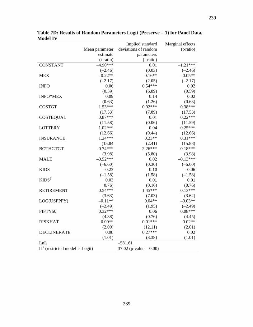
239
239
Table 7D: Results of Random Parameters Logit (Preserve = 1) for Panel Data, Model IV
Mean parameter estimate (t-ratio)
Implied standard deviations of random
parameters (t-ratio)
Marginal effects (t-ratio)
CONSTANT –4.90*** (–2.46)
0.01 (0.03)
–1.21*** (–2.46)
MEX –0.22** (–2.17)
0.16** (2.05)
–0.05** (–2.17)
INFO 0.06 (0.59)
0.54*** (6.89)
0.02 (0.59)
INFO*MEX 0.09 (0.63)
0.14 (1.26)
0.02 (0.63)
COSTGT 1.53*** (17.53)
0.92*** (7.89)
0.38*** (17.53)
COSTEQUAL 0.87*** (11.58)
0.01 (0.06)
0.22*** (11.59)
LOTTERY 1.02*** (12.66)
0.04 (0.44)
0.25*** (12.66)
INSURANCE 1.24*** (15.84
0.23** (2.41)
0.31*** (15.88)
BOTHGTGT 0.74*** (3.98)
2.26*** (5.80)
0.18*** (3.98)
MALE –0.52*** (–6.60)
0.02 (0.30)
–0.13*** (–6.60)
KIDS –0.23 (–1.58)
0.10 (1.58)
–0.06 (–1.58)
KIDS2 0.03 0.76)
0.01 (0.16)
0.01 (0.76)
RETIREMENT 0.54*** (3.63)
1.45*** (7.03)
0.13*** (3.62)
LOG(USPPPY) –0.11** (–2.49)
0.04** (1.95)
–0.03** (–2.49)
FIFTY50 0.32*** (4.38)
0.06 (0.76)
0.08*** (4.45)
RISKHAT 0.09** (2.00)
0.01*** (12.11)
0.02** (2.01)
DECLINERATE 0.08 (1.01)
0.27*** (3.38)
0.02 (1.01)
LnL –581.61 Π2 (restricted model is Logit) 37.02 (p-value = 0.00)

240
240
Figure 1: Game Against Nature Note: Bdev, Bpres, and Cdisease represent the benefits of development, the benefits of preservation, and the cost of the disease, respectively. The Regrets Matrix No Disease Disease/Cure Disease/No Cure Development Bdev – Bpres (Bdev – Cdisease) – Bpres (Bdev – Cdisease) – (Bpres – Cdisease) Preservation Bpres – Bdev Bpres – (Bdev – Cdisease) (Bpres – Cdisease) – (Bdev – Cdisease) (Cells in gray are the maximum in absolute values) Source: Goodstein, 2008 (adapted from Palmini, 1999)
Development
Preservation
No Disease
No Disease
Disease
Disease
No Cure
Cure
Outcomes Bdev
Bdev – Cdisease
Bpres
Bpres – Cdisease
Bpres
State of Nature
241
241
References Anderson L, Mellor J (2008) Predicting health behaviors with experimental measures of risk preference. Journal of Health Economics 27:1260-1274. Andersen S, Harrison G W, Lau M I, Rutström E E (2006) Elicitation using Multiple Price List formats. Experimental Economics 9: 383-405. Andersen S, Harrison G W, Lau M, Rutström E (2008) Eliciting Risk and Time Preferences. Econometrica 76: 583-618. Arrow K, Daily G, Dasgupta P, Levin S, Maler K G, Maskin E, Starrett D, Sterner T, Tietenberg T (2000) Managing ecosystem services. Environmental Science and Technology 34:1401-1406. Atkinson G, Dietz S, Neumayer E (2007) Introduction. In: Atkinson G, Dietz S, Neumayer E (Eds) Handbook of Sustainable Development. Edward Elgar, Cheltenham UK, p 1-26. Berrens R (2001) The safe minimum standard of conservation and endangered species: a review. Environmental Conservation 28(2):104-116. Berrens R, Brookshire D, McKee M, Schmidt C (1998) Implementing the safe minimum standard approach: Two case studies from the U.S. Endangered Species Act. Land Economics 74:147-161. Berrens R, McKee M, Farmer M (1999) Incorporating distributional considerations in the safe minimum standard approach: endangered species and local impacts. Ecological Economics 30:461-474. Bishop R (1978) Endangered species, irreversibility, and uncertainty: the economics of a safe minimum standard. American Journal of Agricultural Economics 60:10-18. Bishop R (1980) Endangered species: An Economic Perspective. Transactions of the North American Wildlife Conference 45:208-218. Boyle K J, Bishop R C (1987) Valuing Wildlife in Benefit-Cost Analyses: A Case Study Involving Endangered Species. Water Resources Research 23(5):943-50. Brewer S J (1993) Search and discovery of plant-derived bioactive chemicals at Monsanto-Searle. Testimony to the Subcommittee on Environment and Natural Resources, Committee on Merchant Marine and Fisheries, US Congress, House of Representatives Ser. No. 103-74, 9 November 1993, p 35–41.

242
242
Castle E (1996) Pluralism and pragmatism in the pursuit of sustainable development. In: Adamowicz W, Boxall P, Luckert M, Phillips W, White W (Eds) Forestry, Economics and the Environment. CAB International, Wallingford UK, pp 1-9. Castle E, Berrens R (1993) Economic analysis, endangered species, and the safe minimum standard. Northwest Environmental Journal 9:108-130. Chesson H, Viscusi W K (2000) The Heterogeneity of Time-risk Tradeoffs. Journal of Behavioral Decision Making 13(2):251-58. Chetan D, Eckel C, Johnson C, Rojas C (2008) Eliciting Risk Preferences: When is Simple Better? Discussion paper, U of Texas-Dallas. Ciriacy-Wantrup S V (1968) Resource Conservation: Economics and Policies 3rd ed. (1st ed. 1952). University of California Press, Berkeley, CA. Cole D (2008) The Stern Review and Its Critics: Implications for the Theory and Practice of Benefit Cost Analysis. Natural Resources Journal 48(1):53-90. Coller M, Williams M B (1999) Eliciting Individual Discount Rates. Experimental Economics 2:107-27. Cummings R, Martinez-Vazquez J, McKee M, Torgler B (2009) Tax morale affects tax compliance: Evidence from surveys and an artefactual field experiment. Journal of Economic Behavior and Organization 70:447-457. Farmer M, Randall A (1998) The rationality of a safe minimum standard of conservation. Land Economics 74:287-302. Farnsworth N R (1990) The role of ethnopharmacology in drug development. In: Chadwick D J, Marsh J (Eds.) Bioactive Compounds from Plants. Ciba Foundation Symposium 154, pp 2–11. Ferraro P, McIntosh C, Opsina M (2007) The effectiveness of the US endangered species act: An econometric analysis using matching methods. Journal of Environmental Economics and Management 54(3):245-262. Frederick S, Loewenstein G, O’Donoghue T (2002) Time Discounting and Time Preference: A Critical Review. Journal of Economic Literature XL: 351-401. Fuchs V R (1986) Time Preference and Health. In: Fuchs V R (ed.) The Health Economy. Harvard University Press, Cambridge MA, pp 214-42. Gilboa I, Schmeidler D (1989) Maxmin Expected Utility with a Non-Unique Prior. Journal of Mathematical Economics 18:141-53.

243
243
Gollier C, Treich N (2003) Decision-making Under Scientific Uncertainty: The Economics of the Precautionary Principle. Journal of Risk and Uncertainty 27(1): 77-103. Gollier C, Jullien B, Treich N (2000) Scientific Progress and Irreversibility: an Economic Interpretation of the Precautionary Principle. Journal of Public Economics 75:229-53. Goodstein, E (2008). Game Theory and the Safe Minimum Standard Appendix 7A. In: Economics and the Environment 5th edn. John Wiley & Sons, Hoboken NJ, p 139. Greenstone M, Gayer, T (2009) Quasi-experimental and experimental approaches to environmental economics. Journal of Environmental Economics and Management 57:21-44.
Hagen D, Vincent J, Welle P (1992) Benefits of Preserving Old-Growth Forests and the Spotted Owl. Contemporary Policy Issues 10:13-26.
Harrison G W, Rutström E E (2008) Risk Aversion in the laboratory. In: Cox J, Harrison G W (eds) Research in Experimental Economics 12:41-196. Holt C A, Laury S K (2002). Risk Aversion and Incentive Effects. American Economic Review 92(5):1644-5. Knight F (1921) Risk, Uncertainty, and Profit. Hart, Schaffner, and Marx, Boston MA. Laury S, Taylor L (2008) Altruism Spillovers: Are Behaviors in Context-Free Experiments Predictive of Altruism toward a Naturally Occurring Public Good? Journal of Economic Behavior and Organization 65:9-29. LeRoy, S. and L.D. Singell (1987) Knight on Risk and Uncertainty. Journal of Political Economy 95 (2): 394-406. Li H, Rosenzweig M, Zhang J (2008) Altruism, Favoritism, and Guilt in the Allocation of Family Resources: Sophie’s Choice in Mao’s Mass Send Down Movement. Working paper No. 54, Yale University. List J A, Margolis M, Osgood D E (2006) Is the Endangered Species Act Endangering Species? NBER working paper #12777. Loomis J, Ekstrand E (1997) Economic Benefits of Critical Habitat for the Mexican Spotted Owl: A Scope Test Using a Multiple-Bounded Contingent Valuation Survey. Journal of Agricultural and Resource Economics 22(2):356-66. Loomis J B, White D S (1996). Economic Benefits of Rare and Endangered Species: Summary and Meta-Analysis. Ecological Economics 18:197-206.

244
244
Lovejoy T (1993) Statement to the Subcommittee on Environment and Natural Resources, Committee on Merchant Marine and Fisheries, US Congress, House of Representatives Ser. No. 103-74, 9 November 1993, pp 3–5. Margolis M, Naevdal E (2008) Safe Minimum Standards in Dynamic Resource Problems: Conditions for Living on the Edge of Risk. Environmental and Resource Economics 40:401-23. McIntosh C R, Shogren J F, Finnoff D C (2007) Invasive Species and Delaying the Inevitable: Results from a Pilot Valuation Experiment. Journal of Agricultural and Applied Economics 39: 81-93. Milnor J (1964) Games against nature. In: Shubik M (ed) Game Theory and Related Approaches to Social Behavior. Wiley Press, New York City NY, pp 20-31. National Wildlife Federation (2006) Medicinal Benefits of Endangered Species. Http://www.nwf.org/wildlife/pdfs/medicinalbenefits9-06.pdf. Cited 8 December 2009. Norton B, Toman M (1997) Sustainability: Ecological and economic Perspectives. Land Economics 73:553-585. Palmini D (1999) Uncertainty, risk aversion, and the game theoretic foundations of the safe minimum standard: a reassessment. Ecological Economics 29:463-472. Randall A (1991) The value of biodiversity. Ambio 21:63-68 Randall A (2007) Benefit-Cost Analysis and a Safe Minimum Standard of Conservation. In: Atkinson G, Dietz S, Neumayer E (Eds) Handbook of Sustainable Development. Edward Elgar, Cheltenham, UK, pp 91-108. Randall A (2009) We already have risk management -- Do we really need the precautionary principle? International Review of Environmental and Resource Economics 3(1):39-74. Randall A, Farmer M (1995) Benefits, costs and a safe minimum standard of conservation. In: Bromley D(ed) Handbook of Environmental Economics, Blackwell, Oxford UK, pp 26-44. Ready R C, Bishop R C (1991) Endangered species and the safe minimum Standard. American Journal of Agricultural Economics 73:309-12. Richardson L, Loomis J (2009) The Total Economic Value of Threatened, Endangered and Rare Species: An Updated Meta-analysis. Ecological Economics 68(2):1535-1548. Rosen, S. 1988. “The Value of Changes in Life Expectancy.” J. of Risk and Uncertainty 1: 285-304.

245
245
Rubin J, Helfand G, Loomis J (1991) A benefit-cost analysis of the northern spotted owl. Journal of Forestry 90:25-29. Samples K C, Dixon J A, Gowen M M (1986) Information Disclosure and Endangered Species. Land Economics 62(3):306-312. Scott A (1999). Trust law, sustainability and responsible action. Ecological Economics 31:139-154. Shaw W D, Woodward R T (2008) Why Environmental and Resource Economists Should Care about Non-Expected Utility Models. Resource and Energy Economics 30: 66-89. Thaler R (1981) Some Empirical Evidence Dynamic Inconsistency. Economics Letters 8(3):201-07. United States Fish and Wildlife Service (2005) Why Save Endangered Species. http://www.fws.gov/endangered/pdfs/why_save_end_species_july_2005.pdf. Cited 8 December 2009. Tol R (2003) Is the uncertainty about climate change too large for expected cost- benefit analysis? Climatic Change 56(3):265-289. Viscusi W K (1990) Do Smokers Underestimate Risks. Journal of Political Economy 98(6):1253-69. Weitzman M (1998) Why the Far-Distant Future Should be Discounted at its Lowest Possible Rate. Journal of Environmental Economics and Management 36:201-08. Weitzman M (2007) The Stern Review of the Economics of Climate Change. Journal of Economic Literature 45(3):703-24. Weitzman M (2009) On modeling and interpreting the economics of catastrophic climate change. Review of Economics and Statistics 91(1):1-19. Woodward R T, Bishop R C (1997) How to Decide When Experts Disagree: Uncertainty-Based Choice Rules in Environmental Policy. Land Economics 73(4):492-507. Wubben M J J, Cremer D, Van Dijk E (2009) When and How Communicated Guilt Affects Contributions in Public Good Dilemmas. Journal of Experimental Social Psychology 45:15-2.
246
What is the Value of a Trip to a National Park? Searching for a Reference Methodology
Dr. John Duffield, Dr. David Patterson, and Chris Neher Department of Mathematical Sciences
University of Montana Missoula, MT 59812
247
Abstract This paper contributes to the literature on the accuracy and reliability of primary
nonmarket valuation methods by comparing observed price response (to entrance fee
increases) at Yellowstone National Park to predicted price response based on several
alternative stated preference methods. We implement a 2 x 2 experimental design with
payment card and dichotomous choice question format and travel cost and entry fee
payment vehicles. The data is from a 2005 survey of Yellowstone National Park visitors
with 1,512 completed surveys and a 64.4% response rate. Based on a censored regression
model, we find that the payment vehicle effect is consistently greater than the elicitation
format effect across three independent (spring, summer, fall) samples. Significant
differences in welfare estimates were identified across both payment vehicle and question
format. For example, median per trip values per travel group for the summer 2005 sample
are $27 for payment card/entry fee, $110 for payment card/travel cost, $76 for
dichotomous choice/entry fee, and $304 for dichotomous choice/travel cost. We test the
hypothesis that the observed price response and the predicted price response (for each
method) are the same. The null hypothesis is rejected for both of the methods using the
entry fee payment vehicle.
Keywords: nonmarket valuation, recreation, contingent valuation, elicitation format,
validation, national parks
JEL classification: D61, Q51, Q25.
248
Introduction
This paper contributes to the literature on the accuracy and reliability of primary
nonmarket valuation methods by comparing observed price response (to entrance fee
increases) at Yellowstone National Park to predicted price response based on several
commonly applied stated preference methods. We implement a 2x2 experimental design
that compares the payment card and dichotomous choice question formats and a travel
cost and entry fee payment vehicle on a 2005 sample of Yellowstone National Park
visitors. The price response from these four models is compared to the observed response
for an increase (actually a doubling) in the entry fee to Yellowstone National Park
(implemented in January 1997) from $10 to $20 per vehicle.
One motivation for this paper is that the economics literature reports a several orders of
magnitude range in estimated willingness to pay (WTP) for visits to national parks, from
around $7 to in excess of $700 (Kaval and Loomis 2003). While some of this difference
can likely be attributed to differences in the visitor populations and length and quality of
the visit experience across parks, benefit transfer functions fitted to these the available
estimates for NPS sites (Duffield, Patterson, Neher, and Loomis 2010), as well as for
other recreation sites (Rosenberger and Loomis 2001), indicate that methodology is the
primary factor explaining the variation in WTP. To the extent variation in WTP is driven
by methods, this obscures the effects of the covariates that would be of greatest utility for
benefit transfer: core economic variables (Bergstrom and Taylor 2006) and site

249
characteristics. Going forward, it would be very useful to public agencies to identify a
reference or standard methodology that could be consistently applied in future work. This
is, in fact, the strategy of the U.S. Fish and Wildlife Service in its National Survey of
Fishing, Hunting and Wildlife-related Recreation. However, there has been no systematic
use of a consistent methodology for the valuation of National Park visits or visits to the
National Forest system.
We test several key methodological design elements for stated preference: question
format and payment vehicle. There is a substantial economics literature that compares the
influence of these methodological choices on welfare estimates. Champ and Bishop
(2006) review some of this literature. However, to our knowledge, there has been no
previous study that controls for both influences. The literature is also thin with respect to
validation of nonmarket methods by comparison to actual market price or quality
changes. Bishop and Heberlein (1979) provide one example; Ready (2003) provides a
more recent paper and cites other related literature.
Specifically with respect to payment vehicle, it has long been thought that entry fees
might elicit responses having more to do with perception of a “reasonable” entry fee
(perhaps based on actual fees at substitute sites) than with measuring WTP (Mitchell and
Carson 1989). Nonetheless, this payment vehicle is still applied; an example of a recent
application is Leggett et al. (2003), where the WTP for visiting Fort Sumpter National
Historic Park is reported to be $8.26 for a payment card question format and an entry fee
payment vehicle. (Parenthetically, in this study’s pretest, the dichotomous choice

250
question format was used with an entry fee vehicle and estimated WTP averaged across
modes of survey administraton was $14.19). Is $8.26 per visit to Fort Sumpter a
meaningful estimate?
The NPS fee demonstration experiment, which began in January 1997, implemented very
substantial changes in entry fees at selected parks. These fee changes provide an
opportunity to compare state preference methods with observed price response. At
Yellowstone, as an example, the standard 7-day entry fee per vehicle was doubled and
increased from $10 to $20.
Several Yellowstone visitor surveys that included nonmarket valuation, one
implemented in 1998-1999 and another in 2005, provide data sets to compare observed
and predicted price response. In this paper we focus on the 2005 data. The 2005 survey
was a unique year long probability sample conducted at entrance stations using Dillman
methods, with a total of 2,406 surveys distributed, 59 undeliverable, and 1,512 completes
for an overall response rate of 64.4%. A 2x2 design was implemented to test both
question format (contingent valuation and payment card) and payment vehicle (entry fee
and travel cost). A censored regression model was estimated using a maximum likelihood
interval approach, which supported pooling the payment card and dichotomous choice
data. Significant differences in welfare estimates based on this model were identified
across both payment vehicle and question format; as described below the estimates vary
across methods (combined effect of payment vehicle and elicitation format) by an order

251
of magnitude. Which of these estimates (if any) tells us the truth about the value of a visit
to Yellowstone?
With respect to observed price response, total visitation to Yellowstone dropped by about
4% in 1997 relative to 1996. However, use rebounded to 1996 levels the following year.
A regression model was fit to time-series visitation for Yellowstone and a parameter was
estimated for trend and a post-price change indicator variable. We test the hypothesis that
the observed price response and the predicted price response (for each model) are the
same (2009).
The primary contributions of this paper are: 1) testing for both question format and
payment vehicle effects using widely applied nonmarket valuation methods on three
independent samples, 2) comparing price response from nonmarket models to observed
price response for a nationally significant recreation resource, and 3) demonstration of a
model that pools payment card and dichotomous choice responses and measures the
relative effect of these two design elements.
Methods
Nonmarket valuation models for visitor trips to Yellowstone National Park were
estimated using the contingent valuation method (Champ, Boyle, and Brown 2003.).
Observed price response was based on the observed change in Yellowstone National Park
visitation in 1997 relative to 1996, and from a fitted time series model with an indicator

252
variable for years 1997 and after. We test the hypothesis that the observed price response
and nonmarket methods predicted price response are significantly different. Because the
survey was implemented after the observed price change in 1997 from $10 to $20, with
the survey we explore the next nearest $10 increment, which for the entry fee payment
vehicle is from $20 to $30, and for the travel cost payment vehicle is a $10 increment.
The specific null hypothesis tested depend on the assumed shape of the demand function:
1) if linear demand, observed price response equals predicted: Ho: Q obs = Q model
or 2) if demand is convex to origin, observed greater than predicted: Ho: Q obs ≥ Q
model.
In contingent valuation potential respondents are asked about their willingness to pay for
the particular service at issue. For current trip values, several question formats
(dichotomous choice and payment card) and payment vehicles (travel cost and entrance
fee) were used to examine the impact of survey methodology on estimated values. The
estimation of willingness to pay models was implemented using a maximum likelihood
interval approach (Welsh and Poe 1998; Cameron and Huppert 1989).
Respondents were asked to choose the highest amount he or she was willing to pay from
a list of possible amounts. It was inferred that the respondent’s true willingness to pay
was some amount located in the interval between the amount the respondent chose and
the next highest amount presented. Let X iL be the maximum amount that the ith person
would be willing to pay and X iU be the lowest presented amount that person would not

253
pay. Given this, WTP (willingness to pay) must lie in the interval [ ]X XiL iU, If
( )F X i ;β is the statistical distribution function for WTPi, with parameter vector β
then the probability that WTPi lies between two given payment bid amounts is
( ) ( )F X F XiU iL; ;β β− and the associated log-likelihood function is:
( ) ( )[ ]ln( ) ln ; ;L F X F XiU iLi
n= −
=∑ β β1
The SAS statistical procedure LIFEREG was used to estimate the parametric model of
willingness to pay based on the underlying payment card responses.
The survey instrument included an initial section that queried the respondent on the
current trip to Yellowstone including activities, previous experience, and preferences. A
following section included questions on trip expenditures and the contingent valuation
questions; the last section collected socio-economic data on the respondent. The actual
wording of the valuation questions are included in Appendix A.
Data Collection
The 2005 Yellowstone National Park Visitor Survey was a year-long survey of park
visitors. The overall focus of the survey was on the economic impact of wolf recovery

254
(Duffield, Neher and Patterson 2008), however the survey was also used as an
opportunity to examine the influence of nonmarket valuation methodology. This survey
had two distinct target populations: 1) all park visitors entering through park entrances,
and 2) park visitors who were stopped along the road within the portion of the Lamar
valley most commonly associated with wolf watching. The focus here is on the sample
of all park visitors contacted at entrance stations.
The 2005 Yellowstone Visitor Survey was designed as a year-long random survey of
park visitors. The primary target population for the 2005 survey was the year-round
population of Yellowstone National Park visitors. The sampling plan for this group was
designed to survey a generally equal number of park visitors at park entry gates in each of
the four seasons. In order to achieve this, the sampling interval was adjusted for each
season to account for the very large differences in total park visitation in the different
seasons. The goal of balanced sample sizes across seasons was chosen to yield sample
sizes in non-summer seasons that would allow meaningful comparison of trip and visitor
characteristics across seasons.
Sampling allocation and sampling intervals were based on total park recreational
visitation, as estimated by the NPS, totaling approximately 2.8 million visitors. The vast
majority of those visitors (almost 2 million) visited during the three summer months of
June, July, and August. The 2004 Yellowstone National Park visitation was used as a
basis for both allocating survey effort throughout the survey year, and for weighting final
survey responses to more closely represent the distribution of actual visitation across

255
seasons and entrances. The procedure followed in administering the survey included a 4-
step process.
1. Yellowstone entrance station personnel (and Lamar survey personnel), following
a specified schedule and sampling interval would intercept visitors and ask them
to participate in the survey. Those who agreed were asked to supply their name
and mailing information. This information was collected by the park personnel
and periodically forwarded to the researchers in Missoula, MT.
2. The visitor contact information was entered into a database and an initial survey
mailing was made including an explanatory letter, survey booklet, and postage
paid return envelope.
3. Following the Dillman (2001) survey procedure, a reminder postcard was sent to
respondents approximately one week after the survey.
4. A second complete survey package was mailed to those visitors who had not
responded to the first two mailings
Based on previous survey experience with this population, and the desire to minimize
survey costs, it was anticipated that a good response rate could be achieved with just the
three Dillman-method contacts and no financial incentive. There were 12 survey waves in
total over the survey year which began on December 18, 2004 and ran through December
17, 2005 for the park entrance sample. A total of 2,406 surveys were mailed, 59 were
undeliverable, and 1,512 were returned for an overall response rate of 64.4%.
Parenthetically, survey response rates were significantly higher for visitors contacted in
256
the Lamar Valley sample than for the general entrance station contacts. This likely
reflects the greater interest the Lamar respondents had in the primary subject of the
survey (wolf presence in the park). Overall, approximately 74% of visitors in the Lamar
sample responded to the survey while 64% of visitors in the entrance station sample
returned completed surveys. Because of changes in entrance procedures for winter
visitors (primarily snowmobile riders), the winter sample goal was not achieved.
However, the target samples for spring, summer and fall were achieved and make for an
interesting data set that can be used to test hypothesis relating to elicitation format and
payment vehicle on not one, but three independent samples.
While every effort was made to gather a sample of Yellowstone National Park visitation
which mirrored the actual distribution of recreational visitation to the park in 2005,
variations in distribution and response rates across months and entrances led to some over
and under sampling of visitors during certain periods and at certain entrances. Prior to
analyzing the survey responses, the sample distribution was examined and responses
were weighted to correct for any over or under-sampling. Responses were also weighted
to correct for disproportionate probabilities of selection to participate in the survey. A
second weight for the entrance sample was constructed which considered the number of
times the respondent had entered the park on their trip, and the number of people in their
vehicle when they were sampled.
Survey responses were also analyzed for non-response bias. Gender and place of
residence was collected for all potential respondents at the entrance stations and
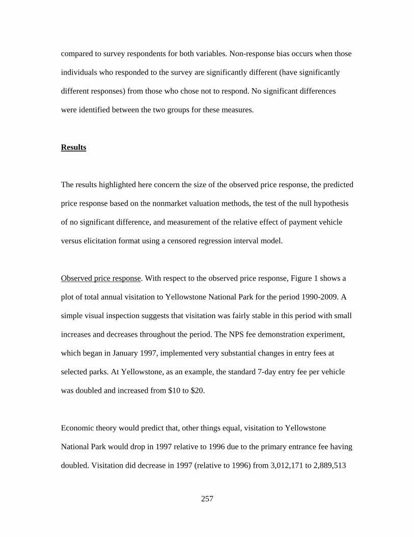
257
compared to survey respondents for both variables. Non-response bias occurs when those
individuals who responded to the survey are significantly different (have significantly
different responses) from those who chose not to respond. No significant differences
were identified between the two groups for these measures.
Results
The results highlighted here concern the size of the observed price response, the predicted
price response based on the nonmarket valuation methods, the test of the null hypothesis
of no significant difference, and measurement of the relative effect of payment vehicle
versus elicitation format using a censored regression interval model.
Observed price response. With respect to the observed price response, Figure 1 shows a
plot of total annual visitation to Yellowstone National Park for the period 1990-2009. A
simple visual inspection suggests that visitation was fairly stable in this period with small
increases and decreases throughout the period. The NPS fee demonstration experiment,
which began in January 1997, implemented very substantial changes in entry fees at
selected parks. At Yellowstone, as an example, the standard 7-day entry fee per vehicle
was doubled and increased from $10 to $20.
Economic theory would predict that, other things equal, visitation to Yellowstone
National Park would drop in 1997 relative to 1996 due to the primary entrance fee having
doubled. Visitation did decrease in 1997 (relative to 1996) from 3,012,171 to 2,889,513

258
or a decrease of 122,658 visits, a 4.1% decrease. A regression model was also fit to time-
series visitation for Yellowstone and a parameter was estimated for trend and a post-price
change indicator variable. The parameter on the price change indicator was, as theory
would predict, negative (with a value of –102,694 and a standard error of 111,062).
Based on this simple model, the fitted effect of the price change was a –3.7% decline in
visitation in the year of the price change and thereafter. The confidence interval on this
estimate includes zero (-11.0% to 4.4%).
A more complex model of this park’s visitation would include other potential covariates
such as road conditions, wildfire, visitor income, and gasoline prices. For our purposes
here, both the simple observed change and the fitted change clearly support the
proposition that the price effect of doubling entrance fees is relatively small and possibly
approaching zero. This is certainly plausible given that Yellowstone is a nationally
significant resource and that many visitors are spending more than $1,000 on primary
destination trip to visit this remarkable park, which is not only the nation’s but also the
world’s first national park. Based on the 2005 data set, the mean trip expenditure by local
(17-county Greater Yellowstone Area residents in Idaho, Montana, Wyoming) summer
visitors was $117 per travel group and $709 per travel group for non-locals. For the
summer season 94% of visitors are non-local. It is a priori unlikely that many such
visitors would be deterred from visiting by a $10 increase in the nominal entrance fee.
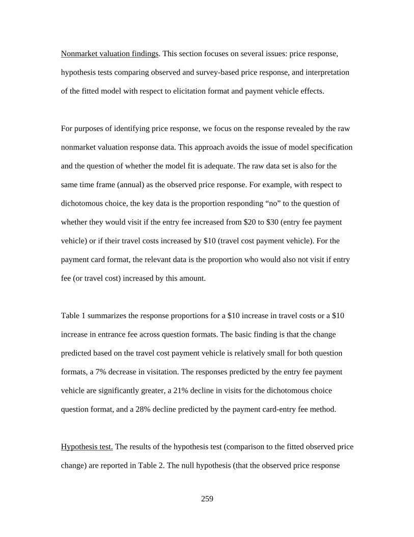
259
Nonmarket valuation findings. This section focuses on several issues: price response,
hypothesis tests comparing observed and survey-based price response, and interpretation
of the fitted model with respect to elicitation format and payment vehicle effects.
For purposes of identifying price response, we focus on the response revealed by the raw
nonmarket valuation response data. This approach avoids the issue of model specification
and the question of whether the model fit is adequate. The raw data set is also for the
same time frame (annual) as the observed price response. For example, with respect to
dichotomous choice, the key data is the proportion responding “no” to the question of
whether they would visit if the entry fee increased from $20 to $30 (entry fee payment
vehicle) or if their travel costs increased by $10 (travel cost payment vehicle). For the
payment card format, the relevant data is the proportion who would also not visit if entry
fee (or travel cost) increased by this amount.
Table 1 summarizes the response proportions for a $10 increase in travel costs or a $10
increase in entrance fee across question formats. The basic finding is that the change
predicted based on the travel cost payment vehicle is relatively small for both question
formats, a 7% decrease in visitation. The responses predicted by the entry fee payment
vehicle are significantly greater, a 21% decline in visits for the dichotomous choice
question format, and a 28% decline predicted by the payment card-entry fee method.
Hypothesis test. The results of the hypothesis test (comparison to the fitted observed price
change) are reported in Table 2. The null hypothesis (that the observed price response

260
and the predicted price response are the same) is rejected for both the payment card-entry
fee method (P< .00001) and the dichotomous choice-entry fee method (P =.0216).
Clearly a 21% or a 28% price response does not appear to have occurred between 1996
and 1997 either based on the simple observed decline of –4.1% or the fitted model
estimate of –3.4%. On the other hand, the null hypothesis for the predicted price response
from the travel cost payment vehicle (for either question format) cannot be rejected.
Censored regression interval model. To explore the influence of the alternative stated
preference methods for welfare estimates, a censored regression interval model was
successfully fitted to the pooled (across question format and payment vehicle) valuation
response data (Table 3). Parameters are highly significant for three independent samples
(spring, summer and fall seasons), including indicator variables for the payment vehicle
and elicitation format effects. A consistent finding across samples is that for our methods,
the payment vehicle effect is greater than the elicitation format effect. This is an
interesting finding given the emphasis in the literature on elicitation format, with
relatively little attention paid to payment vehicle.
A plot of predicted response probabilities across bid levels for the 2005 Yellowstone
National Park summer sample is shown in Figure 2 (for the bid range $0 to $500, the
upper limit of the entry fee bid range) and Figure 3 (for the bid range $0 to $2000,
applicable only to the travel cost payment vehicle applications). As expected, and
consistent with the previous economic literature, this figure indicates substantial
differences across both payment vehicle and question format . These differences are

261
reflected in the welfare measures. Estimates were developed for two parameters of the
WTP distributions for all three seasons, including medians (Table 3) and truncated means
(Table 4). The welfare estimates, for example for medians for summer, differ by more
than an order of magnitude from $27 for payment card/entry fee to $304 for dichotomous
choice/travel cost.
The method-specific values and ranking are relatively stable across these independent
(season specific) samples. This supports the interpretation that these are fairly robust and
stable differences.
Conclusions
This paper tested the null hypothesis that observed price response for visits to
Yellowstone National Park is the same as the price response predicted by several
commonly applied nonmarket valuation methods. These included two question formats,
dichotomous choiee and payment card, and two payment vehicles, entry fee and travel
cost. The main finding is that the null hypothesis is rejected for both of the methods using
an entry fee payment vehicle. The entry fee vehicle predicts a price response that is quite
large (20% to 28%) relative to the observed (3% to 4%) response. The null hypothesis
could not be rejected for either of the question formats used in conjunction with the travel
cost payment vehicle.

262
Another finding, consistent with the literature, is that welfare estimates vary considerably
across the methods, for example, median per trip values per travel group for the summer
2005 sample are $27 for payment card/entry fee, $110 for payment card/travel cost, $76
for dichotomous choice/entry fee, and $304 for dichotomous choice/travel cost. Which of
these estimates (if any) tells us the truth about the value of a visit to Yellowstone? It
appears that for our application welfare estimates based on an entry fee vehicle (as
suggested generally many years ago by Mitchell and Carson (1989)) may not be reliable.
By extension, other entry fee-based estimates in the literature (for example Leggett et al
(2003) estimates for Fort Sumpter) may also not be reliable. Given the consistent
direction of bias indicated by the current results, it would appear that the entry fee-based
estimates are overly conservative.
The findings also provide some support for the conclusion that the travel cost payment
vehicle used with either a payment card or dichotomous choice format are potential
candidates for use as a reference methodology in future applications.
A limitation of the study is that the observed price change preceded the nonmarket
valuation survey by eight years. This is a long enough period of time for changes in the
underlying demand. Additionally, the decision was made in study design to not correct
for inflation in the bid design and to use the same nominal price levels observed in 1997 .
However, this only strengthens the hypothesis test in that in real (constant 1997 dollars)
the $10 price change response measured in 2005 dollars understates the change in real
1997 dollar terms (about a $12 dollar interval) and would lead to even larger

263
overstatement of the price response by the entry fee payment vehicle. Another limitation
is that only a small portion of the response function is being tested, which is in the lowest
part of the bid range. This limits the strength of generalizations about the reliability of the
rest of the stated preference response functions.
There are several extensions to this work that would be useful to undertake. As indicated
earlier, a data set (limited to dichotomous choice with a travel cost payment vehicle) for
Yellowstone also is available for 1998-1999, much closer to the time of the actual price
change. It would be of interest to also test the null hypothesis for this data set and
compare to the corresponding 2005 estimates. Both the earlier and 2005 data set also
include the relevant information to support an individual travel cost model estimate. For
example, a negative binomial count data model following Shaw (1988) and recent
applications by Heberling and Templeton (2009) and Bowker et al. (2010) could be
estimated and also tested against the observed price change. These stated preference and
revealed preference methods could be compared from the standpoint of convergent
validity. Since the comparison would be feasible over the entire bid range, this would
help inform the choice of question format.
Acknowledgements
We gratefully acknowledge the financial support provided by Yellowstone Park
Foundation. Glenn Plumb was Project Director for the 2005 survey effort, and helped
coordinate NPS participation in the project. Many Yellowstone National Park staff

264
members played crucial roles in providing advice, data, personnel hours, and valuable
feedback on the project during including Doug Smith, Wayne Brewster, John Varley,
Tammy Wert, and the YNP Entrance Station Staff. We are especially indebted to Becky
Wyman for her work on the Lamar Valley data collection.

265
Table 1. 2005 Raw Data Stated Preference Response Proportions for a $10 Increase in Travel Costs or a $10 Increase in Entry Fees.
Question Format
Payment Card Dichotomous Choice
Entry Fee 89/318 = .2800 (SE=.0252)
8/39 = .2051 (SE=.0647)
Travel Cost 21/300 = .0700 (SE=.01473)
2/29 = .0690 (SE=.0471)

266
Table 2. Hypothesis Tests: Observed Price Response vs. Raw Data Predicted Response
Question Format
Observed Predicted Difference (SE)
Z P
PC-EF .0341 (.0369)
.2800 (.0252)
.2459 (.0446)
5.51 <.00001
DC-EF .0341 (.0369)
.2051 (.0647)
.1710 (.0744)
2.30 .0216
PC-TC .0341 (.0369)
.0700 (.01473)
.0331 (.0397)
0.90 .37
DC-TC .0341 (.0369)
.0690 (.0471)
.0349 (.0598)
0.58 .56
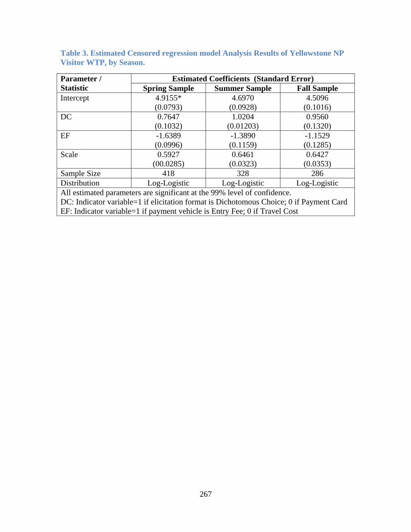
267
Table 3. Estimated Censored regression model Analysis Results of Yellowstone NP Visitor WTP, by Season.
Parameter / Statistic
Estimated Coefficients (Standard Error) Spring Sample Summer Sample Fall Sample
Intercept 4.9155* (0.0793)
4.6970 (0.0928)
4.5096 (0.1016)
DC 0.7647 (0.1032)
1.0204 (0.01203)
0.9560 (0.1320)
EF -1.6389 (0.0996)
-1.3890 (0.1159)
-1.1529 (0.1285)
Scale 0.5927 (00.0285)
0.6461 (0.0323)
0.6427 (0.0353)
Sample Size 418 328 286 Distribution Log-Logistic Log-Logistic Log-Logistic All estimated parameters are significant at the 99% level of confidence. DC: Indicator variable=1 if elicitation format is Dichotomous Choice; 0 if Payment Card EF: Indicator variable=1 if payment vehicle is Entry Fee; 0 if Travel Cost
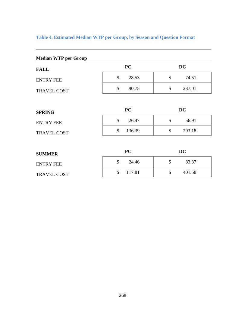
268
Table 4. Estimated Median WTP per Group, by Season and Question Format
Median WTP per Group
FALL PC DC
ENTRY FEE $ 28.53 $ 74.51
TRAVEL COST $ 90.75 $ 237.01
SPRING PC DC
ENTRY FEE $ 26.47 $ 56.91
TRAVEL COST $ 136.39 $ 293.18
SUMMER PC DC
ENTRY FEE $ 24.46 $ 83.37
TRAVEL COST $ 117.81 $ 401.58

269
Table 5. Estimated Truncated Mean WTP per Group, by Season and Question Format
Truncated-mean WTP per Group ($480 truncation limit)
FALL PC DC
ENTRY FEE $ 53.54 $ 120.16
TRAVEL COST $ 140.05 $ 263.97
SPRING PC DC
ENTRY FEE $ 46.25 $ 91.65
TRAVEL COST $ 184.29 $ 296.72
SUMMER PC DC
ENTRY FEE $ 51.50 $ 121.93
TRAVEL COST $ 161.22 $ 299.94

270
Figure 1. Yellowstone NP Annual Recreational Visitation: 1990-2009
Figure 2. 2005 YNP Data: Predicted Response Probabilities at Alternative Bid Levels (Summer sample)
‐
500,000
1,000,000
1,500,000
2,000,000
2,500,000
3,000,000 Rec
reationa
l Visitor
s pe
r Yea
r
00.10.20.30.40.50.60.70.80.9
1
0 100 200 300 400 500
Pro
bability of a
ccep
ting bid am
ount
Bid amount
DC‐EF PC‐EF
DC‐TC PC‐TC
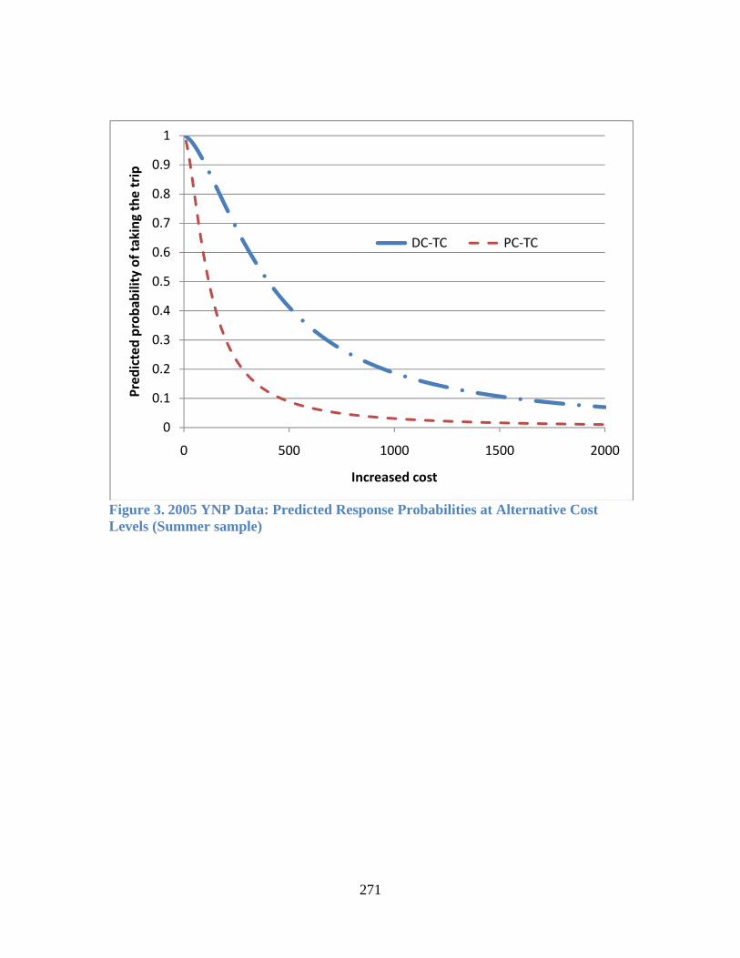
271
Figure 3. 2005 YNP Data: Predicted Response Probabilities at Alternative Cost Levels (Summer sample)
0
0.1
0.2
0.3
0.4
0.5
0.6
0.7
0.8
0.9
1
0 500 1000 1500 2000
Pred
icted prob
ability of taking the trip
Increased cost
DC‐TC PC‐TC

272
References
Bishop, Richard and Tom Heberlein. 1979. Measuring values of extra market goods: Are indirect measures biased? American Journal of Agricultural Economics 61:926-930.
Bowker, J., Starbuck, C., English, D., Bergstrom, J., Rosenberger, R., & McCollum, D. 2009.
Estimating the Net Economic Value of National Forest Recreation: An Application of the National Visitor Use MOnitoring Data Base. Athens, GA: University of Georgia, Department of Agricultural and Applied Economics.
Cameron, Trudy Ann, and Daniel D. Huppert. 1989. "OLS versus ML Estimation of Non-market
Resource Values with Payment Card Interval Data." Journal of Environmental Economics and Management 17:230-246.
Champ, Patricia and Richard Bishop. 2006. “Is Willingness to Pay for a Public Good Sensitive to
Elicitation Format?” Land Economics 82(2) 162-73. Champ, Patricia, Kevin Boyle, and Thomas Brown. (Eds.), 2003. A Primer on Nonmarket
Valuation. Kluwer Academic Publishers, The Netherlands. Dillman, D. 2000. Mail and Internet Surveys: the Tailored Design Method, New York. John
Wiley and Sons. Duffield, John, David Patterson, and Chris Neher. 2008. Economics of Wolf Recovery in
Yellowstone. Yellowstone Science 16(1):20-25. Duffield, John, David Patterson, Chris Neher and John Loomis. 2010. Valuation of Selected
Ecosystem Services in the National Parks: Estimating Models for Benefit Transfer. Working paper.
Heberling, M. and J. Templeton. 2009. Estimating the Economic Value of National Parks with
Count Data Models Using On-Site, Secondary Data: The Case of the Great Sand Dunes National Park and Preserve. Environmental Management 43:(4): 619-627.
Christopher G. Leggett, Naomi S. Kleckner, Kevin J. Boyle, John W. Duffield, and Robert
Cameron Mitchell (2003). “Social Desirability Bias in Contingent Valuation Surveys Administered Through In-Person Interviews” Land Economics 79(4): 561-575
Mitchell, R.C., and R.T. Carson. 1989. Using Surveys to Value Public Goods: the Contingent
Valuation Method. Resources for the Future, Washington, D.C. 463pp Ready, Richard, Donald Epp, and Willard Delavan. 2005. A comparison of revealed, stated and
actual behavior in response to a change in fishing quality. Human Dimensions of Wildlife 10: 1, 39-52.

273
Shaw, D. (1988). On-site Samples Regression: Problems of Non-negative Integers, Truncation and Endogenous Stratification. Journal of Econometrics 37: 211-223.
Welsh, M. and G. Poe. 1998. “Elicitation Effects in Contingent Valuation: Comparisons to a
Multiple-bounded Discrete Choice Approach.” Journal of Environmental Economics and Management 36(2): 170-185.

274
APPENDIX A: Contingent Valuation Survey Questions (1) Travel Cost-Payment Card Question Format : The costs of visiting and recreating in national parks change over time. For example, gas prices and other travel costs rise and fall. What is the largest increase in travel costs the group traveling in your vehicle would have paid to visit Yellowstone National Park during this trip? (Circle the amount)
$0 (would not pay more) $10 $20
$30 $55 $80 $130 $180 $230 $480 $1000 $2000
(2) Travel Cost Dichotomous Choice Question Format : The costs of visiting and recreating in national parks change over time. For example, gas prices and other travel costs rise and fall. Would the group traveling in your vehicle still have chosen to make this trip if the total group costs due to visiting Yellowstone National Park were $_______ more than the amount your group had to pay? (Please check one) __ YES __ NO What is the main reason for your answer?__________________________________________

275
(3) Entry Fee Payment Card Question Format: Visitors to Yellowstone National Park currently pay an entry fee of $20 per vehicle for a seven-day pass. The National Park Service is not currently thinking of increasing this fee. However, there are other recreational experiences where the access price is quite high (for example, a week of golf green fees or ski lift tickets). Out of fairness to the public, park entrance fees will never increase to those levels. In this question we use entry fee increases only to learn how much visiting Yellowstone National Park is worth to you. Some people would not pay more than the current fee of $20 per vehicle to visit Yellowstone National Park and would go elsewhere if the fee were higher. Other people would pay more to visit the park, if necessary, because it has this much value to them. What is the highest entry fee per vehicle the group traveling in your vehicle would have paid to visit Yellowstone National Park during this trip? (Please circle the amount) (If your group has a multi-park pass, please answer as if the pass were not valid for Yellowstone National Park)
$20 (current fee) $30 $40 $50 $75 $100 $150 $200 $250 $500
(4) Entry Fee Dichotomous Choice Question Format: Visitors to Yellowstone National Park currently pay an entry fee of $20 per vehicle for a seven-day pass. The National Park Service is not currently thinking of increasing this fee. However, there are other recreational experiences where the access price is quite high (for example, a week of golf green fees or ski lift tickets). Out of fairness to the public, park entrance fees will never increase to those levels. In this question we use entry fee increases only to learn how much visiting Yellowstone National Park is worth to you. Some people would not pay more than the current fee of $20 per vehicle to visit Yellowstone National Park and would go elsewhere if the fee were higher. Other people would pay more to visit the park, if necessary, because it has this much value to them. Would the group traveling in your vehicle still have chosen to visit Yellowstone National Park on this trip if the park entry fee per vehicle were $_____ ? (If your group has a multi-park pass, please answer as if the pass were not valid for Yellowstone.) (Please check one) __YES __NO
What is the main reason for your answer?_________________________

Rounding in Recreation Demand Models:A Latent Class Count Model
Keith Evans1 Joseph A. HerrigesIowa State University Iowa State University
July 29, 2010
1Contact author information: 260 Heady Hall, Department of Economics, Iowa State University, Ames,IA 50011. email: [email protected]. Phone: 515-294-6173
Abstract
A commonly observed feature of visitation data, elicited via a survey instrument,is a greater propensity for individuals to report trip numbers that are multiples of 5’s,relative to other possible integers (such as 3 or 6). One explanation of this phenomenonis that some survey respondents have difficulty recalling the exact number of tripstaken and instead choose to round their responses. This paper examines the impactthat rounding can have on the estimated demand for recreation and the bias that itmay induce on subsequent welfare estimates. We propose the use of a latent classstructure in which respondents are assumed to be members of either a nonrounding ora rounding class. A series of generated data experiments are provided to illustrate therange of possible impacts that ignoring rounding can have on the estimated parametersof the model and on the welfare implications from site closure. The results suggest thatbiases can be substantial, particularly when then unconditional mean number of tripsis in the range from two to four. An illustrative application is provided using visitationdata to Saylorville Lake in central Iowa.
JEL Codes: Q51, C5
keywords: recreation demand, rounding
2
1 Introduction
Models of recreation demand are used extensively to value both access to and potential
changes in environmental amenities at recreation facilities, such as lakes, rivers and beaches.
Analysts link visitation patterns to the cost of traveling to a site, consumer characteristics
and the attributes of the available sites using a range of modeling frameworks, including
discrete choice Random Utility Maximization (RUM) models, count data models, and the
structural Kuhn-Tucker model. Key to all of these approaches, of course, are data on the
numbers of trips to the sites of interest. Trip data most often take the form of counts of the
trips taken over a fixed time horizon (e.g., a summer season or calendar year) elicited via a
survey instrument, asking the individual to recall (or in some applications to forecast) their
numbers of trips. A commonly observed feature of these counts is a greater propensity for
individuals to report trip numbers that are multiples of 5’s, relative to other possible integers
(such as 3 or 6). One explanation of this phenomenon is that some survey respondents
have difficulty recalling the exact number of trips taken and instead choose to round their
responses.2 While the apparent clumping of trip data around specific integers is a familiar
pattern in recreation demand data, we are aware of no efforts in the literature to date that
attempt to account for this pattern. Instead, practitioners treat the reported counts as an
accurate reflection of the trips taken by the survey respondent. Even in the broader survey
literature, attempts to account for rounding in survey data analyses are rare. Manksi and
Molinari [8] provide one of the few exceptions, developing an approach to partially identify
patterns in probabilistic expectations elicited via survey instruments.
The purpose of this short paper is to examine the impact that rounding can have on the
estimated demand for recreation and the bias that it may induce on subsequent welfare
estimates. In particular, we propose a latent class count data model of visitations to a single
site in which respondents are assumed to be members of either a nonrounding or a rounding
class, with the latter group providing censored responses to trip questions by rounding their
trip counts to the nearest multiple of five. We are agnostic as to why the latter group chooses
to round. As Manski and Molinari [8] suggest, “. . . [t]here are no established conventions
for rounding survey responses. Hence, researchers cannot be sure how much rounding there
may be in survey data. Nor can researchers be sure whether respondents round to simplify
communication or to convey partial knowledge” (p. 219). We go on to suggest the use of
an expectation-maximization (EM) algorithm for the estimation of the model. A series of
generated data experiments are then provided to illustrate the range of possible impacts
2Similar phenomena have been observed in other survey settings. For example, Dominitz and Manski [4]note that in surveys eliciting probabilistic expectations (e.g., the probability of loosing one’s job or living toa specific age), responses tend to bunch around multiples of 5%. See Manksi and Molinari [8] for additionaldiscussion of this phenomenon.
3

that ignoring rounding can have on the estimated parameters of the model and on the
welfare implications from site closure. The results suggest that biases can be substantial,
particularly when the unconditional mean number of trips is in the range of two to four.
Finally, an illustrative application is provided using data on the visitations to Saylorville
Lake, a popular recreational site and reservoir in central Iowa. The paper closes with an
overall summary of our findings and a discussion of possible extensions of the modeling
framework.
2 The Model
We begin this section by formally defining the assumed latent class structure and developing
the necessary notation. Latent class models have emerged in recent years as a popular ap-
proach to incorporating preference heterogeneity in discrete choice models, both in recreation
demand (e.g., [2],[10],[11]) and in the broader literature (e.g., [5],[6],[7]). In our application,
the heterogeneity lies in the individual’s propensity to round. We then propose an EM
algorithm for use in the estimation of the model.
2.1 The Latent Class Count Data Model
The starting point in our approach to examining the impact of rounding in the modeling
of recreation demand is to assume that individuals fall into one of two latent classes : Non-
rounders (N) or Rounders (R). Individual class membership (denoted by C∗i = N or R)
is unknown to the analyst. For each class, the actual number of trips (y∗i ) taken to the
site in question is assumed to be drawn from a Poisson distribution, though the underlying
parameters of the Poisson distribution are allowed to vary by class. Specifically, we assume
that:
Pr(y∗i = k|C∗i = c) =exp(−λic)λkic
k!i = 1, . . . , I; c = N,R, (1)
where
λic = exp(X ′iβc) (2)
denotes the conditional mean trips for individuals in class c given characteristics X i and
the parameter vector βc. For individuals in the nonrounding class, the reported trips yi are
assumed to be the same as the actual number of trips (i.e., yi = y∗i ). Thus, conditional on
knowing that C∗i = N , the individual’s choice probability is simply:
LiN(yi,X i;βN) =exp(−λiN)λyi
iN
yi!(3)
4

In contrast, for individuals in the rounding class, reported trips are assumed to be rounded
to the nearest multiple of five for trips greater than 2.3 Let I5 denote the set of positive
integers that are multiples of five. In this case, conditional on knowing that C∗i = R, the
individual’s choice probability is simply:
LiR(yi,X i;βR) =
exp(−λiR)λyiiR
yi!yi = 0, 1, 2
∑2j=−2
exp(−λiR)λyi+jiR
(yi+j)!yi ∈ I5
0 otherwise.
(4)
Let sR ∈ [0, 1] denote the probability of being in the nonrounding class. Since class mem-
bership is not known, the unconditional choice probability for individual i becomes:
Li(yi,X i;θ) = sRLiR(yi,X i;βR) + (1− sR)LiN(yi,X i;βN), (5)
where θ = (β′N ,β′R, sR)′ denotes the combined parameters of the model. The parameter
vector θ can be obtained using standard maximum likelihood gradient based methods. How-
ever, latent class models are notorious for their difficulty in estimation, particularly since the
class labels are themselves arbitrary. In our generated data experiments and application, we
instead employ the EM algorithm described below.
2.2 The EM Algorithm
EM algorithms were introduced by Dempster, Laird and Rubin [3] as a means dealing with
missing data and have subsequently been adapted to a variety of estimation problems in
which some piece of information in a model is missing.4 In the current application, the
missing piece of information we focus on is the class membership variable C∗i . As with all
EM algorithms, the procedure is iterative. Let θt denote value of the parameter vector at
iteration t. Following the notation in [13], the next iteration on θ (i.e., θt+1) is obtained for
our latent class model by maximizing:
E(θ|θt) =I∑i=1
R∑c=N
htic ln [scLic(yi,X i;βc)] (6)
3We assume that when actual trips (y∗i ) equal 1 or 2, they are not rounded down to zero by the surveyrespondent, even in the case of the rounding class. It seems reasonable to us that, in reporting trips, therounding individual distinguishes taking a trip from staying at home even when the number of trips is small.
4Train [13], chapter 14, provides an excellent overview of EM algorithms, while McLachlan and Krishnan[9] provide a review of applications.
5

where
htic = h(C∗i = c|yi, st) =stcLic(yi,X i;β
tc)
stNLiN(yi,X i;βtN) + stRLiR(yi,X i;β
tR)
(7)
denotes the probability that individual i belongs to class c conditional on the observed choice
of the individual. Given the structure of the problem in (6), this is equivalent to separately
maximizing:
E(s|θt) =I∑i=1
[htiR ln(sR) + htiN ln(1− sR)
](8)
with respect to sR and (for both c = R and N) maximizing
E(βc|βt) =I∑i=1
htic ln [Lic(yi,X i;βc)] (9)
with respect to βc. The solution to the maximization of (8) yields:
st+1R =
∑Ii=1 h
tiR∑I
i=1 (htiN + htiR). (10)
The specific steps involved in the EM algorithm are then:
1. With t denoting the current iteration, set t = 0 and specify the initial values for both
the share of rounders (i.e., s0R) and the parameters of the two classes (i.e., β0
N and β0R).
We set s0R = 0.5. Similar to the approach suggested by [13] in the context of a latent
class logit model (p. 360), the starting values for the parameters of our two latent
classes are obtained by randomly partitioning the sample into two groups (N and R)
and maximizing (9) for each subsample to obtain β0N and β0
R.
2. For each observation i and each class c, the probability htic that individual i belongs to
class c conditional on the observed choice of the individual is computed using (7).
3. The updated class share of rounders (st+1R ) is obtained using (10).
4. The updated parameters for the two latent classes (βt+1N and βt+1
R ) are obtained by
maximizing (9).
5. Check for convergence. If convergence has not been achieved, then t is incremented by
1 and the algorithm returns to step 2. Otherwise, the algorithm ends and the standard
errors for the parameters can be calculated. We use bootstrapped standard errors, but
an alternative approach would be to use the converged values from the EM algorithm
as starting values in a maximum likelihood estimation of θ using (5).
6
3 Generated Data Experiments
In order to investigate the potential impact that rounding can have on both parameter
estimates and subsequent welfare calculations, we conduct a series of generated data exper-
iments. In all of the experiments, the conditional mean number of trips for each class is
assumed to be a linear exponential function of travel cost to the site (denoted by Pi), indi-
vidual income (denoted by Yi), and a demographic variable (Zi) . Specifically, we assume
that:
λic = exp(βc0 + βcPPi + βcY Yi + βcZZi), c = N,R. (11)
Across the experiments we vary two factors: (1) the share of rounders (i.e., sR) and (2) the
mean trips for the two classes (by varying βN0 and βR0).5 The emphasis on sR is obvious,
with our model reducing to the standard count data model when sR = 0. Five values for
sR were considered (sR = 0.1, 0.25, 0.5, 0.75, and 0.9). We focus on mean trips by class,
since the propensity for individuals to round will depend, in part, on their trip frequencies.
If the vast majority of the sample takes 0, 1, or 2 trips, then there will be little room for
rounding to occur. Along these lines, we consider two basic experiments. In experiment #1,
we fix φ0 ≡ βR0/βN0 = 2 (making rounders correspond to somewhat more avid trip takers)
and vary βN0 from 0.5 to 1.5 in steps of 0.25 (increasing the overall trip taking by the two
groups). The resulting intercepts are listed part a of Table 1.6 In experiment #2, we fix
β0 = 12(βN0 + βR0) (i.e., the simple average of the two type intercepts), varying φ0 from 0.5
to 2.0. When φ0 = 0.5, rounders are less frequent trip takers than non-rounders, whereas
when φ0 = 2 the opposite is true. The resulting intercepts are listed in part a of Table 2.
In both experiments, we assume that the price, income and demographic coefficients are the
same across the two classes (i.e., βcP = βP , βcY = βY , and βcZ = βZ for c = N,R). In
total, twenty-five generated data settings were analyzed for each experiment. In all of the
experiments, the sample size was set at I=5000.
Formally, 100 generated data sets (with 5000 observations in each data set) were constructed
for each experiment/setting as follows:
1. Vectors of travel cost (P1, . . . , PI), income (Y1, . . . , YI) and the demographic variable
(Z1, . . . , ZI) were drawn from uniform distributions (i.e., Pi ∼ U [0, 1], Yi ∼ U [0, 1],
and Zi ∼ U [0, 1]).
5We also investigated the impact of varying both the overall price coefficient and differences between βNP
and βRP , but found that this had relatively little impact on the bias induced by rounding.6Variations in these intercepts will induce variations in a group’s unconditional mean number of trips.
Table 1 also provides (in square brackets) the corresponding unconditional mean trips for each group andparameter setting given the assumed data generating process. For example, with β0R = 1, the correspondingunconditional mean trips would be 1.40.
7
2. Using βR0 and βN0 for the given setting, along with βP = −0.75, βY = 0.25, and
βZ = −0.25, λic was computed for each individual and latent class using (11).
3. Each individual in the sample was randomly assigned to either the nonrounding (C∗i =
N) or rounding (C∗i = R) latent class with probabilities sN and sR, respectively, using
a draw from uniform distribution; i.e.,
C∗i =
N ui < sN
R otherwise,(12)
where ui ∼ U [0, 1].
4. Using
λi = 1(C∗i = N)λiN + 1(C∗i = R)λiR, (13)
where 1(·) is the indicator function, the individual’s actual trips (y∗i ) were drawn from
a Poisson distribution with conditional mean λi.
5. Reported trips (yi) were then constructed as
yi =
y∗i yi = 0, 1, 2
1(C∗i = N)y∗i + 1(C∗i = R)rnd5(y∗i ) otherwise,
(14)
where rnd5(x) is the function censoring x to the nearest integer of five.
For each experiment, two models were estimated: (1) The latent class count data model
(LCCM) outlined above and (2) the standard (single class) (SCCM) count data model in
which no rounding is assumed. The resulting parameter estimates are available from the
authors upon request. However, as the ultimate goal of the recreation demand model is
typically for use in policy analysis, we focus our attention here on the potential bias on
subsequent welfare calculations that results from ignoring respondent rounding. Specifically,
we consider the welfare impact of the complete loss of access to the site as measured by
consumer surplus (CS).7 In a Poisson count data model with the linear exponential repre-
sentation of mean trips, the change in consumer surplus resulting from the elimination of
the site is given by:
CSi =λiβiP
, (15)
where
λi = exp(βi0 + βiPPi + βiY Yi + βiZZi) (16)
7Similar results are obtained if either compensating variation (CV) or equivalent variation (EV) are usedinstead to measure the welfare impact.
8

denotes the mean number of trips and βi = (βi0, βiP , βiY , βiZ) denotes individual i’s true
parameter vector. The true welfare loss measures for individual i in the generated data
sample are computed using equation (15). Averaged across the individuals yields the mean
true welfare loss for the sample (denoted CSTr
) for the rth generated data set.
For the single class count data model, the estimated welfare loss measures were computed
for each individual i using the fitted parameter vector from the SCCM specification for the
rth generated data set. Averaged across the individuals yields the mean welfare loss for the
sample predicted using the SCCM specification (denoted CSSr
).
For the latent class count data model, the predicted welfare loss for individual i is a weighted
average of the welfare loss predicted for each latent class; i.e.,
CSLr
i = (1− srR)CSNr
i + srRCSRr
i (17)
where
CScr
i =exp(βrc0 + βrcPPi + βrcY Yi + βrcZZi)
βrcP, for c = N, R (18)
and βrck (k = 0, P, Y, Z) and srR denote the fitted parameter estimates from the LCCM
using the rth generated data set. Averaged across the individuals yields the mean welfare
impact for the sample predicted using the LCCM specification (denoted CSLr
). For each
experiment/setting, we compute the percentage error of each model in predicting the true
consumer surplus. Tables 1b and 2b provide a summary of our findings for experiments 1
and 2, respectively.
Starting with experiment 1, several patterns emerge. First, as we would expect, the LCCM
model does well in predicting the mean welfare loss stemming from the elimination of the
site, since it is the correct specification of the data generating process. In general, the
average error is less than one percent. The errors are typically larger when the share of
rounders sR is small, leaving relatively few observations with which to estimate parameters
for the rounding class. Second, the bias in welfare predictions from ignoring rounding (and
using the standard SCCM) can be substantial. Consumer surplus is overstated by as much
as 37%. Indeed, the extent to which the SCCM consumer surplus measure overstates the
overall welfare loss appears to increase with the latent percentage of rounders in the sample,
but does not increase monotonically as the average number of trips increase. Indeed, the
largest bias occurs when the unconditional mean number of trips for the rounding class is
just over two. This may simply be because, when few trips are taken by the rounding class,
there is little opportunity for rounding, whereas when the rounding class takes many trips
(e.g., with an unconditional mean of 10.32), the percentage error in reported trips is smaller
(e.g., rounding 7 trips to 5 is a larger percentage error than when rounding 47 trips to 45).
9

Turning to the second experiment in Table 2b, we again see that percentage error resulting
from ignoring rounding increases with the size of the rounding class, with the bias being
largest when the unconditional mean trips for the rounding class is in the range from 2
to 3. Even when the coefficients are identical for the two latent classes (i.e., φ0 = 1),
the SCCM welfare measures are biased; consumer surplus is overstated by as much 36%.
This is due to the fact that, within the rounding class, there will be a larger percentage of
individuals rounding up than rounding down (e.g., a larger percentage of the population will
have actual trips of 3 and 4 relative to those having actual trips of 6 and 7). Thus, reported
trips will be a biased indicator of actual trips for the rounding class, with E(yi|X i, Ci =
R) > E(y∗i |X i, Ci = R).
4 Application
As illustration of our proposed methods, we employ data from the Iowa Lakes Valuation
Project. The Iowa Lakes Project, funded by the Iowa Department of Natural Resources
and the US EPA, was a four year effort to gather panel data on the recreational lake usage
patterns of Iowa households. Beginning in 2002, trip counts for the 132 primary recreational
lakes in the state were elicited from a random sample of 8000 state residents. After accounting
for nondeliverables, the overall response rate to the mail survey was approximately 62%.8
In the current paper, we limit our attention to visits to a single site, Saylorville Lake, a
reservoir in central Iowa locate just north of the state capital, Des Moines. We also restrict
our attention to households within a 100 mile radius of the site, leaving a total of I=1395
observations for use in our analysis. Table 3 provides basic summary statistics for the
sample.9 As Table 3 indicates, the mean number of trips taken to Saylorville Lake in 2002
is 1.66, with approximately 69.4% of the sample choosing not visiting the site that year.
Table 4 provides the parameter estimates for the SCCM and two versions of the LCCM
specification. In version 1 of the LCCM, we constrain the parameters of the rounding and
non-rounding groups to be the same (and in doing so focus on rounding alone as a source
of bias), whereas version 2 relaxes restriction. In general, all of the parameter estimates
are statistically significant. The SCCM model finds, as expected, that travel cost negatively
impacts the mean number of visits to the site. The results also suggest that trips increase
with income, but decrease with the individual’s age and education. Similar results are
8Additional details regarding the Iowa Lakes Project can be found in [1]9Travel cost Pi is computed assuming an out-of-pocket trip cost of $0.25 per mile times the individual’s
round trip distance to the site and a time cost of one-third the individual’s hourly times the round trip traveltime to the site. Travel distance and travel time were computed using the software package PCMiler.
10

found in the constrained LCCM model, though the impact of education is now somewhat
larger. The estimated share of rounders is approximately one-third of the population. The
mean consumer surplus associated with closure of Saylorville Lake is approximately 5.3%
higher using the SCCM model ($22.49) compared to estimates based on the constrained
LCCM specification ($21.36), which is line with our generated data experiment. With the
unconditional mean number of trips of 1.66, there is relatively little room for rounding to
impact the results.
Turning to the unconstrained LCCM specification, while the general sign of the marginal
effects are similar to the other two specification, the parameters differ somewhat between the
nonrounding and rounding latent class. Trips are more responsive to age and education for
the rounding class, but less responsive to price and income. As was the case in the constrained
LCCM model, under forty percent of the population is found to belong to the rounding class.
Despite the similarities with the other two model, the unconstrained specification yields a
substantially higher estimate of the consumer surplus loss due to the closure of the site
($43.41). While this is certainly possible, we believe that some caution would be appropriate
in using the unconstrained LCCM specification. Examining the summary statistics in Table
3, it is clear that the data exhibits a form of overdispersion, since the unconditional mean
number of trips (1.66) is much less than the corresponding unconditional variance (24.2).
Intuitively, it seems possible that the unconstrained LCCM results may be using the rounding
class to compensate for overdispersion. A generalization of the LCCM specification (e.g.,
using the negative binomial as the base distribution) could be used to examine this issue
further.
5 Summary and Possible Extensions
The objective of this paper was to illustrate the potential bias that rounding can have
on both the characterization of trip demand and the subsequent welfare estimates derived
from a count data model of recreation demand. We propose a latent class model to allow
for rounding by a subset of the population. Both our generated data experiments and
an application to recreation demand at Saylorville Lake in central Iowa suggest that the
potential bias can be substantial.
There are a number of possible directions for future research. First, our latent class model
assumes that the share of rounders (sR) is a constant. However, it seems reasonable that
the propensity for individuals to round might depend upon their characteristic (e.g., age,
gender, etc.), as well as the circumstance under which the survey is conducted (e.g., involving
11
near-term recall versus recall for time periods further into past). Numerous authors have
made the class membership probability in the latent class model of function of respondent
attributes (e.g., using a logit specification). Second, our latent class model allows for only
one type of rounding (i.e., to the near integer multiple of five). The framework can readily be
generalized to allow for a variety of rounding behaviors (e.g., rounding to multiples of ten) by
introducing addition latent classes. Finally, the Poisson count model underlying our latent
class model specification carries with it the often criticized assumption of equidispersion (with
the conditional mean of the trips being equal to the conditional variance). The latent class
approach used above could, however, be readily generalized by assuming the each class has
actual trips that are from a more general count data distribution allowing for overdispersion
(e.g., the negative binomial or zero inflated Poisson).
12

Table 1: Welfare Performance - Experiment #1a. Parameter Settinga
β0R 1.00 [1.40] 1.50 [2.30] 2.00 [3.80] 2.50 [6.26] 3.00 [10.32]β0N 0.50 [0.85] 0.75 [1.09] 1.00 [1.40] 1.25 [1.79] 1.50 [2.30]
b. Mean Percentage Error in CSsR LCCM SCCM LCCM SCCM LCCM SCCM LCCM SCCM LCCM SCCM
0.10 2.4 2.9 1.8 7.9 1.2 5.9 1.3 2.0 -0.1 -0.20.25 0.6 6.1 1.9 16.8 0.5 12.0 0.1 2.9 0.3 0.50.50 0.5 11.0 0.6 26.0 0.2 19.2 -0.4 2.0 0.1 1.30.75 0.9 15.6 -0.2 32.9 0.5 23.8 0.2 3.2 0.3 0.40.90 1.2 17.3 0.0 36.7 0.1 25.6 0.1 2.7 0.0 0.1aCorresponding unconditional group mean trips in square brackets.
Table 2: Welfare Performance - Experiment #2a. Parameter Settingb
φ0 0.50 0.75 1.00 1.50 2.00β0R 1.00 [1.40] 1.29 [1.86] 1.50 [2.30] 1.80 [3.11] 2.00 [3.80]β0N 2.00 [3.80] 1.71 [2.85] 1.50 [2.30] 1.20 [1.71] 1.00 [1.40]
b. Mean Percentage Error in CSsR LCCM SCCM LCCM SCCM LCCM SCCM LCCM SCCM LCCM SCCM
0.10 0.9 1.1 1.3 2.0 1.2 3.6 1.4 6.4 1.2 5.90.25 0.1 1.7 1.0 6.0 1.0 9.3 1.5 14.1 0.5 12.00.50 0.0 5.0 0.7 12.5 0.8 19.0 1.4 24.8 0.2 19.20.75 0.3 9.6 -0.1 19.9 0.3 28.8 0.1 31.1 0.5 23.80.90 0.4 14.7 0.8 27.0 0.7 35.8 0.6 35.9 0.1 25.6bCorresponding unconditional group mean trips in square brackets.
Table 3: Summary StatisticsVariable Model Variable Mean Std. Dev. Min MaxTotal Day Trips (2002) yi 1.664 4.924 0.000 60.000Travel Cost ($10’s) Pi 3.057 2.095 0.185 17.067Income ($10000’s) Yi 6.300 5.904 0.500 32.500Age (10 years) ZAge,i 5.290 1.744 1.550 8.750College ZEduc,i 0.396 0.489 0.000 1.000
13

Table 4: Parameter Estimates
Model Class β0 βP βY βZ,Age βZ,Educ sRSCCM 2.664 -0.740 0.033 -0.170 -0.030 n.a.
(0.006) (0.002) (0.003) (0.001) (0.004)Constrained 2.626 -0.741 0.033 -0.171 -0.469 0.361
LCCM (0.084) (0.023) (0.004) (0.014) (0.046) (0.097)LCCM Ci = N 3.193 -0.816 0.032 -0.079 -1.621
(0.017) (0.006) (0.001) (0.003) (0.033)LCCM Ci = R 0.866 -0.750 0.014 -0.258 4.093 0.386
(0.125) (0.039) (0.002) (0.018) (0.062) (0.008)
References
[1] Azevedo, C., K. Egan, J. Herriges, and C. Kling (2003). Iowa Lakes Valuation Project:
Summary and Findings from Year One. Final Report to the Iowa Department of Natural
Resources, August.
[2] Boxall, A., and W. Adomowicz (2002). “Understanding Heterogeneous Preferences in
Random Utility Models: A Latent Class Approach,” Environmental and Resource Eco-
nomics, Vol. 23, pp. 421-442.
[3] Dempster, A., N. Laird, and D. Rubin (1977), “Maximum Likelihood from Incomplete
Data via the EM Algorithm,” Journal of the Royal Statistical Society B Vol. 39, pp.
138.
[4] Dominitz, J., and C. Manski (1997). “Perceptions of Economic Insecurity: Evidence
From the Survey of Economic Expectations,” Public Opinion Quarterly, Vol. 61, pp.
261-287.
[5] d’Uva (2005). “Latent Class Models for Use of Primary Care: Evidence from a British
Panel,” Health Economics, Vol. 14, pp. 873-892.
[6] d’Uva (2006). “Latent Class Models for Utilisation of Health Care,” Health Economics,
Vol. 15, pp. 329-343.
[7] Greene, W., and D. Hensher (2003). “A Latent Class Model for Discrete Choice Analy-
sis: Contrasts with Mixed Logit,” Transportation Research, Part B, Vol. 37, pp. 681-698.
[8] Manski, C., and F. Molinari (2010). “Rounding Probabilistic Expectations in Surveys,”
Journal of Business & Economic Statistics, Vol. 28, No. 2, pp. 219-231.
[9] McLachlan, G. and T. Krishnan (1997), The EM Algorithm and Extensions, John Wiley
and Sons, New York
14

[10] Morey, E., J. Thacher, and W. Breffle (2006). “Using Angler Characteristics and At-
titudinal Data to Identify Environmental Preference Classes: A Latent-Class Model,”
Environmental & Resource Economics, Vol. 34, pp. 91-115.
[11] Provencher, B., K. Baerenklau, and R. Bishop (2002). “A Finite Mixture Logit Model
of Recreational Angling with Serially Correlated Random Utility,” American Journal
of Agricultural Economics, Vol. 84, No. 4, pp. 1066-1075.
[12] Train, K. (2008). “EM Algorithms for Nonparametric Estimation of Mixing Distribu-
tions,” Journal of Choice Modelling, Vol. 1, No. 1, pp. 40-69.
[13] Train, K. (2009). Discrete Choice Methods with Simulation, Cambridge University Press,
2nd edition.
15
Capturing Preferences Under Incomplete Scenarios UsingElicited Choice Probabilities.
Subhra Bhattacharjee Joseph A. Herriges1 Catherine L. KlingIowa State University Iowa State University Iowa State University
Preliminary Draft - Please do not Quote without Permission
July 22, 2010
1Contact author information: 260 Heady Hall, Department of Economics, Iowa State University, Ames,IA 50011. email: [email protected]. Phone: 515-294-4964

Abstract
Manski [9] proposed using elicited choice probabilities instead of the standard di-chotomous choice responses when the choice comparisons of interest are only incom-pletely described in the available survey instrument. This allows the survey respondentto express their uncertainty regarding the alternatives they face by revealing ex antethe odds that an alternative will be their preferred option ex post. Recently, Blass etal. [1] provided a strategy for analyzing elicited choice probabilities and an empiricalexample. This paper extend this literature by providing preliminary findings from asplit sample comparison of the elicited choice probability and stated choice elicitationformats using data from the 2009 Iowa Lakes Survey. In addition, we examine theimpact of different information treatments on the two survey format responses.
JEL Codes: Q51, C25
keywords: nonmarket valuation, dichotomous choice, choice probabilities.
2
1 Introduction
The Random Utility Maximization (RUM) model provides the foundation of most empirical
analyses of contingent valuation (CV) and choice experiment exercises used to elicit the value
of environmental amenities and other nonmarket goods. However, a fundamental premise
of the RUM model is that individuals, in making a choice among the available alternatives,
know exactly what utility they will receive from each alternative.2 The error term in the
model reflects, not the respondent’s uncertainty, but rather missing information on the part
of the analyst. This missing information can take the form of unobserved factors affecting
the choice, measurement error, or misspecification of the conditional indirect utility function
itself. The analyst then makes some assumption about the empirical distribution of the
error term, allowing them to specify conditional choice probabilities for each individual and
to then estimate the parameters associated with the assumed distribution.
The assumption that individuals have no uncertainty about the choices they face in a stated
preference survey, while convenient, seems tenuous at best, particularly when individuals
are asked to evaluate goods with which they have little past experience. Indeed, a number
of CV studies have attempted to capture this uncertainty in their survey design by adding
“probably yes,” “probably no,” “uncertain”, and similarly equivocating options to the list
of possible responses (e.g., Wang, [12]; Ready et al. [10]) or by asking respondents to rate
the certainty of their answers on a numerical scale (e.g., Johannesson et al. [4, 5], Li and
Mattsson [6]). The problem with these approaches is that it is no longer clear which response
one should use in defining the choice probabilities and the associated welfare measures. While
a number of studies have sought to calibrate CV responses using parallel “real” experimental
transactions data (e.g., [4, 5],[2],[7]), a consensus has yet to be reached on the form that such
calibrations should take.3
Manski [9] proposed an approach for dealing with a particular form of uncertainty in discrete
choice settings, one stemming from the incomplete description of the choice scenarios. Space
constraints and concerns regarding respondent fatigue lead researchers to provide only a
skeletal depiction of the alternatives, highlighting those attributes the researcher views as
essential. Yet these descriptions leave much to the imagination of the survey respondent,
2One can using the standard RUM model to incorporate preference uncertainty by assuming that theindividual’s choice is made on the basis of expected utility and that the conditional utility function itself isquadratic. The choice between alternatives in the this case would be a function of the perceived mean andvariance of each alternative’s utility. To out knowledge, however, this approach has not been used to date,in part because of the difficulty in eliciting each individual’s perceptions regarding the distribution of theirown conditional utilities.
3There is also the broader and more fundamental issue as to what decision rule survey respondents usewhen answering discrete choice questions under uncertainty (e.g., Wilcox [13, 14]).
3
both in terms of the alternatives directly and in terms of their own situation at the time
when a real choice might arise. For example, a CV survey might ask a respondent to
choose between two alternative lakes with differing levels of water quality. While the survey
might describe the alternatives in terms of average water quality measures (such as Secchi
Transparency or Phosphorous levels), the respondent is left with considerable uncertainty in
terms how these broad scenario descriptions translate into conditions they care about (e.g.,
fish catch rates, water safety, etc.) at the time they are actually faced with choosing between
the two lakes. As Blass et al. [1] note, “. . . [w]hen scenarios are incomplete, stated choices
cannot be more than point predictions of actual choices.” Masnki [9] suggests capturing the
respondent’s uncertainty by eliciting choice probabilities rather than a discrete choice. The
idea itself is simple, yet elegant. In essence, Manski suggests viewing the survey respondent
much like the standard RUM model treats the analyst. The survey respondent ex ante (i.e.,
at the time they are asked to express a preference over, say, option A versus option B) have
incomplete information. As such, they can only express the probability that they would ex
post (i.e., once their information uncertainties are resolved) prefer option A over option B.
Blass, et al. [1] further develop the approach and present the first empirical estimation of a
random utility model using elicited choice probabilities.
This paper extends the literature in two directions. First, Manski [8] suggests that, faced
with a discrete choice question, individuals will compute their subjective choice probability
for each alternative and choose that alternative with the highest choice probability. Using
recent data from the 2009 Iowa Lakes Project, we investigate the convergent validity of
the discrete choice and elicited choice probability formats using a split sample. Half of
the individuals in the survey were asked to choose between two hypothetical lakes (Lake
A and Lake B) with differing attributes, while the other half of the sample were asked to
indicate the probability that they would prefer Lake A over Lake B. Second, the model in
Blass, et al. [1] assumes that the individuals in the sample all have the same underlying
distribution characterizing their informational uncertainties. We investigate the realism of
this assumption by splitting our samples yet again, with half of the sample receiving a high
information treatment, while the other half receives a low information treatment. In this
paper, we present our preliminary results from this study, comparing the choice responses
in the four treatment groups. We also compare welfare estimates for the four groups using
both the model in Blass, et al. [1] and the standard logit specification.
4

2 Modeling Discrete Choices and Elicited Choice Prob-
abilities
We begin by describing the underlying modeling framework for both the standard discrete
choice problem and the elicited choice probability setting. In doing so, we parallel a similar
presentation in Blass, et al. [1], though we pay particular attention to the nature of what is
observable by the survey respondent at the time the survey is administered.
2.1 Discrete Choices
In the standard RUM model of a binary choice from among two options (j = A,B), it is
assumed that the individual i knows the utility that they would receive from each option
(Uij) and simply chooses that option that maximizes their utility. The stochastic nature of
the problem is in the eyes of the analyst alone, who observes only a subset of the factors
influencing the individual’s decision. For example, suppose that
Uij = αj + βxxij + βzzij (1)
where both xij and zij are known to the decision-maker, but only xij is observed by the
analyst. The outcome that option A is chosen (denoted yi = 1) is determined by the
individual by comparing UiA and UiB, with
yi =
{1 UiA ≥ UiB
0 UiA < UiB.(2)
For the analyst, however, the outcome (yi) is random variable, since zij is unknown. The
utility that individual i receives from alternative j takes the form:
Uij = αj + βxxij + εij (3)
= Vij + εij (4)
where Vij ≡ αj + βxxij and εij ≡ βzzij captures the unobservable factors influencing Uij.
Without knowledge of zij (and hence εij), the analyst can only make probabilistic statements
about the choice between options A and B. Specifically, the conditional probability that
option A is chosen (denoted by PiA) is given by
PiA = Pr(yi = 1|xij) (5)
= Pr(UiA ≥ UiB|xij) (6)
= Pr(ViA + εiA ≥ ViB + εiB|xij) (7)
= Pr(εi ≤ Vi|xij), (8)
5

where
Vi ≡ ViA − ViB (9)
= (αA − αB) + βx(xiA − xiB) (10)
= α + βxxi, (11)
with α ≡ αA − αB and xi ≡ xiA − xiB, and
εi ≡ εiB − εiA. (12)
Different assumptions about the unobservables (i.e., the εij) yields different functional forms
for the choice probabilities. For example, if the εij’s are assumed to be iid Type I extreme
value random variables, then a logistic model results, with
PiA =exp(Vi)
1 + exp(Vi)=
exp(α + βxxi)
1 + exp(α + βxxi). (13)
More general RUM models result if we assume that there are unobserved individual attributes
(say si) that interact with xij in determining Uij.4 In this case, we might have
Uij = αj + βxxij + βzzij + γxzxijsi (14)
= αj + (βx + γxzsi)xij + βzzij (15)
= αj + βxixij + εij (16)
where βxi ≡ βx + γxzsi is a random parameter from the analyst’s perspective, capturing
heterogeneity in consumer preferences induced by si. If the εij’s are again assumed to be iid
Type I extreme value random variables, then the mixed logit model results (see, e.g., Train
[11]), with
PiA =
∫exp(α + βxixi)
1 + exp(α + βxixi)f(βxi)dβxi, (17)
where f(βxi) is the assumed distribution of the random parameter βxi.
2.2 Elicited Choice Probabilities
In Manski’s [9] elicited choice probabilities setting, the problem is similar to the discrete
choice problem, except that now we allow for uncertainty on the part of both the analyst
4For ease of notation, we specify these unobserved attributes as a scalar, though this can easily begeneralized.
6
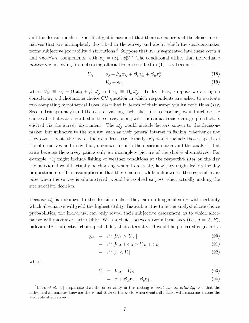
and the decision-maker. Specifically, it is assumed that there are aspects of the choice alter-
natives that are incompletely described in the survey and about which the decision-maker
forms subjective probability distributions.5 Suppose that zij is segmented into these certain
and uncertain components, with zij = (zcij′, zuij
′)′. The conditional utility that individual i
anticipates receiving from choosing alternative j described in (1) now becomes:
Uij = αj + βxxij + βczcij + βuz
uij (18)
= Vij + εij, (19)
where Vij ≡ αj + βxxij + βczcij and εij ≡ βuz
uij. To fix ideas, suppose we are again
considering a dichotomous choice CV question in which respondents are asked to evaluate
two competing hypothetical lakes, described in terms of their water quality conditions (say,
Secchi Transparency) and the cost of visiting each lake. In this case, xij would include the
choice attributes as described in the survey, along with individual socio-demographic factors
elicited via the survey instrument. The zcij would include factors known to the decision-
maker, but unknown to the analyst, such as their general interest in fishing, whether or not
they own a boat, the age of their children, etc. Finally, zuij would include those aspects of
the alternatives and individual, unknown to both the decision-maker and the analyst, that
arise because the survey paints only an incomplete picture of the choice alternatives. For
example, zuij might include fishing or weather conditions at the respective sites on the day
the individual would actually be choosing where to recreate, how they might feel on the day
in question, etc. The assumption is that these factors, while unknown to the respondent ex
ante when the survey is administered, would be resolved ex post, when actually making the
site selection decision.
Because zuij is unknown to the decision-maker, they can no longer identify with certainty
which alternative will yield the highest utility. Instead, at the time the analyst elicits choice
probabilities, the individual can only reveal their subjective assessment as to which alter-
native will maximize their utility. With a choice between two alternatives (i.e., j = A,B),
individual i’s subjective choice probability that alternative A would be preferred is given by:
qiA = Pr [UiA > UiB] (20)
= Pr [ViA + εiA > ViB + εiB] (21)
= Pr [εi < Vi] (22)
where
Vi ≡ ViA − ViB (23)
= α + βxxi + βczci , (24)
5Blass et al. [1] emphasize that the uncertainty in this setting is resolvable uncertainty ; i.e., that theindividual anticipates knowing the actual state of the world when eventually faced with choosing among theavailable alternatives.
7

with zci ≡ zciA − zciB, and
εi ≡ εiB − εiA. (25)
Blass et al. [1] assume that εijiid∼ Type I extreme value, in which case the elicited choice
probabilities take the familiar logistic form
qiA =exp(Vi)
1 + exp(Vi)=
exp(α + βxxi + βczci)
1 + exp(α + βxxi + βczci). (26)
There are several comments that are worth making regarding these subjective choice proba-
bilities. First, the underlying assumption that the εij are iid, while convenient, is a relatively
strong one, requiring that all individuals share the same subjective assessments regarding
the unobserved attributes of the alternatives presented in the survey scenarios (i.e., the zuij).
Second, while the subjective choice probabilities in (26) are similar in structure to those
for the discrete choice setting in (13), they differ in that the subjective choice probabilities
are themselves random variables from the analyst’s perspective, depending as they do on
the attributes zcij, which are unobservable by analyst, but known to the decision-maker.
Blass et al. [1] suggest estimating the parameters associated with xi by using a log-odds
transformation of (26), yielding
ln
(qiAqiB
)= α + βxxi + ηi, (27)
where ηi ≡ βczci . Blass, et al. [1] suggest estimating equation (27) using a LAD estimator.6
As was the case with the discrete choice setting, the elicited choice model can be general-
ized to allow for preference heterogeneity by introducing interaction terms associated with
si, individual specific factors observed by the decision-maker, but not the analyst. The
conditional utility in equation (18) becomes
Uij = αj + βxxij + βczcij + βuz
uij + γxxijsi + γcz
cijsi + γuz
uijsi (28)
= αj + (βx + γxsi)xij + (βc + γcsi)zcij + (βu + γusi)z
uij (29)
= αj + βxixij + βcizcij + βuiz
uij (30)
= Vij + εij, (31)
where now Vij ≡ αj + βxixij + βcizcij has parameters that vary over individuals and εij ≡
βuizuij, where βui = βu +γusi. Note that now, even if individuals share the same subjective
beliefs about the uncertain site characteristics zuij, the error term εij will be heteroskedastic
due to differences in βui. As an example of this, suppose that zuij represents the fishing
6The LAD estimator is proposed to deal with a practical problem in elicited choice probability settings,namely the problem with the log-odds transformation in those cases in which qiA = 0 or 1. The LADestimator is not sensitive to outliers, allowing these extreme cases to be handled by replacing qiA = 0 or 1with δ and 1− δ, respectively, where δ is a small number.
8

conditions at site j and si represents an index on the unit interval indicating an individual’s
general interest in fishing. For an individual who cares about fishing, si will be close to one
and the corresponding βui will be relatively large. Because they like fishing, any uncertainty
they have about fishing conditions at site j (zuij) induces substantial uncertainty in terms
of the utility they anticipate receiving from visiting site j. In contrast, an individual who
does not care about fishing will have an si close to zero and the corresponding βui will
be relatively small. For this non-fisherman, even if they share exactly the same subjective
beliefs about the fishing conditions at site j as the avid fisherman, the uncertainty does not
translate into uncertainty about Uij since they do not care about the fishing conditions.
The implication of this heteroskedasticity is that the identified parameters of the subjective
choice probabilities will now vary by individual. To see this, consider the case in which zuijis a scalar, with the zuij’s assumed to be iid Type I extreme value random variables. Then
εij ≡ βuizuij and the subjective choice probabilities become:
qiA =exp(Vi/βui)
1 + exp(Vi/βui)(32)
=exp
(α+βxixi+βciz
ci
βui
)1 + exp
(α+βxixi+βciz
ci
βui
) (33)
=exp(αi + βxixi + βciz
ci)
1 + exp(αi + βxixi + βcizci). (34)
where
αi ≡α
βui, βxi ≡
βxiβui
, and βci ≡βciβui
. (35)
Note that both βxi and βci will vary by individual, even if the corresponding βxi and βci do
not. The corresponding log-odds equation used for estimation becomes:
ln
(qiAqiB
)= αi + βxixi + βciz
ci (36)
= a+ bxxi + ηi (37)
where a and bx denote the mean values of αi and βxi, respectively, and
ηi ≡ (αi − a) + (βxi − b)xi + βcizci . (38)
3 The Iowa Lakes Data
The data used in this paper are drawn from the 2009 Iowa Lakes Survey. The survey is part
of an ongoing research effort (funded jointly by the Iowa Department of Natural Resources
9

and the U.S. EPA) to understand recreational lake usage in the state and the value residents
place in the site and water quality attributes of Iowa’s primary recreational lakes. The
project began in 2002 with a mail survey of 8000 Iowa households selected at random. The
survey elicited the respondents’ visitation rates to each of 132 primary lakes, as well as socio-
demographic information for each household. Similar surveys were administered to the same
households over the next three years, providing a unique panel data picture of lake usage.7
The most recent survey, administered in late 2009, was mailed to a total 10,000 Iowa house-
holds, consisting of the respondents to the 2005 Lakes Survey (approximately 4500 house-
holds) and an additional random sample of Iowa households. As with earlier surveys, re-
spondents were asked to recall their numbers of day- and overnight-trips to each to the 132
primary lakes over the past year, along with providing socio-demographic information. In
addition, Section 2 of the survey consisted of a contingent valuation (CV) exercise. It is this
section provides the basis for our analysis below.
A total of four versions of the CV exercise were used in the 2009 survey. In all four versions,
respondents were asked to compare two hypothetical lakes (A and B). The lakes differed in
terms of their water quality attributes, with Lake B being substantially cleaner than Lake
A, and in terms of each lake’s the distance from the respondent’s home and the associated
entrance fee. Figure 1 provides the illustration used in both Versions 1 and 3 of the survey.
In addition to the illustration, a textual description of each lake was provided. Versions 2 and
4 of the survey also asked respondents to compare Lakes A and B, however less information
was provided in both the text and the illustration regarding each lake’s condition, especially
in terms its fishing conditions. The purpose of these low information versions of the survey
was induce greater uncertainty for the survey respondent, which should induce corresponding
shifts in the estimated preference parameters.
The other distinguishing feature of the four CV versions was the evaluation format employed.
Versions 1 and 2 elicited choice probabilities, as suggested by Manski [9], using the text:
Assume that you have to choose between visiting one of the two lakes described
on the previous page. What are the chances in percentage terms that you would
choose to visit Lake A rather than Lake B? The chance of each alternative should
be a number between 0 and 100 and the chances given to the two alternatives
should add up to 100. For example, if you give a 5% chance to one alternative it
means that there is almost no possibility that you will choose that alternative. On
7In 2003, the surveys were sent to respondents to the 2002 survey (approximately 4500 households) and toan additional random sample of households used to return the total sample size once again to 8000 household.In 2004 and 2005, the surveys were sent only to those household that responded in the previous year).
10
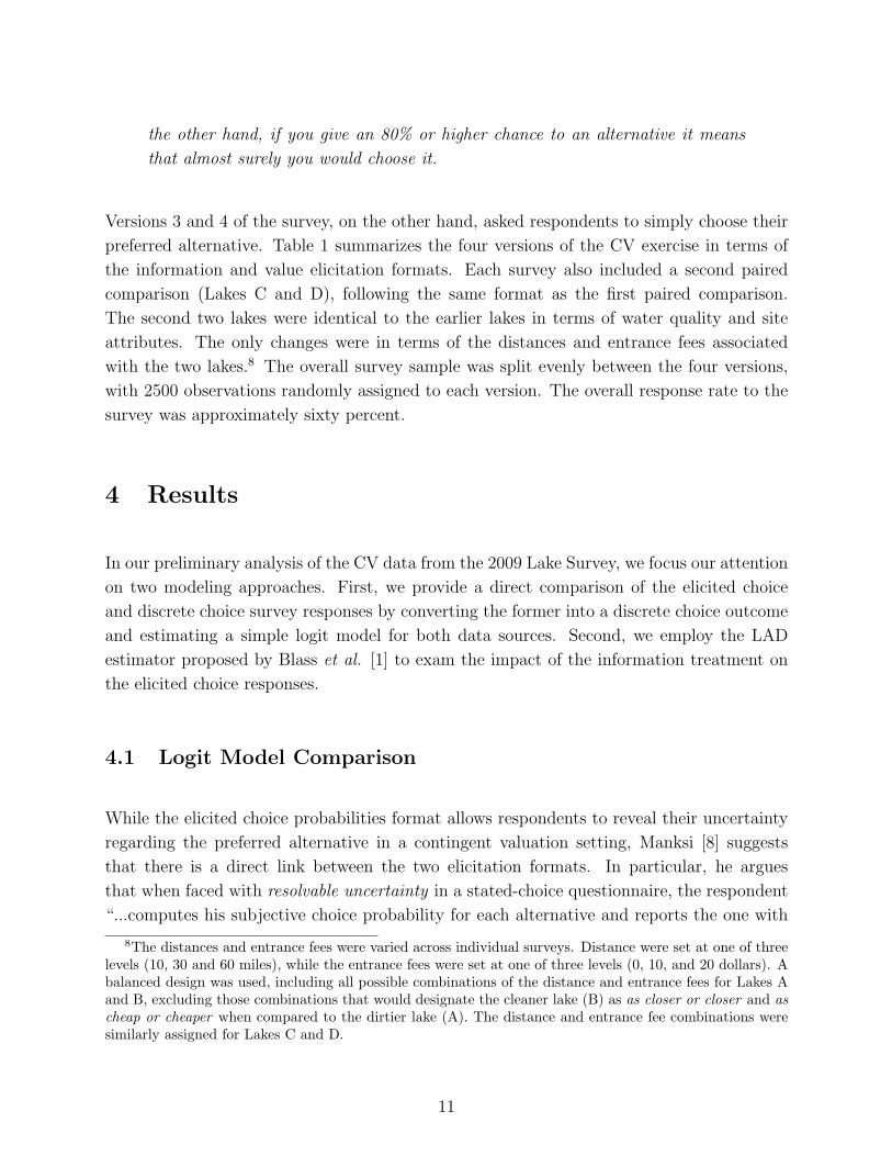
the other hand, if you give an 80% or higher chance to an alternative it means
that almost surely you would choose it.
Versions 3 and 4 of the survey, on the other hand, asked respondents to simply choose their
preferred alternative. Table 1 summarizes the four versions of the CV exercise in terms of
the information and value elicitation formats. Each survey also included a second paired
comparison (Lakes C and D), following the same format as the first paired comparison.
The second two lakes were identical to the earlier lakes in terms of water quality and site
attributes. The only changes were in terms of the distances and entrance fees associated
with the two lakes.8 The overall survey sample was split evenly between the four versions,
with 2500 observations randomly assigned to each version. The overall response rate to the
survey was approximately sixty percent.
4 Results
In our preliminary analysis of the CV data from the 2009 Lake Survey, we focus our attention
on two modeling approaches. First, we provide a direct comparison of the elicited choice
and discrete choice survey responses by converting the former into a discrete choice outcome
and estimating a simple logit model for both data sources. Second, we employ the LAD
estimator proposed by Blass et al. [1] to exam the impact of the information treatment on
the elicited choice responses.
4.1 Logit Model Comparison
While the elicited choice probabilities format allows respondents to reveal their uncertainty
regarding the preferred alternative in a contingent valuation setting, Manksi [8] suggests
that there is a direct link between the two elicitation formats. In particular, he argues
that when faced with resolvable uncertainty in a stated-choice questionnaire, the respondent
“...computes his subjective choice probability for each alternative and reports the one with
8The distances and entrance fees were varied across individual surveys. Distance were set at one of threelevels (10, 30 and 60 miles), while the entrance fees were set at one of three levels (0, 10, and 20 dollars). Abalanced design was used, including all possible combinations of the distance and entrance fees for Lakes Aand B, excluding those combinations that would designate the cleaner lake (B) as as closer or closer and ascheap or cheaper when compared to the dirtier lake (A). The distance and entrance fee combinations weresimilarly assigned for Lakes C and D.
11

the highest probability” [1, p. 5]. Specifically, it is assumed, in a binary choice setting, that:
yi = 1[qiA ≥ qiB], (39)
where 1[·] is the standard indicator function. There are two reasons to question this logic.
First, while the binary choice referendum format has been argued to be incentive compatible,
under certain conditions concerning the consequentiality of the survey, there is no compa-
rable result (to our knowledge) for the elicited choice probability format. Second, while the
conversion in (39) is intuitively appealing, it is not clear how risk aversion would alter the
individual’s choice revelation under scenario uncertainty.
In this subsection, we examine the convergent validity of the elicited choice and stated-choice
formats by converting the elicited choice probabilities to a binary outcome using (39) and
estimating logit models for both data sets. Separate models are estimated for the first (AB)
and second (CD) paired comparisons. Three alternative model specifications are considered.
The first model pools the data from the high and low information treatments. In this simple
specification, it is assumed that Vi in (13) takes the form:
Vi = α + βDOODisti + βCOOCosti (40)
where ODisti and OCosti denote the additional distance and additional entrance cost as-
sociated with the cleaner lake. Since yi = 1 denotes the choice of the dirtier lake in each
paired comparison, we would anticipate both βDO and βCO to be positive. The second
model controls for potential information effects, distinguishing the marginal impacts of the
distance and cost variables for the low and high information treatments. In particular, (40)
is generalized to
Vi = α + γDLi + (βDO + δDDLi)ODisti + (βCO + δCDLi)OCosti (41)
where DLi is a dummy variable indicating that individual i received the low information
treatment. Thus, γ, δD, and δC denote the differential effect for the low information treat-
ment. Constraining these parameters to zero yields the simple model in (40). Finally, one
concern in asking multiple questions in a stated preference survey is that the respondents will
react, not only to conditions of the current question, but will anchor their responses to the
other questions in the survey (See, e.g., Herriges and Shogren [3]). The third specification
allows for cross-question effects, generalizing the simple model (40) to allow an individual’s
choice to depend, not only on the distance and entrance fee comparisons presented in the
paired comparison, but on the distance and entrance fee presented in the “other” paired
comparison. Specifically, we set
Vi = α + βDOODisti + βCOOCosti + βDCCDisti + βCCCCosti (42)
12

where CDisti and CCosti denote the distance and cost differentials in the “other” paired
comparison. Thus, when modeling the AB- paired comparison, CDisti and CCosti denote
the distance and cost differentials in the CD-paired comparison. If there are no spillover
effects, we would anticipate βDC = βCC = 0. If this condition does not hold, then respondents
are making their choices based, not only on the choice in front of them, but on the conditions
outlined in other alternatives.
The results from estimating these three models are presented in Tables 2 and 3 for the
converted elicited choice probabilities and the stated-choices, respectively. Starting with the
simplest model, we see that both data sets yield very similar results. In both cases, the
distance and entrance fees have the anticipated positive signs and are statistically significant
at a 5% level in both the AB- and CD-paired comparisons. The coefficients are similar for
both elicitation formats, though somewhat smaller when the stated-choice format is used.
A formal test has yet to be conducted to determine if these differences are statistically
significant.
Turning to the model with information effects, we see relatively little evidence that the
differing information treatments altered the choices made by survey respondents. Indeed,
only in the CD-paired comparison for the elicited choice probabilities format do we see an
impact. In this case, δD is positive and significant at a 5% level, suggesting that respondents
are more responsive to the distance cost of the cleaner lake when less information is provided
regarding conditions at the two lakes. The corresponding entrance fee coefficient δC is also
positive, though significant only at the 10% level.
Finally, estimates of the third model in (42) suggests little evidence of cross-question effects.
None of the estimates of βDC and βCC differ significantly from zero at a 5% level or lower.
Only in the single case of the CD-paired comparison for the stated choice data do we find a
significant impact for the cross-entrance fee at the 10% level, and then the effect is relatively
small compared to the own-entrance fee coefficient.
4.2 Least Absolute Deviation Model
While the conversion of the elicited choice probabilities to a discrete choice outcome provides
a direct comparison to the state-choice elicitation format, doing so censors much of the
information contained in the choice probabilities. In this section, we focus our attention on
the choice probabilities data, providing least absolute deviation estimates for the parameters
of the log-odds model in (27). Table 4 provides estimates for the three models, analogous
13

in structure to those used in the previous section. It should be kept in mind, however, that
the parameters in Table 4 are not directly comparable to those in Tables 2 and 3 in that
different parameter scalings underly the identified parameters.
Starting with the simplest model, the LAD estimates reveal very similar results to those
obtained using the logit transformation. In particular, we again find that the distance and
entrance fee differentials associated with the cleaner lake have a positive and statistically
significant impact on the respondents propensity to choose the dirtier lake. As was the
case in Table 2, the entrance fee parameters are roughly three times those for the distance
variables. This suggests are marginal implicit mileage cost of approximately $0.16 (since
each distance differential induces two miles of additional round-trip travel).
The information effects, as revealed in Table 4, appear to be substantially stronger for the
AB-paired comparison using the elicited choice probabilities than when using their censored
discrete choice counterparts (in Table 2). All three information parameters are statistically
significant at the 5% level, indicating in general that households are more responsive to the
distance and entrance fee treatments when they have relatively little information regarding
the alternatives than when they are given more detailed water quality and fishing informa-
tion. The information effects, however, do not appear to be as large or statistically significant
in the CD-paired comparisons.
Finally, the LAD log-odds model confirms the earlier results regarding cross-equation effects.
None of the cross-equation terms are statistically significant at the 5% level and only one
is significant at the 10% level. Even in this case, the cross-equation effect is substantially
smaller than the corresponding own-equation parameter.
5 Future Directions
The results described in this paper represent preliminary findings regarding the use of elicited
choice probabilities to capture preferences under incomplete CV scenarios. Further research
is needed to formally test some of the differences between elicited choice probabilities and
stated-choice responses. In addition, it would be preferable to jointly model the AB- and
CD-paired comparisons, allowing for correlation between responses to the two scenarios.
Finally, the models presented here do not control for observable individual characteristics or
for heterogeneity in individual preferences and/or subjective assessments of the uncertainty
associated with the CV scenarios. Mixture models (both continuous and discrete) provide
one logical avenue for examining these issues.
14

6 Tables and Figures
Table 1: CV Survey Treatment OptionsInformation Treatment
Elicitation Method High Information Low Information
Choice Probabilities Version 1 Version 2Discrete Choice Version 3 Version 4
Table 2: Logit Models Using Converted Elicited Choice ProbabilitiesModels
Simple Model Information Effects Cross-Question EffectsParameter AB CD AB CD AB CD
α -1.39∗∗ -1.36∗∗ -1.40∗∗ -1.28∗∗ -1.39∗∗ -1.42∗∗
(0.06) (0.06) (0.08) (0.07) (0.07) (0.07)βDO 0.009∗∗ 0.010∗∗ 0.007∗∗ 0.007∗∗ 0.009∗∗ 0.010∗∗
(0.002) (0.001) (0.002) (0.002) (0.002) (0.001)βCO 0.028∗∗ 0.033∗∗ 0.031∗∗ 0.027∗∗ 0.028∗∗ 0.033∗∗
(0.004) (0.004) (0.005) (.006) (0.004) (0.004)γ 0.01 -0.20
(0.11) (0.11)δD 0.004 0.007∗∗
(0.003) (0.003)δC -0.006 0.012∗
(0.008) (0.008)βDC -0.0008 0.0020
(0.0010) (0.0014)βCC 0.003 0.005
(0.004) (0.004)
15
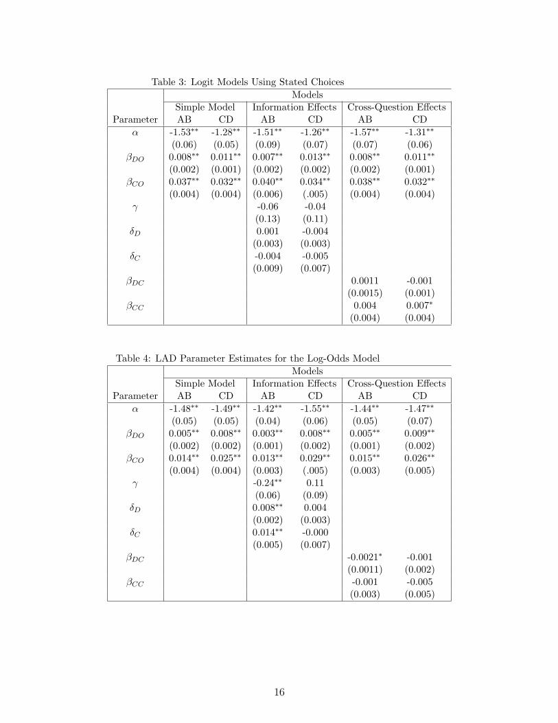
Table 3: Logit Models Using Stated ChoicesModels
Simple Model Information Effects Cross-Question EffectsParameter AB CD AB CD AB CD
α -1.53∗∗ -1.28∗∗ -1.51∗∗ -1.26∗∗ -1.57∗∗ -1.31∗∗
(0.06) (0.05) (0.09) (0.07) (0.07) (0.06)βDO 0.008∗∗ 0.011∗∗ 0.007∗∗ 0.013∗∗ 0.008∗∗ 0.011∗∗
(0.002) (0.001) (0.002) (0.002) (0.002) (0.001)βCO 0.037∗∗ 0.032∗∗ 0.040∗∗ 0.034∗∗ 0.038∗∗ 0.032∗∗
(0.004) (0.004) (0.006) (.005) (0.004) (0.004)γ -0.06 -0.04
(0.13) (0.11)δD 0.001 -0.004
(0.003) (0.003)δC -0.004 -0.005
(0.009) (0.007)βDC 0.0011 -0.001
(0.0015) (0.001)βCC 0.004 0.007∗
(0.004) (0.004)
Table 4: LAD Parameter Estimates for the Log-Odds ModelModels
Simple Model Information Effects Cross-Question EffectsParameter AB CD AB CD AB CD
α -1.48∗∗ -1.49∗∗ -1.42∗∗ -1.55∗∗ -1.44∗∗ -1.47∗∗
(0.05) (0.05) (0.04) (0.06) (0.05) (0.07)βDO 0.005∗∗ 0.008∗∗ 0.003∗∗ 0.008∗∗ 0.005∗∗ 0.009∗∗
(0.002) (0.002) (0.001) (0.002) (0.001) (0.002)βCO 0.014∗∗ 0.025∗∗ 0.013∗∗ 0.029∗∗ 0.015∗∗ 0.026∗∗
(0.004) (0.004) (0.003) (.005) (0.003) (0.005)γ -0.24∗∗ 0.11
(0.06) (0.09)δD 0.008∗∗ 0.004
(0.002) (0.003)δC 0.014∗∗ -0.000
(0.005) (0.007)βDC -0.0021∗ -0.001
(0.0011) (0.002)βCC -0.001 -0.005
(0.003) (0.005)
16
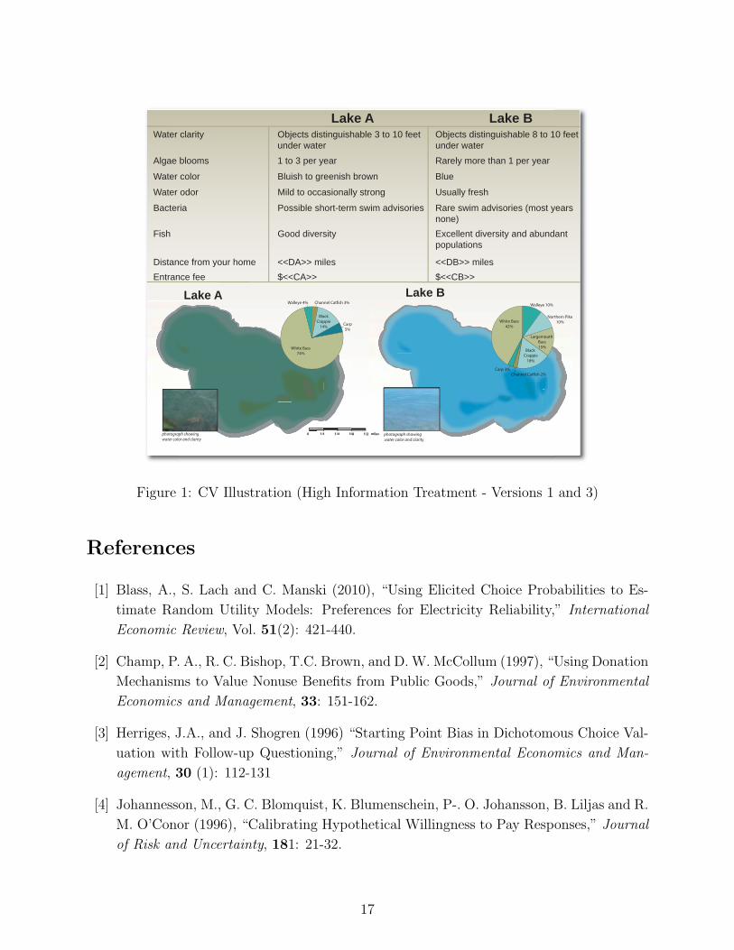
8 / Iowa Lakes Survey
photograph showing water color and clarity
1/8 1/23/81/40 miles photograph showing water color and clarity
milesphotograph showing water color and clarity
1/8 3/1/40photograph showing water color and clarity
Lake A Lake B
White Bass42%
Walleye 10%
Northern Pike10%
Largemouth Bass15%
Black Crappie
18%
Channel Catfish 2%Carp 3%
White Bass74%
Channel Catfish 3%Walleye 4%
BlackCrappie
14%Carp5%
In the following section, we ask you to consider a typical Iowa lake. We describe
the lake in one of two possible conditions and ask you to indicate which set of
conditions you prefer. Please read this information carefully before answering the
questions that follow.
The quality of a lake can be described in many ways. One measure of water quality is the clarity of the lake water. Water clarity is usually described in terms of how far down into the water an object remains visible. For example, a clarity of between 3 and 10 feet means that objects are clearly visible down to a depth of 3 to 10 feet.
Another measure of water quality is the amount of nutrients and other contaminants contained in the water. Water degradation can result from a number of sources, including urban runoff, fertilizer used in agriculture, motor vehicles, and others. Nutrients can result in algae blooms in a lake. Under some circumstances these blooms can be a health concern, causing skin rashes and allergic reactions.
The overall quality of the water can affect other conditions of the lake. Poor water quality can result in undesirable color and odor to the lake water. In addition, the quality of water affects the variety and quantity of fi sh in the lake.
Consider the following two lakes (Lake A and Lake B). Each lake has the same shape, but the lakes differ in terms of water quality and the distance each lake is from your home. Finally, in some cases, the lakes have an entrance fee.
Lake A Lake BWater clarity Objects distinguishable 3 to 10 feet
under waterObjects distinguishable 8 to 10 feet under water
Algae blooms 1 to 3 per year Rarely more than 1 per year
Water color Bluish to greenish brown Blue
Water odor Mild to occasionally strong Usually fresh
Bacteria Possible short-term swim advisories Rare swim advisories (most years none)
Fish Good diversity Excellent diversity and abundant populations
Distance from your home <<DA>> miles <<DB>> milesEntrance fee $<<CA>> $<<CB>>
Figure 1: CV Illustration (High Information Treatment - Versions 1 and 3)
References
[1] Blass, A., S. Lach and C. Manski (2010), “Using Elicited Choice Probabilities to Es-
timate Random Utility Models: Preferences for Electricity Reliability,” International
Economic Review, Vol. 51(2): 421-440.
[2] Champ, P. A., R. C. Bishop, T.C. Brown, and D. W. McCollum (1997), “Using Donation
Mechanisms to Value Nonuse Benefits from Public Goods,” Journal of Environmental
Economics and Management, 33: 151-162.
[3] Herriges, J.A., and J. Shogren (1996) “Starting Point Bias in Dichotomous Choice Val-
uation with Follow-up Questioning,” Journal of Environmental Economics and Man-
agement, 30 (1): 112-131
[4] Johannesson, M., G. C. Blomquist, K. Blumenschein, P-. O. Johansson, B. Liljas and R.
M. O’Conor (1996), “Calibrating Hypothetical Willingness to Pay Responses,” Journal
of Risk and Uncertainty, 181: 21-32.
17
[5] Johannesson, M., B. Liljas, and P.O. Johansson (1998), “An Experimental Comparison
of Dichotomous Choice Contingent Valuation Questions and Real Purchase Decisions,”
Applied Economics, 30: 643-647.
[6] Li, C.Z., and L. Mattsson (1995), “Discrete Choice Under Preference Uncertainty: An
Improved Structural Model for Contingent Valuation,’ Journal of Environmental Eco-
nomics and Management, 28: 256-269.
[7] Loomis, J., and E. Ekstrand (1998), “Alternative Approaches for Incorporating Re-
spondent Uncertainty when Estimating Willingness to Pay: The Case of the Mexican
Spotted Owl,” Ecological Economics, 27: 29-41.
[8] Manski, C.“The Use of Intentions Data to Predict Behavior: A Best Case Analysis,”
Journal of the American Statistical Association 85: 934-40.
[9] Manski, C. (1999), “Analysis of Choice Expectations in Incomplete Scenarios,” Journal
of Risk and Uncertainty, 19: 49-66.
[10] Ready, R.C., J. C. Whitehead, and G. C. Blomquist (1995), “Contingent Valuation
When Respondents are Ambivalent,” Journal of Environmental Economics and Man-
agement, 29: 181-196.
[11] Train, K. E. (2010), Discrete Choice Methods with Simulation, 2nd edition, Cambridge
University Press.
[12] Wang, H. (1997), “Treatment of ’Don’t-Know’ Responses in Contingent Valuation Sur-
veys: A Random Valuation Model,” Journal of Environmental Economics and Man-
agement, 32: 219-232.
[13] Wilcox, N. T. (2008), “Stochastic Models for Binary Discrete Choice Under Risk: A
Critical Stochastic Modeling Primer and Econometric Comparison,” in Cox, J.C., and
G.W. Harrison (eds.) Research in Experimental Economics, Vo. 12: Risk Aversion in
Experiments. Emerald, Bingley, U.K., pp. 197-292.
[14] Wilcox, N. T. (2010), “’Stochastically More Risk Averse:’ A Contextual Theory of
Stochastic Choice Under Risk,” Journal of Econometrics, forthcoming.
18
Related Documents