Speciation and Attenuation of Arsenic and Selenium at Coal Combustion By-Product Management Facilities Volume 1: Field Leachate Final Report October 1, 2002 - September 30, 2005 Mr. Robert Patton U.S. Department of Energy National Energy Technology Laboratory 626 Cochrans Mill Road PO Box 10940, MS 922-273C Pittsburgh, PA 15236-0940 DOE Award Number: DE-FC26-02NT41590 Principal Investigators: K. Ladwig, Electric Power Research Institute B. Hensel, Natural Resource Technology, Inc. D. Wallschlager, Trent University Submitted By: K. Ladwig Electric Power Research Institute 3412 Hillview Avenue Palo Alto, CA 94304

Welcome message from author
This document is posted to help you gain knowledge. Please leave a comment to let me know what you think about it! Share it to your friends and learn new things together.
Transcript

Speciation and Attenuation of Arsenic and Selenium at Coal Combustion By-Product Management Facilities Volume 1: Field Leachate Final Report October 1, 2002 - September 30, 2005 Mr. Robert Patton U.S. Department of Energy National Energy Technology Laboratory 626 Cochrans Mill Road PO Box 10940, MS 922-273C Pittsburgh, PA 15236-0940 DOE Award Number: DE-FC26-02NT41590 Principal Investigators: K. Ladwig, Electric Power Research Institute B. Hensel, Natural Resource Technology, Inc. D. Wallschlager, Trent University Submitted By: K. Ladwig Electric Power Research Institute 3412 Hillview Avenue Palo Alto, CA 94304


i
EPRI DISCLAIMER OF WARRANTIES AND LIMITATION OF LIABILITIES
THIS DOCUMENT WAS PREPARED BY THE ORGANIZATION(S) NAMED BELOW AS AN ACCOUNT OF WORK SPONSORED OR COSPONSORED BY THE ELECTRIC POWER RESEARCH INSTITUTE, INC. (EPRI). NEITHER EPRI, ANY MEMBER OF EPRI, ANY COSPONSOR, THE ORGANIZATION(S) BELOW, NOR ANY PERSON ACTING ON BEHALF OF ANY OF THEM:
(A) MAKES ANY WARRANTY OR REPRESENTATION WHATSOEVER, EXPRESS OR IMPLIED, (I) WITH RESPECT TO THE USE OF ANY INFORMATION, APPARATUS, METHOD, PROCESS, OR SIMILAR ITEM DISCLOSED IN THIS DOCUMENT, INCLUDING MERCHANTABILITY AND FITNESS FOR A PARTICULAR PURPOSE, OR (II) THAT SUCH USE DOES NOT INFRINGE ON OR INTERFERE WITH PRIVATELY OWNED RIGHTS, INCLUDING ANY PARTY'S INTELLECTUAL PROPERTY, OR (III) THAT THIS DOCUMENT IS SUITABLE TO ANY PARTICULAR USER'S CIRCUMSTANCE; OR
(B) ASSUMES RESPONSIBILITY FOR ANY DAMAGES OR OTHER LIABILITY WHATSOEVER (INCLUDING ANY CONSEQUENTIAL DAMAGES, EVEN IF EPRI OR ANY EPRI REPRESENTATIVE HAS BEEN ADVISED OF THE POSSIBILITY OF SUCH DAMAGES) RESULTING FROM YOUR SELECTION OR USE OF THIS DOCUMENT OR ANY INFORMATION, APPARATUS, METHOD, PROCESS, OR SIMILAR ITEM DISCLOSED IN THIS DOCUMENT.
DOE DISCLAIMER
THIS REPORT WAS PREPARED AS AN ACCOUNT OF WORK SPONSORED BY AN AGENCY OF THE UNITED STATES GOVERNMENT. NEITHER THE UNITED STATES GOVERNMENT, NOR ANY AGENCY THEREOF, NOR ANY OF THEIR EMPLOYEES, MAKES ANY WARRANTY, EXPRESS OR IMPLIED, OR ASSUMES ANY LEGAL LIABILITY OR RESPONSIBILITY FOR THE ACCURACY, COMPLETENESS, OR USEFULNESS OF ANY INFORMATION, APPARATUS, PRODUCT, OR PROCESS DISCLOSED OR REPRESENTS THAT ITS USE WOULD NOT INFRINGE PRIVATELY OWNED RIGHTS. REFERENCE HEREIN TO ANY SPECIFIC COMMERCIAL PRODUCT, PROCESS, OR SERVICE BY TRADE NAME, TRADEMARK, MANUFACTURER, OR OTHERWISE DOES NOT NECESSARILY CONSTITUTE OR IMPLY ITS ENDORSEMENT, RECOMMENDATION, OR FAVORING BY THE UNITED STATES GOVERNMENT OR ANY AGENCY THEREOF. THE VIEWS AND OPINIONS OF AUTHORS EXPRESSED HERIN DO NOT NECESSARILY STATE OR REFLECT THOSE OF THE UNITED STATES GOVERNMENT OR ANY AGENCY THEREOF.


iii
ABSTRACT
Field leachate samples were collected from 29 coal combustion product (CCP) management sites from several geographic locations in the United States to provide a broad characterization of major and trace constituents in the leachate. In addition, speciation of arsenic, selenium, chromium, and mercury in the leachates was determined. A total of 81 samples were collected representing a variety of CCP types, management approaches, and source coals. Samples were collected from leachate wells, leachate collection systems, drive-point piezometers, lysimeters, the ash/water interface at impoundments, impoundment outfalls and inlets, and seeps.
Results suggest distinct differences in the chemical composition of leachate from coal ash and flue gas desulfurization (FGD) sludge, landfills and impoundments, and from bituminous and subbituminous/lignite coals. Concentrations of many constituents were higher in landfill leachate than in impoundment leachate. Furthermore, aluminum, carbonates, chloride, chromium, copper, mercury, sodium, and sulfate concentrations were higher in leachates for ash from subbituminous/lignite coal; while antimony, calcium, cobalt, lithium, magnesium, manganese, nickel, thallium, and zinc concentrations were higher in leachate from bituminous coal ash.
FGD leachate had a different chemical signature than ash leachate. Concentrations of most major constituents in FGD leachate were higher than in ash leachate; this is particularly true for chloride and potassium. In addition, median concentrations of boron, strontium, and lithium were higher in FGD leachate than in ash leachate, while concentrations of selenium, vanadium, uranium, and thallium were lower.
Analysis of speciation samples indicated that ash leachate is usually dominated by As(V) and Cr(VI). Selenium was mostly in the form of Se(IV), although there were a significant number of samples dominated by Se(VI). Se(IV) dominated in impoundment settings when the source coal was bituminous or a mixture of bituminous and subbituminous, while Se(VI) was predominant in landfill settings and when the source coal was subbituminous/lignite. Mercury concentrations were very low in all samples, with a median of 3.8 ng/L in ash leachate and 8.3 ng/L in FGD leachate. The organic species of mercury always had low concentration, usually less than 5 percent of the total mercury concentration.


v
CONTENTS
1 INTRODUCTION ....................................................................................................................1-1 Background ...........................................................................................................................1-1 Objectives .............................................................................................................................1-2
2 METHODS ..............................................................................................................................2-1 Site Selection ........................................................................................................................2-1 Sample Collection .................................................................................................................2-2
Direct Push Samples ........................................................................................................2-2 Leachate Wells, Lysimeters, and Leachate Collection Systems ......................................2-3 Surface Water and Sluice Samples..................................................................................2-4 Core Samples...................................................................................................................2-5
Sample Preservation.............................................................................................................2-5 Core Samples...................................................................................................................2-5 Liquid Samples .................................................................................................................2-6
Quality Control ......................................................................................................................2-8 Laboratory Preparation and Analysis ....................................................................................2-8
Determination of Dissolved Arsenic and Selenium by Dynamic Reaction Cell-ICP-MS (DRC-ICP-MS) ...........................................................................................................2-8 Arsenic and Selenium Speciation by Ion-Chromatography Anion Self-Regenerating Suppressor ICP-MS (IC-ASRS-ICP-MS)..........................................................................2-9 Determination of Dissolved Arsenic, Selenium, and Speciation in Sample Splits ..........2-11 Chromium Speciation by Ion-Chromatography Anion Self-Regenerating Suppressor DRC-ICP-MS (IC-ASRS-DRC-ICP-MS)......................................................2-11 Mercury Speciation Methods ..........................................................................................2-13 Trace Element Determinations by Double-Focusing ICP-MS (DF-ICP-MS)...................2-15 Ancillary Parameters ......................................................................................................2-17
3 SAMPLE SUMMARY .............................................................................................................3-1 Site and Sample Attributes....................................................................................................3-1

vi
Location ............................................................................................................................3-1 Facility Type .....................................................................................................................3-2 Sample Methods...............................................................................................................3-2
Landfill Samples ..........................................................................................................3-2 Impoundment Samples................................................................................................3-2 Other Samples.............................................................................................................3-2
Source Power Plant Attributes ..............................................................................................3-3 Boiler Type .......................................................................................................................3-3 Source Coal......................................................................................................................3-3 Emission Controls.............................................................................................................3-4
Fly Ash.........................................................................................................................3-4 FGD .............................................................................................................................3-4
4 LEACHATE QUALITY AT CCP MANAGEMENT FACILITIES..............................................4-1 Major Constituents ................................................................................................................4-2
Ash Leachate....................................................................................................................4-2 FGD Leachate ..................................................................................................................4-7
Minor and Trace Elements ....................................................................................................4-8 Ash Leachate....................................................................................................................4-8 FGD Leachate ................................................................................................................4-10
Comparison of Ash Leachate Concentrations to Site and Plant Attributes .........................4-13 Management in Impoundments Versus Landfills............................................................4-18 Bituminous versus Subbituminous and Lignite Source Coal ..........................................4-21
Evaluation of Unique Samples ............................................................................................4-25
5 SPECIATION OF ARSENIC, SELENIUM, CHROMIUM, AND MERCURY AT CCP MANAGEMENT FACILITIES ....................................................................................................5-1
Evaluation of Speciation Sample Preservation Methods.......................................................5-1 Arsenic ..................................................................................................................................5-2
Overview of Results..........................................................................................................5-2 Comparison of Speciation to Site and Plant Attributes.....................................................5-7
Selenium .............................................................................................................................5-12 Overview of Results........................................................................................................5-12 Comparison of Speciation to Site and Plant Attributes...................................................5-17
Chromium............................................................................................................................5-21 Overview of Results........................................................................................................5-21

vii
Comparison of Speciation to Site and Plant Attributes...................................................5-26 Mercury ...............................................................................................................................5-28
Methylated vs. Inorganic Mercury...................................................................................5-30 Dissolved vs. Particulate Mercury ..................................................................................5-30
6 CONCLUSIONS .....................................................................................................................6-1 Chemical Composition of Coal Ash Field Leachate Samples ...............................................6-1 Chemical Composition of FGD Leachate Field Samples ......................................................6-2 Speciation Analysis in Field Leachate Samples....................................................................6-2
Arsenic..............................................................................................................................6-2 Selenium...........................................................................................................................6-3 Chromium .........................................................................................................................6-3 Mercury.............................................................................................................................6-4
Effects of Power Plant Attributes on CCP Leachate Composition ........................................6-4
7 REFERENCES .......................................................................................................................7-1
A ANALYTICAL RESULTS...................................................................................................... A-1
B BOX PLOTS COMPARING ASH LEACHATE CONCENTRATIONS BY SITE AND PLANT ATTRIBUTES .............................................................................................................. B-1
C EVALUATION OF ARSENIC, SELENIUM, AND CHROMIUM SAMPLE PRESERVATION AND ANALYSIS METHODS....................................................................... C-1
Cryofreezing Overview......................................................................................................... C-1 Evaluation of Preservation Arsenic, Chromium, and Selenium Speciation by Preservation Method ............................................................................................................ C-4 Comparison of Cryofrozen and Hydrochloric Acid-Preserved Replicate Samples............... C-6
Arsenic............................................................................................................................. C-6 Selenium.......................................................................................................................... C-9
Summary............................................................................................................................ C-11
D LABORATORY ANALYTICAL ISSUES PERTAINING TO SPECIATION ANALYSIS........ D-1 Determination of Total Arsenic, Selenium, and Chromium Concentrations ......................... D-1 Determination of Arsenic, Selenium, and Chromium Speciation.......................................... D-5


ix
LIST OF FIGURES
Figure 2-1 Direct push sample collection using a drive point piezometer ..................................2-2 Figure 2-2 Direct-push sample collection using a t-handled probe............................................2-3 Figure 2-3 Seep sampling..........................................................................................................2-5 Figure 2-4 Cryofreezing a leachate sample in liquid nitrogen....................................................2-6 Figure 2-5 Argon bubbling through a leachate sample to vaporize DMM..................................2-7 Figure 2-6 Chromatogram showing 5 ppb each for As(III), As(V), Se(IV), and Se(VI)...............2-9 Figure 2-7 Chromatogram showing selenium and arsenic species for a real sample (10x
dilution).............................................................................................................................2-10 Figure 2-8 Chromatogram showing 0.5 ppb each for Cr(III) and Cr(VI)...................................2-12 Figure 2-9 Chromatogram for sample 034 analyzed at a 2x dilution .......................................2-12 Figure 2-10 GC-ICP-MS chromatogram for the determination of DMM...................................2-13 Figure 2-11 GC-ICP-MS chromatogram for the determination of MeHg by isotope dilution ....2-14 Figure 3-1 Sample site locations by state ..................................................................................3-1 Figure 4-1 Legend for box-whisker plots....................................................................................4-1 Figure 4-2 Eh-pH diagram for ash samples ...............................................................................4-2 Figure 4-3 Ranges for major constituents in CCP leachate.......................................................4-3 Figure 4-4 Ternary plots showing relative percentages of major constituents in ash
leachate..............................................................................................................................4-6 Figure 4-5 Eh-pH diagram for FGD leachate samples...............................................................4-7 Figure 4-6 Ranges of minor constituents in ash leachate..........................................................4-9 Figure 4-7 Ranges of trace constituents in ash leachate...........................................................4-9 Figure 4-8 Ranges of minor constituents in FGD leachate ......................................................4-10 Figure 4-9 Ranges of trace constituents in FGD leachate .......................................................4-11 Figure 4-10 Comparison of median concentrations of minor and trace elements in ash
and FGD leachate ............................................................................................................4-12 Figure 4-11 Comparison of field leachate concentrations for selected constituents:
bituminous coal ash, landfill versus impoundment (See Appendix B for other parameters)......................................................................................................................4-19
Figure 4-12 Comparison of field leachate concentrations for selected constituents: subbituminous/lignite coal ash, landfill versus impoundment (See Appendix B for other parameters).............................................................................................................4-20
Figure 4-13 Comparison of field leachate concentrations for selected constituents: bituminous vs subbituminous/lignite coal ash, landfills (See Appendix B for other parameters)......................................................................................................................4-23

x
Figure 4-14 Comparison of field leachate concentrations for selected constituents: bituminous vs subbituminous/lignite coal ash, impoundments (See Appendix B for other parameters).............................................................................................................4-24
Figure 5-1 Arsenic species recovery..........................................................................................5-7 Figure 5-2 Relative percent of As(V) vs total As concentration .................................................5-9 Figure 5-3 Species predominance as a function of total arsenic concentration in
leachate............................................................................................................................5-11 Figure 5-4 Selenium species recovery.....................................................................................5-12 Figure 5-5 Relative percent of Se(VI) versus total Se concentration .......................................5-18 Figure 5-6 Species predominance as a function of total selenium concentration in
leachate............................................................................................................................5-20 Figure 5-7 Chromium species recovery ...................................................................................5-21 Figure 5-8 percent Cr(VI) versus total Cr concentration ..........................................................5-26 Figure 5-9 Species predominance as a function of total chromium concentration in
leachate............................................................................................................................5-28 Figure 5-10 Comparison of organic and inorganic mercury concentrations.............................5-31 Figure 5-11 Dissolved versus particulate mercury concentrations...........................................5-32 Figure 5-12 Dissolved versus particulate methyl mercury concentrations ...............................5-33 Figure B-1 Comparison of field leachate concentrations: bituminous coal ash, landfill
versus impoundment......................................................................................................... B-1 Figure B-2 Comparison of field leachate concentrations: subbituminous/lignite coal ash,
landfill versus impoundment.............................................................................................. B-8 Figure B-3 Comparison of field leachate concentrations: bituminous vs.
subbituminous/lignite coal ash, landfills .......................................................................... B-15 Figure B-4 Comparison of field leachate concentrations: bituminous vs.
subbituminous/lignite coal ash, impoundments............................................................... B-22 Figure C-1 Comparison of total arsenic concentration and of percent species recovery
for cryofrozen and acid-preserved sample splits............................................................... C-7 Figure C-2 Comparison of total selenium concentration and of percent species recovery
for cryofrozen and acid-preserved sample splits............................................................... C-9 Figure D-1 Agreement between total selenium concentrations determined using the
isotopes 78Se, 80Se and 82Se in all collected water samples (expressed as percent relative standard deviation between the three individual results)...................................... D-3

xi
LIST OF TABLES
Table 2-1 Method Parameters for Total Arsenic, Selenium, and Chromium Determinations by DRC-ICP-MS........................................................................................2-8
Table 2-2 Method Parameters for Arsenic, Selenium, and Chromium Speciation by IC-ASRS-DRC-ICP-MS.........................................................................................................2-10
Table 2-3 Mercury Speciation Methods ...................................................................................2-15 Table 2-4 Trace Metals by DF-ICP-MS....................................................................................2-16 Table 3-1 Attributes of Sample Sites and Source Power Plants................................................3-5 Table 3-2 Leachate Sample Attributes.......................................................................................3-8 Table 3-3 Sample Collection Methods .....................................................................................3-12 Table 4-1 Summary Statistics of CCP Leachate Analytical Results ..........................................4-5 Table 4-2 Sample (A) and Site (B) Categories ........................................................................4-13 Table 4-3 Statistical Summary of Ash Leachate Samples by Management Method and
Coal Type.........................................................................................................................4-14 Table 4-4 Statistical Summary of FGD Leachate Samples by Management Method and
Coal Type.........................................................................................................................4-16 Table 4-5 Comparison of Ash Leachate Concentrations from Landfills and
Impoundments .................................................................................................................4-18 Table 4-6 Comparison of Ash Leachate Concentrations for Bituminous and
Lignite/Subbituminous Source Coal .................................................................................4-22 Table 4-7 Ash Leachate Samples with Maximum Concentrations...........................................4-25 Table 4-8 FGD Leachate Samples with Maximum Concentrations .........................................4-28 Table 5-1 Arsenic Speciation Data ............................................................................................5-3 Table 5-2 Tabulation of Dominant Arsenic Species by Sample...............................................5-10 Table 5-3 Selenium Speciation Data .......................................................................................5-13 Table 5-4 Tabulation of Dominant Selenium Species by Sample............................................5-19 Table 5-5 Chromium Speciation Data......................................................................................5-22 Table 5-6 Tabulation of Dominant Selenium Species by Sample............................................5-27 Table 5-7 Mercury Species Data .............................................................................................5-29 Table A-1 Hydrochemistry and Trace Elements ...................................................................... A-2 Table A-2 Speciation.............................................................................................................. A-12 Table C-1 Arsenic Speciation Mass Balance, Including Losses To Precipitates Formed
During Cryofrozen Storage, For Leachate Samples Collected In 2003 ............................ C-3

xii
Table C-2 Arsenic, Selenium, and Chromium Speciation Using Different Preservatives ........ C-5 Table C-3 Dominant Arsenic Species in Split Samples ........................................................... C-8 Table C-4 Dominant Selenium Species in Split Samples ...................................................... C-10

1-1
1 INTRODUCTION
Background
Coal combustion products (CCPs)—fly ash, bottom ash, boiler slag, and flue gas desulfurization (FGD) solids—are derived primarily from incombustible mineral matter in coal and sorbents used to capture gaseous components from the flue gas, and as such contain a wide range of inorganic constituents. Concentrations of these constituents in CCPs and their leachability can vary widely by coal type and combustion/collection processes. Since CCP leachates commonly have neutral to alkaline pH, mobility of heavy metal cations such as lead and cadmium is limited. Other constituents, such as arsenic and selenium, typically occur as oxyanions, which are more mobile than metal cations under alkaline pH conditions. Knowledge of factors controlling the leachability and mobility in groundwater of the different constituents is critical to development of appropriate CCP management practices, including treatment of ash ponds and groundwater management at dry disposal sites and large scale land application uses.
There has been a large amount of laboratory-generated leachate data produced over the last two decades to estimate CCP leachate concentrations. A wide variety of leaching methodologies have been used, and it is difficult to compare results across test methods. There has been little work done to systematically evaluate field-generated leachates representative of a range of coal types, combustion systems, and management methods.
Arsenic, selenium, chromium, and mercury are of particular interest due to the multiple species that may be present in CCP leachate. The speciation affects both mobility and toxicity. Previous research has indicated that arsenic and selenium concentrations in laboratory-generated ash leachates generally range from less than 1 µg/L to about 800 µg/L (EPRI, 2003a). Arsenic concentrations higher than 1,000 µg/L in ash porewater have been associated with pyrite oxidation in areas where coal mill rejects are concentrated (EPRI, 2003b). Only limited work has been performed to determine the species of arsenic and selenium present in field leachates. The species of arsenic and selenium present in the leachate will have a significant effect on their release from the ash and mobility in groundwater (EPRI, 1994; EPRI, 2000a; EPRI, 2004).
Speciation of chromium and mercury are also important considerations with respect to mobility and toxicity. Hexavalent chromium (Cr(VI)) is more mobile and more toxic then trivalent chromium (Cr(III)), which has relatively low solubility. Mercury may be present in CCP leachates in very low concentrations, on the order of parts per trillion; there are few measurements of mercury species present in field leachates using ultra clean sampling methods.

Introduction
1-2
Objectives
The objective of this research was to characterize CCP leachate samples collected in the field from a wide variety of CCP management settings. Characterization included speciation of arsenic, selenium, chromium, and, in some cases, mercury. This research provides field-scale data that can be compared to laboratory-generated data, and that can be used to model and predict the effects of CCP management methods on leachate quality and the long-term fate of inorganic constituents at CCP management sites.

2-1
2 METHODS
Site Selection
Preliminary information on power plant configurations, emission controls, and CCP management methods was assembled for 274 power plants operated by 32 utilities. A subset of management sites was selected from this list, based on individual site considerations as well as development of a range of site types representative of the industry.
A distribution of sites was selected to encompass:
• a broad geographic distribution;
• a range of CCP types (fly ash, bottom ash, flue gas desulfurization solids);
• a representative distribution of CCP management methods (landfills and impoundments, active and inactive);
• coal types from various coal source regions;
• varying plant characteristics
boiler types;
particulate controls;
NOx controls;
SO2 controls;
units with and without flue gas conditioning.
Individual sites were evaluated based on:
• availability of leachate sampling points;
• whether or not the site was believed to have leachate in sufficient quantities for sampling (i.e., wet CCP).
• utility interest in participation;
Based on these criteria, 33 CP sites in 15 states were selected for sampling.

Methods
2-2
Sample Collection
Leachate samples were collected from several access points, including leachate wells, lysimeters, leachate collection systems, sluice lines, direct push drive-points, core samples, and ponds. The goal was to obtain undiluted samples representative of CCP leachate. Samples were collected by a variety of methods, depending on sample type and accessibility. In all cases, the samples were filtered in-line and collected directly into bottles containing appropriate preservatives.
Direct Push Samples
Shallow porewater samples were collected from within the CCP using two direct-push methods: drive-point piezometers and t-handle probes. The drive-point sampler consisted of a ¾-inch stainless steel drive-point piezometer driven into the CCP to the desired sampling depth using a slide hammer (Figure 2-1). A ½-inch plastic tube was attached to the drive-point and threaded through ¾-inch steel riser pipe. The sample was extracted by sliding chemically-inert ¼-inch FEP tubing through the ½ -inch tubing down the riser pipe and into the screened portion of the stainless steel drive-point. The FEP tubing was then attached to a peristaltic pump via a short length of clean flexible silicone pump tubing.
Figure 2-1 Direct push sample collection using a drive point piezometer
The t-handle probe is composed of a single, thin-diameter stainless steel tube that has small manufactured slots cut into the tip for sample collection (Figure 2-2). A short plastic netting was

Methods
2-3
placed over the tip of the probe just prior to installation to reduce intake of fine-grained sediments. Each t-handle probe was hand-driven into the CCP to a depth of as much as six feet. The top of the t-handle was then connected to a plastic syringe to initiate water flow. Once water flow was established, a short piece of silicone tubing was used to connect ¼-inch FEP tubing to the top of the probe. The ¼-inch FEP tubing was then connected to a peristaltic pump via a short length of clean flexible silicone pump tubing.
Figure 2-2 Direct-push sample collection using a t-handled probe
Leachate Wells, Lysimeters, and Leachate Collection Systems
Leachate wells, lysimeters, and leachate collection systems collect deep porewater within or immediately beneath the CCP. The leachate wells sampled for this study were installed by the utilities for the purpose of monitoring leachate quality. These wells, which consist of small-diameter (2- to 4-inch) polyvinylchloride (PVC) or stainless steel pipe with slotted screens at the bottom, are installed vertically in the CCP. Lysimeters1 were also installed to monitor leachate quality, and differ from leachate wells in that they collect porewater beneath the CCP. Lysimeters are large collection devices, usually lined with plastic and filled with sand or gravel. Leachate percolates through the CCP and into the lysimeter, where it is removed from the sand or gravel through piping that extends to land surface. Leachate collection systems are installed to drain leachate from a CCP management unit, thus preventing head build-up on the liner. These systems typically consist of large-diameter (at least 4 inch) slotted plastic pipe embedded in a sand or gravel layer above the liner. Samples may be collected at clean-out ports where the pipes emerge from beneath the fill deposit, or at the tanks where the collected leachate is stored prior to processing.
1 In a typical installation, lysimeters are installed beneath liners to monitor liner performance. However, the lysimeters monitored for this study were installed immediately beneath the CCP.

Methods
2-4
Whenever possible, low-flow methods were employed while sampling leachate wells to minimize disturbances within the sampling zone. Low-flow sampling is accomplished by pumping water at a rate that is compatible with the rate of recovery for the well (or similar sample point) and the matrix being sampled, using methods that do not cause water surging within the well (Puls and Barcelona, 1995). Purging and sampling were performed with a peristaltic pump or, for deeper wells, a bladder pump. In a few cases with restricted access, a hand-operated Waterra™ pump or bailer was used to retrieve samples.
When low-flow sampling methods could not be performed, either “minimum purge” sampling or “maximum purge” sampling was used. Minimum purge sampling was used in a few instances where CCP surrounding the well had relatively low permeability and would not achieve a stable drawdown during low-flow pumping. This method was only used on wells that were constructed of PVC. Maximum purge sampling was used in the few instances where an existing well was constructed of stainless steel or any other metal, which may have influenced the water sample, if the well could not support low-flow sampling flow rates. In these instances, the well was completely purged the day before sampling.
Lysimeters and leachate collection systems were sampled by lowering the peristaltic pump FEP tubing to the water surface. However, in some cases, the depth to water was too great for sampling with a peristaltic pump, in which case the Waterra pump or a bladder pump connected to Teflon™ tubing was used to withdraw the sample.
Surface Water and Sluice Samples
Surface water samples were collected from ash or FGD ponds. Typically, the pond samples were accessed from structures that extended above the water, or by boat. In either case, ¼-inch FEP tubing was lowered into the water and connected to a peristaltic pump via a short length of clean flexible silicone tubing. Samples were collected from different depths by attaching the FEP tubing to a clean water level indicator and lowering the tubing to the desired depth. In most cases, samples were collected from as near the ash/water interface as possible. Seep, sluice, and outfall samples were collected directly from the sluice pipe or outfall structure in a clean plastic container or plastic dip cup sampler (Figure 2-3). FEP tubing connected to a peristaltic pump via a short length of clean flexible silicone tubing was lowered into the container and the sample was collected.

Methods
2-5
Figure 2-3 Seep sampling
Core Samples
Core samples were collected at selected sites where porewater samples could not otherwise be obtained. A hollow-stem auger drill rig was used to advance a lined split-spoon sampler or core barrel sampler into the CCP deposit. Typically, a preliminary borehole was drilled in advance of the sample borehole in order to log the intervals where the wettest CCP was encountered, and the sampler was then advanced in a second, adjacent borehole to the selected depth. Porewater was then extracted from the core in the laboratory.
Sample Preservation
Core Samples
Core samples for leachate analyses were collected in clear, large-diameter, plastic or Teflon liners. After the liner tubes were recovered, the ends were cut so that no air volume or disturbed sample was included in the tube, and the ends of the tubes were sealed with Parafilm™, plastic end caps, and tape. Tubes were stored in coolers with dry ice for shipment to the laboratory via

Methods
2-6
overnight delivery. Leachate was extracted from wet ash samples in the laboratory by centrifuge, then filtered and preserved as described below for liquid samples.
Liquid Samples
Liquid leachate samples were filtered in the field and then split for the individual analyses. A 0.45 μm filter was used for all liquid samples, and turbid samples were prefiltered using either a 1.0 or 5.0 μm filter.
There are two general approaches for preservation of speciation samples: acid preservation and cryofreezing, each with drawbacks. Acid preservation approaches have limited holding times, and require prior knowledge of redox conditions at the sample point for selection of the appropriate preservation fluid—reducing conditions are particularly problematic. Cryofreezing is not commonly used and there may be nuances to this method that have not been explored. Since prior data on redox conditions were typically not available for this sampling, the freezing approach was employed. Samples for arsenic, selenium, and chromium speciation were immediately cryofrozen in the field using liquid nitrogen (Figure 2-4), and then kept frozen on dry ice with minimal air contact until analysis to prevent changes in speciation by oxidation.
Figure 2-4 Cryofreezing a leachate sample in liquid nitrogen
Methods
2-7
Separate water samples were collected for the determination of dissolved mercury (Hgdiss), dissolved methyl mercury (MeHgdiss), and dimethyl mercury (DMM). New tubing, filter materials, and sampling containers were used to prevent sample contamination. Samples for Hgdiss and MeHgdiss were collected using in-line filtration of a defined sample volume (40 mL for Hgdiss and 250 mL for MeHgdiss) and preserved immediately with HCl. The fresh filters used for each of these filtration steps were collected and stored in Petri dishes for the determination of particulate mercury (Hgpart) and particulate methyl mercury (MeHgpart). DMM was purged from the collected water samples with an argon stream (30 min at 1 L/min) in the field, and collected on Carbotrap™ adsorbent tubes (Figure 2-5). These tubes were dried with an argon stream opposite to the adsorption direction (10 min at 1 L/min), sealed, and kept cold and dark until analysis. All collected samples were double-bagged to prevent contamination, and clean sampling protocols (consistent with USEPA method 1631) were followed.
Figure 2-5 Argon bubbling through a leachate sample to vaporize DMM
Field parameters including pH, conductivity, redox potential, and temperature were measured using an in-line flow cell and/or multi-probe sample collected during sampling.

Methods
2-8
Quality Control
A suite of quality control (QC) samples were analyzed for most sample trips, which consisted of sample and matrix spike duplicates, blanks, and reference materials as appropriate and available. Final data reported may be corrected to reflect the results of the QC samples to yield the most accurate and precise result possible.
Laboratory Preparation and Analysis
Determination of Dissolved Arsenic and Selenium by Dynamic Reaction Cell-ICP-MS (DRC-ICP-MS)
Dissolved arsenic and selenium were determined by a Perkin-Elmer DRC II ICP-MS in dynamic reaction cell (DRC) mode using ammonia as the reaction gas for the determination of arsenic, and a methane/ammonia mixture for selenium. Chromium was also determined together with selenium (under the same conditions), and the obtained results were in good agreement with the DF-ICP-MS results, which were reported in the final data set. Instrument settings and monitored isotopes are reported in Table 2-1, which also contains typical instrumental detection limits (IDLs) for each element. These IDLs represent the overall average of all analytical runs throughout the project, and are comprised of individual IDLs for each data set, which were calculated as three times the standard deviation of four instrument blanks (1 percent HNO3) in each instrument run.
Table 2-1 Method Parameters for Total Arsenic, Selenium, and Chromium Determinations by DRC-ICP-MS
As Se + Cr
Measured masses 75As 80Se, 52 Cr
Monitor masses 77Se, 78Se, 82Se 78Se, 82Se, 53Cr
Dwell time 200 ms/isotope 200 ms/isotope
Reaction gas NH3 = 0.35 mL/min NH3 = 0.3 mL/min
CH4 = 0.45 mL/min
Bandpass RPq = 0.6 RPq = 0.6
Typical IDL [ppb] 0.01 0.01(80Se), 0.01 (52Cr)

Methods
2-9
Arsenic is monoisotopic and therefore has no confirmation isotope; however, 77Se was measured to compensate for the potential interference of 40Ar35Cl on 75As. The major isotope 80Se was used for quantification of selenium. In the absence of interferences, all isotopes of an element should yield the same result, and for most of the samples this was achieved with the selected instrument settings. However in the case of low selenium and high salt concentrations, the three measured selenium isotopes showed different results. In these cases, the result was flagged in the results table (Appendix A). 53Cr was measured as a control isotope for 52Cr, and the two chromium isotopes generally agreed very well. Rhodium and indium were used as internal standards. A certified reference material was analyzed with each analytical run to confirm accurate calibration, and a matrix duplicate, a matrix spike, and a matrix spike duplicate were analyzed with each batch.
Arsenic and Selenium Speciation by Ion-Chromatography Anion Self-Regenerating Suppressor ICP-MS (IC-ASRS-ICP-MS)
As(III), As(V), Se(IV), and Se(VI) were determined simultaneously by IC-ASRS-ICP-MS (Wallschläger and Roehl, 2001; Wallschläger et al., 2005) using a Dionex ion-chromatography system with anion self-regenerating suppressor (ASRS) coupled to a Perkin-Elmer DRC II (Figures 2-6 and 2-7). Method parameters are listed in Table 2-2. The ICP-MS was used in standard mode as the interfering anions are chromatographically separated in time from the analytes. Typical achieved MDLs were 0.1 ppb per species. In addition to the species mentioned above, any other unidentified anionic species such as soluble As-S compounds can be determined by this method.
0
10000
20000
30000
40000
50000
60000
70000
80000
0 200 400 600 800 1000 1200 1400 1600 1800 2000
t [s]
cps As75
Se82
As(III) As(V)
Se(IV)
Se(VI)
Figure 2-6 Chromatogram showing 5 ppb each for As(III), As(V), Se(IV), and Se(VI)

Methods
2-10
0
2000
4000
6000
8000
10000
12000
0 200 400 600 800 1000 1200 1400 1600 1800 2000
t [s]
cps As75
Se82
Se(VI)
Se(IV)
As(V)
Figure 2-7 Chromatogram showing selenium and arsenic species for a real sample (10x dilution)
Table 2-2 Method Parameters for Arsenic, Selenium, and Chromium Speciation by IC-ASRS-DRC-ICP-MS
Arsenic and Selenium Species Chromium Species
Column Dionex AS-16 4-mm + AG-16 4-mm Dionex AS-16 4-mm + AG-16 4-mm
Eluent sulfate in 3 mmol/L NaOH with 2 mmol/L oxalate
0→3 min: 1 mM SO42-
3→4 min: 1→10 mM SO42-
4→14 min: 10 mM SO42-
14→16 min: 10→30 mM SO42-
16→30 min: 30 mM SO42-
30→35 min: 1 mM SO42-
20 mM NaOH
Injection volume
1 mL 1 mL
Flow rate 1.2 mL/min 1.5 mL/min
Reaction gas
none NH3 = 0.3 mL/min
Bandpass none RPq = 0.3
Typical IDL [ppb]
0.1 As(III), 0.4 As(V), 0.05 Se(IV), 0.05 Se(VI)
0.01 Cr(III), 0.01 Cr(VI)
Methods
2-11
Determination of Dissolved Arsenic, Selenium, and Speciation in Sample Splits
A subset of the CCP leachate samples were split and forwarded to a separate laboratory for arsenic and selenium speciation analysis. These samples were field preserved using hydrochloric acid, rather than cryofreezing, and speciation analysis was performed within 48 hours of collection.
Total arsenic and selenium results were determined by Inductively Coupled Plasma Mass Spectrometry (ICP-MS) using scandium and niobium as internal standards. Due to the relatively high concentration of chloride present in the samples, an interference correction was employed for total arsenic during analysis.
Speciation for As(III), As(V), Se(IV), and Se(VI) was achieved by coupling a Hamilton PRP-X100 anion exchange column to the front end (sample introduction) of the ICP-MS instrument operated in a time domain mode. Lab Alliance pumps were used in conjunction with a gradient phosphate buffer mobile phase to elute and separate the compounds. Peak areas were used to quantitate species. Quality control measures performed during these analysis included reanalysis with greater elution times for samples where the sum of species was considerably different from the total concentration, review of chromatograms for unidentified species spikes, analytical sample duplicates, and analytical spike samples.
Chromium Speciation by Ion-Chromatography Anion Self-Regenerating Suppressor DRC-ICP-MS (IC-ASRS-DRC-ICP-MS)
Cr(III) and Cr(VI) were determined by IC-ASRS-DRC-ICP-MS using a Dionex ion-chromatography system with ASRS coupled to a Perkin-Elmer DRC II in DRC mode. This analysis was performed separately from the arsenic and selenium species determination, because Cr(III) must first be derivatized off-line to (EDTA-Cr)- before it can be determined together with Cr(VI) by anion-exchange chromatography prior to ICP-MS detection (Gürleyük and Wallschläger, 2001) (Figures 2-8 and 2-9). Modifications from the originally published method are listed in Table 2-2.

Methods
2-12
0
2000
4000
6000
8000
10000
12000
14000
16000
18000
20000
0 100 200 300 400 500 600 700 800 900
t [s]
cps Cr52
Cr(III)
Cr(VI)
Figure 2-8 Chromatogram showing 0.5 ppb each for Cr(III) and Cr(VI)
0
2000
4000
6000
8000
10000
12000
14000
16000
0 100 200 300 400 500 600 700 800 900
t [s]
cps Cr52
Cr(III)
Cr(VI)
Figure 2-9 Chromatogram for sample 034 analyzed at a 2x dilution

Methods
2-13
Mercury Speciation Methods
Dimethyl Mercury (DMM): DMM was purged from the collected water samples with an argon stream in the field, and collected on Carbotrap™ adsorbent tubes. These tubes were dried with an argon stream opposite to the adsorption direction, sealed, and kept cold and dark until analysis. DMM was desorbed thermally from the adsorbent trap onto an analytical trap, from which DMM was thermo-desorbed and analyzed by gas chromatography–ICP-MS (GC-ICP-MS) (similar to Lindberg et al., 2004). Figure 2-10 shows a typical chromatogram obtained by this technique: the first peak (around 70 s) is caused by elemental mercury (not quantified in this project), while the second peak (around 120 s) is DMM. The retention time of DMM is determined by analysis of DMM standards, and quantification is achieved by injecting gaseous Hg0 standards (which is permissible, because the response of ICP-MS to mercury is species-independent).
0 50 100 150 200time [s]
Hg
sign
al [c
ps]
sample 92DMM standard
Hg0
DMM
Figure 2-10 GC-ICP-MS chromatogram for the determination of DMM
Monomethyl Mercury (MeHg): MeHg was determined by GC-ICP-MS after derivatization to methylethyl mercury with sodium tetraethylborate. MeHg was isolated from filtered waters and

Methods
2-14
particulate matter (yielding dissolved and particulate MeHg) by steam distillation as methyl mercury chloride (MeHgCl), and determined using isotope dilution with isotopically-enriched MeHg. For this purpose, each sample is spiked with a known amount of MeHg labeled with the isotope 201Hg prior to the steam distillation process. The result is a GC-ICP-MS chromatogram (Figure 2-11) in which the MeHg signal (around 110 s) shows an altered isotope ratio (compared to the natural isotope abundance) reflecting the added spike. From the change in isotope ratio (in this case: 201Hg/202Hg), the concentration of MeHg in the native sample is calculated. This isotope dilution technique is used routinely at Trent University for MeHgdiss and Hgdiss determinations (see below), because it effectively corrects for variable procedural recoveries encountered when normal external calibration methods are used (Hintelmann & Ogrinc, 2003). Figure 2-11 shows a second peak (around 50 s), which represents some unspecific source of mercury in the instrumental setup; this signal has the “normal” mercury isotope ratio, proving that it’s not MeHg.
0 50 100 150 200time [s]
Hg
sign
al [c
ps]
202Hg201 Hg
MeHg
Figure 2-11 GC-ICP-MS chromatogram for the determination of MeHg by isotope dilution
Mercury (Hg): Total mercury in filtered waters and on filters with particulate matter (yielding dissolved and particulate mercury, Hgdiss and Hgpart) was determined by cold vapor-ICP-MS

Methods
2-15
(CV-ICP-MS), also using an analog isotope dilution approach with 201Hg for quantification. Samples for Hgdiss analysis were digested with BrCl and pre-reduced with NH2OH•HCl prior to the CV-ICP-MS measurement (Hintelmann and Ogrinc, 2003). Table 2-3 summarizes the different analytical methods used to measure mercury speciation in the collected water samples and their typical performance characteristics. It is noteworthy that the blanks for Hgdiss and Hgpart are typically larger than many of the analyzed samples; however, since blanks are fairly constant, they can be subtracted.
Table 2-3 Mercury Speciation Methods
Parameter Analyzed sample
volume (mL) Typical detection
limit (ng/L) Typical analytical
blank (ng/L)
DMM 105 0.005 none
MeHgdiss 50 0.02 0.02
MeHgpart 250 0.01 0.01
Hgdiss n/a 0.2 1
Hgpart 40 1 5
Trace Element Determinations by Double-Focusing ICP-MS (DF-ICP-MS)
A Thermo Finnigan ELEMENT2 double-focusing inductively coupled plasma-mass spectrometer (DF-ICP-MS) was used in medium resolution mode to determine 22 elements of interest (Table 2-4). Each sample was analyzed at three different dilutions (500x, 100x, and 20x) to cover the different concentration ranges of the elements. Due to the high salt load of the samples, a dilution factor of less than 20x might lead to instrument damage and was therefore avoided; however, all field blanks and equipment blanks were analyzed undiluted because they did not contain salts. According to the typical concentrations encountered for different elements, the 500x diluted samples were analyzed for Li, B, Al, Si, Fe, Sr, and Mo; the 100x diluted samples for Li, Be, B, Al, V, Cr, Mn, Fe, Co, Ni, Cu, Zn, Sr, Mo, Ag, Cd, Sb, Ba, Tl, Pb, and U; and the 20x diluted samples for Li, Be, Al, V, Cr, Mn, Fe, Co, Ni, Cu, Zn, Mo, Ag, Cd, Sb, Ba, Tl, Pb, and U. If one element was analyzed at more than one dilution, the result obtained with the lowest dilution factor under consideration of the calibrated range was reported.

Methods
2-16
Table 2-4 Trace Metals by DF-ICP-MS
Element Measured
Isotope Control Isotope
Isotopes Agree?
Typical IDL [ppb]
Aluminum 27Al monoisotopic 0.1
Antimony 121Sb 123Sb Y 0.004
Barium 136Ba 137Ba Y 0.06
Beryllium 9Be monoisotopic 0.01
Boron 10B 11B Y 0.2
Cadmium 110Cd 111Cd, 114Cd N 0.004
Chromium 53Cr 52Cr Y 0.01
Cobalt 59Co monoisotopic 0.002
Copper 65Cu 63Cu Y 0.01
Iron 56Fe 57Fe Y 0.1
Lead 208Pb 206Pb, 207Pb Y 0.003
Lithium 7Li not measurable 0.04
Manganese 55Mn monoisotopic 0.009
Molybdenum 98Mo 95Mo Y 0.04
Nickel 60Ni 58Ni Y (except in samples with high
Fe concentrations )
0.03
Silica 28Si 30Si Y 0.3
Silver 107Ag 109Ag Y? (concentrations close to MDL)
0.005
Strontium 88Sr 87Sr Y (after Rb correction of 87Sr)
0.05
Thallium 205Tl 203Tl Y? (concentrations close to MDL)
0.002
Uranium 238U not available no interferences 0.001
Vanadium 51V 50V N 0.004
Zinc 66Zn 68Zn Y? (concentrations close to MDL)
0.09

Methods
2-17
At least two isotopes for each element were measured (if possible) to verify the absence of spectrometric interferences. Scandium, indium, rhodium, and germanium were used as internal standards to monitor and correct instrument drift and sample uptake effects. All measured and control isotopes are listed in Table 2-4. Typically, the results obtained for the measured and the control isotope were identical (within the analytical uncertainty); however, some exceptions are explained below. Average IDLs are also listed in Table 2-4. The method detection limit (MDL) was estimated as the IDL times the applicable dilution factor of the analyzed sample. The IDL/MDL was determined with each analytical run and varied slightly depending on the instrument performance on that day. All data reported were instrument-blank corrected. For quality control purposes, a certified reference material (CRM) was analyzed at two different dilutions per analytical run to confirm an accurate calibration. For each sample batch (usually one per sampling trip) one randomly selected sample was analyzed in duplicate and spiked and analyzed in duplicate to assess accuracy and reproducibility.
For some of the elements listed in Table 2-4, the results obtained for the measured and the control isotope did not match. Several elements (e.g., Ag, Zn, Tl) are present in most samples at concentrations of only 5-10 times the detection limit, so that analytical uncertainty and/or insufficient number of samples with detectable concentrations prevented a meaningful isotope comparison. In other cases, the control isotope had a very low abundance and although the sample concentration was very well detectable for the main isotope, the quantification by the minor isotope was impaired by low signal intensities (e.g., 50V; natural abundance 0.25 percent). Also, in the used concentration range, 6Li was not detected in medium resolution mode by the instrument; therefore, it was not used for confirming 7Li.
In medium (or even high) resolution mode, some isobaric and polyatomic interferences could not be resolved: 58Ni was not separated from 58Fe in medium resolution mode (required resolution ~30,000; available resolution ~ 10,000). As the 58Fe abundance is only 0.28 percent, the associated error is normally negligible; however, if the iron concentrations are extremely high, as in some of the analyzed samples, 58Ni will be affected. Also, 87Sr was also not separated from 87Rb in medium resolution mode (required resolution ~300,000); however, the error in this case is not negligible as 87Rb has an abundance of 27.8 percent. If 87Sr is corrected for 87Rb, both 87Sr and 88Sr yield identical results. For cadmium, both 111Cd and 114Cd were interfered with by MoO (required resolution ~100K and ~80K, respectively); in addition, 114Cd was also affected by an isobaric interference of 114Sn. Based on those considerations, 110Cd was used for quantification. Generally, as spectroscopic interferences are normally positive, in the event that two isotopes yield a different result, the lower concentration will most likely be the uninterfered and therefore deliver the correct result.
Ancillary Parameters
Redox potential, pH, conductivity, dissolved oxygen, and temperature were determined in the field on the filtered samples with a YSI multiprobe (for wells, this measurement was made immediately after the low-flow conditions had stabilized; for all other types of water samples, this was done prior to collecting all other aliquots). Separate aliquots were used for these analyses and discarded afterwards.

Methods
2-18
Sodium, potassium, magnesium, and calcium were determined by cation-exchange chromatography with suppressed conductivity detection, and chloride and sulfate were determined by anion-exchange chromatography using the same detection principle, following standard methods. Total carbon (TC) and total inorganic carbon (TIC) were determined by flow injection-infrared spectrometry (Shimadzu Total Organic Carbon Analyzer) following standard methods, where TIC is liberated from the sample by addition of HCl, while TC is liberated by oxygen combustion; total organic carbon (TOC) is then determined by difference TC-TIC, which may lead to imprecise results in samples with low TOC content.

3-1
3 SAMPLE SUMMARY
Site and Sample Attributes
Location
The 33 sample sites are concentrated in the eastern United States where coal-fired power plants predominate (Figure 3-1). Attributes of sampled sites are listed in Table 3-1, and leachate sample attributes are listed in Table 3-2.
IMPLF
FA FGD/SDA
Sites Completed Thru 2005
IMPLFIMPLF
FA FGD/SDA
Sites Completed Thru 2005
IMPLF
Symbols indicate number of sites within a state, but do not correspond to location of sampled sites.
Figure 3-1 Sample site locations by state

Sample Summary
3-2
Facility Type
Samples were collected at 15 impoundments and 17 landfills (Table 3-1). One of the sites counted as an impoundment is the 14093 site. This site is a landfill that receives ash originally sluiced to an impoundment. Washing of ash during sluicing is believed to have an effect on ash leachate concentration; therefore, this site was counted as an impoundment.
The 27413 site is not classified as a landfill or impoundment. Ash was originally sluiced to this site, and later it was managed dry. There were no data to indicate whether the samples were collected in areas where ash was sluiced or managed dry; therefore, this site was not used in comparisons of landfill and impoundment ash.
Sample Methods
Landfill Samples
All of the 29 landfill leachate samples represent interstitial water. Three samples were collected from wells screened in the CCP, two samples were collected from lysimeters screened immediately beneath the CCP, one was collected from a surface seep, and 19 were collected from leachate collection systems (Table 3-3). The remaining four samples were core samples from soil borings; however, these samples did not yield sufficient water for analysis when centrifuged in the laboratory. As a result, 25 landfill leachate samples were analyzed.
The four dry cores were each collected from different sites, and, in each case, the dry core was the only sample collected at that site. These samples and sites are not included in the discussions that follow. As a result, for the remainder of this report, only 29 of the 33 sites will be referenced.
Impoundment Samples
Twenty-seven of the 53 impoundment samples represent interstitial water. These include eight samples collected from wells screened in the CCP, 13 samples collected from drive-point piezometers or push point samplers, three seep samples, and three core extracts (Table 3-3). The remaining 26 leachate samples include 12 collected from impoundments near the ash-water interface, and 14 samples collected from sluice lines or at impoundment outfalls.
Other Samples
The three leachate samples from site 27413 are interstitial water collected from temporary leachate wells.

Sample Summary
3-3
Source Power Plant Attributes
Boiler Type
The majority of sites (24 of 29) sampled received CCP from pulverized coal (PC) plants with dry-bottom boilers (Table 3-1), representing 71 of the 81 leachate samples (Table 3-2). One site (one sample) received CCP from a wet-bottom PC boiler, and three sites (four samples) received CCP from cyclone boilers. The remaining site (five samples) received CCP from a plant that has both dry-bottom PC boilers and cyclones.
A variety of firing configurations are represented in the PC boilers including:
• Tangential: 10 sites, 34 samples
• Wall-fired (mostly opposed): 7 sites, 18 samples
• Multiple configurations: 9 sites, 25 samples
Source Coal
Most sites (11 sites, 48 samples) received CCP from power plants that burned bituminous coal (Tables 3-1 and 3-2). The power plant feeding one of these 11 sites (23214) also burns 5 percent petroleum coke.
Seven sites (13 samples) received CCP from plants that burn subbituminous coal, and four sites (five samples) received CCP from lignite-burning plants. The subbituminous and lignite samples will be grouped together in discussions that follow.
Four sites (seven samples) received CCP from plants that burn a blend of fuels:
• 22346: formerly bituminous, coal units burned a blend of 80 percent subbituminous and 20 percent bituminous coal at the time of sampling. This site also received oil ash.
• 22347: formerly bituminous, coal units burned a blend of 80 percent subbituminous and 20 percent bituminous coal at the time of sampling.
• 25410A and 25410B: an undetermined blend of subbituminous and bituminous coals, plus used tires and petroleum coke.
Three sites (eight samples) have CCP derived from a mixture of sources:
• 50183 received CCP from three different power plants burning bituminous and subbituminous coal.
• 27413 and 50210 received CCP from power plants that switched from bituminous to subbituminous coal.

Sample Summary
3-4
Emission Controls
Six of the 29 sites received CCP from flue gas desulfurization (FGD) systems, the remaining sites received coal ash, either from plants without FGD systems or that was collected prior to the FGD system (Tables 3-1 and 3-2).
Fly Ash
Most fly ash samples came from plants (17 plants, 48 samples) with cold-side electrostatic precipitators (ESPs). Two sites (7 samples) received CCP from plants with hot-side ESPs and one site (1 sample) received CCP from a plant with a fabric filter. Three sites (11 samples) received CCP from multiple sources:
• 50183 received CCP from three plants, two have cold-side precipitators, and one has a hot-side ESP.
• 33104 received CCP from one plant with cold-side and hot-side ESPs on different units.
• 50213 received CCP from a plant with a cold-side ESP on two units, and a hot-side ESP and fabric filter on another unit.
Thirteen of the ash sample sites (41 samples) received CCP from units with flue gas conditioning to improve precipitator performance. NOx controls included low-NOx burners (12 samples), overfired air (5 samples), selective catalytic reduction (5 samples), and multiple types.
FGD
Five of the six FGD sites, representing 13 samples, received CCP from wet FGD systems. Four of these systems were coupled with cold-side ESPs; three of the four systems with ESPs systems used natural oxidation while the other used inhibited oxidation. The other wet FGD system was not coupled with an ESP or fabric filter, and used forced air oxidation. The FGD systems feeding three of these sites used magnesium-lime sorbent, one used lime, and one used limestone.
One site (1 sample) received CCP from a spray dryer system coupled with a fabric filter. The FGD sorbent used in this system was lime.
At one of the six FGD units, flue gas conditioning was used to improve precipitator performance. That unit also had a low-NOx burner.

Sample Summary
3-5
Table 3-1 Attributes of Sample Sites and Source Power Plants
Site
Source Fuel Type
Source Plant Boiler Type PC Boiler Firing
Source Plant Particulate Collection
Source Plant SO2 Control
Source Plant SO2 Sorbent
Source Plant Flue Gas Cond.
Source Plant NOx Control
Byproducts Managed DUP IMP LF QC
23214 Subbit Cyclone ESP cold-side None None None Combustion-OFA FA Class C 1
50183 Mix Dry Bottom PC Boiler multiple types Multiple types None None Yes Multiple types FA, BA 4 1
33106 Bit Dry Bottom PC Boiler tangential ESP cold-side None None Yes Multiple types FA, BA 1 7 3
20094A Bit Dry Bottom PC Boiler wall-fired opposed ESP multiple None None None Multiple types FA, BA 1*
20094B Bit Dry Bottom PC Boiler wall-fired opposed ESP multiple None None None Multiple types FA, BA 1*
34186A Lig Dry Bottom PC Boiler tangential ESP cold-side Wet-natural Mg-Lime None Multiple types FA 1
34186B Lig Dry Bottom PC Boiler tangential ESP cold-side Wet-natural Mg-Lime None Multiple types FGD, BA 2 2
34186C Lig Dry Bottom PC Boiler tangential ESP cold-side Wet-natural Mg-Lime None Multiple types FGD, FA, BA 1 1
33104 Bit Dry Bottom PC Boiler tangential Multiple types None None None Postcombustion SCR FA, BA 1 5 1
50408 Bit Dry Bottom PC Boiler wall-fired ESP cold-side None None None Combustion-none FA, BA 1
35015A Bit Dry Bottom PC Boiler tangential ESP cold-side Wet-natural Mg-Lime Yes Combustion-LNB FGD, FA 6
35015B Bit Multiple types multiple types ESP cold-side None None None Combustion-LNB FA 1 5 1
31192 Subbit Dry Bottom PC Boiler tangential Fabric filter Wet-natural Limestone None Other FA, FGD, BA 1*
13115A Subbit Dry Bottom PC Boiler tangential ESP cold-side None None Yes Multiple types BA, FA 3
13115B Bit Dry Bottom PC Boiler tangential ESP cold-side None None Yes Other FA, BA 3

Sample Summary
3-6
Table 3-1 (Continued) Attributes of Sample Sites and Source Power Plants
Site
Source Fuel Type
Source Plant Boiler Type PC Boiler Firing
Source Plant Particulate Collection
Source Plant SO2 Control
Source Plant SO2 Sorbent
Source Plant Flue Gas Cond.
Source Plant NOx Control
Byproducts Managed DUP IMP LF QC
49003A Bit Dry Bottom PC Boiler wall-fired opposed ESP cold-side None None Yes Multiple types FA 8
49003B Bit Dry Bottom PC Boiler wall-fired opposed ESP cold-side None None None Combustion-LNB FA 4 2
22346 Blend Dry Bottom PC Boiler multiple types ESP cold-side None None Yes Multiple types FA, OA 1 3 3
22347 Blend Dry Bottom PC Boiler tangential ESP cold-side None None Yes Other FA 1
40109 Bit Dry Bottom PC Boiler tangential ESP hot-side None None None Multiple types FA, BA 1 5 1
27412 Subbit Dry Bottom PC Boiler wall-fired opposed ESP cold-side None None None Combustion-OFA FA, BA 1*
27413 Mix Dry Bottom PC Boiler multiple types ESP cold-side None None Yes Multiple types FA 3
50210 Mix Dry Bottom PC Boiler multiple types ESP cold-side None None None Multiple types FA, BA 1
43034 Lig Wet Bottom PC Boiler wall-fired ESP cold-side Wet-inhib Limestone None Multiple types FGD,FA 1
50212 Subbit Dry Bottom PC Boiler wall-fired ESP cold-side None None Yes Multiple types FA 1 2 2+
23223A Subbit Dry Bottom PC Boiler multiple types Fabric filter Spray Dryer Lime no data Multiple types SDA 1
23223B Subbit Dry Bottom PC Boiler multiple types Wet-FO Lime no data Multiple types FGD 3
25410A Blend Cyclone ESP cold-side None None Yes Combustion-OFA FA, BA 2
25410B Blend Cyclone ESP cold-side None None Yes Combustion-OFA FA 1
50211 Bit Dry Bottom PC Boiler wall-fired front Fabric filter None None no data Combustion-LNB FA 1
14093 Bit Dry Bottom PC Boiler multiple types ESP cold-side None None Multiple Multiple types FA (sluiced) 1 3 2

Sample Summary
3-7
Table 3-1 (Continued) Attributes of Sample Sites and Source Power Plants
Site
Source Fuel Type
Source Plant Boiler Type PC Boiler Firing
Source Plant Particulate Collection
Source Plant SO2 Control
Source Plant SO2 Sorbent
Source Plant Flue Gas Cond.
Source Plant NOx Control
Byproducts Managed DUP IMP LF QC
43035 Subbit Dry Bottom PC Boiler wall-fired opposed ESP hot-side None None None Combustion-LNB FA,BA,EA
(sluiced) 1 2 1
50213 Subbit Dry Bottom PC Boiler multiple types Multiple types None None Multiple Multiple types FA 2
Notes: Ash at site 27413 was first sluiced, then managed dry. * indicates that core sample collected at this site did not yield sufficient water for analysis. + one of the two leachate samples collected at site 50212 was treated with CO2
Abbreviations: Bit = bituminous; Subbit = Subbituminous; Mix = CCP from different units burning different coals; Blend = CCP from a single unit burning two different fuels PC = pulverized coal; ESP = electrostatic precipitator; OFA = overfired air; LNB = low-NOx burner FA = fly ash; BA = bottom ash; EA = economizer ash; FGD = flue gas desulfurization sludge; OA = oil ash LF = landfill; IMP = impoundment; DUP = duplicate sample; QC = quality control sample

Sample Summary
3-8
Table 3-2 Leachate Sample Attributes
Sample ID Source Byproduct
Source Fuel Type Site
Source Plant PC Boiler Type PC Boiler Firing
Source Plant Particulate Collection
Source Plant SO2 Control
Source Plant SO2 Sorbent
Source Plant Flue Gas Cond.
Source Plant NOx Control
001 Landfill FA,BA Mix 50210 Dry Bottom PC Boiler multiple types ESP cold-side None None None Multiple types
002 Landfill FA Subbit 50213 Dry Bottom PC Boiler multiple types Multiple types None None Multiple Multiple types
003 Landfill FA Subbit 50213 Dry Bottom PC Boiler multiple types Multiple types None None Multiple Multiple types
004 Landfill FA,BA Mix 50183 Dry Bottom PC Boiler multiple types Multiple types None None Yes Multiple types
005 Landfill FA,BA Mix 50183 Dry Bottom PC Boiler multiple types Multiple types None None Yes Multiple types
006 Landfill SDA Subbit 23223A Dry Bottom PC Boiler multiple types Fabric filter Spray Dryer Lime no data Multiple types
007 Impoundment FGD Subbit 23223B Dry Bottom PC Boiler multiple types Wet-FO Lime no data Multiple types
008 Impoundment FGD Subbit 23223B Dry Bottom PC Boiler multiple types Wet-FO Lime no data Multiple types
009 Impoundment FGD Subbit 23223B Dry Bottom PC Boiler multiple types Wet-FO Lime no data Multiple types
010 Landfill FA Subbit 23214 Cyclone ESP cold-side None None None Combustion-OFA
012 Impoundment FA Bit 14093 Dry Bottom PC Boiler multiple types ESP cold-side None None Multiple Multiple types
013 Impoundment FA Bit 14093 Dry Bottom PC Boiler multiple types ESP cold-side None None Multiple Multiple types
014 Impoundment FA Bit 14093 Dry Bottom PC Boiler multiple types ESP cold-side None None Multiple Multiple types
015 Impoundment FA,BA Blend 25410A Cyclone ESP cold-side None None Yes Combustion-OFA
016 Impoundment FA,BA Blend 25410A Cyclone ESP cold-side None None Yes Combustion-OFA
017 Impoundment FA,BA Subbit 13115A Dry Bottom PC Boiler tangential ESP cold-side None None Yes Multiple types
018 Impoundment FA,BA Bit 13115B Dry Bottom PC Boiler tangential ESP cold-side None None Yes Other
019 Impoundment FA Subbit 13115A Dry Bottom PC Boiler tangential ESP cold-side None None Yes Multiple types
020 Impoundment FA,BA Subbit 13115A Dry Bottom PC Boiler tangential ESP cold-side None None Yes Multiple types
021 Impoundment FA Bit 49003A Dry Bottom PC Boiler wall-fired opposed ESP cold-side None None Yes Multiple types
022 Impoundment FA Bit 49003A Dry Bottom PC Boiler wall-fired opposed ESP cold-side None None Yes Multiple types
023 Impoundment FA Bit 49003A Dry Bottom PC Boiler wall-fired opposed ESP cold-side None None Yes Multiple types
024 Landfill FA Bit 49003B Dry Bottom PC Boiler wall-fired opposed ESP cold-side None None None Combustion-LNB
025 Landfill FA Bit 49003B Dry Bottom PC Boiler wall-fired opposed ESP cold-side None None None Combustion-LNB
026 Impoundment FA Bit 49003A Dry Bottom PC Boiler wall-fired opposed ESP cold-side None None Yes Multiple types
027 Landfill FGD, FA Bit 35015A Dry Bottom PC Boiler tangential ESP cold-side Wet-natural Mg-Lime Yes Combustion-LNB
028 Landfill FGD, FA Bit 35015A Dry Bottom PC Boiler tangential ESP cold-side Wet-natural Mg-Lime Yes Combustion-LNB
029 Landfill FGD, FA Bit 35015A Dry Bottom PC Boiler tangential ESP cold-side Wet-natural Mg-Lime Yes Combustion-LNB

Sample Summary
3-9
Table 3-2 (Continued) Leachate Sample Attributes
Sample ID Source Byproduct
Source Fuel Type Site
Source Plant PC Boiler Type PC Boiler Firing
Source Plant Particulate Collection
Source Plant SO2 Control
Source Plant SO2 Sorbent
Source Plant Flue Gas Cond.
Source Plant NOx Control
030 Impoundment FA Bit 35015B Multiple types multiple types ESP cold-side None None None Combustion-LNB
031 Impoundment FA Bit 35015B Multiple types multiple types ESP cold-side None None None Combustion-LNB
032 Impoundment FA,BA Bit 35015B Multiple types multiple types ESP cold-side None None None Combustion-LNB
037 Impoundment FA Bit 33106 Dry Bottom PC Boiler tangential ESP cold-side None None Yes Multiple types
038 Impoundment FA Bit 33106 Dry Bottom PC Boiler tangential ESP cold-side None None Yes Multiple types
039 Impoundment FA Bit 33106 Dry Bottom PC Boiler tangential ESP cold-side None None Yes Multiple types
042 Impoundment FA Bit 33106 Dry Bottom PC Boiler tangential ESP cold-side None None Yes Multiple types
043 Impoundment FA Bit 33106 Dry Bottom PC Boiler tangential ESP cold-side None None Yes Multiple types
044 Impoundment FA Bit 33106 Dry Bottom PC Boiler tangential ESP cold-side None None Yes Multiple types
049 Impoundment FA,BA Bit 33106 Dry Bottom PC Boiler tangential ESP cold-side None None Yes Multiple types
051 Impoundment FA Bit 40109 Dry Bottom PC Boiler tangential ESP hot-side None None None Multiple types
052 Impoundment FA Bit 40109 Dry Bottom PC Boiler tangential ESP hot-side None None None Multiple types
053 Impoundment FA Bit 40109 Dry Bottom PC Boiler tangential ESP hot-side None None None Multiple types
057 Impoundment FA,BA Bit 40109 Dry Bottom PC Boiler tangential ESP hot-side None None None Multiple types
059 Impoundment FA,BA Bit 40109 Dry Bottom PC Boiler tangential ESP hot-side None None None Multiple types
061 Impoundment FA Bit 33104 Dry Bottom PC Boiler tangential Multiple types None None None Postcombustion SCR
062 Impoundment FA Bit 33104 Dry Bottom PC Boiler tangential Multiple types None None None Postcombustion SCR
064 Impoundment FA Bit 33104 Dry Bottom PC Boiler tangential Multiple types None None None Postcombustion SCR
069 Impoundment FA,BA Bit 33104 Dry Bottom PC Boiler tangential Multiple types None None None Postcombustion SCR
070 Impoundment FA,BA Bit 33104 Dry Bottom PC Boiler tangential Multiple types None None None Postcombustion SCR
079 Impoundment FA,OA Blend 22346 Dry Bottom PC Boiler multiple types ESP cold-side None None Yes Multiple types
082 Impoundment FA,OA Blend 22346 Dry Bottom PC Boiler multiple types ESP cold-side None None Yes Multiple types
083 Impoundment FA Blend 22347 Dry Bottom PC Boiler tangential ESP cold-side None None Yes Other
084 Impoundment FA,OA Blend 22346 Dry Bottom PC Boiler multiple types ESP cold-side None None Yes Multiple types
090 See Notes FA Mix 27413 Dry Bottom PC Boiler multiple types ESP cold-side None None Yes Multiple types
091 See Notes FA Mix 27413 Dry Bottom PC Boiler multiple types ESP cold-side None None Yes Multiple types
092 See Notes FA Mix 27413 Dry Bottom PC Boiler multiple types ESP cold-side None None Yes Multiple types

Sample Summary
3-10
Table 3-2 (Continued) Leachate Sample Attributes
Sample ID Source Byproduct
Source Fuel Type Site
Source Plant PC Boiler Type PC Boiler Firing
Source Plant Particulate Collection
Source Plant SO2 Control
Source Plant SO2 Sorbent
Source Plant Flue Gas Cond.
Source Plant NOx Control
093 Landfill FA,BA Subbit 27412 Dry Bottom PC Boiler wall-fired opposed ESP cold-side None None None Combustion-OFA
097 Landfill FA Subbit 50212 Dry Bottom PC Boiler wall-fired ESP cold-side None None Yes Multiple types
098 Landfill FA,BA Mix 50183 Dry Bottom PC Boiler multiple types Multiple types None None Yes Multiple types
099 Landfill FA,BA Mix 50183 Dry Bottom PC Boiler multiple types Multiple types None None Yes Multiple types
101 Landfill FA,BA Bit 50408 Dry Bottom PC Boiler wall-fired ESP cold-side None None None Combustion-none
102 Landfill FA Bit 50211 Dry Bottom PC Boiler wall-fired front Fabric filter None None no data Combustion-LNB
105 Impoundment FGD Lig 34186B Dry Bottom PC Boiler tangential ESP cold-side Wet-natural Mg-Lime None Multiple types
106 Landfill FGD,FA,BA Lig 34186C Dry Bottom PC Boiler tangential ESP cold-side Wet-natural Mg-Lime None Multiple types
107 Impoundment FGD Lig 34186B Dry Bottom PC Boiler tangential ESP cold-side Wet-natural Mg-Lime None Multiple types
108 Landfill FA Lig 34186A Dry Bottom PC Boiler tangential ESP cold-side Wet-natural Mg-Lime None Multiple types
111 Landfill FA Bit 49003B Dry Bottom PC Boiler wall-fired opposed ESP cold-side None None None Combustion-LNB
112 Landfill FA Bit 49003B Dry Bottom PC Boiler wall-fired opposed ESP cold-side None None None Combustion-LNB
113 Impoundment FA Bit 49003A Dry Bottom PC Boiler wall-fired opposed ESP cold-side None None Yes Multiple types
114 Impoundment FA Bit 49003A Dry Bottom PC Boiler wall-fired opposed ESP cold-side None None Yes Multiple types
115 Impoundment FA Bit 49003A Dry Bottom PC Boiler wall-fired opposed ESP cold-side None None Yes Multiple types
116 Impoundment FA Bit 49003A Dry Bottom PC Boiler wall-fired opposed ESP cold-side None None Yes Multiple types
118 Impoundment FA,BA Bit 35015B Multiple types multiple types ESP cold-side None None None Combustion-LNB
119 Impoundment FA,BA Bit 35015B Multiple types multiple types ESP cold-side None None None Combustion-LNB
120 Landfill FGD, FA Bit 35015A Dry Bottom PC Boiler tangential ESP cold-side Wet-natural Mg-Lime Yes Combustion-LNB
121 Landfill FGD, FA Bit 35015A Dry Bottom PC Boiler tangential ESP cold-side Wet-natural Mg-Lime Yes Combustion-LNB
122 Landfill FGD, FA Bit 35015A Dry Bottom PC Boiler tangential ESP cold-side Wet-natural Mg-Lime Yes Combustion-LNB
123 Landfill FA Bit 20094A Dry Bottom PC Boiler wall-fired opposed ESP multiple None None None Multiple types
124 Landfill FA,BA Bit 20094B Dry Bottom PC Boiler wall-fired opposed ESP multiple None None None Multiple types
126 Impoundment FA,BA Subbit 43035 Dry Bottom PC Boiler wall-fired opposed ESP hot-side None None None Combustion-LNB
127 Impoundment FA,BA Subbit 43035 Dry Bottom PC Boiler wall-fired opposed ESP hot-side None None None Combustion-LNB
128 Landfill FGD,FA Lig 43034 Wet Bottom PC Boiler wall-fired ESP cold-side Wet-inhib Limestone None Multiple types
ES-1 Landfill FGD,FA Subbit 31192 Dry Bottom PC Boiler tangential Fabric filter Wet-natural Limestone None Other

Sample Summary
3-11
Table 3-2 (Continued) Leachate Sample Attributes
Sample ID Source Byproduct
Source Fuel Type Site
Source Plant PC Boiler Type PC Boiler Firing
Source Plant Particulate Collection
Source Plant SO2 Control
Source Plant SO2 Sorbent
Source Plant Flue Gas Cond.
Source Plant NOx Control
HN-1 Impoundment FA,BA Bit 13115B Dry Bottom PC Boiler tangential ESP cold-side None None Yes Other
HN-2 Impoundment FA,BA Bit 13115B Dry Bottom PC Boiler tangential ESP cold-side None None Yes Other
SX-1 Impoundment FA Blend 25410B Cyclone ESP cold-side None None Yes Combustion-OFA Notes: Ash at site 27413 (samples 090, 091, 092) was first sluiced, then managed dry. QC and duplicate samples not listed
Abbreviations: Bit = bituminous; Subbit = Subbituminous; Mix = CCP from different units burning different coals; Blend = CCP from a single unit burning two different fuels PC = pulverized coal; ESP = electrostatic precipitator; OFA = overfired air; LNB = low-NOx burner FA = fly ash; BA = bottom ash; EA = economizer ash; FGD = flue gas desulfurization sludge; OA = oil ash

Sample Summary
3-12
Table 3-3 Sample Collection Methods
Sample ID Site Source Byproduct Point Method 001 50210 Landfill FA,BA Leachate Well Waterra Pump to Peristaltic
002 50213 Landfill FA Lysimeter Bladder Pump
003 50213 Landfill FA Lysimeter Bladder Pump
004 50183 Landfill FA,BA Leachate Collection System Peristaltic Pump
005 50183 Landfill FA,BA Leachate Well Waterra Pump to Peristaltic
006 23223A Landfill SDA Leachate Collection System Peristaltic Pump
007 23223B Impoundment FGD Leachate Well Bladder Pump
008 23223B Impoundment FGD Leachate Well Bladder Pump
009 23223B Impoundment FGD Ash/Water Interface Peristaltic Pump
010 23214 Landfill FA Leachate Collection System Bailer to Peristaltic
012 14093 Impoundment FA Leachate Well Waterra Pump to Peristaltic
013 14093 Impoundment FA Leachate Well Peristaltic Pump
014 14093 Impoundment FA Leachate Well Peristaltic Pump
015 25410A Impoundment FA,BA Ash/Water Interface Peristaltic Pump
016 25410A Impoundment FA,BA Drive Point Piezometer Peristaltic Pump
017 13115A Impoundment FA,BA Ash/Water Interface Peristaltic Pump
018 13115B Impoundment FA,BA Leachate Well Peristaltic Pump
019 13115A Impoundment FA Sluice Line Dip Sampler to Peristaltic Pump
020 13115A Impoundment FA,BA Outfall Peristaltic Pump
021 49003A Impoundment FA Drive Point Piezometer Peristaltic Pump
022 49003A Impoundment FA Ash/Water Interface Peristaltic Pump
023 49003A Impoundment FA Drive Point Piezometer Peristaltic Pump
024 49003B Landfill FA Leachate Collection System Dip Sampler to Peristaltic Pump
025 49003B Landfill FA Leachate Collection System Dip Sampler to Peristaltic Pump
026 49003A Impoundment FA Outfall Dip Sampler to Peristaltic Pump
027 35015A Landfill FGD, FA Leachate Collection System Dip Sampler to Peristaltic Pump
028 35015A Landfill FGD, FA Leachate Collection System Dip Sampler to Peristaltic Pump
029 35015A Landfill FGD, FA Leachate Collection System Dip Sampler to Peristaltic Pump
030 35015B Impoundment FA Seep Dip Sampler to Peristaltic Pump
031 35015B Impoundment FA Drive Point Piezometer Peristaltic Pump
032 35015B Impoundment FA,BA Outfall Peristaltic Pump
037 33106 Impoundment FA Drive Point Piezometer Peristaltic Pump
038 33106 Impoundment FA T-Handle Probe Peristaltic Pump
039 33106 Impoundment FA Drive Point Piezometer Peristaltic Pump
042 33106 Impoundment FA Sluice Line Peristaltic Pump
043 33106 Impoundment FA Sluice Line Peristaltic Pump
044 33106 Impoundment FA Outfall Peristaltic Pump
049 33106 Impoundment FA,BA Ash/Water Interface Peristaltic Pump
051 40109 Impoundment FA Sluice Line Peristaltic Pump
052 40109 Impoundment FA Drive Point Piezometer Peristaltic Pump
053 40109 Impoundment FA T-Handle Probe Peristaltic Pump
057 40109 Impoundment FA,BA Ash/Water Interface Peristaltic Pump
059 40109 Impoundment FA,BA Outfall Peristaltic Pump

Sample Summary
3-13
Table 3-3 (Continued) Sample Collection Methods
Sample ID Site Source Byproduct Point Method 061 33104 Impoundment FA Drive Point Piezometer Peristaltic Pump
062 33104 Impoundment FA Drive Point Piezometer Peristaltic Pump
064 33104 Impoundment FA Sluice Line Peristaltic Pump
069 33104 Impoundment FA,BA Ash/Water Interface Peristaltic Pump
070 33104 Impoundment FA,BA Outfall Peristaltic Pump
079 22346 Impoundment FA,OA Leachate Well Peristaltic Pump
082 22346 Impoundment FA,OA Ash/Water Interface Peristaltic Pump
083 22347 Impoundment FA Ash/Water Interface Peristaltic Pump
084 22346 Impoundment FA,OA Leachate Well Peristaltic Pump
090 27413 See Notes FA Leachate Well Peristaltic Pump
091 27413 See Notes FA Leachate Well Peristaltic Pump
092 27413 See Notes FA Leachate Well Peristaltic Pump
093 27412 Landfill FA,BA Soil Boring Core Extract
097 50212 Landfill FA Leachate Collection System Peristaltic Pump
098 50183 Landfill FA,BA Leachate Collection System Peristaltic Pump
099 50183 Landfill FA,BA Leachate Well Waterra Pump to Peristaltic
101 50408 Landfill FA,BA Leachate Collection System Peristaltic Pump
102 50211 Landfill FA Leachate Collection System Peristaltic Pump
105 34186B Impoundment FGD Ash/Water Interface Peristaltic Pump
106 34186C Landfill FGD,FA,BA Leachate Collection System Dip Sampler to Peristaltic Pump
107 34186B Impoundment FGD Sluice Line Peristaltic Pump
108 34186A Landfill FA Seep Peristaltic Pump
111 49003B Landfill FA Leachate Collection System Dip Sampler to Peristaltic Pump
112 49003B Landfill FA Leachate Collection System Dip Sampler to Peristaltic Pump
113 49003A Impoundment FA T-Handle Probe Peristaltic Pump
114 49003A Impoundment FA T-Handle Probe Peristaltic Pump
115 49003A Impoundment FA Ash/Water Interface Peristaltic Pump
116 49003A Impoundment FA Outfall Dip Sampler to Peristaltic Pump
118 35015B Impoundment FA,BA Ash/Water Interface Peristaltic Pump
119 35015B Impoundment FA,BA Outfall Peristaltic Pump
120 35015A Landfill FGD, FA Leachate Collection System Dip Sampler to Peristaltic Pump
121 35015A Landfill FGD, FA Leachate Collection System Dip Sampler to Peristaltic Pump
122 35015A Landfill FGD, FA Leachate Collection System Dip Sampler to Peristaltic Pump
123 20094A Landfill FA Soil Boring Core Extract
124 20094B Landfill FA,BA Soil Boring Core Extract
126 43035 Impoundment FA,BA Seep Dip Sampler to Peristaltic Pump
127 43035 Impoundment FA,BA Seep Dip Sampler to Peristaltic Pump
128 43034 Landfill FGD,FA Leachate Collection System Peristaltic Pump
ES-1 31192 Landfill FGD,FA Soil Boring Core Extract

Sample Summary
3-14
Table 3-3 (Continued) Sample Collection Methods
Sample ID Site Source Byproduct Point Method HN-1 13115B Impoundment FA,BA Soil Boring Core Extract
HN-2 13115B Impoundment FA,BA Soil Boring Core Extract
SX-1 25410B Impoundment FA Soil Boring Core Extract Notes: Ash at site 27413 (samples 090, 091, 092) was first sluiced, then managed dry. QC and duplicate samples not listed
Abbreviations: FA = fly ash; BA = bottom ash; EA = economizer ash; FGD = flue gas desulfurization sludge; OA = oil ash

4-1
4 LEACHATE QUALITY AT CCP MANAGEMENT FACILITIES
Analytical data were entered in a database and reviewed for outliers; anomalous values were checked and corrected, if appropriate, by the Trent University laboratory. Data are summarized in this section; all results are listed in Appendix A.
Many of the data summaries that follow are based on box-whisker plots, which graphically show the distribution of concentrations for a given group of data (Figure 4-1). Non-detect values were plotted at their detection limit.
0
2000
4000
6000
8000
Con
cent
ratio
n (u
nit)
Legend
Outliers
75th Percentile (Q75)
Median
25th Percentile (Q25)
Highest Non-Outlier Data Value
Inter-Quartile Range (IQR)IQR = Q75 - Q25
A value is plotted as an outlier if it is: Greater than Q75 + (1.5 * IQR)
OrLess Than Q25 – (1.5 * IQR)
Analyte/Group (# samples) Figure 4-1 Legend for box-whisker plots

Leachate Quality at CCP Management Facilities
4-2
Major Constituents
Ash Leachate
The collected leachate samples were generally moderately to strongly oxidizing (positive Eh compared to the standard hydrogen electrode) and moderately to strongly alkaline (Figure 4-2). The subbituminous/lignite ash samples had a slightly higher median pH than bituminous ash, and the highest pH values were from sites receiving subbituminous/lignite ash. The lowest Eh and lowest pH samples were from impoundments.
-100
0
100
200
300
400
500
2 4 6 8 10 12 14
pH
Eh (m
v)
Bit-IMPSub-IMPBit-LFSub-LF
Figure 4-2 Eh-pH diagram for ash samples
Sulfate was the only constituent in the ash leachate samples with a median concentration greater than 100 mg/L (339 mg/L; Figure 4-3, Table 4-1). Most samples had concentrations greater than 100 mg/L, and more than 25 percent of the samples had concentrations greater than 1,000 mg/L. The highest concentration for any constituent in ash leachate was for sulfate in sample 002 (6,690 mg/L; Table 4-1), a leachate sample collected from a landfill receiving subbituminous coal ash.

Leachate Quality at CCP Management Facilities
4-3
0.01
0.1
1
10
100
1,000
10,000
100,000C
once
ntra
tion
(mg/
L)
CO3 (63) TOC (66) TIC (66) K (66) Mg (66) Cl (66) Na (66) HCO3 (63) Ca (66) SO4 (66)
Ash Leachate
0.01
0.1
1
10
100
1,000
10,000
100,000
Con
cent
ratio
n (m
g/L)
CO3 (14) TIC (14) HCO3 (14) TOC (14) Mg (14) Na (14) K (14) Ca (14) Cl (14) SO4 (14)
FGD Leachate
Figure 4-3 Ranges for major constituents in CCP leachate

Leachate Quality at CCP Management Facilities
4-4
More than 25 percent of the calcium, bicarbonate, and sodium concentrations in ash leachate were greater than 100 mg/L, and several sodium concentrations were greater than 1,000 mg/L, with the highest being 3,410 mg/L in sample 002.
Most of the ash leachate sample anion concentrations were dominated by sulfate (Figure 4-4). All of the exceptions were impoundment samples, three of which were porewater (samples 018, 061, and 084) while the other seven samples were pond, sluice, or outfall water. All except one of the exceptions had relatively low sulfate concentrations (two less than 200 mg/L and seven less than 100 mg/L), while sample 018 had a close to median sulfate concentration (339 mg/L) and a relatively high bicarbonate concentration (535 mg/L). All of the exceptions tended toward carbonate/bicarbonate type.
Cation concentrations in the leachate samples were usually dominated by calcium or calcium with varying percentages of sodium and magnesium when the source coal was bituminous, and by sodium when the source coal was subbituminous/lignite. Samples 017, 019, and 020 were exceptions to this relationship, having roughly equal percentages of the cations. The sodium-dominated subbituminous/lignite samples were collected from landfills, while samples 017, 019, and 020 were collected from an impoundment that receives more bottom ash than fly ash.

Leachate Quality at CCP Management Facilities
4-5
Table 4-1 Summary Statistics of CCP Leachate Analytical Results
Ash Leachate Samples FGD Leachate Samples Count Min Median Max % BDL Count Min Median Max % BDL Ag (ug/L) 67 <0.2 <0.2 2.0 93% 14 <0.20 <0.20 <0.20 100% Al (ug/L) 67 <2.0 114 44,400 16% 14 <24 179 890 14% As (ug/L) 67 1.4 25 1,380 0% 14 11 28 230 0% B (ug/L) 67 207 2,160 112,000 0% 14 1,450 9,605 98,500 0% Ba (ug/L) 67 <18 108 657 4% 14 <30 73 158 7% Be (ug/L) 67 <0.2 <0.4 8.6 94% 14 <0.20 <0.80 1.5 93% Ca (mg/L) 66 <2.2 55 681 2% 14 234 589 730 0% Cd (ug/L) 67 <0.2 1.5 65 12% 14 0.50 1.8 13 0% Cl (mg/L) 66 4.5 25 92 0% 14 19 921 2,330 0% Co (ug/L) 67 <0.04 1.0 133 31% 14 <0.028 1.0 78 36% CO3 (mg/L) 63 <0.01 0.60 152 13% 14 <0.010 1.0 21 21% Cr (ug/L) 67 <0.2 0.60 5,100 45% 14 <0.20 <0.50 53 64% Cu (ug/L) 67 <0.2 3.0 494 19% 14 <0.26 2.6 44 14% Fe (ug/L) 67 <3 <50 25,600 52% 14 <4.6 <50 1,200 71% H2CO3 (mg/L) 63 <0.01 <0.01 3.4 87% 14 <0.010 <0.010 0.041 93% HCO3 (mg/L) 63 0.042 53 535 0% 14 0.50 7.5 87 0% Hg (ng/L) 22 0.25 3.8 61 0% 8 0.82 8.3 79 0% K (mg/L) 66 <2.2 11 277 3% 14 10 425 609 0% Li (ug/L) 67 <1.0 129 23,600 13% 14 <20 3,055 7,070 14% Mg (mg/L) 66 <0.05 13 236 8% 14 <0.050 8.9 5,810 14% Mn (ug/L) 67 <0.1 55 4,170 21% 14 <0.10 113 1,170 14% Mo (ug/L) 67 <8.2 405 39,600 3% 14 164 341 60,800 0% Na (mg/L) 66 3.8 52 3,410 0% 14 108 322 4,630 0% Ni (ug/L) 67 <0.6 5.8 189 13% 14 <2.0 3.4 597 36% Pb (ug/L) 67 <0.1 <0.20 8.0 73% 14 <0.14 <0.20 3.5 64% Sb (ug/L) 67 <0.1 2.4 59 3% 14 <0.10 1.00 22 29% Se (ug/L) 67 0.071 19 1,760 0% 14 1.1 6.2 2,360 0% Si (ug/L) 67 221 4,645 19,000 0% 14 400 2,480 45,400 0% SO4 (mg/L) 66 45 339 6,690 0% 14 836 1,615 30,500 0% Sr (ug/L) 67 <30 829 12,000 1% 14 1,500 5,230 16,900 0% TIC (mg/L) 66 0.75 11 115 0% 14 0.95 2.6 18 0% Tl (ug/L) 67 <0.1 0.36 18 46% 14 <0.10 <0.22 2.9 86% TOC (mg/L) 66 <0.09 3.3 57 24% 14 0.51 8.0 50 0% U (ug/L) 67 <0.01 1.2 61 19% 14 <0.010 0.20 16 36% V (ug/L) 67 <0.42 45 5,020 3% 14 <0.69 4.1 400 21% Zn (ug/L) 67 <1.5 5.0 289 46% 14 <2.0 <5.0 68 57% DO (%) 61 0.10 35 165 0% 14 0.20 14 95 0% ORP (mV) 63 -41 241 411 2% 14 1.5 201 356 0% pH (SU) 64 4.3 7.9 12 0% 14 6.2 9.0 12 0% EC (μmho/cm) 64 174 990 12,760 0% 14 2,190 6,461 26,140 0% Temp (ºC) 64 10 21 36 0% 14 9.9 17 27 0% Notes: Dissolved oxygen (DO) is percent saturation

Leachate Quality at CCP Management Facilities
4-6
1 0.8 0.6 0.4 0.2 0Ca
0
0.2
0.4
0.6
0.8
1
Na+K
0
0.2
0.4
0.6
0.8
1
Mg
019 017020 105
107
007
008
009
106
1 0.8 0.6 0.4 0.2 0Cl
0
0.2
0.4
0.6
0.8
1
SO4
0
0.2
0.4
0.6
0.8
1
CO3+
HCO
3
061
018
069
070
083
082
084
019
017020
LegendAsh-BitAsh-Mix/BlendAsh-SubbitFGD
027-029120-122
Figure 4-4 Ternary plots showing relative percentages of major constituents in ash leachate

Leachate Quality at CCP Management Facilities
4-7
FGD Leachate
Leachate samples collected from FGD product management sites (FGD leachates) were moderately to strongly oxidizing (positive Eh compared to the standard hydrogen electrode) and moderately to strongly alkaline (Figure 4-5). Landfill samples, as a group, were less oxic and more alkaline than impoundment samples, although the lowest Eh value was for an impoundment.
-100
0
100
200
300
400
500
2 4 6 8 10 12 14
pH
Eh (m
v)
Bit-IMPSub-IMPBit-LFSub-LF
Figure 4-5 Eh-pH diagram for FGD leachate samples
Concentrations of most major constituents (specifically, calcium, chloride, potassium, sodium, and sulfate) in FGD leachate were higher than in ash leachate (Figure 4-3). The median sulfate concentrations was 1,615 mg/L, and the maximum sulfate concentration was 30,500 mg/L, which was the highest single analytical result returned from the field leachate sampling. The high sulfate concentration was obtained from an impoundment where sluice water is recirculated.2
2 Two of the 14 FGD leachate samples were from impoundments where sluice water is recirculated; however, the median concentrations from FGD sites without recirculation are also significantly higher than the ash leachate medians.

Leachate Quality at CCP Management Facilities
4-8
More than 25 percent of the chloride and sodium concentrations were greater than 1,000 mg/L, and median concentrations of chloride, calcium, potassium, and sodium were greater than 100 mg/L. Overall, the FGD leachate samples have higher concentrations of chloride and potassium, relative to the other major constituents, than ash leachate.
All of the FGD leachate samples from plants burning subbituminous/lignite coal were dominated by sulfate (Figure 4-4), while the six samples (027-029, 120-122) from a plant that burned bituminous coal had equal percentages of sulfate and chloride—sulfate concentrations were relatively low in these samples.3 This plant (35015A) has a wet FGD system that uses magnesium-lime as sorbent, similar to some of the other FGD systems from which leachate samples were collected (Table 3-1).
Cation ratios in FGD leachate samples varied considerably, even among samples collected from the same site, largely due to varying magnesium concentrations. For example, samples 007, 008, and 009, all from the 23223B site, ranged from calcium-sodium to magnesium-sodium, primarily based on a variation in magnesium concentrations. Samples 105 and 107, both from the 34186B site, exhibited a similar range in cation ratios, which was also based on varying magnesium concentrations. However, there was no clear relationship between FGD sorbent, coal type, and cation chemistry in the FGD leachate samples.
Minor and Trace Elements
Box-whisker plots of minor and trace elements in ash and FGD leachate are sorted by median concentration, from highest concentration on the right to lowest concentration on the left.
Ash Leachate
Silica and boron had median concentrations higher than 1,000 μg/L in the ash leachate field samples (Figure 4-6). Median concentrations of strontium, molybdenum, lithium, aluminum, and barium were greater than 100 μg/L (Figure 4-6), while median concentrations of chromium, beryllium, thallium, silver, lead, and mercury were lower than 1 μg/L (Figure 4-7). Silver, beryllium, and lead were rarely detected (26 percent of the samples or less).
3 Due to the low number of samples, the FGD leachate results were not differentiated by source coal in Figure 4-4.

Leachate Quality at CCP Management Facilities
4-9
0.1
1
10
100
1,000
10,000
100,000
1,000,000C
once
ntra
tion
(ug/
L)
Fe (67) Mn (67) Ba (67) Al (67) Li (67) Mo (67) Sr (67) B (67) Si (67)
Ash Leachate
Figure 4-6 Ranges of minor constituents in ash leachate
0.0001
0.001
0.01
0.1
1
10
100
1,000
10,000
Con
cent
ratio
n (u
g/L)
Hg
(22)
Pb
(67)
Ag
(67)
Tl (6
7)
Be
(67)
Cr (
67)
Co
(67)
U (6
7)
Cd
(67)
Sb
(67)
Cu
(67)
Zn (6
7)
Ni (
67)
Se
(67)
As
(67)
V (6
7)
Ash Leachate
Figure 4-7 Ranges of trace constituents in ash leachate

Leachate Quality at CCP Management Facilities
4-10
FGD Leachate
Boron, strontium, lithium, and silica had median concentrations greater than 1,000 μg/L in the FGD field leachate samples (Figure 4-8). Median concentrations of molybdenum, aluminum, and manganese were greater than 100 μg/L (Figure 4-8), while median concentrations of chromium, beryllium, thallium, silver, lead, and mercury were lower than 1 μg/L (Figure 4-9). Silver was not detected in the 14 FGD leachate samples, and beryllium, chromium, iron, lead, and thallium, were detected in less than 40 percent of the samples (Table 4-1).
The relative concentrations of minor and trace elements in FGD leachate were somewhat different than in ash leachate. Median concentrations of boron, strontium, and lithium in FGD leachate were a factor of 3 or more higher than in ash leachate, while concentrations of selenium and vanadium were a factor of 3 or more higher in ash leachate than in FGD leachate (Figure 4-10). Median concentrations of uranium and thallium were also a factor of 3 or more higher in the ash leachate, but the concentrations were very low (1 μg/L or less) in both leachates.
0.1
1
10
100
1,000
10,000
100,000
1,000,000
Con
cent
ratio
n (u
g/L)
Fe (14) Ba (14) Mn (14) Al (14) Mo (14) Si (14) Li (14) Sr (14) B (14)
FGD Leachate
Figure 4-8 Ranges of minor constituents in FGD leachate

Leachate Quality at CCP Management Facilities
4-11
0.0001
0.001
0.01
0.1
1
10
100
1,000
10,000C
once
ntra
tion
(ug/
L)
Hg
(8)
Ag
(14)
Pb
(14)
U (1
4)
Tl (1
4)
Cr (
14)
Be
(14)
Sb
(14)
Co
(14)
Cd
(14)
Cu
(14)
Ni (
14)
V (1
4)
Zn (1
4)
Se
(14)
As
(14)
FGD Leachate
Figure 4-9 Ranges of trace constituents in FGD leachate

Leachate Quality at CCP Management Facilities
4-12
(23.6)
1.9
(4.4)
(6.3)
1.2
(1.6)
1.5
(2.1)
10.9
(1.1)
3.0
1.7
2.0
1.1
2.4
(1.2)
5.8
1.0
2.4
3.3
(2.2)
-30 -20 -10 0 10 20 30
Hg (0.004 ug/L)
Tl (0.36 ug/L)
Cr (0.60 ug/L)
Co (1.0 ug/L)
U (1.2 ug/L)
Cd (1.5 ug/L)
Sb (2.4 ug/L)
Cu (3.0 ug/L)
Zn (5.0 ug/L)
Ni (5.8 ug/L)
Se (19 ug/L)
As (25 ug/L)
V (45 ug/L)
Mn (55 ug/L)
Ba (108 ug/L)
Al (114 ug/L)
Li (129 ug/L)
Mo (405 ug/L)
Sr (829 ug/L)
B (2,160 ug/L)
Si (4,645 ug/L)
Median Concentration Ratio
Negative median concentration ratio indicates that FGD leachate has higher
median concentration
Value in ( ) is the median ash leachate concentration
Figure 4-10 Comparison of median concentrations of minor and trace elements in ash and FGD leachate

Leachate Quality at CCP Management Facilities
4-13
Comparison of Ash Leachate Concentrations to Site and Plant Attributes
Leachate concentrations were compared as a function of source coal type and management method in order to evaluate the differences in leachate quality. Samples from multiple sites are required for such a comparison to be meaningful. As a result, this comparison focused on ash samples because five or more samples from two or more sites were available for each comparison (Table 4-2). Summary statistics listing the count, minimum, median, and maximum concentration of each analyte by management type (landfill, impoundment), and source coal (bituminous, subbituminous/lignite) are listed in Table 4-3 for ash leachate and Table 4-4 for FGD leachate.
Table 4-2 Sample (A) and Site (B) Categories
A. Sample Count Source Coal Bit Blend Lig Mix Subbit total Ash Impoundment 36 7 0 0 5 48 Landfill 6 0 1 5 4 16 Other 0 0 0 3 0 3 total 42 7 1 8 9 67 FGD Impoundment 0 0 2 0 3 5 Landfill 6 0 2 0 1 9 total 6 0 4 0 4 14
All 48 7 5 8 13 81 B. Site Count Source Coal Bit Blend Lig Mix Subbit total
Ash Impoundment 7 4 0 0 2 13 Landfill 3 0 1 2 3 9 Other 0 0 0 1 0 1 total 10 4 1 3 5 23
FGD Impoundment 0 0 1 0 1 2 Landfill 1 0 2 0 1 4 total 1 0 3 0 2 6
All 11 4 4 3 7 29

Leachate Quality at CCP Management Facilities
4-14
Table 4-3 Statistical Summary of Ash Leachate Samples by Management Method and Coal Type
Landfill Landfill Impoundment Impoundment Bituminous Subbituminous/Lignite Bituminous Subbituminous/Lignite Count min med max Count min med max Count min med max Count min med max Ag (ug/L) 6 <0.2 <0.2 <0.2 5 <0.2 <0.2 0.78 36 <0.2 <0.2 2.0 5 <0.2 <0.2 <0.2 Al (ug/L) 6 <2 7.5 52 5 81 2,680 17,500 36 <5.9 62 15,100 5 730 4,190 5,920 As (ug/L) 6 1.4 6.2 11 5 4.1 45 84 36 5.1 58 1,380 5 4.1 5.1 6.4 B (ug/L) 6 11,100 23,050 89,500 5 6,080 18,400 41,500 36 207 1,085 112,000 5 470 860 3,890 Ba (ug/L) 6 23 45 50 5 <18 18 63 36 <30 141 545 5 36 140 350 Be (ug/L) 6 <0.2 <0.2 <0.8 5 <0.2 <1 <1 36 <0.2 <0.4 8.6 5 <0.2 <1 <1 Ca (mg/L) 5 235 405 431 5 6.3 19 596 36 12 51 681 5 <2.5 43 81 Cd (ug/L) 6 4.6 10 36 5 7.6 11 52 36 <0.2 1.2 21 5 <0.3 <0.3 2.1 Cl (mg/L) 5 15 29 73 5 11 28 92 36 4.5 15 87 5 31 72 85 Co (ug/L) 6 0.072 9.1 113 5 <0.42 3.3 133 36 <0.2 1.5 22 5 <0.04 <1 1.1 CO3 (mg/L) 5 0.025 0.11 0.18 5 2.5 50 152 34 <0.01 0.13 16 5 1.1 4.4 36 Cr (ug/L) 6 <0.2 0.17 20 5 0.48 2,000 5,100 36 <0.2 <0.5 29 5 0.66 2.8 108 Cu (ug/L) 6 <0.91 1.1 2.8 5 1.6 43 494 36 <0.38 1.9 452 5 2.4 7.1 12 Fe (ug/L) 6 <8 34 90 5 <3.0 <50 46 36 <5 10 14,700 5 <25 <50 <50 H2CO3 (mg/L) 5 <0.01 <0.01 0.020 5 <0.01 <0.01 <0.01 34 <0.01 <0.01 3.4 5 <0.01 <0.01 <0.01 HCO3 (mg/L) 5 100 229 265 5 1.0 108 481 34 0.042 28 535 5 1.1 110 241 Hg (ng/L) 2 2.1 3.0 3.8 3 14 18 37 7 0.38 1.4 5.2 2 5.4 7.4 9.4 K (mg/L) 5 23 170 219 5 73 80 120 36 <2.2 9.2 277 5 5.5 7.7 40 Li (ug/L) 6 431 5,740 23,600 5 <4.4 <20 27 36 30 213 1,060 5 <7.0 <20 16 Mg (mg/L) 5 69 188 236 5 0.53 6.7 57 36 0.080 6.8 72 5 <0.05 21 28 Mn (ug/L) 6 72 2,060 4,110 5 <1.5 1.5 7.7 36 <0.2 72 4,170 5 <0.2 <4 14 Mo (ug/L) 6 751 3,280 9,630 5 2,680 5,720 25,400 36 8.2 214 6,030 5 <30 80 524 Na (mg/L) 5 80 188 455 5 840 1,700 3,410 36 3.8 19 72 5 53 56 653 Ni (ug/L) 6 3.0 18 189 5 2.2 8.0 75 36 <0.6 7.1 72 5 <0.6 3.7 7.1 Pb (ug/L) 6 <0.12 <0.14 0.12 5 <0.2 0.29 0.29 36 <0.1 <0.15 8.0 5 <0.14 <0.2 0.21 Sb (ug/L) 6 0.14 2.5 9.1 5 0.67 0.90 5.2 36 0.29 6.1 59 5 0.24 0.48 0.62 Se (ug/L) 6 0.67 49 91 5 6.6 413 1,760 36 0.071 13 283 5 1.8 2.5 181 Si (ug/L) 6 2,300 6,075 9,400 5 221 1,540 9,900 36 700 4,715 18,500 5 2,200 3,400 10,300

Leachate Quality at CCP Management Facilities
4-15
Table 4-3 (Continued) Statistical Summary of Ash Leachate Samples by Management Method and Coal Type
Landfill Landfill Impoundment Impoundment Bituminous Subbituminous/Lignite Bituminous Subbituminous/Lignite Count min med max Count min med max Count min med max Count min med max SO4 (mg/L) 5 845 2,350 2,440 5 2,870 3,830 6,690 36 45 171 1,830 5 91 131 1,120 Sr (ug/L) 6 1,320 4,600 10,300 5 <30 303 12,000 36 170 671 5,610 5 530 649 1,830 TIC (mg/L) 5 24 55 80 5 1.7 32 105 36 0.75 5.5 115 5 5.9 22 49 Tl (ug/L) 6 <0.1 0.47 5.3 5 <0.1 <0.1 <0.5 36 <0.1 0.68 18 5 <0.1 <0.1 <0.1 TOC (mg/L) 5 1.3 4.1 4.6 5 5.3 49 55 36 <0.09 0.64 22 5 0.40 6.0 7.9 U (ug/L) 6 7.4 19 37 5 0.22 5.7 21 36 <0.1 0.70 61 5 <0.02 1.1 1.2 V (ug/L) 6 <0.83 3.1 44 5 3.6 635 5,020 36 2.6 39 754 5 10 17 236 Zn (ug/L) 6 <2 45 289 5 <2 <5 12 36 <2 8.7 90 5 <2 8.4 11 DO (%) 6 16 53 95 5 0.20 14 87 34 2.9 40 165 5 1.6 4.5 35 ORP (mV) 6 213 247 280 5 111 240 276 33 41 240 409 5 225 289 303 pH (SU) 6 6.5 6.9 7.4 5 8.8 10 11 34 4.3 7.6 11 5 8.0 8.9 12 EC (umho/cm) 6 2,000 3,682 4,915 5 6,174 7,690 12,760 34 174 578 2,980 5 680 990 4,020 Temp (°C) 6 14 15 17 5 11 17 22 34 10 22 32 5 16 30 36

Leachate Quality at CCP Management Facilities
4-16
Table 4-4 Statistical Summary of FGD Leachate Samples by Management Method and Coal Type
Landfill Landfill Impoundment* Bituminous Subbituminous/Lignite Subbituminous/Lignite Count min med max Count min med max Count min med max
Ag (ug/L) 6 <0.2 <0.2 <0.2 3 <0.2 <0.2 <0.2 5 <0.2 <0.2 <1 Al (ug/L) 6 <24 149 229 3 <26 26 608 5 31 610 890 As (ug/L) 6 11 28 49 3 12 14 110 5 17 29 230 B (ug/L) 6 1,450 2,950 3,260 3 7,310 11,900 15,600 5 26,800 50,200 98,500
Ba (ug/L) 6 58 63 80 3 70 86 134 5 <30 75 158 Be (ug/L) 6 <0.2 <0.5 <0.8 3 <0.2 <0.2 <1 5 <0.2 <1 1.5 Ca (mg/L) 6 669 704 730 3 234 351 528 5 524 570 600 Cd (ug/L) 6 0.51 0.83 1.9 3 0.75 3.8 13 5 0.50 6.6 12 Cl (mg/L) 6 911 1,170 1,260 3 19 98 859 5 345 572 2,330 Co (ug/L) 6 <0.028 <0.55 0.093 3 <0.11 0.11 1.6 5 <0.092 6.1 78
CO3 (mg/L) 6 0.73 2.9 7.3 3 0.047 0.44 21 5 <0.01 <0.01 1.7 Cr (ug/L) 6 <0.2 <0.35 <0.5 3 0.46 0.91 5.7 5 <0.4 <1.7 53 Cu (ug/L) 6 <0.26 0.34 3.5 3 0.60 1.5 3.6 5 0.41 6.9 44 Fe (ug/L) 6 <13 <31.5 <50 3 <4.6 <25 4.6 5 <4.7 4.7 1,200
H2CO3 (mg/L) 6 <0.01 <0.01 <0.01 3 <0.01 <0.01 <0.01 5 <0.01 <0.01 0.041 HCO3 (mg/L) 6 3.4 5.9 16 3 0.50 15 87 5 4.9 7.9 38
Hg (ng/L) 3 1.2 12 21 2 0.82 40 79 3 1.9 4.2 28 K (mg/L) 6 470 500 609 3 10 30 350 5 20 80 500 Li (ug/L) 6 5,890 6,415 7,070 3 <20 33 130 5 <20 1,050 3,390
Mg (mg/L) 6 <2.5 4.3 9.6 3 <0.05 8.2 77 5 23 1,000 5,810 Mn (ug/L) 6 16 50 202 3 <0.1 <4 197 5 113 564 1,170 Mo (ug/L) 6 180 316 368 3 310 910 3,520 5 164 570 60,800 Na (mg/L) 6 247 291 341 3 108 141 2,310 5 606 1,330 4,630 Ni (ug/L) 6 <2 <3 3.5 3 <2 4.3 7.5 5 3.3 153 597 Pb (ug/L) 6 <0.14 <0.17 <0.2 3 <0.14 <0.2 0.39 5 <0.2 0.32 3.5 Sb (ug/L) 6 <0.1 <0.22 0.14 3 1.3 2.3 4.7 5 0.72 4.6 22 Se (ug/L) 6 1.1 2.4 3.9 3 17 51 65 5 3.7 159 2,360 Si (ug/L) 6 1,810 1,950 3,000 3 2,600 3,940 21,000 5 400 10,500 45,400

Leachate Quality at CCP Management Facilities
4-17
Table 4-4 (Continued) Statistical Summary of FGD Leachate Samples by Management Method and Coal Type
Landfill Landfill Impoundment* Bituminous Subbituminous/Lignite Subbituminous/Lignite Count min med max Count min med max Count min med max
SO4 (mg/L) 6 1,350 1,510 1,620 3 836 1,450 4,710 5 2,080 10,200 30,500 Sr (ug/L) 6 3,520 4,095 4,500 3 5,960 9,140 9,730 5 1,500 11,700 16,900
TIC (mg/L) 6 0.95 2.5 3.3 3 3.0 4.3 18 5 1.7 2.4 7.9 Tl (ug/L) 6 <0.1 <0.42 0.34 3 <0.1 <0.1 <0.1 5 <0.1 <0.5 2.9
TOC (mg/L) 6 0.51 1.4 2.4 3 7.9 8.1 19 5 9.9 21 50 U (ug/L) 6 <0.022 <0.15 0.097 3 <0.01 0.97 10 5 <0.2 0.68 16 V (ug/L) 6 <0.69 0.98 4.5 3 4.0 6.8 400 5 <1.8 15 103 Zn (ug/L) 6 <2 <3.5 12 3 <2 5.4 19 5 <2 23 68 DO (%) 6 11 23 81 3 0.40 65 95 5 0.20 0.30 36
ORP (mV) 6 46 104 220 3 18 339 341 5 1.5 271 356 pH (SU) 6 9.0 10.0 10.5 3 7.8 8.0 12.0 5 6.2 7.4 9.0
EC (umho/cm) 6 5,550 6,211 6,897 3 2,190 2,870 11,560 5 4,770 12,950 26,140 Temp (°C) 6 12 16 16 3 19 19 21 5 9.9 19 27
* Impoundment category includes two samples from impoundments where water is recirculated

Leachate Quality at CCP Management Facilities
4-18
Management in Impoundments Versus Landfills
Concentration ranges for ash leachate in impoundments and landfills are compared in Table 4-5, and selected constituents are graphically illustrated in Figure 4-11 for ash from bituminous coal, and Figure 4-12 for ash from subbituminous/lignite coal. Graphical comparisons for all analyzed constituents are presented in Appendix B, Figures B-1 and B-2.
Table 4-5 Comparison of Ash Leachate Concentrations from Landfills and Impoundments
Landfill Concentration Higher Impoundment Concentration Higher Strongly Moderately No Difference Moderately Strongly Ca (mg/L) Cl (mg/L) CO3 (mg/L) HCO3 (mg/L) K (mg/L) Mg (mg/L) Na (mg/L) SO4 (mg/L) Ag (ug/L) Al (ug/L) As (ug/L) B (ug/L) Ba (ug/L) Be (ug/L) Cd (ug/L) Co (ug/L) Cr (ug/L) Cu (ug/L) Fe (ug/L) Hg (ng/L) Li (ug/L) Mn (ug/L) Mo (ug/L) Ni (ug/L) Pb (ug/L) Sb (ug/L) Se (ug/L) Si (ug/L) Sr (ug/L) Tl (ug/L) U (ug/L) V (ug/L) Zn (ug/L) Notes: = bituminous source coal = subbituminous/lignite source coal Strongly indicates that interquartile range of one dataset is higher than the other dataset, or median is one order of magnitude higher in one dataset Moderately indicates that a portion of the interquartile range, and the median, of one dataset is higher than the other dataset.

Leachate Quality at CCP Management Facilities
4-19
1
10
100
1,000
10,000C
once
ntra
tion
(ug/
L)
As-IMP (36) As-LF (6)
100
1,000
10,000
100,000
1,000,000
Con
cent
ratio
n (u
g/L)
B-IMP (36) B-LF (6)
10
100
1,000
10,000
100,000
Con
cent
ratio
n (u
g/L)
Li-IMP (36) Li-LF (6)
100
1,000
10,000
100,000
Con
cent
ratio
n (u
g/L)
Sr-IMP (36) Sr-LF (6)
0.1
1
10
100
1,000
Con
cent
ratio
n (u
g/L)
V-IMP (36) V-LF (6)
0.01
0.1
1
10
100
1,000
Con
cent
ratio
n (u
g/L)
Se-IMP (36) Se-LF (6)
Figure 4-11 Comparison of field leachate concentrations for selected constituents: bituminous coal ash, landfill versus impoundment (See Appendix B for other parameters)

Leachate Quality at CCP Management Facilities
4-20
1
10
100
Con
cent
ratio
n (u
g/L)
As-IMP (5) As-LF (5)
100
1,000
10,000
100,000
Con
cent
ratio
n (u
g/L)
B-IMP (5) B-LF (5)
1
10
100
Con
cent
ratio
n (u
g/L)
Li-IMP (5) Li-LF (5)
1
10
100
1,000
10,000
Con
cent
ratio
n (u
g/L)
Se-IMP (5) Se-LF (5)
10
100
1,000
10,000
100,000
Con
cent
ratio
n (u
g/L)
Sr-IMP (5) Sr-LF (5)
1
10
100
1,000
10,000
Con
cent
ratio
n (u
g/L)
V-IMP (5) V-LF (5) Figure 4-12 Comparison of field leachate concentrations for selected constituents: subbituminous/lignite coal ash, landfill versus impoundment (See Appendix B for other parameters)

Leachate Quality at CCP Management Facilities
4-21
Most constituents (22 out of the 34 analyzed) had higher concentration in the landfill leachate samples than in the impoundment leachate samples. The most significant factor contributing to this result is that the leachate in impoundments has a higher water to solid ratio than leachate in landfills, and is, in essence, more dilute. The pond water is more dilute due to the volume of water required to hydraulically transport ash, and the porewater in impoundments is often more dilute because constituents that are easily leached from the surface of the ash particles are washed off during sluicing.
Bituminous versus Subbituminous and Lignite Source Coal
Concentration ranges for ash leachate in impoundments and landfills are compared in Table 4-6, and selected constituents are graphically illustrated in Figure 4-13 for landfill leachate, and Figure 4-14 for impoundment leachate. All analyzed constituents are graphically illustrated in Appendix B, Figures B-3 and B-4.
The field leachate data demonstrate the dependence of several individual constituents on the source coal type. For major ions, leachate from bituminous coal ash had higher concentrations of calcium in both landfill and impoundment settings, while leachate from subbituminous/lignite coal had higher concentrations of carbonate and sodium in both management settings.
Minor and trace constituents for which concentrations in leachate from bituminous coal ash are higher than in leachate from subbituminous/lignite coal, regardless of management environment, are cobalt, lithium, manganese, nickel, antimony, thallium, and zinc (Table 4-6). The difference for lithium is particularly strong. This non-reactive element had a concentration range of 3,400 to 23,600 μg/L in landfill leachate from bituminous coal versus 5 to 27 μg/L in landfill leachate from subbituminous/lignite coal, and 30-1,060 μg/L (bituminous) versus 7 to 20 μg/L (subbituminous/lignite) in impoundment leachate (Figures 4-13 and 4-14). Manganese had similarly large concentration differences, particularly in the landfill environment. Thallium was only detected in leachate from bituminous coal ash (31 of 42 samples, 74 percent), and was not detected in leachate from subbituminous/lignite coal ash (0 of 10 samples).
Minor and trace constituents for which concentrations in leachate from subbituminous/lignite coal ash were higher than in leachate from bituminous coal, regardless of management environment, are aluminum, chromium, copper, and mercury (Table 4-6). The difference is most notable for aluminum and mercury, where the concentrations are an order of magnitude or more higher for both landfill and impoundment leachate.

Leachate Quality at CCP Management Facilities
4-22
Table 4-6 Comparison of Ash Leachate Concentrations for Bituminous and Lignite/Subbituminous Source Coal
Bituminous Concentration Higher Lig/Subbit Concentration Higher Strongly Moderately No Difference Moderately Strongly Ca (mg/L) Cl (mg/L) CO3 (mg/L) HCO3 (mg/L) K (mg/L) Mg (mg/L) Na (mg/L) SO4 (mg/L) Ag (ug/L) Al (ug/L) As (ug/L) B (ug/L) Ba (ug/L) Be (ug/L) Cd (ug/L) Co (ug/L) Cr (ug/L) Cu (ug/L) Fe (ug/L) Hg (ng/L) Li (ug/L) Mn (ug/L) Mo (ug/L) Ni (ug/L) Pb (ug/L) Sb (ug/L) Se (ug/L) Si (ug/L) Sr (ug/L) Tl (ug/L) U (ug/L) V (ug/L) Zn (ug/L) Notes: = Landfills = Impoundments Strongly indicates that interquartile range of one dataset is higher than the other dataset, or median is one order of magnitude higher in one dataset Moderately indicates that a portion of the interquartile range, and the median, of one dataset is higher than the other dataset.

Leachate Quality at CCP Management Facilities
4-23
1
10
100
Con
cent
ratio
n (u
g/L)
As-Bit (6) As-Subbit (5)
1,000
10,000
100,000
Con
cent
ratio
n (u
g/L)
B-Bit (6) B-Subbit (5)
1
10
100
1,000
10,000
100,000
Con
cent
ratio
n (u
g/L)
Li-Bit (6) Li-Subbit (5)
0.1
1
10
100
1,000
10,000
Con
cent
ratio
n (u
g/L)
Se-Bit (6) Se-Subbit (5)
10
100
1,000
10,000
100,000
Con
cent
ratio
n (u
g/L)
Sr-Bit (6) Sr-Subbit (5)
0.1
1
10
100
1,000
10,000
Con
cent
ratio
n (u
g/L)
V-Bit (6) V-Subbit (5) Figure 4-13 Comparison of field leachate concentrations for selected constituents: bituminous vs subbituminous/lignite coal ash, landfills (See Appendix B for other parameters)

Leachate Quality at CCP Management Facilities
4-24
1
10
100
1,000
10,000C
once
ntra
tion
(ug/
L)
As-Bit (36) As-Subbit (5)
100
1,000
10,000
100,000
1,000,000
Con
cent
ratio
n (u
g/L)
B-Bit (36) B-Subbit (5)
1
10
100
1,000
10,000
Con
cent
ratio
n (u
g/L)
Li-Bit (36) Li-Subbit (5)
0.01
0.1
1
10
100
1,000
Con
cent
ratio
n (u
g/L)
Se-Bit (36) Se-Subbit (5)
100
1,000
10,000
Con
cent
ratio
n (u
g/L)
Sr-Bit (36) Sr-Subbit (5)
1
10
100
1,000
Con
cent
ratio
n (u
g/L)
V-Bit (36) V-Subbit (5) Figure 4-14 Comparison of field leachate concentrations for selected constituents: bituminous vs subbituminous/lignite coal ash, impoundments (See Appendix B for other parameters)

Leachate Quality at CCP Management Facilities
4-25
Key constituents for which a consistent difference between bituminous and subbituminous/lignite leachate were not found included:
• Arsenic: Concentrations in impoundments were significantly higher when the source coal was subbituminous/lignite, and concentrations in landfills were significantly higher when the source coal was bituminous. Site-specific pH and redox conditions play a significant role in arsenic leaching.
• Boron: The highest boron concentrations (50,000 to 112,000 μg/L) were in leachate from bituminous coal ash, while the highest subbituminous/lignite concentration was 41,000 μg/L. However, there were numerous samples from bituminous ash leachate with considerably lower concentration, and as a result, the medians and interquartile ranges for boron were similar for the two coal types.
• Selenium and Vanadium: Concentrations of these two elements were, for the most part, higher in leachate from subbituminous/lignite coal ash than in leachate from bituminous coal ash. However, there were several relatively high concentrations in bituminous ash impoundments that increased the median sufficiently so that there were no significant differences in the interquartile ranges.
• Strontium and Uranium: For landfill leachate, these elements had significantly higher concentration when the source coal was bituminous than when the source coal was subbituminous/lignite. In impoundment leachate, the bituminous median values were lower than the subbituminous/lignite median values, although the maximum concentrations were significantly higher in the bituminous samples.
Evaluation of Unique Samples
Several samples stand out as unique either due to relatively high concentrations of selected constituents or power plant attributes. Table 4-7 and Table 4-8, respectively, list the maximum concentration of each constituent analyzed in ash and FGD leachate, and whether or not this concentration is significantly higher than the next highest concentration from another site. Table 4-8 excludes samples 106 and 107, which are from an FGD impoundment where concentrations of most constituents are very high because sluice water is recirculated.
Table 4-7 Ash Leachate Samples with Maximum Concentrations
Count Max Sample Site Next* Comment
Ag (ug/L) 67 2.0 HN-1 13115B 1.1 The three highest silver concentrations came from core samples.
Al (ug/L) 67 44,400 016 25410A 30,000 This sample also had relatively high concentrations of B, Cd, K, Mo, Pb, Si, V, and Zn.
As (ug/L) 67 1,380 061 33104 727 No consistent correlations to site/plant attributes.
B (ug/L) 67 112,000 013 14093 109,000 Concentration not significantly higher than other samples.
Ba (ug/L) 67 657 092 27413 545 Concentration not significantly higher than other samples.
Be (ug/L) 67 8.6 043 33106 5.2 Only four beryllium detects; these occurred in four of the five samples with pH lower than 6.0.

Leachate Quality at CCP Management Facilities
4-26
Table 4-7 (Continued) Ash Leachate Samples with Maximum Concentrations
Count Max Sample Site Next* Comment Ca (mg/L) 66 681 012 14093 665 Concentration not significantly higher than other samples.
Cd (ug/L) 67 65 016 25410A 52 Two highest concentrations in samples from plants with cyclone boilers, both burn petroleum coke, 25410A also burns used tires.
Cl (mg/L) 66 92 097 50212 87 Concentration not significantly higher than other samples. Co (ug/L) 67 133 002 50213 113 No consistent correlations to site/plant attributes. CO3 (mg/L) 63 152 003 50213 53 No consistent correlations to site/plant attributes.
Cr (ug/L) 67 5,100 002 50213 2,000 May be partially due to erosion of balls (30% Cr) that are used when pulverizing the coal at 50213 plant.
Cu (ug/L) 67 494 002 50213 452 Second lysimeter (003) at this site had a concentration of 62 μg/L.
Fe (ug/L) 67 25,600 079 22346 14,700 No consistent correlations to site/plant attributes. H2CO3 (mg/L) 63 3.4 043 33106 2.8 Highest at sites with low pH.
HCO3 (mg/L) 63 535 097 50212 535 Concentration not significantly higher than other samples.
Hg (ng/L) 22 61 098 50183 37 Resample concentration at this point was 6 ng/L. K (mg/L) 66 277 HN-1 13115B 255 Concentration not significantly higher than other samples.
Li (ug/L) 67 23,600 111 49003B 6,940
Two leachate collection system points were sampled twice at this site. For both sample events, one returned high lithium concentration and one returned lower, although still high lithium concentrations. Similar pH, ORP and DO values.
Mg (mg/L) 66 236 111 49003B 188 Concentration not significantly higher than other samples. Mn (ug/L) 67 4,170 018 13115B 4,110 Concentration not significantly higher than other samples.
Mo (ug/L) 67 39,600 016 25410A 25,400 Two highest concentrations in samples from plants with Cyclone boilers, both burn petroleum coke, 25410A also burns used tires.
Na (mg/L) 66 3,410 002 50213 1,700 Two highest concentrations in samples from this site.
Ni (ug/L) 67 189 111 49003B 128
Two leachate collection system points were sampled twice at this site. For both sample events, one returned high nickel concentration and one returned low nickel concentrations. Similar pH, ORP and DO values.
Pb (ug/L) 67 8.0 051 40109 4.6 Two of three samples with lead higher than 1 μg/L were also the only two samples with pH < 5. Other sample (016) had pH of 11.5.
Sb (ug/L) 67 59 023 49003A 27 Antimony concentrations at this site are unusually high. Se (ug/L) 67 1,760 003 50213 428 Two highest concentrations in samples from this site. Si (ug/L) 67 19,000 016 25410A 18,500 Concentration not significantly higher than other samples. SO4 (mg/L) 66 6,690 002 50213 3,830 Two highest concentrations in samples from this site
Sr (ug/L) 67 12,000 108 34186A 11,100 Concentration not significantly higher than other samples. TIC (mg/L) 66 115 18 13115B 105 Concentration not significantly higher than other samples.
Tl (ug/L) 67 18 032 35015B 12 Concentration not significantly higher than other samples. TOC (mg/L) 66 57 098 50183 55 Concentration not significantly higher than other samples.
U (ug/L) 67 61 023 49003A 37 Several other elements relatively high in this sample.
V (ug/L) 67 5,020 010 23214 1,230 Two highest concentrations in samples from plants with Cyclone boilers, both burn petroleum coke.
Zn (ug/L) 67 289 111 49003B 130
Two leachate collection system points were sampled twice at this site twice. For both sample events, one returned high zinc concentration and one returned low zinc concentrations. Similar pH, ORP and DO values.
* next highest concentration from a different site.

Leachate Quality at CCP Management Facilities
4-27
For ash leachates, samples from three sites had four to seven constituents with the highest concentration: 50213 (7), 25410A (4), and 49003B (4). 50213 site had the highest concentrations of Co, CO3, Cr, Cu, Na, Se, and SO4. The 50213 site is a landfill with pH range from 10.0 to 10.3. The power plant units associated with the 50213 site are dry-bottom PC boilers that have burned subbituminous coal during the active life of the site. Two smaller units have cold-side electrostatic precipitators, while a larger unit utilized a hot-side precipitator for most of the active life of the 50213 site and a fabric filter for the last two years. The larger unit has a low-NOx burner. Leachate was collected in two lysimeters that directly underlie the ash. The leachate at this site was alkaline, with a pH higher than 10. Relatively high ORP values, low iron concentrations, and oxidized forms of arsenic, selenium, and chromium indicate that redox conditions at this site were oxidizing. The only uncommon attributes of this site are the lysimeters used to collect the leachate and the hot-side precipitator. Two other sites received ash from hot-side precipitators (40109 and 43035). These sites did not have similarly high leachate concentrations, however they are both impoundments that receive ash derived from bituminous coal.
The high chromium concentrations at 50213 were attributed by the utility to high chromium concentration in the flue gas as a result of erosion of the balls used to pulverize the coal. Chromium volatilized in the flue gas may condense on the ash particles and then readily leach from the particles in the landfill environment. High concentrations of other elements may be due to limited dilution. The ash is not saturated at this site; instead, the lysimeters collect porewater that was in tight contact with the ash particles.
The 49003B site is also a landfill and had the highest concentrations of Li, Mg, Ni, and Zn, and a pH range from 6.5 to 7.0. The 49003B source power plant has no unusual attributes, yet concentrations of most elements at one of the two leachate collection system sample points were higher than median concentrations for the whole sample set.
The 25410A site is an impoundment and had the highest concentrations of Al, Cd, Mo, and Si, and a pH of 11.7. The 25410A plant is different from most plants in the study in that it burns a blend of fuels including pet coke and tires in a cyclone boiler. The elevated concentrations at the 25410A site may to be associated with either the cyclone boiler or the fuel mixture, or both.
Table 4-8 lists maximum concentrations in FGD leachate samples. In general, there were too few samples to conclusively correlate high or low concentrations to plant and site attributes.

Leachate Quality at CCP Management Facilities
4-28
Table 4-8 FGD Leachate Samples with Maximum Concentrations
Count Max. Sample Site Next* Comment
Ag (ug/L) 12 50183L ND All values below detection limits,
Al (ug/L) 12 890 008 23223B 608 No consistent correlations to site/plant attributes. As (ug/L) 12 110 106 34186C 49 High DO (95%), low ORP (18 mV), pH 12. B (ug/L) 12 98,500 009 23223B 15,600 No consistent correlations to site/plant attributes. Ba (ug/L) 12 134 106 34186C 90 Concentration not significantly higher than other samples.
Be (ug/L) 12 50183L ND All values below detection limits,
Ca (mg/L) 12 730 029 35015A 577 Concentration not significantly higher than other samples. Cd (ug/L) 12 13 106 34186C 12 No consistent correlations to site/plant attributes. Cl (mg/L) 12 1,260 028 35015A 859 No consistent correlations to site/plant attributes. Co (ug/L) 12 78 009 23223B 1.6 No consistent correlations to site/plant attributes. CO3 (mg/L) 12 21 106 34186C 7.3 High value pH related.
Cr (ug/L) 12 53 009 23223B 5.7 No consistent correlations to site/plant attributes. Cu (ug/L) 12 44 008 23223B 3.6 No consistent correlations to site/plant attributes. Fe (ug/L) 12 1,200 007 23223B 4.6 Only sample with pH below 7 (6.2) H2CO3 (mg/L) 12 0.041 007 23223B <0.01 Only sample with pH below 7 (6.2)
HCO3 (mg/L) 12 87 006 23223A 16 No consistent correlations to site/plant attributes.
Hg (ng/L) 8 79 128 43034 28 Most oxidized FGD sample collected. K (mg/L) 12 609 121 35015A 350 No consistent correlations to site/plant attributes. Li (ug/L) 12 7,070 122 35015A 2,720 No consistent correlations to site/plant attributes. Mg (mg/L) 12 1,990 009 23223B 77 No consistent correlations to site/plant attributes. Mn (ug/L) 12 704 007 23223B 202 No consistent correlations to site/plant attributes. Mo (ug/L) 12 60,800 007 23223B 3,520 No consistent correlations to site/plant attributes. Na (mg/L) 12 2,310 106 34186C 1,330 No consistent correlations to site/plant attributes. Ni (ug/L) 12 597 007 23223B 7.5 No consistent correlations to site/plant attributes. Pb (ug/L) 12 3.5 007 23223B 0.39 Detects only for with lignite/subbituminous ash. Sb (ug/L) 12 4.7 006 23223A 4.6 No consistent correlations to site/plant attributes. Se (ug/L) 12 2,360 009 23223B 65 No consistent correlations to site/plant attributes. Si (ug/L) 12 21,000 106 34186C 12,700 No consistent correlations to site/plant attributes. SO4 (mg/L) 12 10,400 009 23223B 4,710 No consistent correlations to site/plant attributes.
Sr (ug/L) 12 16,900 007 23223B 9,730 No consistent correlations to site/plant attributes. TIC (mg/L) 12 18 006 23223A 4.3 No consistent correlations to site/plant attributes.
Tl (ug/L) 12 2.9 009 23223B 0.34 No consistent correlations to site/plant attributes. TOC (mg/L) 12 21 007 23223B 19 No consistent correlations to site/plant attributes.
U (ug/L) 12 10 006 23223A 0.97 No consistent correlations to site/plant attributes. V (ug/L) 12 400 106 34186C 18 No consistent correlations to site/plant attributes. Zn (ug/L) 12 34 009 23223B 23 No consistent correlations to site/plant attributes. * next highest concentration from a different site.

Leachate Quality at CCP Management Facilities
4-29
Typical plant components in this study included wet-bottom coal-fired PC units, cold-side ESPs, and wet FGD systems. Less common were plants with cyclone boilers, non-coal fuel sources, hot-side ESPs, and dry FGD systems. Results for these less common configurations are discussed below:
• Cyclone Boilers: The power plants associated with 23214, 25410A, and 25410B use cyclone boilers. Cyclone boilers tend to burn hotter than PC boilers, and also burn a wider variety of fuels. These plants are the only ones sampled that burn petroleum coke, and the fuel burned at 25410A and 25410B also includes used tires. Leachate sampled at these sites had higher than median concentrations of most elements, and the highest concentrations of cadmium, molybdenum, and vanadium. Vanadium is often associated with petroleum coke. The relatively high concentrations from these samples may reflect the effect of the cyclone boiler, or the fuel. Concentrations at one of the sample locations from 25410A and 25410B were often higher than at 23214, but not sufficiently so to indicate any effects from the tires on ash leachate composition.
• Hot-Side ESPs: The plants associated with the 40109, 43035, and 50213 sites have hot-side ESP’s, while the other plants with ESPs are cold-side. The 40109 and 43035 samples did not stand out in terms of high or low concentration. These sites are impoundments and receive bituminous coal ash. As previously discussed, the 50213 site is a landfill and received subbituminous ash, and had relatively high concentrations of several constituents, including selenium. The high selenium concentration is unusual in that less selenium capture in ash is expected from plants with hot-side ESPs, due to the higher temperatures at the collection point. Presence in the leachate may indicate that the selenium captured in the hot-side is present in a relatively soluble form for the subbituminous coal ash. Similarly, the relatively high concentrations at the 50213 site may indicate increased leachability for the subbituminous ash collected at the hotter temperatures. However, this is only one site and more data from plants burning subbituminous coal with hot-side ESPs are needed to confirm this observation. The relatively low concentrations seen at the 40109 and 43035 sites may suggest that the 50213 data are specific to the particular plant, fuel, or management setting.
• Oil Ash: 22346 is the only site sampled where oil ash was managed with coal ash. The leachate from the ash sampled at this site did not stand out in terms of low or high concentration. Since oil ash is generally high in vanadium and nickel, this result suggests that either the effect of the oil ash is not appreciable due to its volume relative to the coal ash, or that the coal ash geochemically mitigates releases from the oil ash.
• Wet-Bottom PC Boiler: 43034 is the only plant that has a wet-bottom PC boiler. The leachate from the FGD byproduct sampled at this site did not stand out in terms of low or high concentration.
• Dry FGD System: 23223A is associated with the only power plant that used a spray dryer system; all other FGD samples came from power plants with wet FGD systems. With a few exceptions, the leachate from this site tended to have relatively low concentrations. The most notable exception was uranium, which had a concentration of 10 μg/L at this site and less than 1 μg/L at the other FGD sites.

5-1
5 SPECIATION OF ARSENIC, SELENIUM, CHROMIUM, AND MERCURY AT CCP MANAGEMENT FACILITIES
The mobility and toxicity of inorganic constituents is sometimes strongly dependent on their aqueous speciation. This is particularly true for arsenic, selenium, and chromium, which can be present at elevated concentrations in CCP leachate. Important species in leachate and groundwater are As(III) and As(V), Se (IV) and Se(VI), and Cr(III) and Cr(VI). Organic species for the other constituents (e.g., methylarsenic acid) were not considered in this study. Generally speaking, As(III) and Cr(VI) are more toxic and more mobile than As(V) and Cr(III); and Se(IV) is more toxic to most terrestrial and aquatic wildlife than the more mobile Se(VI). It is important to know the species present in leachate in order to assess potential impacts associated with these constituents. Although mercury is generally present only at very low concentrations in ash leachate and is very immobile in groundwater, the organic mercury species (monomethyl mercury) can bioaccumulate to toxic levels in the surface water environment and is therefore of interest.
Evaluation of Speciation Sample Preservation Methods
Speciation of arsenic and selenium in field samples with widely varying matrix characteristics such as the CCP leachate is challenging because preservation techniques and analytical interferences can have a significant impact on the results. Several preservation methods (HCl, cryofreezing, EDTA, HNO3, none) were compared on sample splits from one site, and a comparison of speciation results for 32 split samples from several sites using two preservation methods (HCl and cryofreezing) are presented in Appendix C.
Results varied by sample, and suggested that, regardless of preservation method, a critically important factor was minimizing hold times. Species recovery was poorest for the samples collected in 2003 (samples 001 through 032) due to longer holding times for the frozen samples. Importantly, the split sample data collected during this study indicated that, even when overall species recovery was low, the relative predominance of reduced or oxidized species of arsenic and selenium were similar regardless of preservation method or laboratory used. Speciation results presented in the following sections are for samples that were preserved by cryofreezing in the field with liquid nitrogen.

Speciation of Arsenic, Selenium, Chromium, and Mercury at CCP Management Facilities
5-2
Arsenic
Overview of Results
Total arsenic was detected at concentrations well above the detection limit in all collected water samples (n = 81 after removing all QA samples)4, and at least one species was detected in all except two samples. Review of duplicate samples indicated that analytical results were usually reproducible, particularly when concentrations were greater than 1 µg/L (Table 5-1).
Excluding duplicates, 51 of the 81 samples contained detectable concentrations of arsenite, 73 samples had detectable concentrations of arsenate, and 30 samples contained detectable concentrations of arsenic species other than arsenite or arsenate. These other species are either monomethyl arsenate or soluble arsenic-sulfur (As-S) compounds. Both types of other arsenic species are technically As(V) compounds (i.e., they contain arsenic in the +5 oxidation state); although they were not grouped with As(V) because they potentially have different chemical and environmental characteristics.
Monomethyl arsenate is either formed by microbial methylation of inorganic arsenic or used as a biocide. However, contrary to the case of mercury, the methylated (i.e., organic) forms of arsenic are less toxic than the inorganic forms, and are therefore generally not regarded as a source of concern. The soluble As-S compounds are formed by reaction of arsenite and free sulfide in reducing waters, and there are also some studies suggesting that these species are less toxic than arsenite and arsenate. In all except two samples (which had relatively low total arsenic concentration), the other arsenic species constituted the minority of all arsenic present (<20 percent).
The arsenic speciation mass balance (the sum of all individual species determined in a given sample divided by the independently-determined total arsenic concentration) varied strongly, and was not always satisfactory. Less than half (35 of 81 samples) had a recovery greater than 80 percent (Figure 5-1). Reasons for this somewhat disappointing performance likely originate from the complexity of the studied samples. Species recovery for the 2004/2005 samples was better than for the 2003 samples due to reduced holding times and other laboratory refinements (Appendices C and D).
4 QA samples include blanks and duplicates.

Speciation of Arsenic, Selenium, Chromium, and Mercury at CCP Management Facilities
5-3
Table 5-1 Arsenic Speciation Data
Site Sample Source CCP Coal Total As
(ug/L) As(III) (ug/L)
As(V) (ug/L)
As, other
species (ug/L)
Sum of Species
% Recovery % As(III) % As(V)
% As (other)
50210 001 LF FA,BA Mix 20 <0.3 9.5 2.1 11.6 57% 50213 002 LF FA Subbit 48 <6 47 <6 47.2 98% 0.0% 100.0% 0.0% 50213 003 LF FA Subbit 84 <6 69 <6 68.8 82% 0.0% 100.0% 0.0% 50183 004 LF FA,BA Mix 19 8.4 5.2 <0.3 13.5 73% 50183 005 LF FA,BA Mix 3.0 <0.2 1.3 <0.2 1.3 45%
23223A 006 LF SDA Subbit 12 <0.3 0.94 <0.3 0.9 8% 23223B 007 IMP FGD Subbit 20 <2 <2 <2 0.0 0% 23223B 008 IMP FGD Subbit 17 0.75 <0.5 <0.3 0.7 4% 23223B 009 IMP FGD Subbit 29 <6 <10 <6 0.0 0% 23214 010 LF FA Subbit 22 1.5 10 <0.6 11.5 52% 14093 012 IMP FA Bit 238 97 66 <0.6 163.3 69% 14093 013 IMP FA Bit 22 3.7 <0.5 <0.3 3.7 17% 14093 013D Dup FA Bit 22 1.9 <0.5 <0.3 1.9 9% 14093 014 IMP FA Bit 163 1.9 86 0.86 88.6 54%
25410A 015 IMP FA,BA Blend 24 <0.6 24 <0.6 23.6 99% 0.0% 100.0% 0.0% 25410A 016 IMP FA,BA Blend 69 <0.6 25 <0.6 24.7 36% 13115A 017 IMP FA,BA Subbit 4.1 0.88 <0.08 0.069 1.0 23% 13115B 018 IMP FA,BA Bit 23 0.42 5.2 <0.06 5.6 24% 13115A 019 IMP FA Subbit 5.1 0.57 <0.08 <0.06 0.6 11% 13115A 020 IMP FA,BA Subbit 4.2 1.0 0.53 0.15 1.7 40% 49003A 021 IMP FA Bit 194 2.1 208 <0.3 210.0 108% 1.0% 99.0% 0.0% 49003A 022 IMP FA Bit 11 13 0.49 <0.06 13.0 118% 96.3% 3.7% 0.0% 49003A 023 IMP FA Bit 218 0.79 189 <0.3 189.5 87% 0.4% 99.6% 0.0% 49003B 024 LF FA Bit 11 0.36 <0.2 <0.2 0.4 3% 49003B 025 LF FA Bit 6.5 1.4 <0.08 <0.06 1.4 21% 49003A 026 IMP FA Bit 11 11 0.40 <0.2 11.6 107% 96.5% 3.5% 0.0% 35015A 027 LF FGD, FA Bit 39 13 4.8 1.3 19.4 49% 35015A 028 LF FGD, FA Bit 30 2.4 1.7 0.20 4.3 14% 35015A 029 LF FGD, FA Bit 49 1.7 8.9 0.35 10.9 22%

Speciation of Arsenic, Selenium, Chromium, and Mercury at CCP Management Facilities
5-4
Table 5-1 (Continued) Arsenic Speciation Data
Site Sample Source CCP Coal Total As
(ug/L) As(III) (ug/L)
As(V) (ug/L)
As, other
species (ug/L)
Sum of Species
% Recovery % As(III) % As(V)
% As (other)
35015B 030 IMP FA Bit 43 3.5 29 0.35 33.4 79% 35015B 031 IMP FA Bit 221 201 24 0.69 225.5 102% 89.2% 10.5% 0.3% 35015B 032 IMP FA,BA Bit 25 17 17 0.074 34.5 136% 50.8% 49.0% 0.2% 33106 037 IMP FA Bit 56 0.30 34 34.3 61% 33106 038 IMP FA Bit 123 2.6 53 56.0 46% 33106 039 IMP FA Bit 42 1.4 53 54.2 128% 2.6% 97.4% ND 33106 042 IMP FA Bit 24 <0.1 19 19.2 81% 0.0% 100.0% ND 33106 043 IMP FA Bit 75 <0.05 28 27.6 37% 33106 044 IMP FA Bit 5.1 0.39 2.5 2.9 57% 33106 044D Dup FA Bit 4.9 <0.04 2.3 2.3 48% 33106 049 IMP FA,BA Bit 5.4 <0.04 2.3 <0.04 2.3 43% 40109 051 IMP FA Bit 38 0.70 15 15.7 41% 40109 052 IMP FA Bit 164 23 7.7 30.5 19% 40109 053 IMP FA Bit 279 108 82 0.70 191.0 68% 40109 057 IMP FA,BA Bit 99 <0.2 93 92.5 94% 0.0% 100.0% ND 40109 059 IMP FA,BA Bit 124 <0.2 127 126.6 102% 0.0% 100.0% ND 40109 059D Dup FA,BA Bit 125 <0.2 119 118.5 95% 0.0% 100.0% ND 33104 061 IMP FA Bit 1,380 859 519 1,377.4 100% 62.4% 37.6% ND 33104 062 IMP FA Bit 62 <0.2 37 37.5 61% 33104 064 IMP FA Bit 178 <0.4 150 150.2 84% 0.0% 100.0% ND 33104 069 IMP FA,BA Bit 100 <0.2 94 93.6 94% 0.0% 100.0% ND 33104 070 IMP FA,BA Bit 143 <0.2 136 135.7 95% 0.0% 100.0% ND 33104 070D Dup FA,BA Bit 144 <0.2 137 0.53 137.6 96% 0.0% 99.6% 0.4% 22346 079 IMP FA,OA Blend 99 9.5 104 113.8 115% 8.3% 91.7% ND 22346 079D Dup FA,OA Blend 97 9.9 73 82.5 85% 12.0% 88.0% ND 22346 082 IMP FA,OA Blend 23 0.21 15 14.7 64% 22347 083 IMP FA Blend 6.2 0.23 2.4 2.6 43% 22346 084 IMP FA,OA Blend 727 71 535 606.0 83% 11.8% 88.2% ND

Speciation of Arsenic, Selenium, Chromium, and Mercury at CCP Management Facilities
5-5
Table 5-1 (Continued) Arsenic Speciation Data
Site Sample Source CCP Coal Total As
(ug/L) As(III) (ug/L)
As(V) (ug/L)
As, other
species (ug/L)
Sum of Species
% Recovery % As(III) % As(V)
% As (other)
27413 090 See Notes FA Mix 23 0.28 18 0.67 18.9 84% 1.5% 95.0% 3.5% 27413 091 See Notes FA Mix 11 <0.05 9.4 0.15 9.6 89% 0.0% 98.4% 1.6% 27413 092 See Notes FA Mix 3.3 <0.05 0.49 0.10 0.6 18% 50212 097 LF FA Subbit 45 <0.1 36 <0.1 36.3 81% 0.0% 100.0% 0.0% 50183 098 LF FA,BA Mix 77 0.66 60 0.29 60.5 79% 50183 099 LF FA,BA Mix 4.8 0.10 3.7 0.19 4.0 84% 2.6% 92.7% 4.7% 50408 101 LF FA,BA Bit 2.2 <0.1 0.23 0.62 0.9 38% 50211 102 LF FA Bit 7.2 <0.05 6.3 <0.05 6.3 88% 0.0% 100.0% 0.0%
34186B 105 IMP FGD Lig 230 197 50 3.8 250.6 109% 78.4% 20.1% 1.5% 34186C 106 LF FGD,FA,BA Lig 110 16 63 5.8 84.7 77% 34186C 106D Dup FGD,FA,BA Lig 112 14 77 5.2 96.3 86% 14.3% 80.2% 5.4% 34186B 107 IMP FGD Lig 31 0.95 15 <0.2 16.1 52% 34186A 108 LF FA Lig 4.1 0.37 2.3 <0.05 2.7 65% 49003B 111 LF FA Bit 5.9 <0.1 3.4 <0.1 3.4 58% 49003B 112 LF FA Bit 1.4 0.68 0.95 0.20 1.8 133% 37.1% 52.1% 10.8% 49003A 113 IMP FA Bit 102 0.75 118 0.17 118.7 116% 0.6% 99.2% 0.1% 49003A 114 IMP FA Bit 24 <0.1 20 <0.1 20.5 87% 0.0% 100.0% 0.0% 49003A 115 IMP FA Bit 8.3 3.1 5.3 <0.05 8.3 100% 36.7% 63.3% 0.0% 49003A 116 IMP FA Bit 8.2 1.0 7.4 0.083 8.5 103% 11.9% 87.2% 1.0% 35015B 118 IMP FA,BA Bit 41 0.66 45 0.15 46.3 114% 1.4% 98.3% 0.3% 35015B 118D Dup FA,BA Bit 40 0.18 46 0.11 45.9 116% 0.4% 99.4% 0.2% 35015B 119 IMP FA,BA Bit 30 <0.05 31 0.29 30.8 102% 0.0% 99.1% 0.9% 35015A 120 LF FGD, FA Bit 27 7.2 11 9.3 27.9 104% 25.7% 41.0% 33.2% 35015A 121 LF FGD, FA Bit 11 1.3 6.0 0.57 7.9 72% 35015A 122 LF FGD, FA Bit 26 7.6 8.3 6.0 21.9 86% 34.8% 37.8% 27.4% 43035 126 IMP FA,BA Subbit 5.2 <0.1 3.6 <0.1 3.6 69% 43035 126D Dup FA,BA Subbit 4.9 <0.1 3.2 <0.1 3.2 66% 43035 127 IMP FA,BA Subbit 6.4 <0.2 4.0 <0.2 4.0 63% 43034 128 LF FGD,FA Lig 14 10 2.8 0.45 13.3 94% 75.4% 21.2% 3.4%

Speciation of Arsenic, Selenium, Chromium, and Mercury at CCP Management Facilities
5-6
Table 5-1 (Continued) Arsenic Speciation Data
Site Sample Source CCP Coal Total As
(ug/L) As(III) (ug/L)
As(V) (ug/L)
As, other
species (ug/L)
Sum of Species
% Recovery % As(III) % As(V)
% As (other)
13115B HN-1 IMP FA,BA Bit 60 <0.1 34 0.23 33.8 57% 13115B HN-2 IMP FA,BA Bit 21 <0.1 6.9 0.14 7.1 34% 25410B SX-1 IMP FA Blend 72 0.88 47 <0.1 47.8 66%
Notes: Ash at site 27413 (samples 090, 091, 092) was first sluiced, then managed dry.
Abbreviations: Bit = bituminous; Subbit = Subbituminous; Mix = CCP from different units burning different coals; Blend = CCP from a single unit burning two different fuels FA = fly ash; BA = bottom ash; EA = economizer ash; FGD = flue gas desulfurization sludge; OA = oil ash LF = landfill; IMP = impoundment; DUP = duplicate sample ND = not determined

Speciation of Arsenic, Selenium, Chromium, and Mercury at CCP Management Facilities
5-7
Arsenic
0%
20%
40%
60%
80%
100%
120%
140%
160%
1 10 100 1,000 10,000
Concentration (ug/L)
Per
cent
Spe
cies
Rec
over
y
Does not include duplicates and samples where species detection limits were greater than total concentration
Figure 5-1 Arsenic species recovery
Comparison of Speciation to Site and Plant Attributes
Dominant species and relative percentages of the species were tabulated as a function of management method (landfill or impoundment) and source coal type. Relative species percentage was calculated for samples with greater than 80 percent recovery. The dominant species was determined based on the following criteria:
• For species recovery greater than 80 percent, a species was identified as dominant if its concentration was 60 percent or more of the sum of species.
• If species recovery was greater than 80 percent, and no species concentration was greater than 60 percent of the sum of species, then the sample was listed as “neutral”.
• For species recovery less than 80 percent, a species was identified as dominant if its concentration was greater than 50 percent of the total concentration.5
• Samples with less than 80 percent species recovery in which no species concentration was greater than 50 percent of the total concentration were not tabulated.
5 If the sum of species is 80 percent, and the species concentration is 50 percent of the total concentration, then that species accounts for at least 62.5 percent of the sum of species.

Speciation of Arsenic, Selenium, Chromium, and Mercury at CCP Management Facilities
5-8
The relative percent of species recovery was tabulated for the 35 individual samples (not counting duplicates) in which the sum of species was greater than 80 percent of the total arsenic concentration (Table 5-1). For ash management sites (31 samples), the percentage of As(V) ranged from 3 to 100 percent with a median of 99 percent, the percentage of As(III) ranged from 0 to 96 percent with a median of 0.6 percent, and the percentage of other species ranged from 0 to 11 percent with a median of 0 percent. For FGD management sites (4 samples), the percentage of As(V) ranged from 20 to 41 percent with a median of 30 percent, the percentage of As(III) ranged from 26 to 78 percent with a median of 55 percent, and the percentage of other species ranged from 2 to 33 percent with a median of 15 percent. A more detailed tabulation by management method and source coal yields:
• For ash impoundments, the percentage of As(V) ranged from 3 to 100 percent for plants burning bituminous coal (20 samples), no samples from lignite/subbituminous plants had sufficient species recovery to calculate a ratio, and the percentage of As(V) ranged from 88 to 100 percent for sites receiving ash from units that burn a blend of bituminous and subbituminous coal (3 samples) (Figure 5-2).
• For ash landfills, the percentage of As(V) was 52 to 100 percent for plants burning bituminous coal (2 samples), 100 percent for plants burning lignite/subbituminous coal (3 samples), and 93 percent for a site that received ash from multiple units burning different coals (1 sample).
• One other ash management site (27413) where ash was originally sluiced, then landfilled, and where a mixture of coal sources were used, had 95 to 98 percent As(V) (2 samples).
• For FGD landfills, samples with greater than 80 percent species recovery had roughly equal percentages of As(III), As(V), and other arsenic species at sites receiving bituminous coal ash (2 samples), and a site receiving lignite ash had 72 percent As(III) (1 sample) (Figure 5-2).
• Similarly, an FGD impoundment/lignite sample had 72 percent As(III) (1 sample). There were no FGD impoundment/bituminous samples.

Speciation of Arsenic, Selenium, Chromium, and Mercury at CCP Management Facilities
5-9
Ash Leachate
0%
50%
100%
1 10 100 1,000 10,000
Total As Concentration (ug/L)
Perc
ent A
s(V)
IMP-BitIMP-BlendLF-BitLF-MixLF-Lig/SubbitOther-Mix
FGD Leachate
0%
50%
100%
1 10 100 1,000 10,000
Total As Concentration (ug/L)
Per
cent
As(
V)
IMP-Lig/SubbitLF-BitLF-Lig/Subbit
Figure 5-2 Relative percent of As(V) vs total As concentration
Results of the dominant species analysis corroborates the results of the relative species analysis, and indicates that ash leachate is dominated by As(V) (Table 5-2). As(III) is only dominant in

Speciation of Arsenic, Selenium, Chromium, and Mercury at CCP Management Facilities
5-10
four samples from ash impoundment environments at sites where bituminous coal was burned, and in FGD leachate when bituminous coal was burned.
Table 5-2 Tabulation of Dominant Arsenic Species by Sample
Ash Samples Impoundment Landfill Total 4 – 1 – 20 0 – 1 – 2 4 – 2 – 22 Ash – Bituminous (36) (6) (42) 0 – 0 – 5 0 – 0 – 2 0 – 0 – 9* Ash – Blend/Mix (7) (5) (15*) 0 – 0 – 2 0 – 0 – 4 0 – 0 – 6 Ash – Subbituminous/Lignite (5) (5) (10)
4 – 1 – 27 0 – 1 – 8 4 – 2 – 37* Total (48) (16) (67*) FGD Samples Impoundment Landfill Total
0 – 2 – 1 0 – 2 – 1 FGD – Bituminous (6) (6) FGD – Blend/Mix
1 – 0 – 0 1 – 0 – 1 2 – 0 – 1 FGD – Subbituminous/Lignite (5) (3) (8) 1 – 0 – 0 1 – 2 – 2 2 – 2 – 2 Total (5) (9) (14)
Legend: number of samples in which As(III) dominant - Neutral - As(V) dominant (Total number of samples in group) * Tabulation includes the samples from the 27413 site, which could not be characterized as landfill or impoundment.
The four ash leachate samples dominated by As(III) (022, 026, 031, and 061) came from three different sites (49003A, 35015B, and 33104), indicating that it is not a site-specific occurrence. Furthermore, other samples from each of the three sites were dominated by As(V), indicating that it is not a site-wide occurrence. Total arsenic concentration in the four samples dominated by As(III) ranged from 11 to 1,380 μg/L (Figure 5-3). The pH values of these samples were neutral to slightly alkaline (7.1 to 8.5 SU). Sample 031 had only 6 percent dissolved oxygen and a negative ORP value, indicative of reducing conditions. Most of the other samples with dissolved oxygen concentrations lower than 10 percent were not evaluated because species recovery was too low, and no other sample had a negative ORP value. Sample 061 had abundant dissolved oxygen (65 percent), although it also had a relatively low ORP value of 140 mV and a dissolved iron concentration of 2,170 μg/L, which may be indicative of reducing conditions. The total arsenic concentration for samples 031 and 061 were an order of magnitude or more higher than the other samples collected at these sites. Samples 022 and 026, both collected from the 49003A impoundment had field measurements indicative of oxic conditions, and total arsenic concentrations were at the low end of the range for samples collected at this site.
FGD leachate samples were evenly split between the reduced and oxidized species of arsenic. There was no correlation with pH, dissolved oxygen, or ORP. In fact, the two samples clearly dominated by As(V) (106 and 121) had lower ORP values than the two samples dominated by As(III) (105 and 128).

Speciation of Arsenic, Selenium, Chromium, and Mercury at CCP Management Facilities
5-11
Ash Leachate
0.01
0.1
1
10
100
1000
10000
0% 20% 40% 60% 80% 100%
Percentile
Ars
enic
(tot
al),
ug/L
As(III) Neutral As(V) Low Species Recovery
FGD Leachate
0.01
0.1
1
10
100
1000
0% 20% 40% 60% 80% 100%
Percentile
Ars
enic
(tot
al),
ug/L
As(III) Neutral As(V) Low Species Recovery
Figure 5-3 Species predominance as a function of total arsenic concentration in leachate.

Speciation of Arsenic, Selenium, Chromium, and Mercury at CCP Management Facilities
5-12
Selenium
Overview of Results
Detectable concentrations of selenium were present in all 81 samples (Table 5-3). Review of duplicate sample results indicated that results were highly reproducible across the entire concentration range.
Selenite was detected in 58 of the 81 samples, and selenate was detected in 55 of the 81 samples. Two samples (107 and 128) contained other selenium species, which were theorized to be selenium-sulfur compounds.
Like arsenic, the selenium speciation mass balance varied strongly, and was not always satisfactory. Selenium had the same number of samples (35 of 81 samples) as arsenic with greater than 80 percent recovery (Figure 5-4); although the samples with poor species recovery were not always the same as arsenic.
Selenium
0%
20%
40%
60%
80%
100%
120%
140%
160%
0.01 0.1 1 10 100 1000 10000
Concentration (ug/L)
Per
cent
Spe
cies
Rec
over
y
Does not include duplicates and samples where species detection limits were greater than total concentration
Figure 5-4 Selenium species recovery

Speciation of Arsenic, Selenium, Chromium, and Mercury at CCP Management Facilities
5-13
Table 5-3 Selenium Speciation Data
Site Sample Source CCP Coal Total Se
(ug/L) Se(IV) (ug/L)
Se(VI) (ug/L)
Se, other (ug/L)
Sum of Species
% Recovery % Se(IV) % Se(VI)
% Se (other)
50210 001 LF FA,BA Mix 127 8.3 83 91.3 72% 50213 002 LF FA Subbit 1,730 19 1,300 1,318.6 76% 50213 003 LF FA Subbit 1,760 76 1,240 1,315.9 75% 50183 004 LF FA,BA Mix 50 8.1 22 30.3 61% 50183 005 LF FA,BA Mix 7.6 3.1 0.57 3.7 49%
23223A 006 LF SDA Subbit 17 1.6 11 12.8 76% 23223B 007 IMP FGD Subbit 289 79 119 198.2 69% 23223B 008 IMP FGD Subbit 3.7 <0.1 0.27 0.3 7% 23223B 009 IMP FGD Subbit 2,360 <2 1,660 1,660.0 70% 23214 010 LF FA Subbit 318 24 158 182.3 57% 14093 012 IMP FA Bit 3.2 1.4 <0.2 1.4 43% 14093 013 IMP FA Bit 0.28 <0.1 <0.1 0.0 0% 14093 013D dup FA Bit 0.38 <0.1 <0.1 0.0 0% 14093 014 IMP FA Bit 1.8 0.59 <0.2 0.6 33%
25410A 015 IMP FA,BA Blend 22 15 3.4 18.3 82% 81.2% 18.8% ND 25410A 016 IMP FA,BA Blend 193 101 14 115.4 60% 13115A 017 IMP FA,BA Subbit 2.4 0.26 1.1 1.4 57% 13115B 018 IMP FA,BA Bit 0.50 <0.1 <0.2 0.0 0% 13115A 019 IMP FA Subbit 1.8 0.14 1.3 1.5 82% 9.5% 90.5% ND 13115A 020 IMP FA,BA Subbit 2.5 0.90 0.79 1.7 68% 49003A 021 IMP FA Bit 6.5 5.3 <0.6 5.3 81% 100.0% 0.0% ND 49003A 022 IMP FA Bit 31 20 2.2 22.7 74% 49003A 023 IMP FA Bit 283 217 1.5 218.2 77% 49003B 024 LF FA Bit 18 5.3 6.3 11.6 64% 49003B 025 LF FA Bit 1.9 <0.1 1.1 1.1 59% 49003A 026 IMP FA Bit 32 20 2.2 22.6 72% 35015A 027 LF FGD, FA Bit 1.1 <0.3 <0.3 0.0 0% 35015A 028 LF FGD, FA Bit 2.6 <0.3 1.4 1.4 53% 35015A 029 LF FGD, FA Bit 2.3 <0.3 1.6 1.6 69%

Speciation of Arsenic, Selenium, Chromium, and Mercury at CCP Management Facilities
5-14
Table 5-3 (Continued) Selenium Speciation Data
Site Sample Source CCP Coal Total Se
(ug/L) Se(IV) (ug/L)
Se(VI) (ug/L)
Se, other (ug/L)
Sum of Species
% Recovery % Se(IV) % Se(VI)
% Se (other)
35015B 030 IMP FA Bit 44 27 12 39.5 90% 68.3% 31.7% ND 35015B 031 IMP FA Bit 13 0.92 5.5 6.4 51% 35015B 032 IMP FA,BA Bit 18 13 0.75 14.2 79% 33106 037 IMP FA Bit 2.0 2.6 <1 2.6 131% 100.0% 0.0% ND 33106 038 IMP FA Bit 0.13 <0.5 <1 0.0 0% 33106 039 IMP FA Bit 0.17 0.24 <0.4 0.2 144% 100.0% 0.0% ND 33106 042 IMP FA Bit 43 39 1.9 41.0 96% 95.3% 4.7% ND 33106 043 IMP FA Bit 24 20 <1 20.2 86% 100.0% 0.0% ND 33106 044 IMP FA Bit 14 11 1.7 13.1 94% 86.7% 13.3% ND 33106 044D dup FA Bit 14 12 1.8 13.3 98% 86.7% 13.3% ND 33106 049 IMP FA,BA Bit 10 8.3 0.64 8.9 89% 92.8% 7.2% ND 40109 051 IMP FA Bit 0.45 <0.5 <1 0.0 0% 40109 052 IMP FA Bit 10 6.7 <4 6.7 65% 40109 053 IMP FA Bit 1.2 <2 <4 0.0 0% 40109 057 IMP FA,BA Bit 2.4 2.0 <1 2.0 83% 100.0% 0.0% ND 40109 059 IMP FA,BA Bit 2.6 2.5 <1 2.5 95% 100.0% 0.0% ND 40109 059D dup FA,BA Bit 2.6 2.2 <1 2.2 87% 100.0% 0.0% ND 33104 061 IMP FA Bit 4.3 <10 <20 0.0 0% 33104 062 IMP FA Bit 112 90 32 122.5 110% 73.8% 26.2% ND 33104 064 IMP FA Bit 103 97 <4 97.1 95% 100.0% 0.0% ND 33104 069 IMP FA,BA Bit 36 33 1.7 34.8 96% 95.1% 4.9% ND 33104 070 IMP FA,BA Bit 29 29 <4 28.8 99% 100.0% 0.0% ND 33104 070D dup FA,BA Bit 29 28 <4 27.9 95% 100.0% 0.0% ND 22346 079 IMP FA,OA Blend 0.16 <0.2 <0.3 0.0 0% 22346 079D dup FA,OA Blend 0.16 <0.2 <0.3 0.0 0% 22346 082 IMP FA,OA Blend 19 18 0.26 18.1 95% 98.6% 1.4% ND 22347 083 IMP FA Blend 13 8.7 1.5 10.2 80% 22346 084 IMP FA,OA Blend 0.57 <2 <3 0.0 0% 27413 090 See Notes FA Mix 86 5.2 97 102.3 120% 5.1% 94.9% ND 27413 091 See Notes FA Mix 122 3.6 138 141.9 116% 2.5% 97.5% ND 27413 092 See Notes FA Mix 103 0.56 116 117.0 113% 0.5% 99.5% ND

Speciation of Arsenic, Selenium, Chromium, and Mercury at CCP Management Facilities
5-15
Table 5-3 (Continued) Selenium Speciation Data
Site Sample Source CCP Coal Total Se
(ug/L) Se(IV) (ug/L)
Se(VI) (ug/L)
Se, other (ug/L)
Sum of Species
% Recovery % Se(IV) % Se(VI)
% Se (other)
50212 097 LF FA Subbit 413 38 366 404.2 98% 9.4% 90.6% ND 50183 098 LF FA,BA Mix 51 29 <2 29.3 58% 50183 099 LF FA,BA Mix 2.0 <0.8 <2 0.0 0% 50408 101 LF FA,BA Bit 91 <0.8 104 103.6 114% 0.0% 100.0% ND 50211 102 LF FA Bit 80 5.3 85 90.8 113% 5.9% 94.1% ND
34186B 105 IMP FGD Lig 8.5 <2 <4 <2 0.0 0% 34186C 106 LF FGD,FA,BA Lig 65 <2 64 <2 64.4 99% 0.0% 100.0% 0.0% 34186C 106D dup FGD,FA,BA Lig 65 <2 65 <2 65.1 100% 0.0% 100.0% 0.0% 34186B 107 IMP FGD Lig 159 <2 16 51 66.5 42% 34186A 108 LF FA Lig 6.6 2.6 3.9 <0.5 6.5 98% 39.6% 60.4% 0.0% 49003B 111 LF FA Bit 91 39 72 110.3 122% 35.1% 64.9% ND 49003B 112 LF FA Bit 0.67 <0.5 <1 0.0 0% 49003A 113 IMP FA Bit 29 19 2.6 21.8 75% 49003A 114 IMP FA Bit 0.071 <0.5 <1 0.0 0% 49003A 115 IMP FA Bit 36 30 3.1 32.7 90% 90.7% 9.3% ND 49003A 116 IMP FA Bit 35 31 3.3 34.0 96% 90.2% 9.8% ND 35015B 118 IMP FA,BA Bit 18 18 1.3 18.9 107% 93.0% 7.0% ND 35015B 118D dup FA,BA Bit 18 16 1.3 17.7 96% 92.9% 7.1% ND 35015B 119 IMP FA,BA Bit 28 23 1.7 24.4 87% 93.1% 6.9% ND 35015A 120 LF FGD, FA Bit 3.3 1.8 1.5 3.4 102% 54.7% 45.3% ND 35015A 121 LF FGD, FA Bit 3.9 1.1 2.8 3.9 102% 28.2% 71.8% ND 35015A 122 LF FGD, FA Bit 1.1 <0.5 <1 0.0 0% 43035 126 IMP FA,BA Subbit 89 13 103 <0.3 115.9 131% 10.8% 89.2% 0.0% 43035 126D dup FA,BA Subbit 88 13 104 <0.3 116.9 132% 11.1% 88.9% 0.0% 43035 127 IMP FA,BA Subbit 181 12 245 <0.3 257.5 143% 4.8% 95.2% 0.0% 43034 128 LF FGD,FA Lig 51 17 6.7 1.8 25.9 51%

Speciation of Arsenic, Selenium, Chromium, and Mercury at CCP Management Facilities
5-16
Table 5-3 (Continued) Selenium Speciation Data
Site Sample Source CCP Coal Total Se
(ug/L) Se(IV) (ug/L)
Se(VI) (ug/L)
Se, other (ug/L)
Sum of Species
% Recovery % Se(IV) % Se(VI)
% Se (other)
13115B HN-1 IMP FA,BA Bit 22 2.6 16 19.0 85% 13.9% 86.1% ND 13115B HN-2 IMP FA,BA Bit 9.2 <1 5.8 5.8 64% 25410B SX-1 IMP FA Blend 7.8 1.8 3.6 5.4 70%
Notes: Ash at site 27413 (samples 090, 091, 092) was first sluiced, then managed dry.
Abbreviations: Bit = bituminous; Subbit = Subbituminous; Mix = CCP from different units burning different coals; Blend = CCP from a single unit burning two different fuels FA = fly ash; BA = bottom ash; EA = economizer ash; FGD = flue gas desulfurization sludge; OA = oil ash LF = landfill; IMP = impoundment; DUP = duplicate sample ND = not determined

Speciation of Arsenic, Selenium, Chromium, and Mercury at CCP Management Facilities
5-17
Comparison of Speciation to Site and Plant Attributes
Dominant species and relative percentages of the species were tabulated using the same procedure as for arsenic. For ash management sites (32 samples), the percentage of Se(IV) ranged from 0 to 100 percent with a median of 88 percent, the percentage of Se(VI) ranged from 0 to 100 percent with a median of 12 percent, and the percentage of other species was 0 percent for samples with greater than 80 percent species recovery. For FGD management sites (3 samples), the percentage of Se(IV) ranged from 0 to 55 percent with a median of 28 percent, the percentage of Se(VI) ranged from 45 to 100 percent with a median of 72 percent, and the percentage of other species was 0 percent. A more detailed tabulation by management method and source coal yields:
• For ash impoundments, the percentage of Se(VI) ranged from 0 to 86 percent for plants burning bituminous coal (19 samples), 89 to 95 percent for plants burning lignite/subbituminous coal (3 samples), and 1 to 19 percent for sites receiving ash from units that burn a blend of bituminous and subbituminous coal (2 samples) (Figure 5-5).
• For ash landfills, the percentage of Se(VI) was 65 to 100 percent for plants burning bituminous coal (3 samples), and 60 to 91 percent for plants burning lignite/subbituminous coal (2 samples).
• One other ash management site (27413) where ash was originally sluiced, then landfilled, and where a mixture of coal sources were used, had 95 to 99 percent Se(VI) (3 samples).
• For FGD landfills, the percentage of Se(VI) was 45 to 72 percent for plants burning bituminous coal (2 samples), and 100 percent for plants burning lignite/subbituminous coal (1 sample) (Figure 5-5).
• No FGD impoundment samples had greater than 80 percent species recovery.

Speciation of Arsenic, Selenium, Chromium, and Mercury at CCP Management Facilities
5-18
Ash Leachate
0%
50%
100%
0.1 1.0 10.0 100.0 1,000.0
Total Se Concentration (ug/L)
Per
cent
Se(
VI)
IMP-BitIMP-BlendIMP-Lig/SubbitLF-BitLF-Lig/SubbitOther-Mix
FGD Leachate
0%
50%
100%
0.1 1.0 10.0 100.0 1,000.0
Total Se Concentration (ug/L)
Perc
ent S
e(VI
)
LF-BitLF-Lig/Subbit
Figure 5-5 Relative percent of Se(VI) versus total Se concentration
Results of the dominant species analysis corroborates the relative percentage analysis and indicates that ash leachate is dominated by Se(IV) in impoundment settings when the source coal is bituminous or a mixture of bituminous and subbituminous, while Se(VI) is predominant in

Speciation of Arsenic, Selenium, Chromium, and Mercury at CCP Management Facilities
5-19
landfill settings and when the source coal is subbituminous/lignite (Table 5-4). Most samples with relatively high concentration (>80 μg/L) were dominated by Se(VI) while samples with concentrations lower than 50 μg/L were mostly dominated by Se(IV) (Figure 5-6).
Table 5-4 Tabulation of Dominant Selenium Species by Sample
Ash Samples Impoundment Landfill Total 24 – 0 – 2 0 – 0 – 4 24 – 0 – 6 Ash – Bituminous (36) (6) (42) 4 – 0 – 0 1 – 0 – 1 5 – 0 – 4* Ash – Blend/Mix (7) (5) (15*) 0 – 0 – 3 0 – 0 – 4 0 – 0 – 7 Ash – Subbituminous/Lignite (5) (5) (10)
28 – 0 – 5 1 – 0 – 9 29 – 0 – 17* Total (48) (16) (67*) FGD Samples Impoundment Landfill Total
0 – 1 – 3 0 – 1 – 3 FGD – Bituminous (6) (6) FGD – Blend/Mix
0 – 0 – 1 0 – 0 – 2 0 – 0 – 3 FGD – Subbituminous/Lignite (5) (3) (8) 0 – 0 – 1 0 – 1 – 5 0 – 1 – 6 Total (5) (9) (14)
Legend: number of samples in which Se(IV) dominant - Neutral - Se(VI) dominant (Total number of samples in group) * Tabulation includes the samples from the 27413 site, which could not be characterized as landfill or impoundment.

Speciation of Arsenic, Selenium, Chromium, and Mercury at CCP Management Facilities
5-20
Ash Leachate
0.01
0.1
1
10
100
1000
10000
0% 20% 40% 60% 80% 100%
Percentile
Sele
nium
(tot
al),
ug/L
Se(IV) Neutral Se(VI) Low Species Recovery
FGD Leachate
0.01
0.1
1
10
100
1000
10000
0% 20% 40% 60% 80% 100%
Percentile
Sele
nium
(tot
al),
ug/L
Se(IV) Neutral Se(VI) Low Species Recovery
Figure 5-6 Species predominance as a function of total selenium concentration in leachate.

Speciation of Arsenic, Selenium, Chromium, and Mercury at CCP Management Facilities
5-21
Chromium
Overview of Results
Chromium was detected in 42 of the 81 samples (Table 5-5). Chromium speciation was not always determined in samples for which total concentrations were non-detect or lower than 1 μg/L. Cr(III) analysis was performed for 45 samples, and 29 had detectable concentrations. Cr(VI) was analyzed in 58 samples and 37 had detectable concentrations. Review of duplicate samples indicated that chromium results were reproducible.
The speciation mass balance was good for total chromium concentrations greater than 5 μg/L: 16 of 19 samples with concentration greater than 5 μg/L had species recovery greater than 80 percent (Figure 5-7). The three other samples from this group had greater than 65 percent recovery.
Chromium
0%20%40%60%80%
100%120%140%160%180%200%220%240%260%
0 1 10 100 1,000 10,000
Concentration (ug/L)
Per
cent
Spe
cies
Rec
over
y
Does not include duplicates, samples where species detection limits were greater than total concentration, samples where total Cr is below detection limits, and samples where one or more species were not analyzed
Figure 5-7 Chromium species recovery

Speciation of Arsenic, Selenium, Chromium, and Mercury at CCP Management Facilities
5-22
Table 5-5 Chromium Speciation Data
Site Sample Source Byproduct Coal Total Cr (ug/L)
Cr(III) (ug/L)
Cr(VI) (ug/L)
Sum of Species
% Recovery % Cr(III) % Cr(VI)
50210 001 LF FA,BA Mix <0.5 2.2 2.20 * 50213 002 LF FA Subbit 5,100 340 5,090 5,430.00 106% 6% 94% 50213 003 LF FA Subbit 4,670 190 3,530 3,720.00 80% 50183 004 LF FA,BA Mix 8.8 <0.1 8.1 8.10 92% 0% 100% 50183 005 LF FA,BA Mix 0.66 1.5 1.50 229% 0% 100%
23223A 006 LF SDA Subbit 5.7 <0.1 6.4 6.40 113% 0% 100% 23223B 007 IMP FGD Subbit 1.7 <0.1 2.9 2.90 167% 0% 100% 23223B 008 IMP FGD Subbit <0.5 <0.1 * * 23223B 009 IMP FGD Subbit 53 1.3 47 48.53 92% 3% 97% 23214 010 LF FA Subbit 26 <0.4 22 22.00 85% 0% 100% 14093 012 IMP FA Bit <0.5 1.9 1.90 * 14093 013 IMP FA Bit <0.5 0.70 0.70 * 14093 013D dup FA Bit 0.70 0.70 * 14093 014 IMP FA Bit <0.5 0.50 0.50 *
25410A 015 IMP FA,BA Blend 13 <0.4 13 12.80 99% 0% 100% 25410A 016 IMP FA,BA Blend 3.8 <0.1 <0.5 * 0% 13115A 017 IMP FA,BA Subbit 2.8 <0.04 2.8 2.80 98% 0% 100% 13115B 018 IMP FA,BA Bit <0.5 1.3 1.30 * 13115A 019 IMP FA Subbit 0.96 <0.1 0.90 0.90 94% 0% 100% 13115A 020 IMP FA,BA Subbit 0.66 <0.05 * 0% 49003A 021 IMP FA Bit <0.5 <0.05 * * 49003A 022 IMP FA Bit 0.98 <0.04 0.90 0.90 92% 0% 100% 49003A 023 IMP FA Bit <0.5 <0.5 * * 49003B 024 LF FA Bit <0.5 * * 49003B 025 LF FA Bit <0.5 * * 49003A 026 IMP FA Bit 1.1 <0.04 0.90 0.90 78% 35015A 027 LF FGD, FA Bit <0.5 * * 35015A 028 LF FGD, FA Bit <0.5 * * 35015A 029 LF FGD, FA Bit <0.5 * *

Speciation of Arsenic, Selenium, Chromium, and Mercury at CCP Management Facilities
5-23
Table 5-5 (Continued) Chromium Speciation Data
Site Sample Source Byproduct Coal Total Cr (ug/L)
Cr(III) (ug/L)
Cr(VI) (ug/L)
Sum of Species
% Recovery % Cr(III) % Cr(VI)
35015B 030 IMP FA Bit <0.5 <0.05 * * 35015B 031 IMP FA Bit <0.5 <0.1 * * 35015B 032 IMP FA,BA Bit 1.4 <0.1 <0.05 * 0% 33106 037 IMP FA Bit <0.4 <0.01 <0.01 * * 33106 038 IMP FA Bit <0.4 <0.01 <0.01 * * 33106 039 IMP FA Bit <0.4 <0.01 <0.01 * * 33106 042 IMP FA Bit <0.4 0.17 0.029 0.20 * 33106 043 IMP FA Bit 29 26 <0.1 26.42 91% 100% 0% 33106 044 IMP FA Bit <0.4 0.25 <0.01 0.25 * 33106 044D dup FA Bit <0.4 0.12 <0.01 0.12 * 33106 049 IMP FA,BA Bit <0.4 0.074 <0.01 0.07 * 40109 051 IMP FA Bit 11 9.9 <0.05 9.92 88% 100% 0% 40109 052 IMP FA Bit <0.4 0.16 0.064 0.22 * 40109 053 IMP FA Bit <0.4 0.050 <0.01 0.05 * 40109 057 IMP FA,BA Bit 1.9 1.1 0.41 1.47 77% 40109 059 IMP FA,BA Bit 2.7 0.011 1.3 1.29 48% 40109 059D dup FA,BA Bit 2.5 <0.01 1.2 1.23 49% 33104 061 IMP FA Bit <0.4 0.27 <0.01 0.27 * 33104 062 IMP FA Bit 10 0.95 6.2 7.19 69% 33104 064 IMP FA Bit 22 0.044 23 23.02 103% 0% 100% 33104 069 IMP FA,BA Bit 3.2 0.46 3.0 3.44 107% 13% 87% 33104 070 IMP FA,BA Bit 5.3 0.63 5.3 5.91 111% 11% 89% 33104 070D dup FA,BA Bit 5.4 0.62 5.2 5.78 106% 11% 89% 22346 079 IMP FA,OA Blend <0.2 <0.02 <0.006 * * 22346 079D dup FA,OA Blend <0.2 <0.02 <0.006 * * 22346 082 IMP FA,OA Blend 25 1.2 23 24.19 98% 5% 95% 22347 083 IMP FA Blend 20 2.4 15 17.66 89% 14% 86% 22346 084 IMP FA,OA Blend <0.2 0.039 <0.006 0.04 * 27413 090 See Notes FA Mix 0.75 * * 27413 091 See Notes FA Mix <0.2 * * 27413 092 See Notes FA Mix 122 2.8 109 111.61 91% 2% 98%

Speciation of Arsenic, Selenium, Chromium, and Mercury at CCP Management Facilities
5-24
Table 5-5 (Continued) Chromium Speciation Data
Site Sample Source Byproduct Coal Total Cr (ug/L)
Cr(III) (ug/L)
Cr(VI) (ug/L)
Sum of Species
% Recovery % Cr(III) % Cr(VI)
50212 097 LF FA Subbit 2,000 40 2,230 2,270.00 114% 2% 98% 50183 098 LF FA,BA Mix 2.8 0.16 0.99 1.15 40% 50183 099 LF FA,BA Mix <0.2 * * 50408 101 LF FA,BA Bit 1.5 <0.08 0.075 0.07 5% 50211 102 LF FA Bit 20 0.42 13 13.70 70%
34186B 105 IMP FGD Lig <0.4 * * 34186C 106 LF FGD,FA,BA Lig 0.91 * * 34186C 106D dup FGD,FA,BA Lig 0.88 * * 34186B 107 IMP FGD Lig <2 * * 34186A 108 LF FA Lig 0.48 * * 49003B 111 LF FA Bit 0.54 * * 49003B 112 LF FA Bit <0.2 * * 49003A 113 IMP FA Bit <0.2 * * 49003A 114 IMP FA Bit 0.31 * * 49003A 115 IMP FA Bit 1.5 0.34 0.092 0.43 29% 49003A 116 IMP FA Bit 1.8 0.40 0.31 0.71 39% 35015B 118 IMP FA,BA Bit <0.2 * * 35015B 118D dup FA,BA Bit <0.2 * * 35015B 119 IMP FA,BA Bit 0.23 * * 35015A 120 LF FGD, FA Bit <0.2 * * 35015A 121 LF FGD, FA Bit <0.2 * * 35015A 122 LF FGD, FA Bit <0.2 * * 43035 126 IMP FA,BA Subbit 108 4.1 121 125.04 116% 3% 97% 43035 126D dup FA,BA Subbit 109 2.1 122 124.39 114% 2% 98% 43035 127 IMP FA,BA Subbit 24 0.53 26 26.03 107% 2% 98% 43034 128 LF FGD,FA Lig 0.46 0.16 <0.02 0.16 36%

Speciation of Arsenic, Selenium, Chromium, and Mercury at CCP Management Facilities
5-25
Table 5-5 (Continued) Chromium Speciation Data
Site Sample Source Byproduct Coal Total Cr (ug/L)
Cr(III) (ug/L)
Cr(VI) (ug/L)
Sum of Species
% Recovery % Cr(III) % Cr(VI)
13115B HN-1 IMP FA,BA Bit <0.5 * * 13115B HN-2 IMP FA,BA Bit <0.5 * * 25410B SX-1 IMP FA Blend <0.5 <0.1 * *
Notes: Ash at site 27413 (samples 090, 091, 092) was first sluiced, then managed dry. * indicates that sum of species was not calculated because individual species were not analyzed or not detected, or % recovery was not calculated because the total chromium concentration was below detection limits or individual species were not analyzed.
Abbreviations: Bit = bituminous; Subbit = Subbituminous; Mix = CCP from different units burning different coals; Blend = CCP from a single unit burning two different fuels FA = fly ash; BA = bottom ash; EA = economizer ash; FGD = flue gas desulfurization sludge; OA = oil ash LF = landfill; IMP = impoundment; DUP = duplicate sample ND = not determined

Speciation of Arsenic, Selenium, Chromium, and Mercury at CCP Management Facilities
5-26
Comparison of Speciation to Site and Plant Attributes
For ash leachate samples with greater than 80 percent species recovery (20 samples), the percentage of Cr(III) ranged from 0 to 100 percent, with a median of 2 percent and the range of Cr(VI) was 0 to 100 percent with a median of 98 percent. For FGD leachate (3 samples), Cr(III) ranged from 0 to 3 percent with a median of 0 percent and Cr(VI) ranged from 97 to 100 percent with a median of 100 percent (Figure 5-8).
Ash Leachate
0%
50%
100%
0.1 1.0 10.0 100.0 1,000.0
Total Cr Concentration (ug/L)
Per
cent
Cr(
VI)
IMP-BitIMP-BlendIMP-Lig/SubbitLF-MixLF-Lig/SubbitOther-Mix
FGD Leachate
0%
50%
100%
0.1 1.0 10.0 100.0 1,000.0
Total Cr Concentration (ug/L)
Per
cent
Cr(V
I)
IMP-Lig/SubbitLF-Lig/Subbit
Figure 5-8 Percent Cr(VI) versus total Cr concentration

Speciation of Arsenic, Selenium, Chromium, and Mercury at CCP Management Facilities
5-27
Using the same approach as for arsenic and selenium, the dominant chromium species was determined in 27 samples, and 24 of these were dominated by Cr(VI). The only samples dominated by Cr(III) were obtained from impoundments where the source coal was bituminous (Table 5-6). Two of these samples had very low pH (<4.5) and the other had relatively low concentration. There was no apparent relationship of between chromium speciation and total concentration (Figure 5-9).
The predominance of Cr(VI) matches geochemical expectations, because nearly all leachate samples are neutral to alkaline, and Cr(VI) is very soluble under such conditions, while Cr(III) would precipitate or bind strongly to mineral surfaces. The notable exceptions were samples 043 and 051, which only contained soluble Cr(III), and sample 057 which had a mixture of Cr(III) and Cr(V)), but also had a relatively low total concentration (1.9 μg/L). Samples 043 and 051 had the lowest pH values measured in the study (4.26 and 4.35, respectively; 1.5 pH units lower than the next lowest sample). Under the strongly acidic pH of these samples, the solubility of Cr(III) and Cr(VI) is reversed.
Five samples (002, 003, 092, 097, and 126) had Cr(VI) concentrations greater than 100 μg/L, and three of those samples (002, 003, and 097) had concentrations > 1,000 μg/L. All five samples were strongly alkaline (pH > 9.4) and oxidizing (Eh > 200 mV), and four are known to have had subbituminous coal as the CCP source (the coal source for sample 092 was uncertain).
Table 5-6 Tabulation of Dominant Selenium Species by Sample
Ash Samples Impoundment Landfill Total** 3 – 0 – 6 0 – 0 – 1 3 – 0 – 7 Ash – Bituminous (15) (3) (18) 0 – 0 – 3 0 – 0 – 2 0 – 0 – 6* Ash – Blend/Mix (4) (3) (9*) 0 – 0 – 4 0 – 0 – 4 0 – 0 – 8 Ash – Subbituminous/Lignite (5) (5) (10)
3 – 0 – 13 0 – 0 – 7 3 – 0 – 21* Total (24) (11) (37*) FGD Samples Impoundment Landfill Total**
FGD – Bituminous FGD – Blend/Mix
0 – 0 – 2 0 – 0 – 1 0 – 0 – 3 FGD – Subbituminous/Lignite (2) (3) (5) 0 – 0 – 2 0 – 0 – 1 0 – 0 – 3 Total (2) (3) (5)
Legend: number of samples in which Cr(III) dominant - Neutral - Cr(VI) dominant (Total number of samples in group) * Tabulation includes two samples from the 27413 site, which could not be characterized as landfill or impoundment. ** Sum of total ash and FGD samples is less than 81 because only 42 samples had detectable chromium concentrations.

Speciation of Arsenic, Selenium, Chromium, and Mercury at CCP Management Facilities
5-28
Figure 5-9 Species predominance as a function of total chromium concentration in leachate.
Mercury
Mercury speciation was determined on 31 samples, not counting duplicates (Table 5-7). Dimethyl mercury (DMM) was not determined on four of these samples, either because no sample was collected (due to logistic issues) or because the sample was lost during analysis (due to the fact that the employed analytical technique only allows one analysis attempt per sample). In addition, there was no particulate methyl mercury (MeHgpart) for one sample due to a field equipment problem; and dissolved methyl mercury and particulate mercury were not analyzed in
Ash Leachate
0.01
0.1
1
10
100
1000
10000
0% 20% 40% 60% 80% 100%
Percentile
Chr
omiu
m (t
otal
), ug
/L
Cr(III) Neutral Cr(VI) Low Species Recovery
FGD Leachate
0.01
0.1
1
10
100
0% 20% 40% 60% 80% 100%
Percentile
Sele
nium
(tot
al),
ug/L
Se(IV) Neutral Cr(VI) Low Species Recovery

Speciation of Arsenic, Selenium, Chromium, and Mercury at CCP Management Facilities
5-29
another sample due to insufficient sample volume. The two duplicate samples showed poor reproducibility of results.
Table 5-7 Mercury Species Data
Site Sample Source CCP Coal Hgdiss (ng/L)
DMM (ng/L)
MeHgdiss (ng/L)
Hgpart (ng/L)
MeHgpart (ng/L)
50210 001 LF FA,BA Mix 0.055 0.028 50213 002 LF FA Subbit 14 0.0051 0.11 254 0.032 50213 003 LF FA Subbit 18 <0.005 0.091 26 <0.01 50183 004 LF FA,BA Mix 5.9 <0.005 0.26 <1 0.036 50183 005 LF FA,BA Mix 2.1 0.0097 0.12 44 0.086
23223A 006 LF SDA Subbit 0.82 <0.005 0.54 25 0.092 23223B 007 IMP FGD Subbit 1.9 0.0074 <0.02 16 0.022 23223B 008 IMP FGD Subbit 4.2 <0.005 0.068 <1 0.013 23223B 009 IMP FGD Subbit 28 <0.02 121 0.015 49003A 021 IMP FA Bit 1.4 <0.005 0.034 155 0.020 49003A 022 IMP FA Bit 1.00 <0.005 0.027 53 0.027 49003A 023 IMP FA Bit 1.4 <0.005 <0.02 14 0.026 49003A 026 IMP FA Bit 0.38 <0.005 <0.02 17 <0.01 35015A 027 LF FGD, FA Bit 21 <0.005 1.6 4.3 <0.01 35015A 028 LF FGD, FA Bit 1.2 <0.005 0.18 13 <0.01 35015A 029 LF FGD, FA Bit 12 <0.005 0.70 59 0.011 35015B 030 IMP FA Bit 0.80 0.022 0.063 <1 0.11 35015B 031 IMP FA Bit 5.2 0.050 6.7 30 35015B 032 IMP FA,BA Bit 1.4 0.032 0.047 186 0.055 22346 079 IMP FA,OA Blend 0.25 <0.005 <0.02 5.8 0.058 22346 079D dup FA,OA Blend 0.48 <0.005 0.053 3.0 0.052 22346 082 IMP FA,OA Blend 5.9 <0.005 0.046 18 0.027 22347 083 IMP FA Blend 2.1 0.040 0.17 22 0.16 22346 084 IMP FA,OA Blend 0.58 <0.005 0.056 4.6 0.027 50212 097 LF FA Subbit 37 * 0.22 16 0.054 50183 098 LF FA,BA Mix 61 * 0.76 11 0.015 50183 099 LF FA,BA Mix 5.7 * 0.033 13 <0.01 50408 101 LF FA,BA Bit 2.1 * <0.02 3.0 0.010 50211 102 LF FA Bit 3.8 * 0.12 52 <0.01 43035 126 IMP FA,BA Subbit 9.4 0.17 3.1 0.024 43035 126D dup FA,BA Subbit 2.0 0.21 6.1 0.024 43035 127 IMP FA,BA Subbit 5.4 0.028 3.0 0.018 43034 128 LF FGD,FA Lig 79 6.4 100 0.059
Notes: * Failed QC due to high concentration in the equipment blank sample.
Abbreviations: Bit = bituminous; Subbit = Subbituminous; Mix = CCP from different units burning different coals; Blend = CCP from a single unit burning two different fuels FA = fly ash; BA = bottom ash; EA = economizer ash; FGD = flue gas desulfurization sludge; OA = oil ash LF = landfill; IMP = impoundment; DUP = duplicate sample

Speciation of Arsenic, Selenium, Chromium, and Mercury at CCP Management Facilities
5-30
Total Hgdiss was detected in all 30 samples where collected, with concentrations ranging from 0.25 to 79 ng/L. Particulate mercury was detected in 27 of 30 samples.
DMM results were detectable in only 8 of the 22 samples that passed QC, and detected concentrations were lower than 0.06 ng/L. Samples 097 through 102 reported considerably higher DMM concentrations than the other samples; however, the second highest concentration was from equipment blank sample 084 (0.81 ng/L). As a result, DMM samples 097 through 102, which were collected on a single trip, failed to meet QC criteria, and were not reported here. There was no apparent difference in DMM concentration by coal type or management method.
MeHgdiss was detected in 24 of 30 samples where analyzed, and concentrations ranged from non-detect to 6.7 ng/L. Only three samples had a MeHgdiss concentration greater than 1 ng/L. The site with the highest concentration, 35015A, yielded two other samples with concentrations lower than 0.1 ng/L. There was no clear difference in MeHgdiss concentrations by coal type, but there was a tendency for landfill leachate to yield higher concentrations than impoundment leachate.
Methylated vs. Inorganic Mercury
The relative methyl mercury fraction of the total mercury concentration was calculated as:
f(MeHg) [%] = 100 • [MeHgdiss + DMM)]/Hgdiss
DMM was added to the MeHgdiss concentrations, because it is likely that any DMM present in the collected MeHg samples would have been volatilized by the time the samples were analyzed. There was no apparent correlation between the concentrations of total mercury and methylated mercury compounds (Figure 5-10). Furthermore, methylated mercury compounds constitute only a small fraction of the total mercury concentration in the studied waters, usually less than 5 percent (Figure 5-10). This is in agreement with most previous environmental mercury speciation studies. Only samples 006 and 031 had more than 15.2 percent MeHgdiss. Sample 006 had extremely low (<1 ng/L) Hgdiss and MeHgdiss concentrations, while the MeHgdiss concentration in sample 031 is suspect because: 1) it is higher than the total mercury (Hgdiss) concentration; and 2) it is two orders of magnitude higher than in two other samples (030 and 032) collected at that site on the same day (Table 5-7).
Dissolved vs. Particulate Mercury
Particulate mercury (Hgpart and MeHgpart) is a measure of the mercury on colloids in the water, which accumulate on the filter during sampling. As such, the particulate concentrations are dependent both on the mass of mercury on the particles and the mass of solids collected on the filters. It is of interest because mercury bound to colloids, which can move with groundwater, may be transported more quickly than mercury dissolved in water, which may sorb to the soil under the pH range typical of most groundwater.

Speciation of Arsenic, Selenium, Chromium, and Mercury at CCP Management Facilities
5-31
0.000
1.000
2.000
3.000
4.000
5.000
6.000
7.000
8.000
0 10 20 30 40 50 60 70 80 90
Hgdiss (ng/L)
MeH
g dis
s + D
MM
(ng/
L)
0%
20%
40%
60%
80%
100%
120%
140%
0 10 20 30 40 50 60 70 80 90
Hgdiss (ng/L)
Perc
ent M
eHg
diss
+ D
MM
(ng/
L)
Figure 5-10 Comparison of organic and inorganic mercury concentrations

Speciation of Arsenic, Selenium, Chromium, and Mercury at CCP Management Facilities
5-32
The Hgpart concentrations in the field leachate samples were low, ranging from <1 to 254 ng/L (Table 5-7). The highest concentration (sample 002) was obtained from a lysimeter at Site 50213, where subbituminous fly ash was managed. A second lysimeter at the same site had a particulate concentration of 26 ng/L. Conversely, the Hgdiss concentration associated with these two samples did not exhibit the variability of the particulate concentrations. There was no overall relationship between Hgpart and Hgdiss concentration (Figure 5-11), nor was there a relationship between MeHgpart and MeHgdiss (Figure 5-12).
0
50
100
150
200
250
300
0 10 20 30 40 50 60 70 80 90
Hgdiss (ng/L)
Hg p
art (
ng/L
)
Figure 5-11 Dissolved versus particulate mercury concentrations
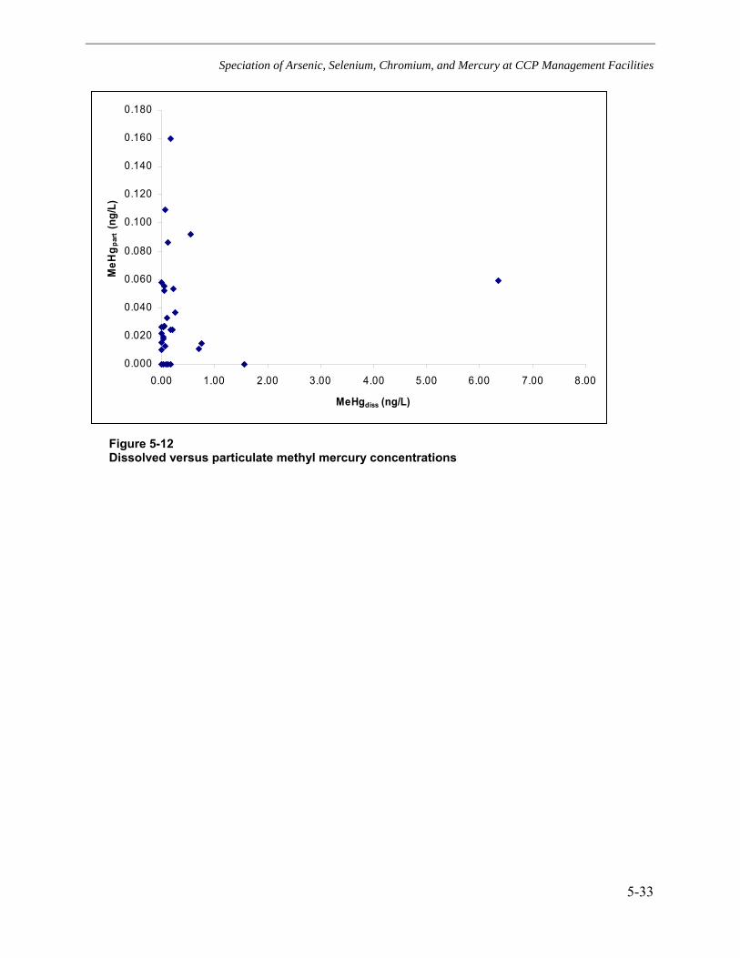
Speciation of Arsenic, Selenium, Chromium, and Mercury at CCP Management Facilities
5-33
0.000
0.020
0.040
0.060
0.080
0.100
0.120
0.140
0.160
0.180
0.00 1.00 2.00 3.00 4.00 5.00 6.00 7.00 8.00
MeHgdiss (ng/L)
MeH
g par
t (ng
/L)
Figure 5-12 Dissolved versus particulate methyl mercury concentrations


6-1
6 CONCLUSIONS
The following conclusions are based on 81 field leachate samples collected at 29 CCP management sites. Due to their unique characteristics, coal ash leachate (67 samples) and FGD leachate (14 samples) were treated separately.
Chemical Composition of Coal Ash Field Leachate Samples • Most leachate samples were moderately to strongly oxidizing and moderately to
strongly alkaline. The subbituminous/lignite ash samples had higher median pH (10.0) than bituminous ash (6.9). Several samples with relatively low Eh and pH were collected from impoundments.
• The anion chemistry of coal ash leachate samples is dominated by sulfate. The median concentration of this constituent was 339 mg/L; this was the only constituent in the leachate with a median concentration greater than 100 mg/L.
• Major cation chemistry was strongly influenced by the type of coal burned at the power plant. Ash leachate derived from bituminous coal was dominated by calcium and magnesium, while ash leachate derived from subbituminous/lignite coal was dominated by sodium.
• Silica and boron had the highest median concentrations (4,645 and 2,160 μg/L, respectively) of the minor and trace constituents. Median concentrations of strontium, molybdenum, lithium, aluminum, and barium were greater than 100 μg/L. Conversely, median concentrations of chromium, beryllium, thallium, silver, lead, and mercury were lower than 1 μg/L; with silver, beryllium, and lead being rarely detected (detected in 7, 6, and 27 percent of the samples, respectively).
• Most constituents (22 out of the 34 analyzed) had higher concentrations in landfill leachate samples than in impoundment leachate samples.
• Leachate samples derived from bituminous coal ash had higher concentrations of calcium, magnesium, cobalt, lithium, manganese, nickel, antimony, thallium, and zinc than leachate from subbituminous coal ash. Lithium and manganese had concentrations an order of magnitude higher in the bituminous ash leachate samples, while thallium was only detected in leachate from bituminous ash.
• Leachate from subbituminous/lignite coal ash had higher concentrations of carbonates, chloride, sodium, sulfate, aluminum, chromium, copper, and mercury than leachate from bituminous coal. The difference was most notable for

Conclusions
6-2
aluminum and mercury, where the concentrations were higher by an order of magnitude or more.
Chemical Composition of FGD Leachate Field Samples • The FGD leachate samples were moderately to strongly oxidizing, and
moderately to strongly alkaline. Landfill samples, as a group, were less oxic and more alkaline than impoundment samples, although the lowest Eh value was for an impoundment.
• Concentrations of most major constituents (specifically, calcium, chloride, potassium, sodium, and sulfate) in FGD leachate were higher than in ash leachate. The median sulfate concentration was 1,615 mg/L, and the maximum sulfate concentration was 30,500 mg/L, which was the highest single analytical result returned from the field leachate sampling. The high sulfate concentration was obtained from an impoundment where sluice water is recirculated.
• More than 25 percent of the chloride and sodium concentrations were greater than 1,000 mg/L, and median concentrations of chloride, calcium, potassium, and sodium were greater than 100 mg/L.
• The FGD leachate samples had higher percentages of chloride and potassium than the ash leachate samples.
• Anion concentrations were largely dominated by sulfate. Major cation concentrations (calcium, magnesium, potassium, sodium) were variable, with samples from the same site having different cation chemistry.
• The relative concentrations of minor and trace elements in FGD leachate were somewhat different than in ash leachate. Median concentrations of boron, strontium, and lithium in FGD leachate were a factor of 3 or more higher than in ash leachate, while concentrations of selenium, vanadium, uranium, and thallium in ash leachate were higher than in FGD leachate by a factor of 3 or more.
• Boron (9,605 μg/L), strontium (5,230 μg/L), lithium (3,055 μg/L), and silica (2,480 μg/L) had median concentrations greater than 1,000 μg/L in the FGD field leachate samples. Median concentrations of molybdenum, aluminum, and manganese were greater than 100 μg/L, while median concentrations of chromium, beryllium, thallium, silver, lead, and mercury were lower than 1 μg/L. Silver was not detected in the 14 FGD leachate samples, while beryllium (7 percent detects), chromium (36 percent), iron (29 percent), lead (36 percent), and thallium (14 percent), were usually not detected.
Speciation Analysis in Field Leachate Samples
Arsenic
• Arsenic concentrations in ash leachate ranged from 1.4 to 1,380 μg/L, with a median of 25 μg/L.

Conclusions
6-3
• The dominant arsenic species was determined in 43 samples. Most ash leachate samples (37) were dominated by As(V). As(III) was only dominant in four samples from impoundments where bituminous coal ash was managed. Two samples had equal amounts of arsenic species.
• Arsenic concentration in FGD leachate ranged from 11 to 230 μg/L, with a median of 28 μg/L.
• The dominant arsenic species was determined in 6 FGD leachate samples. Two were dominated by As(V), two were dominated by As(III), and two samples had equal amounts of the species.
Selenium
• Selenium concentration in ash leachate ranged from 0.07 to 1,760 μg/L, with a median of 19 μg/L.
• The dominant selenium species was determined in 46 leachate samples. Most ash leachate samples (29) were dominated by Se(IV). Se(VI) was dominant in 17 samples. Se(IV) dominated in impoundment settings when the source coal was bituminous or a mixture of bituminous and subbituminous, while Se(VI) was predominant in landfill settings and when the source coal was subbituminous/lignite. Most samples with relatively high concentration (>80 μg/L) were dominated by Se(VI) while samples with concentrations lower than 50 μg/L were mostly dominated by Se(IV).
• Selenium concentration in FGD leachate ranged from 1.1 to 2,360 μg/L, with a median of 6.2 μg/L.
• The dominant selenium species was determined in 7 FGD leachate samples. Six were dominated by Se(VI), one had similar percentages of both species, and none were dominated by Se(IV).
Chromium
• Chromium concentration in ash leachate ranged from <0.2 to 5,100 μg/L, with a median of 0.60 μg/L.
• The dominant chromium species was determined in 27 ash leachate samples. Most ash leachate samples (24) were dominated by Cr(VI). Cr(III) was dominant in three samples, two of which had acidic pH.
• Chromium concentration in FGD leachate ranged from <0.2 to 53 μg/L, with a median concentration below detection limits.
• The dominant chromium species was determined in three FGD leachate samples, and all three were dominated by Cr(VI).

Conclusions
6-4
Mercury
• Mercury concentrations in 22 ash leachate samples were very low, ranging from 0.25 to 61 ng/L, with a median concentration of 3.8 ng/L. Mercury concentrations in 8 FGD leachate samples were also very low, ranging from 0.82 to 79 ng/L, with a median concentration of 8.3 ng/L.
• The organic species of mercury always had low concentration, usually less than 5 percent of the total mercury concentration. Monomethyl mercury concentrations ranged from <0.02 to 6.7 ng/L, with a median concentration of 0.08 ng/L. Dimethyl mercury concentrations ranged from <0.02 to 0.06 ng/L, with a median concentration of <0.02 ng/L. There was no relationship between inorganic and organic mercury concentrations.
• There was no clear relationship between organic mercury concentrations and coal type, although there was a tendency for landfill leachate to yield slightly higher concentrations than impoundment leachate.
Effects of Power Plant Attributes on CCP Leachate Composition • Power plants that have cyclone boilers and burn petroleum coke produced
leachate samples with higher than median concentrations of most elements, and the highest concentrations of cadmium, molybdenum, and vanadium.
• There was no definitive relationship on leachate quality associated with hot-side and cold-side ESPs. Three sites receiving ash from hot-side ESPs were sampled. A landfill yielded the highest concentrations of Co, CO3, Cr, Cu, Na, Se, and SO4 of the sampled ash sites. However two impoundments did not show evidence of high concentrations.
• Oil ash was managed with coal ash at one site. The leachate from the ash sampled at this site did not show any evidence of low or high concentration for any elements.
• Most constituents in leachate from the single plant with a spray-dryer FGD system had lower concentration than leachate samples from the wet FGD systems used at other plants.

7-1
7 REFERENCES
EPRI, 1994. Chemical Attenuation Reactions of Selenium, Palo Alto, CA, Report TR-103535.
EPRI, 2000a. Environmental Chemistry of Arsenic: A Literature Review, Palo Alto, CA, Report 100585.
EPRI, 2000b. Field Evaluation of the Comanagement of Utility Low-Volume Wastes with High-Volume Coal Combustion By-Products: HA Site. Final Report 1000720, October 2000.
EPRI, 2003a. Combustion By-Product Environmental Analysis System, Palo Alto, CA, Report 1005263.
EPRI, 2003b. Field Evaluation of Comanagement of Utility Low-Volume Wastes with High-Volume By-Products: MO Site, Palo Alto, CA, Report 1005267.
EPRI, 2004. Chemical Attenuation Coefficients for Arsenic Species Using Soil Samples from Selected Power Plant Sites, Palo Alto, CA, Report 1005505.
Gürleyük, H. and D. Wallschläger, 2001. Determination of Chromium Species Using Suppressed Ion Chromatography-Inductively-Coupled Plasma-Mass Spectrometry, J. Anal. At. Spectrom. 16, 926-930.
Hintelmann, H. and N. Ogrinc, 2003. Determination of Stable Mercury Isotopes by ICP/MS and Their Application in Environmental Studies, in: Cai, Y. & Braids, O.C. (eds.): Biogeochemistry of environmentally important trace elements, ACS Symposium Series 835, American Chemical Society, 321-338.
Lindberg, S.E., G. Southworth, E.M. Prestbo, D. Wallschläger, M.A. Bogle, and J. Price, 2004. Gaseous Methyl- and Inorganic Mercury in Landfill Gas from Landfills in Florida, Minnesota, Delaware and California, accepted for publication in Atmos. Environ.
Puls, R.W and M.J. Barcelona, 1995. Low-Flow (Minimal Drawdown) Ground-Water Sampling Procedures, U.S. Environmental Protection Agency, EPA Ground Water Issue, EPA540-S-95-504.
Wallschläger, D. and R. Roehl, 2001. Determination of Inorganic Selenium Speciation in Waters by Ion Chromatography-Inductively-Coupled Plasma-Mass Spectrometry Using Eluant Elimination with a Membrane Suppressor, J. Anal. At. Spectrom. 16, 922-925.

References
7-2
Wallschläger, D., R.T. Wilkin, and R.G. Ford, 2005. Soluble Arsenic-Thio Species in Sulfidic Waters, submitted to Environ. Sci. Technol.

A-1
A ANALYTICAL RESULTS

Analytical Results
A-2
Table A-1 Hydrochemistry and Trace Elements
001 002 003 004 005 006 007 008 009 010 012 QA-1 013 Chloride mg/L 86.2 25 11 26 6.5 19 572 371 345 28 9 < 0.01 27.3 Sulfate mg/L 909 6,690 5,450 1,960 350 1,450 3,150 2,080 10,400 3,830 1,650 0.47 1,700 Sodium mg/L 443 3,410 2,910 672 93 108 1,330 606 743 1,700 30 0.4 55 Potassium mg/L 255 80 80 20 < 5 10 80 20 40 118 < 20 < 0.2 75 Magnesium mg/L < 1 0.59 0.53 70 15 77 125 23 1,990 8 13 0.10 36 Calcium mg/L 10 19 9 218 70 528 524 563 577 139 681 0.53 584 TOC mg/L 13.9 55.1 49.8 43.9 4.5 8.1 20.5 16.2 9.9 5.3 1.9 0.4 (a) 6.3 TIC mg/L 6.9 32.2 63.1 29.7 11.9 17.5 2.4 2.7 1.7 1.7 2.0 1.56 16.6 Temperature °C 20.2 21.5 15.4 14.9 21.3 18.7 17.6 26.9 25.6 17.3 22.6 n/a 21.3 Spec. Cond. mS/cm 3.5 12.8 11.2 3.8 0.8 2.9 8.3 4.8 13.0 7.7 2.7 n/a 2.9 Diss. Oxygen % sat. 0.1 0.2 0.2 0.2 0.2 0.4 0.2 0.3 0.3 14 5 n/a 4 pH pH 11.6 10.0 10.3 9.3 7.4 8.0 6.2 8.4 7.4 11.2 9.4 n/a 8.2 ORP (corr.) mV 209 276 271 276 411 341 356 1 342 111 245 n/a 102
Lithium ug/L 2,460 < 20 < 20 < 20 < 20 < 20 170 < 20 2,720 < 20 80 < 20 100 Beryllium ug/L < 1 < 1 < 1 < 1 < 1 < 1 < 1 < 1 < 1 < 1 < 1 < 4 < 1 Boron ug/L 2,120 18,400 31,900 10,800 1,410 15,600 81,500 49,000 98,500 14,000 93,400 < 50 112,000Aluminum ug/L 18,100 2,680 17,500 < 30 < 30 < 30 610 890 190 980 530 < 30 < 30 Silicon ug/L 6,900 5,800 1,200 6,100 6,400 2,600 10,500 400 12,700 9,900 1,500 < 100 18,500 Vanadium ug/L 373 1,070 635 45 < 2 4 15 < 2 18 5,020 195 < 2 4 Manganese ug/L < 4 7 < 4 751 577 < 4 704 113 564 < 4 22 < 4 2,560 Iron ug/L < 50 < 50 < 50 < 50 < 50 < 50 1,200 < 50 < 50 < 50 < 50 < 50 14,700 Cobalt ug/L < 1 133 9 < 1 < 1 < 1 6 < 1 78 < 1 < 1 < 1 7 Nickel ug/L < 3 75 8 14 4 4 597 5 463 8 4 < 20 15 Copper ug/L 11 494 62 6 3 4 14 44 7 15 < 3 < 3 < 3 Zinc ug/L < 5 < 5 < 5 < 5 6 19 23 < 5 34 12 12 < 30 45 Strontium ug/L 800 60 < 30 930 80 9,140 16,900 14,900 11,700 3,900 2,250 < 30 1,260 Molybdenum ug/L 9,740 5,720 6,200 1,200 440 310 60,800 570 320 25,400 740 < 30 100 Silver ug/L < 0.2 < 0.2 < 0.2 < 0.2 < 0.2 < 0.2 < 0.2 < 0.2 < 0.2 < 0.2 < 0.2 < 1 0.2 Cadmium ug/L 17.7 8.8 7.6 1.9 0.8 0.7 12.3 11.8 4.2 51.9 1.5 < 2 0.4 Antimony ug/L 0.9 0.8 0.7 0.6 < 0.3 4.7 2.8 0.7 4.6 1.0 6.7 < 3 0.7 Barium ug/L 50 < 30 < 30 110 40 70 50 < 30 90 50 40 < 30 < 30 Thallium ug/L < 0.1 < 0.5 < 0.5 < 0.1 < 0.1 < 0.1 < 0.5 < 0.1 2.9 < 0.1 < 0.1 <0.01 0.6 Lead ug/L < 0.2 < 0.2 < 0.2 < 0.2 < 0.2 < 0.2 3.5 0.3 < 0.2 0.3 < 0.2 < 1 < 0.2 Uranium ug/L < 0.2 0.2 9.8 1.3 < 0.2 10.4 0.7 < 0.2 0.7 0.3 1.8 < 1 3.3

Analytical Results
A-3
Table A-1 (Continued) Hydrochemistry and Trace Elements
013D 014 QA-2 015 016 SX-1 017 018 019 020 HN-1 HN-2 021 Chloride mg/L 27.5 32.8 0.05 25.3 54.8 22.2 72.0 63.4 84.8 75.9 29.2 45.4 18.0 Sulfate mg/L 1,610 1,370 0.40 782 910 1,530 91.4 339 124 131 1,260 810 193 Sodium mg/L 56 17 0.9 60 731 52 53 57 56 54 72 53 31 Potassium mg/L 74 26 < 0.2 20 229 38 8 9 6 6 277 48 11 Magnesium mg/L 39 7 0.63 33 20 7 21 36 28 23 3 21 13 Calcium mg/L 544 591 1.34 255 15 529 46 231 81 43 302 291 48 TOC mg/L 6.2 3.9 0.6 (a) 5.3 24.0 16.6 6.7 14.2 6.0 0.4 (a) 21.5 22.5 1.2 (a) TIC mg/L 16.7 35.1 1.47 15.4 5.60 11.3 22.4 115.0 48.7 24.8 2.48 2.94 8.03 Temperature °C n/a 20.5 32 31.7 30.6 n/a 29.7 18.3 35.5 29.6 n/a n/a 20.8 Spec. Cond. mS/cm n/a 2.6 0.0 1.6 5.1 n/a 0.7 1.6 1.0 0.7 n/a n/a 0.6 Diss. Oxygen % sat. n/a 5.5 3 3.7 2.9 n/a 1.6 2.9 3.4 4.5 n/a n/a 29.5 pH pH n/a 9.3 5.3 9.3 11.7 n/a 8.8 7.4 8.0 8.9 n/a n/a 7.9 ORP (corr.) mV n/a 240 515 339 124 n/a 289 94 296 303 n/a n/a 245
Lithium ug/L n/a 110 < 20 100 60 50 < 20 30 < 20 < 20 1,060 60 310 Beryllium ug/L n/a < 1 < 4 < 1 < 1 < 0.8 < 1 < 1 < 1 < 1 < 0.8 < 0.8 < 0.8 Boron ug/L n/a 54,900 < 50 3,890 109,000 24,200 860 26,300 470 700 2,350 42,700 850 Aluminum ug/L n/a 300 < 30 100 44,400 < 150 1,920 80 4,190 730 < 150 < 150 80 Silicon ug/L n/a 1,500 < 100 8,800 19,000 2,400 3,000 10,300 3,400 2,200 3,400 3,300 5,400 Vanadium ug/L n/a 36 < 2 550 1,230 11 16 6 10 17 206 41 217 Manganese ug/L n/a 25 < 4 < 4 8 52 < 4 4,170 14 < 4 < 4 < 4 67 Iron ug/L n/a < 50 < 50 < 50 1,530 < 50 < 50 3,190 < 50 < 50 < 50 < 50 300 Cobalt ug/L n/a < 1 < 1 3 2 < 1 < 1 2 1 < 1 < 1 < 1 < 1 Nickel ug/L n/a 5 < 20 16 128 < 3 5 8 7 4 10 7 4 Copper ug/L n/a < 3 < 3 < 3 21 < 3 12 35 8 7 7 5 6 Zinc ug/L n/a 40 < 30 < 5 130 25 8 7 9 11 16 < 5 6 Strontium ug/L n/a 3,140 < 30 4,300 1,200 2,690 530 640 580 720 930 680 730 Molybdenum ug/L n/a 6,030 < 30 420 39,600 3,010 80 100 < 30 < 30 1,910 500 710 Silver ug/L n/a < 0.2 < 1 < 0.2 < 0.2 1.1 < 0.2 < 0.2 < 0.2 < 0.2 2.0 0.8 < 0.2 Cadmium ug/L n/a 21.2 < 2 1.0 64.7 14.0 < 0.3 0.4 < 0.3 < 0.3 8.5 1.5 1.2 Antimony ug/L n/a 2.0 < 3 1.4 2.4 1.3 0.5 0.6 0.6 0.5 3.4 1.6 31.4 Barium ug/L n/a 40 < 30 350 140 80 140 100 350 220 80 60 240 Thallium ug/L n/a < 0.1 <0.01 2.5 0.3 3.1 < 0.1 0.1 < 0.1 < 0.1 < 0.5 < 0.5 1.5 Lead ug/L n/a < 0.2 < 1 < 0.2 4.6 0.8 < 0.2 < 0.2 0.21 < 0.2 0.4 0.4 < 0.2 Uranium ug/L n/a 1.1 < 1 3.7 0.7 12.5 1.1 4.6 1.2 1.2 < 0.2 0.7 2.7

Analytical Results
A-4
Table A-1 (Continued) Hydrochemistry and Trace Elements
022 023 024 025 026 027 028 029 030 031 032 034 035 Chloride mg/L 17.8 28.4 23 15.3 17.9 932 1,260 1,200 33.8 87 55.9 < 0.01 < 0.01 Sulfate mg/L 217 248 2,350 845 219 1,620 1,610 1,510 948 1,830 386 < 0.05 < 0.05 Sodium mg/L 42 33 188 80 43 285 341 297 25 60 32 < 0.1 < 0.1 Potassium mg/L 9 8 170 40 9 470 580 500 20 50 10 < 0.2 < 0.2 Magnesium mg/L 14 28 203 82 14 3 10 4 39 35 50 < 0.05 < 0.05 Calcium mg/L 43 79 405 235 43 671 722 730 332 665 124 < 0.05 < 0.05 TOC mg/L 0.5 (a) 2.2 1.3 (a) 4.1 0.9 (a) 1.9 0.5 (a) 1.4 (a) 0.5 (a) 11.0 0.6 (a) 0.1 (a) 0.1 (a) TIC mg/L 2.49 27.3 54.5 79.9 1.04 1.00 3.25 0.95 10.4 1.53 12.9 0.43 (a) 0.46 (a) Temperature °C 21.6 17.4 15.6 15.2 22.2 16.3 16.1 15.5 15.4 15.6 13.9 23.0 23.6 Spec. Cond. mS/cm 0.6 0.7 4.0 2.0 0.6 5.6 6.6 6.1 1.8 3.0 1.0 0.003 0.002 Diss. Oxygen % sat. 39.1 17.6 16 15.8 22.4 11.8 10.6 17.1 29.6 6.1 14.5 84.7 71.1 pH pH 7.1 7.0 7.0 6.5 7.2 10.0 9.0 9.9 8.5 8.5 7.8 5.67 5.40 ORP (corr.) mV 307 287 268 264 319 71 220 121 308 -41 295 335 306
Lithium ug/L 360 120 18,600 3,430 320 6,920 5,890 6,260 100 410 240 <0.1 <0.1 Beryllium ug/L < 0.8 < 0.8 < 0.8 < 0.8 < 0.8 < 0.8 < 0.8 < 0.8 < 0.8 < 0.8 < 0.8 <0.04 <0.04 Boron ug/L 430 1,970 22,400 11,100 420 1,450 3,260 2,820 3,280 7,610 2,210 0.9 1.4 Aluminum ug/L 40 90 < 30 < 30 40 190 < 30 130 190 140 < 30 0.4 0.8 Silicon ug/L 3,600 3,400 9,400 5,400 3,300 3,000 1,900 2,000 700 3,700 5,400 6.7 18.4 Vanadium ug/L 70 427 4 < 2 63 < 2 < 2 4 18 4 12 0.10 0.06 Manganese ug/L 104 149 3,650 4,110 104 18 202 62 41 269 92 <0.02 0.05 Iron ug/L < 50 120 80 90 < 50 < 50 < 50 < 50 < 50 < 50 < 50 0.4 0.4 Cobalt ug/L 8 2 96 8 8 < 1 < 1 < 1 < 1 1 3 <0.02 <0.02 Nickel ug/L 19 9 167 6 21 3 < 3 < 3 3 8 17 0.08 0.09 Copper ug/L 8 8 < 3 < 3 < 3 < 3 3 < 3 16 < 3 24 0.46 0.47 Zinc ug/L 21 11 148 < 5 14 < 5 12 < 5 90 13 15 <0.3 0.7 Strontium ug/L 430 1,990 6,460 2,290 400 3,520 3,980 4,300 990 2,480 360 <0.4 <0.4 Molybdenum ug/L 410 500 3,870 2,420 400 180 350 300 140 210 120 <0.1 <0.1 Silver ug/L < 0.2 < 0.2 < 0.2 < 0.2 < 0.2 < 0.2 < 0.2 < 0.2 < 0.2 < 0.2 < 0.2 <0.02 <0.02 Cadmium ug/L 1.1 1.0 9.1 5.1 1.6 0.5 0.8 0.6 < 0.3 0.5 1.2 <0.02 <0.02 Antimony ug/L 24.3 59.1 4.9 0.5 23.5 < 0.3 < 0.3 < 0.3 5.0 2.7 3.8 <0.02 <0.02 Barium ug/L 190 110 50 50 190 60 60 80 80 60 160 <0.2 <0.2 Thallium ug/L 12.0 1.3 1.5 0.4 12.3 < 0.5 < 0.5 < 0.5 3.4 < 0.1 17.6 <0.02 <0.02 Lead ug/L < 0.2 < 0.2 < 0.2 < 0.2 < 0.2 < 0.2 < 0.2 < 0.2 < 0.2 < 0.2 < 0.2 0.03 <0.02 Uranium ug/L < 0.2 60.8 13.0 19.3 < 0.2 < 0.2 < 0.2 < 0.2 5.3 2.0 1.0 <0.01 <0.01

Analytical Results
A-5
Table A-1 (Continued) Hydrochemistry and Trace Elements
036 037 038 039 042 043 044 044D 049 050 051 052 053 Chloride mg/L < 0.01 8.8 9.7 9.4 9.7 7.1 9.8 9.1 9.8 < 0.01 5.3 7.6 8.1 Sulfate mg/L < 0.05 123 121 101 57 111 70 70 53 < 0.05 111 128 176 Sodium mg/L < 0.1 3.8 3.9 4.7 8.6 8.5 8.3 8.3 7.0 0.1 11.8 6.8 5.6 Potassium mg/L < 0.2 2.2 2.3 5.3 5.2 7.0 5.0 5.0 4.0 < 0.2 13.6 11.1 9.2 Magnesium mg/L < 0.05 6.91 6.61 3.08 2.06 2.58 2.66 2.67 2.53 < 0.05 1.81 0.08 0.12 Calcium mg/L < 0.05 45.8 45.3 36.1 12.4 19.9 15.4 15.5 13.2 0.09 14.4 58.4 69.5 TOC mg/L 0.1 (a) < 0.09 < 0.09 < 0.09 < 0.09 < 0.09 < 0.09 < 0.09 < 0.09 0.1 (a) < 0.09 0.8 (a) 0.7 (a) TIC mg/L 0.48 (a) 10.4 10.5 6.66 2.01 1.03 0.75 (a) 0.68 (a) 2.18 0.44 (a) 0.92 3.30 4.96 Temperature °C 23.6 22 22.7 24.2 29.4 32 32 31.5 25.8 24.5 26.5 27.1 26.7 Spec. Cond. mS/cm 0.001 0.379 0.381 0.317 0.178 0.293 0.209 0.210 0.174 0.009 0.287 0.588 0.468 Diss. Oxygen % sat. 77 35 27.6 33.5 84.1 75.7 67.9 80.2 77.6 72 82.4 56 40.6 pH pH 5.66 7.05 7.04 6.98 5.79 4.26 5.97 6.03 5.97 4.92 4.35 10.59 8.92 ORP (corr.) mV 299 192 163 184 283 388 285 289 290 300 387 211 212
Lithium ug/L <0.1 82 81 125 179 239 146 145 99 <0.1 520 561 595 Beryllium ug/L <0.04 <0.4 <0.4 <0.4 1.6 8.6 0.8 1.3 <0.4 <0.04 5.2 <0.4 <0.4 Boron ug/L 3.1 1390 1240 917 426 838 429 489 265 43.3 272 4620 7370 Aluminum ug/L 1.0 15 14 6 148 3730 66 72 14 3.5 2150 15100 2010 Silicon ug/L 21.5 7960 7660 7000 4700 5780 4730 5100 4670 15.3 5840 1890 1030 Vanadium ug/L 0.10 13.8 6.9 2.6 70.8 35.6 9.6 9.5 5.6 0.21 4.7 754.4 62.4 Manganese ug/L 0.67 248 244 261 42.7 77.5 86.1 88.6 79.4 23.4 113 0.4 5.9 Iron ug/L 1.0 921 1700 1070 6 722 18 28 7 8.2 3240 16 30 Cobalt ug/L <0.02 1.7 0.7 <0.2 11.5 21.6 8.7 9.0 5.2 0.05 18.9 <0.2 0.2 Nickel ug/L 0.45 7.2 4.2 2.4 37.8 71.9 26.7 27.5 13.6 2.98 58.2 <0.6 1.5 Copper ug/L 0.55 0.5 1.0 <0.4 8.7 152 12.0 11.2 1.9 1.13 452 1.8 8.4 Zinc ug/L 0.7 <3 <3 <3 58.1 80.4 35.6 32.9 18.3 5.6 74.6 <3 5.7 Strontium ug/L <0.4 1350 1360 1120 170 247 272 262 209 <0.4 806 5150 5610 Molybdenum ug/L <0.1 1110 1060 287 127 35 54 54 60 0.2 8 246 360 Silver ug/L <0.02 <0.2 <0.2 <0.2 <0.2 <0.2 <0.2 <0.2 <0.2 <0.02 <0.2 <0.2 <0.2 Cadmium ug/L <0.02 4.6 4.1 1.2 1.3 1.9 0.7 0.8 0.5 <0.02 2.4 0.8 2.3 Antimony ug/L <0.02 4.6 2.4 0.3 13.9 17.8 8.7 8.8 7.1 <0.02 5.9 14.4 2.6 Barium ug/L <0.2 125 169 77 75 131 180 181 195 <0.2 545 250 87 Thallium ug/L <0.02 <0.2 <0.2 <0.2 0.7 4.2 1.6 1.5 0.7 <0.02 6.3 0.4 0.3 Lead ug/L <0.02 <0.1 <0.1 <0.1 0.2 1.9 0.2 <0.1 <0.1 <0.02 8.0 <0.1 0.5 Uranium ug/L <0.01 0.2 0.1 <0.1 <0.1 0.5 <0.1 <0.1 <0.1 <0.01 1.0 0.1 1.7

Analytical Results
A-6
Table A-1 (Continued) Hydrochemistry and Trace Elements
057 059 059D 060 061 062 064 069 070 070D 077 078 079 Chloride mg/L 5.6 4.5 4.6 < 0.01 7.1 15.8 5.0 7.3 12.1 9.7 < 0.01 < 0.01 77.2 Sulfate mg/L 52 55 55 < 0.05 61 117 150 45 50 51 < 0.05 < 0.05 315 Sodium mg/L 8.1 8.5 8.5 < 0.1 9.5 11.4 7.3 6.0 10.8 10.8 < 0.1 < 0.1 63 Potassium mg/L 5.8 6.4 6.4 < 0.2 6.4 9.6 9.4 3.6 5.0 4.9 < 0.2 < 0.2 13 Magnesium mg/L 1.53 1.37 1.43 < 0.05 4.97 0.11 1.49 2.16 1.78 1.81 < 0.05 < 0.05 19.5 Calcium mg/L 16.8 16.8 16.5 0.20 55.1 76.5 58.1 19.0 26.0 26.3 < 0.05 < 0.05 95.3 TOC mg/L < 0.09 < 0.09 < 0.09 < 0.09 < 0.09 < 0.09 < 0.09 < 0.09 < 0.09 < 0.09 0.4 (a) 0.2 (a) 0.3 (a) TIC mg/L 6.02 5.07 4.99 0.43 (a) 38.3 3.98 3.92 6.04 9.44 9.55 0.34 (a) 0.28 (a) 20.6 Temperature °C 28.5 31.2 n/a 25.7 27.6 29 30 27.7 29.4 28.9 28.6 27.0 19.5 Spec. Cond. mS/cm 0.189 0.195 n/a 0.003 0.433 0.765 0.455 0.182 0.244 0.247 0.001 0.002 1.076 Diss. Oxygen % sat. 89.2 165.1 n/a 90.2 65.3 37.9 67.7 63.5 67.9 68.3 64.3 74.3 28.0 pH pH 7.66 9.04 n/a 5.4 7.25 10.95 10.12 7.57 8.91 9.1 5.07 5.58 6.75 ORP (corr.) mV n/a 409 na 277 140 196 214 220 223 220 263 236 114
Lithium ug/L 267 293 288 <0.1 155 243 430 140 160 167 <0.05 <0.05 134 Beryllium ug/L <0.4 <0.4 <0.4 <0.04 <0.4 <0.4 <0.4 <0.4 <0.4 <0.4 <0.01 <0.01 <0.2 Boron ug/L 300 351 309 1.2 2600 494 476 231 207 236 7.1 6.8 1110 Aluminum ug/L 111 356 366 1.8 58 3900 2310 29 468 519 2.3 2.3 <2 Silicon ug/L 5120 5010 5190 8.6 11100 6870 4760 7450 7190 6920 509 513 10100 Vanadium ug/L 31.3 34.4 34.6 0.18 5.6 176.9 229.6 61.3 93.1 94.2 0.22 0.21 0.4 Manganese ug/L 1.6 0.6 0.8 0.04 395 <0.2 <0.2 22.0 0.4 0.7 7.50 4.84 190 Iron ug/L 6 26 25 0.7 2170 17 13 <5 27 46 12.9 2.28 25600 Cobalt ug/L <0.2 <0.2 <0.2 <0.02 0.3 <0.2 <0.2 1.3 <0.2 <0.2 0.007 0.003 0.18 Nickel ug/L 2.3 1.7 1.4 <0.6 4.0 <0.6 0.9 5.4 0.6 <0.6 <0.03 <0.03 <0.6 Copper ug/L 1.3 2.0 1.8 0.5 <0.4 1.2 0.5 0.7 1.8 2.1 0.30 0.27 <0.2 Zinc ug/L <3 4.0 <3 0.4 <3 <3 <3 <3 <3 <3 0.4 0.4 1.5 Strontium ug/L 545 547 576 <0.4 1840 1010 478 340 258 263 3.37 3.39 2190 Molybdenum ug/L 62 63 61 <0.1 95 173 217 78 61 63 <0.02 <0.02 135 Silver ug/L <0.2 <0.2 <0.2 <0.02 <0.2 <0.2 <0.2 <0.2 <0.2 <0.2 <0.01 <0.01 <0.2 Cadmium ug/L <0.2 0.4 <0.2 <0.02 0.3 0.6 0.6 0.3 <0.2 <0.2 <0.01 <0.01 <0.2 Antimony ug/L 6.2 5.6 5.5 <0.02 0.7 8.2 27.4 9.5 7.6 7.9 <0.005 0.005 <0.1 Barium ug/L 182 171 166 <0.2 226 194 319 156 124 132 <0.1 <0.1 99.2 Thallium ug/L 1.0 0.9 0.9 <0.02 0.5 <0.2 0.3 1.0 0.4 0.4 <0.005 <0.005 <0.1 Lead ug/L <0.1 <0.1 <0.1 <0.02 <0.1 <0.1 <0.1 <0.1 <0.1 <0.1 0.04 0.02 <0.1 Uranium ug/L 0.5 1.2 1.3 <0.01 1.4 <0.1 0.7 0.3 2.2 2.2 <0.001 <0.001 1.91

Analytical Results
A-7
Table A-1 (Continued) Hydrochemistry and Trace Elements
079D 082 083 084 088 089 090 091 092 TEB 094 095 096 (1) Chloride mg/L 77.9 72.0 68.4 67.9 < 0.01 0.37 11.8 5.35 4.67 0.22 0.06 0.04 92.4 Sulfate mg/L 315 174 92.8 135 < 0.05 1.50 324 393 448 0.65 < 0.05 < 0.05 2,850 Sodium mg/L 63 68 45 38 0.7 0.9 182 277 109 0.6 < 0.1 < 0.1 1,560 Potassium mg/L 14 5 4 6 < 0.2 0.2 113 84 67 1.2 < 0.2 < 0.2 74 Magnesium mg/L 19.4 19.1 12.6 30.8 < 0.05 0.35 0.15 < 0.05 < 0.05 < 0.05 < 0.05 < 0.05 9 Calcium mg/L 98.0 79.1 34.4 105 < 0.05 0.72 11.9 2.22 287 1.30 < 0.05 < 0.05 9 TOC mg/L 0.8 (a) 2.6 4.7 < 0.09 0.4 (a) 0.5 (a) 12.8 4.3 3.4 0.4 (a) 0.3 (a) 0.3 (a) 49.8 TIC mg/L 19.7 35.9 11.9 60.5 0.28 (a) 1.20 13.8 7.62 0.85 1.37 0.21 (a) 0.23 (a) 128 Temperature °C 18.0 30.2 25.9 19.2 n/a n/a 17.2 16.8 15.9 n/a 12.4 13.7 16.1 Spec. Cond. mS/cm 1.068 0.911 0.547 0.927 n/a n/a 1.59 2.33 1.427 n/a 0.002 0.005 7.295 Diss. Oxygen % sat. 21.0 65.1 100.0 40.7 n/a n/a n/a n/a n/a n/a 84 73.3 67 pH pH 6.84 8.64 9.36 7.78 n/a n/a 10.86 11.52 11.17 n/a 6.2 5.44 7.29 ORP (corr.) mV 87 241 217 198 n/a n/a 246 288 346 n/a 227 261 223
Lithium ug/L 134 60 27 139 <0.05 4 2 5 11 1.25 <0.05 <0.05 5 Beryllium ug/L <0.2 <0.2 <0.2 <0.2 <0.01 0.011 <0.2 <0.2 <0.2 <0.01 <0.01 <0.01 <0.2 Boron ug/L 1200 442 1020 4310 89.6 215 1800 495 1080 240 1.1 0.7 5650 Aluminum ug/L <2 1080 2030 41 1.1 92.9 19900 30000 5140 38.6 7.8 1.3 1700 Silicon ug/L 9970 4210 1050 2300 3780 6740 4200 4390 2460 7100 11.5 9.2 1400 Vanadium ug/L 0.5 103 49.3 11.5 0.09 1.23 365 562 156 1.07 0.13 0.15 473 Manganese ug/L 191 2.0 1.0 91.1 1.50 9.97 0.9 <0.1 <0.1 6.1 0.5 0.22 1.5 Iron ug/L 25200 <3 <3 62.0 52.7 271 29.7 <8 <8 140 5.4 0.51 25.3 Cobalt ug/L 0.18 0.80 0.53 0.81 <0.001 0.17 0.12 0.04 0.40 0.301 <0.001 <0.001 3.27 Nickel ug/L <0.6 3.6 4.4 4.6 <0.05 6.29 14 4 <1 12 0.06 0.08 7 Copper ug/L 1.4 3.8 2.1 <0.2 0.33 2.02 1.4 0.5 1.4 1.2 1.4 2.5 30.0 Zinc ug/L 2.5 <2 3.0 <2 <0.1 6.9 <2 <2 <2 2.9 3.3 4.3 <2 Strontium ug/L 2140 828 1010 2520 9.48 82.6 830 1610 11100 135 0.31 0.11 311 Molybdenum ug/L 132 21.9 27.7 283 0.04 0.83 1890 1390 658 0.75 0.02 <0.01 4510 Silver ug/L <0.2 <0.2 <0.2 <0.2 <0.01 <0.01 <0.2 <0.2 <0.2 <0.01 <0.01 <0.01 <0.2 Cadmium ug/L <0.2 <0.2 0.3 0.7 <0.005 0.037 6.1 4.8 2.8 0.04 0.02 0.01 15.0 Antimony ug/L <0.1 1.1 2.9 1.1 0.021 0.074 2.3 0.5 0.2 0.082 0.007 <0.005 0.8 Barium ug/L 93.6 434 294 176 <0.2 10.7 89.3 259 657 29.7 0.6 <0.2 20 Thallium ug/L <0.1 0.5 <0.1 0.4 <0.005 <0.005 <0.1 <0.1 <0.1 0.021 <0.005 <0.005 <0.1 Lead ug/L <0.1 <0.1 0.2 <0.1 0.01 0.17 <0.1 <0.1 <0.1 0.03 0.09 0.06 <0.1 Uranium ug/L 1.95 2.66 1.23 26.8 <0.0005 0.17 0.39 <0.01 0.01 0.02 <0.0005 <0.0005 5.53

Analytical Results
A-8
Table A-1 (Continued) Hydrochemistry and Trace Elements
096D (1) 097 098 099 100 101 102 103 104 105 106 106D 107 Chloride mg/L 92.5 91.7 38.7 27.3 0.07 37.2 73.0 0.01 0.02 1,080 859 715 2,330 Sulfate mg/L 2,870 2,870 1,800 1,510 0.08 1,610 2,410 < 0.05 0.12 10,200 4,710 4,430 30,500 Sodium mg/L 1,560 1,560 837 651 1.3 117 455 0.2 0.1 3,270 2,310 2,210 4,630 Potassium mg/L 77 73 31 6 < 0.2 23 219 < 0.2 < 0.2 380 350 350 500 Magnesium mg/L 10 7 44 16 < 0.05 188 69 < 0.05 < 0.05 1,000 < 0.05 < 0.05 5,810 Calcium mg/L 11 6 52 73 0.17 392 431 < 0.05 < 0.05 600 234 228 570 TOC mg/L 50.1 48.7 56.8 14.7 0.4 (a) 4.6 3.3 0.1 (a) 0.1 (a) 33.1 19.1 18.6 50.1 TIC mg/L 128 105 39.7 14.1 0.28 (a) 27.8 24.3 0.16 (a) 0.27 (a) 7.88 4.27 4.36 1.85 Temperature °C 16.5 17.4 12.9 15.1 13.4 16.9 15.8 n/a 6.6 9.94 19.0 19.0 19.18 Spec. Cond. mS/cm 7.379 7.340 4.282 3.451 0.003 3.363 4.915 n/a 0.072 18.85 11.56 11.56 26.14 Diss. Oxygen % sat. 61.1 69.4 27.5 37 81.1 86.1 94.7 n/a 64.5 36 95 95 2 pH pH 7.71 9.35 8.58 7.91 5.94 6.74 7.41 n/a 9.54 8.99 11.96 11.96 6.83 ORP (corr.) mV 224 206 39 103 238 213 222 n/a 288 271 18 18 230
Lithium ug/L 5 4 63 <1 <0.05 431 6940 <0.05 <0.05 1050 130 132 3390 Beryllium ug/L <0.2 <0.2 <0.2 <0.2 <0.01 <0.2 <0.2 <0.01 <0.01 <0.2 <0.2 <0.2 1 Boron ug/L 5950 6080 11700 2590 0.8 89500 23700 <0.1 0.2 26800 7310 7460 50200 Aluminum ug/L 1700 4300 117 42 3 52 <2 2.3 2.7 31 608 618 708 Silicon ug/L 1340 1540 4620 4410 25.7 6750 3940 5.9 17.9 2280 21000 22000 45400 Vanadium ug/L 477 500 159 3.8 0.10 0.8 44.3 0.25 0.33 1.8 400 403 103 Manganese ug/L 1.4 1.5 59.8 1230 0.39 1420 72.3 0.33 2.32 473 <0.1 0.1 1170 Iron ug/L 20.1 46.3 <8 126 0.52 12.1 <8 2.05 1.36 4.7 4.6 6.6 52.4 Cobalt ug/L 3.31 3.28 0.88 0.29 <0.001 9.19 0.07 <0.001 0.008 0.09 0.11 0.07 13.0 Nickel ug/L 7 8 9 2 0.18 31 3 <0.03 0.25 3.3 7.5 8.0 153 Copper ug/L 29.9 42.8 1.7 1.5 1.60 2.8 1.6 0.51 0.55 0.4 0.6 0.5 2 Zinc ug/L <2 <2 <2 <2 5 86 <2 0.2 0.7 <2 <2 <2 68 Strontium ug/L 293 303 1700 93 0.72 1320 10300 0.67 3.88 6980 9730 10000 1500 Molybdenum ug/L 4450 4480 2580 2070 0.05 751 9630 <0.04 <0.04 164 3520 3560 1320 Silver ug/L <0.2 <0.2 <0.2 <0.2 <0.01 <0.2 <0.2 <0.01 <0.01 <0.2 <0.2 <0.2 <1 Cadmium ug/L 13.1 13.0 7.7 6.1 0.028 4.6 35.9 0.005 <0.005 0.5 12.8 11.8 6.6 Antimony ug/L 0.8 0.9 0.7 0.2 0.013 0.1 4.4 0.013 <0.005 9.4 2.3 2.2 22.3 Barium ug/L 16 18 34 66 0.7 23 48 <0.1 0.2 75 134 138 158 Thallium ug/L <0.1 <0.1 <0.1 <0.1 <0.005 <0.1 <0.1 <0.005 <0.005 <0.1 <0.1 <0.1 <0.5 Lead ug/L 0.2 0.3 0.3 0.2 <0.1 0.1 0.1 0.017 <0.005 0.2 0.4 0.5 0.8 Uranium ug/L 5.41 5.66 1.87 0.19 <0.0005 36.6 7.38 <0.0007 <0.0007 6.47 <0.01 0.04 16.0

Analytical Results
A-9
Table A-1 (Continued) Hydrochemistry and Trace Elements
108 109 110 111 112 113 114 115 116 117 118 118D 119 Chloride mg/L 84 0.29 0.17 28.5 n/a 13.4 19.6 16.9 16.8 < 0.01 66.2 66.3 64.8 Sulfate mg/L 3,490 < 0.05 0.10 2,440 n/a 203 210 166 163 < 0.05 462 467 441 Sodium mg/L 840 0.2 < 0.1 190 n/a 21 28 31 32 0.3 36 37 36 Potassium mg/L 120 < 0.2 < 0.2 210 n/a 11 11 9 10 < 0.2 13 13 9 Magnesium mg/L 57 < 0.05 < 0.05 236 n/a 22 20 17 16 < 0.05 72 74 67 Calcium mg/L 596 < 0.05 < 0.05 405 n/a 49 53 45 38 < 0.05 121 123 123 TOC mg/L 10.3 0.4 (a) 0.2 (a) 4.1 n/a 1.8 1.4 (a) 1.4 (a) 1.5 0.3 (a) 3.9 4.3 4.1 TIC mg/L 18.8 0.86 0.73 (a) 59.9 n/a 14.2 16.7 1.57 2.48 0.75 (a) 19.2 19.4 21.6 Temperature °C 10.6 n/a n/a 15.05 14.2 20.98 22.03 16.0 15.5 n/a 14.65 14.4 10.48 Spec. Cond. mS/cm 6.174 n/a n/a 4.529 2.765 0.643 0.673 0.567 0.564 n/a 1.348 1.355 1.319 Diss. Oxygen % sat. 87 n/a n/a 58.7 46.7 28.4 15.1 87 98.4 n/a 80.7 120 122.8 pH pH 8.76 n/a n/a 7.18 6.83 7.74 6.99 7.28 7.41 n/a 7.6 7.49 8.6 ORP (corr.) mV 240 n/a n/a 280 229 231 220 261 289 n/a 257 244 240
Lithium ug/L 27 <0.05 <0.05 23600 4540 347 187 318 312 <0.05 253 264 162 Beryllium ug/L <0.2 <0.01 <0.01 <0.2 <0.2 <0.2 <0.2 <0.2 <0.2 <0.01 <0.2 <0.2 <0.2 Boron ug/L 41500 0.9 2.0 27200 13300 1480 931 444 450 0.7 2200 2120 1700 Aluminum ug/L 81 3.5 3.4 27 17 42 51 17 25 4.3 18 13 28 Silicon ug/L 221 26.1 42.2 7440 2300 2840 12000 2890 2970 42.4 3710 3840 2870 Vanadium ug/L 3.6 0.14 0.14 26.9 1.8 402 45.2 53.6 54.3 0.18 3.8 3.5 6.5 Manganese ug/L 7.7 0.57 4.48 2700 531 147 445 59.3 58.1 0.40 155 167 59.6 Iron ug/L 3.0 3.7 0.9 <13 55.4 <13 349 <13 <13 0.4 <13 <13 <13 Cobalt ug/L 0.42 <0.001 0.039 113 8.91 1.76 5.36 7.15 7.05 0.039 3.76 3.53 1.58 Nickel ug/L 2.2 <0.1 0.2 189 5 <2 6 14 14 <0.1 15 14 8 Copper ug/L 1.6 0.64 0.96 1.3 0.9 0.4 1.6 9.8 8.8 0.53 2.5 3.0 1.9 Zinc ug/L <2 0.7 1.0 289 4 <2 6 16 13 0.8 11 9 <2 Strontium ug/L 12000 0.59 40.5 6750 2740 662 771 405 411 0.61 507 513 465 Molybdenum ug/L 2680 0.02 0.11 5100 2690 1280 264 340 336 0.02 131 128 88.7 Silver ug/L 0.8 <0.01 <0.01 <0.2 <0.2 <0.2 <0.2 <0.2 <0.2 <0.01 <0.2 <0.2 <0.2 Cadmium ug/L 10.6 0.02 0.01 23.6 11.8 5.6 1.4 2.0 2.0 <0.005 1.4 1.0 0.6 Antimony ug/L 5.2 <0.005 0.006 9.1 0.6 58.5 4.4 20.0 20.7 <0.005 3.1 2.8 2.5 Barium ug/L 63 <0.1 0.6 40 43 105 62 182 177 0.6 150 153 118 Thallium ug/L <0.1 <0.005 <0.005 5.3 0.6 0.8 0.3 7.6 7.3 <0.005 14.2 11.0 6.8 Lead ug/L 0.3 0.028 0.008 <0.14 <0.14 <0.14 <0.14 <0.14 <0.14 0.013 <0.14 <0.14 <0.14 Uranium ug/L 21.1 <0.0008 0.001 18.9 21.8 7.91 0.20 0.15 0.17 <0.0008 1.75 1.73 2.02

Analytical Results
A-10
Table A-1 (Continued) Hydrochemistry and Trace Elements
120 121 122 125 126 126D 127 128 Chloride mg/L 1,150 1,190 911 0.09 42.5 42.7 31 98 Sulfate mg/L 1,350 1,510 1,430 < 0.05 507 509 1,120 836 Sodium mg/L 255 303 247 0.1 393 393 653 141 Potassium mg/L 500 609 486 < 0.2 20 20 40 30 Magnesium mg/L 5 6 < 2.5 < 0.05 < 0.05 < 0.05 < 0.05 8 Calcium mg/L 710 698 669 < 0.05 < 2.5 < 2.5 13 351 TOC mg/L 1.5 1.3 (a) 2.4 0.6 (a) 6.0 5.8 7.9 7.9 TIC mg/L 2.81 2.53 2.37 0.39 (a) 5.90 5.89 7.40 3.03 Temperature °C 16.16 13.65 12.02 12.08 16.75 17.02 16.4 20.5 Spec. Cond. mS/cm 6.322 6.897 5.906 0.013 2.57 2.76 4.02 2.19 Diss. Oxygen % sat. 81.3 29.8 77.8 46 35 35 13.1 65 pH pH 10.33 10.04 10.53 6.04 11.75 11.75 11.74 7.84 ORP (corr.) mV 87 181 46 373 249 241 225 339
Lithium ug/L 6470 6360 7070 <0.05 7 8 16 33 Beryllium ug/L <0.2 <0.2 <0.2 <0.01 <0.4 <0.4 <0.2 <0.2 Boron ug/L 3080 3160 1560 2.7 3070 2890 3890 11900 Aluminum ug/L 167 24 229 4.2 5590 5620 5920 26 Silicon ug/L 1890 1810 2360 1.1 9450 8860 10300 3940 Vanadium ug/L 4.5 0.7 1.3 0.29 122 120 236 6.8 Manganese ug/L 38.1 113 15.5 0.14 <0.4 <0.4 <0.2 197 Iron ug/L <13 <13 <13 0.3 <25 <25 <25 <25 Cobalt ug/L 0.05 0.09 0.03 0.022 <0.04 <0.04 0.20 1.61 Nickel ug/L 3 <2 <2 <0.1 <0.6 <0.6 <2 <2 Copper ug/L 0.3 0.4 1.4 0.04 4.2 3.9 2.4 1.5 Zinc ug/L <2 <2 <2 0.2 <2 <2 <2 5 Strontium ug/L 4500 4210 3860 0.63 649 648 1830 5960 Molybdenum ug/L 333 368 223 0.02 220 223 524 910 Silver ug/L <0.2 <0.2 <0.2 <0.01 <0.2 <0.2 <0.2 <0.2 Cadmium ug/L 1.9 1.6 0.8 <0.005 1.0 1.0 2.1 3.8 Antimony ug/L 0.1 0.1 <0.1 <0.005 0.4 0.4 0.2 1.3 Barium ug/L 78 65 58 0.4 36 34 64 86 Thallium ug/L 0.3 <0.1 <0.1 <0.005 <0.1 <0.1 <0.1 <0.1 Lead ug/L <0.14 <0.14 <0.14 <0.007 <0.14 <0.14 <0.14 <0.14 Uranium ug/L 0.02 0.10 0.04 <0.0008 <0.02 <0.02 <0.02 0.97

Analytical Results
A-11
Table A-1 (Continued) Hydrochemistry and Trace Elements
Footnotes: (1) = Samples 096 and 096D are samples of leachate that were treated with CO2 prior to analysis. (a) = sample concentration less than 5 times blank n/a = not analyzed

Analytical Results
A-12
Table A-2 Speciation
Sample ID 001 002 003 004 005 006 007 008 009 010 012 QA-1
As, diss. ug/L 20.4 48.4 84 18.6 3.0 12.2 20.1 16.9 28.9 22.3 238 0.11
As(III), diss. ug/L < 0.3 < 6 < 6 8.4 < 0.2 < 0.3 < 2 0.7 (a) < 6 1.5 (a) 97.0 < 0.02
As(V), diss. ug/L 9.5 47 69 5.2 1.3 0.9 (a) < 2 < 0.5 < 10 10 66 < 0.03
As, other ug/L 2.1 < 6 < 6 < 0.3 < 0.2 < 0.3 < 2 < 0.3 < 6 < 0.6 < 0.6 < 0.02
Cr, diss. ug/L < 0.5 5,100 4,670 8.8 0.7 5.7 2 < 0.5 52.9 25.8 < 0.5 < 3
Cr(III), diss. ug/L n/a 340 190 < 0.1 n/a < 0.1 < 0.1 n/a 1 < 0.4 n/a n/a
Cr(VI), diss. ug/L 2.2 5,090 3,530 8.1 1.5 6.4 2.9 < 0.1 47 22 1.9 < 0.05
Se, diss. ug/L 127 1,730 1,760 49.9 7.6 16.8 (b) 289 3.7 (b) 2,360 318 3.24 0.10 (a)
Se(IV), diss. ug/L 8.3 19 76 8.1 3.15 1.6 79.5 < 0.1 < 2 24.4 1.4 < 0.02
Se(VI), diss. ug/L 83.0 1,300 1,240 22.1 0.57 11.2 119 0.27 (a) 1,660 158 < 0.2 < 0.03
Se, other ug/L n/a n/a n/a n/a n/a n/a n/a n/a n/a n/a n/a n/a
Hgdiss. ng/L n/a 14.4 18.4 5.9 2.1 (a) 0.8 (a) 1.9 (a) 4.2 (a) 28.4 n/a n/a n/a
Hgpart. ng/L n/a 254 26 < 1 44 25 (a) 16 (a) < 1 121 n/a n/a n/a
MeHgdiss. ng/L n/a 0.11 0.09 (a) 0.26 0.12 0.54 < 0.02 0.07 (a) < 0.02 n/a n/a n/a
MeHgpart. ng/L 0.03 (a) 0.03 (a) < 0.01 0.04 (a) 0.09 0.09 0.02 (a) 0.01 (a) 0.02 (a) n/a n/a n/a
DMM ng/L 0.055 0.005 < 0.005 < 0.005 0.010 < 0.005 0.007 < 0.005 n/a n/a n/a n/a

Analytical Results
A-13
Table A-2 (Continued) Speciation
Sample ID 013 013D 014 QA-2 015 016 SX-1 017 018 019 020 HN-1 HN-2
As, diss. ug/L 21.6 22 163 0.12 23.8 68.6 72.0 4.11 23.1 5.11 4.19 59.8 20.6
As(III), diss. ug/L 3.7 1.9 1.9 0.02 (a) < 0.6 < 0.6 0.9 0.88 0.42 0.57 1.00 < 0.1 < 0.1
As(V), diss. ug/L < 0.5 < 0.5 86 < 0.03 24 25 46.9 <0.08 5.22 <0.08 0.53 33.6 6.9
As, other ug/L < 0.3 < 0.3 0.9 (a) < 0.02 < 0.6 < 0.6 < 0.1 0.1 < 0.06 < 0.06 0.1 0.2 0.1
Cr, diss. ug/L < 0.5 n/a < 0.5 < 3 12.9 3.8 < 0.5 3 < 0.5 1.0 0.7 < 0.5 < 0.5
Cr(III), diss. ug/L n/a n/a n/a n/a < 0.4 < 0.1 n/a < 0.04 n/a < 0.1 n/a n/a n/a
Cr(VI), diss. ug/L 0.7 0.7 0.5 < 0.05 12.8 < 0.5 < 0.1 2.8 1.3 0.9 < 0.05 n/a n/a
Se, diss. ug/L 0.28 (b) 0.38 (b) 1.81 (b) 0.10 (a) 22.4 193 7.77 2.4 0.50 (b) 1.8 2.5 22.2 9.15
Se(IV), diss. ug/L < 0.1 < 0.1 0.6 (a) < 0.02 14.9 101 2 (a) 0.3 (a) < 0.1 0.1 (a) 0.9 3 (a) < 1
Se(VI), diss. ug/L < 0.1 < 0.1 < 0.2 < 0.03 3.4 14.3 4 (a) 1.1 < 0.2 1.3 0.8 16 6
Se, other ug/L n/a n/a n/a n/a n/a n/a n/a n/a n/a n/a n/a n/a n/a
Hgdiss. ng/L n/a n/a n/a n/a n/a n/a n/a n/a n/a n/a n/a n/a n/a
Hgpart. ng/L n/a n/a n/a n/a n/a n/a n/a n/a n/a n/a n/a n/a n/a
MeHgdiss. ng/L n/a n/a n/a n/a n/a n/a n/a n/a n/a n/a n/a n/a n/a
MeHgpart. ng/L n/a n/a n/a n/a n/a n/a n/a n/a n/a n/a n/a n/a n/a
DMM ng/L n/a n/a n/a n/a n/a n/a n/a n/a n/a n/a n/a n/a n/a

Analytical Results
A-14
Table A-2 (Continued) Speciation
Sample ID 021 022 023 024 025 026 027 028 029 030 031 032 034
As, diss. ug/L 194 11.1 218 11.2 6.47 10.8 39.1 30.0 48.9 42.5 221 25.4 < 0.02
As(III), diss. ug/L 2.1 12.5 0.8 (a) 0.4 (a) 1.35 11.2 13.2 2.4 1.7 3.5 201 17.5 < 0.01
As(V), diss. ug/L 208 0.49 189 <0.2 <0.08 0.4 (a) 4.8 1.7 8.9 29.5 23.6 16.9 < 0.8
As, other ug/L < 0.3 < 0.06 < 0.3 < 0.2 < 0.06 < 0.2 1.3 0.2 0.3 0.4 0.7 0.1 n/a
Cr, diss. ug/L < 0.5 1.0 < 0.5 < 0.5 < 0.5 1.1 < 0.5 < 0.5 < 0.5 < 0.5 < 0.5 1.4 0.08
Cr(III), diss. ug/L n/a < 0.04 n/a n/a n/a < 0.04 n/a n/a n/a n/a n/a < 0.1 0.06
Cr(VI), diss. ug/L < 0.05 0.9 < 0.5 n/a n/a 0.9 n/a n/a n/a < 0.05 < 0.1 < 0.05 < 0.01
Se, diss. ug/L 6.5 30.7 283 18.2 1.9 (b) 31.5 1.05 (b) 2.56 (b) 2.29 44.1 12.5 18.0 < 0.02
Se(IV), diss. ug/L 5.3 20.5 217 5.3 < 0.1 20.4 < 0.3 < 0.3 < 0.3 27.0 0.9 (a) 13.5 < 0.1
Se(VI), diss. ug/L < 0.6 2.2 1.5 6.3 1.1 2.2 < 0.3 1.4 1.6 12.5 5.5 0.7 < 0.2
Se, other ug/L n/a n/a n/a n/a n/a n/a n/a n/a n/a n/a n/a n/a n/a
Hgdiss. ng/L 1.4 (a) 1.0 (a) 1.4 (a) n/a n/a 0.4 (a) 21.3 1.2 (a) 12.4 0.8 (a) 5.2 1.4 (a) n/a
Hgpart. ng/L 155 53 14 (a) n/a n/a 17 (a) 4 (a) 13 (a) 59 < 1 30 186 n/a
MeHgdiss. ng/L 0.03 (a) 0.03 (a) < 0.02 n/a n/a < 0.02 1.56 0.18 0.70 0.06 (a) 6.71 0.05 (a) n/a
MeHgpart. ng/L 0.02 (a) 0.03 (a) 0.03 (a) n/a n/a < 0.01 < 0.01 < 0.01 0.01 (a) 0.11 n/a 0.05 n/a
DMM ng/L < 0.005 < 0.005 < 0.005 n/a n/a < 0.005 < 0.005 < 0.005 < 0.005 0.022 0.050 0.032 n/a

Analytical Results
A-15
Table A-2 (Continued) Speciation
Sample ID 035 036 037 038 039 042 043 044 044D 049 050 051 052
As, diss. ug/L < 0.02 0.03 (a) 56.0 123 42.3 23.7 75.2 5.1 4.9 5.4 0.12 38.1 164
As(III), diss. ug/L < 0.01 < 0.01 0.30 2.63 1.39 < 0.1 < 0.05 0.39 < 0.04 < 0.04 < 0.01 0.70 (a) 22.8
As(V), diss. ug/L < 0.8 < 0.8 34 53 53 19 (a) 28 3 (a) 2 (a) 2 (a) < 0.8 15 8 (a)
As, other ug/L n/a n/a n/a n/a n/a n/a n/a n/a n/a < 0.04 n/a n/a n/a
Cr, diss. ug/L 0.07 0.14 < 0.4 < 0.4 < 0.4 < 0.4 29.2 < 0.4 < 0.4 < 0.4 0.80 11.3 < 0.4
Cr(III), diss. ug/L 0.07 0.07 < 0.01 < 0.01 < 0.01 0.17 26.4 0.25 0.12 0.07 0.84 9.92 0.16
Cr(VI), diss. ug/L < 0.01 < 0.01 < 0.01 < 0.01 < 0.01 0.03 (a) < 0.1 < 0.01 < 0.01 < 0.01 < 0.01 < 0.05 0.06
Se, diss. ug/L < 0.02 0.02 (a) 1.98 (b) 0.13 (a) 0.17 (a) 42.6 23.5 (b) 13.9 13.6 10.0 0.02 (a) 0.45 (b) 10.2
Se(IV), diss. ug/L < 0.1 < 0.1 2.6 < 0.5 0.2 (a) 39.1 20.2 11.4 11.5 8.3 < 0.1 < 0.5 7
Se(VI), diss. ug/L < 0.2 < 0.2 < 1 < 1 < 0.4 1.9 < 1 1.7 1.8 0.6 (a) < 0.2 < 1 < 4
Se, other ug/L n/a n/a n/a n/a n/a n/a n/a n/a n/a n/a n/a n/a n/a
Hgdiss. ng/L n/a n/a n/a n/a n/a n/a n/a n/a n/a n/a n/a n/a n/a
Hgpart. ng/L n/a n/a n/a n/a n/a n/a n/a n/a n/a n/a n/a n/a n/a
MeHgdiss. ng/L n/a n/a n/a n/a n/a n/a n/a n/a n/a n/a n/a n/a n/a
MeHgpart. ng/L n/a n/a n/a n/a n/a n/a n/a n/a n/a n/a n/a n/a n/a
DMM ng/L n/a n/a n/a n/a n/a n/a n/a n/a n/a n/a n/a n/a n/a

Analytical Results
A-16
Table A-2 (Continued) Speciation
Sample ID 053 057 059 059D 060 061 062 064 069 070 070D 077 078
As, diss. ug/L 279 98.6 124 125 < 0.02 1,380 61.5 178 99.5 143 144 < 0.008 0.017 (a)
As(III), diss. ug/L 108 < 0.2 < 0.2 < 0.2 < 0.01 859 < 0.2 < 0.4 < 0.2 < 0.2 < 0.2 < 0.04 < 0.04
As(V), diss. ug/L 82 93 127 119 < 0.8 519 37 150 94 136 137 < 0.8 < 0.8
As, other ug/L 0.7 n/a n/a n/a n/a n/a n/a n/a n/a n/a 0.53 n/a n/a
Cr, diss. ug/L < 0.4 1.9 2.7 2.5 0.10 < 0.4 10.5 22.4 3.2 5.3 5.4 0.02 0.02
Cr(III), diss. ug/L 0.05 1.06 0.01 (a) < 0.01 0.05 0.27 0.95 0.04 (a) 0.46 0.63 0.62 <0.02 0.02
Cr(VI), diss. ug/L < 0.01 0.41 1.28 1.23 < 0.01 < 0.01 6.24 23.0 2.98 5.28 5.17 <0.006 <0.006
Se, diss. ug/L 1.24 (b) 2.44 2.58 (b) 2.55 < 0.02 4.31 112 103 36.4 29.1 29.4 < 0.008 < 0.008
Se(IV), diss. ug/L < 2 2.0 2.5 2.2 < 0.1 <10 90.4 97 33.1 29 28 < 0.04 < 0.04
Se(VI), diss. ug/L < 4 < 1 < 1 < 1 < 0.2 <20 32.1 < 4 1.7 (a) < 4 < 4 < 0.06 < 0.06
Se, other ug/L n/a n/a n/a n/a n/a n/a n/a n/a n/a n/a n/a n/a n/a
Hgdiss. ng/L n/a n/a n/a n/a n/a n/a n/a n/a n/a n/a n/a 1.9 (a) 2.5 (a)
Hgpart. ng/L n/a n/a n/a n/a n/a n/a n/a n/a n/a n/a n/a 3 (a) 4 (a)
MeHgdiss. ng/L n/a n/a n/a n/a n/a n/a n/a n/a n/a n/a n/a < 0.02 0.06 (a)
MeHgpart. ng/L n/a n/a n/a n/a n/a n/a n/a n/a n/a n/a n/a 0.15 0.09
DMM ng/L n/a n/a n/a n/a n/a n/a n/a n/a n/a n/a n/a < 0.005 < 0.005

Analytical Results
A-17
Table A-2 (Continued) Speciation
Sample ID 079 079D 082 083 084 088 089 090 091 092 TEB 094 095
As, diss. ug/L 99.1 97.0 23.0 6.19 727 0.076 (a) 0.896 22.6 10.8 3.33 0.922 0.035 (a) 0.046 (a)
As(III), diss. ug/L 9.5 9.9 0.2 (a) 0.23 71 n/a n/a 0.28 < 0.05 < 0.05 0.01 (a) < 0.01 < 0.01
As(V), diss. ug/L 104 73 15 2.4 (a) 535 n/a n/a 18.0 9.4 0.5 0.09 < 0.02 < 0.02
As, other ug/L n/a n/a n/a n/a n/a n/a n/a 0.67 0.15 (a) 0.10 (a) n/a n/a n/a
Cr, diss. ug/L < 0.2 < 0.2 24.6 19.9 < 0.2 0.22 1.22 0.7 < 0.2 122 0.49 0.03 < 0.01
Cr(III), diss. ug/L <0.02 <0.02 1.25 2.43 0.04 (a) n/a n/a n/a n/a 3 (a) n/a n/a n/a
Cr(VI), diss. ug/L <0.006 <0.006 22.9 15.2 <0.006 n/a n/a n/a n/a 109 n/a n/a n/a
Se, diss. ug/L 0.16 (a) 0.16 (a) 19.1 12.8 0.57 (b) 0.010 (a) 0.194 (b) 85.5 122 103 0.094 (a) 0.037 (a) 0.063 (a)
Se(IV), diss. ug/L < 0.2 < 0.2 17.9 8.72 < 2 n/a n/a 5.2 3.6 0.6 (a) < 0.05 < 0.05 < 0.05
Se(VI), diss. ug/L < 0.3 < 0.3 0.3 (a) 1.5 (a) < 3 n/a n/a 97 138 116 < 0.05 < 0.05 < 0.05
Se, other ug/L n/a n/a n/a n/a n/a n/a n/a n/a n/a n/a n/a n/a n/a
Hgdiss. ng/L 0.2 (a) 0.5 (a) 5.9 2.1 (a) 0.6 (a) n/a n/a n/a n/a n/a n/a 1.9 (a) 0.9 (a)
Hgpart. ng/L 6 (a) 3 (a) 18 (a) 22 (a) 5 (a) n/a n/a n/a n/a n/a n/a 15 (a) 6 (a)
MeHgdiss. ng/L < 0.02 0.05 (a) 0.05 (a) 0.17 0.06 (a) n/a n/a n/a n/a n/a n/a 0.03 (a) 0.06 (a)
MeHgpart. ng/L 0.06 0.05 0.03 (a) 0.16 0.03 (a) n/a n/a n/a n/a n/a n/a < 0.01 0.02 (a)
DMM ng/L < 0.005 < 0.005 < 0.005 0.040 < 0.005 n/a n/a n/a n/a n/a n/a n/a 0.808

Analytical Results
A-18
Table A-2 (Continued) Speciation
Sample ID 096 (1) 096D (1) 097 098 099 100 101 102 103 104 105 106 106D
As, diss. ug/L 38.3 37.8 44.9 76.9 4.80 0.200 2.23 7.24 0.009 (a) 0.031 (a) 230 110 112
As(III), diss. ug/L < 0.1 < 0.1 < 0.1 0.66 0.10 (a) < 0.01 < 0.1 < 0.05 < 0.01 < 0.01 197 15.9 13.8
As(V), diss. ug/L 28.2 28.4 36.3 59.5 3.7 < 0.02 0.2 (a) 6.3 0.11 0.08 50.3 63.0 77.3
As, other ug/L < 0.1 < 0.1 < 0.1 0.29 0.19 n/a 0.62 < 0.05 n/a n/a 3.83 5.78 5.22
Cr, diss. ug/L 1,990 1,980 2,000 2.8 < 0.2 0.03 1.5 19.6 < 0.02 < 0.02 < 0.4 0.9 0.9
Cr(III), diss. ug/L 120 140 40 (a) 0.2 n/a n/a < 0.08 0.4 (a) n/a n/a n/a n/a n/a
Cr(VI), diss. ug/L 2,050 2,030 2,230 0.99 n/a n/a 0.07 13.3 n/a n/a n/a n/a n/a
Se, diss. ug/L 428 427 413 50.7 2.04 (b) 0.047 (a) 91.0 80.5 0.008 (a) 0.008 (a) 8.5 (b) 64.8 65.1
Se(IV), diss. ug/L 37.3 37.6 38.2 29.3 < 0.8 < 0.05 < 0.8 5.3 < 0.05 < 0.05 < 2 < 2 < 2
Se(VI), diss. ug/L 363 367 366 < 2 < 2 < 0.05 104 85 < 0.05 < 0.05 < 4 64 65
Se, other ug/L n/a n/a n/a n/a n/a n/a n/a n/a < 0.05 < 0.05 < 2 < 2 < 2
Hgdiss. ng/L 29.5 32.2 36.5 60.6 5.7 1.5 (a) 2.1 (a) 3.8 (a) n/a n/a n/a n/a n/a
Hgpart. ng/L 23 (a) 10 (a) 16 (a) 11 (a) 13 (a) 3 (a) 3 (a) 52 n/a n/a n/a n/a n/a
MeHgdiss. ng/L 0.22 0.20 0.22 0.76 0.03 (a) < 0.02 < 0.02 0.12 n/a n/a n/a n/a n/a
MeHgpart. ng/L 0.03 (a) 0.03 (a) 0.05 0.01 (a) < 0.01 0.01 (a) 0.01 (a) < 0.01 n/a n/a n/a n/a n/a
DMM ng/L 0.216 0.335 0.262 0.035 0.265 n/a 0.565 2.47 n/a n/a n/a n/a n/a

Analytical Results
A-19
Table A-2 (Continued) Speciation
Sample ID 107 108 109 110 111 112 113 114 115 116 117 118 118D
As, diss. ug/L 30.6 4.09 0.014 (a) 0.055 (a) 5.94 1.36 102 23.5 8.32 8.24 0.015 (a) 40.8 39.5
As(III), diss. ug/L 1.0 0.37 < 0.01 < 0.01 < 0.1 0.7 0.8 < 0.1 3.05 1.01 < 0.01 0.66 0.18
As(V), diss. ug/L 15.1 2.3 < 0.02 0.05 (a) 3.4 0.9 118 20.5 5.3 7.4 < 0.02 45.5 45.6
As, other ug/L < 0.2 < 0.05 n/a n/a < 0.1 0.2 0.2 < 0.1 < 0.05 0.08 n/a 0.15 0.11
Cr, diss. ug/L <2 0.5 0.02 0.03 0.5 < 0.2 < 0.2 0.3 1.5 1.8 0.03 < 0.2 < 0.2
Cr(III), diss. ug/L n/a n/a n/a n/a n/a n/a n/a n/a 0.34 0.40 n/a n/a n/a
Cr(VI), diss. ug/L n/a n/a n/a n/a n/a n/a n/a n/a 0.09 0.31 n/a n/a n/a
Se, diss. ug/L 159 6.56 (b) 0.013 (a) 0.021 (a) 90.5 0.67 (b) 29.3 0.07 (a) 36.1 35.4 0.010 (a) 17.6 18.5
Se(IV), diss. ug/L < 2 2.6 < 0.05 < 0.05 38.7 < 0.5 19.2 < 0.5 29.6 30.7 < 0.05 17.5 16.5
Se(VI), diss. ug/L 16 3.9 < 0.05 < 0.05 72 < 1 3 (a) < 1 3 3 < 0.05 1.3 (a) 1.3 (a)
Se, other ug/L 51 < 0.5 n/a n/a n/a n/a n/a n/a n/a n/a n/a n/a n/a
Hgdiss. ng/L n/a n/a n/a n/a n/a n/a n/a n/a n/a n/a n/a n/a n/a
Hgpart. ng/L n/a n/a n/a n/a n/a n/a n/a n/a n/a n/a n/a n/a n/a
MeHgdiss. ng/L n/a n/a n/a n/a n/a n/a n/a n/a n/a n/a n/a n/a n/a
MeHgpart. ng/L n/a n/a n/a n/a n/a n/a n/a n/a n/a n/a n/a n/a n/a
DMM ng/L n/a n/a n/a n/a n/a n/a n/a n/a n/a n/a n/a n/a n/a

Analytical Results
A-20
Table A-2 (Continued) Speciation
Sample ID 119 120 121 122 125 126 126D 127 128
As, diss. ug/L 30.2 26.8 11.0 25.5 < 0.009 5.20 4.86 6.42 14.3
As(III), diss. ug/L < 0.05 7.2 1.3 7.6 < 0.02 < 0.1 < 0.1 < 0.2 10.1
As(V), diss. ug/L 30.5 11.4 6.0 8.3 < 0.4 4 (a) 3 (a) 4 (a) 3 (a)
As, other ug/L 0.29 9.3 0.6 6.0 < 0.02 < 0.1 < 0.1 < 0.2 0.4
Cr, diss. ug/L 0.2 < 0.2 < 0.2 < 0.2 0.05 108 109 24.4 0.5
Cr(III), diss. ug/L n/a n/a n/a n/a 0.04 4.15 (a) 2.13 (a) 0.5 (a) 0.16
Cr(VI), diss. ug/L n/a n/a n/a n/a 0.02 (a) 121 122 25.5 < 0.02
Se, diss. ug/L 27.9 3.30 (b) 3.86 (b) 1.13 (b) < 0.005 88.7 88.3 181 50.9
Se(IV), diss. ug/L 22.8 1.8 1.1 (a) < 0.5 < 0.06 12.5 13.0 12.3 17.4
Se(VI), diss. ug/L 1.7 2 (a) 3 (a) < 1 < 0.3 103 104 245 7
Se, other ug/L n/a n/a n/a n/a < 0.3 < 0.3 < 0.3 < 0.3 1.8
Hgdiss. ng/L n/a n/a n/a n/a 3.1 (a) 9.4 2.0 (a) 5.4 79.3
Hgpart. ng/L n/a n/a n/a n/a 3 (a) 3 (a) 6 (a) 3 (a) 100
MeHgdiss. ng/L n/a n/a n/a n/a 0.16 0.17 0.21 0.03 (a) 6.36
MeHgpart. ng/L n/a n/a n/a n/a 0.02 (a) 0.02 (a) 0.02 (a) 0.02 (a) 0.06
DMM ng/L n/a n/a n/a n/a n/a n/a n/a n/a n/a
Footnotes: (1) = Samples 096 and 096D are samples of leachate that were treated with CO2 prior to analysis. (a) sample concentration less than 5 times blank (b) isotope ratios do not match n/a = not analyzed

B-1
B BOX PLOTS COMPARING ASH LEACHATE CONCENTRATIONS BY SITE AND PLANT ATTRIBUTES
0.1
1
10
100
1,000
10,000
Con
cent
ratio
n (m
g/L)
Ca-IMP (36) Ca-LF (5)0.1
1
10
100
1,000
10,000
Con
cent
ratio
n (m
g/L)
Mg-IMP (36) Mg-LF (5)
0.1
1
10
100
1,000
10,000
Con
cent
ratio
n (m
g/L)
K-IMP (36) K-LF (5)0.1
1
10
100
1,000
10,000
Con
cent
ratio
n (m
g/L)
Na-IMP (36) Na-LF (5) Figure B-1 Comparison of field leachate concentrations: bituminous coal ash, landfill versus impoundment

Box Plots Comparing Ash Leachate Concentrations By Site and Plant Attributes
B-2
0.1
1
10
100
1,000
10,000C
once
ntra
tion
(mg/
L)
Cl-IMP (36) Cl-LF (5)0.1
1
10
100
1,000
10,000
Con
cent
ratio
n (m
g/L)
HCO3-IMP (34) HCO3-LF (5)
0.01
0.1
1
10
100
1,000
Con
cent
ratio
n (m
g/L)
CO3-IMP (34) CO3-LF (5)0.1
1
10
100
1,000
10,000
Con
cent
ratio
n (m
g/L)
SO4-IMP (36) SO4-LF (5) Figure B-1 (Continued) Comparison of field leachate concentrations: bituminous coal ash, landfill versus impoundment

Box Plots Comparing Ash Leachate Concentrations By Site and Plant Attributes
B-3
0.1
1
10
Con
cent
ratio
n (u
g/L)
Ag-IMP (36) Ag-LF (6)1
10
100
1,000
10,000
100,000
Con
cent
ratio
n (u
g/L)
Al-IMP (36) Al-LF (6)
1
10
100
1,000
10,000
Con
cent
ratio
n (u
g/L)
As-IMP (36) As-LF (6)100
1,000
10,000
100,000
1,000,000
Con
cent
ratio
n (u
g/L)
B-IMP (36) B-LF (6)
10
100
1,000
Con
cent
ratio
n (u
g/L)
Ba-IMP (36) Ba-LF (6)0.1
1
10
Con
cent
ratio
n (u
g/L)
Be-IMP (36) Be-LF (6) Figure B-1 (Continued) Comparison of field leachate concentrations: bituminous coal ash, landfill versus impoundment

Box Plots Comparing Ash Leachate Concentrations By Site and Plant Attributes
B-4
0.1
1
10
100
Con
cent
ratio
n (u
g/L)
Cd-IMP (36) Cd-LF (6)0.01
0.1
1
10
100
1,000
Con
cent
ratio
n (u
g/L)
Co-IMP (36) Co-LF (6)
0.1
1
10
100
Con
cent
ratio
n (u
g/L)
Cr-IMP (36) Cr-LF (6)0.1
1
10
100
1,000
Con
cent
ratio
n (u
g/L)
Cu-IMP (36) Cu-LF (6)
1
10
100
1,000
10,000
100,000
Con
cent
ratio
n (u
g/L)
Fe-IMP (36) Fe-LF (6)10
100
1,000
10,000
100,000
Con
cent
ratio
n (u
g/L)
Li-IMP (36) Li-LF (6) Figure B-1 (Continued) Comparison of field leachate concentrations: bituminous coal ash, landfill versus impoundment

Box Plots Comparing Ash Leachate Concentrations By Site and Plant Attributes
B-5
0.1
1
10
100
1,000
10,000C
once
ntra
tion
(ug/
L)
Mn-IMP (36) Mn-LF (6)1
10
100
1,000
10,000
Con
cent
ratio
n (u
g/L)
Mo-IMP (36) Mo-LF (6)
0.1
1
10
100
1,000
Con
cent
ratio
n (u
g/L)
Ni-IMP (36) Ni-LF (6)0.1
1
10
Con
cent
ratio
n (u
g/L)
Pb-IMP (36) Pb-LF (6)
0.1
1
10
100
Con
cent
ratio
n (u
g/L)
Sb-IMP (36) Sb-LF (6)0.01
0.1
1
10
100
1,000
Con
cent
ratio
n (u
g/L)
Se-IMP (36) Se-LF (6) Figure B-1 (Continued) Comparison of field leachate concentrations: bituminous coal ash, landfill versus impoundment
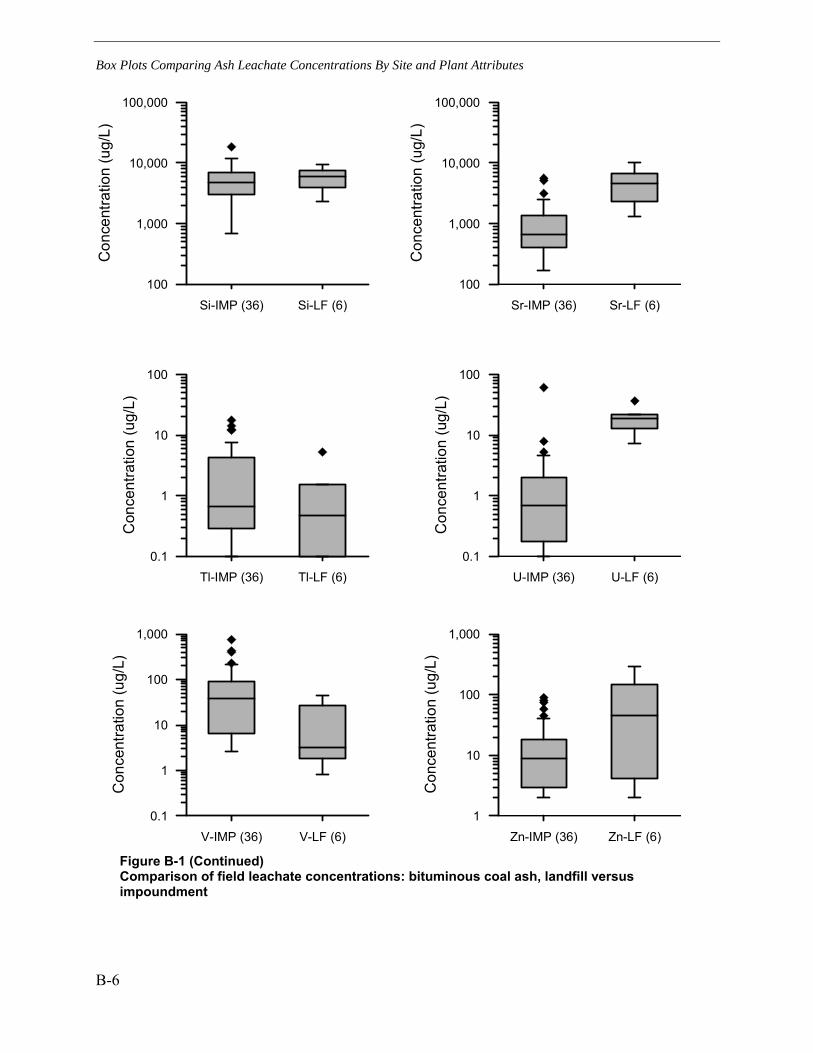
Box Plots Comparing Ash Leachate Concentrations By Site and Plant Attributes
B-6
100
1,000
10,000
100,000C
once
ntra
tion
(ug/
L)
Si-IMP (36) Si-LF (6)100
1,000
10,000
100,000
Con
cent
ratio
n (u
g/L)
Sr-IMP (36) Sr-LF (6)
0.1
1
10
100
Con
cent
ratio
n (u
g/L)
Tl-IMP (36) Tl-LF (6)0.1
1
10
100
Con
cent
ratio
n (u
g/L)
U-IMP (36) U-LF (6)
0.1
1
10
100
1,000
Con
cent
ratio
n (u
g/L)
V-IMP (36) V-LF (6)1
10
100
1,000
Con
cent
ratio
n (u
g/L)
Zn-IMP (36) Zn-LF (6) Figure B-1 (Continued) Comparison of field leachate concentrations: bituminous coal ash, landfill versus impoundment

Box Plots Comparing Ash Leachate Concentrations By Site and Plant Attributes
B-7
0.01
0.1
1
10C
once
ntra
tion
(ng/
L)
Hg-IMP (7) Hg-LF (2)0.01
0.1
1
10
Con
cent
ratio
n (n
g/L)
MeHg-IMP (7) MeHg-LF (2) Figure B-1 (Continued) Comparison of field leachate concentrations: bituminous coal ash, landfill versus impoundment

Box Plots Comparing Ash Leachate Concentrations By Site and Plant Attributes
B-8
0.1
1
10
100
1,000
10,000
Con
cent
ratio
n (m
g/L)
Ca-IMP (5) Ca-LF (5)0.01
0.1
1
10
100
1,000
Con
cent
ratio
n (m
g/L)
Mg-IMP (5) Mg-LF (5)
0.1
1
10
100
1,000
10,000
Con
cent
ratio
n (m
g/L)
K-IMP (5) K-LF (5)0.1
1
10
100
1,000
10,000C
once
ntra
tion
(mg/
L)
Na-IMP (5) Na-LF (5) Figure B-2 Comparison of field leachate concentrations: subbituminous/lignite coal ash, landfill versus impoundment

Box Plots Comparing Ash Leachate Concentrations By Site and Plant Attributes
B-9
0.1
1
10
100
1,000
10,000C
once
ntra
tion
(mg/
L)
Cl-IMP (5) Cl-LF (5)0.1
1
10
100
1,000
10,000
Con
cent
ratio
n (m
g/L)
HCO3-IMP (5) HCO3-LF (5)
0.1
1
10
100
1,000
10,000
Con
cent
ratio
n (m
g/L)
CO3-IMP (5) CO3-LF (5)0.1
1
10
100
1,000
10,000
Con
cent
ratio
n (m
g/L)
SO4-IMP (5) SO4-LF (5) Figure B-2 (Continued) Comparison of field leachate concentrations: subbituminous/lignite coal ash, landfill versus impoundment

Box Plots Comparing Ash Leachate Concentrations By Site and Plant Attributes
B-10
0.1
1C
once
ntra
tion
(ug/
L)
Ag-IMP (5) Ag-LF (5)10
100
1,000
10,000
100,000
Con
cent
ratio
n (u
g/L)
Al-IMP (5) Al-LF (5)
1
10
100
Con
cent
ratio
n (u
g/L)
As-IMP (5) As-LF (5)100
1,000
10,000
100,000
Con
cent
ratio
n (u
g/L)
B-IMP (5) B-LF (5)
10
100
1,000
Con
cent
ratio
n (u
g/L)
Ba-IMP (5) Ba-LF (5)0.1
1
Con
cent
ratio
n (u
g/L)
Be-IMP (5) Be-LF (5) Figure B-2 (Continued) Comparison of field leachate concentrations: subbituminous/lignite coal ash, landfill versus impoundment

Box Plots Comparing Ash Leachate Concentrations By Site and Plant Attributes
B-11
0.1
1
10
100C
once
ntra
tion
(ug/
L)
Cd-IMP (5) Cd-LF (5)0.01
0.1
1
10
100
1,000
Con
cent
ratio
n (u
g/L)
Co-IMP (5) Co-LF (5)
0.1
1
10
100
1,000
10,000
Con
cent
ratio
n (u
g/L)
Cr-IMP (5) Cr-LF (5)1
10
100
1,000C
once
ntra
tion
(ug/
L)
Cu-IMP (5) Cu-LF (5)
1
10
100
Con
cent
ratio
n (u
g/L)
Fe-IMP (5) Fe-LF (5)1
10
100
Con
cent
ratio
n (u
g/L)
Li-IMP (5) Li-LF (5) Figure B-2 (Continued) Comparison of field leachate concentrations: subbituminous/lignite coal ash, landfill versus impoundment

Box Plots Comparing Ash Leachate Concentrations By Site and Plant Attributes
B-12
0.1
1
10
100C
once
ntra
tion
(ug/
L)
Mn-IMP (5) Mn-LF (5)10
100
1,000
10,000
100,000
Con
cent
ratio
n (u
g/L)
Mo-IMP (5) Mo-LF (5)
0.1
1
10
100
Con
cent
ratio
n (u
g/L)
Ni-IMP (5) Ni-LF (5)0.1
1
Con
cent
ratio
n (u
g/L)
Pb-IMP (5) Pb-LF (5)
0.1
1
10
Con
cent
ratio
n (u
g/L)
Sb-IMP (5) Sb-LF (5)1
10
100
1,000
10,000
Con
cent
ratio
n (u
g/L)
Se-IMP (5) Se-LF (5) Figure B-2 (Continued) Comparison of field leachate concentrations: subbituminous/lignite coal ash, landfill versus impoundment

Box Plots Comparing Ash Leachate Concentrations By Site and Plant Attributes
B-13
100
1,000
10,000
100,000
Con
cent
ratio
n (u
g/L)
Si-IMP (5) Si-LF (5)10
100
1,000
10,000
100,000
Con
cent
ratio
n (u
g/L)
Sr-IMP (5) Sr-LF (5)
0.01
0.1
1
10
Con
cent
ratio
n (u
g/L)
Tl-IMP (5) Tl-LF (5)0.01
0.1
1
10
100
Con
cent
ratio
n (u
g/L)
U-IMP (5) U-LF (5)
1
10
100
1,000
10,000
Con
cent
ratio
n (u
g/L)
V-IMP (5) V-LF (5)1
10
100
Con
cent
ratio
n (u
g/L)
Zn-IMP (5) Zn-LF (5) Figure B-2 (Continued) Comparison of field leachate concentrations: subbituminous/lignite coal ash, landfill versus impoundment

Box Plots Comparing Ash Leachate Concentrations By Site and Plant Attributes
B-14
0.01
0.1
1
10
100C
once
ntra
tion
(ng/
L)
Hg-IMP (2) Hg-LF (3)0.01
0.1
1
10
100
Con
cent
ratio
n (n
g/L)
MeHg-IMP (2) MeHg-LF (3) Figure B-2 (Continued) Comparison of field leachate concentrations: subbituminous/lignite coal ash, landfill versus impoundment

Box Plots Comparing Ash Leachate Concentrations By Site and Plant Attributes
B-15
0.1
1
10
100
1,000
10,000C
once
ntra
tion
(mg/
L)
Ca-Bit (5) Ca-Subbit (5)0.1
1
10
100
1,000
10,000
Con
cent
ratio
n (m
g/L)
Mg-Bit (5) Mg-Subbit (5)
0.1
1
10
100
1,000
10,000
Con
cent
ratio
n (m
g/L)
K-Bit (5) K-Subbit (5)0.1
1
10
100
1,000
10,000
Con
cent
ratio
n (m
g/L)
Na-Bit (5) Na-Subbit (5) Figure B-3 Comparison of field leachate concentrations: bituminous vs. subbituminous/lignite coal ash, landfills

Box Plots Comparing Ash Leachate Concentrations By Site and Plant Attributes
B-16
0.1
1
10
100
1,000
10,000C
once
ntra
tion
(mg/
L)
Cl-Bit (5) Cl-Subbit (5)0.1
1
10
100
1,000
10,000
Con
cent
ratio
n (m
g/L)
HCO3-Bit (5) HCO3-Subbit (5)
0.01
0.1
1
10
100
1,000
Con
cent
ratio
n (m
g/L)
CO3-Bit (5) CO3-Subbit (5)0.1
1
10
100
1,000
10,000
Con
cent
ratio
n (m
g/L)
SO4-Bit (5) SO4-Subbit (5) Figure B-3 (Continued) Comparison of field leachate concentrations: bituminous vs. subbituminous/lignite coal ash, landfills

Box Plots Comparing Ash Leachate Concentrations By Site and Plant Attributes
B-17
0.1
1C
once
ntra
tion
(ug/
L)
Ag-Bit (6) Ag-Subbit (5)1
10
100
1,000
10,000
100,000
Con
cent
ratio
n (u
g/L)
Al-Bit (6) Al-Subbit (5)
1
10
100
Con
cent
ratio
n (u
g/L)
As-Bit (6) As-Subbit (5)1,000
10,000
100,000C
once
ntra
tion
(ug/
L)
B-Bit (6) B-Subbit (5)
10
100
Con
cent
ratio
n (u
g/L)
Ba-Bit (6) Ba-Subbit (5)0.1
1
Con
cent
ratio
n (u
g/L)
Be-Bit (6) Be-Subbit (5) Figure B-3 (Continued) Comparison of field leachate concentrations: bituminous vs. subbituminous/lignite coal ash, landfills

Box Plots Comparing Ash Leachate Concentrations By Site and Plant Attributes
B-18
1
10
100C
once
ntra
tion
(ug/
L)
Cd-Bit (6) Cd-Subbit (5)0.01
0.1
1
10
100
1,000
Con
cent
ratio
n (u
g/L)
Co-Bit (6) Co-Subbit (5)
0.1
1
10
100
1,000
10,000
Con
cent
ratio
n (u
g/L)
Cr-Bit (6) Cr-Subbit (5)0.1
1
10
100
1,000C
once
ntra
tion
(ug/
L)
Cu-Bit (6) Cu-Subbit (5)
1
10
100
Con
cent
ratio
n (u
g/L)
Fe-Bit (6) Fe-Subbit (5)1
10
100
1,000
10,000
100,000
Con
cent
ratio
n (u
g/L)
Li-Bit (6) Li-Subbit (5) Figure B-3 (Continued) Comparison of field leachate concentrations: bituminous vs. subbituminous/lignite coal ash, landfills

Box Plots Comparing Ash Leachate Concentrations By Site and Plant Attributes
B-19
1
10
100
1,000
10,000
Con
cent
ratio
n (u
g/L)
Mn-Bit (6) Mn-Subbit (5)100
1,000
10,000
100,000
Con
cent
ratio
n (u
g/L)
Mo-Bit (6) Mo-Subbit (5)
1
10
100
1,000
Con
cent
ratio
n (u
g/L)
Ni-Bit (6) Ni-Subbit (5)0.1
1
Con
cent
ratio
n (u
g/L)
Pb-Bit (6) Pb-Subbit (5)
0.1
1
10
Con
cent
ratio
n (u
g/L)
Sb-Bit (6) Sb-Subbit (5)0.1
1
10
100
1,000
10,000
Con
cent
ratio
n (u
g/L)
Se-Bit (6) Se-Subbit (5) Figure B-3 (Continued) Comparison of field leachate concentrations: bituminous vs. subbituminous/lignite coal ash, landfills

Box Plots Comparing Ash Leachate Concentrations By Site and Plant Attributes
B-20
100
1,000
10,000
Con
cent
ratio
n (u
g/L)
Si-Bit (6) Si-Subbit (5)10
100
1,000
10,000
100,000
Con
cent
ratio
n (u
g/L)
Sr-Bit (6) Sr-Subbit (5)
0.1
1
10
Con
cent
ratio
n (u
g/L)
Tl-Bit (6) Tl-Subbit (5)0.1
1
10
100
Con
cent
ratio
n (u
g/L)
U-Bit (6) U-Subbit (5)
0.1
1
10
100
1,000
10,000
Con
cent
ratio
n (u
g/L)
V-Bit (6) V-Subbit (5)1
10
100
1,000
Con
cent
ratio
n (u
g/L)
Zn-Bit (6) Zn-Subbit (5) Figure B-3 (Continued) Comparison of field leachate concentrations: bituminous vs. subbituminous/lignite coal ash, landfills

Box Plots Comparing Ash Leachate Concentrations By Site and Plant Attributes
B-21
0.01
0.1
1
10
100C
once
ntra
tion
(ng/
L)
Hg-Bit (2) Hg-Subbit (3)0.01
0.1
1
10
100
Con
cent
ratio
n (n
g/L)
MeHg-Bit (2) MeHg-Subbit (3) Figure B-3 (Continued) Comparison of field leachate concentrations: bituminous vs. subbituminous/lignite coal ash, landfills

Box Plots Comparing Ash Leachate Concentrations By Site and Plant Attributes
B-22
0.1
1
10
100
1,000
10,000
Con
cent
ratio
n (m
g/L)
Ca-Bit (36) Ca-Subbit (5)0.01
0.1
1
10
100
1,000
10,000
Con
cent
ratio
n (m
g/L)
Mg-Bit (36) Mg-Subbit (5)
0.1
1
10
100
1,000
10,000
Con
cent
ratio
n (m
g/L)
K-Bit (36) K-Subbit (5)0.1
1
10
100
1,000
10,000C
once
ntra
tion
(mg/
L)
Na-Bit (36) Na-Subbit (5) Figure B-4 Comparison of field leachate concentrations: bituminous vs. subbituminous/lignite coal ash, impoundments

Box Plots Comparing Ash Leachate Concentrations By Site and Plant Attributes
B-23
0.1
1
10
100
1,000
10,000C
once
ntra
tion
(mg/
L)
Cl-Bit (36) Cl-Subbit (5)0.01
0.1
1
10
100
1,000
10,000
Con
cent
ratio
n (m
g/L)
HCO3-Bit (34) HCO3-Subbit (5)
0.01
0.1
1
10
100
1,000
Con
cent
ratio
n (m
g/L)
CO3-Bit (34) CO3-Subbit (5)0.1
1
10
100
1,000
10,000
Con
cent
ratio
n (m
g/L)
SO4-Bit (36) SO4-Subbit (5) Figure B-4 (Continued) Comparison of field leachate concentrations: bituminous vs. subbituminous/lignite coal ash, impoundments

Box Plots Comparing Ash Leachate Concentrations By Site and Plant Attributes
B-24
0.1
1
10
Con
cent
ratio
n (u
g/L)
Ag-Bit (36) Ag-Subbit (5)1
10
100
1,000
10,000
100,000
Con
cent
ratio
n (u
g/L)
Al-Bit (36) Al-Subbit (5)
1
10
100
1,000
10,000
Con
cent
ratio
n (u
g/L)
As-Bit (36) As-Subbit (5)100
1,000
10,000
100,000
1,000,000
Con
cent
ratio
n (u
g/L)
B-Bit (36) B-Subbit (5)
10
100
1,000
Con
cent
ratio
n (u
g/L)
Ba-Bit (36) Ba-Subbit (5)0.1
1
10
Con
cent
ratio
n (u
g/L)
Be-Bit (36) Be-Subbit (5) Figure B-4 (Continued) Comparison of field leachate concentrations: bituminous vs. subbituminous/lignite coal ash, impoundments

Box Plots Comparing Ash Leachate Concentrations By Site and Plant Attributes
B-25
0.1
1
10
100
Con
cent
ratio
n (u
g/L)
Cd-Bit (36) Cd-Subbit (5)0.01
0.1
1
10
100
Con
cent
ratio
n (u
g/L)
Co-Bit (36) Co-Subbit (5)
0.1
1
10
100
1,000
Con
cent
ratio
n (u
g/L)
Cr-Bit (36) Cr-Subbit (5)0.1
1
10
100
1,000
Con
cent
ratio
n (u
g/L)
Cu-Bit (36) Cu-Subbit (5)
1
10
100
1,000
10,000
100,000
Con
cent
ratio
n (u
g/L)
Fe-Bit (36) Fe-Subbit (5)1
10
100
1,000
10,000
Con
cent
ratio
n (u
g/L)
Li-Bit (36) Li-Subbit (5) Figure B-4 (Continued) Comparison of field leachate concentrations: bituminous vs. subbituminous/lignite coal ash, impoundments

Box Plots Comparing Ash Leachate Concentrations By Site and Plant Attributes
B-26
0.1
1
10
100
1,000
10,000
Con
cent
ratio
n (u
g/L)
Mn-Bit (36) Mn-Subbit (5)1
10
100
1,000
10,000
Con
cent
ratio
n (u
g/L)
Mo-Bit (36) Mo-Subbit (5)
0.1
1
10
100
Con
cent
ratio
n (u
g/L)
Ni-Bit (36) Ni-Subbit (5)0.1
1
10
Con
cent
ratio
n (u
g/L)
Pb-Bit (36) Pb-Subbit (5)
0.1
1
10
100
Con
cent
ratio
n (u
g/L)
Sb-Bit (36) Sb-Subbit (5)0.01
0.1
1
10
100
1,000
Con
cent
ratio
n (u
g/L)
Se-Bit (36) Se-Subbit (5) Figure B-4 (Continued) Comparison of field leachate concentrations: bituminous vs. subbituminous/lignite coal ash, impoundments

Box Plots Comparing Ash Leachate Concentrations By Site and Plant Attributes
B-27
100
1,000
10,000
100,000
Con
cent
ratio
n (u
g/L)
Si-Bit (36) Si-Subbit (5)100
1,000
10,000
Con
cent
ratio
n (u
g/L)
Sr-Bit (36) Sr-Subbit (5)
0.1
1
10
100
Con
cent
ratio
n (u
g/L)
Tl-Bit (36) Tl-Subbit (5)0.01
0.1
1
10
100
Con
cent
ratio
n (u
g/L)
U-Bit (36) U-Subbit (5)
1
10
100
1,000
Con
cent
ratio
n (u
g/L)
V-Bit (36) V-Subbit (5)1
10
100
Con
cent
ratio
n (u
g/L)
Zn-Bit (36) Zn-Subbit (5) Figure B-4 (Continued) Comparison of field leachate concentrations: bituminous vs. subbituminous/lignite coal ash, impoundments

Box Plots Comparing Ash Leachate Concentrations By Site and Plant Attributes
B-28
0.01
0.1
1
10C
once
ntra
tion
(ng/
L)
Hg-Bit (7) Hg-Subbit (2)0.01
0.1
1
10
100
Con
cent
ratio
n (n
g/L)
MeHg-Bit (7) MeHg-Subbit (2) Figure B-4 (Continued) Comparison of field leachate concentrations: bituminous vs. subbituminous/lignite coal ash, impoundments

C-1
C EVALUATION OF ARSENIC, SELENIUM, AND CHROMIUM SAMPLE PRESERVATION AND ANALYSIS METHODS
Cryofreezing Overview
Cryofreezing was used as the default sample preservation strategy for the speciation samples in this project for two reasons:
• Recent research has shown that both arsenic and selenium form soluble sulfur species in sulfidic waters, which are decomposed and precipitated under acidic conditions, thereby completely altering the original speciation information. This would have affected all samples that contain detectable concentrations of “other” arsenic or selenium species, although in most cases, these “other” species constituted less than 10 percent of the total concentration of the element, and so the associated error would have been relatively small. However, six samples (five arsenic and one selenium) contained “other” species at fractions > 10 percent of the corresponding total arsenic or selenium concentration. Since it wasn’t known in advance how strongly sulfidic the sampled waters would be, and field observations confirmed (via smell) that some samples had significant concentrations of free reduced sulfur compounds, cryofreezing was used instead of acidification to prevent decomposition of soluble arsenic- and selenium-sulfur compounds.
• It is well established that Cr(VI) gets reduced by dissolved organic matter in acidified samples during storage. Since nearly all samples containing elevated chromium concentrations had Cr(VI) as their major species, this could have led to significantly altered chromium speciation results. Again, cryofreezing circumvents the issue of pH change during storage. This was confirmed in a test of preservation methods performed in 2004 (after analytical issues had been observed in 2003); while the cryofrozen split yielded almost exclusively Cr(VI), acidified splits yielded lower Cr(VI) concentrations (Table C-2) and increasing Cr(III) concentrations over time. This already led to an altered chromium speciation pattern immediately after sample receipt, but yielded a completely reversed speciation result after several weeks of storage. For this reason, Cr(VI) is typically preserved under strongly alkaline conditions, but for the present project, this would have created other analytical issues related to the precipitation of Cr(III) and major trace elements (e.g. iron and manganese), and was thus avoided.
Unfortunately, during the analysis of samples collected in 2003, it was observed that the cryofreezing approach created another, unanticipated problem, during storage. When the cryofrozen samples were thawed prior to analysis, varying degrees of white-yellowish

Evaluation of Arsenic, Selenium, and Chromium Sample Preservation and Analysis Methods
C-2
precipitates were observed in many samples, which did not re-dissolve at room temperature (over a time frame of weeks). When speciation analyses of these samples were conducted, a significant gap in the mass balance (= total element concentration – sum of its individual species) of arsenic and/or selenium was observed; chromium was not significantly affected by this issue. It was theorized that these precipitates were calcium sulfate or carbonate, and geochemical model calculations confirmed that the solubility of these minerals was exceeded in many samples.
To test if the precipitates contained the “missing” fractions of arsenic (for which the mass balance discrepancies were worse than for selenium), the precipitates were digested in nitric acid, and the resulting solutions analyzed for arsenic released from the precipitates. Table C-1 shows that for some samples, the “missing” fraction of arsenic was apparently indeed bound to the observed precipitates, but there are more samples than that for which this did not confirm the postulated loss mechanism. Additionally, significant mass balance discrepancies were also observed in samples containing no visible precipitates. Therefore, while this storage artifact was certainly responsible for incomplete arsenic or selenium speciation mass balance in some samples, it was definitely not the only process involved, and possibly not even the major one. Dissolution of the precipitates in nitric acid changes arsenic speciation, so it remains unclear if any one species of arsenic was selectively or preferentially removed from solution during the formation of the precipitates.
Formation of these precipitates was only observed in samples collected in 2003, because those samples were stored for a long period (up to 6 months) prior to analysis. By comparison, samples collected in 2004 and 2005 were typically analyzed for their arsenic and selenium speciation within four weeks after collection, and the sum of species in these samples was closer to the total concentration than in the 2003 samples. Consequently, it seems likely that the formation of precipitates resulted from excessively long cryofrozen storage, and can be avoided by keeping storage time to one month or less. Attempts to “recreate” the precipitates were unsuccessful (on a time scale of weeks), so no further attempts were made to resolve the issue and correct the speciation mass balance for samples with precipitates.

Evaluation of Arsenic, Selenium, and Chromium Sample Preservation and Analysis Methods
C-3
Table C-1 Arsenic Speciation Mass Balance, Including Losses To Precipitates Formed During Cryofrozen Storage, For Leachate Samples Collected In 2003
Sample ID Lab ID
Total As As(III) As(V)
other As species
precipitated As
mass balance without
precipitated As [%]
mass balance including
precipitated As [%]
001 1 20.4 < 0.3 9.5 2.1 7.04 57 91
002 2 48.4 < 6 47 < 6 1.10 98 100
003 3 84 < 6 69 < 6 7.50 82 91
004 4 18.6 8.4 5.2 < 0.3 0.59 73 76
005 5 3.0 < 0.2 1.3 < 0.2 0.08(a) 45 47 006 6 12.2 < 0.3 0.9(a) < 0.3 <0.05 8 8 007 7 20.1 < 2 < 2 < 2 0.07(a) 0 0 008 8 16.9 0.7(a) < 0.5 < 0.3 0.07(a) 4 5 009 9 28.9 < 6 < 10 < 6 0.09(a) 0 0 010 10 22.3 1.5(a) 10 < 0.6 0.46 52 54 011 11 4.8 < 0.2 0.6 < 0.2 0.26 12 17 012 12 238 97.0 66 < 0.6 38.1 69 85 013 13 21.6 3.7 < 0.5 < 0.3 11.8 17 72
013D 13A 22 1.9 < 0.5 < 0.3 NA 9 9 014 14 163 1.9 86 0.9(a) 25.1 54 70 015 15 23.8 < 0.6 24 < 0.6 1.72 99 106 016 16 68.6 < 0.6 25 < 0.6 23.4 36 70
SX-1 core 3 72.0 0.9 46.9 < 0.1 1.16 66 68 017 17 4.11 0.88 <0.08 0.1 0.26 23 30 018 18 23.1 0.42 5.22 < 0.06 17.8 24 101 019 19 5.11 0.57 <0.08 < 0.06 0.36 11 18 020 20 4.19 1.00 0.53 0.1 0.14(a) 40 43
HN-1 core 1 59.8 < 0.1 33.6 0.2 5.65 57 66 HN-2 core 2 20.6 < 0.1 6.9 0.1 1.64 34 42 021 21 194 2.1 208 < 0.3 2.38 108 110 022 22 11.1 12.5 0.49 < 0.06 0.11(a) 118 119 023 23 218 0.8(a) 189 < 0.3 12.4 87 93 024 24 11.2 0.4(a) <0.2 < 0.2 1.47 3 16 025 25 6.47 1.35 <0.08 < 0.06 1.04 21 37 026 26 10.8 11.2 0.4(a) < 0.2 0.11(a) 107 108 027 27 39.1 13.2 4.8 1.3 2.31 49 55 028 28 30.0 2.4 1.7 0.2 0.17(a) 14 15 029 29 48.9 1.7 8.9 0.3 4.01 22 31 030 30 42.5 3.5 29.5 0.4 0.58 79 80 031 31 221 201 23.6 0.7 3.65 102 103 032 32 25.4 17.5 16.9 0.1 0.43 136 137
(a) = sample concentration less than 5 times blank Concentrations in μg/L

Evaluation of Arsenic, Selenium, and Chromium Sample Preservation and Analysis Methods
C-4
Due to the large heterogeneity of the collected sample set, additional issues related to speciation preservation were observed in individual samples. Some samples showed obvious loss of total arsenic, selenium, and/or chromium upon acidification, which was verified by analyzing total arsenic, total selenium, and total chromium in the cryofrozen speciation samples (and finding significantly higher concentrations). For those samples, the formation of a brownish flocculate was usually observed in the acidified splits, which is probably due to precipitation of humic acids (which are soluble under the original alkaline conditions present in most samples, but insoluble at acidic pH). Evidently, the precipitates removed a fraction of total arsenic, selenium, or chromium from solution, which would have led to a speciation mass balance > 100 percent (barring other analytical issues). In such cases, the corresponding total element concentration measured in the cryofrozen split was used instead of the one in the acidified sample. By contrast, there were also a number of samples in which the formation of brownish precipitates was observed in the non-acidified splits taken for major anion and cation analysis. This reflects the precipitation of iron (oxy)hydroxide minerals caused by oxidation of high Fe(II) concentrations present in reducing waters. This problem was avoided by acidification, unless the process was so rapid that it began as the sample was being pumped and filtered.
In conclusion, the preservation for arsenic and selenium speciation by acidification does not appear suitable for the whole collected sample set, and must certainly be avoided for chromium speciation. Cryofreezing appears to be suitable in principle, but the sample storage time must be minimized to avoid irreversible formation of precipitates. Finally, it appears that the collected sample set is too heterogeneous for any one procedure that will preserve arsenic, selenium, and chromium speciation in all samples reliably; therefore, it might be necessary to collect multiple splits in parallel that are preserved differently.
Evaluation of Preservation Arsenic, Chromium, and Selenium Speciation by Preservation Method
The field team returned to the location of sample 002 and collected replicate samples for analysis of preservatives and differences associated with analytical laboratories. Five preservation techniques were used: no preservation, hydrochloric acid (HCl) in opaque bottles, hydrochloric acid in foil-wrapped (dark) bottles, ethylenediaminetetraacetic acid (EDTA), and nitric acid (HNO3). Sample 002 is geochemically characterized by alkaline pH (>10), ORP of > 200, low dissolved oxygen (0.2%), low iron (<50 μg/L), and high sulfate (> 6,000 mg/L) concentration.
Results varied by analyte, preservation method, and laboratory (Table C-2). Chromium was most strongly effected. Concentrations of Cr(VI) in the acid-preserved samples were less than one-half of the concentration determined in the cryofrozen and unpreserved samples. This analysis clearly suggests that acid-preservation is not an appropriate technique for Cr(IV) in this geochemical environment.
Selenium concentrations were least affected by preservation technique. The poorest result was for the cryofrozen sample (sample 002), in which the sum of species was 76 percent of the total selenium concentration. This sample was collected in 2003 and subject to the issues described

Evaluation of Arsenic, Selenium, and Chromium Sample Preservation and Analysis Methods
C-5
above associated with long hold times. The only apparent laboratory related relationship was for Se(IV); which was below detection limits in all samples other than the cryofrozen sample analyzed by laboratory 1, and detected at concentrations ranging from 76 to 94 μg/L by laboratory 2.
Table C-2 Arsenic, Selenium, and Chromium Speciation Using Different Preservatives
As (III) As (V) As (other) Σ As species
Total Arsenic
% Recovery
Field blank <5 0.02 NA NA 0.24 NA Unpreserved, Lab 1 <5 27.1 6.4 33.5 58.1 58 Unpreserved, Lab 2 4.1 63 NA 67 73 92 Cryofrozen, Lab 1 <6 47 <6 47 48.4 97 0.5% HCl preserved, Lab 1 <5 30.8 9.7 40.5 54.7 74 0.5% HCl preserved, Lab 2 4.9 95 NA 100 82 122 0.5% HCl+ dark preserved, Lab 1 <5 32.2 4.6 36.8 54.9 67 0.5% HCl+ dark preserved, Lab 2 NA NA NA NA NA NA EDTA preserved, Lab 2 4.0 72 NA 76 71 107 0.5% HNO3 preserved, Lab 1 <5 5.1 2.4 7.5 51.7 15 0.5% HNO3 preserved, Lab 2 3.7 65 NA 69 82 84
Cr (III) Cr(VI) Cr (other) Σ Cr species
Total Chromium
% Recovery
Field blank NA <0.1 NA NA 0.11 NA Unpreserved, Lab 1 NA 4138 NA NA 5204 NA Unpreserved, Lab 2 NA NA NA NA NA NA Cryofrozen, Lab 1 340 5090 NA 5430 5100 106 0.5% HCl preserved, Lab 1 NA 2161 NA NA 5217 NA 0.5% HCl preserved, Lab 2 NA NA NA NA NA NA 0.5% HCl+ dark preserved, Lab 1 NA 1314 NA NA 5242 NA 0.5% HCl+ dark preserved, Lab 2 NA NA NA NA NA NA EDTA preserved, Lab 2 NA NA NA NA NA NA 0.5% HNO3 preserved, Lab 1 NA 1760 NA NA 5161 NA 0.5% HNO3 preserved, Lab 2 NA NA NA NA NA NA
Se(IV) Se(VI) Se (Other) Σ Se species
Total Selenium
% Recovery
Field blank <0.05 <0.05 NA <0.05 0.14 -- Unpreserved, Lab 1 <25 1432 16 1448 1312 110 Unpreserved, Lab 2 94 1270 NA 1364 1400 97 Cryofrozen, Lab 1 19 1300 NA 1319 1730 76 0.5% HCl preserved, Lab 1 <25 1348 27 1375 1426 96 0.5% HCl preserved, Lab 2 91 1423 NA 1514 1500 101 0.5% HCl+ dark preserved, Lab 1 <25 1349 14 1363 1424 96 0.5% HCl+ dark preserved, Lab 2 NA NA NA NA NA NA EDTA preserved, Lab 2 87 1478 NA 1565 1400 112 0.5% HNO3 preserved, Lab 1 <25 1307 NA 1307 1392 94 0.5% HNO3 preserved, Lab 2 76 1416 NA 1492 1400 107 Samples collected 4/6/04 except Cryofrozen sample collected 8/5/03 Lab 2 did not analyze chromium NA=not analyzed

Evaluation of Arsenic, Selenium, and Chromium Sample Preservation and Analysis Methods
C-6
Arsenic concentrations were most variable. First, there was a significant difference by laboratory. Laboratory 1 returned total arsenic concentrations between 52 and 58 mg/L (excluding the cryofrozen sample, which was collected on a different date), while laboratory 2 returned total arsenic concentrations between 71 and 82 mg/L. Laboratory 2 also achieved greater species recovery (84 to 122%) than laboratory 1 (15 to 97 percent). For laboratory 2, all preservation methods proved acceptable for preservation of arsenic species. For laboratory 1, only the cryofrozen sample yielded better than 80 percent species recovery. Significantly, all preservation methods identified As(V) as the species with highest concentration.
This test was performed on samples from a geochemical environment where the oxidized species would be expected in leachate samples, and results cannot be extrapolated to other environments, particularly those where the reduced species may be expected. However, the results show that several different preservation methods are capable of identifying the predominant species of arsenic and selenium in water samples from a high pH, high ORP, low oxygen, low iron, high sulfate environment. However, only cryofreezing adequately preserved chromium species.
Comparison of Cryofrozen and Hydrochloric Acid-Preserved Replicate Samples
Splits of 32 field leachate samples6 were preserved in the field with HCl and forwarded to a separate laboratory (laboratory 2) for analysis of arsenic and selenium species. Analyses were performed as described in Section 2.
Arsenic
For arsenic, the cryofrozen sample sets7 typically had lower total concentration than the acid-preserved samples (Figure C-1); however, since the total concentration analyses by both labs were performed on acid-preserved samples, this difference is laboratory related, rather than preservative-related. The percentage difference in total concentration was greatest when values were lower than 10 μg/L; the average difference for samples with concentration greater than 10 μg/L was 27 percent. The difference may be due to a correction applied by laboratory 2 to account for chloride interference.
The sum of arsenic species was compared to the independently measured total arsenic to determine the species recovery. For both sets of samples, the species recovery was typically closer to 100 percent when the total concentration was greater than 10 μg/L. In most cases, the cryofrozen sample had a higher species recovery, and was closer to 100 percent species recovery, than the acid-preserved sample (Figure C-1).
6 The split sample comparison included one sample (085) that was taken at one of the field sites for another study, and is not otherwise included in this evaluation. The acid-preserved splits of samples 084 and 085 were not analyzed for selenium species. 7 The cryofrozen sample sets included acid-preserved samples for total analysis and frozen samples for species analysis.

Evaluation of Arsenic, Selenium, and Chromium Sample Preservation and Analysis Methods
C-7
Comparison of Cryofrozen (CF) and Acid-Preserved (AP) Splits
0.10
1.00
10.00
100.00
1000.00
1 3 5 7 9 11 13 15 17 19 21 23 25 27 29 31
Ars
enic
Con
cent
ratio
n (u
g/L)
0%
50%
100%
150%
200%
250%
300%
350%
400%
Sum
of S
peci
es/T
otal
Con
cent
ratio
n (%
)
CF-total (ug/L) AP-total (ug/L) CF-Species% AP-Species%
Figure C-1 Comparison of total arsenic concentration and of percent species recovery for cryofrozen and acid-preserved sample splits
The dominant species in each sample split was determined based on the following criteria:
• For species recovery greater than 80 percent, a species was identified as dominant if its concentration was 60 percent or more of the sum of species.
• If species recovery was greater than 80 percent, and no species concentration was greater than 60 percent of the sum of species, then the sample was listed as “neutral”.
• For species recovery less than 80 percent, a species was identified as dominant if its concentration was greater than 50 percent of the total concentration.8
• Samples with less than 80 percent species recovery in which no species concentration was greater than 50 percent of the total concentration were not tabulated.
Based on this approach, 27 of the 32 cryofrozen samples, and 22 of the 32 acid-preserved samples can be classified as dominated by As(III), dominated by As(V), or neutral (Table C-3). In 17 of the 20 common splits (where the dominant species could be determined in both samples), the two preservation techniques yielded similar results. In the three splits with 8 If the sum of species is 80 percent, and the species concentration is 50 percent of the total concentration, then that species accounts for at least 62.5 percent of the sum of species.

Evaluation of Arsenic, Selenium, and Chromium Sample Preservation and Analysis Methods
C-8
different results, As(V) was dominant in the cryofrozen sample and As(III) in the acid-preserved sample. Two of these three samples had total arsenic concentration lower than 5 μg/L; the other was sample 106, which had an arsenic concentration of 110 μg/L.
Table C-3 Dominant Arsenic Species in Split Samples
Cryofrozen Acid-Preserved Split %
As(III) %
As(V) %
other %
recov. DS Total
As Split %
As(III) %
As(V) %
recov. DS Total
As T112 50% 70% 14% 133% V 1.36 W112 54% 0% 54% (III) 4.04 T101 0% 10% 28% 38% 2.23 W101 0% 0% 4% 2.50 T92 0% 15% 3% 18% 3.34 W92 0% 47% 47% 4.52
T108 9% 56% 0% 65% (V) 4.09 W108 0% 48% 48% 6.91 T99 2% 78% 4% 84% V 4.80 W99 69% 0% 69% (III) 6.79
T126 0% 69% 0% 69% (V) 5.20 W126 0% 106% 106% V 8.32 T49 0% 43% 0% 43% 5.40 W49 20% 51% 71% (V) 5.94
T111 0% 58% 0% 58% (V) 5.94 W111 0% 27% 27% 14.32 T127 0% 63% 0% 63% (V) 6.42 W127 0% 86% 86% V 10.77 T102 0% 88% 0% 88% V 7.24 W102 0% 94% 94% V 11.74 T116 12% 90% 1% 103% V 8.24 W116 10% 71% 81% V 10.26 T115 37% 63% 0% 100% V 8.32 W115 0% 77% 77% (V) 9.08 T91 0% 88% 1% 89% V 10.76 W91 0% 83% 83% V 9.98
T121 12% 54% 5% 72% (V) 11.00 W121 0% 26% 26% 28.36 T128 71% 20% 3% 94% III 14.27 W128 44% 4% 48% 24.00 T114 0% 87% 0% 87% V 23.53 W114 9% 81% 90% V 26.50 T42 0% 81% 0% 81% V 23.70 W42 8% 75% 83% V 23.26
T122 30% 32% 24% 86% neutral 25.54 W122 44% 8% 52% 36.28 T120 27% 43% 35% 104% neutral 26.79 W120 44% 12% 56% 43.46 T119 0% 101% 1% 102% V 30.20 W119 3% 79% 82% V 34.74 T107 3% 49% 0% 52% 30.64 W107 2% 47% 48% 60.00 T118 2% 112% 0% 114% V 40.78 W118 18% 67% 85% V 48.94 T97 0% 81% 0% 81% V 44.89 W97 0% 60% 60% (V) 46.96 T43 0% 37% 0% 37% 75.20 W43 59% 32% 92% neutral 77.76 T98 1% 77% 0% 79% (V) 76.85 W98 10% 0% 10% 47.96 T57 0% 94% 0% 94% V 98.60 W57 0% 133% 133% V 120.00 T69 0% 94% 0% 94% V 99.50 W69 0% 80% 80% (V) 120.00
T113 1% 115% 0% 116% V 101.98 W113 23% 76% 99% V 120.00 T106 14% 57% 5% 77% (V) 109.83 W106 71% 2% 73% (III) 122.32 T105 85% 22% 2% 109% III 229.95 W105 112% 5% 116% III 233.00 T84 10% 74% 0% 83% V 726.90 W84 8% 83% 90% V 870.00 T85 59% 38% 3% 99% neutral 829.10 W85 52% 41% 93% neutral 950.00
DS indicates the dominant species in the sample, ( ) indicates that total species recovery was less than 80%, but one species was greater than 50% Shading indicates samples where the dominant species could be determined in both splits.
Sample 106 was recirculated FGD system water, presenting a highly alkaline (pH near 12) and more concentrated matrix that may have confounded the analyses. Other complicating factors with sample 106 included high dissolved oxygen (95%) yet low ORP (18 mV), and low dissolved iron (4.6 μg/L).

Evaluation of Arsenic, Selenium, and Chromium Sample Preservation and Analysis Methods
C-9
Selenium
For selenium, the cryofrozen sample sets9 typically had lower total concentration than the acid-preserved samples (Figure C-2). This difference, which, like arsenic, is laboratory related, was greatest when total concentration was lower than 10 μg/L; the average difference for samples with concentration greater than 10 μg/L was 25 percent.
Comparison of Cryofrozen (CF) and Acid-Preserved (AP) Splits
0.10
1.00
10.00
100.00
1000.00
1 3 5 7 9 11 13 15 17 19 21 23 25 27 29
Sele
nium
Con
cent
ratio
n (u
g/L)
0%
50%
100%
150%
200%
250%
300%
350%
400%
Sum
of S
peci
es/T
otal
Con
cent
ratio
n (%
)
CF-total (ug/L) AP-total (ug/L) CF-Species% AP-Species%
Figure C-2 Comparison of total selenium concentration and of percent species recovery for cryofrozen and acid-preserved sample splits
The sum of species for both sets of samples was closer to 100 percent when the total concentration was greater than 10 μg/L. The cryofrozen split typically had higher species recovery than the acid-preserved split; although in some cases, particularly at concentrations near and greater than 100 μg/L, the cryofrozen split recovery was greater than 100 percent and the acid-preserved split recovery was closer to 100 percent. For concentrations greater than 10 μg/L, species recovery correlated well between the two preservation methods (Figure C-2).
9 The cryofrozen sample sets included acid-preserved samples for total analysis and frozen samples for species analysis.

Evaluation of Arsenic, Selenium, and Chromium Sample Preservation and Analysis Methods
C-10
The dominant selenium species was determined using the same approach as for arsenic. Based on this approach, 23 of the 30 cryofrozen sample splits, and 20 of the 30 acid-preserved sample splits can be classified as dominated by Se(IV), dominated by Se(VI), or neutral (Table C-4).
Table C-4 Dominant Selenium Species in Split Samples
Cryofrozen Acid-Preserved Split %
Se(IV) %
Se(VI) %
other %
recov. DS Total
As Split %
Se(IV) %
Se(VI) %
recov. DS Total
As T114 0% 0% 0% 0% 0.07 W114 0% 0% 0% 0.10 T112 0% 0% 0% 0% 0.67 W112 0% 0% 0% 5.00 T122 0% 0% 0% 0% 1.13 W122 0% 0% 0% 15.00 T99 0% 0% 0% 0% 2.04 W99 103% 0% 103% IV 6.12 T57 83% 0% 0% 83% IV 2.44 W57 210% 0% 210% IV 3.23
T120 56% 46% 0% 102% neutral 3.30 W120 0% 0% 0% 14.00 T121 29% 73% 0% 102% VI 3.86 W121 0% 0% 0% 14.00 T108 39% 59% 0% 98% neutral 6.56 W108 38% 39% 77% 13.32 T105 0% 0% 0% 0% 8.47 W105 0% 0% 0% 43.00 T49 83% 6% 0% 89% IV 10.00 W49 70% 0% 70% (IV) 12.01
T118 100% 7% 0% 107% IV 17.62 W118 51% 0% 51% (IV) 23.00 T43 86% 0% 0% 86% IV 23.50 W43 83% 0% 83% IV 32.54
T119 81% 6% 0% 87% IV 27.95 W119 65% 0% 65% (IV) 32.00 T113 66% 9% 0% 75% (IV) 29.27 W113 79% 0% 79% (IV) 33.00 T116 87% 9% 0% 96% IV 35.35 W116 66% 0% 66% (IV) 40.00 T115 82% 8% 0% 90% IV 36.10 W115 75% 0% 75% (IV) 37.00 T69 91% 5% 0% 96% IV 36.40 W69 87% 7% 93% IV 44.54 T42 92% 5% 0% 96% IV 42.60 W42 80% 6% 86% IV 49.94 T98 58% 0% 0% 58% (IV) 50.74 W98 5% 0% 5% 65.98
T128 34% 13% 3% 51% 50.90 W128 0% 5% 5% 106.36 T106 0% 99% 0% 99% VI 64.79 W106 3% 73% 76% (VI) 85.44 T102 7% 106% 0% 113% VI 80.48 W102 5% 89% 94% VI 95.40 T126 14% 117% 0% 131% VI 88.70 W126 14% 88% 102% VI 104.34 T111 43% 79% 0% 122% VI 90.54 W111 38% 53% 91% neutral 91.00 T101 0% 114% 0% 114% VI 91.00 W101 0% 115% 115% VI 104.48 T92 1% 113% 0% 113% VI 103.36 W92 0% 90% 90% VI 90.86 T91 3% 113% 0% 116% VI 122.22 W91 0% 102% 102% VI 102.84
T107 0% 10% 32% 42% 159.00 W107 0% 0% 0% 400.00 T127 7% 136% 0% 143% VI 180.60 W127 5% 95% 100% VI 210.00 T97 9% 89% 0% 98% VI 412.50 W97 16% 95% 111% VI 380.00
DS indicates the dominant species in the sample, ( ) indicates that total species recovery was less than 80%, but one species was greater than 50% Shading indicates samples where the dominant species could be determined in both splits.
In 18 of the 19 common splits (where the dominant species could be determined in both samples), the two preservation techniques yielded similar results. The only exception was sample 111, which was dominated by Se(VI) in the cryofrozen split and was neutral in the acid split. However, both samples had more Se(VI) than Se(IV). The species breakdown for sample 111 was 43 percent Se(IV) and 79 percent Se(VI) in the cryofrozen sample, and 38 percent Se(IV) and 53 percent Se(VI) in the acid-preserved sample. Sample 111 had neutral pH (7.2),

Evaluation of Arsenic, Selenium, and Chromium Sample Preservation and Analysis Methods
C-11
was oxic (280 mV ORP and 59 percent dissolved oxygen), and did not exhibit a sulfur odor; as a result, the acid-preserved sample would not be expected to undergo precipitation of soluble sulfur species.
Summary
In summary, there are conditions under which one of the preservation methods may be more appropriate than the other. However, the split sample data collected during this study indicate that the preservation method does not affect results sufficiently to alter interpretation of the dominant species present in the sample..


D-1
D LABORATORY ANALYTICAL ISSUES PERTAINING TO SPECIATION ANALYSIS
Determination of Total Arsenic, Selenium, and Chromium Concentrations
The determination of total chromium (TCr) by ICP-MS worked very well. Good agreement was obtained between the two isotopes 52Cr and 53Cr, as well as between the two instruments used (ICP-DRC-MS and ICP-DF-MS). Therefore, there is a high degree of confidence in the reported total chromium results, and they are not a reason if the speciation mass balance for chromium did not work out in any sample, which usually only happened in samples with low total chromium concentrations. Unfortunately, the determination of total arsenic and selenium by ICP-MS is more complicated than that of total chromium, and consequently, the quality of these data is somewhat impaired in certain samples, as discussed below. The problems associated with the determination of total arsenic and selenium by ICP-MS stem mostly from molecular interferences that overlap with the mass of the measured arsenic or selenium isotopes, and thus yield artificially-increased results. These interferences are caused either by constituents of the measured water samples or by molecules formed in the argon plasma used in ICP-MS analyses. To illustrate this problem, the method used for total selenium determination in the collected water samples is explained below.
In ICP-MS analyses, it is desirable to use the major isotope of the trace element of interest for its quantification, because it yields the highest signal, which usually translates into the lowest detection limit. Additionally, at least one other isotope of the same element should be measured, and if the concentrations determined in the sample by using two (or more) different isotopes agree well, then there is a high degree of confidence that this result is correct and not impaired by any significant molecular interferences. For selenium, the main isotope is 80Se, but this isotope is impossible to measure by conventional ICP-MS instruments, because the argon plasma generates a large amount of the dimeric ion 40Ar2
+, which has the same nominal mass as the 80Se isotope, and the two signals cannot be separated. Although some publications suggest that ICP-DF-MS can resolve the overlap between analyte and interference for this example when it’s used in the high resolution mode, the particular ICP-DF-MS instrument used by laboratory 1 did not achieve this separation consistently, and an ICP-DRC-MS instrument was used to address this issue, which was successful. The ICP-DRC-MS approach uses a cell with a reactive gas (here methane, CH4) to break up the interference (by collision yielding two Ar atoms of mass 40) between the plasma and the mass spectrometer, while the analyte 80Se remains unaffected, and can thus be determined free of the inference. However, in the collected water samples, there are additional interferences that complicate this approach. High bromide concentrations in the samples lead to the formation of the molecule 1H79Br+, which also has the nominal mass 80, but cannot be eliminated effectively by the reaction gas methane. Therefore, a second reaction gas

Laboratory Analytical Issues Pertaining to Speciation Analysis
D-2
(ammonia, NH3) was added, which undergoes a chemical reaction with HBr, and thus forms reaction products that have masses other than 80, so 80Se can be measured in waters containing bromide.
The minor isotopes used for confirmation of results obtained using the main isotope usually have different interferences than the main isotope, so if the results obtained for different isotopes agree, it is generally accepted that all known interferences have been removed efficiently, as intended during the method development. In the case of selenium, the control isotopes used were 78Se and 82Se, and it turns out that 78Se has an interference from the plasma (40Ar38Ar+), but not from bromide, while 82Se has an interference from bromide (1H81Br+), but not form the plasma, so the control strategy for these two interferences works very well. Unfortunately, due to the fact that the studied waters were often very complex and generally very different from site to site, there were additional interferences in some samples that could not be resolved by the described approach. While some additional interferences were identified, and their influence on the measured total selenium results was compensated for as much as possible (for example, it was found that copper formed ammonia clusters Cu(NH3)+ in the DRC, which interfered with the measurement of 80Se and 82Se), there remained some samples that either contained interferences that were not identifiable, or where known interferences exceeded the compensation capacity of the developed analytical method. In those cases, the total selenium concentrations determined using the three different selenium isotopes disagreed beyond the normal range of analytical error, and such results were flagged10 in the results table (Appendix A). For such samples, the lowest total selenium concentration obtained with any selenium isotope was usually reported, because the molecular interferences are by nature positive (i.e. they mimic selenium), so the lowest result should be the least (or not) interfered.
Figure D-1 shows the agreement between the results obtained for the three measured selenium isotopes as a function of the total selenium concentration: With the exception of three samples, the total selenium concentrations determined using each of the three individual isotopes agree within the analytical uncertainty (± 10 percent) for samples containing total selenium greater than 5 μg/L. Generally, the agreement between the three selenium isotopes is good when total selenium concentrations are higher, and gets worse towards lower concentrations, because a certain amount of an interference caused by the sample matrix would have a bigger impact if the actual selenium signal is small, and because the analytical uncertainty itself increases with decreasing concentration. For those three samples with higher total selenium concentrations where the isotope agreement is not good, the reason probably lies in a combination of complex matrix (high salinity and trace element concentrations) and comparably low total selenium concentration (i.e. too low to resolve the interferences by dilution), although the actual reasons for these discrepancies likely vary from sample to sample, and were not explored further in this project. To eliminate this problem in future similar studies, it would be necessary to either add hydride generation (HG) as a sample introduction technique, which selectively volatilizes the selenium into the plasma while most of the other sample constituents stay behind in the liquid phase and are not introduced into the plasma (so they cannot produce interferences), or switch to a different detection technique altogether (e.g. atomic fluorescence spectrometry, AFS). There are also other potential analytical issues associated with HG and AFS, and there is no guarantee that these approaches would have resolved all problems for the present sample set. 10 Identified in Table A-2 using flag (b), “isotope ratios do not match”

Laboratory Analytical Issues Pertaining to Speciation Analysis
D-3
0
1
10
100
1000
0 0 1 10 100 1,000 10,000
TSe [μg/L]
RSD
[%]
0.10.01
0.1
CCC = 5 μg/L
Figure D-1 Agreement between total selenium concentrations determined using the isotopes 78Se, 80Se and 82Se in all collected water samples (expressed as percent relative standard deviation between the three individual results)
Besides interferences that affect individual selenium isotopes during the ICP-MS measurement, there are also matrix effects that affect all selenium isotopes at once, which relate to processes such as the sample introduction into the ICP-MS and the ionization of selenium in the plasma. The sample flow rate in ICP-MS measurements of bulk samples is regulated by the (constant) rotation speed and tubing diameter of a peristaltic pump, but the uptake of the sample into the plasma depends on its nebulization in the spray chamber; this process is assumed to be constant, and the fraction of the pumped sample nebulized is typically around 3 percent (so 97 percent of the sample goes to waste and is not measured). Parameters like the sample’s viscosity or salinity can alter the nebulization process, and thus lead to higher or lower nebulization efficiency, thereby affecting the selenium signal obtained, which is proportional to the total amount of sample introduced into the plasma. To recognize and correct for such interferences, one or more internal standards (IS) are used, which are other trace elements spiked to the samples at a known concentration before analysis. The idea behind this is that a change in the sample introduction efficiency would affect the IS to the same degree as the analytes, and could thereby be compensated for mathematically.

Laboratory Analytical Issues Pertaining to Speciation Analysis
D-4
The only condition that the IS needs to fulfill to be used for this correction approach is that it cannot be present in the samples in a measurable/significant concentration (so that the IS signal should always be constant if there were no sample uptake variations); for this reason, “exotic” elements like platinum group metals are commonly used for this purpose. In this project, rhodium was routinely used as the primary IS for total selenium measurements, and indium was used as a secondary IS to identify if there were problems associated with the rhodium measurement in any given sample. Several other commonly used IS elements were tried as well, but yielded less satisfactory results, usually because they occurred in the analyzed water samples in significant concentrations. The same was true to a lesser degree for indium, so it was not always usable as an IS, whereas rhodium generally fulfilled the absence condition. However, two additional problems were encountered related to the IS approach, which have not been reported in the literature before, and therefore were unanticipated and had to be recognized and dealt with during this project.
First, it was observed that certain matrix elements present in the studied waters produced interferences in the DRC process that mimicked one of the IS elements (for example, the strontium isotope 86Sr forms an ammonia cluster Sr(NH3)+ in the DRC, which has the same nominal mass as the only rhodium isotope 103Rh). This increases the apparent IS signal and suggests increased sample introduction efficiency for the particular sample, and since the analyte signal is normalized to the IS signal, leads to artificially decreased total selenium concentrations. This interference was recognized by the fact that the secondary IS was not elevated, and compensated for as much as possible by varying instrument parameter like the DRC gas flow rates and Rpa and Rpq (two DRC settings), but could not be eliminated altogether without compromising the efficiency with which the DRC removes the main interferences on the analytes (as discussed above). No alternate IS was found that fulfilled the absence condition and was not affected by this phenomenon, so more research is needed in this respect to find a way to compensate for this problem. One way to address the issue is the method of standard addition, where an interfered sample is measured repeatedly with varying amounts of the analyte added prior to analysis, but this procedure is impractical in routine operation, because every sample would need to be analyzed multiple times.
Secondly, it was noticed that the signal for either IS element increased unspecifically when high concentrations of a matrix element with similar or higher mass were present in the sample, e.g. barium (mass 137) increasing the IS signal for rhodium (mass 103) and indium (mass 115). This effect is the opposite of a well-known process in mass spectrometry called “space-charge effect”, and could thus be referred to as “inverse space-charge effect”. It was beyond the scope of this project to investigate the reasons for this observation, and the effect could not be eliminated by changing instrumental parameters, although it was moderated by increasing the acceleration voltage for the ions through the DRC. Like the previous interference, this issue causes an artificially-increased IS signal and thus leads to reduced total selenium concentrations. Contrary to interferences that lead to decreased sample introduction efficiency (and thereby to elevated apparent total selenium concentrations), these two effects would result in a positive speciation mass balance discrepancy (i.e. recovery > 100 percent), so since most samples showed a negative deviation in their selenium speciation mass balance, these two types of interferences did apparently not affect many of the measured samples; they may, however, explain why the sum of selenium species in some samples was significantly > 100 percent.

Laboratory Analytical Issues Pertaining to Speciation Analysis
D-5
The second type of interference that is commonly compensated for by using internal standards relates to the ionization efficiency of the analyte in the plasma. This is a particular problem for selenium and arsenic, which have very high first ionization energies, and are ionized incompletely (25-50 percent) in the ICP. Major constituents of the matrix can alter the properties of the plasma, and thereby change the degree of ionization for these elements (and consequently their signal intensity); typical examples include major cations like sodium, which are easily ionized and thereby decrease the “energy” of the plasma, leading to reduced arsenic and selenium ionization, and organic carbon, which appears to enhance the ionization of arsenic and selenium by unknown mechanisms. Again, the IS could be used to compensate for these effects, but only if it shows a similar response to such interferences as the analytes of interest. This “similarity condition” is much harder to fulfill than the absence condition, and it’s nearly impossible to fulfill them both perfectly for a large and inhomogeneous sample set, such as the present one. Of all tested IS elements, rhodium yielded that best results, but it has a significantly lower ionization energy than both arsenic and selenium, so that the analyte signals may have been suppressed in some samples without an effect on the IS. Again the result would be an artificially reduced total selenium or total arsenic concentration.
The preceding discussion makes it clear that the determination of total selenium in such complex samples as the studied waters is complicated, and that not all interferences can be compensated for, leading to possibly “wrong” total selenium concentrations, which in turn would impact the selenium speciation mass balance. This is probably one of the main reasons of why this mass balance did not work well in samples with low total selenium and high concentrations of certain matrix elements. Besides the mentioned HG sample introduction, an elegant way to eliminate many of the discussed interferences would be isotope dilution, which involves spiking a known amount of a particular selenium isotope to the sample prior to analysis. This is, however, expensive, because pure selenium isotopes would need to be obtained, and was consequently not available and could not be developed during this project. Given the (eco) toxicological importance of measuring relatively low total selenium concentrations in complex aqueous samples, this is an area which should be explored in future research, so that a much improved and reliable method for total selenium determinations by ICP-MS becomes available.
All analytical issues discussed above hold true for arsenic as well, but contrary to selenium, arsenic is monoisotopic, and consequently does not offer the possibility of compensating for (or even recognizing) certain interferences by “switching” to another isotope, which suggests that the total arsenic data quality should be poorer than for total selenium (which of course cannot be proven directly). The suggested improvements like HG sample introduction would also remedy many of the raised problems, and even isotope dilution with a long-lived arsenic radionuclide could be used for internal standardization. However, similar to selenium, these aspects were not explored during this project, and the fact that the arsenic speciation mass balance did not work well in some samples can certainly be partially attributed to problems associated with the total arsenic determination.
Determination of Arsenic, Selenium, and Chromium Speciation
The determination of Cr(III) and Cr(VI) by AEC-ICP-MS worked quite well, as supported by the reasonable chromium speciation mass balance. The only issue that was addressed during this

Laboratory Analytical Issues Pertaining to Speciation Analysis
D-6
project was the relatively high background caused by the presence of inorganic carbon in the used chromatographic eluant: this leads to the formation of 40Ar12C+, which interferes with the determination of the main chromium isotope 52Cr, but this background was easily eliminated by using NH3 as the reaction gas in the DRC.
For arsenic and selenium, the measurement of their speciation in the collected water samples was more complicated, and a number of significant interferences were encountered. These interferences are generally not related to the presence of spectral interferences, as discussed for the total arsenic and total selenium determinations above, because typically the interfering sample constituent is separated chromatographically in time from the analyte species. As an example, bromide in the samples will still produce a signal on mass 82, but this does not interfere with the measurement of Se(IV) or Se(VI), because the bromide signal either elutes before the Se(IV) peak, or–if the interfering peak is too large–Se(IV) at mass 77 can be used for quantification. Rather, besides the preservation/stability issues discussed above for the cryofrozen sample, the main problems encountered are caused by high salinity in some of the collected water samples, and by the presence of major trace elements that are incompatible with the chosen chromatographic conditions, so both are chromatographic issues occurring in the AEC, and not spectroscopic issues arising in the ICP-MS.
The salinity-based interference is caused by the fact that major anions, especially sulfate in the studied waters, are present in very high concentrations (up to 300 mmol/L), whereas the arsenic and selenium species are present in much lower concentrations (up to 9 μmol/L for selenium and 7 μmol/L for As), so the major anions are present in 30,000-fold excess. During the AEC analysis, the major anion competes with the trace element anions for binding sites on the chromatographic column, and if this competition becomes too strong, then the analytes are “flushed” out of the column without interacting properly with the stationary phase, which results in bad peak shapes that makes quantification inaccurate to impossible, and in the change of retention times, which makes identification uncertain or eliminates separation of different species altogether. The best way to eliminate this problem is by diluting the sample prior to analysis, but this approach is limited by the absolute concentration of the analytes in the same, so if the ratio of major anions to analytes is too large, the samples would have to be diluted to the point where the analytes fall below the detection limits to overcome the chromatographic problems.
This issue was encountered for a large number of the studied samples, and was addressed by modifying the AEC separation. Sulfate (instead of hydroxide) was used as the eluant anion, and this increases the tolerance of the separation for elevated sulfate concentrations in the sample (this approach is called “matrix matching”). However, even this remedy is limited by the absolute binding capacity of the column, so if the total amount of matrix anions injected exceeds this capacity, then proper separation of the analytes is no longer possible. Matrix matching yielded a significant improvement for the speciation mass balance of arsenic and selenium in many samples collected in 2004 and 2005, and for those samples where the mass balance still remained poor, there appeared to be a general correlation with the ratio of sample salinity to analyte concentration.
The second chromatographic issue was caused by high iron and especially manganese concentrations in some of the studied waters. Since the AEC separation is conducted under

Laboratory Analytical Issues Pertaining to Speciation Analysis
D-7
alkaline conditions (even after modification) to prevent the loss of acid-labile arsenic and selenium species, major sample constituents that precipitate under strongly alkaline conditions may cause problems. Although many of the collected samples were alkaline to begin with, the separation conditions were even more alkaline; this pH change during analysis particularly affected those samples that were acidic or circumneutral in the field. Under such conditions, manganese (and iron) can precipitate in the form of (oxy)hydroxide minerals within the AEC, and these precipitates bind the species As(V) and Se(IV) very strongly, which could lead to artificially low results for these two species. This issue was addressed by raising the pH of the eluant by about one unit, and by adding some oxalate into the eluent, which keeps manganese in solution. As for the salinity issue, though, there are limits to this approach, and the problems could not be eliminated in all samples, which is probably the main reason for the very low speciation mass balances encountered in some samples.
As the constitution of real world samples is highly variable and unpredictable, the best way to resolve this problem is by using more sensitive detection principles, because then the problematic samples can be diluted even more. At this point, though, ICP-MS is the most sensitive detection approach, even if certain ICP-MS instruments not available during this project may possibly yield lower detection limits for the AEC-ICP-MS determination of arsenic and selenium species than the used ICP-DRC-MS (in the standard mode for arsenic and selenium speciation). Further increases in detection sensitivity for arsenic and selenium can be achieved by using high-efficiency sample introduction systems, such as HG or membrane desolvation, between the AEC separation and the ICP-MS detection. This, however, is complicated and more expensive for use on a routine basis, and the required equipment was either not available permanently at Trent, or was incompatible with the relatively high chromatographic flow rates (and would thus have necessitated some modifications), so these options were not incorporated into the used methods. It should be noted, though, that AEC-HG-ICP-DRC-MS has been used successfully to measure selenium speciation at ng/L-levels in sea water, so this approach could be used in future studies, because it works in principle for the species As(III)/As(V) and Se(IV)/Se(VI), while its suitability for any other arsenic or selenium species is untested, which constitutes another reason why this technique was not routinely used in this project.
Related Documents