Speaking English in a Globalizing World: Information Technology and Education in India Gauri Kartini Shastry Harvard University PRELIMINARY AND INCOMPLETE March 2007 Abstract I study how the impact of globalization on returns to education and school enroll- ment varies with the elasticity of the skilled labor supply. I exploit variation in the cost of learning English across districts in India, driven by linguistic diversity that made it necessary for individuals to learn additional languages. In India, the two common choices for a second language are English and Hindi, the native lingua franca. Indi- viduals whose native language is linguistically further from Hindi have lower relative opportunity costs of learning English, mainly because they nd Hindi harder to learn but also because they often su/er psychic costs when using Hindi, a language that many non-native Hindi speakers feel was imposed on them. I rst show that linguistic distance from Hindi increases the probability of learning English, even in 1961. Using newly collected data on information technology (IT), I show that districts with lower costs of learning English experienced greater growth in IT after trade reforms in the early 1990s. In addition, these districts experienced greater growth in relative employ- ment of educated workers but smaller growth in skilled wage premiums, due to the greater skilled labor supply elasticity. Finally, I show that these districts experienced greater increases in school enrollment. Correspondence: [email protected]. I am grateful to David Cutler, Esther Duo, Caroline Hoxby, Michael Kremer for their advice and support, David Clingingsmith for access to additional data and all participants of the Research in Labor Economics and Development Economics lunch workshops at Harvard for their comments. In addition, I thank Filipe Campante, Davin Chor, Quoc-Anh Do, Eyal Dvir and Michael Katz for useful conversations and assistance. Finally, I thank Daniel Tortorice for invaluable support and encouragement. All errors are mine.

Welcome message from author
This document is posted to help you gain knowledge. Please leave a comment to let me know what you think about it! Share it to your friends and learn new things together.
Transcript
Speaking English in a Globalizing World: Information
Technology and Education in India
Gauri Kartini Shastry�
Harvard University
PRELIMINARY AND INCOMPLETE
March 2007
Abstract
I study how the impact of globalization on returns to education and school enroll-ment varies with the elasticity of the skilled labor supply. I exploit variation in the costof learning English across districts in India, driven by linguistic diversity that madeit necessary for individuals to learn additional languages. In India, the two commonchoices for a second language are English and Hindi, the native lingua franca. Indi-viduals whose native language is linguistically further from Hindi have lower relativeopportunity costs of learning English, mainly because they �nd Hindi harder to learnbut also because they often su¤er psychic costs when using Hindi, a language thatmany non-native Hindi speakers feel was imposed on them. I �rst show that linguisticdistance from Hindi increases the probability of learning English, even in 1961. Usingnewly collected data on information technology (IT), I show that districts with lowercosts of learning English experienced greater growth in IT after trade reforms in theearly 1990s. In addition, these districts experienced greater growth in relative employ-ment of educated workers but smaller growth in skilled wage premiums, due to thegreater skilled labor supply elasticity. Finally, I show that these districts experiencedgreater increases in school enrollment.
�Correspondence: [email protected]. I am grateful to David Cutler, Esther Du�o, Caroline Hoxby,Michael Kremer for their advice and support, David Clingingsmith for access to additional data and allparticipants of the Research in Labor Economics and Development Economics lunch workshops at Harvardfor their comments. In addition, I thank Filipe Campante, Davin Chor, Quoc-Anh Do, Eyal Dvir and MichaelKatz for useful conversations and assistance. Finally, I thank Daniel Tortorice for invaluable support andencouragement. All errors are mine.
1 Introduction
While most economists agree that free trade has signi�cant bene�ts over autarky for all
countries involved, i.e. that free trade increases the size of the pie, there is some debate over
how the bene�ts of trade are distributed within a country. While several recent empirical
studies have found that trade liberalization in Latin America has caused sizeable increases
in inequality and skill wage premiums,1 there is less evidence from Asian countries and it
is more mixed.2 In contrast, standard Heckscher-Ohlin trade theory unambiguous predicts
that globalization should reduce inequality and skill premia. Under the simplest model with
two goods, two countries and two factors (skilled and unskilled labor), the country abundant
in unskilled labor (the poor country) should specialize in unskilled-labor-intensive industries
after trade liberalization. This increases demand for unskilled labor and drives down the
skilled wage premium. While there are numerous theoretical extensions to help reconcile
the theory with these empirical �ndings,3 an additional, under-emphasized, dimension is
whether labor supply and education responds to the increased wage inequality. The fact that
countries in Latin American countries experienced a much smaller increase in the supply of
skilled workers relative to East-Asian economics may explain the mixed �ndings above.4
In this paper, I explore this dimension of how the e¤ects of liberalization vary within a
developing country and provide evidence on the labor supply response to globalization as well
as how the e¤ect on skill premiums varies with labor supply elasticity. I exploit variation in
the labor supply elasticity of skilled workers due to historically-driven di¤erences in policies
regarding language of instruction. Many countries, particularly those with a colonial past,
have struggled with the question of whether to encourage their people to retain diverse local
1See Goldberg and Pavcnik (2004) for a review of this literature. The literature includes, e.g., Hansonand Harrison (1999), Feenstra and Hanson (1997), Feliciano (1993) and Cragg and Epelbaum (1996) onMexico, Robbins, Gonzales and Menendez (1995) on Argentina, Robbins (1995a) on Chile, Robbins (1996a)and Attanasio, Goldberg and Pavcnik (2004) on Colombia, Robbins and Gindling (1997) on Costa Rica andRobbins (1995b, 1996b) on Uruguay.
2See, e.g., Wood (1997) for a survey, Lindert and Williamson (2001) and Wei and Wu (2001).3See, e.g. Feenstra and Hanson (1996, 1997), Kremer and Maskin (2006) and other extensions discussed
in Goldberg and Pavcnik (2004).4See Attanasio and Szekely (2000), Sanchez-Paramo and Schady (2003).
1
languages, choose a single native language or promote a global lingua franca, such as English.
In particular, the choice of medium of instruction in public schools is one with far-reaching
consequences.5 On one hand, there are costs of promoting a non-native global language.
Native language instruction can strengthen national identity, particularly important in young
countries made up of numerous ethnic groups. In addition, instruction in a foreign language
may impose costs on poor households if they �nd such education less accessible. On the
other hand, there may be bene�ts of promoting a global lingua franca if coveted white-
collar jobs in government or business use that language.6 Instruction in a global language
in public schools may increase economic opportunities for the poor.7 Most importantly,
promoting the learning of English may also allow more people to bene�t from globalization
and technological progress. The ability to integrate better with the world economy may
bring more of the bene�ts of trade liberalization to places that promote English. Since
much technological progress happens in English (for example, in information technology),
the ability to speak English may facilitate the adoption of new technologies.
This paper examines the increased returns to an English education due to economic liber-
alization and technological progress in the 1990s and demonstrates the e¤ect on educational
attainment in India, by exploiting exogenous variation in the cost of learning English across
Indian districts. Using most measures of variation in the cost of learning English, such as the
number of individuals who learn English, would be highly problematic because the cost of
learning English is endogenous. State or local governments that care more about the bene�ts
of promoting a global lingua franca such as access to global opportunities may promote the
teaching of English, but also pursue other policies that increase trade-related jobs. I exploit
variation in costs of learning English that is driven by linguistic and historical forces that are
exogenous to such outward-oriented or forward-looking policies and also to reverse causal-
ity. In fact, this variation in the cost of acquiring English caused people to learn English
5See Human Development Report (2004) and Angrist, Chin and Godoy (2006), e.g.6See Lang and Siniver (2006).7See Angrist and Lavy (1997) and Munshi and Rosenzweig (2006).
2

for non-trade related reasons even in 1961, long before trade liberalization could have been
contemplated. The variation in costs is driven by historical linguistic diversity that made it
necessary to learn a second language even to communicate with others in the same district.
The common choices for a second language in India are English and Hindi, the native lingua
franca. Individuals whose mother tongue is linguistically further from Hindi have a lower
opportunity cost of learning English because they �nd Hindi more di¢ cult to learn, but also
because they are more likely to su¤er psychic costs when speaking Hindi, a language that
many non-native Hindi speakers feel was imposed on them as a national language. Over
time, these historical tendencies led to the growth of institutions that promote the learning
of English in districts where native languages are further from Hindi. I �rst show that this
relationship holds; linguistic distance from Hindi increases the number of native speakers
who learn English and predicts the percent of schools that teach English.
Next, I demonstrate how the impact of globalization during the 1990s has varied by pre-
existing di¤erences in linguistic distance from Hindi. I examine data that I gathered and
coded on the information technology (IT) sector in India, an industry that grew primarily
due to economic liberalization and technological progress in the 1990s and hires educated,
English-speaking workers. Information technology includes both software �rms and business-
process outsourcing such as call centers and data entry �rms. I show that IT �rms were more
likely to locate in districts with lower costs of learning English. I also �nd that these dis-
tricts have greater IT employment. I then posit that in the new more open Indian economy,
there is a greater payo¤ to being educated and English speaking. I provide evidence using
micro-level data that, in the 1990s, districts with lower costs of learning English experienced
a greater increase in employment for educated workers but a smaller increase in the average
skilled wage premium. A simple theoretical model provides intuition for these results. Sepa-
rating out workers by industry, I show that wage premiums in certain industries (�nancing,
insurance, computer related activities, research and development, other business activities)
rose faster in these districts as well. As suggestive evidence for the trade in services channel,
3
I do not �nd a corresponding rise in wage premium for education workers in other industries
(other services, such as public service, education, health; manufacturing; agriculture; ho-
tel and restaurants; wholesale and retail; transportation services; or communications, such
as post, courier and telecommunications). However, I do �nd an increase in all wages in
the transportation and communications industries lending more credibility to trade-related
growth as an important mechanism behind these di¤erential trends. I show how pre-existing
di¤erences in linguistic diversity explain changes in employment and wages between 1987
and 1999; thus, I estimate not just correlations but the di¤erential impact of these lower
costs of English during a period of liberalization.
Finally, these pre-existing di¤erences in linguistic distance to Hindi also explain di¤eren-
tial changes in school enrollment trends during the 1990s relative to pre-existing trends. I
demonstrate that districts where the average person speaks a language that is linguistically
further from Hindi experienced greater increases in urban school enrollment from 1993 to
2002 even relative to pre-existing trends in school enrollment.
Thus, the contributions of this paper are two-fold, corresponding to the two motivating
themes described above. The most conservative interpretation centers on the bene�ts of
language policies that advance the study of a global language in a developing country. In
particular, districts that had more English speakers for these reasons found themselves in
a better position to take advantage of the opportunities from trade after liberalization. In
addition, the paper contributes to the literature on trade liberalization because it con�rms
a possible explanation for mixed evidence on the impact of globalization on wage inequality
and �nds evidence of longer term consequences to this rise in wage inequality. While trade
liberalization may increase wage inequality in the short run, this e¤ect could be dampened
in the longer term as factor supply responds.
Besides the two strains of trade literature and the education literature described above,
this paper is related to Munshi and Rosenzweig (2006). Using a household survey from a
suburb of Mumbai, India, the authors show that increases in the returns to English dwarfed
4
increases in the returns to education and that enrollment rates in English-medium schools
rose in the 1980s and 1990s. My paper di¤ers in a number of ways. First, I show that edu-
cational attainment overall rises, not just in English instruction schools. Second, I use data
from all over India exploiting exogenous variation in the cost of learning English. Lastly, I go
one step further to explore the trade-related mechanism through which the returns to Eng-
lish have risen. Edmonds, Pavcnik and Topalova (2005) also study the relationship between
economic liberalization and educational attainment in India and �nd an adverse impact on
schooling. While the authors isolate the e¤ect on school enrollment of reduced family in-
come due to import competition, I focus on the impact of increases in job opportunities and
returns to English education from exports and integration with world markets.
The paper is organized as follows. Section 2 provides background information on trade
liberalization and information technology in India. Section 3 describes the linguistic diversity,
costs of learning English, and medium of instruction. I show that linguistic distance from
Hindi increases the tendency to learn English, but does not predict other economic measures
prior to economic liberalization. Section 4 describes a simple theoretical model to provide
intuition for the empirical �ndings. Section 5 discusses the empirical methodology, while
section 6 describes the data. Section 7 examines IT �rm location and employment decisions
and provides evidence on employment of educated workers and returns to education. Finally,
in section 8, I show that districts where native languages are farther from Hindi experienced
greater increases in school enrollment. Section 9 concludes.
2 Background on trade liberalization and IT
Throughout much of the post-colonial period, India heavily protected its economy. While
some small steps towards integrating with world markets were taken in the late 1970s and
1980s, even as late as 1990, tari¤ and non-tari¤ barriers posed signi�cant obstacles for trade.
The average tari¤ was 79% and sixty-�ve percent of all imports were subject to non-tari¤
5
barriers (Panagariya 2003). A balance-of-payments crisis due to extensive borrowing in 1991
resulted in a shift towards policies favoring a more open economy. Reforms ended most im-
port licensing requirements for capital goods and reduced tari¤ rates substantially, although
mostly for non-agricultural goods. Service sectors which had previously been heavily reg-
ulated by the government saw signi�cant changes. The 1994 National Telecommunications
Policy and 1999 New Telecom Policy opened cellular and other telephone services to both
private and foreign investors. Foreign direct investment (FDI) in e-commerce was free of all
restrictions and foreign equity in software and electronics was granted automatic approval,
particularly for IT �rms set up exclusively to export (Panagariya 2004). This service sec-
tor liberalization, along with technological progress, led to the remarkable growth in the
outsourcing of services in the information technology sector, to India.
By 2004, India was the single largest destination for foreign companies to purchase IT
services, contributing about two-thirds of global software outsourcing and half of business
process outsourcing. In 2005, IT outsourcing accounted for 5% of India�s GDP and was
forecasted to contribute 17% to India�s projected growth to 2010 (The Economist 2006).
Employment growth has also been strong over the past decade; from 56,000 professionals in
1990-91, the sector employed 813,500 in 2003, implying an annual growth rate of more than
twenty percent (NASSCOM 2004). In particular, the IT sector increased job opportunities
for young, educated workers; the median age of IT professionals is 27.5 years and 81% of
them have at least a bachelor�s degree (NASSCOM 2004). An entry-level job in a call sector
can earn on average Rs. 10,000 ($230) considered very high for a �rst job (The Economist
2005). In addition, the excitement regarding the growth of the IT sector is palpable. IT
�rms advertise heavily in newspapers and on job search websites.
Their young age, export focus and reliance on foreign capital make IT �rms relatively
free to locate based on other inputs. One of the principle factors in the location decision of
IT �rms is manpower, i.e. the availability of an educated, English-speaking population. I
show below that IT �rms choose to locate in places with lower costs of learning English.
6

3 Linguistic distance from Hindi and identi�cation
The 1961 Census of India documented 1652 mother tongues spoken in India from �ve
distinct language families native to India. These language families are quite diverse; while
linguists assert familial relationships between languages as far apart as English and Hindi
(both are Indo-European), they are unwilling to connect many languages native to India such
as Hindi and Kannada, the language spoken in Bangalore. Figures 1 and 2 present maps
of India with the density of native speakers of 114 languages. This linguistic diversity has
had implications for bilingualism (Clingingsmith 2006); most individuals, especially urban,
educated individuals, need to learn a second language to communicate at a local level.
According to the 1991 census, 19.4% of Indians are multilingual. The two most common
languages learned are Hindi, the native lingua franca, and English, due to the British colonial
history. As of the 1991 census, sixty percent of all multilingual people not native in Hindi
learned Hindi as a second language. For English, this fraction was only slightly smaller at
56%.8 The next most popular second language, Kannada, was learned by only 6% of the
multilingual population. In fact, 83% of all multilinguals speak either Hindi or English.
An individual with a more obscure mother tongue has to choose between Hindi and
English. Mechanically, an individual whose mother tongue is linguistically close to Hindi
will �nd it easier to learn Hindi relative to someone whose mother tongue is farther from
Hindi. The history of language in India ampli�es this tendency because of the controversial
decision to make Hindi the national language. During the British occupation, English was
established as the language of government, the medium of instruction and the language of
the elite. After India became independent in 1947, a nationalist movement to make an
indigenous Indian language the o¢ cial language favored Hindi, since it was spoken by more
people than any other native language. This movement was opposed by non-native Hindi
speakers, but after much debate, Hindi was written into the constitution as the language
8Of course since Hindi was spoken by more than three hundred million people as a �rst language, whileEnglish was spoken by only 180,000 as a �rst language, many more people spoke Hindi than English.
7
of administration, meant to replace English within 15 years. This led to riots in non-Hindi
speaking areas, the most violent of which occurred in Tamil Nadu in May 1963. Speakers of
other languages felt at a disadvantage speaking Hindi and �nally, in 1967, the government
passed a law making Hindi and English joint o¢ cial languages (Hohenthal 2003).
This background explains why English is more prevalent among people who speak lan-
guages distant to Hindi. In fact, in some states, more people speak English than Hindi. Over
time, as I show below, the relationship between linguistic distance and English prevalence
became institutionalized through English education. This theory has ambiguous predictions
for whether native Hindi speakers learn English. On one hand, they do not need a second
language to communicate within India; if they choose to learn a second language, it could
be for other reasons. On the other hand, if they choose to learn a second language to com-
municate within India, English would allow them to interact with more additional people
than any other language.
3.1 Medium of instruction in Indian schools
When the British began to colonize India, they did not plan to provide mass education.
They set up schools and colleges in large cities that taught entirely in English, meant to
foster an elite class to help govern the country (Nurullah and Naik 1947, Kamat 1985). By
1850, other institutions such as missionary societies and princely states had set up rural
schools that taught in native languages. Finally, in 1854, the recommendations set forth in
Sir Charles Wood�s Despatch marked the British government�s committed to educating the
entire population (Dakin, Ti¤en and Widdowson 1968). Education spread to lower classes
and an increasing number of schools taught in native languages. University education in
major cities, however, was still primarily in English. Even today, it is the main medium
of post-tertiary instruction (Hohenthal 2003). In 1993, according to the Sixth All India
Educational Survey, there were over 28 di¤erent media of instruction in primary schools
(regardless of government or private funding) across urban areas in India. While Hindi is
8

the most common medium of instruction with 38% of primary schools, English is second
with 9%. At the secondary school level, there are 37 languages taught as a �rst or second
language across urban areas of India.
3.2 Measuring linguistic distance
The 1961 and 1991 Census of India provide data on the number of people in each state
that speak each of 114 distinct mother tongues and how many of them learn each of these
languages as a second language. In addition, at the district level, we know how many people
speak each language as a mother tongue. I �rst calculate various measures of the distance
from Hindi of a language. In order to obtain a measure at the district level, I calculate
the weighted average of the distance from Hindi of all native languages spoken in a district
where the weights are the district population share. For an alternate measure, I calculate
the percent of speakers in a district who speak languages su¢ ciently far from Hindi.
As there is no universally accepted measure of language distance among linguists, I
calculate three independent measures. My preferred measure was developed in consultation
with an expert on Indo-European languages, Jay Jasano¤, the Diebold Professor of Indo-
European Linguistics and Philology at Harvard University. This measure is based on drawing
seven concentric circles of languages around Hindi as they get linguistically more di¤erent
(see �gure 3). I count the circles (and call them degrees) from Hindi to each language.
Figure 4 provides a map of India demonstrating the distribution of the weighted average of
this measure and �gure 5 provides a map of the percent of people who speak languages at
least 3 degrees away from Hindi. Note that much of the variation is across regions (indicated
by thick black lines). However, since we might worry that this variation is correlated with
other factors (e.g. geography, culture), I include region �xed e¤ects and di¤erential trends.
A second measure of linguistic distance is based on language family trees. The most
widely used language trees are from the Ethnologue database, one of the most comprehensive
listings of currently known languages. Many linguists rely on and contribute to the database.
9
Figure 6 provides an extract from the Ethnologue�s language tree that includes all languages
found in the Indian census. I de�ne the distance between two languages as the number of
nodes between the languages. For example, Urdu is two degrees away from Hindi, while
Marwari is four degrees away. In order to link the other language families with Hindi, I
assume there is a node connecting the di¤erent language families.
Another measure is taken from a method called glottochronology, which is used to es-
timate the time of divergence between languages (Swadesh 1972). The method involves
making a list of 210 core words, i.e. words that are the most resistant to change as languages
evolve. Then, using expert judgments on whether these words across languages are cognates
with each other, we can calculate the percent of words that are cognates between each pair of
languages.9 I use the percent of cognates shared between each language and Hindi from the
Dyen et al. (1992) dataset of 95 Indo-European languages. Table 1 provides example core
meanings in English, Bengali and Hindi as well as cognate judgments for each pair of words.
Since the dataset does not provide the words or cognate judgments for non Indo-European
languages, I assume these languages have only 5% of words in common with Hindi, since the
lowest percent of cognates with Hindi among Indo-European languages is 14.6%.10 Finally,
for Indo-European languages in the 1991 Census of India language data which do not appear
in Dyen et al.�s list, I use the percent of cognates with Hindi of the closest language in the
tree that also appears in the list. Close matches exist for the 12 Indo-European languages
that require this.
The correlation between these 3 measures is quite high. Across languages, the correlation
between degrees and nodes between languages is 0.9283. The correlation between these two
measures and the percent of cognates is -0.9358 and -0.9731 respectively. Panel A of table 2
provides summary statistics on these and other measures regarding language in India.
9The original version of this method also involved a formula that converted this percent of cognates intoa time of divergence, which is currently out of favor among linguists. Nevertheless, the percent of cognatesis still an acceptable measure of similarity between languages.10This choice is not arbitrary - linguists use 5% as a signi�cance level when determining whether two
languages are related. If less than 5% of words are cognates, linguists assume that those that are representnoise and the languages are unrelated.
10
3.3 Identi�cation
We cannot estimate the impact of the cost of learning English using most measures of
these costs since they would be endogenous. Local governments can in�uence these costs
based on their preferences. For example, if the government cares about access to global
opportunities, it may both promote education in English and provide incentives for foreign
direct investment. We would also worry about reverse causality, since these outsourcing �rms
often set up English training centers. The variation in the cost of learning English that comes
from linguistic distance to Hindi, however, does not su¤er from these problems. Linguistic
distance to Hindi impacts the cost of learning English in a manner that is orthogonal to
preferences of di¤erent local governments. In addition, government policies or English-
language opportunities will not a¤ect the linguistic distance of a language from Hindi. Large
movements of people across district boundaries may in�uence the linguistic distance from
Hindi of languages spoken in a district, but migration in India is still quite low. According
to the 1987 National Sample Survey, only 12.3% of individuals in urban areas had migrated
in the past �ve years, only 6.8% had moved from outside their current district in this time
and only 2.4% had moved from outside their current state.
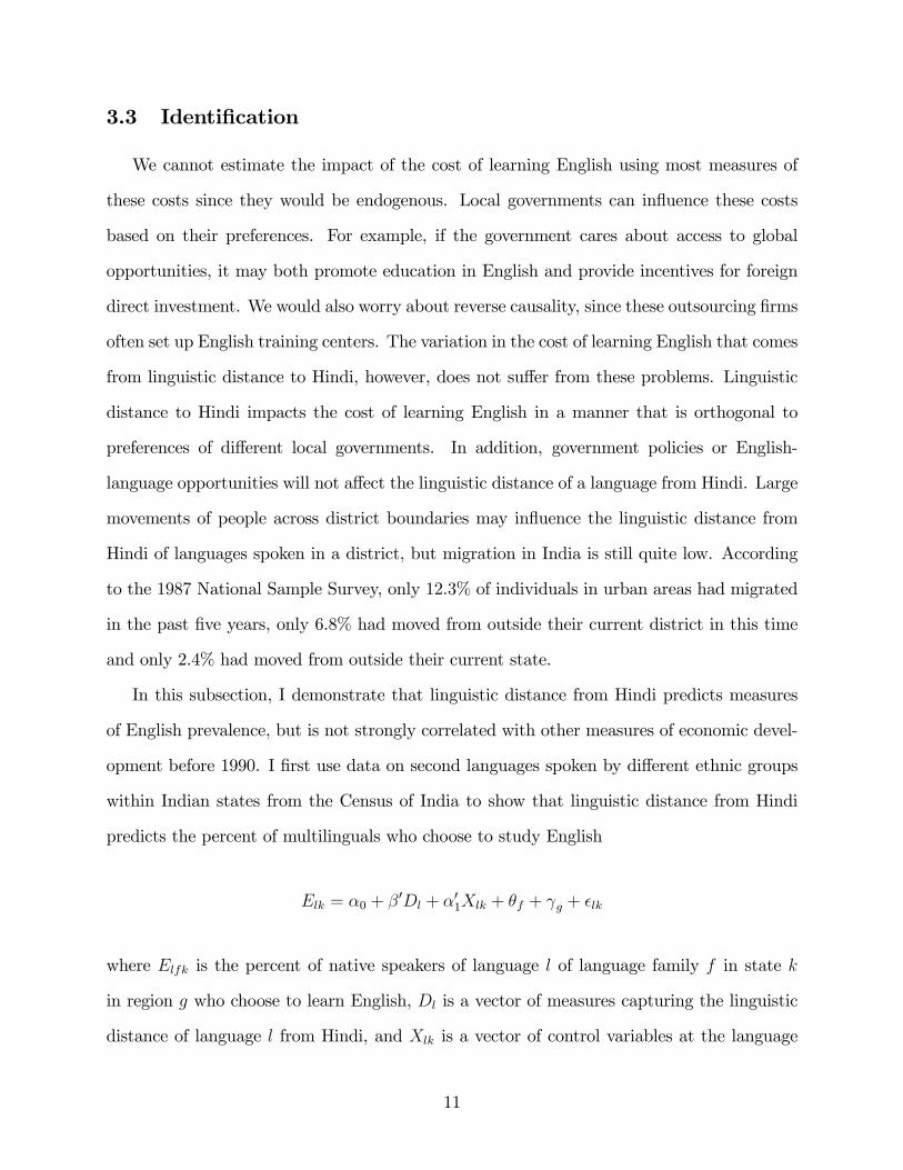
In this subsection, I demonstrate that linguistic distance from Hindi predicts measures
of English prevalence, but is not strongly correlated with other measures of economic devel-
opment before 1990. I �rst use data on second languages spoken by di¤erent ethnic groups
within Indian states from the Census of India to show that linguistic distance from Hindi
predicts the percent of multilinguals who choose to study English
Elk = �0 + �0Dl + �
01Xlk + �f + g + �lk
where Elfk is the percent of native speakers of language l of language family f in state k
in region g who choose to learn English, Dl is a vector of measures capturing the linguistic
distance of language l from Hindi, and Xlk is a vector of control variables at the language
11

and state level. To control for other characteristics of ethnic groups or particular regions
of India, I include language family and region �xed e¤ects. The regions include north,
northeast, east, south, west and central India. The vector Xlk includes indicator variables
for whether language l is Hindi and for whether language l is the most spoken language in
the state. Finally, I control for a quadratic polynomial in the share of speakers of language l
who reside in state k and who reside anywhere in India. I weight observations by the number
of native speakers in the state and cluster at the state level.
The results using the 1991 Census of India are presented in table 3. Column 1 assumes a
linear relationship implying that one degree increases the percent of multilinguals who learn
English by 7.7 percent. Column 2 estimates that a 10% point increase in how many people
speak languages more than two degrees away from Hindi increases the percent of multilingual
English speakers by 2.16 percentage points. Finally, column 3 demonstrates that while the
relationship between linguistic distance and English prevalence does not appear to be linear,
the assumption of monotonicity is not problematic and this is true even excluding language
family �xed e¤ects.11 The omitted group in this regression is Urdu speakers; Urdu is very
close to Hindi (a distance of 0), but considered a separate language. From the F-statistics
shown at the bottom of the table, it is clear that linguistic distance from Hindi does predict
variation in the proportion of native speakers who learn English. In addition, I reject the
hypothesis that having any distance between your mother tongue and Hindi has the same
e¤ect on English learning by testing the equality of all linguistic distance �xed e¤ects (but
allowing them to be di¤erent from Urdu).12
I next explore the relationship between linguistic distance and the percent of all native
speakers who are multilingual (see columns 4-6 in table 3). While the linear measure of
11Note that linguistic distance of 5 degrees is dropped when including �xed e¤ects for each number ofdegrees away from Hindi since the only Indo-European, but not Indo-Aryan language in the data is Englishand I omit observations for English. The results are robust to modifying the measure of linguistic distance toomit this concentric circle (i.e. give all non-Indo-Aryan languages a distance of 5 degrees). In addition, the�xed e¤ect for linguistic distance of 6 is also dropped since it consists of all non-Indo-European languagesand I include language family �xed e¤ects.12These results are also robust to using the percent of all native speakers who choose to learn English.
12
linguistic distance predicts multilingualism, the �xed e¤ects for unit distances speci�cation
demonstrates that the e¤ect is clearly not rising in linguistic distance. In fact, the results
seems to be driven by a greater percent of multilingual individuals at a linguistic distance of
2 units relative to Urdu speakers. I also show that linguistic distance negatively predicts the
percent of all multilingual native speakers who choose to learn Hindi but not English (see
columns 7-9), as my theory would predict.13
Table 4 presents similar results from regressions using data from the 1961 Census of
India. These regressions di¤er slightly due to changes in the data collection, but the results
are very similar. For example, since Hindi and Urdu are categorized together, the omitted
group is languages one degree away from Hindi. The last columns also use a di¤erent
dependent variable, i.e. the percent of multilingual individuals who learn Hindi (even if they
also learn English). These results discredit an important concern with this identi�cation
strategy. The identi�cation strategy would be invalid if, for example, the ethnic groups
speaking languages further from Hindi were more forward-looking or outward-oriented in
the 1980s and anticipated the trade bene�ts to learning English. However, the tendency
for these ethnic groups to learn English was evident in 1961, much before anyone could
anticipate the trade liberalization of the early 1990s and the enormous returns to speaking
English. This supports the use of linguistic distance to highlight exogenous variation in the
costs of learning English. In addition, the number of English bilinguals among ethnic groups
in di¤erent states in 1961 is highly correlated with the number of English learners in 1991.
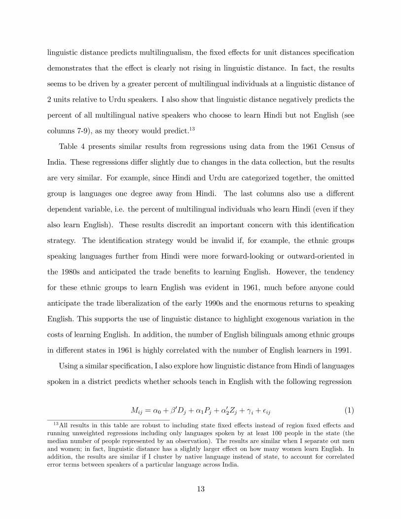
Using a similar speci�cation, I also explore how linguistic distance from Hindi of languages
spoken in a district predicts whether schools teach in English with the following regression
Mij = �0 + �0Dj + �1Pj + �
02Zj + i + �ij (1)
13All results in this table are robust to including state �xed e¤ects instead of region �xed e¤ects andrunning unweighted regressions including only languages spoken by at least 100 people in the state (themedian number of people represented by an observation). The results are similar when I separate out menand women; in fact, linguistic distance has a slightly larger e¤ect on how many women learn English. Inaddition, the results are similar if I cluster by native language instead of state, to account for correlatederror terms between speakers of a particular language across India.
13
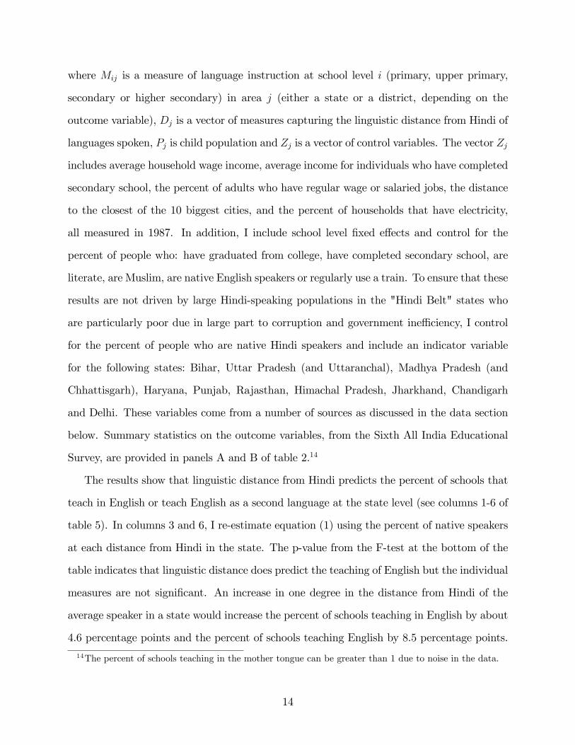
where Mij is a measure of language instruction at school level i (primary, upper primary,
secondary or higher secondary) in area j (either a state or a district, depending on the
outcome variable), Dj is a vector of measures capturing the linguistic distance from Hindi of
languages spoken, Pj is child population and Zj is a vector of control variables. The vector Zj
includes average household wage income, average income for individuals who have completed
secondary school, the percent of adults who have regular wage or salaried jobs, the distance
to the closest of the 10 biggest cities, and the percent of households that have electricity,
all measured in 1987. In addition, I include school level �xed e¤ects and control for the
percent of people who: have graduated from college, have completed secondary school, are
literate, are Muslim, are native English speakers or regularly use a train. To ensure that these
results are not driven by large Hindi-speaking populations in the "Hindi Belt" states who
are particularly poor due in large part to corruption and government ine¢ ciency, I control
for the percent of people who are native Hindi speakers and include an indicator variable
for the following states: Bihar, Uttar Pradesh (and Uttaranchal), Madhya Pradesh (and
Chhattisgarh), Haryana, Punjab, Rajasthan, Himachal Pradesh, Jharkhand, Chandigarh
and Delhi. These variables come from a number of sources as discussed in the data section
below. Summary statistics on the outcome variables, from the Sixth All India Educational
Survey, are provided in panels A and B of table 2.14
The results show that linguistic distance from Hindi predicts the percent of schools that
teach in English or teach English as a second language at the state level (see columns 1-6 of
table 5). In columns 3 and 6, I re-estimate equation (1) using the percent of native speakers
at each distance from Hindi in the state. The p-value from the F-test at the bottom of the
table indicates that linguistic distance does predict the teaching of English but the individual
measures are not signi�cant. An increase in one degree in the distance from Hindi of the
average speaker in a state would increase the percent of schools teaching in English by about
4.6 percentage points and the percent of schools teaching English by 8.5 percentage points.
14The percent of schools teaching in the mother tongue can be greater than 1 due to noise in the data.
14

Finally, I examine the percent of schools at the district level that teach in the regional
mother tongue (see columns 7-9). Since English is not the regional mother tongue anywhere
in India, the percent of schools that do not teach in the mother tongue is an upper bound
for those that teach in English. The results demonstrate that linguistic distance from Hindi
negatively predicts the percent of schools that teach in the mother tongue at the district
level. An increase in one concentric circle in the distance measure reduces the probability
that a school teaches in the region�s mother tongue by 3.4 percentage points.
I next study whether linguistic distance from Hindi is correlated with any other edu-
cational and economic characteristics of these districts by using various outcome variables
in speci�cation (1). The results indicate that linguistic distance from Hindi is not strongly
correlated with other characteristics of the educational system in 1993 (see table 6). Neither
measure of linguistic distance predicts the number of schools in 1993 or the number of higher
secondary schools (grades 11 and 12) o¤ering courses in di¤erent subjects, all normalized
by the population (in 10,000s) of children aged 5-18.15 Similar results for other economic
variables in 1987 can be seen in table 7. Most of the variables are uncorrelated with language
distance except for the percent of the population that have college degrees. The correlation
with the percent of graduates is negative, but the magnitude is very small. A increase in
linguistic distance to Hindi of one degree reduces the population with college degrees by
0.3%. The distance to the 10 biggest cities in India is also positive correlated with linguistic
distance probably because a disproportionate number of these cities are in Hindi-speaking
areas. To save space, I have omitted the results using my alternate measure of linguistic
distance (the percent of speakers of languages 3 or more degrees away from Hindi) which do
not di¤er from the results shown. I have also omitted similar regressions for the population
15In order to save space, I have omitted the results using the percent of speakers at each distance fromHindi which generally support these results, but are more di¢ cult to interpret. These results are also robustto using the absolute number of schools without normalizing. However, there does appear to be a signi�cantnegative correlation between linguistic distance and total enrollment in the arts and a positive, but notsigni�cant correlation between linguistic distance and total enrollment in the sciences (results not shown).Nevertheless, while we do see a correlation of linguistic distance with enrollment in certain subjects, theredoes not appear to be a strong relationship between linguistic distance and the availability of schools teachingthose subjects.
15
growth from 1987 to 1991, average wage for educated workers, the percent who have com-
pleted secondary school and the percent of households with electricity all of which are all
uncorrelated with linguistic distance.
Thus, while linguistic distance does predict how many people learn English and how many
schools teach English or in English, it does not strongly predict the availability of educational
institutions or other economic variables, rea¢ rming the validity of my identi�cation strategy.
4 Theoretical model
In this section, I describe a simple model to provide intuition on how the e¤ects of glob-
alization vary across districts due to di¤erences in the cost of learning English. Consider an
economy made up of two separate districts that di¤er only in the cost of learning English. I
specify a schooling model and production processes, and solve the model without and then
with a globally traded good, i.e. before and after trade liberalization. IT serves as one exam-
ple, but we can also think of this traded good as representing all traded goods and services
that require English speaking workers. Final goods travel freely between these districts, but
the movement of workers is negligible. Individuals choose to work as unskilled labor or ob-
tain instantaneous, though costly, education in either English or the local language, Hindi,
and work as skilled labor. Unskilled workers cannot learn English, but everyone, including
the English-educated workers, speaks Hindi. English and Hindi skilled workers are equally
productive in the production of other goods, but the globally traded good requires only
English-speaking workers. Production of the globally traded good also uses a second factor
that is �xed in the short run. We can think of this �xed factor as representing infrastructure,
such as electricity or telecommunications services, that is slow to change or entrepreneurs
who are immobile. Production of all �nal goods is perfectly competitive.
While the model provides predictions on returns to education and the demand for educa-
tion, I abstract from a central question in the trade literature. I do not attempt to explain
16
why India exports a skilled labor-intensive good contrary to Heckscher-Ohlin predictions. A
number of papers have explored theoretical modi�cations to match this fact. For example,
Feenstra and Hanson (1996, 1997) focus on the role on global outsourcing and Kremer and
Maskin (2006)) emphasize complementarities between people of di¤erent skill levels within
and across countries. Nevertheless, as this paper does not provide any insights for this related
question, I assume the price of the traded good is su¢ ciently high.
After trade liberalization, the globally traded good is produced in both districts; this
simply increases the demand for skilled workers, increasing the return to education and
school enrollment. How these changes di¤er between the two districts is more informative.
Since the elasticity of English speakers is greater in the district with lower costs of learning
English, this district will produce more IT since it can do so at a lower wage and will
experience greater growth in education. The wage for English speakers rises by less, but the
wage for Hindi workers will rise by more. Thus, the average return to education is ambiguous.
4.1 Schooling Decisions
Individuals live for one period and can choose to work as unskilled labor or get instan-
taneous education in English or Hindi and work as skilled labor. There are P people born
each period. Individuals di¤er in a parameter ci which governs the cost of education and
is distributed uniformly between zero and one in each district. Studying in Hindi costs
(t+ ci)w where t is a �xed cost of schooling (0 < t < 1) and w is the unskilled wage.
Studying in English costs �jciw where �j is a district-speci�c parameter, j 2 fLC;HCg,
and 1 < t + 1 < �LC < �HC . LC denotes the district with a lower cost of learning English,
while HC is the high cost district. Note that this cost structure is not symmetric; I chose this
structure to ensure that English and Hindi skilled workers exist in equilibrium both before
and after liberalization. Each individual�s schooling decision is to maximize lifetime income
17

with respect to h = Hindi schooling 2 f0; 1g and e = English schooling 2 f0; 1g
maxh; e
8>>>><>>>>:��jciw +max fqE; qHg if e=1, h=0
�tw � ciw + qH if e=0, h=1
w if e=0, h=0
9>>>>=>>>>;where qH and qE are the wages for Hindi and English skilled workers, respectively. Since
Hindi and English workers are equally productive in the Y sector, qE � qH . Assume that, in
equilibrium, qH � tw > w > qH � tw � w and qE > w > qE � �jw; otherwise either no one
would get any schooling or everyone would get schooling. Solving the individual�s decision
problem is straightforward. There are two cases. In one case, people with low values of ci get
English schooling, and those above do not get schooling. I ignore this case since people still
learn Hindi in India. In the other case, people with low values of ci get English schooling,
those in the middle get Hindi schooling and those with higher values of ci remain unskilled.
Figure 6 demonstrates this case when qE = qH . The labor supply functions are
SE = PQHE = Pwt+max fqE; qHg � qH
w��j � 1
�SH = P (QH �QHE) = P
qH � w � tw
w� wt+max fqE; qHg � qH
w��j � 1
� !
SL = P (1�QH) = P�1� qH � w � tw
w
�
4.2 Production of Y
There is one �nal good, Y, consumed in both districts and produced using
Y = min
�LY�L;HY + EY�H
�
where LY is quantity of unskilled labor used, HY is the quantity of local language skilled
labor used, and EY is the quantity of English speaking skilled labor used and �L > �H set
18
the productivity levels of skilled workers relative to unskilled workers in the production of
good Y. To produce an amount Y , the labor demand functions are
DLY = LY = �LY
DHEY = HY + EY = �HY
Note that �rms can perfectly substitute Hindi skilled workers for English skilled workers,
so if the wage for English-speaking workers is greater, production of good Y will hire only
Hindi skilled workers. The amount of Y produced will be determined by the availability
of labor. Prior to trade liberalization, English speakers must work in the Y industry and
therefore earn qE = qH . If qE > qH , EY = 0. The zero pro�t condition leads to
p = w�L + qH�H (2)
When the economy is open to trade, �rms can set up in either district to produce a
globally traded good X and take the price of X, pX , as given. Production of good X is
Cobb-Douglas and uses English-speaking skilled workers and a �xed factor F :
X = F �E1��X (3)
where EX is the amount of English skilled labor used. The endowment of F in a district is
exogenous and cannot respond, at least in the short run. Since F has no outside return in
this model, the industry will use all F available. To determine how much E is demanded:
maxEprofit = max
EpXF
�E1��X � qEEX � rFF
DEX = F
�qE
pX (1� �)
�� 1�
19
where rF is the return to the �xed factor F and 0 < � < 1. The zero pro�t condition is
pXX = rFF + qEF
�qE
pX (1� �)
�� 1�
(4)
4.3 Characterizing the equilibrium
In equilibrium, the labor market for unskilled workers and skilled workers must clear.
For unskilled workers this condition is simple
DL = SL ) �LY = P
�1� qS � w � tw
w
�(5)
Labor market clearing for skilled workers depends on whether the demand for English speak-
ers exceeds the "natural" supply of English skilled workers. Recall from �gure 6 that even
when qE = qH , there will be some supply of English speakers. If the amount of F is suf-
�ciently small such that in equilibrium, the demand for English workers is less than this
natural supply, then we must have that qE = qH (otherwise �rms could increase pro�ts by
reducing what they pay English workers since there is an excess supply). Call this case A.
The labor market clearing condition for skilled labor is
DHEY +DEX = SH + SE ) �HY + F
�qH
pX (1� �)
�� 1�
= P
�qH � w � tw
w
�(6)
If F is large enough that the demand for English workers exceeds the natural supply of
English workers, then qE > qH and no English workers are hired in the Y industry. Call this
case B. The labor market clearing conditions are
DHEY = SH ) �HY = P
qH � w � tw
w� wt+ qE � qH
w��j � 1
� ! (7)
DEX = SE ) F
�qE
pX (1� �)
�� 1�
= Pwt+ qE � qHw��j � 1
� (8)
20
I set good Y to be the numeraire with a price equal to 1; since �nal goods can move freely
across borders, this price applies to both districts. These labor market clearing conditions
plus the two zero pro�t conditions, equations (2) and (4), and the production function for
good X close the model. Denote the equilibrium values of the endogenous variables (w, qH ,
qE (= qH in case A), r, Y and X), with an asterisk. In addition, it will be useful to have
de�ned two additional terms. De�ne the weighted average return to skill, bq asbq = qHH + qEE
w (H + E)
and the total number of educated people, ED
ED = H + E = P�qHw� 1� t
�The equilibrium without any trade is a special case of case A when F = 0, described
in Proposition 1 below. Since the demand for English skilled workers rises after trade lib-
eralization, the wage for English workers has to rise. Now that fewer English speakers are
working in the Y industry, the wage for Hindi skilled workers has to rise as well since the
ratio of skilled to unskilled workers in Y production has to remain constant. School enroll-
ment responds to these higher wages. To compare how these changes di¤er in districts with
di¤erent levels of �j, we have to �rst solve the equilibrium in both case A and B.
Proposition 1 Case A. If, in equilibrium for a small neighborhood around �j, q�E = q
�H
then a) for all variables Z 2 fw�; q�H ; r�F ; Y �; X�; bq�; ED�g
dZ
d��j � 1
� = 0b)
dE�
d��j � 1
� < 0 anddH�
d��j � 1
� > 021
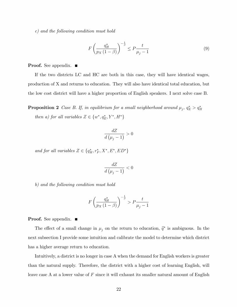
c) and the following condition must hold
F
�q�H
pX (1� �)
�� 1�
� P t
�j � 1(9)
Proof. See appendix.
If the two districts LC and HC are both in this case, they will have identical wages,
production of X and returns to education. They will also have identical total education, but
the low cost district will have a higher proportion of English speakers. I next solve case B.
Proposition 2 Case B. If, in equilibrium for a small neighborhood around �j, q�E > q
�H
then a) for all variables Z 2 fw�; q�E; Y �; H�g
dZ
d��j � 1
� > 0and for all variables Z 2 fq�H ; r�F ; X�; E�; ED�g
dZ
d��j � 1
� < 0b) and the following condition must hold
F
�q�H
pX (1� �)
�� 1�
> Pt
�j � 1
Proof. See appendix.
The e¤ect of a small change in �j on the return to education, bq� is ambiguous. In thenext subsection I provide some intuition and calibrate the model to determine which district
has a higher average return to education.
Intuitively, a district is no longer in case A when the demand for English workers is greater
than the natural supply. Therefore, the district with a higher cost of learning English, will
leave case A at a lower value of F since it will exhaust its smaller natural amount of English
22
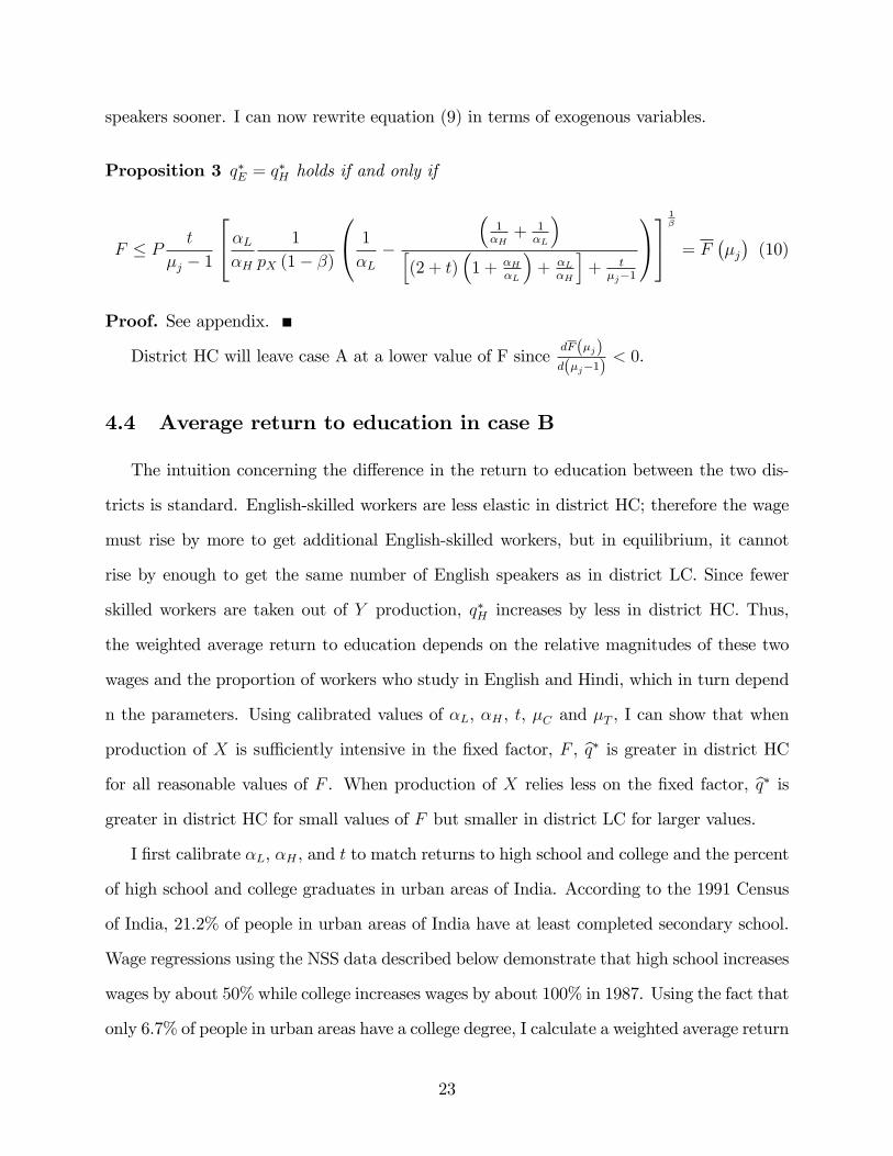
speakers sooner. I can now rewrite equation (9) in terms of exogenous variables.
Proposition 3 q�E = q�H holds if and only if
F � P t
�j � 1
24�L�H
1
pX (1� �)
0@ 1
�L�
�1�H+ 1
�L
�h(2 + t)
�1 + �H
�L
�+ �L
�H
i+ t
�j�1
1A351�
= F��j�(10)
Proof. See appendix.
District HC will leave case A at a lower value of F sincedF(�j)d(�j�1)
< 0.
4.4 Average return to education in case B
The intuition concerning the di¤erence in the return to education between the two dis-
tricts is standard. English-skilled workers are less elastic in district HC; therefore the wage
must rise by more to get additional English-skilled workers, but in equilibrium, it cannot
rise by enough to get the same number of English speakers as in district LC. Since fewer
skilled workers are taken out of Y production, q�H increases by less in district HC. Thus,
the weighted average return to education depends on the relative magnitudes of these two
wages and the proportion of workers who study in English and Hindi, which in turn depend
n the parameters. Using calibrated values of �L, �H , t, �C and �T , I can show that when
production of X is su¢ ciently intensive in the �xed factor, F , bq� is greater in district HCfor all reasonable values of F . When production of X relies less on the �xed factor, bq� isgreater in district HC for small values of F but smaller in district LC for larger values.
I �rst calibrate �L, �H , and t to match returns to high school and college and the percent
of high school and college graduates in urban areas of India. According to the 1991 Census
of India, 21.2% of people in urban areas of India have at least completed secondary school.
Wage regressions using the NSS data described below demonstrate that high school increases
wages by about 50% while college increases wages by about 100% in 1987. Using the fact that
only 6.7% of people in urban areas have a college degree, I calculate a weighted average return
23
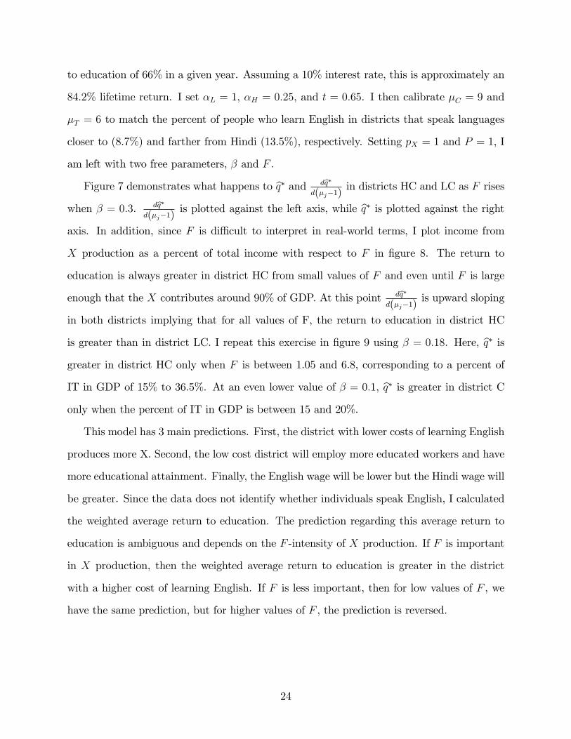
to education of 66% in a given year. Assuming a 10% interest rate, this is approximately an
84.2% lifetime return. I set �L = 1, �H = 0:25, and t = 0:65. I then calibrate �C = 9 and
�T = 6 to match the percent of people who learn English in districts that speak languages
closer to (8.7%) and farther from Hindi (13.5%), respectively. Setting pX = 1 and P = 1, I
am left with two free parameters, � and F .
Figure 7 demonstrates what happens to bq� and dbq�d(�j�1)
in districts HC and LC as F rises
when � = 0:3. dbq�d(�j�1)
is plotted against the left axis, while bq� is plotted against the rightaxis. In addition, since F is di¢ cult to interpret in real-world terms, I plot income from
X production as a percent of total income with respect to F in �gure 8. The return to
education is always greater in district HC from small values of F and even until F is large
enough that the X contributes around 90% of GDP. At this point dbq�d(�j�1)
is upward sloping
in both districts implying that for all values of F, the return to education in district HC
is greater than in district LC. I repeat this exercise in �gure 9 using � = 0:18. Here, bq� isgreater in district HC only when F is between 1.05 and 6.8, corresponding to a percent of
IT in GDP of 15% to 36.5%. At an even lower value of � = 0:1, bq� is greater in district Conly when the percent of IT in GDP is between 15 and 20%.
This model has 3 main predictions. First, the district with lower costs of learning English
produces more X. Second, the low cost district will employ more educated workers and have
more educational attainment. Finally, the English wage will be lower but the Hindi wage will
be greater. Since the data does not identify whether individuals speak English, I calculated
the weighted average return to education. The prediction regarding this average return to
education is ambiguous and depends on the F -intensity of X production. If F is important
in X production, then the weighted average return to education is greater in the district
with a higher cost of learning English. If F is less important, then for low values of F , we
have the same prediction, but for higher values of F , the prediction is reversed.
24
5 Empirical methodology
5.1 Information technology and returns to education
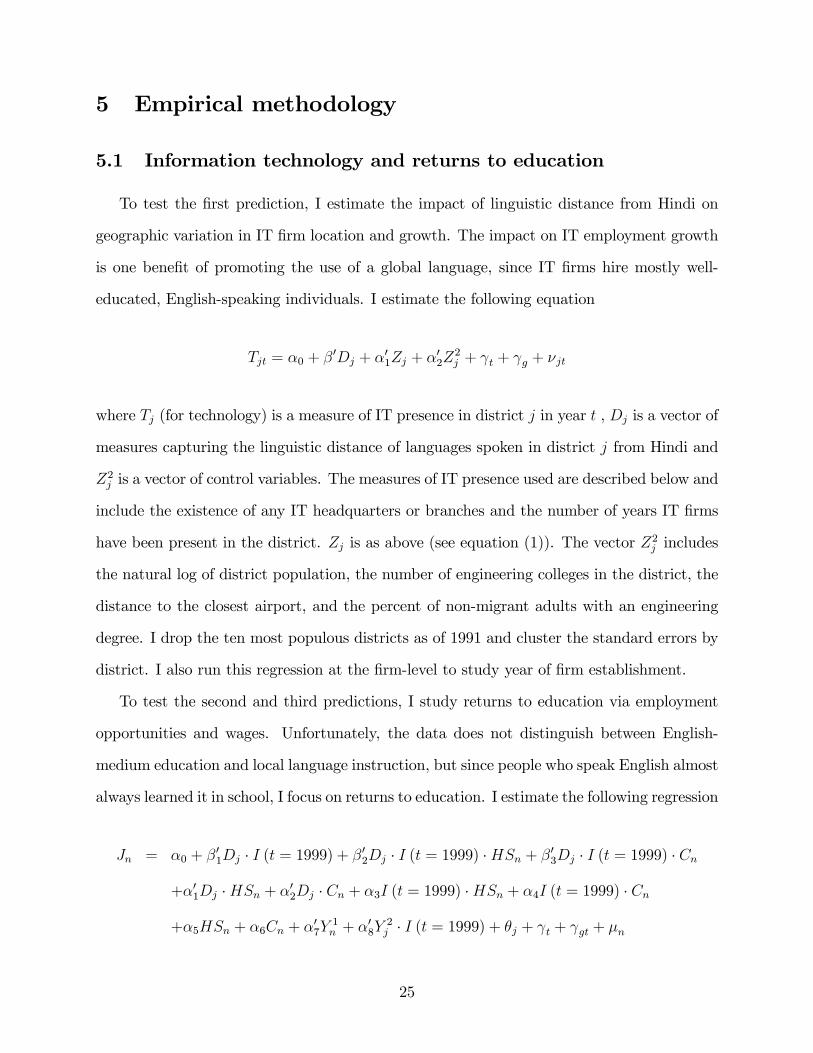
To test the �rst prediction, I estimate the impact of linguistic distance from Hindi on
geographic variation in IT �rm location and growth. The impact on IT employment growth
is one bene�t of promoting the use of a global language, since IT �rms hire mostly well-
educated, English-speaking individuals. I estimate the following equation
Tjt = �0 + �0Dj + �
01Zj + �
02Z
2j + t + g + �jt
where Tj (for technology) is a measure of IT presence in district j in year t , Dj is a vector of
measures capturing the linguistic distance of languages spoken in district j from Hindi and
Z2j is a vector of control variables. The measures of IT presence used are described below and
include the existence of any IT headquarters or branches and the number of years IT �rms
have been present in the district. Zj is as above (see equation (1)). The vector Z2j includes
the natural log of district population, the number of engineering colleges in the district, the
distance to the closest airport, and the percent of non-migrant adults with an engineering
degree. I drop the ten most populous districts as of 1991 and cluster the standard errors by
district. I also run this regression at the �rm-level to study year of �rm establishment.
To test the second and third predictions, I study returns to education via employment
opportunities and wages. Unfortunately, the data does not distinguish between English-
medium education and local language instruction, but since people who speak English almost
always learned it in school, I focus on returns to education. I estimate the following regression
Jn = �0 + �01Dj � I (t = 1999) + �02Dj � I (t = 1999) �HSn + �03Dj � I (t = 1999) � Cn
+�01Dj �HSn + �02Dj � Cn + �3I (t = 1999) �HSn + �4I (t = 1999) � Cn
+�5HSn + �6Cn + �07Y
1n + �
08Y
2j � I (t = 1999) + �j + t + gt + �n
25

where Jn is a measure of employment of individual n in district j at year t 2 f1987; 1999g,
HSn and Cn are indicators for whether individual n has completed high school or college,
respectively and Y 1n and Y2j contain individual and district characteristics. For Jn, I use
whether the individual has a regular wage or salaried job conditional on being in the labor
force (as opposed to being self-employed, a casual laborer or seeking work) and the natural
log of the individual�s wage earnings per week. The vector Y 1n includes the individual�s age,
age squared, gender, marital status (a dummy for being married), and whether the individual
has ever moved. At the district level, Y 2j includes the percent of native English speakers, the
percent of native Hindi speakers and whether the state is in the Hindi belt. I also include
district �xed e¤ects and region �xed e¤ects interacted with time, cluster the standard errors
by district and weight the observations. I run this regression by gender and age and study
the skilled wage premium across industries to establish the role played by trade in services.
5.2 Linguistic distance from Hindi and school enrollment
To further test the second prediction, I estimate the impact of linguistic distance from
Hindi on school enrollment growth using
log (Sijt)� log(Sijt�1) = �0 + �0Dj � I (t = 2002) + �1 log (Sijt�1) + �02Pjt (11)
+�3I (t = 2002) + �04Zj � I (t = 2002) + �j + t + gt + it + �ijt
where Sijt is a measure of enrollment at grade level i in district j in region g at time t 2
f1987; 1993; 2002g, Dj is a vector of measures capturing the linguistic distance of languages
spoken in district j from Hindi, I (�) is an indicator function, and Pjt is a vector of population
at time t and time t� 1. The parameter �j is a district �xed e¤ect allowing each district to
have its own trend in enrollment and it is a cohort e¤ect, controlling for grade-year trends.
The vector Zj includes the same controls as above. I use only data from the urban areas of
all districts and correct the standard errors for intracluster correlation at the district level.
26
I also include �xed e¤ects for region interacted with time. This strategy - using preexisting
di¤erences to predict changes in school enrollment, allowing for individual district e¤ects
and region-speci�c trends and controlling for many other preexisting di¤erences - rules out
a number of other explanations for these results.
Using individual level data, I con�rm these results using the following regression:
Hc = �0 + �01Dj � I (t = 1999) + �02Dj � I (t = 1999) � I (Ac 2 [11; 15]) (12)
+�03Dj � I (t = 1999) � I (Ac 2 [16; 20]) + �01Dj � I (Ac 2 [11; 15])
+�02Dj � I (Ac 2 [16; 20]) + �3I (t = 1999) � I (Ac 2 [11; 15])
+�4I (t = 1999) � I (Ac 2 [16; 20]) + �05Y 1c + �06Y 2j + �j + t + gt + �c
where Hc denotes whether child c (between ages 6 and 20) in district j is attending school at
year t 2 f1987; 1999g, Ac denotes the child�s age, and Y 1c and Y 2j are vectors of characteristics
about the child and the district respectively. I also include district �xed e¤ects and region
�xed e¤ects interacted with time. I weight the observations and cluster the standard errors by
district. The vector Y 1c consists of �xed e¤ects for age, gender, household religion, education
categories of the household head; an indicator for having migrated and household wage
income. Y 2j is as above. I also run the same regression with a measure of educational
achievement as the outcome. This variable takes on values 0 for children who are not
literate, 1 for those who are literate without any formal education, 2 for those who have
completed pre-primary schooling, 3 for primary, 4 for middle, 5 for secondary and 6 for
college graduates. Due to the ordinal nature of this variable, I run this regression with an
ordered probit model as well as linear probability.
While linguistic distance to Hindi is one measure of the cost of learning English, we might
want to estimate the impact of other measures. For example, I estimate all speci�cations
using the percent of schools in the district that teach in the mother tongue. However since
this is endogenous, I instrument with measures of linguistic distance to Hindi.
27

6 Sources of data
6.1 Information technology
I collected and coded data on IT �rms from the National Association of Software and
Service Companies (NASSCOM) directories published in 1995, 1998, 1999-2000, 2002 and
2003. These directories are based on surveys that contain self-reported data from individ-
ual �rms on the location of the headquarters, the number and location of branches, and
the number of employees. According to NASSCOM, the sample accounts for 95% of the
revenue in the industry in most years (Mehta 1995, 1998, 1999; Karnik 2002). To estimate
the impact of linguistic distance from Hindi on the growth in IT, I use a number of di¤er-
ent measures of IT presence. My primary measure is an indicator for the existence of IT
headquarters or branches in a district, but I also examine the year of �rm establishment,
the number of branches and headquarters in a district, number of employees, total revenue,
total exports and total capital subscribed. Since the data only contains this information
at the headquarters level, I either assign them to the headquarters or divide evenly across
branches. Summary statistics of IT presence by year of data can be found in table 8. Note
that revenue and exports data were not available in the 1998 directory.
6.2 Employment, education in 1987 and district-level controls
Data on employment and returns to education are from the Indian National Sample
Surveys (NSS) conducted in 1987-1988 and 1999-2000.16 The NSS provides individual-level
information on wages paid in cash and in-kind as well as employment status, industry and
occupation codes and weights for each observation. Employment status includes working
in household enterprises (i.e. self-employed), as a helper in a household enterprise, as a
regular salaried wage employee and as casual wage labor. In addition, the data reveals
whether individuals are seeking work, attending school or attending to domestic duties.
16An NSS survey was conducted in 1993-1994, but district identi�ers are not available.
28
Matching industry codes across the two time periods allows examining employment growth
and returns to education by industry in agriculture, manufacturing, wholesale/retail/repair,
hotel & restaurant services, transport services, communications (post and courier), �nancial
intermediate/insurance/real estate and other services (education, health care, civil services).
Table 9 provides district averages of employment and wages for the two years in the sample.
This data was also used to calculate enrollment levels from 1987 and district-level control
variables. I construct district-level measures of grade school enrollment at the primary,
upper primary and secondary levels. The NSS also contains household-level information
on household structure, demographics, employment, education, expenditures, migration and
assets, from which I calculate district averages of all control variables mentioned above such
as household wage income, the percent of working-age adults who are engineers, the percent
Muslim, the percent who regularly travel by train and the percent of households that have
electricity. In addition, I use this individual data as a second check of the education results,
although I prefer the SAIES data for these education results since the latest year is more
recent (2002 as opposed to 1999-2000) and as the SAIES is a census, it provides a more
complete measure of district-wide enrollment.
Using latitude and longitude data, I calculate the distance from each district to the
closest of the 10 biggest cities in India and to the closest airport operated by the Airports
Authority of India. As a measure of engineering college presence I count the number of
Indian Institutes of Technology and Regional Engineering Colleges (now called the National
Institutes of Information Technology) in each district. All of them were established prior
to 1990, although some were not given REC/NIIT status until the later 1990s. Summary
statistics for all of these variables can also be found in panel C of table 2.
6.3 Enrollment, achievement and language of instruction
Data on grade school enrollment comes from the Sixth and Seventh All India Educational
Surveys (AIES), conducted by the National Council of Educational Research and Training
29
(NCERT) which began on September 30, 1993 and September 30, 2002 respectively. The
surveys collect data at the school level on enrollment, school facilities, languages taught,
courses available, teacher quali�cations, incentive programs and other aspects of education.
I focus on urban enrollment at each grade in a district. Note that the data consist of the
actual number of students enrolled in each grade, not enrollment rates. In order to account
for this, I control for population and population growth among 5-19 year-olds from the
1991 and 2001 Census of India. I cannot calculate a more accurate measure of the relevant
population for each grade since there is no de�nitive age at which a child should be in
a particular grade, given that children start school at di¤erent ages and often fail to be
promoted. Enrollment in each grade increased dramatically between 1993 and 2002, as can
be seen in table 10. Total enrollment in all grades increased by 32%, but the increases are
greater in the highest grades. I pool all grades and also separate them by school level (grades
1-5 constitute primary, 6-8 upper primary, 9-12 secondary).
7 Impact of linguistic distance on returns to education
7.1 Geographic variation in the growth of information technology
The results indicate strong positive e¤ects of linguistic distance from Hindi on IT presence
(see tables 11 to 13). I �nd that this cost of learning English, when measured either as the
weighted average or the percent of speakers su¢ ciently removed from Hindi, predicts whether
any IT �rm establishes a headquarters or a branch in a district (see columns 1 and 2 of table
11). One degree away from Hindi of the average speaker in a district results in a 6% increase
in the probability of having any IT presence. However, many districts may be very unlikely
to receive IT �rms for a number of reasons. While these reasons should be orthogonal to
linguistic distance to Hindi, it is possible they are not, so I use �rm-level data to focus
on districts that see any IT �rms between 1995 and 2003 (columns 3 and 4 of table 11).
These results con�rm that areas that are linguistically further removed from Hindi saw the
30

establishment of IT �rms earlier, by approximately 3 years per degree of linguistic distance.
Linguistic distance from Hindi also explains geographic variation in the number of head-
quarters and branches and the number of employees when divided evenly by branch (see
columns 1-4 of table 12). However, it does not predict IT �rm employment when assigned
to the �rm headquarters or �rm performance, when measured either way (columns 5-12 of
table 12). There are many possible explanations. First, many employees and much of a �rm�s
production may not be not located at the headquarters. A �rm may set up in a district to
which the founder has personal ties but produce all its revenue at a di¤erent branch. Either
allocation method would then be incorrect and bias the results. Second, the entire e¤ect of
linguistic distance on IT could be at the extensive margin of where �rms establish, not on
the intensive margin. Another possible explanation is that the relationship between linguis-
tic distance and �rm performance could be nonlinear or nonparametric and not captured
by these reduced form measures of linguistic distance from Hindi. This is suggested when
I instrument for the percent of schools that teach in the regional mother tongue with the
percent of people in the district that speak languages at each distance away from Hindi (see
table 13). The F-statistics are su¢ ciently strong and the coe¢ cients suggest an impact of
the correct sign, but the standard errors are too large to judge signi�cance.
7.2 Returns to education
Testing the second and third predictions, I �nd evidence of greater growth in employment
of educated workers but smaller growth in wage premiums in districts with lower costs of
English as predicted by the model. I �rst demonstrate that the college premium for the
probability of regular employment rose faster in districts with lower costs of learning English
from 1987 to 1999 (see table 14). These e¤ects are driven by increases in the employment
for young adults (below the age of 30) rather than older adults. These results are sensible
given that many of the new �rms in services that have risen due to trade, such as in IT, hire
predominantly young adults. The coe¢ cients are also larger for women then men, which is
31

also sensible since IT �rms employee more women relative to traditional Indian �rms. The
male-female ratio among those working was 80:20 according to the 1987 NSS, but 77:23 in
software �rms and 35:65 in business processing �rms (NASSCOM 2004).
At the same time, con�rming the third prediction, I �nd that skilled wage premiums rose
by less in districts with lower costs of English, particularly for secondary school graduates
(see table 15). These results are driven by wages for older adults and the magnitudes are
relatively small. The wage premium for high school graduates rises by 3% less over 12 years
per degree in linguistic distance from Hindi, relative to a premium of 54% for high school
graduates in 1987. Further exploring these wage results by industry, I �nd that the fall
in wage premium for educated workers in these districts seems to be driven by wages in
manufacturing, hotels and restaurants, transportation and communications (see tables 16
and 17). I �nd no evidence of di¤erential changes in wage premium by linguistic distance
from Hindi in agriculture and wholesale, retail and repair. I also �nd an increase in overall
wages in transportation and communications. Studying other industries, I �nd that high
school and college wage premiums rose more in districts linguistically further from Hindi
only in the business services industry, which includes �nancial institutions, insurance, real
estate, computer related activities, research and development and other business activities.
In addition, I �nd no wage e¤ects on other services which includes public service, education,
health, sanitary and community services.
These results are clearly consistent with an increase in trade-related jobs in districts with
lower costs of learning English since most trade in services requiring English would be in
business services. While trade in manufacturing could increase as well following the trade
liberalization in the 1990s, these results indicate that wages did not rise in the manufac-
turing industry, perhaps because tari¤ cuts in the 1990s resulted in import competition in
manufacturing. Export growth in India since the 1990s was driven by services. The increase
in wages in the transportation and communications industries are also consistent with this
story since they are important to trade-related services.
32
8 Impact of linguistic distance on education
Further testing the second prediction, I �nd that educational attainment rises more in
districts with lower costs of learning English. I �rst demonstrate this result using district-
level data, estimating speci�cation (11) (see tables 18 and 19). Both measures of linguistic
distance show an increase in school enrollment, although the results are stronger at di¤erent
levels. At the primary and upper primary levels, the coe¢ cients for girls are larger than boys,
but the increase is comparable at the secondary level. This is partly because enrollment for
girls starts from a lower level than boys and the outcome is a percent improvement.
I �nd similar results, when using the percent of each type of school (primary and upper
primary) that teach in the regional mother tongue as the measure of cost of learning English
and instrumenting with the linguistic distance (see table 20). I instrument both with the
weighted average measure of linguistic distance as well as the percent of speakers each degree
away from Hindi as in table 13. The F-statistics from the excluded variables in the �rst stage
are shown at the bottom of the table; these instruments clearly have su¢ cient predictive
power. The second set of instruments allows for a more �exible relationship between distance
of mother tongues from Hindi and the prevalence of English, increasing the predictive power
of the �rst stage and signi�cantly reducing the standard errors (at least for primary schools).
The magnitudes of these results are economically signi�cant. Using the estimates from
column 1 of table 18, an increase in 1 degree from Hindi of the average speaker�s mother
tongue (44% of 1 standard deviation) would increase enrollment growth by 11% over the 9-
year period. Using estimates from column 1 in table 19, an increase of 1 standard deviation
in how many people speak languages far from Hindi (44%) would increase enrollment by
12% over the 9-year period. Finally, a 1 standard deviation increase in how many primary
schools teach in the mother tongue (22%) would reduce enrollment by 43% over 9 years
(averaging the e¤ect using di¤erent instrument sets). For upper primary schools, an increase
in 1 standard deviation (25 percentage points) would reduce enrollment by 39% over 9 years.
As an additional test of these results, I examine individiual data from another source.
33

Note that the time period in this exercise is 1987 to 1999-2000, so we would expect to �nd
smaller e¤ects. Estimating equation (12) on the NSS data, I �nd that the main interaction
of linguistic distance and post is not signi�cant (in fact, the coe¢ cients are often negative),
but the interactions with older age groups is quite signi�cant (see table 21). For boys, the
most precisely estimated increase in attendance is at ages 16 - 20 while the attendance for
11 - 15 year-old girls seems to respond the most. I �nd similar e¤ects using the alternate
dependent variable of educational achievement (see table 22).17
9 Conclusion
In this paper, I studied the e¤ect of promoting a global language on education and
employment during a period of trade liberalization and globalization, by exploiting exogenous
variation in the cost of learning English across districts in India. This exogenous variation
was determined by historical linguistic diversity in India and the imposition of Hindi as
the o¢ cial language of the country in the 1950s. I �rst showed that linguistic distance from
Hindi does predict whether individuals choose to learn English as a second language and that
linguistic distance from Hindi of languages spoken in a district does predict how many schools
teach English. I showed that one clear bene�t of promoting a global language is access to
global job opportunities such as those in information technology. IT �rms were established
in districts that are linguistically further from Hindi with a greater probability and earlier
than in other districts. I next demonstrated that the high school and college premium in the
probability of having a regular salaried job rose faster, but the wage premium rose by less
for individuals in these districts. Lastly, I showed that districts further removed from Hindi
experienced greater increases in school enrollment growth.
There are two avenues through which new job opportunities created through trade liber-
alization may have increased school enrollment. In this paper, I demonstrated that returns17I get similar results using an ordered probit model. I also repeat the exercise from table 20 using this
speci�cation and �nd the presence of fewer English-instruction schools reduces enrollment growth particularlyfor older children (results not shown).
34
to education rose faster in districts where residents speak languages further from Hindi. An-
other channel could be through increased family income. It is unlikely that this is driving
all the results presented here since the greater job opportunities were concentrated among
young adults. Thus, this should increase enrollment of children at lower grades by more
while the results indicate bigger e¤ects at older ages. In future work, I plan to further distin-
guish between these two e¤ects by exploiting the household structure of the NSS data and
comparing households that are more a¤ected by the increase in labor market opportunities
with other households that would only be a¤ected by general income growth in the district.
Unfortunately, the data is not currently available past 1999. I also hope to �nd additional
data sources which may contain language knowledge for the individual to determine more
directly the consequences of speaking English.
In addition, the interaction of linguistic distance to Hindi and trade liberalization may
have impacted fertility and marriage rates. Anecdotal evidence suggests that women work
in call centers and other business services �rms between �nishing their education and get-
ting married. This might then increase the age of �rst marriage and it might increase the
probability that women continue to work past marriage, potentially impacting fertility rates.
Finally, in the long run, there might be an impact of future job opportunities on child health.
If parents think their daughters are more likely to work for a few years before getting married
(since some business processing �rms such as call centers and medical transcription �rms
prefer to hire women) they may invest more in their daughters�health as well as education.
Thus, I demonstrated how the impact of trade liberalization varies across regions with
di¤erent elasticities of skilled labor - areas with greater labor supply response experience
greater employment of skilled workers and human capital accumulation, but smaller increases
in wage inequality as measured by skilled wage premiums.
35
10 References
Angrist, Joshua, Aimee Chin and Ricardo Godoy (2006). "Is Spanish-Only SchoolingResponsible for the Puerto Rican Language Gap?," NBER Working Paper 12005, NationalBureau of Economic Research, Cambridge, MA.Angrist, Joshua and Lavy, Victor (1997). "The E¤ect of a Change in Language of
Instruction on the Returns to Schooling in Morocco," Journal of Labor Economics, Universityof Chicago Press, vol. 15(1), pages S48-76, January.Attanasio, O., Goldberg P., and N. Pavcnik (2004). �Trade Reforms and Wage Inequality
in Colombia,�Journal of Development Economics 74, 331-366.Attanasio, O. and M. Szekely (2000): �Household Saving in East Asia and Latin America:
Inequality Demographics and All That�, in B. Pleskovic and N. Stern (eds.), Annual WorldBank Conference on Development Economics 2000. Washington, DC: World Bank."Busy signals: Too many chiefs, not enough Indians," The Economist, September 8, 2005.�Can India Fly? A Special Report,�The Economist, June 3-9, 2006.Clingingsmith, David (2006). "Bilingualism, Language Shift and Economic Development
in India, 1931-1961." (mimeo) Harvard University.Cragg, M.I. and M. Epelbaum (1996). �Why Has Wage Dispersion Grown in Mexico? Is
It Incidence of Reforms or Growing Demand for Skills?�Journal of Development Economics51(1), 99-116.Dakin, Julian, Brian Ti¤en, and H.G. Widdowson (1968). Language in Education: The
Problem in Commonwealth Africa and the Indo-Pakistan Sub-continent. Oxford: OxfordUniversity Press.Dyen, Isidore, Joseph Kruskal and Paul Black (1997). FILE IE-DATA1. Available at
http://www.ntu.edu.au/education/langs/ielex/HEADPAGE.html.Edmonds, Eric, Nina Pavcnik and Petia Topalova (2006). "Trade Policy, Child Labor,
and Schooling: Evidence from Indian Districts." (mimeo) Dartmouth College.Feenstra, R.C. and G. Hanson (1996). �Foreign Investment, Outsourcing and Relative
Wages.�In R.C. Feenstra, G.M. Grossman and D.A. Irwin, eds., The Political Economy ofTrade Policy: Papers in Honor of Jagdish Bhagwati, MIT Press, 89-127.Feenstra, R.C. and G. Hanson (1997). �Foreign Direct Investment and Relative Wages:
Evidence from Mexico�s Maquiladoras.�Journal of International Economics, 42(3), 371-393.Feliciano, Z. (1993). �Workers and Trade Liberalization: The Impact of Trade Reforms
in Mexico on Wages and Employment.�(mimeo) Harvard University.Goldberg, Pinelopi K. and Nina Pavcnik (2004). �Trade, Inequality, and Poverty:What
Do We Know? Evidence from Recent Trade Liberalization Episodes in Developing Coun-tries,�Brookings Trade Forum, Washington, DC: Brookings Institution Press: 223�269.Hanson, Gordon H. and Ann Harrison (1999). �Trade, Technology and Wage Inequality
in Mexico.�Industrial and Labor Relations Review 52(2), 271-288.Hohenthal, Annika (2003). "English in India; Loyalty and Attitudes," Language in India,
3, May 5, 2003.Kamat, A.R, 1985. Education and Social Change in India. Bombay: Somaiya Publica-
tions Private Limited.
36
Karnik, Kiran, ed. (2002). Indian IT Software and Services Directory 2002. NationalAssociation of Software and Service Companies, New Delhi.Kremer, Michael and Eric Maskin (2006). �Globalization and Inequality.�(mimeo) Har-
vard University.Lang , Kevin and Erez Siniver (2006). "The Return to English in a Non-English Speaking
Country: Russian Immigrants and Native Israelis in Israel," NBER Working Paper 12464,National Bureau of Economic Research, Cambridge, MA.Lindert, Peter H. and Je¤rey G. Williamson (2001). �Does Globalization Make the World
More Unequal?�NBER Working Paper No. 8228, National Bureau of Economic Research,Cambridge, MA.Mehta, Dewang, ed. (1995). Indian Software Directory 1995-1996. National Association
of Software and Service Companies, New Delhi.Mehta, Dewang, ed. (1998). Indian Software Directory 1998. National Association of
Software and Service Companies, New Delhi.Mehta, Dewang, ed. (1999). Indian IT Software and Services Directory 1999-2000.
National Association of Software and Service Companies, New Delhi.Munshi, Kaivan & Mark Rosenzweig (2006). "Traditional Institutions Meet the Modern
World: Caste, Gender, and Schooling Choice in a Globalizing Economy," American EconomicReview, American Economic Association, vol. 96(4), pages 1225-1252, September.NASSCOM, 2004. Strategic Review 2004. National Association of Software and Service
Companies, New Delhi, 185-194.Nurullah, Syed and J.P. Naik, 1949. A Student�s History of Education in India, 1800-
1947. Bombay: Macmillan and Company Limited.Panagariya, Arvind (2003). "The WTO Trade Policy Review of India, 1998." Interna-
tional Trade 0309012, EconWPA.Panagariya, Arvind (2004). "India�s Trade Reform: Progress, Impact and Future Strat-
egy" International Trade 0403004, EconWPA.Robbins, Donald (1995a). �Earnings Dispersion in Chile after Trade Liberalization.�
Harvard Institute for International Development, Cambridge, MA.Robbins, Donald (1995b). �Trade, Trade Liberalization, and Inequality in Latin America
and East Asia: Synthesis of Seven Country Studies.� Harvard Institute for InternationalDevelopment, Cambridge, MA.Robbins, Donald (1996a). �Stolper-Samuelson (Lost) in the Tropics: Trade Liberaliza-
tion and Wages in Colombia 1976�94.� Harvard Institute for International Development,Cambridge, MA.Robbins, Donald (1996b). �HOS Hits Facts: Facts Win. Evidence on Trade andWages in
the Developing World.�Harvard Institute for International Development, Cambridge, MA.Robbins, Donald, and Thomas Gindling (1997). �Educational Expansion, Trade Liber-
alisation, and Distribution in Costa Rica.�In Albert Berry, ed., Poverty, Economic Reformand Income Distribution in Latin America. Boulder, Colo.: Lynne Rienner Publishers.Robbins, Donald, Martin Gonzales, and Alicia Menendez (1995). �Wage Dispersion in
Argentina, 1976�93: Trade Liberalization amidst In�ation, Stabilization, and Overvalua-tion.�Harvard Institute for International Development, Cambridge, MA.Sanchez-Paramo, C. and N. Schady (2003): �O¤ and Running? Technology, Trade, and
the Rising Demand for Skilled Workers in Latin America,�World Bank Policy Research
37
Working Paper 3015.Washington, DC: World Bank.Swadesh, Morris (1972). "What is glottochronology?" In M. Swadesh, The origin and
diversi�cation of languages. London: Routledge & Kegan Paul: 281-284.United Nations Development Programme, Human Development Report 2004: Cultural
Liberty in Today�s Diverse World, New York: Oxford University Press, 2004.Wei, Shang-Jin and Yi Wu (2001). �Globalization and Inequality: Evidence from Within
China.�NBER Working Paper No. 8611, National Bureau of Economic Research, Cam-bridge, MA.Wood, Adrian (1997). �Openness and Wage Inequality in Developing Countries: The
Latin American Challenge to East Asian Conventional Wisdom.�World Bank EconomicReview, 11(1), 33-57.
11 Appendix A
11.1 Proof of Proposition 1
a) From equations (5) and (6), we can show that
�H�LP
�1� q
�H � w� � tw�
w�
�+ F
�q�H
pX (1� �)
�� 1�
= P
�q�H � w� � tw�
w�
�
Substituting q�H =1�H� aL
�Hw� into this expression implicitly solves for w�:
(2 + t)
�1 +
�HaL
�+�L�H
=1
w�
�1
�H+1
�L
�� FP
�1� �Lw�
�HpX (1� �)
�� 1�
(13)
Note that this expression does not depend on �j. Thus,
dw�
d��j � 1
� = 0The variables, q�H , r
�F , Y
�, X�, bq�, ED� can be written as functions of w� which also do not
depend on �j.
b) These follow from the expressions, E = P t�j�1
andH = P�
1w��H
� �L�H� 1� t� t
�j�1
�.
c) Since q�E = q�H , we know that the supply of English skilled workers does not depend on
the wages. To be in this equilibrium, the demand for English skilled labor fromX production
38
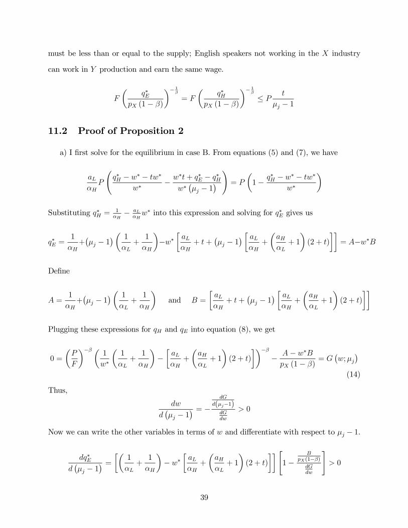
must be less than or equal to the supply; English speakers not working in the X industry
can work in Y production and earn the same wage.
F
�q�E
pX (1� �)
�� 1�
= F
�q�H
pX (1� �)
�� 1�
� P t
�j � 1
11.2 Proof of Proposition 2
a) I �rst solve for the equilibrium in case B. From equations (5) and (7), we have
aL�HP
q�H � w� � tw�
w�� w
�t+ q�E � q�Hw���j � 1
� ! = P �1� q�H � w� � tw�w�
�
Substituting q�H =1�H� aL
�Hw� into this expression and solving for q�E gives us
q�E =1
�H+��j � 1
�� 1
�L+1
�H
��w�
�aL�H
+ t+��j � 1
� � aL�H
+
�aH�L+ 1
�(2 + t)
��= A�w�B
De�ne
A =1
�H+��j � 1
�� 1
�L+1
�H
�and B =
�aL�H
+ t+��j � 1
� � aL�H
+
�aH�L+ 1
�(2 + t)
��
Plugging these expressions for qH and qE into equation (8), we get
0 =
�P
F
��� �1
w�
�1
�L+1
�H
���aL�H
+
�aH�L+ 1
�(2 + t)
����� A� w�BpX (1� �)
= G�w;�j
�(14)
Thus,
dw
d��j � 1
� = � dG
d(�j�1)dGdw
> 0
Now we can write the other variables in terms of w and di¤erentiate with respect to �j � 1.
dq�Ed��j � 1
� = �� 1
�L+1
�H
�� w�
�aL�H
+
�aH�L+ 1
�(2 + t)
��"1�
BpX(1��)dGdw
#> 0
39
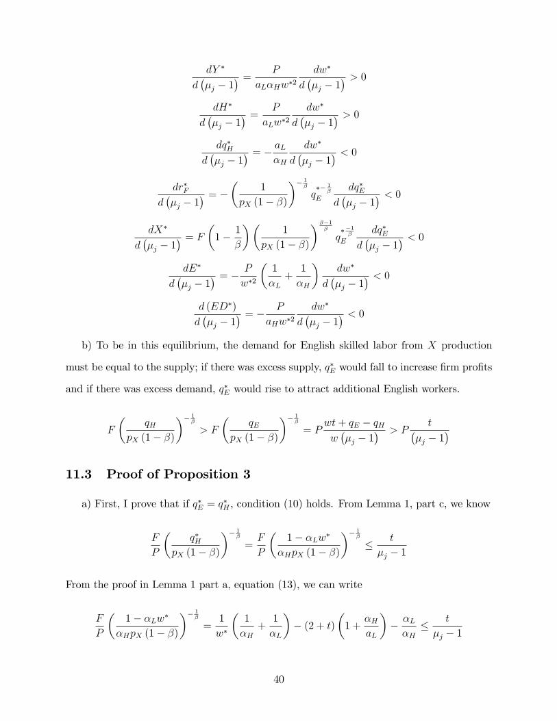
dY �
d��j � 1
� = P
aL�Hw�2dw�
d��j � 1
� > 0dH�
d��j � 1
� = P
aLw�2dw�
d��j � 1
� > 0dq�H
d��j � 1
� = � aL�H
dw�
d��j � 1
� < 0dr�F
d��j � 1
� = �� 1
pX (1� �)
�� 1�
q�� 1
�
E
dq�Ed��j � 1
� < 0dX�
d��j � 1
� = F �1� 1
�
��1
pX (1� �)
���1�
q��1�
E
dq�Ed��j � 1
� < 0dE�
d��j � 1
� = � P
w�2
�1
�L+1
�H
�dw�
d��j � 1
� < 0d (ED�)
d��j � 1
� = � P
aHw�2dw�
d��j � 1
� < 0b) To be in this equilibrium, the demand for English skilled labor from X production
must be equal to the supply; if there was excess supply, q�E would fall to increase �rm pro�ts
and if there was excess demand, q�E would rise to attract additional English workers.
F
�qH
pX (1� �)
�� 1�
> F
�qE
pX (1� �)
�� 1�
= Pwt+ qE � qHw��j � 1
� > Pt�
�j � 1�
11.3 Proof of Proposition 3
a) First, I prove that if q�E = q�H , condition (10) holds. From Lemma 1, part c, we know
F
P
�q�H
pX (1� �)
�� 1�
=F
P
�1� �Lw�
�HpX (1� �)
�� 1�
� t
�j � 1
From the proof in Lemma 1 part a, equation (13), we can write
F
P
�1� �Lw�
�HpX (1� �)
�� 1�
=1
w�
�1
�H+1
�L
�� (2 + t)
�1 +
�HaL
�� �L�H
� t
�j � 1
40

Solving for w�, we get
w� �
�1�H+ 1
�L
�(2 + t)
�1 + �H
aL
�+ �L
�H+ t
�j�1
Rewriting (10) and plugging in this inequality for w�, we get
F � Pt
�j � 1
�1� �Lw�
�HpX (1� �)
� 1�
�
Pt
�j � 1
24�L�H
1
pX (1� �)
0@ 1
�L�
�1�H+ 1
�L
�h(2 + t)
�1 + �H
�L
�+ �L
�H
i+ t
�j�1
1A351�
b) Next I prove that if F � F��j�, then q�E = q�H by contradiction. We know that
q�E � q�H since English skilled workers can take jobs as Hindi skilled workers. Suppose
q�E > q�H . From condition (8), we know that
F =
�qE
pX (1� �)
� 1�
P
t
�j � 1+
1��j � 1
� qE � qHw
!
>
�qE
pX (1� �)
� 1�
P
�t
�j � 1
�> P
t
�j � 1
�1
pX (1� �)
� 1��1� �Lw��H
� 1�
where the �rst inequality is due to q�E � q�H > 0 and the second is due to q�E > q�H = 1��Lw��H
.
Putting this together with F � F��j�and rearranging terms, we can show that
1
w�
�1
�L+1
�H
�<
�(2 + t)
�1 +
�H�L
�+�L�H
�+
t
�j � 1
However, this contradicts what we know from the proof of Lemma 2, part a, equation (14)
1
w�
�1
�L+1
�H
���aL�H
+
�aH�L+ 1
�(2 + t)
�=F
P
�A� w�BpX (1� �)
��1=�=wt+ qE � qHw��j � 1
� >t�
�j � 1�
where the second equality is from the fact that in this equilibrium, DEX = SE and the
inequality is from q�E � q�H > 0. Thus, q�E = q�H .
41

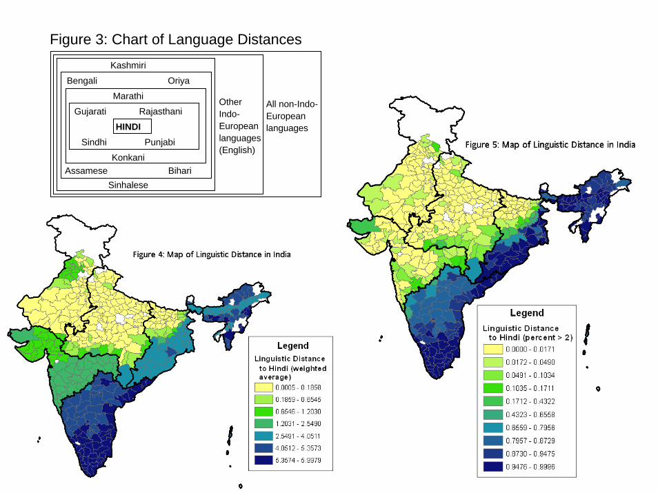
Kashmiri
Bengali Oriya
Marathi
Gujarati Rajasthani
HINDISindhi Punjabi
Konkani Assamese Bihari
Sinhalese
All non-Indo-Europeanlanguages
OtherIndo-Europeanlanguages(English)
Figure 3: Chart of Language Distances
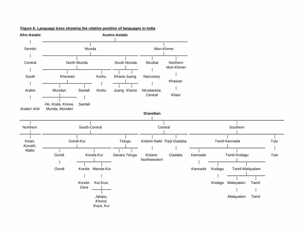
Malayalam TamilJatapu, Khond,
Koya, Kui
Figure 6: Language trees showing the relative position of languages in India
Afro-Asiatic Austro-Asiatic
| || |
Semitic Munda Mon-Khmer
| | || | | |
Central North Munda South Munda Nicobar Northern Mon-Khmer| | | || | | | |South Kherwari Korku Kharia-Juang Nancowry
| | | | | Khasian | | | | |Arabic Mundari Santali Korku Juang Kharia Nicobarese,
Central| | | Khasi|
Arabic/ ArbiHo, Koda, Korwa, Munda, Mundari
Santali
Dravidian|
| | | |Northern South-Central Central Southern
| | | || | | | | | |
Kisan, Kurukh, Malto
Gondi-Kui Telugu Kolami-Naiki Parji-Gadaba Tamil-Kannada Tulu | | | | | || | | | | |
Gondi Konda-Kui Savara Telugu Kolami, Northwestern
Gadaba Kannada Tamil-Kodagu Tulu
| | | || | | |
Gondi Konda Manda-Kui Kannada Kodagu Tamil-Malayalam
| | | || |
Konda-Dora
Kui-Kuvi Kodagu Malayalam Tamil | | ||
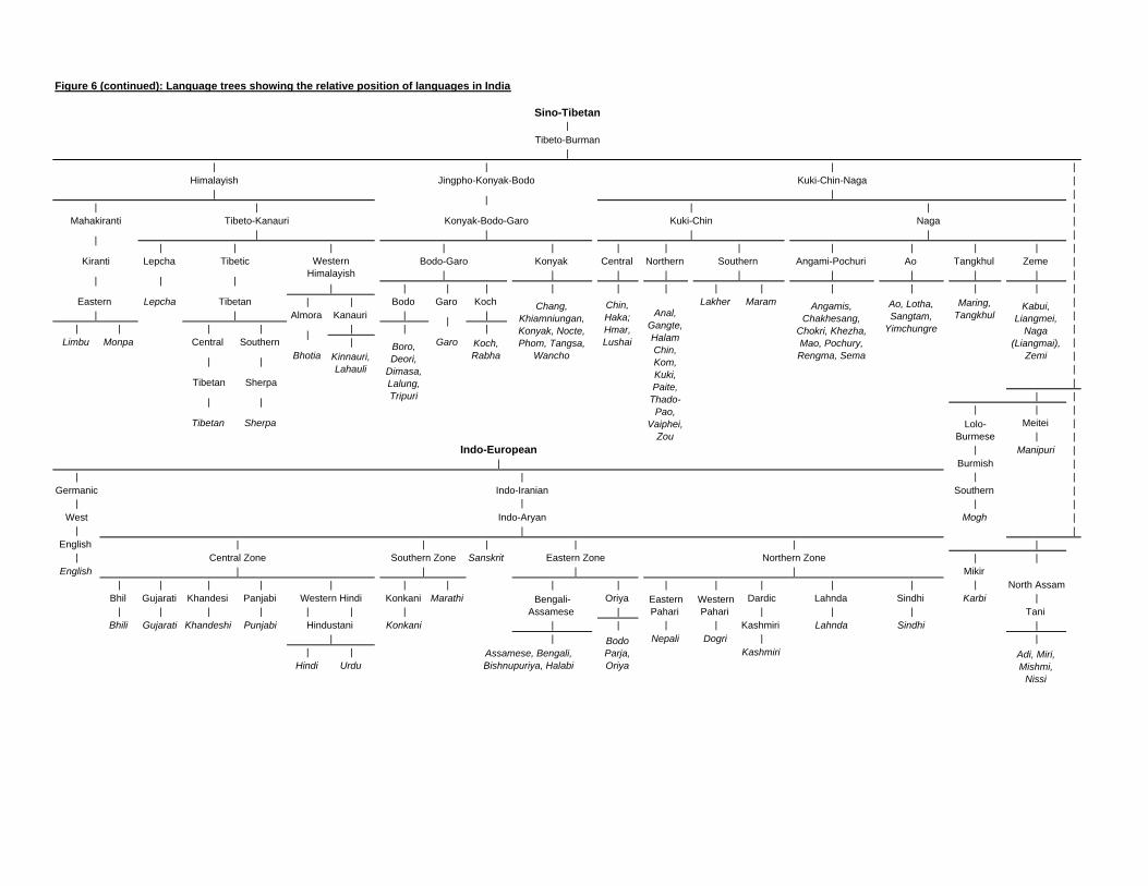
Figure 6 (continued): Language trees showing the relative position of languages in India
Sino-Tibetan|
Tibeto-Burman|
| | | |Himalayish Jingpho-Konyak-Bodo Kuki-Chin-Naga |
| | | || | | | |
Mahakiranti Tibeto-Kanauri Konyak-Bodo-Garo Kuki-Chin Naga |
| | | | | || | | | | | | | | | | | |
Kiranti Lepcha Tibetic Western Himalayish
Bodo-Garo Konyak Central Northern Southern Angami-Pochuri Ao Tangkhul Zeme |
| | | | | | | | | | | | || | | | | | | | | | | | | |
Eastern Lepcha Tibetan | | Bodo Garo Koch Chang, Khiamniungan, Konyak, Nocte, Phom, Tangsa,
Wancho
Chin, Haka; Hmar, Lushai
Anal, Gangte, Halam Chin, Kom, Kuki, Paite,
Thado-Pao,
Vaiphei, Zou
Lakher Maram Angamis, Chakhesang,
Chokri, Khezha, Mao, Pochury, Rengma, Sema
Ao, Lotha, Sangtam,
Yimchungre
Maring, Tangkhul
Kabui, Liangmei,
Naga (Liangmai),
Zemi
|| | Almora Kanauri | | | |
| | | | | | | | |Limbu Monpa Central Southern | Boro,
Deori, Dimasa, Lalung, Tripuri
Garo Koch, Rabha
|
| | Bhotia Kinnauri, Lahauli
||
Tibetan Sherpa |
| | | || | |
Tibetan Sherpa Lolo-Burmese
Meitei || |
Indo-European | Manipuri || Burmish |
| | | |Germanic Indo-Iranian Southern |
| | | |West Indo-Aryan Mogh |
| | |English | | | | | |
| Central Zone Southern Zone Sanskrit Eastern Zone Northern Zone | |English | | | | Mikir
North Assam| | | | | | | | | | | | | | |Bhil Gujarati Khandesi Panjabi Western Hindi Konkani Marathi Bengali-
Assamese Oriya Eastern
Pahari Western Pahari
Dardic Lahnda Sindhi Karbi || | | | | | | | | | | Tani
Bhili Gujarati Khandeshi Punjabi Hindustani Konkani | | | | Kashmiri Lahnda Sindhi || | Bodo
Parja, Oriya
Nepali Dogri | || | Assamese, Bengali,
Bishnupuriya, HalabiKashmiri Adi, Miri,
Mishmi, Nissi
Hindi Urdu

Figure 7: Schooling Decisions
QHQHE
0
0.2
0.4
0.6
0.8
1
1.2
1.4
0 0.1 0.2 0.3 0.4 0.5 0.6 0.7 0.8 0.9 1ci
Hindi skilledEnglish skilledUnskilled
Figure 8: Weighted average return to wages and the differential with respect to μ, β=0.3
0
0.005
0.01
0.015
0.02
0.025
0.03
0.035
0.04
0 10 20 30 40 50 60 70 8F
-1
0
1
2
3
4
5
0
dqhat/d(mieu-1) in district LCdqhat/d(mieu-1) in district HCqhat in district LCqhat in district HC

Figure 10: Weighted average return to wages and the differential with respect to μ, β=0.18
-0.008
-0.006
-0.004
-0.002
0
0.002
0.004
0.006
0.008
0.01
0.012
0 2 4 6 8 10 12F1.75
1.85
1.95
2.05
2.15
2.25
2.35
2.45dqhat/d(mieu-1) in district LCdqhat/d(mieu-1) in district HCqhat in district LCqhat in district HC
Figure 9: X production as a share of GDP in both districts, β=0.3
0
0.1
0.2
0.3
0.4
0.5
0.6
0.7
0.8
0.9
1
0 10 20 30 40 50 60 70 8F
0
%X/GDP in district LC
%X/GDP in district HC
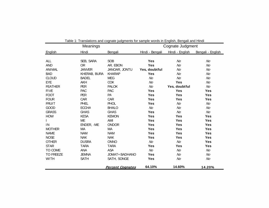
English Hindi Bengali Hindi - Bengali Hindi - English Bengali - English
ALL SEB, SARA SOB Yes No NoAND OR AR, EBON Yes No NoANIMAL JANVER JANOAR, JONTU Yes, doubtful No NoBAD KHERAB, BURA KHARAP Yes No NoCLOUD BADEL MEG No No NoEYE AKH COK No Yes NoFEATHER PER PALOK No Yes, doubtful NoFIVE PAC PAC Yes Yes YesFOOT PER PA Yes Yes YesFOUR CAR CAR Yes Yes YesFRUIT PHEL PHOL Yes No NoGOOD ECCHA BHALO No No NoGRASS GHAS GHAS Yes No NoHOW KESA KEMON Yes Yes YesI ME AMI Yes Yes YesIN ENDER, -ME ONDOR Yes Yes YesMOTHER MA MA Yes Yes YesNAME NAM NAM Yes Yes YesNOSE NAK NAK Yes Yes YesOTHER DUSRA ONNO No No YesSTAR TARA TARA Yes Yes YesTO COME ANA ASA No No NoTO FREEZE JEMNA JOMAT+BADHANO Yes No NoWITH SATH SATH, SONGE Yes No No
Percent Cognates 64.10% 14.60% 14.20%
Meanings Cognate JudgmentTable 1: Translations and cognate judgments for sample words in English, Bengali and Hindi

Table 2: Summary StatisticsVariable abbreviated name Notes Num Obs Mean St. Dev. Min. Max. Panel A (at the district level)Linguistic distance (weighted average) Degree measure of distance from native languages to Hindi 390 2.158 2.281 0.001 5.998Percent with linguistic distance > 2 Percent of people who speak languages at distance > 2 390 0.373 0.443 0.000 1.000Linguistic distance measure 2 Node measure of distance from native languages to Hindi 390 5.063 4.778 0.021 13.994Linguistic distance measure 3 Cognate measure of distance from native languages to Hindi 390 64.814 35.222 5.031 99.991Native Hindi speakers Percent of people who speak Hindi (as a native language) 390 0.424 0.433 0.000 0.996Speakers at distance 0 Percent of people who speak languages at distance 0 390 0.465 0.443 0.000 1.000Speakers at distance 1 Percent of people who speak languages at distance 1 390 0.095 0.265 0.000 0.991Speakers at distance 2 Percent of people who speak languages at distance 2 390 0.067 0.212 0.000 0.958Speakers at distance 3 Percent of people who speak languages at distance 3 390 0.094 0.251 0.000 0.985Speakers at distance 4 Percent of people who speak languages at distance 4 390 0.013 0.069 0.000 0.766Native English Speakers Percent of people who speak languages at distance 5 390 0.000 0.000 0.000 0.007Speakers at distance 6 Percent of people who speak languages at distance 6 390 0.265 0.391 0.000 1.000Primary schools teaching in mother tongue Percent of urban primary schools that teach in the mother tongue 408 0.889 0.222 0 1.08Upper primary schools teaching in mother tongue
Percent of urban upper primary schools that teach in the mother tongue 408 0.840 0.245 0 1.02
Panel B (at the state level, only urban areas)Primary schools teaching English Percent of primary schools that teach English 32 0.263 0.164 0.023 0.664Upper primary schools teaching English % upper primary schools that teach English 32 0.310 0.070 0.233 0.511Secondary schools teaching English % secondary schools that teach English 32 0.337 0.104 0.182 0.615Primary schools teaching in English % primary schools with English instruction 32 0.222 0.237 0 1.00Upper primary schools teaching in English % upper primary schools with English instruction 32 0.321 0.268 0.053 1.00Secondary schools teaching in English % secondary schools with English instruction 32 0.380 0.285 0.047 1.00Higher secondary schools teaching in English % higher secondary schools with English instruction 31 0.470 0.295 0.051 1.00 Panel C (at the district level, only urban areas)Household wage income Average weekly total wage income in 1000s of Rupees 397 0.183 0.178 0 1.763Educated wage Average wage of individuals with at least high school education 396 0.233 0.197 0 2.714Salaried Percent of adults with a regular wage or salaried job 397 0.188 0.082 0 0.568Graduate Percent of people with a college degree 397 0.051 0.043 0 0.5Secondary Percent of people with a high school degree 397 0.125 0.057 0 0.3333333Literate Percent of people who are literate 397 0.625 0.137 0.111111 0.969697Muslim Percent of people who are Muslim 397 0.168 0.193 0 1Train Percent of people who recently made a journey by train 395 0.077 0.094 0 0.686Electricity % households that use electricity as their main energy source 395 0.695 0.203 0 1Hindi belt Districts that are in the Hindi belt 409 0.477 0.500 0 1Child population 1991 District population of 5-19 year olds in 1991 379 181846 278514 631 2952148Child population 2001 District population of 5-19 year olds in 2001 379 181846 278514 631 2952148Child population growth Population growth rate for 5-18 year olds 379 0.318 0.347 -0.422 2.695Distance to closest big city Distance to closest of the 10 biggest cities in India 401 31.495 18.582 0.206 120.363Distance to closest airport Distance to closest airport operated by Airport Authority of India 401 7.797 4.695 0.443 24.761Number of engineering colleges Number of IITs and NITs 409 0.064 0.244 0 1Engineers % engineers among non-migrant 26-65-year-olds 395 0.002 0.008 0 0.065
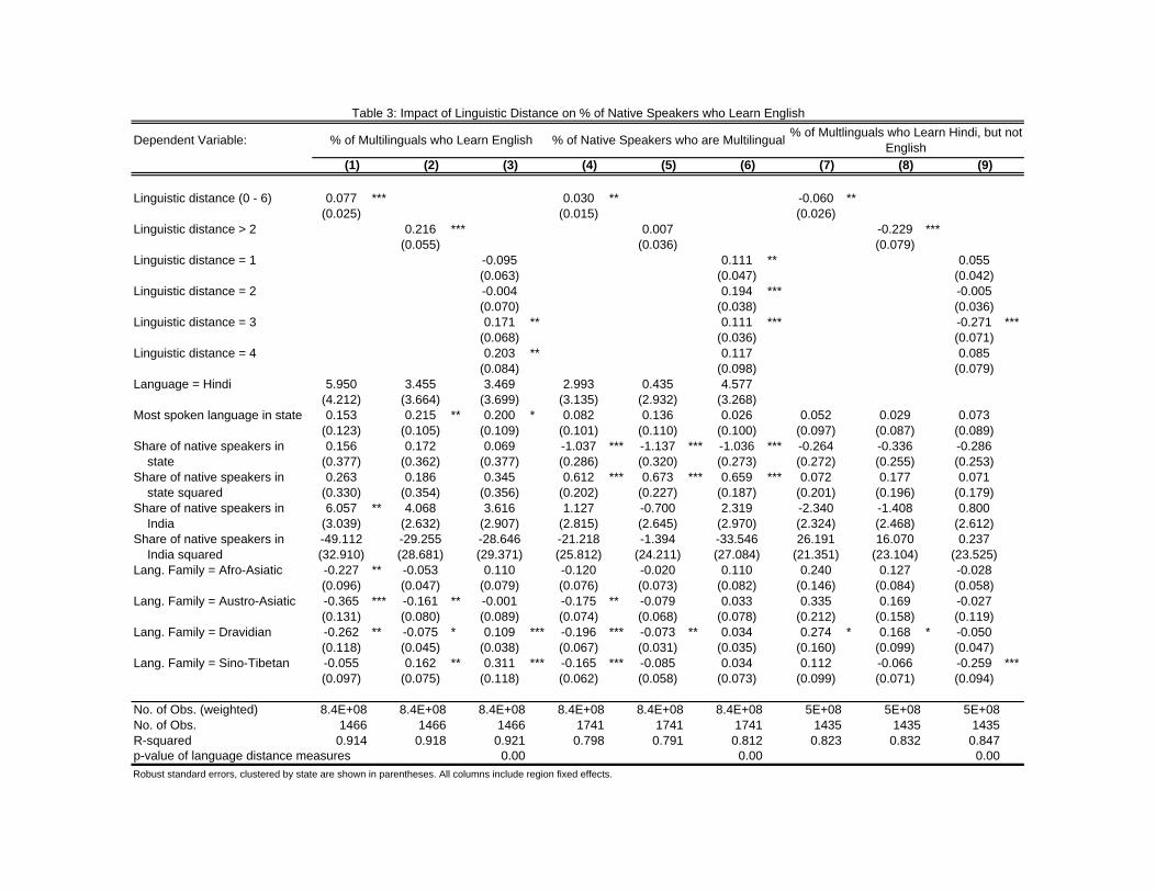
Dependent Variable:
Linguistic distance (0 - 6) 0.077 *** 0.030 ** -0.060 **(0.025) (0.015) (0.026)
Linguistic distance > 2 0.216 *** 0.007 -0.229 ***(0.055) (0.036) (0.079)
Linguistic distance = 1 -0.095 0.111 ** 0.055(0.063) (0.047) (0.042)
Linguistic distance = 2 -0.004 0.194 *** -0.005(0.070) (0.038) (0.036)
Linguistic distance = 3 0.171 ** 0.111 *** -0.271 ***(0.068) (0.036) (0.071)
Linguistic distance = 4 0.203 ** 0.117 0.085(0.084) (0.098) (0.079)
Language = Hindi 5.950 3.455 3.469 2.993 0.435 4.577(4.212) (3.664) (3.699) (3.135) (2.932) (3.268)
Most spoken language in state 0.153 0.215 ** 0.200 * 0.082 0.136 0.026 0.052 0.029 0.073(0.123) (0.105) (0.109) (0.101) (0.110) (0.100) (0.097) (0.087) (0.089)
Share of native speakers in 0.156 0.172 0.069 -1.037 *** -1.137 *** -1.036 *** -0.264 -0.336 -0.286 state (0.377) (0.362) (0.377) (0.286) (0.320) (0.273) (0.272) (0.255) (0.253)Share of native speakers in 0.263 0.186 0.345 0.612 *** 0.673 *** 0.659 *** 0.072 0.177 0.071 state squared (0.330) (0.354) (0.356) (0.202) (0.227) (0.187) (0.201) (0.196) (0.179)Share of native speakers in 6.057 ** 4.068 3.616 1.127 -0.700 2.319 -2.340 -1.408 0.800 India (3.039) (2.632) (2.907) (2.815) (2.645) (2.970) (2.324) (2.468) (2.612)Share of native speakers in -49.112 -29.255 -28.646 -21.218 -1.394 -33.546 26.191 16.070 0.237 India squared (32.910) (28.681) (29.371) (25.812) (24.211) (27.084) (21.351) (23.104) (23.525)Lang. Family = Afro-Asiatic -0.227 ** -0.053 0.110 -0.120 -0.020 0.110 0.240 0.127 -0.028
(0.096) (0.047) (0.079) (0.076) (0.073) (0.082) (0.146) (0.084) (0.058)Lang. Family = Austro-Asiatic -0.365 *** -0.161 ** -0.001 -0.175 ** -0.079 0.033 0.335 0.169 -0.027
(0.131) (0.080) (0.089) (0.074) (0.068) (0.078) (0.212) (0.158) (0.119)Lang. Family = Dravidian -0.262 ** -0.075 * 0.109 *** -0.196 *** -0.073 ** 0.034 0.274 * 0.168 * -0.050
(0.118) (0.045) (0.038) (0.067) (0.031) (0.035) (0.160) (0.099) (0.047)Lang. Family = Sino-Tibetan -0.055 0.162 ** 0.311 *** -0.165 *** -0.085 0.034 0.112 -0.066 -0.259 ***
(0.097) (0.075) (0.118) (0.062) (0.058) (0.073) (0.099) (0.071) (0.094)
No. of Obs. (weighted) 8.4E+08 8.4E+08 8.4E+08 8.4E+08 8.4E+08 8.4E+08 5E+08 5E+08 5E+08No. of Obs. 1466 1466 1466 1741 1741 1741 1435 1435 1435R-squared 0.914 0.918 0.921 0.798 0.791 0.812 0.823 0.832 0.847p-value of language distance measures 0.00 0.00 0.00Robust standard errors, clustered by state are shown in parentheses. All columns include region fixed effects.
(9)(5) (6) (7) (8)(1) (2) (3) (4)
Table 3: Impact of Linguistic Distance on % of Native Speakers who Learn English% of Multlinguals who Learn Hindi, but not
English% of Multilinguals who Learn English % of Native Speakers who are Multilingual

Dependent Variable:
Linguistic distance (0 - 6) 0.184 *** 0.021 -0.067 *(0.044) (0.013) (0.039)
Linguistic distance > 2 0.360 *** 0.032 -0.254 **(0.083) (0.024) (0.113)
Linguistic distance = 2 0.156 * 0.039 * -0.022(0.091) (0.021) (0.049)
Linguistic distance = 3 0.476 *** 0.063 * -0.348 **(0.120) (0.035) (0.150)
Linguistic distance = 4 0.269 ** -0.005 -0.116(0.130) (0.068) (0.144)
Language = Hindi 14.180 ** 9.763 9.893 3.297 * 2.825 * 2.715(5.975) (6.227) (6.344) (1.749) (1.698) (2.173)
Most spoken language in state -0.096 -0.036 -0.130 -0.026 -0.015 -0.039 0.278 ** 0.275 ** 0.291 **(0.167) (0.139) (0.154) (0.033) (0.033) (0.034) (0.133) (0.117) (0.113)
Share of native speakers in -1.725 *** -1.707 *** -1.650 *** -0.861 *** -0.872 *** -0.859 *** -0.010 -0.105 -0.068 state (0.544) (0.611) (0.575) (0.143) (0.144) (0.148) (0.406) (0.403) (0.391)Share of native speakers in 2.452 *** 2.358 *** 2.424 *** 0.464 *** 0.461 *** 0.479 *** -0.196 -0.073 -0.127 state squared (0.461) (0.544) (0.490) (0.100) (0.099) (0.105) (0.259) (0.281) (0.263)Share of native speakers in 11.625 *** 9.113 ** 8.003 * 3.380 *** 3.139 ** 2.732 * -9.618 ** -8.928 ** -7.309 India (4.325) (4.238) (4.607) (1.303) (1.311) (1.623) (4.428) (4.508) (4.796)Share of native speakers in -100.656 ** -72.397 * -70.334 -24.677 ** -21.756 * -20.178 105.347 ** 97.164 ** 84.708 * India squared (40.787) (42.457) (43.606) (12.107) (11.920) (15.173) (44.299) (45.191) (48.930)Lang. Family = Austro-Asiatic -0.705 *** -0.184 ** 0.228 ** -0.079 -0.018 0.026 0.380 0.199 -0.095
(0.177) (0.086) (0.101) (0.060) (0.062) (0.080) (0.234) (0.149) (0.130)Lang. Family = Dravidian -0.645 *** -0.158 ** 0.298 *** -0.089 * -0.030 0.027 0.176 0.083 -0.196 ***
(0.153) (0.067) (0.097) (0.051) (0.034) (0.033) (0.201) (0.125) (0.073)Lang. Family = Sino-Tibetan -0.649 *** -0.107 0.295 * 0.006 0.070 *** 0.111 *** 0.206 0.007 -0.292 *
(0.162) (0.129) (0.177) (0.046) (0.026) (0.037) (0.155) (0.091) (0.151)
Number of Observations 4.2E+08 4.2E+08 4.2E+08 4.2E+08 4.2E+08 4.2E+08 2.4E+08 2.4E+08 2.4E+08R-squared 0.793 0.794 0.806 0.827 0.826 0.829 0.772 0.781 0.786p-value of language distance measures 0.02 0.00 0.11Robust standard errors, clustered by region are shown in parentheses. All columns include region fixed effects.
Table 4: Impact of Linguistic Distance on % of Native Speakers who Learn English in 1961
(4) (5) (6)(1) (2) (3)
% of Native Speakers who are Multilingual% of Multilinguals who Learn English % of Multilinguals who Learn Hindi
(7) (8) (9)
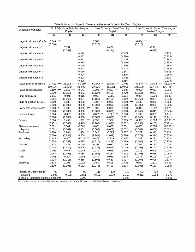
Dependent Variable:
Linguistic distance (0 - 6) 0.046 *** 0.085 *** -0.034 ***(0.010) (0.025) (0.010)
Linguistic distance > 2 0.157 *** 0.406 *** -0.121 ***(0.051) (0.144) (0.042)
Linguistic distance of 1 0.074 -0.677 0.235(0.862) (1.780) (0.228)
Linguistic distance of 2 0.512 -0.383 0.282(0.984) (1.920) (0.253)
Linguistic distance of 3 0.099 -0.955 0.282(0.847) (1.728) (0.242)
Linguistic distance of 4 0.016 0.347 -0.506 *(0.894) (1.836) (0.283)
Linguistic distance of 6 0.303 -0.426 0.106(0.896) (1.855) (0.236)
Native English speakers 27.639 *** 33.392 *** -60.580 60.242 ** 91.428 *** -0.405 -70.574 *** -76.546 *** -61.636 **(10.124) (11.498) (45.040) (27.205) (26.720) (90.986) (24.972) (23.444) (26.770)
Native Hindi speakers 0.159 *** 0.153 *** 0.141 0.303 ** 0.307 * -0.687 -0.003 0.031 0.293(0.039) (0.050) (0.853) (0.137) (0.160) (1.770) (0.057) (0.057) (0.211)
Hindi belt states -0.010 -0.048 0.015 -0.057 -0.065 0.004 -0.054 -0.039 -0.033(0.064) (0.063) (0.057) (0.155) (0.151) (0.112) (0.062) (0.061) (0.074)
Child population in 1991 0.000 0.000 0.000 0.000 * 0.000 0.000 *** 0.000 0.000 0.000(0.000) (0.000) (0.000) (0.000) (0.000) (0.000) (0.000) (0.000) (0.000)
Household wage income 0.000 * 0.000 0.000 *** 0.000 0.000 0.000 -0.044 -0.037 -0.022(0.000) (0.000) (0.000) (0.000) (0.000) (0.000) (0.042) (0.041) (0.046)
Educated wage 0.000 -0.001 0.000 -0.001 ** -0.001 ** 0.000 0.032 0.039 -0.012(0.000) (0.000) (0.000) (0.000) (0.001) (0.001) (0.143) (0.147) (0.141)
Salaried 0.880 * 0.499 1.691 *** 2.336 ** 1.587 2.095 ** -0.397 ** -0.383 ** -0.388 **(0.451) (0.503) (0.445) (1.168) (1.031) (0.862) (0.193) (0.187) (0.191)
Distance to closest 0.001 0.001 -0.001 -0.001 0.000 0.001 -0.003 * -0.004 * -0.003 * big city (0.001) (0.001) (0.001) (0.003) (0.002) (0.002) (0.002) (0.002) (0.002)Graduate 1.386 ** 0.984 1.434 ** 0.046 -0.695 2.837 ** 0.172 0.313 0.138
(0.660) (0.838) (0.560) (2.241) (2.619) (1.226) (0.371) (0.394) (0.336)Secondary -0.918 * -0.857 -1.529 *** -0.468 -0.219 -0.940 0.147 0.121 0.133
(0.558) (0.753) (0.575) (1.310) (1.458) (1.489) (0.266) (0.262) (0.236)Literate 0.173 0.438 0.160 -0.339 0.032 0.099 0.109 0.120 0.030
(0.408) (0.484) (0.506) (0.538) (0.656) (1.025) (0.193) (0.191) (0.179)Muslim -0.099 -0.046 -0.055 0.030 0.098 0.216 0.015 0.009 0.030
(0.084) (0.096) (0.084) (0.156) (0.180) (0.192) (0.068) (0.068) (0.053)Train -0.051 -0.294 -0.353 0.434 0.055 0.538 0.071 0.109 0.025
(0.228) (0.216) (0.458) (0.591) (0.553) (0.907) (0.107) (0.095) (0.107)Electricity 0.173 0.296 -0.025 0.459 0.805 -0.483 -0.073 -0.111 -0.003
(0.120) (0.196) (0.152) (0.346) (0.499) (0.334) (0.105) (0.117) (0.088)
Number of Observations 90 90 90 119 119 119 732 732 732R-squared 0.605 0.538 0.651 0.591 0.570 0.718 0.312 0.294 0.373p-value of language distance measures 0.000 0.000 0.001Robust standard errors, clustered by state, are shown in parentheses. All columns include fixed effects for school level.
% of Schools in State Teaching In English
% of Schools in State Teaching English
% of Schools in District Teaching in Mother Tongue
(6) (7) (8)
Table 5: Impact of Linguistic Distance on Percent of Schools that Teach English
(1) (2) (3) (4) (5) (9)

Linguistic distance 0.096 -0.092 -0.001 0.071 (weighted average) (0.278) (0.065) (0.065) (0.079)Linguistic distance > 2 0.526 -0.195 -0.100 0.349
(0.890) (0.236) (0.245) (0.259)Native English speakers 954 ** 978 ** 135 123 84 80 200 ** 216 **
(449) (452) (136) (132) (92) (88) (99) (95)Native Hindi speakers 2.715 ** 2.681 ** 0.435 0.569 ** 0.301 0.271 0.635 0.597
(1.276) (1.217) (0.303) (0.257) (0.467) (0.461) (0.438) (0.412)Hindi belt states -1.306 -1.271 0.165 0.255 -0.130 -0.167 0.546 0.556
(1.006) (0.971) (0.372) (0.358) (0.413) (0.416) (0.488) (0.482)Child population in 1991 0.000 *** 0.000 *** 0.000 * 0.000 * 0.000 0.000 0.000 * 0.000 **
(0.000) (0.000) (0.000) (0.000) (0.000) (0.000) (0.000) (0.000)Household wage income -0.779 -0.796 -1.038 *** -1.019 ** -0.446 -0.447 -0.917 * -0.930 *
(0.897) (0.896) (0.403) (0.403) (0.298) (0.297) (0.528) (0.529)Educated wage 3.423 ** 3.377 ** 0.310 0.310 -0.201 -0.187 -0.146 -0.175
(1.493) (1.494) (0.435) (0.441) (0.256) (0.256) (0.442) (0.436)Salaried 1.202 1.142 -0.490 -0.459 -0.604 -0.596 0.779 0.738
(4.288) (4.303) (0.885) (0.921) (0.687) (0.695) (0.899) (0.893)Distance to closest 0.024 0.023 0.001 0.000 -0.008 ** -0.007 ** 0.001 0.000 big city (0.018) (0.018) (0.006) (0.006) (0.004) (0.004) (0.006) (0.006)Graduate 14.715 * 14.226 * 3.554 ** 3.889 ** 0.778 0.825 3.341 * 2.999
(8.213) (8.023) (1.728) (1.740) (1.406) (1.370) (1.875) (1.836)Secondary 1.170 1.231 3.233 3.179 0.096 0.094 -0.084 -0.040
(4.897) (4.927) (2.112) (2.161) (1.142) (1.141) (2.159) (2.153)Literate -50.154 ** -49.970 ** -12.713 ** -12.043 ** -6.381 ** -6.638 ** -13.978 ** -13.946 **
(21.698) (22.536) (5.803) (5.747) (3.028) (3.114) (6.128) (6.010)Muslim -1.643 -1.604 -0.529 -0.540 -0.809 *** -0.818 *** -0.886 * -0.860 *
(1.297) (1.295) (0.428) (0.429) (0.276) (0.273) (0.512) (0.518)Train -3.797 * -3.888 * -1.422 * -1.307 -0.403 -0.411 -0.998 -1.068
(2.212) (2.220) (0.820) (0.815) (0.412) (0.420) (0.819) (0.797)Electricity 1.571 1.747 0.859 0.818 1.448 *** 1.407 *** 1.566 *** 1.679 ***
(1.217) (1.297) (0.559) (0.581) (0.259) (0.262) (0.521) (0.499)
Number of Observations 1464 1464 366 366 366 366 366 366R-squared 0.630 0.630 0.288 0.281 0.243 0.244 0.264 0.264Robust standard errors, clustered by state, are shown in parentheses. All columns include fixed effects for school level.
Commerce(3) (4) (5) (6)
Table 6: Impact of Linguistic Distance on Number of Schools
(1) (2)
Number of SchoolsDependent Variable:Number of HS Schools Offering …
Science(7) (8)
Arts

Dependent Variable:
Linguistic distance 0.388 -0.007 -0.005 -0.001 -0.003 ** 0.011 0.000 0.004 3.001 ** -0.172 (weighted average) (1.176) (0.016) (0.003) (0.003) (0.001) (0.007) (0.000) (0.010) (1.465) (0.293)Native English speakers 28621 *** -21.235 0.631 -0.726 0.778 11.693 2.770 ** -16.659 1279.655 52.591
(8752) (21.388) (7.702) (6.102) (1.679) (7.687) (1.230) (10.453) (3004.179) (587.689)Native Hindi speakers -2.497 0.007 -0.053 0.000 0.023 *** -0.013 -0.004 * 0.059 8.350 -1.627
(4.660) (0.053) (0.039) (0.023) (0.006) (0.034) (0.002) (0.067) (8.713) (2.063)Hindi belt states -1.592 0.043 0.065 ** -0.016 -0.005 -0.039 0.002 -0.081 1.755 1.016
(3.678) (0.033) (0.029) (0.022) (0.009) (0.037) (0.003) (0.053) (6.334) (2.314)Child population in 1991 0.000 0.000 0.000 *** 0.000 0.000 0.000 0.000 -0.227 *** -0.044 ***
(0.000) (0.000) (0.000) (0.000) (0.000) (0.000) (0.000) (0.058) (0.012)Household wage income 2.075 0.044 0.039 -0.008 0.034 * 0.002 0.003 -4.189 -0.601
(5.148) (0.044) (0.043) (0.009) (0.020) (0.003) (0.042) (4.891) (1.174)Educated wage 2.484 0.012 0.617 *** 0.104 *** 0.022 * 0.034 0.000 0.045 7.364 0.713
(6.321) (0.066) (0.094) (0.038) (0.013) (0.031) (0.002) (0.051) (7.981) (1.362)Salaried 49.844 *** 0.756 *** 0.191 0.058 * 0.095 0.006 -0.443 *** 20.561 7.306 **
(16.229) (0.236) (0.162) (0.030) (0.097) (0.011) (0.146) (20.862) (3.232)Distance to closest -0.377 *** 0.001 0.000 0.000 0.000 0.000 0.000 * -0.001 -0.022 big city (0.092) (0.001) (0.000) (0.000) (0.000) (0.000) (0.000) (0.001) (0.021)Graduate 34.056 0.164 -0.189 0.262 ** 0.575 *** 0.046 ** -0.175 -15.437 -15.395 **
(37.894) (0.679) (0.228) (0.116) (0.158) (0.019) (0.266) (39.529) (6.984)Secondary 6.334 0.367 0.317 0.129 0.023 0.739 *** 0.007 -0.111 21.331 -11.752 **
(26.307) (0.348) (0.208) (0.101) (0.038) (0.130) (0.009) (0.166) (32.663) (5.702)Literate -16.185 -0.283 0.106 0.061 0.082 *** -0.001 -0.486 *** 10.213 -1.476
(10.776) (0.208) (0.071) (0.064) (0.021) (0.004) (0.172) (18.021) (3.631)Muslim 8.655 * 0.026 0.003 -0.083 *** -0.007 -0.142 *** 0.000 -11.681 -1.393
(4.441) (0.083) (0.038) (0.026) (0.011) (0.039) (0.003) (7.744) (1.788)Train 36.541 * -0.053 0.093 -0.057 * -0.001 0.031 -0.005 ** 0.077 -13.839 1.978
(20.471) (0.137) (0.121) (0.031) (0.015) (0.030) (0.003) (0.114) (10.620) (3.139)Electricity 0.675 0.002 -0.017 0.050 ** 0.016 * 0.181 *** -0.006 0.131 ** -9.980 -3.680 *
(4.491) (0.076) (0.034) (0.024) (0.008) (0.038) (0.003) (0.064) (12.743) (2.111)
Number of Observations 367 367 367 367 367 367 366 367 367 367R-squared 0.476 0.159 0.398 0.396 0.292 0.675 0.104 0.241 0.251 0.163Robust standard errors, clustered by state, are shown in parentheses.
(4)(3)
Percent Engineers
(5) (7)
Percent Literate
Percent with
College Degree
Child population
growth (1991-2001)
Household wage
income
Table 7: Impact of Linguistic Distance on Economic Variables
Percent Muslim
(9) (10)
Child Population in 1991 (in 10,000s)
Distance to Closest Airport
(6) (8)(1) (2)
Distance to closest big city
Percent Salaried
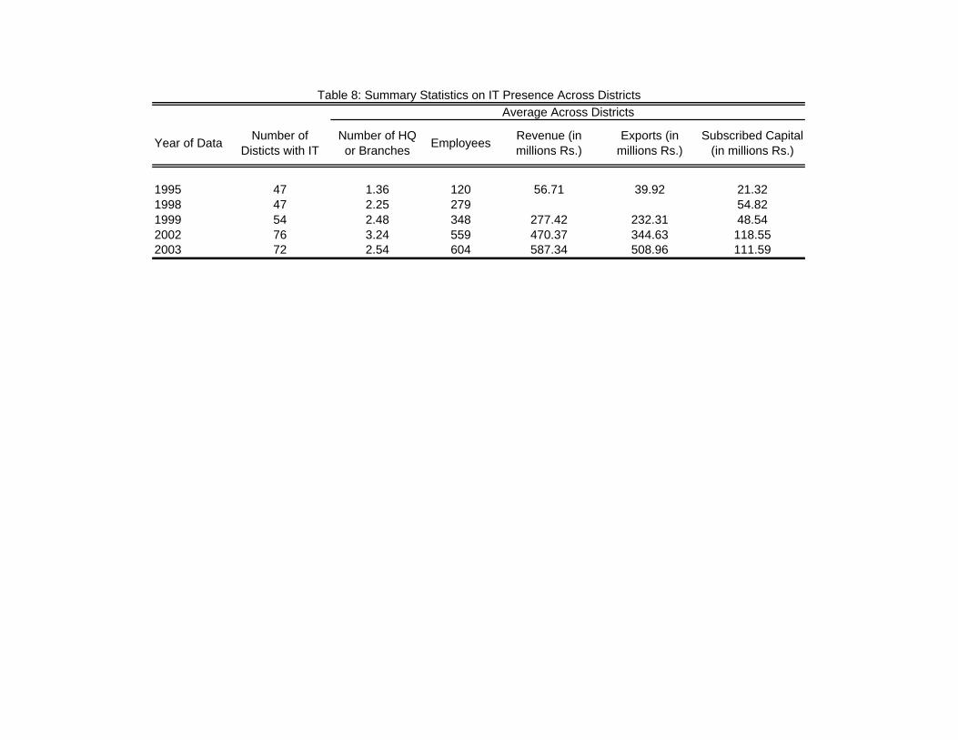
Table 8: Summary Statistics on IT Presence Across DistrictsAverage Across Districts
Year of Data Number of Disticts with IT
Number of HQ or Branches Employees Revenue (in
millions Rs.)Exports (in
millions Rs.)Subscribed Capital
(in millions Rs.)
1995 47 1.36 120 56.71 39.92 21.321998 47 2.25 279 54.821999 54 2.48 348 277.42 232.31 48.542002 76 3.24 559 470.37 344.63 118.552003 72 2.54 604 587.34 508.96 111.59

Table 9: Summary Statistics on Employment, only urban areas1987 1999
Variable nameNum Obs Mean St. Dev. Min. Max.
Num Obs Mean St. Dev. Min. Max.
Salaried Employment 68567 0.412 0.492 0.000 1.000 72993 0.389 0.488 0.000 1.000 if male 56654 0.423 0.494 0.000 1.000 60008 0.393 0.488 0.000 1.000 if female 11913 0.360 0.480 0.000 1.000 12985 0.374 0.484 0.000 1.000 if under age 30 24818 0.333 0.471 0.000 1.000 23880 0.318 0.466 0.000 1.000 if over age 29 43749 0.457 0.498 0.000 1.000 49113 0.424 0.494 0.000 1.000
Log (wage) 35931 5.130 0.976 -4.605 11.292 37390 6.479 0.937 2.639 11.527 if male 29776 5.229 0.902 -4.605 11.292 30657 6.558 0.870 2.708 11.527 if female 6155 4.649 1.160 -1.715 11.097 6733 6.122 1.132 2.639 10.401 if under age 30 11549 4.796 0.889 -1.204 11.252 11248 6.043 0.776 2.708 9.210 if over age 29 24382 5.288 0.976 -4.605 11.292 26142 6.667 0.939 2.639 11.527 in manufacturing 8428 5.045 0.937 -1.715 11.292 7577 6.345 0.822 2.708 9.741 in hotels and restaurants 675 4.781 0.778 0.811 11.252 833 6.190 0.679 3.829 8.448 in agriculture 2222 4.080 0.856 -0.511 9.687 1995 5.454 0.768 3.219 11.527 in wholesale, retail and repair 2320 4.767 0.782 -0.357 10.922 4311 6.117 0.758 2.708 9.306 in business 1630 5.827 0.809 1.253 11.002 1763 7.113 0.914 3.555 10.401 in other services 13687 5.365 0.951 0.049 11.275 12656 6.835 0.943 2.639 9.580 in transportation 3119 5.245 0.791 0.588 9.393 3146 6.550 0.786 3.401 9.770 in communications 353 5.608 0.717 0.952 6.839 459 6.913 0.837 4.248 8.854

Table 10: Summary Statistics on Grade School Enrollment, only urban areas
Group Mean in 1993
Standard Deviation in
1993 Mean in 2002
Standard Deviation in
2002
Class size / Class size in 1st
grade 1993
Class size / Class size in 1st
grade 2002% Growth since 1993
Boys in grade 1 7618 11435 8739 12778 15%Boys in grade 2 6354 10130 7663 11819 83% 88% 21%Boys in grade 3 6146 10068 7416 11662 81% 85% 21%Boys in grade 4 5777 9592 7058 11123 76% 81% 22%Boys in grade 5 5816 9979 7316 11602 76% 84% 26%Boys in grade 6 6066 9789 7330 12284 80% 84% 21%Boys in grade 7 5425 8489 6917 10744 71% 79% 28%Boys in grade 8 5247 8179 6907 10471 69% 79% 32%Boys in grade 9 5301 7416 6609 9231 70% 76% 25%Boys in grade 10 4269 5785 5719 7311 56% 65% 34%Boys in grade 11 2544 3528 5006 6133 33% 57% 97%Boys in grade 12 2366 3329 4503 5205 31% 52% 90%
Girls in grade 1 6707 10639 7775 11601 16%Girls in grade 2 5668 9492 6871 10757 85% 88% 21%Girls in grade 3 5423 9325 6623 10574 81% 85% 22%Girls in grade 4 5059 8761 6282 10007 75% 81% 24%Girls in grade 5 4963 8807 6441 10247 74% 83% 30%Girls in grade 6 5011 8600 6381 10765 75% 82% 27%Girls in grade 7 4529 7613 6064 9729 68% 78% 34%Girls in grade 8 4196 6943 5903 9212 63% 76% 41%Girls in grade 9 3819 6216 5378 8107 57% 69% 41%Girls in grade 10 3041 4768 4666 6485 45% 60% 53%Girls in grade 11 1714 2926 3800 5421 26% 49% 122%Girls in grade 12 1529 2707 3368 4706 23% 43% 120%
Overall: 32%
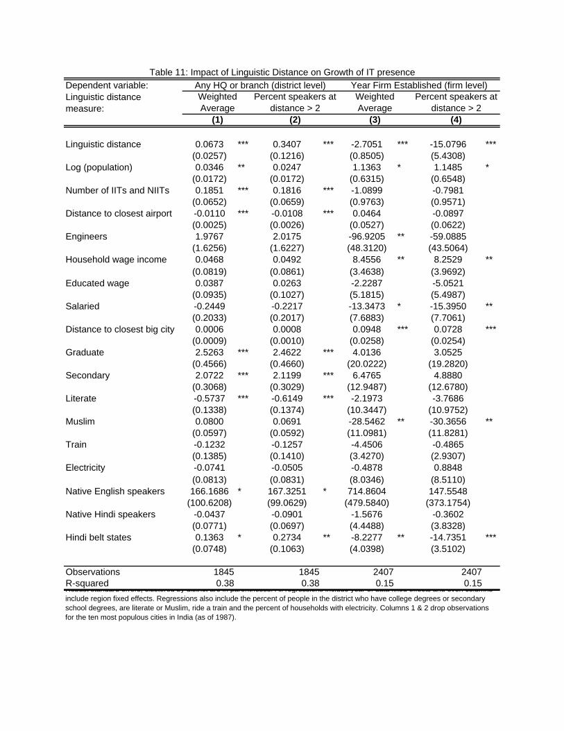
Dependent variable:Linguistic distance measure:
Linguistic distance 0.0673 *** 0.3407 *** -2.7051 *** -15.0796 ***(0.0257) (0.1216) (0.8505) (5.4308)
Log (population) 0.0346 ** 0.0247 1.1363 * 1.1485 *(0.0172) (0.0172) (0.6315) (0.6548)
Number of IITs and NIITs 0.1851 *** 0.1816 *** -1.0899 -0.7981(0.0652) (0.0659) (0.9763) (0.9571)
Distance to closest airport -0.0110 *** -0.0108 *** 0.0464 -0.0897(0.0025) (0.0026) (0.0527) (0.0622)
Engineers 1.9767 2.0175 -96.9205 ** -59.0885(1.6256) (1.6227) (48.3120) (43.5064)
Household wage income 0.0468 0.0492 8.4556 ** 8.2529 **(0.0819) (0.0861) (3.4638) (3.9692)
Educated wage 0.0387 0.0263 -2.2287 -5.0521(0.0935) (0.1027) (5.1815) (5.4987)
Salaried -0.2449 -0.2217 -13.3473 * -15.3950 **(0.2033) (0.2017) (7.6883) (7.7061)
Distance to closest big city 0.0006 0.0008 0.0948 *** 0.0728 ***(0.0009) (0.0010) (0.0258) (0.0254)
Graduate 2.5263 *** 2.4622 *** 4.0136 3.0525(0.4566) (0.4660) (20.0222) (19.2820)
Secondary 2.0722 *** 2.1199 *** 6.4765 4.8880(0.3068) (0.3029) (12.9487) (12.6780)
Literate -0.5737 *** -0.6149 *** -2.1973 -3.7686(0.1338) (0.1374) (10.3447) (10.9752)
Muslim 0.0800 0.0691 -28.5462 ** -30.3656 **(0.0597) (0.0592) (11.0981) (11.8281)
Train -0.1232 -0.1257 -4.4506 -0.4865(0.1385) (0.1410) (3.4270) (2.9307)
Electricity -0.0741 -0.0505 -0.4878 0.8848(0.0813) (0.0831) (8.0346) (8.5110)
Native English speakers 166.1686 * 167.3251 * 714.8604 147.5548(100.6208) (99.0629) (479.5840) (373.1754)
Native Hindi speakers -0.0437 -0.0901 -1.5676 -0.3602(0.0771) (0.0697) (4.4488) (3.8328)
Hindi belt states 0.1363 * 0.2734 ** -8.2277 ** -14.7351 ***(0.0748) (0.1063) (4.0398) (3.5102)
Observations 1845 1845 2407 2407R-squared 0.38 0.38 0.15 0.15
Table 11: Impact of Linguistic Distance on Growth of IT presenceAny HQ or branch (district level)
(1) (2)
Weighted Average
Percent speakers at distance > 2
Year Firm Established (firm level)Weighted Average
Percent speakers at distance > 2
Robust standard errors, clustered by district are in parentheses. All regressions include year of data fixed effects and even columns include region fixed effects. Regressions also include the percent of people in the district who have college degrees or secondary school degrees, are literate or Muslim, ride a train and the percent of households with electricity. Columns 1 & 2 drop observations for the ten most populous cities in India (as of 1987).
(3) (4)
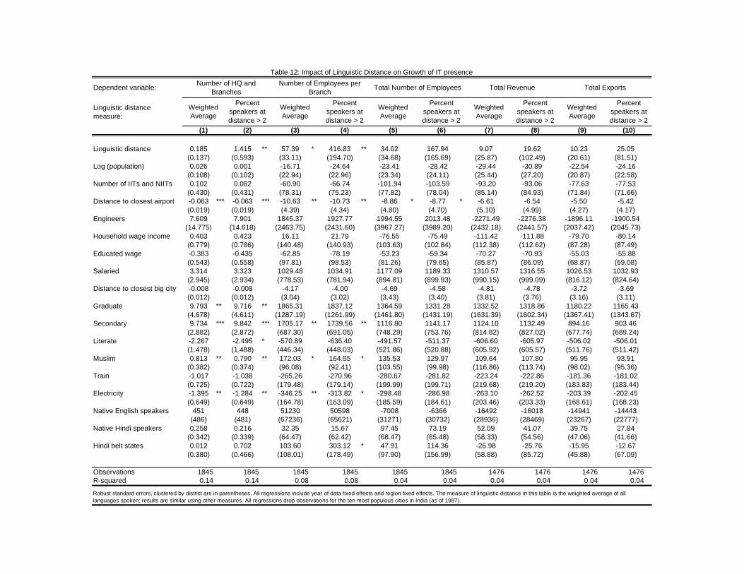
Dependent variable:
Linguistic distance measure:
Linguistic distance 0.185 1.415 ** 57.39 * 416.83 ** 34.02 167.94 9.07 19.62 10.23 25.05(0.137) (0.593) (33.11) (194.70) (34.68) (165.69) (25.87) (102.49) (20.61) (81.51)
Log (population) 0.026 0.001 -16.71 -24.64 -23.41 -28.42 -29.44 -30.89 -22.54 -24.16(0.108) (0.102) (22.94) (22.96) (23.34) (24.11) (25.44) (27.20) (20.87) (22.58)
Number of IITs and NIITs 0.102 0.082 -60.90 -66.74 -101.94 -103.59 -93.20 -93.06 -77.63 -77.53(0.430) (0.431) (78.31) (75.23) (77.82) (78.04) (85.14) (84.93) (71.84) (71.66)
Distance to closest airport -0.063 *** -0.063 *** -10.63 ** -10.73 ** -8.86 * -8.77 * -6.61 -6.54 -5.50 -5.42(0.019) (0.019) (4.39) (4.34) (4.80) (4.70) (5.10) (4.99) (4.27) (4.17)
Engineers 7.609 7.901 1845.37 1927.77 1994.55 2013.48 -2271.49 -2276.38 -1896.11 -1900.54(14.775) (14.618) (2463.75) (2431.60) (3967.27) (3989.20) (2432.18) (2441.57) (2037.42) (2045.73)
Household wage income 0.403 0.423 16.11 21.79 -76.55 -75.49 -111.42 -111.88 -79.70 -80.14(0.779) (0.786) (140.48) (140.93) (103.63) (102.84) (112.38) (112.62) (87.28) (87.49)
Educated wage -0.383 -0.435 -62.85 -78.19 -53.23 -59.34 -70.27 -70.93 -55.03 -55.88(0.543) (0.558) (97.81) (98.53) (81.26) (79.65) (85.87) (86.09) (68.87) (69.08)
Salaried 3.314 3.323 1029.48 1034.91 1177.09 1189.33 1310.57 1316.55 1026.53 1032.93(2.945) (2.934) (778.53) (781.94) (894.81) (899.93) (990.15) (999.09) (816.12) (824.64)
Distance to closest big city -0.008 -0.008 -4.17 -4.00 -4.69 -4.58 -4.81 -4.78 -3.72 -3.69(0.012) (0.012) (3.04) (3.02) (3.43) (3.40) (3.81) (3.76) (3.16) (3.11)
Graduate 9.793 ** 9.716 ** 1865.31 1837.12 1364.59 1331.28 1332.52 1318.86 1180.22 1165.43(4.678) (4.611) (1287.19) (1261.99) (1461.80) (1431.19) (1631.39) (1602.34) (1367.41) (1343.67)
Secondary 9.734 *** 9.842 *** 1705.17 ** 1739.56 ** 1116.80 1141.17 1124.10 1132.49 894.16 903.46(2.882) (2.872) (687.30) (691.05) (748.29) (753.76) (814.82) (827.02) (677.74) (689.24)
Literate -2.267 -2.495 * -570.89 -636.40 -491.57 -511.37 -606.60 -605.97 -506.02 -506.01(1.478) (1.488) (446.34) (448.03) (521.86) (520.88) (605.92) (605.57) (511.76) (511.42)
Muslim 0.813 ** 0.790 ** 172.03 * 164.55 * 135.53 129.97 109.64 107.80 95.95 93.91(0.382) (0.374) (96.08) (92.41) (103.55) (99.98) (116.86) (113.74) (98.02) (95.36)
Train -1.017 -1.038 -265.26 -270.96 -280.67 -281.82 -223.24 -222.86 -181.36 -181.02(0.725) (0.722) (179.48) (179.14) (199.99) (199.71) (219.68) (219.20) (183.83) (183.44)
Electricity -1.395 ** -1.284 ** -346.25 ** -313.82 * -298.48 -286.98 -263.10 -262.52 -203.39 -202.45(0.649) (0.649) (164.78) (163.09) (185.59) (184.61) (203.46) (203.33) (168.61) (168.23)
Native English speakers 451 448 51230 50598 -7008 -6366 -16492 -16018 -14941 -14443(486) (481) (67236) (65621) (31271) (30732) (28936) (28469) (23267) (22777)
Native Hindi speakers 0.258 0.216 32.35 15.67 97.45 73.19 52.09 41.07 39.75 27.84(0.342) (0.339) (64.47) (62.42) (68.47) (65.48) (58.33) (54.56) (47.06) (41.66)
Hindi belt states 0.012 0.702 103.60 303.12 * 47.91 114.36 -26.98 -25.76 -15.95 -12.67(0.380) (0.466) (108.01) (178.49) (97.90) (156.99) (58.88) (85.72) (45.88) (67.09)
Observations 1845 1845 1845 1845 1845 1845 1476 1476 1476 1476R-squared 0.14 0.14 0.08 0.08 0.04 0.04 0.04 0.04 0.04 0.04
Robust standard errors, clustered by district are in parentheses. All regressions include year of data fixed effects and region fixed effects. The measure of linguistic distance in this table is the weighted average of all languages spoken; results are similar using other measures. All regressions drop observations for the ten most populous cities in India (as of 1987).
Weighted Average
Weighted Average
(1) (3)(2) (6) (7)(5)
Percent speakers at distance > 2
Weighted Average
Percent speakers at distance > 2
Table 12: Impact of Linguistic Distance on Growth of IT presence
Total Number of Employees Total Revenue Total Exports
Percent speakers at distance > 2
(8)
Percent speakers at distance > 2
(10)(9)(4)
Number of HQ and Branches
Weighted Average
Percent speakers at distance > 2
Weighted Average
Number of Employees per Branch

Dependent variable:
Teaching in mother tongue -1.035 ** -21.4 *** -2.8 ** -440.7 ** -302.0 -84.5 -61.7 -95.9(0.447) (7.5) (1.1) (201.2) (198.3) (147.9) (118.9) (60.5)
Log (population) 0.081 *** 1.5 ** 0.2 -0.6 -11.6 -24.3 -19.2 2.4(0.030) (0.6) (0.1) (25.4) (24.3) (27.0) (22.5) (5.7)
Number of IITs and NIITs 0.186 *** 3.5 * 0.1 -58.0 -100.3 -91.6 -76.1 23.4(0.071) (1.9) (0.4) (80.7) (76.8) (83.7) (70.5) (28.4)
Distance to closest airport -0.010 *** -0.2 *** -0.1 *** -9.9 ** -8.4 * -6.5 -5.4 -1.2 *(0.003) (0.1) (0.0) (4.5) (4.7) (4.9) (4.1) (0.7)
Engineers 2.468 58.6 7.2 1702.9 1921.7 -2752.4 -2297.7 -611.3(1.819) (56.8) (15.6) (2754.8) (4485.6) (2830.7) (2377.0) (441.7)
Household wage income 0.020 1.9 0.3 2.1 -85.6 -113.1 -81.3 -18.7(0.083) (2.4) (0.7) (132.4) (104.7) (113.3) (88.1) (23.6)
Educated wage 0.075 1.0 -0.3 -44.1 -40.6 -62.2 -48.6 -9.6(0.179) (3.9) (0.7) (122.4) (97.0) (86.5) (69.0) (21.7)
Salaried -0.517 -6.2 2.7 952.9 1119.0 1312.2 1032.8 204.2(0.325) (6.7) (3.0) (789.6) (907.7) (1013.6) (839.0) (146.4)
Distance to closest big city -0.001 0.0 0.0 -4.7 -5.1 -4.8 -3.7 -0.8(0.001) (0.0) (0.0) (3.1) (3.4) (3.7) (3.1) (0.6)
Native English speakers 148.27 2505 414 47807 -9894 -14661 -13050 -1999(92.07) (2557) (465) (62960) (31516) (27452) (21610) (5892)
Native Hindi speakers -0.095 -1.1 0.1 -37.4 58.3 39.5 24.5 22.3(0.078) (1.6) (0.4) (81.9) (70.4) (58.7) (43.4) (18.7)
Hindi belt states -0.022 -0.4 -0.4 2.1 -15.0 -40.2 -29.8 -16.6(0.097) (2.1) (0.4) (86.3) (67.5) (54.0) (43.4) (14.8)
Observations 1840 1840 1840 1840 1840 1472 1472 1840R-squared 0.22 0.19 0.12 0.07 0.04 0.04 0.04 0.04F-statistic of Instruments 31.6 31.6 31.6 31.6 31.6 25.2 25.2 31.6
Number of Employees per
Branch(4)
Any HQ or Branch
Years of IT presence
Robust standard errors, clustered by district are in parentheses. All regressions include year of data fixed effects and region fixed effects, the percent of college graduates, secondary school graduates, literates, Muslims, people who travel by train and households with electricity. The measure of English cost is primary schools that teach in the mother tongue as the measure of costs of English; results are similar using upper primary schools. As instruments I use the percent of speakers at each distance away from Hindi. All regressions drop observations for the ten most populous cities in India (as of 1987).
(1) (2) (5)
Table 13: Impact of Linguistic Distance on Growth of IT presence
(3) (6)
Total ExportsTotal
Subscribed Capital
(7) (8)
Number of HQ and Branches
Total Number of Employees Total Revenue

Dependent variable:Linguistic distance measure:
Linguistic distance * post -0.002 -0.001 -0.019 -0.005 0.000 -0.003 0.010 -0.071 -0.026 0.005(0.013) (0.010) (0.032) (0.014) (0.014) (0.061) (0.050) (0.155) (0.064) (0.070)
High school * Linguistic distance -0.001 -0.001 0.004 0.005 -0.010 ** 0.008 0.001 0.081 0.044 -0.031 * post (0.005) (0.005) (0.011) (0.008) (0.005) (0.026) (0.026) (0.054) (0.041) (0.027)College * Linguistic distance 0.016 *** 0.014 ** 0.021 * 0.024 *** 0.008 0.093 *** 0.077 *** 0.146 ** 0.114 *** 0.061 ** * post (0.005) (0.006) (0.013) (0.009) (0.006) (0.026) (0.028) (0.065) (0.043) (0.030)High school 0.172 *** 0.141 *** 0.411 *** 0.062 *** 0.237 *** 0.188 *** 0.150 *** 0.443 *** 0.080 *** 0.254 ***
(0.017) (0.015) (0.050) (0.017) (0.021) (0.017) (0.015) (0.043) (0.015) (0.021)College 0.288 *** 0.245 *** 0.456 *** 0.180 *** 0.342 *** 0.300 *** 0.250 *** 0.491 *** 0.195 *** 0.356 ***
(0.020) (0.018) (0.049) (0.023) (0.022) (0.020) (0.019) (0.041) (0.023) (0.023)Post -0.028 -0.037 0.115 0.011 -0.052 -0.037 -0.052 0.111 0.012 -0.058
(0.044) (0.042) (0.107) (0.051) (0.049) (0.055) (0.048) (0.136) (0.059) (0.063)High school * post -0.019 -0.013 -0.043 -0.015 -0.019 -0.026 * -0.015 -0.074 ** -0.020 -0.030 *
(0.017) (0.016) (0.048) (0.027) (0.019) (0.015) (0.015) (0.034) (0.022) (0.017)College * post -0.068 *** -0.061 *** -0.072 * -0.092 *** -0.060 *** -0.066 *** -0.058 *** -0.079 ** -0.082 *** -0.065 ***
(0.018) (0.019) (0.042) (0.028) (0.018) (0.017) (0.018) (0.037) (0.026) (0.018)High school * Linguistic distance 0.016 *** 0.016 *** -0.009 0.013 ** 0.021 *** 0.062 ** 0.073 *** -0.115 ** 0.039 0.083 ***
(0.004) (0.004) (0.010) (0.006) (0.004) (0.026) (0.024) (0.056) (0.032) (0.029)College * Linguistic distance 0.009 * 0.011 ** -0.010 0.002 0.015 *** 0.020 0.048 * -0.134 * -0.025 0.052
(0.005) (0.004) (0.013) (0.007) (0.005) (0.029) (0.025) (0.074) (0.037) (0.033)Native English speakers * post 19.80 *** 21.11 *** 15.05 *** 25.68 *** 16.25 *** 19.67 *** 20.88 *** 16.24 *** 25.76 *** 15.98 ***
(4.05) (4.30) (4.87) (3.14) (5.76) (3.99) (4.18) (5.00) (3.15) (5.74)Native Hindi speakers * post -0.038 -0.034 -0.140 0.009 -0.061 -0.037 -0.032 -0.129 0.008 -0.060
(0.037) (0.033) (0.098) (0.049) (0.042) (0.032) (0.029) (0.088) (0.045) (0.037)Hindi belt states * post 0.019 0.019 0.028 -0.035 0.042 0.027 0.032 0.025 -0.035 0.049
(0.032) (0.034) (0.079) (0.041) (0.036) (0.044) (0.041) (0.110) (0.047) (0.052)
Observations 1.25E+08 1.03E+08 2.17E+07 4.35E+07 8.10E+07 1.25E+08 1.03E+08 2.17E+07 4.35E+07 8.10E+07R-squared 0.16 0.15 0.28 0.13 0.19 0.16 0.15 0.28 0.13 0.18
Age < 30 Age > 29(6) (9) (10)
Table 14: Impact of District Linguistic Distance on Returns to Education by Age Group and Gender
Weighted average Percent speakers at distance > 2Salaried Employment
Robust standard errors, clustered by district, in parentheses, also controlling for age, age squared, married, male, whether the individual has ever moved, region fixed effects interacted with post.
All Age < 30 Age > 29(1)
Men Women(2) (4) (5)(3)
Men Women(7) (8)
All

Dependent variable:Linguistic distance measure:
All Men Women Age < 30 Age > 29 All Men Women Age < 30 Age > 29
Linguistic distance * post 0.000 0.013 -0.041 -0.028 0.016 -0.010 0.064 -0.214 -0.065 0.017(0.017) (0.018) (0.046) (0.025) (0.020) (0.088) (0.093) (0.253) (0.148) (0.097)
High school * Linguistic distance -0.033 *** -0.030 *** -0.052 * -0.002 -0.046 *** -0.122 ** -0.116 ** -0.250 -0.002 -0.168 *** * post (0.010) (0.010) (0.031) (0.014) (0.012) (0.055) (0.055) (0.158) (0.070) (0.062)College * Linguistic distance -0.017 * -0.013 -0.028 -0.020 -0.022 ** -0.032 -0.021 -0.078 -0.067 -0.054 * post (0.010) (0.010) (0.024) (0.021) (0.011) (0.052) (0.054) (0.121) (0.101) (0.060)High school 0.553 *** 0.489 *** 0.999 *** 0.457 *** 0.594 *** 0.586 *** 0.506 *** 1.048 *** 0.460 *** 0.647 ***
(0.027) (0.027) (0.074) (0.039) (0.029) (0.026) (0.026) (0.061) (0.033) (0.029)College 0.996 *** 0.904 *** 1.456 *** 0.919 *** 1.022 *** 1.033 *** 0.926 *** 1.510 *** 0.939 *** 1.073 ***
(0.025) (0.021) (0.066) (0.037) (0.029) (0.021) (0.019) (0.062) (0.032) (0.025)Post 1.113 *** 1.094 *** 1.255 *** 1.160 *** 1.082 *** 1.129 *** 1.086 *** 1.337 *** 1.146 *** 1.124 ***
(0.073) (0.074) (0.187) (0.126) (0.082) (0.084) (0.089) (0.237) (0.153) (0.093)High school * post 0.031 0.037 0.044 -0.171 *** 0.118 *** -0.002 0.010 0.006 -0.175 *** 0.074 *
(0.035) (0.036) (0.118) (0.046) (0.042) (0.035) (0.034) (0.104) (0.039) (0.041)College * post 0.109 *** 0.116 *** 0.028 -0.070 0.172 *** 0.085 *** 0.095 *** -0.006 -0.090 0.146 ***
(0.030) (0.035) (0.075) (0.067) (0.036) (0.031) (0.034) (0.071) (0.056) (0.038)High school * Linguistic distance 0.041 *** 0.029 *** 0.056 *** 0.007 0.059 *** 0.174 *** 0.133 *** 0.252 ** 0.036 0.226 ***
(0.009) (0.008) (0.021) (0.013) (0.009) (0.045) (0.043) (0.101) (0.062) (0.049)College * Linguistic distance 0.039 *** 0.027 *** 0.047 ** 0.019 0.049 *** 0.133 *** 0.101 ** 0.155 * 0.062 0.158 ***
(0.008) (0.008) (0.018) (0.012) (0.010) (0.045) (0.043) (0.092) (0.059) (0.055)Native English speakers * post 0.774 2.740 -5.116 5.968 -1.845 0.252 2.211 -5.403 5.581 -2.325
(4.589) (4.486) (9.515) (5.358) (5.985) (4.663) (4.479) (10.164) (5.522) (6.251)Native Hindi speakers * post -0.074 -0.036 -0.174 -0.008 -0.078 -0.064 -0.033 -0.128 0.030 -0.089
(0.067) (0.070) (0.165) (0.117) (0.065) (0.063) (0.065) (0.155) (0.112) (0.060)Hindi belt states * post 0.050 0.042 0.031 -0.048 0.070 0.035 0.058 -0.076 -0.067 0.053
(0.049) (0.052) (0.152) (0.123) (0.054) (0.056) (0.062) (0.190) (0.141) (0.066)
Observations 6.72E+07 5.57E+07 1.16E+07 2.16E+07 4.57E+07 6.72E+07 5.57E+07 1.16E+07 2.16E+07 4.57E+07R-squared 0.67 0.67 0.69 0.65 0.67 0.67 0.67 0.68 0.65 0.67
Table 15: Impact of District Linguistic Distance on Returns to Education by Age Group
Weighted average Percent speakers at distance > 2
(9) (10)(1) (4) (5) (6)
Log (Wages)
Robust standard errors, clustered by district, in parentheses, also controlling for age, age squared, married, male, whether the individual has ever moved, region fixed effects interacted with post and a dummy variable for whether the individual is self-employed.
(2) (3) (7) (8)

Dependent variable: Log (Wages)
Linguistic distance * post 0.045 0.166 0.092 0.552 0.009 -0.080 -0.003 -0.135(0.042) (0.172) (0.071) (0.396) (0.067) (0.303) (0.034) (0.212)
High school * Linguistic distance -0.039 * -0.227 ** 0.023 0.238 -0.079 -0.314 0.022 0.079 * post (0.022) (0.115) (0.041) (0.214) (0.061) (0.330) (0.019) (0.095)College * Linguistic distance 0.027 0.124 -0.147 * -0.825 * -0.050 -0.504 -0.032 -0.095 * post (0.026) (0.128) (0.079) (0.421) (0.095) (0.542) (0.042) (0.240)High school 0.377 *** 0.405 *** 0.363 *** 0.322 *** 0.347 * 0.323 0.322 *** 0.297 ***
(0.042) (0.036) (0.129) (0.122) (0.202) (0.201) (0.057) (0.050)College 0.901 *** 0.921 *** 0.518 ** 0.556 ** 0.740 *** 0.741 *** 0.429 ** 0.425 **
(0.058) (0.045) (0.234) (0.222) (0.267) (0.274) (0.173) (0.173)Post 0.933 *** 0.913 *** 0.925 * 0.780 1.294 *** 1.398 *** 1.393 *** 1.481 ***
(0.124) (0.142) (0.551) (0.601) (0.282) (0.330) (0.197) (0.215)High school * post -0.004 -0.013 0.092 0.060 0.222 0.107 -0.076 -0.049
(0.070) (0.069) (0.157) (0.131) (0.272) (0.244) (0.072) (0.063)College * post -0.101 -0.082 0.552 ** 0.471 ** 0.286 0.400 0.323 * 0.288
(0.097) (0.087) (0.227) (0.210) (0.442) (0.435) (0.173) (0.176)High school * Linguistic distance 0.052 *** 0.262 *** -0.048 -0.231 0.008 0.099 0.002 0.064
(0.017) (0.082) (0.038) (0.199) (0.049) (0.272) (0.014) (0.071)College * Linguistic distance 0.024 0.089 -0.011 -0.160 0.089 0.519 0.044 0.255
(0.024) (0.114) (0.071) (0.375) (0.058) (0.322) (0.037) (0.221)Native English speakers * post -12.669 -12.813 6.610 3.858 -71.522 *** -68.499 *** 3.490 3.290
(10.996) (11.532) (20.558) (21.168) (23.647) (24.495) (8.838) (8.500)Native Hindi speakers * post 0.134 0.093 0.489 0.528 0.003 -0.031 -0.123 -0.138
(0.101) (0.091) (0.718) (0.725) (0.257) (0.240) (0.131) (0.125)Hindi belt states * post 0.015 0.070 0.059 0.175 -0.036 -0.103 0.031 -0.042
(0.090) (0.114) (0.514) (0.480) (0.185) (0.231) (0.177) (0.192)
Observations 1.68E+07 1.68E+07 1337810 1337810 4110879 4110879 6373433 6373433R-squared 0.71 0.71 0.74 0.74 0.73 0.73 0.67 0.67
Table 16: Impact of District Linguistic Distance on Returns to Education By Industry
(6)(3) (4)(1) (2) (5)
Manufacting Agriculture, Hunting, Forestry and FishingHotels and Restaurants Wholesale, Retail and
Repair
Robust standard errors, clustered by district, in parentheses, also controlling for age, age squared, married, male, whether the individual has ever moved, region fixed effects interacted with post and a dummy variable for whether the individual is self-employed.. Odd-numbered columns use the weighted average measure of linguistic distance while even-number columns use the percent of distant speakers.
(7) (8)
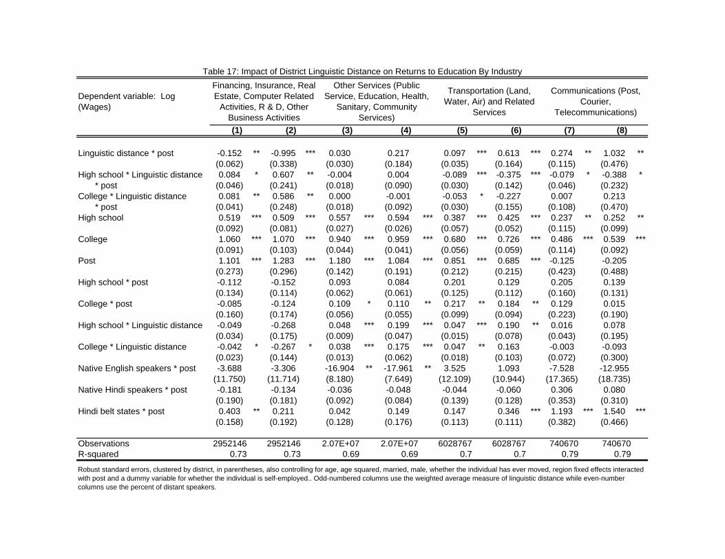
Dependent variable: Log (Wages)
Linguistic distance * post -0.152 ** -0.995 *** 0.030 0.217 0.097 *** 0.613 *** 0.274 ** 1.032 **(0.062) (0.338) (0.030) (0.184) (0.035) (0.164) (0.115) (0.476)
High school * Linguistic distance 0.084 * 0.607 ** -0.004 0.004 -0.089 *** -0.375 *** -0.079 * -0.388 * * post (0.046) (0.241) (0.018) (0.090) (0.030) (0.142) (0.046) (0.232)College * Linguistic distance 0.081 ** 0.586 ** 0.000 -0.001 -0.053 * -0.227 0.007 0.213 * post (0.041) (0.248) (0.018) (0.092) (0.030) (0.155) (0.108) (0.470)High school 0.519 *** 0.509 *** 0.557 *** 0.594 *** 0.387 *** 0.425 *** 0.237 ** 0.252 **
(0.092) (0.081) (0.027) (0.026) (0.057) (0.052) (0.115) (0.099)College 1.060 *** 1.070 *** 0.940 *** 0.959 *** 0.680 *** 0.726 *** 0.486 *** 0.539 ***
(0.091) (0.103) (0.044) (0.041) (0.056) (0.059) (0.114) (0.092)Post 1.101 *** 1.283 *** 1.180 *** 1.084 *** 0.851 *** 0.685 *** -0.125 -0.205
(0.273) (0.296) (0.142) (0.191) (0.212) (0.215) (0.423) (0.488)High school * post -0.112 -0.152 0.093 0.084 0.201 0.129 0.205 0.139
(0.134) (0.114) (0.062) (0.061) (0.125) (0.112) (0.160) (0.131)College * post -0.085 -0.124 0.109 * 0.110 ** 0.217 ** 0.184 ** 0.129 0.015
(0.160) (0.174) (0.056) (0.055) (0.099) (0.094) (0.223) (0.190)High school * Linguistic distance -0.049 -0.268 0.048 *** 0.199 *** 0.047 *** 0.190 ** 0.016 0.078
(0.034) (0.175) (0.009) (0.047) (0.015) (0.078) (0.043) (0.195)College * Linguistic distance -0.042 * -0.267 * 0.038 *** 0.175 *** 0.047 ** 0.163 -0.003 -0.093
(0.023) (0.144) (0.013) (0.062) (0.018) (0.103) (0.072) (0.300)Native English speakers * post -3.688 -3.306 -16.904 ** -17.961 ** 3.525 1.093 -7.528 -12.955
(11.750) (11.714) (8.180) (7.649) (12.109) (10.944) (17.365) (18.735)Native Hindi speakers * post -0.181 -0.134 -0.036 -0.048 -0.044 -0.060 0.306 0.080
(0.190) (0.181) (0.092) (0.084) (0.139) (0.128) (0.353) (0.310)Hindi belt states * post 0.403 ** 0.211 0.042 0.149 0.147 0.346 *** 1.193 *** 1.540 ***
(0.158) (0.192) (0.128) (0.176) (0.113) (0.111) (0.382) (0.466)
Observations 2952146 2952146 2.07E+07 2.07E+07 6028767 6028767 740670 740670R-squared 0.73 0.73 0.69 0.69 0.7 0.7 0.79 0.79
(7) (8)
Robust standard errors, clustered by district, in parentheses, also controlling for age, age squared, married, male, whether the individual has ever moved, region fixed effects interacted with post and a dummy variable for whether the individual is self-employed.. Odd-numbered columns use the weighted average measure of linguistic distance while even-number columns use the percent of distant speakers.
(5) (6)(1) (2) (3) (4)
Table 17: Impact of District Linguistic Distance on Returns to Education By Industry
Transportation (Land, Water, Air) and Related
Services
Communications (Post, Courier,
Telecommunications)
Financing, Insurance, Real Estate, Computer Related
Activities, R & D, Other Business Activities
Other Services (Public Service, Education, Health,
Sanitary, Community Services)
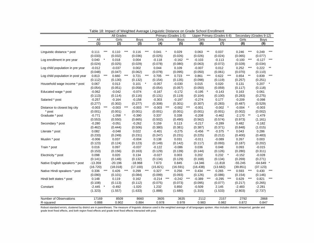
Table 18: Impact of Weighted Average Linguistic Distance on Grade School EnrollmentAll Grades
All Girls Boys Girls Boys Girls Boys Girls Boys
Linguistic distance * post 0.111 *** 0.110 *** 0.116 *** 0.041 * 0.029 0.063 ** 0.037 0.246 *** 0.249 ***(0.033) (0.032) (0.036) (0.025) (0.026) (0.026) (0.024) (0.065) (0.077)
Log enrollment in pre year 0.040 * 0.018 0.004 -0.118 -0.162 ** -0.103 -0.113 -0.100 *** -0.127 ***(0.024) (0.025) (0.029) (0.078) (0.080) (0.063) (0.072) (0.028) (0.034)
Log child population in pre year -0.012 -0.037 0.002 0.044 0.109 -0.007 0.012 0.252 *** 0.222 **(0.048) (0.047) (0.062) (0.078) (0.095) (0.050) (0.061) (0.070) (0.110)
Log child population in post year 0.813 *** 0.660 *** 0.721 *** 0.705 *** 0.723 *** 0.861 *** 0.622 *** 0.654 ** 0.839 ***(0.112) (0.130) (0.132) (0.154) (0.135) (0.098) (0.119) (0.257) (0.251)
Household wage income * post 0.067 0.013 0.101 * -0.057 -0.030 0.015 0.020 0.131 0.207 *(0.054) (0.051) (0.058) (0.054) (0.057) (0.050) (0.059) (0.117) (0.118)
Educated wage * post -0.062 -0.042 -0.074 -0.167 -0.172 -0.195 * -0.143 0.163 0.061(0.113) (0.114) (0.116) (0.131) (0.119) (0.104) (0.100) (0.283) (0.275)
Salaried * post -0.257 -0.164 -0.158 -0.303 -0.197 -0.274 0.177 -0.209 -0.098(0.277) (0.302) (0.277) (0.308) (0.301) (0.307) (0.283) (0.487) (0.529)
Distance to closest big city -0.003 *** -0.003 *** -0.003 *** -0.003 *** -0.002 *** -0.001 -0.002 * -0.004 * -0.003 * post (0.001) (0.001) (0.001) (0.001) (0.001) (0.001) (0.001) (0.002) (0.002)Graduate * post -0.771 -1.058 * -0.390 0.337 0.338 -0.208 -0.462 -2.170 ** -1.479
(0.553) (0.550) (0.665) (0.502) (0.490) (0.562) (0.574) (0.973) (1.161)Secondary * post -0.280 -0.051 -0.262 0.159 0.113 -0.217 -0.289 0.482 -0.182
(0.462) (0.444) (0.506) (0.380) (0.381) (0.387) (0.371) (0.848) (1.015)Literate * post 0.082 -0.048 0.022 -0.401 -0.275 -0.456 ** -0.375 * 0.043 0.286
(0.233) (0.249) (0.231) (0.247) (0.231) (0.225) (0.212) (0.400) (0.483)Muslim * post -0.006 0.037 -0.004 0.138 0.031 -0.011 -0.089 0.267 0.003
(0.123) (0.124) (0.123) (0.149) (0.142) (0.117) (0.093) (0.187) (0.202)Train * post 0.016 0.097 -0.037 -0.122 -0.086 0.036 0.048 0.093 -0.015
(0.153) (0.156) (0.163) (0.129) (0.139) (0.144) (0.126) (0.280) (0.311)Electricity * post 0.098 0.020 0.134 -0.027 0.003 0.202 0.232 * -0.152 -0.028
(0.141) (0.148) (0.132) (0.134) (0.129) (0.168) (0.134) (0.269) (0.271)Native English speakers * post -13.359 -20.196 -18.968 7.673 0.845 -14.346 -11.818 -55.245 -64.649 *
(16.720) (18.018) (17.100) (15.821) (16.591) (16.438) (13.682) (39.851) (37.123)Native Hindi speakers * post 0.336 *** 0.426 *** 0.299 *** 0.327 *** 0.256 *** 0.434 *** 0.265 *** 0.593 *** 0.430 ***
(0.090) (0.101) (0.084) (0.099) (0.093) (0.126) (0.086) (0.154) (0.146)Hindi belt states * post 0.148 0.119 0.162 -0.214 *** -0.242 *** -0.389 *** -0.295 *** 0.629 *** 0.821 ***
(0.108) (0.113) (0.112) (0.075) (0.073) (0.095) (0.077) (0.217) (0.265)Constant -2.445 * -0.492 -1.020 1.232 0.850 -0.509 2.145 -2.483 -2.281
(1.323) (1.557) (1.633) (1.888) (1.680) (1.315) (1.533) (2.803) (2.737)
Number of Observations 17169 8509 8660 3605 3635 2112 2157 2792 2868R-squared 0.888 0.902 0.884 0.978 0.978 0.983 0.982 0.872 0.847Robust standard errors, clustered by district are in parentheses. The measure of linguistic distance used is the weighted average of all languages spoken. Also includes district, timeperiod, gender and grade level fixed effects, and both region fixed effects and grade level fixed effects interacted with post.
(4)(1) (2) (3) (9)(5) (7)(6) (8)
Primary (Grades 1-5) Upper Primary (Grades 6-8) Secondary (Grades 9-12)

Table 19: Impact of Percent Distant Speakers on Grade School EnrollmentAll Grades
All Girls Boys Girls Boys Girls Boys Girls Boys
Linguistic distance * post 0.278 0.255 0.269 0.242 * 0.196 * 0.428 *** 0.288 ** 0.251 0.294(0.172) (0.167) (0.176) (0.139) (0.116) (0.155) (0.122) (0.279) (0.379)
Log enrollment in pre year 0.039 0.017 0.002 -0.117 -0.160 ** -0.105 * -0.113 -0.108 *** -0.135 ***(0.024) (0.025) (0.029) (0.078) (0.079) (0.064) (0.071) (0.028) (0.034)
Log child population in pre year -0.006 -0.030 0.012 0.047 0.108 0.000 0.013 0.263 *** 0.245 **(0.048) (0.047) (0.063) (0.079) (0.095) (0.050) (0.061) (0.071) (0.111)
Log child population in post year 0.842 *** 0.692 *** 0.758 *** 0.720 *** 0.733 *** 0.883 *** 0.639 *** 0.707 *** 0.926 ***(0.110) (0.127) (0.132) (0.152) (0.134) (0.094) (0.119) (0.261) (0.257)
Household wage income * post 0.064 0.008 0.098 * -0.053 -0.027 0.019 0.025 0.109 0.192(0.056) (0.054) (0.059) (0.052) (0.056) (0.051) (0.058) (0.123) (0.126)
Educated wage * post -0.067 -0.046 -0.078 -0.175 -0.178 -0.204 * -0.152 0.155 0.063(0.124) (0.127) (0.128) (0.133) (0.119) (0.104) (0.099) (0.322) (0.302)
Salaried * post -0.231 -0.138 -0.133 -0.311 -0.207 -0.298 0.159 -0.079 -0.038(0.283) (0.308) (0.281) (0.308) (0.300) (0.309) (0.286) (0.501) (0.538)
Distance to closest big city -0.002 ** -0.002 ** -0.002 ** -0.002 ** -0.002 ** -0.001 -0.001 -0.002 -0.002 * post (0.001) (0.001) (0.001) (0.001) (0.001) (0.001) (0.001) (0.002) (0.002)Graduate * post -1.042 * -1.340 ** -0.680 0.293 0.303 -0.302 -0.475 -3.044 *** -2.093 *
(0.613) (0.591) (0.713) (0.527) (0.498) (0.597) (0.612) (1.067) (1.268)Secondary * post -0.335 -0.108 -0.329 0.153 0.115 -0.223 -0.293 0.323 -0.438
(0.475) (0.457) (0.525) (0.374) (0.377) (0.380) (0.363) (0.918) (1.081)Literate * post 0.128 0.006 0.075 -0.424 * -0.298 -0.503 ** -0.410 * 0.262 0.482
(0.229) (0.244) (0.226) (0.252) (0.234) (0.227) (0.218) (0.397) (0.481)Muslim * post -0.035 0.007 -0.035 0.129 0.026 -0.022 -0.093 0.189 -0.071
(0.124) (0.126) (0.124) (0.147) (0.140) (0.117) (0.092) (0.192) (0.203)Train * post 0.014 0.096 -0.037 -0.134 -0.093 0.018 0.035 0.116 0.013
(0.149) (0.153) (0.157) (0.131) (0.140) (0.142) (0.125) (0.265) (0.285)Electricity * post 0.122 0.042 0.157 -0.002 0.023 0.242 0.259 * -0.152 0.003
(0.147) (0.153) (0.139) (0.139) (0.131) (0.173) (0.139) (0.275) (0.278)Native English speakers * post -7.622 -14.532 -12.683 10.936 3.356 -8.434 -8.519 -44.615 -53.783
(16.276) (17.709) (16.515) (16.004) (16.824) (15.806) (13.321) (40.043) (36.768)Native Hindi speakers * post 0.209 *** 0.295 *** 0.163 ** 0.306 *** 0.245 *** 0.408 *** 0.261 *** 0.242 ** 0.100
(0.080) (0.092) (0.071) (0.091) (0.085) (0.124) (0.080) (0.116) (0.115)Hindi belt states * post 0.187 0.145 0.185 -0.111 -0.152 * -0.190 -0.157 0.482 ** 0.678 **
(0.148) (0.138) (0.155) (0.097) (0.084) (0.118) (0.107) (0.198) (0.319)Constant -2.822 ** -0.901 -1.517 1.042 0.735 -0.804 1.944 -3.102 -3.401
(1.319) (1.525) (1.655) (1.881) (1.688) (1.269) (1.528) (2.850) (2.852)
Number of Observations 17169 8509 8660 3605 3635 2112 2157 2792 2868R-squared 0.888 0.902 0.884 0.978 0.978 0.983 0.982 0.870 0.846
(3)
Primary (Grades 1-5) Upper Primary (Grades 6-8) Secondary (Grades 9-12)
Robust standard errors, clustered by district are in parentheses. The measure of linguistic distance used is the percent of speakers at a distance greater than 2. Also includes district, timeperiod, gender and grade level fixed effects, and both region fixed effects and grade level fixed effects interacted with post.
(9)(5) (7)(6) (8)(4)(1) (2)

Table 20: IV Regression of Cost of English on Grade School EnrollmentType of School: Primary Schools Upper Primary Schools
Linguistic Distance Instrument:
All Girls Boys All Girls Boys All Girls Boys All Girls Boys
Teaching in mother tongue -2.87 -2.87 -3.18 -1.05 *** -0.81 *** -1.25 *** -2.09 ** -2.10 ** -2.23 ** -1.07 *** -0.90 *** -1.27 *** * post (1.94) (1.99) (2.21) (0.29) (0.30) (0.33) (0.99) (1.07) (1.02) (0.26) (0.27) (0.29)Log enrollment in pre year 0.04 * 0.02 0.00 0.05 ** 0.03 0.01 0.05 ** 0.03 0.01 0.05 ** 0.03 0.01
(0.02) (0.02) (0.03) (0.02) (0.02) (0.03) (0.02) (0.02) (0.03) (0.02) (0.02) (0.03)Log child population in pre year -0.09 -0.10 -0.13 -0.03 -0.04 -0.04 -0.04 -0.05 -0.07 -0.02 -0.03 -0.03
(0.08) (0.09) (0.13) (0.05) (0.04) (0.06) (0.06) (0.06) (0.08) (0.05) (0.05) (0.06)Log child population in post year 0.60 ** 0.36 0.46 * 0.78 *** 0.64 *** 0.65 *** 0.62 *** 0.40 * 0.49 *** 0.74 *** 0.60 *** 0.61 ***
(0.23) (0.33) (0.28) (0.12) (0.14) (0.15) (0.17) (0.22) (0.19) (0.11) (0.13) (0.13)Household wage income * post 0.01 -0.05 0.03 0.04 -0.02 0.07 0.04 -0.02 0.07 0.05 -0.01 0.08
(0.16) (0.16) (0.18) (0.08) (0.07) (0.10) (0.12) (0.12) (0.13) (0.08) (0.07) (0.09)Educated wage * post 0.08 0.14 0.03 0.02 0.05 -0.01 0.11 0.16 0.08 0.05 0.07 0.03
(0.43) (0.40) (0.49) (0.22) (0.18) (0.25) (0.32) (0.30) (0.35) (0.21) (0.18) (0.24)Salaried * post -0.83 -0.79 -0.71 -0.37 -0.25 -0.29 -0.95 -0.88 -0.88 -0.54 -0.39 -0.51
(0.70) (0.71) (0.75) (0.34) (0.35) (0.37) (0.61) (0.63) (0.63) (0.35) (0.36) (0.38)Distance to closest big city -0.01 * -0.01 * -0.01 0.00 *** 0.00 *** 0.00 *** -0.01 ** -0.01 ** -0.01 ** 0.00 *** 0.00 *** 0.00 *** * post (0.00) (0.00) (0.01) (0.00) (0.00) (0.00) (0.00) (0.00) (0.00) (0.00) (0.00) (0.00)Graduate * post 0.53 0.16 1.16 -0.55 -1.00 * -0.03 -0.48 -0.78 -0.03 -0.82 -1.17 ** -0.36
(1.38) (1.27) (1.80) (0.63) (0.58) (0.80) (0.78) (0.87) (0.87) (0.55) (0.57) (0.65)Secondary * post 0.44 0.65 0.59 0.02 0.18 0.09 0.45 0.65 0.55 0.12 0.28 0.22
(0.84) (0.84) (0.96) (0.53) (0.50) (0.61) (0.65) (0.68) (0.71) (0.48) (0.47) (0.53)Literate * post 0.53 0.36 0.53 0.35 0.19 0.32 0.27 0.11 0.23 0.26 0.12 0.21
(0.52) (0.52) (0.60) (0.26) (0.26) (0.27) (0.37) (0.38) (0.39) (0.26) (0.27) (0.27)Muslim * post 0.13 0.15 0.16 0.05 0.06 0.06 0.08 0.10 0.09 0.04 0.06 0.05
(0.17) (0.17) (0.20) (0.12) (0.12) (0.12) (0.15) (0.15) (0.16) (0.12) (0.12) (0.13)Train * post 0.18 0.23 0.22 0.06 0.12 0.05 0.10 0.16 0.10 0.04 0.11 0.03
(0.30) (0.29) (0.37) (0.16) (0.16) (0.18) (0.26) (0.27) (0.29) (0.17) (0.17) (0.20)Electricity * post -0.32 -0.39 -0.32 -0.11 -0.16 -0.09 -0.20 -0.28 -0.16 -0.10 -0.16 -0.07
(0.35) (0.37) (0.39) (0.14) (0.14) (0.15) (0.23) (0.25) (0.24) (0.14) (0.14) (0.15)Native English speakers * post -127.5 -132.7 -153.1 -50.0 * -46.0 * -66.7 ** -179.8 -187.6 -201.0 * -94.7 * -86.7 * -118.9 *
(97.8) (99.8) (116.4) (27.5) (27.5) (30.8) (114.7) (121.4) (121.8) (52.8) (48.8) (61.1)Native Hindi speakers * post 0.26 * 0.36 ** 0.22 0.19 ** 0.27 *** 0.15 * 0.35 *** 0.44 *** 0.32 ** 0.25 *** 0.33 *** 0.23 ***
(0.14) (0.15) (0.14) (0.09) (0.10) (0.09) (0.13) (0.14) (0.13) (0.09) (0.10) (0.08)Hindi belt states * post -0.19 -0.21 -0.21 -0.06 -0.07 -0.07 -0.09 -0.10 -0.11 -0.04 -0.05 -0.05
(0.21) (0.21) (0.23) (0.11) (0.11) (0.11) (0.15) (0.16) (0.15) (0.10) (0.11) (0.10)Constant 0.71 5.27 4.95 -1.94 -0.35 1.63 0.04 4.32 * 3.85 -1.67 0.00 1.96
(3.10) (4.20) (4.08) (1.35) (1.55) (1.81) (1.96) (2.63) (2.38) (1.20) (1.47) (1.54)
Number of Observations 17121 8485 8636 17121 8485 8636 17121 8485 8636 17121 8485 8636R-squared 0.858 0.875 0.848 0.879 0.895 0.873 0.869 0.884 0.863 0.879 0.895 0.874F-statistic of instruments 277.04 136.08 20.91 447.32 203.73 228.17 411.88 196.82 193.22 387.63 174.86 196.85
Weighted Average Percent Speakers at each distance
(12)(11)(10)
Weighted Average Percent Speakers at each distance
(1) (7)(4)
Robust standard errors, clustered by district are in parentheses. Also includes district, timeperiod, gender and grade level fixed effects, and both region fixed effects and grade level fixed effects interacted with post.
(2) (3) (8) (9)(5) (6)
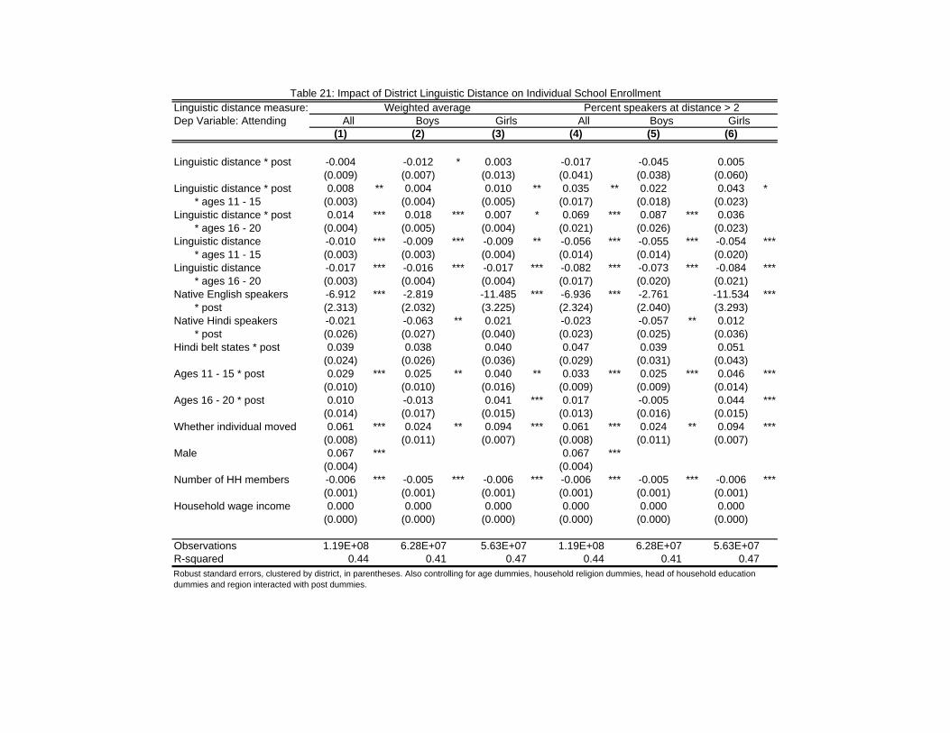
Linguistic distance measure:Dep Variable: Attending
(1) (2) (3) (4) (5) (6)
Linguistic distance * post -0.004 -0.012 * 0.003 -0.017 -0.045 0.005(0.009) (0.007) (0.013) (0.041) (0.038) (0.060)
Linguistic distance * post 0.008 ** 0.004 0.010 ** 0.035 ** 0.022 0.043 * * ages 11 - 15 (0.003) (0.004) (0.005) (0.017) (0.018) (0.023)Linguistic distance * post 0.014 *** 0.018 *** 0.007 * 0.069 *** 0.087 *** 0.036 * ages 16 - 20 (0.004) (0.005) (0.004) (0.021) (0.026) (0.023)Linguistic distance -0.010 *** -0.009 *** -0.009 ** -0.056 *** -0.055 *** -0.054 *** * ages 11 - 15 (0.003) (0.003) (0.004) (0.014) (0.014) (0.020)Linguistic distance -0.017 *** -0.016 *** -0.017 *** -0.082 *** -0.073 *** -0.084 *** * ages 16 - 20 (0.003) (0.004) (0.004) (0.017) (0.020) (0.021)Native English speakers -6.912 *** -2.819 -11.485 *** -6.936 *** -2.761 -11.534 *** * post (2.313) (2.032) (3.225) (2.324) (2.040) (3.293)Native Hindi speakers -0.021 -0.063 ** 0.021 -0.023 -0.057 ** 0.012 * post (0.026) (0.027) (0.040) (0.023) (0.025) (0.036)Hindi belt states * post 0.039 0.038 0.040 0.047 0.039 0.051
(0.024) (0.026) (0.036) (0.029) (0.031) (0.043)Ages 11 - 15 * post 0.029 *** 0.025 ** 0.040 ** 0.033 *** 0.025 *** 0.046 ***
(0.010) (0.010) (0.016) (0.009) (0.009) (0.014)Ages 16 - 20 * post 0.010 -0.013 0.041 *** 0.017 -0.005 0.044 ***
(0.014) (0.017) (0.015) (0.013) (0.016) (0.015)Whether individual moved 0.061 *** 0.024 ** 0.094 *** 0.061 *** 0.024 ** 0.094 ***
(0.008) (0.011) (0.007) (0.008) (0.011) (0.007)Male 0.067 *** 0.067 ***
(0.004) (0.004)Number of HH members -0.006 *** -0.005 *** -0.006 *** -0.006 *** -0.005 *** -0.006 ***
(0.001) (0.001) (0.001) (0.001) (0.001) (0.001)Household wage income 0.000 0.000 0.000 0.000 0.000 0.000
(0.000) (0.000) (0.000) (0.000) (0.000) (0.000)
Observations 1.19E+08 6.28E+07 5.63E+07 1.19E+08 6.28E+07 5.63E+07R-squared 0.44 0.41 0.47 0.44 0.41 0.47
Table 21: Impact of District Linguistic Distance on Individual School Enrollment
Robust standard errors, clustered by district, in parentheses. Also controlling for age dummies, household religion dummies, head of household education dummies and region interacted with post dummies.
Percent speakers at distance > 2Weighted averageAll Boys Girls All Boys Girls

Linguistic distance measure:Dep Variable: Edu. Level
(1) (2) (3) (4) (5) (6)
Linguistic distance * post -0.042 * -0.060 ** -0.029 -0.055 -0.160 0.029(0.025) (0.026) (0.032) (0.119) (0.133) (0.148)
Linguistic distance * post 0.042 *** 0.041 *** 0.039 *** 0.148 *** 0.163 ** 0.120 * * ages 11 - 15 (0.011) (0.013) (0.013) (0.057) (0.067) (0.069)Linguistic distance * post 0.050 *** 0.050 *** 0.040 * 0.200 *** 0.213 *** 0.142 * ages 16 - 20 (0.016) (0.016) (0.022) (0.076) (0.081) (0.105)Linguistic distance 0.012 0.008 0.017 * 0.038 0.023 0.059 * ages 11 - 15 (0.007) (0.009) (0.010) (0.038) (0.043) (0.049)Linguistic distance -0.021 * -0.004 -0.028 -0.141 ** -0.053 -0.191 ** * ages 16 - 20 (0.011) (0.010) (0.018) (0.056) (0.054) (0.088)Native English speakers -37.783 *** -20.039 * -58.485 *** -38.426 *** -20.559 * -59.204 *** * post (9.035) (10.790) (9.499) (9.146) (10.905) (9.484)Native Hindi speakers 0.030 -0.104 0.145 0.064 -0.060 0.178 * post (0.113) (0.127) (0.132) (0.101) (0.118) (0.120)Hindi belt states * post -0.045 -0.067 -0.003 0.000 -0.060 0.063
(0.097) (0.100) (0.130) (0.093) (0.097) (0.133)Ages 11 - 15 * post -0.011 -0.042 0.025 0.024 -0.012 0.065
(0.035) (0.043) (0.044) (0.035) (0.042) (0.042)Ages 16 - 20 * post 0.173 *** 0.047 0.323 *** 0.207 *** 0.077 0.354 ***
(0.050) (0.053) (0.072) (0.045) (0.050) (0.063)Whether individual moved 0.250 *** 0.079 *** 0.389 *** 0.250 *** 0.078 *** 0.389 ***
(0.022) (0.030) (0.027) (0.022) (0.030) (0.027)Male 0.180 *** 0.000 0.000 0.179 *** 0.000 0.000
(0.014) (0.000) (0.000) (0.014) (0.000) (0.000)Number of HH members -0.015 *** -0.015 *** -0.011 * -0.015 *** -0.015 *** -0.011 *
(0.004) (0.004) (0.006) (0.004) (0.004) (0.006)Household wage income 0.000 0.000 0.000 0.000 0.000 0.000
(0.000) (0.000) (0.000) (0.000) (0.000) (0.000)
Observations 1.30E+08 6.84E+07 6.18E+07 1.30E+08 6.84E+07 6.18E+07R-squared 0.47 0.49 0.46 0.47 0.49 0.46
Table 22: Impact of District Linguistic Distance on Individual Educational Achievement
Robust standard errors, clustered by district, in parentheses. Also controlling for age dummies, household religion dummies, head of household education dummies and region interacted with post dummies.
Percent speakers at distance > 2Weighted averageAll Boys Girls All Boys Girls
Related Documents


