SPE 119897 Production Analysis and Forecasting of … 119897 3 reservoir properties and stimulation information. We use both field cases and simulated cases to ...

SPE 119897

Production Analysis and Forecasting of Shale Gas Reservoirs: Case History-Based Approach L. Mattar, B. Gault, K. Morad, Fekete Associates Inc., C.R. Clarkson, EOG Resources, C.M. Freeman, D. Ilk, and T.A. Blasingame, Texas A&M University

Copyright 2008, Society of Petroleum Engineers This paper was prepared for presentation at the 2008 SPE Shale Gas Production Conference held in Fort Worth, Texas, U.S.A., 16–18 November 2008. This paper was selected for presentation by an SPE program committee following review of information contained in an abstract submitted by the author(s). Contents of the paper have not been reviewed by the Society of Petroleum Engineers and are subject to correction by the author(s). The material does not necessarily reflect any position of the Society of Petroleum Engineers, its officers, or members. Electronic reproduction, distribution, or storage of any part of this paper without the written consent of the Society of Petroleum Engineers is prohibited. Permission to reproduce in print is restricted to an abstract of not more than 300 words; illustrations may not be copied. The abstract must contain conspicuous acknowledgment of SPE copyright.

Abstract

In this work we present the current status of production evaluation and prediction for shale gas reservoirs. We focus primarily on the effect of wellbore geometry (vertical vs. horizontal) and fracture stimulation, and consider only relatively simple shale reservoir characteristics. Theoretical production responses from hydraulically-fractured vertical and horizontal wells are first described. Analytical and empirical methods for production data analysis and forecasting of shale reservoirs are then described and demonstrated. The empirical approach used is the recently developed “power-law exponential” rate relation [Ilk, et al (2008b and 2008b)] in addition to the more traditional "hyperbolic" rate relation [Johnson and Bollens (1927)], Arps (1945)]. The analytical methods utilized include production type-curves developed for vertical wells completed in single-porosity, single-phase reservoirs. Finally, numerical approaches for forecasting complex, multi-fractured horizontal wells are also presented. Two approaches for simulating these complex wells, one simple and the other more rigorous, are provided. In the more rigorous approach, the “compound linear flow regime” concept introduced by van Kruysdijk and Dullaert (1989) is verified. The production analysis methods are applied to field and simulated cases to demonstrate their accuracy and practicality. The empirical power-law exponential method, when applied to both simulated and field cases, is shown to be a reliable method for forecasting shale wells. The analytical (type-curve) methods developed for vertical wells can be useful for analyzing vertical shale wells; when applied to horizontal wells, the resulting estimates of reservoir and fracture properties may be inaccurate. A special case of analysis of a 2-phase shale reservoir is also presented; in this case, the analytical tools developed recently for 2-phase CBM reservoirs [Clarkson, et al (2008)], including 2-phase flowing material balance and type-curves, prove useful. Introduction

Shale gas reservoirs are currently being aggressively explored for and developed in North America, with technology, such as multi-fractured horizontal wells, being a key driver for success. The shale reservoirs that have been exploited to date have varied and complex reservoir and production characteristics, making quantitative production analysis and forecasting difficult. The characterization of shale gas reservoirs in terms of production performance has essentially 2 components:

1. Estimation of reservoir properties (permeability, effectiveness of the well completion, and contacted-gas-in-place). 2. Forecasting of the production performance as a means of estimating reserves and to evaluate economic viability.

The analysis of production data is often the only practical way of evaluating tight gas and shale gas reservoirs. The modern methods of production data analysis are quite robust and in many respects these methods parallel those of pressure transient analysis. Obviously, the basic theory is the same — but the assumptions are different. Each methodology (pressure transient analysis and production analysis) is appropriate in its own domain. In simple terms, neither the quality nor the accuracy of production data is comparable to that of well test data, but an extensive production rate and pressure history is data that can be utilized to provide a "full life analysis" of the well — whereas, even when available, pressure transient tests are very short, at best on the order of a few days.

2 SPE 119897

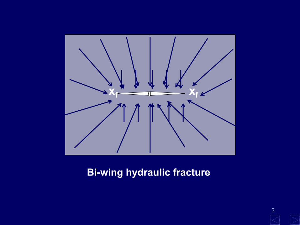
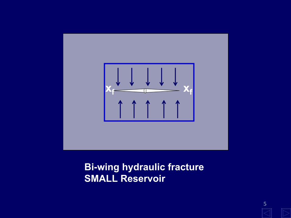
The purpose of our present work is quite straightforward — assess the existing methods for the estimation of reservoir properties for vertical and horizontal wells in shale gas reservoirs (with multiple transverse hydraulic fractures) using production data (rate and pressure histories); and to assess the most practical methods for establishing relevant forecasts of gas production rates from shale gas reservoir systems. In this work, we primarily limit our discussion to relatively simple reservoir properties (single-phase flow, single-porosity). Admittedly, shale reservoirs may exhibit quite complex reservoir behavior including: multi-phase flow (gas+water); dual porosity behavior; stress-dependent permeability and porosity and multi-layer behavior. Production Data Analysis Techniques In this section we discuss the production data analysis techniques (empirical and analytical) techniques used in this study as well as application of these techniques to real and simulated data. Prior to describing the methods, however, a brief discussion of theoretical production responses, related to hydraulic fracture geometry, is warranted. Theoretical Production Responses: Vertical Hydraulically-Fractured Well. In well testing, a hydraulic fracture is modeled as a bi-wing fracture of half length xf, and with infinite or finite conductivity within the fracture (Fig. 1). In recent years, and mostly where shale gas or tight gas exploitation has been taking place, the fracturing operation has been monitored using microseismic techniques. These techniques have resulted in a new interpretation of the fracture mechanics and have suggested a very different model from the bi-wing fracture in some shale reservoirs. Tracking the microseismic events during the hydraulic fracture treatment has led to the hypothesis that:

• often the fracturing is not localized in a bi-wing, but rather it is distributed along the network of fissures • the fissures pre-existed, but healed and had no permeability, the hydraulic fracturing re-opens them and creates the

permeability • the re-opening of the fissures is accompanied by local dislocations. This keeps them propped open to maintain their

permeability • The effective reservoir exists only as far as the fracture extends

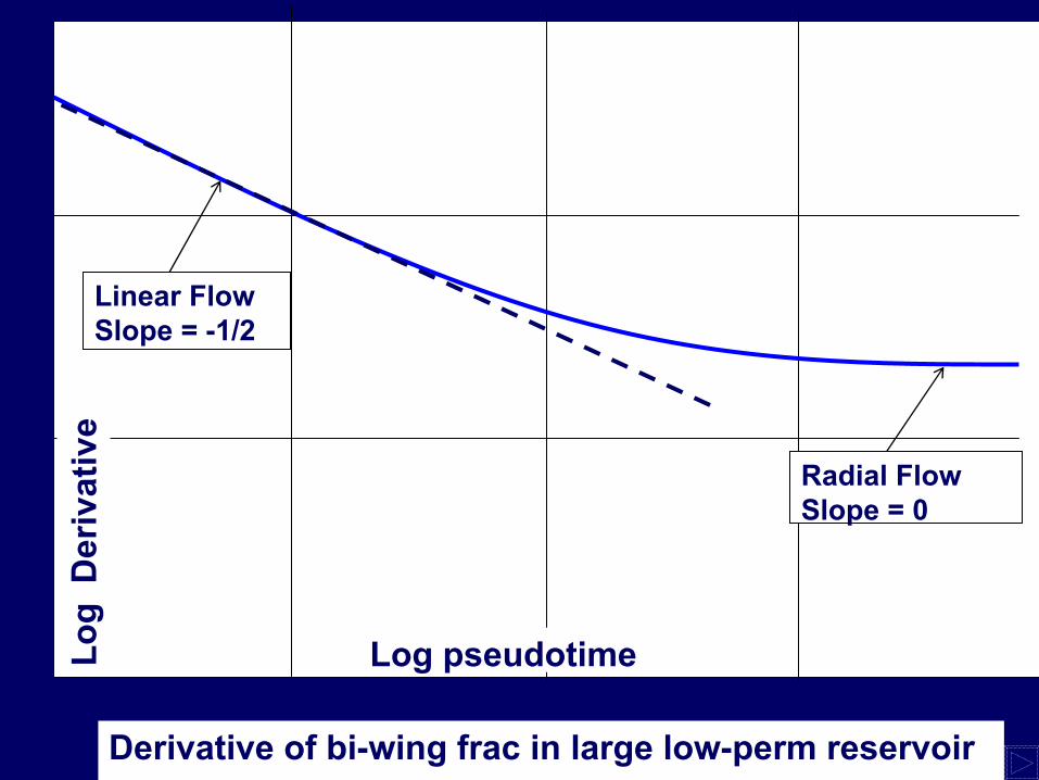
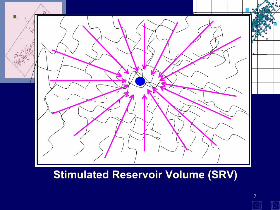
In other words, even though the shale is present extensively (infinite-acting), the actual productive reservoir exists only where the fracture exists. Therefore the productive reservoir has a limited drainage volume (or associated drainage area). This drainage volume, which has been termed the Stimulated Reservoir Volume (SRV) (Warpinski et al. (2005)) is shown schematically in Fig 2. The production responses for the bi-wing and distributed fracture scenarios are as follows (assuming single-porosity, homogeneous reservoir, single-phase flow): Bi-wing: If a bi-wing fracture (or series of bi-wing fractures) is created, in a large (infinite-acting) low permeability reservoir the derivative plot of rate/pressure versus time should behave as shown in Fig. 3. The linear flow (slope = -1/2) caused by flow into the bi-wing frac is followed by radial flow. Boundary Dominated Flow (BDF) which manifests itself as a late time unit slope (-1) is not likely to be seen for many years because of the very low permeability of shales. Distributed fissures: This concept (shown in Fig. 2) will behave as shown in Fig. 4. Initially, there will be an infinite-acting radial flow, which reflects the permeability of the SRV (the network of fissures created by the hydraulic frac treatment). The shale outside the SRV is for all practical purposes non-permeable, and therefore the radial flow will be followed by a unit slope (-1) which represents the volume of the SRV. Hybrid bi-wing/SRV: In our experience, we have observed many situations that look like Fig. 5. Initially, the flow is linear, just as would be expected for a bi-wing frac. However, instead of becoming radial, it enters boundary dominated flow (BDF), which implies the existence of a SRV. Note that the behaviors described above are very often observed in tight gas. However in case of tight gas, an accepted explanation is that the hydraulic fracture is a bi-wing which connects lenticular and heterogeneous pockets of tight gas. Thus the linear flow is followed by boundary dominated flow, but strictly speaking, this BDF is not a SRV. The production responses for a horizontal well with multiple-transverse fractures may be much more complex, exhibiting a variety of flow regimes (see for example, Medeiros et al. (2007)). This case will be discussed in more detail in a later section. Production Analysis Approaches: Analytical. The analytical methods used by the authors include those discussed by Mattar and Anderson (2003); in this work, we focus primarily on the use of vertical well production-type curves to extract

SPE 119897 3

reservoir properties and stimulation information. We use both field cases and simulated cases to illustrate the application of the analytical methods. Field Case 1, shown in Fig. 6, is a hydraulically fractured (100 tons of sand) vertical well in a dry shale reservoir. It has produced for 5 years. The integral derivative of the normalized rate is plotted versus material balance pseudotime (Mattar and Anderson (2003)).

• The transient flow data (first year of flow) is not helpful in characterizing the hydraulic fracture or the reservoir. However the late time data falls clearly on the unit slope line and represents boundary dominated flow, with Original-Gas-In-Place (OGIP) of 0.5 BCF (no isotherm available). The well was abandoned, because of low rates, after producing 0.2 BCF.

• Because the transient data was not analyzable, it is not possible to tell whether the low rates are due to a very low permeability or an ineffective hydraulic-fracture.

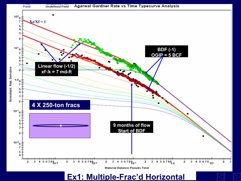
• It is also not possible to say whether this is a bi-wing fracture, an SRV or a hybrid of these two. Field Case 2, shown in Fig. 7, is a multiple-hydraulic fracture, cased-hole horizontal well (4 fracs, 1000 ft apart, each frac 250 tons of sand) in a dry shale reservoir. It has produced 2.5 BCF in 4 years.

• Fig. 7 shows the normalized rate data as well as the derivative. At 9 months of flow, boundary dominated flow is reached. Prior to that, linear flow is clearly evident, and the product xf√k can be determined. There is no radial flow. Therefore k or xf cannot be determined individually. However because there is a rapid transition from linear to boundary dominated flow, it can be inferred that the fracture extends to the edge of the reservoir. The boundary dominated flow is unique and yields a volume of 5 BCF.

• This is an example of the hybrid bi-wing/SRV concept. The frac is a high conductivity frac. It extends to the edge of the reservoir (xe / xf = 1)

Field Case 3 is a multiple-hydraulic fracture, cased-hole horizontal well (3 fracs, 1000 ft apart, each 150 tons of sand) in a dry shale reservoir. It has produced 0.5 BCF in 2 years. There are two possible interpretations as given in Figs. 8 and 9. Figure 8 is the intuitive interpretation of this data set.

• The first 40 days of flow exhibit radial flow, from which permeability and skin can be calculated, as follows: k = 30 μd, s = -3, xf = 15 ft. The effect of the 3*150 ton frac’s is not evident at all. There is no linear flow visible.

• The OGIP = 1 BCF, which translates to an area of 10 acres. • This would be considered to be an example of SRV, where the frac treatment did not create a bi-wing, but instead

enhanced the permeability within a 10-acre region. The permeability of the shale outside the region of influence of the frac (10 acres in this case) is essentially zero.

Fig. 9 presents an alternative interpretation to the dataset of Field Case 3.

• It is possible, though not too convincing, to match the data on a finite conductivity type curve. The dimensionless fracture conductivity, FcD = 0.5

• Assuming the frac goes all the way to the edge of the reservoir, xf=300 ft and k = 30 μd • This interpretation corresponds to a bi-wing frac, but the conductivity inside the frac is finite rather than infinite.

The two alternative interpretations of the data of Field Case 3, hint at the fact that what has been considered to be an enhanced permeability region (SRV) may not be that at all, but may actually be a bi-wing, but finite conductivity frac. The following simulated cases address this possibility. Simulated Case 1. For the simulated cases, an open-hole horizontal well with several transverse hydraulic fractures, as illustrated in Fig. 10, was simulated using a numerical simulator. To speed up the calculations, we took advantage of geometrical symmetry, and modeled only 1 frac and multiplied the answer by the number of fracs. The frac was either infinite conductivity (FcD = 200) or finite conductivity (FcD = 2). A more rigorous method for simulating a multi-fracture horizontal well is discussed in a later section. Typical shale reservoir parameters (Table 1) were used in this example and a 3-year forecast of production was generated at a fixed flowing pressure. The synthetic data was analyzed using the same methods as for the preceding field cases. For the both simulated cases, the adsorbed gas content was set to zero. Fig. 11 shows the type curve match of the synthetic data for the infinite conductivity frac (FcD = 200).

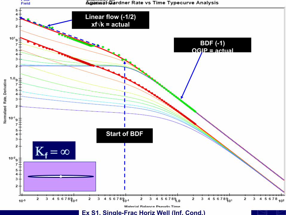
• This is the classic picture one would expect to see for the hybrid bi-wing situation - the linear flow becomes boundary dominated without any intervening radial flow. The reservoir size is co-incident with the frac size.

4 SPE 119897

• Accordingly, only the product of xf√k can be determined. The value obtained is 20 to 30% higher than the actual input value for the fracture. This is explained by the fact that the horizontal well is open-hole, and contributes to the flow and manifests itself as an increased xf√k.

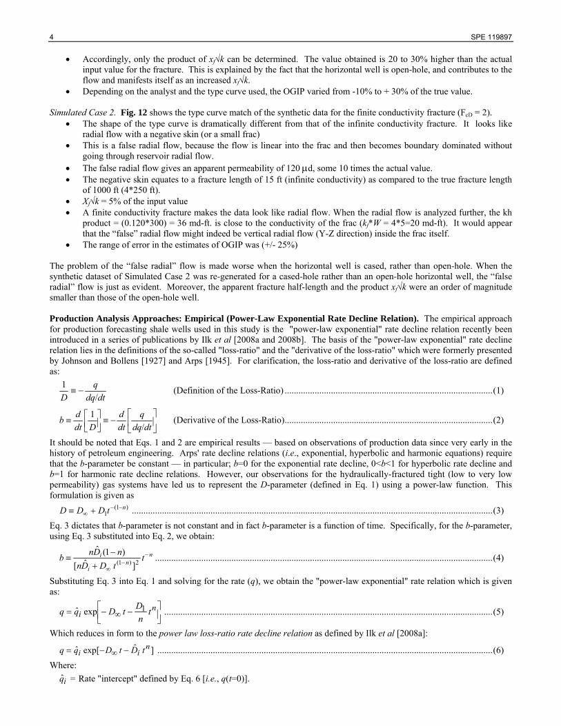
• Depending on the analyst and the type curve used, the OGIP varied from -10% to + 30% of the true value. Simulated Case 2. Fig. 12 shows the type curve match of the synthetic data for the finite conductivity fracture (FcD = 2).

• The shape of the type curve is dramatically different from that of the infinite conductivity fracture. It looks like radial flow with a negative skin (or a small frac)

• This is a false radial flow, because the flow is linear into the frac and then becomes boundary dominated without going through reservoir radial flow.

• The false radial flow gives an apparent permeability of 120 μd, some 10 times the actual value. • The negative skin equates to a fracture length of 15 ft (infinite conductivity) as compared to the true fracture length

of 1000 ft (4*250 ft). • Xf√k = 5% of the input value • A finite conductivity fracture makes the data look like radial flow. When the radial flow is analyzed further, the kh

product = (0.120*300) = 36 md-ft. is close to the conductivity of the frac (kf*W = 4*5=20 md-ft). It would appear that the “false” radial flow might indeed be vertical radial flow (Y-Z direction) inside the frac itself.

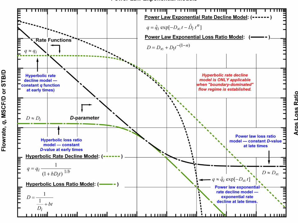
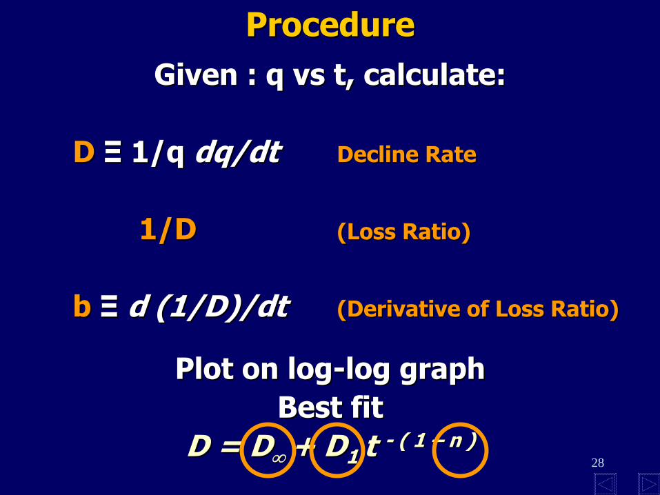
• The range of error in the estimates of OGIP was (+/- 25%) The problem of the “false radial” flow is made worse when the horizontal well is cased, rather than open-hole. When the synthetic dataset of Simulated Case 2 was re-generated for a cased-hole rather than an open-hole horizontal well, the “false radial” flow is just as evident. Moreover, the apparent fracture half-length and the product xf√k were an order of magnitude smaller than those of the open-hole well. Production Analysis Approaches: Empirical (Power-Law Exponential Rate Decline Relation). The empirical approach for production forecasting shale wells used in this study is the "power-law exponential" rate decline relation recently been introduced in a series of publications by Ilk et al [2008a and 2008b]. The basis of the "power-law exponential" rate decline relation lies in the definitions of the so-called "loss-ratio" and the "derivative of the loss-ratio" which were formerly presented by Johnson and Bollens [1927] and Arps [1945]. For clarification, the loss-ratio and derivative of the loss-ratio are defined as:

dtdqq

D /1

−≡ (Definition of the Loss-Ratio) ..........................................................................................(1)

⎥⎦

⎤⎢⎣

⎡−≡⎥⎦

⎤⎢⎣⎡≡

dtdqq

dtd

Ddtdb

/1 (Derivative of the Loss-Ratio)..........................................................................................(2)

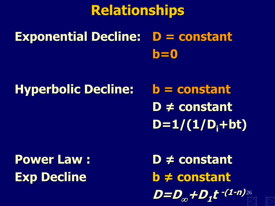
It should be noted that Eqs. 1 and 2 are empirical results — based on observations of production data since very early in the history of petroleum engineering. Arps' rate decline relations (i.e., exponential, hyperbolic and harmonic equations) require that the b-parameter be constant — in particular; b=0 for the exponential rate decline, 0<b<1 for hyperbolic rate decline and b=1 for harmonic rate decline relations. However, our observations for the hydraulically-fractured tight (low to very low permeability) gas systems have led us to represent the D-parameter (defined in Eq. 1) using a power-law function. This formulation is given as

)1(1

ntDDD −−∞ +≡ ............................................................................................................................................................(3)

Eq. 3 dictates that b-parameter is not constant and in fact b-parameter is a function of time. Specifically, for the b-parameter, using Eq. 3 substituted into Eq. 2, we obtain:

nn

i

i ttDDnnDnb −

−∞+−

≡ 2)1( ] ˆ[)1(ˆ

..................................................................................................................................................(4)

Substituting Eq. 3 into Eq. 1 and solving for the rate (q), we obtain the "power-law exponential" rate relation which is given as:

⎥⎦⎤

⎢⎣⎡ −−= ∞

ni t

nDtDqq exp ˆ 1 ..............................................................................................................................................(5)

Which reduces in form to the power law loss-ratio rate decline relation as defined by Ilk et al [2008a]:

] ˆexp[ ˆ n

ii tDtDqq −−= ∞ .................................................................................................................................................(6)

Where:

iq̂ = Rate "intercept" defined by Eq. 6 [i.e., q(t=0)].

SPE 119897 5

D1 = Decline constant "intercept" at 1 time unit defined by Eq. 3 [i.e., D(t=1 day)].

D∞ = Decline constant at "infinite time" defined by Eq. 3 [i.e., D(t=∞)]. iD̂ = Decline constant defined by Eq. 6 [i.e., nDDi /ˆ 1= ]. n = Time "exponent" defined by Eq. 3.

We have applied the form given by Eq. 6 to several hydraulically-fractured tight gas well cases (Ilk et al [2008b]) along with the hyperbolic rate decline relation and concluded that when properly constrained, this formulation is an outstanding predictor of reserves for tight gas reservoir systems. In addition, this formulation (Eq. 6) has the flexibility to model transient, transition and boundary-dominated flow data. Another conclusion that can be drawn from Ilk et al [2008b] is that the computation of the b- and D- parameters provides an excellent diagnostic insight into rate data.

In the following examples, we apply the "power-law exponential" formulation for the reserves estimation (production forecasting) of shale gas reservoirs. We present five (5) field cases obtained from public records for horizontal wells in the Barnett shale (Texas, USA). We note that for these field cases, only monthly production data are publicly available.

Field Case: Barnett Shale — Gas Well 1

As mentioned before, the use of the new formulation offers an alternative way to estimate the reserves where transient, transition and boundary-dominated flow data can be modeled efficiently unlike the traditional decline curve analysis methods (i.e., Arps' rate relations) which are only applicable for boundary-dominated flow regime. Modern production analysis methodologies (including the analytical methods discussed above) require flowing wellbore pressures along with the rate data for flow regime identification and parameter estimation (such as transient flow parameters; k, s, xf, etc. or boundary-dominated flow parameter; reservoir volume). We note that in the absence of flowing wellbore pressure data, modern production analysis methodologies may not be practical or for some complex reservoir systems, rigorous analytical models do not exist. Therefore, using the new formulation could enhance the analyst options for reserves estimation when the situations mentioned above are encountered. Previously, we have shown that the new formulation worked well in the case of tight gas reservoir systems. It is our intention in this work to seek the applicability of the new "power-law exponential" formulation to shale gas reservoir systems for production forecasting.

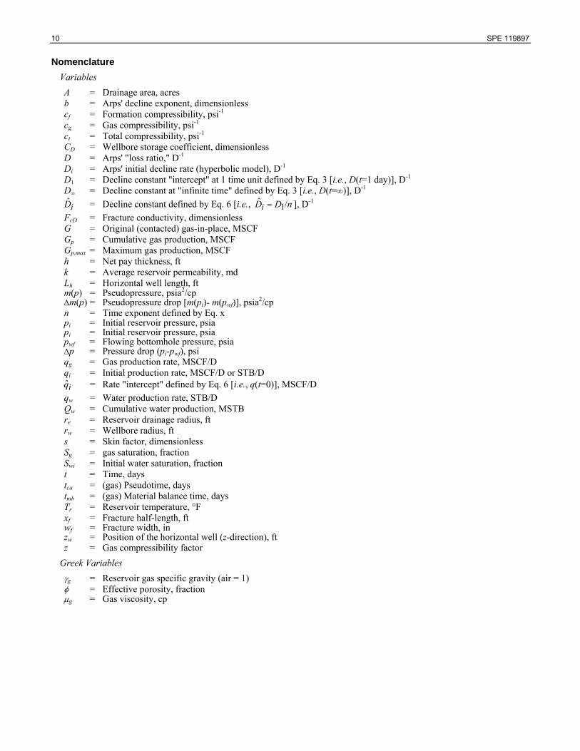
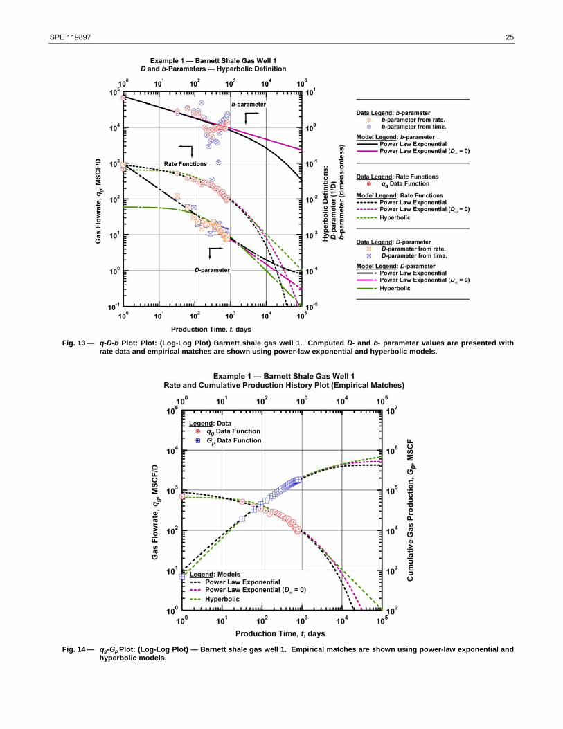
We begin our study with a gas well from Barnett Shale where 3-years of production data (monthly rates) are (publicly) available for this well. Other than the rate data, no information (in particular, pressure data) was accessible. Visual inspection of the rate data suggests that the boundary-dominated flow regime has established. In general rate decline follows a smooth trend. However, fluctuations are observed — we suspect these fluctuations are caused by liquid loading (water production). We begin our procedure by computing the b- and D- parameters by the use of a numerical differentiation algorithm and present the results along with the rate data in Fig. 13. Although noisy, D-parameter data trend roughly indicates a power-law (i.e., straight line on log-log scale) character. Character of b-parameter data trend is severely affected by the noise in the data — however, it could be argued that b-parameter data trend is following a decreasing trend.

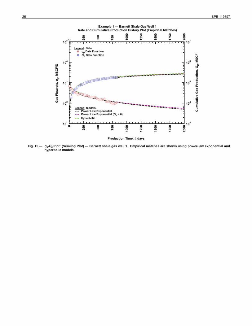
We use the "power-law exponential" formulation and obtain very good matches of D-parameter and rate data with the models (i.e., Eqs 3 and 6). The D∞ term is incorporated into the formulation to take the effects of full closed system behavior into account and as well as to yield a lower bound for the reserves estimate. We prefer to have two values (upper and lower) for the reserves estimate obtained by setting D∞=0 and using the highest optimal value for the D∞ parameter (it is noted that D∞≥0). The reserves estimate results and model parameters for this case are tabulated in Table 2 and production forecasts are shown in log-log and semilog formats in Figs. 14 and 15, respectively. Lastly, we also apply the traditional hyperbolic relation to the production data. The value for the b-parameter in hyperbolic relation is taken as 1 by inspecting the average behavior of b-parameter data trend. A good match of the data with the hyperbolic relation is obtained. However, the reserves estimate using the hyperbolic relation is three times higher.

Field Case: Barnett Shale — Gas Well 2

Our second example includes almost 6 years of monthly production data. We identify a smooth decline throughout the life of this well. Visual inspection of the rate data suggests that full boundary-dominated flow regime has not been established yet. The q-D-b plot (Fig. 16) verifies the power-law behavior of the D-parameter. It is observed that the computed D-parameter data trend is essentially a straight line on the log-log scale. Consequently, computed b-parameter data also follows a decreasing trend. It is worth to mention that b-parameter data do not suggest a constant value. However, for the hyperbolic relation we take the value of b-parameter as 1.4 to obtain the best match with the data. As indicated by the computed b- and D- parameters, the most appropriate way to estimate the reserves for this case would be the use of "power-law exponential" model.

We obtain excellent matches of the data with the model with both using D∞=0 and D∞≠0. Production forecasts are shown in Figs. 17 and 18, respectively and tabulated in Table 3. It is worth to mention that the reserves estimate predicted by the hyperbolic relation is almost 50 times higher than the estimate obtained by using the "power-law exponential" formulation. We attribute this dramatic difference in reserves estimate to the chosen constant value of the b-parameter in hyperbolic relation.

6 SPE 119897

This case is very similar to the previous example (Gas Well 2). Approximately 7 years of production data are available (again no pressure data are reported). Smooth decline trend is observed during the production. We also identify a slight increase in the rate data at almost the end of 6 years. Inspecting the q-D-b plot (Fig. 19), it can be suggested that this well is in transition to boundary-dominated flow. Computed D-parameter data trend is essentially a straight line on log-log scale verifying the applicability of Eq. 3. Computation of the b-parameter data trend is affected by data noise and end-point effects of the differentiation algorithm can be seen in Fig. 19. Although an average b-parameter value is indicated by the data trend, we believe that using this value in the hyperbolic rate relation will cause an over-estimation of reserves — we expect that the b-parameter is not constant and instead it should follow a decreasing trend. We obtain outstanding matches of the rate data with the "power-law exponential' model (with using D∞=0 and D∞≠0).

Figs. 20 and 21 present the production forecasts of this well and Table 4 tabulates the results. The minimum value for the reserves estimate for this well is 2.7 BSCF when D∞ value is not set to zero. On the other hand, we predict 8 times more than this value when D∞ value is set to zero. This process indicates the upper and lower bound for the reserves estimate for this well with relatively high uncertainty. It is worth to note the importance of using modern production data analysis method (model based approaches) as these methods are based on theory rather than observations and we expect that combining the "power-law exponential" formulation with model based analysis would greatly decrease the uncertainty in production forecasting. Finally, using the hyperbolic rate relation yields absurdly high reserves (100 times higher than the reserves predicted by the "power-law exponential" formulation) when b-parameter is set to 1.4 for this case. Therefore, we advise caution when production data are to be evaluated with hyperbolic rate relation, and most importantly, when boundary-dominated flow regime is not established.

Field Case: Barnett Shale —Gas Well 4

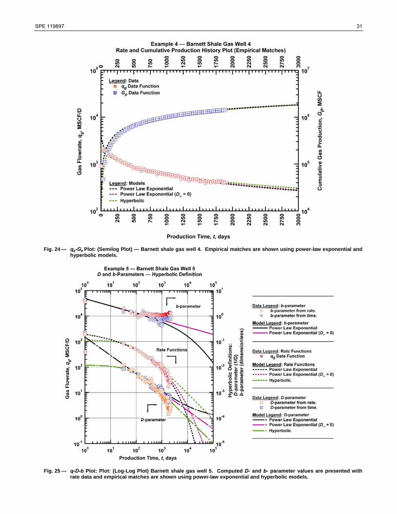
This example contains monthly production data for almost 5.5 years. Rate data look smooth with minor fluctuations. A raw inspection of the rate data indicates this well is still in transient/transition flow regime and boundary-dominated flow regimes have not been established yet. Fig. 22 presents the q-D-b plot and we immediately recognize the power-law behavior exhibited by the computed D-parameter data trend. We note that erratic rate performance at early times (presumably by well-cleanup effects) causes artifacts on the computed D- and b-parameter data trends at earlier times (up to a year).

We observe very good matches of the rate data with the "power-law exponential" model (with using D∞=0 and D∞≠0). Table 5 indicates that there is no big difference between the upper and lower bound of the reserves estimate by the "power-law exponential" model. We observe end-point effects of the numerical differentiation algorithm on the computed D- and b-parameter data trends in Fig. 22. Computed b-parameter data is above 1 and we use 1.4 as the value of b-parameter in hyperbolic rate relation — this again yields absurdly high reserves estimate compared to the estimates predicted by the "power-law exponential" formulation. The main reason is that boundary-dominated flow regime has not been completely established and hyperbolic rate relation is only applicable for boundary-dominated flow regime. Figs. 23 and 24 presents the production forecast for this well predicted by rate relations used in this work.


Our last example includes almost 6.5 years of monthly production data acquired from a gas well completed in the Barnett Shale. This example differs from the previous examples in a way that an erratic rate performance is observed almost after 2 years of production. We assume the erratic rate performance might be caused by liquid loading but we have limited information (i.e., pressure data are missing) on this well to verify this assumption. For this case we note that boundary-dominated flow effects have been established.

In Fig. 25 we present the q-D-b plot for this well and we observe the power-law behavior exhibited by the computed D-parameter data trend despite the noise in the data. At this point we would like to mention that no editing on the rate data is performed prior to numerical differentiation — we believe the smoothing process in the numerical differentiation algorithm eliminates the amplification of the errors in the computation of D-parameter to an extent (see Bourdet et al [1989]). However, end-point effects are present on the computed D- and b-parameter data trends. We observe outstanding matches of the rate data with the "power-law exponential" model (with using D∞=0 and D∞≠0). We set b=1 in the hyperbolic rate relation and this gives almost 5 times higher reserves estimate than predicted by the "power-law exponential" model (see Table 6 for the results and Figs. 26 and 27 for the production forecast). The difference in the reserves estimates predicted by two different relations can be overcome by decreasing the value of the b-parameter in hyperbolic rate relation. The low value of the reserves estimate indicates the limited drainage area in this example. Simulation Modeling of Horizontal Well with Multiple Transverse Fractures

In a previous section, we generated a simple representation of a horizontal well with multiple hydraulic fractures by aggregating multiple single hydraulic fracture models – this was done to assess the possibility of using vertical well analytical solutions to represent horizontal wells with multiple vertical hydraulic fractures. Although this representation of a horizontal well may work in some instances, we apply a more rigorous approach here; the resulting production data is then analyzed with the empirical approach discussed above.


SPE 119897 7

Description of the Reservoir Model. The exploitation of shale gas reservoirs include drilling horizontal wells, perforate 3 to 7 clusters of perforations some 500 to 1000 ft apart. Each cluster is hydraulically fractured (typically slick water fracture treatments are utilized). The geological characterization of shale gas reservoirs can be complex, and mathematical modeling of the production from a shale gas reservoir correspondingly so. Since the common practice in shale gas reservoirs is to produce from horizontal wells with multiple transverse fractures, efforts have been focused into the development of horizontal well models with multiple transverse fractures. To date several semi-analytical models (see van Kruysdijk and Dullaert [1989], Valko and Amini [2007], Medeiros et al [2007]) have been introduced to literature for modeling the horizontal wells with multiple transverse fractures. In addition a much simpler way is to model the horizontal wells with multiple transverse fractures using numerical simulation. However, we suggest that the numerical simulation solutions should be verified by the semi-analytical model solutions (i.e., numerical solution should produce the characteristic behavior exhibited by the semi-analytical model).

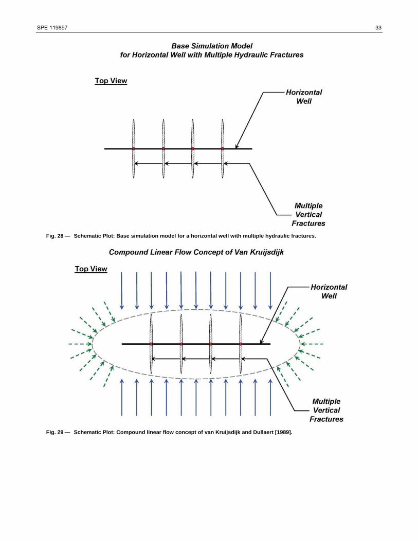
In this work we simulated a case of a horizontal well having four transverse fractures. The schematic for our base simulation model is presented in Fig. 28. Reservoir and fluid properties for the simulation are also provided in Table 7. We simulate infinite-acting and finite-acting reservoir cases. We generate the rate profile of the simulated horizontal well with multiple fractures having infinite conductivity operating under constant flowing bottomhole pressure condition. The whole purpose of this exercise is to mimic the performance of wells in shale gas reservoirs. We note that in our simulation runs adsorption is not taken into account — this remains to be a study for future work.

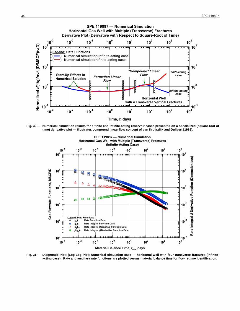
Analysis of the Simulated Production Data using Power-Law Exponential Rate Decline Relation. We first generate the rate profile using the base simulation model under constant flowing bottomhole condition. Our objective is to obtain a similar response to the response presented by van Kruysdijk and Dullaert [1989] (see Fig. 7 of van Kruysdijk and Dullaert [1989]). van Kruysdijk and Dullaert present a log-log plot of the derivative of pressure drop with respect to square root of time versus time to identify the flow regimes and most importantly to introduce their concept of the "compound linear flow". For reference, Fig. 29 presents a schematic of the "compound linear flow" concept of van Kruysdijk and Dullaert — compound linear flow establishes when the linear flow from formation is felt by the group of fractures. In our case we use the reciprocal of the generated rate profile and differentiate it with respect to square root of time. We present our results for both infinite-acting and finite-acting cases in Fig. 30. We observe that the result of the infinite-acting case follow the same trend as put forward by van Kruysdijk and Dullaert and the compound linear flow regime is identified almost after 20 days. We note that the inclusion of the boundaries (i.e., finite-acting system) distorts the compound linear flow regime exhibited by the derivative trend. We also show the rate and auxiliary rate functions versus material balance time (diagnostic plot) in Fig. 31. In this work we only present the data of the rate and its auxiliary functions to show the response character depicted by the numerical simulation.

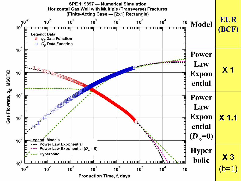
In the next step, we simulate a horizontal well having multiple transverse fractures centered in a 2x1 rectangular reservoir. Our specific goal in this case is to estimate the reserves and compare the results with the simulator input. As illustrated in the previous section, we make use of the "power-law exponential" and hyperbolic rate relations to estimate the reserves. Before proceeding to the reserves estimate, we present the rate and auxiliary rate functions in Fig. 32 and we immediately recognize the difference from the infinite-acting case. We observe that boundary-dominated flow regime has been established almost after 100 days. The q-D-b plot (Fig. 33) suggests a strong power-law behavior when the computed D-parameter is inspected visually. In addition, the curving of the computed D-parameter after 100 days indicates the effect of the boundaries on the response. It is also worth to mention that the computer b-parameter is not constant and follows a decreasing trend.

We apply the "power-law exponential" formulation and present the results in Fig. 33. Excellent matches of the rate data with the model are observed (with using D∞=0 and D∞≠0) across all flow regimes. The reserves estimates predicted by the "power-law exponential" formulation are consistent with the simulator input (slightly higher when D∞=0 and almost the same when D∞≠0). On the other hand, b-parameter is set to 1 for hyperbolic rate relation and the reserves estimate is almost 3 times higher than predicted by "power-law exponential" formulation. The value of b-parameter can be decreased to obtain the same value with the simulator input — but, in practice it is very common that high values for the b-parameter are used in the hyperbolic relation resulting in over-estimation of reserves.

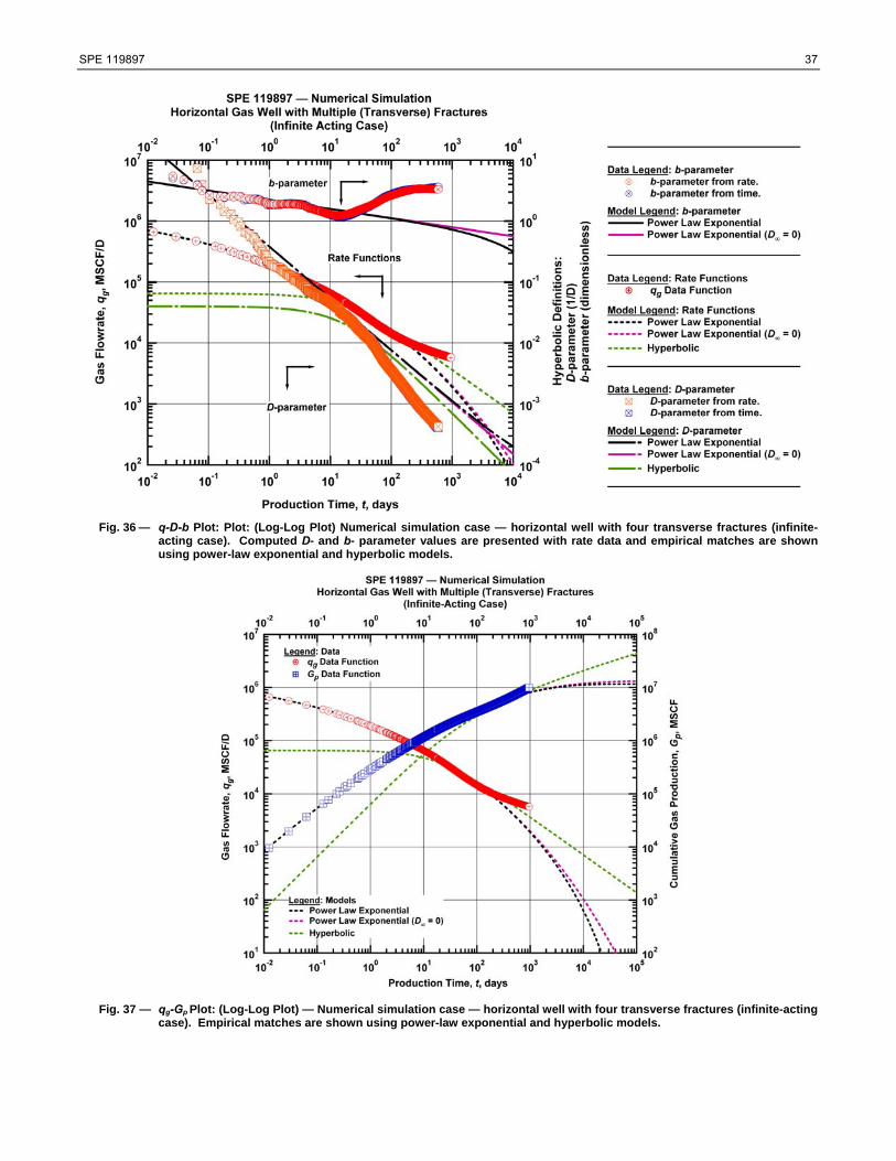
Figs. 34 and 35 present the production forecast for this well on log-log and semilog scales. In addition to the finite-acting case we present the q-D-b plot for the infinite acting case in Fig. 36. Of course, reserves estimation is theoretically impossible when the flow regime is transient. But, at this point we would like to emphasize two points. First, two distinct straight-line trends are exhibited by the computed D-parameter data trend — we believe that the effect of the compound linear flow is reflected as the second straight line on the computed D-parameter data. Second, it is seen that the computed b-parameter data trend exhibits an increasing behavior during transient flow and we again suggest using extreme caution when hyperbolic rate relation is used with b-parameter values higher than 1 as this is an indication that transient flow still exists. Finally, production forecasts are shown in Figs. 37 and 38, respectively for the infinite-acting case using the values obtained from the finite-acting case. The only purpose of these plots is to show the difference between finite- and infinite-acting simulation cases. We conclude this section by emphasizing that the "power-law exponential" formulation is very efficient in estimating the reserves for a horizontal well with multiple transverse fractures.

8 SPE 119897

Discussion In the previous sections, we have demonstrated the applicability of analytical and empirical approaches to analyzing shale gas production data. The current analytical (type-curve) approaches are limited in that they do not account for all the flow regimes that may occur [see Medeiros et al., (2007)]. We have not discussed the use of classic pressure transient analysis methods for analyzing production data; Hagar and Jones (2001) suggested that production data can be treated as a long-term drawdown test and analyzed the radial flow regime in hydraulically-fractured fractured wells using classic derivative analysis to identify the flow regimes. In principal, an approach like this could be used to analyze the various flow regimes (bilinear, radial, linear etc.) identified in multiply-fractured horizontal wells, using diagnostic plots corresponding to the flow regimes. The success of such an approach would depend on data quality; high quality (and frequent) rate/pressure data would be required. We will discuss this approach further in a future paper. The analytical methods used in this work were applied to reservoirs with relatively simple reservoir behavior (single-porosity, single-phase, no desorption etc.); in reality, shale reservoirs developed to date exhibit a wide range in (simple to complex) reservoir behaviors. We are endeavoring to create analytical methods (type-curves, flowing material balance etc.) that can be used for the more complex reservoir behavior encountered in some shale reservoirs. For example, for shale reservoirs exhibiting 2-phase (gas+water) characteristics, we believe some of the analytical methods recently developed for 2-phase CBM reservoirs (Clarkson et al., 2008) may be of use. The Antrim shale is used to test this approach; the Devonian Antrim Shale of the Michigan Basin, with significant exploration and development initiating in the mid- 1980s, is very much unlike most of the shale plays currently being explored and developed. Wells in the Antrim shale perform very much like wells in a 2-phase (gas+ water) coalbed reservoir — and the production in the Antrim shale is presumed to be dominated by natural fractures. The Antrim shale has the following attributes (Reeves et al [1993]):

● Shallow ● Underpressured (< 0.433 psi/ft) ● High adsorbed gas content (can be > 70% of OGIP) ● High permeability (often > 1md) ● Consistent 2-phase flow of gas and water

Table 8 contains data used by Zuber et al [1994] to model a "typical" well illustrates some of these characteristics. Although Zuber et al used a rigorous dual-porosity reservoir simulator (accounting for unsteady-state matrix flow characteristics) to history-match and forecast Antrim shale production, we use a simple analytical CBM ("tank") model in this case. An example is given below (see Fig. 39), where gas and water production has been history-matched using the 2-phase flow analytical simulator, which assumes instantaneous desorption (an approximation). The rate and cumulative production matches are shown in the lower plots. The "hard" (fixed) data input into the model include net thickness, initial reservoir pressure and flowing pressure, adsorption isotherm data and skin, whereas "soft" data include initial phase saturations, absolute and relative permeability (the relative permeability curves used are straight-lines) and drainage area. Two diagnostic plots which are used to validate the match are also included: decline type-curves (upper right) and flowing material balance (upper left). The use of flowing material balance for 2–phase flow CBM reservoirs was discussed previously (see Clarkson et al [2008]); the 2-phase flow type-curves are still under development, but include the use of relative permeability and material balance pseudotime that accounts for desorption. The transformed data in the diagnostic plots are linked to the simulator (i.e., these data honor the same OGIP, pi, etc.) and hence, the diagnostic plots are used for validation only. For example, the FMB plot (upper left) is linear, and points to the same OGIP (0.702 BSCF) as used in the simulator; further, the permeability obtained from the y-axis intercept (see Clarkson et al [2008]) is close to the input value in the simulator (3.53 md versus 3.5 md). The transformed data on the type-curve nearly matches the harmonic stem during depletion; if the OGIP is correct, and the well is draining a volumetric reservoir (with instantaneous desorption), then the data should fall on a b=1 stem. It appears from this limited investigation that techniques developed for 2-phase CBM reservoirs may be applicable to some 2-phase shale gas reservoirs with similar properties. In the above example, we have ignored the matrix transport time (non-instantaneous desorption) and the free-gas porosity in the matrix, which is commonly done in CBM reservoirs. Lewis and (2008) present type-curves for shale reservoirs that exhibit dual-porosity behavior and desorption.

SPE 119897 9 Conclusions

We derive the following conclusions from this work: 1. Using the solution of a single well with an effective fracture as a simplified model for the performance a horizontal

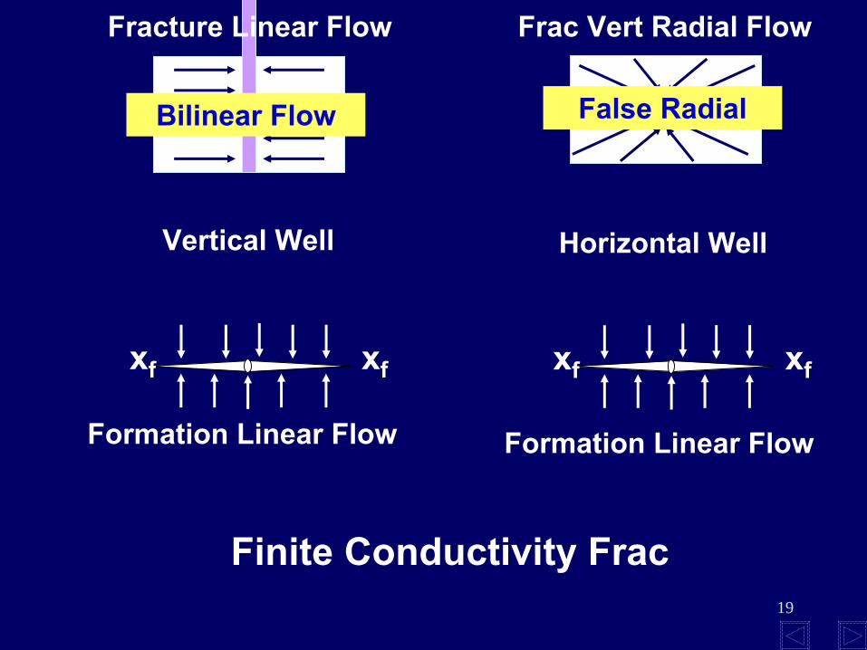
well with multiple transverse fractures may lead to erroneous estimates of the reservoir and fracture parameters: a. A finite conductivity fracture transversely intersecting a horizontal well results in a “false” radial flow.

This is in contrast to the bi-linear flow evident in a vertical well with a finite conductivity fracture. If the fracture is longitudinal (as opposed to transverse) the finite conductivity frac will likely yield a bi-linear flow.

b. The radial flow observed on many multiple-frac shale wells, which has been interpreted as a permeability enhancement caused by the stimulation treatment, may not be that at all. It may be a manifestation of a long, finite conductivity fracture.

c. The concept of Stimulated Reservoir Volume (SRV) which is supported by micro-seismic monitoring of the fracture treatment is not confirmed (nor negated) by the observed radial flow. The radial flow of fractured shale wells is more likely to be a “false” radial flow and may not be representative of the enhanced permeability of the SRV.

d. Ignoring the desorption compressibility and the desorption isotherm gave xf√k and OGIP values that were reasonable. The errors were only nominally larger. The drainage area will be significantly wrong if desorption is not explicitly taken into account, but the OGIP is only marginally affected.

The conclusions of this experiment are based on a limited set of data. A more complete and systematic investigation of the issues is warranted and recommended.

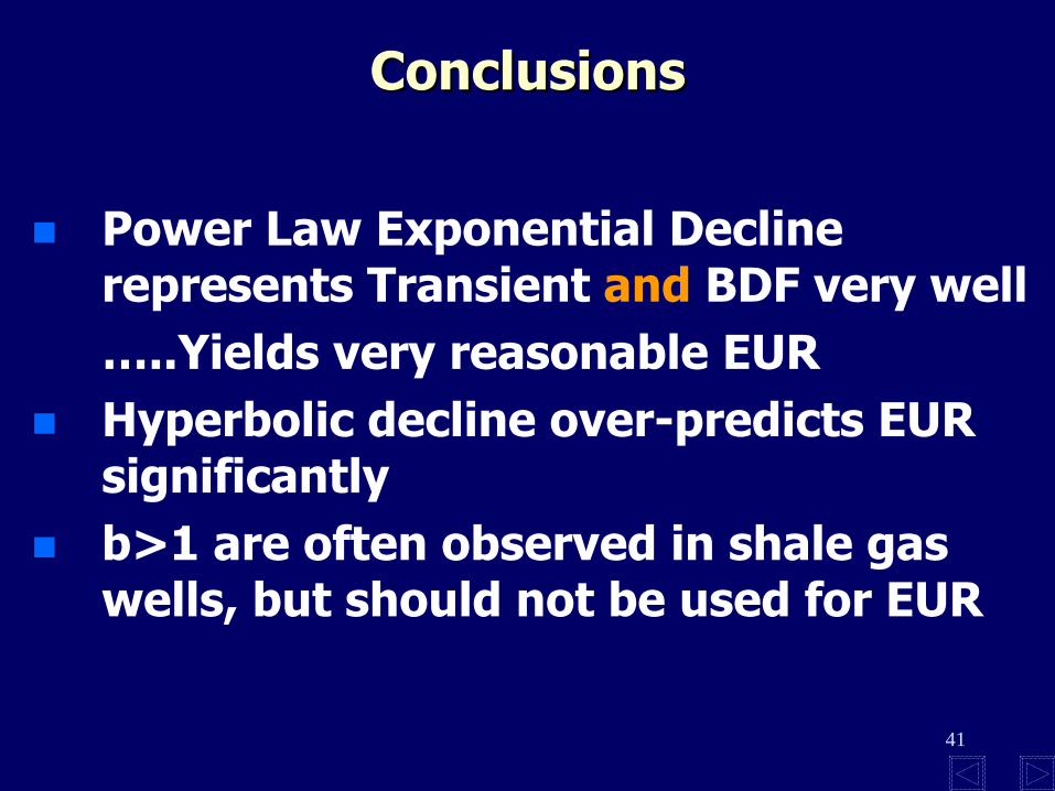
2. When the (publicly available) monthly production data of gas wells from the Barnett Shale are analyzed, it is seen that the recently developed "power-law exponential" rate relation models the rate performance of these wells very successfully (i.e., transient, transition, and boundary-dominated flow regimes can be represented with the new rate relation). This suggests that production forecast of shale gas wells using the "power-law exponential" rate relation should be reliable.

3. We urge extreme caution when hyperbolic rate relation is used. As the present field examples in this work indicate, production from most of shale gas wells would remain in transient flow condition for a considerable period of time (i.e., years). Since the hyperbolic rate relation is only valid for the boundary-dominated flow regime, the analyst should identify/differentiate the flow regimes very carefully prior to using the hyperbolic rate relation. This work also shows that using a b-parameter value higher than 1 to match the part where the data is still in transient/-transition flow regime, yields enormously high reserves estimate which has nothing to do with reality.

4. The "compound linear flow regime" concept, which was earlier put forth by van Kruysdijk and Dullaert [1989] for a horizontal well with multiple transverse fractures, is verified by the numerical simulation results obtained in this work. In other words, we can state that our efforts in the modeling a horizontal well with multiple transverse fractures have been successful.

5. Computed D-parameter data trend using the rate data generated by the simulator suggests a strong power-law behavior indicating that the application of the "power-law exponential" relation in reserves estimate would be very successful. As expected, application of the "power-law exponential" relation to the numerical simulation results yields almost the same reserves as with the gas-in-place input in the simulation. We conclude that production forecasts of the horizontal wells with multiple fractures can consistently be performed with the "power-law exponential" relation.

6. It is possible to analyze some shale gas reservoirs using the techniques developed for 2-phase CBM reservoirs provided that similar reservoir properties exist. We would like to mention that some of the shale gas reservoir systems behave very analogous to that of coal-bed methane systems. However, we urge caution not to generalize this statement to most of the shale gas reservoir systems as each shale gas reservoir system has unique character.

10 SPE 119897

Nomenclature

Variables

A = Drainage area, acres b = Arps' decline exponent, dimensionless cf = Formation compressibility, psi-1 cg = Gas compressibility, psi-1 ct = Total compressibility, psi-1 CD = Wellbore storage coefficient, dimensionless D = Arps' "loss ratio," D-1 Di = Arps' initial decline rate (hyperbolic model), D-1 D1 = Decline constant "intercept" at 1 time unit defined by Eq. 3 [i.e., D(t=1 day)], D-1 D∞ = Decline constant at "infinite time" defined by Eq. 3 [i.e., D(t=∞)], D-1

iD̂ = Decline constant defined by Eq. 6 [i.e., nDDi /ˆ 1= ], D-1 FcD = Fracture conductivity, dimensionless G = Original (contacted) gas-in-place, MSCF Gp = Cumulative gas production, MSCF Gp,max = Maximum gas production, MSCF h = Net pay thickness, ft k = Average reservoir permeability, md Lh = Horizontal well length, ft m(p) = Pseudopressure, psia2/cp Δm(p) = Pseudopressure drop [m(pi)- m(pwf)], psia2/cp n = Time exponent defined by Eq. x pi = Initial reservoir pressure, psia pi = Initial reservoir pressure, psia pwf = Flowing bottomhole pressure, psia Δp = Pressure drop (pi-pwf), psi qg = Gas production rate, MSCF/D qi = Initial production rate, MSCF/D or STB/D

iq̂ = Rate "intercept" defined by Eq. 6 [i.e., q(t=0)], MSCF/D qw = Water production rate, STB/D Qw = Cumulative water production, MSTB re = Reservoir drainage radius, ft rw = Wellbore radius, ft s = Skin factor, dimensionless Sg = gas saturation, fraction Swi = Initial water saturation, fraction t = Time, days tca = (gas) Pseudotime, days tmb = (gas) Material balance time, days Tr = Reservoir temperature, °F xf = Fracture half-length, ft wf = Fracture width, in zw = Position of the horizontal well (z-direction), ft z = Gas compressibility factor

Greek Variables

γg = Reservoir gas specific gravity (air = 1) φ = Effective porosity, fraction μg = Gas viscosity, cp

SPE 119897 11

References

Amini, S., Ilk, D., and Blasingame, T.A. 2007. Evaluation of the Elliptical Flow Period for Hydraulically-Fractured Wells in Tight Gas Sands — Theoretical Aspects and Practical Considerations. Paper SPE 106308 presented at the 2007 SPE Hydraulic Fracturing Technology Conference held in College Station, Texas, U.S.A., 29–31 January 2007.

Arps, J.J. 1945. Analysis of Decline Curves. Trans. AIME 160: 228-247.

Bourdet, D., Ayoub, J.A., and Pirard, Y.M. 1989. Use of Pressure Derivative in Well-Test Interpretation. SPEFE 4 (2): 228-293-302.

Clarkson, C.R., Jordan, C.L., Gierhart, R.R., and Seidle, J.P. 2008 Production Data Analysis of Coalbed-Methane Wells. SPEREE. 11 (2): 311-325.

Johnson, R.H. and Bollens, A.L. 1927. The Loss Ratio Method of Extrapolating Oil Well Decline Curves. Trans. AIME 77: 771.

Hager, C.J. and Jones, J.R. 2001. Analyzing Flowing Production Data with Standard Pressure Transient Methods. Paper SPE 71033 presented at the SPE Rocky Mountain Petroleum Technology Conference, Keystone. Colorado, 21-23 May.

Ilk, D., Mattar, L., and Blasingame, T.A.. 2007a. Production Data Analysis — Future Practices for Analysis and Interpretation. Paper CIM 2007-174 presented at the 58th Annual Technical Meeting of the Petroleum Society, Calgary, AL, Canada, 12-14 June.

Ilk, D., Rushing, J.A., Sullivan, R.B., and Blasingame, T.A. 2007b. Evaluating the Impact of Waterfrac Technologies on Gas Recovery Efficiency: Case Studies Using Elliptical Flow Production Data Analysis. Paper SPE 110187 presented at the 2007 Annual SPE Technical Conference and Exhibition, Anaheim, CA., 11-14 November.

Ilk, D., Rushing, J.A., and Blasingame, T.A. 2008a. Estimating Reserves Using the Arps Hyperbolic Rate-Time Relation — Theory, Practice and Pitfalls. Paper CIM 2008-108 presented at the 59th Annual Technical Meeting of the Petroleum Society, Calgary, Alberta, Canada, 17-19 June. (in preparation)

Ilk, D., Perego, A.D., Rushing, J.A., and Blasingame, T.A. 2008b. Exponential vs. Hyperbolic Decline in Tight Gas Sands — Understanding the Origin and Implications for Reserve Estimates Using Arps' Decline Curves. Paper SPE 116731 presented at the SPE Annual Technical Conference and Exhibition, Denver, Colorado, 21-24 September.

Lewis, A.M. and Hughs, R. G. 2008. Production Data Analysis of Shale Gas Reservoirs. Paper SPE 116688 presented at the SPE Annual Technical Conference and Exhibition, Denver, Colorado, 21-24 September. Mattar, L. and Anderson, D.M. 2003. A Systematic and Comprehensive Methodology for Advanced Analysis of Production Data. Paper SPE 84472 presented at the SPE Annual Technical Conference and Exhibition, Denver, CO, 5–8 October. Medeiros, F., Ozkan, E., and Kazemi, H. 2007. Productivity and Drainage Area of Fractured Horizontal Wells in Tight Gas Reservoirs. Paper SPE 108110 presented at the SPE Rocky Mountain Oil & Gas Technology Symposium, Denver, CO., 16-18 April.

Reeves, S.R., Cox, D.O., Smith, M.B., and Schatz, J.F. 1993. Stimulation Technology in the Antrim Shale. Paper SPE 26203 presented at the SPE Gas Technology Symposium, Calgary, Alberta, 28-30 June.

Valko, P.P., and Amini, S. 2007. The Method of Distributed Volumetric Sources for Calculating the Transient and Pseudosteady-State Productivity of Complex Well-Fracture Configurations. Paper SPE 106279 presented at the SPE Hydraulic Fracturing Conference, College Station, TX, 29-31 January.

van Kruysdijk, C.P.J.W. and Dullaert, G.M. 1989. A Boundary Element Solution of the Transient Pressure Response of Multiply Fractured Horizontal Wells. Paper presented at the 2nd European Conference on the Mathematics of Oil Recovery, Cambridge, England.

Zuber, M.D., Frantz Jr., J.H., Gatens III, J.M. 1994. Reservoir Characterization and Production Forecasting for Antrim Shale Wells: An Integrated Reservoir Analysis Methodology. Paper SPE 28606 presented at the SPE Annual Technical Conference and Exhibition, New Orleans, Louisiana. 25-28 September. Warpinski, N.R, Kramm, R.C.; Heinze, J.R., Waltman, C.K. 2005. Comparison of Single- and Dual-Array Microseismic Mapping Techniques in the Barnett Shale. Paper SPE 95568 Presented at SPE Annual Technical Conference and Exhibition, Dallas, Texas, 9-12 October 2005.

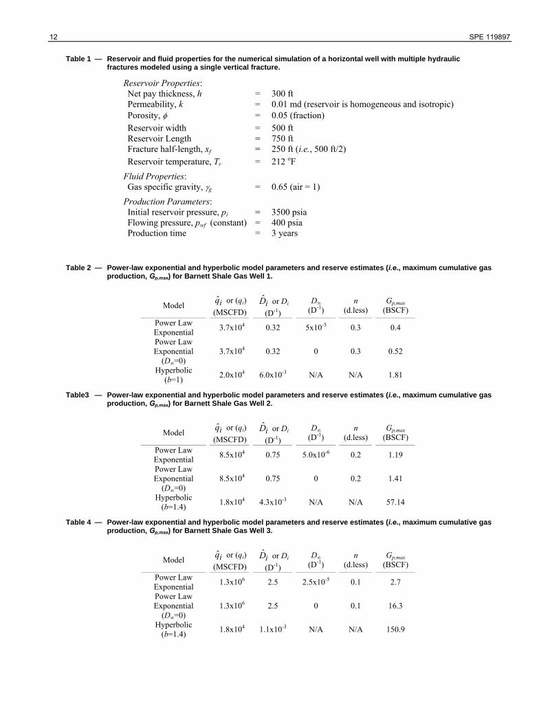
12 SPE 119897

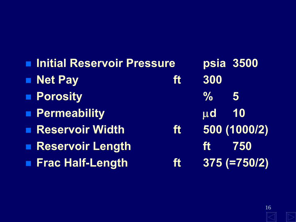
Table 1 — Reservoir and fluid properties for the numerical simulation of a horizontal well with multiple hydraulic fractures modeled using a single vertical fracture.

Reservoir Properties: Net pay thickness, h = 300 ft Permeability, k = 0.01 md (reservoir is homogeneous and isotropic) Porosity, φ = 0.05 (fraction)

Reservoir width = 500 ft Reservoir Length = 750 ft Fracture half-length, xf = 250 ft (i.e., 500 ft/2)

Reservoir temperature, Tr = 212 oF Fluid Properties:

Gas specific gravity, γg = 0.65 (air = 1) Production Parameters:

Initial reservoir pressure, pi = 3500 psia Flowing pressure, pwf (constant) = 400 psia Production time = 3 years

Table 2 — Power-law exponential and hyperbolic model parameters and reserve estimates (i.e., maximum cumulative gas

production, Gp,max) for Barnett Shale Gas Well 1.

Model

iq̂ or (qi)(MSCFD)

iD̂ or Di (D-1)

D∞

(D-1)

n

(d.less)

Gp,max

(BSCF)

Power Law Exponential 3.7x104 0.32 5x10-5 0.3 0.4

Power Law Exponential

(D∞=0) 3.7x104 0.32 0 0.3 0.52

Hyperbolic (b=1) 2.0x104 6.0x10-3 N/A N/A 1.81

Table3 — Power-law exponential and hyperbolic model parameters and reserve estimates (i.e., maximum cumulative gas production, Gp,max) for Barnett Shale Gas Well 2.

Model

iq̂ or (qi)(MSCFD)

iD̂ or Di (D-1)

D∞

(D-1)

n

(d.less)

Gp,max

(BSCF)

Power Law Exponential 8.5x104 0.75 5.0x10-6 0.2 1.19


(D∞=0) 8.5x104 0.75 0 0.2 1.41

Hyperbolic (b=1.4) 1.8x104 4.3x10-3 N/A N/A 57.14

Table 4 — Power-law exponential and hyperbolic model parameters and reserve estimates (i.e., maximum cumulative gas production, Gp,max) for Barnett Shale Gas Well 3.

Model

iq̂ or (qi)(MSCFD)

iD̂ or Di (D-1)

D∞

(D-1)

n

(d.less)

Gp,max

(BSCF)



(D∞=0) 1.3x106 2.5 0 0.1 16.3


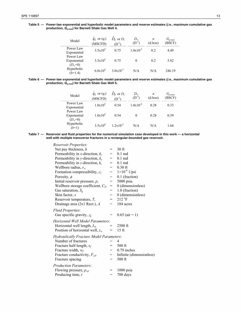
SPE 119897 13

Table 5 — Power-law exponential and hyperbolic model parameters and reserve estimates (i.e., maximum cumulative gas production, Gp,max) for Barnett Shale Gas Well 4.

Model

iq̂ or (qi)(MSCFD)

iD̂ or Di (D-1)

D∞

(D-1)

n

(d.less)

Gp,max

(BSCF)



(D∞=0) 3.5x105 0.75 0 0.2 5.82


Table 6 — Power-law exponential and hyperbolic model parameters and reserve estimates (i.e., maximum cumulative gas

production, Gp,max) for Barnett Shale Gas Well 5.

Model

iq̂ or (qi)(MSCFD)

iD̂ or Di (D-1)

D∞

(D-1)

n

(d.less)

Gp,max

(BSCF)



(D∞=0) 1.0x105 0.54 0 0.28 0.39

Hyperbolic (b=1) 3.5x104 1.2x10-2 N/A N/A 1.64

Table 7 — Reservoir and fluid properties for the numerical simulation case developed in this work — a horizontal

well with multiple transverse fractures in a rectangular-bounded gas reservoir.

Reservoir Properties: Net pay thickness, h = 30 ft Permeability in x-direction, kx = 0.1 md Permeability in y-direction, ky = 0.1 md Permeability in z-direction, kz = 0.1 md Wellbore radius, rw = 0.30 ft Formation compressibility, cf = 1×10-9 1/psi Porosity, φ = 0.1 (fraction) Initial reservoir pressure, pi = 5000 psia Wellbore storage coefficient, CD = 0 (dimensionless) Gas saturation, Sg = 1.0 (fraction) Skin factor, s = 0 (dimensionless) Reservoir temperature, Tr = 212 oF Drainage area (2x1 Rect.), A = 184 acres

Fluid Properties: Gas specific gravity, γg = 0.65 (air = 1)

Horizontal Well Model Parameters: Horizontal well length, Lh = 2500 ft Position of horizontal well, zw = 15 ft

Hydraulically Fracture Model Parameters: Number of fractures = 4 Fracture half-length, xf = 500 ft Fracture width, wf = 0.79 inches Fracture conductivity, FcD = Infinite (dimensionless) Fracture spacing = 500 ft

Production Parameters: Flowing pressure, pwf = 1000 psia Producing time, t = 700 days

14 SPE 119897

Table 8 — Input data of Zuber et al [1994] (dual-porosity reservoir model).

Parameter Zuber et al Base Value

Area, A = 80 acres Flowing Bottomhole Pressure, pwf = 75 psia Net Pay, h = 100 ft Initial Reservoir Pressure, pi = 550 psia Initial Water Saturation, Sw = 750 ft Natural Fracture Porosity, φf = 0.002 (fraction) Initial Water Saturation, Sw = 1 (fraction) Relative Permeability, kr = see Fig. 7 (Zuber et al) Matrix Gas Porosity, φm = 0.03 (fraction) Matrix Permeability, km = 2x10-8 md Bulk Permeability, kb = 5 md Natural Fracture Spacing = 4 ft Hydraulic Fracture Half-Length, xf = 100 ft Hydraulic Fracture Permeability, kf = 7854 md Hydraulic Fracture Conductivity, Fc = 6283 md-ft Langmuir Volume, VL = 97.8 SCF/ton Langmuir Pressure, pL = 729.5 psia Shale Density, ρsh = 2.23 gr/cc Gas-in-place, G = 1.3917 BSCF Peak Gas Production, Gpeak = 0.250 BSCF

SPE 119897 15

xf xf (infinite/finite conductivity)

Fig. 1 - Bi-wing hydraulic fracture

Fig. 2 - Stimulated Reservoir Volume (SRV)

16 SPE 119897

Linear Flow Slope = -1/2

Radial Flow Slope = 0

Log

Der

ivat

ive

Fig. 3 - Derivative Type curve of bi-wing fracture in large low-perm reservoir.

Radial Flow Slope = 0

BDF Flow Slope = -1

Log

Der

ivat

ive

Fig. 4 - Derivative Type curve of SRV.

Log pseudotime

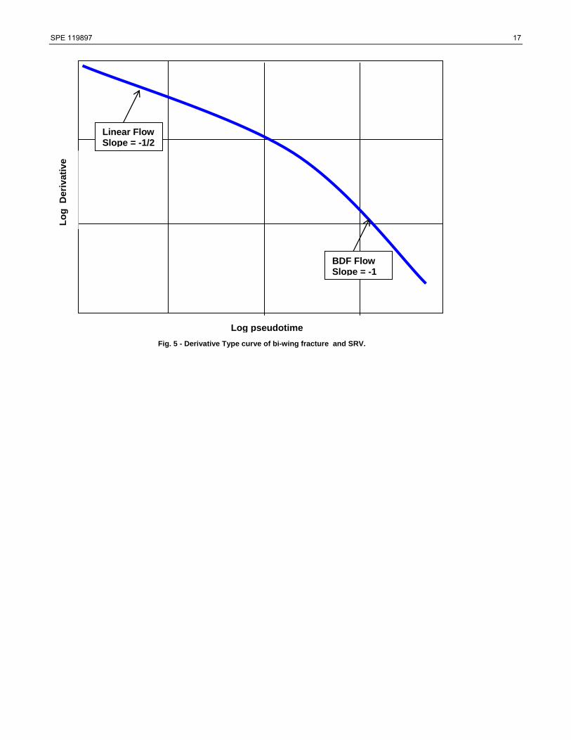
SPE 119897 17

Linear Flow Slope = -1/2

BDF Flow Slope = -1

Log

Der

ivat

ive

Fig. 5 - Derivative Type curve of bi-wing fracture and SRV.

Log pseudotime

18 SPE 119897

Fig. 6 - Field Case 1: Hydraulically-fractured vertical well.

1 year of flow

SPE 119897 19

Xe/Xf = 1

Fig. 7 - Field Case 2: Horizontal well with multiple fractures.

Linear flow (-1/2) xf√k = 7 md-ft

BDF (-1) OGIP = 5 BCF

9 months of flow Start of BDF

20 SPE 119897

Fig. 8 - Field Case 3: Horizontal well with multiple fractures.

BDF OGIP = 1 BCF

40 days of flow Start of BDF

Linear flow (-1/2)

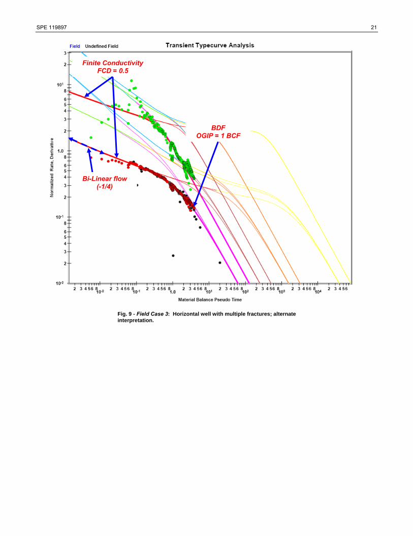
SPE 119897 21

Fig. 9 - Field Case 3: Horizontal well with multiple fractures; alternate interpretation.

BDF OGIP = 1 BCF

Bi-Linear flow (-1/4)

Finite Conductivity FCD = 0.5

22 SPE 119897

Fig. 10— Schematic Plot: Approximation for the performance of a horizontal well with multiple hydraulic fractures using the

solution for only a single vertical well with a hydraulic fracture — multiplied by the number of fractures.

SPE 119897 23

Fig. 11 — Simulated Example 1: Infinite Conductivity Vertical Fracture Case (modeled using FcD=200).

24 SPE 119897

Fig. 12 — Simulated Case 2: Finite Conductivity Vertical Fracture Case (modeled using FcD=2).

SPE 119897 25

Fig. 13 — q-D-b Plot: Plot: (Log-Log Plot) Barnett shale gas well 1. Computed D- and b- parameter values are presented with rate data and empirical matches are shown using power-law exponential and hyperbolic models.

Fig. 14 — qg-Gp Plot: (Log-Log Plot) — Barnett shale gas well 1. Empirical matches are shown using power-law exponential and hyperbolic models.

26 SPE 119897

Fig. 15 — qg-Gp Plot: (Semilog Plot) — Barnett shale gas well 1. Empirical matches are shown using power-law exponential and hyperbolic models.

SPE 119897 27



28 SPE 119897

Fig. 18 — qg-Gp Plot: (Semilog Plot) — Barnett shale gas well 2. Empirical matches are shown using power-law exponential and

hyperbolic models.

Fig. 19 — q-D-b Plot: Plot: (Log-Log Plot) Barnett shale gas well 3. Computed D- and b- parameter values are presented with

rate data and empirical matches are shown using power-law exponential and hyperbolic models.

SPE 119897 29



30 SPE 119897



SPE 119897 31



32 SPE 119897



SPE 119897 33

Fig. 28 — Schematic Plot: Base simulation model for a horizontal well with multiple hydraulic fractures.

Fig. 29 — Schematic Plot: Compound linear flow concept of van Kruijsdijk and Dullaert [1989].

34 SPE 119897

Fig. 30 — Numerical simulation results for a finite and infinite-acting reservoir cases presented on a specialized (square-root of time) derivative plot — illustrates compound linear flow concept of van Kruijsdijk and Dullaert [1989].

Fig. 31 — Diagnostic Plot: (Log-Log Plot) Numerical simulation case — horizontal well with four transverse fractures (infinite-acting case). Rate and auxiliary rate functions are plotted versus material balance time for flow regime identification.

SPE 119897 35

Fig. 32 — Diagnostic Plot: (Log-Log Plot) Numerical simulation case — horizontal well with four transverse fractures (finite-acting case, [2x1] rectangle). Rate and auxiliary rate functions are plotted versus material balance time for flow regime identification.

Fig. 33 — q-D-b Plot: Plot: (Log-Log Plot) Numerical simulation case — horizontal well with four transverse fractures (finite-acting case, [2x1] rectangle). Computed D- and b- parameter values are presented with rate data and empirical matches are shown using power-law exponential and hyperbolic models.

36 SPE 119897

Fig. 34 — qg-Gp Plot: (Log-Log Plot) — Numerical simulation case — horizontal well with four transverse fractures (finite-acting

case, [2x1] rectangle). Empirical matches are shown using power-law exponential and hyperbolic models.

Fig. 35 — qg-Gp Plot: (Semilog Plot) — Numerical simulation case — horizontal well with four transverse fractures (finite-acting

case, [2x1] rectangle). Empirical matches are shown using power-law exponential and hyperbolic models.

SPE 119897 37

Fig. 36 — q-D-b Plot: Plot: (Log-Log Plot) Numerical simulation case — horizontal well with four transverse fractures (infinite-acting case). Computed D- and b- parameter values are presented with rate data and empirical matches are shown using power-law exponential and hyperbolic models.

Fig. 37 — qg-Gp Plot: (Log-Log Plot) — Numerical simulation case — horizontal well with four transverse fractures (infinite-acting case). Empirical matches are shown using power-law exponential and hyperbolic models.

38 SPE 119897

Fig. 38 — qg-Gp Plot: (Semilog Plot) — Numerical simulation case — horizontal well with four transverse fractures (infinite-acting case). Empirical matches are shown using power-law exponential and hyperbolic models.

SPE 119897 39

Fig. 39 — (Dashboard Plot) — Production analysis for a well completed in Antrim shale. Dual porosity CBM model is employed in the analysis of the production data.

2

OutlineOutlineMultiMulti--frac Horizontal Wellsfrac Horizontal Wells–– BiBi--Wing FracturesWing Fractures–– Stimulated Reservoir VolumeStimulated Reservoir Volume

Theoretical / Observed PerformanceTheoretical / Observed Performance

Synthetic ExamplesSynthetic Examples

Power Law DeclinePower Law Decline

3

xf

xf

Bi-wing hydraulic fracture

4

Linear FlowSlope = -1/2

Radial FlowSlope = 0

Log

Der

ivat

ive

Derivative of bi-wing frac in large low-perm reservoir

Log pseudotime

5

xf

xf

Bi-wing hydraulic fractureSMALL Reservoir

6

Linear FlowSlope = -1/2

Boundary-

Dominated FlowSlope = -1

Log

Der

ivat

ive

Derivative of bi-wing frac in SMALL low-perm reservoirLog pseudotime

7

Stimulated Reservoir Volume (SRV)

Micro-seismic Mapping

8

Radial FlowSlope = 0

BDF FlowSlope = -1

Log

Der

ivat

ive

Derivative Type curve of SRV

Log pseudotime

9

Well #1Well #1

10

Xe/Xf

= 1

Ex1: Multiple-Frac’d Horizontal

Linear flow (-1/2)xf√k

= 7 md-ft

BDF (-1)OGIP = 5 BCF

9 months of flowStart of BDF

4 X 250-ton fracs

11

Well #2Well #2

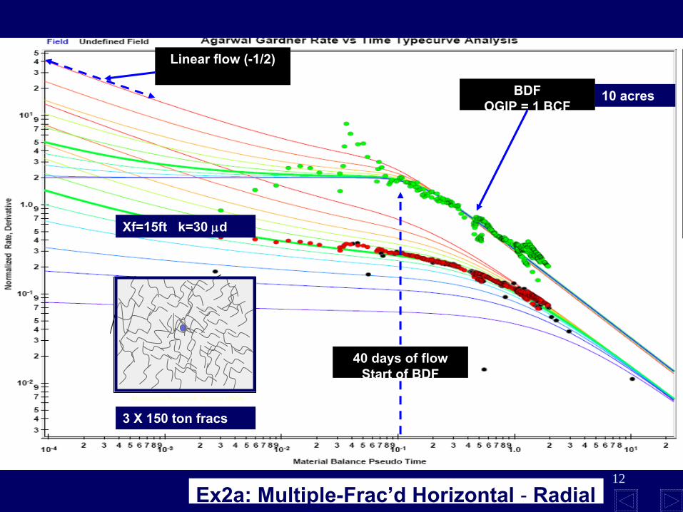
12Ex2a: Multiple-Frac’d Horizontal

- Radial

BDF OGIP = 1 BCF

40 days of flowStart of BDF

Linear flow (-1/2)

Stimulated Reservoir Volume (SRV)

Xf=15ft k=30 μd

3 X 150 ton fracs

10 acres

13Ex2b: Multiple-Frac’d Horizontal Well; Finite Conductivity Frac

BDF OGIP = 1 BCF

Bi-Linear flow (-1/4)

Finite Conductivity FCD = 0.5

3 X 150-ton fracs

Xf=300ft k=30 μd

10 acres

14

Radial Flow Radial Flow –– SRVSRVOrOr

Finite Conductivity FracFinite Conductivity Frac

15

= 4 X

16

Initial Reservoir Pressure psia 3500Net Pay ft 300Porosity % 5Permeability μd 10Reservoir Width ft 500 (1000/2)Reservoir Length ft 750Frac Half-Length ft 375 (=750/2)

17

Ex S1, Single-Frac Horiz

Well (Inf. Cond.)

BDF (-1)OGIP = actual

Start of BDF

Linear flow (-1/2)xf√k

= actual

Κf

= ∞

18

BDF OGIP = actual

FalseRadial Flow

90 days of flowStart of BDF

Ex S2: Single-Frac Horiz

Well (Finite Conductivity)

FCD = 2

k= 120 μd vs 10

μdXf

= 15 ft vs

1000

ft

Small FCD

or

SRVStimulated Reservoir Volume (SRV)

19

xf

xf

Vertical Well

Finite Conductivity Frac

Horizontal Well

xf

xf

Formation Linear FlowFormation Linear Flow

Frac Vert

Radial FlowFracture Linear Flow

Bilinear Flow False Radial

20

Radial Flow Radial Flow –– SRVSRVOrOr

Finite Conductivity FracFinite Conductivity Frac????

K, XK, Xf f ????GasGas--InIn--Place Place YESYESForecast of reserves Forecast of reserves YESYES

21

Rate Decline AnalysisRate Decline Analysis

Exponential Decline:Exponential Decline:q=q=qq

ii

exp (exp (--DtDt))

Hyperbolic Decline:Hyperbolic Decline:q=q=qq

ii

/(1+bD/(1+bD

ii

t)t)1/b1/b

Conventional: b = 0 Conventional: b = 0 …….. 1.. 1Transient: b>1Transient: b>1

22

Summer 2007Summer 2007

Eureka!Eureka!

23

b > 1 ??

24

Rate Decline AnalysisRate Decline Analysis

Universal Curve FitUniversal Curve FitPower Law Exponential Decline:Power Law Exponential Decline:

q=q=qq

ii

exp (exp (--DD

∞∞

tt ––DD

ii

ttnn))

25

Decline Rate Decline Rate D D ΞΞ

1/q 1/q dq/dtdq/dt

Loss RatioLoss Ratio

1/D1/D

Derivative of Loss RatioDerivative of Loss Ratio b b ΞΞ

d (1/D)/dtd (1/D)/dt

DefinitionsDefinitions

26

RelationshipsRelationships

Exponential Decline: Exponential Decline: D = constantD = constantb=0b=0

Hyperbolic Decline: Hyperbolic Decline: b = constant b = constant D D ≠≠

constant constant

D=1/(1/DD=1/(1/D

ii

+bt)+bt)

Power Law : Power Law : D D ≠≠

constantconstantExp Decline Exp Decline b b ≠≠

constantconstant

D=DD=D∞∞

++DD

11

t t --(1(1--n)n)

27

28

Given : q Given : q vsvs

t, calculate:t, calculate:

DD ΞΞ

1/q 1/q dq/dtdq/dt

Decline RateDecline Rate

1/D1/D

(Loss Ratio)(Loss Ratio)

bb ΞΞ

d (1/D)/dt d (1/D)/dt (Derivative of Loss Ratio)(Derivative of Loss Ratio)

Plot on logPlot on log--log graphlog graphBest fitBest fit

D = DD = D

∞∞

+ + DD

1 1 t t -- ( 1 ( 1 –– n )n )

ProcedureProcedure

29

30

Model EUR (BCF)

Power Law

Expon ential0.4 0.4

Power Law

Expon ential

(D∞

=0)

0.50.5

Hyper bolic

(b=1)(b=1)1.81.8

31

32

33

34

35

Model EUR 1(BCF)

EUR 2(BCF)

EUR 3(BCF)

EUR 4(BCF)

EUR 5(BCF)


0.4 0.4 1.21.2 2.72.7 4.54.5 0.30.3


(D∞

=0) 0.50.5 1.41.4 1616 5.85.8 0.40.4

Hyperbolic (b=1) 1.81.8

(b=1)(b=1)5757

(b=1.4)(b=1.4)151 151

(b=1.4)(b=1.4)246 246

(b=1.4)(b=1.4)1.6 1.6

(b=1)(b=1)

36

37

38

Model EUR (BCF)

Power Law

Expon entialX 1 X 1

Power Law

Expon ential

(D∞

=0)

X 1.1X 1.1

Hyper bolic X 3X 3

(b=1)(b=1)

39

40

ConclusionsConclusions

Some shale fracs behave like bi-wing….Some behave like SRVBi-wing, Finite Conductivity Frac in Horizontal well does NOT yield bilinear flow….False Radial

Flow, with very short

frac lengthsOGIP is reasonable, even when desorption is not explicitly used

41

ConclusionsConclusions

Power Law Exponential Decline represents Transient and BDF very well…..Yields very reasonable EURHyperbolic decline over-predicts EUR significantlyb>1 are often observed in shale gas wells, but should not be used for EUR

42

SPE 119897 Production Analysis and Forecasting of … 119897 3 reservoir properties and stimulation information. We use both field cases and simulated cases to ...

Documents