SPATIO-TEMPORAL LOCAL INTERPOLATION OF GLOBAL OCEAN HEAT TRANSPORT USING ARGO FLOATS: A DEBIASED LATENT GAUSSIAN PROCESS APPROACH BY BEOMJO PARK 1,* ,MIKAEL KUUSELA 1,† ,DONATA GIGLIO 2 AND ALISON GRAY 3 1 Dept. of Statistics & Data Science, Carnegie Mellon University, * [email protected]; † [email protected] 2 Dept. of Atmospheric and Oceanic Sciences, University of Colorado Boulder, [email protected] 3 School of Oceanography, University of Washington, [email protected] The world ocean plays a key role in redistributing heat in the climate sys- tem and hence in regulating Earth’s climate. Yet statistical analysis of ocean heat transport suffers from partially incomplete large-scale data intertwined with complex spatio-temporal dynamics, as well as from potential model mis- specification. We present a comprehensive spatio-temporal statistical frame- work tailored to interpolating the global ocean heat transport using in-situ Argo profiling float measurements. We formalize the statistical challenges us- ing latent local Gaussian process regression accompanied by a two-stage fit- ting procedure. We introduce an approximate Expectation-Maximization al- gorithm to jointly estimate both the mean field and the covariance parameters, and refine the potentially under-specified mean field model with a debiasing procedure. This approach provides data-driven global ocean heat transport fields that vary in both space and time and can provide insights into crucial dynamical phenomena, such as El Niño & La Niña, as well as the global cli- matological mean heat transport field, which by itself is of scientific interest. The proposed framework and the Argo-based estimates are thoroughly vali- dated with state-of-the-art multimission satellite products and shown to yield realistic subsurface ocean heat transport estimates. 1. Introduction. The ocean plays a pivotal role in regulating Earth’s climate on regional to global scales (e.g., Bryden and Imawaki, 2001; Macdonald and Baringer, 2013; Stocker, 2013). Notably, it redistributes the excess heat taken up at the equator, transporting it to higher latitudes where it is released to the atmosphere (Trenberth and Solomon, 1994; Ganachaud and Wunsch, 2000; Trenberth and Caron, 2001; Forget and Ferreira, 2019). Convergence and divergence of heat in the ocean also have impacts on regional sea level (via thermal expansion of sea water, e.g., Forget and Ponte (2015)), with implications for local populations. Ocean heat transport can additionally regulate regional temperature extremes in the ocean, with im- plications for marine ecosystems. As an example of the latter, Behrens, Fernandez and Sutton (2019) describe a causal link between ocean heat content and the area and intensity of marine heatwaves in the Tasman Sea: ocean heat content fluctuations in the TasmanSea are largely controlled by meridional transport of heat in the ocean; hence, better estimates of ocean heat transport can help improve forecasts of marine heatwaves, with potential implications for the management of ecosystems in Australasia. Obtaining an accurate picture of the heat transport within and across ocean basins is therefore critical to understanding changes in the climate system and for data-driven policy and decision making in a changing climate. In this paper, we present a statistical framework to characterize ocean heat transport (OHT) over the global ice-free ocean during 2007-2018, based on direct observations of temperature Keywords and phrases: latent Gaussian process regression, local kriging, approximate EM, model misspecifi- cation, physical oceanography. 1 arXiv:2105.09707v2 [stat.AP] 20 Dec 2021

Welcome message from author
This document is posted to help you gain knowledge. Please leave a comment to let me know what you think about it! Share it to your friends and learn new things together.
Transcript
SPATIO-TEMPORAL LOCAL INTERPOLATION OF GLOBAL OCEAN HEATTRANSPORT USING ARGO FLOATS: A DEBIASED LATENT GAUSSIAN
PROCESS APPROACH
BY BEOMJO PARK1,*, MIKAEL KUUSELA1,†, DONATA GIGLIO2 AND ALISON GRAY3
1Dept. of Statistics & Data Science, Carnegie Mellon University, *[email protected]; †[email protected]
2Dept. of Atmospheric and Oceanic Sciences, University of Colorado Boulder, [email protected]
3School of Oceanography, University of Washington, [email protected]
The world ocean plays a key role in redistributing heat in the climate sys-tem and hence in regulating Earth’s climate. Yet statistical analysis of oceanheat transport suffers from partially incomplete large-scale data intertwinedwith complex spatio-temporal dynamics, as well as from potential model mis-specification. We present a comprehensive spatio-temporal statistical frame-work tailored to interpolating the global ocean heat transport using in-situArgo profiling float measurements. We formalize the statistical challenges us-ing latent local Gaussian process regression accompanied by a two-stage fit-ting procedure. We introduce an approximate Expectation-Maximization al-gorithm to jointly estimate both the mean field and the covariance parameters,and refine the potentially under-specified mean field model with a debiasingprocedure. This approach provides data-driven global ocean heat transportfields that vary in both space and time and can provide insights into crucialdynamical phenomena, such as El Niño & La Niña, as well as the global cli-matological mean heat transport field, which by itself is of scientific interest.The proposed framework and the Argo-based estimates are thoroughly vali-dated with state-of-the-art multimission satellite products and shown to yieldrealistic subsurface ocean heat transport estimates.
1. Introduction. The ocean plays a pivotal role in regulating Earth’s climate on regionalto global scales (e.g., Bryden and Imawaki, 2001; Macdonald and Baringer, 2013; Stocker,2013). Notably, it redistributes the excess heat taken up at the equator, transporting it to higherlatitudes where it is released to the atmosphere (Trenberth and Solomon, 1994; Ganachaudand Wunsch, 2000; Trenberth and Caron, 2001; Forget and Ferreira, 2019). Convergence anddivergence of heat in the ocean also have impacts on regional sea level (via thermal expansionof sea water, e.g., Forget and Ponte (2015)), with implications for local populations. Oceanheat transport can additionally regulate regional temperature extremes in the ocean, with im-plications for marine ecosystems. As an example of the latter, Behrens, Fernandez and Sutton(2019) describe a causal link between ocean heat content and the area and intensity of marineheatwaves in the Tasman Sea: ocean heat content fluctuations in the Tasman Sea are largelycontrolled by meridional transport of heat in the ocean; hence, better estimates of ocean heattransport can help improve forecasts of marine heatwaves, with potential implications for themanagement of ecosystems in Australasia. Obtaining an accurate picture of the heat transportwithin and across ocean basins is therefore critical to understanding changes in the climatesystem and for data-driven policy and decision making in a changing climate.
In this paper, we present a statistical framework to characterize ocean heat transport (OHT)over the global ice-free ocean during 2007-2018, based on direct observations of temperature
Keywords and phrases: latent Gaussian process regression, local kriging, approximate EM, model misspecifi-cation, physical oceanography.
1
arX
iv:2
105.
0970
7v2
[st
at.A
P] 2
0 D
ec 2
021
2
and salinity in the upper 2000 m of the ocean. Historically, global OHT has been estimated in-directly by subtracting the atmospheric component from total heat transport estimates (Tren-berth and Solomon, 1994; Trenberth and Caron, 2001), leveraging top-of-the-atmosphereradiation measurements from satellites. Direct OHT estimates are typically made at only afew locations where suitable ship- or mooring-based observations are available and thus donot provide a global view. The Argo array of profiling floats, in contrast, collects observationsof temperature and salinity in the upper 2000 m of the open ocean with unprecedented spatio-temporal coverage (Jayne et al., 2017). These data provide an extraordinary opportunity toquantify, on a global scale, the spatial and temporal variability of upper ocean heat transport.
When Argo measurements are used in scientific analyses, a vast majority of literature re-lies on spatio-temporally interpolated temperature and salinity maps that convert the Argomeasurements sampled irregularly in space and time to a regular spatio-temporal grid (e.g.Roemmich and Gilson, 2009; Good, Martin and Rayner, 2013). However, unlike temperatureand salinity, interpolating OHT faces a critical challenge from the fact that OHT—a verti-cal integral of essentially the product between temperature and velocity—is only partiallyobserved by common oceanographic instruments, including Argo floats. Even though eachfloat records temperature directly, the velocity, and thus OHT, is not directly measured (andcan not be derived from a single observation) but rather has to be inferred as the gradient of avariable computed from the in-situ observations. Such latent construction constitutes the cruxof a statistical challenge distinct from archetypal spatio-temporal interpolation problems.
The latent nature of the problem is intertwined with the classical challenges in modernlarge-scale spatio-temporal statistics: spatio-temporal local dependency, global heterogene-ity, and model misspecification, not to mention the large volume of in-situ Argo data (seee.g., Cressie and Wikle, 2011). In particular, (1) both the latent velocity field and the OHTfield are globally non-stationary spatio-temporal processes; (2) sharp ocean fronts are insuf-ficiently identified when model misspecification is not properly addressed; (3) the massivenumber of irregularly-spaced, sparse spatio-temporal observations demands computationallyefficient methods that are able to account for both the variability and the underlying spatio-temporal structure of the data.
To overcome these challenges, we propose a two-stage statistical framework based on de-biased local Gaussian process regression (LGPR), extending the work of Kuusela and Stein(2018a) on Argo temperature fields. The framework is a comprehensive suite of statisticaltechniques tailored to OHT interpolation, in that we formalize the statistical challenges into alatent LGPR model accompanied by a two-stage fitting procedure, introduce an approximateExpectation-Maximization (EM) algorithm (Dempster, Laird and Rubin, 1977) to jointly es-timate both the mean field and the covariance parameters, and refine the potentially misspeci-fied model with a debiasing procedure. The two-stage procedure solves the spatio-temporallycorrelated latent variable problem by predicting the latent velocity fields on the first stage us-ing LGPR with a related oceanographic variable whose realizations are directly measuredfor each Argo profile. Conditional on the predicted velocity at the observed spatio-temporalcoordinates of the Argo profiles, we then interpolate OHT on the second stage over the entireglobal ocean during years 2007 to 2018 again using LGPR. Our approach is unifying sincethe same LGPR framework succinctly represents both velocity and OHT fields.
We improve the LGPR approach of Kuusela and Stein (2018a) by simultaneously esti-mating both the mean field and the covariance parameters with an iterative EM algorithm ina computationally efficient manner. Kuusela and Stein (2018a) focus on estimating a localspace-time covariance model from mean-centered temperature observations where the meanfield was estimated with ordinary least squares (OLS). Joint estimation on both mean andcovariance parameters is imperative in OHT estimation, as we need to estimate the actualmean field of the latent process not only the mean-centered field. Joint estimation of both
SPATIO-TEMPORAL INTERPOLATION OF GLOBAL OCEAN HEAT TRANSPORT 3
mean and the covariance parameters is not uncommon in spatial statistics. For instance, thesub-optimality of OLS in a regression kriging context is typically resolved using general-ized least squares (GLS), which accounts for the spatio-temporal correlation of the residuals(Cressie, 1993). A similar iterative GLS approach was also adopted to estimate velocitiesfrom Argo data in Gray and Riser (2015). Our approximate EM algorithm shares the samespirit but requires a separate treatment since the LGPR model localizes the spatio-temporalcovariances seasonally along the temporal axis within the span of the spatio-temporal mean.
Predicting the latent velocity field with an under-specified model may result in a concern-ing bias. It is vital to correct the bias since a bias in the latent field would propagate to thesecond stage, degrading the final OHT interpolation. By formalizing an approach previouslyused by oceanographers (Roemmich and Gilson, 2009), we provide an intuitive debiasingprocedure by estimating the bias from the predicted field and then subtracting the estimatedbias in an iterative manner. This data-driven debiasing procedure is shown to capture sharperocean fronts bearing crucial importance in ocean dynamics and to improve prediction andinterpolation, as confirmed by a validation study based on satellite data. While our approachhas close connections to iterative bias-correction in classical regression modeling (Kuk, 1995;Guerrier et al., 2020) and to accounting for model discrepancy in Bayesian computer modelcalibration (Kennedy and O’Hagan, 2001; Bayarri et al., 2007; Brynjarsdóttir and O’Hagan,2014), it has, to the best of our knowledge, not been previously embraced by the spatio-temporal statistics community.
Our work aligns with the oceanographic community’s interests yet does not address allof the challenges in characterizing global OHT with in-situ Argo measurements. Currently,the Argo fleet does not fully resolve the narrow western boundary currents that are a keycomponent of the global OHT, nor does it sample below 2000 m on a global scale (althoughexpansions of the array to address both of these deficiencies are being planned). In addition,the portion of the velocity field directly driven by the winds (i.e., the Ekman velocity) cannotbe estimated from measurements of temperature and salinity, despite playing a non-negligiblerole in OHT. Thus, Argo observations must be integrated with other datasets for full-depth,cross-basin estimates of OHT. Even though our paper focuses only on Argo-based OHT esti-mates, in Section H of the Supplementary Material (Park et al., 2020), we provide improvedestimates in the western North Atlantic Ocean by applying our proposed framework to datafrom both Argo floats and Spray gliders (Rudnick, Davis and Sherman, 2016). An alterna-tive approach for estimating OHT from Argo observations (Verdière, Meunier and Ollitrault,2019) contends with these issues by combining float- and ship-based datasets. That method,however, entails solving two Poisson equations over the entire domain, and thus the resultsdepend heavily on the adhoc specification of accurate boundary conditions.
The rest of the paper is organized as follows. Section 2 defines ocean heat transport andgives a brief overview of the related scientific context and the Argo dataset. In Section 3,we present the complete framework for quantifying global ocean heat transport fields basedon Argo data. This includes the spatio-temporal model specification, estimation, and re-finement procedures. Section 4 presents the estimated latent velocity and OHT fields andillustrates a scientific application of the resulting OHT estimates in the context of the ElNiño–Southern Oscillation. Section 5 validates both our proposed method and the result-ing estimates using state-of-the-art satellite products. Section 6 discusses the results andimplications along with future research directions. Our code is publicly available onlineat https://github.com/beomjopark/OHT_analysis for reproducibility and re-use of the proposed framework.
2. Scientific Background and Data. Before describing our statistical methodology, weprovide a brief introduction to the computation of OHT, as well as relevant details of the
4
Argo profiling float dataset. The reader is referred to Macdonald and Baringer (2013) for adetailed review of OHT and its impact in the climate system and to Wong et al. (2020) for athorough treatment of the Argo dataset.
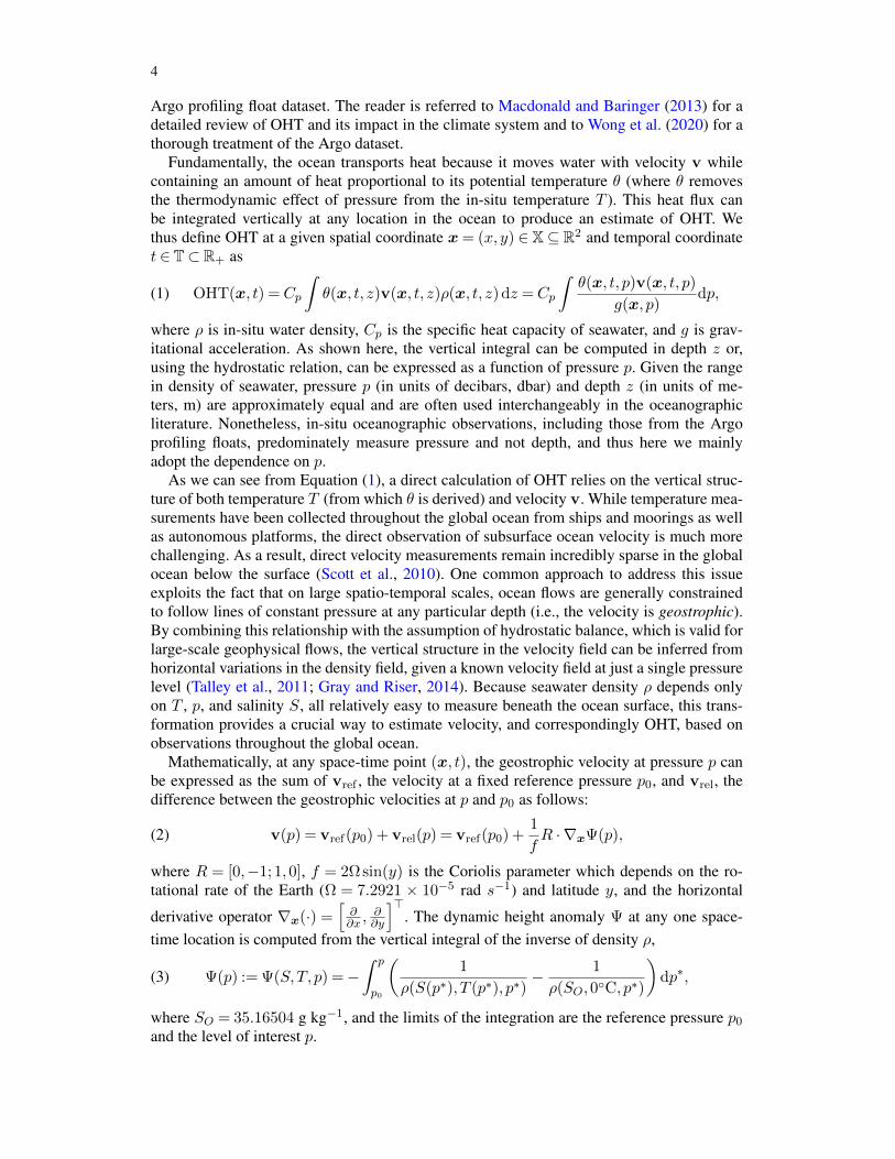
Fundamentally, the ocean transports heat because it moves water with velocity v whilecontaining an amount of heat proportional to its potential temperature θ (where θ removesthe thermodynamic effect of pressure from the in-situ temperature T ). This heat flux canbe integrated vertically at any location in the ocean to produce an estimate of OHT. Wethus define OHT at a given spatial coordinate x= (x, y) ∈ X⊆ R2 and temporal coordinatet ∈ T⊂R+ as
OHT(x, t) =Cp
∫θ(x, t, z)v(x, t, z)ρ(x, t, z) dz =Cp
∫θ(x, t, p)v(x, t, p)
g(x, p)dp,(1)
where ρ is in-situ water density, Cp is the specific heat capacity of seawater, and g is grav-itational acceleration. As shown here, the vertical integral can be computed in depth z or,using the hydrostatic relation, can be expressed as a function of pressure p. Given the rangein density of seawater, pressure p (in units of decibars, dbar) and depth z (in units of me-ters, m) are approximately equal and are often used interchangeably in the oceanographicliterature. Nonetheless, in-situ oceanographic observations, including those from the Argoprofiling floats, predominately measure pressure and not depth, and thus here we mainlyadopt the dependence on p.
As we can see from Equation (1), a direct calculation of OHT relies on the vertical struc-ture of both temperature T (from which θ is derived) and velocity v. While temperature mea-surements have been collected throughout the global ocean from ships and moorings as wellas autonomous platforms, the direct observation of subsurface ocean velocity is much morechallenging. As a result, direct velocity measurements remain incredibly sparse in the globalocean below the surface (Scott et al., 2010). One common approach to address this issueexploits the fact that on large spatio-temporal scales, ocean flows are generally constrainedto follow lines of constant pressure at any particular depth (i.e., the velocity is geostrophic).By combining this relationship with the assumption of hydrostatic balance, which is valid forlarge-scale geophysical flows, the vertical structure in the velocity field can be inferred fromhorizontal variations in the density field, given a known velocity field at just a single pressurelevel (Talley et al., 2011; Gray and Riser, 2014). Because seawater density ρ depends onlyon T , p, and salinity S, all relatively easy to measure beneath the ocean surface, this trans-formation provides a crucial way to estimate velocity, and correspondingly OHT, based onobservations throughout the global ocean.
Mathematically, at any space-time point (x, t), the geostrophic velocity at pressure p canbe expressed as the sum of vref , the velocity at a fixed reference pressure p0, and vrel, thedifference between the geostrophic velocities at p and p0 as follows:
v(p) = vref(p0) + vrel(p) = vref(p0) +1
fR · ∇xΨ(p),(2)
where R = [0,−1; 1,0], f = 2Ω sin(y) is the Coriolis parameter which depends on the ro-tational rate of the Earth (Ω = 7.2921 × 10⁻⁵ rad s−1) and latitude y, and the horizontal
derivative operator ∇x(·) =[∂∂x ,
∂∂y
]>. The dynamic height anomaly Ψ at any one space-
time location is computed from the vertical integral of the inverse of density ρ,
Ψ(p) := Ψ(S,T, p) =−∫ p
p0
(1
ρ(S(p∗), T (p∗), p∗)− 1
ρ(SO,0C, p∗)
)dp∗,(3)
where SO = 35.16504 g kg−1, and the limits of the integration are the reference pressure p0
and the level of interest p.
SPATIO-TEMPORAL INTERPOLATION OF GLOBAL OCEAN HEAT TRANSPORT 5
Bringing together Equations (1) – (3), concurrent measurements of T (p) and S(p), to-gether with an estimate of vref at p0, can be used to compute an observation-based estimate ofOHT. While historically such observations have been sparse and unevenly sampled in spaceand time, over the past two decades the international oceanographic community has built aglobal array of autonomous instruments that provides exactly these measurements with un-precedented spatio-temporal coverage. The Argo array (Roemmich et al., 1998; Riser et al.,2016) consists of nearly 4000 autonomous profiling floats that collect subsurface measure-ments of T , S, and p in the upper 2000 m of the ocean globally, with near-uniform samplingevery 3 × 3 × 10 days in space and time. The number of floats has continuously increasedsince initial deployments began in the early 2000s, reaching the designed spatial coverage in2007. The strength of Argo comes from its high sampling density and global, nearly uniformspatio-temporal coverage, along with its high-precision in-situ measurements (Riser et al.,2016). Each float follows a pre-determined cycle in which it starts by descending to a park-ing depth of 1000 dbar, then drifts for 9 days with the predominant currents at that depth, andsubsequently sinks to a profiling depth of 2000 dbar before slowly ascending to the surfacewhile measuring ocean variables with vertical resolution of up to 2 dbar for modern floats(Roemmich et al., 1998). The set of measurements during the ascent, along with the spatiallocation and time stamp for each cycle (determined from satellite positioning systems whileat the surface), is called a profile. These data are transmitted to shore-based computing sys-tems via satellite communications and made freely available to the public in near real time.
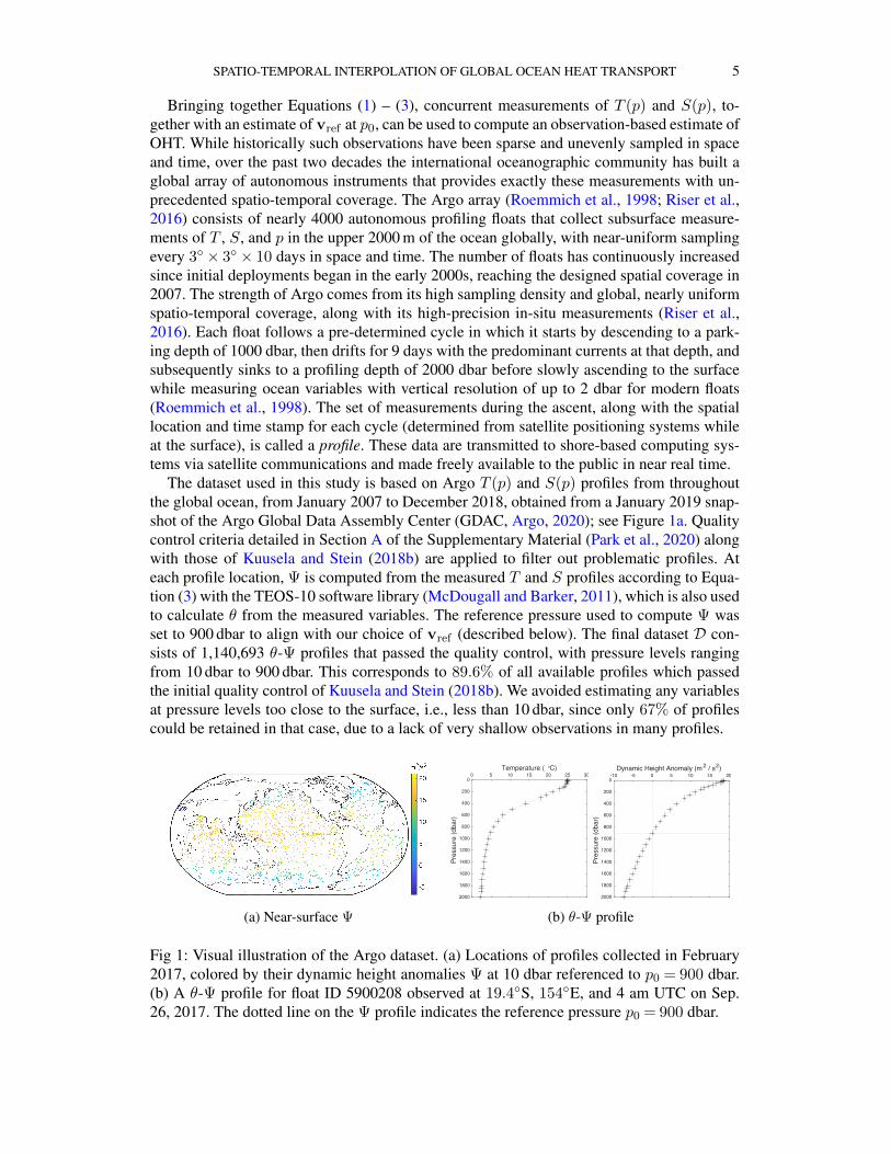
The dataset used in this study is based on Argo T (p) and S(p) profiles from throughoutthe global ocean, from January 2007 to December 2018, obtained from a January 2019 snap-shot of the Argo Global Data Assembly Center (GDAC, Argo, 2020); see Figure 1a. Qualitycontrol criteria detailed in Section A of the Supplementary Material (Park et al., 2020) alongwith those of Kuusela and Stein (2018b) are applied to filter out problematic profiles. Ateach profile location, Ψ is computed from the measured T and S profiles according to Equa-tion (3) with the TEOS-10 software library (McDougall and Barker, 2011), which is also usedto calculate θ from the measured variables. The reference pressure used to compute Ψ wasset to 900 dbar to align with our choice of vref (described below). The final dataset D con-sists of 1,140,693 θ-Ψ profiles that passed the quality control, with pressure levels rangingfrom 10 dbar to 900 dbar. This corresponds to 89.6% of all available profiles which passedthe initial quality control of Kuusela and Stein (2018b). We avoided estimating any variablesat pressure levels too close to the surface, i.e., less than 10 dbar, since only 67% of profilescould be retained in that case, due to a lack of very shallow observations in many profiles.
(a) Near-surface Ψ
0 5 10 15 20 25 30
Temperature ( °C)
0
200
400
600
800
1000
1200
1400
1600
1800
2000
Pre
ssure
(dbar)
-10 -5 0 5 10 15 20
Dynamic Height Anomaly (m2
/ s2)
0
200
400
600
800
1000
1200
1400
1600
1800
2000
Pre
ssu
re (
db
ar)
(b) θ-Ψ profile
Fig 1: Visual illustration of the Argo dataset. (a) Locations of profiles collected in February2017, colored by their dynamic height anomalies Ψ at 10 dbar referenced to p0 = 900 dbar.(b) A θ-Ψ profile for float ID 5900208 observed at 19.4S, 154E, and 4 am UTC on Sep.26, 2017. The dotted line on the Ψ profile indicates the reference pressure p0 = 900 dbar.
6
While the Argo dataset can be used to determine vrel according to Equation (2), a com-plete estimate of the absolute velocity v, and consequently OHT, also requires an estimate ofthe reference velocity vref . However, estimating vref requires a separate treatment since θ-Ψprofiles does not contain direct information on vref . In this study, we assume that the refer-ence velocity is given as there are existing well-studied products for the absolute geostrophicvelocity at the sea surface or at the Argo floats’ parking depth (see, e.g., Lebedev et al., 2007;Willis and Fu, 2008; Ollitrault and Rannou, 2013; Gray and Riser, 2014). For the empiricalanalyses in Section 4, we adopt the reference geostrophic velocity estimates and mapping er-ror estimates derived from Argo float trajectories at p0 = 900 dbar (Gray and Riser, 2014) atall profile spatio-temporal coordinates based on their nearest-neighbor grid point in the dataproduct. These estimates are solely based on direct observations of the Argo float trajecto-ries, which aligns well with our goal to quantify the geostrophic velocity and OHT based onautonomous in-situ observations. We note that the quality of the reference velocity estimatedirectly impacts the accuracy and uncertainty of the resulting estimate of absolute velocityand hence heat transport; improving the reference velocity field is, however, beyond the scopeof the present work.
3. Statistical Methodology.
3.1. Overview. We first overview each component of the statistical methodology and ex-plain how they bind together in a unified framework. The main procedural challenge can beunderstood as a combination of two classical statistical problems: spatio-temporal interpo-lation and latent variable modeling. Given Ψ profiles at some spatio-temporal coordinates,the velocity v can be understood as a spatio-temporally dependent latent function in whichthe dependency structure is heterogeneous across the ocean and the time span. The OHTfield, the final quantity of interest, presents similar spatio-temporal challenges as well. Ne-glecting these unique characteristics of the spatio-temporal (latent) variables could result insuboptimal OHT predictions.
To overcome these challenges, a two-stage procedure based on local Gaussian process re-gression (LGPR) is introduced. LGPR applied particularly to the Argo dataset (Kuusela andStein, 2018a) has shown outstanding interpolation performance compared to that of previousstate-of-the-art methods. We extend the work of Kuusela and Stein (2018a) by consideringlatent LGPR, which is specifically tailored to solving the statistical complications in estimat-ing the OHT field. Based on the scientific framework in the previous section, the first stage ofprocedure estimates the dynamic height anomaly Ψ field at a series of fixed pressure levels,of which the spatial gradients provide the latent relative velocity vrel field according to Equa-tion (2). Next, the results of this step are combined with an independent estimate of vref tocompute spot OHT values at the space-time locations of the Argo profiles using Equation (1).This integral can be calculated across any range of pressure levels, providing the capabilityto examine the contribution of different water layers to the total OHT. Conditional on thepredicted spot OHT, these estimated OHT values are then interpolated to a regular spatio-temporal grid in the second stage of the LGPR procedure. We detail the LGPR framework inSection 3.2 and the latent LGPR with the two-stage procedure in Section 3.3.
We further improve the LGPR approach of Kuusela and Stein (2018a), which focuseson estimating a local space-time covariance model from detrended temperature observationwhose mean field was estimated using OLS, by simultaneously estimating both the mean andthe covariance parameters with an approximate EM algorithm. The procedure shares simi-larities with GLS. However, our EM procedure is able to account for the overlapping localmoving windows of the LGPR covariance structure in a computationally efficient fashionwhen estimating the mean field. We detail the procedure in Section 3.4.
SPATIO-TEMPORAL INTERPOLATION OF GLOBAL OCEAN HEAT TRANSPORT 7
Predicting the gradient field from incomplete observations with a potentially under-specified mean field model may result in a concerning bias. By formalizing a procedurepreviously used by Roemmich and Gilson (2009), we provide in Section 3.5 an intuitive de-biasing procedure that effectively mitigates the bias in the predicted gradient and, if needed,the target field. The procedure captures the asymptotically valid bias field by correcting whichimproves the calibration of both gradient and target field.
3.2. Spatio-temporal LGPR model. We briefly review the LGPR model originally pro-posed for Argo mapping in Kuusela and Stein (2018a) motivated by Haas (1990, 1995),and illustrate the similarities and differences when adopting LGPR specifically for OHT in-terpolation. Consider a real-valued spatio-temporal random field of a quantity of interestΥ(x, t, p)x∈X,t∈T observed at a spatial location x= (x, y) in the open ocean X⊆R2 withlongitude x and latitude y in degrees; time t ∈ T ⊆ [0,365] in yeardays; and at some fixedpressure p. Hereafter, we will use s= (x, t) to denote a spatio-temporal coordinate. The re-sponse field Υ can be either the dynamic height anomaly Ψ or the Ocean Heat TransportOHT, depending on the context, with the same model structure. We express the field as:
Υ(x, t, p) =m(x, t, p) + a(x, t, p) + ε(x, t, p),(4)
where m(x, t, p) denotes a large-scale climatological mean field with a seasonal cycle;a(x, t, p) denotes an anomaly field, i.e., a transient deviation from the climatological mean,and ε is a fine-scale nugget effect. The term mean, denoted by m, is adopted to specifyE[Υ(x, t, p)], the deterministic mean of the process Υ, whereas the term anomaly, and thenotation a, refers to a residual process centered at zero. We drop p hereafter for brevity when-ever the argument does not depend on the choice of p.
In this paper, we consider a locally semiparametric model in the sense that the mean fieldis assumed to be locally parametric whereas the anomaly field is locally nonparametric—specifically, a locally stationary Gaussian process. Nevertheless, both the mean and theanomaly field are actually nonparametric models since the semiparametric distinction hap-pens only at local neighborhoods. Local polynomial regression (Fan et al., 1997), which weemploy for the mean field, is already in itself a nonparametric method. The locally semi-parametric model not only improves estimation efficiency by confining the parameter spacebut also matches our intent that the mean field explains the systematic large-scale patternswhereas the anomaly field captures the transient patterns.
The nugget effect ε is assumed to locally be a Gaussian white noise process with mean zeroand variance σ2
ε and independent of the anomaly field a. This distributional assumption leadsto a closed-form predictive distribution, enabling convenient uncertainty quantification. Eventhough the Gaussian nugget is widely adopted in the literature, Kuusela and Stein (2018a)pointed out that the Gaussian nugget may be insufficient to account for the heavy-tailednugget distribution of subsurface temperature data in certain parts of the ocean. An extensionto a heavy-tailed Student nugget (Kuusela and Stein, 2018a) is possible. However, we onlyfocus on the Gaussian nugget in this paper for simplicity.
We let the pilot model of the large-scale mean field m(x, t) to be a local polynomialregression (Fan et al., 1997) with uniform weights (Stone, 1980). In particular, within a smallcircular spatial windowWλG
(x∗) = x : ‖x−x∗‖G ≤ λG, where ‖·‖G denotes the distancein WGS84 coordinates and λG is a positive bandwidth that controls the size of the spatialneighborhoods in estimating the coefficients, we let
m(x, t) = β0 + βxxc + βyyc + βxyxcyc + βx2x2c + βy2y
2c
+
K∑k=1
[βck cos
(2πkt
365
)+ βsk sin
(2πkt
365
)],
(5)
8
where xc := x− x∗ and yc := y − y∗ are spatial coordinates centered around x∗ and y∗, andK is a predefined maximum number of harmonics. The first line in Equation (5) capturesthe local spatial structure of the mean field, while the second line models the seasonal cyclewithin the window. This regression model with K = 6 has been successfully adopted in theoceanographic literature to model the mean field of Argo observations (Ridgway, Dunn andWilkin, 2002; Roemmich and Gilson, 2009), albeit with slight different estimation method.
The anomaly field is modeled using a zero-mean locally stationary Gaussian process whichis i.i.d. over the years and whose distance metric is defined as the Mahalanobis distance bothin terms of space and time (Kuusela and Stein, 2018a). Let s∗ = (x∗, t∗) be a space-time(intra-annual) grid point for which a prediction is desired. Within a small spatio-temporalwindow Wλ(s∗) =WλG
(x∗)× [t∗ − λt, t∗ + λt] around s∗, we let
aii.i.d.∼ GP(0, k(s1,s2;ξ)), i= 1, . . . , I,(6)
where the index i refers to years, k(s1,s2;ξ) = k(x1 − x2, y1 − y2, t1 − t2;ξ) is a sta-tionary space-time covariance function depending on non-negative hyperparameters ξ =(φ, ξx, ξy, ξt)
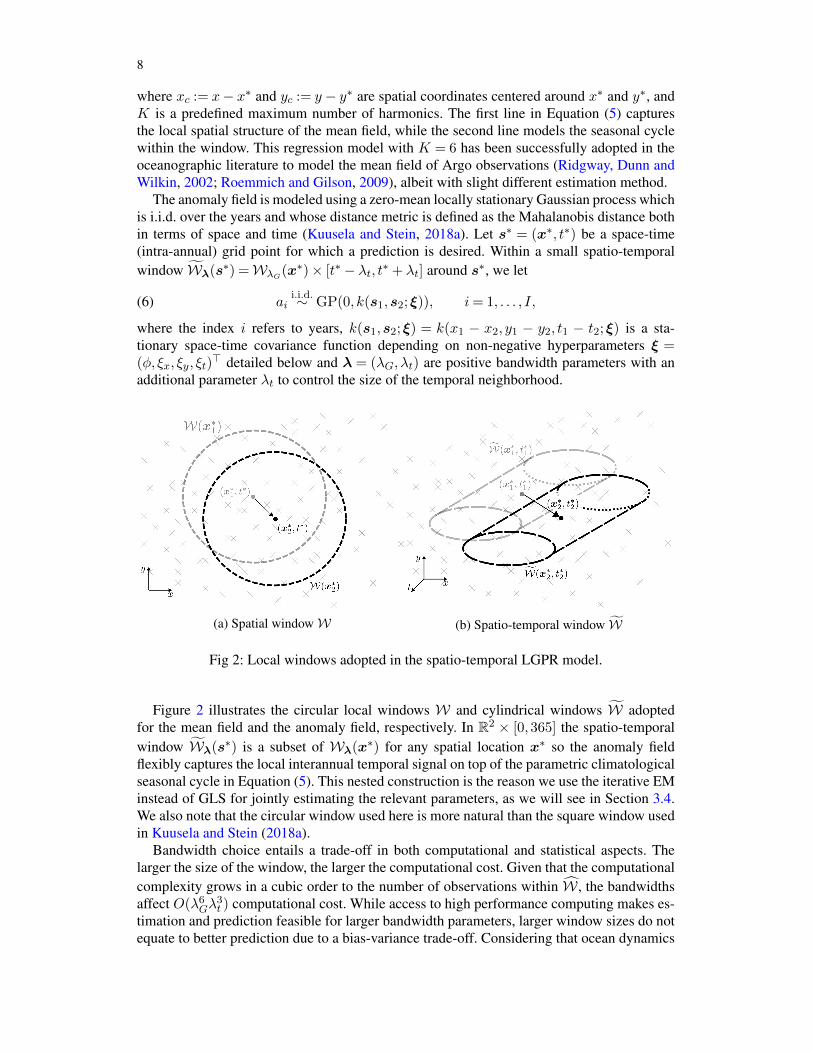
> detailed below and λ = (λG, λt) are positive bandwidth parameters with anadditional parameter λt to control the size of the temporal neighborhood.
(a) Spatial windowW (b) Spatio-temporal window W
Fig 2: Local windows adopted in the spatio-temporal LGPR model.
Figure 2 illustrates the circular local windows W and cylindrical windows W adoptedfor the mean field and the anomaly field, respectively. In R2 × [0,365] the spatio-temporalwindow Wλ(s∗) is a subset of Wλ(x∗) for any spatial location x∗ so the anomaly fieldflexibly captures the local interannual temporal signal on top of the parametric climatologicalseasonal cycle in Equation (5). This nested construction is the reason we use the iterative EMinstead of GLS for jointly estimating the relevant parameters, as we will see in Section 3.4.We also note that the circular window used here is more natural than the square window usedin Kuusela and Stein (2018a).
Bandwidth choice entails a trade-off in both computational and statistical aspects. Thelarger the size of the window, the larger the computational cost. Given that the computationalcomplexity grows in a cubic order to the number of observations within W , the bandwidthsaffect O(λ6
Gλ3t ) computational cost. While access to high performance computing makes es-
timation and prediction feasible for larger bandwidth parameters, larger window sizes do notequate to better prediction due to a bias-variance trade-off. Considering that ocean dynamics
SPATIO-TEMPORAL INTERPOLATION OF GLOBAL OCEAN HEAT TRANSPORT 9
are globally non-stationary, excessively large windows are more likely to violate the assump-tion that the Gaussian process is stationary within the window, resulting in a concerning bias.On the contrary, too small window size suffers from a higher estimation variance or even failto make a prediction, e.g., near the coastal boundary, due to scarce data within the window.Therefore, it is recommended to choose window sizes with which the computation and thelocally stationary assumption are both feasible without losing essential boundary dynamics.
Care has to be taken in specifying the local windows Wλ and Wλ for the OHT field(Υ = OHT) near the equator since geostrophic balance, and thus Equation (2), does not holdas the Coriolis parameter f approaches zero. We threshold the windows to ameliorate thisissue by masking out the tropical latitude band [−ζ, ζ] for some positive parameter ζ . Morerefined methods might be possible, such as using a β-plane approximation (Lagerloef et al.,1999); these are, however, beyond the scope of the present study.
Unlike Kuusela and Stein (2018a), in which an exponential covariance function was used,we choose the Matérn covariance function (Stein, 1999) to ensure that the process is differen-tiable which is required for estimating the velocities. Since a Gaussian process with Matérncovariance with smoothness parameter ν is dνe − 1 times differentiable, we set ν to be 3/2to ensure first-order differentiability. Specifically,
k (s1,s2;ξ) = φ(
1 +√
3‖∆s‖A−1
)exp
(−√
3‖∆s‖A−1
),(7)
where φ is the GP variance, ‖∆s‖A−1 =√
∆s>A−1∆s is the Mahalanobis norm with∆s= s1 − s2 and A=A(ξ) is a positive definite matrix parameterized by ξ. Non-diagonalelements of A represent rotation of the spatio-temporal space although at the expense ofthree additional parameters. Given that we estimate the Gaussian process locally, the numberof parameters increases in the order of the number of local windows. A diagonal covarianceparameter matrix A = diag
(ξ2x, ξ
2y , ξ
2t
)is therefore chosen to efficaciously restrict the pa-
rameter space since we did not see empirical improvements in our application from addingextra off-diagonal parameters, agreeing with Kuusela and Stein (2018a).
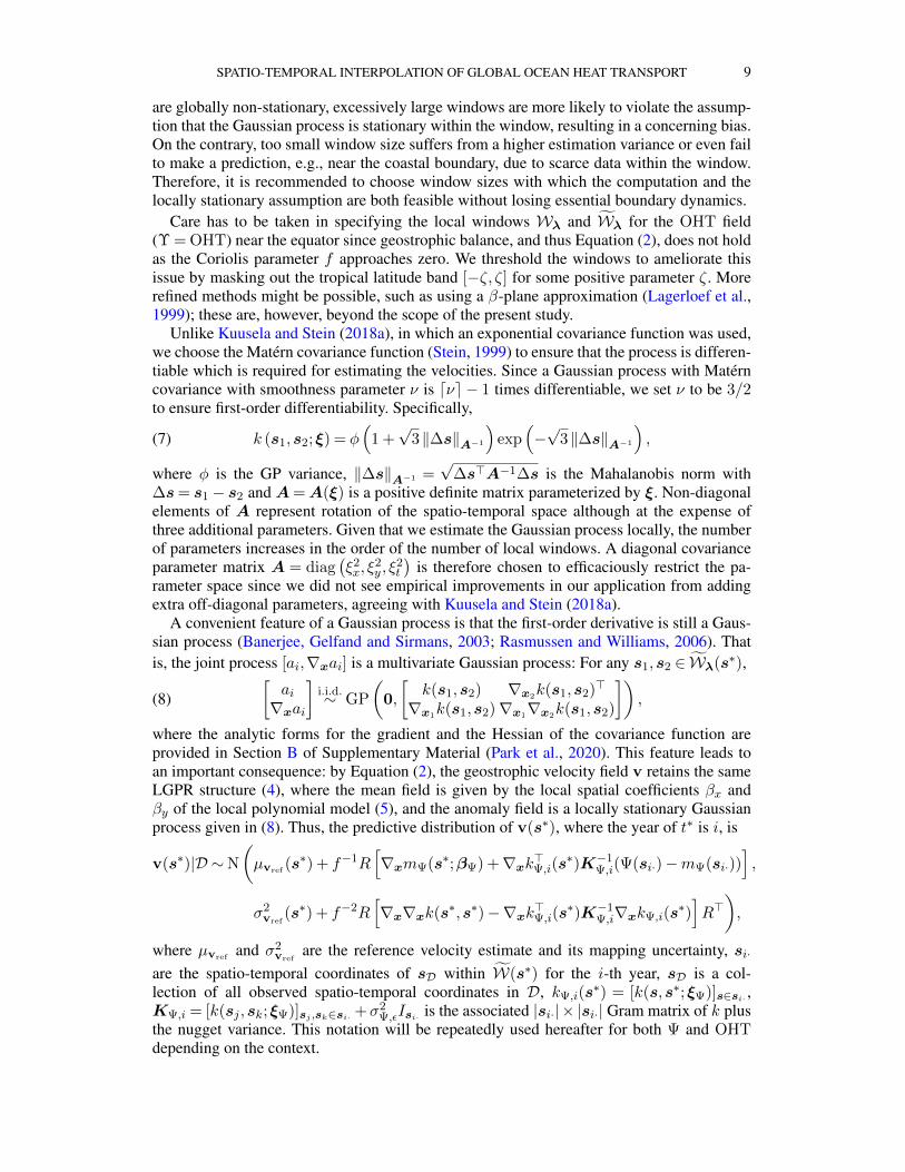
A convenient feature of a Gaussian process is that the first-order derivative is still a Gaus-sian process (Banerjee, Gelfand and Sirmans, 2003; Rasmussen and Williams, 2006). Thatis, the joint process [ai,∇xai] is a multivariate Gaussian process: For any s1,s2 ∈ Wλ(s∗),[
ai∇xai
]i.i.d.∼ GP
(0,
[k(s1,s2) ∇x2
k(s1,s2)>
∇x1k(s1,s2)∇x1
∇x2k(s1,s2)
]),(8)
where the analytic forms for the gradient and the Hessian of the covariance function areprovided in Section B of Supplementary Material (Park et al., 2020). This feature leads toan important consequence: by Equation (2), the geostrophic velocity field v retains the sameLGPR structure (4), where the mean field is given by the local spatial coefficients βx andβy of the local polynomial model (5), and the anomaly field is a locally stationary Gaussianprocess given in (8). Thus, the predictive distribution of v(s∗), where the year of t∗ is i, is
v(s∗)|D ∼N
(µvref
(s∗) + f−1R[∇xmΨ(s∗;βΨ) +∇xk>Ψ,i(s∗)K−1
Ψ,i(Ψ(si·)−mΨ(si·))],
σ2vref
(s∗) + f−2R[∇x∇xk(s∗,s∗)−∇xk>Ψ,i(s∗)K−1
Ψ,i∇xkΨ,i(s∗)]R>),
where µvrefand σ2
vrefare the reference velocity estimate and its mapping uncertainty, si·
are the spatio-temporal coordinates of sD within W(s∗) for the i-th year, sD is a col-lection of all observed spatio-temporal coordinates in D, kΨ,i(s
∗) = [k(s,s∗;ξΨ)]s∈si· ,KΨ,i = [k(sj ,sk;ξΨ)]sj ,sk∈si· +σ2
Ψ,εIsi· is the associated |si·| × |si·| Gram matrix of k plusthe nugget variance. This notation will be repeatedly used hereafter for both Ψ and OHTdepending on the context.
10
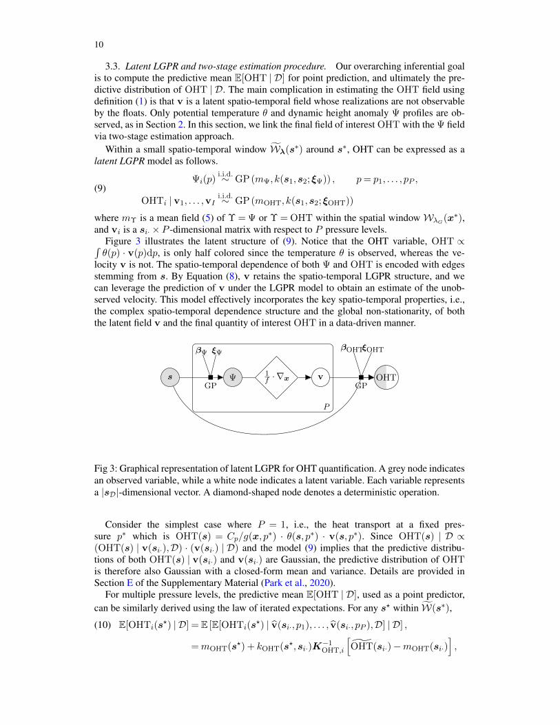
3.3. Latent LGPR and two-stage estimation procedure. Our overarching inferential goalis to compute the predictive mean E[OHT | D] for point prediction, and ultimately the pre-dictive distribution of OHT | D. The main complication in estimating the OHT field usingdefinition (1) is that v is a latent spatio-temporal field whose realizations are not observableby the floats. Only potential temperature θ and dynamic height anomaly Ψ profiles are ob-served, as in Section 2. In this section, we link the final field of interest OHT with the Ψ fieldvia two-stage estimation approach.
Within a small spatio-temporal window Wλ(s∗) around s∗, OHT can be expressed as alatent LGPR model as follows.
Ψi(p)i.i.d.∼ GP (mΨ, k(s1,s2;ξΨ)) , p= p1, . . . , pP ,
OHTi | v1, . . . ,vIi.i.d.∼ GP (mOHT, k(s1,s2;ξOHT))
(9)
where mΥ is a mean field (5) of Υ = Ψ or Υ = OHT within the spatial windowWλG(x∗),
and vi is a si· × P -dimensional matrix with respect to P pressure levels.Figure 3 illustrates the latent structure of (9). Notice that the OHT variable, OHT ∝∫θ(p) · v(p)dp, is only half colored since the temperature θ is observed, whereas the ve-
locity v is not. The spatio-temporal dependence of both Ψ and OHT is encoded with edgesstemming from s. By Equation (8), v retains the spatio-temporal LGPR structure, and wecan leverage the prediction of v under the LGPR model to obtain an estimate of the unob-served velocity. This model effectively incorporates the key spatio-temporal properties, i.e.,the complex spatio-temporal dependence structure and the global non-stationarity, of boththe latent field v and the final quantity of interest OHT in a data-driven manner.
s Ψ
βΨ ξΨ
GP
1f · ∇x v OHT
βOHTξOHT
GP
P
Fig 3: Graphical representation of latent LGPR for OHT quantification. A grey node indicatesan observed variable, while a white node indicates a latent variable. Each variable representsa |sD|-dimensional vector. A diamond-shaped node denotes a deterministic operation.
Consider the simplest case where P = 1, i.e., the heat transport at a fixed pres-sure p∗ which is OHT(s) = Cp/g(x, p∗) · θ(s, p∗) · v(s, p∗). Since OHT(s) | D ∝(OHT(s) | v(si·),D) · (v(si·) | D) and the model (9) implies that the predictive distribu-tions of both OHT(s) | v(si·) and v(si·) are Gaussian, the predictive distribution of OHTis therefore also Gaussian with a closed-form mean and variance. Details are provided inSection E of the Supplementary Material (Park et al., 2020).
For multiple pressure levels, the predictive mean E[OHT | D], used as a point predictor,can be similarly derived using the law of iterated expectations. For any s? within W(s∗),
E[OHTi(s?) | D] = E [E[OHTi(s
?) | v(si·, p1), . . . , v(si·, pP ),D] | D] ,(10)
=mOHT(s?) + kOHT(s?,si·)K−1OHT,i
[OHT(si·)−mOHT(si·)
],
SPATIO-TEMPORAL INTERPOLATION OF GLOBAL OCEAN HEAT TRANSPORT 11
OHT(s) =Cp
∫ pP
p1
θ(s, p) ·E[v(s, p)|D]
g(x, p)dp, ∀s ∈ sD.(11)
Procedurally, this can be viewed as a two-stage method where we first construct the pre-dicted OHT data set D = (s, OHT(s)) : s ∈ sD in the first stage. We then compute theconditional mean E(OHT | D) using the generated dataset in the second stage; see Algo-rithm 1. In practice, Ψ can only be evaluated at a finite set of P pressure levels, which leadsus to approximate the vertical integral when computing OHT. We employ piecewise cubicHermite interpolation (PCHIP, Fritsch and Carlson (1980)) followed by numerical integra-tion. PCHIP is well-suited for this task since it constructs a piecewise cubic interpolant thatrespects the monotonicity of the data, thereby avoiding spurious bumps typical of alternativeinterpolation methods (Barker and McDougall, 2020).
The predictive variance of OHT can be expressed using the law of total variance. For anys? within W(s∗),
V[OHTi(s?) | D] =
[φOHT + σ2
ε,OHT − kOHT(s?,si·)K−1OHT,ikOHT(si·,s
?)]
+ kOHT(s?,si·)K−1OHT,iV [OHT(si·) | D]K−1
OHT,ikOHT(si·,s?).
(12)
This decomposition shows that the predictive variance of OHT is a combination of (i) vari-ation solely from the second stage (the first line), and (ii) the uncertainty that propagatesfrom the first stage to the second stage (the second line). Even though the point predictorE[OHT | D] can be obtained without approximations using Equation (10), the predictive vari-ance would require the knowledge of the vertical correlation to compute V [OHT(si·) | D].This ultimately necessitates an approximation or a conservative upper bound to the predictivevariance. Incorporating the vertical correlation in addition to spatio-temporal correlation isstill an active area of research (see e.g. Yarger, Stoev and Hsing, 2020).
3.4. Approximate Expectation-Maximization algorithm. Given the Argo data1 D :=(Υij ,sij) : i= 1, . . . , I; j = 1, . . . , ni
(either Ψ or OHT|Ψ), we seek to estimate a collec-
tion of β denoted by B = β(x∗) : x∗ ∈ X and a collection of ξ denoted by Ξ = ξ(s∗) :s∗ ∈ S, where S = X × T is a set of target spatio-temporal coordinates s∗ = (x∗, t∗),since the LGPR model specifies the covariance structure on the spatio-temporal windowW(s∗) nested within the spatial windowW(x∗) on which the mean field structure is defined.We wish to find the parameters that maximize the likelihood function L(B,Ξ); however, aclosed-form solution is not available for our LGPR model. We therefore employ an approxi-mate EM algorithm (Dempster, Laird and Rubin, 1977), resulting in a block coordinate ascentalgorithm, to jointly estimate all of the parameters.
We update the parameters at iteration l= 0,1, . . . as follows:
B(l+1) = argmaxBL(B |Ξ(l))(E-Step)
Ξ(l+1) = argmaxΞL(Ξ |B(l+1)),(M-Step)
where the initial guess Ξ(0) corresponds to a set of identity covariance matrices, and thereforeassuming that the process is spatio-temporally uncorrelated within each spatial window W .L is an approximated L which we will detail subsequently. At first glance, the above stepslook like an alternating maximization (AM) algorithm (Csiszar and Tusnady, 1984), whichindeed can be viewed as a special case of the EM algorithm as first suggested by Neal and
1Even though D is originally defined as a collection of the triplets (θ,Ψ,s) as in Algorithm 1, we redefine Das duplets with a slight abuse of notation for this section to better focus on the procedure.
12
Hinton (1998). See Section C of the Supplementary Material (Park et al., 2020) for howthey are connected under our setup. This EM algorithm is a generalization of Kuusela andStein (2018a) since the MLE of the covariance parameters in Kuusela and Stein (2018a)corresponds to the EM algorithm with l = 0, which ignores the spatio-temporal correlationwhen estimating the mean field. Empirical improvement over Kuusela and Stein (2018a) inpredictive performance is demonstrated in Section G.2 of the Supplementary Material.
The M-Step is essentially obtaining the maximum likelihood estimator (MLE) of Ξ fromthe residuals Υ
(l+1)ij := Υij − m(l+1)(sij),∀i, j, where the estimated mean field m(l+1) is
constructed based on the parameters β(l+1)(x∗) updated in the previous E-Step. For everys∗ ∈ S ,
L(ξ(s∗) | β(l+1)(x∗)
)=
I∏i=1
p(Υ
(l+1)i ;ξ(s∗)
),
where Υ(l+1)i is a vector of Υ
(l+1)ij ’s within the window W(s∗) in a specific year i, and
p(Υ(l+1)i ;ξ(s∗)) is the pdf of the multivariate Gaussian distribution with zero mean and
covariance matrixKi(ξ(s∗))+σ2ε (s∗)Ini
. To solve the M-Step, we adopted the BFGS quasi-Newton algorithm (Nocedal, 1980) in the empirical studies in Sections 4 and 5.
E-Step updates the deterministic mean field accounting for the spatio-temporal correlationof the residuals Υ(l) learned in the previous M-Step. This step is analogous to the GLSestimator in regression kriging literature to resolve the sub-optimality of OLS (Cressie, 1993)and shares a similarity with iterative GLS (Gray and Riser, 2015) adopted previously for Argodata. However, in our LGPR model, using the GLS estimator is not straightforward due tothe nested temporal window W within the spatial window W , which limits the availabilityof the correlations at large temporal lags. To aggregate the local spatio-temporal covariancestructures of W into the spatial windowW , we employ the Vecchia approximation (Vecchia,1988) which confines the aggregated covariance structure by thresholding the temporal lagoutside of each W in the conditional distribution. We note that this approach is different fromblock covariance tapering, and the Vecchia approximation is known to have advantages overcovariance tapering (Stein, 2013).
The Vecchia approximation (Vecchia, 1988) is a natural choice both from the perspectiveof LGPR modeling and computational efficiency. Choosing uniform weights on each spatio-temporal window W , we hard-threshold the conditional spatio-temporal dependency alongthe temporal axis in the anomaly field within 2λt temporal lag of the target time point t∗. Thisimplies that the LGPR model assumes observations within W to be uncorrelated beyond thetemporal window. Such a structure is reflected in the approximate likelihood function viaVecchia approximation. Additionally, this choice yields a closed-form E-Step resembling aGLS-like estimator, for which the details are given in Section D of Supplementary Material.
The overall EM procedure (E-Step and M-Step) leads to a computationally efficient al-gorithm since these steps can be viewed as a gather-and-broadcast algorithm. The M-Stepcan be performed fully in parallel across each W once the residuals have been broadcast toeach computing node. The E-Step then gathers the estimated covariance structures from eachcomputing node and updates the aggregated mean parameter withinW . This parallelizationleads to major computational benefits since the main computational bottlenecks of the proce-dure are the numerical optimizations required in the M-Step as opposed to the E-Step wherethe closed form solution is fast to compute.
3.5. Debiasing the mean field. In this section, we describe a simple debiasing procedureto account for potential mean field model misspecification. We have noticed that climate sci-entists oftentimes compute the empirical mean of the estimated anomaly fields across years
SPATIO-TEMPORAL INTERPOLATION OF GLOBAL OCEAN HEAT TRANSPORT 13
and add that back to the mean field to make the resulting estimate of the anomaly fields tem-porally centered at zero (e.g., Roemmich and Gilson, 2009). We formalize this procedure anddemonstrate that it is a legitimate approach to (partially) identifying model misspecificationsand correcting them. For the LGPR model (4), model misspecification may arise in boththe mean and the covariance structure. Specifically, we focus on a potentially misspecifiedmean field, since inferring the climatological mean is of key interest in this application, anda bias arising from mean field misspecification propagates to the localized anomaly fieldswhich leads to biased inference and prediction of the anomalies. The LGPR model (4) uti-lizes a mean field model m given in Equation (5) which is inspired by previous work in theoceanographic literature (Ridgway, Dunn and Wilkin, 2002; Roemmich and Gilson, 2009).Even though this model is known to work well for simple oceanographic variables, such astemperature and salinity, the model may have trouble representing the mean of the OHT orΨ fields with sharp fronts and other localized patterns, which further motivates us to use abias-correction procedure in this application.
The predictive mean Υ(s∗∗) := E(Υ(s∗∗) | D), for any s∗∗ ∈ W(s∗), is an unbiased esti-mator of the true mean field E(Υ(s∗∗)) =m(s∗∗) if the assumed mean field model for Υ iswell-specified following the construction (4). That is, when the year of s∗∗ is i,
E[Υi(s
∗∗)]
= E[m(s∗∗) + k>i (s∗∗)K−1
i (Υi(si·)−m(si·))]
(?)= m(s∗∗).(13)
Suppose the analyst was oblivious to the true mean field m and misspecified the mean fieldmodel as EA(Υ(s∗∗)) := m(s∗∗) + B(s∗∗) by introducing a non-zero bias field B. HereEA denotes the assumed expectation under the analyst’s model. The predictive mean Υ(s∗∗)under the misspecified model becomes
Υi(s∗∗) = EA(Υ(s∗∗)) + k>i (s∗∗)K−1
i (Υi(si·)−EA(Υi(si·))) .
Then, (?) in Equation (13) no longer holds but instead
E[Υi(s
∗∗)]−m(s∗∗) =B(s∗∗)− k>i (s∗∗)K−1
i B(si·).(14)
As the observations si· get denser within W(s∗), Equation (14) essentially converges to zero,and thus Υi→ Υi for every year i under infill asymptotics, despite the misspecification ofthe mean field m. See Stein (1999, Chapter 4, Theorem 8) for a rigorous statement.
Given I years of observations, we estimate B(s∗∗) using the negative average anomaly
B(s∗∗) =−1
I
I∑i=1
k>i (s∗∗)K−1i (Υi(si·)−EA(Υ(s∗∗)))(15)
= EA(Υ(s∗∗))− 1
I
I∑i=1
Υi(s∗∗)
infill,I→∞−−−→ EA(Υ(s∗∗))−E(Υ(s∗∗)) =B(s∗∗).
This leads to a bias-corrected mean field EnewA (Υ) =m+B − B, which asymptotically con-
verges to the true mean field m assuming that the Υ fields are observed densely enough forevery year and that we have observations from a large enough number of years.
The mean field misspecification affects the estimation of both the mean and the anomalyfields since we assumed the true mean field ism+B when initially computing m, and conse-quently assumed EA(ai(si·)) = 0, when in reality E(ai(si·)) =−B(si·), when estimating thecovariance parameters Ξ before correcting the bias. After the bias is identified, we re-estimatethe covariance parameters Ξ based on the corrected residuals Υi(si·)− m(si·) + B(si·), forall i= 1, . . . , I , utilizing the M-Step of the EM procedure. The re-estimation step ensures that
14
the covariances are computed from the correct model structure (4) under which the anomalyfield is truly centered at zero asymptotically. We then recompute the interpolated fields Υbased on the updated covariance parameters.
The proposed debiasing method is directly applicable not only to Ψ or OHT|Ψ in thelatent LGPR model (9) but also to the latent velocity field v without additional computationalburden. Recall that applying the deterministic operation 1
f · ∇x on the Ψ field yields the vfield. Since the operation only consists of linear operators, our bias estimate for the v field is
1
f· ∇x∗∗B(s∗∗) =− 1
f· 1I
I∑i=1
∇x∗∗k>i (s∗∗; ξΨ)K−1i (ξΨ)(Ψ(si·)− mΨ(si·)).(16)
As the analytic form of the gradient of the Matérn covariance function is available (see Sec-tion B of the Supplementary Material (Park et al., 2020)), the additional computational burdento calculate the bias of v is marginal in the process of computing the bias of Ψ.
In Sections 4 and 5.2, we empirically show the importance of accounting for the possiblebias in both Ψ and OHT. Debiasing the Ψ field especially yields a considerable improvementon the latent v field when we do not have direct observations to fit a model for v.
3.6. Complete OHT interpolation framework. Algorithm 1 summarizes the full two-stage procedure we have described throughout this section. Procedures LGPR and DEBIASsummarize the proposed approximate EM algorithm and bias-correction as described in Sec-tions 3.4 and 3.5, respectively. The computational complexity of our framework is dominatedby the procedure LGPR, and thus is analogous to that of Kuusela and Stein (2018a). Givenni observations for each year i = 1, . . . I , the computational complexity of global Gaussianprocess regression is O(
∑Ii=1 n
3i ) due to computing the inverse Gram matrices K−1
i . Thecomputation of LGPR is localized to |S| target grid points at which the windows are cen-tered, with each window containing w · ni observations for each year i (w is the fraction ofdata contained in the window). With the computations parallelized to C threads, the compu-tational complexity of Algorithm 1 is O(P · |S| ·C−1 ·w3 ·
∑Ii=1 n
3i ).
4. OHT Field Estimated from Argo Data. In this section, we present empirical resultsapplying the two-step estimation procedure described in Section 3 to the Argo dataset to pro-duce output fields on a spatio-temporal grid X × T where X is a 1 × 1 spatial grid and Tis a regularly spaced monthly temporal grid centered on the 15th day of each month. Eachquantity of interest is compared before and after applying the debiasing procedure describedin Section 3.5. The bandwidth parameter λG for the spatial window is set to 442 km (ap-proximately 4), and λt for the temporal window is set to 1.5 months. All computations inthe subsequent sections are performed on Cheyenne (Laboratory, 2019), a high performancecomputing cluster at NCAR with 36 CPU nodes with 109 GB of RAM. It takes on average25 min each to execute a single EM iteration and to make predictions on S for each field.
In the subsequent Sections 4.1 and 4.2, we present the time-averaged quantities:
Av (Υ) (x) =1
|T |
∫TE[Υ(x, τ)]dτ,(17)
where Υ can be v or OHT depending on the context. Our product actually generates amonthly varying spatial map, however, we present time-averaged quantities which succinctlysummarize spatial mean variability without loss of generality.
SPATIO-TEMPORAL INTERPOLATION OF GLOBAL OCEAN HEAT TRANSPORT 15
Algorithm 1 Two-stage OHT interpolation framework
Input: Data D = D1, . . . ,DP where Dp = (θij(p),Ψij(p),sij) : i= 1, . . . , I; j = 1, . . . , ni (DenotesD := sij : ∀i, j); Spatio-temporal target s∗
1: function LGPR(Υ, D, S) . Target response Υ can be Ψ or OHT2: repeat3: Estimate mean field coefficients BΥ in the (E-Step)4: Estimate covariance coefficients ΞΥ in the (M-Step)5: until Converge6: return Υ(S) field7: end function
8: procedure DEBIAS(Υ, D, ΞΥ)9: Compute the bias B with (15).
10: Debias Υ and ∇xΥ, respectively, using B and (16).11: Re-estimate ΞΥ with (M-Step) using the bias-corrected residuals.12: Update Υ field based on re-estimated ΞΥ.13: end procedure
14: Estimate pilot predictions Ψ(sD, p)← LGPR(Ψ, Dp, sD) for fine grid of p.15: DEBIAS([Ψ− mΨ](sD, p), Dp, ΞΨ) for fine grid of p.16: Construct a dataset D whose response variable is predicted OHT, OHT(sD), using (11).17: Map OHT(s∗)← LGPR(OHT, D, s∗).18: DEBIAS([OHT− mOHT](s∗), D, ΞOHT).
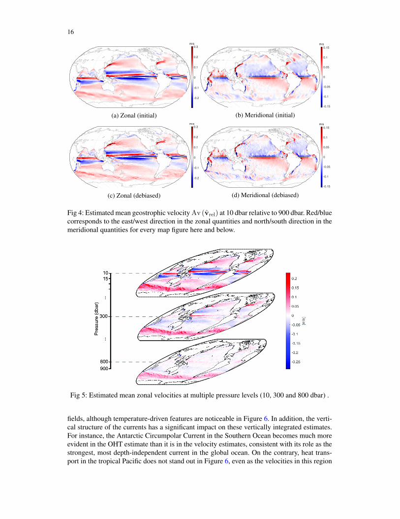
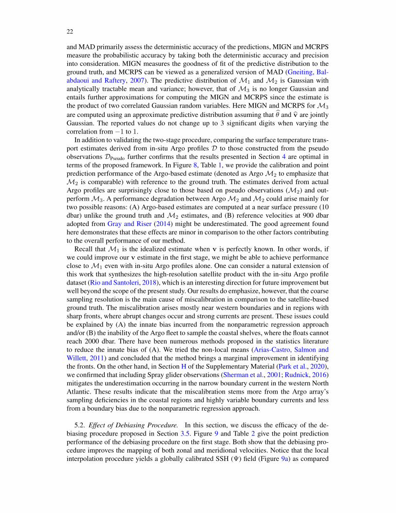
4.1. Geostrophic Velocity v. Recall from Section 3.3 that we only need spot-predictedvelocities v from the first step; however, it is worthwhile to visualize the interpolated latentv field to see if the latent field is well-represented. The estimated mean field for the relativegeostrophic velocity Av (vrel) from the first step can be found in Figure 4. Figures 4a and4b show the non-bias-corrected initial zonal and meridional velocity estimates, respectively.Figures 4c and 4d show the estimated mean field after the debiasing procedure. In all fig-ures, we mask out ±2 equatorial bands, where geostrophic balance is invalid. The estimatesdepict the major ocean currents in each basin, including Equatorial Currents, the AntarcticCircumpolar Current, and (at least partially) the western boundary currents and their exten-sions. The debiasing procedure captures higher-order local features that are not described bythe local second degree polynomial, without introducing spurious noise. This is highlightedin the Kuroshio Current (off the coast of Japan) and the Agulhas Return Current (near thesouthern tip of Africa), where meanders are clearly visible in Panel (d) that are not present inPanel (b) before the bias is corrected. These meanders are known to be quasi-stationary andare also observable in satellite products (see Section F of Supplementary Material), whichindicates that these local features are in fact part of the real signal.
Even though we have only presented the velocity field estimated at 10 dbar in Figure 4,we emphasize that the relative velocity field is estimated at 17 different pressure levels. Thevertical structure of the resulting velocity estimate is illustrated in Figure 5. Note that therelative velocity field in the continent-free Southern Ocean retains much of its strength evenat 800 dbar, as opposed to the other basins, where the relative geostrophic velocities generallydecay more quickly with depth.
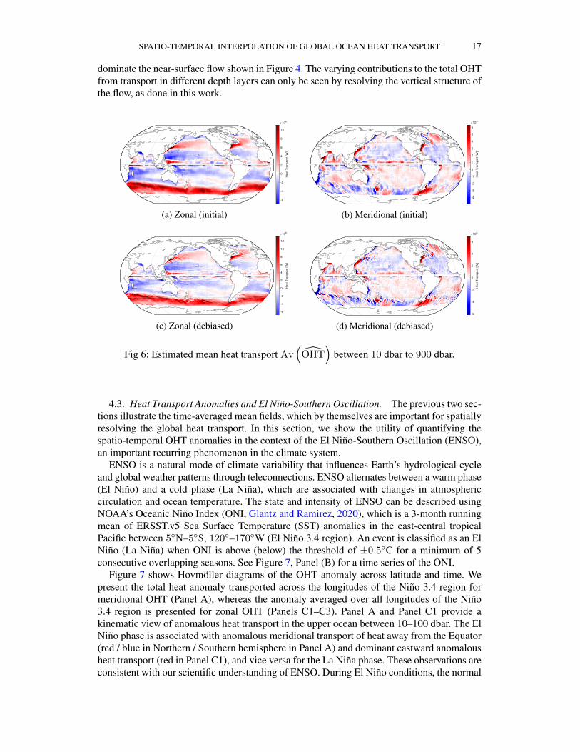
4.2. Heat Transport OHT. Figure 6 shows the estimated mean field of zonal and merid-ional heat transport Av
(OHT
)between 10 dbar to 900 dbar computed using the two-step
procedure in Section 3.3. The heat transport fields largely resemble the geostrophic velocity
16
-0.2
-0.1
0
0.1
0.2
0.3
m/s
(a) Zonal (initial)
-0.15
-0.1
-0.05
0
0.05
0.1
0.15
m/s
(b) Meridional (initial)
-0.2
-0.1
0
0.1
0.2
0.3
m/s
(c) Zonal (debiased)
-0.15
-0.1
-0.05
0
0.05
0.1
0.15
m/s
(d) Meridional (debiased)
Fig 4: Estimated mean geostrophic velocity Av (vrel) at 10 dbar relative to 900 dbar. Red/bluecorresponds to the east/west direction in the zonal quantities and north/south direction in themeridional quantities for every map figure here and below.
Fig 5: Estimated mean zonal velocities at multiple pressure levels (10, 300 and 800 dbar) .
fields, although temperature-driven features are noticeable in Figure 6. In addition, the verti-cal structure of the currents has a significant impact on these vertically integrated estimates.For instance, the Antarctic Circumpolar Current in the Southern Ocean becomes much moreevident in the OHT estimate than it is in the velocity estimates, consistent with its role as thestrongest, most depth-independent current in the global ocean. On the contrary, heat trans-port in the tropical Pacific does not stand out in Figure 6, even as the velocities in this region
SPATIO-TEMPORAL INTERPOLATION OF GLOBAL OCEAN HEAT TRANSPORT 17
dominate the near-surface flow shown in Figure 4. The varying contributions to the total OHTfrom transport in different depth layers can only be seen by resolving the vertical structure ofthe flow, as done in this work.
-6
-4
-2
0
2
4
6
8
10
Heat T
ransport
[W
]
106
(a) Zonal (initial)
-4
-3
-2
-1
0
1
2
3
4
5
6
Heat T
ransport
[W
]
106
(b) Meridional (initial)
-6
-4
-2
0
2
4
6
8
10
12
Heat T
ransport
[W
]
106
(c) Zonal (debiased)-6
-4
-2
0
2
4
6
Heat T
ransport
[W
]
106
(d) Meridional (debiased)
Fig 6: Estimated mean heat transport Av(
OHT)
between 10 dbar to 900 dbar.
4.3. Heat Transport Anomalies and El Niño-Southern Oscillation. The previous two sec-tions illustrate the time-averaged mean fields, which by themselves are important for spatiallyresolving the global heat transport. In this section, we show the utility of quantifying thespatio-temporal OHT anomalies in the context of the El Niño-Southern Oscillation (ENSO),an important recurring phenomenon in the climate system.
ENSO is a natural mode of climate variability that influences Earth’s hydrological cycleand global weather patterns through teleconnections. ENSO alternates between a warm phase(El Niño) and a cold phase (La Niña), which are associated with changes in atmosphericcirculation and ocean temperature. The state and intensity of ENSO can be described usingNOAA’s Oceanic Niño Index (ONI, Glantz and Ramirez, 2020), which is a 3-month runningmean of ERSST.v5 Sea Surface Temperature (SST) anomalies in the east-central tropicalPacific between 5N–5S, 120–170W (El Niño 3.4 region). An event is classified as an ElNiño (La Niña) when ONI is above (below) the threshold of ±0.5C for a minimum of 5consecutive overlapping seasons. See Figure 7, Panel (B) for a time series of the ONI.
Figure 7 shows Hovmöller diagrams of the OHT anomaly across latitude and time. Wepresent the total heat anomaly transported across the longitudes of the Niño 3.4 region formeridional OHT (Panel A), whereas the anomaly averaged over all longitudes of the Niño3.4 region is presented for zonal OHT (Panels C1–C3). Panel A and Panel C1 provide akinematic view of anomalous heat transport in the upper ocean between 10–100 dbar. The ElNiño phase is associated with anomalous meridional transport of heat away from the Equator(red / blue in Northern / Southern hemisphere in Panel A) and dominant eastward anomalousheat transport (red in Panel C1), and vice versa for the La Niña phase. These observations areconsistent with our scientific understanding of ENSO. During El Niño conditions, the normal
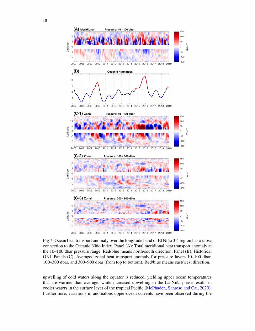
18
2007 2008 2009 2010 2011 2012 2013 2014 2015 2016 2017 2018 2019-2
-1
0
1
2
3Oceanic Nino Index(B)
Pressure: 10 - 100 dbar
2007 2008 2009 2010 2011 2012 2013 2014 2015 2016 2017 2018 2019
-10
-5
0
5
10
Latitu
de
-150
-100
-50
0
50
100
150
MW
m-1
(A) Meridional
Pressure: 10 - 100 dbar
2007 2008 2009 2010 2011 2012 2013 2014 2015 2016 2017 2018 2019
-10
-5
0
5
10
Latitu
de
-150
-100
-50
0
50
100
150
W m
-2
Pressure: 100 - 300 dbar
2007 2008 2009 2010 2011 2012 2013 2014 2015 2016 2017 2018 2019
-10
-5
0
5
10
Latitu
de
-150
-100
-50
0
50
100
150
W m
-2
Pressure: 300 - 900 dbar
2007 2008 2009 2010 2011 2012 2013 2014 2015 2016 2017 2018 2019
-10
-5
0
5
10
Latitu
de
-150
-100
-50
0
50
100
150
W m
-2
(C-1) Zonal
(C-2) Zonal
(C-3) Zonal
Fig 7: Ocean heat transport anomaly over the longitude band of El Niño 3.4 region has a closeconnection to the Oceanic Niño Index. Panel (A): Total meridional heat transport anomaly atthe 10–100 dbar pressure range. Red/blue means north/south direction. Panel (B): HistoricalONI. Panels (C): Averaged zonal heat transport anomaly for pressure layers 10–100 dbar,100–300 dbar, and 300–900 dbar (from top to bottom). Red/blue means east/west direction.
upwelling of cold waters along the equator is reduced, yielding upper ocean temperaturesthat are warmer than average, while increased upwelling in the La Niña phase results incooler waters in the surface layer of the tropical Pacific (McPhaden, Santoso and Cai, 2020).Furthermore, variations in anomalous upper-ocean currents have been observed during the
SPATIO-TEMPORAL INTERPOLATION OF GLOBAL OCEAN HEAT TRANSPORT 19
development of ENSO. Ren et al. (2017) found that, at the equator, eastward (positive) zonalcurrent anomalies strengthened in early 2015 before the anomalous currents turned to thewest (negative) by 2016, in general agreement with the estimate presented in Panel C1.
From Panels C1–C3, we can observe that the anomalous heat transport associated withENSO occurs predominantly in the upper layer of the ocean and that the patterns are subduedin the deeper parts of the ocean, which matches with earlier studies of ocean heat contentvariability (see, e.g., Trenberth et al., 2016). During the 2015–16 super El Niño episode,the strongest El Niño in history, the anomalous zonal heat transport exhibits a coherent pat-tern that extends to the deeper 100–300 dbar layer. Compared to conventional indices orthe rate of change in ocean heat content (Trenberth et al., 2016), Figure 7 reveals intrigu-ing, complex spatial variability (the study of which remains outside the scope of this paper).For example, the meridional component of the anomalous heat transport has a much largerinter-hemispheric asymmetry than does the zonal component.
5. Validation with Satellite Observations. In this section, we provide empirical valida-tion of our method and the resulting estimates by comparing with estimates based on satelliteobservations. The ultimate goal of the validation is to show our estimates align well with theexisting products widely used by the oceanographic community, and ascertain the strength ofthe proposed method, i.e, the two-stage procedure together with the debiasing procedure.
Satellite data offer an excellent tool for validating our gridded near-surface OHT estimates,as satellites capture high-resolution snapshots of SST and sea surface height (SSH, whichcan be used to estimate geostrophic velocity at the surface). Higher resolution is a clearadvantage of satellite observations compared to sparse in-situ data collected from researchvessels, Argo floats, and moorings; in-situ subsurface measurements are, however, crucial forcharacterizing OHT over the depth of the water column, as in Definition (1). In this section,we use the surface temperature transport TT0(s) = θ(s, z0)v(s, z0) instead of OHT, withz0 equal to 0 dbar for satellite based products (which are available only at the surface) and 10dbar for our Argo-based in-situ product (the shallowest depth we considered). Using TT0(s)instead of OHT, which corresponds to ignoring terms that do not impact the comparison,allows us to leverage observations available from satellites for validation analysis.
We adopted two separate satellite gridded products for SST and SSH distributed by theEU Copernicus Marine Environment Monitoring Service (CMEMS). For SST, the EuropeanSpace Agency (ESA) SST Climate Change Initiative (CCI) and Copernicus Climate ChangeService (C3S) reprocessed Level-4 product (Merchant et al., 2019) at daily 0.05 degreespatial resolution is considered. For SSH and its derived geostrophic velocity, sea level TAC-DUACS Level-4 Delayed-Time product (Taburet et al., 2019) is adopted. This product has aquarter-degree spatial resolution, along with daily temporal resolution. The DUACS productcontains state-of-the-art surface geostrophic velocity estimates mainly based on multimissionsatellite altimetry over the global ocean, although in-situ Argo profiles and surface drifters arealso used in part to estimate the Mean Dynamic Topography (Rio et al., 2018). However, theimpact of in-situ observations on the DUACS product is negligible in validating the proposedframework and the estimates from Argo data.
5.1. Comparing the OHT pipelines. The primary reason we propose a two-stage methodis that Argo floats do not directly measure velocity. Such a limitation requires us to firstestimate the velocity and then combine the resulting estimates with in-situ temperature ob-servations before interpolating in any space and time coordinates. The performance of theproposed procedure therefore depends on both the velocity estimation error and the OHTmapping error. Using the satellite-based SST and SSH products, we separately analyze theerrors associated with each of these components.
20
The first step is to establish the ground truth, defined here as the best possible griddedsurface temperature transport field at 1×1 spatial resolution. For this purpose, we computethe product of the gridded SST and velocity fields at 0.25 × 0.25 × 1 day resolution andthen upscale the result to the target resolution using natural-neighbor interpolation (Sibson,1981). This upscaled ground truth is not influenced by any of our proposed interpolationmethods. See Section F of the Supplementary Material (Park et al., 2020) for the resultingground truth time-averaged TT0 field.
A key advantage of utilizing high-resolution satellite products is that we can obtain SST(θ), SSH2 (Ψ), and velocity (v) in any spatio-temporal location up to the resolution eachproduct can resolve. We generated pseudo-observationsDPseudo = (θ(sij),Ψ(sij),v(sij)) :sij ∈ sD, ∀i, j at the same spatio-temporal locations as the Argo array sD by taking thenearest high-resolution spatio-temporal grid point of SST, SSH, and velocity, respectively.Since the nearest high-resolution grid-point from any observed locations in sD is at most0.177 × 0.5 days away, the approximation error is marginal in comparison to the samplingresolution of the Argo array. By construction, these pseudo-observations match the samplingresolution; hence, surface temperature transport estimates derived from in-situ Argo profilesand from pseudo-observations are commensurable, allowing us to assess our method in com-parison to the ground truth.
We consider three candidate methodsMj , j ∈ 1,2,3 to estimate the surface temperaturetransport field TT0(s∗) as follows:
M1 : θ · v(s∗), M2 : θ · v(s∗), M3 : θ(s∗) · v(s∗)
where (·)(s∗) is used to denote the estimate of (·) at any spatio-temporal point s∗ giventhe data DPseudo. Our proposed procedure from Section 3.3 corresponds to M2, where weestimate v from Ψ and interpolate the TT0 field based on the in-situ θ · v. All results hereafterare based on estimates after debiasing on all stages.M1 is a hypothetical procedure where we assume that v can be obtained without estima-
tion which is not feasible in practice (except at the surface where we have access to satellite-based v fields). Given DPseudo,M1 only requires a second stage procedure that reduces tothe local Gaussian process method from Kuusela and Stein (2018a). Thus, the performanceofM1 signifies the idealized interpolation capability of the local Gaussian process methodwhen sparse spatio-temporal measurements are fully observed. Meanwhile,M3 is an alter-native approach detailed in Appendix A, where the two gridded products θ and v can onlybe accessed separately. Such a situation frequently arises in oceanographic data analysis,in which case this approach is deemed a conventional norm. In this scenario, two separateinterpolations—one for θ and the other for v—are needed; OHT is computed as the productof the two gridded fields.
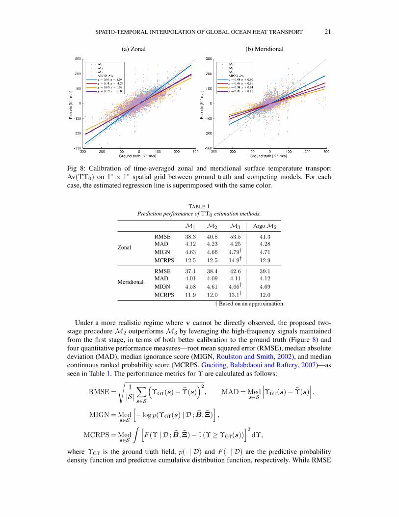
Figure 8 shows the calibration between the time-averaged surface temperature transportfield Av(TT0) on a 1× 1 spatial grid computed with the three methodsM1,M2,M3 andthe ground truth.M1 (in blue) clearly performs the best of the three competing models, asthe velocity v is fully observed in this case (i.e., the first stage estimation achieves zero error).Note that estimating the meridional OHT is an intrinsically harder problem than estimatingthe zonal OHT. This asymmetry most likely stems from the fact that across most of the openocean, the meridional signal is substantially smaller than the zonal signal (Zheng and Giese,2009; Forget and Ferreira, 2019), leading to a decrease in the signal-to-noise ratio.
2Although SSH and dynamic height anomaly are not the same, in this section we also use Ψ to denote SSH,with abuse of notation, since they fulfill the same purpose here.
SPATIO-TEMPORAL INTERPOLATION OF GLOBAL OCEAN HEAT TRANSPORT 21
(a) Zonal (b) Meridional
Fig 8: Calibration of time-averaged zonal and meridional surface temperature transportAv(TT0) on 1 × 1 spatial grid between ground truth and competing models. For eachcase, the estimated regression line is superimposed with the same color.
TABLE 1Prediction performance of TT0 estimation methods.
M1 M2 M3 ArgoM2
Zonal
RMSE 38.3 40.8 53.5 41.3MAD 4.12 4.23 4.25 4.28
MIGN 4.63 4.66 4.79† 4.71
MCRPS 12.5 12.5 14.9† 12.9
Meridional
RMSE 37.1 38.4 42.6 39.1MAD 4.01 4.09 4.11 4.12
MIGN 4.58 4.61 4.66† 4.69
MCRPS 11.9 12.0 13.1† 12.0
† Based on an approximation.
Under a more realistic regime where v cannot be directly observed, the proposed two-stage procedureM2 outperformsM3 by leveraging the high-frequency signals maintainedfrom the first stage, in terms of both better calibration to the ground truth (Figure 8) andfour quantitative performance measures—root mean squared error (RMSE), median absolutedeviation (MAD), median ignorance score (MIGN, Roulston and Smith, 2002), and mediancontinuous ranked probability score (MCRPS, Gneiting, Balabdaoui and Raftery, 2007)—asseen in Table 1. The performance metrics for Υ are calculated as follows:
RMSE =
√1
|S|∑s∈S
(ΥGT(s)− Υ(s)
)2, MAD = Med
s∈S
∣∣∣ΥGT(s)− Υ(s)∣∣∣ ,
MIGN = Meds∈S
[− log p(ΥGT(s) | D ; B, Ξ)
],
MCRPS = Meds∈S
∫ [F (Υ | D ; B, Ξ)− 1(Υ≥ΥGT(s))
]2dΥ,
where ΥGT is the ground truth field, p(· | D) and F (· | D) are the predictive probabilitydensity function and predictive cumulative distribution function, respectively. While RMSE
22
and MAD primarily assess the deterministic accuracy of the predictions, MIGN and MCRPSmeasure the probabilistic accuracy by taking both the deterministic accuracy and precisioninto consideration. MIGN measures the goodness of fit of the predictive distribution to theground truth, and MCRPS can be viewed as a generalized version of MAD (Gneiting, Bal-abdaoui and Raftery, 2007). The predictive distribution of M1 and M2 is Gaussian withanalytically tractable mean and variance; however, that of M3 is no longer Gaussian andentails further approximations for computing the MIGN and MCRPS since the estimate isthe product of two correlated Gaussian random variables. Here MIGN and MCRPS forM3
are computed using an approximate predictive distribution assuming that θ and v are jointlyGaussian. The reported values do not change up to 3 significant digits when varying thecorrelation from −1 to 1.
In addition to validating the two-stage procedure, comparing the surface temperature trans-port estimates derived from in-situ Argo profiles D to those constructed from the pseudoobservations DPseudo further confirms that the results presented in Section 4 are optimal interms of the proposed framework. In Figure 8, Table 1, we provide the calibration and pointprediction performance of the Argo-based estimate (denoted as ArgoM2 to emphasize thatM2 is comparable) with reference to the ground truth. The estimates derived from actualArgo profiles are surprisingly close to those based on pseudo observations (M2) and out-performM3. A performance degradation between ArgoM2 andM2 could arise mainly fortwo possible reasons: (A) Argo-based estimates are computed at a near surface pressure (10dbar) unlike the ground truth and M2 estimates, and (B) reference velocities at 900 dbaradopted from Gray and Riser (2014) might be underestimated. The good agreement foundhere demonstrates that these effects are minor in comparison to the other factors contributingto the overall performance of our method.
Recall that M1 is the idealized estimate when v is perfectly known. In other words, ifwe could improve our v estimate in the first stage, we might be able to achieve performanceclose toM1 even with in-situ Argo profiles alone. One can consider a natural extension ofthis work that synthesizes the high-resolution satellite product with the in-situ Argo profiledataset (Rio and Santoleri, 2018), which is an interesting direction for future improvement butwell beyond the scope of the present study. Our results do emphasize, however, that the coarsesampling resolution is the main cause of miscalibration in comparison to the satellite-basedground truth. The miscalibration arises mostly near western boundaries and in regions withsharp fronts, where abrupt changes occur and strong currents are present. These issues couldbe explained by (A) the innate bias incurred from the nonparametric regression approachand/or (B) the inability of the Argo fleet to sample the coastal shelves, where the floats cannotreach 2000 dbar. There have been numerous methods proposed in the statistics literatureto reduce the innate bias of (A). We tried the non-local means (Arias-Castro, Salmon andWillett, 2011) and concluded that the method brings a marginal improvement in identifyingthe fronts. On the other hand, in Section H of the Supplementary Material (Park et al., 2020),we confirmed that including Spray glider observations (Sherman et al., 2001; Rudnick, 2016)mitigates the underestimation occurring in the narrow boundary current in the western NorthAtlantic. These results indicate that the miscalibration stems more from the Argo array’ssampling deficiencies in the coastal regions and highly variable boundary currents and lessfrom a boundary bias due to the nonparametric regression approach.
5.2. Effect of Debiasing Procedure. In this section, we discuss the efficacy of the de-biasing procedure proposed in Section 3.5. Figure 9 and Table 2 give the point predictionperformance of the debiasing procedure on the first stage. Both show that the debiasing pro-cedure improves the mapping of both zonal and meridional velocities. Notice that the localinterpolation procedure yields a globally calibrated SSH (Ψ) field (Figure 9a) as compared
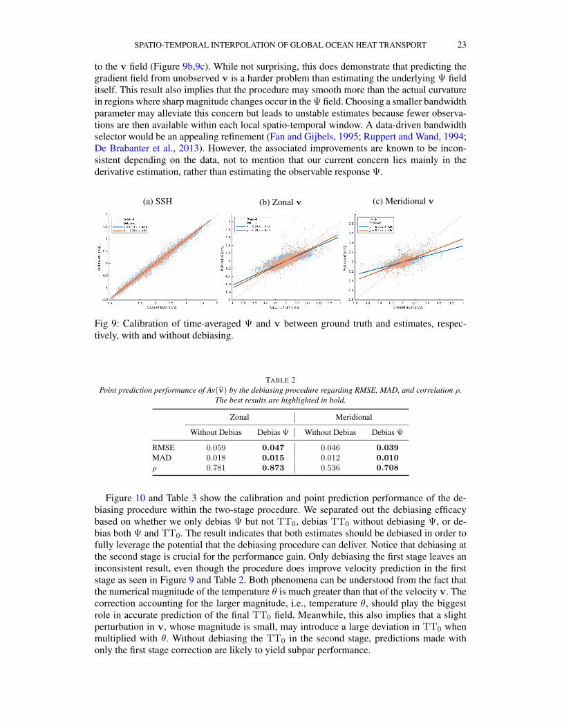
SPATIO-TEMPORAL INTERPOLATION OF GLOBAL OCEAN HEAT TRANSPORT 23
to the v field (Figure 9b,9c). While not surprising, this does demonstrate that predicting thegradient field from unobserved v is a harder problem than estimating the underlying Ψ fielditself. This result also implies that the procedure may smooth more than the actual curvaturein regions where sharp magnitude changes occur in the Ψ field. Choosing a smaller bandwidthparameter may alleviate this concern but leads to unstable estimates because fewer observa-tions are then available within each local spatio-temporal window. A data-driven bandwidthselector would be an appealing refinement (Fan and Gijbels, 1995; Ruppert and Wand, 1994;De Brabanter et al., 2013). However, the associated improvements are known to be incon-sistent depending on the data, not to mention that our current concern lies mainly in thederivative estimation, rather than estimating the observable response Ψ.
(a) SSH (b) Zonal v (c) Meridional v
Fig 9: Calibration of time-averaged Ψ and v between ground truth and estimates, respec-tively, with and without debiasing.
TABLE 2Point prediction performance of Av(v) by the debiasing procedure regarding RMSE, MAD, and correlation ρ.
The best results are highlighted in bold.
Zonal Meridional
Without Debias Debias Ψ Without Debias Debias Ψ
RMSE 0.059 0.047 0.046 0.039MAD 0.018 0.015 0.012 0.010ρ 0.781 0.873 0.536 0.708
Figure 10 and Table 3 show the calibration and point prediction performance of the de-biasing procedure within the two-stage procedure. We separated out the debiasing efficacybased on whether we only debias Ψ but not TT0, debias TT0 without debiasing Ψ, or de-bias both Ψ and TT0. The result indicates that both estimates should be debiased in order tofully leverage the potential that the debiasing procedure can deliver. Notice that debiasing atthe second stage is crucial for the performance gain. Only debiasing the first stage leaves aninconsistent result, even though the procedure does improve velocity prediction in the firststage as seen in Figure 9 and Table 2. Both phenomena can be understood from the fact thatthe numerical magnitude of the temperature θ is much greater than that of the velocity v. Thecorrection accounting for the larger magnitude, i.e., temperature θ, should play the biggestrole in accurate prediction of the final TT0 field. Meanwhile, this also implies that a slightperturbation in v, whose magnitude is small, may introduce a large deviation in TT0 whenmultiplied with θ. Without debiasing the TT0 in the second stage, predictions made withonly the first stage correction are likely to yield subpar performance.
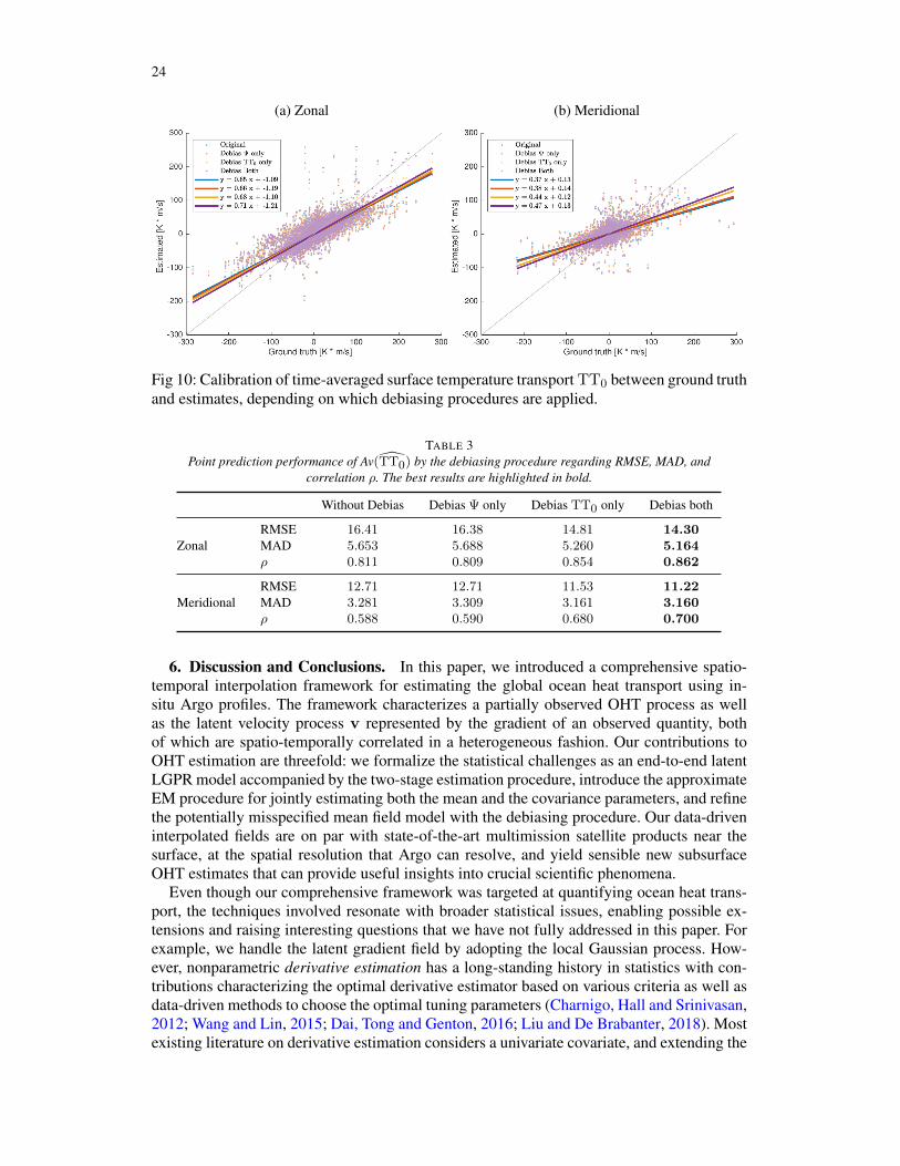
24
(a) Zonal (b) Meridional
Fig 10: Calibration of time-averaged surface temperature transport TT0 between ground truthand estimates, depending on which debiasing procedures are applied.
TABLE 3Point prediction performance of Av(TT0) by the debiasing procedure regarding RMSE, MAD, and
correlation ρ. The best results are highlighted in bold.
Without Debias Debias Ψ only Debias TT0 only Debias both
ZonalRMSE 16.41 16.38 14.81 14.30MAD 5.653 5.688 5.260 5.164ρ 0.811 0.809 0.854 0.862
MeridionalRMSE 12.71 12.71 11.53 11.22MAD 3.281 3.309 3.161 3.160ρ 0.588 0.590 0.680 0.700
6. Discussion and Conclusions. In this paper, we introduced a comprehensive spatio-temporal interpolation framework for estimating the global ocean heat transport using in-situ Argo profiles. The framework characterizes a partially observed OHT process as wellas the latent velocity process v represented by the gradient of an observed quantity, bothof which are spatio-temporally correlated in a heterogeneous fashion. Our contributions toOHT estimation are threefold: we formalize the statistical challenges as an end-to-end latentLGPR model accompanied by the two-stage estimation procedure, introduce the approximateEM procedure for jointly estimating both the mean and the covariance parameters, and refinethe potentially misspecified mean field model with the debiasing procedure. Our data-driveninterpolated fields are on par with state-of-the-art multimission satellite products near thesurface, at the spatial resolution that Argo can resolve, and yield sensible new subsurfaceOHT estimates that can provide useful insights into crucial scientific phenomena.
Even though our comprehensive framework was targeted at quantifying ocean heat trans-port, the techniques involved resonate with broader statistical issues, enabling possible ex-tensions and raising interesting questions that we have not fully addressed in this paper. Forexample, we handle the latent gradient field by adopting the local Gaussian process. How-ever, nonparametric derivative estimation has a long-standing history in statistics with con-tributions characterizing the optimal derivative estimator based on various criteria as well asdata-driven methods to choose the optimal tuning parameters (Charnigo, Hall and Srinivasan,2012; Wang and Lin, 2015; Dai, Tong and Genton, 2016; Liu and De Brabanter, 2018). Mostexisting literature on derivative estimation considers a univariate covariate, and extending the
SPATIO-TEMPORAL INTERPOLATION OF GLOBAL OCEAN HEAT TRANSPORT 25
established results to the spatio-temporal case is not trivial as spatial local regression itselfrequires substantial theoretical considerations (Hallin, Lu and Tran, 2004).
Another interesting direction is jointly modeling the temperature and velocity fields basedon the underlying process for temperature and salinity. Dynamic height anomaly, modeledseparately from temperature in this work, is indeed a nonlinear function of temperature andsalinity, which are the primitive measurements we obtain from the Argo floats. An excitingextension of our approach could be modeling the temperature and dynamic height anomalyfields instead as a bivariate Gaussian process, similar to the approach taken by Yarger, Stoevand Hsing (2020) for jointly modeling temperature and salinity. Admittedly, finding an ap-propriate cross-correlation function between temperature and dynamic height anomaly mightnot be as straightforward as for temperature and salinity.
While we relied on the local Gaussian process to define the spatio-temporal process, thecomplete characterization of the second order structure (covariance kernel) is not enough todescribe the full process when it is non-Gaussian. Even commonly used climate variables,such as temperature, are known to show non-Gaussian properties (Kuusela and Stein, 2018a;Stein, 2019). It could therefore be possible to explore non-Gaussian models (e.g., Bolin andWallin, 2020) to improve the prediction of the spatio-temporal process.
Vertical dependence, i.e., correlation across pressure levels, is an important aspect of anyprofile measurements, including the T -S profiles. The dynamic height anomaly Ψ has anadditional interesting property in that it is a monotonically increasing function of depth bydefinition. While our approach partially accommodates the vertical structure, the vertical de-pendence is not fully modeled. Completely accounting for the vertical structure would yieldseveral improvements, including a truly four-dimensional map of global ocean heat transport,effective confinement of the random fields with respect to depth using the monotonicity con-dition, and a complete uncertainty quantification of the OHT field. Yarger, Stoev and Hsing(2020) proposed functional PCA as a way of handling the vertical dependence, even thoughtheir focus was on modeling temperature and salinity where the monotone constraint is notrequired. Fully characterizing the vertical dependence of the global ocean circulation andassociated OHT is additionally of great interest to the oceanographic community and thusrepresents a priority for future work.
Acknowledgements. We would like to acknowledge high-performance computing sup-port from Cheyenne (doi:10.5065/D6RX99HX) provided by NCAR’s Computational and In-formation Systems Laboratory, sponsored by the National Science Foundation. Donata Giglioacknowledges support from NSF (Award 2026954) and NASA (Award NNH20ZDA001N-PO). Alison Gray acknowledges support from NASA (Award NNX80NSSC19K1252), theU.S. Argo Program through NOAA (Award NA15OAR4320063), and the Microsoft FacultyFellowship program. We are grateful to the Statistical Oceanography and STAMPS groups,and especially to Fred Bingham, Sarah Gille and Matt Mazloff for constructive discussionsand suggestions related to Argo, Spray data and physical oceanography. We appreciate theconstructive feedback by the Editor, the Associate Editor and the two anonymous reviewerswhich substantially improved the utility and readability of the paper.
SUPPLEMENTARY MATERIAL
Supplement A: Supplement to “Spatio-temporal Local Interpolation of Global OceanHeat Transport using Argo Floats: A Debiased Latent Gaussian Process Approach”(doi: COMPLETED BY THE TYPESETTER; .pdf). We provide in the supplement addi-tional details on quality control, analytic formulas regarding the covariance kernel, explicitderivations of the EM procedure, the predictive distribution for single depth OHT, and sup-porting figures, as well as extensive additional analyses where Spray glider profiles are jointlyanalyzed with Argo float profiles.
26
REFERENCES
ARGO (2020). Argo float data and metadata from Global Data Assembly Centre (Argo GDAC). DOI:10.17882/42182.
ARIAS-CASTRO, E., SALMON, J. and WILLETT, R. (2011). Oracle inequalities and minimax rates for non-localmeans and related adaptive kernel-based methods. arXiv:1112.4434 [cs, math, stat]. arXiv: 1112.4434.
BANERJEE, S., GELFAND, A. E. and SIRMANS, C. F. (2003). Directional Rates of Change Under Spatial ProcessModels. Journal of the American Statistical Association 98 946–954.
BARKER, P. M. and MCDOUGALL, T. J. (2020). Two Interpolation Methods Using Multiply-Rotated PiecewiseCubic Hermite Interpolating Polynomials. Journal of Atmospheric and Oceanic Technology 37 605–619.
BAYARRI, M. J., WALSH, D., BERGER, J. O., CAFEO, J., GARCIA-DONATO, G., LIU, F., PALOMO, J.,PARTHASARATHY, R. J., PAULO, R. and SACKS, J. (2007). Computer model validation with functional out-put. The Annals of Statistics 35 1874–1906.
BEHRENS, E., FERNANDEZ, D. and SUTTON, P. (2019). Meridional Oceanic Heat Transport Influences MarineHeatwaves in the Tasman Sea on Interannual to Decadal Timescales. Frontiers in Marine Science 6 228.
BOLIN, D. and WALLIN, J. (2020). Multivariate type G Matérn stochastic partial differential equation randomfields. Journal of the Royal Statistical Society Series B 82 215–239.
BRYDEN, H. L. and IMAWAKI, S. (2001). Chapter 6.1 Ocean heat transport. In International Geophysics,(G. Siedler, J. Church and J. Gould, eds.). Ocean Circulation and Climate 77 455–474. Academic Press.
BRYNJARSDÓTTIR, J. and O’HAGAN, A. (2014). Learning about physical parameters: the importance of modeldiscrepancy. Inverse Problems 30 114007. Publisher: IOP Publishing.
CHARNIGO, R., HALL, B. and SRINIVASAN, C. (2012). A Generalized Cp Criterion for Derivative Estimation.Technometrics.
LABORATORY, C. A. I. S. (2019). Cheyenne: SGI ICE XA Cluster. doi: 10.5065/D6RX99HX.CRESSIE, N. (1993). Statistics for Spatial Data, revised ed. John Wiley & Sons, New York.CRESSIE, N. and WIKLE, C. K. (2011). Statistics for Spatio-Temporal Data. John Wiley & Sons.CSISZAR, I. and TUSNADY, G. (1984). Information geometry and alternating minimization procedures. Statistics
and decisions 1 205–237. Publisher: Oldenburg Verlag.DAI, W., TONG, T. and GENTON, M. G. (2016). Optimal Estimation of Derivatives in Nonparametric Regression.
Journal of Machine Learning Research 17 1–25.DE BRABANTER, K., DE BRABANTER, J., DE MOOR, B. and GIJBELS, I. (2013). Derivative estimation with
local polynomial fitting. The Journal of Machine Learning Research 14 281–301.DEMPSTER, A. P., LAIRD, N. M. and RUBIN, D. B. (1977). Maximum Likelihood from Incomplete Data Via
the EM Algorithm. Journal of the Royal Statistical Society: Series B (Methodological) 39 1–22.FAN, J. and GIJBELS, I. (1995). Data-Driven Bandwidth Selection in Local Polynomial Fitting: Variable Band-
width and Spatial Adaptation. Journal of the Royal Statistical Society: Series B (Methodological) 57 371–394.FAN, J., GASSER, T., GIJBELS, I., BROCKMANN, M. and ENGEL, J. (1997). Local Polynomial Regression:
Optimal Kernels and Asymptotic Minimax Efficiency. Annals of the Institute of Statistical Mathematics 4979–99.
FORGET, G. and FERREIRA, D. (2019). Global ocean heat transport dominated by heat export from the tropicalPacific. Nature Geoscience 12 351–354.
FORGET, G. and PONTE, R. M. (2015). The partition of regional sea level variability. Progress in Oceanography137 173–195.
FRITSCH, F. N. and CARLSON, R. E. (1980). Monotone Piecewise Cubic Interpolation. SIAM Journal on Nu-merical Analysis 17 238–246.
GANACHAUD, A. and WUNSCH, C. (2000). Improved estimates of global ocean circulation, heat transport andmixing from hydrographic data. Nature 408 453–457. Number: 6811 Publisher: Nature Publishing Group.
GLANTZ, M. H. and RAMIREZ, I. J. (2020). Reviewing the Oceanic Niño Index (ONI) to Enhance SocietalReadiness for El Niño’s Impacts. International Journal of Disaster Risk Science 11 394–403.
GNEITING, T., BALABDAOUI, F. and RAFTERY, A. E. (2007). Probabilistic forecasts, calibration and sharpness.Journal of the Royal Statistical Society: Series B (Statistical Methodology) 69 243–268.
GOOD, S. A., MARTIN, M. J. and RAYNER, N. A. (2013). EN4: Quality controlled ocean temperature andsalinity profiles and monthly objective analyses with uncertainty estimates. Journal of Geophysical Research:Oceans 118 6704–6716.
GRAY, A. R. and RISER, S. C. (2014). A Global Analysis of Sverdrup Balance Using Absolute GeostrophicVelocities from Argo. Journal of Physical Oceanography 44 1213–1229.
GRAY, A. R. and RISER, S. C. (2015). A method for multiscale optimal analysis with application to Argo data.Journal of Geophysical Research: Oceans 120 4340–4356.
GUERRIER, S., KAREMERA, M., ORSO, S. and VICTORIA-FESER, M.-P. (2020). Asymptotically Optimal BiasReduction for Parametric Models. arXiv:2002.08757 [math, stat]. arXiv: 2002.08757.
SPATIO-TEMPORAL INTERPOLATION OF GLOBAL OCEAN HEAT TRANSPORT 27
HAAS, T. C. (1990). Kriging and automated variogram modeling within a moving window. Atmospheric Envi-ronment. Part A. General Topics 24 1759–1769.
HAAS, T. C. (1995). Local Prediction of a Spatio-Temporal Process with an Application to Wet Sulfate Deposi-tion. Journal of the American Statistical Association 90 1189–1199.
HALLIN, M., LU, Z. and TRAN, L. T. (2004). Local linear spatial regression. The Annals of Statistics 32 2469–2500.
JAYNE, S., ROEMMICH, D., ZILBERMAN, N., RISER, S., JOHNSON, K., JOHNSON, G. and PIOTROWICZ, S.(2017). The Argo Program: Present and Future. Oceanography 30 18–28.
KENNEDY, M. C. and O’HAGAN, A. (2001). Bayesian calibration of computer models. Journal of the RoyalStatistical Society: Series B (Statistical Methodology) 63 425–464.
KUK, A. Y. C. (1995). Asymptotically Unbiased Estimation in Generalized Linear Models with Random Effects.Journal of the Royal Statistical Society. Series B (Methodological) 57 395–407.
KUUSELA, M. and STEIN, M. L. (2018a). Locally stationary spatio-temporal interpolation of Argo profiling floatdata. Proceedings of the Royal Society A: Mathematical, Physical and Engineering Sciences 474 20180400.
KUUSELA, M. and STEIN, M. L. (2018b). Supplementary material from "Locally stationary spatio-temporalinterpolation of Argo profiling float data".
LAGERLOEF, G. S. E., MITCHUM, G. T., LUKAS, R. and NIILER, P. P. (1999). Tropical Pacific Near-SurfaceCurrents Estimated from Altimeter, Wind, and Drifter Data.
LEBEDEV, K., YOSHINARI, H., MAXIMENKO, N. A. and HACKER, P. W. (2007). YoMaHa’07: Velocity dataassessed from trajectories of Argo floats at parking level and at the sea surface. 4 16.
LIU, Y. and DE BRABANTER, K. (2018). Derivative Estimation in Random Design. In Advances in NeuralInformation Processing Systems 31 (S. Bengio, H. Wallach, H. Larochelle, K. Grauman, N. Cesa-Bianchi andR. Garnett, eds.) 3445–3454. Curran Associates, Inc.
MACDONALD, A. M. and BARINGER, M. (2013). Ocean Heat Transport. In International Geophysics, 103 759–785.
MCDOUGALL, T. and BARKER, P. M. (2011). Getting started with TEOS-10 and the Gibbs Seawater(GSW)Oceanographic Toolbox. SCOR/IAPSO WG 127 1–28.
MCPHADEN, M. J., SANTOSO, A. and CAI, W. (2020). El Niño Southern Oscillation in a Changing Climate.American Geophysical Union (AGU).
MERCHANT, C. J., EMBURY, O., BULGIN, C. E., BLOCK, T., CORLETT, G. K., FIEDLER, E., GOOD, S. A.,MITTAZ, J., RAYNER, N. A., BERRY, D., EASTWOOD, S., TAYLOR, M., TSUSHIMA, Y., WATERFALL, A.,WILSON, R. and DONLON, C. (2019). Satellite-based time-series of sea-surface temperature since 1981 forclimate applications. Scientific Data 6 223. Number: 1 Publisher: Nature Publishing Group.
NEAL, R. M. and HINTON, G. E. (1998). A View of the Em Algorithm that Justifies Incremental, Sparse, andother Variants. In Learning in Graphical Models, (M. I. Jordan, ed.). NATO ASI Series 355–368. SpringerNetherlands, Dordrecht.
NOCEDAL, J. (1980). Updating quasi-Newton matrices with limited storage. Mathematics of Computation 35773–782.
OLLITRAULT, M. and RANNOU, J.-P. (2013). ANDRO: An Argo-Based Deep Displacement Dataset. Journal ofAtmospheric and Oceanic Technology 30 759–788.
PARK, B., KUUSELA, M., GIGLIO, D. and GRAY, A. (2020). Supplement to "Spatio-temporal Local Interpola-tion of Global Ocean Heat Transport using Argo Floats: A Debiased Latent Gaussian Process Approach".
RASMUSSEN, C. E. and WILLIAMS, C. K. I. (2006). Gaussian processes for machine learning. MIT Press.REN, H.-L., WANG, R., ZHAI, P., DING, Y. and LU, B. (2017). Upper-ocean dynamical features and prediction
of the super El Niño in 2015/16: A comparison with the cases in 1982/83 and 1997/98. Journal of Meteoro-logical Research 31 278–294.
RIDGWAY, K. R., DUNN, J. R. and WILKIN, J. L. (2002). Ocean interpolation by four-dimensional weightedleast squares - Application to the waters around Australasia. Journal of Atmospheric and Oceanic Technology19 1357–1375.
RIO, M. H. and SANTOLERI, R. (2018). Improved global surface currents from the merging of altimetry and SeaSurface Temperature data. Remote Sensing of Environment 216 770–785.
RIO, M.-H., MULET, S., ETIENNE, H., PICOT, N. and DIBARBOURE, G. (2018). New CNES-CLS18 MeanDynamic Topography of the global ocean from altimetry, gravity and in-situ data. In OSTST 22.
RISER, S. C., FREELAND, H. J., ROEMMICH, D., WIJFFELS, S., TROISI, A., BELBÉOCH, M., GILBERT, D.,XU, J., POULIQUEN, S., THRESHER, A., LE TRAON, P.-Y., MAZE, G., KLEIN, B., RAVICHANDRAN, M.,GRANT, F., POULAIN, P.-M., SUGA, T., LIM, B., STERL, A., SUTTON, P., MORK, K.-A., VÉLEZ-BELCHÍ, P. J., ANSORGE, I., KING, B., TURTON, J., BARINGER, M. and JAYNE, S. R. (2016). Fifteenyears of ocean observations with the global Argo array. Nature Climate Change 6 145–153.
ROEMMICH, D. and GILSON, J. (2009). The 2004–2008 mean and annual cycle of temperature, salinity, andsteric height in the global ocean from the Argo Program. Progress in Oceanography 82 81–100.
28
ROEMMICH, D., BOEBEL, O., FREELAND, H. J., KING, B. A., LE TRAON, P.-Y., MOLINARI, R.,OWENS, W. B., RISER, S., SEND, U., TAKEUCHI, K. and WIJFFELS, S. E. (1998). On the design and im-plementation of Argo: A global array of profiling floats. ICPO publication series ; 21. GODAE InternationalProject Office, Melbourne, Vic.
ROULSTON, M. S. and SMITH, L. A. (2002). Evaluating Probabilistic Forecasts Using Information Theory.Monthly Weather Review 130 1653–1660.
RUDNICK, D. L. (2016). Ocean Research Enabled by Underwater Gliders. Annual Review of Marine Science 8519–541.
RUDNICK, D. L., DAVIS, R. E. and SHERMAN, J. T. (2016). Spray Underwater Glider Operations. Journal ofAtmospheric and Oceanic Technology 33 1113–1122.
RUPPERT, D. and WAND, M. P. (1994). Multivariate Locally Weighted Least Squares Regression. The Annals ofStatistics 22 1346–1370. MR1311979
SCOTT, R. B., ARBIC, B. K., CHASSIGNET, E. P., COWARD, A. C., MALTRUD, M., MERRYFIELD, W. J.,SRINIVASAN, A. and VARGHESE, A. (2010). Total kinetic energy in four global eddying ocean circulationmodels and over 5000 current meter records. Ocean Modelling 32 157–169.
SHERMAN, J., DAVIS, R. E., OWENS, W. B. and VALDES, J. (2001). The autonomous underwater glider"Spray". IEEE Journal of Oceanic Engineering 26 437–446.
SIBSON, R. (1981). A brief description of natural neighbor interpolation. In Interpolating multivariate data.Chapter 2 21–36. John Wiley & Sons, New York.
STEIN, M. L. (1999). Interpolation of Spatial Data: Some Theory for Kriging. Springer Series in Statistics.Springer-Verlag, New York.
STEIN, M. L. (2013). Statistical Properties of Covariance Tapers. Journal of Computational and Graphical Statis-tics 22 866–885.
STEIN, M. L. (2019). Some Statistical Issues in Climate Science. 17.STOCKER, T. F. (2013). Chapter 1 - The Ocean as a Component of the Climate System. In International Geo-
physics, (G. Siedler, S. M. Griffies, J. Gould and J. A. Church, eds.). Ocean Circulation and Climate 103 3–30.Academic Press.
STONE, C. J. (1980). Optimal Rates of Convergence for Nonparametric Estimators. Annals of Statistics 8 1348–1360. MR594650
TABURET, G., SANCHEZ-ROMAN, A., BALLAROTTA, M., PUJOL, M.-I., LEGEAIS, J.-F., FOURNIER, F.,FAUGERE, Y. and DIBARBOURE, G. (2019). DUACS DT2018: 25 years of reprocessed sea level altimetryproducts. Ocean Science 15 1207–1224.
TALLEY, L. D., PICKARD, G. L., EMERY, W. J. and SWIFT, J. H. (2011). Descriptive Physical Oceanography:An Introduction, 6 ed. Academic Press.
TRENBERTH, K. E. and CARON, J. M. (2001). Estimates of Meridional Atmosphere and Ocean Heat Transports.Journal of Climate 14 3433–3443.
TRENBERTH, K. E. and SOLOMON, A. (1994). The global heat balance: heat transports in the atmosphere andocean. Climate Dynamics 10 107–134.
TRENBERTH, K. E., FASULLO, J. T., SCHUCKMANN, K. V. and CHENG, L. (2016). Insights into Earth’s EnergyImbalance from Multiple Sources. Journal of Climate 29 7495–7505.
VECCHIA, A. V. (1988). Estimation and Model Identification for Continuous Spatial Processes. Journal of theRoyal Statistical Society: Series B (Methodological) 50 297–312.
VERDIÈRE, A. C. D., MEUNIER, T. and OLLITRAULT, M. (2019). Meridional overturning and heat transportfrom Argo floats displacements and the Planetary Geostrophic Method (PGM). Application to the subpolarNorth Atlantic. Journal of Geophysical Research: Oceans 0.
WANG, W. and LIN, L. (2015). Derivative estimation based on difference sequence via locally weighted leastsquares regression. Journal of Machine Learning Research 16 2617–2641.
WILLIS, J. K. and FU, L.-L. (2008). Combining altimeter and subsurface float data to estimate the time-averagedcirculation in the upper ocean. Journal of Geophysical Research: Oceans 113.
WONG, A. P. S., WIJFFELS, S. E., RISER, S. C., POULIQUEN, S., HOSODA, S., ROEMMICH, D.,GILSON, J., JOHNSON, G. C., MARTINI, K., MURPHY, D. J., SCANDERBEG, M., BHASKAR, T. V.S. U., BUCK, J. J. H., MERCEUR, F., CARVAL, T., MAZE, G., CABANES, C., ANDRÉ, X., POFFA, N.,YASHAYAEV, I., BARKER, P. M., GUINEHUT, S., BELBÉOCH, M., IGNASZEWSKI, M., BARINGER, M. O.,SCHMID, C., LYMAN, J. M., MCTAGGART, K. E., PURKEY, S. G., ZILBERMAN, N., ALKIRE, M. B.,SWIFT, D., OWENS, W. B., JAYNE, S. R., HERSH, C., ROBBINS, P., WEST-MACK, D., BAHR, F.,YOSHIDA, S., SUTTON, P. J. H., CANCOUËT, R., COATANOAN, C., DOBBLER, D., JUAN, A. G.,GOURRION, J., KOLODZIEJCZYK, N., BERNARD, V., BOURLÈS, B., CLAUSTRE, H., D’ORTENZIO, F.,LE RESTE, S., LE TRAON, P.-Y., RANNOU, J.-P., SAOUT-GRIT, C., SPEICH, S., THIERRY, V., VER-BRUGGE, N., ANGEL-BENAVIDES, I. M., KLEIN, B., NOTARSTEFANO, G., POULAIN, P.-M., VÉLEZ-BELCHÍ, P., SUGA, T., ANDO, K., IWASASKA, N., KOBAYASHI, T., MASUDA, S., OKA, E., SATO, K.,
SPATIO-TEMPORAL INTERPOLATION OF GLOBAL OCEAN HEAT TRANSPORT 29
NAKAMURA, T., SATO, K., TAKATSUKI, Y., YOSHIDA, T., COWLEY, R., LOVELL, J. L., OKE, P. R.,VAN WIJK, E. M., CARSE, F., DONNELLY, M., GOULD, W. J., GOWERS, K., KING, B. A., LOCH, S. G.,MOWAT, M., TURTON, J., RAMA RAO, E. P., RAVICHANDRAN, M., FREELAND, H. J., GABOURY, I.,GILBERT, D., GREENAN, B. J. W., OUELLET, M., ROSS, T., TRAN, A., DONG, M., LIU, Z., XU, J.,KANG, K., JO, H., KIM, S.-D. and PARK, H.-M. (2020). Argo Data 1999–2019: Two Million Temperature-Salinity Profiles and Subsurface Velocity Observations From a Global Array of Profiling Floats. Frontiers inMarine Science 7. Publisher: Frontiers.
YARGER, D., STOEV, S. and HSING, T. (2020). A functional-data approach to the Argo data. arXiv:2006.05020[stat]. arXiv: 2006.05020.
ZHENG, Y. and GIESE, B. S. (2009). Ocean heat transport in Simple Ocean Data Assimilation: Structure andmechanisms. Journal of Geophysical Research: Oceans 114.
APPENDIX A: ALTERNATIVE DECOMPOSITION OF OHT
One may argue that heat transport can be computed by estimating mass transport andtemperature grids separately. In particular,
Q=
∫θMdz =
∫(θ+ θ′)(M +M ′)dz, M := ρv(18)
Such a decomposition may identify which component—mean or anomaly—in temperatureand mass transport drives heat transport. The decomposition does not need a two-step estima-tion procedure, rather it executes single step estimation for temperature and mass transport,separately. In Section 5, we empirically demonstrate that this strategy is inferior to the pro-posed two-stage method when it comes to prediction performance.
SPATIO-TEMPORAL INTERPOLATION OF GLOBAL OCEAN HEAT TRANSPORT 1
SUPPLEMENTARY MATERIAL
A. Quality Control. On top of the quality control criteria applied in Kuusela and Stein(2018b), we additionally reject potential duplicates of each profile having the same spatiallocation with timestamps within 15 minutes since such duplicates are highly unlikely basedon the Argo sampling design.
In general, salinity measurements are more prone larger biases than the temperature mea-surements by the nature of the CTD sensor and thus stricter quality control criteria are oftenrequired. We inspected the computed dynamic height anomalies and filtered out 34 profilesthat were impacted by problematic salinity measurements. These profiles deviate more than3×interquartile range (IQR) from the median at 10 dbar and more than 10×IQR at deeperdepths.
B. Analytic derivative of Matérn covariance kernel. For our covariance kernelchoice (7), we have the following analytic forms for the gradient and the Hessian of thekernel k:
∂
∂x1k(s1,s2) =−3φ
∆x
ξ2x
exp(−√
3d),(S1)
∂2
∂x1∂x2k(s1,s2) =
3φ
ξ2x
(1−√
3
d
(∆x
ξx
)2)
exp(−√
3d),(S2)
∂2
∂x1∂y2k(s1,s2) =−3
√3φ
d
∆x
ξ2y
∆y
ξ2y
exp(−√
3d),(S3)
where ∆x = x1 − x2 and ∆y = y1 − y2.
C. Alternating Maximization view of the EM procedure. One may ask how does thecoordinate ascent algorithm proposed in the main text link to the EM algorithm. We followthe maximization-maximization viewpoint of the EM algorithm following Neal and Hinton(1998). A similar argument was also made in Andresen and Spokoiny (2016). Under ourLGPR model, let Υ be a set of observed values of the quantity of interest and let Z bea set of unobserved latent data whose joint probability is parameterized using Ξ. The EMalgorithm iteratively computes the following two steps, for l= 1,2, . . . ,
E-Step: Compute a distribution P (l) over the range of Z such that P (l) = P (Z|Υ;Ξ(l−1)).M-Step: Set Ξ(l) = argmaxΞEP (l) [logP (Υ,Z;Ξ)].
When Z = argmaxB P (Υ;B,Ξ) is considered, P (l) is just a point mass at B(l),where B(l) = argmaxB P (Υ;B,Ξ(l−1)). Thus, the E-step is equivalent to finding the Bthat maximizes the likelihood L given the Ξ(l−1) from the previous iteration. Similarly,EP (l) [logP (Υ,Z;Ξ)] = logP (Υ,B(l);Ξ) which implies that the M-step is equivalent tofinding the maximizer of the likelihood L given the B(l) found in the previous E-step.
D. Details of the Approximate EM procedure. The M-step is performed with theresiduals from the previous E-step as described in the paper. In the following, we derive theanalytic solution of the E-step assuming that the temporal grid T consists of center points ofeach month. A generalization to more complex grids is straightforward following the LGPRconstruction. The subscript i, j corresponds to year i and month j, i.e., yi,j is a set of obser-vation in year i within month j. For every x∗ ∈ X , denote β := β(x∗) and ξj := ξ(x∗, t∗j ),
2
where t∗j ∈ T is the center point of month j. Then,
logL(β|Ξ) = log(p(y1,1:3);ξ2) +
12∑j=4
log p(y1,j |y1:(j−1);β,ξ2, . . . ,ξj−1)
+
I∑i=2
12∑j=1
log p(yi,j |y1:i−1,1:12, yi,1:(j−1);β,Ξ),
log L(β|Ξ) = log(p(y1,1:3);ξ2) +
12∑j=4
log p(y1,j |y(j−2):(j−1);β,ξj−1)
+
I∑i=2
[log p(yi,1|yi−1,11:12;β,ξ12) + log p(yi,2|yi−1,12, yi,1;β,ξ1)
+
12∑j=3
log p(yi,j |yi,1:(j−1);β,ξj−1)
],
where L is the Vecchia approximated likelihood with 3-month temporal lag.From hereafter, we show the result for the first year (i = 1) and drop the subscript i for
conciseness. The summand with all years still maintains the same maximizer form with theonly difference in Q and C below.
log L1(β|Ξ)≈ log p(y[1:3];ξ2) +
12∑j=4
log p(yj |y(j−2):(j−1);ξj−1), (Vecchia)
= logφ(y[1:3];η[1:3]β,K(ξ2))
+
12∑j=4
logφ(y[j−2:j];η[j−2:j]β+Kj,−jK−1−j,−j(y−j − η−j)β,Kjj −Kj,−jK
−1−j,−jK−j,j)
(∗)∝β>
η>[3]K(ξ2)−1η[3] +
12∑j=4
(ηj −Kj,−jK−1−j,−jη−j)
>[K−1]jj(ηj −Kj,−jK−1−j,−jη−j)
︸ ︷︷ ︸
:=Q
β
− 2
y>[3]K(ξ2)−1η[3] +
12∑j=4
(yj −Kj,−jK−1−j,−jy−j)
>[K−1]jj(ηj −Kj,−jK−1−j,−jη−j)
︸ ︷︷ ︸
:=C
β,
where φ(y;µ,Σ) is the pdf of multivariate Normal distribution with mean µ and variance Σ;K =K(ξj−1) is a covariance matrix constructed from the parameter ξj−1 and subscript −jcorresponds to all indices except month j. (∗) follows from Woodbery matrix identity,
(Kjj −Kj,−jK−1−j,−jK−j,j)
−1 =K−1jj −K
−1jj Kj,−j
(K−j,−j +K−j,jK
−1jj Kj,−j
)−1K−j,jK
−1jj
= [K−1]jj
Therefore, the maximizer is
β =Q−1C.
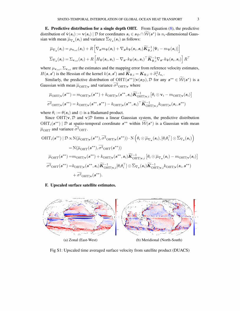
SPATIO-TEMPORAL INTERPOLATION OF GLOBAL OCEAN HEAT TRANSPORT 3
E. Predictive distribution for a single depth OHT. From Equation (8), the predictivedistribution of v(si) := v(si) | D for coordinates si ∈ sD ∩ W(s∗) is ni-dimensional Gaus-sian with mean µ∇x
(si) and variance Σ∇x(si) as follows:
µ∇x(si) = µvref
(si) +R[∇xmΨ(si) +∇xkΨ(si,si)K
−1Ψ,i [Ψi −mΨ(si)]
]Σ∇x
(si) = Σvref(si) +R
[HΨ(si,si)−∇x∗kΨ(si,si)
>K−1Ψ,i∇x∗kΨ(si,si)
]R>
where µvref, Σvref
are the estimates and the mapping error from reference velocity estimates,H(s,s′) is the Hessian of the kernel k(s,s′) and KΨ,i =KΨ,i + σ2
ε Ini.
Similarly, the predictive distribution of OHT(s∗∗)|v(sD),D for any s∗∗ ∈ W(s∗) is aGaussian with mean µOHT|v and variance σ2
OHT|v where
µOHT|v(s∗∗) =mOHT|v(s∗∗) + kOHT|v(s∗∗,si)K−1OHT|v,i
[θi vi −mOHT|v(si)
]σ2
OHT|v(s∗∗) = kOHT|v(s∗∗,s∗∗)− kOHT|v(s∗∗,si)>K−1
OHT|v,ikOHT|v(si,s∗∗)
where θi := θ(si) and is a Hadamard product.Since OHT|v,D and v|D forms a linear Gaussian system, the predictive distribution
OHTi(s∗∗) | D at spatio-temporal coordinate s∗∗ within W(s∗) is a Gaussian with mean
µOHT and variance σ2OHT.
OHTi(s∗∗) | D ∝N(µOHT|v(s∗∗), σ2
OHT|v(s∗∗)) ·N(θi µ∇x
(si), [θiθ>i ]Σ∇x
(si))
= N(µOHT(s∗∗), σ2OHT(s∗∗))
µOHT(s∗∗) =mOHT|v(s∗∗) + kOHT|v(s∗∗,si)K−1OHT|v,i
[θi µ∇x
(si)−mOHT|v(si)]
σ2OHT(s∗∗) =kOHT|v(s∗∗,si)K
−1OHT|v,i[θiθ
>i ]Σ∇x
(si)K−1OHT|v,ikOHT|v(si,s
∗∗)
+ σ2OHT|v(s∗∗).
F. Upscaled surface satellite estimates.
(a) Zonal (East-West) (b) Meridional (North-South)
Fig S1: Upscaled time averaged surface velocity from satellite product (DUACS)
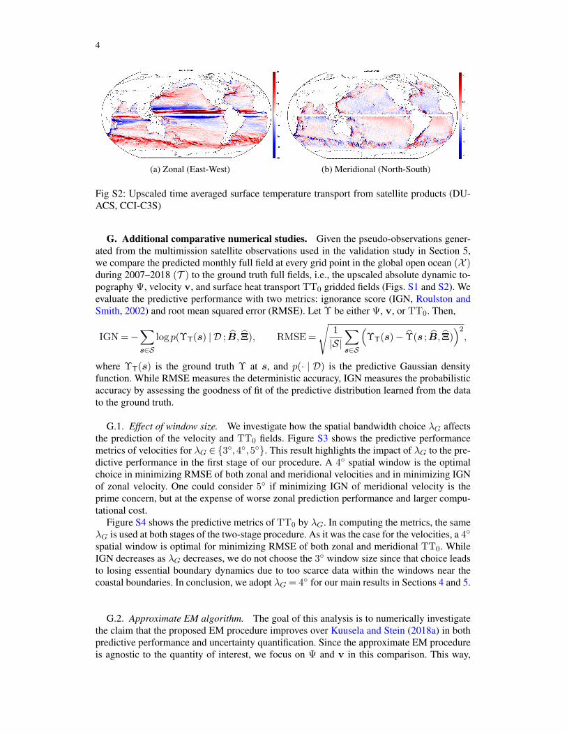
4
(a) Zonal (East-West) (b) Meridional (North-South)
Fig S2: Upscaled time averaged surface temperature transport from satellite products (DU-ACS, CCI-C3S)
G. Additional comparative numerical studies. Given the pseudo-observations gener-ated from the multimission satellite observations used in the validation study in Section 5,we compare the predicted monthly full field at every grid point in the global open ocean (X )during 2007–2018 (T ) to the ground truth full fields, i.e., the upscaled absolute dynamic to-pography Ψ, velocity v, and surface heat transport TT0 gridded fields (Figs. S1 and S2). Weevaluate the predictive performance with two metrics: ignorance score (IGN, Roulston andSmith, 2002) and root mean squared error (RMSE). Let Υ be either Ψ, v, or TT0. Then,
IGN =−∑s∈S
log p(ΥT(s) | D ; B, Ξ), RMSE =
√1
|S|∑s∈S
(ΥT(s)− Υ(s ; B, Ξ)
)2,
where ΥT(s) is the ground truth Υ at s, and p(· | D) is the predictive Gaussian densityfunction. While RMSE measures the deterministic accuracy, IGN measures the probabilisticaccuracy by assessing the goodness of fit of the predictive distribution learned from the datato the ground truth.
G.1. Effect of window size. We investigate how the spatial bandwidth choice λG affectsthe prediction of the velocity and TT0 fields. Figure S3 shows the predictive performancemetrics of velocities for λG ∈ 3,4,5. This result highlights the impact of λG to the pre-dictive performance in the first stage of our procedure. A 4 spatial window is the optimalchoice in minimizing RMSE of both zonal and meridional velocities and in minimizing IGNof zonal velocity. One could consider 5 if minimizing IGN of meridional velocity is theprime concern, but at the expense of worse zonal prediction performance and larger compu-tational cost.
Figure S4 shows the predictive metrics of TT0 by λG. In computing the metrics, the sameλG is used at both stages of the two-stage procedure. As it was the case for the velocities, a 4
spatial window is optimal for minimizing RMSE of both zonal and meridional TT0. WhileIGN decreases as λG decreases, we do not choose the 3 window size since that choice leadsto losing essential boundary dynamics due to too scarce data within the windows near thecoastal boundaries. In conclusion, we adopt λG = 4 for our main results in Sections 4 and 5.
G.2. Approximate EM algorithm. The goal of this analysis is to numerically investigatethe claim that the proposed EM procedure improves over Kuusela and Stein (2018a) in bothpredictive performance and uncertainty quantification. Since the approximate EM procedureis agnostic to the quantity of interest, we focus on Ψ and v in this comparison. This way,
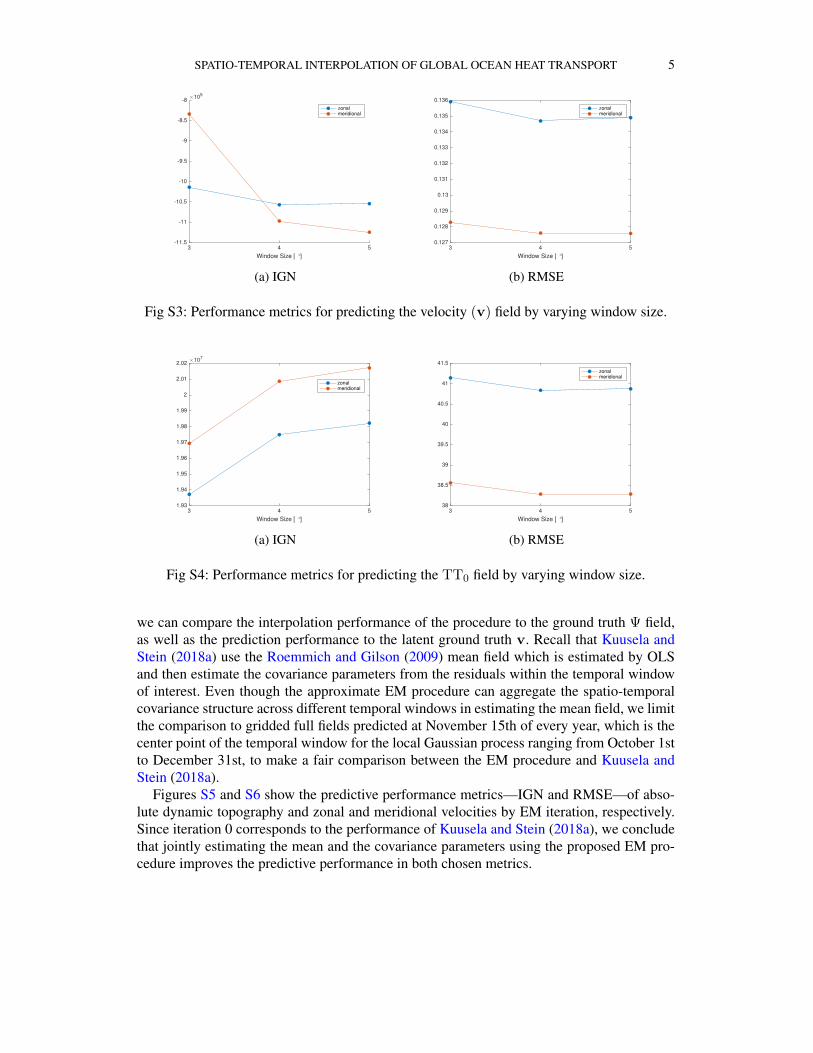
SPATIO-TEMPORAL INTERPOLATION OF GLOBAL OCEAN HEAT TRANSPORT 5
3 4 5
Window Size [ °]
-11.5
-11
-10.5
-10
-9.5
-9
-8.5
-8105
zonalmeridional
(a) IGN
3 4 5
Window Size [ °]
0.127
0.128
0.129
0.13
0.131
0.132
0.133
0.134
0.135
0.136
zonalmeridional
(b) RMSE
Fig S3: Performance metrics for predicting the velocity (v) field by varying window size.
3 4 5
Window Size [ °]
1.93
1.94
1.95
1.96
1.97
1.98
1.99
2
2.01
2.02107
zonalmeridional
(a) IGN
3 4 5
Window Size [ °]
38
38.5
39
39.5
40
40.5
41
41.5
zonalmeridional
(b) RMSE
Fig S4: Performance metrics for predicting the TT0 field by varying window size.
we can compare the interpolation performance of the procedure to the ground truth Ψ field,as well as the prediction performance to the latent ground truth v. Recall that Kuusela andStein (2018a) use the Roemmich and Gilson (2009) mean field which is estimated by OLSand then estimate the covariance parameters from the residuals within the temporal windowof interest. Even though the approximate EM procedure can aggregate the spatio-temporalcovariance structure across different temporal windows in estimating the mean field, we limitthe comparison to gridded full fields predicted at November 15th of every year, which is thecenter point of the temporal window for the local Gaussian process ranging from October 1stto December 31st, to make a fair comparison between the EM procedure and Kuusela andStein (2018a).
Figures S5 and S6 show the predictive performance metrics—IGN and RMSE—of abso-lute dynamic topography and zonal and meridional velocities by EM iteration, respectively.Since iteration 0 corresponds to the performance of Kuusela and Stein (2018a), we concludethat jointly estimating the mean and the covariance parameters using the proposed EM pro-cedure improves the predictive performance in both chosen metrics.
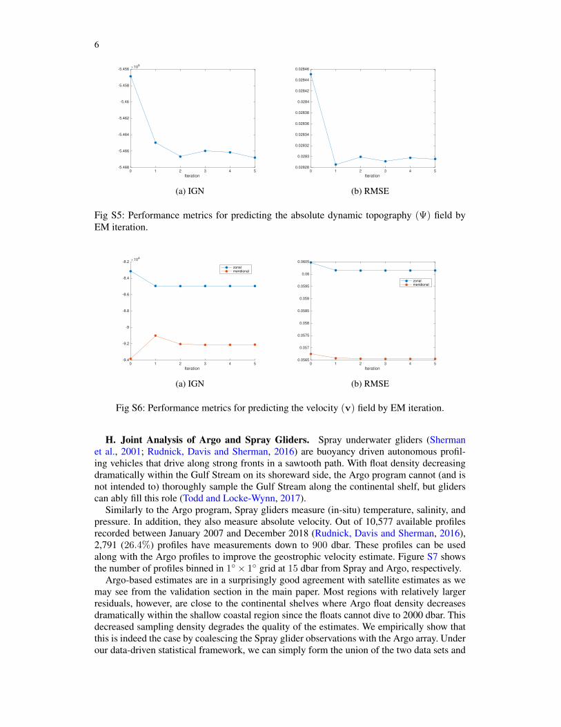
6
0 1 2 3 4 5
Iteration
-5.468
-5.466
-5.464
-5.462
-5.46
-5.458
-5.45610
5
(a) IGN
0 1 2 3 4 5
Iteration
0.02828
0.0283
0.02832
0.02834
0.02836
0.02838
0.0284
0.02842
0.02844
0.02846
(b) RMSE
Fig S5: Performance metrics for predicting the absolute dynamic topography (Ψ) field byEM iteration.
0 1 2 3 4 5
Iteration
-9.4
-9.2
-9
-8.8
-8.6
-8.4
-8.210
4
zonal
meridional
(a) IGN
0 1 2 3 4 5
Iteration
0.0565
0.057
0.0575
0.058
0.0585
0.059
0.0595
0.06
0.0605
zonal
meridional
(b) RMSE
Fig S6: Performance metrics for predicting the velocity (v) field by EM iteration.
H. Joint Analysis of Argo and Spray Gliders. Spray underwater gliders (Shermanet al., 2001; Rudnick, Davis and Sherman, 2016) are buoyancy driven autonomous profil-ing vehicles that drive along strong fronts in a sawtooth path. With float density decreasingdramatically within the Gulf Stream on its shoreward side, the Argo program cannot (and isnot intended to) thoroughly sample the Gulf Stream along the continental shelf, but gliderscan ably fill this role (Todd and Locke-Wynn, 2017).
Similarly to the Argo program, Spray gliders measure (in-situ) temperature, salinity, andpressure. In addition, they also measure absolute velocity. Out of 10,577 available profilesrecorded between January 2007 and December 2018 (Rudnick, Davis and Sherman, 2016),2,791 (26.4%) profiles have measurements down to 900 dbar. These profiles can be usedalong with the Argo profiles to improve the geostrophic velocity estimate. Figure S7 showsthe number of profiles binned in 1 × 1 grid at 15 dbar from Spray and Argo, respectively.
Argo-based estimates are in a surprisingly good agreement with satellite estimates as wemay see from the validation section in the main paper. Most regions with relatively largerresiduals, however, are close to the continental shelves where Argo float density decreasesdramatically within the shallow coastal region since the floats cannot dive to 2000 dbar. Thisdecreased sampling density degrades the quality of the estimates. We empirically show thatthis is indeed the case by coalescing the Spray glider observations with the Argo array. Underour data-driven statistical framework, we can simply form the union of the two data sets and
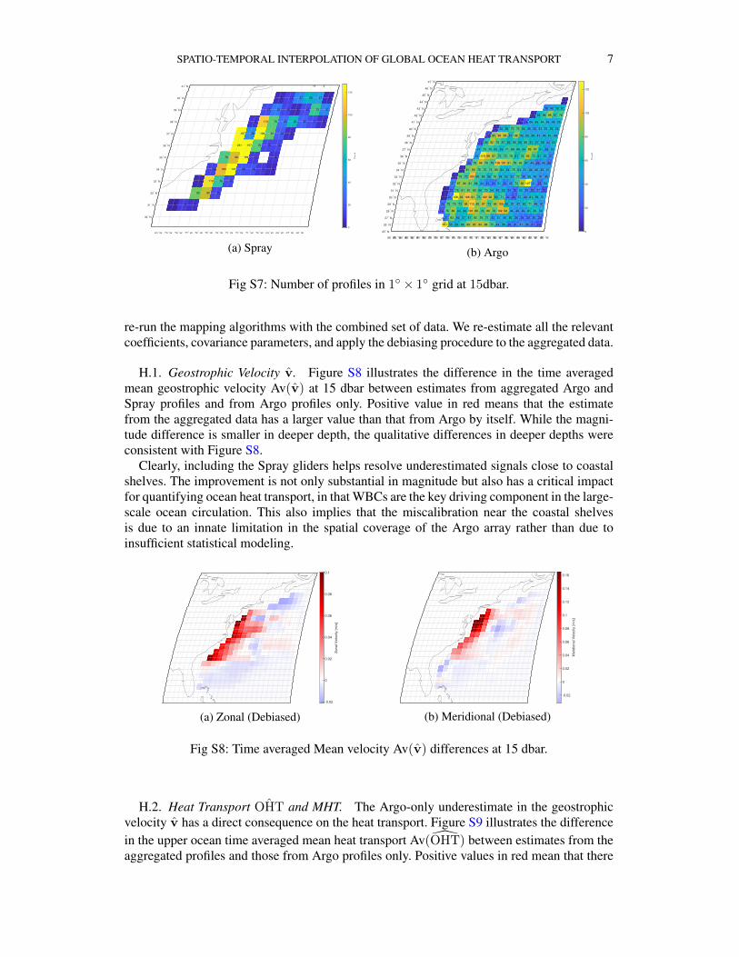
SPATIO-TEMPORAL INTERPOLATION OF GLOBAL OCEAN HEAT TRANSPORT 7
80° W 79
° W 78
° W 77
° W 76
° W 75
° W 74
° W 73
° W 72
° W 71
° W 70
° W 69
° W 68
° W 67
° W 66
° W
30° N
31° N
32° N
33° N
34° N
35° N
36° N
37° N
38° N
39° N
40° N
41° N
1 11 7
82 95 15
3 119 70 17
13 103 147 20 18 11 4
76 99 169 11 9
251 157 79 15 14
187 38 128 81 23 6
8 113 79 29 62 25 17 6
17 33 15 5 16 72 37
5 12 37 59 47 5
11 3
0
20
40
60
80
100
120
Coun
t
(a) Spray 86
° W 85
° W 84
° W 83
° W 82
° W 81
° W 80
° W 79
° W 78
° W 77
° W 76
° W 75
° W 74
° W 73
° W 72
° W 71
° W 70
° W 69
° W 68
° W 67
° W 66
° W 65
° W 64
° W 63
° W 62
° W 61
° W 60
° W
25° N
26° N
27° N
28° N
29° N
30° N
31° N
32° N
33° N
34° N
35° N
36° N
37° N
38° N
39° N
40° N
41° N
42° N
43° N
44° N
45° N
46° N
47° N
121 55 59 68 89 95 94 88 75 44 56 30 31 41 36 27 19
37 83 49 57 67 82 76 71 42 51 48 60 36 28 29 36 29
19 76 88 63 60 101 88 73 88 76 102 94 46 40 40 61 65 50
29 75 79 73 95 112 85 97 73 88 100 60 51 47 62 71 48 41
1 31 128 93 108 91 75 102 92 62 71 32 20 57 40 61 56 51
1 25 75 81 81 80 66 70 54 45 59 34 26 55 39 26 37 16
37 87 86 81 68 44 33 29 51 32 45 73 92 127 41 25 50
5 79 70 105 68 68 56 76 54 55 52 73 38 50 49 41 40
3 81 89 76 75 74 80 63 54 75 64 51 44 46 45 47
26 76 96 78 70 106 101 91 75 83 57 44 28 43 28
45 119 98 87 72 72 78 61 74 92 72 61 55 37
47 73 70 65 59 71 68 66 64 89 87 61 38 52
14 66 92 76 67 60 66 58 66 61 57 58 44 63
12 85 98 93 57 88 52 52 58 47 48 61 49
5 50 58 73 76 62 46 42 53 53 58 52
5 19 50 60 64 50 49 55
3 58 68 88 67 76
36 44 58 61
2
0
20
40
60
80
100
120
Count
(b) Argo
Fig S7: Number of profiles in 1 × 1 grid at 15dbar.
re-run the mapping algorithms with the combined set of data. We re-estimate all the relevantcoefficients, covariance parameters, and apply the debiasing procedure to the aggregated data.
H.1. Geostrophic Velocity v. Figure S8 illustrates the difference in the time averagedmean geostrophic velocity Av(v) at 15 dbar between estimates from aggregated Argo andSpray profiles and from Argo profiles only. Positive value in red means that the estimatefrom the aggregated data has a larger value than that from Argo by itself. While the magni-tude difference is smaller in deeper depth, the qualitative differences in deeper depths wereconsistent with Figure S8.
Clearly, including the Spray gliders helps resolve underestimated signals close to coastalshelves. The improvement is not only substantial in magnitude but also has a critical impactfor quantifying ocean heat transport, in that WBCs are the key driving component in the large-scale ocean circulation. This also implies that the miscalibration near the coastal shelvesis due to an innate limitation in the spatial coverage of the Argo array rather than due toinsufficient statistical modeling.
-0.02
0
0.02
0.04
0.06
0.08
0.1
Zo
na
l V
elo
city [
m/s
]
(a) Zonal (Debiased)
-0.02
0
0.02
0.04
0.06
0.08
0.1
0.12
0.14
0.16M
erid
ion
al V
elo
city [
m/s
]
(b) Meridional (Debiased)
Fig S8: Time averaged Mean velocity Av(v) differences at 15 dbar.
H.2. Heat Transport ˆOHT and MHT. The Argo-only underestimate in the geostrophicvelocity v has a direct consequence on the heat transport. Figure S9 illustrates the differencein the upper ocean time averaged mean heat transport Av(OHT) between estimates from theaggregated profiles and those from Argo profiles only. Positive values in red mean that there
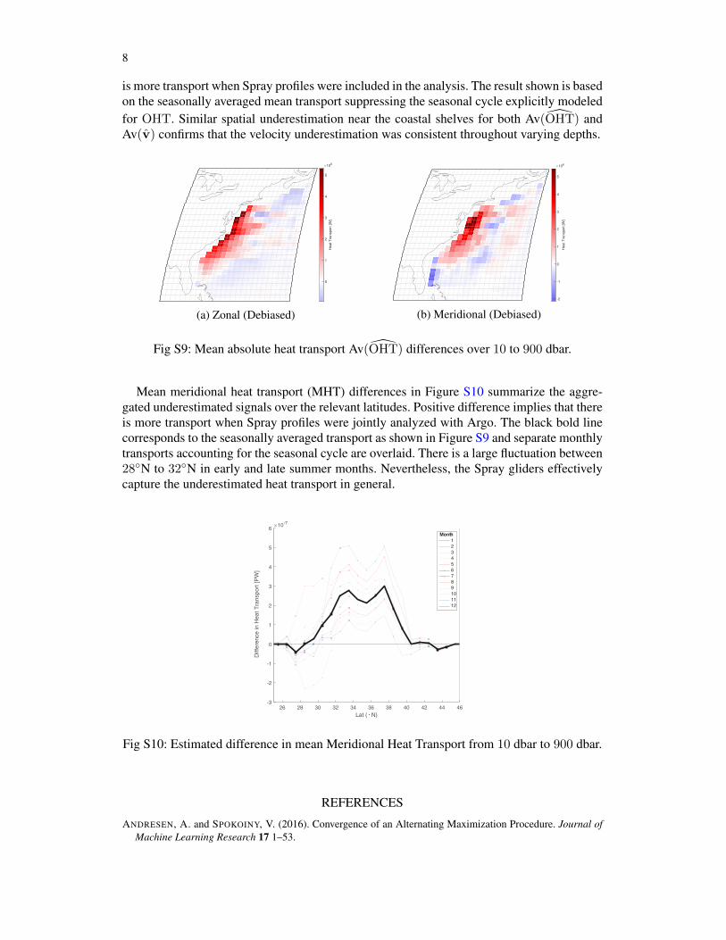
8
is more transport when Spray profiles were included in the analysis. The result shown is basedon the seasonally averaged mean transport suppressing the seasonal cycle explicitly modeledfor OHT. Similar spatial underestimation near the coastal shelves for both Av(OHT) andAv(v) confirms that the velocity underestimation was consistent throughout varying depths.
0
1
2
3
4
5
Heat T
ransport
[W
]
106
(a) Zonal (Debiased)
-2
-1
0
1
2
3
4
5
Heat T
ransport
[W
]
106
(b) Meridional (Debiased)
Fig S9: Mean absolute heat transport Av(OHT) differences over 10 to 900 dbar.
Mean meridional heat transport (MHT) differences in Figure S10 summarize the aggre-gated underestimated signals over the relevant latitudes. Positive difference implies that thereis more transport when Spray profiles were jointly analyzed with Argo. The black bold linecorresponds to the seasonally averaged transport as shown in Figure S9 and separate monthlytransports accounting for the seasonal cycle are overlaid. There is a large fluctuation between28N to 32N in early and late summer months. Nevertheless, the Spray gliders effectivelycapture the underestimated heat transport in general.
26 28 30 32 34 36 38 40 42 44 46
Lat (° N)
-3
-2
-1
0
1
2
3
4
5
6
Diffe
rence in H
eat T
ransport
[P
W]
10-7
1
2
3
4
5
6
7
8
9
10
11
12
Month
Fig S10: Estimated difference in mean Meridional Heat Transport from 10 dbar to 900 dbar.
REFERENCES
ANDRESEN, A. and SPOKOINY, V. (2016). Convergence of an Alternating Maximization Procedure. Journal ofMachine Learning Research 17 1–53.
SPATIO-TEMPORAL INTERPOLATION OF GLOBAL OCEAN HEAT TRANSPORT 9
KUUSELA, M. and STEIN, M. L. (2018a). Supplementary material from "Locally stationary spatio-temporalinterpolation of Argo profiling float data".
KUUSELA, M. and STEIN, M. L. (2018b). Locally stationary spatio-temporal interpolation of Argo profiling floatdata. Proceedings of the Royal Society A: Mathematical, Physical and Engineering Sciences 474 20180400.
NEAL, R. M. and HINTON, G. E. (1998). A View of the Em Algorithm that Justifies Incremental, Sparse, andother Variants. In Learning in Graphical Models, (M. I. Jordan, ed.). NATO ASI Series 355–368. SpringerNetherlands, Dordrecht.
ROEMMICH, D. and GILSON, J. (2009). The 2004–2008 mean and annual cycle of temperature, salinity, andsteric height in the global ocean from the Argo Program. Progress in Oceanography 82 81–100.
ROULSTON, M. S. and SMITH, L. A. (2002). Evaluating Probabilistic Forecasts Using Information Theory.Monthly Weather Review 130 1653–1660.
RUDNICK, D. L., DAVIS, R. E. and SHERMAN, J. T. (2016). Spray Underwater Glider Operations. Journal ofAtmospheric and Oceanic Technology 33 1113–1122.
SHERMAN, J., DAVIS, R. E., OWENS, W. B. and VALDES, J. (2001). The autonomous underwater glider"Spray". IEEE Journal of Oceanic Engineering 26 437–446.
TODD, R. E. and LOCKE-WYNN, L. (2017). Underwater Glider Observations and the Representation of WesternBoundary Currents in Numerical Models. Oceanography 30 88–89.
Related Documents


