Adv. Geosci., 25, 97–102, 2010 www.adv-geosci.net/25/97/2010/ © Author(s) 2010. This work is distributed under the Creative Commons Attribution 3.0 License. Advances in Geosciences Hierarchical Bayesian space-time interpolation versus spatio-temporal BME approach I. Hussain, J. Pilz, and G. Spoeck Department of Statistics, University of Klagenfurt, Klagenfurt, Austria Received: 21 October 2009 – Revised: 9 Februray 2010 – Accepted: 13 February 2010 – Published: 30 March 2010 Abstract. The restrictions of the analysis of natural pro- cesses which are observed at any point in space or time to a purely spatial or purely temporal domain may cause loss of information and larger prediction errors. Moreover, the arbitrary combinations of purely spatial and purely temporal models may not yield valid models for the space-time do- main. For such processes the variation can be characterized by sophisticated spatio-temporal modeling. In the present study the composite spatio-temporal Bayesian maximum en- tropy (BME) method and transformed hierarchical Bayesian space-time interpolation are used in order to predict precip- itation in Pakistan during the monsoon period. Monthly av- erage precipitation data whose time domain is the monsoon period for the years 1974–2000 and whose spatial domain are various regions in Pakistan are considered. The predic- tion of space-time precipitation is applicable in many sectors of industry and economy in Pakistan especially; the agri- cultural sector. Mean field maps and prediction error maps for both methods are estimated and compared. In this pa- per it is shown that the transformed hierarchical Bayesian model is providing more accuracy and lower prediction error compared to the spatio-temporal Bayesian maximum entropy method; additionally, the transformed hierarchical Bayesian model also provides predictive distributions. 1 Introduction Pakistan is located between 23 ◦ and 37 ◦ north latitude and 61 ◦ and 76 ◦ east longitude. The economy of Pakistan is highly supported from the agricultural sector; the occurrence of monsoon (June–September) rainfall being of vital impor- tance for the said sector. The accurate prediction of precip- itation in Pakistan provides useful information for decision Correspondence to: I. Hussain ([email protected]) making. Monthly average precipitation data over a period of twenty-seven years (1974–2000) were collected from the meteorological department of Pakistan, providing monthly average rainfall data for fifty-one gauged sites. Space time data are frequently analyzed through models initially developed for only spatial or temporal distributions. Kyriakidis and Journel (1999) note that the joint space-time dependence is often not fully modeled nor exploited in the es- timation or forecasting at unmonitored locations. Christakos (1992) developed the idea of spatio-temporal random fields (STRF) which can take into account the composite space- time dependence and also utilize the physical knowledge of the natural processes which in turn leads to an improved estimation. This method is based on the Bayesian maxi- mum entropy (BME) approach; BME utilizes the physical knowledge about natural processes in the form of a highly informative prior distribution whereas in absence of physi- cal knowledge about natural process this method is similar to space-time ordinary kriging. Le et al. (1997) proposed a Bayesian hierarchical interpolation method for environmen- tal applications which is very sensitive to non-stationarity. This approach assumes finite dimensional Gaussian distribu- tions with the mean functions depending on an unknown pa- rameter matrix and a vague structure for covariance. The hierarchical framework can take account of the uncertainty of the mean and covariance models and generates space-time predictions that are completely characterized by probability density functions. In the present paper a comparison be- tween BME and hierarchical Bayesian space-time interpola- tion is made. For BME prediction spatial and temporal mean trends are estimated and then separable spatial and tempo- ral co-variograms are determined. The fitted co-variograms are used for BME kriging. For the transformed hierarchical Bayesian model the generalized inverted Wishart distribu- tion is used as prior for the covariance matrix and its hyper- parameters are empirically Bayesian estimated by means of an EM-algorithm. Published by Copernicus Publications on behalf of the European Geosciences Union.

Welcome message from author
This document is posted to help you gain knowledge. Please leave a comment to let me know what you think about it! Share it to your friends and learn new things together.
Transcript
Adv. Geosci., 25, 97–102, 2010www.adv-geosci.net/25/97/2010/© Author(s) 2010. This work is distributed underthe Creative Commons Attribution 3.0 License.
Advances inGeosciences
Hierarchical Bayesian space-time interpolation versusspatio-temporal BME approach
I. Hussain, J. Pilz, and G. Spoeck
Department of Statistics, University of Klagenfurt, Klagenfurt, Austria
Received: 21 October 2009 – Revised: 9 Februray 2010 – Accepted: 13 February 2010 – Published: 30 March 2010
Abstract. The restrictions of the analysis of natural pro-cesses which are observed at any point in space or time toa purely spatial or purely temporal domain may cause lossof information and larger prediction errors. Moreover, thearbitrary combinations of purely spatial and purely temporalmodels may not yield valid models for the space-time do-main. For such processes the variation can be characterizedby sophisticated spatio-temporal modeling. In the presentstudy the composite spatio-temporal Bayesian maximum en-tropy (BME) method and transformed hierarchical Bayesianspace-time interpolation are used in order to predict precip-itation in Pakistan during the monsoon period. Monthly av-erage precipitation data whose time domain is the monsoonperiod for the years 1974–2000 and whose spatial domainare various regions in Pakistan are considered. The predic-tion of space-time precipitation is applicable in many sectorsof industry and economy in Pakistan especially; the agri-cultural sector. Mean field maps and prediction error mapsfor both methods are estimated and compared. In this pa-per it is shown that the transformed hierarchical Bayesianmodel is providing more accuracy and lower prediction errorcompared to the spatio-temporal Bayesian maximum entropymethod; additionally, the transformed hierarchical Bayesianmodel also provides predictive distributions.
1 Introduction
Pakistan is located between 23 and 37 north latitude and61 and 76 east longitude. The economy of Pakistan ishighly supported from the agricultural sector; the occurrenceof monsoon (June–September) rainfall being of vital impor-tance for the said sector. The accurate prediction of precip-itation in Pakistan provides useful information for decision
Correspondence to:I. Hussain([email protected])
making. Monthly average precipitation data over a periodof twenty-seven years (1974–2000) were collected from themeteorological department of Pakistan, providing monthlyaverage rainfall data for fifty-one gauged sites.
Space time data are frequently analyzed through modelsinitially developed for only spatial or temporal distributions.Kyriakidis and Journel(1999) note that the joint space-timedependence is often not fully modeled nor exploited in the es-timation or forecasting at unmonitored locations.Christakos(1992) developed the idea of spatio-temporal random fields(STRF) which can take into account the composite space-time dependence and also utilize the physical knowledge ofthe natural processes which in turn leads to an improvedestimation. This method is based on the Bayesian maxi-mum entropy (BME) approach; BME utilizes the physicalknowledge about natural processes in the form of a highlyinformative prior distribution whereas in absence of physi-cal knowledge about natural process this method is similarto space-time ordinary kriging.Le et al. (1997) proposed aBayesian hierarchical interpolation method for environmen-tal applications which is very sensitive to non-stationarity.This approach assumes finite dimensional Gaussian distribu-tions with the mean functions depending on an unknown pa-rameter matrix and a vague structure for covariance. Thehierarchical framework can take account of the uncertaintyof the mean and covariance models and generates space-timepredictions that are completely characterized by probabilitydensity functions. In the present paper a comparison be-tween BME and hierarchical Bayesian space-time interpola-tion is made. For BME prediction spatial and temporal meantrends are estimated and then separable spatial and tempo-ral co-variograms are determined. The fitted co-variogramsare used for BME kriging. For the transformed hierarchicalBayesian model the generalized inverted Wishart distribu-tion is used as prior for the covariance matrix and its hyper-parameters are empirically Bayesian estimated by means ofan EM-algorithm.
Published by Copernicus Publications on behalf of the European Geosciences Union.
98 I. Hussain et al.: Hierarchical Bayesian space-time interpolation versus spatio-temporal BME approach
2 Material and methods
2.1 Study area
Monthly average precipitation data of fifty-one gauged sitesin Pakistan were collected from the meteorology departmentof Pakistan. Some gauged sites have been recording datasince 1947, the year of the foundation of Pakistan, whilemany other gauged sites were installed later. Data from aperiod of twenty-seven years (1974–2000) were used. Themonsoon period in Pakistan lasts from June to September.The monthly average precipitation data during the monsoonperiod of twenty-seven years are used in the present study.
2.2 Bayesian maximum entropy method
Most of the statistical techniques for the estimation of char-acteristics of space-time processes are based on hard data anddo not take into account any physical knowledge (soft data)for estimation purposes.Christakos et al.(2002) proposedthe Bayesian maximum entropy spatio-temporal estimationmethod which can take into account physical knowledge interms of prior information which, in turn, results in improve-ments for the estimation of space-time processes. The space-time random field is described asZ(s,t) where(s,t) ∈ D ·T :D ⊂ R2 represents spatial coordinates andT ⊂ R+ are posi-tive real numbers describing temporal coordinates. The BMEmethod can be described briefly as consisting of five differentphases: In the first phase the estimation of space-time meantrend is performed, a smooth spatial trend is computed usingan exponential spatial filter which is then applied to the aver-age measurements of each spatial location. A smooth tempo-ral trend for each time replication is computed using an expo-nential temporal filter applied to the averaged measurementsat each time instant. In the second phase the space-time meantrendm(s,t) is interpolated on a grid. In the third phase theresiduals are computed by subtracting the space-time meantrend from the original data i.e.R(s,t) = Z(s,t)−m(s,t).The residual data matrix is then used to estimate the sep-arate spatial covariances, temporal covariances and spatio-temporal experimental co-variograms. In the fourth phasetheoretical covariance models are fitted to the experimentalco-variograms. In the last phase prediction is performed atunobserved locations for any time instant using the fitted co-variogram model and space-time kriging,Christakos(1992),Chiles and Delfiner(1999). Since the co-variograms are es-timated based on residuals the resulting predicted data willcorrespond to residual values. The space-time mean trendsurfaces and predicted residual surfaces are to be added toget predicted values at the original scaling.
2.3 Transformed hierarchical Bayesian model
Let Z[g] andZ[u] be the response variables of gauged andungauged locations and correspondinglyY [g] andY [u] be the
Box-Cox transformed response variables, respectively, i.e.
Y [.]=
(Z[.]λ −1)
λ: λ 6= 0
Y [.]= log(Z[.]) : λ = 0 (1)
The transformed response variables follow a Gaussianmodel conditional on the hyper-trend parameterβ and thecovariance matrix6. The hyper-parameterβ itself follows aGaussian model conditional on the hyper-parameterβ0 andthe covariance matrix6. Finally, the covariance matrix6follows a generalized inverted Wishart distribution. Thus,the suggested model ofLe et al. (1997) for the transformedresponse variable can be expressed as;
Y/β,6 ∼ N(Vβ,In ⊗6)
β/6β0 ∼ N(β0,F
−1⊗6
)6 ∼ GIW (2,δ) (2)
Here N(.,.) denotes the multivariate normal distributionand V represents the matrix ofl covariates describing thetime replications i.e.Vt = (Vt1,...Vt l) remaining constantfor all sites at each time pointt . Since four months(June–September) are taken into consideration for a twenty sevenyears period, we havel = 4 and t = 27. The β0 is anl × (g+u)l matrix of regression hyper-parameters andF−1
is an l · l positive definite matrix specifying covariance be-tween the rows ofβ. In Le et al. (1997) an empiricallyBayesian EM-algorithm is suggested to estimate these hyper-parameters. With regard to the prior specification in the lastline of Eq.2, we follow Brown et al. (1994), where a gener-alized inverted Wishart (GIW) distribution for the covariancematrix6 is proposed and detail this prior as follows:
τ [u]/0[u]∼ N
(τ00,H0⊗0[u]
)0[u]
∼ IW (10⊗,δ0)
τj/0j ∼ N(τ0j ,Hj ⊗0j
),j = 1,2...ng −1
0j ∼ IW(1j ⊗,δj
),j = 1...ng (3)
The abbreviation IW stands for the Inverted Wishart dis-tribution. Hereτu is the slope of optimal linear predic-tors of Y [u] based onY [g] and the residual covariance ofthe optimal linear predictor0[u] ; also τj and 0j for j =
1,2,....ng −1 have similar interpretations. SupposeH is theset of hyper-parameters in Eq.3, i.e.H = (2,δ,F,β) , where2 =
(τ00,H0,10),,..
(τ0ng−1,Hng−1,1ng−1
),1ng
with
degree of freedom parametersδ =(δ0,δ1,..δng
). The di-
mension of theHj ’s and 1j ’s are(gj+1+ ...+gng
)l ·(
gj+1+ ...+gng
)l andgj ·gj respectively. The is a hyper
scale matrix between responses and is assumed to be com-mon across all sites.
2.3.1 Heterogeneous covariance
Sampson and Guttorp(1992) introduced a non-parametricestimation method for spatially nonstationary covariance
Adv. Geosci., 25, 97–102, 2010 www.adv-geosci.net/25/97/2010/
I. Hussain et al.: Hierarchical Bayesian space-time interpolation versus spatio-temporal BME approach 99
structures of random functionsZit = Z(xi,t); here xi =
(1,2,...N) are locations andt = 1,2...T are time replica-tions. The estimation method is based on the assumptionof temporal stationarity but spatial non-stationarity.Samp-son and Guttorp (1992) use the spatial dispersionsd2
ij =
var(Zit −Zj t
)= sii + sjj −2 · sij as natural metric for the
spatial covariance structure model. Their method constructsa smooth mapping of the geographic space of gauged lo-cations onto the dispersion space (D-space) and does notneed any assumption of stationarity. An isotropic variogrammodel is fitted on the basis of observed correlations and dis-tances in D-space. The spatial correlations of ungauged lo-cations can be estimated in conjunction with an estimatedisotropic variogram model by using a thin plate smoothingspline as a nonlinear 1–1 mapping function. The estimatednonstationary covariance model is of the formD2(xa,xb) =
g∣∣f (xa)− f (xb)
∣∣ = g(∣∣yi −yj
∣∣), here for covariance esti-mation yi are referred as D-plane coordinates and for thedetails about functionf andg, seeSampson and Guttorp(1992).
2.3.2 Predictive distributions
The predictive distribution can be specified as matrix t- distri-bution. The transformed random variableYn·m is said to havea matrix t-distribution,Yn·m ∼ tn·m(Yn·m,A⊗B,δ), whereA
is n ·n andB is m ·m, if its density function has the form
f (Y ) ∝
∣∣∣A−m2
∣∣∣∣∣∣B −n2
∣∣∣[In +δ−1
A−1
(Y −Y (0)
)(Y −Y (0)
)B−1
t] δ+m+n−1
2
(4)
The normalizing constant of this density is given byK =[ (δπ2
) nm2 0n+m
δ+m+n−1
2
0n
(δ+n−1
2
)0n+m
(δ+m−1
2
)]
, where0p (t) is the multivariate
Gamma function andY (0) is the mean ofY . The predictivedistribution of the unobserved transformed responses con-ditional on the observed transformed dataY [g] and hyper-parameterH is given by
(Y [u]/Y [g],H
)∼ tnu· nul(
µ[u/g],(δ0−nul+1)−18[u/g]⊗(10⊗),δ0−nul+1
)(5)
whereµ[u/g] = Vβ[u]0 + ε[g]τ0nu , 8[u/g] = Inu +V F−1V +
ε[g]H0ε[g] and ε[g] = Y [g] −Vβ
[g]0 . The software provided
by Le and Zidek (2006) offers the possibility to simulaterealizationsY [u]
i ,i = 1,2,...5000 from the predictive distri-bution Eq.5. These simulated values have just to be back-transformed to the original scale by means of the inverseBox-Cox transformation. Multivariate histograms based onthese back-transformed simulated values are then used to ap-proximate the predictive distributions at the original scale.
Hussain et al.: Hierarchical Bayesian space-time Interpolation versus Spatio-Temporal BME Approach 3
structures of random functions Zit = Z (xi,t); here xi =(1,2,...N) are locations and t = 1,2...T are time replica-tions. The estimation method is based on the assumptionof temporal stationarity but spatial non-stationarity. Samp-son and Guttorp (1992) use the spatial dispersions d2
ij =var(Zit−Zjt) = sii+ sjj−2 · sij as natural metric for thespatial covariance structure model. Their method constructsa smooth mapping of the geographic space of gauged lo-cations onto the dispersion space (D-space) and does notneed any assumption of stationarity. An isotropic variogrammodel is fitted on the basis of observed correlations and dis-tances in D-space. The spatial correlations of ungauged lo-cations can be estimated in conjunction with an estimatedisotropic variogram model by using a thin plate smoothingspline as a nonlinear 1-1 mapping function. The estimatednonstationary covariance model is of the form D2(xa,xb) =g∣∣∣f (xa)− f (xb)
∣∣∣= g(|yi−yj |), here for covariance estima-tion yi are referred as D-plane coordinates and for the detailsabout function f and g (see Sampson and Guttorp (1992)).
2.3.2 Predictive distributions
The predictive distribution can be specified as matrix t- dis-tribution. The transformed random variable Yn×m is said tohave a matrix t-distribution,Yn×m∼ tn×m(Yn×m,A⊗B,δ),where A is n×n and B is m×m, if its density function hasthe form
f (Y )∝∣∣∣A−m
2
∣∣∣∣∣∣B −n2
∣∣∣[In+δ−1
A−1
(Y −Y (0)
)(Y −Y (0)
)B−1
t] δ+m+n−12
(4)
The normalizing constant of this density is given by K =[(δπ2)
nm2 Γn+m δ+m+n−1
2 Γn( δ+n−1
2 )Γn+m( δ+m−12 )
], where Γp(t) is the multivari-
ate Gamma function and Y (0) is the mean of Y . The pre-dictive distribution of the unobserved transformed responsesconditional on the observed transformed data Y [g] and hyper-parameter H is given by(
Y [u]/Y [g],H)∼ tnu× nul(
µ[u/g],(δ0−nul+1)−1Φ[u/g]⊗(∆0⊗Ω),δ0−nul+1)(5)
where µ[u/g] = V β[u]0 + ε[g]τ0nu , Φ[u/g] = Inu +V F−1V +
ε[g]H0ε[g] and ε[g] = Y [g]−V β[g]
0 . The software providedby Le and Zidek (2006) offers the possibility to simulaterealizations Y [u]
i ,i= 1,2,...5000 from the predictive distri-bution Eq.5. These simulated values have just to be back-transformed to the original scale by means of the inverse
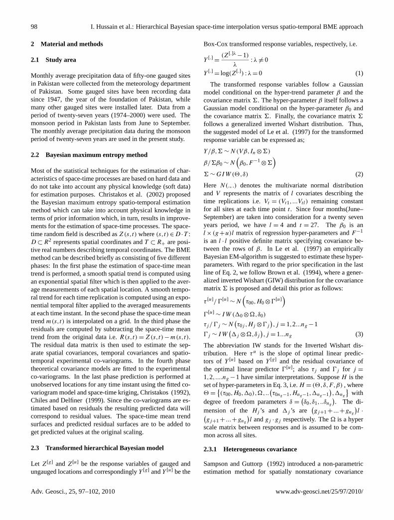
Fig. 1. The map of smoothed mean trend aggregated over time.
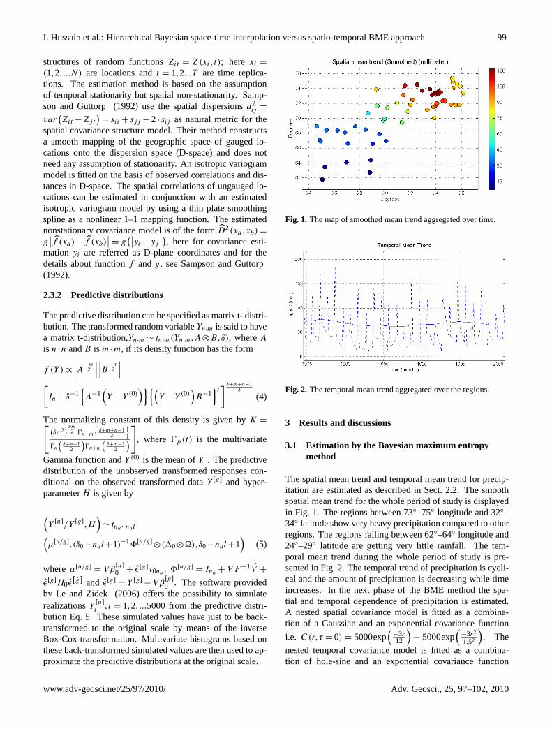
Fig. 2. The temporal mean trend aggregated over the regions.
Box-Cox transformation. Multivariate histograms based onthese back-transformed simulated values are then used to ap-proximate the predictive distributions at the original scale.
3 Results and Discussions
3.1 Estimation by the Bayesian Maximum entropyMethod
The spatial mean trend and temporal mean trend for precipi-tation are estimated as described in section 2.2. The smoothspatial mean trend for the whole period of study is displayedin Fig.1. The regions between 73o − 75o longitude and32o−34o latitude show very heavy precipitation comparedto other regions. The regions falling between 62o−64o lon-gitude and 24o−29o latitude are getting very little rainfall.The temporal mean trend during the whole period of studyis presented in Fig.2. The temporal trend of precipitation iscyclical and the amount of precipitation is decreasing whiletime increases. In the next phase of the BME method the spa-tial and temporal dependence of precipitation is estimated.A nested spatial covariance model is fitted as a combina-tion of a Gaussian and an exponential covariance functioni.e C (r,τ = 0) = 5000exp
(−3r12
)+ 5000exp
(−3r2
1.52
). The
Fig. 1. The map of smoothed mean trend aggregated over time.
Hussain et al.: Hierarchical Bayesian space-time Interpolation versus Spatio-Temporal BME Approach 3
structures of random functions Zit = Z (xi,t); here xi =(1,2,...N) are locations and t = 1,2...T are time replica-tions. The estimation method is based on the assumptionof temporal stationarity but spatial non-stationarity. Samp-son and Guttorp (1992) use the spatial dispersions d2
ij =var(Zit−Zjt) = sii+ sjj−2 · sij as natural metric for thespatial covariance structure model. Their method constructsa smooth mapping of the geographic space of gauged lo-cations onto the dispersion space (D-space) and does notneed any assumption of stationarity. An isotropic variogrammodel is fitted on the basis of observed correlations and dis-tances in D-space. The spatial correlations of ungauged lo-cations can be estimated in conjunction with an estimatedisotropic variogram model by using a thin plate smoothingspline as a nonlinear 1-1 mapping function. The estimatednonstationary covariance model is of the form D2(xa,xb) =g∣∣∣f (xa)− f (xb)
∣∣∣= g(|yi−yj |), here for covariance estima-tion yi are referred as D-plane coordinates and for the detailsabout function f and g (see Sampson and Guttorp (1992)).
2.3.2 Predictive distributions
The predictive distribution can be specified as matrix t- dis-tribution. The transformed random variable Yn×m is said tohave a matrix t-distribution,Yn×m∼ tn×m(Yn×m,A⊗B,δ),where A is n×n and B is m×m, if its density function hasthe form
f (Y )∝∣∣∣A−m
2
∣∣∣∣∣∣B −n2
∣∣∣[In+δ−1
A−1
(Y −Y (0)
)(Y −Y (0)
)B−1
t] δ+m+n−12
(4)
The normalizing constant of this density is given by K =[(δπ2)
nm2 Γn+m δ+m+n−1
2 Γn( δ+n−1
2 )Γn+m( δ+m−12 )
], where Γp(t) is the multivari-
ate Gamma function and Y (0) is the mean of Y . The pre-dictive distribution of the unobserved transformed responsesconditional on the observed transformed data Y [g] and hyper-parameter H is given by(
Y [u]/Y [g],H)∼ tnu× nul(
µ[u/g],(δ0−nul+1)−1Φ[u/g]⊗(∆0⊗Ω),δ0−nul+1)(5)
where µ[u/g] = V β[u]0 + ε[g]τ0nu , Φ[u/g] = Inu +V F−1V +
ε[g]H0ε[g] and ε[g] = Y [g]−V β[g]
0 . The software providedby Le and Zidek (2006) offers the possibility to simulaterealizations Y [u]
i ,i= 1,2,...5000 from the predictive distri-bution Eq.5. These simulated values have just to be back-transformed to the original scale by means of the inverse
Fig. 1. The map of smoothed mean trend aggregated over time.
Fig. 2. The temporal mean trend aggregated over the regions.
Box-Cox transformation. Multivariate histograms based onthese back-transformed simulated values are then used to ap-proximate the predictive distributions at the original scale.
3 Results and Discussions
3.1 Estimation by the Bayesian Maximum entropyMethod
The spatial mean trend and temporal mean trend for precipi-tation are estimated as described in section 2.2. The smoothspatial mean trend for the whole period of study is displayedin Fig.1. The regions between 73o − 75o longitude and32o−34o latitude show very heavy precipitation comparedto other regions. The regions falling between 62o−64o lon-gitude and 24o−29o latitude are getting very little rainfall.The temporal mean trend during the whole period of studyis presented in Fig.2. The temporal trend of precipitation iscyclical and the amount of precipitation is decreasing whiletime increases. In the next phase of the BME method the spa-tial and temporal dependence of precipitation is estimated.A nested spatial covariance model is fitted as a combina-tion of a Gaussian and an exponential covariance functioni.e C (r,τ = 0) = 5000exp
(−3r12
)+ 5000exp
(−3r2
1.52
). The
Fig. 2. The temporal mean trend aggregated over the regions.
3 Results and discussions
3.1 Estimation by the Bayesian maximum entropymethod
The spatial mean trend and temporal mean trend for precip-itation are estimated as described in Sect. 2.2. The smoothspatial mean trend for the whole period of study is displayedin Fig. 1. The regions between 73–75 longitude and 32–34 latitude show very heavy precipitation compared to otherregions. The regions falling between 62–64 longitude and24–29 latitude are getting very little rainfall. The tem-poral mean trend during the whole period of study is pre-sented in Fig.2. The temporal trend of precipitation is cycli-cal and the amount of precipitation is decreasing while timeincreases. In the next phase of the BME method the spa-tial and temporal dependence of precipitation is estimated.A nested spatial covariance model is fitted as a combina-tion of a Gaussian and an exponential covariance function
i.e. C(r,τ = 0) = 5000exp(
−3r12
)+ 5000exp
(−3r2
1.52
). The
nested temporal covariance model is fitted as a combina-tion of hole-sine and an exponential covariance function
www.adv-geosci.net/25/97/2010/ Adv. Geosci., 25, 97–102, 2010
100 I. Hussain et al.: Hierarchical Bayesian space-time interpolation versus spatio-temporal BME approach4 Hussain et al.: Hierarchical Bayesian space-time Interpolation versus Spatio-Temporal BME Approach
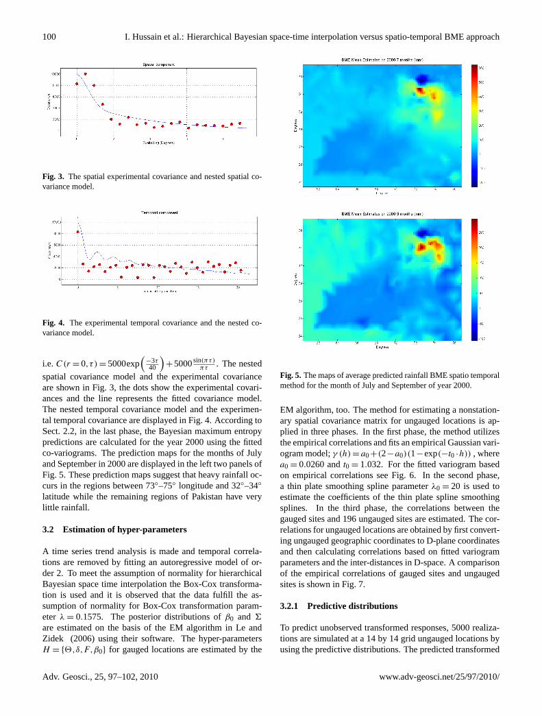
Fig. 3. The spatial experimental covariance and nested spatial co-variance model.
Fig. 4. The experimental temporal covariance and the nested co-variance model.
nested temporal covariance model is fitted as a combina-tion of hole-sine and an exponential covariance function i.eC (r= 0,τ) = 5000exp
(−3τ40
)+ 5000 sin(πτ)
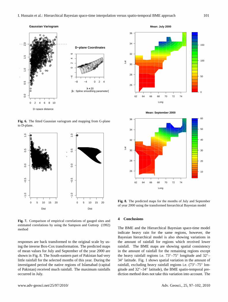
πτ . The nestedspatial covariance model and the experimental covarianceare shown in Fig.3, the dots show the experimental covari-ances and the line represents the fitted covariance model. Thenested temporal covariance model and the experimental tem-poral covariance are displayed in Fig.4. According to sec-tion 2.2, in the last phase, the Bayesian maximum entropypredictions are calculated for the year 2000 using the fittedco-variograms. The prediction maps for the months of Julyand September in 2000 are displayed in the left two panelsof Fig.5. These prediction maps suggest that heavy rain-fall occurs in the regions between 73o−75o longitude and32o− 34o latitude while the remaining regions of Pakistanhave very little rainfall.
3.2 Estimation of hyper-parameters
A time series trend analysis is made and temporal correla-tions are removed by fitting an autoregressive model of or-der 2. To meet the assumption of normality for hierarchicalBayesian space time interpolation the Box-Cox transforma-tion is used and it is observed that the data fulfill the as-sumption of normality for Box-Cox transformation param-eter λ= 0.1575. The posterior distributions of β0 and Σare estimated on the basis of the EM algorithm in Le andZidek (2006) using their software. The hyper-parametersH = Θ,δ,F,β0 for gauged locations are estimated by theEM algorithm, too. The method for estimating a nonsta-tionary spatial covariance matrix for ungauged locations is
Fig. 5. The maps of average predicted rainfall BME spatio temporalmethod for the month of July and September of year 2000.
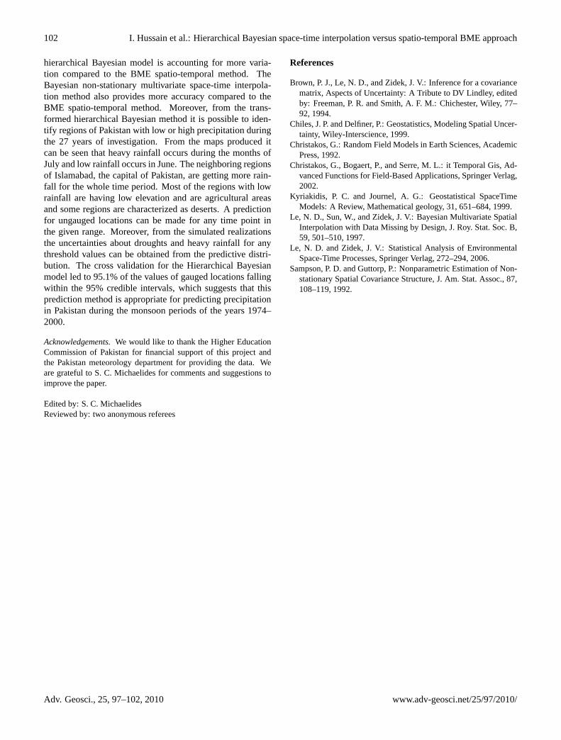
applied in three phases. In the first phase, the method uti-lizes the empirical correlations and fits an empirical Gaussianvariogram model; γ(h) = a0 + (2−a0)(1−exp(−t0×h)), where a0 = 0.0260 and t0 = 1.032. For the fitted vari-ogram based on empirical correlations see Fig.6. In the sec-ond phase, a thin plate smoothing spline parameterλ0 = 20is used to estimate the coefficients of the thin plate splinesmoothing splines. In the third phase, the correlations be-tween the gauged sites and 196 ungauged sites are estimated.The correlations for ungauged locations are obtained by firstconverting ungauged geographic coordinates to D-plane co-ordinates and then calculating correlations based on fittedvariogram parameters and the inter-distances in D-space. Acomparison of the empirical correlations of gauged sites andungauged sites is shown in Fig.7.
3.2.1 Predictive distributions
To predict unobserved transformed responses, 5000 realiza-tions are simulated at a 14 by 14 grid ungauged locations byusing the predictive distributions. The predicted transformedresponses are back transformed to the original scale by us-ing the inverse Box-Cox transformation. The predicted mapsof mean values for July and September of the year 2000 areshown in Fig.8. The South-eastern part of Pakistan had verylittle rainfall for the selected months of this year. During the
Fig. 3. The spatial experimental covariance and nested spatial co-variance model.
4 Hussain et al.: Hierarchical Bayesian space-time Interpolation versus Spatio-Temporal BME Approach
Fig. 3. The spatial experimental covariance and nested spatial co-variance model.
Fig. 4. The experimental temporal covariance and the nested co-variance model.
nested temporal covariance model is fitted as a combina-tion of hole-sine and an exponential covariance function i.eC (r= 0,τ) = 5000exp
(−3τ40
)+ 5000 sin(πτ)
πτ . The nestedspatial covariance model and the experimental covarianceare shown in Fig.3, the dots show the experimental covari-ances and the line represents the fitted covariance model. Thenested temporal covariance model and the experimental tem-poral covariance are displayed in Fig.4. According to sec-tion 2.2, in the last phase, the Bayesian maximum entropypredictions are calculated for the year 2000 using the fittedco-variograms. The prediction maps for the months of Julyand September in 2000 are displayed in the left two panelsof Fig.5. These prediction maps suggest that heavy rain-fall occurs in the regions between 73o−75o longitude and32o− 34o latitude while the remaining regions of Pakistanhave very little rainfall.
3.2 Estimation of hyper-parameters
A time series trend analysis is made and temporal correla-tions are removed by fitting an autoregressive model of or-der 2. To meet the assumption of normality for hierarchicalBayesian space time interpolation the Box-Cox transforma-tion is used and it is observed that the data fulfill the as-sumption of normality for Box-Cox transformation param-eter λ= 0.1575. The posterior distributions of β0 and Σare estimated on the basis of the EM algorithm in Le andZidek (2006) using their software. The hyper-parametersH = Θ,δ,F,β0 for gauged locations are estimated by theEM algorithm, too. The method for estimating a nonsta-tionary spatial covariance matrix for ungauged locations is
Fig. 5. The maps of average predicted rainfall BME spatio temporalmethod for the month of July and September of year 2000.
applied in three phases. In the first phase, the method uti-lizes the empirical correlations and fits an empirical Gaussianvariogram model; γ(h) = a0 + (2−a0)(1−exp(−t0×h)), where a0 = 0.0260 and t0 = 1.032. For the fitted vari-ogram based on empirical correlations see Fig.6. In the sec-ond phase, a thin plate smoothing spline parameterλ0 = 20is used to estimate the coefficients of the thin plate splinesmoothing splines. In the third phase, the correlations be-tween the gauged sites and 196 ungauged sites are estimated.The correlations for ungauged locations are obtained by firstconverting ungauged geographic coordinates to D-plane co-ordinates and then calculating correlations based on fittedvariogram parameters and the inter-distances in D-space. Acomparison of the empirical correlations of gauged sites andungauged sites is shown in Fig.7.
3.2.1 Predictive distributions
To predict unobserved transformed responses, 5000 realiza-tions are simulated at a 14 by 14 grid ungauged locations byusing the predictive distributions. The predicted transformedresponses are back transformed to the original scale by us-ing the inverse Box-Cox transformation. The predicted mapsof mean values for July and September of the year 2000 areshown in Fig.8. The South-eastern part of Pakistan had verylittle rainfall for the selected months of this year. During the
Fig. 4. The experimental temporal covariance and the nested co-variance model.
i.e. C(r = 0,τ ) = 5000exp(
−3τ40
)+5000sin(πτ)
πτ. The nested
spatial covariance model and the experimental covarianceare shown in Fig.3, the dots show the experimental covari-ances and the line represents the fitted covariance model.The nested temporal covariance model and the experimen-tal temporal covariance are displayed in Fig.4. According toSect. 2.2, in the last phase, the Bayesian maximum entropypredictions are calculated for the year 2000 using the fittedco-variograms. The prediction maps for the months of Julyand September in 2000 are displayed in the left two panels ofFig. 5. These prediction maps suggest that heavy rainfall oc-curs in the regions between 73–75 longitude and 32–34
latitude while the remaining regions of Pakistan have verylittle rainfall.
3.2 Estimation of hyper-parameters
A time series trend analysis is made and temporal correla-tions are removed by fitting an autoregressive model of or-der 2. To meet the assumption of normality for hierarchicalBayesian space time interpolation the Box-Cox transforma-tion is used and it is observed that the data fulfill the as-sumption of normality for Box-Cox transformation param-eter λ = 0.1575. The posterior distributions ofβ0 and 6
are estimated on the basis of the EM algorithm inLe andZidek (2006) using their software. The hyper-parametersH = 2,δ,F,β0 for gauged locations are estimated by the
4 Hussain et al.: Hierarchical Bayesian space-time Interpolation versus Spatio-Temporal BME Approach
Fig. 3. The spatial experimental covariance and nested spatial co-variance model.
Fig. 4. The experimental temporal covariance and the nested co-variance model.
nested temporal covariance model is fitted as a combina-tion of hole-sine and an exponential covariance function i.eC (r= 0,τ) = 5000exp
(−3τ40
)+ 5000 sin(πτ)
πτ . The nestedspatial covariance model and the experimental covarianceare shown in Fig.3, the dots show the experimental covari-ances and the line represents the fitted covariance model. Thenested temporal covariance model and the experimental tem-poral covariance are displayed in Fig.4. According to sec-tion 2.2, in the last phase, the Bayesian maximum entropypredictions are calculated for the year 2000 using the fittedco-variograms. The prediction maps for the months of Julyand September in 2000 are displayed in the left two panelsof Fig.5. These prediction maps suggest that heavy rain-fall occurs in the regions between 73o−75o longitude and32o− 34o latitude while the remaining regions of Pakistanhave very little rainfall.
3.2 Estimation of hyper-parameters
A time series trend analysis is made and temporal correla-tions are removed by fitting an autoregressive model of or-der 2. To meet the assumption of normality for hierarchicalBayesian space time interpolation the Box-Cox transforma-tion is used and it is observed that the data fulfill the as-sumption of normality for Box-Cox transformation param-eter λ= 0.1575. The posterior distributions of β0 and Σare estimated on the basis of the EM algorithm in Le andZidek (2006) using their software. The hyper-parametersH = Θ,δ,F,β0 for gauged locations are estimated by theEM algorithm, too. The method for estimating a nonsta-tionary spatial covariance matrix for ungauged locations is
Fig. 5. The maps of average predicted rainfall BME spatio temporalmethod for the month of July and September of year 2000.
applied in three phases. In the first phase, the method uti-lizes the empirical correlations and fits an empirical Gaussianvariogram model; γ(h) = a0 + (2−a0)(1−exp(−t0×h)), where a0 = 0.0260 and t0 = 1.032. For the fitted vari-ogram based on empirical correlations see Fig.6. In the sec-ond phase, a thin plate smoothing spline parameterλ0 = 20is used to estimate the coefficients of the thin plate splinesmoothing splines. In the third phase, the correlations be-tween the gauged sites and 196 ungauged sites are estimated.The correlations for ungauged locations are obtained by firstconverting ungauged geographic coordinates to D-plane co-ordinates and then calculating correlations based on fittedvariogram parameters and the inter-distances in D-space. Acomparison of the empirical correlations of gauged sites andungauged sites is shown in Fig.7.
3.2.1 Predictive distributions
To predict unobserved transformed responses, 5000 realiza-tions are simulated at a 14 by 14 grid ungauged locations byusing the predictive distributions. The predicted transformedresponses are back transformed to the original scale by us-ing the inverse Box-Cox transformation. The predicted mapsof mean values for July and September of the year 2000 areshown in Fig.8. The South-eastern part of Pakistan had verylittle rainfall for the selected months of this year. During the
Fig. 5. The maps of average predicted rainfall BME spatio temporalmethod for the month of July and September of year 2000.
EM algorithm, too. The method for estimating a nonstation-ary spatial covariance matrix for ungauged locations is ap-plied in three phases. In the first phase, the method utilizesthe empirical correlations and fits an empirical Gaussian vari-ogram model;γ (h) = a0+(2−a0)(1−exp(−t0 ·h)) , wherea0 = 0.0260 andt0 = 1.032. For the fitted variogram basedon empirical correlations see Fig.6. In the second phase,a thin plate smoothing spline parameterλ0 = 20 is used toestimate the coefficients of the thin plate spline smoothingsplines. In the third phase, the correlations between thegauged sites and 196 ungauged sites are estimated. The cor-relations for ungauged locations are obtained by first convert-ing ungauged geographic coordinates to D-plane coordinatesand then calculating correlations based on fitted variogramparameters and the inter-distances in D-space. A comparisonof the empirical correlations of gauged sites and ungaugedsites is shown in Fig.7.
3.2.1 Predictive distributions
To predict unobserved transformed responses, 5000 realiza-tions are simulated at a 14 by 14 grid ungauged locations byusing the predictive distributions. The predicted transformed
Adv. Geosci., 25, 97–102, 2010 www.adv-geosci.net/25/97/2010/
I. Hussain et al.: Hierarchical Bayesian space-time interpolation versus spatio-temporal BME approach 101
Hussain et al.: Hierarchical Bayesian space-time Interpolation versus Spatio-Temporal BME Approach 5
0 2 4 6 8 10
0.0
0.5
1.0
1.5
2.0
D−space distance
Dis
pers
ion,
rm
sre
= 0
.206
9
Gaussian Variogram
λλ == 20
−8 −4 0 2 4
−4
02
46
1 2
3
4 5
6
7
8 910
11121314
15
1617
181920
2122
2324
2526
2728
29 3031 3233
34
353637
38 39
40
41 4243
44 4546 47
48495051
D−plane Coordinates
[λλ : Spline smoothing parameter]λλ == 20
Fig. 6. The fitted Gaussian variogram and mapping from G-planeto D-plane.
0 5 10 15 20
−1.
0−
0.5
0.0
0.5
1.0
Dist
Em
pric
al c
orre
latio
n fo
r ga
uged
site
s
0 5 10 15 20
−1.
0−
0.5
0.0
0.5
1.0
Dist
Pre
dict
ed c
orre
latio
n fo
r un
gaug
ed s
ites
Fig. 7. Comparison of empirical correlations of gauged sites andestimated correlations by using the Sampson and Guttorp (1992)method
investigated period the native regions of Islamabad (capitalof Pakistan) received much rainfall. The maximum rainfallsoccurred in July.
0
50
100
150
62 64 66 68 70 72 74
26
28
30
32
34
36
Mean: July 2000
Long
Lat
10
20
30
40
50
60
62 64 66 68 70 72 74
26
28
30
32
34
36
Mean: September 2000
Long
Lat
Fig. 8. The predicted maps for the months of July and Septemberof year 2000 using the transformed hierarchical Bayesian model
3.3 Conclusions
The BME and the Hierarchical Bayesian space-time modelindicate heavy rain for the same regions, however, theBayesian hierarchical model is also showing variations inthe amount of rainfall for regions which received lower rain-fall. The BME maps are showing spatial consistency in theamount of rainfall for the remaining regions except the heavyrainfall regions i.e 73o− 75o longitude and 32o− 34o lati-tude. Fig.1 shows spatial variation in the amount of rain-
Fig. 6. The fitted Gaussian variogram and mapping from G-planeto D-plane.
Hussain et al.: Hierarchical Bayesian space-time Interpolation versus Spatio-Temporal BME Approach 5
0 2 4 6 8 10
0.0
0.5
1.0
1.5
2.0
D−space distance
Dis
pers
ion,
rm
sre
= 0
.206
9
Gaussian Variogram
λλ == 20
−8 −4 0 2 4
−4
02
46
1 2
3
4 5
6
7
8 910
11121314
15
1617
181920
2122
2324
2526
2728
29 3031 3233
34
353637
38 39
40
41 4243
44 4546 47
48495051
D−plane Coordinates
[λλ : Spline smoothing parameter]λλ == 20
Fig. 6. The fitted Gaussian variogram and mapping from G-planeto D-plane.
0 5 10 15 20
−1.
0−
0.5
0.0
0.5
1.0
Dist
Em
pric
al c
orre
latio
n fo
r ga
uged
site
s
0 5 10 15 20
−1.
0−
0.5
0.0
0.5
1.0
Dist
Pre
dict
ed c
orre
latio
n fo
r un
gaug
ed s
ites
Fig. 7. Comparison of empirical correlations of gauged sites andestimated correlations by using theSampson and Guttorp(1992)method
ordinates and then calculating correlations based on fittedvariogram parameters and the inter-distances in D-space. Acomparison of the empirical correlations of gauged sites andungauged sites is shown in Fig.7.
3.2.1 Predictive distributions
To predict unobserved transformed responses, 5000 realiza-tions are simulated at a 14 by 14 grid ungauged locations byusing the predictive distributions. The predicted transformedresponses are back transformed to the original scale by us-ing the inverse Box-Cox transformation. The predicted mapsof mean values for July and September of the year 2000 areshown in Fig.8. The South-eastern part of Pakistan had verylittle rainfall for the selected months of this year. During theinvestigated period the native regions of Islamabad (capitalof Pakistan) received much rainfall. The maximum rainfallsoccurred in July.
3.3 Conclusions
The BME and the Hierarchical Bayesian space-time modelindicate heavy rain for the same regions, however, theBayesian hierarchical model is also showing variations inthe amount of rainfall for regions which received lower rain-fall. The BME maps are showing spatial consistency in theamount of rainfall for the remaining regions except the heavyrainfall regions i.e 73o − 75o longitude and 32o − 34o lati-tude. Fig.1 shows spatial variation in the amount of rain-fall, excluding heavy rainfall regions i.e( 73o
−75o longitudeand 32o −34o latitude), the BME spatio-temporal predictionmethod does not take this variation into account. The hierar-chical Bayesian model is accounting for more variation com-pared to the BME spatio-temporal method. The Bayesiannon-stationary multivariate space-time interpolation methodalso provides more accuracy compared to the BME spatio-temporal method. Moreover, from the transformed hierar-chical Bayesian method it is possible to identify regions ofPakistan with low or high precipitation during the 27 yearsof investigation. From the maps produced it can be seen thatheavy rainfall occurs during the months of July and low rain-fall occurs in June. The neighboring regions of Islamabad,the capital of Pakistan, are getting more rainfall for the wholetime period. Most of the regions with low rainfall are havinglow elevation and are agricultural areas and some regions arecharacterized as deserts. A prediction for ungauged locationscan be made for any time point in the given range. More-over, from the simulated realizations the uncertainties aboutdroughts and heavy rainfall for any threshold values can beobtained from the predictive distribution. The cross valida-tion for the Hierarchical Bayesian model led to 95.1% of thevalues of gauged locations falling within the 95% credibleintervals, which suggests that this prediction method is ap-propriate for predicting precipitation in Pakistan during themonsoon periods of the years 1974-2000.
References
Brown,P.J, Le,N.D, and Zidek,J.V. Inference for a covariance ma-trix. Aspects of Uncertainty: A Tribute to DV Lindley (Eds) PR
www.adv-geosci.net/8/1/2010/ Adv. Geosci., 8, 1–6, 2010
Fig. 7. Comparison of empirical correlations of gauged sites andestimated correlations by using theSampson and Guttorp(1992)method
responses are back transformed to the original scale by us-ing the inverse Box-Cox transformation. The predicted mapsof mean values for July and September of the year 2000 areshown in Fig.8. The South-eastern part of Pakistan had verylittle rainfall for the selected months of this year. During theinvestigated period the native regions of Islamabad (capitalof Pakistan) received much rainfall. The maximum rainfallsoccurred in July.
6 Hussain et al.: Hierarchical Bayesian space-time Interpolation versus Spatio-Temporal BME Approach
0
50
100
150
62 64 66 68 70 72 74
26
28
30
32
34
36
Mean: July 2000
Long
Lat
10
20
30
40
50
60
62 64 66 68 70 72 74
26
28
30
32
34
36
Mean: September 2000
Long
Lat
Fig. 8. The predicted maps for the months of July and Septemberof year 2000 using the transformed hierarchical Bayesian model
Freeman and AFM Smith. Chichester: Wiley, 77-92,1994.Chiles, J. P., and Delfiner, P. Geostatistics: Modeling Spatial Uncer-
tainty, Wiley-Interscience, 1999.Christakos, G. Random Field Models in Earth Sciences, Academic
Press, 1992.Christakos, G., Bogaert, P., and Serre, M. L. it Temporal Gis: Ad-
vanced Functions for Field-Based Applications, Springer Verlag,2002.
Kyriakidis, P. C. and Journel, A. G. Geostatistical SpaceTime Mod-els: A Review, Mathematical geology, 31, 651-684, 1999.
Le, N. D., Sun, W., and Zidek, J. V. Bayesian Multivariate SpatialInterpolation with Data Missing by Design, Journal of the RoyalStatistical Society. Series B Methodological, 59, 501-510, 1997.
Le, N. D., and Zidek, J. V. Statistical Analysis of EnvironmentalSpace-Time Processes, Springer Verlag, 272-294, 2006.
Sampson, P. D., and Guttorp, P. Nonparametric Estimation of Non-stationary Spatial Covariance Structure, Journal of the AmericanStatistical Association, 87, 108-119, 1992.
Adv. Geosci., 8, 1–6, 2010 www.adv-geosci.net/8/1/2010/
Fig. 8. The predicted maps for the months of July and Septemberof year 2000 using the transformed hierarchical Bayesian model
4 Conclusions
The BME and the Hierarchical Bayesian space-time modelindicate heavy rain for the same regions, however, theBayesian hierarchical model is also showing variations inthe amount of rainfall for regions which received lowerrainfall. The BME maps are showing spatial consistencyin the amount of rainfall for the remaining regions exceptthe heavy rainfall regions i.e. 73–75 longitude and 32–34 latitude. Fig.1 shows spatial variation in the amount ofrainfall, excluding heavy rainfall regions i.e. (73–75 lon-gitude and 32–34 latitude), the BME spatio-temporal pre-diction method does not take this variation into account. The
www.adv-geosci.net/25/97/2010/ Adv. Geosci., 25, 97–102, 2010
102 I. Hussain et al.: Hierarchical Bayesian space-time interpolation versus spatio-temporal BME approach
hierarchical Bayesian model is accounting for more varia-tion compared to the BME spatio-temporal method. TheBayesian non-stationary multivariate space-time interpola-tion method also provides more accuracy compared to theBME spatio-temporal method. Moreover, from the trans-formed hierarchical Bayesian method it is possible to iden-tify regions of Pakistan with low or high precipitation duringthe 27 years of investigation. From the maps produced itcan be seen that heavy rainfall occurs during the months ofJuly and low rainfall occurs in June. The neighboring regionsof Islamabad, the capital of Pakistan, are getting more rain-fall for the whole time period. Most of the regions with lowrainfall are having low elevation and are agricultural areasand some regions are characterized as deserts. A predictionfor ungauged locations can be made for any time point inthe given range. Moreover, from the simulated realizationsthe uncertainties about droughts and heavy rainfall for anythreshold values can be obtained from the predictive distri-bution. The cross validation for the Hierarchical Bayesianmodel led to 95.1% of the values of gauged locations fallingwithin the 95% credible intervals, which suggests that thisprediction method is appropriate for predicting precipitationin Pakistan during the monsoon periods of the years 1974–2000.
Acknowledgements.We would like to thank the Higher EducationCommission of Pakistan for financial support of this project andthe Pakistan meteorology department for providing the data. Weare grateful to S. C. Michaelides for comments and suggestions toimprove the paper.
Edited by: S. C. MichaelidesReviewed by: two anonymous referees
References
Brown, P. J., Le, N. D., and Zidek, J. V.: Inference for a covariancematrix, Aspects of Uncertainty: A Tribute to DV Lindley, editedby: Freeman, P. R. and Smith, A. F. M.: Chichester, Wiley, 77–92, 1994.
Chiles, J. P. and Delfiner, P.: Geostatistics, Modeling Spatial Uncer-tainty, Wiley-Interscience, 1999.
Christakos, G.: Random Field Models in Earth Sciences, AcademicPress, 1992.
Christakos, G., Bogaert, P., and Serre, M. L.: it Temporal Gis, Ad-vanced Functions for Field-Based Applications, Springer Verlag,2002.
Kyriakidis, P. C. and Journel, A. G.: Geostatistical SpaceTimeModels: A Review, Mathematical geology, 31, 651–684, 1999.
Le, N. D., Sun, W., and Zidek, J. V.: Bayesian Multivariate SpatialInterpolation with Data Missing by Design, J. Roy. Stat. Soc. B,59, 501–510, 1997.
Le, N. D. and Zidek, J. V.: Statistical Analysis of EnvironmentalSpace-Time Processes, Springer Verlag, 272–294, 2006.
Sampson, P. D. and Guttorp, P.: Nonparametric Estimation of Non-stationary Spatial Covariance Structure, J. Am. Stat. Assoc., 87,108–119, 1992.
Adv. Geosci., 25, 97–102, 2010 www.adv-geosci.net/25/97/2010/
Related Documents