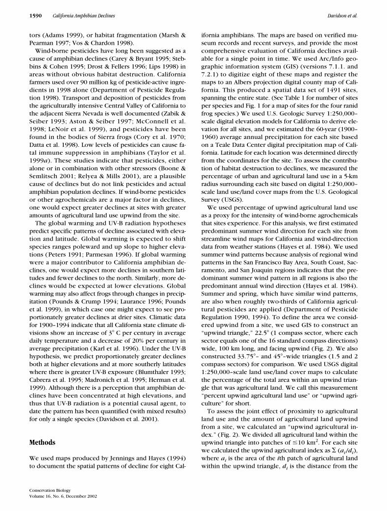
Spatial Tests of the Pesticide Drift, Habitat Destruction ...online.sfsu.edu/carlosd/davidson-consbio-compressed-02.pdf · un factor importante en las declinaciones. Para otras dos

1588

Conservation Biology, Pages 1588–1601Volume 16, No. 6, December 2002

Spatial Tests of the Pesticide Drift, HabitatDestruction, UV-B, and Climate-Change Hypothesesfor California Amphibian Declines

CARLOS DAVIDSON,* H. BRADLEY SHAFFER,† AND MARK R. JENNINGS‡

*Department of Environmental Studies, California State University—Sacramento, 6000 J Street, Sacramento, CA 95819–6001, U.S.A., and Graduate Group in Ecology, University of California, Davis, CA 95616, U.S.A.,email [email protected]

†Section of Evolution and Ecology, and Center for Population Biology, University of California, Davis, CA 95616, U.S.A.‡Rana Resources, 39913 Sharon Avenue, Davis, CA 95616–9456, U.S.A., and Department of Herpetology, California Academy of Sciences, Golden Gate Park, San Francisco, CA 94118, U.S.A.

Abstract:

Wind-borne pesticides have long been suggested as a cause of amphibian declines in areas withoutobvious habitat destruction. In California, the transport and deposition of pesticides from the agriculturally in-tensive Central Valley to the adjacent Sierra Nevada is well documented, and pesticides have been found in thebodies of Sierra frogs. Pesticides are therefore a plausible cause of declines, but to date no direct links have beenfound between pesticides and actual amphibian population declines. Using a geographic information system,we constructed maps of the spatial pattern of declines for eight declining California amphibian taxa, and com-pared the observed patterns of decline to those predicted by hypotheses of wind-borne pesticides, habitat destruc-tion, ultraviolet radiation, and climate change. In four species, we found a strong positive association betweendeclines and the amount of upwind agricultural land use, suggesting that wind-borne pesticides may be an im-portant factor in declines. For two other species, declines were strongly associated with local urban and agricul-tural land use, consistent with the habitat-destruction hypothesis. The patterns of decline were not consistentwith either the ultraviolet radiation or climate-change hypotheses for any of the species we examined.

Pruebas Espaciales de la Deriva de Pesticidas, Destrucción de Hábitat, UV-B e Hipótesis de Cambio Climático parala Declinación de Anfibios de California

Resumen:

Por mucho tiempo se ha sugerido que los pesticidas transportados por el viento son una causa dela declinación de anfibios en áreas sin destrucción de hábitat evidente. En California, el transporte y depósitode pesticidas provenientes del Valle Central, donde se practica la agricultura intensiva, hacia la Sierra Ne-vada adyacente está bien documentado y se han encontrado pesticidas en el cuerpo de ranas de la Sierra. Porlo tanto, los pesticidas son una causa verosímil de las declinaciones, pero a la fecha no se han encontrado rel-aciones directas entre los pesticidas y la declinación de anfibios. Construimos mapas de sistemas de infor-mación geográfica del patrón espacial de las declinaciones de ocho taxones de anfibios de California, y com-

paramos los patrones de declinación observados con los esperados por las hipótesis de pesticidas transportadospor el viento, la destrucción del hábitat, la radiación ultravioleta y el cambio climático. En cuatro especies,encontramos una fuerte asociación positiva entre las declinaciones y la cantidad de tierras de uso agrícolaen dirección contraria a los vientos, lo que sugiere que los pesticidas transportados por el viento pueden serun factor importante en las declinaciones. Para otras dos especies, las declinaciones se asociaron contundent-emente con el uso del suelo urbano y agrícola, lo cual es consistente con la hipótesis de la destrucción delhábitat. Los patrones de declinación no fueron consistentes con la hipótesis de la radiación ultravioleta ni la

de cambio climático para ninguna de las especies examinadas.

Paper submitted January 23, 2001; revised manuscript accepted January 16, 2002.

Conservation BiologyVolume 16, No. 6, December

Davidson et al. California Amphibian Declines

1589

Introduction

During the last decade, amphibian declines have emergedas a key example of the global biodiversity crisis. Al-though a great deal of effort has been expended on deter-mining the worldwide causes of amphibian declines, noconsensus has yet emerged. One critical aspect of thesedeclines is their geographic, or landscape-level, patterns.Over sufficiently large geographic areas, spatial patternsof amphibian decline can be used to evaluate hypothe-sized causes because most hypotheses implicitly makepredictions of the expected spatial patterns of decline.

By developing spatially explicit predictions based oncompeting mechanisms, we used large-scale geographicpatterns of decline to evaluate the importance of fourputative causes of decline. Based on explicit assump-tions, we generated spatial predictions for the hypothe-ses of habitat destruction, UV-B radiation, climatechange, and pesticide drift, and we evaluated each hy-pothesis statistically by comparing predicted and ob-served spatial patterns of decline for eight species of Cal-ifornia amphibians. The power of this strategy resides inits broad, species-wide approach that avoids reliance onone or a few study sites and its ability to simultaneouslyevaluate multiple hypotheses for causes of declines (forrelated geographical approaches to amphibian declinessee Alexander & Eischeid [2001]; Carey et al. [2001];and Middleton et al. [2001]).

California is a hotspot of amphibian decline, withmany species experiencing sharp range contractions(e.g., Jennings 1988; Fellers & Drost 1993; Jennings &Hayes 1994; Drost & Fellers 1996; Fisher & Shaffer1996). The state also has a strong record of historic, mu-seum-based collections and ongoing field surveys, pro-viding the broad baseline of data necessary for our analy-sis (Shaffer et al. 1998). Our study is based on presence/absence data for multiple locations. “Present” sites arethose that are currently occupied by a species, and“absent” sites are those that were previously occupied( based on museum or other historic records) but arecurrently not occupied. “Declines” refers to sites, or pro-portions of sites, that are currently absent.

We developed our spatial analysis strategy while con-ducting a detailed study of declines of the federally threat-ened California red-legged frog (

Rana aurora draytonii

)(Davidson et al. 2001). Although that study successfullyidentified several potential causes of decline, any analysisof patterns of decline for a single species potentially suf-fers from two limitations. First, there is always the possi-bility that factors correlated with but not included in thestudy may be driving actual declines. Second, it may bethat causal interpretations are correct for the single spe-cies but that other declining taxa are responding to a dif-ferent set of factors. For our study of red-legged frogs, weexplored the first possibility by dividing California intothree ecoregions and analyzing the factors associated

with declines within and between regions. In this way,we examined whether the factors associated with de-clines remained significant after unspecified regional fac-tors were controlled for. A more powerful way to addressthe possibility of confounding factors (and that adoptedhere) is to analyze declines of multiple species with dis-tinct ranges. It is unlikely that confounding factors thatmight have created a pattern of decline associated withone species would generate a similar pattern for a secondor third species with a distinct range.

We analyzed eight species of California amphibiansknown to be declining based on federal or state listingstatus or analyses by Jennings and Hayes (1994). To beamenable to spatial analysis, a species must have a largegeographic range in the state and reasonable numbers ofboth present and absent sites. Based on these criteria,we selected the following eight species to analyze: Cali-fornia tiger salamander (

Ambystoma californiense

),western spadefoot (

Spea hammondii

, sometimes re-ferred to as

Scaphiopus

hammondii

), arroyo toad (

Bufocalifornicus

), Yosemite toad (

B. canorus

), Californiared-legged frog (

Rana aurora draytonii

), Cascades frog(

R. cascadae

), foothill yellow-legged frog (

R. boylii

),and Sierra Nevada populations of the mountain yellow-legged frog (

R. muscosa

).Six primary hypotheses have been proposed to explain

amphibian declines: habitat destruction, pesticide drift,increased UV-B radiation, climate change, introduced ex-otic predators, and disease. We chose to analyze the firstfour hypotheses because we could generate clear andtestable predictions for the spatial pattern of declines foreach. In generating spatial predictions, our key underly-ing assumption is that increasing levels of an environmen-tal stressor, be it completely anthropogenic (pesticides,habitat destruction) or human-mediated changes in thelevel of natural conditions (UV-B radiation, temperature),will increase the probability of declines. Our assumptionis consistent with local adaptation as long as adaptationdoes not completely mitigate increased exposure to astressor. Both empirical (Gross & Price 2000) and particu-larly theoretical (Kirkpatrick & Barton 1997) analyses ofspecies’ range limits support the view that adaptationonly partially mitigates stressors and that species cannotinfinitely adapt to environmental gradients. Instead, atthe upper end of environmental gradients, populationsizes decrease and the likelihood of decline increases.

If habitat destruction or modification associated withintensive human activities is contributing to amphibiandeclines, one would expect to see greater declines atsites with greater amounts of surrounding urban or agri-cultural land use than at those surrounded by wildlands.Such habitat effects could be due to direct habitat de-struction or more indirect effects such as increased mor-tality from automobiles (Fahrig et al. 1995), increasedpredation by human commensals and pets (Crooks &Soulé 1999), pond modifications that favor exotic preda-

1590

California Amphibian Declines Davidson et al.

Conservation BiologyVolume 16, No. 6, December 2002

tors (Adams 1999), or habitat fragmentation (Marsh &Pearman 1997; Vos & Chardon 1998).

Wind-borne pesticides have long been suggested as acause of amphibian declines (Carey & Bryant 1995; Steb-bins & Cohen 1995; Drost & Fellers 1996; Lips 1998) inareas without obvious habitat destruction. Californiafarmers used over 90 million kg of pesticide-active ingre-dients in 1998 alone (Department of Pesticide Regula-tion 1998). Transport and deposition of pesticides fromthe agriculturally intensive Central Valley of California tothe adjacent Sierra Nevada is well documented (Zabik &Seiber 1993; Aston & Seiber 1997; McConnell et al.1998; LeNoir et al. 1999), and pesticides have beenfound in the bodies of Sierra frogs (Cory et al. 1970;Datta et al. 1998). Low levels of pesticides can cause fa-tal immune suppression in amphibians (Taylor et al.1999

a

). These studies indicate that pesticides, eitheralone or in combination with other stressors (Boone &Semlitsch 2001; Relyea & Mills 2001), are a plausiblecause of declines but do not link pesticides and actualamphibian population declines. If wind-borne pesticidesor other agrochemicals are a major factor in declines,one would expect greater declines at sites with greateramounts of agricultural land use upwind from the site.

The global warming and UV-B radiation hypothesespredict specific patterns of decline associated with eleva-tion and latitude. Global warming is expected to shiftspecies ranges poleward and up slope to higher eleva-tions (Peters 1991; Parmesan 1996). If global warmingwere a major contributor to California amphibian de-clines, one would expect more declines in southern lati-tudes and fewer declines to the north. Similarly, more de-clines would be expected at lower elevations. Globalwarming may also affect frogs through changes in precip-itation (Pounds & Crump 1994; Laurance 1996; Poundset al. 1999), in which case one might expect to see pro-portionately greater declines at drier sites. Climatic datafor 1900–1994 indicate that all California state climate di-visions show an increase of 3

�

C per century in averagedaily temperature and a decrease of 20% per century inaverage precipitation (Karl et al. 1996). Under the UV-Bhypothesis, we predict proportionately greater declinesboth at higher elevations and at more southerly latitudeswhere there is greater UV-B exposure (Blumthaler 1993;Cabrera et al. 1995; Madronich et al. 1995; Herman et al.1999). Although there is a perception that amphibian de-clines have been concentrated at high elevations, andthus that UV-B radiation is a potential causal agent, todate the pattern has been quantified (with mixed results)for only a single species (Davidson et al. 2001).

Methods

We used maps produced by Jennings and Hayes (1994)to document the spatial patterns of decline for eight Cal-

ifornia amphibians. The maps are based on verified mu-seum records and recent surveys, and provide the mostcomprehensive evaluation of California declines avail-able for a single point in time. We used Arc/Info geo-graphic information system (GIS) (versions 7.1.1. and7.2.1) to digitize eight of these maps and register themaps to an Albers projection digital county map of Cali-fornia. This produced a spatial data set of 1491 sites,spanning the entire state. (See Table 1 for number of sitesper species and Fig. 1 for a map of sites for the four ranidfrog species.) We used U.S. Geologic Survey 1:250,000–scale digital elevation models for California to derive ele-vation for all sites, and we estimated the 60-year (1900–1960) average annual precipitation for each site basedon a Teale Data Center digital precipitation map of Cali-fornia. Latitude for each location was determined directlyfrom the coordinates for the site. To assess the contribu-tion of habitat destruction to declines, we measured thepercentage of urban and agricultural land use in a 5-kmradius surrounding each site based on digital 1:250,000–scale land use/land cover maps from the U.S. GeologicalSurvey (USGS).

We used percentage of upwind agricultural land useas a proxy for the intensity of wind-borne agrochemicalsthat sites experience. For this analysis, we first estimatedpredominant summer wind direction for each site fromstreamline wind maps for California and wind-directiondata from weather stations (Hayes et al. 1984). We usedsummer wind patterns because analysis of regional windpatterns in the San Francisco Bay Area, South Coast, Sac-ramento, and San Joaquin regions indicates that the pre-dominant summer wind pattern in all regions is also thepredominant annual wind direction (Hayes et al. 1984).Summer and spring, which have similar wind patterns,are also when roughly two-thirds of California agricul-tural pesticides are applied (Department of PesticideRegulation 1990, 1994). To define the area we consid-ered upwind from a site, we used GIS to construct an“upwind triangle,” 22.5

�

(1 compass sector, where eachsector equals one of the 16 standard compass directions)wide, 100 km long, and facing upwind (Fig. 2). We alsoconstructed 33.75

�

– and 45

�

–wide triangles (1.5 and 2compass sectors) for comparison. We used USGS digital1:250,000–scale land use/land cover maps to calculatethe percentage of the total area within an upwind trian-gle that was agricultural land. We call this measurement“percent upwind agricultural land use” or “upwind agri-culture” for short.

To assess the joint effect of proximity to agriculturalland use and the amount of agricultural land upwindfrom a site, we calculated an “upwind agricultural in-dex.” (Fig. 2). We divided all agricultural land within theupwind triangle into patches of

�

10 km

2

. For each sitewe calculated the upwind agricultural index as

�

(

a

i

/

d

i

),where

a

i

is the area of the

i

th patch of agricultural landwithin the upwind triangle,

d

i

is the distance from the


Davidson et al. California Amphibian Declines

1591

centroid of the

i

th patch to the amphibian site, and thesummation is across all patches within an upwind trian-gle. The index is thus an inverse-distance, weightedmeasure of the area of agricultural land upwind from asite. In interpreting both the percentage of upwind agri-cultural land use and the upwind agriculture index, wefocused on pesticides because of their toxicity and docu-mented long-range transport. However, a pattern of de-clines statistically associated with upwind agricultural

land use could be driven by other wind-blown agricul-tural substances that negatively affect frogs (e.g., fertiliz-ers; Marco et al. 1999).

We used univariate, nonparametric Mann-Whitneyrank tests (Sokal & Rohlf 1995) to evaluate differences inthe mean value of characteristics for present and absentsites. We also analyzed key variables as categorical vari-ables and plotted them to assess whether there was aconsistent quantitative relationship between changes in

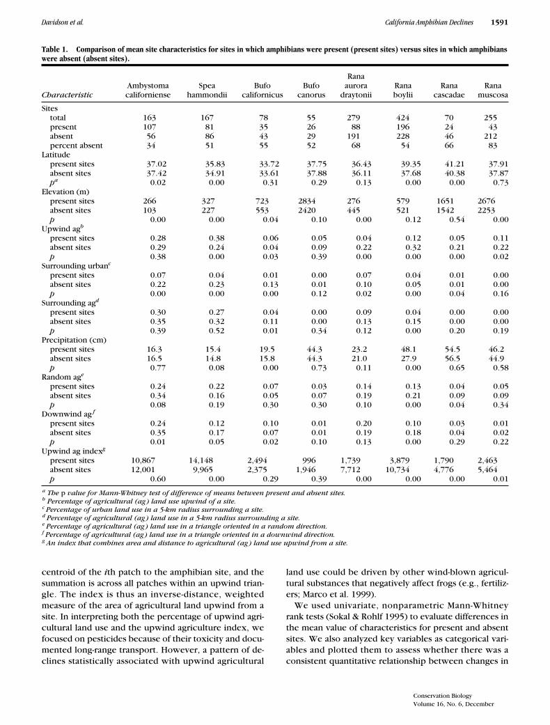
Table 1. Comparison of mean site characteristics for sites in which amphibians were present (present sites) versus sites in which amphibians were absent (absent sites).

Characteristic

Ambystomacaliforniense

Spea hammondii

Bufocalifornicus

Bufocanorus

Ranaaurora

draytoniiRana boylii

Ranacascadae

Ranamuscosa

Sitestotal 163 167 78 55 279 424 70 255present 107 81 35 26 88 196 24 43absent 56 86 43 29 191 228 46 212percent absent 34 51 55 52 68 54 66 83

Latitudepresent sites 37.02 35.83 33.72 37.75 36.43 39.35 41.21 37.91absent sites 37.42 34.91 33.61 37.88 36.11 37.68 40.38 37.87

p

a

0.02 0.00 0.31 0.29 0.13 0.00 0.00 0.73Elevation (m)

present sites 266 327 723 2834 276 579 1651 2676absent sites 103 227 553 2420 445 521 1542 2253

p

0.00 0.00 0.04 0.10 0.00 0.12 0.54 0.00Upwind ag

b

present sites 0.28 0.38 0.06 0.05 0.04 0.12 0.05 0.11absent sites 0.29 0.24 0.04 0.09 0.22 0.32 0.21 0.22

p

0.38 0.00 0.03 0.39 0.00 0.00 0.00 0.02Surrounding urban

c


p

0.00 0.00 0.00 0.12 0.02 0.00 0.04 0.16Surrounding ag

d


p

0.39 0.52 0.01 0.34 0.12 0.00 0.20 0.19Precipitation (cm)


p

0.77 0.08 0.00 0.73 0.11 0.00 0.65 0.58Random ag

e


p

0.08 0.19 0.30 0.30 0.10 0.00 0.04 0.34Downwind ag

f


p

0.01 0.05 0.02 0.10 0.13 0.00 0.29 0.22Upwind ag index

g

present sites 10,867 14,148 2,494 996 1,739 3,879 1,790 2,463absent sites 12,001 9,965 2,375 1,946 7,712 10,734 4,776 5,464

p

0.60 0.00 0.29 0.39 0.00 0.00 0.00 0.01

a

The

p

value for Mann-Whitney test of difference of means between present and absent sites.

b

Percentage of agricultural (ag) land use upwind of a site.

c

Percentage of urban land use in a 5-km radius surrounding a site.

d

Percentage of agricultural (ag) land use in a 5-km radius surrounding a site.

e

Percentage of agricultural (ag) land use in a triangle oriented in a random direction.

f

Percentage of agricultural (ag) land use in a triangle oriented in a downwind direction.

g

An index that combines area and distance to agricultural (ag) land use upwind from a site.

1592 California Amphibian Declines Davidson et al.


Figure 1. Spatial patterns of decline for four California ranid frogs, with the location and current population sta-tus for frog sites used in our analysis. Also shown are the distribution of agricultural lands based on U.S. Geologic Survey land use/land cover maps, and key predominant wind directions based on California Air Resources Board streamline wind maps.


Davidson et al. California Amphibian Declines 1593

the variable and the proportion of sites with declines.We used chi-square tests to evaluate the significance ofthe relationship between population status and each cat-egorical variable and multiple logistic regression to eval-uate the multivariate relationship between declines andgeographic, precipitation, elevational, and land-use vari-ables (Hosmer & Lemeshow 1989). For each species, webuilt a full model with all the variables and then one byone removed variables with statistically insignificant co-efficients to derive a reduced model with only signifi-cant variables.

Our analyses rely on both the spatial accuracy of themaps and the accuracy of the characterization of sitepopulation status (present or absent). We performedseveral analyses to assess the accuracy of Jennings andHayes’s species maps and the sensitivity of our results topossible errors in site spatial location and population sta-tus. To check spatial accuracy, we created maps from

original museum records and the published literature(for methods see Davidson et al. 2001) for

R. a. drayto-nii

and

R. cascadae

and compared these maps to thoseproduced by Jennings and Hayes (1994). We located thesame sites on both maps and calculated the average spa-tial location error, assuming the original records wereaccurate. We chose these two species as exemplars bothof species with large ranges within California and corre-spondingly small-scale maps (

R. a. draytonii

) and ofspecies with small ranges in the state and thereforelarge-scale maps (R. cascadae), and we quantified spatialaccuracy at both scales. To assess the robustness of ourresults to errors in spatial accuracy, we created a data setin which we randomly moved all sites in our originaldata set in a random direction and for a random distanceranging from zero to two times the estimated averagespatial-location error. We used either the estimated R. a.draytonii or R. cascadae spatial-location error, depend-ing on the scale of the original map. The reduced logis-tic regression models were then run on this new data setand the results compared with those on the originaldata. To assess the robustness of our results to possibleerrors in site population status (present/absent), we ran-domly switched status at approximately 10% of sites foreach species and reran the reduced logistic regressionmodels. We repeated this process 10 times and exam-ined the number of times a variable in the original mod-els remained statistically significant.

Results

The percentage of formerly occupied sites that are nowabsent was high for all eight species, ranging from 33%absent (A. californiense) to 83% absent (R. muscosa). Ingeneral, the results of the univariate (Table 1) and multi-variate analyses were similar. We focused on the eightmultiple logistic regression analyses to discern across-species patterns of variables associated with declines(Table 2). In all eight logistic regression models the like-lihood-ratio test for the overall model was significant,the Hosmer-Lemeshow goodness-of-fit test (Hosmer &Lemeshow 1989) indicated that the data fit the model,and the models correctly classified population status for63% (B. canorus) to 83% (R. cascadae and R. muscosa)of all sites. Use of upwind agriculture variables based on33.75�– or 45�–wide triangles produced regression coef-ficients and significance levels nearly identical to thosebased on the triangle 22.5� wide; therefore, we reportonly results based on the 22.5� upwind triangle. Pairwisecorrelations of variables within species were generallybelow 0.5, so we discounted high colinearity in inter-preting our mulitvariate results.

In the multivariate regression models, urbanizationwas a significant negative variable (that is, with increas-ing surrounding urban land use, sites were less likely to

Figure 2. Illustration of measurement of upwind agri-cultural land use. For each amphibian site, we drew a 22.5�, 100 km long “upwind triangle” facing into the direction of the predominant wind. Within the trian-gle, we measured upwind distance to the nearest agri-cultural land use (arrow a) and the percentage of the total area of the triangle consisting of agricultural land. An “upwind agricultural index” was calculated by dividing all agricultural land within the upwind triangle into patches 10 km2 or less (based on the par-tially shown grid). For each patch we calculated patch area divided by the distance from the patch centroid to the amphibian site (arrow b). The index value was then the sum of these calculations across all patches within the upwind triangle.

1594

California Amphibian Declines Davidson et al.


be a present site) for the salamander

A. californiense

and the anurans

S. hammondii

,

B. californicus

, and

R.a. draytonii

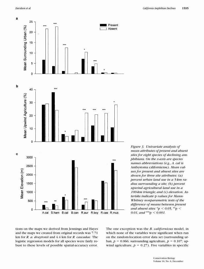
. When viewed in terms of mean urbaniza-tion at present and absent sites, the effect of surround-ing urbanization was particularly striking for the firstthree of these species, with absent sites having 3 (

A. cal-iforniense

) to 13 (

B. californicus

) times greater local ur-banization than sites where the species remainedpresent (Fig. 3). The effect, although statistically signifi-cant, was much less pronounced for

R. a.

draytonii,

whose absent sites on average were only about 50%more intensely urbanized than the present sites (Fig. 3).Surrounding agricultural land use in a 5-km radius was asignificant negative variable for

S. hammondii

,

B. cali-fornicus

, and

R. boylii

.Latitude was a significant positive variable for

R. a.draytonii,

and latitude and precipitation were positivevariables for

R. boylii

. The model for

R. cascadae

wascomplicated by the fact that both latitude and percent-age of upwind agriculture were each highly significantin individual univariate tests, yet the two variables werefairly highly correlated for this species (Pearson correla-tion, 0.64). There was a relatively small latitudinal differ-ence (40 km) between the Lassen area, where the spe-cies has largely disappeared, and the Trinity Alps area,where the species is still common. There was also astrong, stepwise gradient in declines for percentage ofupwind agriculture (Fig. 4) and no similar gradient forlatitude. We therefore modeled declines for

R. cascadae

with the upwind agriculture variable and not latitude.All four ranid frog species (

R. a. draytonii, R. boylii,R. cascadae,

and

R. muscosa

) showed a strong, statisti-cally significant pattern of decline with greater amountsof upwind agriculture (Table 1; Fig. 1). In the univariatecomparisons (Table 1; Fig. 3), the magnitude of this ef-fect was large, with mean upwind agriculture for absentsites ranging from 2.0 (

R. muscosa

) to 4.2 (

R. cascadae

)

times greater than for present sites. The same trend waspresent for the montane toad

B. canorus

, although thedifference in means (9% upwind agriculture for absentsites, 5% for present sites) was not statistically signifi-cant (Fig. 3), and upwind agriculture was not significantin the multivariate regression model for this species (Ta-ble 2). Similarly, the composite area and proximity agri-culture index was greater for all five species at absentsites than present sites, and the difference was signifi-cant for the four ranid frog species but not for

B. can-orus

. All five species showed a dose-response-like rela-tionship with a gradient of greater declines with greateramounts of upwind agriculture ( Fig. 4), and this rela-tionship was significant for

R. a. draytonii, R. boylii

,and

R. cascadae

.Elevation showed an unexpected pattern that was not

consistent with our predictions for the UV-B hypothesis.For seven of eight species (all except

R. a. draytonii;

Fig.3) the mean elevation of present sites was greater thanthat of absent sites, implying that within a species’ range,declines have been concentrated at lower-elevation locali-ties. In the logistic regression models for three species (

A.californiense

, B. canorus, R. muscosa), elevation was asignificant positive variable (that is, the likelihood of a sitebeing a present site increased with elevation).

There was only one significant interaction term in thereduced regression models: a negative term for latitude �urbanization for R. a. draytonii. That is, the negative ef-fect of urbanization on the likelihood of a site beingpresent was stronger at lower latitudes. The interactionterm is consistent with the observation that the speciesis almost entirely absent near southern California urbanareas, whereas it persists in the heavily urbanized SanFrancisco Bay Area.

Our results were reasonably robust to possible errorsin spatial accuracy of the maps and site population sta-tus. The average spatial accuracy error for matched loca-

Table 2. Logistic regression models of site population status for eight California amphibians.a

VariableAmbystomacaliforniense

Speahammondii

Bufocalifornicus

Bufocanorus

Ranaaurora

draytoniiRanaboylii

Ranacascadae

Ranamuscosa

Latitude � � Elevation � � � �Upwind agb � � � � �Surrounding urbanc � � � �Surrounding agd � � �Precipitation �Goodness of fite 0.85 0.23 0.57 0.16 0.13 0.21 0.99 0.67Accuracy f 0.71 0.70 0.69 0.63 0.78 0.72 0.83 0.83a The model for each species is read down the column. The plus (�) and minus (�) signs indicate a significant coefficient for this variable andthe sign (positive or negative) of the coefficient. In all models the dependent variable is site status (present, 1; absent, 0).b Percentage of agricultural (ag) land use upwind of a site.c Percentage of urban land use in a 5-km radius surrounding a site.d Percentage of agricultural (ag) land use in a 5-km radius surrounding a site.e The p value for the Hosmer-Lemeshow test.f Proportion of sites correctly classified as present or absent sites.



tions on the maps we derived from Jennings and Hayesand the maps we created from original records was 7.71km for R. a. draytonii and 4.4 km for R. cascadae. Thelogistic regression models for all species were fairly ro-bust to these levels of possible spatial-accuracy error.

The one exception was the B. californicus model, inwhich none of the variables were significant when runon the random-location error data set (surrounding ur-ban, p � 0.066; surrounding agriculture, p � 0.107; up-wind agriculture, p � 0.27). Five variables in specific

Figure 3. Univariate analysis of mean attributes of present and absent sites for eight species of declining am-phibians. On the x-axis are species names abbreviations (e.g., A. cal is Ambystoma californiense). Mean val-ues for present and absent sites are shown for three site attributes: (a) percent urban land use in a 5-km ra-dius surrounding a site; (b) percent upwind agricultural land use in a 100-km triangle; and (c) elevation. As-terisks indicate p values for Mann-Whitney nonparametric tests of the difference of means between present and absent sites: *p 0.05, **p 0.01, and ***p 0.001.



Figure 4. Categorical variable graphs and associated chi-square tests of the relationship between pop-ulation status and percent upwind agricultural land use for the five am-phibian species with greater upwind agricultural land use at absent sites than at the present sites. Missing bars represent sample sizes of �5 sites.



models were sensitive to possible population status er-rors: urbanization for A. californiense, precipitation forR. boylii, and percent upwind agriculture for B. califor-nicus and R. muscosa.

Discussion

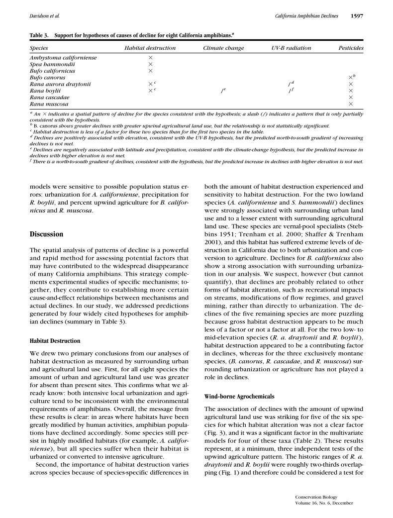
The spatial analysis of patterns of decline is a powerfuland rapid method for assessing potential factors thatmay have contributed to the widespread disappearanceof many California amphibians. This strategy comple-ments experimental studies of specific mechanisms; to-gether, they contribute to establishing more certaincause-and-effect relationships between mechanisms andactual declines. In our study, we addressed predictionsgenerated by four widely cited hypotheses for amphib-ian declines (summary in Table 3).

Habitat Destruction

We drew two primary conclusions from our analyses ofhabitat destruction as measured by surrounding urbanand agricultural land use. First, for all eight species theamount of urban and agricultural land use was greaterfor absent than present sites. This confirms what we al-ready know: both intensive local urbanization and agri-culture tend to be inconsistent with the environmentalrequirements of amphibians. Overall, the message fromthese results is clear: in areas where habitats have beengreatly modified by human activities, amphibian popula-tions have declined accordingly. Some species still per-sist in highly modified habitats (for example, A. califor-niense), but all species suffer when their habitat isurbanized or converted to intensive agriculture.

Second, the importance of habitat destruction variesacross species because of species-specific differences in

both the amount of habitat destruction experienced andsensitivity to habitat destruction. For the two lowlandspecies (A. californiense and S. hammondii ) declineswere strongly associated with surrounding urban landuse and to a lesser extent with surrounding agriculturalland use. These species are vernal-pool specialists (Steb-bins 1951; Trenham et al. 2000; Shaffer & Trenham2001), and this habitat has suffered extreme levels of de-struction in California due to both urbanization and con-version to agriculture. Declines for B. californicus alsoshow a strong association with surrounding urbaniza-tion in our analysis. We suspect, however (but cannotquantify), that declines are probably related to otherforms of habitat alteration, such as recreational impactson streams, modifications of flow regimes, and gravelmining, rather than directly to urbanization. The de-clines of the five remaining species are more puzzlingbecause gross habitat destruction appears to be muchless of a factor or not a factor at all. For the two low- tomid-elevation species (R. a. draytonii and R. boylii ),habitat destruction appeared to be a contributing factorin declines, whereas for the three exclusively montanespecies, (B. canorus, R. cascadae, and R. muscosa) sur-rounding urbanization or agriculture has not played arole in declines.

Wind-borne Agrochemicals

The association of declines with the amount of upwindagricultural land use was striking for five of the six spe-cies for which habitat alteration was not a clear factor(Fig. 3), and it was a significant factor in the multivariatemodels for four of these taxa (Table 2). These resultsrepresent, at a minimum, three independent tests of theupwind agriculture pattern. The historic ranges of R. a.draytonii and R. boylii were roughly two-thirds overlap-ping (Fig. 1) and therefore could be considered a test for

Table 3. Support for hypotheses of causes of decline for eight California amphibians.a

Species Habitat destruction Climate change UV-B radiation Pesticides

Ambystoma californiense �Spea hammondii �Bufo californicus �

Bufo canorus �b

Rana aurora draytonii � c / d �

Rana boylii � c /e / f �Rana cascadae �Rana muscosa �

a An � indicates a spatial pattern of decline for the species consistent with the hypothesis; a slash (/) indicates a pattern that is only partiallyconsistent with the hypothesis.b B. canorus shows greater declines with greater upwind agricultural land use, but the relationship is not statistically significant.c Habitat destruction is less of a factor for these two species than for the first two species in the table.d Declines are positively associated with elevation, consistent with the UV-B hypothesis, but the predicted north-to-south gradient of increasingdeclines is not met.e Declines are negatively associated with latitude and precipitation, consistent with the climate-change hypothesis, but the predicted increase indeclines with higher elevation is not met.f There is a north-to-south gradient of declines, consistent with the hypothesis, but the predicted increase in declines with higher elevation is not met.



a single geographical area. There was virtually no over-lap, however, between the ranges of these two speciesand the ranges of R. cascadae and R. muscosa (Fig. 1).It is intriguing that declines were strongly associatedwith upwind agriculture for all four ranid species, sug-gesting that this group may be particularly sensitive toagrochemicals. Whether this is coincidental or signifi-cant is difficult to determine with only eight species, al-though the odds of getting this taxonomic pattern bychance alone are low ( p � 0.014).

The strong association of decline for four species withthe amount of upwind agricultural land use was not justa reflection of habitat alteration due to agriculture. Al-though the amount of upwind agricultural land use wasassociated with declines, the amount of agricultural landuse in a 5-km radius surrounding a site was generally notassociated with declines, except in the case of R. boylii(Table 2). Similarly, variables for agricultural land use ina downwind or random direction were not significantwhen added to the logistic regression models for thesespecies, suggesting that the association reflects wind-borne agrochemicals rather than some generalized, non-directional influence of agriculture. Additional evidencefor the importance of upwind agriculture across speciescomes from the categorical variable analysis (Fig. 4),which demonstrated clear trends of increasing declineswith increasing amounts of upwind agriculture. Of thefactors we were able to examine, upwind agriculturewas the strongest single factor explaining California de-clines for amphibian taxa in which declines were notdriven primarily by overt habitat destruction.

UV-B Radiation

Our observed patterns of species decline are inconsis-tent with the predictions of the UV-B hypothesis. For alleight species pooled together, there were greater de-clines at higher elevations (above 1500 m, 72% of siteswere absent sites, vs. 56% below 1500 m), which is con-sistent with reports that amphibian declines are concen-trated at higher elevations ( Wake 1991; Carey et al.1999). However, this pattern was driven by greater over-all declines in high-elevation species (mainly R. mus-cosa), rather than trends within species. When viewedindividually, seven of eight species had a higher mean el-evation at present sites than at absent sites (Fig. 3). Thispattern is exactly opposite to the predictions of the UV-Bhypothesis of greater declines at higher elevations. Re-sults of an independent analysis of historical patterns ofdecline for the salamander A. californiense (Fisher &Shaffer 1996) shows this same elevational pattern.

Two species showed patterns partly consistent withthe UV-B hypothesis. Rana a. draytonii had a clear gra-dient of increasing declines with elevation (as predictedby the UV-B hypothesis), but did not display the pre-dicted north-to-south gradient (Davidson et al. 2001).

Rana boylii had the predicted north-to-south gradient ofincreasing declines (which could also be consistent withclimate change) but had greater declines at lower eleva-tions, opposite of that predicted by the UV-B hypothesis.Although UV-B exposure is affected by environmentalvariables such as canopy cover and dissolved organiccontent in water, as well as elevation and latitude, it isunlikely these factors would produce a systematic pat-tern of greater exposure at lower elevations. It is stillpossible that increased UV-B radiation may be adverselyaffecting amphibians, and experimental work on the bi-ological effects of UV-B exposure needs to be evaluatedon a species-by-species basis. However, under the assump-tions of our analysis, the patterns of observed declinesare not consistent with UV-B as a primary cause of am-phibian declines in California.

Climate Change

Only S. hammondii had both significantly greater de-clines in the south and at lower elevations, as we pre-dicted under the climate-change hypothesis. But neithervariable was significant in the logistic regression modelfor the species (Table 2), and neither variable showed agradient pattern in the univariate categorical variableanalysis (data not shown). Declines for S. hammondiiappeared to be more related to habitat degradation (Ta-ble 1; Fig. 3). The spatial pattern of decline for R. boyliiwas the most suggestive of an influence of climatechange, with a strong gradient of increasing declines tothe south and at drier sites. Because site latitude and pre-cipitation are correlated for this species (0.58), we wereunable to separate these two factors. Overall, our multi-species analysis did not implicate climate change, in-cluding precipitation effects, as a primary cause of am-phibian declines in California. Although climate changemay contribute to declines in more subtle or complexways (e.g., Pounds et al. 1999; Kiesecker et al. 2001), wedid not find large-scale spatial patterns of decline consis-tent with climate change, as have been found for othertaxa (e.g., Parmesan 1996).

Other Potential Factors

We were unable to analyze the spatial implications oftwo other important hypotheses for declines: disease(for a review see Carey et al. 1999) and introduced spe-cies (e.g., Hayes & Jennings 1986; Fisher & Shaffer 1996;Kupferberg 1997; Adams 1999; Lawler et al. 1999;Knapp & Matthews 2000; Kiesecker et al. 2001b). Notenough is known about the biology of disease agentssuch as chytrid fungus (Berger et al. 1998; Taylor et al.1999b), Saprolegnia (Blaustein et al. 1994; Kiesecker &Blaustein 1995), or the iridovirus (Cunningham et al.1996) to generate testable spatial predictions. We didnot have detailed site-by-site data on introduced species(primarily fish and bullfrogs [R. catesbeiana]) that



would allow us to include this factor in the current anal-ysis. Disease and introduced exotic species undoubtedlyboth play a role in the decline of many California am-phibians. For example, Bradford (1989), Bradford et al.(1994), Knapp and Matthews (2000), and V. Vredenberg(unpublished data) found that introduced trout havecontributed to the declines of R. muscosa. In mostcases, however, there have also been declines at siteswithout introduced fish (Bradford et al. 1994; Fisher &Shaffer 1996), suggesting that additional factors are in-volved. As field data on introduced predators and infor-mation on the basic biology of pathogens accumulates,spatial analysis can help in the future to evaluate the im-portance of both disease and exotic species.

Conclusions

Our analysis indicates that multiple factors may be re-sponsible for declines of California amphibians. For thespecies inhabiting vernal pools (A. californiense, S.hammondii ), declines were strongly associated withhabitat alteration, principally in the form of surroundingurban and, to a lesser extent, agricultural land use. Bufocalifornicus is a unique habitat specialist that alsoshowed a strong association of decline with habitat alter-ation, although its habitat has been less heavily alteredby urbanization and agriculture. For the remaining fivespecies, declines were generally not consistent withthose expected from the UV-B or climate-change hy-potheses, although there is partial support for each hy-pothesis in a single species. Declines for four of the fivespecies were strongly associated with the amount of up-wind agricultural land use, suggesting that wind-borneagrochemicals may be a factor.

For each of the hypotheses, we have chosen to exam-ine the simplest set of biologically meaningful predic-tions that we can envision. We believe that it is worthexamining these simple predictions before searching formore complex patterns. This strategy has, in somecases, already successfully associated distributionalchanges with a hypothesized cause. For example,Parmesan (1996) found that declines of a butterfly onthe Pacific coast of North America fit the simple climate-change model of range change. Clearly, each of the fourfactors we examined may affect the pattern of decline incomplex ways that might not be detected by our analy-sis. For example, Pounds et al. (1999) linked declines ofmontane amphibians at Monte Verde, Costa Rica, tochanges in daily precipitation associated with global cli-mate change.

Linking observed patterns to presumed underlyingprocesses must be undertaken with caution becausemultiple processes can generate similar patterns. Andgiven potential confounding factors, the absence of apattern should not be taken as proof of the absence of aprocess. Climate change and UV-B radiation may be con-

tributing to amphibian declines in California, despite ourgenerally negative results for these hypotheses. Further-more, multiple factors may interact to cause declines.For example, exposure to pesticides may weaken im-mune systems, increasing susceptibility to disease (Tay-lor et al. 1999a), and the presence or absence of preda-tors can radically change the toxicity of pesticides (Relyea& Mills 2001). Nonetheless, we believe that spatial analy-sis is a valuable approach for examining large-scale ob-servational data and provides a powerful statisticalframework within which to associate declines with plau-sible mechanisms.

Field and laboratory experiments on individual organ-isms are vital to understanding possible mechanismscausing declines, but such experiments are necessarilyrestricted to individuals or small local populations. Pop-ulation changes above the local site level cannot be sub-jected to experiments and can be quantified and ana-lyzed only through large-scale observational studies.Under a reasonable set of biological assumptions, thespatial analysis we conducted generated clear predic-tions that can be tested with field and laboratory studies.Specifically our work should encourage further investi-gation into the role of agrochemicals in amphibian de-clines. Pesticides have been suggested as a cause of de-cline (Carey & Bryant 1995; Stebbins & Cohen 1995;Drost & Fellers 1996; Lips 1998; Green & Kagarise Sher-man 2001), and recent experimental research on am-phibian species in the United States lends support to thissuggestion ( Taylor et al. 1999a; Boone & Semlitsch2001; Relyea & Mills 2001). To date there has been littlefield research on this subject. For example, in both Cen-tral America ( Pounds & Crump 1994; Lips 1998; Lips1999) and Australia ( Richards et al. 1993), major am-phibian declines have occurred in areas close to anddownwind, for part of the year, from large agriculturalzones. Yet little research on contaminants has been con-ducted in these areas.

Acknowledgments

We thank C. Ramirez for geographic information system(GIS) mapping and assistance with data entry; J. Quinnand the Information Center for the Environment at theUniversity of California, Davis (UCD), for GIS facilities;and the Center for Image Processing and IntegratedComputing for use of the supercomputer (NSF ACI 96–19020). S. Lawler, P. Moyle, M. Schwartz, members ofthe Shaffer lab group, and C. Kaufman provided helpfulcomments on earlier drafts of this paper. Funding wasprovided by the Declining Amphibian Populations TaskForce of the World Conservation Union (IUCN)/SpeciesSurvival Commission, the University of California ToxicSubstances Research and Teaching Program, the Gradu-ate Group in Ecology, the Center for Population Biology



at UCD, the UCD Agricultural Experiment Station, andthe National Science Foundation.

Literature Cited

Adams, M. J. 1999. Correlated factors in amphibian decline: Exotic spe-cies and habitat change in western Washington. Journal of WildlifeManagement 63:1162–1171.

Alexander, M. A., and J. K. Eischeid. 2001. Climate variability in re-gions of amphibian declines. Conservation Biology 15:930–942.

Aston, L. S., and J. N. Seiber. 1997. Fate of summertime airborne organo-phosphate pesticide residues in the Sierra Nevada mountains. Jour-nal of Environmental Quality 26:1483–1492.

Berger, L., R. Speare, P. Daszak, D. E. Green, A. A. Cunningham, C. L.Goggin, R. Slocombe, M. A. Ragan, A. D. Hyatt, K. R. McDonald,H. B. Hines, K. R. Lips, G. Marantelli, and H. Parkes. 1998. Chytridio-mycosis causes amphibian mortality associated with population de-clines in the rain forests of Australia and Central America. Proceed-ings of the National Academy of Sciences of the United States ofAmerica 95:9031–9036.

Blaustein, A. R., D. G. Hokit, R. K. Ohara, and R. A. Holt. 1994. Patho-genic fungus contributes to amphibian losses in the Pacific North-west. Biological Conservation 67:251–254.

Blumthaler, M. 1993. Solar UV measurements. Pages 17–79 in M.Tevini, editor. Environmental effects of UV (ultraviolet) radiation.Lewis Publisher, Boca Raton, Florida.

Boone, M. D., and R. D. Semlitsch. 2001. Interactions of an insecticidewith larval density and predation in experimental amphibian com-munities. Conservation Biology 15:228–238.

Bradford, D. F. 1989. Allotopic distribution of native frogs and intro-duced fishes in high Sierra Nevada lakes of California: implicationsof the negative impact of fish introductions. Copeia 1989:775–778.

Bradford, D. F., D. M. Graber, and F. Tabatabai. 1994. Population de-clines of the native frog, Rana muscosa, in Sequoia and Kings Can-yon National Parks, California. Southwestern Naturalist 39:323–327.

Cabrera, S., S. Bozzo, and H. Fuenzalida. 1995. Variations in UV radiationin Chile. Journal of Photochemistry and Photobiology 28:137–142.

Carey, C., and C. J. Bryant. 1995. Possible interrelations among environ-mental toxicants, amphibian development, and decline of amphib-ian populations. Environmental Health Perspectives 103:13–17.

Carey, C., N. Cohen, and L. Rollins-Smith. 1999. Amphibian declines:an immunological perspective. Developmental and ComparativeImmunology 23:459–472.

Carey, C., W. R. Heyer, J. Wilkinson, R. A. Alford, J. W. Arntzen, T. Hal-liday, L. Hungerford, K. R. Lips, E. M. Middleton, S. A. Orchard, andA. S. Rand. 2001. Amphibian declines and environmental change:use of remote-sensing data to identify environmental correlates.Conservation Biology 15:903–913.

Cory, L., P. Fjerd, and W. Serat. 1970. Distribution patterns of DDT res-idues in the Sierra Nevada mountains. Pesticide Monitoring Journal3:204–211.

Crooks, K. R., and M. E. Soulé. 1999. Mesopredator release and avifau-nal extinctions in a fragmented system. Nature 400:563–566.

Cunningham, A. A., T. E. S. Langton, P. M. Bennett, J. F. Lewin, S. E. N.Drury, R. E. Gough, and S. K. MacGregor. 1996. Pathological andmicrobiological findings from incidents of unusual mortality of thecommon frog (Rana temporaria). Philosophical Transactions ofthe Royal Society of London, B 351:1539–1557.

Datta, S., L. Hansen, L. McConnell, J. Baker, J. LeNoir, and J. N. Seiber.1998. Pesticides and PCB contaminants in fish and tadpoles fromthe Kaweah River Basin, California. Bulletin of Environmental Con-tamination and Toxicology 60:829–836.

Davidson, C., H. B. Shaffer, and M. R. Jennings. 2001. Declines of theCalifornia red-legged frog: climate, UV-B, habitat and pesticides hy-potheses. Ecological Applications 11:464–479.

Department of Pesticide Regulation (DPR). 1990. Pesticide use report:1990. DPR, Sacramento, California.



Drost, C. A., and G. M. Fellers. 1996. Collapse of a regional frog faunain the Yosemite area of the California Sierra Nevada, USA. Conser-vation Biology 10:414–425.

Fahrig, L., J. H. Pedlar, S. E. Pope, P. D. Taylor, and J. F. Wegner. 1995.Effect of road traffic on amphibian density. Biological Conservation73:177–182.

Fellers, G. M., and C. A. Drost. 1993. Disappearance of the Cascadesfrog Rana cascadae at the southern end of its range, California,USA. Biological Conservation 65:177–181.

Fisher, R. N., and H. B. Shaffer. 1996. The decline of amphibians in Cal-ifornia’s Great Central Valley. Conservation Biology 10:1387–1397.

Green, D. E., and C. Kagarise Sherman. 2001. Diagnostic histologicalfindings in Yosemite toads (Bufo canorus) from a die-off in the1970s. Journal of Herpetology 35:92–103.

Gross, S. J., and T. D. Price. 2000. Determinants of the northern andsouthern range limits of a warbler. Journal of Biogeography 27:869–878.

Hayes, M. P., and M. R. Jennings. 1986. Decline of ranid frog species inwestern North America: are bullfrogs (Rana catesbeiana) respon-sible? Journal of Herpetology 20:490–509.

Hayes, T. P., J. J. R. Kinney, and N. J. M. Wheeler. 1984. California sur-face wind climatology. California Air Resources Board, Sacramento.

Herman, J. R., N. Krotkov, E. Celarier, D. Larko, and G. Labow. 1999.Distribution of UV radiation at the Earth’s surface from TOMS–mea-sured UV–backscattered radiances. Journal of Geophysical Research104:12,059–12,076.

Hosmer, D. W., and S. Lemeshow. 1989. Applied logistic regression.Wiley, New York.

Jennings, M. R. 1988. Natural history and decline of native ranids in Cali-fornia. Pages 61–72 in H. F. De Lisle, P. R. Brown, B. Kaufman, and B.M. McGurty, editors. Proceedings of the conference on California her-petology. Southwestern Herpetologists Society, Van Nuys, California.

Jennings, M. R., and M. P. Hayes. 1994. Amphibian and reptile speciesof special concern in California. California Department of Fish andGame, Inland Fisheries Division, Rancho Cordova.

Karl, R. T., R. W. Knight, R. R. Easterling, and R. G. Quale. 1996. Indi-ces for climate change for the United States. Bulletin of the Ameri-can Meteorological Society 77:279–292.

Kiesecker, J. M., and A. R. Blaustein. 1995. Synergism between UV-Bradiation and a pathogen magnifies amphibian embryo mortality innature. Proceedings of the National Academy of Sciences of theUnited States of America 92:11049–11052.

Kiesecker, J. M., A. R. Blaustein, and L. K. Belden. 2001a. Complexcauses of amphibian population declines. Nature 410:681–683.

Kiesecker, J. M., A. R. Blaustein, and C. I. Miller. 2001b. Transfer of apathogen from fish to amphibians. Conservation Biology 15:1064–1070.

Kirkpatrick, M., and N. H. Barton. 1997. Evolution of a species’ range.The American Naturalist 150:1–23.

Knapp, R. A., and K. R. Matthews. 2000. Non-native fish introductionsand the decline of the mountain yellow-legged frog from withinprotected areas. Conservation Biology 14:428–438.

Kupferberg, S. J. 1997. Bullfrog (Rana catesbeiana) invasion of a Cali-fornia river: the role of larval competition. Ecology 78:1736–1751.

Laurance, W. F. 1996. Catastrophic declines of Australian rainforestfrogs: Is unusual weather responsible? Biological Conservation 77:203–212.

Lawler, S. P., D. Dritz, T. Strange, and M. Holyoak. 1999. Effects of in-troduced mosquitofish and bullfrogs on the threatened Californiared-legged frog. Conservation Biology 13:613–622.

LeNoir, J. S., L. L. McConnell, M. G. Fellers, T. M. Cahill, and J. N.



Seiber. 1999. Summertime transport of current-use pesticides fromCalifornia’s Central Valley to the Sierra Nevada mountain range,USA. Environmental Toxicology and Chemistry 18:2715–2722.

Lips, K. R. 1998. Decline of a tropical montane amphibian fauna. Con-servation Biology 12:106–117.

Lips, K. R. 1999. Mass mortality and population declines of anurans atan upland site in western Panama. Conservation Biology 13:117–125.

Madronich, S., R. L. McKenzie, M. M. Caldwell, and L. O. Bjorn. 1995.Changes in ultraviolet radiation reaching the earth’s surface. Ambio24:143–152.

Marco, A., C. Quilchano, and A. R. Blaustein. 1999. Sensitivity to ni-trate and nitrite in pond-breeding amphibians from the PacificNorthwest, USA. Environmental Toxicology and Chemistry 18:2836–2839.

Marsh, D. M., and P. B. Pearman. 1997. Effects of habitat fragmentationon the abundance of two species of Leptodactyliid frogs in an An-dean montane forest. Conservation Biology 11:1323–1328.

McConnell, L. L., J. S. LeNoir, S. Datta, and J. N. Seiber. 1998. Wet dep-osition of current-use pesticides in the Sierra Nevada mountainrange, California, USA. Environmental Toxicology and Chemistry17:1908–1916.

Middleton, E. M., J. R. Herman, E. A. Celarier, J. Wilkinson, C. Carey,and R. J. Rusin. 2001. Evaluating ultraviolet radiation exposurewith satellite data at sites of amphibian declines in Central andSouth America. Conservation Biology 15:914–929.

Parmesan, C. 1996. Climate and species’ range. Nature 382:765–766.Peters, R. L. 1991. Consequences of global warming on biological di-

versity. Pages 99–118 in R. L. Wyman, editor. Global climatechange and life on earth. Chapman Hall, New York.

Pounds, J. A., and M. L. Crump. 1994. Amphibian declines and climatedisturbance: the case of the golden toad and the harlequin frog.Conservation Biology 8:72–85.

Pounds, J. A., M. P. L. Fogden, and J. H. Campbell. 1999. Biological re-sponse to climate change on a tropical mountain. Nature 398:611–614.

Relyea, R. A., and M. Mills. 2001. Predator-induced stress makes thepesticide carbaryl more deadly to gray treefrog tadpoles. Proceed-ings of the National Academy of Science of the United States ofAmerica 98:2491–2496.

Richards, S. J., K. R. McDonald, and R. A. Alford. 1993. Declines inpopulations of Australia’s endemic tropical rainforest frogs. PacificConservation Biology 1:66–77.

Shaffer, H. B., and P. C. Trenham. 2001. Species account: Ambystomacaliforniense. In M. J. Lannoo, editor. Status and conservation ofUnited States amphibians. University of California Press, Berkeley.

Shaffer, H. B., R. N. Fisher, and C. Davidson. 1998. The role of naturalhistory collections in documenting species declines. Trends inEcology & Evolution 13:27–30.

Sokal, R. R., and F. J. Rohlf. 1995. Biometry. W. H. Freeman, NewYork.

Stebbins, R. C. 1951. Amphibians of western North America. Univer-sity of California Press, Berkeley.

Stebbins, R. C., and N. W. Cohen. 1995. A natural history of amphibi-ans. Princeton University Press, Princeton, New Jersey.

Taylor, S. K., E. S. Williams, and K. W. Mills. 1999a. Effects of mal-athion on disease susceptibility in Woodhouse’s toads. Journal ofWildlife Diseases 35:536–541.

Taylor, S. K., E. S. Williams, E. T. Thorne, K. W. Mills, D. I. Withers,and A. C. Pier. 1999b. Causes of mortality of the Wyoming toad.Journal of Wildlife Diseases 35:49–57.

Trenham, P. C., H. B. Shaffer, W. D. Koenig, and M. R. Stromberg.2000. Life history and demographic variation in the California tigersalamander (Ambystoma californiense). Copeia 2000:365–377.

Vos, C. C., and J. P. Chardon. 1998. Effects of habitat fragmentationand road density on the distribution pattern of the moor frog Ranaarvalis. Journal of Applied Ecology 35:44–56.

Wake, D. B. 1991. Declining amphibian populations. Science 253:860.Zabik, J. M., and J. N. Seiber. 1993. Atmospheric transport of organo-

phosphate pesticides from California’s Central Valley to the SierraNevada Mountains. Journal of Environmental Quality 22:80–90.

Spatial Tests of the Pesticide Drift, Habitat Destruction ...online.sfsu.edu/carlosd/davidson-consbio-compressed-02.pdf · un factor importante en las declinaciones. Para otras dos

Documents