sustainability Article Spatial-Temporal Analysis of Point Distribution Pattern of Schools Using Spatial Autocorrelation Indices in Bojnourd City Mostafa Ghodousi 1 , Abolghasem Sadeghi-Niaraki 1,2, * , Farzaneh Rabiee 1 and Soo-Mi Choi 2 1 Geoinformation Tech. Center of Excellence, Faculty of Geodesy & Geomatics Engineering, K. N. Toosi University of Technology, Tehran 19697, Iran; [email protected] (M.G.); [email protected] (F.R.) 2 Department of Computer Science and Engineering, Sejong University, Seoul 143-747, Korea; [email protected] * Correspondence: [email protected]; Tel.: +98-21-8887-7070 Received: 28 June 2020; Accepted: 15 September 2020; Published: 19 September 2020 Abstract: In recent years, attention has been given to the construction and development of new educational centers, but their spatial distribution across the cities has received less attention. In this study, the Average Nearest Neighbor (ANN) and the optimized hot spot analysis methods have been used to determine the general spatial distribution of the schools. Also, in order to investigate the spatial distribution of the schools based on the substructure variables, which include the school building area, the results of the general and local Moran and Getis Ord analyses have been investigated. A differential Moran index was also used to study the spatial-temporal variations of the schools’ distribution patterns based on the net per capita variable, which is the amount of school building area per student. The results of the Average Nearest Neighbor (ANN) analysis indicated that the general spatial patterns of the primary schools, the first high schools, and the secondary high schools in the years 2011, 2016, 2018, and 2021 are clustered. Applying the optimized hot spot analysis method also identified the southern areas and the suburbs as cold polygons with less-density. Also, the results of the differential Moran analysis showed the positive trend of the net per capita changes for the primary schools and first high schools. However, the result is different for the secondary high schools. Keywords: spatial-temporal analysis; Average Nearest Neighbor (ANN) analysis; optimized hot spots analysis; general and local analyses of Moran and Getis Ord; the differential Moran index; social justice 1. Introduction The rapid growth of the urban population due to the migration of people from the rural regions to urban centers and the lack of a well-planned and systematic planning system has caused many problems in most cities in Iran. Due to the rapid growth of the population and the physical condition of the cities, issues, which include the lack of proper spatial distribution of the facilities, have arisen. One of the most important problems is the reduction of the per capita urban services, which include the educational services. The public services have different types and roles regarding the support of society functions [1]. A problem that planners often deal with is determining the optimal distribution of the service centers. The equal distribution of the service centers, which include the educational centers, is especially important because of the critical role they play in the knowledge, development, and culture of each society. The schools are crucial components of public city services [2]. The educational services facilitate learning and teaching, which are both physical and spatial. They are the resources that educational Sustainability 2020, 12, 7755; doi:10.3390/su12187755 www.mdpi.com/journal/sustainability

Welcome message from author
This document is posted to help you gain knowledge. Please leave a comment to let me know what you think about it! Share it to your friends and learn new things together.
Transcript

sustainability
Article
Spatial-Temporal Analysis of Point DistributionPattern of Schools Using Spatial AutocorrelationIndices in Bojnourd City
Mostafa Ghodousi 1, Abolghasem Sadeghi-Niaraki 1,2,* , Farzaneh Rabiee 1 and Soo-Mi Choi 2
1 Geoinformation Tech. Center of Excellence, Faculty of Geodesy & Geomatics Engineering,K. N. Toosi University of Technology, Tehran 19697, Iran; [email protected] (M.G.);[email protected] (F.R.)
2 Department of Computer Science and Engineering, Sejong University, Seoul 143-747, Korea;[email protected]
* Correspondence: [email protected]; Tel.: +98-21-8887-7070
Received: 28 June 2020; Accepted: 15 September 2020; Published: 19 September 2020�����������������
Abstract: In recent years, attention has been given to the construction and development of neweducational centers, but their spatial distribution across the cities has received less attention. In thisstudy, the Average Nearest Neighbor (ANN) and the optimized hot spot analysis methods havebeen used to determine the general spatial distribution of the schools. Also, in order to investigatethe spatial distribution of the schools based on the substructure variables, which include the schoolbuilding area, the results of the general and local Moran and Getis Ord analyses have been investigated.A differential Moran index was also used to study the spatial-temporal variations of the schools’distribution patterns based on the net per capita variable, which is the amount of school building areaper student. The results of the Average Nearest Neighbor (ANN) analysis indicated that the generalspatial patterns of the primary schools, the first high schools, and the secondary high schools in theyears 2011, 2016, 2018, and 2021 are clustered. Applying the optimized hot spot analysis method alsoidentified the southern areas and the suburbs as cold polygons with less-density. Also, the resultsof the differential Moran analysis showed the positive trend of the net per capita changes for theprimary schools and first high schools. However, the result is different for the secondary high schools.
Keywords: spatial-temporal analysis; Average Nearest Neighbor (ANN) analysis; optimized hotspots analysis; general and local analyses of Moran and Getis Ord; the differential Moran index;social justice
1. Introduction
The rapid growth of the urban population due to the migration of people from the rural regionsto urban centers and the lack of a well-planned and systematic planning system has caused manyproblems in most cities in Iran. Due to the rapid growth of the population and the physical conditionof the cities, issues, which include the lack of proper spatial distribution of the facilities, have arisen.One of the most important problems is the reduction of the per capita urban services, which includethe educational services. The public services have different types and roles regarding the support ofsociety functions [1]. A problem that planners often deal with is determining the optimal distributionof the service centers. The equal distribution of the service centers, which include the educationalcenters, is especially important because of the critical role they play in the knowledge, development,and culture of each society.
The schools are crucial components of public city services [2]. The educational services facilitatelearning and teaching, which are both physical and spatial. They are the resources that educational
Sustainability 2020, 12, 7755; doi:10.3390/su12187755 www.mdpi.com/journal/sustainability

Sustainability 2020, 12, 7755 2 of 26
administrators, students, and teachers use for a purposeful learning process [3]. Education is notjust a basic human right or a tool to alleviate poverty, it promotes social equality and stimulateseconomic development through the development of a skillful work group [4]. The level of educationof a community is a critical factor for social and economic development and is an indicator of potentialgrowth [5]. Education is essential to the transformation of economy, society, and culture. However,the efficiency of education differs because of the quality, equity, and appropriateness of accessibilityand the spatial distribution of the facilities [6].
In the context of geography and sociology, equality in the distribution of the educational facilitiesis an academic topic that has continued importance. Consequently, more attention has been paidby city planners to the imbalanced design and the spatial optimization of educational facilities inplaces. In particular, they deal with the spatial distribution of the education facilities [7]. Constraintsin the location and the use of educational resources will not support the development of learning andcreativity [8]. Usually, educational services are not often evenly distributed among the population,which is common with most public services. The unbalanced distribution of the services, which isalso common in most societies, has been shown to threaten their accessibility capabilities and use [3].Establishing equal access to educational facilities has been an effective tactic for social equity andjustice. Educational inequity causes communities to be unable to receive equitable opportunities foreducation [9].
Due to its relationship to social, economic growth, education has been a concern for all developedand developing countries. In developing nations, education encounters a series of challenges thatrequire the formulation of different strategies in order to promote their accessibility [3]. The Iraniangovernment has been trying to increase the development of educational services. In Iran, it is rareto determine the spatial distribution of educational services, which therefore restricts the access toeducation. Especially in Bojnourd city, even with the quantitative growth of educational services,it remains unknown how well the facilities have been distributed and how accessible education isto the people. The unequal distribution of the educational facilities through the different regions ofBojnourd has caused the advent of educational inequity. Due to the importance of enhancing thequality of services to satisfy people’s growing demand in the future, an objective evaluation of theexisting circumstances is crucial. Therefore, for educational equity, the spatial distribution of theschools should be evaluated. This evaluation could provide the knowledge necessary to developpolicies for sustainable urban development.
While educational inequity has gained considerable academic interest, little attention has beengiven to the educational facilities’ spatial-temporal patterns. One of the most important issues in thefield of educational spatial justice that is less considered is the study of the spatial-temporal distributionof education facilities in order to evaluate the results of the different scenarios and the policies in thefield at different times. Also, this issue leads to a clear understanding of whether the policies adopted bythe authorities are aimed at promoting social justice and equalizing the distribution of the educationalfacilities in society. In this regard, the main purpose of this research is to investigate the spatial-temporaldistribution of the schools using different types of spatial point analysis methods towards enhancingthe possibility of better prospects for sustainable locations and the spatial distribution of educationalservices. To achieve the goal of this research, the methods of the Average Nearest Neighbor (ANN)analysis, the optimized hot spots analysis, Moran’s I global spatial autocorrelation index, Getis OrdGeneral G spatial autocorrelation index, Getis Ord Gi* local autocorrelation index, Anselin local Moran’sI, and the differential Moran’s I index were used. The differential Moran’s I index is a developedform of the local Moran’s I index that is used to measure the spatial pattern of changes betweentwo-time intervals.
The following is a description of the organization of this paper. The next section reviews theeducational inequality literature. This is followed by the basics of the methods that were used. Then,the area of study and the methodology will be introduced. This is followed by detailed research results.Ultimately, this paper ends with significant findings and implications for policy making.
Sustainability 2020, 12, 7755 3 of 26
2. Literature Review
The equity of education is a crucial factor to make sustainable education growth. The geographicalliterature has conducted abundant research about investigating the spatial patterns of different kindsof services and facilities, but little research about the educational spatial patterns has been conducted.
Talen [10] found significant inequalities with the access to primary schools in the West Virginiaregions. They investigated whether or not the distribution of travel costs among the citizen’s places(blocks) and the educational facilities is equally based on the density and demographics of thepopulation. Thomas et al. [11] investigated the inequity in educational facilities using the Ginicoefficient and the Theil coefficient. Cao et al. [12] evaluated the spatial distribution and the equality ofeducational facilities in Gansu. Ajala et al. [13] examined the inequity of access to primary educationin a state in Ethiopia using different data, which included the number of schools, enrollments, andteachers. They discovered that accessibility to primary education services was not equitable.
Meschi and Scervini [14] presented a broad set of educational attainment and inequity measures.As a metric to measure inequality, they used standard deviation, the coefficient of variation, the Giniindex, the Theil index, the mean logarithmic deviation, and the Atkinson indices. Yu et al. [15] usedthe Gini index to calculate the inequalities. Pengfei et al. [16] identified the regional variations inthe accessibility of elementary schools in Xiantao, which indicated that the city centers have betteraccessibility to elementary schools than rural areas. Lobban [5] analyzed the spatial, the aspatial,and the demographic data in order to identify potential locations for secondary schools in order toguarantee an equal educational facilities distribution. Yang et al. [17] assessed elementary schoolaccessibility considering the impact of roadway slopes in mountainous regions.
Scott et al. [18] analyzed public school spatial inequality based on public transit. Moreno-Monroya et al. [19] found that inequity in the central business district of Sao Paulo in Brazil could beworsened by the unequal accessibility of the secondary schools. They found that the students withlow incomes often have limited accessibility to schools, because they live in places with inadequatetransportation substructures. Xiang et al. [4] discovered disadvantaged groups and their distributions.They also identified possible differences in education accessibility and spatial patterns. Ye et al. [20]examined the accessibility of educational facilities at the neighborhood level in China among thevarious social groups. Their results showed strong spatial inequalities with accessibility to secondaryschool. Zhou et al. [9] used the Gini coefficient to calculate the inequity in educational facilities.
Some research used a spatial pattern analysis. Gao et al. [21] investigated the spatial accessibilitybased on the shortest distance from schools to the inhabitants. They also explored the inequity incompulsory education with the distribution of the spatial accessibility. They used the Theil indexand the spatial autocorrelation analyses. They used global and local Moran’s I and Getis-Ord Gi*.The study of the spatial patterns showed significant global autocorrelation and apparent clusters.Setyono and Cahyono [22] evaluated the number of school catchment areas in each unit, which includedthe villages and the sub-districts. They used Moran’ I spatial autocorrelation analysis to discover thepattern of the primary school facilities. Agbabiaka et al. [3] examined the spatial distribution of thesecondary education services. They investigated the educational facilities’ availability, accessibility,and functionality. They used the Average Nearest Neighbor (ANN) to examine the spatial patternof the secondary school facilities distribution. Bulti et al. [6] investigated the spatial distributionand the accessibility of the elementary school facilities. To analyze the educational facilities’ spatialconcentration and the spatial distribution pattern, they used the location quotient and the AverageNearest Neighbor (ANN) analysis. They indicated the inequity of the service delivery between theneighboring areas and showed a clustered pattern in the overall spatial distribution of the educationalfacilities. Sumari et al. [23] investigated the spatial distribution of the town of Abbottabad’s primaryand secondary schools in Pakistan. They found an unequal pattern distribution with the schools.
Even though educational inequity has attracted wide academic attention, little attention has beenpaid to the educational facilities’ spatial-temporal patterns. Adams and Hannum [24] investigatedvariations in the accessibility of the educational facilities and the inequality over time in China using a

Sustainability 2020, 12, 7755 4 of 26
generalized estimating equation method. Williams and Wang [25] assessed high school accessibility forthe years 1990, 2000, and 2010. They investigated the percentage change in the educational accessibilityin various regions. Relative to the suburban and the rural regions, they discovered that the urban areashad significantly lower accessibility levels. Yang et al. [26] used the Gini index for several years tomeasure China’s educational inequity.
Wan et al. [27] investigated the regional inequity in elementary education. They also investigatedthe temporary inequity by calculating the number of elementary educational facilities for each year.They used the Theil index to assess the elementary schools’ educational facilities’ balances in all counties.Xu et al. [28] introduced a method for social-spatial accessibility in order to evaluate the variousdegrees of accessibility across the geographical, opportunity, and economic aspects for the variouselementary educational facilities. For the years 2008 and 2018, they used a spatial-temporal analysis.Comprehensive studies examining the spatial-temporal patterns have been conducted in other types offacilities, such as parks, green spaces, and public libraries. Xing et al. [29] evaluated the spatial-temporaldifferences between the demand and the supply of two modes of traffic, which included walking anddriving, in the city center in Wuhan between 2000 and 2014. They used the coefficient of variationto measure the alterations, and they used the analysis of spatial correlation to clarify the impacts ofspatial differences by alterations in the accessibility of each mode. They concluded that the supply andthe demand for green space both increased. They found the spatial disparities of the green park spaceswere significantly different in walking and driving modes in various periods. They analyzed the factorsof the changes in inequalities using a bivariate analysis, which confirmed that policies and the strategieswere the critical factors relevant to green space access. They used the spatial autocorrelation method,which included Moran’s I global univariate indices for spatial-temporal autocorrelations of disparityand Moran’s I bivariate indices for correlations of spatially correlated accessibility disparity variables.
Ye et al. [20] investigated the variations in the distribution of green space accessibility amongregions and among communities between the years 2010 and 2015. They concluded that access togreen spaces in Macau is unevenly distributed across regions and population groups. However, greenspace access has become more equally distributed over time despite the decrease in the overall accessto green space.
Page et al. [30] investigated the spatio-temporal differences in the accessibility of the publiclibraries. They indicated that between 2011 and 2018, the degree of spatial accessibility to publiclibraries in Wales decreased on average. This matter was correlated with a significant decrease inpublic library financing during the same period.
This type of research showed spatial inequality with the distribution of critical facilities andservices, and the findings have implications regarding the decisions.
3. Basics of the Used Methods
The necessary concepts of the methods used in the research will be described in this section.
3.1. Average Nearest Neighbor (ANN)
In order to determine the type of distribution of the educational centers in this study, the AverageNearest Neighbor analysis method was used. The results are important, because they facilitate theidentification of the causes that influence the formation of the different deployment systems. The resultsalso provide basic services and essential services needed to implement the general policies and completethe suggested models for the delivery of educational services at the regional level. It should be notedthat as a result of applying the different steps, this method yields an index called the Rate neighborhood(Rn), which ranges from zero to 2.15. The closer the value of Rn is to zero indicates the clusterdistribution pattern. The closer the value of Rn is to 2.15 indicates a regular distribution pattern, andthe number 1 expresses the random spatial distribution. In the Average Nearest Neighbor method,if the index is less than 1, the distribution is clustered, and if the index is greater than 1, there is a

Sustainability 2020, 12, 7755 5 of 26
tendency to disperse. The Average Nearest Neighbor method is very sensitive, and a small change inthe distribution of land use can cause many changes in the computations [31].
3.2. Optimized Hot Spot Analysis
Optimized hot spot analysis implements the Getis-Ord Gi* method use variables extracted fromthe input data features. This method uses the Getis-Ord Gi* statistics to generate a map of statisticallymeaningful hot and cold spots. To generate the optimum outcomes, it assesses the attributes of theinput feature class. This method can be done without selecting a field or by selecting a numericalfield. the optimized hot spot analysis is conducted by applying the following two approaches in thisresearch [32]:
• The events count method inside each cell: this approach aggregates the event point data andcomputes the number of events inside each cell.
• The event count method within each polygon: to aggregate events into count parameters,there must be aggregation polygons to overlay the event point data in the polygons. The eventsare enumerated across each polygon. The method of counting point events within each polygonis commonly used to examine the spatial concentration of the data at different statistical levels,such as statistical districts and statistical blocks.
3.3. Moran’s I
This is a general index that shows whether the pattern is clustered, scattered, or random.Each aggregated point is allocated an intensity amount and needs some variation of the values for themeasurement of this metric. The points that have similar values are expressed in the high Moran Ivalues, which are positive or negative. The Moran index values vary between +1 and −1. The valuesthat approximate to +1 demonstrate clustering, and the values that approximate to −1 demonstraterandom distribution of the data patterns. The significance of the values can be evaluated against anormal distribution. The output of this analysis consists of five parameters of the observed values,which include I, the expected values, the standard deviation, the z-score, and the p-value. In this index,if the observed value of I exceeds the expected value, it indicates a cluster. If the observed values ofI are lower than the expected values, it indicates the absence of a cluster. In addition, if the p-valueprobability is low and the z-score is high, the null hypothesis is rejected and indicates that the datadistribution is clustered [33]. Equation (1) illustrates how the Moran index is calculated [34]:
I =nS0
∑ni=1
∑nj=1 ziz jwi j∑n
i=1 z2i
(1)
In Equation (1), zi is the standard deviation of feature i from the mean (xi −X), is the locationof the two features i and j, n is the total number of features, and S0 is the sum of the weights of thefeatures (in Equation (2)).
S0 =n∑
i=1
n∑j=1
wi j (2)
The z-score can be calculated according to Equation (3). In Equation (3), V [I] is the variance.
zI =I + 1
n−1√V[I]
(3)
3.4. Getis Ord General G
The statistic identifies the clusters that are more likely than the randomly generated clusters anduses the aggregated data. For example, if an area has high values for the number of schools andits neighbors are the same, this test concludes that they are part of a hot spot. This analysis is most

Sustainability 2020, 12, 7755 6 of 26
often used when there is a nearly uniform distribution of the values and we needed to search for theunexpected spatial values. The general G statistic is considered according to Equation (4) [35]:
G =
∑ni=1
∑ni=0 xix jwi, j∑n
i=1∑n
i=0 xix j∀ j , i (4)
In Equation (4), xi and x j are descriptive values for i and j, and wi, j is the weight of the locationamong i and j. The z-score for this statistic is also calculated according to Equation (5). In Equation (5),V [G] is the variance.
zG =G−
∑ni=1
∑ni=0 wi j
n(n−1)√V[G]
(5)
3.5. Differential Moran’s I
The differential Moran’s I is an alternative to the bivariate Moran index between a variable at onepoint in time and its neighbors at the preceding time, and it controls for the locational fixed effectsthrough the difference of variables or, in other words, by calculating the spatial autocorrelation of thevariables (i) at two times t and t-1 (yi,t − yi,t−1). Thus, we consider the correlation when it can be theoutcome of a fixed impact. For example, a series of parameters that determine the value of yi that stayfixed through the time period.
Particularly, if µi is the fixed impact related to the position i, the value of any position at time tcan be summed as the intrinsic value and the fixed value as yi,t = y∗i,t + µi. However, µi does not varyover time. The existence of µi causes a temporal correlation between yi,t and yi,t−1, which exceeds thecorrelation between y∗i,t and y∗t−1. By considering the first difference, the constant effect is removed andguarantees that any residual correlation is based solely on y∗.
In particular, the differential Moran method is also a method of identifying the type of spatial datadistribution that compares a similar variable’s spatial autocorrelation at two various times. This methodis used to detect the clustering or the randomness of a variable’s variations in two dimensions: locationand time.
The scatter plot of differential Moran is easily broken down into 4 segments. The upper-rightsegment and the lower-left segment align to the positive spatial autocorrelation, which are the equivalentvalues at adjacent locations. These parts are considered to be the high-high spatial autocorrelation andthe low-low spatial autocorrelation, respectively. In comparison, the lower-right and the upper-leftsegments align to the negative spatial autocorrelation, which are different values at the adjacentlocations. They are considered the high-low and the low-high spatial autocorrelations, respectively.The slope of the differential Moran scatter plot represents the correlation coefficient of changes of avariable over time [36].
3.6. Anselin Local Moran’s I
In addition to the general Moran index, there is also the local Moran index, which is used todetermine the location of clusters. Moran’s local statistics explain the pattern of the spatial relationof a spatial parameter in the neighborhood. In other words, this statistic determines the degreeof autocorrelation between the adjacent cell values in a geographical area and tests its significance.Its calculation formula is similar to the regression formula where there are two variables x and y, andthe autocorrelation between them is calculated, so the difference of each variable from the mean isobtained. However, here x and y are a point and its neighbor; in fact, we use neighbors as well. Thelocal Moran index is considered according to Equation (6). In this respect, the matrix w is a proximitymatrix that is considered to be a neighbor and adjacent if the number is 1 and not adjacent if thenumber is 0 [33]. The local Moran index is distinct from its general index and is calculated for each cellaccording to Equation (6). Similar to the general Moran index, the results can be analyzed using thez-score [8].

Sustainability 2020, 12, 7755 7 of 26
Ii =xi −X∑n
j=1. j,i wi j
n−1 −X2
n∑j=1. j,i
wi j(xi −X
)(6)
In Equation (6), xi is a value for feature i, X is the mean of the descriptive values, wi, j is the spatialweight between two features i and j where the sum of weights is 1, and n is the total number of features.The z-score is also calculated for this statistic in Equation (7):
zIi =Ii − E[Ii]√
V[Ii](7)
In this statistic, the standard z-score is calculated and tested at the confidence level. In Equation (8)E[Ii] is the mean and V [Ii] is the variance.
V[Ii] = E[I2i
]− E[Ii]2 (8)
In this analysis, if the value of Ii is positive and significant, it indicates that the existing cells areencircled by similar cells. If Ii is a large positive number, it indicates that there are strong clusteringzones, so that the similar values have formed clusters. On the other hand, the significant and negativevalues of Ii indicate that the feature is encircled by the value-less features, which are not at all similarin values. These types of features are called scattered. The presence of these types of effects indicate anegative spatial correlation [37]:
The local Moran index examines the relationship between the points and the neighbors, which canoccur in the following four situations illustrated below.
• High-High: When both its own spatial autocorrelation and its neighbors are positive. In thisgroup, the high-value points are surrounded by the high-value points. This analysis can identifyclusters that have the highest values and are encircled by high values.
• High-Low: When it is a spatial autocorrelation that is positive, and its neighbors’ autocorrelationis negative. In this group, the high values are encircled by the low values.
• Low-High: When it is a spatial autocorrelation that is negative, and its neighbors’ autocorrelationis positive. In this group, the points with low values are encircled by the high value points.
• Low-Low: When both their spatial autocorrelation and their neighbors are negative. In this group,the low points are encircled by other points, which also have low values.
Points where their autocorrelation and their neighbors are both high or both low are importantfor the analysis.
3.7. Getis Ord Gi*
This tool measures the concentration of the high or low points in a given area. It can distinguishbetween the hot spots and the cold spots. In other words, when Gi* is a high number, it indicates ahot spot, and when Gi* is a low number, it indicates a cold spot. In other words, if the observed Gi*values exceed the expected values, it will form a hot spot, and if the observed Gi* values are below theexpected values, it will form a cold spot [33]. Getis Ord Gi*local statistics are computed according toEquation (9) [34]:
G∗i =
∑nj=1 wi jxi −X
∑nj=1 wi j
S
√ [n∑n
j=1 w2i j−
(∑nj=1 wi j
)2]
n−1
(9)
In Equation (9), x j is the descriptive value for j, wi, j is the spatial weight among i and j, and n isthe whole number of features. X represents the mean value (Equation (10)), and S is the standarddeviation (Equation (11)).

Sustainability 2020, 12, 7755 8 of 26
X =
∑nj=1 x j
n(10)
S =
√∑nj=1 x2
j
n−
(X)2
(11)
The G*statistic is itself a z-score, so no further calculations are needed.
4. Materials and Methods
In this section, the study area will be introduced and the methodology will be examined.
4.1. Study Area
Bojnourd City is in Bojnourd County, located in the center of North Khorasan province.According to the administrative divisions, this city includes 3 districts, 11 regions, and 74 neighborhoods.The area of the Bojnourd city is 21,634,693 m2, and its population was 228,931 in the year 2016.
The statistics of the educational spaces in Bojnourd are discussed in the following section. There are19 governmental educational units and ten non-governmental educational units for girls’ primaryschools, and the service area of the governmental primary schools for girls is 15.7% of the entirecity, and 3.9% of the city is covered by the non- governmental girls’ primary schools. There are19 governmental educational units and eight non-governmental educational units for the boys’ primaryschools, and the service area of the governmental and the non-governmental primary schools for boysis 13.9% and 7.9%, respectively. In the boys’ and the girls’ mixed primary schools, there are seveneducational units, and their service area is 11.6% of the area of the city.
The educational system in Iran is a set of programs, methods, educational systems, and basicregulations. These are applied by the education organization in the form of two secondary and primaryeducation courses. The school is established based on the criteria of the education organization, and itis responsible for the approved education programs at a certain educational level. In terms of theschool fees in Iran, they are divided into two categories, which include governmental schools andnon-governmental schools. The students are free to attend governmental schools, and students canonly attend these schools if they meet the age requirements and are within the service area of theseschools. The non-governmental schools are schools that are established and managed through theparticipation of the people, which adhere to certain goals, rules, programs, and the general instructionsof the ministry of education under the supervision of that ministry. These schools operate under thesupervision of the ministry of education, and the school fees are collected from families in accordancewith the rules and regulations.
There are 16 governmental educational facilities, seven non-governmental educational facilities,and one exceptional facility for the girls’ junior high schools. The service area of the governmental,non-governmental, and exceptional junior high schools for girls is 30.4%, 10.8%, and 1.2%,respectively. For the boys’ first junior schools, there are 15 governmental educational facilitiesand four non-governmental educational facilities, and the service area of the governmental and thenon-governmental junior high schools for boys is 41% and 14.3%, respectively. There are 12 governmentaland three non-governmental educational facilities for the boys’ secondary high schools, and their servicearea is 47.6% and 18.11%, respectively. For the girls’ secondary high schools, there are 12 governmentaland five non-governmental educational facilities, and their service area is 43.8% and 16.6%, respectively.The study area is depicted in Figure 1. First, the location of Iran on the world map is shown in Figure 1a.Second, the location of the North Khorasan Province in Iran is shown in Figure 1b. Third, the locationof Boujnourd County in the North Khorasan Province is highlighted in Figure 1c. Finally, the overalldistribution of the schools in Bojnourd city is shown in Figure 1d.

Sustainability 2020, 12, 7755 9 of 26
Sustainability 2020, 12, x FOR PEER REVIEW 9 of 29
Figure 1. The study area: (a) The location of Iran on the world map; (b) the location of North Khorasan Province in Iran; (c) the location of Boujnourd County in the North Khorasan Province, and (d) the distribution of the schools in Bojnourd city.
4.2. Methodology
The main goal of this paper is to compare and evaluate the different types of point pattern analyses to investigate the spatial distribution of the schools. In this regard, for the spatial-temporal analysis of the school distribution patterns, the spatial and the descriptive information of the Bojnourd city schools, such as gender, educational level, region, district, neighborhood, number of students, and the number of classes was collected by the department of education of the North Khorasan Province and completed by field visit. In this regard, focusing on the point patterns, two types of analysis were used to investigate the general pattern of the spatial-temporal distribution of the schools. The first type of analysis investigated the general pattern of the spatial-temporal distribution of the schools without specific parameters. However, the second type of analysis was based on certain parameters, which included the substructure and the net per capita. For the first type of analysis, the Average Nearest Neighbor method and the optimized hot spot analysis were used. In the second type of analysis, the results of the general spatial autocorrelation analysis, such as Moran’s I index, Getis Ord, and the differential Moran, were evaluated to detect the clustering or the randomness of the school distribution based on the different variables. Also, in order to determine the location of the clusters, Anselin local Moran’s I and Getis Ord Gi* were used. The differential Moran method was also used to visualize the changes of the hot spots over time. The above analyses were performed using ArcGIS 10.4.1 and Geoda 1.12 software. Figure 2 shows the steps of the methodological flowchart that will be described below. In the Flowchart illustrated in Figure 2, there are three phases. In phase 1, the types of data used in this study, which include the covering point and statistical data, are displayed. In phase 1, all the required data is collected and prepared for its intended purpose. In this phase variables, descriptive data and statistical data are selected for analysis in the next phase. All types of analyses that were performed, which include spatial and temporal, are described in phase 2. In phase 2, all the analyses are performed for 2011, 2016, and 2018, and their results are compared. For the differential Moran, the 2016–2017, 2017–2018, and 216–2018 time intervals are compared. Due to the fact that the last statistical data was officially collected by the Statistics Center of Iran in 2011 and 2016, these two years were selected. Also, the latest descriptive information about the schools was related to 2018, which is why this year was selected. Finally, the
Figure 1. The study area: (a) The location of Iran on the world map; (b) the location of North KhorasanProvince in Iran; (c) the location of Boujnourd County in the North Khorasan Province, and (d) thedistribution of the schools in Bojnourd city.
4.2. Methodology
The main goal of this paper is to compare and evaluate the different types of point pattern analysesto investigate the spatial distribution of the schools. In this regard, for the spatial-temporal analysisof the school distribution patterns, the spatial and the descriptive information of the Bojnourd cityschools, such as gender, educational level, region, district, neighborhood, number of students, and thenumber of classes was collected by the department of education of the North Khorasan Province andcompleted by field visit. In this regard, focusing on the point patterns, two types of analysis wereused to investigate the general pattern of the spatial-temporal distribution of the schools. The firsttype of analysis investigated the general pattern of the spatial-temporal distribution of the schoolswithout specific parameters. However, the second type of analysis was based on certain parameters,which included the substructure and the net per capita. For the first type of analysis, the AverageNearest Neighbor method and the optimized hot spot analysis were used. In the second type ofanalysis, the results of the general spatial autocorrelation analysis, such as Moran’s I index, Getis Ord,and the differential Moran, were evaluated to detect the clustering or the randomness of the schooldistribution based on the different variables. Also, in order to determine the location of the clusters,Anselin local Moran’s I and Getis Ord Gi* were used. The differential Moran method was also used tovisualize the changes of the hot spots over time. The above analyses were performed using ArcGIS10.4.1 and Geoda 1.12 software. Figure 2 shows the steps of the methodological flowchart that will bedescribed below. In the Flowchart illustrated in Figure 2, there are three phases. In phase 1, the typesof data used in this study, which include the covering point and statistical data, are displayed. In phase1, all the required data is collected and prepared for its intended purpose. In this phase variables,descriptive data and statistical data are selected for analysis in the next phase. All types of analysesthat were performed, which include spatial and temporal, are described in phase 2. In phase 2, all theanalyses are performed for 2011, 2016, and 2018, and their results are compared. For the differentialMoran, the 2016–2017, 2017–2018, and 216–2018 time intervals are compared. Due to the fact that thelast statistical data was officially collected by the Statistics Center of Iran in 2011 and 2016, these twoyears were selected. Also, the latest descriptive information about the schools was related to 2018,

Sustainability 2020, 12, 7755 10 of 26
which is why this year was selected. Finally, the results of the analyses described in phase 2 arepresented in phase 3. In phase 3, the results of the spatial distribution and the cluster discovery areinvestigated. In other words, both the type of distribution and the location of the clusters in this phaseare determined.
Sustainability 2020, 12, x FOR PEER REVIEW 10 of 29
results of the analyses described in phase 2 are presented in phase 3. In phase 3, the results of the spatial distribution and the cluster discovery are investigated. In other words, both the type of distribution and the location of the clusters in this phase are determined.
Data Acquisition/Preparation
Census Data Point Layers
Girls' schools Boys' schools
Primary Schools First High Schools
Secondary High Schools
Neighborhoods Spatial Scale
Statistical Districts Spatial
Scale
Statistical Blocks Spatial Scale
Descriptive Information
Spatial Statistics Data
Educational Level Gender Region District Neighborhood Number of
StudentsNumber of
Classes
Substructure Net per Capita
Spatial-Temporal Analysis
Point Analysis
Dependent Analysis of Various Variables
Independent Analysis of Variables
General spatial autocorrelation analysis
Optimized Hot Spot Analysis
Average Nearest Neighbor
Anselin Local Moran’s I Getis Ord Gi*
Differential Moran’s I Getis Ord Gi Moran’s I
Apply the IDW Method / Create a Continuous Raster Surface
Evaluation The ResultsIdentifying Clusters and
HotspotsGeneral Distribution
Patterns
Local spatial autocorrelation analysis
Phas
e1
Initial Data Collection
Statistical Level
Selection
Variable Selection
Spatial Analysis
Patterns & Clusters
Exploration
Phas
e2Ph
ase3
Temporal Analysis
Compare years: 2011, 2016, 2018, 2021
Compare time intervals: 2016-2017, 2017-2018, 2016- 2018
Compare years: 2011, 2016, 2018
Figure 2. The methodological framework consists of 3 phases: (1) the data acquisition/preparation, (2) the spatial—Temporal analysis, and (3) the evaluation of the results.
5. Results
In the following, the results of the different methods used in this study are presented.
Figure 2. The methodological framework consists of 3 phases: (1) the data acquisition/preparation,(2) the spatial—Temporal analysis, and (3) the evaluation of the results.
5. Results
In the following, the results of the different methods used in this study are presented.

Sustainability 2020, 12, 7755 11 of 26
5.1. Implementation of the Average Nearest Neighbor and the Optimized Hot Spot Analysis
To investigate the overall distribution of the schools for years 2011, 2016, 2018, and 2021,the Average Nearest Neighbor was used. In this analysis, which does not include any variables,the Rate neighborhood (Rn) index is calculated throughout the city area based on the average distanceof each point to its nearest neighbors. As previously mentioned, the closer the value of the Rateneighborhood (Rn) index is to zero, the more it represents a clustered pattern, and the closer it is to 2.15,the more it shows a scattered pattern. An index value of 1 also indicates a random pattern. Based onthe results shown in Table 1, because the Rate neighborhood (Rn) index is close to zero, the overalldistributions of the schools in the years 2011, 2016, 2018, and 2021 are clustered.
Table 1. Results of the Rate neighborhood (Rn) Index for all schools.
Year Index Value z-Score p-Value Pattern
2011 0.584831 −11.655111 0.000000 clustered
2016 0.554407 −12.570115 0.000000 clustered
2018 0.495527 −16.149084 0.000000 clustered
2021 0. 644393 −11.743813 0.000000 clustered
The Average Nearest Neighbor was also analyzed separately for the boys’ and the girls’ primaryschools, first high schools, and secondary high schools in the years 2011, 2016, and 2018. In this partof the analysis, the data for the year 2021 was excluded due to the uncertainty of the gender of theschools to be exploited by 2021. Based on the results of the analyses presented in Tables 2–4, the overalldistributions of the girls’ elementary and secondary schools for years 2011, 2016, and 2018 are clustered.
Table 2. The results of the Rate neighborhood (Rn) Index for all primary schools.
Year Index Value z-Score p-Value Pattern
girls’ 2011 0.550201 −4.553318 0.000005 clustered
boys’ 2011 0.762219 −2.491540 0.012719 clustered
girls’ 2016 0.590847 −4.287238 0.000018 clustered
boys’ 2016 0.723793 −0.035443 0.002402 clustered
girls’ 2018 0.662087 −4.189488 0.000028 clustered
boys’ 2018 0.776685 −2.797703 0.005147 clustered
Table 3. The results of the Rate neighborhood (Rn) Index for all first high schools.
Year Index Value z-Score p-Value Pattern
girls’ 2011 0.713008 −1.901919 0.057182 clustered
boys’ 2011 0.321595 −3.893507 0.000099 clustered
girls’ 2016 1.015512 0.106997 0.914799 random
boys’ 2016 0.693793 −1.852447 0.063962 clustered
girls’ 2018 0.848996 −1.323822 0.185562 clustered
boys’ 2018 0.642046 −3.284141 0.001023 Pattern
Table 4. The results of the Rate neighborhood (Rn) Index for all secondary high schools.
Year Index Value z-Score p-Value Pattern
girls’ 2011 0.589266 −3.768388 0.000164 clustered
boys’ 2011 0.544146 −4.360405 0.000013 clustered
girls’ 2016 0.624394 −3.592799 0.000327 clustered
boys’ 2016 0.580559 −4.091552 0.000043 clustered
girls’ 2018 0.561897 −4.666469 0.000003 clustered
boys’ 2018 0.477865 −5.909464 0.000000 clustered

Sustainability 2020, 12, 7755 12 of 26
In the case of the girls’ secondary schools, the overall distribution of the schools is random in theyears 2016 and 2018. However, for the year 2011, the distribution of the schools is clustered. In the caseof boys’ schools, the overall distributions of the primary schools, first high schools, and secondaryhigh schools for years 2011, 2016, and 2018 are clustered.
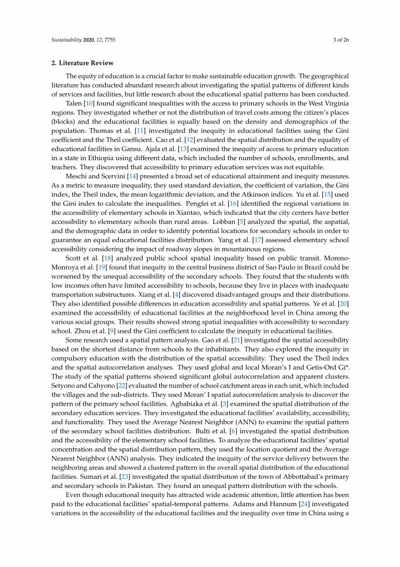
A subsequent analysis that was to investigate and show the overall distribution of the schools isthe optimized hot spot analysis. As previously mentioned, the calculations of this analysis are basedon the Getis Ord Gi* index and can be done in two ways. According to Figure 3, the result of the schoolcounting method per cell for the years 2011, 2016, 2018, and 2021 show the accumulation of hot spotsin the central areas of the city and cold spots in the suburbs of the town and Golestan township.
Sustainability 2020, 12, x FOR PEER REVIEW 12 of 29
In the case of the girls’ secondary schools, the overall distribution of the schools is random in the years 2016 and 2018. However, for the year 2011, the distribution of the schools is clustered. In the case of boys’ schools, the overall distributions of the primary schools, first high schools, and secondary high schools for years 2011, 2016, and 2018 are clustered.
A subsequent analysis that was to investigate and show the overall distribution of the schools is the optimized hot spot analysis. As previously mentioned, the calculations of this analysis are based on the Getis Ord Gi* index and can be done in two ways. According to Figure 3, the result of the school counting method per cell for the years 2011, 2016, 2018, and 2021 show the accumulation of hot spots in the central areas of the city and cold spots in the suburbs of the town and Golestan township.
(a) 2011 (b) 2016
(c) 2018 (d) 2021
Figure 3. Optimized hot spot analysis using the point count method inside each cell for the years 2011, 2016, 2018, and 2021.
By applying optimized hot spot analysis using the point count method within each polygon, which is the school counting method within each polygon, the autocorrelation of the schools at different levels, such as neighborhoods, statistical districts, and statistical blocks was investigated for
Figure 3. Optimized hot spot analysis using the point count method inside each cell for the years 2011,2016, 2018, and 2021.
By applying optimized hot spot analysis using the point count method within each polygon, whichis the school counting method within each polygon, the autocorrelation of the schools at different levels,such as neighborhoods, statistical districts, and statistical blocks was investigated for the year 2018.

Sustainability 2020, 12, 7755 13 of 26
The results indicate that the schools are generally more densely populated in the central areas of thecity, but it was found that the location of the hot and the cold polygons differed. At the neighborhoodlevel, the schools within the neighborhood of Ghiam, Nader, Amiriyeh, Berengy, Bargh, Enghelab,Vosogh, Daneshsara, Behzisti, Park Shahr, Madrese Ferdowsi, Sareban Mahale, Sfa, Mofkham, PadganArtesh, North 17 Shahrivar, Jafar Abad, Mirzakuchek khan, Manba Ab, Sayyidi, Hosseini Masoum,and Koi Imam Reza were more dense, and the density of schools was lower in the neighborhoodsof Malaksh, Halghe Sang, Shahrak Alghadir, Koi Janbazan, Ghale Aziz, and Ahmadabad. At thestatistical districts level, the density of the schools in the districts located in Ghiam, Hosseini Masoum,Sayyidi, Manba Ab, Mirzakuchekkhan, Bargh, Berengy, Amiriyeh, Nader, Padegan Artesh, Enghelab,Vosough, Daneshsara, Madrese Ferdowsi, Sarban Mahale, Safa, Mokhofam, and Sharak Golestanneighborhoods was higher, and in the statistical districts located in Bagh Motahari, Shahrak Hekmat,Imam Khomeini township, Koi Sadeghiyeh, Bagher khan 1, Koi Azadegan, and MohammadabadKorah, the school density was lower. However, at the level of statistical blocks, the density of theschools in the blocks located in the neighborhoods of Imam Reza, Koi Behdari, Ferdowsi, Mosalla,Nader, Amiriyeh, Berengy, Mirazkochekkhan, Manba Ab, Daneshsara, Park Shahr, Vosough, Enghelab,and Mokhofam was higher.
In the next step, the overall distribution of the schools at the spatial scales of neighborhoods,the statistical districts, and the statistical blocks was examined in different years. For the neighborhoodspatial units, by comparing 2011, 2016, 2018, and 2021, it was found that the density of the schoolswas higher in the downtown neighborhoods, and these neighborhoods play the role of hot polygons.Neighborhoods in parts of the south of the city were also identified as cold polygons in terms of theschool density.
At the level of statistical districts, the results indicate that the statistical districts in the downtownareas for the year 2011 are known as hot polygons in terms of the school density. The school densitywas also lower in the statistical districts of the western and the northeastern parts of the city. However,for the years 2016, 2018 and 2021, due to the addition of new schools in the Golestan Shahr township,the density of the schools in these areas has also increased, and the statistical district related to thistownship is also a hot polygon. Also, with the construction of the new schools on the outskirts of the city,the hot spots of the schools in the downtown area has been gradually reduced. However, the statisticaldistricts within the neighborhoods of Bagh Motahari, Zir Bagh Motahhari, Hekmat townships, ImamKhomeini townships, Koi Sadeghiyeh, Koi Azadegan, Bagherkhan 1, and Mohammadabad Korah arecold polygons.
At the level of the statistical blocks, the results indicate that the statistical blocks located in partsof the city center in the year 2018 are known as hot polygons in terms of the school density. However,for years 2011, 2016, and 2021, some of the statistical blocks related to Golestan city are also amongthe high-density polygons. For the year 2021, there are cold polygons in parts of the south of the city,which include fewer schools than the other blocks. The results of these analyses are shown in Figure 4.

Sustainability 2020, 12, 7755 14 of 26Sustainability 2020, 12, x FOR PEER REVIEW 14 of 27
Neighborhoods Spatial Scale Statistical Districts Spatial Scale Statistical Blocks Spatial Scale
(a) neighborhoods level in 2011 (b) statistical districts level in 2011 (c) statistical blocks level in 2011
(d) neighborhoods level in 2016 (e) statistical districts level in 2016 (f) statistical blocks level in 2016
(g) neighborhoods level in 2018 (h) statistical districts level in 2018 (i) statistical blocks level in 2018
(j) neighborhoods level in 2021 (k) statistical districts level in 2021 (l) statistical blocks level in 2021
Figure 4. Optimized hot spot analysis using the point count method within each polygon at three levels in the years of 2011, 2016, 2018, and 2021.
Figure 4. Optimized hot spot analysis using the point count method within each polygon at threelevels in the years of 2011, 2016, 2018, and 2021.
5.2. Implementation of Moran’s I and Getis Ord General G
In this section, in order to investigate the spatial autocorrelation based on the substructure variableand to determine the random or clustered distribution of the schools, Moran’s I and Getis Ord GeneralG indices were used. At first, Moran’s I statistic was used to check for the random or the clustereddistributions of the girls’ primary schools, first high schools, and secondary high schools. It can beconcluded that the overall distributions of the primary schools, first high schools, and the secondaryhigh schools for girls based on the substructure variable in the years 2011, 2016, and 2018 are random,which is due to the closeness of the value of Moran’s coefficient to zero.

Sustainability 2020, 12, 7755 15 of 26
Then, in order to confirm the results of the Moran’s I analysis, the analysis of the Getis Ord GeneralG statistic (which is in regard to the substructure variable) on the point layers of the girls’ primaryschools, first high schools, and secondary high schools was performed for the years 2011, 2016 and2018. According to Tables 5–7, the results show that the overall distributions of the girls’ primaryschools, first high schools, and secondary high schools based on the substructure variable for the years2011, 2016, and 2018 are random, because the z-score is close to zero.
Table 5. The results of the general autocorrelation indices on the girls’ primary schools.
Year Type of Index Index Value z-Score p-Value Pattern
2011Moran’s I −0.065147 −0.374999 0.707661 random
Getis Ord General G 0.000878 −0.600486 0.548182 random
2016Moran’s I −0.018868 0.219213 0.826484 random
Getis Ord General G 0.000774 −0.751317 0.452462 random
2018Moran’s I −0.064881 −0.602344 0.546945 random
Getis Ord General G 0.000452 −1.359548 0.173973 random
Table 6. The results of the general autocorrelation indices on the girls’ first high schools.
Year Type of Index Index Value z-Score p-Value Pattern
2011Moran’s I −0.215821 −1.514629 0.129866 random
Getis Ord General G 0.000686 0.475950 0.634110 random
2016Moran’s I −0.277216 −1.810088 0.070282 scattered
Getis Ord General G 0.000634 0.195381 0.845095 random
2018Moran’s I −0.100539 −0.881583 0.378002 random
Getis Ord General G 0.000893 0.715144 0.474520 random
Table 7. The results of the general autocorrelation indices on the girls’ secondary high schools.
Year Type of Index Index Value z-Score p-Value Pattern
2011Moran’s I −0.078740 −0.441434 0.658899 random
Getis Ord General G 0.000769 −0.963211 0.335442 random
2016Moran’s I −0.045698 −0.058518 0.953336 random
Getis Ord General G 0.000724 −1.179696 0.238121 random
2018Moran’s I −0.033485 −0.001246 0.999006 random
Getis Ord General G 0.000889 −0.515396 0.606276 random
The Moran’s I and Getis Ord General G analyses were conducted on the point data of the boys’primary schools, first high schools, and secondary high schools. The results are shown in Tables 8–10.For the boys’ primary schools, first high schools, and secondary high schools, because the coefficient ofMoran is close to zero for the years 2011, 2016, and 2018, the overall distribution of the boys’ primaryschools based on the substructure variable is random.
The result of the Getis Ord General G analysis on the boys’ primary schools confirms the Moran’sI analysis. This means that the Z-score is close to zero for the years 2011, 2016, and 2018, and theoverall distribution of the boys’ primary schools based on the substructure variable is random. For theboys’ first high schools in the years 2011 and 2018, the distribution of the schools is random, becausethe Z-Score is close to zero. However, for the year 2016, the distribution of schools is clustered witha low concentration or cold spots, because the Z-score is below −1.65. The distributions of the boys’secondary high schools for the years 2011, 2016, and 2018 are also random.

Sustainability 2020, 12, 7755 16 of 26
Table 8. The results of the general autocorrelation indices on the boys’ primary schools.
Year Type of Index Index Value z-Score p-Value Pattern
2011Moran’s I −0.035966 −0.029683 0.976320 random
Getis Ord General G 0.000720 −0.001754 0.998601 random
2016Moran’s I 0.035146 1.162811 0.244906 random
Getis Ord General G 0.000771 0.648049 0.516953 random
2018Moran’s I −0.012310 0.196646 0.844105 random
Getis Ord General G 0.000635 0.804286 0.421232 random
Table 9. The results of the general autocorrelation indices on the boys’ first high schools.
Year Type of Index Index Value z-Score p-Value Pattern
2011Moran’s I 0.447885 1.556101 0.119684 random
Getis Ord General G 0.000460 −1.152230 0.249226 random
2016Moran’s I 0.156625 1.628454 0.103429 random
Getis Ord General G 0.000731 −1.661791 0.096555 clustered (low value)
2018Moran’s I 0.036424 0.526880 0.598277 random
Getis Ord General G 0.000256 −1.215890 0.224027 random
Table 10. The results of the general autocorrelation indices on the boys’ secondary high schools.
Year Type of Index Index Value z-Score p-Value Pattern
2011Moran’s I 0.231860 0.335280 0.737414 random
Getis Ord General G 0.006103 0.727203 0.467102 random
2016Moran’s I 0.231503 0.334473 0.738023 random
Getis Ord General G 0.005579 0.718711 0.472319 random
2018Moran’s I 0.071220 0.139429 0.889111 random
Getis Ord General G 0.002806 0.353849 0.723452 random
To investigate the spatio-temporal variations of the distribution pattern of the schools basedon the net per capita variable, which includes the substructure area and the number of students,the differential Moran method was used. In the differential Moran analysis, which was performedusing Geoda 1.10 software, the weight matrix was defined based on the existence of the commonborder method (0 and 1) according to the Equation (12). Also, in order to achieve a higher accuracy,999 iterations were used for the simulation.
Wi j =
{1 i f i. j are adjacent neighbors
0 otherwise(12)
In this regard, using the calculations of the differential Moran index, the trend of the net per capitachanges for all primary schools, first high schools, and secondary high schools were evaluated in the2016–2017, 2017–2018, and 2016–2018 time intervals. The spatial-temporal autocorrelation results ofthe schools with respect to the net per capita variable are shown in the differential Moran scatter plotin Figure 5, which illustrates the pattern of the net per capita changes of the schools in the desiredtime intervals.

Sustainability 2020, 12, 7755 17 of 26Sustainability 2020, 12, x FOR PEER REVIEW 17 of 27
Net Per Capita in the 2016–2018 Net Per Capita in the 2016–2017 Net Per Capita in the 2017–2018 Pr
imar
y Sc
hool
s
(a) net per capita of primary schools in the 2016–2018
(b) net per capita of primary schools in the 2016–2017
(c) net per capita of primary schools in the 2017–2018
Firs
t Hig
h Sc
hool
s
(d) net per capita of first high schools in the 2016–2018
(e) net per capita of first high schools in the 2016–2017
(f) net per capita of first high schools in the 2017–2018
Seco
ndar
y H
igh
Scho
ols
(g) net per capita of secondary high schools in the 2016–2018
(h) net per capita of secondary high schools in the 2016–2017
(i) net per capita of secondary high schools in the 2017–2018
Figure 5. The differential Moran scatter plots for the net per capita changes of schools in the different time intervals of 2016–2018, 2016–2017, and 2017–2018.
The slope of the differential Moran scatter plot corresponds to the value of the Moran index. For
all primary schools and first high schools, since the value of the Moran index is positive and tends to zero, the resulting pattern is random, and there is a weak positive autocorrelation between the net per capita in the 2016–2017, 2017–2018, and 2016–2018 time intervals, which reflects the positive and slight changes in the net per capita of the schools over time. For all the secondary high schools, the values of the Moran index are negative and tend to zero in the 2016–2017 and 2017–2018 time intervals, so the autocorrelation is negative and weak. That means that the net per capita of the secondary high schools in the 2016–2017 and the 2017–2018 time intervals has not only increased but
Figure 5. The differential Moran scatter plots for the net per capita changes of schools in the differenttime intervals of 2016–2018, 2016–2017, and 2017–2018.
The slope of the differential Moran scatter plot corresponds to the value of the Moran index.For all primary schools and first high schools, since the value of the Moran index is positive and tendsto zero, the resulting pattern is random, and there is a weak positive autocorrelation between the netper capita in the 2016–2017, 2017–2018, and 2016–2018 time intervals, which reflects the positive andslight changes in the net per capita of the schools over time. For all the secondary high schools, thevalues of the Moran index are negative and tend to zero in the 2016–2017 and 2017–2018 time intervals,so the autocorrelation is negative and weak. That means that the net per capita of the secondary highschools in the 2016–2017 and the 2017–2018 time intervals has not only increased but has also shown arelative decline. However, due to the positive value of the Moran index, there is a weak and positiveautocorrelation between the net per capita in the year 2016 and the net per capita in the year 2018.
5.3. Implementation of Anselin Local Moran’s I and Getis Ord Gi*
After confirming that the data distribution is clustered, the local indices were used to determine thelocation of the clusters. By performing the general autocorrelation analyses, it was found that in mostcases the distribution pattern of the schools based on the substructure variable is random. However,

Sustainability 2020, 12, 7755 18 of 26
with respect to the values of the Moran, the Getis Ord indices, and the value of Z-Score, there is aweak spatial autocorrelation among the data. In this regard, to show this kind of autocorrelation,Anselin Local Moran’s I and Getis Ord Gi* analyses were used in this study.
Anselin Local Moran’s I analysis was first performed given the substructure variable for thegirls’ primary schools in 2011, 2016, and 2018. The results show that the substructure of the girls’primary schools in the southwest of the city in the year 2018 was above average (high-high areas),and it was below average in a region of the downtown area (low-low areas), which indicates thepresence of clusters in these areas. However, in another part of downtown, the high outliers that havea value higher than the neighbors were also found. In the year 2016, the high-high areas are seenin the southwestern part of the city. Furthermore, there are high outliers in another part of the citycenter. However, there are no clusters in the city for the year 2011, but there are high outliers in partof downtown.
Next, considering the substructure variable, a hot spot analysis was performed by calculating theGetis Ord Gi* index for the girls’ primary schools in 2011, 2016, and 2018. Then, in order to create acontinuous raster surface, the Inverse Distance Weighting (IDW) interpolation method was applied tothe results of the Getis Ord Gi* method. The results of applying this hybrid method are as follows.For the substructure variable, in the year 2018 in parts of downtown and south of the city in theneighborhoods of Koi Sadeghie, Shahed township, Koi Imam Hossein, Koi Behdari, Villashahr, andTasfiekhane, the distribution of the schools are clustered with high values, and in parts of the northeastof the city in the neighborhoods of Safa, Mokhofam, Madrese Ferdowsi, and North 17 Shahrivar,the distribution of the schools is low-cluster. In the year 2016, in a part of the city center in theneighborhood of Koi Imam Reza, the distribution of the schools is clustered with high values, and inthe Safa neighborhood, the distribution is clustered with low values. In the year 2011, in part of thedowntown in the Berengi neighborhood, the distribution of the clusters with low values is observed.
For the boys’ primary schools, considering the substructure variable, the Anselin Local Moran’s Ianalysis was also performed for the years 2011, 2016, and 2018. The result is that the substructures ofthe boys’ primary schools in 2011, 2016, and 2018 do not have clusters in the city. However, there arehigh outliers in part of the city center in 2011.
Next, the inverse distance weighting interpolation method was used on the results of the GetisOrd Gi* analysis for the boys’ primary schools in 2011, 2016, and 2018. The results of applying thishybrid approach were that for the substructure variable, which was in a small area east of the cityin the Taher Gholam neighborhood, the distribution of the schools is clustered with low values in2011 and 2016. For the year 2018 in the southeast of the city in the Mirzakuchakkhan neighborhood,the distribution of the schools is clustered with high values, and in the Koi Sadeghiyeh neighborhoodwest of the city, the distribution of the schools is clustered with low values. The results of applying theinverse distance weighting interpolation on the results of the Getis Ord Gi* analysis for the girls’ andthe boys’ primary schools are shown in Figure 6.

Sustainability 2020, 12, 7755 19 of 26
Sustainability 2020, 12, x FOR PEER REVIEW 21 of 29
the inverse distance weighting interpolation on the results of the Getis Ord Gi* analysis for the girls’ and the boys’ primary schools are shown in Figure 6.
(a) boys’ primary schools in 2011 (b) girls’ primary schools in 2011
(c) boys’ primary schools in 2016 (d) girls’ primary schools in 2016
(e) boys’ primary schools in 2018 (f) girls’ primary schools in 2018
Figure 6. Applying the inverse distance weighting interpolation on the results of Getis Ord Gi* for the primary schools in 2011, 2016, and 2018. Figure 6. Applying the inverse distance weighting interpolation on the results of Getis Ord Gi* for theprimary schools in 2011, 2016, and 2018.

Sustainability 2020, 12, 7755 20 of 26
Considering the substructure variable, the Anselin Local Moran’s I analysis for the girls’ firsthigh schools in 2011, 2016, and 2018 was also performed. The result indicates that the substructureof the girls’ first high schools does not have any cluster in the city. However, in 2011 and 2016,there are high outliers in a small southeast part of the city. Also, for the year 2018, high outliersare seen in the downtown area. The results of the Getis Ord Gi* analysis for the girls’ first highschools also do not indicate significant statistical significance of the substructure variable in 2011, 2016,and 2018. Subsequently, considering the substructure variable, the Anselin local Moran’s I analysiswas performed for the boys’ first high schools in 2011, 2016, and 2018. The result indicates that thesubstructure of the boys’ first high schools does not have any clusters in the city. However, in the year2018, there are high outliers and low outliers in the southern parts of the city.
Then, the inverse distance weighting interpolation method was applied to the results of the GetisOrd Gi* analysis for the boys’ first high schools in 2011, 2016, and 2018. The results of applying thishybrid method for the substructure variable in the years 2016 and 2018 have no statistical significance inthe city. However, in 2011, the distribution of the schools in part of downtown in the Madrese Ferdowsineighborhood is clustered with high values, and in the Mirzakuchakkhan and Bargh neighborhoods,the distribution is clustered with low values. Due to the lack of significant statistical significance forthe girls’ and the boys’ first high schools, the results of applying the local indexes to these schools havebeen ignored.
For the girls’ secondary high schools, considering the substructure variable, the Anselin LocalMoran’s I was performed in the years 2011, 2016, and 2018. However, in parts of the downtown andthe southern areas of the city in 2011, and in a small part of the city center, high outliers are seen. Also,for the year 2018, there are low outliers in a part of downtown.
The inverse distance weighting interpolation method was applied to the results of the GetisOrd Gi* analysis for the girls’ secondary high schools in the years 2011, 2016, and 2018. The resultsof applying this hybrid approach for the substructure variable are that for the years 2011 and 2016,the distribution of the schools in the southern part of the city in the Alghadir township neighborhood isclustered with high values, and in the northeast of the city in the Jafarabad neighborhood, distributionof schools is clustered with low values. Cold spots are also observed in the 17 Shahrivar and Safaneighborhoods in the year 2016. In the southern part of the city in a neighborhood in the AlghadirTownship, the distribution of the schools is clustered with high values, and in the eastern part of thecity in the Jafar Abad neighborhood, the distribution is clustered with low values in the year 2018.
For the boys’ secondary high schools in 2011, 2016, and 2018, considering the substructure variable,the Anselin Local Moran’s I analysis was also performed. The result is that the substructure of theboys’ secondary high schools in the west and southwest parts of the city is above average (high-highareas) in 2011 and 2016 and indicates the presence of clusters in these areas. However, there are alsohigh outliers in some parts of downtown. There are no clusters in the city for the year 2018, but thereare high outliers in parts of downtown and low outliers in the west part of town.
The results of applying the inverse distance weighting interpolation method on the results of GetisOrd Gi* analysis for the boys’ secondary high schools for the substructure variable for 2011 and 2016years reveal that the distribution of schools in the west and the southwestern parts of the city in theVilashahr and Polemantaghe neighborhoods is clustered with high values. Also, in the central districts inthe North 17 Shahrivar, Mofkham, Safa, Daneshsara, Bargh, Berengi, and Amiriyeh neighborhoods areclustered with low values. In the southwest of the city in the Farrokhi and Polemantaghe neighborhoods,the distribution of schools is clustered with high values, and in the center and northeast of the city in theNorth 17 Shahrivar, Safa, Sareban Mahale, Berengi, and Koi Moallem neighborhoods, the distributionis clustered with low values. The results of the inverse distance weighting interpolation on the resultsof the Getis Ord Gi* analysis for the girls’ and the boys’ secondary high schools are shown in Figure 7.

Sustainability 2020, 12, 7755 21 of 26
Sustainability 2020, 12, x FOR PEER REVIEW 21 of 26
(a) boys’ secondary high schools in 2011 (b) girls’ secondary high schools in 2011
(c) boys’ secondary high schools in 2016 (d) girls’ secondary high schools in 2016
(e) boys’ secondary high schools in 2018 (f) girls’ secondary high schools in 2018
Figure 7. Applying inverse distance weighting interpolation on the Results of the Getis Ord Gi* for the secondary high schools in 2011, 2016, and 2018.
Figure 7. Applying inverse distance weighting interpolation on the Results of the Getis Ord Gi* for thesecondary high schools in 2011, 2016, and 2018.

Sustainability 2020, 12, 7755 22 of 26
6. Discussion
Spatial distribution of the schools in the city plays a big role in educational equity. Therefore, foreducational equity, the spatial distribution of the schools should be evaluated. In addition, one of themost important issues in the field of educational spatial justice is evaluating the results of differentscenarios and the policies in this field at different times. In this regard, this study examined thespatial-temporal distribution of education facilities. To fulfill the purpose of this research, two types ofanalyses were used. The first type of analysis investigated the general pattern of the spatial-temporaldistribution of the schools without specific parameters. For the first type of analysis, the AverageNearest Neighbor and optimized hot spot analysis methods were used. However, the second typeof analysis was based on certain parameters, which included the substructure and the net per capita.Using the Moran’s I and the Getis Ord General G analyses, the distribution pattern of the schools basedon the substructure variable was studied. The differential Moran method was also used to investigatethe spatiotemporal variations of the distribution pattern of the schools based on the net per capitavariables in the 2016–2017, 2017–2018, and 2016–2018 time intervals.
The results of the Average Nearest Neighbor analysis indicate that the overall distribution ofthe primary, first, and the secondary high schools is clustered in the years 2011, 2016, 2018, and 2021.The Average Nearest Neighbor analysis was also performed separately for the girls’ and the boys’schools. The result is that the type of overall distribution of the boys’ primary, first, and secondaryhigh schools are clustered in 2011, 2016, and 2018. Regarding the girls’ schools, the distribution patternof the primary and the secondary high schools is clustered for the years 2011, 2016, and 2018. A clusterpattern was also obtained for the girls’ first high schools in the year 2011, but in the years 2016 and2018, the distribution of the schools is random.
The optimized hot spot analysis was also used to show the overall distribution of the schools andthe location of the clusters. Applying the method of counting point events within each cell indicatedthe accumulation of hot spots in the central areas of the city and cold spots on the outskirts of thecity and the Golestan township. Using the method of counting point events within each polygon,the overall distributions of the schools in different levels, such as neighborhoods, statistical districts,and statistical blocks were evaluated and compared. This overview shows the high density of theschools in the central areas of the city, but the difference between the location of the hot and the coldpolygons can be detected in different spatial units. The distribution patterns of the schools at the spatialscales of neighborhoods, statistical districts, and statistical blocks were studied for the 2011, 2016,2018, and 2021 years. The density of the schools in the city center is higher for all three spatial unitsof neighborhoods, statistical districts, and statistical blocks. At the statistical district level, with theaddition of new schools in the Golestan township, the density of the schools in this area has increasedfor the years 2016, 2018, and 2021. Also, with the construction of new schools on the outskirts ofthe city, the density of the schools in the downtown area has gradually decreased. At the level ofstatistical blocks for years 2011, 2016, and 2021, in addition to the city center, some of the statisticalblocks related to the Golestan township are also high-density polygons. In general, it can be saidthat with the construction of new schools in the years 2018 and 2021, hot spots of the schools in thedowntown area has been reduced, but the density of schools in other parts of the city has increased.However, the southern area and the suburbs of the city are known as cold polygons with lower densityand require more organization and management.
In most of the Moran and Getis Ord analyses performed in this study, considering the substructurevariable, the distribution pattern of the schools is random. This indicates that the schools with a highersubstructure value did not focus on specific areas, and the substructure of the schools is affected byother factors, such as population density, number of classes, and a number of students that havenot been addressed in this study. Based on the results of the local spatial autocorrelation indices forthe girls’ primary schools, the clusters are located in the downtown and southern areas of the city.For the boys’ primary schools, the clusters are located in the east and southeast part of the city. For thesecondary girls’ secondary high schools, the clusters are located in the southern part of the city. For the
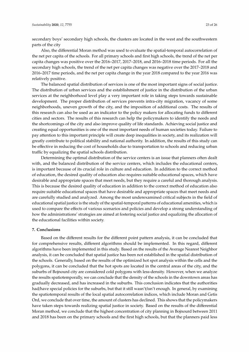
Sustainability 2020, 12, 7755 23 of 26
secondary boys’ secondary high schools, the clusters are located in the west and the southwesternparts of the city
Also, the differential Moran method was used to evaluate the spatial-temporal autocorrelation ofthe net per capita of the schools. For all primary schools and first high schools, the trend of the net percapita changes was positive over the 2016–2017, 2017–2018, and 2016–2018 time periods. For all thesecondary high schools, the trend of the net per capita changes was negative over the 2017–2018 and2016–2017 time periods, and the net per capita change in the year 2018 compared to the year 2016 wasrelatively positive.
The balanced spatial distribution of services is one of the most important signs of social justice.The distribution of urban services and the establishment of justice in the distribution of the urbanservices at the neighborhood level play a very important role in taking steps towards sustainabledevelopment. The proper distribution of services prevents intra-city migration, vacancy of someneighborhoods, uneven growth of the city, and the imposition of additional costs. The results ofthis research can also be used as an indicator to the policy makers for allocating funds to differentcities and sectors. The results of this research can help the policymakers to identify the needs andthe shortcomings of the city and also improve quality of life standards. Achieving social justice andcreating equal opportunities is one of the most important needs of human societies today. Failure topay attention to this important principle will create deep inequalities in society, and its realization willgreatly contribute to political stability and national authority. In addition, the results of this study canbe effective in reducing the cost of households due to transportation to schools and reducing urbantraffic by equalizing the spatial schools distribution.
Determining the optimal distribution of the service centers is an issue that planners often dealtwith, and the balanced distribution of the service centers, which includes the educational centers,is important because of its crucial role in culture and education. In addition to the correct methodof education, the desired quality of education also requires suitable educational spaces, which havedesirable and appropriate spaces that meet needs, but they require a careful and thorough analysis.This is because the desired quality of education in addition to the correct method of education alsorequire suitable educational spaces that have desirable and appropriate spaces that meet needs andare carefully studied and analyzed. Among the most underexamined critical subjects in the field ofeducational spatial justice is the study of the spatial-temporal patterns of educational amenities, which isused to compare the effects of various scenarios and policies and develop a strong understanding ofhow the administrations’ strategies are aimed at fostering social justice and equalizing the allocation ofthe educational facilities within society.
7. Conclusions
Based on the different results for the different point pattern analysis, it can be concluded thatfor comprehensive results, different algorithms should be implemented. In this regard, differentalgorithms have been implemented in this study. Based on the results of the Average Nearest Neighboranalysis, it can be concluded that spatial justice has been not established in the spatial distribution ofthe schools. Generally, based on the results of the optimized hot spot analysis within the cells and thepolygons, it can be concluded that the hot spots are located in the central areas of the city, and thesuburbs of Bojnourd city are considered cold polygons with less-density. However, when we analyzethe results spatiotemporally, we can conclude that the density of the schools in the downtown areas hasgradually decreased, and has increased in the suburbs. This conclusion indicates that the authoritieshad/have special policies for the suburbs, but that it still wasn’t/isn’t enough. In general, by examiningthe spatiotemporal results of the local spatial autocorrelation índices, which include Moran and GetisOrd, we conclude that over time, the amount of clusters has declined. This shows that the policymakershave taken steps towards realizing spatial justice in society. Based on the results of the differentialMoran method, we conclude that the highest concentration of city planning in Bojnourd between 2011and 2018 has been on the primary schools and the first high schools, but that the planners paid less
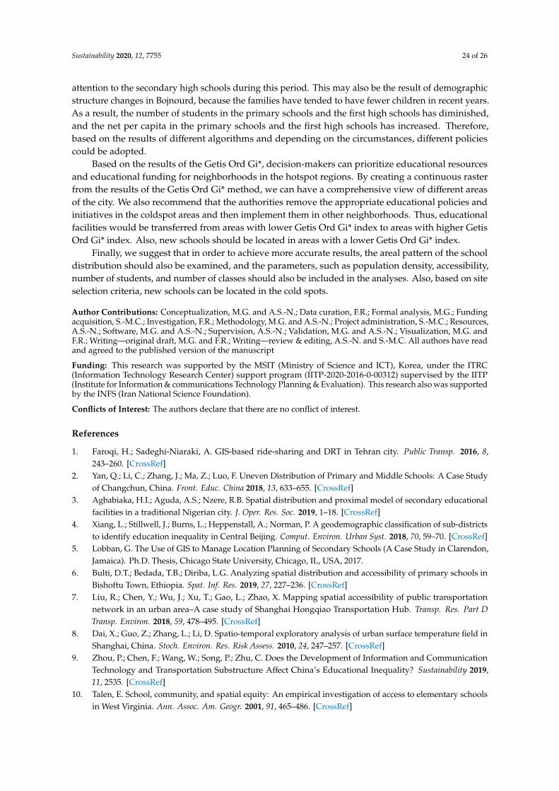
Sustainability 2020, 12, 7755 24 of 26
attention to the secondary high schools during this period. This may also be the result of demographicstructure changes in Bojnourd, because the families have tended to have fewer children in recent years.As a result, the number of students in the primary schools and the first high schools has diminished,and the net per capita in the primary schools and the first high schools has increased. Therefore,based on the results of different algorithms and depending on the circumstances, different policiescould be adopted.
Based on the results of the Getis Ord Gi*, decision-makers can prioritize educational resourcesand educational funding for neighborhoods in the hotspot regions. By creating a continuous rasterfrom the results of the Getis Ord Gi* method, we can have a comprehensive view of different areasof the city. We also recommend that the authorities remove the appropriate educational policies andinitiatives in the coldspot areas and then implement them in other neighborhoods. Thus, educationalfacilities would be transferred from areas with lower Getis Ord Gi* index to areas with higher GetisOrd Gi* index. Also, new schools should be located in areas with a lower Getis Ord Gi* index.
Finally, we suggest that in order to achieve more accurate results, the areal pattern of the schooldistribution should also be examined, and the parameters, such as population density, accessibility,number of students, and number of classes should also be included in the analyses. Also, based on siteselection criteria, new schools can be located in the cold spots.
Author Contributions: Conceptualization, M.G. and A.S.-N.; Data curation, F.R.; Formal analysis, M.G.; Fundingacquisition, S.-M.C.; Investigation, F.R.; Methodology, M.G. and A.S.-N.; Project administration, S.-M.C.; Resources,A.S.-N.; Software, M.G. and A.S.-N.; Supervision, A.S.-N.; Validation, M.G. and A.S.-N.; Visualization, M.G. andF.R.; Writing—original draft, M.G. and F.R.; Writing—review & editing, A.S.-N. and S.-M.C. All authors have readand agreed to the published version of the manuscript
Funding: This research was supported by the MSIT (Ministry of Science and ICT), Korea, under the ITRC(Information Technology Research Center) support program (IITP-2020-2016-0-00312) supervised by the IITP(Institute for Information & communications Technology Planning & Evaluation). This research also was supportedby the INFS (Iran National Science Foundation).
Conflicts of Interest: The authors declare that there are no conflict of interest.
References
1. Faroqi, H.; Sadeghi-Niaraki, A. GIS-based ride-sharing and DRT in Tehran city. Public Transp. 2016, 8,243–260. [CrossRef]
2. Yan, Q.; Li, C.; Zhang, J.; Ma, Z.; Luo, F. Uneven Distribution of Primary and Middle Schools: A Case Studyof Changchun, China. Front. Educ. China 2018, 13, 633–655. [CrossRef]
3. Agbabiaka, H.I.; Aguda, A.S.; Nzere, R.B. Spatial distribution and proximal model of secondary educationalfacilities in a traditional Nigerian city. J. Oper. Res. Soc. 2019, 1–18. [CrossRef]
4. Xiang, L.; Stillwell, J.; Burns, L.; Heppenstall, A.; Norman, P. A geodemographic classification of sub-districtsto identify education inequality in Central Beijing. Comput. Environ. Urban Syst. 2018, 70, 59–70. [CrossRef]
5. Lobban, G. The Use of GIS to Manage Location Planning of Secondary Schools (A Case Study in Clarendon,Jamaica). Ph.D. Thesis, Chicago State University, Chicago, IL, USA, 2017.
6. Bulti, D.T.; Bedada, T.B.; Diriba, L.G. Analyzing spatial distribution and accessibility of primary schools inBishoftu Town, Ethiopia. Spat. Inf. Res. 2019, 27, 227–236. [CrossRef]
7. Liu, R.; Chen, Y.; Wu, J.; Xu, T.; Gao, L.; Zhao, X. Mapping spatial accessibility of public transportationnetwork in an urban area–A case study of Shanghai Hongqiao Transportation Hub. Transp. Res. Part DTransp. Environ. 2018, 59, 478–495. [CrossRef]
8. Dai, X.; Guo, Z.; Zhang, L.; Li, D. Spatio-temporal exploratory analysis of urban surface temperature field inShanghai, China. Stoch. Environ. Res. Risk Assess. 2010, 24, 247–257. [CrossRef]
9. Zhou, P.; Chen, F.; Wang, W.; Song, P.; Zhu, C. Does the Development of Information and CommunicationTechnology and Transportation Substructure Affect China’s Educational Inequality? Sustainability 2019,11, 2535. [CrossRef]
10. Talen, E. School, community, and spatial equity: An empirical investigation of access to elementary schoolsin West Virginia. Ann. Assoc. Am. Geogr. 2001, 91, 465–486. [CrossRef]

Sustainability 2020, 12, 7755 25 of 26
11. Thomas, V.; Wang, Y.; Fan, X. A New Dataset on Inequality in Education: Gini and Theil Indices of Schooling for140 Countries, 1960–2000; World Bank: Washington, DC, USA, 2002.
12. Cao, H. Spatial inequality in children’s schooling in Gansu, Western China: Reality and challenges. Can. Geogr.Géogr. Can. 2008, 52, 331–350. [CrossRef]
13. Ajala, O.A.; Asres, K. Accessibility In equality to Basic Education in Amhara Region, Ethiopia. Ethiop. J.Educ. Sci. 2008, 3, 11–26. [CrossRef]
14. Meschi, E.; Scervini, F. A new dataset on educational inequality. Empir. Econ. 2014, 47, 695–716. [CrossRef]15. Yu, N.; Yu, B.; de Jong, M.; Storm, S. Does inequality in educational attainment matter for China’s economic
growth? Int. J. Educ. Dev. 2015, 41, 164–173. [CrossRef]16. Pengfei, T.A.N.G.; Jingjing, X.I.A.N.G.; Jing, L.U.O.; Guolei, C.H.E.N. Spatial accessibility analysis of
primary schools at the county level based on the improved potential model: A case study of Xiantao City,Hubei Province. Prog. Geogr. 2014, 36, 697–708.
17. Yang, P.F.; He, R.; Hou, H.B. Distribution of primary school based on spatial network comprehensive model inlow-income mountainous cities: A case study in Wanyuan, China. J. Mt. Sci. 2017, 14, 2082–2096. [CrossRef]
18. Scott, M.R.; Marshall, D.T. Public Transit and School Choice in Philadelphia: Exploring Spatial Equity andSocial Exclusion. J. Sch. Choice. 2018, 13, 177–197. [CrossRef]
19. Moreno-Monroy, A.I.; Lovelace, R.; Ramos, F.R. Public transport and school location impacts on educationalinequalities: Insights from São Paulo. J. Transp. Geogr. 2018, 67, 110–118. [CrossRef]
20. Ye, C.; Hu, L.; Li, M. Urban green space accessibility changes in a high-density city: A case study of Macaufrom 2010 to 2015. J. Transp. Geogr. 2018, 66, 106–115. [CrossRef]
21. Gao, Y.; He, Q.; Liu, Y.; Zhang, L.; Wang, H.; Cai, E. Imbalance in spatial accessibility to primary andsecondary schools in china: Guidance for education sustainability. Sustainability 2016, 8, 1236. [CrossRef]
22. Setyono, D.A.; Cahyono, D.D. Spatial Analysis of Educational Facilities Services Pattern in Malang peripheralAreas. In IOP Conference Series: Earth and Environmental Science; IOP Publishing: Bristol, UK, 2018; p. 012038.
23. Sumari, N.S.; Tanveer, H.; Shaoa, Z.; Kira, E.S. Geospatial Distribution and Accessibility of Primary andSecondary Schools: A case of Abbottabad City, Pakistan. Proc. ICA 2019, 2, 1–11. [CrossRef]
24. Adams, J.; Hannum, E. Children’s social welfare in China, 1989–1997: Access to health insurance andeducation. China Q. 2005, 181, 100–121. [CrossRef]
25. Williams, S.; Wang, F. Disparities in accessibility of public high schools, in metropolitan Baton Rouge,Louisiana 1990–2010. Urban Geogr. 2014, 35, 1066–1083. [CrossRef]
26. Yang, J.; Huang, X.; Liu, X. An analysis of education inequality in China. Int. J. Educ. Dev. 2014, 37, 2–10.[CrossRef]
27. Wan, J.; Liu, Y.; Chen, Y.; Hu, J.; Wang, Z. A Tale of North and South: Balanced and Sustainable Developmentof Primary Education in Ningxia, China. Sustainability 2018, 10, 559. [CrossRef]
28. Xu, Y.; Song, W.; Liu, C. Social-Spatial accessibility to urban educational resources under the school districtsystem: A Case Study of Public Primary Schools in Nanjing, China. Sustainability 2018, 10, 2305. [CrossRef]
29. Xing, L.; Liu, Y.; Liu, X.; Wei, X.; Mao, Y. Spatio-temporal disparity between demand and supply of parkgreen space service in urban area of Wuhan from 2000 to 2014. Habitat Int. 2018, 71, 49–59. [CrossRef]
30. Page, N.; Langford, M.; Higgs, G. Exploring spatiotemporal variations in public library provision followinga prolonged period of economic austerity: A GIS approach. Area 2019, 52, 342–353. [CrossRef]
31. Aziz, S.; Ngui, R.; Lim, Y.A.L.; Sholehah, I.; Nur Farhana, J.; Azizan, A.S.; Wan Yusoff, W.S. Spatial pattern of2009 dengue distribution in Kuala Lumpur using GIS application. Trop Biomed. 2012, 29, 113–120.
32. Esri. How Optimized Hot Spot Analysis Works. Available online: https://pro.arcgis.com/en/pro-app/tool-reference/spatial-statistics/how-optimized-hot-spot-analysis-works.htm (accessed on 24 March 2020).
33. Gorr, W.L.; Kurland, K.S. GIS Tutorial for Crime Analysis; Esri Press: Redlands, CA, USA, 2012. Availableonline: https://esripress.esri.com/storage/esripress/bookresources/gistcrime/gistcrime_suppliement10.2.pdf(accessed on 24 April 2020).
34. Ord, J.K.; Getis, A. Local Spatial Autocorrelation Statistics: Distributional Issues and an Application.Geogr. Anal. 1995, 27, 286–306. [CrossRef]
35. Getis, A.; Ord, J.K. The analysis of spatial association by use of distance statistics. In Perspectives on SpatialData Analysis; Springer: Berlin/Heidelberg, Germany, 2010; pp. 127–145.

Sustainability 2020, 12, 7755 26 of 26
36. Anselin, L. Moran Scatter Plot and Spatial Correlogram, Geodacenter. 2018. Available online: https://geodacenter.github.io/workbook/5a_global_auto/lab5a.html (accessed on 4 March 2018).
37. Khosravi, Y.; Bahri, A. Use of spatial statistics techniques in order to spatio-temporal variations of chlorophylla concentration in the Persian Gulf. J. Mar. Biol. 2018, 10, 33–46.
© 2020 by the authors. Licensee MDPI, Basel, Switzerland. This article is an open accessarticle distributed under the terms and conditions of the Creative Commons Attribution(CC BY) license (http://creativecommons.org/licenses/by/4.0/).
Related Documents