Spatial Statistics in Crime Analysis - IACA Home Statistics in Crime Analysis: Using CrimeStat III This book was written by Christopher W. Bruce and Susan C. Smith for police crime

Edition 2.1 October 2011

Spatial Statistics in Crime Analysis:

Using CrimeStat III®

Christopher W. Bruce Susan C. Smith

Spatial Statistics in Crime Analysis Using CrimeStat III®

Edition 2.1

October 2011

Christopher W. Bruce Susan C. Smith

CrimeStat® CrimeStat is a spatial statistics program for the analysis of crime incident locations, developed by Ned Levine & Associates under the direction of Ned Levine, PhD, that was funded by grants from the National Institute of Justice (grants 1997-IJ-CX-0040, 1999-IJ-CX-0044, 2002-IJ-CX-0007, and 2005-IJ-CX-K037). The program is Windows-based and interfaces with most desktop GIS programs. The purpose is to provide supplemental statistical tools to aid law enforcement agencies and criminal justice researchers in their crime mapping efforts. CrimeStat is being used by many police departments around the country as well as by criminal justice and other researchers. The latest version is 3.3. Contact information: Dr. Ned Levine ● Ned Levine & Associates ● Houston, TX [email protected] http://www.icpsr.umich.edu/CrimeStat Spatial Statistics in Crime Analysis: Using CrimeStat III This book was written by Christopher W. Bruce and Susan C. Smith for police crime analysts seeking to use CrimeStat for tactical, strategic, and administrative crime analysis. It was funded by National Institute of Justice grant 2007-IJ-CX-K014. The latest version of the book will be maintained at the web address below. Contact information: Christopher W. Bruce ● Kensington, NH [email protected] http://www.ojp.usdoj.gov/nij/maps/tools.htm#crimestat

Acknowledgements For the completion of this workbook, the authors are grateful to Ned Levine, for answering our many conceptual questions; Police Chief Thomas Casady for unhesitatingly supplying the sample data; and Glendale (AZ) crime analyst Bryan Hill for sharing his knowledge and experience with CrimeStat in daily crime analysis. We are also grateful to the many students who have attended our CrimeStat classes over the last few years, adding their experiences and perspectives with spatial statistics.

1

Table of Contents 1 Introduction .......................................................................... 3 Spatial Statistics in Crime Analysis ...................................................................... 5 CrimeStat III ......................................................................................................... 8 A Note on CrimeStat Analyst ................................................................................ 9 Hardware and Software ...................................................................................... 14 Notes on This Workbook .................................................................................... 14 Summary and Further Reading .......................................................................... 16 2 Working with Data ............................................................... 17 Primary File Setup .............................................................................................. 19 Reference Files .................................................................................................... 22 Measurement Parameters ................................................................................... 23 Exporting Data from CrimeStat ......................................................................... 26 Summary and Further Reading ..........................................................................28 3 Spatial Distribution ............................................................. 29 Central Tendency and Dispersion ...................................................................... 31 Using Spatial Distribution for Tactics and Strategies........................................ 35 Summary and Further Reading .......................................................................... 38 4 Autocorrelation and Distance Analysis ................................ 39 Spatial Autocorrelation ...................................................................................... 40 Nearest Neighbor Analysis ................................................................................. 47 Assigning Primary Points to Secondary Points .................................................. 50 Summary and Further Reading .......................................................................... 55 5 Hot Spot Analysis ................................................................. 57 Mode and Fuzzy Mode ........................................................................................ 59 Nearest Neighbor Hierarchical Spatial Clustering (NNH) ................................ 64 Risk-Adjusted NNH ............................................................................................ 70 Spatial and Temporal Analysis of Crime (STAC) ............................................... 73 K-means Clustering ............................................................................................ 76 Summary of Hot Spot Methods .......................................................................... 79 For Further Reading ........................................................................................... 81 6 Kernel Density Estimation .................................................. 83 The Mechanics of KDE ........................................................................... 84 KDE Parameters ..................................................................................... 87

2

Dual Kernel Density Estimation ............................................................. 95 Summary and Further Reading ............................................................ 100 7 STMA and Correlated Walk ................................................ 101 Time in CrimeStat .................................................................................. 102 Spatial-Temporal Moving Average ........................................................ 103 Correlated Walk Analysis ...................................................................... 106 Summary and Further Reading ............................................................. 115 8 Journey to Crime ................................................................ 117 Calibrating a File ................................................................................... 119 The Journey to Crime Estimation ......................................................... 124 Using a Mathematical Formula ............................................................. 125 Summary and Further Reading ............................................................. 127 9 Conclusions ....................................................................... 129 Glossary .............................................................................. 131 About the Authors .............................................................. 147

3

1

Introduction Spatial Statistics, Crime Analysis, and CrimeStat III

The profession of crime analysis1 traces its history to 1963, when Chicago Police Superintendent O. W. Wilson published his second edition of Police Administration and named “crime analysis” as an ideal section to have within a planning division. The origins of the profession, however, lie nearly half a century earlier, with Wilson’s mentor, Berkeley (California) Police chief August Vollmer (1876-1955). Vollmer has long borne the nickname “the father of American policing” because of his work in patrol, records management, radio communication, scientific investigations, professionalism, and crime analysis. In one of his papers, he notes:

On the assumption of regularity of crime and similar occurrences, it is possible to tabulate these occurrences by areas within a city and thus determine the points which have the greatest danger of such crimes and what points have the least danger2.

Vollmer was talking about “hot spots,” although the term did not yet exist in policing. Over the next 80 years, police administrators and then full-time crime analysts would tabulate such hot spots with colored dots and pushpins stuck on paper maps—a process that did not change until the desktop computing revolution brought computer mapping programs to the world’s police agencies in the 1990s.

Figure 1-1: A 1980s crime map in the Cambridge, Massachusetts Police Department, made with stickers on paper. 1 Bolded entries appear in the glossary. Terms are bolded the first time they appear in each chapter. 2 Quoted in Reinier, G. H., Greenlee, M. R., Gibbens, M. H., & Marshall, S. P. (1977). Crime Analysis in Support of Patrol. Washington, DC: National Institute of Law Enforcement and Criminal Justice, p. 9.

4

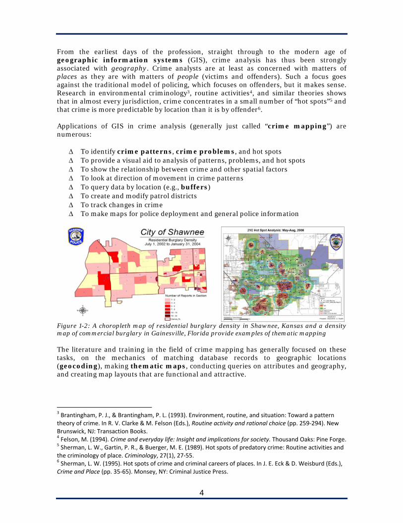
From the earliest days of the profession, straight through to the modern age of geographic information systems (GIS), crime analysis has thus been strongly associated with geography. Crime analysts are at least as concerned with matters of places as they are with matters of people (victims and offenders). Such a focus goes against the traditional model of policing, which focuses on offenders, but it makes sense. Research in environmental criminology3, routine activities4, and similar theories shows that in almost every jurisdiction, crime concentrates in a small number of “hot spots”5 and that crime is more predictable by location than it is by offender6. Applications of GIS in crime analysis (generally just called “crime mapping”) are numerous:

To identify crime patterns, crime problems, and hot spots To provide a visual aid to analysis of patterns, problems, and hot spots To show the relationship between crime and other spatial factors To look at direction of movement in crime patterns To query data by location (e.g., buffers) To create and modify patrol districts To track changes in crime To make maps for police deployment and general police information

Figure 1-2: A choropleth map of residential burglary density in Shawnee, Kansas and a density map of commercial burglary in Gainesville, Florida provide examples of thematic mapping The literature and training in the field of crime mapping has generally focused on these tasks, on the mechanics of matching database records to geographic locations (geocoding), making thematic maps, conducting queries on attributes and geography, and creating map layouts that are functional and attractive.

3 Brantingham, P. J., & Brantingham, P. L. (1993). Environment, routine, and situation: Toward a pattern theory of crime. In R. V. Clarke & M. Felson (Eds.), Routine activity and rational choice (pp. 259‐294). New Brunswick, NJ: Transaction Books. 4 Felson, M. (1994). Crime and everyday life: Insight and implications for society. Thousand Oaks: Pine Forge. 5 Sherman, L. W., Gartin, P. R., & Buerger, M. E. (1989). Hot spots of predatory crime: Routine activities and the criminology of place. Criminology, 27(1), 27‐55. 6 Sherman, L. W. (1995). Hot spots of crime and criminal careers of places. In J. E. Eck & D. Weisburd (Eds.), Crime and Place (pp. 35‐65). Monsey, NY: Criminal Justice Press.

5

However, actually producing a map—even a well-designed thematic map—is only the first step in the crime analysis process. The analyst must then analyze the mapped data to answer whatever questions he or she is employing crime mapping to answer: Is there a pattern? What is the nature of the pattern? What are its dimensions? Where are the hot spots for this type of crime? What things might be influencing those hot spots? Where might a serial offender strike next? For most analysts, the predominant paradigm to answer these questions has been visual interpretation: simply looking at the map and using common sense, judgment, and knowledge of the jurisdiction and its crime. With many crime analysis tasks, visual interpretation works adequately. It can usually identify the spatial concentration of a pattern, it allows the analyst to recognize the most serious hot spots, and it provides enough information to generate reasonable answers to common questions involving geography and space.

Figure 1-3: Nothing but visual interpretation was required to identify the pattern and likely offender in this brief residential burglary series (left), but visual interpretation entirely fails in identifying hot spots out of thousands of data points (right). But there are times in which visual interpretation does not do the job. It cannot easily pick out hot spots among thousands of data points. It cannot detect subtle shifts in the geography of a pattern over time. It cannot calculate correlations between two or more geographic variables. It cannot analyze travel times among complex road networks. And it cannot apply complicated journey-to-crime calculations across tens of thousands of grid cells. For these things, and more, we need spatial statistics. This is where CrimeStat comes in.

Spatial Statistics in Crime Analysis To be a crime analyst in the 21st century, you must be skilled in crime mapping, and you must be skilled in statistics. Consequently, spatial statistics—which combines the two subjects—should come naturally to most analysts. Spatial statistics are much like regular statistics in that they can be descriptive, inferential, and multivariate. Where data elements for regular crime analysis statistics might include date, time, dollar value of property, age of offender, number of crimes in a time period, or days between offenses, spatial statistics use data of spatial interest, including:

6

Geographic coordinates

Distance between points

Angles of movement (bearing)

Volume of data at certain locations (or within certain grid cells)

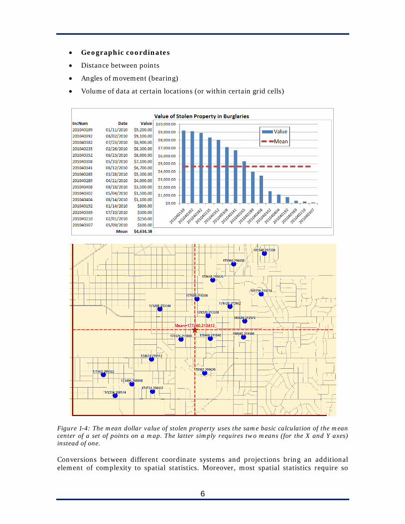
Figure 1-4: The mean dollar value of stolen property uses the same basic calculation of the mean center of a set of points on a map. The latter simply requires two means (for the X and Y axes) instead of one. Conversions between different coordinate systems and projections bring an additional element of complexity to spatial statistics. Moreover, most spatial statistics require so

7

many inputs that to perform them without a computer program is functionally impossible (hand-calculating kernel density values for tens of thousands of grid cells would be an exercise in futility). But in concept, they share the same characteristics as normal statistical methods. Thus, to the extent that regular descriptive, inferential, and multivariate statistics are useful for different types of crime analysis, so are spatial statistics. Table 1-1 summarizes some of the more common uses of spatial statistics in different types of crime analysis. Type of Analysis Definition Uses of Spatial Statistics Tactical Analysis Identification and analysis of crime

patterns and crime series for the purpose of tactical intervention by patrol or investigations.

Identification of clustering or area of concentration

Identification of movement trends within the pattern

Prediction of future events in space and time Estimate of most likely location of offender

residence or “home base” Strategic Analysis Identification and analysis of

trends in crime for purposes of long-term planning and strategy development.

Spatial distributions of various types of crime Identification of hot spots and changes in hot

spots over time Risk assessments of jurisdiction based on

locations of known crime Comparison of demographic and

environmental factors to crime hot spots Problem Analysis Analysis of long-term or chronic

problems for the development of crime prevention strategies; assessment of those strategies

Identification of hot spots and changes in hot spots over time

Comparison of demographic and environmental factors to crime hot spots

Assessment of displacement and diffusion after strategies are implemented

Administrative Analysis

Provision of statistics, maps, graphics, and data for administrative purposes within a police agency

Provision of specific figures, index values, and correlation values to researchers and program funders

Operations Analysis

Analysis to support the optimal allocation of personnel and resources by time, geography, and department function

Configuration of patrol boundaries based on crime and call-for-service volume, demographic factors, and environmental factors

Identification of optimal police station (or sub-station) points

Calculation of response time estimates to and from various points

Investigative Analysis

Identification of likely characteristics of an offender based on evidence and data collected from crime scenes

Estimate of most likely location of offender residence or “home base” based on crime locations

Intelligence Analysis

Analysis of data (often collected covertly) about criminal organizations or networks to support strategies that dismantle or block such organizations

Predictions of routes, origins, and destinations for various types of activity

Assessment of territories or regions of control for some organizations

Table 1-1: Uses of spatial statistics in crime analysis In discussing spatial statistics in crime analysis, it is important to note that the technology has outpaced the science. This means that there are more routines available in CrimeStat and other spatial statistics applications, and more possibilities with those routines, than have been fully explored in crime analysis literature, training, and practice. Analysts seeking answers to basic questions such as the best settings for interpolation method and

8

choice of bandwidth in kernel density estimation, or the relative merits of the journey to crime and Bayesian journey to crime routines, will find few clear answers in the available literature. Indeed, few crime analysis techniques have undergone rigorous evaluation for accuracy and consistency. Thus, our recommendations for the use of spatial statistics are based largely on our own experience and logic. CrimeStat III CrimeStat, developed over the last 13 years by Ned Levine & Associates with funding from the National Institute of Justice, has sought to aggregate all of the various spatial statistics used by criminologists and crime analysts. Before CrimeStat, those seeking to apply spatial statistics had to either acquire an entire catalog of applications that only did one thing each, or they had to spend hours calculating the statistics by hand.

Figure 1-5: The CrimeStat III welcome screen

9

Version 1 of CrimeStat was released in August 1999. The current version, 3.3, was released in July 2010. CrimeStat III is a Microsoft Windows-based application that reads geo-referenced files in multiple formats, performs the spatial calculations, and renders output files in formats read by most modern GIS applications (including ArcGIS and MapInfo). CrimeStat is not itself a GIS; it does not create or display crime maps. To use it effectively, the analyst or researcher must use it in conjunction with a GIS to create the source data and analyze the results. Analysts will switch back and forth between CrimeStat and the GIS frequently.

Figure 1-6: A screen shot from CrimeStat version 3.3 Given the coordinates of crimes (or other types of police data), either individually or aggregated into polygons, CrimeStat III can perform each of the spatial statistics discussed in table 1-1 and generate various outputs. The rest of this book discusses the use of these spatial statistics for various crime analysis applications. CrimeStat III is not the only spatial statistics application available to crime analysts. ArcGIS and MapInfo come with tools and scripts that allow various forms of spatial analysis, including add-on packages like ESRI’s Spatial Analyst and MapInfo’s Crime Profiler. Geographic profiling software includes Rigel by ECRI and Dragnet from the Center for Investigative Psychology. Analysts could also export crime data, with coordinates, to Microsoft Excel, SPSS, or other statistics applications, and calculate spatial statistics on their own. CrimeStat’s virtue is collecting different methods of spatial statistics into a single application that works with multiple GIS applications, is fairly easy to use given the complexity of the underlying calculations, and is free. A Note on CrimeStat Analyst CrimeStat Analyst, developed by the South Carolina Research Authority (SCRA) in 2011, uses the CrimeStat calculations and libraries, but it focuses on those spatial statistics that are useful to crime analysts working within police agencies. It also incorporates two

10

new routines: the Near-Repeat Calculator developed by Dr. Jerry Ratcliffe in 2009, and the SPIDER tactical analysis application developed by Dr. Derek Paulsen in 2010. Moreover, CrimeStat Analyst contains some extra features that make it easier and quicker to use than in CrimeStat III:

A Data Editor allows you to change the data in your source file, and to select a subset of records for analysis. (In CrimeStat, you have to analyze the entire file; if you want a subset, you must query out certain records within the GIS, export it, and then analyze it in CrimeStat.)

A Geographic Plot allows you to view the overall distribution of your data without having to open it in a GIS first.

CrimeStat Analyst offers basic charting capabilities.

CrimeStat Analyst will export data to Google Earth’s KML (Keyhole Markup Language) format, allowing an analyst without a GIS to still read the results in a free mapping program.

Because CrimeStat Analyst does not incorporate every routine used by CrimeStat, the former does not “replace” the latter; rather, it simply makes certain analytical tasks easier, quicker, and more intuitive. Crime analysts seeking to fully explore different spatial statistics should still read this book and learn the routines in CrimeStat III.

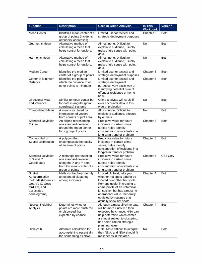
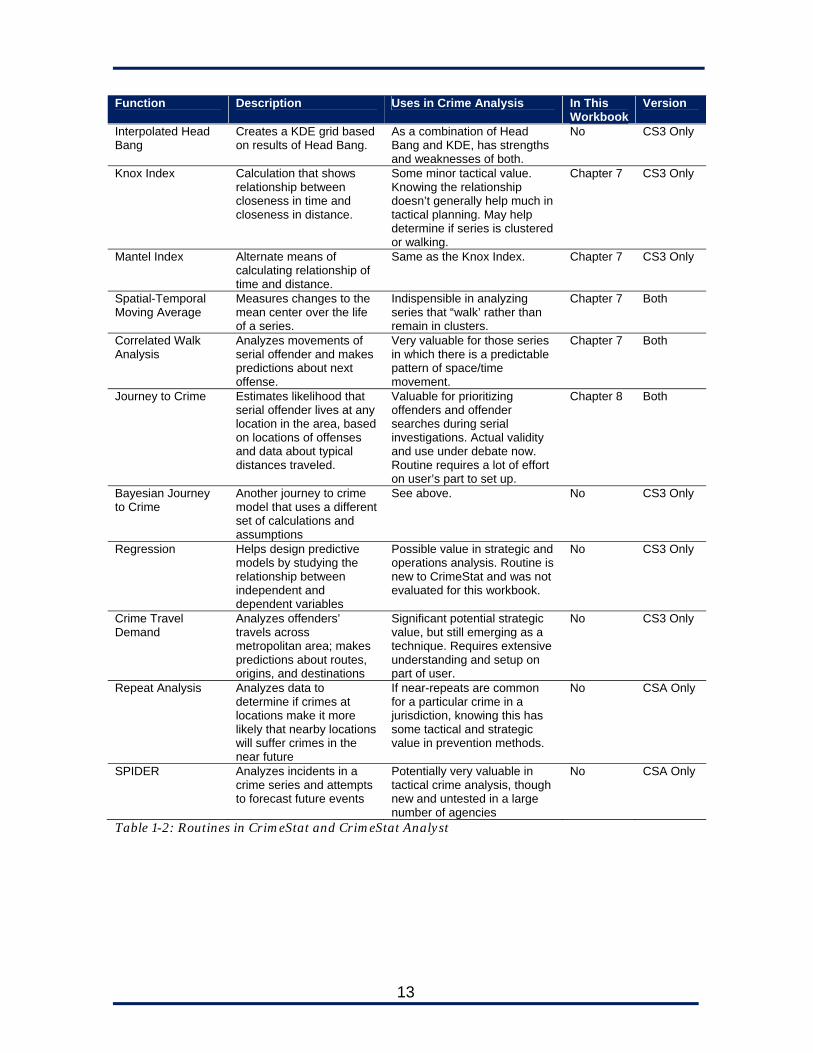
Figure 1-7: CrimeStat Analyst contains features not found in CrimeStat, such as a data editor, charting, and a geographic plot Table 1-2 lists the different routines used by CrimeStat and CrimeStat Analyst and provides the authors’ opinions on their uses in crime analysis.

11

Function Description Uses in Crime Analysis In This Workbook

Version

Mean Center Identifies mean center of a group of points (incidents, offenders’ addresses)

Limited use for tactical and strategic deployment purposes

Chapter 3 Both

Geometric Mean Alternative method of calculating a mean that helps control for outliers.

Almost none. Difficult to explain to audience, usually makes little sense with point data.

No Both

Harmonic Mean Alternative method of calculating a mean that helps control for outliers.

Almost none. Difficult to explain to audience, usually makes little sense with point data.

No Both

Median Center Identifies the median center of a group of points

Limited use for tactical and strategic deployment purposes

Chapter 3 Both

Center of Minimum Distance

Identifies the point at which the distance to all other points is minimum

Limited use for tactical and strategic deployment purposes; very basic way of identifying potential area of offender residence or home base

Chapter 3 Both

Directional Mean and Variance

Similar to mean center but for data in angular (polar coordinate) systems

Crime analysts will rarely if ever encounter data in this type of projection

No Both

Triangulated Mean A mean calculated by intersection of vectors from corners of plot area

Almost none. Difficult to explain to audience, affected by outliers.

No Both

Standard Deviation Ellipse

An ellipse representing one standard deviation around the mean center for a group of points

Predictive value for future incidents in certain crime series; helps identify concentration of incidents in a long-term trend or problem

Chapter 3 Both

Convex Hull of Spatial Distribution

A polygon that encompasses the totality of an area of points


Chapter 3 Both

Standard Deviation of X and Y Coordinates

A rectangle representing one standard deviation along the X and Y axes from the mean center of a group of points


Chapter 3 CS3 Only

Spatial Autocorrelation methods (Moran’s I, Geary’s C, Getis-Ord’s G, and associated correlograms)

Methods that help identify an extent of clustering among incidents

Limited. At best, tells you whether hot spots tend to be located near other hot spots. Perhaps useful in creating a crime profile of an unfamiliar jurisdiction but has almost no operational value. Generally obviated by routines that actually show hot spots.

Chapter 4 Both

Nearest Neighbor Analysis

Determines whether points are more clustered or dispersed than expected by chance

Although almost all crime data will be more clustered than expected by chance, NNA can help determine which crimes are most subject to clustering; has some limited strategic planning value.

Chapter 4 Both

Ripley’s K Alternate calculation for accomplishing essentially the same thing as NNA.

Little. More difficult to interpret than NNA, and NNA should fit most needs in this area.

No Both

12


Version

Assign primary points to secondary points

Matches points from one file with their closest neighbors from another file or from within a polygon; sums the results.

Very valuable if you do not already have a GIS function that does this. Can assign crimes to nearest police station, incidents to nearest offender addresses, etc.

No CS3 Only

Distance matrices Creates a matrix of distances between points in one or two files.

Might be useful for some special projects, but in general, no.

No CS3 Only

Mode (hot spot) Counts the number of incidents at each pair of coordinates.

The function itself is very useful in crime analysis to identify the top “hot addresses,” but this is easily done in most GIS programs.

Chapter 5 Both

Fuzzy mode Builds on mode hot spot analysis by creating a radius around each point and capturing all points within the radius

Takes care of some of the problems with plain modal hot spots, but also results in non-intuitive results in some cases.

Chapter 5 Both

Nearest Neighbor Hierarchical Spatial Clustering (NNH)

Based on parameters you input, creates ellipses around points of unusually dense volume

One of the most useful routines, with broad uses in strategic analysis.

Chapter 5 Both

Risk-Adjusted NNH Builds on NNH but adjusts results based on interpolated assessment of available targets

Only hot spot routine that can be adjusted for underlying risk. Difficult to get source data but worth the effort.

Chapter 5 Both

Spatial and Temporal Analysis of Crime

Alternate means for identifying clusters of points

Another very useful hot spot routine; should be used in conjunction with NNH.

Chapter 5 Both

K-means Clustering Partitions all points into a number of clusters identified by the user

Some strategic value if the goal is to maintain a specific number of hot spots in your analysis. Not as useful as the other two.

Chapter 5 Both

Anselin’s Local Moran

Determines whether polygons have high volume relative to their broader neighborhoods

Some limited use in strategic analysis.

No Both

Getis-Ord Local G Alternate means of local autocorrelation similar to Anselin’s Local Moran

Some limited use in strategic analysis

No CS3 Only

Kernel Density Estimation

Interpolates crime volume across a region based on crimes at known points; creates risk surface.

Broad strategic value. One of the most popular types of maps created by crime analysts; CrimeStat gives you control over the process in a way that many other products do not.

Chapter 6 Both

Dual Kernel Density Estimation

Adjusts KDE calculations by considering a second file, either as a supplement or a denominator

Quite valuable if the user can obtain the source data. Allows adjustment of density estimate based on, for instance, underlying target availability.

Chapter 6 Both

Head Bang A polygon-based technique that smoothes extreme values into nearest neighbors

Dubious validity for raw volume but can be useful for rates in areas where small denominators create large values.

No CS3 Only

13


Version

Interpolated Head Bang

Creates a KDE grid based on results of Head Bang.

As a combination of Head Bang and KDE, has strengths and weaknesses of both.

No CS3 Only

Knox Index Calculation that shows relationship between closeness in time and closeness in distance.

Some minor tactical value. Knowing the relationship doesn’t generally help much in tactical planning. May help determine if series is clustered or walking.

Chapter 7 CS3 Only

Mantel Index Alternate means of calculating relationship of time and distance.

Same as the Knox Index. Chapter 7 CS3 Only

Spatial-Temporal Moving Average

Measures changes to the mean center over the life of a series.

Indispensible in analyzing series that “walk’ rather than remain in clusters.

Chapter 7 Both

Correlated Walk Analysis

Analyzes movements of serial offender and makes predictions about next offense.

Very valuable for those series in which there is a predictable pattern of space/time movement.

Chapter 7 Both

Journey to Crime Estimates likelihood that serial offender lives at any location in the area, based on locations of offenses and data about typical distances traveled.

Valuable for prioritizing offenders and offender searches during serial investigations. Actual validity and use under debate now. Routine requires a lot of effort on user’s part to set up.

Chapter 8 Both

Bayesian Journey to Crime

Another journey to crime model that uses a different set of calculations and assumptions

See above. No CS3 Only

Regression Helps design predictive models by studying the relationship between independent and dependent variables

Possible value in strategic and operations analysis. Routine is new to CrimeStat and was not evaluated for this workbook.

No CS3 Only

Crime Travel Demand

Analyzes offenders’ travels across metropolitan area; makes predictions about routes, origins, and destinations

Significant potential strategic value, but still emerging as a technique. Requires extensive understanding and setup on part of user.

No CS3 Only

Repeat Analysis Analyzes data to determine if crimes at locations make it more likely that nearby locations will suffer crimes in the near future

If near-repeats are common for a particular crime in a jurisdiction, knowing this has some tactical and strategic value in prevention methods.

No CSA Only

SPIDER Analyzes incidents in a crime series and attempts to forecast future events

Potentially very valuable in tactical crime analysis, though new and untested in a large number of agencies

No CSA Only

Table 1-2: Routines in CrimeStat and CrimeStat Analyst

14

Hardware and Software CrimeStat was developed for the Microsoft Windows operating system. It will work on machines with Windows 2000, Windows XP, Windows Vista, and Windows 7. Minimum requirements for CrimeStat III are 256 MB of RAM and an 800 MHz processor speed, but an optimal configuration is 1 GB of RAM and a 1.6 MHz processor. Some of the routines used by CrimeStat, depending on the size of the data file, may require millions of calculations per output. Obviously, more RAM and a greater processor speed will provide a faster CrimeStat experience. Multi-processor machines will also run CrimeStat considerably faster. Many of CrimeStat’s outputs are meant to be displayed in a GIS, and you will likely need a GIS to generate the types of files CrimeStat can read (see Chapter 2). Therefore, analysts who want to get the most use from CrimeStat should also have the latest version of ArcGIS, MapInfo Professional, or whatever other GIS application they prefer. Notes on This Workbook Spatial Statistics in Crime Analysis: Using CrimeStat III was written to accompany a three-day course in the software and its uses in crime analysis. We have chosen the CrimeStat routines and techniques that we think are most valuable to crime analysts and yet still accessible to analysts who are using CrimeStat for the first time. Some techniques we excluded because their complexity requires more attention than we could give in an introductory course (e.g., Crime Travel Demand); others we excluded because they seemed to have limited utility for the typical police crime analyst. The latter point is not meant as a criticism of the program; CrimeStat was developed for criminologists and researchers as well as crime analysts. Although we cover some GIS issues in Chapter 2, both this book and this course generally assume that you are already an intermediate or advanced GIS user. This means that you should know how to:

Arrange layers in a GIS to create a basemap Geocode data Create thematic maps Import into your GIS data created by other applications Understand different projections and coordinate systems and troubleshoot issues

associated with them Interpret different file types and their associated extensions Modify and update attribute data for your GIS layers Export data, with coordinates, from your GIS to other file types

The GIS screen shots in this book come mostly from ArcGIS 9.3, and the training course that accompanies this workbook also uses ArcGIS. Analysts who use other GIS systems can still follow the steps in the workbook; they will just have to change the output types to their preferred GIS.

15

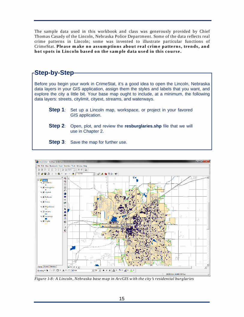
The sample data used in this workbook and class was generously provided by Chief Thomas Casady of the Lincoln, Nebraska Police Department. Some of the data reflects real crime patterns in Lincoln; some was invented to illustrate particular functions of CrimeStat. Please make no assumptions about real crime patterns, trends, and hot spots in Lincoln based on the sample data used in this course.

Step-by-Step Before you begin your work in CrimeStat, it’s a good idea to open the Lincoln, Nebraska data layers in your GIS application, assign them the styles and labels that you want, and explore the city a little bit. Your base map ought to include, at a minimum, the following data layers: streets, citylimit, cityext, streams, and waterways.

Step 1: Set up a Lincoln map, workspace, or project in your favored GIS application.

Step 2: Open, plot, and review the resburglaries.shp file that we will

use in Chapter 2. Step 3: Save the map for further use.

Figure 1-8: A Lincoln, Nebraska base map in ArcGIS with the city’s residential burglaries

16

Summary

Spatial statistics are important tools to crime analysts, enhancing analysts' existing GIS capabilities.

Spatial statistics are required when visual interpretation of data fails, usually because the data are too numerous or because the patterns are too subtle for visual detection.

Most spatial statistics have analogs in non-spatial statistics (e.g., the mean of a series of numbers vs. the mean center of several pairs of coordinates); spatial statistics simply apply regular statistics to coordinates, angles, and distances.

Spatial statistics have uses in all types of crime analysis, including forecasting future events, identifying hot spots, and estimating journey to crime.

CrimeStat, developed in the late 1990s, collects numerous spatial statistics for use by individuals and institutions working with crime data.

CrimeStat works with existing GIS applications, both for the source data and to read the outputs. It is not itself a GIS.

For Further Reading Boba, R. (2009). Crime analysis with crime mapping (2nd ed.). Thousand Oaks, CA:

Sage. Chainey, S., & Ratcliffe, J. (2005). GIS and crime mapping. Chichester, UK: John Wiley &

Sons. International Association of Crime Analysts. (2008). Exploring crime analysis (2nd ed.).

Overland Park, KS: Author.

17

2

Working with Data Importing, Parameters, and Exporting

Figure 2-1: The initial CrimeStat data setup screen. CrimeStat depends on data that has already been created, queried, and marked with geographic coordinates. Most analysts will have to geocode their data in their geographic information systems first, and then open the resulting file in CrimeStat. Analysts who work for agencies in which their records management or computer-aided dispatch systems automatically assign geographic coordinates will be able to import this data into CrimeStat without going through their GIS applications first. CrimeStat reads files in a large number of formats, including: Delimited ASCII (.txt or .dat), dBASE (.dbf) files, MapInfo attribute tables (.dat), ArcGIS Shapefiles (.shp), Microsoft Access databases (.mdb), and ODBC data sources.

18

Any modern RMS or CAD system should be able to export data to one of these formats, either directly or through an intermediate system like Excel or Access. But for CrimeStat to analyze the data, the table must contain X and Y coordinates within the attribute data. This is not always the case with geocoded data. MapInfo .dat files, for instance, do not contain X and Y coordinates by default—the user must add them through the “update field” function in the MapInfo software. The one exception to this rule is ArcGIS Shapefiles: CrimeStat will interpret the geography and automatically add the X and Y coordinates as the first columns in the table.

Figure 2-2: Because it has columns for X and Y coordinates, CrimeStat can read this Microsoft Access table of traffic accidents. CrimeStat will read, interpret, calculate, and output data in spherical, projected, or angular coordinate systems; the user must simply tell CrimeStat what system the data uses. It is rare to encounter crime data in angular coordinates, and most users will either have spherical (longitude and latitude) or projected data (e.g., U.S. State Plane Coordinates, Transverse Mercator). The user’s GIS system should be able to tell what type of coordinate system is used by the data, and if the data is projected, what measurement units (likely feet or meters) that it uses. Most CrimeStat calculations require only a single primary file, but some routines also require a secondary file. Secondary files must have the same coordinate systems as the primary files.

19

Primary File Setup All CrimeStat routines require at least one primary file, which is loaded onto the “Primary File” screen on the “Data setup” tab by clicking “Select Files.” Once the file is loaded, the user selects which fields in the table correspond with which variables needed by CrimeStat. The only variables required for all routines are the X coordinate, the Y coordinate, and the type of coordinate system. Intensity, weight, and other variables are only used by certain routines.

The “Select Files” box shows the file path for primary files. Although CrimeStat allows you to load multiple primary files at once, it can only work with one at a time. Loading more than one primary file tends to confuse the application and the user, and it is best to “Remove” primary files not in active use.

Figure 2-3: Selecting a primary file

20

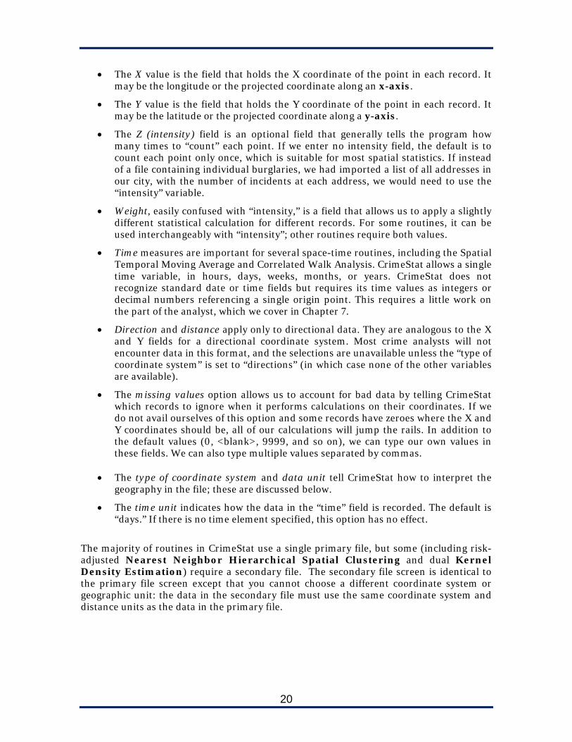
The X value is the field that holds the X coordinate of the point in each record. It may be the longitude or the projected coordinate along an x-axis.

The Y value is the field that holds the Y coordinate of the point in each record. It may be the latitude or the projected coordinate along a y-axis.

The Z (intensity) field is an optional field that generally tells the program how many times to “count” each point. If we enter no intensity field, the default is to count each point only once, which is suitable for most spatial statistics. If instead of a file containing individual burglaries, we had imported a list of all addresses in our city, with the number of incidents at each address, we would need to use the “intensity” variable.

Weight, easily confused with “intensity,” is a field that allows us to apply a slightly different statistical calculation for different records. For some routines, it can be used interchangeably with “intensity”; other routines require both values.

Time measures are important for several space-time routines, including the Spatial Temporal Moving Average and Correlated Walk Analysis. CrimeStat allows a single time variable, in hours, days, weeks, months, or years. CrimeStat does not recognize standard date or time fields but requires its time values as integers or decimal numbers referencing a single origin point. This requires a little work on the part of the analyst, which we cover in Chapter 7.

Direction and distance apply only to directional data. They are analogous to the X and Y fields for a directional coordinate system. Most crime analysts will not encounter data in this format, and the selections are unavailable unless the “type of coordinate system” is set to “directions” (in which case none of the other variables are available).

The missing values option allows us to account for bad data by telling CrimeStat which records to ignore when it performs calculations on their coordinates. If we do not avail ourselves of this option and some records have zeroes where the X and Y coordinates should be, all of our calculations will jump the rails. In addition to the default values (0, <blank>, 9999, and so on), we can type our own values in these fields. We can also type multiple values separated by commas.

The type of coordinate system and data unit tell CrimeStat how to interpret the

geography in the file; these are discussed below.

The time unit indicates how the data in the “time” field is recorded. The default is “days.” If there is no time element specified, this option has no effect.

The majority of routines in CrimeStat use a single primary file, but some (including risk-adjusted Nearest Neighbor Hierarchical Spatial Clustering and dual Kernel Density Estimation) require a secondary file. The secondary file screen is identical to the primary file screen except that you cannot choose a different coordinate system or geographic unit: the data in the secondary file must use the same coordinate system and distance units as the data in the primary file.

21

Figure 2-4: The “missing values” field allows us to warn CrimeStat about values that should be ignored.

Step-by-Step Our first lessons will set up a primary file in CrimeStat

Step 1: Launch CrimeStat and click on the splash screen to dismiss it.

Step 2: On “Primary File” sub-tab of the “Data setup” tab, click the “Select Files” button, choose a “Shape file,” and browse to the burglaryseries.shp file in your CrimeStat data directory.

Step 3: Set the X and Y values to the “X” and “Y” fields (CrimeStat

automatically created these based on the Shapefile). Set the Z value to the “STOLEN” field.

22

Step 4: Set the “Missing values” field for X, Y, and Z to ignore both blanks and zeroes. You can accomplish this by entering both <Blank> and 0 in the field, separated by a comma, as in figure 2-5.

Step 5: Set the “Type of coordinate system” to “Projected,” with the distance units in “Feet.”

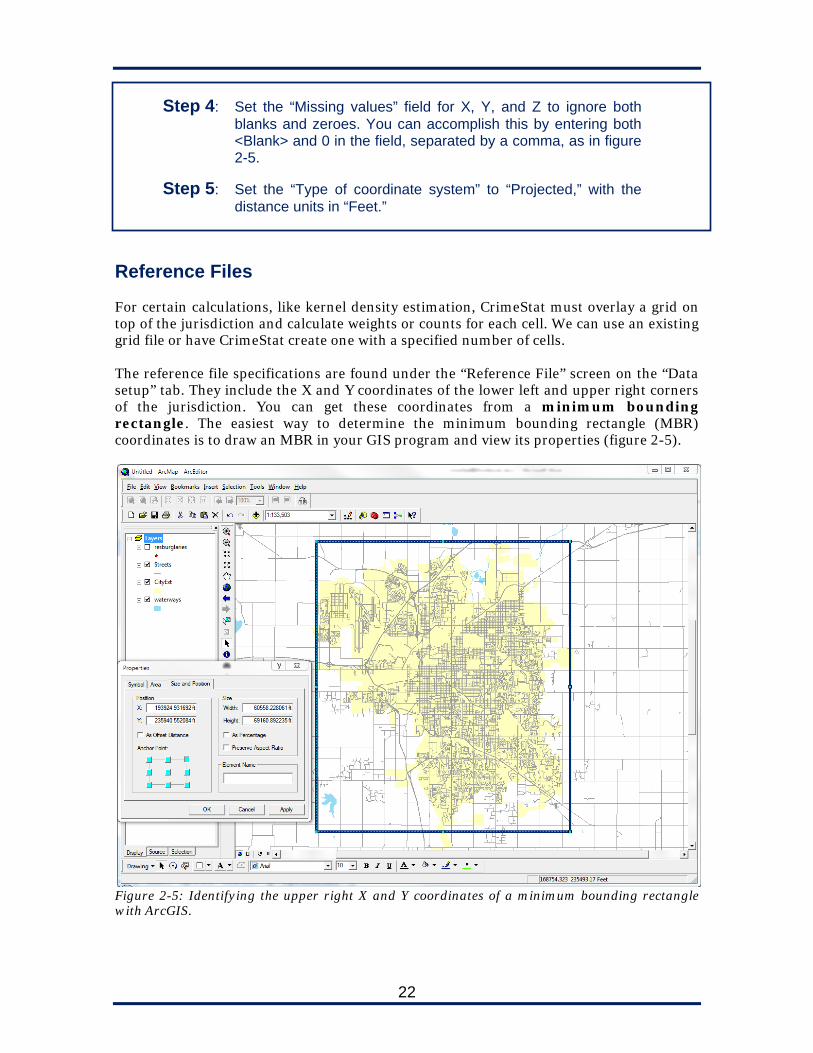
Reference Files For certain calculations, like kernel density estimation, CrimeStat must overlay a grid on top of the jurisdiction and calculate weights or counts for each cell. We can use an existing grid file or have CrimeStat create one with a specified number of cells. The reference file specifications are found under the “Reference File” screen on the “Data setup” tab. They include the X and Y coordinates of the lower left and upper right corners of the jurisdiction. You can get these coordinates from a minimum bounding rectangle. The easiest way to determine the minimum bounding rectangle (MBR) coordinates is to draw an MBR in your GIS program and view its properties (figure 2-5).

Figure 2-5: Identifying the upper right X and Y coordinates of a minimum bounding rectangle with ArcGIS.

23

Since each grid cell is a square, the number of columns determines the number of rows (and the cell size). In a perfectly square jurisdiction 10 miles across, setting the number of columns to 250 will create 250 x 250 = 62,500 grid cells of 10/250 = 0.04 miles (211.2 feet) each. 250 columns serves as a good default cell size, but you will want to adjust this figure depending on the overall purpose of the resulting map. You can also set the reference grid based on size rather than number of columns. The more cells in the reference grid, the “finer” the resulting density map will be. The fewer cells, the more “pixilated” it will look at lower zoom levels (figure 2-6). The number of cells should not greatly affect the relative weights of the cells themselves (and thus the final map result), unless the size of the cells is so large that you are effectively not creating a density map. However, the more cells in the grid, the longer it will take to run the calculations. You will have to experiment to find the right balance of aesthetics and processing speed.

Figure 2-6: A kernel density estimation of the same area with 100 columns (left) versus 400 columns (right). Measurement Parameters Certain routines in CrimeStat require parameters for the size of the jurisdiction (as covered by a minimum bounding rectangle), the length of the street network, and the preferred distance measure. These are entered on the “measurement parameters” section of the “Data setup” tab. You can determine the coverage area from the same minimum bounding rectangle explained in the previous section (note the “area” tab in figure 2-5). The length of the street network is more difficult to determine, but most GIS systems can perform the calculation by summing the individual lengths of the streets.

24

In the “type of distance measurement” setting, we tell CrimeStat how we want to see distances calculated. There are three options, and figure 2-7 shows the differences among them.

Direct distance is the shortest distance between two points: “as the crow files.” This is the easiest measurement to understand, if the least “true” in a practical sense.

Indirect distance or Manhattan distance measures distances using an east-west line and a north-south line connected by a 90-degree angle. This type of measurement makes sense for cities with a gridded street pattern.

Network distance measures use the jurisdiction’s actual road network, as stored in a DBF or ArcGIS Shapefile. This requires us to specify a file that contains the jurisdiction’s street and to set up some other parameters. It cannot account for one-way streets or distinguish between major streets and alleys, but it is still more accurate in its measurements than either of the other measures. The disadvantage is that it takes longer to perform the calculations.

Figure 2-7: The differences among CrimeStat’s three distance measures The three measures will impact CrimeStat outputs primarily in terms of size. Because the distance between points is smallest when measuring directly and (usually) largest when measuring by street network, means and standard deviations of those distances will also be smallest and largest when using those measures, respectively. Indirect measures will be somewhere in between.

Upper left: direct distance Lower left: indirect distance Lower right: network distance

25

Step-by-Step

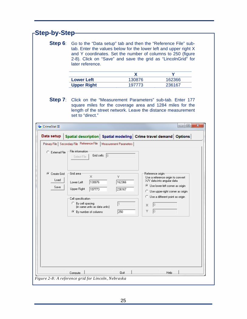
Step 6: Go to the “Data setup” tab and then the “Reference File” sub-tab. Enter the values below for the lower left and upper right X and Y coordinates. Set the number of columns to 250 (figure 2-8). Click on “Save” and save the grid as “LincolnGrid” for later reference.

X Y Lower Left 130876 162366 Upper Right 197773 236167

Step 7: Click on the “Measurement Parameters” sub-tab. Enter 177 square miles for the coverage area and 1284 miles for the length of the street network. Leave the distance measurement set to “direct.”

Figure 2-8: A reference grid for Lincoln, Nebraska

26

Exporting Data from CrimeStat CrimeStat has several output options depending on the type of routine. All routines allow the user to save the result as a text file. Others create a table of records and allow the user to save as a dBASE (.dbf) file. Most routines can result in the creation of map objects (e.g., hot spot ellipses, probability grids) with coordinates, in which case you have the option to export the result as an ArcGIS Shapefile (.shp), a MapInfo Interchange File (.mif), or an Atlas GIS boundary file (.bna). You can then open or import these files into your GIS and view them. We will do this frequently in the lessons to come. Note that if you are a MapInfo user, you will generally find it easier to export the objects as ArcGIS Shapefiles and open them in MapInfo (allowed in version 7.0 or above) than to engage the complicated settings involved with creating and importing a MIF file, especially for projected data.

Figure 2-9: Exporting a CrimeStat routine The name you give the file when exporting is not the final name that CrimeStat will use. Instead, it will append a prefix to the file indicating which routine was run. If, for instance, you create a Shapefile out of the mean center and standard distance deviation calculations and call them both “Burglary,” CrimeStat will name them MCBurglary.shp and SDDBurglary.shp respectively.

27

Saving and Loading Parameters Everything we have done in this chapter—input file specifications, measurement parameters, data editing, subsets, reference file specifications—will be lost when we quit CrimeStat. To avoid this happening, we can save our current session for later use by selecting “Save Parameters” under the “Options” tab. Later, when we want to use these parameters again, we can restore them with “Load Parameters” at the same location.

Step-by-Step

Step 8: Click on the “Options” sub-tab and click the “Save parameters” button.

Step 9: Save the parameters as burgseries.param in your CrimeStat directory.

Figure 2-10: Saving parameters for later use

28

Summary

CrimeStat depends on data that has already been created and geocoded.

The data must have X and Y coordinates in either spherical or projected systems.

Fields required for certain routines include a time variable, an intensity variable, a weight, the area of the jurisdiction, the length of the street network, and the specifications for a grid layer.

CrimeStat can read data in dBASE, MapInfo, ArcGIS Shapefiles, and Access database formats, as well as ODBC connections. Depending on the routine, it will export to text file, dBASE, ArcGIS Shapefile, MapInfo, or Atlas GIS formats.

To run a CrimeStat routine, you load the data files, choose the routine to run, and click the "Compute” button. You can run a single routine or every routine in the application at the same time (not recommended for processing reasons).

Saving your parameters will preserve them for later use.

For Further Reading Levine, N. (2005). Chapter 3: Entering data into CrimeStat. In CrimeStat III: A spatial

statistics program for the analysis of crime incident locations (pp. 3.1–3.45). Houston, TX: Ned Levine & Associates. Retrieved from http://www.icpsr.umich.edu/CrimeStat/files/CrimeStatChapter.3.pdf

Chang, K. (2011). Introduction to geographic information systems (6th ed.). New York:

McGraw-Hill.

29

3

Spatial Distribution Analysis and Forecasting

In this chapter, we begin a series of exercises that analyze the various spatial characteristics of crimes and other public safety problems. Some of these techniques apply to series; some to long-term trends; some to both. Implicit in these exercises is the concept of forecasting: identifying the most likely locations and (in some techniques) times of future events. “Forecasting,” as a term, comes from meteorology, and as in meteorology, crime analysis forecasting depends on probabilities rather than certainties. Both meteorological and criminological forecasting are part-art, part-science, and both are subject to “chaos theory,” in which the beating wings of a butterfly can defeat the most sincere and scientific attempt and prediction. When a crime analyst’s forecast isn’t “wrong,” it often seems wrong because police activity changes the pattern. Here is an unexaggerated quote received (in various forms) more than once in your author’s career: “You said the thief was most likely to strike in the TGI Friday’s lot last night between 18:00 and 21:00. Well, I was parked in that lot all night, and nothing happened!” Because of the possibility—probability, really—of such errors, many analysts insist that they do not forecast. This is nonsense. Forecasting is inherent in any spatial or temporal analysis. Just because you avoid the terms “forecast” or “predict” doesn’t mean you aren’t forecasting. If you describe the spatial dimensions or direction of a crime pattern, you are implicitly suggesting that future events will follow the same pattern. Stating “the burglaries are concentrated in half-mile radius around Sevieri Park” suggests that future burglaries will probably be within a half-mile radius of Sevieri Park. There’s no way to avoid it. Hence, we try to get better at it instead. Spatial forecasting in tactical crime analysis is essentially a two-step process:

1. Identify the target area for the next incident 2. Identify potential targets within the target area

There is generally an inverse relationship between the predictability of the target area and the availability of potential targets. That is, when the offender prefers very specific targets (e.g., banks open on Saturday mornings, fast food restaurants of a particular chain), his next strike will be determined by the locations of those targets. This may take him in any direction. On the other hand, when the target area is highly predictable (e.g., the offender is moving in a linear manner across the city), it’s usually because there are plentiful targets (pedestrians, parked cars, houses) distributed within the area. Most series fall in between.

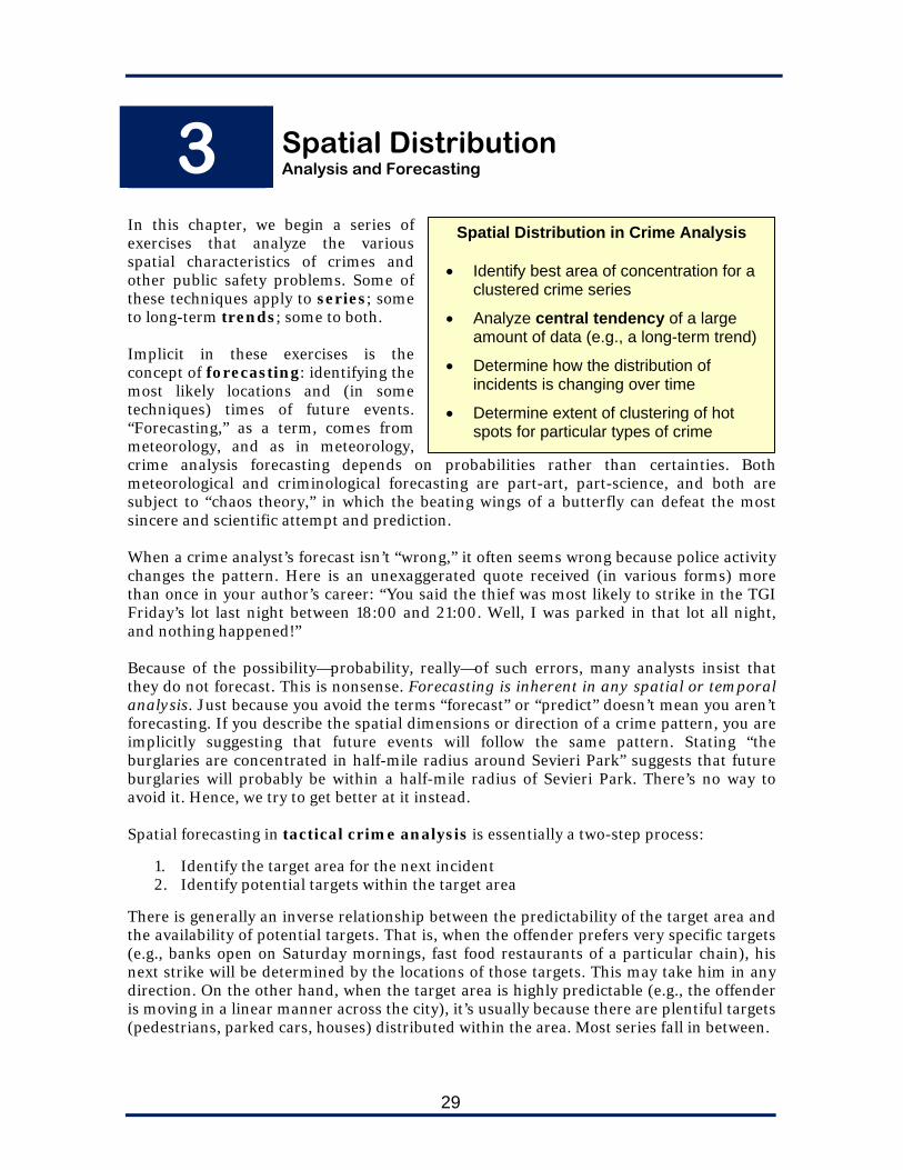
Spatial Distribution in Crime Analysis Identify best area of concentration for a

clustered crime series

Analyze central tendency of a large amount of data (e.g., a long-term trend)

Determine how the distribution of incidents is changing over time

Determine extent of clustering of hot spots for particular types of crime

30

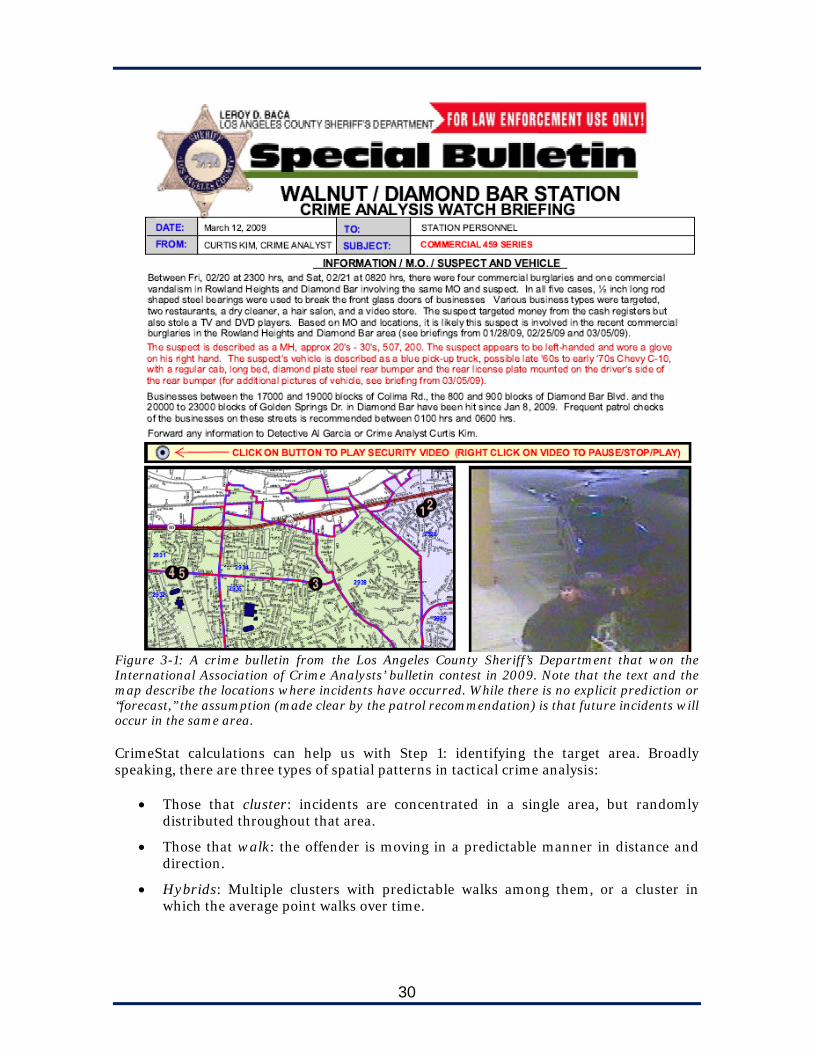
Figure 3-1: A crime bulletin from the Los Angeles County Sheriff’s Department that won the International Association of Crime Analysts’ bulletin contest in 2009. Note that the text and the map describe the locations where incidents have occurred. While there is no explicit prediction or “forecast,” the assumption (made clear by the patrol recommendation) is that future incidents will occur in the same area. CrimeStat calculations can help us with Step 1: identifying the target area. Broadly speaking, there are three types of spatial patterns in tactical crime analysis:

Those that cluster: incidents are concentrated in a single area, but randomly distributed throughout that area.

Those that walk: the offender is moving in a predictable manner in distance and direction.

Hybrids: Multiple clusters with predictable walks among them, or a cluster in which the average point walks over time.

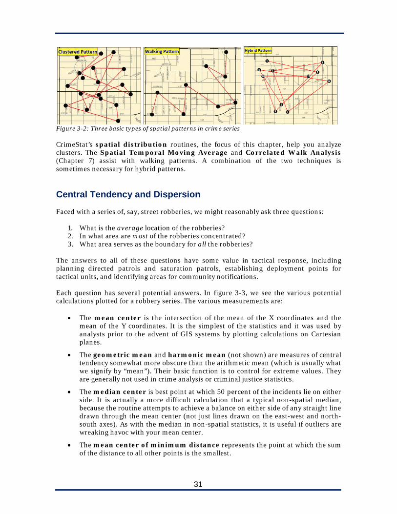
31

Figure 3-2: Three basic types of spatial patterns in crime series CrimeStat’s spatial distribution routines, the focus of this chapter, help you analyze clusters. The Spatial Temporal Moving Average and Correlated Walk Analysis (Chapter 7) assist with walking patterns. A combination of the two techniques is sometimes necessary for hybrid patterns. Central Tendency and Dispersion Faced with a series of, say, street robberies, we might reasonably ask three questions:

1. What is the average location of the robberies? 2. In what area are most of the robberies concentrated? 3. What area serves as the boundary for all the robberies?

The answers to all of these questions have some value in tactical response, including planning directed patrols and saturation patrols, establishing deployment points for tactical units, and identifying areas for community notifications. Each question has several potential answers. In figure 3-3, we see the various potential calculations plotted for a robbery series. The various measurements are:

The mean center is the intersection of the mean of the X coordinates and the mean of the Y coordinates. It is the simplest of the statistics and it was used by analysts prior to the advent of GIS systems by plotting calculations on Cartesian planes.

The geometric mean and harmonic mean (not shown) are measures of central tendency somewhat more obscure than the arithmetic mean (which is usually what we signify by “mean”). Their basic function is to control for extreme values. They are generally not used in crime analysis or criminal justice statistics.

The median center is best point at which 50 percent of the incidents lie on either side. It is actually a more difficult calculation that a typical non-spatial median, because the routine attempts to achieve a balance on either side of any straight line drawn through the mean center (not just lines drawn on the east-west and north-south axes). As with the median in non-spatial statistics, it is useful if outliers are wreaking havoc with your mean center.

The mean center of minimum distance represents the point at which the sum of the distance to all other points is the smallest.

32

Figure 3-3: Spatial distribution measurements for a robbery series. The polygons seek to measure the concentration, rather than the specific central point, of the series.

The standard deviation of the X and Y coordinates creates a rectangle representing one standard deviation along the X and Y axes from the mean center.

The standard distance deviation calculates the linear distance from each point to the mean center point, then draws a circle representing this average plus one standard deviation.

The standard deviation ellipse produces an ellipse that represents one standard deviation of the X and Y coordinates from the mean center. It is based on coordinates rather than distance and thus accounts for skewed distributions. Generally about half to two-thirds of the incidents will fall within a single standard deviation ellipse and all but a few incidents will fall within a two-standard deviations ellipse.

The convex hull polygon encloses the outer reaches of the series. No point lies outside the polygon, and all of the angles in the creation of the polygon are convex. Outliers will increase the size and skew the shape of the polygon.

All of these measures have some predictive value for the future of the crime series—provided it is not a walking series (for that, see Chapter 7). Unless the offender changes his

33

activities significantly, he will probably strike within the standard distance deviation or the standard deviation ellipse, and he will almost certainly strike within the two-standard-deviation ellipse or convex hull. We can then refine our forecast by looking for suitable targets within the area in question. This is somewhat easier in, say, a bank robbery series than it is in a residential burglary series. But even when there are thousands of houses, we might be able to refine the list of locations by noting that the offender prefers, for instance, houses on corners, or houses with circular driveways.

Step-by-Step Our goal in this lesson is to analyze a series of residential burglaries affecting a Lincoln neighborhood. We will use the same data setup as in Chapter 2.

Step 1: Open the burglaryseries.shp file in your GIS program to view its extent and characteristics.

Step 2: Launch CrimeStat. If you already have the burglaryseries.shp

file set up as in Chapter 2, skip to Step 4. Step 3: On the “Primary File” tab, choose “select files” and add the

burglaryseries.shp file from your CrimeStat directory. Set the X and Y coordinates values to “X” and “Y.” Under the “Type of coordinate system,” make sure it is set to “Projected” with the data units in feet. Reference files and measurement parameters are not necessary for spatial distribution.

Step 4: Click on the “Spatial description” tab and the “Spatial

Distribution” sub-tab. Check all of the boxes except for “Directional mean and variance” (this only applies to directional data, which we do not have).

Step 5: For each of the routines checked, click the “Save result to…”

button next to it and choose to save it as a ArcView Shapefile in your preferred directory. Name the file burglaryseries (figure 3-4).

Step 6: Click “Compute” at the bottom of the screen.

The “CrimeStat Results” window (figure 3-5) should show five tabs with information about the mean center and standard distance deviation, the standard deviation ellipses, the mean center of minimum distance, the median center, and the convex hull. Browsing this window can be informative and can help us determine if the routine ran correctly or encountered errors, but of course to truly get value from these calculations, we must be able to visualize them.

Step 7: In your GIS program, add the Shapefiles that were created. They will all be called “burglaryseries” but with the following prefixes: 2SDE, CHull, GM, HM, MC, Mcmd, MdnCntr SDD, SDE, XYD.

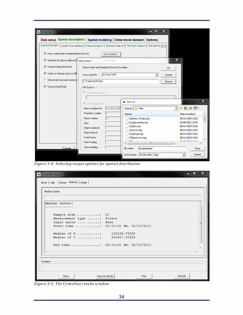
34

Figure 3-4: Selecting output options for spatial distribution

Figure 3-5: The CrimeStat results window

35

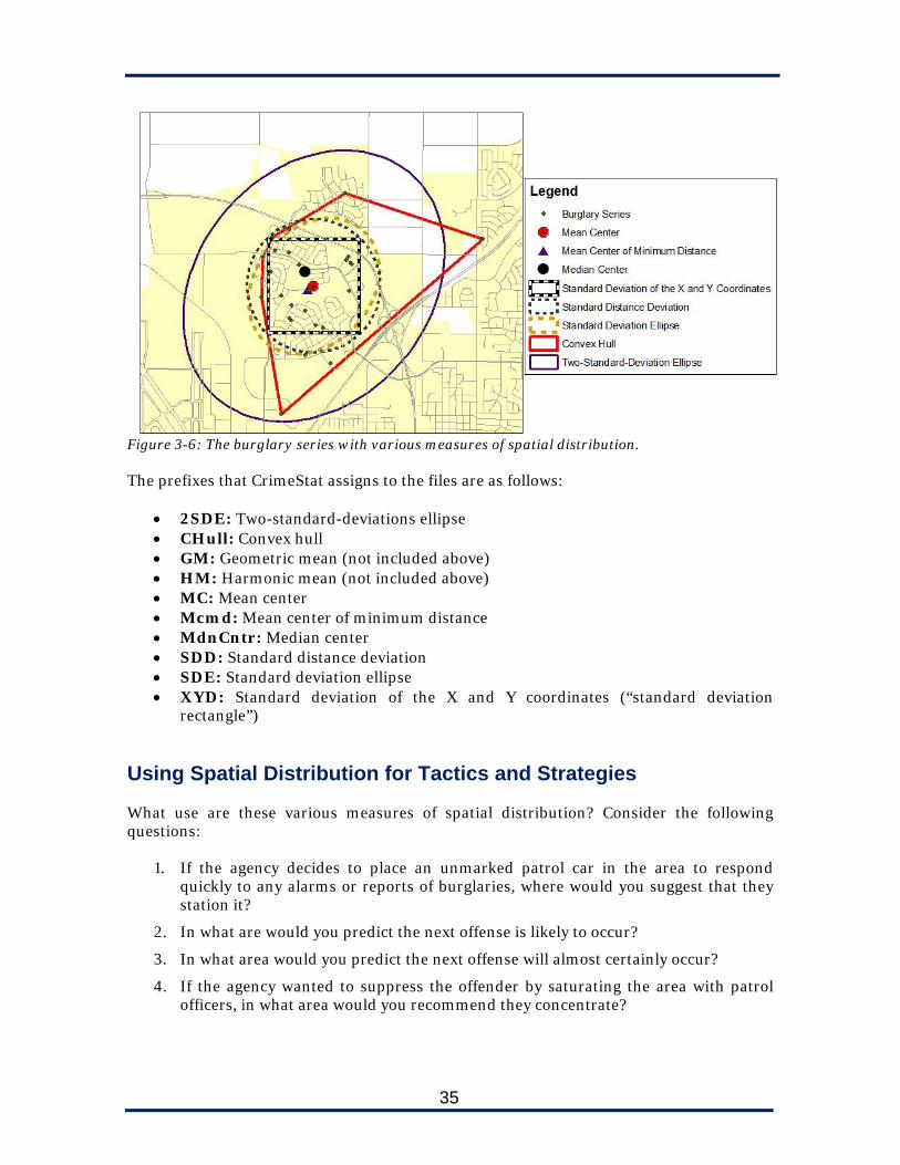
Figure 3-6: The burglary series with various measures of spatial distribution. The prefixes that CrimeStat assigns to the files are as follows:

2SDE: Two-standard-deviations ellipse CHull: Convex hull GM: Geometric mean (not included above) HM: Harmonic mean (not included above) MC: Mean center Mcmd: Mean center of minimum distance MdnCntr: Median center SDD: Standard distance deviation SDE: Standard deviation ellipse XYD: Standard deviation of the X and Y coordinates (“standard deviation

rectangle”) Using Spatial Distribution for Tactics and Strategies What use are these various measures of spatial distribution? Consider the following questions:

1. If the agency decides to place an unmarked patrol car in the area to respond quickly to any alarms or reports of burglaries, where would you suggest that they station it?

2. In what are would you predict the next offense is likely to occur?

3. In what area would you predict the next offense will almost certainly occur?

4. If the agency wanted to suppress the offender by saturating the area with patrol officers, in what area would you recommend they concentrate?

36

5. If the agency wanted to station “scarecrow cars” in the area to deter the offender, where would you recommend that they station them?

6. If the agency wanted to alert residents about the series, encouraging potential future victims to lock doors and hide valuables, in what area should they call or leave notices?

These are our answers. If yours differ slightly based on your analytical judgment, that’s fine; there are no absolute “rights” and “wrongs” here.

1. An unmarked car stationed to respond quickly to incidents would probably best be stationed at one of the mean center calculations (in this case, it doesn’t matter much, but the mean center of minimum distance would minimize response times). That would be about halfway along West Harvest Drive.

2. Assuming we are correct that the series doesn’t “walk,” the next offense is most likely to occur within a single standard deviation of the mean center. The single standard deviation ellipse, the standard deviation rectangle, and the standard distance deviation all provide good estimates of the densest concentration.

3. The next offense will almost certainly occur within the two standard deviation ellipse or the convex hull polygon, unless the offender does something complete new for his next burglary. These of course have the disadvantage of being larger and thus harder to concentrate resources within.

4. Saturation patrol would best be concentrated in the single standard deviation ellipse, because it encloses a majority of the incidents and conforms best to the street geography in this part of the city.

5. This is a bit of a trick question because it’s not fully answerable with these CrimeStat calculations. But note that the standard distance deviation encompasses a neighborhood with few entries and exits. An offender would almost certainly have to pass cruisers stationed at four locations: the intersection of NW 12th St and W Highland Blvd; NW 13th St and W Fletcher Ave; NW 1st St and W Fletcher Ave; and NW 1st St and W Highland Blvd.

6. To reach all potential targets, the two standard deviation ellipse or convex hull would be the best choices.

At this point, you might think: “This is all great, but I could have drawn this by hand and done just as good a job!” You are probably correct. Analysts must always ask whether the time and effort necessary to calculate and display any spatial statistic improves upon what they could have accomplished on their own with a piece of paper and a magic marker. But we would point out the following:

Your hand drawing wouldn’t account for multiple incidents at a single location. CrimeStat does.

This series has a limited number of points. If analyzing a larger series, or a year’s worth of crime, your ability to visually interpret the points would suffer significantly.

37

While you may be able to draw a center point and ellipse by hand, CrimeStat’s calculations are more precise, and there’s always virtue in better precision.

In general, while taking the time to run the routines through CrimeStat may not help your analysis, failing to take this time when necessary will certainly hurt your analysis.

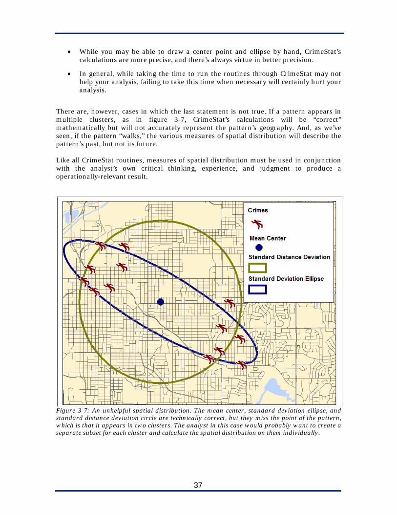
There are, however, cases in which the last statement is not true. If a pattern appears in multiple clusters, as in figure 3-7, CrimeStat’s calculations will be “correct” mathematically but will not accurately represent the pattern’s geography. And, as we’ve seen, if the pattern “walks,” the various measures of spatial distribution will describe the pattern’s past, but not its future. Like all CrimeStat routines, measures of spatial distribution must be used in conjunction with the analyst’s own critical thinking, experience, and judgment to produce a operationally-relevant result.

Figure 3-7: An unhelpful spatial distribution. The mean center, standard deviation ellipse, and standard distance deviation circle are technically correct, but they miss the point of the pattern, which is that it appears in two clusters. The analyst in this case would probably want to create a separate subset for each cluster and calculate the spatial distribution on them individually.

38

Summary

Spatial distribution calculations apply measures of central tendency (mean, median) and dispersion (standard deviation) to spatial data.

The convex hull is a polygon that encompasses all of the data points.

There are two major classifications of crime series: clustered series, which concentrate in an area with no pattern of movement; and walking series, which progress geographically over time.

Spatial distribution can help predict the target area for a next strike in clustered series.

To complete a proper forecast, the analyst must still seek potential targets within the target area

Different spatial distribution calculations are helpful for different purposes. Limited areas serve best for tactics like directed patrol and surveillance; larger areas work better for strategies like public information and crime prevention.

For Further Reading Levine, N. (2005). Chapter 4: Spatial distribution. In CrimeStat III: A spatial statistics

program for the analysis of crime incident locations (pp. 4.1–4.72). Houston, TX: Ned Levine & Associates. Retrieved from http://www.icpsr.umich.edu/CrimeStat/ files/CrimeStatChapter.4.pdf

39

4

Autocorrelation & Distance Analysis Assessing Clustering and Dispersion

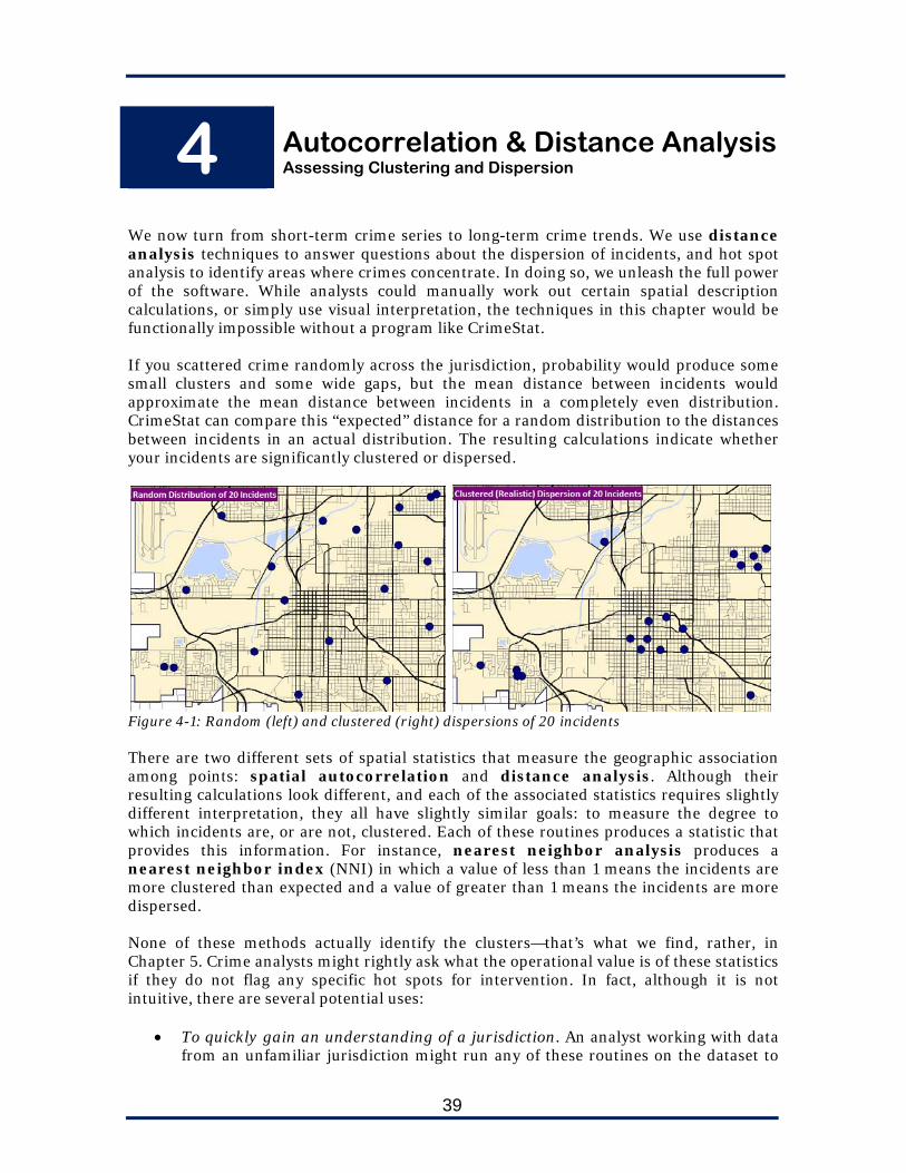
We now turn from short-term crime series to long-term crime trends. We use distance analysis techniques to answer questions about the dispersion of incidents, and hot spot analysis to identify areas where crimes concentrate. In doing so, we unleash the full power of the software. While analysts could manually work out certain spatial description calculations, or simply use visual interpretation, the techniques in this chapter would be functionally impossible without a program like CrimeStat. If you scattered crime randomly across the jurisdiction, probability would produce some small clusters and some wide gaps, but the mean distance between incidents would approximate the mean distance between incidents in a completely even distribution. CrimeStat can compare this “expected” distance for a random distribution to the distances between incidents in an actual distribution. The resulting calculations indicate whether your incidents are significantly clustered or dispersed.

Figure 4-1: Random (left) and clustered (right) dispersions of 20 incidents There are two different sets of spatial statistics that measure the geographic association among points: spatial autocorrelation and distance analysis. Although their resulting calculations look different, and each of the associated statistics requires slightly different interpretation, they all have slightly similar goals: to measure the degree to which incidents are, or are not, clustered. Each of these routines produces a statistic that provides this information. For instance, nearest neighbor analysis produces a nearest neighbor index (NNI) in which a value of less than 1 means the incidents are more clustered than expected and a value of greater than 1 means the incidents are more dispersed. None of these methods actually identify the clusters—that’s what we find, rather, in Chapter 5. Crime analysts might rightly ask what the operational value is of these statistics if they do not flag any specific hot spots for intervention. In fact, although it is not intuitive, there are several potential uses:

To quickly gain an understanding of a jurisdiction. An analyst working with data from an unfamiliar jurisdiction might run any of these routines on the dataset to

40

get a quick snapshot. For instance, if the analyst was working with auto theft data, an NNI of 0.15 would immediately suggest that auto thefts are highly clustered in a few hot spots, whereas an NNI of 0.8 would suggest they are more or less evenly dispersed throughout the city.

To identify the best strategy for a particular crime. Crimes that are more

clustered will respond better to location-specific strategies such as directed patrols, stakeouts, surveillance cameras, and warning signs. By comparing the statistics for particular crime types, or particular areas, or particular months or seasons, crime analysts can get a sense of when, where, and under what circumstances to recommend these strategies.

To evaluate an intervention. One way to evaluate the effects of a police strategy or

tactic is to look at the change in crime from the “before” period to the “after” period. Naturally, the primary variable we usually measure is the change in volume of incidents, but it is also valuable to look at the change in the characteristics of those incidents. Assume, for instance, that an agency is testing an aggressive directed patrol strategy at auto theft hot spots, with some of the zones in the city designated experimental and some control. The results are as follows:

Zone Pre-Intervenion Thefts

Post-Intervention Thefts

Difference Pre-Intervention NNI

Post-Intervention NNI

Experimental 180 140 -22% 0.38 0.74 Control 160 150 -6% 0.44 0.40

In this case, we could say that not only did the intervention show a statistically significant effect on the total number of thefts, but it also showed a significant effect on the clustering of those thefts—the intervention “broke up” hot spots.

The rest of this chapter covers the different methods of measuring relative clustering and dispersion among incidents. There are two primary classifications of such measurement: spatial autocorrelation and distance analysis. Generally speaking, spatial autocorrelation works best for data aggregated by polygons, like census tracks or police beats, and distance analysis measures work best for point data, like individual crimes or offender residences. Spatial Autocorrelation The key to understanding spatial autocorrelation is to understand its opposite: spatial independence. When volumes (e.g., crimes, people) are spatially independent, they have no spatial relationship to each other and will be distributed randomly throughout an area (not evenly, but randomly). When they are autocorrelated, areas of high volume are close to other areas with high volume, areas with low volume are close to other areas with low volume, or both. As in regular correlation, this relationship does not imply causation. Rather, it is more likely that the appearance of multiple hot spots close together is influenced by a third factor, such as proximity of available targets, or environmental variables favorable to crime. CrimeStat offers three measures of spatial autocorrelation with associated correlograms. All of these measures work with data aggregated by polygons, such as census blocks, police

41

beats, or grid cells. CrimeStat requires the X and Y coordinates of the polygon’s centerpoint and an “intensity” value indicating how many incidents are located within the polygon. Each measure finds a slightly different type of autocorrelation or measures it in a slightly different way. Figure 4-2 helps illustrate the four basic types of autocorrelation that we might identify. 1. Random dispersion of hot and cold zones (no spatial autocorrelation)

2A. Many hot zones close together (high positive spatial autocorrelation)

2B. Many cold zones close together (high positive spatial autocorrelation)

3. Hot and cold spots highly dispersed (high negative spatial autocorrelation)

Figure 4-2: the four basic types of spatial autocorrelation With these distinctions in mind, let’s look at CrimeStat’s three measures:

42

1. A weighted Moran’s I Statistic, a measure of autocorrelation on a scale of -1 (inverse correlation) to 1 (positive correlation). A value close to 0 would suggest no correlation. Moran’s I would find all of the different types of autocorrelation on the previous page, but it does not distinguish between 2A and 2B: a high positive correlation could indicate either hot spots close together or cold spots close together.

Figure 4-3: volume of auto thefts by census block group in the City of Baltimore and Baltimore County, Maryland. Note how polygons with high volume tend to be located near other polygons of high or at least moderate volume. The spatial autocorrelation value was 0.012464, which was significant at the <.001 level. Image from Levine, N. (2004). CrimeStat III: A spatial statistics program for the analysis of crime incident locations. Houston, TX: Ned Levine & Associates, p. 4.55, retrieved from http://www.icpsr.umich.edu/CrimeStat/files/CrimeStatChapter.4.pdf 2. A weighted Geary’s C Statistic, a measure of autocorrelation on a scale of 0 (positive correlation) to roughly 2 (inverse correlation; Geary’s C can be higher than 2, but in practice it rarely is). A value close to 1 would suggest no correlation. Like Moran’s I, it does not distinguish between 2A or 2B: a value close to 0 could indicate an autocorrelation caused by either hot spots or cold spots. 3. The Getis-Ord G statistic, which shows only positive spatial autocorrelation on a scale of 0 to 1. It cannot detect negative (inverse) spatial autocorrelation (3), but since in practice this really occurs, it does not harm the utility of the statistic. Its main advantage is that once the calculation is completed, the user can study the Z-test statistic to determine if the autocorrelation is because of “hot spots” (2A) or because of “cold spots” (2B). Moran’s I and Geary’s C do not provide this information.

43

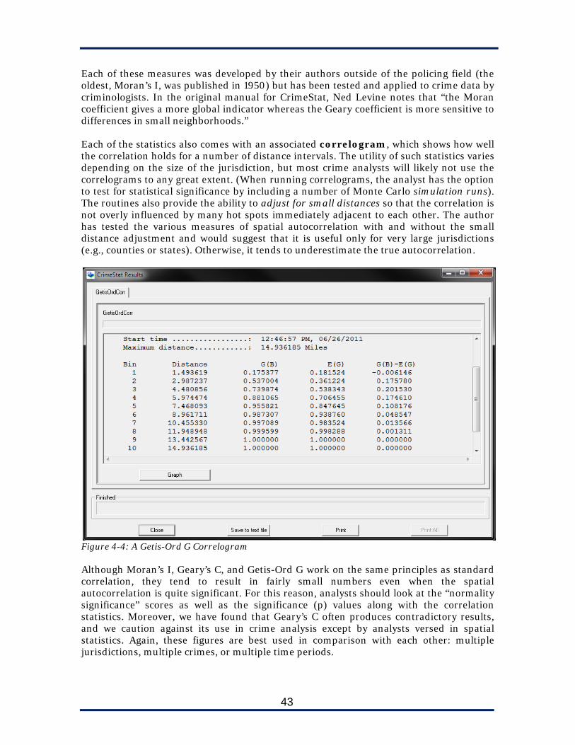
Each of these measures was developed by their authors outside of the policing field (the oldest, Moran’s I, was published in 1950) but has been tested and applied to crime data by criminologists. In the original manual for CrimeStat, Ned Levine notes that “the Moran coefficient gives a more global indicator whereas the Geary coefficient is more sensitive to differences in small neighborhoods.” Each of the statistics also comes with an associated correlogram, which shows how well the correlation holds for a number of distance intervals. The utility of such statistics varies depending on the size of the jurisdiction, but most crime analysts will likely not use the correlograms to any great extent. (When running correlograms, the analyst has the option to test for statistical significance by including a number of Monte Carlo simulation runs). The routines also provide the ability to adjust for small distances so that the correlation is not overly influenced by many hot spots immediately adjacent to each other. The author has tested the various measures of spatial autocorrelation with and without the small distance adjustment and would suggest that it is useful only for very large jurisdictions (e.g., counties or states). Otherwise, it tends to underestimate the true autocorrelation.

Figure 4-4: A Getis-Ord G Correlogram Although Moran’s I, Geary’s C, and Getis-Ord G work on the same principles as standard correlation, they tend to result in fairly small numbers even when the spatial autocorrelation is quite significant. For this reason, analysts should look at the “normality significance” scores as well as the significance (p) values along with the correlation statistics. Moreover, we have found that Geary’s C often produces contradictory results, and we caution against its use in crime analysis except by analysts versed in spatial statistics. Again, these figures are best used in comparison with each other: multiple jurisdictions, multiple crimes, or multiple time periods.

44

Step-by-Step Our goal in this lesson is to analyze the extent of clustering and dispersion for various incidents in Lincoln, Nebraska over a calendar year. This routine requires data aggregated at the polygon level; we are using a grid layer with the fields RESBURGS, ROBS, LMVS, PAROLEES, and NOISE indicating the numbers of residential burglaries, robberies, thefts from vehicles, parolees, and noise complaints in the given cells.

Step 1: View the grid.shp file in your GIS program and create a choropleth map for one or more of the variables above. Note the extent to which “hot” and “cold” cells do or do not lie close to each other.

Step 2: Launch CrimeStat. If it is already open, clear the active

primary file on the Data setup tab by selecting it and clicking “Remove.”

Step 3: Add grid.dbf as the primary file. Set the X coordinate to

CENTERX, the Y coordinate to CENTERY, and make sure the coordinate system is set to “projected” with the geographic unit in “feet.” Set the “Z (intensity)” variable to RESBURGS.

Figure 4-5: Setting up the grid.dbf file to run autocorrelation

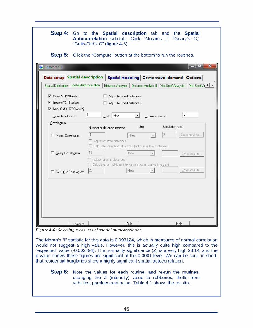
45

Step 4: Go to the Spatial description tab and the Spatial Autocorrelation sub-tab. Click “Moran’s I,” “Geary’s C,” “Getis-Ord’s G” (figure 4-6).

Step 5: Click the “Compute” button at the bottom to run the routines.

Figure 4-6: Selecting measures of spatial autocorrelation The Moran’s “I” statistic for this data is 0.093124, which in measures of normal correlation would not suggest a high value. However, this is actually quite high compared to the “expected” value (-0.002494). The normality significance (Z) is a very high 23.14, and the p-value shows these figures are significant at the 0.0001 level. We can be sure, in short, that residential burglaries show a highly significant spatial autocorrelation.

Step 6: Note the values for each routine, and re-run the routines, changing the Z (intensity) value to robberies, thefts from vehicles, parolees and noise. Table 4-1 shows the results.

46

Figure 4-7: Moran’s I results for thefts from vehicles in Lincoln, Nebraska.

Incident Type

Moran’s I I Z I Sig. Geary’s C C Z C Sig. Getis-Ord G

G Z G Sig.

Residential Burglary

0.0932 23.1639 0.0001 1.0335 3.2885 0.0010 0.0526 11.9237 0.0001

Robbery 0.0940 23.2917 0.0001 1.0672 6.6005 0.0001 0.1171 16.8670 0.0001 Thefts fm. Vehicles

0.1225 30.2403 0.0001 0.9900 -0.9768 N.S. 0.0481 12.6868 0.0001

Parolees 0.0350 9.0740 0.0001 1.0692 6.7928 0.0001 0.0336 5.4256 0.0001 Noise 0.0042 1.6213 0.1000 1.0100 0.9782 N.S. 0.0199 1.0748 N.S.

Table 4-1: Moran’s I, Geary’s C, and Getis-Ord G results for five variables The results for Moran’s I show that while all variables except noise complaints show a statistically significant autocorrelation, thefts from vehicles are the most strongly autocorrelated. As noted above, the Geary’s C routine produces contradictory results—indicating no correlation or negative correlations in all of the variables; we would have to conduct a detailed analysis of the correlogram to explain this, but it is, in our experience, par for the course with Geary’s C and, again, we caution against its use with most crime analysis data. The Getis-Ord G statistics mirror Moran’s I. Since all of the “Z” values are positive, the autocorrelation for each variable is due to hot spots and not “cold” spots. With the G statistic, noise complaints are not autocorrelated at any acceptable level of significance.

47

Distance Analysis Distance analysis uses a different set of measures than spatial autocorrelation, and it requires point data rather than data aggregated into polygons, but the overall concept is the same: to determine if incidents are more clustered than you would expect on the basis of chance. (Strictly speaking, distance analysis also tells you whether they are more dispersed than you would expect on the basis of chance, but this almost never happens with police data). CrimeStat offers two primary measures for distance analysis, both of which have several options and sub-calculations. These are nearest neighbor analysis (NNA) and Ripley’s K statistic. Both work with point data, as opposed to spatial autocorrelation, which works with polygon data. Nearest neighbor analysis (NNA) measures the distance of each point to its nearest neighbor, determines the mean distance, and compares the mean distance to what would have been expected in a random distribution. The user can control whether to compare each point to its single nearest neighbor or to run the routine against the second-nearest, third-nearest, and so on. NNA produces a calculation called the nearest neighbor index (NNI). In the NNI, a score of 1 would indicate absolutely no discrepancy between the expected distances in a random distribution and the measured distances in the actual distribution. Scores lower than 1 indicate that incidents are more clustered than would be expected in a random distribution, and scores higher than 1 indicate the incidents are more dispersed than would be expected in a random distribution. Significance levels are offered for the NNI. To calculate an expected random nearest neighbor distance, CrimeStat must know the total coverage area of the jurisdiction; hence, the “Coverage Area” parameter must be entered on the “Measurement Parameters” tab under “Data setup.” For its distance calculations; CrimeStat will use the settings (direct, indirect, network) on this same screen; different settings here can have a significant influence on the NNI. For instance, incidents that seem clustered using a linear measure may actually turn out to be fairly dispersed if we measure by the street network. It will come as no surprise to most crime analysts that many crime types—perhaps all—show statistically significant degrees of clustering. The average geographic area simply does not provide the conditions necessary for a truly random allocation of incidents. Housebreaks will not occur in locations with no houses, and will naturally be clustered in dense population centers. Business crimes cannot occur where there are no businesses, and will thus be concentrated in commercial areas. There will be few, if any, crimes in the middle of lakes and fields. “Hot spots” crop up for a variety of reasons all over the place. As with autocorrelation, the primary value for analysts is to conduct distance analysis for several datasets and compare the results to each other. This will help the analyst determine which offenses are most clustered into “hot spots,” and which are more randomly spread across the jurisdiction. These datasets can include multiple crimes, multiple time periods for the same crime, or multiple geographic areas.

48

Figure 4-8: The NNA output screen for house burglaries in Lincoln, Nebraska. Note that the NNI for the coverage area entered manually (0.3866) is slightly lower than the NNI for the coverage area CrimeStat calculated with a minimum bounding rectangle (0.4490). Both suggest a high degree of clustering among house burglaries, and both are significant at the 0.0001 level.

Step-by-Step In these lessons, we assess the degree of clustering or dispersion among three crimes in Lincoln, Nebraska, in 2007.

Step 1: Launch CrimeStat. On the “Data setup” tab, click “Select Files,” choose a Shapefile, and from your CrimeStat data directory, choose robberies.shp.

49

Step 2: Set the X and Y variables to “X” and “Y.” Make sure the “Type of coordinate system” is projected, in feet. On the “Measurement Parameters” tab, make sure that the coverage area is set to 177 square miles.

Step 3: On the “Spatial Description” tab, click on the “Distance

Analysis I” sub-tab. Check “Nearest neighbor analysis (Nna)” (figure 4-9).

Figure 4-9: Setting up nearest neighbor analysis.

Step 4: Click “Compute.” Note the results.

Step 5: Repeat Steps 1-4 with the resburglaries.shp and theftfromautos.shp files.

Table 4-2 shows the results you should receive.

Incident Type Actual Expected NNIRobbery 1066.8578 2655.0429 0.40182Residential Burglary 348.7187 902.0715 0.38658Thefts from Vehicles 236.2347 633.5914 0.37285

Table 4-2: Nearest neighbor index for three crimes.

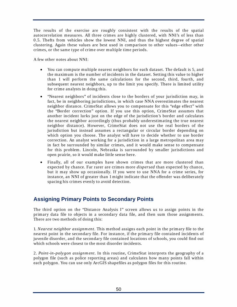
50

The results of the exercise are roughly consistent with the results of the spatial autocorrelation measures. All three crimes are highly clustered, with NNI’s of less than 0.5. Thefts from vehicles show the lowest NNI, and thus the highest degree of spatial clustering. Again these values are best used in comparison to other values—either other crimes, or the same type of crime over multiple time periods. A few other notes about NNI:

You can compute multiple nearest neighbors for each dataset. The default is 5, and the maximum is the number of incidents in the dataset. Setting this value to higher than 1 will perform the same calculations for the second, third, fourth, and subsequent nearest neighbors, up to the limit you specify. There is limited utility for crime analysts in doing this.

“Nearest neighbors” of incidents close to the borders of your jurisdiction may, in fact, be in neighboring jurisdictions, in which case NNA overestimates the nearest neighbor distance. CrimeStat allows you to compensate for this “edge effect” with the “Border correction” option. If you use this option, CrimeStat assumes that another incident lurks just on the edge of the jurisdiction’s border and calculates the nearest neighbor accordingly (thus probably underestimating the true nearest neighbor distance). However, CrimeStat does not use the real borders of the jurisdiction but instead assumes a rectangular or circular border depending on which option you choose. The analyst will have to decide whether to use border correction. An analyst working for a jurisdiction in a large metropolitan area may in fact be surrounded by similar crimes, and it would make sense to compensate for this problem. Lincoln, Nebraska is surrounded by smaller jurisdictions and open prairie, so it would make little sense here.

Finally, all of our examples have shown crimes that are more clustered than expected by chance. Far rarer are crimes more dispersed than expected by chance, but it may show up occasionally. If you were to use NNA for a crime series, for instance, an NNI of greater than 1 might indicate that the offender was deliberately spacing his crimes evenly to avoid detection.

Assigning Primary Points to Secondary Points The third option on the “Distance Analysis I” screen allows us to assign points in the primary data file to objects in a secondary data file, and then sum those assignments. There are two methods of doing this: 1. Nearest neighbor assignment. This method assigns each point in the primary file to the nearest point in the secondary file. For instance, if the primary file contained incidents of juvenile disorder, and the secondary file contained locations of schools, you could find out which schools were closest to the most disorder incidents. 2. Point-in-polygon assignment. In this routine, CrimeStat interprets the geography of a polygon file (such as police reporting areas) and calculates how many points fall within each polygon. You can use only ArcGIS shapefiles as polygon files for this routine.

51

The distinction between the two is important. In the simplified diagram in figure 4-10, showing precinct boundaries and locations of station houses

Point 1 is in Precinct 2’s boundaries and is also closest to the Precinct 2 station house.

Point 2 is in Precinct 1’s boundaries but is actually closest to the Precinct 3 station house.

Figure 4-10: The difference between point-in-polygon and nearest neighbor assignment. In other words, nearest neighbor assignment would assign Point 2 to Precinct 3, whereas point-in-polygon assignment would assign it to Precinct 1. Most GIS systems will perform point-in-polygon assignments (both ArcGIS and MapInfo do it quite easily), but very few perform nearest neighbor assignments without special scripts. The outputs of the two routines are dBASE (.dbf) files, with the geographic coordinates, the associated data from the secondary file, and the count of records in the primary file (in a field called “FREQ”). You can open these .dbf files in your GIS application, plot the results, and use them to create graduated or proportional symbol maps.

52

Step-by-Step In these lessons, we look at a problem of afternoon residential burglaries in Lincoln. We will first use a point-in-polygon assignment to count the number of afternoon residential burglaries in each grid cell and make a graduated symbol map based on it. Afterwards, we analyze a hypothesis that these burglaries are students on their way home from school.

Step 1: Add the afternoonhousebreaks.dbf file to your GIS program and plot the incidents based on the X and Y fields. Note the spatial distribution.

Step 2: In CrimeStat, add the afternoonhousebreaks.dbf to the

“Primary File” screen. Set the X and Y coordinates to those fields, and tell CrimeStat that it uses a projected coordinate system in feet.

Step 3: On the “Secondary File” screen, add the grid.dbf file. Set the

X and Y fields to “CENTERX” and “CENTERY,” respectively. Step 4: Click on “Spatial description” and then “Distance Analysis I.”

Click the “Assign primary points to secondary points” option, and choose “Point in polygon” as the method of assignment. Load grid.shp as the “Zone file” (figure 4-11).

Step 5: Click the “Save Result To” button and save the result in your

data directory as ahbgrid.dbf.

Step 6: Click “Compute” to run the routine. Load the resulting .dbf file into your GIS program and create a graduated or proportional symbol map to visualize the results.

This routine has a somewhat limited utility since it results in a .dbf file instead of a shapefile based on the original polygons. Thus, creating a choropleth based on this data will require a spatial join with the original polygon file, and if we wanted to do a spatial join, we could have done it with the original afternoonhousebreaks.dbf file and skipped the step of going into CrimeStat. Nearest neighbor assignment is more valuable, since no out-of-the-box GIS routine will accomplish it.

Step 7: In CrimeStat, return to the “Secondary File” screen and remove the grid.dbf file. Replace it with the schools.dbf file in your data directory. Set the X coordinate to “CENTROIDX” and the Y coordinate to “CENTROIDY.”

Step 8: Click on the “Spatial description” tab and the “Distance

Analysis I” sub-tab. Check “Assign primary points to secondary points” (if not already checked from the previous routine) and choose the “nearest neighbor” method.

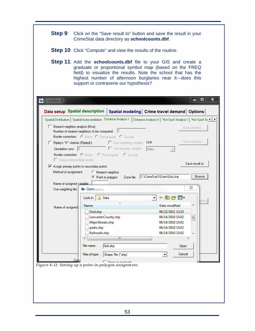
53

Step 9: Click on the “Save result to” button and save the result in your CrimeStat data directory as schoolcounts.dbf.

Step 10: Click “Compute” and view the results of the routine. Step 11: Add the schoolcounts.dbf file to your GIS and create a

graduate or proportional symbol map (based on the FREQ field) to visualize the results. Note the school that has the highest number of afternoon burglaries near it—does this support or contravene our hypothesis?

Figure 4-11: Setting up a point-in-polygon assignment.

54

Figure 4-12: A graduated symbol map of afternoon housebreaks by grid cell.

Figure 4-13: The result of assigning primary points to secondary points Assigning primary points to secondary points is more of a utility than a spatial statistics routine, but it does help significantly in preparing files for routines that require aggregated data, such as spatial autocorrelation.

55

The routines covered in this chapter have in common the measuring of distances between points, whether individual data points or polygon center points. In the case of spatial autocorrelation and nearest neighbor analysis, this is done to assess the extent of clustering or dispersion. Although the results of these routines do not identify specific hot spots, and thus lack utility for regular operational purposes, they can be valuable for broad profiles of a jurisdiction, trend analysis, and evaluation. Moreover, knowing a little about how distance analysis works helps us better understand what happens in Chapters 5 and 6, with hot spot analysis (particularly Nearest Neighbor Hierarchical Spatial Clustering, which builds directly on Nearest Neighbor Analysis) and kernel density estimation. Summary

Autocorrelation and nearest neighbor analysis both assess the extent of clustering or dispersion among variables, such as crime incidents or offender addresses.

Autocorrelation requires data aggregated into polygons, while nearest neighbor analysis requires individual points.

There are three measures of autocorrelation in CrimeStat: Moran’s I, Geary’s C, and Getis-Ord G. Each operates on a slightly different scale but accomplishes the same general purpose. Moran and Geary can test both positive and negative autocorrelation. Getis-Ord can only test positive correlation but it can also determine whether the correlation is due to many hot spots or many cold spots.

Nearest Neighbor Analysis compares the actual distribution of points to what would be expected on the basis of random chance. It does not actually identify clusters, but it forms the basis for Nearest Neighbor Hierarchical Spatial Clustering, a technique covered in the next chapter.

CrimeStat has utilities that assign points from one file to points in another file, based either on whether they fall in a polygon, or on proximity.

For Further Reading Levine, N. (2005). Chapter 4: Spatial distribution. In CrimeStat III: A spatial statistics


Levine, N. (2005). Chapter 5: Distance analysis I and II. In CrimeStat III: A spatial


56

57

5

Hot Spot Analysis Identifying Concentrations of Crime

In the last chapter, we looked at some routines that tell us how clustered our incidents are compared to what we would expect in a random distribution. We also saw that this statistic offered limited utility to the analyst. In this chapter, we look at routines that do something a lot more useful: actually identify hot spots. A hot spot is a spatial concentration of crime. Crime analysts and criminologists have rarely tried to come up with a definition more precise than that. A NIJ special report on hot spot notes that researchers and police have applied the term to specific addresses, street segments, blocks, and block clusters. They conclude:

Though common definition of the term “hot spot of crime” exists, the common understanding is that a hot spot is an area that has a greater than average number of criminal or disorder events, or an area where people have a higher than average risk of victimization.7

For the purpose of spatial statistics, however, both the terms “area” and “higher than average” seem too vague. We would propose a more limited definition for use when considering these routines: a geographic area representing a small percentage of the study area which contains a high percentage of the studied phenomenon. The scale of the “spot” depends on the scale of the study area: in a city, a hot spot might be an address, building, complex, parking lot, block, park, or some other relatively small area. In a state, however, a hot spot might be an entire city. The definition is still quite vague because “small percentage” and “high percentage” can include quite a large range of numbers, but this is as precise as we can get and still include most of the routines in CrimeStat and theories in the available literature. In both GIS and spatial statistics programs, hot spots are identified and displayed through one of two primary means:

Aggregation. Points can be aggregated (generally just counted, but sometimes also weighted) by specific address, street segment, grid cell, beat, census block, or some other unit of geography. CrimeStat’s mode and fuzzy mode routines are methods of aggregation, as are choropleth maps. Anselin’s Local Moran statistic relies on aggregation by geographic zone.

Adaptive scan. Scanning methods do not attempt to summarize or aggregate

points in reference to another object. Rather, they leave the points where they are and create polygons of varying sizes to encompass points with dense concentrations. CrimeStat’s Nearest Neighbor Hierarchical Spatial Clustering, STAC, and K-means Clustering routines are examples of scans.

7 Eck, J. E., Chainey, S., Cameron, J. G., Leitner, M., & Wilson, R. (2005). Mapping crime: Understanding hot spots. Washington, DC: U.S. Department of Justice, National Institute of Justice, p. 2.

58

Figure 5-1: Choropleth mapping and graduated symbol mapping aggregate points into hot spots. Maps taken from Velasco, M., & Boba, R. (2000). Manual of crime analysis map production. Washington, DC: U.S. Department of Justice, Office of Community-Oriented Policing Services.

Figure 5-2: Adaptive methods expand and contract the size of the hot spots to fit the specific points that make them up. CrimeStat has a number of routines to study different types of hot spots:

1. Mode: identifies the geographic coordinates with the highest number of incidents.

2. Fuzzy Mode: identifies the geographic coordinates, plus a user-specified surrounding radius, with the highest number of incidents.

3. Nearest-Neighbor Hierarchical Spatial Clustering: builds on the nearest neighbor analysis (NNA) that we saw in Chapter 4 by identifying clusters of incidents.

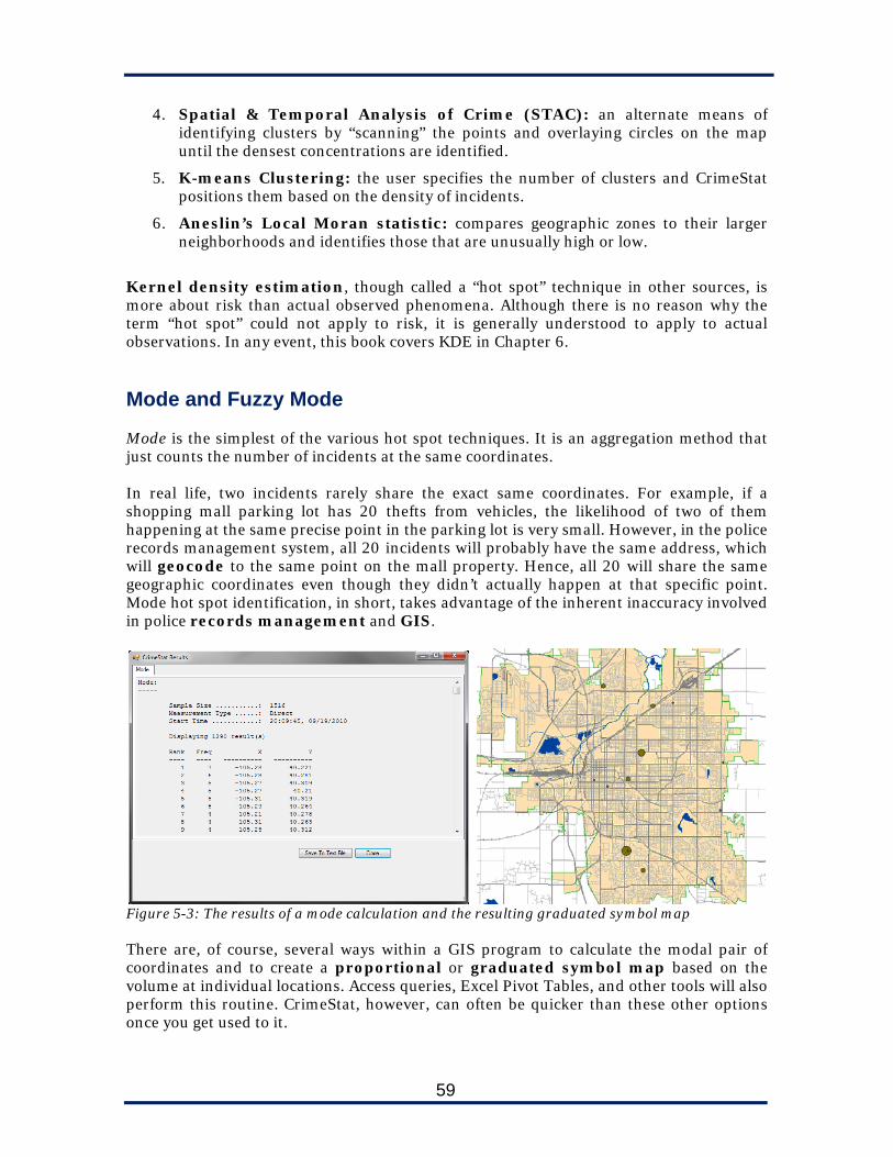
59

4. Spatial & Temporal Analysis of Crime (STAC): an alternate means of identifying clusters by “scanning” the points and overlaying circles on the map until the densest concentrations are identified.

5. K-means Clustering: the user specifies the number of clusters and CrimeStat positions them based on the density of incidents.

6. Aneslin’s Local Moran statistic: compares geographic zones to their larger neighborhoods and identifies those that are unusually high or low.

Kernel density estimation, though called a “hot spot” technique in other sources, is more about risk than actual observed phenomena. Although there is no reason why the term “hot spot” could not apply to risk, it is generally understood to apply to actual observations. In any event, this book covers KDE in Chapter 6. Mode and Fuzzy Mode Mode is the simplest of the various hot spot techniques. It is an aggregation method that just counts the number of incidents at the same coordinates. In real life, two incidents rarely share the exact same coordinates. For example, if a shopping mall parking lot has 20 thefts from vehicles, the likelihood of two of them happening at the same precise point in the parking lot is very small. However, in the police records management system, all 20 incidents will probably have the same address, which will geocode to the same point on the mall property. Hence, all 20 will share the same geographic coordinates even though they didn’t actually happen at that specific point. Mode hot spot identification, in short, takes advantage of the inherent inaccuracy involved in police records management and GIS.

Figure 5-3: The results of a mode calculation and the resulting graduated symbol map There are, of course, several ways within a GIS program to calculate the modal pair of coordinates and to create a proportional or graduated symbol map based on the volume at individual locations. Access queries, Excel Pivot Tables, and other tools will also perform this routine. CrimeStat, however, can often be quicker than these other options once you get used to it.

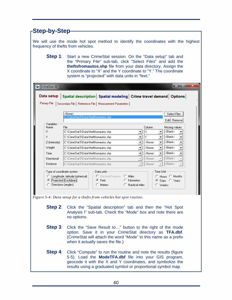
60

Step-by-Step We will use the mode hot spot method to identify the coordinates with the highest frequency of thefts from vehicles.

Step 1: Start a new CrimeStat session. On the “Data setup” tab and the “Primary File” sub-tab, click “Select Files” and add the theftsfromautos.shp file from your data directory. Assign the X coordinate to “X” and the Y coordinate to “Y.” The coordinate system is “projected” with data units in “feet.”

Figure 5-4: Data setup for a thefts from vehicles hot spot routine.

Step 2: Click the “Spatial description” tab and then the “Hot Spot Analysis I” sub-tab. Check the “Mode” box and note there are no options.

Step 3: Click the “Save Result to…” button to the right of the mode

option. Save it in your CrimeStat directory as TFA.dbf. (CrimeStat will attach the word “Mode” to this name as a prefix when it actually saves the file.)

Step 4: Click “Compute” to run the routine and note the results (figure

5-5). Load the ModeTFA.dbf file into your GIS program, geocode it with the X and Y coordinates, and symbolize the results using a graduated symbol or proportional symbol map.

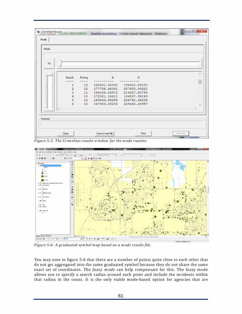
61

Figure 5-5: The CrimeStat results window for the mode routine.

Figure 5-6: A graduated symbol map based on a mode results file. You may note in figure 5-6 that there are a number of points quite close to each other that do not get aggregated into the same graduated symbol because they do not share the same exact set of coordinates. The fuzzy mode can help compensate for this. The fuzzy mode allows you to specify a search radius around each point and include the incidents within that radius in the count. It is the only viable mode-based option for agencies that are

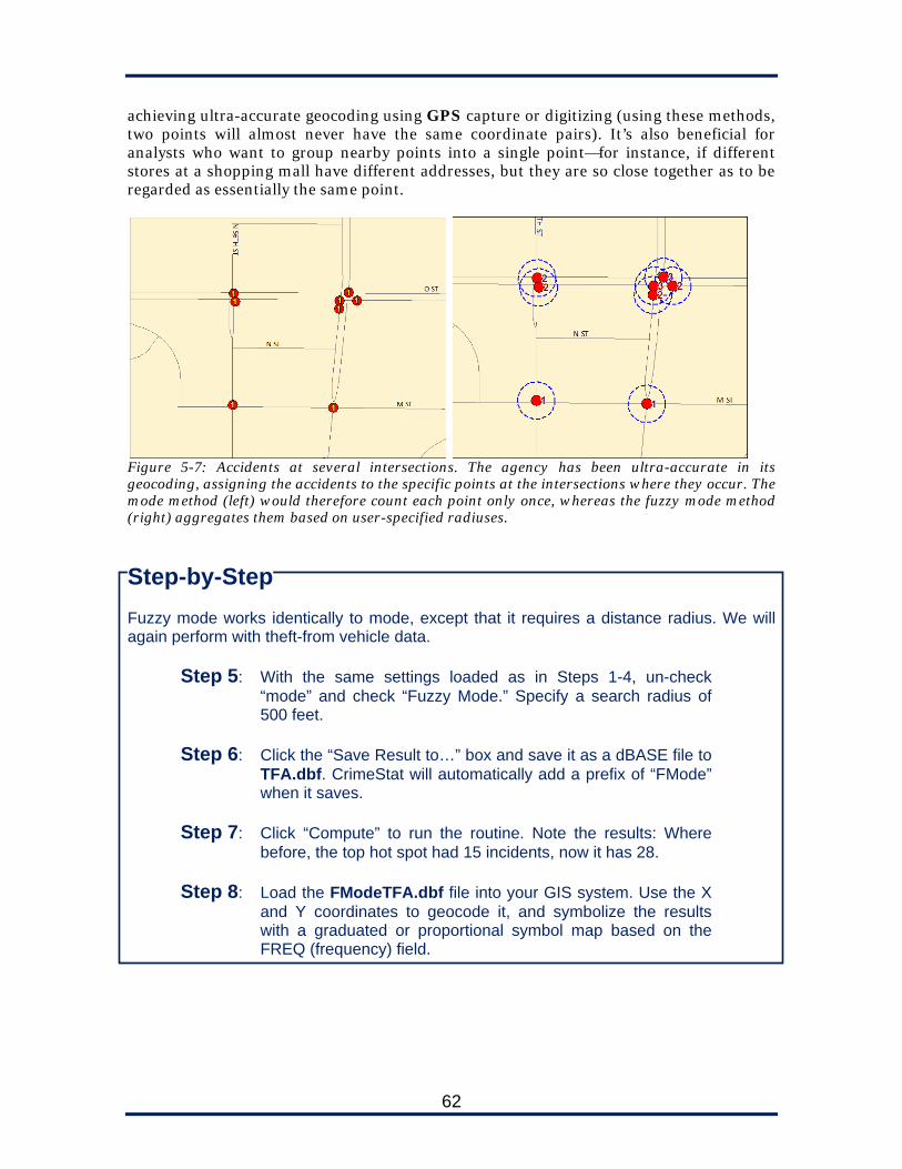
62

achieving ultra-accurate geocoding using GPS capture or digitizing (using these methods, two points will almost never have the same coordinate pairs). It’s also beneficial for analysts who want to group nearby points into a single point—for instance, if different stores at a shopping mall have different addresses, but they are so close together as to be regarded as essentially the same point.

Figure 5-7: Accidents at several intersections. The agency has been ultra-accurate in its geocoding, assigning the accidents to the specific points at the intersections where they occur. The mode method (left) would therefore count each point only once, whereas the fuzzy mode method (right) aggregates them based on user-specified radiuses.

Step-by-Step Fuzzy mode works identically to mode, except that it requires a distance radius. We will again perform with theft-from vehicle data.

Step 5: With the same settings loaded as in Steps 1-4, un-check “mode” and check “Fuzzy Mode.” Specify a search radius of 500 feet.

Step 6: Click the “Save Result to…” box and save it as a dBASE file to

TFA.dbf. CrimeStat will automatically add a prefix of “FMode” when it saves.

Step 7: Click “Compute” to run the routine. Note the results: Where

before, the top hot spot had 15 incidents, now it has 28. Step 8: Load the FModeTFA.dbf file into your GIS system. Use the X

and Y coordinates to geocode it, and symbolize the results with a graduated or proportional symbol map based on the FREQ (frequency) field.

63

Figure 5-8: The results window for the fuzzy mode routine in CrimeStat.

Figure 5-9: Thefts from cars in Lincoln using the fuzzy mode One major disadvantage to fuzzy mode becomes apparent when we map the results (figure 5-9). Because CrimeStat calculates a radius and count for every point, points close together will fall in one another’s radii. In areas of very dense concentration, this will result in multiple hot spots that are all counting each other.

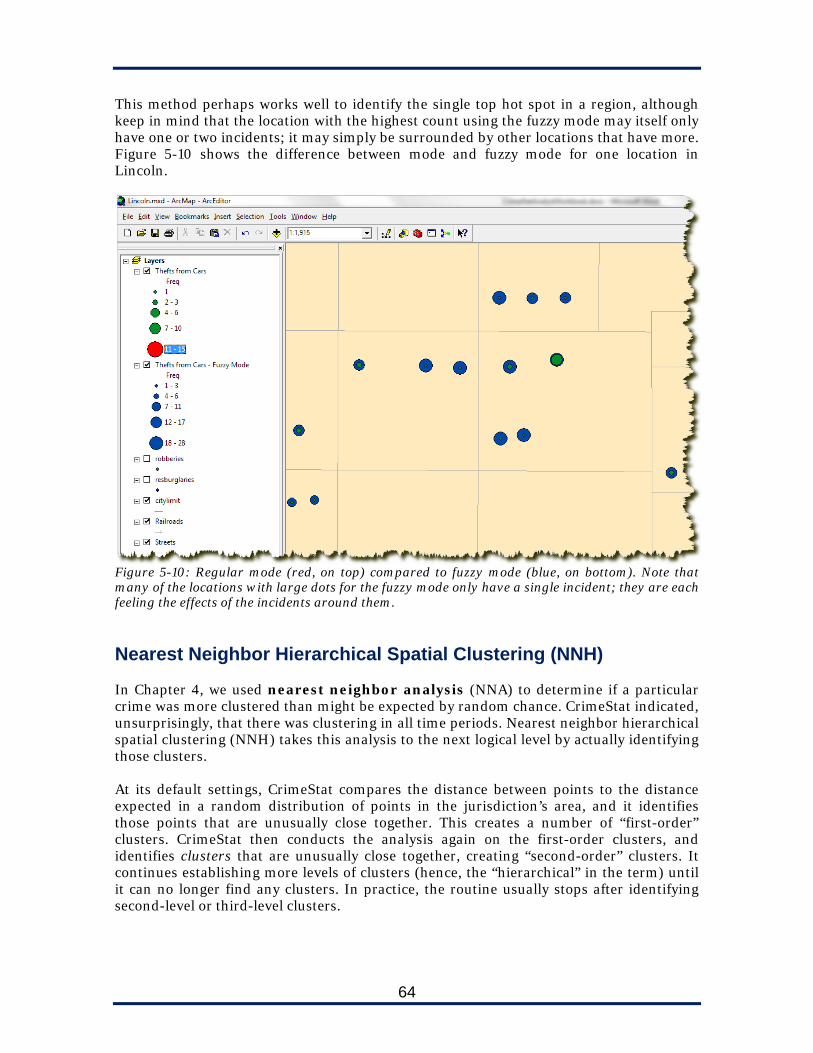
64

This method perhaps works well to identify the single top hot spot in a region, although keep in mind that the location with the highest count using the fuzzy mode may itself only have one or two incidents; it may simply be surrounded by other locations that have more. Figure 5-10 shows the difference between mode and fuzzy mode for one location in Lincoln.

Figure 5-10: Regular mode (red, on top) compared to fuzzy mode (blue, on bottom). Note that many of the locations with large dots for the fuzzy mode only have a single incident; they are each feeling the effects of the incidents around them. Nearest Neighbor Hierarchical Spatial Clustering (NNH) In Chapter 4, we used nearest neighbor analysis (NNA) to determine if a particular crime was more clustered than might be expected by random chance. CrimeStat indicated, unsurprisingly, that there was clustering in all time periods. Nearest neighbor hierarchical spatial clustering (NNH) takes this analysis to the next logical level by actually identifying those clusters. At its default settings, CrimeStat compares the distance between points to the distance expected in a random distribution of points in the jurisdiction’s area, and it identifies those points that are unusually close together. This creates a number of “first-order” clusters. CrimeStat then conducts the analysis again on the first-order clusters, and identifies clusters that are unusually close together, creating “second-order” clusters. It continues establishing more levels of clusters (hence, the “hierarchical” in the term) until it can no longer find any clusters. In practice, the routine usually stops after identifying second-level or third-level clusters.

65

CrimeStat will create both standard deviation ellipses and convex hulls (see Chapter 3) around the hot spots it identifies. You can then import these into your GIS for display and analysis.

Figure 5-11: An NNH map of residential burglary hot spots in Lincoln, Nebraska, color-coded by volume, with a minimum of 10 points per cluster. Note the one second-order cluster encircling ten first-order clusters. There are a number of options that the user can tweak when running NNH.

Instead of basing the threshold distance on the expectations of a random distribution, the user can specify a fixed distance. Although it looks like a minor setting, switching to a user-defined threshold substantially alters the nature of the technique: instead of an objective measure based on probability, it becomes a subjective measure based on the analyst’s own judgment. However, this can be useful if you already know the operational purpose of the map and you want to tailor the size of the hot spots to fit that purpose (e.g., a large search radius for neighborhood warning posters, a smaller one for foot patrol, and a very small one for stakeouts).

Even if two points are related in a “cluster,” an analyst probably won’t be interested in seeing that cluster among thousands of data points. The minimum points per cluster option allows you to reduce the number of identified clusters by specifying a minimum number of incidents within each one. The default is set at 10.

By default, the routine identifies clusters that have less than a 50% chance of being randomly allocated. In other words, there is only a 50% chance that the points are

66

indeed a “cluster” and not a statistical fluke. By adjusting the search radius bar, you can adjust the threshold and therefore the associated probability. (This works only for the “Random NN distance” option.) At the furthest position to the left, CrimeStat uses the smallest distance but offers a 99.999% confidence of a true cluster; at the furthest position to the right, it uses the largest distance but offers only a 0.1% confidence of a true cluster. If the analyst was studying all clusters, including pairs, he or she would probably want to lower the bar to the fifth position, which represents a 95% confidence level—the standard significance test in most social science applications. In practice, however, the “minimum number of points” setting greatly reduces the likelihood that CrimeStat will identify “false positives” in its NNH analysis. We recommend leaving the bar at its default setting.

Figure 5-12: The Hot Spot Analysis I screen with various NNH options. If you’re outputting your results as ellipses, you’ll need to specify the number of

standard deviations for the ellipses. (CrimeStat calculates the mean center and 1-2 standard deviations for all the points that make up the hot spot, much as in spatial distribution). A single standard deviation, the default, creates small ellipses that can be hard to view at a small map scale. On the other hand, two standard

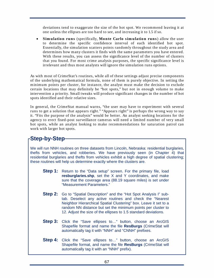
67

deviations tend to exaggerate the size of the hot spot. We recommend leaving it at one unless the ellipses are too hard to see, and increasing it to 1.5 if so.

Simulation runs (specifically, Monte Carlo simulation runs) allow the user to determine the specific confidence interval of each identified hot spot. Essentially, the simulation scatters points randomly throughout the study area and determines how many clusters it finds with the same parameters you have entered. With these results, you can assess the significance level of the number of clusters that you found. For most crime analysis purposes, the specific significance level is irrelevant and thus most analysts will ignore the simulation runs options.

As with most of CrimeStat’s routines, while all of these settings adjust precise components of the underlying mathematical formula, none of them is purely objective. In setting the minimum points per cluster, for instance, the analyst must make the decision to exclude certain locations that may definitely be “hot spots,” but not in enough volume to make intervention a priority. Small tweaks will produce significant changes in the number of hot spots identified and their relative sizes. In general, the CrimeStat manual warns, “the user may have to experiment with several runs to get a solution that appears right.” “Appears right” is perhaps the wrong way to say it. “Fits the purpose of the analysis” would be better. An analyst seeking locations for the agency to erect fixed-post surveillance cameras will need a limited number of very small hot spots, while an analyst looking to make recommendations for saturation patrol can work with larger hot spots.

Step-by-Step We will run NNH routines on three datasets from Lincoln, Nebraska: residential burglaries, thefts from vehicles, and robberies. We have previously seen (in Chapter 4) that residential burglaries and thefts from vehicles exhibit a high degree of spatial clustering; these routines will help us determine exactly where the clusters are.

Step 1: Return to the “Data setup” screen. For the primary file, load resburglaries.shp, set the X and Y coordinates, and make sure that the coverage area (88.19 square miles) is set under “Measurement Parameters.”

Step 2: Go to “Spatial Description” and the “Hot Spot Analysis I” sub-

tab. Deselect any active routines and check the “Nearest Neighbor Hierarchical Spatial Clustering” box. Leave it set to a random NN distance but set the minimum points per cluster to 12. Adjust the size of the ellipses to 1.5 standard deviations.

Step 3: Click the “Save ellipses to…” button, choose an ArcGIS

Shapefile format and name the file ResBurgs (CrimeStat will automatically tag it with “NNH” and “CNNH” prefixes.

Step 4: Click the “Save ellipses to…” button, choose an ArcGIS

Shapefile format, and name the file ResBurgs (CrimeStat will automatically tag it with an “NNH” prefix).

68

Step 5: Click the “Save convex hulls to…” button, choose an ArcGIS Shapefile format, and name the file ResBurgs (CrimeStat will automatically tag It with a “CNNH” prefix).

Step 6: Click “Compute” to run the routine. Note in the results window

(figure 5-13) that CrimeStat finds 22 hot spots: 20 first-order clusters and two second-order clusters.

Figure 5-13: The results window for the NNH routine.

Step 7: Add the following files to your Lincoln GIS project: CNNH1ResBurgs.shp, CNNH2ResBurgs.shp, NNH1ResBurgs.ship, NNH2ResBurgs.shp. You may want to symbolize CNNH1 and NNH1 with a graduated color map using the “FREQ” field (figure 5-14).

Step 8: Return to CrimeStat and run the routine again after making

adjustments any of the settings used in this lesson. Note the effects of these changes on the map (which you just need to refresh in your GIS project).

Step 9: If desired, repeat Steps 1-8 with the theftsfromautos.shp and

the robberies.shp files.

As you study the results of the NNH clustering, you will probably want to choose between the ellipses and the convex hulls. Keep in mind that while the ellipses are more eye-pleasing objects, graphically, the convex hulls are more precise in that they fully encompass all the points, and only the points, that make up an identified hot spot.

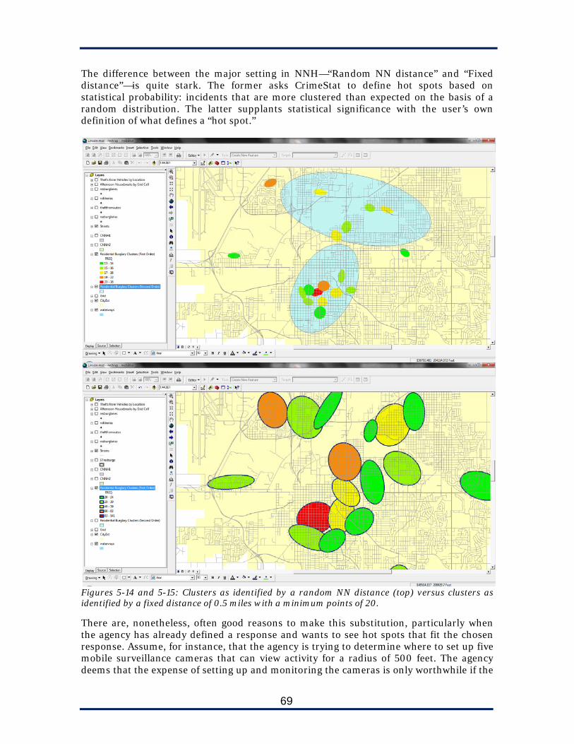
69

The difference between the major setting in NNH—“Random NN distance” and “Fixed distance”—is quite stark. The former asks CrimeStat to define hot spots based on statistical probability: incidents that are more clustered than expected on the basis of a random distribution. The latter supplants statistical significance with the user’s own definition of what defines a “hot spot.”

Figures 5-14 and 5-15: Clusters as identified by a random NN distance (top) versus clusters as identified by a fixed distance of 0.5 miles with a minimum points of 20.

There are, nonetheless, often good reasons to make this substitution, particularly when the agency has already defined a response and wants to see hot spots that fit the chosen response. Assume, for instance, that the agency is trying to determine where to set up five mobile surveillance cameras that can view activity for a radius of 500 feet. The agency deems that the expense of setting up and monitoring the cameras is only worthwhile if the

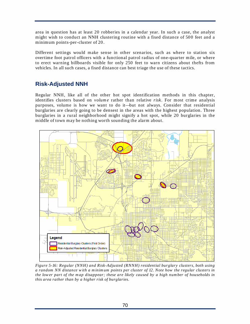
70

area in question has at least 20 robberies in a calendar year. In such a case, the analyst might wish to conduct an NNH clustering routine with a fixed distance of 500 feet and a minimum points-per-cluster of 20. Different settings would make sense in other scenarios, such as where to station six overtime foot patrol officers with a functional patrol radius of one-quarter mile, or where to erect warning billboards visible for only 250 feet to warn citizens about thefts from vehicles. In all such cases, a fixed distance can best triage the use of these tactics. Risk-Adjusted NNH Regular NNH, like all of the other hot spot identification methods in this chapter, identifies clusters based on volume rather than relative risk. For most crime analysis purposes, volume is how we want to do it—but not always. Consider that residential burglaries are clearly going to be densest in the areas with the highest population. Three burglaries in a rural neighborhood might signify a hot spot, while 20 burglaries in the middle of town may be nothing worth sounding the alarm about.

Figure 5-16: Regular (NNH) and Risk-Adjusted (RNNH) residential burglary clusters, both using a random NN distance with a minimum points per cluster of 12. Note how the regular clusters in the lower part of the map disappear; these are likely caused by a high number of households in this area rather than by a higher risk of burglaries.

71

CrimeStat offers one technique to normalize hot spots this way: Risk-Adjusted Nearest Neighbor Hierarchical Spatial Clustering (RNNH). It relies on a secondary file containing some kind of denominator—perhaps the number of houses when studying housebreaks, or the number of parking spaces when studying auto thefts. A census block layer with population totals is a common example, although not suitable for all crimes. To perform the risk adjustment, CrimeStat smoothes the data from a point file using the same routines as Kernel Density Estimation, which this book covers in Chapter 6. We will refer you to that chapter for an understanding of methods of interpolation, choice of bandwidth, and other KDE settings.

Step-by-Step For RNNH, we will look at residential burglaries divided by the number of households in the underlying area. The secondary file used for this denominator is a layer of census block centerpoints.

Step 1: Start a new CrimeStat session. For the “Primary File,” add resburglaries.shp. Set the X and Y coordinates and make sure you set the type of coordinate system as “Projected.”

Step 2: Move to the “Secondary File” screen. Load the

censusblocks.dbf file and set the X and Y coordinates to the fields of those names. For the “Z (Intensity)” variable, set the HOUSEHOLDS field.

Figure 5-17: Setting up a secondary file. Note that coordinate system options are unavailable, as it must have the same system as the primary file.

72

Step 3: On the “Measurement Parameters” screen, make sure the coverage area is set to 88 square miles.

Step 4: Move to the “Spatial description” tab and the “Hot Spot

Analysis I” sub-tab. Check the “Nearest-Neighbor Hierarchical Spatial Clustering” box and the “Risk-adjusted” box beneath it. Also check “Use intensity variable on secondary file.”

Step 5: Click the “Risk Parameters” button. Choose a “Uniform”

method of interpolation with a “Fixed Interval” bandwidth of 0.5 miles (you will learn more about these settings in Chapter 6). Click “OK.”

Figure 5-18: Setting the parameters for a risk-adjusted NNH.

Step 6: Click the “Save ellipses to…” and “Save convex hulls to…” buttons and save both in your data directory as Shapefiles with the name ResBurgs. CrimeStat will automatically attach “RNNH” and “CRNNH” as prefixes.

73

Step 7: Set the number of standard deviations for the ellipses to 1.5

and the minimum points per cluster to 12. Step 8: Click “Compute” to run the routine. Add the resulting

Shapefiles to your GIS map and note the differences between the risk-adjusted hot spots and the regular hot spots.

There are times in which you will want to look only at raw volume, and times that you will want to consider the underlying risk, depending on the purposes of the map. If your agency intends to perform directed patrols or other targeted enforcement, you will probably go to where the highest volume is, regardless of the risk. But to identify areas in need of a community- or problem-oriented policing focus, risk-adjusted maps may tell a more valid story. Spatial and Temporal Analysis of Crime (STAC) STAC was originally developed as a separate program for the Illinois Criminal Justice Information Authority by Richard and Carolyn Block. CrimeStat integrated it in Version 2. Like NNH, STAC produces ellipses and convex hulls but uses a different method for generating them. The original STAC included two routines: Time Analyzer and Space Analyzer8. Only the Space Analyzer is included in CrimeStat and Crime. Hence, despite the word “temporal” in its name, there is no temporal aspect to the STAC routine in CrimeStat. STAC’s algorithm scans the data by placing a series of overlapping circles (the radius specified by the user) on top of the points on your map and counting the number of points it finds in the radius. Each time it finds a radius with the minimum number of points per cluster, it records that location. If multiple polygons with the minimum number of points overlap, it aggregates them into a single polygon. Thus, hot spots may vary in size. STAC offers some of the same parameters as a fixed-interval NNH, including the search radius, the minimum number of points per cluster, and the number of standard deviations for the ellipses. As with fixed-interval NNH clusters, it makes sense to approach the question of size with the ultimate uses in mind: larger clusters for vehicle patrol, for instance, and smaller ones for foot patrol. The grid that STAC overlays on the map is 20 x 20 no matter how large the area. Thus, analysts may want to create several reference files—perhaps one for each police district—and run STAC in these more limited areas one by one, thus increasing the chances of finding hot spots. Finally, when running STAC, the scan type can make a large difference in the resulting map. For guidance, the authors of STAC offer that the user should use a rectangular scan

8 Illinois Criminal Justice Information Authority. (2009). STAC facts. Retrieved September 20, 2010, from http://www.icjia.state.il.us/public/index.cfm?metasection=Data&metapage=StacFacts

74

type for areas with a gridded street pattern and a triangular scan type for areas with an irregular street pattern. The analyst should try both methods with his or her data and choose the one that consistently produces the most valid result.

Figure 5-19: STAC searches for hot spots by scanning the centerpoints of grid cells with the user-defined search radius and identifying those with the user-defined minimum points.

Step-by-Step We’ll use STAC to identify theft-from-vehicle hot spots in Lincoln.

Step 1: Start a new CrimeStat session. For the “Primary File,” add theftfromautos.shp. Set the X and Y coordinates and make sure you set the type of coordinate system as “Projected.”

Step 2: Go to the “Spatial Description” tab and the “Hot Spot Analysis

II” sub-tab. Check “Spatial and Temporal Analysis of Crime (STAC).”

Step 3: Click the “STAC Parameters” button. Set an initial search

radius of 0.25 miles and 25 minimum points per cluster. If you still have the reference file set from the previous lesson, leave the “boundary” option set to “From reference file.” Otherwise, change it to “From data set.” Because Lincoln has an irregular street pattern, we will set the scan type to “Triangular.” Finally, set the standard deviation ellipses to 1.5. Click “OK.”

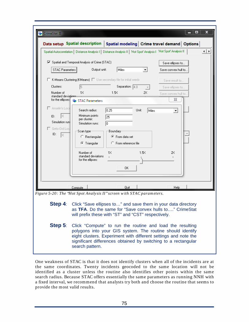
75

Figure 5-20: The “Hot Spot Analysis II” screen with STAC parameters.

Step 4: Click “Save ellipses to…” and save them in your data directory as TFA. Do the same for “Save convex hulls to….” CrimeStat will prefix these with “ST” and “CST” respectively.

Step 5: Click “Compute” to run the routine and load the resulting

polygons into your GIS system. The routine should identify eight clusters. Experiment with different settings and note the significant differences obtained by switching to a rectangular search pattern.

One weakness of STAC is that it does not identify clusters when all of the incidents are at the same coordinates. Twenty incidents geocoded to the same location will not be identified as a cluster unless the routine also identifies other points within the same search radius. Because STAC offers essentially the same parameters as running NNH with a fixed interval, we recommend that analysts try both and choose the routine that seems to provide the most valid results.

76

Figure 5-21: STAC identifies eight clusters with at least 25 thefts from vehicles within a 0.25 mile radius. K-means Clustering K-means, despite its location on CrimeStat’s screens (and in this book) is less a “hot spot” method than a partitioning method. In some ways, it is the opposite of the routines discussed so far. Instead of specifying parameters and generating a varying number of polygons based on the parameters, with K-means, the user specifies the number of polygons and CrimeStat “finds” hot spots equal to that number. To run K-means, CrimeStat places a grid over the surface of the map and counts the number of points in each grid cell. The top k (user specified number) cells become the centerpoints of k polygons. CrimeStat then assigns each point on the map to the closest centerpoint and runs a series of adjustments to keep large clusters of incidents in the same polygon. To prevent groupings too close to each other, CrimeStat uses a separation value: the higher the separation, the higher the minimum distance between the initial choices for polygon locations. K-means is often used by commercial enterprises and government planning organizations to identify the optimal locations for stores, social service locations, and government facilities based on the distributions of population. It has potential uses in operations analysis (identifying best locations for police facilities and districts), but the scenario in which most analysts will use it is when the police agency knows that it will be deploying k teams or units to combat a particular problem, and it needs to create zones for the

77

deployments. The result of the routine will be k polygons in which the densest clustering should occur roughly in the polygon center. There are only three settings in K-means:

Number of clusters (k). This is the number of clusters or zones the analyst wishes to identify.

Separation value. A higher value ensures greater separation of the cluster centerpoints as CrimeStat begins the search. Theoretically, this decreases the odds that particularly dense concentrations of crime will be split into multiple clusters, although the final result depends largely on the original distribution of points. The specific number is related to an exponent in a formula and does not have any direct meaning (e.g., “7” does not signify 7 miles); simply think of the numbers as a scale from 1 to 10.

Number of standard deviations for the ellipses. This works much as in Nearest-Neighbor Hierarchical Spatial Clustering and spatial distribution. However as we will see, the convex hulls become a much better way to visualize the results of K-means.

Step-by-Step We will remain with thefts from vehicles and imagine that, to combat the problem, the Lincoln Police Department is deploying 10 squads on directed patrols during peak times. We will use K-means to identify the best locations for those patrols.

Step 1: Start a new CrimeStat session. For the “Primary File,” add theftfromautos.shp. Set the X and Y coordinates and make sure you set the type of coordinate system as “Projected.”

Step 2: Go to the “Spatial Description” tab and the “Hot Spot Analysis

II” sub-tab. Check “K-Means” Clustering. Step 3: Set the number of clusters to 10 and, because we don’t want

the units on top of each other, we’ll choose a high separation value of 7 (figure 5-22).

Step 4: Set the standard deviation ellipses to 1.5 and save both the

standard deviation ellipses and convex hulls as Shapefiles with the name “TFA.” CrimeStat will prefix these with “KM” and “CKM” respectively.

Step 5: Click “Compute,” allow the routine to run, and load the

resulting Shapefiles into your GIS application (figure 5-23). Note how the convex hulls give the impression of 10 different “districts” (at least within the part of the city that has thefts from vehicles). Experiment with other settings and refresh.

78

Figure 5-22: Setting options for K-means

Figure 5-23: K-means ellipses and convex hulls for thefts from vehicles in Lincoln. Note how the “zones” generally make logical sense given the distribution of offenses.

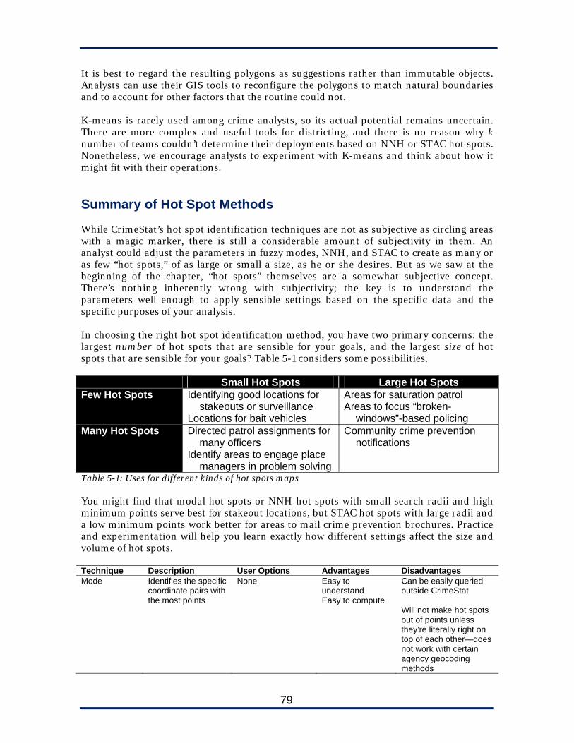
79

It is best to regard the resulting polygons as suggestions rather than immutable objects. Analysts can use their GIS tools to reconfigure the polygons to match natural boundaries and to account for other factors that the routine could not. K-means is rarely used among crime analysts, so its actual potential remains uncertain. There are more complex and useful tools for districting, and there is no reason why k number of teams couldn’t determine their deployments based on NNH or STAC hot spots. Nonetheless, we encourage analysts to experiment with K-means and think about how it might fit with their operations. Summary of Hot Spot Methods While CrimeStat’s hot spot identification techniques are not as subjective as circling areas with a magic marker, there is still a considerable amount of subjectivity in them. An analyst could adjust the parameters in fuzzy modes, NNH, and STAC to create as many or as few “hot spots,” of as large or small a size, as he or she desires. But as we saw at the beginning of the chapter, “hot spots” themselves are a somewhat subjective concept. There’s nothing inherently wrong with subjectivity; the key is to understand the parameters well enough to apply sensible settings based on the specific data and the specific purposes of your analysis. In choosing the right hot spot identification method, you have two primary concerns: the largest number of hot spots that are sensible for your goals, and the largest size of hot spots that are sensible for your goals? Table 5-1 considers some possibilities. Small Hot Spots Large Hot Spots Few Hot Spots Identifying good locations for

stakeouts or surveillance Locations for bait vehicles

Areas for saturation patrol Areas to focus “broken-

windows”-based policing Many Hot Spots Directed patrol assignments for

many officers Identify areas to engage place

managers in problem solving

Community crime prevention notifications

Table 5-1: Uses for different kinds of hot spots maps You might find that modal hot spots or NNH hot spots with small search radii and high minimum points serve best for stakeout locations, but STAC hot spots with large radii and a low minimum points work better for areas to mail crime prevention brochures. Practice and experimentation will help you learn exactly how different settings affect the size and volume of hot spots. Technique Description User Options Advantages Disadvantages Mode Identifies the specific

coordinate pairs with the most points

None Easy to understand Easy to compute

Can be easily queried outside CrimeStat Will not make hot spots out of points unless they’re literally right on top of each other—does not work with certain agency geocoding methods

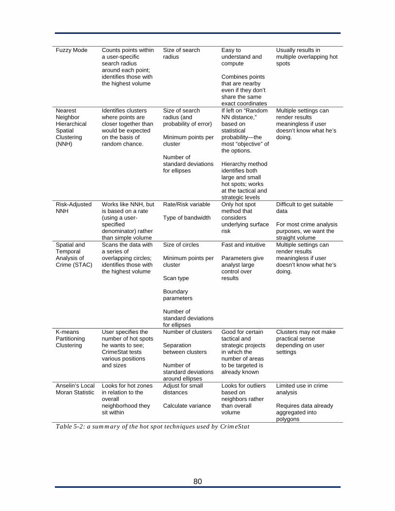
80

Fuzzy Mode Counts points within a user-specific search radius around each point; identifies those with the highest volume

Size of search radius

Easy to understand and compute Combines points that are nearby even if they don’t share the same exact coordinates

Usually results in multiple overlapping hot spots

Nearest Neighbor Hierarchical Spatial Clustering (NNH)

Identifies clusters where points are closer together than would be expected on the basis of random chance.

Size of search radius (and probability of error) Minimum points per cluster Number of standard deviations for ellipses

If left on “Random NN distance,” based on statistical probability—the most “objective” of the options. Hierarchy method identifies both large and small hot spots; works at the tactical and strategic levels

Multiple settings can render results meaningless if user doesn’t know what he’s doing.

Risk-Adjusted NNH

Works like NNH, but is based on a rate (using a user-specified denominator) rather than simple volume

Rate/Risk variable Type of bandwidth

Only hot spot method that considers underlying surface risk

Difficult to get suitable data For most crime analysis purposes, we want the straight volume

Spatial and Temporal Analysis of Crime (STAC)

Scans the data with a series of overlapping circles; identifies those with the highest volume

Size of circles Minimum points per cluster Scan type Boundary parameters Number of standard deviations for ellipses

Fast and intuitive Parameters give analyst large control over results

Multiple settings can render results meaningless if user doesn’t know what he’s doing.

K-means Partitioning Clustering

User specifies the number of hot spots he wants to see; CrimeStat tests various positions and sizes

Number of clusters Separation between clusters Number of standard deviations around ellipses

Good for certain tactical and strategic projects in which the number of areas to be targeted is already known

Clusters may not make practical sense depending on user settings

Anselin’s Local Moran Statistic

Looks for hot zones in relation to the overall neighborhood they sit within

Adjust for small distances Calculate variance

Looks for outliers based on neighbors rather than overall volume

Limited use in crime analysis Requires data already aggregated into polygons

Table 5-2: a summary of the hot spot techniques used by CrimeStat

81

For Further Reading Levine, N. (2005). Chapter 6: ‘Hot spot’ analysis I. In CrimeStat III: A spatial statistics


Levine, N. (2005). Chapter 7: ‘Hot spot’ analysis II. In CrimeStat III: A spatial statistics


Eck, J., Chainey, S., Cameron, J. G., Leitner, M., & Wilson, R. E. (2005). Mapping crime:

Understanding hot spots. Washington, DC: National Institute of Justice. Retrieved from https://www.ncjrs.gov/pdffiles1/nij/209393.pdf

82

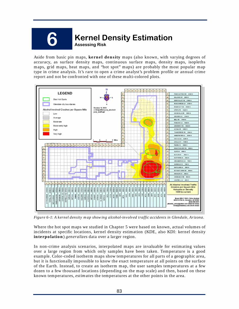
83

6

Kernel Density Estimation Assessing Risk

Aside from basic pin maps, kernel density maps (also known, with varying degrees of accuracy, as surface density maps, continuous surface maps, density maps, isopleths maps, grid maps, heat maps, and “hot spot” maps) are probably the most popular map type in crime analysis. It’s rare to open a crime analyst’s problem profile or annual crime report and not be confronted with one of these multi-colored plots.

Figure 6-1: A kernel density map showing alcohol-involved traffic accidents in Glendale, Arizona. Where the hot spot maps we studied in Chapter 5 were based on known, actual volumes of incidents at specific locations, kernel density estimation (KDE, also KDI: kernel density interpolation) generalizes data over a larger region. In non-crime analysis scenarios, interpolated maps are invaluable for estimating values over a large region from which only samples have been taken. Temperature is a good example. Color-coded isotherm maps show temperatures for all parts of a geographic area, but it is functionally impossible to know the exact temperature at all points on the surface of the Earth. Instead, to create an isotherm map, the user samples temperatures at a few dozen to a few thousand locations (depending on the map scale) and then, based on these known temperatures, estimates the temperatures at the other points in the area.

84

Figure 6-2: An interpolated map of temperatures across the United States for September 29, 2010. While every part of the map has some color, The Weather Channel has not actually measured temperatures at every point (it cannot; there are an infinite number); instead it estimates temperatures for all points based on known sample points. The question always arises, then, about how accurate this method is for crime analysis. After all, we are not “sampling” our crime data; we generally map our entire population of data. We don’t need to estimate. Unlike temperature, not every point on the Earth’s surface has a number of crimes. KDE maps for crime analysis, then, are best viewed as “risk surfaces.” Although not every point on the Earth’s surface has crime, every point on the Earth’s surface does have a chance of crime. KDE estimates this probability based on locations where crimes have occurred in the past. It assumes, to some extent, that each crime is “radioactive” or “contagious” for some radius around where it actually occurs. A robbery that happens on one street corner transmits some risk of robbery down nearby streets. If a burglary happens at one house, there was a risk that it might happen at the house next door or on the next block. KDE allows us to specify the extent and strength of this risk and aggregate the results for all crimes on a single map.

The Mechanics of KDE With KDE, every point on the map has a density estimate based on its proximity to crime incidents (or whatever it is we’re mapping). Because CrimeStat cannot literally calculate the density estimate for every point (there an infinite number), it overlays a grid on top of your map and calculates the density estimate for the centerpoint of each grid cell. The specific number of cells in the grid is defined by the user on the “Data setup” screen.

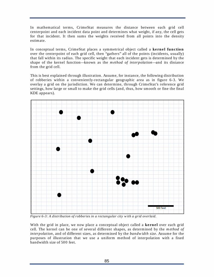
85

In mathematical terms, CrimeStat measures the distance between each grid cell centerpoint and each incident data point and determines what weight, if any, the cell gets for that incident. It then sums the weights received from all points into the density estimate. In conceptual terms, CrimeStat places a symmetrical object called a kernel function over the centerpoint of each grid cell, then “gathers” all of the points (incidents, usually) that fall within its radius. The specific weight that each incident gets is determined by the shape of the kernel function—known as the method of interpolation—and its distance from the grid cell. This is best explained through illustration. Assume, for instance, the following distribution of robberies within a conveniently-rectangular geographic area as in figure 6-3. We overlay a grid on the jurisdiction. We can determine, through CrimeStat’s reference grid settings, how large or small to make the grid cells (and, thus, how smooth or fine the final KDE appears).

Figure 6-3: A distribution of robberies in a rectangular city with a grid overlaid. With the grid in place, we now place a conceptual object called a kernel over each grid cell. The kernel can be one of several different shapes, as determined by the method of interpolation, and of different sizes, as determined by the bandwidth size. Assume for the purposes of illustration that we use a uniform method of interpolation with a fixed bandwidth size of 500 feet.

86

Figure 6-4: Values for selected cells based on a 500 foot radius with a uniform distribution. The kernel fits over the centerpoint of each cell and then determines the weight the cell receives based on the number of points it finds in the radius. In a uniform method of distribution, every identified point receives an equal weight, but in other methods of distribution, points found closer to the edges of the radius receive a lower weight than those found near the center. Figure 6-5 shows an example of a triangular or linear kernel.

Figure 6-5: A triangular kernel assigns the most weight to points found in the center of the radius, and a descending amount of weight to points found near the edges of the radius (represented here with concentric circles, although the smoothing is actually a constant).

87

When displaying the final result on a map, the grid cells are color-coded based on the density. At large scales (zoomed in), the grid cells might be obvious, but at smaller scales, the distribution takes on a smoother appearance. Specifying a large number of cells at the outset will make the final result appear smoother at a larger scale.

Figure 6-6: Our hypothetical KDE followed by an actual KDE at decreasing scales. KDE Parameters There are many parameters to understand when running a KDE in CrimeStat. As with hot spot analysis, many of these parameters depend on the analyst’s own experience and judgment, and sometimes only experimentation can lead to the “correct” settings. First, CrimeStat will allow a single or dual kernel density estimate. Single estimates work for most crime analysis purposes. Dual estimates can help normalize data for population or other risk factors. The shape and size of the kernel is referred to as its bandwidth, and it can be specified to some degree by the user. The shape of the bandwidth is specified by the method of interpolation. CrimeStat offers five interpolation methods: 1. Normal distribution. A normal distribution kernel, represented by a bell curve, peaks above the data point, declines rapidly for one standard deviation, and then enters a less dramatic rate of decline for subsequent standard deviations. Unlike the other methods (including the uniform and triangular ones above), the normal distribution does not have

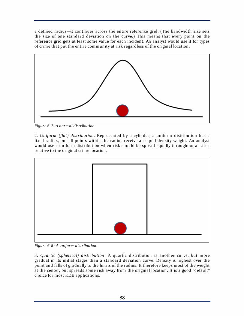
88

a defined radius—it continues across the entire reference grid. (The bandwidth size sets the size of one standard deviation on the curve.) This means that every point on the reference grid gets at least some value for each incident. An analyst would use it for types of crime that put the entire community at risk regardless of the original location.

Figure 6-7: A normal distribution. 2. Uniform (flat) distribution. Represented by a cylinder, a uniform distribution has a fixed radius, but all points within the radius receive an equal density weight. An analyst would use a uniform distribution when risk should be spread equally throughout an area relative to the original crime location.

Figure 6-8: A uniform distribution. 3. Quartic (spherical) distribution. A quartic distribution is another curve, but more gradual in its initial stages than a standard deviation curve. Density is highest over the point and falls of gradually to the limits of the radius. It therefore keeps most of the weight at the center, but spreads some risk away from the original location. It is a good “default” choice for most KDE applications.

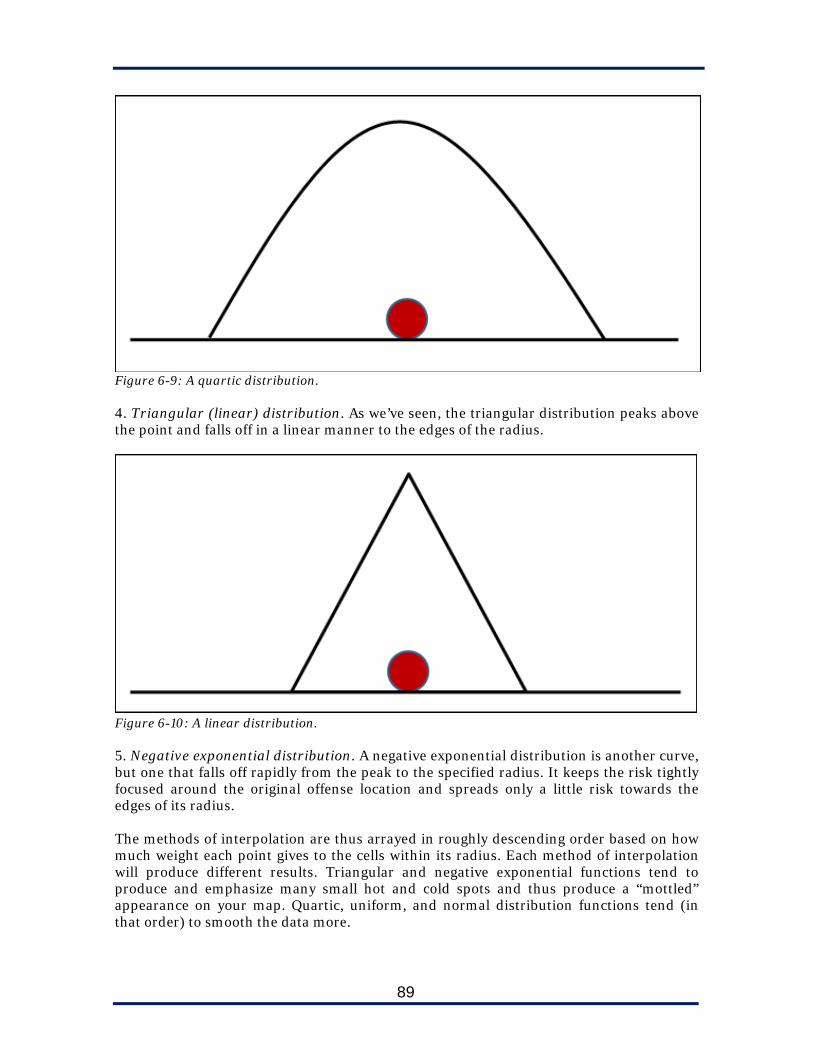
89

Figure 6-9: A quartic distribution. 4. Triangular (linear) distribution. As we’ve seen, the triangular distribution peaks above the point and falls off in a linear manner to the edges of the radius.

Figure 6-10: A linear distribution. 5. Negative exponential distribution. A negative exponential distribution is another curve, but one that falls off rapidly from the peak to the specified radius. It keeps the risk tightly focused around the original offense location and spreads only a little risk towards the edges of its radius. The methods of interpolation are thus arrayed in roughly descending order based on how much weight each point gives to the cells within its radius. Each method of interpolation will produce different results. Triangular and negative exponential functions tend to produce and emphasize many small hot and cold spots and thus produce a “mottled” appearance on your map. Quartic, uniform, and normal distribution functions tend (in that order) to smooth the data more.

90

Figure 6-11: A negative exponential distribution.

Figure 6-12: Residential burglaries in Lincoln smoothed with the negative exponential distribution method (left) and the normal distribution method (right). The choice of bandwidth, minimum sample size, and interval parameters are all related, and they all work together to specify the size of the bandwidth. If you choose an “adaptive” bandwidth, CrimeStat will adjust the size of the kernel until it’s large enough to contain the minimum sample size. If you choose a “Fixed Interval” bandwidth, you specify the size. Adaptive sizes are best confined to projects in which you are using a true sample and need to achieve a certain minimum sample size to properly interpolate the map. Most analysis projects use an entire population of data (e.g., all robberies for a year), an in such cases it is best to use a fixed bandwidth, thus ensuring that each grid cell is treated equally. Visually, it does not matter which output unit you choose, since the grid cells will remain the same relative to each other and will therefore “map” the same. The output unit does make a difference in terms of your legend, and how you explain the results.

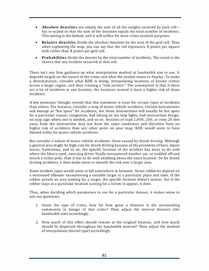
91

Absolute densities are simply the sum of all the weights received by each cell—but re-scaled so that the sum of the densities equals the total number of incidents. This setting is the default, and it will suffice for most crime analysis purposes.

Relative densities divide the absolute densities by the area of the grid cell. Thus when explaining the map, you can say that the red represents X points per square mile rather than X points per grid cell.

Probabilities divide the density by the total number of incidents. The result is the chance that any incident occurred in that cell.

There isn’t any firm guidance on what interpolation method or bandwidth size to use. It depends largely on the nature of the crime and what the analyst wants to display. To make a determination, consider what KDE is doing: interpolating locations of known crimes across a larger region, and thus creating a “risk surface.” The assumption is that if there are a lot of incidents at one location, the locations around it have a higher risk of those incidents. A few moments’ thought reveals that this statement is truer for certain types of incidents than others. For instance, consider a map of motor vehicle accidents. Certain intersections will emerge as “hot spots” for accidents, but those intersections will usually be hot spots for a particular reason: congestion, bad timing on the stop lights, bad intersection design, no stop sign where one is needed, and so on. Sections of road 2,000, 200, or even 20 feet away from the intersection may not have the same conditions and therefore have no higher risk of accidents than any other point on your map. KDE would seem to have limited utility for motor vehicle accidents. But consider a subset of motor vehicle accidents: those caused by drunk driving. Although a general area might be high-risk for drunk driving because of the proximity of bars, liquor stores, fraternities, and so on, the specific location of the accident has more to do with where the bleary-eyed, swerving driver finally encountered another car, or nodded off and struck a utility pole, than it has to do with anything about the exact location. So for drunk driving accidents, it does make sense to smooth the risk over a larger area. Some incident types would seem to fall somewhere in between. Street robberies depend on a motivated offender encountering a suitable target at a particular place and time. If the robber prowls an area looking for a target, the specific location doesn’t matter, but if the robber stays at a particular location waiting for a victim to appear, it does. Thus, when deciding which parameters to use for a particular dataset, it makes sense to ask two questions:

1. Given the type of crime, how for how great a distance is the surrounding community in danger of that crime? Then adjust the interval distance (the bandwidth size) accordingly.

2. How much of this effect should remain at the original location, and how much

should be dispersed throughout the bandwidth interval? Then adjust the method of interpolation (kernel type) accordingly.

92

Table 6-1 offers suggestions for different types of crime, but we hasten to add that these suggestions are based on our own reasoning and analytical experience, and not on any formal research. The nature of these phenomena may very well differ in your jurisdiction. Incident Type Interval Interpolation

Method Reasoning

Residential burglaries 1 mile Moderately dispersed: quartic or uniform

Some burglars choose particular houses, but most cruise neighborhoods looking for likely targets. A housebreak in any part of a neighborhood transfers risk to the rest of the neighborhood.

Aggravated Assaults 0.1 mile Tightly focused: negative exponential

Aggravated assaults occur among specific individuals or at specific locations for specific reasons. Incidents at one location do not have much chance of being contagious in the surrounding area.

Commercial robberies 2 miles Focused: triangular or negative exponential

A commercial robber probably chooses to strike in a general area, and then looks for preferred targets (banks, convenience stores) within that area. The wide area may thus be at some risk, but the brunt of the weight should remain with the particular target that has already been struck.

Thefts from vehicles 0.25 mile Dispersed: uniform If a parking lot experiences a lot of thefts from vehicles, your GIS will probably geocode them at the center of the parcel. This method ensures that the risk disperses evenly across the parcel and part of the surrounding area (which probably makes sense)—but not too far, since we know that parking lots tend to be hot spots for specific reasons.

Table 6-1: Interpolation method and interval possibilities for different types of crime Use similar considerations to determine your own initial values for whatever type of offense or other phenomenon you’re studying.

Step-by-Step We will use kernel density to study robberies in Lincoln, Nebraska.

Step 1: Start a new CrimeStat session and load robberies.shp as the primary file. Set the X and Y coordinates and set the type of coordinate system as “Projected” with the distance units in feet.

Step 2: Go to the “Data setup” tab and then the “Reference File” sub-

tab. If you previously saved the Lincoln grid, you can “Load” it; otherwise, enter the values below for the lower left and upper right X and Y coordinates. Set the number of columns to 250.

93


Step 3: Go to the “Spatial modeling” tab and the “Interpolation I” sub-

tab. Check the box for a “Single” KDE. Set the method of interpolation as “Uniform,” the choice of bandwidth to “Fixed interval,” and the interval to 0.5 miles.

Step 4: Click the “Save result to…” button and save the Shapefile as

robberies. CrimeStat will prefix this with “K.” Step 5: Click “Compute” to run the routine (it may take a few minutes).

Add the resulting Shapefile to your GIS application and symbolize (color) the grid cells based on the “Z” field. Examine the results and experiment with different settings to get a sense of what they do.

Figure 6-13: Options for a single kernel density estimate.

94

Figure 6-14: A completed KDE on the robbery file A note on symbology is important. Kernel density estimation is one of the few CrimeStat routines with which the result can vary considerably not only based on the routine’s settings but also based on the way the user chooses to visualize the results in the map. Most analysts do not pore over the specific cell weights but instead simply assign the cells a color based on the “Z” value as calculated by CrimeStat. Analysts typically choose between four and six categories on a color ramp. The method of classification (natural breaks, quantile, equal interval, standard deviation, and so on) determines how many cells fall into each color category and thus the overall appearance of the map. Because it is virtually impossible to explain the meaning of the Z values (“the sum of densities calculated for that grid cell based on the method of interpolation and size of bandwidth, scaled so that the sum total of weight is equal to the points on the map”), most analysts choose to label their legend with simple words like “Low” and “High,” as in figure 6-14. The lack of precision is regrettable but the clarity in communication is much better. Finally, we would note that many analysts like to create multiple KDEs to compare crimes across multiple time periods. Comparing multiple KDEs only really works if the classifications are set to the same values, however. In such cases, we recommend setting the classifications based on the KDE with the maximum number of points. Then manually adjust the classifications for all other KDEs using the values from the maximum. This may result in situations in which some KDEs have no cells in the “hottest” zones, but this is

95

okay—it might show, for instance, that there are no significant hot spots during certain times of day, or certain months of the year.

Figure 6-15: Residential burglaries across four quarters. Keeping the range values the same across all maps allows for a comparison in hot spot changes, even if the fourth quarter shows no locations in the hottest category. Dual Kernel Density Estimation A dual KDE is simply a kernel density estimation based on two files, one primary and one secondary. The results of the two KDEs are then added to, subtracted from, or expressed as a ratio of each other. If we wanted to analyze two crimes at one time, for instance, we could assign one as the primary file and one as the secondary file. We could then tell CrimeStat to add the densities for the two files. However, it would be somewhat easier just to include both crimes in the database query from which we produce the original primary file.

96

A common use of a dual KDE is to normalize for risk, much as we saw with risk-adjusted Nearest-Neighbor Hierarchical Spatial Clustering in Chapter 5. One of the fundamental problems with a single KDE is that it assumes a uniform risk surface. Hot spots are based entirely on volume. But 60 residential burglaries in a neighborhood with 600 houses is much worse than 60 residential burglaries in a neighborhood with 6,000 houses. By having CrimeStat divide the housebreak density by this risk variable (number of houses), we can produce a better estimation of relative risk. Although normalizing data this way is generally a good idea, there are four things to keep in mind:

1. Sometimes you want a normalized volume, sometimes you don’t. It depends on the ultimate uses of the analysis. For certain tactical and strategic interventions, you want to target the areas of the highest volume, regardless of the underlying risk.

2. Data to use for the secondary file is very hard to come by. Yes, we have census population data, which we’ll use in a moment, but using population as a denominator only makes sense for a limited number of crimes that occur primarily at residences. Normalizing commercial burglary or commercial robberies would require data on the number of businesses (or, even better, the total square footage of businesses), and normalizing auto thefts or thefts from automobiles would best be done with data on the number of parking spaces. None of this data is easily obtained and it may require extensive research on the part of the crime analyst.

3. CrimeStat requires point data for the secondary file and interpolates it just like the primary file. To normalize by population data contained in census block boundaries, we include a file containing the centerpoints of those census blocks. Thus, CrimeStat does not read whether the primary point is “in” a particular census block. Instead, it smoothes the population from each census block centerpoint. Instead of an interpolation normalized by underlying geography, you end up with an interpolation normalized by another interpolation.

4. You cannot use a different interpolation method for each file. Thus, the bandwidth size and interpolation method that you choose may have to be a compromise between what works best for each of the files.

The final dual KDE option is to subtract one KDE from another, either in terms of absolute or relative differences. This type of analysis will be the focus of this assignment. This type of dual KDE shows which areas became “hotter” or “cooler” between two periods. The parameters for the secondary file are the same as we discussed for the primary file until the “Output Units” option. There are six options for the final density calculation:

1. Ratio of densities: the default option and the most common. It divides the density in the primary file by the density in the secondary file. This is best used for the type of “normalization” we discussed above.

2. Log ratio of densities: a logarithmic function that helps control extreme highs and lows in your data. The CrimeStat manual suggests this function for strongly skewed distributions in which most reference cells have very low densities but a few have very high densities.

97

3. Absolute difference in densities: subtracts the secondary file densities from the primary file densities. This option is valuable if your primary file has crimes for one time period and your secondary file has the same type of crime for another time period. The resulting map will show how the crime changed from one time period to the next.

4. Relative difference in densities: like the relative density option for the primary file, this option divides the primary and secondary file densities by the area of the cells before subtracting them. It will result in the same ratios, and thus the same map, as the absolute difference.

5. Sum of densities: adds the two densities together—useful if you want to show the combined effects of two types of crime.

6. Relative sum of densities: divides the primary and secondary files by the area of the cells before adding them.

Step-by-Step We will create a dual KDE that measures changes in residential burglary volume from the first half of 2007 to the second.

Step 1: Start a new CrimeStat session by loading ResBurgs2ndHalf.dbf as the primary file. Set the X and Y coordinates and the coordinate system to “Projected” with the units in Feet.

Step 2: Click the “Secondary File” tab and load ResBurgs1stHalf.dbf as the secondary file. Set the X and Y coordinates.

Step 3: Go to the “Reference File” tab. If you have not already saved a Lincoln grid (in which case, load it), enter the values below for the lower left and upper right X and Y coordinates. Set the number of columns to 250.


Step 4: Go to the “Spatial modeling” tab and the “Interpolation I” sub-

tab. Check the box for a “Dual” KDE. Use a “Uniform” method of interpolation with a “Fixed Interval” bandwidth of 0.75 miles. Set the calculation method to “Absolute Differences in Densities.”

Step 5: Click the “Save result to…” button and save the result as a

Shapefile in your preferred directory. Click “Compute” to run the routine.

98

Figure 6-16: Settings for a dual KDE in CrimeStat.

Step 6: Open the Shapefile in your GIS program. Symbolize (color) the

grid cells based on the “Z” field (standard deviation is a good categorization model for this one). Examine the results (figure 6-17) and note that the middle of the city cooled down significantly between the periods, while hot spots developed along the edges and in the south center. A major hot spot in the northwest part of the city seems to have moved slightly northeast between the two periods.

In some ways, kernel density estimation is another “hot spot” technique, but unlike the techniques reviewed in Chapter 5, KDE’s hot spots are part theoretical. Although KDE maps are attractive and fairly intuitive, it’s important to keep in mind:

KDE maps are interpolations: incidents did not occur at all of the locations within the hottest color.

99

Unless you have CrimeStat calculate a dual KDE, KDEs assume a uniform risk surface. This is usually not the case. Residential burglaries cannot occur where there are no residences, and if your jurisdiction has only two banks, they are the only points at risk for bank robberies, no matter what the KDE interpolates between them. Real-life natural barriers such as rivers and highways will not stop kernel radiuses from extending into them, and you will therefore find density estimates in lakes, forests, and fields.

Intelligent control of the parameters can minimize these issues, but it’s always best to interpret a KDE as a relative risk surface for those suitable targets that may exist within them. With all those caveats in mind, KDEs can be a powerful and easily-understood tool for tactical and strategic analysis and planning.

Figure 6-17: A dual KDE comparing the first half of the year to the second.

100

Summary

Kernel density estimation is a interpolation method that estimates density based on locations of known points. Since in crime analysis, we almost always have a map of all our points, kernel density is best regarded as a risk assessment tool.

KDE calculate values for a number of grid cells placed over the study area. You can

make the grid cells so small that the resulting map looks smooth and continuous, but the more cells the longer CrimeStat takes to calculate the values.

There are various methods of interpolation to choose from, including those that

spread the influence of incidents over a wide area, and somewhat uniformly, and those that keep the influence focused near where the incidents actually occurred. Choosing the best settings is a matter of thinking logically (or studying the research) about the geographic “contagiousness” of the type of crime under study.

The method of categorization used in the GIS program is as important as the

settings in CrimeStat in determining the overall look of the KDE.

Dual KDE adds, subtracts, or divides the results from separate KDEs on two layers. For Further Reading Levine, N. (2005). Chapter 8: Kernel density interpolation. In CrimeStat III: A spatial

statistics program for the analysis of crime incident locations (pp. 8.1–8.42). Houston, TX: Ned Levine & Associates. Retrieved from http://www.icpsr.umich.edu/CrimeStat/ files/CrimeStatChapter.8.pdf

Chainey, S. (2005). Methods and techniques for understanding crime hot spots. In J. Eck,

S. Chainey, J. G. Cameron, M. Leitner, & R. E. Wilson (eds.). Mapping crime: Understanding hot spots (pp. 15–34). Washington, DC: National Institute of Justice. Retrieved from https://www.ncjrs.gov/pdffiles1/nij/209393.pdf

Chainey, S., & Ratcliffe, J. (2005). Identifying crime hotspots. In GIS and crime mapping

(pp. 145-182). Chichester, UK: John Wiley & Sons.

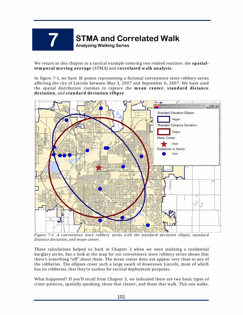
101

7

STMA and Correlated Walk Analyzing Walking Series

We return in this chapter to a tactical example covering two related routines: the spatial-temporal moving average (STMA) and correlated walk analysis. In figure 7-1, we have 18 points representing a fictional convenience store robbery series affecting the city of Lincoln between May 3, 2007 and September 6, 2007. We have used the spatial distribution routines to capture the mean center, standard distance deviation, and standard deviation ellipse.

Figure 7-1: A convenience store robbery series with the standard deviation ellipse, standard distance deviation, and mean center. These calculations helped us back in Chapter 3 when we were studying a residential burglary series, but a look at the map for our convenience store robbery series shows that there’s something “off” about them. The mean center does not appear very close to any of the robberies. The ellipses cover such a large swath of downtown Lincoln, most of which has no robberies, that they’re useless for tactical deployment purposes. What happened? If you’ll recall from Chapter 3, we indicated there are two basic types of crime patterns, spatially speaking: those that cluster, and those that walk. This one walks.

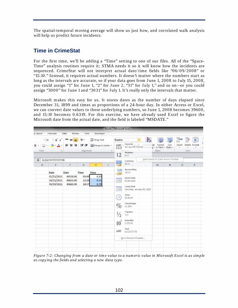
102

The spatial-temporal moving average will show us just how, and correlated walk analysis will help us predict future incidents. Time in CrimeStat For the first time, we’ll be adding a “Time” setting to one of our files. All of the “Space-Time” analysis routines require it; STMA needs it so it will know how the incidents are sequenced. CrimeStat will not interpret actual date/time fields like “06/09/2008” or “15:10.” Instead, it requires actual numbers. It doesn’t matter where the numbers start as long as the intervals are accurate, so if your data goes from June 1, 2008 to July 15, 2008, you could assign “1” for June 1, “2” for June 2, “31” for July 1,” and so on—or you could assign “3000” for June 1 and “3031” for July 1. It’s really only the intervals that matter. Microsoft makes this easy for us. It stores dates as the number of days elapsed since December 31, 1899 and times as proportions of a 24-hour day. In either Access or Excel, we can convert date values to these underlying numbers, so June 1, 2008 becomes 39600, and 15:10 becomes 0.6319. For this exercise, we have already used Excel to figure the Microsoft date from the actual date, and the field is labeled “MSDATE.”

Figure 7-2: Changing from a date or time value to a numeric value in Microsoft Excel is as simple as copying the fields and selecting a new data type.

103

Spatial-Temporal Moving Average (STMA) The spatial temporal moving average calculates the mean center at each point in the series, thereby tracking how it moves over time. The user specifies how many points are included in each calculation using the “span” parameter. Assume we have a moving pattern of 10 incidents and we tell CrimeStat to calculate the spatial-temporal moving average with a span of 3. For each point, CrimeStat calculates the average for that point and the point on either side of it in the sequence. At the first and last points, it only calculates the moving average for two points, since there is no point before the first one and no point after the last one.

Figure 7-3: points included, and results, in four out of 10 moving average calculations. The final result is a series of moving average points tied together with a path (figure 7-4). Examining this path helps determine the overall spatial progression of the series. If the path remains rooted near the mean center of the series, or if it continually returns to its starting point (as in figure 7-6), it would suggest that the pattern is not a walking pattern, and spatial distribution (Chapter 3) provides the best forecast for the next event. The span is the only parameter in the spatial-temporal moving average calculation. We, and the CrimeStat developer, recommend an odd number because it causes the center observation to fall on an actual incident, with an even number on both sides of it. The default of 5 is generally adequate, although you might want to raise it for very large series. If you go too high, your moving averages will begin to approximate the actual average for the series, and you won’t see much movement at all. If you go too low, you’ll simply be

104

viewing changes from one incident to the next rather than a true moving average. (A span of 1, however, can be useful for drawing a literal pathway between the incidents.)

Figure 7-4: all 10 moving average calculations with the path between them

Step-by-Step We will begin our analysis of this convenience store robbery pattern by calculating the spatial-temporal moving average.

Step 1: Load the CSRobSeries.shp file into your GIS application and view the incidents in the series. You may want to calculate spatial distribution before moving on to STMA, as in figure 7-1.

Step 2: Start a new CrimeStat session. On the “Data setup” screen,

choose “Select Files” and load the CSRobSeries.shp file. Set the X and Y coordinates and set the coordinate system to “projected” in “feet.” Set the “Time” variable to MSDATE and ensure that the “Time Unit” is listed in “Days” (figure 7-5).

Step 3: Click the “Spatial Modeling” tab and then the “Space-time

analysis” sub-tab. Check the “Spatial-temporal moving average” box and set the span to 3 observations.

105

Figure 7-5: Data setup for spatial-temporal moving average.

106

Step 4: Click “Save path” to save the line that traverses the calculated mean centers as a Shapefile called CSRobSeries. CrimeStat will prefix this with “STMA.”

Step 5: Click “Compute” to run the routine. Note the results and then

load the STMACSRobSeries Shapefile into your GIS program. Symbolize the line as an arrow so you can see its directionality. Experiment with different span settings and refresh, noting how higher spans smooth out the line.

Figure 7-6: The robbery series with the path through the moving averages. Correlated Walk Analysis Spatial temporal moving average shows the past tendency of crimes in a series. Correlated walk analysis builds on STMA by attempting to predict, based on this past pattern, where and when an offender is likely to strike next. Tactical crime analysis techniques offer

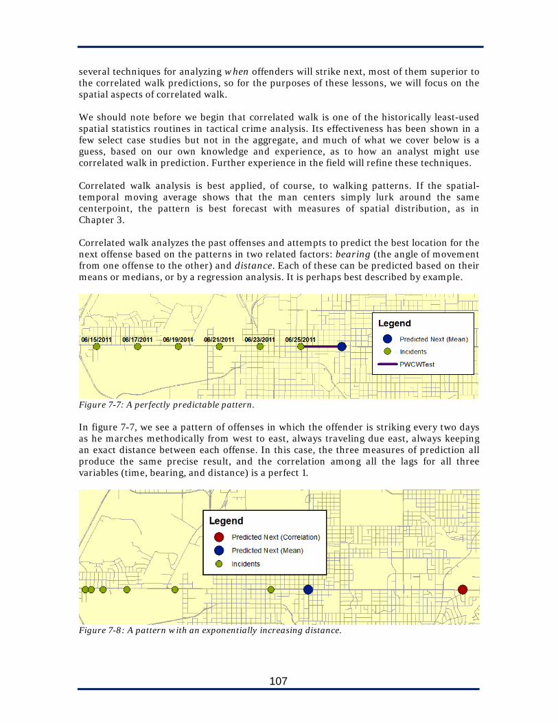
107

several techniques for analyzing when offenders will strike next, most of them superior to the correlated walk predictions, so for the purposes of these lessons, we will focus on the spatial aspects of correlated walk. We should note before we begin that correlated walk is one of the historically least-used spatial statistics routines in tactical crime analysis. Its effectiveness has been shown in a few select case studies but not in the aggregate, and much of what we cover below is a guess, based on our own knowledge and experience, as to how an analyst might use correlated walk in prediction. Further experience in the field will refine these techniques. Correlated walk analysis is best applied, of course, to walking patterns. If the spatial-temporal moving average shows that the man centers simply lurk around the same centerpoint, the pattern is best forecast with measures of spatial distribution, as in Chapter 3. Correlated walk analyzes the past offenses and attempts to predict the best location for the next offense based on the patterns in two related factors: bearing (the angle of movement from one offense to the other) and distance. Each of these can be predicted based on their means or medians, or by a regression analysis. It is perhaps best described by example.

Figure 7-7: A perfectly predictable pattern. In figure 7-7, we see a pattern of offenses in which the offender is striking every two days as he marches methodically from west to east, always traveling due east, always keeping an exact distance between each offense. In this case, the three measures of prediction all produce the same precise result, and the correlation among all the lags for all three variables (time, bearing, and distance) is a perfect 1.

Figure 7-8: A pattern with an exponentially increasing distance.

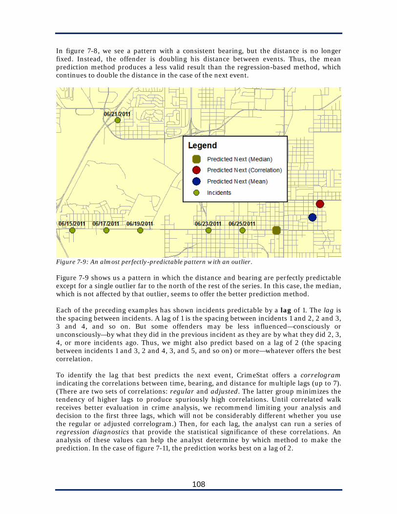
108

In figure 7-8, we see a pattern with a consistent bearing, but the distance is no longer fixed. Instead, the offender is doubling his distance between events. Thus, the mean prediction method produces a less valid result than the regression-based method, which continues to double the distance in the case of the next event.

Figure 7-9: An almost perfectly-predictable pattern with an outlier. Figure 7-9 shows us a pattern in which the distance and bearing are perfectly predictable except for a single outlier far to the north of the rest of the series. In this case, the median, which is not affected by that outlier, seems to offer the better prediction method. Each of the preceding examples has shown incidents predictable by a lag of 1. The lag is the spacing between incidents. A lag of 1 is the spacing between incidents 1 and 2, 2 and 3, 3 and 4, and so on. But some offenders may be less influenced—consciously or unconsciously—by what they did in the previous incident as they are by what they did 2, 3, 4, or more incidents ago. Thus, we might also predict based on a lag of 2 (the spacing between incidents 1 and 3, 2 and 4, 3, and 5, and so on) or more—whatever offers the best correlation. To identify the lag that best predicts the next event, CrimeStat offers a correlogram indicating the correlations between time, bearing, and distance for multiple lags (up to 7). (There are two sets of correlations: regular and adjusted. The latter group minimizes the tendency of higher lags to produce spuriously high correlations. Until correlated walk receives better evaluation in crime analysis, we recommend limiting your analysis and decision to the first three lags, which will not be considerably different whether you use the regular or adjusted correlogram.) Then, for each lag, the analyst can run a series of regression diagnostics that provide the statistical significance of these correlations. An analysis of these values can help the analyst determine by which method to make the prediction. In the case of figure 7-11, the prediction works best on a lag of 2.

109

Figure 7-10: A series of incidents in which only a regression-based prediction on a lag of 2 correctly places the next point. On lags of 1, the incidents alternate between a southern and northeastern direction, but on lags of 2, they all relentlessly march eastward.

Figure 7-11: The Correlogram shows the correlations between each lag and time, distance, and bearing.

110

The prediction routine provides five output files:

1. An events file that shows the progression from each incident to the next in a line. It is the same as if one chose spatial-temporal moving average with a span of one.

2. A point of origin file that is simply the mean center of minimum distance (see Chapter 3) of the series. It is not the true point of origin, of course, but the hypothetical point of origin if the offender was minimizing his total travel distance between his home and the incidents in the series.

3. A predicted destination file indicating the results of prediction routine (more below).

4. A path between the point of origin and the predicted destination.

5. A path between the last incident and the predicted destination.

A disadvantage to correlated walk analysis is that it always produces a single point as its prediction, regardless of the strength of the correlation. Analysts will have to study the series carefully—including the spatial-temporal moving average, the spatial distribution, the correlogram, and the regression diagnostics, to determine how strongly to trust the point. Even when it seems reliable, it rarely marks the exact location of the next offense, and analysts would do best to treat it as a starting point to begin a search for potential targets. In the case of the convenience store robbery series, we would look for convenience stores near the predicted destination location.

Step-by-Step We will perform a correlated walk analysis on our convenience store robbery series to see what kind of prediction the routine gives us.

Step 1: If it is not already there from the previous lesson, load CSRobSeries.shp as the primary file. Set the X and Y coordinates, and set the “Time” variable to MSDATE.

Step 2: Click the “Spatial modeling” tab and the “Space-time analysis” sub-tab. Check the “Correlogram” checkbox and then click “Compute” to run.

Scroll down to the “regular” correlogram. We will limit our analysis to the first three lags, as they use the most data points. The strongest distance correlation is found in a lag of 2 (0.29381). The strongest bearing correlation is found with a lag of 1 (-0.45541).

Step 3: Close the correlogram results and un-check “Correlogram.” Check “Regression diagnostics,” choose a lag of 2, and click “Compute.”

111

Figure 7-12: Regression diagnostics for a lag of 2 The regression diagnostics show that at a lag of 2, the distance correlation is significant at the 0.30242 level.. This is far above the value required by most social science, which is 0.05. Even allowing for a relaxed standard for police practice, it is too high to use as a predictive variable. We will use the mean method instead.

Step 4: Close the diagnostic results and change the lag for the regression diagnostics to 1. Click “Compute” again.

At a lag of 1, the bearing correlation is significant at the 0.08301 level. This is still above the 0.05 level required by most social scientists, but it falls below a more relaxed 0.10 level that we often allow for police practice. In this case, we will use it as a predictor.

Step 5: Close the diagnostic results and un-check the “Regression diagnostics” box. Check the “Prediction” box and set the distance method as “Mean” with a lag of 1, and the bearing method as “Regression” with a lag of 1. (We are not concerned about time prediction for this example.

112

Step 6: Click the “Save output to…” button and save the output as a Shapefile with the name CSRobSeries. CrimeStat will create five files using this name, with the following prefixes: Events, Path, POrig, PredDest, and PW.

Step 7: Click “Compute” to run the prediction. Open the five output

files in your GIS application and symbolize them as you deem appropriate.

Figure 7-13: Setting the values to make a correlated walk prediction. As we can see in figure 7-14, the incidents have been progressing in a kind of arc around the center of the city, moving north, then west, and then south. The predicted destination continues this arc by projecting a location to the south of the most recent. Again, however, this single point should not be taken as a full prediction: CrimeStat will identify a single point no matter how strong or weak the correlation in bearing and distance. It is, rather, perhaps best regarded as a starting point for a search for potential targets. The next step is to use business databases to identify convenience stores (particularly those that match any characteristics of the offender’s previous targets) in the general area of the prediction.

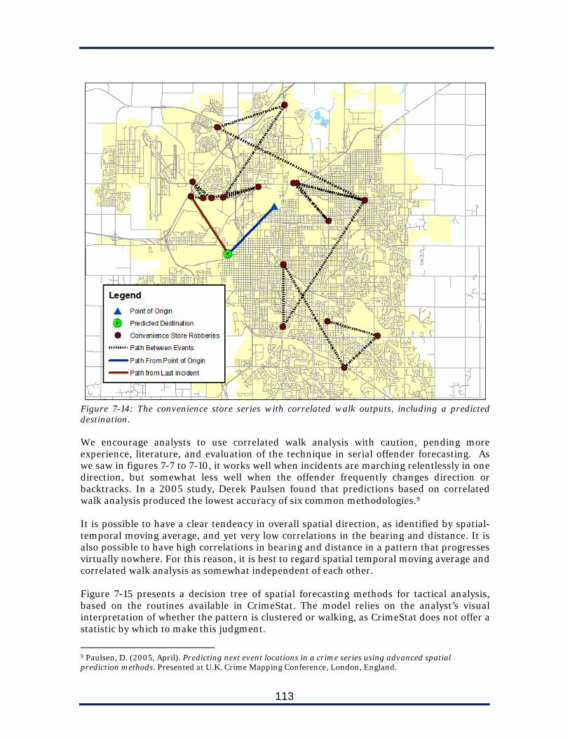
113

Figure 7-14: The convenience store series with correlated walk outputs, including a predicted destination. We encourage analysts to use correlated walk analysis with caution, pending more experience, literature, and evaluation of the technique in serial offender forecasting. As we saw in figures 7-7 to 7-10, it works well when incidents are marching relentlessly in one direction, but somewhat less well when the offender frequently changes direction or backtracks. In a 2005 study, Derek Paulsen found that predictions based on correlated walk analysis produced the lowest accuracy of six common methodologies.9 It is possible to have a clear tendency in overall spatial direction, as identified by spatial-temporal moving average, and yet very low correlations in the bearing and distance. It is also possible to have high correlations in bearing and distance in a pattern that progresses virtually nowhere. For this reason, it is best to regard spatial temporal moving average and correlated walk analysis as somewhat independent of each other. Figure 7-15 presents a decision tree of spatial forecasting methods for tactical analysis, based on the routines available in CrimeStat. The model relies on the analyst’s visual interpretation of whether the pattern is clustered or walking, as CrimeStat does not offer a statistic by which to make this judgment.

9 Paulsen, D. (2005, April). Predicting next event locations in a crime series using advanced spatial prediction methods. Presented at U.K. Crime Mapping Conference, London, England.

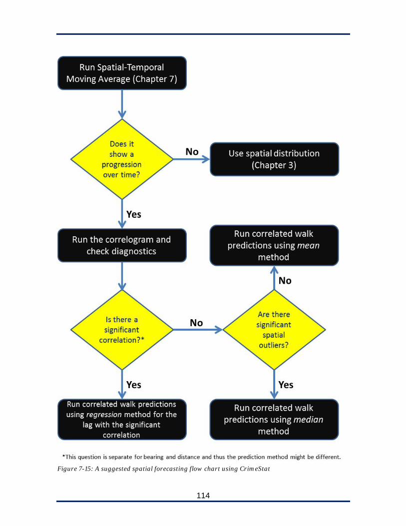
114

Figure 7-15: A suggested spatial forecasting flow chart using CrimeStat

115

There may be other factors related to geography and environment that these spatial statistics do not account for. An analyst’s judgment, if based on experience and a solid consideration of the facts of the series, outweighs the product of a spatial statistics routine. Summary

The spatial-temporal moving average (STMA) shows how the mean center of a crime series progresses over time. It helps determine if a series is clustered or walking.

STMA’s one setting is the “span,” which is the number of incidents for which it calculates the mean center during each iteration.

Correlated walk analysis attempts to predict the location of the next event in walking series, based on an analysis of bearing and distance.

If the analyst identifies strong correlations among various lags in bearing or distance, he or she may use the regression method to predict the next event. Regression diagnostics can help determine whether observed correlations are statistically significant.

If there are no strong correlations in a walking series, the analyst may attempt a prediction using the mean or median methods.

Correlated walk analysis has not been well-evaluated in police departments, and few agencies have used it to make predictions. It should be used with caution.

Both STMA and correlated walk analysis rely on a time variable on the primary file screen. CrimeStat does not read standard date or time fields but instead requires a number that represents the increments between hours, days, weeks, or months. Microsoft makes it easy to make this conversion in Excel or Access.

For Further Reading Levine, N. (2005). Chapter 9: Space-time analysis. In CrimeStat III: A spatial statistics


116

117

8

Journey to Crime Estimating the Home Base of the Serial Offender

Whether one is eager to shop at a convenience store or to rob it, one does not undertake a grueling odyssey deep into foreign lands. Rather, one goes to a closely available location in an area in which one is familiar. In the case of criminal activity, we refer to the offender’s travel from his or her home or “base” to the offense location as journey to crime. Journey to crime analysis studies offenders’ travel patterns and applies the results to current crime series, assessing the likelihood that various points on the map serve as the residence or home base of a serial offender. Analysts can use these results to prioritize investigative leads and database searches for potential offenders, and to recommend specific tactics to operational divisions. Journey to crime analysis assumes several key principles: 1. Some offenders prefer not to strike in the immediate vicinity of their home bases. Many offenders keep a buffer zone around their immediate residences, workplaces, and other locations in which they are intimately familiar. There may be various psychological, social, and practical reasons for this buffer (or, as Ned Levine points out in the CrimeStat manual, it may simply be a function of the location of available targets; no qualitative research has been published in which offenders validate buffer zones). 2. Outside this buffer zone (when it exists), offenders seek to minimize their travel distance between their home base and their offenses. Thus, points close to an offense have a generally higher probability of being an offender’s home base than points far away. As the distance from the offense increases, the likelihood that an offender lives at that distance decreases. This phenomenon is known as distance decay. 3. Buffer zones and distance decay vary for different types of offenders. Certain crimes are favored by offenders willing to travel long distances, while others are chosen by offenders who keep close to home. (For instance, some of the earliest journey to crime research found that property crime offenders travel farther than violent crime offenders.) Thus, each type of offense will require a different set of calculations for the buffer zones and the rate of distance decay. 4. Buffer zones and distance decay vary across different jurisdictions. Offenders in high-population-density jurisdictions with public transportation may travel shorter distances than those with cars in rural areas. Given an appropriate dataset, researchers can determine the average distance traveled between each crime and the offender’s home, and can thus predict where a known offender is likely to offend. The journey to crime estimation routine reverses this formula and, given the locations of known crimes, attempts to determine the most likely locations of the offenders’ home bases. Because of principles #3 and #4 above, CrimeStat’s journey to crime routine does not assume a universal buffer zone or rate of decay. Rather, analysts determine the settings for their own jurisdictions based on a calibrated data file that

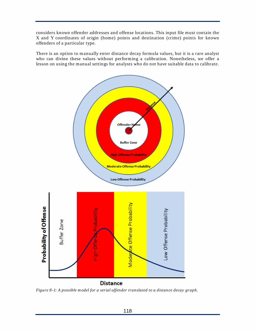
118

considers known offender addresses and offense locations. This input file must contain the X and Y coordinates of origin (home) points and destination (crime) points for known offenders of a particular type. There is an option to manually enter distance decay formula values, but it is a rare analyst who can divine these values without performing a calibration. Nonetheless, we offer a lesson on using the manual settings for analysts who do not have suitable data to calibrate.

Figure 8-1: A possible model for a serial offender translated to a distance decay graph.

119

Calibrating a File The best way to approach journey to crime is to calibrate your own distance decay functions using files of known offenders and the crimes they committed. The calibration routine requires a file with at least four files: the X and Y coordinates of the offender’s home, and the X and Y coordinates of the crime. If the same offender is known to have committed multiple crimes, he or she can appear multiple times in the file, although no single offender should account for more than 10% of the records in the file.

Figure 8-2: A sample file suitable for journey to crime calibration, with coordinates in longitude and latitude. Most analysts will generate this file by exporting offenders’ addresses and offense addresses from their records management systems, geocoding them, and using an attribute join (via the incident number) to combine them into a single file. Naturally, the resulting file will only contain records in which the offender was arrested or is otherwise known. This process has the disadvantage of assuming that the offenders’ home addresses are their “bases,” which is not always the case, but there is little we can do about this shortcoming except to exhaustively research each offender and edit the “origin” coordinates to more accurately reflect his base (whether it was a workplace, a family member’s house, a hotel, or some other place not connected to his home). As different types of offenders have different travel patterns, analysts should calibrate multiple files for different offenses: street robberies, commercial robberies, residential burglaries, thefts from vehicles, auto theft, and so on. We even recommend more finite calibrations (bank robbers, convenience store robbers, thieves who steal copper, juvenile residential burglars, and so on), as long as the data file has a minimum of 30 records. To help analyze travel patterns and distance, CrimeStat offers a “Draw Crime Trips” feature that shows direct travel paths between origin points and destination points. This becomes valuable as we run the calibration process, because it allows us to assess what interpolation method works best during the calibration process. This feature is also useful for uses unrelated to journey to crime, such as drawing lines between locations of stolen vehicles and their recoveries.

120

Step-by-Step To create a calibration file necessary to analyze our pattern of convenience store robberies, we will calibrate a file of known commercial robbers. We will begin by drawing the trips between origins and destinations for these robbers.

Step 1: In a new CrimeStat session, load any file as the primary file and set the X and Y coordinates. The CSRobSeries.shp file is a good choice since we will be running journey to crime calculations in this soon. (The “draw crime trips” routine requires a primary file to be set up, even though it doesn’t use it.)

Step 2: Click the “Spatial modeling” tab and the “Journey-to-Crime” sub-tab. Check the “Draw crime trips” box at the bottom.

Step 3: Click the “Select data file” button and load

commrobberies.dbf as the primary file. Set the origin X and Y coordinates to HOMEX and HOMEY and the destination X and Y coordinates to CRIMEX and CRIMEY. Set the ID to INCNUM in both cases. Set the type of coordinate system as “projected” in feet and click “OK.”

Figure 8-3: Setting options for drawing crime trips

121

Step 4: Click the “Save output to” button. Save the result as a Shapefile called robberytrips. CrimeStat will automatically prefix this with “DRAW.” Click “OK” and “Compute” to run the routine.

Step 5: Load the DRAWrobberytrips.shp file into your GIS system

along with the commrobberies.dbf file. Using the CRIMEX and CRIMEY coordinates, create a layer for the offense locations, and using the HOMEX and HOMEY coordinates, create a layer for the offender locations. Your resulting map (figure 8-4) will show the direction between each offender and his or her offenses.

Figure 8-4: Offenders, offenses, and the trips between them. By calculating the length of the lines in our GIS program, we can get a sense of the central tendency and dispersion (figure 8-5). If we group the trips into bins of one mile and graph the results (figure 8-6), we see that the data approximates a normal curve, with a standard deviation of about 1.5 miles. The graph supports the idea, in this case, of a buffer zone around the offenders’ residences, ramping up to a peak distance outside the zone, then decaying beyond this. This helps us determine the best method of interpolation to use in Step 8 below.

122

Figure 8-5: Analyzing the length of crime trips

Figure 8-6: Graphing the crime trips into bins of one mile.

Step 6: Back in CrimeStat, un-check “Draw crime trips” and click the button at the top of the journey to crime screen that says “Select data file for calibration.” Load the commrobberies.dbf file, set the origin X and Y coordinates to HOMEX and HOMEY and the destination coordinates to CRIMEX and CRIMEY. Set the type of coordinate system to “projected” in feet. Click “OK.”

Step 7: Click “Select output file” and save the file as a DBF file with the

name commrobbers.

0%

5%

10%

15%

20%

25%

30%

35%

0 1 2 3 4 5 6 7

Miles Traveled

Crime Trips

123

Figure 8-7: Selecting a data file for calibration.

Step 8: Click “Select kernel parameters.” Choose a normal method of interpolation with a fixed interval bandwidth of 1.5 miles. Leave the number of bins set to the defaults. Click “OK” and then click “Calibrate” to save the data file.

The “kernel parameters” step helps CrimeStat create a smooth distance decay function (see “Using a Mathematical Formula” below) out of the limited number of records that an offender file typically produces. Some interpolation is necessary to estimate the nature of the curve. During this step, you may try to set the variables yourself based on an analysis of the distance data (as in figures 8-5 and 8-6), or you may accept the default settings. Analysts who use journey to crime report that the default settings work tolerably well even when they do not precisely match the curve. If you wish to set these settings manually, the methods of interpolation and choice of bandwidth perform the same functions as in kernel density estimation (Chapter 6), although the purpose is different.

124

The Journey to Crime Estimation Once you have a data file calibrated, or know the manual settings (see the next section), you’re ready to run the journey to crime estimation. The routine produces a density grid, much as in kernel density estimation, except that the values in the cells estimate the relative likelihood, based on known distance decay for offenders of the same type, that the serial offender lives (or is based in) each cell.

Figure 8-8: Setting up a journey to crime estimation

Step-by-Step We will run a journey to crime estimation for our convenience store robbery series.

Step 1: In your CrimeStat session, load CSRobSeries.shp as the primary file. Make sure that the X and Y coordinates are set and the “Type of coordinate system” is set to “projected” in feet.

125

Step 2: On the “Reference File” tab, enter the following values for the

grid area, and set the number of columns to 250 (or just “Load” the Lincoln grid if you previously saved it.


Step 3: Go to the “Spatial modeling” tab and the “Journey-to-Crime”

sub-tab. Click the “Journey-to-crime estimation” box. Choose the “already-calibrated distance function” option and click on “Browse” to find the comrobbers.dbf file that we created in the previous lesson.

Step 4: Click “Save output to…” and save the result as a Shapefile

called CSRobSeries in your data directory. CrimeStat will automatically prefix this with “JTC.” Click “Compute” when finished.

Step 5: Open the resulting JTCCSRobSeries.shp grid in your GIS

program. Color the cells by the “Z” field. You may want to experiment with different methods of classification, including manual methods, to ensure that the highest probability area holds a relatively small percentage of the cells.

Figure 8-9 shows a completed journey to crime map for our convenience store robbery series. The question becomes what to do with this information once calculated. Although there is a single grid cell with the highest probability, this does not serve as an “X” that marks the spot of the serial offender, and we cannot use this information to start knocking down doors. The best use of a journey to crime estimation is to prioritize potential suspects and leads. In the case of this convenience store robbery series, we have several known commercial robbers living within the area of the peak likelihood, and several others living nearby. The analyst could start checking these individuals to see if they match the suspect description of the robber in the current series, or if any of his known vehicles match the vehicle information in the current series. In some serial offenses, members of the public call in tips that, if overwhelming, could be prioritized (in part) based on distance to the area of the peak likelihood for travel. Using a Mathematical Formula If you do not have a large enough dataset to calibrate a file of known offenders and their crimes, you have the option to enter the values for the distance decay equation yourself. Approach this with care; as the CrimeStat manual notes, “in most circumstances, a mathematical function will give less precision than an empirically-derived one” (p. 10.41).

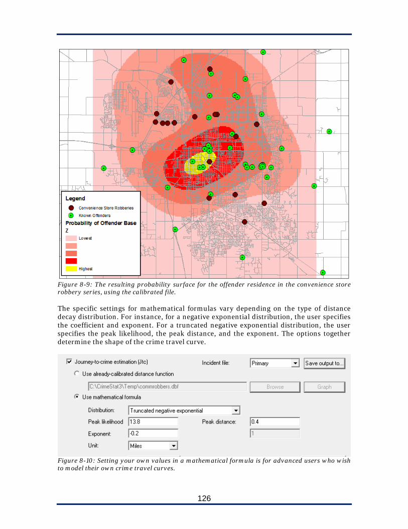
126

Figure 8-9: The resulting probability surface for the offender residence in the convenience store robbery series, using the calibrated file. The specific settings for mathematical formulas vary depending on the type of distance decay distribution. For instance, for a negative exponential distribution, the user specifies the coefficient and exponent. For a truncated negative exponential distribution, the user specifies the peak likelihood, the peak distance, and the exponent. The options together determine the shape of the crime travel curve.

Figure 8-10: Setting your own values in a mathematical formula is for advanced users who wish to model their own crime travel curves.

127

Summary

Journey to crime analysis applies travel distances for offenders of a particular type to a single offender in a particular series. It attempts estimate the likelihood that the serial offender lives (or has his home base) in various places on the map.

Journey to crime analysis works best when analysts calibrate a series of distance

decay functions based on known offenders in their jurisdictions. This requires multiple files of origin (home) and destination (crime) points for different types of offenders.

The “Draw crime trips” routine shows linear distance between offenders’ homes

and crime locations. The utility is also useful for purposes unrelated to journey to crime analysis, such as showing travel paths from a crime to the recovery of stolen property.

Journey to crime analysis does not provide the specific location of an offender’s

home, but it does allow the analyst to prioritize searches for known offenders based on the areas of peak likelihood.

For Further Reading Levine, N. (2005). Chapter 10: Journey to crime estimation. In CrimeStat III: A spatial


Canter, D., & Youngs, D. (2008). Principles of geographical offender profiling Aldershot,

UK: Ashgate. Rossmo, D. K. (2000). Geographic profiling. Boca Raton, FL: CRC.

128

129

9

Conclusions Moving Forward with Spatial Statistics

Although crime analysts have used certain basic techniques of spatial statistics for decades, on the whole, the use of spatial statistics in crime analysis is in its childhood. Applications like CrimeStat provide a large array of tools, many based on solid theoretical foundations, but few thoroughly evaluated in actual police agencies. The profession of crime analysis lacks a strong body of literature, experience, and assessment in spatial statistics. Nonetheless, crime analysts will continue to use spatial statistics no matter what the state of the science. Analysts’ jobs revolve around the daily identification and analysis of crime patterns, series, trends, and hot spots, and forecasting is always implicit in this analysis. All analysis is inherently predictive, even if not explicit, and the more experience the profession can develop with the routines in CrimeStat (as well as other applications), the more accuracy with which we can predict. If you are an analyst applying the spatial statistics in this book, keep in mind that “scientific” does not necessarily mean “quantitative.” In any crime analysis application—indeed, in any social science application—there is a place for qualitative influence on quantitative analysis. We are dealing with human beings here. The spatial statistics routines offered by CrimeStat do not account for all potential variables—no statistical model really can—and it is up to you, as the one who has read the crime reports, studied the geography, visited the crime scenes, interacted with police officers, interviewed offenders, and consoled victims, to regard the results of any calculation with a critical eye. If, in the end, you believe—and can justify—that your hand-drawn ellipse is a better predictor than a spatial distribution calculation, or that your assessment of the most likely offender’s residence is correct despite its location in the lowest probability zone, go ahead and use it. Then figure out why the model failed to make the “correct” prediction, and help us refine these techniques for the future. As a spatial statistics application, CrimeStat offers one enormous advantage over many others: transparency. The CrimeStat manual, written by Ned Levine, exhaustively documents the formulas used by the routines, and in most cases, the user can tweak each and every variable. The results windows (not emphasized in this book, but seen after each routine) show the specific calculations and allow the user to check for inconsistencies. Moreover, because the user must geocode, analyze, and export a data file before loading it into CrimeStat, there is no question about what data is being used or what variables are included. To an analyst concerned with accuracy and validity, these features of CrimeStat make it more than worth the extra difficulty associated with transitioning between it and a GIS. As you use CrimeStat and spatial statistics, please share your results with the authors of this workbook and with the professional community at large. Only through your experiences can the crime analysis profession’s use of spatial statistics continue to grow.

130

131

Glossary Absolute Densities In kernel density estimation, the default method of calculating the densities for each grid cell. The method sums up the densities received from all the points found inside the kernel, but scales them so that the sum of all the absolute densities equals the number of points on the map. Compare to relative densities and probabilities. Adaptive Bandwidth In kernel density estimation, a setting that adjusts the size of the bandwidth around each cell until it finds the minimum sample size. Compare to fixed interval. Administrative Crime Analysis In the field of crime analysis, the provision of statistics, maps, graphics, and data for administrative purposes within a police agency Aggregation In statistics, summarizing by category; for instance, using individual records of crimes to count the number of crimes in each year or in each geographic zone, or calculating the average property value stolen by crime type. Angular Coordinate System A method of identifying locations on the Earth’s surface by specifying the bearing (angle) and distance of each location from a fixed origin point. It is also called a polar coordinate system. Although CrimeStat supports data in angular systems, such data is rarely encountered in crime analysis; instead, most crime data will be in a spherical coordinate system or projected coordinate system. Anselin’s Local Moran A technique for identifying hot spots that, unlike most other techniques, uses data aggregated in zones (e.g., police reporting districts, census blocks, grid cells). The routine identifies areas that have a density of crime unusual for their zone. This is in contrast to other hot spot techniques, which consider only raw volume. ArcGIS A suite of applications produced by ESRI that together constitute the most widely-used geographic information system programs among U.S. crime analysts. ArcGIS comes in four license levels (ArcReader, ArcView, ArcEditor, and ArcInfo; the second is the most common for analysts) and several integrated applications (e.g., ArcMap, ArcCatalog, ArcToolbox). The Shapefile vector data format read by CrimeStat was originally developed for ArcGIS. ASCII An encoding scheme used in text files (the acronym stands for “American Standard Code for Information Interchange”) and often used synonymously with “text file.” A delimited or fixed-width ASCII file is the simplest of database formats and can thus be exported from and imported into most database applications, including CrimeStat.

132

Atlas GIS A geographic information system developed by AtlasCT. Though rarely used in crime analysis, CrimeStat can read Atlas GIS files. Bandwidth In kernel density estimation, the width of the radius of the kernel when placed over each grid cell. In other statistical applications, the size of the “bins” in which we subdivide continuous variables. For instance, when analyzing distances between crimes that range from 0 to 40 miles, we might use a bandwidth of 5 miles, which would give us 8 groupings or bins. Basemap A map containing fundamental information about the geographic area—such as roads, waterways, key buildings, and other important features—that the analyst uses as a starting point for his or her analysis. Bayesian Journey to Crime Like journey to crime, a routine for estimating the most likely home base of a serial offender. The routine is more advanced than basic journey to crime, using a distance matrix between particular origins and particular destinations to fine-tune the journey to crime estimate. Buffer A radius around an object or group of objects, generally used in geographic information systems to identify and gather secondary points occurring in spatial proximity to primary points (e.g., crimes within 1000 feet of schools). Buffer Zone In journey to crime theory, the distance around an offender’s residence or home base in which he is unlikely to commit a crime, either for fear of recognition and apprehension, or for various psychological reasons. Choropleth Map A type of thematic map in which polygons are colored or patterned based on the value of a variable in the attribute data—for instance, darker colors for polygons with higher crime volume. It is thus a basic hot spot technique that requires no spatial statistics. Clustered Pattern In crime analysis, a clustered pattern is one in which the offender is striking irregularly within a geographic area, rather than moving in a predictable manner from each incident to the next. Contrast with walking pattern. Because clustered patterns exhibit no correlations in movement, they are best forecast with methods of spatial distribution. Computer-Aided Dispatch (CAD) System A database that stores data about police, fire, and EMS calls for service, including the time the call was received, the type of call, the units dispatched, and the call disposition. In some agencies, it is the same database as the records management system. Crime analysts often use CAD data to analyze police activity for which no officers’ report was written.

133

Convex Hull A polygon that encompasses the extent of a group of points in such a way that all of the polygon’s external angles are convex (greater than 180 degrees). Essentially, a convex hull “connects the dots” for the outermost points in a distribution. Coordinates See Geographic Cooordinates Correlated Walk Analysis A routine that analyzes the spatial and temporal sequencing of incidents, including the distance, bearing, and time interval, to predict the most likely location of the next incident. Correlation The statistical relationship between two variables. Correlogram A grid that shows all correlations among multiple variables. Crime Analysis A law enforcement profession dedicated to the study of crime and other police data for tactical, strategic, administrative, and operational purposes. Crime analysts identify and analyze series, patterns, trends, problems, hot spots, and other crime phenomena to help agencies apprehend offenders, prevent crime and disorder, evaluate programs, and effectively allocate resources. See also Tactical Crime Analysis, Strategic Crime Analysis. Crime Mapping The application of geographic information system (GIS) technology to crime and police data. Crime Pattern Two or more crimes related through a common causal factor, including the same offender (crime series) or same location (hot spot). Crime Problem A set of interrelated behaviors and characteristics that give rise to numerous crimes over a long term, or on a chronic, recurring basis. The term generally encompasses both the crimes themselves and their root causes. Examples include gang violence in impoverished areas, prostitution in budget motels, thefts of car parts from unsecured auto dealership, and robberies of drug stores by offenders addicted to painkillers. Crime Series Two or more crimes of the same type committed by the same offender. Series are a type of crime pattern. Crime Travel Demand A complex modeling technique to estimate crime trips over a large metropolitan area.

134

Crime Trend An increase or decrease in crime over a long period. CrimeStat A Windows-based spatial statistics software package designed to work with a geographic information system to analyze crime data. CrimeStat Analyst An application developed by the South Carolina Research Authority in 2011. CrimeStat Analyst uses some of the CrimeStat libraries and routines but in a format that enhances functionality for crime analysts. It also includes two modules not found in CrimeStat: the SPIDER forecasting application and a repeat analysis calculator. dBASE A common database management system used by multiple computer platforms. Developed by Ashton-Tate in 1979, the rights were sold to Borland in 1991 and dataBased Intelligence in 1999. The format is widely used by various programs, including ArcGIS in its Shapefile format. CrimeStat can interpret dBASE (.dbf) files. Density Map A type of thematic map created from a kernel density estimation, with colors or patterns used to represented the interpolated densities. Descriptive Statistics Statistics that describe and summarize the features of a data set, including central tendency and dispersion. Direct Distance A shortest-possible measurement between two points; “as the crown flies.” Compare to indirect distance and network distance. Directional Mean The mean center of a series of points stored in an angular coordinate system. Distance Analysis A category of CrimeStat routines which are all concerned with the distances between points. These include nearest neighbor analysis, Ripley’s K statistic, assigning primary points to secondary points, and creating distance matrices. Distance Decay The theory that the relationship between two points lessens as the distance between them lengthens. For most crimes, for instance, we find that the further an offender lives from a particular location, the less likely he is to commit a crime there. Distance decay functions can thus be used to estimate the likelihood that an offender lives in a particular area based on where the crimes occur. See journey to crime. Distance Matrices A set of CrimeStat routines that calculate the distances between points in a file, between points in one file and points in another file, or between points in one file and a grid.

135

Equal Interval (Classification) A method of classifying data on thematic maps that maintains an equality among intervals (e.g., 1-10, 11-20, 21-30) regardless of how many values are found in each category. Like the quantile method, the equal interval method has its uses but does not consider the overall distribution of the data. Fixed Interval In kernel density estimation, a choice of bandwidth in which the user specifies the search radius around each grid cell. Contrast to adaptive interval. Forecasting In crime analysis, techniques associated with predicting future events. In tactical analysis, this might include the most likely times, dates, and locations for future incidents in a crime series. In strategic analysis, it might include overall volume for specific crimes in future time periods. Fuzzy Mode A hot spot method. Where the regular mode method simply counts how many points occur at each pair of coordinates, the fuzzy mode method counts how many points occur within a user-defined radius around each pair of coordinates. Geary’s C A measure of spatial autocorrelation on a scale of 0 (positive correlation) to roughly 2 (inverse correlation; Geary’s C can be higher than 2, but in practice it rarely is). A value close to 1 would suggest no correlation. Like Moran’s I, it does not distinguish between high correlations caused by “hot spots” and those caused by “cold spots.” Geocoding Determining geographic coordinates from attribute data, such as street addresses. This process takes place in a geographic information system and is accomplished by matching the attributes of the source data to a GIS layer that has already been geocoded. Geographic Coordinates A set of numbers that identifies a point on the surface of the Earth. Most geographic coordinates in crime analysis are two-dimensional, with one number representing the location on an X-axis (horizontal, or east-west axis) and a Y-axis (vertical, or north-south axis). Longitude (X-axis) and Latitude (Y-axis) are the most common spherical coordinate systems, but equally as common are projected coordinate systems, which render the curved surface of the earth on a flat map. Data in longitude and latitude use The Prime Meridian running through Greenwich, England as the X-axis origin point, and the equator as the Y-axis origin point; all other points on the map are referenced in “degrees” from these origins. Projected data uses a random origin point to the south and west of the study area and references points in distance units along the X and Y axes. Geographic Information System (GIS) Hardware and software that collects, stores, retrieves, manipulates, queries, analyzes, and displays spatial data. GIS is a fusion of computerized maps with underlying databases that provide information about map objects. See also ArcGIS, MapInfo, and Crime Mapping.

136

Geometric Mean A calculation of central tendency that multiples each value and then calculates the nth root of the result. The calculation helps control for outliers and the result always falls between the harmonic mean and the arithmetic mean. In spatial statistics, it rarely differs substantially from the mean center and is thus rarely used by crime analysts. Getis-Ord G A measure of spatial autocorrelation only positive spatial autocorrelation on a scale of 0 to 1. It cannot detect negative (inverse) spatial autocorrelation, but unlike other measures, it can distinguish between a high autocorrelation caused by hot spots and one caused by “cold spots.” Getis-Ord Local G A method of spatial autocorrelation that compares the variances in the Getis-Ord G autocorrelation within smaller zones. Global Positioning System (GPS) A navigation system, sponsored and maintained by the United States government, that uses signals from orbital satellites to identify an object’s location in space and time. Graduated Symbol Map A type of thematic map that adjusts the size of symbols based on an intensity variable (e.g., larger dots at locations with more crimes). While proportional symbol maps create a continually-scaling symbol size for each value, graduated symbol maps group multiple values into categories and offer one symbol size for each category (e.g., a 14-point circle at locations with 15–20 robberies). Harmonic Mean A method of calculating a mean that takes the inverse of each value (1/x), calculates the mean, and inverts the mean. It results in a smaller value than the arithmetic mean (what we usually think of as the “mean”) and in theory it helps control for outliers. In practice, both the geometric mean and the harmonic mean often occur in close proximity, or on top of, the mean center, and the calculation is rarely used in crime analysis. Head Bang A polygon-based technique that smoothes extreme values into nearest neighbors. Hot Spot A geographic area representing a small percentage of the study area but containing a large percentage of crime (or other variable of concern to police agencies). The term is deliberately vague and can refer to a single address or an entire city depending on the scale of the study. Indirect Distance A measure, also known as Manhattan distance, in which the distance between two points is measured on along a grid (e.g., east, then north) rather than along a direct distance or “as the crow files.” Indirect distance uses the two sides of a right triangle drawn using the two points rather than the hypotenuse.

137

Inferential Statistics Statistical techniques that infer values for a population based on a sample. Unlike descriptive statistics, inferential statistics use probabilities and models to reach their conclusions. Intelligence Analysis Analysis of data (often collected covertly) about criminal organizations or networks to support strategies that dismantle or block such organizations. Interpolation The process of estimating a value at an unknown point based on values at known points nearby. Investigative Analysis Identification of likely characteristics of an offender based on evidence and data collected from crime scenes. Journey to crime The study of offenders’ travel patterns between home bases and crime locations. These analyses are used to estimate the likelihood that an offender lives, or has a “home base” in a particular location based on where he or she commits his or her crimes. CrimeStat’s journey to crime routines use a distance decay function to produce a probability grid which can be used to prioritize investigations. K-Means Clustering A routine that creates a user-defined (k) number of geographic zones around clusters of points. Although offered on the hot spot tabs in CrimeStat, K-Means is more of a partitioning method, creating “districts” around centerpoints of concentration. Kernel A symmetrical mathematic function used to interpolate values across a surface based on values at known locations. It is synonymous in CrimeStat with the “method of interpolation” and includes normal distribution, uniform distribution, quartic distribution, triangular distribution, and negative exponential distribution. Kernel Density Estimation (KDE) A technique, also called kernel density interpolation, that estimates values for an entire geographic area based on known sample points. Such estimates are usually rendered into maps that color-code an area based on a scale from high to low densities. Since most crime analysis applications of KDE use entire datasets rather than samples, KDE as applied to crime data is best considered an assessment of risk of crime based on locations of known crime. Knox Index A routine that calculates the correlation between distance and time for pairs of incidents in a series.

138

Lag The intervals between various events in a series. For instance, in a series of 10 incidents, a lag of 1 describes the interval between incidents 1 and 2, 2 and 3, 3 and 4, and so on. A lag of 3 describes the interval between incidents 1 and 4, 2 and 5, 3 and 6, and so on. Some space-time analysis techniques perform calculations for various lags. Linear Distribution See Triangular Distribution. Manhattan Distance See indirect distance. Mantel Index A routine that calculates the correlation between distance and time for pairs of incidents in a series. MapInfo A geographic information system formerly produced by the MapInfo Corporation and now by Pitney-Bowes. Its first release was in 1986; it is currently on version 11. It is the second most widely-used GIS among U.S. law enforcement agencies, and it still has market dominance in some other nations. CrimeStat reads files in the MapInfo Interchange Format (MIF). Mean Center In spatial distribution, the location representing the mean of the X coordinates and the mean of the Y coordinates. Contrast with the two entries below. Mean Center of Minimum Distance (MCMD) In spatial distribution, the point at which the distance to all other points is minimized. Unlike the mean center and median center, the MCMD uses distance measures rather than coordinates. In certain journey to crime applications, it is often used as a proxy for the offender’s residence, since an offender who wished to minimize his travel time from his home to each offense location would live at (or near) the MCMD. Median Center A point representing the median of the X coordinates and the median of the Y coordinates in a dataset. As with regular statistics, the median center is less affected by outliers than the mean center. Minimum Bounding Rectangle (MBR) A rectangle drawn with lines through the minimum and maximum X and Y coordinates of a dataset. The result is the smallest possible rectangle that still encompasses all of the objects in the dataset. MBRs are useful as coordinates for reference files. Minimum Sample Size A setting in kernel density estimation when using an adaptive interval bandwidth. The setting determines the minimum number of points that the routine must find within each cell’s radius to properly interpolate values across the map.

139

Mode In descriptive statistics, the value that appears most frequently in a dataset. In CrimeStat, mode is a hot spot method that counts the number of incidents at each pair of coordinates (the literal “mode” is the pair with the highest number of incidents). See also fuzzy mode. Monte Carlo Simulation A computational modeling technique that creates random simulations of a dataset and tests the results against the real dataset to help calibrate statistical significance. For instance, if an analyst is using nearest-neighbor hierarchical spatial clustering and identifies 15 hot spots, he might determine how many hot spots are found in a series of random simulations of the same number of points. If the simulations find a nearly equal number, it calls into question the significance of the analyst’s findings, whereas if the simulations find no or few hot spots, the analyst’s 15 become more significant. Moran’s I A measure of spatial autocorrelation on a scale of -1 (inverse correlation) to 1 (positive correlation). A value close to 0 suggests no correlation. It does not distinguish between high correlations caused by “hot spots” and those caused by “cold spots.” Multivariate Statistics Statistical techniques that simultaneously analyze more than one variable, including correlation and regression analysis. National Institute of Justice (NIJ) The research and evaluation arm of the U.S. Department of Justice (DOJ). In the DOJ hierarchy, it falls under the Office of Justice Programs. Grants from NIJ funded the development of CrimeStat and this workbook. NIJ also operates a Mapping and Analysis for Public Safety (MAPS) program, which features a periodic conference. Natural Breaks (Classification) In thematic mapping, a classification method, also called the Jenks natural breaks classification method, which looks for groupings of similar values in a range of data. The routine sets the category boundaries at natural “low points” within the data values. It is the default method for categorization in ArcGIS. Nearest Neighbor Analysis A series of routines that calculate and analyze distances between each point and its nearest neighboring points, determining if the points are more clustered or dispersed than would be expected on the basis of random chance. Nearest Neighbor Hierarchical Spatial Clustering (NNH) A hot spot identification routine. A random NNH, given a distribution of points and the size of the coverage area, identifies points that are more clustered than would be expected on the basis of random chance. The user can tweak the statistical significance of this identification and set a minimum number of points per cluster. The user also has the option to specify a fixed distance and thus create his or her own definition of a hot spot—for instance, “at least 25 crimes within a 0.5 mile radius.” In either case, the routine creates multiple hierarchies of hot spots, with the first order representing clusters of points, the second order representing clusters of first-order clusters, and so on.

140

Nearest Neighbor Index (NNI) A mathematical function representing the observed mean nearest neighbor value divided by the expected mean nearest neighbor value. Values close to 0 indicate highly clustered data; values greater than 1 indicate points more dispersed than would be expected based on random chance. See nearest neighbor analysis. Network Distance One of three distance measures used by CrimeStat. Where direct distance measures the distance between two points “as the crow flies” and indirect distance measures along a grid, network distance measures the distance along the actual street network. It is thus the most “realistic” of the three distance measures and, as such, can significantly affect calculations like mean center of minimum distance and standard distance deviation, especially for jurisdictions with irregular street patterns. Negative Exponential Distribution A distribution option used by several CrimeStat routines, including kernel density estimation and journey to crime. The negative exponential distribution occurs when values drop off sharply after reaching a peak. In the case of KDE, for instance, an analyst might assign a negative exponential method of interpolation when she wants most of the weight for each crime to stay in the area of the actual crime, and only a little weight to spread to the edges of the search radius. Normal Distribution The most common probability distribution in statistics, the normal distribution is represented by a symmetrical, bell-shaped curve, showing that the peak density occurs at the mean, most values are clustered within one standard deviation of the mean, almost all are clustered within two standard deviations of the mean, and the tails never touch the x-axis, indicating a probability (if miniscule) of values that are 4 or more standard deviations from the mean. In kernel density estimation, a kernel shaped like a normal distribution can be used to interpolate values across the map. Unlike other methods of interpolation, with the normal distribution, the radius is limitless (thought he user specifies the size of the one-standard-deviation radius), meaning that all crimes have some effect (if almost undetectable) one all parts of the map. ODBC “Open Database Connectivity”; a technology developed by Microsoft that allows applications that use databases to access multiple database formats. Crime analysts often use ODBC technology to connect directly to their records management systems from common querying and mapping applications. Operations Analysis Analysis to support the optimal allocation of personnel and resources by time, geography, and department function. Primary File In CrimeStat, the main file on which the user intends to perform a routine. All CrimeStat routines require at least one primary file.

141

Probabilities A method of calculating weighted values in kernel density estimation that divides the absolute densities by the sum of all densities. Because the grid cells still scale the same way relative to each other, the resulting map looks the same as either of the other two methods, although some analysts have an easier time explaining the probability values. Problem Analysis In the field of crime analysis, the analysis of long-term or chronic crime problems for the development of crime prevention strategies and the assessment of those strategies. Projected Coordinate System A category of geographic coordinate systems in which a position on the Earth’s surface is represented by coordinates along an X-axis and a Y-axis. Projected coordinate systems differ from spherical coordinate systems in that they use a geographic projection which renders the curved surface of the Earth on a flat map—sacrificing some aspect of distance, size, or shape to do so. The coordinates used in projected systems usually start at an origin point to the south and west of the projection area and are represented by distance units (feet, meters, miles) along the axes. Projected coordinates are quite common in crime analysis data. Proportional Symbol Map A type of thematic map in which the size of a symbol is continually adjusted based on an intensity variable (e.g., larger dots at locations with more crimes). Unlike graduated symbol maps, the symbols in proportional symbol maps are not grouped into categories. Quantile (Classification) A method of grouping values by placing an equal number of observations in each category. Because the method does not consider the overall distribution of data, it may result in extremely wide or narrow ranges. Quartic Distribution In kernel density estimation, a method of interpolation that falls off gradually from its peak. It provides more weight at the edges of its radius than the triangular distribution but less than the uniform distribution. It is generally regarded as the default for most KDE applications. Records Management System (RMS) A computer database used by a police agency to store data about crimes, including the dates, times, locations, offense types, involved persons, involved property, involved vehicles, and officers’ narratives of the events. There are many companies that sell RMSes, and each offers a different selection of modules and capabilities, but all store (at a minimum) core crime information. The RMS usually has some relationship with the computer-aided dispatch (CAD) system and may, in fact, be the same database. Reference File In CrimeStat’s data setup, the external file or grid that CrimeStat uses for several routines, including kernel density estimation and journey to crime. The reference file must cover the full extent of the study area. The user specifies its specific coordinates and the number or size of the grid cells.

142

Regression A set of statistical techniques that model the relationship between independent and dependent variables, allowing the analyst to predict the dependent value (e.g., violent crime totals) based on changes in one or more independent values (e.g., population density, unemployment rate). Relative Densities One method of calculating densities in kernel density estimation. The method divides the absolute densities by the area of the grid cell. The routine produces the same result, in terms of the appearance of the map, as absolute densities. Repeat Analysis Also called near repeat calculation, a set of techniques that analyze the likelihood that one crime will be followed by additional crimes at the same location or nearby locations within a short time period. Ripley’s K An index that helps determine if distances between points and their nearest neighbors are closer together than would be expected by random chance. Risk-Adjusted Nearest-Neighbor Hierarchical Spatial Clustering The only hot spot routine in CrimeStat that considers the underlying population density and thus produces hot spots based on risk rather than absolute volume. Compare with regular nearest-neighbor hierarchical spatial clustering. Secondary File In CrimeStat, a file that is added two, subtracted from, or divided into the primary file in certain routines. The parameters for the secondary file are identical to the primary file. Series See Crime Series. Shapefile A format for geographical vector data used by ESRI’s ArcGIS and interpreted by many other geographic information systems. CrimeStat is able to interpret Shapefiles. Simulation Run See Monte Carlo Simulation. Spatial and Temporal Analysis of Crime (STAC) A set of spatial and temporal analysis tools developed by the Illinois Criminal Justice Information Authority in 1989. CrimeStat integrates STAC’s hot spot identification tool, which scans the map for a user-defined minimum points in a user-defined search radius. It is thus one of several hot spot identification routines in CrimeStat. Spatial Autocorrelation Various routines—including Moran’s I, Geary’s C, and Getis-Ord G—that measure the distances between high-volume and low-volume areas and determine if there is a relationship among them. In datasets with high spatial autocorrelation, hot spots tend to be found close to other hot spots, and “cold spots” close to other cold spots.

143

Spatial Distribution A set of routines in that measure the overall central tendency and dispersion of data, including mean center, standard deviation ellipses, and standard distance deviation. Spatial Statistics Descriptive, multivariate, and inferential statistical techniques as applied to spatial data, including coordinates, distances, and bearings. Spatial-Temporal Moving Average A routine that calculates the mean center for every user-specified number of incidents in a crime series, then draws a path through them. Tactical crime analysts use it to determine whether a serial offender is engaged in a walking pattern. Spherical Coordinate System One of three geographic coordinate systems supported by CrimeStat (the other two are angular and projected). Spherical coordinate data is represented by longitude and latitude and is commonly encountered in crime analysis scenarios. SPIDER A spatial statistics routine for analyzing and predicting future incidents in crime series. Developed by Dr. Derek J. Paulsen of Eastern Kentucky University, this routine is available only in CrimeStat Analyst. Standard Deviation A measure of dispersion in descriptive statistics, indicating the normal amount of dispersion from the mean in a data set. In a normal distribution, 68% of values lie within one standard deviation of the mean and 95% lie within two standard deviations. In spatial statistics, the calculation is used to identify rectangles and ellipses in spatial distribution routines. Standard Deviation (Classification) A method of classifying ranges in certain thematic maps, classifying ranges by how many standard deviations they occur from the mean. This method, useful for roughly normal distributions, assigns most of the polygons to the middle color range and only a few to the highest and lowest ranges. Standard Deviation Ellipse In spatial distribution, a polygon representing one standard deviation from the mean center. It identifies the geographic area in which roughly 1/2 to 2/3 of the incidents in the distribution fall and is thus a useful method of forecasting for clustered patterns. Standard Distance Deviation A method of spatial distribution that represents the mean distance plus one standard deviation from the mean center of a set of data points. Roughly 2/3 of the incidents in the dataset will fall within its radius. Unlike the standard deviation ellipse, it uses distance measures instead of coordinates and thus always results in a circle, the size of which varies considerably depending on the distance measures used.

144

Strategic Crime Analysis In the field of crime analysis, identification and analysis of crime trends for purposes of long-term planning and strategy development. Tactical Crime Analysis In the field of crime analysis, the identification and analysis of crime patterns and crime series for the purpose of tactical intervention by patrol or investigations. Thematic Map A type of map that highlights a particular theme or tells a story, using symbology that does not strictly represent physical geography—for instance, areas color-coded by crime volume (a choropleth map) or symbols scaled in size to represent relative amounts of crime at particular locations (a graduated symbol map). Trend See Crime Trend Triangular Distribution In kernel density estimation, a distribution that falls off in a direct, linear manner on both sides of its peak. The amount of weight given to the edges of the radius is less than with a quartic distribution but greater than with a negative exponential distribution. Triangulated Mean A mean calculated at the interaction of vectors from the corners of the study area. Uniform Distribution In kernel density estimation, a method of interpolation that gives an equal weight to all points found within the search radius. Walking Pattern In tactical crime analysis, a pattern in which the offender is moving in a predictable manner throughout the course of the series. For instance, the offender may start in the southwest part of the city and slowly move to the northeast (with perhaps occasional back-tracks) between the first and ninth incidents, or he may continually move back and forth between one part of the city and another. Walking patterns can be analyzed and forecasted with techniques like correlated walk analysis. Contrast with clustered pattern. Weight (Variable) A variable in CrimeStat that, if present in the original data, allows the user to count some points more than others—for instance, by giving greater weight to more serious crimes when calculating a kernel density estimation. It is generally interchangeable with the Z (intensity) variable. X (Axis, Coordinate, Value) By convention, the designation of the horizontal or east-west axis in a geographic coordinate system. The “X coordinate” is the distance along this axis from a fixed origin point, represented in feet, meters, or some other distance unit (in a projected coordinate system) or decimal degrees (in a spherical coordinate system). In the

145

latter, the X coordinate corresponds with the longitude, and the prime meridian, running north and south through Greenwich, England, is the origin point. Outside of spatial coordintes, the “X” value is usually the independent variable in multivariate analysis. Y (Axis, Coordinate, Value) By convention, the designation of the vertical or north-south axis in a geographic coordinate system. The “Y coordinate” is the distance along this axis from a fixed origin point, represented in feet, meters, or some other distance unit (in a projected coordinate system) or decimal degrees (in a spherical coordinate system). In the latter, the X coordinate corresponds with the latitude, and the Earth’s equator is the origin point. Outside of spatial coordinates, the “Y” value is usually the dependent variable in multivariate analysis. Z (Axis, Coordinates, Values) A variable designation that can mean several things. CrimeStat uses it as an intensity variable, in which it is generally interchangeable with the weight (it is rare to use both). In three-dimensional spatial coordinates (not often used in crime analysis), the Z value usually represents elevation.

146

147

About the Authors Christopher W. Bruce served as a crime analyst in Massachusetts for 17 years, for the Danvers (MA) and Cambridge (MA) Police Departments. He is currently the contracted Analytical Specialist for the Data-Driven Approaches to Crime and Traffic Safety (DDACTS) program of the National Highway Traffic Safety Administration. He became President of the International Association of Crime Analysts (IACA) in 2007 after serving six years as Vice President of Administration. He was also President of the Massachusetts Association of Crime Analysts (MACA) between 2000 and 2004. He served as the senior editor for the IACA’s 2004 publication, Exploring Crime Analysis. His other publications include Better Policing with Microsoft Office 2007 (2009, with Mark Stallo). Christopher frequently teaches spatial statistics and crime mapping, as well as other crime analysis topics, at various venues in the U.S. and other countries. He has lectured at 15 IACA conferences, 14 MACA conferences, and many other regional crime analysis conferences. He has taught crime mapping and analysis for NIJ’s Crime Mapping and Analysis Program (CMAP), and he has lectured for Tiffin University, Suffolk University, the University of Massachusetts at Lowell, Westfield State University, and Western Oregon University. Susan C. Smith is a crime analyst for the Shawnee (KS) Police Department. She previously worked for the Overland Park (KS) Police Department, the Kansas State Prison, and the Kansas State Parole Office. She is the current Vice President of the International Association of Crime Analysts and the Past President of the Mid-America Regional Crime Analysis Network. As a contractor for various National Institute of Justice initiatives, she has managed NIJ’s Technical Working Groups, the Crime Mapping and Analysis Program (CMAP), and the publication of this book. Susan’s publications include Introduction to Crime Analysis: Basic Resources for Criminal Justice Practice (with Deborah Osborne, 2003) and case studies in both editions of Crime Mapping Case Studies: Successes in the Field. She has lectured for Tiffin University, Johnson County Community College, and the University of Missouri at Kansas City. Susan holds a Bachelor of Science in Human Services and Criminal justice and a Master of Science in Management from University of Saint Mary in Leavenworth, Kansas. She is currently pursuing a PhD in Public Policy and Administration, with a concentration in criminal justice, from Walden University.

Spatial Statistics in Crime Analysis - IACA Home Statistics in Crime Analysis: Using CrimeStat III This book was written by Christopher W. Bruce and Susan C. Smith for police crime

Documents