Spatial scaling of effective modulus and correlation of deformation near the critical point of fracturing

Spatial Scaling of Effective Modulus and Correlation of Deformation

Near the Critical Point of Fracturing

KES HEFFER1 and PETER KING

2

Abstract—Many observations point to the lithosphere being metastable and close to a critical

mechanical point. Exercises in modelling deformation, past or present, across subsurface reservoirs need to

take account of this criticality in an efficient way. Using a renormalization technique, the spatial scaling of

effective elastic modulus is derived for 2-D and 3-D bodies close to the critical point of through-going

fracturing. The resulting exponent, dl, of spatial scaling of effective modulus with size, Ldl, takes the values

� )2.5 and )4.2 in two- and three-dimensional space, respectively. The exponents are compatible with

those for scaling of effective modulus with fracture density near the percolation threshold determined by

other workers from numerical experiments; the high absolute values are also approximately consistent with

empirical data from a) fluctuations in depth of a seismic surface; b) ‘1/k’ scaling of heterogeneities observed

in one-dimensional well-log samples; c) spatial correlation of slip displacements induced by water injection.

The effective modulus scaling modifies the spatial correlation of components of displacement or strain for a

domain close to the critical point of fracturing. This correlation function has been used to geostatistically

interpolate components of the strain tensor across subsurface reservoirs with the prime purpose of

predicting fracture densities between drilled wells. Simulations of strain distributions appear realistic and

can be conditioned to surface depths and observations at wells of fracture-related information such as

densities and orientations, welltest permeabilities, changes in well-test permeabilities, etc.

Key words: Effective modulus, critical point, correlation function, renormalization, fractures, scaling.

Introduction

Fracture Modelling

One of the prime objectives of current research in geological modelling is to

develop realistic methods for prediction of fracture configurations and conductiv-

ities, particularly by interpolation between data available at sparse well locations.

However, the detail with which these need to be interpreted in order to confidently

predict well productivities or flow properties for, say, oilfield development planning

is fortunately not always necessarily at the individual fracture scale. In many cases it

1 Institute of Petroleum Engineering, Heriot Watt University, Riccarton, Edinburgh, EH14 4AS, UK.E-mail: [email protected]; [email protected]

2 Department of Earth Science and Engineering, Imperial College, Exhibition Road, London, SW72AZ, UK.

Pure appl. geophys. 163 (2006) 2223–22420033–4553/06/102223–20DOI 10.1007/s00024-006-0119-x

� Birkhauser Verlag, Basel, 2006

Pure and Applied Geophysics

is expected that local fracture properties might be reasonably predicted from local

values of the components of the total strain tensor.

For calibration, estimates of local values of the strain tensor can be made from

the fractures observed in cores or image logs from wells. However, to do so requires

measurement of fracture displacements: apertures or shear displacements (or in the

case of stylolites, horizontal or vertical, the degree of dissolution). These are difficult

to determine and so, even with plentiful data on fractures at wells, the local estimate

of strain is approximate only. Existing estimates of fracture permeability under

modern-day stress conditions are also often available from well tests, if the

contribution to permeability due to the matrix rock can be backed out from the test

permeabilities. Although only scalar permeabilities are thereby available, they can be

used as additional conditioning data for modelling (and might well be the best

available data in some cases).

Curvature analysis of surfaces is a technique which has been used for several

decades in the hydrocarbon industry as a guide to interpolating fracture densities (and

strike orientations if the principal axes of the full curvature tensor are analyzed).

However, the success rate of this technique has not generally been high. One reason

for this is that curvature analysis only examines the dilatational component of strain

of the rock. The shear components of deformation are ignored. For dip-slip shear

displacements on (micro-)faults, a high local curvature of an intersected surface would

be interpreted but which is not necessarily associated with high densities of extension

fractures; for strike-slip displacements, no local curvature of the surface would be

interpreted, and yet there may well be extensional strain and conductive fractures due

to lateral displacements. In order to interpret the full 3-D strain tensor, it is necessary

to make an estimate of the lateral (horizontal) displacements. These are invisible to

conventional seismic surveys (with the exception of modern anisotropy surveys).

Interpolation of strain data between wells can be better effected with the 2-point

correlation function. Although using just 1- and 2-point statistics neglects the likely

multifractal nature of structural features (e.g., COWIE et al., 1995; OUILLON et al., 1996;

MARSAN and BEAN, 2003), conditioning to measured well data should ameliorate this

potential distortion. It is the purpose of this paper to describe one form of spatial

correlation that draws on basic elastic theory, but modified to account for the presence

of fractures. The correlation involves the spatial scaling of effective modulus near a

critical point, which is newly developed in this paper using real-space renormalization.

HEFFER et al. (1999) proposed such a geostatistical method for spatially

interpolating the strain field between conditioning data available from local strain

estimates based upon observations of fractures at well locations. The Appendix

describes an adaptation of LANDAU and LIFSHITZ (1975) to derive the spectral density

function of the 2-point correlation function for elastic displacements, in which non-

interacting cracks are assumed to give rise to a Boltzmann or power-law distribution

of elastic strain energy: it is given in terms of the Fourier components of the

displacement vector u(k) as:

2224 K. Heffer and P. King Pure appl. geophys.,

ui kð Þ:uj kð Þ� �

¼ Eh i2l

k�2 dij �1

2 1� tð Þkikj

k2

� �; ð1Þ

where k is the wavenumber, or spatial frequency, l is the shear modulus of elasticity,

m is Poisson’s ratio and hE i is the average strain energy. The eigenvectors of the

correlation matrix at each wavenumber can be shown to correspond to the three

modes of deformation: 1 dilatational and 2 shear. [Note that, although the elasticity

or stiffness tensor is in general associated with six eigenstrains (e.g., KELVIN, 1856 or

MEHRABADI and COWIN, 1990), any three of those eigenstrains are redundant in a

deformed body, because of the constraints of the Saint-Venant compatability

equations (e.g., JAEGER and COOK, 1979, p. 44), which ensure that the line integral of

strain along any arbitrary line between two points gives the same change in

displacement values.] Expressions for the correlation of strain components can be

derived from the correlations of the displacements by differentiation.

During the derivation of spatial covariances of displacements in the Appendix

fractures were taken into account in the limited sense of assuming the frequency

distribution of strain energy that would accompany a general configuration of

fractures, but that energy was calculated on an elastic basis, without correcting the

elastic moduli for the presence of fractures. Fractures reduce the strain energy in the

rock. Also, as crack densities increase, the strain energies associated with crack-crack

interactions become important. Nevertheless, equation (1) was an improvement upon

curvature analysis (to which it reduces in the case of no shear deformation, and only

conditioning to a single surface).

Lithosphere at a Point of Self-organized Criticality

Since the early 1980s there has been growing evidence for the concept of self-

organized criticality (or near-criticality) as a general model of deformation of the

lithosphere, in which the continuous dissipative transfer of energy (strain, hydraulic,

thermal, chemical, etc.) results in percolating paths of metastable structures (e.g.,

MAIN, 1996; BAK, 1997). Such a system is characterized by power-law distributions,

metastability (or large susceptibility to perturbations), and long-range correlations.

In order therefore to develop a full theory of strain correlation, we need to take into

account the following factors:

� near-criticality, at which fracture interactions are vital,

� large range of fracture sizes,

� anisotropy of fractures,

� non-random configurations of fractures.

One way of dealing with the contribution to energy from the fractures is to retain

the same form as equation (1) for the spatial covariance of displacements, but to

modify the scalar elastic modulus to an effective value that takes into account the

presence of fractures.

Vol. 163, 2006 Spatial Scaling of Effective Modulus 2225

Renormalization techniques were developed specifically for analyzing critical

phenomena in systems over a large range of scales. They overcome the problem that is

associated with mean-field approaches by incorporating configurations that depart

from the average, but which significantly affect the scaling. Renormalization in real

space was first introduced by KADANOFF (1966) and is given extensive discussion in

BINNEY et al. (1992). Following this method, a means of tackling the large range in

fracture sizes is to treat them in a hierarchy of scales, in which the effective modulus

from incorporating fractures at one scale is used as the ‘matrix’ modulus for the next

scale up. This will lead to a scale-dependence of the effective modulus, which at the

critical point for through-going deformation, where there is no characteristic length

scale, will approach a power-law. Renormalization assumes that the energy of a system

near the critical point has the same functional form at all scales. In our case, strain

energy = effective modulus · (strain)2; or, in general tensorial form, E ¼ 12eijle

ijklekl.

At each stage of the renormalization, use is still made of a large background of

mean-field approaches to effective moduli produced, mainly by workers studying

acoustic wave properties in fractured rock. A summary of those approaches is given

in the next section.

Existing Literature on the Effect of Fractures on Elastic Moduli

KEMENY and COOK (1986) and SAYERS and KACHANOV (1991) give good

summaries of developments in this topic, and the following paraphrases those. For

higher crack densities, when crack interactions cannot be neglected, O’CONNELL and

BUDIANSKY (1974) and BUDIANSKY and O’CONNELL (1976) proposed a self-

consistent scheme for the calculation of the elastic moduli for random crack

orientation statistics. In this method, the effect of crack interactions is included by

assuming that each crack is embedded in a medium with the effective stiffness of the

cracked body. As pointed out by BRUNER (1976) and HENYEY and POMPHREY (1982),

this self-consistent scheme may overestimate the crack interactions. They proposed a

similar scheme, that only differed by increasing the crack density in small steps after

each of which the elastic properties are recalculated. This is referred to as the

‘differential’ scheme, for which ZIMMERMAN (1985) gave the exact solution, and

ZIMMERMAN (1991a) provided detailed discussion. KEMENY and COOK (1986)

incorporated in this approach strong interactions between fractures through the

device of ‘external’ cracks (two parallel notches in opposite sides of a domain, whose

tips approach one other). This modification therefore caters for large fracture

densities, although still assuming random orientations and consequent isotropic

effective moduli. HUDSON (1980, 1981, 1986) has given results for both randomly

orientated and parallel cracks that are correct to second order in the crack density.

His results however, are restricted to small crack densities and give an unrealistic

increase of the moduli with crack density for moderate crack densities, as shown by

SAYERS and KACHANOV (1991). SAYERS and KACHANOV (1991) themselves presented

2226 K. Heffer and P. King Pure appl. geophys.,

a simple scheme for finding the effective elastic properties of solids for arbitrary

orientation statistics at finite crack densities, based on a tensorial transformation of

the effective elastic constants. This transformation, known for randomly oriented

penny-shaped cracks was extended, to the case of arbitrary orientation statistics,

through the use of a second-order crack density tensor characterizing the averaged

geometry of the crack array. SHEN and LI (2004) included in their review of methods

for calculating effective moduli further variations that have been devised by other

authors to cope with crack interactions.

Real-space Renormalization Approach

The renormalization method iteratively calculates average values of the param-

eters of the system (the effective modulus in our case) in terms of their values at the

previous scale, taking into account the discrete probabilities of all (or most of) the

possible configurations of the system (BINNEY et al., 1992).

A possible route is to perform a finite-element geomechanical simulation of a very

finely gridded domain loaded close to failure, and to coarsen the variables of the grid

in a Monte Carlo renormalization scheme (BINNEY et al., 1992, section 5.10), in

which average values of various groupings of a state variable (stress or strain

components) comprising the Hamiltonian (energy) on the original grid are related to

their corresponding values on the coarsened grid through a matrix. The exponents of

the scaling characteristics of the model parameters (i.e., the components of effective

moduli) would then be related to the eigenvalues of that matrix.

However, as with all Monte Carlo renormalization approaches, a major problem

is to ensure an adequate sampling of all possible configurations: This would require

sophisticated treatment of the boundary conditions for the finite element model. The

renormalization approach described below assumes a much simpler model, which

allows the full space of configurations to be examined.

ALLEGRE et al. (1982) made use of a renormalization group theory in real space in

developing a model of fracturing. In this, fractures at one scale were combined under

a simple rule for deciding whether fracturing existed at a renormalized scale. The

non-linear equation linking the probability of fracturing at the smaller scale with the

probability at the larger scale shows a critical point at which the probability of

fracturing is scale-independent. When probability of small fractures occurring is

below that critical point, then fracturing is limited in scale; with probability at or

above the critical point, then fracturing extends to all scales. SMALLEY et al. (1985),

TURCOTTE (1986) and ALLEGRE and LE MOUEL (1994) also used the renormalization

group approach to model the fracture behavior of rocks. ALLEGRE and LE MOUEL

(1994) extended the work of ALLEGRE et al. (1982) to incorporate interactions

between neighboring fractures, which can also be at different angles to each other. In

this present approach, the method of ALLEGRE et al. (1982) is supplemented by

Vol. 163, 2006 Spatial Scaling of Effective Modulus 2227

calculating not only the probability of fracture from one scale to the next, but also

the average effective modulus of each configuration. Note that in this paper the

elastic modulus, l, is assumed to be a scalar for the purposes of calculating its spatial

scaling, and can be taken as either the Young’s or shear modulus. This approach

could be extended to the renormalization of anisotropic elastic tensors via the

multi-dimensional model of fracturing assumed in ALLEGRE and LE MOUEL (1994).

It is also possible that the renormalization equations for the effective moduli in the

larger cell could be formulated directly from their values in each of the sub-cells,

without invoking the effective medium approach; KING (1989) developed such

renormalization equations for averaging heterogeneous permeabilities.

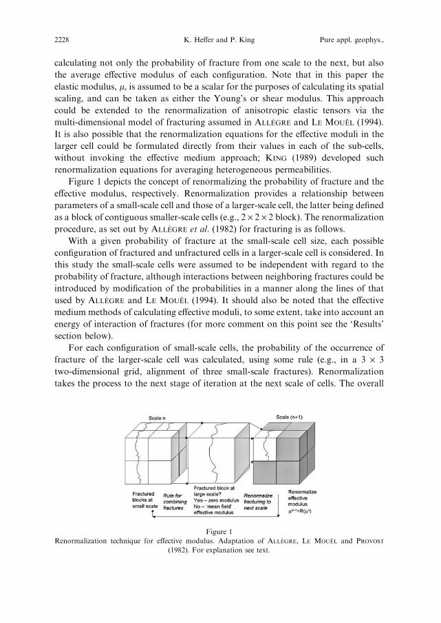
Figure 1 depicts the concept of renormalizing the probability of fracture and the

effective modulus, respectively. Renormalization provides a relationship between

parameters of a small-scale cell and those of a larger-scale cell, the latter being defined

as a block of contiguous smaller-scale cells (e.g., 2 · 2 · 2 block). The renormalization

procedure, as set out by ALLEGRE et al. (1982) for fracturing is as follows.

With a given probability of fracture at the small-scale cell size, each possible

configuration of fractured and unfractured cells in a larger-scale cell is considered. In

this study the small-scale cells were assumed to be independent with regard to the

probability of fracture, although interactions between neighboring fractures could be

introduced by modification of the probabilities in a manner along the lines of that

used by ALLEGRE and LE MOUEL (1994). It should also be noted that the effective

medium methods of calculating effective moduli, to some extent, take into account an

energy of interaction of fractures (for more comment on this point see the ‘Results’

section below).

For each configuration of small-scale cells, the probability of the occurrence of

fracture of the larger-scale cell was calculated, using some rule (e.g., in a 3 · 3

two-dimensional grid, alignment of three small-scale fractures). Renormalization

takes the process to the next stage of iteration at the next scale of cells. The overall

Figure 1

Renormalization technique for effective modulus. Adaptation of ALLEGRE, LE MOUEL and PROVOST

(1982). For explanation see text.

2228 K. Heffer and P. King Pure appl. geophys.,

relationship between probability of fracture of the larger-scale cell and that of the

small-scale cells is derived by taking into account all possible configurations of

fracturing. The relationship generally has a (non-trivial) critical point at which the

probability of fracturing is constant across all scales. During a sequence of increasing

strain in a domain of rock, fracturing is limited in scale until the density reaches the

critical point, at which there is catastrophic failure.

Renormalization of the average effective modulus of the fractured system is

formulated in parallel with the renormalization of fracturing. At each scale the mean

effective modulus is calculated, considering all possible configurations of small-scale

fractures, governed overall by the critical density. No correlation in the fractures is

assumed, and all knowledge of where fractures existed at the previous scale is

discarded at each renormalization. This is in line with the approach used by ALLEGRE

et al. (1982). The background ‘matrix’ modulus is taken to be the mean effective

modulus calculated at the previous scale. The details are as follows:

a) If the larger-scale cell of the configuration is deemed under the assumed rule to

be ‘fractured’, its effective modulus at that scale is taken as zero. This ignores any

stiffness that might be provided to shear fractures by friction, although, again, this

might be added in future studies.

b) If the larger-scale cell of the configuration is ‘unfractured’, its effective

modulus, ln+1, is calculated from that at the small-scale average effective modulus,

ln, by recourse to one of the effective medium techniques that have been described

earlier. Note that the mean-field approach is being used only for the approximation

to the interaction of the lower density configurations of fractures in ‘unfractured’

large-scale cells; fracture coalescences in higher density cells are catered for by the

more drastic reductions in effective modulus executed in a). Approximations such as

this are common in renormalization schemes, which are affected more by config-

urational geometries than by details of interactions. The relationship for effective

medium theories is ln+1= a.ln, where a takes the following forms in terms of the

fracture density, q, appropriate for the specific configuration being considered:

a = (1+b*q))1 for non-interacting fractures

a = (1)b*q) for the self-consistent approach of O’CONNELL and BUDIANSKY

(1974) and BUDIANSKY and O’CONNELL (1976)

a = exp()b*q) for the differential scheme of BRUNER (1976), HENYEY and

POMPHREY (1982), and ZIMMERMAN (1985).

The geometrical constant, b, as outlined in KEMENY and COOK (1986), is, for a

unidirectional set of fractures:

b ¼ 2pð1�t2Þ cL

� �2in 2-dimensions, and . . .

b ¼163ð1�t2Þ c

L

� �3in 3-dimensions,

Vol. 163, 2006 Spatial Scaling of Effective Modulus 2229

where c/L is the radius of each fracture as a proportion of the cell dimension at any

scale, and m is Poisson’s ratio (assumed constant across scales in this work). The

effective modulus associated with each possible configuration, i, of fracturing is

weighted by the probability, pi, of occurrence of that configuration at the critical

fracture density, and the mean effective modulus at the new scale obtained from the

weighted sum over all possible configurations: lnþ1� �¼P

ipnþ1

i lnþ1i . The spatial

scaling of modulus is obtained from the ratio between mean effective moduli at

consecutive scales. Recognizing that there is no characteristic scale at the critical

point of fracturing, the mean effective modulus will be a power-law function of

length scale, L; i.e., hlni� ðLnÞdl : The exponent, dl, is therefore obtained from the

ratio between consecutive scales of the mean effective modulus as:

dl ¼ loglnþ1� �

lnh i

� �= log

Lnþ1

Ln

� �:

Results

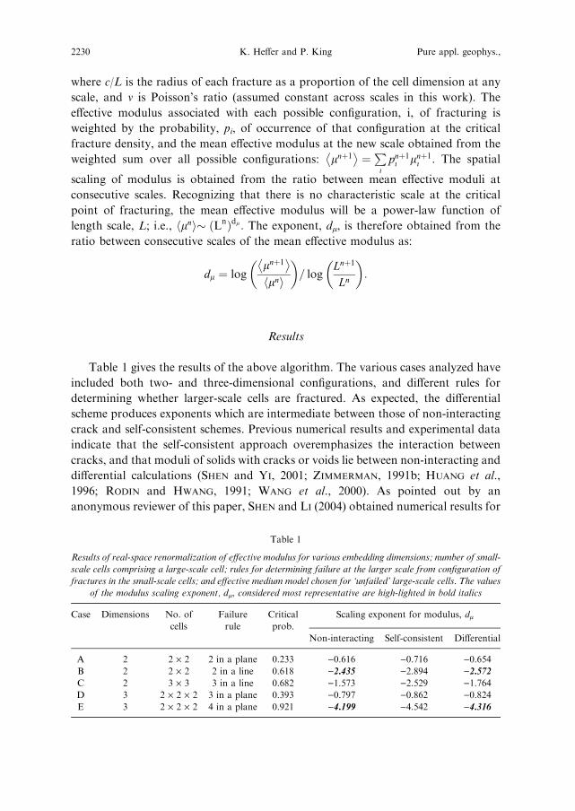
Table 1 gives the results of the above algorithm. The various cases analyzed have

included both two- and three-dimensional configurations, and different rules for

determining whether larger-scale cells are fractured. As expected, the differential

scheme produces exponents which are intermediate between those of non-interacting

crack and self-consistent schemes. Previous numerical results and experimental data

indicate that the self-consistent approach overemphasizes the interaction between

cracks, and that moduli of solids with cracks or voids lie between non-interacting and

differential calculations (SHEN and YI, 2001; ZIMMERMAN, 1991b; HUANG et al.,

1996; RODIN and HWANG, 1991; WANG et al., 2000). As pointed out by an

anonymous reviewer of this paper, SHEN and LI (2004) obtained numerical results for

Table 1

Results of real-space renormalization of effective modulus for various embedding dimensions; number of small-

scale cells comprising a large-scale cell; rules for determining failure at the larger scale from configuration of

fractures in the small-scale cells; and effective medium model chosen for ‘unfailed’ large-scale cells. The values

of the modulus scaling exponent, dl, considered most representative are high-lighted in bold italics

Case Dimensions No. of

cells

Failure

rule

Critical

prob.

Scaling exponent for modulus, dl

Non-interacting Self-consistent Differential

A 2 2 · 2 2 in a plane 0.233 )0.616 )0.716 )0.654B 2 2 · 2 2 in a line 0.618 )2.435 )2.894 )2.572C 2 3 · 3 3 in a line 0.682 )1.573 )2.529 )1.764D 3 2 · 2 · 2 3 in a plane 0.393 )0.797 )0.862 )0.824E 3 2 · 2 · 2 4 in a plane 0.921 )4.199 )4.542 )4.316

2230 K. Heffer and P. King Pure appl. geophys.,

random sizes of cracks that were very close to the predictions of the differential

method, supporting the assertion by SALGANIK (1973) that the differential method

should be more accurate as the crack size distribution becomes broader. However, in

the renormalization method of this paper the effective modulus of the system is

calculated at each stage with cracks of only one scale. It is therefore a moot point, left

for future investigation, as to whether SHEN and LI’S conclusion is applicable here,

and we restrict ourselves to concluding that the exponents from the non-interacting

cracks and differential schemes are more representative.

The range of exponents resulting from the different configurations and schemes

can be roughly interpreted, favoring the most appropriate failure rules, to indicate

that the spatial scaling of average effective modulus has exponent, dl , of about )2.5for two dimensions and about –4.2 for three dimensions. The value for three

dimensions is in line with those obtained by previous theoretical investigations, and

the value for two dimensions is within the range of previous theoretical values. The

high absolute values of the exponents indicate very rapid softening of effective

modulus for larger and larger domains. Remember that this only applies at, or near,

the critical point of fracturing. It implies that displacements are more closely

correlated (or anti-correlated, depending on orientation) at larger separation

displacements. Although initially this might seem counter-intuitive, it is consistent

with coherent displacements at either end of a fracture, or fault: the larger the

fracture, the greater the displacements involved. Also note that, because the scaling

of modulus is applicable only near to the critical point of inelastic deformation, it

does not imply any dispersion in seismic body waves (as would a scale-dependency in

modulus for elastic deformation).

Consistency with Previous Investigations of Scaling of Modulus

CHAKRABATI and BENGUIGUI (1997) discuss from a theoretical viewpoint the

scaling of modulus close to failure. They look (their section 3.4) at a disordered solid

modelled by a percolation model. They consider a random bond network with both

central (along bond) and bond-bending (changing bond angles) force constants that

govern the elastic energy due to bond stretching and bond-bending, respectively.

When the bond occupation concentration p is below the percolation threshold, pc, the

elastic modulus is of course zero. As p rises above pc, the elastic modulus grows

according to the power-law: l � p � pcð ÞTe for p > pc, where Te is called the elastic

exponent. Extensive numerical studies have ascertained that Te � 3.96 and 3.75 in 2

and 3 dimensions, respectively. Experimental results also compare well with the

numerically estimated exponents. FENG (1985) reviews the values of Te that have

been found by other workers as in the range 3.2–3.7 in two dimensions and 3.6 in

three dimensions. KANTOR (1985) deduced theoretical upper and lower bounds on

the elastic modulus exponent, Te, for a central and bond-bending model: these are

close to 4 for any dimension.

Vol. 163, 2006 Spatial Scaling of Effective Modulus 2231

Following ARBABI and SAHIMI (1988) we can obtain a length scaling relationship

for modulus by a finite-size scaling argument in which we consider the scaling

behavior of the correlation length close to the percolation threshold:

n pð Þ � p � pcj j�t for p � pcj j << pc, where t has values 4/3 and 0.88 in 2 and 3

dimensions, respectively. The correlation length is the average over all clusters of the

RMS distance between pairs of sites belonging to the same finite cluster. Therefore, a

domain of size L in a system close to the percolation threshold will have behavior

indistinguishable on average from a system at the threshold, n � Lð Þ, if the

corresponding deviation of the bond occupation concentration from the threshold

value in the parent system is p � pcj j � L�1=t, and so we obtain for the modulus

scaling at the threshold: l � L�Te=t. The exponent for modulus spatial scaling �Te=t,has the values 2.97 and 4.26 in d = 2 and 3 dimensions, respectively.

GUYON et al. (1989) review the results of applying percolation theory to a central-

force lattice, which comprises a 2-D triangular lattice of springs rotating freely at

their nodes. In the same random dilution problem in which a proportion (1-p) of

randomly distributed bonds are missing, they state the same power-law for elastic

modulus, but above the rigidity threshold, pr = 0.642, which is higher than the

normal connectivity percolation threshold (pc = 0.5), because simple connectivity

does not ensure the rigidity of the structure in this case. Nevertheless their

numerically determined exponent ratio: Tce=tce ¼ 3:0� 0:4, is still very close to that

for bond-bending percolation. However, as noted by FENG (1985), two other

estimates of Tce by FENG and SEN (1984) and LEMIEUX et al. (1985) do not agree.

Additionally CHAKRABATI and BENGUIGUI (1997) quote a value for

Tce=tce ¼ 1:12� 0:05 in two dimensions. ARBABI and SAHIMI (1988) found

Tce=tce ¼ 1:14� 1:42 from a two-dimensional model with central forces and

proposed that there may not be universality of elastic exponents for such models.

ZHOU and SHENG (1993) investigated the effect of isolated pockets of fluid in a

2-D continuum elastic solid. The changes in shape of the fluid pockets during shear

means that the fluid exerts an extra stiffening effect to the shear modulus, which was

found to scale with an exponent of 0.91 � 0.02, rather than 2.6 � 0.3 determined for

a solid-vacuum continuum. The authors note that the stiffening effect of the fluid

would be minimal if liquid flow is possible.

So, whilst there are some variations in determined values of the elastic modulus

scaling exponent, the consensus with the bond-bending model is for high values (3 or

4): modulus decays very rapidly with scale in a system near criticality.

Incorporation of Scale Dependency of Effective Modulus into Correlations

of Deformation

The value of effective modulus appropriate to a spectral component of fluctuation

with wavenumber, k, is that associated with the lengthscale � 1/k. So scaling of

2232 K. Heffer and P. King Pure appl. geophys.,

modulus is lðkÞ � kTe=t. Note that we do not take the Fourier transform over space

of L�Te=t, since we are considering the general scaling of moduli for various sizes of

domain, or various wavenumbers in Fourier space, rather than the specific variation

of modulus with position over a given domain. We can now make an heuristic

adaptation of the elastic theory of correlation function derived in the Appendix.

Since the elastic theory is developed for each wavenumber, then it can be modified to

the inelastic case by substitution of the appropriate effective modulus for each

wavenumber, l (k). The shear modulus appears in the denominator of the expression

for the covariance of displacements, so that the exponent of the magnitude of

wavenumber, k, in that expression, when amended for inelastic behavior, changes

from –2 to � 2þ Te=tð Þ� )5 to –6 in three-dimensions. As noted by KALLESTAD

(1998), the Fourier transform of r�k in D-dimensional space is given by:

F r�k

ðkÞ ¼ p�k�D=2 C kþD2

� �

C �k2

� � kk�D;

where C () is the gamma function.

So k)6 (k ¼ �3) corresponds to r3 in three-dimensional space. Also noted by

KALLESTAD (1998), the function rk, where k > �D, is a positive-definite function in

D-dimensional space. Therefore, the exponent of –6 for the wavenumber is the

minimum value for ensuring a valid correlation function in real space.

Sample Simulations

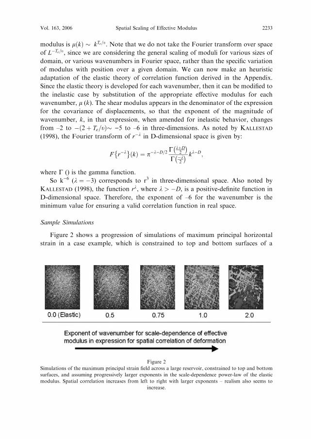
Figure 2 shows a progression of simulations of maximum principal horizontal

strain in a case example, which is constrained to top and bottom surfaces of a

Figure 2

Simulations of the maximum principal strain field across a large reservoir, constrained to top and bottom

surfaces, and assuming progressively larger exponents in the scale-dependence power-law of the elastic

modulus. Spatial correlation increases from left to right with larger exponents – realism also seems to

increase.

Vol. 163, 2006 Spatial Scaling of Effective Modulus 2233

formation. From left to right the simulations have used progressively higher values of

the exponent of wavenumber in the correlation of displacements. As expected, it is

seen that higher values of the exponent lead to greater spatial correlation in trends of

high or low strain. The longer correlation lengths look qualitatively more realistic.

Variations in the thickness of the formation are converted by the application of the

algorithm into laterally consistent lineations in horizontal strain.

Comparisons with Empirical Data

Autocorrelation of Stratigraphical Surfaces

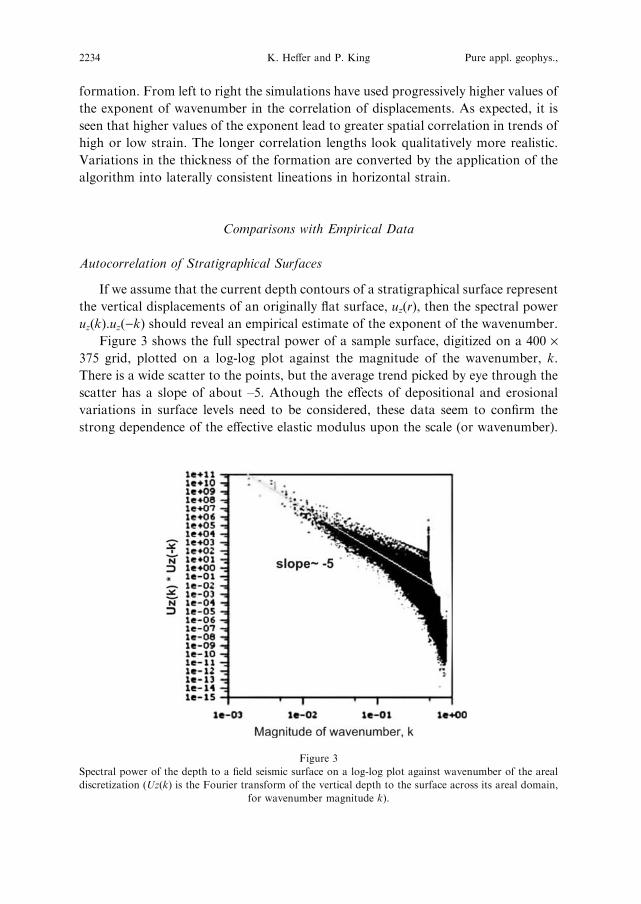
If we assume that the current depth contours of a stratigraphical surface represent

the vertical displacements of an originally flat surface, uz(r), then the spectral power

uz(k).uz()k) should reveal an empirical estimate of the exponent of the wavenumber.

Figure 3 shows the full spectral power of a sample surface, digitized on a 400 ·375 grid, plotted on a log-log plot against the magnitude of the wavenumber, k.

There is a wide scatter to the points, but the average trend picked by eye through the

scatter has a slope of about –5. Athough the effects of depositional and erosional

variations in surface levels need to be considered, these data seem to confirm the

strong dependence of the effective elastic modulus upon the scale (or wavenumber).

Figure 3

Spectral power of the depth to a field seismic surface on a log-log plot against wavenumber of the areal

discretization (Uz(k) is the Fourier transform of the vertical depth to the surface across its areal domain,

for wavenumber magnitude k).

2234 K. Heffer and P. King Pure appl. geophys.,

1/k Scaling of Heterogeneities in 1-D Samples

The scaling of correlation of displacements near the critical point of inelastic

three-dimensional deformation, derived above as k)5 to k)6, implies that the

correlation of three-dimensional inelastic strain, the first derivative of displacement,

near the critical point will scale as k)3 to k)4. In real three-dimensional space, the

associated correlation of strains varies with lag distance, r, as r0 (or log(r)) to r. A

one-dimensional sample through such correlated strain with these forms will have the

same scaling in real space, of which the spectral power in Fourier space will be k)1 to

k)2. This has a possible relationship with widespread observations of so-called

‘flicker’, or ‘pink’, ‘noise’ (also referred to as ‘1/f noise’, or, with k rather than f as the

scalar spatial frequency, ‘1/k noise’) in one-dimensional well logs of different

variables (porosity, density, permeability, etc.) e.g., LEARY (2002). In terms of

wavenumber, k, the spectral power densities of the heterogeneities show power-law

behavior S(k) � 1/kb where b � 1.0 to 1.6. This hints strongly at the possibility that

the basis of this behavior is the scaling of fluctuations in strain. The link is most

plausible for measurements of fracture porosity in fractured crystalline rocks. In

sedimentary rocks it is possible that palaeo-strains provided an original framework

that was later exploited and amplified by diagenetic trends; alternatively, the

geomorphology associated with palaeo-structural trends may have influenced the

actual depositional patterns directly. Here comparison is made with the Landau-

Ginzburg ‘meta-model’, commonly used for critical phenomena in thermodynamic

equilibrium. Fluctuations in the order parameter of a three-dimensional process are

associated with spectral densities that vary as 1/k2)g, where, in the Landau-Ginzburg

model, g takes a small value �0.1 (BINNEY et al., 1992). If we take the order

parameter of deformation to be the total strain, fluctuations would have spectral

densities � k)2 from this model, corresponding to a spectral density for displace-

ments �k)4, in contrast with �k)2 for the case of non-interacting cracks in equation

(1).

In contrast, the value of the correlation exponent, g, that corresponds to 1/k

scaling of one-dimensional samples (or k)3 scaling of three-dimensional fields), is g =

)1. In real space renormalization g = )1 is also associated with the ‘low

temperature’ value of the normalization parameter, xc = (d + 2 ) g)/(2d) = 1

(BINNEY et al., 1992, section 5.4.1). It implies that renormalization in real space of the

order parameter takes the form of a simple arithmetic averaging over the smaller cells

comprising a renormalized cell. Although xc cannot be determined for a linear real-

space renormalization scheme, arithmetic averaging is as expected if we take the

components of the conventional (infinitesimal) strain tensor as the order parameters

of inelastic deformation near the critical point. It is conjectured that there may be

better order parameters than strain that scale more closely, with different values of

scaling exponent and of g and xc. However, the familiarity of strain and the

empirically observed scaling of the porosity of fractured crystalline rock imply that

Vol. 163, 2006 Spatial Scaling of Effective Modulus 2235

strain is a satisfactory, if approximate, order parameter for renormalization. Then,

because strain averages arithmetically, it is necessarily associated with xc � 1 and g�)1. It is worth noting that the ‘high temperature’ value of x = ½ , corresponding to

g = +2, would imply k+2 scaling of strain in one-dimensional samples, or k0 scaling

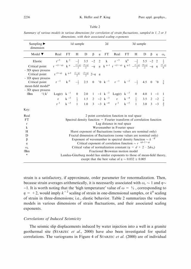
of strain in three-dimensions; i.e., elastic behavior. Table 2 summarizes the various

models in various dimensions of strain fluctuations, and their associated scaling

exponents.

Correlations of Induced Seismicity

The seismic slip displacements induced by water injection into a well in a granite

geothermal site (STARZEC et al., 2000) have also been investigated for spatial

correlations. The variograms in Figure 4 of STARZEC et al. (2000) are of individual

Table 2

Summary of various models in various dimensions for correlation of strain fluctuations, sampled in 1, 2 or 3

dimensions, with their associated scaling exponents

Sampling c

dimension

1d sample 2d 3d sample

Model . Real FT H D b g FT Real FT H D b g xc

Elastic r)3 k 2 �32 3.5 )2 2 k r )3 k0 �3

2 5.5 )2 2 12

Critical point

- 3D space process

r )(1+g) k g �ð1þgÞ2

ð5þgÞ2 )g g k g)1 r )(1+g) k g-2 �ð1þgÞ

2ð9þgÞ

2 )g g ð5�gÞ6

Critical point

- 1D space process

r (1)g) k g-2 ð1�gÞ2

ð3þgÞ2 2)g g

Critical point

mean-field model*

- 3D space process

r )1 k 0 �12 2.5 0 ~0 k )1 r )1 k )2 �1

2 4.5 0 ~0 56

fBm ‘1/k’ Log(r) k )1 0 2.0 1 )1 k )2 Log(r) k )3 0 4.0 1 )1 1

r k )2 12 1.5 2 )2 k )3 r k )4 1

2 3.5 2 )2 76

r 2 k )3 1 1.0 3 )3 k )4 r 2 k )5 1 3.0 3 )3 43

Key:

Real 2 point correlation function in real space

FT Spectral density function = Fourier transform of correlation function

r Lag distance in real space

k Wavenumber in Fourier space

H Hurst exponent of fluctuations (some values are nominal only)

D Fractal dimension of fluctuations (some values are nominal only)

b Exponent of wavenumber in spectral density function � k )b

g Critical exponent of correlation function � r –(d)2+g)

xc Critical value of normalization constant (g = d + 2 – 2dxc)

fBm Fractional Brownian motion model

* Landau-Ginzburg model has similar exponents to those of mean-field theory,

except that the best value of g � 0.032 � 0.005

2236 K. Heffer and P. King Pure appl. geophys.,

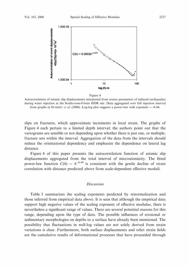
slips on fractures, which approximate increments in local strain. The graphs of

Figure 4 each pertain to a limited depth interval; the authors point out that the

variograms are sensible or not depending upon whether there is just one, or multiple,

fracture sets within the interval. Aggregation of the data from the intervals should

reduce the orientational dependency and emphasize the dependence on lateral lag

distance.

Figure 4 of this paper presents the autocorrelation function of seismic slip

displacements aggregated from the total interval of microseismicity. The fitted

power-law function C(h) � h)0.44 is consistent with the gentle decline of strain

correlation with distance predicted above from scale-dependent effective moduli.

Discussion

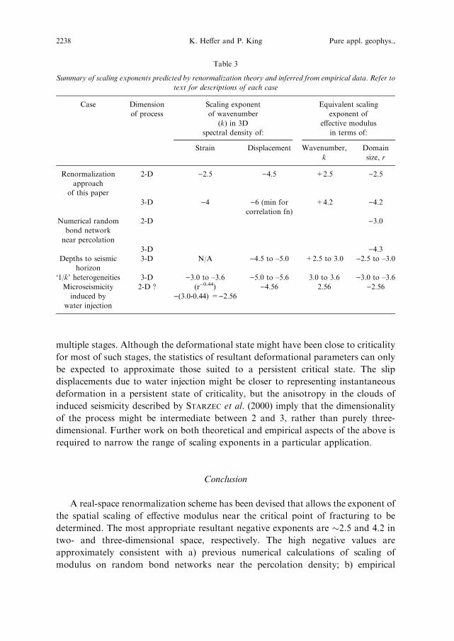
Table 3 summarizes the scaling exponents predicted by renormalization and

those inferred from empirical data above. It is seen that although the empirical data

support high negative values of the scaling exponent of effective modulus, there is

nevertheless a significant range of values. There are several potential reasons for this

range, depending upon the type of data. The possible influences of erosional or

sedimentary morphologies on depths to a surface have already been mentioned. The

possibility that fluctuations in well-log values are not solely derived from strain

variations is clear. Furthermore, both surface displacements and relict strain fields

are the cumulative results of deformational processes that have proceeded through

Figure 4

Autocorrelation of seismic slip displacements interpreted from source parameters of induced earthquakes

during water injection at the Soultz-sous-Forets HDR site. Data aggregated over full injection interval

from graphs in STARZEC et al. (2000). Log-log plot suggests a power-law with exponent �)0.44.

Vol. 163, 2006 Spatial Scaling of Effective Modulus 2237

multiple stages. Although the deformational state might have been close to criticality

for most of such stages, the statistics of resultant deformational parameters can only

be expected to approximate those suited to a persistent critical state. The slip

displacements due to water injection might be closer to representing instantaneous

deformation in a persistent state of criticality, but the anisotropy in the clouds of

induced seismicity described by STARZEC et al. (2000) imply that the dimensionality

of the process might be intermediate between 2 and 3, rather than purely three-

dimensional. Further work on both theoretical and empirical aspects of the above is

required to narrow the range of scaling exponents in a particular application.

Conclusion

A real-space renormalization scheme has been devised that allows the exponent of

the spatial scaling of effective modulus near the critical point of fracturing to be

determined. The most appropriate resultant negative exponents are �2.5 and 4.2 in

two- and three-dimensional space, respectively. The high negative values are

approximately consistent with a) previous numerical calculations of scaling of

modulus on random bond networks near the percolation density; b) empirical

Table 3

Summary of scaling exponents predicted by renormalization theory and inferred from empirical data. Refer to

text for descriptions of each case

Case Dimension

of process

Scaling exponent

of wavenumber

(k) in 3D

spectral density of:

Equivalent scaling

exponent of

effective modulus

in terms of:

Strain Displacement Wavenumber,

k

Domain

size, r

Renormalization

approach

of this paper

2-D )2.5 )4.5 +2.5 )2.5

3-D )4 )6 (min for

correlation fn)

+4.2 )4.2

Numerical random

bond network

near percolation

2-D )3.0

3-D )4.3Depths to seismic

horizon

3-D N/A )4.5 to –5.0 +2.5 to 3.0 )2.5 to –3.0

‘1/k’ heterogeneities 3-D )3.0 to –3.6 )5.0 to –5.6 3.0 to 3.6 )3.0 to –3.6

Microseismicity

induced by

water injection

2-D ? (r)0.44)

)(3.0-0.44) =)2.56)4.56 2.56 )2.56

2238 K. Heffer and P. King Pure appl. geophys.,

observations of depth profiles of surfaces; c) ‘1/k’ scaling of fluctuations in one-

dimensional samples of geological heterogeneities; d) spatial correlation of micro-

seismic emissions resulting from water injection. The power-law spatial scaling of

effective modulus has been substituted for the modulus appearing in the directional

form of the 2-point correlation of elastic displacements. Although deformational

statistics might be more closely characterized by multifractality, the resultant

correlation function has been used to interpolate the full displacement vector across a

field conditioned on its upper and lower surfaces to give a map of maximum principal

strain that shows more realism as the scaling becomes more long-range.

Acknowledgements

Part of the work leading to this paper was financed by BP Exploration Ltd., the

Department of Trade and Industry (UK), and Roxar Ltd. Very helpful discussions

were also held with Dr. Colin Daly at Roxar Ltd, Professor Stuart Crampin at the

University of Edinburgh and Dr. Peter Leary.

Appendix: Spatial Correlation of Fractures, Elastic Case.

The following is an adaptation of Chapter 4 of LANDAU and LIFSHITZ (1975) on

the treatment of elastic deformations in the presence of a distribution of dislocations.

The total energy per unit volume is the work done by the elastic forces on the

total strain. That is E ¼ 12r

eije

eji. All terms in this have well-defined Fourier

Transforms so we can work throughout in Fourier space. The definition of elastic

strain is

eeij ¼ i

2

� �ue

i kj þ uejki

� �¼ i

2

� �dajdil þ daidjl� �

kauel :

Similarly the elastic contribution to the stress can be written reij ¼ ikijalkaue

l , where

kijal is the standard isotropic elasticity tensor, related to the Lame constants, k and l,by kdijdal þ l diadjl þ dildja

� �. Contracting these terms together leads to an expression

for the elastic energy:

E ¼ 12 kþ lð Þkkkl þ lk2dkl �

uek kð Þ ue

l �kð Þ ¼ 12l k2dkl þ 1

1�2t� �

kkkl �

uek kð Þ ue

l �kð Þ

¼ l2 Lkl kð Þ ue

k kð Þ uel �kð Þ;

where Lij is the usual linear operator of isotropic elasticity and is the inverse of the

Green’s function, LijGjk ¼ dik .

Vol. 163, 2006 Spatial Scaling of Effective Modulus 2239

The Boltzmann distribution for the elastic energy can be expressed as

p Eð Þ ¼ Z�1 exp � 1

Eh i

Zd3k E kð Þ

� �¼ Z�1 exp � l

Eh i

Zd3k Lkl kð Þ ue

k kð Þ uel �kð Þ

� �

where hEi is the mean energy and Z is the partition function (normalization

constant). Assuming Boltzmann statistics, it is then easy to demonstrate that the

spatial correlation in the elastic displacement is given by:

cij kð Þ ¼ uei kð Þ ue

j �kð ÞD E

¼ Eh i2l

L�1ij ¼Eh i2l

Gij ¼Eh i

2lk2dij �

1

2 1� tð Þkikj

k2

� �:

In real space the correlation of displacements takes the form:

uei rð Þ:ue

j 0ð ÞD E

¼ Eh i16p 1� tð Þ

1

r3� 4tð Þdij þ

rirj

r2

h i:

There is some evidence that the energy actually follows a power-law

(i.e., P Eð Þ � Ea), attributable to the degeneracy of states with a given energy that

dominates the Boltzmann distribution near the critical point (MAIN and BURTON,

1994; MAIN and AL-KINDY, 2002). Note that a power-law distribution is not

normalizable unless a cut-off is applied (whether or not this is an ultra-violet or an

infra-red cut-off depends on the value of a). In fact the spatial correlation is very

similar to that for the Boltzmann distribution in that the correlations essentially

depend on the inverse of the kernel of the energy function. In addition there are some

multiplicative terms involving the cut-off which is required to ensure that the

integrals are well defined. It is readily shown that the essential correlation structure is

the same as that for the Boltzmann distribution.

REFERENCES

ALLEGRE, C.J., LE MOUEL, J.L., and PROVOST, A. (1982), Scaling rules in rock fracture and possible

implications for earthquake prediction, Nature 297, 47–49.

ALLEGRE, C.J. and LE MOUEL J.L. (1994), Introduction of scaling techniques in brittle fracture of rocks,

Phys. Earth Planet Inter. 87, 85–93.

ARBABI, S. and SAHIMI, M. (1988), Absence of universality in percolation models of disordered elastic media

with central forces, J. Phys. A: Math. Gen. 21, L863–L868.

BAK, P., How Nature Works – the Science of Self-Organized Criticality (Oxford University Press, Oxford

1997). BINNEY, J.J., DOWRICK, N.J., FISHER, A.J., and NEWMAN, M.E.J. The Theory of Critical

Phenomena – An Introduction to the Renormalization Group (Oxford University Press, Oxford 1992).

BRUNER, W.M. (1976), Comment on ‘Seismic velocities in dry and saturated cracked solids’ by O’Connell and

Budiansky, J. Geophys. Res. 81, 2573–2576.

BUDIANSKY, B. and O’CONNELL, R.J. (1976), Elastic moduli of a cracked solid, Int. J. Solids Struct. 12, 81–

97.

CHAKRABARTI, B.K. and BENGUIGUI, L.G., Statistical Physics of Fracture and Breakdown in Disordered

Systems (Oxford University Press, Oxford 1997).

2240 K. Heffer and P. King Pure appl. geophys.,

COWIE, P. A., SORNETTE, D., and VANNESTE C. (1995), Multifractal scaling properties of a growing fault

population, Geophys. J. Int. 122, 457–469.

FENG, S., Elasticity and percolation in scaling phenomena. In Disordered Systems (eds. R. Pynn and A.

Skjeltorp), (NATO ASI Series B: Physics, vol.133, Plenum Press, New York and London 1985).

FENG, S. and SEN, P.N. (1984), Percolation on elastic networks: New exponent and threshold, Phys. Rev.

Lett. 52, 216.

GUYON, E., HANSEN, A., HINRISCHEN, E., and ROUX, S. (1989), Critical behaviors of central-force lattices,

Physica A 157, 580–586.

HEFFER, K.J., KING, P.R., and JONES, A.D.W. (1999), Fracture modelling as part of integrated reservoir

characterization, Society of Petroleum Engineers paper SPE 53347.

HENYEY, F.S. and POMPHREY, N. (1982), Self-consistent moduli of cracked solid, Geophys. Res. Lett. 9,

903–906.

HUANG, Y., CHANDRA, A., JIANG, Z.Q., WEI, X., and HU, K.X. (1996), The numerical calculation of two-

dimensional effective moduli for microcracked solids, J. Solids Struc. 33, 1575–1586.

HUDSON, J. A. (1980), Overall properties of a cracked solid, Math. Proc. Cambridge Phil. Soc. 88, 371–384.

HUDSON, J.A. (1981), Wave speeds and attenuation of elastic waves in material containing cracks. Geophys.

J. Roy. Astr. Soc. 64, 133–150.

HUDSON, J.A. (1986), A higher-order approximation to the wave propagation constants for a cracked solid,

Geophys. J. Roy. Astr. Soc. 87, 265–274.

JAEGER, J.C. and COOK, N.G.W., Fundamentals of Rock Mechanics, Third Edition (Chapman and Hall,

London, 1979).

KADANOFF, L.P. (1966), The introduction of the idea that exponents could be derived from real-space scaling

arguments, Physics 2, 263–273.

KALLESTAD, E. (1998), Stochastic simulation of Gaussian vector fields, Diploma Thesis in the Faculty of

Physics, Informatics and Mathematics, Norwegian University of Science and Technology, (NTNU)

Trondheim.

KANTOR, Y. (1985), Elastic properties of random systems. In Scaling Phenomena in Disordered Systems (eds.

R. Pynn and A. Skjeltorp), (NATO ASI Series B: Physics, vol. 133, Plenum Press, New York and

London 1985).

KELVIN, LORD (William Thomson) (1856), Elements of a mathematical theory of elasticity, Part 1, On

stresses and strains, Phil. Trans. Roy. Soc. 166, 481–498.

KEMENY, J. and COOK, N.G.W. (1986), Effective moduli, non-linear deformation and strength of a cracked,

elastic solid, Int. J. Rock Mech. Min. Sci. and Geomech. Abstr. 23, 2, 107–118.

KING, P.R. (1989), The use of renormalization for calculating effective permeability, Trans. Por. Media 4,

37–58.

LANDAU, L. D. and LIFSHITZ, E. M., Theory of Elasticity (Pergamon, New York 1975).

LEARY, P.C., Fractures and physical heterogeneity in crustal rock. In Heterogeneity in the Crust and Upper

Mantle: Nature, Scaling and Seismic Properties (eds. Goff, J.A. and Holliger, K.) (Kluwer Academic,

New York 2002).

LEMIEUX, M.A., BRETON, P., and TREMBLAY, A-M.S. (1985), J. Phys. (Paris) Lett. 46, L-1.

MAIN, I.G. (1996), Statistical physics, seismogenesis and seismic hazard, Rev. Geophys. 34, 4, 433–462.

MAIN, I.G. and AL-KINDY, F.H. (2002), Entropy, energy and proximity to criticality in global earthquake

populations, Geophys. Res. Lett. 29, 7, 25–1:4.

MAIN, I.G. and BURTON, P.W. (1984), Information theory and the earthquake magnitude frequency

distribution, Bull. Seismol. Soc. Am. 74, 1409–1426.

MARSAN, D. and BEAN, C.J. (2003), Multifractal modelling and analyses of crustal heterogeneity. In

Heterogeneity in the Crust and Upper Mantle: Nature, Scaling and Seismic Properties (eds. Goff, J.A. and

Holliger, K.) (Kluwer Academic, New York 2002).

MEHRABADI, M.M. and COWIN, S.C. (1990), Eigentensors of linear anisotropic elastic materials, Mech.

Appl. Math. 43, Pt 1, 15–41.

O’CONNELL, R.J. and BUDIANSKY, B. (1974), Seismic velocities in dry and saturated cracked solids,

J Geophys. Res. 79, 5412–5426.

OUILLON G., CASTAING, C., and SORNETTE, D. (1996), Hierarchical geometry of faulting, J. Geophys. Res.

191, 5477–5487.

Vol. 163, 2006 Spatial Scaling of Effective Modulus 2241

RODIN, G.J. and HWANG, Y.L. (1991), On the problem of linear elasticity for an infinite region containing a

finite number of non-intersecting spherical inhomogeneities, Int. J. Sol. Struct. 27, 145–159.

SALGANIK, R.L. (1973), Mechanics of bodies with many cracks, Mech. Solids 8, 135–143.

SAYERS, C. and KACHANOV, M. (1991), A simple technique for finding effective elastic constants of cracked

solids for arbitrary crack orientation statistics, Int. J. Sol. Struct. 27, 6, 671–680.

SHEN, L. and LI, J. (2004), A numerical simulation for effective elastic moduli of plates with various

distributions and sizes of cracks, Int. J. Sol. Struct. 41, 7471–7492.

SHEN, L. and YI, S. (2001), An effective inclusion model for effective moduli of heterogeneous materials with

ellipsoidal inhomogeneities, Int. J. Sol. Struct. 38, 5789–5805.

SMALLEY, J., TURCOTTE, D.L., and SOLLA, R.J. (1985), A renormalization group approach to the stick-slip

behaviour of fault, J. Geophys. Res. 90, 1894–1900.

STARZEC, P., FEHLER, M., BARIA, R., and NIITSUMA, H. (2000), Spatial correlation of seismic slip at the

HDR-Soultz geothermal site: Qualitative approach, Bull. Seismol. Soc. Am. 90, 6, 1528–1534.

TURCOTTE, D.L. (1986), Fractals and fragmentation, J. Geophys. Res. 91, 1921–1926.

WANG, J., FANG, J., and KARIHALOO, B.L. (2000), Asymptotic bounds on overall moduli of cracked bodies,

Int. J. Sol. Struct. 37, 6221–6237.

ZIMMERMAN, R.W. (1985), The effect of microcracks on the elastic moduli of brittle materials, J. Mater. Sci.

Lett. 4, 1457–60.

ZIMMERMAN, R.W., Compressibility of Sandstones. Developments in Petroleum Science. (Elsevier,

Amsterdam 1991a).

ZIMMERMAN, R.W. (1991b), Elastic moduli of a solid containing spherical inclusions, Mech. Mater. 12, 17–

24.

ZHOU, M. and SHENG, P. (1993), Shear rigidity in 2D solid-liquid composites, Phys. Rev. Lett. 71, 26, 4358–

4360.

(Received March 15, 2005, revised December 1, 2005, accepted January 4, 2006)

To access this journal online:

http://www.birkhauser.ch

2242 K. Heffer and P. King Pure appl. geophys.,