Spatial Optimization Layout of Best Management Practices ...

Spatial Optimization Layout of Best ManagementPractices through SWAT and Interval FractionalProgramming Under UncertaintyJinjin Gu ( [email protected] )

Hefei University of TechnologyYuan Cao

College of Architecture and Art, Hefei University of TechnologyMin Wu

College of Architecture and Art, Hefei University of TechnologyMin Song

College of Architecture and Art, Hefei University of TechnologyLin Wang

College of Architecture and Art, Hefei University of Technology

Research Article

Keywords: Best management practices, Interval fractional programming, Uncertainty, Spatial optimizationlayout

Posted Date: June 7th, 2021

DOI: https://doi.org/10.21203/rs.3.rs-509238/v1

License: This work is licensed under a Creative Commons Attribution 4.0 International License. Read Full License

https://doi.org/10.21203/rs.3.rs-509238/v1

mailto:[email protected]

https://doi.org/10.21203/rs.3.rs-509238/v1

https://creativecommons.org/licenses/by/4.0/

Spatial Optimization Layout of Best Management Practices through SWAT and

Interval Fractional Programming under uncertainty

Jinjin Gua,*, Yuan Caob, Min Wua, Min Songa, Lin Wanga

aDepartment of Urban and Rural Planning, College of Architecture and Art, Hefei

University of Technology, Hefei 230601, China

bDepartment of Architecture, College of Architecture and Art, Hefei University of

Technology, Hefei 230601, China

Abstract

Uncertainty in nature and human society affect pollution control efficiency and the

rationality of the scheme of spatial optimization layout of best management practices

(BMP) for agricultural non-point-source (NPS) pollution treatment. Based on this idea,

the study innovatively develops a mathematical model that integrates soil and water

assessment tool (SWAT) model and interval fractional programming. The advantage of

the model are the following: (1) ability to process a BMP spatial optimization layout in

watershed in uncertain situations, (2) ability to effectively reflect the uncertain factors

involved in the scheme without having to set all the variables as uncertain factors, and

(3) results are in the form of schemes in upper and lower limit scenarios, thereby

reflecting the limit of uncertainty impact on the schemes.

The results of this study can provide decision-makers with a wide range of optional

schemes. This study examines how to set up the BMP spatial optimal layout scheme for

agricultural non-point-source pollution treatment under the influence of uncertain

factors. The proposed method is universal and can be extended to other cases.

Keyword: Best management practices; Interval fractional programming; Uncertainty;

Spatial optimization layout

1. Introduction

A spatial optimal layout of best management practices (BMPs) can effectively

alleviate non-point source (NPS) pollution in a river basin. However, deep-rooted

uncertainties in nature and human society exist in BMPs, such as in cost and pollutant

treatment efficiency (Gu et al, 2020). These uncertainties influence the NPS pollution

efficiency and cost of the BMP spatial optimal layout. For example, BMP treatment of

NPS pollutants involves many factors, such as reaction time, temperature, rainfall, and

various vegetation and microbial species. These factors determine that the efficiency

and variation in any one of them would cause variations in the treatment effect.

Therefore, the removal effect of pollutants in related studies is expressed in the form of

floating intervals, which represent the possible scale of the results caused by

uncertainties (Gu et al, 2020). For the uncertainty of cost, the economic cost of BMPs

is subject to market fluctuations, and the change reflects the character of the market.

Thus, the economic cost is also expressed in the form of floating intervals.

Uncertainties would cause the result of the BMP spatial optimization allocation to

be unable to achieve the desired purpose by affecting the pollution treatment efficiency

of BMPs. Therefore, the uncertainty factor would also affect the rationality of the

spatial optimal layout scheme of BMPs. The reference factors, such as treatment

efficiency and cost of BMPs in formulating schemes, are generally set as the definite

value. Thus, the change in the value of reference factors possibly affect the rationality

of the spatial optimization scheme.

Many studies have been conducted to solve the problem of uncertain factors in the

BMP spatial optimization layout, and genetic algorithm (GA) is widely used (Kaini et

al, 2012; Wu et al, 2018). The spatial layout method based on the GA can process the

uncertainty and obtain definite results, but the following problems occur in related

studies with the GA method:

(1) With GAs, all the related variables need to be set as uncertain values, but in

practice, not all variables are uncertain numbers. Therefore, the studies using this

method have to set all the related variable factors as uncertainty values with mean

values.

(2) It is not convenient for the GA to set complex constraint equations. In general,

relevant studies use mathematical software, such as Matlab, to build a GA optimization

equation. However, the complex constraints are always difficult to set in these software

due to the constraints of integrated software packages. In practical terms, complex

constraints for variables are encountered in planning inevitably, whereas the related

software with the GA method are not highly suitable for the operator and planner.

(3) It is not convenient for GA to set weight values between multi-objective

functions while avoiding subjective judgement. Particularly in dealing with the multi-

objective problem of maximum objective function and minimum objective function,

setting appropriate weight values between maximization and minimization without

subjective judgement is difficult.

Therefore, an important task is to develop a method for BMP spatial optimization

layout under uncertainty. The method has to process uncertainty and avoid subjective

weights in multi-objective optimization, and should be able to address multiple

complex constraints.

1.1 NPS pollution control in watersheds

The first step in NPS pollution control in watersheds is to determine the amount

of NPS pollution that should be controlled. In farmland areas, NPS pollution is usually

due to nitrogen and phosphorus (P) produced by agricultural activities (Wu and Lu,

2019). The release of NPS pollution can be simulated effectively by using hydrological

software. Soil and water assessment tool (SWAT) software is an effective NPS pollution

analysis tool that considers environmental factors such as regional topography, soil,

land use map, and climate. In addition, this software can systematically analyze the land

surface process and channel behavior of pollutant loss, and evaluate the efficiency of

the pollution control scheme (Feng and Shen, 2021). When the BMP spatial

optimization layout is used to control NPS pollution in watersheds, SWAT software can

be used to divide the studied watershed into sub-watershed or hydrology response unit

(HRU), and the BMP facilities are allocated to each sub-watershed or HRU (Qiu et al,

2019).

1.2 Spatial optimization layout of BMP facilities

During the BMP spatial optimization layout, the problems of pollutant treatment

efficiency and total cost should be considered. Fractional planning can be used to solve

the conflict between maximum and minimum objectives, and such planning can

effectively avoid the subjective setting for objective function weights (Gu et al, 2018).

In addition, writing of fractional programming in a more open and basic mathematical

programming software can easily load diverse and complex constraint equations.

Fractional programming has been used in many fields.

1.3 Uncertainty analysis

In general, uncertain factors can be expressed in mathematical form according to

their mathematical properties, and the form of uncertain numbers can be categorized as

interval, random, and fuzzy numbers (Guo et al, 2014). Integrating these uncertain

numbers into the optimization model make up the uncertainty optimization model.

When uncertainty numbers are integrated into fractional programming, the integrated

uncertainty fractional model could be in different forms according to the distribution

forms of uncertainty (Zhang et al, 2019). To perform uncertainty programming, the

confidence distribution interval is first identified according to the distribution form of

the uncertainty number, and then taking the upper and lower boundaries of the interval

number into the optimization model to solve the problem. Finally, the upper and lower

limit values of the programming model are obtained (Li et al, 2019).

At present, although many studies about uncertain BMP spatial optimization

layout have been conducted, most of the related studies use GA to perform the

optimization, among which the constraints on the parameter variables are relatively

simple (Qi et al, 2020; Getahun and Keefer, 2016). Few studies can reflect the complex

constraints for variables in practical problems. Besides, most of the related studies

obtain the definite scheme results. Although the definite schemes based on GA consider

the uncertainty factors, the results lack the flexibility to deal with these factors, and it

would cause decision-makers to lack the right to choose other schemes according to the

complex environment.

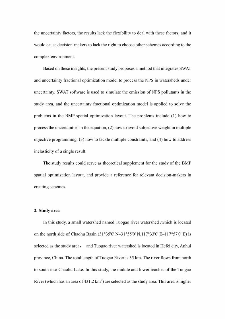
Based on these insights, the present study proposes a method that integrates SWAT

and uncertainty fractional optimization model to process the NPS in watersheds under

uncertainty. SWAT software is used to simulate the emission of NPS pollutants in the

study area, and the uncertainty fractional optimization model is applied to solve the

problems in the BMP spatial optimization layout. The problems include (1) how to

process the uncertainties in the equation, (2) how to avoid subjective weight in multiple

objective programming, (3) how to tackle multiple constraints, and (4) how to address

inelasticity of a single result.

The study results could serve as theoretical supplement for the study of the BMP

spatial optimization layout, and provide a reference for relevant decision-makers in

creating schemes.

2. Study area

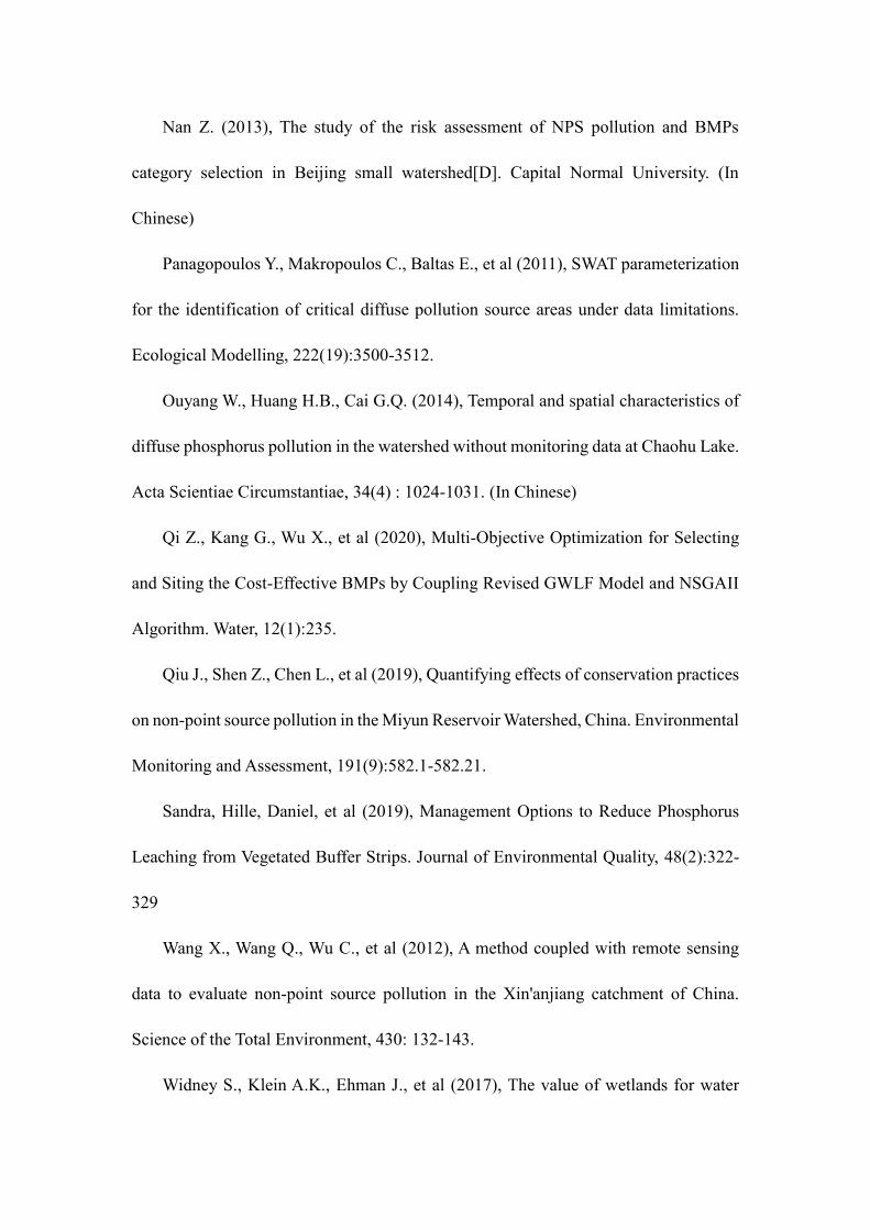
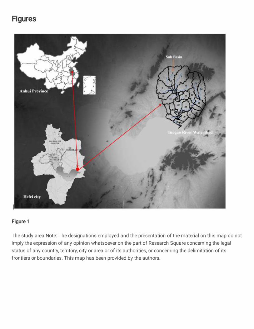
In this study, a small watershed named Tuogao river watershed ,which is located

on the north side of Chaohu Basin (31°35'0' N–31°55'0' N,117°33'0' E–117°57'0' E) is

selected as the study area， and Tuogao river watershed is located in Hefei city, Anhui

province, China. The total length of Tuogao River is 35 km. The river flows from north

to south into Chaohu Lake. In this study, the middle and lower reaches of the Tuogao

River (which has an area of 431.2 km2) are selected as the study area. This area is higher

in the north and lower in the south. It is located in a plain polder area, which refers to a

plain river network or lakeside and other low-lying waterlogging areas. This area is

formed through embankments, sluices, and pumping stations. The purpose of

constructing a polder area is to resist floods and waterlogging. The study area is

characterized by a north subtropical humid monsoon climate, with annual precipitation

of 1000–1158 mm, annual evaporation of 1469–1629 mm, and rainfall concentrated

mostly in summer (Cao et al, 2007). At present, the main part of the study area is

agricultural land, and the rest consists of grassland, woodland, and residential land .

The study area is listed in figure 1.

(Put figure 1 here)

The study area faces problems of eutrophication and algae growth, and P is a key

factor. P comes from NPS pollution caused by local agricultural activities.

The purpose of this study is to reduce the total P release of the study area through

BMP spatial optimal allocation. Taking July, when NPS pollution is worst, as an

example, this study analyzes the schemes of BMP spatial allocation layout under

different reduction targets of P pollution, specifically, 20%, 40%, and 60%.

3. Methodology and material

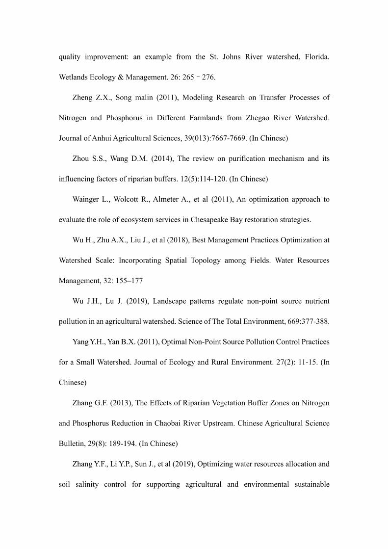
3.1 Study process

The study process consists of the following steps:

(1) Construction of watershed hydrological model: This task includes collecting

basic data on the study area, establishing the basic database of the research area (DEM,

soil, and land use), using the SWAT model to divide the study area into sub-basins, and

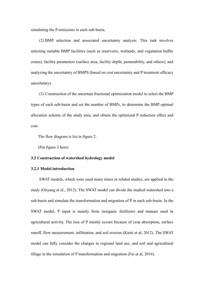
simulating the P emissions in each sub-basin.

(2) BMP selection and associated uncertainty analysis: This task involves

selecting suitable BMP facilities (such as reservoirs, wetlands, and vegetation buffer

zones); facility parameters (surface area, facility depth, permeability, and others); and

analyzing the uncertainty of BMPS (based on cost uncertainty and P treatment efficacy

uncertainty).

(3) Construction of the uncertain fractional optimization model to select the BMP

types of each sub-basin and set the number of BMPs, to determine the BMP optimal

allocation scheme of the study area, and obtain the optimized P reduction effect and

cost.

The flow diagram is list in figure 2.

(Put figure 2 here)

3.2 Construction of watershed hydrology model

3.2.1 Model introduction

SWAT models, which were used many times in related studies, are applied in the

study (Ouyang et al., 2012). The SWAT model can divide the studied watershed into a

sub-basin and simulate the transformation and migration of P in each sub-basin. In the

SWAT model, P input is mainly from inorganic fertilizers and manure used in

agricultural activity. The loss of P mainly occurs because of crop absorption, surface

runoff, flow measurement, infiltration, and soil erosion (Kaini et al, 2012). The SWAT

model can fully consider the changes in regional land use, and soil and agricultural

tillage in the simulation of P transformation and migration (Fei et al, 2016).

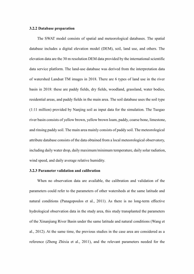
3.2.2 Database preparation

The SWAT model consists of spatial and meteorological databases. The spatial

database includes a digital elevation model (DEM), soil, land use, and others. The

elevation data are the 30 m resolution DEM data provided by the international scientific

data service platform. The land-use database was derived from the interpretation data

of watershed Landsat TM images in 2018. There are 6 types of land use in the river

basin in 2018: these are paddy fields, dry fields, woodland, grassland, water bodies,

residential areas, and paddy fields in the main area. The soil database uses the soil type

(1:11 million) provided by Nanjing soil as input data for the simulation. The Tuogao

river basin consists of yellow brown, yellow brown loam, paddy, coarse bone, limestone,

and rinsing paddy soil. The main area mainly consists of paddy soil. The meteorological

attribute database consists of the data obtained from a local meteorological observatory,

including daily water drop, daily maximum/minimum temperature, daily solar radiation,

wind speed, and daily average relative humidity.

3.2.3 Parameter validation and calibration

When no observation data are available, the calibration and validation of the

parameters could refer to the parameters of other watersheds at the same latitude and

natural conditions (Panagopoulos et al., 2011). As there is no long-term effective

hydrological observation data in the study area, this study transplanted the parameters

of the Xinanjiang River Basin under the same latitude and natural conditions (Wang et

al., 2012). At the same time, the previous studies in the case area are considered as a

reference (Zheng Zhixia et al., 2011), and the relevant parameters needed for the

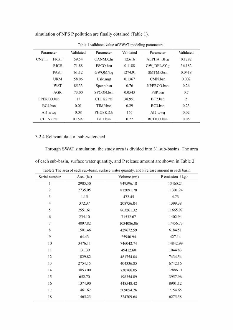
simulation of NPS P pollution are finally obtained (Table 1).

Table 1 validated value of SWAT modeling parameters

Parameter Validated value

Parameter Validated value

Parameter Validated valueCN2.m

gtFRST 59.54 CANMX.hr

u12.616 ALPHA_BF.g

w0.1282

RICE 71.88 ESCO.hru 0.1188 GW_DELAY.gw

36.182

PAST 61.12 GWQMN.gw

1274.91 SMTMP.bsn 0.0418

URML

58.06 Usle.mgt 0.1367 CMN.bsn 0.002

WATR

85.33 Spexp.bsn 0.76 NPERCO.bsn 0.26

AGRL

73.00 SPCON.bsn 0.0543 PSP.bsn 0.7

PPERCO.bsn 15 CH_K2.rte 38.951 BC2.bsn 2

BC4.bsn 0.01 TIMP.bsn 0.29 BC3.bsn 0.23

AI1.wwq 0.08 PHOSKD.bsn

165 AI2.wwq 0.02

CH_N2.rte 0.1597 BC1.bsn 0.22 RCDCO.bsn 0.05

3.2.4 Relevant data of sub-watershed

Through SWAT simulation, the study area is divided into 31 sub-basins. The area

of each sub-basin, surface water quantity, and P release amount are shown in Table 2.

Table 2 The area of each sub-basin, surface water quantity, and P release amount in each basin

Serial number Area (ha) Volume (m3) P emission（kg）

1 2905.30 949596.18 13460.24

2 2735.05 812091.78 11301.24

3 1.15 472.45 4.73

4 372.37 208756.04 1399.38

5 2551.61 863261.32 11665.97

6 234.10 71532.67 1402.94

7 4097.82 1034086.06 17456.73

8 1501.46 429672.59 6184.51

9 64.43 25940.94 427.14

10 3476.11 746042.74 14842.99

11 131.39 49412.60 1044.83

12 1829.82 481754.04 7434.54

13 2754.15 404336.85 6742.16

14 3053.00 730766.05 12886.71

15 652.70 198354.89 3957.96

16 1374.90 448548.42 8901.12

17 1461.62 509054.26 7154.65

18 1465.23 324709.64 6275.58

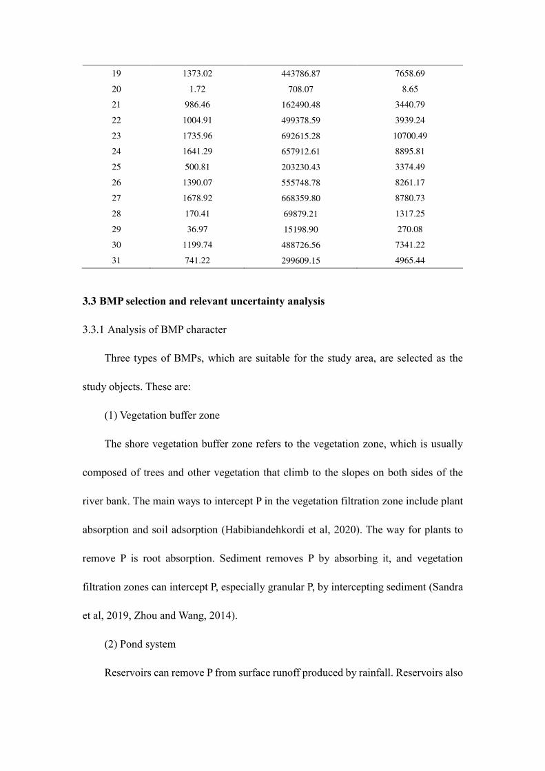
19 1373.02 443786.87 7658.69

20 1.72 708.07 8.65

21 986.46 162490.48 3440.79

22 1004.91 499378.59 3939.24

23 1735.96 692615.28 10700.49

24 1641.29 657912.61 8895.81

25 500.81 203230.43 3374.49

26 1390.07 555748.78 8261.17

27 1678.92 668359.80 8780.73

28 170.41 69879.21 1317.25

29 36.97 15198.90 270.08

30 1199.74 488726.56 7341.22

31 741.22 299609.15 4965.44

3.3 BMP selection and relevant uncertainty analysis

3.3.1 Analysis of BMP character

Three types of BMPs, which are suitable for the study area, are selected as the

study objects. These are:

(1) Vegetation buffer zone

The shore vegetation buffer zone refers to the vegetation zone, which is usually

composed of trees and other vegetation that climb to the slopes on both sides of the

river bank. The main ways to intercept P in the vegetation filtration zone include plant

absorption and soil adsorption (Habibiandehkordi et al, 2020). The way for plants to

remove P is root absorption. Sediment removes P by absorbing it, and vegetation

filtration zones can intercept P, especially granular P, by intercepting sediment (Sandra

et al, 2019, Zhou and Wang, 2014).

(2) Pond system

Reservoirs can remove P from surface runoff produced by rainfall. Reservoirs also

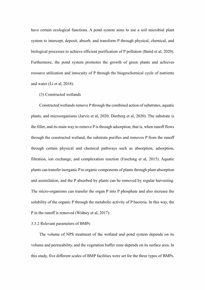
have certain ecological functions. A pond system aims to use a soil microbial plant

system to intercept, deposit, absorb, and transform P through physical, chemical, and

biological processes to achieve efficient purification of P pollution (Baird et al, 2020).

Furthermore, the pond system promotes the growth of green plants and achieves

resource utilization and innocuity of P through the biogeochemical cycle of nutrients

and water (Li et al, 2018).

(3) Constructed wetlands

Constructed wetlands remove P through the combined action of substrates, aquatic

plants, and microorganisms (Jarvie et al, 2020; Dierberg et al, 2020). The substrate is

the filler, and its main way to remove P is through adsorption, that is, when runoff flows

through the constructed wetland, the substrate purifies and removes P from the runoff

through certain physical and chemical pathways such as absorption, adsorption,

filtration, ion exchange, and complexation reaction (Fasching et al, 2015). Aquatic

plants can transfer inorganic P to organic components of plants through plant absorption

and assimilation, and the P absorbed by plants can be removed by regular harvesting.

The micro-organisms can transfer the organ P into P phosphate and also increase the

solubility of the organic P through the metabolic activity of P bacteria. In this way, the

P in the runoff is removed (Widney et al, 2017).

3.3.2 Relevant parameters of BMPs

The volume of NPS treatment of the wetland and pond system depends on its

volume and permeability, and the vegetation buffer zone depends on its surface area. In

this study, five different scales of BMP facilities were set for the three types of BMPs.

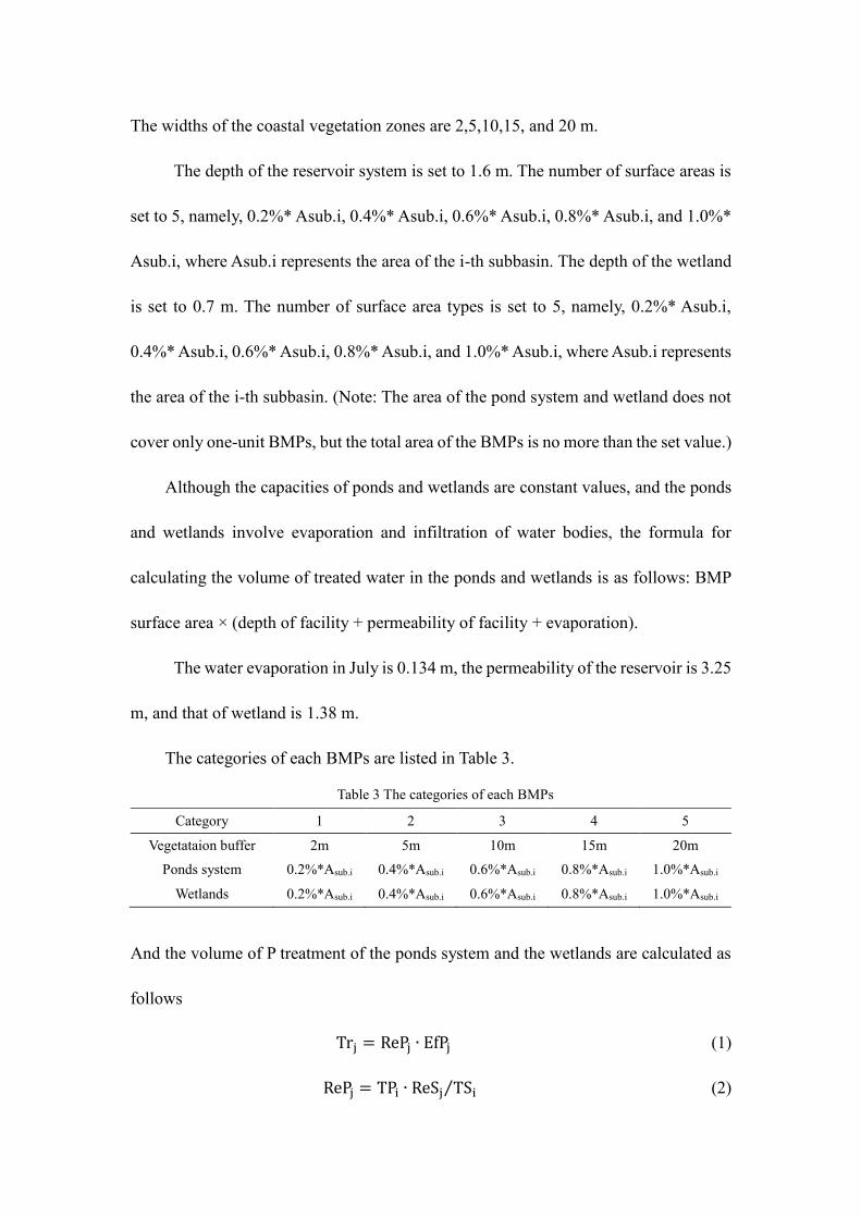
The widths of the coastal vegetation zones are 2,5,10,15, and 20 m.

The depth of the reservoir system is set to 1.6 m. The number of surface areas is

set to 5, namely, 0.2%* Asub.i, 0.4%* Asub.i, 0.6%* Asub.i, 0.8%* Asub.i, and 1.0%*

Asub.i, where Asub.i represents the area of the i-th subbasin. The depth of the wetland

is set to 0.7 m. The number of surface area types is set to 5, namely, 0.2%* Asub.i,

0.4%* Asub.i, 0.6%* Asub.i, 0.8%* Asub.i, and 1.0%* Asub.i, where Asub.i represents

the area of the i-th subbasin. (Note: The area of the pond system and wetland does not

cover only one-unit BMPs, but the total area of the BMPs is no more than the set value.)

Although the capacities of ponds and wetlands are constant values, and the ponds

and wetlands involve evaporation and infiltration of water bodies, the formula for

calculating the volume of treated water in the ponds and wetlands is as follows: BMP

surface area × (depth of facility + permeability of facility + evaporation).

The water evaporation in July is 0.134 m, the permeability of the reservoir is 3.25

m, and that of wetland is 1.38 m.

The categories of each BMPs are listed in Table 3.

Table 3 The categories of each BMPs

Category 1 2 3 4 5

Vegetataion buffer 2m 5m 10m 15m 20m

Ponds system 0.2%*Asub.i 0.4%*Asub.i 0.6%*Asub.i 0.8%*Asub.i 1.0%*Asub.i

Wetlands 0.2%*Asub.i 0.4%*Asub.i 0.6%*Asub.i 0.8%*Asub.i 1.0%*Asub.i

And the volume of P treatment of the ponds system and the wetlands are calculated as

follows

Trj = RePj ∙ EfPj (1) RePj = TPi ∙ ReSj TSi⁄ (2)

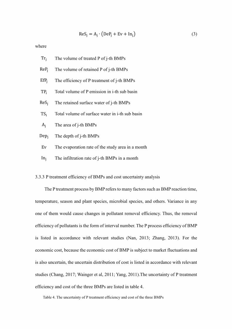
ReSj = Aj ∙ (DePj + Ev + Inj) (3)

where Trj The volume of treated P of j-th BMPs RePj The volume of retained P of j-th BMPs EfPj The efficiency of P treatment of j-th BMPs TPi Total volume of P emission in i-th sub basin ReSj The retained surface water of j-th BMPs TSi Total volume of surface water in i-th sub basin Aj The area of j-th BMPs Depj The depth of j-th BMPs Ev The evaporation rate of the study area in a month Inj The infiltration rate of j-th BMPs in a month

3.3.3 P treatment efficiency of BMPs and cost uncertainty analysis

The P treatment process by BMP refers to many factors such as BMP reaction time,

temperature, season and plant species, microbial species, and others. Variance in any

one of them would cause changes in pollutant removal efficiency. Thus, the removal

efficiency of pollutants is the form of interval number. The P process efficiency of BMP

is listed in accordance with relevant studies (Nan, 2013; Zhang, 2013). For the

economic cost, because the economic cost of BMP is subject to market fluctuations and

is also uncertain, the uncertain distribution of cost is listed in accordance with relevant

studies (Chang, 2017; Wainger et al, 2011; Yang, 2011).The uncertainty of P treatment

efficiency and cost of the three BMPs are listed in table 4.

Table 4. The uncertainty of P treatment efficiency and cost of the three BMPs

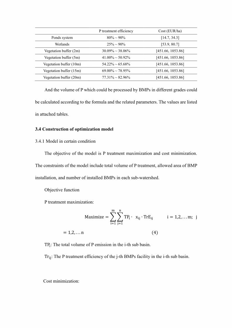
P treatment efficiency Cost (EUR/ha)

Ponds system 80% ~ 90% [14.7, 34.3]

Wetlands 25% ~ 90% [53.9, 80.7]

Vegetation buffer (2m) 30.09% ~ 38.06% [451.66, 1053.86]





And the volume of P which could be processed by BMPs in different grades could

be calculated according to the formula and the related parameters. The values are listed

in attached tables.

3.4 Construction of optimization model

3.4.1 Model in certain condition

The objective of the model is P treatment maximization and cost minimization.

The constraints of the model include total volume of P treatment, allowed area of BMP

installation, and number of installed BMPs in each sub-watershed.

Objective function

P treatment maximization:

Maximize = ∑ ∑ TPinj=1 ∙ xij ∙ TrEij i = 1,2, . . . m; jm

i=1= 1,2, . . . n (4) TPi: The total volume of P emission in the i-th sub basin. Trij: The P treatment efficiency of the j-th BMPs facility in the i-th sub basin.

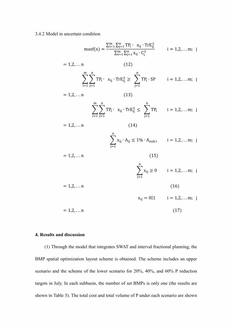
Cost minimization:

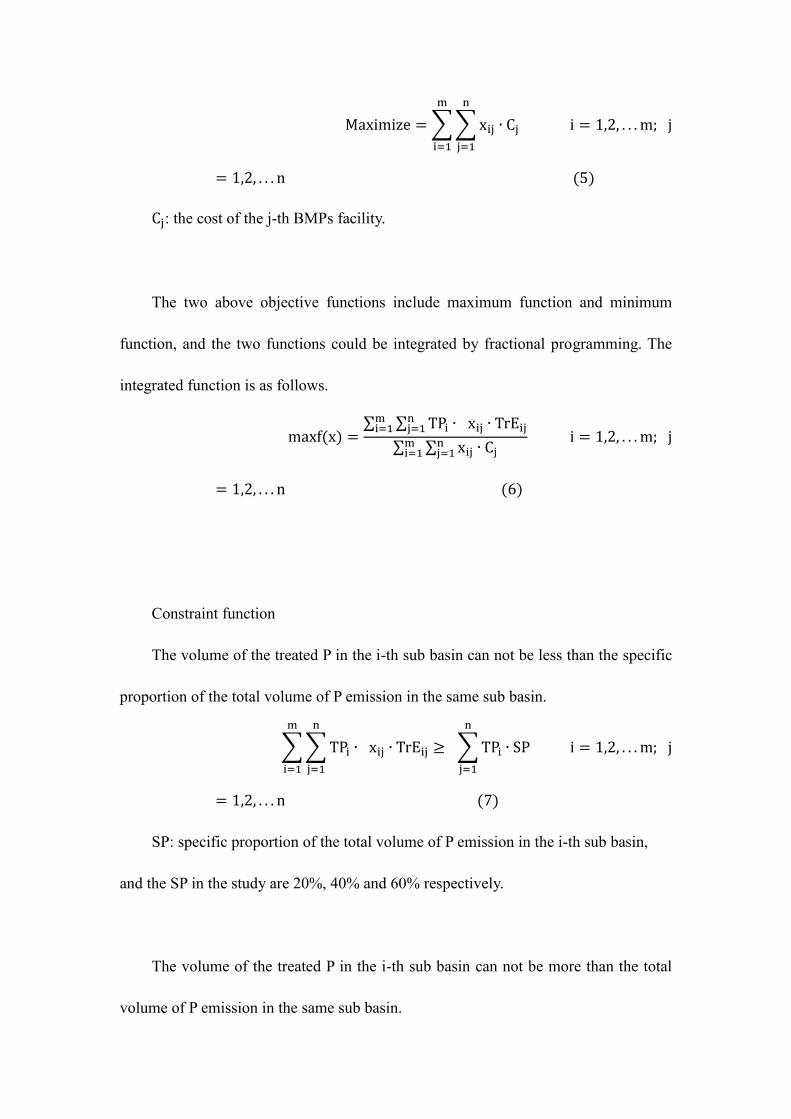
Maximize = ∑ ∑ xij ∙ Cjnj=1 i = 1,2, . . . m; jm

i=1= 1,2, . . . n (5) Cj: the cost of the j-th BMPs facility.

The two above objective functions include maximum function and minimum

function, and the two functions could be integrated by fractional programming. The

integrated function is as follows.

maxf(x) = ∑ ∑ TPinj=1 ∙ xij ∙ TrEijmi=1∑ ∑ xij ∙ Cjnj=1mi=1 i = 1,2, . . . m; j= 1,2, . . . n (6)

Constraint function

The volume of the treated P in the i-th sub basin can not be less than the specific

proportion of the total volume of P emission in the same sub basin.

∑ ∑ TPinj=1 ∙ xij ∙ TrEij ≥ ∑ TPin

j=1 ∙ SP i = 1,2, . . . m; jmi=1= 1,2, . . . n (7)

SP: specific proportion of the total volume of P emission in the i-th sub basin,

and the SP in the study are 20%, 40% and 60% respectively.

The volume of the treated P in the i-th sub basin can not be more than the total

volume of P emission in the same sub basin.

∑ ∑ TPinj=1 ∙ xij ∙ TrEij ≤ ∑ TPin

j=1 i = 1,2, . . . m; jmi=1= 1,2, . . . n (8)

SP: specific proportion of the total volume of P emission in the i-th sub basin.

The allowed area of BMPs installation in the i-th sub basin can not be more than

1% of the area of the same sub basin.

∑ xij ∙ Aij ≤ 1% ∙ Asub.inj=1 i = 1,2, . . . m; j

= 1,2, . . . n (9) Asub.i: the area of the i-th sub basin.

None negative for the variables

∑ xij ≥ 0nj=1 i = 1,2, . . . m; j

= 1,2, . . . n (10)

01 setting for BMPs installation xij = 0|1 i = 1,2, . . . m; j= 1,2, . . . n (11)

3.4.2 Model in uncertain condition

maxf(x) = ∑ ∑ TPinj=1 ∙ xij ∙ TrEij±mi=1∑ ∑ xij ∙ Cj±nj=1mi=1 i = 1,2, . . . m; j= 1,2, . . . n (12)

∑ ∑ TPinj=1 ∙ xij ∙ TrEij± ≥ ∑ TPin

j=1 ∙ SP i = 1,2, . . . m; jmi=1= 1,2, . . . n (13)

∑ ∑ TPinj=1 ∙ xij ∙ TrEij± ≤ ∑ TPin

j=1 i = 1,2, . . . m; jmi=1= 1,2, . . . n (14)

∑ xij ∙ Aij ≤ 1% ∙ Asub.inj=1 i = 1,2, . . . m; j

= 1,2, . . . n (15)

∑ xij ≥ 0nj=1 i = 1,2, . . . m; j

= 1,2, . . . n (16) xij = 0|1 i = 1,2, . . . m; j= 1,2, . . . n (17)

4. Results and discussion

(1) Through the model that integrates SWAT and interval fractional planning, the

BMP spatial optimization layout scheme is obtained. The scheme includes an upper

scenario and the scheme of the lower scenario for 20%, 40%, and 60% P reduction

targets in July. In each subbasin, the number of set BMPs is only one (the results are

shown in Table 5). The total cost and total volume of P under each scenario are shown

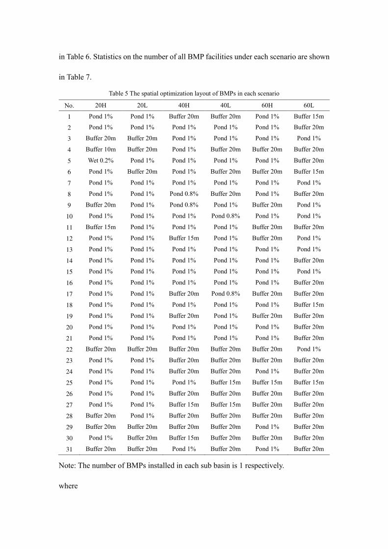
in Table 6. Statistics on the number of all BMP facilities under each scenario are shown

in Table 7.

Table 5 The spatial optimization layout of BMPs in each scenario

No. 20H 20L 40H 40L 60H 60L

1 Pond 1% Pond 1% Buffer 20m Buffer 20m Pond 1% Buffer 15m

2 Pond 1% Pond 1% Pond 1% Pond 1% Pond 1% Buffer 20m

3 Buffer 20m Buffer 20m Pond 1% Pond 1% Pond 1% Pond 1%

4 Buffer 10m Buffer 20m Pond 1% Buffer 20m Buffer 20m Buffer 20m

5 Wet 0.2% Pond 1% Pond 1% Pond 1% Pond 1% Buffer 20m

6 Pond 1% Buffer 20m Pond 1% Buffer 20m Buffer 20m Buffer 15m

7 Pond 1% Pond 1% Pond 1% Pond 1% Pond 1% Pond 1%

8 Pond 1% Pond 1% Pond 0.8% Buffer 20m Pond 1% Buffer 20m

9 Buffer 20m Pond 1% Pond 0.8% Pond 1% Buffer 20m Pond 1%

10 Pond 1% Pond 1% Pond 1% Pond 0.8% Pond 1% Pond 1%

11 Buffer 15m Pond 1% Pond 1% Pond 1% Buffer 20m Buffer 20m

12 Pond 1% Pond 1% Buffer 15m Pond 1% Buffer 20m Pond 1%





17 Pond 1% Pond 1% Buffer 20m Pond 0.8% Buffer 20m Buffer 20m


19 Pond 1% Pond 1% Buffer 20m Pond 1% Buffer 20m Buffer 20m



22 Buffer 20m Buffer 20m Buffer 20m Buffer 20m Buffer 20m Pond 1%

23 Pond 1% Pond 1% Buffer 20m Buffer 20m Buffer 20m Buffer 20m

24 Pond 1% Pond 1% Buffer 20m Buffer 20m Pond 1% Buffer 20m

25 Pond 1% Pond 1% Pond 1% Buffer 15m Buffer 15m Buffer 15m



28 Buffer 20m Pond 1% Buffer 20m Buffer 20m Buffer 20m Buffer 20m

29 Buffer 20m Buffer 20m Buffer 20m Buffer 20m Pond 1% Buffer 20m

30 Pond 1% Buffer 20m Buffer 15m Buffer 20m Buffer 20m Buffer 20m

31 Buffer 20m Buffer 20m Pond 1% Buffer 20m Pond 1% Buffer 20m

Note: The number of BMPs installed in each sub basin is 1 respectively.

where

Pond: Ponds system

Buffer: Vegetation buffer

Wet: Wetland

Table 6 The total cost and the total volume of the treated P

20% 40% 60%

+ - + - + -

Total cost (EUR) 3990.58 6585.58 5699.22 10955.14 6573.14 17509.48

Total treated P (kg) 38904.15 40483.60 89900.35 80739.23 80622.07 121235.31

Table 7 The number of installed BMPs in each scenario

Type of BMPs 20% 40% 60%

+ - + - + -

wetland 0.20% 1 0 0 0 0 0

0.40% 0 0 0 0 0 0

0.60% 0 0 0 0 0 0

0.80% 0 0 0 0 0 0

1.00% 0 0 0 0 0 0

Pond 0.20% 0 0 0 0 0 0

0.40% 0 0 0 0 0 0

0.60% 0 0 0 0 0 0

0.80% 0 0 2 3 0 0

1.00% 22 23 17 14 17 8

Vegetation

buffer 2m 0 0 0 0 0 0

5m 0 0 0 0 0 0

10m 1 0 0 0 0 0

15m 1 0 3 2 0 4

20m 6 8 9 12 14 19

Total number of BMPs 31 31 31 31 31 31

(2) Table 4 shows that under the condition of the same area, whether in the upper

or lower limit, according to the P treatment capacity, green buffer zone > reservoir >

wetland. Taking the sub basin 1 as an example, we find that Table 8 corresponds to the

BMP treatment effect of sub basin 1, and the P control effect of each BMP facility can

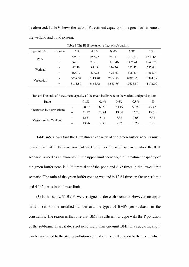
be observed. Table 9 shows the ratio of P treatment capacity of the green buffer zone to

the wetland and pond system.

Table 8 The BMP treatment effect of sub basin 1

Type of BMPs Scenario 0.2% 0.4% 0.6% 0.8% 1%

Pond - 328.14 656.27 984.41 1312.54 1640.68

+ 369.15 738.31 1107.46 1476.61 1845.76

Wetland - 45.59 91.18 136.76 182.35 227.94

+ 164.12 328.23 492.35 656.47 820.59

Vegetation

buffer

- 4038.07 5518.70 7268.53 9287.56 10364.38

+ 5114.89 6864.72 8883.76 10633.59 11172.00

Table 9 The ratio of P treatment capacity of the green buffer zone to the wetland and pond system

Ratio 0.2% 0.4% 0.6% 0.8% 1%

Vegetation buffer/Wetland - 88.57 60.53 53.15 50.93 45.47

+ 31.17 20.91 18.04 16.20 13.61

Vegetation buffer/Pond - 12.31 8.41 7.38 7.08 6.32

+ 13.86 9.30 8.02 7.20 6.05

Table 4-5 shows that the P treatment capacity of the green buffer zone is much

larger than that of the reservoir and wetland under the same scenario, when the 0.01

scenario is used as an example. In the upper limit scenario, the P treatment capacity of

the green buffer zone is 6.05 times that of the pond and 6.32 times in the lower limit

scenario. The ratio of the green buffer zone to wetland is 13.61 times in the upper limit

and 45.47 times in the lower limit.

(3) In this study, 31 BMPs were assigned under each scenario. However, no upper

limit is set for the installed number and the types of BMPs per subbasin in the

constraints. The reason is that one-unit BMP is sufficient to cope with the P pollution

of the subbasin. Thus, it does not need more than one-unit BMP in a subbasin, and it

can be attributed to the strong pollution control ability of the green buffer zone, which

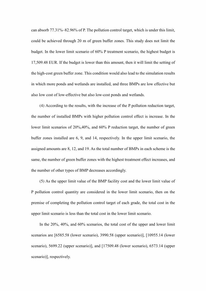
can absorb 77.31%–82.96% of P. The pollution control target, which is under this limit,

could be achieved through 20 m of green buffer zones. This study does not limit the

budget. In the lower limit scenario of 60% P treatment scenario, the highest budget is

17,509.48 EUR. If the budget is lower than this amount, then it will limit the setting of

the high-cost green buffer zone. This condition would also lead to the simulation results

in which more ponds and wetlands are installed, and three BMPs are low effective but

also low cost of low-effective but also low-cost ponds and wetlands.

(4) According to the results, with the increase of the P pollution reduction target,

the number of installed BMPs with higher pollution control effect is increase. In the

lower limit scenarios of 20%,40%, and 60% P reduction target, the number of green

buffer zones installed are 6, 9, and 14, respectively. In the upper limit scenario, the

assigned amounts are 8, 12, and 19. As the total number of BMPs in each scheme is the

same, the number of green buffer zones with the highest treatment effect increases, and

the number of other types of BMP decreases accordingly.

(5) As the upper limit value of the BMP facility cost and the lower limit value of

P pollution control quantity are considered in the lower limit scenario, then on the

premise of completing the pollution control target of each grade, the total cost in the

upper limit scenario is less than the total cost in the lower limit scenario.

In the 20%, 40%, and 60% scenarios, the total cost of the upper and lower limit

scenarios are [6585.58 (lower scenario), 3990.58 (upper scenario)], [10955.14 (lower

scenario), 5699.22 (upper scenario)], and [17509.48 (lower scenario), 6573.14 (upper

scenario)], respectively.

(6) As the lower limit of the BMP pollution control efficiency is set in the lower

limit scenario, and the upper limit is set in the upper limit scenario, the number of green

buffer zones with high cost and high pollution control effect in the upper limit scenario

under each control target is also smaller than that in the lower limit scenario. This

condition means that solving the same volume requires a smaller number of BMP

facilities with high P pollution treatment efficiency and high cost.

(7) As the cost and P treatment efficacy in this study are considered as the upper

and lower limit values, the uncertain values of the cost and treatment efficiency of

BMPs are also expressed as interval numbers. Thus, the results are in the form of the

upper and lower limit scenarios. The results represent the upper and lower limits of the

corresponding schemes under uncertainty impact, which means that the schemes are

reasonable when their results are in the interval range.

5. Conclusion

(1) The innovation of this study is that it designs a model that integrates SWAT

and interval fractional programming to optimize the BMP spatial optimization layout

in watersheds under uncertainty. The model can effectively reflect and deal with the

uncertainty in P pollution treatment efficiency and cost of BMPs. Thus far, the method

has not been applied to studies on BMP spatial optimization layout.

(2) According to the spatial layout scheme corresponding to the upper and lower

limit scenarios under different P pollution reduction targets, the upper and lower limit

scenarios represent the limit of uncertainty impact on the scheme. The scheme is

reasonable when it is in the interval. The total costs in the research results are also

interval numbers, and the total cost in practical terms is also in the interval.

(3) The developed method provides the schemes that correspond to the upper and

lower limit scenarios. The method can provide more reasonable schemes for decision-

makers under uncertain conditions.

(4) Different from the genetic algorithm method usually used in BMPs spatial

optimization layout, this study does not need to set all variables as uncertainty number,

nor does it need to set the average value for uncertainty numbers. Because it is always

difficult to identify the uncertainty distribution mode in practice. Therefore, the

developed method in this study can be better used in practical condition.

Declaration

Ethical Approval

Not applicable. There is no human experiment or animal experiment in the study, and

the study does not address the ethical issue.

Consent to Participate

Not applicable.

Consent to Publish

Not applicable.

Authors Contributions

Jinjin Gu developed the model and calculated the data.

Yuan Cao analyzed the uncertainty of the related data and draw the figure.

Min Wu, Min Song and Lin Wang help collect the data and helped develop the model

and also helped examine the manuscript.

All authors read and approved the final manuscript.

Funding

We gratefully acknowledge financial supports for this research from projects of

National Natural Science Foundation of China (Grant No. 41601581); Fundamental

Research Funds for the Central Universities (Grant No. JZ2019HGBZ0163);

Philosophy and Social Science Cultivation Program of Hefei University of Technology

(Grant No. JS2020HGXJ0021).

Competing Interests

The authors declare that there are no conflicts of interest regarding the publication of

this paper.

Availability of data and materials

All data generated or analyzed during this study are included in the manuscript and

attached table.

References

Baird J.B., Winston R.J., Hunt W.F. (2020), Evaluating the hydrologic and water

quality performance of novel infiltrating wet retention ponds. Blue-Green Systems,

2(1):282-299.

Cao Q, Tao W.Y., Ma Z.Y., et al (2007), Study on features of chaohu lake basin’s

evaporation and trend of its variation. Resource Development and Market, 23(9): 811-

814.

Chang J. (2017), The applied research of best management practices based on

SWAT model[D]. Zhejiang University. (In Chinese)

Dierberg FE, Debusk TA, MD Kharbanda, et al (2020), Long-term sustainable

phosphorus (P) retention in a low-P stormwater wetland for Everglades restoration[J].

Science of The Total Environment, 756:143386.

Fasching S., Norland J., Desutter T., et al (2015), The Use of Sediment Removal to

Reduce Phosphorus Levels in Wetland Soils. Ecological Restoration, 33(2):131-134.

Fei X., Dong G., Wang Q., et al (2016), Impacts of DEM uncertainties on critical

source areas identification for non-point source pollution control based on SWAT model.

Journal of Hydrology, 540:355-367.

Feng M., Shen Z. (2021), Assessment of the Impacts of Land Use Change on Non-

Point Source Loading under Future Climate Scenarios Using the SWAT Model. Water,

13(6):874.

Getahun E., Keefer L., et al (2016), Integrated modeling system for evaluating

water quality benefits of agricultural watershed management practices: Case study in

the Midwest. Sustainability of Water Quality and Ecology, 8:14-29.

Gu J.J., Hu H., Wang L., et al (2020), Fractional Stochastic Interval Programming

for Optimal Low Impact Development Facility Category Selection under Uncertainty.

Water Resources Management, 34:1567–1587.

Gu J.J., Zhang Q., Gu D.Z., et al (2018), The Impact of Uncertainty Factors on

Optimal Sizing and Costs of Low-Impact Development: a Case Study from Beijing,

China. Water Resources Management, 32: 4217-4238

Gu J.J., Zhang X., Xuan X., et al (2020), Land use structure optimization based on

uncertainty fractional joint probabilistic chance constraint programming. Stochastic

Environmental Research and Risk Assessment, 34(11):1699-1712.

Guo P., Chen X., Mo L., et al (2014), Fuzzy chance-constrained linear fractional

programming approach for optimal water allocation. Stochastic Environmental

Research & Risk Assessment, 28(6):1601-1612.

Habibiandehkordi R., Lobb D.A., Sheppard S.C., et al (2020), Uncertainties in

vegetated buffer strip function in controlling phosphorus export from agricultural land

in the Canadian prairies. Environmental Science and Pollution Research, 24(2):1-11.

Jarvie H.P., Pallett D.W., Schfer S.M., et al (2020), Biogeochemical and climate

drivers of wetland phosphorus and nitrogen release: Implications for nutrient legacies

and eutrophication risk. Journal of Environmental Quality, 49(6).

Kaini P., Artita K., Nicklow J.W. (2012), Optimizing Structural Best

Management Practices Using SWAT and Genetic Algorithm to Improve Water Quality

Goals. Water Resources Management, 26(7):1827-1845.

Li M., Li J., Singh V.P., et al (2019), Efficient allocation of agricultural land and

water resources for soil environment protection using a mixed optimization-simulation

approach under uncertainty. Geoderma, 353:55-69.

Li Y.F., Liu H.Y., Liu Z.J, Lou C.Y., Wang J. (2018), Effect of different multi-pond

network landscape structures on nitrogen retention over agricultural watersheds. 39(11):

161-168. (In Chinese)

Nan Z. (2013), The study of the risk assessment of NPS pollution and BMPs

category selection in Beijing small watershed[D]. Capital Normal University. (In

Chinese)

Panagopoulos Y., Makropoulos C., Baltas E., et al (2011), SWAT parameterization

for the identification of critical diffuse pollution source areas under data limitations.

Ecological Modelling, 222(19):3500-3512.

Ouyang W., Huang H.B., Cai G.Q. (2014), Temporal and spatial characteristics of

diffuse phosphorus pollution in the watershed without monitoring data at Chaohu Lake.

Acta Scientiae Circumstantiae, 34(4) : 1024-1031. (In Chinese)

Qi Z., Kang G., Wu X., et al (2020), Multi-Objective Optimization for Selecting

and Siting the Cost-Effective BMPs by Coupling Revised GWLF Model and NSGAII

Algorithm. Water, 12(1):235.

Qiu J., Shen Z., Chen L., et al (2019), Quantifying effects of conservation practices

on non-point source pollution in the Miyun Reservoir Watershed, China. Environmental

Monitoring and Assessment, 191(9):582.1-582.21.

Sandra, Hille, Daniel, et al (2019), Management Options to Reduce Phosphorus

Leaching from Vegetated Buffer Strips. Journal of Environmental Quality, 48(2):322-

329

Wang X., Wang Q., Wu C., et al (2012), A method coupled with remote sensing

data to evaluate non-point source pollution in the Xin'anjiang catchment of China.

Science of the Total Environment, 430: 132-143.

Widney S., Klein A.K., Ehman J., et al (2017), The value of wetlands for water

quality improvement: an example from the St. Johns River watershed, Florida.

Wetlands Ecology & Management. 26: 265–276.

Zheng Z.X., Song malin (2011), Modeling Research on Transfer Processes of

Nitrogen and Phosphorus in Different Farmlands from Zhegao River Watershed.

Journal of Anhui Agricultural Sciences, 39(013):7667-7669. (In Chinese)

Zhou S.S., Wang D.M. (2014), The review on purification mechanism and its

influencing factors of riparian buffers. 12(5):114-120. (In Chinese)

Wainger L., Wolcott R., Almeter A., et al (2011), An optimization approach to

evaluate the role of ecosystem services in Chesapeake Bay restoration strategies.

Wu H., Zhu A.X., Liu J., et al (2018), Best Management Practices Optimization at

Watershed Scale: Incorporating Spatial Topology among Fields. Water Resources

Management, 32: 155–177

Wu J.H., Lu J. (2019), Landscape patterns regulate non-point source nutrient

pollution in an agricultural watershed. Science of The Total Environment, 669:377-388.

Yang Y.H., Yan B.X. (2011), Optimal Non-Point Source Pollution Control Practices

for a Small Watershed. Journal of Ecology and Rural Environment. 27(2): 11-15. (In

Chinese)

Zhang G.F. (2013), The Effects of Riparian Vegetation Buffer Zones on Nitrogen

and Phosphorus Reduction in Chaobai River Upstream. Chinese Agricultural Science

Bulletin, 29(8): 189-194. (In Chinese)

Zhang Y.F., Li Y.P., Sun J., et al (2019), Optimizing water resources allocation and

soil salinity control for supporting agricultural and environmental sustainable

development in Central Asia. Science of The Total Environment, 704:135281.

Figures

Figure 1

The study area Note: The designations employed and the presentation of the material on this map do notimply the expression of any opinion whatsoever on the part of Research Square concerning the legalstatus of any country, territory, city or area or of its authorities, or concerning the delimitation of itsfrontiers or boundaries. This map has been provided by the authors.

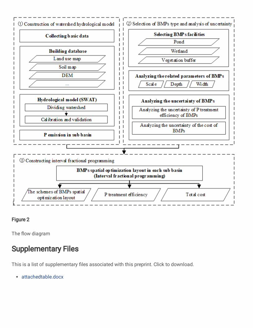
Figure 2

The �ow diagram

Supplementary Files

This is a list of supplementary �les associated with this preprint. Click to download.

attachedtable.docx

https://assets.researchsquare.com/files/rs-509238/v1/399e56a2b43ed04bdc858e02.docx

Spatial Optimization Layout of Best Management Practices ...

Documents