Spatial Finite Non-Gaussian Mixtures for Color Image Segmentation Ali Sefidpour A Thesis in The Concordia Institute for Information Systems Engineering Presented in Partial Fulfillment of the Requirements for the Degree of Master of Applied Science (Quality Systems Engineering) at Concordia University Montr´ eal, Qu´ ebec, Canada August 2011 c Ali Sefidpour, 2011

Welcome message from author
This document is posted to help you gain knowledge. Please leave a comment to let me know what you think about it! Share it to your friends and learn new things together.
Transcript
Spatial Finite Non-Gaussian Mixtures forColor Image Segmentation
Ali Sefidpour
A Thesis
in
The Concordia Institute
for
Information Systems Engineering
Presented in Partial Fulfillment of the Requirements
for the Degree of Master of Applied Science (Quality Systems Engineering) at
Concordia University
Montreal, Quebec, Canada
August 2011
c© Ali Sefidpour, 2011

CONCORDIA UNIVERSITYSchool of Graduate Studies
This is to certify that the thesis prepared
By:
Entitled:
and submitted in partial fulfillment of the requirements for the degree of
complies with the regulations of the University and meets the accepted standards withrespect to originality and quality.
Signed by the final examining committee:
______________________________________ Chair
______________________________________ Examiner
______________________________________ Examiner
______________________________________ Supervisor
Approved by ________________________________________________Chair of Department or Graduate Program Director
________________________________________________Dean of Faculty
Date ________________________________________________
Ali Sefidpour
Spatial Finite Non-Gaussian Mixtures for Color Image Segmentation
Master of Applied Science (Quality Systems Engineering)
Dr. C. Assi
Dr. J. Bentahar
Dr. A. Hamou-Lhadj
Dr. N. Bouguila
September 7, 2011
Abstract
Spatial Finite Non-Gaussian Mixtures for Color Image SegmentationAli Sefidpour
Finite mixture models are one of the most widely and commonly used probabilistic techniques
for image segmentation. Although the most well known and commonly used distribution when
considering mixture models is the Gaussian, it is certainly not the best approximation for image
segmentation and other related image processing problems. It is well known, for instance, that
the statistics of natural images are not Gaussian at all. In this thesis, we propose to use finite
Dirichlet mixture model (DMM), finite generalized Dirichlet mixture model (GDMM) and finite
Beta-Liouville mixture model (BLMM), which offer more flexibility in data modeling, for image
segmentation. A maximum likelihood (ML) based algorithm is applied for estimating the resulted
segmentation model’s parameters. Spatial information is also employed for figuring out the number
of regions in an image and two color spaces are investigated and compared. The experimental
results show that the proposed segmentation framework yields good overall performance that is
better than a comparable technique based on Gaussian mixture model.
iii
Acknowledgements
It is a great pleasure to express my utmost gratitude to my supervisor, Professor Nizar Bouguila,
who has supported me throughout my research career in Concordia University, and also for his
intelligent guidance, encouragement and patience for allowing me to experience in my own way.
I would like to thank all my friendly fellow lab mates who made our lab a delightful and convenient
place for research, in particular many thanks goes to Taoufik and Ali that I took benefit of their
discussions during my research.
It is noteworthy to mention my gratitude to the faculty members and administrative staff of CIISE
department, which were always ready to help with smiling faces.
Last but not the least, my deepest gratitude goes to my family for their endless love and support
throughout my life, without their support, simply I could not do this.
iv
Table of Contents
List of Tables vii
List of Figures viii
1 Introduction 11.1 Introduction and Related Works . . . . . . . . . . . . . . . . . . . . . . . . . . . 11.2 Contributions . . . . . . . . . . . . . . . . . . . . . . . . . . . . . . . . . . . . . 31.3 Thesis Overview . . . . . . . . . . . . . . . . . . . . . . . . . . . . . . . . . . . 4
2 Segmentation Models 52.1 Introduction . . . . . . . . . . . . . . . . . . . . . . . . . . . . . . . . . . . . . . 52.2 Finite Dirichlet Mixture Model . . . . . . . . . . . . . . . . . . . . . . . . . . . . 5
2.2.1 Integration of Spatial Information into Mixture Models . . . . . . . . . . . 62.2.2 Parameter Estimation . . . . . . . . . . . . . . . . . . . . . . . . . . . . . 82.2.3 Initialization and Segmentation algorithm . . . . . . . . . . . . . . . . . . 11
2.3 Finite Generalized Dirichlet Mixture Model . . . . . . . . . . . . . . . . . . . . . 122.3.1 Parameter Estimation . . . . . . . . . . . . . . . . . . . . . . . . . . . . . 122.3.2 Initialization and Segmentation algorithm . . . . . . . . . . . . . . . . . . 15
2.4 Finite Beta-Liouville Mixture Model . . . . . . . . . . . . . . . . . . . . . . . . . 162.4.1 Parameter Estimation . . . . . . . . . . . . . . . . . . . . . . . . . . . . . 172.4.2 Initialization and Segmentation algorithm . . . . . . . . . . . . . . . . . . 19
3 Experimental Results 213.1 Introduction . . . . . . . . . . . . . . . . . . . . . . . . . . . . . . . . . . . . . . 213.2 Design of Experiments . . . . . . . . . . . . . . . . . . . . . . . . . . . . . . . . 213.3 Experiment 1 . . . . . . . . . . . . . . . . . . . . . . . . . . . . . . . . . . . . . 223.4 Experiment 2 . . . . . . . . . . . . . . . . . . . . . . . . . . . . . . . . . . . . . 27
v
4 Conclusions 32
List of References 34
vi
List of Tables
2.1 Parameters and number of parameters for Multivariate Gaussian Distribution (MGD),Dirichlet Distribution (DD), Generalized Dirichlet Distribution (GDD) and Beta-Liouville Distribution (BLD). . . . . . . . . . . . . . . . . . . . . . . . . . . . . . 17
3.1 NPR index sample mean for Gaussian mixture model (GMM), Dirichlet mixturemodel (DMM), generalized Dirichlet mixture model (GDMM) and Beta-Liouvillemixture model (BLMM) in rgb color space. . . . . . . . . . . . . . . . . . . . . . 25
3.2 NPR index sample mean for Gaussian mixture model (GMM), Dirichlet mixturemodel (DMM), generalized Dirichlet mixture model (GDMM) and Beta-Liouvillemixture model (BLMM) in l1l2l3 color space. . . . . . . . . . . . . . . . . . . . . 28
3.3 Color space selection percentage by different metrics for Gaussian mixture model(GMM), Dirichlet mixture model (DMM), generalized Dirichlet mixture model(GDMM) and Beta-Liouville mixture model (BLMM). . . . . . . . . . . . . . . . 29
vii
List of Figures
2.1 (a) Simulated data of a bivariate Dirichlet mixture. (b) Estimated results for wronglysupposed two clusters. (c) Strong relation between points and their prospectivepeers. (d) The combination of clusters. . . . . . . . . . . . . . . . . . . . . . . . . 8
3.1 Baboon image segmentation in the rgb color space. (a) Original image, (b) Seg-mentation using the Gaussian mixture (M = 12), (c) Segmentation using theDirichlet mixture (M = 4), (d) Segmentation using the Generalized Dirichlet mix-ture (M = 4), (e) Segmentation using the Beta-Liouville mixture (M = 4). . . . . 23
3.2 Examples of images segmentation results in the rgb color space. (a,f,k,p) Origi-nal images from the Berkeley Database. (b,g,l,q) Segmentation results using theGaussian mixture model. (c,h,m,r) Segmentation results using the Dirichlet mix-ture model. (d,i,n,s) Segmentation results using the generalized Dirichlet mixturemodel. (e,j,o,t) Segmentation results using the Beta-Liouville mixture model. . . . 24
3.3 Examples of images used to calculate the NPR index of each segmentation ap-proach in the rgb color space. First column contains the original images. Secondcolumn contains the segmentation results using the Gaussian mixture model. Thirdcolumn contains the segmentation results using the Dirichlet mixture model. Forthcolumn contains segmentation results using generalized Dirichlet model. Fifth col-umn contains segmentation results using Beta-Liouville model. Columns 6, 7, 8and 9 contains the ground truth segmentations. . . . . . . . . . . . . . . . . . . . . 26
3.4 Baboon image segmentation in the l1l2l3 color space. (a) Segmentation usingthe Gaussian mixture (M = 10), (b) Segmentation using the Dirichlet mixture(M = 4), (c) Segmentation using the generalized Dirichlet mixture (M = 4), (d)Segmentation using the Beta-Liouville mixture (M = 4). . . . . . . . . . . . . . . 26
viii
3.5 Images segmentation in the l1l2l3 color space. First column: segmentation usingthe Gaussian mixture model. Second column: segmentation using the Dirichletmixture. Third column: segmentation using the generalized Dirichlet mixture.Forth column: segmentation using the Beta-Liouville mixture. . . . . . . . . . . . 27
3.6 Images segmentation in each set for rgb and l1l2l3 color spaces for all 4 mixturemodels. Column 1: original image. Columns 2 and 3: segmentation using theGaussian mixture model. Columns 4 and 5: segmentation using the Dirichlet mix-ture. Columns 6 and 7: segmentation using the generalized Dirichlet mixture.Columns 8 and 9: segmentation using the Beta-Liouville mixture. . . . . . . . . . 30
3.7 Images segmentation in each set for rgb and l1l2l3 color spaces for all 4 mixturemodels. Column 1: original image. Columns 2 and 3: segmentation using theGaussian mixture model. Columns 4 and 5: segmentation using the Dirichlet mix-ture. Columns 6 and 7: segmentation using the generalized Dirichlet mixture.Columns 8 and 9: segmentation using the Beta-Liouville mixture. . . . . . . . . . 31
ix
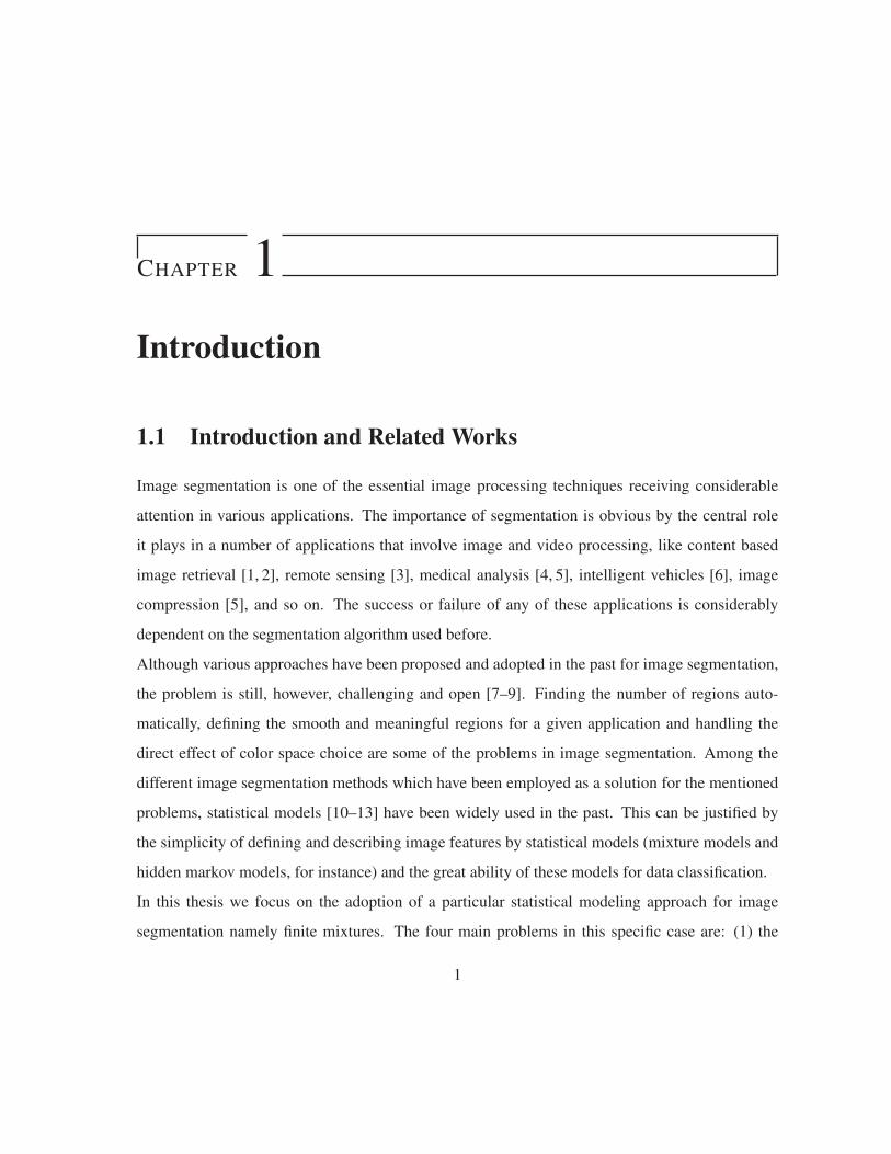
CHAPTER 1Introduction
1.1 Introduction and Related Works
Image segmentation is one of the essential image processing techniques receiving considerable
attention in various applications. The importance of segmentation is obvious by the central role
it plays in a number of applications that involve image and video processing, like content based
image retrieval [1, 2], remote sensing [3], medical analysis [4, 5], intelligent vehicles [6], image
compression [5], and so on. The success or failure of any of these applications is considerably
dependent on the segmentation algorithm used before.
Although various approaches have been proposed and adopted in the past for image segmentation,
the problem is still, however, challenging and open [7–9]. Finding the number of regions auto-
matically, defining the smooth and meaningful regions for a given application and handling the
direct effect of color space choice are some of the problems in image segmentation. Among the
different image segmentation methods which have been employed as a solution for the mentioned
problems, statistical models [10–13] have been widely used in the past. This can be justified by
the simplicity of defining and describing image features by statistical models (mixture models and
hidden markov models, for instance) and the great ability of these models for data classification.
In this thesis we focus on the adoption of a particular statistical modeling approach for image
segmentation namely finite mixtures. The four main problems in this specific case are: (1) the
1
automatic determination of the number of clusters (i.e. number of regions in a given image), (2)
the integration of the spatial information to achieve smooth segmentation results, (3) the accurate
choice of the probability density functions that shall describe the image regions, and (4) the esti-
mation of the resulted segmentation mixture model’s parameters. In the majority of the works that
have dealt with image segmentation, the often-cited difficulty is the automatic determination of the
number of regions and a lot of approaches have been proposed with relative success. For instance,
a bootstrapping approach has been applied in [13]. A variety of information criteria have been
considered to select automatically the number of regions (see, [14, 15], for instance, for detailed
discussions), also. The most successful approaches, however, have been based on the consideration
of the spatial information as an implicit prior information about the expected number of regions.
Indeed, since each region is composed by similar adjacent pixels which follow almost the same
color or pattern, using spatial information will naturally lead us to find out smooth and accurate
segments. For instance, an adaptive clustering algorithm based on K-means and eight-neighbor
Gibbs random field model has been proposed in [16] and applied to pictures of industrial objects,
buildings, optical characters, faces and aerial photographs. The authors in [17, 18] have used this
information to improve their segmentation results on medical images while the authors in [10, 19]
have employed spatial information for segmenting brain MR images. In another interesting pa-
per [11] a segmentation statistical model, inspired from [10], based on the integration of spatial
information and Gaussian mixtures has been developed to automatically determine the number of
regions and then generate smooth regions. The main problem with the majority of the approaches
that have tackled the combination of mixture models and spatial information is that the image re-
gions have been supposed to follow Gaussian distributions. This assumption is unfortunately very
restrictive and unrealistic in many real-world vision problems. Although the finite Gaussian mix-
ture is a popular model in image analysis, it is not necessarily the best solution as it is thoroughly
shown in several studies (see, for instance, [20–23]).
Moreover, the influence of the chosen color spaces have not been investigated within the proposed
segmentation statistical models, despite the fact that this specific choice has been shown to have a
2
noticeable effect on the final results in several other image processing and computer vision appli-
cations [24, 25].
Hence, in this thesis we propose the integration of spatial information into finite Dirichlet mixture
model, finite generalize Dirichlet mixture model and finite Beta-Liouville mixture model for the
segmentation of color images. The choice of these mixture models is motivated by their flexi-
bility (i.e. they can be symmetric or asymmetric) in modeling data [21, 23, 26]. As in [10, 11],
the spatial information is used as indirect prior knowledge, encoded via contextual constraints of
neighboring pixels, for estimating the number of clusters. Finally, two appropriate color spaces
are investigated within the proposed segmentation framework. Experiments show that incorporat-
ing the spatial information into generalized Dirichlet mixture models and Beta-Liouville mixture
models and choosing appropriate color spaces achieves accurate image segmentation results.
1.2 Contributions
The contributions of this thesis are as follows:
� Integration of spatial information into different non Gaussian finite mixture models: Our ap-
proach suggests the integration of spatial information into three different finite mixture mod-
els (Dirichlet mixture model, generalized Dirichlet mixture model and Beta-Liouville mix-
ture model) to produce smooth and more meaningful regions in color image segmentation
while offering more flexibility and ease of use for data modeling in comparison to well
known and commonly used finite Gaussian mixture models.
� Automatic determination of the number of regions by using the proposed approaches: The
proposed approach also made it possible to find the number of segmentation regions automat-
ically, this would be an extensive boost for realtime applications of color image segmentation
which needs no human interference.
3

� Revealing the effect of color space on color image segmentation: We compare the effect of
two different color spaces on the color image segmentation process and we show that differ-
ent color spaces can lead to different segmentation results.
1.3 Thesis Overview
The organization of this thesis is as follows:
� Chapter 1 introduces the challenging problems in color image segmentations, the major role
of finite mixture models in clustering the data and the beneficial integration of spatial in-
formation to determine the accurate number of regions and to produce the homogeneous
regions.
� Chapter 2 presents three powerful finite mixture models (Dirichlet mixture model, generalize
Dirichlet mixture model and Beta-Liouville mixture model), gives the details of integration
of spatial information into these models and follows by estimation of the required parameters
for these models.
� Chapter 3 is devoted to the presentation of our experimental results and quantitative evalua-
tion of proposed models as compared to the Gaussian mixture model.
� Chapter 4 summarizes the various approaches and concludes the thesis while proposing the
room for future works.
4
CHAPTER 2Segmentation Models
2.1 Introduction
In previous chapter we presented the challenging problems related to color image segmentation
and we also pointed out to finite mixture models as a particular statistical technique for color im-
age segmentation. We continue in this chapter by introducing finite mixture models and the way
we integrate spatial information into these models. Three flexible and powerful distributions will
be employed to present our new models which will be learned using well known maximum like-
lihood estimation (MLE) within an expectation maximization (EM) optimization framework. The
whole segmentation process will be summarized at the end by presenting the steps of segmentation
algorithm.
2.2 Finite Dirichlet Mixture Model
Let X be an image represented by a set of pixels X = { �X1, . . . , �XN} where each pixel is denoted
by a random vector �Xn = (Xn1, . . . , XnD)1 and N is the number of pixels. Now if the random
vector �X follows a Dirichlet distribution with parameters �α = (α1, α2, . . . , αD+1), the joint density
1The dimensionality D will depend on the number of features used to describe a given pixel. For instance, if weuse only the color information in an RGB space, then D = 3.
5
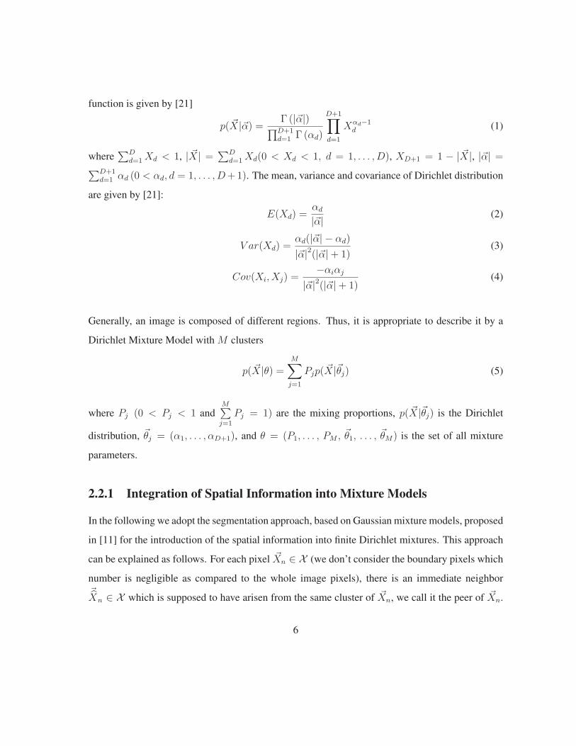
function is given by [21]
p( �X|�α) = Γ (|�α|)∏D+1d=1 Γ (αd)
D+1∏d=1
Xαd−1d (1)
where∑D
d=1 Xd < 1, | �X| = ∑Dd=1 Xd(0 < Xd < 1, d = 1, . . . , D), XD+1 = 1 − | �X|, |�α| =∑D+1
d=1 αd (0 < αd, d = 1, . . . , D+1). The mean, variance and covariance of Dirichlet distribution
are given by [21]:
E(Xd) =αd
|�α| (2)
V ar(Xd) =αd(|�α| − αd)
|�α|2(|�α|+ 1)(3)
Cov(Xi, Xj) =−αiαj
|�α|2(|�α|+ 1)(4)
Generally, an image is composed of different regions. Thus, it is appropriate to describe it by a
Dirichlet Mixture Model with M clusters
p( �X|θ) =M∑j=1
Pjp( �X|�θj) (5)
where Pj (0 < Pj < 1 andM∑j=1
Pj = 1) are the mixing proportions, p( �X|�θj) is the Dirichlet
distribution, �θj = (α1, . . . , αD+1), and θ = (P1, . . . , PM , �θ1, . . . , �θM) is the set of all mixture
parameters.
2.2.1 Integration of Spatial Information into Mixture Models
In the following we adopt the segmentation approach, based on Gaussian mixture models, proposed
in [11] for the introduction of the spatial information into finite Dirichlet mixtures. This approach
can be explained as follows. For each pixel �Xn ∈ X (we don’t consider the boundary pixels which
number is negligible as compared to the whole image pixels), there is an immediate neighbor�Xn ∈ X which is supposed to have arisen from the same cluster of �Xn, we call it the peer of �Xn.
6
Since it is supposed that the peers stay in the same clusters, this spatial information can be used
as indirect information for estimating the number of clusters. In this scenario, if a larger value
is assigned to M , there would be a conflict with the indirect information, provided by the pixels
spatial repartition, of M , which means that a true cluster is wrongly divided into two sub-clusters.
These two sub-clusters have then to be merged to form a new cluster which related parameters have
to be estimated again. In this case, one of the clusters’ mixing probabilities will drop suddenly and
approaches zero, that can be neglected easily, so the number of clusters will gradually decrease to
reach the true number of clusters (i.e. image regions).
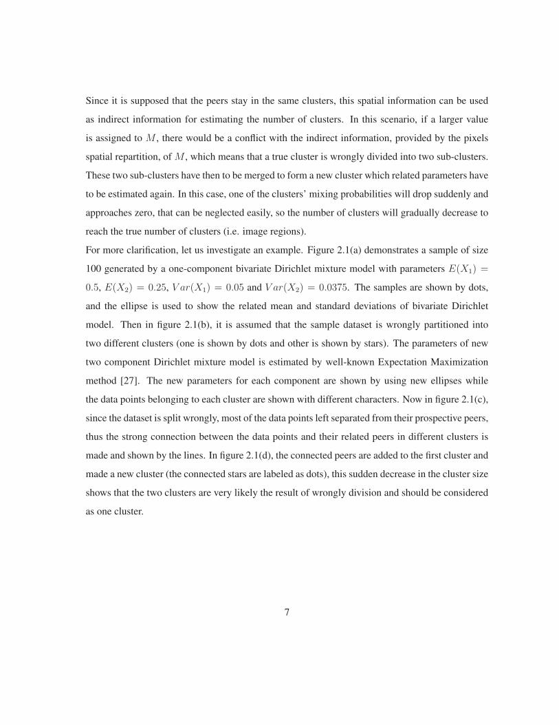
For more clarification, let us investigate an example. Figure 2.1(a) demonstrates a sample of size
100 generated by a one-component bivariate Dirichlet mixture model with parameters E(X1) =
0.5, E(X2) = 0.25, V ar(X1) = 0.05 and V ar(X2) = 0.0375. The samples are shown by dots,
and the ellipse is used to show the related mean and standard deviations of bivariate Dirichlet
model. Then in figure 2.1(b), it is assumed that the sample dataset is wrongly partitioned into
two different clusters (one is shown by dots and other is shown by stars). The parameters of new
two component Dirichlet mixture model is estimated by well-known Expectation Maximization
method [27]. The new parameters for each component are shown by using new ellipses while
the data points belonging to each cluster are shown with different characters. Now in figure 2.1(c),
since the dataset is split wrongly, most of the data points left separated from their prospective peers,
thus the strong connection between the data points and their related peers in different clusters is
made and shown by the lines. In figure 2.1(d), the connected peers are added to the first cluster and
made a new cluster (the connected stars are labeled as dots), this sudden decrease in the cluster size
shows that the two clusters are very likely the result of wrongly division and should be considered
as one cluster.
7
(a) (b)
(c) (d)
Figure 2.1: (a) Simulated data of a bivariate Dirichlet mixture. (b) Estimated results for wronglysupposed two clusters. (c) Strong relation between points and their prospective peers. (d) Thecombination of clusters.
2.2.2 Parameter Estimation
Now that the model is ready, the related parameters estimation would be the next step. Mix-
tures models parameters estimation has been studied as an interesting topic recently and many
approaches have been developed [28]. Maximum likelihood (ML) approach is one of the most
popular estimation methods. The main idea behind ML is to find the parameters which maximize
8
the joint probability density function of the available data (or the data likelihood). This can be per-
formed through the expectation maximization (EM) algorithm [27] which is the most widely used
technique in the case of missing data. The missing data in our case is the knowledge of the pixels
classes. For convenience, we usually deal with the data log-likelihood, instead of the likelihood.
Let X and the set of peers X = { �X1, . . . ,�XN} be our observed data. The set of group indicators
for all pixels Z = {�Z1, . . . , �ZN} will form the unobserved data, where �Zn = (zn,1, . . . , zn,M) de-
notes the missing group indicator and zn,j is equal to one if �Xn and �Xn belong to the same cluster
j, or zero, otherwise. The complete data likelihood is given by
p(X , X ,Z|Θ) =N∏
n=1
M∏j=1
[Pjp( �Xn|�θj)Pjp(
�Xn|�θj)
]zn,j (6)
As it is mentioned earlier for more convenience, the complete log likelihood is used as
L(X , X ,Z|θ) =N∑
n=1
M∑j=1
zn,j(2 logPj + log p( �Xn|�θj) + log p(�Xn|�θj)) (7)
Using the EM algorithm, the parameters which maximize the completed log likelihood function
are estimated iteratively in 2 different steps. The Expectation (E) step and Maximization (M) step.
In E-step, the conditional expectation of the complete data likelihood is calculated as
E[L(X , X ,Z|θ)] = Q(X , X , θ) =N∑
n=1
M∑j=1
p(j| �Xn,�Xn, �α
(k)j )
× (2 logPj + log p( �Xn|�αj) + log p(�Xn|�αj)) (8)
where p(j| �Xn,�Xn, �αj) is the posterior probability which indicates the probability that �Xn and �
Xn
are assigned to cluster j:
p(j| �Xn,�Xn, �αj) =
Pjp( �Xn|�αj)Pjp(�Xn|�αj)∑M
j′=1 Pj′p( �Xn|�αj′)Pj′p(�Xn|�αj′)
(9)
9
Then, in M-step, Q(X , X , θ) (equation 8) will be maximized which give us the following for the
mixing proportions:
P(k+1)j =
1
N
N∑n=1
p(j| �Xn,�Xn, α
(k)j ) (10)
A closed-form solution does not exist for the αj parameters. Thus, we shall employ a Newton-
Raphson approach:
�α(k+1)j = �α
(k)j −H−1(�α
(k)j )× (
∂Q(X , X , θ)
∂�αj
) (11)
where H is the Hessian matrix, which can be evaluated by using the second and mixed derivatives
of Q(X , X , θ). For the first derivative with respect to �αj we have
∂Q(X , X , θ)
∂αjd
=N∑
n=1
p(j| �Xn,�Xn, �αj)
∂
∂αjd
log p( �Xn|�αj) +∂
∂αjd
log p(�Xn|�αj)
=N∑
n=1
p(j| �Xn,�Xn, �αj)×
[2(Ψ(|�αj|)−Ψ(αjd)) + logXnd + log Xnd
](12)
where Ψ(.) is the digamma function. The second derivative is given by
∂Q(X , X , θ)
∂2αjd
= [2(Ψ′(|�αj|)−Ψ′(αjd))]N∑
n=1
p(j| �Xn,�Xn, �αj) (13)
and the mixed derivative is
∂Q(X , X , θ)
∂αjd1∂αjd2
= 2(Ψ′(|�αj|))N∑
n=1
p(j| �Xn,�Xn, �αj) (14)
where in both equations Ψ′(.) is the trigamma function. Now by using the second derivatives as
the diagonal of the Hessian matrix and mixing derivatives as the other non-diagonal elements of
the Hessian matrix, we can make our Hessian matrix as follow
Hj = 2N∑
n=1
P
(j| �Xn,
�Xn, �αj
)⎛⎜⎜⎜⎝Ψ′ (|�αj|)−Ψ′ (αj1) · · · Ψ′ (|�αj|)
... . . . ...
Ψ′ (|�αj|) · · · Ψ′ (|�αj|)−Ψ′ (αjD+1)
⎞⎟⎟⎟⎠ (15)
Then, the inverse of Hessian can be easily calculated using the approach proposed in [21]. By
having the inverse of Hessian matrix we can update the new values for �θ by using equation 11.
10
2.2.3 Initialization and Segmentation algorithm
Parameters initialization is an important issue for mixture models parameter estimation when using
the EM algorithm. Our initialization algorithm is done through well known K-means and the
method of moments (MM) algorithms. According to [21], the method of moments for Dirichlet
can be calculated as
αd =(x′
11−x′21)x
′1d
x′21−(x′
11)2 d = 1, ..., D (16)
αD+1 =
(x′11 − x′
21)
(1−
D∑d=1
x′1d
)x′21 − (x′
11)2 (17)
x′1d =
1N
N∑n=1
xnd d = 1, ..., D + 1 (18)
x′21 =
1
N
N∑n=1
x2n1 (19)
Thus, the proposed segmentation algorithm can be summarized as follows:
1. Choose a large initial value for M as number of image regions (this value should be larger
than the expected number of the regions in the image).
2. Initialize the algorithm using K-means and method of moments.
3. Use the image data points and related peer points to update generalized Dirichlet mixture
parameters by alternating the following two steps:
• E-Step: Compute the posterior probabilities using equation 9.
• M-Step: Update the mixture parameters using equations 10 and 11.
4. Check the mixing parameters Pj values. If a value is close to zero its related cluster should
be removed and the number of clusters, M , should be reduced by one.
11
5. Go to 3 until convergence.
Since for each pixel (r, c) there are 4 main neighbors that are likely to be in the same region, we
can use one of them as the corresponding peer of the pixel. In our experiments, following [11] we
shall use the pixel (r + 1, c) as the corresponding peer.
2.3 Finite Generalized Dirichlet Mixture Model
Because of the known Dirichlet distribution limitations (such as its negative covariance matrix)
[23], Connor et al [29] have generalized the Dirichlet distribution as follows:
p( �X|�α) =D∏
d=1
Γ (αd + βd)
Γ (αd) Γ (βd)Xαd−1
d
(1−
d∑i=1
Xi
)γd
(20)
forD∑
d=1
Xd < 1 and 0 < Xd < 1 for d = 1, . . . , D where γd = βd − αd+1 − βd+1 for d =
1, . . . , D − 1 and γD = βD − 1. Note that the generalized Dirichlet distribution is reduced to a
Dirichlet distribution when βd = αd+1 + βd+1. The mean, variance and covariance of generalize
Dirichlet distribution are given by [23]:
E(Xd) =αd
αd + βd
d−1∏i=1
βi + 1
αi + βi
(21)
V ar(Xd) = E(Xd)
(αd + 1
αd + βd + 1
d−1∏i=1
βi + 1
αi + βi
+ 1− E(Xd)
)(22)
Cov(Xi, Xj) = E(Xj)
(αi
αi + βi + 1
i−1∏k=1
βk + 1
αk + βk
+ 1− E(Xi)
)(23)
while some other interesting properties of this distribution can be found in [30].
2.3.1 Parameter Estimation
The integration of spatial information and complete data likelihood for generalized Dirichlet model
follow the same structure as Dirichlet model, so we will start this section with parameter estimation
12
by using EM algorithm. But before applying EM algorithm, we use an interesting property of
generalized Dirichlet distribution to refine the estimates. If a vector �Xn follows a generalized
Dirichlet distribution, then we can construct a vector �Wn = (Wn1, . . . ,WnD) using the following
geometric transformation Wnd = T (Xnd)
T (Xnd) =
⎧⎨⎩ Xnd, if d = 1
Xnd
1−Xn1−···−Xnd−1, if d = 2, 3, . . . , D
(24)
In this vector �Wn, each Wnd, d = 1, . . . , D, has a Beta distribution with parameters αjd and βjd,
and the parameters {αjd, βjd, d = 1, . . . , D} define the generalized Dirichlet distribution which
characterizes �Xn [23]. Thus, the problem of estimating the parameters of a generalized Dirichlet
mixture can be reduced to estimation of the parameters of d Beta mixtures. Now to accomplish
this, the new form of equation (7) will be given by
L(W , W ,Z|θ) =N∑
n=1
M∑j=1
zn,j(2 logPj + log pbeta( �Wnd|�θjd) + log pbeta(Wnd|�θjd)) (25)
where W = (W1d, . . . ,WNd), 0 < d < D, �θj = (αj1, βj1, . . . , αjD, βjD), and θ = (P1, . . . , PM ,
�θ1, . . . , �θM) is the set of all mixture parameters.
In E-step, the conditional expectation of the complete data likelihood is calculated as
E[L(W , W ,Z|θ)] = Q(W , W , θ) =N∑
n=1
M∑j=1
pbeta(j| �Wnd,�W nd, �θjd) (26)
× (2 logPj + log pbeta( �Wnd|�θjd) + log pbeta(�W nd|�θjd))
where pbeta(j| �Wnd,�W nd, �θjd) is the posterior probability which indicates the probability that �Wnd
and �W nd are assigned to cluster j:
pbeta(j| �Wnd,�W nd, �θjd) =
Pjpbeta( �Wnd|�θjd)Pjpbeta(�W nd|�θjd)∑M
j′=1 Pj′pbeta( �Wnd|�θj′d)Pj′pbeta(�W nd|�θj′d)
(27)
13
Then, in M-step, Q(W , W , θ) (equation 26) will be maximized which give us the following for the
mixing proportions:
P(k+1)j =
1
N
N∑n=1
pbeta(j| �Wnd,�W nd, θ
(k)jd ) (28)
A closed-form solution does not exist for the θjd parameters. Thus, we shall employ a Newton-
Raphson approach:
�θ(k+1)jd = �θ
(k)jd −H−1(�θ
(k)jd )× (
∂Q(W , W , θ)
∂�θjd) (29)
where H is the Hessian matrix, which can be evaluated by using the second and mixed derivatives
of Q(W , W , θ). For the first derivative with respect to �αjd and �βjd we have
∂Q(W , W , θ)
∂αjd
=N∑
n=1
pbeta(j| �Wnd,�W nd, �θjd)
∂
∂αjd
log pbeta( �Wnd|�θjd) + ∂
∂αjd
log pbeta(�W nd|�θjd)
=N∑
n=1
pbeta(j| �Wnd,�W nd, �θjd)×
[2(Ψ(αjd + βjd)−Ψ(αjd)) + logWnd + log Wnd
](30)
∂Q(W , W , θ)
∂βjd
=N∑
n=1
pbeta(j| �Wnd,�W nd, �θjd)
∂
∂βjd
log pbeta( �Wnd|�θjd) + ∂
∂βjd
log pbeta(�W nd|�θjd)
=N∑
n=1
pbeta(j| �Wnd,�W nd, �θjd)×
[2(Ψ(αjd + βjd)−Ψ(βjd)) + log(1−Wnd) + log(1− Wnd)
](31)
where Ψ(.) is the digamma function. The second derivatives are given by
∂Q(W , W , θ)
∂2αjd
= [2(Ψ′(αjd + βjd)−Ψ′(αjd))]N∑
n=1
pbeta(j| �Wnd,�W nd, �θjd) (32)
∂Q(W , W , θ)
∂2βjd
= [2(Ψ′(αjd + βjd)−Ψ′(βjd))]N∑
n=1
pbeta(j| �Wnd,�W nd, �θjd) (33)
and the mixed derivative is
∂Q(W , W , θ)
∂αjd∂βjd
= 2(Ψ′(αjd + βjd))N∑
n=1
pbeta(j| �Wnd,�W nd, �θjd) (34)
14
where in both equations Ψ′(.) is the trigamma function. Then, the inverse of Hessian can be easily
calculated using the approach proposed in [21]. By having the inverse of Hessian matrix we can
update the new values for �θ by using equation 29.
2.3.2 Initialization and Segmentation algorithm
Parameters initialization is an important issue for mixture models parameter estimation when us-
ing the EM algorithm. Our initialization algorithm is done through well known K-means and the
method of moments (MM) algorithms [23]. Thus, the proposed segmentation algorithm can be
summarized as follows:
1. Choose a large initial value for M as number of image regions (this value should be larger
than the expected number of the regions in the image).
2. Initialize the algorithm using the approach in [23].
3. Use the image data points and related peer points to update generalized Dirichlet mixture
parameters by alternating the following two steps:
• E-Step: Compute the posterior probabilities using equation 27.
• M-Step: Update the mixture parameters using equations 28 and 29.
4. Check the mixing parameters Pj values. If a value is close to zero its related cluster should
be removed and the number of clusters, M , should be reduced by one.
5. Go to 3 until convergence.
15
2.4 Finite Beta-Liouville Mixture Model
Although generalized Dirichlet distribution can overcome the disadvantages of Dirichlet distribu-
tion (for instance, the covariance matrix is not restricted to be negative anymore) [23], it involves
a large number of parameters (It has 2D parameters in dimension D). Another good choice for
random vector �Xn = (Xn1, . . . , XnD) would be Liouville distribution of second kind, which has
D + 2 parameters in dimension D.
If random vector �X follows a Liouville distribution of second kind with positive parameters
�α = (α1, α2, . . . , αD), with density function f(.), then [31]
p( �X|�α) = Γ(∑D
d=1 αd)
u∑D
d=1 αd−1f(u)
D∏d=1
Xαd−1d
Γ(αd)(35)
where u =D∑
d=1
Xd < 1,0 < Xd,d = 1, . . . , D. A flexible univariate distribution that can be a
suitable choice as our density function is Beta distribution [26] which has positive parameters α
and β
f(u|α, β) = Γ(α + β)
Γ(α)Γ(β)uα−1(1− u)β−1 (36)
Replacing the equation 36 into the equation 35 gives us the following:
p(�X|α1, α2, . . . , αD, α, β
)=
Γ(∑D
d αd
)Γ (α + β)
Γ (α) Γ (β)
D∏d=1
Xαd−1d
Γ (αd)
(D∑
d=1
Xd
)α−D∑
d=1αd(1−
D∑d=1
Xd
)β−1
(37)
which has positive parameters θ = (α1, α2, . . . , αD, α, β) and is called Beta-Liouville distribution
[31]. It is noteworthy to mention that Beta-Liouville distribution of second kind can be reduced to
Dirichlet distribution with parameters α1, ..., αD+1 by choosing∑D
d=1 αd and αD+1 as parameters
of Beta component of the distribution. The mean and variance of the Beta-Liouville distribution of
second kind can be calculated as
E (Xd) =α
α + β
αd∑Dd=1 αd
(38)
16
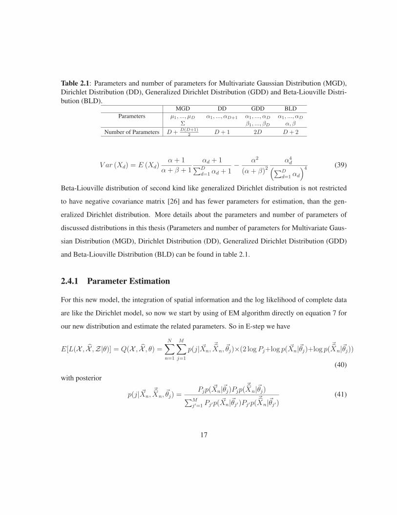
Table 2.1: Parameters and number of parameters for Multivariate Gaussian Distribution (MGD),Dirichlet Distribution (DD), Generalized Dirichlet Distribution (GDD) and Beta-Liouville Distri-bution (BLD).
MGD DD GDD BLDParameters μ1, ..., μD α1, ..., αD+1 α1, ..., αD α1, ..., αD
Σ β1, ..., βD α, β
Number of Parameters D + D(D+1)2 D + 1 2D D + 2
V ar (Xd) = E (Xd)α + 1
α + β + 1
αd + 1∑Dd=1 αd + 1
− α2
(α + β)2α4d(∑D
d=1 αd
)4 (39)
Beta-Liouville distribution of second kind like generalized Dirichlet distribution is not restricted
to have negative covariance matrix [26] and has fewer parameters for estimation, than the gen-
eralized Dirichlet distribution. More details about the parameters and number of parameters of
discussed distributions in this thesis (Parameters and number of parameters for Multivariate Gaus-
sian Distribution (MGD), Dirichlet Distribution (DD), Generalized Dirichlet Distribution (GDD)
and Beta-Liouville Distribution (BLD) can be found in table 2.1.
2.4.1 Parameter Estimation
For this new model, the integration of spatial information and the log likelihood of complete data
are like the Dirichlet model, so now we start by using of EM algorithm directly on equation 7 for
our new distribution and estimate the related parameters. So in E-step we have
E[L(X , X ,Z|θ)] = Q(X , X , θ) =N∑
n=1
M∑j=1
p(j| �Xn,�Xn, �θj)×(2 logPj+log p( �Xn|�θj)+log p(
�Xn|�θj))
(40)
with posterior
p(j| �Xn,�Xn, �θj) =
Pjp( �Xn|�θj)Pjp(�Xn|�θj)∑M
j′=1 Pj′p( �Xn|�θj′)Pj′p(�Xn|�θj′)
(41)
17
Then by maximizing equation 40, the new mixing proportions can be derived as
P(k+1)j =
1
N
N∑n=1
p(j| �Xn,�Xn, θ
(k)j ) (42)
The new values of model parameters can be estimated by Newton-Raphson approach:
�θ(k+1)j = �θ
(k)j −H−1(�θ
(k)j )× (
∂Q(X , X , θ)
∂�θj) (43)
For evaluating the Hessian matrix, the first derivative with respect to αj , βj and αjd would be
∂Q(X , X , θ)
∂αj
=N∑
n=1
p(j| �Xn,�Xn, �θj)
∂
∂αj
log p( �Xn|�θj) + ∂
∂αj
log p(�Xn|�θj) (44)
=N∑
n=1
p(j| �Xn,�Xn, �θj)
[2 (Ψ(αj + βj)−Ψ(αj)) + log
D∑d=1
Xnd + logD∑
d=1
Xnd
]
∂Q(X , X , θ)
∂βj
=N∑
n=1
p(j| �Xn,�Xn, �θj)
∂
∂βjd
log p( �Xn|�θj) + ∂
∂βjd
log p(�Xn|�θj)
=N∑
n=1
p(j| �Xn,�Xn, �θj)
[2 (Ψ(αj + βj)−Ψ(βj)) + log
(1−
D∑d=1
Xnd
)
+ log
(1−
D∑d=1
Xnd
)] (45)
∂Q(X , X , θ)
∂αjd
=N∑
n=1
p
(j| �Xn,
�Xn, �θj
)∂
∂αjd
log p(�Xn|�θj
)+
∂
∂αjd
log p
(�Xn|�θj
)
=N∑
n=1
p
(j| �Xn,
�Xn, �θj
)[2
(Ψ
(D∑
d=1
αjd
))+
(logXnd −Ψ(αjd)− log
D∑d=1
Xnd
)
+
(log Xnd −Ψ(αjd)− log
D∑d=1
Xnd
)] (46)
The second and mixed derivatives are given by
∂Q(X , X , θ)
∂2αj
=[2(Ψ
′(αj + βj)−Ψ
′(αj)
)] N∑n=1
p(j| �Xn,�Xn, �θj) (47)
18
∂Q(X , X , θ)
∂2βj
=[2(Ψ
′(αj + βj)−Ψ
′(βj)
)] N∑n=1
p(j| �Xn,�Xn, �θj) (48)
∂Q(X , X , θ
)∂αjd1∂αjd2
=
⎧⎪⎪⎨⎪⎪⎩[2
(Ψ
′(
D∑d=1
αjd
))− 2
(Ψ
′(αjd)
)] N∑n=1
p
(j| �Xn,
�Xn, �θj
), if αjd1 = αjd2[
2
(Ψ
′(
D∑d=1
αjd
))]N∑
n=1
p
(j| �Xn,
�Xn, �θj
), otherwise
(49)∂Q(X , X , θ)
∂αj∂βj
=∂Q(X , X , θ)
∂βj∂αj
=[2(Ψ
′(αj + βj)
)] N∑n=1
p(j| �Xn,�Xn, �θj) (50)
∂Q(X , X , θ)
∂αj∂αjd
=∂Q(X , X , θ)
∂βj∂αjd
=∂Q(X , X , θ)
∂αjd∂βj
=∂Q(X , X , θ)
∂αjd∂βj
= 0 (51)
We can show that the Hessian has a block diagonal matrix format
H (θj) = blockdiag (Ha, Hb) =
⎡⎣ Ha 0
0 Hb
⎤⎦ (52)
where
Ha = H (αj, βj) =
⎡⎣ ∂Q(X ,X ,θ)∂2αj
∂Q(X ,X ,θ)∂αj∂βj
∂Q(X ,X ,θ)∂βj∂αj
∂Q(X ,X ,θ)∂2βj
⎤⎦ (53)
Hb = H (αj1, . . . , αjD) =∂Q
(X , X , θ
)∂αjdi∂αjdk
,where i, k ∈ {1, . . . , D} (54)
Then, the inverse of H (θj) can be easily computed as
H(−1)(θj) = (blockdiag(Ha, Hb))(−1) = blockdiag
((Ha)
(−1), (Hb)(−1)
)(55)
By having the inverse of Hessian, we can update the new values for �θj by using equation 43
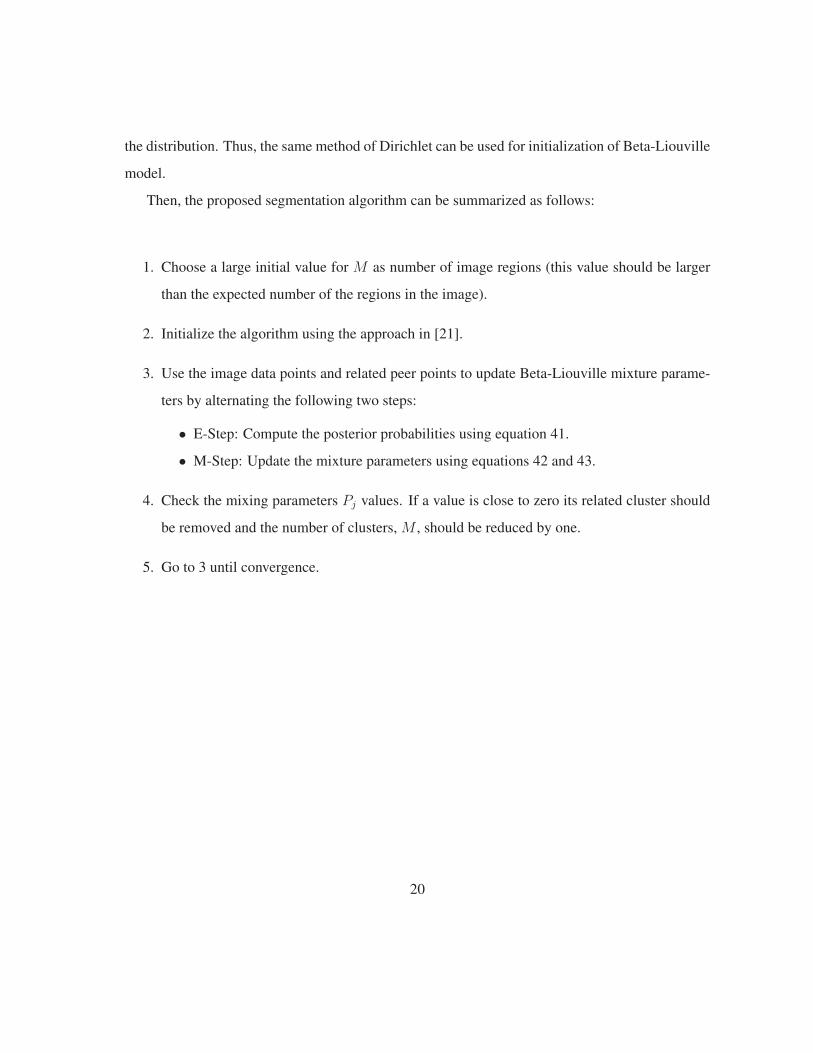
2.4.2 Initialization and Segmentation algorithm
For initialization phase, the k-means and method of moments are used again, with considering the
fact, that Beta-Liouville distribution of second kind can be reduced to Dirichlet distribution with
parameters α1, ..., αD+1 by using∑D
d=1 αd and αD+1 as the parameters of the Beta component of
19
the distribution. Thus, the same method of Dirichlet can be used for initialization of Beta-Liouville
model.
Then, the proposed segmentation algorithm can be summarized as follows:
1. Choose a large initial value for M as number of image regions (this value should be larger
than the expected number of the regions in the image).
2. Initialize the algorithm using the approach in [21].
3. Use the image data points and related peer points to update Beta-Liouville mixture parame-
ters by alternating the following two steps:
• E-Step: Compute the posterior probabilities using equation 41.
• M-Step: Update the mixture parameters using equations 42 and 43.
4. Check the mixing parameters Pj values. If a value is close to zero its related cluster should
be removed and the number of clusters, M , should be reduced by one.
5. Go to 3 until convergence.
20
CHAPTER 3Experimental Results
3.1 Introduction
In this chapter we validate our models, and we also investigate how the choice of distinctive color
spaces can make difference in color image segmentation.
3.2 Design of Experiments
The main goal of this section is to investigate the performance of the proposed approaches (Dirich-
let , generalized Dirichlet and Beta-Liouville mixtures) as compared to the one developed in [11]
which has been based on the integration of the spatial information into Gaussian mixture models.
It is noteworthy that an important problem when dealing with color images is the choice of the
color space. In the case of image segmentation, it is highly desirable that the chosen color space
be robust against varying illumination, concise, discriminatory and robust to noise. Some of such
color spaces have been analyzed, evaluated and discussed in [24]. Among these spaces, we have
the RGB normalized color space which rgb planes are defined by [24, 32]
r(R,G,B) =R
R +G+B(1)
g(R,G,B) =G
R +G+B(2)
21
b(R,G,B) =B
R +G+B(3)
and the l1l2l3 color space defined by [24]
l1(R,G,B) =(R−G)2
(R−G)2 + (R−B)2 + (G− B)2(4)
l2(R,G,B) =(R−B)2
(R−G)2 + (R−B)2 + (G− B)2(5)
l3(R,G,B) =(G− B)2
(R−G)2 + (R−B)2 + (G− B)2(6)
which is a photometric color invariant for matte and shiny spaces [24]. The rgb and l1l2l3 have
been shown to outperform the widely used RGB space [24] and thus will be considered in our
experiments. To have a fair comparison, in all cases (i.e. Gaussian, Dirichlet, generalized Dirichlet
and Beta-Liouville mixtures), the initial values for the number of clusters M are set to 30.
3.3 Experiment 1
In addition to the famous Baboon image, which is widely used to evaluate image segmentation
algorithms, we have employed 300 images from the well-known publicly available Berkeley seg-
mentation data set [33]. This database is composed of a variety of natural color images generally
used as a reliable way to compare image segmentation algorithms. Figure 3.1 shows a comparison
between the segmentation results obtained by our approach and the technique developed in [11]
when we consider the rgb color space. Figure 3.1(a) shows the original Baboon image, while
figures 3.1(b), 3.1(c), 3.1(d) and 3.1(e) show the results obtained with the Gaussian mixture,
the Dirichlet mixture, generalized Dirichlet mixture and Beta-Liouville mixture, respectively. The
algorithm in [11] selected 12 regions for the baboon image while our proposed algorithms consid-
ered 4 regions for all Dirichlet, generalized Dirichlet and Beta-Liouville mixture models. As the
figure indicates, in addition to the less number of regions preferred by our algorithms, the regions
provided are more meaningful. In this image the nose of baboon is almost composed of two clear
22
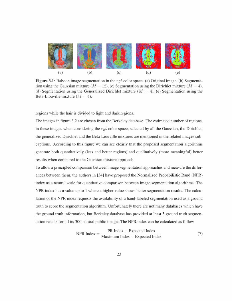
(a) (b) (c) (d) (e)
Figure 3.1: Baboon image segmentation in the rgb color space. (a) Original image, (b) Segmenta-tion using the Gaussian mixture (M = 12), (c) Segmentation using the Dirichlet mixture (M = 4),(d) Segmentation using the Generalized Dirichlet mixture (M = 4), (e) Segmentation using theBeta-Liouville mixture (M = 4).
regions while the hair is divided to light and dark regions.
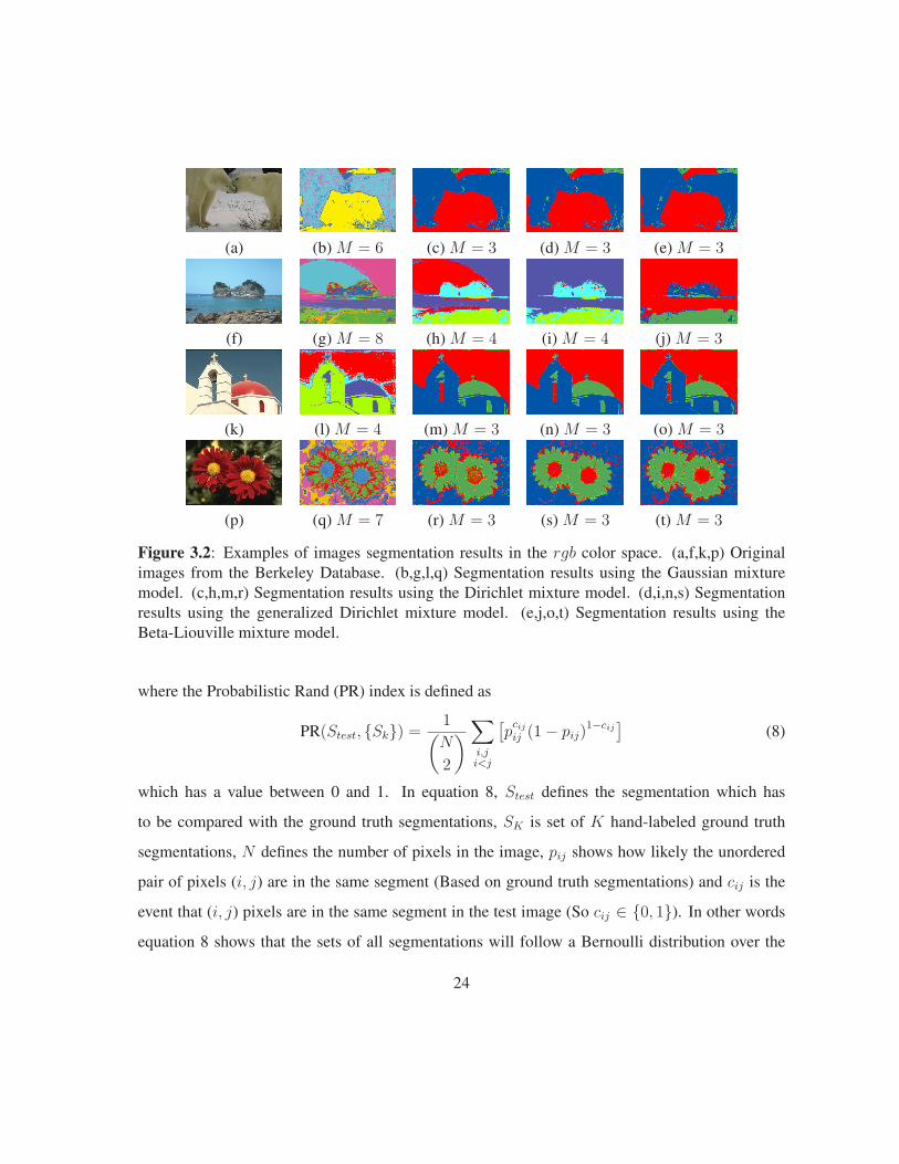
The images in figure 3.2 are chosen from the Berkeley database. The estimated number of regions,
in these images when considering the rgb color space, selected by all the Gaussian, the Dirichlet,
the generalized Dirichlet and the Beta-Liouville mixtures are mentioned in the related images sub-
captions. According to this figure we can see clearly that the proposed segmentation algorithms
generate both quantitatively (less and better regions) and qualitatively (more meaningful) better
results when compared to the Gaussian mixture approach.
To allow a principled comparison between image segmentation approaches and measure the differ-
ences between them, the authors in [34] have proposed the Normalized Probabilistic Rand (NPR)
index as a neutral scale for quantitative comparison between image segmentation algorithms. The
NPR index has a value up to 1 where a higher value shows better segmentation results. The calcu-
lation of the NPR index requests the availability of a hand-labeled segmentation used as a ground
truth to score the segmentation algorithm. Unfortunately there are not many databases which have
the ground truth information, but Berkeley database has provided at least 5 ground truth segmen-
tation results for all its 300 natural public images.The NPR index can be calculated as follow
NPR Index =PR Index − Expected Index
Maximum Index − Expected Index(7)
23
(a) (b) M = 6 (c) M = 3 (d) M = 3 (e) M = 3
(f) (g) M = 8 (h) M = 4 (i) M = 4 (j) M = 3
(k) (l) M = 4 (m) M = 3 (n) M = 3 (o) M = 3
(p) (q) M = 7 (r) M = 3 (s) M = 3 (t) M = 3
Figure 3.2: Examples of images segmentation results in the rgb color space. (a,f,k,p) Originalimages from the Berkeley Database. (b,g,l,q) Segmentation results using the Gaussian mixturemodel. (c,h,m,r) Segmentation results using the Dirichlet mixture model. (d,i,n,s) Segmentationresults using the generalized Dirichlet mixture model. (e,j,o,t) Segmentation results using theBeta-Liouville mixture model.
where the Probabilistic Rand (PR) index is defined as
PR(Stest, {Sk}) = 1(N
2
) ∑i,ji<j
[pcijij (1− pij)
1−cij]
(8)
which has a value between 0 and 1. In equation 8, Stest defines the segmentation which has
to be compared with the ground truth segmentations, SK is set of K hand-labeled ground truth
segmentations, N defines the number of pixels in the image, pij shows how likely the unordered
pair of pixels (i, j) are in the same segment (Based on ground truth segmentations) and cij is the
event that (i, j) pixels are in the same segment in the test image (So cij ∈ {0, 1}). In other words
equation 8 shows that the sets of all segmentations will follow a Bernoulli distribution over the
24
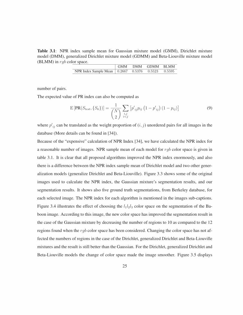
Table 3.1: NPR index sample mean for Gaussian mixture model (GMM), Dirichlet mixturemodel (DMM), generalized Dirichlet mixture model (GDMM) and Beta-Liouville mixture model(BLMM) in rgb color space.
GMM DMM GDMM BLMMNPR Index Sample Mean 0.2667 0.5376 0.5523 0.5595
number of pairs.
The expected value of PR index can also be computed as
E [PR(Stest, {Sk})] = 1(N
2
) ∑i,ji<j
[p′ijpij
(1− p′ij
)(1− pij)
](9)
where p′ij can be translated as the weight proportion of (i, j) unordered pairs for all images in the
database (More details can be found in [34]).
Because of the “expensive” calculation of NPR Index [34], we have calculated the NPR index for
a reasonable number of images. NPR sample mean of each model for rgb color space is given in
table 3.1. It is clear that all proposed algorithms improved the NPR index enormously, and also
there is a difference between the NPR index sample mean of Dirichlet model and two other gener-
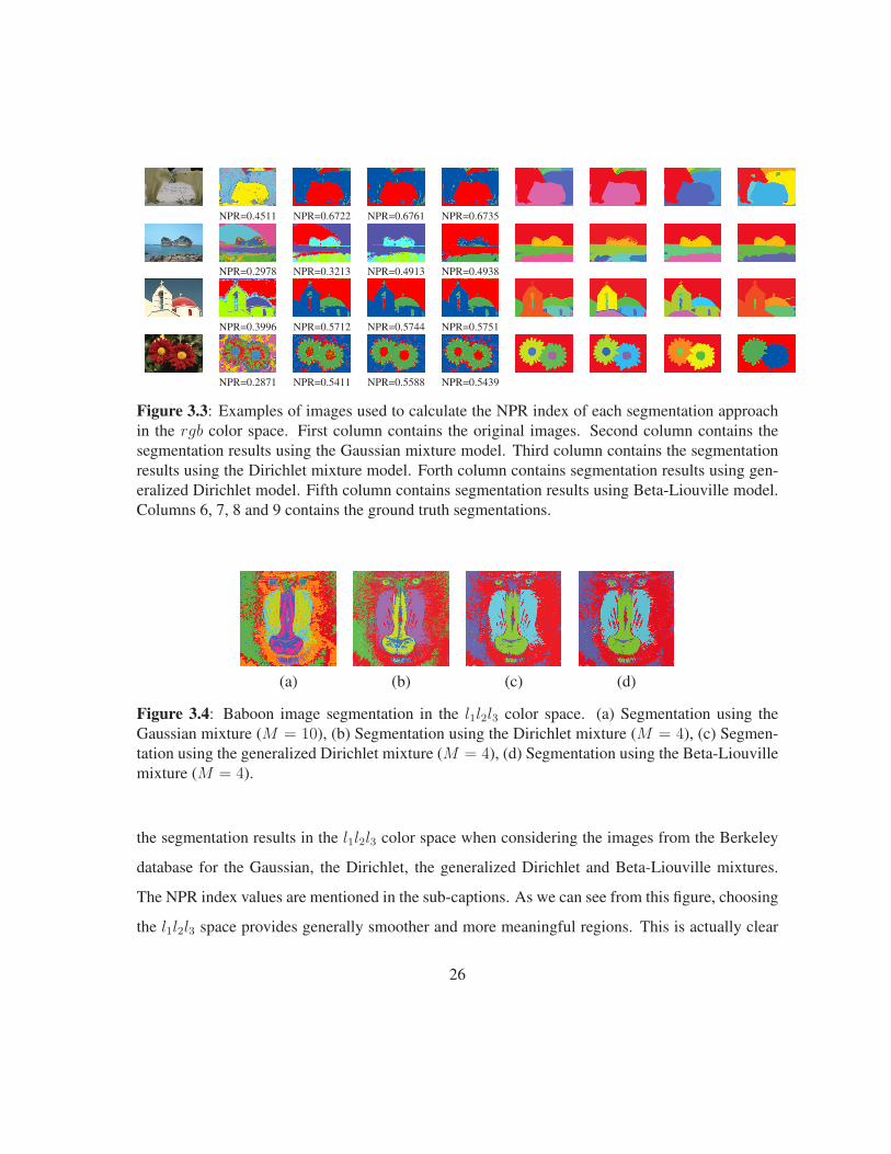
alization models (generalize Dirichlet and Beta-Liouville). Figure 3.3 shows some of the original
images used to calculate the NPR index, the Gaussian mixture’s segmentation results, and our
segmentation results. It shows also five ground truth segmentations, from Berkeley database, for
each selected image. The NPR index for each algorithm is mentioned in the images sub-captions.
Figure 3.4 illustrates the effect of choosing the l1l2l3 color space on the segmentation of the Ba-
boon image. According to this image, the new color space has improved the segmentation result in
the case of the Gaussian mixture by decreasing the number of regions to 10 as compared to the 12
regions found when the rgb color space has been considered. Changing the color space has not af-
fected the numbers of regions in the case of the Dirichlet, generalized Dirichlet and Beta-Liouville
mixtures and the result is still better than the Gaussian. For the Dirichlet, generalized Dirichlet and
Beta-Liouville models the change of color space made the image smoother. Figure 3.5 displays
25
NPR=0.4511 NPR=0.6722 NPR=0.6761 NPR=0.6735
NPR=0.2978 NPR=0.3213 NPR=0.4913 NPR=0.4938
NPR=0.3996 NPR=0.5712 NPR=0.5744 NPR=0.5751
NPR=0.2871 NPR=0.5411 NPR=0.5588 NPR=0.5439
Figure 3.3: Examples of images used to calculate the NPR index of each segmentation approachin the rgb color space. First column contains the original images. Second column contains thesegmentation results using the Gaussian mixture model. Third column contains the segmentationresults using the Dirichlet mixture model. Forth column contains segmentation results using gen-eralized Dirichlet model. Fifth column contains segmentation results using Beta-Liouville model.Columns 6, 7, 8 and 9 contains the ground truth segmentations.
(a) (b) (c) (d)
Figure 3.4: Baboon image segmentation in the l1l2l3 color space. (a) Segmentation using theGaussian mixture (M = 10), (b) Segmentation using the Dirichlet mixture (M = 4), (c) Segmen-tation using the generalized Dirichlet mixture (M = 4), (d) Segmentation using the Beta-Liouvillemixture (M = 4).
the segmentation results in the l1l2l3 color space when considering the images from the Berkeley
database for the Gaussian, the Dirichlet, the generalized Dirichlet and Beta-Liouville mixtures.
The NPR index values are mentioned in the sub-captions. As we can see from this figure, choosing
the l1l2l3 space provides generally smoother and more meaningful regions. This is actually clear
26

by comparing the NPR indexes in figures 3.5 and 3.3.
NPR=0.4777 NPR=0.6783 NPR=0.6822 NPR=0.6800
NPR=0.3101 NPR=0.3556 NPR=0.5081 NPR=0.5100
NPR= 0.4015 NPR=0.5817 NPR=0.5823 NPR=0.5854
NPR= 0.3092 NPR=0.5553 NPR=0.5595 NPR=0.6573
Figure 3.5: Images segmentation in the l1l2l3 color space. First column: segmentation usingthe Gaussian mixture model. Second column: segmentation using the Dirichlet mixture. Thirdcolumn: segmentation using the generalized Dirichlet mixture. Forth column: segmentation usingthe Beta-Liouville mixture.
The NPR index sample mean of all models for l1l2l3 color space is shown table 3.2. Comparing
the results in table 3.1 and table 3.2 indicate a segmentation improvement where the l1l2l3 color
space is considered.
3.4 Experiment 2
In this experiment, we mainly focus on the effect of distinctive color spaces on color image seg-
mentation while we can still compare the effectiveness of the proposed approaches comparing to
27
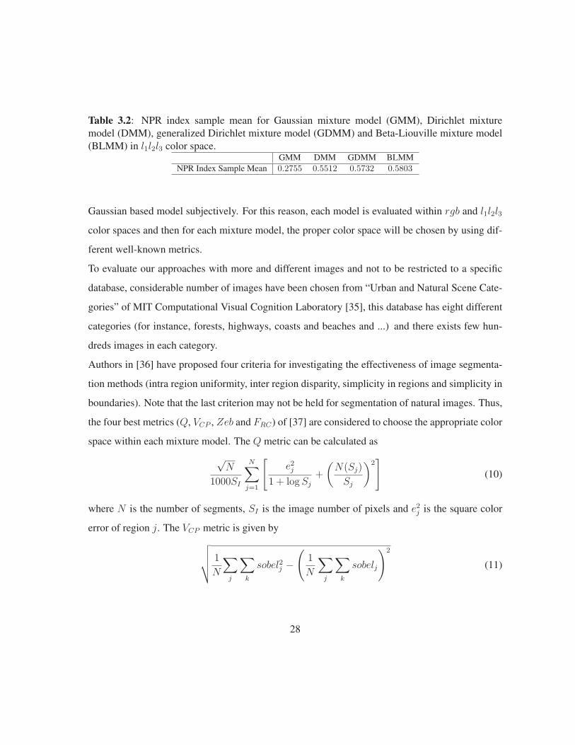
Table 3.2: NPR index sample mean for Gaussian mixture model (GMM), Dirichlet mixturemodel (DMM), generalized Dirichlet mixture model (GDMM) and Beta-Liouville mixture model(BLMM) in l1l2l3 color space.
GMM DMM GDMM BLMMNPR Index Sample Mean 0.2755 0.5512 0.5732 0.5803
Gaussian based model subjectively. For this reason, each model is evaluated within rgb and l1l2l3
color spaces and then for each mixture model, the proper color space will be chosen by using dif-
ferent well-known metrics.
To evaluate our approaches with more and different images and not to be restricted to a specific
database, considerable number of images have been chosen from “Urban and Natural Scene Cate-
gories” of MIT Computational Visual Cognition Laboratory [35], this database has eight different
categories (for instance, forests, highways, coasts and beaches and ...) and there exists few hun-
dreds images in each category.
Authors in [36] have proposed four criteria for investigating the effectiveness of image segmenta-
tion methods (intra region uniformity, inter region disparity, simplicity in regions and simplicity in
boundaries). Note that the last criterion may not be held for segmentation of natural images. Thus,
the four best metrics (Q, VCP , Zeb and FRC) of [37] are considered to choose the appropriate color
space within each mixture model. The Q metric can be calculated as
√N
1000SI
N∑j=1
[e2j
1 + logSj
+
(N(Sj)
Sj
)2]
(10)
where N is the number of segments, SI is the image number of pixels and e2j is the square color
error of region j. The VCP metric is given by√√√√ 1
N
∑j
∑k
sobel2j −(
1
N
∑j
∑k
sobelj
)2
(11)
28
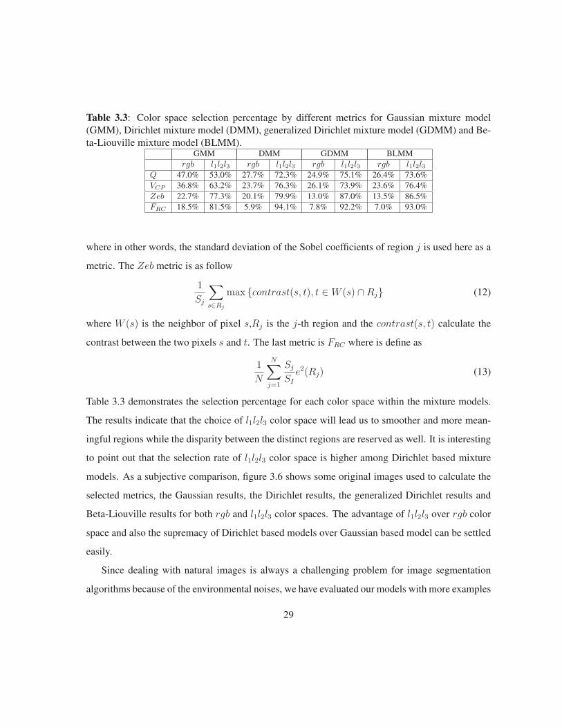
Table 3.3: Color space selection percentage by different metrics for Gaussian mixture model(GMM), Dirichlet mixture model (DMM), generalized Dirichlet mixture model (GDMM) and Be-ta-Liouville mixture model (BLMM).
GMM DMM GDMM BLMMrgb l1l2l3 rgb l1l2l3 rgb l1l2l3 rgb l1l2l3
Q 47.0% 53.0% 27.7% 72.3% 24.9% 75.1% 26.4% 73.6%VCP 36.8% 63.2% 23.7% 76.3% 26.1% 73.9% 23.6% 76.4%Zeb 22.7% 77.3% 20.1% 79.9% 13.0% 87.0% 13.5% 86.5%FRC 18.5% 81.5% 5.9% 94.1% 7.8% 92.2% 7.0% 93.0%
where in other words, the standard deviation of the Sobel coefficients of region j is used here as a
metric. The Zeb metric is as follow
1
Sj
∑s∈Rj
max {contrast(s, t), t ∈ W (s) ∩Rj} (12)
where W (s) is the neighbor of pixel s,Rj is the j-th region and the contrast(s, t) calculate the
contrast between the two pixels s and t. The last metric is FRC where is define as
1
N
N∑j=1
Sj
SI
e2(Rj) (13)
Table 3.3 demonstrates the selection percentage for each color space within the mixture models.
The results indicate that the choice of l1l2l3 color space will lead us to smoother and more mean-
ingful regions while the disparity between the distinct regions are reserved as well. It is interesting
to point out that the selection rate of l1l2l3 color space is higher among Dirichlet based mixture
models. As a subjective comparison, figure 3.6 shows some original images used to calculate the
selected metrics, the Gaussian results, the Dirichlet results, the generalized Dirichlet results and
Beta-Liouville results for both rgb and l1l2l3 color spaces. The advantage of l1l2l3 over rgb color
space and also the supremacy of Dirichlet based models over Gaussian based model can be settled
easily.
Since dealing with natural images is always a challenging problem for image segmentation
algorithms because of the environmental noises, we have evaluated our models with more examples
29
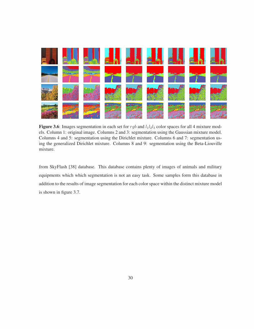
Figure 3.6: Images segmentation in each set for rgb and l1l2l3 color spaces for all 4 mixture mod-els. Column 1: original image. Columns 2 and 3: segmentation using the Gaussian mixture model.Columns 4 and 5: segmentation using the Dirichlet mixture. Columns 6 and 7: segmentation us-ing the generalized Dirichlet mixture. Columns 8 and 9: segmentation using the Beta-Liouvillemixture.
from SkyFlash [38] database. This database contains plenty of images of animals and military
equipments which which segmentation is not an easy task. Some samples form this database in
addition to the results of image segmentation for each color space within the distinct mixture model
is shown in figure 3.7.
30
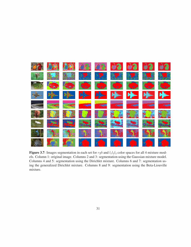
Figure 3.7: Images segmentation in each set for rgb and l1l2l3 color spaces for all 4 mixture mod-els. Column 1: original image. Columns 2 and 3: segmentation using the Gaussian mixture model.Columns 4 and 5: segmentation using the Dirichlet mixture. Columns 6 and 7: segmentation us-ing the generalized Dirichlet mixture. Columns 8 and 9: segmentation using the Beta-Liouvillemixture.
31
CHAPTER 4Conclusions
In this thesis, we have presented different algorithms for color image segmentation by integrating
spatial information into finite mixture models. The selection of these mixture models is motivated
by their flexibility in approximation of data points in different shapes in contrast to the well known
gaussian mixture model which always keeps the symmetric bell shape. First we chose Dirichlet
mixture model for its flexibility in data modeling and its few number of parameters for estimation,
but its restrictive covariance matrix was the negative point. This disadvantage has been handled
by generalized Dirichlet mixture model in cost of an increase in the number of parameters. So
finally the motivation for choosing the Beta-Liouville mixture model was its flexibility in shapes
and its few number of parameters as compared to Gaussian and Generalized Dirichlet distribu-
tions. Then the spatial information is included in this model by considering pixels neighborhoods
and by using this information as a prior knowledge in our model, we got the ability to estimate
the number of segmentation regions automatically. The resulted image segmentation statistical
model has been learned using maximum likelihood estimation within an expectation maximization
framework. Results, which have concerned the segmentation of an important number of images
from the well-known Berkeley images database, show that the proposed algorithms perform better
than an approach which has been based on finite Gaussian mixture models. The effect of distinct
color spaces on color image segmentation was also investigated by using different metrics over the
famous MIT images database. Future works can be devoted to the application of the developed
32
Chapter 4. Conclusions
segmentation algorithm for object detection and recognition and also a promising extension of
this work would be on the integration of more visual features to improve further the segmentation
results. Video segmentation could be considered as another interesting application which has to
be done in an online fashion. So a potential future work could be the extension of the proposed
approach to segment frames in a real-time stream.
33
List of References
[1] C. Carson, S. Belongie, H. Greenspan, and J. Malik. Blobworld: image segmentation us-
ing expectation-maximization and its application to image querying. IEEE Transactions on
Pattern Analysis and Machine Intelligence, 24(8):1026 – 1038, 2002.
[2] M. Ozden and E. Polat. A Color Image Segmentation Approach for Content-Based Image
Retrieval. Pattern Recognition, 40(4):1318–1325, 2007.
[3] D. Ziou, N. Bouguila, M. S. Allili, A. El Zaart. Finite Gamma Mixture Modeling Using
Minimum Message Length Inference: Application to SAR Image Analysis. International
Journal of Remote Sensing, 30(3):771–792, 2009.
[4] W. M. Wells, W. E. L. Grimson, R. Kikinis, F. A. Jolesz. Adaptive Segmentation of MRI
Data. IEEE Transactions on Medical Imaging, 15(4):429–442, 1996.
[5] Liang Shen and R.M. Rangayyan. A segmentation-based lossless image coding method
for high-resolution medical image compression. IEEE Transactions on Medical Imaging,
16(3):301–307, 1997.
[6] T. Bucher, C. Curio, J. Edelbrunner, C. Igel, D. Kastrup, I. Leefken, G. Lorenz, A. Steinhage,
and W. von Seelen. Image processing and behavior planning for intelligent vehicles. IEEE
Transactions on Industrial Electronics, 50(1):62–75, 2003.
34
References
[7] J. Shi and J. Malik. Normalized cuts and image segmentation. IEEE Transactions on Pattern
Analysis and Machine Intelligence, 22(8):888 –905, 2000.
[8] S. C. Zhu and A. Yuille. Region competition: Unifying snakes, region growing, and
bayes/mdl for multiband image segmentation. IEEE Transactions on Pattern Analysis and
Machine Intelligence, 18(9):884–900, 1996.
[9] Nikhil R Pal and Sankar K Pal. A review on image segmentation techniques. Pattern Recog-
nition, 26(9):1277 – 1294, 1993.
[10] Y. Zhang, M. Brady, and S. Smith. Segmentation of brain MR images through a hidden
Markov random field model and the expectation-maximization algorithm. IEEE Transactions
on Medical Imaging, 20(1):45 –57, 2001.
[11] X. Yang and Sh. M. Krishnan. Image Segmentation using Finite Mixtures and Spatial Infor-
mation. Image and Vision Computing, 22(9):735–745, 2004.
[12] C. Nikou, N. P. Galatsanos, and A. C. Likas. A Class-Adaptive Spatially Variant Mixture
Model for Image Segmentation. IEEE Transactions on Image Processing, 16:1121–1130,
2007.
[13] W. L. Hung, M. Sh. Yang, and D. H. Chen. Bootstrapping approach to feature-weight selec-
tion in fuzzy c-means algorithms with an application in color image segmentation. Pattern
Recognition Letters, 29(9):1317 – 1325, 2008.
[14] N. Bouguila and D. Ziou. Unsupervised Selection of a Finite Dirichlet Mixture Model:
An MML-Based Approach. IEEE Transactions on Knowledge and Data Engineering,
18(8):993–1009, 2006.
[15] N. Bouguila and D.Ziou. On Fitting Finite Dirichlet Mixture Using ECM and MML. In S.
Singh, M. Singh, C. Apte and P. Perner, editor, Pattern Recognition and Data Mining, Third
35
References
International Conference on Advances in Pattern Recognition, ICAPR (1), pages 172–182.
Springer, LNCS 3686, 2005.
[16] T. N. Pappas. An adaptive clustering algorithm for image segmentation. IEEE Transactions
on Signal Processing, 40(4):901–914, 1992.
[17] J. Luo, C. W. Chen and K. J. Parker. On the Application of Gibbs Random Field in Image
Processing: From Segmentation to Enhancement. Journal of Electronic Imaging, 4(2):187–
198, 1995.
[18] K. Sh. Chuang, H. L. Tzeng, Sh. Chen, J. Wu, and T. J. Chen. Fuzzy c-means clustering with
spatial information for image segmentation. Computerized Medical Imaging and Graphics,
30(1):9–15, 2006.
[19] K. Held, E. R. Kops, B. J. Krause, W. M. Welles III, R. Kikinis, H-W. Muller-Gartner.
Markov Random Field Segmentation of Brain MR Images. IEEE Transactions on Medical
Imaging, 16(6):878–886, 1997.
[20] N. Bouguila, D. Ziou and J. Vaillancourt. Novel Mixtures Based on the Dirichlet Distribution:
Application to Data and Image Classification. In Machine Learning and Data Mining in
Pattern Recognition (MLDM), pages 172–181. Springer, LNAI 2734, 2003.
[21] N. Bouguila, D. Ziou, and J. Vaillancourt. Unsupervised learning of a finite mixture model
based on the dirichlet distribution and its application. IEEE Transactions on Image Process-
ing, 13(11):1533–1543, 2004.
[22] N. Bouguila and D. Ziou. Using unsupervised learning of a finite Dirichlet mixture model
to improve pattern recognition applications. Pattern Recognition Letters, 26(12):1916–1925,
2005.
36
References
[23] N. Bouguila and D. Ziou. A hybrid sem algorithm for high-dimensional unsupervised learn-
ing using a finite generalized dirichlet mixture. IEEE Transactions on Image Processing,
15(9):2657–2668, 2006.
[24] T. Gevers, A. W. M. Smeulders. Color-Based Object Recognition. Pattern Recognition,
32(3):453–464, 1999.
[25] N. Bouguila and D. Ziou. A Probabilistic Approach for Shadows Modeling and Detection.
In Proc. of the IEEE International Conference on Image Processing (ICIP), pages 329–332,
2005.
[26] N. Bouguila. Bayesian hybrid generative discriminative learning based on finite liouville
mixture models. Pattern Recognition, 44(6):1183 – 1200, 2011.
[27] G. J. McLachlan and T. Krishnan. The EM Algorithm and Extensions. New York: Wiley-
Interscience, 1997.
[28] G.J. McLachlan and D. Peel. Finite Mixture Models. New York: Wiley, 2000.
[29] R. J. Connor and J. E. Mosimann. Concepts of independence for proportions with a gen-
eralization of the dirichlet distribution. Journal of the American Statistical Association,
64(325):194–206, 1969.
[30] T. T. Wong. Generalized dirichlet distribution in bayesian analysis. Applied Mathematics
and Computation, 97(2-3):165 – 181, 1998.
[31] K.T. Fang, S. Kotz, and K.W. Ng. Symmetric multivariate and related distributions. Mono-
graphs on statistics and applied probability. Chapman and Hall, 1990.
[32] N. Bouguila and D. Ziou. Dirichlet-Based Probability Model Applied to Human Skin De-
tection. In Proc. of the IEEE International Conference on Acoustics, Speech, and Signal
Processing (ICASSP), pages 521–524, 2004.
37
References
[33] D. Martin, C. Fowlkes, D. Tal, and J. Malik. A database of human segmented natural images
and its application to evaluating segmentation algorithms and measuring ecological statistics.
In Computer Vision Proc. 8th IEEE Int’l Conf., volume 2, pages 416–423, 2001.
[34] R. Unnikrishnan, C. Pantofaru, and M. Hebert. Toward objective evaluation of image seg-
mentation algorithms. IEEE Transactions on Pattern Analysis and Machine Intelligence,
29:929–944, 2007.
[35] A. Oliva and A. Torralba. Modeling the shape of the scene: A holistic representation
of the spatial envelope. International Journal of Computer Vision, 42:145–175, 2001.
10.1023/A:1011139631724.
[36] R. M. Haralick and L. G. Shapiro. Image segmentation techniques. Computer Vision, Graph-
ics, and Image Processing, 29(1):100 – 132, 1985.
[37] H. Zhang, J. E. Fritts, and S. A. Goldman. Image segmentation evaluation: A survey of
unsupervised methods. Computer Vision and Image Understanding, 110(2):260 – 280, 2008.
[38] http://www.sky-flash.com/.
38
Related Documents