Link¨ oping Studies in Science and Technology Thesis No. 755 Spatial Domain Methods for Orientation and Velocity Estimation Gunnar Farneb¨ ack LIU-TEK-LIC-1999:13 Department of Electrical Engineering Link¨ opings universitet, SE-581 83 Link¨ oping, Sweden Link¨ oping March 1999

Welcome message from author
This document is posted to help you gain knowledge. Please leave a comment to let me know what you think about it! Share it to your friends and learn new things together.
Transcript
Linkoping Studies in Science and Technology
Thesis No. 755
Spatial Domain Methods forOrientation and Velocity
Estimation
Gunnar Farneback
LIU-TEK-LIC-1999:13
Department of Electrical EngineeringLinkopings universitet, SE-581 83 Linkoping, Sweden
Linkoping March 1999

Spatial Domain Methods for Orientation and Velocity Estimation
c© 1999 Gunnar Farneback
Department of Electrical EngineeringLinkopings universitetSE-581 83 Linkoping
Sweden
ISBN 91-7219-441-3 ISSN 0280-7971

iii
To Lisa

iv
v
Abstract
In this thesis, novel methods for estimation of orientation and velocity are pre-sented. The methods are designed exclusively in the spatial domain.
Two important concepts in the use of the spatial domain for signal processingis projections into subspaces, e.g. the subspace of second degree polynomials, andrepresentations by frames, e.g. wavelets. It is shown how these concepts can beunified in a least squares framework for representation of finite dimensional vectorsby bases, frames, subspace bases, and subspace frames.
This framework is used to give a new derivation of Normalized Convolution,a method for signal analysis that takes uncertainty in signal values into accountand also allows for spatial localization of the analysis functions.
With the help of Normalized Convolution, a novel method for orientation es-timation is developed. The method is based on projection onto second degreepolynomials and the estimates are represented by orientation tensors. A new con-cept for orientation representation, orientation functionals, is introduced and itis shown that orientation tensors can be considered a special case of this repre-sentation. A very efficient implementation of the estimation method is presentedand by evaluation on a test sequence it is demonstrated that the method performsexcellently.
Considering an image sequence as a spatiotemporal volume, velocity can beestimated from the orientations present in the volume. Two novel methods forvelocity estimation are presented, with the common idea to combine the orienta-tion tensors over some region for estimation of the velocity field according to amotion model, e.g. affine motion. The first method involves a simultaneous seg-mentation and velocity estimation algorithm to obtain appropriate regions. Thesecond method is designed for computational efficiency and uses local neighbor-hoods instead of trying to obtain regions with coherent motion. By evaluationon the Yosemite sequence, it is shown that both methods give substantially moreaccurate results than previously published methods.

vi
vii
Acknowledgements
This thesis could never have been written without the contributions from a largenumber of people. In particular I want to thank the following persons:
Lisa, for love and patience.
All the people at the Computer Vision Laboratory, for providing a stimulatingresearch environment and good friendship.
Professor Gosta Granlund, the head of the research group and my supervisor, forshowing confidence in my work and letting me pursue my research ideas.
Dr. Klas Nordberg, for taking an active interest in my research from the first dayand contributing with countless ideas and discussions.
Associate Professor Hans Knutsson, for a never ending stream of ideas, some ofwhich I have even been able to understand and make use of.
Bjorn Johansson and visiting Professor Todd Reed, for constructive criticism onthe manuscript and many helpful suggestions.
Drs. Peter Hackman, Arne Enqvist, and Thomas Karlsson at the Department ofMathematics, for skillful teaching of undergraduate mathematics and for consul-tations on some of the mathematical details in the thesis.
Professor Lars Elden, also at the Department of Mathematics, for help with thenumerical aspects of the thesis.
Dr. Jorgen Karlholm, for much inspiration and a great knowledge of the relevantliterature.
Johan Wiklund, for keeping the computers happy.
The Knut and Alice Wallenberg foundation, for funding the research within theWITAS project.

viii

Contents
1 Introduction 11.1 Motivation . . . . . . . . . . . . . . . . . . . . . . . . . . . . . . . 11.2 Organization . . . . . . . . . . . . . . . . . . . . . . . . . . . . . . 21.3 Contributions . . . . . . . . . . . . . . . . . . . . . . . . . . . . . . 21.4 Notation . . . . . . . . . . . . . . . . . . . . . . . . . . . . . . . . . 3
2 A Unified Framework for Bases, Frames, Subspace Bases, andSubspace Frames 52.1 Introduction . . . . . . . . . . . . . . . . . . . . . . . . . . . . . . . 52.2 Preliminaries . . . . . . . . . . . . . . . . . . . . . . . . . . . . . . 5
2.2.1 Notation . . . . . . . . . . . . . . . . . . . . . . . . . . . . . 52.2.2 The Linear Equation System . . . . . . . . . . . . . . . . . 62.2.3 The Linear Least Squares Problem . . . . . . . . . . . . . . 62.2.4 The Minimum Norm Problem . . . . . . . . . . . . . . . . . 62.2.5 The Singular Value Decomposition . . . . . . . . . . . . . . 72.2.6 The Pseudo-Inverse . . . . . . . . . . . . . . . . . . . . . . 72.2.7 The General Linear Least Squares Problem . . . . . . . . . 82.2.8 Numerical Aspects . . . . . . . . . . . . . . . . . . . . . . . 8
2.3 Representation by Sets of Vectors . . . . . . . . . . . . . . . . . . . 82.3.1 Notation . . . . . . . . . . . . . . . . . . . . . . . . . . . . . 82.3.2 Definitions . . . . . . . . . . . . . . . . . . . . . . . . . . . 92.3.3 Dual Vector Sets . . . . . . . . . . . . . . . . . . . . . . . . 92.3.4 Representation by a Basis . . . . . . . . . . . . . . . . . . . 92.3.5 Representation by a Frame . . . . . . . . . . . . . . . . . . 102.3.6 Representation by a Subspace Basis . . . . . . . . . . . . . 102.3.7 Representation by a Subspace Frame . . . . . . . . . . . . . 102.3.8 The Double Dual . . . . . . . . . . . . . . . . . . . . . . . . 112.3.9 A Note on Notation . . . . . . . . . . . . . . . . . . . . . . 11
2.4 Weighted Norms . . . . . . . . . . . . . . . . . . . . . . . . . . . . 122.4.1 Notation . . . . . . . . . . . . . . . . . . . . . . . . . . . . . 122.4.2 The Weighted General Linear Least Squares Problem . . . 122.4.3 Representation by Vector Sets . . . . . . . . . . . . . . . . 122.4.4 Dual Vector Sets . . . . . . . . . . . . . . . . . . . . . . . . 13
2.5 Weighted Seminorms . . . . . . . . . . . . . . . . . . . . . . . . . . 14
x Contents
2.5.1 The Seminorm Weighted General Linear Least Squares Prob-lem . . . . . . . . . . . . . . . . . . . . . . . . . . . . . . . 14
2.5.2 Representation by Vector Sets and Dual Vector Sets . . . . 15
3 Normalized Convolution 173.1 Introduction . . . . . . . . . . . . . . . . . . . . . . . . . . . . . . . 173.2 Definition of Normalized Convolution . . . . . . . . . . . . . . . . . 18
3.2.1 Signal and Certainty . . . . . . . . . . . . . . . . . . . . . . 183.2.2 Basis Functions and Applicability . . . . . . . . . . . . . . . 193.2.3 Definition . . . . . . . . . . . . . . . . . . . . . . . . . . . . 193.2.4 Comments on the Definition . . . . . . . . . . . . . . . . . . 20
3.3 Implementational Issues . . . . . . . . . . . . . . . . . . . . . . . . 213.4 Example . . . . . . . . . . . . . . . . . . . . . . . . . . . . . . . . . 223.5 Output Certainty . . . . . . . . . . . . . . . . . . . . . . . . . . . . 233.6 Normalized Differential Convolution . . . . . . . . . . . . . . . . . 243.7 Reduction to Ordinary Convolution . . . . . . . . . . . . . . . . . . 253.8 Application Examples . . . . . . . . . . . . . . . . . . . . . . . . . 27
3.8.1 Normalized Averaging . . . . . . . . . . . . . . . . . . . . . 273.8.2 The Cubic Facet Model . . . . . . . . . . . . . . . . . . . . 30
3.9 Choosing the Applicability . . . . . . . . . . . . . . . . . . . . . . . 313.10 Further Generalizations of Normalized Convolution . . . . . . . . . 31
4 Orientation Estimation 334.1 Introduction . . . . . . . . . . . . . . . . . . . . . . . . . . . . . . . 334.2 The Orientation Tensor . . . . . . . . . . . . . . . . . . . . . . . . 34
4.2.1 Representation of Orientation for Simple Signals . . . . . . 344.2.2 Estimation . . . . . . . . . . . . . . . . . . . . . . . . . . . 354.2.3 Interpretation for Non-Simple Signals . . . . . . . . . . . . 35
4.3 Orientation Functionals . . . . . . . . . . . . . . . . . . . . . . . . 354.4 Signal Model . . . . . . . . . . . . . . . . . . . . . . . . . . . . . . 374.5 Construction of the Orientation Tensor . . . . . . . . . . . . . . . . 38
4.5.1 Linear Neighborhoods . . . . . . . . . . . . . . . . . . . . . 394.5.2 Quadratic Neighborhoods . . . . . . . . . . . . . . . . . . . 394.5.3 General Neighborhoods . . . . . . . . . . . . . . . . . . . . 41
4.6 Properties of the Estimated Tensor . . . . . . . . . . . . . . . . . . 424.7 Fast Implementation . . . . . . . . . . . . . . . . . . . . . . . . . . 44
4.7.1 Equivalent Correlation Kernels . . . . . . . . . . . . . . . . 454.7.2 Cartesian Separability . . . . . . . . . . . . . . . . . . . . . 45
4.8 Computational Complexity . . . . . . . . . . . . . . . . . . . . . . 504.9 Relation to First and Second Derivatives . . . . . . . . . . . . . . . 534.10 Evaluation . . . . . . . . . . . . . . . . . . . . . . . . . . . . . . . . 54
4.10.1 The Importance of Isotropy . . . . . . . . . . . . . . . . . . 564.10.2 Gaussian Applicabilities . . . . . . . . . . . . . . . . . . . . 594.10.3 Choosing γ . . . . . . . . . . . . . . . . . . . . . . . . . . . 594.10.4 Best Results . . . . . . . . . . . . . . . . . . . . . . . . . . 59
4.11 Possible Improvements . . . . . . . . . . . . . . . . . . . . . . . . . 61
Contents xi
4.11.1 Multiple Scales . . . . . . . . . . . . . . . . . . . . . . . . . 614.11.2 Different Radial Functions . . . . . . . . . . . . . . . . . . . 624.11.3 Additional Basis Functions . . . . . . . . . . . . . . . . . . 62
5 Velocity Estimation 635.1 Introduction . . . . . . . . . . . . . . . . . . . . . . . . . . . . . . . 635.2 From Orientation to Motion . . . . . . . . . . . . . . . . . . . . . . 635.3 Estimating a Parameterized Velocity Field . . . . . . . . . . . . . . 64
5.3.1 Motion Models . . . . . . . . . . . . . . . . . . . . . . . . . 655.3.2 Cost Functions . . . . . . . . . . . . . . . . . . . . . . . . . 655.3.3 Parameter Estimation . . . . . . . . . . . . . . . . . . . . . 67
5.4 Simultaneous Segmentation and Velocity Estimation . . . . . . . . 695.4.1 The Competitive Algorithm . . . . . . . . . . . . . . . . . . 705.4.2 Candidate Regions . . . . . . . . . . . . . . . . . . . . . . . 705.4.3 Segmentation Algorithm . . . . . . . . . . . . . . . . . . . . 71
5.5 A Fast Velocity Estimation Algorithm . . . . . . . . . . . . . . . . 725.6 Evaluation . . . . . . . . . . . . . . . . . . . . . . . . . . . . . . . . 75
5.6.1 Implementation and Performance . . . . . . . . . . . . . . . 765.6.2 Results for the Yosemite Sequence . . . . . . . . . . . . . . 775.6.3 Results for the Diverging Tree Sequence . . . . . . . . . . . 82
6 Future Research Directions 856.1 Phase Functionals . . . . . . . . . . . . . . . . . . . . . . . . . . . 856.2 Adaptive Filtering . . . . . . . . . . . . . . . . . . . . . . . . . . . 866.3 Irregular Sampling . . . . . . . . . . . . . . . . . . . . . . . . . . . 88
Appendices 93A A Matrix Inversion Lemma . . . . . . . . . . . . . . . . . . . . . . 93B Cartesian Separable and Isotropic Functions . . . . . . . . . . . . . 95C Correlator Structure for Separable Normalized Convolution . . . . 98D Angular RMS Error . . . . . . . . . . . . . . . . . . . . . . . . . . 99E Removing the Isotropic Part of a 3D Tensor . . . . . . . . . . . . . 100

xii Contents

Chapter 1
Introduction
1.1 Motivation
In this licenciate thesis, spatial domain methods for orientation and velocity esti-mation are developed, together with a solid framework for design of signal process-ing algorithms in the spatial domain. It is more conventional for such methods tobe designed, at least partially, in the Fourier domain. To understand why we wishto avoid the use of the Fourier domain altogether, it is necessary to have somebackground information.
The theory and methods presented in this thesis are results of the researchwithin the WITAS1 project [57]. The goal of this project is to develop an au-tonomous flying vehicle and naturally the vision subsystem is an important com-ponent. Unfortunately the needed image processing has a tendency to be com-putationally very demanding and therefore it is of interest to find ways to reducethe amount of processing. One way to do this is to emulate biological vision byusing foveally sampled images, i.e. having a higher sampling density in an areaof interest and gradually lower sampling density further away. In contrast to theusual rectangular grids, this approach leads to highly irregular sampling patterns.
Except for some very specific sampling patterns, e.g. the logarithmic polar[10, 42, 47, 58], the theory for irregularly sampled multidimensional signals is farless developed than the corresponding theory for regularly sampled signals. Somework has been done on the problem of reconstructing irregularly sampled band-limited signals [16]. In contrast to the regular case this turns out to be quitecomplicated, one reason being that the Nyquist frequency varies spatially withthe local sampling density. In fact the use of the Fourier domain in general, e.g.for filter design, becomes much more complicated and for this reason we turn ourattention to the spatial domain.
So far all work has been restricted to regularly sampled signals, with adaptationof the methods to the irregularly sampled case as a major future research goal.Even without going to the irregularly sampled case, however, the spatial domain
1Wallenberg laboratory for Information Technology for Autonomous Systems.
2 Introduction
approach has turned out to be successful, since the resulting methods are efficientand have excellent accuracy.
1.2 Organization
An important concept in the use of the spatial domain for signal processing isprojections into subspaces, e.g. the subspace of second degree polynomials. Chap-ter 2 presents a unified framework for representations of finite dimensional vectorsby bases, frames, subspace bases, and subspace frames. The basic idea is that allthese representations by sets of vectors can be regarded as solutions to various leastsquares problems. Generalizations to weighted least squares problems are exploredand dual vector sets are derived for efficient computation of the representations.
In chapter 3 the theory developed in the previous chapter is used to derive themethod called Normalized Convolution. This method is a powerful tool for signalanalysis in the spatial domain, being able to take uncertainties in the signal valuesinto account and allowing spatial localization of the analysis functions.
Chapter 4 introduces orientation functionals for representation of orientationand it is shown that orientation tensors can be regarded as a special case of thisconcept. With the use of Normalized Convolution, a spatial domain method forestimation of orientation tensors, based on projection onto second degree poly-nomials, is developed. It is shown that, properly designed, this method can beimplemented very efficiently and by evaluation on a test volume that it in practiceperforms excellently.
In chapter 5 the orientation tensors from the previous chapter are utilizedfor velocity estimation. With the idea to estimate velocity over whole regionsaccording to some motion model, two different algorithms are developed. The firstone is a simultaneous segmentation and velocity estimation algorithm, while thesecond one gains in computational efficiency by disregarding the need for a propersegmentation into regions with coherent motion. By evaluation on the Yosemitesequence it is shown that both algorithms are substantially more accurate thanpreviously published methods for velocity estimation.
The thesis concludes with chapter 6 and a look at future research directions.It is sketched how orientation functionals can be extended to phase functionals,how the projection onto second degree polynomials can be employed for adaptivefiltering, and how Normalized Convolution can be adapted to irregularly sampledsignals. Since Normalized Convolution is the key tool for the orientation andvelocity estimation algorithms, these will require only small amounts of additionalwork to be adapted to irregularly sampled signals. This chapter also explains howthe cover image relates to the thesis.
1.3 Contributions
It is never easy to say for sure what ideas and methods are new and which havebeen published somewhere previously. The following is an attempt at listing theparts of the material that are original and more or less likely to be truly novel.

1.4 Notation 3
The main contribution in chapter 2 is the unification of the seemingly disparateconcepts of frames and subspace bases in a least squares framework, together withbases and subspace frames. Other original ideas is the simultaneous weighting inboth the signal and coefficient spaces for subspace frames, the full generalizationof dual vector sets to the weighted norm case in section 2.4.4, and most of theresults in section 2.5 on the weighted seminorm case. The concept of weightedlinear combinations in section 2.4.4 may also be novel.
The method of Normalized Convolution in Chapter 3 is certainly not originalwork. The primary contribution here is the presentation of the method. By takingadvantage of the framework from chapter 2 to derive the method, the goal is toachieve greater clarity than in earlier presentations. There are also some newcontributions to the theory, such as parts of the discussion about output certaintyin section 3.5, most of section 3.9, and all of section 3.10.
In chapter 4 everything is original except section 4.2 about the tensor repre-sentation of orientation and estimation of tensors by means of quadrature filterresponses. The main contributions are the concept of orientation functionals insection 4.3, the method to estimate orientation tensors from the projection ontosecond degree polynomials in section 4.5, the efficient implementation of the esti-mation method in section 4.7, and the observation of the importance of isotropy insection 4.10.1. The results on separable computation of Normalized Convolutionin sections 5.5 and 4.8 are not limited to a polynomial basis but applies to any setof Cartesian separable basis functions and applicabilities. This makes it possibleto do the computations significantly more efficient and is obviously an importantcontribution to the theory of Normalized Convolution.
Chapter 5 mostly contains original work too, with the exception of sections 5.2and 5.3.1. The main contributions here are the methods for estimation of motionmodel parameters in section 5.3, the algorithm for simultaneous segmentation andvelocity estimation in section 5.4, and the fast velocity estimation algorithm insection 5.5.
Large parts of the material in chapter 5 were developed for my master’s thesisand has been published in [13, 14]. The material in chapter 2 has been acceptedfor publication at the SCIA’99 conference [15].
1.4 Notation
Lowercase letters in boldface (v) are used for vectors and in matrix algebra con-texts they are always column vectors. Uppercase letters in boldface (A) are usedfor matrices. The conjugate transpose of a matrix or a vector is denoted A∗. Thetranspose of a real matrix or vector is also denoted AT . Complex conjugationwithout transpose is denoted v. The standard inner product between two vectorsis written (u,v) or u∗v. The norm of a vector is induced from the inner product,
‖v‖ =√
v∗v. (1.1)
Weighted inner products are given by
(u,v)W = (Wu,Wv) = u∗W∗Wv (1.2)
4 Introduction
and the induced weighted norms by
‖v‖W =√
(v,v)W =√
(Wv,Wv) = ‖Wv‖, (1.3)
where W normally is a positive definite Hermitian matrix. In the case that it isonly positive semidefinite we instead have a weighted seminorm. The norm of amatrix is assumed to be the Frobenius norm, ‖A‖2 = tr (A∗A), where the traceof a quadratic matrix, trM, is the sum of the diagonal elements. The pseudo-inverse of a matrix is denoted A†. Somewhat nonstandard is the use of u · v todenote pointwise multiplication of the elements of two vectors. Finally v is used todenote vectors of unit length and v is used for dual vectors. Additional notationis introduced where needed, e.g. f ? g to denote unnormalized cross correlation insection 3.7.

Chapter 2
A Unified Framework for
Bases, Frames, Subspace
Bases, and Subspace Frames
2.1 Introduction
Frames and subspace bases, and of course bases, are well known concepts, whichhave been covered in several publications. Usually, however, they are treatedas disparate entities. The idea behind this presentation of the material is togive a unified framework for bases, frames, and subspace bases, as well as thesomewhat less known subspace frames. The basic idea is that the coefficientsin the representation of a vector in terms of a frame, etc., can be described assolutions to various least squares problems. Using this to define what coefficientsshould be used, expressions for dual vector sets are derived. These results are thengeneralized to the case of weighted norms and finally also to the case of weightedseminorms. The presentation is restricted to finite dimensional vector spaces andrelies heavily on matrix representations.
2.2 Preliminaries
To begin with, we review some basic concepts from (Numerical) Linear Algebra.All of these results are well known and can be found in any modern textbook onNumerical Linear Algebra, e.g. [19].
2.2.1 Notation
Let Cn be an n-dimensional complex vector space. Elements of this space aredenoted by lower-case bold letters, e.g. v, indicating n×1 column vectors. Upper-case bold letters, e.g. F, denote complex matrices. With Cn is associated the
6 A Unified Framework . . .
standard inner product, (f ,g) = f∗g, where ∗ denotes conjugate transpose, andthe Euclidian norm, ‖f‖ =
√
(f , f).In this section A is an n × m complex matrix, b ∈ Cn, and x ∈ Cm.
2.2.2 The Linear Equation System
The linear equation system
Ax = b (2.1)
has a unique solution
x = A−1b (2.2)
if and only if A is square and non-singular. If the equation system is overdeter-mined it does in general not have a solution and if it is underdetermined there arenormally an infinite set of solutions. In these cases the equation system can besolved in a least squares and/or minimum norm sense, as discussed below.
2.2.3 The Linear Least Squares Problem
Assume that n ≥ m and that A is of rank m (full column rank). Then the equationAx = b is not guaranteed to have a solution and the best we can do is to minimizethe residual error.
The linear least squares problem
arg minx∈Cn
‖Ax − b‖ (2.3)
has the unique solution
x = (A∗A)−1A∗b. (2.4)
If A is rank deficient the solution is not unique, a case which we return to insection 2.2.7.
2.2.4 The Minimum Norm Problem
Assume that n ≤ m and that A is of rank n (full row rank). Then the equationAx = b may have more than one solution and to choose between them we takethe one with minimum norm.
The minimum norm problem
arg minx∈S
‖x‖, S = {x ∈ Cm;Ax = b}. (2.5)
has the unique solution
x = A∗(AA∗)−1b. (2.6)
If A is rank deficient it is possible that there is no solution at all, a case to whichwe return in section 2.2.7.

2.2 Preliminaries 7
2.2.5 The Singular Value Decomposition
An arbitrary matrix A of rank r can be factored by the Singular Value Decompo-sition, SVD, as
A = UΣV∗, (2.7)
where U and V are unitary matrices, n×n and m×m respectively. Σ is a diagonaln × m matrix
Σ = diag(σ1, . . . , σr, 0, . . . , 0
), (2.8)
where σ1, . . . , σr are the non-zero singular values. The singular values are all realand σ1 ≥ . . . ≥ σr > 0. If A is of full rank we have r = min(n,m) and all singularvalues are non-zero.
2.2.6 The Pseudo-Inverse
The pseudo-inverse1 A† of any matrix A can be defined via the SVD given by(2.7) and (2.8) as
A† = VΣ†U∗, (2.9)
where Σ† is a diagonal m × n matrix
Σ† = diag(
1σ1
, . . . , 1σr
, 0, . . . , 0). (2.10)
We can notice that if A is of full rank and n ≥ m, then the pseudo-inverse canalso be computed as
A† = (A∗A)−1A∗ (2.11)
and if instead n ≤ m then
A† = A∗(AA∗)−1. (2.12)
If m = n then A is quadratic and the condition of full rank becomes equivalentwith non-singularity. It is obvious that both the equations (2.11) and (2.12) reduceto
A† = A−1 (2.13)
in this case.Regardless of rank conditions we have the following useful identities:
(A†)† = A (2.14)
(A∗)† = (A†)∗ (2.15)
A† = (A∗A)†A∗ (2.16)
A† = A∗(AA∗)† (2.17)
1This pseudo-inverse is also known as the Moore-Penrose inverse.
8 A Unified Framework . . .
2.2.7 The General Linear Least Squares Problem
The remaining case is when A is rank deficient. Then the equation Ax = b is notguaranteed to have a solution and there may be more than one x minimizing theresidual error. This problem can be solved as a simultaneous least squares andminimum norm problem.
The general (or rank deficient) linear least squares problem is stated as
arg minx∈S
‖x‖, S = {x ∈ Cm; ‖Ax − b‖ is minimum}, (2.18)
i.e. among the least squares solutions, choose the one with minimum norm. Clearlythis formulation contains both the ordinary linear least squares problem and theminimum norm problem as special cases. The unique solution is given in terms ofthe pseudo-inverse as
x = A†b (2.19)
Notice that by equations (2.11) – (2.13) this solution is consistent with (2.2), (2.4),and (2.6).
2.2.8 Numerical Aspects
Although the above results are most commonly found in books on Numerical Lin-ear Algebra, only their algebraic properties are being discussed here. It should,however, be mentioned that e.g. equations (2.9) and (2.11) have numerical prop-erties that differ significantly. The interested reader is referred to [5].
2.3 Representation by Sets of Vectors
If we have a set of vectors {fk} ⊂ Cn and wish to represent2 an arbitrary vector vas a linear combination
v ∼∑
ckfk (2.20)
of the given set, how should the coefficients {ck} be chosen? In general thisquestion can be answered in terms of linear least squares problems.
2.3.1 Notation
With the set of vectors, {fk}mk=1 ⊂ Cn, is associated an n × m matrix
F = [f1, f2, . . . , fm], (2.21)
which effectively is a reconstructing operator because multiplication with an m×1vector c, Fc, produces linear combinations of the vectors {fk}. In terms of thereconstruction matrix, equation (2.20) can be rewritten as
v ∼ Fc, (2.22)
2Ideally we would like to have equality in equation (2.20) but that cannot always be obtained.
2.3 Representation by Sets of Vectors 9
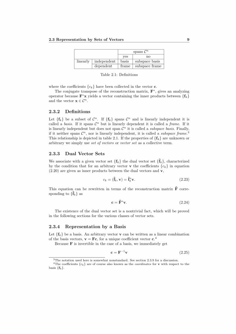
spans Cn
yes nolinearly independent basis subspace basis
dependent frame subspace frame
Table 2.1: Definitions
where the coefficients {ck} have been collected in the vector c.The conjugate transpose of the reconstruction matrix, F∗, gives an analyzing
operator because F∗x yields a vector containing the inner products between {fk}and the vector x ∈ Cn.
2.3.2 Definitions
Let {fk} be a subset of Cn. If {fk} spans Cn and is linearly independent it iscalled a basis. If it spans Cn but is linearly dependent it is called a frame. If itis linearly independent but does not span Cn it is called a subspace basis. Finally,if it neither spans Cn, nor is linearly independent, it is called a subspace frame.3
This relationship is depicted in table 2.1. If the properties of {fk} are unknown orarbitrary we simply use set of vectors or vector set as a collective term.
2.3.3 Dual Vector Sets
We associate with a given vector set {fk} the dual vector set {fk}, characterizedby the condition that for an arbitrary vector v the coefficients {ck} in equation(2.20) are given as inner products between the dual vectors and v,
ck = (fk,v) = f∗kv. (2.23)
This equation can be rewritten in terms of the reconstruction matrix F corre-sponding to {fk} as
c = F∗v. (2.24)
The existence of the dual vector set is a nontrivial fact, which will be provedin the following sections for the various classes of vector sets.
2.3.4 Representation by a Basis
Let {fk} be a basis. An arbitrary vector v can be written as a linear combinationof the basis vectors, v = Fc, for a unique coefficient vector c.4
Because F is invertible in the case of a basis, we immediately get
c = F−1v (2.25)
3The notation used here is somewhat nonstandard. See section 2.3.9 for a discussion.4The coefficients {ck} are of course also known as the coordinates for v with respect to the
basis {fk}.
10 A Unified Framework . . .
and it is clear from comparison with equation (2.24) that F exists and is given by
F = (F−1)∗. (2.26)
In this very ideal case where the vector set is a basis, there is no need to statea least squares problem to find c or F. That this could indeed be done is discussedin section 2.3.7.
2.3.5 Representation by a Frame
Let {fk} be a frame. Because the frame spans Cn, an arbitrary vector v can still bewritten as a linear combination of the frame vectors, v = Fc. This time, however,there are infinitely many coefficient vectors c satisfying the relation. To get auniquely determined solution we add the requirement that c be of minimum norm.This is nothing but the minimum norm problem of section 2.2.4 and equation (2.6)gives the solution
c = F∗(FF∗)−1v. (2.27)
Hence the dual frame exists and is given by
F = (FF∗)−1F. (2.28)
2.3.6 Representation by a Subspace Basis
Let {fk} be a subspace basis. In general, an arbitrary vector v cannot be writtenas a linear combination of the subspace basis vectors, v = Fc. Equality only holdsfor vectors v in the subspace spanned by {fk}. Thus we have to settle for the cgiving the closest vector v′ = Fc in the subspace. Since the subspace basis vectorsare linearly independent we have the linear least squares problem of section 2.2.3with the solution given by equation (2.4) as
c = (F∗F)−1F∗v. (2.29)
Hence the dual subspace basis exists and is given by
F = F(F∗F)−1. (2.30)
Geometrically v′ is the orthogonal projection of v onto the subspace.
2.3.7 Representation by a Subspace Frame
Let {fk} be a subspace frame. In general, an arbitrary vector v cannot be writtenas a linear combination of the subspace frame vectors, v = Fc. Equality onlyholds for vectors v in the subspace spanned by {fk}. Thus we have to settle forthe c giving the closest vector v′ = Fc in the subspace. Since the subspace framevectors are linearly dependent there are also infinitely many c giving the sameclosest vector v′, so to distinguish between these we choose the one with minimum
2.3 Representation by Sets of Vectors 11
norm. This is the general linear least squares problem of section 2.2.7 with thesolution given by equation (2.19) as
c = F†v. (2.31)
Hence the dual subspace frame exists and is given by
F = (F†)∗. (2.32)
The subspace frame case is the most general case since all the other ones can beconsidered as special cases. The only thing that happens to the general linear leastsquares problem formulated here is that sometimes there is an exact solution v =Fc, rendering the minimum residual error requirement superfluous, and sometimesthere is a unique solution c, rendering the minimum norm requirement superfluous.Consequently the solution given by equation (2.32) subsumes all the other ones,which is in agreement with equations (2.11) – (2.13).
2.3.8 The Double Dual
The dual of {fk} can be computed from equation (2.32), applied twice, togetherwith (2.14) and (2.15).
˜F = F†∗ = F†∗†∗ = F†∗∗† = F†† = F. (2.33)
What this means is that if we know the inner products between v and {fk} wecan reconstruct v using the dual vectors. To summarize we have the two relations
v ∼ F(F∗v) =∑
k
(fk,v)fk and (2.34)
v ∼ F(F∗v) =∑
k
(fk,v)fk. (2.35)
2.3.9 A Note on Notation
Usually a frame is defined by the frame condition,
A‖v‖2 ≤∑
k
|(fk,v)|2 ≤ B‖v‖2, (2.36)
which must hold for some A > 0, some B < ∞, and all v ∈ Cn. In the finitedimensional setting used here the first inequality holds if and only if {fk} spansall of Cn and the second inequality is a triviality as soon as the number of framevectors is finite.
The difference between this definition and the one used in section 2.3.2 is thatthe bases are included in the set of frames. As we have seen that equation (2.28)is consistent with equation (2.26), the same convention could have been used here.The reason for not doing so is that the presentation would have become moreinvolved.
12 A Unified Framework . . .
Likewise, we may allow the subspace bases to span the whole Cn, making basesa special case. Indeed, as has already been discussed to some extent, if subspaceframes are allowed to be linearly independent, and/or span the whole Cn, all theother cases can be considered special cases of subspace frames.
2.4 Weighted Norms
An interesting generalization of the theory developed so far is to exchange theEuclidian norms used in all minimizations for weighted norms.
2.4.1 Notation
Let the weighting matrix W be an n× n positive definite Hermitian matrix. Theweighted inner product (·, ·)W on Cn is defined by
(f ,g)W = (Wf ,Wg) = f∗W∗Wg = f∗W2g (2.37)
and the induced weighted norm ‖ · ‖W is given by
‖f‖W =√
(f , f)W =√
(Wf ,Wf) = ‖Wf‖. (2.38)
In this section M and L denote weighting matrices for Cn and Cm respectively.The notation from previous sections carry over unchanged.
2.4.2 The Weighted General Linear Least Squares Problem
The weighted version of the general linear least squares problem is stated as
arg minx∈S
‖x‖L, S = {x ∈ Cm; ‖Ax − b‖M is minimum}. (2.39)
This problem can be reduced to its unweighted counterpart by introducing x′ =Lx, whereby equation (2.39) can be rewritten as
arg minx′∈S
‖x′‖, S = {x′ ∈ Cm; ‖MAL−1x′ − Mb‖ is minimum}. (2.40)
The solution is given by equation (2.19) as
x′ = (MAL−1)†Mb, (2.41)
which after back-substitution yields
x = L−1(MAL−1)†Mb. (2.42)
2.4.3 Representation by Vector Sets
Let {fk} ⊂ Cn be any type of vector set. We want to represent an arbitrary vectorv ∈ Cn as a linear combination of the given vectors,
v ∼ Fc, (2.43)
where the coefficient vector c is chosen so that
2.4 Weighted Norms 13
1. the distance between v′ = Fc and v, ‖v′ − v‖M, is smallest possible, and
2. the length of c, ‖c‖L, is minimized.
This is of course the weighted general linear least squares problem of the previoussection, with the solution
c = L−1(MFL−1)†Mv. (2.44)
From the geometry of the problem one would suspect that M should not in-fluence the solution in the case of a basis or a frame, because the vectors spanthe whole space so that v′ equals v and the distance is zero, regardless of norm.Likewise L should not influence the solution in the case of a basis or a subspacebasis. That this is correct can easily be seen by applying the identities (2.11) –(2.13) to the solution (2.44). In the case of a frame we get
c = L−1(MFL−1)∗((MFL−1)(MFL−1)∗)−1Mv
= L−2F∗M(MFL−2F∗M)−1Mv
= L−2F∗(FL−2F∗)−1v,
(2.45)
in the case of a subspace basis
c = L−1((MFL−1)∗(MFL−1))−1(MFL−1)∗Mv
= L−1(L−1F∗M2FL−1)−1L−1F∗M2v
= (F∗M2F)−1F∗M2v,
(2.46)
and in the case of a basis
c = L−1(MFL−1)−1Mv = F−1v. (2.47)
2.4.4 Dual Vector Sets
It is not completely obvious how the concept of a dual vector set should be gener-alized to the weighted norm case. We would like to retain the symmetry relationfrom equation (2.33) and get correspondences to the representations (2.34) and(2.35). This can be accomplished by the weighted dual5
F = M−1(L−1F∗M)†L, (2.48)
which obeys the relations
˜F = F, (2.49)
v ∼ FL−2F∗M2v, and (2.50)
v ∼ FL−2F∗M2v. (2.51)
5To be more precise we should say ML-weighted dual, denoted FML. In the current contextthe extra index would only weigh down the notation, and has therefore been dropped.
14 A Unified Framework . . .
Unfortunately the two latter relations are not as easily interpreted as (2.34)and (2.35). The situation simplifies a lot in the special case where L = I. Thenwe have
F = M−1(F∗M)†, (2.52)
which can be rewritten by identity (2.17) as
F = F(F∗M2F)†. (2.53)
The two relations (2.50) and (2.51) can now be rewritten as
v ∼ F(F∗M2v) =∑
k
(fk,v)M fk, and (2.54)
v ∼ F(F∗M2v) =∑
k
(fk,v)M fk. (2.55)
Returning to the case of a general L, the factor L−2 in (2.50) and (2.51)should be interpreted as a weighted linear combination, i.e. FL−2c would be anL−1-weighted linear combination of the vectors {fk}, with the coefficients givenby c, analogously to F∗M2v being the set of M-weighted inner products between{fk} and a vector v.
2.5 Weighted Seminorms
The final level of generalization to be addressed here is when the weighting ma-trices are allowed to be semidefinite, turning the norms into seminorms. This hasfundamental consequences for the geometry of the problem. The primary differ-ence is that with a (proper) seminorm not only the vector 0 has length zero, buta whole subspace has. This fact has to be taken into account with respect to theterms spanning and linear dependence.6
2.5.1 The Seminorm Weighted General Linear Least Squares
Problem
When M and L are allowed to be semidefinite7 the solution to equation (2.39) isgiven by Elden in [12] as
x = (I − (LP)†L)(MA)†Mb + P(I − (LP)†LP)z, (2.56)
where z is arbitrary and P is the projection
P = I − (MA)†MA. (2.57)
6Specifically, if a set of otherwise linearly independent vectors have a linear combination ofnorm zero, we say that they are effectively linearly dependent, since they for all practical purposesmay as well have been.
7M and L may in fact be completely arbitrary matrices of compatible sizes.
2.5 Weighted Seminorms 15
Furthermore the solution is unique if and only if
N (MA) ∩N (L) = {0}, (2.58)
where N (·) denotes the null space. When there are multiple solutions, the firstterm of (2.56) gives the solution with minimum Euclidian norm.
If we make the restriction that only M may be semidefinite, the derivation insection 2.4.2 still holds and the solution is unique and given by equation (2.42) as
x = L−1(MAL−1)†Mb. (2.59)
2.5.2 Representation by Vector Sets and Dual Vector Sets
Here we have exactly the same representation problem as in section 2.4.3, ex-cept that that M and L may now be semidefinite. The consequence of M beingsemidefinite is that residual errors along some directions does not matter, while Lbeing semidefinite means that certain linear combinations of the available vectorscan be used for free. When both are semidefinite it may happen that some linearcombinations can be used freely without affecting the residual error. This causesan ambiguity in the choice of the coefficients c, which can be resolved by the addi-tional requirement that among the solutions, c is chosen with minimum Euclidiannorm. Then the solution is given by the first part of equation (2.56) as
c = (I − (L(I − (MF)†MF))†L)(MF)†Mv. (2.60)
Since this expression is something of a mess we are not going explore thepossibilities of finding a dual vector set or analogues of the relations (2.50) and(2.51). Let us instead turn to the considerably simpler case where only M isallowed to be semidefinite. As noted in the previous section, we can now use thesame solution as in the case with weighted norms, reducing the solution (2.60) tothat given by equation (2.44),
c = L−1(MFL−1)†Mv. (2.61)
Unfortunately we can no longer define the dual vector set by means of equation(2.48), due to the occurrence of an explicit inverse of M. Applying identity (2.16)on (2.61), however, we get
c = L−1(L−1F∗M2FL−1)†L−1F∗M2v (2.62)
and it follows that
F = FL−1(L−1F∗M2FL−1)†L (2.63)
yields a dual satisfying the relations (2.49) – (2.51). In the case that L = I thisexpression simplifies further to (2.53), just as for weighted norms. For futurereference we also notice that (2.61) reduces to
c = (MF)†Mv. (2.64)

16 A Unified Framework . . .
Chapter 3
Normalized Convolution
3.1 Introduction
Normalized Convolution is a method for signal analysis that takes uncertaintiesin signal values into account and at the same time allows spatial localization ofpossibly unlimited analysis functions. The method was primarily developed byKnutsson and Westin [38, 40, 60] and has later been described and/or used in e.g.[22, 35, 49, 50, 51, 59]. The conceptual basis for the method is the signal/certaintyphilosophy [20, 21, 36, 63], i.e. separating the values of a signal from the certaintyof the measurements.
Most of the previous presentations of Normalized Convolution have primarilybeen set in a tensor algebra framework, with only some mention of the relations toleast squares problems. Here we will skip the tensor algebra approach completelyand instead use the framework developed in chapter 2 as the theoretical basis forderiving Normalized Convolution. Specifically, we will use the theory of subspacebases and the connections to least squares problems. Readers interested in thetensor algebra approach are referred to [38, 40, 59, 60].
Normalized Convolution can, for each neighborhood of the signal, geometricallybe interpreted as a projection into a subspace which is spanned by the analysisfunctions. The projection is equivalent to a weighted least squares problem, wherethe weights are induced from the certainty of the signal and the desired localizationof the analysis functions. The result of Normalized Convolution is at each signalpoint a set of expansion coefficients, one for each analysis function.
While neither least squares fitting, localization of analysis functions, nor han-dling of uncertain data in themselves are novel ideas, the unique strength of Nor-malized Convolution is that it combines all of them simultaneously in a well struc-tured and theoretically sound way. The method is a generally useful tool for signalanalysis in the spatial domain, which formalizes and generalizes least squares tech-niques, e.g. the facet model [23, 24, 26], that have been used for a long time. Infact, the primary use of normalized convolution in the following chapters of thisthesis is for filter design in the spatial domain.
18 Normalized Convolution
3.2 Definition of Normalized Convolution
Before defining normalized convolution, it is necessary to get familiar with theterms signal, certainty, basis functions, and applicability, in the context of themethod. To begin with we assume that we have discrete signals, and explore thestraightforward generalization to continuous signals in section 3.2.4.
3.2.1 Signal and Certainty
It is important to be aware that normalized convolution can be considered as apointwise operation, or more strictly, as an operation on a neighborhood of eachsignal point. This is no different from ordinary convolution, where the convolutionresult at each point is effectively the inner product between the conjugated andreflected filter kernel and a neighborhood of the signal.
Let f denote the whole signal while f denotes the neighborhood of a givenpoint. It is assumed that the neighborhood is of finite size1, so that f can beconsidered an element of a finite dimensional vector space Cn. Regardless of thedimensionality of the space in which it is embedded2, f is represented by an n× 1column vector.3
Certainty is a measure of the confidence in the signal values at each point,given by non-negative real numbers. Let c denote the whole certainty field, whilethe n × 1 column vector c denotes the certainty of the signal values in f .
Possible causes for uncertainty in signal values are, e.g., defective sensor ele-ments, detected (but not corrected) transmission errors, and varying confidence inthe results from previous processing. The most important, and rather ubiquitouscase of uncertainty, however, is missing data outside the border of the signal, socalled edge effects. The problem is that for a signal of limited extent, the neighbor-hood of points close to the border will include points where no values are given.This has traditionally been handled in a number of different ways. The mostcommon is to assume that the signal values are zero outside the border, whichimplicitly is done by standard convolution. Another way is to assume cyclical rep-etition of the signal values, which implicitly is done when convolution is computedin the frequency domain. Yet another way is to extend with the values at theborder. None of these is completely satisfactory, however. The correct way to doit, from a signal/certainty perspective, is to set the certainty for points outsidethe border to zero, while the signal value is left unspecified.
It is obvious that certainty zero means missing data, but it is not so clear howpositive values should be interpreted. An exact interpretation must be postponedto section 3.2.4, but of course a larger certainty corresponds to a higher confidencein the signal value. It may seem natural to limit certainty values to the range[0, 1], with 1 meaning full confidence, but this is not really necessary.
1This condition can be lifted, as discussed in section 3.2.4. For computational reasons, how-ever, it is in practice always satisfied.
2E.g. dimensionality 2 for image data.3The elements of the vector are implicitly the coordinates relative to some orthonormal basis,
typically a pixel basis.
3.2 Definition of Normalized Convolution 19
3.2.2 Basis Functions and Applicability
The role of the basis functions is to give a local model for the signal. Each basisfunction has the size of the neighborhood mentioned above, i.e. it is an element ofCn, represented by an n × 1 column vector bi. The set {bi}m
1 of basis functionsare stored in an n × m matrix B,
B =
| | |b1 b2 . . . bm
| | |
. (3.1)
Usually we have linearly independent basis functions, so that the vectors {bi} doconstitute a basis for a subspace of Cn. In most cases m is also much smaller thann.
The applicability is a kind of “certainty” for the basis functions. Rather thanbeing a measure of certainty or confidence, however, it indicates the significance orimportance of each point in the neighborhood. Like the certainty, the applicabilitya is represented by an n × 1 vector with non-negative elements. Points where theapplicability is zero might as well be excluded from the neighborhood altogether,but for practical reasons it may be convenient to keep them. As for certainty itmay seem natural to limit the applicability values to the range [0, 1] but there isreally no reason to do this because the scaling of the values turns out to be of nosignificance.
The basis functions may actually be defined for a larger domain than theneighborhood in question. They can in fact be unlimited, e.g. polynomials orcomplex exponentials, but values at points where the applicability is zero simplydo not matter. This is an important role of the applicability, to enforce a spatiallocalization of the signal model. A more extensive discussion on the choice ofapplicability follows in section 3.9.
3.2.3 Definition
Let the n × n matrices Wa = diag(a), Wc = diag
(c), and W2 = WaWc.
4 Theoperation of normalized convolution is at each signal point a question of represent-ing a neighborhood of the signal, f , by the set of vectors {bi}, using the weightednorm (or seminorm) ‖ · ‖W in the signal space and the Euclidian norm in thecoefficient space. The result of normalized convolution is at each point the set ofcoefficients r used in the vector set representation of the neighborhood.
As we have seen in chapter 2, this can equivalently be stated as the seminormweighted general linear least squares problem
arg minr∈S
‖r‖, S = {r ∈ Cm; ‖Br − f‖W is minimum}. (3.2)
In the case that the basis functions are linearly independent with respect to the(semi)norm ‖ · ‖W, this can be simplified to the more ordinary weighted linear
4We set W2 = WaWc to keep in line with the established notation. Letting W = WaWc
would be equally valid, as long as a and c are interpreted accordingly, and somewhat morenatural in the framework used here.
20 Normalized Convolution
least squares problem
arg minr∈Cm
‖Br − f‖W. (3.3)
In any case the solution is given by equation (2.64) as
r = (WB)†Wf . (3.4)
For various purposes it is useful to rewrite this formula. We start by expandingthe pseudo-inverse in (3.4) by identity (2.16), leading to
r = (B∗W2B)†B∗W2f , (3.5)
which can be interpreted in terms of inner products as
r =
(b1,b1)W . . . (b1,bm)W...
. . ....
(bm,b1)W . . . (bm,bm)W
†
(b1, f)W...
(bm, f)W
. (3.6)
Replacing W2 with WaWc and using the assumption that the vectors {bi} consti-tute a subspace basis with respect to the (semi)norm W, so that the pseudo-inversein (3.5) and (3.6) can be replaced with an ordinary inverse, we get
r = (B∗WaWcB)−1B∗WaWcf (3.7)
and with the convention that · denotes pointwise multiplication, we arrive at theexpression5
r =
(a · c · b1,b1) . . . (a · c · b1,bm)...
. . ....
(a · c · bm,b1) . . . (a · c · bm,bm)
−1
(a · c · b1, f)...
(a · c · bm, f)
. (3.8)
3.2.4 Comments on the Definition
In previous formulations of Normalized Convolution, it has been assumed thatthe basis functions actually constitute a subspace basis, so that we have a uniquesolution to the linear least squares problem (3.3), given by (3.7) or (3.8). Theproblem with this assumption is that if we have a neighborhood with lots of missingdata, it can happen that the basis functions effectively become linearly dependentin the seminorm given by W, so that the inverses in (3.7) and (3.8) do not exist.
We can solve this problem by exchanging the inverses for pseudo-inverses, equa-tions (3.5) and (3.6), which removes the ambiguity in the choice of resulting coef-ficients r by giving the solution to the more general linear least squares problem(3.2). This remedy is not without risks, however, since the mere fact that the basisfunctions turn linearly dependent, indicates that the values of at least some of the
5This is almost the original formulation of Normalized Convolution. The final step is post-poned until section 3.3.
3.3 Implementational Issues 21
coefficients may be very uncertain. More discussion on this follows in section 3.5.Taking proper care in the interpretation of the result, however, the pseudo-inversesolutions should be useful when the signal certainty is very low. They are alsonecessary in certain generalizations of Normalized Convolution, see section 3.10.
To be able to use the framework from chapter 2 in deriving the expressionsfor Normalized Convolution, we restricted ourselves to the case of discrete signalsand neighborhoods of finite size. When we have continuous signals and/or infiniteneighborhoods we can still use (3.6) or (3.8) to define normalized convolution,simply by using an appropriate weighted inner product. The corresponding leastsquares problems are given by obvious modifications to (3.2) and (3.3).
The geometrical interpretation of the least squares minimization is that thelocal neighborhood is projected into the subspace spanned by the basis functions,using a metric that is dependent on the certainty and the applicability. From theleast squares formulation we can also get an exact interpretation of the certaintyand the applicability. The certainty gives the relative importance of the signalvalues when doing the least squares fit, while the applicability gives the relativeimportance of the points in the neighborhood. Obviously a scaling of the certaintyor applicability values does not change the least squares solution, so there is noreason to restrict these values to the range [0, 1].
3.3 Implementational Issues
While any of the expressions (3.4) – (3.8) can be used to compute NormalizedConvolution, there are some differences with respect to computational complex-ity and numeric stability. Numerically (3.4) is somewhat preferable to the otherexpressions, because values get squared in the rest of them, raising the conditionnumbers. Computationally, however, the computation of the pseudo-inverse iscostly and WB is typically significantly larger than B∗W2B. We rather wish toavoid the pseudo-inverses altogether, leaving us with (3.7) and (3.8). The inversesin these expressions are of course not computed explicitly, since there are moreefficient methods to solve linear equation systems. In fact, the costly operationnow is to compute the inner products in (3.8). Remembering that these compu-tations have to be performed at each signal point, we can improve the expressionsomewhat by rewriting (3.8) as
r =
(a · b1 · b1, c) . . . (a · b1 · bm, c)...
. . ....
(a · bm · b1, c) . . . (a · bm · bm, c)
−1
(a · b1, c · f)...
(a · bm, c · f)
, (3.9)
where bi denotes complex conjugation of the basis functions. This is actuallythe original formulation of Normalized Convolution [38, 40, 60], although withdifferent notation. By precomputing the quantities {a ·bk · bl}, {a ·bk}, and c · f ,we can decrease the total number of multiplications at the cost of a small increasein storage requirements.
22 Normalized Convolution
To compute Normalized Convolution at all points of the signal we essentiallyhave two strategies. The first is to compute all inner products and to solve thelinear equation system for one point before continuing to the next point. Thesecond is to compute the inner product for all points before continuing with thenext inner product and at the very last solve all the linear equation systems. Theadvantage of the latter approach is that the inner products can be computed asstandard convolutions, an operation which is often available in heavily optimizedform, possibly in hardware. The disadvantage is that large amounts of extra stor-age must be used, which even if it is available could lead to problems with respectto data locality and cache performance. Further discussion on how NormalizedConvolution can be computed more efficiently in certain cases can be found insections 3.7, 4.7, and 4.8.
3.4 Example
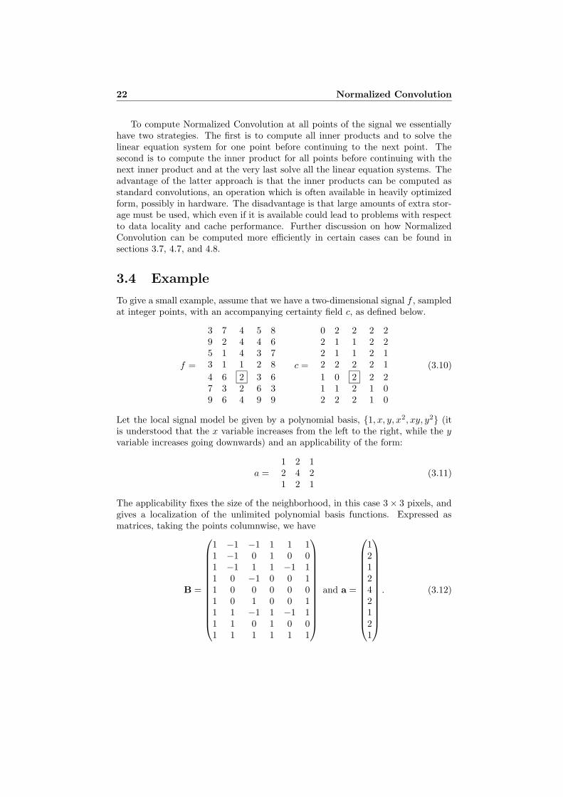
To give a small example, assume that we have a two-dimensional signal f , sampledat integer points, with an accompanying certainty field c, as defined below.
f =
3 7 4 5 89 2 4 4 65 1 4 3 73 1 1 2 8
4 6 2 3 67 3 2 6 39 6 4 9 9
c =
0 2 2 2 22 1 1 2 22 1 1 2 12 2 2 2 1
1 0 2 2 21 1 2 1 02 2 2 1 0
(3.10)
Let the local signal model be given by a polynomial basis, {1, x, y, x2, xy, y2} (itis understood that the x variable increases from the left to the right, while the yvariable increases going downwards) and an applicability of the form:
a =1 2 12 4 21 2 1
(3.11)
The applicability fixes the size of the neighborhood, in this case 3 × 3 pixels, andgives a localization of the unlimited polynomial basis functions. Expressed asmatrices, taking the points columnwise, we have
B =
1 −1 −1 1 1 11 −1 0 1 0 01 −1 1 1 −1 11 0 −1 0 0 11 0 0 0 0 01 0 1 0 0 11 1 −1 1 −1 11 1 0 1 0 01 1 1 1 1 1
and a =
121242121
. (3.12)
3.5 Output Certainty 23
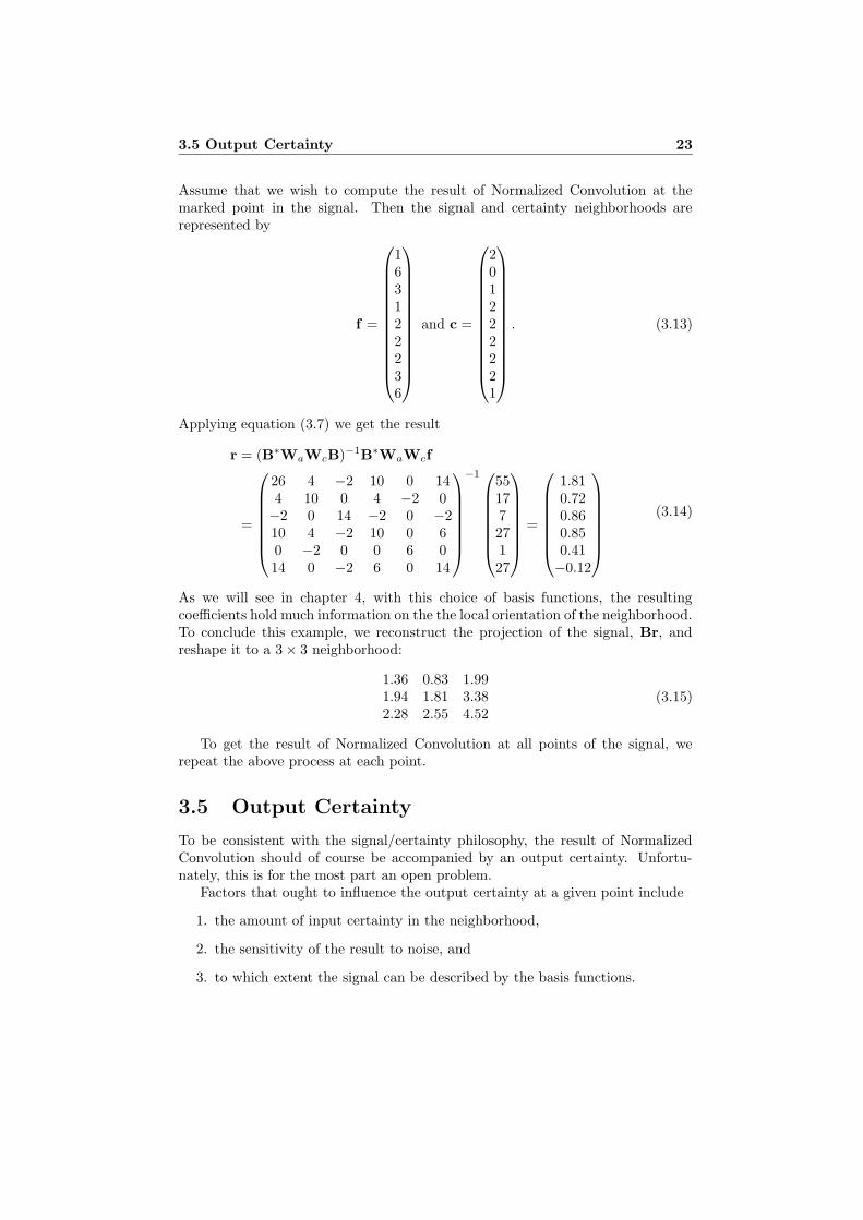
Assume that we wish to compute the result of Normalized Convolution at themarked point in the signal. Then the signal and certainty neighborhoods arerepresented by
f =
163122236
and c =
201222221
. (3.13)
Applying equation (3.7) we get the result
r = (B∗WaWcB)−1B∗WaWcf
=
26 4 −2 10 0 144 10 0 4 −2 0−2 0 14 −2 0 −210 4 −2 10 0 60 −2 0 0 6 014 0 −2 6 0 14
−1
5517727127
=
1.810.720.860.850.41−0.12
(3.14)
As we will see in chapter 4, with this choice of basis functions, the resultingcoefficients hold much information on the the local orientation of the neighborhood.To conclude this example, we reconstruct the projection of the signal, Br, andreshape it to a 3 × 3 neighborhood:
1.36 0.83 1.991.94 1.81 3.382.28 2.55 4.52
(3.15)
To get the result of Normalized Convolution at all points of the signal, werepeat the above process at each point.
3.5 Output Certainty
To be consistent with the signal/certainty philosophy, the result of NormalizedConvolution should of course be accompanied by an output certainty. Unfortu-nately, this is for the most part an open problem.
Factors that ought to influence the output certainty at a given point include
1. the amount of input certainty in the neighborhood,
2. the sensitivity of the result to noise, and
3. to which extent the signal can be described by the basis functions.
24 Normalized Convolution
The sensitivity to noise is smallest when the basis functions are orthogonal6,because the resulting coefficients are essentially independent. Should two basisfunctions be almost parallel, on the other hand, they both tend to get relativelylarge coefficients, and input noise in a certain direction gets amplified.
Two possible measures of output certainty have been published, by Westelius[59] and Karlholm [35] respectively. Westelius has used
cout =
(
detG
detG0
) 1
m
, (3.16)
while Karlholm has used
cout =1
‖G0‖2‖G−1‖2. (3.17)
In both expressions we have
G = B∗WaWcB and G0 = B∗WaB, (3.18)
where G0 is the same as G if the certainty is identically one.Both these measures take the points 1 and 2 above into account. A disad-
vantage, however, is that they give a single certainty value for all the resultingcoefficients, which makes sense with respect to 1 but not with respect to the sen-sitivity issues. Clearly, if we have two basis functions that are nearly parallel, butthe rest of them are orthogonal, we have good reason to mistrust the coefficientscorresponding to the two almost parallel basis functions, but not necessarily therest of the coefficients.
A natural measure of how well the signal can be described by the basis functionsis given by the residual error in (3.2) or (3.3),
‖Br − f‖W. (3.19)
In order to be used as a measure of output certainty, some normalization withrespect to the amplitude of the signal and the input certainty should be performed.
One thing to be aware of in the search for a good measure of output certainty,is that it probably must depend on the application, or more precisely, on how theresult is further processed.
3.6 Normalized Differential Convolution
When doing signal analysis, it may be important to be invariant to certain irrel-evant features. A typical example can be seen in chapter 4, where we want toestimate the local orientation of a multidimensional signal. It is clear that thelocal DC level gives no information about the orientation, but we cannot simplyignore it because it would affect the computation of the interesting features. The
6Remember that orthogonality depends on the inner product, which in turn depends on thecertainty and the applicability.
3.7 Reduction to Ordinary Convolution 25
solution is to include the features to which we wish to be invariant in the sig-nal model. This means that we expand the set of basis functions, but ignore thecorresponding coefficients in the result.
Since we do not care about some of the resulting coefficients, it may seemwasteful to use (3.7), which computes all of them. To avoid this we start bypartitioning
B =(B1 B2
)and r =
(r1
r2
)
, (3.20)
where B1 contains the basis functions we are interested in, B2 contains the basisfunctions to which we wish to be invariant, and r1 and r2 are the correspondingparts of the resulting coefficients. Now we can rewrite (3.7) in partitioned form as
(r1
r2
)
=
(B∗
1WaWcB1 B∗1WaWcB2
B∗2WaWcB1 B∗
2WaWcB2
)−1(B∗
1WaWcfB∗
2WaWcf
)
(3.21)
and continue the expansion with an explicit expression for the inverse of a parti-tioned matrix [34]:
(A CC∗ B
)−1
=
(A−1 + E∆−1F −E∆−1
−∆−1F ∆−1
)
,
∆ = B − C∗A−1C, E = A−1C, F = C∗A−1
(3.22)
The resulting algorithm is called Normalized Differential Convolution [35, 38,40, 60, 61]. The primary advantage over the expression for Normalized Convolutionis that we get smaller matrices to invert, but on the other hand we need to actuallycompute the inverses here7, instead of just solving a single linear equation system,and there are also more matrix multiplications to perform. It seems unlikely thatit would be worth the extra complications to avoid computing the uninterestingcoefficients, unless B1 and B2 contain only a single vector each, in which case theexpression for Normalized Differential Convolution simplifies considerably.
In the following chapters we use the basic Normalized Convolution, even if weare not interested in all the coefficients.
3.7 Reduction to Ordinary Convolution
If we have the situation that the certainty field remains fixed while the signalvaries, we can save a lot of work by precomputing the matrices
B∗ = (B∗WaWcB)−1B∗WaWc (3.23)
at every point, at least if we can afford the extra storage necessary. A possiblescenario for this situation is that we have a sensor array where we know that certain
7This is not quite true, since it is sufficient to compute factorizations that allow us to solvecorresponding linear equation systems, but we need to solve several of these instead of just one.
26 Normalized Convolution
sensor elements are not working or give less reliable measurements. Another case,which is very common, is that we simply do not have any certainty information atall and can do no better than setting the certainty for all values to one. Notice,however, that if the extent of the signal is limited, we have certainty zero outsidethe border. In this case we have the same certainty vector for many neighborhoodsand only have to compute and store a small number of different B.
As can be suspected from the notation, B can be interpreted as a dual basismatrix. Unfortunately it is not the weighted dual subspace basis given by (2.53),because the resulting coefficients are computed by (bi, f) rather than by usingthe proper8 inner product (bi, f)W. We will still use the term dual vectors here,although somewhat improperly.
If we assume that we have constant certainty one and restrict ourselves tocompute Normalized Convolution for the part of the signal that is sufficiently farfrom the border, we can reduce Normalized Convolution to ordinary convolution.At each point the result can be computed as
r = B∗f (3.24)
or coefficient by coefficient as
ri = (bi, f). (3.25)
Extending these computations over all points under consideration, we can write
ri(x) = (bi, Txf), (3.26)
where Tx is a translation operator, Txf(u) = f(u + x). This expression can inturn be rewritten as a convolution
ri(x) = (ˇbi ∗ f)(x), (3.27)
where we letˇbi denote the conjugated and reflected bi.
The need to reflect and conjugate the dual basis functions in order to getconvolution kernels is a complication that we would prefer to avoid. We can dothis by replacing the convolution with an unnormalized cross correlation, usingthe notation from Bracewell [9],
g ? h =∑
u
g(u)h(u + x). (3.28)
With this operation, (3.27) can be rewritten as
ri(x) = (bi ? f)(x). (3.29)
The cross correlation is in fact a more natural operation to use in this contextthan ordinary convolution, since we are not much interested in the properties thatotherwise give convolution an advantage. We have, e.g., no use for the property
8Proper with respect to the norm used in the minimization (3.3).
3.8 Application Examples 27
that g ∗ h = h ∗ g, since we have a marked asymmetry between the signal and thebasis functions. The ordinary convolution is, however, a much more well knownoperation, so while we will use the cross correlation further on, it is useful toremember that we get the corresponding convolution kernels simply by conjugatingand reflecting the dual basis functions.
To get a better understanding of the dual basis functions, we can rewrite (3.23),with Wc = I, as
| | |b1 b2 . . . bm
| | |
=
| | |a · b1 a · b2 . . . a · bm
| | |
G−1, (3.30)
where G = B∗WaB. Hence we obtain the duals as linear combinations of the basisfunctions bi, windowed by the applicability a. The role of G−1 is to compensatefor dependencies between the basis functions when they are not orthogonal. Noticethat this includes non-orthogonalities caused by the windowing by a. A concreteexample of dual basis functions can be found in section 4.7.1.
3.8 Application Examples
Applications where Normalized Convolution has been used include interpolation[40, 60, 64], frequency estimation [39], estimation of texture gradients [50], depthsegmentation [49, 51], phase-based stereopsis and focus-of-attention control [59,62], and orientation and motion estimation [35]. In the two latter applications,Normalized Convolution is utilized to compute quadrature filter responses on un-certain data.
3.8.1 Normalized Averaging
The most striking example is perhaps, despite its simplicity, normalized averagingto interpolate missing samples in an image. We illustrate this technique with apartial reconstruction of the example given in [22, 40, 60, 64].
In figure 3.1(a) the well-known Lena image has been degraded so that only 10%of the pixels remain.9 The remaining pixels have been selected randomly withuniform distribution from a 512 × 512 grayscale original. Standard convolutionwith a smoothing filter, given by figure 3.2(a), leads to a highly non-satisfactoryresult, figure 3.1(b), because no compensation is made for the variation in localsampling density. An ad hoc solution to this problem would be to divide theprevious convolution result with the convolution between the smoothing filter andthe certainty field, with the latter being an estimate of the local sampling density.
This idea can easily be formalized by means of Normalized Convolution. Thesignal and the certainty are already given. We use a single basis function, a
9The removed pixels have been replaced by zeros, i.e. black. For illustration purposes, missingsamples are rendered white in figures 3.1(a) and 3.3(a).

28 Normalized Convolution
(a) (b)
(c) (d)
Figure 3.1: Normalized averaging. (a) Degraded test image, only 10% of thepixels remain. (b) Standard convolution with smoothing filter. (c) Normalizedaveraging with applicability given by figure 3.2(a). (d) Normalized averaging withapplicability given by figure 3.2(b).
3.8 Application Examples 29
−50
5
−5
0
5
0
0.2
0.4
0.6
0.8
1
−50
5
−5
0
5
0
0.2
0.4
0.6
0.8
1
(a) a =
{
cos2 πr16 , r < 8
0, otherwise(b) a =
1, r < 1
0.5r−3, 1 ≤ r < 8
0, otherwise
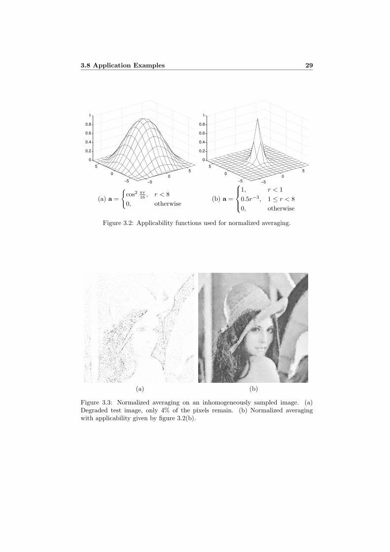
Figure 3.2: Applicability functions used for normalized averaging.
(a) (b)
Figure 3.3: Normalized averaging on an inhomogeneously sampled image. (a)Degraded test image, only 4% of the pixels remain. (b) Normalized averagingwith applicability given by figure 3.2(b).

30 Normalized Convolution
constant one, and use the smoothing filter as the applicability.10 The result fromthis operation, figure 3.1(c), can be interpreted as a weighted and normalizedaverage of the pixels present in the neighborhood, and is identical to the ad hocsolution above. In figure 3.1(d) we see the result of normalized averaging with amore localized applicability, given by figure 3.2(b).
To expand on the example, we notice that instead of having a uniform distri-bution of the remaining pixels, it would be advantageous to have more samples inareas of high contrast. Figure 3.3(a) is such a test image, only containing 4% ofthe original pixels. The result of normalized averaging, with applicability given byfigure 3.2(b), is shown in figure 3.3(b).
3.8.2 The Cubic Facet Model
In the cubic facet model [24], it is assumed that in each neighborhood of an image,the signal can be described by a cubic polynomial
f(x, y) = k1 + k2x + k3y + k4x2 + k5xy + k6y
2
+ k7x3 + k8x
2y + k9xy2 + k10y3.
(3.31)
The coefficients {ki} are determined by a least squares fit within a square windowof some size. A typical application of the cubic facet model is to estimate the imagederivatives from the polynomial model and to use these to get the curvature
κ =f2
xfyy + f2y fxx − 2fxfyfxy
(f2x + f2
y )3/2=
2(k22k6 + k3k4 − k2k3k5)
(k22 + k2
3)3/2
. (3.32)
We see that the cubic facet model has much in common with to NormalizedConvolution, except that it lacks provision for certainty and applicability. Hencewe can regard this model as a special case of Normalized Convolution, with thirddegree polynomials as basis functions, certainty identically one, and applicabilityidentically one on a square window. We can also note that in the computation ofthe curvature by equation (3.32), some of the estimated coefficients are not used,which can be compared to the idea of Normalized Differential Convolution, section3.6.
Facet models in general11 can of course also be described in terms of Normal-ized Convolution, by changing the set of basis functions accordingly. Applicationsfor the facet model include gradient edge detection, zero-crossing edge detection,image segmentation, line detection, corner detection, three-dimensional shape es-timation from shading, and determination of optic flow [25]. By extension, thesame approaches can be taken with Normalized Convolution and probably withbetter results, since the availability of the applicability mechanism allows bettercontrol of the process. As discussed in the following section, an appropriate choiceof applicability is especially important if we want to estimate orientation.12
10Notice that by equation (3.30), the equivalent correlation kernel when we have constantcertainty is given by a multiple of the applicability, since we have only one basis function, whichis a constant.
11With other basis functions than the cubic polynomials.12Notice in particular the dramatic difference between a square applicability, implicitly used
3.9 Choosing the Applicability 31
3.9 Choosing the Applicability
The choice of applicability depends very much on the application. It is in fact allbut impossible to give general guidelines. For most applications, however, it seemsmore or less unavoidable that we wish to give higher importance to points in thecenter of the neighborhood than to points farther away. Thus the applicabilityshould be monotonically decreasing in all directions.
Another property to be aware of is isotropy. Unless a specific direction de-pendence is wanted, one probably had better taking care to get an isotropic ap-plicability. This is, in fact, of utmost importance in the orientation estimationalgorithm presented in chapter 4, see in particular section 4.10.1.
If we look at a specific application, the normalized averaging from section3.8.1, we can see a trade-off between excessive blurring with a wide applicabilityfunction and noise caused by the varying certainty with a narrow applicability.The motivation for the very narrow applicability in figure 3.2(a) is that we wantto interpolate from values as close as possible to the point of interest and more orless ignore information farther away. In other applications it is necessary to havea wider applicability, because we actually want to analyze a whole neighborhood,e.g. to estimate orientation. In these cases the size of the applicability is relatedto the scale of the analyzed features. Another reason for a wider applicability is tobecome less sensitive to signal noise.
3.10 Further Generalizations of Normalized Con-
volution
In the formulation of Normalized Convolution, it is traditionally assumed that thelocal signal model is spanned by a set of vectors constituting a subspace basis. Aswe have already discussed in section 3.2, this assumption is not without complica-tions, since the vectors may effectively become linearly dependent in the seminormgiven by W. This typically happens in areas with large amounts of missing data.A first generalization is therefore to allow linearly dependent vectors in the signalmodel, i.e. exchanging the subspace basis for a subspace frame. Except that welose the simplifications to the expressions (3.7) and (3.8), this case has alreadybeen covered by the presentation in section 3.2.
With a subspace frame instead of a subspace basis, another possible general-ization is to use a weighted norm L in the coefficient space instead of the Euclidiannorm, i.e. generalizing the seminorm weighted general linear least squares problem(3.2) somewhat to
arg minr∈S
‖r‖L, S = {r ∈ Cm; ‖Br − f‖W is minimum}. (3.33)
If we require L to be positive definite, the solution is now given by (2.61) as
r = L−1(WBL−1)†Wf (3.34)
by the facet model, and a Gaussian applicability in table 4.3.
32 Normalized Convolution
or by (2.62) as
r = L−1(L−1B∗W2BL−1)†L−1B∗W2f . (3.35)
If we allow L to be semidefinite we have to resort to the solution given by (2.60).If L is diagonal, the elements can be interpreted as the relative cost of using
each subspace frame vector. This case is not very interesting, however, since thesame effect could have been achieved simply by an amplitude scaling of the framevectors. A more general L allows varying the costs for specific linear combinationsof the subspace frame vectors, leading to more interesting possibilities.
That it would be pointless to introduce L in the case of a subspace basis isclear from section 2.4.3, since it would not affect the solution at all, unless wehave the case where the seminorm W turns the basis vectors effectively linearlydependent. Correspondingly, it does not make much sense to use a basis or a framefor the whole space as signal model, since in this case the weighting by W wouldbe superfluous as the error to be minimized in (3.2) would be zero regardless ofnorm. Hence neither the certainty nor the applicability would make a differenceto the solution.
Another generalization that could be solved by the framework from chapter 2is to have a non-diagonal weight matrix W. Unfortunately we still have no goodidea what interpretation this could have but it is possible that the certainty partWc could naturally be non-diagonal if the primary measurements of the signalwere collected, e.g., in the frequency domain or as line integrals.
A different generalization, that is not covered by the framework from the pre-vious chapter, is to replace the general linear least squares problem (3.2) with thesimultaneous minimization of signal error and coefficient norm,
arg minr
α‖Br − f‖W + β‖r‖. (3.36)
This approach could possibly be more robust when the basis functions are nearlylinearly dependent, but we will not investigate it further here.
Chapter 4
Orientation Estimation
4.1 Introduction
Orientation is a feature that fundamentally distinguishes multidimensional signalsfrom one-dimensional signals, since the concept lacks meaning in the latter case.It is also a feature that is far from trivial both to represent and to estimate, aswell as to define strictly for general signals.
The one case where there is no question how the orientation should be definedis for non-constant simple signals, i.e. signals that can be written as
f(x) = h(xT n) (4.1)
for some non-constant function h of one variable and for some vector n. Thismeans that the function is constant on all hyper-planes perpendicular to n and wesay that the signal is oriented in the direction of n. Notice however that n is notunique in (4.1) since we could replace n by any multiple. Even if we normalize nto get the unit directional vector n, there is still an ambiguity between n and −n.This is one problem that must be addressed by the representation of orientation.
Of course the class of globally simple signals is too restricted to be of much use,so we need to generalize the definition of orientation to more arbitrary signals. Tobegin with we notice that we usually are not interested in a global orientation. Infact it is understood throughout the rest of this thesis that we by “orientation”mean “local orientation”, i.e. we only look at the signal behavior in some neigh-borhood of a point of interest. We can, however, still not rely on always havinglocally simple neighborhoods.
Unfortunately there is no obvious way in which to generalize the definitionof orientation to non-simple signals. Assume for example that we have a signalcomposed as the sum of two simple signals with different orientations. Should theorientation now be some mean value of the two orientations, both orientations, orsomething else? To illustrate what kind of problems we have here we take a closerlook at two examples. They are both two-dimensional and we are interested inthe orientation at a neighborhood of the origin.
1. Let f1(x, y) = x and f2(x, y) = y. Now the sum f(x, y) = f1(x, y) +

34 Orientation Estimation
f2(x, y) = x + y is simple as well, oriented in the ( 1 1 )T direction.
2. Let f1(x, y) = x2 and f2(x, y) = y2. This time the sum f(x, y) = f1(x, y) +f2(x, y) = x2+y2 is very isotropic and we cannot possibly prefer one directionover another.
In practice, exactly how we define the orientation of non-simple signals tendsto be a consequence of how we choose to represent the orientation and what pro-cedure we use to estimate it. In this presentation we represent orientation bytensors, essentially along the lines of Knutsson [22, 36], although with a somewhatdifferent interpretation. The method used here for estimation of the orientation iscompletely novel and based on Normalized Convolution with a polynomial basis.A related concept is the inertia tensor by Bigun [4].
4.2 The Orientation Tensor
In this section we give an overview of Knutsson’s orientation tensor representationand estimation by means of quadrature filter responses [22, 36]. It should be notedthat this estimation method is included only for reference and comparison. Theestimation method used in this thesis is described in sections 4.4 and 4.5.
4.2.1 Representation of Orientation for Simple Signals
The orientation tensor is a representation of orientation that for N-dimensionalsignals takes the form of an N ×N real symmetric matrix1. A simple signal in thedirection n, as defined by equation (4.1), is represented by the tensor
T = AnnT , (4.2)
where A is some constant that may encode other information than orientation,such as certainty or local signal energy. It is obvious that this representation mapsn and −n to the same tensor and that the orientation can be recovered from theeigensystem of T.
By design the orientation tensor satisfies the following two conditions:
Invariance The normalized tensor T = T
‖T‖ does not depend on the function h
in equation (4.1).
Equivariance The orientation tensor locally preserves the angle metric of theoriginal space, i.e.
‖δT‖ ∝ ‖δn‖. (4.3)
The tensor norm used above is the Frobenius norm, ‖T‖2 = tr (TT T).
1Symmetric matrices constitute a subclass of tensors. Readers who are more familiar withmatrix algebra than with tensor algebra may safely substitute “symmetric matrix” for “tensor”throughout this chapter.
4.3 Orientation Functionals 35
4.2.2 Estimation
The orientation tensor can be computed by means of the responses of a set ofquadrature filters. Each quadrature filter is spherically separable and real in theFourier domain,
Fk(u) = R(‖u‖)Dk(u), (4.4)
where the radial function R can be chosen more or less arbitrary, with typicaldesign restrictions given by desired center frequency, bandwidth, locality, andscale. The directional function is given by
Dk(u) =
{
(u · nk)2, u · nk > 0,
0, otherwise,(4.5)
where {nk} is a set of direction vectors, usually evenly distributed in the signalspace. It turns out that the minimum number of filters is 3 in 2D, 6 in 3D, and12 in 4D.
The orientation tensor is constructed from the magnitudes of the filter re-sponses {qk} at each point by
T =∑
k
|qk|Mk, (4.6)
where {Mk} are the duals of the outer product tensors {nknTk }.
4.2.3 Interpretation for Non-Simple Signals
The above construction is guaranteed to give a tensor as defined in equation (4.2)only for simple signals. For non-simple signals the tensor is analyzed by means ofthe eigenvalue decomposition, which can be written as
T =∑
k
λk ekeTk , (4.7)
where λ1 ≥ λ2 ≥ . . . ≥ λN are the eigenvalues and {ek} are the correspondingeigenvectors. In 3D, e.g., this can be rewritten as
T = (λ1 − λ2)e1eT1 + (λ2 − λ3)(e1e
T1 + e2e
T2 ) + λ3I. (4.8)
The tensor is here represented as a linear combination of three tensors. The firstcorresponds to a simple neighborhood, i.e. locally planar, the second to a rank 2neighborhood, i.e. locally constant on lines, and the last term corresponds to anisotropic neighborhood, e.g. non-directed noise.
For further details the reader is referred to [22].
4.3 Orientation Functionals
Here we take the view that the orientation tensor is an instance of the new conceptof orientation functionals, defined below.
36 Orientation Estimation
Let U denote the set of unit vectors in RN ,
U = {u ∈ RN ; ‖u‖ = 1}. (4.9)
An orientation functional φ is a mapping
φ : U −→ R+ ∪ {0} (4.10)
that to each direction vector assigns a non-negative real value. The value is inter-preted as a measure of how well the signal locally is consistent with an orientationhypothesis in the given direction. Since we do not distinguish between two oppositedirections, we require that φ be even, i.e. that
φ(−u) = φ(u), all u ∈ U . (4.11)
We also set some restrictions on the mapping from signal neighborhoods tothe associated orientation functionals. The signal f is assumed to be expressed ina local coordinate system, so that we always discuss the local orientation at theorigin.
1. Assume that the signal is rotated around the origin, so that f(x) is replacedby f(x) = f(Rx), where R is a rotation matrix. Then the orientationfunctional φ associated to f should relate to φ by φ(u) = φ(Ru), i.e. berotated in the same way. This relation should also hold for other orthogonalmatrices R, characterized by RT R = I. These matrices represent isometrictransformations, which in addition to rotations also include reflections andcombinations of rotation and reflection.
2. In directions along which the signal is constant, φ should be zero.
3. For a simple signal in the direction n, φ should have its maximum value forn and −n. It should also decrease monotonically as the angle to the closerof these two directions increases.
4. If a constant is added to the signal, φ should not change, i.e. the orientationfunctional should be invariant to the DC level.
5. If the signal is multiplied by a positive constant α, f(x) = αf(x), the neworientation functional should be proportional to the old one, φ(u) = βφ(u),where the positive constant β is not necessarily equal to α but should varymonotonically with α.
6. If the signal values are negated, φ should remain unchanged.
One might also think that the orientation functional should remain unchanged ifthe signal is scaled. This is, however, not the case. Orientation is a local propertyand a signal may look completely different at different scales. Thus we have thefollowing non-requirement.
7. If the signal is uniformly scaled, f(x) = f(λx), |λ| 6= 1, no additional re-striction is set on the behavior of φ.

4.4 Signal Model 37
To transform an orientation tensor into an orientation functional, we simplyuse the construction
φT(u) = uT Tu. (4.12)
Hence the orientation tensors are the subclass of orientation functionals which arepositive semidefinite2 quadratic forms in u.
Orientation functionals can in 2D and 3D be illustrated by polar plots, asshown in figure 4.1. For a generalization of the orientation functional concept, seesection 6.1.
(a) φ(u) = uT
(1 00 0
)
u (b) φ(u) = uT
1 0 00 0.5 00 0 0
u
Figure 4.1: Polar plots of orientation functionals.
4.4 Signal Model
For estimation of orientation we use the assumption that local projection ontosecond degree polynomials gives sufficient information. Thus we have the localsignal model, expressed in a local coordinate system,
f(x) ∼ xT Ax + bT x + c, (4.13)
where A is a symmetric matrix, b a vector and c a scalar. The coefficients ofthe model can be estimated in terms of Normalized Convolution with the basis
2As it happens, the estimation method described in section 4.2.2 can sometimes yield anindefinite tensor. We will not consider that case further.
38 Orientation Estimation
functions
{1, x, y, x2, y2, xy} (4.14)
for the 2D case and obvious generalizations to higher dimensionalities. The relationbetween the coefficients obtained from Normalized Convolution, {ri} and the signalmodel (4.13) is straightforward. In e.g. 2D we have
c = r1, b =
(r2
r3
)
, and A =
(r4
r6
2r6
2 r5
)
, (4.15)
so that
(x y
)A
(xy
)
+ bT
(xy
)
+ c = r1 + r2x + r3y + r4x2 + r5y
2 + r6xy. (4.16)
The choice of applicability can in principle be made freely but as we will seein sections 4.6 and 4.10 it is important that it is isotropic and in particular doesGaussian applicability turn out to be very useful, see section 4.7. Local orienta-tion can be estimated for signal structures of different scale and the size of theapplicability is directly related to this scale.
We can notice that A captures information about the even part of the signal,excluding DC, that b captures information about the odd part of the signal, andthat c varies with the local DC level. While the latter gives no information aboutorientation, it is necessary to include it in the signal model because otherwise theDC level would affect the computation of A.
Although the use of Normalized Convolution allows us to have signals withvarying certainty, we are not going to explore this case in any depth, mainlylimiting ourselves to border effects. As a consequence we can be certain that thebasis functions are linearly independent3 and that we can use equation (3.8) tocompute Normalized Convolution. As noted in section 3.2.4, this equation canalso be used for continuous signals if we introduce a suitable inner product. Herewe use the standard L2 inner product
(f, g) =
∫
RN
f(x)g(x) dx. (4.17)
Although we do not limit ourselves to L2 functions, it is assumed that all integralsare convergent, typically by requiring that the applicability has finite support ordecreases exponentially while the basis functions and the signals are bounded bysome polynomial.
4.5 Construction of the Orientation Tensor
To find out how the orientation tensor should be constructed from the coefficientsof the local signal model, we start by studying purely linear and quadratic neigh-borhoods.
3Unless we are using an applicability of very small size, e.g. in 2D an applicability with onlyfive non-zero values, which certainly is not sufficient for the six basis functions.
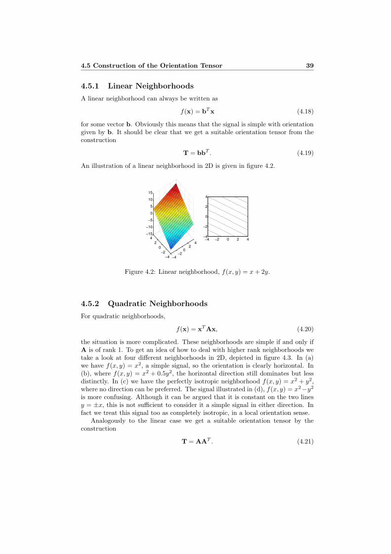
4.5 Construction of the Orientation Tensor 39
4.5.1 Linear Neighborhoods
A linear neighborhood can always be written as
f(x) = bT x (4.18)
for some vector b. Obviously this means that the signal is simple with orientationgiven by b. It should be clear that we get a suitable orientation tensor from theconstruction
T = bbT . (4.19)
An illustration of a linear neighborhood in 2D is given in figure 4.2.
−4−2
02
4
−4−2
02
4−15
−10
−5
0
5
10
15
−4 −2 0 2 4−4
−2
0
2
4
Figure 4.2: Linear neighborhood, f(x, y) = x + 2y.
4.5.2 Quadratic Neighborhoods
For quadratic neighborhoods,
f(x) = xT Ax, (4.20)
the situation is more complicated. These neighborhoods are simple if and only ifA is of rank 1. To get an idea of how to deal with higher rank neighborhoods wetake a look at four different neighborhoods in 2D, depicted in figure 4.3. In (a)we have f(x, y) = x2, a simple signal, so the orientation is clearly horizontal. In(b), where f(x, y) = x2 + 0.5y2, the horizontal direction still dominates but lessdistinctly. In (c) we have the perfectly isotropic neighborhood f(x, y) = x2 + y2,where no direction can be preferred. The signal illustrated in (d), f(x, y) = x2−y2
is more confusing. Although it can be argued that it is constant on the two linesy = ±x, this is not sufficient to consider it a simple signal in either direction. Infact we treat this signal too as completely isotropic, in a local orientation sense.
Analogously to the linear case we get a suitable orientation tensor by theconstruction
T = AAT . (4.21)
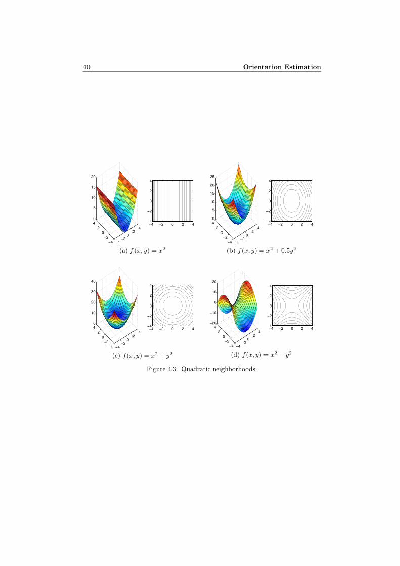
40 Orientation Estimation
−4−2
02
4
−4−2
02
40
5
10
15
20
−4 −2 0 2 4−4
−2
0
2
4
(a) f(x, y) = x2
−4−2
02
4
−4−2
02
40
5
10
15
20
25
−4 −2 0 2 4−4
−2
0
2
4
(b) f(x, y) = x2 + 0.5y2
−4−2
02
4
−4−2
02
40
10
20
30
40
−4 −2 0 2 4−4
−2
0
2
4
(c) f(x, y) = x2 + y2
−4−2
02
4
−4−2
02
4−20
−10
0
10
20
−4 −2 0 2 4−4
−2
0
2
4
(d) f(x, y) = x2 − y2
Figure 4.3: Quadratic neighborhoods.
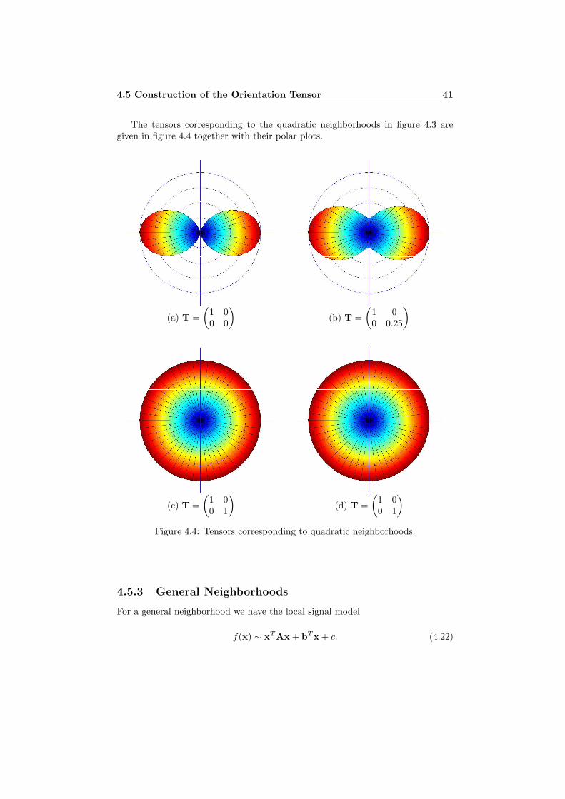
4.5 Construction of the Orientation Tensor 41
The tensors corresponding to the quadratic neighborhoods in figure 4.3 aregiven in figure 4.4 together with their polar plots.
(a) T =
(1 00 0
)
(b) T =
(1 00 0.25
)
(c) T =
(1 00 1
)
(d) T =
(1 00 1
)
Figure 4.4: Tensors corresponding to quadratic neighborhoods.
4.5.3 General Neighborhoods
For a general neighborhood we have the local signal model
f(x) ∼ xT Ax + bT x + c. (4.22)
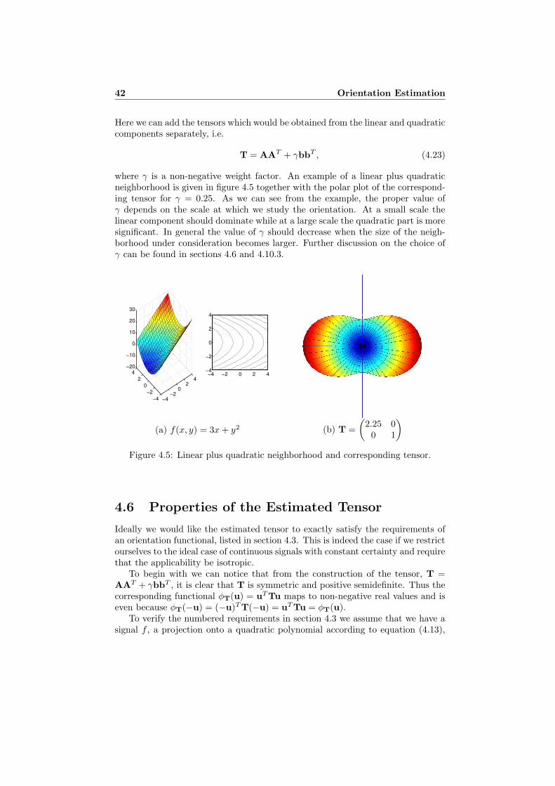
42 Orientation Estimation
Here we can add the tensors which would be obtained from the linear and quadraticcomponents separately, i.e.
T = AAT + γbbT , (4.23)
where γ is a non-negative weight factor. An example of a linear plus quadraticneighborhood is given in figure 4.5 together with the polar plot of the correspond-ing tensor for γ = 0.25. As we can see from the example, the proper value ofγ depends on the scale at which we study the orientation. At a small scale thelinear component should dominate while at a large scale the quadratic part is moresignificant. In general the value of γ should decrease when the size of the neigh-borhood under consideration becomes larger. Further discussion on the choice ofγ can be found in sections 4.6 and 4.10.3.
−4−2
02
4
−4−2
02
4−20
−10
0
10
20
30
−4 −2 0 2 4−4
−2
0
2
4
(a) f(x, y) = 3x + y2 (b) T =
(2.25 00 1
)
Figure 4.5: Linear plus quadratic neighborhood and corresponding tensor.
4.6 Properties of the Estimated Tensor
Ideally we would like the estimated tensor to exactly satisfy the requirements ofan orientation functional, listed in section 4.3. This is indeed the case if we restrictourselves to the ideal case of continuous signals with constant certainty and requirethat the applicability be isotropic.
To begin with we can notice that from the construction of the tensor, T =AAT + γbbT , it is clear that T is symmetric and positive semidefinite. Thus thecorresponding functional φT(u) = uT Tu maps to non-negative real values and iseven because φT(−u) = (−u)T T(−u) = uT Tu = φT(u).
To verify the numbered requirements in section 4.3 we assume that we have asignal f , a projection onto a quadratic polynomial according to equation (4.13),
4.6 Properties of the Estimated Tensor 43
the corresponding tensor T given by equation (4.23), and the corresponding ori-entation functional φ(u) = uT Tu.
1. If f is rotated to yield f(x) = f(Rx), the projection onto a quadratic poly-nomial is rotated similarly,
f(x) ∼ (Rx)T A(Rx) + bT Rx + c = xT (RT AR)x + (RT b)T x + c. (4.24)
This follows from the fact that the set of quadratic polynomials is closedunder rotation and the assumptions that the certainty is constant (and thusisotropic) and that the applicability is isotropic. Now we get the tensorcorresponding to f by
T = (RT AR)(RT AR)T + γ(RT b)(RT b)T
= RT AAT R + γRTbbT R = RT TR.(4.25)
From this it follows that
φ(u) = uT Tu = uT RT TRu = (Ru)T T(Ru) = φ(Ru). (4.26)
The only property of R that we have used above is RRT = I, so thisderivation is equally valid for other isometric transformations.
2. Assume that f is constant along the first coordinate axis, and let u1 be thecorresponding direction vector. Then f does not depend on the first variableand neither does the projection on a quadratic polynomial. Thus we haveAu1 = AT u1 = 0 and bT u1 = 0 so that
φ(u1) = uT1 AAT u1 + γuT
1 bbT u1 = 0. (4.27)
If f is constant along some other direction the conclusion still follows becauseproperty 1 allows us to rotate this direction onto u1.
3. If f is N-dimensional and simple in the direction n, there is a set of N − 1orthogonal directions along which it is constant. From property 2 it followsthat these directions are eigenvectors of T corresponding to the eigenvaluezero and as a consequence T is at most of rank one. Hence we have
T = αnnT , (4.28)
for some non-negative α and
φ(u) = αuT nnT u = α(nT u)2 = α cos2 θ, (4.29)
where θ is the angle between n and u.
4. If a constant is added to f , this only affects the value of c in the projectiononto a quadratic polynomial. Since c is discarded in the construction of T,the tensor remains unchanged.
44 Orientation Estimation
5. If the amplitude of the signal is multiplied by a constant α, f(x) = αf(x),the projection is multiplied by the same constant, i.e.
f(x) ∼ xT (αA)x + (αb)T x + αc. (4.30)
Hence the new tensor is given by
T = (αA)(αA)T + γ(αb)(αb)T = α2T (4.31)
and the corresponding orientation functional
φ(u) = α2φ(u). (4.32)
6. If the signal values are negated, the tensor is unchanged. This follows fromequation (4.31) with α = −1.
7. If the signal is uniformly scaled, f(x) = f(λx), things become more compli-cated. To begin with, if the signal is a quadratic polynomial, we have
f(x) = (λx)T A(λx) + bT (λx) + c = xT (λ2A)x + (λb)T x + c, (4.33)
and the new orientation tensor is given by
T = λ4AAT + λ2γbbT . (4.34)
Hence the relative weight between the quadratic and linear parts of the tensoris altered. For a general signal the projection on a polynomial may changearbitrarily, because it may look completely different at varying scales. In thecase where the applicability is scaled identically with the signal, however,the projection is scaled according to equation (4.33) and to get a new tensorproportional to the old one, we need to scale the weight factor γ by λ2.
In practice, with discretized signals of limited extent, we cannot guarantee thatall of these requirements be perfectly fulfilled. The primary reason is that we can-not even perform an arbitrary rotation of a discretized signal without introducingerrors, so we cannot really hope to do any better with the orientation descriptor.
4.7 Fast Implementation
A drawback with Normalized Convolution is that it is computationally demanding.If we assume that the certainty is constant, however, it can be reduced to ordinaryconvolution or cross correlation4, as shown in section 3.7. To improve further onthe computational complexity, it turns out that the resulting correlation kernelsare Cartesian separable for suitable choices of applicability.
4We prefer to use the latter operation, but remember that a real correlation kernel alwayscan be transformed into a convolution kernel simply by reflecting it.
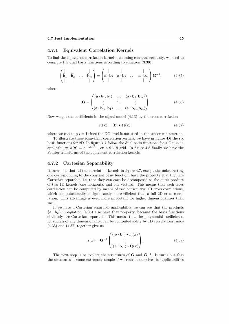
4.7 Fast Implementation 45
4.7.1 Equivalent Correlation Kernels
To find the equivalent correlation kernels, assuming constant certainty, we need tocompute the dual basis functions according to equation (3.30),
| | |b1 b2 . . . bm
| | |
=
| | |a · b1 a · b2 . . . a · bm
| | |
G−1, (4.35)
where
G =
(a · b1,b1) . . . (a · b1,bm)...
. . ....
(a · bm,b1) . . . (a · bm,bm)
(4.36)
Now we get the coefficients in the signal model (4.13) by the cross correlation
ri(x) = (bi ? f)(x), (4.37)
where we can skip i = 1 since the DC level is not used in the tensor construction.To illustrate these equivalent correlation kernels, we have in figure 4.6 the six
basis functions for 2D. In figure 4.7 follow the dual basis functions for a Gaussian
applicability, a(x) = e−0.5xTx, on a 9 × 9 grid. In figure 4.8 finally we have the
Fourier transforms of the equivalent correlation kernels.
4.7.2 Cartesian Separability
It turns out that all the correlation kernels in figure 4.7, except the uninterestingone corresponding to the constant basis function, have the property that they areCartesian separable, i.e. that they can each be decomposed as the outer productof two 1D kernels, one horizontal and one vertical. This means that each crosscorrelation can be computed by means of two consecutive 1D cross correlations,which computationally is significantly more efficient than a full 2D cross corre-lation. This advantage is even more important for higher dimensionalities thantwo.
If we have a Cartesian separable applicability we can see that the products{a · bk} in equation (4.35) also have that property, because the basis functionsobviously are Cartesian separable. This means that the polynomial coefficients,for signals of any dimensionality, can be computed solely by 1D correlations, since(4.35) and (4.37) together give us
r(x) = G−1
((a · b1) ? f)(x)...
((a · bm) ? f)(x)
. (4.38)
The next step is to explore the structures of G and G−1. It turns out thatthe structures become extremely simple if we restrict ourselves to applicabilities
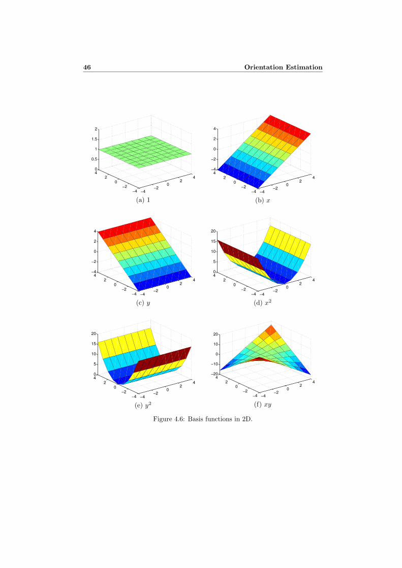
46 Orientation Estimation
−4−2
02
4
−4−2
02
40
0.5
1
1.5
2
(a) 1
−4−2
02
4
−4−2
02
4−4
−2
0
2
4
(b) x
−4−2
02
4
−4−2
02
4−4
−2
0
2
4
(c) y
−4−2
02
4
−4−2
02
40
5
10
15
20
(d) x2
−4−2
02
4
−4−2
02
40
5
10
15
20
(e) y2
−4−2
02
4
−4−2
02
4−20
−10
0
10
20
(f) xy
Figure 4.6: Basis functions in 2D.
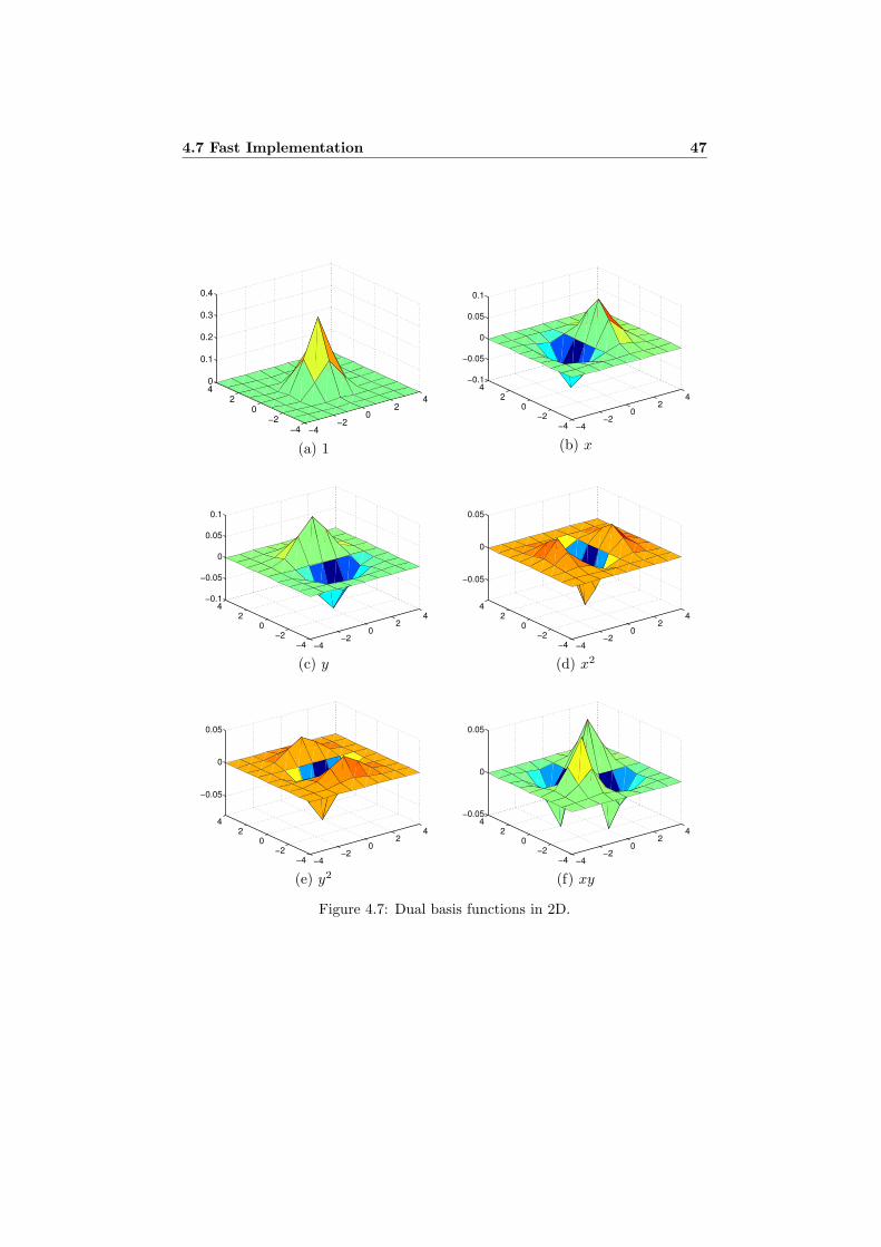
4.7 Fast Implementation 47
−4−2
02
4
−4−2
02
40
0.1
0.2
0.3
0.4
(a) 1
−4−2
02
4
−4−2
02
4−0.1
−0.05
0
0.05
0.1
(b) x
−4−2
02
4
−4−2
02
4−0.1
−0.05
0
0.05
0.1
(c) y
−4−2
02
4
−4−2
02
4
−0.05
0
0.05
(d) x2
−4−2
02
4
−4−2
02
4
−0.05
0
0.05
(e) y2
−4−2
02
4
−4−2
02
4−0.05
0
0.05
(f) xy
Figure 4.7: Dual basis functions in 2D.
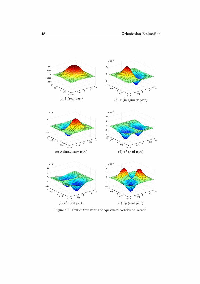
48 Orientation Estimation
−0.01
−0.005
0
0.005
0.01
ππ/2
0−π/2
−π−π−π/2
0π/2
π
(a) 1 (real part)
−5
0
5
x 10−3
ππ/2
0−π/2
−π−π−π/2
0π/2
π
(b) x (imaginary part)
−5
0
5
x 10−3
ππ/2
0−π/2
−π−π−π/2
0π/2
π
(c) y (imaginary part)
−4
−2
0
2
4
x 10−3
ππ/2
0−π/2
−π−π−π/2
0π/2
π
(d) x2 (real part)
−4
−2
0
2
4
x 10−3
ππ/2
0−π/2
−π−π−π/2
0π/2
π
(e) y2 (real part)
−4
−2
0
2
4
x 10−3
ππ/2
0−π/2
−π−π−π/2
0π/2
π
(f) xy (real part)
Figure 4.8: Fourier transforms of equivalent correlation kernels.

4.7 Fast Implementation 49
which are even and identical along all axes, i.e. invariant under reflection andpermutation of the axes. Then most of the inner products {(a ·bk,bl)} in equation(4.36) become zero since most of the products {a · bk · bl} are odd along at leastone axis. In fact, the only non-zero inner products are {(a·bk,bk)}, {(a·b1,bx2
i)},
and {(a ·bx2
i,bx2
j)}. Thus we have the structure of G, illustrated in the 3D case,
G =
a b b b 1b x
b yb z
b c d d x2
b d c d
y2
b d d c z2
d xyd xz
d yz1 x y z x2 y2 z2 xy xz yz
. (4.39)
Surprisingly enough we get an even simpler structure for the inverse,
G−1 =
a e e e 1b x
b yb z
e c x2
e c
y2
e c z2
d xyd xz
d yz1 x y z x2 y2 z2 xy xz yz
. (4.40)
This result is proved in appendix A.Now we can see that all the dual basis functions except the first one5 are indeed
separable. By (4.38) and (4.40) the duals can be written as
b1 = a · (ab1 + e
∑
bx2
i),
bxi= ba · bxi
,
bx2
i= a · (eb1 + cbx2
i) = β a · (bx2
i− αb1),
bxixj= da · bxixj
, i 6= j,
(4.41)
where we can notice that the constant α turns out to have precisely the value whichmakes the DC response of those dual basis functions zero. This should come as
5Notice that we always have the constant function as b1. Thus there is no ambiguity whetherthe subscript refers to the position number or the zeroth degree monomial.
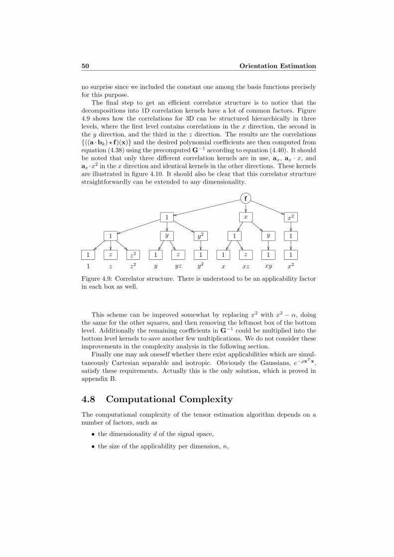
50 Orientation Estimation
no surprise since we included the constant one among the basis functions preciselyfor this purpose.
The final step to get an efficient correlator structure is to notice that thedecompositions into 1D correlation kernels have a lot of common factors. Figure4.9 shows how the correlations for 3D can be structured hierarchically in threelevels, where the first level contains correlations in the x direction, the second inthe y direction, and the third in the z direction. The results are the correlations{((a ·bk) ? f)(x)} and the desired polynomial coefficients are then computed fromequation (4.38) using the precomputed G−1 according to equation (4.40). It shouldbe noted that only three different correlation kernels are in use, ax, ax · x, andax ·x2 in the x direction and identical kernels in the other directions. These kernelsare illustrated in figure 4.10. It should also be clear that this correlator structurestraightforwardly can be extended to any dimensionality.
?>=<89:;f
1ssggggggggggggggggggggg
1ttjjjjjjjjjjjjjj
1||zzzzz
1
z²²
z
z2""DDDDD
z2
y²²
1¦¦¯
¯
y
z¼¼2
222
yz
y2&&MMMMMMMM
1²²
y2
x²²
1¦¦¯
¯
1¦¦¯
¯
x
z¼¼2
222
xz
y""DDDDD
1²²
xy
x2((RRRRRRRRRRR
1²²
1²²
x2
Figure 4.9: Correlator structure. There is understood to be an applicability factorin each box as well.
This scheme can be improved somewhat by replacing x2 with x2 − α, doingthe same for the other squares, and then removing the leftmost box of the bottomlevel. Additionally the remaining coefficients in G−1 could be multiplied into thebottom level kernels to save another few multiplications. We do not consider theseimprovements in the complexity analysis in the following section.
Finally one may ask oneself whether there exist applicabilities which are simul-
taneously Cartesian separable and isotropic. Obviously the Gaussians, e−ρxTx,
satisfy these requirements. Actually this is the only solution, which is proved inappendix B.
4.8 Computational Complexity
The computational complexity of the tensor estimation algorithm depends on anumber of factors, such as
• the dimensionality d of the signal space,
• the size of the applicability per dimension, n,
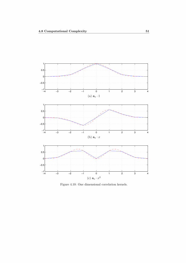
4.8 Computational Complexity 51
−4 −3 −2 −1 0 1 2 3 4−1
−0.5
0
0.5
1
(a) ax · 1
−4 −3 −2 −1 0 1 2 3 4−1
−0.5
0
0.5
1
(b) ax · x
−4 −3 −2 −1 0 1 2 3 4−1
−0.5
0
0.5
1
(c) ax · x2
Figure 4.10: One dimensional correlation kernels.
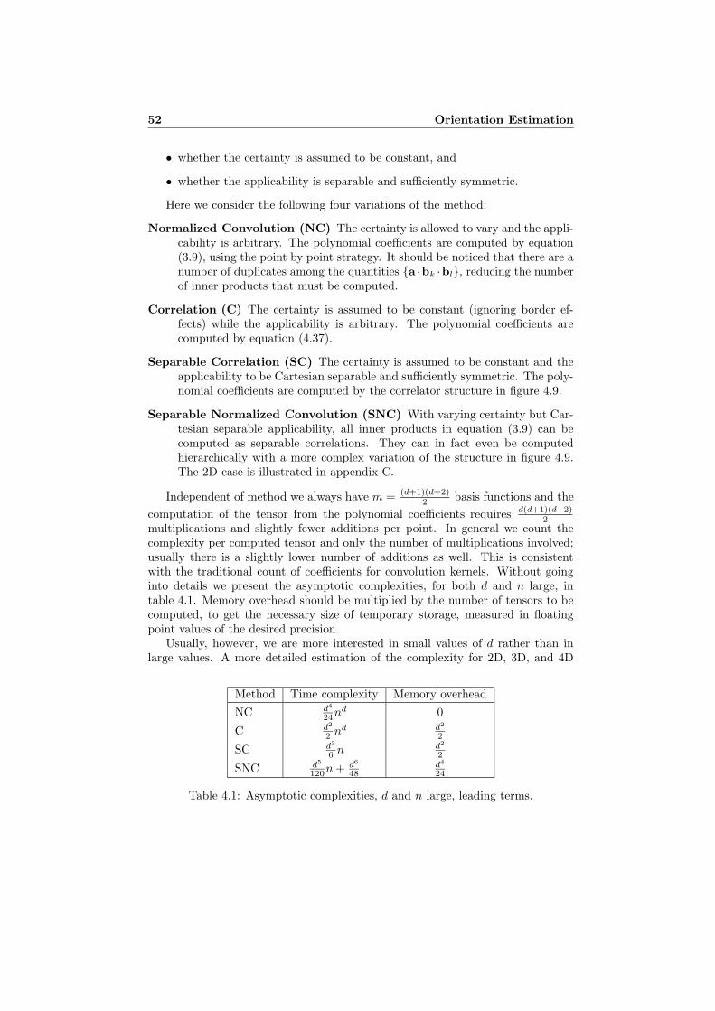
52 Orientation Estimation
• whether the certainty is assumed to be constant, and
• whether the applicability is separable and sufficiently symmetric.
Here we consider the following four variations of the method:
Normalized Convolution (NC) The certainty is allowed to vary and the appli-cability is arbitrary. The polynomial coefficients are computed by equation(3.9), using the point by point strategy. It should be noticed that there are anumber of duplicates among the quantities {a ·bk ·bl}, reducing the numberof inner products that must be computed.
Correlation (C) The certainty is assumed to be constant (ignoring border ef-fects) while the applicability is arbitrary. The polynomial coefficients arecomputed by equation (4.37).
Separable Correlation (SC) The certainty is assumed to be constant and theapplicability to be Cartesian separable and sufficiently symmetric. The poly-nomial coefficients are computed by the correlator structure in figure 4.9.
Separable Normalized Convolution (SNC) With varying certainty but Car-tesian separable applicability, all inner products in equation (3.9) can becomputed as separable correlations. They can in fact even be computedhierarchically with a more complex variation of the structure in figure 4.9.The 2D case is illustrated in appendix C.
Independent of method we always have m = (d+1)(d+2)2 basis functions and the
computation of the tensor from the polynomial coefficients requires d(d+1)(d+2)2
multiplications and slightly fewer additions per point. In general we count thecomplexity per computed tensor and only the number of multiplications involved;usually there is a slightly lower number of additions as well. This is consistentwith the traditional count of coefficients for convolution kernels. Without goinginto details we present the asymptotic complexities, for both d and n large, intable 4.1. Memory overhead should be multiplied by the number of tensors to becomputed, to get the necessary size of temporary storage, measured in floatingpoint values of the desired precision.
Usually, however, we are more interested in small values of d rather than inlarge values. A more detailed estimation of the complexity for 2D, 3D, and 4D
Method Time complexity Memory overhead
NC d4
24nd 0
C d2
2 nd d2
2
SC d3
6 n d2
2
SNC d5
120n + d6
48d4
24
Table 4.1: Asymptotic complexities, d and n large, leading terms.

4.9 Relation to First and Second Derivatives 53
Time complexity Memory overheadMethod d = 2 d = 3 d = 4 d = 2 d = 3 d = 4
NC 21n2 + 105 45n3 + 351 85n4 + 966 0 0 0
C 5n2 + 12 9n3 + 30 14n4 + 60 6 10 15SC 9n + 19 19n + 42 34n + 78 6 10 15SNC 29n + 105 74n + 351 159n + 966 21 45 85
Table 4.2: Time complexity and memory overhead for 2D, 3D, and 4D.
can be found in table 4.2. The values relate to reasonably straightforward imple-mentations of the methods and can likely be improved somewhat. The first termof the time complexities is the total number of coefficients involved in the corre-lation kernels, while the second is the count for the tensor construction from thecorrelation results. Included in the latter part for NC and SNC is the solution of
an m×m symmetric positive definite equation system, estimated at m3
6 + 3m2
2 + m3
operations [45].To sum this analysis up, it is clear that Separable Correlation is by far the most
efficient method. The restriction set on the applicability is no limitation becausethose properties are desired anyway. The requirement of constant certainty is aproblem, however, since such an assumption surely fails at least in a neighborhoodof the borders and the method is more than likely to yield significantly biasedtensors there. Proper attention to the vanishing certainty outside the border ispaid by the NC and SNC methods, which on the other hand have a high timecomplexity and a large memory overhead, respectively. A good solution for signalswith constant certainty would be to use Separable Correlation for the inner part ofthe signal and Normalized Convolution or Separable Normalized Convolution forthe border parts. It must be stressed, however, that while Normalized Convolutionwill reduce the negative impact of missing information outside the borders, it willcertainly not remove it completely. The best solution is, as always, to keep awayfrom those parts as much as possible.
4.9 Relation to First and Second Derivatives
By the Maclaurin expansion, a sufficiently differentiable signal can in a neighbor-hood of the origin be expanded as
f(x) = f(0) + (∇f)T x +1
2xT Hx + O(‖x‖3), (4.42)
where the gradient ∇f contains the first derivatives of f at the origin and theHessian H contains the second derivatives,
∇f =
fx1(0)...
fxn(0)
, H =
fx1x1(0) . . . fx1xn
(0)...
. . ....
fxnx1(0) . . . fxnxn
(0)
. (4.43)
54 Orientation Estimation
Clearly this expansion looks identical to the signal model (4.13) with A = 12H,
b = ∇f , and c = f(0). There is, however, conceptually an important difference.The Maclaurin expansion is intended to be correct for an infinitesimal neighbor-hood, while our signal model is intended to approximate the signal over a largerneighborhood, specified by the applicability.
The Maclaurin expansion also has the principal problem that the mathematicaldefinition of derivatives requires signal values arbitrarily close to the origin, whichare not available for discretized signals. Another complication is that perfectdifferentiation would be extremely sensitive to noise. One way to get around this,which also allows computing “derivatives at different scales”, is to first convolvethe signal with a Gaussian,
h = f ∗ g, g(x) = e−x
Tx
2σ2 (4.44)
and then differentiate the filtered signal h. By the laws of convolution, the partialderivatives of h can be computed as f convolved with the partial derivatives of g,which are known explicitly. In e.g. 2D we have
hx = f ∗ gx, gx = − x
σ2g,
hy = f ∗ gy, gy = − y
σ2g,
hxx = f ∗ gxx, gxx =
(x2
σ4− 1
σ2
)
g, (4.45)
hxy = f ∗ gxy, gxy =xy
σ4g,
hyy = f ∗ gyy, gyy =
(y2
σ4− 1
σ2
)
g,
and we can see that the structure of the partial derivatives of g agrees with thedual basis functions in (4.41) for Gaussian applicability. These functions are alsoillustrated in figure 4.7.
We would like to stress, however, that this fact is purely coincidental and aneffect of the special properties of the Gaussians. For other applicabilities we do nothave this relation. Likewise we cannot compute the tensor from the responses ofany filter set that implements some approximation of first and second derivativesand automatically assume that it will have all the good properties that we havederived for the orientation tensors. Still it may help the intuition to think of Aand b in terms of image derivatives.
4.10 Evaluation
The tensor estimation algorithm has been evaluated on a 3D test volume consistingof concentric spherical shells. The volume is 64 × 64 × 64 and selected slices aredisplayed in figure 4.11. Except at the center of the volume the signal is locallyplanar and all possible orientations are present. As in [2, 37] the performance of
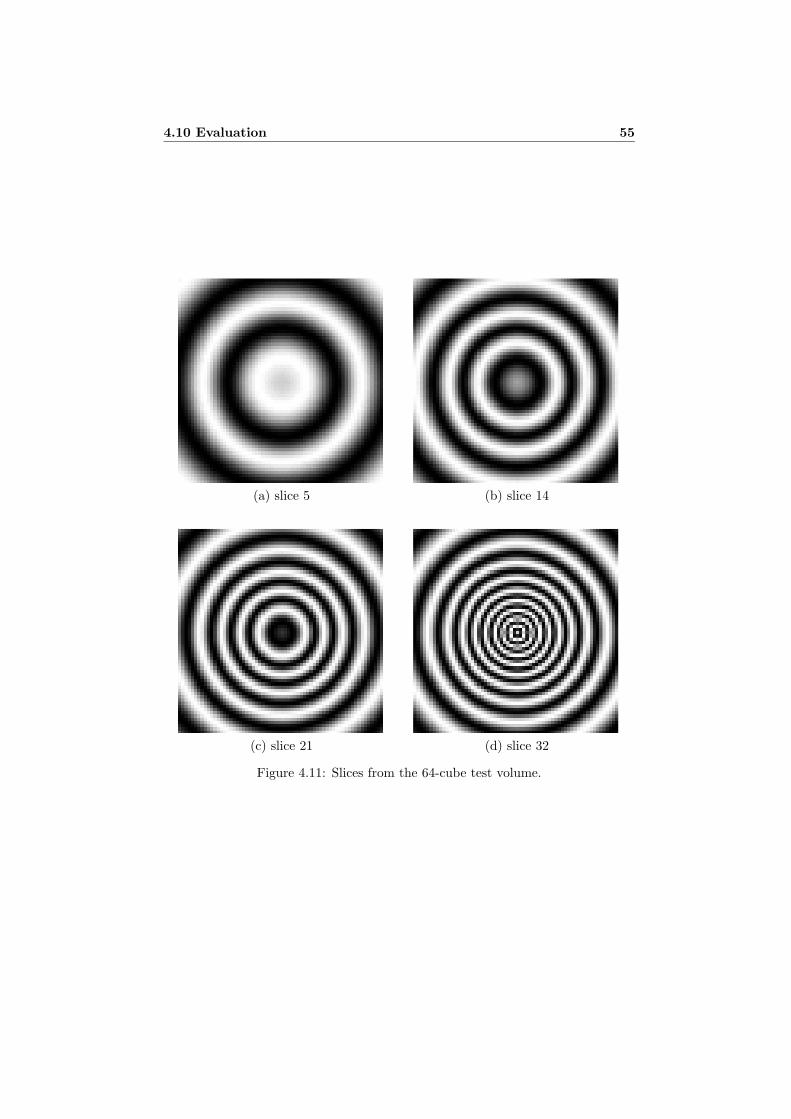
4.10 Evaluation 55
(a) slice 5 (b) slice 14
(c) slice 21 (d) slice 32
Figure 4.11: Slices from the 64-cube test volume.
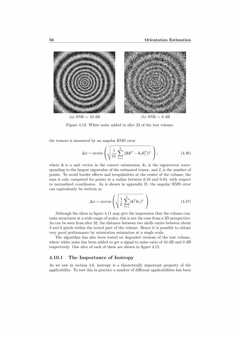
56 Orientation Estimation
(a) SNR = 10 dB (b) SNR = 0 dB
Figure 4.12: White noise added to slice 32 of the test volume.
the tensors is measured by an angular RMS error
∆φ = arcsin
√√√√ 1
2L
L∑
l=1
‖xxT − e1eT1 ‖2
, (4.46)
where x is a unit vector in the correct orientation, e1 is the eigenvector corre-sponding to the largest eigenvalue of the estimated tensor, and L is the number ofpoints. To avoid border effects and irregularities at the center of the volume, thesum is only computed for points at a radius between 0.16 and 0.84, with respectto normalized coordinates. As is shown in appendix D, the angular RMS errorcan equivalently be written as
∆φ = arccos
√√√√ 1
L
L∑
l=1
(xT e1)2
. (4.47)
Although the slices in figure 4.11 may give the impression that the volume con-tains structures at a wide range of scales, this is not the case from a 3D perspective.As can be seen from slice 32, the distance between two shells varies between about3 and 6 pixels within the tested part of the volume. Hence it is possible to obtainvery good performance by orientation estimation at a single scale.
The algorithm has also been tested on degraded versions of the test volume,where white noise has been added to get a signal to noise ratio of 10 dB and 0 dBrespectively. One slice of each of these are shown in figure 4.12.
4.10.1 The Importance of Isotropy
As we saw in section 4.6, isotropy is a theoretically important property of theapplicability. To test this in practice a number of different applicabilities has been
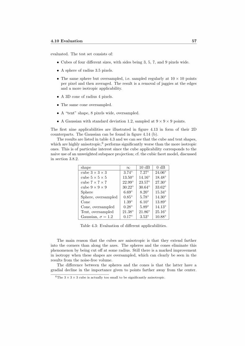
4.10 Evaluation 57
evaluated. The test set consists of:
• Cubes of four different sizes, with sides being 3, 5, 7, and 9 pixels wide.
• A sphere of radius 3.5 pixels.
• The same sphere but oversampled, i.e. sampled regularly at 10 × 10 pointsper pixel and then averaged. The result is a removal of jaggies at the edgesand a more isotropic applicability.
• A 3D cone of radius 4 pixels.
• The same cone oversampled.
• A “tent” shape, 8 pixels wide, oversampled.
• A Gaussian with standard deviation 1.2, sampled at 9 × 9 × 9 points.
The first nine applicabilities are illustrated in figure 4.13 in form of their 2Dcounterparts. The Gaussian can be found in figure 4.14 (b).
The results are listed in table 4.3 and we can see that the cube and tent shapes,which are highly anisotropic,6 performs significantly worse than the more isotropicones. This is of particular interest since the cube applicability corresponds to thenaive use of an unweighted subspace projection; cf. the cubic facet model, discussedin section 3.8.2.
shape ∞ 10 dB 0 dBcube 3 × 3 × 3 3.74◦ 7.27◦ 24.06◦
cube 5 × 5 × 5 13.50◦ 14.16◦ 18.48◦
cube 7 × 7 × 7 22.99◦ 23.57◦ 27.30◦
cube 9 × 9 × 9 30.22◦ 30.64◦ 33.62◦
Sphere 6.69◦ 8.20◦ 15.34◦
Sphere, oversampled 0.85◦ 5.78◦ 14.30◦
Cone 1.39◦ 6.10◦ 13.89◦
Cone, oversampled 0.28◦ 5.89◦ 14.13◦
Tent, oversampled 21.38◦ 21.86◦ 25.16◦
Gaussian, σ = 1.2 0.17◦ 3.53◦ 10.88◦
Table 4.3: Evaluation of different applicabilities.
The main reason that the cubes are anisotropic is that they extend fartherinto the corners than along the axes. The spheres and the cones eliminate thisphenomenon by being cut off at some radius. Still there is a marked improvementin isotropy when these shapes are oversampled, which can clearly be seen in theresults from the noise-free volume.
The difference between the spheres and the cones is that the latter have agradial decline in the importance given to points farther away from the center.
6The 3 × 3 × 3 cube is actually too small to be significantly anisotropic.

58 Orientation Estimation
−50
5
−5
0
50
0.5
1
(a) Cube 3 × 3 × 3
−50
5
−5
0
50
0.5
1
(b) Cube 5 × 5 × 5
−50
5
−5
0
50
0.5
1
(c) Cube 7 × 7 × 7
−50
5
−5
0
50
0.5
1
(d) Cube 9 × 9 × 9
−50
5
−5
0
50
0.5
1
(e) Sphere, radius 3.5
−50
5
−5
0
50
0.5
1
(f) Sphere, oversampled
−50
5
−5
0
50
0.5
1
(g) Cone, radius 4
−50
5
−5
0
50
0.5
1
(h) Cone, oversampled
−50
5
−5
0
50
0.5
1
(i) Tent, oversampled
Figure 4.13: Applicabilities used to test orientation estimation.
−50
5
−5
0
50
0.5
1
(a) σ = 0.3
−50
5
−5
0
50
0.5
1
(b) σ = 1.2
−50
5
−5
0
50
0.5
1
(c) σ = 4.8
Figure 4.14: Gaussian applicabilities with different standard deviations.
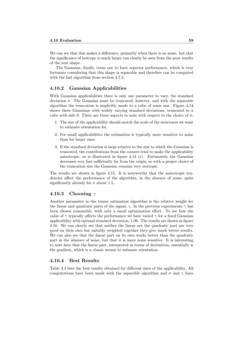
4.10 Evaluation 59
We can see that this makes a difference, primarily when there is no noise, but thatthe significance of isotropy is much larger can clearly be seen from the poor resultsof the tent shape.
The Gaussian, finally, turns out to have superior performance, which is veryfortunate considering that this shape is separable and therefore can be computedwith the fast algorithm from section 4.7.2.
4.10.2 Gaussian Applicabilities
With Gaussian applicabilities there is only one parameter to vary, the standarddeviation σ. The Gaussian must be truncated, however, and with the separablealgorithm the truncation is implicitly made to a cube of some size. Figure 4.14shows three Gaussians with widely varying standard deviations, truncated to acube with side 9. There are three aspects to note with respect to the choice of σ:
1. The size of the applicability should match the scale of the structures we wantto estimate orientation for.
2. For small applicabilities the estimation is typically more sensitive to noisethan for larger ones.
3. If the standard deviation is large relative to the size to which the Gaussian istruncated, the contributions from the corners tend to make the applicabilityanisotropic, as is illustrated in figure 4.14 (c). Fortunately the Gaussiandecreases very fast sufficiently far from the origin, so with a proper choice ofthe truncation size the Gaussian remains very isotropic.
The results are shown in figure 4.15. It is noteworthy that the anisotropic ten-dencies affect the performance of the algorithm, in the absence of noise, quitesignificantly already for σ about 1.5.
4.10.3 Choosing γ
Another parameter in the tensor estimation algorithm is the relative weight forthe linear and quadratic parts of the signal, γ. In the previous experiments γ hasbeen chosen reasonably, with only a small optimization effort. To see how thevalue of γ typically affects the performance we have varied γ for a fixed Gaussianapplicability with optimal standard deviation, 1.06. The results are shown in figure4.16. We can clearly see that neither the linear nor the quadratic part are verygood on their own but suitably weighted together they give much better results.We can also see that the linear part on its own works better than the quadraticpart in the absence of noise, but that it is more noise sensitive. It is interestingto note here that the linear part, interpreted in terms of derivatives, essentially isthe gradient, which is a classic means to estimate orientation.
4.10.4 Best Results
Table 4.4 lists the best results obtained for different sizes of the applicability. Allcomputations have been made with the separable algorithm and σ and γ have

60 Orientation Estimation
0 1 2 3 4 50
5
10
15
20
25
30
35
40
45
σ
angu
lar e
rror
, deg
rees
Figure 4.15: Angular errors for Gaussians with varying standard deviations. Thesolid lines refer to 9 × 9 × 9 kernels while the dashed lines refer to 11 × 11 × 11kernels. The three curve pairs are for 0, 10, and ∞ SNR respectively.
10−5 100 1050
5
10
15
20
25
γ
angu
lar e
rror
, deg
rees
(a)
10−5 100 1050
0.5
1
1.5
2
2.5
3
γ
angu
lar e
rror
, deg
rees
(b)
Figure 4.16: (a) Angular errors for varying γ values. The three curves are for 0,10, and ∞ SNR respectively. (b) A magnification of the results for the noise-freetest volume.
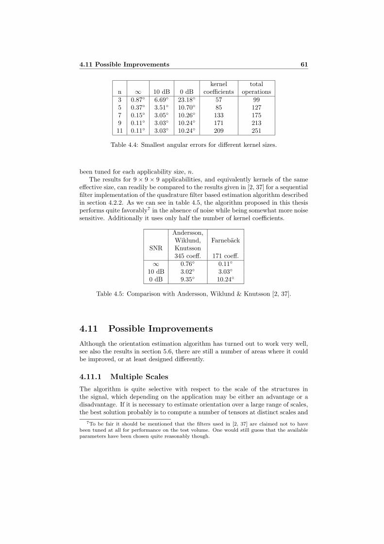
4.11 Possible Improvements 61
kernel totaln ∞ 10 dB 0 dB coefficients operations3 0.87◦ 6.69◦ 23.18◦ 57 995 0.37◦ 3.51◦ 10.70◦ 85 1277 0.15◦ 3.05◦ 10.26◦ 133 1759 0.11◦ 3.03◦ 10.24◦ 171 21311 0.11◦ 3.03◦ 10.24◦ 209 251
Table 4.4: Smallest angular errors for different kernel sizes.
been tuned for each applicability size, n.The results for 9 × 9 × 9 applicabilities, and equivalently kernels of the same
effective size, can readily be compared to the results given in [2, 37] for a sequentialfilter implementation of the quadrature filter based estimation algorithm describedin section 4.2.2. As we can see in table 4.5, the algorithm proposed in this thesisperforms quite favorably7 in the absence of noise while being somewhat more noisesensitive. Additionally it uses only half the number of kernel coefficients.
Andersson,Wiklund, Farneback
SNR Knutsson345 coeff. 171 coeff.
∞ 0.76◦ 0.11◦
10 dB 3.02◦ 3.03◦
0 dB 9.35◦ 10.24◦
Table 4.5: Comparison with Andersson, Wiklund & Knutsson [2, 37].
4.11 Possible Improvements
Although the orientation estimation algorithm has turned out to work very well,see also the results in section 5.6, there are still a number of areas where it couldbe improved, or at least designed differently.
4.11.1 Multiple Scales
The algorithm is quite selective with respect to the scale of the structures inthe signal, which depending on the application may be either an advantage or adisadvantage. If it is necessary to estimate orientation over a large range of scales,the best solution probably is to compute a number of tensors at distinct scales and
7To be fair it should be mentioned that the filters used in [2, 37] are claimed not to havebeen tuned at all for performance on the test volume. One would still guess that the availableparameters have been chosen quite reasonably though.

62 Orientation Estimation
subsequently combine them into a single tensor. Preliminary experiments indicatethat it is sufficient to simply add the tensors together, taking the scaling relationsof equation (4.34) into account.
4.11.2 Different Radial Functions
The basis functions can in 2D be written in polar coordinates as
{1, ρ cos φ, ρ sin φ, ρ2 cos2 φ, ρ2 sin2 φ, ρ2 cos φ sinφ}. (4.48)
It is easy to show that it is only the angular functions that are essential for therotation equivariance and other properties of the tensor. The radial functionsmay well be something else than ρ for the linear basis functions and ρ2 for thequadratic ones. One possibility would be to have the radial function ρ for all thebasis functions except the constant. As a consequence both parts of the tensorwould scale equally if both signal and applicability is scaled and there would beno need to adjust γ, cf. equation (4.34). Another possibility would be to try toobtain matching radial functions in the Fourier domain, which currently is not thecase.
One should be aware, however, that changing the radial functions would destroythe separability of the basis functions.
4.11.3 Additional Basis Functions
It would be conceivable to expand the signal model, equation (4.13), e.g. withhigher degree polynomials, cf. the cubic facet model discussed in section 3.8.2. Itis not obvious that this would actually improve anything, however, but it wouldcertainly increase the computational complexity.
To make the increased complexity worthwhile it would probably be necessary tofind a way to ensure that the additional basis functions reduce the noise sensitivityof the algorithm, possibly by introducing some kind of redundancy.
Chapter 5
Velocity Estimation
5.1 Introduction
If an image sequence is considered as a spatiotemporal volume, it is possible touse the orientation information in the volume for estimation of the motion in thesequence. In particular the tensor representation of orientation allows straight-forward estimation of the motion, see e.g. [22, 28, 29, 30, 31, 32, 60] and section5.2. The tensor can also be used more indirectly to provide constraints on themotion in order to estimate parameterized motion models, which is the basis forthe methods developed in this chapter. Related approaches have also been used byKarlholm [35]. For overviews of other methods for motion estimation, the readeris referred to [3] and [11].
The algorithms presented in sections 5.3 and 5.4 were developed for my master’sthesis [13, 14], at that time using orientation tensors estimated by quadraturefilters and with emphasis on segmentation of the motion field rather than onvelocity estimation. The simplified algorithm in section 5.5 and the results insection 5.6 have not been published before. All these algorithms are novel andtogether with orientation tensors estimated by the algorithms from chapter 4 theygive excellent performance, as demonstrated in section 5.6.
5.2 From Orientation to Motion
By stacking the frames of an image sequence onto each other we obtain a spatiotem-poral image volume with two spatial dimensions and a third temporal dimension.It is easy to see that there is a strong correspondence between the motions in theimage sequence and the orientations in the image volume. A moving line, e.g., isconverted into a plane in the volume and from the orientation of the plane we canrecover the velocity component perpendicular to the line. The fact that we canonly obtain the perpendicular component is a fundamental limitation known asthe aperture problem; the parallel velocity component of a linear structure cannotbe determined simply because it does not induce any change in the local signal. A

64 Velocity Estimation
moving point, on the other hand, is converted into a line in the volume and fromthe direction of the line we can obtain the true motion.
In terms of orientation tensors, the first case corresponds to a rank 1 tensor,where the largest eigenvector gives the orientation of the planar structure, whilethe second case corresponds to a rank 2 tensor, where the smallest eigenvectorgives the direction along the linear structure. More precisely, with the tensor Texpressed by the eigenvalue decomposition as in equation (4.7),
T = λ1e1eT1 + λ2e2e
T2 + λ3e3e
T3 , (5.1)
the velocity in the two cases can be computed by, taken from [22],
vnormal = −x3(x1ξ1 + x2ξ2)/(x21 + x2
2)
x1 = e1 · ξ1
x2 = e1 · ξ2
x3 = e1 · t
moving line case, (5.2)
and
v = (x1ξ1 + x2ξ2)/x3
x1 = e3 · ξ1
x2 = e3 · ξ2
x3 = e3 · t
moving point case, (5.3)
where ξ1 and ξ2 are the orthogonal unit vectors defining the image plane and t isa unit vector in the time direction.
One problem with this approach to velocity estimation is that we at each pointmust decide whether we can compute true velocity or have to be content with thenormal component. Another problem is robustness. The method is sensitive bothto noise and to errors in the tensor estimation. A common method to increase therobustness is averaging of the tensors in a neighborhood of each point, discussedfurther in section 5.5.
5.3 Estimating a Parameterized Velocity Field
Rather than estimating the velocity from the tensors point for point we assumethat the velocity field over a region can be parameterized according to some motionmodel and we use all the tensors in the region to compute the parameters. To beginwith we assume that we somehow have access to a region in the current frame ofthe sequence, within which the motion can be described, at least approximately,by some relatively simple parametric motion model.
5.3 Estimating a Parameterized Velocity Field 65
5.3.1 Motion Models
The simplest possible motion model is to assume that the velocity is constant overthe region,
vx(x, y) = a,
vy(x, y) = b,(5.4)
where x and y are the spatial coordinates, vx and vy are the x and y componentsof the velocity, and a and b are the model parameters. Geometrically this motionmodel corresponds to objects undergoing a pure translation under orthographicprojection. A more powerful alternative is the affine motion model,
vx(x, y) = ax + by + c,
vy(x, y) = dx + ey + f,(5.5)
which applies to planar patches undergoing rigid body motion, i.e. translationplus rotation, under orthographic projection. To also account for a perspectiveprojection we need the eight parameter motion model,
vx(x, y) = a1 + a2x + a3y + a7x2 + a8xy,
vy(x, y) = a4 + a5x + a6y + a7xy + a8y2.
(5.6)
The usefulness of these models does of course depend on the application but itis useful to notice that sufficiently far away most surfaces can be approximated asplanar and if the distance to the scene is much larger than the variation in distancewithin the scene, perspective projection can be approximated by orthographicprojection. More details on the derivation of these motion models can be found in[11].
Of course it would be possible to design other motion models for specific ex-pected velocity fields, but we will only consider those listed above in this presenta-tion. Requirements on the motion models in order to be useful with the methodsdeveloped in this chapter are given in section 5.3.3.
5.3.2 Cost Functions
A 2D velocity vector (vx, vy)T , measured in pixels per frame, can be extended toa 3D spatiotemporal directional vector v and a unit directional vector v by
v =
vx
vy
1
, v =v
‖v‖ . (5.7)
Ideally, in the case of a constant translation1, we obtain a spatiotemporalneighborhood which is constant in the v direction. By property 2 of section 4.3we therefore have the constraint that
φT(v) = vT Tv = 0. (5.8)
1In the image plane.
66 Velocity Estimation
This is consistent with the discussion in section 5.2 since in the moving point case,the least eigenvector has eigenvalue zero and is parallel to v, while in the movingline case, all v with the correct normal velocity component satisfies equation (5.8).
In a less ideal case, where the motion is not a translation, where the motion isa translation but it varies over time, or in the presence of noise, we typically haveto deal with rank 3 tensors, meaning that the constraint (5.8) cannot be fulfilled.As discussed in section 4.3, the interpretation of the orientation functional φT isthat the value in a given direction is a measure of how well the signal locally isconsistent with an orientation hypothesis in that direction. In this case we aresearching for directions along which the signal varies as little as possible and thuswe wish to minimize vT Tv.
Rewriting the tensor as
T = λ1e1eT1 + λ2e2e
T2 + λ3e3e
T3
= (λ1 − λ3)e1eT1 + (λ2 − λ3)e2e
T2 + λ3I = T + λ3I,
(5.9)
where λ3I is the isotropic part of the tensor, cf. section 4.2.3, we can see that
vT Tv = vT Tv + λ3vT Iv = vT Tv + λ3. (5.10)
Thus it is clear that the isotropic part of the tensor can be removed withoutaffecting the minimization problem, i.e. the minimum is obtained for the samedirections. In fact it is necessary to remove it, because we will see that for compu-tational reasons it is preferable to minimize an expression involving v rather thanv.2 Then we have the minimization of
vT Tv = vT Tv + λ3vT v, (5.11)
which would be clearly biased against large velocities compared to (5.10). Hencewe remove the isotropic part of the tensor in a preprocessing step to obtain anisotropy compensated tensor
T = T − λ3I. (5.12)
Notice that this operation does not require a full eigenvalue decomposition of T;it is sufficient to compute the smallest eigenvalue. An efficient algorithm for thisis given in appendix E.
To simplify the notation it is understood throughout the rest of the chapter thatT denotes the preprocessed tensor.
Now we can define two cost functions,
d1(v,T) = vT Tv, (5.13)
d2(v,T) =vT Tv
‖v‖2 trT=
vT Tv
trT, (5.14)
2Notice that both problems are well-defined. In the latter case we have the constraint that v
be of unit length while in the former case the last component of v has to be 1.
5.3 Estimating a Parameterized Velocity Field 67
both giving a statement about to what extent a velocity hypothesis is consistentwith a given tensor. A perfect match gives the value zero, while increasing valuesindicate increasing inconsistencies. The distinction between the two cost functionsis that d1 is suitable for minimization over a region, while d2 is more useful forcomparisons of the consistency of motion hypotheses at different points.
5.3.3 Parameter Estimation
Assume now that we again have a region given and that we have a motion modelthat assigns velocities vi to each point of the region. By summing the costs ateach point we obtain
dtot =∑
i
d1(vi,Ti), (5.15)
giving a total cost for the motion model over the entire region. With a parame-terized motion model the next step is to find the parameters that minimize dtot.To explain this procedure we use the affine motion model (5.5), which can berewritten as
v =
vx
vy
1
=
a b cd e f0 0 1
xy1
=
x y 1 0 0 0 00 0 0 x y 1 00 0 0 0 0 0 1
︸ ︷︷ ︸
S
abcdef1
︸ ︷︷ ︸
p
. (5.16)
Hence we get
d1(v,T) = vT Tv = pT ST TSp = pT Qp, (5.17)
where Q = ST TS is a positive semidefinite quadratic form. Summing these overthe region transforms equation (5.15) into
dtot(p) =∑
i
d1(vi,Ti) =∑
i
pT STi TiSip
= pT
(∑
i
Qi
)
p = pT Qtotp,
(5.18)
68 Velocity Estimation
which should be minimized under the constraint that the last element of p be 1.3
In order to do this we partition p and Qtot as
p =
(p1
)
, Qtot =
(Q qqT α
)
, (5.20)
turning (5.18) into
dtot(p) = pT Qp + pT q + qT p + α. (5.21)
If Q is invertible we can complete the square to get
dtot(p) = (p + Q−1q)T Q(p + Q−1q) + α − qT Q−1q (5.22)
and it is clear that the minimum value
α − qT Q−1q (5.23)
is obtained for
p = −Q−1q. (5.24)
If Q should happen to be singular, the minimum value α+qT p is obtained for allsolutions to the equation
Qp = −q (5.25)
and to choose between the solutions some additional constraint is needed. Onereasonable possibility is to require that the mean squared velocity over the regionis taken as small as possible, i.e. minimizing
∑
i
pT STi Sip = pT
(∑
i
STi Si
)
p = pT L2p = ‖p‖L, (5.26)
where S is S with the last column removed. The solution to this problem can befound in section 2.4.2 or in section 2.5.1 if L should be semidefinite.
In order to use this method of parameter estimation, the necessary and suf-ficient property of the motion model is that it is linear in its parameters. Thisproperty is demonstrated by equation (5.16) for the affine motion model. Thecorresponding matrices S and p for the constant velocity motion model (5.4) aregiven by
S =
1 0 00 1 00 0 1
, p =
ab1
, (5.27)
3Now it should be clear why we prefer to minimize an expression involving vT Tv rather thanvT Tv. In the latter case equation 5.18 would be replaced by
dtot(p) =X
i
pT ST
iTiSip
pT ST
iS
ip
(5.19)
and the minimization problem would become substantially harder to solve.

5.4 Simultaneous Segmentation and Velocity Estimation 69
and for the eight parameter motion model (5.6) by
S =
1 x y 0 0 0 x2 xy 00 0 0 1 x y xy y2 00 0 0 0 0 0 0 0 1
, (5.28)
p =(a1 a2 a3 a4 a5 a6 a7 a8 1
)T. (5.29)
There are two important advantages to estimating the velocity over a wholeregion rather than point by point. The first advantage is that the effects of noiseand inaccuracies in the tensor estimation typically are reduced significantly. Thesecond advantage is that even if the aperture problem is present in some part ofthe region, information obtained from other parts can help to fill in the missingvelocity component. There does remain a possibility that the motion field cannotbe uniquely determined, but that requires the signal structures over the wholeregion to be oriented in such a way that the motion becomes ambiguous; a gener-alized aperture problem.4 This case is characterized by Q becoming singular, sothat equation (5.25) has multiple solutions. The secondary requirement to mini-mize the mean squared velocity generalizes the idea to compute only the normalvelocity component in the case of the ordinary aperture problem.
A disadvantage with velocity estimation over a whole region is that it is as-sumed that the true velocity field is at least reasonably consistent with the chosenmotion model. A problem here is that even if we know, e.g. from the geometryof the scene, that the velocity field should be patchwise affine, we still need toobtain regions not covering patches with different motion parameters. There aremany possible solutions to this problem, including graylevel segmentation and theideal case of a priori knowledge of suitable regions. Another solution is given inthe following section, where a simultaneous segmentation and velocity estimationalgorithm is presented. A different alternative is to ignore the need for correct seg-mentation and instead simply average the Q matrices. This approach is detailedin section 5.5.
5.4 Simultaneous Segmentation and Velocity Es-
timation
In this section we present an efficient algorithm for simultaneous segmentationand velocity estimation, only given an orientation tensor field for one frame. Thegoal of the segmentation is to partition the image into a set of disjoint regions, sothat each region is characterized by a coherent motion, with respect to the chosenmotion model. In this section a region R is defined to be a nonempty, connected setof pixels. The segmentation algorithm is based on a competitive region growingapproach. The basic algorithm is first presented in abstract form.
4A nontrivial example of this generalized aperture problem is a signal consisting of concentriccircles, which simultaneously expand and rotate around their center. Only the radial velocitycomponent can be recovered.
70 Velocity Estimation
5.4.1 The Competitive Algorithm
To each region R is associated a cost function CR(x), which is defined for allpixels in the image. Regions are extended by adding one pixel at a time. Topreserve connectivity the new pixel must be adjacent to the region, and to preservedisjointedness it must not already be assigned to some other region. The new pixelis also chosen as cheap as possible. The details are as follows.
Let the border ∆R of region R be the set of unassigned pixels in the imagewhich are adjacent to some pixel in R. For each region R, the possible candidate,N(R), to be added to the region is the cheapest pixel bordering to R, i.e.
N(R) = arg minx∈∆R
CR(x). (5.30)
The corresponding minimum cost for adding the candidate to the region is denotedCmin(R). In the case of an empty border, N(R) is undefined and Cmin(R) isinfinite.
Assuming that a number of regions {Rn} in some way have been obtained, therest of the image is partitioned as follows.
1. Find the region Ri for which the cost to add a new pixel is the least, i.e.i = arg minn Cmin(Rn).
2. Add the cheapest pixel N(Ri) to Ri.
3. Repeat the first two steps until no unassigned pixels remain.
Notice that it does not matter what the actual values of the cost functionsare. It is only relevant which of them is lowest. Hence the algorithm is calledcompetitive.
5.4.2 Candidate Regions
A fundamental problem with the simultaneous segmentation and velocity estima-tion approach is that we typically need a segmentation in order to compute themotion model parameters, and we need motion models in order to partition theimage into regions. Since we assume no a priori knowledge about the segmenta-tion of the image, we use the concept of candidate regions to introduce preliminaryregions into the algorithm.
To begin with we arbitrarily fill the image with a large number of overlappingrectangular candidate regions5. For each candidate region we then compute theoptimal motion model parameters as described in section 5.3. Obviously theserectangular regions are not at all adapted to the motion field of the image and asa consequence the computed motion models are likely to be suboptimal. In orderto improve the candidate regions we use a procedure called regrowing.
The regrowing procedure is the first application of the competitive algorithm.Regrowing is performed for one candidate region at a time, which means that
5e.g. squares of the size 21 × 21, with a distance between the center points of 4 pixels. Theexact numbers are not critical.
5.4 Simultaneous Segmentation and Velocity Estimation 71
there is no competition between different regions but rather between the pixels.To begin with the candidate region contains only one pixel, its starting point,which was also the center point of the initial rectangle. The cost function used isd2 from equation (5.14), where v is the velocity given by the candidate region’scurrent motion model. The competitive algorithm is then run until the candidateregion has grown to a specified size. This size is called the candidate region size,m0 and is a design parameter of the segmentation algorithm. The effect of theregrowing procedure is that the candidate region now consists of the m0 connectedpixels, starting from a fixed point, that are most consistent with the candidateregion’s motion model. When the candidate region has been regrown, new optimalparameters are computed.
Each candidate region is regrown twice, a number which seems to be sufficientto obtain reasonably coherent regions.
5.4.3 Segmentation Algorithm
Having obtained candidate regions, the rest of the segmentation algorithm is amatter of alternately converting candidate regions into real regions and letting thelatter grow. In contrast to the candidate regions, the real regions are not allowedto overlap but has to be disjoint. While the candidate regions are allowed tooverlap each other they must not overlap the real regions, which means that theyhave to be regrown from time to time, taking this restriction into account. Toaccomodate the inclusion of new regions, the competitive algorithm is extendedto have the following steps, to be iterated as long as there are empty pixels left:
1. Regrow the candidate regions which are currently overlapping a real region.If a candidate region cannot be regrown to its full size, it is removed. Thesame thing happens when a candidate region’s starting point becomes occu-pied by a real region. The cost of the most expensive included pixel is calledthe maximum cost of the candidate region.
2. Find the candidate region with the least maximum cost. This is the aspirantfor inclusion among the real regions.
3. As in the competitive algorithm, find the cheapest pixel that may be addedto one of the already existing real regions.
4. Compare the least maximum cost from step 2 with the cost of the cheapestpixel in step 3.
(a) If the least maximum cost is smallest, raise the corresponding candidateregion to the status of a real region.
(b) Otherwise, add the cheapest pixel to the corresponding region.
In the first iteration there are no real regions yet, so the first thing that happensis that the best candidate region is transformed into the first real region.
To see how the segmentation algorithm works, frame 12 of the flower gardensequence, illustrated in figure 5.1, has been segmented. In figure 5.2 we can seehow the regions develop and how new regions are added.
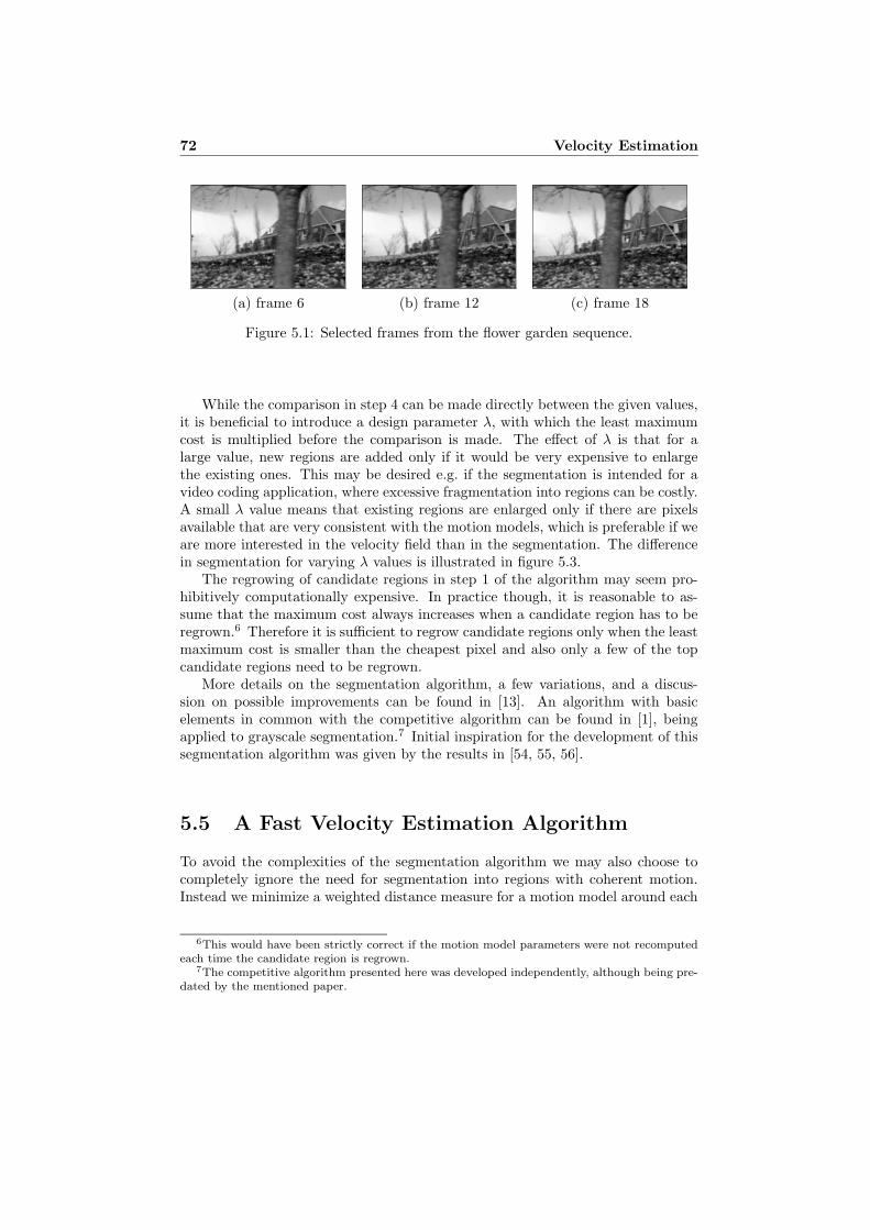
72 Velocity Estimation
(a) frame 6 (b) frame 12 (c) frame 18
Figure 5.1: Selected frames from the flower garden sequence.
While the comparison in step 4 can be made directly between the given values,it is beneficial to introduce a design parameter λ, with which the least maximumcost is multiplied before the comparison is made. The effect of λ is that for alarge value, new regions are added only if it would be very expensive to enlargethe existing ones. This may be desired e.g. if the segmentation is intended for avideo coding application, where excessive fragmentation into regions can be costly.A small λ value means that existing regions are enlarged only if there are pixelsavailable that are very consistent with the motion models, which is preferable if weare more interested in the velocity field than in the segmentation. The differencein segmentation for varying λ values is illustrated in figure 5.3.
The regrowing of candidate regions in step 1 of the algorithm may seem pro-hibitively computationally expensive. In practice though, it is reasonable to as-sume that the maximum cost always increases when a candidate region has to beregrown.6 Therefore it is sufficient to regrow candidate regions only when the leastmaximum cost is smaller than the cheapest pixel and also only a few of the topcandidate regions need to be regrown.
More details on the segmentation algorithm, a few variations, and a discus-sion on possible improvements can be found in [13]. An algorithm with basicelements in common with the competitive algorithm can be found in [1], beingapplied to grayscale segmentation.7 Initial inspiration for the development of thissegmentation algorithm was given by the results in [54, 55, 56].
5.5 A Fast Velocity Estimation Algorithm
To avoid the complexities of the segmentation algorithm we may also choose tocompletely ignore the need for segmentation into regions with coherent motion.Instead we minimize a weighted distance measure for a motion model around each
6This would have been strictly correct if the motion model parameters were not recomputedeach time the candidate region is regrown.
7The competitive algorithm presented here was developed independently, although being pre-dated by the mentioned paper.
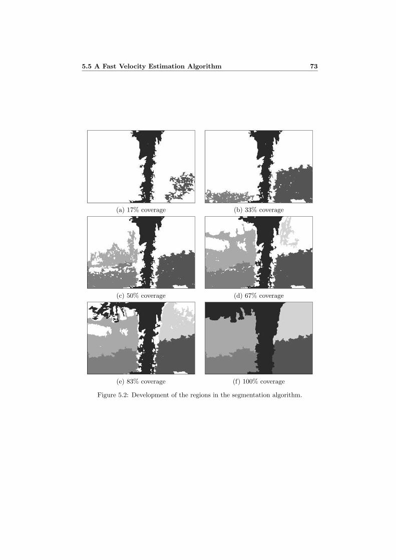
5.5 A Fast Velocity Estimation Algorithm 73
(a) 17% coverage (b) 33% coverage
(c) 50% coverage (d) 67% coverage
(e) 83% coverage (f) 100% coverage
Figure 5.2: Development of the regions in the segmentation algorithm.
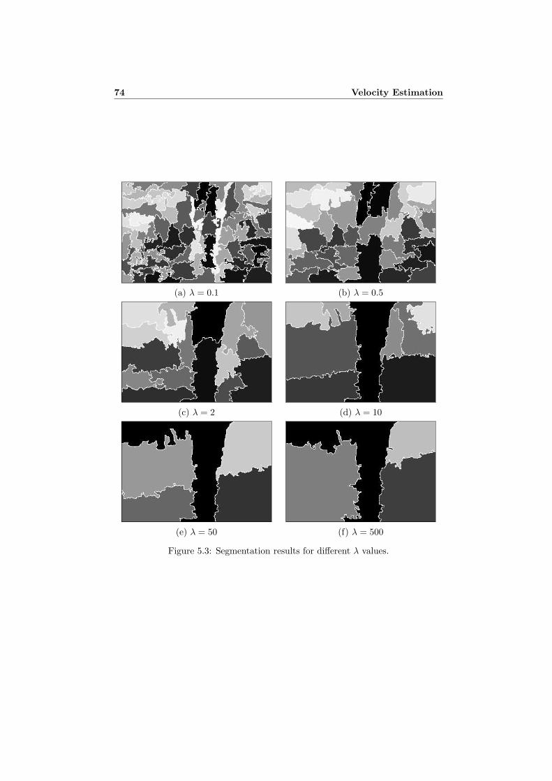
74 Velocity Estimation
(a) λ = 0.1 (b) λ = 0.5
(c) λ = 2 (d) λ = 10
(e) λ = 50 (f) λ = 500
Figure 5.3: Segmentation results for different λ values.
5.6 Evaluation 75
point, i.e. equation (5.18) is replaced by
dtot(p) =∑
i
wid1(vi,Ti) = pT
(∑
i
wiQi
)
p = pT Qtotp, (5.31)
where the sum is taken over a neighborhood of the current point and the weights wi
are given by, e.g., a Gaussian. In effect this means that we convolve the quadraticforms Qi over the image with the weight function, and this operation can beefficiently computed by separable convolution as soon as the weight function isseparable. Another way to look at this operation is as an application of normalizedaveraging, see section 3.8.1, with the weight function as applicability.8 By takingthis view we have the opportunity to set the certainty field to zero close to theborders, which is appropriate if we only use the very fast separable correlationmethod from section 4.7 to compute the tensors, as that method gives incorrectresults at the borders.
The optimal parameters and the corresponding velocity estimates at each pointare computed exactly as in section 5.3.3 and it also turns out that the minimumvalue (5.23) can be used as a confidence measure,9 since it indicates how well thelocal neighborhood is consistent with the motion model in use.
In the simplest case of a constant velocity motion model, we have S = I andhence the averaging of the quadratic forms Qi reduces to an averaging of the tensorfield. This is in fact a well known idea to improve the robustness of the tensors[60], but there are a few important differences. The first one is that we here donot average the original tensor field, but rather the isotropy compensated field.The second difference is that we compute the velocity by equation (5.24), solvingan equation system, rather than by (5.2) or (5.3), which involves the computationof at least one eigenvector.
To summarize the whole algorithm we have the following five steps:
1. Compute the orientation tensor field for the frame, preferably using theseparable correlation method for maximum computational efficiency.
2. Remove the isotropic part of the tensors.
3. Compute quadratic forms, Qi = STi TiSi, according to the chosen motion
model.
4. Apply normalized averaging to the quadratic forms.
5. Solve for the optimal parameters pi and compute the corresponding velocityestimates vi = Sipi.
5.6 Evaluation
The velocity estimation algorithms have been evaluated on two commonly used testsequences with known velocity fields, Lynn Quam’s Yosemite sequence [27], figure
8Notice that this gives a somewhat different scaling of the results, especially at the borders.9Actually it is a reversed confidence measure since small values indicate high confidence.

76 Velocity Estimation
(a) frame 2 (b) frame 9
(c) frame 16 (d) velocity field
Figure 5.4: Selected frames from the Yosemite sequence and the true velocity fieldcorresponding to frame 9 (subsampled).
5.4, and David Fleet’s diverging tree sequence [17], figure 5.5. Both sequences aresynthetic but differs in that the Yosemite sequence is generated with the help ofa digital terrain map and therefore has a motion field with depth variation anddiscontinuities at occlusion boundaries. The diverging tree sequence on the otherhand is only a textured planar surface towards which the camera translates. Hencethe motion field is very regular but the lack of image details leads to difficulties inthe velocity estimation.
5.6.1 Implementation and Performance
All algorithms have been implemented in Matlab, with Normalized Convolution,ordinary convolution/correlation, the segmentation algorithm, and solution of mul-tiple equation systems in the form of C mex files and the rest as highly vectorizedmatlab code.
Typical running times for the different algorithms on a SUN Ultra 60 are givenbelow and relate to the computation of the velocity for one frame of the 252× 316

5.6 Evaluation 77
(a) frame 20 (b) velocity field
Figure 5.5: One frame from the diverging tree sequence and the correspondingtrue velocity field (subsampled).
Yosemite sequence.Velocity estimation with the segmentation algorithm takes about 66 seconds,
distributed with 1.6 seconds for tensor estimation with the separable convolutionmethod, 37 seconds for estimation of the tensors along the border with the normal-ized convolution method,10 0.5 seconds for isotropy compensation, and 27 secondsfor the segmentation algorithm, most of which is spent on the construction of can-didate regions. Here the affine motion model is used, effective size of the kernelsin the tensor estimation is 9 × 9 × 9, and candidate region size m0 is 500.
The fast algorithm with the affine motion model, 11 × 11 × 11 tensors, and a41×41 averaging kernel takes about 16 seconds. Of these, 1.8 seconds are spent ontensor estimation with the separable convolution method, 0.5 seconds on isotropycompensation, 0.3 seconds on computation of the quadratic forms, 8.6 seconds onnormalized averaging, and 4.8 seconds on solving for the velocity.
Finally we have the fast algorithm with the constant velocity motion model,9 × 9 × 9 tensors and 15 × 15 normalized averaging. Here the running time isabout 3.5 seconds, with 1.6 seconds for tensor estimation, 0.5 seconds for isotropycompensation, 1.2 seconds for normalized averaging, and 0.2 seconds for solvingfor the velocity.
5.6.2 Results for the Yosemite Sequence
The accuracy of the velocity estimates has been measured using the average spa-tiotemporal angular error, arccos(vT
estvtrue) [3]. In the Yosemite sequence the skyregion is excluded from the error analysis.
10This can be reduced drastically by the use of separable normalized convolution, which hasnot been implemented yet. In the order of one second should be possible.
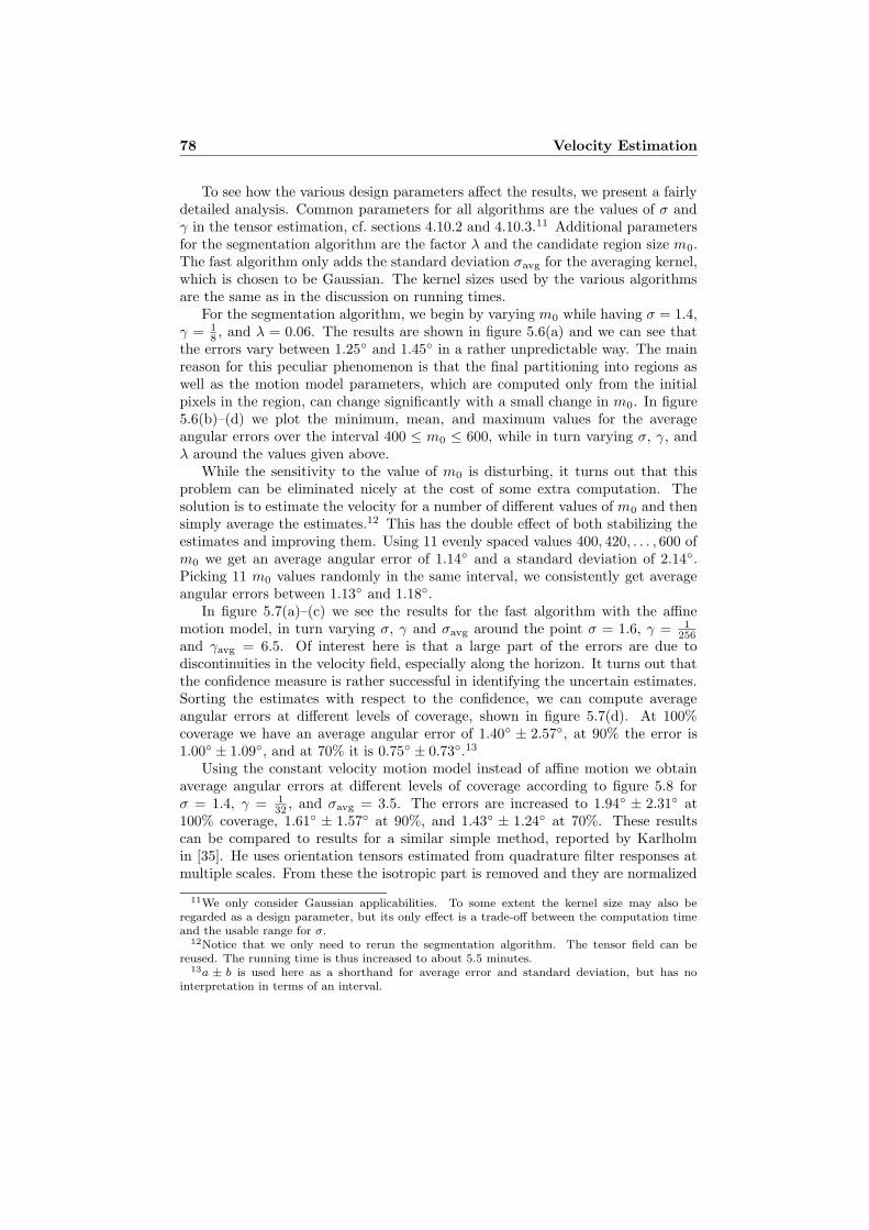
78 Velocity Estimation
To see how the various design parameters affect the results, we present a fairlydetailed analysis. Common parameters for all algorithms are the values of σ andγ in the tensor estimation, cf. sections 4.10.2 and 4.10.3.11 Additional parametersfor the segmentation algorithm are the factor λ and the candidate region size m0.The fast algorithm only adds the standard deviation σavg for the averaging kernel,which is chosen to be Gaussian. The kernel sizes used by the various algorithmsare the same as in the discussion on running times.
For the segmentation algorithm, we begin by varying m0 while having σ = 1.4,γ = 1
8 , and λ = 0.06. The results are shown in figure 5.6(a) and we can see thatthe errors vary between 1.25◦ and 1.45◦ in a rather unpredictable way. The mainreason for this peculiar phenomenon is that the final partitioning into regions aswell as the motion model parameters, which are computed only from the initialpixels in the region, can change significantly with a small change in m0. In figure5.6(b)–(d) we plot the minimum, mean, and maximum values for the averageangular errors over the interval 400 ≤ m0 ≤ 600, while in turn varying σ, γ, andλ around the values given above.
While the sensitivity to the value of m0 is disturbing, it turns out that thisproblem can be eliminated nicely at the cost of some extra computation. Thesolution is to estimate the velocity for a number of different values of m0 and thensimply average the estimates.12 This has the double effect of both stabilizing theestimates and improving them. Using 11 evenly spaced values 400, 420, . . . , 600 ofm0 we get an average angular error of 1.14◦ and a standard deviation of 2.14◦.Picking 11 m0 values randomly in the same interval, we consistently get averageangular errors between 1.13◦ and 1.18◦.
In figure 5.7(a)–(c) we see the results for the fast algorithm with the affinemotion model, in turn varying σ, γ and σavg around the point σ = 1.6, γ = 1
256and γavg = 6.5. Of interest here is that a large part of the errors are due todiscontinuities in the velocity field, especially along the horizon. It turns out thatthe confidence measure is rather successful in identifying the uncertain estimates.Sorting the estimates with respect to the confidence, we can compute averageangular errors at different levels of coverage, shown in figure 5.7(d). At 100%coverage we have an average angular error of 1.40◦ ± 2.57◦, at 90% the error is1.00◦ ± 1.09◦, and at 70% it is 0.75◦ ± 0.73◦.13
Using the constant velocity motion model instead of affine motion we obtainaverage angular errors at different levels of coverage according to figure 5.8 forσ = 1.4, γ = 1
32 , and σavg = 3.5. The errors are increased to 1.94◦ ± 2.31◦ at100% coverage, 1.61◦ ± 1.57◦ at 90%, and 1.43◦ ± 1.24◦ at 70%. These resultscan be compared to results for a similar simple method, reported by Karlholmin [35]. He uses orientation tensors estimated from quadrature filter responses atmultiple scales. From these the isotropic part is removed and they are normalized
11We only consider Gaussian applicabilities. To some extent the kernel size may also beregarded as a design parameter, but its only effect is a trade-off between the computation timeand the usable range for σ.
12Notice that we only need to rerun the segmentation algorithm. The tensor field can bereused. The running time is thus increased to about 5.5 minutes.
13a ± b is used here as a shorthand for average error and standard deviation, but has nointerpretation in terms of an interval.
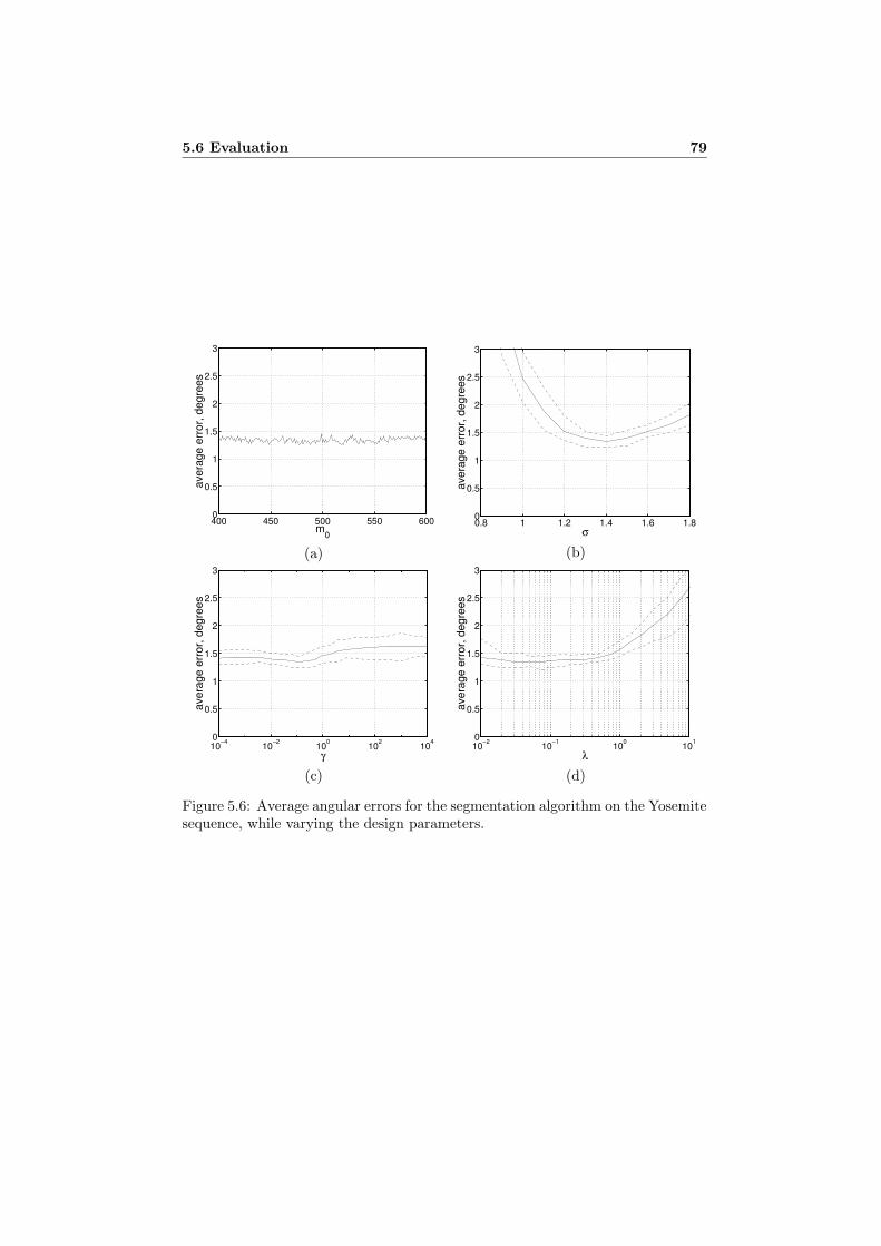
5.6 Evaluation 79
400 450 500 550 6000
0.5
1
1.5
2
2.5
3
m0
aver
age
erro
r, de
gree
s
(a)
0.8 1 1.2 1.4 1.6 1.80
0.5
1
1.5
2
2.5
3
σ
aver
age
erro
r, de
gree
s
(b)
10−4 10−2 100 102 1040
0.5
1
1.5
2
2.5
3
γ
aver
age
erro
r, de
gree
s
(c)
10−2 10−1 100 1010
0.5
1
1.5
2
2.5
3
λ
aver
age
erro
r, de
gree
s
(d)
Figure 5.6: Average angular errors for the segmentation algorithm on the Yosemitesequence, while varying the design parameters.

80 Velocity Estimation
1 1.2 1.4 1.6 1.8 2 2.20
0.5
1
1.5
2
2.5
3
σ
aver
age
erro
r, de
gree
s
(a)
10−4 10−2 100 102 1040
0.5
1
1.5
2
2.5
3
γ
aver
age
erro
r, de
gree
s
(b)
2 4 6 8 10 12 140
0.5
1
1.5
2
2.5
3
σ2
aver
age
erro
r, de
gree
s
(c)
0 20 40 60 80 1000
0.5
1
1.5
2
2.5
3
Coverage (%)
aver
age
erro
r, de
gree
s
(d)
Figure 5.7: (a)–(c): Average angular errors for the fast algorithm with the affinemotion model on the Yosemite sequence, while varying the design parameters. (d):Average angular errors at different levels of coverage. The dashed lines are thecorresponding standard deviations.

5.6 Evaluation 81
0 20 40 60 80 1000
0.5
1
1.5
2
2.5
3
Coverage (%)
aver
age
erro
r, de
gree
s
Figure 5.8: Average angular errors for the fast algorithm with the constant velocitymotion model on the Yosemite sequence at different levels of coverage. The dashedline gives the corresponding standard deviations.
with respect to the largest eigenvalue. Finally the squared tensors are averagedusing a 21 × 21 Gaussian kernel with standard deviation 6 and the velocity isestimated from the smallest eigenvector as in equation (5.3). This gives averageangular errors of 2.44◦ ± 2.06◦ at 90% coverage and 2.23◦ ± 1.94◦ at 70%, usingthe quotient λ2
λ1
as confidence measure.It would also be conceivable to use the eight parameter motion model with the
fast algorithm but it turns out to give no better results than the affine motionmodel. In fact the results are slightly worse, probably due to model overfitting.14
Some statistics on the distribution of errors for the three evaluated methodsare given in table 5.1. Comparison with previously published results, table 5.2,shows that the algorithms presented here are substantially more accurate thanexisting methods.
segmentation fast, affine fast, constantAverage error 1.14◦ 1.40◦ 1.94◦
Standard deviation 2.14◦ 2.57◦ 2.31◦
< 0.5◦ 32.0% 35.8% 14.1%Proportion < 1◦ 64.4% 65.0% 39.7%of estimates < 2◦ 87.8% 82.1% 70.5%with errors < 3◦ 94.0% 89.7% 83.4%below: < 5◦ 98.0% 95.4% 92.8%
< 10◦ 99.7% 98.8% 98.6%
Table 5.1: Distribution of errors for the Yosemite sequence.
14The constant velocity motion model and the eight parameter motion model can of coursebe used with the segmentation algorithm too, but do not lead to any improvements for thissequence.
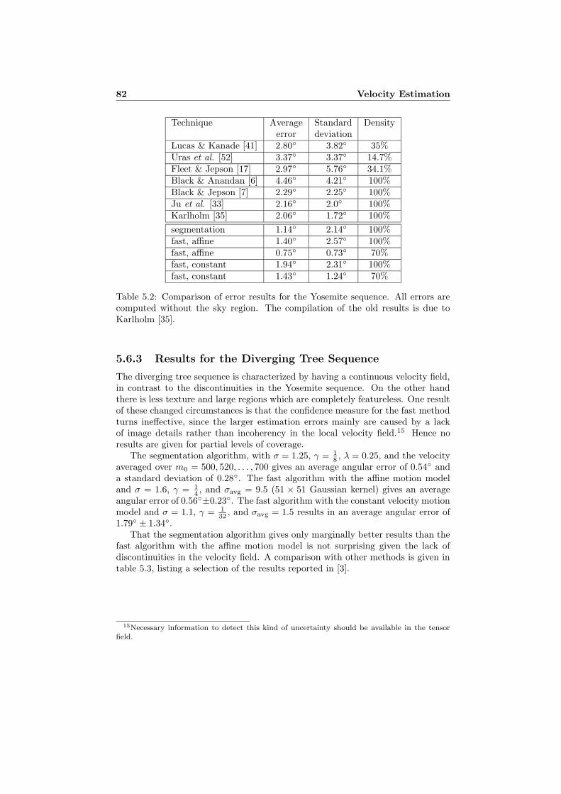
82 Velocity Estimation
Technique Average Standard Densityerror deviation
Lucas & Kanade [41] 2.80◦ 3.82◦ 35%Uras et al. [52] 3.37◦ 3.37◦ 14.7%Fleet & Jepson [17] 2.97◦ 5.76◦ 34.1%Black & Anandan [6] 4.46◦ 4.21◦ 100%Black & Jepson [7] 2.29◦ 2.25◦ 100%Ju et al. [33] 2.16◦ 2.0◦ 100%Karlholm [35] 2.06◦ 1.72◦ 100%
segmentation 1.14◦ 2.14◦ 100%fast, affine 1.40◦ 2.57◦ 100%fast, affine 0.75◦ 0.73◦ 70%fast, constant 1.94◦ 2.31◦ 100%fast, constant 1.43◦ 1.24◦ 70%
Table 5.2: Comparison of error results for the Yosemite sequence. All errors arecomputed without the sky region. The compilation of the old results is due toKarlholm [35].
5.6.3 Results for the Diverging Tree Sequence
The diverging tree sequence is characterized by having a continuous velocity field,in contrast to the discontinuities in the Yosemite sequence. On the other handthere is less texture and large regions which are completely featureless. One resultof these changed circumstances is that the confidence measure for the fast methodturns ineffective, since the larger estimation errors mainly are caused by a lackof image details rather than incoherency in the local velocity field.15 Hence noresults are given for partial levels of coverage.
The segmentation algorithm, with σ = 1.25, γ = 18 , λ = 0.25, and the velocity
averaged over m0 = 500, 520, . . . , 700 gives an average angular error of 0.54◦ anda standard deviation of 0.28◦. The fast algorithm with the affine motion modeland σ = 1.6, γ = 1
4 , and σavg = 9.5 (51 × 51 Gaussian kernel) gives an averageangular error of 0.56◦±0.23◦. The fast algorithm with the constant velocity motionmodel and σ = 1.1, γ = 1
32 , and σavg = 1.5 results in an average angular error of1.79◦ ± 1.34◦.
That the segmentation algorithm gives only marginally better results than thefast algorithm with the affine motion model is not surprising given the lack ofdiscontinuities in the velocity field. A comparison with other methods is given intable 5.3, listing a selection of the results reported in [3].
15Necessary information to detect this kind of uncertainty should be available in the tensorfield.
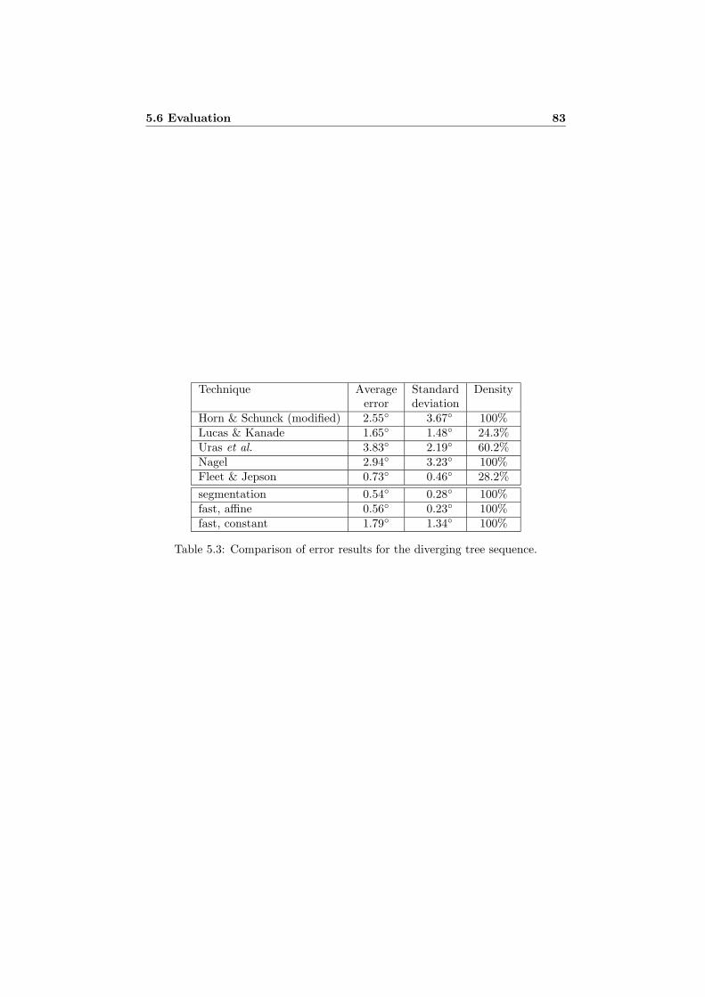
5.6 Evaluation 83
Technique Average Standard Densityerror deviation
Horn & Schunck (modified) 2.55◦ 3.67◦ 100%Lucas & Kanade 1.65◦ 1.48◦ 24.3%Uras et al. 3.83◦ 2.19◦ 60.2%Nagel 2.94◦ 3.23◦ 100%Fleet & Jepson 0.73◦ 0.46◦ 28.2%
segmentation 0.54◦ 0.28◦ 100%fast, affine 0.56◦ 0.23◦ 100%fast, constant 1.79◦ 1.34◦ 100%
Table 5.3: Comparison of error results for the diverging tree sequence.

84 Velocity Estimation
Chapter 6
Future Research Directions
In this chapter we look at some further developments of the ideas and methodspresented in the thesis. The first two sections expand the spatial domain frame-work to phase estimation and adaptive filtering respectively, while the last sectionoutlines the strategy for adapting the framework to irregularly sampled signals.Since this is research in progress, the presentation is by necessity short and sketchy.
6.1 Phase Functionals
The concept of orientation functionals from section 4.3 can straightforwardly beextended to a novel and powerful representation for phase, or rather a combinedorientation and phase representation.
With U defined by equation (4.9), a phase functional is a mapping
θ : U −→ C (6.1)
that to each direction vector assigns a complex value. The magnitude of the valueis interpreted as a measure of the signal variation along the direction, while theargument of the value is interpreted as the local phase of the signal with respectto the direction. If we reverse the direction the magnitude should be unchangedwhile the argument should be negated. Hence we require that θ be Hermitian, i.e.that
θ(−u) = θ(u)∗, all u ∈ U . (6.2)
It is clear that by taking the magnitude1 of a phase functional we obtain anorientation functional.
The method for estimation of orientation tensors in section 4.5 can be extendedto estimation of phase after some preparations. To begin with we use a more liberaldefinition of signal phase than is usual. Instead of relating it to the phase of asinusoidal it is interpreted as some relation between the odd and even parts of the
1Or the squared magnitude or something similar.

86 Future Research Directions
arg φ ei arg φ interpretation0 1 even, local maximumπ2 i odd, decreasing
π −1 even, local minimum−π
2 −i odd, increasing
Table 6.1: Interpretation of local phase.
signal, DC component excluded. A similar approach to the definition of phase istaken by Nordberg in [43]. Table 6.1 lists the primary characteristics of the phase.With the signal model given by equation (4.13) it is clear that A represents theeven part of the signal, excluding the DC component, while b represents the oddpart. Thus it should be possible to construct a phase functional from A and b.
Unfortunately we cannot use a quadratic form to represent phase, as we didwith the tensor for orientation. The reason for this is that quadratic forms bynecessity give even functionals, a property that is compatible with being Hermitianonly if they are also real-valued. A way to get around this is to add one dimensionto the representation and use a quadratic form with respect to
u =
(u1
)
. (6.3)
By setting the phase tensor
P = −(
A iγbiγbT 0
)
, (6.4)
where γ has a similar role to that in the construction of the orientation tensor, weobtain the phase functional
θP(u) = uT Pu = −uT Au − i2γbT u. (6.5)
If we take the magnitude of this phase functional we obtain an orientation func-tional that is different from the orientation tensor in section 4.5 but it is interestingto notice that the latter appears in
uT PP∗u = uT (AAT + γ2bbT + γ2(bT b)I)u, (6.6)
with only an extra isotropic term in the tensor.
6.2 Adaptive Filtering
The idea of adaptive filtering, as described in [22], is to apply a space-variantfilter to a signal, where the filter shape at each point is determined by the localorientation. In order for this operation to be practically feasible, it is required thatthe different filter shapes can be constructed as linear combinations of a small set
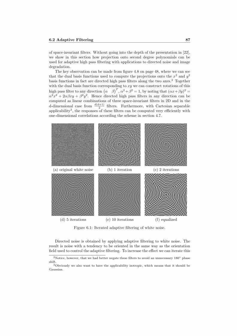
6.2 Adaptive Filtering 87
of space-invariant filters. Without going into the depth of the presentation in [22],we show in this section how projection onto second degree polynomials can beused for adaptive high pass filtering with applications to directed noise and imagedegradation.
The key observation can be made from figure 4.8 on page 48, where we can seethat the dual basis functions used to compute the projections onto the x2 and y2
basis functions in fact are directed high pass filters along the two axes.2 Togetherwith the dual basis function corresponding to xy we can construct rotations of this
high pass filter to any direction(α β
)T, α2+β2 = 1, by noting that (αx+βy)2 =
α2x2 + 2αβxy + β2y2. Hence directed high pass filters in any direction can becomputed as linear combinations of three space-invariant filters in 2D and in the
d-dimensional case from d(d+1)2 filters. Furthermore, with Cartesian separable
applicability3, the responses of these filters can be computed very efficiently withone-dimensional correlations according the scheme in section 4.7.
(a) original white noise (b) 1 iteration (c) 2 iterations
(d) 5 iterations (e) 10 iterations (f) equalized
Figure 6.1: Iterated adaptive filtering of white noise.
Directed noise is obtained by applying adaptive filtering to white noise. Theresult is noise with a tendency to be oriented in the same way as the orientationfield used to control the adaptive filtering. To increase the effect we can iterate this
2Notice, however, that we had better negate these filters to avoid an unnecessary 180◦ phaseshift.
3Obviously we also want to have the applicability isotropic, which means that it should beGaussian.
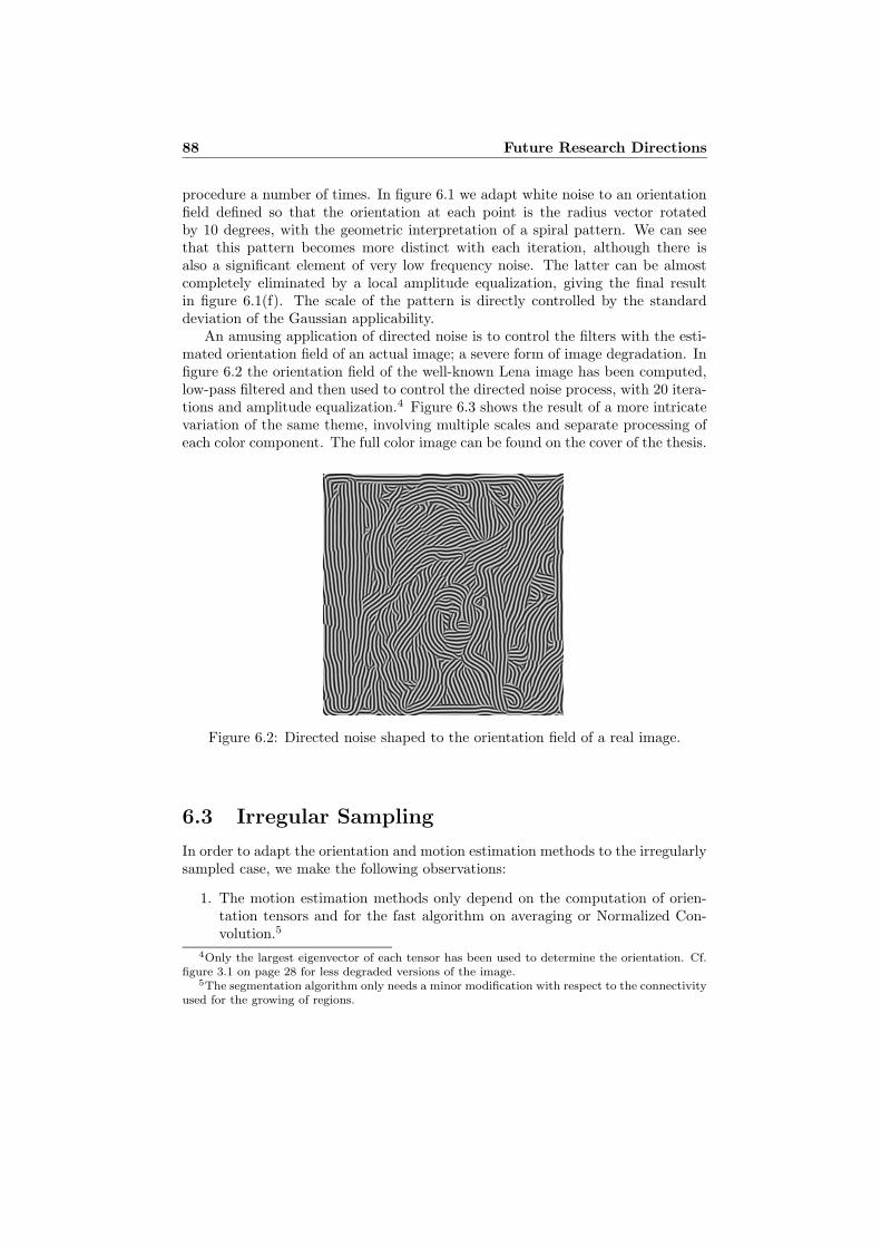
88 Future Research Directions
procedure a number of times. In figure 6.1 we adapt white noise to an orientationfield defined so that the orientation at each point is the radius vector rotatedby 10 degrees, with the geometric interpretation of a spiral pattern. We can seethat this pattern becomes more distinct with each iteration, although there isalso a significant element of very low frequency noise. The latter can be almostcompletely eliminated by a local amplitude equalization, giving the final resultin figure 6.1(f). The scale of the pattern is directly controlled by the standarddeviation of the Gaussian applicability.
An amusing application of directed noise is to control the filters with the esti-mated orientation field of an actual image; a severe form of image degradation. Infigure 6.2 the orientation field of the well-known Lena image has been computed,low-pass filtered and then used to control the directed noise process, with 20 itera-tions and amplitude equalization.4 Figure 6.3 shows the result of a more intricatevariation of the same theme, involving multiple scales and separate processing ofeach color component. The full color image can be found on the cover of the thesis.
Figure 6.2: Directed noise shaped to the orientation field of a real image.
6.3 Irregular Sampling
In order to adapt the orientation and motion estimation methods to the irregularlysampled case, we make the following observations:
1. The motion estimation methods only depend on the computation of orien-tation tensors and for the fast algorithm on averaging or Normalized Con-volution.5
4Only the largest eigenvector of each tensor has been used to determine the orientation. Cf.figure 3.1 on page 28 for less degraded versions of the image.
5The segmentation algorithm only needs a minor modification with respect to the connectivityused for the growing of regions.
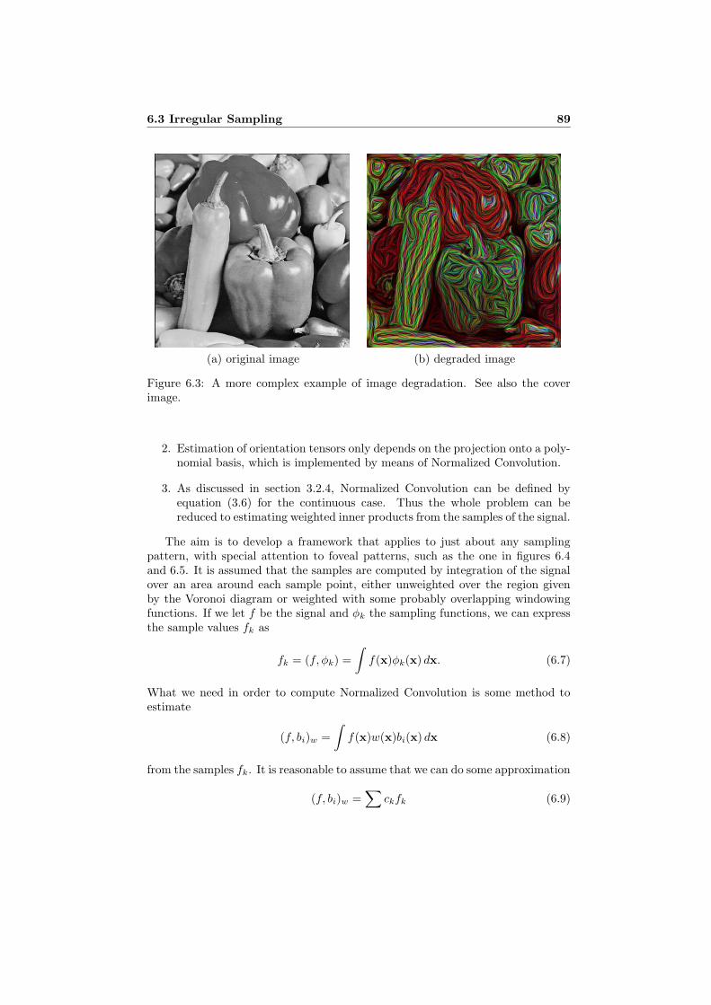
6.3 Irregular Sampling 89
(a) original image (b) degraded image
Figure 6.3: A more complex example of image degradation. See also the coverimage.
2. Estimation of orientation tensors only depends on the projection onto a poly-nomial basis, which is implemented by means of Normalized Convolution.
3. As discussed in section 3.2.4, Normalized Convolution can be defined byequation (3.6) for the continuous case. Thus the whole problem can bereduced to estimating weighted inner products from the samples of the signal.
The aim is to develop a framework that applies to just about any samplingpattern, with special attention to foveal patterns, such as the one in figures 6.4and 6.5. It is assumed that the samples are computed by integration of the signalover an area around each sample point, either unweighted over the region givenby the Voronoi diagram or weighted with some probably overlapping windowingfunctions. If we let f be the signal and φk the sampling functions, we can expressthe sample values fk as
fk = (f, φk) =
∫
f(x)φk(x) dx. (6.7)
What we need in order to compute Normalized Convolution is some method toestimate
(f, bi)w =
∫
f(x)w(x)bi(x) dx (6.8)
from the samples fk. It is reasonable to assume that we can do some approximation
(f, bi)w =∑
ckfk (6.9)
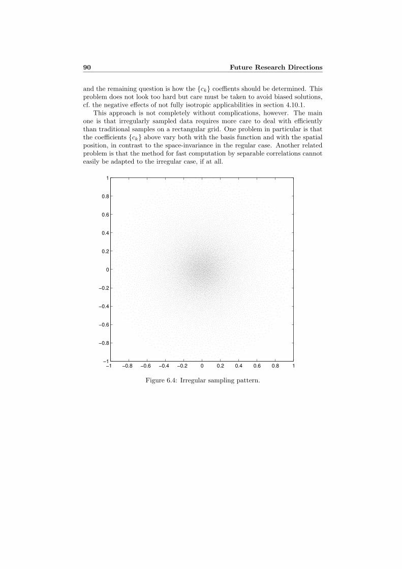
90 Future Research Directions
and the remaining question is how the {ck} coeffients should be determined. Thisproblem does not look too hard but care must be taken to avoid biased solutions,cf. the negative effects of not fully isotropic applicabilities in section 4.10.1.
This approach is not completely without complications, however. The mainone is that irregularly sampled data requires more care to deal with efficientlythan traditional samples on a rectangular grid. One problem in particular is thatthe coefficients {ck} above vary both with the basis function and with the spatialposition, in contrast to the space-invariance in the regular case. Another relatedproblem is that the method for fast computation by separable correlations cannoteasily be adapted to the irregular case, if at all.
−1 −0.8 −0.6 −0.4 −0.2 0 0.2 0.4 0.6 0.8 1−1
−0.8
−0.6
−0.4
−0.2
0
0.2
0.4
0.6
0.8
1
Figure 6.4: Irregular sampling pattern.
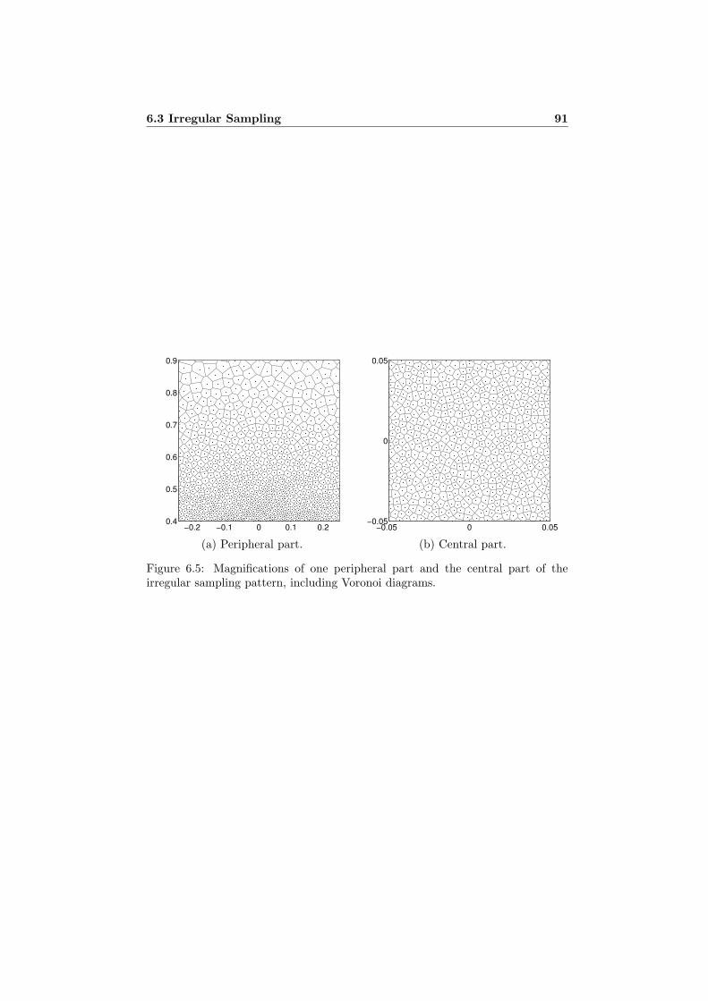
6.3 Irregular Sampling 91
−0.2 −0.1 0 0.1 0.20.4
0.5
0.6
0.7
0.8
0.9
(a) Peripheral part.
−0.05 0 0.05−0.05
0
0.05
(b) Central part.
Figure 6.5: Magnifications of one peripheral part and the central part of theirregular sampling pattern, including Voronoi diagrams.

92 Future Research Directions
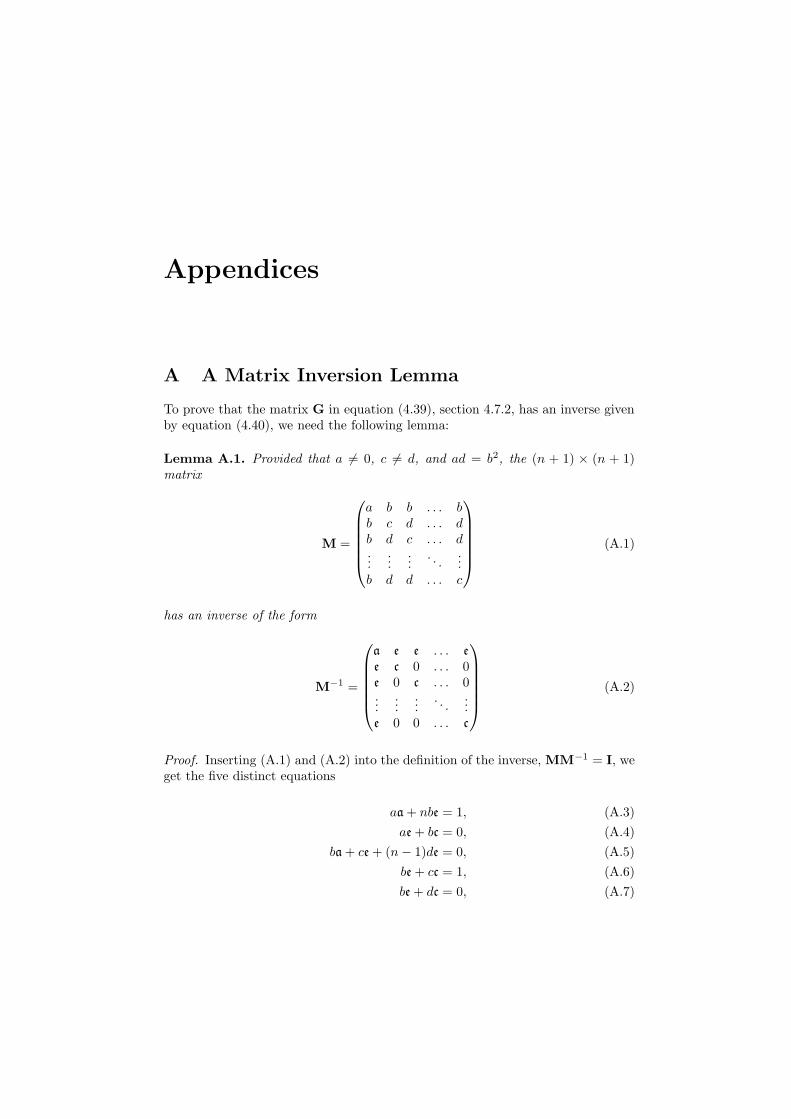
Appendices
A A Matrix Inversion Lemma
To prove that the matrix G in equation (4.39), section 4.7.2, has an inverse givenby equation (4.40), we need the following lemma:
Lemma A.1. Provided that a 6= 0, c 6= d, and ad = b2, the (n + 1) × (n + 1)matrix
M =
a b b . . . bb c d . . . db d c . . . d...
......
. . ....
b d d . . . c
(A.1)
has an inverse of the form
M−1 =
a e e . . . e
e c 0 . . . 0e 0 c . . . 0...
......
. . ....
e 0 0 . . . c
(A.2)
Proof. Inserting (A.1) and (A.2) into the definition of the inverse, MM−1 = I, weget the five distinct equations
aa + nbe = 1, (A.3)
ae + bc = 0, (A.4)
ba + ce + (n − 1)de = 0, (A.5)
be + cc = 1, (A.6)
be + dc = 0, (A.7)
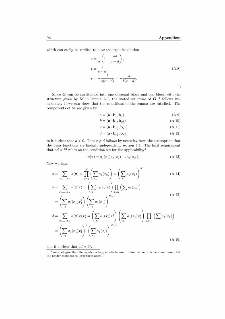
94 Appendices
which can easily be verified to have the explicit solution
a =1
a
(
1 +nd
c − d
)
,
c =1
c − d,
e = − b
a(c − d)= − d
b(c − d).
(A.8)
Since G can be partitioned into one diagonal block and one block with thestructure given by M in lemma A.1, the stated structure of G−1 follows im-mediately if we can show that the conditions of the lemma are satisfied. Thecomponents of M are given by
a = (a · b1,b1) (A.9)
b = (a · b1,bx2
i) (A.10)
c = (a · bx2
i,bx2
i) (A.11)
d = (a · bx2
i,bx2
j) (A.12)
so it is clear that a > 0. That c 6= d follows by necessity from the assumption thatthe basis functions are linearly independent, section 4.4. The final requirementthat ad = b2 relies on the condition set for the applicability1
a(x) = a1(x1)a1(x2) . . . a1(xN ). (A.13)
Now we have
a =∑
x1,...,xN
a(x) =N∏
k=1
(∑
xk
a1(xk)
)
=
(∑
x1
a1(x1)
)N
(A.14)
b =∑
x1,...,xN
a(x)x2i =
(∑
xi
a1(xi)x2i
)∏
k 6=i
(∑
a1(xk))
=
(∑
x1
a1(x1)x21
)(∑
x1
a1(x1)
)N−1(A.15)
d =∑
x1,...,xN
a(x)x2i x
2j =
(∑
xi
a1(xi)x2i
)
∑
xj
a1(xj)x2j
∏
k 6=i,j
(∑
a1(xk))
=
(∑
x1
a1(x1)x21
)2(∑
x1
a1(x1)
)N−2
(A.16)
and it is clear that ad = b2.1We apologize that the symbol a happens to be used in double contexts here and trust that
the reader manages to keep them apart.
B Cartesian Separable and Isotropic Functions 95
B Cartesian Separable and Isotropic Functions
As we saw in section 4.7.2, a desirable property of the applicability is to simulta-neously be Cartesian separable and isotropic. In this appendix we show that theonly interesting class of functions having this property is the Gaussians.
Lemma B.1. Assume that f : RN −→ R, N ≥ 2, is Cartesian separable,
f(x) = f1(x1)f2(x2) . . . fN (xN ), some {fk : R −→ R}Nk=1, (B.1)
isotropic,
f(x) = g(xT x), some g : R+ ∪ {0} −→ R, (B.2)
and partially differentiable. Then f must be of the form
f(x) = AeCxTx, (B.3)
for some real constants A and C.
Proof. We first assume that f is zero for some x. Then at least one factor in (B.1)is zero and by varying the remaining coordinates it follows that
g(t) = 0, all t ≥ α2, (B.4)
where α is the value of the coordinate in the zero factor. By taking
x =α√N
(1 1 . . . 1
)T(B.5)
we can repeat the argument to get
g(t) = 0, all t ≥ α2
N. (B.6)
and continuing like this we find that g(t) = 0, all t > 0, and since f is partiallydifferentiable there cannot be a point discontinuity at the origin, so f must beidentically zero. This is clearly a valid solution.
If instead f is nowhere zero we can compute the partial derivatives as
∂∂xk
f(x)
f(x)=
f ′k(xk)
fk(xk)= 2xk
g′(xT x)
g(xT x), k = 1, 2, . . . , N. (B.7)
Restricting ourselves to one of the hyper quadrants, so that all xk 6= 0, we get
g′(xT x)
g(xT x)=
f ′1(x1)
2x1f1(x1)=
f ′2(x2)
2x2f2(x2)= · · · =
f ′N (xN )
2xNfN (xN ), (B.8)
which is possible only if they all have a common constant value C. Hence we getg from the differential equation
g′(t) = Cg(t) (B.9)
96 Appendices
with the solution
g(t) = AeCt. (B.10)
It follows that f in each hyper quadrant must have the form
f(x) = AeCxTx (B.11)
and in order to get isotropy, the constants must be the same for all hyper quad-rants. The case A = 0 corresponds to the identically zero solution.
A weakness of this result is the condition that f be partially differentiable,which is not a natural requirement of an applicability function. If we remove thiscondition it is easy to find one new solution, which is zero everywhere except atthe origin. What is not so easy to see however, and quite contra-intuitive, is thatthere also exist solutions which are discontinuous and everywhere positive. Toconstruct these we need another lemma.
Lemma B.2. There do exist discontinuous functions L : R −→ R which areadditive, i.e.
L(x + y) = L(x) + L(y), x, y ∈ R. (B.12)
Proof. See [48] or [18].
With L from the lemma we get a Cartesian separable and isotropic functionby the construction
f(x) = eL(xTx). (B.13)
This function is very bizarre, however, because it has to be discontinuous at everypoint and unbounded in every neighborhood of every point. It is also completelyuseless as an applicability since it is unmeasurable, i.e. it cannot be integrated.
To eliminate this kind of strange solutions it is sufficient to introduce some veryweak regularity constraints2 on f . Unfortunately the proofs become very technicalif we want to have a bare minimum of regularity. Instead we explore what can beaccomplished with a regularization approach.
Let the functions φσ and Φσ be normalized Gaussians with standard deviationσ in one and N dimensions respectively,
φσ(x) =1√2πσ
e−x2
2σ2 (B.14)
Φσ(x) =1
(2π)N2 σN
e−x
Tx
2σ2 =
N∏
k=1
φσ(xk) (B.15)
2See e.g. [18] and exercise 9.18 in [44].
B Cartesian Separable and Isotropic Functions 97
We now make the reasonable assumption that f is regular enough to be convolvedwith Gaussians,3
fσ(x) = (f ∗ Φσ)(x) =
∫
RN
f(x − y)Φσ(y) dy, σ > 0. (B.16)
The convolved functions retain the properties of f to be Cartesian separable andisotropic. The first property can be verified by
fσ(x) =
∫
RN
f1(x1 − y1) . . . fN (xN − yN )φσ(y1) . . . φσ(yN ) dy
=N∏
k=1
∫
R
fk(xk − yk)φσ(yk) dyk.
(B.17)
To show the second property we notice that isotropy is equivalent to rotationinvariance, i.e. for an arbitrary rotation matrix R we have f(Rx) = f(x). Sincethe Gaussians are rotation invariant too, we have
fσ(Rx) =
∫
RN
f(Rx − y)Φσ(y) dy
=
∫
RN
f(Rx − Ru)Φσ(Ru) du
=
∫
RN
f(x − u)Φσ(u) du = fσ(x).
(B.18)
Another property that the convolved functions obtain is a high degree of regularity.Without making additional assumptions on the regularity of f , fσ is guaranteed tobe infinitely differentiable because Φσ has that property. This means that lemmaB.1 applies to fσ, which therefore has to be a Gaussian.
To connect the convolved functions to f itself we notice that the GaussiansΦσ approach the Dirac distribution as σ approaches zero; they become more andmore concentrated to the origin. As a consequence the convolved functions fσ
approach f and in the limit we find that f has to be a Gaussian, at least almosteverywhere.4
Another way to reach this conclusion is to assume that f can be Fourier trans-
formed. Then equation (B.16) turns into fσ(u) = f(u)Φσ(u), so that f(u) = fσ(u)
Φσ(u)
is a quotient of two Gaussians and hence itself a Gaussian. Inverse Fourier trans-formation gives the desired result.
3This mainly requires f to be locally integrable. The point is, however, that it would beuseless as an applicability if it could not be convolved with Gaussians.
4Almost everywhere is quite sufficient because the applicability is only used in integrals.
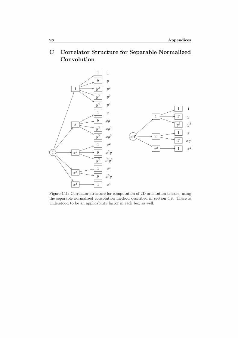
98 Appendices
C Correlator Structure for Separable Normalized
Convolution
?>=<89:;c
1II·······························
1::uuuuuuuuu
1
y55jjjjjjjj
y
y2// y2
y3))TTTTTTTT
y3
y4$$IIIIIIIII
y4
xBB¦¦¦¦¦¦¦¦¦¦¦¦¦¦¦
177ppppppppp
x
y22eeeeeeeexy
y2,,YYYYYYYYxy2
y3''NNNNNNNNN
xy3
x2//
155jjjjjjjj
x2
y// x2y
y2))TTTTTTTT
x2y2
x3!!CCCCCCCCCCCC
122eeeeeeee x3
y,,YYYYYYYYx3y
x4½½66666666666666666
1// x4
GFED@ABCc·f
1=={{{{{{{{{{{
155jjjjjjjj
1
y// y
y2))TTTTTTTT
y2
x//122eeeeeeee x
y,,YYYYYYYYxy
x2''NNNNNNNNN
1// x2
Figure C.1: Correlator structure for computation of 2D orientation tensors, usingthe separable normalized convolution method described in section 4.8. There isunderstood to be an applicability factor in each box as well.
D Angular RMS Error 99
D Angular RMS Error
In this appendix we verify the equivalence between the expressions (4.46) and(4.47) for the angular RMS error in section 4.10.
Starting with
∆φ = arcsin
√√√√ 1
2L
L∑
l=1
‖xxT − e1eT1 ‖2
, (D.1)
we expand the squared Frobenius norm, using the relation ‖T‖2 = tr (TT T), toget
‖xxT − e1eT1 ‖2 = tr
((xxT − e1e
T1 )T (xxT − e1e
T1 ))
= tr(xxT − (xT e1)xeT
1 − (eT1 x)e1x
T + e1eT1
).
(D.2)
To simplify this expression we use the fact that the trace operator is linear andthat tr(abT ) = tr(bT a). Thus we have
‖xxT − e1eT1 ‖2 = 1 − (xT e1)
2 − (eT1 x)2 + 1 = 2(1 − (xT e1)
2) (D.3)
and continuing with the original expression,
∆φ = arcsin
√√√√ 1
2L
L∑
l=1
2(1 − (xT e1)2)
= arcsin
√√√√1 − 1
L
L∑
l=1
(xT e1)2
= arccos
√√√√ 1
L
L∑
l=1
(xT e1)2
.
(D.4)
100 Appendices
E Removing the Isotropic Part of a 3D Tensor
To remove the isotropic part of a 3D tensor we need to compute the smallesteigenvalue of a symmetric and positive semidefinite 3 × 3 matrix T. There are anumber of ways to do this, including inverse iterations and standard methods foreigenvalue factorization. Given the small size of the matrix in this case, however,we additionally have the option of computing the eigenvalues algebraically, sincethese can be expressed as the roots of the third degree characteristic polynomial,p(λ) = det(T − λI).
To find the solutions to z3 + az2 + bz + c = 0 we first remove the quadraticterm with the translation z = x − a
3 , yielding
x3 + px + q = 0. (E.1)
It is well known that the solutions to this equation can be given by Cardano’sformula [53]
D =(p
3
)3
+(q
2
)2
, (E.2)
u = 3
√
−q
2+
√D, (E.3)
v = 3
√
−q
2−
√D, (E.4)
x1 = u + v, (E.5)
x2 = −u + v
2+
u − v
2i√
3, (E.6)
x3 = −u + v
2− u − v
2i√
3. (E.7)
Unfortunately this formula leads to some complications in the choice of thecomplex cubic roots if D < 0, which happens exactly when we have three distinctreal roots. Since we have a symmetric and positive semidefinite matrix we knowa priori that all eigenvalues are real and non-negative.5
A better approach in this case, still following [53], is to make the scaling x =√
− 4p3 y, leading to
4y3 − 3y =3q
p√
− 4p3
. (E.8)
Taking advantage of the identity cos 3α = 4 cos3 α − 3 cos α, we make the substi-tution y = cosα to get the equation
cos 3α =3q
p√
− 4p3
, (E.9)
5For the following discussion it is sufficient that we have a symmetric matrix and thus realeigenvalues.
E Removing the Isotropic Part of a 3D Tensor 101
where the right hand side is guaranteed to have an absolute value less than orequal to one if all the roots are indeed real. Hence it is clear that we obtain thethree real solutions to (E.1) from
β =
√
−4p
3, (E.10)
α =1
3arccos
3q
pβ, (E.11)
x1 = β cosα, (E.12)
x2 = β cos
(
α − 2π
3
)
, (E.13)
x3 = β cos
(
α +2π
3
)
. (E.14)
Furthermore, since we have 0 ≤ α ≤ π3 , it follows that x1 ≥ x2 ≥ x3.
In terms of the tensor T, the above discussion leads to the following algorithmfor removal of the isotropic part:
1. Remove the trace of T by computing
T′ = T − trT
3I =
a d ed b fe f c
. (E.15)
This is equivalent to removing the quadratic term from the characteristicpolynomial.
2. The eigenvalues of T′ are now given as the solutions to x3 + px + q = 0,where
p = ab + ac + bc − d2 − e2 − f2, (E.16)
q = af2 + be2 + cd2 − 2def − abc. (E.17)
3. Let
β =
√
−4p
3, (E.18)
α =1
3arccos
3q
pβ, (E.19)
so that the eigenvalues of T′ are given by (E.12) – (E.14).
4. Let
x3 = β cos
(
α +2π
3
)
(E.20)
and compute the isotropy compensated tensor T′′ as
T′′ = T′ − x3I. (E.21)

102 Appendices
It should be noted that this method may numerically be somewhat less accuratethan standard methods for eigenvalue factorization. For the current application,however, this is not an issue at all.6
A slightly different formula for the eigenvalues of a real, symmetric 3 × 3 ma-trix can be found in [46] and a closed form formula for eigenvectors as well aseigenvalues in [8].
6Except making sure that the magnitude of the argument to the arccosine is not very slightlylarger than one.
Bibliography
[1] R. Adams and L. Bischof. Seeded region growing. IEEE Transactions onPattern Analysis and Machine Intelligence, 16(6):641–647, June 1994.
[2] M. Andersson, J. Wiklund, and H. Knutsson. Sequential Filter Treesfor Efficient 2D 3D and 4D Orientation Estimation. Report LiTH-ISY-R-2070, ISY, SE-581 83 Linkoping, Sweden, November 1998. URL:http://www.isy.liu.se/cvl/ScOut/TechRep/TechRep.html.
[3] J. L. Barron, D. J. Fleet, and S. S. Beauchemin. Performance of optical flowtechniques. Int. J. of Computer Vision, 12(1):43–77, 1994.
[4] J. Bigun. Local Symmetry Features in Image Processing. PhD thesis,Linkoping University, Sweden, 1988. Dissertation No 179, ISBN 91-7870-334-4.
[5] A. Bjorck. Numerical Methods for Least Squares Problems. SIAM, Societyfor Industrial and Applied Mathematics, 1996.
[6] M. J. Black and P. Anandan. The robust estimation of multiple motions:Parametric and piecewise-smooth flow fields. Computer Vision and ImageUnderstanding, 63(1):75–104, Jan. 1996.
[7] M. J. Black and A. Jepson. Estimating optical flow in segmented images usingvariable-order parametric models with local deformations. IEEE Transactionson Pattern Analysis and Machine Intelligence, 18(10):972–986, 1996.
[8] A.W. Bojanczyk and A. Lutoborski. Computation of the euler angles of asymmetric 3 × 3 matrix. SIAM J. Matrix Anal. Appl., 12(1):41–48, January1991.
[9] R. Bracewell. The Fourier Transform and its Applications. McGraw-Hill, 2ndedition, 1986.
[10] K. Daniilidis and V. Kruger. Optical flow computation in the log-polar plane.In Proceedings 6th Int. Conf. on Computer Analysis of Images and Patterns,pages 65–72. Springer-Verlag, Berlin, Germany, 1995.
104 Bibliography
[11] F. Dufaux and F. Moscheni. Segmentation-based motion estimation for secondgeneration video coding techniques. In L. Torres and M. Kunt, editors, VideoCoding: The Second Generation Approach, chapter 6, pages 219–263. KluwerAcademic Publishers, 1996.
[12] L. Elden. A Weighted Pseudoinverse, Generalized Singular Values, and Con-strained Least Squares Problems. BIT, 22:487–502, 1982.
[13] G. Farneback. Motion-based Segmentation of Image Sequences. Master’s The-sis LiTH-ISY-EX-1596, Computer Vision Laboratory, SE-581 83 Linkoping,Sweden, May 1996.
[14] G. Farneback. Motion-based segmentation of image sequences using orien-tation tensors. In Proceedings of the SSAB Symposium on Image Analysis,pages 31–35, Stockholm, March 1997. SSAB.
[15] G. Farneback. A unified framework for bases, frames, subspace bases, andsubspace frames. In Proceedings of the 11th Scandinavian Conference onImage Analysis, Kangerlussuaq, Greenland, June 1999. SCIA. Accepted forpublication.
[16] H. G. Feichtinger and K. H. Grochenig. Theory and practice of irregularsampling. In J. Benedetto and M. Frazier, editors, Wavelets: Mathematicsand Applications, pages 305–363. CRC Press, 1994.
[17] D. J. Fleet and A. D. Jepson. Computation of Component Image Velocityfrom Local Phase Information. Int. Journal of Computer Vision, 5(1):77–104,1990.
[18] James Foran. Fundamentals of Real Analysis. M. Dekker, New York, 1991.ISBN 0-8247-8453-7.
[19] G. H. Golub and C. F. Van Loan. Matrix Computations. The Johns HopkinsUniversity Press, second edition, 1989.
[20] G. H. Granlund. In search of a general picture processing operator. ComputerGraphics and Image Processing, 8(2):155–178, 1978.
[21] G. H. Granlund and H. Knutsson. Contrast of structured and homogenousrepresentations. In O. J. Braddick and A. C. Sleigh, editors, Physical andBiological Processing of Images, pages 282–303. Springer Verlag, Berlin, 1983.
[22] G. H. Granlund and H. Knutsson. Signal Processing for Computer Vision.Kluwer Academic Publishers, 1995. ISBN 0-7923-9530-1.
[23] R. M. Haralick. Edge and region analysis for digital image data. ComputerGraphics and Image Processing, 12(1):60–73, January 1980.
[24] R. M. Haralick. Digital step edges from zero crossing of second directionalderivatives. IEEE Transactions on Pattern Analysis and Machine Intelli-gence, PAMI-6(1):58–68, January 1984.
Bibliography 105
[25] R. M. Haralick and L. G. Shapiro. Computer and robot vision, volume 2.Addison-Wesley, 1993.
[26] R. M. Haralick and L. Watson. A facet model for image data. ComputerGraphics and Image Processing, 15(2):113–129, February 1981.
[27] D. J. Heeger. Model for the extraction of image flow. J. Opt. Soc. Am. A,4(8):1455–1471, 1987.
[28] B. Jahne. Motion determination in space-time images. In Image ProcessingIII, pages 147–152. SPIE Proceedings 1135, International Congress on OpticalScience and Engineering, 1989.
[29] B. Jahne. Motion determination in space-time images. In O. Faugeras, editor,Computer Vision-ECCV90, pages 161–173. Springer-Verlag, 1990.
[30] B. Jahne. Digital Image Processing: Concepts, Algorithms and ScientificApplications. Springer Verlag, Berlin, Heidelberg, 1991.
[31] B. Jahne. Spatio-Temporal Image Processing: Theory and Scientific Applica-tions. Springer Verlag, Berlin, Heidelberg, 1993. ISBN 3-540-57418-2.
[32] B. Jahne. Practical Handbook on Image Processing for Scientific Applications.CRC Press LLC, 1997. ISBN 0-8493-8906-2.
[33] S. X. Ju, M. J. Black, and A. D. Jepson. Skin and bones: Multi-layer,locally affine, optical flow and regularization with transparency. In ProceedingsCVPR’96, pages 307–314. IEEE, 1996.
[34] T. Kailath. Linear Systems. Information and System Sciences Series. Prentice-Hall, Englewood Cliffs, N.J., 1980.
[35] J. Karlholm. Local Signal Models for Image Sequence Analysis. PhD thesis,Linkoping University, Sweden, SE-581 83 Linkoping, Sweden, 1998. Disserta-tion No 536, ISBN 91-7219-220-8.
[36] H. Knutsson. Representing local structure using tensors. In The 6th Scan-dinavian Conference on Image Analysis, pages 244–251, Oulu, Finland, June1989. Report LiTH–ISY–I–1019, Computer Vision Laboratory, LinkopingUniversity, Sweden, 1989.
[37] H. Knutsson and M. Andersson. Optimization of Sequential Filters.In Proceedings of the SSAB Symposium on Image Analysis, pages 87–90, Linkoping, Sweden, March 1995. SSAB. LiTH-ISY-R-1797. URL:http://www.isy.liu.se/cvl/ScOut/TechRep/TechRep.html.
[38] H. Knutsson and C-F. Westin. Normalized and Differential Convolution:Methods for Interpolation and Filtering of Incomplete and Uncertain Data.In Proceedings of IEEE Computer Society Conference on Computer Visionand Pattern Recognition, pages 515–523, New York City, USA, June 1993.IEEE.
106 Bibliography
[39] H. Knutsson, C-F. Westin, and G. H. Granlund. Local Multiscale Frequencyand Bandwidth Estimation. In Proceedings of IEEE International Conferenceon Image Processing, pages 36–40, Austin, Texas, November 1994. IEEE.
[40] H. Knutsson, C-F. Westin, and C-J. Westelius. Filtering of Uncertain Irregu-larly Sampled Multidimensional Data. In Twenty-seventh Asilomar Conf. onSignals, Systems & Computers, pages 1301–1309, Pacific Grove, California,USA, November 1993. IEEE.
[41] B. Lucas and T. Kanade. An Iterative Image Registration Technique withApplications to Stereo Vision. In Proc. Darpa IU Workshop, pages 121–130,1981.
[42] L. Massone, G. Sandini, and V. Tagliasco. “Form-invariant” topological map-ping strategy for 2d shape recognition. Computer Vision, Graphics, and Im-age Processing, 30(2):169–188, May 1985.
[43] K. Nordberg. Signal Representation and Processing using Operator Groups.PhD thesis, Linkoping University, Sweden, SE-581 83 Linkoping, Sweden,1995. Dissertation No 366, ISBN 91-7871-476-1.
[44] W. Rudin. Real and Complex Analysis. McGraw-Hill, 3rd edition, 1987. ISBN0-07-054234-1.
[45] H. R. Schwarz. Numerical Analysis: A Comprehensive Introduction. JohnWiley & Sons Ltd., 1989. ISBN 0-471-92064-9.
[46] O. K. Smith. Eigenvalues of a symmetric 3 × 3 matrix. Communications ofthe ACM, 4(4):168, 1961.
[47] M. Tistarelli and G. Sandini. On the advantages of polar and log-polar map-ping for direct estimation of time-to-impact from optical flow. IEEE Trans-actions on Pattern Analysis and Machine Intelligence, 15(4):401–410, April1993.
[48] A. Torchinsky. Real Variables. Addison-Wesley, 1988. ISBN 0-201-15675-X.
[49] M. Ulvklo, G. Granlund, and H. Knutsson. Adaptive reconstruction usingmultiple views. In Proceedings of the IEEE Southwest Symposium on ImageAnalysis and Interpretation, pages 47–52, Tucson, Arizona, USA, April 1998.IEEE. LiTH-ISY-R-2046.
[50] M. Ulvklo, G. H. Granlund, and H. Knutsson. Texture Gradient in SparseTexture Fields. In Proceedings of the 9th Scandinavian Conference on ImageAnalysis, pages 885–894, Uppsala, Sweden, June 1995. SCIA.
[51] M. Ulvklo, H. Knutsson, and G. Granlund. Depth segmentation and occludedscene reconstruction using ego-motion. In Proceedings of the SPIE Conferenceon Visual Information Processing, pages 112–123, Orlando, Florida, USA,April 1998. SPIE.

Bibliography 107
[52] S. Uras, F. Girosi, A. Verri, and V. Torre. A computational approach tomotion perception. Biological Cybernetics, pages 79–97, 1988.
[53] B. L. v. d. Waerden. Algebra, volume 1. Springer-Verlag, Berlin, Gottingen,Heidelberg, 5 edition, 1960.
[54] J. Y. A. Wang and E. H. Adelson. Representing moving images with lay-ers. IEEE Transactions on Image Processing Special Issue: Image SequenceCompression, 3(5):625–638, September 1994.
[55] J. Y. A. Wang and E. H. Adelson. Spatio-temporal segmentation of videodata. In Proceedings of the SPIE Conference: Image and Video ProcessingII, volume 2182, pages 120–131, San Jose, California, February 1994.
[56] J. Y. A. Wang, E. H. Adelson, and U. Y. Desai. Applying mid-level visiontechniques for video data compression and manipulation. In Proceedings ofthe SPIE: Digital Video Compression on Personal Computers: Algorithmsand Technologies, volume 2187, pages 116–127, San Jose, California, February1994.
[57] WITAS web page.http://www.ida.liu.se/ext/witas/eng.html.
[58] C. F. R. Weiman and G. Chaikin. Logarithmic spiral grids for image pro-cessing and display. Computer Graphics and Image Processing, 11:197–226,1979.
[59] C-J. Westelius. Focus of Attention and Gaze Control for Robot Vision. PhDthesis, Linkoping University, Sweden, SE-581 83 Linkoping, Sweden, 1995.Dissertation No 379, ISBN 91-7871-530-X.
[60] C-F. Westin. A Tensor Framework for Multidimensional Signal Processing.PhD thesis, Linkoping University, Sweden, SE-581 83 Linkoping, Sweden,1994. Dissertation No 348, ISBN 91-7871-421-4.
[61] C-F. Westin, K. Nordberg, and H. Knutsson. On the Equivalence of Normal-ized Convolution and Normalized Differential Convolution. In Proceedings ofIEEE International Conference on Acoustics, Speech, & Signal Processing,pages 457–460, Adelaide, Australia, April 1994. IEEE.
[62] C-F. Westin, C-J. Westelius, H. Knutsson, and G. Granlund. Attention Con-trol for Robot Vision. In Proceedings of IEEE Computer Society Conferenceon Computer Vision and Pattern Recognition, pages 726–733, San Francisco,California, June 1996. IEEE Computer Society Press.
[63] R. Wilson and H. Knutsson. Uncertainty and inference in the visual sys-tem. IEEE Transactions on Systems, Man and Cybernetics, 18(2):305–312,March/April 1988.
[64] R. Wilson and H. Knutsson. Seeing Things. Report LiTH-ISY-R-1468, Com-puter Vision Laboratory, SE-581 83 Linkoping, Sweden, 1993.

108 Bibliography
Related Documents