Spatial and Temporal Data Mining V. Megalooikonomou Preliminaries (some slides are based on notes from “Searching multimedia databases by content” by C.

Spatial and Temporal Data Mining

V. Megalooikonomou

Preliminaries

(some slides are based on notes from “Searching multimedia databases by content” by C. Faloutsos and notes from Anne Mascarin)

General Overview

Fourier analysis Discrete Cosine Transform (DCT) Wavelets Karhunen-Loeve Singular Value Decomposition

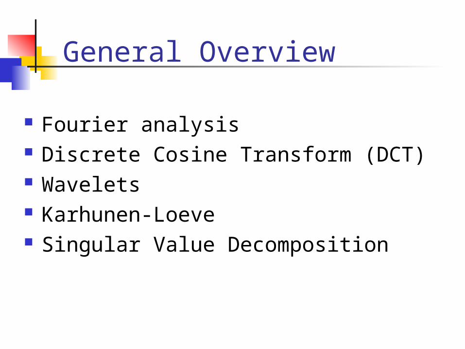
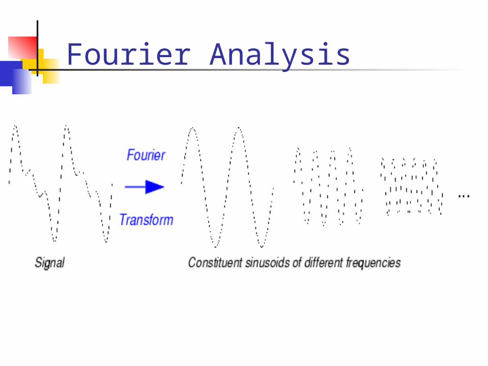
Fourier Analysis Fourier’s Theorem:

Every continuous function can be considered as a sum of sinusoidal functions

Discrete case – n-point Discrete Fourier Transform of a signal is defined to be a sequence of n complex numbers given by

where j is the imaginary unit ( ) We denote a DFT pair as

1,,0],[ nixx i

X

1,,0, nfX f

1,,1,0)/2exp(/11

0

nfnfijxnX

n

i if

1jXx

Fourier Analysis

The signal can be recovered by the inverse transform:

is a complex number with the exception of

which is real if the signal is real

x

1,,1,0)/2exp(/11

0

ninfijXnx

n

f fi

fX

0X x

Fourier Analysis

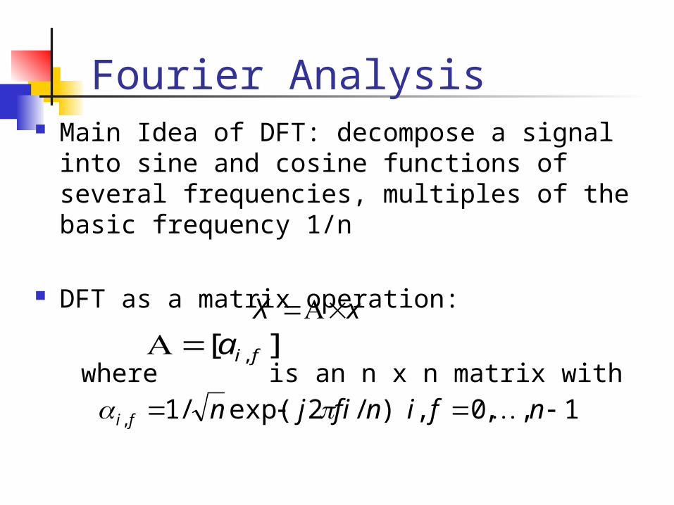
Fourier Analysis Main Idea of DFT: decompose a signal into

sine and cosine functions of several frequencies, multiples of the basic frequency 1/n

DFT as a matrix operation: where is an n x n matrix with

xX

][ , fia

1,,0,)/2exp(/1, nfinfijnfi

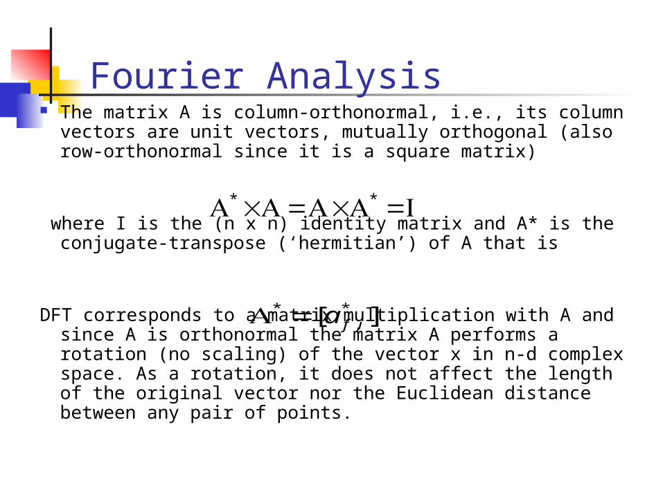
Fourier Analysis The matrix A is column-orthonormal, i.e., its column

vectors are unit vectors, mutually orthogonal (also row-orthonormal since it is a square matrix)

where I is the (n x n) identity matrix and A* is the

conjugate-transpose (‘hermitian’) of A that is DFT corresponds to a matrix multiplication with A and since

A is orthonormal the matrix A performs a rotation (no scaling) of the vector x in n-d complex space. As a rotation, it does not affect the length of the original vector nor the Euclidean distance between any pair of points.

**

][ *,

*ifa

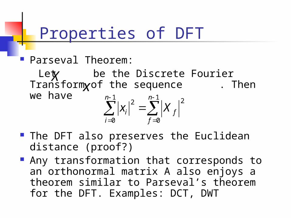
Properties of DFT Parseval Theorem: Let be the Discrete Fourier Transform

of the sequence . Then we have

The DFT also preserves the Euclidean distance (proof?)

Any transformation that corresponds to an orthonormal matrix A also enjoys a theorem similar to Parseval’s theorem for the DFT. Examples: DCT, DWT

X

x

1

0

21

0

2n

ff

n

ii Xx

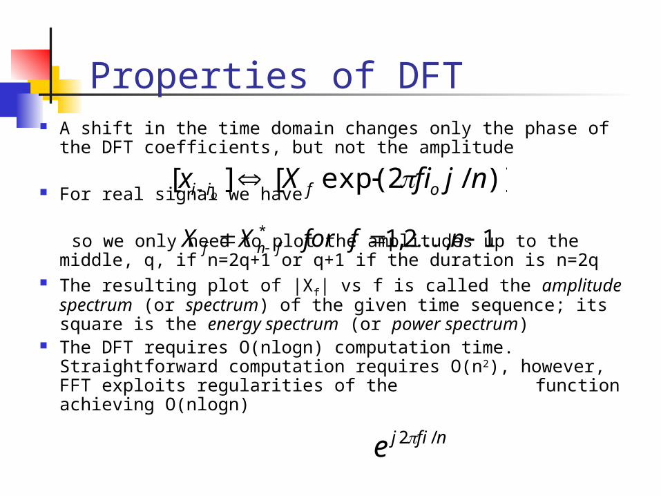
Properties of DFT A shift in the time domain changes only the phase of the

DFT coefficients, but not the amplitude For real signal we have

so we only need to plot the amplitudes up to the middle, q, if n=2q+1 or q+1 if the duration is n=2q

The resulting plot of |Xf| vs f is called the amplitude spectrum (or spectrum) of the given time sequence; its square is the energy spectrum (or power spectrum)

The DFT requires O(nlogn) computation time. Straightforward computation requires O(n2), however, FFT exploits regularities of the function achieving O(nlogn)

)]/2exp([][ njfiXx ofii o

1,2,1* nfforXX fnf

nfije /2

Examples

Discrete Cosine Transform (DCT)

Objective: to concentrate the energy into a few coefficients as possible

DFT is helpful to highlight periodicities in the signal through its amplitude spectrum

When successive values are correlated DCT is better than DFT

DCT avoids the ‘frequency leak’ that DFT has when the signal has a ‘trend’

DCT’s coefficients are always real (as opposed to complex)

DCT reflects the original sequence in the time axis around the last point and takes DFT on the twice-as-long (symmetric) sequence -> all the coefficients are reals, their amplitute is symmetric along the middle (Xf=X2n-f), thus only the first n need to be kept

Discrete Cosine Transform (DCT)

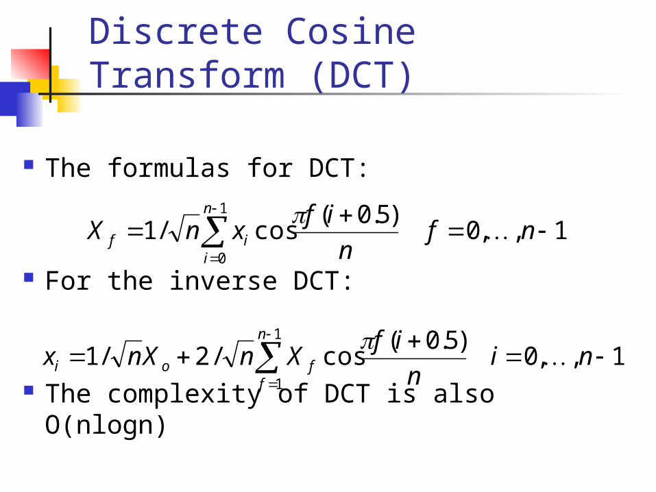
The formulas for DCT:

For the inverse DCT:

The complexity of DCT is also O(nlogn)

1,,0)5.0(

cos/11

0

nfn

ifxnX

n

iif

1,,0)5.0(

cos/2/11

1

nin

ifXnXnx

n

ffoi

m-Dimensional DFT/DCT (JPEG)

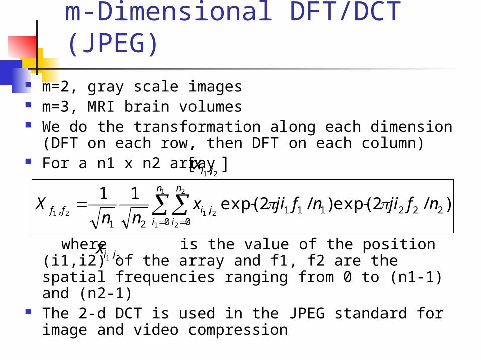
m=2, gray scale images m=3, MRI brain volumes We do the transformation along each dimension

(DFT on each row, then DFT on each column) For a n1 x n2 array

where is the value of the position (i1,i2) of the array and f1, f2 are the spatial frequencies ranging from 0 to (n1-1) and (n2-1)

The 2-d DCT is used in the JPEG standard for image and video compression

][21 ,iix

)/2exp()/2exp(11

2220 0

111,

21

,

1

1

2

2

2121nfjinfjix

nnX

n

i

n

iiiff

21 ,iix

Wavelets

It is believed that it avoids the ‘frequency leak’ problem of DFTeven better than DCT

Short Window Fourier Transform (SWFT): restricted frequency leak

In the time domain each values gives full information about that instant (no info about f)

DFT’s coefficients give full info about a given f but it needs all frequencies to recover the value at a given instant in time

SWFT is in between SWFT: how to choose the width w of the window? Discrete Wavelet Transform: let w be variable

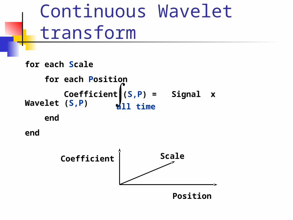
Continuous Wavelet transform

Position

all time

Coefficient Scale

for each Scale

for each Position

Coefficient (S,P) = Signal x Wavelet (S,P)

end

end

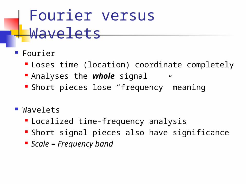
Fourier Loses time (location) coordinate completely Analyses the whole signal Short pieces lose “frequency” meaning

Wavelets Localized time-frequency analysis Short signal pieces also have significance Scale = Frequency band

Fourier versus Wavelets

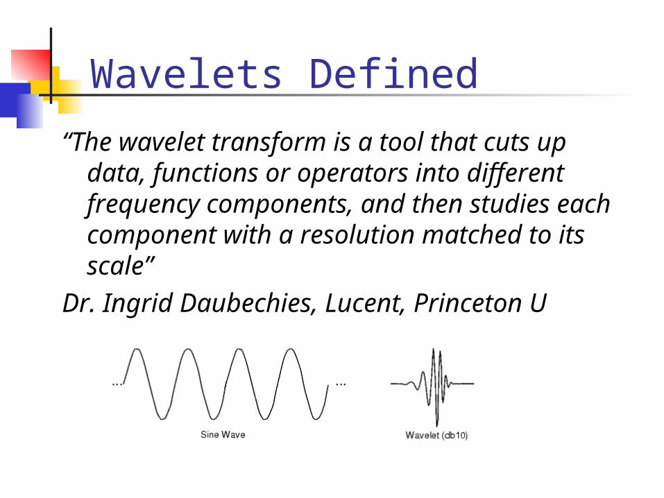
Wavelets Defined

“The wavelet transform is a tool that cuts up data, functions or operators into different frequency components, and then studies each component with a resolution matched to its scale”

Dr. Ingrid Daubechies, Lucent, Princeton U

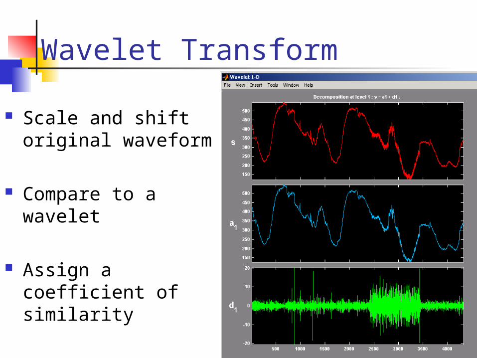
Wavelet Transform

Scale and shift original waveform

Compare to a wavelet

Assign a coefficient of similarity

Some wavelets – different shapes, different properties

Db3

Mexican hat Gauss

Continuous Wavelet transform:shift wavelet and compare, …

C = 0.0004

C = 0.0034

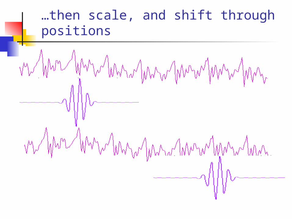
…then scale, and shift through positions

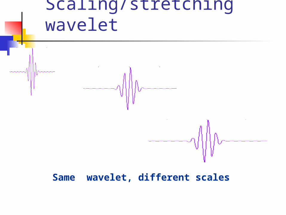
Scaling/stretching wavelet

Same wavelet, different scales

Wavelet transform: Scaling – value of “stretch”

f(t) = sin(t)

scale factor1

f(t) = sin(2t)scale factor 2

f(t) = sin(3t)scale factor 3

More on scaling It lets you either narrow down the

frequency band of interest, or determine the frequency content in a narrower time interval

Scaling = frequency band

Good for non-stationary data

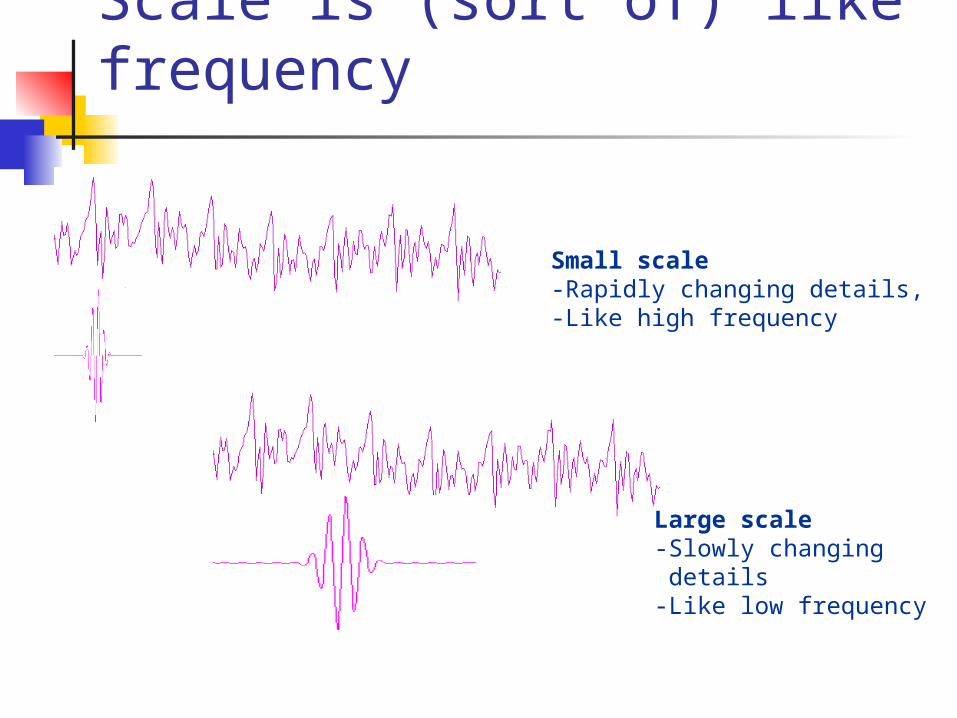
Scale is (sort of) like frequency

Small scale-Rapidly changing details, -Like high frequency

Large scale-Slowly changing details-Like low frequency

Discrete Wavelet Transform

“Subset” of scale and position based on power of two rather than every “possible” set of scale and

position in continuous wavelet transform

Behaves like a filter bank: signal in, coefficients out

Down-sampling necessary (twice as much data as original signal)

Discrete Wavelet transform

signal

filters

Approximation(a)

Details(d)

lowpass highpass

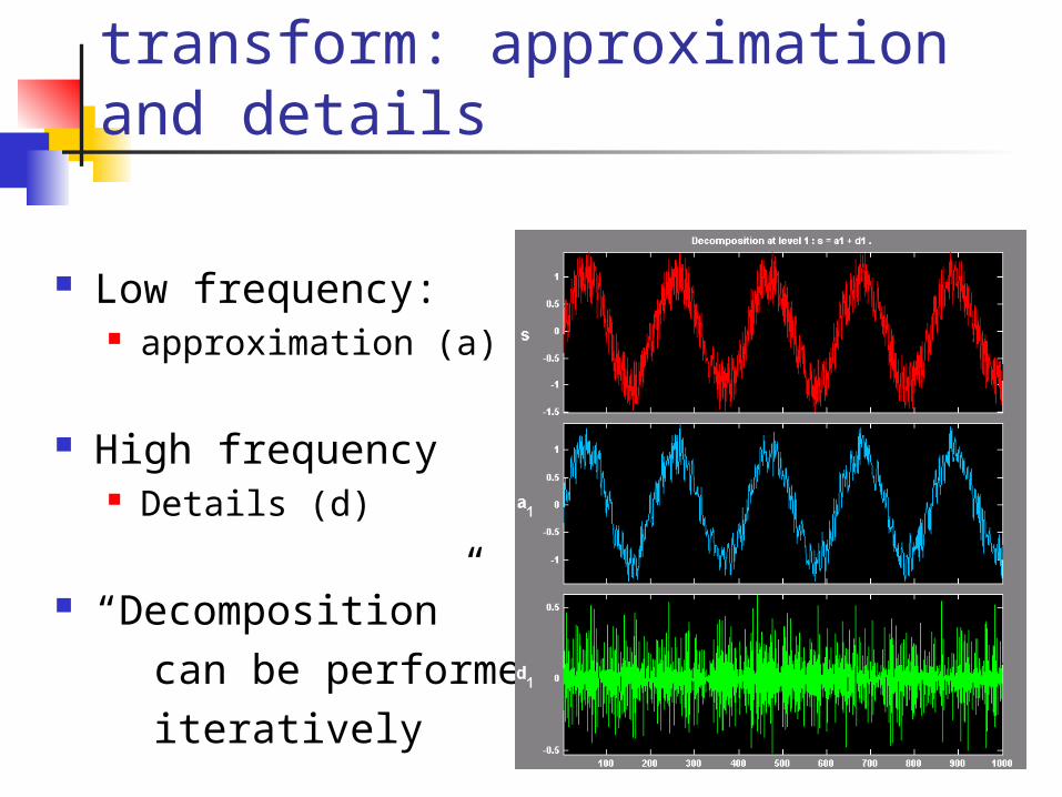
Results of wavelet transform: approximation and details

Low frequency: approximation (a)

High frequency Details (d)

“Decomposition” can be performed iteratively

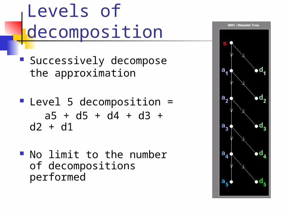
Levels of decomposition Successively decompose

the approximation

Level 5 decomposition = a5 + d5 + d4 + d3 + d2

+ d1

No limit to the number of decompositions performed

Wavelet synthesis

•Re-creates signal from coefficients•Up-sampling required

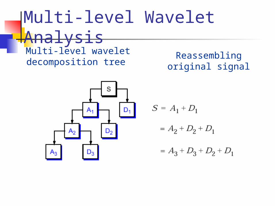
Multi-level Wavelet Analysis

Multi-level wavelet decomposition tree

Reassembling original signal

The Wavelet Toolbox (Matlab)

The Wavelet Toolbox contains graphical tools and command-line functions for analysis, synthesis, de-noising, and compression of signals and images. These tools work particularly well in “non-stationary data”

These tools are used for de-noising, compression, feature extraction, enhancement, pattern recognition in MANY types of applications and industries

Applications of wavelets Pattern recognition

Biotech: to distinguish the normal from the pathological membranes

Biometrics: facial/corneal/fingerprint recognition Feature extraction

Metallurgy: characterization of rough surfaces Trend detection:

Finance: exploring variation of stock prices Perfect reconstruction

Communications: wireless channel signals Video compression – JPEG 2000

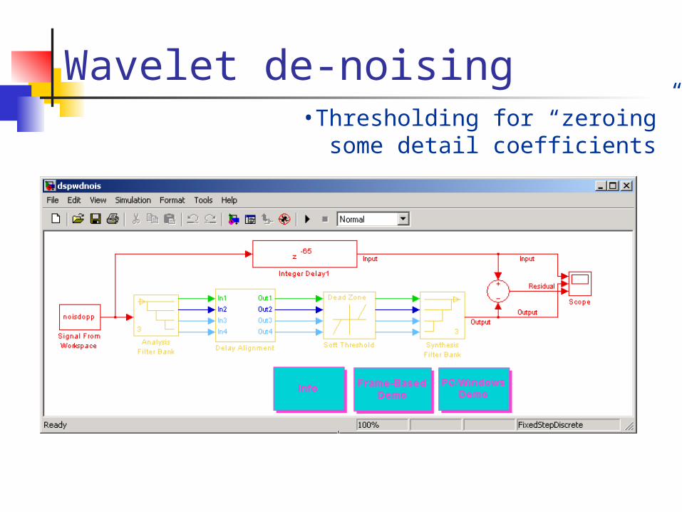
Wavelet de-noising•Thresholding for “zeroing” some detail coefficients

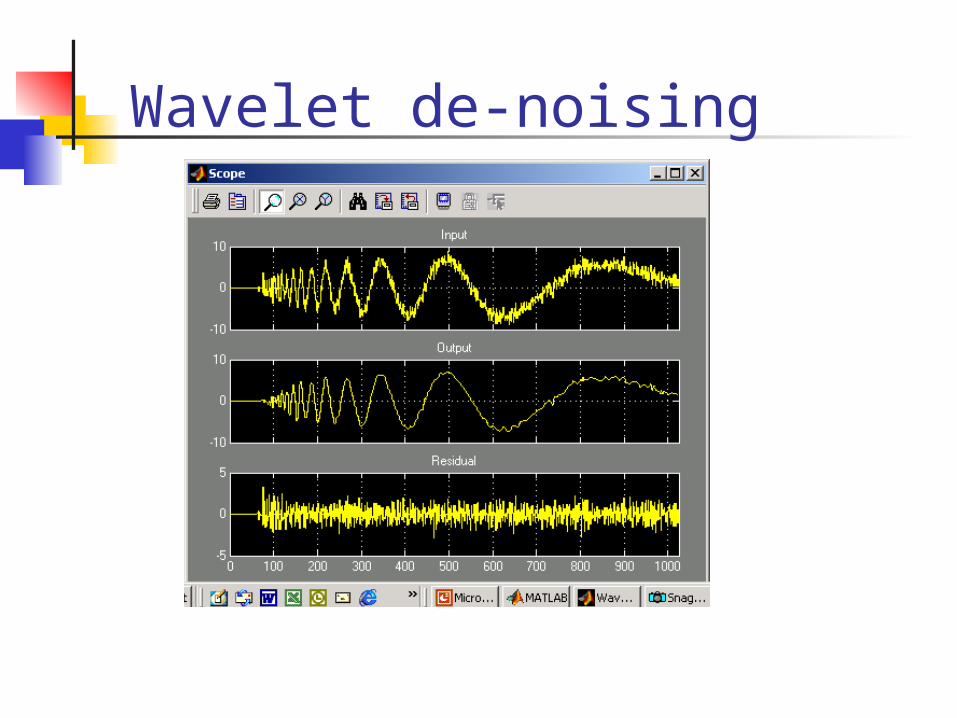
Wavelet de-noising

A demo

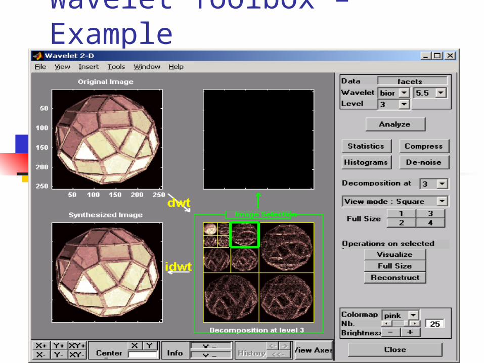
Wavelet Toolbox – Example

Wavelets: more information

References Wavelets and Filter Banks by Gilbert

Strang and Truong Nguyen A Friendly Guide to Wavelets by Gerald

Kaiser Web Resources

Wavelet Digest http://www.wavelet.org/ Amara’s Wavelet Page

http://www.amara.com/current/wavelet.html