1/30 Spatial Analysis and GIS: A Primer Gilberto Câmara 1 , Antônio Miguel Monteiro 1 , Suzana Druck Fucks 2 , Marília Sá Carvalho 3 1 Image Processing Division, National Institute for Space Research (INPE), Av dos Astronautas 1758, São J osé dos Campos, Brazil 2 Brazilian Agricultural Research Agency (EMBRAPA), Rodovia Brasília-Fortaleza, BR 020, Km 18, Planaltina, Brazil 3 National School for Public Health , Fundacao Oswaldo Cruz R. Leopoldo Bulhoes, 1480/810, Rio de Janeiro, Brazil Introduction Understanding the spatial distribution of data from phenomena that occur in space constitute today a great challenge to the elucidation of central questions in many areas of knowledge, be it in health, in environment, in geology, in agronomy, among many others. Such studies are becoming more and more common, due to the availability of low cost Geographic Information System (GIS) with user-friendly interfaces. These systems allow the spatial visualization of variables such as individual populations, quality of life indexes or company sales in a region using maps. To achieve that it is enough to have a database and a geographic base (like a map of the municipalities), and the GIS is capable of presenting a colored map that allows the visualization of the spatial pattern of the phenomenon. Besides the visual perception of the spatial distribution of the phenomenon, it is very useful to translate the existing patterns into objective and measurable considerations, like in the following cases:

Welcome message from author
This document is posted to help you gain knowledge. Please leave a comment to let me know what you think about it! Share it to your friends and learn new things together.
Transcript

8/3/2019 Spatial Analysis Primer
http://slidepdf.com/reader/full/spatial-analysis-primer 1/30
1/30
Spatial Analysis and GIS: A Primer
Gilberto Câmara
1
, Antônio Miguel Monteiro
1
, Suzana Druck Fucks
2
, Marília SáCarvalho3
1Image Processing Division, National Institute for Space Research (INPE),
Av dos Astronautas 1758, São José dos Campos, Brazil2Brazilian Agricultural Research Agency (EMBRAPA),
Rodovia Brasília-Fortaleza, BR 020, Km 18, Planaltina, Brazil3National School for Public Health , Fundacao Oswaldo Cruz
R. Leopoldo Bulhoes, 1480/810, Rio de Janeiro, Brazil
Introduction
Understanding the spatial distribution of data from phenomena that occur
in space constitute today a great challenge to the elucidation of central questions
in many areas of knowledge, be it in health, in environment, in geology, in
agronomy, among many others. Such studies are becoming more and more
common, due to the availability of low cost Geographic Information System (GIS)with user-friendly interfaces. These systems allow the spatial visualization of
variables such as individual populations, quality of life indexes or company sales
in a region using maps. To achieve that it is enough to have a database and a
geographic base (like a map of the municipalities), and the GIS is capable of
presenting a colored map that allows the visualization of the spatial pattern of the
phenomenon.
Besides the visual perception of the spatial distribution of thephenomenon, it is very useful to translate the existing patterns into objective and
measurable considerations, like in the following cases:

8/3/2019 Spatial Analysis Primer
http://slidepdf.com/reader/full/spatial-analysis-primer 2/30
2/30
• Epidemiologists collect data about the occurrence of diseases. Does the
distribution of cases of a disease form a pattern in space? Is there any
association with any source of pollution? Is there any evidence of
contagion? Did it vary with time?
• We want to investigate if there is any spatial concentration in the
distribution of theft. Are thefts that occur in certain areas correlated to
socio-economic characteristics of these areas?
• Geologists desire to estimate, from some samples, the extension of a
mineral deposit in a region. Can those samples be used to estimate the
mineral distribution in that region?
• We want to analyze a region for agricultural zoning purposes. How to
choose the independent variables – soil, vegetation or geomorphology –and determine what the contribution of each one of them is to define
where each type of crop is more adequate?
All of these problems are part of spatial analysis of geographical data.
The emphasis of Spatial Analysis is to measure properties and relationships,
taking into account the spatial localization of the phenomenon under study in a
direct way. That is, the central idea is to incorporate space into the analysis to be
made. This book presents a set of tools that try to address these issues. It isintended to help those interested to study, explore and model processes that
express themselves through a distribution in space, here called geographic
phenomena.
A pioneer example, where the space category was intuitively incorporated
to the analyses performed took place in the 19th century carried out by John
Snow. In 1854, one the many cholera epidemics was taking place in London,
brought from the Indies. At that time, nobody knew much about the causes of thedisease. Two scientific schools tried to explain it: one relating it to miasmas
concentrated in the lower and swampy regions of the city and another to the
ingestion of contaminated water. The map (Figure 1) presents the location of

8/3/2019 Spatial Analysis Primer
http://slidepdf.com/reader/full/spatial-analysis-primer 3/30
3/30
deaths due to cholera and the water pumps that supplied the city, allowing the
clear identification of one of the locations, in Broad Street, as the epicenter of the
epidemics. Later studies confirmed this hypothesis, corroborated by other
information like the localization of the water pump down river from the city, in a
place where there was a maximum concentration of waste, including excrements
from choleric patients. This was one of the first examples of spatial analysis
where the spatial relationship of the data significantly contributed to the
advancement in the comprehension of a phenomenon.
Figure 1 – London Map showing deaths from cholera identified by dots and water
pumps represented by crosses.
Data types in spatial analysis
The most used taxonomy to characterize the problems of spatial analysis
consider three types of data:
• Events or point patterns – phenomena expressed through occurrences
identified as points in space, denominated point processes. Some examples
are: crime spots, disease occurrences, and the localization of vegetal
species.

8/3/2019 Spatial Analysis Primer
http://slidepdf.com/reader/full/spatial-analysis-primer 4/30
4/30
• Continuous surfaces – estimated from a set of field samples that can be
regularly or irregularly distributed. Usually, this type of data results from
natural resources survey, which includes geological, topographical,
ecological, phitogeographic, and pedological maps.
• Areas with Counts and Aggregated Rates – means data associated to
population surveys, like census and health statistics, and that are originally
referred to individuals situated in specific points in space. For
confidentiality reasons these data are aggregated in analysis units, usually
delimited by closed polygons (census tracts, postal addressing zones,
municipalities).
From the data types above, it can be verified that the problems of spatial
analysis deal with environmental and socioeconomic data. In both cases, the
spatial analysis is composed by a set of chained procedure that aims at choosing
of an inferential model that explicitly considers the spatial relationships present in
the phenomenon. In general, the modeling process is preceded by a phase of
exploratory analysis, associated to the visual presentation of the data in the form
of graphs and maps and the identification of spatial dependency patterns in the
phenomenon under study.
In the case of point pattern analysis the object of interest is the very spatial
location of the events under study. Similarly to the situation analyzed by Snow,
the objective is to study the spatial distribution of these points, testing hypothesis
about the observed pattern: if it is random or, on the contrary, if it presents itself
in agglomerates or is regularly distributed. It is also the matter of studies aiming at
estimating the risk of diseases around nuclear plants. Another case is to establish a
relationship between the occurrence of events with the characteristics of the
individual, incorporating possible environmental factors about which there is no
data available. For example, would the mortality by tuberculosis, even
considering the known risk factors, vary with the address of the patient? As an
example, Figure 2 illustrates the application of point pattern analysis for the case
of mortality by external causes in the city of Porto Alegre, with 1996 data, carried

8/3/2019 Spatial Analysis Primer
http://slidepdf.com/reader/full/spatial-analysis-primer 5/30
5/30
out by Simone Santos and Christovam Barcellos, from FIOCRUZ. The homicide
locations (red), traffic accidents (yellow) and suicides (blue) is shown in Figure 2
(left). On the right, a surface for the estimated intensity is presented, that could be
thought as the “temperature of violence”. The interpolated surface shows a pattern
of point distribution with a strong concentration in the downtown of the city,
decreasing in the direction of the more remote quarters.
Figure 2 – Distribution of cases of mortality by external causes in Porto Alegre in
1996 and the intensity estimator.
For surface analysis, the objective is to reconstruct the surface from which
the samples were removed and measured. For example, consider the distribution
of profiles and soil samples, for the state of Santa Catarina and surrounding areas,
and the spatial distribution map of the saturation by bases variable, produced by
Simone Bönisch, from INPE, and presented in Figure 1-3.
* Perfis* Amostras
55,437 (%)
8,250
Figure 3 – Profiles and soil samples distribution in Santa Catarina (left) and
estimated continuous distribution of the saturation by bases variable (right).

8/3/2019 Spatial Analysis Primer
http://slidepdf.com/reader/full/spatial-analysis-primer 6/30
6/30
How did we build this map? The highlighted crosses indicate the
localization of the points of soil sampling; from these measures a spatial
dependency model was estimated allowing the interpolation of the surface
presented in the map. The inferential model has the objective of quantifying the
spatial dependence among the sample values. This model utilizes the techniques
of geostatistics, whose central hypothesis is the concept of stationarity (discussed
later in this chapter) that supposes a homogeneous behavior on the structure of
spatial correlation in the region of study. Since environmental data are the result
of natural phenomena of medium and long duration (like the geological
processes), the stationarity hypothesis is derived from the relative stability of
these processes; in practice, this implies that stationarity is present in a great
number of situations. It must be observed that stationarity is a non-restrictive
work hypothesis in the approach of non-stationary problems. Methods likeuniversal kriging, fai-k, external derivation, co-kriging, and disjunctive kriging
are meant for the treatment of non-stationary phenomena.
In the case of the areal analysis, most of the data are drawn from
population survey like census, health statistics and real estate cadastre. These
areas are usually delimited by closed polygons where supposedly there is internal
homogeneity, that is, important changes only occur in the limits. Clearly, this is a
premise that is not always true, given that frequently the survey units are definedby operational (census tracts) or political (municipalities) criteria and there is no
guarantee that the distribution of the event is homogeneous within these units. In
countries with great social contrasts like Brazil, it is frequent that different social
groups be aggregated in one same region of survey – slums and noble areas –
resulting in calculated indicators that represent the mean between different
populations. In many regions the sampling units present important differences in
area and population. In this case, both the presentation in choropleth maps and the
simple calculation of population indicators can lead to distortions in the indicators
obtained and it will be necessary to use distribution adjustment techniques.

8/3/2019 Spatial Analysis Primer
http://slidepdf.com/reader/full/spatial-analysis-primer 7/30
7/30
As an example of data aggregated by area consider Figure 4 (left), that
presents the spatial distribution of the social inclusion/exclusion index of São
Paulo, produced by the team leaded by Prof. Aldaíza Sposati (PUC/SP). The
indicators of social inclusion/exclusion were generated from survey data on 6
districts of São Paulo, based on the 1991 Census. From this map it was possible to
extract a cluster of social inclusion/exclusion, shown in Figure 4 (right) that
indicates the extremes of social inclusion and exclusion in the city.
Figure 4 – Social Inclusion/Exclusion Map of São Paulo (1991) and social
exclusion clusters (South and East Zones) and social inclusion (downtown).
1.1 Computational representation of geographic data
The term Geographic Information System (GIS) is applied to systems that
perform the computational treatment of geographic data and that store the
geometry and the attributes of data that are georeferenced, that is, situated on the
earth surface and represented in a cartographic projection. In general we can say
that a GIS has the following components, as shown in Figure 5:
• User interface;
• Data input and integration;
• Graph and image processing functions;
8/3/2019 Spatial Analysis Primer
http://slidepdf.com/reader/full/spatial-analysis-primer 8/30
8/30
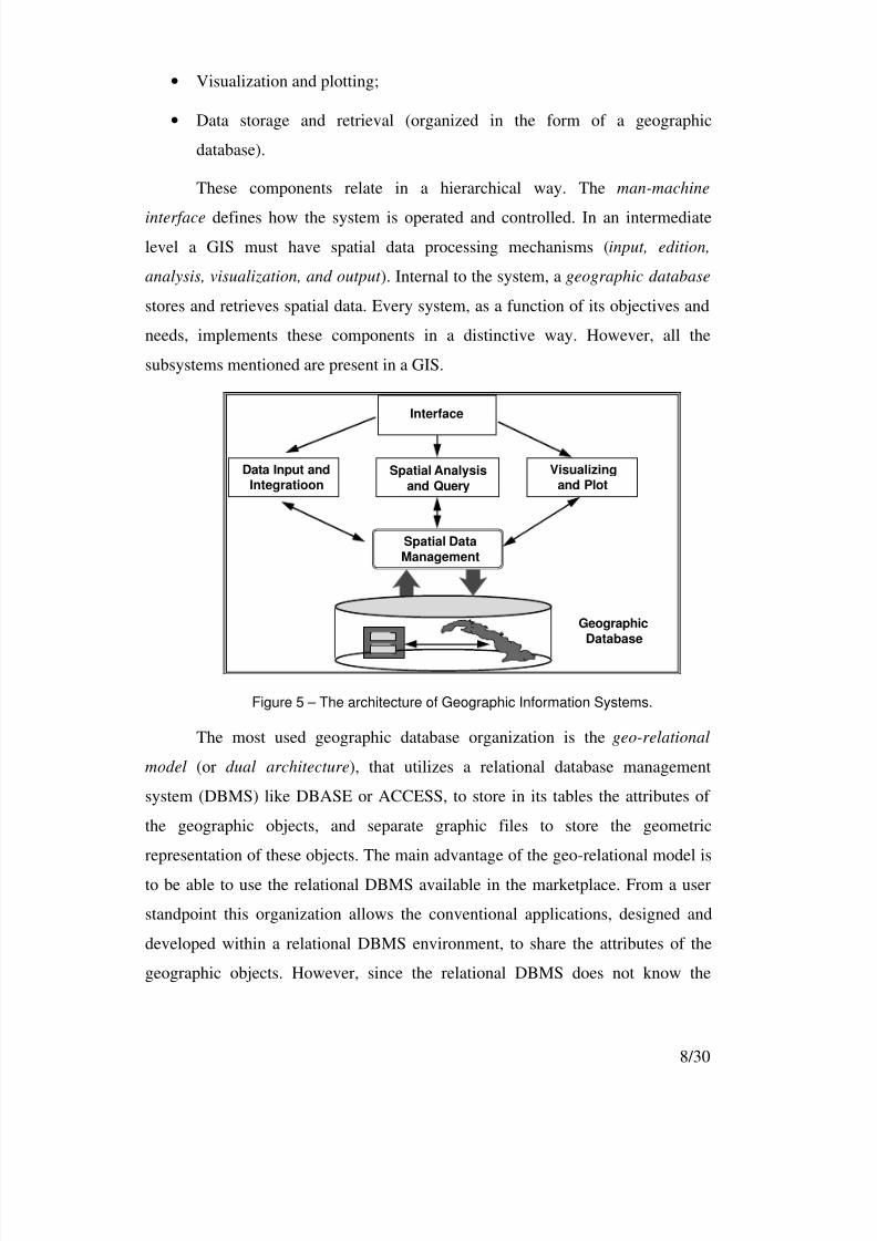
• Visualization and plotting;
• Data storage and retrieval (organized in the form of a geographic
database).
These components relate in a hierarchical way. The man-machine
interface defines how the system is operated and controlled. In an intermediatelevel a GIS must have spatial data processing mechanisms (input, edition,
analysis, visualization, and output ). Internal to the system, a geographic database
stores and retrieves spatial data. Every system, as a function of its objectives and
needs, implements these components in a distinctive way. However, all the
subsystems mentioned are present in a GIS.
Interface
Spatial Analysis
and Query
Data Input andIntegratioon
Visualizingand Plot
Spatial Data
Management
Geographic
Database
Figure 5 – The architecture of Geographic Information Systems.
The most used geographic database organization is the geo-relational
model (or dual architecture), that utilizes a relational database management
system (DBMS) like DBASE or ACCESS, to store in its tables the attributes of
the geographic objects, and separate graphic files to store the geometric
representation of these objects. The main advantage of the geo-relational model is
to be able to use the relational DBMS available in the marketplace. From a user
standpoint this organization allows the conventional applications, designed and
developed within a relational DBMS environment, to share the attributes of the
geographic objects. However, since the relational DBMS does not know the

8/3/2019 Spatial Analysis Primer
http://slidepdf.com/reader/full/spatial-analysis-primer 9/30
9/30
external graphic structure, there is a serious risk of introducing inconsistencies in
the geographic database. Imagine, for example, that a user of a strictly
alphanumeric application is able to remove an alphanumeric register, which is part
of a set of attributes of a certain geographic entity. In this case, this geographic
entity has no longer its attributes, becoming inconsistent. Therefore, the access to
the alphanumeric attributes of geographic data can only be done in a careful way,
within rigid controls that must be implemented by the application, since the geo-
relational model does not offer any features to automatically guarantee the data
integrity.
The geometric representations used include the following options:
• 2D Points: A 2D point is an ordered pair (x,y) of spatial coordinates. A
point indicates the place of occurrence of an event, like in the case of
mortality by external causes, shown in Figure 2.
• Polygons: A polygon is a set of ordered pairs {(x,y)} of spatial
coordinates, in such a way that the last point is identical to the first thus
forming a closed region in the plane. In the simplest situation, each
polygon delimits an individual object (like in the case of the districts of
São Paulo in Figure 4); in the most general case, an individual region of
interest can be delimited by several polygons.
• Samples: consist of ordered pairs {(x,y,z)} where the (x,y) pairs indicate the
geographic coordinates and z indicates the value of the studied
phenomenon for that localization. Usually the samples are associated to
field surveys, such as geophysical, geochemical, and oceanographic data.
The concept of a sample can be generalized to the case of multiple
measurements on the same locality.
• Regular Grid : is a matrix where each element is associated to a numericvalue. This matrix is associated to a region on the earth surface. Starting
from an initial coordinate, usually referred to the lower left corner of the

8/3/2019 Spatial Analysis Primer
http://slidepdf.com/reader/full/spatial-analysis-primer 10/30
10/30
matrix, and with regular spacing in both the horizontal and vertical
directions.
• Image: is a matrix where each element is associated to an integer value
(usually in the 0 to 255 range), used for visualization. This matrix is used
for the graphic presentation of a regular grid. The numeric values in the
grid are scaled to fit within the presentation range of the image; the bigger
values are shown in lighter gray colors, and the lower ones in darker gray
tones. Most of the GISs offer the capability of presenting a regular grid in
the form of an image (in black and white or in colors), with a conversion
that can be automatic or controlled by the user. Figure 1-3 (right) shows an
image of the distribution of the saturation by bases in the state of Santa
Catarina.
The geometries associated to points, samples and polygons are presented
in Figure 6 while the regular grid is shown in Figure 7. Usually, the geographic
reference of the data is kept in the coordinates of the data structure, that is
associated to a planar cartographic projection, or to latitude (Y coordinate) and
longitude (X coordinate) values.
Figure 6 Geometries: 2DPoint, Sample and Polygon.

8/3/2019 Spatial Analysis Primer
http://slidepdf.com/reader/full/spatial-analysis-primer 11/30
11/30
Figure 7 Geometric representation of the Regular Grid
In the geo-relational model, the descriptive attributes of each object are
organized in the form of a table, where the lines correspond to the data and the
column names correspond to the attribute names. Each line in the table
corresponds to the values associated to a geographic object; to each geographic
object a unique identifier or label is associated, and that label is used to make a
logical connection between its attributes and its geometric representation.
Concerning the three basic data types used in spatial data analysis, the
areas are stored in a GIS with a dual strategy in the form presented in Figure 8.
Each area, that could be a census tract, health district or municipality, is
graphically represented by a closed polygon and its attributes are stored in a table
in a relational DBMS. Figure 1-8 shows the farm of a forestry enterprise, divided
in tracts, for cultivation purposes. Each tract receives an identifier that is
associated at the same time to the polygon that delimits it and to the line in the
table that contain its attributes. In the example the link is done through the
registers in the field “TALHÃO” (tract). The same type of logical relationship is
done in all the other cases such as: residents in a lot, the lots in a block, the blocks
in a quarter, the quarters in a city; the hydrants or pay phones along an avenue;
service stations and restaurants alongside a road.

8/3/2019 Spatial Analysis Primer
http://slidepdf.com/reader/full/spatial-analysis-primer 12/30
12/30
Figure 8 – Dual strategy for geographic database.
In the case of events, these can also be associated to a relational DBMS,
for example, recording the address where a homicide occurred and its motive. The
same principle can be applied to the case of areas: each event is associated to an
identifier that works as the link between the geographic coordinates file and the
table in the database.
For the surfaces the most common situation is dealing only with graphic
files, without the storage of results in a relational DBMS. In this case, the most
usual situation is that the input data are stored as samples, added to the polygon of
the limits of the region under study. The estimation process produces a regular
grid describing approximately the phenomenon in the region under study. This
grid can be transformed into an image for presentation purposes (like in Figure 3).

8/3/2019 Spatial Analysis Primer
http://slidepdf.com/reader/full/spatial-analysis-primer 13/30
13/30
Basic concepts in spatial analysis
Spatial Dependency
Spatial dependency is a key concept on understanding and analyzing a
spatial phenomena.. Such notion stems from what Waldo Tobler calls the first lawof geography: “everything is related to everything else, but near things are more
related than distant things.” Or, as Noel Cressie states, “the [spatial] dependency
is present in every direction and gets weaker the more the dispersion in the data
localization increases.” Generalizing we can state that most of the occurrences,
natural or social, present among themselves a relationship that depends on
distance. What does this principle imply? If we find pollution on a spot in a lake it
is very probable that places close to this sample spot are also polluted. Or that the
presence of an adult tree inhibits the development of others, such inhibition
decreases with distance, and beyond a certain radius other big trees will be found.
Spatial Autocorrelation
The computational expression of the concept of spatial dependence is the
spatial autocorrelation. This term comes from the statistical concept of
correlation, used to measure the relationship between two random variables. Thepreposition “auto” indicates that the measurement of the correlation is done with
the same random variable, measured in different places in space. We can use
different indicators to measure the spatial autocorrelation, all of them based on the
same idea: verifying how the spatial dependency varies by comparing the values
of a sample and their neighbors’. The autocorrelation indicators are a special case
of a crossed products statistics like
= ==Γ
n
i
n
jijij d wd 1 1 )()( ξ (1)
This index expresses the relationship between different random variables
as a product of two matrixes. Given a certain distance d , a matrix wij provides a
measure of spatial contiguity between the random variables zi and z j, for example,

8/3/2019 Spatial Analysis Primer
http://slidepdf.com/reader/full/spatial-analysis-primer 14/30
14/30
informing if they are separated by a distance shorter than d . Matrix ij provides a
measure of the correlation between these random variables that could be the
product of these variables, as in the case of Moran’s index for areas, discussed in
chapter 5 of this book, and that can be expressed as
=
= =
−
−−
= n
ii
n
i
n
j jiij
z z
z z z zw I
1
2
1 1
)(
))(( (2)
where wij is 1 if the geographic areas associated to zi and z j touch each other, and 0
otherwise. Another example of indicator is the variogram, discussed in chapter 3,
where we compute the square of the difference of the values, like in the case of
the expression that follows
= +−=
)(
1
2)]()([)(2
1)(ˆ
d N
iii d x z x zd N d γ (3)
where N(d) is the number of samples separated by distance d .
In both cases the values obtained should be compared with the values that
would be produced if no spatial relationship existed between the variables.
Significant values of the spatial autocorrelation indexes are evidences of spatial
dependency and indicate that the postulate of independence between the samples,
basis for most of the statistical inference procedures, is invalid and that the
inferential models for these cases should explicitly take the space into account in
its formulations.
Statistical Inference for Spatial Data
An important consequence of spatial dependence is that statistical
inferences on this type of data won’t be as efficient as in the case of independent
samples of the same size. In other words, the spatial dependence leads to a loss of
explanatory power. In general, this reflects on higher variances for the estimates,lower levels of significance in hypothesis tests and a worse adjustment for the
estimated models, compared to data of the same dimension that exhibit
independence.

8/3/2019 Spatial Analysis Primer
http://slidepdf.com/reader/full/spatial-analysis-primer 15/30
15/30
In most cases the more adequate perspective is to consider that spatial data
not as a set of independent samples, rather as one realization of a stochastic
process. Contrary to the usual independent samples vision, where each
observation carries an independent information, in the case of a stochastic process
all the observations are used in a combined way to describe the spatial pattern of
the studied phenomenon. The hypothesis created in this case is that for each point
u in a region A, continuous in 2ℜ , the values inferred of the attribute z - )(ˆ u z - are
realizations of a process }),({ Auu Z ∈ . In this case it is necessary to create
hypothesis about the stability of the stochastic process when assuming, for
example, that it is stationary and/or isotropic, concepts discussed in what follows.
Stationarity and Isotropy
The main statistical concepts that define the spatial structure of the data
relate to the effects of 1st and 2nd order. 1st order effect is the expected value, that
is, the mean of the process in space. 2nd order effect is the covariance between
areas si and s j. Stationarity is an important concept in this type of study. A process
is considered stationary if the effects of 1st and 2nd order are constant, in the whole
region under study, that is there is no trend. A process is isotropic if, besides being
stationary, the covariance depends only on the distance between the points and not
on the direction between them. A stochastic process Z is said to be stationary of second order if the expectation of Z(u) is constant in all the region under study A,
that is, it doesn’t depend on its position
mu Z E =)}({ (4)
and the spatial covariance structure depends solely on the relative vector between
points h = u-u’
C( h)=E { Z(u) · Z(u+ h)}-E { Z(u)}E { Z(u+ h)} (5)

8/3/2019 Spatial Analysis Primer
http://slidepdf.com/reader/full/spatial-analysis-primer 16/30
16/30
Given a specific spatial process, the stationarity hypothesis can be
corroborated by explanatory analysis procedures and descriptive statistics, whose
calculation should explicitly consider the spatial localization. In spatial covariance
C | h| the vector h comprises the distance | h| and the direction. The covariance is
called anisotropic when its structure varies with distance and simultaneously as a
function of its direction. When the spatial dependence is the same in all directions,
we have an isotropic phenomenon. The modeling of the spatial covariance
structure is better detailed in the chapters that follow. For now it’s important to
emphasize the basic characteristics of a spatial covariance structure in order to
make the concepts used in this book comprehensible.
The spatial analysis process
The spatial analysis is composed by a set of chained procedures whose aim
is to choose an inferential model that explicitly considers the spatial relationship
present in the phenomenon. The initial procedures of analysis include the set of
generic methods of exploratory analysis and the visualization of data, in general
through maps. These techniques permit the description of the distribution of the
variables of study, the identification of observations that are outliers not only in
relation to the type of distribution but also in relation to its neighbors, and to look
for the existence of patterns in the spatial distribution. Through these procedures it
is possible to propose hypothesis about the observations, in a way of selecting the
best inferential model supported by the data.
The spatial inferential models are usually presented in three great groups:
continuous variation, discrete variation, and the point processes. The resolution of
a spatial problem may involve the utilization of one of them or the interaction of
some or even all of them. The example below illustrates the differences among
these models, how they can be used and how they interact inside the same process
where questions, based on real facts, must be responded.

8/3/2019 Spatial Analysis Primer
http://slidepdf.com/reader/full/spatial-analysis-primer 17/30
17/30
Visceral Leishmaniasis is basically an animal disease but that also affects
humans. The dogs are the main domestic reservoirs of the urban disease and there
is no treatment for them. The disease is spread by mosquitoes, that reproduce in
the soil and in decomposing organic matter, like banana trees and fallen leaves. In
the last years there were some epidemic outbreaks in Brazilian cities like Belo
Horizonte, Araçatuba, Cuiabá, Teresina, and Natal. The control of the disease is
based on the combat against the insect and on the elimination of affected dogs
inside the disease focus, an area of 200 meters around the human or canine case.
However, the intensive application of these measures has not resulted in the
desired results, and the endemic goes on. On the other side, the population,
although cooperative in a first moment, by the time of the discovery of serious
human cases, after a few months of survey, refuse the elimination of dog. The
problem is serious, and yet without a solution. It is necessary to evaluate theefficacy of the control strategies in the urban context. Using the spatial analysis
tools, some investigation may accumulate information to give a response to that
problem. For example:
What is the radius of dispersion of the mosquito around its habitat?
Two models can be used for modeling the dispersion of the Leishmaniasis
vector which is essential for estimating the radius of dispersion of the mosquito
that will define the area of spray around the cases of incidence of the disease:
• Models of continuous variation, where the objective is to generate
continuous surfaces determining the areas of greater risk from a sample of
places where the mosquitoes were collected (sample of discontinuous
points).
• The point processes, where the objective is to model the probability of
capture of the mosquitoes. In this case, the random variable is not the
value of an attribute (presence or absence of the mosquito) but the place
where it has been captured.

8/3/2019 Spatial Analysis Primer
http://slidepdf.com/reader/full/spatial-analysis-primer 18/30
18/30
In the urban area, what is the preferred environment for the mosquito
reproduction?
To estimate the mosquito nursery places it is necessary to identify in a certain
region, the areas of concentration of some environmental attributes that encourage
the emergence of the mosquito like, for example, organic matter and soil
condition. In this case the continuous variation models could be used to infer
surfaces with the values of these attributes.
Is there any relationship between the canine prevalence and the socioeconomic
conditions of the population?
Mosquitoes only do not perpetuate the epidemic. It is necessary that sick animals
exist from whom they feed from, such as dogs. However, it is known that the
presence and resistance of dogs to the illness depends on their nutritional
condition and consequently on the socioeconomic situation - the acceptance of the
elimination of sick animals is also related to the income. Thus it is necessary to
study both the illness incidence on dogs and the socioeconomic profile of the
population as well as the prevalence of human cases. In this case, the analysis
should involve counts by area, for example, socioeconomic indicators. That is, the
available information about the region is complete, with data grouped by area.
Thus, we aim at studying the relationship between the different indicators
considering their spatial structure. In those cases, the discrete variation model isused.
The application of the basic inferential models was exemplified and we
also discussed about how these procedures might contribute to the resolution of a
certain question. We will present next the basic concepts of each one of them.

8/3/2019 Spatial Analysis Primer
http://slidepdf.com/reader/full/spatial-analysis-primer 19/30
19/30
Inferential Models
Motivated by different application areas, the inferential models were separately
developed for each of the situations described above. The unification of this field
is not yet completely defined, and it is frequently possible to apply more than one
type of modeling to the same data set, as we can see in the example above. Then
what would be the advantages of a form upon the other? Sometimes, of course,
the phenomenon under study presents discrete spatial variation, that is, isolated
points in space. However, frequently the discrete models are frequently used for
practical reasons, like the availability of area data only. One of the advantages of
continuous models is that the inference does not limit itself to arbitrarily defined
areas. On the other hand, discrete models allow the easier estimation of
association parameters between the variables. The researcher will make the final
choice, for he knows there is no such thing as the “correct model”, but searchesfor a model that better adjusts to the data and that offers the greatest potential for
the comprehension of the phenomenon under study.
Point processes
Point processes are defined as a set of irregularly distributed points in a
terrain, whose location was generated by a stochastic mechanism. The localization
of points is the object of study, which has the objective of understanding its
generating mechanism. A set of points (u1 , u2 , …, un) in a certain region A isconsidered where events occurred. For example, if the phenomenon under study is
homicides occurred in a certain region, we wish to verify if there is any
geographic pattern for this kind of crime, that is, to find sub-regions in A with
greater probability of occurrence.
The point process is modeled considering subregions S in A through its
expectancy E [ N(S)] and the covariance C [ N(Si), N(S j)], where N(S) denotes the
number of events in S. If the objective of analysis is the estimation of the probablelocations for the occurrence of certain events, these statistics should be inferred
considering the limit value for the quantity of events per area. This limit value
corresponds to the expectancy of N(S) for a small region du around point u, when

8/3/2019 Spatial Analysis Primer
http://slidepdf.com/reader/full/spatial-analysis-primer 20/30
20/30
that tends to zero. This expectancy is denominated intensity (first order property),
defined as:
}||
)]([{lim)(
0|| du
du N E u
du →
=λ , (6)
Second order properties can be defined the same way, considering the jointintensity (ui ,u j) between infinitesimal regions |du| and |du j| that contain points ui
and u j.
ji
ji
dudu ji dudu
du N du N C ud ud
ji ,
)](),([{lim))(),((
0, →
=λ (7)
When the process is stationary, (u) is a constant, (u)= ; if it is also
isotropic, (ui ,u j) reduces to (|h|) , being |h| the distance between the two points.
When the process is non-stationary, that is, the mean intensity varies in region A,
the modeling of the dependency structure (ui ,u j) must incorporate the variation of
(u).
Continuous variation
The inferential models of continuous variation consider a stochastic
process },),({ 2ℜ⊂∈ A Auu Z whose values can be known in every point of the
study area. Starting from a sample of one attribute z, collected in various u points
contained in A, { z(u), =1, 2,…,n}, we aim at inferring a continuous surface of
values of z. The estimation of this stochastic process can be done in a completely
non-parametric way or from kriging estimators, like the ones described in chapters
3 and 4 of this book. These classical inferential models of surfaces estimation are
denominated geostatistics. Geostatistics uses two types of estimation procedures:
the kriging and the stochastic simulation. In kriging, at each point u0, a value of
the random variable Z is estimated, )(ˆ 0u z , using an estimator )(ˆ0u Z , that is a
function of the data and of the spatial covariance structure ))(,()(ˆ 0 nC f u Z = .
These estimators present some important properties: they are not biased and are
optimal in the sense that they minimize the functions of the inferential errors.

8/3/2019 Spatial Analysis Primer
http://slidepdf.com/reader/full/spatial-analysis-primer 21/30
21/30
In stochastic simulation, the procedures reproduce images of the random
function Z through the equiprobable realization of the model of the established
stochastic process. Each realization, also called stochastic image, reflect the
properties considered in the model of the random function used. Generally the
realizations must honor the data and reproduce the function of accumulated
univariate distribution, F(z), and the spatial covariance structure considered.
Kriging has thus as an objective to compose the surface z through optimal
point estimates, )(ˆ u z , while the objective simulation aims at reproducing the
spatial variability of such surface through possible global representations of the
random function model. In order to permit the realization of the inferential
processes of kriging and simulation, it is necessary to assume the hypothesis that
the stochastic process is stationary of second order, that is, a process whose mean
is constant in space and whose covariance depends only on the distance vector
between the samples.
Discrete variation
The inferential models of discrete variation concern the distribution of
events whose localization is associated to areas delimited by polygons. This case
occurs much frequently when we deal with phenomena aggregated by
municipalities, quarters or census tracts, like population, mortality and income. In
this case, we don’t have the exact locality of the events, but value aggregated by
area. The objective is to model the pattern of spatial occurrence of the geographic
phenomenon under study.
In this type of modeling we consider that the geographic space under
study, region A, is a fixed set of spatial units. The most used model of distribution
considers a stochastic process {Z i:i=1,2,…,n}, composed of a set of random
variables. We seek to construct an approximation of the joint distribution of these
variables Z={Z 1 ,…,Z n }, where each random variable is associated to one of the
areas and has a distribution to be estimated. If the process is stationary, the
expected value of Zi is the global mean of the region and the covariance structure
depend only on distance, or on the neighborhood structure between the areas.

8/3/2019 Spatial Analysis Primer
http://slidepdf.com/reader/full/spatial-analysis-primer 22/30
22/30
Conclusions
This review presented the main concepts of the spatial geographic data
analysis and the main types of data and its computational representations. The
different types and problems of Spatial Analysis of Geographic Data are
summarized in Table 1Table 1-1
Types of Data and Problems in Spatial Analysis.
Data Types Example Typical problems
Analysis of point
patterns
Localized events Disease incidence Determination of
Patterns and
Aggregations
Surface analysis Samples of fields
and matrixes
Mineral deposits Interpolation and
uncertainty measures
Areal analysis Polygons and
attributes
Census data Regression and joint
distributions
To summarize the discussion, it is important to consider the conceptual
problem of the spatial analysis from the point of view of the user, as synthesized
in Figure 9. The specialists in the domains of knowledge (like Soils Sciences,
Geology, and Public Health) develop theories about the phenomena, with supportof the visualization techniques of the GIS. These theories include general
hypothesis about the spatial behavior of the data. From these theories it is
necessary that the specialist formulate quantitative inferential models, that can be
submitted to validation and corroboration tests, through the procedures of Spatial
Analysis. Then, the numerical results can then give support or help reject
qualitative concepts of knowledge domain theories.

8/3/2019 Spatial Analysis Primer
http://slidepdf.com/reader/full/spatial-analysis-primer 23/30
23/30
InferentialModels
Theories
QualitativeConcepts
TestableHypothesis
SpatialAnalysis
Knowledge Domains
Figure 9 – Relationship between spatial analysis and the knowledge domains
theories
As discussed in this chapter and exemplified in the case of VisceralLeishmaniasis, there is no such thing as a “correct model” for each problem. The
inferential models are useful above all to gain a better knowledge about the
problem. Many times it will be necessary to combine the different approaches
(point processes, continuous variation and discrete variation) to aggregate
information to the problem studied. In this case, there is no “magic formula” and
whatever the knowledge domain, the specialists will benefit knowing all the
techniques presented here.
This vision expresses at the same time the potential and the limitations of
the Spatial Analysis. The quantitative techniques of Spatial Analysis should
always be at the service of the knowledge of the specialists and never be used as
an end in itself. Its consistent use requires that two pre-conditions be satisfied: the
domain of the fundamental theories of Geoprocessing and Spatial Statistics and a
solid work methodology, result of the association of mathematical models with
the specialist subjective interpretation.
The need to combine different inferential models and to have a solid
knowledge of the different techniques derives from the very nature of the
geographic space. To employ the formulation of Milton Santos, the space is a

8/3/2019 Spatial Analysis Primer
http://slidepdf.com/reader/full/spatial-analysis-primer 24/30
24/30
whole, expressed by the dualities between form and function and between
structure and process; these polarities are made evident when we utilize analytical
tools. Using GIS and spatial analysis, we can adequately characterize the form of
the space organization, but not the function of each of its components. We can
also establish what the structure of the space is when we model the phenomenon
under study, but hardly will we be able to establish the dynamic nature of the
processes, be they natural or social. The relationship between structure and
process can only be solved when the combination of analytical techniques (that
describe the structure of the organization of space) and the specialist (that
understands the dynamic of the process).
This approach allows us to build a non-manichaean vision of the
technologies of Spatial Analysis and Geoprocessing. Neither a panacea with
universal application procedures, nor a mere instrument for the automation of
established techniques, requires from their users an active and critical attitude.
This equilibrium between form and function and between structure and process is
essential to the correct use of the concepts presented in this book.
References
The basic textbook about spatial analysis, written in a pedagogical way
with lots of examples is named “Spatial Data Analysis by Example” (Bailey and
Gattrel, 1995). Its contents and the discussions with Prof. Trevor Bailey were the
main influence for the authors. Another general introductory textbook is
Fotheringham et al. (2001), that, although less pedagogical than Bailey and
Gattrel’s, presents more recent results. For the socioeconomic data, the book by
Martin (1995) still represents a good introduction, despite its many limitations in
spatial statistics. In Portuguese, the recent book by Renato Assunção (2001)
represents an updated and well-written source of reference, especially about
Bayesian estimators and conglomerates tests for areas and events. For students
with a more solid mathematical background, the text by Cressie (1991) presents
some fundamentals about the subject, with emphasis on models of continuous

8/3/2019 Spatial Analysis Primer
http://slidepdf.com/reader/full/spatial-analysis-primer 25/30
25/30
variation. One basic reference on geostatistics, with an extensive set of examples
is the book by Issaks and Srivastava (1989). The description of GSLIB, one of the
most used for the development of programs in geostatistics, can be found in the
book by Deutsch and Journel (1992).
For a general introduction to Geoprocessing, the reader may consult
Câmara et al. (2001) or Burroughs and McDonnell (1998). With relation to the
integration between geostatistics and GISs the reader may refer to Camargo
(1997), that describes the development of a geostatistical module in the SPRING
environment. The example in Santa Catarina is based o the work by Bönisch
(2001). Spatial Analysis applications on public health problems are discussed in
Carvalho (1997).
Assunção, R. (2001). Estatística Espacial com Aplicações em Epidemiologia, Economia,Sociologia. Belo Horizonte, UFMG. (disponível em <www.est.ufmg.br/~assuncao>)
Bailey, T. and A. Gattrel (1995). Spatial Data Analysis by Example. London, Longman.
Bönisch, S. (2001) Geoprocessamento Ambiental com Tratamento de Incerteza: O Casodo Zoneamento Pedoclimático para a Soja no Estado de Santa Catarina. Dissertação
(Mestrado em Sensoriamento Remoto) – Instituto Nacional de Pesquisas Espaciais,
São José dos Campos.
Burrough, P.A.; McDonell, R.; Principles of Geographical Information Systems. Oxford,
Oxford University Press, 1998.
Câmara, G.; Davis.C.; Monteiro, A.M.; D'Alge, J.C. Introdução à Ciência daGeoinformação. São José dos Campos, INPE, 2001 (2a. edição, revista e ampliada,
disponível em www.dpi.inpe.br/gilberto/livro).
Camargo, E. (1997). Desenvolvimento, Implementação e Teste de ProcedimentosGeoestatísticos (Krigeagem) no Sistema de Processamento de InformaçõesGeorreferenciadas (SPRING). Dissertação (Mestrado em Sensoriamento Remoto) –
Instituto Nacional de Pesquisas Espaciais, São José dos Campos.
Carvalho, M.S. (1997) Aplicação de Métodos de Análise Espacial na Caracterização de Áreas de Risco à Saúde. Tese de Doutorado em Engenharia Biomédica,
COPPE/UFRJ. (Internet: <www.procc.fiocruz.br/~carvalho> ).
Cressie, N. (1991) Statistics for Spatial Data. Chichester, John Wiley.
Deutsch, C. e A. Journel (1992). GSLIB: Geostatistical Software Library and user’sguide. New York, Oxford University Press.

8/3/2019 Spatial Analysis Primer
http://slidepdf.com/reader/full/spatial-analysis-primer 26/30
26/30
Fotheringham, A.S., C. Brunsdon and M.E. Charlton (2000), Quantitative Geography,
London: Sage.
Issaks, M. e E. Srivastava (1989). An Introduction to Applied Geostatistics. New York,
Oxford University Press, 1989.
Martin, D. (1995). Geographic Information Systems: Socioeconomic Applications. London, Routledge.
Tufte, E. (1983). The Visual Display of Quantitative Information. Cheshire, CT, GraphicsPress.

8/3/2019 Spatial Analysis Primer
http://slidepdf.com/reader/full/spatial-analysis-primer 27/30
27/30
Appendix - Software for Spatial Analysis
The popularity of geographic information systems and the development
and validation of the techniques of spatial statistics, described in this book, have
motivated enterprises and institutions involved in software development to seek
ways of unifying these approaches. Until a short time ago, it was very hard to find
GISs with spatial analysis functions. More recently, this situation has been
changing rapidly and a good part of the techniques described in this book is
already integrated to some of the GISs available in Brazil. Due to wide range of
techniques described here, not all of them are integrated to same software and the
specialist may need to combine different systems.
For the reader information, we have included ahead a description of
libraries and software specialized in spatial analysis and geographic information
systems that feature spatial analysis functions. Given the rapid changes, we ask
the reader to consider this as an incomplete list. For an updated version of the
subject we recommend a visit to www.ai-geostats.org, maintained by Gregorie
Dubois, which is an excellent site on the subject. Besides the software mentioned
ahead, we must stress that the IDRISI and the GRASS, two very popular GISs,
have interface with the GSTAT environment and can perform geostatistical
analysis. See the contents of Table 3.
Table 2 - GSLIB – Geostatistics Library
!
"#$%&
"''('')#*&
*#%&*#+&

8/3/2019 Spatial Analysis Primer
http://slidepdf.com/reader/full/spatial-analysis-primer 28/30
28/30
,%
*-,,.*-
/0010-0
*1--
/2
"#$%&
"#&'('')#*&
*#%&0
*#+&
,+
-.22
2#&
*!)
#334,ൻ&
#5&
/

8/3/2019 Spatial Analysis Primer
http://slidepdf.com/reader/full/spatial-analysis-primer 29/30
29/30
,6
-.-
-
74!7
890:
195'(89:
/
,;
--.-
-)<
"890:#&89*9:
"))"-1#--/&
#6&

8/3/2019 Spatial Analysis Primer
http://slidepdf.com/reader/full/spatial-analysis-primer 30/30
,=
-2104*
*)--*-03
042/(02
"777
"#$%&890:#&89*9:
19589:
"'')#*0&
/#$&#%&*#+&
,>
*0-.*
/:*0-#&
55'/-109
"#$%&,
"''('?'
#%&*#+&
Related Documents


