IEEE Proof IEEE TRANSACTIONS ON INFORMATION THEORY 1 A Unified Formulation of Gaussian Versus Sparse Stochastic Processes—Part I: Continuous-Domain Theory Michael Unser, Fellow, IEEE , Pouya D. Tafti, and Qiyu Sun Abstract—We introduce a general distributional framework 1 that results in a unifying description and characterization of a 2 rich variety of continuous-time stochastic processes. The corner- 3 stone of our approach is an innovation model that is driven by 4 some generalized white noise process, which may be Gaussian or 5 not (e.g., Laplace, impulsive Poisson, or alpha stable). This allows 6 for a conceptual decoupling between the correlation properties 7 of the process, which are imposed by the whitening operator 8 L, and its sparsity pattern, which is determined by the type of 9 noise excitation. The latter is fully specified by a Lévy measure. 10 We show that the range of admissible innovation behavior 11 varies between the purely Gaussian and super-sparse extremes. 12 We prove that the corresponding generalized stochastic processes 13 are well-defined mathematically provided that the (adjoint) 14 inverse of the whitening operator satisfies some L p bound for 15 p ≥ 1. We present a novel operator-based method that yields 16 an explicit characterization of all Lévy-driven processes that are 17 solutions of constant-coefficient stochastic differential equations. 18 When the underlying system is stable, we recover the family of 19 stationary CARMA processes, including the Gaussian ones. The AQ:1 20 approach remains valid when the system is unstable and leads 21 to the identification of potentially useful generalizations of the 22 Lévy processes, which are sparse and non-stationary. Finally, we 23 show that these processes admit a sparse representation in some 24 matched wavelet domain and provide a full characterization of 25 their transform-domain statistics. 26 Index Terms— XXXXX. AQ:2 27 I. I NTRODUCTION 28 I N RECENT years, the research focus in signal process- 29 ing has shifted away from the classical linear paradigm, 30 which is intimately linked with the theory of stationary 31 Gaussian processes [1], [2]. Instead of considering Fourier 32 transforms and performing quadratic optimization, researchers 33 are presently favoring wavelet-like representations and have 34 adopted sparsity as design paradigm [3]–[8]. The property that 35 a signal admits a sparse expansion can be exploited elegantly 36 Manuscript received September 21, 2012; revised October 7, 2013; accepted December 13, 2013. This work was supported in part by the Swiss National Science Foundation under Grant 200020-144355, in part by the European Commission under Grant ERC-2010-AdG-267439-FUNSP, and in part by the National Science Foundation under Grant DMS 1109063. M. Unser and P. D. Tafti are with the Biomedical Imaging Group, École Polytechnique Fédérale de Lausanne, Lausanne CH-1015, Switzerland (e-mail: michael.unser@epfl.ch; pouya.tafti@epfl.ch). Q. Sun is with the Department of Mathematics, University of Central Florida, Orlando, FL 32816 USA (e-mail: [email protected]). Communicated by V. Borkar, Associate Editor for Communication Networks. Color versions of one or more of the figures in this paper are available online at http://ieeexplore.ieee.org. Digital Object Identifier 10.1109/TIT.2014.2298453 for compressive sensing, which is presently a very active area 37 of research (cf. special issue of the Proceedings of the IEEE 38 [9], [10]). The concept is equally helpful for solving inverse 39 problems and has resulted in significant algorithmic advances 40 for the efficient resolution of large scale 1 -norm minimization 41 problems [11]–[13]. 42 The current formulations of compressed sensing and sparse 43 signal recovery are fundamentally deterministic. Also, they are 44 predominantly discrete and based on finite-dimensional mathe- 45 matics, with the notable exception of the works of Eldar [14], 46 Adcock and Hansen [15]. By drawing on the analogy with 47 the classical theory of signal processing, it is likely that 48 further progress may be achieved by adopting a statistical 49 (or estimation theoretic) point of view for the description 50 of sparse signals in the analog domain. This stands as our 51 primary motivation for the investigation of the present class 52 of continuous-time stochastic processes, the greater part of 53 which is sparse by construction. These processes are specified 54 as a superset of the Gaussian ones, which is essential for 55 maintaining backward compatibility with traditional statistical 56 signal processing. 57 The present construction is a generalization of a classical 58 idea in communication theory and signal processing which is 59 to view a stochastic process as filtered version of a white noise 60 (a.k.a. innovation) [16]. The fundamental aspect here is that 61 the modeling is done in the continuous domain, which, as we 62 shall see, imposes strong constraints on the class of admissible 63 innovations; that is, the generalized white noise that constitutes 64 the input of the innovation model. The second ingredient is a 65 powerful operational calculus (the generalization of the idea 66 of filtering) for solving stochastic differential equations (SDE), 67 including unstable ones, which is essential for inducing inter- 68 esting (non-stationary) behaviors such as self-similarity. The 69 combination of these ingredients results in the specification 70 of an extended class of stochastic processes that are either 71 Gaussian or sparse, at the exclusion of any other type. The 72 proposed theory has a unifying character in that it connects a 73 number of contemporary topics in signal processing, statistics 74 and approximation theory: 75 sparsity (in relation to compressed sensing) [3], [4] 76 signals with a finite rate of innovation [17], [18] 77 the classical theory of Gaussian stationary processes [1], 78 [16] 79 non-Gaussian continuous-domain modeling of signals 80 [19], [20] 81 0018-9448 © 2014 IEEE. Translations and content mining are permitted for academic research only. Personal use is also permitted, but republication/redistribution requires IEEE permission. See http://www.ieee.org/publications_standards/publications/rights/index.html for more information.

Sparse stochastic processes Part I
Oct 23, 2015
Paper on stochastic processes
Welcome message from author
This document is posted to help you gain knowledge. Please leave a comment to let me know what you think about it! Share it to your friends and learn new things together.
Transcript
IEEE
Proo
f
IEEE TRANSACTIONS ON INFORMATION THEORY 1
A Unified Formulation of Gaussian VersusSparse Stochastic Processes—Part I:
Continuous-Domain TheoryMichael Unser, Fellow, IEEE, Pouya D. Tafti, and Qiyu Sun
Abstract— We introduce a general distributional framework1
that results in a unifying description and characterization of a2
rich variety of continuous-time stochastic processes. The corner-3
stone of our approach is an innovation model that is driven by4
some generalized white noise process, which may be Gaussian or5
not (e.g., Laplace, impulsive Poisson, or alpha stable). This allows6
for a conceptual decoupling between the correlation properties7
of the process, which are imposed by the whitening operator8
L, and its sparsity pattern, which is determined by the type of9
noise excitation. The latter is fully specified by a Lévy measure.10
We show that the range of admissible innovation behavior11
varies between the purely Gaussian and super-sparse extremes.12
We prove that the corresponding generalized stochastic processes13
are well-defined mathematically provided that the (adjoint)14
inverse of the whitening operator satisfies some L p bound for15
p ≥ 1. We present a novel operator-based method that yields16
an explicit characterization of all Lévy-driven processes that are17
solutions of constant-coefficient stochastic differential equations.18
When the underlying system is stable, we recover the family of19
stationary CARMA processes, including the Gaussian ones. TheAQ:1 20
approach remains valid when the system is unstable and leads21
to the identification of potentially useful generalizations of the22
Lévy processes, which are sparse and non-stationary. Finally, we23
show that these processes admit a sparse representation in some24
matched wavelet domain and provide a full characterization of25
their transform-domain statistics.26
Index Terms— XXXXX.AQ:2 27
I. INTRODUCTION28
IN RECENT years, the research focus in signal process-29
ing has shifted away from the classical linear paradigm,30
which is intimately linked with the theory of stationary31
Gaussian processes [1], [2]. Instead of considering Fourier32
transforms and performing quadratic optimization, researchers33
are presently favoring wavelet-like representations and have34
adopted sparsity as design paradigm [3]–[8]. The property that35
a signal admits a sparse expansion can be exploited elegantly36
Manuscript received September 21, 2012; revised October 7, 2013; acceptedDecember 13, 2013. This work was supported in part by the Swiss NationalScience Foundation under Grant 200020-144355, in part by the EuropeanCommission under Grant ERC-2010-AdG-267439-FUNSP, and in part by theNational Science Foundation under Grant DMS 1109063.
M. Unser and P. D. Tafti are with the Biomedical Imaging Group,École Polytechnique Fédérale de Lausanne, Lausanne CH-1015, Switzerland(e-mail: [email protected]; [email protected]).
Q. Sun is with the Department of Mathematics, University of CentralFlorida, Orlando, FL 32816 USA (e-mail: [email protected]).
Communicated by V. Borkar, Associate Editor for CommunicationNetworks.
Color versions of one or more of the figures in this paper are availableonline at http://ieeexplore.ieee.org.
Digital Object Identifier 10.1109/TIT.2014.2298453
for compressive sensing, which is presently a very active area 37
of research (cf. special issue of the Proceedings of the IEEE 38
[9], [10]). The concept is equally helpful for solving inverse 39
problems and has resulted in significant algorithmic advances 40
for the efficient resolution of large scale �1-norm minimization 41
problems [11]–[13]. 42
The current formulations of compressed sensing and sparse 43
signal recovery are fundamentally deterministic. Also, they are 44
predominantly discrete and based on finite-dimensional mathe- 45
matics, with the notable exception of the works of Eldar [14], 46
Adcock and Hansen [15]. By drawing on the analogy with 47
the classical theory of signal processing, it is likely that 48
further progress may be achieved by adopting a statistical 49
(or estimation theoretic) point of view for the description 50
of sparse signals in the analog domain. This stands as our 51
primary motivation for the investigation of the present class 52
of continuous-time stochastic processes, the greater part of 53
which is sparse by construction. These processes are specified 54
as a superset of the Gaussian ones, which is essential for 55
maintaining backward compatibility with traditional statistical 56
signal processing. 57
The present construction is a generalization of a classical 58
idea in communication theory and signal processing which is 59
to view a stochastic process as filtered version of a white noise 60
(a.k.a. innovation) [16]. The fundamental aspect here is that 61
the modeling is done in the continuous domain, which, as we 62
shall see, imposes strong constraints on the class of admissible 63
innovations; that is, the generalized white noise that constitutes 64
the input of the innovation model. The second ingredient is a 65
powerful operational calculus (the generalization of the idea 66
of filtering) for solving stochastic differential equations (SDE), 67
including unstable ones, which is essential for inducing inter- 68
esting (non-stationary) behaviors such as self-similarity. The 69
combination of these ingredients results in the specification 70
of an extended class of stochastic processes that are either 71
Gaussian or sparse, at the exclusion of any other type. The 72
proposed theory has a unifying character in that it connects a 73
number of contemporary topics in signal processing, statistics 74
and approximation theory: 75
sparsity (in relation to compressed sensing) [3], [4] 76
signals with a finite rate of innovation [17], [18] 77
the classical theory of Gaussian stationary processes [1], 78
[16] 79
non-Gaussian continuous-domain modeling of signals 80
[19], [20] 81
0018-9448 © 2014 IEEE. Translations and content mining are permitted for academic research only. Personal use is also permitted,but republication/redistribution requires IEEE permission. See http://www.ieee.org/publications_standards/publications/rights/index.html for more information.
unser
Inserted Text
(continuous-time autoregressive moving average)
unser
Inserted Text
sparsity, non-Gaussian stochastic processes, innovation modeling, continuous-time signals, stochastic differential equations, wavelet expansion, Lévy process, infinite divisibility
unser
Cross-Out
unser
Replacement Text
Research Counsel

IEEE
Proo
f
2 IEEE TRANSACTIONS ON INFORMATION THEORY
stochastic differential equations [21], [22]82
splines, wavelets and linear system theory [5], [23].83
Most importantly, it explains why certain classes of processes84
admit a sparse representation in a matched wavelet-like basis85
(see introductory example in Section II where the Haar trans-86
form outperfoms the classical Karhunen-Loève transform).87
Since these models are the natural functional extension of the88
Gaussian stationary processes, they may stimulate the develop-89
ment of novel algorithms for statistical signal processing. This90
has already been demonstrated in the context of biomedical91
image reconstruction [24], the derivation of statistical priors92
for discrete-domain signal representation [25], optimal signal93
denoising [26], and MMSE interpolation [27].94
Because the proposed model is intrinsically linear, we have95
adopted a formulation that relies on generalized functions,96
rather than the traditional mathematical concepts (random97
measures and Ito integrals) from the theory of stochastic98
differential equations [21], [22], [28]. We are then taking99
advantage of the theory of generalized stochastic processes100
of Gelfand (arguably, the second most famous Soviet math-101
ematician after Kolmogorov) and some powerful tools of102
functional analysis (Minlos-Bochner’s theorem) [29] that are103
not widely known to engineers nor statisticians. While this104
may look like an unnecessary abstraction at first sight, it is105
very much in line with the intuition of an engineer who prefers106
to work with analog filters and convolution operators rather107
than with stochastic integrals. We are then able to use the108
whole machinery of linear system theory and the power of the109
characteristic functional to derive the statistics of the signal in110
any (linearly) transformed domain.111
The paper is organized as follows. The basic flavor112
of the innovation model is conveyed in Section II by113
focusing on a first-order differential system which results in114
the generation of Gaussian and non-Gaussian AR(1) stochastic115
processes. We use of this model to illustrate that a properly-116
matched wavelet transform can outperform the classical117
Karhunen-Loève transform (or the DCT) for the compres-118
sion of (non-Gaussian) signals. In Section III, we review119
the foundations of Gelfand’s theory of generalized stochas-120
tic processes. In particular, we characterize the complete121
class of admissible continuous-time white noise processes122
(innovations) and give some argumentation as to why the123
non-Gaussian brands are inherently sparse. In Section IV,124
we give a high-level description of the general innova-125
tion model and provide a novel operator-based method126
for the solution of SDE. In Section V, we make use of127
Gelfand’s formalism to fully characterize our extended class of128
(non-Gaussian) stochastic processes including the special129
cases of CARMA and N th-order generalized Lévy processes.130
We also derive the statistics of the wavelet-domain representa-131
tion of these signals, which allows for a common (stationary)132
treatment of the two latter classes of processes, irrespective133
of any stability consideration. Finally, in Section VI, we134
turn back to our introductory example by moving into the135
unstable regime (single pole at the origin) which yields a136
non-conventional system-theoretic interpretation of classical137
Lévy processes[28], [30], [31]. We also point out the structural138
similarity between the increments of Lévy processes and 139
their Haar wavelet coefficients. For higher-order illustrations 140
of sparse processes, we refer to our companion paper [32], 141
which is specifically devoted to the study of the discrete-time 142
implication of the theory and the way to best decouple (e.g. 143
“sparsify”) such processes. The notation, which is common to 144
both papers, is summarized in [32, Table II]. 145
II. MOTIVATION: GAUSSIAN VS. NON-GAUSSIAN 146
AR(1) PROCESSES 147
A continuous-time Gaussian AR(1) (or Gauss-Markov) 148
process can be formally generated by applying a first-order 149
analog filter to a Gaussian white noise process w: 150
sα(t) = (ρα ∗ w)(t) (1) 151
where ρα(t) = �+(t)eαt with Re(α) < 0 and �+(t) is the 152
unit-step function. Next, we observe that ρα = (D −αId)−1δ 153
where δ is the Dirac impulse and where D = ddt and Id are the 154
derivative and identity operators, respectively. These operators 155
as well as the inverse are to be interpreted in the distributional 156
sense (see Section III-A). This suggests that sα satisfies the 157
“innovation” model (cf.[1], [16]) 158
(D − αId)sα(t) = w(t), (2) 159
or, equivalently, the stochastic differential equation (cf.[22]) 160
dsα(t)− αsα(t)dt = dW (t), 161162
where W (t) = ∫ t0 w(τ)dτ is a standard Brownian motion 163
(or Wiener process) excitation. In the statistical literature, 164
the solution of the above first-order SDE is often called the 165
Ornstein-Uhlenbeck process. 166
Let (sα[k] = sα(t)|k=t )k∈Z denote the sampled version of 167
the continuous-time process. Then, one can show that sα[·] is 168
a discrete AR(1) autoregressive process that can be whitened 169
by applying the first-order linear predictor: 170
sα[k] − eαsα[k − 1] = u[k] (3) 171
where u[·] (prediction error) is an i.i.d. Gaussian sequence. 172
Alternatively, one can decorrelate the signal by computing its 173
discrete cosine transform (DCT), which is known to be asymp- 174
totically equivalent to the Karhunen-Loève transform (KLT) of 175
the process [33], [34]. Eq. (3) provides the basis for classical 176
linear predictive coding (LPC), while the decorrelation prop- 177
erty of the DCT is often invoked to justify the popular JPEG 178
transform-domain coding scheme [35]. 179
In this paper, we are concerned with the non-Gaussian 180
counterpart of this story, which, as we shall see, will result 181
in the identification of sparse processes. The idea is to retain 182
the simplicity of the classical innovation model, while substi- 183
tuting the continuous-time Gaussian noise by some generalized 184
Lévy innovation (to be properly defined in the sequel). This 185
translates into Eqs. (1)–(3) remaining valid, except that the 186
underlying random variates are no longer Gaussian. The more 187
significant finding is that the KLT (or its discrete approxi- 188
mation by the DCT) is no longer optimal for producing the 189
best M-term approximation of the signal. This is illustrated in 190
unser
Cross-Out
unser
Replacement Text
Itô
unser
Inserted Text
[space]
IEEE
Proo
f
UNSER et al.: UNIFIED FORMULATION OF GAUSSIAN SPARSE STOCHASTIC PROCESSES 3
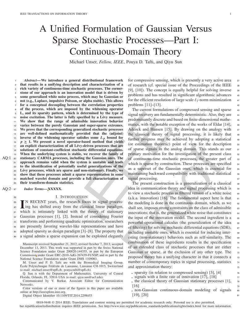
Fig. 1. Wavelets vs. KLT (or DCT) for the M-term approximation ofGaussian vs. sparse AR(1) processes with α = −0.1: (a) classical Gaussianscenario, (b) sparse scenario with symmetric Cauchy innovations. The E-splinewavelets are matched to the innovation model. The displayed results (relativequadratic error as a function of M/N ) are averages over 1000 realizationsfor AR(1) signals of length N = 1024; the performance of DCT and KLT isundistinguishable.
Fig. 1, which compares the performance of various transforms191
for the compression of two kinds of AR(1) processes with192
correlation e−0.1 ≈ 0.90: Gaussian vs. sparse where the latter193
innovation follows a Cauchy distribution. The key observation194
is that the E-spline wavelet transform, which is matched to the195
operator L = D − αId, provides the best results in the non-196
Gaussian scenario over the whole range of experimentation197
[cf. Fig. 1(b)], while the outcome in the Gaussian case is as198
predicted by the classical theory with the KLT being superior.199
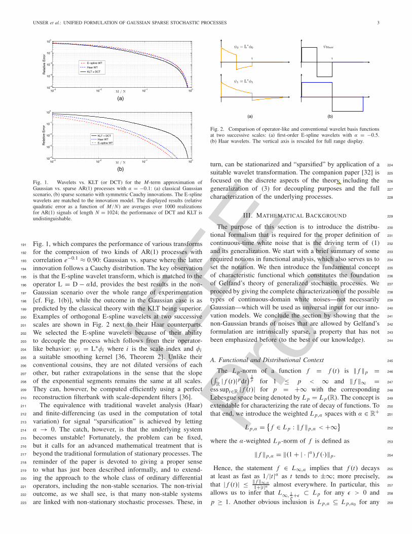
Examples of orthogonal E-spline wavelets at two successive200
scales are shown in Fig. 2 next to their Haar counterparts.201
We selected the E-spline wavelets because of their ability202
to decouple the process which follows from their operator-203
like behavior: ψi = L∗φi where i is the scale index and φi204
a suitable smoothing kernel [36, Theorem 2]. Unlike their205
conventional cousins, they are not dilated versions of each206
other, but rather extrapolations in the sense that the slope207
of the exponential segments remains the same at all scales.208
They can, however, be computed efficiently using a perfect209
reconstruction filterbank with scale-dependent filters [36].210
The equivalence with traditional wavelet analysis (Haar)211
and finite-differencing (as used in the computation of total212
variation) for signal “sparsification” is achieved by letting213
α → 0. The catch, however, is that the underlying system214
becomes unstable! Fortunately, the problem can be fixed,215
but it calls for an advanced mathematical treatment that is216
beyond the traditional formulation of stationary processes. The217
reminder of the paper is devoted to giving a proper sense218
to what has just been described informally, and to extend-219
ing the approach to the whole class of ordinary differential220
operators, including the non-stable scenarios. The non-trivial221
outcome, as we shall see, is that many non-stable systems222
are linked with non-stationary stochastic processes. These, in223
Fig. 2. Comparison of operator-like and conventional wavelet basis functionsat two successive scales: (a) first-order E-spline wavelets with α = −0.5.(b) Haar wavelets. The vertical axis is rescaled for full range display.
turn, can be stationarized and “sparsified” by application of a 224
suitable wavelet transformation. The companion paper [32] is 225
focused on the discrete aspects of the theory including the 226
generalization of (3) for decoupling purposes and the full 227
characterization of the underlying processes. 228
III. MATHEMATICAL BACKGROUND 229
The purpose of this section is to introduce the distribu- 230
tional formalism that is required for the proper definition of 231
continuous-time white noise that is the driving term of (1) 232
and its generalization. We start with a brief summary of some 233
required notions in functional analysis, which also serves us to 234
set the notation. We then introduce the fundamental concept 235
of characteristic functional which constitutes the foundation 236
of Gelfand’s theory of generalized stochastic processes. We 237
proceed by giving the complete characterization of the possible 238
types of continuous-domain white noises—not necessarily 239
Gaussian—which will be used as universal input for our inno- 240
vation models. We conclude the section by showing that the 241
non-Gaussian brands of noises that are allowed by Gelfand’s 242
formulation are intrinsically sparse, a property that has not 243
been emphasized before (to the best of our knowledge). 244
A. Functional and Distributional Context 245
The L p-norm of a function f = f (t) is ‖ f ‖p = 246
(∫R
| f (t)|pdt) 1
p for 1 ≤ p < ∞ and ‖ f ‖∞ = 247
ess supt∈R | f (t)| for p = +∞ with the corresponding 248
Lebesgue space being denoted by L p = L p(R). The concept is 249
extendable for characterizing the rate of decay of functions. To 250
that end, we introduce the weighted L p,α spaces with α ∈ R+
251
L p,α = {f ∈ L p : ‖ f ‖p,α < +∞}
252
where the α-weighted L p-norm of f is defined as 253
‖ f ‖p,α = ‖(1 + | · |α) f (·)‖p . 254
Hence, the statement f ∈ L∞,α implies that f (t) decays 255
at least as fast as 1/|t|α as t tends to ±∞; more precisely, 256
that | f (t)| ≤ ‖ f ‖∞,α
1+|t |α almost everywhere. In particular, this 257
allows us to infer that L∞, 1p +ε ⊂ L p for any ε > 0 and 258
p ≥ 1. Another obvious inclusion is L p,α ⊆ L p,α0 for any 259
unser
Inserted Text
,
IEEE
Proo
f
4 IEEE TRANSACTIONS ON INFORMATION THEORY
α ≥ α0. In the limit, we end up with the space of rapidly-260
decreasing functions R = {f : ‖ f ‖∞,m < +∞, ∀m ∈ Z
+},261
which is included in all the others.1262
We use ϕ = ϕ(t) to denote a generic function in Schwartz’s263
class S of rapidly-decaying and infinitely-differentiable test264
functions. Specifically, Schwartz’s space is defined as:265
S = {ϕ ∈ C∞ : ‖Dnϕ‖∞,m < +∞, ∀m, n ∈ Z
+},266
with the operator notation Dn = dn
dt n and the convention that267
D0 = Id (identity). S is a complete topological vector space268
with respect to the topology induced by the series of semi-269
norm ‖Dn · ‖∞,m with m, n ∈ Z+. Its topological dual is270
the space of tempered distributions S ′; a distribution φ ∈ S ′271
is a continuous linear functional on S that is characterized272
by a duality product rule φ(ϕ) = 〈φ, ϕ〉 = ∫Rφ(t)ϕ(t)dt273
with ϕ ∈ S where the right-hand side expression has a literal274
interpretation as an integral only when φ(t) is true function275
of t . The prototypical example of a tempered distribution is the276
Dirac distribution δ, which is defined as δ(ϕ) = 〈δ, ϕ〉 = ϕ(0).277
In the sequel, we will drop the explicit dependence of the278
distribution on the generic test function ϕ ∈ S and simply279
write φ, φ(·) or even φ(t) (with an abuse of notation) where t280
as the generic time index. For instance, we shall denote the281
shifted Dirac impulse2 by δ(· − t0), or δ(t − t0) which is the282
conventional notation used by engineers.283
Let T be a continuous3 linear operator that maps S into284
itself (or eventually some enlarged topological space such285
as L p). It is then possible to extend the action of T over286
S ′ (or an appropriate subset of it) based on the definition287
〈Tφ, ϕ〉 = 〈φ,T∗ϕ〉 for φ ∈ S ′ if T∗ is the adjoint of T288
which maps ϕ to another test function T∗ϕ ∈ S continuously.289
An important example is the Fourier transform whose classical290
definition is F{ f }(ω) = f (ω) = ∫R
f (t)e− jωt dt . Since F is291
a S-continuous operator, it is extendable to S ′ based on the292
adjoint relation 〈Fφ, ϕ〉 = 〈φ,Fϕ〉 for all ϕ ∈ S (generalized293
Fourier transform).294
A linear, shift-invariant (LSI) operator that is well-defined295
over S can always be written as a convolution product:296
TLSI{ϕ} = h ∗ ϕ =∫
R
h(τ )ϕ(· − τ )dτ297
where h = TLSI{δ} is the impulse response of the system.298
The adjoint operator is the convolution with the time-reversed299
version of h:300
h∨(t) ≡ h(−t).301
The better-known categories of LSI operators are the302
BIBO-stable (bounded input, bounded output) filters, and303
the ordinary differential operators. While the latter are not304
BIBO-stable, they do work well with test functions.305
1The topology of R is defined by the family of semi-norms ‖ · ‖∞,m ,m = 1, 2, 3, . . .
2The precise definition is 〈δ(· − t0), ϕ〉 = ϕ(t0) for all ϕ ∈ S .3An operator T is continuous from a sequential topological vector space
V into another one iff. ϕk → ϕ in the topology of V implies that Tϕk → Tϕin the topology (or norm) of the second space. If the two spaces coincide, wesay that T is V-continuous.
1) L p-Stable LSI Operators: The BIBO-stable filters corre- 306
spond to the case where h ∈ L1, or, more generally, when h 307
corresponds to a complex-valued Borel measure of bounded 308
variation. The latter extension allows for discrete filters of the 309
form hd = ∑n∈Z
d[n]δ(·−n) with d[n] ∈ �1. We will refer to 310
these filters as L p-stable because they specify bounded oper- 311
ators in all the L p spaces (by Young’s inequality). L p-stable 312
convolution operators satisfy the properties of commutativity, 313
associativity, and distributivity with respect to addition. 314
2) S-Continuous LSI Operators: For an L p-stable filter to 315
yield a Schwartz function as output, it is necessary that its 316
impulse response (continuous or discrete) be rapidly-decaying. 317
In fact, the condition h ∈ R (which is much stronger than inte- 318
grability) ensures that the filter is S-continuous. The nth-order 319
derivative Dn and its adjoint Dn∗ = (−1)nDn are in the 320
same category. The nth-order weak derivative of the tempered 321
distribution φ is defined as Dnφ(ϕ) = 〈Dnφ, ϕ〉 = 〈φ,Dn∗ϕ〉 322
for any ϕ ∈ S. The latter operator—or, by extension, any 323
polynomial of distributional derivatives PN (D) = ∑Nn=1 anDn
324
with constant coefficients an ∈ C—maps S ′ into itself. The 325
class of these differential operators enjoys the same properties 326
as its classical counterpart: shift-invariance, commutativity, 327
associativity and distributivity. 328
B. Notion of Generalized Stochastic Process 329
Classically, a stochastic process is a random function 330
s(t), t ∈ R whose statistical description is provided by the 331
probability law of its point values {s(t1), s(t2), . . . , s(tn), . . . } 332
for any finite sequence of time instants {tn}Nn=1. The implicit 333
assumption there is that one has a mechanism for probing the 334
value of the function s at any time t ∈ R, which is only 335
achievable approximately in the real physical world. 336
The leading idea in Gelfand and Vilenkin’s theory of 337
generalized stochastic processes is to replace the point mea- 338
surements {s(tn)} by a series of scalar products {〈s, ϕn〉} with 339
suitable “test” functions ϕ1, . . . , ϕN ∈ S [29]. The physical 340
motivation that these authors give is that Xn = 〈s, ϕn〉 may 341
represent the reading of a finite-resolution detector whose 342
output is some “averaged” value∫R
s(t)ϕn(t)dt , which is a 343
more plausible form of probing than ideal sampling. The 344
additional hypothesis is that the linear measurement X = 〈s, ϕ〉 345
depends continuously on ϕ and that the quantities Xn = 〈s, ϕn〉 346
obtained for different test functions {ϕn} are mutually compat- 347
ible. Mathematically, this translates into defining a generalized 348
stochastic process as a continuous linear random functional on 349
some topological vector space such as S. 350
Let s be such a generalized process. We first observe 351
that the scalar product X1 = 〈s, ϕ1〉 with a given test 352
function ϕ1 is a conventional (scalar) random variable that 353
is characterized by its probability density function (pdf) 354
pX1(x1); the latter is in one-to-one correspondence (via the 355
Fourier transform) with the characteristic function pX1(ω1) = 356
E{e jω1 X1} = ∫R
e jω1x1 pX1(x1)dx1 = E{e j 〈s,ω1ϕ1〉} where E{·} 357
is the expectation operator. The same applies for the 2nd-order 358
pdf pX1,X2(x1, x2) associated with a pair of test functions ϕ1 359
and ϕ2 which is the inverse Fourier transform of the 2-D 360
characteristic function pX1,X2(ω1, ω2) = E{e j 〈s,ω1ϕ1+ω2ϕ2〉}, 361
and so forth if one wants to specify higher-order dependencies. 362
unser
Cross-Out
unser
Replacement Text
stands as our
unser
Cross-Out
unser
Inserted Text
, which
unser
Cross-Out
unser
Replacement Text
,
IEEE
Proo
f
UNSER et al.: UNIFIED FORMULATION OF GAUSSIAN SPARSE STOCHASTIC PROCESSES 5
The foundation for the theory of generalized stochastic363
processes is that one can deduce the complete statistical364
information about the process from the knowledge of its365
characteristic form366
Ps(ϕ) = E{e j 〈s,ϕ〉} (4)367
which is a continuous, positive-definite functional over S such368
that Ps(0) = 1. Since the variable ϕ in Ps(ϕ) is completely369
generic, it provides the equivalent of an infinite-dimensional370
generalization of the characteristic function. Indeed, any finite371
dimensional version can be recovered by direct substitution of372
ϕ = ω1ϕ1 +· · ·+ωNϕN in Ps(ϕ) where the ϕn are fixed and373
where ω = (ω1, · · · , ωN ) takes the role of the N-dimensional374
Fourier variable.375
In fact, Gelfand’s theory rests upon the principle that speci-376
fying an admissible functional Ps(ϕ) is equivalent to defining377
the underlying generalized stochastic process (Bochner-Minlos378
theorem). To explain this remarkable result, we start by379
recalling the fundamental notion of positive-definiteness for380
univariate functions [37].381
Definition 1: A complex-valued function f of the real382
variable ω is said to be positive-definite iff.383
N∑
m=1
N∑
n=1
f (ωm − ωn)ξmξ n ≥ 0384
for every possible choice of ω1, . . . , ωN ∈ R, ξ1, . . . , ξN ∈ C385
and N ∈ Z+.386
This is equivalent to the requirement that the N × N matrix387
F whose elements are given by [F]mn = f (ωm − ωn) is388
positive semi-definite (that is, non-negative definite) for all389
N , no matter how the ωn’s are chosen.390
Bochner’s theorem states that a bounded, continuous func-391
tion p is positive-definite if and only if it is the Fourier392
transform of a positive and finite Borel measure P:393
p(ω) =∫
R
e jωxdP(x).394
In particular, Bochner’s theorem implies that a function pX (ω)395
is a valid characteristic function—that is, pX (ω) = E{e jωX } =396 ∫R
e jωx PX (dx) = ∫R
e jωx pX (x)dx where X is a random397
variable with probability measure PX (or pdf pX )—iff. pX is398
continuous, positive-definite and such that pX (0) = 1.399
The power of functional analysis is that these concepts400
carry over to functionals on some abstract nuclear space X ,401
the prime example being Schwartz’s class S of smooth and402
rapidly-decreasing test functions[29].403
Definition 2: A complex-valued functional F(ϕ) defined404
over the function space X is said to be positive-definite iff.405
N∑
m=1
N∑
n=1
F(ϕm − ϕn)ξmξ∗n ≥ 0406
for every possible choice of ϕ1, . . . , ϕN ∈ X , ξ1, . . . , ξN ∈ C407
and N ∈ Z+.408
Definition 3: A functional F : X → R (or C) is said to409
be continuous (with respect to the topology of the function410
space X ) if, for any convergent sequence (ϕi ) in X with limit 411
ϕ ∈ X , the sequence F(ϕi ) converges to F(ϕ); that is, 412
limi
F(ϕi ) = F(limiϕi ). 413
Theorem 1 (Minlos-Bochner): Given a functional Ps(ϕ) 414
on a nuclear space X that is continuous, positive-definite and 415
such that Ps(0) = 1, there exists a unique probability measure 416
Ps on the dual space X ′ such that 417
Ps(ϕ) = E{e j 〈s,ϕ〉} =∫
X ′e j 〈s,ϕ〉dPs(s), 418
where 〈s, ϕ〉 is the dual pairing map. One further has the 419
guarantee that all finite dimensional probabilities measures 420
derived from Ps(ϕ) by setting ϕ = ω1ϕ1 + · · · + ωNϕN are 421
mutually compatible. 422
The characteristic form therefore uniquely specifies the 423
generalized stochastic process s = s(ϕ) (via the infinite- 424
dimensional probability measure Ps) in essentially the 425
same way as the characteristic function fully determines 426
the probability measure of a scalar or multivariate random 427
variable. 428
C. White Noise Processes (Innovations) 429
We define a white noise w as a generalized random process 430
that is stationary and whose measurements for non-overlapping 431
test functions are independent. A remarkable aspect of the 432
theory of generalized stochastic processes is that it is 433
possible to deduce the complete class of such noises based 434
on functional considerations only [29]. To that end, Gelfand 435
and Vilenkin consider the generic class of functionals of the 436
form 437
Pw(ϕ) = exp
(∫
R
f(ϕ(t)
)dt
)
(5) 438
where f is a continuous function on the real line and ϕ 439
is a test function from some suitable space. This functional 440
specifies an independent noise process if Pw is continuous 441
and positive-definite and Pw(ϕ1 + ϕ2) = Pw(ϕ1)Pw(ϕ2) 442
whenever ϕ1 and ϕ2 have non-overlapping support. The latter 443
property is equivalent to having f (0) = 0 in (5). Gelfand 444
and Vilenkin then go on to prove that the complete class of 445
functionals of the form (5) with the required mathematical 446
properties (continuity, positive-definiteness and factorizability) 447
is obtained by choosing f to be a Lévy exponent, as defined 448
below. 449
Definition 4: A complex-valued continuous function f (ω) 450
is a valid Lévy exponent if and only if f (0) = 0 and gτ (ω) = 451
eτ f (ω) is a positive-definite function of ω for all τ ∈ R+. 452
In doing so, they actually establish a one-to-one corre- 453
spondence between the characteristic form of an indepen- 454
dent noise processes (5) and the family of infinite-divisible 455
laws whose characteristic function takes the form pX (ω) = 456
e f (ω) = E{e jωX } [38], [39]. While Definition 4 is hard to 457
exploit directly, the good news is that there exists a complete 458
constructive, characterization of Lévy exponents, which is a 459
classical result in probability theory: 460
unser
Pencil
unser
Sticky Note
P({\rm d}x)
unser
Pencil
unser
Sticky Note
\mathscr{P}({\rm d}s)
IEEE
Proo
f
6 IEEE TRANSACTIONS ON INFORMATION THEORY
Theorem 2 (Lévy-Khintchine Formula): f (ω) is a valid461
Lévy exponent if and only if it can be written as462
f (ω) = jb′1ω − b2ω
2
2463
+∫
R\{0}[e jaω − 1 − jaω�{|a|<1}(a)] V (da)464
(6)465
where b′1 ∈ R and b2 ∈ R
+ are some constants and V is a466
Lévy measure, that is, a (positive) Borel measure on R\{0}467
such that468 ∫
R\{0}min(1, a2) V (da) < ∞. (7)469
The notation � (a) refers to the indicator function that takes470
the value 1 if a ∈ and zero otherwise. Theorem 2 is funda-471
mental to the classical theories of infinite-divisible laws and472
Lévy processes [28], [31], [39]. To further our mathematical473
understanding of the Lévy-Khintchine formula (6), we note474
that e jaω − 1 − jaω�{|a|<1}(a) ∼ − 12 a2ω2 as a → 0. This475
ensures that the integral is convergent even when the Lévy476
measure V is singular at the origin to the extent allowed by477
the admissibility condition (7). If the Lévy measure is finite or478
symmetrical (i.e., V (E) = V (−E) for any E ⊂ R), it is then479
also possible to use the equivalent, simplified form of Lévy480
exponent481
f (ω) = jb1ω − b2ω2
2+
∫
R\{0}(e jaω − 1
)V (da) (8)482
with b1 = b′1 − ∫
0<|a|<1 aV (da). The bottomline is that483
a particular brand of independent noise process is thereby484
completely characterized by its Lévy exponent or, equivalently,485
its Lévy triplet (b1, b2, v) where v is the so-called Lévy density486
associated with V such that487
V (E) =∫
Ev(a)da488
for any Borel set E ⊆ R. With this latter convention, the489
three primary types of innovations encountered in the signal490
processing and statistics literature are specified as follows:491
1) Gaussian: b1 = 0, b2 = 1, v = 0492
fGauss(ω) = −|ω|22,493
Pw(ϕ) = e− 1
2 ‖ϕ‖2L2 . (9)494
2) Compound Poisson [18]: b1 = 0, b2 = 0, v(a) =495
λ pA(a) with∫R
pA(a)da = pA(0) = 1,496
fPoisson(ω; λ, pA) = λ
∫
R
(e jaω − 1
)pA(a)da,497
Pw(ϕ) = exp
(
λ
∫
R
∫
R
(e jaϕ(t) − 1) pA(a)dadt
)
.498
(10)499
3) Symmetric alpha-stable (SαS) [40]: b1 = 0, b2 =500
0, v(a) = Cα|a|α+1 with 0 < α < 2 and Cα = sin( πα2 )
π a501
suitable normalization constant, 502
fα(ω) = −|ω|αα! , 503
Pw(ϕ) = e− 1α! ‖ϕ‖αLα . (11) 504
The latter follows from the fact that −|ω|αα! is the generalized 505
Fourier transform of Cα|t |α+1 with the convention that α! = 506
�(α + 1) where � is Euler’s Gamma function [41]. 507
While none of these innovations has a classical interpre- 508
tation as a random function of t , we can at least provide an 509
explicit description of the Poisson noise as an infinite random 510
sequence of Dirac impulses (cf.[18, Theorem 1]) 511
wλ(t) =∑
k
akδ(t − tk) 512
where the tk are random locations that are uniformly distrib- 513
uted over R with density λ, and where the weights ak are 514
i.i.d. random variables with pdf pA(a). Remarkably, this is 515
the only innovation process in the family that has a finite rate 516
of innovation [17]; however, it is, by far, not the only one that 517
is sparse as explained next. 518
D. Gaussian Versus Sparse Categorization 519
To get a better understanding of the underlying class of 520
white noises w, we propose to probe them through some 521
localized analysis window ϕ, which will yield a conventional 522
i.i.d. random variable X = 〈w,ϕ〉 with some pdf pϕ(x). The 523
most convenient choice is to pick the rectangular analysis 524
window ϕ(t) = rect(t) = �[− 12 ,
12 ](t) when 〈w, rect〉 is 525
well-defined. By using the fact that e jaωrect(t)−1 = e jaω−1 for 526
t ∈ [− 12 ,
12 ], and zero otherwise, we find that the characteristic 527
function of X is simply given by 528
prect(ω) = Pw (ω · rect(t)) = exp ( f (ω)) , 529
which corresponds to the generic (Lévy-Khinchine) form asso- 530
ciated with an infinitely-divisible distribution [31], [39], [42]. 531
The above result makes the mapping between generalized 532
white noise processes and classical infinite-divisible (id) laws4533
explicit: The “canonical” id pdf of w, pid(x) = prect(x), is 534
obtained by observing the noise through a rectangular window. 535
Conversely, given the Lévy exponent of an id distribution, 536
f (ω) = log (F{pid}(ω)), we can specify a corresponding 537
innovation process w via the characteristic form Pw(ϕ) by 538
merely substituting the frequency variable ω by the generic 539
test function ϕ(t), adding an integration over R and taking 540
the exponential as in (5). 541
We note, in passing, that sparsity in signal processing may 542
refer to two distinct notions. The first is that of a finite rate 543
of innovation; i.e., a finite (but perhaps random) number of 544
innovations per unit of time and/or space, which results in a 545
mass at zero in the histogram of observations. The second 546
possibility is to have a large, even infinite, number of 547
innovations, but with the property that a few large innovations 548
4A random variable X with pdf pX (x) is said to be infinitely divisible (id)if for any n ∈ Z
+ there exist i.i.d. random variables X1, . . . , Xn with pdf saypn(x) such that X = X1 + · · · + Xn in law.
unser
Cross-Out
unser
Replacement Text
$A_k$
unser
Cross-Out
unser
Replacement Text
A_k
IEEE
Proo
f
UNSER et al.: UNIFIED FORMULATION OF GAUSSIAN SPARSE STOCHASTIC PROCESSES 7
dominate the overall behavior. In this case the histogram of549
observations is distinguished by its ‘heavy tails’. (A combina-550
tion of the two is also possible, for instance in a compound551
Poisson process with a heavy-tailed amplitude distribution.552
For such a process one may observe a change of behavior553
in passing from one dominant type of sparsity to the other).554
Our framework permits us to consider both types of sparsity,555
in the former case with compound Poisson models and in the556
latter with heavy-tailed infinitely-divisible innovations.557
To make our point, we consider two distinct scenarios.558
1) Finite Variance Case: We first assume that the second559
moment m2 = ∫R\{0} a2 V (da) of the Lévy measure V in (6)560
is finite. This allows us to rewrite the classical Lévy-Khinchine561
representation as562
f (ω) = jc1ω − b2ω2
2+
∫
R\{0}[e jaω − 1 − jaω] V (da)563
with c1 = b′′1 + ∫
|a|>1 aV (da) and where the Poisson part564
of the functional is now fully compensated. Indeed, we are565
guaranteed that the above integral is convergent because566
|e jaω − 1 − jωa| � |aω|2 as a → 0 and |e jaω − 1 − jωa| ∼567
|aω| as a → ±∞. An interesting non-Poisson example of568
infinitely-divisible probability laws that falls into this category569
(with non-finite V ) is the Laplace distribution with Lévy triplet570
(0, 0, v(a) = e−|a||a| ) and pid(x) = 1
2 e−|x |. This model is571
particularly relevant for sparse signal processing because it572
provides a tight connection between Lévy processes and total573
variation regularization [18, Section VI].574
Now, if the Lévy measure is finite∫R
V (da) = λ < ∞,575
the admissibility condition yields∫R\{0} a V (da) < ∞, which576
allows us to pull the bias correction out of the integral. The577
representation then simplifies to (8). This implies that we578
can decompose X into the sum of two independent Gaussian579
and compound Poisson random variables. The variances of580
the Gaussian and Poisson components are σ 2 = b2 and581 ∫R
a2V (da), respectively. The Poisson component is sparse582
because its pdf exhibits a mass distribution e−λδ(x) at the583
origin, meaning that the chances for a continuous amplitude584
distribution of getting zero are overwhelmingly higher than585
any other value, especially for smaller values of λ > 0. It is586
therefore justifiable to use 0 ≤ e−λ < 1 as our Poisson sparsity587
index.588
2) Infinite Variance Case: We now turn our attention to589
the case where the second moment of the Lévy measure590
is unbounded, which we like to label as the “super-sparse”591
one. To substantiate this claim, we invoke the Ramachandran-592
Wolfe theorem which states that the pth moment E{|X |p}593
with p ∈ R+ of an infinitely divisible distribution is finite594
iff.∫|a|>1 |a|p V (da) < ∞ [43], [44]. For p ≥ 2, the595
latter is equivalent to∫R\{0} |a|p V (da) < ∞ because of the596
admissibility condition (7). It follows that the cases that are597
not covered by the previous scenario (including the Gaussian598
+ Poisson model) necessarily give rise to distributions whose599
moments of order p are unbounded for p ≥ 2. The proto-600
typical representatives of such heavy tail distributions are the601
alpha-stable ones or, by extension, the broad family of infinite602
divisible probability laws that are in their domain of attraction.603
Note that these distributions all fulfill the stringent conditions 604
for �p compressibility[45], [46]. 605
IV. INNOVATION APPROACH TO CONTINUOUS-TIME 606
STOCHASTIC PROCESSES 607
Specifying a stochastic process through an innovation model 608
(or an equivalent stochastic differential equation) is attractive 609
conceptually, but it presupposes that we can provide an inverse 610
operator (in the form of an integral transform) that transforms 611
the innovation back into the initial stochastic process. This is 612
the reason why, after laying out general conditions for exis- 613
tence, we shall spend the greater part of our effort investigating 614
suitable inverse operators. 615
A. Stochastic Differential Equations 616
Our aim is to define the generalized process with whitening 617
operator L : S ′ → S ′ and Lévy exponent f as the solution of 618
the stochastic linear differential equation 619
Ls = w, (12) 620
where w is an innovation process, as described in 621
Section III-C. This definition is obviously only usable if we 622
can construct an inverse operator T = L−1 that solves this 623
equation. For the cases where the inverse is not unique, we will 624
need to select one preferential operator, which is equivalent 625
to imposing specific boundary conditions. We are then able 626
to formally express the stochastic process as a transformed 627
version of a white noise 628
s = L−1w. (13) 629
The requirement for such a solution to be consistent with (12) 630
is that the operator satisfies the right-inverse property LL−1 = 631
Id over the underlying class of tempered distributions. By 632
using the adjoint relation 〈s, ϕ〉 = 〈L−1w,ϕ〉 = 〈w,L−1∗ϕ〉, 633
we can then transfer the action of the operator onto the test 634
function inside the characteristic form and obtain a com- 635
plete statistical characterization of the so-defined generalized 636
stochastic process 637
Ps(ϕ) = PL−1w(ϕ) = Pw(L−1∗ϕ), (14) 638
where Pw is given by (5) (or one of the specific forms in the 639
list at the end of Section III-C) and where we are implicitly 640
requiring that the adjoint L−1∗ is mathematically well-defined 641
(continuous) over S, and that its composition with Pw is 642
well-defined for all ϕ ∈ S. 643
In order to realize the above idea mathematically, it isusually easier to proceed backwards: one specifies an operatorT that satisfies the left-inverse property: ∀ϕ ∈ S, TL∗ϕ = ϕ,and that is continuous (i.e., bounded in the proper norm(s))over the chosen class of test functions. One then characterizesthe adjoint of T, which is the operator T∗ : S ′ → S ′ (or anappropriate subset thereof) such that, for a given φ ∈ S ′,
∀ϕ ∈ S, 〈φ, ϕ〉 = 〈LT∗φ, ϕ〉 = 〈φ, TL∗︸︷︷︸
Id
ϕ〉.
Finally, we set L−1 = T∗, which yields the proper distribu- 644
tional definition of the right inverse of L in (13). 645
unser
Cross-Out
unser
Replacement Text
{\rm d}
unser
Inserted Text
[space]
IEEE
Proo
f
8 IEEE TRANSACTIONS ON INFORMATION THEORY
B. General Conditions for Existence646
To validate the proposed innovation model, we need to647
ensure that the solution s = L−1w is a bona fide generalized648
stochastic process.649
In order to simplify the analysis, we shall restrict our650
attention to an appropriate subclass of Lévy exponents.651
Definition 5: A Lévy exponent f with derivative f ′ is652
p-admissible with 1 ≤ p ≤ 2 if there exists a positive constant653
C such that | f (ω)| + |ω| · | f ′(ω)| ≤ C|ω|p for all ω ∈ R.654
Note that this p-admissibility condition is not very con-655
straining and that it is satisfied by the great majority of656
members of the Lévy-Kintchine family (see Section III-C).657
For instance in the compound Poisson case, we can show that658
|ω| · | f ′(ω)| ≤ λ|ω| E{|A|} and f (ω) ≤ λ|ω| E{|A|} by659
using the fact |e j x − 1| ≤ |x |; this implies that the bound660
in Definition 5 with p = 1 is always satisfied provided661
that the first (absolute) moment of the amplitude pdf pA(a)662
in (10) is finite. Similarly, all symmetric Lévy exponents with663
− f ′′(0) < ∞ (finite variance case) are p-admissible with664
p = 2, the prototypical example being the Gaussian. The only665
cases we are aware of that do not fulfill the condition are the666
alpha-stable noises with 0 < α < 1, which are notorious for667
their exotic behavior.668
The first advantage of imposing p-admissibility is that it669
allows us to extend the set of acceptable analysis functions670
from S to L p which is crucial if we intend to do conventional671
signal processing.672
Theorem 3: If the Lévy exponent f is p-admissible, then673
the characteristic form Pw(ϕ) = exp(∫
Rf(ϕ(t)
)dt
)is a674
continuous, positive-definite functional over L p .675
Proof: Since the exponential function is continuous, it is676
sufficient to consider the functional677
F(ϕ) = log Pw(ϕ) =∫
R
f (ϕ(t))dt,678
which is such that F(0) = 0. To show that F(ϕ)(and hence679
Pw(ϕ))
is well-defined over L p , we note that680
|F(ϕ)| ≤∫
R
| f (ϕ(t))| dt ≤ C‖ϕ‖pp,681
which follows from the p-admissibility condition. The positive682
definiteness of Pw(ϕ) over S is a direct consequence of f683
being a Lévy exponent and is therefore also transferable to684
L p . For the interested reader, this can be shown quite easily685
by proving that F(ϕ) is conditionally positive-definite of order686
one (see [20]).687
The only remaining work is to establish the L p-continuity688
of F(ϕ). To that end, we observe that689
| f (u)− f (v)| =∣∣∣
∫ u
vf ′(t)dt
∣∣∣690
≤ C∣∣∣
∫ u
vt p−1dt
∣∣∣691
(by the assumption on f )692
≤ C max(|u|p−1, |v|p−1)|u − v|693
≤ C(|v|p−1 + |u − v|p−1)|u − v|.694
(by the triangle inequality)695
Next, we pick a convergent sequence in L p , {ϕn}∞n=1, whose 696
limit is denoted by ϕ. The convergence in L p is expressed as 697
limn→∞ ‖ϕn − ϕ‖p = 0. (15) 698
We then have 699
∣∣∣
∫
R
f (ϕn(t))dt −∫
R
f (ϕ(t))dt∣∣∣ 700
≤C∫
R
|ϕ(t)|p−1|ϕn(t)− ϕ(t)| + |ϕn(t)− ϕ(t)|pdt 701
≤C(‖ϕ‖p−1
p ‖ϕn − ϕ‖p + ‖ϕn − ϕ‖pp
)
(by Hölder’s inequality)
702
→0 as n → ∞, (by (15)) 703704
which proves the continuity of the functional Pw on L p . 705
Thanks to this result, we can then rely on the Minlos- 706
Bochner theorem (Theorem 1) to state basic conditions on 707
T = L−1∗ that ensure that s = T∗w is a well-defined 708
generalized process over S ′. 709
Theorem 4 (Existence of Generalized Process): Let f be a 710
valid Lévy exponent and T be an operator acting on ϕ ∈ S 711
such that any one of the conditions below is met: 712
1) T is a continuous linear map from S into itself, 713
2) T is a continuous linear map from S into L p and the 714
Lévy exponent f is p-admissible. 715
Then, Ps(ϕ) = exp(∫
Rf(Tϕ(t)
)dt
)is a continuous, positive- 716
definite functional on S such that Ps(0) = 1. 717
Proof: We already know that Pw is a continuous 718
functional on S (resp., on L p when f is p-admissible) by 719
construction. This, together with the assumption that T is a 720
continuous operator on S (resp., from S to L p), implies that 721
the composed functional Ps(ϕ) := Pw(Tϕ) is continuous 722
on S. 723
Given the functions ϕ1, . . . , ϕN in S and some complex 724
coefficients ξ1, . . . , ξN , 725
∑
1≤m,n≤N
Ps(ϕm − ϕn)ξmξn 726
=∑
1≤m,n≤N
Pw
(T(ϕm − ϕn)
)ξmξn 727
=∑
1≤m,n≤N
Pw(Tϕm − Tϕn)ξmξn
(by the linearity of the operator T)
728
≥ 0. (by the positivity of Pw over S or L p) 729730
This proves the positive definiteness of the functional Ps 731
on S. 732
Lastly, Ps(0) = Pw(T0) = Pw(0) = 1. 733
The final fundamental issue relates to the interpretation 734
of s = L−1w as an ordinary stochastic process; that is, a 735
random function s(t) of the time variable t . This presupposes 736
that the shaping operator L−1 performs a minimal amount of 737
smoothing since the driving term of the model, w, is too rough 738
to admit a pointwise representation. 739
Theorem 5 (Interpretationas anOrdinaryStochasticProcess): 740
Let s be the generalized stochastic process whose 741
characteristic function is given by (14) where f is a 742
unser
Cross-Out
unser
Replacement Text
=
unser
Cross-Out
unser
Replacement Text
(Interpretation as Ordinary Stochastic Process)
IEEE
Proo
f
UNSER et al.: UNIFIED FORMULATION OF GAUSSIAN SPARSE STOCHASTIC PROCESSES 9
p-admissible Lévy exponent and L−1∗ is a continuous743
operator from S to L p (or a subset thereof). We also define744
the (generalized) impulse response745
h(t, τ ) = L−1{δ(· − τ )}(t), (16)746
with a slight abuse of notation since h is not necessarily747
an ordinary function. Then, s = L−1w admits the pointwise748
representation for t ∈ R749
s(t) = 〈w, h(t, ·)〉 (17)750
provided that h(t, ·) ∈ L p (with t fixed).751
The form of h(t, τ ) in (16) is the “time-domain” transcrip-752
tion of Schwartz’s kernel theorem which gives the integral753
representation of a linear operator in terms of a (generalized)754
kernel h ∈ S ′ × S ′ (the infinite-dimensional generalization of755
a matrix multiplication). The more standard definition used756
in the theory of generalized functions is 〈h(·, ·), ϕ1 ⊗ ϕ2〉 =757
〈L−1∗{ϕ1}, ϕ2〉, where ϕ1 ⊗ ϕ2(t, τ ) = ϕ1(t)ϕ2(τ ) for all758
ϕ1, ϕ2 ∈ S.759
Proof: The existence of the generalized stochastic process760
s = L−1w is ensured by Theorem 4. We then consider the761
observation of the innovation X0 = 〈w,ϕ0〉 where ϕ0 =762
h(t0, ·) with ϕ0 ∈ L p . Since Pw admits a continuous exten-763
sion over L p (by Theorem 3), we can specify the characteristic764
function of X0 as765
pX0(ω) = E{e jωX0} = Pw(ωϕ0)766
with ϕ0 fixed. Thanks to the functional properties of Pw,767
pX0(ω) is a continuous, positive-definite function of ω such768
that pX0(0) = 1 so that we can invoke Bochner’s theorem769
to establish that X0 is a well-defined conventional random770
variable with pdf pX0 (the inverse Fourier transform of pX0 ).771
772
C. Inverse Operators773
Before presenting our general method of solution, we need774
to identify a suitable set of elementary inverse operators that775
satisfy the continuity requirement in Theorem 4.776
Our approach relies on the factorization of a differen-777
tial operator into simple first-order components of the form778
(D−αnId) with αn ∈ C, which can then be treated separately.779
Three possible cases need to be considered.780
1) Causal-Stable: Re(αn) < 0. This is the classical textbook781
hypothesis which leads to a causal-stable convolution system.782
It is well known from the theory of distributions and linear783
systems (e.g., [47, Section 6.3], [48]) that the causal Green784
function of (D−αnId) is the causal exponential function ραn (t)785
already encountered in the introductory example in Section II.786
Clearly, ραn (t) is absolutely integrable (and rapidly-decaying)787
iff. Re(αn) < 0. It follows that (D − αnId)−1 f = ραn ∗ f788
with ραn ∈ R ⊂ L1. In particular, this implies that T =789
(D − αnId)−1 specifies a continuous LSI operator on S. The790
same holds for T∗ = (D − αnId)−1∗, which is defined as791
T∗ f = ρ∨αn
∗ f .792
2) Anti-Causal Stable: Re(αn) > 0. This case is usu-793
ally excluded because the standard Green function ραn (t) =794
�+(t)eαn t grows exponentially, meaning that the system does795
not have a stable causal solution. Yet, it is possible to consider796
an alternative anti-causal Green function ρ′αn(t) = −ρ∨−αn
(t) = 797
ραn (t)− eαnt , which is unique in the sense that it is the only 798
Green function5 of (D−αnId) that is Lebesgue-integrable and, 799
by the same token, the proper inverse Fourier transform of 800
1jω−αn
for Re(αn) > 0. In this way, we are able to specify 801
an anti-causal inverse filter (D − αnId)−1 f = ρ′αn
∗ f with 802
ρ′αn
∈ R that is L p-stable and S-continuous. In the sequel, 803
we will drop the ′ superscript with the convention that ρα(t) 804
systematically refers to the unique Green function of (D−αId) 805
that is rapidly-decay when Re(α) �= 0. For now on, we shall 806
therefore use the definition 807
ρα(t) ={�+(t)eαt if Re(α) ≤ 0−�+(−t)eαt otherwise.
(18) 808
which also covers the next scenario. 809
3) Marginally Stable: Re(αn) = 0 or, equivalently, αn = 810
jω0 with ω0 ∈ R. This third case, which is incompatible 811
with the conventional formulation of stationary processes, is 812
most interesting theoretically because it opens the door to 813
important extensions such as Lévy processes, as we shall see in 814
Section V. Here, we will show that marginally-stable systems 815
can be handled within our generalized framework as well, 816
thanks to the introduction of appropriate inverse operators. 817
The first natural candidate for (D − jω0Id)−1 is the inversefilter whose frequency response is
ρ jω0(ω) = 1
j (ω − ω0)+ πδ(ω − ω0).
It is a convolution operator whose time-domain definition is 818
Iω0ϕ(t) = (ρ jω0 ∗ ϕ)(t) 819
= e jω0t∫ t
−∞e− jω0τ ϕ(τ )dτ. (19) 820
Its impulse response ρ jω0(t) is causal and compatible with 821
Definition (18), but not (rapidly) decaying. The adjoint of Iω0 822
is given by 823
I∗ω0ϕ(t) = (ρ∨
jω0∗ ϕ)(t) 824
= e− jω0t∫ +∞
te jω0τ ϕ(τ )dτ. (20) 825
While Iω0ϕ(t) and I∗ω0ϕ(t) are both well-defined when ϕ ∈ L1, 826
the problem is that these inverse filters are not BIBO stable 827
since their impulse responses, ρ jω0(t) and ρ∨jω0(t), are not 828
in L1. In particular, one can easily see that Iω0ϕ (resp., I∗ω0ϕ) 829
with ϕ ∈ S is generally not in L p with 1 ≤ p < +∞, 830
unless ϕ(ω0) = 0 (resp., ϕ(−ω0) = 0). The conclusion is 831
that I∗ω0fails to be a bounded operator over the class of test 832
functions S. 833
This leads us to introduce some “corrected” version of the 834
adjoint inverse operator I∗ω0, 835
I∗ω0,t0ϕ(t) = I∗ω0
{ϕ − ϕ(−ω0)e
− jω0t0δ(· − t0)}(t) 836
= I∗ω0ϕ(t)− ϕ(−ω0)e
− jω0t0ρ∨jω0(t − t0), (21) 837
where t0 ∈ R is a fixed location parameter and where 838
ϕ(−ω0) = ∫R
e jω0tϕ(t)dt is the complex sinusoidal moment 839
associated with the frequency ω0. The idea is to correct for 840
5: ρ is a Green functions of (D −αn Id) iff. (D −αn Id)ρ = δ; the completeset of solutions is given ρ(t) = ραn (t)+Ceαn t which is the sum of the causalGreen function ραn (t) plus an arbitrary exponential component that is in thenull space of the operator.
unser
Inserted Text
ing

IEEE
Proo
f
10 IEEE TRANSACTIONS ON INFORMATION THEORY
the lack of decay of I∗ω0ϕ(t) as t → −∞ by subtracting841
a properly weighted version of the impulse response of the842
operator. An equivalent Fourier-based formulation is provided843
by the formula at the bottom of Table I; the main difference844
with the corresponding expression for Iω0ϕ is the presence of a845
regularization term in the numerator that prevents the integrant846
from diverging at ω = ω0. The next step is to identify the847
adjoint of I∗ω0,t0 , which is achieved via the following inner-848
product manipulation849
〈ϕ, I∗ω0,t0φ〉 = 〈ϕ, I∗ω0φ〉 − φ(−ω0)e
− jω0t0〈ϕ, ρ∨jω0(· − t0)〉850
= 〈Iω0ϕ, φ〉 − 〈e jω0·, φ〉 e− jω0t0 Iω0ϕ(t0)851
(using(19))852
= 〈Iω0ϕ, φ〉 − 〈e jω0(·−t0)Iω0ϕ(t0), φ〉.853
Since the above is equal to 〈Iω0,t0ϕ, φ〉 by definition, we obtain854
that855
Iω0,t0ϕ(t) = Iω0ϕ(t)− e jω0(t−t0) Iω0ϕ(t0). (22)856
Interestingly, this operator imposes the boundary condition857
Iω0,t0ϕ(t0) = 0 via the subtraction of a sinusoidal component858
that is in the null space of the operator (D − jω0Id), which859
gives a direct interpretation of the location parameter t0.860
Observe that expressions (21) and (22) define linear operators,861
albeit not shift-invariant ones, in contrast with the classical862
inverse operators Iω0 and I∗ω0.863
For analysis purposes, it is convenient to relate the proposed864
inverse operators to the anti-derivatives corresponding to the865
case ω0 = 0. To that end, we introduce the modulation866
operator867
Mω0ϕ(t) = e jω0tϕ(t)868
which is a unitary map on L2 with the property that869
M−1ω0
= M−ω0 .870
Proposition 1: The inverse operators defined by (19), (20),871
(22), and (21) satisfy the modulation relations872
Iω0ϕ(t) = Mω0 I0 M−1ω0ϕ(t),873
I∗ω0ϕ(t) = M−1
ω0I∗0 Mω0ϕ(t),874
Iω0,t0ϕ(t) = Mω0 I0,t0 M−1ω0ϕ(t),875
I∗ω0,t0ϕ(t) = M−1ω0
I∗0,t0 Mω0ϕ(t).876
Proof: These follow from the modulation property of877
the Fourier transform (i.e, F{Mω0ϕ}(ω) = F{ϕ}(ω − ω0))878
and the observations that Iω0δ(t) = ρ jω0(t) = Mω0ρ0(t) and879
I∗ω0δ(t) = ρ∨
jω0(t) = M−ω0ρ
∨0 (t) with ρ0(t) = �+(t) (the unit880
step function).881
The important functional property of I∗ω0,t0 is that it essentially882
preserves decay and integrability, while Iω0,t0 fully retains sig-883
nal differentiability. Unfortunately, it is not possible to have the884
two simultaneously unless Iω0ϕ(t0) and ϕ(−ω0) are both zero.885
Proposition 2: If f ∈ L∞,α with α > 1, then there exists886
a constant Ct0 such that887
|I∗ω0,t0 f (t)| ≤ Ct0‖ f ‖∞,α
1 + |t|α−1 ,888
which implies that I∗ω0,t0 f ∈ L∞,α−1.889
Proof: Since modulation does not affect the decay properties 890
of a function, we can invoke Proposition 1 and concentrate on 891
the investigation of the anti-derivative operator I∗0,t0 . Without 892
loss of generality, we can also pick t0 = 0 and transfer the 893
bound to any other finite value of t0 by adjusting the value of 894
the constant Ct0 . Specifically, for t < 0, we write this inverse 895
operator as 896
I∗0,0 f (t) = I∗0 f (t)− f (0) 897
=∫ +∞
tf (τ )dτ −
∫ ∞
−∞f (τ )dτ 898
= −∫ t
−∞f (τ )dτ. 899
This implies that 900
|I∗0,0 f (t)| =∣∣∣∣
∫ t
−∞f (τ )dτ
∣∣∣∣ ≤ ‖ f ‖∞,α
∫ t
−∞1
1 + |τ |α dτÊ 901
≤(
2α
α − 1
) ‖ f ‖∞,α
1 + |t|α−1 902
for all t < 0. For t > 0, I∗0,0 f (t) = ∫ ∞t f (τ )dτ so that the 903
above upper bounds remain valid. 904
The interpretation of the above result is that the inverse 905
operator I∗ω0,t0 reduces inverse polynomial decay by one order. 906
Proposition 2 actually implies that the operator will preserve 907
the rapid decay of the Schwartz functions which are included 908
in L∞,α for any α ∈ R+. It also guarantees that I∗ω0,t0ϕ belongs 909
to L p for any Schwartz function ϕ. However, I∗ω0,t0 will spoil 910
the global smoothness properties of ϕ because it introduces a 911
discontinuity at t0, unless ϕ(−ω0) is zero in which case the 912
output remains in the Schwartz class. This allows us to state 913
the following theorem which summarizes the higher-level part 914
of those results for further reference. 915
Theorem 6: The operator I∗ω0,t0 defined by (22) is a continu- 916
ous linear map from R into R (the space of bounded functions 917
with rapid decay). Its adjoint Iω0,t0 is given by (21) and has the 918
property that Iω0,t0ϕ(t0) = 0. Together, these operators satisfy 919
the complementary left- and right-inverse relations 920
{I∗ω0,t0(D − jω0Id)∗ϕ = ϕ
(D − jω0Id)Iω0,t0ϕ = ϕ921
922
for all ϕ ∈ S. 923
Having a tight control on the action of I∗ω0,t0 over S allows 924
us to extend the right-inverse operator Iω0,t0 to an appropriate 925
subset of tempered distributions φ ∈ S ′ according to the rule 926
〈Iω0,t0φ, ϕ〉 = 〈φ, I∗ω0,t0ϕ〉. Our complete set of inverse oper- 927
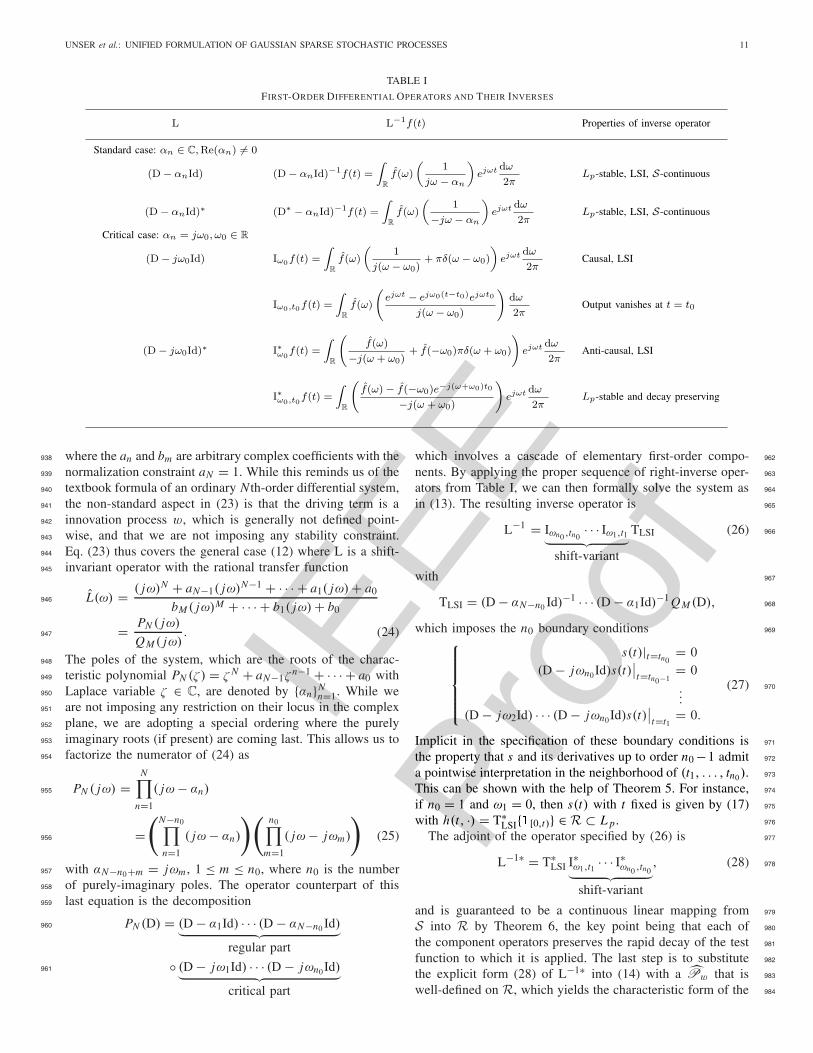
ators is summarized in Table I together with their equivalent 928
Fourier-based definitions which are also interpretable in the 929
generalized sense of distributions. The first three entries of 930
the table are standard results from the theory of linear systems 931
(e.g., [49, Table 4.1]), while the other operators are specific 932
to this work. 933
D. Solution of Generic Stochastic Differential Equation 934
We now have all the elements to solve the generic stochastic 935
linear differential equation 936
N∑
n=0
anDns =M∑
m=0
bmDmw (23) 937
IEEE
Proo
f
UNSER et al.: UNIFIED FORMULATION OF GAUSSIAN SPARSE STOCHASTIC PROCESSES 11
TABLE I
FIRST-ORDER DIFFERENTIAL OPERATORS AND THEIR INVERSES
where the an and bm are arbitrary complex coefficients with the938
normalization constraint aN = 1. While this reminds us of the939
textbook formula of an ordinary N th-order differential system,940
the non-standard aspect in (23) is that the driving term is a941
innovation process w, which is generally not defined point-942
wise, and that we are not imposing any stability constraint.943
Eq. (23) thus covers the general case (12) where L is a shift-944
invariant operator with the rational transfer function945
L(ω) = ( jω)N + aN−1( jω)N−1 + · · · + a1( jω)+ a0
bM ( jω)M + · · · + b1( jω)+ b0946
= PN ( jω)
QM ( jω). (24)947
The poles of the system, which are the roots of the charac-948
teristic polynomial PN (ζ ) = ζ N + aN−1ζn−1 + · · · + a0 with949
Laplace variable ζ ∈ C, are denoted by {αn}Nn=1. While we950
are not imposing any restriction on their locus in the complex951
plane, we are adopting a special ordering where the purely952
imaginary roots (if present) are coming last. This allows us to953
factorize the numerator of (24) as954
PN ( jω) =N∏
n=1
( jω− αn)955
=(
N−n0∏
n=1
( jω− αn)
) (n0∏
m=1
( jω− jωm)
)
(25)956
with αN−n0+m = jωm , 1 ≤ m ≤ n0, where n0 is the number957
of purely-imaginary poles. The operator counterpart of this958
last equation is the decomposition959
PN (D) = (D − α1Id) · · · (D − αN−n0 Id)︸ ︷︷ ︸
regular part
960
◦ (D − jω1Id) · · · (D − jωn0 Id)︸ ︷︷ ︸
critical part
961
which involves a cascade of elementary first-order compo- 962
nents. By applying the proper sequence of right-inverse oper- 963
ators from Table I, we can then formally solve the system as 964
in (13). The resulting inverse operator is 965
L−1 = Iωn0 ,tn0· · · Iω1,t1
︸ ︷︷ ︸shift-variant
TLSI (26) 966
with 967
TLSI = (D − αN−n0 Id)−1 · · · (D − α1Id)−1 QM (D), 968
which imposes the n0 boundary conditions 969
⎧⎪⎪⎪⎪⎨
⎪⎪⎪⎪⎩
s(t)|t=tn0= 0
(D − jωn0 Id)s(t)∣∣t=tn0−1
= 0...
(D − jω2Id) · · · (D − jωn0 Id)s(t)∣∣t=t1
= 0.
(27) 970
Implicit in the specification of these boundary conditions is 971
the property that s and its derivatives up to order n0 −1 admit 972
a pointwise interpretation in the neighborhood of (t1, . . . , tn0). 973
This can be shown with the help of Theorem 5. For instance, 974
if n0 = 1 and ω1 = 0, then s(t) with t fixed is given by (17) 975
with h(t, ·) = T∗LSI{�[0,t)} ∈ R ⊂ L p . 976
The adjoint of the operator specified by (26) is 977
L−1∗ = T∗LSI I∗ω1,t1 · · · I∗ωn0 ,tn0︸ ︷︷ ︸
shift-variant
, (28) 978
and is guaranteed to be a continuous linear mapping from 979
S into R by Theorem 6, the key point being that each of 980
the component operators preserves the rapid decay of the test 981
function to which it is applied. The last step is to substitute 982
the explicit form (28) of L−1∗ into (14) with a Pw that is 983
well-defined on R, which yields the characteristic form of the 984
IEEE
Proo
f
12 IEEE TRANSACTIONS ON INFORMATION THEORY
stochastic process s defined by (23) subject to the boundary985
conditions (27).986
We close this section with a comment about commutativity:987
while the order of application of the operators QM (D) and988
(D − αnId)−1 in the LSI part of (26) is immaterial (thanks to989
the commutativity of convolution), it is not so for the inverse990
operators Iωm ,t0 that appear in the “shift-variant” part of the991
decomposition. The latter do not commute and their order of992
application is tightly linked to the boundary conditions.993
V. SPARSE STOCHASTIC PROCESSES994
This section is devoted to the characterization and inves-995
tigation of the properties of the broad family of stochastic996
processes specified by the innovation model (12) where L is997
LSI. It covers the non-Gaussian stationary processes (V-A),998
which are generated by conventional analog filtering of a999
sparse innovation, as well as the whole class of processes1000
that are solution of the (possibly unstable) differential equa-1001
tion (23) with a Lévy noise excitation (V-B). The latter1002
category constitutes the higher-order generalization of the1003
classical Lévy processes, which are non-stationary. The pro-1004
posed method is constructive and essentially boils down to1005
the specification of appropriate families of shaping operators1006
L−1 and to making sure that the admissibility conditions in1007
Theorem 4 are met.1008
A. Non-Gaussian Stationary Processes1009
The simplest scenario is when L−1 is LSI and can be1010
decomposed into a cascade of BIBO-stable and ordinary differ-1011
ential operators. If the BIBO-stable part is rapidly-decreasing,1012
then L−1 is guaranteed to be S-continuous. In particular, this1013
covers the case of an N th-order differential system without1014
any pole on the imaginary axis, as justified by our analysis in1015
Section IV-D.1016
Proposition 3 (Generalized StationaryProcesses): Let L−11017
(the right-inverse of some operator L) be a S-continuous1018
convolution operator characterized by its impulse response1019
ρL = L−1δ. Then, the generalized stochastic processes1020
that are defined by Ps(ϕ) = exp(∫
Rf(ρ∨
L ∗ ϕ(t))dt)
1021
where f (ω) is of the generic form (6) are stationary and1022
well-defined solutions of the operator equation (12) driven by1023
some corresponding innovation process w.1024
Proof: The fact that these generalized processes are1025
well-defined is a direct consequence of the Minlos-Bochner1026
Theorem since L−1∗ (the convolution with ρ∨L ) satisfies the1027
first admissibility condition in Theorem 4. The stationarity1028
property is equivalent to Ps(ϕ) = Ps(ϕ(· − t0)) for all1029
t0 ∈ R; it is established by simple change of variable in1030
the inner integral using the basic shift-invariance property of1031
convolution; i.e.,(ρ∨
L ∗ ϕ(· − t0))(t) = (ρ∨
L ∗ ϕ)(t − t0).1032
The above characterization is not only remarkably con-1033
cise, but also quite general. It extends the traditional theory1034
of stationary Gaussian processes, which corresponds to the1035
choice f (ω) = − σ 202 ω
2. The Gaussian case results in the1036
simplified form∫R
f (L−1∗ϕ(t))dt = − σ 202 ‖ρ∨
L ∗ ϕ‖2L2
=1037
− 14π
∫R�s(ω)|ϕ(ω)|2dω (using Parseval’s identity) where1038
�s(ω) = σ 20
|L(−ω)|2 is the spectral power density that is associ- 1039
ated with the innovation model. The interest here is that we get 1040
access to a much broader family of non-Gaussian processes 1041
(e.g., generalized Poisson or alpha-stable) with matched spec- 1042
tral properties since they share the same whitening operator L. 1043
The characteristic form condenses all the statistical 1044
information about the process. For instance, by setting 1045
ϕ = ωδ(· − t0), we can explicitly determine Ps(ϕ) = 1046
E{e j 〈s,ϕ〉} = E{e jωs(t0)} = F{p(s(t0)
)}(−ω), which yields 1047
the characteristic function of the first-order probability den- 1048
sity, p(s(t0)) = p(s), of the sample values of the 1049
process. In the present stationary scenario, we find that 1050
p(s) = F−1{exp(∫
Rf( − ωρL(t)
)dt
)}(s), which requires 1051
the evaluation of an integral followed by an inverse Fourier 1052
transform. While this type of calculation is only tractable 1053
analytically in special cases, it may be performed numerically 1054
with the help of the FFT. Higher-order density functions are 1055
accessible as well as at the cost of some multi-dimensional 1056
inverse Fourier transforms. The same applies for moments 1057
which can be obtained through a simpler differentiation 1058
process, as exemplified in Section V-C. 1059
B. Generalized Lévy Processes 1060
The further reaching aspect of the present formulation is that 1061
it is also applicable to the characterization of non-stationary 1062
processes such as Brownian motion and Lévy processes, which 1063
are usually treated separately from the stationary ones, and 1064
that it naturally leads to the identification of a whole variety 1065
of higher-order extensions. The commonality is that these non- 1066
stationary processes can all be derived as solutions of an 1067
(unstable) N th-order differential equation with some poles on 1068
the imaginary axis. This corresponds to the setting in Section 1069
IV-D with n0 > 0. 1070
Proposition 4 (Generalized Nth-order Lévy Processes): 1071
Let L−1 (the right-inverse of an N th-order differential 1072
operator L) be specified by (26) with at least one 1073
non-shift-invariant factor Iω1,t1 . Then, the generalized 1074
stochastic processes that are defined by Ps(ϕ) = 1075
exp(∫
Rf(L−1∗ϕ(t)
)dt
)where f is a p-admissible 1076
Lévy exponent are well-defined solutions of the stochastic 1077
differential equation (23) driven by some corresponding 1078
Lévy innovation w. These processes satisfy the boundary 1079
conditions (27) and are non-stationary. 1080
Proof: The result is a direct consequence of the 1081
analysis in Section IV-D—in particular, Eqs. (26)–(28)—and 1082
Proposition 2. The latter implies that L−1∗ϕ is bounded in all 1083
L∞,m norms with m ≥ 1. Since S ⊂ L∞,m ⊂ L p and the 1084
Schwartz topology is the strongest in this chain, we can infer 1085
that L−1∗ is a continuous operator from S onto any of the L p 1086
spaces with p ≥ 1. The existence claim then follows from the 1087
combination of Theorem 4 and Minlos-Bochner. Since L−1∗ϕ 1088
is not shift-invariant, there is no chance for these processes 1089
to be stationary, not to mention the fact that they fulfill the 1090
boundary conditions (27). 1091
Conceptually, we like to view the generalized stochastic 1092
processes of Proposition 4 as “adjusted” versions of the 1093
stationary ones that include some additional sinusoidal (or 1094

IEEE
Proo
f
UNSER et al.: UNIFIED FORMULATION OF GAUSSIAN SPARSE STOCHASTIC PROCESSES 13
polynomial) trends. While the generation mechanism of these1095
trends is random, there is a deterministic aspect to it because1096
it imposes the boundary conditions (27) at t1, · · · , tn0 . The1097
class of such processes is actually quite rich and the formalism1098
surprisingly powerful. We shall illustrate the use of1099
Proposition 4 in Section V with the simplest possible operator1100
L = D which will gets us back to Brownian motion and the1101
celebrated family of Lévy processes. We shall also show how1102
the well-known properties of Lévy processes can be readily1103
deduced from their characteristic form.1104
C. Moments and Correlation1105
The covariance form of a generalized (complex-valued)1106
process s is defined as:1107
Bs(ϕ1, ϕ2) = E{〈s, ϕ1〉 · 〈s, ϕ2〉}.1108
where 〈s, ϕ2〉 = 〈s, ϕ2〉 when s is real-valued. Thanks to1109
the moment generating properties of the Fourier transform,1110
this functional can be calculated from the characteristic form1111
Ps(ϕ) as1112
Bs(ϕ1, ϕ2) = (− j)2∂2Ps(ω1ϕ1 + ω2ϕ2)
∂ω1∂ω2
∣∣∣∣∣ω1=0,ω2=0
, (29)1113
where we are implicitly assuming that the required partial1114
derivative of the characteristic functional exists. The autocor-1115
relation of the process is then obtained by making the formal1116
substitution ϕ1 = δ(· − t1) and ϕ2 = δ(· − t2):1117
Rs(t1, t2) = E{s(t1)s(t2)} = Bs (δ(· − t1), δ(· − t2)) .1118
Alternatively, we can also retrieve the autocorrelation1119
function by invoking the kernel theorem: Bs(ϕ1, ϕ2) =1120 ∫R2 Rs(t1, t2)ϕ1(t1)ϕ(t2)dt1dt2.1121
The concept also generalizes for the calculation of the1122
higher-order correlation form61123
E{〈s, ϕ1〉 · 〈s, ϕ2〉 · · · 〈s, ϕN 〉}1124
= (− j)N ∂N Ps(ω1ϕ1 + · · · + ωNϕN )
∂ω1 · · · ∂ωN
∣∣∣∣∣ω1=0,··· ,ωN =0
1125
which provides the basis for the determination of higher-order1126
moments and cumulants.1127
Here, we concentrate on the calculation of the second-order1128
moments, which happen to be independent upon the specific1129
type of noise. For the cases where the covariance is defined1130
and finite, it is not hard to show that the generic covariance1131
form of the innovation processes defined in Section III-C is1132
Bw(ϕ1, ϕ2) = σ 20 〈ϕ1, ϕ2〉,1133
where σ 20 is a suitable normalization constant that depends on1134
the noise parameters (b1, b2, v) in (7)–(10). We then perform1135
the usual adjoint manipulation to transfer the above formula1136
to the filtered version s = L−1w of such a noise process.1137
Property 1 (Generalized Correlation): The covariance1138
form of the generalized stochastic process whose characteristic1139
6For simplicity, we are only giving the formula for a real-valued process.
form is Ps(ϕ) = Pw(L−1∗ϕ) where Pw is a white noise 1140
functional is given by 1141
Bs(ϕ1, ϕ2) = σ 20 〈L−1∗ϕ1,L−1∗ϕ2〉 = σ 2
0 〈L−1L−1∗ϕ1, ϕ2〉, 1142
and corresponds to the correlation function 1143
Rs(t1, t2) = E{s(t1) · s(t2)} = σ 20 〈L−1L−1∗δ(· − t1),δ(·−t2)〉. 1144
The latter characterization requires the determination of the 1145
impulse response of L−1L−1∗. In particular, when L−1 is LSI 1146
with convolution kernel ρL ∈ L1, we get that 1147
Rs(t1, t2) = σ 20 L−1L−1∗δ(t2 − t1) = rs(t2 − t1) 1148
= σ 20 (ρL ∗ ρ∨
L )(t2 − t1), 1149
which confirms that the underlying process is wide-sense sta- 1150
tionary. Since the autocorrelation function rs(τ ) is integrable, 1151
we also have a one-to-one correspondence with the traditional 1152
notion of power spectrum: �s(ω) = F{rs}(ω) = σ 20
|L(−ω)|2 , 1153
where L(ω) is the frequency response of the whitening oper- 1154
ator L. 1155
The determination of the correlation function for the non- 1156
stationary processes associated with the unstable versions 1157
of (23) is more involved. We shall see in [32] that it can be 1158
bypassed if, instead of s(t), we consider the generalized incre- 1159
ment process sd(t) = Lds(t) where Ld is a discrete version 1160
(finite-difference type operator) of the whitening operator L. 1161
D. Sparsification in a Wavelet-Like Basis 1162
The implicit assumption for the next properties is that 1163
we have a wavelet-like basis {ψi,k }i∈Z,k∈Z available that is 1164
matched to the operator L. Specifically, the basis functions 1165
ψi,k (t) = ψi (t − 2i k) with scale and location indices (i, k) 1166
are translated versions of some normalized reference wavelet 1167
ψi = L∗φi where φi is an appropriate scale-dependent 1168
smoothing kernel. It turns out that such operator-like wavelets 1169
can be constructed for the whole class of ordinary differential 1170
operators considered in this paper [36]. They can be specified 1171
to be orthogonal and/or compactly supported (cf. examples in 1172
Fig. 2). In the case of the classical Haar wavelet, we have that 1173
ψHaar = Dφi where the smoothing kernels φi ∝ φ0(t/2i ) are 1174
rescaled versions of a triangle function (B-spline of degree 1). 1175
The latter dilation property follows from the fact that the 1176
derivative operator D commutes with scaling. 1177
We note that the determination of the wavelet coefficients 1178
vi [k] = 〈s, ψi,k 〉 of the random signal s at a given scale 1179
i is equivalent to correlating the signal with the wavelet 1180
ψi (continuous wavelet transform) and sampling thereafter. 1181
The goods news is that this has a stationarizing and decoupling 1182
effect. 1183
Property 2 (Wavelet-Domain Probability Laws): Let 1184
vi (t) = 〈s, ψi (· − t)〉 with ψi = L∗φi be the i th channel of 1185
the continuous wavelet transform of a generalized (stationary 1186
or non-stationary) Lévy process s with whitening operator 1187
L and p-admissible Lévy exponent f . Then, vi (t) is a 1188
generalized stationary process with characteristic functional 1189
Pvi (ϕ) = Pw(φi ∗ϕ) where Pw is defined by (5). Moreover, 1190
the characteristic function of the (discrete) wavelet coefficient 1191

IEEE
Proo
f
14 IEEE TRANSACTIONS ON INFORMATION THEORY
vi [k] = vi (2i k)—that is, the Fourier transform of the pdf1192
pvi (v)—is given by pvi (ω) = Pw(ωφi ) = e fi (ω) and is1193
infinitely divisible with modified Lévy exponent1194
fi (ω) =∫
R
f(ωφi (t)
)dt .1195
Proof: Recalling that s = L−1w, we get1196
vi (t) = 〈s, ψi (· − t)〉 = 〈L−1w,L∗φi (· − t)〉1197
= 〈w,L−1∗L∗φi (· − t)〉 = (φ∨
i ∗ w)(t)1198
where we have used the fact that L−1∗ is a valid (continuous)1199
left-inverse of L∗. The wavelet smoothing kernel φi ∈ R has1200
rapid decay (e.g., compactly-support or, at worst, exponential1201
decay); this allows us to invoke Proposition 3 to prove the first1202
part.1203
As for the second part, we start from the definition of the1204
characteristic function:1205
pvi (ω) = E{e jωvi } = E{e jω〈s,ψi,k 〉} = E{e j 〈s,ωψi 〉}1206
(by stationarity)1207
= Ps(ωψi ) = Pw(L−1∗L∗φiω)1208
= Pw(ωφi ) = exp
(∫
R
f(ωφi (t)
)dt
)
1209
where we have used the left-inverse property of L−1∗ and1210
the expression of the Lévy noise functional. The result then1211
follows by identi fication. 71212
We determine the joint characteristic function of any two1213
wavelet coefficients Y1 = 〈s, ψi1 ,k1〉 and Y2 = 〈s, ψi2 ,k2 〉 with1214
indices (i1, k1) and (i2, k2) using a similar technique.1215
Property 3 (Wavelet Dependencies): The joint characteris-1216
tic function of the wavelet coefficients Y1 = vi1 [k1] =1217
〈s, ψi1 ,k1 〉 and Y2 = vi2 [k2] = 〈s, ψi2 ,k2 〉 of the generalized1218
stochastic process s in Property 2 is given by1219
pY1,Y2(ω1, ω2) = exp
(∫
R
f(ω1φi1(t − 2i1 k1)1220
+ω2φi2 (t − 2i2 k2))dt
)1221
where f is the Lévy exponent of the innovation process w.1222
The coefficients are independent if the kernels φi1(t − 2i1 k1)1223
and φi2 (t − 2i2 k2) have disjoint support; their correlation is1224
given by1225
E{Y1Y2} = σ 20 〈φi1 (· − 2i1 k1), φi2 (· − 2i2 k2)〉.1226
under the assumption that the variance σ 20 of w is finite.1227
Proof: The first formula is obtained by substitution of1228
ϕ = ω1ψi1,k1 + ω2ψi2,k2 in E{e j 〈s,ϕ〉} = Pw(L−1∗ϕ), and1229
simplification using the left-inverse property of L−1∗. The1230
statement about independence follows from the exponential1231
nature of the characteristic function and the property that1232
f (0) = 0, which allows for the factorization of the charac-1233
teristic function when the support of the kernels are distinct1234
7A technical remark is in order here: the substitution of a non-smoothfunction such as φi ∈ R in the characteristic noise functional Pw is legitimateprovided that the domain of continuity of the functional can be extendedfrom S to R, or, even less restrictively, to L p when f is p-admissible (seeTheorem 3).
(independence of the noise at every point). The correlation 1235
formula is obtained by direct application of the first result 1236
in Property 1 with ϕ1 = ψi1,k1 = L∗φi1(· − 2i1 k1) and 1237
ϕ2 = ψi2 ,k2 = L∗φi2 (· − 2i2 k2). 1238
These results provide a complete characterization of the 1239
statistical distribution of sparse stochastic processes in some 1240
matched wavelet domain. They also indicate that the repre- 1241
sentation is intrinsically sparse since the transformed-domain 1242
statistics are infinitely divisible. Practically, this translates 1243
into the wavelet domain pdfs being heavier tailed than a 1244
Gaussian (unless the process is Gaussian) (cf. argumentation in 1245
Section III-D). 1246
To make matters more explicit, we consider the case where 1247
the innovation process is SαS. The application of Property 2 1248
with f (ω) = −|ω|αα! yields fi (ω) = −|σiω|α
α! with disper- 1249
sion parameter σi = ‖φi‖Lα . This proves that the wavelet 1250
coefficients of a generalized SαS stochastic process follow 1251
SαS distributions with the spread of the pdf at scale i being 1252
determined by the Lα norm of the corresponding wavelet 1253
smoothing kernels. This strongly suggests that, for α < 2, 1254
the process is compressible in the sense that the essential part 1255
of the “energy content” is carried by a tiny fraction of wavelet 1256
coefficients, as illustrated in Fig. 1. 1257
It should be noted, however, that the quality of the decou- 1258
pling is strongly dependent upon the spread of the wavelet 1259
smoothing kernels φi which should be chosen to be max- 1260
imally localized for best performance. In the case of the 1261
first-order system (cf. example in Section II), the basis func- 1262
tions for i fixed are not overlapping which implies that the 1263
wavelet coefficients within a given scale are independent. 1264
This is not so across scale because of the cone-shaped region 1265
where the support of the kernels φi1 and φi2 overlap, which 1266
induces dependencies. Incidentally, the inter-scale correlation 1267
of wavelet coefficients is often exploited for improving coding 1268
performance [50] and signal reconstruction by imposing joint 1269
sparsity constraints [51]. 1270
VI. LÉVY PROCESSES REVISITED 1271
We now illustrate our method by specifying classical Lévy 1272
processes—denoted by W (t)—via the solution of the (mar- 1273
ginally unstable) stochastic differential equation 1274
d
dtW (t) = w(t) (30) 1275
where the driving term w is one of the independent noise 1276
processes defined earlier. It is important to keep in mind that 1277
Eq. (30), which is the limit of (2) as α → 0, is only a notation 1278
whose correct interpretation is 〈DW, ϕ〉 = 〈w,ϕ〉 for all ϕ ∈ 1279
S. We shall consider the solution W (t) for all t ∈ R, but we 1280
shall impose the boundary condition W (t0) = 0 with t0 = 0 1281
to make our construction compatible with the classical one 1282
which is defined for t ≥ 0. 1283
A. Distributional Characterization of Lévy Processes 1284
The direct application of the operator formalism developed 1285
in Section III yields the solution of (30): 1286
W (t) = I0,0w(t) 1287
unser
Cross-Out
unser
Replacement Text
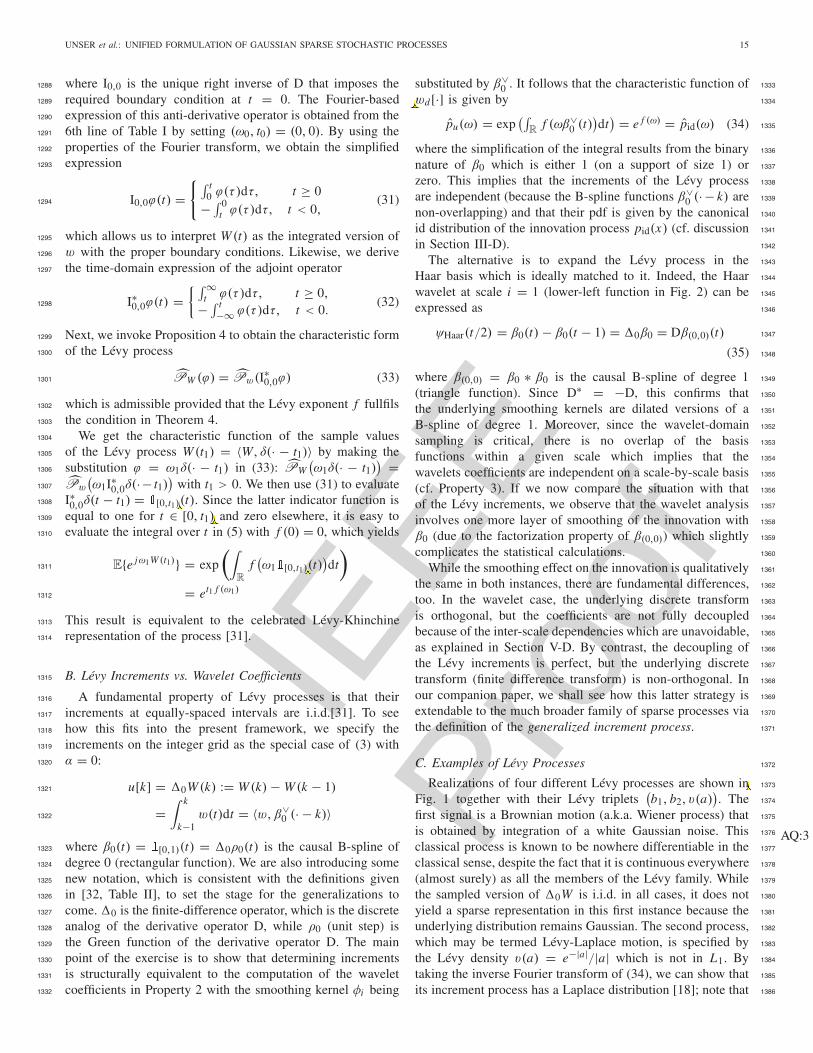
IEEE
Proo
f
UNSER et al.: UNIFIED FORMULATION OF GAUSSIAN SPARSE STOCHASTIC PROCESSES 15
where I0,0 is the unique right inverse of D that imposes the1288
required boundary condition at t = 0. The Fourier-based1289
expression of this anti-derivative operator is obtained from the1290
6th line of Table I by setting (ω0, t0) = (0, 0). By using the1291
properties of the Fourier transform, we obtain the simplified1292
expression1293
I0,0ϕ(t) ={∫ t
0 ϕ(τ)dτ, t ≥ 0− ∫ 0
t ϕ(τ)dτ, t < 0,(31)1294
which allows us to interpret W (t) as the integrated version of1295
w with the proper boundary conditions. Likewise, we derive1296
the time-domain expression of the adjoint operator1297
I∗0,0ϕ(t) ={ ∫ ∞
t ϕ(τ)dτ, t ≥ 0,− ∫ t
−∞ ϕ(τ)dτ, t < 0.(32)1298
Next, we invoke Proposition 4 to obtain the characteristic form1299
of the Lévy process1300
PW (ϕ) = Pw(I∗0,0ϕ) (33)1301
which is admissible provided that the Lévy exponent f fullfils1302
the condition in Theorem 4.1303
We get the characteristic function of the sample values1304
of the Lévy process W (t1) = 〈W, δ(· − t1)〉 by making the1305
substitution ϕ = ω1δ(· − t1) in (33): PW(ω1δ(· − t1)
) =1306
Pw
(ω1I∗0,0δ(·− t1)
)with t1 > 0. We then use (31) to evaluate1307
I∗0,0δ(t − t1) = �[0,t1)(t). Since the latter indicator function is1308
equal to one for t ∈ [0, t1) and zero elsewhere, it is easy to1309
evaluate the integral over t in (5) with f (0) = 0, which yields1310
E{e jω1W (t1)} = exp
(∫
R
f(ω1�[0,t1)(t)
)dt
)
1311
= et1 f (ω1)1312
This result is equivalent to the celebrated Lévy-Khinchine1313
representation of the process [31].1314
B. Lévy Increments vs. Wavelet Coefficients1315
A fundamental property of Lévy processes is that their1316
increments at equally-spaced intervals are i.i.d.[31]. To see1317
how this fits into the present framework, we specify the1318
increments on the integer grid as the special case of (3) with1319
α = 0:1320
u[k] = �0W (k) := W (k)− W (k − 1)1321
=∫ k
k−1w(t)dt = 〈w,β∨
0 (· − k)〉1322
where β0(t) = �[0,1)(t) = �0ρ0(t) is the causal B-spline of1323
degree 0 (rectangular function). We are also introducing some1324
new notation, which is consistent with the definitions given1325
in [32, Table II], to set the stage for the generalizations to1326
come.�0 is the finite-difference operator, which is the discrete1327
analog of the derivative operator D, while ρ0 (unit step) is1328
the Green function of the derivative operator D. The main1329
point of the exercise is to show that determining increments1330
is structurally equivalent to the computation of the wavelet1331
coefficients in Property 2 with the smoothing kernel φi being1332
substituted by β∨0 . It follows that the characteristic function of 1333
wd [·] is given by 1334
pu(ω) = exp(∫
Rf (ωβ∨
0 (t))dt
) = e f (ω) = pid(ω) (34) 1335
where the simplification of the integral results from the binary 1336
nature of β0 which is either 1 (on a support of size 1) or 1337
zero. This implies that the increments of the Lévy process 1338
are independent (because the B-spline functions β∨0 (·− k) are 1339
non-overlapping) and that their pdf is given by the canonical 1340
id distribution of the innovation process pid(x) (cf. discussion 1341
in Section III-D). 1342
The alternative is to expand the Lévy process in the 1343
Haar basis which is ideally matched to it. Indeed, the Haar 1344
wavelet at scale i = 1 (lower-left function in Fig. 2) can be 1345
expressed as 1346
ψHaar(t/2) = β0(t)− β0(t − 1) = �0β0 = Dβ(0,0)(t) 1347
(35) 1348
where β(0,0) = β0 ∗ β0 is the causal B-spline of degree 1 1349
(triangle function). Since D∗ = −D, this confirms that 1350
the underlying smoothing kernels are dilated versions of a 1351
B-spline of degree 1. Moreover, since the wavelet-domain 1352
sampling is critical, there is no overlap of the basis 1353
functions within a given scale which implies that the 1354
wavelets coefficients are independent on a scale-by-scale basis 1355
(cf. Property 3). If we now compare the situation with that 1356
of the Lévy increments, we observe that the wavelet analysis 1357
involves one more layer of smoothing of the innovation with 1358
β0 (due to the factorization property of β(0,0)) which slightly 1359
complicates the statistical calculations. 1360
While the smoothing effect on the innovation is qualitatively 1361
the same in both instances, there are fundamental differences, 1362
too. In the wavelet case, the underlying discrete transform 1363
is orthogonal, but the coefficients are not fully decoupled 1364
because of the inter-scale dependencies which are unavoidable, 1365
as explained in Section V-D. By contrast, the decoupling of 1366
the Lévy increments is perfect, but the underlying discrete 1367
transform (finite difference transform) is non-orthogonal. In 1368
our companion paper, we shall see how this latter strategy is 1369
extendable to the much broader family of sparse processes via 1370
the definition of the generalized increment process. 1371
C. Examples of Lévy Processes 1372
Realizations of four different Lévy processes are shown in 1373
Fig. 1 together with their Lévy triplets(b1, b2, v(a)
). The 1374
first signal is a Brownian motion (a.k.a. Wiener process) that 1375
is obtained by integration of a white Gaussian noise. This 1376
classical process is known to be nowhere differentiable in the 1377
classical sense, despite the fact that it is continuous everywhere 1378
(almost surely) as all the members of the Lévy family. While 1379
the sampled version of �0W is i.i.d. in all cases, it does not 1380
yield a sparse representation in this first instance because the 1381
underlying distribution remains Gaussian. The second process,
AQ:3
1382
which may be termed Lévy-Laplace motion, is specified by 1383
the Lévy density v(a) = e−|a|/|a| which is not in L1. By 1384
taking the inverse Fourier transform of (34), we can show that 1385
its increment process has a Laplace distribution [18]; note that 1386
unser
Inserted Text
Fig. 3
unser
Pencil
unser
Cross-Out
unser
Replacement Text
_{(0,t_1]}
unser
Cross-Out
unser
Replacement Text
_{(0,t_1]}
unser
Cross-Out
unser
Replacement Text
(0,t_1]
unser
Cross-Out
unser
Replacement Text
u
unser
Cross-Out
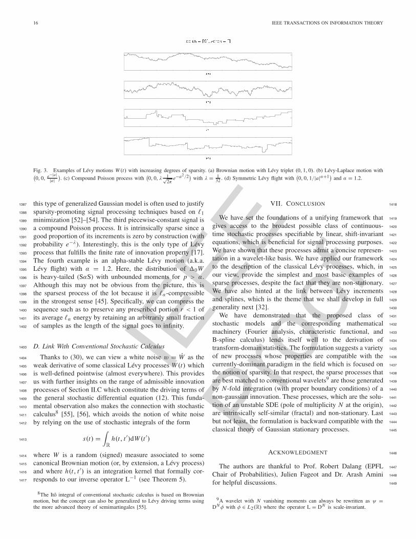
IEEE
Proo
f
16 IEEE TRANSACTIONS ON INFORMATION THEORY
Fig. 3. Examples of Lévy motions W (t) with increasing degrees of sparsity. (a) Brownian motion with Lévy triplet (0, 1, 0). (b) Lévy-Laplace motion with(0, 0, e−|a|
|a|). (c) Compound Poisson process with
(0, 0, λ 1√
2πe−a2/2)
with λ = 132 . (d) Symmetric Lévy flight with
(0, 0, 1/|a|α+1)
and α = 1.2.
this type of generalized Gaussian model is often used to justify1387
sparsity-promoting signal processing techniques based on �11388
minimization [52]–[54]. The third piecewise-constant signal is1389
a compound Poisson process. It is intrinsically sparse since a1390
good proportion of its increments is zero by construction (with1391
probability e−λ). Interestingly, this is the only type of Lévy1392
process that fulfills the finite rate of innovation property [17].1393
The fourth example is an alpha-stable Lévy motion (a.k.a.1394
Lévy flight) with α = 1.2. Here, the distribution of �0W1395
is heavy-tailed (SαS) with unbounded moments for p > α.1396
Although this may not be obvious from the picture, this is1397
the sparsest process of the lot because it is �α-compressible1398
in the strongest sense [45]. Specifically, we can compress the1399
sequence such as to preserve any prescribed portion r < 1 of1400
its average �α energy by retaining an arbitrarily small fraction1401
of samples as the length of the signal goes to infinity.1402
D. Link With Conventional Stochastic Calculus1403
Thanks to (30), we can view a white noise w = W as the1404
weak derivative of some classical Lévy processes W (t) which1405
is well-defined pointwise (almost everywhere). This provides1406
us with further insights on the range of admissible innovation1407
processes of Section II.C which constitute the driving terms of1408
the general stochastic differential equation (12). This funda-1409
mental observation also makes the connection with stochastic1410
calculus8 [55], [56], which avoids the notion of white noise1411
by relying on the use of stochastic integrals of the form1412
s(t) =∫
R
h(t, t ′)dW (t ′)1413
where W is a random (signed) measure associated to some1414
canonical Brownian motion (or, by extension, a Lévy process)1415
and where h(t, t ′) is an integration kernel that formally cor-1416
responds to our inverse operator L−1 (see Theorem 5).1417
8The Itô integral of conventional stochastic calculus is based on Brownianmotion, but the concept can also be generalized to Lévy driving terms usingthe more advanced theory of semimartingales [55].
VII. CONCLUSION 1418
We have set the foundations of a unifying framework that 1419
gives access to the broadest possible class of continuous- 1420
time stochastic processes specifiable by linear, shift-invariant 1421
equations, which is beneficial for signal processing purposes. 1422
We have shown that these processes admit a concise represen- 1423
tation in a wavelet-like basis. We have applied our framework 1424
to the description of the classical Lévy processes, which, in 1425
our view, provide the simplest and most basic examples of 1426
sparse processes, despite the fact that they are non-stationary. 1427
We have also hinted at the link between Lévy increments 1428
and splines, which is the theme that we shall develop in full 1429
generality next [32]. 1430
We have demonstrated that the proposed class of 1431
stochastic models and the corresponding mathematical 1432
machinery (Fourier analysis, characteristic functional, and 1433
B-spline calculus) lends itself well to the derivation of 1434
transform-domain statistics. The formulation suggests a variety 1435
of new processes whose properties are compatible with the 1436
currently-dominant paradigm in the field which is focused on 1437
the notion of sparsity. In that respect, the sparse processes that 1438
are best matched to conventional wavelets9 are those generated 1439
by N-fold integration (with proper boundary conditions) of a 1440
non-gaussian innovation. These processes, which are the solu- 1441
tion of an unstable SDE (pole of multiplicity N at the origin), 1442
are intrinsically self-similar (fractal) and non-stationary. Last 1443
but not least, the formulation is backward compatible with the 1444
classical theory of Gaussian stationary processes. 1445
ACKNOWLEDGMENT 1446
The authors are thankful to Prof. Robert Dalang (EPFL 1447
Chair of Probabilities), Julien Fageot and Dr. Arash Amini 1448
for helpful discussions. 1449
9A wavelet with N vanishing moments can always be rewritten as ψ =DNφ with φ ∈ L2(R) where the operator L = DN is scale-invariant.
IEEE
Proo
f
UNSER et al.: UNIFIED FORMULATION OF GAUSSIAN SPARSE STOCHASTIC PROCESSES 17
REFERENCES1450
[1] A. Papoulis, Probability, Random Variables, and Stochastic Processes.1451
New York, NY, USA: McGraw-Hill, 1991.1452
[2] R. Gray and L. Davisson, An Introduction to Statistical Signal Process-1453
ing. Cambridge, U.K.: Cambridge Univ. Press, 2004.1454
[3] E. J. Candès and M. B. Wakin, “An introduction to compressive1455
sampling,” IEEE Signal Process. Mag., vol. 25, no. 2, pp. 21–30,1456
Mar. 2008.1457
[4] A. M. Bruckstein, D. L. Donoho, and M. Elad, “From sparse solutions of1458
systems of equations to sparse modeling of signals and images,” SIAM1459
Rev., vol. 51, no. 1, pp. 34–81, 2009.1460
[5] S. Mallat, A Wavelet Tour of Signal Processing: The Sparse Way, 3rd ed.1461
San Diego, CA, USA: Academic Press, 2009.1462
[6] J.-L. Starck, F. Murtagh, and J. M. Fadili, Sparse Image and Signal1463
Processing: Wavelets, Curvelets, Morphological Diversity. Cambridge.1464
U.K.: Cambridge Univ. Press, 2010.1465
[7] M. Elad, Sparse and Redundant Representations. From Theory to1466
Applications in Signal and Image Processing. New York, NY, USA:1467
Springer-Verlag, 2010.1468
[8] Y. C. Eldar and G. Kutyniok, Compressed Sensing: Theory and Appli-1469
cations. Cambridge, U.K.: Cambridge Univ. Press, 2012.1470
[9] R. Baraniuk, E. Candes, M. Elad, and Y. Ma, “Applications of sparse1471
representation and compressive sensing,” Proc. IEEE, vol. 98, no. 6,1472
pp. 906–909, Jun. 2010.1473
[10] M. Elad, M. Figueiredo, and Y. Ma, “On the role of sparse and1474
redundant representations in image processing,” Proc. IEEE, vol. 98,1475
no. 6, pp. 972–982, Jun. 2010.1476
[11] M. A. T. Figueiredo and R. D. Nowak, “An EM algorithm for wavelet-1477
based image restoration,” IEEE Trans. Image Process., vol. 12, no. 8,1478
pp. 906–916, Aug. 2003.1479
[12] I. Daubechies, M. Defrise, and C. De Mol, “An iterative thresholding1480
algorithm for linear inverse problems with a sparsity constraint,” Com-1481
mun. Pure Appl. Math., vol. 57, no. 11, pp. 1413–1457, 2004.1482
[13] A. Beck and M. Teboulle, “A fast iterative shrinkage-thresholding1483
algorithm for linear inverse problems,” SIAM J. Imag. Sci., vol. 2, no. 1,1484
pp. 183–202, 2009.1485
[14] Y. C. Eldar, “Compressed sensing of analog signals in shift-invariant1486
spaces,” IEEE Trans. Signal Process., vol. 57, no. 8, pp. 2986–2997,1487
Aug. 2009.1488
[15] B. Adcock and A. Hansen, Generalized Sampling and Infinite-1489
Dimensional Compressed Sensing. Cambridge, U.K.: Cambridge Univ.1490
Press, 2011.1491
[16] T. Kailath, “The innovations approach to detection and estimation1492
theory,” Proc. IEEE, vol. 58, no. 5, pp. 680–695, May 1970.1493
[17] M. Vetterli, P. Marziliano, and T. Blu, “Sampling signals with finite1494
rate of innovation,” IEEE Trans. Signal Process., vol. 50, no. 6,1495
pp. 1417–1428, Jun. 2002.1496
[18] M. Unser and P. D. Tafti, “Stochastic models for sparse and1497
piecewise-smooth signals,” IEEE Trans. Signal Process., vol. 59, no. 3,1498
pp. 989–1005, Mar. 2011.1499
[19] A. Swami, G. B. Giannakis, and J. M. Mendel, “Linear modeling of1500
multidimensional non-Gaussian processes using cumulants,” Multidi-1501
mensional Syst. Signal Process., vol. 1, no. 1, pp. 11–37, 1990.1502
[20] P. Rao, D. Johnson, and D. Becker, “Generation and analysis of non-1503
Gaussian Markov time series,” IEEE Trans. Signal Process., vol. 40,1504
no. 4, pp. 845–856, Apr. 1992.1505
[21] I. Karatzas and S. Shreve, Brownian Motion and Stochastic Calculus,1506
2nd ed. New York, NY, USA: Springer-Verlag, 1991.1507
[22] B. Økensdal, Stochastic Differential Equations, 6th ed. New York, NY,1508
USA: Springer-Verlag, 2007.1509
[23] M. Unser, “Cardinal exponential splines: Part II—Think analog, act1510
digital,” IEEE Trans. Signal Process., vol. 53, no. 4, pp. 1439–1449,1511
Apr. 2005.1512
[24] E. Bostan, U. Kamilov, M. Nilchian, and M. Unser, “Sparse stochastic1513
processes and discretization of linear inverse problems,” IEEE Trans.1514
Image Process., vol. 22, no. 7, pp. 2699–2710, Jul. 2013.1515
[25] A. Amini, U. S. Kamilov, E. Bostan, and M. Unser, “Bayesian estimation1516
for continuous-time sparse stochastic processes,” IEEE Trans. Signal1517
Process., vol. 61, no. 4, pp. 907–920, Feb. 2013.1518
[26] U. S. Kamilov, P. Pad, A. Amini, and M. Unser, “MMSE estimation1519
of sparse Lévy processes,” IEEE Trans. Signal Process., vol. 61, no. 1,1520
pp. 137–147, Jan. 2013.1521
[27] A. Amini, P. Thévenaz, J. Ward, and M. Unser, “On the linearity1522
of Bayesian interpolators for non-Gaussian continuous-time AR(1)1523
processes,” IEEE Trans. Inf. Theory, vol. 59, no. 8, pp. 5063–5074,1524
Aug. 2013.1525
[28] D. Appelbaum, Lèvy Processes and Stochastic Calculus, 2nd ed. 1526
Cambridge, U.K.: Cambridge Univ. Press, 2009. 1527
[29] I. M. Gelfand and N. Y. Vilenkin, Generalized Functions, vol. 4. 1528
San Diego, CA, USA: Academic press, 1964. 1529
[30] P. Lévy, Le mouvement Brownien. Paris, France: Gauthier–Villars, 1954. 1530
[31] K.-I. Sato, Lévy Processes and Infinitely Divisible Distributions. Boston, 1531
MA, USA: Chapman & Hall, 1994. 1532
[32] M. Unser, P. D. Tafti, A. Amini, and H. Kirshner, “A unified formulation 1533
of Gaussian vs. sparse stochastic processes—Part II: Discrete-domain 1534
theory,” IEEE Trans. Inf. Theory, Jan. 2013. AQ:41535
[33] N. Ahmed, “Discrete cosine transform,” IEEE Trans. Commun., vol. 23, 1536
no. 1, pp. 90–93, Sep. 1974. 1537
[34] M. Unser, “On the approximation of the discrete Karhunen-Loève 1538
transform for stationary processes,” Signal Process., vol. 7, no. 3, 1539
pp. 231–249, Dec. 1984. 1540
[35] N. S. Jayant and P. Noll, Digital Coding of Waveforms: Principles 1541
and Application to Speech and Video Coding. Upper Saddle River, NJ, 1542
USA:Prentice-Hall, 1984. 1543
[36] I. Khalidov and M. Unser, “From differential equations to the construc- 1544
tion of new wavelet-like bases,” IEEE Trans. Signal Process., vol. 54, 1545
no. 4, pp. 1256–1267, Apr. 2006. 1546
[37] J. Stewart, “Positive definite functions and generalizations, an histor- 1547
ical survey,” Rocky Mountain J. Math., vol. 6, no. 3, pp. 409–434, 1548
1976. 1549
[38] W. Feller, An Introduction to Probability Theory and its Applications, 1550
vol. 2. 2nd ed. New York, NY, USA: Wiley, 1971. 1551
[39] F. W. Steutel and K. Van Harn, Infinite Divisibility of Probability 1552
Distributions on the Real Line. New York, NY, USA: Marcel Dekker, 1553
2003. 1554
[40] G. Samorodnitsky and M. Taqqu, Stable Non-Gaussian Random 1555
Processes: Stochastic Models with Infinite Variance. Boston, MA, USA: 1556
Chapman & Hall, 1994. 1557
[41] I. M. Gelfand and G. Shilov, Generalized Functions, vol. 1. New York, 1558
NY, USA: Academic press, 1964. 1559
[42] A. Bose, A. Dasgupta, and H. Rubin, “A contemporary review and 1560
bibliography of infinitely divisible distributions and processes,” Indian 1561
J. Statist., Ser. A, vol. 64, no. 3, pp. 763–819, 2002. 1562
[43] B. Ramachandran, “On characteristic functions and moments,” Indian J. 1563
Statist., Ser. A, vol. 31, no. 1, pp. 1–12, 1969. 1564
[44] S. J. Wolfe, “On moments of infinitely divisible distribution functions,” 1565
Ann. Math. Statist., vol. 42, no. 6, pp. 2036–2043, 1971. 1566
[45] A. Amini, M. Unser, and F. Marvasti, “Compressibility of deterministic 1567
and random infinite sequences,” IEEE Trans. Signal Process., vol. 59, 1568
no. 11, pp. 5193–5201, Nov. 2011. 1569
[46] R. Gribonval, V. Cevher, and M. E. Davies, “Compressible distributions 1570
for high-dimensional statistics,” IEEE Trans. Inf. Theory, vol. 58, no. 8, 1571
pp. 5016–5034, Aug. 2012. 1572
[47] A. H. Zemanian, Distribution Theory and Transform Analysis: An 1573
Introduction to Generalized Functions, with Applications. New York, 1574
NY, USA: Dover, 2010. 1575
[48] W. Kaplan, Operational Methods for Linear Systems. Reading, MA, 1576
USA: Addison-Wesley, 1962. 1577
[49] B. Lathi, Signal Processing and Linear Systems. Cambridge, U.K.: 1578
Cambridge Univ. Press, 1998. 1579
[50] J. Shapiro, “Embedded image coding using zerotrees of wavelet coef- 1580
ficients,” IEEE Trans. Acoust., Speech Signal Process., vol. 41, no. 12, 1581
pp. 3445–3462, Dec. 1993. 1582
[51] M. S. Crouse, R. D. Nowak, and R. G. Baraniuk, “Wavelet-based 1583
statistical signal processing using hidden Markov models,” IEEE Trans. 1584
Signal Process., vol. 46, no. 4, pp. 886–902, Apr. 1998. 1585
[52] C. Bouman and K. Sauer, “A generalized Gaussian image model for 1586
edge-preserving MAP estimation,” IEEE Trans. Image Process., vol. 2, 1587
no. 3, pp. 296–310, Jul. 1993. 1588
[53] M. W. Seeger and H. Nickisch, “Compressed sensing and Bayesian 1589
experimental design,” in Proc. 25th Int. Conf. Mach. Learn., 2008, 1590
pp. 912–919. 1591
[54] S. Babacan, R. Molina, and A. Katsaggelos, “Bayesian compressive 1592
sensing using Laplace priors,” IEEE Trans. Image Process., vol. 19, 1593
no. 1, pp. 53–64, Jan. 2010. 1594
[55] P. Protter, Stochastic Integration and Differential Equations. New York, 1595
NY, USA: Springer-Verlag, 2004. 1596
[56] P. J. Brockwell, “Lèvy-driven CARMA processes,” Ann. Inst. Statist. 1597
Math., vol. 53, no. 1, pp. 113–124, 2001. 1598
unser
Cross-Out
unser
Replacement Text
DAMTP Tech. Rep. 2011/NA13
unser
Cross-Out
unser
Cross-Out
unser
Replacement Text
in press
IEEE
Proo
f
18 IEEE TRANSACTIONS ON INFORMATION THEORY
Michael Unser (M’89–SM’94–F’99) received the M.S. (summa cum laude)1599
and Ph.D. degrees in Electrical Engineering in 1981 and 1984, respectively,1600
from the Ecole Polytechnique Fédérale de Lausanne (EPFL), Switzerland.1601
From 1985 to 1997, he worked as a scientist with the National Institutes1602
of Health, Bethesda USA. He is now full professor and Director of the1603
Biomedical Imaging Group at the EPFL.1604
His main research area is biomedical image processing. He has a strong1605
interest in sampling theories, multiresolution algorithms, wavelets, the use of1606
splines for image processing, and, more recently, stochastic processes. He has1607
published about 250 journal papers on those topics.1608
Dr. Unser is currently member of the editorial boards of IEEE1609
J. SELECTED TOPICS IN SIGNAL PROCESSING, Foundations and Trends1610
in Signal Processing, SIAM J. Imaging Sciences, and the PROCEEDINGS1611
OF THE IEEE. He co-organized the first IEEE International Symposium on1612
Biomedical Imaging (ISBI2002) and was the founding chair of the technical1613
committee of the IEEE-SP Society on Bio Imaging and Signal Processing1614
(BISP).1615
He received three Best Paper Awards (1995, 2000, 2003) from the IEEE1616
Signal Processing Society, and two IEEE Technical Achievement Awards1617
(2008 SPS and 2010 EMBS). He is an EURASIP Fellow and a member1618
of the Swiss Academy of Engineering Sciences.1619
Pouya D. Tafti was born in Tehran in 1981. He received his BSc degree 1620
in Electrical Engineering from Sharif University of Technology, Tehran, in 1621
2003, his MASc in Electrical and Computer Engineering from McMaster 1622
University, Hamilton, Ontario, in 2006, and his PhD in Computer, Information, 1623
and Communication Sciences from EPFL, Lausanne, in 2011. From 2006 to 1624
2012 he was with the Biomedical Imaging Group at EPFL, where he worked 1625
on vector field imaging and statistical models for signal and image processing. 1626
He currently resides in Germany where he works as a data scientist. 1627
Qiyu Sun received the BSc and PhD degree in mathematics from Hangzhou 1628
University, China in 1985 and 1990 respectively. He is a full professor with the 1629
Department of Mathematics, University of Central Florida. His prior position 1630
was with Zhejiang University (China), National University of Singapore 1631
(Singapore), Vanderbilt University, and University of Houston. 1632
His research interests include sampling theory, Wiener’s lemma, wavelet 1633
and frame theory, linear and nonlinear inverse problems, and Fourier analysis. 1634
He has published more than 100 papers on mathematics and signal processing, 1635
and written a book An Introduction to Multiband Wavelets (Zhejiang Univer- 1636
sity Press, 2001) with Ning Bi and Daren Huang. He is on the editorial 1637
board of the journals Advance in Computational Mathematics, Numerical 1638
Functional Analysis and Optimization and Sampling Theory in Signal and 1639
Imaging Processing. 1640

IEEE
Proo
f
AUTHOR QUERIES
AQ:1 = Please provide the expansion for “CARMA.”AQ:2 = Please supply index terms/keywords for your paper. To download the IEEE Taxonomy, go to
http://www.ieee.org/documents/taxonomy_v101.pdf.AQ:3 = Fig. 3 is not cited in body text. Please indicate where it should be cited.AQ:4 = Please provide the volume no. issue no., and page range for ref. [32].
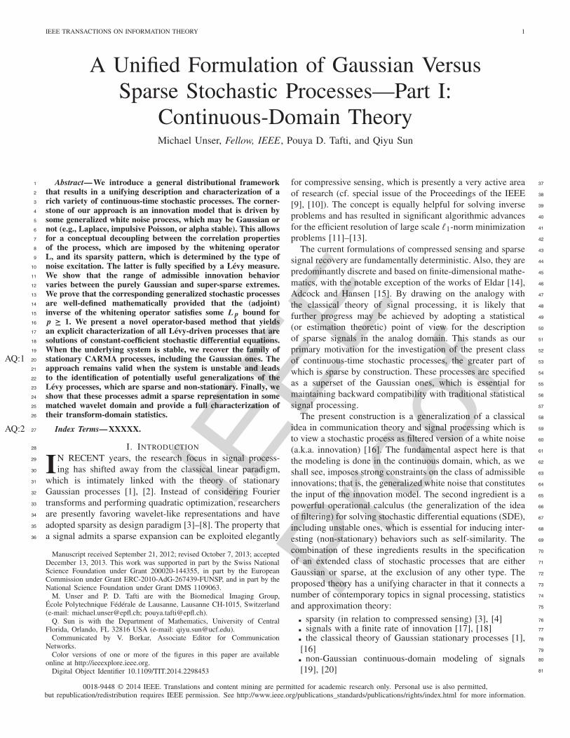
IEEE
Proo
f
IEEE TRANSACTIONS ON INFORMATION THEORY 1
A Unified Formulation of Gaussian VersusSparse Stochastic Processes—Part I:
Continuous-Domain TheoryMichael Unser, Fellow, IEEE, Pouya D. Tafti, and Qiyu Sun
Abstract— We introduce a general distributional framework1
that results in a unifying description and characterization of a2
rich variety of continuous-time stochastic processes. The corner-3
stone of our approach is an innovation model that is driven by4
some generalized white noise process, which may be Gaussian or5
not (e.g., Laplace, impulsive Poisson, or alpha stable). This allows6
for a conceptual decoupling between the correlation properties7
of the process, which are imposed by the whitening operator8
L, and its sparsity pattern, which is determined by the type of9
noise excitation. The latter is fully specified by a Lévy measure.10
We show that the range of admissible innovation behavior11
varies between the purely Gaussian and super-sparse extremes.12
We prove that the corresponding generalized stochastic processes13
are well-defined mathematically provided that the (adjoint)14
inverse of the whitening operator satisfies some L p bound for15
p ≥ 1. We present a novel operator-based method that yields16
an explicit characterization of all Lévy-driven processes that are17
solutions of constant-coefficient stochastic differential equations.18
When the underlying system is stable, we recover the family of19
stationary CARMA processes, including the Gaussian ones. TheAQ:1 20
approach remains valid when the system is unstable and leads21
to the identification of potentially useful generalizations of the22
Lévy processes, which are sparse and non-stationary. Finally, we23
show that these processes admit a sparse representation in some24
matched wavelet domain and provide a full characterization of25
their transform-domain statistics.26
Index Terms— XXXXX.AQ:2 27
I. INTRODUCTION28
IN RECENT years, the research focus in signal process-29
ing has shifted away from the classical linear paradigm,30
which is intimately linked with the theory of stationary31
Gaussian processes [1], [2]. Instead of considering Fourier32
transforms and performing quadratic optimization, researchers33
are presently favoring wavelet-like representations and have34
adopted sparsity as design paradigm [3]–[8]. The property that35
a signal admits a sparse expansion can be exploited elegantly36
Manuscript received September 21, 2012; revised October 7, 2013; acceptedDecember 13, 2013. This work was supported in part by the Swiss NationalScience Foundation under Grant 200020-144355, in part by the EuropeanCommission under Grant ERC-2010-AdG-267439-FUNSP, and in part by theNational Science Foundation under Grant DMS 1109063.
M. Unser and P. D. Tafti are with the Biomedical Imaging Group,École Polytechnique Fédérale de Lausanne, Lausanne CH-1015, Switzerland(e-mail: [email protected]; [email protected]).
Q. Sun is with the Department of Mathematics, University of CentralFlorida, Orlando, FL 32816 USA (e-mail: [email protected]).
Communicated by V. Borkar, Associate Editor for CommunicationNetworks.
Color versions of one or more of the figures in this paper are availableonline at http://ieeexplore.ieee.org.
Digital Object Identifier 10.1109/TIT.2014.2298453
for compressive sensing, which is presently a very active area 37
of research (cf. special issue of the Proceedings of the IEEE 38
[9], [10]). The concept is equally helpful for solving inverse 39
problems and has resulted in significant algorithmic advances 40
for the efficient resolution of large scale �1-norm minimization 41
problems [11]–[13]. 42
The current formulations of compressed sensing and sparse 43
signal recovery are fundamentally deterministic. Also, they are 44
predominantly discrete and based on finite-dimensional mathe- 45
matics, with the notable exception of the works of Eldar [14], 46
Adcock and Hansen [15]. By drawing on the analogy with 47
the classical theory of signal processing, it is likely that 48
further progress may be achieved by adopting a statistical 49
(or estimation theoretic) point of view for the description 50
of sparse signals in the analog domain. This stands as our 51
primary motivation for the investigation of the present class 52
of continuous-time stochastic processes, the greater part of 53
which is sparse by construction. These processes are specified 54
as a superset of the Gaussian ones, which is essential for 55
maintaining backward compatibility with traditional statistical 56
signal processing. 57
The present construction is a generalization of a classical 58
idea in communication theory and signal processing which is 59
to view a stochastic process as filtered version of a white noise 60
(a.k.a. innovation) [16]. The fundamental aspect here is that 61
the modeling is done in the continuous domain, which, as we 62
shall see, imposes strong constraints on the class of admissible 63
innovations; that is, the generalized white noise that constitutes 64
the input of the innovation model. The second ingredient is a 65
powerful operational calculus (the generalization of the idea 66
of filtering) for solving stochastic differential equations (SDE), 67
including unstable ones, which is essential for inducing inter- 68
esting (non-stationary) behaviors such as self-similarity. The 69
combination of these ingredients results in the specification 70
of an extended class of stochastic processes that are either 71
Gaussian or sparse, at the exclusion of any other type. The 72
proposed theory has a unifying character in that it connects a 73
number of contemporary topics in signal processing, statistics 74
and approximation theory: 75
sparsity (in relation to compressed sensing) [3], [4] 76
signals with a finite rate of innovation [17], [18] 77
the classical theory of Gaussian stationary processes [1], 78
[16] 79
non-Gaussian continuous-domain modeling of signals 80
[19], [20] 81
0018-9448 © 2014 IEEE. Translations and content mining are permitted for academic research only. Personal use is also permitted,but republication/redistribution requires IEEE permission. See http://www.ieee.org/publications_standards/publications/rights/index.html for more information.
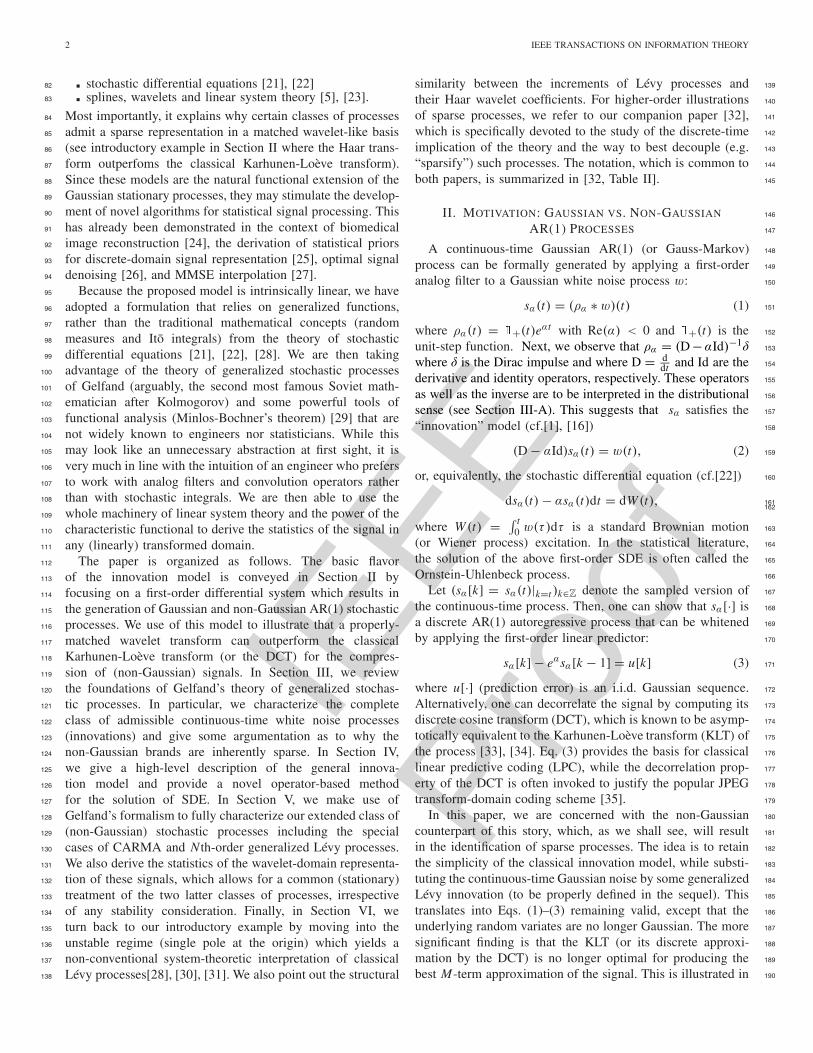
IEEE
Proo
f
2 IEEE TRANSACTIONS ON INFORMATION THEORY
stochastic differential equations [21], [22]82
splines, wavelets and linear system theory [5], [23].83
Most importantly, it explains why certain classes of processes84
admit a sparse representation in a matched wavelet-like basis85
(see introductory example in Section II where the Haar trans-86
form outperfoms the classical Karhunen-Loève transform).87
Since these models are the natural functional extension of the88
Gaussian stationary processes, they may stimulate the develop-89
ment of novel algorithms for statistical signal processing. This90
has already been demonstrated in the context of biomedical91
image reconstruction [24], the derivation of statistical priors92
for discrete-domain signal representation [25], optimal signal93
denoising [26], and MMSE interpolation [27].94
Because the proposed model is intrinsically linear, we have95
adopted a formulation that relies on generalized functions,96
rather than the traditional mathematical concepts (random97
measures and Ito integrals) from the theory of stochastic98
differential equations [21], [22], [28]. We are then taking99
advantage of the theory of generalized stochastic processes100
of Gelfand (arguably, the second most famous Soviet math-101
ematician after Kolmogorov) and some powerful tools of102
functional analysis (Minlos-Bochner’s theorem) [29] that are103
not widely known to engineers nor statisticians. While this104
may look like an unnecessary abstraction at first sight, it is105
very much in line with the intuition of an engineer who prefers106
to work with analog filters and convolution operators rather107
than with stochastic integrals. We are then able to use the108
whole machinery of linear system theory and the power of the109
characteristic functional to derive the statistics of the signal in110
any (linearly) transformed domain.111
The paper is organized as follows. The basic flavor112
of the innovation model is conveyed in Section II by113
focusing on a first-order differential system which results in114
the generation of Gaussian and non-Gaussian AR(1) stochastic115
processes. We use of this model to illustrate that a properly-116
matched wavelet transform can outperform the classical117
Karhunen-Loève transform (or the DCT) for the compres-118
sion of (non-Gaussian) signals. In Section III, we review119
the foundations of Gelfand’s theory of generalized stochas-120
tic processes. In particular, we characterize the complete121
class of admissible continuous-time white noise processes122
(innovations) and give some argumentation as to why the123
non-Gaussian brands are inherently sparse. In Section IV,124
we give a high-level description of the general innova-125
tion model and provide a novel operator-based method126
for the solution of SDE. In Section V, we make use of127
Gelfand’s formalism to fully characterize our extended class of128
(non-Gaussian) stochastic processes including the special129
cases of CARMA and N th-order generalized Lévy processes.130
We also derive the statistics of the wavelet-domain representa-131
tion of these signals, which allows for a common (stationary)132
treatment of the two latter classes of processes, irrespective133
of any stability consideration. Finally, in Section VI, we134
turn back to our introductory example by moving into the135
unstable regime (single pole at the origin) which yields a136
non-conventional system-theoretic interpretation of classical137
Lévy processes[28], [30], [31]. We also point out the structural138
similarity between the increments of Lévy processes and 139
their Haar wavelet coefficients. For higher-order illustrations 140
of sparse processes, we refer to our companion paper [32], 141
which is specifically devoted to the study of the discrete-time 142
implication of the theory and the way to best decouple (e.g. 143
“sparsify”) such processes. The notation, which is common to 144
both papers, is summarized in [32, Table II]. 145
II. MOTIVATION: GAUSSIAN VS. NON-GAUSSIAN 146
AR(1) PROCESSES 147
A continuous-time Gaussian AR(1) (or Gauss-Markov) 148
process can be formally generated by applying a first-order 149
analog filter to a Gaussian white noise process w: 150
sα(t) = (ρα ∗ w)(t) (1) 151
where ρα(t) = �+(t)eαt with Re(α) < 0 and �+(t) is the 152
unit-step function. Next, we observe that ρα = (D −αId)−1δ 153
where δ is the Dirac impulse and where D = ddt and Id are the 154
derivative and identity operators, respectively. These operators 155
as well as the inverse are to be interpreted in the distributional 156
sense (see Section III-A). This suggests that sα satisfies the 157
“innovation” model (cf.[1], [16]) 158
(D − αId)sα(t) = w(t), (2) 159
or, equivalently, the stochastic differential equation (cf.[22]) 160
dsα(t)− αsα(t)dt = dW (t), 161162
where W (t) = ∫ t0 w(τ)dτ is a standard Brownian motion 163
(or Wiener process) excitation. In the statistical literature, 164
the solution of the above first-order SDE is often called the 165
Ornstein-Uhlenbeck process. 166
Let (sα[k] = sα(t)|k=t )k∈Z denote the sampled version of 167
the continuous-time process. Then, one can show that sα[·] is 168
a discrete AR(1) autoregressive process that can be whitened 169
by applying the first-order linear predictor: 170
sα[k] − eαsα[k − 1] = u[k] (3) 171
where u[·] (prediction error) is an i.i.d. Gaussian sequence. 172
Alternatively, one can decorrelate the signal by computing its 173
discrete cosine transform (DCT), which is known to be asymp- 174
totically equivalent to the Karhunen-Loève transform (KLT) of 175
the process [33], [34]. Eq. (3) provides the basis for classical 176
linear predictive coding (LPC), while the decorrelation prop- 177
erty of the DCT is often invoked to justify the popular JPEG 178
transform-domain coding scheme [35]. 179
In this paper, we are concerned with the non-Gaussian 180
counterpart of this story, which, as we shall see, will result 181
in the identification of sparse processes. The idea is to retain 182
the simplicity of the classical innovation model, while substi- 183
tuting the continuous-time Gaussian noise by some generalized 184
Lévy innovation (to be properly defined in the sequel). This 185
translates into Eqs. (1)–(3) remaining valid, except that the 186
underlying random variates are no longer Gaussian. The more 187
significant finding is that the KLT (or its discrete approxi- 188
mation by the DCT) is no longer optimal for producing the 189
best M-term approximation of the signal. This is illustrated in 190
IEEE
Proo
f
UNSER et al.: UNIFIED FORMULATION OF GAUSSIAN SPARSE STOCHASTIC PROCESSES 3
Fig. 1. Wavelets vs. KLT (or DCT) for the M-term approximation ofGaussian vs. sparse AR(1) processes with α = −0.1: (a) classical Gaussianscenario, (b) sparse scenario with symmetric Cauchy innovations. The E-splinewavelets are matched to the innovation model. The displayed results (relativequadratic error as a function of M/N ) are averages over 1000 realizationsfor AR(1) signals of length N = 1024; the performance of DCT and KLT isundistinguishable.
Fig. 1, which compares the performance of various transforms191
for the compression of two kinds of AR(1) processes with192
correlation e−0.1 ≈ 0.90: Gaussian vs. sparse where the latter193
innovation follows a Cauchy distribution. The key observation194
is that the E-spline wavelet transform, which is matched to the195
operator L = D − αId, provides the best results in the non-196
Gaussian scenario over the whole range of experimentation197
[cf. Fig. 1(b)], while the outcome in the Gaussian case is as198
predicted by the classical theory with the KLT being superior.199
Examples of orthogonal E-spline wavelets at two successive200
scales are shown in Fig. 2 next to their Haar counterparts.201
We selected the E-spline wavelets because of their ability202
to decouple the process which follows from their operator-203
like behavior: ψi = L∗φi where i is the scale index and φi204
a suitable smoothing kernel [36, Theorem 2]. Unlike their205
conventional cousins, they are not dilated versions of each206
other, but rather extrapolations in the sense that the slope207
of the exponential segments remains the same at all scales.208
They can, however, be computed efficiently using a perfect209
reconstruction filterbank with scale-dependent filters [36].210
The equivalence with traditional wavelet analysis (Haar)211
and finite-differencing (as used in the computation of total212
variation) for signal “sparsification” is achieved by letting213
α → 0. The catch, however, is that the underlying system214
becomes unstable! Fortunately, the problem can be fixed,215
but it calls for an advanced mathematical treatment that is216
beyond the traditional formulation of stationary processes. The217
reminder of the paper is devoted to giving a proper sense218
to what has just been described informally, and to extend-219
ing the approach to the whole class of ordinary differential220
operators, including the non-stable scenarios. The non-trivial221
outcome, as we shall see, is that many non-stable systems222
are linked with non-stationary stochastic processes. These, in223
Fig. 2. Comparison of operator-like and conventional wavelet basis functionsat two successive scales: (a) first-order E-spline wavelets with α = −0.5.(b) Haar wavelets. The vertical axis is rescaled for full range display.
turn, can be stationarized and “sparsified” by application of a 224
suitable wavelet transformation. The companion paper [32] is 225
focused on the discrete aspects of the theory including the 226
generalization of (3) for decoupling purposes and the full 227
characterization of the underlying processes. 228
III. MATHEMATICAL BACKGROUND 229
The purpose of this section is to introduce the distribu- 230
tional formalism that is required for the proper definition of 231
continuous-time white noise that is the driving term of (1) 232
and its generalization. We start with a brief summary of some 233
required notions in functional analysis, which also serves us to 234
set the notation. We then introduce the fundamental concept 235
of characteristic functional which constitutes the foundation 236
of Gelfand’s theory of generalized stochastic processes. We 237
proceed by giving the complete characterization of the possible 238
types of continuous-domain white noises—not necessarily 239
Gaussian—which will be used as universal input for our inno- 240
vation models. We conclude the section by showing that the 241
non-Gaussian brands of noises that are allowed by Gelfand’s 242
formulation are intrinsically sparse, a property that has not 243
been emphasized before (to the best of our knowledge). 244
A. Functional and Distributional Context 245
The L p-norm of a function f = f (t) is ‖ f ‖p = 246
(∫R
| f (t)|pdt) 1
p for 1 ≤ p < ∞ and ‖ f ‖∞ = 247
ess supt∈R | f (t)| for p = +∞ with the corresponding 248
Lebesgue space being denoted by L p = L p(R). The concept is 249
extendable for characterizing the rate of decay of functions. To 250
that end, we introduce the weighted L p,α spaces with α ∈ R+
251
L p,α = {f ∈ L p : ‖ f ‖p,α < +∞}
252
where the α-weighted L p-norm of f is defined as 253
‖ f ‖p,α = ‖(1 + | · |α) f (·)‖p . 254
Hence, the statement f ∈ L∞,α implies that f (t) decays 255
at least as fast as 1/|t|α as t tends to ±∞; more precisely, 256
that | f (t)| ≤ ‖ f ‖∞,α
1+|t |α almost everywhere. In particular, this 257
allows us to infer that L∞, 1p +ε ⊂ L p for any ε > 0 and 258
p ≥ 1. Another obvious inclusion is L p,α ⊆ L p,α0 for any 259
IEEE
Proo
f
4 IEEE TRANSACTIONS ON INFORMATION THEORY
α ≥ α0. In the limit, we end up with the space of rapidly-260
decreasing functions R = {f : ‖ f ‖∞,m < +∞, ∀m ∈ Z
+},261
which is included in all the others.1262
We use ϕ = ϕ(t) to denote a generic function in Schwartz’s263
class S of rapidly-decaying and infinitely-differentiable test264
functions. Specifically, Schwartz’s space is defined as:265
S = {ϕ ∈ C∞ : ‖Dnϕ‖∞,m < +∞, ∀m, n ∈ Z
+},266
with the operator notation Dn = dn
dt n and the convention that267
D0 = Id (identity). S is a complete topological vector space268
with respect to the topology induced by the series of semi-269
norm ‖Dn · ‖∞,m with m, n ∈ Z+. Its topological dual is270
the space of tempered distributions S ′; a distribution φ ∈ S ′271
is a continuous linear functional on S that is characterized272
by a duality product rule φ(ϕ) = 〈φ, ϕ〉 = ∫Rφ(t)ϕ(t)dt273
with ϕ ∈ S where the right-hand side expression has a literal274
interpretation as an integral only when φ(t) is true function275
of t . The prototypical example of a tempered distribution is the276
Dirac distribution δ, which is defined as δ(ϕ) = 〈δ, ϕ〉 = ϕ(0).277
In the sequel, we will drop the explicit dependence of the278
distribution on the generic test function ϕ ∈ S and simply279
write φ, φ(·) or even φ(t) (with an abuse of notation) where t280
as the generic time index. For instance, we shall denote the281
shifted Dirac impulse2 by δ(· − t0), or δ(t − t0) which is the282
conventional notation used by engineers.283
Let T be a continuous3 linear operator that maps S into284
itself (or eventually some enlarged topological space such285
as L p). It is then possible to extend the action of T over286
S ′ (or an appropriate subset of it) based on the definition287
〈Tφ, ϕ〉 = 〈φ,T∗ϕ〉 for φ ∈ S ′ if T∗ is the adjoint of T288
which maps ϕ to another test function T∗ϕ ∈ S continuously.289
An important example is the Fourier transform whose classical290
definition is F{ f }(ω) = f (ω) = ∫R
f (t)e− jωt dt . Since F is291
a S-continuous operator, it is extendable to S ′ based on the292
adjoint relation 〈Fφ, ϕ〉 = 〈φ,Fϕ〉 for all ϕ ∈ S (generalized293
Fourier transform).294
A linear, shift-invariant (LSI) operator that is well-defined295
over S can always be written as a convolution product:296
TLSI{ϕ} = h ∗ ϕ =∫
R
h(τ )ϕ(· − τ )dτ297
where h = TLSI{δ} is the impulse response of the system.298
The adjoint operator is the convolution with the time-reversed299
version of h:300
h∨(t) ≡ h(−t).301
The better-known categories of LSI operators are the302
BIBO-stable (bounded input, bounded output) filters, and303
the ordinary differential operators. While the latter are not304
BIBO-stable, they do work well with test functions.305
1The topology of R is defined by the family of semi-norms ‖ · ‖∞,m ,m = 1, 2, 3, . . .
2The precise definition is 〈δ(· − t0), ϕ〉 = ϕ(t0) for all ϕ ∈ S .3An operator T is continuous from a sequential topological vector space
V into another one iff. ϕk → ϕ in the topology of V implies that Tϕk → Tϕin the topology (or norm) of the second space. If the two spaces coincide, wesay that T is V-continuous.
1) L p-Stable LSI Operators: The BIBO-stable filters corre- 306
spond to the case where h ∈ L1, or, more generally, when h 307
corresponds to a complex-valued Borel measure of bounded 308
variation. The latter extension allows for discrete filters of the 309
form hd = ∑n∈Z
d[n]δ(·−n) with d[n] ∈ �1. We will refer to 310
these filters as L p-stable because they specify bounded oper- 311
ators in all the L p spaces (by Young’s inequality). L p-stable 312
convolution operators satisfy the properties of commutativity, 313
associativity, and distributivity with respect to addition. 314
2) S-Continuous LSI Operators: For an L p-stable filter to 315
yield a Schwartz function as output, it is necessary that its 316
impulse response (continuous or discrete) be rapidly-decaying. 317
In fact, the condition h ∈ R (which is much stronger than inte- 318
grability) ensures that the filter is S-continuous. The nth-order 319
derivative Dn and its adjoint Dn∗ = (−1)nDn are in the 320
same category. The nth-order weak derivative of the tempered 321
distribution φ is defined as Dnφ(ϕ) = 〈Dnφ, ϕ〉 = 〈φ,Dn∗ϕ〉 322
for any ϕ ∈ S. The latter operator—or, by extension, any 323
polynomial of distributional derivatives PN (D) = ∑Nn=1 anDn
324
with constant coefficients an ∈ C—maps S ′ into itself. The 325
class of these differential operators enjoys the same properties 326
as its classical counterpart: shift-invariance, commutativity, 327
associativity and distributivity. 328
B. Notion of Generalized Stochastic Process 329
Classically, a stochastic process is a random function 330
s(t), t ∈ R whose statistical description is provided by the 331
probability law of its point values {s(t1), s(t2), . . . , s(tn), . . . } 332
for any finite sequence of time instants {tn}Nn=1. The implicit 333
assumption there is that one has a mechanism for probing the 334
value of the function s at any time t ∈ R, which is only 335
achievable approximately in the real physical world. 336
The leading idea in Gelfand and Vilenkin’s theory of 337
generalized stochastic processes is to replace the point mea- 338
surements {s(tn)} by a series of scalar products {〈s, ϕn〉} with 339
suitable “test” functions ϕ1, . . . , ϕN ∈ S [29]. The physical 340
motivation that these authors give is that Xn = 〈s, ϕn〉 may 341
represent the reading of a finite-resolution detector whose 342
output is some “averaged” value∫R
s(t)ϕn(t)dt , which is a 343
more plausible form of probing than ideal sampling. The 344
additional hypothesis is that the linear measurement X = 〈s, ϕ〉 345
depends continuously on ϕ and that the quantities Xn = 〈s, ϕn〉 346
obtained for different test functions {ϕn} are mutually compat- 347
ible. Mathematically, this translates into defining a generalized 348
stochastic process as a continuous linear random functional on 349
some topological vector space such as S. 350
Let s be such a generalized process. We first observe 351
that the scalar product X1 = 〈s, ϕ1〉 with a given test 352
function ϕ1 is a conventional (scalar) random variable that 353
is characterized by its probability density function (pdf) 354
pX1(x1); the latter is in one-to-one correspondence (via the 355
Fourier transform) with the characteristic function pX1(ω1) = 356
E{e jω1 X1} = ∫R
e jω1x1 pX1(x1)dx1 = E{e j 〈s,ω1ϕ1〉} where E{·} 357
is the expectation operator. The same applies for the 2nd-order 358
pdf pX1,X2(x1, x2) associated with a pair of test functions ϕ1 359
and ϕ2 which is the inverse Fourier transform of the 2-D 360
characteristic function pX1,X2(ω1, ω2) = E{e j 〈s,ω1ϕ1+ω2ϕ2〉}, 361
and so forth if one wants to specify higher-order dependencies. 362
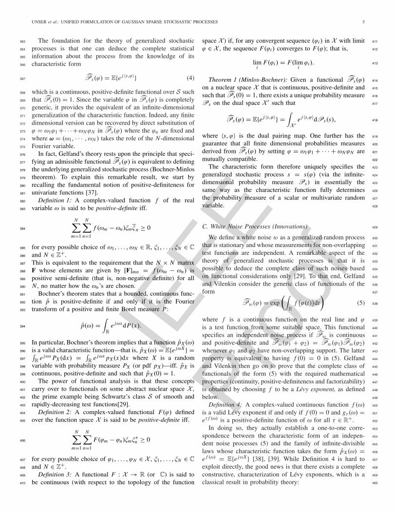
IEEE
Proo
f
UNSER et al.: UNIFIED FORMULATION OF GAUSSIAN SPARSE STOCHASTIC PROCESSES 5
The foundation for the theory of generalized stochastic363
processes is that one can deduce the complete statistical364
information about the process from the knowledge of its365
characteristic form366
Ps(ϕ) = E{e j 〈s,ϕ〉} (4)367
which is a continuous, positive-definite functional over S such368
that Ps(0) = 1. Since the variable ϕ in Ps(ϕ) is completely369
generic, it provides the equivalent of an infinite-dimensional370
generalization of the characteristic function. Indeed, any finite371
dimensional version can be recovered by direct substitution of372
ϕ = ω1ϕ1 +· · ·+ωNϕN in Ps(ϕ) where the ϕn are fixed and373
where ω = (ω1, · · · , ωN ) takes the role of the N-dimensional374
Fourier variable.375
In fact, Gelfand’s theory rests upon the principle that speci-376
fying an admissible functional Ps(ϕ) is equivalent to defining377
the underlying generalized stochastic process (Bochner-Minlos378
theorem). To explain this remarkable result, we start by379
recalling the fundamental notion of positive-definiteness for380
univariate functions [37].381
Definition 1: A complex-valued function f of the real382
variable ω is said to be positive-definite iff.383
N∑
m=1
N∑
n=1
f (ωm − ωn)ξmξ n ≥ 0384
for every possible choice of ω1, . . . , ωN ∈ R, ξ1, . . . , ξN ∈ C385
and N ∈ Z+.386
This is equivalent to the requirement that the N × N matrix387
F whose elements are given by [F]mn = f (ωm − ωn) is388
positive semi-definite (that is, non-negative definite) for all389
N , no matter how the ωn’s are chosen.390
Bochner’s theorem states that a bounded, continuous func-391
tion p is positive-definite if and only if it is the Fourier392
transform of a positive and finite Borel measure P:393
p(ω) =∫
R
e jωxdP(x).394
In particular, Bochner’s theorem implies that a function pX (ω)395
is a valid characteristic function—that is, pX (ω) = E{e jωX } =396 ∫R
e jωx PX (dx) = ∫R
e jωx pX (x)dx where X is a random397
variable with probability measure PX (or pdf pX )—iff. pX is398
continuous, positive-definite and such that pX (0) = 1.399
The power of functional analysis is that these concepts400
carry over to functionals on some abstract nuclear space X ,401
the prime example being Schwartz’s class S of smooth and402
rapidly-decreasing test functions[29].403
Definition 2: A complex-valued functional F(ϕ) defined404
over the function space X is said to be positive-definite iff.405
N∑
m=1
N∑
n=1
F(ϕm − ϕn)ξmξ∗n ≥ 0406
for every possible choice of ϕ1, . . . , ϕN ∈ X , ξ1, . . . , ξN ∈ C407
and N ∈ Z+.408
Definition 3: A functional F : X → R (or C) is said to409
be continuous (with respect to the topology of the function410
space X ) if, for any convergent sequence (ϕi ) in X with limit 411
ϕ ∈ X , the sequence F(ϕi ) converges to F(ϕ); that is, 412
limi
F(ϕi ) = F(limiϕi ). 413
Theorem 1 (Minlos-Bochner): Given a functional Ps(ϕ) 414
on a nuclear space X that is continuous, positive-definite and 415
such that Ps(0) = 1, there exists a unique probability measure 416
Ps on the dual space X ′ such that 417
Ps(ϕ) = E{e j 〈s,ϕ〉} =∫
X ′e j 〈s,ϕ〉dPs(s), 418
where 〈s, ϕ〉 is the dual pairing map. One further has the 419
guarantee that all finite dimensional probabilities measures 420
derived from Ps(ϕ) by setting ϕ = ω1ϕ1 + · · · + ωNϕN are 421
mutually compatible. 422
The characteristic form therefore uniquely specifies the 423
generalized stochastic process s = s(ϕ) (via the infinite- 424
dimensional probability measure Ps) in essentially the 425
same way as the characteristic function fully determines 426
the probability measure of a scalar or multivariate random 427
variable. 428
C. White Noise Processes (Innovations) 429
We define a white noise w as a generalized random process 430
that is stationary and whose measurements for non-overlapping 431
test functions are independent. A remarkable aspect of the 432
theory of generalized stochastic processes is that it is 433
possible to deduce the complete class of such noises based 434
on functional considerations only [29]. To that end, Gelfand 435
and Vilenkin consider the generic class of functionals of the 436
form 437
Pw(ϕ) = exp
(∫
R
f(ϕ(t)
)dt
)
(5) 438
where f is a continuous function on the real line and ϕ 439
is a test function from some suitable space. This functional 440
specifies an independent noise process if Pw is continuous 441
and positive-definite and Pw(ϕ1 + ϕ2) = Pw(ϕ1)Pw(ϕ2) 442
whenever ϕ1 and ϕ2 have non-overlapping support. The latter 443
property is equivalent to having f (0) = 0 in (5). Gelfand 444
and Vilenkin then go on to prove that the complete class of 445
functionals of the form (5) with the required mathematical 446
properties (continuity, positive-definiteness and factorizability) 447
is obtained by choosing f to be a Lévy exponent, as defined 448
below. 449
Definition 4: A complex-valued continuous function f (ω) 450
is a valid Lévy exponent if and only if f (0) = 0 and gτ (ω) = 451
eτ f (ω) is a positive-definite function of ω for all τ ∈ R+. 452
In doing so, they actually establish a one-to-one corre- 453
spondence between the characteristic form of an indepen- 454
dent noise processes (5) and the family of infinite-divisible 455
laws whose characteristic function takes the form pX (ω) = 456
e f (ω) = E{e jωX } [38], [39]. While Definition 4 is hard to 457
exploit directly, the good news is that there exists a complete 458
constructive, characterization of Lévy exponents, which is a 459
classical result in probability theory: 460
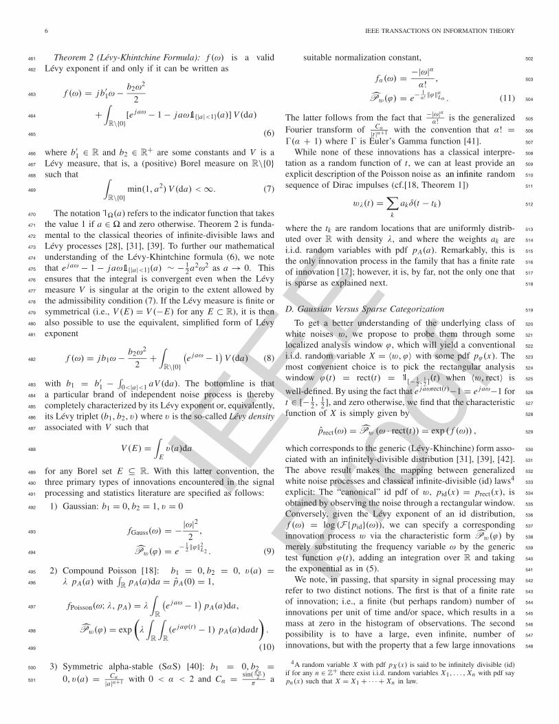
IEEE
Proo
f
6 IEEE TRANSACTIONS ON INFORMATION THEORY
Theorem 2 (Lévy-Khintchine Formula): f (ω) is a valid461
Lévy exponent if and only if it can be written as462
f (ω) = jb′1ω − b2ω
2
2463
+∫
R\{0}[e jaω − 1 − jaω�{|a|<1}(a)] V (da)464
(6)465
where b′1 ∈ R and b2 ∈ R
+ are some constants and V is a466
Lévy measure, that is, a (positive) Borel measure on R\{0}467
such that468 ∫
R\{0}min(1, a2) V (da) < ∞. (7)469
The notation � (a) refers to the indicator function that takes470
the value 1 if a ∈ and zero otherwise. Theorem 2 is funda-471
mental to the classical theories of infinite-divisible laws and472
Lévy processes [28], [31], [39]. To further our mathematical473
understanding of the Lévy-Khintchine formula (6), we note474
that e jaω − 1 − jaω�{|a|<1}(a) ∼ − 12 a2ω2 as a → 0. This475
ensures that the integral is convergent even when the Lévy476
measure V is singular at the origin to the extent allowed by477
the admissibility condition (7). If the Lévy measure is finite or478
symmetrical (i.e., V (E) = V (−E) for any E ⊂ R), it is then479
also possible to use the equivalent, simplified form of Lévy480
exponent481
f (ω) = jb1ω − b2ω2
2+
∫
R\{0}(e jaω − 1
)V (da) (8)482
with b1 = b′1 − ∫
0<|a|<1 aV (da). The bottomline is that483
a particular brand of independent noise process is thereby484
completely characterized by its Lévy exponent or, equivalently,485
its Lévy triplet (b1, b2, v) where v is the so-called Lévy density486
associated with V such that487
V (E) =∫
Ev(a)da488
for any Borel set E ⊆ R. With this latter convention, the489
three primary types of innovations encountered in the signal490
processing and statistics literature are specified as follows:491
1) Gaussian: b1 = 0, b2 = 1, v = 0492
fGauss(ω) = −|ω|22,493
Pw(ϕ) = e− 1
2 ‖ϕ‖2L2 . (9)494
2) Compound Poisson [18]: b1 = 0, b2 = 0, v(a) =495
λ pA(a) with∫R
pA(a)da = pA(0) = 1,496
fPoisson(ω; λ, pA) = λ
∫
R
(e jaω − 1
)pA(a)da,497
Pw(ϕ) = exp
(
λ
∫
R
∫
R
(e jaϕ(t) − 1) pA(a)dadt
)
.498
(10)499
3) Symmetric alpha-stable (SαS) [40]: b1 = 0, b2 =500
0, v(a) = Cα|a|α+1 with 0 < α < 2 and Cα = sin( πα2 )
π a501
suitable normalization constant, 502
fα(ω) = −|ω|αα! , 503
Pw(ϕ) = e− 1α! ‖ϕ‖αLα . (11) 504
The latter follows from the fact that −|ω|αα! is the generalized 505
Fourier transform of Cα|t |α+1 with the convention that α! = 506
�(α + 1) where � is Euler’s Gamma function [41]. 507
While none of these innovations has a classical interpre- 508
tation as a random function of t , we can at least provide an 509
explicit description of the Poisson noise as an infinite random 510
sequence of Dirac impulses (cf.[18, Theorem 1]) 511
wλ(t) =∑
k
akδ(t − tk) 512
where the tk are random locations that are uniformly distrib- 513
uted over R with density λ, and where the weights ak are 514
i.i.d. random variables with pdf pA(a). Remarkably, this is 515
the only innovation process in the family that has a finite rate 516
of innovation [17]; however, it is, by far, not the only one that 517
is sparse as explained next. 518
D. Gaussian Versus Sparse Categorization 519
To get a better understanding of the underlying class of 520
white noises w, we propose to probe them through some 521
localized analysis window ϕ, which will yield a conventional 522
i.i.d. random variable X = 〈w,ϕ〉 with some pdf pϕ(x). The 523
most convenient choice is to pick the rectangular analysis 524
window ϕ(t) = rect(t) = �[− 12 ,
12 ](t) when 〈w, rect〉 is 525
well-defined. By using the fact that e jaωrect(t)−1 = e jaω−1 for 526
t ∈ [− 12 ,
12 ], and zero otherwise, we find that the characteristic 527
function of X is simply given by 528
prect(ω) = Pw (ω · rect(t)) = exp ( f (ω)) , 529
which corresponds to the generic (Lévy-Khinchine) form asso- 530
ciated with an infinitely-divisible distribution [31], [39], [42]. 531
The above result makes the mapping between generalized 532
white noise processes and classical infinite-divisible (id) laws4533
explicit: The “canonical” id pdf of w, pid(x) = prect(x), is 534
obtained by observing the noise through a rectangular window. 535
Conversely, given the Lévy exponent of an id distribution, 536
f (ω) = log (F{pid}(ω)), we can specify a corresponding 537
innovation process w via the characteristic form Pw(ϕ) by 538
merely substituting the frequency variable ω by the generic 539
test function ϕ(t), adding an integration over R and taking 540
the exponential as in (5). 541
We note, in passing, that sparsity in signal processing may 542
refer to two distinct notions. The first is that of a finite rate 543
of innovation; i.e., a finite (but perhaps random) number of 544
innovations per unit of time and/or space, which results in a 545
mass at zero in the histogram of observations. The second 546
possibility is to have a large, even infinite, number of 547
innovations, but with the property that a few large innovations 548
4A random variable X with pdf pX (x) is said to be infinitely divisible (id)if for any n ∈ Z
+ there exist i.i.d. random variables X1, . . . , Xn with pdf saypn(x) such that X = X1 + · · · + Xn in law.
IEEE
Proo
f
UNSER et al.: UNIFIED FORMULATION OF GAUSSIAN SPARSE STOCHASTIC PROCESSES 7
dominate the overall behavior. In this case the histogram of549
observations is distinguished by its ‘heavy tails’. (A combina-550
tion of the two is also possible, for instance in a compound551
Poisson process with a heavy-tailed amplitude distribution.552
For such a process one may observe a change of behavior553
in passing from one dominant type of sparsity to the other).554
Our framework permits us to consider both types of sparsity,555
in the former case with compound Poisson models and in the556
latter with heavy-tailed infinitely-divisible innovations.557
To make our point, we consider two distinct scenarios.558
1) Finite Variance Case: We first assume that the second559
moment m2 = ∫R\{0} a2 V (da) of the Lévy measure V in (6)560
is finite. This allows us to rewrite the classical Lévy-Khinchine561
representation as562
f (ω) = jc1ω − b2ω2
2+
∫
R\{0}[e jaω − 1 − jaω] V (da)563
with c1 = b′′1 + ∫
|a|>1 aV (da) and where the Poisson part564
of the functional is now fully compensated. Indeed, we are565
guaranteed that the above integral is convergent because566
|e jaω − 1 − jωa| � |aω|2 as a → 0 and |e jaω − 1 − jωa| ∼567
|aω| as a → ±∞. An interesting non-Poisson example of568
infinitely-divisible probability laws that falls into this category569
(with non-finite V ) is the Laplace distribution with Lévy triplet570
(0, 0, v(a) = e−|a||a| ) and pid(x) = 1
2 e−|x |. This model is571
particularly relevant for sparse signal processing because it572
provides a tight connection between Lévy processes and total573
variation regularization [18, Section VI].574
Now, if the Lévy measure is finite∫R
V (da) = λ < ∞,575
the admissibility condition yields∫R\{0} a V (da) < ∞, which576
allows us to pull the bias correction out of the integral. The577
representation then simplifies to (8). This implies that we578
can decompose X into the sum of two independent Gaussian579
and compound Poisson random variables. The variances of580
the Gaussian and Poisson components are σ 2 = b2 and581 ∫R
a2V (da), respectively. The Poisson component is sparse582
because its pdf exhibits a mass distribution e−λδ(x) at the583
origin, meaning that the chances for a continuous amplitude584
distribution of getting zero are overwhelmingly higher than585
any other value, especially for smaller values of λ > 0. It is586
therefore justifiable to use 0 ≤ e−λ < 1 as our Poisson sparsity587
index.588
2) Infinite Variance Case: We now turn our attention to589
the case where the second moment of the Lévy measure590
is unbounded, which we like to label as the “super-sparse”591
one. To substantiate this claim, we invoke the Ramachandran-592
Wolfe theorem which states that the pth moment E{|X |p}593
with p ∈ R+ of an infinitely divisible distribution is finite594
iff.∫|a|>1 |a|p V (da) < ∞ [43], [44]. For p ≥ 2, the595
latter is equivalent to∫R\{0} |a|p V (da) < ∞ because of the596
admissibility condition (7). It follows that the cases that are597
not covered by the previous scenario (including the Gaussian598
+ Poisson model) necessarily give rise to distributions whose599
moments of order p are unbounded for p ≥ 2. The proto-600
typical representatives of such heavy tail distributions are the601
alpha-stable ones or, by extension, the broad family of infinite602
divisible probability laws that are in their domain of attraction.603
Note that these distributions all fulfill the stringent conditions 604
for �p compressibility[45], [46]. 605
IV. INNOVATION APPROACH TO CONTINUOUS-TIME 606
STOCHASTIC PROCESSES 607
Specifying a stochastic process through an innovation model 608
(or an equivalent stochastic differential equation) is attractive 609
conceptually, but it presupposes that we can provide an inverse 610
operator (in the form of an integral transform) that transforms 611
the innovation back into the initial stochastic process. This is 612
the reason why, after laying out general conditions for exis- 613
tence, we shall spend the greater part of our effort investigating 614
suitable inverse operators. 615
A. Stochastic Differential Equations 616
Our aim is to define the generalized process with whitening 617
operator L : S ′ → S ′ and Lévy exponent f as the solution of 618
the stochastic linear differential equation 619
Ls = w, (12) 620
where w is an innovation process, as described in 621
Section III-C. This definition is obviously only usable if we 622
can construct an inverse operator T = L−1 that solves this 623
equation. For the cases where the inverse is not unique, we will 624
need to select one preferential operator, which is equivalent 625
to imposing specific boundary conditions. We are then able 626
to formally express the stochastic process as a transformed 627
version of a white noise 628
s = L−1w. (13) 629
The requirement for such a solution to be consistent with (12) 630
is that the operator satisfies the right-inverse property LL−1 = 631
Id over the underlying class of tempered distributions. By 632
using the adjoint relation 〈s, ϕ〉 = 〈L−1w,ϕ〉 = 〈w,L−1∗ϕ〉, 633
we can then transfer the action of the operator onto the test 634
function inside the characteristic form and obtain a com- 635
plete statistical characterization of the so-defined generalized 636
stochastic process 637
Ps(ϕ) = PL−1w(ϕ) = Pw(L−1∗ϕ), (14) 638
where Pw is given by (5) (or one of the specific forms in the 639
list at the end of Section III-C) and where we are implicitly 640
requiring that the adjoint L−1∗ is mathematically well-defined 641
(continuous) over S, and that its composition with Pw is 642
well-defined for all ϕ ∈ S. 643
In order to realize the above idea mathematically, it isusually easier to proceed backwards: one specifies an operatorT that satisfies the left-inverse property: ∀ϕ ∈ S, TL∗ϕ = ϕ,and that is continuous (i.e., bounded in the proper norm(s))over the chosen class of test functions. One then characterizesthe adjoint of T, which is the operator T∗ : S ′ → S ′ (or anappropriate subset thereof) such that, for a given φ ∈ S ′,
∀ϕ ∈ S, 〈φ, ϕ〉 = 〈LT∗φ, ϕ〉 = 〈φ, TL∗︸︷︷︸
Id
ϕ〉.
Finally, we set L−1 = T∗, which yields the proper distribu- 644
tional definition of the right inverse of L in (13). 645
IEEE
Proo
f
8 IEEE TRANSACTIONS ON INFORMATION THEORY
B. General Conditions for Existence646
To validate the proposed innovation model, we need to647
ensure that the solution s = L−1w is a bona fide generalized648
stochastic process.649
In order to simplify the analysis, we shall restrict our650
attention to an appropriate subclass of Lévy exponents.651
Definition 5: A Lévy exponent f with derivative f ′ is652
p-admissible with 1 ≤ p ≤ 2 if there exists a positive constant653
C such that | f (ω)| + |ω| · | f ′(ω)| ≤ C|ω|p for all ω ∈ R.654
Note that this p-admissibility condition is not very con-655
straining and that it is satisfied by the great majority of656
members of the Lévy-Kintchine family (see Section III-C).657
For instance in the compound Poisson case, we can show that658
|ω| · | f ′(ω)| ≤ λ|ω| E{|A|} and f (ω) ≤ λ|ω| E{|A|} by659
using the fact |e j x − 1| ≤ |x |; this implies that the bound660
in Definition 5 with p = 1 is always satisfied provided661
that the first (absolute) moment of the amplitude pdf pA(a)662
in (10) is finite. Similarly, all symmetric Lévy exponents with663
− f ′′(0) < ∞ (finite variance case) are p-admissible with664
p = 2, the prototypical example being the Gaussian. The only665
cases we are aware of that do not fulfill the condition are the666
alpha-stable noises with 0 < α < 1, which are notorious for667
their exotic behavior.668
The first advantage of imposing p-admissibility is that it669
allows us to extend the set of acceptable analysis functions670
from S to L p which is crucial if we intend to do conventional671
signal processing.672
Theorem 3: If the Lévy exponent f is p-admissible, then673
the characteristic form Pw(ϕ) = exp(∫
Rf(ϕ(t)
)dt
)is a674
continuous, positive-definite functional over L p .675
Proof: Since the exponential function is continuous, it is676
sufficient to consider the functional677
F(ϕ) = log Pw(ϕ) =∫
R
f (ϕ(t))dt,678
which is such that F(0) = 0. To show that F(ϕ)(and hence679
Pw(ϕ))
is well-defined over L p , we note that680
|F(ϕ)| ≤∫
R
| f (ϕ(t))| dt ≤ C‖ϕ‖pp,681
which follows from the p-admissibility condition. The positive682
definiteness of Pw(ϕ) over S is a direct consequence of f683
being a Lévy exponent and is therefore also transferable to684
L p . For the interested reader, this can be shown quite easily685
by proving that F(ϕ) is conditionally positive-definite of order686
one (see [20]).687
The only remaining work is to establish the L p-continuity688
of F(ϕ). To that end, we observe that689
| f (u)− f (v)| =∣∣∣
∫ u
vf ′(t)dt
∣∣∣690
≤ C∣∣∣
∫ u
vt p−1dt
∣∣∣691
(by the assumption on f )692
≤ C max(|u|p−1, |v|p−1)|u − v|693
≤ C(|v|p−1 + |u − v|p−1)|u − v|.694
(by the triangle inequality)695
Next, we pick a convergent sequence in L p , {ϕn}∞n=1, whose 696
limit is denoted by ϕ. The convergence in L p is expressed as 697
limn→∞ ‖ϕn − ϕ‖p = 0. (15) 698
We then have 699
∣∣∣
∫
R
f (ϕn(t))dt −∫
R
f (ϕ(t))dt∣∣∣ 700
≤C∫
R
|ϕ(t)|p−1|ϕn(t)− ϕ(t)| + |ϕn(t)− ϕ(t)|pdt 701
≤C(‖ϕ‖p−1
p ‖ϕn − ϕ‖p + ‖ϕn − ϕ‖pp
)
(by Hölder’s inequality)
702
→0 as n → ∞, (by (15)) 703704
which proves the continuity of the functional Pw on L p . 705
Thanks to this result, we can then rely on the Minlos- 706
Bochner theorem (Theorem 1) to state basic conditions on 707
T = L−1∗ that ensure that s = T∗w is a well-defined 708
generalized process over S ′. 709
Theorem 4 (Existence of Generalized Process): Let f be a 710
valid Lévy exponent and T be an operator acting on ϕ ∈ S 711
such that any one of the conditions below is met: 712
1) T is a continuous linear map from S into itself, 713
2) T is a continuous linear map from S into L p and the 714
Lévy exponent f is p-admissible. 715
Then, Ps(ϕ) = exp(∫
Rf(Tϕ(t)
)dt
)is a continuous, positive- 716
definite functional on S such that Ps(0) = 1. 717
Proof: We already know that Pw is a continuous 718
functional on S (resp., on L p when f is p-admissible) by 719
construction. This, together with the assumption that T is a 720
continuous operator on S (resp., from S to L p), implies that 721
the composed functional Ps(ϕ) := Pw(Tϕ) is continuous 722
on S. 723
Given the functions ϕ1, . . . , ϕN in S and some complex 724
coefficients ξ1, . . . , ξN , 725
∑
1≤m,n≤N
Ps(ϕm − ϕn)ξmξn 726
=∑
1≤m,n≤N
Pw
(T(ϕm − ϕn)
)ξmξn 727
=∑
1≤m,n≤N
Pw(Tϕm − Tϕn)ξmξn
(by the linearity of the operator T)
728
≥ 0. (by the positivity of Pw over S or L p) 729730
This proves the positive definiteness of the functional Ps 731
on S. 732
Lastly, Ps(0) = Pw(T0) = Pw(0) = 1. 733
The final fundamental issue relates to the interpretation 734
of s = L−1w as an ordinary stochastic process; that is, a 735
random function s(t) of the time variable t . This presupposes 736
that the shaping operator L−1 performs a minimal amount of 737
smoothing since the driving term of the model, w, is too rough 738
to admit a pointwise representation. 739
Theorem 5 (Interpretationas anOrdinaryStochasticProcess): 740
Let s be the generalized stochastic process whose 741
characteristic function is given by (14) where f is a 742

IEEE
Proo
f
UNSER et al.: UNIFIED FORMULATION OF GAUSSIAN SPARSE STOCHASTIC PROCESSES 9
p-admissible Lévy exponent and L−1∗ is a continuous743
operator from S to L p (or a subset thereof). We also define744
the (generalized) impulse response745
h(t, τ ) = L−1{δ(· − τ )}(t), (16)746
with a slight abuse of notation since h is not necessarily747
an ordinary function. Then, s = L−1w admits the pointwise748
representation for t ∈ R749
s(t) = 〈w, h(t, ·)〉 (17)750
provided that h(t, ·) ∈ L p (with t fixed).751
The form of h(t, τ ) in (16) is the “time-domain” transcrip-752
tion of Schwartz’s kernel theorem which gives the integral753
representation of a linear operator in terms of a (generalized)754
kernel h ∈ S ′ × S ′ (the infinite-dimensional generalization of755
a matrix multiplication). The more standard definition used756
in the theory of generalized functions is 〈h(·, ·), ϕ1 ⊗ ϕ2〉 =757
〈L−1∗{ϕ1}, ϕ2〉, where ϕ1 ⊗ ϕ2(t, τ ) = ϕ1(t)ϕ2(τ ) for all758
ϕ1, ϕ2 ∈ S.759
Proof: The existence of the generalized stochastic process760
s = L−1w is ensured by Theorem 4. We then consider the761
observation of the innovation X0 = 〈w,ϕ0〉 where ϕ0 =762
h(t0, ·) with ϕ0 ∈ L p . Since Pw admits a continuous exten-763
sion over L p (by Theorem 3), we can specify the characteristic764
function of X0 as765
pX0(ω) = E{e jωX0} = Pw(ωϕ0)766
with ϕ0 fixed. Thanks to the functional properties of Pw,767
pX0(ω) is a continuous, positive-definite function of ω such768
that pX0(0) = 1 so that we can invoke Bochner’s theorem769
to establish that X0 is a well-defined conventional random770
variable with pdf pX0 (the inverse Fourier transform of pX0 ).771
772
C. Inverse Operators773
Before presenting our general method of solution, we need774
to identify a suitable set of elementary inverse operators that775
satisfy the continuity requirement in Theorem 4.776
Our approach relies on the factorization of a differen-777
tial operator into simple first-order components of the form778
(D−αnId) with αn ∈ C, which can then be treated separately.779
Three possible cases need to be considered.780
1) Causal-Stable: Re(αn) < 0. This is the classical textbook781
hypothesis which leads to a causal-stable convolution system.782
It is well known from the theory of distributions and linear783
systems (e.g., [47, Section 6.3], [48]) that the causal Green784
function of (D−αnId) is the causal exponential function ραn (t)785
already encountered in the introductory example in Section II.786
Clearly, ραn (t) is absolutely integrable (and rapidly-decaying)787
iff. Re(αn) < 0. It follows that (D − αnId)−1 f = ραn ∗ f788
with ραn ∈ R ⊂ L1. In particular, this implies that T =789
(D − αnId)−1 specifies a continuous LSI operator on S. The790
same holds for T∗ = (D − αnId)−1∗, which is defined as791
T∗ f = ρ∨αn
∗ f .792
2) Anti-Causal Stable: Re(αn) > 0. This case is usu-793
ally excluded because the standard Green function ραn (t) =794
�+(t)eαn t grows exponentially, meaning that the system does795
not have a stable causal solution. Yet, it is possible to consider796
an alternative anti-causal Green function ρ′αn(t) = −ρ∨−αn
(t) = 797
ραn (t)− eαnt , which is unique in the sense that it is the only 798
Green function5 of (D−αnId) that is Lebesgue-integrable and, 799
by the same token, the proper inverse Fourier transform of 800
1jω−αn
for Re(αn) > 0. In this way, we are able to specify 801
an anti-causal inverse filter (D − αnId)−1 f = ρ′αn
∗ f with 802
ρ′αn
∈ R that is L p-stable and S-continuous. In the sequel, 803
we will drop the ′ superscript with the convention that ρα(t) 804
systematically refers to the unique Green function of (D−αId) 805
that is rapidly-decay when Re(α) �= 0. For now on, we shall 806
therefore use the definition 807
ρα(t) ={�+(t)eαt if Re(α) ≤ 0−�+(−t)eαt otherwise.
(18) 808
which also covers the next scenario. 809
3) Marginally Stable: Re(αn) = 0 or, equivalently, αn = 810
jω0 with ω0 ∈ R. This third case, which is incompatible 811
with the conventional formulation of stationary processes, is 812
most interesting theoretically because it opens the door to 813
important extensions such as Lévy processes, as we shall see in 814
Section V. Here, we will show that marginally-stable systems 815
can be handled within our generalized framework as well, 816
thanks to the introduction of appropriate inverse operators. 817
The first natural candidate for (D − jω0Id)−1 is the inversefilter whose frequency response is
ρ jω0(ω) = 1
j (ω − ω0)+ πδ(ω − ω0).
It is a convolution operator whose time-domain definition is 818
Iω0ϕ(t) = (ρ jω0 ∗ ϕ)(t) 819
= e jω0t∫ t
−∞e− jω0τ ϕ(τ )dτ. (19) 820
Its impulse response ρ jω0(t) is causal and compatible with 821
Definition (18), but not (rapidly) decaying. The adjoint of Iω0 822
is given by 823
I∗ω0ϕ(t) = (ρ∨
jω0∗ ϕ)(t) 824
= e− jω0t∫ +∞
te jω0τ ϕ(τ )dτ. (20) 825
While Iω0ϕ(t) and I∗ω0ϕ(t) are both well-defined when ϕ ∈ L1, 826
the problem is that these inverse filters are not BIBO stable 827
since their impulse responses, ρ jω0(t) and ρ∨jω0(t), are not 828
in L1. In particular, one can easily see that Iω0ϕ (resp., I∗ω0ϕ) 829
with ϕ ∈ S is generally not in L p with 1 ≤ p < +∞, 830
unless ϕ(ω0) = 0 (resp., ϕ(−ω0) = 0). The conclusion is 831
that I∗ω0fails to be a bounded operator over the class of test 832
functions S. 833
This leads us to introduce some “corrected” version of the 834
adjoint inverse operator I∗ω0, 835
I∗ω0,t0ϕ(t) = I∗ω0
{ϕ − ϕ(−ω0)e
− jω0t0δ(· − t0)}(t) 836
= I∗ω0ϕ(t)− ϕ(−ω0)e
− jω0t0ρ∨jω0(t − t0), (21) 837
where t0 ∈ R is a fixed location parameter and where 838
ϕ(−ω0) = ∫R
e jω0tϕ(t)dt is the complex sinusoidal moment 839
associated with the frequency ω0. The idea is to correct for 840
5: ρ is a Green functions of (D −αn Id) iff. (D −αn Id)ρ = δ; the completeset of solutions is given ρ(t) = ραn (t)+Ceαn t which is the sum of the causalGreen function ραn (t) plus an arbitrary exponential component that is in thenull space of the operator.
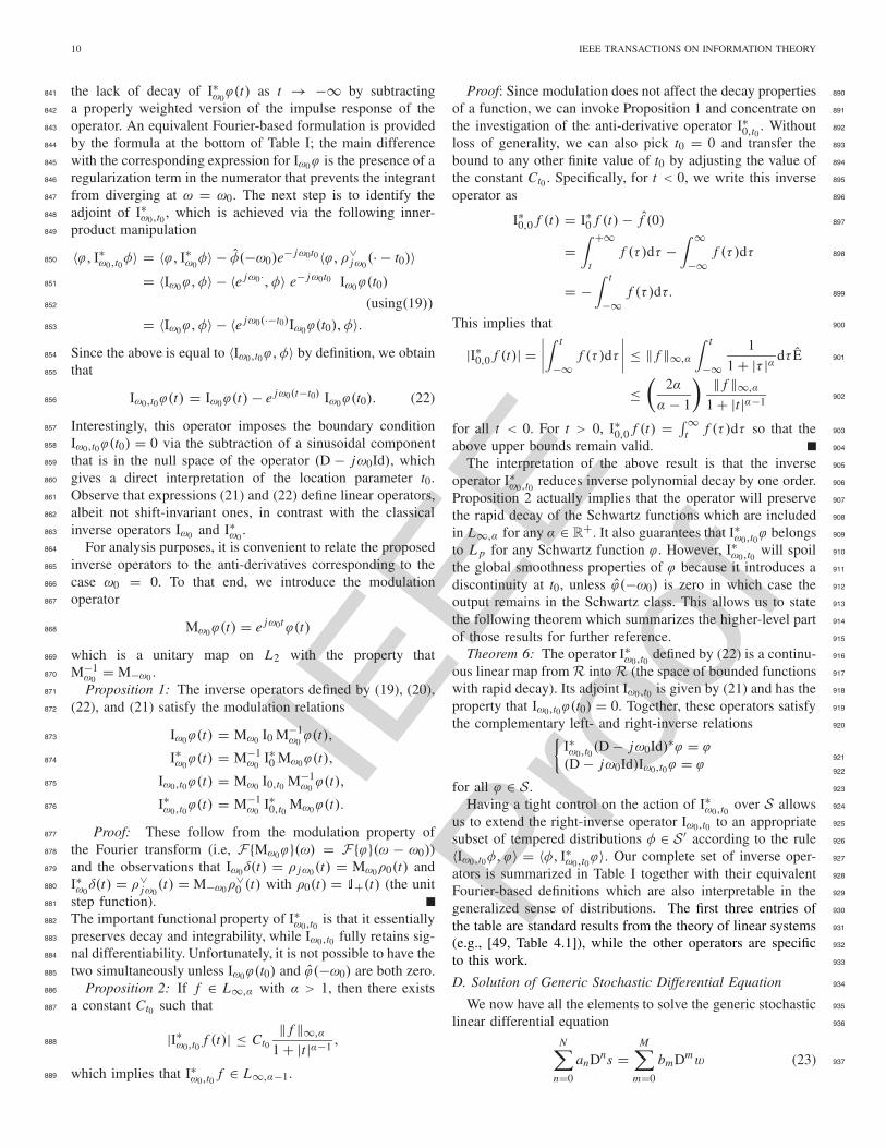
IEEE
Proo
f
10 IEEE TRANSACTIONS ON INFORMATION THEORY
the lack of decay of I∗ω0ϕ(t) as t → −∞ by subtracting841
a properly weighted version of the impulse response of the842
operator. An equivalent Fourier-based formulation is provided843
by the formula at the bottom of Table I; the main difference844
with the corresponding expression for Iω0ϕ is the presence of a845
regularization term in the numerator that prevents the integrant846
from diverging at ω = ω0. The next step is to identify the847
adjoint of I∗ω0,t0 , which is achieved via the following inner-848
product manipulation849
〈ϕ, I∗ω0,t0φ〉 = 〈ϕ, I∗ω0φ〉 − φ(−ω0)e
− jω0t0〈ϕ, ρ∨jω0(· − t0)〉850
= 〈Iω0ϕ, φ〉 − 〈e jω0·, φ〉 e− jω0t0 Iω0ϕ(t0)851
(using(19))852
= 〈Iω0ϕ, φ〉 − 〈e jω0(·−t0)Iω0ϕ(t0), φ〉.853
Since the above is equal to 〈Iω0,t0ϕ, φ〉 by definition, we obtain854
that855
Iω0,t0ϕ(t) = Iω0ϕ(t)− e jω0(t−t0) Iω0ϕ(t0). (22)856
Interestingly, this operator imposes the boundary condition857
Iω0,t0ϕ(t0) = 0 via the subtraction of a sinusoidal component858
that is in the null space of the operator (D − jω0Id), which859
gives a direct interpretation of the location parameter t0.860
Observe that expressions (21) and (22) define linear operators,861
albeit not shift-invariant ones, in contrast with the classical862
inverse operators Iω0 and I∗ω0.863
For analysis purposes, it is convenient to relate the proposed864
inverse operators to the anti-derivatives corresponding to the865
case ω0 = 0. To that end, we introduce the modulation866
operator867
Mω0ϕ(t) = e jω0tϕ(t)868
which is a unitary map on L2 with the property that869
M−1ω0
= M−ω0 .870
Proposition 1: The inverse operators defined by (19), (20),871
(22), and (21) satisfy the modulation relations872
Iω0ϕ(t) = Mω0 I0 M−1ω0ϕ(t),873
I∗ω0ϕ(t) = M−1
ω0I∗0 Mω0ϕ(t),874
Iω0,t0ϕ(t) = Mω0 I0,t0 M−1ω0ϕ(t),875
I∗ω0,t0ϕ(t) = M−1ω0
I∗0,t0 Mω0ϕ(t).876
Proof: These follow from the modulation property of877
the Fourier transform (i.e, F{Mω0ϕ}(ω) = F{ϕ}(ω − ω0))878
and the observations that Iω0δ(t) = ρ jω0(t) = Mω0ρ0(t) and879
I∗ω0δ(t) = ρ∨
jω0(t) = M−ω0ρ
∨0 (t) with ρ0(t) = �+(t) (the unit880
step function).881
The important functional property of I∗ω0,t0 is that it essentially882
preserves decay and integrability, while Iω0,t0 fully retains sig-883
nal differentiability. Unfortunately, it is not possible to have the884
two simultaneously unless Iω0ϕ(t0) and ϕ(−ω0) are both zero.885
Proposition 2: If f ∈ L∞,α with α > 1, then there exists886
a constant Ct0 such that887
|I∗ω0,t0 f (t)| ≤ Ct0‖ f ‖∞,α
1 + |t|α−1 ,888
which implies that I∗ω0,t0 f ∈ L∞,α−1.889
Proof: Since modulation does not affect the decay properties 890
of a function, we can invoke Proposition 1 and concentrate on 891
the investigation of the anti-derivative operator I∗0,t0 . Without 892
loss of generality, we can also pick t0 = 0 and transfer the 893
bound to any other finite value of t0 by adjusting the value of 894
the constant Ct0 . Specifically, for t < 0, we write this inverse 895
operator as 896
I∗0,0 f (t) = I∗0 f (t)− f (0) 897
=∫ +∞
tf (τ )dτ −
∫ ∞
−∞f (τ )dτ 898
= −∫ t
−∞f (τ )dτ. 899
This implies that 900
|I∗0,0 f (t)| =∣∣∣∣
∫ t
−∞f (τ )dτ
∣∣∣∣ ≤ ‖ f ‖∞,α
∫ t
−∞1
1 + |τ |α dτÊ 901
≤(
2α
α − 1
) ‖ f ‖∞,α
1 + |t|α−1 902
for all t < 0. For t > 0, I∗0,0 f (t) = ∫ ∞t f (τ )dτ so that the 903
above upper bounds remain valid. 904
The interpretation of the above result is that the inverse 905
operator I∗ω0,t0 reduces inverse polynomial decay by one order. 906
Proposition 2 actually implies that the operator will preserve 907
the rapid decay of the Schwartz functions which are included 908
in L∞,α for any α ∈ R+. It also guarantees that I∗ω0,t0ϕ belongs 909
to L p for any Schwartz function ϕ. However, I∗ω0,t0 will spoil 910
the global smoothness properties of ϕ because it introduces a 911
discontinuity at t0, unless ϕ(−ω0) is zero in which case the 912
output remains in the Schwartz class. This allows us to state 913
the following theorem which summarizes the higher-level part 914
of those results for further reference. 915
Theorem 6: The operator I∗ω0,t0 defined by (22) is a continu- 916
ous linear map from R into R (the space of bounded functions 917
with rapid decay). Its adjoint Iω0,t0 is given by (21) and has the 918
property that Iω0,t0ϕ(t0) = 0. Together, these operators satisfy 919
the complementary left- and right-inverse relations 920
{I∗ω0,t0(D − jω0Id)∗ϕ = ϕ
(D − jω0Id)Iω0,t0ϕ = ϕ921
922
for all ϕ ∈ S. 923
Having a tight control on the action of I∗ω0,t0 over S allows 924
us to extend the right-inverse operator Iω0,t0 to an appropriate 925
subset of tempered distributions φ ∈ S ′ according to the rule 926
〈Iω0,t0φ, ϕ〉 = 〈φ, I∗ω0,t0ϕ〉. Our complete set of inverse oper- 927
ators is summarized in Table I together with their equivalent 928
Fourier-based definitions which are also interpretable in the 929
generalized sense of distributions. The first three entries of 930
the table are standard results from the theory of linear systems 931
(e.g., [49, Table 4.1]), while the other operators are specific 932
to this work. 933
D. Solution of Generic Stochastic Differential Equation 934
We now have all the elements to solve the generic stochastic 935
linear differential equation 936
N∑
n=0
anDns =M∑
m=0
bmDmw (23) 937
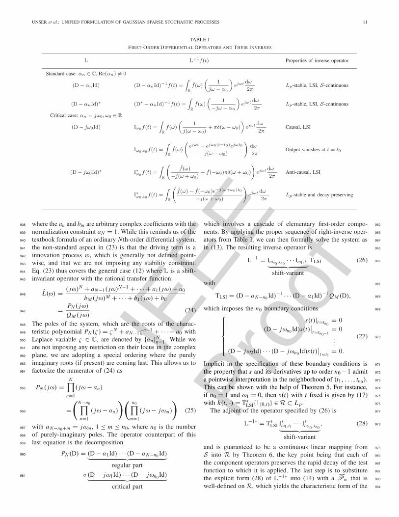
IEEE
Proo
f
UNSER et al.: UNIFIED FORMULATION OF GAUSSIAN SPARSE STOCHASTIC PROCESSES 11
TABLE I
FIRST-ORDER DIFFERENTIAL OPERATORS AND THEIR INVERSES
where the an and bm are arbitrary complex coefficients with the938
normalization constraint aN = 1. While this reminds us of the939
textbook formula of an ordinary N th-order differential system,940
the non-standard aspect in (23) is that the driving term is a941
innovation process w, which is generally not defined point-942
wise, and that we are not imposing any stability constraint.943
Eq. (23) thus covers the general case (12) where L is a shift-944
invariant operator with the rational transfer function945
L(ω) = ( jω)N + aN−1( jω)N−1 + · · · + a1( jω)+ a0
bM ( jω)M + · · · + b1( jω)+ b0946
= PN ( jω)
QM ( jω). (24)947
The poles of the system, which are the roots of the charac-948
teristic polynomial PN (ζ ) = ζ N + aN−1ζn−1 + · · · + a0 with949
Laplace variable ζ ∈ C, are denoted by {αn}Nn=1. While we950
are not imposing any restriction on their locus in the complex951
plane, we are adopting a special ordering where the purely952
imaginary roots (if present) are coming last. This allows us to953
factorize the numerator of (24) as954
PN ( jω) =N∏
n=1
( jω− αn)955
=(
N−n0∏
n=1
( jω− αn)
) (n0∏
m=1
( jω− jωm)
)
(25)956
with αN−n0+m = jωm , 1 ≤ m ≤ n0, where n0 is the number957
of purely-imaginary poles. The operator counterpart of this958
last equation is the decomposition959
PN (D) = (D − α1Id) · · · (D − αN−n0 Id)︸ ︷︷ ︸
regular part
960
◦ (D − jω1Id) · · · (D − jωn0 Id)︸ ︷︷ ︸
critical part
961
which involves a cascade of elementary first-order compo- 962
nents. By applying the proper sequence of right-inverse oper- 963
ators from Table I, we can then formally solve the system as 964
in (13). The resulting inverse operator is 965
L−1 = Iωn0 ,tn0· · · Iω1,t1
︸ ︷︷ ︸shift-variant
TLSI (26) 966
with 967
TLSI = (D − αN−n0 Id)−1 · · · (D − α1Id)−1 QM (D), 968
which imposes the n0 boundary conditions 969
⎧⎪⎪⎪⎪⎨
⎪⎪⎪⎪⎩
s(t)|t=tn0= 0
(D − jωn0 Id)s(t)∣∣t=tn0−1
= 0...
(D − jω2Id) · · · (D − jωn0 Id)s(t)∣∣t=t1
= 0.
(27) 970
Implicit in the specification of these boundary conditions is 971
the property that s and its derivatives up to order n0 −1 admit 972
a pointwise interpretation in the neighborhood of (t1, . . . , tn0). 973
This can be shown with the help of Theorem 5. For instance, 974
if n0 = 1 and ω1 = 0, then s(t) with t fixed is given by (17) 975
with h(t, ·) = T∗LSI{�[0,t)} ∈ R ⊂ L p . 976
The adjoint of the operator specified by (26) is 977
L−1∗ = T∗LSI I∗ω1,t1 · · · I∗ωn0 ,tn0︸ ︷︷ ︸
shift-variant
, (28) 978
and is guaranteed to be a continuous linear mapping from 979
S into R by Theorem 6, the key point being that each of 980
the component operators preserves the rapid decay of the test 981
function to which it is applied. The last step is to substitute 982
the explicit form (28) of L−1∗ into (14) with a Pw that is 983
well-defined on R, which yields the characteristic form of the 984
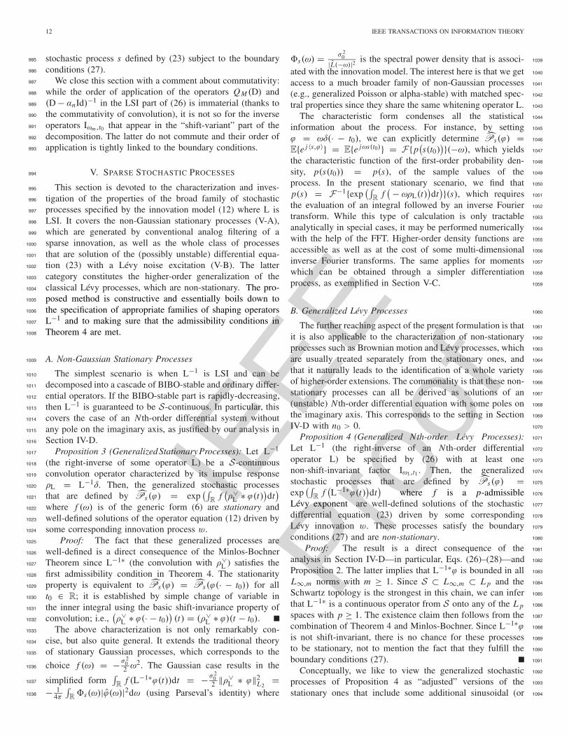
IEEE
Proo
f
12 IEEE TRANSACTIONS ON INFORMATION THEORY
stochastic process s defined by (23) subject to the boundary985
conditions (27).986
We close this section with a comment about commutativity:987
while the order of application of the operators QM (D) and988
(D − αnId)−1 in the LSI part of (26) is immaterial (thanks to989
the commutativity of convolution), it is not so for the inverse990
operators Iωm ,t0 that appear in the “shift-variant” part of the991
decomposition. The latter do not commute and their order of992
application is tightly linked to the boundary conditions.993
V. SPARSE STOCHASTIC PROCESSES994
This section is devoted to the characterization and inves-995
tigation of the properties of the broad family of stochastic996
processes specified by the innovation model (12) where L is997
LSI. It covers the non-Gaussian stationary processes (V-A),998
which are generated by conventional analog filtering of a999
sparse innovation, as well as the whole class of processes1000
that are solution of the (possibly unstable) differential equa-1001
tion (23) with a Lévy noise excitation (V-B). The latter1002
category constitutes the higher-order generalization of the1003
classical Lévy processes, which are non-stationary. The pro-1004
posed method is constructive and essentially boils down to1005
the specification of appropriate families of shaping operators1006
L−1 and to making sure that the admissibility conditions in1007
Theorem 4 are met.1008
A. Non-Gaussian Stationary Processes1009
The simplest scenario is when L−1 is LSI and can be1010
decomposed into a cascade of BIBO-stable and ordinary differ-1011
ential operators. If the BIBO-stable part is rapidly-decreasing,1012
then L−1 is guaranteed to be S-continuous. In particular, this1013
covers the case of an N th-order differential system without1014
any pole on the imaginary axis, as justified by our analysis in1015
Section IV-D.1016
Proposition 3 (Generalized StationaryProcesses): Let L−11017
(the right-inverse of some operator L) be a S-continuous1018
convolution operator characterized by its impulse response1019
ρL = L−1δ. Then, the generalized stochastic processes1020
that are defined by Ps(ϕ) = exp(∫
Rf(ρ∨
L ∗ ϕ(t))dt)
1021
where f (ω) is of the generic form (6) are stationary and1022
well-defined solutions of the operator equation (12) driven by1023
some corresponding innovation process w.1024
Proof: The fact that these generalized processes are1025
well-defined is a direct consequence of the Minlos-Bochner1026
Theorem since L−1∗ (the convolution with ρ∨L ) satisfies the1027
first admissibility condition in Theorem 4. The stationarity1028
property is equivalent to Ps(ϕ) = Ps(ϕ(· − t0)) for all1029
t0 ∈ R; it is established by simple change of variable in1030
the inner integral using the basic shift-invariance property of1031
convolution; i.e.,(ρ∨
L ∗ ϕ(· − t0))(t) = (ρ∨
L ∗ ϕ)(t − t0).1032
The above characterization is not only remarkably con-1033
cise, but also quite general. It extends the traditional theory1034
of stationary Gaussian processes, which corresponds to the1035
choice f (ω) = − σ 202 ω
2. The Gaussian case results in the1036
simplified form∫R
f (L−1∗ϕ(t))dt = − σ 202 ‖ρ∨
L ∗ ϕ‖2L2
=1037
− 14π
∫R�s(ω)|ϕ(ω)|2dω (using Parseval’s identity) where1038
�s(ω) = σ 20
|L(−ω)|2 is the spectral power density that is associ- 1039
ated with the innovation model. The interest here is that we get 1040
access to a much broader family of non-Gaussian processes 1041
(e.g., generalized Poisson or alpha-stable) with matched spec- 1042
tral properties since they share the same whitening operator L. 1043
The characteristic form condenses all the statistical 1044
information about the process. For instance, by setting 1045
ϕ = ωδ(· − t0), we can explicitly determine Ps(ϕ) = 1046
E{e j 〈s,ϕ〉} = E{e jωs(t0)} = F{p(s(t0)
)}(−ω), which yields 1047
the characteristic function of the first-order probability den- 1048
sity, p(s(t0)) = p(s), of the sample values of the 1049
process. In the present stationary scenario, we find that 1050
p(s) = F−1{exp(∫
Rf( − ωρL(t)
)dt
)}(s), which requires 1051
the evaluation of an integral followed by an inverse Fourier 1052
transform. While this type of calculation is only tractable 1053
analytically in special cases, it may be performed numerically 1054
with the help of the FFT. Higher-order density functions are 1055
accessible as well as at the cost of some multi-dimensional 1056
inverse Fourier transforms. The same applies for moments 1057
which can be obtained through a simpler differentiation 1058
process, as exemplified in Section V-C. 1059
B. Generalized Lévy Processes 1060
The further reaching aspect of the present formulation is that 1061
it is also applicable to the characterization of non-stationary 1062
processes such as Brownian motion and Lévy processes, which 1063
are usually treated separately from the stationary ones, and 1064
that it naturally leads to the identification of a whole variety 1065
of higher-order extensions. The commonality is that these non- 1066
stationary processes can all be derived as solutions of an 1067
(unstable) N th-order differential equation with some poles on 1068
the imaginary axis. This corresponds to the setting in Section 1069
IV-D with n0 > 0. 1070
Proposition 4 (Generalized Nth-order Lévy Processes): 1071
Let L−1 (the right-inverse of an N th-order differential 1072
operator L) be specified by (26) with at least one 1073
non-shift-invariant factor Iω1,t1 . Then, the generalized 1074
stochastic processes that are defined by Ps(ϕ) = 1075
exp(∫
Rf(L−1∗ϕ(t)
)dt
)where f is a p-admissible 1076
Lévy exponent are well-defined solutions of the stochastic 1077
differential equation (23) driven by some corresponding 1078
Lévy innovation w. These processes satisfy the boundary 1079
conditions (27) and are non-stationary. 1080
Proof: The result is a direct consequence of the 1081
analysis in Section IV-D—in particular, Eqs. (26)–(28)—and 1082
Proposition 2. The latter implies that L−1∗ϕ is bounded in all 1083
L∞,m norms with m ≥ 1. Since S ⊂ L∞,m ⊂ L p and the 1084
Schwartz topology is the strongest in this chain, we can infer 1085
that L−1∗ is a continuous operator from S onto any of the L p 1086
spaces with p ≥ 1. The existence claim then follows from the 1087
combination of Theorem 4 and Minlos-Bochner. Since L−1∗ϕ 1088
is not shift-invariant, there is no chance for these processes 1089
to be stationary, not to mention the fact that they fulfill the 1090
boundary conditions (27). 1091
Conceptually, we like to view the generalized stochastic 1092
processes of Proposition 4 as “adjusted” versions of the 1093
stationary ones that include some additional sinusoidal (or 1094
IEEE
Proo
f
UNSER et al.: UNIFIED FORMULATION OF GAUSSIAN SPARSE STOCHASTIC PROCESSES 13
polynomial) trends. While the generation mechanism of these1095
trends is random, there is a deterministic aspect to it because1096
it imposes the boundary conditions (27) at t1, · · · , tn0 . The1097
class of such processes is actually quite rich and the formalism1098
surprisingly powerful. We shall illustrate the use of1099
Proposition 4 in Section V with the simplest possible operator1100
L = D which will gets us back to Brownian motion and the1101
celebrated family of Lévy processes. We shall also show how1102
the well-known properties of Lévy processes can be readily1103
deduced from their characteristic form.1104
C. Moments and Correlation1105
The covariance form of a generalized (complex-valued)1106
process s is defined as:1107
Bs(ϕ1, ϕ2) = E{〈s, ϕ1〉 · 〈s, ϕ2〉}.1108
where 〈s, ϕ2〉 = 〈s, ϕ2〉 when s is real-valued. Thanks to1109
the moment generating properties of the Fourier transform,1110
this functional can be calculated from the characteristic form1111
Ps(ϕ) as1112
Bs(ϕ1, ϕ2) = (− j)2∂2Ps(ω1ϕ1 + ω2ϕ2)
∂ω1∂ω2
∣∣∣∣∣ω1=0,ω2=0
, (29)1113
where we are implicitly assuming that the required partial1114
derivative of the characteristic functional exists. The autocor-1115
relation of the process is then obtained by making the formal1116
substitution ϕ1 = δ(· − t1) and ϕ2 = δ(· − t2):1117
Rs(t1, t2) = E{s(t1)s(t2)} = Bs (δ(· − t1), δ(· − t2)) .1118
Alternatively, we can also retrieve the autocorrelation1119
function by invoking the kernel theorem: Bs(ϕ1, ϕ2) =1120 ∫R2 Rs(t1, t2)ϕ1(t1)ϕ(t2)dt1dt2.1121
The concept also generalizes for the calculation of the1122
higher-order correlation form61123
E{〈s, ϕ1〉 · 〈s, ϕ2〉 · · · 〈s, ϕN 〉}1124
= (− j)N ∂N Ps(ω1ϕ1 + · · · + ωNϕN )
∂ω1 · · · ∂ωN
∣∣∣∣∣ω1=0,··· ,ωN =0
1125
which provides the basis for the determination of higher-order1126
moments and cumulants.1127
Here, we concentrate on the calculation of the second-order1128
moments, which happen to be independent upon the specific1129
type of noise. For the cases where the covariance is defined1130
and finite, it is not hard to show that the generic covariance1131
form of the innovation processes defined in Section III-C is1132
Bw(ϕ1, ϕ2) = σ 20 〈ϕ1, ϕ2〉,1133
where σ 20 is a suitable normalization constant that depends on1134
the noise parameters (b1, b2, v) in (7)–(10). We then perform1135
the usual adjoint manipulation to transfer the above formula1136
to the filtered version s = L−1w of such a noise process.1137
Property 1 (Generalized Correlation): The covariance1138
form of the generalized stochastic process whose characteristic1139
6For simplicity, we are only giving the formula for a real-valued process.
form is Ps(ϕ) = Pw(L−1∗ϕ) where Pw is a white noise 1140
functional is given by 1141
Bs(ϕ1, ϕ2) = σ 20 〈L−1∗ϕ1,L−1∗ϕ2〉 = σ 2
0 〈L−1L−1∗ϕ1, ϕ2〉, 1142
and corresponds to the correlation function 1143
Rs(t1, t2) = E{s(t1) · s(t2)} = σ 20 〈L−1L−1∗δ(· − t1),δ(·−t2)〉. 1144
The latter characterization requires the determination of the 1145
impulse response of L−1L−1∗. In particular, when L−1 is LSI 1146
with convolution kernel ρL ∈ L1, we get that 1147
Rs(t1, t2) = σ 20 L−1L−1∗δ(t2 − t1) = rs(t2 − t1) 1148
= σ 20 (ρL ∗ ρ∨
L )(t2 − t1), 1149
which confirms that the underlying process is wide-sense sta- 1150
tionary. Since the autocorrelation function rs(τ ) is integrable, 1151
we also have a one-to-one correspondence with the traditional 1152
notion of power spectrum: �s(ω) = F{rs}(ω) = σ 20
|L(−ω)|2 , 1153
where L(ω) is the frequency response of the whitening oper- 1154
ator L. 1155
The determination of the correlation function for the non- 1156
stationary processes associated with the unstable versions 1157
of (23) is more involved. We shall see in [32] that it can be 1158
bypassed if, instead of s(t), we consider the generalized incre- 1159
ment process sd(t) = Lds(t) where Ld is a discrete version 1160
(finite-difference type operator) of the whitening operator L. 1161
D. Sparsification in a Wavelet-Like Basis 1162
The implicit assumption for the next properties is that 1163
we have a wavelet-like basis {ψi,k }i∈Z,k∈Z available that is 1164
matched to the operator L. Specifically, the basis functions 1165
ψi,k (t) = ψi (t − 2i k) with scale and location indices (i, k) 1166
are translated versions of some normalized reference wavelet 1167
ψi = L∗φi where φi is an appropriate scale-dependent 1168
smoothing kernel. It turns out that such operator-like wavelets 1169
can be constructed for the whole class of ordinary differential 1170
operators considered in this paper [36]. They can be specified 1171
to be orthogonal and/or compactly supported (cf. examples in 1172
Fig. 2). In the case of the classical Haar wavelet, we have that 1173
ψHaar = Dφi where the smoothing kernels φi ∝ φ0(t/2i ) are 1174
rescaled versions of a triangle function (B-spline of degree 1). 1175
The latter dilation property follows from the fact that the 1176
derivative operator D commutes with scaling. 1177
We note that the determination of the wavelet coefficients 1178
vi [k] = 〈s, ψi,k 〉 of the random signal s at a given scale 1179
i is equivalent to correlating the signal with the wavelet 1180
ψi (continuous wavelet transform) and sampling thereafter. 1181
The goods news is that this has a stationarizing and decoupling 1182
effect. 1183
Property 2 (Wavelet-Domain Probability Laws): Let 1184
vi (t) = 〈s, ψi (· − t)〉 with ψi = L∗φi be the i th channel of 1185
the continuous wavelet transform of a generalized (stationary 1186
or non-stationary) Lévy process s with whitening operator 1187
L and p-admissible Lévy exponent f . Then, vi (t) is a 1188
generalized stationary process with characteristic functional 1189
Pvi (ϕ) = Pw(φi ∗ϕ) where Pw is defined by (5). Moreover, 1190
the characteristic function of the (discrete) wavelet coefficient 1191
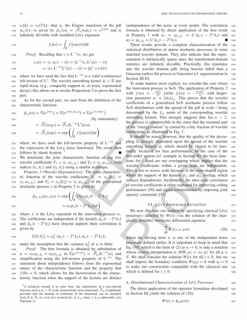
IEEE
Proo
f
14 IEEE TRANSACTIONS ON INFORMATION THEORY
vi [k] = vi (2i k)—that is, the Fourier transform of the pdf1192
pvi (v)—is given by pvi (ω) = Pw(ωφi ) = e fi (ω) and is1193
infinitely divisible with modified Lévy exponent1194
fi (ω) =∫
R
f(ωφi (t)
)dt .1195
Proof: Recalling that s = L−1w, we get1196
vi (t) = 〈s, ψi (· − t)〉 = 〈L−1w,L∗φi (· − t)〉1197
= 〈w,L−1∗L∗φi (· − t)〉 = (φ∨
i ∗ w)(t)1198
where we have used the fact that L−1∗ is a valid (continuous)1199
left-inverse of L∗. The wavelet smoothing kernel φi ∈ R has1200
rapid decay (e.g., compactly-support or, at worst, exponential1201
decay); this allows us to invoke Proposition 3 to prove the first1202
part.1203
As for the second part, we start from the definition of the1204
characteristic function:1205
pvi (ω) = E{e jωvi } = E{e jω〈s,ψi,k 〉} = E{e j 〈s,ωψi 〉}1206
(by stationarity)1207
= Ps(ωψi ) = Pw(L−1∗L∗φiω)1208
= Pw(ωφi ) = exp
(∫
R
f(ωφi (t)
)dt
)
1209
where we have used the left-inverse property of L−1∗ and1210
the expression of the Lévy noise functional. The result then1211
follows by identi fication. 71212
We determine the joint characteristic function of any two1213
wavelet coefficients Y1 = 〈s, ψi1 ,k1〉 and Y2 = 〈s, ψi2 ,k2 〉 with1214
indices (i1, k1) and (i2, k2) using a similar technique.1215
Property 3 (Wavelet Dependencies): The joint characteris-1216
tic function of the wavelet coefficients Y1 = vi1 [k1] =1217
〈s, ψi1 ,k1 〉 and Y2 = vi2 [k2] = 〈s, ψi2 ,k2 〉 of the generalized1218
stochastic process s in Property 2 is given by1219
pY1,Y2(ω1, ω2) = exp
(∫
R
f(ω1φi1(t − 2i1 k1)1220
+ω2φi2 (t − 2i2 k2))dt
)1221
where f is the Lévy exponent of the innovation process w.1222
The coefficients are independent if the kernels φi1(t − 2i1 k1)1223
and φi2 (t − 2i2 k2) have disjoint support; their correlation is1224
given by1225
E{Y1Y2} = σ 20 〈φi1 (· − 2i1 k1), φi2 (· − 2i2 k2)〉.1226
under the assumption that the variance σ 20 of w is finite.1227
Proof: The first formula is obtained by substitution of1228
ϕ = ω1ψi1,k1 + ω2ψi2,k2 in E{e j 〈s,ϕ〉} = Pw(L−1∗ϕ), and1229
simplification using the left-inverse property of L−1∗. The1230
statement about independence follows from the exponential1231
nature of the characteristic function and the property that1232
f (0) = 0, which allows for the factorization of the charac-1233
teristic function when the support of the kernels are distinct1234
7A technical remark is in order here: the substitution of a non-smoothfunction such as φi ∈ R in the characteristic noise functional Pw is legitimateprovided that the domain of continuity of the functional can be extendedfrom S to R, or, even less restrictively, to L p when f is p-admissible (seeTheorem 3).
(independence of the noise at every point). The correlation 1235
formula is obtained by direct application of the first result 1236
in Property 1 with ϕ1 = ψi1,k1 = L∗φi1(· − 2i1 k1) and 1237
ϕ2 = ψi2 ,k2 = L∗φi2 (· − 2i2 k2). 1238
These results provide a complete characterization of the 1239
statistical distribution of sparse stochastic processes in some 1240
matched wavelet domain. They also indicate that the repre- 1241
sentation is intrinsically sparse since the transformed-domain 1242
statistics are infinitely divisible. Practically, this translates 1243
into the wavelet domain pdfs being heavier tailed than a 1244
Gaussian (unless the process is Gaussian) (cf. argumentation in 1245
Section III-D). 1246
To make matters more explicit, we consider the case where 1247
the innovation process is SαS. The application of Property 2 1248
with f (ω) = −|ω|αα! yields fi (ω) = −|σiω|α
α! with disper- 1249
sion parameter σi = ‖φi‖Lα . This proves that the wavelet 1250
coefficients of a generalized SαS stochastic process follow 1251
SαS distributions with the spread of the pdf at scale i being 1252
determined by the Lα norm of the corresponding wavelet 1253
smoothing kernels. This strongly suggests that, for α < 2, 1254
the process is compressible in the sense that the essential part 1255
of the “energy content” is carried by a tiny fraction of wavelet 1256
coefficients, as illustrated in Fig. 1. 1257
It should be noted, however, that the quality of the decou- 1258
pling is strongly dependent upon the spread of the wavelet 1259
smoothing kernels φi which should be chosen to be max- 1260
imally localized for best performance. In the case of the 1261
first-order system (cf. example in Section II), the basis func- 1262
tions for i fixed are not overlapping which implies that the 1263
wavelet coefficients within a given scale are independent. 1264
This is not so across scale because of the cone-shaped region 1265
where the support of the kernels φi1 and φi2 overlap, which 1266
induces dependencies. Incidentally, the inter-scale correlation 1267
of wavelet coefficients is often exploited for improving coding 1268
performance [50] and signal reconstruction by imposing joint 1269
sparsity constraints [51]. 1270
VI. LÉVY PROCESSES REVISITED 1271
We now illustrate our method by specifying classical Lévy 1272
processes—denoted by W (t)—via the solution of the (mar- 1273
ginally unstable) stochastic differential equation 1274
d
dtW (t) = w(t) (30) 1275
where the driving term w is one of the independent noise 1276
processes defined earlier. It is important to keep in mind that 1277
Eq. (30), which is the limit of (2) as α → 0, is only a notation 1278
whose correct interpretation is 〈DW, ϕ〉 = 〈w,ϕ〉 for all ϕ ∈ 1279
S. We shall consider the solution W (t) for all t ∈ R, but we 1280
shall impose the boundary condition W (t0) = 0 with t0 = 0 1281
to make our construction compatible with the classical one 1282
which is defined for t ≥ 0. 1283
A. Distributional Characterization of Lévy Processes 1284
The direct application of the operator formalism developed 1285
in Section III yields the solution of (30): 1286
W (t) = I0,0w(t) 1287
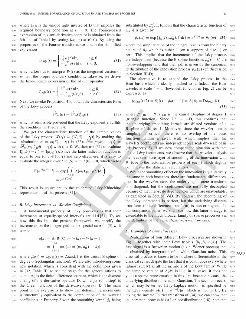
IEEE
Proo
f
UNSER et al.: UNIFIED FORMULATION OF GAUSSIAN SPARSE STOCHASTIC PROCESSES 15
where I0,0 is the unique right inverse of D that imposes the1288
required boundary condition at t = 0. The Fourier-based1289
expression of this anti-derivative operator is obtained from the1290
6th line of Table I by setting (ω0, t0) = (0, 0). By using the1291
properties of the Fourier transform, we obtain the simplified1292
expression1293
I0,0ϕ(t) ={∫ t
0 ϕ(τ)dτ, t ≥ 0− ∫ 0
t ϕ(τ)dτ, t < 0,(31)1294
which allows us to interpret W (t) as the integrated version of1295
w with the proper boundary conditions. Likewise, we derive1296
the time-domain expression of the adjoint operator1297
I∗0,0ϕ(t) ={ ∫ ∞
t ϕ(τ)dτ, t ≥ 0,− ∫ t
−∞ ϕ(τ)dτ, t < 0.(32)1298
Next, we invoke Proposition 4 to obtain the characteristic form1299
of the Lévy process1300
PW (ϕ) = Pw(I∗0,0ϕ) (33)1301
which is admissible provided that the Lévy exponent f fullfils1302
the condition in Theorem 4.1303
We get the characteristic function of the sample values1304
of the Lévy process W (t1) = 〈W, δ(· − t1)〉 by making the1305
substitution ϕ = ω1δ(· − t1) in (33): PW(ω1δ(· − t1)
) =1306
Pw
(ω1I∗0,0δ(·− t1)
)with t1 > 0. We then use (31) to evaluate1307
I∗0,0δ(t − t1) = �[0,t1)(t). Since the latter indicator function is1308
equal to one for t ∈ [0, t1) and zero elsewhere, it is easy to1309
evaluate the integral over t in (5) with f (0) = 0, which yields1310
E{e jω1W (t1)} = exp
(∫
R
f(ω1�[0,t1)(t)
)dt
)
1311
= et1 f (ω1)1312
This result is equivalent to the celebrated Lévy-Khinchine1313
representation of the process [31].1314
B. Lévy Increments vs. Wavelet Coefficients1315
A fundamental property of Lévy processes is that their1316
increments at equally-spaced intervals are i.i.d.[31]. To see1317
how this fits into the present framework, we specify the1318
increments on the integer grid as the special case of (3) with1319
α = 0:1320
u[k] = �0W (k) := W (k)− W (k − 1)1321
=∫ k
k−1w(t)dt = 〈w,β∨
0 (· − k)〉1322
where β0(t) = �[0,1)(t) = �0ρ0(t) is the causal B-spline of1323
degree 0 (rectangular function). We are also introducing some1324
new notation, which is consistent with the definitions given1325
in [32, Table II], to set the stage for the generalizations to1326
come.�0 is the finite-difference operator, which is the discrete1327
analog of the derivative operator D, while ρ0 (unit step) is1328
the Green function of the derivative operator D. The main1329
point of the exercise is to show that determining increments1330
is structurally equivalent to the computation of the wavelet1331
coefficients in Property 2 with the smoothing kernel φi being1332
substituted by β∨0 . It follows that the characteristic function of 1333
wd [·] is given by 1334
pu(ω) = exp(∫
Rf (ωβ∨
0 (t))dt
) = e f (ω) = pid(ω) (34) 1335
where the simplification of the integral results from the binary 1336
nature of β0 which is either 1 (on a support of size 1) or 1337
zero. This implies that the increments of the Lévy process 1338
are independent (because the B-spline functions β∨0 (·− k) are 1339
non-overlapping) and that their pdf is given by the canonical 1340
id distribution of the innovation process pid(x) (cf. discussion 1341
in Section III-D). 1342
The alternative is to expand the Lévy process in the 1343
Haar basis which is ideally matched to it. Indeed, the Haar 1344
wavelet at scale i = 1 (lower-left function in Fig. 2) can be 1345
expressed as 1346
ψHaar(t/2) = β0(t)− β0(t − 1) = �0β0 = Dβ(0,0)(t) 1347
(35) 1348
where β(0,0) = β0 ∗ β0 is the causal B-spline of degree 1 1349
(triangle function). Since D∗ = −D, this confirms that 1350
the underlying smoothing kernels are dilated versions of a 1351
B-spline of degree 1. Moreover, since the wavelet-domain 1352
sampling is critical, there is no overlap of the basis 1353
functions within a given scale which implies that the 1354
wavelets coefficients are independent on a scale-by-scale basis 1355
(cf. Property 3). If we now compare the situation with that 1356
of the Lévy increments, we observe that the wavelet analysis 1357
involves one more layer of smoothing of the innovation with 1358
β0 (due to the factorization property of β(0,0)) which slightly 1359
complicates the statistical calculations. 1360
While the smoothing effect on the innovation is qualitatively 1361
the same in both instances, there are fundamental differences, 1362
too. In the wavelet case, the underlying discrete transform 1363
is orthogonal, but the coefficients are not fully decoupled 1364
because of the inter-scale dependencies which are unavoidable, 1365
as explained in Section V-D. By contrast, the decoupling of 1366
the Lévy increments is perfect, but the underlying discrete 1367
transform (finite difference transform) is non-orthogonal. In 1368
our companion paper, we shall see how this latter strategy is 1369
extendable to the much broader family of sparse processes via 1370
the definition of the generalized increment process. 1371
C. Examples of Lévy Processes 1372
Realizations of four different Lévy processes are shown in 1373
Fig. 1 together with their Lévy triplets(b1, b2, v(a)
). The 1374
first signal is a Brownian motion (a.k.a. Wiener process) that 1375
is obtained by integration of a white Gaussian noise. This 1376
classical process is known to be nowhere differentiable in the 1377
classical sense, despite the fact that it is continuous everywhere 1378
(almost surely) as all the members of the Lévy family. While 1379
the sampled version of �0W is i.i.d. in all cases, it does not 1380
yield a sparse representation in this first instance because the 1381
underlying distribution remains Gaussian. The second process,
AQ:3
1382
which may be termed Lévy-Laplace motion, is specified by 1383
the Lévy density v(a) = e−|a|/|a| which is not in L1. By 1384
taking the inverse Fourier transform of (34), we can show that 1385
its increment process has a Laplace distribution [18]; note that 1386

IEEE
Proo
f
16 IEEE TRANSACTIONS ON INFORMATION THEORY
Fig. 3. Examples of Lévy motions W (t) with increasing degrees of sparsity. (a) Brownian motion with Lévy triplet (0, 1, 0). (b) Lévy-Laplace motion with(0, 0, e−|a|
|a|). (c) Compound Poisson process with
(0, 0, λ 1√
2πe−a2/2)
with λ = 132 . (d) Symmetric Lévy flight with
(0, 0, 1/|a|α+1)
and α = 1.2.
this type of generalized Gaussian model is often used to justify1387
sparsity-promoting signal processing techniques based on �11388
minimization [52]–[54]. The third piecewise-constant signal is1389
a compound Poisson process. It is intrinsically sparse since a1390
good proportion of its increments is zero by construction (with1391
probability e−λ). Interestingly, this is the only type of Lévy1392
process that fulfills the finite rate of innovation property [17].1393
The fourth example is an alpha-stable Lévy motion (a.k.a.1394
Lévy flight) with α = 1.2. Here, the distribution of �0W1395
is heavy-tailed (SαS) with unbounded moments for p > α.1396
Although this may not be obvious from the picture, this is1397
the sparsest process of the lot because it is �α-compressible1398
in the strongest sense [45]. Specifically, we can compress the1399
sequence such as to preserve any prescribed portion r < 1 of1400
its average �α energy by retaining an arbitrarily small fraction1401
of samples as the length of the signal goes to infinity.1402
D. Link With Conventional Stochastic Calculus1403
Thanks to (30), we can view a white noise w = W as the1404
weak derivative of some classical Lévy processes W (t) which1405
is well-defined pointwise (almost everywhere). This provides1406
us with further insights on the range of admissible innovation1407
processes of Section II.C which constitute the driving terms of1408
the general stochastic differential equation (12). This funda-1409
mental observation also makes the connection with stochastic1410
calculus8 [55], [56], which avoids the notion of white noise1411
by relying on the use of stochastic integrals of the form1412
s(t) =∫
R
h(t, t ′)dW (t ′)1413
where W is a random (signed) measure associated to some1414
canonical Brownian motion (or, by extension, a Lévy process)1415
and where h(t, t ′) is an integration kernel that formally cor-1416
responds to our inverse operator L−1 (see Theorem 5).1417
8The Itô integral of conventional stochastic calculus is based on Brownianmotion, but the concept can also be generalized to Lévy driving terms usingthe more advanced theory of semimartingales [55].
VII. CONCLUSION 1418
We have set the foundations of a unifying framework that 1419
gives access to the broadest possible class of continuous- 1420
time stochastic processes specifiable by linear, shift-invariant 1421
equations, which is beneficial for signal processing purposes. 1422
We have shown that these processes admit a concise represen- 1423
tation in a wavelet-like basis. We have applied our framework 1424
to the description of the classical Lévy processes, which, in 1425
our view, provide the simplest and most basic examples of 1426
sparse processes, despite the fact that they are non-stationary. 1427
We have also hinted at the link between Lévy increments 1428
and splines, which is the theme that we shall develop in full 1429
generality next [32]. 1430
We have demonstrated that the proposed class of 1431
stochastic models and the corresponding mathematical 1432
machinery (Fourier analysis, characteristic functional, and 1433
B-spline calculus) lends itself well to the derivation of 1434
transform-domain statistics. The formulation suggests a variety 1435
of new processes whose properties are compatible with the 1436
currently-dominant paradigm in the field which is focused on 1437
the notion of sparsity. In that respect, the sparse processes that 1438
are best matched to conventional wavelets9 are those generated 1439
by N-fold integration (with proper boundary conditions) of a 1440
non-gaussian innovation. These processes, which are the solu- 1441
tion of an unstable SDE (pole of multiplicity N at the origin), 1442
are intrinsically self-similar (fractal) and non-stationary. Last 1443
but not least, the formulation is backward compatible with the 1444
classical theory of Gaussian stationary processes. 1445
ACKNOWLEDGMENT 1446
The authors are thankful to Prof. Robert Dalang (EPFL 1447
Chair of Probabilities), Julien Fageot and Dr. Arash Amini 1448
for helpful discussions. 1449
9A wavelet with N vanishing moments can always be rewritten as ψ =DNφ with φ ∈ L2(R) where the operator L = DN is scale-invariant.

IEEE
Proo
f
UNSER et al.: UNIFIED FORMULATION OF GAUSSIAN SPARSE STOCHASTIC PROCESSES 17
REFERENCES1450
[1] A. Papoulis, Probability, Random Variables, and Stochastic Processes.1451
New York, NY, USA: McGraw-Hill, 1991.1452
[2] R. Gray and L. Davisson, An Introduction to Statistical Signal Process-1453
ing. Cambridge, U.K.: Cambridge Univ. Press, 2004.1454
[3] E. J. Candès and M. B. Wakin, “An introduction to compressive1455
sampling,” IEEE Signal Process. Mag., vol. 25, no. 2, pp. 21–30,1456
Mar. 2008.1457
[4] A. M. Bruckstein, D. L. Donoho, and M. Elad, “From sparse solutions of1458
systems of equations to sparse modeling of signals and images,” SIAM1459
Rev., vol. 51, no. 1, pp. 34–81, 2009.1460
[5] S. Mallat, A Wavelet Tour of Signal Processing: The Sparse Way, 3rd ed.1461
San Diego, CA, USA: Academic Press, 2009.1462
[6] J.-L. Starck, F. Murtagh, and J. M. Fadili, Sparse Image and Signal1463
Processing: Wavelets, Curvelets, Morphological Diversity. Cambridge.1464
U.K.: Cambridge Univ. Press, 2010.1465
[7] M. Elad, Sparse and Redundant Representations. From Theory to1466
Applications in Signal and Image Processing. New York, NY, USA:1467
Springer-Verlag, 2010.1468
[8] Y. C. Eldar and G. Kutyniok, Compressed Sensing: Theory and Appli-1469
cations. Cambridge, U.K.: Cambridge Univ. Press, 2012.1470
[9] R. Baraniuk, E. Candes, M. Elad, and Y. Ma, “Applications of sparse1471
representation and compressive sensing,” Proc. IEEE, vol. 98, no. 6,1472
pp. 906–909, Jun. 2010.1473
[10] M. Elad, M. Figueiredo, and Y. Ma, “On the role of sparse and1474
redundant representations in image processing,” Proc. IEEE, vol. 98,1475
no. 6, pp. 972–982, Jun. 2010.1476
[11] M. A. T. Figueiredo and R. D. Nowak, “An EM algorithm for wavelet-1477
based image restoration,” IEEE Trans. Image Process., vol. 12, no. 8,1478
pp. 906–916, Aug. 2003.1479
[12] I. Daubechies, M. Defrise, and C. De Mol, “An iterative thresholding1480
algorithm for linear inverse problems with a sparsity constraint,” Com-1481
mun. Pure Appl. Math., vol. 57, no. 11, pp. 1413–1457, 2004.1482
[13] A. Beck and M. Teboulle, “A fast iterative shrinkage-thresholding1483
algorithm for linear inverse problems,” SIAM J. Imag. Sci., vol. 2, no. 1,1484
pp. 183–202, 2009.1485
[14] Y. C. Eldar, “Compressed sensing of analog signals in shift-invariant1486
spaces,” IEEE Trans. Signal Process., vol. 57, no. 8, pp. 2986–2997,1487
Aug. 2009.1488
[15] B. Adcock and A. Hansen, Generalized Sampling and Infinite-1489
Dimensional Compressed Sensing. Cambridge, U.K.: Cambridge Univ.1490
Press, 2011.1491
[16] T. Kailath, “The innovations approach to detection and estimation1492
theory,” Proc. IEEE, vol. 58, no. 5, pp. 680–695, May 1970.1493
[17] M. Vetterli, P. Marziliano, and T. Blu, “Sampling signals with finite1494
rate of innovation,” IEEE Trans. Signal Process., vol. 50, no. 6,1495
pp. 1417–1428, Jun. 2002.1496
[18] M. Unser and P. D. Tafti, “Stochastic models for sparse and1497
piecewise-smooth signals,” IEEE Trans. Signal Process., vol. 59, no. 3,1498
pp. 989–1005, Mar. 2011.1499
[19] A. Swami, G. B. Giannakis, and J. M. Mendel, “Linear modeling of1500
multidimensional non-Gaussian processes using cumulants,” Multidi-1501
mensional Syst. Signal Process., vol. 1, no. 1, pp. 11–37, 1990.1502
[20] P. Rao, D. Johnson, and D. Becker, “Generation and analysis of non-1503
Gaussian Markov time series,” IEEE Trans. Signal Process., vol. 40,1504
no. 4, pp. 845–856, Apr. 1992.1505
[21] I. Karatzas and S. Shreve, Brownian Motion and Stochastic Calculus,1506
2nd ed. New York, NY, USA: Springer-Verlag, 1991.1507
[22] B. Økensdal, Stochastic Differential Equations, 6th ed. New York, NY,1508
USA: Springer-Verlag, 2007.1509
[23] M. Unser, “Cardinal exponential splines: Part II—Think analog, act1510
digital,” IEEE Trans. Signal Process., vol. 53, no. 4, pp. 1439–1449,1511
Apr. 2005.1512
[24] E. Bostan, U. Kamilov, M. Nilchian, and M. Unser, “Sparse stochastic1513
processes and discretization of linear inverse problems,” IEEE Trans.1514
Image Process., vol. 22, no. 7, pp. 2699–2710, Jul. 2013.1515
[25] A. Amini, U. S. Kamilov, E. Bostan, and M. Unser, “Bayesian estimation1516
for continuous-time sparse stochastic processes,” IEEE Trans. Signal1517
Process., vol. 61, no. 4, pp. 907–920, Feb. 2013.1518
[26] U. S. Kamilov, P. Pad, A. Amini, and M. Unser, “MMSE estimation1519
of sparse Lévy processes,” IEEE Trans. Signal Process., vol. 61, no. 1,1520
pp. 137–147, Jan. 2013.1521
[27] A. Amini, P. Thévenaz, J. Ward, and M. Unser, “On the linearity1522
of Bayesian interpolators for non-Gaussian continuous-time AR(1)1523
processes,” IEEE Trans. Inf. Theory, vol. 59, no. 8, pp. 5063–5074,1524
Aug. 2013.1525
[28] D. Appelbaum, Lèvy Processes and Stochastic Calculus, 2nd ed. 1526
Cambridge, U.K.: Cambridge Univ. Press, 2009. 1527
[29] I. M. Gelfand and N. Y. Vilenkin, Generalized Functions, vol. 4. 1528
San Diego, CA, USA: Academic press, 1964. 1529
[30] P. Lévy, Le mouvement Brownien. Paris, France: Gauthier–Villars, 1954. 1530
[31] K.-I. Sato, Lévy Processes and Infinitely Divisible Distributions. Boston, 1531
MA, USA: Chapman & Hall, 1994. 1532
[32] M. Unser, P. D. Tafti, A. Amini, and H. Kirshner, “A unified formulation 1533
of Gaussian vs. sparse stochastic processes—Part II: Discrete-domain 1534
theory,” IEEE Trans. Inf. Theory, Jan. 2013. AQ:41535
[33] N. Ahmed, “Discrete cosine transform,” IEEE Trans. Commun., vol. 23, 1536
no. 1, pp. 90–93, Sep. 1974. 1537
[34] M. Unser, “On the approximation of the discrete Karhunen-Loève 1538
transform for stationary processes,” Signal Process., vol. 7, no. 3, 1539
pp. 231–249, Dec. 1984. 1540
[35] N. S. Jayant and P. Noll, Digital Coding of Waveforms: Principles 1541
and Application to Speech and Video Coding. Upper Saddle River, NJ, 1542
USA:Prentice-Hall, 1984. 1543
[36] I. Khalidov and M. Unser, “From differential equations to the construc- 1544
tion of new wavelet-like bases,” IEEE Trans. Signal Process., vol. 54, 1545
no. 4, pp. 1256–1267, Apr. 2006. 1546
[37] J. Stewart, “Positive definite functions and generalizations, an histor- 1547
ical survey,” Rocky Mountain J. Math., vol. 6, no. 3, pp. 409–434, 1548
1976. 1549
[38] W. Feller, An Introduction to Probability Theory and its Applications, 1550
vol. 2. 2nd ed. New York, NY, USA: Wiley, 1971. 1551
[39] F. W. Steutel and K. Van Harn, Infinite Divisibility of Probability 1552
Distributions on the Real Line. New York, NY, USA: Marcel Dekker, 1553
2003. 1554
[40] G. Samorodnitsky and M. Taqqu, Stable Non-Gaussian Random 1555
Processes: Stochastic Models with Infinite Variance. Boston, MA, USA: 1556
Chapman & Hall, 1994. 1557
[41] I. M. Gelfand and G. Shilov, Generalized Functions, vol. 1. New York, 1558
NY, USA: Academic press, 1964. 1559
[42] A. Bose, A. Dasgupta, and H. Rubin, “A contemporary review and 1560
bibliography of infinitely divisible distributions and processes,” Indian 1561
J. Statist., Ser. A, vol. 64, no. 3, pp. 763–819, 2002. 1562
[43] B. Ramachandran, “On characteristic functions and moments,” Indian J. 1563
Statist., Ser. A, vol. 31, no. 1, pp. 1–12, 1969. 1564
[44] S. J. Wolfe, “On moments of infinitely divisible distribution functions,” 1565
Ann. Math. Statist., vol. 42, no. 6, pp. 2036–2043, 1971. 1566
[45] A. Amini, M. Unser, and F. Marvasti, “Compressibility of deterministic 1567
and random infinite sequences,” IEEE Trans. Signal Process., vol. 59, 1568
no. 11, pp. 5193–5201, Nov. 2011. 1569
[46] R. Gribonval, V. Cevher, and M. E. Davies, “Compressible distributions 1570
for high-dimensional statistics,” IEEE Trans. Inf. Theory, vol. 58, no. 8, 1571
pp. 5016–5034, Aug. 2012. 1572
[47] A. H. Zemanian, Distribution Theory and Transform Analysis: An 1573
Introduction to Generalized Functions, with Applications. New York, 1574
NY, USA: Dover, 2010. 1575
[48] W. Kaplan, Operational Methods for Linear Systems. Reading, MA, 1576
USA: Addison-Wesley, 1962. 1577
[49] B. Lathi, Signal Processing and Linear Systems. Cambridge, U.K.: 1578
Cambridge Univ. Press, 1998. 1579
[50] J. Shapiro, “Embedded image coding using zerotrees of wavelet coef- 1580
ficients,” IEEE Trans. Acoust., Speech Signal Process., vol. 41, no. 12, 1581
pp. 3445–3462, Dec. 1993. 1582
[51] M. S. Crouse, R. D. Nowak, and R. G. Baraniuk, “Wavelet-based 1583
statistical signal processing using hidden Markov models,” IEEE Trans. 1584
Signal Process., vol. 46, no. 4, pp. 886–902, Apr. 1998. 1585
[52] C. Bouman and K. Sauer, “A generalized Gaussian image model for 1586
edge-preserving MAP estimation,” IEEE Trans. Image Process., vol. 2, 1587
no. 3, pp. 296–310, Jul. 1993. 1588
[53] M. W. Seeger and H. Nickisch, “Compressed sensing and Bayesian 1589
experimental design,” in Proc. 25th Int. Conf. Mach. Learn., 2008, 1590
pp. 912–919. 1591
[54] S. Babacan, R. Molina, and A. Katsaggelos, “Bayesian compressive 1592
sensing using Laplace priors,” IEEE Trans. Image Process., vol. 19, 1593
no. 1, pp. 53–64, Jan. 2010. 1594
[55] P. Protter, Stochastic Integration and Differential Equations. New York, 1595
NY, USA: Springer-Verlag, 2004. 1596
[56] P. J. Brockwell, “Lèvy-driven CARMA processes,” Ann. Inst. Statist. 1597
Math., vol. 53, no. 1, pp. 113–124, 2001. 1598
IEEE
Proo
f
18 IEEE TRANSACTIONS ON INFORMATION THEORY
Michael Unser (M’89–SM’94–F’99) received the M.S. (summa cum laude)1599
and Ph.D. degrees in Electrical Engineering in 1981 and 1984, respectively,1600
from the Ecole Polytechnique Fédérale de Lausanne (EPFL), Switzerland.1601
From 1985 to 1997, he worked as a scientist with the National Institutes1602
of Health, Bethesda USA. He is now full professor and Director of the1603
Biomedical Imaging Group at the EPFL.1604
His main research area is biomedical image processing. He has a strong1605
interest in sampling theories, multiresolution algorithms, wavelets, the use of1606
splines for image processing, and, more recently, stochastic processes. He has1607
published about 250 journal papers on those topics.1608
Dr. Unser is currently member of the editorial boards of IEEE1609
J. SELECTED TOPICS IN SIGNAL PROCESSING, Foundations and Trends1610
in Signal Processing, SIAM J. Imaging Sciences, and the PROCEEDINGS1611
OF THE IEEE. He co-organized the first IEEE International Symposium on1612
Biomedical Imaging (ISBI2002) and was the founding chair of the technical1613
committee of the IEEE-SP Society on Bio Imaging and Signal Processing1614
(BISP).1615
He received three Best Paper Awards (1995, 2000, 2003) from the IEEE1616
Signal Processing Society, and two IEEE Technical Achievement Awards1617
(2008 SPS and 2010 EMBS). He is an EURASIP Fellow and a member1618
of the Swiss Academy of Engineering Sciences.1619
Pouya D. Tafti was born in Tehran in 1981. He received his BSc degree 1620
in Electrical Engineering from Sharif University of Technology, Tehran, in 1621
2003, his MASc in Electrical and Computer Engineering from McMaster 1622
University, Hamilton, Ontario, in 2006, and his PhD in Computer, Information, 1623
and Communication Sciences from EPFL, Lausanne, in 2011. From 2006 to 1624
2012 he was with the Biomedical Imaging Group at EPFL, where he worked 1625
on vector field imaging and statistical models for signal and image processing. 1626
He currently resides in Germany where he works as a data scientist. 1627
Qiyu Sun received the BSc and PhD degree in mathematics from Hangzhou 1628
University, China in 1985 and 1990 respectively. He is a full professor with the 1629
Department of Mathematics, University of Central Florida. His prior position 1630
was with Zhejiang University (China), National University of Singapore 1631
(Singapore), Vanderbilt University, and University of Houston. 1632
His research interests include sampling theory, Wiener’s lemma, wavelet 1633
and frame theory, linear and nonlinear inverse problems, and Fourier analysis. 1634
He has published more than 100 papers on mathematics and signal processing, 1635
and written a book An Introduction to Multiband Wavelets (Zhejiang Univer- 1636
sity Press, 2001) with Ning Bi and Daren Huang. He is on the editorial 1637
board of the journals Advance in Computational Mathematics, Numerical 1638
Functional Analysis and Optimization and Sampling Theory in Signal and 1639
Imaging Processing. 1640

IEEE
Proo
f
AUTHOR QUERIES
AQ:1 = Please provide the expansion for “CARMA.”AQ:2 = Please supply index terms/keywords for your paper. To download the IEEE Taxonomy, go to
http://www.ieee.org/documents/taxonomy_v101.pdf.AQ:3 = Fig. 3 is not cited in body text. Please indicate where it should be cited.AQ:4 = Please provide the volume no. issue no., and page range for ref. [32].
Related Documents